
Global Contrarian strategy: Equilibrium of endogenous trading… ANNUAL ME… · ·...
53
Global Contrarian strategy: Equilibrium of endogenous trading? Alain Wouassom 1 Gulnur Muradoglu 2 Nicholas Tsitsianis 3 Abstract We examine the profitability of the contrarian strategy internationally and find an economically-important and predictive reversal effect after considering the price reversal among countries’ indices as a Global, coordinated and generalized phenomenon. Indices’ portfolios formed on the basis of prior 48 months, prior losers outperform prior winners by 10.40% per year during the subsequent 60 months. Interestingly, the reversal effect is substantially stronger for emerging countries where it yields 17.70% per year. It remains profitable in the period post-globalization, countering the concern to whether the integration of equity markets synchronized the prices reversal worldwide. Returns’ differences consistent with portfolios formation approaches are also observed 4 . EFM Classification: 310, 320, 330, 350, 370, 380 Keywords: contrarian strategy, reversal phenomenon, overlapping and non-overlapping portfolios, globalization, dynamics 1 Corresponding author: Queen Mary University of London, School of Business and Management, Mile End Road, London, E1 4NS, Tel: +44 (0)7985368855, email: [email protected]. 2 Professor of finance Queen Mary University of London, School of Business and Management, Mile End Road, London, E1 4NS, Tel: +44 (0)2078826929 [email protected]. 3 Reader in finance Queen Mary University of London, School of Business and Management, Mile End Road, London E1 4NS, Tel: +44 (0)2078826540, [email protected]. 4 We will like to thank Professor Werner De Bondt for valuable comments and suggestions. The 2015 Doctoral travel grant from the American Finance Association is greatly appreciated. We are also grateful to Natalia Bailey who was involved in the design of the initial flowchart, the strategy breakdown structure and the training in MATLAB programming by providing useful review comments and technical check during the progress of this study.
Transcript of Global Contrarian strategy: Equilibrium of endogenous trading… ANNUAL ME… · ·...
Global Contrarian strategy: Equilibrium of endogenous trading?
Alain Wouassom1 Gulnur Muradoglu2
Nicholas Tsitsianis3
Abstract
We examine the profitability of the contrarian strategy internationally and find an
economically-important and predictive reversal effect after considering the price reversal
among countries’ indices as a Global, coordinated and generalized phenomenon. Indices’
portfolios formed on the basis of prior 48 months, prior losers outperform prior winners by
10.40% per year during the subsequent 60 months. Interestingly, the reversal effect is
substantially stronger for emerging countries where it yields 17.70% per year. It remains
profitable in the period post-globalization, countering the concern to whether the integration of
equity markets synchronized the prices reversal worldwide. Returns’ differences consistent
with portfolios formation approaches are also observed4.
EFM Classification: 310, 320, 330, 350, 370, 380
Keywords: contrarian strategy, reversal phenomenon, overlapping and non-overlapping
portfolios, globalization, dynamics
1 Corresponding author: Queen Mary University of London, School of Business and Management, Mile End Road, London, E1 4NS, Tel: +44 (0)7985368855, email: [email protected]. 2 Professor of finance Queen Mary University of London, School of Business and Management, Mile End Road, London, E1 4NS, Tel: +44 (0)2078826929 [email protected]. 3 Reader in finance Queen Mary University of London, School of Business and Management, Mile End Road, London E1 4NS, Tel: +44 (0)2078826540, [email protected]. 4 We will like to thank Professor Werner De Bondt for valuable comments and suggestions. The 2015 Doctoral
travel grant from the American Finance Association is greatly appreciated. We are also grateful to Natalia Bailey who was involved in the design of the initial flowchart, the strategy breakdown structure and the training in MATLAB programming by providing useful review comments and technical check during the progress of this study.

1. Introduction
The difficulty with using the contrarian strategy to uncover the long-term return reversal effects
in equities market today reside in the fact that, the globalization of the economy has fuelled the
concentration of assets within institutional investors. The key insight is that the concentration
of equity in the hands of institutional investors activated the international equity trading, given
that it offers the prospect of worldwide investment opportunities as institutional investors have
the expertise and the logistic to trade globally. These institutional investors and fund managers
seek to maximize their shareholder value from the opportunity by trading in many markets at
the same time, while constructing and holding portfolio that includes assets from a wide range
of countries using highly profitable investment strategies such as contrarian strategy. They
always try to find the combination of securities that has the greatest overall appeal to investors,
the combination that maximizes the market values of their portfolios.
Since De Bondt and Thaler published their landmark paper "Does the Stock Market
Overreact?" in 1985, researchers all over the world have argued but come to the consensus that
contrarian investment strategies yield superior returns. Most of the controversies on the
contrarian strategies topic are related to the source of profitability instead of the superior return
itself. They reported that paradoxically, long-term past losers outperform long-term past
winners over the subsequent three to five years period. The losing stock earned about 0.694%
per month more than the winners over three years on the US stock market from 1926 to 1982,
and suggested that the profitability of the contrarian strategies can be associated with investor’s
overreaction. These findings were complimented by Chan, Jegadeesh, and Lakonishok (1996)
which suggested that stock price over- or under-react to information, that winners and losers
often show reversal patterns which are consistent with the overreaction hypothesis and
psychological influences (Dreman, 1998).
Following these findings, further evidence on return reversal behaviour of the stock market
occurred in different countries around the world with different time series: Choe et al. (1999)
in Korea; Otchere and Chan (2003) in the Hong Kong market; Chen, et al. (2012) in China; Li
et al. (2009) in the UK. Kulpmann (2002) also find evidences of reversal effect on the German
market. Malin and Bornholt (2013) suggested that, the late-stage strategy is consistently more

profitable than the traditional pure contrarian strategy and that it provides significant evidence
of reversal in long-term returns for both the developed and the emerging markets. Jordan (2012)
reported that the long-term contrarian anomaly disappears when time-varying alpha are
considered. He suggested that the benefits from the trades on long-term reversal do not go
against a strategy based on diversification.
Watching the increasing development of the globalization of the equities market, it appears
obvious that the correlation between international equity markets and international portfolio
management become especially interesting for investment practitioners. Our thought is that it
is essential to update the findings on international Contrarian Investment Strategy.
Given this consideration, we propose an alternative way of generating extra return while
focusing on a global coordinate contrarian phenomenon. The logic is to construct a strategy
that allows investors to divest in selected well-performing countries (winners) and invest in
selected poor-performing countries (losers) based on countries' past indices performances. This
study constructs deciles and quintiles portfolios using raw returns and aims to carefully re-
examine the international evidences for the long-term contrarian predictability in different
market states and provide alternative explanations of the international profitability of the
contrarian strategies5. Our expectation is that the Global contrarian strategies will be more
profitable and less risky than the pure contrarian strategy as it focuses on indices and select
only the extreme losers and winners. This should lead to the ability to accurately detect any
underlying long-tern reversal effect worldwide in different market states. Helping investors to
better understand the relationship between global contrarian trading strategies performances in
different market state which should allow them to switch their portfolio constituents between
5 Our work suggests a lush research agenda given that little theoretical work has been done on time-series
movement of return reversal internationally, and there is no theory that link the contrarian strategy taken as global
and generalize phenomenon, and the change in international equity market state. This implies that a model of
contrarian equilibrium with endogenous trading across different market state would be desirable. We expect our
work to serve and inspire research in these areas as it reiterates that the size of contrarian return will depend upon
speed of the rising and the falling market phases.

countries, and switch their strategies horizon to avoid resulting losses from negative contrarian
payoff and gain consistent return.
2. Data and Methodology
The portfolios will be formed by sorting monthly indexes return based on previous indexes
prices' data collected from DataStream. The data will be composed of 47 countries equity
market price indices, and comprised of 23 developed markets and 24 emerging markets. The
length of the sample period is from December 1969 to February 2014.The sample will include
all available countries’ indexes constituent of the MSCI world index. This analysis is conducted
based on stock indices denominated in US dollars to match with previous studies and led over
the length of the study and in different time point according the historical appearances of new
countries, in order to understand the change and the impact on the global contrarian
profitability. The data used will be monthly data in order to generate enough samples in
conformity with previous studies on contrarian trading. Indexes price will be used to compute
the periodical continuous compounding returns as:
𝑟𝑖,𝑡 = ln(𝑝𝑡) − ln(𝑝𝑡−1) (1)
Where𝑟𝑖,𝑡 is the monthly return on index?
𝑝𝑡is the index price at time t and 𝑝𝑡−1is the index price at time t-1.
In order to make the study easily understandable, and comparable to other studies, data will be
analysed as a full sample as shown in Table 1 below, then portfolio of winners and losers will
be constructed and analysed periodically as it seems more appropriate to do so in accordance
with the fact that this study will cover approximately 45 years and the global stock market
expands endlessly.
[Please insert Table 1 here]
Table1 above presents the statistic characteristics (average return, standard deviation,
skewness, and kurtosis) and the results from a well know test of normality, namely the Shapiro-
Wilk test of 47 countries’ price indices. The Developed countries price indices returns' statistics
characteristics are presented in Panel A and the Emerging countries statistic characteristics in
Panel B. The first monthly return is measured in January 1970 for the firsts 18 countries (USA,
Japan, UK, Australia, France, Germany, Italy, Canada, Hong Kong, Singapore, Spain,
Switzerland, Belgium, Sweden, Austria, Netherlands, Norway, and Denmark), these indices
are available for the full sample period. 2 developed countries indices (New Zealand and
Finland) start in December 1981. 2 developed countries indices (Ireland and Portugal), and 11
Emerging countries indices (Brazil, Korea, Turkey, Indonesia, Mexico, Taiwan, Thailand,
Argentina, Malaysia, Chile, and Jordan) start in December 1987. 1 developed country indices
(Israel) and 8 emerging countries indices (China, India, South Africa, Colombia, Poland,
Pakistan, Sri Lanka, and Peru) start in December 1992, and 5 emerging countries indices
(Russia, Egypt, CZECH Rep, Hungary, and Morocco) start in December 1994.
We can see from the Table 1 that, the highest mean return recorded in developed countries is
0.92 (Finland) compared to 1.33 in Emerging market (Mexico). The lowest mean return is
recorded in Developed countries 0.01 compared to 0.21 in Emerging countries (China). The
highest standard deviation in developed countries is 0.01 compared to 0.16 in Emerging market
(Turkey). The lowest standard deviation in Developed countries is 0.04 (USA) compared to
0.07 in Emerging countries (Chile). This indicated that the most volatile countries is in
emerging market given that the largest price change is recorded in Emerging markets.
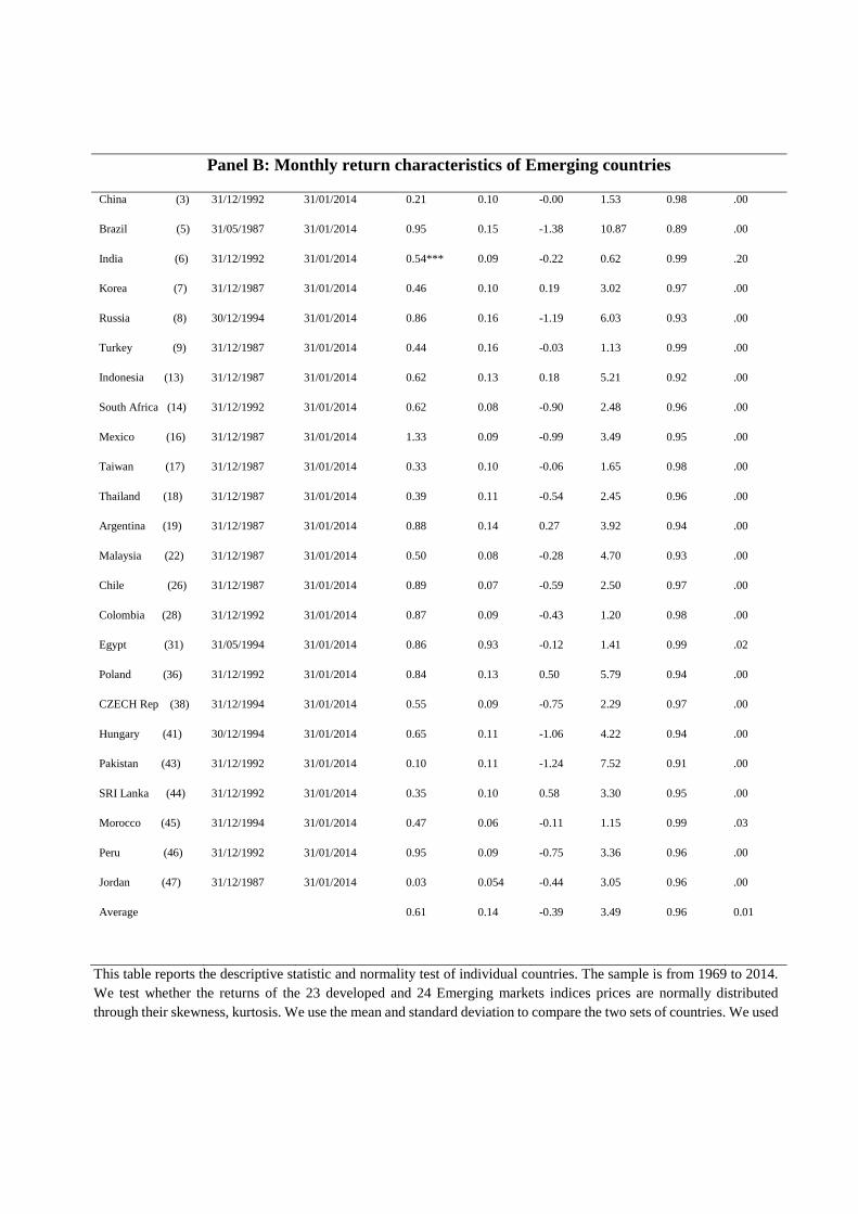
For most countries the skewness are negative and further away from zero; which indicates that
on average the data in our sample are not normally distributed. On average the Kurtosis are
different from 3. In some cases, (Korea and Jordan) a normal kurtosis does not necessary
converge with the skewness which makes the statistics results difficult to interpret by means
of the skewness and kurtosis values.
This study refers to the Shapiro-Wilk test that seems more appropriate as a test for normality
as it takes into account both skewness and kurtosis. It shows that, out of 47 countries indices
only 2 developed countries indices prices (Japan and Italy) have passed the normality test
(significant above 0.10) and 1 Emerging country indices, India ( significant above 0.05). The
Table 1 also shows that on average the standard deviation is relatively large (0.07) with respect
to the mean (0.53) in developed countries and even larger in Emerging countries (0.14) with a
mean return of (0.61). This indicates that the return value in the distributions of indices prices
in our dataset are dispersed and non-normal between 1969 and 2014 for the Developed
countries indices prices, and even more for the Emerging countries with the exception made
on Japan, Italy and India.
To establish whether the contrarian strategy is profitable internationally, this study uses the De
Bondt and Thaler’s (1985) approach, and long loser stock indices and short winner stock
indices over: The full sample period 1969-2014 (47 countries), then conducts the same
experiment in different time periods: the 1969-2014 sub-set that contains all countries indices
price available from 1969 only (18 countries); the 1994-2014 sub-set that contains all countries
including Emerging countries with data available from 1994 (47 countries); the developed
countries sub-set, that contains all developed countries only with data available from 1969 (23
countries); the Emerging countries sub-set, that contains all Emerging countries and starts in
December 1987 (24 countries). This is to enhance the robustness of our results, to test if the
results of these analyses are similar and consistent in different time periods and different
markets conditions (Developed and Emerging markets), and check whether they hold under
different specifications.
Global contrarian strategy method
The test of the global contrarian strategy is designed as followed. At the beginning of the
month, the indices are ranked based on their past J-month returns (J=36, 48, or 60 months).
Each month, the strategy buys the long-term loser portfolio consisting of the 10% indices that
have the lowest past J-month returns (extreme losers) and sells the long-term winner portfolio
comprised of the 10% of indices that have the highest past J-month returns (extreme winners).
By doing this, the study adopts the Jegadeesh and Titman's (1993) overlapping portfolio
approach for holding period and reports the average monthly return for the k-month holding
period as equal-weighted average of the portfolio returns. The contrarian arbitrage portfolio
(loser-winner) buys the long term losers and sells the long-term winners. Portfolios are held
for K-month holding period where (K= 36, 48, or 60 months) in keeping with De Bondt and
Thaler’s (1985) study. The compounding returns will be computed using the standard formula
as follows:
𝑅𝑖,𝑗 =∑ 𝑟𝑖,𝑡0
𝑡=−𝐽 (2)
𝑟𝑖,𝑡, is the return of the county i in t month (s).
𝑅𝑖,𝑗, is the computed cumulative return of the country i based on the formation period j
This study uses the return 𝑟𝑖,𝑡 of the index i at month t to select the winner and the loser indexes.
𝑅𝑖,𝑗, is used to compute the periodical return of index i at j month formation Period of the
formation date T.
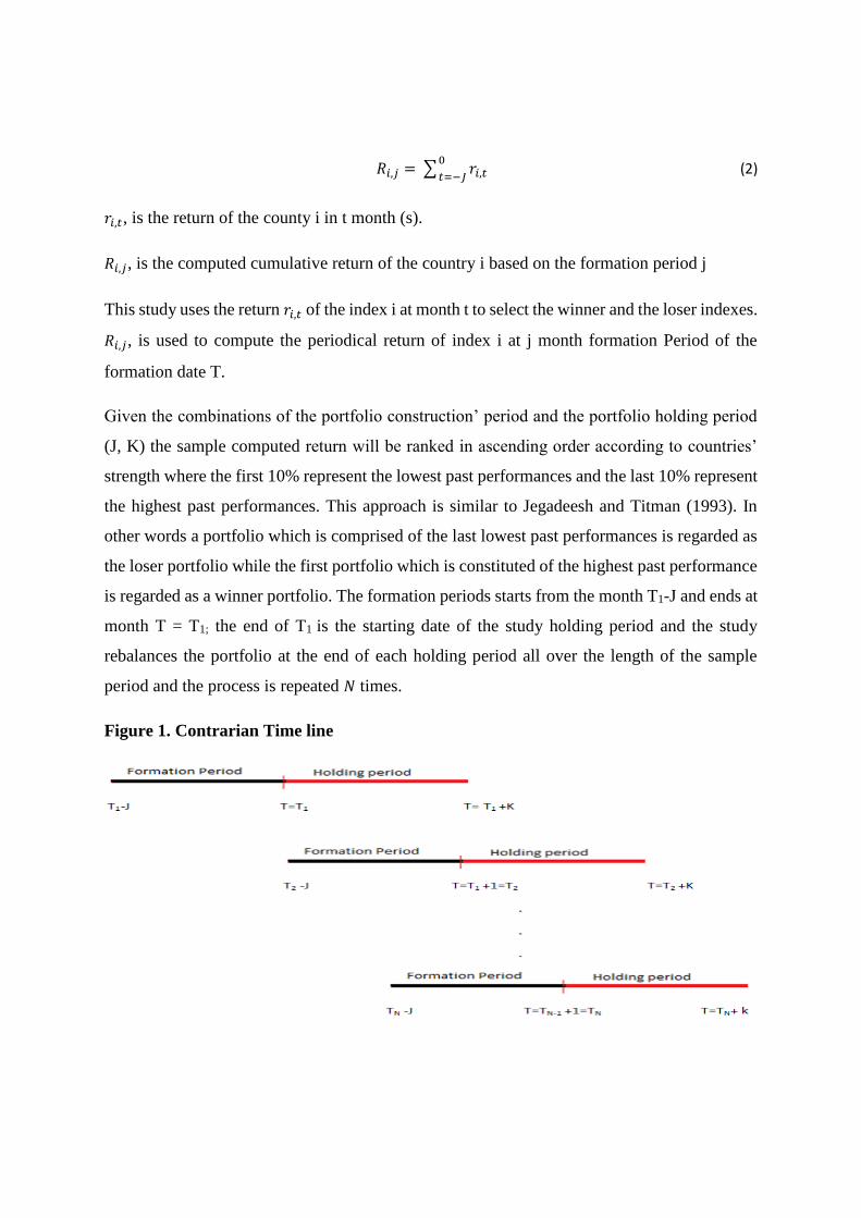
Given the combinations of the portfolio construction’ period and the portfolio holding period
(J, K) the sample computed return will be ranked in ascending order according to countries’
strength where the first 10% represent the lowest past performances and the last 10% represent
the highest past performances. This approach is similar to Jegadeesh and Titman (1993). In
other words a portfolio which is comprised of the last lowest past performances is regarded as
the loser portfolio while the first portfolio which is constituted of the highest past performance
is regarded as a winner portfolio. The formation periods starts from the month T1-J and ends at
month T = T1; the end of T1 is the starting date of the study holding period and the study
rebalances the portfolio at the end of each holding period all over the length of the sample
period and the process is repeated 𝑁 times.
Figure 1. Contrarian Time line
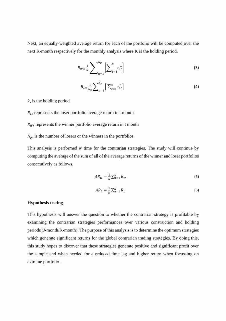
Next, an equally-weighted average return for each of the portfolio will be computed over the
next K-month respectively for the monthly analysis where K is the holding period.
𝑅𝑊=1
𝑁∑ [∑ 𝑟𝑖,𝑡
𝑤𝑘
𝑡=1]
𝑁𝑝
𝑛=1
(3)
𝑅𝐿=1
𝑁𝑝∑ [∑ 𝑟𝑖,𝑡
𝐿𝑘
𝑡=1]
𝑁𝑝
𝑛=1 (4)
𝑘, is the holding period
𝑅𝐿, represents the loser portfolio average return in t month
𝑅𝑊, represents the winner portfolio average return in t month
𝑁𝑝, is the number of losers or the winners in the portfolios.
This analysis is performed 𝑁 time for the contrarian strategies. The study will continue by
computing the average of the sum of all of the average returns of the winner and loser portfolios
consecutively as follows.
𝐴𝑅𝑤 =1
𝑁∑ 𝑅𝑤𝑁𝑛=1 (5)
𝐴𝑅𝐿 =1
𝑁∑ 𝑅𝐿𝑁𝑛=1 (6)
Hypothesis testing
This hypothesis will answer the question to whether the contrarian strategy is profitable by
examining the contrarian strategies performances over various construction and holding
periods (J-month/K-month). The purpose of this analysis is to determine the optimum strategies
which generate significant returns for the global contrarian trading strategies. By doing this,
this study hopes to discover that these strategies generate positive and significant profit over
the sample and when needed for a reduced time lag and higher return when focussing on
extreme portfolio.
Ho: did the arbitrage portfolio (losers-winners) issue from the contrarian strategy across the
global financial market generated positive and significant returns?
𝐻0: (𝐴𝑅𝐿 − 𝐴𝑅𝑊) > 0 (7)
After all, if the cumulative average return of the loser portfolio at this point is higher than the
winner portfolio return, we will conclude that we have a contrarian profit.
Fama and French (1996) find that skipping a time lag between the formation and the holding
periods produces stronger contrarian results because it avoids the long term reversal effect
being offset by the short-term continuation, which is consistent with De Bondt and Thaler’s
(1985) study that suggested that one year holding period did not produce significant contrarian
return. While the profitability of the contrarian strategy relies on the portfolios reversing in the
future, our thought is that, indices may not equally reverse at the same time, given that the
reversal effect might be different from portfolios of stock to portfolio of indices. Some indices
may reverse earlier (during the first 12 month). Given the consideration that some of the indices
may reverse earlier, ignoring this may lead to a loss of opportunity that reduces the contrarian
strategy profitability and may perhaps not be the most efficient approach to construct optimum
contrarian portfolios of indices which are ready to reverse. To enhance the global contrarian
profitability and uncover the early indices reversal effect, we keep a month gap between the
end of the J-month formation period and the beginning of the K-month holding period.
To evaluate the contrarian profitability with a month lag, we computed the difference between
the returns of the winners’ portfolios and the losers’ portfolios during the N horizons. If the
cumulative average return (𝐴𝑅𝐿) of the loser portfolio at this point is higher than the winner
portfolio return (𝐴𝑅𝑤), we will conclude that we have a contrarian profit but if it is lower we
may conclude that it is a contrarian loss.
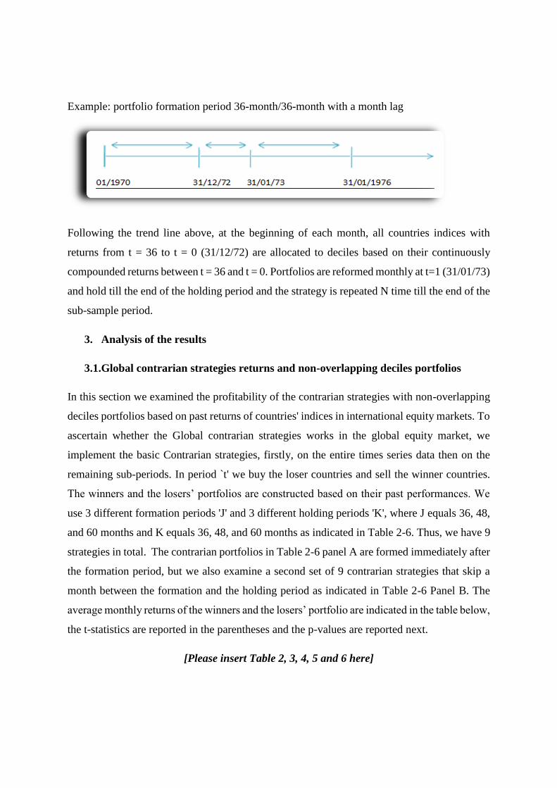
Example: portfolio formation period 36-month/36-month with a month lag
Following the trend line above, at the beginning of each month, all countries indices with
returns from t = 36 to t = 0 (31/12/72) are allocated to deciles based on their continuously
compounded returns between t = 36 and t = 0. Portfolios are reformed monthly at t=1 (31/01/73)
and hold till the end of the holding period and the strategy is repeated N time till the end of the
sub-sample period.
3. Analysis of the results
3.1.Global contrarian strategies returns and non-overlapping deciles portfolios
In this section we examined the profitability of the contrarian strategies with non-overlapping
deciles portfolios based on past returns of countries' indices in international equity markets. To
ascertain whether the Global contrarian strategies works in the global equity market, we
implement the basic Contrarian strategies, firstly, on the entire times series data then on the
remaining sub-periods. In period `t' we buy the loser countries and sell the winner countries.
The winners and the losers’ portfolios are constructed based on their past performances. We
use 3 different formation periods 'J' and 3 different holding periods 'K', where J equals 36, 48,
and 60 months and K equals 36, 48, and 60 months as indicated in Table 2-6. Thus, we have 9
strategies in total. The contrarian portfolios in Table 2-6 panel A are formed immediately after
the formation period, but we also examine a second set of 9 contrarian strategies that skip a
month between the formation and the holding period as indicated in Table 2-6 Panel B. The
average monthly returns of the winners and the losers’ portfolio are indicated in the table below,
the t-statistics are reported in the parentheses and the p-values are reported next.
[Please insert Table 2, 3, 4, 5 and 6 here]
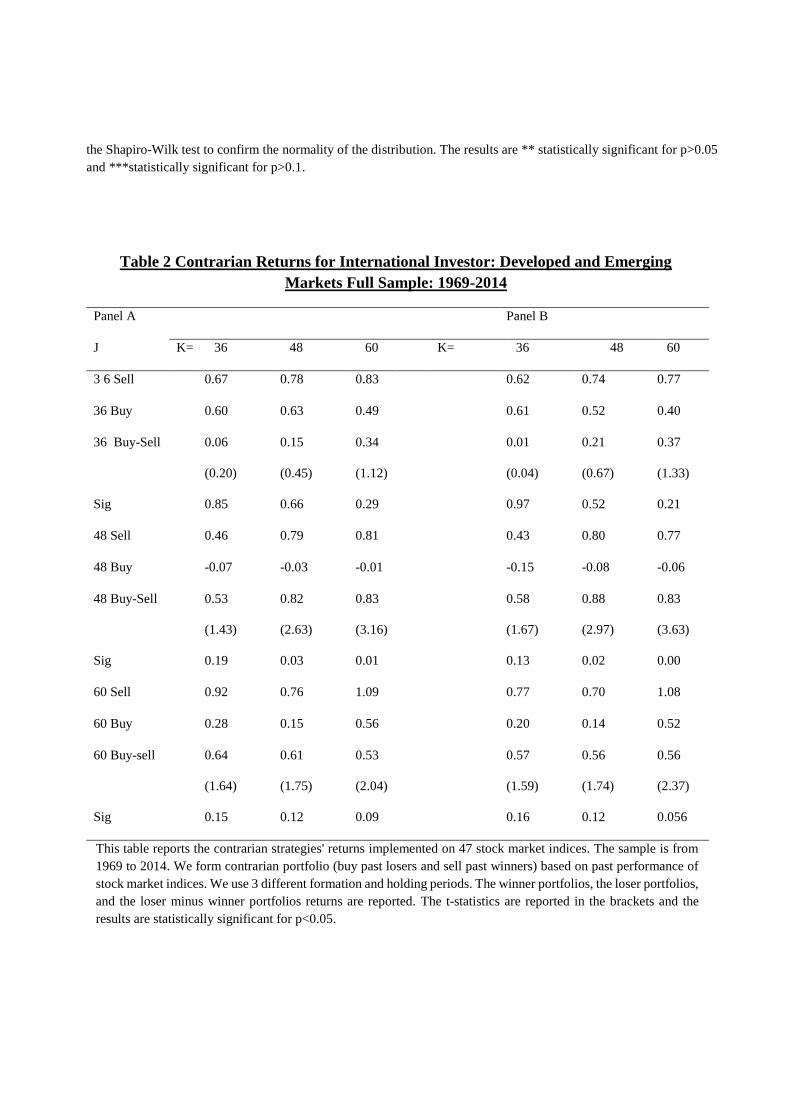
Our findings indicate evidences of contrarian profitability. The contrarian strategies have
shown to be profitable on average over the full sample period, and the 48-month/60-month
strategy being the most profitable strategy, this strategy yields 0.83% per month (10.40% per
year) with a t-statistic of 3.16 and a p-value of 0.01 (Table 2 Panel A), when there is not time
lag between the portfolio formation period and the holding period. Although the contrarian
return could rise considerably when the strategy skips a time lag between the portfolio
formation period and the holding period, the overall result is not exceptionally significant as it
appears that only 4 strategies out of 18 are significant at 5% level. We also uncover that the
48-month formation period generates significant return for both the 48- and the 60-month
holding periods, with the exception made on the 36-month holding period. This indicates that
the price started to reverse consistently sometimes after 36-month and continue to reverse
throughout the first 60-month of the post-formation period.
These results are consistent between unbalance and established market sub-sample where the
contrarian strategy yields return as high as 0.84% per month (10.49% per year) with a t-statistic
of 2.59 and a p-value of 0.029 when there is not time lag between the formation period and the
holding period with the 48-month/36-month strategy (Table 3 Panel A). It is also observable
that all contrarian return are positives in period post-globalization but none is statistically
significant (Table 4). These evidences also indicate that the contrarian strategies are highly
profitable in emerging countries where the highest returns might be observed with an effective
return of 1.37% per month (17.70% per year) with a t-statistic of 5.15, and a p-value of 0.01
(Table 6 Panel A) with the 60-month/ 48-month. The developed countries' contribution are
less significant and inconsistent, even though a consistent contrarian return of 0.93% per month
(11.72% per year) with a t-statistic of 2.49 and a p-value of 0.04 (Table 5 Panel A) could be
observed in developed countries with the 60-month/48-month strategy when there is a time lag
between the portfolio formation period and the holding period.
Even more interesting this study on the whole did not find evidence of consistent return
continuation among countries' indices and skipping a time lag between the formation and the
holding periods is not always beneficial (Table 2-6 Panel B). This contradicts the initial finding
by Fama and French (1996) that suggested that when the preceding months/year is included in
the test, short-term continuation tends to offsets long-term reversal, and past losers have lower
future returns than past winners for portfolios formed with up to four years past returns. It also
points to a greater return given that Fama and French suggested 1.16% average return per
month for the loser portfolio and 0.42 % per month for the winner portfolio, this implies that
the loser minus winner portfolio yields 0.74% per month (9.25% per year) on the average.
Overall the results as indicated in Table 2-6 validate the initial tests hypothesis that long-term
contrarian strategies are profitable internationally. They are consistent with other studies such
as De Bondt and Thaler (1985) in US stock market that suggested that 3 to 5 years after a past
performance based portfolio formation, losers' portfolios outperformed winners' portfolios by
approximately 25% over 3 years (8.33 per year) and 8% annually for 5 years post-ranking
period and indicates a better contrarian return than Jordan (2012) study that suggested that
contrarian strategies are internationally profitable. He reported about 5.60% per year with
earning above the risk free rate; and that the long-term contrarian profits is not a robust
phenomenon internationally. Our findings also endow with a greater return than Malin and
Bornholt's (2013) study that suggested 0.46% contrarian return per month (5.66% per year) in
developed market and 0.68% per month (8.47 per year) in emerging market, and Richards's
(1996) study that found 6.60% per year over 3 years holding period and 5.80% per year over 4
years.
To increase the power of the test this study also performs similar analysis on contrarian
strategies with overlapping portfolios where, contrarian deciles portfolio in any particular
month holds indices ranked in the deciles in any of the previous J months.
3.2.Contrarian strategies and overlapping deciles portfolios
In this section we examine whether contrarian strategies earn significant return after increasing
the power of the test. We construct overlapping portfolios, where contrarian deciles portfolio
in any particular month holds stocks ranked in those deciles in any of the previous k ranking
months. We start the analysis by implementing the basic contrarian strategies first, on the entire
times series data and the remaining sub-periods. In period `t’ we buy the losers countries and

sell the winners countries. The winners and the losers’ portfolios are constructed based on their
past performances.
We use 3 different formation periods 'J' and 3 different holding periods 'K', where 'J' equals 36,
48, and 60 months and 'K' equals 36, 48, and 60 month as indicated in Table7-11. This gives a
total of 9 strategies. The contrarian portfolios in Table 7-11; panel A are formed immediately
after the formation period, but we also examine a second set of 9 contrarian strategies that skip
a month between the formation and the holding period as indicated in Table 7-11 Panel B. The
average monthly returns of the winners and the losers' portfolio are indicated in the tables, the
T-statistics are reported in the parentheses and the p-values are reported next. The sample
period is from December 1969 to January 2014.
[Please insert Table 7, 8, 9, 10 and 11 here]
The tests of the contrarian strategy with overlapping deciles portfolios based on past returns of
countries’ indices in international equity markets, indicate evidences of contrarian profitability.
The 48-month/48-month strategy has shown to generate the highest effective contrarian return
of 0.55% per month (6.80% per year) with a t-statistic of 11.30% and a p-value of 0.00 over
the full sample period (Table 7 Panel A). However, the contrarian strategies are on average
positives and the returns may vary considerably from one market condition to another. More
importantly, the contrarian strategies become on average profitable and statistically significant
in the period post-1994 with the overlapping portfolios (Table 9). These evidences also indicate
that the contrarian strategies’ returns are on average lower but significant with the overlapping
approach (Table 7-11). These strategies remain profitable in emerging countries (Table 11),
but it is important to reiterate that on average they are more statically significant with
overlapping portfolios.
Even more interesting, this study did not find evidence of return continuation with the
contrarian strategies among countries’ indices when using overlapping portfolios and the
contrarian strategies are highly profitable in emerging countries and that developed countries'
contribution are less significant, which, are in line with our initial findings.
3.3.Contrarian strategies with quintiles portfolios
To test whether the Global contrarian strategies return vary with the portfolio size we construct
quintile portfolio. In other words a contrarian with quintile portfolios in any particular month
holds indices ranked in that quintile in any of the previous J month ranking months. A winner
portfolio comprises 20 percent of the indices with the highest returns over previous J months
and inversely6. We implement the global Contrarian strategies, firstly, on the entire times series
data and the remaining sub-periods. In period `t’ we buy the loser countries and sell the winner
6 Jordan's study were initially done on individual market index where stocks are sorted by their past 3-year buy-
and-hold return and the losers and winners represented respectively the 25% bottom and 25% top.

countries. The winners and the losers’ portfolios are constructed based on their past
performances. We use 3 different formation periods 'J' and 3 for different holding periods 'K'.
Where J equals 36, 48, and 60 months and K equals 36, 48, and 60 months thus, we have 9
strategies in total. The contrarian portfolios in Table 12-16 panel A are formed immediately
after the formation period, but we also examine a second set of 9 contrarian strategies that skip
a month between the formation and the holding period as indicated in Table 12-16 Panel B.
The average monthly returns of the winners and the losers’ portfolio are indicated in the Tables
12-16. The t-statistics are reported in the parentheses and the p-values are reported next.
[Please insert Table 12 to 21 here]
Our findings indicate that, contrarian strategies with non-overlapping quintile portfolios are
profitable over the full sample period. The 48-month/60-month strategy generates a return as
high as 0.71% per month (8.89% per year) with a t-statistic of 4.78 and a p-value of 0.00 when
there is not time lag between the portfolio formation period and the holding period (Table 12
Panel A). These returns are not statistically significant on the average and vary considerably
from one market condition to another. More importantly, the contrarian strategies remain on
the average profitable and significant in the period post-1994 (Table 14). Alike, the contrarian
strategies remain profitable in emerging countries (Table 16), but it is important to reiterate
that on average the results are more statistically significant with overlapping quintile portfolios
(Table 17-21) than the non-overlapping portfolios.
Taken as a whole these evidence indicate that the contrarian strategies’ yield on average higher
returns with the non-overlapping portfolio than the equivalent overlapping approaches for both
deciles and quintiles portfolios and that the contrarian strategy are on the average considerably
greater with deciles portfolios than quintiles portfolios. These results demonstrate that the
contrarian strategies are consistently profitable internationally with both quintile and deciles
portfolio and point to significantly high returns when trading with the global contrarian
strategy7.
7 These findings are complementary given that De Bondt and Thaler (1985), and Jordan (2012) studies did not
look at the contrarian phenomenon as a generalized phenomenon.

So far, we have argued that contrarian strategy is on the average profitable in international
market. However, from the theoretical point of view, there is reason to believe that contrarian
trading is a risky process and therefore, it is only of limited effectiveness. In principle, any
example of persistent mispricing is evidence of limited arbitrage (Barberis and Thaler, 2002).
The difficult is that while the profitability of the contrarian strategy could be interpreted as
price deviation from fundamental value it required consistent analysis in different market states
and time periods to provide evidence of consistency and inefficiency. Since the world has just
experienced one of its worst bear markets since the Great Depression, there is an even greater
need to start by studying contrarian performance in the past bull and bear markets to make
long-term decisions about investing using the global contrarian strategy. By providing
information on contrarian performance over different market state and different time period
investors could define a model of contrarian equilibrium with endogenous trading across
different state of the economy based on their preference.
3.4.Contrarian returns following bear and bull markets
To examine the extent to which contrarian performances are associated to the bull and bear
phase, we refer to the popular agreement that the bull markets are associated with persistently
rising share prices, but it can be noted that there still does not exist a general consensus as to
the objective definition of a bull market (Gonzalez et al. 2005). This study utilizes a formal
procedure to objectively identify bear and bull phases in stock index series that indicate the
meaningful time intervals corresponding to a bear or a bull phase and then examines the
magnitude of the contrarian profitability achieved following bull and bear markets using data
from the MSCI World index.
We examine how the performances of the optimum strategy 48-month/60-month are associated
with different phases of the world equity market, because the bull and the bear markets are
broad market movements and would best capture the impact of market state changes and
expected that the global contrarian should earn more pronounced return following bull markets.
The sample periods is divided into bear and bull phase following Siganos and Chelley-Steeley’s
(2006) approach. This paper defines bull phase as the period when the market return is positive
for 3, 6, 9 and 12 month before the test period, and the bear state when the market return is
negative for 3, 6, 9 and 12 month before the test and the results are shown in the Table 22
below.
[Please insert Table 22 here]
Table 22 presents the bear and bull market performances between December 1969 and January
2014, and the average contrarian profits accomplished after bull, bear markets, and the 12
months market performance of the defined phases. This study noted significant negative market
return following bear market phases and inversely in bull market, however we cannot identify
a regular pattern toward consecutive bear and bull market duration period. The optimum
contrarian strategy 48-month/60-month is associated with the 12-month duration where the bull
market performance (-1.43%) is relatively higher than the equivalent bear market (1.09%) in
absolute value and the bear frequency (25%) is the lowest while the bull frequency (75%) is
the highest compared to other horizon (3, 6 and 9). These observations suggest that the
contrarian strategy generates superior gains when the market rises slowly in bull and/or fall
quickly in bear phase as the high market performance indicates a high and positive change in
indices prices and inversely. Therefore, a forecast of a slow recovery could be seen as good
news for contrarian investors while the inverse is not necessary a bad news for global contrarian
investors comparatively. These results are in line with Klein (2001) that suggested that higher
price restores equilibrium because it induces more selling by investors who are locked into a
given security, and causes less buying by investors who wish to acquire exposure to the risk
characteristics of this security. The higher equilibrium price implies that expected returns in
subsequent periods are lower. However this study reiterates that the size of contrarian return
will depend upon speed of the rising and the falling market phases.
To restate, the primary goal of this study is to test whether the contrarian strategy is profitable
internationally and whether prices reversal effect is predictive. In other words, as we focus on
indices that go through more extreme return experiences during the formation period,
subsequent price reversals should be pronounced over the test period. De Bondt and Thaler
(1985) suggested that, an easy way to generate more or less extreme observations for any given
formation period is to compare the test period performances over time. Following this view we
examine whether the cumulative average return for various formation period (36, 48 and 60-
month) grows consistently larger over the test period and identified when the subsequent
reversal occur during the test period, to consider whether there is a seasonal pattern among
contrarian returns with different formation periods over different holding periods (1, 3, 6, 12,
24, 36, and 60-month) as indicated in Table 23.
[Please insert Table 23 here]
Table 23 shows that no reversal is observed for formation period 36, 48 and 60-month in the
first 2 years. As the cumulative average returns of holding periods as short as 2 year-period do
not always grow larger. The results also indicate sign of return reversal in period after 2 years
for the 36 and 48-month formation periods but the 60-month formation period shows opposite
effect as the cumulative average returns of the holding period after 2 years plunge lower.
Table 23 further indicates evidence of seasonality in indices price for the experiments with all
holding period above 3 years. Throughout the test period, all three experiments are clearly
affected by the same underlying seasonal pattern. For most holding period the 48-month
formation exceeds the same statistic and generates greater return than both 36-month and 60
month. The 60-month formation also generates returns greater than the 36-month for all
holding period. These results are broadly consistent with the prediction of the return reversal
in international equity market. However, several aspects of the contrarian return internationally
remain without adequate explanation mainly in the first 2 years.
[Please insert Figure 2 here]
Fig 2. Presents the contrarian profit trend from 1969 to 2014 and provides an indication of the
consistent rise of the contrarian return following bad market state and sharp fall after good
market state. In general, the good state tend to predict bad future contrarian performances while
the bad state predicts a worthy contrarian future. One possible explanation of this pattern as
indicated by the contrarian return from 1978 to 1986 and 1998 to 2006 is that when past
movement of the market has upward movement, most of the share prices have achieved gain,
and investors become optimistic for the future. The stronger the achieved lagged market gains,
the more optimism appears among traders, generating increasing reversal effect (Siganos and
Chelley-Steley, 2006).
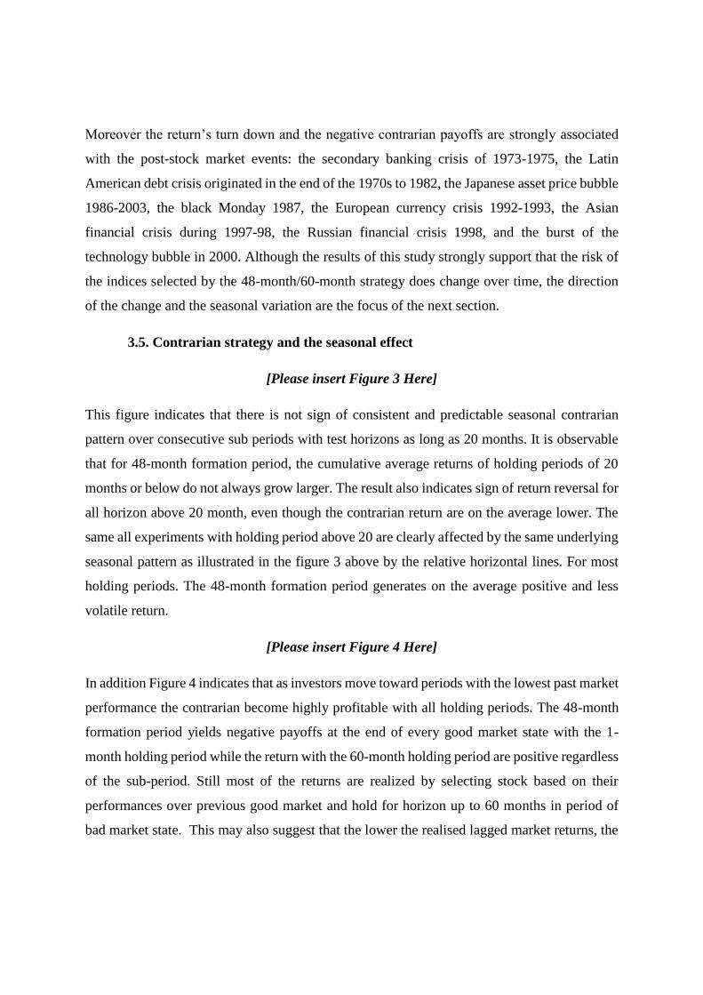
Moreover the return’s turn down and the negative contrarian payoffs are strongly associated
with the post-stock market events: the secondary banking crisis of 1973-1975, the Latin
American debt crisis originated in the end of the 1970s to 1982, the Japanese asset price bubble
1986-2003, the black Monday 1987, the European currency crisis 1992-1993, the Asian
financial crisis during 1997-98, the Russian financial crisis 1998, and the burst of the
technology bubble in 2000. Although the results of this study strongly support that the risk of
the indices selected by the 48-month/60-month strategy does change over time, the direction
of the change and the seasonal variation are the focus of the next section.
3.5. Contrarian strategy and the seasonal effect
[Please insert Figure 3 Here]
This figure indicates that there is not sign of consistent and predictable seasonal contrarian
pattern over consecutive sub periods with test horizons as long as 20 months. It is observable
that for 48-month formation period, the cumulative average returns of holding periods of 20
months or below do not always grow larger. The result also indicates sign of return reversal for
all horizon above 20 month, even though the contrarian return are on the average lower. The
same all experiments with holding period above 20 are clearly affected by the same underlying
seasonal pattern as illustrated in the figure 3 above by the relative horizontal lines. For most
holding periods. The 48-month formation period generates on the average positive and less
volatile return.
[Please insert Figure 4 Here]
In addition Figure 4 indicates that as investors move toward periods with the lowest past market
performance the contrarian become highly profitable with all holding periods. The 48-month
formation period yields negative payoffs at the end of every good market state with the 1-
month holding period while the return with the 60-month holding period are positive regardless
of the sub-period. Still most of the returns are realized by selecting stock based on their
performances over previous good market and hold for horizon up to 60 months in period of
bad market state. This may also suggest that the lower the realised lagged market returns, the

more pessimism appears among the trader, leading to short term under reaction that upset the
contrarian return and medium to long term to overreaction that heighten the contrarian result.
Furthermore if the reversal effect survives the globalisation impact we should be able to detect
this following a longitudinal analysis of the sub-period average contrarian return.
Figure 4. Also indicates that significant return come from period after 1994; this shows that the
integration of equity markets together with the international correlation among markets do not
synchronized the prices reversal effect around the world.
[Please insert Figure 5 Here]
The results of the contrarian tests developed with non-overlapping portfolio on the full sample
period are found in Figure 5. They are consistent with the reversal effect and the contrarian
strategy profitability, the loser earn about 7.31% cumulative return, while the winner earn -
0.13. The difference in cumulative return shows that the loser outperform the winner by an
average of 0.83% per month (10.37% per year). Figure 5 also shows the movement as we
progress through the sample period.
[Please insert Figure 6. Here]
These findings have other notable aspects as indicated in Figure 68. First, most of the contrarian
return come from the loser. Secondly the highest contrarian return are realised around 1982
and 2002 when the market is in the process of reverse from a bearish trend. This emphasis our
initial findings and are in line with the thought that indicated that when past market movement
are upward, most of the share prices have achieved gain, and investors become optimistic for
the future. Another possible explanation of the contrarian superior return is that, it is relatively
less difficult to account for bad news than good news. This implies that investors react to bad
news, by massive selling, thus overestimating bad news impact on prices, and subsequently
8 In addition, our findings are essential and deviate from previous studies on contrarian trading, in the sense that
we uses deciles portfolio to demonstrate how trading on extreme losers and winners, contrarian investors could
generate superior return compare to other approaches (quintile portfolios) and that the global contrarian based
on countries indices is highly profitable by comparison to trading on individual stock. Given that De Bondt and
Thaler (1985) and Fama and French (1996) studies were conducted on US stocks only.

revise their expectation and start buying back stock or invest after periods of bad news. This
explanation means investors are not rational, that all information are not included in share
prices and that it takes time to be fully included on the stock price, given that investors take
time to reflect on bad news.
3.5. Conclusion
This study examines the profitability of the contrarian strategy internationally while
considering the contrarian strategy as a global phenomenon as we progress over the period
1969 to 2014. Thus the study promotes a better understanding of the dynamics of contrarian
profitability by analysis the contrarian co-movements across different market states (Emerging,
Developed market). We also take a step towards linking the global contrarian profitability to
different phases (Bear and bull phases), and different time period. This includes the effect of
global chocks such as global financial crisis on the contrarian strategy profit, which in turn,
helps enhance our understanding of the factors that drive contrarian return across different time
period and different market states. Our analysis takes on particular significance given the
association between lagged market movement (share prices) and investor's optimism that
appears among traders, generating increasing reversal effect (Siganos and Chelley-Steley,
2006), and also has direct implication for predicting and controlling trading costs associated
with asset allocation strategies.
Some of our findings are as follows: The contrarian strategies are highly profitable in emerging
markets with a return as high as 1.38% per month (17.70% per year) with the 60-month/ 48-
month strategy. Developed countries' contribution are less significant, still a consistent
contrarian return of 0.93% per month (11.72% per year) could be observed in developed
countries with the 60-month/48-month strategy when the strategy skips a time lag between the
portfolio formation period and the holding period.
Our findings also indicate that, contrarian strategies with non-overlapping quintile portfolios
are profitable over the full sample period. The 48-month/60-month strategy generates a return
as high as 0.71 per month (8.89% per year). These returns are not statistically significant on
the average and vary considerably from one market condition to another. More importantly,

the contrarian strategies remain on the average profitable and significant in the period post-
1994 but are not particularly distinctive, which imply that the reversal effect survive the
globalisation impact and indicate that the integration of equity markets together with the
international correlation among markets do not synchronized the prices reversal effect around
the world.
Moreover, the contrarian strategies remain profitable in emerging countries, but it is important
to reiterate that on average they are more statistically significant with overlapping portfolios
than the non-overlapping portfolios. Taken as a whole, these evidences indicate that the
contrarian strategies’ yield on average higher return with the non-overlapping portfolio than
the equivalent overlapping approaches for both deciles and quintiles portfolios and that the
contrarian strategy are on the average considerably greater with deciles portfolios than quintiles
portfolios.
Furthermore there is not sign of consistent and predictable seasonal contrarian pattern over
consecutive sub periods with test horizons as long as 20 months. For 48-month formation
period, the cumulative average return of holding period of 20-month period or below do not
always grow larger. This result also indicates sign of return reversal for all horizon above 20
months, even though the contrarian return are on the average lower. The same all experiments
with holding period above 20 are clearly affected by the same underlying seasonal pattern as
illustrated in the figure 3. For most holding period, the 48-month formation generates positive
and less volatile return. Most of the contrarian return come from the loser and the highest
contrarian return are realised around when the market is in the process of reverse from a bearish
trend (1982 and 2002). At a more general level, the results present the global contrarian strategy
as a highly profitable strategy and indicate the need for considerable care in constructing and
evaluating the global contrarian internationally.
Reference
Barberis, N., and Thaler, R. (2002) `A survey of Behavioural Finance’, NBER working paper No
9222
Chan, L. K. C., Jegadeesh, N., and Lakonishok, J. (1996) `Momentum Strategies’ Journal of
Finance 51 (5) [online] available from < SSRN: http://ssrn.com/abstract=7836>
Chen, Q., Jiang, Y., and Li, Y. (2012) `The state of the market and the contrarian strategy:
evidence from China’s stock market’, Journal of Chinese Economics and Business Studies, 10
(1) 89-108
Choe, H., Kho, Bong-chan., and Stulz, R. M. (1999) `Do foreign investors destabilize stock
markets? The Korean experience in 1997’, Journal of Financial Economic, 54 (2) 227-264
De Bondt, W. F.M., and Thaler, R (1985) ‘Does the Stock Market Overreact?’ The Journal of
Finance, 40 793 – 805
De Bondt, W.F.M., Thaler, R. (1987) ‘Further evidence on investor overreaction and stock market
seasonality’ Journal of Finance 42, (3) 557– 581
Dreman, D. N. (1998) Contrarian investment strategies: the next generation: beat the market by
going against the crowd. 1 edn New York: Simon and Schuster
Fama, F., E., and French, R., K. (1996) `Multifactor Explanations of Asset Pricing Anomalies’
Journal of Finance, 51 (1) 55-84
Gonzalez, L., Powell, J. G., Shi, J., and Wilson, A. (2005) "Two Centuries of bull and bear market
cycles", International Review of Economics and Finance, 14 (2005) 469-486
Jegadeesh, N., and Titman, S. (1993) ‘Returns to Buying Winners and Selling Losers:
Implications for Stock Market Efficiency’, Journal of Finance, Volume 48, (1) 65-91
Jegadeesh, N., And Titman, S. (1995) `Overreaction, delayed reaction, and contrarian Profits’,
Oxford Journal, 8 (4) 973-993

Jordan, S. J. (2012) `Time-varying risk and long-term reversals: A re-examination of the
international evidence’, Journal of International Business Studies 43 (2012)123-142
Kulpmann, M. (2002) Stock Market Overreaction and Fundamental Valuation: Theory and
Empirical Evidence. 1 edn, Berlin and New York: Springer-Verlag
Malin, M., and Bomholt, G. (2012) `Long-Term Reversal: Evidence from International Market
Indices’, [online] available from, <http://papers.ssrn.com/sol3/papers.cfm?abstract_id=2121150>
Otchere, I., and Chan, J. (2003) `Short-term overreaction in the Hong Kong Stock Market: Can a
contrarian trading strategy beat the market?’ Journal of Behavioural Finance, 4 (3) 157-171
Siganos, A., and Chelley-Steeley, P. (2005) `Momentum Profits following bull and bear markets’,
Journal of Asset Management, 6 (5) 381-388
Richards, A. J. (1997) `Winner-loser reversal in national stock market indices: Can they be
explained?’ Journal of Finance 52 (5), 2129-2144
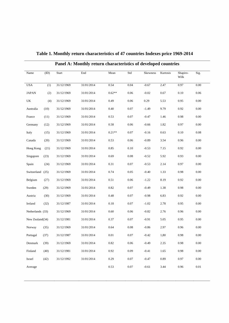
Table 1. Monthly return characteristics of 47 countries Indexes price 1969-2014
Panel A: Monthly return characteristics of developed countries
Name (ID) Start End Mean Std Skewness Kurtosis Shapiro-
Wilk
Sig.
USA (1) 31/12/1969 31/01/2014 0.54 0.04 -0.67 2.47 0.97 0.00
JAPAN (2) 31/12/1969 31/01/2014 0.62** 0.06 -0.02 0.67 0.10 0.06
UK (4) 31/12/1969 31/01/2014 0.49 0.06 0.29 5.53 0.95 0.00
Australia (10) 31/12/1969 31/01/2014 0.40 0.07 -1.49 9.79 0.92 0.00
France (11) 31/12/1969 31/01/2014 0.53 0.07 -0.47 1.46 0.98 0.00
Germany (12) 31/12/1969 31/01/2014 0.58 0.06 -0.66 1.82 0.97 0.00
Italy (15) 31/12/1969 31/01/2014 0.21** 0.07 -0.16 0.63 0.10 0.08
Canada (20) 31/12/1969 31/01/2014 0.53 0.06 -0.89 3.54 0.96 0.00
Hong Kong (21) 31/12/1969 31/01/2014 0.85 0.10 -0.53 7.15 0.92 0.00
Singapore (23) 31/12/1969 31/01/2014 0.69 0.08 -0.52 5.92 0.93 0.00
Spain (24) 31/12/1969 31/01/2014 0.31 0.07 -0.53 2.14 0.97 0.00
Switzerland (25) 31/12/1969 31/01/2014 0.74 0.05 -0.40 1.33 0.98 0.00
Belgium (27) 31/12/1969 31/01/2014 0.51 0.06 -1.22 8.19 0.92 0.00
Sweden (29) 31/12/1969 31/01/2014 0.82 0.07 -0.49 1.38 0.98 0.00
Austria (30) 31/12/1969 31/01/2014 0.48 0.07 -0.98 6.83 0.92 0.00
Ireland (32) 31/12/1987 31/01/2014 0.18 0.07 -1.02 2.78 0.95 0.00
Netherlands (33) 31/12/1969 31/01/2014 0.60 0.06 -0.82 2.76 0.96 0.00
New Zealand(34) 31/12/1981 31/01/2014 0.37 0.07 -0.91 5.05 0.95 0.00
Norway (35) 31/12/1969 31/01/2014 0.64 0.08 -0.86 2.97 0.96 0.00
Portugal (37) 31/12/1987 31/01/2014 0.01 0.07 -0.42 1,80 0.98 0.00
Denmark (39) 31/12/1969 31/01/2014 0.82 0.06 -0.49 2.35 0.98 0.00
Finland (40) 31/12/1981 31/01/2014 0.92 0.09 -0.41 1.65 0.98 0.00
Israel (42) 31/12/1992 31/01/2014 0.29 0.07 -0.47 0.89 0.97 0.00
Average 0.53
0.07
-0.61
3.44
0.96
0.01
Panel B: Monthly return characteristics of Emerging countries
China (3) 31/12/1992 31/01/2014 0.21 0.10 -0.00 1.53 0.98 .00
Brazil (5) 31/05/1987 31/01/2014 0.95 0.15 -1.38 10.87 0.89 .00
India (6) 31/12/1992 31/01/2014 0.54*** 0.09 -0.22 0.62 0.99 .20
Korea (7) 31/12/1987 31/01/2014 0.46 0.10 0.19 3.02 0.97 .00
Russia (8) 30/12/1994 31/01/2014 0.86 0.16 -1.19 6.03 0.93 .00
Turkey (9) 31/12/1987 31/01/2014 0.44 0.16 -0.03 1.13 0.99 .00
Indonesia (13) 31/12/1987 31/01/2014 0.62 0.13 0.18 5.21 0.92 .00
South Africa (14) 31/12/1992 31/01/2014 0.62 0.08 -0.90 2.48 0.96 .00
Mexico (16) 31/12/1987 31/01/2014 1.33 0.09 -0.99 3.49 0.95 .00
Taiwan (17) 31/12/1987 31/01/2014 0.33 0.10 -0.06 1.65 0.98 .00
Thailand (18) 31/12/1987 31/01/2014 0.39 0.11 -0.54 2.45 0.96 .00
Argentina (19) 31/12/1987 31/01/2014 0.88 0.14 0.27 3.92 0.94 .00
Malaysia (22) 31/12/1987 31/01/2014 0.50 0.08 -0.28 4.70 0.93 .00
Chile (26) 31/12/1987 31/01/2014 0.89 0.07 -0.59 2.50 0.97 .00
Colombia (28) 31/12/1992 31/01/2014 0.87 0.09 -0.43 1.20 0.98 .00
Egypt (31) 31/05/1994 31/01/2014 0.86 0.93 -0.12 1.41 0.99 .02
Poland (36) 31/12/1992 31/01/2014 0.84 0.13 0.50 5.79 0.94 .00
CZECH Rep (38) 31/12/1994 31/01/2014 0.55 0.09 -0.75 2.29 0.97 .00
Hungary (41) 30/12/1994 31/01/2014 0.65 0.11 -1.06 4.22 0.94 .00
Pakistan (43) 31/12/1992 31/01/2014 0.10 0.11 -1.24 7.52 0.91 .00
SRI Lanka (44) 31/12/1992 31/01/2014 0.35 0.10 0.58 3.30 0.95 .00
Morocco (45) 31/12/1994 31/01/2014 0.47 0.06 -0.11 1.15 0.99 .03
Peru (46) 31/12/1992 31/01/2014 0.95 0.09 -0.75 3.36 0.96 .00
Jordan (47) 31/12/1987 31/01/2014 0.03 0.054 -0.44 3.05 0.96 .00
Average 0.61
0.14
-0.39
3.49
0.96
0.01
This table reports the descriptive statistic and normality test of individual countries. The sample is from 1969 to 2014.
We test whether the returns of the 23 developed and 24 Emerging markets indices prices are normally distributed
through their skewness, kurtosis. We use the mean and standard deviation to compare the two sets of countries. We used
the Shapiro-Wilk test to confirm the normality of the distribution. The results are ** statistically significant for p>0.05
and ***statistically significant for p>0.1.
Table 2 Contrarian Returns for International Investor: Developed and Emerging
Markets Full Sample: 1969-2014
Panel A Panel B
J K= 36 48 60 K= 36 48 60
3 6 Sell 0.67 0.78 0.83 0.62 0.74 0.77
36 Buy 0.60 0.63 0.49 0.61 0.52 0.40
36 Buy-Sell
Sig
0.06
(0.20)
0.85
0.15
(0.45)
0.66
0.34
(1.12)
0.29
0.01
(0.04)
0.97
0.21
(0.67)
0.52
0.37
(1.33)
0.21
48 Sell 0.46 0.79 0.81 0.43 0.80 0.77
48 Buy -0.07 -0.03 -0.01 -0.15 -0.08 -0.06
48 Buy-Sell
Sig
0.53
(1.43)
0.19
0.82
(2.63)
0.03
0.83
(3.16)
0.01
0.58
(1.67)
0.13
0.88
(2.97)
0.02
0.83
(3.63)
0.00
60 Sell 0.92 0.76 1.09 0.77 0.70 1.08
60 Buy 0.28 0.15 0.56 0.20 0.14 0.52
60 Buy-sell
Sig
0.64
(1.64)
0.15
0.61
(1.75)
0.12
0.53
(2.04)
0.09
0.57
(1.59)
0.16
0.56
(1.74)
0.12
0.56
(2.37)
0.056
This table reports the contrarian strategies' returns implemented on 47 stock market indices. The sample is from
1969 to 2014. We form contrarian portfolio (buy past losers and sell past winners) based on past performance of
stock market indices. We use 3 different formation and holding periods. The winner portfolios, the loser portfolios,
and the loser minus winner portfolios returns are reported. The t-statistics are reported in the brackets and the
results are statistically significant for p<0.05.
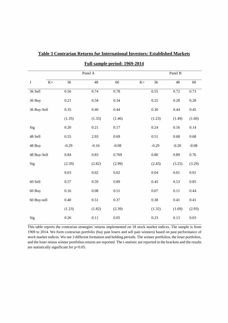
Table 3 Contrarian Returns for International Investors: Established Markets
Full sample period: 1969-2014
Panel A Panel B
J K= 36 48 60 K= 36 48 60
36 Sell 0.56 0.74 0.78 0.55 0.72 0.73
36 Buy 0.21 0.34 0.34 0.25 0.28 0.28
36 Buy-Sell
Sig
0.35
(1.35)
0.20
0.40
(1.33)
0.21
0.44
(1.46)
0.17
0.30
(1.23)
0.24
0.44
(1.49)
0.16
0.45
(1.60)
0.14
48 Sell 0.55 2.93 0.69 0.51 0.68 0.68
48 Buy -0.29 -0.16 -0.08 -0.29 -0.20 -0.08
48 Buy-Sell
Sig
0.84
(2.59)
0.03
0.83
(2.82)
0.02
0.769
(2.99)
0.02
0.80
(2.43)
0.04
0.89
(3.25)
0.01
0.76
(3.29)
0.01
60 Sell 0.57 0.59 0.89 0.45 0.53 0.85
60 Buy 0.16 0.08 0.51 0.07 0.11 0.44
60 Buy-sell
Sig
0.40
(1.23)
0.26
0.51
(1.82)
0.11
0.37
(2.39)
0.05
0.38
(1.32)
0.23
0.41
(1.69)
0.13
0.41
(2.93)
0.03
This table reports the contrarian strategies' returns implemented on 18 stock market indices. The sample is from
1969 to 2014. We form contrarian portfolio (buy past losers and sell past winners) based on past performance of
stock market indices. We use 3 different formation and holding periods. The winner portfolios, the loser portfolios,
and the loser minus winner portfolios returns are reported. The t-statistic are reported in the brackets and the results
are statistically significant for p<0.05.
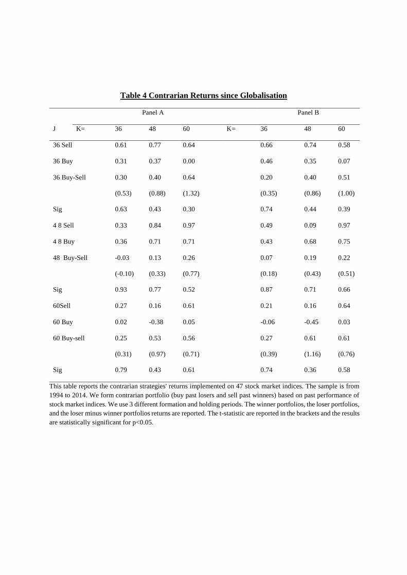
Table 4 Contrarian Returns since Globalisation
Panel A Panel B
J K= 36 48 60 K= 36 48 60
36 Sell 0.61 0.77 0.64 0.66 0.74 0.58
36 Buy 0.31 0.37 0.00 0.46 0.35 0.07
36 Buy-Sell
Sig
0.30
(0.53)
0.63
0.40
(0.88)
0.43
0.64
(1.32)
0.30
0.20
(0.35)
0.74
0.40
(0.86)
0.44
0.51
(1.00)
0.39
4 8 Sell 0.33 0.84 0.97 0.49 0.09 0.97
4 8 Buy 0.36 0.71 0.71 0.43 0.68 0.75
48 Buy-Sell
Sig
-0.03
(-0.10)
0.93
0.13
(0.33)
0.77
0.26
(0.77)
0.52
0.07
(0.18)
0.87
0.19
(0.43)
0.71
0.22
(0.51)
0.66
60Sell 0.27 0.16 0.61 0.21 0.16 0.64
60 Buy 0.02 -0.38 0.05 -0.06 -0.45 0.03
60 Buy-sell
Sig
0.25
(0.31)
0.79
0.53
(0.97)
0.43
0.56
(0.71)
0.61
0.27
(0.39)
0.74
0.61
(1.16)
0.36
0.61
(0.76)
0.58
This table reports the contrarian strategies' returns implemented on 47 stock market indices. The sample is from
1994 to 2014. We form contrarian portfolio (buy past losers and sell past winners) based on past performance of
stock market indices. We use 3 different formation and holding periods. The winner portfolios, the loser portfolios,
and the loser minus winner portfolios returns are reported. The t-statistic are reported in the brackets and the results
are statistically significant for p<0.05.
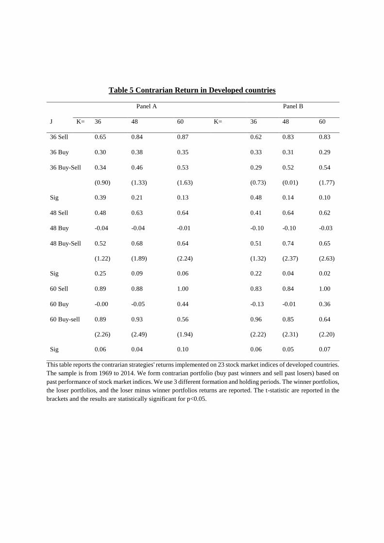
Table 5 Contrarian Return in Developed countries
Panel A Panel B
J K= 36 48 60 K= 36 48 60
36 Sell 0.65 0.84 0.87 0.62 0.83 0.83
36 Buy 0.30 0.38 0.35 0.33 0.31 0.29
36 Buy-Sell
Sig
0.34
(0.90)
0.39
0.46
(1.33)
0.21
0.53
(1.63)
0.13
0.29
(0.73)
0.48
0.52
(0.01)
0.14
0.54
(1.77)
0.10
48 Sell 0.48 0.63 0.64 0.41 0.64 0.62
48 Buy -0.04 -0.04 -0.01 -0.10 -0.10 -0.03
48 Buy-Sell
Sig
0.52
(1.22)
0.25
0.68
(1.89)
0.09
0.64
(2.24)
0.06
0.51
(1.32)
0.22
0.74
(2.37)
0.04
0.65
(2.63)
0.02
60 Sell 0.89 0.88 1.00 0.83 0.84 1.00
60 Buy -0.00 -0.05 0.44 -0.13 -0.01 0.36
60 Buy-sell
Sig
0.89
(2.26)
0.06
0.93
(2.49)
0.04
0.56
(1.94)
0.10
0.96
(2.22)
0.06
0.85
(2.31)
0.05
0.64
(2.20)
0.07
This table reports the contrarian strategies' returns implemented on 23 stock market indices of developed countries.
The sample is from 1969 to 2014. We form contrarian portfolio (buy past winners and sell past losers) based on
past performance of stock market indices. We use 3 different formation and holding periods. The winner portfolios,
the loser portfolios, and the loser minus winner portfolios returns are reported. The t-statistic are reported in the
brackets and the results are statistically significant for p<0.05.
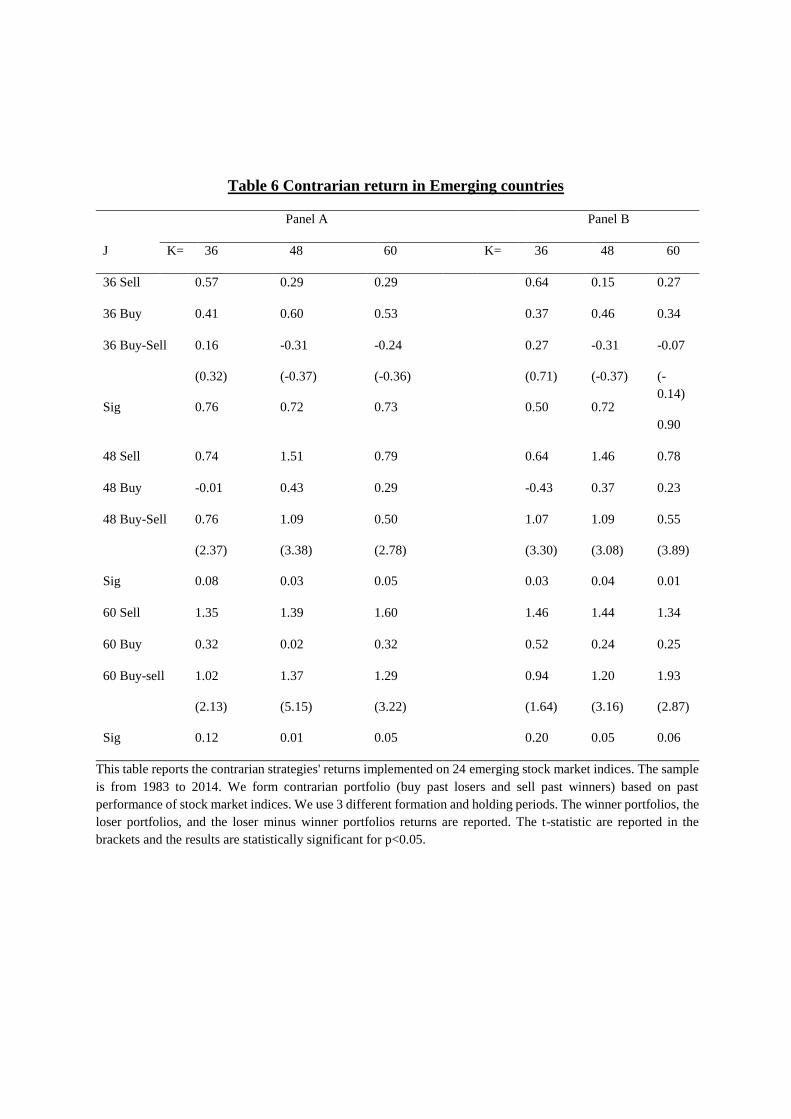
Table 6 Contrarian return in Emerging countries
Panel A Panel B
J K= 36 48 60 K= 36 48 60
36 Sell 0.57 0.29 0.29 0.64 0.15 0.27
36 Buy 0.41 0.60 0.53 0.37 0.46 0.34
36 Buy-Sell
Sig
0.16
(0.32)
0.76
-0.31
(-0.37)
0.72
-0.24
(-0.36)
0.73
0.27
(0.71)
0.50
-0.31
(-0.37)
0.72
-0.07
(-
0.14)
0.90
48 Sell 0.74 1.51 0.79 0.64 1.46 0.78
48 Buy -0.01 0.43 0.29 -0.43 0.37 0.23
48 Buy-Sell
Sig
0.76
(2.37)
0.08
1.09
(3.38)
0.03
0.50
(2.78)
0.05
1.07
(3.30)
0.03
1.09
(3.08)
0.04
0.55
(3.89)
0.01
60 Sell 1.35 1.39 1.60 1.46 1.44 1.34
60 Buy 0.32 0.02 0.32 0.52 0.24 0.25
60 Buy-sell
Sig
1.02
(2.13)
0.12
1.37
(5.15)
0.01
1.29
(3.22)
0.05
0.94
(1.64)
0.20
1.20
(3.16)
0.05
1.93
(2.87)
0.06
This table reports the contrarian strategies' returns implemented on 24 emerging stock market indices. The sample
is from 1983 to 2014. We form contrarian portfolio (buy past losers and sell past winners) based on past
performance of stock market indices. We use 3 different formation and holding periods. The winner portfolios, the
loser portfolios, and the loser minus winner portfolios returns are reported. The t-statistic are reported in the
brackets and the results are statistically significant for p<0.05.
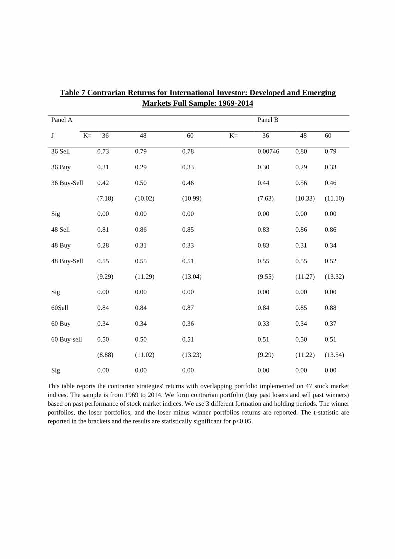
Table 7 Contrarian Returns for International Investor: Developed and Emerging
Markets Full Sample: 1969-2014
Panel A Panel B
J K= 36 48 60 K= 36 48 60
36 Sell 0.73 0.79 0.78 0.00746 0.80 0.79
36 Buy 0.31 0.29 0.33 0.30 0.29 0.33
36 Buy-Sell
Sig
0.42
(7.18)
0.00
0.50
(10.02)
0.00
0.46
(10.99)
0.00
0.44
(7.63)
0.00
0.56
(10.33)
0.00
0.46
(11.10)
0.00
48 Sell 0.81 0.86 0.85 0.83 0.86 0.86
48 Buy 0.28 0.31 0.33 0.83 0.31 0.34
48 Buy-Sell
Sig
0.55
(9.29)
0.00
0.55
(11.29)
0.00
0.51
(13.04)
0.00
0.55
(9.55)
0.00
0.55
(11.27)
0.00
0.52
(13.32)
0.00
60Sell 0.84 0.84 0.87 0.84 0.85 0.88
60 Buy 0.34 0.34 0.36 0.33 0.34 0.37
60 Buy-sell
Sig
0.50
(8.88)
0.00
0.50
(11.02)
0.00
0.51
(13.23)
0.00
0.51
(9.29)
0.00
0.50
(11.22)
0.00
0.51
(13.54)
0.00
This table reports the contrarian strategies' returns with overlapping portfolio implemented on 47 stock market
indices. The sample is from 1969 to 2014. We form contrarian portfolio (buy past losers and sell past winners)
based on past performance of stock market indices. We use 3 different formation and holding periods. The winner
portfolios, the loser portfolios, and the loser minus winner portfolios returns are reported. The t-statistic are
reported in the brackets and the results are statistically significant for p<0.05.
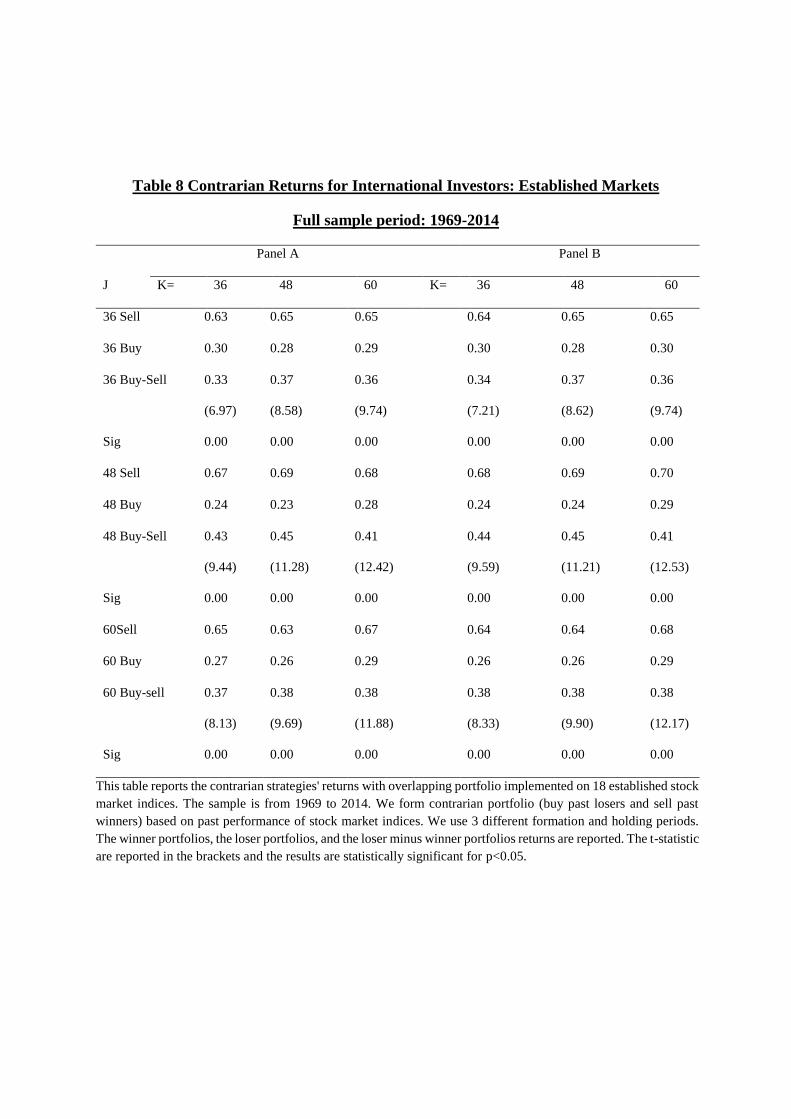
Table 8 Contrarian Returns for International Investors: Established Markets
Full sample period: 1969-2014
Panel A Panel B
J K= 36 48 60 K= 36 48 60
36 Sell 0.63 0.65 0.65 0.64 0.65 0.65
36 Buy 0.30 0.28 0.29 0.30 0.28 0.30
36 Buy-Sell
Sig
0.33
(6.97)
0.00
0.37
(8.58)
0.00
0.36
(9.74)
0.00
0.34
(7.21)
0.00
0.37
(8.62)
0.00
0.36
(9.74)
0.00
48 Sell 0.67 0.69 0.68 0.68 0.69 0.70
48 Buy 0.24 0.23 0.28 0.24 0.24 0.29
48 Buy-Sell
Sig
0.43
(9.44)
0.00
0.45
(11.28)
0.00
0.41
(12.42)
0.00
0.44
(9.59)
0.00
0.45
(11.21)
0.00
0.41
(12.53)
0.00
60Sell 0.65 0.63 0.67 0.64 0.64 0.68
60 Buy 0.27 0.26 0.29 0.26 0.26 0.29
60 Buy-sell
Sig
0.37
(8.13)
0.00
0.38
(9.69)
0.00
0.38
(11.88)
0.00
0.38
(8.33)
0.00
0.38
(9.90)
0.00
0.38
(12.17)
0.00
This table reports the contrarian strategies' returns with overlapping portfolio implemented on 18 established stock
market indices. The sample is from 1969 to 2014. We form contrarian portfolio (buy past losers and sell past
winners) based on past performance of stock market indices. We use 3 different formation and holding periods.
The winner portfolios, the loser portfolios, and the loser minus winner portfolios returns are reported. The t-statistic
are reported in the brackets and the results are statistically significant for p<0.05.
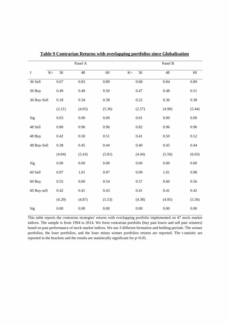
Table 9 Contrarian Returns with overlapping portfolios since Globalisation
Panel A Panel B
J K= 36 48 60 K= 36 48 60
36 Sell 0.67 0.83 0.89 0.68 0.84 0.89
36 Buy 0.49 0.49 0.50 0.47 0.48 0.51
36 Buy-Sell
Sig
0.18
(2.21)
0.03
0.34
(4.65)
0.00
0.38
(5.36)
0.00
0.22
(2.57)
0.01
0.36
(4.90)
0.00
0.38
(5.44)
0.00
48 Sell 0.80 0.96 0.96 0.82 0.96 0.96
48 Buy 0.42 0.50 0.51 0.41 0.50 0.52
48 Buy-Sell
Sig
0.38
(4.04)
0.00
0.45
(5.43)
0.00
0.44
(5.81)
0.00
0.40
(4.44)
0.00
0.45
(5.56)
0.00
0.44
(6.03)
0.00
60 Sell 0.97 1.01 0.97 0.99 1.01 0.98
60 Buy 0.55 0.60 0.54 0.57 0.60 0.56
60 Buy-sell
Sig
0.42
(4.29)
0.00
0.41
(4.87)
0.00
0.43
(5.53)
0.00
0.41
(4.38)
0.00
0.41
(4.95)
0.00
0.42
(5.56)
0.00
This table reports the contrarian strategies' returns with overlapping portfolio implemented on 47 stock market
indices. The sample is from 1994 to 2014. We form contrarian portfolio (buy past losers and sell past winners)
based on past performance of stock market indices. We use 3 different formation and holding periods. The winner
portfolios, the loser portfolios, and the loser minus winner portfolios returns are reported. The t-statistic are
reported in the brackets and the results are statistically significant for p<0.05.
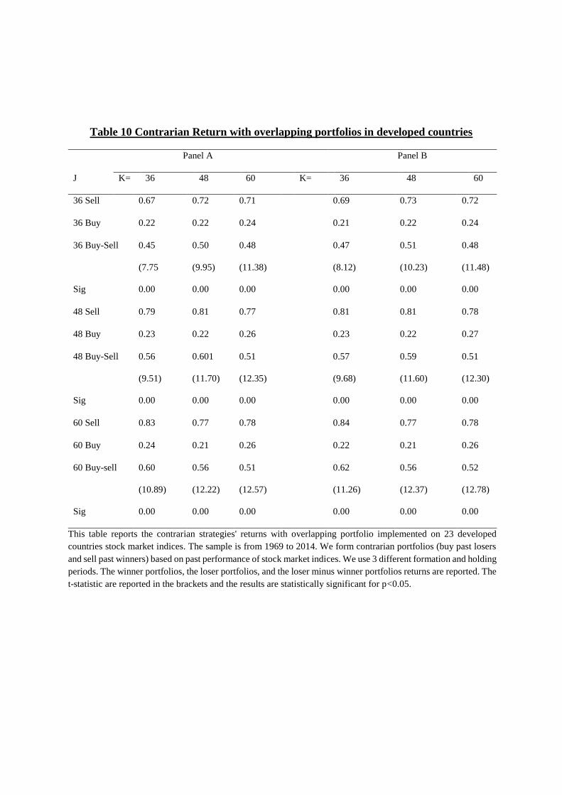
Table 10 Contrarian Return with overlapping portfolios in developed countries
Panel A Panel B
J K= 36 48 60 K= 36 48 60
36 Sell 0.67 0.72 0.71 0.69 0.73 0.72
36 Buy 0.22 0.22 0.24 0.21 0.22 0.24
36 Buy-Sell
Sig
0.45
(7.75
0.00
0.50
(9.95)
0.00
0.48
(11.38)
0.00
0.47
(8.12)
0.00
0.51
(10.23)
0.00
0.48
(11.48)
0.00
48 Sell 0.79 0.81 0.77 0.81 0.81 0.78
48 Buy 0.23 0.22 0.26 0.23 0.22 0.27
48 Buy-Sell
Sig
0.56
(9.51)
0.00
0.601
(11.70)
0.00
0.51
(12.35)
0.00
0.57
(9.68)
0.00
0.59
(11.60)
0.00
0.51
(12.30)
0.00
60 Sell 0.83 0.77 0.78 0.84 0.77 0.78
60 Buy 0.24 0.21 0.26 0.22 0.21 0.26
60 Buy-sell
Sig
0.60
(10.89)
0.00
0.56
(12.22)
0.00
0.51
(12.57)
0.00
0.62
(11.26)
0.00
0.56
(12.37)
0.00
0.52
(12.78)
0.00
This table reports the contrarian strategies' returns with overlapping portfolio implemented on 23 developed
countries stock market indices. The sample is from 1969 to 2014. We form contrarian portfolios (buy past losers
and sell past winners) based on past performance of stock market indices. We use 3 different formation and holding
periods. The winner portfolios, the loser portfolios, and the loser minus winner portfolios returns are reported. The
t-statistic are reported in the brackets and the results are statistically significant for p<0.05.
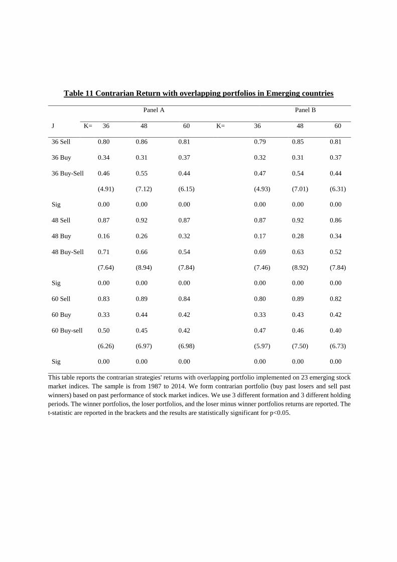
Table 11 Contrarian Return with overlapping portfolios in Emerging countries
Panel A Panel B
J K= 36 48 60 K= 36 48 60
36 Sell 0.80 0.86 0.81 0.79 0.85 0.81
36 Buy 0.34 0.31 0.37 0.32 0.31 0.37
36 Buy-Sell
Sig
0.46
(4.91)
0.00
0.55
(7.12)
0.00
0.44
(6.15)
0.00
0.47
(4.93)
0.00
0.54
(7.01)
0.00
0.44
(6.31)
0.00
48 Sell 0.87 0.92 0.87 0.87 0.92 0.86
48 Buy 0.16 0.26 0.32 0.17 0.28 0.34
48 Buy-Sell
Sig
0.71
(7.64)
0.00
0.66
(8.94)
0.00
0.54
(7.84)
0.00
0.69
(7.46)
0.00
0.63
(8.92)
0.00
0.52
(7.84)
0.00
60 Sell 0.83 0.89 0.84 0.80 0.89 0.82
60 Buy 0.33 0.44 0.42 0.33 0.43 0.42
60 Buy-sell
Sig
0.50
(6.26)
0.00
0.45
(6.97)
0.00
0.42
(6.98)
0.00
0.47
(5.97)
0.00
0.46
(7.50)
0.00
0.40
(6.73)
0.00
This table reports the contrarian strategies' returns with overlapping portfolio implemented on 23 emerging stock
market indices. The sample is from 1987 to 2014. We form contrarian portfolio (buy past losers and sell past
winners) based on past performance of stock market indices. We use 3 different formation and 3 different holding
periods. The winner portfolios, the loser portfolios, and the loser minus winner portfolios returns are reported. The
t-statistic are reported in the brackets and the results are statistically significant for p<0.05.
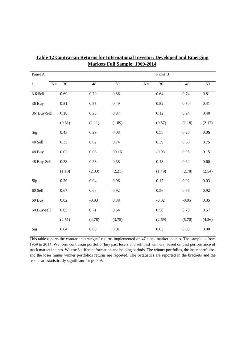
Table 12 Contrarian Returns for International Investor: Developed and Emerging
Markets Full Sample: 1969-2014
Panel A Panel B
J K= 36 48 60 K= 36 48 60
3 6 Sell 0.69 0.79 0.86 0.64 0.74 0.81
36 Buy 0.51 0.55 0.49 0.52 0.50 0.41
36 Buy-Sell
Sig
0.18
(0.81)
0.43
0.23
(1.11)
0.29
0.37
(1.89)
0.08
0.12
(0.57)
0.58
0.24
(1.18)
0.26
0.40
(2.12)
0.06
48 Sell 0.35 0.62 0.74 0.39 0.68 0.75
48 Buy 0.02 0.08 00.16 -0.03 0.05 0.15
48 Buy-Sell
Sig
0.33
(1.13)
0.29
0.53
(2.33)
0.04
0.58
(2.21)
0.06
0.43
(1.49)
0.17
0.62
(2.78)
0.02
0.60
(2.54)
0.03
60 Sell 0.67 0.68 0.92 0.56 0.66 0.92
60 Buy 0.02 -0.03 0.38 -0.02 -0.05 0.35
60 Buy-sell
Sig
0.65
(2.51)
0.04
0.71
(4.78)
0.00
0.54
(3.75)
0.01
0.58
(2.69)
0.03
0.70
(5.70)
0.00
0.57
(4.36)
0.00
This table reports the contrarian strategies' returns implemented on 47 stock market indices. The sample is from
1969 to 2014. We form contrarian portfolio (buy past losers and sell past winners) based on past performance of
stock market indices. We use 3 different formation and holding periods. The winner portfolios, the loser portfolios,
and the loser minus winner portfolios returns are reported. The t-statistics are reported in the brackets and the
results are statistically significant for p<0.05.
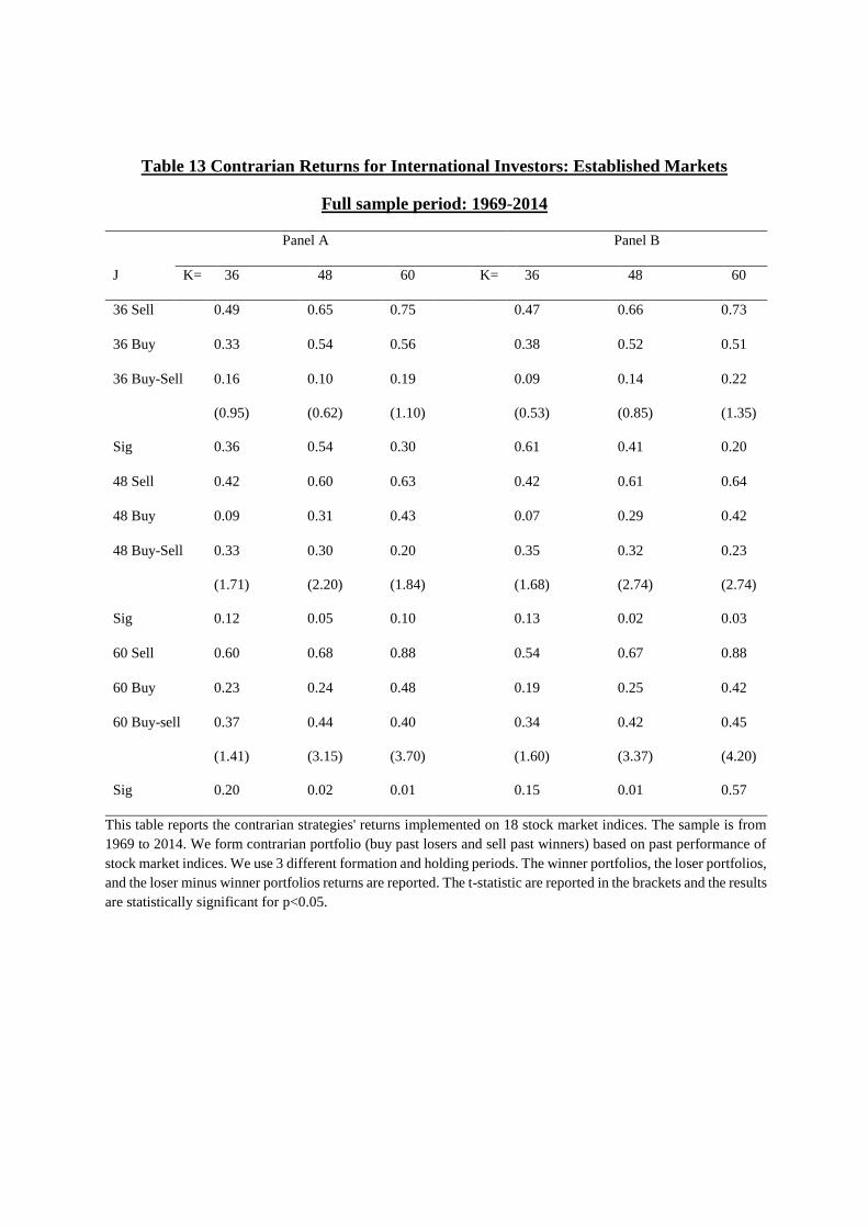
Table 13 Contrarian Returns for International Investors: Established Markets
Full sample period: 1969-2014
Panel A Panel B
J K= 36 48 60 K= 36 48 60
36 Sell 0.49 0.65 0.75 0.47 0.66 0.73
36 Buy 0.33 0.54 0.56 0.38 0.52 0.51
36 Buy-Sell
Sig
0.16
(0.95)
0.36
0.10
(0.62)
0.54
0.19
(1.10)
0.30
0.09
(0.53)
0.61
0.14
(0.85)
0.41
0.22
(1.35)
0.20
48 Sell 0.42 0.60 0.63 0.42 0.61 0.64
48 Buy 0.09 0.31 0.43 0.07 0.29 0.42
48 Buy-Sell
Sig
0.33
(1.71)
0.12
0.30
(2.20)
0.05
0.20
(1.84)
0.10
0.35
(1.68)
0.13
0.32
(2.74)
0.02
0.23
(2.74)
0.03
60 Sell 0.60 0.68 0.88 0.54 0.67 0.88
60 Buy 0.23 0.24 0.48 0.19 0.25 0.42
60 Buy-sell
Sig
0.37
(1.41)
0.20
0.44
(3.15)
0.02
0.40
(3.70)
0.01
0.34
(1.60)
0.15
0.42
(3.37)
0.01
0.45
(4.20)
0.57
This table reports the contrarian strategies' returns implemented on 18 stock market indices. The sample is from
1969 to 2014. We form contrarian portfolio (buy past losers and sell past winners) based on past performance of
stock market indices. We use 3 different formation and holding periods. The winner portfolios, the loser portfolios,
and the loser minus winner portfolios returns are reported. The t-statistic are reported in the brackets and the results
are statistically significant for p<0.05.
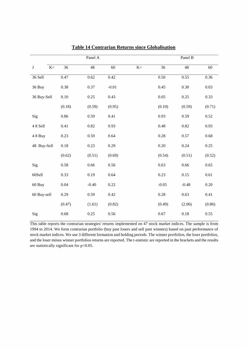
Table 14 Contrarian Returns since Globalisation
Panel A Panel B
J K= 36 48 60 K= 36 48 60
36 Sell 0.47 0.62 0.42 0.50 0.55 0.36
36 Buy 0.38 0.37 -0.01 0.45 0.30 0.03
36 Buy-Sell
Sig
0.10
(0.18)
0.86
0.25
(0.59)
0.59
0.43
(0.95)
0.41
0.05
(0.10)
0.93
0.25
(0.59)
0.59
0.33
(0.71)
0.52
4 8 Sell 0.41 0.82 0.93 0.48 0.82 0.93
4 8 Buy 0.23 0.59 0.64 0.28 0.57 0.68
48 Buy-Sell
Sig
0.18
(0.62)
0.58
0.23
(0.51)
0.66
0.29
(0.69)
0.56
0.20
(0.54)
0.63
0.24
(0.51)
0.66
0.25
(0.52)
0.65
60Sell 0.33 0.19 0.64 0.23 0.15 0.61
60 Buy 0.04 -0.40 0.22 -0.05 -0.48 0.20
60 Buy-sell
Sig
0.29
(0.47)
0.68
0.59
(1.61)
0.25
0.42
(0.82)
0.56
0.28
(0.49)
0.67
0.63
(2.06)
0.18
0.41
(0.86)
0.55
This table reports the contrarian strategies' returns implemented on 47 stock market indices. The sample is from
1994 to 2014. We form contrarian portfolio (buy past losers and sell past winners) based on past performance of
stock market indices. We use 3 different formation and holding periods. The winner portfolios, the loser portfolios,
and the loser minus winner portfolios returns are reported. The t-statistic are reported in the brackets and the results
are statistically significant for p<0.05.
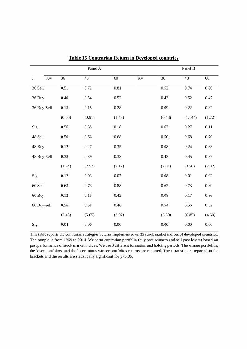
Table 15 Contrarian Return in Developed countries
Panel A Panel B
J K= 36 48 60 K= 36 48 60
36 Sell 0.51 0.72 0.81 0.52 0.74 0.80
36 Buy 0.40 0.54 0.52 0.43 0.52 0.47
36 Buy-Sell
Sig
0.13
(0.60)
0.56
0.18
(0.91)
0.38
0.28
(1.43)
0.18
0.09
(0.43)
0.67
0.22
(1.144)
0.27
0.32
(1.72)
0.11
48 Sell 0.50 0.66 0.68 0.50 0.68 0.70
48 Buy 0.12 0.27 0.35 0.08 0.24 0.33
48 Buy-Sell
Sig
0.38
(1.74)
0.12
0.39
(2.57)
0.03
0.33
(2.12)
0.07
0.43
(2.01)
0.08
0.45
(3.56)
0.01
0.37
(2.82)
0.02
60 Sell 0.63 0.73 0.88 0.62 0.73 0.89
60 Buy 0.12 0.15 0.42 0.08 0.17 0.36
60 Buy-sell
Sig
0.56
(2.48)
0.04
0.58
(5.65)
0.00
0.46
(3.97)
0.00
0.54
(3.59)
0.00
0.56
(6.85)
0.00
0.52
(4.60)
0.00
This table reports the contrarian strategies' returns implemented on 23 stock market indices of developed countries.
The sample is from 1969 to 2014. We form contrarian portfolio (buy past winners and sell past losers) based on
past performance of stock market indices. We use 3 different formation and holding periods. The winner portfolios,
the loser portfolios, and the loser minus winner portfolios returns are reported. The t-statistic are reported in the
brackets and the results are statistically significant for p<0.05.
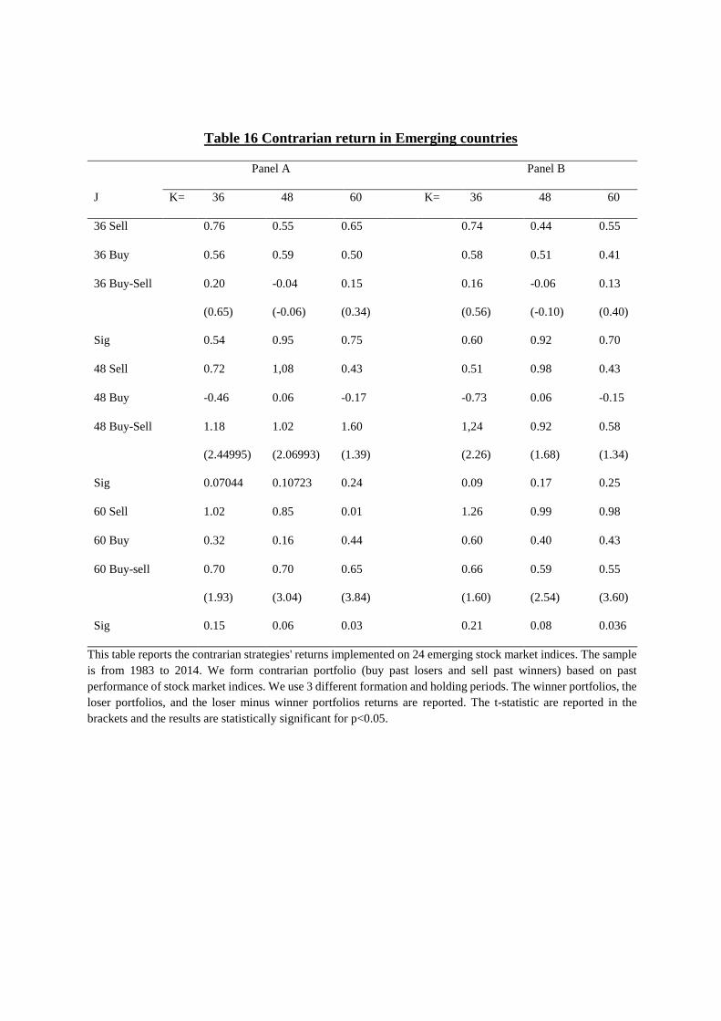
Table 16 Contrarian return in Emerging countries
Panel A Panel B
J K= 36 48 60 K= 36 48 60
36 Sell 0.76 0.55 0.65 0.74 0.44 0.55
36 Buy 0.56 0.59 0.50 0.58 0.51 0.41
36 Buy-Sell
Sig
0.20
(0.65)
0.54
-0.04
(-0.06)
0.95
0.15
(0.34)
0.75
0.16
(0.56)
0.60
-0.06
(-0.10)
0.92
0.13
(0.40)
0.70
48 Sell 0.72 1,08 0.43 0.51 0.98 0.43
48 Buy -0.46 0.06 -0.17 -0.73 0.06 -0.15
48 Buy-Sell
Sig
1.18
(2.44995)
0.07044
1.02
(2.06993)
0.10723
1.60
(1.39)
0.24
1,24
(2.26)
0.09
0.92
(1.68)
0.17
0.58
(1.34)
0.25
60 Sell 1.02 0.85 0.01 1.26 0.99 0.98
60 Buy 0.32 0.16 0.44 0.60 0.40 0.43
60 Buy-sell
Sig
0.70
(1.93)
0.15
0.70
(3.04)
0.06
0.65
(3.84)
0.03
0.66
(1.60)
0.21
0.59
(2.54)
0.08
0.55
(3.60)
0.036
This table reports the contrarian strategies' returns implemented on 24 emerging stock market indices. The sample
is from 1983 to 2014. We form contrarian portfolio (buy past losers and sell past winners) based on past
performance of stock market indices. We use 3 different formation and holding periods. The winner portfolios, the
loser portfolios, and the loser minus winner portfolios returns are reported. The t-statistic are reported in the
brackets and the results are statistically significant for p<0.05.
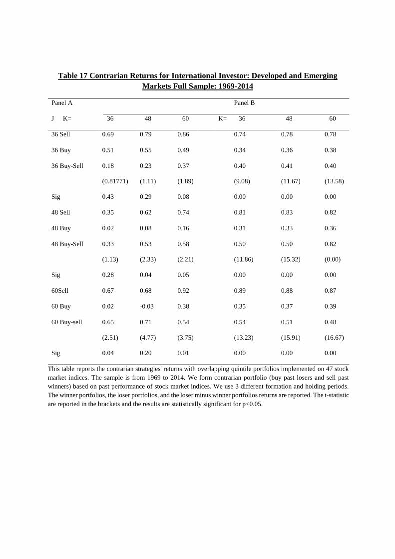
Table 17 Contrarian Returns for International Investor: Developed and Emerging
Markets Full Sample: 1969-2014
Panel A Panel B
J K= 36 48 60 K= 36 48 60
36 Sell 0.69 0.79 0.86 0.74 0.78 0.78
36 Buy 0.51 0.55 0.49 0.34 0.36 0.38
36 Buy-Sell
Sig
0.18
(0.81771)
0.43
0.23
(1.11)
0.29
0.37
(1.89)
0.08
0.40
(9.08)
0.00
0.41
(11.67)
0.00
0.40
(13.58)
0.00
48 Sell 0.35 0.62 0.74 0.81 0.83 0.82
48 Buy 0.02 0.08 0.16 0.31 0.33 0.36
48 Buy-Sell
Sig
0.33
(1.13)
0.28
0.53
(2.33)
0.04
0.58
(2.21)
0.05
0.50
(11.86)
0.00
0.50
(15.32)
0.00
0.82
(0.00)
0.00
60Sell 0.67 0.68 0.92 0.89 0.88 0.87
60 Buy 0.02 -0.03 0.38 0.35 0.37 0.39
60 Buy-sell
Sig
0.65
(2.51)
0.04
0.71
(4.77)
0.20
0.54
(3.75)
0.01
0.54
(13.23)
0.00
0.51
(15.91)
0.00
0.48
(16.67)
0.00
This table reports the contrarian strategies' returns with overlapping quintile portfolios implemented on 47 stock
market indices. The sample is from 1969 to 2014. We form contrarian portfolio (buy past losers and sell past
winners) based on past performance of stock market indices. We use 3 different formation and holding periods.
The winner portfolios, the loser portfolios, and the loser minus winner portfolios returns are reported. The t-statistic
are reported in the brackets and the results are statistically significant for p<0.05.
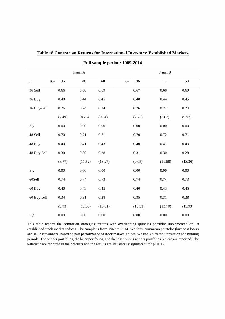
Table 18 Contrarian Returns for International Investors: Established Markets
Full sample period: 1969-2014
Panel A Panel B
J K= 36 48 60 K= 36 48 60
36 Sell 0.66 0.68 0.69 0.67 0.68 0.69
36 Buy 0.40 0.44 0.45 0.40 0.44 0.45
36 Buy-Sell
Sig
0.26
(7.49)
0.00
0.24
(8.73)
0.00
0.24
(9.84)
0.00
0.26
(7.73)
0.00
0.24
(8.83)
0.00
0.24
(9.97)
0.00
48 Sell 0.70 0.71 0.71 0.70 0.72 0.71
48 Buy 0.40 0.41 0.43 0.40 0.41 0.43
48 Buy-Sell
Sig
0.30
(8.77)
0.00
0.30
(11.52)
0.00
0.28
(13.27)
0.00
0.31
(9.05)
0.00
0.30
(11.58)
0.00
0.28
(13.36)
0.00
60Sell 0.74 0.74 0.73 0.74 0.74 0.73
60 Buy 0.40 0.43 0.45 0.40 0.43 0.45
60 Buy-sell
Sig
0.34
(9.93)
0.00
0.31
(12.36)
0.00
0.28
(13.61)
0.00
0.35
(10.31)
0.00
0.31
(12.70)
0.00
0.28
(13.93)
0.00
This table reports the contrarian strategies' returns with overlapping quintiles portfolio implemented on 18
established stock market indices. The sample is from 1969 to 2014. We form contrarian portfolio (buy past losers
and sell past winners) based on past performance of stock market indices. We use 3 different formation and holding
periods. The winner portfolios, the loser portfolios, and the loser minus winner portfolios returns are reported. The
t-statistic are reported in the brackets and the results are statistically significant for p<0.05.
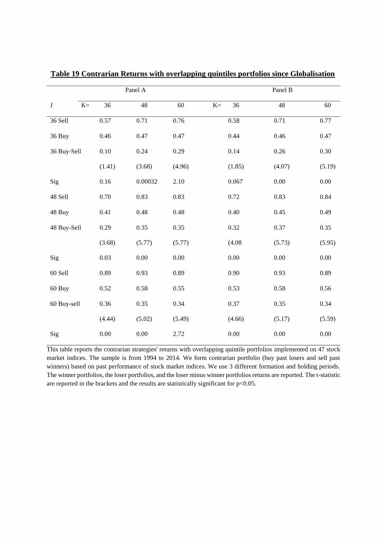
Table 19 Contrarian Returns with overlapping quintiles portfolios since Globalisation
Panel A Panel B
J K= 36 48 60 K= 36 48 60
36 Sell 0.57 0.71 0.76 0.58 0.71 0.77
36 Buy 0.46 0.47 0.47 0.44 0.46 0.47
36 Buy-Sell
Sig
0.10
(1.41)
0.16
0.24
(3.68)
0.00032
0.29
(4.96)
2.10
0.14
(1.85)
0.067
0.26
(4.07)
0.00
0.30
(5.19)
0.00
48 Sell 0.70 0.83 0.83 0.72 0.83 0.84
48 Buy 0.41 0.48 0.48 0.40 0.45 0.49
48 Buy-Sell
Sig
0.29
(3.68)
0.03
0.35
(5.77)
0.00
0.35
(5.77)
0.00
0.32
(4.08
0.00
0.37
(5.73)
0.00
0.35
(5.95)
0.00
60 Sell 0.89 0.93 0.89 0.90 0.93 0.89
60 Buy 0.52 0.58 0.55 0.53 0.58 0.56
60 Buy-sell
Sig
0.36
(4.44)
0.00
0.35
(5.02)
0.00
0.34
(5.49)
2.72
0.37
(4.66)
0.00
0.35
(5.17)
0.00
0.34
(5.59)
0.00
This table reports the contrarian strategies' returns with overlapping quintile portfolios implemented on 47 stock
market indices. The sample is from 1994 to 2014. We form contrarian portfolio (buy past losers and sell past
winners) based on past performance of stock market indices. We use 3 different formation and holding periods.
The winner portfolios, the loser portfolios, and the loser minus winner portfolios returns are reported. The t-statistic
are reported in the brackets and the results are statistically significant for p<0.05.
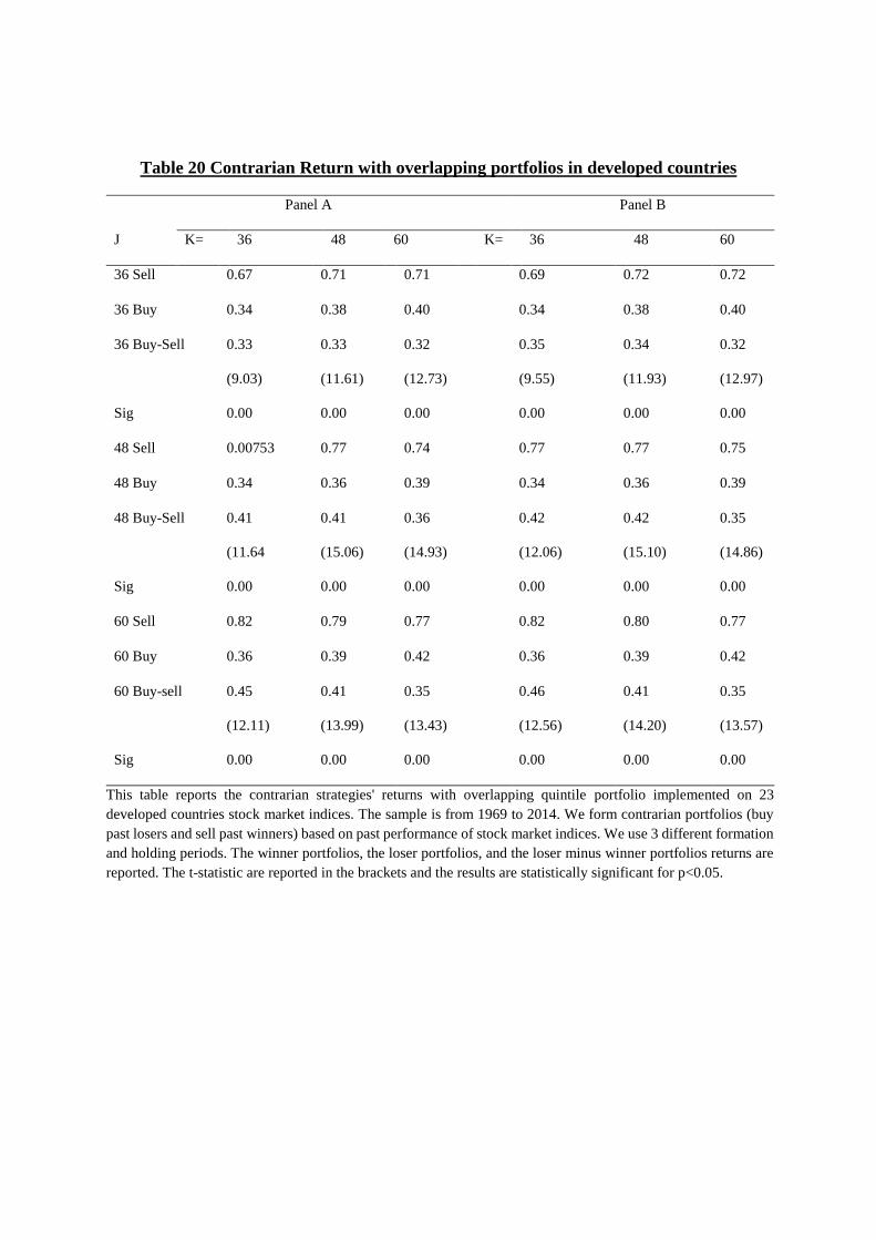
Table 20 Contrarian Return with overlapping portfolios in developed countries
Panel A Panel B
J K= 36 48 60 K= 36 48 60
36 Sell 0.67 0.71 0.71 0.69 0.72 0.72
36 Buy 0.34 0.38 0.40 0.34 0.38 0.40
36 Buy-Sell
Sig
0.33
(9.03)
0.00
0.33
(11.61)
0.00
0.32
(12.73)
0.00
0.35
(9.55)
0.00
0.34
(11.93)
0.00
0.32
(12.97)
0.00
48 Sell 0.00753 0.77 0.74 0.77 0.77 0.75
48 Buy 0.34 0.36 0.39 0.34 0.36 0.39
48 Buy-Sell
Sig
0.41
(11.64
0.00
0.41
(15.06)
0.00
0.36
(14.93)
0.00
0.42
(12.06)
0.00
0.42
(15.10)
0.00
0.35
(14.86)
0.00
60 Sell 0.82 0.79 0.77 0.82 0.80 0.77
60 Buy 0.36 0.39 0.42 0.36 0.39 0.42
60 Buy-sell
Sig
0.45
(12.11)
0.00
0.41
(13.99)
0.00
0.35
(13.43)
0.00
0.46
(12.56)
0.00
0.41
(14.20)
0.00
0.35
(13.57)
0.00
This table reports the contrarian strategies' returns with overlapping quintile portfolio implemented on 23
developed countries stock market indices. The sample is from 1969 to 2014. We form contrarian portfolios (buy
past losers and sell past winners) based on past performance of stock market indices. We use 3 different formation
and holding periods. The winner portfolios, the loser portfolios, and the loser minus winner portfolios returns are
reported. The t-statistic are reported in the brackets and the results are statistically significant for p<0.05.
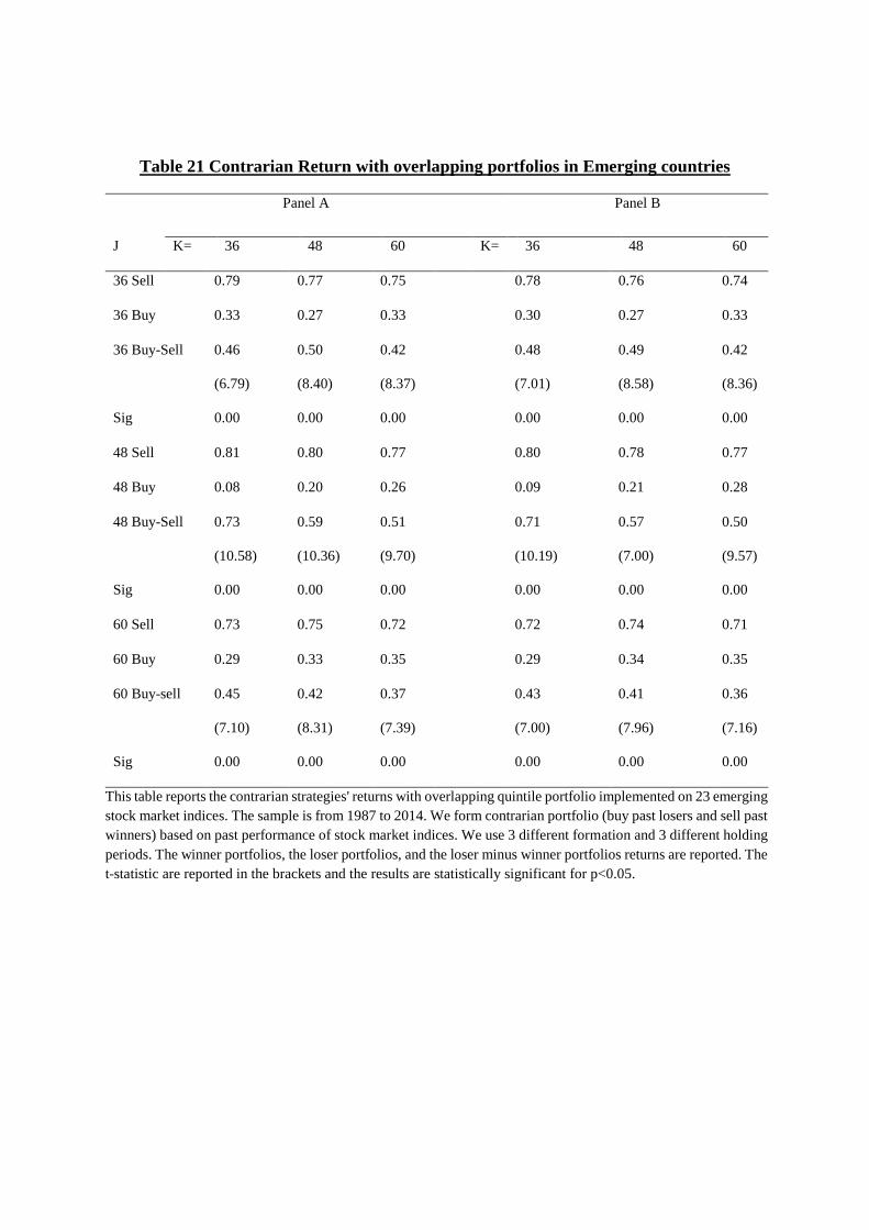
Table 21 Contrarian Return with overlapping portfolios in Emerging countries
Panel A Panel B
J K= 36 48 60 K= 36 48 60
36 Sell 0.79 0.77 0.75 0.78 0.76 0.74
36 Buy 0.33 0.27 0.33 0.30 0.27 0.33
36 Buy-Sell
Sig
0.46
(6.79)
0.00
0.50
(8.40)
0.00
0.42
(8.37)
0.00
0.48
(7.01)
0.00
0.49
(8.58)
0.00
0.42
(8.36)
0.00
48 Sell 0.81 0.80 0.77 0.80 0.78 0.77
48 Buy 0.08 0.20 0.26 0.09 0.21 0.28
48 Buy-Sell
Sig
0.73
(10.58)
0.00
0.59
(10.36)
0.00
0.51
(9.70)
0.00
0.71
(10.19)
0.00
0.57
(7.00)
0.00
0.50
(9.57)
0.00
60 Sell 0.73 0.75 0.72 0.72 0.74 0.71
60 Buy 0.29 0.33 0.35 0.29 0.34 0.35
60 Buy-sell
Sig
0.45
(7.10)
0.00
0.42
(8.31)
0.00
0.37
(7.39)
0.00
0.43
(7.00)
0.00
0.41
(7.96)
0.00
0.36
(7.16)
0.00
This table reports the contrarian strategies' returns with overlapping quintile portfolio implemented on 23 emerging
stock market indices. The sample is from 1987 to 2014. We form contrarian portfolio (buy past losers and sell past
winners) based on past performance of stock market indices. We use 3 different formation and 3 different holding
periods. The winner portfolios, the loser portfolios, and the loser minus winner portfolios returns are reported. The
t-statistic are reported in the brackets and the results are statistically significant for p<0.05.
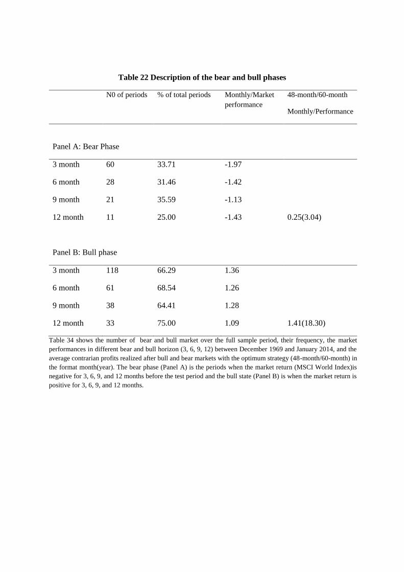
Table 22 Description of the bear and bull phases
N0 of periods % of total periods Monthly/Market
performance
48-month/60-month
Monthly/Performance
Panel A: Bear Phase
3 month 60 33.71 -1.97
6 month 28 31.46 -1.42
9 month 21 35.59 -1.13
12 month 11 25.00 -1.43 0.25(3.04)
Panel B: Bull phase
3 month 118 66.29 1.36
6 month 61 68.54 1.26
9 month 38 64.41 1.28
12 month 33 75.00 1.09 1.41(18.30)
Table 34 shows the number of bear and bull market over the full sample period, their frequency, the market
performances in different bear and bull horizon (3, 6, 9, 12) between December 1969 and January 2014, and the
average contrarian profits realized after bull and bear markets with the optimum strategy (48-month/60-month) in
the format month(year). The bear phase (Panel A) is the periods when the market return (MSCI World Index)is
negative for 3, 6, 9, and 12 months before the test period and the bull state (Panel B) is when the market return is
positive for 3, 6, 9, and 12 months.
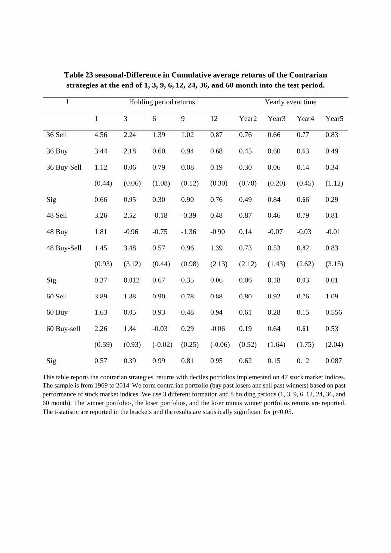
Table 23 seasonal-Difference in Cumulative average returns of the Contrarian
strategies at the end of 1, 3, 9, 6, 12, 24, 36, and 60 month into the test period.
J Holding period returns Yearly event time
1 3 6 9 12 Year2 Year3 Year4 Year5
36 Sell 4.56 2.24 1.39 1.02 0.87 0.76 0.66 0.77 0.83
36 Buy 3.44 2.18 0.60 0.94 0.68 0.45 0.60 0.63 0.49
36 Buy-Sell
Sig
1.12
(0.44)
0.66
0.06
(0.06)
0.95
0.79
(1.08)
0.30
0.08
(0.12)
0.90
0.19
(0.30)
0.76
0.30
(0.70)
0.49
0.06
(0.20)
0.84
0.14
(0.45)
0.66
0.34
(1.12)
0.29
48 Sell 3.26 2.52 -0.18 -0.39 0.48 0.87 0.46 0.79 0.81
48 Buy 1.81 -0.96 -0.75 -1.36 -0.90 0.14 -0.07 -0.03 -0.01
48 Buy-Sell
Sig
1.45
(0.93)
0.37
3.48
(3.12)
0.012
0.57
(0.44)
0.67
0.96
(0.98)
0.35
1.39
(2.13)
0.06
0.73
(2.12)
0.06
0.53
(1.43)
0.18
0.82
(2.62)
0.03
0.83
(3.15)
0.01
60 Sell 3.89 1.88 0.90 0.78 0.88 0.80 0.92 0.76 1.09
60 Buy 1.63 0.05 0.93 0.48 0.94 0.61 0.28 0.15 0.556
60 Buy-sell
Sig
2.26
(0.59)
0.57
1.84
(0.93)
0.39
-0.03
(-0.02)
0.99
0.29
(0.25)
0.81
-0.06
(-0.06)
0.95
0.19
(0.52)
0.62
0.64
(1.64)
0.15
0.61
(1.75)
0.12
0.53
(2.04)
0.087
This table reports the contrarian strategies' returns with deciles portfolios implemented on 47 stock market indices.
The sample is from 1969 to 2014. We form contrarian portfolio (buy past losers and sell past winners) based on past
performance of stock market indices. We use 3 different formation and 8 holding periods (1, 3, 9, 6, 12, 24, 36, and
60 month). The winner portfolios, the loser portfolios, and the loser minus winner portfolios returns are reported.
The t-statistic are reported in the brackets and the results are statistically significant for p<0.05.
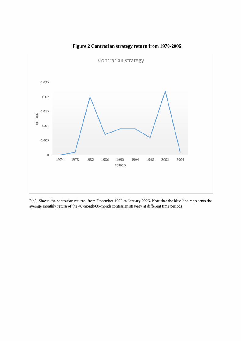
Figure 2 Contrarian strategy return from 1970-2006
Fig2. Shows the contrarian returns, from December 1970 to January 2006. Note that the blue line represents the
average monthly return of the 48-month/60-month contrarian strategy at different time periods.
1974 1978 1982 1986 1990 1994 1998 2002 2006
0
0.005
0.01
0.015
0.02
0.025
PERIOD
RET
UR
N
Contrarian strategy
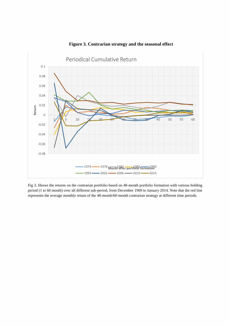
Figure 3. Contrarian strategy and the seasonal effect
Fig 3. Shows the returns on the contrarian portfolio based on 48-month portfolio formation with various holding
period (1 to 60 month) over all different sub-period, from December 1969 to January 2014. Note that the red line
represents the average monthly return of the 48-month/60-month contrarian strategy at different time periods.
1 5 10 15 20 25 30 35 40 45 50 55 60
-0.08
-0.06
-0.04
-0.02
0
0.02
0.04
0.06
0.08
0.1
Month after portfolio formation
Re
turn
Periodical Cumulative Return
1974 1978 1982 1986 1990
1994 2002 2006 2010 2014
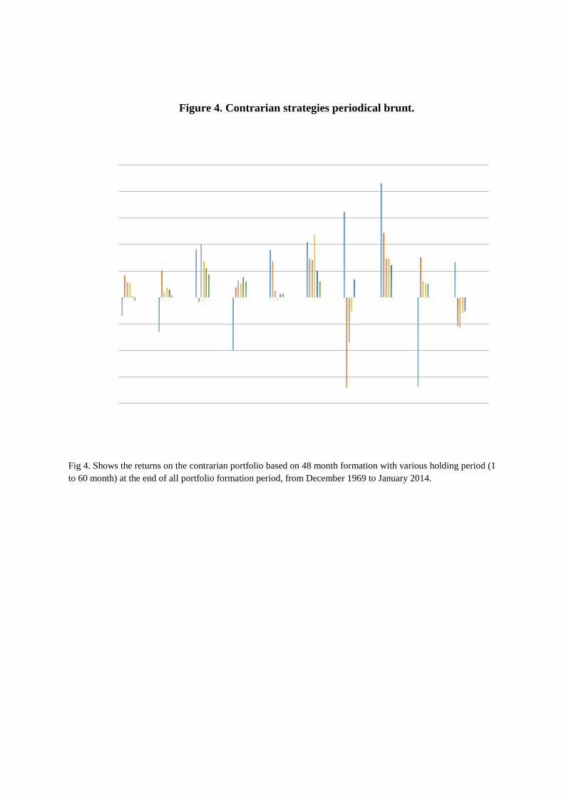
Figure 4. Contrarian strategies periodical brunt.
Fig 4. Shows the returns on the contrarian portfolio based on 48 month formation with various holding period (1
to 60 month) at the end of all portfolio formation period, from December 1969 to January 2014.
1974 1978 1982 1986 1990 1994 2002 2006 2010 2014
-0.08
-0.06
-0.04
-0.02
0
0.02
0.04
0.06
0.08
0.1
PERIOD
RET
UR
N
PERIODICAL RETURN
1 5 10 15 20 25 30 35 40 45 50 55 60
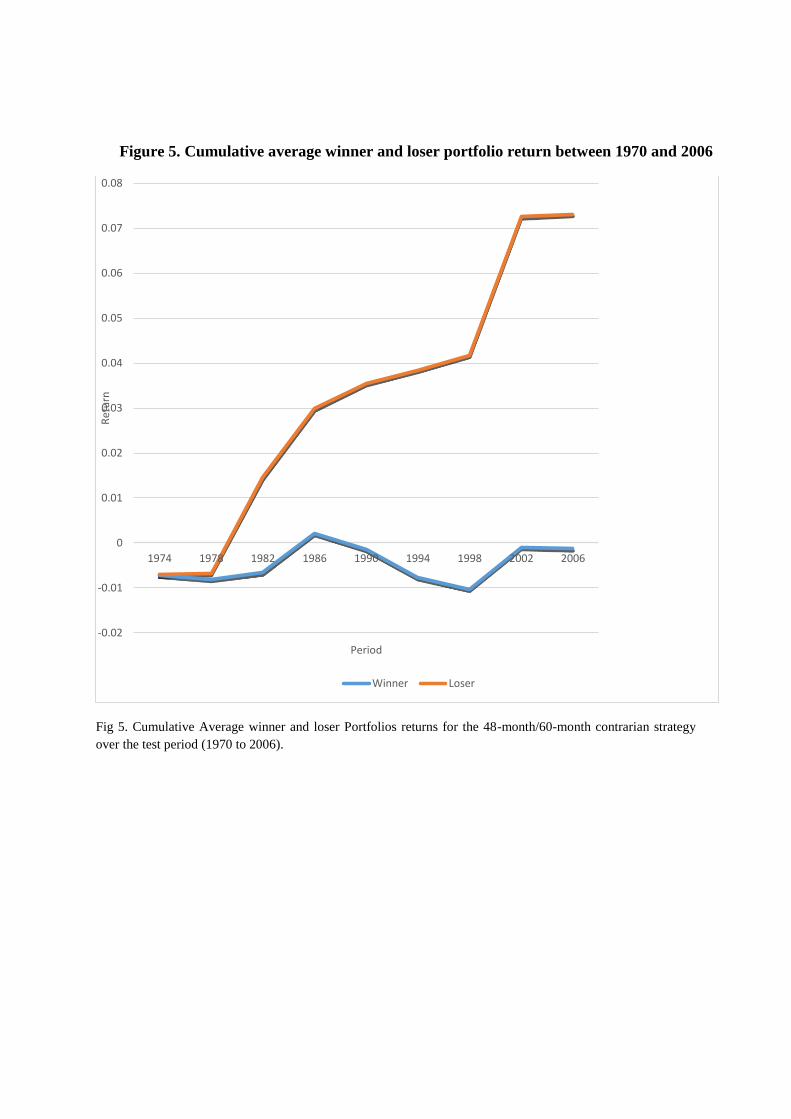
Figure 5. Cumulative average winner and loser portfolio return between 1970 and 2006
Fig 5. Cumulative Average winner and loser Portfolios returns for the 48-month/60-month contrarian strategy
over the test period (1970 to 2006).
1974 1978 1982 1986 1990 1994 1998 2002 2006
-0.02
-0.01
0
0.01
0.02
0.03
0.04
0.05
0.06
0.07
0.08
Period
Ret
urn
Winner Loser
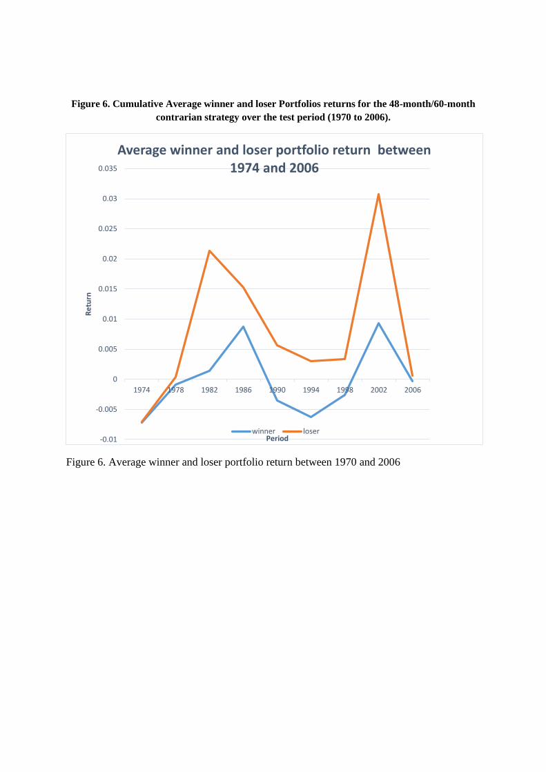
Figure 6. Cumulative Average winner and loser Portfolios returns for the 48-month/60-month
contrarian strategy over the test period (1970 to 2006).
Figure 6. Average winner and loser portfolio return between 1970 and 2006
1974 1978 1982 1986 1990 1994 1998 2002 2006
-0.01
-0.005
0
0.005
0.01
0.015
0.02
0.025
0.03
0.035
Period
Re
turn
Average winner and loser portfolio return between 1974 and 2006
winner loser