Global Carbon Budget 2016 - earth-syst-sci-data.net · C. Le Quéré et al.: Global Carbon Budget...
45
Earth Syst. Sci. Data, 8, 605–649, 2016 www.earth-syst-sci-data.net/8/605/2016/ doi:10.5194/essd-8-605-2016 © Author(s) 2016. CC Attribution 3.0 License. Global Carbon Budget 2016 Corinne Le Quéré 1 , Robbie M. Andrew 2 , Josep G. Canadell 3 , Stephen Sitch 4 , Jan Ivar Korsbakken 2 , Glen P. Peters 2 , Andrew C. Manning 5 , Thomas A. Boden 6 , Pieter P. Tans 7 , Richard A. Houghton 8 , Ralph F. Keeling 9 , Simone Alin 10 , Oliver D. Andrews 1 , Peter Anthoni 11 , Leticia Barbero 12,13 , Laurent Bopp 14 , Frédéric Chevallier 14 , Louise P. Chini 15 , Philippe Ciais 14 , Kim Currie 16 , Christine Delire 17 , Scott C. Doney 18 , Pierre Friedlingstein 19 , Thanos Gkritzalis 20 , Ian Harris 21 , Judith Hauck 22 , Vanessa Haverd 23 , Mario Hoppema 22 , Kees Klein Goldewijk 24 , Atul K. Jain 25 , Etsushi Kato 26 , Arne Körtzinger 27 , Peter Landschützer 28 , Nathalie Lefèvre 29 , Andrew Lenton 30 , Sebastian Lienert 31,32 , Danica Lombardozzi 33 , Joe R. Melton 34 , Nicolas Metzl 29 , Frank Millero 35 , Pedro M. S. Monteiro 36 , David R. Munro 37 , Julia E. M. S. Nabel 28 , Shin-ichiro Nakaoka 38 , Kevin O’Brien 39 , Are Olsen 40 , Abdirahman M. Omar 40 , Tsuneo Ono 41 , Denis Pierrot 12,13 , Benjamin Poulter 42,43 , Christian Rödenbeck 44 , Joe Salisbury 45 , Ute Schuster 4 , Jörg Schwinger 46 , Roland Séférian 17 , Ingunn Skjelvan 46 , Benjamin D. Stocker 47 , Adrienne J. Sutton 39,10 , Taro Takahashi 48 , Hanqin Tian 49 , Bronte Tilbrook 50 , Ingrid T. van der Laan-Luijkx 51 , Guido R. van der Werf 52 , Nicolas Viovy 14 , Anthony P. Walker 53 , Andrew J. Wiltshire 54 , and Sönke Zaehle 44 1 Tyndall Centre for Climate Change Research, University of East Anglia, Norwich Research Park, Norwich, NR4 7TJ, UK 2 Center for International Climate and Environmental Research – Oslo (CICERO), Oslo, Norway 3 Global Carbon Project, CSIRO Oceans and Atmosphere, GPO Box 3023, Canberra, ACT 2601, Australia 4 College of Life and Environmental Sciences, University of Exeter, Exeter, EX4 4RJ, UK 5 Centre for Ocean and Atmospheric Sciences, School of Environmental Sciences, University of East Anglia, Norwich Research Park, Norwich, NR4 7TJ, UK 6 Carbon Dioxide Information Analysis Center (CDIAC), Oak Ridge National Laboratory, Oak Ridge, TN, USA 7 National Oceanic & Atmospheric Administration, Earth System Research Laboratory (NOAA/ESRL), Boulder, CO 80305, USA 8 Woods Hole Research Center (WHRC), Falmouth, MA 02540, USA 9 University of California, San Diego, Scripps Institution of Oceanography, La Jolla, CA 92093-0244, USA 10 National Oceanic & Atmospheric Administration/Pacific Marine Environmental Laboratory (NOAA/PMEL), 7600 Sand Point Way NE, Seattle, WA 98115, USA 11 Karlsruhe Institute of Technology, Institute of Meteorology and Climate Research/Atmospheric Environmental Research, 82467 Garmisch-Partenkirchen, Germany 12 Cooperative Institute for Marine and Atmospheric Studies, Rosenstiel School for Marine and Atmospheric Science, University of Miami, Miami, FL 33149, USA 13 National Oceanic & Atmospheric Administration/Atlantic Oceanographic & Meteorological Laboratory (NOAA/AOML), Miami, FL 33149, USA 14 Laboratoire des Sciences du Climat et de l’Environnement, Institut Pierre-Simon Laplace, CEA-CNRS-UVSQ, CE Orme des Merisiers, 91191 Gif sur Yvette CEDEX, France 15 Department of Geographical Sciences, University of Maryland, College Park, MD 20742, USA 16 National Institute of Water and Atmospheric Research (NIWA), Dunedin 9054, New Zealand 17 Centre National de Recherche Météorologique, Unite mixte de recherche 3589 Météo-France/CNRS, 42 Avenue Gaspard Coriolis, 31100 Toulouse, France 18 Woods Hole Oceanographic Institution (WHOI), Woods Hole, MA 02543, USA 19 College of Engineering, Mathematics and Physical Sciences, University of Exeter, Exeter, EX4 4QF, UK 20 Flanders Marine Institute, InnovOcean, Wandelaarkaai 7, 8400 Ostend, Belgium 21 Climatic Research Unit, University of East Anglia, Norwich Research Park, Norwich, NR4 7TJ, UK Published by Copernicus Publications.
Transcript of Global Carbon Budget 2016 - earth-syst-sci-data.net · C. Le Quéré et al.: Global Carbon Budget...
Earth Syst. Sci. Data, 8, 605–649, 2016www.earth-syst-sci-data.net/8/605/2016/doi:10.5194/essd-8-605-2016© Author(s) 2016. CC Attribution 3.0 License.
Global Carbon Budget 2016
Corinne Le Quéré1, Robbie M. Andrew2, Josep G. Canadell3, Stephen Sitch4, Jan Ivar Korsbakken2,Glen P. Peters2, Andrew C. Manning5, Thomas A. Boden6, Pieter P. Tans7, Richard A. Houghton8,
Ralph F. Keeling9, Simone Alin10, Oliver D. Andrews1, Peter Anthoni11, Leticia Barbero12,13,Laurent Bopp14, Frédéric Chevallier14, Louise P. Chini15, Philippe Ciais14, Kim Currie16,
Christine Delire17, Scott C. Doney18, Pierre Friedlingstein19, Thanos Gkritzalis20, Ian Harris21,Judith Hauck22, Vanessa Haverd23, Mario Hoppema22, Kees Klein Goldewijk24, Atul K. Jain25,
Etsushi Kato26, Arne Körtzinger27, Peter Landschützer28, Nathalie Lefèvre29, Andrew Lenton30,Sebastian Lienert31,32, Danica Lombardozzi33, Joe R. Melton34, Nicolas Metzl29, Frank Millero35,
Pedro M. S. Monteiro36, David R. Munro37, Julia E. M. S. Nabel28, Shin-ichiro Nakaoka38,Kevin O’Brien39, Are Olsen40, Abdirahman M. Omar40, Tsuneo Ono41, Denis Pierrot12,13,
Benjamin Poulter42,43, Christian Rödenbeck44, Joe Salisbury45, Ute Schuster4, Jörg Schwinger46,Roland Séférian17, Ingunn Skjelvan46, Benjamin D. Stocker47, Adrienne J. Sutton39,10, Taro Takahashi48,
Hanqin Tian49, Bronte Tilbrook50, Ingrid T. van der Laan-Luijkx51, Guido R. van der Werf52,Nicolas Viovy14, Anthony P. Walker53, Andrew J. Wiltshire54, and Sönke Zaehle44
1Tyndall Centre for Climate Change Research, University of East Anglia, Norwich Research Park,Norwich, NR4 7TJ, UK
2Center for International Climate and Environmental Research – Oslo (CICERO), Oslo, Norway3Global Carbon Project, CSIRO Oceans and Atmosphere, GPO Box 3023, Canberra, ACT 2601, Australia
4College of Life and Environmental Sciences, University of Exeter, Exeter, EX4 4RJ, UK5Centre for Ocean and Atmospheric Sciences, School of Environmental Sciences, University of East Anglia,
Norwich Research Park, Norwich, NR4 7TJ, UK6Carbon Dioxide Information Analysis Center (CDIAC), Oak Ridge National Laboratory, Oak Ridge, TN, USA
7National Oceanic & Atmospheric Administration, Earth System Research Laboratory (NOAA/ESRL),Boulder, CO 80305, USA
8Woods Hole Research Center (WHRC), Falmouth, MA 02540, USA9University of California, San Diego, Scripps Institution of Oceanography, La Jolla, CA 92093-0244, USA
10National Oceanic & Atmospheric Administration/Pacific Marine Environmental Laboratory (NOAA/PMEL),7600 Sand Point Way NE, Seattle, WA 98115, USA
11Karlsruhe Institute of Technology, Institute of Meteorology and Climate Research/AtmosphericEnvironmental Research, 82467 Garmisch-Partenkirchen, Germany
12Cooperative Institute for Marine and Atmospheric Studies, Rosenstiel School for Marine andAtmospheric Science, University of Miami, Miami, FL 33149, USA
13National Oceanic & Atmospheric Administration/Atlantic Oceanographic & Meteorological Laboratory(NOAA/AOML), Miami, FL 33149, USA
14Laboratoire des Sciences du Climat et de l’Environnement, Institut Pierre-Simon Laplace,CEA-CNRS-UVSQ, CE Orme des Merisiers, 91191 Gif sur Yvette CEDEX, France
15Department of Geographical Sciences, University of Maryland, College Park, MD 20742, USA16National Institute of Water and Atmospheric Research (NIWA), Dunedin 9054, New Zealand
17Centre National de Recherche Météorologique, Unite mixte de recherche 3589 Météo-France/CNRS,42 Avenue Gaspard Coriolis, 31100 Toulouse, France
18Woods Hole Oceanographic Institution (WHOI), Woods Hole, MA 02543, USA19College of Engineering, Mathematics and Physical Sciences, University of Exeter, Exeter, EX4 4QF, UK
20Flanders Marine Institute, InnovOcean, Wandelaarkaai 7, 8400 Ostend, Belgium21Climatic Research Unit, University of East Anglia, Norwich Research Park, Norwich, NR4 7TJ, UK
Published by Copernicus Publications.

606 C. Le Quéré et al.: Global Carbon Budget 2016
22Alfred Wegener Institute Helmholtz Centre for Polar and Marine Research, Postfach 120161,27515 Bremerhaven, Germany
23CSIRO Oceans and Atmosphere, GPO Box 1700, Canberra, ACT 2601, Australia24PBL Netherlands Environmental Assessment Agency, The Hague/Bilthoven and Utrecht University,
Utrecht, the Netherlands25Department of Atmospheric Sciences, University of Illinois, Urbana, IL 61821, USA
26Institute of Applied Energy (IAE), Minato-ku, Tokyo 105-0003, Japan27GEOMAR Helmholtz Centre for Ocean Research Kiel, Düsternbrooker Weg 20, 24105 Kiel, Germany
28Max Planck Institute for Meteorology, Bundesstr. 53, 20146 Hamburg, Germany29Sorbonne Universités (UPMC, Univ Paris 06), CNRS, IRD, MNHN, LOCEAN/IPSL Laboratory,
75252 Paris, France30CSIRO Oceans and Atmosphere, P.O. Box 1538, Hobart, TAS, Australia
31Climate and Environmental Physics, Physics Institute, University of Bern, Bern, Switzerland32Oeschger Centre for Climate Change Research, University of Bern, Bern, Switzerland
33National Center for Atmospheric Research, Climate and Global Dynamics, Terrestrial Sciences Section,Boulder, CO 80305, USA
34Climate Research Division, Environment and Climate Change Canada, Victoria, Canada35Department of Ocean Sciences, RSMAS/MAC, University of Miami, 4600 Rickenbacker Causeway, Miami,
FL 33149, USA36Ocean Systems and Climate, CSIR-CHPC, Cape Town, 7700, South Africa
37Department of Atmospheric and Oceanic Sciences and Institute of Arctic and Alpine Research,University of Colorado, Campus Box 450, Boulder, CO 80309-0450, USA
38Center for Global Environmental Research, National Institute for Environmental Studies (NIES),16-2 Onogawa, Tsukuba, Ibaraki 305-8506, Japan
39Joint Institute for the Study of the Atmosphere and Ocean, University of Washington, Seattle,WA 98195, USA
40Geophysical Institute, University of Bergen and Bjerknes Centre for Climate Research, Allégaten 70,5007 Bergen, Norway
41National Research Institute for Far Sea Fisheries, Japan Fisheries Research and Education Agency 2-12-4Fukuura, Kanazawa-Ku, Yokohama 236-8648, Japan
42NASA Goddard Space Flight Center, Biospheric Science Laboratory, Greenbelt, MD 20771, USA43Department of Ecology, Montana State University, Bozeman, MT 59717, USA
44Max Planck Institute for Biogeochemistry, P.O. Box 600164, Hans-Knöll-Str. 10, 07745 Jena, Germany45University of New Hampshire, Ocean Process Analysis Laboratory, 161 Morse Hall, 8 College Road,
Durham, NH 03824, USA46Uni Research Climate, Bjerknes Centre for Climate Research, Nygårdsgaten 112, 5008 Bergen, Norway
47Imperial College London, Life Science Department, Silwood Park, Ascot, Berkshire, SL5 7PY, UK48Lamont-Doherty Earth Observatory of Columbia University, Palisades, NY 10964, USA
49School of Forestry and Wildlife Sciences, Auburn University, 602 Ducan Drive, Auburn, AL 36849, USA50CSIRO Oceans and Atmosphere and Antarctic Climate and Ecosystems Cooperative Research Centre,
Hobart, TAS, Australia51Department of Meteorology and Air Quality, Wageningen University & Research, P.O. Box 47,
6700AA Wageningen, the Netherlands52Faculty of Earth and Life Sciences, VU University Amsterdam, Amsterdam, the Netherlands
53Environmental Sciences Division & Climate Change Science Institute, Oak Ridge National Laboratory,Oak Ridge, TN, USA
54Met Office Hadley Centre, FitzRoy Road, Exeter, EX1 3PB, UK
Correspondence to: Corinne Le Quéré ([email protected])
Received: 5 October 2016 – Published in Earth Syst. Sci. Data Discuss.: 12 October 2016Revised: 12 October 2016 – Accepted: 18 October 2016 – Published: 14 November 2016
Abstract. Accurate assessment of anthropogenic carbon dioxide (CO2) emissions and their redistributionamong the atmosphere, ocean, and terrestrial biosphere – the “global carbon budget” – is important to betterunderstand the global carbon cycle, support the development of climate policies, and project future climate
Earth Syst. Sci. Data, 8, 605–649, 2016 www.earth-syst-sci-data.net/8/605/2016/

C. Le Quéré et al.: Global Carbon Budget 2016 607
change. Here we describe data sets and methodology to quantify all major components of the global carbon bud-get, including their uncertainties, based on the combination of a range of data, algorithms, statistics, and modelestimates and their interpretation by a broad scientific community. We discuss changes compared to previousestimates and consistency within and among components, alongside methodology and data limitations. CO2emissions from fossil fuels and industry (EFF) are based on energy statistics and cement production data, respec-tively, while emissions from land-use change (ELUC), mainly deforestation, are based on combined evidencefrom land-cover change data, fire activity associated with deforestation, and models. The global atmosphericCO2 concentration is measured directly and its rate of growth (GATM) is computed from the annual changesin concentration. The mean ocean CO2 sink (SOCEAN) is based on observations from the 1990s, while the an-nual anomalies and trends are estimated with ocean models. The variability in SOCEAN is evaluated with dataproducts based on surveys of ocean CO2 measurements. The global residual terrestrial CO2 sink (SLAND) isestimated by the difference of the other terms of the global carbon budget and compared to results of indepen-dent dynamic global vegetation models. We compare the mean land and ocean fluxes and their variability toestimates from three atmospheric inverse methods for three broad latitude bands. All uncertainties are reportedas ±1σ , reflecting the current capacity to characterise the annual estimates of each component of the global car-bon budget. For the last decade available (2006–2015), EFF was 9.3± 0.5 GtC yr−1, ELUC 1.0± 0.5 GtC yr−1,GATM 4.5± 0.1 GtC yr−1, SOCEAN 2.6± 0.5 GtC yr−1, and SLAND 3.1± 0.9 GtC yr−1. For year 2015 alone, thegrowth in EFF was approximately zero and emissions remained at 9.9± 0.5 GtC yr−1, showing a slowdown ingrowth of these emissions compared to the average growth of 1.8 % yr−1 that took place during 2006–2015.Also, for 2015, ELUC was 1.3± 0.5 GtC yr−1, GATM was 6.3± 0.2 GtC yr−1, SOCEAN was 3.0± 0.5 GtC yr−1,and SLAND was 1.9± 0.9 GtC yr−1.GATM was higher in 2015 compared to the past decade (2006–2015), reflect-ing a smaller SLAND for that year. The global atmospheric CO2 concentration reached 399.4± 0.1 ppm averagedover 2015. For 2016, preliminary data indicate the continuation of low growth in EFF with +0.2 % (range of−1.0 to +1.8 %) based on national emissions projections for China and USA, and projections of gross domesticproduct corrected for recent changes in the carbon intensity of the economy for the rest of the world. In spite ofthe low growth of EFF in 2016, the growth rate in atmospheric CO2 concentration is expected to be relativelyhigh because of the persistence of the smaller residual terrestrial sink (SLAND) in response to El Niño conditionsof 2015–2016. From this projection of EFF and assumed constant ELUC for 2016, cumulative emissions of CO2will reach 565± 55 GtC (2075± 205 GtCO2) for 1870–2016, about 75 % from EFF and 25 % from ELUC. Thisliving data update documents changes in the methods and data sets used in this new carbon budget compared withprevious publications of this data set (Le Quéré et al., 2015b, a, 2014, 2013). All observations presented here canbe downloaded from the Carbon Dioxide Information Analysis Center (doi:10.3334/CDIAC/GCP_2016).
1 Introduction
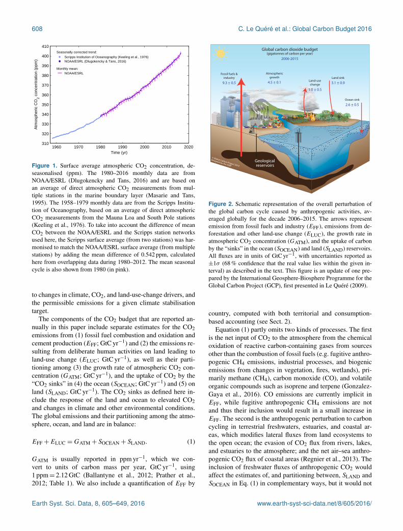
The concentration of carbon dioxide (CO2) in the atmospherehas increased from approximately 277 parts per million(ppm) in 1750 (Joos and Spahni, 2008), the beginning of theindustrial era, to 399.4± 0.1 ppm in 2015 (Dlugokencky andTans, 2016). The Mauna Loa station, which holds the longestrunning record of direct measurements of atmospheric CO2concentration (Tans and Keeling, 2014), went above 400 ppmfor the first time in May 2013 (Scripps, 2013). The globalmonthly average concentration was above 400 ppm in Marchthrough May 2015 and again since November 2015 (Dlu-gokencky and Tans, 2016; Fig. 1). The atmospheric CO2increase above pre-industrial levels was, initially, primar-ily caused by the release of carbon to the atmosphere fromdeforestation and other land-use-change activities (Ciais etal., 2013). While emissions from fossil fuels started beforethe industrial era, they only became the dominant sourceof anthropogenic emissions to the atmosphere from around
1920, and their relative share has continued to increase untilpresent. Anthropogenic emissions occur on top of an activenatural carbon cycle that circulates carbon between the reser-voirs of the atmosphere, ocean, and terrestrial biosphere ontimescales from sub-daily to millennia, while exchanges withgeologic reservoirs occur at longer timescales (Archer et al.,2009).
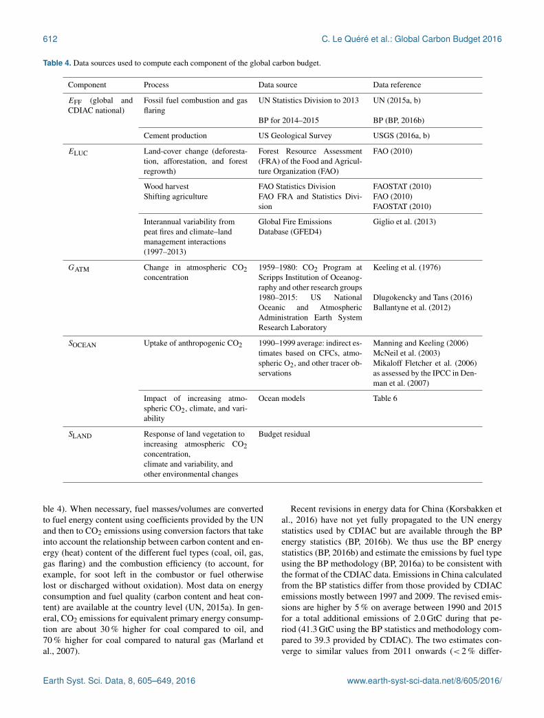
The global carbon budget presented here refers to themean, variations, and trends in the perturbation of CO2 inthe atmosphere, referenced to the beginning of the industrialera. It quantifies the input of CO2 to the atmosphere by emis-sions from human activities, the growth rate of atmosphericCO2 concentration, and the resulting changes in the storageof carbon in the land and ocean reservoirs in response to in-creasing atmospheric CO2 levels, climate change and vari-ability, and other anthropogenic and natural changes (Fig. 2).An understanding of this perturbation budget over time andthe underlying variability and trends of the natural carbon cy-cle is necessary to understand the response of natural sinks
www.earth-syst-sci-data.net/8/605/2016/ Earth Syst. Sci. Data, 8, 605–649, 2016
608 C. Le Quéré et al.: Global Carbon Budget 2016
1960 1970 1980 1990 2000 2010 2020310
320
330
340
350
360
370
380
390
400
410
Time (yr)
Atm
osph
eric
CO
2 con
cent
ratio
n (p
pm)
Seasonally corrected trend:
Monthly mean:
Scripps Institution of Oceanography (Keeling et al., 1976)NOAA/ESRL (Dlugokencky & Tans, 2016)
NOAA/ESRL
Figure 1. Surface average atmospheric CO2 concentration, de-seasonalised (ppm). The 1980–2016 monthly data are fromNOAA/ESRL (Dlugokencky and Tans, 2016) and are based onan average of direct atmospheric CO2 measurements from mul-tiple stations in the marine boundary layer (Masarie and Tans,1995). The 1958–1979 monthly data are from the Scripps Institu-tion of Oceanography, based on an average of direct atmosphericCO2 measurements from the Mauna Loa and South Pole stations(Keeling et al., 1976). To take into account the difference of meanCO2 between the NOAA/ESRL and the Scripps station networksused here, the Scripps surface average (from two stations) was har-monised to match the NOAA/ESRL surface average (from multiplestations) by adding the mean difference of 0.542 ppm, calculatedhere from overlapping data during 1980–2012. The mean seasonalcycle is also shown from 1980 (in pink).
to changes in climate, CO2, and land-use-change drivers, andthe permissible emissions for a given climate stabilisationtarget.
The components of the CO2 budget that are reported an-nually in this paper include separate estimates for the CO2emissions from (1) fossil fuel combustion and oxidation andcement production (EFF; GtC yr−1) and (2) the emissions re-sulting from deliberate human activities on land leading toland-use change (ELUC; GtC yr−1), as well as their parti-tioning among (3) the growth rate of atmospheric CO2 con-centration (GATM; GtC yr−1), and the uptake of CO2 by the“CO2 sinks” in (4) the ocean (SOCEAN; GtC yr−1) and (5) onland (SLAND; GtC yr−1). The CO2 sinks as defined here in-clude the response of the land and ocean to elevated CO2and changes in climate and other environmental conditions.The global emissions and their partitioning among the atmo-sphere, ocean, and land are in balance:
EFF+ELUC =GATM+ SOCEAN+ SLAND. (1)
GATM is usually reported in ppm yr−1, which we con-vert to units of carbon mass per year, GtC yr−1, using1 ppm= 2.12 GtC (Ballantyne et al., 2012; Prather et al.,2012; Table 1). We also include a quantification of EFF by
Fossil fuels & industry
9.3 ± 0.5 Land-use change
1.0 ± 0.5
Land sink
3.1 ± 0.9
Ocean sink
2.6 ± 0.5
Atmospheric growth
4.5 ± 0.1
Geological reservoirs
Global carbon dioxide budget (gigatonnes of carbon per year)
2006-2015
© Global Carbon Project 2014
Designed by the IGBP
Figure 2. Schematic representation of the overall perturbation ofthe global carbon cycle caused by anthropogenic activities, av-eraged globally for the decade 2006–2015. The arrows representemission from fossil fuels and industry (EFF), emissions from de-forestation and other land-use change (ELUC), the growth rate inatmospheric CO2 concentration (GATM), and the uptake of carbonby the “sinks” in the ocean (SOCEAN) and land (SLAND) reservoirs.All fluxes are in units of GtC yr−1, with uncertainties reported as±1σ (68 % confidence that the real value lies within the given in-terval) as described in the text. This figure is an update of one pre-pared by the International Geosphere-Biosphere Programme for theGlobal Carbon Project (GCP), first presented in Le Quéré (2009).
country, computed with both territorial and consumption-based accounting (see Sect. 2).
Equation (1) partly omits two kinds of processes. The firstis the net input of CO2 to the atmosphere from the chemicaloxidation of reactive carbon-containing gases from sourcesother than the combustion of fossil fuels (e.g. fugitive anthro-pogenic CH4 emissions, industrial processes, and biogenicemissions from changes in vegetation, fires, wetlands), pri-marily methane (CH4), carbon monoxide (CO), and volatileorganic compounds such as isoprene and terpene (Gonzalez-Gaya et al., 2016). CO emissions are currently implicit inEFF, while fugitive anthropogenic CH4 emissions are notand thus their inclusion would result in a small increase inEFF. The second is the anthropogenic perturbation to carboncycling in terrestrial freshwaters, estuaries, and coastal ar-eas, which modifies lateral fluxes from land ecosystems tothe open ocean; the evasion of CO2 flux from rivers, lakes,and estuaries to the atmosphere; and the net air–sea anthro-pogenic CO2 flux of coastal areas (Regnier et al., 2013). Theinclusion of freshwater fluxes of anthropogenic CO2 wouldaffect the estimates of, and partitioning between, SLAND andSOCEAN in Eq. (1) in complementary ways, but it would not
Earth Syst. Sci. Data, 8, 605–649, 2016 www.earth-syst-sci-data.net/8/605/2016/

C. Le Quéré et al.: Global Carbon Budget 2016 609
Table 1. Factors used to convert carbon in various units (by convention, unit 1= unit 2 · conversion).
Unit 1 Unit 2 Conversion Source
GtC (gigatonnes of carbon) ppm (parts per million)a 2.12b Ballantyne et al. (2012)GtC (gigatonnes of carbon) PgC (petagrams of carbon) 1 SI unit conversionGtCO2 (gigatonnes of carbon dioxide) GtC (gigatonnes of carbon) 3.664 44.01/12.011 in mass equivalentGtC (gigatonnes of carbon) MtC (megatonnes of carbon) 1000 SI unit conversion
a Measurements of atmospheric CO2 concentration have units of dry-air mole fraction. “ppm” is an abbreviation for micromole per mole of dry air. b The use ofa factor of 2.12 assumes that all the atmosphere is well mixed within one year. In reality, only the troposphere is well mixed and the growth rate of CO2concentration in the less well-mixed stratosphere is not measured by sites from the NOAA network. Using a factor of 2.12 makes the approximation that thegrowth rate of CO2 concentration in the stratosphere equals that of the troposphere on a yearly basis.
affect the other terms. These flows are omitted in the absenceof annual information on the natural vs. anthropogenic per-turbation terms of these loops of the carbon cycle, and theyare discussed in Sect. 2.7.
The CO2 budget has been assessed by the Intergovern-mental Panel on Climate Change (IPCC) in all assessmentreports (Ciais et al., 2013; Denman et al., 2007; Prentice etal., 2001; Schimel et al., 1995; Watson et al., 1990), as wellas by others (e.g. Ballantyne et al., 2012). These assessmentsincluded budget estimates for the decades of the 1980s and1990s (Denman et al., 2007) and, most recently, the period2002–2011 (Ciais et al., 2013). The IPCC methodology hasbeen adapted and used by the Global Carbon Project (GCP,http://www.globalcarbonproject.org), which has coordinateda cooperative community effort for the annual publicationof global carbon budgets up to year 2005 (Raupach et al.,2007; including fossil emissions only), year 2006 (Canadellet al., 2007), year 2007 (published online; GCP, 2007), year2008 (Le Quéré et al., 2009), year 2009 (Friedlingstein et al.,2010), year 2010 (Peters et al., 2012b), year 2012 (Le Quéréet al., 2013; Peters et al., 2013), year 2013 (Le Quéré et al.,2014), year 2014 (Friedlingstein et al., 2014; Le Quéré et al.,2015b), and most recently year 2015 (Jackson et al., 2016;Le Quéré et al., 2015a). Each of these papers updated pre-vious estimates with the latest available information for theentire time series. From 2008, these publications projectedfossil fuel emissions for one additional year.
We adopt a range of ±1 standard deviation (σ ) to reportthe uncertainties in our estimates, representing a likelihoodof 68 % that the true value will be within the provided rangeif the errors have a Gaussian distribution. This choice reflectsthe difficulty of characterising the uncertainty in the CO2fluxes between the atmosphere and the ocean and land reser-voirs individually, particularly on an annual basis, as well asthe difficulty of updating the CO2 emissions from land-usechange. A likelihood of 68 % provides an indication of ourcurrent capability to quantify each term and its uncertaintygiven the available information. For comparison, the FifthAssessment Report of the IPCC (AR5) generally reported alikelihood of 90 % for large data sets whose uncertainty iswell characterised, or for long time intervals less affected byyear-to-year variability. Our 68 % uncertainty value is near
the 66 % which the IPCC characterises as “likely” for valuesfalling into the±1σ interval. The uncertainties reported herecombine statistical analysis of the underlying data and ex-pert judgement of the likelihood of results lying outside thisrange. The limitations of current information are discussed inthe paper and have been examined in detail elsewhere (Bal-lantyne et al., 2015).
All quantities are presented in units of gigatonnes of car-bon (GtC, 1015 gC), which is the same as petagrams of car-bon (PgC; Table 1). Units of gigatonnes of CO2 (or billiontonnes of CO2) used in policy are equal to 3.664 multipliedby the value in units of GtC.
This paper provides a detailed description of the data setsand methodology used to compute the global carbon bud-get estimates for the period pre-industrial (1750) to 2015and in more detail for the period 1959 to 2015. We alsoprovide decadal averages starting in 1960 including thelast decade (2006–2015), results for the year 2015, and aprojection for year 2016. Finally, we provide cumulativeemissions from fossil fuels and land-use change since year1750, the pre-industrial period, and since year 1870, thereference year for the cumulative carbon estimate used bythe IPCC (AR5) based on the availability of global tem-perature data (Stocker et al., 2013). This paper will beupdated every year using the format of “living data” tokeep a record of budget versions and the changes in newdata, revision of data, and changes in methodology thatlead to changes in estimates of the carbon budget. Addi-tional materials associated with the release of each new ver-sion will be posted at the Global Carbon Project (GCP)website (http://www.globalcarbonproject.org/carbonbudget),with fossil fuel emissions also available through the GlobalCarbon Atlas (http://www.globalcarbonatlas.org). With thisapproach, we aim to provide the highest transparency andtraceability in the reporting of CO2, the key driver of climatechange.
2 Methods
Multiple organisations and research groups around the worldgenerated the original measurements and data used to com-plete the global carbon budget. The effort presented here is
www.earth-syst-sci-data.net/8/605/2016/ Earth Syst. Sci. Data, 8, 605–649, 2016

610 C. Le Quéré et al.: Global Carbon Budget 2016
Table 2. How to cite the individual components of the global carbon budget presented here.
Component Primary reference
Global emissions from fossil fuels and industry (EFF),total and by fuel type
Boden and Andres (2016; CDIAC; http://cdiac.ornl.gov/trends/emis/meth_reg.html)
National territorial emissions from fossil fuels and in-dustry (EFF)
CDIAC source: Boden and Andres (2016; as above)UNFCCC source: (2016; http://unfccc.int/national_reports/annex_i_ghg_inventories/national_inventories_submissions/items/8108.php; last access: June 2016)
National consumption-based emissions from fossil fu-els and industry (EFF) by country (consumption)
Peters et al. (2011b) updated as described in this paper
Land-use-change emissions (ELUC) Houghton et al. (2012) combined with Giglio etal. (2013)
Growth rate in atmospheric CO2 concentration (GATM) Dlugokencky and Tans (2016; NOAA/ESRL: http://www.esrl.noaa.gov/gmd/ccgg/trends/global.html; lastaccess: July 2016)
Ocean and land CO2 sinks (SOCEAN and SLAND) This paper for SOCEAN and SLAND and references inTable 6 for individual models
thus mainly one of synthesis, where results from individualgroups are collated, analysed, and evaluated for consistency.We facilitate access to original data with the understandingthat primary data sets will be referenced in future work (seeTable 2 for how to cite the data sets). Descriptions of themeasurements, models, and methodologies follow below andin-depth descriptions of each component are described else-where.
This is the 11th version of the global carbon budget andthe fifth revised version in the format of a living data up-date. It builds on the latest published global carbon budgetof Le Quéré et al. (2015a). The main changes are (1) the in-clusion of data to year 2015 (inclusive) and a projection forfossil fuel emissions for year 2016; (2) the introduction of aprojection for the full carbon budget for year 2016 using ourfossil fuel projection, combined with preliminary data (Dlu-gokencky and Tans, 2016) and analysis by others (Betts etal., 2016) of the growth rate in atmospheric CO2 concentra-tion; and (3) the use of BP data from 1990 (BP, 2016b) toestimate emissions in China to ensure all recent revisions inChinese statistics are incorporated. The main methodologicaldifferences between annual carbon budgets are summarisedin Table 3.
2.1 CO2 emissions from fossil fuels and industry (EFF)
2.1.1 Emissions from fossil fuels and industry and theiruncertainty
The calculation of global and national CO2 emissions fromfossil fuels, including gas flaring and cement production(EFF), relies primarily on energy consumption data, specif-ically data on hydrocarbon fuels, collated and archived by
several organisations (Andres et al., 2012). These includethe Carbon Dioxide Information Analysis Center (CDIAC),the International Energy Agency (IEA), the United Nations(UN), the United States Department of Energy (DoE) En-ergy Information Administration (EIA), and more recentlyalso the Planbureau voor de Leefomgeving (PBL) Nether-lands Environmental Assessment Agency. Where available,we use national emissions estimated by the countries them-selves and reported to the UNFCCC for the period 1990–2014 (40 countries). We assume that national emissions re-ported to the UNFCCC are the most accurate because na-tional experts have access to additional and country-specificinformation, and because these emission estimates are peri-odically audited for each country through an established in-ternational methodology overseen by the UNFCCC. We alsouse global and national emissions estimated by CDIAC (Bo-den and Andres, 2016). The CDIAC emission estimates arethe only data set that extends back in time to 1751 with con-sistent and well-documented emissions from fossil fuels, ce-ment production, and gas flaring for all countries and theiruncertainty (Andres et al., 2014, 2012, 1999); this makes thedata set a unique resource for research of the carbon cycleduring the fossil fuel era.
The global emissions presented here are based onCDIAC’s analysis, which provides an internally consistentglobal estimate including bunker fuels, minimising the ef-fects of lower-quality energy trade data. Thus, the compari-son of global emissions with previous annual carbon budgetsis not influenced by the use of national data from UNFCCCreports.
During the period 1959–2013, the emissions from fossilfuels estimated by CDIAC are based primarily on energy dataprovided by the UN Statistics Division (UN, 2015a, b; Ta-
Earth Syst. Sci. Data, 8, 605–649, 2016 www.earth-syst-sci-data.net/8/605/2016/

C. Le Quéré et al.: Global Carbon Budget 2016 611
Tabl
e3.
Mai
nm
etho
dolo
gica
lcha
nges
inth
egl
obal
carb
onbu
dget
sinc
efir
stpu
blic
atio
n.U
nles
ssp
ecifi
edbe
low
,the
met
hodo
logy
was
iden
tical
toth
atde
scri
bed
inth
ecu
rren
tpap
er.
Furt
herm
ore,
met
hodo
logi
calc
hang
esin
trod
uced
inon
eye
arar
eke
ptfo
rth
efo
llow
ing
year
sun
less
note
d.E
mpt
yce
llsm
ean
ther
ew
ere
nom
etho
dolo
gica
lcha
nges
intr
oduc
edth
atye
ar.
Foss
ilfu
elem
issi
ons
Res
ervo
irs
Publ
icat
ion
year
aG
loba
lC
ount
ry(t
erri
tori
al)
Cou
ntry
(con
sum
ptio
n)L
UC
emis
sion
sA
tmos
pher
eO
cean
Lan
dU
ncer
tain
tyan
dot
herc
hang
es
2006
Rau
pach
etal
.(20
07)
Split
into
regi
ons
2007
Can
adel
leta
l.(2
007)
EL
UC
base
don
FAO
-FR
A20
05;
cons
tantE
LU
Cfo
r20
06
1959
–197
9da
tafr
omM
auna
Loa
;da
taaf
ter
1980
from
glob
alav
er-
age
Bas
edon
one
ocea
nm
odel
tune
dto
repr
o-du
ced
obse
rved
1990
ssi
nk
±1σ
prov
ided
for
all
com
-po
nent
s
2008
(onl
ine)
Con
stan
tEL
UC
for2
007
2009
Le
Qué
réet
al.(
2009
)Sp
litbe
twee
nA
nnex
Ban
dno
n-A
nnex
BR
esul
tsfr
oman
inde
pen-
dent
stud
ydi
scus
sed
Fire
-bas
edem
issi
onan
omal
ies
used
for
2006
–20
08
Bas
edon
four
ocea
nm
odel
sno
rmal
ised
toob
serv
atio
nsw
ithco
n-st
antd
elta
Firs
tuse
offiv
eD
GV
Ms
toco
mpa
rew
ithbu
dget
resi
d-ua
l
2010
Frie
dlin
gste
inet
al.(
2010
)
Proj
ectio
nfo
rcu
rren
tye
arba
sed
onG
DP
Em
issi
ons
for
top
emit-
ters
EL
UC
upda
ted
with
FAO
-FR
A20
10
2011
Pete
rset
al.(
2012
b)Sp
litbe
twee
nA
nnex
Ban
dno
n-A
nnex
B
2012
Le
Qué
réet
al.(
2013
)Pe
ters
etal
.(20
13)
129
coun
trie
sfr
om19
5912
9co
untr
ies
and
regi
ons
from
1990
to20
10ba
sed
onG
TAP8
.0
EL
UC
for
1997
–201
1in
-cl
udes
inte
rann
ual
anom
a-lie
sfr
omfir
e-ba
sed
emis
-si
ons
All
year
sfr
omgl
obal
aver
age
Bas
edon
five
ocea
nm
odel
sno
rmal
ised
toob
serv
atio
nsw
ithra
tio
Ten
DG
VM
sav
aila
ble
for
SL
AN
D;
first
use
offo
urm
odel
sto
com
pare
with
EL
UC
2013
Le
Qué
réet
al.(
2014
)25
0co
untr
iesb
134
coun
trie
san
dre
gion
s19
90–2
011
base
don
GTA
P8.1
,w
ithde
taile
des
timat
esfo
rye
ars
1997
,20
01,2
004,
and
2007
EL
UC
for
2012
estim
ated
from
2001
–201
0av
erag
eB
ased
onsi
xm
odel
sco
mpa
red
with
two
data
prod
ucts
toye
ar20
11
Coo
rdin
ated
DG
VM
ex-
peri
men
tsfo
rS
LA
ND
and
EL
UC
Con
fiden
cele
vels
;cu
mul
ativ
eem
issi
ons;
budg
etfr
om17
50
2014
Le
Qué
réet
al.(
2015
b)T
hree
year
sof
BP
data
Thr
eeye
ars
ofB
Pda
taE
xten
ded
to20
12w
ithup
-da
ted
GD
Pda
taE
LU
Cfo
r19
97–2
013
in-
clud
esin
tera
nnua
lan
oma-
lies
from
fire-
base
dem
is-
sion
s
Bas
edon
seve
nm
od-
els
com
pare
dw
ithth
ree
data
prod
ucts
toye
ar20
13
Bas
edon
10m
odel
sIn
clus
ion
ofbr
eakd
own
ofth
esi
nks
inth
ree
lati-
tude
band
san
dco
mpa
riso
nw
ithth
ree
atm
osph
eric
in-
vers
ions
2015
Le
Qué
réet
al.(
2015
a)Ja
ckso
net
al.(
2016
)
Proj
ectio
nfo
rcu
rren
tye
arba
sed
onJa
n–A
ugda
ta
Nat
iona
lem
issi
ons
from
UN
FCC
Cex
-te
nded
to20
14al
sopr
ovid
ed(a
long
with
CD
IAC
)
Det
aile
des
timat
esin
tro-
duce
dfo
r20
11ba
sed
onG
TAP9
Bas
edon
eigh
tm
odel
sco
mpa
red
with
two
data
prod
ucts
Bas
edon
10m
odel
sw
ithas
sess
men
tofm
inim
umre
-al
ism
The
deca
dal
unce
rtai
nty
for
the
DG
VM
ense
mbl
em
ean
now
uses±
1σof
the
deca
dal
spre
adac
ross
mod
els
2016
(thi
sst
udy)
Two
year
sof
BP
data
;C
HN
emis
sion
sfr
om19
90fr
omB
Pda
ta
Add
edth
ree
smal
lco
untr
ies;
CH
Nem
is-
sion
sfr
om19
90fr
omB
Pda
ta
Prel
imin
aryE
LU
Cus
ing
FRA
-201
5sh
own
for
com
-pa
riso
n;us
eof
five
DG
VM
s
Bas
edon
seve
nm
odel
sco
mpa
red
with
two
data
prod
ucts
Bas
edon
14m
odel
sD
iscu
ssio
nof
proj
ectio
nfo
rfu
llbu
dget
forc
urre
ntye
ar
aT
hena
min
gco
nven
tion
ofth
ebu
dget
sha
sch
ange
d.U
pto
and
incl
udin
g20
10,t
hebu
dget
year
(Car
bon
Bud
get2
010)
repr
esen
ted
the
late
stye
arof
the
data
.Fro
m20
12,t
hebu
dget
year
(Car
bon
Bud
get2
012)
refe
rsto
the
initi
alpu
blic
atio
nye
ar.b
The
CD
IAC
data
base
has
abou
t250
coun
trie
s,bu
twe
show
data
for2
19co
untr
ies
sinc
ew
eag
greg
ate
and
disa
ggre
gate
som
eco
untr
ies
tobe
cons
iste
ntw
ithcu
rren
tcou
ntry
defin
ition
s(s
eeSe
ct.2
.1.1
form
ore
deta
ils).
www.earth-syst-sci-data.net/8/605/2016/ Earth Syst. Sci. Data, 8, 605–649, 2016
612 C. Le Quéré et al.: Global Carbon Budget 2016
Table 4. Data sources used to compute each component of the global carbon budget.
Component Process Data source Data reference
EFF (global andCDIAC national)
Fossil fuel combustion and gasflaring
UN Statistics Division to 2013 UN (2015a, b)
BP for 2014–2015 BP (BP, 2016b)
Cement production US Geological Survey USGS (2016a, b)
ELUC Land-cover change (deforesta-tion, afforestation, and forestregrowth)
Forest Resource Assessment(FRA) of the Food and Agricul-ture Organization (FAO)
FAO (2010)
Wood harvest FAO Statistics Division FAOSTAT (2010)Shifting agriculture FAO FRA and Statistics Divi-
sionFAO (2010)FAOSTAT (2010)
Interannual variability frompeat fires and climate–landmanagement interactions(1997–2013)
Global Fire EmissionsDatabase (GFED4)
Giglio et al. (2013)
GATM Change in atmospheric CO2concentration
1959–1980: CO2 Program atScripps Institution of Oceanog-raphy and other research groups
Keeling et al. (1976)
1980–2015: US NationalOceanic and AtmosphericAdministration Earth SystemResearch Laboratory
Dlugokencky and Tans (2016)Ballantyne et al. (2012)
SOCEAN Uptake of anthropogenic CO2 1990–1999 average: indirect es-timates based on CFCs, atmo-spheric O2, and other tracer ob-servations
Manning and Keeling (2006)McNeil et al. (2003)Mikaloff Fletcher et al. (2006)as assessed by the IPCC in Den-man et al. (2007)
Impact of increasing atmo-spheric CO2, climate, and vari-ability
Ocean models Table 6
SLAND Response of land vegetation toincreasing atmospheric CO2concentration,climate and variability, andother environmental changes
Budget residual
ble 4). When necessary, fuel masses/volumes are convertedto fuel energy content using coefficients provided by the UNand then to CO2 emissions using conversion factors that takeinto account the relationship between carbon content and en-ergy (heat) content of the different fuel types (coal, oil, gas,gas flaring) and the combustion efficiency (to account, forexample, for soot left in the combustor or fuel otherwiselost or discharged without oxidation). Most data on energyconsumption and fuel quality (carbon content and heat con-tent) are available at the country level (UN, 2015a). In gen-eral, CO2 emissions for equivalent primary energy consump-tion are about 30 % higher for coal compared to oil, and70 % higher for coal compared to natural gas (Marland etal., 2007).
Recent revisions in energy data for China (Korsbakken etal., 2016) have not yet fully propagated to the UN energystatistics used by CDIAC but are available through the BPenergy statistics (BP, 2016b). We thus use the BP energystatistics (BP, 2016b) and estimate the emissions by fuel typeusing the BP methodology (BP, 2016a) to be consistent withthe format of the CDIAC data. Emissions in China calculatedfrom the BP statistics differ from those provided by CDIACemissions mostly between 1997 and 2009. The revised emis-sions are higher by 5 % on average between 1990 and 2015for a total additional emissions of 2.0 GtC during that pe-riod (41.3 GtC using the BP statistics and methodology com-pared to 39.3 provided by CDIAC). The two estimates con-verge to similar values from 2011 onwards (< 2 % differ-
Earth Syst. Sci. Data, 8, 605–649, 2016 www.earth-syst-sci-data.net/8/605/2016/

C. Le Quéré et al.: Global Carbon Budget 2016 613
ence). We propagate these new estimates for China throughto the global total to ensure consistency.
Our emission totals for the UNFCCC-reporting countrieswere recorded as in the UNFCCC submissions, which havea slightly larger system boundary than CDIAC. Additionalemissions come from carbonates other than in cement manu-facture, and thus UNFCCC totals will be slightly higher thanCDIAC totals in general, although there are multiple sourcesof differences. We use the CDIAC method to report emis-sions by fuel type (e.g. all coal oxidation is reported under“coal”, regardless of whether oxidation results from combus-tion as an energy source), which differs slightly from UN-FCCC.
For the most recent 1–2 years when the UNFCCC esti-mates (1 year) and UN statistics (2 years) used by CDIAC arenot yet available, we generated preliminary estimates basedon the BP annual energy review by applying the growth ratesof energy consumption (coal, oil, gas) for 2015 to the na-tional and global emissions from the UN national data in2014, and for 2014 and 2015 to the CDIAC national andglobal emissions in 2013. BP’s sources for energy statis-tics overlap with those of the UN data but are compiledmore rapidly from about 70 countries covering about 96 %of global emissions. We use the BP values only for the year-to-year rate of change, because the rates of change are lessuncertain than the absolute values and to avoid discontinu-ities in the time series when linking the UN-based data withthe BP data. These preliminary estimates are replaced by themore complete UNFCCC or CDIAC data based on UN statis-tics when they become available. Past experience and workby others (Andres et al., 2014; Myhre et al., 2009) show thatprojections based on the BP rate of change are within the un-certainty provided (see Sect. 3.2 and Supplement from Peterset al., 2013).
Estimates of emissions from cement production byCDIAC are based on data on growth rates of cement produc-tion from the US Geological Survey up to year 2013 (USGS,2016a). For 2014 and 2015 we use estimates of cement pro-duction made by the USGS for the top 18 countries (rep-resenting 85 % of global production; USGS, 2016b), whilefor all other countries we use the 2013 values (zero growth).Some fraction of the CaO and MgO in cement is returnedto the carbonate form during cement weathering, but this isneglected here.
Estimates of emissions from gas flaring by CDIAC are cal-culated in a similar manner to those from solid, liquid, andgaseous fuels and rely on the UN energy statistics to supplythe amount of flared or vented fuel. For the most recent 1–2emission years, flaring is assumed constant from the most re-cent available year of data (2014 for countries that report tothe UNFCCC, and 2013 for the remainder). The basic data ongas flaring report atmospheric losses during petroleum pro-duction and processing that have large uncertainty and donot distinguish between gas that is flared as CO2 or vented asCH4. Fugitive emissions of CH4 from the so-called upstream
sector (e.g. coal mining and natural gas distribution) are notincluded in the accounts of CO2 emissions except to the ex-tent that they are captured in the UN energy data and countedas gas “flared or lost”.
The published CDIAC data set includes 255 countries andregions. This list includes countries that no longer exist, suchas the USSR and East Pakistan. For the carbon budget, wereduce the list to 219 countries by reallocating emissions tothe currently defined territories. This involved both aggrega-tion and disaggregation, and does not change global emis-sions. Examples of aggregation include merging East andWest Germany to the currently defined Germany. Examplesof disaggregation include reallocating the emissions from theformer USSR to the resulting independent countries. For dis-aggregation, we use the emission shares when the currentterritories first appeared. The disaggregated estimates shouldbe treated with care when examining countries’ emissionstrends prior to their disaggregation. For the most recent years,2014 and 2015, the BP statistics are more aggregated, but weretain the detail of CDIAC by applying the growth rates ofeach aggregated region in the BP data set to its constituentindividual countries in CDIAC.
Estimates of CO2 emissions show that the global total ofemissions is not equal to the sum of emissions from all coun-tries. This is largely attributable to emissions that occur ininternational territory, in particular the combustion of fuelsused in international shipping and aviation (bunker fuels),where the emissions are included in the global totals but arenot attributed to individual countries. In practice, the emis-sions from international bunker fuels are calculated based onwhere the fuels were loaded, but they are not included withnational emissions estimates. Other differences occur be-cause globally the sum of imports in all countries is not equalto the sum of exports and because of inconsistent national re-porting, differing treatment of oxidation of non-fuel uses ofhydrocarbons (e.g. as solvents, lubricants, feedstocks), andchanges in stock (Andres et al., 2012).
The uncertainty in the annual emissions from fossil fuelsand industry for the globe has been estimated at±5 % (scaleddown from the published ±10 % at ±2σ to the use of ±1σbounds reported here; Andres et al., 2012). This is consis-tent with a more detailed recent analysis of uncertainty of±8.4 % at ±2σ (Andres et al., 2014) and at the high endof the range of ±5–10 % at ±2σ reported by Ballantyne etal. (2015). This includes an assessment of uncertainties inthe amounts of fuel consumed, the carbon and heat contentsof fuels, and the combustion efficiency. While we considera fixed uncertainty of ±5 % for all years, in reality the un-certainty, as a percentage of the emissions, is growing withtime because of the larger share of global emissions fromnon-Annex B countries (emerging economies and develop-ing countries) with less precise statistical systems (Marlandet al., 2009). For example, the uncertainty in Chinese emis-sions has been estimated at around ±10 % (for ±1σ ; Gregget al., 2008), and important potential biases have been iden-
www.earth-syst-sci-data.net/8/605/2016/ Earth Syst. Sci. Data, 8, 605–649, 2016

614 C. Le Quéré et al.: Global Carbon Budget 2016
tified suggesting China’s emissions could be overestimatedin published studies (Liu et al., 2015). Generally, emissionsfrom mature economies with good statistical bases have anuncertainty of only a few percent (Marland, 2008). Furtherresearch is needed before we can quantify the time evolu-tion of the uncertainty, as well as its temporal error correla-tion structure. We note that even if they are presented as 1σestimates, uncertainties in emissions are likely to be mainlycountry-specific systematic errors related to underlying bi-ases of energy statistics and to the accounting method usedby each country. We assign a medium confidence to the re-sults presented here because they are based on indirect esti-mates of emissions using energy data (Durant et al., 2011).There is only limited and indirect evidence for emissions,although there is a high agreement among the available es-timates within the given uncertainty (Andres et al., 2014,2012), and emission estimates are consistent with a range ofother observations (Ciais et al., 2013), even though their re-gional and national partitioning is more uncertain (Franceyet al., 2013).
2.1.2 Emissions embodied in goods and services
National emission inventories take a territorial (production)perspective and “include greenhouse gas emissions and re-movals taking place within national territory and offshore ar-eas over which the country has jurisdiction” (Rypdal et al.,2006). That is, emissions are allocated to the country whereand when the emissions actually occur. The territorial emis-sion inventory of an individual country does not include theemissions from the production of goods and services pro-duced in other countries (e.g. food and clothes) that are usedfor consumption. Consumption-based emission inventoriesfor an individual country are another attribution point ofview that allocates global emissions to products that are con-sumed within a country; these inventories are conceptuallycalculated as the territorial emissions minus the “embedded”territorial emissions to produce exported products plus theemissions in other countries to produce imported products(consumption= territorial− exports+ imports). The differ-ence between the territorial- and consumption-based emis-sion inventories is the net transfer (exports minus imports) ofemissions from the production of internationally traded prod-ucts. Consumption-based emission attribution results (e.g.Davis and Caldeira, 2010) provide additional information toterritorial-based emissions that can be used to understandemission drivers (Hertwich and Peters, 2009), quantify emis-sion transfers by the trade of products between countries (Pe-ters et al., 2011b), and potentially design more effective andefficient climate policy (Peters and Hertwich, 2008).
We estimate consumption-based emissions from 1990 to2014 by enumerating the global supply chain using a globalmodel of the economic relationships between economic sec-tors within and between every country (Andrew and Peters,2013; Peters et al., 2011a). Our analysis is based on the eco-
nomic and trade data from the Global Trade and AnalysisProject (GTAP; Narayanan et al., 2015), and we make de-tailed estimates for the years 1997 (GTAP version 5), 2001(GTAP6), and 2004, 2007, and 2011 (GTAP9.1) (using themethodology of Peters et al., 2011b). The results cover 57sectors and up to 141 countries and regions. The detailed re-sults are then extended into an annual time series from 1990to the latest year of the GDP data (2014 in this budget), usingGDP data by expenditure in current exchange rate of US dol-lars (USD; from the UN National Accounts Main AggregatesDatabase; UN, 2015c) and time series of trade data fromGTAP (based on the methodology in Peters et al., 2011b).
We estimate the sector-level CO2 emissions using our owncalculations based on the GTAP data and methodology, in-clude flaring and cement emissions from CDIAC, and thenscale the national totals (excluding bunker fuels) to matchthe CDIAC estimates from the most recent carbon budget.We do not include international transportation in our esti-mates of national totals, but include them in the global to-tal. The time series of trade data provided by GTAP coversthe period 1995–2013 and our methodology uses the tradeshares as this data set. For the period 1990–1994 we assumethe trade shares of 1995, while for 2014 we assume the tradeshares of 2013.
Comprehensive analysis of the uncertainty in consumptionemissions accounts is still lacking in the literature, althoughseveral analyses of components of this uncertainty have beenmade (e.g. Dietzenbacher et al., 2012; Inomata and Owen,2014; Karstensen et al., 2015; Moran and Wood, 2014). Forthis reason we do not provide an uncertainty estimate forthese emissions, but based on model comparisons and sen-sitivity analysis, they are unlikely to be larger than for theterritorial emission estimates (Peters et al., 2012a). Uncer-tainty is expected to increase for more detailed results, andto decrease with aggregation (Peters et al., 2011b; e.g. theresults for Annex B countries will be more accurate than thesector results for an individual country).
The consumption-based emissions attribution method con-siders the CO2 emitted to the atmosphere in the productionof products, but not the trade in fossil fuels (coal, oil, gas). Itis also possible to account for the carbon trade in fossil fu-els (Andrew et al., 2013), but we do not present those datahere. Peters et al. (2012a) additionally considered trade inbiomass.
The consumption data do not modify the global averageterms in Eq. (1) but are relevant to the anthropogenic car-bon cycle as they reflect the trade-driven movement of emis-sions across the Earth’s surface in response to human activ-ities. Furthermore, if national and international climate poli-cies continue to develop in an un-harmonised way, then thetrends reflected in these data will need to be accommodatedby those developing policies.
Earth Syst. Sci. Data, 8, 605–649, 2016 www.earth-syst-sci-data.net/8/605/2016/

C. Le Quéré et al.: Global Carbon Budget 2016 615
2.1.3 Growth rate in emissions
We report the annual growth rate in emissions for adjacentyears (in percent per year) by calculating the difference be-tween the two years and then comparing to the emissions
in the first year:[EFF(t0+1)−EFF(t0)
EFF(t0)
]× 100 % yr−1. This is
the simplest method to characterise a 1-year growth com-pared to the previous year and is widely used. We apply aleap-year adjustment to ensure valid interpretations of annualgrowth rates. This affects the growth rate by about 0.3 % yr−1
(1/365) and causes growth rates to go up approximately0.3 % if the first year is a leap year and down 0.3 % if thesecond year is a leap year.
The relative growth rate of EFF over time periods ofgreater than 1 year can be re-written using its logarithmequivalent as follows:
1EFF
dEFF
dt=
d(lnEFF)dt
. (2)
Here we calculate relative growth rates in emissions formulti-year periods (e.g. a decade) by fitting a linear trendto ln(EFF) in Eq. (2), reported in percent per year. We fitthe logarithm of EFF rather than EFF directly because thismethod ensures that computed growth rates satisfy Eq. (6).This method differs from previous papers (Canadell et al.,2007; Le Quéré et al., 2009; Raupach et al., 2007) that com-puted the fit to EFF and divided by average EFF directly, butthe difference is very small (< 0.05 % yr−1) in the case ofEFF.
2.1.4 Emissions projections
Energy statistics from BP are normally available around Junefor the previous year. To gain insight on emission trends forthe current year (2016), we provide an assessment of globalemissions for EFF by combining individual assessments ofemissions for China and the USA (the two biggest emittingcountries) and the rest of the world.
We specifically estimate emissions in China because thedata indicate a significant departure from the long-termtrends in the carbon intensity of the economy used in emis-sions projections in previous global carbon budgets (e.g.Le Quéré et al., 2015a), resulting from a rapid deceleration inemissions growth against continued growth in economic out-put. This departure could be temporary (Jackson et al., 2016).Our 2016 estimate for China uses (1) coal consumption esti-mates from the China Coal Industry Association for Januarythrough September (CCIA, 2016), (2) estimated consump-tion of natural gas (IEW, 2016; NDRC, 2016a) and domes-tic production plus net imports of petroleum (NDRC, 2016b)for January through July from the National Development andReform Commission, and (3) production of cement reportedfor January to September (NBS, 2016). Using these data,we estimate the change in emissions for the corresponding
months in 2016 compared to 2015 assuming a 2 % increasein the energy (and thus carbon) content of coal for 2016 re-sulting from improvements in the quality of the coal used, inline with the trends reported by the National Bureau of Statis-tics for recent years. We then assume that the relative changesduring the first months will persist throughout the year. Themain sources of uncertainty are from the incomplete data onstock changes, the carbon content of coal, and the assump-tion of persistent behaviour for the rest of the year. These arediscussed further in Sect. 3.2.1.
For the USA, we use the forecast of the US Energy In-formation Administration (EIA) for emissions from fossilfuels (EIA, 2016). This is based on an energy forecastingmodel which is revised monthly, and takes into account heat-ing degree days, household expenditures by fuel type, energymarkets, policies, and other effects. We combine this withour estimate of emissions from cement production using themonthly US cement data from USGS for January–July, as-suming changes in cement production over the first sevenmonths apply throughout the year. While the EIA’s forecastsfor current full-year emissions have on average been reviseddownwards, only seven such forecasts are available, so weconservatively use the full range of adjustments followingrevision, and additionally assume symmetrical uncertainty togive ±2.3 % around the central forecast.
For the rest of the world, we use the close relationshipbetween the growth in GDP and the growth in emissions(Raupach et al., 2007) to project emissions for the currentyear. This is based on the so-called Kaya identity (alsocalled IPAT identity, the acronym standing for human im-pact (I ) on the environment, which is equal to the prod-uct of population (P ), affluence (A), and technology (T )),whereby EFF (GtC yr−1) is decomposed by the product ofGDP (USD yr−1) and the fossil fuel carbon intensity of theeconomy (IFF; GtC USD−1) as follows:
EFF = GDP× IFF. (3)
Such product-rule decomposition identities imply that therelative growth rates of the multiplied quantities are additive.Taking a time derivative of Eq. (3) gives
dEFF
dt=
d(GDP× IFF)dt
(4)
and, applying the rules of calculus,
dEFF
dt=
dGDPdt× IFF+GDP×
dIFF
dt. (5)
Finally, dividing Eq. (5) by Eq. (3) gives
1EFF
dEFF
dt=
1GDP
dGDPdt+
1IFF
dIFF
dt, (6)
where the left-hand term is the relative growth rate of EFF,and the right-hand terms are the relative growth rates of GDP
www.earth-syst-sci-data.net/8/605/2016/ Earth Syst. Sci. Data, 8, 605–649, 2016

616 C. Le Quéré et al.: Global Carbon Budget 2016
and IFF, respectively, which can simply be added linearly togive overall growth rate. The growth rates are reported in per-cent by multiplying each term by 100. As preliminary esti-mates of annual change in GDP are made well before the endof a calendar year, making assumptions on the growth rate ofIFF allows us to make projections of the annual change inCO2 emissions well before the end of a calendar year. TheIFF is based on GDP in constant PPP (purchasing power par-ity) from the IEA up to 2013 (IEA/OECD, 2015) and ex-tended using the IMF growth rates for 2014 and 2015 (IMF,2016). Interannual variability in IFF is the largest source ofuncertainty in the GDP-based emissions projections. We thususe the standard deviation of the annual IFF for the period2006–2015 as a measure of uncertainty, reflecting a ±1σ asin the rest of the carbon budget. This is ±1.0 % yr−1 for therest of the world (global emissions minus China and USA).
The 2016 projection for the world is made of the sum ofthe projections for China, USA, and the rest of the world. Theuncertainty is added in quadrature among the three regions.The uncertainty here reflects the best of our expert opinion.
2.2 CO2 emissions from land use, land-use change,and forestry (ELUC)
Land-use-change emissions reported here (ELUC) includeCO2 fluxes from deforestation, afforestation, logging (for-est degradation and harvest activity), shifting cultivation (cy-cle of cutting forest for agriculture and then abandoning),and regrowth of forests following wood harvest or abandon-ment of agriculture. Only some land management activitiesare included in our land-use-change emissions estimates (Ta-ble 5). Some of these activities lead to emissions of CO2 tothe atmosphere, while others lead to CO2 sinks. ELUC is thenet sum of all anthropogenic activities considered. Our an-nual estimate for 1959–2010 is from a bookkeeping method(Sect. 2.2.1) primarily based on net forest area change andbiomass data from the Forest Resource Assessment (FRA)of the Food and Agriculture Organization (FAO), which areonly available at intervals of 5 years. We use the bookkeep-ing method based on FAO FRA 2010 here (Houghton et al.,2012) and present preliminary results of an update using theFAO FRA 2015 (Houghton and Nassikas, 2016). Interannualvariability in emissions due to deforestation and degradationhave been coarsely estimated from satellite-based fire activ-ity in tropical forest areas (Sect. 2.2.2; Giglio et al., 2013; vander Werf et al., 2010). The bookkeeping method is used toquantify the ELUC over the time period of the available data,and the satellite-based deforestation fire information to incor-porate interannual variability (ELUC flux annual anomalies)from tropical deforestation fires. The satellite-based defor-estation and degradation fire emissions estimates are avail-able for years 1997–2015. We calculate the global annualanomaly in deforestation and degradation fire emissions intropical forest regions for each year, compared to the 1997–2010 period, and add this annual flux anomaly to the ELUC
estimated using the published bookkeeping method that isavailable up to 2010 only and assumed constant at the 2010value during the period 2011–2015. We thus assume thatall land management activities apart from deforestation anddegradation do not vary significantly on a year-to-year ba-sis. Other sources of interannual variability (e.g. the impactof climate variability on regrowth fluxes) are accounted forin SLAND. In addition, we use results from dynamic globalvegetation models (see Sect. 2.2.3 and Table 6) that calcu-late net land-use-change CO2 emissions in response to land-cover change reconstructions prescribed to each model in or-der to help quantify the uncertainty in ELUC and to explorethe consistency of our understanding. The three methods aredescribed below, and differences are discussed in Sect. 3.2. Adiscussion of other methods to estimate ELUC was providedin the 2015 update (Le Quéré et al., 2015a; Sect. 2.2.4).
2.2.1 Bookkeeping method
Land-use-change CO2 emissions are calculated by a book-keeping method approach (Houghton, 2003) that keeps trackof the carbon stored in vegetation and soils before deforesta-tion or other land-use change, and the changes in forest ageclasses, or cohorts, of disturbed lands after land-use change,including possible forest regrowth after deforestation. Themethod tracks the CO2 emitted to the atmosphere immedi-ately during deforestation, and over time due to the follow-up decay of soil and vegetation carbon in different pools,including wood products pools after logging and deforesta-tion. It also tracks the regrowth of vegetation and associatedbuild-up of soil carbon pools after land-use change. It consid-ers transitions between forests, pastures, and cropland; shift-ing cultivation; degradation of forests where a fraction of thetrees is removed; abandonment of agricultural land; and for-est management such as wood harvest and, in the USA, firemanagement. In addition to tracking logging debris on theforest floor, the bookkeeping method tracks the fate of carboncontained in harvested wood products that is eventually emit-ted back to the atmosphere as CO2, although a detailed treat-ment of the lifetime in each product pool is not performed(Earles et al., 2012). Harvested wood products are partitionedinto three pools with different turnover times. All fuel woodis assumed burned in the year of harvest (1.0 yr−1). Pulp andpaper products are oxidised at a rate of 0.1 yr−1, timber isassumed to be oxidised at a rate of 0.01 yr−1, and elementalcarbon decays at 0.001 yr−1. The general assumptions aboutpartitioning wood products among these pools are based onnational harvest data (Houghton, 2003).
The primary land-cover change and biomass data for thebookkeeping method analysis is the Forest Resource Assess-ment of the FAO which provides statistics on forest-coverchange and management at intervals of 5 years (FAO, 2010).The data are based on countries’ self-reporting, some ofwhich include satellite data in more recent assessments (Ta-ble 4). Changes in land cover other than forest are based
Earth Syst. Sci. Data, 8, 605–649, 2016 www.earth-syst-sci-data.net/8/605/2016/

C. Le Quéré et al.: Global Carbon Budget 2016 617
Table 5. Comparison of the processes included in the bookkeeping method and DGVMs in their estimates of ELUC and SLAND. See Table 6for model references. All models include deforestation and forest regrowth after abandonment of agriculture (or from afforestation activitieson agricultural land). Processes relevant for ELUC are only described for the DGVMs used with land-cover change in this study (Fig. 6 toppanel).
Boo
kkee
ping
CA
BL
E
CL
ASS
-CT
EM
CL
M
DL
EM
ISA
M
JSB
AC
H
JUL
ES
LPJ
-GU
ESS
LPJ
LPX
-Ber
n
OC
N
OR
CH
IDE
E
SDG
VM
VIS
IT
Processes relevant for ELUC
Wood harvest and for-est degradationa
yes yes no no no yes
Shifting cultivation yesb no no no no noCropland harvest yes yes no yes no yesPeat fires no no no no no no
Processes also relevant for SLAND
Fire simulation and/orsuppression
for US only no yes yes yes no yes no yes yes yes no no yes yes
Climate and variability no yes yes yes yes yes yes yes yes yes yes yes yes yes yesCO2 fertilisation no yes yes yes yes yes yes yes yes yes yes yes yes yes yesCarbon–nitrogen inter-actions, including N de-position
no yes no yes yes yes no no yes no yes yes no yesc no
a Refers to the routine harvest of established managed forests rather than pools of harvested products. b Not in the recent update (Houghton and Nassikas, 2016). c Verylimited. Nitrogen uptake is simulated as a function of soil C, and Vcmax is an empirical function of canopy N. Does not consider N deposition.
on annual, national changes in cropland and pasture areasreported by the FAO Statistics Division (FAOSTAT, 2010).Land-use-change country data are aggregated by regions.The carbon stocks on land (biomass and soils), and their re-sponse functions subsequent to land-use change, are based onFAO data averages per land-cover type, per biome, and perregion. Similar results were obtained using forest biomasscarbon density based on satellite data (Baccini et al., 2012).The bookkeeping method does not include land ecosys-tems’ transient response to changes in climate, atmosphericCO2, and other environmental factors, and the growth/decaycurves are based on contemporary data that will implicitlyreflect the effects of CO2 and climate at that time. Publishedresults from the bookkeeping method are available from 1850to 2010, with preliminary results available to 2015.
2.2.2 Fire-based interannual variability in ELUC
CO2 emissions associated with land-use change calculatedfrom satellite-based fire activity in tropical forest areas (vander Werf et al., 2010) provide information on emissions dueto tropical deforestation and degradation that are comple-mentary to the bookkeeping approach. They do not pro-vide a direct estimate of ELUC as they do not include non-combustion processes such as respiration, wood harvest,wood products, or forest regrowth. Legacy emissions such
as decomposition from on-ground debris and soils are notincluded in this method either. However, fire estimates pro-vide some insight in the year-to-year variations in the sub-component of the total ELUC flux that result from immedi-ate CO2 emissions during deforestation caused, for example,by the interactions between climate and human activity (e.g.there is more burning and clearing of forests in dry years)that are not represented by other methods. The “deforesta-tion fire emissions” assume an important role of fire in re-moving biomass in the deforestation process and thus can beused to infer gross instantaneous CO2 emissions from defor-estation using satellite-derived data on fire activity in regionswith active deforestation. The method requires informationon the fraction of total area burned associated with defor-estation vs. other types of fires, and this information can bemerged with information on biomass stocks and the fractionof the biomass lost in a deforestation fire to estimate CO2emissions. The satellite-based deforestation fire emissionsare limited to the tropics, where fires result mainly from hu-man activities. Tropical deforestation is the largest and mostvariable single contributor to ELUC.
Fire emissions associated with deforestation and tropi-cal peat burning are based on the Global Fire EmissionsDatabase (GFED4; accessed July 2016) described in vander Werf et al. (2010) but with updated burned area (Giglioet al., 2013) as well as burned area from relatively small
www.earth-syst-sci-data.net/8/605/2016/ Earth Syst. Sci. Data, 8, 605–649, 2016

618 C. Le Quéré et al.: Global Carbon Budget 2016
Table 6. References for the process models and data products included in Figs. 6–8. All models and products are updated with new data toend of year 2015.
Model/data name Reference Change from Le Quéré et al. (2015a)
Dynamic global vegetation models
CABLE Zhang et al. (2013) Not applicable (not used in 2015)CLASS-CTEM Melton and Arora (2016) Not applicable (not used in 2015)CLM Oleson et al. (2013) No changeDLEM Tian et al. (2010) Not applicable (not used in 2015)ISAM Jain et al. (2013) Updated to account for dynamic phenology and dynamic rooting distribution and depth param-
eterisations for various ecosystem types as described in El Masri et al. (2015). These parame-terisations account for light, water, and nutrient stresses while allocating the assimilated carbonto leaf, stem, and root pools.
JSBACH Reick et al. (2013)a No changeJULESb Clark et al. (2011)c Updated to code release 4.6 and configuration JULES-C-1.1. This version includes improve-
ments to the seasonal cycle of soil respiration.LPJ-GUESS Smith et al. (2014) Use of CRU-NCEP. Crop representation in LPJ-GUESS was adopted from Olin et al. (2015),
applying constant fertiliser rate and area fraction under irrigation, as in Elliott et al. (2015).LPJd Sitch et al. (2003)e No changeLPX-Bern Stocker et al. (2014)f Not applicable (not used in 2015)OCN Zaehle and Friend
(2010)gUpdated to v1.r278. Biological N fixation is now simulated dynamically according to the OPTscheme of Meyerholt et al. (2016).
ORCHIDEE Krinner et al. (2005)h Updated revision 3687, including a new hydrological scheme with 11 layers and a completediffusion scheme, a new parameterisation of photosynthesis, an improved scheme for represen-tation of snow, and a new representation of soil albedo based on satellite data.
SDGVM Woodward et al. (1995)i Not applicable (not used in 2015)VISIT Kato et al. (2013)j Updated to use CRU-NCEP shortwave radiation data instead of using internally estimated radi-
ation from CRU cloudiness data.
Data products for land-use-change emissions
Bookkeeping Houghton et al. (2012) No changeBookkeeping usingFAO2015
Houghton and Nassikas(2016)
Not applicable (not used in 2015)
Fire-based emissions van der Werf et al. (2010) No change
Ocean biogeochemistry models
NEMO-PlankTOM5 Buitenhuis et al. (2010)k No changeNEMO-PISCES (IPSL) Aumont and Bopp (2006) No changeCCSM-BEC Doney et al. (2009) No changeMICOM-HAMOCC(NorESM-OC)
Schwinger et al. (2016) No change
NEMO-PISCES(CNRM)
Séférian et al. (2013)l No change
CSIRO Oke et al. (2013) No changeMITgcm-REcoM2 Hauck et al. (2016) Nanophytoplankton chlorophyll degradation rate set to 0.1 per day
Data products for ocean CO2 flux
Landschützer Landschützer et al. (2015) No changeJena CarboScope Rödenbeck et al. (2014) Updated to version oc_1.4 with longer spin-up/down periods both before and after the data-
constrained period.
Atmospheric inversions for total CO2 fluxes (land-use-change+ land+ ocean CO2 fluxes)
CarbonTracker Peters et al. (2010) Updated to version CTE2016-FT with minor changes in the inversion setup.Jena CarboScope Rödenbeck et al. (2003) Updated to version s81_v3.8.CAMSm Chevallier et al. (2005) Updated to version 15.2 with minor changes in the inversion setup.a See also Goll et al. (2015). b Joint UK Land Environment Simulator. c See also Best et al. (2011). d Lund–Potsdam–Jena. e Compared to published version, decreased LPJ wood harvest efficiency sothat 50 % of biomass was removed off-site compared to 85 % used in the 2012 budget. Residue management of managed grasslands increased so that 100 % of harvested grass enters the litter pool.f Compared to published version: changed several model parameters, due to new tuning with multiple observational constraints. No mechanistic changes. g See also Zaehle et al. (2011). h Compared topublished version: revised parameters values for photosynthetic capacity for boreal forests (following assimilation of FLUXNET data), updated parameters values for stem allocation, maintenancerespiration and biomass export for tropical forests (based on literature), and CO2 down-regulation process added to photosynthesis. i See also Woodward and Lomas (2004). Changes from publicationsinclude sub-daily light downscaling for calculation of photosynthesis and other adjustments. j See also Ito and Inatomi (2012). k With no nutrient restoring below the mixed layer depth. l Uses windsfrom Atlas et al. (2011). m The CAMS (Copernicus Atmosphere Monitoring Service) v15.2 CO2 inversion system, initially described by Chevallier et al. (2005), relies on the global tracer transportmodel LMDZ (see also Supplement of Chevallier, 2015; Hourdin et al., 2006).
Earth Syst. Sci. Data, 8, 605–649, 2016 www.earth-syst-sci-data.net/8/605/2016/

C. Le Quéré et al.: Global Carbon Budget 2016 619
fires that are detected by satellite as thermal anomalies butnot mapped by the burned-area approach (Randerson et al.,2012). The burned-area information is used as input data ina modified version of the satellite-driven Carnegie–Ames–Stanford Approach (CASA) biogeochemical model to esti-mate carbon emissions associated with fires, keeping trackof what fraction of fire emissions was due to deforestation(see van der Werf et al., 2010). The CASA model uses differ-ent assumptions to compute decay functions compared to thebookkeeping method, and does not include historical emis-sions or regrowth from land-use change prior to the avail-ability of satellite data. Comparing coincident CO emissionsand their atmospheric fate with satellite-derived CO concen-trations allows for some validation of this approach (e.g. vander Werf et al., 2008). Results from the fire-based method toestimate land-use-change emissions anomalies added to thebookkeeping mean ELUC estimate are available from 1997to 2015. Our combination of land-use-change CO2 emissionswhere the variability in annual CO2 deforestation emissionsis diagnosed from fires assumes that year-to-year variabilityis dominated by variability in deforestation.
2.2.3 Dynamic global vegetation models (DGVMs)
Land-use-change CO2 emissions have been estimated usingan ensemble of DGVM simulations. New model experimentsup to year 2015 have been coordinated by the project “Trendsand drivers of the regional-scale sources and sinks of carbondioxide” (TRENDY; Sitch et al., 2015). We use only modelsthat have estimated land-use-change CO2 emissions follow-ing the TRENDY protocol (see Sect. 2.5.2). Models use theirlatest configurations, summarised in Tables 5 and 6.
Two sets of simulations were performed with the DGVMs,first forced with historical changes in land-cover distribution,climate, atmospheric CO2 concentration, and N deposition,and second, as further described below with a time-invariantpre-industrial land-cover distribution, allowing for estima-tion of, by difference with the first simulation, the dynamicevolution of biomass and soil carbon pools in response toprescribed land-cover change. Because of the limited avail-ability of the land-use forcing (see below), 14 DGVMs per-formed historical simulations with time-invariant land-coverdistribution, but only 5 DGVMs managed to simulate realis-tic simulations with time varying land-cover change. Theselatter DGVMs accounted for deforestation and (to some ex-tent) regrowth, the most important components of ELUC, butthey do not represent all processes resulting directly fromhuman activities on land (Table 5). All DGVMs representprocesses of vegetation growth and mortality, as well as de-composition of dead organic matter associated with naturalcycles, and include the vegetation and soil carbon responseto increasing atmospheric CO2 levels and to climate variabil-ity and change. In addition, eight models explicitly simulatethe coupling of C and N cycles and account for atmosphericN deposition (Table 5), with three of those models used for
land-use-change simulations. The DGVMs are independentof the other budget terms except for their use of atmosphericCO2 concentration to calculate the fertilisation effect of CO2on primary production.
For this global carbon budget, the DGVMs used theHYDE land-use-change data set (Klein Goldewijk et al.,2011), which provides annual, half-degree, fractional dataon cropland and pasture. These data are based on annualFAO statistics of change in agricultural area available to 2012(FAOSTAT, 2010). For the years 2013 to 2015, the HYDEdata were extrapolated by country for pastures and croplandseparately based on the trend in agricultural area over the pre-vious 5 years. The more comprehensive harmonised land-usedata set (Hurtt et al., 2011), which also includes fractionaldata on primary vegetation and secondary vegetation, as wellas all underlying transitions between land-use states, has notbeen made available yet for this year. Hence, the reduced en-semble of DGVMs that can simulate the LUC flux from theHYDE data set only. The HYDE data are independent of thedata set used in the bookkeeping method (Houghton, 2003,and updates), which is based primarily on forest area changestatistics (FAO, 2010). The HYDE land-use-change data setdoes not indicate whether land-use changes occur on forestedor non-forested land; it only provides the changes in agri-cultural areas. Hence, it is implemented differently withineach model (e.g. an increased cropland fraction in a grid cellcan be at the expense of either grassland or forest, the latterresulting in deforestation; land-cover fractions of the non-agricultural land differ between models). Thus, the DGVMforest area and forest area change over time is not consis-tent with the Forest Resource Assessment of the FAO forestarea data used for the bookkeeping model to calculate ELUC.Similarly, model-specific assumptions are applied to convertdeforested biomass or deforested area, and other forest prod-uct pools, into carbon in some models (Table 5).
The DGVM runs were forced by either 6-hourly CRU-NCEP or by monthly CRU temperature, precipitation, andcloud cover fields (transformed into incoming surface radi-ation) based on observations and provided on a 0.5◦× 0.5◦
grid and updated to 2015 (Harris et al., 2014; Viovy, 2016).The forcing data include both gridded observations of cli-mate and global atmospheric CO2, which change over time(Dlugokencky and Tans, 2016), and N deposition (as usedin some models; Table 5). As mentioned before, ELUC is di-agnosed in each model by the difference between a modelsimulation with prescribed historical land-cover change anda simulation with constant, pre-industrial land-cover distribu-tion. Both simulations were driven by changing atmosphericCO2, climate, and, in some models, N deposition over theperiod 1860–2015. Using the difference between these twoDGVM simulations to diagnose ELUC is not fully consis-tent with the definition of ELUC in the bookkeeping method(Gasser and Ciais, 2013; Stocker and Joos, 2015). TheDGVM approach to diagnose land-use-change CO2 emis-sions would be expected to produce systematically higher
www.earth-syst-sci-data.net/8/605/2016/ Earth Syst. Sci. Data, 8, 605–649, 2016

620 C. Le Quéré et al.: Global Carbon Budget 2016
Table 7. Comparison of results from the bookkeeping method and budget residuals with results from the DGVMs and inverse estimates forthe periods 1960–1969, 1970–1979, 1980–1989, 1990–1999, and 2000–2009, as well as the last decade and last year available. All valuesare in GtC yr−1. The DGVM uncertainties represent ±1σ of the decadal or annual (for 2015 only) estimates from the individual models; forthe inverse models all three results are given where available.
Mean (GtC yr−1)
1960–1969 1970–1979 1980–1989 1990–1999 2000–2009 2006–2015 2015
Land-use-change emissions (ELUC)
Bookkeeping method 1.5± 0.5 1.3± 0.5 1.4± 0.5 1.6± 0.5 1.0± 0.5 1.0± 0.5 1.3± 0.5DGVMsa 1.2± 0.3 1.2± 0.3 1.2± 0.2 1.2± 0.2 1.1± 0.2 1.3± 0.3 1.2± 0.4
Residual terrestrial sink (SLAND)
Budget residual 1.7± 0.7 1.7± 0.8 1.6± 0.8 2.6± 0.8 2.6± 0.8 3.1± 0.9 1.9± 0.9DGVMsa 1.2± 0.5 2.2± 0.5 1.7± 0.6 2.3± 0.5 2.8± 0.6 2.8± 0.7 1.0± 1.4
Total land fluxes (SLAND−ELUC)
Budget (EFF−GATM− SOCEAN) 0.2± 0.5 0.4± 0.6 0.1± 0.6 1.0± 0.6 1.6± 0.6 2.2± 0.7 0.6± 0.7DGVMsa
−0.2± 0.7 1.1± 0.5 0.4± 0.5 1.1± 0.3 1.8± 0.4 1.7± 0.5 −0.1± 1.4Inversions (CTE2016-FT/JenaCarboScope/CAMS)b
–/–/– –/–/– –/0.2b/0.9b –/1.0b/1.9b 1.5b/1.6b/2.5b 2.2b/2.3b/3.4b 1.9b/2.6b/2.6b
a Note that for DGVMs, the mean reported for the total land fluxes is not equal to the difference between the means reported for SLAND and ELUC as a different set of models contributed to thesetwo estimates (see Sect. 2.2.3). b Estimates are not corrected for the influence of river fluxes, which would reduce the fluxes by 0.45 GtC yr−1 when neglecting the anthropogenic influence on land(Sect. 2.7.2). See Table 6 for model references.
ELUC emissions than the bookkeeping approach if all the pa-rameters of the two approaches were the same, which is notthe case (see Sect. 2.5.2).
2.2.4 Uncertainty assessment for ELUC
Differences between the bookkeeping, the addition of fire-based interannual variability to the bookkeeping, and DGVMmethods originate from three main sources: the land-cover-change data set, the different approaches used in models, andthe different processes represented (Table 5). We examine theresults from the DGVMs and of the bookkeeping method toassess the uncertainty in ELUC.
The uncertainties in annual ELUC estimates are examinedusing the standard deviation across models, which averages0.3 GtC yr−1 from 1959 to 2015 (Table 7). The mean of themulti-modelELUC estimates is consistent with a combinationof the bookkeeping method and fire-based emissions (Ta-ble 7), with the multi-model mean and bookkeeping methoddiffering by less than 0.5 GtC yr−1 over 85 % of the time.Based on this comparison, we determine that an uncertaintyof ±0.5 GtC yr−1 provides a semi-quantitative measure ofuncertainty for annual emissions and reflects our best valuejudgement that there is at least 68 % chance (±1σ ) that thetrue land-use-change emission lies within the given range,for the range of processes considered here. This is consis-tent with the uncertainty analysis of Houghton et al. (2012),which partly reflects improvements in data on forest areachange using data and partly more complete understandingand representation of processes in models.
The uncertainties in the decadal ELUC estimates are alsoexamined using the DGVM ensemble, although they are
likely correlated between decades. The correlations betweendecades come from (1) common biases in system bound-aries (e.g. not counting forest degradation in some models),(2) common definition for the calculation of ELUC from thedifference of simulations with and without land-use change(a source of bias vs. the unknown truth), (3) common anduncertain land-cover change input data which also cause abias (though if a different input data set is used each decade,decadal fluxes from DGVMs may be partly decorrelated),and (4) model structural errors (e.g. systematic errors inbiomass stocks). In addition, errors arising from uncertainDGVM parameter values would be random but they are notaccounted for in this study, since no DGVM provided an en-semble of runs with perturbed parameters.
Prior to 1959, the uncertainty in ELUC is taken as ±33 %,which is the ratio of uncertainty to mean from the 1960s inthe bookkeeping method (Table 7), the first decade avail-able. This ratio is consistent with the mean standard devia-tion of DGVMs land-use-change emissions over 1870–1958(0.32 GtC) over the multi-model mean (0.9 GtC).
2.3 Growth rate in atmospheric CO2concentration (GATM)
Global growth rate in atmospheric CO2 concentration
The rate of growth of the atmospheric CO2 concentra-tion is provided by the US National Oceanic and Atmo-spheric Administration Earth System Research Laboratory(NOAA/ESRL; Dlugokencky and Tans, 2016), which is up-dated from Ballantyne et al. (2012). For the 1959–1980 pe-riod, the global growth rate is based on measurements of
Earth Syst. Sci. Data, 8, 605–649, 2016 www.earth-syst-sci-data.net/8/605/2016/

C. Le Quéré et al.: Global Carbon Budget 2016 621
atmospheric CO2 concentration averaged from the MaunaLoa and South Pole stations, as observed by the CO2 Pro-gram at Scripps Institution of Oceanography (Keeling et al.,1976). For the 1980–2015 time period, the global growth rateis based on the average of multiple stations selected fromthe marine boundary layer sites with well-mixed backgroundair (Ballantyne et al., 2012), after fitting each station with asmoothed curve as a function of time, and averaging by lati-tude band (Masarie and Tans, 1995). The annual growth rateis estimated by Dlugokencky and Tans (2016) from atmo-spheric CO2 concentration by taking the average of the mostrecent December–January months corrected for the averageseasonal cycle and subtracting this same average 1 year ear-lier. The growth rate in units of ppm yr−1 is converted to unitsof GtC yr−1 by multiplying by a factor of 2.12 GtC ppm−1
(Ballantyne et al., 2012) for consistency with the other com-ponents.
The uncertainty around the annual growth rate basedon the multiple stations data set ranges between 0.11 and0.72 GtC yr−1, with a mean of 0.61 GtC yr−1 for 1959–1979and 0.19 GtC yr−1 for 1980–2015, when a larger set of sta-tions were available (Dlugokencky and Tans, 2016). It isbased on the number of available stations, and thus takesinto account both the measurement errors and data gaps ateach station. This uncertainty is larger than the uncertaintyof ±0.1 GtC yr−1 reported for decadal mean growth rate bythe IPCC because errors in annual growth rate are stronglyanti-correlated in consecutive years leading to smaller er-rors for longer timescales. The decadal change is com-puted from the difference in concentration 10 years apartbased on a measurement error of 0.35 ppm. This error isbased on offsets between NOAA/ESRL measurements andthose of the World Meteorological Organization World DataCentre for Greenhouse Gases (NOAA/ESRL, 2015) for thestart and end points (the decadal change uncertainty is the√(
2(0.35ppm)2)(10yr)−1 assuming that each yearly mea-surement error is independent). This uncertainty is also usedin Table 8.
The contribution of anthropogenic CO and CH4 is ne-glected from the global carbon budget (see Sect. 2.7.1). Weassign a high confidence to the annual estimates ofGATM be-cause they are based on direct measurements from multipleand consistent instruments and stations distributed aroundthe world (Ballantyne et al., 2012).
In order to estimate the total carbon accumulated in the at-mosphere since 1750 or 1870, we use an atmospheric CO2concentration of 277± 3 or 288± 3 ppm, respectively, basedon a cubic spline fit to ice core data (Joos and Spahni, 2008).The uncertainty of ±3 ppm (converted to ±1σ ) is taken di-rectly from the IPCC’s assessment (Ciais et al., 2013). Typi-cal uncertainties in the growth rate in atmospheric CO2 con-centration from ice core data are ±1–1.5 GtC per decade asevaluated from the Law Dome data (Etheridge et al., 1996)
for individual 20-year intervals over the period from 1870 to1960 (Bruno and Joos, 1997).
2.4 Ocean CO2 sink
Estimates of the global ocean CO2 sink are based on a com-bination of a mean CO2 sink estimate for the 1990s fromobservations, as well as a trend and variability in the oceanCO2 sink for 1959–2015 from seven global ocean biogeo-chemistry models. We use two observation-based estimatesof SOCEAN available for recent decades to provide a qualita-tive assessment of confidence in the reported results.
2.4.1 Observation-based estimates
A mean ocean CO2 sink of 2.2± 0.4 GtC yr−1 for the 1990swas estimated by the IPCC (Denman et al., 2007) based onindirect observations and their spread: ocean–land CO2 sinkpartitioning from observed atmospheric O2 /N2 concentra-tion trends (Manning and Keeling, 2006), an oceanic in-version method constrained by ocean biogeochemistry data(Mikaloff Fletcher et al., 2006), and a method based on pen-etration timescale for CFCs (McNeil et al., 2003). This iscomparable with the sink of 2.0± 0.5 GtC yr−1 estimated byKhatiwala et al. (2013) for the 1990s, and with the sink of1.9 to 2.5 GtC yr−1 estimated from a range of methods forthe period 1990–2009 (Wanninkhof et al., 2013), with uncer-tainties ranging from±0.3 to±0.7 GtC yr−1. The most directway for estimating the observation-based ocean sink is fromthe product of (sea–air pCO2 difference)× (gas transfer co-efficient). Estimates based on sea–air pCO2 are fully con-sistent with indirect observations (Wanninkhof et al., 2013),but their uncertainty is larger mainly due to difficulty in cap-turing complex turbulent processes in the gas transfer coeffi-cient (Sweeney et al., 2007) and because of uncertainties inthe pre-industrial river outgas of CO2 (Jacobson et al., 2007).
The two observation-based estimates (Landschützer et al.,2015; Rödenbeck et al., 2014) used here compute the oceanCO2 sink and its variability using interpolated measurementsof surface ocean fugacity of CO2 (pCO2 corrected for thenon-ideal behaviour of the gas; Pfeil et al., 2013). The mea-surements were from the Surface Ocean CO2 Atlas version 4,which is an update of version 3 (Bakker et al., 2016) andcontains data to 2015 (see data attribution Table 1a). Incontrast to last year’s global carbon budget, where prelim-inary data were used for the past year, data used here arefully quality-controlled following standard SOCAT proce-dures. The SOCAT v4 were mapped using a data-driven di-agnostic method (Rödenbeck et al., 2013) and a combinedself-organising map and feed-forward neural network (Land-schützer et al., 2014). The global observation-based esti-mates were adjusted to remove a background (not part ofthe anthropogenic ocean flux) ocean source of CO2 to theatmosphere of 0.45 GtC yr−1 from river input to the ocean(Jacobson et al., 2007) in order to make them comparable to
www.earth-syst-sci-data.net/8/605/2016/ Earth Syst. Sci. Data, 8, 605–649, 2016

622 C. Le Quéré et al.: Global Carbon Budget 2016
Table 8. Decadal mean in the five components of the anthropogenic CO2 budget for the periods 1960–1969, 1970–1979, 1980–1989, 1990–1999, and 2000–2009, as well as the last decade and last year available. All values are in GtC yr−1. All uncertainties are reported as ±1σ .A data set containing data for each year during 1959–2014 is available at http://cdiac.ornl.gov/GCP/carbonbudget/2015/. Please follow theterms of use and cite the original data sources as specified in the data set.
Mean (GtC yr−1)
1960–1969 1970–1979 1980–1989 1990–1999 2000–2009 2006–2015 2015
Emissions
Fossil fuels and industry (EFF) 3.1± 0.2 4.7± 0.2 5.5± 0.3 6.3± 0.3 8.0± 0.4 9.3± 0.5 9.9± 0.5Land-use-change emissions(ELUC)
1.5± 0.5 1.3± 0.5 1.4± 0.5 1.6± 0.5 1.0± 0.5 1.0± 0.5 1.3± 0.5
Partitioning
Growth rate in atmosphericCO2 concentration (GATM)
1.7± 0.1 2.8± 0.1 3.4± 0.1 3.1± 0.1 4.0± 0.1 4.5± 0.1 6.3± 0.2
Ocean sink (SOCEAN) 1.2± 0.5 1.5± 0.5 1.9± 0.5 2.2± 0.5 2.3± 0.5 2.6± 0.5 3.0± 0.5Residual terrestrial sink(SLAND)
1.7± 0.7 1.7± 0.8 1.6± 0.8 2.6± 0.8 2.6± 0.8 3.1± 0.9 1.9± 0.9
SOCEAN, which only represents the annual uptake of anthro-pogenic CO2 by the ocean. Several other data-based prod-ucts are available, but they show large discrepancies with ob-served variability that need to be resolved. Here we used thetwo data products that had the best fit to observations for theirrepresentation of tropical and global variability (Rödenbecket al., 2015).
We use the data-based product of Khatiwala et al. (2009)updated by Khatiwala et al. (2013) to estimate the anthro-pogenic carbon accumulated in the ocean during 1765–1958 (60.2 GtC) and 1870–1958 (47.5 GtC), and assume anoceanic uptake of 0.4 GtC for 1750–1765 (for which time nodata are available) based on the mean uptake during 1765–1770. The estimate of Khatiwala et al. (2009) is based onregional disequilibrium between surface pCO2 and atmo-spheric CO2, and a Green’s function utilising transient oceantracers like CFCs and 14C to ascribe changes through time.It does not include changes associated with changes in oceancirculation, temperature, and climate, but these are thoughtto be small over the time period considered here (Ciais etal., 2013). The uncertainty in cumulative uptake of ±20 GtC(converted to ±1σ ) is taken directly from the IPCC’s reviewof the literature (Rhein et al., 2013), or about ±30 % for theannual values (Khatiwala et al., 2009).
2.4.2 Global ocean biogeochemistry models
The trend in the ocean CO2 sink for 1959–2015 is computedusing a combination of seven global ocean biogeochemistrymodels (Table 6). The models represent the physical, chemi-cal, and biological processes that influence the surface oceanconcentration of CO2 and thus the air-sea CO2 flux. Themodels are forced by meteorological reanalysis and atmo-spheric CO2 concentration data available for the entire time
period. Models do not include the effects of anthropogenicchanges in nutrient supply, which could lead to an increasein the ocean sink of up to about 0.3 GtC yr−1 over the indus-trial period (Duce et al., 2008). They compute the air-sea fluxof CO2 over grid boxes of 1 to 4◦ in latitude and longitude.The ocean CO2 sink for each model is normalised to the ob-servations by dividing the annual model values by their mod-elled average over 1990–1999 and multiplying this by theobservation-based estimate of 2.2 GtC yr−1 (obtained fromManning and Keeling, 2006; McNeil et al., 2003; MikaloffFletcher et al., 2006). The ocean CO2 sink for each year (t)in GtC yr−1 is therefore
SOCEAN(t)=1n
m=n∑m=1
SmOCEAN(t)SmOCEAN(1990–1999)
× 2.2, (7)
where n is the number of models. This normalisation ensuresthat the ocean CO2 sink for the global carbon budget is basedon observations, whereas the trends and annual values in CO2sinks are from model estimates. The normalisation based ona ratio assumes that if models over or underestimate the sinkin the 1990s, it is primarily due to the process of diffusion,which depends on the gradient of CO2. Thus, a ratio is moreappropriate than an offset as it takes into account the timedependence of CO2 gradients in the ocean. The mean un-corrected ocean CO2 sink from the models for 1990–1999ranges between 1.7 and 2.4 GtC yr−1, with a multi-modelmean of 2.0 GtC yr−1.
2.4.3 Uncertainty assessment for SOCEAN
The uncertainty around the mean ocean sink of anthro-pogenic CO2 was quantified by Denman et al. (2007) for the1990s (see Sect. 2.4.1). To quantify the uncertainty around
Earth Syst. Sci. Data, 8, 605–649, 2016 www.earth-syst-sci-data.net/8/605/2016/
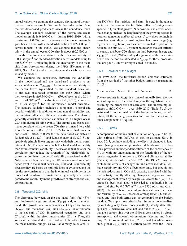
C. Le Quéré et al.: Global Carbon Budget 2016 623
annual values, we examine the standard deviation of the nor-malised model ensemble. We use further information fromthe two data-based products to assess the confidence level.The average standard deviation of the normalised oceanmodel ensemble is 0.16 GtC yr−1 during 1980–2010 (with amaximum of 0.33), but it increases as the model ensemblegoes back in time, with a standard deviation of 0.22 GtC yr−1
across models in the 1960s. We estimate that the uncer-tainty in the annual ocean CO2 sink is about ±0.5 GtC yr−1
from the fractional uncertainty in the data uncertainty of±0.4 GtC yr−1 and standard deviation across models of up to±0.33 GtC yr−1, reflecting both the uncertainty in the meansink from observations during the 1990s (Denman et al.,2007; Sect. 2.4.1) and in the interannual variability as as-sessed by models.
We examine the consistency between the variabilityin the model-based and the data-based products to as-sess confidence in SOCEAN. The interannual variability ofthe ocean fluxes (quantified as the standard deviation)of the two data-based estimates for 1986–2015 (wherethey overlap) is ± 0.34 GtC yr−1 (Rödenbeck et al., 2014)and± 0.41 GtC yr−1 (Landschützer et al., 2015), comparedto ±0.29 GtC yr−1 for the normalised model ensemble.The standard deviation includes a component of trend anddecadal variability in addition to interannual variability, andtheir relative influence differs across estimates. The phase isgenerally consistent between estimates, with a higher oceanCO2 sink during El Niño events. The annual data-based esti-mates correlate with the ocean CO2 sink estimated here witha correlation of r = 0.71 (0.51 to 0.77 for individual models),and r = 0.81 (0.66 to 0.79) for the data-based estimates ofRödenbeck et al. (2014) and Landschützer et al. (2015), re-spectively (simple linear regression), with their mutual corre-lation at 0.65. The agreement is better for decadal variabilitythan for interannual variability. The use of annual data for thecorrelation may reduce the strength of the relationship be-cause the dominant source of variability associated with ElNiño events is less than one year. We assess a medium confi-dence level to the annual ocean CO2 sink and its uncertaintybecause they are based on multiple lines of evidence, and theresults are consistent in that the interannual variability in themodel and data-based estimates are all generally small com-pared to the variability in the growth rate of atmospheric CO2concentration.
2.5 Terrestrial CO2 sink
The difference between, on the one hand, fossil fuel (EFF)and land-use-change emissions (ELUC) and, on the otherhand, the growth rate in atmospheric CO2 concentration(GATM) and the ocean CO2 sink (SOCEAN) is attributableto the net sink of CO2 in terrestrial vegetation and soils(SLAND), within the given uncertainties (Eq. 1). Thus, thissink can be estimated as the residual of the other terms inthe mass balance budget, as well as directly calculated us-
ing DGVMs. The residual land sink (SLAND) is thought tobe in part because of the fertilising effect of rising atmo-spheric CO2 on plant growth, N deposition, and effects of cli-mate change such as the lengthening of the growing season innorthern temperate and boreal areas. SLAND does not includegross land sinks directly resulting from land-use change (e.g.regrowth of vegetation) as these are estimated as part of thenet land-use flux (ELUC). System boundaries make it difficultto exactly attribute CO2 fluxes on land between SLAND andELUC (Erb et al., 2013), and by design most of the uncertain-ties in our method are allocated to SLAND for those processesthat are poorly known or represented in models.
2.5.1 Residual of the budget
For 1959–2015, the terrestrial carbon sink was estimatedfrom the residual of the other budget terms by rearrangingEq. (1):
SLAND = EFF+ELUC− (GATM+ SOCEAN). (8)
The uncertainty in SLAND is estimated annually from the rootsum of squares of the uncertainty in the right-hand termsassuming the errors are not correlated. The uncertainty av-erages to ±0.8 GtC yr−1 over 1959–2015 (Table 7). SLANDestimated from the residual of the budget includes, by defi-nition, all the missing processes and potential biases in theother components of Eq. (8).
2.5.2 DGVMs
A comparison of the residual calculation of SLAND in Eq. (8)with estimates from DGVMs as used to estimate ELUC inSect. 2.2.3, but here excluding the effects of changes in landcover (using a constant pre-industrial land-cover distribu-tion), provides an independent estimate of the consistency ofSLAND with our understanding of the functioning of the ter-restrial vegetation in response to CO2 and climate variability(Table 7). As described in Sect. 2.2.3, the DGVM runs thatexclude the effects of changes in land cover include all cli-mate variability and CO2 effects over land, but they do notinclude reductions in CO2 sink capacity associated with hu-man activity directly affecting changes in vegetation coverand management, which by design is allocated to ELUC. Thiseffect has been estimated to have led to a reduction in theterrestrial sink by 0.5 GtC yr−1 since 1750 (Gitz and Ciais,2003). The models in this configuration estimate the meanand variability of SLAND based on atmospheric CO2 and cli-mate, and thus both terms can be compared to the budgetresidual. We apply three criteria for minimum model realismby including only those models with (1) steady state afterspin-up; (2) where available, net land fluxes (SLAND−ELUC)that are a carbon sink over the 1990s as constrained by globalatmospheric and oceanic observations (Keeling and Man-ning, 2014; Wanninkhof et al., 2013); and (3) where avail-able, global ELUC that is a carbon source over the 1990s.
www.earth-syst-sci-data.net/8/605/2016/ Earth Syst. Sci. Data, 8, 605–649, 2016

624 C. Le Quéré et al.: Global Carbon Budget 2016
Fourteen models met criteria (1), and five of the models thatprovided ELUC met all three criteria.
The standard deviation of the annual CO2 sink across theDGVMs’ averages to ±0.8 GtC yr−1 for the period 1959 to2015. The model mean, over different decades, correlateswith the budget residual with r = 0.68 (0.51 to r = 0.77for individual models). The standard deviation is similar tothat of the five model ensembles presented in Le Quéréet al. (2009), but the correlation is improved compared tor = 0.54 obtained in the earlier study. The DGVM resultssuggest that the sum of our knowledge on annual CO2 emis-sions and their partitioning is plausible (see Sect. 4), and pro-vide insight on the underlying processes and regional break-down. However, as the standard deviation across the DGVMs(0.8 GtC yr−1 on average) is of the same magnitude as thecombined uncertainty due to the other components (EFF,ELUC, GATM, SOCEAN; Table 7), the DGVMs do not pro-vide further reduction of uncertainty in the annual terrestrialCO2 sink compared to the residual of the budget (Eq. 8). Yet,DGVM results are largely independent of the residual of thebudget, and it is worth noting that the residual method andensemble mean DGVM results are consistent within their re-spective uncertainties. We attach a medium confidence levelto the annual land CO2 sink and its uncertainty because theestimates from the residual budget and averaged DGVMsmatch well within their respective uncertainties, and the es-timates based on the residual budget are primarily dependenton EFF and GATM, both of which are well constrained.
2.6 The atmospheric perspective
The worldwide network of atmospheric measurements canbe used with atmospheric inversion methods to constrain thelocation of the combined total surface CO2 fluxes from allsources, including fossil and land-use-change emissions andland and ocean CO2 fluxes. The inversions assume EFF to bewell known, and they solve for the spatial and temporal dis-tribution of land and ocean fluxes from the residual gradientsof CO2 between stations that are not explained by emissions.Inversions used atmospheric CO2 data to the end of 2015(including preliminary values in some cases), and three at-mospheric CO2 inversions (Table 6) to infer the total CO2flux over land regions, and the distribution of the total landand ocean CO2 fluxes for the mid- to high-latitude NorthernHemisphere (30–90◦ N), tropics (30◦ S–30◦ N) and mid- tohigh-latitude region of the Southern Hemisphere (30–90◦ S).We focus here on the largest and most consistent sources ofinformation and use these estimates to comment on the con-sistency across various data streams and process-based esti-mates.
Atmospheric inversions
The three inversion systems used in this release are the Car-bonTracker (Peters et al., 2010), the Jena CarboScope (Rö-
denbeck, 2005), and CAMS (Chevallier et al., 2005). SeeTable 6 for version numbers. They are based on the sameBayesian inversion principles that interpret the same, for themost part, observed time series (or subsets thereof), but usedifferent methodologies that represent some of the many ap-proaches used in the field. This mainly concerns the timeresolution of the estimates (i.e. weekly or monthly), spa-tial breakdown (i.e. grid size), assumed correlation struc-tures, and mathematical approach. The details of these ap-proaches are documented extensively in the references pro-vided. Each system uses a different transport model, whichwas demonstrated to be a driving factor behind differencesin atmospheric-based flux estimates, and specifically theirglobal distribution (Stephens et al., 2007).
The three inversions use atmospheric CO2 observationsfrom various flask and in situ networks. They prescribe spa-tial and global EFF that can vary from that presented here.The CarbonTracker and CAMS inversions prescribed thesame global EFF as in Sect. 2.1.1, during 2010–2015 forCarbonTracker and during 1979–2015 in CAMS. The JenaCarboScope inversion uses EFF from EDGAR (2011) v4.2.Different spatial and temporal distributions of EFF were pre-scribed in each inversion.
Given their prescribed EFF, each inversion estimates nat-ural fluxes from a similar set of surface CO2 measurementstations, and CarbonTracker additionally uses two sites ofaircraft CO2 vertical profiles over the Amazon and Siberia,regions where surface observations are sparse. The atmo-spheric transport models of each inversion are TM5 forCarbonTracker, TM3 for Jena CarboScope, and LMDZ forCAMS. These three models are based on the same ECMWFwind fields. The three inversions use different prior naturalfluxes, which partly influences their optimised fluxes. CAMSassumes that the prior land flux is zero on the annual meanin each grid cell of the transport model, so that any sink orsource on land is entirely reflecting the information broughtby atmospheric measurements. CarbonTracker simulates asmall prior sink on land from the SIBCASA model that re-sults from regrowth following fire disturbances of an other-wise net zero biosphere. Jena CarboScope assumes a priorsink on land as well from the LPJ model. Inversion resultsfor the sum of natural ocean and land fluxes (Fig. 8) aremore constrained in the Northern Hemisphere (NH) than inthe tropics, because of the higher measurement stations den-sity in the NH.
Finally, results from atmospheric inversions include thenatural CO2 fluxes from rivers (which need to be taken intoaccount to allow comparison to other sources) and chemi-cal oxidation of reactive carbon-containing gases (which areneglected here). These inverse estimates are not truly inde-pendent of the other estimates presented here as the atmo-spheric observations include a set of observations used to es-timate the global growth rate in atmospheric CO2 concentra-tion (Sect. 2.3). However, they provide new information onthe regional distribution of fluxes.
Earth Syst. Sci. Data, 8, 605–649, 2016 www.earth-syst-sci-data.net/8/605/2016/

C. Le Quéré et al.: Global Carbon Budget 2016 625
We focus the analysis on two known strengths of the in-verse approach: the derivation of the year-to-year changes intotal land fluxes (SLAND−ELUC) consistent with the wholenetwork of atmospheric observations, and the spatial break-down of land and ocean fluxes (SLAND−ELUC+ SOCEAN)across large regions of the globe. The spatial breakdown isdiscussed in Sect. 3.1.3.
2.7 Processes not included in the global carbon budget
2.7.1 Contribution of anthropogenic CO and CH4 to theglobal carbon budget
Anthropogenic emissions of CO and CH4 to the atmosphereare eventually oxidised to CO2 and thus are part of the globalcarbon budget. These contributions are omitted in Eq. (1), butan attempt is made in this section to estimate their magnitudeand identify the sources of uncertainty. Anthropogenic COemissions are from incomplete fossil fuel and biofuel burningand deforestation fires. The main anthropogenic emissionsof fossil CH4 that matter for the global carbon budget arethe fugitive emissions of coal, oil, and gas upstream sectors(see below). These emissions of CO and CH4 contribute a netaddition of fossil carbon to the atmosphere.
In our estimate of EFF we assumed (Sect. 2.1.1) that allthe fuel burned is emitted as CO2; thus, CO anthropogenicemissions and their atmospheric oxidation into CO2 within afew months are already counted implicitly in EFF and shouldnot be counted twice (same for ELUC and anthropogenic COemissions by deforestation fires). Anthropogenic emissionsof fossil CH4 are not included in EFF, because these fugitiveemissions are not included in the fuel inventories. Yet theycontribute to the annual CO2 growth rate after CH4 gets oxi-dised into CO2. Anthropogenic emissions of fossil CH4 rep-resent 15 % of total CH4 emissions (Kirschke et al., 2013)that is 0.061 GtC yr−1 for the past decade. Assuming steadystate, these emissions are all converted to CO2 by OH oxida-tion and thus explain 0.06 GtC yr−1 of the global CO2 growthrate in the past decade, or 0.07–0.1 GtC yr−1 using the higherCH4 emissions reported recently (Schwietzke et al., 2016).
Other anthropogenic changes in the sources of CO andCH4 from wildfires, biomass, wetlands, ruminants, or per-mafrost changes are similarly assumed to have a small effecton the CO2 growth rate.
2.7.2 Anthropogenic carbon fluxes in the land to oceanaquatic continuum
The approach used to determine the global carbon budgetconsiders only anthropogenic CO2 emissions and their parti-tioning among the atmosphere, ocean, and land. In this anal-ysis, the land and ocean reservoirs that take up anthropogenicCO2 from the atmosphere are conceived as independent car-bon storage repositories. This approach omits the fact thatcarbon is continuously displaced from the land to the ocean
through the land–ocean aquatic continuum (LOAC) compris-ing freshwaters, estuaries, and coastal areas (Bauer et al.,2013; Regnier et al., 2013). A significant fraction of this lat-eral carbon flux is entirely “natural” and is thus a steady-state component of the pre-industrial carbon cycle. However,changes in environmental conditions and land-use changehave caused an increase in the lateral transport of carbon intothe LOAC – a perturbation that is relevant for the global car-bon budget presented here.
The results of the analysis of Regnier et al. (2013) can besummarised in two points of relevance for the anthropogenicCO2 budget. First, the anthropogenic perturbation has in-creased the organic carbon export from terrestrial ecosystemsto the hydrosphere at a rate of 1.0± 0.5 GtC yr−1, mainly ow-ing to enhanced carbon export from soils. Second, this ex-ported anthropogenic carbon is partly respired through theLOAC, partly sequestered in sediments along the LOACand, to a lesser extent, transferred in the open ocean whereit may accumulate. The increase in storage of land-derivedorganic carbon in the LOAC and open ocean combined isestimated by Regnier et al. (2013) at 0.65± 0.35 GtC yr−1.The implication of a substantial LOAC carbon accumula-tion is that SLAND corresponds to carbon sequestered bothin land ecosystems and in LOAC. We do not attempt to sep-arate these two storage components in our study focused onSLAND.
3 Results
3.1 Global carbon budget averaged over decades andits variability
The global carbon budget averaged over the last decade(2006–2015) is shown in Fig. 2. For this time period, 91%of the total emissions (EFF+ELUC) were caused by fossilfuels and industry, and 9 % by land-use change. The totalemissions were partitioned among the atmosphere (44 %),ocean (26 %), and land (30 %). All components except land-use-change emissions have grown since 1959 (Figs. 3 and4), with important interannual variability in the growth ratein atmospheric CO2 concentration and in the land CO2 sink(Fig. 4) and some decadal variability in all terms (Table 8).
3.1.1 CO2 emissions
Global CO2 emissions from fossil fuels and industry have in-creased every decade from an average of 3.1± 0.2 GtC yr−1
in the 1960s to an average of 9.3± 0.5 GtC yr−1 during2006–2015 (Table 8 and Fig. 5). The growth rate in theseemissions decreased between the 1960s and the 1990s, with4.5 % yr−1 in the 1960s (1960–1969), 2.8 % yr−1 in the1970s (1970–1979), 1.9 % yr−1 in the 1980s (1980–1989),and 1.1 % yr−1 in the 1990s (1990–1999). After this period,the growth rate began increasing again in the 2000s at anaverage growth rate of 3.5 % yr−1, decreasing to 1.8 % yr−1
www.earth-syst-sci-data.net/8/605/2016/ Earth Syst. Sci. Data, 8, 605–649, 2016

626 C. Le Quéré et al.: Global Carbon Budget 2016
Time (yr)
CO
2 flux
(G
tC y
r−1 )
Emissions
Partitioning
Fossil fuels and industry
Land−use change
Land
Atmosphere
Ocean
1880 1900 1920 1940 1960 1980 2000 2020−12
−8
−4
0
4
8
12
Figure 3. Combined components of the global carbon budget il-lustrated in Fig. 2 as a function of time, for emissions from fossilfuels and industry (EFF; grey) and emissions from land-use change(ELUC; brown), as well as their partitioning among the atmosphere(GATM; purple), land (SLAND; green), and oceans (SOCEAN; darkblue). All time series are in GtC yr−1. GATM and SOCEAN (and byconstruction also SLAND) prior to 1959 are based on different meth-ods. The primary data sources for fossil fuels and industry are fromBoden and Andres (2016), with uncertainty of about ±5 % (±1σ );land-use-change emissions are from Houghton et al. (2012) withuncertainties of about±30 %; growth rate in atmospheric CO2 con-centration prior to 1959 is from Joos and Spahni (2008) with un-certainties of about ±1–1.5 GtC decade−1 or ±0.1–0.15 GtC yr−1
(Bruno and Joos, 1997), and from Dlugokencky and Tans (2016)from 1959 with uncertainties of about± 0.2 GtC yr−1; the oceansink prior to 1959 is from Khatiwala et al. (2013) with uncertaintyof about± 30%, and from this study from 1959 with uncertaintiesof about ±0.5 GtC yr−1; and the residual land sink is obtained bydifference (Eq. 8), resulting in uncertainties of about ±50 % priorto 1959 and ±0.8 GtC yr−1 after that. See the text for more detailsof each component and their uncertainties.
for the last decade (2006–2015). In contrast, CO2 emissionsfrom land-use change have remained relatively constant ataround 1.3± 0.5 GtC yr−1 during 1960–2015. A decrease inemissions from land-use change is suggested between the1990s and 2000s by the combination of bookkeeping andfire-based emissions used here (Table 7), but it is highlyuncertain due to uncertainty in the underlying land-cover-change data. This decrease is not found in the current ensem-ble of the DGVMs (Fig. 6), which are otherwise consistentwith the bookkeeping method within their respective uncer-tainty (Table 7). The decrease is also not found in the studyof tropical deforestation of Achard et al. (2014), where thefluxes in the 1990s were similar to those of the 2000s and
1960 1970 1980 1990 2000 2010 20200
2
4
6
8
10
12(a) Fossil fuels and industry
1960 1970 1980 1990 2000 2010 2020−2
0
2
4
6
8
10
Time (yr)
CO
2 em
issi
ons
(GtC
yr−
1 )
(b) Land−use change
1960 1970 1980 1990 2000 2010 2020−2
0
2
4
6
8
10(c) Atmospheric growth
1960 1970 1980 1990 2000 2010 2020−2
0
2
4
6
8
10
CO
2 par
titio
ning
(G
tC y
r−1 )
(d) Ocean sink
1960 1970 1980 1990 2000 2010 2020−2
0
2
4
6
8
10
Time (yr)
(e) Land sink
Figure 4. Components of the global carbon budget and their uncer-tainties as a function of time, presented individually for (a) emis-sions from fossil fuels and industry (EFF), (b) emissions from land-use change (ELUC), (c) growth rate in atmospheric CO2 concentra-tion (GATM), (d) the ocean CO2 sink (SOCEAN; positive indicatesa flux from the atmosphere to the ocean), and (e) the land CO2 sink(SLAND; positive indicates a flux from the atmosphere to the land).All time series are in GtC yr−1 with the uncertainty bounds repre-senting ±1σ in shaded colour. Data sources are as in Fig. 3. Theblack dots in (a, e) show values for 2014 and 2015 that originatefrom a different data set to the remainder of the data, while thedashed line in (b) highlights the start of satellite data use to esti-mate the interannual variability and extend the series in time (seetext).
outside our uncertainty range. A new study based on FAOdata to 2015 (Federici et al., 2015) suggests that ELUC de-creased during 2011–2015 compared to 2001–2010.
3.1.2 Partitioning among the atmosphere, ocean,and land
Emissions are partitioned among the atmosphere, ocean,and land (Eq. 1). The growth rate in atmospheric CO2level increased from 1.7± 0.1 GtC yr−1 in the 1960sto 4.5± 0.1 GtC yr−1 during 2006–2015 with importantdecadal variations (Table 8). Both ocean and land CO2 sinksincreased roughly in line with the atmospheric increase, butwith significant decadal variability on land (Table 8). Theocean CO2 sink increased from 1.2± 0.5 GtC yr−1 in the1960s to 2.6± 0.5 GtC yr−1 during 2006–2015, with inter-annual variations of the order of a few tenths of GtC yr−1
Earth Syst. Sci. Data, 8, 605–649, 2016 www.earth-syst-sci-data.net/8/605/2016/

C. Le Quéré et al.: Global Carbon Budget 2016 627
1960 1970 1980 1990 2000 2010 20200
2
4
6
8
10
12(a)
Global
1960 1970 1980 1990 2000 2010 20200
1
2
3
4
5
CO
2 em
issi
ons
(GtC
yr−
1 )
Coal
Oil
Gas
Cement
(b)
1960 1970 1980 1990 2000 2010 20200
1
2
3
4
5
6
7
Time (yr)
Annex B
Non−Annex B
Emissions transfers
(c)
1960 1970 1980 1990 2000 2010 20200
0.5
1
1.5
2
2.5
3
CO
2 em
issi
ons
(GtC
yr−
1 )
China
USA
EU28
India
(d)
1960 1970 1980 1990 2000 2010 20200
1
2
3
4
5
6
7
Time (yr)Per
cap
ita e
mis
sion
s (t
C p
erso
n−1 y
r−1 )
India
USA
China
EU28
Global
(e)
Figure 5. CO2 emissions from fossil fuels and industry for (a) theglobe, including an uncertainty of ±5 % (grey shading), the emis-sions extrapolated using BP energy statistics (black dots), and theemissions projection for year 2016 based on GDP projection (reddot). (b) Global emissions by fuel type, including coal (salmon),oil (olive), gas (turquoise), and cement (purple), and excludinggas flaring which is small (0.6 % in 2013). (c) Territorial (solidline) and consumption (dashed line) emissions for the countrieslisted in Annex B of the Kyoto Protocol (salmon lines; mostlyadvanced economies with emissions limitations) vs. non-Annex Bcountries (green lines); also shown are the emissions transfer fromnon-Annex B to Annex B countries (light-blue line). (d) Territo-rial CO2 emissions for the top three country emitters (USA – olive;China – salmon; India – purple) and for the European Union (EU;turquoise for the 28 member states of the EU as of 2012). (e) Percapita emissions for the top three country emitters and the EU (allcolours as in panel (d) and the world (black). In (b–e), the dotsshow the data that were extrapolated from BP energy statistics for2014 and 2015. All time series are in GtC yr−1 except the per capitaemissions (e), which are in tonnes of carbon per person per year(tC person−1 yr−1). Territorial emissions are primarily from Bodenand Andres (2016) except for national data for the USA and EU28for 1990–2014, which are reported by the countries to the UNFCCCas detailed in the text, and for China from 1990, which are esti-mated here from BP energy statistics (the latter shown as a dash-dot line); consumption-based emissions are updated from Peters etal. (2011a). See Sect. 2.1.1 for details of the calculations and datasources.
generally showing an increased ocean sink during El Niñoevents (i.e. 1982–1983, 1997–1998, 2015–2016) (Fig. 7; Rö-denbeck et al., 2014). Although there is some coherence be-tween the ocean models and data products and among dataproducts regarding the mean, decadal variability, and trend,the ocean models and data products show poor agreement forinterannual variability (Sect. 2.4.3 and Fig. 7). As shown inFig. 7, the two data products and most model estimates pro-duce a mean CO2 sink for the 1990s that is below the meanassessed by the IPCC from indirect (but arguably more re-liable) observations (Denman et al., 2007; Sect. 2.4.1). Thisdiscrepancy suggests we may need to reassess estimates ofthe mean ocean carbon sinks, with some implications for thecumulative carbon budget (Landschützer et al., 2016).
The residual terrestrial CO2 sink increased from1.7± 0.7 GtC yr−1 in the 1960s to 3.1± 0.9 GtC yr−1
during 2006–2015, with important interannual variations ofup to 2 GtC yr−1 generally showing a decreased land sinkduring El Niño events, overcompensating for the increasein ocean sink and accounting for the enhanced growth ratein atmospheric CO2 concentration during El Niño events.The high uptake anomaly around year 1991 is thought tobe caused by the effect of the volcanic eruption of MountPinatubo on climate and is not generally reproduced by theDGVMs, but it is assigned to the land by the two inversesystems that include this period (Fig. 6). The larger land CO2sink during 2006–2015 compared to the 1960s is reproducedby all the DGVMs in response to combined atmosphericCO2 increase, climate, and variability, consistent with thebudget residual and reflecting a common knowledge ofthe processes (Table 7). The DGVM ensemble mean of2.8± 0.7 GtC yr−1 also reproduces the observed mean forthe period 2006–2015 calculated from the budget residual(Table 7).
The total CO2 fluxes on land (SLAND−ELUC) constrainedby the atmospheric inversions show in general very goodagreement with the global budget estimate, as expected giventhe strong constrains of GATM and the small relative uncer-tainty assumed on SOCEAN and EFF by inversions. The to-tal land flux is of similar magnitude for the decadal average,with estimates for 2006–2015 from the three inversions of2.2, 2.3, and 3.4 GtC yr−1 compared to 2.1± 0.7 GtC yr−1
for the total flux computed with the carbon budget fromother terms in Eq. (1) (Table 7). The total land sink from thethree inversions is 1.8, 1.8, and 3.0 GtC yr−1 when includ-ing a mean river flux adjustment of 0.45 GtC yr−1, thoughthe exact adjustment is in fact smaller because the anthro-pogenic contribution to river fluxes is only a fraction of thetotal river flux (Sect. 2.7.2). The interannual variability inthe inversions also matched the residual-based SLAND closely(Fig. 6). The total land flux from the DGVM multi-modelmean also compares well with the estimate from the carbonbudget and atmospheric inversions, with a decadal mean of1.7± 0.5 GtC yr−1 (Table 7; 2006–2015), although individ-ual models differ by several GtC for some years (Fig. 6).
www.earth-syst-sci-data.net/8/605/2016/ Earth Syst. Sci. Data, 8, 605–649, 2016

628 C. Le Quéré et al.: Global Carbon Budget 2016
1960 1970 1980 1990 2000 2010 2020−2
−1
0
1
2
3
4
5
6
7
CO
2 (G
tC y
r−1 )
(a)
Land−use change emissions
1960 1970 1980 1990 2000 2010 2020−2
−1
0
1
2
3
4
5
6
7
CO
2 (G
tC y
r−1 )
(b)
Residual land sink
1960 1970 1980 1990 2000 2010 2020−3
−2
−1
0
1
2
3
4
5
6
Time (yr)
CO
2 (G
tC y
r−1 )
(c)
Total land
Figure 6. CO2 exchanges between the atmosphere and the terres-trial biosphere. (a) Comparison of the global carbon budget valuesof CO2 emissions from land-use change (ELUC; black with ±1σuncertainty in grey shading), with CO2 emissions from land-usechange showing individual DGVM results (green) and the multi-model mean (olive), as well as fire-based results (orange); land-use-change data prior to 1997 (dashed black) highlights the pre-satelliteyears; preliminary results using the FAO FRA 2015 (Houghton andNassikas, 2016) are also shown in dark grey. (b) Land CO2 sink(SLAND; black with uncertainty in grey shading) showing individ-ual DGVM results (green) and multi-model mean (olive). (c) Totalland CO2 fluxes (b–a; black with uncertainty in grey shading), fromDGVM results (green) and the multi-model mean (olive), and atmo-spheric inversions Chevallier et al. (2005; CAMSv15.2) in purple;Rödenbeck et al. (2003; Jena CarboScope, s81_v3.8) in violet; Pe-ters et al. (2010; Carbon Tracker, CTE2016-FT) in salmon; and thecarbon balance from Eq. (1) (black). Five DGVMs are plotted in (a)and 14 in (b, c); see Table 5 for the list and Table 6 for the descrip-tion. In (c) the inversions were corrected for the pre-industrial landsink of CO2 from river input by removing a sink of 0.45 GtC yr−1
(Jacobson et al., 2007). This correction does not take into accountthe anthropogenic contribution to river fluxes (see Sect. 2.7.2).
1960 1970 1980 1990 2000 2010 20200
1
2
3
4
Time (yr)
CO
2 (G
tC y
r−1 )
Figure 7. Comparison of the anthropogenic atmosphere–oceanCO2 flux showing the budget values of SOCEAN (black; with ±1σuncertainty in grey shading), individual ocean models before nor-malisation (blue), and the two ocean data-based products (Röden-beck et al. (2014) in salmon and Landschützer et al. (2015) inpurple; see Table 6). Both data-based products were adjusted forthe pre-industrial ocean source of CO2 from river input to theocean, which is not present in the models, by adding a sink of0.45 GtC yr−1 (Jacobson et al., 2007), to make them comparableto SOCEAN. This adjustment does not take into account the anthro-pogenic contribution to river fluxes (see Sect. 2.7.2).
3.1.3 Regional distribution
Figure 8 shows the partitioning of the total surface fluxes ex-cluding emissions from fossil fuels and industry (SLAND+
SOCEAN−ELUC) according to the process models in theocean and on land, as well as to the three atmospheric inver-sions. The total surface fluxes provide information on the re-gional distribution of those fluxes by latitude bands (Fig. 8).The global mean CO2 fluxes from process models for 2006–2015 is 4.2± 0.6 GtC yr−1. This is comparable to the fluxesof 4.8± 0.5 GtC yr−1 inferred from the remainder of the car-bon budget (EFF−GATM in Eq. 1; Table 8) within their re-spective uncertainties. The total CO2 fluxes from the three in-versions range between 4.6 and 4.9 GtC yr−1, consistent withthe carbon budget as expected from the constraints on the in-versions.
In the south (south of 30◦ S), the atmospheric inversionsand process models all suggest a CO2 sink for 2006–2015 ofbetween 1.2 and 1.6 GtC yr−1 (Fig. 8), although the detailsof the interannual variability are not fully consistent acrossmethods. The interannual variability in the south is low be-cause of the dominance of ocean area with low variabilitycompared to land areas.
In the tropics (30◦ S–30◦ N), both the atmospheric inver-sions and process models suggest the carbon balance in thisregion is close to neutral over the past decade, with fluxes for2006–2015 ranging between −0.5 and +0.6 GtC yr−1. Boththe process-based models and the inversions consistently al-
Earth Syst. Sci. Data, 8, 605–649, 2016 www.earth-syst-sci-data.net/8/605/2016/

C. Le Quéré et al.: Global Carbon Budget 2016 629
Figure 8. CO2 fluxes between the atmosphere and the surface(SOCEAN+ SLAND−ELUC) by latitude bands for the (a) north(north of 30◦ N), (b) tropics (30◦ S–30◦ N), and (c) south (south of30◦ S). Estimates from the combination of the multi-model meansfor the land and oceans are shown (turquoise) with ±1σ of themodel ensemble (in grey). Results from the three atmospheric inver-sions are shown from Chevallier et al. (2005; CAMSv15.2) in pur-ple, Rödenbeck et al. (2003; Jena CarboScope, s81_v3.8) in blue,and Peters et al. (2010; CarbonTracker, CTE2016-FT) in salmon;see Table 6. Where available, the uncertainty in the inversions isalso shown.
locate more year-to-year variability in CO2 fluxes to the trop-ics compared to the north (north of 30◦ N; Fig. 8), this vari-ability being dominated by land fluxes.
In the north (north of 30◦ N), the inversions and processmodels are not in agreement on the magnitude of the CO2
sink with the ensemble mean of the process models sug-gesting a total Northern Hemisphere sink for 2006–2015 of2.3± 0.4 GtC yr−1, while the three inversions estimate a sinkof 2.7, 3.8, and 3.8 GtC yr−1. The mean difference can onlypartly be explained by the influence of river fluxes, whichis seen by the inversions but not included in the processmodels, as this flux in the Northern Hemisphere would beless than 0.45 GtC yr−1, particularly when only the anthro-pogenic contribution to river fluxes is accounted for. The Car-bonTracker inversion is close to the one standard deviation ofthe process models for the mean sink during their overlap pe-riod. CAMS and Jena CarboScope give a higher sink in thenorth than the process models, and a correspondingly highersource in the tropics. Differences between CarbonTrackerand CAMS, Jena CarboScope may be related to differencesin inter-hemispheric mixing time of their transport models,and other inversion settings. Differences between the meanfluxes of CAMS, Jena CarboScope, and the ensemble of pro-cess models cannot be explained easily. They could reflecta bias either in these two inversions or in missing processesor biases in the process models, such as the lack of adequateparameterisations for forest management in the north and forforest degradation emissions in tropics for the DGVMs.
The estimated contribution of the north and its uncertaintyfrom process models is sensitive both to the ensemble of pro-cess models used and to the specifics of each inversion. Allthree inversions show substantial differences in variabilityand/or trend, and one inversion shows a substantial differ-ence in the mean Northern Hemisphere sink.
3.2 Global carbon budget for year 2015
3.2.1 CO2 emissions
Global CO2 emissions from fossil fuels and industry re-mained nearly constant at 9.9± 0.5 GtC in 2015 (Fig. 5), dis-tributed among coal (41 %), oil (34 %), gas (19 %), cement(5.6 %), and gas flaring (0.7 %). Compared to the previousyear, emissions from coal and cement decreased by−1.8 and−1.9 %, respectively, while emissions from oil and gas in-creased by 1.9 and 1.7 %, respectively. Due to lack of data,gas flaring in 2014 and 2015 is assumed the same as 2013.
Growth in emissions in 2015 was not statistically differ-ent from zero, at 0.06 % higher than in 2014, in stark con-trast with the decadal average of 1.8 % yr−1 (2006–2015).Growth in 2015 is in the range of our projection changeof −0.6 [−1.6 to +0.5] % made last year (Le Quéré et al.,2015a) based on national emissions projections for Chinaand the USA, and projections of gross domestic product cor-rected for IFF improvements for the rest of the world. How-ever, the specific projection for 2015 for China made lastyear (likely range of −4.6 to −1.1 %) was for a larger de-crease in emissions than realised (−0.7 %). This is due tolower decline in coal production in the last 4 months of theyear compared to January–August and to improvements in
www.earth-syst-sci-data.net/8/605/2016/ Earth Syst. Sci. Data, 8, 605–649, 2016
630 C. Le Quéré et al.: Global Carbon Budget 2016
energy content of coal through improvements in the qualityof the coal used which were at the top of the range of im-provements considered in our projection.
In 2015, the largest contributions to global CO2 emissionswere from China (29 %), the USA (15 %), the EU (28 mem-ber states; 10 %), and India (6.3 %). The percentages arethe fraction of the global emissions including bunker fuels(3.2 %). These four regions account for 59 % of global emis-sions. Growth rates for these countries from 2014 to 2015were −0.7 % (China), −2.6 % (USA), +1.4 % (EU28), and+5.2 % (India). The per capita CO2 emissions in 2015 were1.3 tC person−1 yr−1 for the globe, and were 4.6 (USA), 2.1(China), 1.9 (EU28), and 0.5 tC person−1 yr−1 (India) for thefour highest emitting countries (Fig. 5e).
Territorial emissions in Annex B countries decreasedby −0.2 % yr−1 on average during 1990–2014. Trends ob-served for consumption emissions were less monotonic, with0.8 % yr−1 growth over 1990–2007 and a −1.5 % yr−1 de-crease over 2007–2014 (Fig. 5c). In non-Annex B coun-tries during 1990–2014, territorial emissions have grownat 4.7 % yr−1, while consumption emissions have grown at4.4 % yr−1. In 1990, 65 % of global territorial emissions wereemitted in Annex B countries (33 % in non-Annex B, and 2 %in bunker fuels used for international shipping and aviation),while in 2014 this had reduced to 37 % (60 % in non-AnnexB, and 3 % in bunker fuels). In terms of consumption emis-sions this split was 67 % in 1990 and 41 % in 2014 (33 to59 % in non-Annex B). The difference between territorial andconsumption emissions (the net emission transfer via interna-tional trade) from non-Annex B to Annex B countries has in-creased from near zero in 1990 to 0.3 GtC yr−1 around 2005and remained relatively stable afterwards until the last yearavailable (2014; Fig. 5). The increase in net emission trans-fers of 0.30 GtC yr−1 between 1990 and 2014 compares withthe emission reduction of 0.4 GtC yr−1 in Annex B countries.These results show the importance of net emission transfervia international trade from non-Annex B to Annex B coun-tries, as well as the stabilisation of emissions transfers whenaveraged over Annex B countries during the past decade. In2014, the biggest emitters from a consumption perspectivewere China (25 % of the global total), USA (16 %), EU28(12 %), and India (5 %).
Based on fire activity, the global CO2 emissions from land-use change are estimated as 1.3± 0.5 GtC in 2015, slightlyabove the 2006–2015 average of 1.0± 0.5 GtC yr−1. Theslight rise in ELUC in 2015 is consistent with estimates ofpeat fires in Asia based on atmospheric data (Yin et al.,2016). However, the estimated annual variability is not gen-erally consistent between methods, except that all methodsestimate that variability in ELUC is small relative to the vari-ability from SLAND (Fig. 6a). This could be partly due tothe design of the DGVM experiments, which use flux dif-ferences between simulations with and without land-coverchange, and thus their variability may differ due to, for ex-ample, fires in forest regions where the contemporary forest
cover is smaller than pre-industrial cover used in the “with-out land-cover change” runs.
3.2.2 Partitioning among the atmosphere, ocean,and land
The growth rate in atmospheric CO2 concentration was6.3± 0.2 GtC in 2015 (2.97± 0.09 ppm; Fig. 4; Dlugo-kencky and Tans, 2016). This is well above the 2006–2015average of 4.5± 0.1 GtC yr−1 and reflects the large interan-nual variability in the growth rate of atmospheric CO2 con-centration associated with El Niño and La Niña events.
The ocean CO2 sink was 3.0± 0.5 GtC yr−1 in 2015, an in-crease of 0.15 GtC yr−1 over 2015 according to ocean mod-els. Five of the seven ocean models produce an increase inthe ocean CO2 sink in 2015 compared to 2014, with near-zero changes in the last two models (Fig. 7). However, thetwo data products disagree over changes in the last year,with a decrease of −0.4 GtC yr−1 found in Rödenbeck etal. (2014) and an increase of 0.3 GtC yr−1 found in Land-schützer et al. (2015). Thus, there is no overall consistencyin the annual change in the ocean CO2 sink, although thereis an indication of increasing convergence among productsfor the assessment of multi-year changes, as suggested bythe time-series correlations reported in Sect. 2.4.3 (see alsoLandschützer et al., 2015). An increase in the ocean CO2 sinkin 2015 would be consistent with the observed El Niño con-ditions and continued rising atmospheric CO2. All estimatessuggest an ocean CO2 sink for 2015 that is larger than their2006–2015 average.
The terrestrial CO2 sink calculated as the residual fromthe carbon budget was 1.9± 0.9 GtC in 2015, well below the3.1± 0.9 GtC yr−1 averaged over 2006–2015 (Fig. 4), and re-flecting the onset of the El Niño conditions in the second halfof 2015. The DGVM mean produces a sink of 1.0± 1.4 GtCin 2015, also well below the 2006–2015 average (Table 7).Both models and inversions suggest that the lower sink in2015 primarily originated in the tropics (Fig. 8).
3.3 Emission projections and the global carbon budgetfor year 2016
3.3.1 CO2 emissions
Using separate projections for China, the USA, and the restof the world as described in Sect. 2.1.4, we project a con-tinued low growth in global CO2 emissions from fossil fuelsand cement production in 2016 of +0.5 % (range of −0.7to +2.1 %) from 2015 levels (Table 9), or +0.2 % (−1.0to +1.8 %) after adjusting for leap year (see Sect. 2.1.3).Our method is imprecise and contains several assumptionsthat could influence the results beyond the given range, andas such is indicative only. Within the given assumptions,global emissions remain nearly constant at 9.9± 0.5 GtC(36.4± 1.8 GtCO2) in 2016, but they are still 63% above
Earth Syst. Sci. Data, 8, 605–649, 2016 www.earth-syst-sci-data.net/8/605/2016/

C. Le Quéré et al.: Global Carbon Budget 2016 631
Table 9. Actual CO2 emissions from fossil fuels and industry (EFF) compared to projections made the previous year based on world GDP(IMF October 2015) and the fossil fuel intensity of GDP (IFF) based on subtracting the CO2 and GDP growth rates. The “Actual” values arethe latest estimate available and the “Projected” value for 2016 refers to those presented in this paper. No correction for leap years is applied(Sect. 2.1.3).
EFF GDP IFFProjected Actual Projected Actual Projected Actual
2009a−2.8 % −1.1 % −1.1 % −0.05 % −1.7 % −1.1 %
2010b > 3 % 5.7 % 4.8 % 5.4 % >−1.7 % +0.3 %2011c 3.1± 1.5 % 4.1 % 4.0 % 4.2 % −0.9± 1.5 % −0.2 %2012d 2.6 %i 1.7 % 3.3 % 3.5 % −0.7 % −1.8 %
(1.9 to 3.5)2013e 2.1 % 1.1 % 2.9 % 3.3 % −0.8 % −2.2 %
(1.1 to 3.1)2014f 2.5 % 0.8 % 3.3 % 3.0 % −0.7 % −2.6 %
(1.3 to 3.5)
Change in method
EFF EFF (China) EFF (USA) EFF (rest of world)Projected Actual Projected Actual Projected Actual Projected Actual
2015g−0.6 % 0.05 % −3.9 % −0.7 % −1.5 % −2.6 % 1.2 % 1.2 %
(−1.6 to 0.5) (−4.6 to −1.1) (−5.5 to 0.3) (−0.2 to 2.6)2016h
+0.5 %i – −0.2 %i – −1.4 %i – +1.3 %i –(−1.7 to +2.1) (−3.5 to +1.6) (−3.7 to +0.9) (−0.2 to +2.8)
a Le Quéré et al. (2009). b Friedlingstein et al. (2010). c Peters et al. (2013). d Le Quéré et al. (2013). e Le Quéré et al. (2014). f Friedlingstein et al. (2014) andLe Quéré et al. (2015b). g Jackson et al. (2016) and Le Quéré et al. (2015a). h This study. i These numbers are not adjusted for leap years (see Sect. 2.1.3 forleap-year adjustments).
emissions in 1990. The drivers of the trends in EFF are dis-cussed elsewhere (Peters et al., 2016).
For China, the expected change based on available dataduring January to July or September (see Sect. 2.1.4) is for anincrease in emissions of −0.2 % (range of −3.5 to +1.6 %)in 2016 compared to 2015, or −0.5 % (range of −3.8 to+1.3 %) after adjusting for leap year (see Sect. 2.1.3). This isbased on estimated decreases in coal consumption (−1.8 %)and estimated growth in apparent oil (+4.0 %) and natu-ral gas (+7.2 %) consumption and in cement production(+2.6 %). The uncertainty range considers the spread be-tween different data sources, as well as differences betweenJuly/August and end-of-year data observed in 2014 and2015. The estimated reduction in coal consumption also in-corporates an assumed 2 % increase in the energy density ofcoal – based on increases in the last 2 years, which are as-sumed to continue given production limits in 2016 that arelikely to affect production of low-quality coal more – and theuncertainty range also reflects uncertainty in this figure.
For the USA, the EIA emissions projection for 2016 com-bined with cement data from USGS gives a decrease of−1.4 % (range of −3.7 to +0.9 %) compared to 2015, or−1.7 % (range of −4.0 to +0.6 %) after adjusting for leapyear (see Sect. 2.1.3).
For the rest of the world, the expected growth for 2016 of+1.3 % (range of−0.2 to+2.8 %), or+1.0 % (range of−0.4
to+2.5 %) after adjusting for leap year (see Sect. 2.1.3). Thisis computed using the GDP projection for the world exclud-ing China and the USA of 2.5 % made by the IMF (IMF,2016) and a decrease in IFF of −1.2 % yr−1, which is theaverage from 2006 to 2015. The uncertainty range is basedon the standard deviation of the interannual variability in IFFduring 2006–2015 of±1.0 % yr−1 and our estimate of uncer-tainty in the IMF’s GDP forecast of ±0.5 %.
3.3.2 Partitioning among the atmosphere, ocean,and land
The growth in atmospheric CO2 concentration (GATM)was projected to be high again in 2016, at 6.7± 1.1 GtC(3.15± 0.53 ppm) for the Mauna Loa station (Betts et al.,2016). Growth at Mauna Loa is closely correlated withthe global growth (r = 0.95 for 1959–2015). Therefore, theglobal growth rate in atmospheric CO2 concentration isalso expected to be high in 2016. In the 8-month periodbetween December 2015 and August 2016, the observedglobal growth in atmospheric CO2 concentration was already2.3 ppm (Dlugokencky and Tans, 2016) after seasonal adjust-ment, supporting the projection of Betts et al. (2016). Evenwith a return to El Niño neutral or possible emerging LaNiña conditions for the second half of 2016, positive growthin atmospheric CO2 would still be expected during the last
www.earth-syst-sci-data.net/8/605/2016/ Earth Syst. Sci. Data, 8, 605–649, 2016

632 C. Le Quéré et al.: Global Carbon Budget 2016
4 months of the year because of the continuing persistentemissions. For example, during the transitions from El Niñoto La Niña of 1986–1987, 1998–1999, and 2010–2011, at-mospheric CO2 growth of 0.3, 0.6, and 0.9 ppm, respectively,was observed in the last 4 months of the year.
Combining projected EFF and GATM suggests a total forthe combined land and ocean (SLAND+ SOCEAN−ELUC) ofabout 3 GtC only. SOCEAN was 3.0 GtC in 2015 and is ex-pected to slightly increase in 2016 from a delayed responseto El Niño conditions (Feely et al., 1999). ELUC was 1.3 GtCin 2015, above the decadal mean average of 1.0 GtC yr−1,and is expected to return to average or below average in 2016based on fire activity related to land management so far (upto August). Hence, for 2016, the residual land sink SLANDis expected to be well below its 2006–2015 average and ap-proximately balance ELUC. This is consistent with our un-derstanding of the response of the terrestrial vegetation to ElNiño conditions and increasing atmospheric CO2 concentra-tions, though the uncertainties in GATM and of the partition-ing among SLAND and SOCEAN are substantial.
3.4 Cumulative emissions
Cumulative emissions for 1870–2015 were 410± 20 GtC forEFF, and 145± 50 GtC for ELUC based on the bookkeep-ing method of Houghton et al. (2012) for 1870–1996 anda combination with fire-based emissions for 1997–2015 asdescribed in Sect. 2.2 (Table 10). The cumulative emissionsare rounded to the nearest 5 GtC. The total cumulative emis-sions from fossil and land-use change for 1870–2015 are555± 55 GtC. These emissions were partitioned among theatmosphere (235± 5 GtC based on atmospheric measure-ments in ice cores of 288 ppm (Sect. 2.3; Joos and Spahni,2008) and recent direct measurements of 399.1 ppm (Dlugo-kencky and Tans, 2016), ocean (160± 20 GtC using Khati-wala et al. , 2013, prior to 1959 and Table 8 otherwise), andland (160± 60 GtC by the difference).
Cumulative emissions for the early period 1750–1869were 3 GtC for EFF and about 45 GtC for ELUC (rounded tonearest 5), of which 10 GtC was emitted in the period 1850–1870 (Houghton et al., 2012) and 30 GtC in the period 1750–1850 based on the average of four publications (22 GtC byPongratz et al., 2009; 15 GtC by van Minnen et al., 2009;64 GtC by Shevliakova et al., 2009; and 24 GtC by Zaehle etal., 2011). The growth rate in atmospheric CO2 concentra-tion during that time was about 25 GtC, and the ocean uptakeabout 20 GtC, implying a land uptake of 5 GtC. These num-bers have large relative uncertainties but balance within thelimits of our understanding.
Cumulative emissions for 1750–2015 based on the sumof the two periods above (before rounding to the nearest5 GtC) were 410± 20 GtC for EFF, and 190± 65 GtC forELUC, for a total of 600± 70 GtC, partitioned among theatmosphere (260± 5 GtC), ocean (175± 20 GtC), and land(165± 70 GtC).
Cumulative emissions through to year 2016 can be es-timated based on the 2016 projections of EFF (Sect. 3.2),the largest contributor, and assuming a constant ELUC of1.0 GtC (average of last decade). For 1870–2016, these are565± 55 GtC (2075± 205 GtCO2) for total emissions, withabout 75 % contribution from EFF (420± 20 GtC) and about25 % contribution from ELUC (150± 50 GtC). Cumulativeemissions since year 1870 are higher than the emissions of515 [445 to 585] GtC reported in the IPCC (Stocker et al.,2013) because they include an additional 55 GtC from emis-sions in 2012–2016 (mostly from EFF). The uncertainty pre-sented here (±1σ ) is smaller than the range of 90 % usedby IPCC, but both estimates overlap within their uncertaintyranges.
4 Discussion
Each year when the global carbon budget is published, eachcomponent for all previous years is updated to take into ac-count corrections that are the result of further scrutiny andverification of the underlying data in the primary input datasets. The updates have generally been relatively small and fo-cused on the most recent years, except for land-use change,where they are more significant but still generally within theprovided uncertainty range (Fig. 9). The difficulty in access-ing land-cover change data to estimate ELUC is the key prob-lem to providing continuous records of emissions in this sec-tor. Current FAO estimates are based on statistics reportedat the country level and are not spatially explicit. Advancesin satellite recovery of land-cover change could help to keeptrack of land-use change through time (Achard et al., 2014;Harris et al., 2012). Revisions in ELUC for the 2008/2009budget were the result of the release of FAO 2010, which con-tained a major update to forest cover change for the period2000–2005 and provided the data for the following 5 yearsto 2010 (Fig. 9b). The differences this year could be at-tributable to both the different data and the different methods.Comparison of global carbon budget components releasedannually by GCP since 2006 show that update differenceswere highest at 0.82 GtC yr−1 for the growth rate in atmo-spheric CO2 concentration (from a one-off correction backto year 1979), 0.24 GtC yr−1 for fossil fuels and industry, and0.52 GtC yr−1 for the ocean CO2 sink (from a change fromone to multiple models; Fig. 9d). The update for the resid-ual land CO2 sink was also large (Fig. 9e), with a maximumvalue of 0.83 GtC yr−1, directly reflecting revisions in otherterms of the budget.
Our capacity to constrain the global carbon budget can beevaluated by adding the five components of Eq. (1) usingDGVM estimates for SLAND, thus using largely independentestimates for each component (Fig. 10). This residual globalbudget represents all the carbon unaccounted currently. Fig-ure 10 shows that the mean global residual is close to zero,and there is no trend over the entire time period. However,
Earth Syst. Sci. Data, 8, 605–649, 2016 www.earth-syst-sci-data.net/8/605/2016/

C. Le Quéré et al.: Global Carbon Budget 2016 633
Table 10. Cumulative CO2 emissions for different time periods in gigatonnes of carbon (GtC). We also provide the 1850–2005 time periodused in a number of model evaluation publications. All uncertainties are reported as ±1σ . All values are rounded to the nearest 5 GtC as inStocker et al. (2013), reflecting the limits of our capacity to constrain cumulative estimates. Thus, some columns will not exactly balancebecause of rounding errors.
Units of GtC 1750–2015 1850–2005 1870–2015 1870–2016
Emissions
Fossil fuels and industry (EFF) 410± 20 320± 15 410± 20 420± 20∗
Land-use-change emissions (ELUC) 190± 65 150± 55 145± 50 150± 50∗
Total emissions 600± 70 470± 55 555± 55 565± 55∗
Partitioning
Growth rate in atmospheric CO2 concentration (GATM) 260± 5 195± 5 235± 5Ocean sink (SOCEAN) 175± 20 160± 20 160± 20Residual terrestrial sink (SLAND) 165± 70 115± 60 160± 60
∗ The extension to year 2016 uses the emissions projections for fossil fuels and industry for 2016 (Sect. 3.2) and assumes a constant ELUC flux(Sect. 2.2).
it also highlights periods of multiple years where the sum ofthe estimates differs significantly from zero. These include anunaccounted flux from the surface to the atmosphere (or un-derestimated emissions) during 1973–1979 and 1997–2001and an unaccounted sink from the atmosphere to the surface(or overestimated emissions) during 1961–1965 and 1990–1992. This unaccounted variability could come from errorsin our estimates of the five components of Equation (1; Li etal., 2016), or from missing factors in the global carbon bud-get, including but not limited to those discussed in Sect. 2.7.This unaccounted variability limits our ability to verify re-ported emissions and limits our confidence in the underlyingprocesses regulating the carbon cycle feedbacks with climatechange.
Another semi-independent way to evaluate the results isprovided through the comparison with the atmospheric inver-sions and their regional breakdown. The comparison shows afirst-order consistency between inversions and process mod-els but with substantial discrepancies, particularly for the al-location of the mean sink between the tropics and the North-ern Hemisphere. Understanding these discrepancies and fur-ther analysis of regional carbon budgets would provide addi-tional information to quantify and improve our estimates, ashas been shown by the project REgional Carbon Cycle As-sessment and Processes (RECCAP; Canadell et al., 2012).
Annual estimates of each component of the global carbonbudgets have their limitations, some of which could be im-proved with better data and/or better understanding of carbondynamics. The primary limitations involve resolving fluxeson annual timescales and providing updated estimates for re-cent years for which data-based estimates are not yet avail-able or only beginning to emerge. Of the various terms in theglobal budget, only the burning of fossil fuels and the growthrate in atmospheric CO2 concentration terms are based pri-marily on empirical inputs supporting annual estimates inthis carbon budget. While these models represent the current
state of the art, they provide only simulated changes in pri-mary carbon budget components. For example, the decadaltrends in global ocean uptake and the interannual varia-tions associated with the El Niño–Southern Ocean Oscilla-tion (ENSO) are not directly constrained by observations,although many of the processes controlling these trends aresufficiently well known that the model-based trends still havevalue as benchmarks for further validation. Data-based prod-ucts for the ocean CO2 sink provide new ways to evaluatethe model results, and could be used directly as data be-come more rapidly available and methods for creating suchproducts improve. However, there are still large discrepan-cies among data-based estimates, in large part due to the lackof routine data sampling, which precludes their direct use fornow (Rödenbeck et al., 2015). Estimates of land-use emis-sions and their year-to-year variability have even larger un-certainty, and much of the underlying data are not availableas an annual update. Efforts are underway to work with an-nually available satellite area change data or FAO reporteddata in combination with fire data and modelling to provideannual updates for future budgets.
Our approach also depends on the reliability of the en-ergy and land-cover change statistics provided at the countrylevel, which are potentially subject to biases. Thus, it is crit-ical to develop multiple ways to estimate the carbon balanceat the global and regional level, including estimates fromthe inversion of atmospheric CO2 concentration, the use ofother oceanic and atmospheric tracers, and the compilation ofemissions using alternative statistics (e.g. sectors). It is alsoimportant to challenge the consistency of information acrossobservational streams, for example to contrast the coherenceof temperature trends with those of CO2 sink trends. Multi-ple approaches ranging from global to regional scale wouldgreatly help increase confidence and reduce uncertainty inCO2 emissions and their fate.
www.earth-syst-sci-data.net/8/605/2016/ Earth Syst. Sci. Data, 8, 605–649, 2016
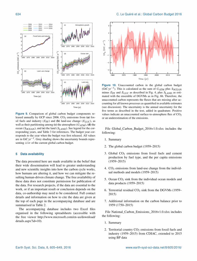
634 C. Le Quéré et al.: Global Carbon Budget 2016
1960 1970 1980 1990 2000 2010 20200
2
4
6
8
10
12(a) Fossil fuels and industry
2006200720082009
2010201120122013
201420152016
1960 1970 1980 1990 2000 2010 20200
1
2
3
4
Time (yr)
CO
2 em
issi
ons
(GtC
yr−
1 )
(b) Land−use change
1960 1970 1980 1990 2000 2010 20200
2
4
6
8(c) Atmospheric growth
1960 1970 1980 1990 2000 2010 20200
1
2
3
4
CO
2 par
titio
ning
(G
tC y
r−1 )
(d) Ocean sink
1960 1970 1980 1990 2000 2010 2020−2
0
2
4
6
Time (yr)
(e) Land sink
Figure 9. Comparison of global carbon budget components re-leased annually by GCP since 2006. CO2 emissions from (a) fos-sil fuels and industry (EFF) and (b) land-use change (ELUC), aswell as their partitioning among (c) the atmosphere (GATM), (d) theocean (SOCEAN), and (e) the land (SLAND). See legend for the cor-responding years, and Table 3 for references. The budget year cor-responds to the year when the budget was first released. All valuesare in GtC yr−1. Grey shading shows the uncertainty bounds repre-senting ±1σ of the current global carbon budget.
5 Data availability
The data presented here are made available in the belief thattheir wide dissemination will lead to greater understandingand new scientific insights into how the carbon cycle works,how humans are altering it, and how we can mitigate the re-sulting human-driven climate change. The free availability ofthese data does not constitute permission for publication ofthe data. For research projects, if the data are essential to thework, or if an important result or conclusion depends on thedata, co-authorship may need to be considered. Full contactdetails and information on how to cite the data are given atthe top of each page in the accompanying database and aresummarised in Table 2.
The accompanying database includes two Excel filesorganised in the following spreadsheets (accessible withthe free viewer http://www.microsoft.com/en-us/download/details.aspx?id=10).
Figure 10. Unaccounted carbon in the global carbon budget(GtC yr−1). This is calculated as the sum of GATM plus SOCEANminus EFF and ELUC as described in Fig. 4, plus SLAND as esti-mated with the ensemble of DGVMs as in Fig. 6b. Therefore, theunaccounted carbon represents the fluxes that are missing after ac-counting for all known processes as quantified in available estimates(see discussion). The uncertainty is the annual uncertainty for thefive terms as described in the text, added in quadrature. Positivevalues indicate an unaccounted surface-to-atmosphere flux of CO2or an underestimation of the emissions.
File Global_Carbon_Budget_2016v1.0.xlsx includes thefollowing:
1. Summary
2. The global carbon budget (1959–2015)
3. Global CO2 emissions from fossil fuels and cementproduction by fuel type, and the per capita emissions(1959–2015)
4. CO2 emissions from land-use change from the individ-ual methods and models (1959–2015)
5. Ocean CO2 sink from the individual ocean models anddata products (1959–2015)
6. Terrestrial residual CO2 sink from the DGVMs (1959–2015)
7. Additional information on the carbon balance prior to1959 (1750–2015)
File National_Carbon_Emissions_2016v1.0.xlsx includesthe following:
1. Summary
2. Territorial country CO2 emissions from fossil fuels andindustry (1959–2015) from CDIAC, extended to 2015using BP data
Earth Syst. Sci. Data, 8, 605–649, 2016 www.earth-syst-sci-data.net/8/605/2016/

C. Le Quéré et al.: Global Carbon Budget 2016 635
3. Territorial country CO2 emissions from fossil fuels andindustry (1959–2015) from CDIAC with UNFCCC dataoverwritten where available, extended to 2015 using BPdata
4. Consumption country CO2 emissions from fossil fuelsand industry and emissions transfer from the interna-tional trade of goods and services (1990–2014) usingCDIAC/UNFCCC data (worksheet 3 above) as refer-ence
5. Emissions transfers (consumption minus territorialemissions; 1990–2014)
6. Country definitions
7. Details of disaggregated countries
8. Details of aggregated countries
National emissions data are also available from the GlobalCarbon Atlas (http://globalcarbonatlas.org).
6 Conclusions
The estimation of global CO2 emissions and sinks is a majoreffort by the carbon cycle research community that requires acombination of measurements and compilation of statisticalestimates and results from models. The delivery of an annualcarbon budget serves two purposes. First, there is a large de-mand for up-to-date information on the state of the anthro-pogenic perturbation of the climate system and its underpin-ning causes. A broad stakeholder community relies on thedata sets associated with the annual carbon budget, includ-ing scientists, policy makers, businesses, journalists, and thebroader society increasingly engaged in adapting to and mit-
igating human-driven climate change. Second, over the lastdecade we have seen unprecedented changes in the humanand biophysical environments (e.g. increase in the growth offossil fuel emissions, ocean temperatures, and strength of theland sink), which call for more frequent assessments of thestate of the planet and, by implication, a better understandingof the future evolution of the carbon cycle. Both the oceanand the land surface presently remove a large fraction of an-thropogenic emissions. Any significant change in the func-tion of carbon sinks is of great importance to climate policy-making, as they affect the excess carbon dioxide remainingin the atmosphere and therefore the compatible emissions forany climate stabilisation target. Better constraints of carboncycle models against contemporary data sets raise the capac-ity for the models to become more accurate at future projec-tions.
This all requires more frequent, robust, and transparentdata sets and methods that can be scrutinised and replicated.After 11 annual releases from the GCP, the effort is growingand the traceability of the methods has become increasinglycomplex. Here, we have documented in detail the data setsand methods used to compile the annual updates of the globalcarbon budget, explained the rationale for the choices madeand the limitations of the information, and finally highlightedthe need for additional information where gaps exist.
This paper via “living data” will help to keep track of newbudget updates. The evolution over time of the carbon budgetis now a key indicator of the anthropogenic perturbation ofthe climate system, and its annual delivery joins a set of otherclimate indicators to monitor the evolution of human-inducedclimate change, such as the annual updates on the global sur-face temperature, sea level rise, and minimum Arctic sea iceextent.
www.earth-syst-sci-data.net/8/605/2016/ Earth Syst. Sci. Data, 8, 605–649, 2016

636 C. Le Quéré et al.: Global Carbon Budget 2016
Appendix A
Table A1. Attribution of fCO2 measurements for year 2015 included in addition to SOCAT v4 (Bakker et al., 2016) to inform ocean dataproducts.
Vessel Start date yyyy-mm-dd End date yyyy-mm-dd Regions No. of samples Principal investigators DOI (if available)/comment
Atlantic Companion 2015-03-03 2015-03-10 North Atlantic 8496 Steinhoff, T.; Becker,M.; Körtzinger, A.
doi:10.3334/CDIAC/OTG.VOS_Atlantic_Companion_Line_2015
Atlantic Companion 2015-03-30 2015-04-07 North Atlantic 9265 Steinhoff, T.; Becker,M.; Körtzinger, A.
doi:10.3334/CDIAC/OTG.VOS_Atlantic_Companion_Line_2015
Aurora Australis 2014-12-05 2015-01-24 Southern Ocean 41 463 Tilbrook, B. doi:10.3334/CDIAC/OTG.VOS_AA_2014Benguela Stream 2015-01-08 2015-01-14 North Atlantic,
Tropical Atlantic4664 Schuster, U.; Jones, S.D.; Wat-
son, A.J.doi:10.3334/CDIAC/OTG.VOS_BENGUELA_STREAM_2015
Benguela Stream 2015-02-05 2015-02-12 North Atlantic,Tropical Atlantic
4056 Schuster, U.; Jones, S.D.; Wat-son, A.J.
doi:10.3334/CDIAC/OTG.VOS_BENGUELA_STREAM_2015
Benguela Stream 2015-02-22 2015-03-01 North Atlantic,Tropical Atlantic
6158 Schuster, U.; Jones, S.D.; Wat-son, A.J.
doi:10.3334/CDIAC/OTG.VOS_BENGUELA_STREAM_2015
Benguela Stream 2015-04-30 2015-05-07 North Atlantic,Tropical Atlantic
6125 Schuster, U.; Jones, S.D.; Wat-son, A.J.
doi:10.3334/CDIAC/OTG.VOS_BENGUELA_STREAM_2015
Benguela Stream 2015-05-17 2015-05-24 North Atlantic,Tropical Atlantic
6152 Schuster, U.; Jones, S.D.; Wat-son, A.J.
doi:10.3334/CDIAC/OTG.VOS_BENGUELA_STREAM_2015
Benguela Stream 2015-05-27 2015-06-04 North Atlantic,Tropical Atlantic
6116 Schuster, U.; Jones, S.D.; Wat-son, A.J.
doi:10.3334/CDIAC/OTG.VOS_BENGUELA_STREAM_2015
Benguela Stream 2015-06-24 2015-07-02 North Atlantic,Tropical Atlantic
6538 Schuster, U.; Jones, S.D.; Wat-son, A.J.
doi:10.3334/CDIAC/OTG.VOS_BENGUELA_STREAM_2015
Benguela Stream 2015-07-11 2015-07-19 North Atlantic,Tropical Atlantic
6220 Schuster, U.; Jones, S.D.; Wat-son, A.J.
doi:10.3334/CDIAC/OTG.VOS_BENGUELA_STREAM_2015
Benguela Stream 2015-07-22 2015-07-30 North Atlantic,Tropical Atlantic
6534 Schuster, U.; Jones, S.D.; Wat-son, A.J.
doi:10.3334/CDIAC/OTG.VOS_BENGUELA_STREAM_2015
Benguela Stream 2015-08-08 2015-08-16 North Atlantic,Tropical Atlantic
6727 Schuster, U.; Jones, S.D.; Wat-son, A.J.
doi:10.3334/CDIAC/OTG.VOS_BENGUELA_STREAM_2015
Benguela Stream 2015-08-19 2015-08-27 North Atlantic,Tropical Atlantic
6811 Schuster, U.; Jones, S.D.; Wat-son, A.J.
doi:10.3334/CDIAC/OTG.VOS_BENGUELA_STREAM_2015
Cap Blanche 2015-03-28 2015-04-10 Tropical Pacific,Southern Ocean
6117 Cosca C.; Feely R.; Alin S. doi:10.3334/CDIAC/OTG.VOS_CAP_BLANCHE_2015
Cap Blanche 2015-09-30 2015-10-12 Tropical Pacific,Southern Ocean
5582 Cosca C.; Feely R.; Alin S. doi:10.3334/CDIAC/OTG.VOS_CAP_BLANCHE_2015
Cap Blanche 2015-11-20 2015-12-04 Tropical Pacific,Southern Ocean
6677 Cosca C.; Feely R.; Alin S. doi:10.3334/CDIAC/OTG.VOS_CAP_BLANCHE_2015
Cap San Lorenzo 2015-02-28 2015-03-12 North Atlantic,Tropical Atlantic
5699 Lefèvre, N., Diverrès D.
Cap San Lorenzo 2015-03-31 2015-04-06 Tropical Atlantic 2654 Lefèvre, N., Diverrès D.Cap San Lorenzo 2015-04-28 2015-05-07 North Atlantic,
Tropical Atlantic4335 Lefèvre, N., Diverrès D.
Cap San Lorenzo 2015-06-20 2015-07-01 North Atlantic,Tropical Atlantic
5833 Lefèvre, N., Diverrès D.
Cap San Lorenzo 2015-07-29 2015-08-04 North Atlantic 2934 Lefèvre, N., Diverrès D.Colibri 2015-02-26 2015-03-10 North Atlantic,
Tropical Atlantic4615 Lefèvre, N., Diverrès D.
Colibri 2015-03-12 2015-03-23 North Atlantic,Tropical Atlantic
5561 Lefèvre, N., Diverrès D.
Colibri 2015-05-26 2015-06-04 North Atlantic,Tropical Atlantic
3683 Lefèvre, N., Diverrès D.
Colibri 2015-06-07 2015-06-18 North Atlantic,Tropical Atlantic
5613 Lefèvre, N., Diverrès D.
Equinox 2015-02-24 2015-03-06 Tropical Atlantic 3563 Wanninkhof, R.; Pierrot, D.;Barbero, L.
doi:10.3334/CDIAC/OTG.VOS_EQNX_2015
Equinox 2015-03-07 2015-03-11 Tropical Atlantic 1588 Wanninkhof, R.; Pierrot, D.;Barbero, L.
doi:10.3334/CDIAC/OTG.VOS_EQNX_2015
Equinox 2015-03-19 2015-03-27 Tropical Atlantic 2694 Wanninkhof, R.; Pierrot, D.;Barbero, L.
doi:10.3334/CDIAC/OTG.VOS_EQNX_2015
Equinox 2015-03-27 2015-04-06 Tropical Atlantic 3607 Wanninkhof, R.; Pierrot, D.;Barbero, L.
doi:10.3334/CDIAC/OTG.VOS_EQNX_2015
Equinox 2015-04-06 2015-04-17 Tropical Atlantic 3750 Wanninkhof, R.; Pierrot, D.;Barbero, L.
doi:10.3334/CDIAC/OTG.VOS_EQNX_2015
Equinox 2015-04-17 2015-04-27 Tropical Atlantic 3611 Wanninkhof, R.; Pierrot, D.;Barbero, L.
doi:10.3334/CDIAC/OTG.VOS_EQNX_2015
Equinox 2015-04-28 2015-05-11 North Atlantic,Tropical Atlantic
5151 Wanninkhof, R.; Pierrot, D.;Barbero, L.
doi:10.3334/CDIAC/OTG.VOS_EQNX_2015
Equinox 2015-05-11 2015-05-21 North Atlantic 2323 Wanninkhof, R.; Pierrot, D.;Barbero, L.
doi:10.3334/CDIAC/OTG.VOS_EQNX_2015
Equinox 2015-05-21 2015-06-02 North Atlantic 3565 Wanninkhof, R.; Pierrot, D.;Barbero, L.
doi:10.3334/CDIAC/OTG.VOS_EQNX_2015
Equinox 2015-06-02 2015-06-04 North Atlantic 484 Wanninkhof, R.; Pierrot, D.;Barbero, L.
doi:10.3334/CDIAC/OTG.VOS_EQNX_2015
Explorer of the Seas 2014-12-27 2015-01-04 Tropical Atlantic 2804 Wanninkhof, R.; Pierrot, D.;Barbero, L.
doi:10.3334/CDIAC/OTG.VOS_EXP2014
Explorer of the Seas 2015-01-04 2015-01-09 Tropical Atlantic 1698 Wanninkhof, R.; Pierrot, D.;Barbero, L.
doi:10.3334/CDIAC/OTG.VOS_EXP2015
Explorer of the Seas 2015-01-09 2015-01-18 Tropical Atlantic 3176 Wanninkhof, R.; Pierrot, D.;Barbero, L.
doi:10.3334/CDIAC/OTG.VOS_EXP2015
Explorer of the Seas 2015-01-18 2015-01-24 Tropical Atlantic 2058 Wanninkhof, R.; Pierrot, D.;Barbero, L.
doi:10.3334/CDIAC/OTG.VOS_EXP2015
Explorer of the Seas 2015-01-24 2015-01-29 Tropical Atlantic 1587 Wanninkhof, R.; Pierrot, D.;Barbero, L.
doi:10.3334/CDIAC/OTG.VOS_EXP2015
Earth Syst. Sci. Data, 8, 605–649, 2016 www.earth-syst-sci-data.net/8/605/2016/
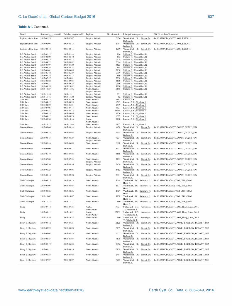
C. Le Quéré et al.: Global Carbon Budget 2016 637
Table A1. Continued.
Vessel Start date yyyy-mm-dd End date yyyy-mm-dd Regions No. of samples Principal investigators DOI (if available)/comment
Explorer of the Seas 2015-01-29 2015-02-07 Tropical Atlantic 3176 Wanninkhof, R.; Pierrot, D.;Barbero, L.
doi:10.3334/CDIAC/OTG.VOS_EXP2015
Explorer of the Seas 2015-02-07 2015-02-12 Tropical Atlantic 1707 Wanninkhof, R.; Pierrot, D.;Barbero, L.
doi:10.3334/CDIAC/OTG.VOS_EXP2015
Explorer of the Seas 2015-02-12 2015-02-15 Tropical Atlantic 1289 Wanninkhof, R.; Pierrot, D.;Barbero, L.
doi:10.3334/CDIAC/OTG.VOS_EXP2015
F.G. Walton Smith 2015-01-12 2015-01-14 Tropical Atlantic 816 Millero, F.; Wanninkhof, R.F.G. Walton Smith 2015-04-09 2015-04-10 Tropical Atlantic 613 Millero, F.; Wanninkhof, R.F.G. Walton Smith 2015-04-13 2015-04-17 Tropical Atlantic 2078 Millero, F.; Wanninkhof, R.F.G. Walton Smith 2015-04-22 2015-05-02 Tropical Atlantic 3514 Millero, F.; Wanninkhof, R.F.G. Walton Smith 2015-05-07 2015-05-20 Tropical Atlantic 6523 Millero, F.; Wanninkhof, R.F.G. Walton Smith 2015-05-26 2015-05-27 Tropical Atlantic 684 Millero, F.; Wanninkhof, R.F.G. Walton Smith 2015-06-01 2015-06-05 Tropical Atlantic 2038 Millero, F.; Wanninkhof, R.F.G. Walton Smith 2015-06-10 2015-06-27 Tropical Atlantic 7319 Millero, F.; Wanninkhof, R.F.G. Walton Smith 2015-07-14 2015-07-15 Tropical Atlantic 689 Millero, F.; Wanninkhof, R.F.G. Walton Smith 2015-07-27 2015-08-01 Tropical Atlantic 2258 Millero, F.; Wanninkhof, R.F.G. Walton Smith 2015-08-22 2015-09-04 Tropical Atlantic 6600 Millero, F.; Wanninkhof, R.F.G. Walton Smith 2015-09-21 2015-09-25 Tropical Atlantic 2096 Millero, F.; Wanninkhof, R.F.G. Walton Smith 2015-09-28 2015-10-02 Tropical Atlantic 1990 Millero, F.; Wanninkhof, R.F.G. Walton Smith 2015-10-27 2015-11-06 North Atlantic,
Tropical Atlantic3896 Millero, F.; Wanninkhof, R.
F.G. Walton Smith 2015-11-10 2015-11-11 Tropical Atlantic 271 Millero, F.; Wanninkhof, R.F.G. Walton Smith 2015-11-16 2015-11-20 Tropical Atlantic 82 Millero, F.; Wanninkhof, R.G.O. Sars 2015-01-17 2015-02-10 North Atlantic 9661 Lauvset, S.K.G.O. Sars 2015-04-12 2015-04-25 North Atlantic 11 719 Lauvset, S.K.; Skjelvan, I.G.O. Sars 2015-04-29 2015-05-01 North Atlantic 2939 Lauvset, S.K.; Skjelvan, I.G.O. Sars 2015-07-05 2015-07-14 North Atlantic 8921 Lauvset, S.K.; Skjelvan, I.G.O. Sars 2015-07-21 2015-08-13 North Atlantic 20 088 Lauvset, S.K.; Skjelvan, I.G.O. Sars 2015-08-18 2015-09-05 North Atlantic 18 076 Lauvset, S.K.; Skjelvan, I.G.O. Sars 2015-09-12 2015-09-25 North Atlantic 11 327 Lauvset, S.K.; Skjelvan, I.G.O. Sars 2015-09-30 2015-10-14 Arctic,
North Atlantic13 610 Lauvset, S.K.; Skjelvan, I.
G.O. Sars 2015-10-27 2015-11-03 North Atlantic 6937 Lauvset, S.K.; Skjelvan, I.Gordon Gunter 2015-03-04 2015-03-14 Tropical Atlantic 4678 Wanninkhof, R.; Pierrot, D.;
Barbero, L.doi:10.3334/CDIAC/OTG.COAST_GU2015_UW
Gordon Gunter 2015-03-18 2015-04-02 Tropical Atlantic 5015 Wanninkhof, R.; Pierrot, D.;Barbero, L.
doi:10.3334/CDIAC/OTG.COAST_GU2015_UW
Gordon Gunter 2015-04-15 2015-04-27 North Atlantic,Tropical Atlantic
4334 Wanninkhof, R.; Pierrot, D.;Barbero, L.
doi:10.3334/CDIAC/OTG.COAST_GU2015_UW
Gordon Gunter 2015-05-16 2015-06-05 North Atlantic 9118 Wanninkhof, R.; Pierrot, D.;Barbero, L.
doi:10.3334/CDIAC/OTG.COAST_GU2015_UW
Gordon Gunter 2015-06-09 2015-06-12 North Atlantic 1031 Wanninkhof, R.; Pierrot, D.;Barbero, L.
doi:10.3334/CDIAC/OTG.COAST_GU2015_UW
Gordon Gunter 2015-06-19 2015-07-03 North Atlantic 5688 Wanninkhof, R.; Pierrot, D.;Barbero, L.
doi:10.3334/CDIAC/OTG.COAST_GU2015_UW
Gordon Gunter 2015-07-08 2015-07-24 North Atlantic,Tropical Atlantic
7293 Wanninkhof, R.; Pierrot, D.;Barbero, L.
doi:10.3334/CDIAC/OTG.COAST_GU2015_UW
Gordon Gunter 2015-07-30 2015-08-16 Tropical Atlantic 7434 Wanninkhof, R.; Pierrot, D.;Barbero, L.
doi:10.3334/CDIAC/OTG.COAST_GU2015_UW
Gordon Gunter 2015-08-23 2015-09-06 Tropical Atlantic 6452 Wanninkhof, R.; Pierrot, D.;Barbero, L.
doi:10.3334/CDIAC/OTG.COAST_GU2015_UW
Gordon Gunter 2015-09-14 2015-09-28 Tropical Atlantic 6111 Wanninkhof, R.; Pierrot, D.;Barbero, L.
doi:10.3334/CDIAC/OTG.COAST_GU2015_UW
Gulf Challenger 2015-03-13 2015-03-13 North Atlantic 1148 Vandemark, D.; Salisbury, J.;Hunt, C.
doi:10.3334/CDIAC/otg.TSM_UNH_GOM
Gulf Challenger 2015-06-05 2015-06-05 North Atlantic 1071 Vandemark, D.; Salisbury, J.;Hunt, C.
doi:10.3334/CDIAC/otg.TSM_UNH_GOM
Gulf Challenger 2015-08-26 2015-08-26 North Atlantic 1127 Vandemark, D.; Salisbury, J.;Hunt, C.
doi:10.3334/CDIAC/otg.TSM_UNH_GOM
Gulf Challenger 2015-10-07 2015-10-07 North Atlantic 1078 Vandemark, D.; Salisbury, J.;Hunt, C.
doi:10.3334/CDIAC/otg.TSM_UNH_GOM
Gulf Challenger 2015-11-18 2015-11-18 North Atlantic 960 Vandemark, D.; Salisbury, J.;Hunt, C.
doi:10.3334/CDIAC/otg.TSM_UNH_GOM
Healy 2015-07-14 2015-07-24 Arctic,North Pacific
4121 Sutherland, S.C.; Newberger,T.; Takahashi, T.
doi:10.3334/CDIAC/OTG.VOS_Healy_Lines_2015
Healy 2015-08-11 2015-10-21 Arctic,North Pacific
27 033 Sutherland, S.C.; Newberger,T.; Takahashi, T.
doi:10.3334/CDIAC/OTG.VOS_Healy_Lines_2015
Healy 2015-10-26 2015-10-28 North Pacific 960 Sutherland, S.C.; Newberger,T.; Takahashi, T.
doi:10.3334/CDIAC/OTG.VOS_Healy_Lines_2015
Henry B. Bigelow 2015-03-12 2015-03-21 North Atlantic 3525 Wanninkhof, R.; Pierrot, D.;Barbero, L.
doi:10.3334/CDIAC/OTG.AOML_BIGELOW_ECOAST_2015
Henry B. Bigelow 2015-03-23 2015-04-03 North Atlantic 5059 Wanninkhof, R.; Pierrot, D.;Barbero, L.
doi:10.3334/CDIAC/OTG.AOML_BIGELOW_ECOAST_2015
Henry B. Bigelow 2015-04-07 2015-04-23 North Atlantic 6155 Wanninkhof, R.; Pierrot, D.;Barbero, L.
doi:10.3334/CDIAC/OTG.AOML_BIGELOW_ECOAST_2015
Henry B. Bigelow 2015-04-27 2015-05-07 North Atlantic 4638 Wanninkhof, R.; Pierrot, D.;Barbero, L.
doi:10.3334/CDIAC/OTG.AOML_BIGELOW_ECOAST_2015
Henry B. Bigelow 2015-05-19 2015-06-03 North Atlantic 6456 Wanninkhof, R.; Pierrot, D.;Barbero, L.
doi:10.3334/CDIAC/OTG.AOML_BIGELOW_ECOAST_2015
Henry B. Bigelow 2015-06-11 2015-06-19 North Atlantic 3839 Wanninkhof, R.; Pierrot, D.;Barbero, L.
doi:10.3334/CDIAC/OTG.AOML_BIGELOW_ECOAST_2015
Henry B. Bigelow 2015-06-24 2015-07-02 North Atlantic 3401 Wanninkhof, R.; Pierrot, D.;Barbero, L.
doi:10.3334/CDIAC/OTG.AOML_BIGELOW_ECOAST_2015
Henry B. Bigelow 2015-07-27 2015-08-07 North Atlantic 5265 Wanninkhof, R.; Pierrot, D.;Barbero, L.
doi:10.3334/CDIAC/OTG.AOML_BIGELOW_ECOAST_2015
www.earth-syst-sci-data.net/8/605/2016/ Earth Syst. Sci. Data, 8, 605–649, 2016

638 C. Le Quéré et al.: Global Carbon Budget 2016
Table A1. Continued.
Vessel Start date yyyy-mm-dd End date yyyy-mm-dd Regions No. of samples Principal investigators DOI (if available)/comment
Henry B. Bigelow 2015-08-12 2015-08-21 North Atlantic 4315 Wanninkhof, R.; Pierrot, D.;Barbero, L.
doi:10.3334/CDIAC/OTG.AOML_BIGELOW_ECOAST_2015
Henry B. Bigelow 2015-09-01 2015-09-17 North Atlantic 7836 Wanninkhof, R.; Pierrot, D.;Barbero, L.
doi:10.3334/CDIAC/OTG.AOML_BIGELOW_ECOAST_2015
Henry B. Bigelow 2015-09-23 2015-09-30 North Atlantic 3382 Wanninkhof, R.; Pierrot, D.;Barbero, L.
doi:10.3334/CDIAC/OTG.AOML_BIGELOW_ECOAST_2015
Henry B. Bigelow 2015-10-07 2015-10-22 North Atlantic 7186 Wanninkhof, R.; Pierrot, D.;Barbero, L.
doi:10.3334/CDIAC/OTG.AOML_BIGELOW_ECOAST_2015
Henry B. Bigelow 2015-10-27 2015-11-06 North Atlantic 4472 Wanninkhof, R.; Pierrot, D.;Barbero, L.
doi:10.3334/CDIAC/OTG.AOML_BIGELOW_ECOAST_2015
Henry B. Bigelow 2015-11-12 2015-11-17 North Atlantic 2402 Wanninkhof, R.; Pierrot, D.;Barbero, L.
doi:10.3334/CDIAC/OTG.AOML_BIGELOW_ECOAST_2015
Laurence M. Gould 2014-12-30 2015-02-07 Southern Ocean 7302 Sweeney, C.; Takahashi, T.;Newberger, T.; Sutherland,S.C.; Munro, D.R.
doi:10.3334/CDIAC/OTG.VOS_LM_GOULD_2014
Laurence M. Gould 2015-02-14 2015-03-16 Southern Ocean 9450 Sweeney, C.; Takahashi, T.;Newberger, T.; Sutherland,S.C.; Munro, D.R.
doi:10.3334/CDIAC/OTG.VOS_LM_GOULD_2015
Laurence M. Gould 2015-03-21 2015-04-03 Southern Ocean 2602 Sweeney, C.; Takahashi, T.;Newberger, T.; Sutherland,S.C.; Munro, D.R.
doi:10.3334/CDIAC/OTG.VOS_LM_GOULD_2015
Laurence M. Gould 2015-04-08 2015-05-11 Southern Ocean 7691 Sweeney, C.; Takahashi, T.;Newberger, T.; Sutherland,S.C.; Munro, D.R.
doi:10.3334/CDIAC/OTG.VOS_LM_GOULD_2015
Laurence M. Gould 2015-05-16 2015-06-16 Southern Ocean 9497 Sweeney, C.; Takahashi, T.;Newberger, T.; Sutherland,S.C.; Munro, D.R.
doi:10.3334/CDIAC/OTG.VOS_LM_GOULD_2015
Laurence M. Gould 2015-06-21 2015-06-30 Southern Ocean 2379 Sweeney, C.; Takahashi, T.;Newberger, T.; Sutherland,S.C.; Munro, D.R.
doi:10.3334/CDIAC/OTG.VOS_LM_GOULD_2015
Marcus G. Langseth 2015-04-13 2015-04-22 North Atlantic 1948 Sutherland, S.C.; Newberger,T.; Takahashi, T.; Sweeney, C.
doi:10.3334/CDIAC/OTG.VOS_MG_LANGSETH_LINES_2015
Marcus G. Langseth 2015-06-01 2015-06-23 North Atlantic 8608 Sutherland, S.C.; Newberger,T.; Takahashi, T.; Sweeney, C.
doi:10.3334/CDIAC/OTG.VOS_MG_LANGSETH_LINES_2015
Marcus G. Langseth 2015-07-31 2015-09-12 North Atlantic 14 519 Sutherland, S.C.; Newberger,T.; Takahashi, T.; Sweeney, C.
doi:10.3334/CDIAC/OTG.VOS_MG_LANGSETH_LINES_2015
Marion Dufresne 2015-01-07 2015-02-06 Indian Ocean, South-ern Ocean
4529 Metzl, N.; Lo Monaco, C. doi:10.3334/CDIAC/OTG.VOS_OISO_24
Mooring 2014-03-07 2015-03-22 Tropical Atlantic 3048 Sutton, A.; Sabine, C.;Manzello, D.; Musielewicz, S.;Maenner, S.; Dietrich, C.; Bott,R.; Osborne, J.
doi:10.3334/CDIAC/OTG.CHEECA_80W_25N
Mooring 2014-03-07 2015-04-03 Tropical Pacific 3129 Sutton, A.; Sabine, C.; Maen-ner, S.; Musielewicz, S.; Bott,R.; Osborne, J.
doi:10.3334/CDIAC/otg.TSM_Stratus_85W_20S
Mooring 2014-05-02 2015-04-28 North Pacific 2630 Sutton, A.; Sabine, C.; Send,U.; Ohman, M.; Musielewicz,S.; Maenner, S.; Dietrich, C.;Bott, R.; Osborne, J.
doi:10.3334/CDIAC/OTG.TSM_CCE2_121W_34N
Mooring 2014-05-06 2015-01-27 North Pacific 2122 Mathis, J.; Monacci, N.;Musielewicz, S.; Maenner, S.
doi:10.3334/CDIAC/OTG.TSM_Southeast_AK_56N_134W
Mooring 2014-05-24 2015-05-06 Tropical Pacific 2447 Sutton, A.; Sabine, C.; DeCarlo, E.; Musielewicz, S.;Maenner, S.; Dietrich, C.; Bott,R.; Osborne, J.
doi:10.3334/CDIAC/OTG.TSM_Kaneohe_158W_21N
Mooring 2014-07-21 2015-07-07 North Atlantic 2796 Sutton, A.; Sabine, C.; An-dersson, A.; Bates, N.;Musielewicz, S.; Maenner,S.; Dietrich, C.; Bott, R.;Osborne, J.
doi:10.3334/CDIAC/OTG.TSM_Crescent_64W_32N
Mooring 2014-10-06 2015-01-07 North Atlantic 741 Sutton, A.; Sabine, C.; Maen-ner, S.; Musielewicz, S.; Bott,R.; Osborne, J.
doi:10.3334/CDIAC/OTG.TSM_Hog_Reef_64W_32N
Nathaniel B. Palmer 2015-01-06 2015-01-18 Southern Ocean 4320 Sutherland, S.C.; Newberger,T.; Takahashi, T.; Sweeney, C.
doi:10.3334/CDIAC/OTG.VOS_PALMER_2015
Nathaniel B. Palmer 2015-01-23 2015-03-14 Southern Ocean 17 383 Sutherland, S.C.; Newberger,T.; Takahashi, T.; Sweeney, C.
doi:10.3334/CDIAC/OTG.VOS_PALMER_2015
Nathaniel B. Palmer 2015-03-27 2015-04-28 Southern Ocean 10 623 Sutherland, S.C.; Newberger,T.; Takahashi, T.; Sweeney, C.
doi:10.3334/CDIAC/OTG.VOS_PALMER_2015
Nathaniel B. Palmer 2015-05-12 2015-05-28 Southern Ocean 5654 Sutherland, S.C.; Newberger,T.; Takahashi, T.; Sweeney, C.
doi:10.3334/CDIAC/OTG.VOS_PALMER_2015
Nathaniel B. Palmer 2015-08-05 2015-08-28 Southern Ocean 7528 Sutherland, S.C.; Newberger,T.; Takahashi, T.; Sweeney, C.
doi:10.3334/CDIAC/OTG.VOS_PALMER_2015
Nathaniel B. Palmer 2015-09-08 2015-10-18 Southern Ocean,Tropical Atlantic
13 871 Sutherland, S.C.; Newberger,T.; Takahashi, T.; Sweeney, C.
doi:10.3334/CDIAC/OTG.VOS_PALMER_2015
New Century 2 2014-12-12 2015-01-12 North Pacific,Tropical Pacific
3221 Nakaoka, S. doi:10.3334/CDIAC/OTG.VOS_New_Century_2_2014
New Century 2 2015-03-16 2015-03-31 North Pacific 1343 Nakaoka, S. doi:10.3334/CDIAC/OTG.VOS_New_Century_2_2015New Century 2 2015-04-01 2015-04-14 North Pacific 1417 Nakaoka, S. doi:10.3334/CDIAC/OTG.VOS_New_Century_2_2015New Century 2 2015-04-16 2015-05-03 North Pacific 1668 Nakaoka, S. doi:10.3334/CDIAC/OTG.VOS_New_Century_2_2015New Century 2 2015-05-04 2015-05-17 North Pacific 1616 Nakaoka, S. doi:10.3334/CDIAC/OTG.VOS_New_Century_2_2015New Century 2 2015-05-20 2015-06-04 North Pacific 1569 Nakaoka, S. doi:10.3334/CDIAC/OTG.VOS_New_Century_2_2015
Earth Syst. Sci. Data, 8, 605–649, 2016 www.earth-syst-sci-data.net/8/605/2016/

C. Le Quéré et al.: Global Carbon Budget 2016 639
Table A1. Continued.
Vessel Start date yyyy-mm-dd End date yyyy-mm-dd Regions No. of samples Principal investigators DOI (if available)/comment
New Century 2 2015-06-05 2015-06-21 North Pacific 1545 Nakaoka, S. doi:10.3334/CDIAC/OTG.VOS_New_Century_2_2015New Century 2 2015-06-23 2015-07-07 North Pacific 1376 Nakaoka, S. doi:10.3334/CDIAC/OTG.VOS_New_Century_2_2015New Century 2 2015-07-07 2015-07-20 North Pacific 1440 Nakaoka, S. doi:10.3334/CDIAC/OTG.VOS_New_Century_2_2015New Century 2 2015-07-23 2015-08-07 North Pacific 1538 Nakaoka, S. doi:10.3334/CDIAC/OTG.VOS_New_Century_2_2015New Century 2 2015-08-09 2015-08-21 North Pacific 1460 Nakaoka, S. doi:10.3334/CDIAC/OTG.VOS_New_Century_2_2015New Century 2 2015-08-26 2015-09-24 North Pacific,
Tropical Pacific2422 Nakaoka, S. doi:10.3334/CDIAC/OTG.VOS_New_Century_2_2015
New Century 2 2015-09-24 2015-10-23 North Atlantic, NorthPacific, Tropical At-lantic, Tropical Pa-cific
3157 Nakaoka, S. doi:10.3334/CDIAC/OTG.VOS_New_Century_2_2015
Nuka Arctica 2015-10-21 2015-11-08 North Atlantic 5318 Omar, A.; Olsen, A.; Johan-nessen, T.
Nuka Arctica 2015-12-01 2015-12-21 North Atlantic 10 558 Omar, A.; Olsen, A.; Johan-nessen, T.
Polarstern 2014-12-03 2015-01-31 Southern Ocean 58 046 van Heuven, S.; Hoppema, M. doi:10.3334/CDIAC/OTG.OA_VOS_POLARSTERN_2014Polarstern 2015-05-19 2015-06-27 Arctic,
North Atlantic39 056 van Heuven, S.; Hoppema, M. doi:10.3334/CDIAC/OTG.OA_VOS_POLARSTERN_2015
Polarstern 2015-06-29 2015-08-14 Arctic,North Atlantic
20 164 van Heuven, S.; Hoppema, M. doi:10.3334/CDIAC/OTG.OA_VOS_POLARSTERN_2015
Polarstern 2015-08-18 2015-10-11 Arctic,North Atlantic
43 709 van Heuven, S.; Hoppema, M. doi:10.3334/CDIAC/OTG.OA_VOS_POLARSTERN_2015
Polarstern 2015-10-30 2015-12-01 North Atlantic,Southern Ocean,Tropical Atlantic
27 178 van Heuven, S.; Hoppema, M. doi:10.3334/CDIAC/OTG.OA_VOS_POLARSTERN_2015
Ronald H. Brown 2015-01-15 2015-01-29 North Pacific,Tropical Pacific
4855 Wanninkhof, R.; Pierrot, D.;Barbero, L.
doi:10.3334/CDIAC/OTG.VOS_RB_2015
Ronald H. Brown 2015-01-30 2015-02-12 North Pacific 5365 Wanninkhof, R.; Pierrot, D.;Barbero, L.
doi:10.3334/CDIAC/OTG.VOS_RB_2015
Ronald H. Brown 2015-03-01 2015-03-30 Tropical Pacific 13 576 Wanninkhof, R.; Pierrot, D.;Barbero, L.
doi:10.3334/CDIAC/OTG.VOS_RB_2015
Ronald H. Brown 2015-04-10 2015-05-12 Tropical Pacific 15 021 Wanninkhof, R.; Pierrot, D.;Barbero, L.
doi:10.3334/CDIAC/OTG.VOS_RB_2015
Ronald H. Brown 2015-05-25 2015-06-24 North Pacific,Tropical Pacific
13 690 Wanninkhof, R.; Pierrot, D.;Barbero, L.
doi:10.3334/CDIAC/OTG.VOS_RB_2015
Ronald H. Brown 2015-07-14 2015-07-31 North Pacific 5862 Wanninkhof, R.; Pierrot, D.;Barbero, L.
doi:10.3334/CDIAC/OTG.VOS_RB_2015
Ronald H. Brown 2015-08-06 2015-08-21 Arctic,North Pacific
6365 Wanninkhof, R.; Pierrot, D.;Barbero, L.
doi:10.3334/CDIAC/OTG.VOS_RB_2015
Ronald H. Brown 2015-08-22 2015-09-04 Arctic,North Pacific
6298 Wanninkhof, R.; Pierrot, D.;Barbero, L.
doi:10.3334/CDIAC/OTG.VOS_RB_2015
Ronald H. Brown 2015-11-22 2015-12-18 Tropical Pacific 10 838 Wanninkhof, R.; Pierrot, D.;Barbero, L.
doi:10.3334/CDIAC/OTG.VOS_RB_2015
S.A. Agulhas II 2014-12-08 2015-02-16 Southern Ocean 23 342 Monteiro, P.M.S.; Joubert,W.R.; Gregor, L.
doi:10.3334/CDIAC/OTG.VOS_SA_Agulhas_II_2015
S.A. Agulhas II 2015-07-23 2015-08-12 Southern Ocean 16 271 Monteiro, P.M.S.; Joubert,W.R.; Gregor, L.
doi:10.3334/CDIAC/OTG.VOS_SA_Agulhas_II_2015
S.A. Agulhas II 2015-09-04 2015-10-06 Southern Ocean 12 371 Monteiro, P.M.S.; Joubert,W.R.; Gregor, L.
doi:10.3334/CDIAC/OTG.VOS_SA_Agulhas_II_2015
Simon Stevin 2015-06-01 2015-06-01 North Atlantic 445 Gkritzalis, T.; Cattrijsse, A.Simon Stevin 2015-06-04 2015-06-04 North Atlantic 909 Gkritzalis, T.; Cattrijsse, A.Simon Stevin 2015-06-08 2015-06-08 North Atlantic 440 Gkritzalis, T.; Cattrijsse, A.Simon Stevin 2015-06-23 2015-06-23 North Atlantic 749 Gkritzalis, T.; Cattrijsse, A.Simon Stevin 2015-06-24 2015-06-24 North Atlantic 1234 Gkritzalis, T.; Cattrijsse, A.Simon Stevin 2015-06-25 2015-06-25 North Atlantic 787 Gkritzalis, T.; Cattrijsse, A.Simon Stevin 2015-06-30 2015-06-30 North Atlantic 425 Gkritzalis, T.; Cattrijsse, A.Simon Stevin 2015-07-02 2015-07-02 North Atlantic 154 Gkritzalis, T.; Cattrijsse, A.Simon Stevin 2015-07-06 2015-07-06 North Atlantic 168 Gkritzalis, T.; Cattrijsse, A.Simon Stevin 2015-07-10 2015-07-10 North Atlantic 357 Gkritzalis, T.; Cattrijsse, A.Simon Stevin 2015-07-13 2015-07-13 North Atlantic 223 Gkritzalis, T.; Cattrijsse, A.Simon Stevin 2015-07-14 2015-07-14 North Atlantic 54 Gkritzalis, T.; Cattrijsse, A.Simon Stevin 2015-07-15 2015-07-15 North Atlantic 477 Gkritzalis, T.; Cattrijsse, A.Simon Stevin 2015-07-16 2015-07-16 North Atlantic 465 Gkritzalis, T.; Cattrijsse, A.Simon Stevin 2015-07-22 2015-07-22 North Atlantic 87 Gkritzalis, T.; Cattrijsse, A.Simon Stevin 2015-07-23 2015-07-23 North Atlantic 428 Gkritzalis, T.; Cattrijsse, A.Simon Stevin 2015-07-24 2015-07-24 North Atlantic 299 Gkritzalis, T.; Cattrijsse, A.Simon Stevin 2015-07-31 2015-07-31 North Atlantic 401 Gkritzalis, T.; Cattrijsse, A.Simon Stevin 2015-08-03 2015-08-03 North Atlantic 394 Gkritzalis, T.; Cattrijsse, A.Simon Stevin 2015-08-04 2015-08-04 North Atlantic 412 Gkritzalis, T.; Cattrijsse, A.Simon Stevin 2015-08-07 2015-08-07 North Atlantic 463 Gkritzalis, T.; Cattrijsse, A.Simon Stevin 2015-08-10 2015-08-10 North Atlantic 479 Gkritzalis, T.; Cattrijsse, A.Simon Stevin 2015-08-12 2015-08-12 North Atlantic 341 Gkritzalis, T.; Cattrijsse, A.Simon Stevin 2015-08-17 2015-08-17 North Atlantic 439 Gkritzalis, T.; Cattrijsse, A.Simon Stevin 2015-08-18 2015-08-18 North Atlantic 414 Gkritzalis, T.; Cattrijsse, A.Simon Stevin 2015-08-19 2015-08-19 North Atlantic 470 Gkritzalis, T.; Cattrijsse, A.Simon Stevin 2015-08-21 2015-08-21 North Atlantic 401 Gkritzalis, T.; Cattrijsse, A.Simon Stevin 2015-08-24 2015-08-24 North Atlantic 450 Gkritzalis, T.; Cattrijsse, A.Simon Stevin 2015-08-27 2015-08-27 North Atlantic 373 Gkritzalis, T.; Cattrijsse, A.Simon Stevin 2015-08-28 2015-08-28 North Atlantic 455 Gkritzalis, T.; Cattrijsse, A.Simon Stevin 2015-09-02 2015-09-02 North Atlantic 961 Gkritzalis, T.; Cattrijsse, A.Simon Stevin 2015-09-03 2015-09-03 North Atlantic 450 Gkritzalis, T.; Cattrijsse, A.Simon Stevin 2015-09-04 2015-09-04 North Atlantic 307 Gkritzalis, T.; Cattrijsse, A.Simon Stevin 2015-09-08 2015-09-08 North Atlantic 464 Gkritzalis, T.; Cattrijsse, A.
www.earth-syst-sci-data.net/8/605/2016/ Earth Syst. Sci. Data, 8, 605–649, 2016

640 C. Le Quéré et al.: Global Carbon Budget 2016
Table A1. Continued.
Vessel Start date yyyy-mm-dd End date yyyy-mm-dd Regions No. of samples Principal investigators DOI (if available)/comment
Simon Stevin 2015-09-09 2015-09-09 North Atlantic 436 Gkritzalis, T.; Cattrijsse, A.Simon Stevin 2015-09-10 2015-09-10 North Atlantic 469 Gkritzalis, T.; Cattrijsse, A.Simon Stevin 2015-09-11 2015-09-11 North Atlantic 443 Gkritzalis, T.; Cattrijsse, A.Simon Stevin 2015-09-15 2015-09-15 North Atlantic 729 Gkritzalis, T.; Cattrijsse, A.Simon Stevin 2015-09-16 2015-09-16 North Atlantic 1081 Gkritzalis, T.; Cattrijsse, A.Simon Stevin 2015-09-21 2015-09-21 North Atlantic 366 Gkritzalis, T.; Cattrijsse, A.Simon Stevin 2015-09-25 2015-09-25 North Atlantic 454 Gkritzalis, T.; Cattrijsse, A.Simon Stevin 2015-09-28 2015-09-28 North Atlantic 440 Gkritzalis, T.; Cattrijsse, A.Simon Stevin 2015-09-29 2015-09-29 North Atlantic 701 Gkritzalis, T.; Cattrijsse, A.Simon Stevin 2015-09-30 2015-09-30 North Atlantic 850 Gkritzalis, T.; Cattrijsse, A.Simon Stevin 2015-10-05 2015-10-05 North Atlantic 453 Gkritzalis, T.; Cattrijsse, A.Simon Stevin 2015-10-06 2015-10-06 North Atlantic 491 Gkritzalis, T.; Cattrijsse, A.Simon Stevin 2015-10-07 2015-10-07 North Atlantic 423 Gkritzalis, T.; Cattrijsse, A.Simon Stevin 2015-10-08 2015-10-08 North Atlantic 437 Gkritzalis, T.; Cattrijsse, A.Simon Stevin 2015-10-10 2015-10-10 North Atlantic 488 Gkritzalis, T.; Cattrijsse, A.Simon Stevin 2015-10-11 2015-10-11 North Atlantic 448 Gkritzalis, T.; Cattrijsse, A.Simon Stevin 2015-10-20 2015-10-20 North Atlantic 435 Gkritzalis, T.; Cattrijsse, A.Simon Stevin 2015-10-21 2015-10-21 North Atlantic 319 Gkritzalis, T.; Cattrijsse, A.Simon Stevin 2015-11-01 2015-11-01 North Atlantic 387 Gkritzalis, T.; Cattrijsse, A.Simon Stevin 2015-11-04 2015-11-04 North Atlantic 272 Gkritzalis, T.; Cattrijsse, A.Simon Stevin 2015-11-05 2015-11-05 North Atlantic 415 Gkritzalis, T.; Cattrijsse, A.Simon Stevin 2015-11-06 2015-11-06 North Atlantic 114 Gkritzalis, T.; Cattrijsse, A.Simon Stevin 2015-11-12 2015-11-12 North Atlantic 202 Gkritzalis, T.; Cattrijsse, A.Simon Stevin 2015-12-07 2015-12-07 North Atlantic 217 Gkritzalis, T.; Cattrijsse, A.Simon Stevin 2015-12-08 2015-12-08 North Atlantic 336 Gkritzalis, T.; Cattrijsse, A.Simon Stevin 2015-12-09 2015-12-09 North Atlantic 156 Gkritzalis, T.; Cattrijsse, A.Soyo Maru 2015-05-08 2015-05-11 North Pacific, Tropi-
cal Pacific3972 Ono, T.
Soyo Maru 2015-08-01 2015-08-07 North Pacific 8354 Ono, T.Soyo Maru 2015-10-26 2015-11-03 North Pacific 10 759 Ono, T.Tangaroa 2015-01-28 2015-03-10 Southern Ocean 34 868 Currie, K. doi:10.3334/CDIAC/OTG.VOS_Tangaroa_2015Tangaroa 2015-03-27 2015-04-14 Southern Ocean 15 297 Currie, K. doi:10.3334/CDIAC/OTG.VOS_Tangaroa_2015Tangaroa 2015-04-17 2015-04-22 Southern Ocean 4797 Currie, K. doi:10.3334/CDIAC/OTG.VOS_Tangaroa_2015Tangaroa 2015-04-23 2015-04-30 Southern Ocean 5791 Currie, K. doi:10.3334/CDIAC/OTG.VOS_Tangaroa_2015Tangaroa 2015-05-04 2015-05-21 Southern Ocean 12 051 Currie, K. doi:10.3334/CDIAC/OTG.VOS_Tangaroa_2015Tangaroa 2015-05-23 2015-06-01 Southern Ocean 7985 Currie, K. doi:10.3334/CDIAC/OTG.VOS_Tangaroa_2015Tangaroa 2015-07-04 2015-08-02 Southern Ocean 26 898 Currie, K. doi:10.3334/CDIAC/OTG.VOS_Tangaroa_2015Tangaroa 2015-08-04 2015-08-26 Southern Ocean 18 553 Currie, K. doi:10.3334/CDIAC/OTG.VOS_Tangaroa_2015Tangaroa 2015-09-05 2015-09-24 Southern Ocean 12 776 Currie, K. doi:10.3334/CDIAC/OTG.VOS_Tangaroa_2015Tangaroa 2015-09-26 2015-10-04 Tropical Pacific 7207 Currie, K. doi:10.3334/CDIAC/OTG.VOS_Tangaroa_2014Tangaroa 2015-10-13 2015-10-25 Southern Ocean 10 658 Currie, K. doi:10.3334/CDIAC/OTG.VOS_Tangaroa_2015Trans Future 5 2015-01-10 2015-01-24 North Pacific, South-
ern Ocean,Tropical Pacific
1507 Nojiri, Y. doi:10.3334/CDIAC/OTG.VOS_TF5_2015
Trans Future 5 2015-01-31 2015-02-10 North Pacific, Tropi-cal Pacific
1179 Nojiri, Y. doi:10.3334/CDIAC/OTG.VOS_TF5_2015
Trans Future 5 2015-02-11 2015-02-24 Southern Ocean,Tropical Pacific
922 Nojiri, Y. doi:10.3334/CDIAC/OTG.VOS_TF5_2015
Trans Future 5 2015-02-25 2015-03-08 North Pacific, South-ern Ocean, TropicalPacific
1379 Nojiri, Y. doi:10.3334/CDIAC/OTG.VOS_TF5_2015
Trans Future 5 2015-03-14 2015-03-24 North Pacific, Tropi-cal Pacific
1083 Nojiri, Y. doi:10.3334/CDIAC/OTG.VOS_TF5_2015
Trans Future 5 2015-04-25 2015-05-05 North Pacific, Tropi-cal Pacific
1090 Nakaoka, S. doi:10.3334/CDIAC/OTG.VOS_TF5_2015
Trans Future 5 2015-05-06 2015-05-20 Southern Ocean,Tropical Pacific
913 Nakaoka, S. doi:10.3334/CDIAC/OTG.VOS_TF5_2015
Trans Future 5 2015-05-21 2015-06-01 North Pacific, South-ern Ocean, TropicalPacific
1381 Nakaoka, S. doi:10.3334/CDIAC/OTG.VOS_TF5_2015
Trans Future 5 2015-06-06 2015-06-15 North Pacific, Tropi-cal Pacific
1138 Nakaoka, S. doi:10.3334/CDIAC/OTG.VOS_TF5_2015
Trans Future 5 2015-06-16 2015-06-28 Southern Ocean,Tropical Pacific
911 Nakaoka, S. doi:10.3334/CDIAC/OTG.VOS_TF5_2015
Trans Future 5 2015-06-29 2015-07-12 North Pacific, South-ern Ocean, TropicalPacific
1431 Nakaoka, S. doi:10.3334/CDIAC/OTG.VOS_TF5_2015
Trans Future 5 2015-07-18 2015-07-30 North Pacific, Tropi-cal Pacific
1112 Nakaoka, S. doi:10.3334/CDIAC/OTG.VOS_TF5_2015
Trans Future 5 2015-07-30 2015-08-11 Southern Ocean,Tropical Pacific
884 Nakaoka, S. doi:10.3334/CDIAC/OTG.VOS_TF5_2015
Trans Future 5 2015-08-12 2015-08-24 North Pacific, South-ern Ocean, TropicalPacific
1400 Nakaoka, S. doi:10.3334/CDIAC/OTG.VOS_TF5_2015
Trans Future 5 2015-09-26 2015-10-07 North Pacific, Tropi-cal Pacific
811 Nakaoka, S. doi:10.3334/CDIAC/OTG.VOS_TF5_2015
Trans Future 5 2015-10-07 2015-10-19 Southern Ocean,Tropical Pacific
889 Nakaoka, S. doi:10.3334/CDIAC/OTG.VOS_TF5_2015
Trans Future 5 2015-10-21 2015-11-01 North Pacific, South-ern Ocean, TropicalPacific
1427 Nakaoka, S. doi:10.3334/CDIAC/OTG.VOS_TF5_2015
Wakataka Maru 2015-06-30 2015-07-04 North Pacific 6356 Kuwata, A.; Tadokoro, K.,Ono, T.
Wakataka Maru 2015-07-11 2015-07-21 North Pacific 14 479 Kuwata, A.; Tadokoro, K.,Ono, T.
Wakataka Maru 2015-07-29 2015-08-05 North Pacific 9773 Kuwata, A.; Tadokoro, K.,Ono, T.
Wakataka Maru 2015-09-30 2015-10-15 North Pacific 15 111 Kuwata, A.; Tadokoro, K.,Ono, T.
Earth Syst. Sci. Data, 8, 605–649, 2016 www.earth-syst-sci-data.net/8/605/2016/
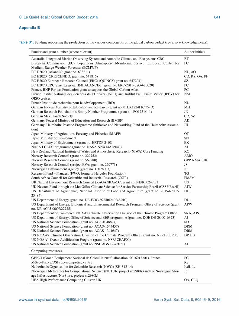
C. Le Quéré et al.: Global Carbon Budget 2016 641
Appendix B
Table B1. Funding supporting the production of the various components of the global carbon budget (see also acknowledgements).
Funder and grant number (where relevant) Author initials
Australia, Integrated Marine Observing System and Antarctic Climate and Ecosystems CRC BTEuropean Commission (EC) Copernicus Atmosphere Monitoring Service, European Centre forMedium-Range Weather Forecasts (ECMWF)
FC
EC H2020 (AtlantOS; grant no. 633211) NL, AOEC H2020 (CRESCENDO; grant no. 641816) CD, RS, OA, PFEC H2020 European Research Council (ERC) (QUINCY; grant no. 647204). SZEC H2020 ERC Synergy grant (IMBALANCE-P; grant no. ERC-2013-SyG-610028) PCFrance, BNP Paribas Foundation grant to support the Global Carbon Atlas PCFrench Institut National des Sciences de l’Univers (INSU) and Institut Paul Emile Victor (IPEV) forOISO cruises
NM
French Institut de recherche pour le développement (IRD) NLGerman Federal Ministry of Education and Research (grant no. 01LK1224I ICOS-D) MHGerman Research Foundation’s Emmy Noether Programme (grant no. PO1751/1-1) JNGerman Max Planck Society CR, SZGermany, Federal Ministry of Education and Research (BMBF) AKGermany, Helmholtz Postdoc Programme (Initiative and Networking Fund of the Helmholtz Associa-tion)
JH
Japan Ministry of Agriculture, Forestry and Fisheries (MAFF) OTJapan Ministry of Environment SNJapan Ministry of Environment (grant no. ERTDF S-10) EKNASA LCLUC programme (grant no. NASA NNX14AD94G) AJNew Zealand National Institute of Water and Atmospheric Research (NIWA) Core Funding KCNorway Research Council (grant no. 229752) AMONorway Research Council (grant no. 569980) GPP, RMA, JIKNorway Research Council (project EVA; grant no. 229771) JSNorwegian Environment Agency (grant no. 16078007) ISResearch Fund – Flanders (FWO; formerly Hercules Foundation) TGSouth Africa Council for Scientific and Industrial Research (CSIR) PMSMUK Natural Environment Research Council (RAGANRAoCC; grant no. NE/K002473/1) USUK Newton Fund through the Met Office Climate Science for Service Partnership Brazil (CSSP Brazil) AJWUS Department of Agriculture, National Institute of Food and Agriculture (grant no. 2015-67003-23485)
DL
US Department of Energy (grant no. DE-FC03-97ER62402/A010) DLUS Department of Energy, Biological and Environmental Research Program, Office of Science (grantno. DE-AC05-00OR22725)
APW
US Department of Commerce, NOAA’s Climate Observation Division of the Climate Program Office SRA, AJSUS Department of Energy, Office of Science and BER programme (grant no. DOE DE-SC0016323) AJUS National Science Foundation (grant no. AGS-1048827) SDUS National Science Foundation (grant no. AOAS-1543457) DRMUS National Science Foundation (grant no. AOAS-1341647) DRMUS NOAA’s Climate Observation Division of the Climate Program Office (grant no. N8R1SE3P00);US NOAA’s Ocean Acidification Program (grant no. N8R3CEAP00)
DP, LB
US National Science Foundation (grant no. NSF AGS 12-43071) AJ
Computing resources
GENCI (Grand Équipement National de Calcul Intensif; allocation t2016012201), France FCMétéo-France/DSI supercomputing centre RSNetherlands Organisation for Scientific Research (NWO) (SH-312-14) IvdL-LNorwegian Metacenter for Computational Science (NOTUR, project nn2980k) and the Norwegian Stor-age Infrastructure (NorStore, project ns2980k)
JS
UEA High Performance Computing Cluster, UK OA, CLQ
www.earth-syst-sci-data.net/8/605/2016/ Earth Syst. Sci. Data, 8, 605–649, 2016
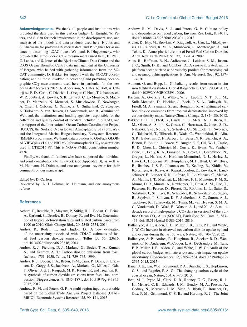
642 C. Le Quéré et al.: Global Carbon Budget 2016
Acknowledgements. We thank all people and institutions whoprovided the data used in this carbon budget; C. Enright, W. Pe-ters, and S. Shu for their involvement in the development, use, andanalysis of the models and data products used here; F. Joos andS. Khatiwala for providing historical data; and P. Regnier for assis-tance in describing LOAC fluxes. We thank E. Dlugokencky, whoprovided the atmospheric CO2 measurements used here; B. Pfeil,C. Landa, and S. Jones of the Bjerknes Climate Data Centre and theICOS Ocean Thematic Centre data management at the Universityof Bergen, who helped with gathering information from the SO-CAT community; D. Bakker for support with the SOCAT coordi-nation; and all those involved in collecting and providing oceano-graphic CO2 measurements used here, in particular for the newocean data for years 2015: A. Andersson, N. Bates, R. Bott, A. Cat-trijsse, E. De Carlo, C. Dietrich, L. Gregor, C. Hunt, T. Johannessen,W. R. Joubert, A. Kuwata, S. K. Lauvset, C. Lo Monaco, S. Maen-ner, D. Manzello, N. Monacci, S. Musielewicz, T. Newberger,A. Olsen, J. Osborne, C. Sabine, S. C. Sutherland, C. Sweeney,K. Tadokoro, S. van Heuven, D. Vandemark, and R. Wanninkhof.We thank the institutions and funding agencies responsible for thecollection and quality control of the data included in SOCAT, andthe support of the International Ocean Carbon Coordination Project(IOCCP), the Surface Ocean Lower Atmosphere Study (SOLAS),and the Integrated Marine Biogeochemistry, Ecosystem Research(IMBER) programme. We thank data providers to ObsPack GLOB-ALVIEWplus v1.0 and NRT v3.0 for atmospheric CO2 observationsused in CTE2016-FT. This is NOAA-PMEL contribution number4576.
Finally, we thank all funders who have supported the individualand joint contributions to this work (see Appendix B), as well asM. Heimann, H. Dolman, and one anonymous reviewer for theircomments on our manuscript.
Edited by: D. CarlsonReviewed by: A. J. Dolman, M. Heimann, and one anonymousreferee
References
Achard, F., Beuchle, R., Mayaux, P., Stibig, H. J., Bodart, C., Brink,A., Carboni, S., Desclée, B., Donnay, F., and Eva, H.: Determina-tion of tropical deforestation rates and related carbon losses from1990 to 2010, Glob. Change Biol., 20, 2540–2554, 2014.
Andres, R., Boden, T., and Higdon, D.: A new evaluationof the uncertainty associated with CDIAC estimates of fos-sil fuel carbon dioxide emission, Tellus B, 66, 23616,doi:10.3402/tellusb.v66.23616, 2014.
Andres, R. J., Fielding, D. J., Marland, G., Boden, T. A., Kumar,N., and Kearney, A. T.: Carbon dioxide emissions from fossilfuel use, 1751–1950, Tellus, 51, 759–765, 1999.
Andres, R. J., Boden, T. A., Bréon, F.-M., Ciais, P., Davis, S., Erick-son, D., Gregg, J. S., Jacobson, A., Marland, G., Miller, J., Oda,T., Olivier, J. G. J., Raupach, M. R., Rayner, P., and Treanton, K.:A synthesis of carbon dioxide emissions from fossil-fuel com-bustion, Biogeosciences, 9, 1845–1871, doi:10.5194/bg-9-1845-2012, 2012.
Andrew, R. M. and Peters, G. P.: A multi-region input-output tablebased on the Global Trade Analysis Project Database (GTAP-MRIO), Economic Systems Research, 25, 99–121, 2013.
Andrew, R. M., Davis, S. J., and Peters, G. P.: Climate policyand dependence on traded carbon, Environ. Res. Lett., 8, 34011,doi:10.1088/1748-9326/8/3/034011, 2013.
Archer, D., Eby, M., Brovkin, V., Ridgwell, A., Cao, L., Mikolajew-icz, U., Caldeira, K. M., K., Munhoven, G., Montenegro, A., andTokos, K.: Atmospheric Lifetime of Fossil Fuel Carbon Dioxide,Annu. Rev. Earth Planet. Sc., 37, 117-134, 2009.
Atlas, R., Hoffman, R. N., Ardizzone, J., Leidner, S. M., Jusem,J. C., Smith, D. K., and Gombos, D.: A cross-calibrated, multi-platform ocean surface wind velocity product for meteorologicaland oceanographic applications, B. Am. Meteorol. Soc., 92, 157–174, 2011.
Aumont, O. and Bopp, L.: Globalizing results from ocean in situiron fertilization studies, Global Biogeochem. Cyc., 20, GB2017,doi:10.1029/2005GB002591, 2006.
Baccini, A., Goetz, S. J., Walker, W. S., Laporte, N. T., Sun, M.,Sulla-Menashe, D., Hackler, J., Beck, P. S. A., Dubayah, R.,Friedl, M. A., Samanta, S., and Houghton, R. A.: Estimated car-bon dioxide emissions from tropical deforestation improved bycarbon-density maps, Nature Climate Change, 2, 182–186, 2012.
Bakker, D. C. E., Pfeil, B., Landa, C. S., Metzl, N., O’Brien, K.M., Olsen, A., Smith, K., Cosca, C., Harasawa, S., Jones, S. D.,Nakaoka, S.-I., Nojiri, Y., Schuster, U., Steinhoff, T., Sweeney,C., Takahashi, T., Tilbrook, B., Wada, C., Wanninkhof, R., Alin,S. R., Balestrini, C. F., Barbero, L., Bates, N. R., Bianchi, A. A.,Bonou, F., Boutin, J., Bozec, Y., Burger, E. F., Cai, W.-J., Castle,R. D., Chen, L., Chierici, M., Currie, K., Evans, W., Feather-stone, C., Feely, R. A., Fransson, A., Goyet, C., Greenwood, N.,Gregor, L., Hankin, S., Hardman-Mountford, N. J., Harlay, J.,Hauck, J., Hoppema, M., Humphreys, M. P., Hunt, C. W., Huss,B., Ibánhez, J. S. P., Johannessen, T., Keeling, R., Kitidis, V.,Körtzinger, A., Kozyr, A., Krasakopoulou, E., Kuwata, A., Land-schützer, P., Lauvset, S. K., Lefèvre, N., Lo Monaco, C., Manke,A., Mathis, J. T., Merlivat, L., Millero, F. J., Monteiro, P. M. S.,Munro, D. R., Murata, A., Newberger, T., Omar, A. M., Ono, T.,Paterson, K., Pearce, D., Pierrot, D., Robbins, L. L., Saito, S.,Salisbury, J., Schlitzer, R., Schneider, B., Schweitzer, R., Sieger,R., Skjelvan, I., Sullivan, K. F., Sutherland, S. C., Sutton, A. J.,Tadokoro, K., Telszewski, M., Tuma, M., van Heuven, S. M. A.C., Vandemark, D., Ward, B., Watson, A. J., and Xu, S.: A multi-decade record of high-quality fCO2 data in version 3 of the Sur-face Ocean CO2 Atlas (SOCAT), Earth Syst. Sci. Data, 8, 383–413, doi:10.5194/essd-8-383-2016, 2016.
Ballantyne, A. P., Alden, C. B., Miller, J. B., Tans, P. P., and White,J. W. C.: Increase in observed net carbon dioxide uptake by landand oceans during the last 50 years, Nature, 488, 70–72, 2012.
Ballantyne, A. P., Andres, R., Houghton, R., Stocker, B. D., Wan-ninkhof, R., Anderegg, W., Cooper, L. A., DeGrandpre, M., Tans,P. P., Miller, J. B., Alden, C., and White, J. W. C.: Audit of theglobal carbon budget: estimate errors and their impact on uptakeuncertainty, Biogeosciences, 12, 2565–2584, doi:10.5194/bg-12-2565-2015, 2015.
Bauer, J. E., Cai, W.-J., Raymond, P. A., Bianchi, T. S., Hopkinson,C. S., and Regnier, P. A. G.: The changing carbon cycle of thecoastal ocean, Nature, 504, 61–70, 2013.
Best, M. J., Pryor, M., Clark, D. B., Rooney, G. G., Essery, R. L.H., Ménard, C. B., Edwards, J. M., Hendry, M. A., Porson, A.,Gedney, N., Mercado, L. M., Sitch, S., Blyth, E., Boucher, O.,Cox, P. M., Grimmond, C. S. B., and Harding, R. J.: The Joint
Earth Syst. Sci. Data, 8, 605–649, 2016 www.earth-syst-sci-data.net/8/605/2016/

C. Le Quéré et al.: Global Carbon Budget 2016 643
UK Land Environment Simulator (JULES), model description –Part 1: Energy and water fluxes, Geosci. Model Dev., 4, 677–699,doi:10.5194/gmd-4-677-2011, 2011.
Betts, R. A., Jones, C. D., Knight, J. R., Keeling, R. F., and Kennedy,J. J.: El Nino and a record CO2 rise, Nature Climate Change, 6,806–810, 2016.
Boden, T. A. and Andres, R. J.: Global, Regional, and NationalFossil-Fuel CO2 Emissions, available at: http://cdiac.ornl.gov/trends/emis/overview_2013.html (last access: April 2016), OakRidge National Laboratory, US Department of Energy, OakRidge, Tenn., USA, 2016.
BP: Change in methodology for calculatingCO2 emissions from energy use, available at:http://www.bp.com/content/dam/bp/pdf/energy-economics/statistical-review-2016/bp-statistical-review-of-world-energy-2016-carbon-emissions-methodology.pdf (last access: Septem-ber 2016), 2016a.
BP: Statistical Review of World Energy 2016, availableat: https://www.bp.com/content/dam/bp/pdf/ energy-economics/statistical-review-2016/bp-statistical-review-of-world-energy-2016-full-report.pdf (last access: June 2016),2016b.
Bruno, M. and Joos, F.: Terrestrial carbon storage during the past200 years: A monte carlo analysis of CO2 data from ice core andatmospheric measurements, Global Biogeochem. Cy., 11, 111–124, 1997.
Buitenhuis, E. T., Rivkin, R. B., Sailley, S., and Le Quéré, C.:Biogeochemical fluxes through microzooplankton, Global Bio-geochem. Cy., 24, GB4015, doi:10.1029/2009gb003601, 2010.
Canadell, J., Ciais, P., Sabine, C., and Joos, F. (Eds.): REgionalCarbon Cycle Assessment and Processes (RECCAP), Biogeo-sciences, http://www.biogeosciences.net/special_issue107.html,2012.
Canadell, J. G., Le Quéré, C., Raupach, M. R., Field, C. B., Buiten-huis, E. T., Ciais, P., Conway, T. J., Gillett, N. P., Houghton, R.A., and Marland, G.: Contributions to accelerating atmosphericCO2 growth from economic activity, carbon intensity, and effi-ciency of natural sinks, P. Natl. Acad. Sci. USA, 104, 18866–18870, 2007.
CCIA: China Coal Industry Association, 2016 First Three Quar-ters of Economic Operation of Coal, available at: http://www.coalchina.org.cn/detail/16/10/25/00000007/content.html, last ac-cess: 29 October 2016 (in Chinese).
Chevallier, F.: On the statistical optimality of CO2 atmosphericinversions assimilating CO2 column retrievals, Atmos. Chem.Phys., 15, 11133–11145, doi:10.5194/acp-15-11133-2015, 2015.
Chevallier, F., Fisher, M., Peylin, P., Serrar, S., Bousquet,P., Bréon, F.-M., Chédin, A., and Ciais, P.: Inferring CO2sources and sinks from satellite observations: Method andapplication to TOVS data, J. Geophys. Res., 110, D24309,doi:10.1029/2005JD006390, 2005.
Ciais, P., Sabine, C., Govindasamy, B., Bopp, L., Brovkin, V.,Canadell, J., Chhabra, A., DeFries, R., Galloway, J., Heimann,M., Jones, C., Le Quéré, C., Myneni, R., Piao, S., and Thorn-ton, P.: Chapter 6: Carbon and Other Biogeochemical Cycles,in: Climate Change 2013 The Physical Science Basis, edited by:Stocker, T., Qin, D., and Platner, G.-K., Cambridge UniversityPress, Cambridge, 2013.
Clark, D. B., Mercado, L. M., Sitch, S., Jones, C. D., Gedney, N.,Best, M. J., Pryor, M., Rooney, G. G., Essery, R. L. H., Blyth, E.,Boucher, O., Harding, R. J., Huntingford, C., and Cox, P. M.: TheJoint UK Land Environment Simulator (JULES), model descrip-tion – Part 2: Carbon fluxes and vegetation dynamics, Geosci.Model Dev., 4, 701–722, doi:10.5194/gmd-4-701-2011, 2011.
Davis, S. J. and Caldeira, K.: Consumption-based accounting ofCO2 emissions, P. Natl. Acad. Sci. USA, 107, 5687–5692, 2010.
Denman, K. L., Brasseur, G., Chidthaisong, A., Ciais, P., Cox, P.M., Dickinson, R. E., Hauglustaine, D., Heinze, C., Holland, E.,Jacob, D., Lohmann, U., Ramachandran, S., da Silva Dias, P. L.,Wofsy, S. C., and Zhang, X.: Couplings Between Changes in theClimate System and Biogeochemistry, in: Climate Change 2007:The Physical Science Basis. Contribution of Working Group I tothe Fourth Assessment Report of the Intergovernmental Panel onClimate Change, edited by: Solomon, S., Qin, D., Manning, M.,Chen, Z., Marquis, M., Averyt, K. B., Tignor, M., and Miller, H.L., Cambridge University Press, Cambridge, UK and New York,USA, 2007.
Dietzenbacher, E., Pei, J. S., and Yang, C. H.: Trade, productionfragmentation, and China’s carbon dioxide emissions, J. Environ.Econ. Manag., 64, 88–101, 2012.
Dlugokencky, E. and Tans, P.: Trends in atmospheric carbon diox-ide, National Oceanic & Atmospheric Administration, Earth Sys-tem Research Laboratory (NOAA/ESRL), available at: http://www.esrl.noaa.gov/gmd/ccgg/trends/global.html, last access: 28October 2016.
Doney, S. C., Lima, I., Feely, R. A., Glover, D. M., Lindsay, K.,Mahowald, N., Moore, J. K., and Wanninkhof, R.: Mechanismsgoverning interannual variability in upper-ocean inorganic car-bon system and air–sea CO2 fluxes: Physical climate and atmo-spheric dust, Deep-Sea Res. Pt. II, 56, 640–655, 2009.
Duce, R. A., LaRoche, J., Altieri, K., Arrigo, K. R., Baker, A.R., Capone, D. G., Cornell, S., Dentener, F., Galloway, J.,Ganeshram, R. S., Geider, R. J., Jickells, T., Kuypers, M. M.,Langlois, R., Liss, P. S., Liu, S. M., Middelburg, J. J., Moore,C. M., Nickovic, S., Oschlies, A., Pedersen, T., Prospero, J.,Schlitzer, R., Seitzinger, S., Sorensen, L. L., Uematsu, M., Ul-loa, O., Voss, M., Ward, B., and Zamora, L.: Impacts of atmo-spheric anthropogenic nitrogen on the open ocean, Science, 320,893–897, 2008.
Durant, A. J., Le Quéré, C., Hope, C., and Friend, A. D.: Eco-nomic value of improved quantification in global sources andsinks of carbon dioxide, Philos. T. Roy. Soc. A, 369, 1967–1979,doi:10.1098/rsta.2011.0002, 2011.
Earles, J. M., Yeh, S., and Skog, K. E.: Timing of carbon emissionsfrom global forest clearance, Nature Climate Change, 2, 682–685, 2012.
EDGAR: Global Emissions EDGAR v4.2 (November 2011), avail-able at: http://edgar.jrc.ec.europa.eu/overview.php?v=42 (last ac-cess: October 2016), 2011.
EIA: US Energy Information Administration, Short-Term Energyand Winter Fuels Outlook, available at: http://www.eia.gov/forecasts/steo/outlook.cfm, last access: October 2016.
Elliott, J., Müller, C., Deryng, D., Chryssanthacopoulos, J., Boote,K. J., Büchner, M., Foster, I., Glotter, M., Heinke, J., Iizumi, T.,Izaurralde, R. C., Mueller, N. D., Ray, D. K., Rosenzweig, C.,Ruane, A. C., and Sheffield, J.: The Global Gridded Crop ModelIntercomparison: data and modeling protocols for Phase 1 (v1.0),
www.earth-syst-sci-data.net/8/605/2016/ Earth Syst. Sci. Data, 8, 605–649, 2016

644 C. Le Quéré et al.: Global Carbon Budget 2016
Geosci. Model Dev., 8, 261–277, doi:10.5194/gmd-8-261-2015,2015.
El Masri, B., Shu, S., and Jain, A. K.: Implementation of a dynamicrooting depth and phenology into a land surface model: Eval-uation of carbon, water, and energy fluxes in the high latitudeecosystems, Agr. Forest Meteorol., 211–212, 85–99, 2015.
Erb, K.-H., Kastner, T., Luyssaert, S., Houghton, R. A., Kuemmerle,T., Olofsson, P., and Haberl, H.: Bias in the attribution of forestcarbon sinks, Nature Climate Change, 3, 854–856, 2013.
Etheridge, D. M., Steele, L. P., Langenfelds, R. L., and Francey, R.J.: Natural and anthropogenic changes in atmospheric CO2 overthe last 1000 years from air in Antarctic ice and firn, J. Geophys.Res., 101, 4115–4128, 1996.
FAO: Global Forest Resource Assessment 2010, 378 pp., Foodand Agriculture Organization of the United Nations, Rome, Italy2010.
FAOSTAT: Food and Agriculture Organization Statistics Division,available at: http://faostat.fao.org/ (last access: October 2012),2010.
Federici, S., Tubiello, F. N., Salvatore, M., Jacobs, H., and Schmid-huber, J.: New estimates of CO2 forest emissions and removals:1990–2015, Forest Ecol. Manage., 352, 89–98, 2015.
Feely, R. A., Wanninkhof, R., Takahashi, T., and Tans, P.: Influenceof El Nino on the equatorial Pacific contribution to atmosphericCO2 accumulation, Nature, 398, 597–601, 1999.
Francey, R. J., Trudinger, C. M., van der Schoot, M., Law, R. M.,Krummel, P. B., Langenfelds, R. L., Steele, L. P., Allison, C. E.,Stavert, A. R., Andres, R. J., and Rodenbeck, C.: Reply to “An-thropogenic CO2 emissions”, Nature Climate Change, 3, 604–604, 2013.
Friedlingstein, P., Houghton, R. A., Marland, G., Hackler, J., Boden,T. A., Conway, T. J., Canadell, J. G., Raupach, M. R., Ciais, P.,and Le Quéré, C.: Update on CO2 emissions, Nat. Geosci., 3,811–812, 2010.
Friedlingstein, P., Andrew, R. M., Rogelj, J., Peters, G. P., Canadell,J. G., Knutti, R., Luderer, G., Raupach, M. R., Schaeffer, M., vanVuuren, D. P., and Le Quéré, C.: Persistent growth of CO2 emis-sions and implications for reaching climate targets, Nat. Geosci.,7, 709–715, doi:10.1038/ngeo2248, 2014.
Gasser, T. and Ciais, P.: A theoretical framework for the net land-to-atmosphere CO2 flux and its implications in the definition of“emissions from land-use change”, Earth Syst. Dynam., 4, 171–186, doi:10.5194/esd-4-171-2013, 2013.
GCP: The Global Carbon Budget 2007, available at: http://www.globalcarbonproject.org/carbonbudget/archive.htm (last access:7 November 2016), 2007.
Giglio, L., Randerson, J., and van der Werf, G.: Analysis of daily,monthly, and annual burned area using the fourth-generationglobal fire emissions database (GFED4), J. Geophys. Res.-Biogeo., 118, 317–328, doi:10.1002/jgrg.20042, 2013.
Gitz, V. and Ciais, P.: Amplifying effects of land-use change on fu-ture atmospheric CO2 levels, Global Biogeochem. Cy., 17, 1024,doi:10.1029/2002GB001963, 2003.
Goll, D. S., Brovkin, V., Liski, J., Raddatz, T., Thum, T., and Todd-Brown, K. E. O.: Strong dependence of CO2 emissions from an-thropogenic land cover change on initial land cover and soil car-bon parametrization, Global Biogeochem. Cy., 29, 1511–1523,doi:10.1002/2014gb004988, 2015.
Gonzalez-Gaya, B., Fernandez-Pinos, M. C., Morales, L., Me-janelle, L., Abad, E., Pina, B., Duarte, C. M., Jimenez,B., and Dachs, J.: High atmosphere-ocean exchange ofsemivolatile aromatic hydrocarbons, Nat. Geosci., 9, 438–442,doi:10.1038/ngeo2714, 2016.
Gregg, J. S., Andres, R. J., and Marland, G.: China: Emissionspattern of the world leader in CO2 emissions from fossil fuelconsumption and cement production, Geophys. Res. Lett., 35,L08806, doi:10.1029/2007GL032887, 2008.
Harris, I., Jones, P. D., Osborn, T. J., and Lister, D. H.: Updatedhigh-resolution grids of monthly climatic observations – theCRU TS3.10 Dataset, Int. J. Climatol., 34, 623–642, 2014.
Harris, N., Brown, S., and Hagen, S. C.: Baseline map of carbonemissions from deforestation in tropical regions, Science, 336,1573–1576, 2012.
Hauck, J., Köhler, P., Wolf-Gladrow, D., and Völker, C.: Iron fer-tilisation and century-scale effects of open ocean dissolution ofolivine in a simulated CO2 removal experiment, Environ. Res.Lett., 11, 024007, doi:10.1088/1748-9326/11/2/024007, 2016.
Hertwich, E. G. and Peters, G. P.: Carbon Footprint of Nations: AGlobal, Trade-Linked Analysis, Environ. Sci. Tech., 43, 6414–6420, doi:10.1021/es803496a, 2009.
Houghton, R. A.: Revised estimates of the annual net flux of carbonto the atmosphere from changes in land use and land manage-ment 1850–2000, Tellus B, 55, 378–390, 2003.
Houghton, R. A. and Nassikas, A. A.: Global and regional fluxes ofcarbon from land use and land-cover change 1850–2015, GlobalBiogeochem. Cy., submitted, 2016.
Houghton, R. A., House, J. I., Pongratz, J., van der Werf, G. R., De-Fries, R. S., Hansen, M. C., Le Quéré, C., and Ramankutty, N.:Carbon emissions from land use and land-cover change, Biogeo-sciences, 9, 5125–5142, doi:10.5194/bg-9-5125-2012, 2012.
Hourdin, F., Musat, I., Bony, S., Braconnot, P., Codron, F.,Dufresne, J.-L., Fairhead, L., Filiberti, M.-A., Freidlingstein, P.,Grandpeix, J.-Y., Krinner, G., LeVan, P., Li, Z.-X., and Lott, F.:The LMDZ4 general circulation model: climate performance andsensitivity to parametrized physics with emphasis on tropicalconvection, Clim. Dynam., 27, 787–813, doi:10.1007/s00382-006-0158-0, 2006.
Hurtt, G. C., Chini, L. P., Frolking, S., Betts, R. A., Feddema, J.,Fischer, G., Fisk, J. P., Hibbard, K., Houghton, R. A., Janetos,A., Jones, C. D., Kindermann, G., Kinoshita, T., Goldewijk, K.K., Riahi, K., Shevliakova, E., Smith, S., Stehfest, E., Thom-son, A., Thornton, P., van Vuuren, D. P., and Wang, Y. P.: Har-monization of land-use scenarios for the period 1500-2100: 600years of global gridded annual land-use transitions, wood har-vest, and resulting secondary lands, Climatic Change, 109, 117–161, doi:10.1007/s10584-011-0153-2, 2011.
IEA/OECD: CO2 emissions from fuel combustion, InternationalEnergy Agency/Organisation for Economic Cooperation and De-velopment, Paris, 152 pp., 2015.
IEW: International Energy Web, available at: http://gas.in-en.com/html/gas-2517194.shtml, last access: 11 October 2016 (in Chi-nese).
IMF: World Economic Outlook of the International Monetary Fund,available at: http://www.imf.org/external/ns/cs.aspx?id=29, lastaccess: September 2016.
Earth Syst. Sci. Data, 8, 605–649, 2016 www.earth-syst-sci-data.net/8/605/2016/

C. Le Quéré et al.: Global Carbon Budget 2016 645
Inomata, S. and Owen, A.: COMPARATIVE EVALUATION OFMRIO DATABASES, Economic Systems Research, 26, 239–244, 2014.
Ito, A. and Inatomi, M.: Use of a process-based model for assessingthe methane budgets of global terrestrial ecosystems and evalua-tion of uncertainty, Biogeosciences, 9, 759–773, doi:10.5194/bg-9-759-2012, 2012.
Jackson, R. B., Canadell, J. G., Le Quéré, C., Andrew, R.M., Korsbakken, J. I., Peters, G. P., and Nakicenovic, N.:Reaching peak emissions, Nature Climate Change, 6, 7–10,doi:10.1038/nclimate2892„ 2016.
Jacobson, A. R., Mikaloff Fletcher, S. E., Gruber, N., Sarmiento,J. L., and Gloor, M.: A joint atmosphere-ocean inver-sion for surface fluxes of carbon dioxide: 1. Methods andglobal-scale fluxes, Global Biogeochem. Cy., 21, GB1019,doi:10.1029/2005GB002556, 2007.
Jain, A. K., Meiyappan, P., Song, Y., and House, J. I.: CO2 Emis-sions from Land-Use Change Affected More by Nitrogen Cycle,than by the Choice of Land Cover Data, Glob. Change Biol., 9,2893–2906, 2013.
Joos, F. and Spahni, R.: Rates of change in natural and anthro-pogenic radiative forcing over the past 20,000 years, P. Natl.Acad. Sci. USA, 105, 1425–1430, 2008.
Karstensen, J., Peters, G. P., and Andrew, R. M.: Uncertainty in tem-perature response of current consumption-based emissions esti-mates, Earth Syst. Dynam., 6, 287–309, doi:10.5194/esd-6-287-2015, 2015.
Kato, E., Kinoshita, T., Ito, A., Kawamiya, M., and Yamagata, Y.:Evaluation of spatially explicit emission scenario of land-usechange and biomass burning using a process-based biogeochem-ical model, Journal of Land Use Science, 8, 104–122, 2013.
Keeling, C. D., Bacastow, R. B., Bainbridge, A. E., Ekdhal, C. A.,Guenther, P. R., and Waterman, L. S.: Atmospheric carbon diox-ide variations at Mauna Loa Observatory, Hawaii, Tellus, 28,538–551, 1976.
Keeling, R. F. and Manning, A. C.: 5.15 – Studies of RecentChanges in Atmospheric O2 Content, in: Treatise on Geo-chemistry (Second Edition), edited by: Holland, H. D. andTurekian, K. K., Elsevier, Oxford, 385–404, doi:10.1016/B978-0-08-095975-7.00420-4, 2014.
Khatiwala, S., Primeau, F., and Hall, T.: Reconstruction of the his-tory of anthropogenic CO2 concentrations in the ocean, Nature,462, 346–350, 2009.
Khatiwala, S., Tanhua, T., Mikaloff Fletcher, S., Gerber, M.,Doney, S. C., Graven, H. D., Gruber, N., McKinley, G. A.,Murata, A., Ríos, A. F., and Sabine, C. L.: Global ocean stor-age of anthropogenic carbon, Biogeosciences, 10, 2169–2191,doi:10.5194/bg-10-2169-2013, 2013.
Kirschke, S., Bousquet, P., Ciais, P., Saunois, M., Canadell, J. G.,Dlugokencky, E. J., Bergamaschi, P., Bergmann, D., Blake, D.R., Bruhwiler, L., Cameron Smith, P., Castaldi, S., Chevallier, F.,Feng, L., Fraser, A., Heimann, M., Hodson, E. L., Houweling,S., Josse, B., Fraser, P. J., Krummel, P. B., Lamarque, J., Lan-genfelds, R. L., Le Quéré, C., Naik, V., O’Doherty, S., Palmer,P. I., Pison, I., Plummer, D., Poulter, B., Prinn, R. G., Rigby, M.,Ringeval, B., Santini, M., Schmidt, M., Shindell, D. T., Simpson,I. J., Spahni, R., Steele, L. P., Strode, S. A., Sudo, K., Szopa, S.,van der Werf, G. R., Voulgarakis, A., van Weele, M., Weiss, R. F.,
Williams, J. E., and Zeng, G.: Three decades of global methanesources and sinks, Nat. Geosci., 6, 813–823, 2013.
Klein Goldewijk, K., Beusen, A., van Drecht, G., and de Vos, M.:The HYDE 3.1 spatially explicit database of human-inducedglobal land-use change over the past 12,000 years, Glob. Ecol.Biogeogr., 20, 73–86, 2011.
Korsbakken, J. I., Peters, G. P., and Andrew, R. M.: Uncertaintiesaround reductions in China’s coal use and CO2 emissions, NatureClimate Change, 6, 687–690, doi:10.1038/nclimate2963, 2016.
Krinner, G., Viovy, N., de Noblet, N., Ogée, J., Friedlingstein, P.,Ciais, P., Sitch, S., Polcher, J., and Prentice, I. C.: A dynamicglobal vegetation model for studies of the coupled atmosphere-biosphere system, Global Biogeochem. Cy., 19, 1–33, 2005.
Landschützer, P., Gruber, N., Bakker, D. C. E., and Schuster, U.:Recent variability of the global ocean carbon sink, Global Bio-geochem. Cy., 28, 927–949, doi:10.1002/2014GB004853, 2014.
Landschützer, P., Gruber, N., Haumann, F. A., Rödenbeck, C.,Bakker, D. C. E., van Heuven, S., Hoppema, M., Metzl, N.,Sweeney, C., Takahashi, T., Tilbrook, B., and Wanninkhof, R.:The reinvigoration of the Southern Ocean carbon sink, Science,349, 1221–1224, 2015.
Landschützer, P., Gruber, N., and Bakker, D. C. E.: Decadal vari-ations and trends of the global ocean carbon sink, Global Bio-geochem. Cy., doi:10.1002/2015GB005359, online first, 2016.
Le Quéré, C.: Closing the global budget for CO2, Global Change,74, 28–31, 2009.
Le Quéré, C., Raupach, M. R., Canadell, J. G., Marland, G., Bopp,L., Ciais, P., Conway, T. J., Doney, S. C., Feely, R. A., Foster,P., Friedlingstein, P., Gurney, K., Houghton, R. A., House, J. I.,Huntingford, C., Levy, P. E., Lomas, M. R., Majkut, J., Metzl,N., Ometto, J. P., Peters, G. P., Prentice, I. C., Randerson, J. T.,Running, S. W., Sarmiento, J. L., Schuster, U., Sitch, S., Taka-hashi, T., Viovy, N., van der Werf, G. R., and Woodward, F. I.:Trends in the sources and sinks of carbon dioxide, Nat. Geosci.,2, 831–836, 2009.
Le Quéré, C., Andres, R. J., Boden, T., Conway, T., Houghton, R.A., House, J. I., Marland, G., Peters, G. P., van der Werf, G. R.,Ahlström, A., Andrew, R. M., Bopp, L., Canadell, J. G., Ciais,P., Doney, S. C., Enright, C., Friedlingstein, P., Huntingford, C.,Jain, A. K., Jourdain, C., Kato, E., Keeling, R. F., Klein Gold-ewijk, K., Levis, S., Levy, P., Lomas, M., Poulter, B., Raupach,M. R., Schwinger, J., Sitch, S., Stocker, B. D., Viovy, N., Zaehle,S., and Zeng, N.: The global carbon budget 1959–2011, EarthSyst. Sci. Data, 5, 165–185, doi:10.5194/essd-5-165-2013, 2013.
Le Quéré, C., Peters, G. P., Andres, R. J., Andrew, R. M., Boden,T. A., Ciais, P., Friedlingstein, P., Houghton, R. A., Marland,G., Moriarty, R., Sitch, S., Tans, P., Arneth, A., Arvanitis, A.,Bakker, D. C. E., Bopp, L., Canadell, J. G., Chini, L. P., Doney,S. C., Harper, A., Harris, I., House, J. I., Jain, A. K., Jones, S.D., Kato, E., Keeling, R. F., Klein Goldewijk, K., Körtzinger, A.,Koven, C., Lefèvre, N., Maignan, F., Omar, A., Ono, T., Park,G.-H., Pfeil, B., Poulter, B., Raupach, M. R., Regnier, P., Röden-beck, C., Saito, S., Schwinger, J., Segschneider, J., Stocker, B.D., Takahashi, T., Tilbrook, B., van Heuven, S., Viovy, N., Wan-ninkhof, R., Wiltshire, A., and Zaehle, S.: Global carbon budget2013, Earth Syst. Sci. Data, 6, 235–263, doi:10.5194/essd-6-235-2014, 2014.
Le Quéré, C., Moriarty, R., Andrew, R. M., Canadell, J. G., Sitch, S.,Korsbakken, J. I., Friedlingstein, P., Peters, G. P., Andres, R. J.,
www.earth-syst-sci-data.net/8/605/2016/ Earth Syst. Sci. Data, 8, 605–649, 2016

646 C. Le Quéré et al.: Global Carbon Budget 2016
Boden, T. A., Houghton, R. A., House, J. I., Keeling, R. F., Tans,P., Arneth, A., Bakker, D. C. E., Barbero, L., Bopp, L., Chang,J., Chevallier, F., Chini, L. P., Ciais, P., Fader, M., Feely, R. A.,Gkritzalis, T., Harris, I., Hauck, J., Ilyina, T., Jain, A. K., Kato,E., Kitidis, V., Klein Goldewijk, K., Koven, C., Landschützer,P., Lauvset, S. K., Lefèvre, N., Lenton, A., Lima, I. D., Metzl,N., Millero, F., Munro, D. R., Murata, A., Nabel, J. E. M. S.,Nakaoka, S., Nojiri, Y., O’Brien, K., Olsen, A., Ono, T., Pérez,F. F., Pfeil, B., Pierrot, D., Poulter, B., Rehder, G., Rödenbeck,C., Saito, S., Schuster, U., Schwinger, J., Séférian, R., Steinhoff,T., Stocker, B. D., Sutton, A. J., Takahashi, T., Tilbrook, B., vander Laan-Luijkx, I. T., van der Werf, G. R., van Heuven, S., Van-demark, D., Viovy, N., Wiltshire, A., Zaehle, S., and Zeng, N.:Global Carbon Budget 2015, Earth Syst. Sci. Data, 7, 349–396,doi:10.5194/essd-7-349-2015, 2015a.
Le Quéré, C., Moriarty, R., Andrew, R. M., Peters, G. P., Ciais, P.,Friedlingstein, P., Jones, S. D., Sitch, S., Tans, P., Arneth, A.,Boden, T. A., Bopp, L., Bozec, Y., Canadell, J. G., Chini, L. P.,Chevallier, F., Cosca, C. E., Harris, I., Hoppema, M., Houghton,R. A., House, J. I., Jain, A. K., Johannessen, T., Kato, E., Keel-ing, R. F., Kitidis, V., Klein Goldewijk, K., Koven, C., Landa,C. S., Landschützer, P., Lenton, A., Lima, I. D., Marland, G.,Mathis, J. T., Metzl, N., Nojiri, Y., Olsen, A., Ono, T., Peng, S.,Peters, W., Pfeil, B., Poulter, B., Raupach, M. R., Regnier, P., Rö-denbeck, C., Saito, S., Salisbury, J. E., Schuster, U., Schwinger,J., Séférian, R., Segschneider, J., Steinhoff, T., Stocker, B. D.,Sutton, A. J., Takahashi, T., Tilbrook, B., van der Werf, G. R.,Viovy, N., Wang, Y.-P., Wanninkhof, R., Wiltshire, A., and Zeng,N.: Global carbon budget 2014, Earth Syst. Sci. Data, 7, 47–85,doi:10.5194/essd-7-47-2015, 2015b.
Li, W., Ciais, P., Wang, Y., Peng, S., Broquet, G., Ballantyne, A.P., Canadell, J. G., Cooper, L., Friedlingstein, P., Le Quéré,C., Myneni, R., Peters, G. P., Piao, S., and Pongratz, J.: Re-ducing uncertainties in decadal variability of the global car-bon budget with multiple datasets, P. Natl. Acad. Sci. USA,doi:10.1073/pnas.1603956113, in press, 2016.
Liu, Z., Guan, D., Wei, W., Davis, S. J., Ciais, P., Bai, J., Peng, S.,Zhang, Q., Hubacek, K., Marland, G., Andres, R. J., Crawford-Brown, D., Lin, J., Zhao, H., Hong, C., Boden, T. A., Feng, K.,Peters, G. P., Xi, F., Liu, J., Li, Y., Zhao, Y., Zeng, N., and He,K.: Reduced carbon emission estimates from fossil fuel com-bustion and cement production in China, Nature, 524, 335–338,doi:10.1038/nature14677, 2015.
Manning, A. C. and Keeling, R. F.: Global oceanic and land bi-otic carbon sinks from the Scripps atmospheric oxygen flasksampling network, Tellus B, 58, 95–116, doi:10.1111/j.1600-0889.2006.00175.x, 2006.
Marland, G.: Uncertainties in accounting for CO2 from fossil fuels,J. Ind. Ecol., 12, 136–139, 2008.
Marland, G., Andres, R. J., Blasing, T. J., Boden, T. A., Broniak,C. T., Gregg, J. S., Losey, L. M., and Treanton, K.: Energy, in-dustry and waste management activities: An introduction to CO2emissions from fossil fuels, A report by the US Climate ChangeScience Program and the Subcommittee on Global Change Re-search, in: The First State of the Carbon Cycle Report (SOCCR):The North American Carbon Budget and Implications for theGlobal Carbon Cycle, edited by: King, A. W., Dilling, L., Zim-merman, G. P., Fairman, D. M., Houghton, R. A., Marland, G.,
Rose, A. Z., and Wilbanks, T. J., National Oceanic and Atmo-spheric Administration, Asheville, NC, 2007.
Marland, G., Hamal, K., and Jonas, M.: How Uncertain Are Esti-mates of CO2 Emissions?, J. Ind. Ecol., 13, 4–7, 2009.
Masarie, K. A. and Tans, P. P.: Extension and integratino of atmo-spheric carbon dioxide data into a globally consistent measure-ment record, J. Geophys. Res.-Atmos., 100, 11593–11610, 1995.
McNeil, B. I., Matear, R. J., Key, R. M., Bullister, J. L., andSarmiento, J. L.: Anthropogenic CO2 uptake by the ocean basedon the global chlorofluorocarbon data set, Science, 299, 235–239, 2003.
Melton, J. R. and Arora, V. K.: Competition between plantfunctional types in the Canadian Terrestrial EcosystemModel (CTEM) v. 2.0, Geosci. Model Dev., 9, 323–361,doi:10.5194/gmd-9-323-2016, 2016.
Meyerholt, J., Zaehle, S., and Smith, M. J.: Variability of projectedterrestrial biosphere responses to elevated levels of atmosphericCO2 due to uncertainty in biological nitrogen fixation, Biogeo-sciences, 13, 1491–1518, doi:10.5194/bg-13-1491-2016, 2016.
Mikaloff Fletcher, S. E., Gruber, N., Jacobson, A. R., Doney, S.C., Dutkiewicz, S., Gerber, M., Follows, M., Joos, F., Lindsay,K., Menemenlis, D., Mouchet, A., Müller, S. A., and Sarmiento,J. L.: Inverse estimates of anthropogenic CO2 uptake, transport,and storage by the oceans, Global Biogeochem. Cy., 20, GB2002,doi:10.1029/2005GB002530, 2006.
Moran, D. and Wood, R.: CONVERGENCE BETWEENTHE EORA, WIOD, EXIOBASE, AND OPENEU’SCONSUMPTION-BASED CARBON ACCOUNTS, EconomicSystems Research, 26, 245–261, 2014.
Myhre, G., Alterskjær, K., and Lowe, D.: A fast method for up-dating global fossil fuel carbon dioxide emissions, Environ. Res.Lett., 4, 034012, doi:10.1088/1748-9326/4/3/034012, 2009.
Narayanan, B., Aguiar, A., and McDougall, R.: available at: https://www.gtap.agecon.purdue.edu/databases/v9/default.asp, last ac-cess: September 2015.
NBS: National Bureau of Statistic, Industrial Production Operationin September 2016, available at: http://www.stats.gov.cn/english/PressRelease/201610/t20161020_1411993.html, last access: Oc-tober 2016.
NDRC: National Development and Reform Commission, Nat-ural Gas, available at: http://www.sdpc.gov.cn/jjxsfx/201608/t20160826_816043.html, last access: 26 August 2016a.
NDRC: National Development and Reform Commission, Re-fined oil, available at: http://www.sdpc.gov.cn/jjxsfx/201608/t20160826_816042.html (last access: August 2016), 2016b.
NOAA/ESRL: available at: http://www.esrl.noaa.gov/gmd/ccgg/about/global_means.html, last access: 7 October 2015.
Oke, P. R., Griffin, D. A., Schiller, A., Matear, R. J., Fiedler, R.,Mansbridge, J., Lenton, A., Cahill, M., Chamberlain, M. A., andRidgway, K.: Evaluation of a near-global eddy-resolving oceanmodel, Geosci. Model Dev., 6, 591–615, doi:10.5194/gmd-6-591-2013, 2013.
Oleson, K. W., Lawrence, D. M., Bonan, G. B., Drewniak, B.,Huang, M., Koven, C. D., Levis, S., Li, F., Riley, W. J.,Subin, Z. M., Swenson, S. C., Thornton, P. E., Bozbiyik, A.,Fisher, R., Heald, C. L., Kluzek, E., Lamarque, J., Lawrence,P. J., Leung, L. R., Lipscomb, W., Muszala, S., Ricciuto, D.M., Sacks, W., Tang, J., and Yang, Z.: Technical Descrip-tion of version 4.5 of the Community Land Model (CLM),
Earth Syst. Sci. Data, 8, 605–649, 2016 www.earth-syst-sci-data.net/8/605/2016/
C. Le Quéré et al.: Global Carbon Budget 2016 647
National Center for Atmospheric Research, Boulder, CO,USA, available at: http://www.cesm.ucar.edu/models/cesm1.2/clm/CLM45_Tech_Note.pdf (last access: 8 November 2016),2013.
Olin, S., Lindeskog, M., Pugh, T. A. M., Schurgers, G., Wårlind, D.,Mishurov, M., Zaehle, S., Stocker, B. D., Smith, B., and Arneth,A.: Soil carbon management in large-scale Earth system mod-elling: implications for crop yields and nitrogen leaching, EarthSyst. Dynam., 6, 745–768, doi:10.5194/esd-6-745-2015, 2015.
Peters, G. P. and Hertwich, E. G.: Post-Kyoto Greenhouse Gas In-ventories: Production versus Consumption, Climatic Change, 86,51–66, doi:10.1007/s10584-007-9280-1, 2008.
Peters, G. P., Andrew, R., and Lennos, J.: Constructing a multi-regional input-output table using the GTAP database, EconomicSystems Research, 23, 131–152, 2011a.
Peters, G. P., Minx, J. C., Weber, C. L., and Edenhofer, O.: Growthin emission transfers via international trade from 1990 to 2008,P. Natl. Acad. Sci. USA, 108, 8903–8908, 2011b.
Peters, G. P., Davis, S. J., and Andrew, R.: A synthesis ofcarbon in international trade, Biogeosciences, 9, 3247–3276,doi:10.5194/bg-9-3247-2012, 2012a.
Peters, G. P., Marland, G., Le Quéré, C., Boden, T. A., Canadell, J.G., and Raupach, M. R.: Correspondence: Rapid growth in CO2emissions after the 2008–2009 global financial crisis, Nature Cli-mate Change, 2, 2–4, 2012b.
Peters, G. P., Andrew, R. M., Boden, T., Canadell, J. G., Ciais, P.,Le Quéré, C., Marland, G., Raupach, M. R., and Wilson, C.: Thechallenge to keep global warming below 2 ◦C, Nature ClimateChange, 3, 4–6, 2013.
Peters, G. P., Andrew, R. M., Canadell, J. G., Fuss, S., Jackson, R.B., Korsbakken, J. I., Le Quéré, C., and Nakicenovic, N.: Keyindicators to track current progress and future ambition of theParis Agreement, Nature Climate Change, in review, 2016.
Peters, W., Krol, M. C., van der Werf, G. R., Houweling, S., Jones,C. D., Hughes, J., Schaefer, K., Masarie, K. A., Jacobson, A. R.,Miller, J. B., Cho, C. H., Ramonet, M., Schmidt, M., Ciattaglia,L., Apadula, F., Heltai, D., Meinhardt, F., Di Sarra, A. G., Pi-acentino, S., Sferlazzo, D., Aalto, T., Hatakka, J., Ström, J.,Haszpra, L., Meijer, H. A. J., Van Der Laan, S., Neubert, R.E. M., Jordan, A., Rodó, X., Morguí, J.-A., Vermeulen, A. T.,Popa, E., Rozanski, K., Zimnoch, M., Manning, A. C., Leuen-berger, M., Uglietti, C., Dolman, A. J., Ciais, P., Heimann, M.,and Tans, P. P.: Seven years of recent European net terrestrial car-bon dioxide exchange constrained by atmospheric observations,Glob. Change Biol., 16, 1317–1337, 2010.
Pfeil, B., Olsen, A., Bakker, D. C. E., Hankin, S., Koyuk, H., Kozyr,A., Malczyk, J., Manke, A., Metzl, N., Sabine, C. L., Akl, J.,Alin, S. R., Bates, N., Bellerby, R. G. J., Borges, A., Boutin,J., Brown, P. J., Cai, W.-J., Chavez, F. P., Chen, A., Cosca, C.,Fassbender, A. J., Feely, R. A., González-Dávila, M., Goyet,C., Hales, B., Hardman-Mountford, N., Heinze, C., Hood, M.,Hoppema, M., Hunt, C. W., Hydes, D., Ishii, M., Johannessen,T., Jones, S. D., Key, R. M., Körtzinger, A., Landschützer, P.,Lauvset, S. K., Lefèvre, N., Lenton, A., Lourantou, A., Merlivat,L., Midorikawa, T., Mintrop, L., Miyazaki, C., Murata, A., Naka-date, A., Nakano, Y., Nakaoka, S., Nojiri, Y., Omar, A. M., Padin,X. A., Park, G.-H., Paterson, K., Perez, F. F., Pierrot, D., Poisson,A., Ríos, A. F., Santana-Casiano, J. M., Salisbury, J., Sarma, V. V.S. S., Schlitzer, R., Schneider, B., Schuster, U., Sieger, R., Skjel-
van, I., Steinhoff, T., Suzuki, T., Takahashi, T., Tedesco, K., Tel-szewski, M., Thomas, H., Tilbrook, B., Tjiputra, J., Vandemark,D., Veness, T., Wanninkhof, R., Watson, A. J., Weiss, R., Wong,C. S., and Yoshikawa-Inoue, H.: A uniform, quality controlledSurface Ocean CO2 Atlas (SOCAT), Earth Syst. Sci. Data, 5,125–143, doi:10.5194/essd-5-125-2013, 2013.
Pongratz, J., Reick, C. H., Raddatz, T., and Claussen, M.: Ef-fects of anthropogenic land cover change on the carbon cycleof the last millennium, Global Biogeochem. Cy., 23, GB4001,doi:10.1029/2009GB003488, 2009.
Prather, M. J., Holmes, C. D., and Hsu, J.: Reactive greenhousegas scenarios: Systematic exploration of uncertainties and therole of atmospheric chemistry, Geophys. Res. Lett., 39, L09803,doi:10.1029/2012GL051440, 2012.
Prentice, I. C., Farquhar, G. D., Fasham, M. J. R., Goulden, M. L.,Heimann, M., Jaramillo, V. J., Kheshgi, H. S., Le Quéré, C., Sc-holes, R. J., and Wallace, D. W. R.: The Carbon Cycle and Atmo-spheric Carbon Dioxide. In: Climate Change 2001: The Scien-tific Basis. Contribution of Working Group I to the Third Assess-ment Report of the Intergovernmental Panel on Climate Change,edited by: Houghton, J. T., Ding, Y., Griggs, D. J., Noguer, M.,van der Linden, P. J., Dai, X., Maskell, K., and Johnson, C. A.,Cambridge University Press, Cambridge, United Kingdom andNew York, NY, USA, 2001.
Randerson, J. T., Chen, Y., van der Werf, G. R., Rogers, B. M., andMorton, D. C.: Global burned area and biomass burning emis-sions from small fires, J. Geophys. Res.-Biogeo., 117, G04012,doi:10.1029/2012JG002128, 2012.
Raupach, M. R., Marland, G., Ciais, P., Le Quéré, C., Canadell, J.G., Klepper, G., and Field, C. B.: Global and regional driversof accelerating CO2 emissions, P. Natl. Acad. Sci. USA, 104,10288–10293, 2007.
Regnier, P., Friedlingstein, P., Ciais, P., Mackenzie, F. T., Gruber,N., Janssens, I. A., Laruelle, G. G., Lauerwald, R., Luyssaert,S., Andersson, A. J., Arndt, S., Arnosti, C., Borges, A. V., Dale,A. W., Gallego-Sala, A., Goddéris, Y., Goossens, N., Hartmann,J., Heinze, C., Ilyina, T., Joos, F., La Rowe, D. E., Leifeld, J.,Meysman, F. J. R., Munhoven, G., Raymond, P. A., Spahni, R.,Suntharalingam, P., and Thullner M.: Anthropogenic perturba-tion of the carbon fluxes from land to ocean, Nat. Geosci., 6,597–607, 2013.
Reick, C. H., T. Raddatz, V. Brovkin, and Gayler, V.: The represen-tation of natural and anthropogenic land cover change in MPI-ESM, J. Adv. Model. Earth Syst., 5, 459–482, 2013.
Rhein, M., Rintoul, S. R., Aoki, S., Campos, E., Chambers, D.,Feely, R. A., Gulev, S., Johnson, G. C., Josey, S. A., Kostianoy,A., Mauritzen, C., Roemmich, D., Talley, L. D., and Wang, F.:Chapter 3: Observations: Ocean. In: Climate Change 2013 ThePhysical Science Basis, Cambridge University Press, 2013.
Rödenbeck, C.: Estimating CO2 sources and sinks from atmo-spheric mixing ratio measurements using a global inversion ofatmospheric transport, Max Plank Institute, MPI-BGC, 2005.
Rödenbeck, C., Houweling, S., Gloor, M., and Heimann, M.: CO2flux history 1982–2001 inferred from atmospheric data using aglobal inversion of atmospheric transport, Atmos. Chem. Phys.,3, 1919–1964, doi:10.5194/acp-3-1919-2003, 2003.
Rödenbeck, C., Keeling, R. F., Bakker, D. C. E., Metzl, N.,Olsen, A., Sabine, C., and Heimann, M.: Global surface-oceanpCO2 and sea–air CO2 flux variability from an observation-
www.earth-syst-sci-data.net/8/605/2016/ Earth Syst. Sci. Data, 8, 605–649, 2016
648 C. Le Quéré et al.: Global Carbon Budget 2016
driven ocean mixed-layer scheme, Ocean Sci., 9, 193–216,doi:10.5194/os-9-193-2013, 2013.
Rödenbeck, C., Bakker, D. C. E., Metzl, N., Olsen, A., Sabine,C., Cassar, N., Reum, F., Keeling, R. F., and Heimann, M.:Interannual sea–air CO2 flux variability from an observation-driven ocean mixed-layer scheme, Biogeosciences, 11, 4599–4613, doi:10.5194/bg-11-4599-2014, 2014.
Rödenbeck, C., Bakker, D. C. E., Gruber, N., Iida, Y., Jacobson, A.R., Jones, S., Landschützer, P., Metzl, N., Nakaoka, S., Olsen,A., Park, G.-H., Peylin, P., Rodgers, K. B., Sasse, T. P., Schus-ter, U., Shutler, J. D., Valsala, V., Wanninkhof, R., and Zeng,J.: Data-based estimates of the ocean carbon sink variability –first results of the Surface Ocean pCO2 Mapping intercompari-son (SOCOM), Biogeosciences, 12, 7251–7278, doi:10.5194/bg-12-7251-2015, 2015.
Rypdal, K., Paciomik, N., Eggleston, S., Goodwin, J., Irving, W.,Penman, J., and Woodfield, M.: Chapter 1 Introduction to the2006 Guidelines, in: 2006 IPCC Guidelines for National Green-house Gas Inventories, edited by: Eggleston, S., Buendia, L.,Miwa, K., Ngara, T., and Tanabe, K., Institute for Global Envi-ronmental Strategies (IGES), Hayama, Kanagawa, Japan, 2006.
Schimel, D., Alves, D., Enting, I., Heimann, M., Joos, F., Raynaud,D., Wigley, T., Prater, M., Derwent, R., Ehhalt, D., Fraser, P.,Sanhueza, E., Zhou, X., Jonas, P., Charlson, R., Rodhe, H., Sada-sivan, S., Shine, K. P., Fouquart, Y., Ramaswamy, V., Solomon,S., Srinivasan, J., Albritton, D., Derwent, R., Isaksen, I., Lal, M.,and Wuebbles, D.: Radiative Forcing of Climate Change, in: Cli-mate Change 1995 The Science of Climate Change. Contributionof Working Group I to the Second Assessment Report of the In-tergovernmental Panel on Climate Change, edited by: Houghton,J. T., Meira Rilho, L. G., Callander, B. A., Harris, N., Kattenberg,A., and Maskell, K., Cambridge University Press, Cambridge,United Kingdom and New York, NY, USA, 1995.
Schwietzke, S., Sherwood, O. A., Bruhwiler, L. M. P., Miller, J.B., Etiope, G., Dlugokencky, E. J., Michel, S. E., Arling, V. A.,Vaughn, B. H., White, J. W. C., and Tans, P. P.: Upward revi-sion of global fossil fuel methane emissions based on isotopedatabase, Nature, 538, 88–91, 2016.
Schwinger, J., Goris, N., Tjiputra, J. F., Kriest, I., Bentsen, M.,Bethke, I., Ilicak, M., Assmann, K. M., and Heinze, C.: Eval-uation of NorESM-OC (versions 1 and 1.2), the ocean carbon-cycle stand-alone configuration of the Norwegian Earth Sys-tem Model (NorESM1), Geosci. Model Dev., 9, 2589–2622,doi:10.5194/gmd-9-2589-2016, 2016.
Scripps: The Keeling Curve, available at: http://keelingcurve.ucsd.edu/, last access: 7 November 2013.
Séférian, R., Bopp, L., Gehlen, M., Orr, J., Ethé, C., Cadule, P.,Aumont, O., Salas y Mélia, D., Voldoire, A., and Madec, G.: Skillassessment of three earth system models with common marinebiogeochemistry, Clim. Dynam., 40, 2549–2573, 2013.
Shevliakova, E., Pacala, S. W., Malyshev, S., Hurtt, G. C., Milly,P. C. D., Caspersen, J. P., Sentman, L. T., Fisk, J. P., Wirth,C., and Crevoisier, C.: Carbon cycling under 300 years of landuse change: Importance of the secondary vegetation sink, GlobalBiogeochem. Cy., 23, GB2022, doi:10.1029/2007GB003176,2009.
Sitch, S., Smith, B., Prentice, I. C., Arneth, A., Bondeau, A.,Cramer, W., Kaplan, J. O., Levis, S., Lucht, W., Sykes, M. T.,Thonicke, K., and Venevsky, S.: Evaluation of ecosystem dynam-
ics, plant geography and terrestrial carbon cycling in the LPJ dy-namic global vegetation model, Glob. Change Biol., 9, 161–185,2003.
Sitch, S., Friedlingstein, P., Gruber, N., Jones, S. D., Murray-Tortarolo, G., Ahlström, A., Doney, S. C., Graven, H., Heinze,C., Huntingford, C., Levis, S., Levy, P. E., Lomas, M., Poul-ter, B., Viovy, N., Zaehle, S., Zeng, N., Arneth, A., Bonan,G., Bopp, L., Canadell, J. G., Chevallier, F., Ciais, P., Ellis,R., Gloor, M., Peylin, P., Piao, S. L., Le Quéré, C., Smith, B.,Zhu, Z., and Myneni, R.: Recent trends and drivers of regionalsources and sinks of carbon dioxide, Biogeosciences, 12, 653–679, doi:10.5194/bg-12-653-2015, 2015.
Smith, B., Wårlind, D., Arneth, A., Hickler, T., Leadley, P., Silt-berg, J., and Zaehle, S.: Implications of incorporating N cy-cling and N limitations on primary production in an individual-based dynamic vegetation model, Biogeosciences, 11, 2027–2054, doi:10.5194/bg-11-2027-2014, 2014.
Stephens, B. B., Gurney, K. R., Tans, P. P., Sweeney, C., Peters, W.,Bruhwiler, L., Ciais, P., Ramonet, M., Bousquet, P., Nakazawa,T., Aoki, S., Machida, T., Inoue, G., Vinnichenko, N., Lloyd,J., Jordan, A., Heimann, M., Shibistova, O., Langenfelds, R. L.,Steele, L. P., Francey, R. J., and Denning, A. S.: Weak Northernand Strong Tropical Land Carbon Uptake from Vertical Profilesof Atmospheric CO2, Science, 316, 1732–1735, 2007.
Stocker, B. D. and Joos, F.: Quantifying differences in land useemission estimates implied by definition discrepancies, EarthSyst. Dynam., 6, 731–744, doi:10.5194/esd-6-731-2015, 2015.
Stocker, B. D., Feissli, F., Strassmann, K. M., Spahni, R., andJoos, F.: Past and future carbon fluxes from land use change,shifting cultivation and wood harvest, Tellus B, 66, 23188,doi:10.3402/tellusb.v66.23188, 2014.
Stocker, T., Qin, D., and Platner, G.-K.: Climate Change 2013 ThePhysical Science Basis, Cambridge University Press, 2013.
Sweeney, C., Gloor, E., Jacobson, A. R., Key, R. M., McKin-ley, G., Sarmiento, J. L., and Wanninkhof, R.: Constrain-ing global air-sea gas exchange for CO2 with recent bomb14C measurements, Global Biogeochem. Cy., 21, GB2015,doi:10.1029/2006GB002784, 2007.
Tans, P. and Keeling, R. F.: Trends in atmospheric carbon diox-ide, National Oceanic & Atmospheric Administration, Earth Sys-tem Research Laboratory (NOAA/ESRL) & Scripps Institutionof Oceanography, available at: http://www.esrl.noaa.gov/gmd/ccgg/trends/ and http://scrippsco2.ucsd.edu/ (last access: 8 Au-gust 2014), NOAA/ESRL, 2014.
Tian, H., Liu, M., Z, h. C., Ren, W., Xu, X., Chen, G., Lu, C., andTao, B.: The Dynamic Land Ecosystem Model (DLEM) for Sim-ulating Terrestrial Processes and Interactions in the Context ofMultifactor Global Change, Acta Geographica Sinica, 65, 1027–1047, 2010.
UN: United Nations Statistics Division: Energy Statistics, availableat: http://unstats.un.org/unsd/energy/, last access: October 2015a.
UN: United Nations Statistics Division: Industry Statistics, avail-able at: http://unstats.un.org/unsd/industry/default.asp, last ac-cess: October 2015b.
UN: United Nations Statistics Division: National Accounts MainAggregates Database, available at: http://unstats.un.org/unsd/snaama/Introduction.asp (last access: December 2015), 2015c.
USGS: 2014 Minerals Yearbook – Cement, US Geological Survey,Reston, Virginia, 2016a.
Earth Syst. Sci. Data, 8, 605–649, 2016 www.earth-syst-sci-data.net/8/605/2016/
C. Le Quéré et al.: Global Carbon Budget 2016 649
USGS: Mineral Commodities Summaries: Cement, USGS, Reston,Virginia, 2016b.
van der Werf, G. R., Dempewolf, J., Trigg, S. N., Randerson, J. T.,Kasibhatla, P., Giglio, L., Murdiyarso, D., Peters, W., Morton,D. C., Collatz, G. J., Dolman, A. J., and DeFries, R. S.: Climateregulation of fire emissions and deforestation in equatorial Asia,P. Natl. Acad. Sci. USA, 15, 20350–20355, 2008.
van der Werf, G. R., Randerson, J. T., Giglio, L., Collatz, G. J., Mu,M., Kasibhatla, P. S., Morton, D. C., DeFries, R. S., Jin, Y., andvan Leeuwen, T. T.: Global fire emissions and the contribution ofdeforestation, savanna, forest, agricultural, and peat fires (1997–2009), Atmos. Chem. Phys., 10, 11707–11735, doi:10.5194/acp-10-11707-2010, 2010.
van Minnen, J. G., Goldewijk, K. K., Stehfest, E., Eickhout, B., vanDrecht, G., and Leemans, R.: The importance of three centuriesof land-use change for the global and regional terrestrial carboncycle, Climatic Change, 97, 123–144, 2009.
Viovy, N.: CRUNCEP data set, available at: ftp://nacp.ornl.gov/synthesis/2009/frescati/temp/land_use_change/original/readme.htm (last access: June 2016), 2016.
Wanninkhof, R., Park, G.-H., Takahashi, T., Sweeney, C., Feely, R.,Nojiri, Y., Gruber, N., Doney, S. C., McKinley, G. A., Lenton,A., Le Quéré, C., Heinze, C., Schwinger, J., Graven, H., andKhatiwala, S.: Global ocean carbon uptake: magnitude, variabil-ity and trends, Biogeosciences, 10, 1983–2000, doi:10.5194/bg-10-1983-2013, 2013.
Watson, R. T., Rodhe, H., Oeschger, H., and Siegenthaler, U.:Greenhouse Gases and Aerosols, in: Climate Change: TheIPCC Scientific Assessment. Intergovernmental Panel on Cli-mate Change (IPCC), edited by: Houghton, J. T., Jenkins, G.J., and Ephraums, J. J., Cambridge University Press, Cambridge,1990.
Woodward, F. I. and Lomas, M. R.: Vegetation dynamics – sim-ulating responses to climatic change, Biol. Rev., 79, 643–670,doi:10.1017/S1464793103006419, 2004.
Woodward, F. I., Smith, T. M., and Emanuel, W. R.: A global landprimary productivity and phytogeography model, Global Bio-geochem. Cy., 9, 471–490, 1995.
Yin, Y., Ciais, P., Chevallier, F., van der Werf, G. R., Fanin, T., Bro-quet, G., Boesch, H., Cozic, A., Hauglustaine, D., Szopa, S., andWang, Y.: Variability of fire carbon emissions in Equatorial Asiaand its non-linear sensitivity to El Niño, Geophys. Res. Lett., 43,10472–10479, 2016.
Zaehle, S. and Friend, A. D.: Carbon and nitrogen cycle dynamicsin the O-CN land surface model: 1. Model description, site-scaleevaluation, and sensitivity to parameter estimates, Global Bio-geochem. Cy., 24, GB1005, doi:10.1029/2009GB003521, 2010.
Zaehle, S., Ciais, P., Friend, A. D., and Prieur, V.: Carbon benefitsof anthropogenic reactive nitrogen offset by nitrous oxide emis-sions, Nat. Geosci., 4, 601–605, 2011.
Zhang, H. Q., Pak, B., Wang, Y. P., Zhou, X. Y., Zhang, Y. Q.,and Zhang, L.: Evaluating Surface Water Cycle Simulated bythe Australian Community Land Surface Model (CABLE) acrossDifferent Spatial and Temporal Domains, J. of Hydrometeorol.,14, 1119–1138, 2013.
www.earth-syst-sci-data.net/8/605/2016/ Earth Syst. Sci. Data, 8, 605–649, 2016