Gleason’s theorem

Helena Granstrom

August 31, 2006

Abstract

Gleason’s theorem is a central result in mathematical physics. From it can be derived thestandard method of calculating quantum probabilites, by taking the trace of the productbetween (the matrix representation of) the relevant projection operator and the so-calleddensity matrix.In this diploma work, a thorough presentation is first given of Gleason’s original argument.We then proceed to look at a Gleason-type theorem for so-called POVMs, relaxing theassumptions of a proof published in 2003 and reaching the same result. Thereafter, aGleason-type theorem is proved for two restricted classes of POVMs.Kochen-Specker’s theorem (KS), implied by the Gleason result, is then presented. Thetheorem (which is easily translated in terms of colourings) holds interesting implicationsfor the formulation of so-called hidden variables theories.Here, a particular (incomplete) KS colouring is explored in some depth. We investigatehow effective the colouring will be in three and higher dimensions, using two different mea-sures of this. Finally, we show that a restricted class of POVMs does not enforce the KSresult.

Sammanfattning

Gleasons teorem ar ett centralt resultat inom den matematiska fysiken. Fran det foljerdet vanliga sattet att berakna sannolikheter inom kvantmekaniken, genom att ta sparet avprodukten mellan (matrisrepresentation av) en lampligt vald projektionsoperator och dens.k. tathetsmatrisen.Detta examensarbete inleds med en noggrann genomgang av Gleasons ursprungliga argu-ment. Vi presenterar en sats av Gleason-typ for s.k. POVM:er som bevisades 2003, ochvisar att vi med svagare antaganden an de som gjordes i originalbeviset kan na sammaresultat. Darefter visar vi ett resultat analogt med Gleasons for tva begransade klasser avPOVM:er.Vi gar sedan vidare med en presentation av Kochen-Speckers teorem (KS), som foljer avGleasons resultat. Denna sats (som enkelt kan oversattas i termer av fargningar) har in-tressanta implikationer for teorier med s.k. dolda variabler.Har utforskar vi narmare en sarskild (ofullstandig) KS-fargning. Vi undersoker hur effektivdenna fargning ar i dimension tre och hogre, med tva olika matt pa detta. Slutligen visarvi att en begransad klass av POVM:er inte tvingar fram Kochen-Speckers resultat.

Acknowledgements

THANKS

Asa, Hans, Mattias, Mathias, Andreas, Patrik, Emil for handling crises of the LaTex,integral and colouring variety. Those who should be thanked for handling all other typesof crises know who they are. Thanks are also due to my supervisor Ingemar Bengtssonwho, in addition to being a devoted and respectful teacher, falls into both of the abovecategories.

’Und es wurde fertig, das Leidenswerk. Es wurde vielleicht nicht gut, aberes wurde fertig. Und als es fertig war, siehe, da war es auch gut.’

— Thomas Mann

Contents

1 Gleason explained 2

1.1 The proof of Gleason’s theorem . . . . . . . . . . . . . . . . . . . . . . . . 3

2 A Gleason-type theorem for POVMs 19

2.1 Linearity with respect to the non-negative rationals . . . . . . . . . . . . . 212.2 Continuity . . . . . . . . . . . . . . . . . . . . . . . . . . . . . . . . . . . . 222.3 Linearity and the inner product . . . . . . . . . . . . . . . . . . . . . . . . 23

3 Gleason’s theorem for informationally complete POVMs 25

3.1 The quantum probability rule for a first class of POVMs . . . . . . . . . . 293.2 The quantum probability rule for a second class of POVMs . . . . . . . . . 303.3 Summary . . . . . . . . . . . . . . . . . . . . . . . . . . . . . . . . . . . . 32

4 Kochen-Specker’s theorem 33

4.1 Kochen-Specker’s theorem . . . . . . . . . . . . . . . . . . . . . . . . . . . 334.2 A KS colouring in arbitrary dimensions . . . . . . . . . . . . . . . . . . . . 344.3 KS coloured bases . . . . . . . . . . . . . . . . . . . . . . . . . . . . . . . . 404.4 KS for a restricted class of sic-POVMs . . . . . . . . . . . . . . . . . . . . 46

5 Conclusions and open questions 48

1

Chapter 1

Gleason explained

Gleason’s theorem, formulated and proved by Andrew M. Gleason in 1957, is a state-ment about measures on Hilbert spaces of dimension at least three. The theorem statesthat the only possible probability measures on such spaces are measures µ of the formµ(a) = Tr(ρPa), where ρ is a positive semi-definite self-adjoint operator of unit trace, andwhere Pa is a projection operator for projection onto the subspace a.Postulating that any orthogonal basis in some Hilbert space corresponds to a measure-ment and that quantum systems can be represented by such spaces, we can understandthe projection operators as representing yes-no observables a1, commuting projectors cor-responding to yes-no questions that can be simultaneously answered (or asked). Any(measurable) property a of the system is then uniquely associated with a subspace (whichcould be one-dimensional i.e. a vector) of the system’s Hilbert space - within this frame-work, Gleason’s statement is one about the probability of obtaining a given outcome whenmaking a measurement on a quantum system. The theorem is of profound importance tomodern physics due to its strong implications for how probabilities can be introduced intoquantum mechanics. Put another way, it is a statement about the validity and uniquenessof the quantum probability rule.

Gleason’s original proof [1] has over the years acquired a reputation of being impenetrableand hard to grasp. While the proof is rather compactly written it is not at all, however,impossible to understand. In the following section we will go through Gleason’s argumentstep by step, trying to make explicit the implicit statements made in the original. Thesteps will be more or less identical to those made by Gleason himself, but some things willbe expanded upon, and the structure of the proof will hopefully be made more visible.

One aspect of the theorem, which we will return to in our discussion of the Kochen-Specker theorem in chapter 4, is that it contains a non-contextuality assumption; that is,the assumption that the value2 assigned to a vector v is independent of which basis weconsider this vector to be a part of. As Gleason’s theorem shows, this is a strong assump-

1I.e. answers to questions like ’Is the spin up in the z direction?’2In effect, probability.

2

tion, and it has turned out to be of non-trivial importance in relation to attempts to reducethe indeterminate-probabilistic nature of quantum mechanics by means of hidden variablestheories.

1.1 The proof of Gleason’s theorem

We will start out with some definitions. First, let us remind ourselves of the definition ofa Hilbert space.

Definition 1.1.1 Any real or complex vector3 space H with an inner product 〈· | ·〉 can beascribed a norm | · | according to

| x |=√

〈x | x〉.

If H is complete4 under this norm, H is called a Hilbert space.

We will also give some more specific definitions.

Definition 1.1.2 A frame function of weight W for a separable5 Hilbert space H is areal-valued function defined on the unit sphere of H such that for any orthonormal basis{xi} of H ,

∑

i

f(xi) = W (1.1)

Definition 1.1.3 A frame function f is regular if and only if there exists a self-adjointoperator ρ defined on H such that

f(x) = 〈x | ρ | x〉

for all unit vectors x.

On the space of operators, itself a Hilbert space, we will use the inner product

〈A | B〉 = Tr(A†B) (1.2)

which will also define the norm| A |=

√

〈A | A〉 (1.3)

3Throughout this section the words point and vector will be used interchangeably, so that the statementthat two points are orthogonal amounts to saying that the respective position vectors specifying the twopoints are orthogonal.

4A metric space M is said to be complete if every Cauchy sequence of points in M has a limit that isalso in M .

5Separable in this context means that some countable subset of the space is dense in it. This meansthat the space has some countable subset with which all its elements can be approached, in the sense of amathematical limit. An example of this is how any real number can be approximated to arbitrarily highaccuracy by rational numbers.

3

On the space of vectors, the inner product will be the regular scalar product, and bracketnotation will be used. No difference in notation will be made between these two operations,since it should be clear from the context which is referred to.The crux of Gleason’s proof is the realization that proving the theorem for a Hilbert spaceof arbitrary dimension n ≥ 3 is accomplished by proving it for every two-dimensional sub-space of a three-dimensional Hilbert space. This insight is indeed non-trivial.

Proving Gleason’s theorem in three or higher dimensions is in effect equivalent to show-ing that any non-negative frame function defined on a real or complex Hilbert space H

of dimension at least three is regular. Gleason arrives at this conclusion by consideringsubspaces of H of dimension two, and embedding them in a three-dimensional subspace(which can be done, because dimH ≥ 3.) Therafter he makes use of the fact that f isregular on any such two-dimensional subspace, and that this means that f is regular on thewhole of its domain of definition. (Reaching these results, however, requires some work.)Let’s start out by investigating some properties of frame functions in H 3, and two-dimensional subspaces thereof.

Lemma 1.1.1 In a finite-dimensional real Hilbert space a frame function is regular if andonly if it is the restriction to the unit sphere of a quadratic form.

Proof : This is clear from the definition of regularity - the restriction to the unit sphereaccounts for the fact that the definition of regularity only involves unit vectors x.�

Lemma 1.1.2 A function f on the unit circle in R2, f = cosnθ, where θ is defined as the

angle relative the positive x-axis, is a frame function if and only if n = 0 or n ≡ 2 (mod4).

Proof : Assume that f has weight W . Since f is a frame function and unit vectors in thedirections θ and θ + π

2constitute an orthonormal basis in two dimensions, we must have

thatcosnθ + cosn(θ +

π

2) = cosnθ + cosnθ cosn

π

2− sinnθ sinn

π

2=

(1 + cosnπ

2) cosnθ − sinn

π

2sinnθ = W

for all θ, 0 ≤ θ < 2π.This is true if and only if either n = 0 or

1 + cosnπ

2= 0 ⇔ cosn

π

2= −1 ⇔

nπ

2= π + k2π ⇔ n = 2 + 4k ⇔ n ≡ 2(mod 4).�

4

Theorem 1.1.1 Every continuous frame function on the unit sphere in R3 is regular.

Proof : Let C denote the space of continuous functions on the unit sphere S in R3 with

norm given by the standard inner product on R3 as defined above. The rotation group G

in R3 is represented by a group of linear operators acting on C if we define

Uσh = h ◦ σ−1, σ ∈ G, h ∈ C (1.4)

Applying the rotation σ to h is of course the same as applying the inverse rotation σ−1 tothe argument of h before h acts on it.

Let Ql denote the space of spherical harmonics Ylm of degree l. As we know, the sphericalharmonics are solutions of the Laplace equation in R

3. These Ql are irreducible, rota-tionally invariant subspaces of C - in fact they are the only such subspaces. Let F bethe subspace of C consisting of continuous frame functions on S. From the definition ofa frame function we can deduce that F is a closed subspace of C , a subspace which isinvariant under rotations.

We know that every continuous function on the unit sphere can be expressed as a sumof spherical harmonics Ylm, and we would like to find out what harmonics contribute tothe sums for the elements of F . In order to do this, we note the following properties ofthe spherical harmonics. The θ and φ, or for cartesian coordinates (n)z and (n)x + i(n)y,dependencies can be separated, according to

Ylm(n) = Ylm(θ, φ) =

√

(2l + 1)

4π

(l −m)!

(l +m)!Pm

l (cos θ)eimφ (1.5)

From this it follows how the spherical harmonics transform under reflection, parity andconjugation.

Ylm(n) = (−1)l+mYlm(π − θ, φ) = (−1)mYlm(θ, φ+ π) = (−1)lYlm(−n) = (−1)mY ∗l−m(n)

(1.6)Q0 is a space of constant functions, and since every constant function is a frame function,we see that Q0 ⊂ F , so that in the expansion of a frame function f on the sphere, Y00 cancontribute. Q1 consists of linear functions on R

3 restricted to S. These functions changesign under parity as can be seen from equation (1.6), which we know is not the case forframe functions; if {xi} is an orthonormal basis, so of course is {−xi}, and hence we knowthem to sum to the same constant, with no change of sign. Hence, Q1 6⊂ F and no Y1msoccur in the parametrization of f . Q2, on the other hand, contains the restrictions to S ofquadratic forms of zero trace6. Quadratic forms of zero trace on S are frame functions ofweight 0 on S, meaning that Q2 ⊂ F .

6The reader can convince herself that this is likely, considering that the space Q2 has five linearlyindependent components, namely those of different m, with m ∈ [−2, 2], which is just equal to the numberof independent components of a symmetric traceless 3 × 3-matrix.

5

To check if any Ql with l > 2 is a subset of F we proceed as follows. As noted above, thespherical harmonics are solutions to the Laplace equation in R

3. In cylindrical coordinates,this equation reads

1

r

∂

∂r(r∂φ

∂r) +

1

r2

∂2φ

∂θ2+∂2φ

∂z2(1.7)

By insertion, it’s easily verified that φ1 = rl cos lθ and φ2 = (r2−2(l−1)z2)rl−2 cos (l − 2)θare both solutions of this equation of order l, and as such are elements in Ql and can bewritten as a linear combination of Ylms.

Under the assumption that Ql ⊂ F these functions would be frame functions not onlyon S, but also on the unit circle in the xy-plane by restriction. Consider a family of or-thogonal triples of vectors {x1, x2, x3} with one vector, say x1, fixed. Let f be a framefunction defined on this set such that

f(x1) + f(x2) + f(x3) = W (1.8)

For all orthogonal pairs of vectors {x2, x3} lying in the plane orthogonal to x1 we will havethat

f(x2) + f(x3) = W − f(x1) (1.9)

so f is a frame function also on the great circle orthogonal to the fix vector x1.

The assumption that l > 2, however, then contradicts the statement of lemma 1.1.2,namely that a function of the form cosnθ (or, as in this case, proportional to cosnθ) willbe a frame function if and only if n = 0 or n ≡ 2 (mod 4). Because this cannot be satisfiedby both l and l − 2 simultaneously (for l > 2) we conclude that Ql 6⊂ F for l > 2. Bythis we can conclude that F is the closed linear span7 of Q0 and Q2, which in this case isequivalent with saying that F = Q0 + Q2. This means that in the parametrization of aframe function f on the unit sphere, possible under the assumption that f is continuous,only Y00 and Y2m, m = −2,−1, 0, 1, 2, can contribute.

As noted in lemma 1.1.1, a frame function is regular if and only if it is the restrictionto the unit sphere of a quadratic form. That this is the case with the functions of Q2 isclear. As for the constant functions of Q0, they too can be considered as restrictions ofquadratic forms, because on S the constant 1 = x2 +y2 +z2, which no doubt is a quadraticform. So, the fact that F , the space of continuous frame functions on S, is exactly thespace Q0 + Q2 and thereby consists only of restrictions to the unit sphere of quadraticforms, amounts, by lemma 1.1.1, to the result that all elements of F are regular; that is,every continuous frame function on S is regular.�

7The closed linear span of a subset S of some Hilbert space H is the smallest closed linear subspaceof H containing S.

6

The statement of theorem 1.1.1 is an important result, which we will be able to make useof in proving the main theorem, but we will need it in a slightly stronger form. The nextstep is to show that all non-negative frame functions on S are in fact continuous, henceregular by theorem 1.1.1. Armed with this result we will then take the step from realto complex two-dimensional Hilbert spaces, which will then show up in our later consid-erations as subspaces of a larger Hilbert space. So, we now proceed to show that everynon-negative frame function on S is regular. In order two show this we will make use ofthree intermediate results related to how much f is allowed to vary over a small open disk,one of which requires some rather subtle geometric arguments.

We will also need the following definition.

Definition 1.1.4 : If f is a real-valued function defined on the set X we denote byosc(f,X) the number sup{f(x) | x ∈ X} - inf{f(x) | x ∈ X}.

A great circle is defined as a circle on the sphere of maximal diameter, or equivalently, acircle on the sphere the plane of which intersects the origin. Of course, every point of thesphere lies on infinitely many great circles. Here, given a point q, we will be interested in theparticular great circle for which q is the point with the smallest value of θ or equivalently,the great circle which has a tangent that coincide with that of a circle in the plane θ = θq

at the point q, θq being the value of the polar angle θ at the point q. The latter circle will,given a point q, be denoted Cq. In the following, this specific great circle will be referredto as the Great Circle through q.

Lemma 1.1.3 Suppose p3 ∈ N , where N is the set of points n such that θn ≤ π2, with

p3 6= (0, 0, 1). Consider the set P1 of all points p1 ∈ N such that for some point p2

(a) p2 is on the Great Circle through p1,(b) p3 is on the Great Circle through p2.Then the set P1 has a non-empty interior8.

Proof : The fact that the set P1 is non-empty can be seen in figure 1.1. Consider twoinfinitesimally separated points p21 and p22 that are the respective highest points of twoneighboring great circles in the continuum of great circles passing through a given pointp3. With some help from figure 1.1, we can realize that p21 will give rise to a set of points{p11} that are the highest points on great circles passing through p21, a curve segment ofthis set is sketched in the figure. If we look at the corresponding set {p12} for p22 we realizethat this set will be a curve lying infinitesimally close to the curve {p11}. By continuouslyvarying p2 in this way, we can conclude that the set P1 indeed has a non-empty interior.It is, however, possible to find out more about this set P1 by deriving an analytic expressionfor the set of points p2 satisfying (b). Let the point p3 have coordinates (sin θ, 0, cos θ)9

in some orthonormal coordinate system (x, y, z), and let p2 = (a, b, c), | l |= a2+b2+c2 = 1.

8The interior of a set K is the union of all open sets that are subsets of K.9As opposed to in Gleason’s original, our θ is the usual polar angle of spherical polar coordinates defined

as the angle relative the positive z-axis.

7

Figure 1.1: Some of the great circles that pass through p3, the highest point p2 of oneof them and a great circle with highest point p1 passing through p2. In the figure is alsosketched a curve segment consisting of points that are the highest points on some greatcircle through p2 - p1 of course lies on this curve.

The tangent to the great circle connecting two points p2 and p3 at the point p2 is a vectorin the plane in which p2 and p3 lie, and which is orthogonal to p2. Such a vector, call it tc,can be created by the following maneuver:

tc = p3 −(p3 · p2)p2

p2 · p2

,

that is, just starting from p3 and eliminating its component along p2.

We want to find the points p2 such that this tangent coincides with the tangent of thecircle Cp2

of points on the sphere with θ = θp2at the point p2, call it t2. This tangent we

know to lie in the xy-plane and to be orthogonal to p2, which gives (normalization aside)t2 = (−b, a, 0).

The condition that tc and t2 be parallell at the point p2 means that αt2 = tc for somenumber α, giving the three equations

−αb = sin θ − a2 sin θ − ac cos θ (1.10)

αa = −ab sin θ − bc cos θ (1.11)

8

0 = cos θ − ac sin θ − c2 cos θ = cos θ − ac sin θ − (1 − (a2 + b2)) cos θ (1.12)

⇔ 0 = (aN2 + bN2) cos θ − ac sin θ (1.13)

However, we need only use the last of these equations in order to specify the points p2 thatsatisfy (b). The reason for this is that the only way in which the tangent of a great circlethrough p2 can lie entirely in the xy-plane is by also being a tangent to the surface of thesphere in the xy-plane, and thereby parallell to the tangent of Cp2

. So, the set P2 of pointsp2 = (a, b, c) satisfying (b) are given by

Ψ = (a2 + b2) cos θ − ac sin θ = 0 (1.14)

-0.5 -0.25 0.25 0.5 0.75 1

-1

-0.5

0.5

1

Figure 1.2: Stereographic visualization of the set P2 for some values of p3. Each point onthe P2 curves will in turn give rise to a new curve according to the same pattern - theunion of these curves will be the set P1.

Lemma 1.1.4 Suppose that f is a frame function on the unit sphere S in R3 and that for

a certain neighborhood10 U of a point p on S, osc(f, U) = α. Then every point on the greatcircle the plane of which is orthogonal to p has a neighborhood V for which osc(f, V ) ≤ 2α.

Proof : We choose coordinates so that p = (0, 0, 1). Let us define the neighborhood U ofp as all points with θ < ϑ . Let q0 be any point on the sphere for which θ = π

2(all such

points are orthogonal to p) and let r be the point with the same φ-coordinate as q0, and

10The neighborhood of a point z0 is defined as the set of points z satisfying | z − z0 |< ρ for some ρ,which is an open disk with radius ρ centered at z0.

9

with θr = π2

+ ϑ2. Let C0 be the unique great circle that connects r and q0 (this circle will

pass through the point p as well, because r has the same value of φ as q0) and let r′ andq′0 be points in N ∩ C0 such that r ⊥ r′ and q0 ⊥ q′0. For both these points to lie in U , weneed to have ϑ

2≤ ϑ which is satisfied for all ϑ ≥ 0, so both r′ and q′0 lie in U . This will be

true also if we substitute for q0 a point q in some neighborhood V of q0, holding r fixed.

So, let q1 and q2 be two points in V and, repeating the above procedure, let Ci be thegreat circle connecting r and qi and choose points r′i and q′i in N ∩Ci such that r ⊥ r′i andqi ⊥ q′i (i = 1, 2). Then (because all the vectors specifying points on the unit sphere havemodulus one) {r, r′i} and {qi, q

′i} both form orthonormal bases for Ci (i = 1, 2). Therefore,

if we apply the frame function f to both these sets of vectors, using the frame functioncondition we get

f(r) + f(r′i) = f(qi) + f(q′i), i = 1, 2 (1.15)

Subtracting the equations obtained for i = 1 and i = 2 and taking the modulus we get

| f(q1)− f(q2) |=| f(r′1)− f(r′2) + f(q′2)− f(q′1) |≤| f(r′1)− f(r′2) | + | f(q′2)− f(q′1) |≤ 2α(1.16)

where we in the last step made use of the fact that r′1, r′2, q

′1, q

′2 ∈ U . So, for any pair of

points q1 and q2 both in V , | f(q1) − f(q2) |≤ 2α, which shows that osc(f, V ) ≤ 2α.�

The result of lemma 1.1.4 can be generalized quite straightforwardly - this is done inlemma 1.1.5.

Lemma 1.1.5 Suppose that f is a frame function on the unit sphere S in R3 and that for

a certain non-empty open set U , osc(f, U) = α. Then every point of S has a neighborhoodW such that osc(f,W ) ≤ 4α.

Proof : To realize this we need only apply lemma 1.1.4 twice - using the fact that we can,from an arbitrary point in the sphere, reach any given point in two steps of arc length π

2.

Assuming that osc(f, U) = α where U is the neighborhood of some point p, there existsa point q orthogonal to p which has a neighborhood V for which osc(f, V ) ≤ 2α. And,by the same reasoning there is a neighborhood W of a point w orthogonal to q for whichosc(f,W ) ≤ 4α. Since any point on S can be reached in this way, we are done.�

Next, we will show that every non-negative frame function on S in R3 is continuous,

which together with theorem 1.1.1 implies that every non-negative frame function on S inR

3 is regular. As the two preceeding lemmas indicate, we will go about this by showingthat a limited oscillation in the neighborhood of some point on the sphere leads to sucha limitation for all points. Showing that this oscillation is arbitrarily small amounts, ofcourse, to showing continuity.

10

Theorem 1.1.2 Every non-negative frame function on S in R3 is regular.

Proof : Let f be a non-negative frame function on S with weight W . Subtracting a constantfrom f only changes its weight, but the result is still a frame function, as can easily beverified. Thus we can, with no loss of generality, assume that inff(x) = 0 for x ∈ S.Now, let ε be some small positive number and set η = ε

88. This choice of η is of course

made for later convenience, however, η will also be a small positive number, provided thatε is. If inff = 0 on S we can, by the definition of infimum, always find a point p ∈ S suchthat f(p) ≤ η.Let σ denote the transformation σx(θx, φx) = x(θx, φx + π

2), and define the function

g(x) = f(x) + f(σx).

If {x1, x2, x3} is an orthogonal triple, then so is {σx1, σx2, σx3}, so that

3∑

i=1

g(x) =3∑

i=1

f(x) +3∑

i=1

f(σx) = W +W = 2W

so g is a frame function with weight 2W .For q on the equator, q ⊥ σq, and p, q and σq are all mutually orthogonal. This meansthat

g(q) = f(q) + f(σq) = f(q) + f(σq) + f(p) − f(p) = W − f(p),

and since this holds for any point q on the equator we can deduce that g is constant onthe equator.

Now, consider a point r ∈ N − {p}. Let C be the Great Circle through r. Because ris the highest point on C, the point at which C intersects the equator will be orthogonalto r, call it q. This orthogonality means that g(r) + g(q) ≤ 2W and since we know thatg(r) + g(q) = g(r) + W − f(p) from above, we see that g(x) ≤ W + f(p) ≤ W + η ∀x ∈ N − {p} where the last inequality follows from how p was chosen.

Consider also a point s ∈ C ∩ N and a point t ∈ C ∩ N orthogonal to s. Because sand t span the plane of C, as do r and q, the third orthogonal vector, call it w, is the samefor these two pairs, and we have g(r) + g(q) + g(w) = g(s) + g(t) + g(w), so that

g(r) + g(q) = g(r) +W − f(p) = g(s) + g(t) ≤ g(s) +W + η (1.17)

⇒ g(r) ≤ g(s) + 2η (1.18)

∀ r ∈ N − {p} and s ∈ C ∩N , where we have again used that f(p) ≤ η.

Let β = inf{g(x) | x ∈ N − {p}} and choose a point z ∈ N − {p} for which g(z) ≤ β + η.By definition of infimum, such a point can always be found. Now we consider a vector xsatisfying the conditions of lemma 1.1.3, namely that x ∈ N − {p} is such that for some y

11

(a) y is on the Great Circle through x(b) z is on the Great Circle through ywith z as defined above.

According to lemma 1.1.3 the set of points x satisfying these conditions is non-empty(in fact has a non-empty interior), so such an x can always be found.Then, by equation (1.18), we have that

g(x) ≤ g(y) + 2η (1.19)

andg(y) ≤ g(z) + 2η (1.20)

so thatβ ≤ g(x) ≤ g(z) + 2η + 2η ≤ β + 5η (1.21)

This means that for U the non-empty interior of the set X of such points x, osc(g, U) ≤ 5η,which by lemma 1.1.5 gives that there exists a neighborhood V of any point on the sphere,hence of p, with osc(g, V ) ≤ 20η. But because p = σp we have that

g(p) = 2f(p) ≤ 2η

⇒ sup{g(x) | x ∈ V } ≤ 22η (1.22)

Applying lemma 1.1.5 once again, we can infer that every point u on the sphere has aneighborhood W such that

osc(f(u),W ) ≤ 88η = ε (1.23)

∀ u ∈ S. Because ε can be arbitrarily small this proves the continuity of f on S, and fromthis regularity follows, according to theorem 1.1.1.�

This concludes the second part of Gleasons proof, devoted to proving the continuity off on S. Continuing, we will need the following

Definition 1.1.5 We will say that a real-linear subspace K of a Hilbert space H iscompletely real if the inner product takes only real values on K × K .

Because we have proved the regularity of f on S, which can be considered as a completelyreal subspace of, for instance, a complex two-dimensional Hilbert space, we are interestedin finding out if regularity on such a space has any implications for the regularity of f ona larger Hilbert space, of which the smaller space can be considered a subspace. The nextsection of the proof is devoted to this investigation.

We can start off by noting that a completely real subspace of any Hilbert space H isitself a Hilbert space under restriction of the inner product on H . So, a frame functionfor H becomes a frame function when restricted to a completely real subspace of H .

12

Lemma 1.1.6 If f is a non-negative frame function of weight W on a real Hilbert space,then for any unit vectors x1 and x2

| f(x1) − f(x2) |≤ 2W | x1 − x2 |

Proof : That f is regular means that there exists a symmetric self-adjoint operator ρ suchthat f(x) = 〈x | ρ | x〉. Because f is non-negative we have 〈x | ρ | x〉 ≥ 0 and because ofthe frame function condition, 〈x | ρ | x〉 ≤ W , so we have that

0 ≤ 〈x | ρ | x〉 ≤ W (1.24)

for all unit vectors x, and | ρ |≤ W .Because we are in a real Hilbert space, 〈x1 | ρ | x2〉 = 〈x2 | ρ | x1〉, so

〈x1 + x2 | ρ | x1 − x2〉 = 〈x1 | ρ | x1〉 − 〈x2 | ρ | x2〉 = f(x1) − f(x2) (1.25)

Therefore, we have that

| f(x1)−f(x2) |≤| ρ || x1+x2 || x1−x2 |=| ρ |√x1 · x1 + 2x1 · x2 + x2 · x2 | x1−x2 | (1.26)

whence| f(x1) − f(x2) |≤ 2W | x1 − x2 | (1.27)

for unit vectors x1 and x2.�

We will now show that the regularity of f on every completely real subspace of a two-dimensional complex Hilbert space implies regularity on the whole space, a result whichwill prove very useful in our coming considerations.

Lemma 1.1.7 Suppose that f is a non-negative frame function on a two-dimensional com-plex Hilbert space H 2 which is regular on every completely real subspace. Then f is regular.

Proof : Let W be the weight of f and let M = sup{f(x) | x ∈ H 2}. We can choose asequence of unit vectors {xn} so that ∀ ε > 0 ∃ N such that | f(xn) −M |≤ ε ∀ n ≥ N .Because every compact metric space E, and a Hilbert space is such space, is known to havethe property that every infinite sequence in E has a limit point in E, we can also assumethat ∀ δ > 0 ∃ N such that | xn − y |≤ δ ∀ n ≥ N , y ∈ H 2. We now construct a vector

λn = 〈y|xn〉|〈y|xn〉| , chosen to have unit norm, and to be such that 〈λnxn | y〉 is real. With this

choice of λn we see that λn → 1, λnxn → y.For any number λ with | λ |= 1 we have

f(λx) = f(x) (1.28)

for all unit vectors x and all frame functions f . This is because if f is a frame functionfor some Hilbert space H it is a frame function for any closed subspace S of H by

13

restriction. If we consider a one-dimensional S, the frame function condition immediatelygives equation (1.28). Since | λn |= 1, f(λnxn) = f(xn). Also,

〈λnxn | y〉 =〈y | xn〉〈xn | y〉

| 〈y | xn〉 |=

〈y | xn〉〈y | xn〉∗| 〈y | xn〉 |

∈ R (1.29)

so λnxn and y span a completely real subspace as defined above. Because a closed com-pletely real subspace of a Hilbert space H is itself a real Hilbert space with respect to therestriction of the inner product on H , lemma 1.1.6 applies to give (using (1.28))

| f(y) −M |=| (f(y) − f(λnxn)) + (f(xn) −M) |≤| f(y) − f(λnxn) | + | f(xn) −M |≤≤ 2W | y − λnxn | + | f(xn) −M |⇒

⇒ f(y) = M (1.30)

Let us now define a function F on H by

F (v) =| v |2 f(v

| v |) (1.31)

if v 6= 0,F (0) = 0 (1.32)

The assumption that f(x) is regular, hence can be written as 〈x | ρ | x〉, on every com-pletely real subspace, implies that F is a quadratic form under restriction to any completelyreal subspace. Moreover, because of (1.28) we have that F (λv) =| λ |2 F (v) for all scalarsλ and vectors v.

Let z be a unit vector orthogonal to y, and consider the completely real subspace spannedby y and z. Since F restricts to be a frame function on this subspace, we have F (y) =f(y) = M and F (z) = f(z) = W − f(y) = W −M . On the yz-subspace, F is by theregularity assumption a quadratic form which by choice of M as supf obtains its maximumvalue on the unit circle at y. Hence, the matrix for F relative to the basis (y, z) is diagonal.This can be made likely by letting y = (1, 0) and z = (0, 1). If F were not diagonal in the(y, z)-basis we would obtain a larger value of F than that at y at some point y obtainedby adding a component along the z-direction to y.So,

F (αy + βz) = α2F (y) + β2F (z) = α2M + β2(W −M), α, β ∈ R (1.33)

With the following maneuver we are, again using (1.28), able to take the step from realto complex Hilbert space. Let λ and µ be non-zero complex numbers, and construct thevector

z′ =µ

| µ || λ |λz

It’s easy to check that z′ will also be a unit vector orthogonal to y. Thus, using (1.28) and(1.33)

F (λy+µz) = F ((| λ |λ

)(λy+µz)) = F (| λ | y+ | µ | z ′) = M | λ |2 +(W−M) | µ |2 (1.34)

14

Because every vector in H can be expressed as a complex linear combination of y and z

we have shown thatF (x) = 〈x | ρ | x〉 (1.35)

for all x ∈ H , where ρ is the self-adjoint operator with the matrix representation(M 00 W −M

)

relative the basis (y, z). This completes the proof that f is regular on all of H .�

Above, the regularity was extended from every completely real two-dimensional subspaceto all two-dimensional Hilbert spaces. The next step serves to generalize regularity onevery two-dimensional subspace to regularity on any Hilbert space H for which regularityon any two-dimensional subspace holds.

Lemma 1.1.8 Suppose that f is a non-negative frame function for a Hilbert space H

(that can be either real or complex) and suppose that f is regular when restricted to anytwo-dimensional subspace of H . Then f is regular.

Proof : We repeat the definition of F from the previous lemma:

F (v) =| v |2 f(v

| v |) (1.36)

if v 6= 0,F (0) = 0 (1.37)

Because f is regular on any two-dimensional subspace S of H by assumption, there existsa bilinear or Hermitian11 form AS such that

F (x) = AS(x, x) ∝ 〈x | ρ | x〉 (1.38)

for all x ∈ S. Now, we can define a form A on all of H × H by

A(x, y) = AS(x, y) (1.39)

if x ∈ S, y ∈ S. A is defined on all of H × H because any pair of vectors x and y

can of course be considered as elements in the subspace that they span. This subspace istwo-dimensional in all cases except for when x and y are parallell, so that y = λx for someλ. Then, on the other hand, the bilinearity of AS gives that

AS(x, y) = AS(x, λx) = λF (x) (1.40)

irrespective of how S is chosen.Using the polarization identity we define AS(x, y) by

AS(x, y) =1

4(AS(x+ y, x+ y) − AS(x− y, x− y)) (1.41)

11Corresponding to the real and complex case, respectively.

15

when H is real and

AS(x, y) =1

4(AS(x+ y, x+ y)−AS(x− y, x− y)+ i(AS(x+ iy, x+ iy)−AS(x− iy, x− iy))

(1.42)when H is complex. Using that AS is linear in its first argument and conjugate linear inits second (as was used in deriving (1.40)) it’s easily verified that these expressions givethe desired result in the respective cases.From (1.39), (1.41) and (1.42) we can deduce that

A(αx, y) = α∗A(x, y)A(x, y) = A(y, x)∗

4ReA(x, y) = F (x+ y) − F (x− y)2F (x) + 2F (y) = F (x+ y) + F (x− y)

Using these relations, we have that

8ReA(x, z) + 8ReA(y, z) = 2F (x+ z) − 2F (x− z) + 2F (y + z) − 2F (y − z) =

= F (x+z+y+z)−F (x−z+y−z)+F (x−y)−F (x−y) = F (x+y+2z)−F (x+y−2z) =

4ReA(x+ y, 2z) = 8ReA(x+ y, z)

so thatReA(x, z) +ReA(y, z) = ReA(x+ y, z) (1.43)

Letting x→ ix and y → iy, we find

ImA(x, z) + ImA(y, z) = Im(A, x+ y, z) (1.44)

(1.43) + (1.44) ⇒ A(x, z) + A(y, z) = A(x+ y, z) (1.45)

which with the first two properties of A shows that A is bilinear or Hermitian on all ofH × H .

The next step towards the proof of full regularity is showing that A is bounded, whichis done as follows.

Let x and y be vectors such that | x |≤ 1, | y |≤ 1. We can choose ω ∈ C, with| ω |= 1, so that A(ωx, y) is real, which gives

4 | A(x, y) |= 4A(ωx, y) = 4ReA(ωx, y) = F (ωx+ y) − F (ωx− y) ≤≤M(| ωx+ y |2 + | ωx− y |2) = 2M(| ωx |2 + | y |2) ≤ 4M

so| A(x, y) |≤M (1.46)

andA is a bounded sesquilinear form. Thus, we can apply the Riesz representation theorem,which states the following.

16

Theorem 1.1.3 Let H1, H2 be Hilbert spaces and let h : H1 × H2 → k be a boundedsesquilinear form.Then h has a representation h(x, y) = 〈x | S | y〉 where S : H1 → H2 isa bounded linear operator. S is uniquely determined by h and has a norm | S |=| h |.

By this theorem, there exists a bounded self adjoint operator, let us call it ρ such that

A(x, y) = 〈x | ρ | y〉 (1.47)

for all x, y ∈ H. Sincef(x) = F (x) = A(x, x) = 〈x | ρ | x〉 (1.48)

for all unit vectors x ∈ H , this concludes the proof.�

At this point, the results of theorem 1.1.2 and lemma 1.1.7 will be tied together in thestrong statement that every non-negative frame function on a Hilbert space H N withN ≥ 3 is regular. The method that has been used throughout the proof, namely thatof transferring properties of subspaces to the Hilbert space of which they are a part, willprove useful in this step as well.

Theorem 1.1.4 Every non-negative frame function on a (real or complex) Hilbert spaceH of dimension at least three is regular.

Proof : As has been noted earlier, a frame function for a Hilbert space H by restrictionbecomes a frame function (in general, of course, of different weight) for any completely realsubspace of H . Because we have assumed that the dimH ≥ 3, any such two-dimensionalsubspace can be embedded in a completely real three-dimensional subspace of H , mak-ing possible the application of theorem 1.1.2 because this three-dimensional space will beisomorphic to R

3. This shows that any non-negative frame function f is regular on anycompletely real two-dimensional subspace of H . By lemma 1.1.7, if a frame function isregular on every completely real two-dimensional subspace it is in fact real on all two-dimensional subspaces; and by the statement of the last lemma, f is regular on all of H .�

We are almost there - the crux of Gleason’s theorem is contained in theorem 1.1.4. Themain result, however, is the following.

Theorem 1.1.5 Let p be a measure on the closed subspaces of a separable (real or complex)Hilbert space H with dimH ≥ 3. There exists a positive semi-definite self-adjoint operatorρ of the trace class12 such that for all closed subspaces A of H

p(A) = Tr(ρPA) (1.49)

12A trace class operator is a compact operator for which a trace may be defined, such that the traceis finite and independent of the choice of basis. When the dimension is finite any operator will be of thetrace class, because we can always choose a matrix representation for it and define its trace as the sumof its diagonal elements - the concept of trace class becomes meaningful only when dealing with infinitedimensional spaces.

17

where PA is the orthogonal projection of H onto A.In particular, any assignment of probabilities to the vectors in H has to be of this form.

Proof : If Bx is the one-dimensional subspace spanned by the unit vector x, f(x) = p(Bx)defines a non-negative frame function f . Since f is regular on all Hilbert spaces of di-mension at least three, there is by definiton of regularity a self-adjoint operator ρ suchthat

f(x) = p(Bx) = 〈x | ρ | x〉for all unit vectors x. The fact that 〈x | ρ | x〉 ≥ 0 for all unit vectors x shows that ρ hasto be positive semi-definite. Given an orthonormal basis {xi} of H , we have that

p(H ) =∑

i

p(Bxi) =

∑

i

〈xi | ρ | xi〉 (1.50)

The sum on the far right converges; so we see that ρ is in the trace class with Trρ = p(H ).

For any closed subspace A of H we can always expand an orthonormal basis {yi} forA to an orthonormal basis for H by adjoining to {yi} vectors {zi}, so that {yi, zi} is anorthonormal basis for H .Then, with PA the projection operator for orthogonal projection onto the subspace A,PAyi = yi for all i, and of course PAzj = 0 for all j. Consequently,

p(A) =∑

i

p(Byi) =

∑

i

〈yi | ρ | yi〉 =∑

i

〈PAyi | ρ | yi〉 +∑

i

〈PAzi | ρ | zi〉 = Tr(ρPA)

and we have shown thatp(A) = Tr(ρPA) (1.51)

thereby deriving the standard quantum rule, and proving Gleason’s theorem. �

It is of some importance to note that the last step is valid only for Hilbert spaces of dimen-sion three and higher. Nowhere in this proof we have shown that a frame function has to beregular on any two-dimensional space - the statement, based primarily on theorem 1.1.2,is that every frame function is regular on the real unit sphere S, considered as a subspaceof R

3. From Gleason’s result follows the uniqueness of the density matrix as the means ofassigning probabilities to vectors in Hilbert spaces in a consistent way.

18

Chapter 2

A Gleason-type theorem for POVMs

The statement of Gleason’s theorem, that any quantum state is given by a density operator,was originally formulated using frame functions defined on sets of orthogonal projectiveoperators summing to one. The probability of outcome A when performing a measurementis then given by an inner product between the projector PA corresponding to outcome Aand the density matrix of the system, which fully specifies (our knowledge of) its state.The assumption made was

∑

Pj∈X

f(Pj) = 1 (2.1)

X = {Pj ∈ Dd |∑

j

Pj = 1, PiPj = δij} (2.2)

with Dd the set of projection operators in d dimensions.

By allowing ourselves to make somewhat stronger assumptions about the frame functionthan those originally made by Gleason, we can prove a Gleason-type theorem by muchsimpler means than those available to Gleason. The frame function assumption, originallymade only for sets of orthogonal projectors, will here be made for the more general POVMs.A POVM (Positive Operator Valued Measure) is a resolution of the identity operator intopositive operators, called effects, which just as the set considered by Gleason sum to onebut with the orthogonality constraint relaxed. Formally, a POVM is a set of n positiveoperators Ei that act on an N dimensional Hilbert space H N , and that satisfy

n∑

i=1

Ei = 1, E†i = Ei, Ei ≥ 0, i = 0, 1, ..., n (2.3)

Note in particular that the number of elements of a POVM need not equal the dimensionof the Hilbert space. Both PVMs (Projective Valued Measures - in effect, ON bases; or-thogonal resolutions of the identity) and POVMs can be said to represent measurements

19

of some quantity, but the POVM is a realization of a more general notion of measure-ment. For a PVM, the results obtained are mutually exclusive (for instance, m = j meansm 6= j − 1, ...,−j). For a POVM, however, this is not the case. Also, while the projectorsof a PVM always commute, no such assumption is made for the effects of a general POVM.Any POVM can (according to what is known as Naimark’s theorem), however, always bedescribed in terms of a projective measurement, if the latter is performed in a higher di-mension [2]. Because of this, the concept of a POVM is naturally inherent in the formalism.

A Gleason-type derivation of the standard quantum probability rule has indeed provedpossible using frame functions defined on POVMs, both general and restricted. For someconfigurations, the fact that the quantum rule is not valid, has also been shown. In a 2003paper, Caves et al [3] prove a Gleason-type theorem, originally formulated and proved byBusch [4], and also investigate some specific types of POVMs, using the assumption

∑

Ej∈X

f(Ej) = 1 (2.4)

X = {Ej ∈ Kd |∑

j

Ej = 1} (2.5)

Kd being the set of effects in d dimensions.

It turns out that making the frame function assumption only for POVMs with two or threeelements, rather than for all POVMs, still enforces the quantum probability rule. In thefollowing, we will stay close to what is done in [3], noting specifically when extra consid-erations have to be made related to the number of elements in the POVM. The proof isdivided into several steps; first linearity with respect to non-negative rationals is provedin section 2.1, thereafter continuity in section 2.2. These two results add up to linearity,which is related to an inner product in section 2.3.

The assumption we make is the following.

n∑

j=1

f(Ej) = 1 (2.6)

for

Ej ∈ Kd,

n∑

j=1

Ej = 1, n = 2, 3 (2.7)

Note that we here have chosen to normalize the frame function f so that the weight is1, rather than ascribing to it the weight W . This, however, is only a question of normal-ization and means no loss of generality.

20

Apart from the domain of definition of the frame function f , and the fact that this re-sult is valid also for qubits (two-dimensional systems) the theorem is fully equivalent withGleason’s original; stating that the density matrix description of a system is the only onepossible. The N = 2 case is of great importance in Gleasons original proof as well, al-though the two-dimensional spaces he considers are always assumed to be subspaces ofsome larger H ; in the end, his result is not valid for the qubit case. In using POVMs withthree elements, corresponding to projective measurements in higher dimensions, the sameassumption is in some sense implicit, which is arguably one of the reasons for the greatsimplification of the proof in the POVM case.

The result we set out to prove is the following.

Theorem 2.0.6 For every frame function f : Kd → [0, 1], there is a unique unit-tracepositive operator ρ such that f(E) = (ρ,E) = Tr(ρE), where Kd is the set of effects in d

dimensions.

The proof follows.

2.1 Linearity with respect to the non-negative ratio-

nals

The first step is to prove additivity. This step necessitates making the frame functionassumption for both two- and three-element POVMs, since we consider the two POVMs{E1, E2, E3} and {E1 + E2, E3}.

Using the frame function property we obtain f(E1)+ f(E2)+ f(E3) = f(E1 +E2)+ f(E3)and hence

f(E1) + f(E2) = f(E1 + E2).

From additivity homogenity linearity with respect to non-negative rationals follows. Con-sider the effect n

mE. Applying the frame function and making use of the additivity yields

mf(n

mE) = f(

n

mE) + f(

n

mE) + ....+ f(

n

mE)

︸ ︷︷ ︸

m times

= f(mn

mE) = f(nE) = f(E + E + .....+ E

︸ ︷︷ ︸

n times

)

= f(E) + f(E) + ...+ f(E)︸ ︷︷ ︸

n times

= nf(E)

⇒ f(n

mE) =

n

mf(E) (2.8)

This linearity with respect to non-negative rationals in combination with continuity ofcourse implies full linearity, since the set of rationals is dense in the space of real numbers,

21

meaning that any real number s can be given to arbitrary accuracy by two rational num-bers, one smaller and one larger than s. Hence, the next step is to prove that the framefunction is continuous.

2.2 Continuity

We will show that discontinuity of the frame function would lead to a contradiction withhow f is defined. Continuity in metric spaces is defined as follows

Definition 2.2.1 : f is continuous at x0 if ∀ ε > 0 ∃ δ > 0 such that | f(x)− f(x0) |< ε,∀ x satisfying | x− x0 |< δ. The norm on the space of operators | A |=

√

(A,A) is definedthrough the inner product (A,B) = Tr(A†B).

We begin by showing continuity at the zero operator. Additivity implies that f(0) = 0;f(E) = f(E+ 0) = f(E) + f(0). Assume that f is discontinuous at the zero operator.Thismeans that ∃ ε > 0 such that ∀ δ > 0 ∃ some effect E such that | E |< δ and f(E) ≥ ε.

Choose δ = 1N< ε, with N ∈ Z

+, and let E be an effect satisfying | E |< 1N

and f(E) ≥ ε.

Multiplying E by N gives F = NE, which is also an effect since | F |= N | E |< 1,implying that the sum of the squares of its eigenvalues is less than 1. However, the additiveproperty (or the linearity with respect to non-negative rationals) of the frame functiongives f(F ) = Nf(E) ≥ Nε > 1. f , however, is a function to the closed interval [0, 1] fromthe set of effects that are members of POVMs with two or three elements, and since for anyarbitrary effect E1 we can always find E2 such that E1 + E2 = 1, this is a contradiction.From this we can conclude that f is indeed continuous at the zero operator.

To generalize this result to include any arbitrary effect E0 we proceed as follows. LetE be an effect in the neighborhood of E0, and consider the difference | E − E0 | . Thisdifference can be diagonalized and divided into non-negative and negative eigenvalue parts,so that E−E0 = A−B, where A is the non-negative part, and -B is the part with negativeeigenvalues.

We have that | A |, | B | ≤ | A−B | = | E − E0 | . This follows from

| A−B |2= Tr((A−B)†(A−B))

= Tr(A†A− A†B −B†A+B†B) = Tr(A†A+B†B) ≥ Tr(A†A),Tr(B†B) (2.9)

From this, and from the fact that A and B are positive operators, we can conclude, pro-vided | E − E0 |≤ 1, that A and B are effects.

The frame function can be applied to the equation E + B = E0 + A (f is defined on

22

these operators for the same reason as given above - they are positive, and can always beconsidered as being part of a two or three element POVM). Using additivity, this yieldsf(E) − f(E0) = f(A) − f(B).

Because of continuity at the zero operator as shown, we know that ∀ ε = ε′

2> 0 ∃ δ > 0

such that | A |, | B |< δ ⇒ f(A), f(B) < ε′.

This means that if | E − E0 |=| A− B |< δ we have | A |, | B |< δ and | f(E) − f(E0) |==| f(A) − f(B) |≤| f(A) | + | f(B) |< 2ε′ = ε.

This completes the proof that f is continuous on all of Kd, and taken together with theresults of section 2.2 this establishes that f is a linear function on Kd.

2.3 Linearity and the inner product

Having proved that f is linear, we will make use of the fact that any linear function on avector space can be expressed by means of an inner product on this space. In order to doso, we need to extend f to the entire vector space of operators, which is done as follows.Let H be an arbitrary Hermitian operator. Such an operator can always be expressed asa difference between two positive operators, call them G1 and G2. The most obvious wayto accomplish this is to diagonalize H and let G1 and −G2 be the positive- and negative-eigenvalue parts, respectively.Any positive operator G can be expressed as G = αE for some positive real number α andsome effect E.Now, define f(H) = f(G1)−f(G2) = α1f(E1)−α2f(E2), using the additivity and linearityof f . Although the decomposition of H is not unique the extension is, which can be provedas follows. Assume thatH = α1E1−α2E2 = α3E3−α4E4. Choose β such that β ≥ max{αi}and divide both sides of the above equation by β to give

α1

βE1 +

α4

βE4 =

α2

βE2 +

α3

βE3 (2.10)

It is clear that these operators are all now in the original domain of f , meaning that theframe function can be applied. This gives

α1f(E1) + α4f(E4) = α2f(E2) + α3f(E3) (2.11)

By this we have a linear function f on the whole space of Hermitian operators. To makethe extension to the space of all operators we note that any operator C can be written(uniquely) as C = A+ iB for Hermitian operators A and B.

Getting back to the task of writing this linear function as an inner product on the vectorspace of operators, we choose an orthonormal basis of operators {τj}, enabling us to ex-

pand any arbitrary operator A as the sum A =∑d

j τj(τj, A), d being the dimension of the

23

operator space.Applying the frame function, we get f(A) =

∑d

j f(τj)(τj, A).We can now define the operator ρ as being the solution of the equations f(τj) = (ρ, τj).This is d2 equations for the d2 components of ρ, so the solution is unique.The requirements that the frame function is non-negative and normalized (that is,

∑

i f(xi) =1) guarantee that ρ has the density matrix properties positivity and unit trace. Positivityfollows from the fact that for any normalized vector | ψ〉 we have, due to non-negativityof the frame function, 0 ≤ f(| ψ〉〈ψ |) = 〈ψ | ρ | ψ〉. That ρ has unit trace is seen byexpanding the unit matrix using the normalization of the frame function:

Trρ = (ρ, 1) = (ρ,∑

j

Ej) =∑

j

(ρ,Ej) =∑

j

f(Ej) = 1.

This completes the proof. �

It should be noted that this last consideration is not affected by the weaker frame functionassumption, and also that the dimension of the Hilbert space of operators does not enterinto these calculations.

As noted above, the POVM version of Gleason’s theorem is valid for two-dimensionalHilbert spaces, in contrast to the original statement. One may say that one reason thatthe proof simplifies to such a great extent for POVMs is that we in this case get a framefunction that is regular on two-dimensional Hilbert spaces, so that no embedding in higherdimensional spaces is needed. However, the two-dimensional case is highly present in bothproofs.

24

Chapter 3

Gleason’s theorem for

informationally complete POVMs

As noted above, the POVM analogue of Gleason’s theorem is valid also for two-state sys-tems, so-called qubits. The purpose of this chapter is to investigate whether a Gleason-typetheorem can be proved for two restricted classes of POVMs, namely two ’semi-symmetrical’families of asymmetrical POVMs with four elements, in the qubit case. As we know, everyPOVM can be seen as representing a measurement, the outcomes of which are in generalnot mutually exclusive. In this particular case, we will be looking at the situation when wehave two possible states for our system, but four possible outcomes of a single measurement.

The four element POVMs discussed below are particularly interesting because they areinformationally complete. In dimension N the density matrix (a Hermitian operator oftrace one) is represented by a N ×N matrix, and is fully specified by N 2 real numbers, ofwhich N 2 − 1 are independent. A POVM with N 2 elements will give exactly N 2 probabil-ities, of which N 2 − 1 are independent. Therefore, when the number of POVM elementsis the square of the dimension of the system (two in the qubit case) it is informationallycomplete, in the sense that its statistics give enough information to construct the densitymatrix.1 The symmetric variety of such POVMs, the symmetric informationally completePOVM, or sic-POVM for short, has been shown by Caves et al [2] not to necessitate thequantum probability rule. In some sense, the failure of the proof in the sic case is due tothe great degree of symmetry present2 - the argument appears to go through for all othertypes of four element POVMs.In the following, in contrast to in chapter 1 and 2, the continuity of the frame function willnot be proved, but assumed.

Using the fact that (two-dimensional) Hermitian operators can be expressed in terms of

1A PVM will always have its number of elements equal to the dimension of the system, and will giveN − 1 independent numbers upon measurement. Because of this, no PVM can be complete - we needN + 1 PVMs to determine the density matrix; (N + 1)(N − 1) = N 2 − 1.

2This was suggested by C. Fuchs, private communication.

25

the Pauli matrices, we can write the general two-dimensional effect as

E = r1 + s · σ = r1 + sn · σ (3.1)

where 1 is the unit matrix and n is a unit vector.

Using this expression, we will end up working on the Bloch-sphere, which is a two-spherequite distinct from the S2 of the Gleason proof. The points on this sphere are non-zerovectors in a two-dimensional complex Hilbert space taken modulo a complex number, andorthogonal vectors (states) as usually defined, correspond to antipodal points on the sphere(on the sphere considered by Gleason, antipodal points were identified).

The restricted sets of POVMs considered in this section all consist of effects that aremultiples of one-dimensional projectors so that r = s ≤ 1

2and E = r(1 + n · σ), and all

effects also have the same weight r, namely 1N

for a N outcome POVM. We see that aPOVM is then fully specified by the n vectors of its elements, that sum to zero in orderfor the effects to sum to one, which is clear from the equality

N∑

i=1

Ei = N1

N+

1

N

N∑

i=1

ni · σ (3.2)

So,N∑

j=1

nj = 0 (3.3)

for any POVM with N elements.Moreover, we will assume rotational invariance, so that all POVMs that are the same upto a three-dimensional rotation are considered equivalent.

We will now be interested in frame functions f( 1N

(1 + n · σ)) ≡ f(n) defined on thisset. From the right hand side of this equation it is clear that f is a function on the unitsphere in three dimensions. The frame function condition will here as in chapter 2 benormalized according to

N∑

i=1

f(ni) = 1 (3.4)

Proving a Gleason-type theorem is equivalent to showing that a frame function satisfy-ing (3.4) has to be of the form

f(n) = Tr(ρE) =1

N(1 + n · P ) (3.5)

for some ρ, where P = Tr(ρσ) is a three component vector satisfying | P |≤ 1. Becausethe frame function is evidently a function on the unit sphere (continuous by assumption)

26

it can be written as a sum of spherical harmonics Ylm;

f(n) =∑

lm

clmYlm (3.6)

The quantum rule for the frame function evidently contains only harmonics with l = 0 andl = 1; explicitly

1

N(1+n·P ) =

√

4π

NY00+

√

2π

3NPx(Y1,−1−Y1,1)+i

√

2π

3Py(Y1,−1+Y1,1)+

√

4π

3NPzY10 (3.7)

Note here the difference between this and the case considered by Gleason, where the quan-tum rule allowed only l = 0 and l = 2. Again, this is because we are working with adifferent sphere than did Gleason.

So, what we will want to do is to expand the frame function over the particular POVMwe are looking at in terms of spherical harmonics, and check what values of l contributeto the sum. In fact, it is possible to derive a property that has to hold if the lth harmonicis to be allowed in the expansion of a frame function f(n), namely clm

∑N

j=1 Ylr(nj) = δl0for all l, m and r.

For l = 0 this condition is trivial, and is accomplished simply by normalization.

For l ≥ 1 it is equivalent to either

clm = 0, m = −l, ..., l (3.8)

or

N∑

j=1

Ylr(nj) = 0, r = −l, ..., l (3.9)

This means that if the lth harmonic contributes to a frame function f(n) that is, if notall of the clm are equal to zero, then the n vectors of the POVM must satisfy equation (3.9).

If we can show that for a certain POVM no l-values other than l = 0 and l = 1 can satisfythis for all m, we will have derived the quantum rule, thereby proving a Gleason-type the-orem. Due to the property of the POVM n-vectors (3.3), equation (3.9) is automaticallysatisfied for l = 1.

In investigating whether higher values of l can contribute we will make use of some prop-erties of the spherical harmonics (restated here just as in equation (1.5) and equation (1.6)for convenience), namely the way that the θ and φ, or for cartesian coordinates (n)z and

27

(n)x + i(n)y, dependencies can be separated, according to

Ylm(n) = Ylm(θ, φ) =

√

(2l + 1)

4π

(l −m)!

(l +m)!Pm

l (cos θ)eimφ = (3.10)

= hlm((n)z)((n)x + i(n)y)m (3.11)

where

hlm((n)z) =

√

(2l + 1)

4π

(l −m)!

(l +m)!

Pml ((n)z)

(√

1 − (n)zN2)m(3.12)

and also, how the spherical harmonics transform under reflection, parity and conjugation

Ylm(n) = (−1)l+mYlm(π − θ, φ) = (−1)mYlm(θ, φ+ π) = (−1)lYlm(−n) = (−1)mY ∗l−m(n)

(3.13)It should be noted that continuity of the frame function, necessary for a spherical harmonicsexpansion to be possible, is here assumed, as opposed to in chapters 1 and 2.A particularly useful form of equation (3.11) is that for m = l, in which case

Ylm(n) = Yll(n) ∝ ((n)x + i(n)y)l (3.14)

The function hlm((n)z) will in this case be independent of (n)z because the factor (√

1 − (n)2z)

l

in P ll ((n)z) will cancel the explicit dependence of equation (3.12), so that

4∑

j=1

Yll(n) ∝4∑

j=1

((nj)x + i(nj)y)l (3.15)

Another result that will be of great importance in the following is

Theorem 3.0.1 Any two non-zero associated Legendre functions Pmn (z) and P s

n(z), wheren is an integer such that n ≥ 1 and m 6= ±s, have on the open interval (−1, 1) either nocommon zero or exactly one common zero. The latter occurs if and only if n− | m | andn− | s | are both odd and positive.

This 1984 result is due to N.H.J. Lacroix [5] and its proof, which is purely analytic andquite elementary3, uses the fact that the associated Legendre functions are solutions ofLegendre’s associated equation, which is a second order differential equation.

For a POVM with four elements, the vectors {ni} specify the vertices of a tetrahedron.What we will do in the following is to express this tetrahedron in terms of Ylm(ni) andmake use of the fact that the sum

∑4i=1 Ylm(ni) has to be zero for all m in order for the l:th

harmonic to contribute to the expression for f(n). Having concluded that only harmonicswith l = 0, 1 can contribute to the sum for a given POVM a Gleason result immediatelyfollows, because the fact that the frame function is real requires that the harmonics appearin exactly the combinations of equation (3.7).

3It does, however, involve properties of the so-called Prufer polar coordinates, see [6] for more on those.

28

3.1 The quantum probability rule for a first class of

POVMs

As mentioned above, the unit vectors n of the effects of a POVM determine the POVMcompletely. The unit vectors of a sic-POVM form a regular tetrahedron. If this tetrahe-dron is stretched, using a parameter θ, a class of POVMs is obtained. In this first case, wewill choose the θ dependence so that cos θ = 0 and cos θ = ±1, correspond to the squareand the line, respectively. All values in between correspond to a specific tetrahedron (i.e.a four element POVM).

The four unit vectors specifying a POVM in this class of deformations of the sic-POVMcan be expressed as

n1 = (sin θ cos 3π2, sin θ sin 3π

2, cos θ) = (0,− sin θ, cos θ)

n2 = (sin θ cos π2, sin θ sin π

2, cos θ) = (0, sin θ, cos θ)

n3 = (sin θ − π cos 0, sin θ − π sin 0, cos π − θ) = (sin θ, 0,− cos θ)n4 = (sin θ − π cos π, sin θ − π sinπ, cos π − θ) = (− sin(θ), 0,− cos θ)

(3.16)

It’s easily verified that the vectors sum to zero, just as they are supposed to if they are torepresent a POVM. Using the symmetrical condition that the inner product between thevectors spanning the POVM is the same for any pair in the set, one sees that the regulartetrahedron corresponds to

θsym = arccos1√3

(3.17)

To investigate what harmonics can contribute, we start by looking at the sum

4∑

j=1

Yll(nj)

According to equation (3.15), this sum is proportional to

4∑

j=1

((nj)x + i(nj)y).

Using (3.16),4∑

j=1

Yll(nj) ∝ 1l + (−1)l + (i)l + (−i)l (3.18)

We see that this sum is zero for l = 0, 1, 2 and odds. This means that harmonics withthese values of l can contribute to the sum. To find out if they actually do, we have tocheck whether the sum

∑4j=1 Ylm(nj) is zero for all m, not only for m = l. For l = 2, the

29

sum will be zero for all m and all θ except for m = 0. However, for the values of θ that aresolutions of P 0

2 (cos θ) = 0 the l = 2 harmonic will contribute to the sum, and the quantumrule will not hold.

The zeros of P 02 (cos θ) are cos θ = ±1, 0,± 1√

3; that is, the line, the square and the reg-

ular tetrahedron. For l = 3 the only sum which does not give zero for all values of θ is∑4

j=1 P23 (cos θ), the zeros of which are cos θ = 0 and ±1.

Also for l = 5, the sum for l = 2 differs from zero for all θ but those satisfying P 25 (cos θ) = 0.

The zeros are the same as those for P 23 (cos θ). This is consistent with the results of Caves

et al.[2].

For any odd l, l+ 2 will be odd, so that Pml (cos(π− θ)) = −Pm

l (cos θ) by equation (3.13).Also, the φ dependence is periodic with period 4π. This means that

∑4j=1 P

ml (cos θ) will

be non-zero for all odd l and m ≡ 2 (mod 4). The condition for the l:th harmonic tocontribute is that the sum

∑4j=1 Ylm(nj) is zero for all m.

For odd l ≥ 7 (even values of l have already been excluded) only those values of θ cancontribute that are zeros of both P 2

l (cos θ), P 6l (cos θ) and so on all the way up to m = l−1.

Hence, in order for harmonics with l ≥ 7, for which at least∑4

j=1 Yl2(nj) and∑4

j=1 Yl6(nj)are non-zero, to contribute for specific values θ0 of θ we need these θ0 to be common zerosof the l:th associated Legendre functions Pm

l (cos θ) for different m. By theorem 3.0.1 nosuch common zeros of the associated Legendre functions exist, other than cos θ = ±1 and0. That ±1 will always be a root of the associated Legendre functions is clear from thefirst factor in the expression

Pml (x) = (1 − x2)

m2

dm

dxm(Pl(x)) (3.19)

So, we have found that for this family of tetrahedrons, we have a Gleason-type theorem(meaning that the quantum rule for calculating probabilites is valid and unique) for all con-figurations except for the (lower-dimensional) extreme points and the regular tetrahedronrepresenting the sic-POVM.

3.2 The quantum probability rule for a second class

of POVMs

The same reasoning can be applied to another family of POVMs, with similar semi-regularproperties. This time, we choose the deformation parameter θ so that the unit vectorsof this class of POVMs span tetrahedrons whose base is always a regular triangle (in theextremal point, one of the vectors is the zero vector, and the configuration is just a trine).

30

This subset of tetrahedrons can be parametrized as

n1 = (0, 0,−3 cos θ cos 0) = (0, 0,−3 cos θ)

n2 = (sin θcos2π3, sin θ sin 2π

3, cos θ) = (−1

2sin θ,

√3

2sin θ, cos θ)

n3 = (sin θcos4π3, sin θ sin 4π

3, cos θ) = (−1

2sin θ,−

√3

2sin θ, cos θ)

n4 = (sin θ cos 0, sin θ sin 0, cos θ) = (sin θ, 0, cos θ)

(3.20)

The symmetrical case corresponds to cos θ = 13, which is seen as follows.

The symmetrical condition of the pairwise inner product between the POVM vectors beingthe same for all pairs in the set, and specifically

n1 · n2 = n2 · n3 (3.21)

gives

−3 cos θ2 =1

4sin θ2 − 3

4sin θ2 + cos θ2 ⇒

⇒ 4cosθ2 =1

2(1 − cos θ2) ⇒ 9

2cos θ2 =

1

2⇒

⇒ cos θ = ±1

3(3.22)

The case θ = π2

is just the two-dimensional regular trine, while θ = π and θ = 0 both givethe straight line.

Proceeding in analogue with the previous case, we consider the sum

∑4j=1 Yll(nj) ∝ (−1

2+ i

√3

2)l + (−1

2− i

√3

2)l + 1l =

= (eilα + eilβ + 1) ∝ eilα + eilβ + 1

with

α ≡ arctan−√

3 = π3

β ≡ arctan√

3 = 4π3

This expression being equal to zero of course means that its real and imaginary parts arezero separately. This leads to the condition

cos lα + cos lβ + 1 = 0

andsin lα + sin lβ = 0

31

which givescos lα = cos lβ

⇒ 2 cos lα + 1 = 0

So, the condition for the Yll’s to sum to zero is

cos lα = cos lπ

3= −1

2⇒ l = 0, l = 2, l ≡ 1 (mod 2) ∧ l 6≡ 0 (mod 3)

(3.23)Hence, the harmonics that can possibly contribute for this type of tetrahedrons have lequal to zero, two or to an odd number that is not a multiple of three.

To find out if these values of l really do contribute, resulting, for any l 6= 0, 1 contributing,in the lack of a Gleason theorem, we proceed as in the previous case. Due to the φ

dependence, the cases in which the sum

4∑

j=1

Ylm(nj)

will be non-zero occur for m = 3, 6, 9...and so on. For l = 5, m = 3 is the only allowedmultiple of three, and for the values of θ that give P 3

5 (cos θ) = 0 the l = 5 harmoniccontributes, and we do not have a Gleason theorem. The zeros of P 3

5 are, apart from 0and ±1, ±1

3, which as noted above, is exactly the regular tetrahedron. Higher values of l

either will be even or will allow at least two m-values that are multiples of three. Due tothe lack of common zeroes of the associated Legendre polynomials for different m as statedin theorem 3.0.1, we can deduce that only l = 0, 2 can contribute, so that we do get thestandard quantum rule, except for the cases which give P 3

5 (cos θ) = 0.

3.3 Summary

To summarize, we have found (assuming continuity, not proving it, n.b.) that a Gleason-type theorem can be proved for all POVMs in these two families, apart from the regular one.These two ways of deforming a regular tetrahedron are arguably the two most symmetricways of creating an irregular tetrahedron, and seeing as how it appears to be the highdegree of symmetry that causes the proof to fail in the sic case, it is not likely that anyother tetrahedrons would exhibit a behaviour like that of the regular tetrahedron.

32

Chapter 4

Kochen-Specker’s theorem

4.1 Kochen-Specker’s theorem

The theorem known as Kochen and Specker’s theorem (KS) was formulated by SimonKochen and Ernst Specker [7] in 1967. The effective statement of the theorem, sometimesreferred to as the Bell-Kochen-Specker theorem [9], is that it in a Hilbert space of dimen-sion N ≥ 3 is impossible to assign definite values from {0, 1} to all projection operators,i.e. vectors1, in such a way that in each set of N orthogonal vectors exactly one vectoris assigned the value 1. This is, in effect, a corollary to Gleason’s theorem, since it canbe shown that no density matrices give rise to such probabilities, but it can be and wasproved independently of Gleason’s result (albeit 10 years later).

The physical implications of KS in relation to theories of so-called hidden variables havebeen much discussed, and the most common interpretation is that the theorem places severerestrictions on any such theory; in effect, that the theorem implies that any well-definedproperties possessed by particles would necessarily have to be contextual - the originalauthors themselves thought their result to establish the ’nonexistence of hidden variables’.Recently, however, arguments have been made for an understanding of KS rather as anepistemological statement about the limitation of the knowledge possible to obtain throughmeasurement. [8]

A problem that over the years has evolved into a downright contest, is that of findinga finite set of KS uncolourable vectors. Kochen and Specker in their proof used 117 vectorsarranged in an ingenious way; the current record (in three dimensions) is due to Conwayand Kochen and lies at 31 - a number that can be further reduced in higher dimensions.2

With a slight change of the rules, however, all of these records are easily broken. In twodimensions, consider four points equally spaced on a circle, and first treat them as a four

1We will in the following look at unit vectors but are in fact interested in rays rather than vectors,because in establishing orthogonality relations only directions are relevant; consequently, each unit vectorwill represent all vectors with the same direction.

2See for example Peres, [10]

33

element POVM. This necessitates a colouring that renders one of the points black and theremaining three white. However, the two pairs of anti-parallell vectors also form two two-dimensional PVMs, which requires exactly one vector in each pair to be coloured black,resulting in two of the four points to be black - and we have a contradiction.In section 4.4 we will consider another finite set of vectors in an attempt to prove a KSresult for sic-POVMs - a set that is shown not to suffice for this purpose.

4.2 A KS colouring in arbitrary dimensions

Let us first consider the three-dimensional case. We are interested in assigning value 0 or1 to vectors in H 3 in such a way that no set of three mutually orthogonal vectors areall assigned the value 0, and no pair of orthogonal vectors both have the value 1. Theseconditions can be expressed as

g : S2 → {0, 1} (4.1)

g(P1) + g(P2) + g(P3) = 1 (4.2)

for all sets of orthogonal vectors {P1, P2, P3}, S2 being the unit two-sphere. Letting whiterepresent the value 0 and black the value 1, this problem can be translated into the problemof colouring S2, in a way that satisfies the conditions just stated.

Any such assignment of truth values (probabilites from {0, 1}) to all vectors in the Hilbertspace of some system would correspond to (the possibility of) the system having well-defined properties, existing independent of measurement. That is, for any possible observ-able the outcome of the corresponding measurement would be fully determined in advance.However, by the Kochen-Specker theorem, a complete such assigment of truth values isimpossible. Hence, what we will try to do in the following is to assign probabilites from{0, 1} according to (4.2) to some of the vectors in H - some vectors will necessarily remainuncoloured, by KS.

One way to go about this, suggested by Appleby [8], is to start out by colouring thetwo polar caps defined by | tan θ |< 1 black, and the region around the equator boundedby | tan θ |=

√2 white, where θ is the usual polar angle. This type of colouring is sketched

in figure 4.1.

These limits are derived as follows. The two polar caps are made small enough so that notwo vectors in an orthogonal triple can simultaneously lie in the black region, which meansthat they will extend down to θ = π

4. The white section around the equator is just wide

enough so that not all three vectors can lie in it at the same time.

An explicit expression for the limit of the latter section is derived as follows, see figure4.2. The case we primarily have to guard against is when all three vectors lie at the same θ

34

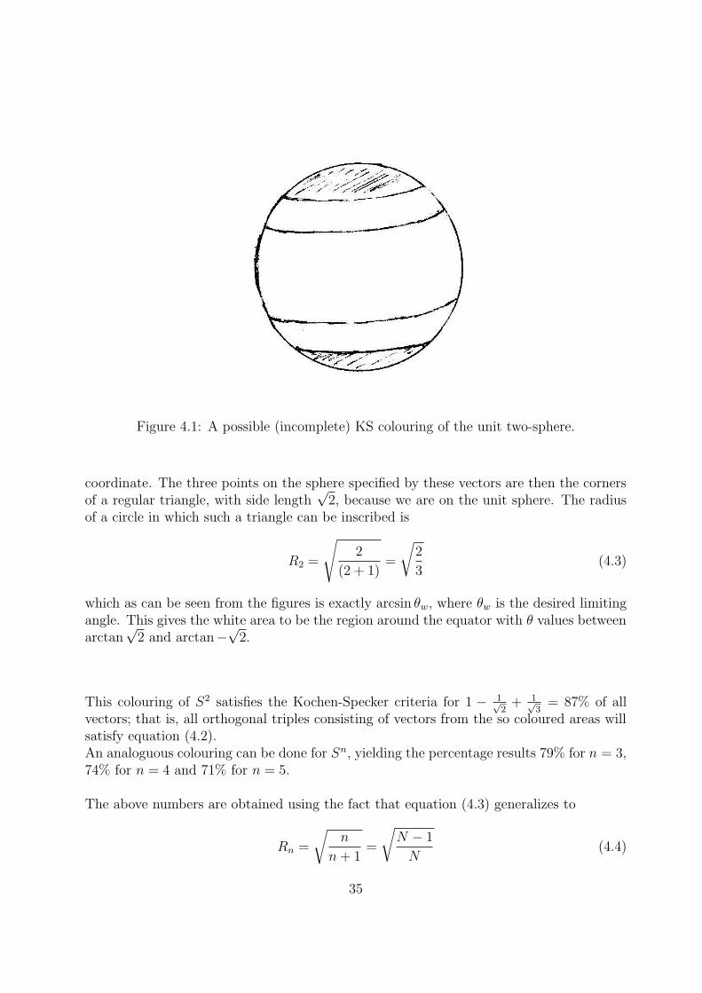
Figure 4.1: A possible (incomplete) KS colouring of the unit two-sphere.

coordinate. The three points on the sphere specified by these vectors are then the cornersof a regular triangle, with side length

√2, because we are on the unit sphere. The radius

of a circle in which such a triangle can be inscribed is

R2 =

√

2

(2 + 1)=

√

2

3(4.3)

which as can be seen from the figures is exactly arcsin θw, where θw is the desired limitingangle. This gives the white area to be the region around the equator with θ values betweenarctan

√2 and arctan−

√2.

This colouring of S2 satisfies the Kochen-Specker criteria for 1 − 1√2

+ 1√3

= 87% of allvectors; that is, all orthogonal triples consisting of vectors from the so coloured areas willsatisfy equation (4.2).An analoguous colouring can be done for Sn, yielding the percentage results 79% for n = 3,74% for n = 4 and 71% for n = 5.

The above numbers are obtained using the fact that equation (4.3) generalizes to

Rn =

√n

n+ 1=

√

N − 1

N(4.4)

35

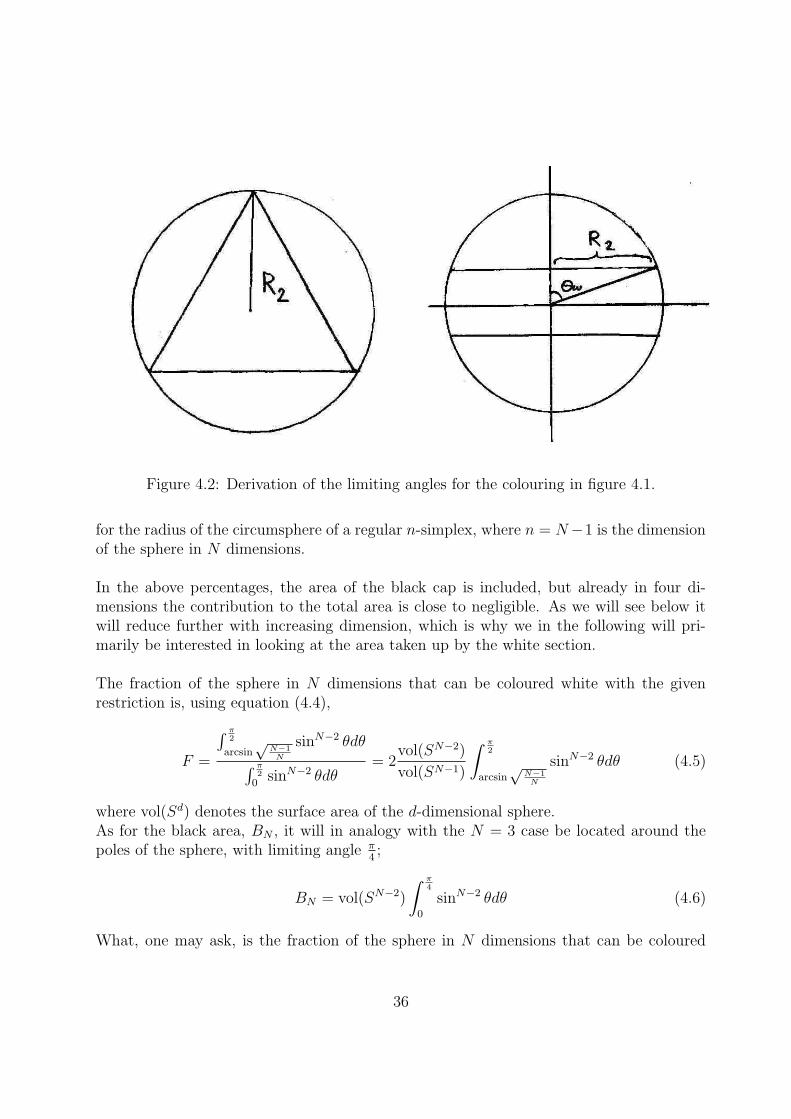
Figure 4.2: Derivation of the limiting angles for the colouring in figure 4.1.

for the radius of the circumsphere of a regular n-simplex, where n = N−1 is the dimensionof the sphere in N dimensions.

In the above percentages, the area of the black cap is included, but already in four di-mensions the contribution to the total area is close to negligible. As we will see below itwill reduce further with increasing dimension, which is why we in the following will pri-marily be interested in looking at the area taken up by the white section.

The fraction of the sphere in N dimensions that can be coloured white with the givenrestriction is, using equation (4.4),

F =

∫ π2

arcsin√

N−1

N

sinN−2 θdθ

∫ π2

0sinN−2 θdθ

= 2vol(SN−2)

vol(SN−1)

∫ π2

arcsin√

N−1

N

sinN−2 θdθ (4.5)

where vol(Sd) denotes the surface area of the d-dimensional sphere.As for the black area, BN , it will in analogy with the N = 3 case be located around thepoles of the sphere, with limiting angle π

4;

BN = vol(SN−2)

∫ π4

0

sinN−2 θdθ (4.6)

What, one may ask, is the fraction of the sphere in N dimensions that can be coloured

36

using this method in the limit N → ∞? As can be seen from the expression

vol(Sd) = vol(Sd−1)

∫ π

0

sind−1 θdθ (4.7)

for high dimensions, the fraction of the area of the sphere that will lie around the polesis negligible, due to the increasingly sharp peak around θ = π

2of the sine function when

raised to a large number. Thus the fraction of the surface area taken up by the blacksection will be very small.

To determine the fraction of the sphere taken up by the white section requires a bit morecareful analysis. We will need to evaluate the expression

limN→∞

2vol(SN−2)

vol(SN−1)

∫ π2

arcsin√

N−1

N

sinN−2 θdθ (4.8)

The volume of the sphere in d dimensions is

vol(Sd) =2π

d+1

2

Γ(d+12

)(4.9)

so thatvol(SN−2)

vol(SN−1)=

1√π

Γ(N2)

Γ(N−12

)(4.10)

Equation (4.8) can then be written as

limN→∞

21√π

Γ(N2)

Γ(N−12

)

∫ π2

arcsin√

N−1

N

sinN−2 θdθ

We will treat the Gamma function part and the integral part of the expression separately,starting out by looking at the fraction

Γ(N2)

Γ(N−12

)

In the limit of large N we can apply Stirling’s approximation to the Gamma function

Γ(z) =√

2πe−zzz− 1

2 (1 +1

12z+O(

1

z2)), | argz |< π, | z |→ ∞ (4.12)

and consider the expression

√2πe−

N2

N2

N2− 1

2 (1 + 212N

+O( 1N2 ))

√2πe−

N−1

2N−1

2

N−1

2− 1

2 (1 + 212(N−1)

+O( 1(N−1)2

))→

√e√e

√N√2

(1 − 1

N) →

√N√2, N → ∞

(4.13)

37

where we have used that

(N − 1

2)

N2−1 = (

N

2)

N2−1(1 − 1

N)

N2−1 =

= (N

2)

N2−1((1 − 1

N)−N)−

1

2

1

(1 − 1N

)→ (

N

2)

N2−1 1√

e

1

(1 − 1N

), N → ∞ (4.14)

and(1 + 2

12N+O( 1

N2 ))

(1 + 212(N−1)

+O( 1(N−1)2

))→ 1, N → ∞ (4.15)

Thus, we can conclude that

limN→∞

Γ(N2)

Γ(N−12

)=

√N√2

Next, let us take a look at the behaviour of the integral

∫ π2

arcsin√

N−1

N

sinN−2 θdθ

in the limit of large N .

It’s not hard to convince oneself that this is equivalent to looking at the integral

∫ arccos√

N−1

N

0

cosN−2 θdθ

which simplifies the calculations because all expansions can be done around zero.In the limit of large N we can use

arccos

√

N − 1

N=

1√N

+O(1

N3

2

) (4.17)

Expanding cos t around t = 0, we get

cos t|t=0 = 1 − t2

2!+O(t4) (4.18)

so that, using the regular binomial expansion and the fact that when N is large N − 2 canbe approximated with N ,

limN→∞

cosN−2 θ = (1 − θ2

2)N + h(θ,N) = h(θ,N) + 1 −N

θ2

2+N2

2!

θ4

4− N3

3!

θ6

8+ ... (4.19)

where h(θ,N) is a function such that

limN→∞

√N

∫ arccos√

N−1

N

0

h(θ,N) = 0

38

Integrating term by term and using equations (4.18) and (4.17), we get

limN→∞

∫ arccos√

N−1

N

0

cosN−2 θdθ = [θ − N

6θ3 +

N2

40θ5 − N3

336θ7 + ...]

θ=arccos√

N−1

N

θ=0

=1√N

∞∑

k=0

1

2k

1

k!

(−1)k

(2k + 1)(4.21)

The sum in (4.21) is in fact equal to

√π

2erf(

1√2)

with erf the statistic-probabilistic error function;

erf(z) ≡ 2√π

∫ z

0

e−t2dt (4.22)

Putting all of this together, we have the result

limN→∞

2vol(Sn−2)

vol(Sn−1)

∫ π2

arcsin√

N−1

N

sinN−2 θdθ = erf(1√2) ≈ 0.68 (4.23)

So, approaching the limit of an infinite number of dimensions of the Hilbert space H

in which our projective measurements are conducted, binary probabilities (correspondingto well-defined, non-contextual properties of the system with available states in H ) canbe assigned to approximately 68% of the vectors in H . The behaviour of the percentageas a function of dimension3 is given in figure 4.3.

The minimum occurs around 12.465, and the integer giving the least percentage is N = 12;about 66.76%.

What has been derived above is a lower limit for the area of the sphere that is KS colourablein arbitrary dimensions. The possibility remains, however, that a maximally effectivecolouring could cover a much larger area - possibly, in fact, as much as 99%4 of the spherein R

3 [8].

3Treated in the diagram as a continuous variable.4There are some measure theoretical subtleties that can be used to colour even more of the sphere, in

fact ’almost’ all of it, in a very special sense of the word. For more on this, see for example [11].

39

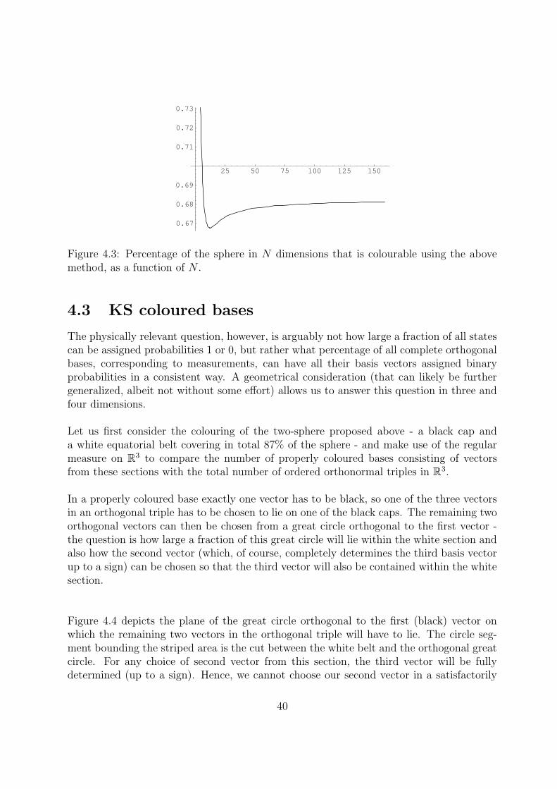
25 50 75 100 125 150

0.67

0.68

0.69

0.71

0.72

0.73

Figure 4.3: Percentage of the sphere in N dimensions that is colourable using the abovemethod, as a function of N .

4.3 KS coloured bases

The physically relevant question, however, is arguably not how large a fraction of all statescan be assigned probabilities 1 or 0, but rather what percentage of all complete orthogonalbases, corresponding to measurements, can have all their basis vectors assigned binaryprobabilities in a consistent way. A geometrical consideration (that can likely be furthergeneralized, albeit not without some effort) allows us to answer this question in three andfour dimensions.

Let us first consider the colouring of the two-sphere proposed above - a black cap anda white equatorial belt covering in total 87% of the sphere - and make use of the regularmeasure on R

3 to compare the number of properly coloured bases consisting of vectorsfrom these sections with the total number of ordered orthonormal triples in R

3.

In a properly coloured base exactly one vector has to be black, so one of the three vectorsin an orthogonal triple has to be chosen to lie on one of the black caps. The remaining twoorthogonal vectors can then be chosen from a great circle orthogonal to the first vector -the question is how large a fraction of this great circle will lie within the white section andalso how the second vector (which, of course, completely determines the third basis vectorup to a sign) can be chosen so that the third vector will also be contained within the whitesection.

Figure 4.4 depicts the plane of the great circle orthogonal to the first (black) vector onwhich the remaining two vectors in the orthogonal triple will have to lie. The circle seg-ment bounding the striped area is the cut between the white belt and the orthogonal greatcircle. For any choice of second vector from this section, the third vector will be fullydetermined (up to a sign). Hence, we cannot choose our second vector in a satisfactorily

40

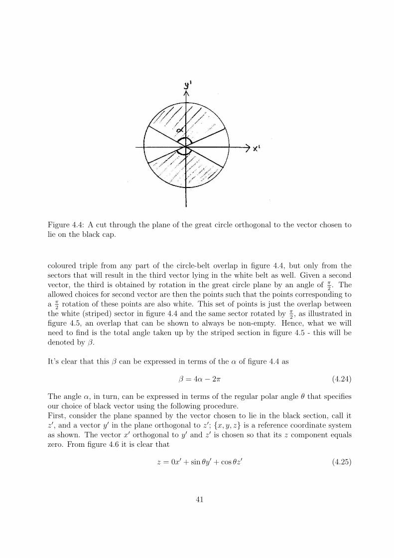
Figure 4.4: A cut through the plane of the great circle orthogonal to the vector chosen tolie on the black cap.

coloured triple from any part of the circle-belt overlap in figure 4.4, but only from thesectors that will result in the third vector lying in the white belt as well. Given a secondvector, the third is obtained by rotation in the great circle plane by an angle of π

2. The

allowed choices for second vector are then the points such that the points corresponding toa π

2rotation of these points are also white. This set of points is just the overlap between

the white (striped) sector in figure 4.4 and the same sector rotated by π2, as illustrated in

figure 4.5, an overlap that can be shown to always be non-empty. Hence, what we willneed to find is the total angle taken up by the striped section in figure 4.5 - this will bedenoted by β.

It’s clear that this β can be expressed in terms of the α of figure 4.4 as

β = 4α− 2π (4.24)

The angle α, in turn, can be expressed in terms of the regular polar angle θ that specifiesour choice of black vector using the following procedure.First, consider the plane spanned by the vector chosen to lie in the black section, call itz′, and a vector y′ in the plane orthogonal to z′; {x, y, z} is a reference coordinate systemas shown. The vector x′ orthogonal to y′ and z′ is chosen so that its z component equalszero. From figure 4.6 it is clear that

z = 0x′ + sin θy′ + cos θz′ (4.25)

41

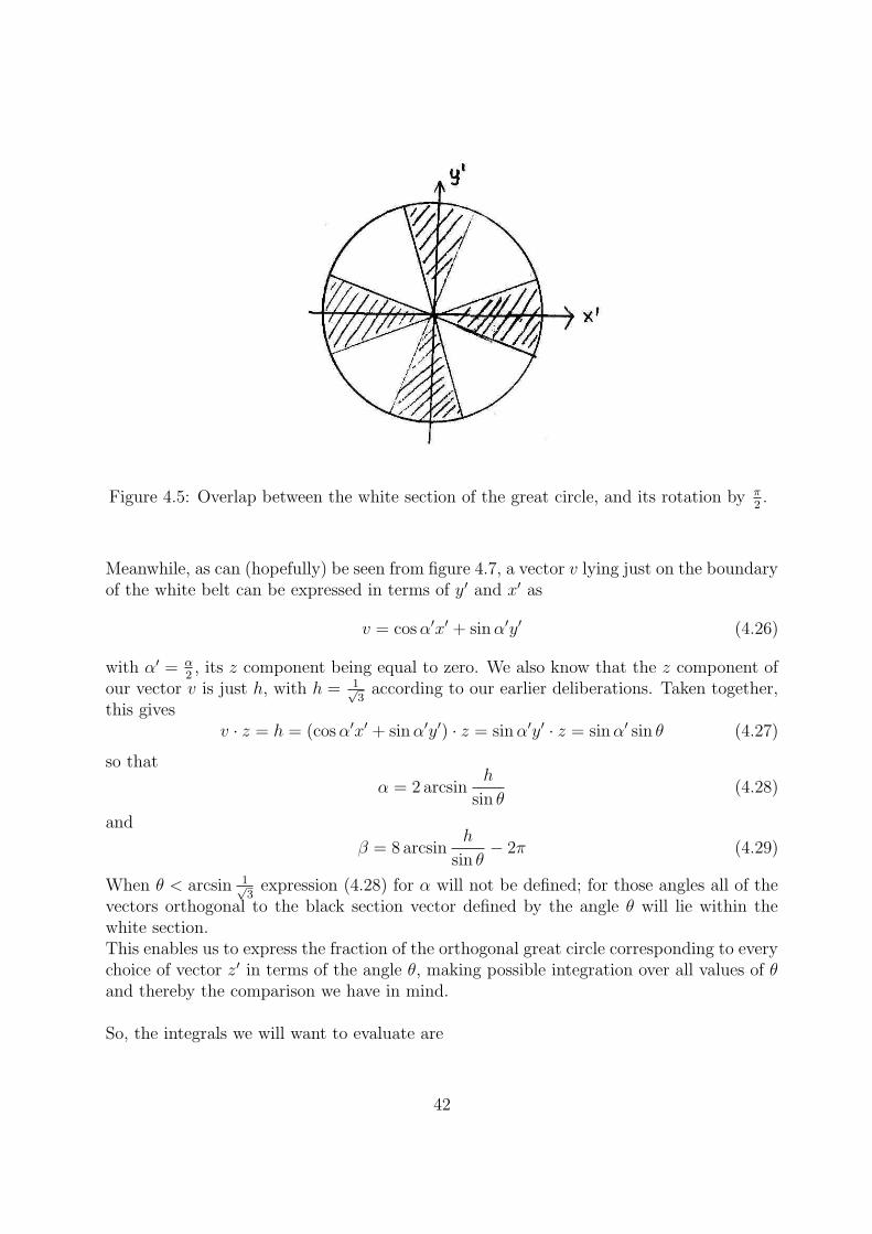
Figure 4.5: Overlap between the white section of the great circle, and its rotation by π2.

Meanwhile, as can (hopefully) be seen from figure 4.7, a vector v lying just on the boundaryof the white belt can be expressed in terms of y′ and x′ as

v = cosα′x′ + sinα′y′ (4.26)

with α′ = α2, its z component being equal to zero. We also know that the z component of

our vector v is just h, with h = 1√3

according to our earlier deliberations. Taken together,this gives

v · z = h = (cosα′x′ + sinα′y′) · z = sinα′y′ · z = sinα′ sin θ (4.27)

so that

α = 2 arcsinh

sin θ(4.28)

and

β = 8 arcsinh

sin θ− 2π (4.29)

When θ < arcsin 1√3

expression (4.28) for α will not be defined; for those angles all of thevectors orthogonal to the black section vector defined by the angle θ will lie within thewhite section.This enables us to express the fraction of the orthogonal great circle corresponding to everychoice of vector z′ in terms of the angle θ, making possible integration over all values of θand thereby the comparison we have in mind.

So, the integrals we will want to evaluate are

42

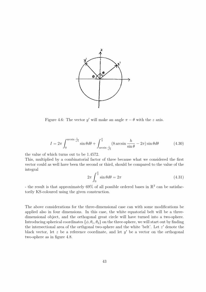
Figure 4.6: The vector y′ will make an angle π − θ with the z axis.

I = 2π

∫ arcsin 1√3

0

sin θdθ +

∫ π4

arcsin 1√3

(8 arcsinh

sin θ− 2π) sin θdθ (4.30)

the value of which turns out to be 1.4572.This, multiplied by a combinatorial factor of three because what we considered the firstvector could as well have been the second or third, should be compared to the value of theintegral

2π

∫ π2

0

sin θdθ = 2π (4.31)

- the result is that approximately 69% of all possible ordered bases in R3 can be satisfac-

torily KS-coloured using the given construction.

The above considerations for the three-dimensional case can with some modifications beapplied also in four dimensions. In this case, the white equatorial belt will be a three-dimensional object, and the orthogonal great circle will have turned into a two-sphere.Introducing spherical coordinates {φ, θ1, θ2} on the three-sphere, we will start out by findingthe intersectional area of the orthgonal two-sphere and the white ’belt’. Let z ′ denote theblack vector, let z be a reference coordinate, and let y′ be a vector on the orthogonaltwo-sphere as in figure 4.8.

43

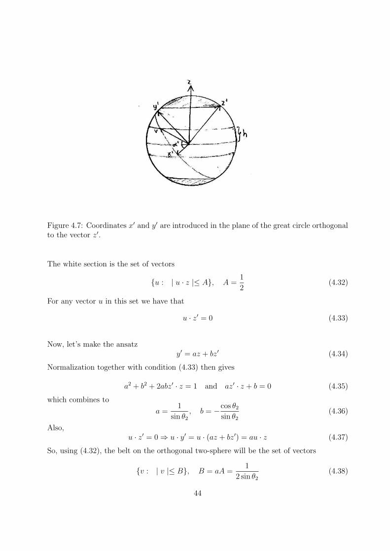
Figure 4.7: Coordinates x′ and y′ are introduced in the plane of the great circle orthogonalto the vector z′.

The white section is the set of vectors

{u : | u · z |≤ A}, A =1

2(4.32)

For any vector u in this set we have that

u · z′ = 0 (4.33)

Now, let’s make the ansatzy′ = az + bz′ (4.34)

Normalization together with condition (4.33) then gives

a2 + b2 + 2abz′ · z = 1 and az′ · z + b = 0 (4.35)

which combines to

a =1

sin θ2

, b = −cos θ2

sin θ2

(4.36)

Also,u · z′ = 0 ⇒ u · y′ = u · (az + bz′) = au · z (4.37)

So, using (4.32), the belt on the orthogonal two-sphere will be the set of vectors

{v : | v |≤ B}, B = aA =1

2 sin θ2

(4.38)

44

Figure 4.8: y′ lies on the two-sphere orthogonal to the vector z ′.

For 0 ≤ θ2 ≤ arcsin 12

the entire orthogonal two-sphere will lie within the white section.

This intersection between the orthogonal two-sphere and the white section on the three-sphere can now be treated in analogue with the previuos case. Given a black first vector,when placing the second vector in the white section, the segment of the great circle or-thogonal to this second vector on which we can choose the third in order for the fourth tolie in the white section is given by

γ = 8 arcsinB

sin θ1

− 2π (4.39)

Also in analogy with the previous case, all of the orthogonal great circle will be white forarccosB ≤ θ1 ≤ arcsinB. To summarize, we have integration over the angle θ2 whichruns between 0 and π

2, covering the black cap, and the possibilities available for choosing

the remaining three vectors are governed by a function of θ2, obtained from an integrationover the angle θ1 between arccosB and π

2, that is, over the white section of the two-sphere

orthogonal to the first vector specified by θ2, B being a function of θ2.

To make all of this explicit, we have the following integrals

I = 2π

∫ arcsin B

arccos B

sin θ1dθ1 +

∫ π2

arcsin B

(8 arcsinB

sin θ1

− 2π) sin θ1dθ1 (4.40)

and, finally

4π

∫ arcsin 1

2

0

sin2 θ2dθ2 +

∫ π4

arcsin 1

2

I sin2 θ2dθ2 (4.41)

45

The result when comparing this, multiplied by an overall combinatorial factor of four, tothe value of the expression

4π

∫ π2

0

sin2 θdθ (4.42)

is that 32% of the ordered orthogonal triples in R4 are properly coloured using the chosen

method.

4.4 KS for a restricted class of sic-POVMs

As mentioned in the introduction to this chapter, a lot of people have been working onthe problem of proving the KS theorem by finite means. This quest has focused mainly onPVMs, that is orthogonal resolutions of the identity, but some work has also been done forPOVMs of different types. Cabello, for instance, has shown the KS theorem for a singlequbit using eight element POVMs [12] by inscribing cubes in dodecahedrons. MasahiroNakamura has done the same using POVMs with four elements. As noted earlier, theKS result follows trivially if one simultaneously allows POVMs with different numbers ofelements.

It should be noted that the lack of a Gleason type theorem for sic-POVMs in the qubit caseopens up for the possibility that we don’t have the restriction of the KS result either. Itgives no further information, though, if this is actually the case. It is therefore worthwhileto investigate some more obvious sets of four-element POVMs to see if they can be KScoloured.

Here, we will make use of the dodecahedron method proposed by Cabello. For the restrictedclass of regular tetrahedrons that can be inscribed in a regular dodecahedron so that thevertices of the two configurations coincide, it is possible to by explicit construction provethat the KS result is not applicable. The reader can convince herself that an inscribedregular tetrahedron will have corners lying on four mutually next-to-next-to-adjacent ver-tices. For a fixed dodecahedron, there are 10 possible ways to inscribe a regular tetrahedron.

A satisfactory Kochen-Specker colouring is then given, as in figure 4.9, by

A I M Q F C P SA H P R J C L TE G N Q J B R NE H L U K D G TF D M U K B I S

where boldface characters imply that the corresponding vertex is coloured black.

46

Figure 4.9: Colouring of the vertices of a regular dodecahedron, corresponding to a negationof the KS-theorem for the class of regular tetrahedrons that can be inscribed.

Consequently, the KS result is not valid for this restricted class of symmetric information-ally complete POVMs, and whether or not we have the KS result for all sic-POVMs is stillan open question.

47

Chapter 5

Conclusions and open questions

We have seen that it suffices to make the frame function assumption for POVMs withtwo and three elements in order to prove a Gleason type theorem for general POVMs. Inthe case of two-dimensional quantum systems, qubits, the sic-POVM does not yield theGleason result, as has been shown by Caves et al. [3]. The considerations of this diplomawork, however, have made likely that for all other four element POVMs the quantum ruleholds.Generalizing a method of colouring proposed by Appleby in three dimensions [8], we havealso found a lower limit for the area of the n-sphere that can be KS coloured, but we arestill ignorant as to a sharp upper limit.In three and four dimensions, we have calculated how many of all possible bases the colouredarea corresponds to. In order to make the lower limit mentioned above more physicallyinteresting, one would need to answer this question in arbitrary dimensions - somethingthat appears to be non-trivial.The Appleby colouring has the advantage that it generalizes easily to higher dimensions.As for a maximally effective colouring, there are no arguments to support that this wouldbe the case. In particular, it is in no way obvious that the same method of colouring wouldbe maximal in different dimensions.Another question left unanswered is that about the existence of a finite set of vectors thatcan be used to prove the KS theorem for sic-POVMs - as of yet, no such set has beenpresented.

48

Bibliography

[1] Andrew M. Gleason, Measures on the closed subspaces of a Hilbert space, Journal ofMathematics and Mechanics, Vol. 6, No. 6, 885-893 (1957)

[2] N.I. Akhiezer, I.M. Glazman, Theory of Linear Operators in Hilbert Space, (Ungar,New York, 1963)

[3] C.M. Caves, C.A. Fuchs, K. Manne and J.M. Renes,’Gleason-type Derivations ofthe Quantum Probability Rule for Generalized Measurements’, quant-ph/0306179;Found. Phys. 34, 193 (2004)

[4] Paul Busch, ‘Quantum states and generalized observables: a simple proof of Gleason’stheorem’, quant-ph/9909073; Phys. Rev. Lett. 91, 120403 (2003)

[5] Norbert H.J. Lacroix, On Common Zeros of Legendre’s Associated Functions, Math-ematics of Computation, Vol. 43, No. 167, 243-245 (1984)

[6] Hans Sagan, Boundary and Eigenvalue Problems in Mathematical Physics, (Chelsea,New York, 1955)

[7] S. Kochen and E.P. Specker, The Problem of Hidden Variables in Quantum Mechanics,J. Math. Mech., Vol. 17, No. 1, 59-87 (1967)

[8] D.M. Appleby, ’The Bell-Kochen-Specker theorem’, quant-ph/0308114; Stud. Hist.Philos. Mod. Phys. 36 (2005)

[9] J.S. Bell, On the Problem of Hidden Variables in Quantum Mechanics, Rev. Mod.Phys., Vol. 38, No. 3, 447-452 (1966)

[10] A. Peres, Quantum theory: Concepts and Methods,(Kluwer Academic Publishers, Dor-drecht, 1995)

[11] I. Pitowsky, Quantum Mechanics and Value definiteness, Philos. Sci., Vol. 52, No. 1,154-156 (1985)

[12] Adan Cabello, ’Kochen-Specker Theorem for a Single Qubit Using Positive Operator-Valued Measures’, quant-ph/0210082; Phys. Rev. Lett. 90 (2003)

49