GETTING THE RIGHT PROFILE -...
21
1 Wheel-Rail Contact: GETTING THE RIGHT PROFILE Simon Iwnicki, Julian Stow and Adam Bevan Rail Technology Unit Manchester Metropolitan University The Contact The contact patch between a wheel and a rail is typically the size of a 5p piece and its shape depends on the geometry of both bodies. The theory developed by Hertz (when he was a 24 year old research assistant!) can be used as a good approximation and this gives an elliptical shape and distribution of the normal force. 2a 2b
Transcript of GETTING THE RIGHT PROFILE -...

1
Wheel-Rail Contact:GETTING THE RIGHT PROFILE
Simon Iwnicki, Julian Stow and Adam Bevan
Rail Technology UnitManchester Metropolitan University
The ContactThe contact patch between a wheel and a rail is typically the sizeof a 5p piece and its shape depends on the geometry of both bodies.
The theory developed by Hertz (when he was a 24 year old research assistant!) can be used as a good approximation and this gives an elliptical shape and distribution of the normal force.
2a
2b

2
Alternative contact modelsIn practice the geometry at the contact patch is often more complicated and the contact patch isfar from elliptical. Possible alternative models are:
• Hertz theory in strips
• Finite elementsCan give good results but very slow
FE model of wheel rail contact
Courtesy Tom Kay
Corus Rail technologies

3
The Forces
• Vertical / Normal:(the vehicle load)• P0, P1 and P2 forces
• Lateral / Tangential:(traction, braking, curving)• Gravitational stiffness forces • Creep forces
Creep forces
Linear Non-
linear
Saturated
Creep force
Creepage
A tangential force related to ‘creepage’ or microslip in the contact patch
Pure rolling Full slip

4
Alternative creep force models
• Carter– linear relationship between creepage and creep force
• Johnson and Vermeulen– modification due to saturation
• Kalker– theoretical full solution
• Shen Hedrick Elkins– refined and simplified based on measurements
• Pollach– useful for high slip
• Falling creep force– essential for stick-slip and squeal
The ProfilesWheel and rail profiles wear and their geometry changes from the original design.
Miniprof measured rail profile
Profiles can be measured and combined to produce the effective conicity or a table of radii and contact angles.
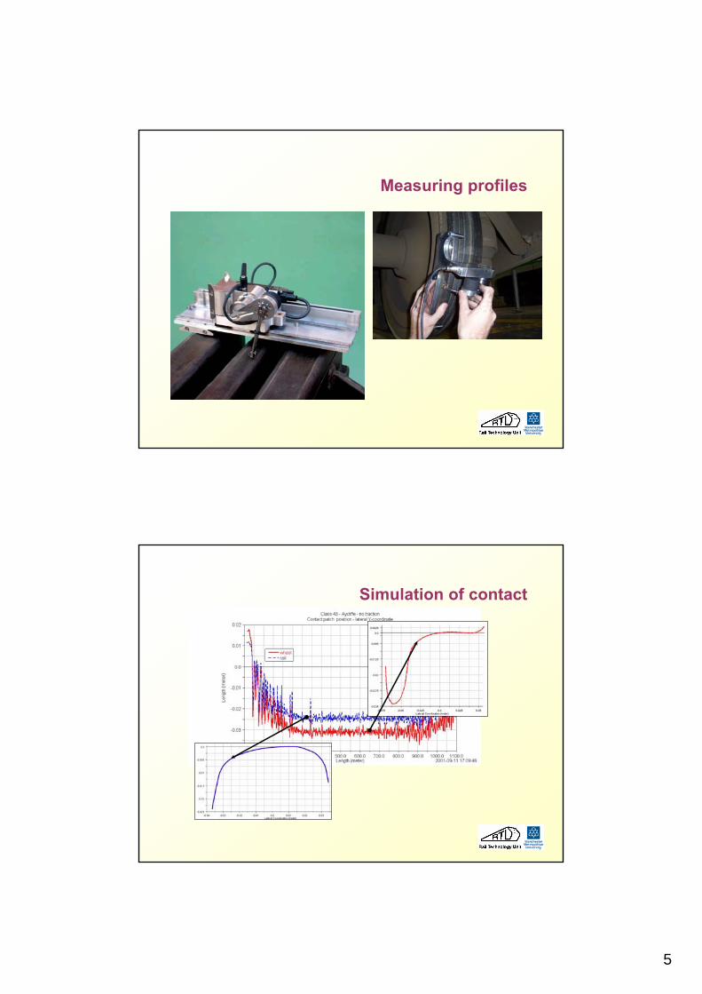
5
Measuring profiles
Simulation of contact

6
Simulation of forces
Contact - animation

7
Current profiles
• Tread cone angle + Flange angle + Radius– eg P1
• Worn profile– eg P8, S1002 (P10)
The UK P8 - a worn profile

8
Tools for designing new profiles
• Rules of thumb– Flange angle– Cone angle
• Geometry analysis – contact location• Rolling radius difference plot – curving, stability• Shakedown curve – Rolling Contact Fatigue• Wear prediction – profile life
Geometry analysis
680 690 700 710 720 730 740 750 760 770 780 790-40
-30
-20
-10
0
10
20
30
40
50
60
70
0 3.8 -4.5 -4.5 -10
3.8
10

9
Rolling radius difference
Sharp Conicity Increase
Wheelset rolls offset
From centre of track
Low Conicity
RCF Assessment
Two current methods:
- Shakedown curve(more later)
- Weighted Tγ
10
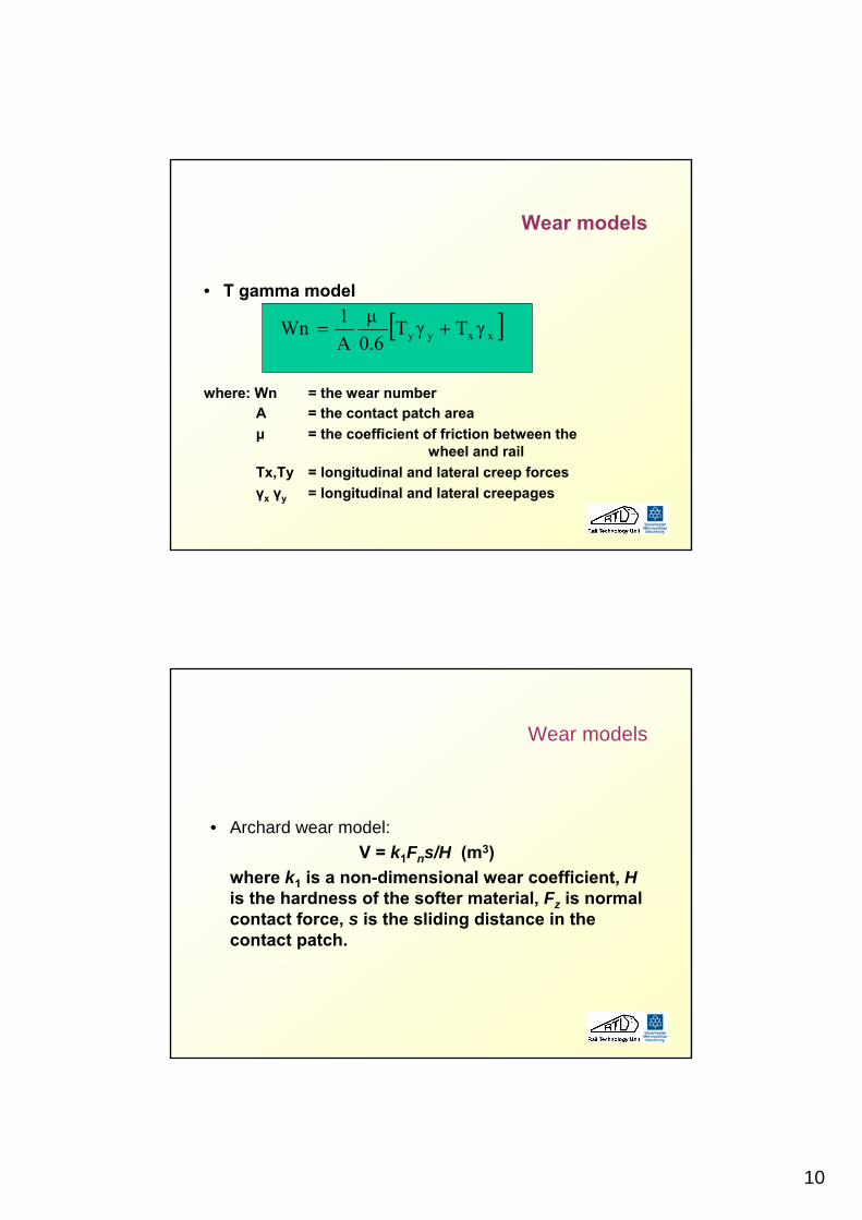
Wear models
• T gamma model
where: Wn = the wear numberA = the contact patch areaµ = the coefficient of friction between the
wheel and railTx,Ty = longitudinal and lateral creep forcesγx γy = longitudinal and lateral creepages
[ ]xxyy γTγT0.6µ
A1Wn +=
Wear models
• Archard wear model:V = k1Fns/H (m3)
where k1 is a non-dimensional wear coefficient, H is the hardness of the softer material, Fz is normal contact force, s is the sliding distance in the contact patch.

11
-a
0
a
-b
0
b
0
0.5
1
1.5
2
x 10-11
xy
δz
Local wear rate in the contact patch(Archard model)
Adhesion zone – no wear
Slip zone – wear
Rolling direction
adhesion
slidingWear /m
-800 -790 -780 -770 -760 -750 -740 -730 -720 -710 -700 -690-40
-30
-20
-10
0
10
(mm
)
Simulated Distance 54210km
SimulatedMeasuredNew
-800 -790 -780 -770 -760 -750 -740 -730 -720 -710 -700 -690-0.5
0
0.5
1
1.5
2
(mm)
Wea
r Di
strib
utio
n(m
m)
SimulatedMeasured
Simulated and measured wheel profile and wear distribution example 1 -after 54000 km

12
-800 -790 -780 -770 -760 -750 -740 -730 -720 -710 -700 -690-40
-30
-20
-10
0
10
(mm
)
Simulated Distance 128344km
-800 -790 -780 -770 -760 -750 -740 -730 -720 -710 -700 -690-1
0
1
2
3
4
(mm)
Wea
r D
istri
butio
n(m
m)
SimulatedMeasured
SimulatedMeasuredNew
Simulated and measured wheel profile and wear distribution example 2 - after 128000 km
An Example:
The WRISA2 anti-RCFwheel profile
(development funded by RSSB)
13
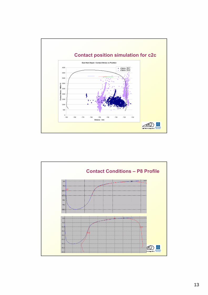
Contact position simulation for c2cEast Ham Depot - Contact Stress vs Position
0
500
1000
1500
2000
2500
3000
3500
4000
4500
-790 -780 -770 -760 -750 -740 -730 -720 -710
Distance /mm
Con
tact
Str
ess
/ M
N/m
^2
class 357class 312S i 2
Contact Conditions – P8 Profile

14
New P1 Wheel
on New BS113a Rail
No contact in these positions
Heavy Worn P1 Wheel
on Worn BS113a Rail
Contact Conditions – P1 Profile
P1 wheel on c2c

15
The WRISA2 anti-RCF profile
RCF Sensitive Region
Anti-RCF ‘Relief’
WRISA2 profile designed by NRC to:
•Include an Anti-RCF ‘relief’ in flange root area of the profile
•Reduce the contact stress in mid-gauge region of rail
•Reduce the rolling radius difference when curving to reduce longitudinal creepages and tangential forces
•Include a smoother tread run-off to eliminate geometric stress raisers caused by transition.
New P1 (Red), New P8 (Green), Light Worn P8 (Blue), WRISA2 (Purple)
WRISA2 Rolling Radius Difference
16
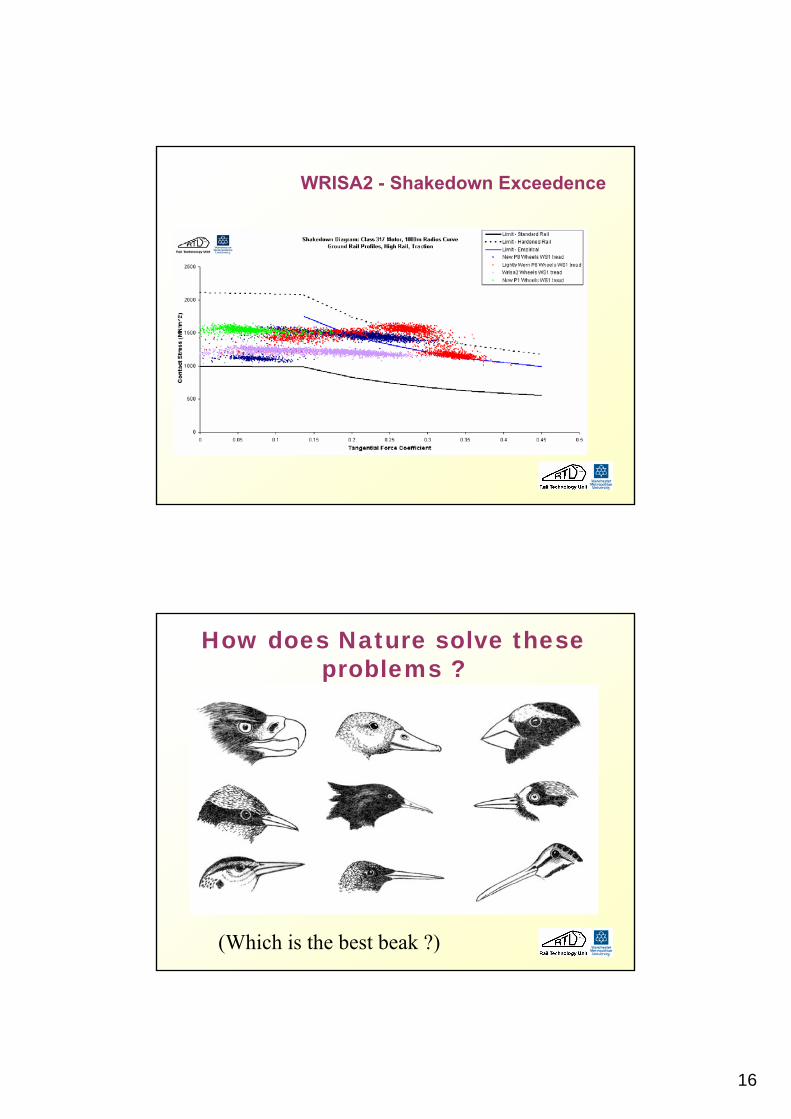
WRISA2 - Shakedown Exceedence
How does Nature solve these problems ?
(Which is the best beak ?)

17
Genetic Algorithm
Basic Method - (simulates natural evolution)• Profile digitised and converted to a binary ‘gene’• 2 parent profiles selected and their genes ‘mated’
to produce ‘child’ genes• Child genes converted back to profiles• Simulation used to evaluate each child profile• Best profiles selected as parents and process
repeated • More details in Persson and Iwnicki paper
presented at 18th IAVSD conference 2003
The genesx: 12.459 mm
y:5.223mm
x: 12.909 mm
y:6.201 mm
X: .....11010101
01110101
10011011
11001100
... 1101010101110101100110111100...

18
Mating
1101011010111000110101110101100110111100...
1010101011000101010101110101100110111100...
Bits are copied with random switches between the parents
1101011011000101010101110101100110111100...=
+
Reconstructing the new profile
x: 12.459 mm
y:5.223mm
x: 12.909 mm
y:6.201 mm
X: .....
11010101
01110101
10011011
11001100
... 1101010101110101100110111100...

19
Survival of the fittest• Each profile is assessed by running a vehicle simulation over a typical track case.
•The best profiles become the parents for the next generation.
• Mutations can be added to avoid local minima.
Some interim results

20
Assessing the new profiles
The Penalty Index - the sum of sub factors:
• Ride comfort penalty factor • Lateral track shifting force penalty factor• Maximum derailment quotient penalty factor• Wear penalty factor• Maximum contact stress penalty factor
(Other factors are possible and each can be weighted according to importance)
Results - ‘stiff bogie’
21
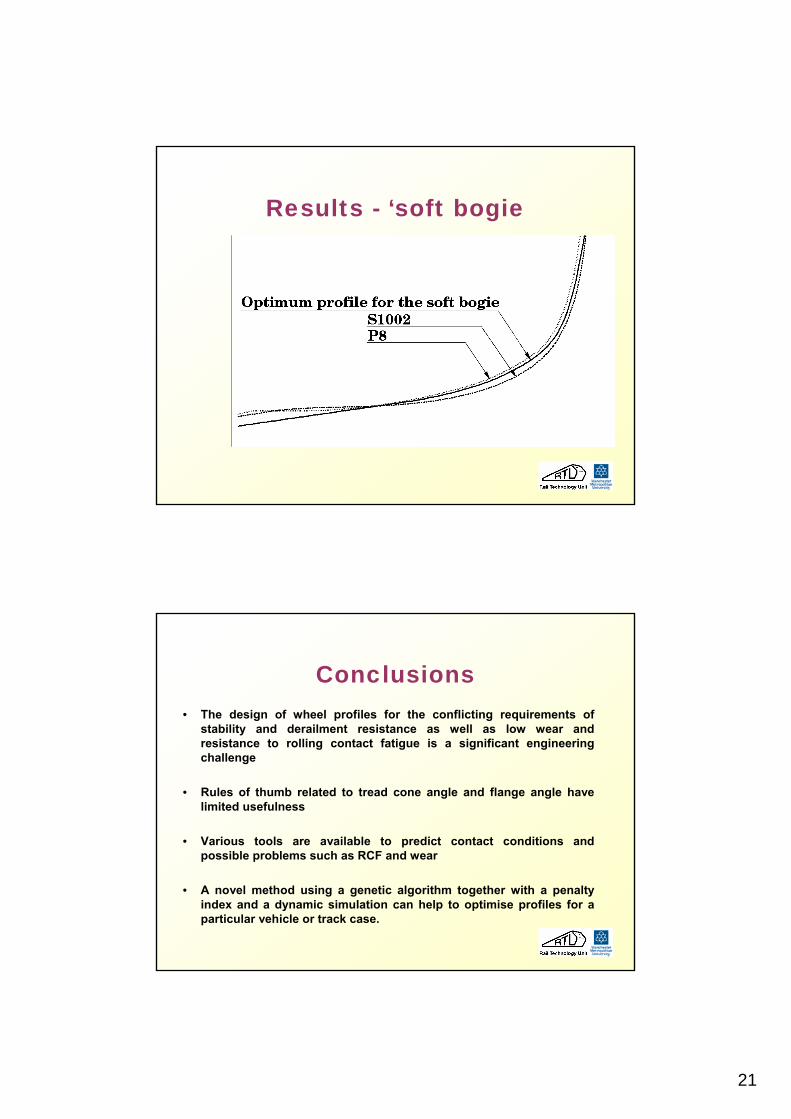
Results - ‘soft bogie
Conclusions• The design of wheel profiles for the conflicting requirements of
stability and derailment resistance as well as low wear and resistance to rolling contact fatigue is a significant engineering challenge
• Rules of thumb related to tread cone angle and flange angle havelimited usefulness
• Various tools are available to predict contact conditions and possible problems such as RCF and wear
• A novel method using a genetic algorithm together with a penaltyindex and a dynamic simulation can help to optimise profiles for a particular vehicle or track case.