WP 15/10

Getting a healthy start: The effectiveness of targeted

benefits for improving dietary choices

Rachel Griffith, Stephanie von Hinke & Sarah Smith

September 2015

http://www.york.ac.uk/economics/postgrad/herc/hedg/wps/

1

Getting a healthy start:

The effectiveness of targeted benefits for improving dietary choices

Rachel Griffith,* Stephanie von Hinke,† and Sarah Smith‡

Abstract

There is growing policy concern with encouraging better dietary choices. We show that a

nationally-implemented voucher policy - the UK Healthy Start Scheme - increased spending on

fruit and vegetables by 15 percent. However, the effects were heterogeneous: only households

that previously spent less than the value of the voucher increased spending; the voucher was

equivalent to a cash benefit for households already spending more than this value. These

responses are in line with standard economic predictions. Although aspects of the policy might

have been expected to stimulate a wider behavioural response, there is no evidence for this.

Key words: dietary choices; targeted benefits; healthy start scheme

JEL classification: D12, I18

Acknowledgements: We gratefully acknowledge financial support from the UK Medical

Research Council (reference number G1002345), the European Research Council (ERC) under

ERC-2009-AdG grant agreement number 249529, and the Economic and Social Research

Council (ESRC) under the Centre for the Microeconomic Analysis of Public Policy (CPP),

grant number RES-544-28-0001. Data supplied by TNS UK Limited. The use of TNS UK Ltd.

data in this work does not imply the endorsement of TNS UK Ltd. in relation to the

interpretation or analysis of the data. All errors and omissions remained the responsibility of

the authors.

* Institute for Fiscal Studies and University of Manchester; rgriffith@ifs.org.uk † University of Bristol and Institute for Fiscal Studies; s.scholder@bristol.ac.uk ‡ University of Bristol and Institute for Fiscal Studies; sarah.smith@bristol.ac.uk

2

1. Introduction

Increasing rates of obesity and diet-related disease are major challenges across the developed

world, leading to growing interest amongst the policy community in how to improve dietary

choices (Lancet, 2011, Gortmaker et al, 2011). One possible way for the government to improve

dietary choices among low-income households is to target benefits on the purchase of healthy

food, such as fruit and vegetables. This policy option is under discussion in the US because of

the large number of recipients of the Supplemental Nutrition Assistance Program (SNAP;

formerly Food Stamps) and high levels of obesity among SNAP recipients.

Our contribution in this paper is to show that the introduction of a large-scale, nationally-

implemented voucher scheme – the UK Healthy Start Scheme – that aimed to increase fruit and

vegetable consumption among low-income families led to increased spending on fruit and

vegetables by 15 per cent (equivalent to two-thirds of a portion per household member per day).

Introduced in November 2006, the Healthy Start Scheme is a targeted benefit given to low-

income households with young children. It is distributed in the form of vouchers (Healthy Start

Vouchers) that can only be spent on specific healthy foods (fruit, vegetables and milk).4

We show that the way in which the vouchers affected spending was fully in line with the

predictions of standard economic analysis. That is, there was a large effect on spending among

a subset of recipient households who were distorted (i.e. who would otherwise spend less than

the value of the voucher on fruit and vegetables). For other, infra-marginal households, who

already spent more than this value, the effect was similar to an income-equivalent cash benefit.

In this context, this is, arguably, a surprising finding since there were several aspects of the

4 The Scheme replaced the Welfare Food Scheme, which was introduced in the 1940s. The Welfare Food Scheme

operated similarly to the Healthy Start Scheme, but vouchers could only be used to purchase milk. Reforms to the

scheme were introduced to specifically promote fruit and vegetable consumption, following recommendations

made by the UK Committee on Medical Aspects of Food and Nutrition Policy (Department of Health, 2002) and

the WHO (1990, 2003).

3

policy that might have been expected to lead to a wider, behavioural response that would have

increased spending even among infra-marginal consumers. Indeed, the vouchers were given a

prescriptive “label”, which a number of recent studies have found to affect the way benefit

income is spent (Kooreman, 2000; Thaler and Sunstein, 2008; Benhassine et al., 2014; Beatty

et al, 2014). The vouchers were delivered through healthcare professionals who acted as

gatekeepers for the programme and provided information and advice on healthy eating

including the importance of five portions of fruit and vegetables a day. Finally, the policy was

targeted at a low-income group, thought to be more susceptible to behavioural responses (see

e.g. Banks, O’Dea and Oldfield, 2010; Abeler and Markheim, 2010; Benjamin, Brown and

Shapiro, 2013). Indeed, when the scheme was introduced, the UK government anticipated some

(non-standard) effect, stating that parents would use the vouchers “for the benefit of their

children as opposed to viewing the scheme simply as financial support” (Department of Health,

Social Services and Public Safety, 2011). However, the evidence we present here is not

consistent with any wider behavioural response.

The focus of our empirical analysis is on how the voucher policy affected spending on fruit and

vegetables. Specifically, we compare the marginal propensity to consume (MPC) fruit and

vegetables out of vouchers to the MPC fruit and vegetables out of regular income across

distorted and infra-marginal households, defined using pre-reform levels of spending. Our

identification strategy is a triple differences approach. We compare the change in behaviour

(before/after the reform) for distorted and infra-marginal households among households that

are eligible for the vouchers to the change in behaviour across the same groups among ineligible

households. Eligibility is defined by age of children: low-income households with children aged

0-3, or where the woman is at least three months pregnant, are eligible. We use low-income

households with a woman in the period before being pregnant or with children aged 4-8 as a

4

control group of ineligible households.5

Figure 1 illustrates our main result. The top graph shows mean log monthly household

expenditure on fruit and vegetables for distorted households, distinguishing between eligible

(the solid line) and ineligible households, before and after the introduction of the scheme

(represented by the vertical line). The bottom figure shows the same thing for infra-marginal

households. We see similar trends in expenditure prior to the introduction of the scheme, but

an increase in expenditure by eligible distorted households after the introduction, and no

increase for ineligible distorted households, and no clear effects for infra-marginal households.6

In the rest of this paper, we show that this result is robust to a large number of potentially

important confounding factors.

Key to our analysis is the rich data we use. We have panel data including detailed and precise

information on all food and groceries brought into the home, reducing concerns about

measurement error and allowing us to identify the effect of the reform. The precise nature of

the data allows us to cleanly identify purchases of products that can be purchased with the

vouchers. Panel data allows us to control for unobserved heterogeneity across households. In

addition, it allows us to use information on household spending prior to the introduction of the

Scheme to cleanly distinguish between households that are likely to be distorted and those likely

to be infra-marginal.

Our paper is closely related to an existing literature on the effect of targeted benefits (for an

overview, see Currie and Ghavari, 2008). A number of papers on the Supplemental Nutrition

Assistance Program that can identify the exogenous effect of the programme find responses

fully in line with standard consumer theory. Examining the initial roll out of the programme,

5 Women become eligible to receive vouchers from week 10 of pregnancy. However, the majority of midwife

appointments (where women are made aware of the Scheme) take place at 12 weeks gestation. We therefore

consider pregnancy to start at 12 weeks. 6 Whilst ineligible distorted households also show an increase in spending in the first month (December 2006),

this is driven by the relatively high expenditures in December 2006 only, which drop continuously afterwards.

5

Hoynes and Schanzenbach (2009) fail to reject that the vouchers had the same effect as cash

benefits. Moffitt (1989) reaches a similar conclusion, investigating the cash out of Food Stamps

in Puerto Rico. Whitmore (2002) explores the randomized cash out of Food Stamps and finds

that voucher recipients spent more on food than cash recipients, but only among the sub-group

of recipients who are distorted. Cunha (2014) studies a randomized food assistance program in

Mexico and finds that in-kind food transfers lead to the same increase in total food consumption

as cash transfers, but with large variation in the extent to which individual foods are affected.

Our contribution to this literature is that Healthy Start Vouchers, in contrast to Food Stamps for

example, were introduced explicitly to change dietary choices and promote healthy eating and

had features that might be expected to have a wider effect. There are some similarities with the

recent Healthy Incentive Pilots, which trialled a 30% price subsidy for a randomly-selected sub-

group of SNAP recipients and found a 25% increase in fruit and vegetables consumption

(USDA, 2013).

A number of recent studies have found evidence of behavioural responses to labelling cash

benefits, albeit in different contexts. For example, child benefit is more likely than cash to be

spent on goods for children (Kooreman, 2000); Beatty et al. (2014) show that UK pensioners

were more likely to spend their Winter Fuel Allowance on heating than they would an increase

in income; Benhassine et al. (2014) use an RCT to study the effect of a small cash transfer in

Morocco labelled as an “education support programme” and find large gains in school

participation relative to a conditional cash transfer. We extend this literature by evaluating a

large scale national policy that is directly related to food choice.

Also related to our work are studies that investigate the effects of information or promotional

campaigns in relation to healthy eating, which provide mixed results. For example, Bollinger,

Leslie and Sorensen (2011) show that calorie posting in Starbucks decreased the average

calories purchased per transaction, arguing this is due to learning and salience. Capacci and

6

Mazzocchi (2011) find that the 5-a-day information campaign increased fruit and vegetable

consumption, particularly among the lower incomes, although Stables et al. (2002) find that

most of the increase in US fruit and vegetable consumption between 1991 and 1997 can be

attributed to demographic changes in the US population, rather than information. Finally, a

number of small-scale experiments suggest that nudging might be effective in improving

individuals' dietary choices. For example, a field experiment that makes ordering healthy

options in a fast-food chain slightly more convenient can reduce total calorie intake (Downs et

al., 2009; Wisdom et al., 2010). Similarly, the frequency with which healthy foods are chosen

increases when healthy foods: are made more visible in the school lunch room (Wansink, Just

and Smith, 2011), and are first (rather than later) in line in cafeterias (Wansink and Just, 2011).

Relative to these studies, our contribution is to evaluate a large-scale, voucher scheme that

combined standard economic incentives with information as well as labelling.

The structure of the rest of the paper is as follows. The next section presents details of the

scheme and discusses its likely effect on behaviour. Section 3 describes the data. Section 4

presents our empirical strategy and main empirical results, with further robustness tests in

section 5. The final section summarises and provides a concluding discussion.

2. Healthy Start Vouchers

2.1 The scheme

The Healthy Start Scheme was rolled out nationally across the UK on 27 November 2006.7 It

provides vouchers to low-income pregnant women and households with children up to and

including age three, which they can spend on plain fresh fruit and vegetables, cow’s milk or

infant formula. The Scheme was explicitly intended to promote healthy lifestyles by increasing

fruit and vegetable consumption; this is in contrast to targeted food programs in the US, such

7 It was piloted from November 2005 in Devon and Cornwall. We drop households in the South West of England

from our empirical analysis.

7

as Food Stamps or the Special Supplemental Nutrition Program for Women, Infants, and

Children (WIC), which primarily aim to ensure basic levels of nutrition.

Health professionals play a key gatekeeper role in the Healthy Start Scheme. In the UK, there

is a comprehensive state-provided system of maternity and early years’ healthcare. Every

pregnant woman is allocated to a midwife unit in a Children's Centre, a GP surgery or hospital

and will have up to ten antenatal appointments for her first child and seven appointments for

subsequent children. Care continues after birth through the Healthy Child Programme, a series

of regular reviews, screening tests and vaccinations led by a health visitor. The Healthy Start

Scheme is administered by midwives and health visitors, and these health professionals were

given a pivotal role in introducing households to the Scheme and countersigning the application

form. Take-up of Healthy Start Vouchers is high, in part due to the way it was introduced

through the existing healthcare system: according to official figures, 79-80% of all eligible

households receive the vouchers, and 90% of the vouchers are used. Government research also

show limited abuse of the scheme, with official figures indicating 12 out of every one million

vouchers being used for purposes other than those for which they were intended, including re-

sale (Department of Health, 2009).

Under the Healthy Start Scheme, households receive weekly vouchers for each eligible

household member: one for a pregnant woman and for children aged 1, 2 or 3, and two vouchers

for each child in their first year. The monetary value of a Healthy Start Voucher was initially

set at £2.80 ($4.70) per voucher per week, and increased to £3.00 ($5.05) in April 2008.8 So a

household with a child aged 5 months and another child aged 3 years would receive three

vouchers, or the equivalent of £9.30 per week.

8 As a comparison, the average funding available per recipient through the US Special Supplemental Nutrition

Program for Women, Infants, and Children is $700 per year, compared to approximately £240 ($400) for the

average family receiving Healthy Start Vouchers.

8

The Healthy Start Scheme replaced the Welfare Food Scheme, which targeted the same

households, but provided one token each week that could be exchanged for seven pints of milk.

Table 1 compares the key features of the Scheme and further information is given in Appendix

A, where we discuss how we deal with the previous scheme in our analysis. Supported by the

data, we assume that milk is an essential good for families with young children and is consumed

in relatively fixed quantities, depending on family size. For example, it was well known that

few households purchased the full seven pints since these had to be purchased all in one go and

were too much for most families (Department of Health, 2002). We also show that spending

on milk did not change before and after the reform, and our results are robust to including milk

spending with spending on fruit and vegetables. Furthermore, we consider the policy to be

neutral with respect to the purchase of formula, since the Healthy Start Scheme provides

additional vouchers to households with a child aged less than one to compensate them for the

loss of tokens for formula milk.

2.2 Effects on spending

Figure 2 illustrates the economic incentive effects of the Healthy Start Scheme. For simplicity

we consider the case without the Welfare Food Scheme – we discuss below how the pre-existing

scheme affects our analysis. The line A-A’ represents the initial budget constraint, where the

household decides between spending on fruit and vegetables and spending on other goods. The

introduction of the vouchers shifts the budget constraint outwards, but also introduces a kink,

since the extra income can only be spent on fruit and vegetables (the line A-B-B’). The budget

constraint for an equivalent value cash benefit without constraints on spending would be B’’-

B’.

Standard economic theory suggests that vouchers have the greatest effect on spending among

“distorted households” (represented by 𝑈1) who would spend less than the value of the vouchers

on fruit and vegetables if they were given cash. Vouchers increase spending on the targeted

9

good by more than would an equivalent cash benefit, leading these households to consume at

point B (Southworth, 1945). For “infra-marginal households” (represented by 𝑈2), however,

the effect of the vouchers is the same as cash benefits.

In practice, the effect of Healthy Start Vouchers is complicated by the pre-existing Welfare

Food Scheme. As discussed in Appendix A, the qualitative predictions of the effect of the

Healthy Start Vouchers, however, are unaffected by its presence since milk is assumed to be

essential for the recipient households. In this case, the effect of introducing Healthy Start

Vouchers is still equivalent to an increase in income for infra-marginal households and a

distortion of spending for households who would spend less on fruit and vegetables if given

cash. However, the net value of Healthy Start Vouchers is less than a situation with no pre-

existing scheme. In other words, when we estimate the marginal propensity to consume out of

one £ of vouchers, we will underestimate the true response. We attempt to deal with this in the

robustness analyses, where we estimate the ‘true’ value of the vouchers. One other important

aspect of the change from the Welfare Food Scheme to the Healthy Start Scheme is that

households with children aged three or over became ineligible. In principle, this could suggest

a (difference in) regression discontinuity design to identification, but we lack sufficient

observations to identify the effects of the reform precisely using this approach and instead adopt

a difference-in-differences approach which we describe in more detail in section 4.

What about the other aspects of the policy, namely the prescriptive labelling and delivery

through healthcare professionals? The recent literature has highlighted a number of possible

channels through which labelling of cash benefits might affect behaviour even among infra-

marginal consumers, including making categories of spending more salient (Benhassine et al,

2014), signalling how the additional money should be spent (Thaler and Sunstein, 2008), or the

benefit income being allocated to the targeted good under “mental accounting” (Thaler, 1985,

1999; Currie and Gahvari, 2008). Delivery through the health system, together with advice on

10

healthy eating, might also have been expected to have a wider effect. Of course, one behavioural

story might be that the vouchers signalled to infra-marginal households that they were spending

“enough” on fruit and vegetables, but we think that this is unlikely because a high profile “five

a day” campaign was running at the same time and was incorporated into healthy eating

messages from healthcare professionals. We show below that 95 per cent of infra-marginal

households were consuming below this recommended level and our results are robust to

excluding those that consume five or more portions of fruit and vegetables.

This type of behavioural response has been shown to be more common amongst lower socio-

economic groups, who may exert less control over their budgets or have lower levels of

education and cognitive functioning (Banks, O’Dea and Oldfield, 2010; Abeler and Markheim,

2010; Benjamin, Brown and Shapiro, 2013). In our case, infra-marginal and distorted

households among both eligible and ineligible households (where eligibility is defined by age

of children) are drawn from the same low-income group on benefits; we present additional

evidence that both groups are similar along a number of dimensions of their decision-making

in relation to spending (in particular, the degree of planning and self-control) and their rate of

time preference.

The focus of our empirical analysis is to compare the spending response to the introduction of

Healthy Start Vouchers to the spending response to changes in regular income across distorted

and infra-marginal households. As summarized below, both standard and behavioural models

would predict that the marginal propensity to consume fruit and vegetables out of vouchers

(MPCHSV) will be greater than the MPC out of regular income (MPCcash) for distorted

households. For infra-marginal households, evidence that the MPC out of vouchers is greater

than the MPC out of regular income would signal a wider behavioural effect, beyond that

through the standard economic incentives.

11

Distorted households Infra-marginal households

Economic incentives: MPCHSV > MPCcash MPCHSV = MPCcash

Labelling effect: MPCHSV > MPCcash MPCHSV > MPCcash

3. Data

We use data on all grocery purchases brought into the home, made by a rolling panel of

households in the UK over the period December 2004 to November 2008, a period that runs

two years prior to the introduction of the scheme (December 2004 to November 2006) and two

years after the scheme was introduced (December 2006 to November 2008). The data are

collected by the market research firm Kantar as part of their Worldpanel; they are similar in

nature to the Nielsen Homescan data that are commonly used to study US consumer purchases

(see, amongst many others, Aguiar and Hurst (2007) and in more aggregated form Berry,

Levinsohn and Pakes (1995), Nevo (2001) and Dubois, Griffith and Nevo (2014)).

Purchases are recorded at the individual transaction level using a handheld scanner in the home.

The advantages of these data are that they are longitudinal, households typically remain in the

sample for several years, and they provide very detailed data on the foods that households

purchase and bring home, along with detailed demographic and attitudinal information.

Standard consumer surveys, such as the Expenditure and Food Survey in the UK or the

Consumer Expenditure Survey in the US, are cross-sectional and do not record information at

such a disaggregate level. In addition, the UK Expenditure and Food Survey does not record

purchases made with Healthy Start Vouchers and Welfare Food Tokens,9 whereas the Kantar

data does. The Kantar data include rich demographic information, including the month of birth

9 Purchases of fresh milk are included, but not formula milk. As discussed in the previous section, we assume that

the reform was neutral with RESPECT to purchases of formula.

12

of all household members. This allows us to identify which households are eligible for vouchers

based on the exact age and presence of children.

The detailed product information allows us to precisely identify which products can be

purchased with the vouchers, and the transaction level data allows us to accurately identify the

timing of purchases. One complicating factor is that not all households are required to scan

loose items: around 20% of household-month observations only scan items that have a barcode,

so they do not scan items such as loose fruit and vegetables, or meat and fish purchased over

the counter. In the UK approximately 28% of all fruit and vegetable purchases consist of loose

produce. We deal with this in two ways. First, all our analyses include household fixed effects,

exploiting within-household changes in fruit and vegetables spending. As the requirement to

scan loose items does not vary within a household, any differences in levels of spending are

captured in the fixed effects. Second, in the robustness checks, we exclude the 20% of

observations that do not record loose fruit and vegetables, with no differences in the results.

There are important advantages of using these data, but as with all data, there are potential

concerns. Households record the data themselves, and while Kantar carries out a number of

important checks, nonetheless the data might be subject to recording error. In addition, there

might be concerns about selection into the sample, fatigue in reporting or attrition. These issues

are considered by Leicester and Oldfield (2009) and Griffith and O'Connell (2009). They

conclude that overall the data are consistent with other data sources, including industry data

and government consumption surveys. A similar conclusion is reached regarding the US data

by Einav, Leibtag and Nevo (2010).

One specific limitation of the data for our purposes is that we do not directly observe whether

the household receives means-tested benefits (including the Vouchers), nor do we observe

complete information on household income. We exploit the fact that the receipt of benefits in

the UK is a function of the number of hours worked: benefits are only available to individuals

13

who work less than 16 hours a week with a partner who is working less than 24 hours a week.

The employment status of the head of household and the main shopper is recorded in the Kantar

data in the following categories: not working, unemployed, in education, working less than 8

hours a week, working between 8 and 29 hours, and working 30 or more hours a week. We

define households that we can be confident are “on benefits” as those where the head (and the

main shopper in couples) work(s) less than 8 hours a week, or is unemployed. Our empirical

analysis focuses on this set of households. We use longitudinal data, where hours of work can

vary over time. As changes in benefit status might affect household shopping behaviour, for

example, due to differences in the availability of time, we only include households that are

always on benefits. We examine the sensitivity of this restriction in the robustness analysis.

To assess how well our simple rule does in predicting which households are on benefits, we

look at data from the Expenditure and Food Survey (EFS), which contains both hours worked

and actual benefit receipt. We do a very good job in correctly assigning households that are in

receipt of benefits. Among the households that we predict to be “on benefits” (i.e. where the

head and spouse work less than 8 hours a week), 91.7% actually did receive benefits. Table B1

in Appendix B provides further details. However, some households on benefits are not captured

by our definition. Using only hours worked, we identify 68.3% of all households who are

actually on benefits. There are some selection effects among the households that we do capture:

they are more likely to have a head who is not in work and not married. In addition, spending

on milk, fruit and vegetables amongst the households that we do identify as being on benefits

is lower than amongst those households that are on benefits but which we do not capture. As a

robustness check, we also take a different approach and use a wider set of characteristics that

are available in both the Kantar and in the EFS to predict the probability of being on benefits.

We use this probability in two ways. First, to define a discrete group of households that are on

benefits, and second, to use the probability of being on benefits as a weight in an analysis that

14

includes all households.

In order to identify whether any effects of the scheme come through standard economic

incentive effects, as opposed to through labelling, we distinguish distorted from infra-marginal

households. We exploit the panel nature of our data and use information on households’

spending on fruit, vegetables and milk prior to the introduction of Healthy Start Vouchers to

identify which households are distorted and which are infra-marginal. We identify distorted

households as those who spent less than the value of the vouchers on milk, fruit and vegetables

per 0-8 year old child at any time prior to the introduction of the scheme, while infra-marginal

households are those who never spent less than that amount on milk, fruit and vegetables per

child. To mitigate any potential mean reversion, we only consider households who are observed

at least four months prior to the reform. Using ineligible households as a control group provides

an additional check for mean reversion. We also consider the sensitivity of our results to

alternative measures of distorted versus infra-marginal households.

Our full sample includes 266 households (4506 household-months) in the Kantar panel that are

observed both before and after the introduction of the scheme, predicted to be on benefits, and

have at least one child aged 8 or less or are pregnant at some point during the period December

2004 to November 2008. This is after dropping a small number of outliers, defined as

observations in the top percentile of the expenditure and quantity distribution, households that

never purchase milk, fruit or vegetables, households that spend less than £50 a month on all

foods combined, or that have periods of non-recording longer than seven days. Based on the

age and presence of children, 50% of the household-month observations are eligible for Healthy

Start Vouchers (defined by the woman being pregnant or having young children in the house).

The majority of these (67%) are eligible for one voucher; 25% are eligible for two, and 8%

three or more. Based on household average spending prior to the introduction of the scheme,

62% of households are distorted, and 38% are infra-marginal.

15

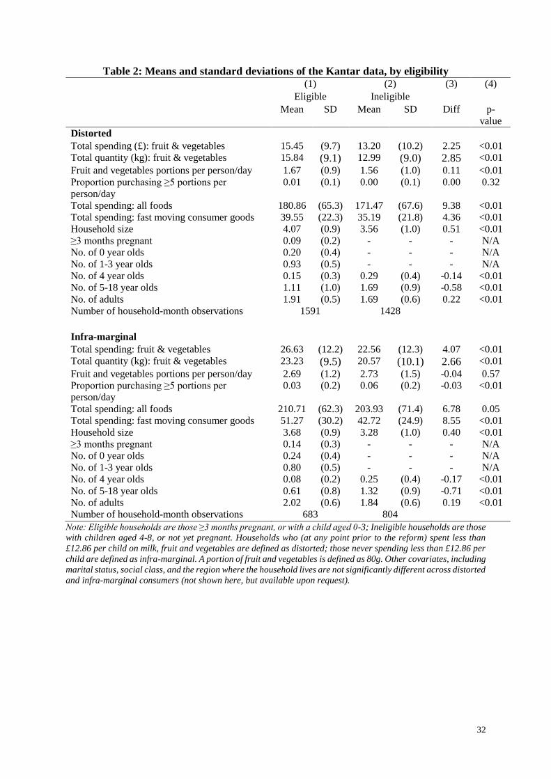
Table 2 presents the means and standard deviations of a set of characteristics for households in

our sample, which are all estimated to be on benefits. We show these separately for eligible and

ineligible households (columns (1) and (2)), and for distorted and infra-marginal households

(the top and bottom panels); the means and standard deviations for the full sample are given in

Appendix B, Table B3.

We start with monthly spending on different foods, including fruit and vegetables. There are

small differences between eligible (with young children) and ineligible households (with older

children); the group of eligibles tend to spend more on fruit and vegetables, as well as on all

foods together, and on fast moving consumer goods (other items that are commonly purchased

in supermarkets, such as toiletries and household products). Looking at household size, we see

that they are also slightly larger than ineligible households. In our analysis we control for

household fixed effects, and therefore only identify the effects of the scheme from changes

within households. We also account for time-varying household characteristics, including the

number of adults and children in the household, and a second order polynomial in the age (in

months) of the youngest and oldest child in the household. As a robustness check, we also allow

the effects of these covariates on spending to change after the introduction of the scheme.

Crucially for our analysis, which relies on a triple differences approach (comparing the change

before/after the introduction of the scheme in spending for distorted/infra-marginal across

eligible/ineligible groups), any differences in characteristics between eligible and ineligible

households are similar for distorted and infra-marginal households. Indeed, a difference-in-

difference analysis, comparing the difference between distorted eligible and ineligible

households with the difference between infra-marginal eligible and ineligible households,

shows no significant differences for any household characteristics.10 Our identifying

10 Including characteristics not shown here, such as marital status, social class, and the region where the household

lives (available upon request).

16

assumption is that, absent the reform, spending among distorted and infra-marginal eligible

households would have evolved in the same way as spending among the same groups defined

over ineligible households. Figure 1 shows trends in pre-reform spending to be similar across

distorted and infra-marginal households among both eligible and ineligible groups.

One final point we take from Table 2 is that it is very infrequent for households to purchase the

recommended five portions of fruit and vegetables a day, this happens in only between 0% and

6% of household-months, indicating there is sufficient scope for all households to increase their

spending on fruit and vegetables. Over the period both before and after the introduction of

Health Start Vouchers there was a widespread 5-a-day campaign in the UK, which would be

likely to offset any perception among households already spending at the level of the Vouchers

that they were consuming a healthy level of fruit and vegetables.

Finally, exploiting the rich Kantar data, we are able to directly investigate attitudes, preferences

and household decision making in relation to spending. We focus on a comparison between

distorted and infra-marginal households. This allows us to address directly a possible concern

that there may be differences in behavioural biases between the two groups that may lead to

differences in how they respond to labelling. Table 3 presents the proportion of households who

agree with a number of statements about their attitudes, preferences and behaviours. We order

these by the p-value indicating whether the proportion agreeing with each statement is

significantly different across the two groups (distorted and infra-marginal). We expect the two

groups to be very similar, as they are both drawn from a group of low-income households on

benefits with children, and the data support this; there is no evidence that one group exhibits

systematically greater behavioural bias than the other.

4. Empirical strategy and main results

Our main interest in this paper is in understanding the nature of the spending response to

17

Healthy Start Vouchers. Our identification strategy is a triple differences approach. Comparing

the change in spending before and after the introduction of the scheme across eligible and

ineligible households (where eligibility is defined by age of children) allows us to identify the

overall effect of the policy; we specifically identify the mechanism through which the policy

affected spending by additionally comparing responses across distorted and infra-marginal

households. This allows us to say whether the observed response is in line with standard

economic analysis or indicates any wider behavioural response. Our analysis is based on a

sample of households who are all on benefits, and observed both before and after the reform.

Motivated by the discussion in section 2, our formal test of the mechanisms compares marginal

propensities to consume out of income and vouchers. However, we start with a simpler

“treatment effect” specification that tests for differences in the overall effect of the reform

across distorted and infra-marginal households:

𝑙𝑛(𝐹𝑉ℎ𝑡) = 𝛽0 + 𝛽1𝑃𝑜𝑠𝑡𝑡 + (𝛽2 + 𝛽3𝑃𝑜𝑠𝑡𝑡)𝐸ℎ𝑡𝐷 + (𝛽4 + 𝛽5𝑃𝑜𝑠𝑡𝑡)𝐸ℎ𝑡

𝐼𝑀 + 𝐗ℎ𝑡

+𝜙ℎ + 𝜏𝑡 + 𝑒ℎ𝑡 (1)

where 𝑙𝑛(𝐹𝑉ℎ𝑡) is the logarithm of expenditure on fruit and vegetables for household ℎ in

month 𝑡. 𝑃𝑜𝑠𝑡𝑡 is a binary indicator for months after November 2006, when the scheme was

introduced. 𝐸ℎ𝑡 is a binary indicator for whether the household is eligible for Healthy Start

Vouchers, based on the presence and age of children in the household. Interacting 𝑃𝑜𝑠𝑡𝑡 and

𝐸ℎ𝑡 captures the overall effect of the reform. We allow this to vary by whether households are

distorted (D) or infra-marginal (IM), denoted by the superscript; we also report the pooled

estimate. The vector 𝐗ℎ𝑡 includes other time-varying household-level covariates, including a

full set of fixed effects for the number of children and number of adults in the family to control

for varying food needs across households (Currie, 2003). We also control flexibly for the age

of the youngest and the oldest child (in months). Household fixed effects 𝜙ℎ control for time

invariant differences in preferences across households, and year and month effects, 𝜏𝑡, pick up

18

common annual and seasonal fluctuations in spending. 𝑒ℎ𝑡 is an idiosyncratic error, clustered

by household. The coefficients 𝛽3 and 𝛽5 are our parameters of interest, capturing the effect of

the reform for distorted and infra-marginal households respectively.

The results are presented in Table 4. Column (1) reports the coefficient from the pooled

specification, showing that the reform led to a significant and sizeable 15.5% increase in

spending on fruit and vegetables among eligible households compared to the ineligible control

group. Column (4) shows that there was a corresponding increase in the quantity of fruit and

vegetables purchased, equivalent to 1.84kg per month, or over two-thirds of a portion per

household per day. Columns (2) and (5) show that the aggregate effects on spending and

quantity were driven entirely by distorted households who increased their spending by 23.2%

(equivalent to more than one portion per household per day), while there was no (statistically

significant) increase in spending among infra-marginal households. The difference between the

coefficients for distorted and infra-marginal households is statistically significant (p<0.001).

Our formal test of economic incentives versus labelling follows Moffitt (1989) and Hoynes and

Schanzenbach (2009). Specifically, we test for equality of responses to vouchers and cash

income separately for distorted and infra-marginal households, using the following

specification:

𝑙𝑛(𝐹𝑉ℎ𝑡) = + 𝛽1𝑃𝑜𝑠𝑡𝑡 + (𝛽2 + 𝛽3𝑃𝑜𝑠𝑡𝑡)𝐸ℎ𝑡𝐷 𝑉𝑎𝑙𝑢𝑒ℎ𝑡 + (𝛽4 + 𝛽5𝑃𝑜𝑠𝑡𝑡)𝐸ℎ𝑡

𝐼𝑀𝑉𝑎𝑙𝑢𝑒ℎ𝑡

+𝜃𝐷𝐸ℎ𝑡𝐷 𝑌ℎ𝑡 + 𝜃𝐼𝑀𝐸ℎ𝑡

𝐼𝑀𝑌ℎ𝑡 + 𝐗ℎ𝑡 + 𝜙ℎ + 𝜏𝑡 + 𝑒ℎ𝑡 (2)

where 𝑉𝑎𝑙𝑢𝑒ℎ𝑡 denotes the value of the Healthy Start Vouchers (in £) that the family is eligible

for, which we interact with indicators for distorted (D) and infra-marginal (IM) households,

denoted by the superscript, and with a post-reform indicator. We also allow spending to depend

on income (𝑌ℎ𝑡), measured in £s and proxied by total spending on fast moving consumer goods.

The marginal propensity to consume fruit and vegetables out of cash is the derivative of

𝑙𝑛(𝐹𝑉ℎ𝑡) with respect to 𝑌ℎ𝑡. We allow this to differ across distorted and infra-marginal

19

households, estimated by the coefficients 𝜃𝐷 and 𝜃𝐼𝑀. We present a number of sensitivity

checks allowing more flexibility in the way that 𝑌ℎ𝑡 enters in the robustness analysis below.

Since we proxy income by total grocery spending, it includes the value of the vouchers. The

parameters 𝛽3 and 𝛽5 therefore capture the difference in the MPC out of vouchers compared to

cash for distorted and infra-marginal households respectively. We expect 𝛽3 > 0, since both the

economic incentives and labelling would cause distorted households to spend more out of

vouchers than they would out of cash: i.e. MPCHSV > MPCcash. Among infra-marginal

households, the economic incentive effects would cause them to spend the vouchers in the same

way as cash, i.e. MPCHSV = MPCcash, implying 𝛽5 = 0, while labelling would cause them to

spend the vouchers differently, i.e. MPCHSV > MPCcash, implying 𝛽5 > 0.

The results are presented in Table 4, column (3). The parameter 𝛽3 is positive and statistically

significant implying that, for distorted households, there is an additional increase in fruit and

vegetable expenditures of 0.7% per £1 of vouchers (compared to £1 cash income). By contrast,

𝛽5 is not significantly different from zero, implying that infra-marginal households treat the

vouchers in the same way as cash. The p-value shows that the effects for distorted and infra-

marginal households are significantly different (p=0.024).

The results for the quantity consumed (in kg) are presented in columns (4) to (6), the magnitude

of which is consistent with the results on expenditures. With an average spending on fruit and

vegetables for eligible distorted households of £15.45 per month (see Table 2), the increase in

fruit and vegetable spending of 0.7% per £1 of vouchers is equivalent to approximately £0.11

per £1. On average, families purchase around 1kg of fruit and vegetables per £1 (see Table 2

and Table B3), suggesting that the increase in the quantity of fruit and vegetables purchased per

£1 of voucher is approximately 100g; similar to our estimate in column (6).

5. Robustness

20

In this section we carry out a number of robustness checks. These address the common trends

assumption underlying the triple differences strategy, the functional form specification, the

definition of distorted and infra-marginal households, the set of foods considered, the sample

of households used and the definition of benefit receipt. We start by examining a number of

placebo tests, looking at cases where we do not expect to find any effect of the scheme. We

then test and discuss the robustness of our main result to alternative specifications.

5.1 Placebo tests

We test the robustness of our common trends assumption through a number of placebo tests. A

particular concern might be whether our results are driven by mean reversion, since we define

distorted and infra-marginal households by their pre-reform levels of spending. We already deal

with this in a number of ways. First, we select only households that are observed for at least

four months prior to the reform. Second, our triple differences strategy would imply that mean

reversion would apply differentially across eligible and ineligible households. Here, we run

additional tests. First, we look at a pseudo reform introduced in November 2005 (one year prior

to the true start of the scheme) and restrict the data to December 2004 to November 2006. We

define distorted and infra-marginal households in the same way as before, but based on their

spending prior to November 2005. Columns (1) and (2) of Table 5 show that neither distorted

nor infra-marginal households respond to this pseudo reform, suggesting that trends were

similar beforehand. Although there is a negative MPC out of vouchers for distorted households

(column (2)), we do not see this for the overall effect shown in column (1).

Second, we analyse the effects of the Healthy Start Scheme on similar foods that were not

allowed to be purchased with the vouchers. Columns (3) to (6) of Table 5 present the effects on

spending on fruit juice and on frozen fruit and vegetables respectively, showing no significant

responses among either distorted or infra-marginal households.

21

5.2 Functional form

We test our functional form specification using the same sample and variables of interest as

those in our main analyses. Estimation of the MPC out of cash depends on how income is

included in the regression. Although both distorted and infra-marginal groups are low-income

households on benefits, Table 2 shows that the level of spending among the infra-marginal

group is higher than among the distorted group. Our main specification controls linearly for

income, but we test the robustness to alternative specifications.

Column (1) in Table 6 replicates our main result (column (3) in Table 4) for comparison.

Column (2) includes a separate quadratic polynomial in income for distorted and infra-marginal

households. Column (3) uses total food spending as the proxy for income, and column (4)

instruments this with total spending on fast-moving consumer goods. Column (5) constrains the

marginal propensity to consume out of income to be the same across distorted and infra-

marginal households. Finally, column (6) allows the effects of time-varying covariates (number

of adults and children in the household, and a quadratic polynomial in age of the youngest and

oldest child) to change after the introduction of the scheme. The results are robust across the

different specifications.

5.3 Distorted/ infra-marginal households

Our main specification splits the sample according to whether households spent less than £12.86

a month per child at any time prior to the introduction of the policy (distorted households) and

those who never spent less than £12.86 a month per child (infra-marginal households). As a

robustness check, we define distorted (infra-marginal) households as those who (never) spent

less than £12.86 per voucher. The results are presented in column (1) of Table 7, showing

similar results to those above.

One possible interpretation of the labelling might be that the value of the Vouchers provides a

22

‘benchmark’ level of spending on fruit and vegetables, which would differentially affect

spending among distorted and infra-marginal households. This could mean that infra-marginal

households do not respond because they already purchase very high levels of fruit and

vegetables. We believe we can rule this out; the WHO recommends individuals to consume at

least five portions of fruit and vegetables a day and there was a widespread 5-a-day campaign

in the UK from 2004. Table 2 shows that the vast majority of households (including infra-

marginals) buy fewer than this. In additional robustness analysis (not shown here), we drop

households who, at any point, purchase five or more daily portions of fruit and vegetables per

person. Although the estimate for distorted households remains unchanged, the estimate for

infra-marginal households becomes negative. The direction of this change is inconsistent with

an explanation that the vouchers create a norm, since the largest reduction would be exactly

among the group who consume the most fruit and vegetables to start with. We also think it is

unlikely that households would have seen the vouchers as a signal to reduce their spending on

fruit and vegetables, since the widespread 5-a-day campaign would have made it clear that

households should have been consuming considerably above their current level.11

5.4 Loose fruit and vegetables

As discussed in Section 3, approximately 20% of our sample do not scan items without a

barcode, such as loose fruit and vegetables, or meat and fish purchased over the counter. We

re-run our analyses using the sample of households that do scan loose items. This is presented

in column (2) of Table 7, showing very similar estimates to those obtained in the full sample.

5.5 Estimating the ‘true’ value of the vouchers

Due to the pre-existing Welfare Food Scheme that provided households with milk tokens, the

11 The ‘5-a-day’ campaign does not count potatoes as a vegetable, whereas the Healthy Start Scheme allows

households to spend their vouchers on plain fresh potatoes. Our results (available upon request) show that the

increase in spending is driven by an increase in spending on vegetables more generally, rather than simply by an

increase in spending on potatoes.

23

net value of Healthy Start Vouchers is less than a situation without the pre-existing scheme.

This implies that our estimates of the MPC out of vouchers are likely to underestimate the true

response. We argue that households consume milk in relatively fixed quantities, depending on

household size. Assuming that milk is separable from other food spending, conditional on

household size, we can therefore approximate the value of the voucher for fruit and vegetables

net of what households spend on milk, more precisely estimating the marginal propensity to

consume fruit and vegetables out of vouchers. We do this by subtracting households’ milk

spending from the total value of the vouchers they are eligible for, and comparing the MPC out

of vouchers to that out of income using this new definition.

Column (3) in Table 7 presents the results, showing larger estimates than those above: distorted

households additionally increase their fruit and vegetable expenditures by 1.1% per £ of

vouchers (compared to a £ of cash income). Consistent with the above, we find that infra-

marginal households do not respond differently to vouchers compared to cash.

5.6 Benefit recipients

Finally, we explore the robustness of our analysis to different ways of defining benefit receipt.

Our main specification uses hours worked, and includes only households always on benefits.

First, we explore whether our results are robust to the use of a different sample, also including

households whose benefit status changes over time. Column (4) still restricts the sample to

benefit recipients, but also includes households who may have changed benefit status over time.

Second, we specify an alternative definition of benefit receipt. Although our definition of

benefit receipt based on hours worked does a good job at capturing households who are truly

on benefits, we omit some household who are on benefits. To consider whether this is important

we also use a wider set of characteristics available in both the Kantar data and in the Expenditure

and Food Survey (EFS) to predict benefit receipt in the EFS (see Appendix B, and Table B2).

We apply the estimated coefficients from the EFS to the Kantar data to create a predicted

24

probability of benefit receipt. We define households as being on benefits when their predicted

probability exceeds 0.7.

This approach also does a good job at capturing those who truly receive benefits: the EFS data

shows that, among those defined as being on benefits (i.e. having a probability of benefit receipt

that exceeds 0.7), 92% actually receive benefits (not shown here, but available upon request).

Using this different sample of benefit recipients, we estimate the effect of the Healthy Start

Scheme on fruit and vegetable consumption. The results are presented in column (5) of Table

7. Finally, column (6) uses the full sample of households with children aged 0-8, specifying the

probability of benefit receipt, as predicted from the EFS estimates, as weights in the analysis

(Arellano and Meghir, 1992).

Our results are robust to these alternative specifications. We therefore believe that our results

provide strong evidence that the effects of the reform operated through distorted households,

not infra-marginal households, consistent with the underlying economic incentives in the policy

and not through labelling.

6. Summary and discussion

Our analysis of the Healthy Start Scheme makes two substantive contributions to the ongoing

academic and policy debate about how to bring improve dietary choices. First, we identify that

targeted benefits can be effective in increasing purchases of fruit and vegetables. Second, we

present evidence on the mechanisms through which targeted benefits affect behaviour. Our

evidence is consistent with a response in line with the underlying economic incentive effects

and not with a wider behavioural response. We discuss each of these findings in turn.

Our estimates indicate that the Healthy Start Scheme has increased spending on fruit and

vegetables by around 1.8 kg per household per month, equivalent to two-thirds of a portion per

household per day. Among distorted households the increase has been more than one portion

25

per day. Given low levels of spending prior to the reform, the scheme has made a sizeable

contribution to households moving closer to five a day, although it has not been enough to

ensure that all households receiving the Vouchers meet that target.

Our estimate of the effect of the reform is an intention to treat effect, since we look at eligible

and ineligible households, rather than actual voucher recipients. The advantage of this approach

is that eligibility is solely determined by the (exogenous) age of children in the household,

implying that our estimate is not upwardly biased by households selecting into the scheme. If

anything, we are likely to underestimate the true effect of the scheme, since (i) the net value of

the voucher is less than what we observe due to the pre-existing Welfare Food Scheme, (ii)

approximately 80% of eligible households receive the vouchers, and (iii) we estimate that

approximately 8% of the group we define as being “on benefits” may not truly receive benefits.

For policy-makers, the finding that infra-marginal households treated the vouchers like cash

has implications for the cost-effectiveness of vouchers for promoting healthier dietary choices

from a policy perspective. One potential promise of recent studies on labelling effects was that

targeted vouchers could be a more cost-effective policy tool (i.e. could achieve the desired

policy outcome at a lower level of public spending). The question remains as to why we find

no evidence for behavioural effects in this setting. As we have shown, it cannot be explained

by differences in behavioural biases across the groups. One possibility is that dietary

preferences are deeply ingrained and simply hard to shift. A number of small-scale studies have

demonstrated positive impacts from behavioural nudges (primarily via the positioning of

healthy options in menus and/or canteens). Our results indicate that more work may be needed

to understand if and why behavioural mechanisms affect dietary choices and how they can be

exploited for the purposes of policy-making.

26

References

Abeler, Johannes and Felix Marklein. 2010. “Fungibility, Labels and Consumption.” University

of Nottingham, Working Paper

Aguiar, Mark and Eric Hurst. 2007. "Life-cycle prices and production", American Economic

Review, 97: 5, 1533-1559.

Arellano, Manuel and Costas Meghir. 1992. "Female Labour Supply and On-the-job Search:

An Empirical Model Estimated Using Complementary Data Sets" Review of Economic

Studies, 59(3), 537-559.

Banks, James, Cormac O'Dea and Zoë Oldfield. 2010. "Cognitive function, numeracy and

retirement saving trajectories", The Economic Journal, 120:548, F381-F410

Beatty, Timothy, Laura Blow, Thomas Crossley, Cormac O’Dea. 2014. “Cash by any other

name? Evidence on labelling from the UK Winter Fuel Payment.” Journal of Public

Economics, 118, pp. 86–96

Benhassine, Najy, Florencia Devoto, Esther Duflo, Pascaline Dupas, and Victor Pouliquen.

2014. “Turning a shove into a nudge? A ‘labeled cash transfer’ for education.” Forthcoming,

American Economic Journal: Economic Policy.

Benjamin, Daniel, Sebastian Brown and Jesse Shapiro. 2013. "Who is Behavioral? Cognitive

Ability and Anomalous Preferences" Journal of the European Economic Association, 11: 6,

1231-1255

Berry, Steven, James Levinsohn and Ariel Pakes. 1995. "Automobile prices in market

equilibrium" Econometrica 63 (4), 841–890

Bollinger, Bryan, Phillip Leslie and Alan Sorensen. 2010. Calorie posting in chain restaurants.

NBER WP 15648.

Capacci, Sara and Mario Mazzochi. 2011. "Five-a-day, a price to pay: An evaluation of the UK

program impact accounting for market forces", Journal of Health Economics, 30(1), 87-98.

Cunha, Jesse M. 2014. “Testing Paternalism: Cash vs. In-Kind Transfers”, American Economic

Journal: Economic Policy, 6(2), 195-230

Currie, Janet. 2003. U.S. Food and Nutrition Programs. R.A. Moffitt (Ed.), in: Means-Tested

Transfer Programs in the U.S., Cambridge, MA: NBER

Currie, Janet and Firouz Gahvari. 2008. “Transfers in cash and in kind: Theory meets the data.”

Journal of Economic Literature, 46(2), 333-383.

Department of Health, Social Services and Public Safety. 2011. Delivering a Healthy Start for

pregnant women, new mums, babies and young children. Department of Health.

Department of Health. 2002. Scientific Review of the Welfare Food Scheme: Report of the

Panel on Child and Maternal Nutrition of the Committee on Medical Aspects of Food and

Nutrition Policy. Report on Health and Social Subjects No.51. London: TSO.

Department of Health. 2009. “Healthy Start Factfile” [Accessed on 17 June 2013] Available at:

www.foodwm.org.uk/resources/Healthy_Start_Factfile_West_ Midlands_Sept_09.pdf

Downs, Julie S, George Loewenstein and Jessica Wisdom. 2009. "Strategies for Promoting

Healthier Choices" American Economic Review Papers & Proceedings, 99:2, 159-164

Dubois, Pierre, Rachel Griffith and Aviv Nevo. 2014. "Do Prices and Attributes Explain

27

International Differences in Food Purchases?" American Economic Review, 104:3, 832-867

Einav, Liran, Ephraim Leibtag and Aviv Nevo. 2010. "Recording discrepancies in Nielsen

Homescan data: are they present and do they matter?" Quantitiave Marketing and Economics,

8, 207-239

Ford, Fiona, Theodora Mouratidou, Wademan Sarah, Fraser Robert. 2009. “Effect of the

introduction of 'Healthy Start' on dietary behaviour during and after pregnancy: early results

from the 'before and after' Sheffield study.” British Journal of Nutrition, 101(12):1828-36.

Gortmaker Steven L., Boyd A. Swinburn, David Ley, Rob Carter, Patricia L. Mabry, Diane T.

Finegood, Terry Huang, Tim Marsh and Marjory L. Moodie. 2011. "Changing the future of

obesity: science, policy, and action" The Lancet, 378: 838-847

Griffith, Rachel and Martin O'Connell. 2009. "The Use of Scanner Data for Research into

Nutrition", Fiscal Studies, 30(34), 339-365.

Hoynes, Hilary, Diane Whitmore Schanzenbach. 2009. Consumption Responses to In-Kind

Transfers: Evidence from the Introduction of the Food Stamp Program. American Economic

Journal: Applied Economics, 1, 109-139.

Hills D, Child C, Junge K, Wilkinson E, Sullivan F. 2006. Healthy Start. Rapid evaluation of

early impact on beneficiaries, health professionals, retailers and contractors. London:

Tavistock & Symbia.

Kooreman Peter. 2000. “The Labeling Effect of a Child Benefit System.” American Economic

Review, 90(3), 571-583.

Lancet. 2011. "Urgently Needed: A Framework Convention for Obesity Control" 378 (9792),

741.

Leicester, Andrew and Zoe Oldfield. 2009. “Using Scanner Technology to Collect Expenditure

Data.” Fiscal Studies, 30, 309-337.

Loewenstein, George, Troyen Brennan, and Kevin Volpp. 2007. “Asymmetric Paternalism to

improve health behaviors.” JAMA, 298(20): 2415-2417.

Lucas, Patricia, Tricia Jessiman, Ailsa Cameron, Meg Wiggins, Katie Hollingworth and Chloe

Austerberry. 2013. “Healthy start vouchers study: The views and experiences of parents,

professionals and small retailers in England.” [Accessed on 17 June 2013] Available:

www.bristol.ac.uk/sps/research/projects/completed/2013/finalreport.pdf

Moffitt, Robert. A. 1989. “Estimating the Value of an In-Kind Transfer: The Case of Food

Stamps.” Econometrica, 57(2), 385-409.

Nevo, Aviv. 2001. "Measuring market power in the ready-to-eat cereal industry" Econometrica,

69: 2, March 2001, 307-342

New York Times. 2013. “Britain’s Ministry of Nudges.”

www.nytimes.com/2013/12/08/business/international/britains-ministry-of-nudges.html?_r=0

(accessed on 14/1/2014)

Schanzenbach, Diane. 2013. Strengthening SNAP for a more food-secure, Healthy America,

The Hamilton Project Discussion Paper 2013-06.

Southworth, Herman. 1945. “The Economics of Public Measures to Subsidize Food

Consumption.” Journal of Farm Economics, 27(1): 38–66.

Stables, Gloria, Amy Subar, Blossom Patterson, Kevin Dodd, Jerianne Heimendinger, Mary

Ann van Duyn and Linda Nebeling. 2002. "Changes in vegetables and fruit consumption and

28

awareness among US adults: results of the 1991 and 1997 5 a day for better health program

surveys" Journal of the Amer Dietetic Assoc, 102, 809-817.

Thaler, Richard. 1985. "Mental accounting and consumer choice", Marketing Science 4, 199-

214.

Thaler, Richard. 1999. “Mental accounting matters.” Journal of Behavioral Decision Making,

12, 183-206.

Thaler, Richard. H. and Cass R. Sunstein. 2003. “Libertarian paternalism”, American Economic

Review Papers and Proceedings 93, 175-179.

Thaler, Richard H. and Cass R. Sunstein. 2008. Nudge: Improving decisions about health,

wealth, and happiness. New Haven, CT: Yale University Press.

USDA, United States Department of Agriculture. 2013. Healthy Incentive Pilot: Interim Report

http://www.fns.usda.gov/sites/default/files/HIP_Interim.pdf

USDA, United States Department of Agriculture. 2014. Competitive grant to establish a USDA

Center for Behavioral Economics and Healthy Food Choice Research, AP-063. U.S.

Department of Agriculture, Economic Research Service.

Wansink, Brian, David Just and Laura Smith. 2011. “Move the fruit: Putting fruit in new bowls

and new places doubles lunchroom sales.” Journal of Nutrition Education and Behaviour,

43(4), S1.

Wansink, Brian, and David Just. 2011. “Healthy Foods First: Students take the first lunchroom

food 11% more often than the third.” Journal of Nutrition Education and Behaviour, 43(4),

S8.

Whitmore, Diane. 2002. “What Are Food Stamps Worth?” Working Paper #468, Princeton

University, Industrial Relations Section.

WHO (1990) "Diet, Nutrition and the Prevention of Chronic Disease, WHO Geneva

WHO (2003) "Diet, Nutrition and the Prevention of Chronic Diseases" WHO Technical Report

Series 916

Wisdom, Jessica, Julie S. Downs, and George Loewenstein. 2010. “Promoting Healthy

Choices: Information versus Convenience.” American Economic Journal: Applied

Economics, 2(2): 164-78.

29

Figure 1: Expenditures on fruit and vegetables among distorted and infra-marginal,

eligible and ineligible households

Note: Each symbol represents mean spending on fruit and vegetables in that year-month across households,

conditional on household mean levels. The lines are added for ease of legibility, obtained from locally weighted

regressions. The vertical line indicates when the scheme was introduced. Eligible households, indicated by x and

the solid line, are those with children aged 0-3 or where the woman is at least 3 months pregnant; ineligible

households, indicated by solid dots and dashed line, are those with children aged 4-8, and those where the woman

is not yet pregnant, but will become pregnant (and therefore eligible) during our observation period. Households

who prior to the reform spent less than £12.86 per child on milk, fruit and vegetables are defined as distorted;

those never spending less than £12.86 per child are defined as infra-marginal. We observe 1591 and 683

household-months for distorted and infra-marginal eligible households respectively; and 1428 and 804 household-

months for distorted and infra-marginal ineligible households.

-.4

-.2

0

.2

.4

.6

ln(fru

it a

nd v

egeta

ble

spendin

g)

Jan 2005 Jan 2006 Jan 2007 Jan 2008 Jan 2009

Date

Eligible, Distorted Ineligible, Distorted

Spending on fruit and vegetables, distorted households

-.4

-.2

0

.2

.4

.6

ln(fru

it a

nd v

egeta

ble

spendin

g)

Jan 2005 Jan 2006 Jan 2007 Jan 2008 Jan 2009

Date

Eligible, Infra-marginal Ineligible, Infra-marginal

Spending on fruit and vegetables, infra-marginal households

30

Figure 2: Effect of targeted benefits

31

Table 1: Comparison of the Welfare Food Scheme and the Healthy Start Scheme

Welfare Food Scheme Healthy Start Scheme

Families on benefits receive: One voucher per family

with children aged ≤ 4 One voucher per pregnant woman,

one voucher per child aged ≤ 3

(two vouchers per infant aged 0-1) The value per voucher: Approximately £2.80 * £2.80 from 27 November 2006 £3.00 from 6 April 2008

Vouchers can be spent on: 7 pints of cows’ milk

(or 900g of formula for infants

aged 0-1)

Milk, plain fresh fruit and

vegetables

Notes: Both schemes apply to households who receive Income Support, Income-based Jobseeker’s Allowance, or

Child Tax Credit with an income below a certain year-specific threshold (£13,230 in 2003/04, £13,480 in 2004/05,

£13,910 in 2005/06, £14,155 in 2006/07, £14,495 in 2007/08, £15,575 in 2008/09).

* The value of a voucher during the Welfare Food Scheme depends on the price of milk, as each voucher was

exchangeable for 7 pints of cow’s milk. In 2006, the price of a pint of cow’s milk was approximately 40p, so 7

pints is equal to approximately £2.80.

32

Table 2: Means and standard deviations of the Kantar data, by eligibility

(1) (2) (3) (4)

Eligible Ineligible

Mean SD Mean SD Diff p-

value Distorted Total spending (£): fruit & vegetables 15.45 (9.7) 13.20 (10.2) 2.25 <0.01 Total quantity (kg): fruit & vegetables 15.84 (9.1) 12.99 (9.0) 2.85 <0.01

Fruit and vegetables portions per person/day 1.67 (0.9) 1.56 (1.0) 0.11 <0.01 Proportion purchasing ≥5 portions per

person/day 0.01 (0.1) 0.00 (0.1) 0.00 0.32

Total spending: all foods 180.86 (65.3) 171.47 (67.6) 9.38 <0.01 Total spending: fast moving consumer goods 39.55 (22.3) 35.19 (21.8) 4.36 <0.01 Household size 4.07 (0.9) 3.56 (1.0) 0.51 <0.01 ≥3 months pregnant 0.09 (0.2) - - - N/A No. of 0 year olds 0.20 (0.4) - - - N/A No. of 1-3 year olds 0.93 (0.5) - - - N/A No. of 4 year olds 0.15 (0.3) 0.29 (0.4) -0.14 <0.01 No. of 5-18 year olds 1.11 (1.0) 1.69 (0.9) -0.58 <0.01 No. of adults 1.91 (0.5) 1.69 (0.6) 0.22 <0.01 Number of household-month observations 1591 1428

Infra-marginal Total spending: fruit & vegetables 26.63 (12.2) 22.56 (12.3) 4.07 <0.01 Total quantity (kg): fruit & vegetables 23.23 (9.5) 20.57 (10.1) 2.66 <0.01

Fruit and vegetables portions per person/day 2.69 (1.2) 2.73 (1.5) -0.04 0.57 Proportion purchasing ≥5 portions per

person/day 0.03 (0.2) 0.06 (0.2) -0.03 <0.01

Total spending: all foods 210.71 (62.3) 203.93 (71.4) 6.78 0.05 Total spending: fast moving consumer goods 51.27 (30.2) 42.72 (24.9) 8.55 <0.01 Household size 3.68 (0.9) 3.28 (1.0) 0.40 <0.01 ≥3 months pregnant 0.14 (0.3) - - - N/A No. of 0 year olds 0.24 (0.4) - - - N/A No. of 1-3 year olds 0.80 (0.5) - - - N/A No. of 4 year olds 0.08 (0.2) 0.25 (0.4) -0.17 <0.01 No. of 5-18 year olds 0.61 (0.8) 1.32 (0.9) -0.71 <0.01 No. of adults 2.02 (0.6) 1.84 (0.6) 0.19 <0.01 Number of household-month observations 683 804

Note: Eligible households are those ≥3 months pregnant, or with a child aged 0-3; Ineligible households are those

with children aged 4-8, or not yet pregnant. Households who (at any point prior to the reform) spent less than

£12.86 per child on milk, fruit and vegetables are defined as distorted; those never spending less than £12.86 per

child are defined as infra-marginal. A portion of fruit and vegetables is defined as 80g. Other covariates, including

marital status, social class, and the region where the household lives are not significantly different across distorted

and infra-marginal consumers (not shown here, but available upon request).

33

Table 3: Differences in behavioural characteristics of distorted versus infra-marginal households

Distorted Infra-marginal

Mean Std. dev. Mean Std. dev. p-value

I Often Buy Foods Because I've Seen Them Advertised 0.533 (0.500) 0.414 (0.495) 0.061 I Regularly Buy National Lottery Tickets 0.194 (0.397) 0.293 (0.457) 0.075 I Decide Which Brands To Buy Before I Go Shopping 0.230 (0.422) 0.333 (0.474) 0.077 I Make Sure I Eat Well-Balanced Meals 0.315 (0.466) 0.424 (0.497) 0.079 Once I Find A Brand I Like I Tend To Stick To It 0.673 (0.471) 0.566 (0.498) 0.086 I Like To Spend As Little Time As Possible Food Shopping 0.212 (0.410) 0.141 (0.350) 0.138 I Tend To Consider Various Brands On The Shelf Before Making My Choice 0.594 (0.493) 0.515 (0.502) 0.215 I Often Buy Things Just Because I See Them On The Shelf 0.648 (0.479) 0.586 (0.495) 0.315 I Like To Enjoy Life And Don't Worry About The Future 0.545 (0.499) 0.606 (0.491) 0.336 I'm Prepared To Pay More For Products That Make Life Easier 0.176 (0.382) 0.222 (0.418) 0.368 I try to lead a healthy lifestyle 0.448 (0.499) 0.505 (0.503) 0.376 I Try To Buy a Healthy Range Of Foods These Days 0.370 (0.484) 0.424 (0.497) 0.384 I Like To Plan For The Future 0.255 (0.437) 0.303 (0.462) 0.401 I Tend To Eat When I Am Bored 0.394 (0.490) 0.354 (0.480) 0.512 I Spend More Money In The Supermarket Than I Intend To 0.255 (0.437) 0.222 (0.418) 0.550 I Make A Shopping List Before I Go Out And Stick To It 0.182 (0.387) 0.212 (0.411) 0.554 I Use Money Off Coupons Whenever I Get The Chance 0.442 (0.498) 0.414 (0.495) 0.654 I Always Compare Prices Between Different Brands Before Choosing 0.473 (0.501) 0.444 (0.499) 0.657 I Work To A Strict Budget When I'm Buying Groceries 0.533 (0.500) 0.505 (0.503) 0.658 I Tend To Spend Money Without Thinking 0.224 (0.418) 0.232 (0.424) 0.880 When My Favourite Brands Go On Offer I Stock Up On Them 0.339 (0.475) 0.333 (0.474) 0.920 Number of households 165 99

Note: The response to each statement is 1 "agree strongly", 2 "agree", 3 "neither", 4 "disagree", or 5 "disagree strongly". The table shows the means and standard deviations

of the proportion of households in the sample that agree or strongly agree, distinguishing between distorted and infra-marginal households. Households who (at any point prior

to the reform) spent less than £12.86 per child on milk, fruit and vegetables are defined as distorted; those never spending less than £12.86 per child are defined as infra-

marginal. The p-value comes from a t-test that the mean for distorted equals the mean for infra-marginal household. We do not observe these behavioural characteristics for 2

households in our sample.

34

Table 4: The effect of Healthy Start Vouchers

(1) (2) (3) (4) (5) (6)

Dependent variable: ln(fruit and vegetable expenditure) fruit and vegetable quantity (in kg)

𝐸ℎ𝑡 × 𝑃𝑜𝑠𝑡ℎ𝑡 0.155*** 1.838***

(0.047) (0.690)

𝐸ℎ𝑡𝐷 × 𝑃𝑜𝑠𝑡ℎ𝑡: Distorted 0.232*** 2.629***

(0.050) (0.715)

𝐸ℎ𝑡𝐼𝑀 × 𝑃𝑜𝑠𝑡ℎ𝑡: Infra-marginal -0.025 -0.050

(0.065) (1.090) 𝐸ℎ𝑡 -0.126** -1.952***

(0.055) (0.739)

𝐸ℎ𝑡𝐷 : Distorted -0.207*** -2.982***

(0.068) (0.854)

𝐸ℎ𝑡𝐼𝑀: Infra-marginal 0.040 0.149

(0.069) (0.973)

𝑉𝑎𝑙𝑢𝑒ℎ𝑡 (£) × 𝑃𝑜𝑠𝑡ℎ𝑡 × 𝐸ℎ𝑡𝐷 (3): Distorted 0.007*** 0.093***

(0.002) (0.030)

𝑉𝑎𝑙𝑢𝑒ℎ𝑡 (£) × 𝑃𝑜𝑠𝑡ℎ𝑡 × 𝐸ℎ𝑡𝐼𝑀 (5): Infra-marginal 0.001 0.029

(0.002) (0.044)

𝐸ℎ𝑡𝐷 𝑌ℎ𝑡:Total grocery spending, Distorted 0.004*** 0.051***

(0.000) (0.003)

𝐸ℎ𝑡𝐼𝑀𝑌ℎ𝑡: Total grocery spending, Infra-marginal 0.003*** 0.046***

(0.000) (0.007)

p-value: 𝐸ℎ𝑡𝐷 × 𝑃𝑜𝑠𝑡ℎ𝑡 = 𝐸ℎ𝑡

𝐼𝑀 × 𝑃𝑜𝑠𝑡ℎ𝑡 <0.001 0.015

p-value: 3 =5 0.024 0.176 Notes: Sample includes 4506 observations on 266 households between December 2004 - November 2008. All columns include household, month and year fixed effects, age and

age squared of youngest and oldest child (in months), dummies for whether household includes: 2 adults, 3+ adults, 1 child, 2 children, 3 children, 4+ children, and a dummy

indicating whether the household did not buy any fruit and vegetables that month. 𝐸ℎ𝑡 equals 1 for households with a child aged 0-3 or where the woman is ≥3 months pregnant.

𝑃𝑜𝑠𝑡ℎ𝑡 equals 1 for the period December 2006 onwards. “D” indicates distorted households, “IM” indicates infra-marginal households. Total grocery spending is spending

on food and fast moving consumer goods. Robust standard errors in parentheses, clustered by household. * p<0.10, ** p<0.05, *** p<0.01.

35

Table 5: The effect of Healthy Start Vouchers: robustness I

(1) (2) (3) (4) (5) (6)

Placebo: Dec04 – Nov06

Full sample: Dec04 – Nov08

Full sample: Dec04 – Nov08

Dependent variable: ln(fruit and vegetable

expenditure) ln(fruit juice expenditure) ln(frozen fruit and vegetable

expenditure)

𝐸ℎ𝑡𝐷 × 𝑃𝑜𝑠𝑡ℎ𝑡: Distorted -0.037 0.126 0.179

(0.087) (0.253) (0.287)

𝐸ℎ𝑡𝐼𝑀 × 𝑃𝑜𝑠𝑡ℎ𝑡: Infra-marginal -0.065 0.051 -0.117

(0.091) (0.376) (0.467)

𝐸ℎ𝑡𝐷 : Distorted -0.243** -0.263 -0.164

(0.115) (0.268) (0.404)

𝐸ℎ𝑡𝐼𝑀: Infra-marginal 0.022 -0.224 -0.878*

(0.091) (0.275) (0.491)

𝑉𝑎𝑙𝑢𝑒ℎ𝑡 (£) × 𝑃𝑜𝑠𝑡ℎ𝑡 × 𝐸ℎ𝑡𝐷 (3): Distorted -0.009** -0.002 -0.008

(0.004) (0.013) (0.014)

𝑉𝑎𝑙𝑢𝑒ℎ𝑡 (£) × 𝑃𝑜𝑠𝑡ℎ𝑡 × 𝐸ℎ𝑡𝐼𝑀 (5): Infra-marginal -0.004 -0.007 -0.009

(0.005) (0.019) (0.031)

𝐸ℎ𝑡𝐷 𝑌ℎ𝑡:Total grocery spending, Distorted 0.005*** 0.007*** 0.019***

(0.000) (0.001) (0.001)

𝐸ℎ𝑡𝐼𝑀𝑌ℎ𝑡: Total grocery spending, Infra-marginal 0.002*** 0.006*** 0.018***

(0.000) (0.001) (0.002)

p-value: 𝐸ℎ𝑡𝐷 × 𝑃𝑜𝑠𝑡ℎ𝑡 = 𝐸ℎ𝑡

𝐼𝑀 × 𝑃𝑜𝑠𝑡ℎ𝑡 0.693 0.851 0.572

p-value: 3 =5 0.153 0.803 0.968

No. of households 224 224 266 266 266 266 No. of household-months 2232 2232 4506 4506 4506 4506

Notes: All columns include household, month and year fixed effects, age and age squared of youngest and oldest child (in months), dummies for whether household includes: 2

adults, 3+ adults, 1 child, 2 children, 3 children, 4+ children, and a dummy indicating whether the household did not buy any fruit and vegetables that month. 𝐸ℎ𝑡 equals 1 for

households with a child aged 0-3 or where the woman is ≥3 months pregnant. 𝑃𝑜𝑠𝑡ℎ𝑡 equals 1 for the period December 2006 onwards. “D” indicates distorted households,

“IM” indicates infra-marginal households. Total grocery spending is spending on food and fast moving consumer goods. Robust standard errors in parentheses, clustered by

household. * p<0.10, ** p<0.05, *** p<0.01. The placebo test in columns (1) and (2) defines the introduction of the scheme as November 2005.

36

Table 6: The effect of Healthy Start Vouchers: robustness II

(1) (2) (3) (4) (5) (6)

Main

specification Quadratic in

spending Using food

spending Instrumenting

food spending MPCcash same

for D&IM Include

𝑃𝑜𝑠𝑡ℎ𝑡 × 𝐗ℎ𝑡 Dependent variable: ln(fruit and vegetable expenditure)

𝑉𝑎𝑙𝑢𝑒ℎ𝑡 (£) × 𝑃𝑜𝑠𝑡ℎ𝑡 × 𝐸ℎ𝑡𝐷 (3): Distorted 0.007*** 0.007*** 0.007*** 0.007*** 0.008*** 0.005*

(0.002) (0.002) (0.002) (0.002) (0.003) (0.003)

𝑉𝑎𝑙𝑢𝑒ℎ𝑡 (£) × 𝑃𝑜𝑠𝑡ℎ𝑡 × 𝐸ℎ𝑡𝐼𝑀 (5): Infra-marginal 0.001 0.002 0.001 0.001 0.000 -0.002

(0.002) (0.002) (0.002) (0.002) (0.002) (0.003)

𝐸ℎ𝑡𝐷 𝑌ℎ𝑡 :Total grocery spending, Distorted 0.004*** 0.009*** 0.004***

(0.000) (0.001) (0.000)

𝐸ℎ𝑡𝐷 𝑌ℎ𝑡

2 :Total grocery spending, Distorted -0.000***

(0.000)

𝐸ℎ𝑡𝐼𝑀𝑌ℎ𝑡 :Total grocery spending, infra-marginal 0.003*** 0.008*** 0.003***

(0.000) (0.001) (0.000)

𝐸ℎ𝑡𝐼𝑀𝑌ℎ𝑡

2 :Total grocery spending, infra-marginal -0.000***

(0.000) 𝑌ℎ𝑡: Total grocery spending 0.004***

(0.000)

𝐸ℎ𝑡𝐷 𝑌ℎ𝑡:Total grocery spending, Distorted 0.006*** 0.005***

(0.000) (0.001)

𝐸ℎ𝑡𝐼𝑀𝑌ℎ𝑡: Total grocery spending, Infra-marginal 0.004*** 0.004***

(0.000) (0.001) Kleibergen-Paap rk F-statistic 45.07

p-value: 3 =5 0.024 0.040 0.053 0.029 0.011 0.012 Notes: Sample includes 4506 observations on 266 households between Dec ‘04 - Nov ‘08. All columns include household, month and year fixed effects, age and age squared of

youngest and oldest child (in months), dummies for whether household includes: 2 adults, 3+ adults, 1 child, 2 children, 3 children, 4+ children, and a dummy indicating

whether the household did not buy any fruit and vegetables that month. 𝐸ℎ𝑡 equals 1 for households with a child aged 0-3 or where the woman is ≥3 months pregnant. 𝑃𝑜𝑠𝑡ℎ𝑡

equals 1 for the period December 2006 onwards. “D” indicates distorted households, “IM” indicates infra-marginal households. Total grocery spending is spending on food

and fast moving consumer goods. Robust standard errors in parentheses, clustered by household. * p<0.10, ** p<0.05, *** p<0.01. Column 1 and 2 control for a first and

second order polynomial in total spending. Column 3 controls for total food spending, and column 4 instruments this with total spending on fast moving consumer goods. The

Kleibergen-Paap rk F-statistic shows the strength of the first stage. Column 5 constrains the MPC out of income to be the same across distorted and infra-marginal households.

Column 6 allows the effects of the time-varying covariates to change after the introduction of the scheme.

37

Table 7: The effect of Healthy Start Vouchers: robustness III

(1) (2) (3) (4) (5) (6)

Alternative

definition of

D and IM

Drop hhs not

recording

loose F&V

𝑉𝑎𝑙𝑢𝑒ℎ𝑡 minus milk

spending

Include those

on benefits at

any point

Benefits

defined as

Pr(ben)>0.7

Benefit

probability

used as

weights Dependent variable: ln(fruit and vegetable

expenditure)

𝑉𝑎𝑙𝑢𝑒ℎ𝑡 (£) × 𝑃𝑜𝑠𝑡ℎ𝑡 × 𝐸ℎ𝑡𝐷 (3): Distorted 0.007*** 0.008*** 0.011*** 0.005*** 0.006** 0.006***

(0.002) (0.003) (0.003) (0.02) (0.002) (0.002)

𝑉𝑎𝑙𝑢𝑒ℎ𝑡 (£) × 𝑃𝑜𝑠𝑡ℎ𝑡 × 𝐸ℎ𝑡𝐼𝑀 (5): Infra-marginal -0.001 0.002 0.002 -0.000 -0.000 -0.001

(0.003) (0.003) (0.003) (0.002) (0.003) (0.002)

𝐸ℎ𝑡𝐷 𝑌ℎ𝑡:Total grocery spending, Distorted 0.004*** 0.004*** 0.004*** 0.004*** 0.004*** 0.004***

(0.000) (0.000) (0.000) (0.000) (0.000) (0.000)

𝐸ℎ𝑡𝐼𝑀𝑌ℎ𝑡: Total grocery spending, Infra-marginal 0.003*** 0.003*** 0.003*** 0.003*** 0.003*** 0.003***

(0.000) (0.000) (0.000) (0.000) (0.000) (0.000)

p-value: 3 =5 0.010 0.055 0.037 0.028 0.064 0.001

No. of households 266 210 266 413 225 1521 No. of household-months 4506 3825 4506 5644 3836 26133

Notes: F&V denotes fruit and vegetables. All columns include household, month and year fixed effects, age and age squared of youngest and oldest child (in months), dummies

for 2 adults, 3+ adults, 1 child, 2 children, 3 children, 4+ children, and a dummy indicating whether the household did not buy any fruit and vegetables that month. 𝑃𝑜𝑠𝑡ℎ𝑡

equals 1 for the period December 2006 onwards. “D” indicates distorted households, i.e. those that spent less than £12.86 per child on milk, fruit and vegetables (at any point

prior to treatment); “IM” indicates that infra-marginal households, i.e. those never spending less than £12.86 per child prior to treatment. Total grocery spending is spending

on foods and fast moving consumer goods (goods purchased in supermarkets). Column 1 defines distorted households as those who, prior to the introduction of the scheme,

spent less than £12.86 per voucher (rather than per child); infra-marginal households are those who never spent less than £12.86 per voucher. Column 2 drops households that

do not record purchases of loose fruit and vegetables. Column 3 defines the value of the voucher as the value minus spending on milk. Column 4 also includes households whose

benefit status changes over time. Column 5 uses households with a predicted probability of receiving benefits (using the EFS) over 0.7. Column 6 uses these predicted

probabilities as weights. Robust standard errors in parentheses, clustered by household. * p<0.10, ** p<0.05, *** p<0.01.

38

FOR ONLINE PUBLICATION

Appendix A: The Welfare Food Scheme and the Healthy Start Scheme

Welfare Food Scheme

Concerns about access to nutritional foods during wartime rationing led to the introduction of

the Welfare Food Scheme (WFS) in the 1940s (Department of Health, 2002). The scheme

provided free access to milk and vitamins for low-income pregnant women and low-income

households with children under five. Households that received certain social security benefits

were sent one token each week that could be exchanged for seven pints of liquid milk, or 900g

of infant formula. These benefits included Income Support, Income-based Jobseeker’s

Allowance, or Child Tax Credit with a family income less than a year-specific threshold (e.g.

£13,480 in the tax year 2004/05; see also Table 1). The scheme changed little over the first 60

years, but was substantially reformed in 2006, when it was replaced by the Healthy Start

Scheme.

Healthy Start Scheme

The Healthy Start Scheme replaced the Welfare Food Scheme on 27 November 2006 after being

piloted in Devon and Cornwall from November 2005. The scheme was explicitly intended to

promote healthy lifestyles by changing diets. Households are sent vouchers that can be spent

on plain fresh fruit and vegetables, cow’s milk, or infant formula. Vouchers cannot be spent on

fruit and vegetables that have any other ingredient added, such as potato salad, or seasoned

vegetables. From 2011, they could additionally be spent on frozen fruit and vegetables; we do

not consider that here.

On introduction of the Healthy Start Scheme in November 2006, the monetary value of a

voucher was £2.80 (this gradually increased over time; see Table 1). Similar to the Welfare

Food Scheme, the receipt of certain benefits determines whether the family receives Healthy

Start Vouchers, including Income Support, Income-based Jobseekers’ Allowance, and Child

Tax Credit with a family income less than a year-specific threshold.12

Take-up and use of Healthy Start Vouchers is high. An estimated 79-80% of all eligible

households receive the vouchers, of which 90% are used (Department of Health, 2009). Many

retailers accept Healthy Start Vouchers, including supermarkets, corner shops, milkmen,

chemists, market stalls and greengrocers. Households can find information about which

12 From October 2008, the benefits also include Income-related Employment and Support Allowance. We do not

consider that here, as our sample ends in November 2008.

39

retailers accept vouchers on the Healthy Start website, or by calling their helpline.

All applications to the Healthy Start Scheme have to be countersigned by a health visitor or

midwife, who is also expected to provide information and advice on breastfeeding and healthy

eating. Eligible households are sent four vouchers per 4-week period per child (eight vouchers

for children aged between 0 and 1). Vouchers are only valid for this four week period, after

which they can no longer be used.

To date, there have not been any large-scale evaluations of the Healthy Start Scheme, though

there are three small (qualitative) studies. One focuses on the views and experiences of parents,

professionals and small retailers (Lucas et al., 2013), whilst the others examine whether it

affected food consumption. They find an increase in reported fruit and vegetable consumption

(Hills et al., 2006) and intakes of energy, calcium, folate, iron and vitamin C (Ford et al., 2009),

but sample sizes are small (n = 58 and 336 respectively).

Milk spending

We argue that households consume milk in relatively fixed quantities, depending on household

size. Our analyses in Table A1 below support this, showing the estimates of a simple difference-

in-difference analysis, comparing milk spending of eligible and ineligible households before

and after the introduction of the Scheme (we discuss the estimation in more detail in Section

4). Column 2 presents the estimates of a triple differences analysis, additionally distinguishing

between distorted and infra-marginal households. Column 3 and 4 show the same for the

quantity of milk purchased (in litres). These analyses show no evidence that milk spending

changed with the introduction of Healthy Start Vouchers.

Figure A1 below shows the distributions of monthly spending on milk and on fruit and

vegetables, conditional on the number of adults, the number and ages of children, year, month

and household fixed effects. This shows that the distribution of monthly milk expenditures is

very concentrated, and much more concentrated than monthly spending on fruit and vegetables,

with no large differences between eligible, ineligible, distorted, or infra-marginal households.

Analyses (not shown here, but available from the authors upon request) show that the standard

deviation of milk spending is significantly smaller than the standard deviation of spending on

fruit and vegetables.

We also confirm findings from the UK Committee on Medical Aspects of Food and Nutrition

Policy (Department of Health, 2002), who state that the vast majority of households did not

consume the amount of milk they could purchase with a token under the Welfare Food Scheme.

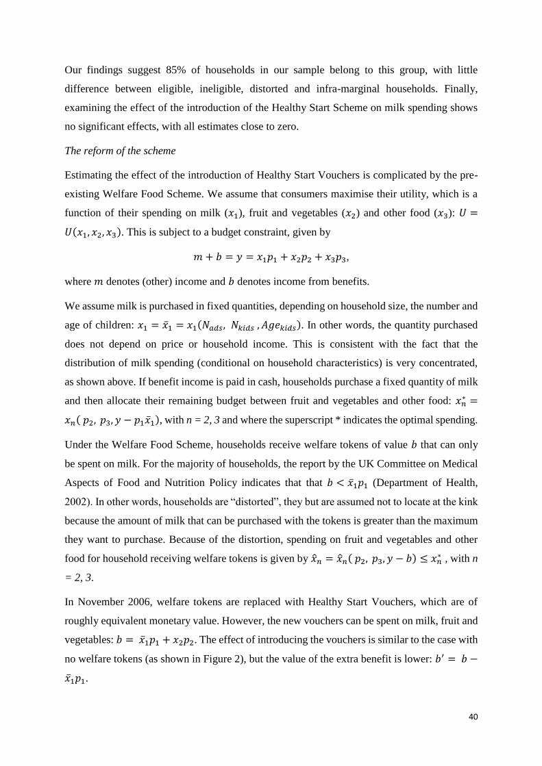
40

Our findings suggest 85% of households in our sample belong to this group, with little

difference between eligible, ineligible, distorted and infra-marginal households. Finally,

examining the effect of the introduction of the Healthy Start Scheme on milk spending shows

no significant effects, with all estimates close to zero.

The reform of the scheme

Estimating the effect of the introduction of Healthy Start Vouchers is complicated by the pre-

existing Welfare Food Scheme. We assume that consumers maximise their utility, which is a

function of their spending on milk (𝑥1), fruit and vegetables (𝑥2) and other food (𝑥3): 𝑈 =

𝑈(𝑥1, 𝑥2, 𝑥3). This is subject to a budget constraint, given by

𝑚 + 𝑏 = 𝑦 = 𝑥1𝑝1 + 𝑥2𝑝2 + 𝑥3𝑝3,

where 𝑚 denotes (other) income and 𝑏 denotes income from benefits.

We assume milk is purchased in fixed quantities, depending on household size, the number and

age of children: 𝑥1 = �̅�1 = 𝑥1(𝑁𝑎𝑑𝑠, 𝑁𝑘𝑖𝑑𝑠 , 𝐴𝑔𝑒𝑘𝑖𝑑𝑠). In other words, the quantity purchased

does not depend on price or household income. This is consistent with the fact that the

distribution of milk spending (conditional on household characteristics) is very concentrated,

as shown above. If benefit income is paid in cash, households purchase a fixed quantity of milk

and then allocate their remaining budget between fruit and vegetables and other food: 𝑥𝑛∗ =

𝑥𝑛( 𝑝2, 𝑝3, 𝑦 − 𝑝1�̅�1), with n = 2, 3 and where the superscript * indicates the optimal spending.

Under the Welfare Food Scheme, households receive welfare tokens of value 𝑏 that can only

be spent on milk. For the majority of households, the report by the UK Committee on Medical

Aspects of Food and Nutrition Policy indicates that that 𝑏 < �̅�1𝑝1 (Department of Health,

2002). In other words, households are “distorted”, they but are assumed not to locate at the kink

because the amount of milk that can be purchased with the tokens is greater than the maximum

they want to purchase. Because of the distortion, spending on fruit and vegetables and other

food for household receiving welfare tokens is given by �̂�𝑛 = �̂�𝑛( 𝑝2, 𝑝3, 𝑦 − 𝑏) ≤ 𝑥𝑛∗ , with n

= 2, 3.

In November 2006, welfare tokens are replaced with Healthy Start Vouchers, which are of

roughly equivalent monetary value. However, the new vouchers can be spent on milk, fruit and

vegetables: 𝑏 = �̅�1𝑝1 + 𝑥2𝑝2. The effect of introducing the vouchers is similar to the case with

no welfare tokens (as shown in Figure 2), but the value of the extra benefit is lower: 𝑏′ = 𝑏 −

�̅�1𝑝1.

41

We can distinguish between two groups. First, those who are infra-marginal under Healthy Start

Vouchers: 𝑏 ≤ �̅�1𝑝1 + 𝑥2∗𝑝2, and who therefore choose optimal spending �̅�1, 𝑥2

∗, 𝑥3∗. Following

introduction of Healthy Start Vouchers, there is no change in spending on milk, while spending

on fruit and vegetables and other food increase in line with 𝑏′ (from �̂�𝑛 to 𝑥𝑛∗ ) due to an income

effect.

Second, those who are distorted under Healthy Start Vouchers spend �̅�1𝑝1 on milk, �̌�2𝑝2 =

(𝑏 − �̅�1𝑝1) ≥ 𝑥2∗𝑝2 on fruit and vegetables and �̌�3 = �̌�3(�̅�1, �̌�2, 𝑝3, 𝑚) < 𝑥3

∗ on other food.

This predicts that the increase in spending on fruit and vegetables is greater among distorted

than among infra-marginal consumers (from �̂�2 to �̌�2), whilst the increase in spending on other

foods is less among distorted than infra-marginal consumers (from �̂�3 to �̌�3).

Before the introduction of the reform, we observe �̅�1𝑝1 + �̂�2𝑝2. Using the cut-off 𝑏 will

therefore cause some distorted consumers to be included in the infra-marginal group, leading

to an overestimate of any change in fruit and vegetable spending for the infra-marginal group.

Table A1: Effect on Milk Spending and Quantity

(1) (2) (3) (4)

Dependent variable: ln(milk expenditure) Milk quantity (in litres) 𝐸𝑙𝑖𝑔𝑖𝑏𝑙𝑒ℎ𝑡 × 𝑃𝑜𝑠𝑡ℎ𝑡 0.020 0.039

(0.060) (0.768) 𝐸𝑙𝑖𝑔𝑖𝑏𝑙𝑒ℎ𝑡 × 𝑃𝑜𝑠𝑡ℎ𝑡: Distorted 0.081 0.546

(0.063) (0.899)

𝐸𝑙𝑖𝑔𝑖𝑏𝑙𝑒ℎ𝑡 × 𝑃𝑜𝑠𝑡ℎ𝑡: Infra-marginal -0.119 -1.152

(0.090) (1.138)

𝐸𝑙𝑖𝑔𝑖𝑏𝑙𝑒ℎ𝑡 -0.012 0.467

(0.063) (0.824) 𝐸𝑙𝑖𝑔𝑖𝑏𝑙𝑒ℎ𝑡: Distorted -0.055 -0.099

(0.083) (1.104)

𝐸𝑙𝑖𝑔𝑖𝑏𝑙𝑒ℎ𝑡: Infra-marginal 0.073 1.617*

(0.059) (0.834)

Notes: Sample includes 4506 observations on 266 households between December 2004 - November 2008. All

columns include household, month and year fixed effects, age and age squared of youngest and oldest child (in

months), dummies for whether household includes: 2 adults, 3+ adults, 1 child, 2 children, 3 children, 4+ children,

and a dummy indicating whether the household did not buy any milk that month. 𝐸𝑙𝑖𝑔𝑖𝑏𝑙𝑒ℎ𝑡 equals 1 for

households with a child aged 0-3 or where the woman is ≥3 months pregnant. 𝑃𝑜𝑠𝑡ℎ𝑡 equals 1 for the period

December 2006 onwards. Robust standard errors in parentheses, clustered by household. * p<0.10, ** p<0.05,

*** p<0.01.

42

Figure A1: Conditional distributions of monthly expenditures on milk and on fruit and

vegetables

Note: Expenditure is conditional on the number of adults, the number and ages of children in the household, year,

month and household fixed effects.

43

Appendix B: Identifying households on benefits in the Kantar data

We define a household as being “on benefits” if the head (and the main shopper in couples) are

not in work, unemployed, in education, or work less than 8 hours a week. To assess how well

this simple rule does in predicting which households are on benefits, we look at data from the

Expenditure and Food Survey (EFS; a repeated cross-sectional study of households in the UK),

which contains both hours worked and actual benefits receipt. Using this definition, we find

that 17.8% of all households with a child aged 0-8, or where the woman is pregnant in the EFS

are on benefits, compared to 20.7% in a similar sample in the Kantar data. In addition, we

compare our definition of being on benefits (based on hours worked) in the EFS to the share of

these households that are truly on benefits. Table B1 shows that we do well in capturing

households that are truly on benefits. The rows show the work status of the head of household,

recoded to the categories observed in the Kantar data; the columns show the hours worked by

the spouse (or that there is no spouse present in the household).

The shaded area indicates the sample used in our analysis: those we predict to be on benefits

using hours worked. We show the number of households observed in each cell, the number who

is in on benefits, and the probability that households in each cell are on benefits. For example,

the upper left hand cell shows that of single parent households where the parent is not in work,

95% of households in the EFS are in receipt of benefits. Similarly, of households where the

head works between 1-8 hours and there is no spouse 90.3% are on benefits. Overall, among

those households in the EFS that we predict to be on benefits based on the hours worked, 91.7%

actually received benefits.

We examine the robustness of our findings to an alternative definition of benefit receipt, where

rather than using hours worked, we predict the probability of receiving benefits as a function of

covariates in the EFS. Table B2 shows the marginal effects of a probit regression using the EFS.

This suggests that we predict benefit receipt well: a simple probit using the cross-sectional EFS

provides a pseudo R2 of 0.54.

Figure B1 compares the distribution of the predicted probability of being on benefits in the

Kantar data (predicted using the estimates from the EFS) with that from the EFS data. This

shows that they line up well: the majority of individuals are predicted not to be on benefits, with

the largest densities for probabilities of benefit receipt less than 0.4. The density increases again

for probabilities above around 0.7. In our robustness analysis, we use Pr(benefits)>0.7 as the

cut-point to define a household as being on benefits, though the results are robust to using

44

different cut-points ranging from 0.6 to 0.9. Comparing this predicted benefit receipt (based on

Pr(benefits)>0.7) to the actual benefit receipt in the EFS, we find that, among those we define

as being on benefits, 92% receives benefits.

Figure B1: The densities of Pr(on benefits) from the EFS and Kantar data

Table B1: Number and percent of households on benefits by demographic status (EFS)

Spouse: Head: no

spouse not in work

1-8 hours

8-30 hours

30+ hours

Total

not in work N in group 804 326 2 48 149 1,329 N on benefits 764 284 1 25 33 1,107

% on benefits 95.0% 87.1% 50.0% 52.1% 22.1% 83.3%

1-8 hours N in group 31 6 0 2 7 46 N on benefits 28 2 0 0 2 32

% on benefits 90.3% 33.3% - 0% 28.6% 69.6%

8-30 hours N in group 313 109 5 43 181 651 N on benefits 50 33 1 11 9 104

% on benefits 16.0% 30.3% 20.0% 25.6% 5.0% 16.0%

30+ hours N in group 250 1,242 106 1,540 1,160 4,298 N on benefits 15 151 10 93 15 284

% on benefits 6.0% 12.2% 9.4% 6.0% 1.3% 6.6%

Total N in group 1,398 1,683 113 1,633 1,497 6,324 N on benefits 857 470 12 129 59 1,527

% on benefits 61.3% 27.3% 10.6% 7.9% 3.9% 24.1% Note: For each demographic group, the table provides the total number of households in that group, the number

of households in that group who receive benefits, and the percent of households on benefits (i.e. (N on benefits/N

in group)*100). The shaded area is the main sample definition used in the Kantar data. Calculations from the

Expenditure and Food Survey.

45

Table B2: Determinants of benefit receipt: marginal effects from a probit regression

using the EFS Pr(on benefits)

2 adults -0.082 (0.057)

3 adults -0.076*** (0.024)

Pregnancy -0.035** (0.016)

No. aged 0 0.004 (0.018)

No. aged 1 0.011 (0.017)

No. aged 2 0.020 (0.019)

No. aged 3 0.017 (0.017)

No. aged 4 0.018 (0.018)

No. aged 5 0.016 (0.017)

No. aged 6 0.014 (0.018)

No. aged 7 0.024 (0.018)

No. aged 8 0.003 (0.017)

No. aged 9 -0.023 (0.020)

No. aged 10 0.021 (0.020)

No. aged 11 0.025 (0.021)

No. aged 12 0.034 (0.028)

No. aged 13 0.007 (0.024)

No. aged 14 -0.028 (0.024)

No. aged 15 0.006 (0.029)

No. aged 16 0.040 (0.028)

No. aged 17 0.019 (0.036)

No. aged 18 0.082** (0.041)

Household size squared -0.001 (0.002)

Married -0.032 (0.051)

Widowed/divorced/separated -0.029* (0.016)

Non-manual social class 0.234*** (0.054)

Manual social class 0.464*** (0.056)

Semi-skilled social class 0.387*** (0.068)

Unskilled social class 0.383*** (0.085)

Unemployed 0.572*** (0.075)

Head works less than 8 hours per week -0.021 (0.044)

Head works between 8 and 30 hours per week -0.127*** (0.010)

Head works 30 or more hours per week -0.368*** (0.046)

Shopper works less than 8 hours per week 0.007 (0.029)

Shopper works between 8 and 30 hours per week -0.095*** (0.010)

Shopper works 30 or more hours per week -0.181*** (0.010)

Household owns 1 TV 0.106 (0.064)

Household owns 2 TVs 0.072 (0.054)

Household owns 3 TVs 0.083 (0.058)

Household owns 4 TVs 0.082 (0.060)

Household owns 2 cars 0.006 (0.013)

Household owns 3 cars 0.053** (0.025)

Household owns a PC 0.010 (0.015)

Household owns a freezer -0.007 (0.044)

Household owns a drier 0.006 (0.011)

Household has internet -0.043*** (0.017)

Household owns a microwave 0.009 (0.022)

Household owns a dishwasher -0.034*** (0.011)

Pseudo R2 0.54

Observations 6891

Notes: Regression uses data from the Expenditure and Food Survey (EFS) 2004-2008. Year and region dummies

included. Standard errors in parentheses, * p < 0.10, ** p < 0.05, *** p < 0.01

46

Table B3: Means and standard deviations of the Kantar data, full sample by eligibility

(1) (2) (3)

Full sample Eligible Ineligible

Mean SD Mean SD Mean SD

Full sample Total spending (£): fruit & vegetables 17.70 (11.8) 18.81 (11.7) 16.57 (11.9) Total quantity (kg): fruit & vegetables 16.90 (10.1) 18.06 (9.8) 15.72 (10.1) Fruit and vegetables portions per person/day 1.98 (1.2) 1.98 (1.1) 1.98 (1.3) Proportion purchasing ≥5 portions per person/day 0.02 (0.1) 0.01 (0.1) 0.03 (0.2) Total spending: all foods 186.5 (68.4) 189.8 (65.9) 183.2 (70.7) Total spending: fast moving consumer goods 40.5 (24.5) 43.1 (25.5) 37.9 (23.2) Household size 3.71 (1.0) 3.94 (0.9) 3.45 (1.0) ≥3 months pregnant 0.06 (0.2) 0.11 (0.3) - - No. of 0 year olds 0.11 (0.3) 0.21 (0.4) - - No. of 1-3 year olds 0.46 (0.6) 0.89 (0.5) - - No. of 4 year olds 0.20 (0.4) 0.12 (0.3) 0.27 (0.4) No. of 5-18 year olds 1.23 (1.0) 0.94 (1.0) 1.55 (0.9) No. of adults 1.85 (0.6) 1.95 (0.5) 1.75 (0.6) Number of household-month observations 4506 2274 2232

Note: Eligible households are those ≥3 months pregnant, or with a child aged 0-3; Ineligible households are those with children aged 4-8, or not yet pregnant. Households who

(at any point prior to the reform) spent less than £12.86 per child on milk, fruit and vegetables are defined as distorted; those never spending less than £12.86 per child are

defined as infra-marginal. A portion of fruit and vegetables is defined as 80g. Other covariates, including marital status, social class, and the region where the household lives

are not significantly different across distorted and infra-marginal consumers (not shown here, but available upon request).