FIFTH FRAMEWORK RESEARCH PROGRAMME (1998-2002)

Democratic Participation and Political Communication in Systems of Multi-level Governance

Germany:

Supplementing sense of duty by cognitive mobilisation

Hans Rattinger and Sandra Wagner

Lehrstuhl fuer Politikwissenschaft II

Universitaet Bamberg

Work in Progress

April 2003

Draft text not to be quoted without permission of the authors.

Content 1. Aspects of turnout: what the chapter is all about....................................... 6 1.1 Introduction .......................................................Error! Bookmark not defined. 1.2 Chapter outline and data.................................................................................. 6 2. General patterns and trends in turnout in Germany................................... 7 2.1 Turnout at different levels of government from 1979 to 1999........................... 7 2.2 Geographical differences in turnout ................................................................. 8 2.3 Stability and change of turnout ...................................................................... 12 2.4 Voter transition rates: evidence from ECOL................................................... 16 3. Facilitation and mobilisation of voters ...................................................... 18 3.1 Institutional facilitation and mobilisation ......................................................... 18 3.2 Socio-economic structure as facilitation factor: evidence from the ecological data ............................................................................................... 20 3.3 Facilitation at the individual level: evidence from the survey data.................. 29 3.4 Individual mobilisation.................................................................................... 33 3.4.1. Bivariate analysis of individual mobilisation ................................................... 33 3.4.2. Multivariate analysis of individual mobilisation............................................... 38 4. Conclusion ................................................................................................... 52

List of Tables Table 1: Factor analysis of turnout variables, West-Germany............................................14 Table 2: Factor analysis of turnout variables, East-Germany.............................................15 Table 3: Cluster Analysis of turnout factors: 6-cluster-solution...........................................15 Table 4: Voter mobility between elections: holding rates....................................................17 Table 5: Stepwise OLS regression for mean turnout in European Parliament Elections....21 Table 6: Stepwise OLS regression for mean turnout in European Parliament Elections,

only Kreise without concurrent local elections in West Germany .........................22 Table 7: Stepwise OLS regression for mean turnout in federal elections...........................25 Table 8: Stepwise OLS regression for mean turnout in state elections ..............................25 Table 9: Stepwise OLS regression for mean turnout in European Parliament Elections,

federal elections, state elections and local elections in Bavaria ...........................26 Table 10: Stepwise OLS regression for mean turnout in European Parliament Elections,

federal elections, state elections and local elections in North Rhine Westphalia .26 Table 11: Factor analysis of independent variables at county level, West-Germany ...........27 Table 12: Factor analysis of independent variables at county level, East-Germany ............28 Table 13: Mean factor scores in turnout clusters, West-Germany........................................28 Table 14: Mean factor scores in turnout clusters, East-Germany.........................................29 Table 15: Recall electoral participation in European elections 1994 and 1999 in percent ...30 Table 16: Intended electoral participation EE 2004 in Germany ..........................................30 Table 17: Interest in politics, 1994........................................................................................33 Table 18: Knowledge of President of the Commission and national commissioner .............34 Table 19: Campaign Exposure .............................................................................................34 Table 20: Participation in European election 1994 by political involvement, controlled for

campaign exposure ..............................................................................................37 Table 21: Mean perception of Power of European Parliament and turnout in European

elections 1994 and 1999.......................................................................................37 Table 22: Party differentials at European Parliament elections and national elections ........38 Table 23: Mean party differential (10 point scale) European Parliament Elections ..............38 Table 24: Bivariate logistic regressions. Dependent variable: turnout in European Parliament

elections 1994 and 1999.......................................................................................40 Table 25: Multivariate stepwise logistic regressions. Dependent variable: turnout in

European Parliament elections 1994 and 1999....................................................42 Table 26: Multivariate stepwise logistic regressions. Dependent variable: turnout in

European Parliament election 1999, without and with additional independent variables ...............................................................................................................43

Table 27: Bivariate logistic regressions, federal elections (white cells means that variable did not exist in that survey) ...................................................................................45

Table 28: Multivariate stepwise logistic Regression, federal elections (white cells means that variable did not exist in that survey) .....................................................................46

Table 29: Multivariate stepwise logistic Regression, federal elections (white cells means that variable did not exist in that survey) .....................................................................47

Table 30: Bivariate logistic regressions of voter turnout at federal, local and European level 49

Table 31: Multivariate stepwise logistic regressions of voter turnout at federal, European and local elections ................................................................................................50

List of Figures Figure 1: Turnout in Germany: Federal, state and European elections, 1949 - 2000............8 Figure 2: State Elections – Turnout 1979-1999 by States .....................................................9 Figure 3: Federal Elections – Turnout 1979-1999 by States ...............................................10 Figure 4: European Parliament Elections – Turnout 1979-1999 by States..........................10 Figure 5: Turnout State Elections Since 1978: Observed and Predicted.............................13 Figure 6: Turnout Federal Elections Since 1980: Observed and Predicted.........................13 Figure 7: Turnout European Parliament Elections Since 1979: Observed and Predicted ...14 Figure 8: Difference between power of European Parliament and power of the national

parliament .............................................................................................................20 Figure 9: Electoral participation in European Parliament elections by education ................31 Figure 10: Electoral participation in European Parliament elections by income ....................31 Figure 11: Electoral participation in European Parliament elections by sector of employment .

........................................................................................................................32 Figure 12: Electoral participation in European Parliament election 1994 by age...................32 Figure 13: Mean campaign exposure by age categories in 1994 and 1999 ..........................35 Figure 14: Mean campaign exposure by education (age when stopped full-time education) in

1994 and 1999......................................................................................................35 Figure 15: Mean campaign exposure by sector of employment in 1994 and 1999 ...............36 Figure 16: Campaign exposure by political interest, 1994.....................................................36

List of Maps Map 1: Mean turnout in European, federal and state elections, 1979 - 1999 (East-Germany

1990 – 1999).........................................................................................................11 Map 2: Mean turnout in European, federal and state elections, 1990 - 1999.........................11 Map 3: Clusters, resulting from the factor analysis of the dimensions of turnout ...................16

1. Aspects of turnout: what the chapter is all about

1.1 The relevance of turnout The first thing of interest after an election is usually not the level of turnout, but the result in terms of which party got most of the votes, which parties lost or won votes compared to the last election and what this means for the future government. Only in the more detailed analy-ses following the elections turnout comes under scrutiny. At least that is true as long as turn-out is within the normal range. Against this background some thoughts should be devoted to the question, why a detailed analysis of electoral participation is of relevance. The first reason is derived from the discussions in the theories of democracy. The question of what level of turnout is the optimum for a democratic political system is a normative one as Scharpf points out (Scharpf: 21 ff). While in input-oriented theories a high level of participa-tion is crucial to any democracy and therefore of great interest, output-oriented theories are not so concerned about turnout, as the main task of an election according to them is to gen-erate an authorized and legitimated government. So at least from an output-oriented point of view turnout is not of major interest. This discussion shall not be deepened here, however, it gives a good background to think about the relevance of turnout. As so often the truth might lie somewhere in the middle. The level of participation can be taken as an indicator for politi-cal as well as societal developments in a democracy, as a starting point to search for their reasons. In many cases, more than the pure level of turnout, changes in participation rates call attention among the academics and politicians. Especially the latter are more interested in the practical consequences than in theoretical implications of changes in turnout as these might affect their parties’ chances and as a consequence their personal political fate. In the case of declining participation the questions are: Do people from all parts of society stay at home to the same extent, which would not change the chances of the parties? Or does the group of new non-voters consist of people with certain socio-demographic characteristics or attitudes, who tended to vote for a certain party earlier? Is the decline in turnout a conse-quence of fading trust in parties and politicians or can it be interpreted as satisfaction with the current political situation? This short introduction shows that turnout is a relevant factor in a democracy and that it is worth the effort to analyse it in all its different aspects. In the following these aspects are re-called before a short overview on the rest of the chapter is given. Turnout varies over countries as becomes very obvious in this book. So the first aspect of turnout is the level in a certain country in comparison to other countries. As elections in Ger-many take place at different levels of governance this first aspect includes the different levels of participation in European, federal, state and local elections within Germany, as well. The second aspect of turnout concerns its development over time at all levels of governance. The third aspect is differential turnout in geographical terms and the fourth concerns the question, why some individuals vote while others abstain. It is not always possible to separate these different aspects analytically. In this chapter all four aspects of turnout will be addressed and by means of analyses of a wide range of data it will be tried to fix some pieces of the turnout puzzle.

1.2 Chapter outline and data In the first section of the chapter the main focus will lie on the description of turnout in Ger-many over the 20 years from 1979 to 1999. After giving a short overview over the develop-ment of turnout at European, federal and state level we will turn to the description of geo-graphical differences in electoral participation. Following that very descriptive beginning, sta-bility and change of turnout will be explored by means of ECOL, a program which allows in-ferences from aggregate level data to the individual level. Those analyses are based on ag-

7

gregate data from official statistics of the German Statistical Office for the 440 counties of Germany. If the description of turnout is like looking at the various pieces of the turnout puzzle, provid-ing explanations for variations in turnout over time, at different levels and with regard to ge-ography is needed to fix at least some pieces of the puzzle. In this book the theoretical ap-proach to an explanation of differential turnout is based on the idea of facilitation and mobili-sation. Therefore, in the third section of this chapter the German electoral systems at the different levels are considered in terms of these concepts. The next step is then to find correlates of turnout on an aggregate basis of counties to be able to explain differential geographical turnout. In addition to the data based on the 440 counties, for two federal states, Bavaria and North Rhine Westphalia, aggregate data are available at the commune level: 2056 communes in Bavaria and 396 in North Rhine West-phalia. Finally we turn to survey data to investigate the determinants of participation at the individual level. The data sets used are Eurobarometers 41.1, which contains recall of par-ticipation in the 1994 European Parliament election, and Eurobarometer 52, which contains the recall for the 1999 European election. In Eurobarometer 54.1 intended electoral participa-tion for the European election of 2004 is included. Beyond the Eurobarometer data the Asia-Europe survey (ASES) provides additional insight in the causes of differential turnout. A short summary of the findings of this chapter and a more comprehensive assessment of the impli-cations of turnout at different levels of governance over the 20 years is provided in the con-clusion. 2. General patterns and trends in turnout in Germany

2.1 Turnout at different levels of government from 1979 to 1999 As in many other member states of the EU turnout in Germany traditionally used to be very high compared e.g. to the United States. This applies for federal elections as well as sub-national elections at the state level. The highest turnout in a federal election was reached in 1972 with 91,1% and it kept stable at about 90% until the one of 1983 inclusively (figure 1). However, in the federal election of 1987 and the subsequent elections at national, as well as sub-national and supranational level, a drop in electoral participation was observed, that wor-ried the political elites as well as parts of the social science academics. Many explanations for that development have been given, most of which see the most impor-tant reason in the dissolution of closed cultural milieus in a modern society. The traditional cleavages of religion and labour that existed in Germany as in most other European coun-tries, began to dissolve and social affiliation becomes less binding in a more and more mo-bile society. As a consequence social and moral norms, one of them the duty to vote (“Wahl-norm”), lose their importance (Eilfort 1994: 323). This means, that people who went to the polls because of this moral norm, although not interested, might now prefer to stay home (Roth 1992: ???). Others might not see any differences between the parties any longer, as those tend to offer more and more similar party programs to be able to attract the middle class voter. Political scientists agree largely on the analysis so far, not, however, on the as-sessment of this development. An important question is, how non-voting has to be inter-preted. Is it just non-interested people staying at home? Is it worrying then, if people, who do not care about politics, do not vote, or is it just a sensible thing not to vote if not interested and informed? Or has the decline in electoral participation to be seen as a protest against current politics and politicians’ behaviour?1 The 1998 federal election as well as the latest one in 2002 showed a recovering of turnout at the national level (82.2% in 1998 and 79.1% in 2002). The downward trend has stopped at a

1 The discussion, if the decline in turnout is a ‘normalization’ or indicates a ‘crisis’, started at the beginning of the nineties with articles of Ursula Feist (1992) and Dieter Roth (1992). Two comprehensive monographs fol-lowed in the middle of the nineties: Eilfort, Michael (1994) and Kleinhenz, Thomas (1995).

8

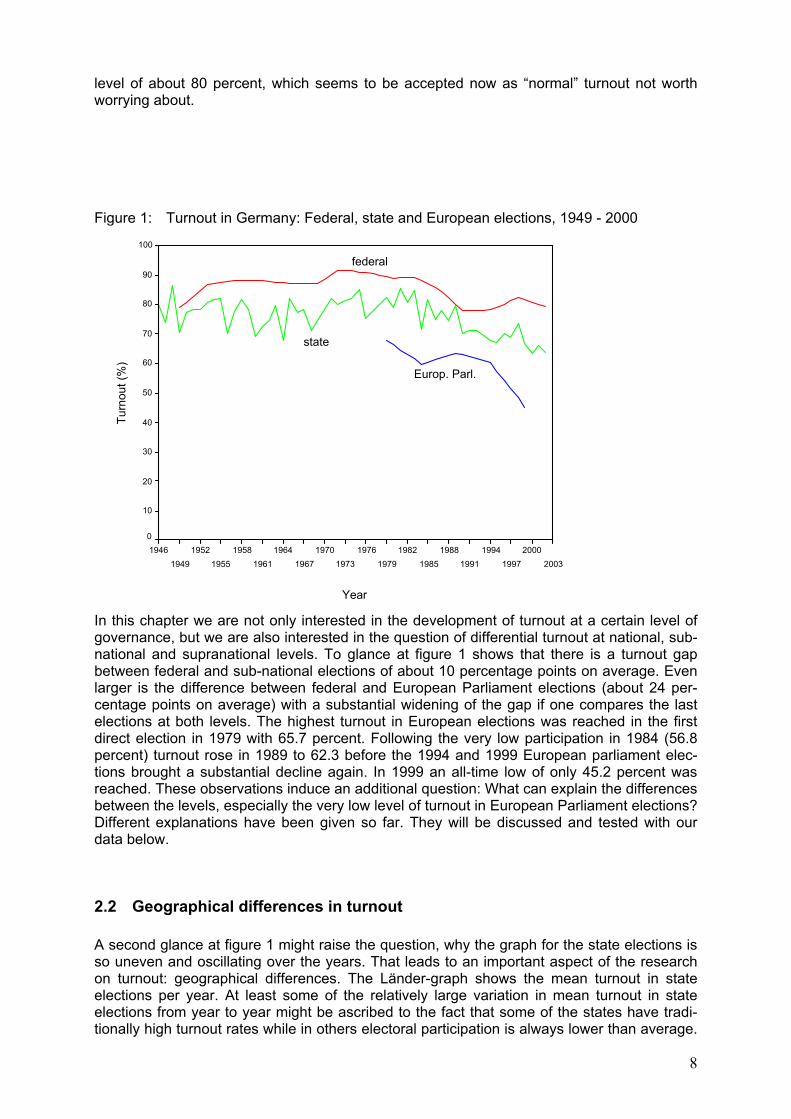
level of about 80 percent, which seems to be accepted now as “normal” turnout not worth worrying about. Figure 1: Turnout in Germany: Federal, state and European elections, 1949 - 2000

Year

20032000

19971994

19911988

19851982

19791976

19731970

19671964

19611958

19551952

19491946

Turn

out (

%)

100

90

80

70

60

50

40

30

20

10

0

federal

state

Europ. Parl.

In this chapter we are not only interested in the development of turnout at a certain level of governance, but we are also interested in the question of differential turnout at national, sub-national and supranational levels. To glance at figure 1 shows that there is a turnout gap between federal and sub-national elections of about 10 percentage points on average. Even larger is the difference between federal and European Parliament elections (about 24 per-centage points on average) with a substantial widening of the gap if one compares the last elections at both levels. The highest turnout in European elections was reached in the first direct election in 1979 with 65.7 percent. Following the very low participation in 1984 (56.8 percent) turnout rose in 1989 to 62.3 before the 1994 and 1999 European parliament elec-tions brought a substantial decline again. In 1999 an all-time low of only 45.2 percent was reached. These observations induce an additional question: What can explain the differences between the levels, especially the very low level of turnout in European Parliament elections? Different explanations have been given so far. They will be discussed and tested with our data below.

2.2 Geographical differences in turnout A second glance at figure 1 might raise the question, why the graph for the state elections is so uneven and oscillating over the years. That leads to an important aspect of the research on turnout: geographical differences. The Länder-graph shows the mean turnout in state elections per year. At least some of the relatively large variation in mean turnout in state elections from year to year might be ascribed to the fact that some of the states have tradi-tionally high turnout rates while in others electoral participation is always lower than average.

9

Elections in low turnout states can squeeze the average turnout in that year substantially, if one takes into consideration that there take place only two to five state elections per year. Figure 2, which shows the development of turnout separately for all states, illustrates that there are substantial differences in the level of turnout in state elections between the states. A glance at the next two figures, which show turnout in federal and European elections sepa-rately for the states, makes clear that the order between the states concerning their turnout rates is almost always the same: While Bavaria and Baden-Wuerttemberg are at the lower end of the scale, Rhineland-Palatinate, Saarland and Hesse are found at the top. Figure 2: State Elections – Turnout 1979-1999 by States

10

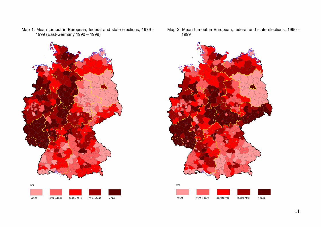
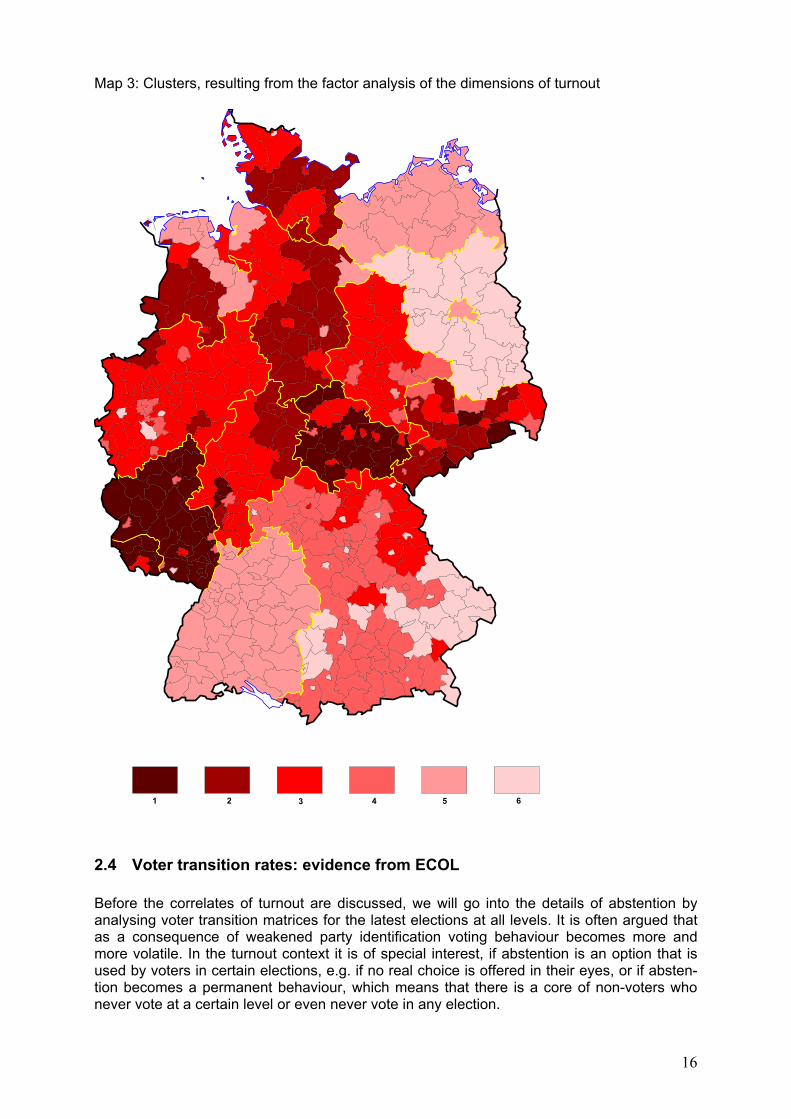
Figure 3: Federal Elections – Turnout 1979-1999 by States Figure 4: European Parliament Elections – Turnout 1979-1999 by States The fact, that there are regions with high and others with low average turnout is shown by the first map as well. In the map there is displayed the mean turnout in European, federal and state elections from 1979 to 1999. However, one has to be careful with interpretation as the number of elections the average turnout rates are based on is not the same everywhere. In East-Germany the first free elections took place in 1990. That means that we can look back at only three federal elections, three Länder elections and only two European elections in each of the five new states, while in the old states of West-Germany the average is based on 14 federal elections, 14 state elections and five European elections. That is not only prob-lematic because the weight of a single election is heavier in East-Germany, but also because all the elections in East-Germany fall in a period when the times of very high turnout of about 90% were over in the West, as well. Therefore map 2 shows the mean turnout for all types of elections from 1990 to 1999 only. However, even with that in mind it becomes obvious that electoral participation is on average lower in the southern states Bavaria and Baden-Wuerttemberg, in the very industrial and urban area (“Ruhrgebiet”) in North Rhine-Westphalia as well as in large parts of East-Germany. Most noticeable is that all counties in Brandenburg belong to the lowest turnout pentile with an average participation of less than 67.58 percent. So it seems that in Branden-burg turnout is even lower than in the other Eastern states. However, an explanation for that is readily found: Brandenburg is the only state where European Parliament elections never took place with local elections simultaneously, which was the case in 1994 and 1999 in Mecklenburg, Saxony, Saxony-Anhalt and Thuringia. Concurrent local elections can explain differences in mean turnout for some of the West-German states as well: in Saarland and Rhineland-Palatinate simultaneous local elections took place with all five European elections. In Baden-Wuerttemberg that was the case in 1994. Interesting about this finding is that local elections boost turnout in European elections. What is also striking is that in bigger towns and cities turnout is mostly lower than in the sur-rounding areas. This fact becomes very clear in Bavaria, Thuringia as well as in Saxony, where the bigger towns and cities are represented by pale spots on the map. There seems to be a correlation between turnout and urbanity, which will be analysed in detail later.

11

Map 1: Mean turnout in European, federal and state elections, 1979 - 1999 (East-Germany 1990 – 1999)

< 67.58 67.58 to 70.11 70.12 to 72.15 72.16 to 74.43 > 74.43

in %

Map 2: Mean turnout in European, federal and state elections, 1990 - 1999

< 66.41 66.41 to 68.71 68.72 to 70.52 70.53 to 72.52 > 72.52

in %

12

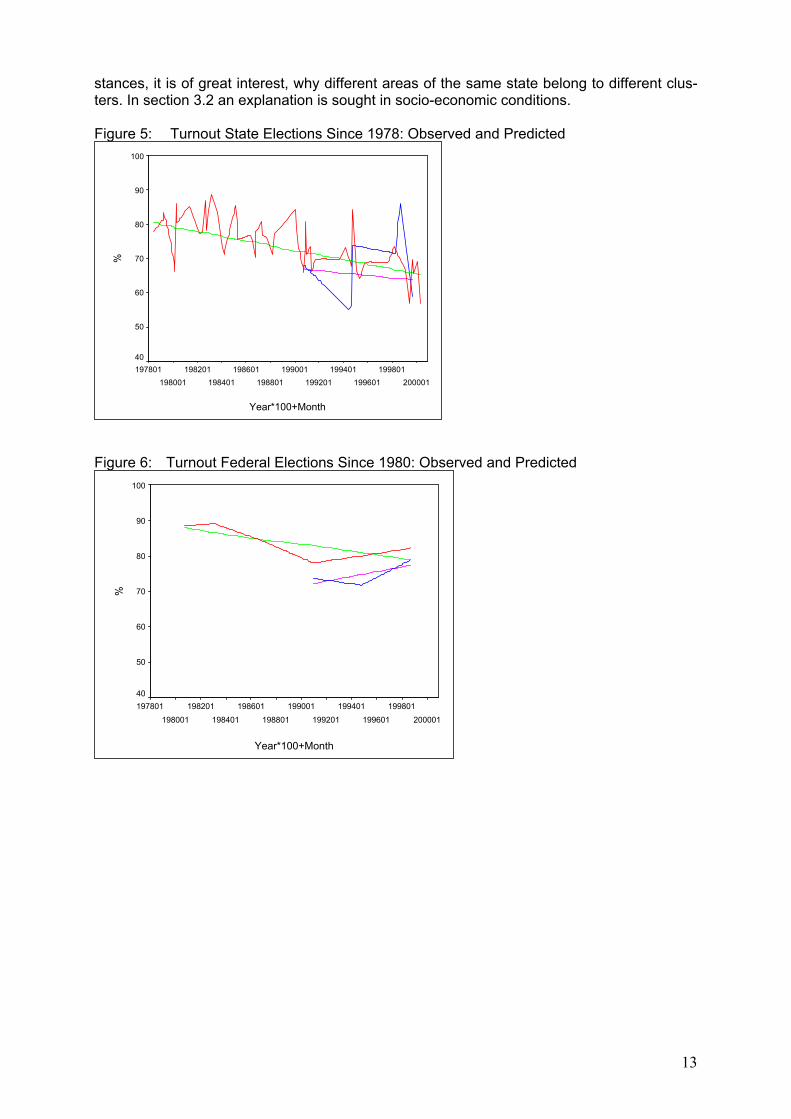
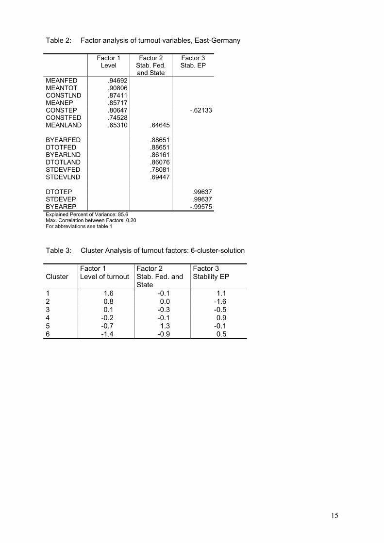
2.3 Stability and change of turnout From the figures 1 to 4 it becomes clear already that turnout varies between election types, but also between elections at the same level over time, as well as in geographical terms. The purpose of the following section is to get some deeper insights in these different aspects of variation in turnout. To test the hypothesis of declining turnout, regression analysis is employed in the following. By calculating linear regressions for each county with turnout as the dependent variable and time as the independent variable there results a factor by which turnout changes each year according to the linear model. R square is a measure of the model fit. These regressions are calculated separately for each type of election. In the graphs 5 to 7 observed turnout as well as turnout predicted from the regressions is displayed, each separately for West and East-Germany. For state elections figure 5 shows that the line representing predicted turnout is falling over the time period and approximates, at least for West-Germany, observed turnout quite well. The mean R square for the West German counties is .65, indicating that on aver-age 65 percent of the variance of turnout within a county can be explained by the factor time alone. In the East-German states the variation in turnout is higher than in the old German states reaching from 54.8 percent in Sachsen-Anhalt in 1994 to 79.4 percent in Mecklenburg-Western Pomerania in 1998. However, the mean R square for all East-German counties is still .55. Figure 6 contains observed and predicted turnout for federal elections in the period between 1980 and 1999. While for West-Germany again there is found a declining trend, which ex-plains on average 56% of the variation in a county, for East-Germany it is not. In all East German states, except for Mecklenburg-Western Pomerania, the lowest turnout for federal elections was measured in 1994 before it increased considerably in the 1998 federal elec-tion. The regression coefficients are positive in 100 of the 112 counties. For European elec-tions there is only interpreted the result for the West as only two European elections have taken place (figure 7). There is also measured a downward trend which must be ascribed primarily to the last European election in 1999 when only 44.5 percent of eligible voters in West-Germany turned out. Summarizing the description of turnout over the period of 1979 to 1999 there has to be stated that a considerable variance of participation can be explained by time. In a second step factor analysis is applied to find dimensions of variation in turnout. As vari-ables for this factor analysis the results (regression coefficients) of the above regressions in addition to ten other variables (mean turnout for each type of election, mean turnout over all elections, standard deviation for each type of election and difference between last and first election for each type) were used. Because of the different conditions in West and East the analyses were run separately for West and East-Germany. As a result four factors for West-Germany were found (table 1): The first factor indicates the level of turnout, with high factor scores meaning that over all elections turnout is above average. The other three factors indi-cate stability of turnout at the different levels. For East-Germany three factors resulted, the first of which again can be interpreted as a level factor (table 2). However, different from the analysis for West-Germany variables indicating stability in federal and state elections load on a common factor here. The third factor represents stability in European elections. The factor scores were then used to find clusters of counties with certain turnout patterns concerning level of turnout and stability at different types of elections. To be able to do that for Germany as a whole the two stability factors for West-Germany for federal and state elec-tions were merged. The result of the cluster analysis with 6 clusters can be viewed in table 3 and map 3. The clusters in the map are ordered by the level of turnout: the darker the higher average turnout. With the six cluster solution 70.5 percent of the variance in the tree factors (level, stability federal and state elections, stability EP elections) can be explained by cluster membership. Again it can be observed from the map that neighbouring counties have a ten-dency to fall into the same cluster, this giving a hint that certain areas, sometimes the whole state like Baden-Wuerttemberg, show the same turnout pattern over time. While in the case of a whole state falling into one cluster, this might be ascribed to state-specific circum-

13

stances, it is of great interest, why different areas of the same state belong to different clus-ters. In section 3.2 an explanation is sought in socio-economic conditions. Figure 5: Turnout State Elections Since 1978: Observed and Predicted

Year*100+Month

200001199801

199601199401

199201199001

198801198601

198401198201

198001197801

%

100

90

80

70

60

50

40

Figure 6: Turnout Federal Elections Since 1980: Observed and Predicted

Year*100+Month

200001199801

199601199401

199201199001

198801198601

198401198201

198001197801

%

100

90

80

70

60

50

40

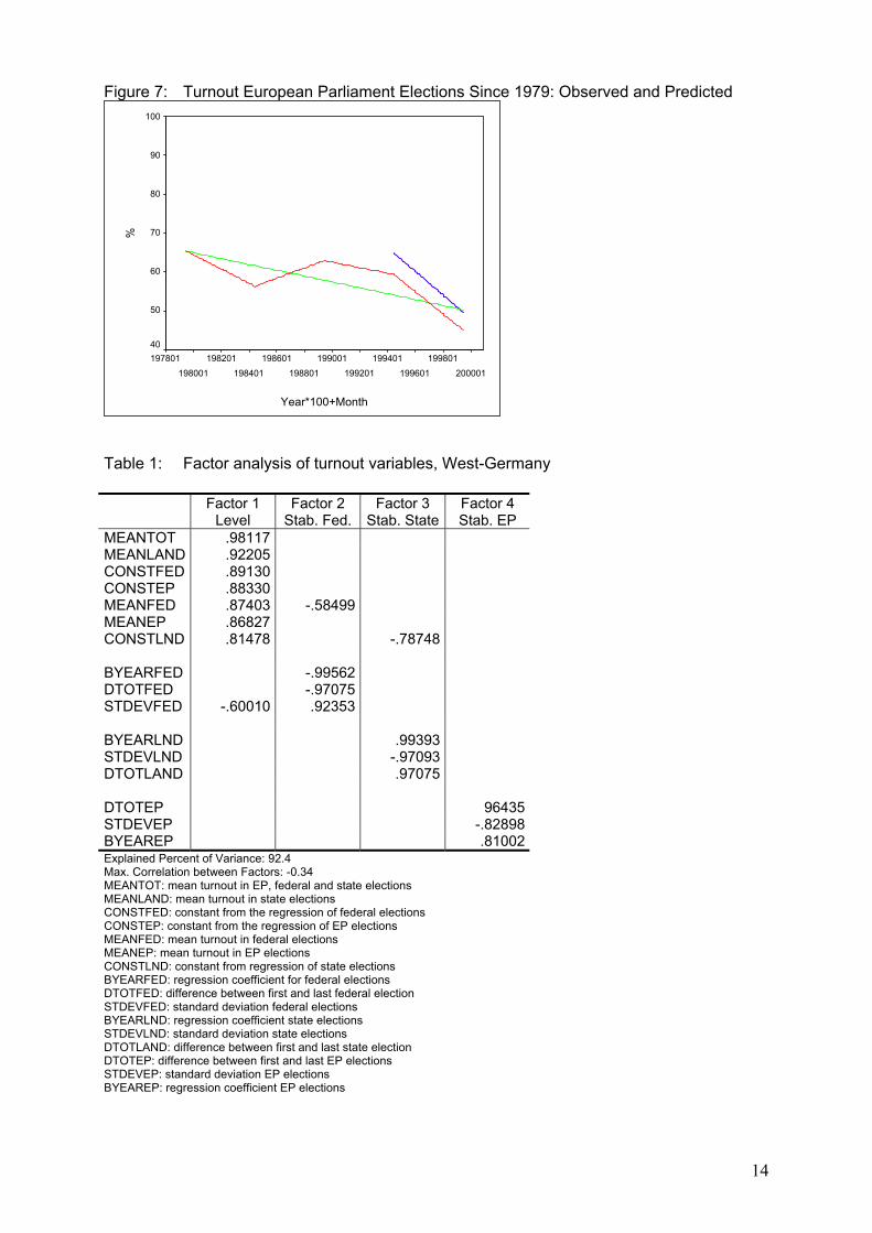
14

Figure 7: Turnout European Parliament Elections Since 1979: Observed and Predicted

Year*100+Month

200001199801

199601199401

199201199001

198801198601

198401198201

198001197801

%100

90

80

70

60

50

40

Table 1: Factor analysis of turnout variables, West-Germany Factor 1

Level Factor 2

Stab. Fed. Factor 3

Stab. State Factor 4 Stab. EP

MEANTOT .98117 MEANLAND .92205 CONSTFED .89130 CONSTEP .88330 MEANFED .87403 -.58499 MEANEP .86827 CONSTLND .81478 -.78748 BYEARFED -.99562 DTOTFED -.97075 STDEVFED -.60010 .92353 BYEARLND .99393 STDEVLND -.97093 DTOTLAND .97075 DTOTEP 96435 STDEVEP -.82898 BYEAREP .81002 Explained Percent of Variance: 92.4 Max. Correlation between Factors: -0.34 MEANTOT: mean turnout in EP, federal and state elections MEANLAND: mean turnout in state elections CONSTFED: constant from the regression of federal elections CONSTEP: constant from the regression of EP elections MEANFED: mean turnout in federal elections MEANEP: mean turnout in EP elections CONSTLND: constant from regression of state elections BYEARFED: regression coefficient for federal elections DTOTFED: difference between first and last federal election STDEVFED: standard deviation federal elections BYEARLND: regression coefficient state elections STDEVLND: standard deviation state elections DTOTLAND: difference between first and last state election DTOTEP: difference between first and last EP elections STDEVEP: standard deviation EP elections BYEAREP: regression coefficient EP elections

15

Table 2: Factor analysis of turnout variables, East-Germany Factor 1

Level Factor 2

Stab. Fed. and State

Factor 3 Stab. EP

MEANFED .94692 MEANTOT .90806 CONSTLND .87411 MEANEP .85717 CONSTEP .80647 -.62133 CONSTFED .74528 MEANLAND .65310 .64645 BYEARFED .88651 DTOTFED .88651 BYEARLND .86161 DTOTLAND .86076 STDEVFED .78081 STDEVLND .69447 DTOTEP .99637 STDEVEP .99637 BYEAREP -.99575 Explained Percent of Variance: 85.6 Max. Correlation between Factors: 0.20 For abbreviations see table 1 Table 3: Cluster Analysis of turnout factors: 6-cluster-solution Cluster

Factor 1 Level of turnout

Factor 2 Stab. Fed. and State

Factor 3 Stability EP

1 1.6 -0.1 1.1 2 0.8 0.0 -1.6 3 0.1 -0.3 -0.5 4 -0.2 -0.1 0.9 5 -0.7 1.3 -0.1 6 -1.4 -0.9 0.5

16

Map 3: Clusters, resulting from the factor analysis of the dimensions of turnout

1 2 3 4 5 6

2.4 Voter transition rates: evidence from ECOL Before the correlates of turnout are discussed, we will go into the details of abstention by analysing voter transition matrices for the latest elections at all levels. It is often argued that as a consequence of weakened party identification voting behaviour becomes more and more volatile. In the turnout context it is of special interest, if abstention is an option that is used by voters in certain elections, e.g. if no real choice is offered in their eyes, or if absten-tion becomes a permanent behaviour, which means that there is a core of non-voters who never vote at a certain level or even never vote in any election.

17

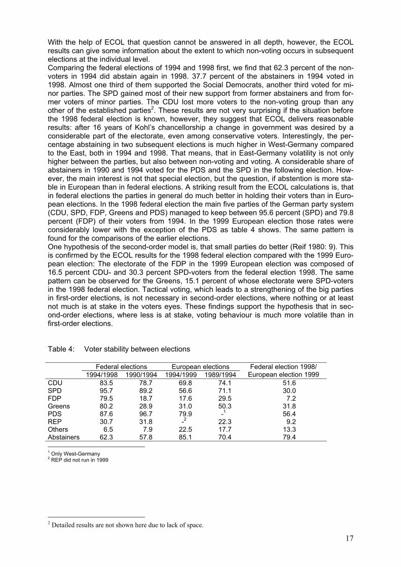
With the help of ECOL that question cannot be answered in all depth, however, the ECOL results can give some information about the extent to which non-voting occurs in subsequent elections at the individual level. Comparing the federal elections of 1994 and 1998 first, we find that 62.3 percent of the non-voters in 1994 did abstain again in 1998. 37.7 percent of the abstainers in 1994 voted in 1998. Almost one third of them supported the Social Democrats, another third voted for mi-nor parties. The SPD gained most of their new support from former abstainers and from for-mer voters of minor parties. The CDU lost more voters to the non-voting group than any other of the established parties2. These results are not very surprising if the situation before the 1998 federal election is known, however, they suggest that ECOL delivers reasonable results: after 16 years of Kohl’s chancellorship a change in government was desired by a considerable part of the electorate, even among conservative voters. Interestingly, the per-centage abstaining in two subsequent elections is much higher in West-Germany compared to the East, both in 1994 and 1998. That means, that in East-Germany volatility is not only higher between the parties, but also between non-voting and voting. A considerable share of abstainers in 1990 and 1994 voted for the PDS and the SPD in the following election. How-ever, the main interest is not that special election, but the question, if abstention is more sta-ble in European than in federal elections. A striking result from the ECOL calculations is, that in federal elections the parties in general do much better in holding their voters than in Euro-pean elections. In the 1998 federal election the main five parties of the German party system (CDU, SPD, FDP, Greens and PDS) managed to keep between 95.6 percent (SPD) and 79.8 percent (FDP) of their voters from 1994. In the 1999 European election those rates were considerably lower with the exception of the PDS as table 4 shows. The same pattern is found for the comparisons of the earlier elections. One hypothesis of the second-order model is, that small parties do better (Reif 1980: 9). This is confirmed by the ECOL results for the 1998 federal election compared with the 1999 Euro-pean election: The electorate of the FDP in the 1999 European election was composed of 16.5 percent CDU- and 30.3 percent SPD-voters from the federal election 1998. The same pattern can be observed for the Greens, 15.1 percent of whose electorate were SPD-voters in the 1998 federal election. Tactical voting, which leads to a strengthening of the big parties in first-order elections, is not necessary in second-order elections, where nothing or at least not much is at stake in the voters eyes. These findings support the hypothesis that in sec-ond-order elections, where less is at stake, voting behaviour is much more volatile than in first-order elections. Table 4: Voter stability between elections Federal elections European elections 1994/1998 1990/1994 1994/1999 1989/1994

Federal election 1998/ European election 1999

CDU 83.5 78.7 69.8 74.1 51.6 SPD 95.7 89.2 56.6 71.1 30.0 FDP 79.5 18.7 17.6 29.5 7.2 Greens 80.2 28.9 31.0 50.3 31.8 PDS 87.6 96.7 79.9 -1 56.4 REP 30.7 31.8 -2 22.3 9.2 Others 6.5 7.9 22.5 17.7 13.3 Abstainers 62.3 57.8 85.1 70.4 79.4 1 Only West-Germany 2 REP did not run in 1999

2 Detailed results are not shown here due to lack of space.

18

3. Facilitation and mobilisation of voters

3.1 Institutional facilitation and mobilisation Before we get to the analysis of the correlates of turnout, the institutional arrangements in Germany for the three types of elections shall be outlined briefly. On the one hand that might be necessary to decide if differential turnout at different levels of governance within Germany is influenced by those institutional and electoral arrangements. On the other hand some knowledge might be helpful for the international comparison following in a later chapter. The concept underlying this book suggests to distinguish between institutional facilitation and institutional mobilisation as shown in figure ???. To begin with institutional facilitation we have a look at • the day of voting • hours of opening of polls and • postal voting possibilities • the month of voting. However, in Germany most of these organisational characteristics of elections do neither differ between the levels of elections nor did they change over the time period from 1979 to 1999. All elections take place on a Sunday, opening hours of the polls are from 8 a.m. to 6 p.m.. Postal voting exists since the third national election in 1957 and is also possible in state and European elections. It is officially only allowed for persons who are not in their precinct at the day of the election, because of important reasons, or for people who are not able to go to the polls because of physical disabilities. In fact, however, everybody can vote by post as the reasons are not investigated. The last feature, month of voting, can change from election to election – at least at national and sub-national level. National elections are usually held in September or October, with three exceptions during the period from 1979 onwards. European Parliament Elections are the only ones that have always taken place in the same month, namely in June, a time when many people might be on holidays. In 1999, for example, the voting day, June 13, fell in va-cations in seven of the sixteen German states. In spite of the possibility of postal voting in the case of absence because of holidays, some people might not use this offer. Though the Eurobarometer survey data for the 1999 European election do ask for the reasons of absten-tion, it is unfortunately impossible to investigate the effect of a voting day falling within school holidays as there are not enough cases if one breaks down the non-voters by state. So we can conclude: With the exception of the month of voting in case of European elections there is hardly any evidence that institutional facilitation factors can explain differences in turnout, neither over time nor over different levels within Germany. If we come to institutional mobilisation, we have to look at • powers of levels of governance and • variations in electoral systems. The substantial difference between elections at the European level on the one hand and fed-eral and state level on the other is, that European elections do not offer any prospect of a change of government3, while on both of the other two levels voters judge the old govern-ment and decide on the new one at least indirectly. The Bundestag, which is elected directly in federal elections, elects the German chancellor. That means, that the outcome of German national elections has substantial impact on the next government. Of course, the proportional representation electoral system in connection with a party system with five parties (CDU, 3 This is a problem already identified before the first direct European election in 1979 (Blumler 1982: 4). Al-though the powers of the parliament have been expanded, it still does lack the most important function of na-tional parliaments, the formation of a government. The European Parliament’s role in the process of the resigna-tion of the Commission before the 1999 European election did not change the view of the population on its im-portance dramatically (Cautrès 2002: 18).

19

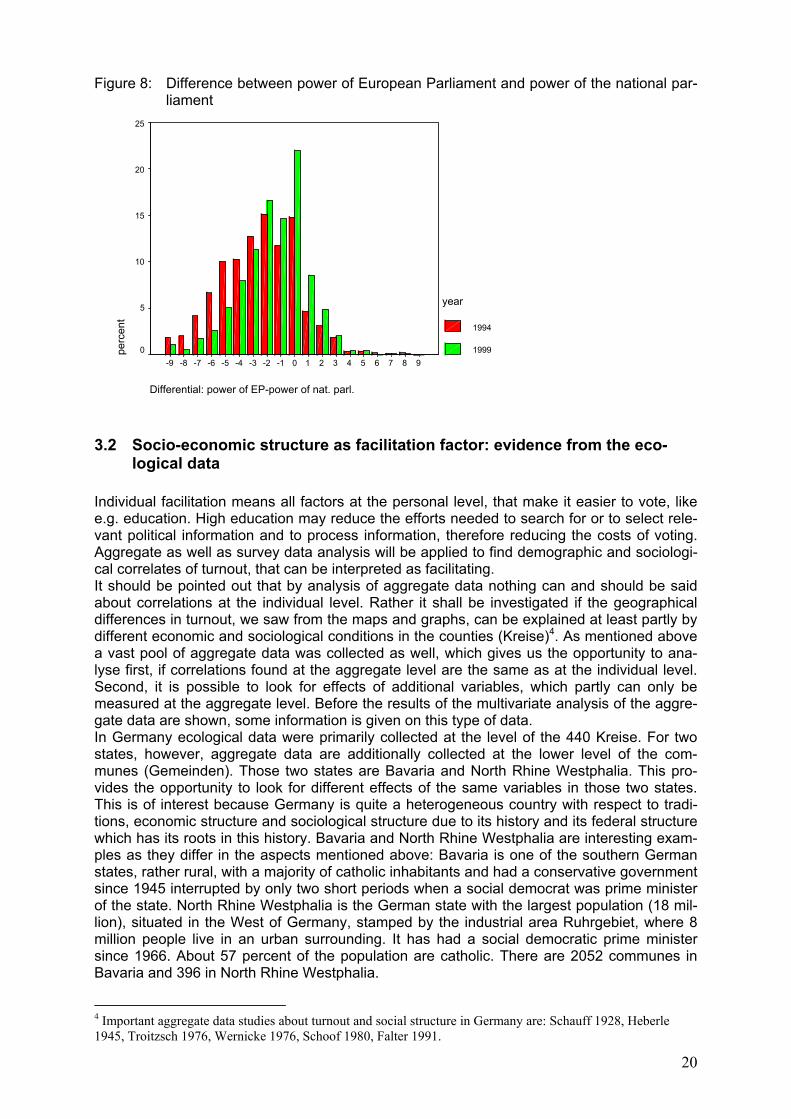
SPD, Greens, FDP and PDS) leaves some room for coalition formation, so that the govern-ment does not have to be determined by a certain election outcome. Usually, however, the chancellor comes from the strongest party. The political systems of the states are very simi-lar to the national political system, with the prime ministers elected by the parliaments of the Länder (Landtage), whereas in the European Union there is no government responsible to the European Parliament and European Parliament Elections are therefore not determining in any way the executive of the Union. Due to this relative insignificance of the European parliament, European elections lack any competitive element, which is truly derived from European issues and politics. It does not matter much to the people, who is sitting in there. The lack of competition and choice between alternative programs and candidates has also important effects on the campaigns for European Parliament Elections as there is hardly any personalisation between top-candidates. This fact is undoubtedly one reason why European Elections are of minor interest to the media and are therefore not covered in the same way as national or even sub-national elections. Besides the fact that the European Parliament does not elect a responsible government, it has less power as a legislative organ than the Bundestag, the German federal assembly. The Bundestag has the right to initiate legislation, and all bills have to be adopted by the Bundestag. The powers of the European Parliament are more restricted in that respect. First of all the EP does not have the right to initiate legislation. Second, not all European law has to be adopted by a majority in the EP. There exist four different procedures for the EP to in-fluence European legislation, only two of which give the EP a veto power (co-decision proce-dure and assent procedure). Under the consultation procedure and the cooperation proce-dure the EP can only delay proposals by the Commission and decision making by the Coun-cil (LIT). To assess the powers of the sub-national parliaments, the Landtage, is not easy in a highly complex federal system. First of all it has to be mentioned that the states participate in fed-eral legislation via the Bundesrat, the second chamber, where the state governments are represented. Basically there are three areas of legislation: one is exclusive federal legisla-tion, where the states have no say, the second is exclusive state legislation, where the fed-eral government is not involved, and the third are the so-called “Gemeinschaftsaufgaben”, where both levels have to give their assent. In the areas of legislation, that are residing at the state level, the Länder parliaments have full legislative powers. That areas shrunk since the beginning of the Federal Republic, while the number of bills requiring approval of both the Bundestag and the Bundesrat rose (Margedant 2003: 6). The states, however, still have sub-stantial influence on large parts of the legislation, not only at state level but also at the federal level. The powers of the parliaments at different levels of governance, however, can only be of any importance for turnout if those differences are realised by the eligible population. Figure 8 shows the differentials between the perceptions of powers of the EP and the Bundestag in 1994 and 1999, negative numbers meaning that the national parliament is considered to have more power than the EP, positive numbers meaning that the EP has more power than the Bundestag. Respondents were asked to assess the power of both parliaments on a ten point scale. Obviously most people do perceive the relative weakness of the EP. However, the comparison between 1994 and 1999 shows a decreasing perceived differential. In 1999 a share of more than 20 percent of the respondents rated both parliaments equal, indicated by a value of zero on the scale. The relationship between the perception of power of the EP and turnout will be analysed later. The second criterion of institutional mobilisation of voters mentioned above is the electoral system. In Germany the electoral system in all elections is basically proportional representa-tion. Although it is supplemented in national elections and in some state elections by a sec-ond vote for a candidate in the constituency, it is still primarily a proportional representation system. That means that voters do not have to adapt to a “new” electoral system in Euro-pean elections. It has to be concluded that institutional facilitation as well as institutional mobilisation cannot explain the differential turnout between federal and European elections within Germany as the organisational contexts are very similar at all levels of governance.

20

Figure 8: Difference between power of European Parliament and power of the national par-liament

Differential: power of EP-power of nat. parl.

9876543210-1-2-3-4-5-6-7-8-9

perc

ent

25

20

15

10

5

0

year

1994

1999

3.2 Socio-economic structure as facilitation factor: evidence from the eco-logical data

Individual facilitation means all factors at the personal level, that make it easier to vote, like e.g. education. High education may reduce the efforts needed to search for or to select rele-vant political information and to process information, therefore reducing the costs of voting. Aggregate as well as survey data analysis will be applied to find demographic and sociologi-cal correlates of turnout, that can be interpreted as facilitating. It should be pointed out that by analysis of aggregate data nothing can and should be said about correlations at the individual level. Rather it shall be investigated if the geographical differences in turnout, we saw from the maps and graphs, can be explained at least partly by different economic and sociological conditions in the counties (Kreise)4. As mentioned above a vast pool of aggregate data was collected as well, which gives us the opportunity to ana-lyse first, if correlations found at the aggregate level are the same as at the individual level. Second, it is possible to look for effects of additional variables, which partly can only be measured at the aggregate level. Before the results of the multivariate analysis of the aggre-gate data are shown, some information is given on this type of data. In Germany ecological data were primarily collected at the level of the 440 Kreise. For two states, however, aggregate data are additionally collected at the lower level of the com-munes (Gemeinden). Those two states are Bavaria and North Rhine Westphalia. This pro-vides the opportunity to look for different effects of the same variables in those two states. This is of interest because Germany is quite a heterogeneous country with respect to tradi-tions, economic structure and sociological structure due to its history and its federal structure which has its roots in this history. Bavaria and North Rhine Westphalia are interesting exam-ples as they differ in the aspects mentioned above: Bavaria is one of the southern German states, rather rural, with a majority of catholic inhabitants and had a conservative government since 1945 interrupted by only two short periods when a social democrat was prime minister of the state. North Rhine Westphalia is the German state with the largest population (18 mil-lion), situated in the West of Germany, stamped by the industrial area Ruhrgebiet, where 8 million people live in an urban surrounding. It has had a social democratic prime minister since 1966. About 57 percent of the population are catholic. There are 2052 communes in Bavaria and 396 in North Rhine Westphalia.

4 Important aggregate data studies about turnout and social structure in Germany are: Schauff 1928, Heberle 1945, Troitzsch 1976, Wernicke 1976, Schoof 1980, Falter 1991.

21

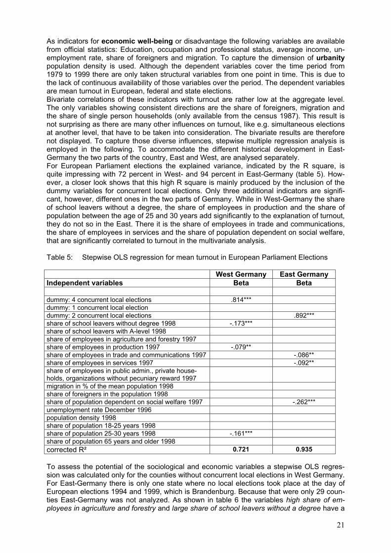
As indicators for economic well-being or disadvantage the following variables are available from official statistics: Education, occupation and professional status, average income, un-employment rate, share of foreigners and migration. To capture the dimension of urbanity population density is used. Although the dependent variables cover the time period from 1979 to 1999 there are only taken structural variables from one point in time. This is due to the lack of continuous availability of those variables over the period. The dependent variables are mean turnout in European, federal and state elections. Bivariate correlations of these indicators with turnout are rather low at the aggregate level. The only variables showing consistent directions are the share of foreigners, migration and the share of single person households (only available from the census 1987). This result is not surprising as there are many other influences on turnout, like e.g. simultaneous elections at another level, that have to be taken into consideration. The bivariate results are therefore not displayed. To capture those diverse influences, stepwise multiple regression analysis is employed in the following. To accommodate the different historical development in East-Germany the two parts of the country, East and West, are analysed separately. For European Parliament elections the explained variance, indicated by the R square, is quite impressing with 72 percent in West- and 94 percent in East-Germany (table 5). How-ever, a closer look shows that this high R square is mainly produced by the inclusion of the dummy variables for concurrent local elections. Only three additional indicators are signifi-cant, however, different ones in the two parts of Germany. While in West-Germany the share of school leavers without a degree, the share of employees in production and the share of population between the age of 25 and 30 years add significantly to the explanation of turnout, they do not so in the East. There it is the share of employees in trade and communications, the share of employees in services and the share of population dependent on social welfare, that are significantly correlated to turnout in the multivariate analysis. Table 5: Stepwise OLS regression for mean turnout in European Parliament Elections West Germany East Germany Independent variables Beta Beta dummy: 4 concurrent local elections .814*** dummy: 1 concurrent local election dummy: 2 concurrent local elections .892*** share of school leavers without degree 1998 -.173*** share of school leavers with A-level 1998 share of employees in agriculture and forestry 1997 share of employees in production 1997 -.079** share of employees in trade and communications 1997 -.086** share of employees in services 1997 -.092** share of employees in public admin., private house-holds, organizations without pecuniary reward 1997

migration in % of the mean population 1998 share of foreigners in the population 1998 share of population dependent on social welfare 1997 -.262*** unemployment rate December 1996 population density 1998 share of population 18-25 years 1998 share of population 25-30 years 1998 -.161*** share of population 65 years and older 1998 corrected R² 0.721 0.935 To assess the potential of the sociological and economic variables a stepwise OLS regres-sion was calculated only for the counties without concurrent local elections in West Germany. For East-Germany there is only one state where no local elections took place at the day of European elections 1994 and 1999, which is Brandenburg. Because that were only 29 coun-ties East-Germany was not analyzed. As shown in table 6 the variables high share of em-ployees in agriculture and forestry and large share of school leavers without a degree have a

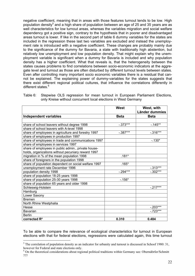
22

negative coefficient, meaning that in areas with those features turnout tends to be low. High population density5 and a high share of population between an age of 25 and 35 years are as well characteristics for low turnout areas, whereas the variables migration and social welfare dependency got a positive sign, contrary to the hypothesis that in poorer and disadvantaged areas turnout is lower. If like in the second part of table 6 dummy variables for the states are included in the regression these last two variables are excluded and instead the unemploy-ment rate is introduced with a negative coefficient. These changes are probably mainly due to the significance of the dummy for Bavaria, a state with traditionally high abstention, but relatively low unemployment and low population density. That might explain why the unem-ployment variable is significant when a dummy for Bavaria is included and why population density has a higher coefficient. What that reveals is, that the heterogeneity between the states causes problems to find correlations between socio-economic indicators at the aggre-gate level and turnout as those are often disturbed by different turnout levels between states. Even after controlling many important socio economic variables there is a residual that can-not be explained. The explaining power of dummy-variables for the states suggests that there exist different regional political cultures, that influence the correlations differently in different states.6 Table 6: Stepwise OLS regression for mean turnout in European Parliament Elections,

only Kreise without concurrent local elections in West Germany West West, with

Länder dummies Independent variables Beta Beta share of school leavers without degree 1998 -.373*** -.145** share of school leavers with A-level 1998 share of employees in agriculture and forestry 1997 -.387*** -.316*** share of employees in production 1997 share of employees in trade and communications 1997 -.130* share of employees in services 1997 share of employees in public admin., private house-holds, organizations without pecuniary reward 1997

migration in % of the mean population 1998 .181* share of foreigners in the population 1998 share of population dependent on social welfare 1997 .165* unemployment rate December 1996 -.313*** population density 1998 -.294*** -.302*** share of population 18-25 years 1998 share of population 25-30 years 1998 -.156* share of population 65 years and older 1998 Schleswig-Holstein -.217*** Hamburg Lower Saxony Bremen North Rhine Westphalia Hesse -.203*** Bavarian -.723*** Berlin corrected R² 0.310 0.484 To be able to compare the relevance of ecological characteristics for turnout in European elections with that for federal elections, regressions were calculated again, this time turnout 5 The correlation of population density as an indicator for urbanity and turnout is discussed in Schoof 1980: 31, however for Federal and state elections only. 6 On the theoretical considerations about regional political traditions within Germany see: Oberndörfer/Schmitt ???

23

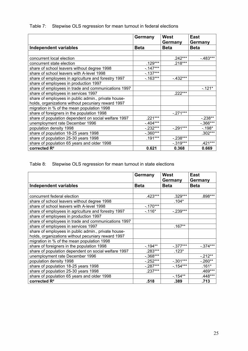
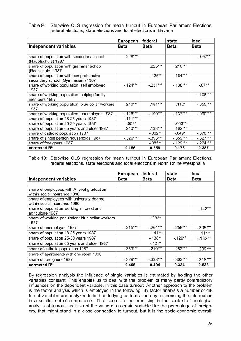
in federal elections being the dependent variable. Most obvious, concurrent elections do not play a role as prominent as with European elections. This is not surprising as it cannot be expected that simultaneous second order elections boost turnout in first order elections. The findings in table 7 are quite puzzling, if one looks at the column for Germany as a whole first. It is surprising that the variable high share of school leavers has a negative sign, while the variables share of population dependent on social welfare and high share of population be-tween the age of 25 and 30 have a positive one. Most of these unexpected results are due to the big differences between East and West Germany as the separate regressions in the sec-ond and third column show. In federal elections, turnout in East Germany has always been lower compared to the West, which means that most of the variance, that is tried to explain in the first regression for the whole of Germany, is the one between East and West. The regression for West Germany shows the importance of the agriculture variable, which has a negative impact on turnout. Kreise with turnout below average in the West are further characterized by a high share of population over 65 years, high population density and high share of foreigners and by a high share of population with an age of 25 to 30 years. Kreise with a strong service sector as well as with concurrent local or state elections show higher turnout. The regression for East Germany surprisingly shows that concurrent local elections are negatively correlated to turnout. Also different from the patterns we saw before, high share of young people between 18 and 25 as well as a high share of old people are posi-tively correlated to turnout in federal elections in East Germany. Not surprising is the nega-tive coefficient for the share of social welfare dependents, a high unemployment rate and high population density. The stepwise regression that was calculated for mean turnout in state elections (table 9) shows a rather similar result as for federal elections. The significant coefficients have the same directions for both types of elections. Again, the regression for West- and East-Germany together results in coefficients which partly explain the variance between the two parts of the country. This is true for the indicator school leavers with A-level7 as well as for the unemployment rate. From columns two and three follows that some variables are only relevant for West-Germany, while others are so only for the East. Consistently correlated to turnout in state elections is again population density, the share of foreigners and, not surpris-ing, the concurrence of a federal election. If it comes to the analysis of the two states, Bavaria (table 9) and North Rhine Westphalia (table 10) the first thing that attracts attention is that in North Rhine Westphalia it is possible to explain much more of the variance than for Bavaria. In North Rhine Westphalia the share of catholic population seems to be a very important variable, highly significant for all three types of elections, European, federal and state elections. Two other variables with significant impact for all election types are the share of foreigners and the share of unemployed people, both negatively correlated to turnout at the level of the communes. For federal elections there are the age variables included, as well. Contrary to what we saw in the individual data analy-sis a high share of 18 to 25 year old population is positively correlated to turnout at the mu-nicipal level. A high share of blue collar workers among the working population has a slightly negative effect on turnout. For Bavaria the most important variable is the share of single person households, which is an indicator for urban areas, where turnout is usually lower than in rural areas. While the educa-tional structure has no effect on turnout in North Rhine Westphalia, it is correlated to turnout in Bavaria in the expected direction: low education gets a negative sign while higher secon-dary education variables show positive signs. Contrary to North Rhine Westphalia a high share of blue collar works has a positive sign for all three types of elections, and the variable share of catholic population gets a negative one and is not as important in Bavaria as it is in North Rhine Westphalia. In both states the variance that can be explained is highest for local elections. It seems as if turnout at the commune level is even more than in other election types influenced by the ur-banity factor. For Bavaria that is indicated by the share of blue collar workers and the share of foreigners, both having a negative sign and being highly significant. Those groups of the

7 The percentage of school leavers with A-level is higher in East-Germany with Brandenburg ranking first.

24

population are more likely to be found in cities and big towns. For North-Rhine Westphalia rurality is indicated by the share of people employed in forestry and agriculture. The reason for that finding might be that in rural, mostly small communes a local election is more per-sonalized, that providing an additional incentive to turn out. What the comparison shows is that with the aggregate data analysis it is very important to consider the different circumstances and particularities. Being catholic can have totally differ-ent implications in a state where Catholicism is not the dominant denomination than in a state where it is dominating.

25

Table 7: Stepwise OLS regression for mean turnout in federal elections Germany West

Germany East Germany

Independent variables Beta Beta Beta concurrent local election .242*** -.483*** concurrent state election .129*** .218*** share of school leavers without degree 1998 -.147*** share of school leavers with A-level 1998 -.137*** share of employees in agriculture and forestry 1997 -.163*** -.432*** share of employees in production 1997 share of employees in trade and communications 1997 -.121* share of employees in services 1997 .222*** share of employees in public admin., private house-holds, organizations without pecuniary reward 1997

migration in % of the mean population 1998 share of foreigners in the population 1998 -.271*** share of population dependent on social welfare 1997 .221*** -.238** unemployment rate December 1996 -.404*** -.366*** population density 1998 -.232*** -.291*** -.198* share of population 18-25 years 1998 -.360*** .302*** share of population 25-30 years 1998 .191*** -.238*** share of population 65 years and older 1998 -.319*** .421*** corrected R² 0.621 0.368 0.669 Table 8: Stepwise OLS regression for mean turnout in state elections Germany West

Germany East Germany

Independent variables Beta Beta Beta concurrent federal election .423*** .329*** .898*** share of school leavers without degree 1998 .104* share of school leavers with A-level 1998 -.170*** share of employees in agriculture and forestry 1997 -.116* -.239*** share of employees in production 1997 share of employees in trade and communications 1997 share of employees in services 1997 .167** share of employees in public admin., private house-holds, organizations without pecuniary reward 1997

migration in % of the mean population 1998 share of foreigners in the population 1998 -.194** -.377*** -.374*** share of population dependent on social welfare 1997 .283*** .123* unemployment rate December 1996 -.368*** -.212** population density 1998 -.252*** -.301*** -.260** share of population 18-25 years 1998 -.287*** -.154*** .161* share of population 25-30 years 1998 .237*** .469*** share of population 65 years and older 1998 -.154** .448*** corrected R² .518 .389 .713

26

Table 9: Stepwise OLS regression for mean turnout in European Parliament Elections, federal elections, state elections and local elections in Bavaria

European federal state local Independent variables Beta Beta Beta Beta share of population with secondary school (Hauptschule) 1987

-.228*** -.097**

share of population with grammar school (Realschule) 1987

.225*** .210***

share of population with comprehensive secondary school (Gymnasium) 1987

.125** .164***

share of working population: self employed 1987

-.124*** -.231*** -.138*** -.071*

share of working population: helping family members 1987

-.108***

share of working population: blue collar workers 1987

.240*** .181*** .112* -.355***

share of working population: unemployed 1987 -.126*** -.199*** -.137*** -.090*** share of population 18-25 years 1987 .111*** share of population 25-30 years 1987 -.058* -.063** share of population 65 years and older 1987 .240*** .138*** .162*** share of catholic population 1987 -.062** -.049* -.070*** share of single person households 1987 -.326*** -.393*** -.359*** -.327*** share of foreigners 1987 -.085** -.129*** -.224*** corrected R² 0.156 0.256 0.173 0.387 Table 10: Stepwise OLS regression for mean turnout in European Parliament Elections,

federal elections, state elections and local elections in North Rhine Westphalia European federal state local Independent variables Beta Beta Beta Beta share of employees with A-level graduation within social insurance 1990

share of employees with university degree within social insurance 1990

share of population working in forest and agriculture 1987

.142**

share of working population: blue collar workers 1987

-.082*

share of unemployed 1987 -.215*** -.264*** -.258*** -.305*** share of population 18-25 years 1987 .141** .111* share of population 25-30 years 1987 -.138** -.129** -.132** share of population 65 years and older 1987 -.121* share of catholic population 1987 .353*** .219*** .252*** .209*** share of apartments with one room 1990 share of foreigners 1987 -.329*** -.338*** -.303*** -.318*** corrected R² 0.408 0.494 0.334 0.533 By regression analysis the influence of single variables is estimated by holding the other variables constant. This enables us to deal with the problem of many partly contradictory influences on the dependent variable, in this case turnout. Another approach to the problem is the factor analysis which is employed in the following. By factor analysis a number of dif-ferent variables are analyzed to find underlying patterns, thereby condensing the information in a smaller set of components. That seems to be promising in the context of ecological analysis of turnout, as it is not the value of a certain variable like the percentage of foreign-ers, that might stand in a close connection to turnout, but it is the socio-economic overall-

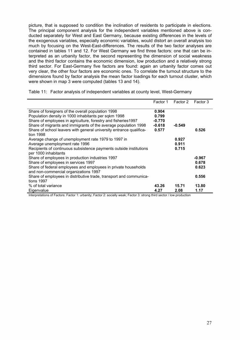
27

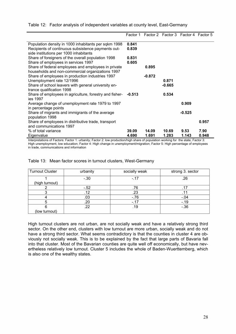
picture, that is supposed to condition the inclination of residents to participate in elections. The principal component analysis for the independent variables mentioned above is con-ducted separately for West and East Germany, because existing differences in the levels of the exogenous variables, especially economic variables, would distort an overall analysis too much by focusing on the West-East-differences. The results of the two factor analyses are contained in tables 11 and 12. For West Germany we find three factors: one that can be in-terpreted as an urbanity factor, the second representing the dimension of social weakness and the third factor contains the economic dimension, low production and a relatively strong third sector. For East-Germany five factors are found: again an urbanity factor comes out very clear, the other four factors are economic ones. To correlate the turnout structure to the dimensions found by factor analysis the mean factor loadings for each turnout cluster, which were shown in map 3 were computed (tables 13 and 14). Table 11: Factor analysis of independent variables at county level, West-Germany

Factor 1 Factor 2 Factor 3

Share of foreigners of the overall population 1998 0.904 Population density in 1000 inhabitants per sqkm 1998 0.799 Share of employees in agriculture, forestry and fisheries1997 -0.770 Share of migrants and immigrants of the average population 1998 -0.618 -0.549 Share of school leavers with general university entrance qualifica-tion 1998

0.577 0.526

Average change of unemployment rate 1979 to 1997 in 0.927 Average unemployment rate 1996 0.911 Recipients of continuous subsistence payments outside institutions per 1000 inhabitants

0.715

Share of employees in production industries 1997 -0.967 Share of employees in services 1997 0.678 Share of federal employees and employees in private households and non-commercial organizations 1997

0.623

Share of employees in distributive trade, transport and communica-tions 1997

0.556

% of total variance 43.26 15.71 13.80 Eigenvalue 4.27 2.08 1.17 Interpretations of Factors: Factor 1: urbanity; Factor 2: socially weak; Factor 3: strong third sector / low production

28

Table 12: Factor analysis of independent variables at county level, East-Germany

Factor 1 Factor 2 Factor 3 Factor 4 Factor 5

Population density in 1000 inhabitants per sqkm 1998 0.841 Recipients of continuous subsistence payments out-side institutions per 1000 inhabitants

0.839

Share of foreigners of the overall population 1998 0.831 Share of employees in services 1997 0.605 Share of federal employees and employees in private households and non-commercial organizations 1997

0.895

Share of employees in production industries 1997 -0.872 Unemployment rate 12/1996 0.871 Share of school leavers with general university en-trance qualification 1998

-0.665

Share of employees in agriculture, forestry and fisher-ies 1997

-0.513 0.534

Average change of unemployment rate 1979 to 1997 in percentage points

0.909

Share of migrants and immigrants of the average population 1998

-0.525

Share of employees in distributive trade, transport and communications 1997

0.957

% of total variance 39.09 14.09 10.69 9.53 7.90 Eigenvalue 4.690 1.691 1.283 1.143 0.948 Interpretations of Factors: Factor 1: urbanity; Factor 2: low production/high share of population working for the state; Factor 3: High unemployment, low education; Factor 4: High change in unemployment/migration; Factor 5: High percentage of employees in trade, communications and information Table 13: Mean factor scores in turnout clusters, West-Germany Turnout Cluster urbanity socially weak strong 3. sector

1 (high turnout)

-.30 -.17 .26

2 -.52 .76 .17 3 .12 .23 .11 4 .03 -.76 -.04 5 .20 -.17 -.19 6

(low turnout) .22 .19 -.36

High turnout clusters are not urban, are not socially weak and have a relatively strong third sector. On the other end, clusters with low turnout are more urban, socially weak and do not have a strong third sector. What seems contradictory is that the counties in cluster 4 are ob-viously not socially weak. This is to be explained by the fact that large parts of Bavaria fall into that cluster. Most of the Bavarian counties are quite well off economically, but have nev-ertheless relatively low turnout. Cluster 5 includes the whole of Baden-Wuerttemberg, which is also one of the wealthy states.

29

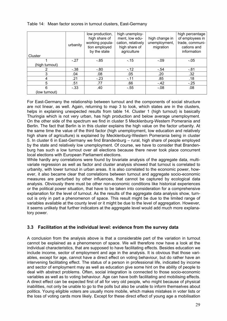
Table 14: Mean factor scores in turnout clusters, East-Germany

Cluster

urbanity

low production, high share of

working popula-tion employed by the state

high unemploy-ment, low edu-

cation, relatively high share of

agriculture

high change in unemployment,

migration

high percentage of employees in trade, communi-

cations and information

1

(high turnout) -.27 -.85 -.15 -.09 -.05

2 -.38 -.80 -.12 -.54 -.81 3 .04 .08 .05 .20 .32 4 .21 -.23 -.11 .85 .18 5 .51 .77 .66 -.42 -.25 6

(low turnout) -.33 .40 -.55 -.08 .08

For East-Germany the relationship between turnout and the components of social structure are not linear, as well. Again, returning to map 3 to look, which states are in the clusters, helps in explaining unexpected results from table 14. Cluster 1 (high turnout) is basically Thuringia which is not very urban, has high production and below average unemployment. On the other side of the spectrum we find in cluster 5 Mecklenburg-Western Pomerania and Berlin. The fact that Berlin is in this cluster explains the high value on the factor urbanity. At the same time the value of the third factor (high unemployment, low education and relatively high share of agriculture) is explained by Mecklenburg-Western Pomerania being in cluster 5. In cluster 6 in East-Germany we find Brandenburg – rural, high share of people employed by the state and relatively low unemployment. Of course, we have to consider that Branden-burg has such a low turnout over all elections because there never took place concurrent local elections with European Parliament elections. While hardly any correlations were found by bivariate analysis of the aggregate data, multi-variate regression as well as factor and cluster analysis showed that turnout is correlated to urbanity, with lower turnout in urban areas. It is also correlated to the economic power, how-ever, it also became clear that correlations between turnout and aggregate socio-economic measures are perturbed by other influences, that cannot be captured by ecological data analysis. Obviously there must be other non-economic conditions like historical experiences or the political power situation, that have to be taken into consideration for a comprehensive explanation for the level of turnout. As the results of the aggregate data analysis show, turn-out is only in part a phenomenon of space. This result might be due to the limited range of variables available at the county level or it might be due to the level of aggregation. However, it seems unlikely that further indicators at the aggregate level would add much more explana-tory power.

3.3 Facilitation at the individual level: evidence from the survey data A conclusion from the analysis above is that a considerable part of the variation in turnout cannot be explained as a phenomenon of space. We will therefore now have a look at the individual characteristics, that are supposed to have facilitating effects. Besides education we include income, sector of employment and age in the analysis. It is obvious that those vari-ables, except for age, cannot have a direct effect on voting behaviour, but do rather have an intervening facilitating effect. The status of a person in professional life, indicated by income and sector of employment may as well as education give some hint on the ability of people to deal with abstract problems. Often, social integration is connected to those socio-economic variables as well as to voting behaviour. Age can have both facilitating and mobilising effects. A direct effect can be expected first of all for very old people, who might because of physical inabilities, not only be unable to go to the polls but also be unable to inform themselves about politics. Young eligible voters are usually more mobile, which makes mistakes in voter lists or the loss of voting cards more likely. Except for these direct effect of young age a mobilisation

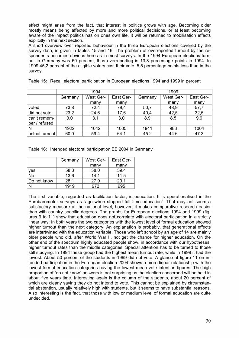
30

effect might arise from the fact, that interest in politics grows with age. Becoming older mostly means being affected by more and more political decisions, or at least becoming aware of the impact politics has on ones own life. It will be returned to mobilisation effects explicitly in the next section. A short overview over reported behaviour in the three European elections covered by the survey data, is given in tables 15 and 16. The problem of overreported turnout by the re-spondents becomes obvious here as in most surveys. In the 1994 European elections turn-out in Germany was 60 percent, thus overreporting is 13,8 percentage points in 1994. In 1999 45,2 percent of the eligible voters cast their vote, 5,5 percentage points less than in the survey. Table 15: Recall electoral participation in European elections 1994 and 1999 in percent 1994 1999 Germany West Ger-

many East Ger-

many Germany West Ger-

many East Ger-

many voted 73.8 72.4 79,4 50,7 48,9 57,7 did not vote 23.2 24.6 17,6 40,4 42,5 32,5 can’t remem-ber / refused

3.0 3.1 3,0 8,9 8,5 9,9

N 1922 1042 1005 1941 983 1004 actual turnout 60.0 59.4 64.1 45.2 44.6 47.3 Table 16: Intended electoral participation EE 2004 in Germany Germany West Ger-

many East Ger-

many yes 58.3 58.0 59.4 No 13.6 14.1 11.5 Do not know 28.1 27.9 29.1 N 1919 972 995 The first variable, regarded as facilitation factor, is education. It is operationalised in the Eurobarometer surveys as “age when stopped full time education”. That may not seem a satisfactory measure at the national level, however, it makes comparative research easier than with country specific degrees. The graphs for European elections 1994 and 1999 (fig-ures 9 to 11) show that education does not correlate with electoral participation in a strictly linear way: In both years the two categories with the lowest level of formal education showed higher turnout than the next category. An explanation is probably, that generational effects are intertwined with the education variable. Those who left school by an age of 14 are mainly older people who did, after World War II, not get the chance for higher education. On the other end of the spectrum highly educated people show, in accordance with our hypotheses, higher turnout rates than the middle categories. Special attention has to be turned to those still studying. In 1994 these group had the highest mean turnout rate, while in 1999 it had the lowest. About 50 percent of the students in 1999 did not vote. A glance at figure 11 on in-tended participation in the European election 2004 shows a more linear relationship with the lowest formal education categories having the lowest mean vote intention figures. The high proportion of “do not know” answers is not surprising as the election concerned will be held in about five years time. Interesting again is the column of the students, about 20 percent of which are clearly saying they do not intend to vote. This cannot be explained by circumstan-tial abstention, usually relatively high with students, but it seems to have substantial reasons. Also interesting is the fact, that those with low or medium level of formal education are quite undecided.

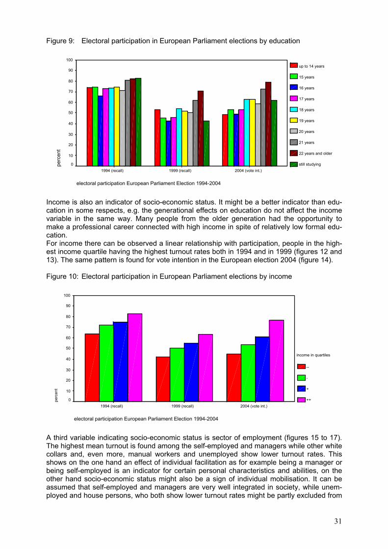
31

Figure 9: Electoral participation in European Parliament elections by education

electoral participation European Parliament Election 1994-2004

2004 (vote int.)1999 (recall)1994 (recall)

perc

ent

100

90

80

70

60

50

40

30

20

10

0

up to 14 years

15 years

16 years

17 years

18 years

19 years

20 years

21 years

22 years and older

still studying

Income is also an indicator of socio-economic status. It might be a better indicator than edu-cation in some respects, e.g. the generational effects on education do not affect the income variable in the same way. Many people from the older generation had the opportunity to make a professional career connected with high income in spite of relatively low formal edu-cation. For income there can be observed a linear relationship with participation, people in the high-est income quartile having the highest turnout rates both in 1994 and in 1999 (figures 12 and 13). The same pattern is found for vote intention in the European election 2004 (figure 14). Figure 10: Electoral participation in European Parliament elections by income

electoral participation European Parliament Election 1994-2004

2004 (vote int.)1999 (recall)1994 (recall)

perc

ent

100

90

80

70

60

50

40

30

20

10

0

income in quartiles

--

-

+

++

A third variable indicating socio-economic status is sector of employment (figures 15 to 17). The highest mean turnout is found among the self-employed and managers while other white collars and, even more, manual workers and unemployed show lower turnout rates. This shows on the one hand an effect of individual facilitation as for example being a manager or being self-employed is an indicator for certain personal characteristics and abilities, on the other hand socio-economic status might also be a sign of individual mobilisation. It can be assumed that self-employed and managers are very well integrated in society, while unem-ployed and house persons, who both show lower turnout rates might be partly excluded from

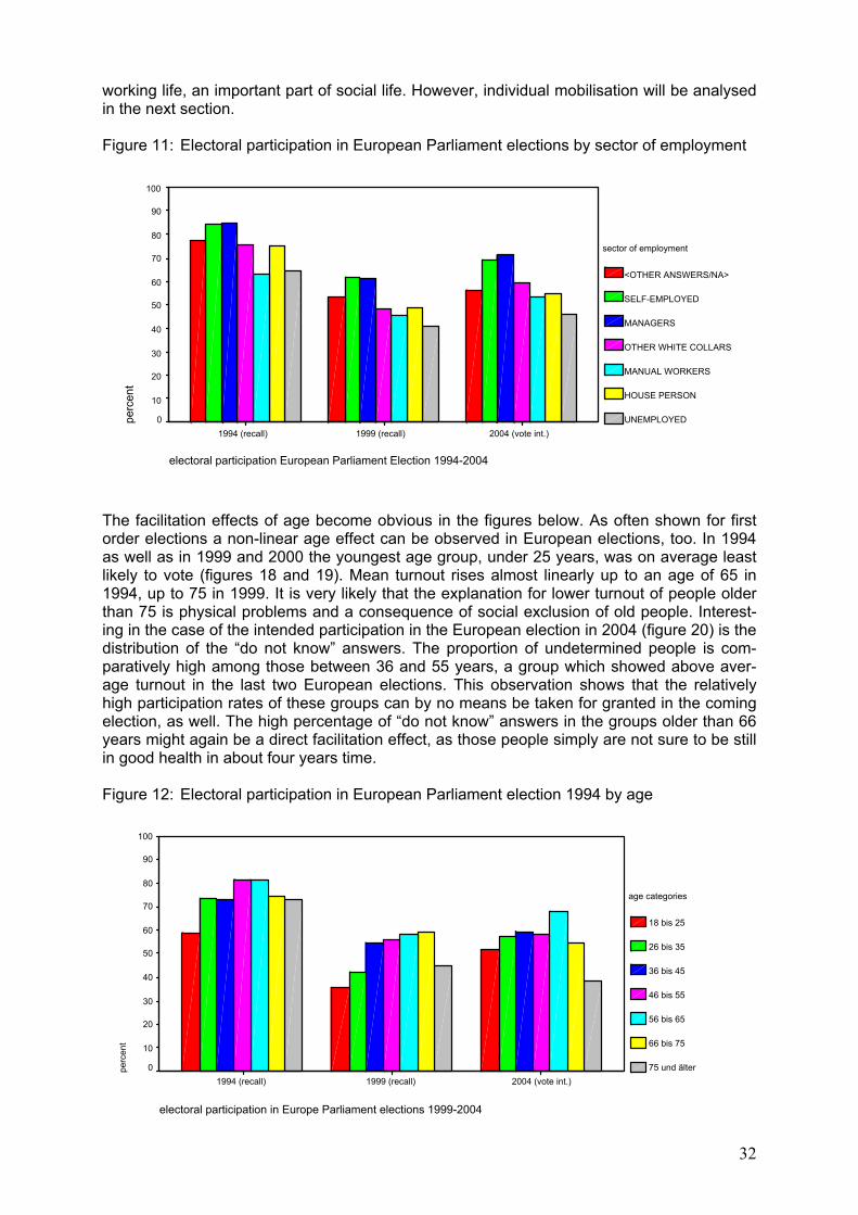
32

working life, an important part of social life. However, individual mobilisation will be analysed in the next section. Figure 11: Electoral participation in European Parliament elections by sector of employment

electoral participation European Parliament Election 1994-2004

2004 (vote int.)1999 (recall)1994 (recall)

perc

ent

100

90

80

70

60

50

40

30

20

10

0

sector of employment

<OTHER ANSWERS/NA>

SELF-EMPLOYED

MANAGERS

OTHER WHITE COLLARS

MANUAL WORKERS

HOUSE PERSON

UNEMPLOYED

The facilitation effects of age become obvious in the figures below. As often shown for first order elections a non-linear age effect can be observed in European elections, too. In 1994 as well as in 1999 and 2000 the youngest age group, under 25 years, was on average least likely to vote (figures 18 and 19). Mean turnout rises almost linearly up to an age of 65 in 1994, up to 75 in 1999. It is very likely that the explanation for lower turnout of people older than 75 is physical problems and a consequence of social exclusion of old people. Interest-ing in the case of the intended participation in the European election in 2004 (figure 20) is the distribution of the “do not know” answers. The proportion of undetermined people is com-paratively high among those between 36 and 55 years, a group which showed above aver-age turnout in the last two European elections. This observation shows that the relatively high participation rates of these groups can by no means be taken for granted in the coming election, as well. The high percentage of “do not know” answers in the groups older than 66 years might again be a direct facilitation effect, as those people simply are not sure to be still in good health in about four years time. Figure 12: Electoral participation in European Parliament election 1994 by age

electoral participation in Europe Parliament elections 1999-2004

2004 (vote int.)1999 (recall)1994 (recall)

perc

ent

100

90

80

70

60

50

40

30

20

10

0

age categories

18 bis 25

26 bis 35

36 bis 45

46 bis 55

56 bis 65

66 bis 75

75 und älter

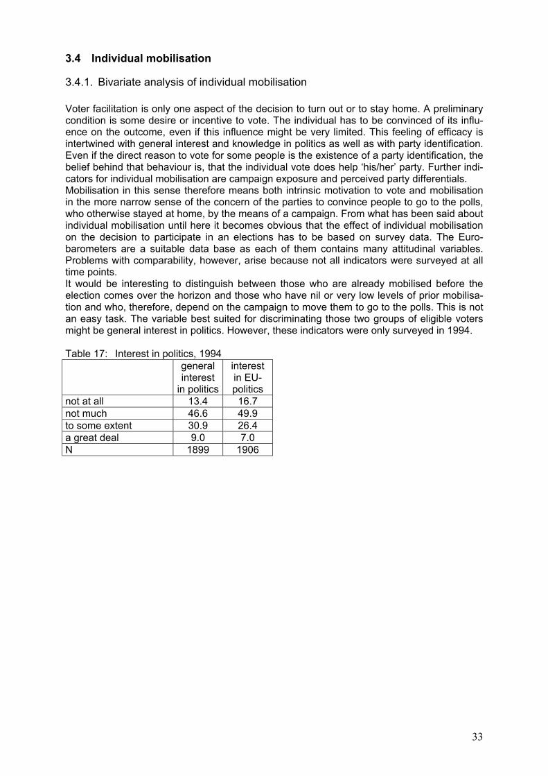
33

3.4 Individual mobilisation

3.4.1. Bivariate analysis of individual mobilisation Voter facilitation is only one aspect of the decision to turn out or to stay home. A preliminary condition is some desire or incentive to vote. The individual has to be convinced of its influ-ence on the outcome, even if this influence might be very limited. This feeling of efficacy is intertwined with general interest and knowledge in politics as well as with party identification. Even if the direct reason to vote for some people is the existence of a party identification, the belief behind that behaviour is, that the individual vote does help ‘his/her’ party. Further indi-cators for individual mobilisation are campaign exposure and perceived party differentials. Mobilisation in this sense therefore means both intrinsic motivation to vote and mobilisation in the more narrow sense of the concern of the parties to convince people to go to the polls, who otherwise stayed at home, by the means of a campaign. From what has been said about individual mobilisation until here it becomes obvious that the effect of individual mobilisation on the decision to participate in an elections has to be based on survey data. The Euro-barometers are a suitable data base as each of them contains many attitudinal variables. Problems with comparability, however, arise because not all indicators were surveyed at all time points. It would be interesting to distinguish between those who are already mobilised before the election comes over the horizon and those who have nil or very low levels of prior mobilisa-tion and who, therefore, depend on the campaign to move them to go to the polls. This is not an easy task. The variable best suited for discriminating those two groups of eligible voters might be general interest in politics. However, these indicators were only surveyed in 1994. Table 17: Interest in politics, 1994 general

interest in politics

interest in EU-politics

not at all 13.4 16.7 not much 46.6 49.9 to some extent 30.9 26.4 a great deal 9.0 7.0 N 1899 1906

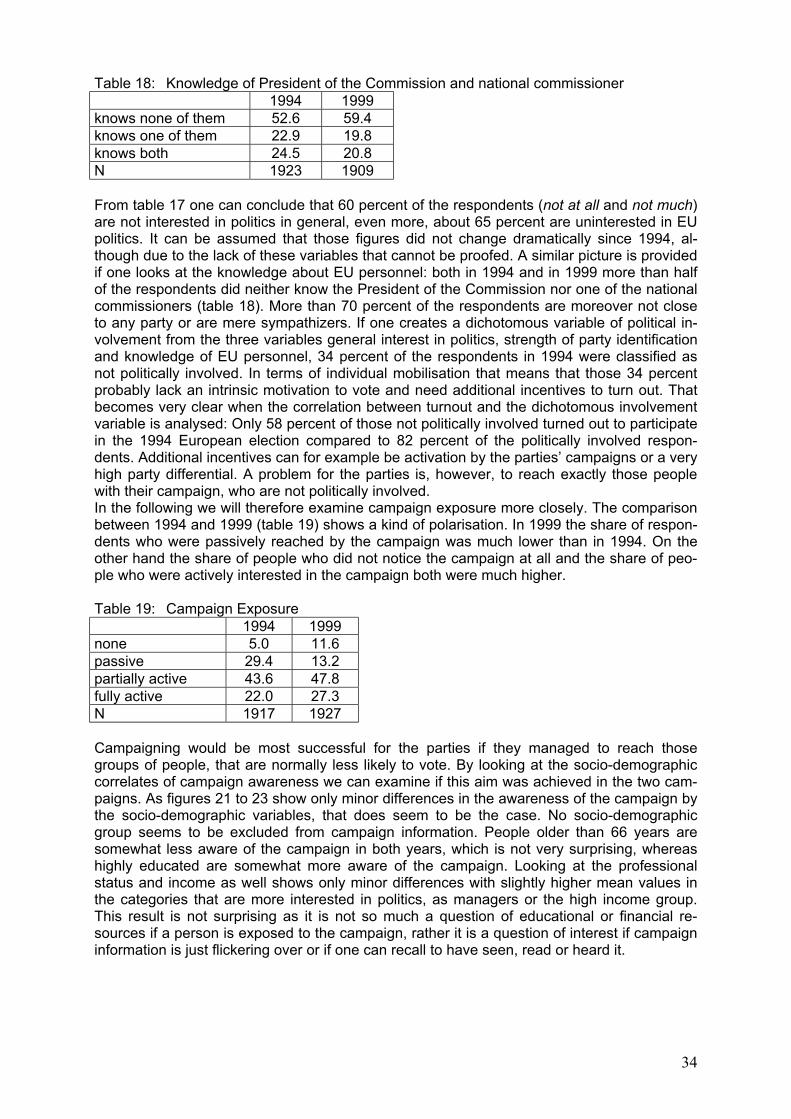
34

Table 18: Knowledge of President of the Commission and national commissioner 1994 1999 knows none of them 52.6 59.4 knows one of them 22.9 19.8 knows both 24.5 20.8 N 1923 1909 From table 17 one can conclude that 60 percent of the respondents (not at all and not much) are not interested in politics in general, even more, about 65 percent are uninterested in EU politics. It can be assumed that those figures did not change dramatically since 1994, al-though due to the lack of these variables that cannot be proofed. A similar picture is provided if one looks at the knowledge about EU personnel: both in 1994 and in 1999 more than half of the respondents did neither know the President of the Commission nor one of the national commissioners (table 18). More than 70 percent of the respondents are moreover not close to any party or are mere sympathizers. If one creates a dichotomous variable of political in-volvement from the three variables general interest in politics, strength of party identification and knowledge of EU personnel, 34 percent of the respondents in 1994 were classified as not politically involved. In terms of individual mobilisation that means that those 34 percent probably lack an intrinsic motivation to vote and need additional incentives to turn out. That becomes very clear when the correlation between turnout and the dichotomous involvement variable is analysed: Only 58 percent of those not politically involved turned out to participate in the 1994 European election compared to 82 percent of the politically involved respon-dents. Additional incentives can for example be activation by the parties’ campaigns or a very high party differential. A problem for the parties is, however, to reach exactly those people with their campaign, who are not politically involved. In the following we will therefore examine campaign exposure more closely. The comparison between 1994 and 1999 (table 19) shows a kind of polarisation. In 1999 the share of respon-dents who were passively reached by the campaign was much lower than in 1994. On the other hand the share of people who did not notice the campaign at all and the share of peo-ple who were actively interested in the campaign both were much higher. Table 19: Campaign Exposure 1994 1999 none 5.0 11.6 passive 29.4 13.2 partially active 43.6 47.8 fully active 22.0 27.3 N 1917 1927 Campaigning would be most successful for the parties if they managed to reach those groups of people, that are normally less likely to vote. By looking at the socio-demographic correlates of campaign awareness we can examine if this aim was achieved in the two cam-paigns. As figures 21 to 23 show only minor differences in the awareness of the campaign by the socio-demographic variables, that does seem to be the case. No socio-demographic group seems to be excluded from campaign information. People older than 66 years are somewhat less aware of the campaign in both years, which is not very surprising, whereas highly educated are somewhat more aware of the campaign. Looking at the professional status and income as well shows only minor differences with slightly higher mean values in the categories that are more interested in politics, as managers or the high income group. This result is not surprising as it is not so much a question of educational or financial re-sources if a person is exposed to the campaign, rather it is a question of interest if campaign information is just flickering over or if one can recall to have seen, read or heard it.

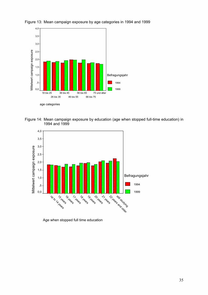
35

Figure 13: Mean campaign exposure by age categories in 1994 and 1999

age categories

75 und älter66 bis 75

56 bis 6546 bis 55

36 bis 4526 bis 35

18 bis 25

Mitt

elw

ert c

ampa

ign

expo

sure

4,0

3,5

3,0

2,5

2,0

1,5

1,0

,5

0,0

Befragungsjahr

1994

1999

Figure 14: Mean campaign exposure by education (age when stopped full-time education) in

1994 and 1999

Age when stopped full time education

still studying

22 years and older

21 years

20 years

19 years

18 years

17 years

16 years

15 years

up to 14 years

Mitt

elw

ert c

ampa

ign

expo

sure

4,0

3,5

3,0

2,5

2,0

1,5

1,0

,5

0,0

Befragungsjahr

1994

1999

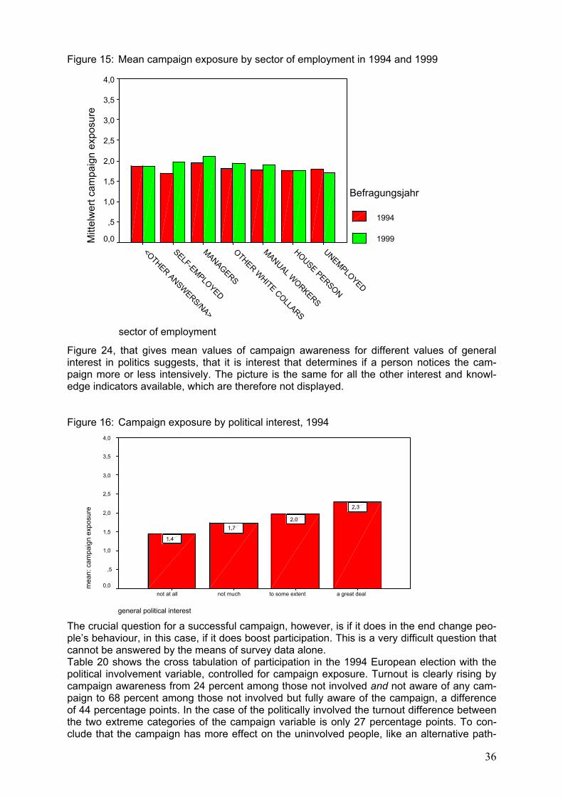
36

Figure 15: Mean campaign exposure by sector of employment in 1994 and 1999

sector of employment

UNEMPLOYED

HOUSE PERSON

MANUAL WORKERS

OTHER WHITE COLLARS

MANAGERS

SELF-EMPLOYED

<OTHER ANSWERS/NA>

Mitt

elw

ert c

ampa

ign

expo

sure

4,0

3,5

3,0

2,5

2,0

1,5

1,0

,5

0,0

Befragungsjahr

1994

1999

Figure 24, that gives mean values of campaign awareness for different values of general interest in politics suggests, that it is interest that determines if a person notices the cam-paign more or less intensively. The picture is the same for all the other interest and knowl-edge indicators available, which are therefore not displayed. Figure 16: Campaign exposure by political interest, 1994

general political interest

a great dealto some extentnot muchnot at all

mea

n: c

ampa

ign

expo

sure

4,0

3,5

3,0

2,5

2,0

1,5

1,0

,5

0,0

2,3

2,01,7

1,4

The crucial question for a successful campaign, however, is if it does in the end change peo-ple’s behaviour, in this case, if it does boost participation. This is a very difficult question that cannot be answered by the means of survey data alone. Table 20 shows the cross tabulation of participation in the 1994 European election with the political involvement variable, controlled for campaign exposure. Turnout is clearly rising by campaign awareness from 24 percent among those not involved and not aware of any cam-paign to 68 percent among those not involved but fully aware of the campaign, a difference of 44 percentage points. In the case of the politically involved the turnout difference between the two extreme categories of the campaign variable is only 27 percentage points. To con-clude that the campaign has more effect on the uninvolved people, like an alternative path-

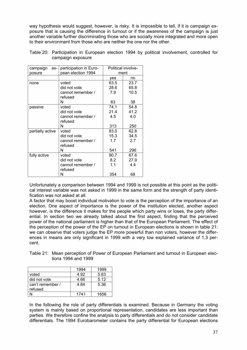
37

way hypothesis would suggest, however, is risky. It is impossible to tell, if it is campaign ex-posure that is causing the difference in turnout or if the awareness of the campaign is just another variable further discriminating those who are socially more integrated and more open to their environment from those who are neither the one nor the other. Table 20: Participation in European election 1994 by political involvement, controlled for

campaign exposure campaign ex-posure

participation in Euro-pean election 1994

Political involve-ment

yes no none voted 63.5 23.7 did not vote 28.6 65.8 cannot remember /

refused 7.9 10.5

N 63 38 passive voted 74.1 54.8 did not vote 21.4 41.2 cannot remember /

refused 4.5 4.0

N 313 250 partially active voted 83.0 62.8 did not vote 15.3 34.5 cannot remember /

refused 1.7 2.7

N 541 296 fully active voted 90.7 67.6 did not vote 8.2 27.9 cannot remember /

refused 1.1 4.4

N 354 68 Unfortunately a comparison between 1994 and 1999 is not possible at this point as the politi-cal interest variable was not asked in 1999 in the same form and the strength of party identi-fication was not asked at all. A factor that may boost individual motivation to vote is the perception of the importance of an election. One aspect of importance is the power of the institution elected, another aspect however, is the difference it makes for the people which party wins or loses, the party differ-ential. In section two we already talked about the first aspect, finding that the perceived power of the national parliament is higher than that of the European Parliament. The effect of the perception of the power of the EP on turnout in European elections is shown in table 21: we can observe that voters judge the EP more powerful than non voters, however the differ-ences in means are only significant in 1999 with a very low explained variance of 1,3 per-cent. Table 21: Mean perception of Power of European Parliament and turnout in European elec-

tions 1994 and 1999 1994 1999 voted 4.92 5.63 did not vote 4.66 5.12 can’t remember / refused

4.84 5.36

N 1741 1656 In the following the role of party differentials is examined. Because in Germany the voting system is mainly based on proportional representation, candidates are less important than parties. We therefore confine the analysis to party differentials and do not consider candidate differentials. The 1994 Eurobarometer contains the party differential for European elections

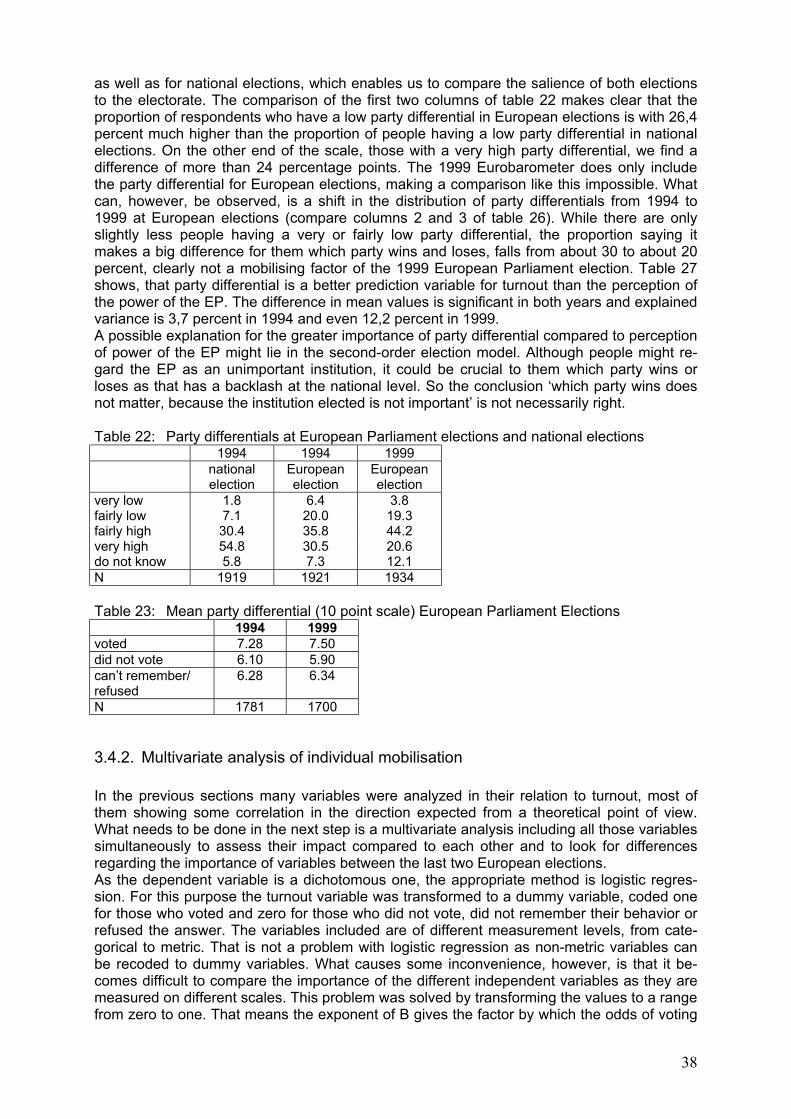
38

as well as for national elections, which enables us to compare the salience of both elections to the electorate. The comparison of the first two columns of table 22 makes clear that the proportion of respondents who have a low party differential in European elections is with 26,4 percent much higher than the proportion of people having a low party differential in national elections. On the other end of the scale, those with a very high party differential, we find a difference of more than 24 percentage points. The 1999 Eurobarometer does only include the party differential for European elections, making a comparison like this impossible. What can, however, be observed, is a shift in the distribution of party differentials from 1994 to 1999 at European elections (compare columns 2 and 3 of table 26). While there are only slightly less people having a very or fairly low party differential, the proportion saying it makes a big difference for them which party wins and loses, falls from about 30 to about 20 percent, clearly not a mobilising factor of the 1999 European Parliament election. Table 27 shows, that party differential is a better prediction variable for turnout than the perception of the power of the EP. The difference in mean values is significant in both years and explained variance is 3,7 percent in 1994 and even 12,2 percent in 1999. A possible explanation for the greater importance of party differential compared to perception of power of the EP might lie in the second-order election model. Although people might re-gard the EP as an unimportant institution, it could be crucial to them which party wins or loses as that has a backlash at the national level. So the conclusion ‘which party wins does not matter, because the institution elected is not important’ is not necessarily right. Table 22: Party differentials at European Parliament elections and national elections 1994 1994 1999 national

election European election

European election

very low 1.8 6.4 3.8 fairly low 7.1 20.0 19.3 fairly high 30.4 35.8 44.2 very high 54.8 30.5 20.6 do not know 5.8 7.3 12.1 N 1919 1921 1934 Table 23: Mean party differential (10 point scale) European Parliament Elections 1994 1999 voted 7.28 7.50 did not vote 6.10 5.90 can’t remember/ refused

6.28 6.34

N 1781 1700

3.4.2. Multivariate analysis of individual mobilisation In the previous sections many variables were analyzed in their relation to turnout, most of them showing some correlation in the direction expected from a theoretical point of view. What needs to be done in the next step is a multivariate analysis including all those variables simultaneously to assess their impact compared to each other and to look for differences regarding the importance of variables between the last two European elections. As the dependent variable is a dichotomous one, the appropriate method is logistic regres-sion. For this purpose the turnout variable was transformed to a dummy variable, coded one for those who voted and zero for those who did not vote, did not remember their behavior or refused the answer. The variables included are of different measurement levels, from cate-gorical to metric. That is not a problem with logistic regression as non-metric variables can be recoded to dummy variables. What causes some inconvenience, however, is that it be-comes difficult to compare the importance of the different independent variables as they are measured on different scales. This problem was solved by transforming the values to a range from zero to one. That means the exponent of B gives the factor by which the odds of voting

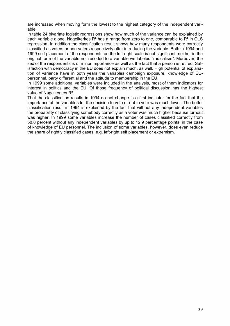
39

are increased when moving form the lowest to the highest category of the independent vari-able. In table 24 bivariate logistic regressions show how much of the variance can be explained by each variable alone. Nagelkerkes R² has a range from zero to one, comparable to R² in OLS regression. In addition the classification result shows how many respondents were correctly classified as voters or non-voters respectively after introducing the variable. Both in 1994 and 1999 self placement of the respondents on the left-right scale is not significant, neither in the original form of the variable nor recoded to a variable we labeled “radicalism”. Moreover, the sex of the respondents is of minor importance as well as the fact that a person is retired. Sat-isfaction with democracy in the EU does not explain much, as well. High potential of explana-tion of variance have in both years the variables campaign exposure, knowledge of EU-personnel, party differential and the attitude to membership in the EU. In 1999 some additional variables were included in the analysis, most of them indicators for interest in politics and the EU. Of those frequency of political discussion has the highest value of Nagelkerkes R². That the classification results in 1994 do not change is a first indicator for the fact that the importance of the variables for the decision to vote or not to vote was much lower. The better classification result in 1994 is explained by the fact that without any independent variables the probability of classifying somebody correctly as a voter was much higher because turnout was higher. In 1999 some variables increase the number of cases classified correctly from 50,8 percent without any independent variables by up to 12,9 percentage points, in the case of knowledge of EU personnel. The inclusion of some variables, however, does even reduce the share of rightly classified cases, e.g. left-right self placement or extremism.

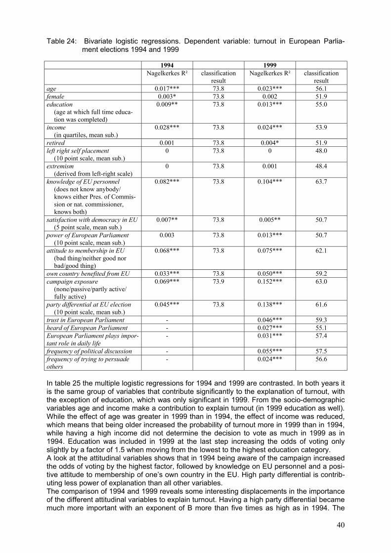
40

Table 24: Bivariate logistic regressions. Dependent variable: turnout in European Parlia-ment elections 1994 and 1999

1994 1999 Nagelkerkes R² classification

result Nagelkerkes R² classification

result age 0.017*** 73.8 0.023*** 56.1 female 0.003* 73.8 0.002 51.9 education

(age at which full time educa-tion was completed)

0.009** 73.8 0.013*** 55.0

income (in quartiles, mean sub.)

0.028*** 73.8 0.024*** 53.9

retired 0.001 73.8 0.004* 51.9 left right self placement

(10 point scale, mean sub.) 0 73.8 0 48.0

extremism (derived from left-right scale)

0 73.8 0.001 48.4

knowledge of EU personnel (does not know anybody/ knows either Pres. of Commis-sion or nat. commissioner, knows both)

0.082*** 73.8 0.104*** 63.7

satisfaction with democracy in EU (5 point scale, mean sub.)

0.007** 73.8 0.005** 50.7

power of European Parliament (10 point scale, mean sub.)

0.003 73.8 0.013*** 50.7

attitude to membership in EU (bad thing/neither good nor bad/good thing)

0.068*** 73.8 0.075*** 62.1

own country benefited from EU 0.033*** 73.8 0.050*** 59.2 campaign exposure

(none/passive/partly active/ fully active)

0.069*** 73.9 0.152*** 63.0

party differential at EU election (10 point scale, mean sub.)

0.045*** 73.8 0.138*** 61.6

trust in European Parliament - 0.046*** 59.3 heard of European Parliament - 0.027*** 55.1 European Parliament plays impor-tant role in daily life

- 0.031*** 57.4

frequency of political discussion - 0.055*** 57.5 frequency of trying to persuade others

- 0.024*** 56.6

In table 25 the multiple logistic regressions for 1994 and 1999 are contrasted. In both years it is the same group of variables that contribute significantly to the explanation of turnout, with the exception of education, which was only significant in 1999. From the socio-demographic variables age and income make a contribution to explain turnout (in 1999 education as well). While the effect of age was greater in 1999 than in 1994, the effect of income was reduced, which means that being older increased the probability of turnout more in 1999 than in 1994, while having a high income did not determine the decision to vote as much in 1999 as in 1994. Education was included in 1999 at the last step increasing the odds of voting only slightly by a factor of 1.5 when moving from the lowest to the highest education category. A look at the attitudinal variables shows that in 1994 being aware of the campaign increased the odds of voting by the highest factor, followed by knowledge on EU personnel and a posi-tive attitude to membership of one’s own country in the EU. High party differential is contrib-uting less power of explanation than all other variables. The comparison of 1994 and 1999 reveals some interesting displacements in the importance of the different attitudinal variables to explain turnout. Having a high party differential became much more important with an exponent of B more than five times as high as in 1994. The

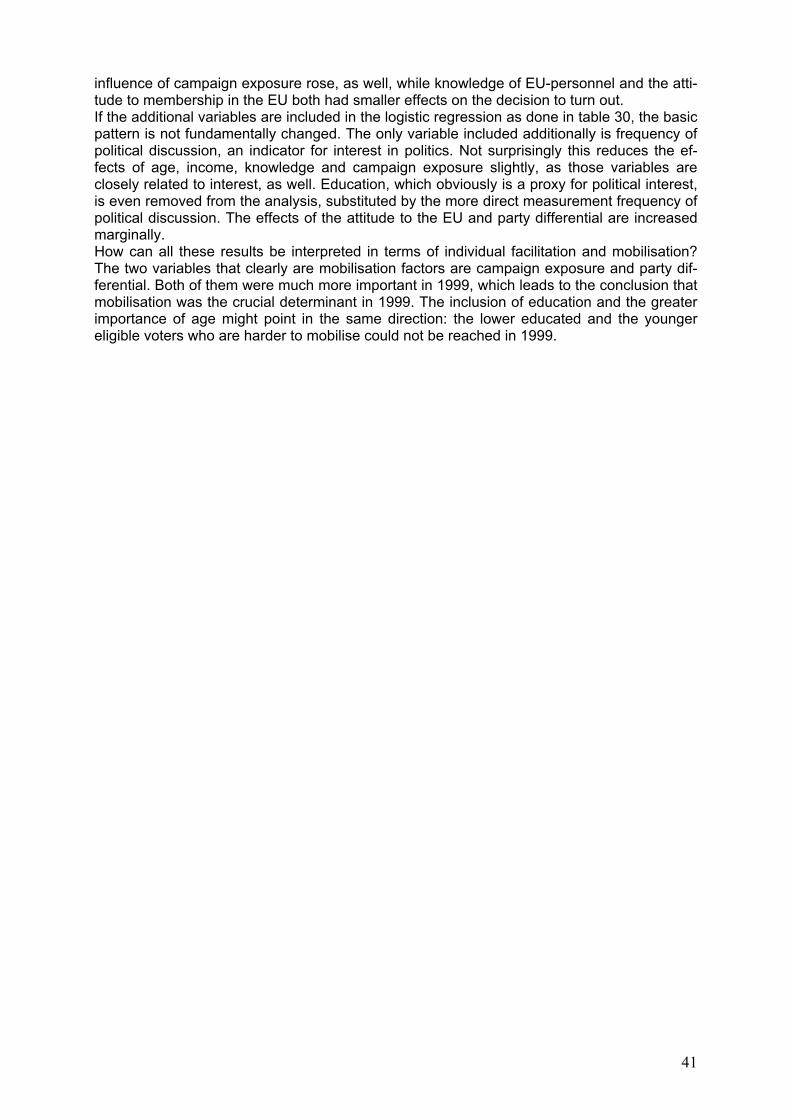
41

influence of campaign exposure rose, as well, while knowledge of EU-personnel and the atti-tude to membership in the EU both had smaller effects on the decision to turn out. If the additional variables are included in the logistic regression as done in table 30, the basic pattern is not fundamentally changed. The only variable included additionally is frequency of political discussion, an indicator for interest in politics. Not surprisingly this reduces the ef-fects of age, income, knowledge and campaign exposure slightly, as those variables are closely related to interest, as well. Education, which obviously is a proxy for political interest, is even removed from the analysis, substituted by the more direct measurement frequency of political discussion. The effects of the attitude to the EU and party differential are increased marginally. How can all these results be interpreted in terms of individual facilitation and mobilisation? The two variables that clearly are mobilisation factors are campaign exposure and party dif-ferential. Both of them were much more important in 1999, which leads to the conclusion that mobilisation was the crucial determinant in 1999. The inclusion of education and the greater importance of age might point in the same direction: the lower educated and the younger eligible voters who are harder to mobilise could not be reached in 1999.

42

Table 25: Multivariate stepwise logistic regressions. Dependent variable: turnout in European Parliament elections 1994 and 1999 1994 1999 Variables in the regression: B Exp(B) entered on

step classification

result B Exp(B) entered on

step classification

result age 1.389*** 4.010 4 75.8 1.882*** 6.565 4 70.5 female - - - - - - - education

(age at which full time education was com-pleted)

- - - - .383* 1.467 7 71.5

income (in quartiles, mean sub.)

.802*** 2.230 5 75.7 .507** 1.661 6 71.5

retired - - - - - - - - Left right self placement

(10 point scale, mean sub.) - - - - - - - -

extremism (derived from left-right scale)

- - - - - - - -

knowledge of EU personnel (does not know anybody/ knows either Pres. of Commission or nat. commissioner, knows both)

1.204*** 3.335 1 73.8 .917*** 2.501 3 68.5

satisfaction with democracy in EU (5 point scale, mean sub.)

- - - - - - - -

power of EP (10 point scale, mean sub.)

- - - - - - - -

attitude to membership in EU (bad thing/neither good nor bad/good thing)

1.069*** 2.913 2 75.1 .792*** 2.208 5 70.1

own country benefited from EU - - - - - - - - campaign exposure

(none/passive/partly active/ fully active) 1.463*** 4.320 3 75.4 2.021*** 7.545 1 63.0

party differential EU elections (10 point scale, mean sub.)

.743*** 2.101 6 75.5 2.490*** 12.065 2 67.2

constant 2.276*** -4.747*** Nagelkerkes R-Quadrat: 0.214 Nagelkerkes R-Quadrat: 0.327

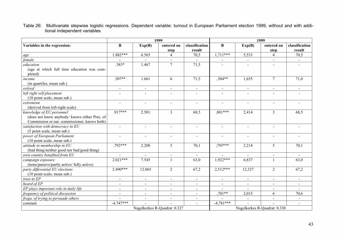
43

Table 26: Multivariate stepwise logistic regressions. Dependent variable: turnout in European Parliament election 1999, without and with addi-tional independent variables

1999 1999 Variables in the regression: B Exp(B) entered on

step classification

result B Exp(B) entered on

step classification

result age 1.882*** 6.565 4 70,5 1,711*** 5,533 4 70,5 female - - - - - - - - education

(age at which full time education was com-pleted)

.383* 1.467 7 71,5 - - - -

income (in quartiles, mean sub.)

.507** 1.661 6 71,5 ,504** 1,655 7 71,0

retired - - - - - - - - left right self placement

(10 point scale, mean sub.) - - - - - - - -

extremism (derived from left-right scale)

- - - - - - - -

knowledge of EU personnel (does not know anybody/ knows either Pres. of Commission or nat. commissioner, knows both)

.917*** 2.501 3 68,5 ,881*** 2,414 3 68,5

satisfaction with democracy in EU (5 point scale, mean sub.)

- - - - - - - -

power of European Parliament (10 point scale, mean sub.)

- - - - - - - -

attitude to membership in EU (bad thing/neither good nor bad/good thing)

.792*** 2.208 5 70,1 ,795*** 2,214 5 70,1

own country benefited from EU - - - - - - - - campaign exposure

(none/passive/partly active/ fully active) 2.021*** 7.545 1 63,0 1,922*** 6,837 1 63,0

party differential EU elections (10 point scale, mean sub.)

2.490*** 12.065 2 67,2 2,512*** 12,327 2 67,2

trust in EP - - - - - - - - heard of EP - - - - - - - - EP plays important role in daily life - - - - - - - - frequency of political discussion - - - - ,701** 2,015 6 70,6 frequ. of trying to persuade others - - - - - - - - constant -4.747*** - - - -4,781*** - - - Nagelkerkes R-Quadrat: 0.327 Nagelkerkes R-Quadrat: 0.330

44

Tables 27 to 29 show the results of logistic regressions for turnout in federal elections. As with turnout in European elections the first step was to calculate bivariate logistic regressions, which give the power of explanation of each single variable (table 27). One might wonder why variables with reference to Europe were included. It is obviously not important to know the Commissioners for Germany in the European Commission if the body that is voted is the national parliament. How-ever, it is interesting to see if those who are well informed about the European arena are those who vote in federal elections, as well. As in European elections interest in politics (interest in poli-tics in general in 1994, frequency of political discussion in 1999 and 2000) is the variable best suited to explain turnout in national elections, too. This finding is supported by looking at the indica-tors for knowledge and campaign exposure, both indicators for political interest as well. Socio-demographic variables clearly contribute less to explain if a person votes or not. It is interesting that the Nagelkerkes R² for age is about the same for participation in the national election of 1990 like for participation in the European elections, but it has very limited influence on the vote intention in national elections. Education seems to be more important in the European context as well as income. In tables 28 and 29 there are displayed the results of stepwise logistic regressions for participation in federal elections. Comparing the stepwise logistic regressions for European and federal elections shows that Na-gelkerkes R square is higher for European elections. Not surprising is that it is again interest in politics that is introduced on the first step. Campaign exposure is, at least in 1994, a good indicator as well. It is remarkable that with the vote intention for federal election 1994 the attitude to the question if Germany benefited from being member of the EU is the second one included in the re-gression, because it is not at all in the other three stepwise regressions for turnout in federal elec-tions. The comparison of the logistic regressions is difficult because of various reasons. First, we do not have the same variables for all years, second, we compare recall of participation (federal election 1990, European Elections) with vote intentions (for federal elections 1994 and 2002), third, the time distances to the elections differ extremely. Those difficulties in mind, a conclusion is, that interest is the most important predictor of turnout in both types of elections, European and national. Attitudes to the EU and European integration, measured by the membership and the benefit questions, seem to be less important. Diffuse support, expressed by saying membership is a good thing, seems to play a more important role than a calculation of costs and benefits that might stand be-hind the benefit question.

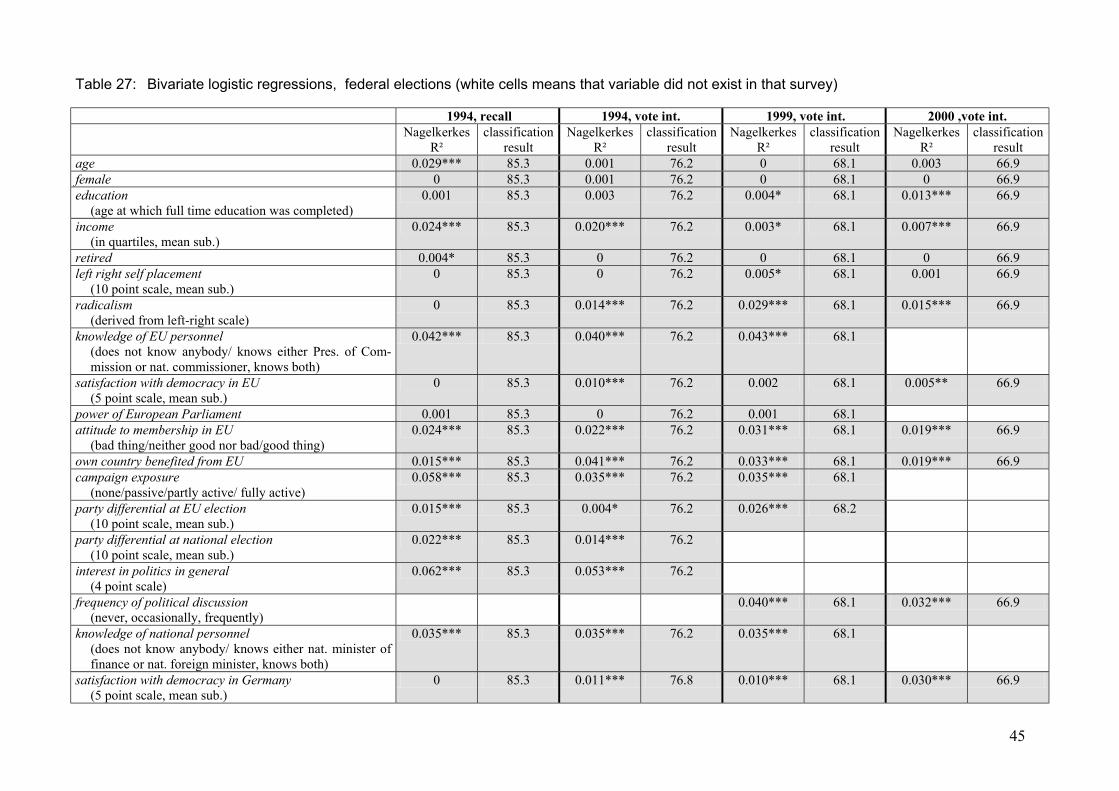
45

Table 27: Bivariate logistic regressions, federal elections (white cells means that variable did not exist in that survey) 1994, recall 1994, vote int. 1999, vote int. 2000 ,vote int. Nagelkerkes

R² classification

result Nagelkerkes

R² classification

result Nagelkerkes

R² classification

result Nagelkerkes

R² classification

result age 0.029*** 85.3 0.001 76.2 0 68.1 0.003 66.9 female 0 85.3 0.001 76.2 0 68.1 0 66.9 education

(age at which full time education was completed) 0.001 85.3 0.003 76.2 0.004* 68.1 0.013*** 66.9

income (in quartiles, mean sub.)

0.024*** 85.3 0.020*** 76.2 0.003* 68.1 0.007*** 66.9

retired 0.004* 85.3 0 76.2 0 68.1 0 66.9 left right self placement

(10 point scale, mean sub.) 0 85.3 0 76.2 0.005* 68.1 0.001 66.9

radicalism (derived from left-right scale)

0 85.3 0.014*** 76.2 0.029*** 68.1 0.015*** 66.9

knowledge of EU personnel (does not know anybody/ knows either Pres. of Com-mission or nat. commissioner, knows both)

0.042*** 85.3 0.040*** 76.2 0.043*** 68.1

satisfaction with democracy in EU (5 point scale, mean sub.)

0 85.3 0.010*** 76.2 0.002 68.1 0.005** 66.9

power of European Parliament 0.001 85.3 0 76.2 0.001 68.1 attitude to membership in EU

(bad thing/neither good nor bad/good thing) 0.024*** 85.3 0.022*** 76.2 0.031*** 68.1 0.019*** 66.9

own country benefited from EU 0.015*** 85.3 0.041*** 76.2 0.033*** 68.1 0.019*** 66.9 campaign exposure

(none/passive/partly active/ fully active) 0.058*** 85.3 0.035*** 76.2 0.035*** 68.1

party differential at EU election (10 point scale, mean sub.)

0.015*** 85.3 0.004* 76.2 0.026*** 68.2

party differential at national election (10 point scale, mean sub.)

0.022*** 85.3 0.014*** 76.2

interest in politics in general (4 point scale)

0.062*** 85.3 0.053*** 76.2

frequency of political discussion (never, occasionally, frequently)

0.040*** 68.1 0.032*** 66.9

knowledge of national personnel (does not know anybody/ knows either nat. minister of finance or nat. foreign minister, knows both)

0.035*** 85.3 0.035*** 76.2 0.035*** 68.1

satisfaction with democracy in Germany (5 point scale, mean sub.)

0 85.3 0.011*** 76.8 0.010*** 68.1 0.030*** 66.9

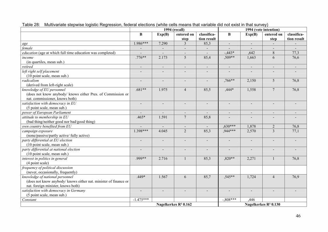
46

Table 28: Multivariate stepwise logistic Regression, federal elections (white cells means that variable did not exist in that survey) 1994 (recall) 1994 (vote intention) B Exp(B) entered on

step classifica-tion result

B Exp(B) entered on step

classifica-tion result

age 1.986*** 7.290 3 85,3 - - - - female - - - - - - - - education (age at which full time education was completed) - - - - -,443* ,642 8 77,3 income

(in quartiles, mean sub.) .776** 2.173 5 85,4 ,509** 1,663 6 76,6

retired - - - - - - - - left right self placement

(10 point scale, mean sub.) - - - - - - - -

radicalism (derived from left-right scale)

- - - - ,766** 2,150 5 76,8

knowledge of EU personnel (does not know anybody/ knows either Pres. of Commission or nat. commissioner, knows both)

.681** 1.975 4 85,5 ,444* 1,558 7 76,8

satisfaction with democracy in EU (5 point scale, mean sub.)

- - - - - - - -

power of European Parliament - - - - - - - - attitude to membership in EU

(bad thing/neither good nor bad/good thing) .465* 1.591 7 85,8 - - - -

own country benefited from EU - - - - ,630*** 1,878 2 76,8 campaign exposure

(none/passive/partly active/ fully active) 1.398*** 4.045 2 85,3 ,944*** 2,570 3 77,1

party differential at EU election (10 point scale, mean sub.)

- - - - - - - -

party differential at national election (10 point scale, mean sub.)

- - - - - - - -

interest in politics in general (4 point scale)

.999** 2.716 1 85,3 ,820** 2,271 1 76,8

frequency of political discussion (never, occasionally, frequently)

knowledge of national personnel (does not know anybody/ knows either nat. minister of finance or nat. foreign minister, knows both)

.449* 1.567 6 85,7 ,545** 1,724 4 76,9

satisfaction with democracy in Germany (5 point scale, mean sub.)

- - - - - - - -

Constant -1.475*** -,808*** ,446 Nagelkerkes R² 0.162 Nagelkerkes R² 0.130

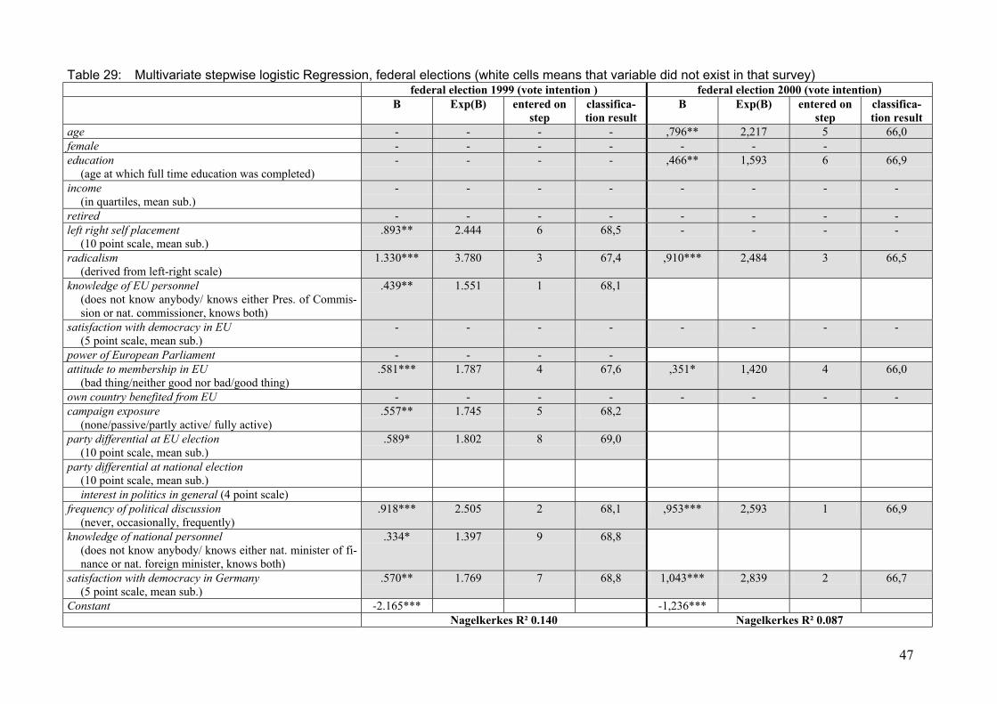
47

Table 29: Multivariate stepwise logistic Regression, federal elections (white cells means that variable did not exist in that survey) federal election 1999 (vote intention ) federal election 2000 (vote intention) B Exp(B) entered on

step classifica-tion result

B Exp(B) entered on step

classifica-tion result

age - - - - ,796** 2,217 5 66,0 female - - - - - - - education

(age at which full time education was completed) - - - - ,466** 1,593 6 66,9

income (in quartiles, mean sub.)

- - - - - - - -

retired - - - - - - - - left right self placement

(10 point scale, mean sub.) .893** 2.444 6 68,5 - - - -

radicalism (derived from left-right scale)

1.330*** 3.780 3 67,4 ,910*** 2,484 3 66,5

knowledge of EU personnel (does not know anybody/ knows either Pres. of Commis-sion or nat. commissioner, knows both)

.439** 1.551 1 68,1

satisfaction with democracy in EU (5 point scale, mean sub.)

- - - - - - - -

power of European Parliament - - - - attitude to membership in EU

(bad thing/neither good nor bad/good thing) .581*** 1.787 4 67,6 ,351* 1,420 4 66,0

own country benefited from EU - - - - - - - - campaign exposure

(none/passive/partly active/ fully active) .557** 1.745 5 68,2

party differential at EU election (10 point scale, mean sub.)

.589* 1.802 8 69,0

party differential at national election (10 point scale, mean sub.)

interest in politics in general (4 point scale) frequency of political discussion

(never, occasionally, frequently) .918*** 2.505 2 68,1 ,953*** 2,593 1 66,9

knowledge of national personnel (does not know anybody/ knows either nat. minister of fi-nance or nat. foreign minister, knows both)

.334* 1.397 9 68,8

satisfaction with democracy in Germany (5 point scale, mean sub.)

.570** 1.769 7 68,8 1,043*** 2,839 2 66,7

Constant -2.165*** -1,236*** Nagelkerkes R² 0.140 Nagelkerkes R² 0.087

48

For a further analysis of the reasons of differential turnout another study, the Asia-Europe survey (ASES), might provide additional clues. The survey was conducted in 18 countries, half of which were in Europe, including 1025 German respondents. The respondents were not asked about their voting behavior in a certain election. Instead three more general questions were asked, of which the dependent variables in the following are derived: frequency of voting at federal, European and local elections. The question design of the turnout questions in this study is rather crude, because the last of the three questions, which in most other countries referred to local elections addresses both local and state elections in the German case. For the analysis of multi-level turnout one would have wished a clearer distinction, however electoral behavior was not the actual concern of the Asia-Europe survey. Respondents were given five answer categories from ‘voted in almost all of them’ to ‘never voted in … election’. This question design is suitable for tracing the causes of dif-ferential turnout, because it addresses participation in a more general way than the usual recall or vote intention questions, thereby avoiding the problems arising of circumstantial abstention in a single election. From those three questions three voter types were identified: non-voters (n=226), voters in local and federal elections (n=165) and voters in local, federal and European elections (n=517). Respondents were coded as voters very restrictively, only if they said, they had voted in almost all of them. Of course, one could imagine other types, however, these turned out to be em-pirically relevant. For the logistic regressions three different dependent variables were computed and used for the different models in table 34. In the first model those voting in local (local and state elections) and federal elections are contrasted to non-voters. In the second model people voting in local and federal elections only are compared with respondents voting in all elections, local, federal and European. In the third model, the dependent variable splits non-voters and voters in all elec-tions. This approach enables to look for social characteristics and attitudes that distinguish the voter types. In table 30 the R squares of bivariate regressions are shown. While the free rider abstention is the variable best discriminating between non-voters and voters at local and federal level (model 1), in the other two models it is the duty to vote. The results of the multivariate logistic regressions in table 31 are revealing some interesting details. First, as the Nagelkerkes R² shows, it is hardly possible to explain why people who voted in almost all local and federal elections did not vote in European elections (model 2). The most important variable in that respect is the acceptance of voting as a citizen’s duty. Only one other variable is significant, which is the consumption of na-tional media. In model 1, which compares voters at local and federal elections to non-voters, the variable first entered is free-rider abstention, the approval of the statement “since so many people vote in elections, it really doesn’t matter whether I vote or not”, followed by interest in politics, age and the existence of a PID. However, the second column, which gives the factor by which the probability of voting in local and federal elections increases by moving to the highest category of the independent variable, shows that age, interest in politics and the duty to vote are the most im-portant variables in model 1. Nagelkerkes R² is, not surprisingly, much higher than for model 2, but somewhat lower than for model 3, in which non-voters and voters at all levels are compared. While the significant variables and their coefficients in model 3 are similar to model 1, some differences can be found. The duty to vote, entered on the first step here, existence of PID and education do contribute more to distinguish these two groups than those from model 1, while age is less impor-tant. What becomes quite clear from the three models is, that the mobilizing factor for participation in European elections is the involvement in politics, indicated by a higher coefficient for PID in model 3 compared to model 1and by the fact, that attention to national media is significant here as well. Most important for participation in European elections, however, is the feeling of duty to vote.

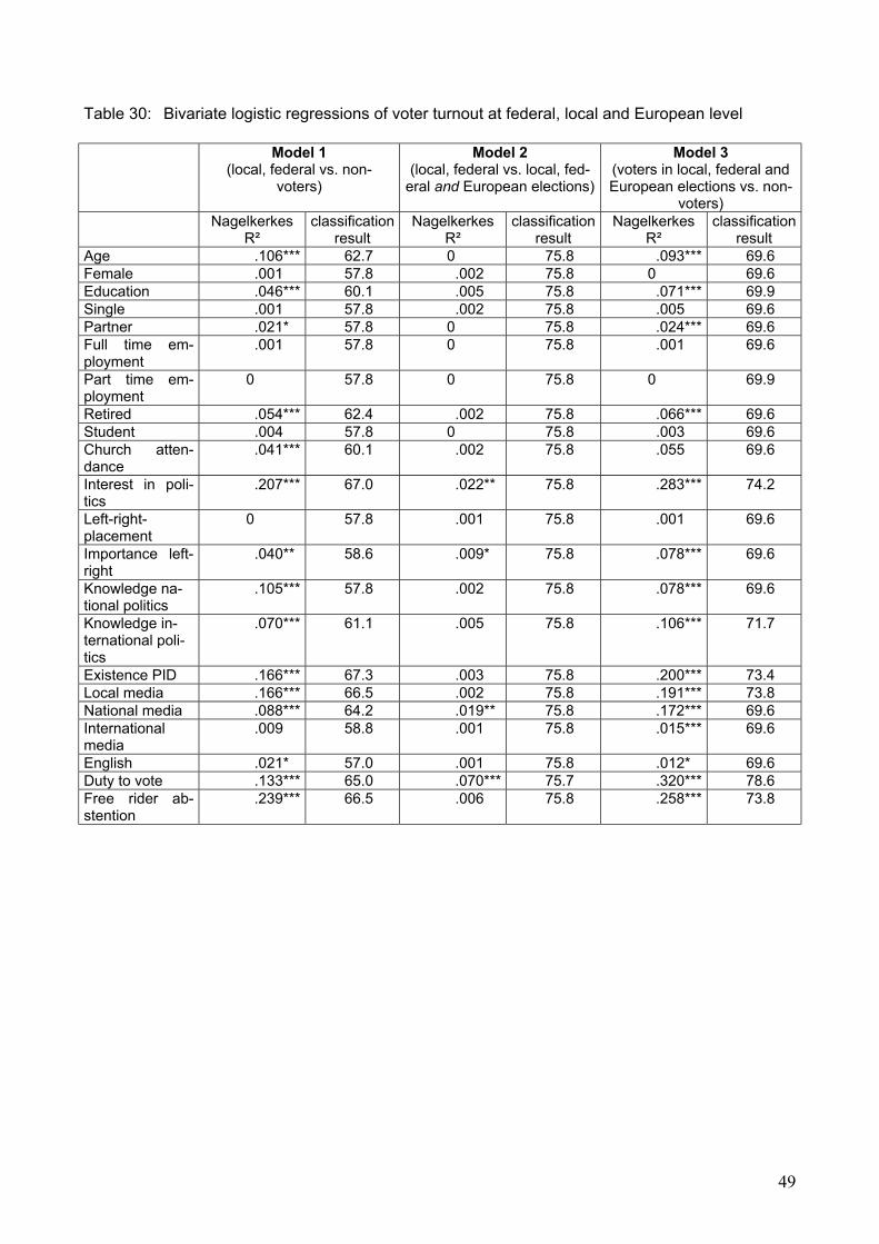
49

Table 30: Bivariate logistic regressions of voter turnout at federal, local and European level Model 1

(local, federal vs. non-voters)

Model 2 (local, federal vs. local, fed-

eral and European elections)

Model 3 (voters in local, federal and European elections vs. non-

voters) Nagelkerkes

R² classification

result Nagelkerkes

R² classification

result Nagelkerkes

R² classification

result Age .106*** 62.7 0 75.8 .093*** 69.6 Female .001 57.8 .002 75.8 0 69.6 Education .046*** 60.1 .005 75.8 .071*** 69.9 Single .001 57.8 .002 75.8 .005 69.6 Partner .021* 57.8 0 75.8 .024*** 69.6 Full time em-ployment

.001 57.8 0 75.8 .001 69.6

Part time em-ployment

0 57.8 0 75.8 0 69.9

Retired .054*** 62.4 .002 75.8 .066*** 69.6 Student .004 57.8 0 75.8 .003 69.6 Church atten-dance

.041*** 60.1 .002 75.8 .055 69.6

Interest in poli-tics

.207*** 67.0 .022** 75.8 .283*** 74.2

Left-right-placement

0 57.8 .001 75.8 .001 69.6

Importance left-right

.040** 58.6 .009* 75.8 .078*** 69.6

Knowledge na-tional politics

.105*** 57.8 .002 75.8 .078*** 69.6

Knowledge in-ternational poli-tics

.070*** 61.1 .005 75.8 .106*** 71.7

Existence PID .166*** 67.3 .003 75.8 .200*** 73.4 Local media .166*** 66.5 .002 75.8 .191*** 73.8 National media .088*** 64.2 .019** 75.8 .172*** 69.6 International media

.009 58.8 .001 75.8 .015*** 69.6

English .021* 57.0 .001 75.8 .012* 69.6 Duty to vote .133*** 65.0 .070*** 75.7 .320*** 78.6 Free rider ab-stention

.239*** 66.5 .006 75.8 .258*** 73.8

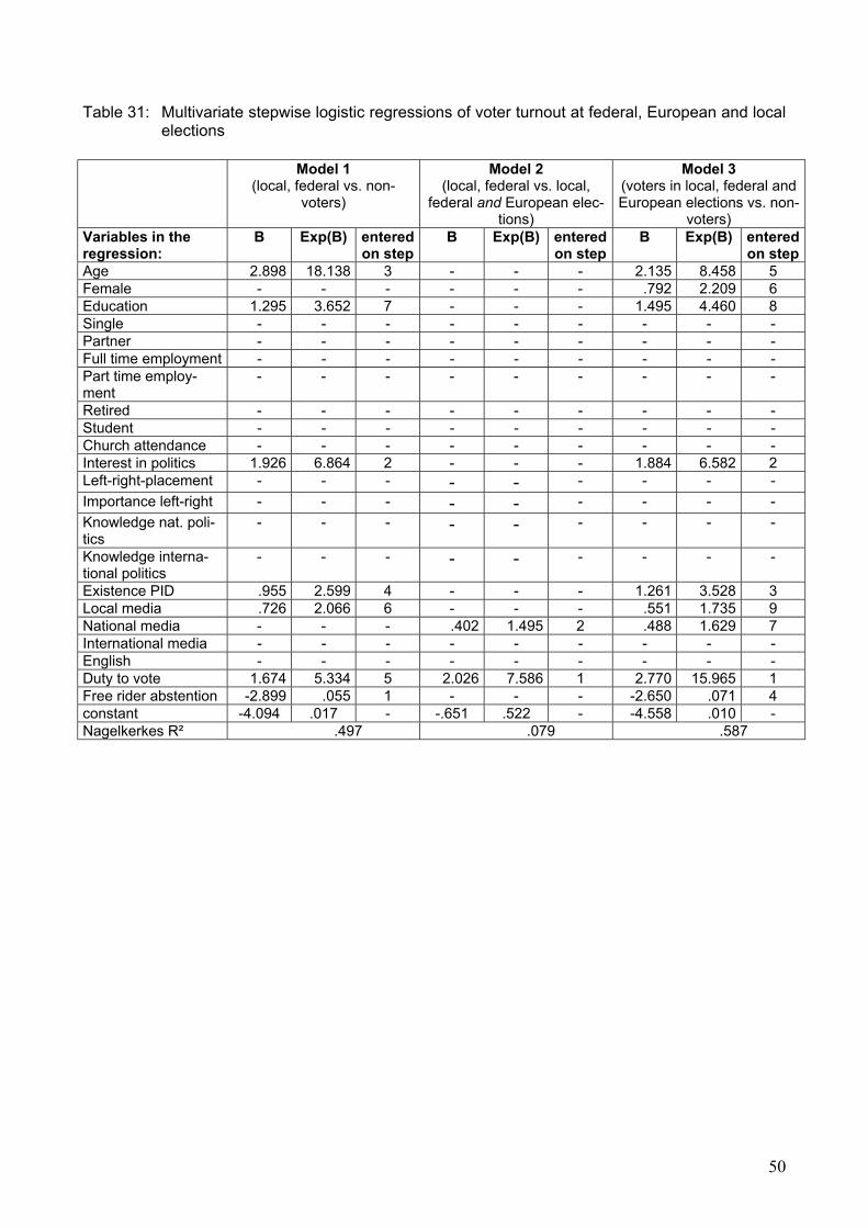
50

Table 31: Multivariate stepwise logistic regressions of voter turnout at federal, European and local elections

Model 1

(local, federal vs. non-voters)

Model 2 (local, federal vs. local,

federal and European elec-tions)

Model 3 (voters in local, federal and European elections vs. non-

voters) Variables in the regression:

B Exp(B) entered on step

B Exp(B) entered on step

B Exp(B) entered on step

Age 2.898 18.138 3 - - - 2.135 8.458 5 Female - - - - - - .792 2.209 6 Education 1.295 3.652 7 - - - 1.495 4.460 8 Single - - - - - - - - - Partner - - - - - - - - - Full time employment - - - - - - - - - Part time employ-ment

- - - - - - - - -

Retired - - - - - - - - - Student - - - - - - - - - Church attendance - - - - - - - - - Interest in politics 1.926 6.864 2 - - - 1.884 6.582 2 Left-right-placement - - - - - - - - - Importance left-right - - - - - - - - - Knowledge nat. poli-tics

- - - - - - - - -

Knowledge interna-tional politics

- - - - - - - - -

Existence PID .955 2.599 4 - - - 1.261 3.528 3 Local media .726 2.066 6 - - - .551 1.735 9 National media - - - .402 1.495 2 .488 1.629 7 International media - - - - - - - - - English - - - - - - - - - Duty to vote 1.674 5.334 5 2.026 7.586 1 2.770 15.965 1 Free rider abstention -2.899 .055 1 - - - -2.650 .071 4 constant -4.094 .017 - -.651 .522 - -4.558 .010 - Nagelkerkes R² .497 .079 .587

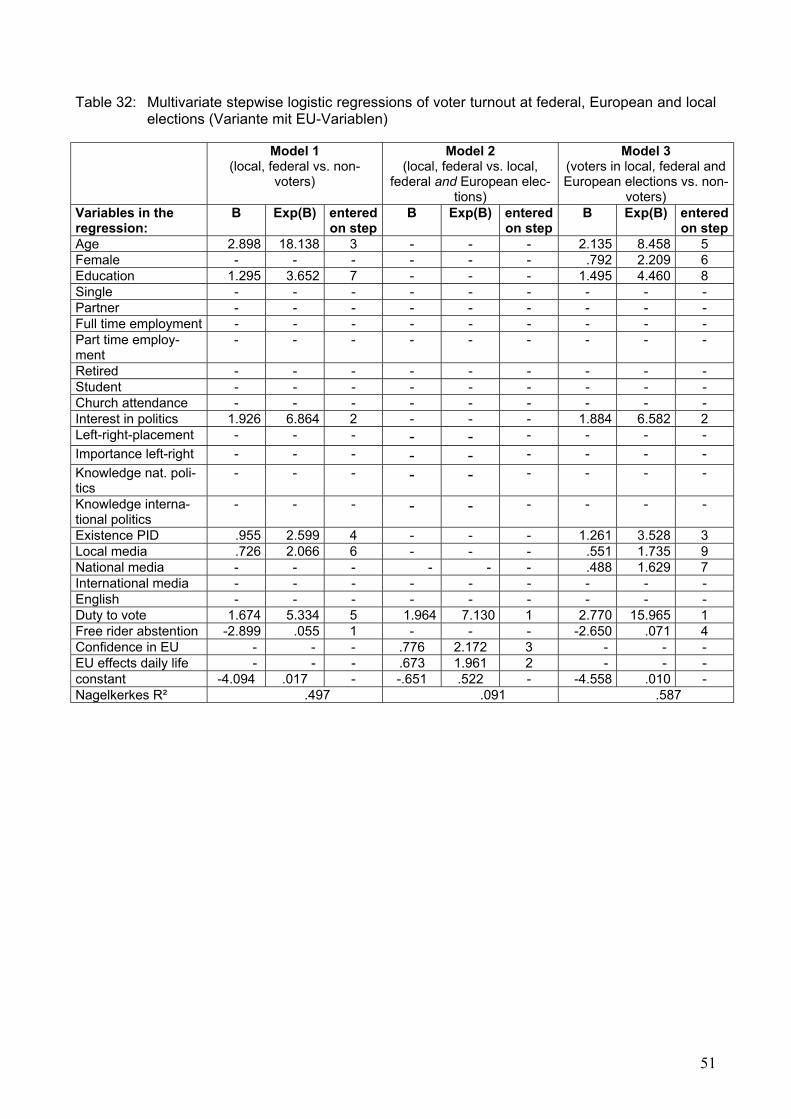
51

Table 32: Multivariate stepwise logistic regressions of voter turnout at federal, European and local elections (Variante mit EU-Variablen)

Model 1

(local, federal vs. non-voters)

Model 2 (local, federal vs. local,

federal and European elec-tions)

Model 3 (voters in local, federal and European elections vs. non-

voters) Variables in the regression:

B Exp(B) entered on step

B Exp(B) entered on step

B Exp(B) entered on step

Age 2.898 18.138 3 - - - 2.135 8.458 5 Female - - - - - - .792 2.209 6 Education 1.295 3.652 7 - - - 1.495 4.460 8 Single - - - - - - - - - Partner - - - - - - - - - Full time employment - - - - - - - - - Part time employ-ment

- - - - - - - - -

Retired - - - - - - - - - Student - - - - - - - - - Church attendance - - - - - - - - - Interest in politics 1.926 6.864 2 - - - 1.884 6.582 2 Left-right-placement - - - - - - - - - Importance left-right - - - - - - - - - Knowledge nat. poli-tics

- - - - - - - - -

Knowledge interna-tional politics

- - - - - - - - -

Existence PID .955 2.599 4 - - - 1.261 3.528 3 Local media .726 2.066 6 - - - .551 1.735 9 National media - - - - - - .488 1.629 7 International media - - - - - - - - - English - - - - - - - - - Duty to vote 1.674 5.334 5 1.964 7.130 1 2.770 15.965 1 Free rider abstention -2.899 .055 1 - - - -2.650 .071 4 Confidence in EU - - - .776 2.172 3 - - - EU effects daily life - - - .673 1.961 2 - - - constant -4.094 .017 - -.651 .522 - -4.558 .010 - Nagelkerkes R² .497 .091 .587

52

4. Conclusion In this chapter it once more proved true that the turnout puzzle has too many pieces to be fixed completely. We will summarize what the data told us, referring to the four different aspects of turnout that were explicated in the introduction. Differences in turnout rates between levels of governance are a well known phe-nomenon, usually explained by the second-order election model. However, that model does not specify why a certain election type is second-order. It rather talks about the consequences of the general perception that less is at stake in certain types of elections. The consequences predicted by the second-order model were confirmed by the ECOL analysis in this chapter. The concepts of facilitation and mo-bilisation were proposed in this book as possible explanations that can tell us more about why people do perceive European Parliament elections as less important. Fa-cilitation, however, can only be a meaningful explanation if there is variation. Within Germany this variation is limited, as the electoral rules are, if not the same, quite similar. Mobilisation in the rather broad definition seems to be better suited for ex-plaining differences in turnout between levels. For the individual decision to turn out, the voters might not calculate costs and benefits explicitly, however, they do ask themselves, what they are to decide on and if it matters to them what alternative will be chosen. In the case of European elections, many people do not know much about what the parliament does, however, they do know or feel that it has less power than the Bundestag. As parties do not polarize about European questions even in cam-paigns, voters do not anticipate any big difference between one party winning or the other. Consequently, individual data analysis showed that it is even for the voters in European elections not the special interest in EU-politics, but a feeling of a duty to vote, in the best case to support the system in general, that mobilizes them. Development of turnout over time was mainly discussed in this chapter in a descrip-tive manner. The regression analysis showed that we can talk about a decline of turnout, at least in West-Germany. For East-Germany simultaneous elections and the short time period cause problems in assessing a trend, especially for European elec-tions. The survey data give some evidence that a rather unexciting and not very po-larizing campaign like in the course of the 1999 European election does contribute to low participation rates. For analysing turnout in geographical terms Germany provides an interesting, but also difficult case. Interesting, because of the heterogeneity of the country in terms of economic development, political history and present political situation, difficult, be-cause federalism produces many different settings for a certain election in different states. Simultaneous elections are the most obvious case, the existence of two dif-ferent party systems in West- and East-Germany, however, might have some influ-ence on turnout as well as different power constellations between the parties in the states. This causes problems for analysing turnout with aggregate data, because those variations in settings had to be included. That more effort is needed to capture those variation becomes obvious when dummy variables for states do contribute substantially to explain variance of turnout. In some respects the German case re-sembles more a comparative study in itself. For improving the explanation of turnout by aggregate data we therefore might need to incorporate indicators developed in comparative studies. The last aspect of turnout is probably the one that has been studied most in recent years: correlates of turnout at the individual level. The results of that previous re-search are confirmed here in large parts. While socio-demographics like age, income and education, that in many respects have facilitating effects, do contribute some explanatory power, the more direct reason to participate in elections is interest in

53

politics coming along with knowledge and the feeling of efficacy. To identify the char-acteristics of voters in European elections, however, proves a difficult task. The data available are not perfectly suited as the Eurobarometers hardly contain any vote in-tention other than for European and sometimes federal elections. In the ASES data set indicators for interest in EU politics and attitudes to the EU are rare. However, with these restrictions in mind, the ASES survey reveals an interesting finding. A feel-ing of a duty to vote and consumption of national media, which might be a proxy for interest in more than only the immediate surroundings in the local area, are the only characteristics that distinguish voters in European elections from non-voters in Euro-pean elections. However, the conclusion that voters in European elections do not vote because of an interest in European issues, but more or less because of a sense of duty, might be too premature as those attitudes towards Europe could not be in-cluded. There remain many pieces of the puzzle to be fixed!

54

Eilfort, Michael (1994) Die Nichtwähler: Wahlenthaltung als Form des Wahlverhaltens. Paderborn: Schöningh. Roth, Dieter (1992) Sinkende Wahlbeteiligung – eher Normalisierung als Krisensymptom, in Starzacher, Karl et al. (Ed.), Protestwähler und Wahlverweigerer: Krise der Demokratie? Köln: Bund-Verlag, 58-68. Feist, Ursula (1992) Niedrige Wahlbeteiligung - Normalisierung oder Krisensymptom der Demokratie in Deutschland? in Starzacher, Karl et al. (Ed.), Protestwähler und Wahlverweigerer. Köln: Bund-Verlag, 40-57. Kleinhenz, Thomas (1995) Die Nichtwähler. Opladen: Westdeutscher Verlag GmbH. Reif, Karlheinz, Hermann Schmitt (1980) Nine Second-Order National Elections – A Conceptual Framework for the Analysis of European Elections Results, in: European Journal of Political Research 1980, Vol. 8: 3-44. Blumler, Jay G., Anthony D. Fox (1982): The European Voter: Popular responses to the first Community election, London: Policy Studies Institute. Cautrès, Bruno, Richard Sinnott (2002): The 1999 European Parliament Elections and the Political Culture of European Integration, in: Perrineau, Pascal, Gérard Grunberg and Colette Ysmal: Europe at the Polls: The European Elections of 1999, New York: Palgrave, 3-21. Margedant, Udo (2003): Die Föderalismusdiskussion in Deutschland, in: Aus Politik und Zeitgeschichte, B29-30 (2003), 6-13. Falter, Jürgen (1991): Hitlers Wähler, München: C.H. Beck. Schauff, Johannes (1928): Das Wahlverhalten der deutschen Katholiken im Kaiserreich und in der Weimarer Republik. Untersuchungen aus dem Jahre 1928, Köln: Bachem. Troitzsch, Klaus G. (1976): Sozialstruktur und Wählerverhalten. Möglichkeiten und Grenzen ökologischer Wahlanalyse, dargestellt am Beispiel der Wahlen in Hamburg von 1949 bis 1979, Meisenheim am Glan: Hain. Wernicke, Immo H. (1976): Die Bedingungen politischer Partizipation. Eine international vergleichende Kontext- und Aggregatdatenanalyse für Großbritannien, Norwegen, Deutschland (BRD) und Frankreich, Meisenheim am Glan: Hain. Schoof, Peter (1980): Wahlbeteiligung und Sozialstruktur in der Bundesrepublik Deutschland. Eine politikwissenschaftlich-statistische Aggregatdatenanalyse sozialstruktureller und ökonomischer Bestimmungsfaktoren der Wahlbeteiligung bei Bundes- und Landtagswahlen zwischen 1972 und 1976, Frankfurt a.M.: Haag und Herchen. Heberle, Rudolf (1963): Landbevölkerung und Nationalsozialismus. Eine soziologische Untersuchung der politischen Willensbildung in Schleswig-Holstein 1918 bis 1932. Stuttgart: DVA.

55