Geophysics/Meteorology Honours Projects 2011-2012

Course organiser: David Stevenson (dstevens@staffmail.ed.ac.uk), Crew 314

Course secretary: Emma Latto (emma.latto@ed.ac.uk), Grant 332

This document lists the projects on offer for senior honours (4th

year) students

registered on the Geophysics/Geophysics and Geology/Geophysics and Meteorology

programs. The meteorology projects (and potentially some of the others too) are also

on offer to Physics with Meteorology students (if Physics with Met students are

unsure whether projects are suitable, they should contact the CO/supervisor).

If you are interested in a particular project, please contact the main supervisor to

discuss what is involved in more detail. You need to choose a project and also a

second choice, for each semester (semester 2 choices can be revised later). In some

cases you won’t be able to do your first choice (for example if it is chosen by multiple

people, and the supervisor cannot run several variants of the same project). If you

can’t do your first choice, we will try and make sure you do get your first choice in

semester 2. Where projects are over-subscribed, the decision of the CO (generally in

consultation with the supervisor) will be final.

Project choices for semester 1 (and provisional choices for semester 2) should be

emailed to the CO (email address above) by Wednesday in Week 1 (21st Sept), and

finalised allocations will be made by the end of Week 1 (23rd

Sept) so that you have

sufficient time to fully tackle the project.

Exceptionally, students can propose their own projects, but they will need to identify

a suitable supervisor (amongst the geophysics/meteorology staff), and convince that

supervisor and the CO that the project is sensible and feasible. Again, students should

do this as soon as possible in the semester, to fit with the above timetable.

Most projects listed here are one semester, 20-credit projects. In some cases, semester

1 projects can be extended to be 40-credit projects (and some are offered on this basis

from the outset). If students wish to extend their semester 1 project, they will need to

get the supervisor’s and the CO’s agreement, before week 7 of semester 1.

Any projects/combinations of projects can be taken, irrespective of whether you are a

Geophysics or a Geophysics and Meteorology/Geology student.

As part of the introduction to year 4 (Thursday September 15, 10 to ~1130, in Grant

304b) projects will be introduced by the CO, along with examples of good (and bad)

practice in how students should tackle their projects, including writing them up. It is

up to students to contact potential project supervisors to discuss projects (supervisor’s

contact details should be included in the project descriptions). If supervisors cannot be

contacted, please let the CO know.

In the middle of semester 2 (during ‘Innovative Learning Week’: 20-24 February

2012), students will be expected to give a short presentation on their semester 1

project, or, if they are doing a single 40-credit project, on that. This presentation will

not count towards your final project mark, but does contribute towards the final mark

on the ‘Transferable Skills for Geophysicists’ course.

Influence of Quaternary climate change on landscape evolution at geological time scales.

Mikaël Attal, Simon Tett & Richard Essery

(mikael.attal@ed.ac.uk, simon.tett@ed.ac.uk, richard.essery@ed.ac.uk)

20 credits (S1 or S2; possibility of extending to 40 credits)

Over the last decades, theoretical, experimental and numerical modelling studies have

shown that a landscape experiencing constant uplift and climate eventually reaches a

stable form characterized by erosion rates matching uplift rates at any point in the

landscape. The morphology of these landscapes in “steady-state” has been described

by these studies. For example, the simplest model predicts concave up river profiles

and an inverse power relationship between slope and drainage area, typically with an

exponent -0.5. Scientists have been using these criteria to assess whether landscapes

are in steady-state and met some success in a number of tectonically active areas such

as Taiwan or the Oregon Coast Range (USA). However, other studies have

demonstrated that the response time of landscapes to a disturbance (tectonic or

climatic change) is typically of the order of 105-10

6 years. Climate has been changing

dramatically over the Quaternary (last 2 Ma), alternating between glacial and

interglacial periods over time scales of 104-10

5 years. One can thus ask: how can any

modern terrestrial landscape be in steady-state? Or, alternatively, can a landscape

forced by a cyclic climate exhibit features that mimic steady-state landscapes?

These are the questions that this project will address. The project will use the

Channel-Hillslope Integrated Landscape Development (CHILD) model coupled with

Matlab code to analyse the evolution and morphology of a series of well studied

catchments in the Apennines (Italy). The model will be fed with climate data which

have been generated by the regional climate model HadRM3 for the Apennines for the

present and for the Last Glacial Maximum (LGM). This study will investigate the

differences in morphology between catchments experiencing (1) constant climate and

(2) alternating glacial-interglacial periods during the Quaternary.

Figure 1: November

mean rainfall rate

(kg.m-2

s-1

) predicted

by HadRM3 for the

Pre-Industrial period

(PI) and LGM

(courtesy Ian

McKenzie).

References:

Attal, M., P. A. Cowie, A. C. Whittaker, D. Hobley, G. E. Tucker, and G. P. Roberts (2011), Testing

fluvial erosion models using the transient response of bedrock rivers to tectonic forcing in the

Apennines, Italy, J. Geophys. Res., 116, F02005, doi:10.1029/2010JF001875.

Tucker, G. E., and R. L. Slingerland (1997), Drainage basin responses to climate change, Water

Resour. Res., 33, 2031– 2047.

Detection of anomalous signals in geomagnetic observatories: the subtle impact of man-

made noise in measurements

Ciarán Beggan (BGS) [ciar@bgs.ac.uk], David Kerridge (BGS) and Kathy Whaler (School of GeoSciences)

Geomagnetic observatories have traditionally been

located in isolated areas far from the unwanted

electric and magnetic influence of daily human

activity. In the UK, the first observatories were

moved from central London to the countryside in

Devon (Hartland) and southern Scotland

(Eskdalemuir), after the start of the electrification of

the train network in 1909. However, over time, even

these remote locations have become influenced by

man-made noise, as local infrastructure such as

roads, buildings and electrical networks impinge on

the once peaceful environment (see Figure).

Geomagnetic observatories will soon move to issuing

one-second records of the magnetic field (rather than

one-minute). This will result in greater sensitivity to

unwanted noise. As we cannot realistically move the

observatories to quieter locations, we must now develop tools to detect and remove signals in the data

which do not occur naturally. Obvious spikes and offsets are detectable by the trained human eye, but

subtle noise sources can pervade the data and are particularly difficult to spot. These unwanted signals

can have a major impact on the quality of the long-term record at an observatory, degrading the

usefulness of the data over timescales of years to decades and perhaps even centuries.

We propose to use a signal processing technique employing wavelet transforms to analyse data for

certain types of noise. Wavelet transforms are often compared with the Fourier transform, in which

signals are represented as a sum of sinusoids. The main difference is that wavelets can be localized in

both time and frequency whereas the standard Fourier transform is only localized in frequency.

Wavelets are very flexible and can be defined to enhance or optimally process a particular frequency of

interest, for example. Their use in time series analysis is now widespread throughout earth and

atmospheric sciences.

The project will be broken into two parts: (a) examination of synthetic data generated by adding noise to

an observatory record to see which types of wavelet can identify the noise correctly and (b) the

examination of several observatory datasets with known issues of man-made contamination to see if

wavelets can identify the sources, and provide a possible method for reducing their influence in the data.

This project will use Matlab and/or the R programming language to process the (real and synthetic)

observatory data. Much of the code has already been developed in the (free) R package, which is well

suited to this type of analysis. Example observatory data and code will be supplied by BGS and the

student will update and adapt this code for the project, using similar skills to those learnt with Matlab.

This is envisaged as a one-semester project (available in S1 or S2), though extendable by agreement to a

two-semester project (if started in S1).

References: R Development Core Team (2008), R: A Language and Environment for Statistical Computing, R Foundation for Statistical

Computing, Vienna, Austria, ISBN 3-900051-07-0; www.R-project.org.

Reda, J., Fouassier, D., Isac, A., Linthe, H-J., Matzka J., and C.W. Turbitt (2011), Improvements in Geomagnetic Observatory

Data Quality, Geomagnetic Observations and Models, IAGA Special Sopron Book Series, Volume 5, 127-148, DOI:

10.1007/978-90-481-9858-0_6

Valens, C., (2010), A Really Friendly Guide to Wavelets, http://polyvalens.pagesperso-

orange.fr/clemens/wavelets/wavelets.html

Hartland Geomagnetic

Observatory

Encroachment of Hartland Village towards the BGS

geomagnetic observatory

Is the Earth's core 'ringing' with periods of 6, 80 or 160 years? Empirical Mode

Decomposition of long-term geomagnetic observatory data

Ciarán Beggan (BGS) [ciar@bgs.ac.uk] and Kathy Whaler (School of GeoSciences)

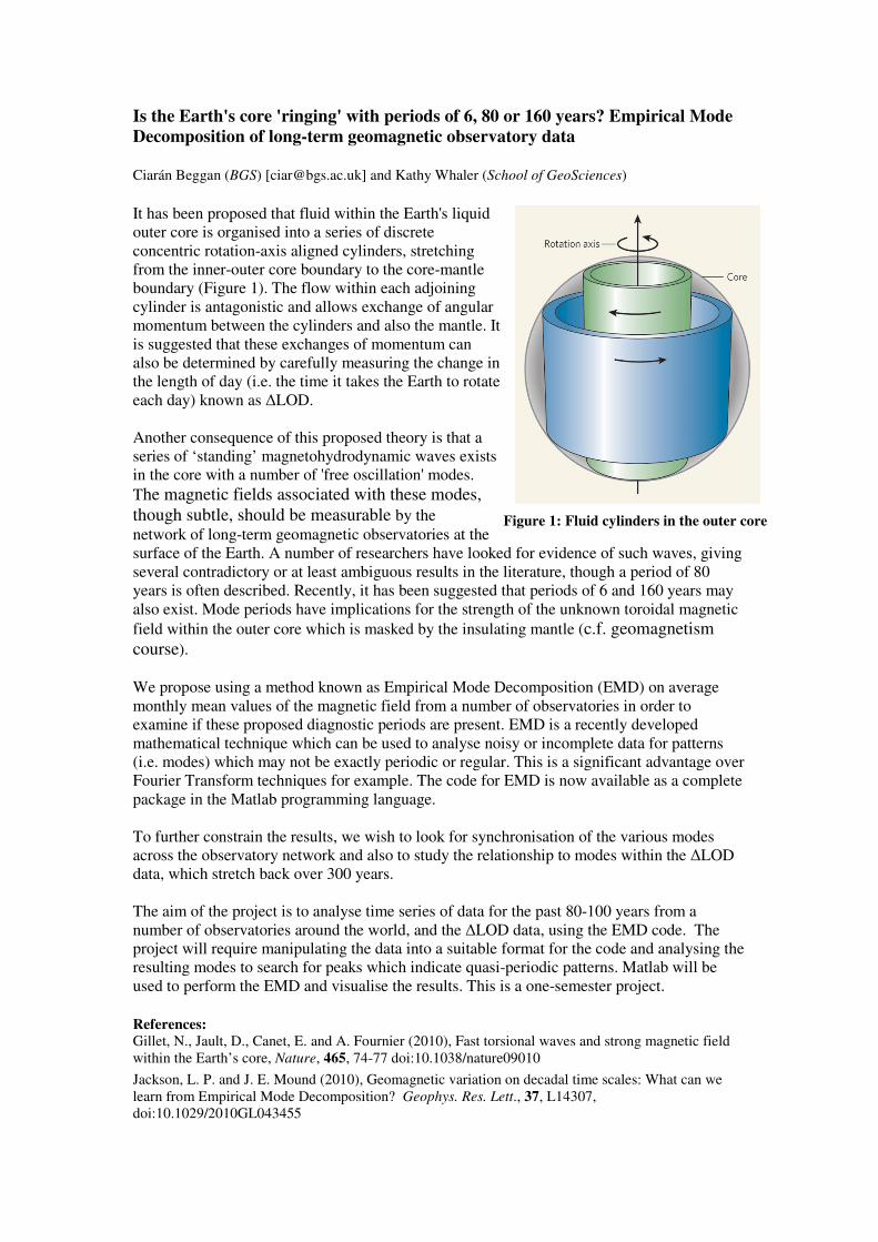
It has been proposed that fluid within the Earth's liquid

outer core is organised into a series of discrete

concentric rotation-axis aligned cylinders, stretching

from the inner-outer core boundary to the core-mantle

boundary (Figure 1). The flow within each adjoining

cylinder is antagonistic and allows exchange of angular

momentum between the cylinders and also the mantle. It

is suggested that these exchanges of momentum can

also be determined by carefully measuring the change in

the length of day (i.e. the time it takes the Earth to rotate

each day) known as �LOD.

Another consequence of this proposed theory is that a

series of ‘standing’ magnetohydrodynamic waves exists

in the core with a number of 'free oscillation' modes.

The magnetic fields associated with these modes,

though subtle, should be measurable by the

network of long-term geomagnetic observatories at the

surface of the Earth. A number of researchers have looked for evidence of such waves, giving

several contradictory or at least ambiguous results in the literature, though a period of 80

years is often described. Recently, it has been suggested that periods of 6 and 160 years may

also exist. Mode periods have implications for the strength of the unknown toroidal magnetic

field within the outer core which is masked by the insulating mantle (c.f. geomagnetism

course).

We propose using a method known as Empirical Mode Decomposition (EMD) on average

monthly mean values of the magnetic field from a number of observatories in order to

examine if these proposed diagnostic periods are present. EMD is a recently developed

mathematical technique which can be used to analyse noisy or incomplete data for patterns

(i.e. modes) which may not be exactly periodic or regular. This is a significant advantage over

Fourier Transform techniques for example. The code for EMD is now available as a complete

package in the Matlab programming language.

To further constrain the results, we wish to look for synchronisation of the various modes

across the observatory network and also to study the relationship to modes within the �LOD

data, which stretch back over 300 years.

The aim of the project is to analyse time series of data for the past 80-100 years from a

number of observatories around the world, and the �LOD data, using the EMD code. The

project will require manipulating the data into a suitable format for the code and analysing the

resulting modes to search for peaks which indicate quasi-periodic patterns. Matlab will be

used to perform the EMD and visualise the results. This is a one-semester project.

References: Gillet, N., Jault, D., Canet, E. and A. Fournier (2010), Fast torsional waves and strong magnetic field

within the Earth’s core, Nature, 465, 74-77 doi:10.1038/nature09010

Jackson, L. P. and J. E. Mound (2010), Geomagnetic variation on decadal time scales: What can we

learn from Empirical Mode Decomposition? Geophys. Res. Lett., 37, L14307,

doi:10.1029/2010GL043455

Figure 1: Fluid cylinders in the outer core

Coulomb stress changes and earthquakes associated with the Afar dyke sequence, 2005-2011

Andrew Bell (a.bell@ed.ac.uk) and Kathy Whaler (kathy.whaler@ed.ac.uk)

Understanding the processes responsible for earthquake triggering is an important

outstanding challenge in geophysics. Changes in the Coulomb stress (a combination

of the normal and shear stresses) acting on a fault are likely to play a role in

earthquake triggering; however, the effect is difficult to quantify in tectonic

seismicity. Coulomb stress changes are also associated with magmatic processes and

may explain the spatial distribution of earthquakes associated with magma

emplacement. In this project, the student will use a Matlab application, Coulomb 3.0

(http://earthquake.usgs.gov/research/modeling/coulomb/), to investigate the evolution

of Coulomb stress associated with a sequence of dyking episodes in the Afar region of

Ethiopia and the correlation with earthquake occurrence. A previous student installed

and tested the software, and set up data files and scripts, which are available for

modification for this project.

Afar is in the late stages of continental break-up, with

strain localised along magmatic segments, very similar

to slow-spreading mid-oceanic ridge segments, which

are episodically active. An on-going sequence of

dyking events began on the Dabbahu segment in

September 2005. In the first event, 2.5 km3

of magma

was intruded in two weeks along a 60km dyke (Wright

et al., 2006). 12 subsequent events have been

identified, intruding a further 0.6 km3 of magma,

mostly in dykes ~10km long and 0.5-2m wide. Work

on the 2005 dyke suggests a good correlation between

coulomb stress changes and earthquake occurrence and

has refined a hypothesis for earthquake triggering by

dykes. This project will test this hypothesis by

calculating time-dependent Coulomb stress changes

for the subsequent dykes (based on their propagation

direction and speed, as inferred from seismicity and

inSAR data), and comparing them to the spatial and

temporal evolution of seismicity.

References Hamling, I., A. Ayele, L. Bennati, E. Calais, C.J. Ebinger, D. Keir, E. Lewi, T.J. Wright & G.Yirgu

(2009), Geodetic observations of the ongoing Dabbahu rifting episode: new dyke intrusions in 2006

and 2007. Geophysical Journal International, doi:10.1111/j.1365-246X.2009.04163.x

Wright, T.J., C. Ebinger, J. Biggs, A. Ayele, G. Yirgu, D. Keir & A. Stork, (2006) , Magma-maintained

rift segmentation at continental rupture in the 2005 Afar dyking episode. Nature, 442, 291-294

Belachew, M., C. Ebinger, D. Coté, D. Keir, J. V. Rowland, J. O. S. Hammond, and A. Ayele (2011),

Comparison of dike intrusions in an incipient seafloor-spreading segment in Afar, Ethiopia: Seismicity

perspectives, J. Geophys. Res., 116, B06405, doi:10.1029/2010JB007908

Calculated Coulomb stress changes

and earthquake epicentres during the

2005 dyke intrusion at Afar.

An investigation of Gurevich’s model for velocity and attenuation of partially

saturated rocks.

Mark Chapman (Mark.Chapman@ed.ac.uk)

Many geophysical problems, such as hydrocarbon reservoir characterization and

monitoring of CO2 sequestration, require knowledge of the seismic properties of

rocks saturated with multiple fluids. Unfortunately, we have no uniformly accepted

model for wave propagation in such media. Various simple approaches (such as

combining the “Gassmann” and “Wood” equations) have had some success but many

problems remain. In particular, great uncertainty surrounds the modelling of seismic

attenuation. A recent paper by Gurevich et al. (2011) advances a simple model with

some appealing features.

In this project, the student will write code to implement Gurevich’s model in an

environment such as MATLAB. This will allow a numerical investigation of the

predictions of the model concerning variations in factors such as gas saturation and

fluid pressure for a variety of rock types. The predictions will be compared against

those from alternative approaches developed recently in Edinburgh, allowing the

student to judge the relative strengths and weaknesses of the models and assess the

robustness of recently proposed schemes to invert seismic data for gas-saturation on

the basis of dispersive properties.

Reference

Gurevich, B., Makarynska, D., Bastos de Paula, O. and Pervukhina, M., 2011. A

simple model for squirt-flow dispersion and attenuation in fluid-saturated granular

rocks. Geophysics, 75, No. 6, N109-120.

Measuring changes in seismic velocity beneath Eyjafjallajökull and Katla using passive seismic interferometry, and assessing

their relationship with volcanic activity

Andrew Curtis (University of Edinburgh, andrew.curtis@ed.ac.uk) Brian Baptie (British Geological Survey)

Project Summary

A fundamental goal of volcanology is improved forecasting of volcanic eruptions through long term monitoring of changes in volcanic behaviour. This requires reliable methods to measure small changes in sub-surface properties over long periods of time that may be related to changes in volcanic activity.

Recent research has shown that the cross correlation of the background seismic noise recorded at two seismic stations can provide an effective estimate of the elastic properties of the Earth, or indeed ‘virtual’ seismograms between the two stations as though a source had existed at the location of one or other. This novel imaging method, seismic interferometry, is revolutionising subsurface monitoring as it can be used to measure tiny changes in seismic velocity that might result from magma pressurization, lava dome collapse or other changes in the stress field. The technique requires only one or a few permanent seismic monitoring stations and does not require an external earthquake or active source, so can provide information even during periods of seismic quiescence.

The aim of this study is to identify possible spatial and temporal changes in seismic velocity using data recorded during the eruption of Eyjafjallajökull on Iceland, to integrate these with new data from Katla (which is expected to erupt within the next few years), and to investigate the relationship between such changes and volcanic activity. Reference seismograms from specific time periods will be used to measure spatial and temporal changes by comparison with seismograms calculated using interferometry over shorter time periods. Any temporal changes in seismic velocity will be identified and the results will be compared with geodetic observations recorded during the course of the survey.

Improved understanding of the relationship between changes in seismic velocity measured from the seismic noise field and volcanic processes could provide valuable near-real-time information with which to monitor and predict changes in a volcano’s behaviour and, ultimately, to forecast eruptions.

[1 or 2 semester project]

Figure: The eruption of Eyjafjallajökull

on Iceland.

����������� ���������������� ��������� ��������� ���

������ �����

������������ ������������������������������������� �������������������������

�� ��������� ����� � � �� ������������� �������������� � � ��������� ���� ���� ���� � ��

����������� ��� ���������� �� ������ ������������� �� ���� � � �� �� ����� ��� ���

����������� �� ������ �� ��������� ��� ����������� ������ ������ ����� ���� ����� ����� �������

�������������������������������������������������������� � ������������� ����� �����

���� ��� ���� !� ���� ����������� ��� ���� ������ ���� ���� ������ ����������� ������� ���� ����

�� ������� � � ���������� � ��� ���� �� �� ��� � ������� ������� ���������� ����� ����

��������� ������������� ������������������������� ������ �������������� �"�� �#���������

���������������� ��������������������������������� �� �������������������������� ��

�������� ����� � � �� �������� �� ������ ���������� � ����� ���������� ���� ���� "�� ���#�

�� ���������

���������������������������������� ��� $����������� �� ������ ������������������

����� �������� ����� �����%�������&� ������������ �� �������������������������������

������ ����� ������������������������������������������������������������� �� ����������

��������������������������� �� ������������ ������������������ ������������������# �

�������� ����� ������� ����� ���������� ���� ��� ������ ��� '������ ( �!� �� � �� �� ������

������ ��� )���������� ������ *�+� ��� �� ��� ����������� ����� ������� ����� �� �� ��

������� ������� ,+�)�� ���� ����� ������ ��� '������ ( �!� �� � ���� �������� �� ������

�����������������������������������-.��� �������� �� ������ ����������� ����� �

,+�)����*�+��/�������������������� ��������������������������� ��'������( �!� �� �����

�� ������������� ������� ���������������������� ���� �� ����� ��������������������

���������������������� �������������������������)���������� �� ����������������������� �

������������������������ ������������������������������������������

�

�

�

�

�

�

�

�

����� ��� �!� �� ����� � ���

)���������� ����� � *�+� ���,+�)� ���

0$(. ������� �!�������� �����������

���� ���� ��� 1�0 � ������ '���

2������������� 3..0!��

�!� �!�

��� ��� !� "#� $�%�������& � 4�� �� ������ � ��5���� ��� ������������ ������6������!� �������

��� ������ ��� ����� ���� �����2���� ��������� ����� ��� ��������������� ����'������

3�������������������� ��� ���������������� /��� ����������3.((!���

$��� ��%� �'� ���� ��� ��� ��� �� ������ �� �� ��%����� ���&� �� ���'��%� �������� ����%���

����'���%����(����������%�%���������������"#)�������������'����������%��������

%������ ��� ������ �� ���������� ��� ������ �'� ��� �(��'���� �'� ��� "#�� $���� %��� �����

����������������'����(�������� ������������'���*+��%�������� ������������������

7�� ���� ��� ����������������� ��� ��8/49� ����������� �������� ��� �������� �� ������

��� ������ ��������� ������� � ���� � � %2�� ��������� � � )�&��/��� ����� ��� � ��5����

��������� ���������:���� ��6��������2���������,����� ���� ����

,���������-������&�

)���� ������6�� ���������2����;���2�������;������<���������=���3..>��2�� ����4�������������

?����������� ������ �������$���.�������/���������(.@3�?�(.A3�� ���������������B��

������ ��������C��� C������ �!���

/��� �������)���� ������:������:������6������������3.((��2�� ����4������������������������

/� ������������������:���� ��4 �� ��*������� �������6���� � D�� �������� ���

������������B�������� ��������C��� C������ �!��

2�������/���)��������,���2�������+������;��E�������,���3..0������$;� ������2������$<����

���������������������2�� ����/� ������������ !"����01(0��(>(0�?�(>(@��

�

�

�������;������������������ ����������� � ��� �!� 0� ��� �� ��� �!� (3� ��� �� 2�� ������ �� ������

��������������������� ��

�!� �!�

Cloud properties and lightning

Ruth Doherty (ruth.doherty@ed.ac.uk), Hugh Pumphrey (H.C.Pumphrey@ed.ac.uk)

20 credits (S1 or S2; possibility of extending to 40 credits)

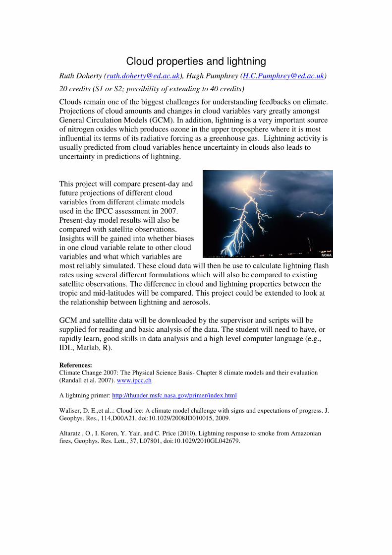
Clouds remain one of the biggest challenges for understanding feedbacks on climate.

Projections of cloud amounts and changes in cloud variables vary greatly amongst

General Circulation Models (GCM). In addition, lightning is a very important source

of nitrogen oxides which produces ozone in the upper troposphere where it is most

influential its terms of its radiative forcing as a greenhouse gas. Lightning activity is

usually predicted from cloud variables hence uncertainty in clouds also leads to

uncertainty in predictions of lightning.

This project will compare present-day and

future projections of different cloud

variables from different climate models

used in the IPCC assessment in 2007.

Present-day model results will also be

compared with satellite observations.

Insights will be gained into whether biases

in one cloud variable relate to other cloud

variables and what which variables are

most reliably simulated. These cloud data will then be use to calculate lightning flash

rates using several different formulations which will also be compared to existing

satellite observations. The difference in cloud and lightning properties between the

tropic and mid-latitudes will be compared. This project could be extended to look at

the relationship between lightning and aerosols.

GCM and satellite data will be downloaded by the supervisor and scripts will be

supplied for reading and basic analysis of the data. The student will need to have, or

rapidly learn, good skills in data analysis and a high level computer language (e.g.,

IDL, Matlab, R).

References: Climate Change 2007: The Physical Science Basis- Chapter 8 climate models and their evaluation

(Randall et al. 2007). www.ipcc.ch

A lightning primer: http://thunder.msfc.nasa.gov/primer/index.html

Waliser, D. E.,et al..: Cloud ice: A climate model challenge with signs and expectations of progress. J.

Geophys. Res., 114,D00A21, doi:10.1029/2008JD010015, 2009.

Altaratz , O., I. Koren, Y. Yair, and C. Price (2010), Lightning response to smoke from Amazonian

fires, Geophys. Res. Lett., 37, L07801, doi:10.1029/2010GL042679.

Winter storm traits and the North Atlantic Oscillation (NAO)

Ruth Doherty (ruth.doherty@ed.ac.uk)

20 credits (S2 only)

The last two winters have been extremely cold in the UK. The winter of 2010/2011

was associated with a persistent high pressure system over Greenland and low

pressure over the Baltics. The high pressure blocked westerly winds from crossing the

Atlantic and dragged bitterly cold winds out of the Arctic down over Europe. A

temperature of −21.2 °C was recorded in the Scottish

Highlands at 10 am on the 2 December. It was the coldest

December recorded in the UK since 1890 and as you may

remember the city of Edinburgh had 18 cm of snowfall! The

North Atlantic Oscillation was thought to be the culprit. The

NAO index measures the difference of atmospheric pressure

at sea level between the Icelandic low and the Azores high. A

positive NAO is associated with greater storminess and wetter

weather over northern Europe, whilst a

negative NAO is typically associated with

fewer storms and colder weather. Fred

Pearce from the media reported “the NAO is

an old friend that has swapped its raincoat

and galoshes for gloves and a fur hat.” This

is because typically the NAO has been in a

positive phase since the 1970s but it

switched to a negative phase in 2008/2009

as can be seen in the figure here. However,

in addition to the NAO, another mode of climate variability, the El Niño Southern

Oscillation, may influence weather in the eastern Atlantic (Seager et al. 2010). ENSO

was in different phases in 2009/2010 and 2010/2011.

This project will examine storminess characteristics across the Atlantic and the UK

during negative and positive phases of the NAO. It will use NAO and ENSO index

time-series data and the output from a storm track model (TRACK: http://www.nerc-

essc.ac.uk/~kih/TRACK/Track.html) to examine storm characteristics such as

frequency and intensity of storms and the prevalent locations of the storm tracks.

Questions to be addressed include: Is there a clear association between the NAO and

blocking high pressure systems over Greenland? How do storm characteristics differ

when they originate in cold Arctic air to when they originate in the western North

Atlantic? Are storm numbers and storm tracks locations during negative NAO events

influenced by the phase of ENSO?

References: T. Jung, F. Vitart, L. Ferranti, and J.J. Morcrette (2011), Origin and predictability of the extreme

negative NAO winter of 2009/10, Geophys. Res. Lett., 38, L07701, doi:10.1029/2011GL046786.

R. Seager, Y. Kushnir, J. Nakamura, M. Ting, and N. Naik (2010), Northern Hemisphere winter snow

anomalies: ENSO, NAO and the winter of 2009/10, Geophys. Res. Lett., 37, L14703,

doi:10.1029/2010GL043830.

http://www.cgd.ucar.edu/cas/jhurrell/nao.stat.winter.html

http://www.dailymail.co.uk/sciencetech/article-1341618/Why-cold-Simple--North-Atlantic-Oscillation-

-got-bit-stuck.html

Weather-related health warnings in the UK associated with projections of climate change

Ruth Doherty (ruth.doherty@ed.ac.uk), David Stevenson (dstevens@staffmail.ed.ac.uk)

20 credits (S2 only)

The European heat wave of 2003 resulted in over 2000 premature deaths in the UK as

temperatures soared above 30°C in many areas of the southern UK. As a result, the UK Met

Office operates a Heat-Health Watch system in

England and Wales from 1 June to 15 September

each year in association with the Department of

Health.

The Heat-Health Watch system comprises four

levels of response based upon threshold maximum

daytime and minimum night-time temperatures for

different UK regions. For example, in North-East

England, if temperatures exceed 28°C during the

day, then fail to fall below 15°C on the following

night, and there is a 90% chance that the forecast

for the next day is also >28°C, a level 3 (the

second highest) warning is issued.

UKCP09 is the latest assessment of future climate

projections across the UK based on low, medium

and high future emissions scenarios. These

projections are based around the idea of providing

probabilistic information as opposed to a “best”

estimate of future climate change. Uncertainty estimates are associated with uncertainty in

initial conditions (chaos theory) and results from different climate models. The aim of this

project is to use UKCP09 projections of daily minimum and maximum temperature to

quantify the likelihood of issuing heat and cold warnings (extreme cold spells also have

implications for health) in the future for different regions under different scenarios. Heat

warnings will be based on Met Office heat-health guidelines for England and Wales and

extended to Scotland, and cold warnings based on evidence in the literature (e.g. Wilkinson

et al. 2004) and discussions with Met Office/health impacts colleagues. The project will

make use of the UKCIP web interface that allows multiple options for data visualisation to

enable the results to be displayed in multiple ways, as well as the UKCP09 weather

generator to statistically generate daily weather based on monthly data. If time permits the

likelihood of changes in flood warnings in relation to changes in extreme precipitation and

storm surges could also be evaluated.

References:

http://www.metoffice.gov.uk/weather/uk/heathealth/

http://ukclimateprojections.defra.gov.uk/

Wilkinson, P.; Pattenden, S.; Armstrong, B.; Fletcher, A.; Kovats, R.S.; Mangtani, P.; McMichael, A.J.;

Vulnerability to winter mortality in elderly people in Britain: population based study, British Medical Journal,

2004; 329(7467):647

Figure 1. Temperature anomalies

across Europe during the 2003

heat-wave.

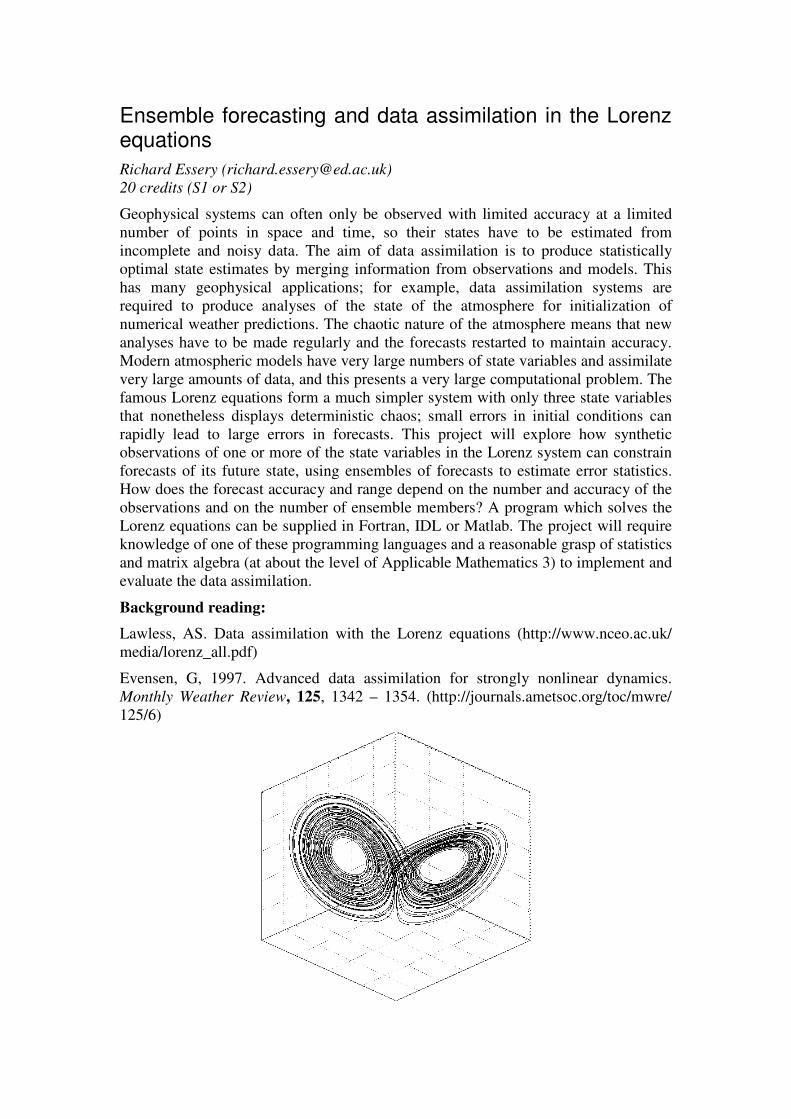
Ensemble forecasting and data assimilation in the Lorenz equations

Richard Essery (richard.essery@ed.ac.uk)

20 credits (S1 or S2)

Geophysical systems can often only be observed with limited accuracy at a limited

number of points in space and time, so their states have to be estimated from

incomplete and noisy data. The aim of data assimilation is to produce statistically

optimal state estimates by merging information from observations and models. This

has many geophysical applications; for example, data assimilation systems are

required to produce analyses of the state of the atmosphere for initialization of

numerical weather predictions. The chaotic nature of the atmosphere means that new

analyses have to be made regularly and the forecasts restarted to maintain accuracy.

Modern atmospheric models have very large numbers of state variables and assimilate

very large amounts of data, and this presents a very large computational problem. The

famous Lorenz equations form a much simpler system with only three state variables

that nonetheless displays deterministic chaos; small errors in initial conditions can

rapidly lead to large errors in forecasts. This project will explore how synthetic

observations of one or more of the state variables in the Lorenz system can constrain

forecasts of its future state, using ensembles of forecasts to estimate error statistics.

How does the forecast accuracy and range depend on the number and accuracy of the

observations and on the number of ensemble members? A program which solves the

Lorenz equations can be supplied in Fortran, IDL or Matlab. The project will require

knowledge of one of these programming languages and a reasonable grasp of statistics

and matrix algebra (at about the level of Applicable Mathematics 3) to implement and

evaluate the data assimilation.

Background reading:

Lawless, AS. Data assimilation with the Lorenz equations (http://www.nceo.ac.uk/

media/lorenz_all.pdf)

Evensen, G, 1997. Advanced data assimilation for strongly nonlinear dynamics.

Monthly Weather Review, 125, 1342 – 1354. (http://journals.ametsoc.org/toc/mwre/

125/6)

Simulating the seasonal variability and climate sensitivity of Northern Hemisphere snow cover

Richard Essery (richard.essery@ed.ac.uk)

20 credits (S1 or S2; possibility of extending to 40 credits)

Snow covers a large fraction of the Northern Hemisphere land surface in winter and

has a large influence on the surface energy balance because of its high albedo, with

strong feedbacks on the climate system. Moreover, because snow cover is sensitive to

changes in temperature and precipitation, and is relatively easy to measure by remote

sensing, it can provide an important indicator of climate change. In this project, a

simple but physically-based snow model with three adjustable parameters will be

driven with gridded meteorological data over the Northern Hemisphere to predict

snow cover for the period 1983-1995. The European Space Agency has recently

released snow extent and snow water equivalent maps based on microwave satellite

data going back to 1979 (http://www.globsnow.info). How closely can the modelled

seasonal cycle of hemispheric snow cover be made to match satellite records by

adjustment of the model parameters? What conclusions can be drawn about the

climate sensitivity of snow cover and its regional variation from interannual variations

in snow cover, temperature and precipitation?

The model will be supplied as a Fortran program but is very simple and could easily

be reprogrammed in Matlab or another language of choice. The main computational

challenge will be in plotting and analyzing the model output, so some experience with

a suitable programming language will be necessary.

Background reading:

Essery, RLH, and P Etchevers, 2004. Parameter sensitivity in simulations of

snowmelt. Journal of Geophysical Research, 109, doi:10.1029/2004JD005036.

Lemke et al., 2007. Observations: Changes in Snow, Ice and Frozen Ground. In:

Climate Change 2007: The Physical Science Basis. (http://www.ipcc.ch/

publications_and_data/ar4/wg1/en/ch4.html)

Free convection: experimental results and similarity theory

Richard Essery (richard.essery@ed.ac.uk) and Brian Cameron

20 credits, S1 or S2

Free convection – the transfer of heat due to fluid movements driven by buoyancy

gradients – is an important process in the mantle, the oceans and the atmosphere.

Linear stability theory gives good predictions for the onset of convection but fails to

predict the rates of heat and mass transfer, due to non-linearities in the equations of

motion. Simple models of convection are therefore often based on similarity theories

containing coefficients that have to be determined by field, numerical or laboratory

experiments.

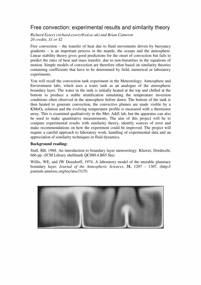
You will recall the convection tank experiment in the Meteorology: Atmosphere and

Environment labs, which uses a water tank as an analogue of the atmospheric

boundary layer. The water in the tank is initially heated at the top and chilled at the

bottom to produce a stable stratification simulating the temperature inversion

conditions often observed in the atmosphere before dawn. The bottom of the tank is

then heated to generate convection, the convective plumes are made visible by a

KMnO4 solution and the evolving temperature profile is measured with a thermistor

array. This is examined qualitatively in the Met: A&E lab, but the apparatus can also

be used to make quantitative measurements. The aim of this project will be to

compare experimental results with similarity theory, identify sources of error and

make recommendations on how the experiment could be improved. The project will

require a careful approach to laboratory work, handling of experimental data and an

appreciation of similarity techniques in fluid dynamics.

Background reading:

Stull, RB, 1988. An introduction to boundary layer meteorology. Kluwer, Dordrecht,

666 pp. (JCM Library shelfmark QC880.4.B65 Stu)

Willis, WE, and JW Deasdorff, 1974. A laboratory model of the unstable planetary

boundary layer. Journal of the Atmospheric Sciences, 31, 1297 – 1307. (http://

journals.ametsoc.org/toc/atsc/31/5)

Modelling and measuring the radiation balance of Edinburgh’s urban canyons

Richard Essery (richard.essery@ed.ac.uk) and Tim Reid

20 credits (S1 or S2; possibility of extending to 40 credits)

The underlying topography and the tenement buildings of Edinburgh’s Old Town

make some dramatic urban canyons, such as the Cowgate, in which local air

temperatures can differ from those in the more open areas of town and surrounding

rural areas. One of the reasons for this is modification of the surface radiation

balance; shadows cast by buildings reduce the solar radiation and heating at street

level during the day, but blocking of sky view reduces the loss of thermal radiation

and cooling at night. Most models of urban climate have used idealized geometries to

represent these influences, but airborne laser scanning gives a method of producing

highly detailed digital elevation maps of real urban areas. A high-resolution map of

Edinburgh is now freely available and will be used in this project for modelling

radiation geometry. Under which meteorological conditions does the radiative

influence of urban geometry contribute a net warming or cooling? Simple instruments

familiar to anyone who attended the radiation lab in Meteorology: Atmosphere and

Environment can be used to take some field measurements to evaluate model

predictions.

A certain amount of trigonometry and integral calculus will suffice for calculating

shading and sky view at selected points, but a much more detailed study would be

possible with the use of some programming language with good image processing

capabilities such as IDL or Matlab.

Background reading:

Oke, TR, 1987. Boundary layer climates. Routledge, London, 435 pp. (Darwin

Library shelfmark QC981.7.M5 Oke.)

Grimmond, S, 2007. Urbanization and global environmental change: local effects of

urban warming. Geographical Journal, 173, 83 – 88. (http://www.kcl.ac.uk/ip/

suegrimmond/publishedpapers/GJ_Grimmond2007.pdf)

Geological forcing of climate transitions

Richard Essery (richard.essery@ed.ac.uk) and Linda Kirstein

20 credits (S1 or S2)

The changing locations of continents and heights of mountains on geological

timescales have major effects on atmospheric circulation and climate. The Cenozoic,

for example, was a period of major geological changes (including opening of the

Drake Passage and Himalayan uplift) and climate changes (for example, onset of the

Asian monsoon and permanent Antarctic glaciation), and it has long been thought that

these changes are related in the coupled climate system (Raymo and Ruddiman 1992).

Climate models now provide tools for investigating these suggestions, at least for

snapshots of geological time.

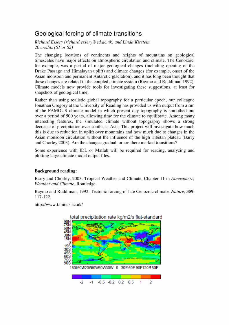
Rather than using realistic global topography for a particular epoch, our colleague

Jonathan Gregory at the University of Reading has provided us with output from a run

of the FAMOUS climate model in which present day topography is smoothed out

over a period of 500 years, allowing time for the climate to equilibrate. Among many

interesting features, the simulated climate without topography shows a strong

decrease of precipitation over southeast Asia. This project will investigate how much

this is due to reduction in uplift over mountains and how much due to changes in the

Asian monsoon circulation without the influence of the high Tibetan plateau (Barry

and Chorley 2003). Are the changes gradual, or are there marked transitions?

Some experience with IDL or Matlab will be required for reading, analyzing and

plotting large climate model output files.

Background reading:

Barry and Chorley, 2003. Tropical Weather and Climate. Chapter 11 in Atmosphere,

Weather and Climate, Routledge.

Raymo and Ruddiman, 1992. Tectonic forcing of late Cenozoic climate. Nature, 359,

117-122.

http://www.famous.ac.uk/

El Nino variability and teleconnections in the 20th century

Supervisor: Tom Russon and G. Hegerl (contact gabi.hegerl@ed.ac.uk if interested)

20 credit project, S2 only, more detail available in S2.

The El Nino Southern Oscillation is a mode of variability of the ocean-atmosphere

system centered in the tropical Pacific. It substantially influences interannual global

temperature and precipitation variability, and causes strong regional impacts of

climate variability across the globe, see http://www.elnino.noaa.gov/.

In order to reconstruct El Nino variability and change in the past, pre-instrumental

time, these so-called teleconnections of regional climate to the tropical Pacific are

often used to attempt to reconstruct past El Nino timing and amplitude. This project

explores, from the literature and largely timeseries analysis, how strongly the various

indicators are actually coupled to El Nino, and to what extent indices used for

reconstructions fully represent 20th

century El Nino variability.

Background reading:

Kenyon, J and G. C. Hegerl (2008): The Influence of ENSO, NAO and NPI on global temperature extremes. J. Climate 21, 3872-3889, doi 10.1175/2008JCLI2125.1

And references herein as well as a recent review paper (to be provided) Figure:

NOAA

The early 20th century warming

Supervisor: Gabi Hegerl, Chris Merchant (designed as 40 credits)

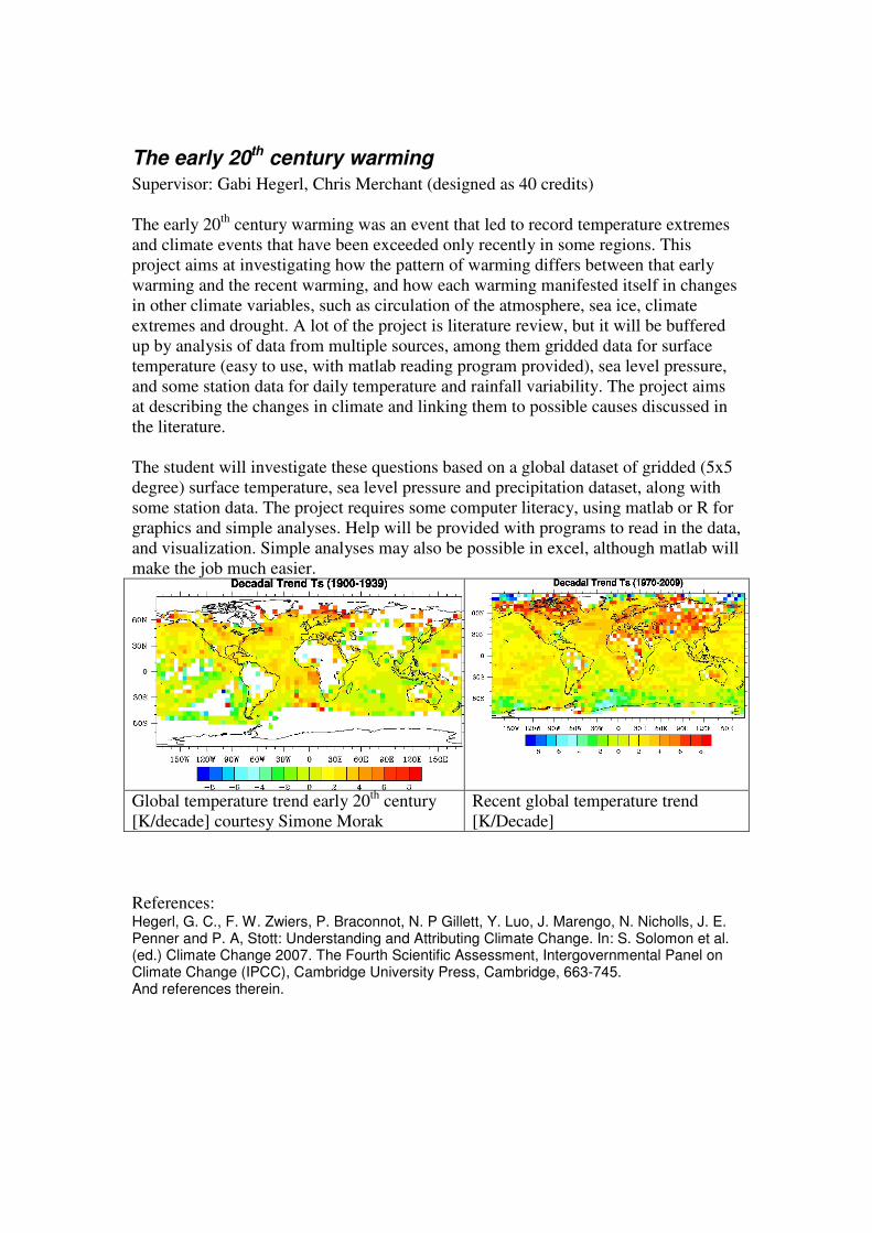
The early 20

th century warming was an event that led to record temperature extremes

and climate events that have been exceeded only recently in some regions. This

project aims at investigating how the pattern of warming differs between that early

warming and the recent warming, and how each warming manifested itself in changes

in other climate variables, such as circulation of the atmosphere, sea ice, climate

extremes and drought. A lot of the project is literature review, but it will be buffered

up by analysis of data from multiple sources, among them gridded data for surface

temperature (easy to use, with matlab reading program provided), sea level pressure,

and some station data for daily temperature and rainfall variability. The project aims

at describing the changes in climate and linking them to possible causes discussed in

the literature.

The student will investigate these questions based on a global dataset of gridded (5x5

degree) surface temperature, sea level pressure and precipitation dataset, along with

some station data. The project requires some computer literacy, using matlab or R for

graphics and simple analyses. Help will be provided with programs to read in the data,

and visualization. Simple analyses may also be possible in excel, although matlab will

make the job much easier.

Global temperature trend early 20th

century

[K/decade] courtesy Simone Morak

Recent global temperature trend

[K/Decade]

References: Hegerl, G. C., F. W. Zwiers, P. Braconnot, N. P Gillett, Y. Luo, J. Marengo, N. Nicholls, J. E. Penner and P. A, Stott: Understanding and Attributing Climate Change. In: S. Solomon et al. (ed.) Climate Change 2007. The Fourth Scientific Assessment, Intergovernmental Panel on Climate Change (IPCC), Cambridge University Press, Cambridge, 663-745. And references therein.

A comparison of seismic and electrical/EM imaging techniques at Rosslyn Glen Ian Main (ian.main@ed.ac.uk) and Kathy Whaler (two field-based

projects to run concurrently over one term, 1st semester)

The second year seismic practical currently uses data taken from a

previous 4th year project at Rosslyn Glen, a glacial valley filled with till.

The aim of this project is to carry out and interpret seismic and

electrical/EM (DC resistivity and TDEM) surveys, one student being

primarily responsible for each. The seismic lines will be shot parallel and

perpendicular to strike, with electrical/EM data collected along the same

profiles. Co-located seismic velocity and electrical resistivity information

may help resolve the interpretation ambiguity of the previous seismic

survey. Two students will act as field assistants for each other, and

collaborate on a joint interpretation after writing up their own

independently.

RainWarning.app �

������������� ����������������

���������� ���������������������������������� ���������

�

�������������������� ���������� ������������������������� �� �� ��������

�� ����� ���� ���������� ������������� ������������������ ������������� ���

������ �������������� ���� ���������������� ����������������������� ����������

������� ��������������������������������� !�����" �����������������������!�

���������#��$���������������� ��������� � �� ������������������ ����������� �

%� �&����������������������� ���������� ��������� ���� ��������������� ����

�������������������������������� ��'��������������� ���������� � ������� ���

()�������������� �������������� ������ ���%� �&������ *������+#��

��

������������ ��������������� �����������������������

�������������������������� ������������������������

�

!������'�� �����,��������������� �� ����������

�������� �������'#�� ���������� �� �����

��������������������� ������ �� �������� ���

��� ����� ������������ ������ ���������� ������ ���

�������� ��������������������'����� �

��� ����� �������������������� � ��������� � ����

�

*����������������������� ������������ ��

����� �����������������+�'�����������-���������

���� ����.���������/�%�����++�� 0� �������������

����������������������������� ���� ����� ��� �����

�������� ��1����� ����� ��������� ����� ���

����� �#�0������������ ������� �� �� ���������������������2������� ���� ���

����������������������������������� �������������������1��� ���������� ������

������ ������� ������+3��#�����������

�������������������� �

���� ���� ���������������

������������� !�����

"��� ��������# ���������

����$��������������� ����

%��&����'������������

�������������� ���������

���� ��������������� ����

� �����"�����(��������

��������# ��������������$�

"��� �������������)�

���� ���������"������� ���

�������������������

���������������������������� ������ � ����� ������������ ���+����#���.��

����� ������ � �4������ ����������� ���5����������������4 ������ ������ #���

Mapping Human Discomfort across London during a Heatwave Event �

������������� ����������������

���������� ���������

�

��������������� ����������������������������������������������������������

�����������������������������������������������������������������������

������������������������������������������������������������������������������

���������������������������������������������������������������������

�������������������������������������������������������������������������

�����������������������������������������������������������������������������

���������������������������������������������������������������������������

���������������������������������������������������������������� ��!�������

��"����������������������������������������������������������������������

#���$���������������� ��

�

%������������������&���������������������������������������������������

������������������������������������������������������������������������������

#'����������(���)**+$��!�����������������������#������������$�������������

������������������������������������������������������������������������,����

-�"������������#���������������������������������������������������������������

������"���������������������'�����$��

�

.��������,��/����������������������������

���������������������������������������������

������������������������������������������

�����������������������������������������������

���������������������������������0�

�

1�������������������������������������

���������������������������������������������2�

����������������������������������������� �

#�%/�$���

�

.��������)��/�����������������������������%/��

�����������������������������������������

�����������������#��������������������������������������������������������$����

������������������%/�����������������������������������������������0�

�����������

�����33�����������3�������33������������������3�����3'�����4����3�56�!7'!%7��������7�����7����7/8�����

6�������9�6��4��������:��'�����;������������#)*,*$�!��������������������

�������������������������<�������������������������������������� ������

,*�,**)3&���))))�

Estimating sources of CO, CO2 and CH4 from Canadian forest fires during summer

2011 using aircraft and satellite measurements

Paul Palmer (pip@ed.ac.uk)

40 credit course

The burning of boreal forests, of which approximately 5 to 20 million hectares burn

annually (mainly in Russia and North America), removes vegetation, changes land-

surface properties, and emits trace gases, aerosols, and smoke in prodigious quantities.

Consequently, wildfires are amongst the most important global contributors to a number

of key atmospheric species (e.g., CO2, CH4, CO, NOx, black carbon) and their long-range

transport impact Earth’s radiation budget, air quality and processes such as tropospheric

O3 production far from the source region.

The University of Edinburgh leads the BORTAS project (www.geos.ed.ac.uk/

eochem/bortas/) to investigate the connection between the composition and distribution

of biomass burning outflow, O3 production and loss with that outflow, and the resulting

perturbation to chemistry in the troposphere. The focal point of the project is a 3-week

aircraft campaign over the North Atlantic during July 2011 (seasonal peak of Canadian

forest fires), which involves additional measurements over mainland Canada and the

Azores. One of our main analysis tools to interpret these data is the GEOS-Chem global

3-D chemistry transport model (http://www.geos-chem.org/), which relates surface

sources and sinks of gases and particles to atmospheric concentrations.

This project will include (1) the interpretation of observed concentration observations of

CO2, CH4, CO during BORTAS using the GEOS-Chem model; and (2) the application of

an optimal estimation inverse model to estimate the sources and sinks of these trace gases

from the observed concentration measurements. The candidate will also use satellite

observations of atmospheric chemistry and land-surface properties to help interpret the

spatial and temporal distribution of burning emissions over North America during

BORTAS. The project will involve computer programming and data analysis. Ideal

candidates will have knowledge of IDL or Python.

Title: The composition of the mesosphere using ground-based mm-wave remote sensing

Area: Atmospheric physics

Contact: Hugh Pumphrey (Room 313, Crew Building, extn. 50 6026, email:

hugh.pumphrey@ed.ac.uk)

Available: 20pt in S1 or S2.

The mesosphere, lying at altitudes between 50 and 80 km, is one of the least-understood regions of the

atmosphere. One way to study its composition is to use a millimetre-wave receiver (essentially a radio

telescope) sited on the ground (preferably on a high mountain). The spectra from such an instrument

can provide information on the mixing ratio of a variety of chemical species of interest. Recent

improvements in technology are permitting easier access to higher frequencies.

This, then, poses these questions: which species might one usefully measure with this technique? What

characteristics (bandwidth, resolution, noise level) would a spectrometer require in order to make the

measurement? How badly affected would the measurement be by a wet troposphere (and hence, how

high a mountain would you need)? The basic technique of the project is to simulate a measurement

using a readily-available radiative-transfer model (ARTS: see http://www.sat.ltu.se/arts) and apply the

standard techniques of inverse theory[1] to the simulation to determine what information the

measurements would contain. Several projects along these lines would be possible, to answer such

questions as:

• Which of the various absorption lines of CO is most suitable for sounding the mesosphere?

• Is it possible to use ground-based sensing of HCl to track the chlorine loading of the middle

atmosphere?

Two years of measurements of the 230GHz carbon monoxide spectral line taken from the Norwegian Antarctic base using

the British Antarctic Survey’s microwave radiometer.

These projects would probably be 20-point projects available in either semester. It would be suitable for

students on any physics or geophysics-based degree programme. The ARTS output would be analysed

using a data analysis language such as R, MATLAB or Octave. [1] Inverse Methods for Atmospheric Sounding: Theory and practice by Clive D. Rodgers (World Scientific, ISBN 981-02-

2740-X)

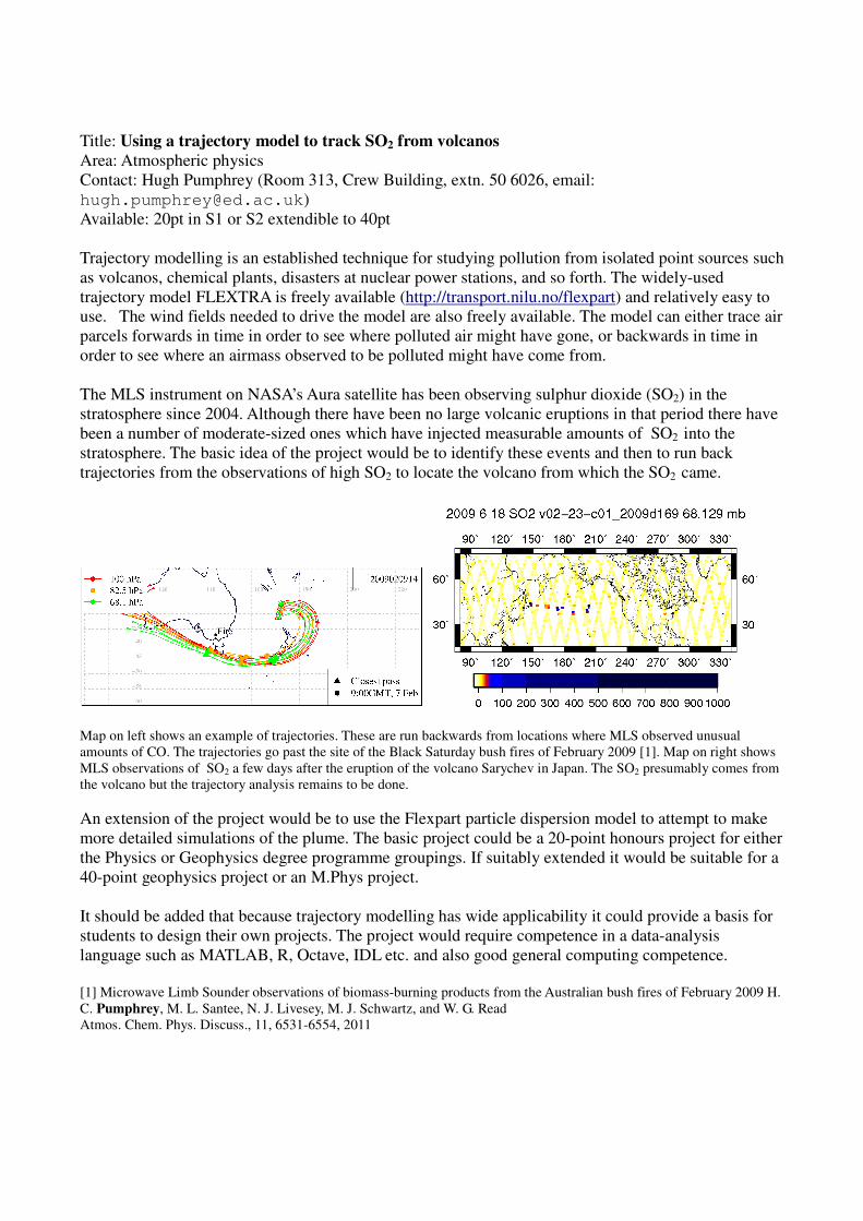
Title: Using a trajectory model to track SO2 from volcanos

Area: Atmospheric physics

Contact: Hugh Pumphrey (Room 313, Crew Building, extn. 50 6026, email:

hugh.pumphrey@ed.ac.uk)

Available: 20pt in S1 or S2 extendible to 40pt

Trajectory modelling is an established technique for studying pollution from isolated point sources such

as volcanos, chemical plants, disasters at nuclear power stations, and so forth. The widely-used

trajectory model FLEXTRA is freely available (http://transport.nilu.no/flexpart) and relatively easy to

use. The wind fields needed to drive the model are also freely available. The model can either trace air

parcels forwards in time in order to see where polluted air might have gone, or backwards in time in

order to see where an airmass observed to be polluted might have come from.

The MLS instrument on NASA’s Aura satellite has been observing sulphur dioxide (SO2) in the

stratosphere since 2004. Although there have been no large volcanic eruptions in that period there have

been a number of moderate-sized ones which have injected measurable amounts of SO2 into the

stratosphere. The basic idea of the project would be to identify these events and then to run back

trajectories from the observations of high SO2 to locate the volcano from which the SO2 came.

Map on left shows an example of trajectories. These are run backwards from locations where MLS observed unusual

amounts of CO. The trajectories go past the site of the Black Saturday bush fires of February 2009 [1]. Map on right shows

MLS observations of SO2 a few days after the eruption of the volcano Sarychev in Japan. The SO2 presumably comes from

the volcano but the trajectory analysis remains to be done.

An extension of the project would be to use the Flexpart particle dispersion model to attempt to make

more detailed simulations of the plume. The basic project could be a 20-point honours project for either

the Physics or Geophysics degree programme groupings. If suitably extended it would be suitable for a

40-point geophysics project or an M.Phys project.

It should be added that because trajectory modelling has wide applicability it could provide a basis for

students to design their own projects. The project would require competence in a data-analysis

language such as MATLAB, R, Octave, IDL etc. and also good general computing competence.

[1] Microwave Limb Sounder observations of biomass-burning products from the Australian bush fires of February 2009 H.

C. Pumphrey, M. L. Santee, N. J. Livesey, M. J. Schwartz, and W. G. Read

Atmos. Chem. Phys. Discuss., 11, 6531-6554, 2011

Title: How ageostrophic is the surface wind?

Area: Atmospheric physics

Contact: Hugh Pumphrey (Room 313, Crew Building, extn. 50 6026, email:

hugh.pumphrey@ed.ac.uk)

Available: 20pt in S1 or S2

Standard meteorological theory states that friction causes winds near the surface to be slower than the

geostrophic wind and to blow somewhat towards low pressure. (The geostrophic wind is exactly

parallel to the isobars, that is, perpendicular to the pressure gradient.) Is the theory correct? One way to

test it is to compare the measured wind to a direct estimate of the geostrophic wind. To that end, I have

collected several months worth of hourly wind recordings from Edinburgh airport, together with

pressure recordings from airports across Scotland and northern England. The project would consist of

calculating a time series of the pressure gradient at Edinburgh directly from the pressure data; this is an

inverse theory problem. The geostrophic wind can then be calculated directly from the pressure

gradient and compared to the true wind. It should be possible to determine whether the ageostrophic-

ness of the wind depends on wind speed, direction, time of day etc. The project would require

competence in a data-analysis language such as MATLAB, R, Octave, IDL etc. or the ability to learn

this reasonably quickly. This would be suitable as a 20-point honours project for either the Physics or

Geophysics degree programme groupings.

Analysis of air quality over the UK – the Easter 2011 smog episode

Supervisors: David Stevenson (dstevens@staffmail.ed.ac.uk) and Massimo Vieno

(CEH)

(Available S1 or S2 as a 20-credit project; may be extendable to 40-credits)

Over a few weeks in April 2011, the UK experienced unusually warm temperatures

(e.g., London > 25°C) for the time of year, associated with high pressure, light winds,

and long hours of sunshine. The fine weather was accompanied by a progressive

deterioration in air quality (e.g., Figure 1). On Thursday 21st April, Defra issued a

‘summer smog’ alert1, for high levels of the air pollutants O3 (ozone) and PM10

(particulate matter less than 10 �m in diameter).

Data (air quality and meteorological) from multiple sites across the UK are available

over the time period (e.g., hourly ozone, temperature and PM data; also vertical

temperature profiles). This project will collect together this data, to produce a

synoptic view of the episode and interpret the processes that contributed to the high

levels of pollution. It may also be possible to analyse model simulations of the

episode, to determine the model’s performance.

The project will involve data analysis, including statistics, and the student will need

some competence in using computers for data analysis of relatively large data sets.

Figure 1. Ozone and PM10 measurements from Leicester Centre site, for April 16-23,

2011.

1. http://www.defra.gov.uk/news/2011/04/21/summer-smog/

Analysis of weather station data (there is potential for several projects)

Supervisors: David Stevenson (dstevens@staffmail.ed.ac.uk) and Massimo Vieno

(Available S1 or S2 as a 20-credit project; may be extendable to 40-credits)

The University of Edinburgh weather station

(www.geos.ed.ac.uk/abs/Weathercam/station) has been collecting data (pressure,

rainfall, wind, temperature, humidity, and solar flux) for over 4 years, at high

temporal resolution (every minute; e.g., see figure). There is wide scope for various

analyses associated with these data – some specific suggestions are listed below, but

students with alternative ideas are invited to put forward their own suggestions.

1) An analysis of the exceptional winter of 2010-2011 in Edinburgh. Last year’s

winter broke records, with temperatures throughout much of December remaining

sub-zero for weeks on end. How was the event recorded by the JCMB weather

station? What synoptic conditions produced such an exceptional event? Using longer

time series of data from other nearby stations, just how exceptional was last winter?

2) Characterisation of biases for the station. The station is located on the top of

JCMB, a far from standard setting, and this influences the measurements. By careful

comparison with data from nearby official Met Office stations, biases can be

estimated. Comparison could also be made to temperature and humidity data from the

Stevenson screens on top of JCMB, to characterise very local factors. A second sensor

has been set up to simultaneously log measurements from the Stevenson screen as

well as from the roof. Analysis of these two measurement streams for the same

variable reveal important information about how accurately instruments measure

temperature.

3) Fourier analyses. This should reveal the clear annual and diurnal cycles in most

variables, but there may also be other timescales of variability in the data. Some

previous analyses have found weekly cycles (or weekend effects) in meteorological

data, a clear indicator of anthropogenic influence. Sub-diurnal signals (e.g. associated

with man’s activities, such as rush-hours on the roads, or the daily cycle of activity in

JCMB) may also be present in the data

4) Windspeed analyses. Before siting a wind turbine, you are generally advised to

collect data on wind speeds and variability for periods of a few months. The existing

data could be used to calculate the viability of installing a wind turbine on the roof of

JCMB, and estimating its potential. In addition, it would be interesting to look at how

dependent the estimated potential is on the time period of data – e.g., are all 3 month

periods within 10% of the 4 year average?

Electrical resistivity studies in Sri Lanka for investigating geothermal potential

Supervisors: Kathy Whaler (kathy.whaler@ed.ac.uk); Nick Johnson; Bruce Hobbs

(Pentland Geophysics)

There are a number of hot springs in Sri Lanka and one theory is that they are

connected to deep and extensive geothermal regions. If this is the case there is

potential for the extraction of geothermal energy. The University of Edinburgh, in

conjunction with the Institute for Fundamental Studies and Geological Survey and

Mines Bureau, Sri Lanka, conducted geophysical surveys over a number of hot spring

sites in summer 2010 in order to investigate the possibility of these springs being

associated with deep, high enthalpy regions. Our technique probes the electrical

resistivity of the sub-surface, which is very sensitive to the presence of fluids. Recent

research suggests there is a clay mineral signature associated with geothermal activity

that the method is also able to detect.

Magnetotelluric (MT) data consist of time series of horizontal electric and magnetic

field variations; the ratios of electric to magnetic field contain the information on the

electrical resistivity of the sub-surface. Spectral analysis gives the signal as a function

of period which, through the skin depth (over which electromagnetic signals are

attenuated to 1/e of their initial amplitude), acts as a depth proxy. This project will use

processed MT data from one or more of the less noisy profiles. The project will

involve several stages of data analysis and cleaning to optimise the data for two-

dimensional inversion, including correcting for distortion of the data by near-surface

inhomogeneities and determining any prominent strike direction(s) reflecting sub-

surface structures; if time permits, inversion for sub-surface resistivity will also be

undertaken.

Fortran computer code exists to undertake the necessary processing steps, with scripts

to run them and plot results. It is not necessary to understand the details of the fortran

language to undertake the project, but the student will need to modify the scripts to

treat the particular data set, and then run the various codes. The main skill and effort

will come in making sure the runs have proceeded as intended and in analysing the

results.

Amplitude of the

North electric to

East magnetic field

components as a

function of period

for one of the Sri

Lanka profiles

Crustal thickness in Africa

Kathy Whaler (kathy.whaler@ed.ac.uk)

The most reliable estimates of crustal thickness come from seismic data, but these are

unavailable in many parts of the world. Previous research suggests that the

magnetisation amplitude deduced from low orbiting satellite data correlates tolerably

well with seismic crustal thickness estimates. A recent paper (Tedla et al., 2011)

provides regularly spaced estimates of crustal thickness over Africa from a satellite-

based gravity field model, and finds good agreement with seismically determined

Moho depth estimates where available. This project will explore the extent to which

the magnetisation amplitude correlates with the gravity and seismic estimates of

crustal thickness and, if the correlation is significant, the scaling factor that converts

magnetisation amplitude to crustal thickness estimate. Before undertaking the

correlation with the gravity-derived values, it will be important to decide the

resolution of the two models, and hence how many independent estimates of

thickness/magnetisation amplitude it is reasonable to correlate. The gravity data set

will then have to be averaged or decimated to the required resolution. The statistical

significance of the resulting correlation coefficient will be calculated and interpreted.

Regional or tectonic terrane correlations can be used to determine whether the

agreement (or lack of it!) varies over the continent, as suggested by the Tedla et al.

study. An alternative to correlation is to linearly regress one data series onto the other,

which allows for a constant offset as well as a scaling factor between the two; this

could also be investigated if time allowed.

fortran code to estimate magnetisation from the model coefficients will need

modification to estimate magnetisation at the locations of the gravity and seismic

points, but this can easily be done with knowledge of a structured programming

language like matlab. It is straightforward to correlate two sets of points in matlab.

However, manipulating the gravity data set to get values at the required spacing could

be fiddly, so the project will probably only suit a student who is willing to persevere

at, and gains satisfaction from, such tasks!

Comparison of crustal thickness

estimates. Seismic estimates from

seismic refraction profiles

(diamonds) and receiver functions

(circles). Seismic symbols in green

where the seismic and gravity

thicknesses agree to within ±5 km,

in red otherwise. Background

colour is the difference between

gravity estimates and a 2º x2º

global surface wave model crustal

thickness. From Tedla,G E, et al.,

2011, A crustal thickness map of

Africa derived from a global

gravity field model using Euler

deconvolution, Geophys. J. Int.,

doi: 10.1111/j.1365-

246X.2011.05140.x