Geophysical Journal International · Geophysical Journal International Geophys ... A geometric...

Geophysical Journal InternationalGeophys. J. Int. (2012) 190, 476–498 doi: 10.1111/j.1365-246X.2012.05491.x

GJI

Sei

smol

ogy

A geometric setting for moment tensors

Walter Tape1 and Carl Tape2

1Department of Mathematics, University of Alaska, Fairbanks, Alaska 99775, USA2Geophysical Institute and Department of Geology & Geophysics, University of Alaska, Fairbanks, Alaska 99775, USA . E-mail: [email protected]

Accepted 2012 March 30. Received 2012 March 16; in original form 2011 December 5

S U M M A R YWe describe a parametrization of moment tensors that is suitable for use in algorithms formoment tensor inversion. The parameters are conceptually natural and can be easily visualized.The ingredients of the parametrization are present in the literature; we have consolidated theminto a concise statement in a geometric setting. We treat several familiar moment tensor topicsin the same geometric setting as well. These topics include moment tensor decompositions,crack-plus-double-couple moment tensors, and the parameter ε that measures the differencebetween a deviatoric moment tensor and a double couple. The geometric approach clarifiesconcepts that are sometimes obscured by calculations.

Key words: Theoretical seismology.

1 I N T RO D U C T I O N

The seismic moment tensor is a mathematical description for earth-quake sources. A moment tensor can represent a single earthquake,as in the case of a small-to-moderate event, or it can represent asubevent within a large, long-duration earthquake. Moment tensorsrange qualitatively from the classical double couple, which is as-sociated with relative slip along a fault plane, to ‘non-deviatoric’moment tensors that are associated with events other than con-ventional earthquakes. These events include those in volcanic andgeothermal regions (e.g. Julian & Sipkin 1985; Foulger et al. 2004;Minson et al. 2007), as well as nuclear explosions, mine collapsesand events associated with glaciers or hydraulic fracturing (Dreger& Woods 2002; Ford et al. 2009; Walter et al. 2009; Baig &Urbancic 2010). See also the reviews by Julian et al. (1998) andMiller et al. (1998).

Computationally a moment tensor is a 3 × 3 symmetric matrixthat describes an earthquake source as a sum of three force couples.Recorded seismic waveforms can be modelled as a linear combina-tion of derivatives of Green’s functions, which describe the seismicwavefield at a station due to an impulsive source for a given struc-tural model. The coefficients of the linear combination are the sixindependent entries of the moment tensor matrix. An inverse prob-lem can be constructed in which measurements between recordedand simulated seismograms are used to estimate a moment tensorfor a particular earthquake (e.g. Dziewonski et al. 1981).

Non-deviatoric events have been recorded by seismometers.Their moment tensors have been inferred using ‘full’ moment tensorinversion algorithms that place no constraints on the six elementsof the moment tensor (e.g. Dufumier & Rivera 1997; Minson &Dreger 2008). The unknown model vector describing the momenttensor has six elements, and therefore the model parameter space issix-dimensional. The parameters need not, however, be the matrixentries. In this paper we do two things:

(i) Specifically: We define a parametrization of moment tensorsthat is conceptually natural. Although we perform no inversions inthis study, we envision the parametrization as the basis for sampling-based, non-linear moment tensor inversions. Associated with theparametrization is a natural scheme for displaying the results ofmoment tensor inversions—both the moment tensors themselvesand the uncertainties associated with full moment tensor inversions.The parametrization is given in Proposition 3 of Section 7.

(ii) More generally: We present familiar concepts of moment ten-sors in a conceptual setting that complements calculations withpictures whenever feasible. Moment tensors are drawn as beach-balls. Beachball patterns (moment tensor source types) are depictedon what is essentially the lune of Riedesel & Jordan (1989), andbeachball orientations are depicted in a solid block. Any momenttensor is then determined by a pair of points—one in the luneand one in the block—together with a positive number that givesits norm. In this way we get a coherent picture of all momenttensors.

We use several topics to illustrate this geometric approach. InSection 4 we consider moment tensor decompositions, and in Sec-tion 9 we consider crack-plus-double-couple moment tensors. InSection 8 we consider the parameter ε that measures how much anearthquake source departs from the classic model of slip along afault, and we suggest the longitudinal coordinate γ on the lune as analternative to ε. More generally, in Tape & Tape (2012) we favourthe lune as an alternative to the Tk source-type plots of Hudsonet al. (1989). In Section 10 we use the lune to plot source typesfrom several recent studies.

Many authors, as we do, have organized moment tensors accord-ing to eigenvalues (moment tensor source types), or eigenvectors(moment tensor orientations), or both (e.g. Hudson et al. 1989;Pearce & Rogers 1989; Riedesel & Jordan 1989; Frohlich 1992,2001; Dufumier & Rivera 1997; Julian et al. 1998; Kagan 2005;

476 C© 2012 The Authors

Geophysical Journal International C© 2012 RAS

A geometric setting for moment tensors 477

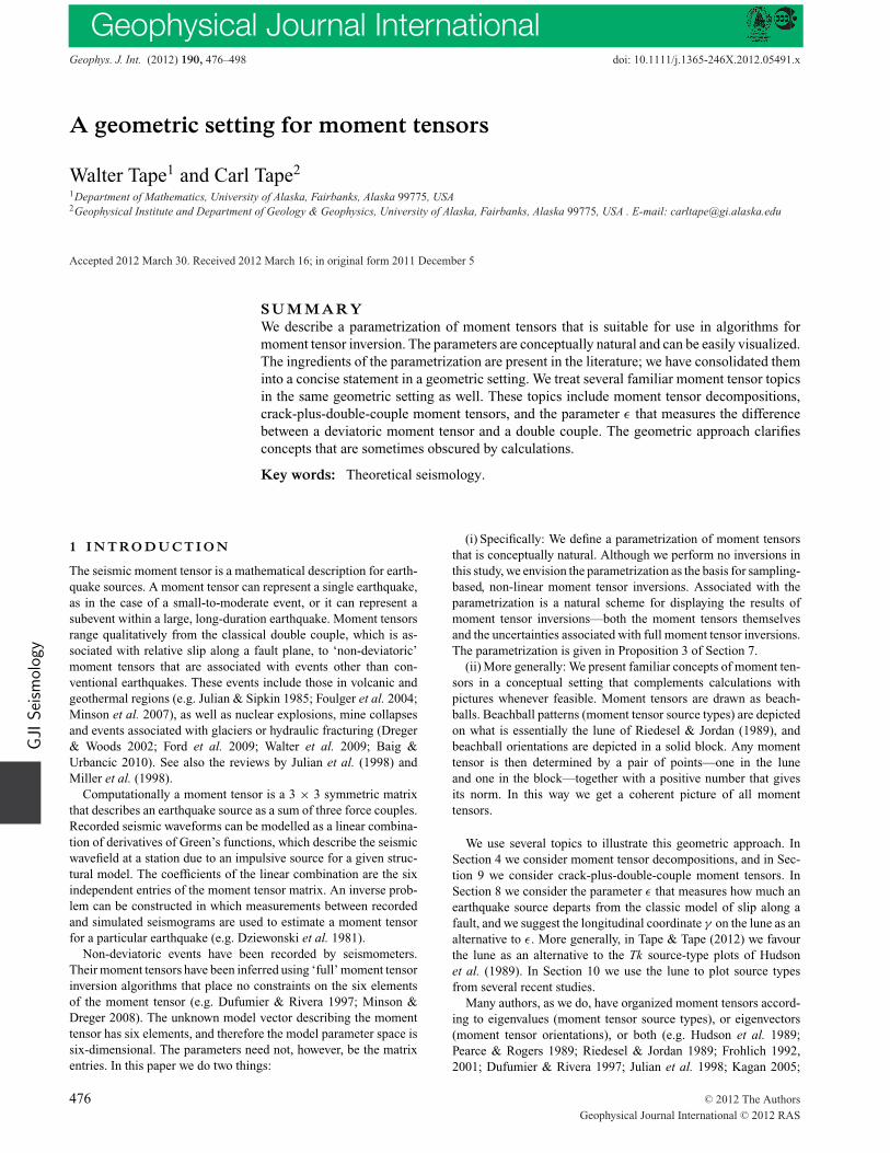
Figure 1. Home for beachball patterns (moment tensor source types)—thefundamental lune L of the unit sphere. Each point on the lune represents abeachball pattern. The magenta equatorial arc is for deviatoric tensors, thered meridian is for sums of double couple and isotropic tensors, and theblack arc is for crack + double couple tensors having Poisson ratio ν =1/4 (Section 9). Above the upper blue arc all beachballs are only red, andbelow the lower blue arc all balls are only white. ISO, isotropic; DC, doublecouple; LVD, linear vector dipole; CLVD, compensated linear vector dipole;C, tensile crack with Poisson ratio ν = 1/4.

Minson & Dreger 2008; Sileny & Milev 2008; Walter et al. 2010;Chapman & Leaney 2012). For representing source types, Riedesel& Jordan (1989) proposed what is essentially our Fig. 1. Chapman &Leaney (2012) recently compared the source-type plots of Riedeseland Jordan with the Tk plots of Hudson et al. (1989). As we do,Chapman and Leaney prefer the plots of Riedesel and Jordan; thatis, they prefer the representation on the sphere.

2 L I N E A R T R A N S F O R M AT I O N S ,B E A C H B A L L S A N D λ- S PA C E

A moment tensor M is a certain kind of linear transformation ofthree-space, and it can therefore be thought of as a vector field. Thatis, at each point e in space it attaches an arrow M(e). In particular,M attaches an arrow to each point of the unit sphere. Where thearrows point outwards, the sphere is coloured red (say), and wherethe arrows point inwards, the sphere is coloured white. Except forscale, this is the beachball associated with M . The moment tensordetermines the beachball.

Mathematically, moment tensors are exactly the self-adjoint lin-ear transformations. They are the transformations that have threemutually perpendicular eigenvectors. The associated principal axesare in the directions of the eigenvectors, but they are lines ratherthan vectors. Each principal axis is associated with an eigenvalue λ,where, for any point e on the principal axis, M(e) = λ e. Along eachprincipal axis the attached arrows are therefore radial, with the signof λ determining whether the arrows point directly to or directlyaway from the origin. The principal axes and their correspondingeigenvalues determine the moment tensor.

The beachball is a device for keeping track of the principal axesand their eigenvalues, and hence of the moment tensor itself. If the

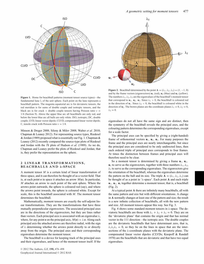
Figure 2. Beachball determined by the point � = (λ1, λ2, λ3) = (1,−1, 0)and by the frame vectors (eigenvectors) u1 (red), u2 (blue) and u3 (yellow).The numbers λ1, λ2, λ3 are the eigenvalues of the beachball’s moment tensorthat correspond to u1, u2, u3. Since λ1 > 0, the beachball is coloured redin the direction of u1. Since λ2 < 0, the beachball is coloured white in thedirection of u2. The brown planes are the coordinate planes λ1 = 0, λ2 = 0,λ3 = 0.

eigenvalues do not all have the same sign and are distinct, thenthe symmetry of the beachball reveals the principal axes, and thecolouring pattern determines the corresponding eigenvalues, exceptfor a scale factor.

The principal axes can be specified by giving a (right-handed)frame of orthonormal vectors u1, u2, u3. For many purposes theframe and the principal axes are nearly interchangeable, but sincethe principal axes are considered to be only undirected lines, theneach ordered triple of principal axes corresponds to four frames.At times the distinction between frames and principal axes willtherefore need to be clear.

So a moment tensor is determined by giving a frame u1, u2,

u3 to serve as the eigenvectors, together with three numbers λ1, λ2,λ3 to serve as the corresponding eigenvalues. The eigenvectors givethe orientation of the beachball, whereas the eigenvalues determinethe pattern on the ball and its size. The triple � = (λ1, λ2, λ3) canbe thought of as a point in ‘λ-space’. Each point � and each tripleu1, u2, u3 together determine a moment tensor, that is, a beachball(Fig. 2).

At a typical point � there are infinitely many beachballs, all withthe same pattern and size but with different orientations. A changein � normally changes at least one of the pattern and size; the resultis a new infinite collection of beachballs, all with the new patternand size. All moment tensors appear this way. See Fig. 3.

Fig. 4 shows some standard moment tensors in λ-space. The de-viatoric beachballs are those with λ1 + λ2 + λ3 = 0. They are onthe ‘deviatoric plane’ that contains the origin and that has normalvector in the 111 direction—the isotropic axis. The double couplesare the deviatoric beachballs that have determinant zero, that is,λ1λ2λ3 = 0, so they lie on the lines in space that are the inter-sections of the λ-coordinate planes with the deviatoric plane. Thecompensated linear vector dipoles (CLVDs; Knopoff & Randall1970) are the beachballs that are deviatoric and that have two equaleigenvalues.

C© 2012 The Authors, GJI, 190, 476–498


478 W. Tape and C. Tape

Figure 3. Beachballs at �1 = √31(1, −1, 0) and �2 = (1, −6, 5). The

colouring patterns are determined as explained in Fig. 2. As before, thered, blue and yellow arrows on the beachballs indicate the frame vectorsu1, u2, u3, respectively. The patterns at �1 are all the same, with any twoof the beachballs there differing by a rotation. The same is true at �2.

Figure 4. Some standard moment tensors—a double couple (DC), twoCLVDs and a positive isotropic tensor (ISO). The double couple and thetwo CLVDs are in the deviatoric plane (purple, λ1 + λ2 + λ3 = 0). Doublecouples are at the intersections of the deviatoric plane with the coordinateplanes. Isotropic tensors are on the isotropic axis (blue, normal to the devi-atoric plane). Principal axes p1, p2, p3 are shown on the double couple.

From Fig. 3 it should be clear that our λ-space need have noparticular relation with ordinary physical space. This differs fromRiedesel & Jordan (1989); their analogues of our λ1, λ2, λ3 axes arein the direction of the T , N and P axes of a moment tensor that theyare depicting.

2.1 Conventions

A given moment tensor corresponds to just one linear transforma-tion, but it has many matrix representations. We will write momenttensors as matrices, but the matrices will always be with respect tothe ‘standard basis’. For much of this paper, the standard basis canbe chosen arbitrarily. However, if strike, slip, and dip in eqs (27) areto have their conventional meanings, then the standard basis mustbe north-west-up.

When specifying points on the unit sphere, we will sometimesgive their directions from the origin rather than the normalizedpoints themselves. Thus the point referred to as (1, −2, 1) is really

1√6(1, −2, 1).Seismologists usually depict beachballs as viewed from above,

and with the top hemispheres removed. We do not do that; we wantto be able to show whole beachballs from various perspectives inthree dimensions.

Appendix D has a glossary of notation.

3 A F I R S T PA R A M E T R I Z AT I O N O FM O M E N T T E N S O R S

A square matrix U is orthogonal if UUT = I . It is a rotation matrixif it is orthogonal and det U = 1. Orthogonal matrices preservelengths and angles. Rotation matrices in addition preserve handed-ness. We use U to denote the group of rotation matrices.

For � = (λ1, λ2, λ3) and U a rotation matrix, we let

[�] =

⎛⎜⎝

λ1 0 0

0 λ2 0

0 0 λ3

⎞⎟⎠, (1a)

[�]U = U [�]U−1. (1b)

(More generally, if A is a moment tensor and U is a rotation matrix,then AU = U A U−1.) As in Fig. 5, the matrix [�] describes a beach-ball with eigenvalues λ1, λ2, λ3 and with corresponding eigenvectorsin the x, y, z coordinate directions. The matrix [�]U describes thesame beachball after being rotated by the matrix U . As a purelyphysical object, the beachball would be transformed by applyingU to each of its points. But as a moment tensor—an operator—thebeachball is transformed by conjugation by U , as in eq. (1b).

x

x

z

z

y

y

[Λ][Λ]U

Figure 5. A first parametrization [�]U of moment tensors. The matrix[�] describes the beachball with eigenvalues � = (λ1, λ2, λ3) and withcorresponding eigenvectors in the x, y, z coordinate directions. The matrix[�]U describes the same beachball after being rotated by the matrix U . Here� = (0, 1, −1) and U is a 20◦ rotation about the x-axis.

C© 2012 The Authors, GJI, 190, 476–498



Proposition 1. Let � = (λ1, λ2, λ3) and let U be a rotationmatrix. Then M = [�]U is the moment tensor whose eigenvaluesare λ1, λ2, λ3 and whose corresponding eigenvectors are the columnsof U .

Proof . M(Uei ) = U [�]U−1(Uei ) = λiUei , where e1, e2, e3 isthe standard basis for R

3. Thus Ue1, Ue2, Ue3—the columns ofU—are eigenvectors of M with eigenvalues λ1, λ2, λ3. Since U isa rotation then Ue1, Ue2, Ue3 are orthonormal and hence M is amoment tensor. �

The notation [�]U emphasizes that the moment tensor is givenby � and U . The point � determines the pattern and size of thebeachball, and U gives the orientation. The rotation matrix U isthe (eigen-) frame associated with the representation [�]U , and thecolumns of U—the eigenvectors—are the frame vectors.

4 M O M E N T T E N S O R D E C O M P O S I T I O N S

4.1 Closest double couple

If some moment tensors all happen to have the same principal axes,then their frames can be chosen to be the same as well. In that casethe distances and angles between their eigenvalue triples � are thesame as distances and angles between the corresponding momenttensors. This section has some examples.

Suppose we wish to find the closest double couple MDC to thegiven moment tensor M = [(2, 1, −3)]. ‘Close’ means close in R

9.That is, the space M 3×3 of 3 × 3 matrices is essentially R

9 and hencehas its own scalar product with associated distances and angles. Sothe distance between M and MDC makes sense.

In λ-space the double couples occupy the six black spokes inFig. 6. Although at each point on a spoke there are infinitely manymoment tensors, all with different orientations, it turns out that inlooking for MDC we need only consider one moment tensor at eachpoint, namely, the one that has the same frame as M . And because theframes are the same, distances in λ-space are the same as distancesin M 3×3. The desired MDC can therefore be seen by inspection ofthe figure, and it can be calculated either by trigonometry or, better,using eq. (7). The result is MDC = [(5/2, 0, −5/2)].

What makes this simple is Proposition 8 of Appendix C. It guar-antees that the closest double couple to M will have the same frameas M .

4.2 Lengths and angles for moment tensors

To be more explicit about scalar products of matrices, define thefunction F : M 3×3 → R

9 by

F

⎛⎜⎝

a11 a12 a13

a21 a22 a23

a31 a32 a33

⎞⎟⎠ = (a11, a12, a13, a21, a22, a23, a31, a32, a33).

(2)

Then the scalar product of matrices is defined by1

A · B = F(A) · F(B), A, B ∈ M 3×3, (3)

where the dot on the right-hand side is the ordinary scalar productin R

9. Then lengths and angles in M 3×3 are defined in terms of the

1 In the continuum mechanics literature this scalar product is often writtenas A : B.

Figure 6. Finding the closest double couple MDC to M = [(2, 1, −3)]. Thecandidates for MDC are the moment tensors that have the same frame as Mand that are located on the six black spokes in λ-space. Thus on the spokein the (0, 1, −1) direction, for example, the candidates would have the forms[(0, 1, −1)], s > 0. Among all spokes the only serious candidates wouldbe at the three red dots, and, of those, the indicated MDC is clearly closestto M . Distances between points in λ-space give correct distances betweenthe corresponding moment tensors because the moment tensors have thesame frames. The λ-space is oriented so that we are looking down on thedeviatoric plane (grey), which is shown as a disc of radius

√14 = ‖M‖. All

six black spokes are in the deviatoric plane.

scalar product in M 3×3. The M 3×3 scalar product has the expectedproperties. Also

AU · BU = A · B, U ∈ U, A, B ∈ M 3×3. (4)

Therefore, in the notation of eq. (1b),

[�1]U · [�2]U = �1 · �2 (5a)

∠(

[�1]U , [�2]U

) = ∠(�1, �2) (5b)

∥∥ [�1]U − [�2]U

∥∥ = ‖�1 − �2‖ (5c)

‖ [�]U ‖ = ‖�‖. (5d)

Thus if two moment tensors have the same frame U , then the angleand distance between them can be correctly depicted in λ-space.

4.3 Decompositions

Treatments of moment tensors (e.g. Wallace 1985; Jost & Herrmann1989) often ‘decompose’ moment tensors, that is, they write themas sums of other moment tensors. When the component tensors arerequired to have the same frame as the given tensor, the decomposi-tions can be depicted in λ-space. Although the decompositions givenbelow are well known, the accompanying figures may neverthelessbe useful.

C© 2012 The Authors, GJI, 190, 476–498



If M = [�]U (eq. 1b), where � = �1 + �2, then

M = [�1 + �2]U = [�1]U + [�2]U = M1 + M2. (6)

Thus each decomposition � = �1 + �2 of the vector � gives riseautomatically to a decomposition M = M1 + M2. (See, however,Section 4.3.2.) But it is important to realize that M , M1 and M2

all have the same principal axes, since U is the same for all three.Thus although we can generate moment tensor decompositions withabandon, using eq. (6), the decompositions are very special. Sec-tion 9 has examples of moment tensor decompositions in which theprincipal axes for the components are not the same as for the givenmoment tensor.

The remainder of this section (Section 4.3) has examples of mo-ment tensor decompositions based on eq. (6). It is enough just togive the decomposition of the vector �. We will loosely refer to �

as the moment tensor itself, whereas in fact it is only the triple ofeigenvalues.

Let pr�′� be the vector projection of � on �′. That is,

pr�′� = � · �′

‖�′‖2�′. (7)

Then the decomposition of � into its deviatoric and isotropic parts�DEV and �ISO is

� = pr(1,1,1)� + (� − pr(1,1,1)�)

= tr �

3(1, 1, 1)︸︷︷︸�ISO

+ � − tr �

3(1, 1, 1)︸︷︷︸

�DEV

, (8)

where tr � (trace) is λ1 + λ2 + λ3.The deviatoric part �DEV can be further decomposed into its

closest double couple and complement. Equivalently, the original� can be decomposed into its components on the isotropic axis, theclosest double couple axis, and the CLVD axis that is orthogonal toboth:

� = pr(1, 0, −1)�︸︷︷︸�DC

+ pr(−1, 2, −1)�︸︷︷︸�CLVD

+ pr(1, 1, 1)�︸︷︷︸�ISO

, (λ1 > λ2 > λ3).

(9)

As a vector identity, eq. (9) is correct for all �. The restriction λ1 >

λ2 > λ3 is added so that the double couple component pr(1, 0, −1)�

is the closest double couple to �, and so that the correspondingmoment tensor decomposition is well defined, as explained in Sec-tion 4.3.2. Fig. 7 illustrates both eqs (8) and (9).

4.3.1 Decomposition of deviatoric tensors

The decompositions in this section are stated for � = (λ1, λ2, λ3)in the fundamental sector D of the deviatoric plane, or in its interiorD0:

D = {� : λ1 + λ2 + λ3 = 0, λ1 ≥ λ2 ≥ λ3},D0 = {� : λ1 + λ2 + λ3 = 0, λ1 > λ2 > λ3}. (10)

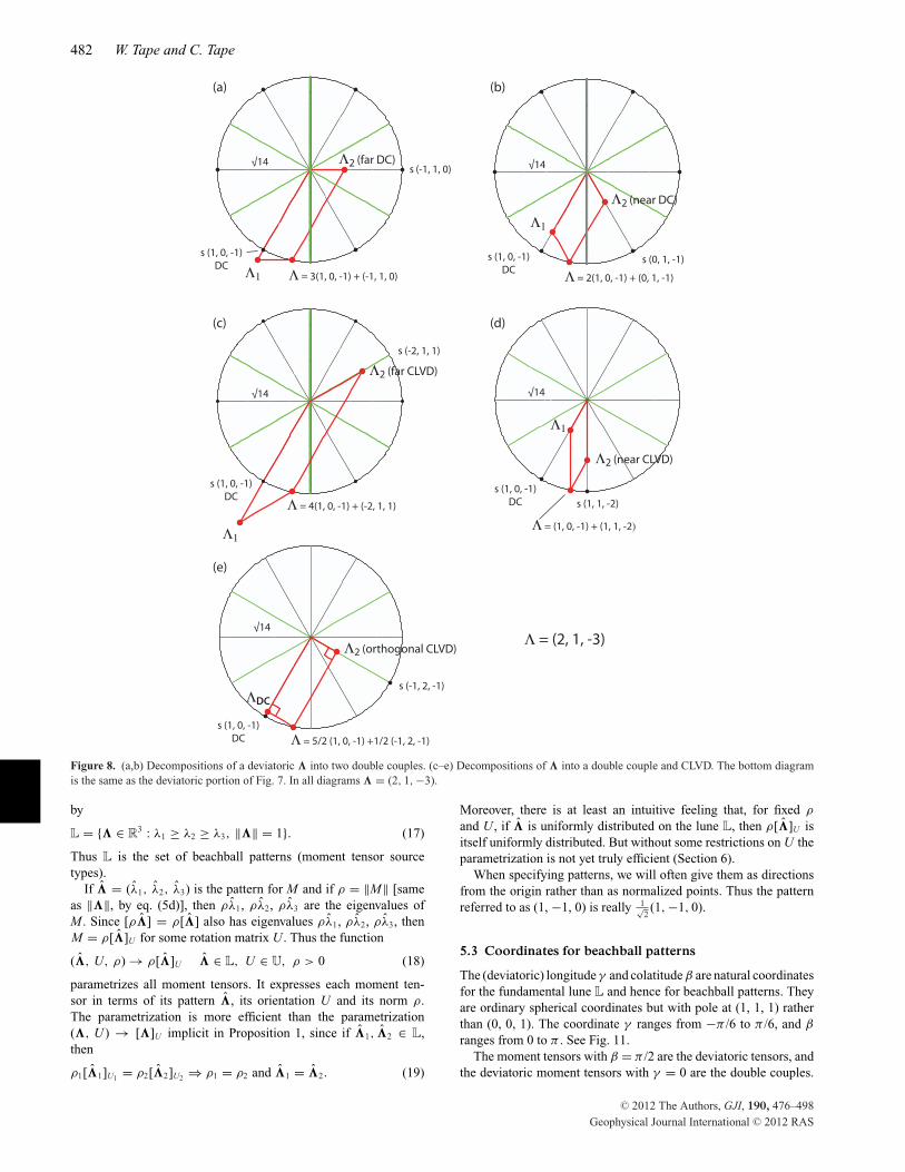
Two double couples. Suppose � (deviatoric) is to be decomposedinto ‘major’ and ‘minor’ double couples �1 and �2. There are threeDC axes—lines through the origin and a double couple—with the‘major’ DC axis being (in our terminology) the closest of the threeto �. If the point �1 is required to lie on the major DC axis, then�2 must lie on the line through � and parallel to that axis, as inthe diagrams of Fig. 8. That leaves two possibilities for the doublecouple �2; it can be the ‘near’ (to �) or the ‘far’ (from �) minordouble couple.

In general, if � = (λ1, λ2, λ3) is deviatoric and λ1 > λ2 > λ3,then the decomposition using the far minor DC is (Fig. 8a)

� =

⎧⎪⎪⎪⎪⎨⎪⎪⎪⎪⎩

(−λ3)(1, 0, −1)︸︷︷︸major DC

+ λ2(−1, 1, 0)︸︷︷︸far minor DC

, (� ∈ D0, λ2 ≥ 0)

λ1(1, 0, −1)︸︷︷︸major DC

+ (−λ2)(0,−1, 1)︸︷︷︸far minor DC

, (� ∈ D0, λ2 < 0).

(11)

For the decomposition using the near minor DC (Fig. 8b), theanalogue of eqs (11) is similar. We omit it.

DC and CLVD. For a decomposition into a double couple andCLVD, we take the axis for the double couple component �1 to bethe closest DC axis to �. Then, as with the decomposition into twodouble couples, �2 must lie on the line through � and parallel tothat axis. That leaves three choices for the CLVD component �2: the‘far’ CLVD, the ‘near’ CLVD and the ‘orthogonal’ CLVD, shown inFigs 8(c)–(e).

If �2 is to be the orthogonal CLVD component (Fig. 8e), then

� = λ1 − λ3

2(1, 0, −1)︸︷︷︸

�DC = closest DC

+ λ2

2(−1, 2, −1)︸︷︷︸

orthogonal CLVD

, (� ∈ D0) (12)

In eq. (12), the magnitude M0 = (λ1 − λ3)/2 of �DC is familiarfrom Dziewonski & Woodhouse (1983). Eq. (12) is the special caseof eq. (9) in which � is deviatoric.

If �2 is the near CLVD component (Fig. 8d), then

�=

⎧⎪⎪⎪⎨⎪⎪⎪⎩

(2λ1 + λ3)(1, 0, −1)︸︷︷︸DC

+ λ2(1, 1, −2)︸︷︷︸near CLVD

(� ∈ D, λ2 ≥ 0)

(λ1 + 2λ2)(1, 0, −1)︸︷︷︸DC

+ (−λ2)(2, −1, −1)︸︷︷︸near CLVD

(� ∈ D, λ2 < 0).

(13)

The equations for the case where �2 is the far CLVD component(Fig. 8c) are similar, but the domain for � is D0 rather than D. Theequations are omitted.

Three double couples. Ben-Menahem & Singh (1981) and Jost &Herrmann (1989) give a decomposition of a deviatoric � into threedouble couples. That is, � is written as a linear combination of(1, 0, −1), ( − 1, 1, 0) and (0, −1, 1). Since the three double couplesare necessarily linearly dependent, there are infinitely many choicesfor the coefficients in the linear combination, and the decompositionis far from unique. Thus

� = t(1, 0, −1)︸︷︷︸DC

+ (t − λ1)(−1, 1, 0)︸︷︷︸DC

+ (t + λ3)(0, −1, 1)︸︷︷︸DC

,

(λ1, λ2, λ3 distinct)(14)

where t is arbitrary. For Jost & Herrmann, t = (λ1 − λ3)/3. Thedecompositions into two double couples (Figs 8a and b) are specialcases of eq. (14) where one of the coefficients is zero.

From the examples above, it is clear that it is trivial to concoctdecompositions. The substantive part comes in providing physicalrationales for them (e.g. Frohlich 1994; Julian et al. 1998; Milleret al. 1998). And we emphasize again that the decompositions ofthis section are special in that the component moment tensors havethe same principal axes as the given tensor.

4.3.2 A subtle point

Eq. (6) contains more than meets the eye. For a given moment tensorM with eigenvalue triple � = �1 + �2, the equation appears togive a decomposition of M into moment tensors M1 and M2 having

C© 2012 The Authors, GJI, 190, 476–498



Figure 7. Decompositions � = �DEV + �ISO (eq. 8) and � = �DC + �CLVD + �ISO (eq. 9). The grey rectangle is in the deviatoric plane, and its edgesare parallel to the 101 (DC) and 121 (CLVD) directions. The volumes of the beachballs are proportional to their norms. We are referring to the momenttensors in terms of their �s, but note that all of the moment tensors have the same principal axes. � = (3, 2,−2), �DEV = (2, 1,−3), �ISO = (1, 1, 1),�DC = (5/2, 0,−5/2) and �CLVD = (−1/2, 1,−1/2). The orientation of the sphere is the same as that of the decomposition diagram; the deviatoric plane(grey) is horizontal, and the isotropic axis—the 111 direction—is vertical.

eigenvalue triples �1 and �2. But a frame U is involved, and if Mcan be written in the form [�]U in more ways than one, then M1

and M2 might not be well-defined functions of M .If M = [�]U = [�]V , with � = �1 + �2, and if the entries of

� are distinct, then V = UW for some W = X π , Yπ , Zπ or I , byProposition 5 of Appendix A. And then [�1]V = [�1]U W = [�1]U ;we get the same M1 from eq. (6) whether using U or V . And similarlyfor M2. The moment tensors M1 and M2 are well-defined functionsof M .

By way of contrast, consider the decomposition of the CLVD� = (1, 1, −2) into its DC and orthogonal CLVD components �1

and �2 (eq. 12). We attempt to mimic the argument of the pre-vious paragraph, with M = [�]U = [�]V and � = �1 + �2.Because � has repeated entries, this time we can conclude only thatV = UW for some W in Cz , the group of rotational symmetriesof a vertical cylinder (Proposition 6 of Appendix A). The rotationW , for example, might be Zπ/6, a thirty degree rotation about thez-axis. In that case, V = UZπ/6 = [UZπ/6U−1]U , so that the frameV would be the result of rotating the frame U thirty degrees aboutUe3 = V e3, the main symmetry axis of the beachball for M ; seeFig. 9. Now [�1]U = [�1]V and [�2]U = [�2]V , and thus nei-ther M1 nor M2 is a well-defined function of M . Or one can takethe point of view that there are now infinitely many moment ten-sor decompositions of M determined by the vector decomposition� = �1 + �2. The complication in this example is that the beach-balls [�1] and [�2] do not have all of the symmetries possessedby the beachball [�]. Equivalently, the triple � is more degeneratethan �1 and �2.

In general, a necessary and sufficient condition that eq. (6) de-termine a well-defined decomposition of M is that �1 and �2 eachbe at least as degenerate as �. That is, if two entries of � coin-cide, then the corresponding entries of �1 should coincide, and thecorresponding entries of �2 should coincide. (If the condition fails,one still gets a decomposition, but the decomposition depends on

which of the infinitely many possible frames U for M is chosen.)If � has distinct entries—by far the most common case—then thecondition is automatically satisfied and hence the moment tensordecomposition is well defined. But in the Fig. 9 example above,� = (1, 1, −2) had two equal entries, while �1 and �2 did not.

5 B E A C H B A L L PAT T E R N S

5.1 Permuting the eigenvalues

As in Fig. 10, a typical moment tensor will appear at six points inλ-space, the points being permutations of each other. Each transpo-sition of � = (λ1, λ2, λ3) corresponds to a reflection in one of themirror planes λ1 = λ2, λ2 = λ3, λ3 = λ1, and the six points are there-fore symmetrically disposed with respect to the planes. The mirrorplanes divide λ-space into six congruent infinite wedges, with eachwedge corresponding to an eigenvalue ordering. Our ‘fundamentalwedge’ W is

W = {� ∈ R3 : λ1 ≥ λ2 ≥ λ3}. (15)

The technicalities of the permutation of eigenvalues and ofthe associated permutation of eigenvectors are deferred toAppendix A.

5.2 Beachball patterns

Informally, the beachball pattern is the moment tensor informationthat is neither orientation nor size. Precisely, we define the pattern� of a moment tensor M by

� = (λ1, λ2, λ3)

(λ21 + λ2

2 + λ23)1/2

= �

‖�‖ λ1 ≥ λ2 ≥ λ3, (16)

where λ1, λ2, λ3 are the eigenvalues of M , ordered as indicated.Beachball patterns lie on the ‘fundamental lune’ L (Fig. 11) defined

C© 2012 The Authors, GJI, 190, 476–498



Figure 8. (a,b) Decompositions of a deviatoric � into two double couples. (c–e) Decompositions of � into a double couple and CLVD. The bottom diagramis the same as the deviatoric portion of Fig. 7. In all diagrams � = (2, 1,−3).

by

L = {� ∈ R3 : λ1 ≥ λ2 ≥ λ3, ‖�‖ = 1}. (17)

Thus L is the set of beachball patterns (moment tensor sourcetypes).

If � = (λ1, λ2, λ3) is the pattern for M and if ρ = ‖M‖ [sameas ‖�‖, by eq. (5d)], then ρλ1, ρλ2, ρλ3 are the eigenvalues ofM . Since [ρ�] = ρ[�] also has eigenvalues ρλ1, ρλ2, ρλ3, thenM = ρ[�]U for some rotation matrix U . Thus the function

(�, U, ρ) → ρ[�]U � ∈ L, U ∈ U, ρ > 0 (18)

parametrizes all moment tensors. It expresses each moment ten-sor in terms of its pattern �, its orientation U and its norm ρ.The parametrization is more efficient than the parametrization(�, U ) → [�]U implicit in Proposition 1, since if �1, �2 ∈ L,then

ρ1[�1]U1 = ρ2[�2]U2 ⇒ ρ1 = ρ2 and �1 = �2. (19)

Moreover, there is at least an intuitive feeling that, for fixed ρ

and U , if � is uniformly distributed on the lune L, then ρ[�]U isitself uniformly distributed. But without some restrictions on U theparametrization is not yet truly efficient (Section 6).

When specifying patterns, we will often give them as directionsfrom the origin rather than as normalized points. Thus the patternreferred to as (1, −1, 0) is really 1√

2(1, −1, 0).

5.3 Coordinates for beachball patterns

The (deviatoric) longitude γ and colatitude β are natural coordinatesfor the fundamental lune L and hence for beachball patterns. Theyare ordinary spherical coordinates but with pole at (1, 1, 1) ratherthan (0, 0, 1). The coordinate γ ranges from −π /6 to π /6, and β

ranges from 0 to π . See Fig. 11.The moment tensors with β = π /2 are the deviatoric tensors, and

the deviatoric moment tensors with γ = 0 are the double couples.

C© 2012 The Authors, GJI, 190, 476–498



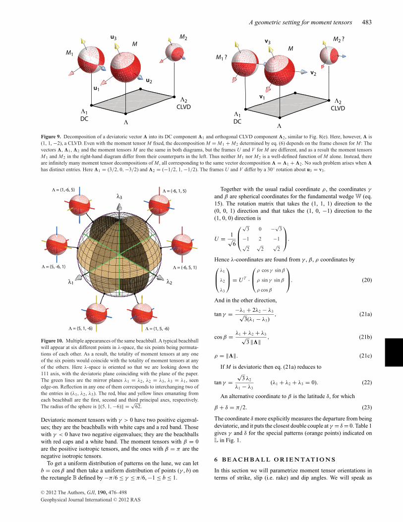
Figure 9. Decomposition of a deviatoric vector � into its DC component �1 and orthogonal CLVD component �2, similar to Fig. 8(e). Here, however, � is(1, 1, −2), a CLVD. Even with the moment tensor M fixed, the decomposition M = M1 + M2 determined by eq. (6) depends on the frame chosen for M : Thevectors �, �1, �2 and the moment tensors M are the same in both diagrams, but the frames U and V for M are different, and as a result the moment tensorsM1 and M2 in the right-hand diagram differ from their counterparts in the left. Thus neither M1 nor M2 is a well-defined function of M alone. Instead, thereare infinitely many moment tensor decompositions of M , all corresponding to the same vector decomposition � = �1 + �2. No such problem arises when �

has distinct entries. Here �1 = (3/2, 0, −3/2) and �2 = (−1/2, 1,−1/2). The frames U and V differ by a 30◦ rotation about u3 = v3.

Figure 10. Multiple appearances of the same beachball. A typical beachballwill appear at six different points in λ-space, the six points being permuta-tions of each other. As a result, the totality of moment tensors at any oneof the six points would coincide with the totality of moment tensors at anyof the others. Here λ-space is oriented so that we are looking down the111 axis, with the deviatoric plane coinciding with the plane of the paper.The green lines are the mirror planes λ1 = λ2, λ2 = λ3, λ3 = λ1, seenedge-on. Reflection in any one of them corresponds to interchanging two ofthe entries in (λ1, λ2, λ3). The red, blue and yellow lines emanating fromeach beachball are the first, second and third principal axes, respectively.The radius of the sphere is ‖(5, 1, −6)‖ = √

62.

Deviatoric moment tensors with γ > 0 have two positive eigenval-ues; they are the beachballs with white caps and a red band. Thosewith γ < 0 have two negative eigenvalues; they are the beachballswith red caps and a white band. The moment tensors with β = 0are the positive isotropic tensors, and the ones with β = π are thenegative isotropic tensors.

To get a uniform distribution of patterns on the lune, we can letb = cos β and then take a uniform distribution of points (γ , b) onthe rectangle B defined by −π /6 ≤ γ ≤ π /6, −1 ≤ b ≤ 1.

Together with the usual radial coordinate ρ, the coordinates γ

and β are spherical coordinates for the fundamental wedge W (eq.15). The rotation matrix that takes the (1, 1, 1) direction to the(0, 0, 1) direction and that takes the (1, 0, −1) direction to the(1, 0, 0) direction is

U = 1√6

⎛⎜⎝

√3 0 −√

3

−1 2 −1√

2√

2√

2

⎞⎟⎠.

Hence λ-coordinates are found from γ , β, ρ coordinates by⎛⎜⎝

λ1

λ2

λ3

⎞⎟⎠ = U T ·

⎛⎜⎝

ρ cos γ sin β

ρ sin γ sin β

ρ cos β

⎞⎟⎠. (20)

And in the other direction,

tan γ = −λ1 + 2λ2 − λ3√3(λ1 − λ3)

, (21a)

cos β = λ1 + λ2 + λ3√3 ‖�‖ , (21b)

ρ = ‖�‖. (21c)

If M is deviatoric then eq. (21a) reduces to

tan γ =√

3 λ2

λ1 − λ3(λ1 + λ2 + λ3 = 0). (22)

An alternative coordinate to β is the latitude δ, for which

β + δ = π/2. (23)

The coordinate δ more explicitly measures the departure from beingdeviatoric, and it puts the closest double couple at γ = δ = 0. Table 1gives γ and δ for the special patterns (orange points) indicated onL in Fig. 1.

6 B E A C H B A L L O R I E N TAT I O N S

In this section we will parametrize moment tensor orientations interms of strike, slip (i.e. rake) and dip angles. We will speak as

C© 2012 The Authors, GJI, 190, 476–498



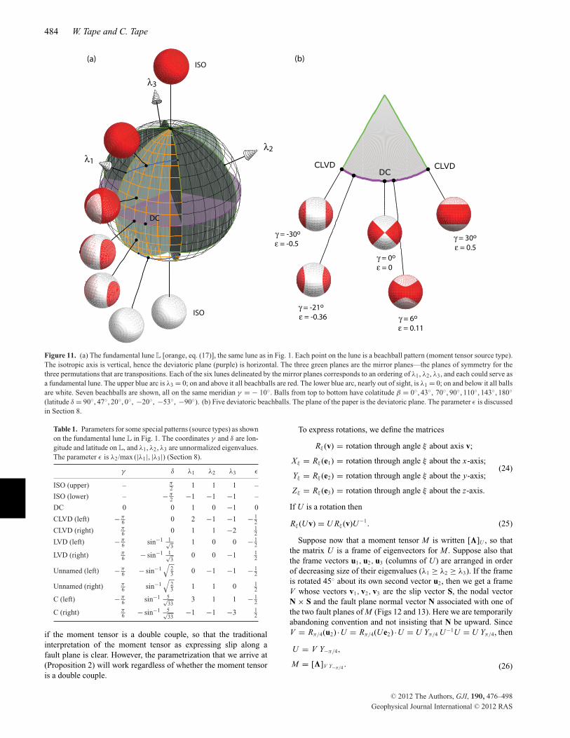
Figure 11. (a) The fundamental lune L [orange, eq. (17)], the same lune as in Fig. 1. Each point on the lune is a beachball pattern (moment tensor source type).The isotropic axis is vertical, hence the deviatoric plane (purple) is horizontal. The three green planes are the mirror planes—the planes of symmetry for thethree permutations that are transpositions. Each of the six lunes delineated by the mirror planes corresponds to an ordering of λ1, λ2, λ3, and each could serve asa fundamental lune. The upper blue arc is λ3 = 0; on and above it all beachballs are red. The lower blue arc, nearly out of sight, is λ1 = 0; on and below it all ballsare white. Seven beachballs are shown, all on the same meridian γ = − 10◦. Balls from top to bottom have colatitude β = 0◦, 43◦, 70◦, 90◦, 110◦, 143◦, 180◦(latitude δ = 90◦, 47◦, 20◦, 0◦, −20◦, −53◦, −90◦). (b) Five deviatoric beachballs. The plane of the paper is the deviatoric plane. The parameter ε is discussedin Section 8.

Table 1. Parameters for some special patterns (source types) as shownon the fundamental lune L in Fig. 1. The coordinates γ and δ are lon-gitude and latitude on L, and λ1, λ2, λ3 are unnormalized eigenvalues.The parameter ε is λ2/max (|λ1|, |λ3|) (Section 8).

γ δ λ1 λ2 λ3 ε

ISO (upper) – π2 1 1 1 –

ISO (lower) – − π2 −1 −1 −1 –

DC 0 0 1 0 −1 0

CLVD (left) − π6 0 2 −1 −1 − 1

2

CLVD (right) π6 0 1 1 −2 1

2

LVD (left) − π6 sin−1 1√

31 0 0 − 1

2

LVD (right) π6 − sin−1 1√

30 0 −1 1

2

Unnamed (left) − π6 − sin−1

√23 0 −1 −1 − 1

2

Unnamed (right) π6 sin−1

√23 1 1 0 1

2

C (left) − π6 sin−1 5√

333 1 1 − 1

2

C (right) π6 − sin−1 5√

33−1 −1 −3 1

2

if the moment tensor is a double couple, so that the traditionalinterpretation of the moment tensor as expressing slip along afault plane is clear. However, the parametrization that we arrive at(Proposition 2) will work regardless of whether the moment tensoris a double couple.

To express rotations, we define the matrices

Rξ (v) = rotation through angle ξ about axis v;

Xξ = Rξ (e1) = rotation through angle ξ about the x-axis;

Yξ = Rξ (e2) = rotation through angle ξ about the y-axis;

Zξ = Rξ (e3) = rotation through angle ξ about the z-axis.

(24)

If U is a rotation then

Rξ (Uv) = U Rξ (v)U−1. (25)

Suppose now that a moment tensor M is written [�]U , so thatthe matrix U is a frame of eigenvectors for M . Suppose also thatthe frame vectors u1, u2, u3 (columns of U) are arranged in orderof decreasing size of their eigenvalues (λ1 ≥ λ2 ≥ λ3). If the frameis rotated 45◦ about its own second vector u2, then we get a frameV whose vectors v1, v2, v3 are the slip vector S, the nodal vectorN × S and the fault plane normal vector N associated with one ofthe two fault planes of M (Figs 12 and 13). Here we are temporarilyabandoning convention and not insisting that N be upward. SinceV = Rπ/4(u2) ·U = Rπ/4(Ue2) ·U = U Yπ/4 U−1U = U Yπ/4, then

U = V Y−π/4,

M = [�]V Y−π/4 . (26)

C© 2012 The Authors, GJI, 190, 476–498



Figure 12. Frame U of eigenvectors u1, u2, u3 of a double couple, andframe V of slip, nodal and normal vectors v1 = S, v2 = N × S and v3 = Nfor one of the two fault planes of the double couple. If the frame vectorsof U are ordered according to decreasing size of their eigenvalues, as here,then the frames U and V differ by a 45◦ rotation about their common secondvector u2 = v2.

Of the two frames U and V , the frame U is the more naturalmathematically, but V is more directly tied to the strike, slip anddip angles. The slip and normal vectors S and N, and hence M =[�]V Y−π/4 , can be expressed in terms of the strike, slip and dipangles κ , σ and θ . As in Fig. 14,

K = Rφ(e3) · e1 = Zφ · e1 (strike vector) (27a)

N = Rθ (K) · e3 (normal vector) (27b)

S = Rσ (N) · K (slip vector), (27c)

where the standard basis is e1 (north), e2 (west), e3 (zenith), andwhere φ = −κ , so that positive κ will be clockwise. Since we areallowing the normal N to be downwards, then the dip angle θ variesfrom 0 to π rather than the conventional 0 to π /2. Since the matrixV is a function of S and N, namely,

V (S, N) = (S, N × S, N), (28)

Figure 14. Diagram for eqs (27) and (40), showing strike vector K, slipvector S and normal vector N. Everything green is horizontal.

then the moment tensor M = [�]V Y−π/4 is a function of κ , σ and θ

(and �). (The vectors S, N × S and N must be regarded as columnvectors, and in fact they are the columns of V .)

If N is not vertical then eqs (27) define κ (mod 2π ), σ (mod 2π )and θ (0 < θ < π ) as functions of (S, N), using the fact that

K = e3 × N

‖e3 × N‖ = e3 × N

sin θ. (29)

6.1 An efficient parametrization

If � is fixed and the angles φ, σ , θ are allowed to vary, with −2π

≤ φ ≤ 0, −π ≤ σ ≤ π and 0 ≤ θ ≤ π , then the parametrization

Figure 13. Strike vector K, slip vector S and fault normal vector N, together with strike angle κ , slip angle σ and dip angle θ . The block on the N side of thefault slips in the direction S relative to the other block. The quadrant of the double couple beachball between S and N should therefore be red. Our slip vectorS is a unit vector, so S gives only the direction, not the magnitude, of slip.

C© 2012 The Authors, GJI, 190, 476–498



Figure 15. The same double couple moment tensor, with four different triples of strike, slip and dip coordinates (κ , σ , θ ). The four triples correspond to slipand normal vector pairs (S, N), (−S, −N), (N, S) and (−N, −S). Black arrows are the normal vectors, and orange arrows are the slip vectors. Green arrowsare the strike vectors. The discs are the fault planes for the normals. The pairs (S, N) and (−S, −N) correspond to one fault plane and motion, and the pairs(N, S) and (−N, −S) correspond to the other. One of the four coordinate triples (κ , σ , θ ), namely the one with θ ≤ π /2 and |σ | ≤ π /2, must be in the set P ofProposition 2.

(φ, σ, θ ) → [�]V Y−π/4 generates all moment tensors having eigen-values �, but it does so with duplication, since more than one pair(S, N) give the same moment tensor, as illustrated in Fig. 15. Toconfirm the duplication, let

Px = Y−π/4 · Xπ · Yπ/4,

Py = Y−π/4 · Yπ · Yπ/4 = Yπ ,

Pz = Y−π/4 · Zπ · Yπ/4. (30)

Then

Px =

⎛⎜⎝

0 0 1

0 −1 0

1 0 0

⎞⎟⎠, Pz =

⎛⎜⎝

0 0 −1

0 −1 0

−1 0 0

⎞⎟⎠, (31)

V (S, N) · Px = V (N, S),

V (S, N) · Py = V (−S, −N),

V (S, N) · Pz = V (−N, −S).

(32)

Since X π , Yπ , Zπ all commute with [�], then Px, Py, Pz all commutewith [�]Y−π/4 , and

[�]V (S, N) Y−π/4 = [�]V (−S, −N) Y−π/4

= [�]V (N, S) Y−π/4 = [�]V (−N, −S) Y−π/4 . (33)

In other words, the four slip and normal vector pairs (S, N),(−S, −N), (N, S) and (−N, −S) all give the same moment ten-sor. See Fig. 15.

For the parametrizing function, we want to choose just one ofthe four pairs. Let us assume for the moment that neither S norN is vertical. If κ ′, σ ′, θ ′ are coordinates for the sign-changed pair(S′, N′) = (−S, −N), then

θ ′ = π − θ (for sign change) (34a)

σ ′ = −σ (for sign change). (34b)

Thus 0 ≤ θ ≤ π /2 or 0 ≤ θ ′ ≤ π /2.If instead κ ′, σ ′, θ ′ are coordinates for the swapped pair (S′, N′) =

(N, S), then

cos σ = K · S

= (e3 × N) · S

sin θ,

(35)

cos σ ′ = K′ · S′

= (e3 × N′) · S′

sin θ ′

= (e3 × S) · N

sin θ ′ .

(36)

Since (e3 × S) · N = −(e3 × N) · S, then

cos σ ′ sin θ ′ = − cos σ sin θ (for swap). (37)

Thus cos σ and cos σ ′ have opposite signs, and so |σ | ≤ π /2 or|σ ′| ≤ π /2. The same conclusion holds for a combined swap andsign change, since the sign change of the slip and normal pair onlychanges the sign of σ , not the magnitude. Thus one of the four pairs(S, N), (−S, −N), (N, S) and (−N, −S) associated with eq. (33)will have its σ and θ coordinates satisfying |σ | ≤ π /2 and 0 ≤ θ ≤π /2; again see Fig. 15. And if one of S or N happens to be vertical,then the other is horizontal, and then one of the four slip and normalpairs will have σ = ±π /2 and θ = π /2, and so the conclusion stillholds: there is no loss in generality in assuming |σ | ≤ π /2 and0 ≤ θ ≤ π /2.

For fixed � we now have an efficient parametrization of momenttensors that have eigenvalues �. Proposition 2, next, is a summary.In it we use the parameter h = cos θ instead of θ , to make the frameV of slip, nodal and normal vectors uniformly distributed (Sec-tion 6.2). The form for the slip and normal vectors in the propositionis consistent with eq. (4.88) of Aki & Richards (2002).

Proposition 2. Let � = (λ1, λ2, λ3) and let P (Fig. 16) consist ofpoints (κ , σ , h) such that

0 ≤ κ ≤ 2π, −π

2≤ σ ≤ π

2, 0 ≤ h ≤ 1.

Let V = V (κ, σ, h) = (S, N × S, N) be (from eqs 27 and 28)⎛⎜⎜⎜⎜⎜⎜⎜⎜⎜⎜⎝

cos κ cos σ h sin κ cos σ −√1 − h2 sin κ

+h sin κ sin σ − cos κ sin σ

− sin κ cos σ h cos κ cos σ −√1 − h2 cos κ

+h cos κ sin σ + sin κ sin σ

√1 − h2 sin σ

√1 − h2 cos σ h

⎞⎟⎟⎟⎟⎟⎟⎟⎟⎟⎟⎠

.

C© 2012 The Authors, GJI, 190, 476–498



Figure 16. Physical map of the solid block P that is the orientation parameter space of Proposition 2. Except on the very top (h = 1), each line segment ofP parallel to the σ -axis corresponds to a distinct fault plane. Moving along such a segment corresponds to varying the slip angle σ in a diagram like Fig. 13while leaving the fault plane unchanged. Also see Fig. 17.

Then the function

(κ, σ, h) → [�]V Y−π/4 , (κ, σ, h) ∈ P (38)

parametrizes all moment tensors having eigenvalues � (in any or-der). If λ1, λ2, λ3 are distinct then the parametrization is one-to-one(but not quite onto) on the set P0 ⊂ P consisting of points with0 ≤ κ < 2π , −π /2 < σ < π /2, 0 < h < 1.

Proof . It only remains to verify the claim about one-to-one. Sup-pose that [�]V1 Y−π/4 = [�]V2 Y−π/4 , where Vi = V (κi , σi , hi ) =(Si , Ni × Si , Ni ) and (κi , σi , hi ) ∈ P0. [We need to show (κ1, σ 1,h1) = (κ2, σ 2, h2).] Letting Ui = V iY−π/4, we find from Proposition5 in Appendix A that U2 = U1W , where W is one of I , X π , Yπ or Zπ .That in turn means (eqs 30 and 32) that (S2, N2) is one of (S1, N1),(−S1, −N1), (N1, S1) or (−N1, −S1). But due to eqs (34b) and(37), only one of (S1, N1), (−S1, −N1), (N1, S1) and (−N1, −S1)can have its coordinates in P0. Therefore (S1, N1) = (S2, N2) and(κ1, σ 1, h1) = (κ2, σ 2, h2). �

If λ1 >λ2 >λ3, then the angles κ , σ and θ = cos −1h are the strike,slip and dip angles for one of the two fault planes associated withthe closest double couple to [�]V Y−π/4 . Fig. 16 shows the locationsin P of parameters (κ , σ , h) for some familiar types of faults andslips. See also Fig. 17, which shows several double couple momenttensors at their parameter points in P. Although P is big enoughto accommodate all double couple moment tensors (or any othermoment tensors with fixed �), it only directly depicts about a halfof the associated faults and slips, namely, those with |σ | ≤ π /2.The other half have |σ | ≥ π /2 and are the second fault planes of thedouble couples. They are found from (S, N) (first and third columnsof V ) by swapping S and N and then, if necessary, changing the signsof both, so that the new normal is upwards.

6.2 Uniformity of the frames, not the moment tensors

If we define V ′ = Rσ (N) · Rθ (K) · Zφ , then V ′ is a rotation matrixthat takes e1 and e3 to S and N, respectively. In detail, from Fig. 14,

V ′ : e1Zφ−→ K

Rθ (K)−→ KRσ (N)−→ S,

V ′ : e3Zφ−→ e3

Rθ (K)−→ NRσ (N)−→ N. (39)

Since V (Proposition 2) also takes e1 and e3 to S and N, thenV = V ′, that is,

V = Rσ (N) · Rθ (K) · Zφ. (40)

The coordinates φ and θ determine N = V e3 and K, and then σ tellshow much to rotate K about N to get S = V e1. Since φ − π /2 andθ are the ordinary spherical coordinates (longitude and colatitude,respectively) for

N = (cos(φ − π/2) sin θ, sin(φ − π/2) sin θ, cos θ) , (41)

then N will be uniformly distributed on the unit sphere if φ (i.e. −κ)is uniformly distributed and if h = cos θ is uniformly distributed onthe interval [−1, 1]. If also σ is uniformly distributed then the frameV should be uniformly distributed. This is the reason for using theparameter h instead of θ in Proposition 2; a uniform distribution of(κ , σ , h) gives a uniform distribution of frames.

A uniform distribution of frames does not, however, ensure auniform distribution of moment tensors. This is easy to see whenγ ≈ ±π /6, since in that case the beachball nearly has cylindricalsymmetry. A uniform distribution of frames will waste frames thatdiffer from each other approximately by a rotation whose axis isclose to the cylinder axis. The same point has been made by Hudsonet al. (1989).

For a more rigorous discussion of uniformly distributed frames,see Miles (1965) and Robbin (2006).

6.3 From moment tensor to strike, slip and dip

We are given a moment tensor M with distinct eigenvalues. Wheredoes M get located in the set P of Proposition 2? The answer islargely contained in Fig. 12. We find a frame U of eigenvectors ofM that are ordered according to decreasing size of their eigenvalues.From U we get the frame V = U Yπ/4. Then the four candidates forslip and normal vector pairs (S, N) are (v1, v3), (−v1, −v3), (v3, v1)and (−v3, −v1). We calculate σ and θ for each, using eqs (27) and(29). The pair (S, N) that is wanted is the one with |σ | ≤ π /2 and0 ≤ θ ≤ π /2. Some qualification is needed to accommodate excep-tional cases such as horizontal faults; see Appendix B.

C© 2012 The Authors, GJI, 190, 476–498



Figure 17. Some double couple moment tensors, each located at its parameter point (κ , σ , h) in P. Black arrows are fault normal vectors, green are strikevectors and orange are slip vectors. The discs are the fault planes for the normals. At the right are normal dip slips, σ = −π /2, and at the left are reverse dipslips, σ = +π /2. At the centre are strike-slips, σ = 0. For σ = 0 the slip vector coincides with the strike vector and is not seen. All strike angles here are κ =π /2. In this diagram the κ and σ axes are aligned with the spatial x (north) and y (west) axes as shown. The dimensions of P are not drawn to scale, and thevertical axis is sin −1h = π /2 − θ (elevation angle of N) rather than h, both done in order to display the beachballs better.

7 PA R A M E T R I Z I N G A L L M O M E N TT E N S O R S

Combining the results of Proposition 2 and eq. (18), we have anefficient and conceptually reasonable parametrization of the spaceM of all moment tensors (Proposition 3, next). Recall that γ andβ = cos −1b are longitude and colatitude for the lune L, and that κ ,σ and θ = cos −1h are the strike, slip and dip angles for the closestdouble couple. Also recall that

B ={

(γ, b) : −π

6≤ γ ≤ π

6, −1 ≤ b ≤ 1

}, (42a)

P ={

(κ, σ, h) : 0 ≤ κ ≤ 2π, −π

2≤ σ ≤ π

2, 0 ≤ h ≤ 1

}. (42b)

Proposition 3. Define M : B × P × R+ → M by

M(γ, b, κ, σ, h, ρ) = ρ[�]V Y−π/4 ,

where

� = �(γ, b) [from eq. 20 with ρ = 1],

V = V (κ, σ, h) [from Proposition 2],

ρ > 0.

Then the function M parametrizes all moment tensors. It is one-to-one (but not quite onto M) if its domain is restricted to B0×P0×R

+,where

B0 = {(γ, b) : −π

6< γ <

π

6, −1 < b < 1} ⊂ B,

P0 = {(κ, σ, h) : 0 ≤ κ < 2π, −π

2< σ <

π

2, 0 < h < 1} ⊂ P.

(B0 consists of coordinates for patterns that have distinct entries.)

Proof . It only remains to verify the claim about one-to-one. Sosuppose that ρ1[�1]U1 = ρ2[�2]U2 , where �i = �(bi ), bi ∈ B0,Ui = V (pi ) Y−π/4, pi ∈ P0, ρ i > 0. Then

|ρ1| = ‖ ρ1[�1]U1 ‖ = ‖ ρ2[�2]U2 ‖ = |ρ2|,and so ρ1 = ρ2. Then [�1]U1 and [�2]U2 are equal and hence havethe same eigenvalues, so that �2 is a permutation of �1. Since�i ∈ L, then �1 = �2 = �. Then [�]V (p1) Y−π/4 = [�]V (p2) Y−π/4 .

Since bi ∈ B0 then the entries of � are distinct and hence p1 = p2,by Proposition 2, since pi ∈ P0. Since bi ∈ B0 and �1 = �2 thenb1 = b2. �

Fig. 18 illustrates the making of the moment tensor M =ρ[�]V Y−π/4 in Proposition 3. The coordinates γ and b determine

the pattern � = (λ1, λ2, λ3) ∈ L, and the coordinates κ , σ , h deter-mine the rotation matrix V . The beachball [�] has eigenvalues �

and eigenvectors e1, e2, e3, the standard basis vectors. That beach-ball is then rotated 45◦ clockwise about the y-axis, resulting in thebeachball [�]Y−π/4 ; the vectors e1 and e3 are slip and normal vectorsfor one of the two slip motions associated with it. The vectors V e1

and V e3—the first and third columns of V—must therefore be slipand normal vectors for the beachball [�]V Y−π/4 , which is the resultof an additional rotation by means of V . Lastly the ball would bescaled by the factor ρ, not shown in the figure.

In Appendix B we construct a set P1, with P0 ⊂ P1 ⊂ P, suchthat, when restricted to B0×P1×R

+, the function M in Proposition 3is one-to-one and parametrizes all moment tensors that have distincteigenvalues. For seismological applications the fine distinction be-tween P0, P1 and P is apt to be irrelevant, since minor duplicationof moment tensors is usually acceptable within grid search algo-rithms, but the fact that duplication occurs—on the boundary ofP—does matter. The duplication shows dramatically that distances

C© 2012 The Authors, GJI, 190, 476–498



Figure 18. Creating the moment tensor [�]V Y−π/4 of Proposition 3, with pattern � and slip–nodal–normal frame V = {S, N × S, N}. For purposes of

illustration, � is taken to be a double couple, namely, � = 1√2

(1, 0, −1). (a) The double couple [�]. The standard basis vectors e1, e2, e3 are its eigenvectors.

(b) The double couple [�]Y−π/4 . The clockwise 45◦ rotation about the y-axis has made the slip and normal vectors S0 and N0 of the new tensor coincide with e1

and e3. (This depends on the fact that λ1 ≥ λ2 ≥ λ3.) (c) The double couple [�]V Y−π/4 , the result of applying the rotation matrix V to the previous beachball.The first and third columns of V are necessarily slip and normal vectors for the new tensor. Here V is a (minus) 25◦ rotation about the x-axis.

Figure 19. (Top) Duplication of moment tensors on the back face σ = π /2 of P. For fixed pattern � and norm ρ, the moment tensors at p0 = (κ0, π/2, cos θ0)and p1 = (κ0 + π, π/2, sin θ0) will be the same. (The points p0 and p1 are at the centres of the balls, on the back face.) The motions are reverse dip slipsthat differ from each other by a swap of their slip and normal vectors. As a result of the duplication, half of the back face of P can be dispensed with inparametrizing moment tensors, as indicated in Fig. B1. Here κ0 = θ0 = π /3, ρ = 1 and � = 1√

2(1, 0,−1). (Bottom) Contour plot of the distance function

d(p) = ‖M(p) − M(p0‖ on the back face. (M(p) is the moment tensor [�]V (p)Y−π/4 .) That is, d(p) is the distance from the ball at p = (κ, π/2, h) to the ballat p0, but with the distance being in moment tensor space and hence measured as explained in Section 4.2. Distances between moment tensors can be quitedifferent from distances in κσh-space.

in moment tensor space are not as they appear in P. Fig. 19 is anillustration. The moment tensors at p0 and p1 are the same, andhence the distance between them is zero, and this is reflected inthe contour plot of distance. So although moment tensors with fixed

pattern and norm can be plotted in P, the interpretation of the resultscan be tricky. By way of contrast, moment tensors with fixed ori-entation can be plotted in λ-space, and distances between momenttensors are then the same as distances in λ-space (eq. 5c).

C© 2012 The Authors, GJI, 190, 476–498



We intend to incorporate the parametrization in Proposition 3 intoan algorithm for moment tensor inversion. That is, the parametriza-tion will be used to construct a grid for use in a grid search. Theradial coordinate ρ should be truncated, both above and below, atsome reasonable values. Then, rather than search over equal incre-ments in ρ, we will let ρ = eq and then search over equal incrementsin q. Since scalar seismic moment is usually defined as M0 = 1√

2ρ,

and since moment magnitude Mw ∝ ln M0, searching over equalincrements of q corresponds to searching over equal increments ofMw. For the remaining five variables, equal increments are proba-bly acceptable, though the resulting moment tensors will not be asequally distributed as we would like.

8 T H E PA R A M E T E R ε

Seismologists have used a certain parameter ε to measure the extentto which a deviatoric eigenvalue triple � = (λ1, λ2, λ3) departsfrom being a double couple. We follow Giardini (1984) and define

ε(�) = λ2

max(|λ1|, |λ3|) , (λ1 ≥ λ2 ≥ λ3). (43)

However, most authors reverse the sign, giving ε = −λ2/max (|λ1|,|λ3|) (e.g. Giardini 1983; Kuge & Kawakatsu 1990). We use theformulation in eq. (43) because it makes ε, λ2 and the deviatoriclongitude γ all have the same sign.

The parameter γ serves the same purpose as ε, and we think thatγ is more transparent than ε. Fig. 11(b) shows some sample valuesof γ and ε for various deviatoric �. The angle γ varies from −π /6to π /6, with γ = 0 at the double couple. The parameter ε variesfrom −0.5 to 0.5, again with ε = 0 at the double couple.

To relate ε and γ analytically: Without loss of generality, � can beassumed to lie on the unit cube (with λ1 + λ2 + λ3 = 0 and λ1 ≥ λ2 ≥λ3), in which case ε is λ2. If λ2 ≥ 0 then � = (1 − λ2, λ2, −1) andthen, from eq. (22),

tan γ =√

3 λ2

λ1 − λ3=

√3 ε

2 − ε, (λ2 ≥ 0). (44)

The case λ2 ≤ 0 is similar. Combined with eq. (44), it gives

tan γ = ε√

3

2 − |ε| . (45)

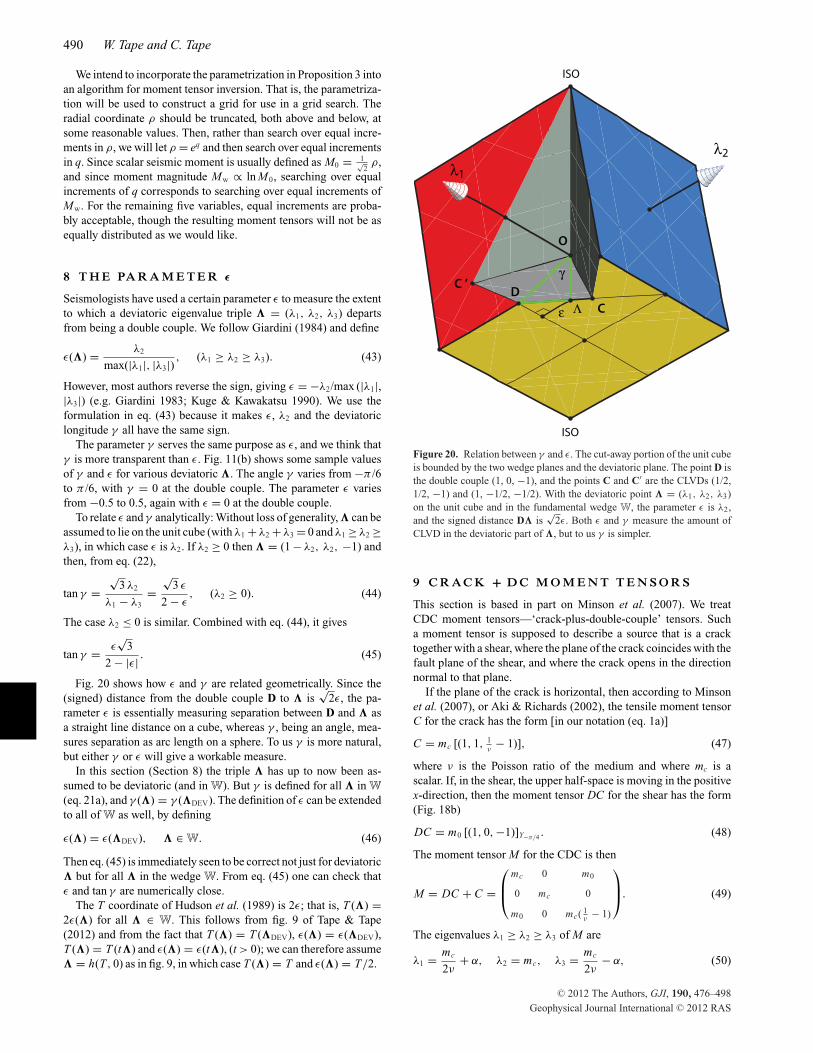
Fig. 20 shows how ε and γ are related geometrically. Since the(signed) distance from the double couple D to � is

√2ε, the pa-

rameter ε is essentially measuring separation between D and � asa straight line distance on a cube, whereas γ , being an angle, mea-sures separation as arc length on a sphere. To us γ is more natural,but either γ or ε will give a workable measure.

In this section (Section 8) the triple � has up to now been as-sumed to be deviatoric (and in W). But γ is defined for all � in W

(eq. 21a), and γ (�) = γ (�DEV). The definition of ε can be extendedto all of W as well, by defining

ε(�) = ε(�DEV), � ∈ W. (46)

Then eq. (45) is immediately seen to be correct not just for deviatoric� but for all � in the wedge W. From eq. (45) one can check thatε and tan γ are numerically close.

The T coordinate of Hudson et al. (1989) is 2ε; that is, T (�) =2ε(�) for all � ∈ W. This follows from fig. 9 of Tape & Tape(2012) and from the fact that T (�) = T (�DEV), ε(�) = ε(�DEV),T (�) = T (t�) and ε(�) = ε(t�), (t > 0); we can therefore assume� = h(T, 0) as in fig. 9, in which case T (�) = T and ε(�) = T/2.

Figure 20. Relation between γ and ε. The cut-away portion of the unit cubeis bounded by the two wedge planes and the deviatoric plane. The point D isthe double couple (1, 0, −1), and the points C and C′ are the CLVDs (1/2,1/2, −1) and (1, −1/2, −1/2). With the deviatoric point � = (λ1, λ2, λ3)on the unit cube and in the fundamental wedge W, the parameter ε is λ2,and the signed distance D� is

√2ε. Both ε and γ measure the amount of

CLVD in the deviatoric part of �, but to us γ is simpler.

9 C R A C K + D C M O M E N T T E N S O R S

This section is based in part on Minson et al. (2007). We treatCDC moment tensors—‘crack-plus-double-couple’ tensors. Sucha moment tensor is supposed to describe a source that is a cracktogether with a shear, where the plane of the crack coincides with thefault plane of the shear, and where the crack opens in the directionnormal to that plane.

If the plane of the crack is horizontal, then according to Minsonet al. (2007), or Aki & Richards (2002), the tensile moment tensorC for the crack has the form [in our notation (eq. 1a)]

C = mc [(1, 1, 1ν

− 1)], (47)

where ν is the Poisson ratio of the medium and where mc is ascalar. If, in the shear, the upper half-space is moving in the positivex-direction, then the moment tensor DC for the shear has the form(Fig. 18b)

DC = m0 [(1, 0, −1)]Y−π/4 . (48)

The moment tensor M for the CDC is then

M = DC + C =

⎛⎜⎝

mc 0 m0

0 mc 0

m0 0 mc( 1ν

− 1)

⎞⎟⎠. (49)

The eigenvalues λ1 ≥ λ2 ≥ λ3 of M are

λ1 = mc

2ν+ α, λ2 = mc, λ3 = mc

2ν− α, (50)

C© 2012 The Authors, GJI, 190, 476–498



where

α =√

m2c

(1 − 2ν

2ν

)2

+ m20. (51)

Hence

λ2

λ1 + λ3= ν. (52)

Eq. (52) holds for any CDC moment tensor, since eq. (49) can beconjugated by any rotation matrix U , and since a suitable choiceof U can achieve any desired configuration of crack plane and slipdirection.

Proposition 4 is a kind of converse to eq. (52). It tells how tofind the double couple and tensile components for a moment tensorwhose eigenvalues satisfy eq. (52).

Proposition 4. If λ1 ≥ λ2 ≥ λ3 and λ2/(λ1 + λ3) = ν, then thediagonal matrix [�] = [(λ1, λ2, λ3)] is a CDC moment tensorwith Poisson parameter ν. Two decompositions of [�] into a doublecouple and a tensile crack are

[�] = m0 [(1, 0, −1)]Yχ− π4

+ mc

[(1, 1, 1

ν− 1)

]Yχ

, (53a)

[�] = m0 [(1, 0, −1)]Y−χ+ π4

+ mc

[(1, 1, 1

ν− 1)

]Y−χ

, (53b)

where Yχ is rotation through angle χ about the y-axis and where

m0 =√

λ1 − λ2

√λ2 − λ3, (54a)

mc = λ2, (54b)

tan2 χ = λ1 − λ2

λ2 − λ3= sin(π/6 − γ )

sin(π/6 + γ )0 ≤ χ ≤ π

2. (54c)

The normal vectors to the crack planes for the two decompositionsare

N1 = Yχ · (0, 0, 1) = (sin χ, 0, cos χ ),

N2 = Y−χ · (0, 0, 1) = (− sin χ, 0, cos χ ),

and the angle between the planes is 2χ .Proof . From eq. (54c) we find

Yχ =

⎛⎜⎜⎜⎜⎜⎜⎜⎝

√λ2 − λ3

λ1 − λ30

√λ1 − λ2

λ1 − λ3

0 1 0

−√

λ1 − λ2

λ1 − λ30

√λ2 − λ3

λ1 − λ3

⎞⎟⎟⎟⎟⎟⎟⎟⎠

and then

[�]Y−χ= Y−χ · [�] · Yχ

=

⎛⎜⎝

λ2 0√

λ1 − λ2√

λ2 − λ3

0 λ2 0√

λ1 − λ2√

λ2 − λ3 0 λ1 − λ2 + λ3

⎞⎟⎠

=√

λ1 − λ2

√λ2 − λ3

⎛⎜⎝

0 0 1

0 0 0

1 0 0

⎞⎟⎠+λ2

⎛⎜⎜⎝

1 0 0

0 1 0

0 0λ1 + λ3

λ2− 1

⎞⎟⎟⎠

= m0 [(1, 0, −1)]Y−π/4 + mc

[(1, 1, 1

ν− 1)

]. (55)

Comparison with eqs (47) and (48) shows that the two terms onthe right-hand side of eq. (55) are double couple and tensile tensorswith a horizontal crack plane. Conjugating by Yχ gives eq. (53a)and rotates the crack plane through angle χ about the y-axis. Thenconjugating eq. (53a) by X π gives eq. (53b), since X π Yχ = Y−χ X π .See Fig. 21.

The second equality in eq. (54c) follows from eq. (21a) and

sin(π/6 − γ )

sin(π/6 + γ )= 1 − √

3 tan γ

1 + √3 tan γ

. (56)

�

A consequence of eq. (54c) is

cos 2χ =√

3 tan γ. (57)

Proposition 4 generalizes to an arbitrary M = [�]U , since eqs(53a) and (53b) can be conjugated by U . The beachballs, the crackplanes and the slip directions all get rotated by U .

Proposition 4 makes no assumptions about the Poisson ratio ν.Theoretical bounds for ν are −1 ≤ ν ≤ 0.5, and most crustal mate-rials have ν in the vicinity of ν = 0.25 (Christensen 1996).

9.1 CDC patterns on the lune

Eq. (52) and Proposition 4 show that for any moment tensor M ,

M is a CDC for ν ⇐⇒ λ2

λ1 + λ3= ν, (58)

where λ1 ≥ λ2 ≥ λ3 are the eigenvalues of M . Since the conditionλ2 = ν(λ1 + λ3) describes a plane through the points (0, 0, 0) and(1, 0, −1), then on the fundamental lune the locus of CDC momenttensor patterns for ν is an arc of a great circle through the doublecouple (1, 0, −1). See Fig. 22.

Fig. 23 shows CDC loci for several values of ν. If ν = −1 then(1, 1, −2) is a CDC pattern for ν, by eq. (58), and so the CDC locusis the deviatoric arc β = π /2. And if ν = 1/2 then (1, 1, 1) is a CDCpattern for ν, and the CDC locus is the meridian γ = 0 consistingof sums of double couple and pure isotropic patterns.

Fig. 23 also shows two CDC beachballs on the meridian γ =−10◦ of the lune. According to eq. (54c) or eq. (57), meridiansare contours for the function 2χ that gives the angle between crackplanes in the CDC decompositions, so here the angles are the samefor the two beachballs.

1 0 M O M E N T T E N S O R PAT T E R N S F O RR E A L E V E N T S

According to Minson et al. (2007), the Miyakejima volcanic earth-quake swarm in the year 2000 contained many events whose sourceswere far from being double couples and in fact were far frombeing deviatoric. For each of 18 of the Miyakejima earthquakes,Minson computed five moment tensors: one was unconstrained, andthe other four were constrained so that one was a double couple,one was deviatoric, one was double couple plus isotropic, and onewas a CDC with ν = 0.25. In Fig. 24 we have plotted the patterns(source types) of their moment tensors on our fundamental lune L.

Fig. 25 shows patterns from five published compilations of fullmoment tensor inversions, including those of Minson above. Themoment tensors of Walter et al. (2009, 2010) are derived fromevents that were within glacial ice or at the base of the glacier. Mostof these are extremely isotropic, with β ≤ 10◦, but one cluster of

C© 2012 The Authors, GJI, 190, 476–498



Figure 21. Illustrating the decompositions in eqs (53a) and (53b), which are here abbreviated to [�] = D1 + C1 and [�] = D2 + C2, respectively. Theplane through each beachball Di and Ci is the plane of the crack. The original [�] is shown again on the right-hand side, with both of the possible crackplanes together. The beachballs are drawn so that their volumes are proportional to their norms. The arrows are in the x, y, z coordinate directions. Thosedirections constitute a principal axis system for the original [�], but the principal axis systems for Di and Ci are different from each other and different fromthe principal axis system for [�]. These decompositions are therefore more subtle than those of Section 4, in which all principal axis systems were the same.Here � = (2, 1,−4).

Figure 22. CDC moment tensors for ν = −0.5. Their patterns lie on a great circle arc through the double couple (1, 0, −1). The planes through the beachballsare the two possible crack planes. The orientations of the balls depend on the choice of principal axes (red, blue and yellow arrows). The plot shows the angle2χ between fault planes as a function of the longitude γ on the lune (eq. 57, independent of ν). The points � are given without their normalizing factors.

C© 2012 The Authors, GJI, 190, 476–498



Figure 23. CDC moment tensor loci (blue arcs) for ν = −1, −0.5,0, 0.2, 0.5. The special case ν = −1 gives the deviatoric tensors, and thespecial case ν = 0.5 gives the moment tensors that are double couple pluspure isotropic. The contours of 2χ , which is the angle between the twopossible CDC crack planes, are meridians on the lune, and so the two CDCbeachballs shown here, both on the meridian γ = −10◦, have the same anglebetween crack planes. For Earth’s crust, only values of ν somewhere nearν = 0.25 are realistic.

events from Walter et al. (2009), ‘surface cluster B’, has a moderatenegative isotropic component. The 18 Miyakejima volcanic eventsfrom Minson et al. (2007) are predominantly positive isotropicwith negative γ values. The 26 geothermal events from Foulgeret al. (2004) have moderate isotropic components, either positiveor negative. The 32 Nevada events of Ford et al. (2009) comprise17 nuclear explosions, 12 earthquakes and three collapses (twomines, one cavity). The three different event types fall into threeclusters, as presented in Ford et al. (2009) and evident in Fig. 25.The moment tensors derived from nuclear explosions are stronglyisotropic, though not as isotropic as most of the glacier events.

The GCMT catalogue contains deviatoric moment tensors frommost global events, 1976–2011, with magnitudes Mw > 5.4(Dziewonski et al. 1981). Because the GCMT algorithm constrainsthe output tensors to be deviatoric (with λ1 ≥ λ2 ≥ λ3), their patternsare confined to the deviatoric arc β = π /2 of the lune.

Moment tensor orientations can be similarly displayed on thesolid block P, but they are less informative unless the viewer hasthe option of rotating the block within a digital animation.

1 1 S U M M A RY A N D D I S C U S S I O N

In Proposition 1 moment tensors are written in the form [�]U .The triple � = (λ1, λ2, λ3) determines the pattern and size of theassociated beachball, and the rotation matrix U gives the orientation.No assumption is made about the order of the eigenvalues λ1, λ2, λ3

or about U . As a result, this parametrization, that is, (�, U ) →[�]U , is inefficient, in the sense that it is far from being one-to-one; many pairs (�, U ) can give the same moment tensor [�]U .Nevertheless, this parametrization is sometimes useful. It is thesensible way to express moment tensors all of which have the sameprincipal axes, since the moment tensors can then be depicted in

Figure 24. (Top) Moment tensor patterns (source types) for the Miyake-jima earthquake events EVT1 (orange), EVT3 (green) and EVT5 (blue) ascalculated by Minson et al. (2007). They calculated five moment tensorsfor each event: a double couple, a deviatoric tensor, a CDC tensor with ν

= 0.25, a double couple plus isotropic tensor, and a full (unconstrained)moment tensor. The double couple patterns are omitted here, since they allcoincide. (Bottom) Full moment tensor patterns for all 18 of the Miyakejimaearthquakes in Minson.

λ-space, with distances in λ-space giving true distances betweenmoment tensors.

In Proposition 3, moment tensors are written in the formρ[�]V Y−π/4 , where � is restricted to the fundamental lune L (Fig. 1),and where the matrix V (or rather its coordinate triple) is in the blockP (Fig. 16), and where ρ > 0. The triple � gives the pattern, thematrix V gives the slip–nodal–normal frame for the closest doublecouple to the moment tensor, and ρ gives the scalar seismic momentvia M0 = 1√

2ρ. A moment tensor is therefore depicted as a point in

L, a point in P and a point on the real half-line. This parametrization,that is, (�, V, ρ) → ρ[�]V Y−π/4 , is nearly one-to-one and shouldbe suitable for use in moment tensor inversions, though it is not asuniform as we would like.

The lune L represents moment tensor patterns (source types) in astraightforward way. The block P represents moment tensor orienta-tions based on strike, slip and dip angles. The block representation istherefore natural from a traditional geology point of view (Fig. 16),but distances in P are not proportional to distances in moment tensorspace (Fig. 19).

C© 2012 The Authors, GJI, 190, 476–498



Figure 25. (Left-hand side) Some non-deviatoric moment tensor patterns (i.e. source types) on the fundamental lune. Five data sets are shown: Walter et al.(2010), purple; Walter et al. (2009), blue; Minson et al. (2007), green; Foulger et al. (2004), orange; Ford et al. (2009), red. The points of Walter et al. (2010) arenear the north pole and are barely visible. The dashed line is the theoretical locus of CDC patterns (Section 9) with ν = 0.25. Also see Section 10. (Right-handside) Distribution of angle γ for 35 070 moment tensors from the GCMT catalogue. Since GCMT tensors are constrained to be deviatoric, their patterns wouldplot on the equatorial arc of the lune, and γ is therefore the only parameter needed to specify the patterns.

The pattern � in Proposition 3 is expressed in terms of thelongitude γ and colatitude β on the lune. The frame V is expressed interms of strike κ , slip σ and dip θ . Then to make the parametrizationmore uniform, the parameters β and θ are replaced by b = cos β

and h = cos θ . (Hence b is the coordinate on the isotropic axis, andh is the height of the unit fault normal N.) Thus a moment tensor isa function of the six parameters γ , b, κ , σ , h and ρ. The coordinatesγ and b determine the moment tensor pattern, while κ , σ and hdetermine the orientation, and ρ determines the seismic moment.

We anticipate using the parameters γ , b, κ , σ , h and ρ of Propo-sition 3 for sampling-based moment tensor inversions that eitherperform direct grid searches or use more sophisticated approachessuch as simulated annealing, the Metropolis algorithm, or the neigh-bourhood algorithm. In these inversion algorithms, a misfit functionquantifies the differences between a set of recorded seismogramsand a set of synthetic seismograms produced from a moment tensorand a structural model. Parameters other than γ , b, κ , σ , h and ρ

can be used as well, such as the six independent entries mij of themoment tensor. Regardless of the parameters chosen for the inver-sion, the lune L and the block P can be used to depict the set ofplausible moment tensors, that is, the moment tensors that generatesynthetic seismograms with reasonably low misfit values.

Sections 4, 8 and 9 illustrate our geometric approach—and thepower of pictures. Figures 7 and 8 in Section 4 show familiar decom-positions. Though the figures are trivial, they seem to be missingfrom the literature and may be conceptually helpful. Fig. 20 in Sec-tion 8 graphically relates the parameters γ and ε, both of which aresupposed to measure the departure of a deviatoric moment tensorpattern from being a double couple. Proposition 4 in Section 9 is asuccinct description of crack-plus-double-couple decompositions.One such decomposition is shown in Fig. 21.

A C K N OW L E D G M E N T S

We thank two anonymous reviewers for helpful suggestions.

R E F E R E N C E S

Aki, K. & Richards, P.G., 2002. Quantitative Seismology, 2nd edn, Univer-sity Science Books, San Francisco, CA. [2009 Corrected printing.]

Baig, A. & Urbancic, T., 2010. Microseismic moment tensors: a path tounderstanding frac growth, Leading Edge, 29, 320–324.

Ben-Menahem, A. & Singh, S.J., 1981. Seismic Waves and Sources,Springer-Verlag, New York, NY.

Chapman, C.H. & Leaney, W.S., 2012. A new moment-tensor decompositionfor seismic events in anisotropic media, Geophys. J. Int., 188, 343–370.

Christensen, N.I., 1996. Poisson’s ratio and crustal seismology, J. geophys.Res., 101(B2), 3139–3156.

Dreger, D. & Woods, B., 2002. Regional distance seismic moment tensorsof nuclear explosions, Tectonophysics, 356, 139–156.

Dufumier, H. & Rivera, L., 1997. On the resolution of the isotropic compo-nent in moment tensor inversion, Geophys. J. Int., 131, 595–606.

Dziewonski, A. & Woodhouse, J.H., 1983. An experiment in the systematicstudy of global seismicity: centroid-moment tensor solutions for 201 mod-erate and large earthquakes of 1981, J. geophys. Res., 88(B4), 3247–3271.

Dziewonski, A., Chou, T.-A. & Woodhouse, J.H., 1981. Determination ofearthquake source parameters from waveform data for studies of globaland regional seismicity, J. geophys. Res., 86(B4), 2825–2852.

Ford, S.R., Dreger, D.S. & Walter, W.R., 2009. Identifying isotropic eventsusing a regional moment tensor inversion, J. geophys. Res., 114, B01306,doi:10.1029/2008JB005743.

Foulger, G.R., Julian, B.R., Hill, D.P., Pitt, A.M., Malin, P.E. & Shalev,E., 2004. Non-double-couple microearthquakes at Long Valley Caldera,California, provide evidence for hydraulic fracturing, J. Volc. Geotherm.Res., 132, 45–71.

Frohlich, C., 1992. Triangle diagrams: ternary graphs to display similarityand diversity of earthquake focal mechanisms, Phys. Earth planet. Inter.,75, 193–198.

Frohlich, C., 1994. Earthquakes with non-double-couple mechanisms,Science, 264, 804–809.

Frohlich, C., 2001. Display and quantitative assessment of distributions ofearthquake focal mechanisms, Geophys. J. Int., 144, 300–308.

Giardini, D., 1983. Regional deviation of earthquake source mechanismsfrom the ‘double-couple’ model, in Earthquakes: Observation, The-ory and Interpretation: Notes from the International School of Physics

C© 2012 The Authors, GJI, 190, 476–498



“Enrico Fermi” (1982: Varenna, Italy), Vol. LXXXV, pp. 345–353, edsKanamori, H. & Boschi, E., North-Holland Pub., Amsterdam.

Giardini, D., 1984. Systematic analysis of deep seismicity: 200 centroid-moment tensor solutions for earthquakes between 1977 and 1980, Geo-phys. J. R. astr. Soc., 77, 883–914.

Hudson, J.A., Pearce, R.G. & Rogers, R.M., 1989. Source time plot forinversion of the moment tensor, J. geophys. Res., 94(B1), 765–774.

Jost, M.L. & Herrmann, R.B., 1989. A student’s guide to and review ofmoment tensors, Seism. Res. Lett., 60(2), 37–57.

Julian, B.R. & Sipkin, S.A., 1985. Earthquake processes in the Long ValleyCaldera area, California, J. geophys. Res., 90(B13), 11 155–11 169.

Julian, B.R., Miller, A.D. & Foulger, G.R., 1998. Non-double-couple earth-quakes: 1. Theory, Rev. Geophys., 36(4), 525–549.

Kagan, Y.Y., 2005. Double-couple earthquake focal mechanism: randomrotation and display, Geophys. J. Int., 163, 1065–1072.

Knopoff, L. & Randall, M.J., 1970. The compensated linear-vector dipole:a possible mechanism for deep earthquakes, J. geophys. Res., 75(26),4957–4963.

Kuge, K. & Kawakatsu, H., 1990. Analysis of a deep “non double cou-ple” earthquake using very broadband data, Geophys. Res. Lett., 17(3),227–230.

Miles, R.E., 1965. On random rotations in R3, Biometrika, 52, 636–639.Miller, A.D., Foulger, G.R. & Julian, B.R., 1998. Non-double-couple earth-

quakes: 2. Observations, Rev. Geophys., 36(4), 551–568.Minson, S.E. & Dreger, D.S., 2008. Stable inversions for complete moment

tensors, Geophys. J. Int., 174, 585–592.Minson, S.E., Dreger, D.S., Burgmann, R., Kanamori, H. & Larson, K.M.,

2007. Seismically and geodetically determined nondouble-couple sourcemechanisms from the 2000 Miyakejima volcanic earthquake swarm, J.geophys. Res., 112, B10308, doi:10.1029/2006JB004847.

Mochizuki, E., 1989. On double couple solutions derived from momenttensors, Phys. Earth planet. Inter., 54, 1–3.

Pearce, R.G. & Rogers, R.M., 1989. Determination of earthquake momenttensors from teleseismic relative amplitude observations, J. geophys. Res.,94(B1), 775–786.

Riedesel, M.A. & Jordan, T.H., 1989. Display and assessment of seismicmoment tensors, Bull. seism. Soc. Am., 79(1), 85–100.

Robbin, J.W., 2006. The probability distribution of the angle of rota-tion, http://www.math.wisc.edu/∼robbin/angelic/rotationprobability.pdf(last accessed 2012 March).

Sileny, J. & Milev, A., 2008. Source mechanism of mining induced seis-mic events: resolution of double couple and non double couple models,Tectonophysics, 456, 3–15.

Strelitz, R.A., 1989. Choosing the ‘best’ double couple from a moment-tensor inversion, Geophys. J. Int., 99, 811–815.

Tape, W. & Tape, C., 2012. A geometric comparison of source-typeplots for moment tensors, Geophys. J. Int., in press, doi:10.1111/j.1365-246X.2012.05490.x (this issue).

Wallace, T.C., 1985. A reexamination of the moment tensor solutionsof the 1980 Mammoth Lakes earthquakes, J. geophys. Res., 90(B13),11 171–11 176.

Walter, F., Clinton, J.F., Deichmann, N., Dreger, D.S., Minson, S.E. & Funk,M., 2009. Moment tensor inversions of icequakes on Gornergletscher,Switzerland, Bull. seism. Soc. Am., 99(2A), 852–870.

Walter, F., Dreger, D.S., Clinton, J.F., Deichmann, N. & Funk, M., 2010.Evidence for near-horizontal tensile faulting at the base of Gorner-gletscher, a Swiss Alpine Glacier, Bull. seism. Soc. Am., 100(2), 458–472.

Willemann, R.J., 1993. Cluster analysis of seismic moment tensor orienta-tions, Geophys. J. Int., 115, 617–634.

A P P E N D I X A : P E R M U T I N G T H EE I G E N VA LU E S

Redundancy in the parametrization M = [�]U (Proposition 1)arises from the fact that � and U give more information than isneeded to specify the moment tensor. The matrix U is a frame of

eigenvectors of M , and � is the corresponding eigenvalue triple.Although each eigenvector is associated with a specific eigenvalue,there is no pre-assigned order to either the eigenvalues or the eigen-vectors. Thus the eigenvectors can be permuted in any of six ways,so long as the eigenvalues are suitably permuted to compensate.The directions of any two of the eigenvectors can also be reversed.In all, that makes for 6 × 4 = 24 possible frames U . So there are(at least) 24 pairs (�, U ) that give the same moment tensor.

This appendix makes precise the above informal description.Proposition 5, later, is used in the proofs of Proposition 2 and Propo-sition 7 and in Section 4.3.2. Proposition 6 is used in Section 4.3.2.Eq. (A4) is used in the proof of Proposition 8.

Let V be the group of 24 rotational symmetries of the cube.Those are the 3 × 3 matrices that have determinant +1 and thathave exactly one non-zero entry in each row and column, with thenon-zero entry being ±1. An example is the matrix

V =

⎛⎜⎝

0 −1 0

0 0 −1

1 0 0

⎞⎟⎠. (A1)

For any matrix V = (vi j ) ∈ V, let PV be the permutation matrix

PV = (|vi j |). (A2)

Then for V, V1, V2 ∈ V,

PV1 PV2 = PV1V2 , (A3a)

PW = I (W = I, Xπ , Yπ , Zπ ), (A3b)

[�]V = [PV �]. (A3c)

(In eq. A3c and elsewhere, � must be treated as a column vector,in order to make the matrix multiplication work.)

For example, if V is as in eq. (A1), then PV permutes the threeentries of � cyclically:

PV � =

⎛⎜⎝

0 1 0

0 0 1

1 0 0

⎞⎟⎠

⎛⎜⎝

λ1

λ2

λ3

⎞⎟⎠ =

⎛⎜⎝

λ2

λ3

λ1

⎞⎟⎠,

and eq. (A3c) becomes

[(λ1, λ2, λ3)]V = [(λ2, λ3, λ1)].

That is, we can conjugate by V or we can permute � by PV ; theresult is the same.

Returning to the general case, we find from eq. (A3c) that, forU ∈ U and V ∈ V,

[�]U V = [PV �]U

[P−1V �]U V = [�]U .

(A4)

According to eq. (A4), there are 24 pairs (P−1V �, U V )—one pair

for each V in V—that all give the same moment tensor as (�, U ).

Proposition 5. Let � = (λ1, λ2, λ3) have distinct entries. Then[�]U1 = [�]U2 iff U2 = U1W for W = X π , Yπ , Zπ or I .Proof . Suppose [�]U1 = [�]U2 . Then W [�] = [�]W , whereW = U−1

2 U1. Then

[�]W e j = W [�]e j = Wλ j e j = λ j W e j ,

so that W e j is an eigenvector of [�] with eigenvalue λj. Since λ1,λ2, λ3 are distinct, then the only eigenvectors of [�] with eigenvalue

C© 2012 The Authors, GJI, 190, 476–498



λj are multiples of e j , and so W e j must itself be a multiple of e j .And since W is orthogonal then in fact

W e j = ±e j , j = 1, 2, 3.

So

W =

⎛⎜⎝

±1 0 0

0 ±1 0

0 0 ±1

⎞⎟⎠.

Since det W = 1, then W = X π , Yπ , Zπ or I .The converse is eq. (A4) with V = W . �

If the entries of � are distinct, then the beachball [�] has onlyfour rotational symmetries, namely, the four rotations I , X π , Yπ , Zπ

mentioned in Proposition 5. (They are the same as the rotationalsymmetries of the unit cube when coloured with three colours,opposite faces being coloured the same.) If, say, λ1 = λ2 = λ3, thenthe rotational symmetries of [�] are the same as those of a verticalcylinder. The analogue of Proposition 5 is then as follows:

Proposition 6. Let λ1 = λ2 = λ3. Let Cz be the group of rotationalsymmetries of a vertical cylinder. That is, Cz consists of all rotationsabout the z-axis, together with all 180◦ rotations about axes in thexy-plane. Then [�]U1 = [�]U2 iff U2 = U1W for some W ∈ Cz .

The proof of Proposition 6 is nearly identical to that of Proposition5 and is omitted. Proposition 6 has obvious variants for the casesλ2 = λ3 = λ1 and λ1 = λ3 = λ2; those, too, are omitted.

Proposition 7. Let �1 and �2 have distinct entries. Then [�1]U1 =[�2]U2 iff there is V ∈ V such that

U2 = U1V and �2 = P−1V �1.

Proof . If [�1]U1 = [�2]U2 , then �1 and �2 are permutations ofeach other. Hence there is a permutation matrix P such that, with�1 and �2 regarded as column vectors, �1 = P�2. Choose V ′ ∈ V

so that P = PV ′ . Then

[�1] = [P�2] = [PV ′�2] = [�2]V ′ ,

[�2]U2 = [�1]U1 = [�2]U1V ′ .

Proposition 5 gives U2 = U1V ′W for some W = X π , Yπ , Zπ or I .Letting V = V ′W , we have U2 = U1V and P−1

V �1 = P−1V ′ �1 = �2.

The converse is eq. (A4). �

A P P E N D I X B : A S M A L L E R B L O C K P1 ⊂ P

Throughout this appendix the triple � = (λ1, λ2, λ3) is assumedto be fixed, with distinct entries.

According to Proposition 2, the function (κ, σ, h) → [�]V Y−π/4 ,with domain P, parametrizes all moment tensors having eigenvalues� (in any order). The function is not quite one-to-one, due to theduplication of moment tensors that occurs on the boundary of P.According to the proposition, the function can be made one-to-oneby restricting it to P0 ⊂ P. The function then fails, however, toproduce all of the same moment tensors as before. In this appendixwe construct an intermediate set P1, with P0 ⊂ P1 ⊂ P, on whichthe function (κ, σ, h) → [�]V Y−π/4 is one-to-one and producesall moment tensors with eigenvalues �. The idea is to delete theboundary portions of P where duplication occurs. The resulting

Figure B1. The set P1. If � has distinct entries, then on P1 the parametriza-tion (κ, σ, h) → [�]V Y−π/4 in Proposition 2 is one-to-one and yet stillproduces all moment tensors with eigenvalues �. The set P1 consists of theinterior of P together with certain subsets of the boundary of P, namely, thegreen lines and rectangles shown here. The red lines are excluded.

set P1 is shown in Fig. B1. Following is an outline of the deletingprocedure.

The top face h = 1 of P is peculiar, but the peculiarity only stemsfrom the familiar singularity of spherical coordinates at the poles.From eqs (40), (27) and (25),

V = Rσ (N) · Rθ (K) · Zφ

= Rθ (K) · Zσ · Rθ (K)−1 · Rθ (K) · Zφ

= Zφ · Xθ · Z−φ · Zσ · Zφ

= Zφ · Xθ · Zσ

= Z−κ · Xθ · Zσ . (B1)

Thus if h = 1 (i.e. θ = 0), then V = Zσ−κ , and so [�]V Y−π/4 isconstant on each line σ − κ = constant (blue, Fig. B2) of the topface. That means that the entire top face of P can be replaced by, say,its centre line σ = 0. This amounts to agreeing that for a horizontalfault plane the strike vector—which is otherwise undefined—willcoincide with the slip vector.

Once we have agreed to keep the centre line of the top face, wecan delete the four edges of P that are parallel to the κ-axis. Thereasoning is illustrated in Fig. B2.

Half of the back face σ = π /2 can also be deleted, due to theduplication illustrated in Fig. 19. The situation on the front faceis similar. Half of the bottom face can be deleted as well, due tosimilar reasoning. The end face κ = 2π can obviously be deleted,due to the periodicity of κ . This leaves us with the set P1 in Fig. B1.

The preceding reasoning, if fleshed out, shows that P1 is bigenough so that the function (κ, σ, h) → [�]V Y−π/4 , when restrictedto P1, still produces all moment tensors having eigenvalues �. Theproof that the function is one-to-one on P1 is like the proof of one-to-one in Proposition 2. One has to argue that P1 is small enough sothat only one of (S, N), (−S,−N), (N, S) and (−N, −S) can haveits κ , σ , h coordinates in P1.

A P P E N D I X C : C L O S E S T B E A C H B A L L

Proposition 8 was used in Section 4.1 to find the closest doublecouple by drawing a picture.

Proposition 8. Let �, �′ ∈ R3, each with its entries distinct. Let

M = [�]U0 and let

M(�′) = {[�′]U : U ∈ U},

C© 2012 The Authors, GJI, 190, 476–498



Figure B2. Duplication of moment tensors on the top face of P and on the four edges of P that are parallel to the κ-axis. The moment tensors [�]V Y−π/4 arethe same at the points (κ , −π /2, 1) (upper left), (κ + π , π /2, 1) (upper right), (κ + π , −π /2, 0) and (κ , π /2, 0), as well as everywhere on the diagonal blue linejoining the upper two points. The four edges parallel to the κ-axis, as well as the entire top face, can therefore be replaced by the green centre line σ = 0 of thetop face. Black arrows are normal vectors, green are strike vectors, orange are slip vectors. Here κ = π /3.

where U is the group of rotation matrices. [The set M(�′) consists ofall beachballs obtained by rotating the beachball [�′] arbitrarily.] IfM ′ is the closest moment tensor in M(�′) to M , then M ′ = [P�′]U0

for some permutation P. Thus the eigenvector frame U0 for M isalso an eigenvector frame for M ′.

Mochizuki (1989) states a special case of Proposition 8 with onlya partial proof, saying that the remainder is easy. This makes usthink that our proof can be simplified, but we do not see it. Strelitz(1989) also discusses a related problem. The proof of our lemma isdue in part to Ed Bueler.

Lemma 1. Let U = (uij) be orthogonal and let

U =

⎛⎜⎝

u21 u31 u22 u32 u23 u33

u31 u11 u32 u12 u33 u13

u11 u21 u12 u22 u13 u23

⎞⎟⎠.

If rank U = 1 and if U� = 0, then � has the form (x, x, z), (x, y, y)or (x, y, x).

Proof . Since rank U = 1, then some row of U , say the first, is notall zeros. Suppose all of the first row entries are non-zero. Since,again, rank U = 1, the second row is a multiple of the first:

(u31 u11, u32 u12, u33 u13) = t (u21 u31, u22 u32, u23 u33)

u31 u11

u21 u31= u32 u12

u22 u32= u33 u13

u23 u33= t

u11

u21= u12

u22= u13

u23= t

(u11, u12, u13) = t (u21 u22, u23),

which contradicts the orthogonality of U . So the first row of Uhas the form (x, y, 0) [or (x, 0, z) or (0, y, z)]. The sum of its entriesmust be zero, again by orthogonality, and so the first row becomes(x, −x, 0). The matrix U is then row equivalent to

⎛⎜⎝

1 −1 0

0 0 0

0 0 0

⎞⎟⎠.

With obvious modifications for the other cases, this proves thelemma. �

Proof of Proposition 8. It is enough to consider the case U0 = I .We have

Uc�′−→onto

M(�′)

ı ↓ ı ↓M3×3

c�′−→ M3×3f�−→ R

1,

where M 3×3 consists of all 3 × 3 matrices, where ι is inclusion,where c�′ (or just c) is conjugation, and where f� (or just f ) is thedistance function (squared).

c�′ (U ) = [�′]U ,

f�(M ′) = ‖M ′ − [�]‖2.

Now suppose M ′ = c(U ) = U [�′]U T is the closest point of M(�′)to M = [�]. Then M ′ is a critical point of f on M(�′), that is, thedirectional derivative of f at M ′ is zero in all directions tangent to

C© 2012 The Authors, GJI, 190, 476–498



M(�′). With X t, Y t, Zt as in eq. (24), let

Kx = d Xt

dt

∣∣∣∣∣t=0

=

⎛⎜⎝

0 0 0

0 0 −1

0 1 0

⎞⎟⎠,

Ky = dYt

dt

∣∣∣∣∣t=0

=

⎛⎜⎝

0 0 1

0 0 0

−1 0 0

⎞⎟⎠,

Kz = d Zt

dt

∣∣∣∣∣t=0

=

⎛⎜⎝

0 −1 0

1 0 0

0 0 0

⎞⎟⎠.

The vectors (matrices)

T1 = d

dt

(c(XtU )

)|t=0 = Kx M ′ − M ′Kx ,

T2 = d

dt

(c(YtU )

)|t=0 = Ky M ′ − M ′Ky,

T3 = d

dt

(c(ZtU )

)|t=0 = Kz M ′ − M ′Kz

are tangent to M(�′) at M ′. The condition that the gradient of f beorthogonal to T1, T2, T3 at M ′ reduces to

(u21u31λ′1 + u22u32λ

′2 + u23u33λ

′3)(λ2 − λ3) = 0

(u31u11λ′1 + u32u12λ

′2 + u33u13λ

′3)(λ1 − λ3) = 0

(u11u21λ′1 + u12u22λ

′2 + u13u23λ

′3)(λ1 − λ2) = 0,

where � = (λ1, λ2, λ3) and �′ = (λ′1, λ

′2, λ

′3). Since λ1, λ2, λ3 are

distinct,⎛⎜⎝

u21u31 u22u32 u23u33

u31u11 u32u12 u33u13

u11u21 u12u22 u13u23

⎞⎟⎠

︸︷︷︸U

·

⎛⎜⎝

λ′1

λ′2

λ′3

⎞⎟⎠

︸︷︷︸�′

=

⎛⎜⎝

0

0

0

⎞⎟⎠. (C1)

Since U is orthogonal, the sum of each row of U must be zero. Thatgives

U ·

⎛⎜⎝

1

1

1

⎞⎟⎠ =

⎛⎜⎝

0

0

0

⎞⎟⎠.

Hence rank U ≤ 2. Since �′ in eq. (C1) is not a multiple of (1, 1,1), then rank U ≤ 1. And since the entries of �′ are distinct, thenrank U = 1, according to Lemma 1, and so U must be the zeromatrix.

It follows that each row and column of U has exactly one non-zero entry, and that that entry must be ±1. Then since det U = 1 thepossibilities for U are exactly the 24 rotational symmetries of thecube. Then from eq. (A3c), M ′ = [�′]U = [PU �′], as desired. �

A P P E N D I X D : G L O S S A RY O F N O TAT I O N

This glossary is not an index; third column entries are not comprehensive.

b b = cos β Section 6B, B0 Closed and open γ b rectangles Eq. (42a), Proposition 3D, D0 Closed and open deviatoric sectors Eq. (10)e1, e2, e3 Standard basis for R

3

h h = cos θ Section 6I Identity matrixK, S, N Strike, slip and normal vectors Section 6L Fundamental lune Eq. (17)M 3×3 Set of 3 × 3 matrices Section 4.1M ⊂ M 3×3 Set of moment tensorsM(�) Appendix CP, P0, P1 Proposition 3, Fig. B1, eq. (42b)Rξ (v) Rotation matrix with axis v and angle ξ Eq. (24)R

1, R+, R

3 Reals, positive reals, three-spaceU Group of rotation matrices Section 3V Group of rotational symmetries of the cube Appendix AW Fundamental wedge Eq. (15)X ξ , Y ξ , Zξ Rotations through angle ξ about the x, y, z-axes Eq. (24)[�], [�]U Eq. (1)� Eigenvalue triple�DEV Deviatoric part of � Eq. (8)� Moment tensor pattern (i.e. source type) Eq. (16)β, γ Colatitude and longitude with pole (1, 1, 1) Section 5.3δ Latitude with pole (1, 1, 1) Section 5.3φ Ordinary spherical coordinate for longitudeθ Ordinary spherical coordinate for colatitudeε Section 8κ , σ , θ Strike, slip and dip angles Section 6ν Poisson ratio Section 9ρ (λ2

1 + λ22 + λ2

3)1/2 Eq. (21c)χ Half-angle between possible crack planes in CDC Fig. 22

C© 2012 The Authors, GJI, 190, 476–498


Geophysical Journal International · Geophysical Journal International Geophys ... A geometric...

Documents

Transcript of Geophysical Journal International · Geophysical Journal International Geophys ... A geometric...