Geophysical Journal International - UC Berkeley...

Geophysical Journal InternationalGeophys. J. Int. (2015) 201, 207–223 doi: 10.1093/gji/ggv010

GJI Seismology

Extraction of weak PcP phases using the slant-stacklet transform —I: method and examples

Sergi Ventosa1 and Barbara Romanowicz1,2,3

1Institut de Physique du Globe de Paris, Paris, France. E-mail: [email protected] de France, Paris, France3University of California, Berkeley Seismological Laboratory, Berkeley, CA, USA

Accepted 2015 January 6. Received 2014 October 16; in original form 2014 June 8

S U M M A R YIn order to study fine scale structure of the Earth’s deep interior, it is necessary to extractgenerally weak body wave phases from seismograms that interact with various discontinuitiesand heterogeneities. The recent deployment of large-scale dense arrays providing high-qualitydata, in combination with efficient seismic data processing techniques, may provide importantand accurate observations over large portions of the globe poorly sampled until now. Majorchallenges are low signal-to-noise ratios (SNR) and interference with unwanted neighbouringphases. We address these problems by introducing scale-dependent slowness filters that pre-serve time-space resolution. We combine complex wavelet and slant-stack transforms to obtainthe slant-stacklet transform. This is a redundant high-resolution directional wavelet transformwith a direction (here slowness) resolution that can be adapted to the signal requirements. Toillustrate this approach, we use this expansion to design coherence-driven filters that allow usto obtain clean PcP observations (a weak phase often hidden in the coda of the P wave), forevents with magnitude Mw > 5.4 and distances up to 80◦. In this context, we then minimize alinear misfit between P and PcP waveforms to improve the quality of PcP–P traveltime mea-surements as compared to a standard cross-correlation method. This significantly increasesboth the quantity and the quality of PcP–P differential traveltime measurements available forthe modelling of structure near the core–mantle boundary. The accuracy of our measurementsis limited mainly by the highest frequencies of the signals used and the level of noise. Weapply this methodology to two examples of high-quality data from dense arrays located innorth America. While focusing here on body-wave separation, the tools we propose are moregeneral and may contribute to enhancing seismic signal observations in global seismology insituations of low SNR and high signal interference.

Key words: Time-series analysis; Wavelet transform; Spatial analysis; Mantle processes;Body waves.

1 I N T RO D U C T I O N

Seismologists interested in the Earth’s deep structure use measure-ments of traveltimes and amplitudes of a variety of short-periodteleseismic body wave phases that interact with discontinuities indifferent parts of the mantle and the core. However, typically, a par-ticular phase type can only be used within a limited distance rangewhere it is well isolated from other interfering phases. In order toexpand the range of measurements and therefore the sampling ofthe Earth’s interior, one can devise waveform modelling approachesin which observed seismograms are compared to synthetics that al-ready incorporate the effects of such interferences. This is currentlythe trend in the context of global and continental scale tomogra-phy, where progress has recently been achieved, owing to improvedmeans of accurately computing the seismic wavefield in the pres-

ence of realistic 3-D heterogeneity using numerical methods (e.g.Fichtner & Igel 2008; Tape et al. 2010; Lekic & Romanowicz 2011;Zhu et al. 2012; French et al. 2013). These approaches are howevercomputationally heavy, increasingly so at short periods, limitingtheir current applications to periods longer than 30–40 s, and tothe modelling of phases with relatively high signal-to-noise ratio(SNR).

Alternatively, array processing techniques have been developed inorder to enhance the signal of weak short-period body-wave phasesand isolate them from unwanted neighbouring phases. While thesetechniques have often been developed in the context of communica-tions, radio astronomy and exploration geophysics, among others,they are becoming increasingly relevant to global seismology, owingto the deployment of dense large scale arrays, such as the USArrayof Earthscope or Hi-net in Japan.

C© The Authors 2015. Published by Oxford University Press on behalf of The Royal Astronomical Society. This is an Open Access articledistributed under the terms of the Creative Commons Attribution License (http://creativecommons.org/licenses/by/4.0/), which permitsunrestricted reuse, distribution, and reproduction in any medium, provided the original work is properly cited. 207

mailto:[email protected]

208 S. Ventosa and B. Romanowicz

Most studies use data-independent (using prior information only)array-processing techniques to improve SNR and to isolate coher-ent signals of weak body-wave phases, through a delay-and-sum(i.e., slant-stack) approach. These intuitive approaches are impor-tant to observe weaker signals to improve our understanding ofmantle heterogeneities, topography of main discontinuities, and dy-namics and evolutions of the core and inner core. For example,the use of phase-weighed stacks (Schimmel & Paulssen 1997) hasprovided observations on the extremely elusive PKJKP phase (valu-able to model inner-core shear velocity) data from the IRIS/IDA andGEOSCOPE networks (Deuss et al. 2000), from the Grafenberg ar-ray in Germany (Cao et al. 2005) and from Hi-net (Wookey &Helffrich 2008).

In the context of the study of fine scale structure near the core–mantle boundary (CMB), Thomas et al. (2002) achieve observa-tions of the weak PdP phase (P wave reflected at the top of D′ ′, andcloser to P than PcP) with data from the Yellowknife array (19 short-period seismometers deployed in two lines in area of 20 × 20 km)using vespagrams (i.e. slant-stacks) and frequency–wavenumber (f–k) analysis. These PdP observations reveal a discontinuity around241 km above CMB near the Kamchatka peninsula. Rost & Thomas(2010) observe PdP and PuP (P wave reflected at the top of an ul-tralow velocity zone, i.e. ULVZ) at closer epicentral distances (lessthan 32◦) using the same array to infer the presence or absenceof an ULVZ. They combine stacks on the theoretical slowness andbackazimuth of PcP to form a source array, a limited kind of double-array stacking scheme (Scherbaum et al. 1997). Cobden & Thomas(2013) obtain amplitudes and polarities of PdP and SdS applyingfourth-root slant stacks to small arrays to study the origin of D′ ′

reflections in several regions. Frost et al. (2013) present evidenceof scattered PKP waves at the eastern edge of the African LLSVPusing the Yellowknife array. They use the F-statistic for a variety ofslownesses and backazimuths to achieve higher resolution and in-coherent noise rejection compared to linear slant-stack approaches.

Within the array-processing literature, a classic much better al-ternative to data-independent approaches are data-dependent (ro-bust) Capon beamformers (e.g. Li et al. 2003; Lorenz & Boyd2005). They define optimum sums in the least-square sense, withthe constraint of keeping the signals of interest intact. Robust Caponbeamformers seek various strategies to overcome uncertainties inthe direction of arrival and in the elements of the array. Alternativeconvex optimization approaches have recently been proposed, seeGershman et al. (2010) for a review. Other techniques used in thegeosciences are parametric methods for spectral estimation such asMUSIC (Schmidt 1986) and blind-source-separation methods suchas independent components analysis (Hyvarinen & Oja 2000).

A direct application of conventional array-processing approachesis typically hindered by the low directional discrimination of theseismometers (e.g. as opposed to telescopes) and the relatively highinterstation distance (in wavelengths) of dense large scale seismicarrays. When array deployments are dense and close to regular, suchas the ones used in exploration geophysics to obtain high resolutionprofiles, tools developed with image processing applications in mindhave proven useful in data-independent approaches.

Radon-based methods project signals to sparser transformed do-mains where they are enhanced and better separated, and if needed,they are back-transformed to the original domain. Traditionally usedin exploration for filtering and migration (Yilmaz 2001), in seismol-ogy they help, for example for mapping upper-mantle discontinu-ities (Gu & Sacchi 2009). A variety of multiscale transformationswith spatial, directional and frequency selectivity originating fromimage processing (e.g. Jacques et al. 2011) are used in similar appli-

cations to help with feature extraction by efficiently concentratingthe information of local plane waves in a few coefficients. For ex-ample, curvelets, introduced to better capture edge information inimages, have been used for denoising (e.g. Ma & Plonka 2010)among other applications.

The short time duration of body waves and the uncertainties intheir instantaneous slowness, especially along their codas, hindersoptimal data-dependent approaches. Since our objective is to createsimple and flexible designs with a reduced beamformer complexity,we here opt for a data-independent strategy built around the slant-stacklet transform that we introduce in the next section. Originallydesigned for close to regular 1-D arrays in the context of explorationgeophysics (Ventosa et al. 2011), we here extend this approach tomore irregular large-scale 2-D seismic arrays.

Next, we illustrate the proposed method in an application to thecase of teleseismic P and PcP waves as observed on the USArray.Here PcP is a weak phase often hidden in the coda of the P wave, andgenerally difficult to isolate. We also introduce a method to estimatetraveltime differences based on the minimization of a linear misfitbetween the P and PcP waveforms in order to improve the quality ofPcP–P differential traveltime measurements compared to the widelyused cross-correlation method. We finally apply these tools to obtainclean PcP–P observations on two events that are representative ofthe main practical difficulties, with a special focus on the analysisof the main sources of bias.

Although we focus on body-wave separation, and in particularillustrate our approach for the case of P and PcP, as observed onUSAarray, with the ultimate goal of studying CMB topography,the tools proposed here are generic, and they may prove useful inapplications where signal can be isolated or enhanced using high-resolution slowness filters.

2 T H E S L A N T - S TA C K L E T T R A N S F O R M

Our purpose is to overcome the challenge in the observation of seis-mic waves with low SNR and in the presence of interference fromother signals. Here noise is a random process while interference(i.e. other signals or coherent-noise) is not. We conventionally dealwith a low SNR through stacking, in which case the SNR improvesby

√N if the signals are identical across all stations and their noises

are independent, Gaussian and of equal power. Observations in lowsignal-to-interference ratio (SIR) environments are more challeng-ing. In the absence of noise, N fairly well-located stations suffice toseparate N uncorrelated signals coming from N different directions.However, their often finite SNR, close direction of arrival, and highcross-correlation hinder their separation and increase the numberof stations required to minimize their cross-interference.

Body waves are finite-duration broad-band signals with distinctpolarization, traveltime, slowness and waveform. We exploit the factthat teleseismic waves can be locally approximated by plane waves,in order to separate them according to their instantaneous slowness.The slant-stacklet transform approach we introduce here is closerin spirit to other multiscale directional frames developed in imageprocessing in the context of wavelet analysis (e.g. Jacques et al.2011). Our main distinctive design goal is to promote flexibility inthe choice of optimal-resolution compromises in analysis operatorsthat expand wavefields in slowness. Scale diversity helps in control-ling slowness resolution in different frequency bands. Compared tonon-redundant approaches, redundant expansions provide a muchgreater flexibility, in return for a higher computational cost, andoften lead to algorithms able to retrieve signals with a lower SNR

Extraction of PcP using slant stacklets — I 209

and SIR. This redundancy enables the slant-stacklet transform toachieve extremely-adaptable resolution compromises, and reducesthe complexity of filters with a much higher slowness resolution. Inparticular, we distinguish two adaptive-filtering schemes dependingon the cross-interference among signals in the transformed domain.In Section 2.2, cross-interferences can be considered negligible anda direct selection thus suffices; while in Section 2.3 they are not,and more involved synthesis operations are required. The design ofthe actual filters is often a tedious task due to the non-stationarity ofthe seismic waves and the high dimensionality of the transformeddomain. In Section 2.4, we overcome this practical drawback byintroducing signal-adapted filters based on instantaneous slownessmeasurements.

2.1 Analysis

The slant-stacklet transform is conceptually a combination of localslant-stack transform (LSST), for example Ventosa et al. (2012b),and the continuous wavelet transform (CWT). We write the localslant-stack decomposition of a wavefield u(t, x) as a weighted sumaround a location xc along a set of wave fronts with slowness p:

vp,xc (τ ) =∫ ∞

−∞a(x − xc)u[τ + pT (x − xc), x] dx . (1)

Here pT denote the transpose p vector. The time-space trajectory ofthe wave front with a slowness p is t = τ + pT(x − xc), where τ isdelay, x − xc distance between locations x and xc, and x, xc, p ∈ R

N .The spatial-weighting function a(x) is smooth and has unit area.

The CWT of u(t, x) along the time axis and is defined as:

W ux (τ, λ) =∫ ∞

−∞u(t, x)

1√λ

ψ∗(

t − τ

λ

)dt, (2)

where λ is scale and ψ(t) is the mother wavelet, conventionally, azero-mean unit-energy function. ψ∗(t) denotes the complex conju-gate of ψ(t). Then the slowness expansion of Wux(τ , λ) equivalentto eq. (1) is:

Wvp,xc (τ, λ) =∫ ∞

−∞aλ(x − xc)W ux [τ + pT (x − xc), λ] dx, (3)

where a(x) may be function of λ and xc.CWT is translation invariant [i.e. a translation on u(t) results in

a translation on Wu(τ , λ)]. This property enables us to include thedelay component that varies with distance, pT(x − xc) in eq. (2), inthe mother wavelet as an extra delay term,

Wvp,xc (τ, λ) =∫ ∞

−∞

∫ ∞

−∞u(t, x)φp,λ(t − τ, x − xc) dt dx (4)

with

φp,λ(t, x) = aλ(x)1√λ

ψ∗(

t − pT x

λ

). (5)

The family of functions φp, λ(t, x) controls the resolution of theslant-stacklet expansion in the time, scale, space and slownessaxes (Appendix A). The directional mother wavelet φp(t, x) re-sembles a localized planar wavefield with a slowness p, instead ofthe 1-D function employed in eq. (2). This wavelet oscillates inthe time dimension and remains smooth along the wave front withslowness p.

In summary, the slant-stacklet transform expands a time-spacewavefield into a time-scale space-slowness domain, where spaceand slowness are real vectors with no more than three components.

2.2 Filtering and synthesis: separable signals

A synthesis operator derived from the frame inequality eq. (B1) isthe pseudo-inverse or dual frame. The analysis frame and its dualframe are equal when the frame is tight. When these operators areused, filtering operations, for example denoising, are conventionallyperform using threshold functions (Mallat 2009). Our interest isseparating signals that can be modelled locally as plane waves, fromother signals and noise. Instead of following the pseudo-inverseapproach, we opt to exploit previous knowledge on these signals tobe able to define synthesis operators and high resolution slownessfilters specifically adapted for them. In particular, we define punctualsynthesis operators that do not use information from neighbouringstations, in contrast to the dual frame.

Let u denote R overlapping plane waves of slowness qr,

u(t, x) =R∑

r=1

ur

(t − qT

r x). (6)

and its slant-stacklet transform Wvp,xc (τ, λ). The most simple in-verse operation we can write when these signals are well separatedin slowness is probably the ‘lazy inverse’. In the previous section,we introduce the slant-stacklet transform, eq. (4), as a combinationof the LSST, eq. (1) and the CWT eq. (2). Therefore, when signalsare clearly separated in slowness in the transform domain (equiva-lently, with the LSST alone), we can select their components at eachslowness and space locations (e.g. p = qr and xc = x to estimate ur),and apply the inverse wavelet transform to the result. This is:

ur (t, x) = 1

Cψ

∫ ∞

0

∫ ∞

−∞W uqr ,x (τ, λ)

1√λ

ψ

(t − τ

λ

)dτ

dλ

λ2(7)

where

Cψ =∫ ∞

0|ψ(ω)|2 dω

ω< ∞ (8)

is called the wavelet admissibility condition. Although sub-optimal,this constitutes a fast and trivial solution that suffices in applicationswhere spatial-resolution constraints allow the use of an array aper-ture large enough to clearly separate each signal in the transformeddomain.

The filter above applied to the R overlapping plane waves ofeq. (6) writes in frequency:

vp(ω, xc) =R∑

r=1

h(ω, qr − p)ur (ω)e− j xcqr ω, (9)

where the transfer function of the filter is:

h(ω, qr − p) = 1

Cψ

∫ ∞

0aλ[(qr − p)T ω]|ψ(λω)|2 dλ

λ, (10)

where vp is the estimated signal. This filter preserves the spectrumof signals with slowness qr because we define a(0) = 1 and thush(ω, qr − p)|p=qr = 1. However, signals with close slowness arenot fully rejected because a is not impulsive, that is the aperture ofthe array is finite and hence also its slowness resolution.

The main parameter controlling slowness resolution is the scalingfunction of a with λ, f(λ) (Appendix A). Two particular cases are ofinterest, no scaling and scaling proportional to λ.

2.2.1 No spatial-weighting scaling

When no scaling is used, aλ(x) = a(x), h(ω, qr − p) =a[(qr − p)T ω] equals the transfer function of the p–f transform(Forbriger 2003). This is equivalent to the LSST (Ventosa et al.


2012b), where a[(qr − p)T ω]|p=qr = 1, and for any other slownessaλ[(qr − p)T ω]|p =qr is a low-pass filter with a cut-off frequencyproportional to 1/(qr − p).

2.2.2 Spatial-weighting scaling proportional to λ

The transfer function of the filter is independent of frequency whenthe scaling of the spatial-weighting function is proportional to scale,aλ(x) = λ−1a(λ−1x). In this case, eq. (10) writes,

h(ω, qr − p) = 1

Cψ

∫ ∞

0a[(qr − p)T λω]|ψ(λω)|2 dλ

λ. (11)

Applying the change of variables b = λω, db = ω dλ, the frequencydependence of the transfer function vanishes:

h(qr − p) = 1

Cψ

∫ ∞

0φ∗

qr −p(b)ψ(b)db

b= Cφqr −p ,ψ

Cψ

, (12)

where we define φ∗qr −p(ω) = a[(qr − p)T ω]ψ∗(ω) to clearly distin-

guish the analysis and synthesis operators, φ and ψ respectively.Note that Cφqr −p ,ψ equals the wavelet admissibility coefficient ofa wavelet transform using different analysis and synthesis motherwavelets. This reduces to Cψ , eq. (8), when p = qr.

2.3 Filtering and synthesis: non-separable signals

Apart from requirements of optimal spatial-resolution, slowness andwaveform variations along signal wave fronts are major constraintson the maximum aperture of the weighting function due to theplane wave assumption. Limited apertures often impede defining aslant-stacklet expansion capable of fully separating signals in thetransformed domain, and consequently hinders the design of filtersto isolate them. We can still separate close signals in these scenarios,despite their cross-interference, as long as we are able to distinguishtheir individual maxima.

We improve the slowness selectivity of filters built with the lazyinverse significantly, keeping the framework of the slant-stackletexpansion, by modelling the cross-interference of plane waves. Wesee in eq. (12) that if aλ(x) scales proportionally with λ, f(λ) = λ,a wavefield composed by R overlapping plane wave of slowness qr

expands in slowness as:

vs(t, xc) =R∑

r=1

ur (t − qr xc)h(qr − ps). (13)

where ps is discretized slowness and s ∈ Z the slowness index(Appendix B). This allows us to improve the slowness resolution offilters further from the slant-stacklet transform limitations, througha deconvolution operation.

In general, cross-interference in slowness changes with scalewhen f(λ) = λ and, to a lower extent, with delay. We consider inthe following the delay dependency negligible in practice, to focuson the scale dependency. As a result we approximate the wavefieldexpansion in slowness and scale as:

Wvs,xc (τ, λ) R∑

r=1

W ur (τ − qr xc, λ)h(λ, qr − ps), (14)

modelling the cross terms (including the synthesis operation) inslowness at each scale as:

h(λ, qr − ps) = 1

λ2Cψ

∫ ∞

−∞φ∗

λ(τ, qr − ps)ψλ(τ ) dτ. (15)

Similar to (eq. 12), φ and ψ are the analysis and synthesis operators,respectively. However here the scaling of φ is not proportional to λ

and thus eq. (15) does not simplifies.Filters based on this cross-interference estimation can be written

as weighted sums in slowness,

W yxc (τ, λ) =∑

s

f (τ, λ, ps)Wvs,xc (τ, λ), (16)

where f denotes the filter to design, and W yxc (τ, λ) the filtered signalin the time-space-scale domain. We then use the inverse wavelettransform to obtain y(t, xc) back in the time-space domain.

Let us assume the slownesses of R signals are different andknown, and let gr(τ , λ) be the imposed gain at each slowness,which may vary according to τ , λ and xc. Then any filter f satisfyingeq. (16) has to satisfy the following R equations,

S−1∑s=0

f (τ, λ, ps)h(λ, qr − ps) = gr (τ, λ) ∀r ∈ [1, R]. (17)

Equivalently, in vector notation,

H(λ)f(τ, λ) = g(τ, λ) (18)

where

H =

⎡⎢⎢⎢⎢⎢⎢⎢⎢⎢⎣

hλ(q1− p1) · · · hλ(q1− ps) · · · hλ(q1− pS)

......

...

hλ(qr − p1) · · · hλ(qr − ps) · · · hλ(qr − pS)

......

...

hλ(qR − p1) · · · hλ(qR − ps) · · · hλ(qR − pS)

⎤⎥⎥⎥⎥⎥⎥⎥⎥⎥⎦

(19)

is a rectangular matrix that varies with λ, f a vector of filter coeffi-cients that are functions of τ and λ, and g a vector of gain constraintsin slowness.

The number of constraints R is in practice much smaller thanthe number of slowness components S. We thus have an underdeter-mined system of equations with an infinite number of solutions. Thestability of these solutions for a given hλ(p) is directly determinedby the slowness differences of contrasting gain conditions on g. Asthese slowness differences get smaller, H becomes closer to singu-lar, and hence smaller inaccuracies on H lead to larger errors on thefilter solution. The ability to separate two close signals is limitedultimately by the approximation made in modelling the cross termsin eq. (15). Next, we focus on two of these solutions, the minimumnoise and the minimum interference solutions.

2.3.1 Minimum noise

When the slowness of all signals is well-known, the least-squaresolution leads to a minimum noise level. The general solution f(τ, λ)with minimum energy under the R constraints of eq. (18),

minf(τ,λ)

fT (τ, λ)f(τ, λ) with H(λ)f(τ, λ) = g(τ, λ), (20)

is a function of the noise distribution (see, e.g. Kay 1993). Theparticular solution for white Gaussian noise is the pseudo-inverse:

f(τ, λ) = [HT (λ)H(λ)

]−1HT (λ)g(τ, λ). (21)

As long as the system of equations defined in eq. (20) is not closeto singular, this solution leads to smooth filters that employ all theslowness components available.


2.3.2 Minimum interference

In the previous solution, we implicitly classified all signals within aseismic wavefield into two clearly separate groups: coherent signalsand non-coherent signals or noise. We have prior information onthe number and instantaneous slowness of the first ones, and onthe distribution of the second ones. In scenarios where this sepa-ration is clear, we measure signals with an optimal SNR; however,seismic wavefields are usually very complex, and this separation isfrequently not very clear.

Among relatively strong coherent signals and background noise,there exist a large number of much weaker and less coherent signals,for example those due to scattering. This set of signals consists ofmany waves with very complex travel paths, traditionally referredto as coherent noise; but also includes waves with long travel pathsand/or high attenuation. We consequently interpret coherent noiseas a group of coherent signals for which the exact number andindividual slownesses are unknown.

A simple method to reduce the effects of coherent noise is to focusexclusively on the slowness components where coherent signalsare expected to be stronger. With this constraint, the system ofequations defined in eq. (17) reduces to a full system of equationswith, typically, a single solution,

f(τ, λ) = HR−1(λ)g(τ, λ), (22)

where HR is formed by the subset of columns of H satisfying ps = qr

with r ∈ [1, R]. This is

HR =

⎡⎢⎢⎢⎢⎢⎢⎢⎢⎢⎣

1 · · · hλ(q1−qr ) · · · hλ(q1−qR)

.... . .

......

hλ(qr −q1) · · · 1 · · · hλ(qr −qR)

......

. . ....

hλ(qR −q1) · · · hλ(qR −qr ) · · · 1

⎤⎥⎥⎥⎥⎥⎥⎥⎥⎥⎦, (23)

where hλ(0) = 1. Note that this is equivalent to the lazy inverseshown in Section 2.2 for negligible off-diagonal elements.

2.4 Signal adaptation

To design minimum noise or interference filters, previous knowl-edge about the slowness of the signals is required to set g(τ, λ)appropriately. When prior information is not accurate, we can esti-mate slowness using any method, for example Bear & Pavlis (1997).A trivial approach is to search for energy maxima of the slant-stacklet expansion close to the expected slowness. This approachoften poses problems because of the wide dynamic range of theenergy of seismic signals and of variations of the noise level thathinder the definition of thresholds able to distinguish signals fromnoise. Alternatively, we can seek solutions more closely related toSNR or to waveform similarity along the wave front, while reduc-ing the dynamic range of the observations. Coherence estimatorsare useful in this context. They measure similarity of two or moresignals, with values within the range of [0, 1] or [−1, 1], typically.

In particular, to assess slowness, we search for coherency maximaof plane waves in the transformed domain. We basically replace thespatial-weighting function a(x) used in the slant-stacklet expansion,eq. (4), with a coherence estimator. Then, we search for coherencymaxima close to the expected theoretical values. With this approach,we achieve slowness maxima defined directly by the quality orclearness of the signal, and not by its local power, much morepolluted by noise.

To measure instantaneous slowness, we opt for coherence es-timators for analytic signals because they are independent ofthe instantaneous phase, see appendix of Taner et al. (1979).Equivalent coherence estimators for real signals require smooth-ing, and thus sacrifice time-resolution, to avoid zero-crossing un-certainties. Coherence estimators for analytic signals do not havethis problem, even when no smoothing is applied, as long as theenvelope is not close to zero.

In summary, our master pieces to assess slowness are: (1) theanalytic wavelet transform, (2) coherence estimators for analyticsignals and (3) algorithms to search and track slowness maxima.

A wavelet transform is called analytic if the negative frequenciesof the mother wavelet are zero, ψa(ω) = 0 ∀ω < 0, or equiva-lently, Real(ψa(t)) = ψ(t). The wavelet transform of a wavefieldu(t, x) is then:

W u p,xc (τ, λ, x) =∫ ∞

−∞u(t, x)

1√λ

ψ∗a

[t − τ − pT (x − xc)

λ

]dt,

(24)

where ψ∗a (t − pT x) is the analytic mother wavelet. As in eq. (3), the

additional factor pT(x − xc) plays the role of an independent delayterm that accounts for the relative traveltime difference between xand xc of a wavefield with slowness p.

A diversity of coherence estimators for analytic signals are avail-able in the literature (e.g. Taner et al. 1979; Schimmel & Paulssen1997). The main differences among them originate in the particulardefinitions of what is similar and what is not, and the propertiesof the signal domain chosen. Nonetheless, many of them are in-timately related. We define similarity as a measure of how closethe waveforms of two or more signals are, independently of theiramplitude. We accordingly employ coherence estimators based onnormalized cross-correlations or phase stack, instead of energy ra-tios such as semblance. We specifically apply coherence estimatorsalong x around xc, with an optional smoothing along τ in low SNRsettings.

Let us define si [k] = W u p,xc (τ + k, λ, xc + xi ). A natural coher-ence estimator based on cross-correlations calculates the mean ofgeometrically normalized cross-correlations between all the pairsat zero delay (this is τ for si[k]):

CGNCC = 2

M (M − 1)

M∑i=1

M∑j>i

ri j√rii r j j

, (25)

where M is the number of stations, i and j signal indices, rij cross-correlation between si and sj at zero delay, and rii and rjj theirauto-correlations. CGNCC ∈ [−1/(M − 1), 1], fully coherent signalsattain the maximum value, while totally incoherent signals givezero. The phase-stack coherence estimator (Schimmel & Paulssen1997) is a much faster alternative that can be expressed as:

CvPS =

∑k

∣∣∣∣∣1

M

M∑i=1

si [k]

|si [k]|

∣∣∣∣∣v

, (26)

where M is the number of stations used,∑

k smoothing along thetime dimension, and v a power factor accounting for different means.CPS ∈ [0, 1], similarly to CGNCC, Cv

PS = 1 for fully coherent signals,and Cv

PS = M−v for the totally incoherent ones. Both estimatorsare independent of the relative amplitude of the signals, the keydifference between them is in the weighting of each signal in time.CGNCC promotes signals along time according to their envelope,while CPS is totally independent of their instantaneous amplitude.


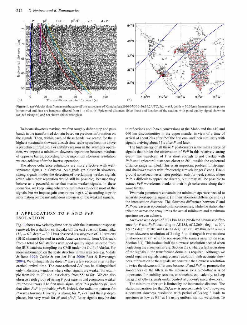
Figure 1. (a) Velocity data from an earthquake off the east coasts of Kamchatka (2010/07/30 3:56:19.2 UTC, Mw = 6.3, depth = 30.3 km). Instrument responseis removed and data are bandpass filtered from 1 to 60 s. (b) Epicentral distances (blue lines) and location of the stations with good quality signal shown in(a) (red triangles) and not shown (black triangles).

To locate slowness maxima, we first roughly define stop and passbands in the transformed domain based on previous information onthe signals. Then, within each of these bands, we search for the nhighest maxima in slowness at each time-scale-space location abovea predefined threshold. For stability reasons in the synthesis opera-tion, we impose a minimum slowness separation between maximaof opposite bands, according to the maximum slowness resolutionwe can achieve after the inverse operation.

The above coherence estimators are more effective with well-separated signals in slowness. As signals get closer in slowness,strong signals hinder the detection of overlapping weaker signals(even when their separation would still be possible), because theybehave as a powerful noise that masks weaker signals. In thesescenarios, we keep using coherence estimators to locate most of thesignals, but we impose gain constraints in g(τ, λ) according to priorinformation on the instantaneous slowness of the weakest signals.

3 A P P L I C AT I O N T O P A N D P c PI S O L AT I O N

Fig. 1 shows raw velocity time-series with the instrument responseremoved, for a shallow earthquake off the east coast of Kamchatka(Mw = 6.3, depth = 30.3 km) observed at a subgroup of 119 stations(BHZ channel) located in north America (mostly from USArray),from a total of 640 stations with good quality signal selected fromthe IRIS database sampling the CMB under the Gulf of Alaska. Formore information on the scale structure in this area (see e.g. Vidale& Benz 1992; Castle & van der Hilst 2000; Rost & Revenaugh2004). We distinguish the direct P wave a few seconds after its the-oretical arrival time. The core-reflected PcP can be distinguishedonly in distance windows where other signals are weaker, for exam-ple from 65◦ to 70◦ and less clearly from 55◦ to 60◦. We can alsoobserve a rich group of strong P post-cursors and even some weakerPcP post-cursors. The first main signal after P is probably pP, andthat after PcP is probably pPcP. Indeed, the radiation pattern forP waves towards USArray is strong for P, PcP and their p depthphases, but very weak for sP and sPcP. Later signals may be due

to reflections and P-to-s conversions at the Moho and the 410 and660 km discontinuities in the upper mantle, in view of a time ofarrival of about 20 s after P of the first one, and their similarity withsignals arriving about 35 s after P and later.

The high energy of all these P post-cursors is the main source ofsignals that hinder the observation of PcP in this relatively strongevent. The waveform of P is short enough to not overlap withPcP until epicentral distances closer to 80◦, outside the epicentraldistance range sampled. This is an important problem in strongerand shallower events with, frequently, a much longer P coda. Back-ground noise becomes a major problem only for weak events, wherePcP is difficult to appreciate directly, but it may still be possible toextract PcP waveforms thanks to their high coherence along theirwave fronts.

Two main parameters constrain the minimum aperture needed toseparate overlapping signals: (1) their slowness difference and (2)the inter-station distance. The slowness difference between P andPcP decreases as epicentral distance increases, while the station dis-tribution across the array limits the actual minimum and maximumaperture we can achieve.

An event with depth of 30.3 km has a predicted slowness differ-ence for P and PcP, according to AK135, of 2.860 s deg−1 at 60◦,1.912 s deg−1 at 70◦ and 1.467 s deg−1 at 75◦. We thus need a min-imum slowness resolution of 3 s deg−1 to distinguish two maximain slowness at 75◦ with the non-separable signals assumption (e.g.Section 2.3). This is about half the slowness resolution needed whenneglecting the cross terms (e.g. Section 2.2), where a full separationof the signals in the transformed domain is required. Although wecould separate signals using coarse resolution with accurate slow-ness information on the signals, we constrain the slowness resolutionto twice the slowness difference between P and PcP, to promote thesmoothness of the filters in the slowness axis. Smoothness is ofimportance for stability reasons, or somehow equivalently, to keepthe gain of other signals under control at unconstrained slowness.

The minimum aperture is limited by the interstation distance. Thestation separation for the USArray is approximately 0.6◦; however,a constant slowness resolution with period of 3 s deg−1 leads toapertures as low as 0.3◦ at 1 s using uniform station weighting. To


Figure 2. Time-slowness sections at a distance of 60.24◦ (TA.H27A) for the data shown in Fig. 1. (a) Amplitude and (b) coherence at a period of 2 s.(c) Amplitude and (d) coherence at 8 s. Black dots mark the slowness components where we impose gain constraints on the synthesis operation.

avoid these anomalous apertures, we impose a minimum value of2◦ (aperture at 6 s period), wide enough to enclose 8 stations, and amaximum aperture of 6.7◦ for practical purposes.

Aliasing in slowness may become problematic at short periods.The extreme case occurs when the interstation separation equalstheir separation in epicentral distance, in the case of USArray thisis about 0.6◦, which would produce aliasing at ±nT/0.6, where T isperiod and n ∈ N. This is at ±3.33◦ at a period of 2 s. This aliasingis reduced in practice for a variety of reasons, for example thesignals have a short duration, arrays are not regularly spaced, andstations have different epicentral distances. However, they becomethe main source of biases at very short periods. We therefore opt fornot using periods shorter than 1 s at this stage.

Fig. 2 shows time-slowness sections of a record section cen-tred around an epicentral distance of 60.24◦ (Fig. 1) expanded inthe time-scale-slowness domain. We choose the complex Morletwavelet for analysis, because it has optimal time and frequency res-olution and it is approximately analytic. Its mother wavelet has theform:

ψ(t) = π−1/4e−iω0t e−t2/2, (27)

where t is time and ω0 is central frequency. A standard choice ofω0 = π

√2/ ln 2 makes the amplitude of the side lobes equal to half

of the main lobe.

We generate a frame of time-space wavelets in scale and slow-ness according to Appendix B. The subsampled wavelet frame,eq. (B4), uses four voices, six octaves and a sampling period ofb0 = 1. The central frequency of the wavelet with the lowest scaleis 1 Hz. The periods analysed then range from 1 s to about 54 s. Thesampling in slowness is about 10 times the actual slowness resolu-tion at each scale, with a minimum value of 3 smpl (s deg−1)−1.We think this high level of redundancy achieves a balance be-tween implementation efficiency and filter flexibility. This balanceallows for a relatively fast implementation (still far slower thannon-redundant alternatives) and, in return, it simplifies the designof the filter, improves signal adaptation, and makes the configura-tion extremely flexible. Figs 2(a) and (c) display amplitude mea-surements at periods of 2 and 8 s, while Figs 2(b) and (d) showthe corresponding measurements of coherence using phase-stack,eq. (26), with v = 2 and a square window of five samples. This isa length of 4 s at a period of 2 s and 16 s at a period of 8 s. Notethat the finite time resolution at individual scales of the symmetricwavelets used produces relatively wide maxima in the time-scaledomain, which may extend before the time of arrival of signalsat low frequencies. This does not limit the actual time resolution,which is determined by the low scale components, and helps in thefiltering.

We use coherence to measure the instantaneous slowness of Pand its post-cursors. PcP, far weaker than P, is still usually strong


Figure 3. P and PcP extractions from data shown in Fig. 1. (a) P extracted. (b) Data minus the P extracted. (c) PcP extracted. (d) Data minus the PcP extracted.Signals in (a) and (c) are clean but spatially smoothed, while in (b) and (d), they are not smoothed but noiser. All figures use the amplitude normalization usedfor the raw data.

enough to obtain a robust measurement of its slowness at theseperiods. We can identify PcP in all figures with the first mainlobe at slowness of about 4 s deg−1 at around 50 s arrival time.However, the use of 1-D model predictions usually provides moreaccurate information, especially at large epicentral distances wherethe slownesses of P and PcP are closer, and PcP coherence maximaare masked by the P coda. We can additionally appreciate that thetwo main lobes of Fig. 2(a) have weak side lobes with slownessmaxima about 1.5 s deg−1 (at the top edge of the figure), producedby aliasing effects.

Fig. 3 presents results after the filtering and synthesis operationsusing the minimum noise solution, eq. (21). Fig. 3(a) shows P andits post-cursors extracted with a gain constraint of 1 at the slownessof P and a gain of 0 at the slowness of PcP. Fig. 3(b) shows theresult after subtracting this result from the raw data (Figs 1–3a).Similarly, Fig. 3(c) shows PcP and their post-cursors using the sameslowness constraints but with their gains exchanged, and Fig. 3(d)its subtraction from the raw data.

Figs 3(a) and (c) show clean and smooth observations of P, pP,PcP, pPcP and other signals. Comparing Fig. 3(c) with the rawdata (Fig. 1), we see a dramatic attenuation of P and all the post-

cursors as well as of the noise level. We can only distinguish a verysmall remainder of P caused mainly by waveform differences andmisalignments. In contrast to the raw data, now it is possible toclearly see PcP at all epicentral distances, even at distance largerthan 70◦ where pP and P post-cursors were very strong. Differentialobservations from Figs 3(b) and (d) are valuable to validate moreaccurate extracted observations from Figs 3(a) and (c).

An inherent shortcoming that may arise in some applications isdue to the smoothing produced by the local stacks. In the PcP–Papplication, the resolution lost at the CMB is not significant untilreaching long periods, as scaling is proportional to period for thearray aperture and to its square root for the Fresnel zone. To bemore precise, the Fresnel zone at 2 s is about 3◦ (diameter) for azero epicentral distance. And it reduces to 8◦ on epicentral directionand to 3.5◦ orthogonal to it for epicentral distances of 60◦ (incidenceangle at the CMB of 64.4◦). Then, for an array aperture equal to1/3 deg s−1 at all periods, the resolution at the CMB on orthogonalepicentral direction equals the resolution of the array at a periodof 130 s. We use a minimum aperture of 2◦ (resolution of 1.83◦ atthe CMB) in order to enclose a minimum number of stations. Thisresolution is sufficient in the period range we consider.


Figure 4. (a) Velocity data from an earthquake in the Svalbard region (2009/06/22 18:15:40.09 UTC, Mw = 5.4, depth = 13.1 km). Instrument response isremoved and data are bandpass filtered from 1 to 60 s. (b) Epicentral distances (blue lines) and location of the stations with good quality signal shown in (a) (redtriangles) and not shown (black triangles). (c) P extracted and (d) PcP extracted from the data shown in (a). All figures use the same amplitude normalization.

When smoothing is not admissible, we can use the differences(Figs 3b and d) instead of the extractions. These observations arenoisier than the previous ones since random noise is not attenuated.However, we are able to obtain relatively clean observations of PcPwithout any smoothing because we remove most of the P signal andits post-cursors.

Fig. 4(a) shows velocity time-series from a shallow earthquakeof magnitude Mw = 5.4 observed in north America (Fig. 4b).Due to its low magnitude, low SNR is the main problem to beaddressed in this example in order to observe PcP. At these az-imuths P post-cursors caused by Moho and upper-mantle discon-tinuities appear much weaker than in Fig. 1. Figs 4(c) and (d)present results after the filtering and synthesis operations usingthe configurations applied in the previous example. The noise at-tenuation is high enough to observe clearly several P post-cursorson Fig. 4(c) and PcP on Fig. 4(d). SNR can be further improvedby increasing the array aperture in exchange for reducing spatialresolution.

In summary, the extracted observations from raw data improveSNR and SIR but are smoothed, while differential observationsimprove SIR and do not suffer from smoothing, but result in lowerSNR.

4 P c P – P T R AV E LT I M E D I F F E R E N C EE S T I M AT I O N W I T H T W O S L I D I N GW I N D OW S

The traveltime difference or delay between two seismic phasesis obtained as an optimal solution of a given objective function.These functions conventionally define a distance between two sig-nals based on their similarity or coherence. Valid notions of distanceare any norm and some non-linear functions. The definition of sim-ilarity is also non-unique. It can be based on the actual signals,on their waveforms (neglecting amplitude differences), on their in-stantaneous phase, among others. For example, let x1 and x2 betwo similar uniformly continuous signals separated by an unknowndelay td and let us write the objective function most frequentlyused as:

min ‖x1(t) − x2(t − td )‖2 . (28)

Then it can be proven that the optimal solution is the delay corre-sponding to the absolute maximum of cross-correlation between x1

and x2, if similarity involves waveform and amplitude. If similar-ity involves only waveform, it is the delay with the maximum of‘geometrically normalized’ cross-correlation.


Main difficulties conventionally arise from random noise and ad-ditional correlated signals. Broadly, noise reduces accuracy, whilesignals introduce bias. The reference seismic phase, signal x1 ineq. (28), is chosen to be a clear signal, but its inherently limitedfrequency content and short duration may produce suboptimal solu-tions, due to, for example cycle-skipping effects. Additional signalsarriving close in time may introduce additional suboptimal solu-tions. Noise has a direct impact on the accuracy of all solutions anddeteriorates their amplitudes. When the effects of random noise arecombined with uncertainties in the time of arrival of the referencesignal and with lack of previous knowledge on td, the selection ofthe solution of choice among all optimal and suboptimal solutionsbecomes non-trivial.

The quality of PcP–P traveltime difference observations is ex-posed to noise and other correlated signals. Here, P is the referencesignal x1 and PcP x2, leading to positive delays. PcP is a relativelyweak signal with low SNR, which limits accuracy. Of more impor-tance are the P and PcP depth phases. These signals may introduceadditional solutions, as a result of their high similarity with the directphases that arise from their close travel paths. The high similarityand particularly their close arrival times may introduce significantbias. In shallow events, less than 100 km depth, pP and pPcP arriveabout 0.25 s km−1 after P and PcP, respectively per kilometre ofthe hypocentral depth, and sP and sPcP about 0.36 s km−1. Thisis not a problem for very shallow events where differences amongthe observed PcP–P, pPcP–pP and sPcP–sP compared to predic-tions obtained with 1-D models are negligible. In fact, extra pairsof signals close to P and PcP and with very similar traveltime dif-ferences (below the actual resolution) often contribute to enhanceaccuracy. It is also not a problem for much deeper events where Pand PcP depth phases arrive later than P and PcP. In this scenario,depth phases actually provide genuine information derived fromsignificant differences in their travel paths, and hence in the CMBsampling. Depth phases are problematic at intermediate depths dueto their close time of arrival but still significant traveltime differ-ence. This leads to substantial bias when pPcP–pP or sPcP–sP aremisinterpreted as PcP–P.

Other coherent signals may be present but their lower amplitudeand/or different time of arrival make them less problematic. Thisis the case of PdP, a seismic phase with a travel path analogous toPcP but with a reflection at the top of D′ ′ instead of CMB. Thisphase arrives a few seconds before PcP and has a slightly higherslowness. PdP observations provide precious information on thetopography of D′ ′. The similar travel paths of PdP and PcP butan often lower reflection coefficient at the top of D′ ′ than at CMBhinders PdP observations. The presence of this phase may lead to asolution for PdP–P traveltime difference clearly separated from themost likely PcP–P traveltime difference, which should not lead tomisinterpretations.

4.1 The two sliding window approach

A blind selection of an optimal portion of the seismogram as a ref-erence signal in the sense of maximizing SNR and SIR based onpredictions of 1-D models is in general problematic. Uncertaintieson arrival time of P are higher than on the PcP–P traveltime differ-ence, strong depth phases are not always present, and signal durationhas strong variations. A long window guarantees that a major por-tion of the reference signal is covered, but leads to low SNR, anddepth phases may not be excluded. Additionally, late portions of theP coda in strong events may suffer from non-negligible attenuationeffects, in the sense of t* operator, and introduce additional bias.

A short window enables the maximization of SNR while rejectingdepth phases, but cycle-skipping problems may become more se-vere, and uncertainties on the time of arrival of the reference signalhinders the optimal location window.

To overcome this dilemma we opt for short windows, but insteadof using a fixed window on P and a sliding window on PcP, we letboth move. Given the objective function shown in eq. (28), this isequivalent to adding a delay term in x1 and x2,

min ‖x1(t − ta) − x2(t − td − ta)‖2 . (29)

In summary, the 1-D search along td in eq. (28) turns into a 2-Dsearch along the td and ta variables in eq. (29). We could searchfor the global optimal solution, but it is far more powerful to relaxconstraints on ta and td and search for optimal and suboptimalsolutions. With this approach, we can potentially observe variationsof PcP–P traveltimes along their waveforms, as well as those ofpPcP–P and sPcP–sP, and other coherent signals such as PdP–P,among other signals that could be due to noise and cycle-skipping.In this scenario, the main complexity is to develop algorithms smartenough to identify all these signals using the prior informationavailable.

The definition of similarity in objective functions for PcP–P trav-eltime difference estimation are based on the waveform. Amplitudedifferences are neglected due to the additional attenuation that PcPsuffers compared to P as a result of its longer travel path. In fact,amplitude differences provide valuable observations on their own todistinguish velocity perturbations from topography. However, fullyignoring amplitudes may lead to optimal solutions with unrealisticattenuation values. Similarly, another issue that derives from usingmany reference signals, one for every ta value used, eventually mayarise when strong minima appear even when x1(t − ta) only con-tains weak signals from the coda of the P wave, or just noise. Toovercome these problems, we define a slightly different objectivefunction to search for the signal x2 that obtains the maximum energyreduction using the reference signal. We also add extra constraintson the amplitude difference to avoid unrealistic values. This writes

max f (td , ta), (30)

with

f (td , ta) = ‖x2(t − td − ta)‖2 − ‖ax1(t − ta) − x2(t − td − ta)‖2 ,

(31)

where a is a real attenuation scalar.The energy reduction varies according to td, ta and a. The ob-

jective function f(td, ta) is maximized with respect to td when thesecond term is minimized. The optimal solution for attenuation ata given ta and td that minimizes this term is:

a(td , ta) = 〈x1(t − ta), x2(t − td − ta)〉‖x1(t − ta)‖2

, (32)

where 〈x1(t), x2(t)〉 is the inner product between x1 and x2. This is theoptimum estimator of the PcP/P amplitude ratio using their actualsignals in the least-square sense.

Introducing the optimal solution for attenuation in eq. (31), andsimplifying we obtain

f (td , ta) = |〈x1(t − ta), x2(t − td − ta)〉|2‖x1(t − ta)‖2

. (33)

Using eq. (32), the objective function defined in eq. (33) can beinterpreted as

f (td , ta) = a(td , ta) 〈x1(t − ta), x2(t − td − ta)〉 . (34)


This equation facilitates the interpretation of thresholds in both thePcP/P amplitude ratio and the inner product between P and PcPsignals.

We impose maximum and minimum thresholds as additionalconstraints on the amplitude ratio a. The first threshold contributesto the rejection of unlikely low-energy reference signals, since weexpect PcP to have lower energy than P, while the second rejects x2

signals with an unlikely low energy that leads to anomalously lowPcP/P amplitude ratios.

4.2 Bias due to intrinsic attenuation

The accuracy of observations of both traveltime differences andamplitude ratios varies strongly with the signal quality but also withtheir similarity. Intrinsic attenuation has an effect on amplitude butalso introduces frequency-dependent dispersion that may eventuallycause a significant waveform distortion, leading to important bias.To a first order approximation (e.g. Shearer 2011) we can modelattenuation as a function of travelled distance x, frequency ω andtime t as

A(x, ω, t) = A0e−ωt∗0 /2e−iω(t−x/c0)e−iωt∗0 ln(ω/ω0)/π , (35)

where t∗0 = x/c0 Q (‘tstar’), c0 is the velocity at the reference

frequency ω0 and Q the quality factor, inversely proportional toattenuation. Note that the Fourier convention is opposite here:u(ω) = ∫ ∞

−∞ u(t)e+iωt dt . The last exponential term in eq. (35) mod-els the traveltime delay that intrinsic attenuation introduces at fre-quencies that deviate from ω0. An option to reduce the effects ofwaveform distortion in differential traveltime measurements is tocompensate for the integral of t∗

0 ln(ω/ω0)/π along the travel pathsconsidered, according to a reference model of velocity and attenua-tion. Intrinsic attenuation attains higher values in the upper mantlethan in the lower mantle, Qμ is as low as 80 for the asthenosphere(depths from 80 to 220 km) compared to 312 in the lower mantlein PREM (Dziewonski & Anderson 1981). To evaluate waveformdistortion, we use the value given by PREM in the lower mantle,Qβ = Qμ = 312, along the full travel path, considering that theP and PcP paths diverge mostly in the lower mantle, where theyspend most of their time, especially at large epicentral distances.This translates into a Qα = (9/4)Qμ = 702 assuming infinite Qκ ,and writes:

(PcP–P)t∗0 (tPcP − tP )ln(ω/ω0)

Qαπ. (36)

Dispersion due to intrinsic attenuation is thus approximately propor-tional to PcP–P traveltime difference. Here it may become signifi-cant only at low frequencies and large epicentral distances becauseQα is relatively high. Thus, we can safely ignore it in a first approx-imation because the high frequencies components of the signals,where dispersion is lower, provide accuracy to PcP–P traveltimeobservations. However, since corrections using eq. (36) in the fre-quency domain are simple, we do opt to correct for waveformdistortion to maximize P and PcP similarity. These corrections maybecome mandatory in other applications such as ScS–S, due to theirhigher differential traveltimes, lower Q, and lower frequencies.

5 A P P L I C AT I O N T O P c P – PT R AV E LT I M E D I F F E R E N C E S

The resolution of the objective function in td is proportional to thecross-correlation length of x1 and x2, which is roughly inverselyproportional to the maximum frequency components. However the

resolution is far lower in ta because the signal waveforms and thewindows have finite width in time. This in practice produces rela-tively long and smooth ridges of suboptimal solutions along ta witha relatively constant td value. To evaluate every solution, we firstgroup them in separate ridges and then we estimate their significancebased on the impact on energy reduction of the reference signal,f(td, ta). We group individual suboptimal solutions along increasingta in a single ridge as long as variations on td and gaps are small,and f(td, ta) does not reduce significantly. Ridges far shorter thanthe window length are discarded. To evaluate the rest, we calculatesmooth histograms along td weighed by f(td, ta). More specifically,every solution along the ridge adds a narrow raised cosine function(Hann window) to a 1-D function with amplitude equal to f(td, ta)and centred at td. Once every solution is considered, the amplitudeof the highest peak gives an estimate of the quality of the ridge andits position the traveltime difference. We finally identify the ridgethat best represents PcP–P, or any other signal, based on its qualityand its offset with respect to the prediction made using the priormodel.

Figs 5 and 6 illustrate the objective function in two scenarios,(1) strong direct and depth phases and (2) moderate cycle-skippingambiguity. Figs 5(a) and 6(a) present velocity seismograms with theinstrument response removed and filtered with a bandpass filter from1 to 60 s. The next two figures show the estimation of P (Figs 5band 6b) and PcP (Figs 5c and 6c) using the slant-stacklet trans-form introduced in the previous section. Then, Figs 5(d) and 6(d)show the objective functions together with their main optimal so-lutions grouped in ridges in white and the values of PcP–P andpPcP–pP predicted by the global 1-D model AK135 (corrected forellipticity) in magenta. We use a square window of 12 s to evaluatethe objective function, and for the predicted solutions we considerthat all signals are delta functions located at the predicted time ofarrival.

In the first scenario (Fig. 5d), we can clearly identify PcP–P withthe first strong ridge from about −2 to 9 s, and pPcP–pP with thesecondary maximum from 14 to 22 s. Both traveltime differencesagree with predictions. The traveltime differences along the mainpart of the PcP–P maximum ridge are very stable. We only havedeviations at the extremes were maxima reduce severely, thus theydo not perturb the observation, that is the location of the main peakof the amplitude-weighted histogram (Fig. 5e) is not affected bythe extrema of the ridge due to their fluctuations and much lowermaxima. The waveforms of pP and especially pPcP are weaker, andmore affected by high frequency noise. This widens the secondarymaxima and generates a far more unstable ridge.

In the second scenario (Fig. 6d), depth phases are extremely weakdue to a low radiation in their direction of propagation; consequently,we can identify PcP–P as the main ridge from −4 to 6 s and, farweaker, pPcP–pP as the ridge between 7 and 18 s. The traveltimedifference values are higher (positive) than predicted. Comparingthe waveform of P and PcP is difficult to distinguish if P is fasterthan predicted, PcP is slower or both. In the evaluation of the ob-jective function (Fig. 6d), we obtain a very stable ridge that leads toa PcP–P traveltime difference of about 0.5 s. The secondary ridgewith traveltime difference of about −4 s is probably due to moder-ate cycle-skipping effects. They are produced by the combination oftwo factors, differences in P and PcP waveforms and the presenceof secondary lobes. Waveform differences between P and PcP mayreduce the amplitude of this solution below the values of othersproduced by weaker signals but that better resemble the referencesignal. From 46 to about 49 s (Fig. 6c) we can observe a weak lobewhich has a similar waveform to P. This matching produces the


Figure 5. PcP–P traveltime estimation from an earthquake near theeast coast of Kamchatka (2006/08/24 21:50:36.7 UTC, Mw = 6.5,depth = 54.2 km) with strong pP and pPcP signals towards the USAr-ray. (a) Original signal at a distance of 57.2◦ (TA.N10A). (b) ObservedP wave, x1. (c) Observed PcP wave, x2. (d) Objective function, eq. (34),with ridges in white and predictions from the AK135 model (corrected forellipticity) in magenta. Vertical axis is traveltime difference variation withrespect to predicted PcP–P with AK135, td, and horizontal axis is the timeat the centre of the reference window, ta. (e) Smooth histogram of traveltimedifferences of all ridges starting from −6 to 6 s having a minimum lengthof 4 s.

ridge in Fig. 6(d) with a traveltime difference of about −4 s. Withthe actual SNR it is difficult to distinguish if this signal has a realorigin, for example PuP (caused by a drop in compressional wavespeed in an ULVZ), or it is just coherent-noise.

We test robustness of PcP–P traveltime observations to stronginterferences (i.e. P post-cursors and scatters), building syntheticseismograms using DSM (Kawai et al. 2006) with the isotropicPREM model (Dziewonski & Anderson 1981). In Fig. 7(a), we

Figure 6. PcP–P traveltime estimation from an earthquake near the coastof northern Chile (2010/05/06 2:42:47.9 UTC, Mw = 6.2, depth = 46.8 km)with a minor cycle skipping problem. (a) Original signal at a distance of58.72◦ (TA.X34A). (b) Observed P wave. (c) Observed PcP wave. (d)Objective function with ridges indicated. (e) Smooth histogram of traveltimedifferences of all ridges.

model the seismograms from the event shown in Fig. 1 using theglobal CMT solution for the moment tensor (Dziewonski et al.1981; Ekstrom et al. 2012) with a maximum frequency of 2 Hz,but with an event depth of 100 km. We extract P (Fig. 7c) andPcP (Fig. 7d) from this data set using the configuration of theslant-stacklet transform used in Figs 1 and 4. Figs 7(e) and (f) plotPcP–P differential traveltime observations, assessed using the twosliding window approach, according to theoretical values for theisotropic PREM model calculated with the TauP Toolkit (Crowellet al. 1999) with the same ellipticity corrections used in DSM. Onthe raw data results (Fig. 7e), we see that the PcP–P observationsare contaminated by the strong energy of the P coda, pP and sP;while on the extracted signals (Fig. 7f), PcP–P observations areclose to zero (mean of −0.12 s and standard deviation of 0.08 s),


Figure 7. PcP–P traveltime differences on synthetics (DSM) compared to expected observations (TauP) using the isotropic PREM model. (a) Synthetics arefor the geometry shown in Fig. 1 but with an event depth of 100 km. (b) Epicentral distances (blue lines) and location of the stations shown in (a) (red triangles)and not shown (black triangles). Extracted P (c) and PcP (d) using the slant-stacklet transform. PcP–P traveltime difference variations using the method of twosliding windows on (e) the raw synthetics and (f) on the extracted P and PcP.

as it is expected from using the same 1-D model in DSM and TauP.Remaining variations are mainly due to the non-ideal separation ofP and PcP and their limited high frequency contents.

5.1 Illustration on real data

Fig. 8 shows observed traveltime difference variations accordingto the AK135 1-D model corrected for ellipticity for the eventshown in Fig. 1 along epicentral distance. Seeing the distributionof the observations in Fig. 8, we consider outliers as any obser-vation outside the interval of ±2 s. Fig. 8(a) shows observations

taken using the raw data, Fig. 8(b) using the extracted P and PcPsignals (Figs 3a and c), and Fig. 8(c) using their differences (Figs 3band d).

PcP–P differential traveltime observations are based on theirwaveform similarity. However, as P, pP and later signals of sim-ilar slowness are highly cross-correlated, it is hard to distinguishmaxima of the objective function caused by PcP or other signals.When we measure PcP–P on the raw data (Fig. 8a), these signalsbecome the major interference. Their often higher amplitude andsimilarity compared to PcP produce higher maxima which maylead to systematic errors such as those observed in Fig. 8(a), where


Figure 8. Observed PcP–P traveltime difference variations compared toAK135 1-D model, (PcP−P)data − (PcP−P)model, using (a) the raw data ofFig. 1, (b) the P and PcP extractions (Figs 3a and c), (c) the data minus theextracted P and the data minus the extracted PcP (Figs 3b and d).

most observations are aligned along anomalous diagonal lines. Thisproblem is fully solved in Fig. 8(b) by using the extracted P andPcP signals, and even when we use the difference measurementsin Fig. 8(c), no systematic error appears. In the latter case, we canobserve a higher number of random outliers, and a slightly higherdispersion on the observations, which is expected considering thatrandom noise is not attenuated in this case and that P and PcP do notsuffer any spatial smoothing. Interpretation of these results in termsof structure in the vicinity of the CMB requires an additional step tocorrect for mantle structure. In this example, correcting for mantlestructure reduces the variance of the observations significantly, inparticular, from 65◦ to 70◦. This will be addressed in a companionpaper (Ventosa & Romanowicz 2015).

Equivalently to Fig. 8, Fig. 9 shows observed PcP–P traveltimedifference variation for the event shown in Fig. 4. PcP–P observa-tions are not possible in the raw data (Fig. 9a) due to the low SNR ofPcP; however, in Fig. 9(b) we observe relatively clean observationsusing the extracted P and PcP signals (Figs 4c and d). In this fig-ure, most observations concentrate at about zero. Small variationsaround this value are due to local variations and, to a smaller extent,to measurement uncertainties. SNR can be further enhanced usingwider array apertures at the cost of reducing spatial resolution. Weconsider spatially close observations far from this main trend as out-liers. In this scenario the observations on the differences (Fig. 9c)

Figure 9. Observed PcP–P traveltime difference variations compared toAK135 1-D model corrected for ellipticity, (PcP–P)data − (PcP–P)model,using (a) the raw data of Fig. 4(a), (b) the P and PcP extractions (Figs 4cand d), (c) the data minus the extracted P and the data minus theextracted PcP.

perform closer to the raw data because noise is not attenuated andother correlated signals are relatively small.

6 C O N C LU S I O N S

We have shown that we can obtain PcP–P traveltime difference mea-surements of unprecedented quality using array data in the presenceof interfering signals. The key ingredients which make these obser-vations possible are accurate signal extraction and local traveltimedifference measurements.

The slant-stacklet transform achieves a high slowness selectivitywithout sacrificing flexibility on the resolution compromises. Thisfeature has proven useful in P and PcP signal extraction. Now itis possible to obtain clean observations of PcP even when it ishidden in the coda of P. The high slowness resolution allows theseparation of P and PcP up to 80◦ of epicentral distance, wheretheir slowness difference and time difference are very small, andprobably more importantly, it allows a high level of rejection ofinterfering signals, such as pP and sP, even when their accurateslowness and time of arrival are not precisely known in advance.Our present limit in signal extraction is the level of noise. Working atlarger epicentral distances is possible with larger apertures; however,P and PcP kernels converge (at 85◦ the bottoming point of P is


slightly deeper than 2500 km) and may partially overlap at relativelyshort periods, making them less attractive. When it is not possibleto attain the slowness resolution required in the signal extractiondue to spatial resolution constraints, alternative approaches basedon the prediction of interfering signals followed by their adaptivesubtraction with no slowness and spatial resolution limitations (e.g.Ventosa et al. 2012a; Pham et al. 2014) may be of interest.

The main problem in the estimation of the traveltime differenceis the high cross-correlation with other close and usually strongersignals. Although the slant-stacklet transform removes the strongestcorrelated signals that mask PcP, a local traveltime difference es-timation is nearly as important to reduce bias and outliers. In par-ticular, the objective function we introduce maximizes the energyreduction on the objective signal (PcP). We conclude that its so-lution is less sensitive to noise than the standard cross-correlationsolution and naturally allows the introduction of additional con-straints on the amplitude ratio of the two signals. Furthermore, its2-D representation (time – differential time), in addition to pro-viding a less ambiguous PcP–P identification, allows a more in-volved analysis of many often weaker signals with precious com-plementary information such as pPcP–pP, sPcP–sP, PdP–P, amongothers.

At least as important as the accuracy of PcP–P observations is anexhaustive analysis of all sources of bias. We conclude that althoughepicentre mislocation and intrinsic attenuation biases are present,they are negligible compared to the accuracy of our observations.As we will show in our companion paper, they are much smallerthan the bias caused by mantle heterogeneities.

Although we illustrate these tools with PcP data, they addressgeneral problems of teleseismic signal processing. Hence, theyshould be useful for a wider range of applications. Apart from ap-plications under similar conditions using other phases constrainingCMB and D′ ′ or the inner-core boundary, the slant-stacklet trans-form may prove useful in applications that benefit from removingrandom noise and interfering signals in slowness without com-promising resolution, such as in the imaging of the upper-mantlediscontinuities using SS precursors (e.g. Zheng et al. 2015), or inthe observation of weak signals from the core.

A C K N OW L E D G E M E N T S

The data used in this work were obtained from the IRIS DataManagement Center. The slant-stacklet transform has its originin the PhD thesis of Sergi Ventosa at the UTM-CSIC super-vised by Carine Simon, Martin Schimmel and Juanjo Danobeitia.We thank to anonymous reviewers for helping improve the clar-ity of the manuscript. We also acknowledge the support from theEuropean Research Council under the European Community’s Sev-enth Framework Programme (FP7-IDEAS-ERC)/ERC AdvancedGrant WAVETOMO.

R E F E R E N C E S

Bear, L.K. & Pavlis, G.L., 1997. Estimation of slowness vectors and theiruncertainties using multi-wavelet seismic array processing, Bull. seism.Soc. Am., 87(3), 755–769.

Cao, A., Romanowicz, B. & Takeuchi, N., 2005. An observation of PKJKP:inferences on inner core shear properties, Science, 308(5727), 1453–1455.

Castle, J.C. & van der Hilst, R.D., 2000. The core-mantle boundary underthe Gulf of Alaska: no ULVZ for shear waves, Earth planet. Sci. Lett.,176(3), 311–321.

Cobden, L. & Thomas, C., 2013. The origin of D′′ reflections: a system-atic study of seismic array data sets, Geophys. J. Int., 194(2), 1091–1118.

Crowell, H.P., Owens, T.J. & Ritsema, J., 1999. The TauP Toolkit: Flexibleseismic travel-time and ray-path utilities, Seism. Res. Lett., 70, 154–160.

Deuss, A., Woodhouse, J.H., Paulssen, H. & Trampert, J., 2000. The obser-vation of inner core shear waves, Geophys. J. Int., 142(1), 67–73.

Dziewonski, A.M. & Anderson, D.L., 1981. Preliminary reference Earthmodel, Phys. Earth planet. Inter., 25(4), 297–356.

Dziewonski, A.M., Chou, T.-A. & Woodhouse, J.H., 1981. Determination ofearthquake source parameters from waveform data for studies of globaland regional seismicity, J. geophys. Res., 86, 2825–2852.

Ekstrom, G., Nettles, M. & Dziewonski, A.M., 2012. The global CMTproject 2004–2010: centroid-moment tensors for 13,017 earthquakes,Phys. Earth planet. Inter., 200–201, 1–9.

Fichtner, A. & Igel, H., 2008. Efficient numerical surface wave propagationthrough the optimization of discrete crustal models—a technique basedon non-linear dispersion curve matching (DCM), Geophys. J. Int., 173(2),519–533.

Forbriger, T., 2003. Inversion of shallow-seismic wavefields – I: wavefieldtransformation, Geophys. J. Int., 153(3), 719–734.

French, S., Lekic, V. & Romanowicz, B., 2013. Waveform tomographyreveals channeled flow at the base of the oceanic asthenosphere, Science,342(6155), 227–230.

Frost, D.A., Rost, S., Selby, N.D. & Stuart, G.W., 2013. Detection ofa tall ridge at the core-mantle boundary from scattered PKP energy,Geophys. J. Int., 195(1), 558–574.

Gershman, A.B., Sidiropoulos, N.D., Shahbazpanahi, S., Bengtsson, M.& Ottersten, B., 2010. Convex optimization-based beamforming: fromreceive to transmit and network designs, IEEE Signal Process. Mag.,27(3), 62–75.

Gu, Y.J. & Sacchi, M., 2009. Radon transform methods and their applica-tions in mapping mantle reflectivity structure, Surv. Geophys., 30(4-5),327–354.

Hyvarinen, A. & Oja, E., 2000. Independent component analysis: algorithmsand applications, Neural Networks, 13(4), 411–430.

Jacques, L., Duval, L., Chaux, C. & Peyre, G., 2011. A panorama on mul-tiscale geometric representations, intertwining spatial, directional andfrequency selectivity, Signal Process., 91(12), 2699–2730.

Kawai, K., Takeuchi, N. & Geller, R.J., 2006. Complete synthetic seismo-grams up to 2 Hz for transversely isotropic spherically symmetric media,Geophys. J. Int., 164, 411–424.

Kay, S.M., 1993. Fundamentals of Statistical Signal Processing,Prentice-Hall.

Lekic, V. & Romanowicz, B., 2011. Inferring upper-mantle structure by fullwaveform tomography with the spectral element method, Geophys. J. Int.,185(2), 799–831.

Li, J., Stoica, P. & Wang, Z., 2003. On robust Capon beamforming anddiagonal loading, IEEE Trans. Signal Process., 51(7), 1702–1715.

Lorenz, R. & Boyd, S., 2005. Robust minimum variance beamforming,IEEE Trans. Signal Process., 53(5), 1684–1696.

Ma, J. & Plonka, G., 2010. The Curvelet transform—a review of recentapplications, IEEE Signal Process. Mag., 27(2), 118–133.

Mallat, S., 2009. A Wavelet Tour of Signal Processing: The Sparse Way, 3rdedn, Academic Press.

Pham, M.Q., Duval, L., Chaux, C. & Pesquet, J.-C., 2014. A primal-dualproximal algorithm for sparse template-based adaptive filtering: applica-tion to seismic multiple removal, IEEE Trans. Signal Process., 62(16),4256–4269.

Rost, S. & Revenaugh, J., 2004. Small-scale changes of core-mantle bound-ary reflectivity studied using core reflected PcP, Phys. Earth planet. Inter.,145(1), 19–36.

Rost, S. & Thomas, C., 2010. High resolution CMB imaging from migrationof short-period core reflected phases, Phys. Earth planet. Inter., 183(1–2),143–150.

Scherbaum, F., Kruger, F. & Weber, M., 1997. Double beam imaging: map-ping lower mantle heterogeneities using combinations of source and re-ceiver arrays, J. geophys. Res.: Solid Earth, 102(B1), 507–522.


Schimmel, M. & Paulssen, H., 1997. Noise reduction and detection of weak,coherent signals through phase-weighted stacks, Geophys. J. Int., 130(2),497–505.

Schmidt, R., 1986. Multiple emitter location and signal parameter estima-tion, IEEE. Antenn. Propag., 34(3), 276–280.

Shearer, P.M., 2011. Introduction to Seismology, 2nd edn, Cambridge Univ.Press.

Taner, M.T., Koehler, F. & Sheriff, R.E., 1979. Complex seismic trace anal-ysis, Geophysics, 44(6), 1041–1063.

Tape, C., Liu, Q., Maggi, A. & Tromp, J., 2010. Seismic tomography of thesouthern California crust based on spectral-element and adjoint methods,Geophys. J. Int., 180(1), 433–462.

Thomas, C., Heesom, T. & Kendall, J.M., 2002. Investigating the hetero-geneity of the D′′ region beneath the northern Pacific using a seismic array,J. geophys. Res., 107(B11), ESE 3–1–ESE 3–7.

Ventosa, S. & Romanowicz, B., 2015. Extraction of weak PcP phases us-ing the slant-stacklet transform – II: constraints on lateral variations ofstructures near the core-mantle boundary, Geophys. J. Int., in press.

Ventosa, S., Rabeson, H. & Duval, L., 2011. Coherent noise removal inseismic data with redundant multiscale directional filters, in Proceedingsof the 19th European Signal Processing Conference, pp. 1150–1154,Barcelona, Spain.

Ventosa, S., Roy, S.L., Huard, I., Pica, A., Rabeson, H., Ricarte, P. &Duval, L., 2012a. Adaptive multiple subtraction with wavelet-based com-plex unary wiener filters, Geophysics, 77(6), V183–V192.

Ventosa, S., Simon, C. & Schimmel, M., 2012b. Window length selec-tion for optimum slowness resolution of the local-slant-stack transform,Geophysics, 77(2), V31–V40.

Vidale, J.E. & Benz, H.M., 1992. A sharp and flat section of the core-mantleboundary, Nature, 359, 627–629.

Wookey, J. & Helffrich, G., 2008. Inner-core shear-wave anisotropy andtexture from an observation of PKJKP waves, Nature, 454(7206),873–876.

Yilmaz, O., 2001. Seismic Data Analysis, Vol. 1, Society of ExplorationGeophysicists.

Zheng, Z., Ventosa, S. & Romanowicz, B., 2015. High resolution uppermantle discontinuity images across the Pacific Ocean from SS precursorsusing local slant stack filters, Geophys. J. Int., in press.

Zhu, H., Bozdag, E., Peter, D. & Tromp, J., 2012. Structure of the Euro-pean upper mantle revealed by adjoint tomography, Nat. Geosci., 5(7),493–498.

A P P E N D I X A : R E S O LU T I O N A NA LY S I S

The slant-stacklet expansion shown in eq. (4) can be rewritten usingthe convolution operator over t and x:

Wvp,xc (τ, λ) = u � φp,λ(−τ, −xc). (A1)

The Fourier transform of φλ, p(t, x) is

φλ,p(ω, k) =√

λψ∗(−λω)aλ(k + pω), (A2)

where ω is frequency in rad s−1 and k wavenumber in rad deg−1.ψ(ω) denotes the Fourier transform of ψ(ω).

This equation involves the product of the Fourier transforms ofthe wavelet family of functions,

√λψ∗(−λω), and a set of slowness

bandpass filters, aλ(k + pω). The first term is the transfer func-tion of a set of bandpass filters of bandwidth proportional to ω,that is of constant quality factor, and central frequency η/λ, whereη = 1

2π

∫ ∞0 ω|ψ(ω)|2dω. The second term decomposes the Fourier

transformed domain into a set of diagonal bands with slope of −1/pcentred at the origin. This is illustrated in Fig. A1.

The time and frequency resolutions are controlled by ψτ , λ(t),while the spatial and wavenumber resolutions by aλ(x). The

Figure A1. Frequency wavenumber resolution of two slant-stacklet atomswith aλ(x) = λ−1a(λ−1x) and x, p ∈ R.

resolution in time is λσ t, in frequency σω/λ, and the area of theHeisenberg box is σ tσω. Similarly, the energy spread in the spacedimension is:

1

‖aλ(x)‖2

∫ ∞

−∞x2 |aλ(x)|2 dx = f 2(λ)σ 2

x (A3)

and in wavenumber

1

2π ‖aλ(x)‖2

∫ ∞

−∞k2 |aλ(k)|2 dk = σ 2

k

f 2(λ). (A4)

The space and slowness resolutions are thus controlled by f(λ). Theresolution in space is f(λ)σ x and in wavenumber σ k/f(λ). The spacewavenumber area remains equal to σ xσ k.

The slowness resolution at the scale λ is the ratio between thewavenumber resolution and the central frequency of the wavelet atthis scale, σ p = σ kλ/ηf(λ). The function f(λ) is in general smooth.When this function is constant, f(λ) = b, this leads to the same fre-quency wavenumber resolution as the LSST (Ventosa et al. 2012b),σ p = σ kλ/bη; and when it is proportional to scale, f(λ) = bλ, toslant-stacklet atoms whose shape and slowness resolution remainconstant with scale, σ p = σ k/bη (see Fig. A1).

A P P E N D I X B : D I S C R E T I Z AT I O N

The actual resolution of the slant-stacklet expansion is not regularacross the transformed space. A wavefield u can be recovered fromits inner products with a finite family of functions generated fromφτ,λ,p,xc (t, x) if this family of functions satisfies the frame inequality(i.e. constitutes a frames)

A ≤∑n∈�

|φn(ω, k)|2 ≤ B, (B1)

where B ≥ A > 0 are two constants for almost all ω and k in RN ,

n is a shorthand for the indices τ , λ, p, xc and � for their domains.When A = B the frame is called tight and if additionally {φn}n ∈ �

are linearly independent, the frame is not redundant and is called anorthonormal basis.

We search for a close to tight frame, A B, because thebalance it provides between simplicity—having a nearly perfect


reconstruction to reduce estimation errors on the signals extracted—and maximum freedom when setting the expansion. In addition, it isconvenient to have freedom in the choice of the mother wavelet, andof the slowness bandpass filter and its scaling law to maximize theperformance of filtering operations. For these reasons, we opt forcomplex-wavelet transforms based on frames of wavelets with sev-eral voices per octave, and a sampling of the slowness dimensionsproportional to the actual resolution. We preserve at this stage thesampling across the spatial dimensions of the wavefield, frequentlysparse and always limited.

We thus define the family of functions as

φr, j,v,s,xc (t, x) = a j,v(x − xc)ψ∗r, j,v

(t − pT

s (x − xc))

(B2)

with

a j,v(x) = 1

f (2 j+v/V )a

(x

f (2 j+v/V )

)(B3)

and

ψ∗r, j,v(t) = 1√

2 j+v/Vψ∗

(t − rb02 j

2 j+v/V

), (B4)

where scale is λ = 2j + v/V and delay τ = rb02j, where j ∈ Z is an oc-tave, v ∈ [0, V − 1], a voice, V the number of voices, r ∈ Z delay andb0 sampling period. We discretize slowness as ps = p0 + sλc0/f(λ),considering that slowness resolution is inversely proportional to fre-quency and controlled by f(λ), where s ∈ Z slowness index and c0

slowness sampling period.

Geophysical Journal International - UC Berkeley...

Documents

Transcript of Geophysical Journal International - UC Berkeley...