Geometric determinants of human spatial memory - Institute of

Geometric determinants of human spatial memory

Tom Hartleya,b,*, Iris Trinklera,b, Neil Burgessa,b

aInstitute of Cognitive Neuroscience, UCL, 17 Queen Sq., London WC1N 3AR, UKbDepartment of Anatomy and Developmental Biology, UCL, Gower Street, London WC1E 6BT, UK

Received 14 February 2003; revised 23 October 2003; accepted 12 December 2003

Abstract

Geometric alterations to the boundaries of a virtual environment were used to investigate the

representations underlying human spatial memory. Subjects encountered a cue object in a simple

rectangular enclosure, with distant landmarks for orientation. After a brief delay, during which they

were removed from the arena, subjects were returned to it at a new location and orientation and asked

to mark the place where the cue had been. On some trials the geometry (size, aspect ratio) of the

arena was varied between presentation and testing. Responses tended to lie somewhere between a

location that maintained fixed distances from nearby walls and a location that maintained fixed

ratios of the distances between opposing walls. The former were more common after expansions and

for cued locations nearer to the edge while the latter were more common after contractions and for

locations nearer to the center. The spatial distributions of responses predicted by various simple

geometric models were compared to the data. The best fitting model was one derived from

the response properties of ‘place cells’ in the rat hippocampus, which matches the ‘proximities’

1=ðd þ cÞ of the cue to the four walls of the arena, where d is the distance to a wall and c is a global

constant. Subjects also tended to adopt the same orientation at presentation and testing, although this

was not due to using a view matching strategy, which could be ruled out in 50% of responses.

Disoriented responses were most often seen where the cued location was near the center of the arena

or where the long axis of a rectangular arena was changed between presentation and testing,

suggesting that the geometry of the arena acts as a weak cue to orientation. Overall, the results

suggest a process of visual landmark matching to determine orientation, combined with an abstract

representation of the proximity of the cued location to the walls of the arena consistent with the

neural representation of location in the hippocampus.

q 2004 Elsevier B.V. All rights reserved.

Keywords: Hippocampus; Path integration; Cognitive map; Computational model

0022-2860/$ - see front matter q 2004 Elsevier B.V. All rights reserved.

doi:10.1016/j.cognition.2003.12.001

Cognition 94 (2004) 39–75

www.elsevier.com/locate/COGNIT

* Corresponding author. Address: Institute of Cognitive Neuroscience, UCL, 17 Queen Sq., London WC1N

3AR, UK.

E-mail address: [email protected] (T. Hartley).

http://www.elsevier.com/locate/COGNIT

1. Introduction

The ability to return to a previously visited location is an important part of everyday

behavior. Where the location is either unmarked or out of sight, this ability clearly depends

on memory. However, several different forms of representation have been postulated for

spatial memory, which we outline below. We then discuss evidence from cognitive

neuroscience, which suggests that, far from being mutually exclusive, all of these

postulated forms of representation might be available in the brain. In the final two sections

of the introduction we review previous behavioral investigations of the nature of the

representations in spatial memory and then outline the rationale for the experiment

presented here.

One of our aims is to build a bridge between the behavioral and neurophysiological data

regarding spatial representations. By manipulating the aspect ratio of a rectangular arena,

O’Keefe and Burgess (1996) showed how the neural representation of location in the rat

hippocampus was determined by geometric properties of the environment. Here we apply

the same manipulations in a behavioral investigation of human spatial memory. The

effects of these manipulations on the spatial distribution of subjects’ responses are then

compared with the effects predicted by alternative geometric models, including one

derived from the neurophysiological experiment (Burgess & O’Keefe, 1996; Hartley,

Burgess, Lever, Cacucci, & O’Keefe, 2000).

1.1. Representations in spatial memory

1.1.1. Perceptual representations

Perhaps the simplest type of model of spatial memory stresses the use of perceptual

representations. For example, one’s memory for a location and the relationship of objects

near to it could be stored as a set of visual ‘snapshots’ (Roskos-Ewoldsen, McNamara,

Shelton, & Carr, 1998). The potential uses of such perceptual memories are not limited to

the recognition of previously experienced scenes. For instance, they could support object

recognition from novel viewpoints (see Ullman, 1998). When combined with an ability to

assess how well stored snapshots match the current sensory scene, they could also support

navigation, providing some aspect of the target is visible from the starting location

(Cartwright & Collett, 1982).

1.1.2. Path integration

‘Path integration’ models (Mittelstaedt & Mittelstaedt, 1980) use a cumulative record

of the movements made by the subject since visiting a given location to maintain and

update the vector back to the location during movement of the subject. Since this vector is

relative to the subject’s body, path integration can be thought of as a type of ‘egocentric’

representation of the location from which the movement started. These models often stress

the role of idiothetic information (e.g. vestibular and proprioceptive information) in

tracking movement, though external feedback from self-motion (e.g. optic flow) could

also play a role. However self-motion is computed, it is clear that any errors in the process

will be cumulative, making path integration inaccurate for all but the shortest, simplest

paths. For path integration to be of use over more elaborate paths or longer durations, these

T. Hartley et al. / Cognition 94 (2004) 39–7540

errors must be corrected with reference to an independent representation based on external

cues (Etienne, Maurer, & Seguinot, 1996).

1.1.3. Dynamically updated egocentric representations

A further drawback of the simple path integration model outlined above is that it can

only provide ‘homing’ information about locations that have actually been visited by the

subject. Accordingly, more general processes have been proposed by which self-motion

information can be used to dynamically update egocentric representations of locations

distant from the body (Rieser, 1989; Wang & Simons, 1999). This ‘spatial updating’

process seems to demand a rather more abstract form of egocentric representation than

could be provided by perceptual snapshots.

1.1.4. Allocentric representations

In their most abstracted forms spatial representations need not correspond to any single

perspective; a location can be represented in terms of its spatial relationships to other

locations, rather than to any particular standpoint. This form of representation is referred to

as ‘allocentric’ (i.e. world-centered). The proponents of ‘cognitive map’ theories argue that

allocentric representations are required for finding an accurate new route to a destination

that is not visible from the starting point, since egocentric or path integrative information

alone will not suffice (O’Keefe & Nadel, 1978; Tolman, 1948). It has also been argued that

(working in conjunction with the egocentric processes of perception and action) allocentric

representations are useful where there is a substantial delay between encoding and retrieval

(Milner, Dijkerman, & Carey, 1999). This is because the spatial relationships between

different locations are stable over long periods whereas the relationship between the subject

and each location changes as the subject moves around and spatial updating processes are

unlikely to be able to track these movements accurately over long periods.

Making use of allocentric representations would require processes by which the

subject’s current location and orientation relative to the environment can be computed as

the subject moves about. These processes might involve monitoring self-motion (e.g. path

integration), and matching of the current scene to familiar landmarks (i.e. reference to a

perceptual representation). Furthermore, any allocentric system for spatial memory will

necessarily interact with the egocentric systems responsible for perception and the control

of action. Thus, while allocentric representations appear well suited to the demands of

spatial memory, they could not be built-up or acted upon without interaction with

egocentric systems.

1.2. Neural bases of spatial representations

1.2.1. Forms of neural representation

Significant progress has been made towards identifying the neural bases of spatial

representation in animals and humans, and some of the relevant findings are reviewed

below. In the current context, the significance of these findings is that mechanisms capable

of supporting all the main categories of spatial representation outlined above exist in the

brain. From a psychological perspective, our task is thus to determine which of these

mechanisms, or which combination, is involved in memory for unmarked locations.

T. Hartley et al. / Cognition 94 (2004) 39–75 41

Very briefly, recognition of the familiarity of visual patterns appears to depend on the

ventral visual processing stream (Goodale & Milner, 1992; Ungerleider & Mishkin, 1982)

and most probably the parahippocampal cortex for spatial scenes (Epstein & Kanwisher,

1998) and perirhinal cortex for objects (Meunier, Bachevalier, Mishkin, & Murray, 1993).

This ventral stream system could play a role in spatial memory by supporting sensory

representations of scenes including salient locations.

The egocentric locations of visual stimuli are represented in posterior parietal cortex in

monkeys (e.g. position relative to the eye, head, body or hand) in such a way that they can be

translated between these reference frames (Andersen, Essick, & Siegel, 1985) or between

body-centered and world-centered reference frames (Snyder, Grieve, Brotchie, & Andersen,

1998). In humans, this dorsal stream system plays a role in tasks requiring actions to be

directed towards spatial locations (e.g. visually guided reaching) spatial awareness (e.g.

visual search) or access to spatial representations (as indicated by representational neglect;

see e.g. Burgess, Jeffery, & O’Keefe, 1999; Thier & Karnath, 1997 for reviews).

Less is known about the neural basis of path integration, but the basal ganglia appear to

be involved in memory for body turns as opposed to memory for places (Packard &

McGaugh, 1996). In addition, the idiothetic inputs stressed in path integration models are

believed to be an important part of the input to the hippocampal representation of place,

see below.

Allocentric representations of location have been found in the rat hippocampus. ‘Place

cells’ (O’Keefe & Dostrovsky, 1971) in this part of the brain fire whenever the rat is in a

small region of its environment (the cell’s ‘place field’, O’Keefe, 1976). In open

environments, the place system provides a representation of the rat’s current location that

is independent of its orientation (McNaughton, Barnes, & O’Keefe, 1983; Muller,

Bostock, Taube, & Kubie, 1994). By contrast, ‘head direction cells’ in the mammillary

bodies, anterior thalamus and postsubiculum (Taube, Muller, & Ranck, 1990a) provide a

representation of orientation independent of location so that, for instance, a given cell

might fire whenever the animal is facing North.

The hippocampal place system appears to be involved in spatial memory, the best-known

demonstration being the Morris watermaze paradigm, in which rats learn to escape from a

pool of opaque liquid by finding a platform hidden beneath the surface (Morris, Garrud,

Rawlins, & O’Keefe, 1982). Animals with hippocampal lesions are impaired on this task

and fail to search at the correct location when the hidden platform is removed on probe trials.

The activity of place cells suggests a very simple and direct mechanism that could

explain the involvement of the hippocampus in such tasks. In a population of cells, place

fields overlap to cover the environment, so that by looking at the pattern of firing across a

number of cells, it is possible to determine the animal’s location (Wilson & McNaughton,

1993). It would thus be possible to store an unmarked location in memory in terms of the

distinctive pattern of place cell firing it produced (Burgess & O’Keefe, 1996).

Many of the detailed properties of place cells are now known and many studies

show a link between these and the animal’s responses in spatial memory tasks

(Lenck-Santini, Muller, Save, & Poucet, 2002; O’Keefe & Speakman, 1987; Pico,

Gerbrandt, Pondel, & Ivy, 1985). Comparable allocentric representations of physical

location (Matsumura et al., 1999) and location of gaze (Rolls, Robertson, &

Georges-Francois, 1997) have been reported in non-human primates. The recent discovery


of place cells in the human hippocampus (Ekstrom et al., 2003) suggests that some of their

properties (discussed below) may be applicable to understanding human spatial behavior.

In this virtual navigation task, the firing of many of these cells was modulated according to

the current goal. This suggests that they play a functional role in navigation, rather than

merely representing the current location.

Neuropsychological data is also consistent with a hippocampal role in spatial memory

in humans: patients with hippocampal lesions show impaired memory for object locations

(Abrahams et al., 1999; Smith & Milner, 1981; Vargha-Khadem et al., 1997), particularly

when allocentric information is required (Bohbot et al., 1998; Holdstock et al., 2000; King,

Burgess, Hartley, Vargha-Khadem, & O’Keefe, 2001; Spiers, Burgess, Hartley,

Vargha-Khadem, & O’Keefe, 2002). However, since Scoville and Milner’s classic case

study (Scoville & Milner, 1957; see Spiers, Maguire, & Burgess, 2001 for a recent review

of hippocampal amnesia) it has been clear that amnesia for non-spatial information also is

associated with hippocampal lesions, indicating that the hippocampus plays a more

general role in human memory (O’Keefe & Nadel, 1978; Cohen & Eichenbaum, 1993;

Squire & Zola-Morgan, 1991).

1.2.2. Environmental cues to location and orientation

Much is already known about the environmental cues that determine the neural

representations of an animal’s location and orientation within its environment. For

example, many manipulations do not affect the spatial firing fields of hippocampal place

cells, including the removal of subsets of visual cues (O’Keefe & Conway, 1978) and the

movement of small objects within the environment (Cressant, Muller, & Poucet, 1997).

However, place fields can be distorted by changing the shape and size of the environment.

Typically the fields move so that their peaks remain a fixed distance from the nearest two

walls, but they may also stretch or become bimodal when the environment is expanded

(Gothard, Skaggs, & McNaughton, 1996; O’Keefe & Burgess, 1996). These results fit a

simple quantitative model (Burgess, Jackson, Hartley, & O’Keefe, 2000; Burgess &

O’Keefe, 1996; Hartley et al., 2000; O’Keefe & Burgess, 1996) in which a place cell’s

firing is determined by summing inputs, each of which is responsive to boundaries at a

given distance from the animal and in a given allocentric direction. Inputs sensitive to

boundaries at short distances are more sharply tuned and thus more influential than those

sensitive to more distant boundaries. The overall orientation of the representation

(governing the directions along which inputs respond) is thought to be controlled by the

head-direction system (Burgess & Hartley, 2002).

Empirical data show that the place and head direction systems yield consistent

representations such that manipulations affecting the orientation of one have a similar

effect on the other (Knierim, Kudrimoti, & McNaughton, 1995). The orientations of both

place (Muller & Kubie, 1987; O’Keefe & Conway, 1978) and head-direction (Taube,

Muller, & Ranck, 1990b) representations are controlled by stable visual cues at or beyond

the boundary of the area accessible to the rat. The aspect ratio of a rectangular

environment also provides (weaker) influence on the orientation of these representations

(Jeffery, Donnett, Burgess, & O’Keefe, 1997). Both representations remain stable in the

absence of visual cues (O’Keefe & Speakman, 1987; Muller & Kubie, 1987), apparently


combining external and idiothetic information (Jeffery et al., 1997; O’Keefe & Nadel,

1978; Taube, 1998; Stackman, Clark, & Taube, 2002).

In summary, these results indicate that the boundaries of the environment play an

important role in determining the place cell representation of the rat’s location, and do so

to an extent depending on their proximity. Meanwhile stable distal cues control the

orientation of this representation, which is also weakly affected by the global geometry of

the environment. If these observations extend to humans, and if locations are represented

in terms of patterns of place cell firing, we might expect to see behavioral correlates in a

location memory task where the geometry of the environment and/or distal cues are

manipulated.

1.3. Behavioral studies of spatial representation in humans and animals

In investigating spatial memory in humans the behavioral effects of manipulations of

the environment can be used to infer the reference frame or frames involved in a given

task. For instance, behavioral evidence for the involvement of allocentric representations

in human spatial memory comes from accuracy or reaction time advantages which are

observed when object location memory is tested from novel viewpoints aligned with the

walls of the testing room (Mou & McNamara, 2002; Shelton & McNamara, 2001) or with

external landmarks (Burgess, Spiers, & Paleologou, in press; McNamara, Rump, &

Werner, 2003). These results suggest that representations of the objects’ locations include

their relationship to cues which are fixed with respect to the world, even though these cues

vary in their relationship to the subject. There is also some evidence that discrete objects

within an environment are less likely to exert control over an allocentric representation

than extended objects (such as walls) or distant landmarks (Gouteux & Spelke, 2001),

consistent with the determinants of allocentric neural representations as discussed above.

On the other hand, evidence for spatial updating of egocentric representations comes

from the finding that the locations of objects on a circular table-top can be better

remembered following movement of the subject around the table than following an

equivalent rotation of the table-top (Wang & Simons, 1999). These findings suggest a

special role for vestibular or proprioceptive signals in spatial memory consistent with the

use of egocentric representations of the objects’ locations combined with an automatic

updating process driven by internal cues to self-motion. However, some studies indicate

that a similar kind of cumulative updating process may occur at the point of retrieval,

rather than concurrent with movement (Diwadkar & McNamara, 1997), or even in the

absence of physical movement (Christou & Bulthoff, 1999; Wraga, Creem, & Proffitt,

2000). In addition, there is evidence that the egocentric representations of different objects

are updated independently, in that the additional error in pointing to object locations due to

disorientation varies more between objects than would be expected from the mean within-

object variation (Wang & Spelke, 2000). By contrast, the additional error in pointing to

features of the testing room did not vary more than expected from the mean within-feature

variation, indicating a more coherent representation of the room than of the array of

objects within it.

Behavioral studies involving animals and comparisons between species are also

illuminating. Particularly relevant to the current study are investigations of the effects of


the configuration of landmarks on search behavior. One paradigm examines the locus of

search for an object presented in a location equidistant to 2, 3 or 4 landmarks, how it

changes after expansion of the array of landmarks, and how responses vary between

different species. Gerbils (Collett, Cartwright, & Smith, 1986) and pigeons (Spetch,

Cheng, & MacDonald, 1996; Spetch et al., 1997) tend to search in locations that maintain

the distance and angle to individual landmarks consistent with a model in which the

vectors from the landmarks to the objects’ locations are stored. Experiments probing a

location nearer to one of two landmarks show that the vector from the landmark nearer to the

target location is more influential than that from the farther landmark. This is consistent with

a ‘vector sum’ model (Cheng, 1989) in which each stored vector separately provides a

vector from the subject to the target location, and the weighted sum of these vectors is used

to guide the subject’s movement. In this model the weight for each vector depends on the

proximity of the corresponding landmark to the target location, and all weights must sum to

one. However, the exact form of proximity weighting was not clear, and might differ across

individuals. When humans search for a central location after expansion of the array of

landmarks their searches focus on a location that preserves all angles to the landmarks and

thus also preserves the ratios of distances between the landmarks rather than the distance to a

given landmark (Spetch et al., 1996; Spetch et al., 1997).

Waller, Loomis, Gollege, and Beall (2000) used a similar approach when using virtual

reality to test human spatial memory. Subjects were asked to identify a cued location in an

immersive virtual environment (i.e. one which tracked their physical movements while the

virtual environment was presented using a head mounted display). The environment was

featureless but for three distinctive landmarks (virtual posts) which defined an array within

which they learned a fixed location. Their task was to return to this location from a new

starting point, while the configuration of the array varied between presentation and testing.

The manipulation of the landmark array was such that responses conserving distance

information would be incompatible with angle information and vice versa. The results

showed that responses tended to preserve distance rather than angle information.

1.4. Rationale for the current study

Can we deduce constraints on the form of the representation of spatial locations in

human memory from behavior in situations analogous to those used in O’Keefe and

Burgess’ (1996) place cell study? If so we could begin to reconcile neurophysiological and

behavioral accounts of spatial memory. Our approach builds on those of Spetch et al.

(1996, 1997) and Waller et al. (2000) by probing a variety of locations within a walled

arena with a variety of manipulations of environmental shape and size taking place

between presentation and testing.

We presented subjects with a marked location in a virtual environment, removed them

briefly from the environment before returning them at a new location and orientation

(disrupting path integration/spatial updating information in the process). We then asked

them to indicate where they thought the marked location had been. In some trials, the

geometry of the environment was varied between presentation and testing. Salient distant

visual cues were present which would enable subjects to maintain orientation despite the

changes in the geometry of the environment.


If memory for the cued location depends on specific geometric properties of the

environment, then we would expect responses in the distorted environment to cluster

around the locations providing the best match in terms of those properties. For example, in

our model (Hartley et al., 2000) of place cell firing, the influence of a particular boundary

on the representation of a location is proportional to its ‘proximity’ 1=ðd þ cÞ to that

location. We might thus expect response locations to show a good match to the cue

location in terms of these proximities if they are based on a stored place cell

representation. Alternatively, we can imagine other forms of representation which

would be revealed in response locations matching other geometrical aspects of the cue

location. For instance, subjects might encode the ratio of distances between opposing

walls or the distances to the nearer walls alone, or the angles from the cue to the corners of

the arena. Critically, all of these forms of representation predict subtly different

distributions of responses following different manipulations of the environment, enabling

us to identify which are most likely to be driving behavior.

2. Method

2.1. Subjects

Fifteen subjects (8 male, 7 female; mean age 27.6 years) were recruited from a pool of

volunteers who had responded to advertisements both within and outside the university.

Fourteen had prior experience of video games including first person VR games.

Volunteers gave informed consent. Ethical approval was given by the UCL/UCLH ethics

committee.

2.2. The virtual environment

The task took place in a virtual environment constructed for the experiment,

displayed on a 1900 monitor using a modified version of the computer game Quake2 (id

Software) running on a PC with Pentium II processor and 3D graphics accelerator card.

The software provides a first person perspective of the environment, which can be

explored by pressing keys to move forward or backward, or to turn left or right. The

subject’s virtual heading and location were recorded every tenth of a second throughout

the experiment.

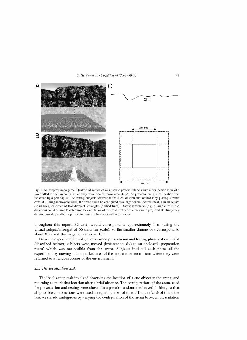
The main part of the experiment took place in an open arena with low walls (see

Fig. 1). Over the walls, a 3608 panoramic image of a desert landscape was visible. The

landscape provided directional cues that the subjects could use to orient themselves

within the environment. For instance, there was a large cliff in one direction (shown

directly ahead in Fig. 1A) and small distinctive peaks scattered about the horizon in

other directions. This background image was projected at infinity, so that parallax could

not be used to determine one’s location within the arena. The geometry of the walls

could be varied between four different rectangular configurations, ‘small’ (256 £ 256

units), ‘large’ (512 £ 512), ‘tall’ (256 £ 512, longer axis perpendicular to the cliff) and

‘wide’ (512 £ 256, longer axis parallel to the cliff). In the coordinate system used


throughout this report, 32 units would correspond to approximately 1 m (using the

virtual subject’s height of 56 units for scale), so the smaller dimensions correspond to

about 8 m and the larger dimensions 16 m.

Between experimental trials, and between presentation and testing phases of each trial

(described below), subjects were moved (instantaneously) to an enclosed ‘preparation

room’ which was not visible from the arena. Subjects initiated each phase of the

experiment by moving into a marked area of the preparation room from where they were

returned to a random corner of the environment.

2.3. The localization task

The localization task involved observing the location of a cue object in the arena, and

returning to mark that location after a brief absence. The configurations of the arena used

for presentation and testing were chosen in a pseudo-random interleaved fashion, so that

all possible combinations were used an equal number of times. Thus, in 75% of trials, the

task was made ambiguous by varying the configuration of the arena between presentation

Fig. 1. An adapted video game (Quake2, id software) was used to present subjects with a first person view of a

low-walled virtual arena, in which they were free to move around. (A) At presentation, a cued location was

indicated by a golf flag. (B) At testing, subjects returned to the cued location and marked it by placing a traffic

cone. (C) Using removable walls, the arena could be configured as a large square (dotted lines), a small square

(solid lines) or either of two different rectangles (dashed lines). Distant landmarks (e.g. a large cliff in one

direction) could be used to determine the orientation of the arena, but because they were projected at infinity they

did not provide parallax or perspective cues to locations within the arena.


and testing. In such circumstances there is no ‘correct’ mapping between locations in the

presentation arena and locations in the response arena. The aim was to determine which

properties of the arena were most important in determining the mapping subjects made in

this ambiguous situation. To avoid biasing subjects toward any particular determinant, the

instructions framed the experiment as a simple memory task (no mention was made of the

changing configuration of the arena). Subjects were advised to do their best if they were in

any doubt as to where the markers should be placed, and that there would be no further

instructions.

2.4. Practice

Before beginning the experiment, subjects practiced the task four times, once for

each of the different arena configurations. In these practice trials, the configuration of

the environment did not change between presentation and testing phases. There was

thus an unambiguously correct response for each practice trial. Subjects were required

to achieve a criterion level of performance on the task before progressing to the

experiment (mean placement error and variance within half of what would be expected

given random marker placement). This was to ensure that they understood the

experimental instructions, and were sufficiently familiar with the virtual environment

and keyboard controls to complete the experiment in a reasonable time. If a subject

failed to reach the criterion performance level they were given another opportunity to

complete the practice trials. One subject was rejected at this stage having failed to

complete the second set of practice trials satisfactorily. The cue locations used during

practice were not used during the experiment.

2.5. Presentation phase

The geometry of the environment was set as necessary. A cue object (golf flag) was

placed in the arena. The subject was placed in the arena, facing toward a randomly selected

corner. The subject was free to move about the arena, observing the flag from different

places until they had formed a clear impression of the location, at which point they pressed

a key to return to the preparation room (the ‘ready’ response).

2.6. Testing phase

The geometry of the environment was changed or not as necessary. The cue object was

removed from the arena. The subject was placed in the arena near to one of its corners and

facing outwards. The subject moved about the arena, and could place a marker object

(traffic cone) anywhere within it by pressing a key. When the key was pressed the marker

appeared 48 units ahead of the subject on the ground. The subject was free to continue

moving and repositioning the marker until content with its location, at which point they

pressed another key to confirm their response (‘ready’ response). The subjects were then

repositioned at a new starting location, and the process was repeated until four marker

locations had been stored. Each of the four corners were used as a starting location in a

random order. The subject then pressed a key to return to the preparation room.


2.7. Experimental design

All 16 possible geometric transformations of the environment between presentation and

testing (4 presentation configurations £ 4 testing configurations) were used. The relative

distances of the cue flag from the walls of the presentation arena were also varied to

determine whether locations nearer to the walls were represented differently to those

further away. Three distinct cue positions (described below) were probed in each

presentation environment making a total of 48 trials (16 arena transformations £ 3 cue

locations) per subject.

The cue positions were defined in terms of a unit square centered at the origin, and then

scaled to the dimensions of the presentation arena (i.e. they were fixed with respect to the

proportion of the total distance between walls). The three coordinates used were (0.1, 0.25),

(0.25, 0.4), and (0.1, 0.4). Due to the symmetry of the arenas, these proportional coordinates

could be mapped to any of 8 equivalent locations by means of a reflection in y ¼ x and/or

rotation through 90, 180 or 2708 relative to the external background cues (the resulting cued

location could thus be in any one of eight segments of the arena). As it was not practical to

test all these equivalent locations equally, we used a different pseudo-random sequence of

reflections/rotations for each subject, such that there was no obvious pattern in the segment

used in each trial. Where the presentation environment was rectangular, each of the

proportions (0.1, 0.25, 0.4) applied to the longer axis on half the trials.

3. Results

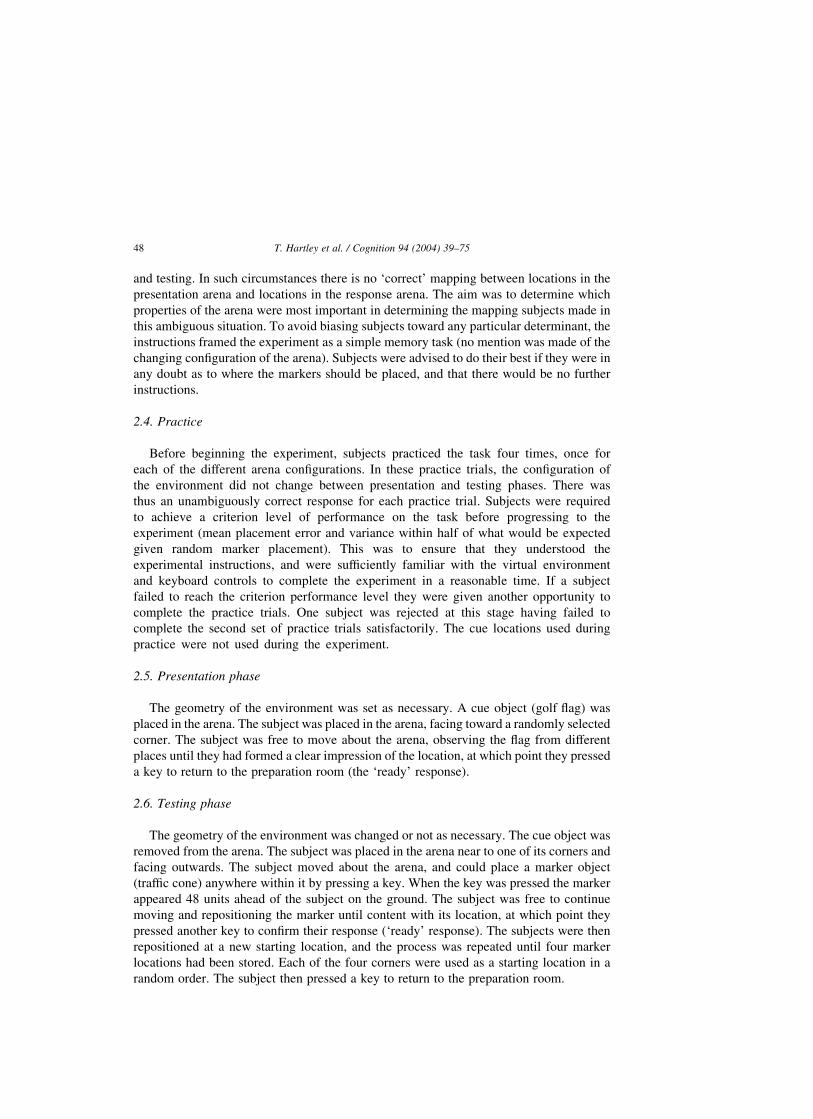
To visualize the data it is useful to collate the responses in each condition as a 2D

spatial distribution or response field. To calculate response density, we counted responses

occurring within each bin in a grid of 24 £ 24 unit bins (corresponding to approximately

75 £ 75 cm2), and then smoothed the resulting data with a 3 £ 3 (bin) square kernel. The

response density maps are shown in Fig. 2, where the leftmost column shows the location

of the cue flag in the presentation arena (4 presentation configurations £ 3 probe

locations ¼ 12 rows). The four right-hand columns show the density of responses in each

of the four testing arena configurations. To arrive at the response fields shown in Fig. 2, we

first ‘standardized’ the responses: collapsing them across geometrically equivalent

positions (i.e. reversing the effect of the randomly applied rotations and reflections of cue

location, so that the top right quadrant always corresponds to the quadrant in which the cue

was presented). Note that because the reflections and rotations are chosen randomly for

each subject, the design is not balanced with respect to these standardized conditions.

However each standardized condition shown in Fig. 2 includes data from at least 8 subjects

and includes at least 40 responses.

3.1. Baseline conditions

The trials where the box did not change shape between presentation and testing

(outlined in bold in Fig. 2) acted as a control task for the conditions involving geometric

transformations. They provide a baseline measure of performance in a geometrically


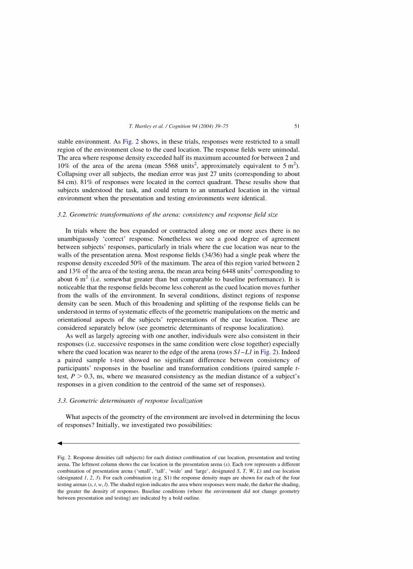
stable environment. As Fig. 2 shows, in these trials, responses were restricted to a small

region of the environment close to the cued location. The response fields were unimodal.

The area where response density exceeded half its maximum accounted for between 2 and

10% of the area of the arena (mean 5568 units2, approximately equivalent to 5 m2).

Collapsing over all subjects, the median error was just 27 units (corresponding to about

84 cm). 81% of responses were located in the correct quadrant. These results show that

subjects understood the task, and could return to an unmarked location in the virtual

environment when the presentation and testing environments were identical.

3.2. Geometric transformations of the arena: consistency and response field size

In trials where the box expanded or contracted along one or more axes there is no

unambiguously ‘correct’ response. Nonetheless we see a good degree of agreement

between subjects’ responses, particularly in trials where the cue location was near to the

walls of the presentation arena. Most response fields (34/36) had a single peak where the

response density exceeded 50% of the maximum. The area of this region varied between 2

and 13% of the area of the testing arena, the mean area being 6448 units2 corresponding to

about 6 m2 (i.e. somewhat greater than but comparable to baseline performance). It is

noticeable that the response fields become less coherent as the cued location moves further

from the walls of the environment. In several conditions, distinct regions of response

density can be seen. Much of this broadening and splitting of the response fields can be

understood in terms of systematic effects of the geometric manipulations on the metric and

orientational aspects of the subjects’ representations of the cue location. These are

considered separately below (see geometric determinants of response localization).

As well as largely agreeing with one another, individuals were also consistent in their

responses (i.e. successive responses in the same condition were close together) especially

where the cued location was nearer to the edge of the arena (rows S1–L1 in Fig. 2). Indeed

a paired sample t-test showed no significant difference between consistency of

participants’ responses in the baseline and transformation conditions (paired sample t-

test, P . 0:3; ns, where we measured consistency as the median distance of a subject’s

responses in a given condition to the centroid of the same set of responses).

3.3. Geometric determinants of response localization

What aspects of the geometry of the environment are involved in determining the locus

of responses? Initially, we investigated two possibilities:

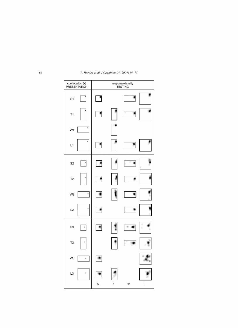
Fig. 2. Response densities (all subjects) for each distinct combination of cue location, presentation and testing

arena. The leftmost column shows the cue location in the presentation arena ðxÞ: Each row represents a different

combination of presentation arena (‘small’, ‘tall’, ‘wide’ and ‘large’, designated S, T, W, L) and cue location

(designated 1, 2, 3). For each combination (e.g. S1) the response density maps are shown for each of the four

testing arenas (s, t, w, l). The shaded region indicates the area where responses were made, the darker the shading,

the greater the density of responses. Baseline conditions (where the environment did not change geometry

between presentation and testing) are indicated by a bold outline.

R


(i) The cue’s location is represented in terms of its distance to each of the nearer walls of

the arena (e.g. the cue is 5 m from the North wall, 1 m from the East wall). Under this

fixed distance model we expect these distances to be maintained in the responses.

(ii) The cue’s location is represented in terms of the proportion of the distance between

opposing walls (e.g. the cue is a quarter of the distance between East and West

walls). Under this fixed ratio model, responses are expected to reflect these

proportions.

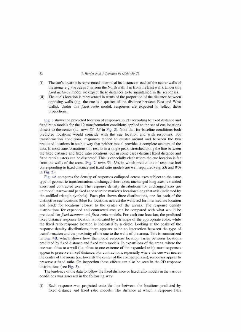
Fig. 3 shows the predicted location of responses in 2D according to fixed distance and

fixed ratio models for the 12 transformation conditions applied to the set of cue locations

closest to the center (i.e. rows S3–L3 in Fig. 2). Note that for baseline conditions both

predicted locations would coincide with the cue location and with responses. For

transformation conditions, responses tended to cluster around and between the two

predicted locations in such a way that neither model provides a complete account of the

data. In most transformations this results in a single peak, stretched along the line between

the fixed distance and fixed ratio locations, but in some cases distinct fixed distance and

fixed ratio clusters can be discerned. This is especially clear where the cue location is far

from the walls of the arena (Fig. 2, rows S3–L3), in which predictions of response loci

corresponding to fixed distance and fixed ratio models are well separated (e.g. S3l and W3t

in Fig. 2).

Fig. 4A compares the density of responses collapsed across axes subject to the same

type of geometric transformation: unchanged short axes; unchanged long axes; extended

axes; and contracted axes. The response density distributions for unchanged axes are

unimodal, narrow and peaked at or near the marker’s location along that axis (indicated by

the unfilled triangle symbols). Each plot shows three distributions, one for each of the

distinctive cue locations (blue for locations nearest the wall, red for intermediate location

and black for locations closest to the center of the arena). The response density

distributions for expanded and contracted axes can be compared with what would be

predicted for fixed distance and fixed ratio models. For each cue location, the predicted

fixed distance response location is indicated by a triangle of the appropriate color, while

the fixed ratio response location is indicated by a circle. Looking at the peaks of the

response density distributions, there appears to be an interaction between the type of

transformation and the proximity of the cue to the walls of the arena. This is summarized

in Fig. 4B, which shows how the modal response location varies between locations

predicted by fixed distance and fixed ratio models. In expansions of the arena, where the

cue was close to a wall (i.e. close to one extreme of the expanded axis), most responses

appear to preserve a fixed distance. For contractions, especially where the cue was nearer

the center of the arena (i.e. towards the center of the contracted axis), responses appear to

preserve a fixed ratio. On inspection these effects can also be seen in the 2D response

distributions (see Fig. 3).

The tendency of the data to follow the fixed distance or fixed ratio models in the various

conditions was assessed in the following way:

(i) Each response was projected onto the line between the locations predicted by

fixed distance and fixed ratio models. The distance at which a response falls


along this line measures its similarity to a fixed distance or fixed ratio response.

As the distance between fixed distance and ratio predictions varies dependent

on the type of transformation, we normalized the data such that a marker

placed at the fixed distance location has value 21, a marker at the fixed ratio

position has value 1.

Fig. 3. Predicted response locations according to fixed distance and fixed ratio models in the 12 different

transformation conditions (cued location corresponds to rows S3–L3 in Fig. 2). Each row shows a different

presentation arena in the leftmost column, with cue position marked by an x: The three rightmost columns show

the loci predicted by both models in the three transformed testing arenas. The triangle marks the location

predicted by the fixed distance model (a point that maintains its distance from the nearer two walls), the circle

marks the location predicted by the fixed ratio model (a point that maintains the ratio of distances between each

pair of opposing walls). The corresponding response density data from Fig. 2 rows S3–L3 is shown faintly for

comparison. A dashed contour delineates the region in which response density was greater than half the maximum

for each transformation.


(ii) As noted below (see ‘Interactions between transformed an unchanged axes’),

changes to one axis are not strictly independent of changes to the other, we

thus considered marker placement relative to the expanded/contracted axis only

in trials where the other axis did not change.

(iii) The spatial distributions of responses are bounded (by the walls of the box) in

a way that affects the mean marker placement and is not independent of the

type of transformation. We thus used the median normalized marker placement

(which is less susceptible to this artifact) as the dependent variable in our

statistical analysis.

(iv) Individual subjects may show idiosyncratic response patterns which are

obscured in the group data considered in Figs. 2 and 4. We therefore used a

repeated measures ANOVA to assess the significance of within-subjects effects

of cue position and transformation (expansion or contraction) on median marker

placement in each of the 3 (cue position) by 2 (transformation) critical

conditions.

There was no main effect of transformation on its own, but cue location (Fð2;28Þ ¼ 8:13;

P , 0:01) and its interaction with geometric transformation (Fð2;28Þ ¼ 3:68; P , 0:05)

were statistically significant determinants of where the marker was placed relative to the

locations predicted by the two models. These effects are summarized in Fig. 4B which

shows for each cue position the modal response location (from the response distributions

in Fig. 4A) relative to the peak location predicted by fixed distance and fixed ratio models.

The results are consistent with a representation of space that includes both distance and

proportion information, in which the relative weight placed on each differs between

conditions. But can we account for the observed effect of cue location and its interaction

with transformation type in terms of a single model? We considered a number of

alternative geometric models (i.e. forms for the stored representation of the cue location)

in addition to the fixed distance and fixed ratio models outlined above. Then, using

identical assumptions for all the models, we determined the response distribution

predicted by each—allowing us to make a quantitative comparison between models in

terms of the likelihood of the data under each one (see Appendix B).

In addition to the fixed distance and fixed ratio models, we considered three further

models, making five in total:

(i) Fixed distance model: the cue’s location is represented in terms of the perpendicular

distance from it to the two nearer walls.

(ii) Fixed ratio model: the cue’s location is represented as a fixed proportion of the

distances between opposing walls (i.e. perpendicular distance to the North wall as a

proportion of the distance between North and South walls; perpendicular distance to

the East wall as a proportion of the distance between East and West walls).

(iii) The cue’s location is represented in terms of the directions from the cue to the

corners of the arena. Under this corner angle model responses will be close to

the location at which the angles to the corners are most similar to those subtended by

the cue at presentation.


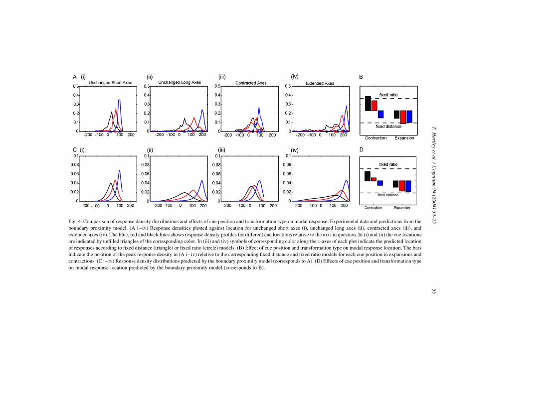
Fig. 4. Comparison of response density distributions and effects of cue position and transformation type on modal response: Experimental data and predictions from the

boundary proximity model. (A i–iv) Response densities plotted against location for unchanged short axes (i), unchanged long axes (ii), contracted axes (iii), and

extended axes (iv). The blue, red and black lines shows response density profiles for different cue locations relative to the axis in question. In (i) and (ii) the cue locations

are indicated by unfilled triangles of the corresponding color. In (iii) and (iv) symbols of corresponding color along the x-axes of each plot indicate the predicted location

of responses according to fixed distance (triangle) or fixed ratio (circle) models. (B) Effect of cue position and transformation type on modal response location. The bars

indicate the position of the peak response density in (A i–iv) relative to the corresponding fixed distance and fixed ratio models for each cue position in expansions and

contractions. (C i–iv) Response density distributions predicted by the boundary proximity model (corresponds to A). (D) Effects of cue position and transformation type

on modal response location predicted by the boundary proximity model (corresponds to B).

T.

Ha

rtleyet

al.

/C

og

nitio

n9

4(2

00

4)

39

–7

55

5

(iv) The cue’s location is represented in terms of the absolute distances to all four walls

of the arena. Any transformation of the environment will mean that there is no

location where all four distances are maintained. However, under this absolute

distance model responses are expected to cluster around locations which provide the

best match to the distances at presentation—each distance being equally weighted.

(v) The cue’s location is represented in terms of the ‘proximity’ to each of the four

walls given by 1=ðd þ cÞ where d is the distance to the wall and c is a constant.

Under this boundary proximity model responses will tend to maintain a fixed

distance to nearby walls (because shorter distances are weighted more strongly

in the representation), but would maintain a fixed ratio for a cue at the center of

the arena (since the weight given to opposing walls would be equal). For cued

locations between the center and the edge of the environment, responses will lie

somewhere between the locations predicted by fixed distance and fixed ratio

models. Responses will be closer to preserving ratios for high values of c and

closer to preserving distances to nearby boundaries for low values of c:

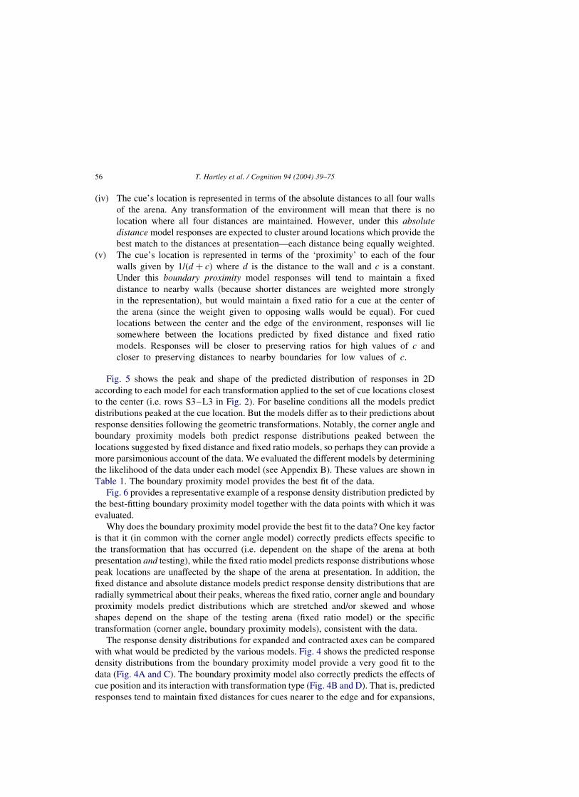
Fig. 5 shows the peak and shape of the predicted distribution of responses in 2D

according to each model for each transformation applied to the set of cue locations closest

to the center (i.e. rows S3–L3 in Fig. 2). For baseline conditions all the models predict

distributions peaked at the cue location. But the models differ as to their predictions about

response densities following the geometric transformations. Notably, the corner angle and

boundary proximity models both predict response distributions peaked between the

locations suggested by fixed distance and fixed ratio models, so perhaps they can provide a

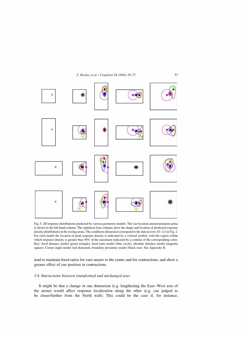
more parsimonious account of the data. We evaluated the different models by determining

the likelihood of the data under each model (see Appendix B). These values are shown in

Table 1. The boundary proximity model provides the best fit of the data.

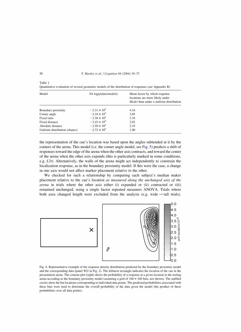
Fig. 6 provides a representative example of a response density distribution predicted by

the best-fitting boundary proximity model together with the data points with which it was

evaluated.

Why does the boundary proximity model provide the best fit to the data? One key factor

is that it (in common with the corner angle model) correctly predicts effects specific to

the transformation that has occurred (i.e. dependent on the shape of the arena at both

presentation and testing), while the fixed ratio model predicts response distributions whose

peak locations are unaffected by the shape of the arena at presentation. In addition, the

fixed distance and absolute distance models predict response density distributions that are

radially symmetrical about their peaks, whereas the fixed ratio, corner angle and boundary

proximity models predict distributions which are stretched and/or skewed and whose

shapes depend on the shape of the testing arena (fixed ratio model) or the specific

transformation (corner angle, boundary proximity models), consistent with the data.

The response density distributions for expanded and contracted axes can be compared

with what would be predicted by the various models. Fig. 4 shows the predicted response

density distributions from the boundary proximity model provide a very good fit to the

data (Fig. 4A and C). The boundary proximity model also correctly predicts the effects of

cue position and its interaction with transformation type (Fig. 4B and D). That is, predicted

responses tend to maintain fixed distances for cues nearer to the edge and for expansions,


tend to maintain fixed ratios for cues nearer to the center and for contractions, and show a

greater effect of cue position in contractions.

3.4. Interactions between transformed and unchanged axes

It might be that a change in one dimension (e.g. lengthening the East–West axis of

the arena) would affect response localization along the other (e.g. cue judged to

be closer/further from the North wall). This could be the case if, for instance,

Fig. 5. 2D response distributions predicted by various geometric models. The cue location and presentation arena

is shown in the left hand column. The rightmost four columns show the shape and location of predicted response

density distributions in the testing arena. The conditions illustrated correspond to the data in rows S3–L3 in Fig. 2.

For each model the location of peak response density is indicated by a colored symbol, with the region within

which response density is greater than 50% of the maximum indicated by a contour of the corresponding color.

Key: fixed distance model (green triangle), fixed ratio model (blue circle), absolute distance model (magenta

square), Corner angle model (red diamond), boundary proximity model (black star). See Appendix B.


the representation of the cue’s location was based upon the angles subtended at it by the

corners of the arena. This model (i.e. the corner angle model, see Fig. 5) predicts a shift of

responses toward the edge of the arena when the other axis contracts, and toward the center

of the arena when the other axis expands (this is particularly marked in some conditions,

e.g. L3t). Alternatively, the walls of the arena might act independently to constrain the

localization response, as in the boundary proximity model. If this were the case, a change

in one axis would not affect marker placement relative to the other.

We checked for such a relationship by comparing each subject’s median maker

placement relative to the cue’s location as measured along the unchanged axis of the

arena in trials where the other axis either (i) expanded or (ii) contracted or (iii)

remained unchanged, using a single factor repeated measures ANOVA. Trials where

both axes changed length were excluded from the analysis (e.g. wide ! tall trials).

Table 1

Quantitative evaluation of several geometric models of the distribution of responses (see Appendix B)

Model Fit logðpðdatalmodelÞÞ Mean factor by which response

locations are more likely under

Model than under a uniform distribution

Boundary proximity 22.31 £ 104 4.16

Corner angle 22.34 £ 104 3.85

Fixed ratio 22.38 £ 104 3.34

Fixed distance 22.43 £ 104 2.82

Absolute distance 22.50 £ 104 2.19

Uniform distribution (chance) 22.72 £ 104 1.00

Fig. 6. Representative example of the response density distribution predicted by the boundary proximity model

and the corresponding data (panel W2l in Fig. 2). The leftmost rectangle indicates the location of the cue in the

presentation arena. The contour plot (right) shows the probability of a response at a given location in the testing

arena according to the boundary proximity model (assuming a grid of 160 £ 160 bins, not shown). The unfilled

circles show the bin locations corresponding to individual data points. The predicted probabilities associated with

these bins were used to determine the overall probability of the data given the model (the product of these

probabilities over all data points).


Surprisingly, we did find a statistically significant effect of transformation on the ‘error’

relative to the unchanged axis (Fð2;28Þ ¼ 3:891; P , 0:05). Contractions tended to

produce responses further from the center of the arena than in baseline conditions,

whereas expansions produced the opposite result. However, although reliable, the size

of the effect was very small (the mean shift relative to baseline was of the order ^5

units, about 16 cm) particularly when compared to the magnitude of the contrac-

tion/expansion of the other axis (256 units, equivalent to about 8 m). Qualitatively, the

effect is compatible with a representation of the cue location based on the angles to the

corners of the arena, but quantitatively it is much too small to indicate that these angles

play a significant role relative to boundary proximity information in the representation

of the cue’s location.

3.5. Orientation dependence of responses

What were subjects looking at when they encoded the object’s location and when they

made their responses? Although we have analyzed subjects’ responses in terms of possible

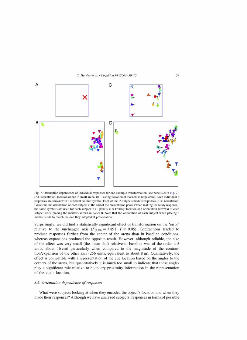
Fig. 7. Orientation dependence of individual responses for one example transformation (see panel S2l in Fig. 2).

(A) Presentation: location of cue in small arena. (B) Testing: location of markers in large arena. Each individual’s

responses are shown with a different colored symbol. Each of the 15 subjects made 4 responses. (C) Presentation:

Locations and orientation of each subject at the end of the presentation phase (when making the ready response),

the same symbols are used for each subject in all panels. (D) Testing: location and orientation (arrows) of each

subject when placing the markers shown in panel B. Note that the orientation of each subject when placing a

marker tends to match the one they adopted at presentation.


geometric representations, these representations must be derived from the visual display in

some way. The nature of these lower level mechanisms may be informed by an analysis of

the subjects’ view throughout the experiment. For instance, subjects may place their

markers relative to locations yielding the same or similar views to those encountered when

viewing the cue. In order to investigate this possibility we analyzed the direction subjects

faced when making the ‘ready’ response at presentation and when the marker was (finally)

placed at testing. This is illustrated for a typical pair of arenas (S2l) in Fig. 7.

Unsurprisingly, subjects tended to face the cue when making the ‘ready’ response at

presentation, and necessarily faced towards the marker when placing it. However, we also

found a very strong tendency for subjects to face the same ‘compass’ direction at

presentation and testing (the median absolute discrepancy between orientations at

presentation and recall was just 158, P , 0:0001; see footnote 1).

This observation might suggest that subjects sought a location and orientation

yielding a similar view of the environment to the one they adopted at presentation. That

is, subjects may be attempting to match a stored perceptual snapshot of the arena.

Subject 1, for instance, represented by red circles in Fig. 7, has a very similar view of

the arena at presentation and testing. This same does not apply for subjects facing

inwards (i.e. toward the center of the arena) when viewing the cue and placing the

marker, where any transformation of the environment will yield a different view

between presentation and testing. For instance, subject 10 (represented by green circles

in Fig. 7) faces in the same direction at presentation and testing, but from his point of

view, the opposite wall was much further away a testing than at presentation. We found

that almost exactly half of responses in transformation trials were made with the

subject facing inward. It thus appears that orientation, rather than view, is matched in

making a response.

3.6. Disorientation

In the vast majority of trials, there was no evidence of disorientation (e.g. responses

in the opposite quadrant in rectangular baseline trials) which indicates that the distant

landmarks provided good cues to orientation. However, in both baseline and

transformation trials we see evidence of individuals becoming disoriented in some

trials, especially those involving rectangular arenas where the cue location is nearer the

center of the environment, and in tall ! wide and wide ! tall transformations.

Although it is impossible to be certain, these conditions produce clusters of responses

(normally due to a single individual) distant from the peak and approximately

consistent with application of the boundary proximity model to the ‘wrong’ axes (see

conditions W2l, T2w, T3t, T3w, T3l, S3t in Fig. 2). We note that in the tall ! wide and

wide ! tall transformations the two potential orientation cues (distant landmarks or

arena geometry) are in conflict and it is perhaps not surprising that subjects

1 The sum of unit vectors representing the view orientation at presentation and recall had a median length of

1.98, whereas a value of 1.41 ðffiffi2

pÞ is predicted for random pairs of unit vectors. A Monte Carlo simulation

showed that the probability of a sample of 2880 random pairs having a median sum with length 1.98 is less than 1

in 10,000.


occasionally used the ambiguous arena geometry. It is also notable that disoriented

responses were more likely in trials where the cue location was near to the center of the

arena. Disoriented responses did not occur for cue locations near to the edge of the

arena, even in the more radical rectangle ! rectangle transformations (T1w, W1t). By

contrast, disorientation was even seen in one of the baseline conditions (T3t) when the

cue was nearer the center of the arena.

4. Discussion

In the baseline conditions, we saw that subjects understood the task, and were able to

accurately place their markers at the unmarked cue location after brief delay. The distant

landmarks provided a strong orientational reference frame, enabling the vast majority of

responses to be placed in the correct quadrant. On the transformation trials the pattern of

responses occasionally became elongated or bimodal. Peaks in response density lay

between locations that maintain fixed distances to the nearer walls and locations that

maintain a fixed ratio of the distances between opposing walls. The fixed ratio model fitted

best where the environment contracted, or where the cue location was near the center of

the arena. The fixed distance model fitted best where the environment expanded, or where

the cue was nearer the edge of the arena (the effect of cue position being stronger in

contractions than expansions). Neither of these simple models was sufficient to capture the

pattern of responses across all conditions. However, the ‘boundary proximity’ model did

capture the major features of this pattern and provided the best overall fit to the data of

the several alternatives we investigated. The boundary proximity model is closely related

to our place cell model (Hartley et al., 2000). It is approximately equivalent to storing

the firing rates at the cue location of the place cell inputs which are maximally active there,

and responding at the location that best matches this pattern in the testing arena2.

The success of the boundary proximity model is due, in large measure, to the way in

which it explains the effects of cue location and its interaction with transformation type.

These features are natural consequences of a boundary proximity representation of the cue

location. Near to the center of the environment this approximates a ratio representation

because the influence of opposing walls is approximately equal. At the edges of the arena

this approximates a distance representation because the distant walls have little influence

compared to the proximal ones. The model also predicts the observed interaction between

cue position and transformation type: in contractions, the boundary proximity model

predicts ratio-like responses because in these circumstances walls which were furthest

2 An important difference from the behavioral prediction in Hartley et al. (2000) is that we previously assumed

that searching maximized the dot product between the vector of current place cell firing rates and the stored vector

of cue location during presentation (Burgess & O’Keefe, 1996). In such a model, the influence of a given cell is

proportional to its firing rate. This produces responses resembling the fixed distance model as high-rate cells tend

to be sensitive to nearby walls, and produces inaccurate responses when the arena does not change between

presentation and retrieval (showing a central tendency). In the current model searching minimizes the Euclidean

distance between the current and stored vectors. This has the effect of giving equal weight to equal changes in

firing rate, regardless of the cells’ baseline firing rates—better balancing the influence of cells sensitive to near

and far walls.


from the cue at presentation become more influential at testing (they ‘move closer’ on

average), and in doing so they play a more important role in ‘pushing’ the response away

from them. In expansions, the small weight given to the more distant walls of the arena is

further diminished at testing (they ‘move further away’ on average), leaving responses to

be determined largely by the distance to the walls which were nearest the cue at testing.

The corner angle model also provided a reasonably good fit to the data. While fitting the

data rather less well than the boundary proximity model it is also somewhat simpler (the

corner angle model has no free parameters, whereas the proximity model has one, c). We

are inclined to favor the boundary proximity model for two reasons. Firstly, it fits the data

well over a range of values for c: Indeed variations in c could account for some between-

subject variation: some subjects consistently made more ratio-like responses while others

consistently made more fixed distance responses, corresponding to the effect of varying c:

Secondly, it captures the qualitative pattern of results in which the effect of cue position is

greater for contractions of an environment than for expansions (the corner angle model

predicts the reverse pattern).

There are nonetheless hints in the data that angle information might play some role in

the representation of the cue’s location. In particular a representation based on the bearings

from the cue to the corners of the arena would result in an effect of manipulations of one

axis of the arena on responses density along the other (unchanged) axis. A very small, but

statistically reliable, effect of this type was observed. This form of representation was

originally suggested by the results of an experiment by Spetch et al. (1996, Experiment 4)

in which humans searched for an object that had been seen at a location equidistant to two

isolated landmarks, but offset from the line between them. They found that after expansion

or contraction of the landmark array, searches focused on an area preserving the angles to

the landmarks. This location also preserves the ratio of the distances to the landmarks,

while the perpendicular distance from the line between the landmarks changes (increasing/

decreasing by the expansion/contraction factor). However, in our data, the analogous

perpendicular shift is much too small to be consistent with this (or with the corner angle

model), being more consistent with the boundary proximity model. Nonetheless, the

reliability of the effect suggests that representations in spatial memory may include angle

information, but if so it appears that metric information carries more weight than angular

information (as in Waller et al., 2000).

Because we used rectangular arenas, Cheng’s (1989) vector sum model (storing the

vectors from the corners of the arena) could be consistent with several of the models

explored here, depending on the form of proximity weighting used. If only the vector from

the nearest corner were used, it would be equivalent to the fixed distance model.

Alternatively, it would be equivalent to the fixed ratio model if vectors from corners were

weighted by the ratio measure of the position of the target location along the direction

between the corners (i.e. weights 2/3 and 1/3 if the target location had been twice as close

to one side of the arena than the other). If a proximity weighting of 1=ðd þ cÞ were used, the

vector sum model would produce similar results to the boundary proximity model (though

not identical, if it used the distance to the corner rather than to the wall). The vector sum

model thus suggests one way in which the boundary proximity model could be extended to

locations defined by several isolated landmarks rather than by environmental boundaries.

The boundary proximity model could also be extended to environments of arbitrary shape


by explicitly simulating a population of cells tuned to respond to the presence of a

boundary at arbitrary distances and directions, as in Hartley et al. (2000). The response

distribution would then be focused at locations in the testing arena where the pattern of

firing amongst these cells best matches the pattern seen at the cue. Developing a model that

applies to both isolated landmarks and arbitrary boundaries will be the subject of future

work.

While the geometric models discussed above, and the boundary-proximity model in

particular, provide a good account of response locations in the experiment, none of them

says anything about how subjects orient themselves with respect to the environment. In

fact, subjects showed a strong tendency to adopt the same orientation at presentation and

testing. This ‘orientation matching’ did not correspond to exact ‘view matching’ because,

in at least half of the transformation trials, prominent features of the environment (the

walls) within the field of view had ‘moved’ relative to the subject due to the geometric

transformation. In these circumstances, only the distant background cues (which do not

provide any metric information) are consistent between presentation and testing. The

orientation matching thus suggests that subjects store information about the directions of

these cues relative to their view of the environment at presentation, and they make use of

this information to orient themselves at testing.

4.1. Role of path integration and spatial updating

The experimental paradigm we used goes a long way toward excluding the use of

simple path-integrative or spatial updating mechanisms as a means of remembering

the cue location. First, the use of desktop VR means that idiothetic cues to self-motion are

unavailable, leaving only optic flow (Waller et al., 2000). Second, the subject is moved

abruptly from the presentation arena to the preparation room, and then back to a random

corner of the testing arena. The subject thus cannot use information about the path taken

between presentation and test either to guide them back to the cue location, or to update

any egocentric representation.

One remaining possibility is that subjects could store the path taken from an identifiable

landmark in the presentation arena to the cue, and then return to this landmark location in

the testing arena before ‘retracing their steps’ back to mark the cue location. Use of this

strategy would result in responses fixed with respect to the landmark location. The only

such landmark that would yield responses in the correct quadrant in transformation trials is

the corner nearest to the cue. Responses based on this strategy would be made while facing

inwards and would correspond to the predictions of the fixed distance model which

provides a much poorer fit to the data than the boundary proximity model. Since this model

provides a poor overall fit to the data (Table 1), path integration could only account for a

small subset of responses. Detailed inspection of the paths taken during the testing phase

of the experiment indicated that some subjects on some trials had indeed retraced their

steps from the nearest corner, though these formed a small minority of responses. Of the

four possible combinations, 28% of all responses were fixed distance, inward facing

responses, a slight excess over the 25% that would be expected to arise by chance. To

determine whether this strategy in any way influenced the effects of geometric

manipulation, we conducted a further experiment (see Appendix A) in which procedural


changes were employed to discourage the use of corners as fixed reference points for path

integration. Here the proportion of fixed distance inward facing responses fell to 13%. At

the same time, effects of cue position and its interaction with transformation type were

replicated, along with many qualitative aspects of the data (compare Figs. 2 and 8).

Thus, we believe a path integration strategy contributed directly to only a small

proportion of responses in the main experiment. Overall, the data appear to rule out an

explanation in which memory for the cue location is based solely on the tracking of self-

motion information, whether this takes the form of path integration or some more general

spatial updating mechanism. Geometric manipulations produce systematic effects in the

response density data evident, for instance, in the interaction between transformation type

and response location. Since geometric changes to the arena would not affect self-motion

information, it is hard to see how these effects might emerge from path integration or

spatial updating mechanisms. However, an indirect contribution of these mechanisms in

evaluating boundary proximities is quite likely. Knowledge of the proximity of a boundary

that is behind the subject is probably aided by short-term spatial updating since that

boundary was last seen.

A recent synthesis of studies of spatial memory (Wang & Spelke, 2002) concludes that

memory for object locations is supported solely by egocentric representations and processes

of spatial updating, while a ‘geometric module’ serves only for the reorientation of

disoriented subjects (see below). Our results are hard to reconcile with this picture but

could perhaps be interpreted as shedding light on the workings of the geometric module.

As mentioned above, it is hard to see how any simple spatial updating mechanism could

account for the effects of geometric manipulations captured by the boundary-proximity

model (Fig. 4). On the contrary, our data suggest that environmental geometry plays a

crucial role in representing the location of the cue object while, conversely, the orientation

of the subject seems to depend predominantly on the distant visual landmarks.

4.2. Disorientation

The pattern of the occasional disoriented responses (see conditions W2l, T2w, T3t, T3w,

T3l, S3t in Fig. 2) is reminiscent of Hermer and Spelke’s (1994) findings in young children

returning to a cued location in a rectangular environment following disorientation. They

found that, for these subjects, geometric cues (i.e. the aspect ratio of the environment)

overwhelmed other visual information that could have been used for reorientation, leading

to a high proportion of disoriented responses. A similar result had previously been found in

Fig. 8. Response densities (all subjects) for each distinct combination of cue location, presentation and testing

arena used in a second experiment (see Appendix A). As in Fig. 2, the leftmost column shows the cue location in

the presentation arena ðxÞ: Each row represents a different combination of presentation arena and cue location. For

each combination the response density maps are shown for each of the four testing arenas. The shaded region

indicates the area where responses were made, the darker the shading, the greater the density of responses.

Baseline conditions (where the environment did not change geometry between presentation and testing) are

indicated by a bold outline. The procedure was similar to that in the main experiment, except that potential use of

the corners of the environment as reference points for path integration was discouraged by moving the subject to a

random location before making each response. The pattern of responses is similar to that in Fig. 2.

R


rats in a similar ‘reorientation’ paradigm (Cheng, 1988). This pattern of responses is

typically not seen in larger rooms (Learmonth, Newcombe, & Huttenlocher, 2001), or in

adult subjects, although it has been reported in adults when performing a demanding

concurrent verbal task (Hermer-Vazquez, Spelke, & Katsnelson, 1999).

In our own experiment the absence of idiothetic cues and instantaneous virtual

movement of the subject to and from the preparation room presumably mimics the effect

of a disorientation procedure, ruling out direct path-integration between presentation and

testing. Environmental geometry can also be seen to influence orientation in our

experiment, despite the presence of distant visual cues, but only in a very small number of

trials. This is most noticeable following tall to wide or wide to tall transformations in

which the geometry of the environment provides an orientational cue in conflict with the

distant landmarks. However, in our experiment, the effect of environmental geometry on

orientation is much weaker than the anchoring effect of the distant landmarks.

Our model of spatial memory has some implications for future reorientation

experiments. Firstly we note that, in rats, proximal visual landmarks have a much weaker

effect on the orientation of the place cell representation than distal visual landmarks

(Cressant et al., 1997). Thus, if behavior in reorientation paradigms depends on a similar

system in humans, we would expect distant landmarks beyond the immediate

environmental boundaries to reduce the incidence of disoriented responses. Secondly, in

the disorientation paradigms discussed above, effects of geometry on orientation were

observed in memory for locations right in the corner of the environment. However,

we would expect a greater incidence of disoriented responses if locations nearer to the

center were probed (as seems to be the case in our results). See Wang, Hermer, and Spelke

(1999) for further discussion of disorientation studies in rats and humans.

4.3. Reference frames

Can our results best be described in terms of supporting ‘egocentric’ or ‘allocentric’

representations? If representations were strictly egocentric (including the observer’s

position as well as orientation) we would expect to see view-matching responses. On the

other hand if they were strictly allocentric (i.e. viewpoint independent) we would not

expect to see orientation-matching at all. Thus it might be better to assume that both

allo- and egocentric representations exist (consistent with the neurophysiological

evidence outlined in the introduction) and that the use they are put to depends on the

task at hand.

The observation of orientation matching suggests the involvement of an egocentric

process of landmark matching to determine the subject’s orientation. This might depend

on an egocentric sensory (or more abstract) representation being used to store the bearings

to distal cues between presentation and testing phases. However, the involvement of

egocentric representations does not seem to extend to the location of the cue within the

arena. Here the effects of geometric manipulation on response density seem incompatible

with the use of sensory representations, which we would expect to produce view-matching

responses. Neither can they be explained by simple path integration or more abstract,

dynamically updated egocentric representations. Instead the cue location appears to be

represented relative to the boundary of the environment rather than relative to the subject’s


position at encoding. That is, the representation of the cue location is best described as

allocentric.

Though rare in our paradigm, some disorientated responses seem to correspond to

application of a geometric representation to the ‘wrong’ axes suggesting that orientation

processes can operate independently of the location representation. This separation would

mirror the distinction between place and head-direction systems found in the rat’s brain

(Muller, Ranck, & Taube, 1996; Taube, 1998) and in our model of place cell firing

(Hartley et al., 2000; O’Keefe & Burgess, 1996). The relative importance of distant

landmarks as orientation cues (compared to geometric information) is also approximately

consistent with their relative influence on the place cell representation in similar

circumstances (Jeffery et al., 1997).

All these observations would be compatible with the hippocampal place cell

representation, as modeled by Hartley et al. (2000) and Burgess & O’Keefe (1996), on

the assumption that the head-direction system (which is believed to control its

orientation) is calibrated by the postulated landmark matching process (see e.g.

Hahnloser, 2003; Skaggs, Knierim, Kudrimoti, & McNaughton, 1995; Taube, 1998).

Operation of this process could also help to explain the egocentric bias in reaction-time

and performance measures often found in spatial memory (Diwadkar & McNamara,

1997; see also King et al., 2002) and increased performance in spatial memory tasks

where novel viewpoints are aligned with distal cues (McNamara et al., 2003; Burgess

et al., in press; Shelton & McNamara, 2001).

5. Conclusion

The experimental paradigm used in the current study provides a new point of contact

between neurophysiological studies of spatial representations (Ekstrom et al., 2003;

Jeffery et al., 1997; Morris et al., 1982; O’Keefe & Burgess, 1996), animal behavioral

studies (Cheng, 1986,1989; Collett et al., 1986; Spetch et al., 1996, 1997) and

psychological investigations (Hermer & Spelke, 1994; King et al., 2002; Shelton &

McNamara, 2001; Wang & Spelke, 2000), all of which can be brought to bear in

interpreting our findings. Such contact is useful since it means that insights gained at the

physiological level can inform experiments at the behavioral level, and vice versa. In this

case we extend a theoretical framework originally based on neural representations in the

rat hippocampus to help explain and (in principle) predict human behavior in a simple

spatial task.

We found that subjects could accurately remember the cued location in the

baseline conditions in which the arena did not change shape between presentation and

retrieval. In the transformation conditions, responses fell between locations that

matched the distance to the nearest two walls to the cued location and locations that

matched the ratio of the distances between opposing walls. Responses clustered near

to the fixed distance model after expansions of the arena and for cued locations

nearer to the edge, while falling nearer to the fixed ratio model after contractions of

the arena and for cued locations nearer to the center. When responding, subjects

showed a tendency to assume the same orientation as at presentation, while not


necessarily matching their view. This pattern is consistent with an allocentric

representation of location relative to the boundaries of the environment, in which the

salience of a given boundary depends on its proximity to the cued location, combined

with an egocentric process of landmark-matching which determines the overall

orientation of the location representation.

Human spatial memory is sensitive to geometric manipulations of the environment. The

effects of these manipulations shed light on the complementary egocentric and allocentric

systems that underlie human spatial memory. Our boundary proximity model was inspired

by the properties of place cells in the rat and provides a robust fit to the data. This,

combined with the recent discovery that place cells also exist in the human hippocampus

(Ekstrom et al., 2003), lends weight to the view that it will ultimately be possible to

understand aspects of human spatial cognition in terms of the physiological properties of

its neural substrates.

Acknowledgements

We thank John Morton, Graham Hitch, Daniel Haun and 3 anonymous reviewers for

their helpful comments on earlier versions of the manuscript. We also thank John O’Keefe

and Peter Dayan for useful discussions, and Douglas Ku for help collecting data. This

research was supported by an MRC Senior Fellowship to NB and an MRC Co-op grant to

the ICN. IT is supported by UCL Graduate School and Overseas Research Students Award

Scheme Scholarships.

Appendix A. Replication with procedural variation to discourage the use of corners

as reference points

Below we describe another experiment, very similar to that described in the main body

of the text, which replicated the major findings of the main experiment, while discouraging

the use of the corners of the arena as reference points and strategies involving path

integration from such reference points. This was achieved by increasing the number of

markers to be placed on each trial to 10, and by moving the subject to a new, random

location in the arena prior to placing each marker. In other respects the experiment was

almost identical to the one described previously but for the following changes:

There were 12 subjects, (all students, mean age 21.2, 10 with prior experience with first

person videogames).

Subjects initiated each phase of the experiment completing a circuit around the virtual

preparation room. This manipulation was intended to disrupt any path integration

representation of the cued location.

To encourage subjects to spread out their responses they were advised that if they were

uncertain as to the exact location to mark they should spread their responses so that at

least one would be close to the correct location. Instead of placing a visible marker

object (traffic cone) subjects pressed a key to invisibly mark their current location.


They were not given the opportunity to revise this placement.

We used a different set of cue locations, defined as in the main experiment relative to a

unit square centered at the origin. The three coordinates used were (0.3, 0.4), (0.1, 0.2),

and (0.4, 0.1) giving more positions (relative to a given wall) than in experiment 1. As

in the main experiment, these locations were randomly transformed, so that the cue

could appear in any quadrant of the arena, and with respect to either axis. However, this

time the same set of transformations were used for each cue location, and each subject.

Thus each subject did the same subset of transformations, making a much larger

number of observations per tested condition especially when combined with the

increased number of markers. However, due to time constraints some possible

combinations of cue location and geometric transformation were not included (hence

the ‘missing’ transformations in Fig. 8). The sequence of trials was randomized

between subjects.

The response fields obtained are shown in Fig. 8 (cf. Fig. 2). Despite the subtle

differences in experimental procedure, we see a markedly similar pattern of results.

A.1. Baseline conditions

The median distance of markers from the cued location was 39 units (corresponding to

approximately l m, i.e. more spread than in the main experiment). All response fields were

unimodal in the baseline conditions. The greater spread of responses is probably due to

three factors: (i) subjects placed more markers in this experiment and were explicitly

encouraged to spread their responses when uncertain as to the ‘correct location’; (ii) the

random relocation of subjects between each marker placement may have prevented them

from using fixed points (e.g. corners) as references to guide marker placement; (iii) one of

the cued locations used (0.3, 0.4) was nearer the center of the arena than any we probed in

the main experiment, and therefore more likely to produce disoriented responses, i.e.

responses in the wrong quadrant.

A.2. Geometric transformations of the arena

Results were generally consistent with those seen in the main experiment. Responses

tended to form unimodal fields which were centered near locations predicted by fixed

distance and ratio models. Bimodal fields were also observed in 2/29 geometrically

distinct conditions (S3t, S2l), both involving expansions. However, there was no

significant difference in the consistency of responses (measured as in the main experiment)

between baseline and transformation trials. Analyzing the responses relative to axes that

had been expanded or contracted between presentation and testing, we observed the same

pattern of interaction between cue position and geometric transformation as in the main

experiment. Responses tended to maintain a fixed distance from the nearer walls, where

the cue had originally appeared near to the walls of the environment, especially following

expansion of the arena. Where the cue was nearer the center of the arena, and especially

following contractions of the environment, responses tended to maintain a fixed ratio of

the distance between opposing walls. As in the main experiment, this interaction was


statistically significant (Fð2;22Þ ¼ 6:632; P , 0:05), as was the main effect of cue position

(Fð2;22Þ ¼ 3:735; P , 0:05).

A.3. Orientation matching and path integration

Again we observed a strong tendency to match orientations at presentation and recall

(median discrepancy 158, P , 0:0001), replicating the finding in the main experiment. In

the main experiment, a small minority of responses appeared to result from subjects

retracing their steps from the nearer corner of the arena to the cued location. Although there

was again a slight tendency for responses nearer to the fixed distance model than to the fixed

ratio model to be more prevalent when facing inwards (43% versus 34% when facing

outwards). This compares with 56% inward versus 40% outward facing responses in the

main experiment). These inward facing fixed distance responses comprise only 13% of all

responses.

Appendix B. Evaluating models of response density distributions

In the main body of the text we set out five simple geometric models.

(a) fixed distance model

(b) fixed ratio model

(c) absolute distance model

(d) corner angle model

(e) boundary proximity model

These models specified the geometric properties of the environment which would be

preserved in responses, and thus the expected peak of response density. To define response

density distributions for each model we made the following assumptions (which could be

extended to any similar model):

(i) the geometric parameters relating to the cue’s location at presentation are stored as a

vector nc where each element is one of the stored parameters:

a. fixed distance model: distances to the two nearest perpendicular walls, e.g. for

cue in north eastern quadrant, nc ¼ ðdN; dEÞ:

b. fixed ratio model: ratios of distances between opposing walls, nc ¼ ðrNS;rEWÞ:

c. absolute distance model: distances to all four walls, nc ¼ ðdN; dS; dE; dWÞ:

d. corner angle model: nc ¼ ðcosðuNEÞ; sinðuNEÞ; cosðuNWÞ; sinðuNWÞ; cosðuSWÞ;

sinðuSWÞ; cosðuSEÞ; sinðuSEÞÞ;

e. boundary proximity model, nc ¼ ð1=ðdN þ cÞ; 1=ðdS þ cÞ; 1=ðdE þ cÞ; 1=ðdW þ

cÞÞ: In the reported simulations we used a value of 128 units for c:

where d denotes the perpendicular distance from the cue to a given wall (N, E, S,

or W), r gives the ratio of distances between opposing walls (e.g. rNS corresponds to

dN=ðdN þ dSÞ) and u gives the bearing of a given corner (NE, NW, SW, SE) from


the cue, relative to an arbitrary reference direction. The order of elements within a

given vector is not important provided a consistent ordering is used for a given

model. Note that in the corner angle model it is necessary to use two elements for

each angle—sinðuÞ and cosðuÞ—to ensure that the representation of these bearings

‘wraps’ properly (i.e. so that bearings of, say, 08 and 3598 have similar

representations).

(ii) For each location ðx; yÞ in the testing arena we constructed a compatible vector nt

with the same number of elements and ordering as in nc but where the elements refer to the

distances ðd0Þ; ratios ðr0Þ or angles ðu0Þ from ðx; yÞ to the relevant features of the testing

arena:

a. fixed distance model (cue in north eastern corner): nt ¼ ðd0N; d

0EÞ:

b. fixed ratio model: nt ¼ ðr0NS; r0EWÞ:

c. absolute distance model: nt ¼ ðd0N; d

0S; d

0E; d

0WÞ:

d. corner angle model: nt ¼ ðcosðu0NEÞ; sinðu0NEÞ; cosðu0NWÞ; sinðu0NWÞ; cosðu0SWÞ;

sinðu0SWÞ; cosðu0SEÞ; sinðu0SEÞÞ;

e. boundary proximity model: nt ¼ ð1=ðd0N þ cÞ;1=ðd0

S þ cÞ;1=ðd0E þ cÞ;1=ðd0

W þ cÞÞ:

Note that for the fixed distance model the elements of the vector correspond to the walls

which were closest to the cue at presentation.

(iii) The difference between the representation of ðx; yÞ and the representation of the cued

location is defined in terms of the Euclidean distance, i.e. dxy ¼��nc 2 nt

��: The similarity of

the two representations is defined as sxy ¼ maxxyðdxyÞ2 dxy:

(iv) sxy is determined for the center of each of a large number of regularly spaced bins.

We divided the small arena in 80 £ 80 bins and the other arenas used proportionally larger

grids.

(v) The probability of a response ðRxyÞ in a bin at (x,y) is given by the softmax function

of the corresponding sxy:

pðRxyÞ ¼ expð2sxy=tÞ=X

xy

expð2sxy=tÞ

The parameter t controls the sharpness of the distribution which can vary between

uniform (t infinite) to one in which all responses are predicted to be in a single bin where s

is minimized ðt! 0Þ:

(vi) For each model the value of t is varied systematically while the log likelihood of the

data given the model is computed (see below). The best fitting value of t is determined and

used for all further comparisons with the data or with other models.

(vii) For each response in the experiment the probability of a response at that location

under a given model is estimated by looking up the probability of a response i within the

appropriate bin (bi) in the discrete probability distribution pðbiÞ: The overall probability

of all responses is assumed to be pðdatalmodelÞ ¼ PiðpðbiÞÞ; and the logarithm of this,

SiðlogðpðbiÞÞÞ; is calculated and reported in Table 1.

(viii) As pðdatalmodelÞ depends both on the number of responses and the number of bins

used to model the response distributions we also report the mean factor by which a single

response is more likely under a given model than under a uniform distribution. This was

calculated as the ratio of GðpðRxylmodelÞÞ to GðpðRxyluniformÞÞ where G corresponds to


the geometric mean over all responses Rxy: This ratio can be calculated as

expððlogðpðdatalmodelÞÞ2 logðpðdataluniformÞÞÞ=n) where n is the number of responses

and pðdataluniformÞ is the probability of the dataset under a uniform distribution.

References

Abrahams, S., Morris, R. G., Polkey, C. E., Jarosz, J. M., Cox, T. C., Graves, M., et al. (1999). Hippocampal

involvement in spatial and working memory: a structural MRI analysis of patients with unilateral mesial

temporal lobe sclerosis. Brain Cognition, 41, 39–65.

Andersen, R. A., Essick, G. K., & Siegel, R. M. (1985). Encoding of spatial location by posterior parietal neurons.

Science, 230, 456–458.

Bohbot, V. D., Kalina, M., Stepankova, K., Spackova, N., Petlides, M., & Nadel, L. (1998). Spatial memory

deficits in patients with lesions to the right hippocampus and to the right parahippocampal cortex.

Neuropsychologia, 36, 1217–1238.

Burgess, N., & Hartley, T. (2002). Orientational and geometric determinants of place and head direction. In

T.G. Dietterich, S. Becker & Z. Ghahramani (Eds.), Neural information processing systems 14(1) (pp. 165–

172). Cambridge, MA: MIT Press.

Burgess, N., Jackson, A., Hartley, T., & O’Keefe, J. (2000). Predictions derived from modelling the hippocampal

role in navigation. Biological Cybernetics, 83, 301–312.

Burgess, N., Jeffery, K. J., & O’Keefe, J. (1999). The hippocampal and parietal foundations of spatial cognition.

Oxford: Oxford University Press.

Burgess, N., & O’Keefe, J. (1996). Neuronal computations underlying the firing of place cells and their role in

navigation. Hippocampus, 6, 749–762.

Burgess, N., Spiers, H. J., Paleologou, E. (in press). Orientational manoeuvres in the dark: dissociating allocentric

and egocentric influences on spatial memory. Cognition.

Cartwright, B. A., & Collett, T. S. (1982). How honey bees use landmarks to guide their return to a food source.

Nature, 295, 560–564.

Cheng, K. (1986). A purely geometric module in the rat’s spatial representation. Cognition, 23, 149–178.

Cheng, K. (1988). Some psychophysics of the pigeon’s use of landmarks. Journal of Comparative Physiology A,

162, 815–826.

Cheng, K. (1989). The Vector Sum Model of Pigeon Landmark Use. Journal of Experimental Psychology—

Animal Behavior Processes, 15, 366–375.

Christou, C. G., & Bulthoff, H. H. (1999). View dependence in scene recognition after active learning. Memory &

Cognition, 27, 996–1007.

Cohen, N. J., & Eichenbaum, H. (1993). Memory, amnesisa and the hippocampal system. Cambridge, MA: MIT

Press.

Collett, T. S., Cartwright, B. A., & Smith, B. A. (1986). Landmark learning and visuo-spatial memories in gerbils.

Journal of Comparative Physiology A, 158, 835–851.

Cressant, A., Muller, R. U., & Poucet, B. (1997). Failure of centrally placed objects to control the firing fields of

hippocampal place cells. Journal Neuroscience, 17, 2531–2542.

Diwadkar, V. A., & McNamara, T. P. (1997). Viewpoint dependence in scene recognition. Psychological

Science, 8, 302–307.

Ekstrom, A. D., Kahana, M. J., Caplan, J. B., Fields, T. A., Isham, E. A., Newman, E. L., et al. (2003). Cellular

networks underlying human spatial navigation. Nature, 425, 184–188.

Epstein, R., & Kanwisher, N. (1998). A cortical representation of the local visual environment. Nature, 392,

598–601.

Etienne, A. S., Maurer, R., & Seguinot, V. (1996). Path integration in mammals and its interaction with visual

landmarks. Journal of Experimental Biology, 199, 201–209.

Goodale, M. A., & Milner, A. D. (1992). Separate visual pathways for perception and action. Trends in

Neuroscience, 15, 20–25.


Gothard, K. M., Skaggs, W. E., & McNaughton, B. L. (1996). Dynamics of mismatch correction in the

hippocampal ensemble code for space: interaction between path integration and environmental cues. Journal


Gouteux, S., & Spelke, E. S. (2001). Children’s use of geometry and landmarks to reorient in an open space.

Cognition, 81, 119–148.

Hahnloser, R. H. (2003). Emergence of neural integration in the head-direction system by visual supervision.


Hartley, T., Burgess, N., Lever, C., Cacucci, F., & O’Keefe, J. (2000). Modeling place fields in terms of the

cortical inputs to the hippocampus. Hippocampus, 10, 369–379.

Hermer, L., & Spelke, E. S. (1994). A geometric process for spatial reorientation in young children. Nature, 370,

57–59.

Hermer-Vazquez, L., Spelke, E. S., & Katsnelson, A. S. (1999). Sources of flexibility in human cognition: dual-

task studies of space and language. Cognitive Psychology, 39, 3–36.

Holdstock, J. S., Mayes, A. R., Cezayirli, E., Isaac, C. L., Aggleton, J. P., & Roberts, N. (2000). A comparison of

egocentric and allocentric spatial memory in a patient with selective hippocampal damage. Neuropsycho-

logia, 38, 410–425.

Jeffery, K. J., Donnett, J. G., Burgess, N., & O’Keefe, J. (1997). Directional control of hippocampal place fields.

Experimental Brain Research, 117, 131–142.

King, J. A., Burgess, N., Hartley, T., Vargha-Khadem, F., & O’Keefe, J. (2002). The human hippocampus and

viewpoint dependence in spatial memory. Hippocampus, 12, 811–820.

Knierim, J. J., Kudrimoti, H. S., & McNaughton, B. L. (1995). Place cells, head direction cells, and the learning of

landmark stability. Journal of Neuroscience, 15, 1648–1659.

Learmonth, A. E., Newcombe, N. S., & Huttenlocher, J. (2001). Toddlers’ use of metric information and

landmarks to reorient. Journal of Experimental Child Psychology, 80, 225–244.

Lenck-Santini, P. P., Muller, R. U., Save, E., & Poucet, B. (2002). Relationships between place cell firing fields

and navigational decisions by rats. Journal of Neuroscience, 22, 9035–9047.

Matsumura, N., Nishijo, H., Tamura, R., Eifuku, S., Endo, S., & Ono, T. (1999). Spatial- and task-dependent

neuronal responses during real and virtual translocation in the monkey hippocampal formation. Journal of


McNamara, T. P., Rump, B., & Werrier, S. (2003). Egocentric and geocentric frames of reference in memory of

large-scale space. Psychonomic Bulletin and Review, 10, 589–595.

McNaughton, B. L., Bames, C. A., & O’Keefe, J. (1983). The contributions of position, direction, and velocity to

single unit activity in the hippocampus of freely-moving rats. Experimental Brain Research, 52, 41–49.

Meunier, M., Bachevalier, J., Mishkin, M., & Murray, E. A. (1993). Effects on visual recognition of combined and

separate ablations of the entorhinal and perirhinal cortex in rhesus monkeys. Journal of Neuroscience, 13,

5418–5432.

Milner, A. D., Dijkerman, H. C., & Carey, D. P. (1999). Visuospatial processing in a case of visual form agnosia.

In N. Burgess, K. J. Jeffery, & J. O’Keefe (Eds.), The hippocampal and parietal foundations of spatial

cognition (pp. 443–466). Oxford: Oxford University Press.

Mittelstaedt, M. L., & Mittelstaedt, H. (1980). Homing by path integration in a mammal. Naturwissenchaft, 67,

566–567.

Morris, R. G. M., Garrud, P., Rawlins, J. N., & O’Keefe, J. (1982). Place navigation impaired in rats with

hippocampal lesions. Nature, 297, 681–683.

Mou, W., & McNamara, T. P. (2002). Intrinsic frames of reference in spatial memory. Journal of Experimental

Psychology. Learning, Memory, and Cognition, 28, 162–170.

Muller, R. U., Bostock, E., Taube, J. S., & Kubie, J. L. (1994). On the directional firing properties of hippocampal

place cells. Journal of Neuroscience, 14, 7235–7251.

Muller, R. U., & Kubie, J. L. (1987). The effects of changes in the environment on the spatial firing of

hippocampal complex-spike cells. Journal of Neuroscience, 7, 1951–1968.

Muller, R. U., Ranck, J. B., Jr, & Taube, J. S. (1996). Head direction cells: properties and functional significance.

Current Opinion in Neurobiology, 6, 196–206.

O’Keefe, J. (1976). Place units in the hippocampus of the freely moving rat. Experimental Neurology, 51,

78–109.


O’Keefe, J., & Burgess, N. (1996). Geometric determinants of the place fields of hippocampal neurons. Nature,

381, 425–428.

O’Keefe, J., & Conway, D. H. (1978). Hippocampal place units in the freely moving rat: why they fire where they

fire. Experimental Brain Research, 31, 573–590.

O’Keefe, J., & Dostrovsky, J. (1971). The hippocampus as a spatial map. Preliminary evidence from unit activity

in the freely-moving rat. Brain Research, 34, 171–175.

O’Keefe, J., & Nadel, L. (1978). The hippocampus as a cognitive map. Oxford: Oxford University Press.

O’Keefe, J., & Speakman, A. (1987). Single unit activity in the rat hippocampus during a spatial memory task.

Experimental Brain Research, 68, 1–27.

Packard, M. G., & McGaugh, J. L. (1996). Inactivation of hippocampus or caudate nucleus with lidocaine

differentially affects expression of place and response learning. Neurobiology of Learning and Memory, 65,

65–72.

Pico, R. M., Gerbrandt, L. K., Pondel, M., & Ivy, G. (1985). During stepwise cue deletion, rat place behaviors

correlate with place unit responses. Brain Research, 330, 369–372.

Rieser, J. J. (1989). Access to knowledge of spatial structure at novel points of observation. Journal of

Experimental Psychology. Learning, Memory, and Cognition, 15, 1157–1165.

Rolls, E. T., Robertson, R. G., & Georges-Francois, P. (1997). Spatial view cells in the primate hippocampus.

Europian Journal of Neuroscience, 9, 1789–1794.

Roskos-Ewoldsen, B., McNamara, T. P., Shelton, A. L., & Carr, W. (1998). Mental representations of large and

small spatial layouts are orientation dependent. Journal of Experimental Psychology. Learning, Memory, and

Cognition, 24, 215–226.

Scoville, W. B., & Milner, B. (1957). Loss of recent memory after bilateral hippocampal lesions. Journal of

Neurology, Neurosurgery, and Psychiatry, 20, 11–21.

Shelton, A. L., & McNamara, T. P. (2001). Systems of spatial reference in human memory. Cognititive

Psychology, 43, 274–310.

Skaggs, W. E., Knierim, J. J., Kudrimoti, H., & McNaughton, B. L. (1995). A model of the neural basis of the rat’s

sense of direction. In S. J. Hanson, J. D. Cowan, & C. L. Giles (Eds.), Neural Information Processing Systems

7 (pp. 173–180). Cambridge, MA: MIT Press.

Smith, M. L., & Milner, B. (1981). The role of the right hippocampus in the recall of spatial location.

Neuropsychologia, 19, 781–793.

Snyder, L. H., Grieve, K. L., Brotchie, P., & Andersen, R. A. (1998). Separate body- and world-referenced

representations of visual space in parietal cortex. Nature, 394, 887–891.

Spetch, M. L., Cheng, K., & MacDonald, S. E. (1996). Learning the configuration of a landmark array. I. Touch-

screen studies with pigeons and humans. Journal of Comparative Psychology, 110, 55–68.

Spetch, M. L., Cheng, K., MacDonald, S. E., Linkenhoker, B. A., Kelly, D. M., & Doerkson, S. R. (1997). Use of

landmark configuration in pigeons and humans. 2. Generality across search tasks. Journal of Comparative

Psychology, 111, 14–24.

Spiers, H. J., Burgess, N., Hartley, T., Vargha-Khadem, F., & O’Keefe, J. (2001). Bilateral hippocampal

pathology impairs topographical and episodic memory but not visual pattern matching. Hippocampus, 11,

715–725.

Spiers, H. J., Maguire, E. A., & Burgess, N. (2001). Hippocampal amnesia. Neurocase, 7, 357–382.

Squire, L. R., & Zola-Morgan, S. (1991). The medial temporal lobe memory system. Science, 253, 1380–1386.

Stackman, R. W., Clark, A. S., & Taube, J. S. (2002). Hippocampal spatial representations require vestibular

input. Hippocampus, 12, 291–303.

Taube, J. S. (1998). Head direction cells and the neuropsychological basis for a sense of direction. Progress

Neurobiology, 55, 225–256.

Taube, J. S., Muller, R. U., & Ranck, J. B., Jr. (1990a). Head-direction cells recorded from the postsubiculum in

freely moving rats. I. Description and quantitative analysis. Journal of Neuroscience, 10, 420–435.

Taube, J. S., Muller, R. U., & Ranck, J. B., Jr. (1990b). Head-direction cells recorded from the postsubiculum in

freely moving rats. II. Effects of environmental manipulations. Journal of Neuroscience, 10, 436–447.

Thier, P., & Kamath, H. O. (1997). Parietal lobe contributions to orientation in 3D space. Heidelberg: Springer.

Tolman, E. C. (1948). Cognitive maps in rats and men. Psychology Review, 55, 189–208.


Ullman, S. (1998). Three-dimensional object recognition based on the combination of views. Cognition, 67,

21–44.

Ungerleider, L. G., & Mishkin, M. (1982). Two cortical visual systems. In M. A. Goodale, & R. J. W. Mansfield

(Eds.), Analysis of visual behavior (pp. 549–586). Cambridge, MA: MIT Press.

Vargha-Khadem, F., Gadian, D. G., Watkins, K. E., Connelly, A., Van Paesschen, W., & Mishkin, M. (1997).

Differential effects of early hippocampal pathology on episodic and semantic memory. Science, 277,

376–380.

Waller, D., Loomis, J. M., Gollege, R. G., & Beall, A. C. (2000). Place learning in humans: the role of distance

and direction information. Spatial Cognition and Computation, 2, 333–354.

Wang, R. F., Hermer, L., & Spelke, E. S. (1999). Mechanisms of reorientation and object localization by children:

a comparison with rats. Behavioral Neuroscience, 113, 475–485.

Wang, R. F., & Simons, D. J. (1999). Active and passive scene recognition across views. Cognition, 70, 191–210.

Wang, R. F., & Spelke, E. (2000). Updating egocentric representations in human navigation. Cognition, 77,

215–250.

Wang, R. F., & Spelke, E. S. (2002). Human spatial representation: insights from animals. Trends in Cognitive

Sciences, 6, 376–382.

Wilson, M. A., & McNaughton, B. L. (1993). Dynamics of the hippocampal ensemble code for space. Science,

261, 1055–1058.

Wraga, M., Creem, S. H., & Proffitt, D. R. (2000). Updating displays after imagined object and viewer rotations.

Journal of Experimental Psychology: Learning, Memory, and Cognition, 26, 151–168.


Geometric determinants of human spatial memory - Institute of

Documents

Transcript of Geometric determinants of human spatial memory - Institute of