J. Space Weather Space Clim. 2018, 8, A22© T. Podladchikova et al., Published by EDP Sciences 2018https://doi.org/10.1051/swsc/2018017

Available online at:www.swsc-journal.org

Developing New Space Weather Tools: Transitioning fundamental sc

ience to operational prediction systems

RESEARCH ARTICLE

Geomagnetic storm forecasting service StormFocus: 5 years online

Tatiana Podladchikova1,*, Anatoly Petrukovich2 and Yuri Yermolaev2

1 Skolkovo Institute of Science and Technology, Moscow, Russia2 Space Research Institute, Moscow, Russia

Received 24 May 2017 / Accepted 18 February 2018

*Correspon

This is anOp

Abstract – Forecasting geomagnetic storms is high

ly important for many space weather applications. Inthis study, we review performance of the geomagnetic storm forecasting service StormFocus during 2011–2016. The service was implemented in 2011 at SpaceWeather.Ru and predicts the expected strength ofgeomagnetic storms as measured by Dst index several hours ahead. The forecast is based on L1 solar windand IMF measurements and is updated every hour. The solar maximum of cycle 24 is weak, so most of thestatistics are on rather moderate storms. We verify quality of selection criteria, as well as reliability of real-time input data in comparison with the final values, available in archives. In real-time operation 87% ofstorms were correctly predicted while the reanalysis running on final OMNI data predicts successfully 97%of storms. Thus the main reasons for prediction errors are discrepancies between real-time and final data(Dst, solar wind and IMF) due to processing errors, specifics of datasets.

Keywords: Solar wind / magnetic field / storm / forecasting / validation

1 Introduction

When the southward interplanetary magnetic field (IMF)embedded in the solar wind affects the Earths magnetic fieldduring several hours, a substantial energy is transferred into themagnetosphere. The entire magnetosphere becomes disturbedand this state is characterized as “geomagnetic storm” (e.g.,Gonzalez et al., 1994). The common measure of intensity of ageomagnetic storm is Dstp geomagnetic index—a depressionof equatorial geomagnetic field, associated primarily with themagnetospheric ring current. The strength of geomagneticstorm is characterized by the maximum negative value of theindex, which is denoted hereafter as Dstp.

Operational forecasting of geomagnetic storms is highlyimportant for space weather applications. The geomagneticstorms can be predicted qualitatively, when the large scaleevents on the Sun (flares, CMEs or coronal holes) are detected.The propagation time of solar wind from Sun to Earth is about1–5 days, creating the natural time interval for suchpredictions. However, the magnetic structure of an interplane-tary perturbation (magnetic cloud or stream interface), inparticular IMF Bz profile (hereafter GSM frame of reference isused), which is of prime importance for the magnetosphericdynamics, can not be determined for now from solarobservations. Thus, detailed forecast of a storm strengthseveral days in advance is currently impossible.

ding author: t.podladchikova@skoltech.ru

en Access article distributed under the terms of the Creative CommonsAunrestricted use, distribution, and reproduction in any m

Quantitative geomagnetic predictions can be performedusing the measurements of interplanetary magnetic field andsolar wind by a spacecraft in the libration point L1. Thedifference in the propagation time from L1 to Earth betweenradio signal and solar wind is typically one hour, providing thechance for the short-term forecast. Intrinsic solar wind and IMFvariations can deteriorate the quality of such a forecast, changingthe input on the way from L1 to the magnetosphere. However, asshown in Petrukovich et al. (2001), the relatively large-scalestorm-grade interplanetary disturbances are well preservedbetween L1 and Earth, while the smaller-scale substorm-gradedisturbances indeed can change substantially. The gap betweentwo currently available methods (solar and L1) might be filled, inparticular, by developing the methods of advance forecastingseveral hours ahead of available solar wind data.

The modeling of Dst index is relatively well performedusing IMF and solar wind as input. Current approaches can be,in general, divided into several groups. The first variant isbased on the statistical dependence of the Dst minima duringstorms on geoefficient solar wind parameters (southwardmagnetic field or coupling functions) (e.g., Akasofu, 1981;Petrukovich and Klimov, 2000; Yermolaev and Yermolaev,2002; Gonzalez and Echer, 2005; Yermolaev et al., 2005; Kaneand Echer, 2007; Echer et al., 2008;Mansilla, 2008; Yermolaevet al., 2010; Echer et al., 2013; Rathore et al., 2014).

The second approach is based on a first-order differentialequation of Dst index evolution depending on geoeffectivesolar wind parameters (Burton et al., 1975). This approachwith the later modifications (O'Brien and McPherron, 2000a,b;

ttribution License (http://creativecommons.org/licenses/by/4.0), which permitsedium, provided the original work is properly cited.

T. Podladchikova et al.: J. Space Weather Space Clim. 2018, 8, A22

Siscoe et al., 2005; Nikolaeva et al., 2014) proved to be verysuccessful and helps to model dynamics of Dst index in detail.

The third group uses various black box-type statisticalmodels, relating the solar wind and Dst index: artificial neuralnetworks, nonlinear auto-regression schemes, etc. (Valdiviaet al., 1996; Vassiliadis et al., 1999; Lundstedt et al., 2002;Temerin and Li, 2002, 2006; Wei et al., 2004; Pallocchia et al.,2006; Sharifie et al., 2006; Zhu et al., 2006, 2007; Amata et al.,2008; Boynton et al., 2011, 2013; Caswell, 2014; Revallo et al.,2014; Andriyas and Andriyas, 2015). These models with rathercomplex structure are capable to extract information about theprocess without any prior assumptions. A detailed comparisonof several suchmodelswas done for large storms (Dst<�100nT)by Ji et al. (2012).

Finally some physics-based magnetospheric models arecapable in modeling Dst (e.g., Katus et al., 2015). Rastätteret al. (2013) compared statistical and physics-based modelsand also presented a nice review of approaches.

Operational use of such Dst models with the L1 real-timesolar wind naturally provides a forecast with the lead time ofthe order of one hour. Forecasting Dst several hours ahead (ofavailable solar wind) is a more challenging topic. One cangenerate such a forecast as a simple extension of the “black-box” approach described above. Wu and Lundstedt (1997) andSharifie et al. (2006) used the neural network and local linearneuro-fuzzy models, however these results were not presentedin sufficient details. A similar approach was used to predict Kpahead of solar wind by Wing et al. (2005). Bala and Reiff(2012) used an artificial neural network to forecast severalindices via the empirical estimate of the Earth's polar cappotential. Frequently authors also discuss the “one step ahead”forecast (Revallo et al., 2014).

Considering approaches to multi-hour forecasts it ishelpful to keep in mind the following aspects: (1) Multi-hour forecasts require some supposition on the expected solarwind behavior. In the “black-box” type models this informa-tion is hidden from the user. However it might be essential tohave full control on assumption about solar wind input. (2)Since evidently some certainty in the input is lost, it is naturalto step back also in the forecast details. For example, one canformulate results in terms of thresholds. (3) The continuousDst timeline is dominated by geomagnetically quiet intervals,thus it might be more reasonable to check the model qualityonly on storm events.

Several approaches were suggested, which essentiallyfollow these ideas. Mansilla (2008) showed the straightrelation between the peak Dstp and the peak value of the solarwind velocity V, and determined the time delay between Dstpand maximum negative Bz to be about several hours. However,this particular method needs statistical justification of specificforecasts. Chen et al. (2012) used bayesian model to forecastthresholds of storm strength, using the past statistics ofamplitude and duration of southward IMF Bz, in particular formagnetic clouds.

Often the past measured Dst indices are also used as input,as currently the quick-look Dst is available almost immedi-ately. In a case of delay in quick-look Dst, the index can bereasonably well reconstructed using solar wind (e.g.,Lundstedt et al., 2002; Wei et al., 2004; Sharifie et al.,2006; Zhu et al., 2007).

Page 2 o

In the first publication (Podladchikova and Petrukovich,2012) we developed the prediction technique of thegeomagnetic storm peak strength Dstp at the first relevantsigns of storm-grade input in the solar wind. It uses theextrapolation of the Burton-type Dst model with the constantsolar wind input to provide the forecast several hours ahead ofavailable solar wind data. The method essentially relies on therelative persistency of large-scale storm-grade solar wind andIMF structures and on the cumulative nature of Dst index,partially integrating out input variations. In fact, the stronger isthe expected storm, the easier is such forecast. On the basis ofthe proposed technique a new online geomagnetic stormforecasting service was implemented in 2011 at SpaceWeather.Ru. Since 2017, we adopted the name StormFocus. In thisstudy, we review performance of StormFocus duringmore thanfive years of operation 2011–2016 and verify the algorithmthresholds and other calculation details. The solar maximum ofthe cycle 24 is rather weak, so most of new statistics are rathermoderate storms. We also analyze the origins of the observederrors. Besides some imperfectness of the algorithm, anothermajor real-time error type proved to be related with the missingdata and the calibration-related differences between the real-time and the final data. These latter errors are often notrecognized, but actually account for a significant part of theforecast uncertainty.

More specifically, all models are designed on the finalquality solar wind data, usually from the OMNI dataset, whichappear with the delay of several months. OMNI data are takenfrom one of the several available spacecraft, verified, andshifted to Earth with a relatively complicated algorithm. Thereal-time data provided by NOAA are unverified, not shiftedand come only from ACE (currently also from DSCOVR). Asconcerns Dst, the final index is available until 2010 (as ofbeginning 2017), while the provisional one is for 2011–2016. Itmight be quite different from the real-time Dst, which is usedin the model (as the previous value) or which is compared withthe forecast result in real-time. Our archived forecast historyincludes also input data and allows us to analyze these errors indetail, comparing real-time algorithm performance with thereanalysis on final OMNI and ACE/Wind spacecraft data, aswell as directly comparing real-time and final input data (seealso end of Sect. 2).

In Section 2, we explain our method. Section 3 describesthe statistics of the forecast quality over the period of serviceoperation July 2011–December 2016 (hereafter—the testperiod), including both real-time results and reanalysis usingfinal data. Section 4 analyzes the actual error sources,including the differences between real-time and final data.Section 5 concludes with Discussion.

2 Methodology

The geomagnetic storm forecasting service StormFocuswas implemented in 2011 at the website of Space ResearchInstitute, Russian Academy of Sciences (IKI, Moscow)SpaceWeather.Ru. The full details of the prediction algorithmwere in our first publication (Podladchikova and Petrukovich,2012) and are now included in Appendix A. ACE real-timedata, obtained fromNOAASWPC and real-time quicklookDstare used as input. The prediction algorithms were initially

f 14

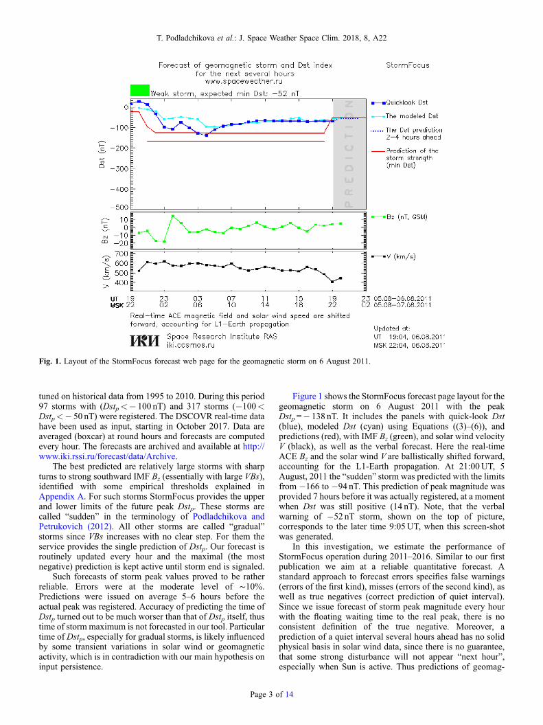
Fig. 1. Layout of the StormFocus forecast web page for the geomagnetic storm on 6 August 2011.

T. Podladchikova et al.: J. Space Weather Space Clim. 2018, 8, A22

tuned on historical data from 1995 to 2010. During this period97 storms with (Dstp<� 100 nT) and 317 storms (�100<Dstp<� 50 nT) were registered. The DSCOVR real-time datahave been used as input, starting in October 2017. Data areaveraged (boxcar) at round hours and forecasts are computedevery hour. The forecasts are archived and available at http://www.iki.rssi.ru/forecast/data/Archive.

The best predicted are relatively large storms with sharpturns to strong southward IMF Bz (essentially with large VBs),identified with some empirical thresholds explained inAppendix A. For such storms StormFocus provides the upperand lower limits of the future peak Dstp. These storms arecalled “sudden” in the terminology of Podladchikova andPetrukovich (2012). All other storms are called “gradual”storms since VBs increases with no clear step. For them theservice provides the single prediction of Dstp. Our forecast isroutinely updated every hour and the maximal (the mostnegative) prediction is kept active until storm end is signaled.

Such forecasts of storm peak values proved to be ratherreliable. Errors were at the moderate level of ∼10%.Predictions were issued on average 5–6 hours before theactual peak was registered. Accuracy of predicting the time ofDstp turned out to be much worser than that of Dstp itself, thustime of storm maximum is not forecasted in our tool. Particulartime of Dstp, especially for gradual storms, is likely influencedby some transient variations in solar wind or geomagneticactivity, which is in contradiction with our main hypothesis oninput persistence.

Page 3 o

Figure 1 shows the StormFocus forecast page layout for thegeomagnetic storm on 6 August 2011 with the peakDstp=� 138 nT. It includes the panels with quick-look Dst(blue), modeled Dst (cyan) using Equations ((3)–(6)), andpredictions (red), with IMF Bz (green), and solar wind velocityV (black), as well as the verbal forecast. Here the real-timeACE Bz and the solar wind V are ballistically shifted forward,accounting for the L1-Earth propagation. At 21:00UT, 5August, 2011 the “sudden” storm was predicted with the limitsfrom �166 to �94 nT. This prediction of peak magnitude wasprovided 7 hours before it was actually registered, at a momentwhen Dst was still positive (14 nT). Note, that the verbalwarning of �52 nT storm, shown on the top of picture,corresponds to the later time 9:05UT, when this screen-shotwas generated.

In this investigation, we estimate the performance ofStormFocus operation during 2011–2016. Similar to our firstpublication we aim at a reliable quantitative forecast. Astandard approach to forecast errors specifies false warnings(errors of the first kind), misses (errors of the second kind), aswell as true negatives (correct prediction of quiet interval).Since we issue forecast of storm peak magnitude every hourwith the floating waiting time to the real peak, there is noconsistent definition of the true negative. Moreover, aprediction of a quiet interval several hours ahead has no solidphysical basis in solar wind data, since there is no guarantee,that some strong disturbance will not appear “next hour”,especially when Sun is active. Thus predictions of geomag-

f 14

T. Podladchikova et al.: J. Space Weather Space Clim. 2018, 8, A22

netically quiet intervals (though it may be of interest to someapplications) are not a part of our forecast. We aim to predictonly storms with Dst<� 50 nT.

In our scheme true misses are very unlikely, since L1spacecraft is a reliable upstream monitor and no storms occurwithout corresponding interplanetary disturbance. However, insome cases the first satisfactory forecast could be issued ratherlate, well inside the developing storm. Our prime goal was tominimize false warnings (predictions of too large storms).

During quality checks we first identify all storms (below50 nT) and their Dstp. Then we search for the earliest correct(within 25%) forecast before each observed peak. If allforecasts (before actual Dstp) are more than 25% weaker (lessnegative) than Dstp, the storm is considered as missed (thoughthe forecast still may reach “correct” amplitude later than theactualDstpwas observed). If there is no correct forecast beforethe actual peak, but there is prediction 25% stronger (morenegative) than the peakDstp, the storm amplitude is consideredoverestimated (false warning). To check the usefulness of theforecast we also determine the advance time, when thesuccessful forecast was issued (relative to actualDstp), andDstvalues at the moment of forecasts.

One more characteristic is the maximal prediction issuedwithin a storm. The third variant of an error is identified, whenthis maximal prediction happens after the first correct forecastand overestimates trueDstp bymore than 25%. This is called inthe following “overestimated maximum prediction”.

We verify the general prediction accuracy in three variantswith respect to the used data. The first variant is “truecomparison” of the forecast (using ACE real-time solar wind,IMF and previous quicklook Dst) with the storm magnitude asmeasured by quicklookDstp. However, from a point of view ofa general user, it might be more correct to compare the forecastwith actual (final) Dst. This is the second variant of ourcomparison. For the third variant we rerun the algorithm usingfinal solar wind, IMF and Dst from OMNI and compare withthe storm magnitude as measured with final (or provisional)Dstp. This latter approach is also known as reanalysis.

For the ACE real-time solar wind, IMF and quicklook Dstdata we use our own archive for 2011–2016, which was filledin the course of operation. Final solar wind and IMF data aretaken from OMNI dataset (shifted and merged data) as well asfrom CDAWeb for individual ACE and Wind spacecraft (notshifted original data). The final Dst is available only before2011, thus for the later time we use provisional Dst (see alsodiscussion in Sect. 4). In the latter text (if not explicitly statedoppositely) we use the term “final” to characterize OMNI solarwind and provisional or final Dst as opposed to the real-timedata.

3 Forecast statistics

In this section, we present the statistics of the forecastquality over the period of StormFocus operation July 2011–December 2016, as well as the reanalysis using the final data.The Dstp of relatively large “sudden” storms with thesufficiently sharp increase of VBs (see criteria inAppendix A (A.10) and (A.11) is forecasted with the lowerand upper magnitude limits. During the test period the suddenstorm criteria in real-time were activated only for 10 storms.

Page 4 o

However with the final data reanalysis there were 23 “sudden”storms. These storms were weaker than that for 1995–2010 (53storms) used by Podladchikova and Petrukovich (2012) todesign the prediction algorithms. Over the last 5 years, onlythree storms were below �150 nT, while for 1995–2000, 50%of such storms were with peak Dstp<� 150 nT. The “sudden”storm forecast works best for larger storms, so the conditionsduring last five years were not favorable in this sense.

Figure 2a shows the forecast statistics for 23 “sudden”geomagnetic storms (as determined in final data). We usereal-time data input compared with the final geomagneticindex, and storms are ordered by the final Dstp (black line).The bars in Figure 2a show the forecast for 10 events, forwhich the “sudden” criterion was “on” in real-time, and bothupper and lower forecast limits were calculated. Theremaining 13 storms (marked by single points) werecharacterized as “gradual” in real-time, for which onlyone-point forecast (Appendix A) was produced. The red barand red point indicate unsuccessful forecasts for two events.Thus, StormFocus service issued a successful forecast usingthe real-time input data for 21 storms, though in 9 cases itwas provided with two limits and in 12 cases � with a singlepoint. Storm forecasts were produced when the Dst indexwas on average weaker by 75% than the final Dstp, and insome cases the warnings were issued, when Dst index waspositive (not shown here). The advance time of the real-timeforecasts was 1–20 hours with the average value of about 7hours (Fig. 2c).

Figure 2b shows the results of reanalysis on final data for23 geomagnetic storms. The blue bars show the successfulforecast of upper and lower limits of Dstp (black solid line)based on final OMNI data for 22 storms. The only red bar givesunsuccessful “overestimate” forecast, which was more than25% stronger (more negative) than actual Dstp. Note, that thisforecast was still produced in advance, and the storm was infact detected, though the strength was overestimated. To checkthe usefulness of forecast we also determined the final Dstindex at the issue time ofDstp forecast. On average it is weakerby 84% than the final peak Dstp.

Storms with no “sudden” criterion are categorized asgradual and their magnitude Dstp is predicted with the singlenumber based on the three-hour forecast Dst (Appendix A).Five “gradual” storms had Dstp<�100 nT and 92 storms had�100<Dstp<� 50 nT. The classification of storms is madeusing more reliable final Dst. Additionally, 33 storms had real-time Dstp<� 50 nT, but final Dstp>� 50 nT. These stormswere also included to the forecast statistics.

Figure 3 presents the statistics of gradual storms relativeto final Dstp. With the real-time forecast, the earliest“successful” prediction (blue line in Fig. 3a) of final Dstp(black line) was produced for 109 out of 130 cases. Theoutliers are marked with red points, including 10 “over-estimated” events, and 11 missed predictions. Cyan lineshows the maximal predictions issued later within a storm.The number of overestimated maximal predictions was 37(red points). Note that for these events the earliest forecastwas successful. Mainly small storms were overestimated,when errors of a baseline are relatively more important. Thestorm forecasts were produced when the Dst index was onaverage weaker by 57% than the final Dstp, confirmingthe usefulness of prediction service. The advance time of the

f 14

Fig. 2. Forecast statistics for “sudden” geomagnetic storms. (a) Storm predictions using real-time data input. (1) final Dstp; (2) the earliestprediction of both upper and lower limits of Dstp within 25% of actual storm magnitude; (3) the earliest prediction of Dstp with 3-hour forecast(not “sudden” in real-time); (4) and (5) the predictions of Dstp, which were out of 25% range from actual Dstp. (b) Storm predictions using finaldata input. (6) final Dstp; (7) the earliest prediction of both upper and lower limits of Dstp within 25% of actual storm magnitude; (8) thepredictions of Dstp, which were out of 25% range from actual storm magnitude. (c) The advance warning time (in hours) of the Dstp forecastusing real-time input.

T. Podladchikova et al.: J. Space Weather Space Clim. 2018, 8, A22

real-time forecasts was 1–20 hours with the average value ofabout 8 hours (Fig. 3c).

With the reanalysis using final OMNI data (Fig. 3b), 126out of 130 storms were successfully predicted. The blue linegives the earliest prediction, which is in 25% range from finalDstp. The red points show unsuccessful missed forecast at fourevents. Cyan line shows the maximal predictions of Dstpissued later within a storm. The number of overestimatedmaximal predictions with the final data is about a half of thatwith real-time input (in comparison with Fig. 3a)—just 21storms.Dst at the issue time of forecast was on average weakerby 54% than the final OMNI Dstp.

Table 1 summarizes the forecast statistics. It includes thethree variants of the forecast run: real-timeDstp prediction usingreal-time input (“RR”), final Dstp prediction using final input(“FF”), final Dstp prediction using real-time input (“RF”).“Successful forecast” gives the number of storms with theearliest forecast of peak Dstp within 25% of the actual stormmagnitude. “Overestimate” and “missed” represent the numberof unsuccessful forecasts. “Overestimated maximal prediction”shows the number of overestimating forecasts issued laterwithin a storm (when the earliest forecast was successful).

Page 5 o

As it is clear from Table 1, over the test period ourprediction algorithm performed best for the reanalysis (finalinput compared with final Dstp), providing 148 successfulpredictions of Dstp out of 153 storms. Real-time forecastcompared with final Dstp resulted in 130 successes. Real-timeforecast compared with real-time quicklook Dstp had 129successes. Thus the usage of real-time input IMF, solar wind,and Dst decreased the quality of the earliest forecasts for 21storms as compared with the final input.

In addition there were events with overestimation ofmaximal predictions issued later within a storm (when theearliest forecast is successful). The worst quality with respect tothis criterion has the real-time forecast as compared with finalindex (RF variant). The number of errors was almost twicelarger than for RR variant, and almost four times larger than forFF variant (42 compared with 24 and 11). The most of errorswere for smaller storms (left side of Fig. 3).Most likely the mainreason is the baseline difference between real-time and finalDst.In the RF-variant the forecast is computed with the real-timequicklook Dst index, while comparison is with final Dst.

All possible outcomes for the forecasts of Dstp can bedescribed by the number of hits (successful forecast), misses,

f 14

Fig. 3. Forecast statistics for “gradual” geomagnetic storms. (a) Storm predictions using real-time data input. (1) final Dstp; (2) the earliestprediction of Dstp within 25% of actual storm magnitude; (3) the predictions of Dstp, which were out of 25% range; (4) maximal predictions ofDstp obtained during the storm development; (5) maximal predictions out of 25% range. (b) Storm predictions using final data input. (6) finalDstp; (7) the earliest prediction of Dstp within 25%; (8) the predictions of Dstp, which were out of 25% range; (9) maximal predictions of Dstpobtained during the storm development; (10) maximal predictions out of 25% range. (c) The advance warning time (in hours) of theDstp forecastusing real-time input.

Table 1. Forecast statistics for: “RR”� real-time quicklookDstp prediction using real-time input; “FF”� finalDstp prediction using final input;“RF” � final Dstp prediction using real-time input.

Numberof storms

Successfulforecast

Overestimated Missed Overestimatedmaximalprediction

RR FF RF RR FF RF RR FF RF RR FF RFSudden stormsSharp increase of VBs 23 21 22 21 1 1 1 1–1 2 3 5

Gradual stormsDstp�� 100 nT 5 3 5 5 1 � � 1 � � – 1 1

Gradual storms�100<Dstp<� 50 nT 92 78 88 81 2 � 2 12 4 9 7 10 22

Gradual stormsFinal Dstp>� 50 nT, Quicklook Dstp<� 50 nT 33 27 33 23 1 � 6 5 � 4 2 10 14

Total 153 129 148 130 5 1 9 19 4 14 11 24 42

Page 6 of 14

T. Podladchikova et al.: J. Space Weather Space Clim. 2018, 8, A22

Table 2. The probability of detection (POD) and the ratio of overestimated forecasts (ROF) of the earliest and maximal forecasts for the threetypes of the forecast run: “RR”� real-time quicklookDstp prediction using real-time input; “FF”� finalDstp prediction using final input; “RF”� final Dstp prediction using real-time input.

RR FF RF

POD129

129þ19 ¼ 0:87 148148þ4 ¼ 0:97 130

130þ14 ¼ 0:9

ROF earliest forecast 5129þ5 ¼ 0:04 1

148þ1 ¼ 0:007 9130þ9 ¼ 0:06

ROF maximal forecast 11129þ11 ¼ 0:08 24

148þ24 ¼ 0:14 42130þ42 ¼ 0:24

Fig. 4. The deviation of hourly averaged final data (OMNI) fromhourly averaged real-time data for disturbed periods Dst<� 50 nTover the period of July 2011–December 2016. (a) Dst index (nT). (b)Southward IMF Bz (nT). (c) Solar wind velocity V (km/s). (d) Solarwind density N (cm�3).

T. Podladchikova et al.: J. Space Weather Space Clim. 2018, 8, A22

and false alarms. We can calculate the following verificationmeasures such as the probability of detection (POD) and theratio of overestimated forecasts (ROF) (Tab. 2).

POD ¼ hits

hits þ misses; ð1Þ

ROF ¼ overestimated forecasts

hitsþ overestimated forecasts: ð2Þ

The highest probability of detection (0.97) and the lowest ratioof overestimated forecast (0.007) is for FF reanalysis variant.The probability of detection decreased to 0.87 and the ratio ofoverestimated forecast increased to 0.04 for the real-timequicklook Dstp prediction using real-time input (RR). Thenumbers for RF variant remain similar to that for RR.Overestimates of the maximal forecast after successfulwarning are at the level of 24% for RF variant and about10% for RR and RF variants.

Among errors in Table 1, there were in total 49 storms withsome forecast errors in real-time and correct forecast with finaldata. These 49 errors can be definitely ascribed to real-timedata errors. In the next section we analyze in detail the reasonsof these differences.

Page 7 o

4 Analysis of reasons for the decrease ofthe forecast quality using real-time input

Forecasting services use data available in real-time, whichcan be substantially different from the final calibrated dataappearing later in the scientific archives. However, the forecastalgorithms of Dst are designed using the final data. Theforecast errors due to this factor are often overlooked, but canbe equally important as those due to an algorithm imperfection.Our analysis in Section 3 shows that the number of the forecasterrors is indeed much smaller if the final quality data are used.In this section we analyze specific sources of our forecasterrors and the differences between real-time and final data ingeneral.

Figure 4 shows the difference between the hourly averagedfinal data and real-time ACE and Dst values for the disturbedperiods Dst<� 50 nT over July 2011–December 2016st indexis mostly overestimated, as quick-look index available in real-time is smaller than the provisionalDst (67% of points) and formore than half of cases the difference exceeds 10 nT (Fig. 4a).This effect is responsible for the half of events under analysis(28 out of 49, Tab. 3, detailed description is below).

It should be noted additionally that quicklookDst is usuallyupdated approximately half an hour after the first appearance.We do not have in hand the statistics of this change. Severalyears later provisional Dst is replaced by final Dst, and thescatter between these two index types is a factor of 2–3 smaller,than that for the real-time—provisional pair. Also, the finalDstis on average again weaker (more positive) than the provisionalindex by few nT.

Figure 5 shows the specific example of the forecast errordue to the difference between quicklook and provisionalDst. Panel (a) gives the provisional Dst and prediction of itspeak Dstp using final input, as well as the same pair for thereal-time data. Panel (b) shows IMF Bz from ACE real-time,final OMNI, final ACE, and final Wind. Final OMNI solarwind speed V and ACE real-time V are in panel (c). Panel (d)has the final OMNI driving parameter VBs and ACE real-time VBs.

According to real-time data the storm reached the peakDstp of �107 nT at 6:00 UT on 27 August 2015, howeverthe provisional Dst peak was significantly weaker reachingonly �77 nT. The first “successful” real-time forecast(�81 nT) of Dstp was issued 4 hours in advance. Themaximal prediction of Dstp issued later in real-time withinthe storm reached �102 nT, producing more accurateprediction of quicklook Dstp. However it was 32% stronger(more negative) than the actual storm strength determinedby final Dstp. The primary computational reason for this

f 14

Table 3. The summary of reasons for the decrease of forecast quality using real-time input.

Quality decrease forthe earliest forecastin 21 storms

Overestimatedmaximal predictionin 28 storms

In total, the decreaseof forecast qualityin 49 storms

Overestimated for 10 storms Missed for 11 stormsDst verestimated 6 – 22 28VBs overestimated 2 – 2 4Dst and VBs overestimated 2 – 4 6

ACE failureVBs underestimated – 6 – 6VBs underestimated – 4 – 4Dst underestimated – 1 – 1

Fig. 5. The geomagnetic storm on 26–28 August 2015. (a) Provisional Dst (dashed blue); predictions of the peak Dstp using final OMNI input(solid blue); real-time quicklook Dst (dashed cyan); predictions of real-time Dstp using real-time input (solid cyan). (b) Final OMNI IMF Bz

(blue); ACE real-time IMF Bz (cyan); Final ACE IMF Bz (level 2, black); Wind Bz (not shifted original data, red). (c) Final OMNI solar windspeed V (cyan); ACE real-time solar wind speed V (blue). (d) Final OMNI parameter VBs (cyan); ACE real-time parameter VBs (blue).

T. Podladchikova et al.: J. Space Weather Space Clim. 2018, 8, A22

overestimate was the large difference of about 20 nTbetween real-time and provisional Dst (the current real-timequicklook Dst index is used in forecast as initial condition).This storm has three clear intensifications. The two otherwere at 21:00UT on 26 August and 21:00–23:00UT on27 August, and they were well predicted, since, in

Page 8 o

particular, the difference between quicklook and provision-al Dst was small. At 7:00 UT on 27 August 2015, there werealso significant differences in VBs between OMNI andindividual satellites (Fig. 5b), but the accuracy ofprediction was not affected as it happened one hour afterthe storm peak.

f 14

Fig. 6. The same as Figure 5 except for the geomagnetic storm on 1–2 November 2011.

T. Podladchikova et al.: J. Space Weather Space Clim. 2018, 8, A22

The deviations between final OMNI and ACE real-time Bz

were greater than 4 nT in 9% of cases (Fig. 4b), and thedifference between final OMNI and ACE real-time solar windspeed was less than 50 km/s in 97% of cases (Fig. 4c). TheACE real-time solar wind density N was mainly under-estimated compared to the final OMNI (87% of cases) and thedifference was greater than 5 cm�3 nT in 17% of cases(Fig. 4d). Thus Bz differences could be much more importantthan the solar wind speed differences. The density errors inreal-time are also large. However, in our model we do not usedensity as input, since these errors could overweight theadvantages of the Dst models, accounting for Chapman-Ferraro currents.

IMF and solar wind speed differences can come from theseveral sources: (1) errors of real-time data, corrected later inthe final variant; (2) gaps in real-time data (filled with theprevious values during forecast); (3) peculiarities ofaveraging/projection to the bow shock nose in OMNI andreal-time algorithms; (4) actual differences between measure-ments of ACE and Wind spacecraft (over the test periodOMNI dataset is filled with 97% of Wind data and only 3% ofACE data).

Figure 6 shows the example of forecast of the geomagneticstorm on 1–2 November 2011 with the error in ACE real-timedata. At 16:00UT on 1 November 2011 the storm reached thepeak Dstp of�66 nT according to the provisional Dst. The first“successful” forecast was issued 6 hours in advance. Within

Page 9 o

this storm the ACE real-time Bz was around �10 nT for threehours 15:00–17:00UT, while Bz from final ACE, Wind, andOMNI were significantly greater (around �2 nT). Thus thereal-time forecast provided the wrong warning at thisintensification.

Figure 7 shows the example of “successful” forecast on 11September 2011, using the real-time input, while the forecastwith the final OMNI input failed. At 21:00UT final OMNI Bz

and Wind Bz (used in OMNI for this storm) were positivearound 3 nT, while the ACE real-time and final ACE Bz

reached the negative value of around �7 nT. The earliest“successful” forecast of final peak Dstp was issued 3 hours inadvance in case of real-time input data and no warning wasissued for the final data variant. Dst intensification wasdefinitely more consistent with the ACE observation. Windspacecraft for years 2011–2016 was in L1 halo orbit with theradius up to 600 000 km, about twice larger than that for ACE(Fig. 8), thus using Wind might be less appropriate for theforecast training.

Relatively ubiquitous were single-point (for the houraveraging) discrepancies between ACE real-time and finalOMNI data. They could be caused by relatively short-durationreal-time errors or differences between spacecraft as well as byspecifics of time-shifts and averaging. In terms of forecastquality such single-point discrepancies were mostly importantfor the qualification of the “sudden” storms with sharp increaseof VBs.

f 14

Fig. 7. The same as Figure 5 except for the geomagnetic storm on 11 September 2011.

Fig. 8. Position of ACE (blue) and Wind (red) in 2011.

T. Podladchikova et al.: J. Space Weather Space Clim. 2018, 8, A22

Table 3 summarizes the reasons for the decrease of forecastquality for 49 storms, for which the real-time forecast of Dstpfailed, but the forecast of Dstp with the final data wassuccessful. This number includes 21 storms for which the real-time earliest forecast of Dstp failed, and 28 storms for whichmaximal predictions ofDstp issued later were overestimated incase of real-time input. These 49 forecast failures can bedefinitely ascribed to the errors in the real-time data relative tothe final input. Besides that there were 18 events with the errorsin both the real-time forecast of Dstp and reanalysis with thefinal data and 7 events with the errors only in the runs with thefinal data. These two latter types of errors may originate fromvariety of sources and are not analyzed here.

Page 10

The main reason of errors (more than half, 28 out of 49)was overestimation of Dst index in real-time. On averagequicklook Dst is stronger (more negative) than theprovisional index. In all cases it caused an overestimatedforecast. The opposite situation happened only once, onemissed forecast was due to Dst underestimation in real-time.Four errors with the overestimated forecast were due to VBsoverestimation in real-time, while six such errors were due toboth Dst and VBs overestimation. Four errors with the missedstorms were related with VBs underestimate in real-time.Finally six errors with missed storms were related with ACEdata absence in real-time at the moment of the storm onset. Insuch a case, the forecast algorithm uses previous (pre-storm)

of 14

T. Podladchikova et al.: J. Space Weather Space Clim. 2018, 8, A22

values of solar wind and IMF, which results in underestimateof VBs.

5 Conclusion

In this study, we review performance of the geomagneticstorm forecasting service StormFocus at SpaceWeather.Ruduring more than 5 years of operation from July 2011 toDecember 2016. The service provides the warnings on theexpected geomagnetic storm magnitude for the next severalhours on an hourly basis. The maximum of the solar cycle 24was weak, so the most of statistics were rather moderatestorms. We verify the quality of forecasts and selection criteria,as well as the reliability of online input data to predict thegeomagnetic storm strength in comparison with the finalvalues available in archives. We also analyze the sources ofprediction errors and identified the errors that cannot beremoved in real-time and those that can be fixed by improvingthe prediction algorithm.

StormFocus service on the basis of ACE real-time andquicklook Dst data issued the successful forecast of peak Dstp(within 25% of the actual storm magnitude) for 129 out of 153geomagnetic storms with the detection probability of 0.87. Thealgorithm rerun on final OMNI data provided the successfulforecast for 148 storms with the detection probability of 0.97.An important measure of the practical usefulness of the real-time forecast is the prediction of the actual final Dstp using thereal-time input. It was successful for 130 storms with thedetection probability of 0.9. Therefore we confirmed thegeneral reliability of the StormFocus service to provide theadvance warnings of geomagnetic storm strength over theperiod 2011–2016.

Several error sources require special attention. First of all,forecast in real-time operation is somewhat less reliable, thanon the final archived data due to errors or imperfections of thereal-time input, both solar wind, IMF and Dst. Such reasonsaccounted for more than a half of all forecast errors. Inparticular such reasons most likely explain a strong increase ofa number of later overestimates (after successful forecast wasgiven) from ∼10% to 24%, when the real-time data arecompared with the final index.

Real-time errors are often overlooked during performanceanalysis, since they are nominally beyond control during analgorithm design. One can advise to verify the forecast qualityadditionally on the real-time data streams if available.Statistics on expected differences between real-time and finaldata would be also very helpful. Alternatively one may use theforecast models with the probabilistic output (providing therange of possible values with some degree of certainty),however such models require much larger data amounts fortraining.

The second substantial error was related with thegeneration of the “sudden” storm warning, based on a sharpincrease of VBs. In real-time about a half of the “sudden”storms were missed and several false warnings were generated.The primary reason was again related with the differencesbetween real-time and final data. To remediate such errors weadditionally introduced in the algorithm a condition, cancelingthe warning in a case it was caused by a single-point peak inVBs. However, it should be noted, that the sudden storm variant

Page 11

of the forecast was designed to warn on very strong storms (asit was during period 1995–2010, used for the design). Strongerstorms are usually related with more stable solar wind and IMFinput and develop faster, thus extrapolations in our forecast aremore reliable. During the test period the storms were muchweaker on average, practically all “sudden” storms wereweaker (less negative) than �150 nT. For such events“sudden” storm warnings are expected to be less reliable.

In conclusion, the geomagnetic storm forecasting serviceStormFocus that provides the warnings of future geomagneticstorm magnitude proved to be quite successful after more thanfive years of online operation and can be recommended forapplications. A few of the most registered forecast failureswere caused by the errors in the real-time input data (relative tofinal data, appearing later). This source of errors needs specialattention during the forecast algorithm design.

Acknowledgements. The authors are grateful to the NationalSpace Science Data Center for the OMNI 2 database, to theNational Oceanic and Atmospheric Administration (NOAA)for ACE real-time solar wind (RTSW) data, to the WDC forGeomagnetism (Kyoto) for the Dst index data. We thank thereferee for valuable comments on this study. The work wassupported by Russian Science Foundation, N16-12-10062. Theeditor thanks two anonymous referees for their assistance inevaluating this paper.

References

Akasofu SI. 1981. Prediction of development of geomagnetic stormsusing the solar wind-magnetosphere energy coupling functionepsilon. Planet Space Sci 29: 1151–1158.

Amata E, Pallocchia G, Consolini G, Marcucci MF, Bertello I. 2008.Comparison between three algorithms for Dst predictions over the2003–2005 period. J Atmos Solar-Terr Phys 70: 496–502.

Andriyas T, Andriyas S. 2015. Relevance vector machines as a toolfor forecasting geomagnetic storms during years 1996–2007. JAtmos Solar-Terr Phys 125: 10–20.

Bala R, Reiff P. 2012. Improvements in short-term forecasting ofgeomagnetic activity. Space Weather 10: S06001.

Boynton RJ, Balikhin MA, Billings SA, Amariutei OA. 2013.Application of nonlinear autoregressive moving average exoge-nous input models to geospace: advances in understanding andspace weather forecasts. Ann Geophys 31: 1579–1589.

Boynton RJ, Balikhin MA, Billings SA, Sharma AS, Amariutei OA.2011. Data derived NARMAX Dst model. Ann Geophys 29: 965–971.

Burton RK, McPherron RL, Russell CT. 1975. An empiricalrelationship between interplanetary conditions and Dst. J GeophysRes 80: 4204–4214.

Caswell JM. 2014. A nonlinear autoregressive approach to statisticalprediction of disturbance storm time geomagnetic fluctuationsusing solar data. J Signal Inf Process 5: 42–53.

Chen J, Slinker SP, Triandaf I. 2012. Bayesian prediction ofgeomagnetic storms: wind data, 1996–2010. Space Weather 10:S04005.

Echer E, Gonzalez WD, Tsurutani BT, Gonzalez ALC. 2008.Interplanetary conditions causing intense geomagnetic storms(Dst�� 100 nT) during solar cycle 23. J Geophys Res 113:A05221.

Echer E, Tsurutani BT, Gonzalez WD. 2013. Interplanetary origins ofmoderate (100 nT<Dst�� 50 nT) geomagnetic storms during

of 14

T. Podladchikova et al.: J. Space Weather Space Clim. 2018, 8, A22

solar cycle 23 (1996-2008). J Geophys Res: Space Phys 118: 385–392.

Gonzalez WD, Echer E. 2005. A study on the peak Dst and peaknegative Bz relationship during intense geomagnetic storms. Geo-phys Res Lett 32: L18103.

Gonzalez WD, Joselyn JA, Kamide Y, Kroehl HW, Rostoker G,Tsurutani BT, Vasyliunas VM. 1994.What is a geomagnetic storm?J Geophys Res 99: 5771–5792.

Ji EY, Moon YJ, Gopalswamy N, Lee DH. 2012. Comparison of Dstforecast models for intense geomagnetic storms. J Geophys Res(Space Phys) 117: A03209.

Kane RP, Echer E. 2007. Phase shift (time) between storm-timemaximum negative excursions of geomagnetic disturbance indexDst and interplanetary Bz. J Atmos Sol Terr Phys 69: 1009–1020.

Katus RM, LiemohnMW, Ionides EL, Ilie R,Welling D, Sarno-SmithLK. 2015. Statistical analysis of the geomagnetic response todifferent solar wind drivers and the dependence on storm intensity.J Geophys Res: Space Phys 120: 310–327.

Lundstedt H, Gleisner H,Wintoft P. 2002. Operational forecasts of thegeomagnetic Dst index. Geophys Res Lett 29: 2181.

Mansilla GA. 2008. Solar wind and IMF parameters associated withgeomagnetic storms with Dst ��50 nT. Phys Scr 78: 045902.

Nikolaeva NS, Yermolaev YI, Lodkina IG. 2014. Dependence ofgeomagnetic activity during magnetic storms on the solar windparameters for different types of streams: 4. Simulation formagnetic clouds. Geomagn Aeron 54: 152–161.

O'Brien TP,McPherron RL. 2000a. An empirical phase space analysisof ring current dynamics: solar wind control of injection and decay.J Geophys Res 105: 7707–7720.

O'Brien TP, McPherron RL. 2000b. Forecasting the ring current indexDst in real time. J Atmos Sol Terr Phys 62: 1295–1299.

Pallocchia G, Amata E, Consolini G, Marcucci MF, Bertello I. 2006.Geomagnetic Dst index forecast based on IMF data only. AnnGeophys 24: 989–999.

Petrukovich AA, Klimov SI. 2000. The use of solar wind measure-ments for the analysis and prediction of geomagnetic activity.CosmRes 38: 433.

Petrukovich AA, Klimov SI, Lazarus A, Lepping RP. 2001.Comparison of the solar wind energy input to the magnetospheremeasured by Wind and Interball-1. J Atmos Solar-Terr Phys 63:1643–1647.

Podladchikova TV, Petrukovich AA. 2012. Extended geomagneticstorm forecast ahead of available solar wind measurements. SpaceWeather 10: S07001.

Rastätter L, Kuznetsova MM, Glocer A, Welling D, Meng X et al.2013. Geospace environment modeling 2008-2009 challenge: Dstindex. Space Weather 11: 187–205.

Page 12

Rathore BS, Dinesh CG, Parashar KK. 2014. A nonlinearautoregressive approach to statistical prediction of disturbancestorm time geomagnetic fluctuations using solar data. J Signal InfProcess 5: 42–53.

Revallo M, Valach F, Hejda P, Bochníček J. 2014. A neural networkDst index model driven by input time histories of the solar wind-magnetosphere interaction. J Atmos Sol-Terr Phys 110: 9–14.

Sharifie J, Lucas C, Araabi B. 2006. Locally linear neurofuzzymodeling and prediction of geomagnetic disturbances based onsolar wind conditions. Space Weather 4: S06003.

Siscoe G, McPherron RL, Liemohn MW, Ridley AJ, Lu G. 2005.Reconciling prediction algorithms for Dst. J Geophys Res 110:A02215.

Temerin M, Li X. 2002. A new model for the prediction of Dst on thebasis of the solar wind. J Geophys Res 107: 1472.

Temerin M, Li X. 2006. Dst model for 1995–2002. J Geophys Res111: A04221.

Valdivia JA, SharmaAS, Papadopoulos K. 1996. Prediction of magneticstorms by nonlinear models. Geophys Res Lett 23: 2899–2902.

Vassiliadis D, Klimas A, Baker D. 1999. Models of Dst geomagneticactivity and of its coupling to solar wind parameters. Phys ChemEarth 24: 107–112.

Wei HL, Billings SA, Balikhin M. 2004. Prediction of the Dst indexusing multiresolution wavelet models. J Geophys Res 109:A07212.

Wing S, Johnson JR, Jen J, Meng CI, Sibeck DG, Bechtold K,Freeman J, Costello K, BalikhinM, Takahashi K. 2005. Kp forecastmodels. J Geophys Res (Space Phys) 110: A04203.

Wu JG, Lundstedt H. 1997. Geomagnetic storm predictions fromsolar wind data with the use of dynamic neural networks. JGeophys Res 102: 14255–14268.

Yermolaev YI, Nikolaeva NS, Lodkina IG, Yermolaev MY. 2010.Specific interplanetary conditions for CIR-, Sheath-, and ICME-induced geomagnetic storms obtained by double superposed epochanalysis. Ann Geophys 28: 2177–2186.

Yermolaev YI, Yermolaev MY. 2002. Statistical relationshipsbetween solar, interplanetary, and geomagnetospheric disturban-ces, 1976–2000. Cosm Res 40: 1–14.

Yermolaev YI, Yermolaev MY, Zastenker GN, Zelenyi LM,Petrukovich AA, Sauvaud JA. 2005. Statistical studies ofgeomagnetic storm dependencies on solar and interplanetaryevents: a review. Planet Space Sci 53: 189–186.

Zhu D, Billings SA, Balikhin M, Wing S, Coca D. 2006. Data derivedcontinuous time model for the Dst dynamics. Geophys Res Lett 33:L04101.

Zhu D, Billings SA, Balikhin MA, Wing S, Alleyne H. 2007. Multi-input data derived Dst model. Geophys Res Lett 112: A06205.

Cite this article as: Podladchikova T, Petrukovich A, Yermolaev Y. 2018. Geomagnetic storm forecasting service StormFocus: 5 yearsonline. J. Space Weather Space Clim. 8: A22

of 14

T. Podladchikova et al.: J. Space Weather Space Clim. 2018, 8, A22

Appendices

Appendix A : The prediction of stormstrength

The prediction technique of the peak Dstp duringgeomagnetic storms is based on the differential equation ofthe Dst index evolution introduced by Burton et al. (1975) as afunctional relation between solar wind and Dst.

dDst�

dt¼ QðtÞ � Dst�

tðtÞ : ðA:1Þ

Here Q (mV/m) is the solar wind input function. We use themodel variant by O'Brien and McPherron (2000b), where theparameter Q is linearly connected with the driving parameterVBs.

QðtÞ ¼ �4:4ðVBs� 0:5Þ tðtÞ ¼ 2:4e9:74

4:69þVBs; ðA:2Þ

VBs ¼ jVBzj; Bz < 0;0; Bz ≥ 0:

�ðA:3Þ

Dst� ¼ Dst � 7:26ffiffiffiffiffiffiffiffiffiPdyn

p þ 11: ðA:4Þ

Here V (km/s) is solar wind plasma speed, Bs (nT) is southwardcomponent of IMF in GSM, Pdyn (nPa) is solar wind dynamicpressure, and t (hours) is decay time constant, associated withthe loss processes in the inner magnetosphere. Dst* is thepressure corrected Dst index, from which the effects of themagnetopause currents have been removed. However, weneglect the difference between Dst and Dst*, and do notcompute this pressure correction, because generally it is rathersmall, and often real-time solar wind density is quite differentfrom the calibrated data, appearing later in the archives.

To predict future strength of a storm we use the solution ofthe differential Equation (A.1) with an initial condition (solarwind, IMF and quick-look Dst) taken at some “zero” momentand assuming stationary solar wind input, equal to that at theinitial point (hereafter Q0, t0).

DstðtÞ ¼ e� tt0 ⋅ðDstð0Þ � Q0⋅t0Þ þ Q0⋅t0: ðA:5Þ

This solution is the monotonously decreasing function of time,and when t!∞, it approaches the steady-state value.

We compute two variants of the forecast Dst. The stormsaturation level reached at the steady-state solution is used as aprediction of the lower limit of peak Dstp.

Dstð∞Þ ¼ limt∞!

DstðtÞ ¼ Q0⋅t0: ðA:6Þ

To predict the upper limit we select the intermediate point onthe saturation trajectory determined by the solution of thediscrete variant of Equation (A.1) given by

Page 13

Dstðk þ 1Þ ¼ DstðkÞ � 1

tðkÞDstðkÞ þ QðkÞ: ðA:7Þ

The solution of this equation k hours ahead for constant Q andt is

Dstðk þ 1Þ ¼ 1� 1

t0

� �kþ1

Dstð0Þ þ Q0

Xki¼0

1� 1

t0

� �i

: ðA:8Þ

As the upper limit we use the three-hours-ahead extrapolation,which was justified by the statistics.

D̂stðþ3Þ ¼ 1� 1

t0

� �3

Dstð0Þ þX2i¼0

1� 1

t0

� �i

Q0: ðA:9Þ

D̂stðþ3Þ is computed routinely every hour, and to avoid itsexcessive variability the final prediction Dst is kept at theminimum of all D̂stðþ3Þ obtained after the last “storm end”flag. The “storm end” is signaled and Dst returns to the currentD̂stðþ3Þ, when IMF Bz≥ 1 nT during 3 hours or IMFBz≥� 1.8 nT during 11 hours.

The prediction of both upper and lower limits, Dst and Dst(∞), of the peak Dstp is proved to be useful only for a group oflarger “sudden” storms, associated with a sufficiently sharpincrease of VBs. All other storms are then called gradual.

We introduced the following criteria for the sharp increaseof VBs: I(k) =VBs(k)�VBs(k� 1):

IðkÞ > 4:4 andXkj¼k�2

Ij > 5:7; ðA:10Þ

VBsðkÞ > 6:2 or ðVBsðkÞ > 5:5 and Iðk � 1Þ > 0Þ: ðA:11Þ

The thresholds in (A.10), (A.11) are given in mV/m. Condition(A.10) checks for the sharp increase of VBs during last threehours and the last hour in particular. Condition (A.11) requiresthat VBs is sufficient to cause a strong enough storm.Numerical coefficients in (A.10), (A.11) were selectedempirically on historical data to perform the best possibleforecast.

We issue a forecast of future “sudden” storm strength at aspecific moment of VBs jump when both criteria (A.10), (A.11)are fulfilled. We expect a stable prolonged storm-grade solarwind input and define both a lower limit Dst(∞) and an upperlimit D̂stðþ3Þ, so that the real peak value is expected to bebetween Dstð∞Þ < Dstp < Dst. For weaker storms withVBs< 10.9mV/m, when Dst(∞)<� 150 nT, we use Dst(∞) =0.85Q0 ⋅ t0, since such storms require too long time toapproach their saturation value. This two-level forecast worksbest for the strongest storms, with shorter saturation times(proportional to t in Burton equation).

Gradually developing storms (for which “sudden” criterionis not fulfilled) usually has longer saturation times, whilevariability of the input is larger, thus such events are rarelyreaching expected saturation level. For such events the

of 14

T. Podladchikova et al.: J. Space Weather Space Clim. 2018, 8, A22

prediction of peak Dstp is performed on the basis of three-hourforecastDst only. The storm alert is issued when the forecast ofpeak Dstp reaches the threshold of �50 nT.

Reviewing the performance of the algorithm during morethan 5 years of operation, we partially modified the criteria todetect “sudden” storms, associated with a sharp increase ofVBs. Single-point outliers in real-time VBs are actuallyobserved more often than in final data. To minimize the risk of

Page 14

false “sudden” storm warnings, the jump criteria (A.10),(A.11) are now augmented with the rule, cancelling the“sudden” storm warning if it was generated due to a single-point outlier in Q: The lower limit is removed from theforecast, when VBs� 3 at step k, VBs< 5.5 over two hours atsteps k� 2 and k� 3, and the conditions (A.10), (A.11) werefulfilled at previous step k� 1. Over the period of July 2011–December 2016 there were 5 such cases.

of 14