This content has been downloaded from IOPscience. Please scroll down to see the full text.

Download details:

IP Address: 157.92.4.72

This content was downloaded on 18/08/2015 at 17:50

Please note that terms and conditions apply.

Supersonic mixing layers: Stability of magnetospheric flanks models

View the table of contents for this issue, or go to the journal homepage for more

2009 J. Phys.: Conf. Ser. 166 012022

(http://iopscience.iop.org/1742-6596/166/1/012022)

Home Search Collections Journals About Contact us My IOPscience

Supersonic mixing layers: stability of magnetospheric flanks models

G Gnavi1,4, F T Gratton1,2, C J Farrugia3 and L E Bilbao1 1 Instituto de Física del Plasma, Consejo Nacional de Investigaciones Científicas y Técnicas y Facultad de Ciencias Exactas y Naturales, Universidad de Buenos Aires, Ciudad Universitaria, 1428 Buenos Aires, Argentina 2 Departamento de Física, Facultad de Ciencias Fisicomatemáticas e Ingeniería, Pontificia Universidad Católica Argentina, Buenos Aires, Argentina 3 Space Science Center, University of New Hampshire, Durham, NH, 03824, USA

4E-mail: graciela@tinfip.lfp.uba.ar

Abstract. Compressibility has a strong influence on the stability of velocity shear layers when the difference of velocity ∆V across the flow becomes supersonic. The flanks of the Earth's magnetopause are normally supersonic Ms > 1, and super-Alfvénic MA > 1, depending on the distance from the dayside terminator (Ms and MA are the sonic and Alfvén Mach numbers of the magnetosheath plasma, respectively). The stability of MHD supersonic flows depends, also on several other features, such as the finite thickness ∆ of the boundary layer, the relative orientation of velocity and magnetic fields, the density jump across the boundary and the magnetic shear angle. We analyze the MHD stability of some representative flank sites modeled after data from spacecraft crossings of the magnetopause under different interplanetary conditions, complementing these cases with extrapolations of likely conditions upstream, and downstream of the crossing site. Under northward interplanetary magnetic field conditions, there are solar wind regimes such that the near, but already supersonic, flank of the magnetopause may be locally stable. Stability is possible, e.g., when Ms becomes larger than ~1.2-1.4 while MA remains smaller than 1.2, and there is magnetic shear between the geomagnetic and the interplanetary magnetic field. Solar winds favouring local stability of the boundary layer are cold, not-too-dense plasmas, with strong magnetic fields, so that MA is smaller, while Ms is larger, than normal values of the magnetosheath flow. A gap between dayside and tail amplifying regions of Kelvin-Helmholtz disturbances over the magnetopause may exist when the above conditions are realized.

1. Introduction: aims and content. The interplanetary plasma flow around the terrestrial magnetopause (MP) flanks is supersonic Ms > 1 and super-Alfvénic MA > 1 (Ms =U1/cs: sonic Mach number; MA=U1/VA: Alfvénic Mach number; U1: adjacent magnetosheath speed; cs: sound velocity; VA: Alfvén velocity). Both Mach numbers increase toward the magnetopause (MP) tail. Possible exceptions are regions at the near flanks close to the terminator, depending on interplanetary conditions.

Plasma compressibility exerts a considerable influence on the stability of a velocity shear flow when ∆V, the velocity difference across the gradient layer, becomes supersonic. Landau [1] in his study of a uniform density gas flow showed that the Kelvin-Helmholtz (KH) modes of a tangential discontinuity (TD: model in which there is an abrupt velocity jump across a surface or a negligibly

X Meeting on Recent Advances in the Physics of Fluids and their Applications IOP PublishingJournal of Physics: Conference Series 166 (2009) 012022 doi:10.1088/1742-6596/166/1/012022

c© 2009 IOP Publishing Ltd 1

thin layer) with k // ∆V (k: wave vector of the modes) are stable when Ms > 2 (Ms =∆V /cs) while, of course, an incompressible treatment would indicate instability. In a TD model, however, other modes for which the projection ∆Vκ = κ .∆V (where κ = k/|k|) is subsonic remain unstable. For long wavelength waves the magnetopause can be approximated locally by a TD, but the KH stability of the MP is a more complex issue because it depends on many other factors. The non-uniform density of the transition layer, the existence of magnetic shear across the boundary, the ratio λ/∆ of the mode wavelength (λ =2π/|k|) to the scale-length of the velocity gradient, ∆, the possible presence of a multiple-scale boundary layer, the distance of the locale from the subsolar point, the physical state of the interplanetary plasma are all factors contributing to the complexity.

Figure 1. Waves at the near-tail (~13 RE). Magnetic field data (intensity and GSM components) recorded by Interball-Tail on January 11, 1997. Magnetosonic waves in the magnetosheath of f ~ 0.15 Hz Doppler shifted with respect to similar waves on the frontside. KH waves on the magnetopause, λ ~ 13-14 RE and f ~ 3.6 mHz. These waves appear as an envelope modulation of the magnetosonics.

A considerable body of experimental, theoretical, and numerical simulation studies has been published on the KH instability of the MP. For particular cases, analyses of plasma processes beyond ideal MHD, and even an advanced kinetic investigation, have been done to achieve deeper physical insight. We refer the reader to review papers and the literature cited therein, see [2] - [7]. In spite of the valuable and extensive literature the understanding of KH and its consequences for the magnetosphere is not yet complete. In particular the variety of conditions for the KH stability of the MP has not yet been fully explored, and for that purpose ideal MHD is a reliable model.

An important feature of the structure of the MP, both at the flanks as well as on the dayside, is the existence of the low latitude boundary layer (LLBL), a region where plasma quantities take values intermediate between those of the magnetosheath and those of the magnetosphere proper. The shear of the magnetic lines together with a density change often occurs abruptly at the MP, and then in the rest of the LLBL the direction of B stays close to that of the magnetosphere. The velocity, instead, decreases over a longer distance across the boundary layer, without changing its antisunward direction, except occasionally when a weaker counter-flow appears in the magnetosphere.

We may conjecture that the instability mechanism can feed better at the LLBL when the scale-length of the velocity gradient is comparable with the width of this region, because the magnetic tensions inside the LLBL can be switched-off by modes with Bκ=B . κ ≈ 0, known as flute modes.

X Meeting on Recent Advances in the Physics of Fluids and their Applications IOP PublishingJournal of Physics: Conference Series 166 (2009) 012022 doi:10.1088/1742-6596/166/1/012022

2

Moreover, at the LLBL the plasma flow is ordinarily in a subsonic regime because the velocity has decreased, while the sound speed has increased, with respect to magnetosheath values. The latter effect is due to the large temperature increment as we move into the magnetospheric plasma. Conversely, the stabilizing effects of magnetic tensions and compressibility are expected to be more effective at the MP interface. These are, however, local properties, while the KH instability depends on a global perturbation that extends across the whole transition layer and beyond. The penetration distance of the modes, i.e., the distance over which the amplitude decreases by 1/e on either side of the gradient layer, is normally comparable with ∆, so that an overall balance of several effects is what finally decides the stability of the configuration. To find the outcome a full theoretical calculation with continuous field profiles model is necessary.

This paper examines the MHD stability of boundary layer models that describe flow conditions at the near-equatorial magnetopause flanks during periods of northward pointing interplanetary magnetic fields IMF). The cases analyzed are based on actual data returned by spacecraft crossing the MP, when the IMF had a dominant north component. This interplanetary condition is the most favorable for the excitation of KH perturbations, while at the same time no reconnection of magnetic field lines at the front side is possible. Vortices generated by the KH instability at the boundary layer become important agents of momentum, energy, and possibly mass, transport from the solar wind to the magnetosphere. On the other hand, when the IMF points south, reconnection is the dominant coupling process that competes in matters of transport with the velocity shear instability.

Figure 2. January 11, 1997 event. Growth rate γ d/U1 as a function of the wavenumber kd, normalized quantities. Modes with k to V angle for maximum growth rate: ϕ = -4.33°.

The paper is, therefore, a study of the Kelvin - Helmholtz instability at the supersonic near-equatorial flanks of the magnetopause for northward IMF and requires a compressible MHD treatment. We focus on the boundary layer configuration during two events observed by spacecraft crossings under northward IMF conditions, and on a hypothetical scenario suggested by flank data. The layout of the paper is as follows. The second section gives the equations of the theory, describes features of the LLBL models employed, and comments upon the stabilizing effects. Section 3 deals with a stability analysis for the January 11, 1997 event, with data from an Interball-tail crossing, extending the study of reference [8] to include compressibility. We also explore possible sunward and tailward scenarios based on arrangement of fields similar to those observed by Interball-tail, but varying the values of Ms and MA with changing distance from noon. A MP scenario suggested by the

X Meeting on Recent Advances in the Physics of Fluids and their Applications IOP PublishingJournal of Physics: Conference Series 166 (2009) 012022 doi:10.1088/1742-6596/166/1/012022

3

competition between compressibility and magnetic shear is the theme of Section 4, where we argue that gaps of local stability in the near flanks are possible when certain physical conditions occur. Section 5 considers the stability of the MP for the November 20, 2001 event recorded by CLUSTER during a long journey in the LLBL. This case is stable from the point of view of a TD approximation (long wavelength limit) but it is in fact unstable when examined by a continuous, finite thickness model. A more realistic two-scale treatment of the same event is also shown, and by comparison with the one-scale model the study reveals the sensitivity of the orientation of k for unstable modes with particular features of the boundary layer structure. Section 7 contains our final remarks.

Among the main points presented we show that local stability of the low latitude boundary layer (LLBL) is possible when the sonic Mach number Ms=U1/cs is close to but greater than 1.2 - 1.4 while the Alfvénic Mach number MA=U1/VA is a bit smaller, near to but less than 1.2 (U1: magnetosheath flow velocity, cs: sound speed, and VA: Alfvén velocity, all magnetosheath values). The effect is due to the stabilizing effect of compressibility on the outer supersonic side, combined with magnetic tensions in the inner subsonic part of the LLBL. We conclude, then, that when there is a significant magnetic shear between the geomagnetic and the interplanetary magnetic field, gaps of local stability of the supersonic boundary layer in the near flanks are possible. 2. KH equation, boundary layer models, and main points 2.1 The Kelvin-Helmholtz boundary value problem in MHD. In this work the theory of the KH instability relies on the set of compressible, ideal (non resistive, and inviscid) MHD equations,

( ) ( ) ,.41

8.

2

BBB

pvvtv

∇+⎟⎟

⎠

⎞

⎜⎜

⎝

⎛+−∇=∇+

∂∂

ππρρ (1)

( ),BvtB

××∇=∂∂

(2)

,0. =∇ B (3)

( ) ,0=∇+∂∂ v

tρρ

(4)

( ) ,0. =⎟⎠⎞

⎜⎝⎛ ∇+

∂∂

apvt

γρ (5)

where γa is the adiabatic ratio. These equations are then linearized with respect to a state that represents a steady state, laminar, plasma flow, or a state defined by the average value of fields and flow if the background is already supporting fluctuations.

For applications to the magnetopause the most common configuration is that of a parallel flow, in which the velocity does not change direction across the MP, so that it is convenient to set the x axis of a local coordinate system along the direction of the velocity field. The magnetic field, instead, in general changes direction from the magnetosheath to the magnetosphere so that the MP is a current sheet. We study the stability of planar stratified flows, where physical quantities are constant in (x,z) planes and vary only along the normal direction y. For the velocity and magnetic field, we set V=(Vx(y),0,0), B=(Bx(y),0,Bz(y)), respectively. Similarly, we write ρ(y)=mp n(y) for the mass density, and T(y) for the temperature (n indicates the number of particles density, while ρ is the mass density; mp is the proton mass).

For ideal MHD perturbations, the amplitude of KH Fourier modes is governed by the following second order differential equation,

X Meeting on Recent Advances in the Physics of Fluids and their Applications IOP PublishingJournal of Physics: Conference Series 166 (2009) 012022 doi:10.1088/1742-6596/166/1/012022

4

,011 2 =−⎥⎦

⎤⎢⎣

⎡⎟⎠⎞

⎜⎝⎛ − ζζ Hk

dyd

MH

dyd

(6)

first derived in [9]. The modes are of the form

( ) ( ),exp zikxiktiy zx ++−=Ξ ωζ (7)

where Ξ is the y component of the Lagrangian displacement of any plasma element from the unperturbed position, and ζ is the corresponding amplitude. The (complex) angular frequency of the modes is denoted by ω =ωr+iγ. The real part represents the oscillation frequency of the perturbation, and the imaginary part gives the temporal rate of growth. The wave vector of the mode is represented by k = (kx,0,kz), and k= |k| denotes the absolute value, so that k2= kx

2+kz2. A complex phase velocity

(ω /k) is denoted by c. We also introduce ϕ, the angle between k and V. The coefficients H and M in the ζ equation are defined as follows,

( )( ) ( )[ ],)( 22 yVyVcyH Aκκρ −−= (8)

( ) ( ) ,)()(

1 4

22

2

22

κ

κ

κ VccV

VccVyM sAsA

−+

−+

−= (9)

where VA is the Alfvén speed, cs is the speed of sound, Vκ , Bκ are the projections on the k direction of V and B, respectively, Vκ=κ . V, Bκ=κ . B, and VAκ=Bκ /4π ρ, with κ =k /|k|) and all these quantities are functions of y. The analysis follows the classical viewpoint (also called temporal) in which the (real) wavenumber of the mode is given as a Fourier component of the initial perturbation, and the response of the system determines the (complex) value of c. The intricacy of the boundary value problem for the ζ equation arises from the fact that c does not appear as an eigenvalue, but rather as a characteristic value entangled in a non-linear fashion in the coefficients H and M. Moreover, when the direction k changes, the functions Vκ(y), VAκ(y) also change, and the analysis requires the solution of different differential equations (an example of these functions is shown in figure 8, section 5).

Figure 3. January 11, 1997 event. Normalized growth rate γ d/U1 as a function of ϕ, the k to V angle. The modes are for kd=0.65, the wavenumber for fastest growth when ϕ = -4.33°.

X Meeting on Recent Advances in the Physics of Fluids and their Applications IOP PublishingJournal of Physics: Conference Series 166 (2009) 012022 doi:10.1088/1742-6596/166/1/012022

5

We solve numerically the boundary value problem that determines the characteristic value c with a conventional shooting method (see, for instance, [10]). The compact form of the stability equation facilitates the implementation of shooting methods. Finite difference methods, instead, are suited to deal with a set of linear first order differential equations as in [11]. The former method needs a good seed value for c. In the latter it is not always easy to discriminate spurious c roots. A combination of both ways, finite differences to find possible seeds and shooting to control the result and refine c, is perhaps the best approach. 2.2 Boundary layer models with hyperbolic functions One- and two-scale models of the MP interface are built with hyperbolic tangents like tanh(y/d) for the equilibrium fields of the present study. The length d, half the width ∆ of the velocity gradient layer, normalizes the y coordinate. In the two-scale model there is also a second length d´, half the width δ of the current sheet, which in most cases is smaller than d. The list of all the physical parameters of the boundary layer model is as follows. The values on both sides of the transition (with index 1 for the magnetosheath, and 2 for the magnetosphere) of the vector fields intensities V = |V| and B = B|, of the scalar fields ρ =n mp and T, the angle θ formed by B with the x axis, and two basic lengths, the width ∆ =2d of the velocity gradient layer, and δ = 2d´ the width of the current sheet, which define the ratio of the two scales rs=δ/∆. With these elements, using Y=y/d as a normalized variable, the basic equations of field profiles for the LLBL model are the following,

( ) ( ) ( ) ,)cos(,tanh21

21

2121 ϕκ xx VVYUUUUV =−++= (10)

( ) ( ) ,tanh21

21

2121 ⎟⎟⎠

⎞⎜⎜⎝

⎛+++=

srYρρρρρ (11)

( ) ( ) ,tanh21

21

2121 ⎟⎟⎠

⎞⎜⎜⎝

⎛−++=

srYBBBBB (12)

( ) ( ) ,tanh21

21

2121 ⎟⎟⎠

⎞⎜⎜⎝

⎛−++=

srYθθθθθ (13)

,)sin(,)cos( θθ BBBB zx == (14)

.)cos()sin()cos( ϕθϕϕκ −=+= BBBB zx (15)

A frequent case has V2=0, corresponding to zero velocity on the magnetospheric side. Magnetic field and density may vary on a distance shorter than the velocity gradient scale-length. The temperature function T(y) is a consequence of the previously given profiles and the pressure balance equation across the boundary layer,

,.8

2

constBp =+π

(16)

which lead to

.8

)(8)(2

)(22

11 ⎥

⎦

⎤⎢⎣

⎡−+=

ππρyBBp

ykm

yTB

p (17)

X Meeting on Recent Advances in the Physics of Fluids and their Applications IOP PublishingJournal of Physics: Conference Series 166 (2009) 012022 doi:10.1088/1742-6596/166/1/012022

6

This function defines the change of the sound speed across the layer, which cannot be assigned independently from the previous hyperbolic tangent profiles. The ratio rs=δ /∆ is 1 for the one-scale model, or is estimated from data of spacecraft crossings in the two-scale model. We may keep ∆ as a free quantity in the computations, and estimate a posteriori a value from experimental data (see sections 3, and 5). An example of these functions for a model is given in figure 8, section 5. 2.3 Remarks on stabilizing effects At large |y| (|y|/∆ » 1) all quantities attain their constant values on either side of the boundary layer, so that the solutions are, asymptotically,

0,1

exp1

11 >⎟⎟

⎠

⎞⎜⎜⎝

⎛

−−→ y

MMkyAζ (18)

,0,1

exp2

22 <⎟⎟

⎠

⎞⎜⎜⎝

⎛

−+→ y

MMkyAζ (19)

(M1, M2, are the constant values taken by coefficient M on each side). The normal modes are surface perturbations and must approach zero on both sides of the MP, that is, ζ → 0 when y → ± ∞, so that the branch of the square root must be defined as

.2,1,01

=>⎟⎟⎠

⎞⎜⎜⎝

⎛

−ℜ a

MM

a

a (20)

with the exception of possible critical values of c for which either Ma ≈ 0, or Ma -1≈ 0 (a=1,2). Usually

,O(1)~1 ⎟⎟

⎠

⎞⎜⎜⎝

⎛

−ℜ

a

a

MM

(21)

so that the penetration distance of the modes is normally of order λ /2π on both sides. We may note that in the case of an unstable mode, ℑ(c)>0, Ma are complex valued, so that the square root has also an imaginary part, and therefore when |y|/∆ » 1 the mode oscillates spatially along y, while its amplitude tends to zero.

When cs → ∞, the coefficient M → ∞, and the KH equation reduces to

,0)( 2 =−⎥⎦⎤

⎢⎣⎡ ζζ Hkd

dYdH

dYd

(22)

the incompressible limit (written with Y=y/d). The asymptotic behavior of the modes on both sides is exp(±ky), exactly. When the transition layer is very thin, kd → 0, we can derive the dispersion relation of a thin model (also called tangential discontinuity, TD) by integrating the equation across the discontinuity (assumed to be at Y=0). We obtain

,021 =+ HH (23)

where H1 and H2, are the values taken by H on each side, from which follows a well-known formula for the KH instability of the (incompressible) thin model. The extension to the (much more complex) compressible TD in MHD is studied in [12]. The term ρ(y)VAκ

2(y) in H represents the magnetic tensions Bκ

2/4π acting on the KH mode. In fact the roots of H = 0 give transverse Alfvén waves propagating with respect to the plasma flow

)(yVVc κκ ±=− (24)

X Meeting on Recent Advances in the Physics of Fluids and their Applications IOP PublishingJournal of Physics: Conference Series 166 (2009) 012022 doi:10.1088/1742-6596/166/1/012022

7

Thus, VAκ2(y) acts on the KH instability as a stabilizing effect of magnetic origin. It cannot be

switched-off completely except when the magnetic field is unidirectional, a case in which modes with Bκ=0, known in the literature as flute modes, are possible. In general, the directions of the magnetic field lines are different on either side, i.e., a rotation of the magnetic field orientation across the boundary layer occurs, a feature called magnetic shear, which prevents the existence of flute modes and gives always a stabilizing contribution.

Note that the roots of M=0 give the phase velocity of MHD fast and slow modes propagating with respect to the local plasma velocity

( ) ( ) 22222222 421

21)( sAsAsA cVcVcVVc κκ −+±+=− (25)

Thus, a coupling of the KH mode with these magnetoacoustic waves is expected to have the coefficient M « 1, and so a penetration distance much larger than λ /2π, the usual order of magnitude for the KH instability. And since the amplitude grows on both sides by transferring positive energy density of a perturbation on one side to a negative energy density perturbation on the other side, when magnetoacoustic effects are significant the same energy amount is spread on a wider plasma volume. Therefore the growth rate is reduced. The argument gives a qualitative explanation of the stabilizing effect of compressibility.

Figure 4. Normalized growth rate γd/U1 for flank scenarios by varying the solar wind speed. The geometry of the fields, the ratio of inner/outer values, and the k-mode remain fixed while Ms and MA change, keeping a constant ratio. 3. The unstable MP observed by Interball-tail on January 11, 1997 The event occurred during Earth passage of the trailing part of a large interplanetary magnetic cloud. From 1:00-2:00 UT a plasma plug of high density passed the Earth. There was a large increase (~ 30 times normal value) of the dynamic pressure, Pdyn, of the solar wind, while the interplanetary magnetic field (IMF) turned to north. In the following hours the pressure subsided, and the clock angle (the angle between the IMF and the geomagnetic north) decreased in stepwise fashion, as the IMF became strongly northward. Interball-tail was left out in the magnetosheath by the huge compression of the boundary. It explored the outer region adjacent to the MP during some time, and then reentered the

X Meeting on Recent Advances in the Physics of Fluids and their Applications IOP PublishingJournal of Physics: Conference Series 166 (2009) 012022 doi:10.1088/1742-6596/166/1/012022

8

magnetosphere as the size returned to normality, slowly crossing the low latitude boundary layer (LLBL) at a near dusk flank position, distant ~ 13 RE in the anti-sunward direction (RE : Earth radius).

Figure 1 shows a sample of magnetic field fluctuations recorded by Interball-tail during an interval in the magnetosheath, close to the MP boundary. The high frequency waves are identified as mirror modes convected by the magnetosheath flow from dayside regions, while the low frequency amplitude modulation is produced by a surface wave of KH origin traveling on the adjacent MP. Thus, mirror waves in the magnetosheath are riding on envelope KH surface perturbations. A description of the complex event, and a discussion of the data fluctuations observed by the spacecraft over the MP and in the LLBL, which were interpreted as KH waves, is given in [8].

Here we report a stability study with the one-scale model for a period of the event (about 3:00 UT). The calculation extends the earlier analysis by considering compressibility. The basic parameters derived from Interball-tail data are summarized below

Table 1. Input parameters for the period ~ 03:00 U,

Magnetosheath (1) Magnetosphere (2) n1 10 cm-3 n2 1 cm-3 B1 30 nT B2 20 nT U1 300 km/s U2 ~ 0 km/s T1 0.130 keV T2 ~ 1.9 keV

θB1V 100° θB2V 30°

The local values of the main Mach numbers based on magnetosheath quantities, are Ms = 1.90, MA = 1.67, so that a KH calculation requires a compressible treatment (not given in [8]. The growth rate γ =ℑ(ω) is computed from the imaginary part of c. Figure 2 shows the growth rate g =γ d/U1 versus the wave number kd (k = |k|), both given as normalized quantities. The result is computed for modes with a particular orientation of k, which subtends the angle ϕ = - 4.33° to V. This direction of k gives the maximum growth rate of the instability.

The last statement is illustrated in figure 3 that shows the dependence of g on ϕ, while kd = 0.65 remains fixed at the value associated with the mode of maximum growth rate, γ d/U1 =0.05 of figure 2. We note that modes that deviate by D ϕ ≈ ±15° from the optimal k direction are stable.

We may evaluate approximately the wavelength of the mode of fastest growth as λ ≈ 4.8 RE, assuming ∆ ≈ 1 RE, for the LLBL width, an estimate often quoted for the flanks (see also section 5). The corresponding e-folding time for the instability is then τe ≈ 3.5 minutes. 3.1 Possible upstream and downstream scenarios The KH instability is convective and is carried downstream by the flow, while the growth continues if the supporting background is amplifying. Thus, the perturbations observed by a spacecraft are not generated locally but come from places further upstream. It is therefore of interest to infer, from the evidence obtained at the Interball-tail position, the possible conditions for KH growth at MP sites closer to the dayside, or to conjecture about the amplification properties of the MP further tailward, where the perturbations are finally transported.

Figure 4 shows the result of an exploration of sunward and tailward scenarios with the same basic configuration of magnetic field, density, temperature, and relative fields angles, varying only the solar wind speed U1. The configuration of the fields and the k-mode, remain fixed but Ms and MA are changed, keeping a constant ratio. We note that the stabilization trend at upstream stations is due to the increasing strength of the magnetic tensions with decreasing MA, while the compressibility effect becomes weaker. Therefore, upstream stabilization can be attributed to magnetic shear. Conversely, downstream compressibility increases with Ms, while magnetic tensions become weaker as MA increases. Thus, downstream stabilization is mainly due to compressibility.

X Meeting on Recent Advances in the Physics of Fluids and their Applications IOP PublishingJournal of Physics: Conference Series 166 (2009) 012022 doi:10.1088/1742-6596/166/1/012022

9

These statements must be taken as indications of trends, not as realistic extrapolations of the Interball-tail data: the scenarios are only possible configurations at the flanks. Moving away from the spacecraft locale, the fields change because of the 3-D shape of the magnetopause, and the spatial variation of the interplanetary parameters. In particular, at the distant tail the geomagnetic field is much weaker than at the near flanks. Thus, the magnetic tensions inside the boundary layer are small and flute modes with respect to the IMF may switch-off almost completely magnetic effects. As we reach the far tail the MP flank becomes KH unstable again.

Another calculation was done with the same basic configuration of magnetic field, density, temperature, and relative fields angles, but with a reduced magnetosheath speed U1, such that Ms = 1.00, MA = 0.88. This is a possible MP scenario upstream, at a moderate anti-sunward distance from the Interball-tail site in the same event. The KH instability is then carried downstream and continues to grow. At the upstream locale the growth rate g is smaller as expected, however it is worth noting that the fastest growing mode occurs at a longer λ.

Figure 5. A scenario with supersonic flow and magnetic shear in the LLBL. Normalized growth rate γd/U1 vs. kd for the k-angle of fastest growth, ϕ = 15°. 4. Local stability gaps of the near flanks The previous case and companion extrapolations suggest a hypothetical LLBL scenario with supersonic flow and large magnetic shear. The geomagnetic field is a bit stronger than the outer field. The flow is supersonic Ms = 1.4, and slightly super Alfvénic MA = 1.2. The magnetic shear across the LLBL is 45°. The maximum growth rate (after optimization over k and the k-angle ϕ) is found to be very small: e-folding time for ∆ = 6000 km, U1 = 300 km/s, τe =0.5 hour, which means that the growth is negligible. Upstream, where Ms = 1.2 and MA= 1 (U1 smaller by 20%), no amplification at all is found: the boundary layer is locally stable.

The normalized growth rate g = γ d/U1 as a function of the normalized wave number kd is shown in figure 5. The result is shown for the mode with optimal direction of the k-vector, ϕ =+15°. For very long λ's (the range near kd = 0) the growth rate is zero at a small but finite kd value. A thin model (tangential discontinuity) for Ms = 1.4 and MA= 1.2 fails to predict this instability. Therefore a "pitfall"

X Meeting on Recent Advances in the Physics of Fluids and their Applications IOP PublishingJournal of Physics: Conference Series 166 (2009) 012022 doi:10.1088/1742-6596/166/1/012022

10

of the TD model (see [13]) occurs also for supersonic flows. This is worth keeping in mind when the popular TD model is used in the flanks for downstream estimates. There, γ could achieve significant values for continuous profiles due to the increase of U1, while TD might predict stability. 5. A long journey in the boundary layer Due to an unusual combination of circumstances on November 20, 2001 the CLUSTER flotilla remained about 10 hours in the LLBL of the near magnetospheric dusk flank (at a GSM X position ~ -4 RE). The IMF was northward during this interval, with long lapses of low (≤ 30°) clock angle. The spacecrafts recorded series of intermittent bursts (3 - 4) of nearly periodic, large amplitude, signals during most of the time of the long LLBL exploration. Very neat wavy features are seen in the data records of the magnetic field, and plasma density. A sample of CLUSTER data for this event is shown in figure 6.

For a stability analysis, the input parameters estimated from CLUSTER data for a period ~ 14:00-17:00 UT, are the following

Table 2. Input parameters for the period ~ 14:00-17:00 UT

Magnetosheath (1) Magnetosphere (2) n1 10 cm-3 n2 1 cm-3 B1 20 nT B2 20 nT U1 300 km/s U2 ~ 0 km/s T1 0.3 keV T2 ~ 2 keV

θB1V 80° θB2V 30°

Some values are similar to the Interball-tail case of January 11, 1997, but we note that here B1 = B2, so that the current sheath only turns the field but does not change its intensity, and the angles of the field configuration are different. The significant changes in the stability analysis between the two events show how sensitive is the KH process to the input values. 5.1 One-scale and two-scale models In this case Ms = 1.36 and MA=1.97, and using a one-scale model the fastest growing mode is found for ϕ = -28°. Figure 7 shows the normalized growth rate g as a function of kd for a one-scale and a two-scale model. A feature worth noting is that the limit of very long wavelengths λ » ∆ is stable, while the calculation shows instability at the CLUSTER site for λ ~ ∆. This means that a stability analysis performed with a TD model for the MP would arrive at a wrong conclusion, i.e., a stability verdict while in fact the site is unstable (on this issue see [13]).

The average period observed by CLUSTER was T =120-150 s. Using the one-scale model results, we may estimate both, λ =2π /k, and ∆, from the experimental value for ωr =2π/Τ assuming that the observed perturbations are due to the KH mode of largest growth (kd ≈ 0.7). These should pass by CLUSTER with a phase velocity ℜ(c)=vph ≈ 2/3U1 (magnetosheet speed U1=300 km/s). We find λ =3.71 - 4.64 RE, and estimate the LLBL thickness as ∆ = 0.8 – 1 RE, depending on the chosen value for T. This estimate is in agreement with values quoted for the near flank in other works.

The data, however, show evidence that the MP structure was stratified with a scale-length for B, n, and a different one for V. Another calculation was done, therefore, with a two-scale model. An example of field profiles for this case is shown in figure 8. Although it was not easy to ascertain, an estimate of 0.2 for the ratio rs=δ /∆ was employed. A striking result is that the growth rates of the KH modes with a k direction ϕ = -28° is now negligible. This is the k direction of maximum growth rate for the one-scale model. The instability was found instead, by changing the orientation of the k-vector until it was nearly perpendicular to the magnetospheric field, i.e., ϕ =-60°.

The maximum growth rate is for kd = 0.5 (a 1.4×λ increase) and is reduced by a factor ≈ 3.25 with

X Meeting on Recent Advances in the Physics of Fluids and their Applications IOP PublishingJournal of Physics: Conference Series 166 (2009) 012022 doi:10.1088/1742-6596/166/1/012022

11

FGM/CODIF Cluster 4 November 20, 2001

14 15 16 17-30-20-10

010

Bx

(nT

)

14 15 16 17-20-10

01020

By

(nT

)

14 15 16 17010203040

Bz

(nT

)

14 15 16 17010203040

B (

nT)

14 15 16 17UT0

60

120

0

Ang

(o )

14 15 16 1702468

10

Np

(/cc

)

14 15 16 170

100200300400

Vp

(km

/s)

14 15 16 17UT

106

107

Tp

(K)

Figure 6. Magnetic field and plasma parameters measured by the FGM and CODIF instruments on Cluster 4 from 14 to17 UT, November 20, 2001. From top to bottom the panels show the components of the magnetic field and the total field, the angle between B and V, the number density, bulk speed and temperature of the protons. respect to the one-scale model value, see figure 7. The direction of k most favorable for instability in the two-scale model is such that the magnetic field in the LLBL and the magnetosphere is fluted by the perturbation, so that the magnetic tensions are turned off on that side.

Comparing results of one- and two-scale models, the important changes found show how responsive is the stability of the MP to fine structure properties of the LLBL. It is worth commenting

X Meeting on Recent Advances in the Physics of Fluids and their Applications IOP PublishingJournal of Physics: Conference Series 166 (2009) 012022 doi:10.1088/1742-6596/166/1/012022

12

that the sensitivity of the k orientation on the structure of the boundary layer has important consequences for the subsequent nonlinear evolution of the KH instability, as shown in [14].

kd

γd/U1

kd

γd/U1

Figure 7. November 20, 2001 event. Results for one-scale and two-scale mixing layer models. Growth rate γ d/U1 as a function of wavenumber kd, normalized quantities. For the one-scale model we show the modes with most unstable angle ϕ = -28°. For the two-scale model the best angle ϕ for the instability occurs at -60°. The growth rate is much less than that of the one-scale model. The circle emphasizes that long wavelength modes are stable (see text). 6. Summary The KH instability is a major wave source and thus a major contributor to viscous coupling of the magnetosphere with the solar wind. Particularly in periods of IMF Bz > 0 of long duration corresponding to the Bz > 0 phase of a magnetic cloud passage.

The KH instability that develops in special strips of the front side MP during northward IMF periods generate perturbations that are convected tailwards [15]. The oscillations may enter a neutral stability gap of the MP before they reach the far flank, which is again unstable due to the weakening of magnetic tensions in the LLBL.

A magnetopause flank locale may be locally KH-stable but yet wavy as it receives KH-waves generated in the KH-active strips further upstream. Under conditions shown here the source of the LLBL turbulence is not the upstream neighborhood within a few KH amplification lengths, but rather the far away subsonic regions on the dayside: the unstable MP strips of low magnetic shear. Solar winds with northward IMF favorable to stable gaps at the supersonic flanks have cold, not too dense, plasmas, and strong magnetic fields, so that MA is larger, while Ms is smaller, than average values.

X Meeting on Recent Advances in the Physics of Fluids and their Applications IOP PublishingJournal of Physics: Conference Series 166 (2009) 012022 doi:10.1088/1742-6596/166/1/012022

13

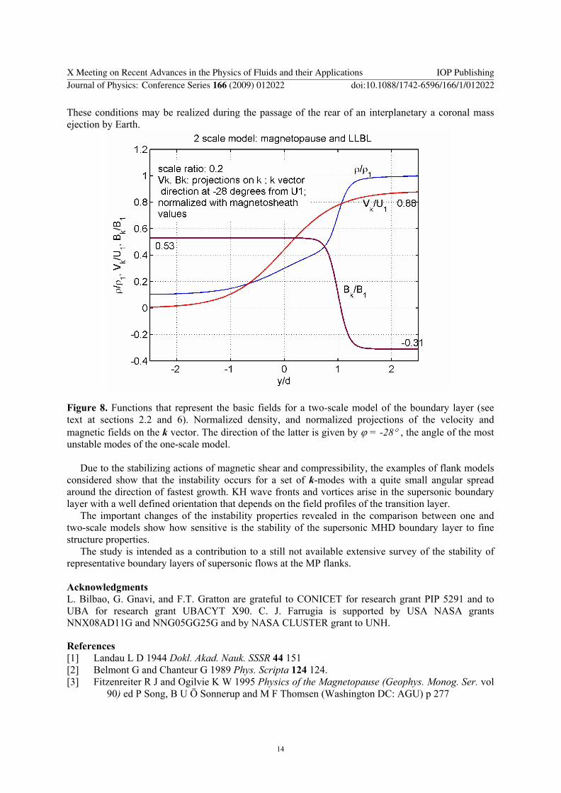
These conditions may be realized during the passage of the rear of an interplanetary a coronal mass ejection by Earth.

Figure 8. Functions that represent the basic fields for a two-scale model of the boundary layer (see text at sections 2.2 and 6). Normalized density, and normalized projections of the velocity and magnetic fields on the k vector. The direction of the latter is given by ϕ = -28° , the angle of the most unstable modes of the one-scale model.

Due to the stabilizing actions of magnetic shear and compressibility, the examples of flank models considered show that the instability occurs for a set of k-modes with a quite small angular spread around the direction of fastest growth. KH wave fronts and vortices arise in the supersonic boundary layer with a well defined orientation that depends on the field profiles of the transition layer.

The important changes of the instability properties revealed in the comparison between one and two-scale models show how sensitive is the stability of the supersonic MHD boundary layer to fine structure properties.

The study is intended as a contribution to a still not available extensive survey of the stability of representative boundary layers of supersonic flows at the MP flanks. Acknowledgments L. Bilbao, G. Gnavi, and F.T. Gratton are grateful to CONICET for research grant PIP 5291 and to UBA for research grant UBACYT X90. C. J. Farrugia is supported by USA NASA grants NNX08AD11G and NNG05GG25G and by NASA CLUSTER grant to UNH.

References [1] Landau L D 1944 Dokl. Akad. Nauk. SSSR 44 151 [2] Belmont G and Chanteur G 1989 Phys. Scripta 124 124. [3] Fitzenreiter R J and Ogilvie K W 1995 Physics of the Magnetopause (Geophys. Monog. Ser. vol

90) ed P Song, B U Ö Sonnerup and M F Thomsen (Washington DC: AGU) p 277

X Meeting on Recent Advances in the Physics of Fluids and their Applications IOP PublishingJournal of Physics: Conference Series 166 (2009) 012022 doi:10.1088/1742-6596/166/1/012022

14

[4] Kivelson M G and Chen S-H 1995 Physics of the Magnetopause (Geophys. Monog. Ser. vol 90) ed P Song, B U Ö Sonnerup and M F Thomsen (Washington DC: AGU) p 257

[5] Miura A 1995 Physics of the Magnetopause (Geophys. Monog. Ser. vol 90) ed P Song, B U Ö Sonnerup and M F Thomsen (Washington DC: AGU) p 285

[6] Lotko W and Sonnerup B U Ö 1995 Physics of the Magnetopause (Geophys. Monog. Ser. vol 90) ed P Song, B U Ö Sonnerup and M F Thomsen (Washington DC: AGU) p 371

[7] Farrugia C J, Gratton F T and Torbert R B 2001 Space Science Rev. 95 443 [8] Farrugia C J et al. 2000 J. Geophys. Res. A 105 7639-7667 [9] Gratton J, Gratton F T and González A G 1988 Plasma Phys. Contr. Fusion 30 435-456 [10] Keller H B 1992 Numerical methods for two point boundary-value problems (New York:

Dover) [11] Miura A and Pritchett P L 1982 J. Geophys. Res. A 87 7431 [12] González A G and Gratton J 1994 J. Plasma Phys. 51 43-60 González A G and Gratton J 1994 J. Plasma Phys. 52 223-244 [13] Gratton F T, Bender L, Farrugia C J and Gnavi G 2004 J. Geophys. Res. A 109 doi: 10.102

V2003JA010146 Gratton F T, Gnavi G, Farrugia C J and Bender L 2005 Brazilian J. Phys. 34 1804-1813 [14] Gratton F T, Bilbao L E, Farrugia C J and Gnavi G 2008 JOP: Conf. Series (in press) [15] Farrugia C J , Gratton F T, Bender L, Biernat H K, Erkaev N V, Denisenko V, Torbert R B and

Quinn J M 1998 J. Geophys. Res. A 103 6703

X Meeting on Recent Advances in the Physics of Fluids and their Applications IOP PublishingJournal of Physics: Conference Series 166 (2009) 012022 doi:10.1088/1742-6596/166/1/012022

15