GEOMAGNETIC ACTIVITY FORECASTING: THE STATE OF THE...

GEOMAGNETIC ACTIVITY FORECASTING:THE STATE OF THE ART

Jo Ann JoselynNOAA Space Environment LaboratoryBoulder, Colorado

Abstract. Short-term (days to weeks) geomagneticforecasts are valuable for a variety of public and pri-vate sector endeavors. However, forecast skill, asmeasured by the success of predicting geomagneticindices, is disappointing, especially for disturbed con-ditions. Possible reasons for this lack of proficiencyinclude an incomplete understanding of the solar ori-gins of interplanetary disturbances, insufficient obser-vations of solar phenomena and interplanetary distur-

bances, and an underestimation of magnetospheric-ionospheric control of observed geomagnetic activity.Until more progress can be made on each of theseproblems, desirable forecasting precision is likely toremain elusive. The best opportunity for improvedservice to those agencies requiring advance notice ofgeomagnetic disturbances is "nowcasting" using real-time, near-Earth observations of the approaching solarwind.

1. INTRODUCTION

The level of disturbance of the geomagnetic fieldserves as a convenient proxy that characterizes thelevel of disturbance of the near-Earth space environ-ment, namely, the ionosphere and magnetosphere. Forexample, a study addressing basic, undisturbed iono-spheric behavior might begin with the collection ofdata on geomagnetically quiet days; in contrast, adisturbed ionosphere is virtually guaranteed on geo-magnetically active days. A particular advantage ofgeomagnetic data is that beginning with the earliestscientific studies of geomagnetic records, the datahave been characterized, or indexed, by the level ofdisturbance. The earliest was the C index, developedin 1906, whereby the observer rated each day as 0, 1,or 2, depending on whether the day was exceptionallyquiet, moderately disturbed (the normal circum-stance), or significantly disturbed [Lincoln, 1967]. In-dexing greatly facilitates the sorting of chronologicalgeophysical data inventories into activity bins andprovides a well-defined forecast parameter that can beunderstood and interpreted by a diverse geophysicalcommunity. Examples of geophysical models formu-lated using global geomagnetic indices are the thermo-spheric mass spectrometer-incoherent scatter modelMSIS-86 [Hedin, 1987] and the Magnetospheric Spec-ification and Forecasting Model (MSFM), a particleflux specification model developed for operational use[Bales et al., 1993; Freeman et al., 1993].

Indices necessarily represent a selected timescale ofvariation. The timescales of variation in Earth's mag-netic field range from geologic reversals [e.g., Jacobs,

1984] to subsecond micropulsations [Lanzerotti et al.1990]. The longest timescales are caused by internal(geologic) processes, but shorter-term geomagnetic ac-tivity is driven by variability on the Sun and fluctua-tions in the solar wind; indeed, geomagnetic activitycycles have been related to decade-long solar activitycycles [e.g., Feynman and Crooker, 1978; Feynman,1982; Feynman and Gu, 1986; Legrand and Simon,1981]. Proxy records of geomagnetic activity (auroralsightings) were used to infer solar behavior even be-fore the time when solar observations began [e.g.,Feynman and Silverman, 1980, Feynman and Foug-ere, 1984]. The geomagnetic field has a diurnal varia-tion caused by tides and currents driven by a solar-heated ionosphere [e.g., Matsushita, 1967]. Variationson shorter timescales are ultimately driven by solarwind-magnetosphere interactions [e.g., Axford, 1967],whose physics and dynamics are open topics ofresearch.

The level of disturbance of the space environment isof more than academic interest. Such private and pub-lic endeavors as communication and navigation sys-tems, electric power networks, geophysical explora-tion, spacecraft control, and scientific researchcampaigns [e.g., Lanzerotti, 1979; Joselyn, 1986b] areaffected by geomagnetic fluctuations. Daily reportsand forecasts of geomagnetic activity are routine prod-ucts of the 10 Regional Warning Centers of the In-ternational URSIgram and World Days Service(IUWDS). These international centers, located in theUnited States of America, France, Canada, China,Japan, India, Czech Republic, Poland, Russia, andAustralia, serve the scientific and user communities

This paper is npt subject to U.S. copyright.

Published in 1995 by the American Geophysical Union.

Reviews of Geophysics, 33, 3 / August 1995pages 383-401

Paper number 95RG01304• 383 •

384 • Joselyn: GEOMAGNETIC ACTIVITY FORECASTING 33, 3 / REVIEWS OF GEOPHYSICS

within their own geographical regions; they also pro-vide, exchange, and relay data and advice on spaceweather to the other centers [Thompson et a/., 1993].In the U.S., the agency responsible for this work is theSpace Environment Laboratory (SEL) of the NationalOceanic and Atmospheric Administration (NOAA).SEL's Space Environment Services Center (SESC)works around the clock to monitor more than 1400separate data streams, which sense solar, magneto-spheric, and ionospheric parameters. When certainpredetermined threshold levels are exceeded, espe-cially geomagnetic activity indices, SESC personnelimmediately take action to inform subscribers.

Since 1808, episodes of extraordinary levels of geo-magnetic disturbance have been known as "storms,"a term attributed to Alexander von Humboldt [Chap-man, 1968]. Magnetic storms denote variations inEarth's magnetic field intensity which may be as largeas several percent of the undisturbed value measuredat the surface. The frequency of storm occurrencevaries over a roughly 11-year cycle but is not neces-sarily synchronous with the well-known sunspot cy-cle. At magnetic cycle maxima, most of the days of amonth (but not all) can be disturbed. However, even atcycle minima, it is unusual that a month goes bywithout a stormy day.

A particularly severe geomagnetic storm occurredin March 1989 [Alien et al.9 1989]; it was the biggeststorm since 1960 and has not been equaled through1994. Reported geophysical effects of that storm in-cluded widespread auroras; satellite anomalies; a sys-tem-wide power blackout in Quebec, Canada; andpeculiar radio propagation conditions [Cliffswallow,1993]. While the enormity of the sunspot group and thefrequency of significant flares had led SESC forecast-ers to predict the possibility of geomagnetic activity,the date and severity of the storm were not accuratelyforecast. This lack of forecasting accuracy is unfortu-nately not unusual.

What is the state of the art? Verification data (com-parisons of forecasts with observed indices and fore-casts with observed events) for the past 7 years indi-cate that for 1-day forecasts, overall SESC forecastquality is better than that obtained by simple tech-niques such as recurrence or persistence (explainedfurther below). However, forecast accuracy tends todecrease over the longer term (K. A. Doggett, manu-script in preparation, 1995). On an annual basis, for 2of the past 7 years, sample climatology (the simpleaverage of the observed parameter that is being fore-cast) has been more skillful than the 1-day SESCforecast. For rare events (e.g., storms), SESC capa-bility has been disappointing (missed events and falsealarms occur more often than accurate forecasts).

This paper reviews the current state of short-term(days to weeks) forecasts of diurnally averaged geo-magnetic activity without the benefit of timely solarwind data. Predictions of geomagnetic activity -using

solar wind data near 1 AU (essentially "nowcasts")are beyond the scope of this review; however, ongoingdevelopments in understanding how the magneto-sphere extracts and processes energy from the solarwind, and the hope of acquiring data from new solarwind monitors, make such nowcasts a particularlyexciting and operationally relevant endeavor. This re-view asks the question, "Do we now have the requiredknowledge and data to accurately forecast a geomag-netic storm a day or so in advance of its onset?" Toanswer this question, the following evidence is pre-sented. First, the index now used to describe andpredict geomagnetic activity is briefly explained. Thisindex, particularly well suited for Earth's heavily pop-ulated middle latitudes, sums the effects of multiplegeophysical current systems driven by separate phys-ical processes. By choosing to predict this index, wehave selected a formidable task. Next, we discuss thegeneral forecasts of this index using a variety of simplemethods and compare it with SESC verification re-sults, concluding that there is room for improvement.In the following two sections we review the physicaltools that SESC uses to forecast activity, and try todetermine which are more robust, leading to a courseof action to improve geomagnetic services.

2. MEASURES OF GEOMAGNETIC ACTIVITY

J. Bartels fashioned the K index, the geomagneticindex in widest use today, in 1932 [e.g., Chapman andBartels, 1940]. An excellent review and description ofthe K index and related global indices is given byMenvielle and Bert he Her [1991]. The K index is aquasi-logarithmic number between 0 and 9 that is as-signed at the end of specified 3-hour periods (0000-0300, 0300-0600, etc.), by measuring the maximumdeviation (in nanoteslas) of the observed field beyondexpected quiet field conditions, for each of the threemagnetic field vector components. The largest of themaxima is converted to a K index by using a look-uptable appropriate for that particular observing site.Table 1 shows the values used for Boulder, Colorado,and Fredericksburg, Virginia. This process standard-izes the data by correcting for expected geophysicalbiases between observing sites. By way of contrast, atCollege, Alaska, where the magnetic field is naturallymore variable owing to the proximity of the auroralelectrojet, a deviation between 0 and 20 nT is coded asa K of 0, and a deviation of 2500 nT or more isnecessary to code a AT of 9.

At individual stations, to combine the eight daily Kindices into one number representative of overall ac-tivity for the whole day, each K is converted to an aindex as shown in Table 2; the a index linearizes thequasi-logarithmic K index. Then the eight a indices arearithmetically averaged to yield a daily A index. ThisA index is used to define a storm and describe its

33, 3 / REVIEWS OF GEOPHYSICS Joselyn: GEOMAGNETIC ACTIVITY FORECASTING • 385

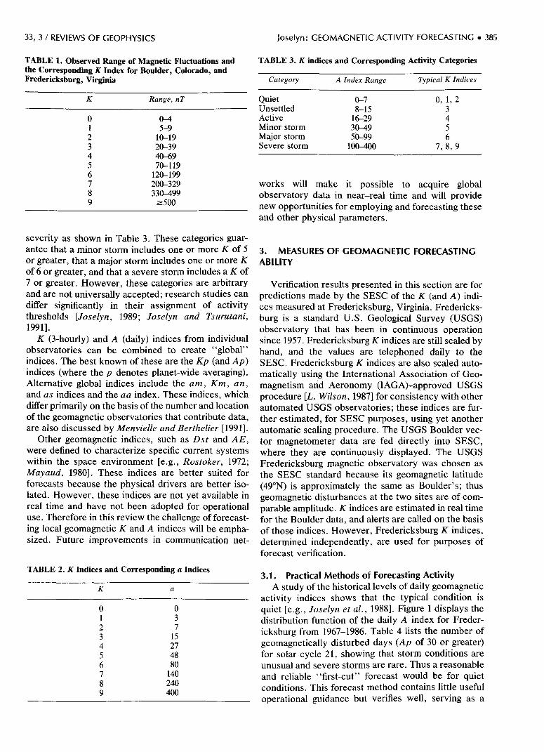
TABLE 1. Observed Range of Magnetic Fluctuations andthe Corresponding K Index for Boulder, Colorado, andFredericksburg, Virginia

TABLE 3. K indices and Corresponding Activity Categories

Category A Index Range Typical K Indices

K Range, nT

0123456789

0-45-9

10-1920-3940-6970-119

120-199200-329330-499

>500

severity as shown in Table 3. These categories guar-antee that a minor storm includes one or more K of 5or greater, that a major storm includes one or more Kof 6 or greater, and that a severe storm includes a K of7 or greater. However, these categories are arbitraryand are not universally accepted; research studies candiffer significantly in their assignment of activitythresholds [Joselyn, 1989; Joselyn and Tsurutani,1991].

K (3-hourly) and A (daily) indices from individualobservatories can be combined to create "global"indices. The best known of these are the Kp (and Ap)indices (where the p denotes planet-wide averaging).Alternative global indices include the am, Km, an,and as indices and the aa index. These indices, whichdiffer primarily on the basis of the number and locationof the geomagnetic observatories that contribute data,are also discussed by Menvielle and Berthelier [1991].

Other geomagnetic indices, such as Dst and AE,were defined to characterize specific current systemswithin the space environment [e.g., Rostoker, 1972;May and, 1980]. These indices are better suited forforecasts because the physical drivers are better iso-lated. However, these indices are not yet available inreal time and have not been adopted for operationaluse. Therefore in this review the challenge of forecast-ing local geomagnetic K and A indices will be empha-sized. Future improvements in communication net-

TABLE 2. K Indices and Corresponding a Indices

K

0123456789

037

15274880

140240400

QuietUnsettledActiveMinor stormMajor stormSevere storm

0-78-15

16-2930-4950-99

100-400

0, 1,23456

7,8 ,9

works will make it possible to acquire globalobservatory data in near-real time and will providenew opportunities for employing and forecasting theseand other physical parameters.

3. MEASURES OF GEOMAGNETIC FORECASTINGABILITY

Verification results presented in this section are forpredictions made by the SESC of the K (and A) indi-ces measured at Fredericksburg, Virginia. Fredericks-burg is a standard U.S. Geological Survey (USGS)observatory that has been in continuous operationsince 1957. Fredericksburg K indices are still scaled byhand, and the values are telephoned daily to theSESC. Fredericksburg K indices are also scaled auto-matically using the International Association of Geo-magnetism and Aeronomy (lAGA)-approved USGSprocedure [L. Wilson, 1987] for consistency with otherautomated USGS observatories; these indices are fur-ther estimated, for SESC purposes, using yet anotherautomatic scaling procedure. The USGS Boulder vec-tor magnetometer data are fed directly into SESC,where they are continuously displayed. The USGSFredericksburg magnetic observatory was chosen asthe SESC standard because its geomagnetic latitude(49°N) is approximately the same as Boulder's; thusgeomagnetic disturbances at the two sites are of com-parable amplitude. K indices are estimated in real timefor the Boulder data, and alerts are called on the basisof those indices. However, Fredericksburg K indices,determined independently, are used for purposes offorecast verification.

3.1. Practical Methods of Forecasting ActivityA study of the historical levels of daily geomagnetic

activity indices shows that the typical condition isquiet [e.g., Joselyn et al., 1988]. Figure 1 displays thedistribution function of the daily A index for Freder-icksburg from 1967-1986. Table 4 lists the number ofgeomagnetically disturbed days (Ap of 30 or greater)for solar cycle 21, showing that storm conditions areunusual and severe storms are rare. Thus a reasonableand reliable "first-cut" forecast would be for quietconditions. This forecast method contains little usefuloperational guidance but verifies well, serving as a


A Fredericksburg 1967-1986

20 40 60A Index

80 100 120

Figure 1. The A index is a daily measure of geomagneticactivity that ranges between 0 and 400 in units of 2 nT. Themode, or most frequently observed, geomagnetic A index forFredericksburg, Virginia, between February 1966 and May1983 was 6, which is quiet. The median index was 10.

reminder to builders of geomagnetic forecasting algo-rithms that they must adequately predict the norm:quiet conditions.

An improvement to a blind forecast of quiet condi-tions is one that includes knowledge of longer-termaverage conditions, or climatology. The strong semi-annual periodicity in geomagnetic storm occurrence isillustrated in Figure 2. This tendency has been exam-ined by a long list of researchers [e.g., Bartels, 1963;Russell and McPherron, 1973; Green, 1984, Clua deGonzalez et al., 1993] and is still under study. Theunderlying physical explanations for this behavior canbe applied to specific forecasting situations, as is dis-cussed below. However, a climatological forecast caninclude these inherent trends even when a specificsolar wind disturbance has not been identified.Monthly Fredericksburg climatology tables are a com-ponent in SESC forecasts, and "sample climatology"(average conditions observed during the forecast timeframe) is a standard for forecast comparison.

A common, simple forecast technique is persis-tence: the assumption that tomorrow's conditions willmimic today's. This is a respected maxim of weatherforecasting that is used as a standard of comparison forSESC forecasts. As is shown below, SESC forecastsare usually more accurate than those that would beobtained using persistence alone.

TABLE 4. Number of Disturbed Days in Solar Cycle 21

Daily GeomagneticAp Index

(Lower Limit)

Ap > 30Ap > 50Ap > 100

Number ofDays

417128

18

Percent ofAll Days

11%3%

0.5%

Another forecasting technique is 27-day recurrence.The recurrence technique builds on the knowledgethat the Sun rotates once approximately every 27days, and assumes that stable streams of geoeffectivesolar wind will return like a rotating searchlight. Long-term spectral analyses of the Ap index [Fraser-Smith,1972; Clua de Gonzalez, 1993] as well as of the inter-planetary field [Gonzalez and Gonzalez, 1987] showthis 27-day peak. Recurrence is not reliable; however,it is particularly useful during the declining phase ofthe solar cycle, when high-speed streams of solar windare stable [e.g., Sargent, 1986; Hapgood, 1993]. Fore-cast guidance based on the recurrence technique isavailable for daily SESC use.

There are other numerical or proxy methods forforecasting geomagnetic activity. For example, linearprediction filters have been applied to self-predictingthe Ap index [Thomson et al, 1993]. Thomson [1993]further applied a neural network algorithm and foundsome improvement in prediction accuracy. However,these techniques cannot be expected to predict stormonsets any more accurately than do the other climato-logical techniques.

3.2. Verification ResultsK. A. Doggett (manuscript in preparation, 1995) has

evaluated all of SESC's 1987-1993 forecasts. This sec-tion reports comparisons of SESC daily A index fore-casts with the corresponding observed (hand-scaled)USGS Fredericksburg daily A indices. Figure 3 dis-plays forecast-observation pairs in a format that showsthe number of occurrences of matching forecasts andobservations, for forecasts made a day in advance ofthe observation. Perfectly correlated pairs would lieon the line of slope 1; in actual fact, forecast valuesoften exceed observed values.

Jan Feb Mar Apr May Jun Jul Aug Sep Oct Nov Dec

Months (from 1932-1992)

Figure 2. The Ap index is a global daily measure of geomag-netic activity. An index of 50 or more constitutes a majorgeomagnetic storm. A count of the total number of stormdays between January 1932 and December 1992 in eachmonth of the year reveals that the equinoctial months havemore storms, statistically, than do solstitial months.


60 r

Figure 3. A good correlation between the A index forecast for Fredericksburg and the observed valuewould show points clustered near a line of slope 1 in the x-y plane. The linear correlation betweenforecasts and observation is 0.45. The data shown are the number of occurrences of daily forecast-observation pairs for 1987-1993, for forecasts made 1 day ahead.

Forecast quality can be measured in several ways.The linear correlation r is one way; over the interval1987-1993, r = 0.45 (the best result would be r = 1).Another, "accuracy," measures the average degree ofcorrespondence between individual forecast-observa-tion pairs and is usually given as mean square error(MSE) or root-mean-square error (RMSE). "Bias,"also called the mean error or "reliability," examinesthe tendency of the average forecast to be consistentlygreater than (over) or less than (under) that of theobserved average value; zero bias is desirable.

Individual forecasters typically have a consistentbias (either to overforecast or to under-forecast) thatthey can learn to correct once this tendency is identi-fied. Figure 4 illustrates these measures for 1-daySESC forecasts for consecutive years since 1987. Fig-ure 4a displays forecast accuracy, as measured byRMSE, with the actual value of the annual average ofthe Fredericksburg A index. The average RMSEs areall comparable to the observed values. The pattern ofbias (Figure 4b) shows that the annual average SESCforecast usually exceeded the annual average observa-tion; this was especially true during 1988, when solaractivity was building up in the early years of the solarcycle. Apparently, more activity was anticipated thanwas observed. Geomagnetic activity was generally un-derforecast only during 1991, a year of extraordinarysolar and geomagnetic activity. The annual correla-tions (Figure 4c) range between approximately 0.2 and0.6. Correlations were lowest in 1987-1988, when solarand magnetic activity were low. The highest correla-

tion was for 1991. An intermediate correlation wasseen for 1989, the year of maximum sunspot numberfor solar cycle 22.

Figure 5 shows comparisons of the accuracy of theSESC forecasts with that obtained by the simple ref-erence forecast methods of climatology, persistence,and recurrence, using annual skill scores. Skill is de-fined as the MSE of the reference method (e.g., clima-tology) minus the MSE of the SESC forecasts, alldivided by the MSE of the reference. If the forecastshave equal accuracy, the skill score is zero. Positivenumbers indicate that the SESC forecasts were moreskillful than the reference, and negative numbers indi-cate that the reference was more accurate. For 1987-1993, annual average SESC forecaster accuracy a dayin advance of a storm was always better than recur-rence (which assumes that the observed value 27 daysago will repeat), was better than persistence (in 6 ofthe 7 years, and was better than sample climatology (aconstant forecast of the annual average observed Aindex) for 5 of the 7 years. On an annual basis, the bestof the simple reference forecasts was climatology, theaverage of all observations for that year. This resulturges restraint when forecasters are tempted by cir-cumstances to predict more extreme geomagnetic ac-tivity (quiet or storm levels) than typical, averageconditions.

Does SESC forecast quality degrade as lead timeincreases? Every day, SESC forecasters predict theFredericksburg A index for each of the 7 upcomingdays. Figure 6 combines the data for 1989-1993 and


16:141210-6420

••*>

~ * 'y/^ ^

\. •-^-

j*^^*^ ^

9 ~•̂̂

- •

^0

1987 1988 1989 1990 1991 1992 1993

Accuracy (RMSE)

Average Fredericksburg A Index

Over J]1-

0.50-

-0.51 InHor 1

-1.5

^

jii<r\

^\.\

» ———— *vX,

\/^^*

^

1987 1988 1989 1990 1991 1992 1993

Bias (ME)

1987 1988 1989 1990 1991 1992 1993

Correlation (r)

Figure 4. Annual SESC forecast verifications made one dayahead can be characterized in three ways: (a) the root-mean-square error (the actual annual average A index is alsoshown for comparison), (b) the bias toward over forecasts orunderforecasts, and (c) the annual correlation coefficient.

illustrates several measures of forecast accuracy as afunction of lead time. Figure 6a shows the SESC MSBand indicates that the forecast quality decreases withlead time to day 4, whereupon it effectively levels out.This pattern appears in the other panels of Figure 6 aswell, especially in 6b, which shows the linear correla-tion coefficient for days forecast farther into the future(compare Figure 3). Figure 6c shows that SESC next-day forecasts, averaged over the past 5 years, areunbiased but become progressively more negativelybiased (underforecasts) for each additional day in ad-vance. Figure 6d shows that SESC forecasts are lessaccurate than sample climatology for 3 days and far-ther into the future.

As is shown in Table 4 and Figure 7, geomagneticstorms are relatively rare. SESC forecast accuracy is

particularly disappointing when storms are considered(a storm forecast is defined as a prediction of an Aindex >30). Of the total number of days in 1987-1993,173 (6.8%) were storm days. Out of 173 storm days, 47(27%) were predicted and 126 (73%) were missed.While there were near-misses that might count as"moral victories" (e.g., a storm arrived a day earlieror later than expected, or the observed A index wasless than 30 even though a K index of 6 or even higheroccurred), these results indicate a lack of proficiencyin the task of forecasting geomagnetic storms.

Figure 8 summarizes categories of SESC forecasts aday in advance vis-a-vis observed conditions duringthe 6 years 1987-1993. Forecasts of quiet conditionswere generally rewarded with the occurrence of quietconditions, and forecasts of unsettled conditions wereusually followed by unsettled conditions; forecasts ofactive or storm conditions were less definitive.

4. SOLAR ORIGINS OF GEOMAGNETIC ACTIVITY

Prior to the availability of space-based solar opticaland interplanetary solar wind data, solar flares and "Mregions" served as solar progenitors of geomagneticactivity. When no flare was observed, nonrecurrentgeomagnetic activity was often attributed to unseenflares on the back side of the Sun [e.g., Dodson et al.,1979]. Then solar images in X ray wavelengths re-vealed "coronal holes," which were soon associatedwith high-speed solar wind streams and episodes ofrecurrent geomagnetic activity [e.g., Hundhausen,1977]. Sector boundaries were also found to have astatistical signature in geomagnetic indices; this topicis discussed in more detail below.

Skylab's discovery of coronal mass ejections(CMEs) and their intimate association with eruptingprominences gave rise to suggestions that disappearingsolar filaments could predict geomagnetic activity [Jo-selyn and Mclntosh, 1981; McNamara and Wright,1982; Wright and McNamara, 1983]. However, effortsto forecast geomagnetic storms on the basis of specificflares, filament disappearances, or coronal holes usu-ally yielded ambiguous results, and some storms hadno obvious solar precursor [Tang et al., 1985; Joselyn,1986a; Neugebauer, 1988]. To further complicate mat-ters, flares, coronal holes, and filament disappearancesfar outnumber geomagnetic effects. It has also beensuggested that separate forms of solar activity are notnecessarily independent. For example, Dodson andHedeman [1972] noted an apparent relationship be-tween flares and filament disappearances, and Sheeleyet al. [1983] noted that filament disappearances some-times accompany the birth of coronal holes. This in-coherent picture of the solar origins of geomagneticactivity underlies the poor record of geomagnetic fore-cast verification.

Lately, however, the picture has been improving.


u.i

0.6^

Better 0.5 -^0.4^

n *}

0.2^

0.1-

0-.

-0.1-

Wor^p -0 2V V \Jl Ow w.i.

-ns

*

//•V

/

/^A

*

/v

A • •/

•,^ *•^/

- -A*X

>/

.A

A' N

"A

*>

VV-

V

A

-^m —Figure 5. SESC forecasts made one day inadvance are compared with simple refer-ence forecasts. If both forecasts are simi-larly accurate, the score is zero; if theSESC forecast is more accurate, the scoreis positive. Since 1989, SESC forecastshave beaten" the simple forecasts of clima-tology, persistence, and recurrence.

1987 1988 1989 1990 1991 1992 1993

sample climatology - • - persistence - A - recurrence

For example, the value of solar flares as a predictor ofnonrecurrent geomagnetic activity has been formallychallenged, and a new paradigm is emerging that placescoronal mass ejections in the central role [Gosling et aL,1990; Kahler, 1992; Gosling, 1993]. The forecastingtask remains difficult, however: first the CME must beidentified; then it must be proven to drive or becomean interplanetary disturbance [Wilson and Hildner,1984; Webb, 1993].

Coronal mass ejections at 1 AU generally havedistinct plasma and field signatures by which they canbe distinguished from ordinary solar wind [Gosling,1990]. The phrase "magnetic cloud" [Klein andBurlaga,1982; Burlaga, 1991] presents a descriptive image of aCME-caused interplanetary disturbance. The cloudcarries an intrinsic magnetic field, often with the char-acteristics of a flux rope [Marubashi, 1986]; it interactswith other solar wind structures and with the ambientmedium [Burlaga et aL, 1987; McComas et aL, 1989].Magnetic clouds have been identified with geomag-netic effects at Earth [e.g., R. M. Wilson, 1987; 1990;Zhang and Burlaga, 1988; Gosling et aL, 1991]. Othermeasureable characteristics of potentially geoeffectiveparcels of solar wind include bidirectional electronheat flux events, interpreted as populations of elec-trons traveling along interplanetary magnetic fieldlines which either are rooted at both ends in the Sun orelse are on closed loops entirely disconnected from theSun [Gosling et al. 1987], and, similarly, bidirectionalproton events [Marsden et aL, 1987]. Some noncom-pressive density enhancements (high densities ob-served when the solar wind bulk flow speed is nearlyconstant or falling) [Gosling et aL, 1977], which have

been associated with coronal streamers, may also havea transient origin.

Of all of the characteristics measured in the solarwind, it is now well understood that a necessary andsufficient condition for geomagnetic storms is a strongsouthward component of the interplanetary magneticfield, Bz [e.g., Russell et aL, 1974; Gonzalez and Tsu-rutani, 1987; Gonzalez et aL, 1994, and referencestherein]. This southward component "reconnects" orcouples with the northward pointing intrinsic geomag-netic field, in intuitive agreement with the principlethat opposite magnetic fields attract, while like fieldsrepel. Under "attractive" conditions, solar wind en-ergy is converted into magnetic energy stored in adistorted geomagnetic field. It is the release of thisenergy, in a variety of forms, that becomes manifest ingeomagnetic activity. Other relevant solar wind pa-rameters besides the interplanetary field are highspeed and, perhaps, increased momentum flux. Canthis new paradigm of CMEs as the source of geoeffec-tive solar wind be employed to improve geomagneticforecast accuracy for transient events? The next sec-tion examines this question; it is followed by a reviewof our present understanding of the solar source ofrecurrent geomagnetic activity.

4.1. CMEs and Nonrecurrent Geomagnetic ActivityThe release of mass and energy into the solar wind

accompanying CMEs provides the raw material fornonrecurrent geomagnetic activity. Thus if a CME isobserved or suspected, there is reason to consider thelikelihood of a geomagnetic storm. Coronagraphs atEarth observe CMEs beyond the rim of the Sun, pro-


£. IU-

onn

190-

180-

170-

160-

15O

/^

I

f1

CM

Q

/

/

CO>»0}Q

S

\Q

^^

IO

1

N^

CO

Q

^

1̂£Q

Accuracy (MSE)

0.4 -!n QKn ̂

0 P5U.4-O

0.2-0.15-0.1-

f\ f\r"n :

\\\\

>̂,»^-^

T- CM>. >*CO COQ Q

CO

I &CO N.I I

Correlation (r)

0.5q

0--0.5-

-1--1.5-

-2-_o c

Q

0 C

-4

\

^^

CM

I

-\

CO

%Q

\

\

£03Q

\<

10

£Q

^*— .

CO

%Q

--*^

1̂ .

£a

w

0 1R. 1 O

0.1f\ f\f-

0--0.05--0.1-

-0.15-

\

1

vCM

1

\

CO

1

^

1Q

—•—

ini—— *̂

CO

1(^

Bias (ME) Skill (sampleclimatology)

Figure 6. Various characterizations of SESC forecasts made more than 1 day ahead are shown. These are(a) accuracy or mean square error, (b) the correlation coefficient, (c) bias (negative values indicate anunderforecast), and (d) skill against climatology (the simple average of observed A indices). Data shownare for 1987-1993.

jected into the plane of the sky. CMEs seen in this waymay not be geoeffective because they are apparentlyaimed away from Earth. However, if the CME is large(the average width of approximately 1200 CMEs ob-served by the Solar Maximum Mission (SMM) was 47°[Hundhausen, 1993] or its release site is sufficientlyclose to solar central meridian, an associated inter-planetary magnetic cloud could impact Earth andspawn geomagnetic effects.

The first problem is that of recognizing the exis-tence of a CME at all. Several proxy signatures ofCMEs have been identified. These are long-durationsolar X ray events (LDEs), filament disappearances,certain radio sweeps usually accompanying majorflares, and solar energetic particles. However, sinceonly 66% of the CMEs observed by SMM during 1980could be associated with reported solar activity [Webband Hundhausen, 1987], the absence of a CME proxydoes not imply the absence of a CME.

In an effort to evaluate the reliability of X rayevents as a CME proxy, Sheeley et al. [1983] exam-

ined the enhanced soft X ray emission accompanyingflares and filament eruptions; they found that longer-duration X ray events were more likely to be associ-ated with CMEs; events lasting 6 hours or more werealways associated with CMEs, but some shorter burstsalso had CMEs. Unfortunately, the converse is nottrue: many CMEs have no X ray signature [e.g., Webband Hundhausen, 1987]. In SESC practice, an X rayevent, often a flare, is flagged as a possible CME whenthe time between X ray maximum and recovery to halfof the peak amplitude is 30 min or more. Because theimportance of a flare in hydrogen light was found to bea poor indicator of its interplanetary effects [Schwenn,1983], the duration of the X ray signature is helpful toalert forecasters of a possible geoeffective event.

Metric radio bursts, a common component of sig-nificant solar flares, are variously associated withCMEs. The relationship between type II bursts andCMEs is not definitive [Kahler, 1992]. For example,Sheeley et al. [1984] found that 70% of the type IIbursts on their list were associated with CMEs but that


47 Hits

173 Storms Observed(6.8% of Total)

126 Storm Forecasts(4.9% of Total)

All Forecasts/Observations (1987-1993) Storms

Figure 7. The observed A index for most days between 1987 and 1993 was less than 30, the threshold fora storm. Of the 6.8% of the days that were storm days, only 27% (47 of 173) were forecast. Of the 126storms that were forecast, 63% were false alarms.

some CMEs, even fast ones (super Alfvenic, withvelocity v of >400 km s"1), were not. These bursts areneither necessary nor sufficient for the occurrence ofinterplanetary shocks [Sheeley et al., 1985], nor arethey well correlated with geomagnetic sudden im-pulses or geomagnetic storms. When type IV broad-band radio emission occurs, it is generally associatedwith CMEs, especially with fast ones [Cane andReames, 1988]. Type III radio bursts may presageCMEs. Jackson et al. [1980] looked at type III burstrates preceding known CMEs and found a peak about8 hours prior to CME initiation. However, the inverse

study has not been successful: type III radio bursts,per se, are not a helpful diagnostic for geomagneticactivity. SESC forecasters use type II and type IVradio bursts as possible CME proxies but do not usetype III bursts.

Prominence eruptions and filament disappearancesare strongly associated with CMEs [Sheeley et al.,1975; Munro et al., 1979; Wilson and Hildner, 1986;Webb and Hundhausen, 1987]. Wright and Webb[1990] searched for signatures in solar wind data at 1AU 2.5-5.5 days following large filament disappear-ances and concluded that several CME-associated,

Figure 8. A pictorial representation showsSESC success in forecasting categories ofgeomagnetic activity, defined in Table 3.Data shown are for 1-day forecasts, 1987-1993.


interplanetary disturbance features (shocks, increasesin solar wind proton density, and increases in magneticflux density) were evident, lending credence to theirvalue as CME proxies.

Prompt solar energetic particle (SEP) events, inter-planetary particle streams of MeV energies, are favor-ably associated with CMEs [Kahler et al. 1978, 1984].Long-duration particle events (lasting for days) areeven more strongly associated with CMEs [Kahler,1993b]; these energetic protons are almost certainlyproduced in interplanetary space by CME-associatedshock structures, with or without a flare [Reames,1993].

A good association between energetic protonevents and subsequent geomagnetic storms can beshown [e.g., diver and Crooker, 1993]. Between 1976and 1989, 62% of the 92 SESC solar proton events(strictly defined as an episode of at least 30 min dura-tion with a flux of more than 10 protons cm~2 s"1 ofenergies exceeding 10 MeV) preceded geomagneticstorms (Ap >30) within 2-3 days; 75% of the largerevents (peak fluxes exceeding 100 flux units) werefollowed by storms. Thus of all the CME proxies, theobservation of a proton event at Earth offers the bestwarning of a possible geomagnetic storm within 24-72hours.

"Remote sensing" methods that identify coronaltransients and interplanetary disturbances have beenreviewed by Bird and Edenhofer [1990]. Within 0.5AU, Doppler scintillation measurements of spacecrafttelemetry signals exhibit transients that have beenmatched with interplanetary shocks [Woo et al., 1985],in situ observations of magnetic clouds [Woo andSchwenn, 1991], CMEs [Woo, 1993], and compressedplasma at the leading edges of high-speed streams[Woo and Gazis, 1993]. Doppler scintillation can pro-vide data potentially useful for forecasting purposes,but this method requires an advantageously locatedinterplanetary probe (it is a point measurement) andfurther interpretation because, as in the case of coro-nagraph CMEs, the information is integrated along theline of sight.

Beyond 0.5 AU, ground-based interplanetary scin-tillation (IPS) observations of radio sources that arespread over an extended portion of the celestial spherehave been used to infer transient interplanetary distur-bances from daily maps of the spatial distribution ofhigh- and low-density fluctuation regions [e.g., Erskineet al., 1978; Watanabe and Schwenn, 1989, and refer-ences therein]. Physical interpretations of the IPS fluc-tuations are disputed [e.g., Bravo et al., 1991; Mooreand Harrison, 1994], and attempts to use IPS obser-vations in an operational mode have not met withsuccess [Leinbach et al., 1994].

Finally, there is an optical method to track inter-planetary disturbances. Zodiacal light photometers onthe Helios spacecraft imaged coronal mass ejectionsand traced them out to 0.5 AU [Jackson and Leinert,

1985]. A second-generation scattered-light optical im-ager has been proposed that could operate from anear-Earth polar-orbiting platform [Jackson et al.,1991]. A weakness of all of the remote-sensing meth-ods is that they do not include information about thedirection of the interplanetary magnetic field, the mostimportant parameter for geoeffectiveness.

Once a CME is suspected, especially one with aphotospheric signature, an assessment of its probableinternal magnetic structure is the critical next step.This question involves the prediction of a strongsouthward, out-of-the ecliptic magnetic field compo-nent. Burlaga et al. [1987] investigated 17 large geo-magnetic storms with adequate solar wind data thatoccurred between 1972 and 1983. They determinedthat there is no single cause of large geomagneticstorms. Some storms were linked with magneticclouds, some were caused by interacting (compound)streams, and some could be identified with both. Thelargest storm, on July 13, 1982, was caused by acompound stream. Tsurutani et al. [1988] investigatedthe origins of the southward fields that were the ulti-mate cause of 10 intense geomagnetic storms in 1978-1979. The various causes included southward fieldsentrained in a cloud, shock compression of preexistingsouthward fields, turbulence behind shocks, and drap-ing over a noncompressive density enhancement.Tang et al. [1989] looked for the corresponding solarsources and found plausible CMEs or CME proxies foreach: either long-duration X ray flare events or prom-inence eruptions. However, these authors concludethat the solar sources of intense geomagnetic activitydo not have to be optically large or energetic solarevents.

Efforts to use observed solar magnetic field patternsto predict Bz at Earth have had inconsistent success.Pudovkin and Chertkov [1976] found an association oflarge-scale southward fields (and not northward fields)at flare sites with subsequent geomagnetic storms.Tang et al. [1985, 1989] found no simple relationshipbetween the magnetic orientation at flare sites and thesolar wind Bz orientation at Earth.

The possibility of using magnetic field orientationnear disappearing filaments to infer the interplanetarymagnetic field direction is conceptually more favorablethan using flares because filaments are generally large,quasi-linear features that lie on large-scale magneticinversion lines [Mclntosh, 1972]. Close associationshave been made between filament disappearances,CMEs, and "flux rope" magnetic structures (smoothrotations of the magnetic field vector over a largeangle) in clouds [Wilson and Hildner, 1986;Marubashi, 1986; Wilson, 1990]. Wright [1986][defineda coordinate system based on the size, location, andphotospheric orientation of the erupting filament andfound some tendencies for geoeffective filaments tohave a preferred orientation; however, the resultswere not definitive.


TABLE 5. Association of DSF Orientation With Subsequent Geomagnetic Storms

Orientation

Number of casesNumber of storms

62

70

52

72

41

42

60

72

DSF, filament disappearance.

Bothmer and Schwenn [1994] studied the relation-ship between the magnetic field orientation of disap-pearing solar filaments and magnetic clouds observedby Helios; they concluded that eruptive prominenceswere a probable source of the magnetic clouds and thatthe magnetic flux rope structure of the clouds was thesame as that of the associated filament. This suggeststhat an analysis of the orientation of the disappearingsolar filament would be useful as predictive guidance.However, an investigation of the magnetic orientationof 46 major filament disappearances (DSFs), filamentsof 20° or more in extent that are "normal" or "dark"in hydrogen spectroheliograms, near solar central me-ridian in 1979 produced the discouraging results shownin Table 5. In this table the orientation of the filamentis shown as a bar, horizontal, vertical, or slanted toshow the approximate appearance of the filament onthe disk, along with the appropriate polarity, positive(+) or negative (—), of the solar magnetic field oneither side of the filament. Presumably, the most fa-vorable orientation of a filament would be east-west(horizontal) with positive polarity north of the fila-ment; if the arcade of magnetic field lines archingabove the filament preserved its structure as it propa-gated or extended to Earth, the interplanetary mag-netic field would be predominately southward, andgeomagnetic activity would occur. In the table theDSF was associated with a storm (Ap >30) if a stormoccurred within 3-5 days of the date that filament waslast seen (this assumes an average travel speed ofapproximately 600-350 km s"1). No attempt was madeto exempt storms that might have been due to othercauses, so the number of storms counted may beoverestimated. The results of this limited but practicaltest using good examples of filament disappearanceswere that no storms were associated with the leastfavorable orientation (negative fields north of an east-west filament), but that few storms could be associatedwith the most favorable orientation. Another clearresult is that filament disappearances, of any orienta-tion, are not a reliable predictor of geomagneticstorms.

Thus in the absence of additional information, theobserved filament orientation per se does not providedefinitive predictive guidance. Perhaps, however, us-ing solar photospheric fields is not an appropriateapproach to improving forecasting. Kahler [1992]

pointed out that the filament field generally lies at alarge angle to the overlying field that may be thedominant orientation in the CME plasma. He ques-tioned whether we know the topology of the appropri-ate coronal fields and, if we do, whether large-scaleeruptive coronal fields maintain either their integrity ordirection in the interplanetary medium.

Hoeksema andZhao [1992] extrapolated the photo-spheric magnetic field to the high coronal altitudes thatmay be regarded as the base of the solar wind and, forthree of five cases, matched northward or southwardorientations for the active-region CMEs in their studywith the same orientation at Earth. However, Kahler[1993a] criticized several of their assumptions (includ-ing the relationship of the flares to the CMEs); hefurther investigated the geomagnetic consequences ofthe simplest possible coronal field-interplanetary ori-entation: the solar dipole field at solar minimum. Hereasoned that if the dipole orientation were preservedeven approximately in the coronal ejecta, then thetime (18 months) of those solar minima for which thesolar dipole field points southward (the northern solarpole currently has a positive polarity) would, statisti-cally, be more geomagnetically active than that ofminima with the reversed orientation. Five minima ofeach orientation were analyzed; each set had approx-imately the same number of storms. No evidence ofsolar cycle dependence of Bz was found, implying thatit is not reasonable to expect that Bz can be inferredfrom the more complicated coronal fields near solarmaxima [Kahler, 1993a].

Some conditions of interplanetary propagation thatlead to geoeffective solar wind are not apparent insolar observations. While interplanetary clouds occurin both fast and slow transient flow [Burlaga et al.,1987; Gosling et al., 1987], most of the largest geomag-netic storms are associated with storm sudden com-mencements, which are primarily caused by interplan-etary shocks. Most interplanetary shocks can beassociated with fast (>500 km s-1) CMEs [Sheeley etal., 1985; Schwenn, 1986], and, importantly for geo-magnetic effects, the most intense interplanetary fieldsfollow shocks [Burlaga and King, 1979]. Shock driv-ers, the interplanetary material responsible for theformation of the shock, generally extend up to 100° inlongitude and are centered on the presumed solarsource longitude; 80% of shocks from presumed


sources near the central meridian are followed bydrivers [Richardson and Cane, 1993; Richardson etal., 1994]. Kahler [1992] reviewed the characteristicsof high-speed driver-gas plasmas behind interplanetaryshocks. Cane et al. [1986] identified six interplanetaryshocks associated with filament eruptions, showingthat rapid release of energy is not necessary for theformation of an interplanetary shock. Gosling et al.[1991] found that about three fourths of 37 geomag-netic storm events between August 1978 and October1982 were associated with Earth passages of CMEsand their related shocks; however, only half of theobserved CME shocks resulted in a storm. Of interestfor prediction, draping of the ambient interplanetaryfield about the rapidly ejected material could lead to anincreased out-of-the-ecliptic (northward or southward)magnetic field [Gosling and McComas, 1987], butthere is no a priori way to predict whether drapingeffects will be substantial in any given situation [Mc-Comas et al., 1989].

4.2. Recurrent Geomagnetic ActivityEver since geomagnetic activity was routinely

charted, it has been known that some activity recursapproximately every 27 days [e.g., Bartels, 1963].Subsequent studies found that 27-day recurrence ismost significant in the declining phase of even-num-bered solar cycles [e.g., Sargent, 1986; Hapgood,1993]. These recurrent geomagnetic disturbances wereassociated by Neupert and Pizzo [1974] with solarcoronal holes observed by OGO 7.

Skylab's X ray images of the Sun, together withinterplanetary plasma data from other spacecraft, al-lowed rapid progress in relating coronal holes withhigh-speed, low-density solar wind [Nolte et al., 1976].Understanding of the relationships between coronalholes, high-speed solar wind streams, and geomag-netic disturbances was further developed by Sheeleyand Harvey [1981] and Legrand and Simon [1991].Sheeley and Harvey [1981] noted that the speed ofstreams from coronal holes is solar cycle dependent(greatest in the years of cycle decline, when the holesare largest and extend across the solar equator). Theyalso substantiated the presence of the Russell-McPher-ron effect in coronal hole polarity [Russell andMcPherron, 1973], namely, that negative polarityholes (with the magnetic field pointing inward towardthe solar surface) are more geoeffective in the springand positive holes are more geoeffective in the fallbecause the tilt of the geomagnetic axis with respect tothe rotational axis transforms an interplanetary fieldlying in the ecliptic into a field with an apparent south-ward field component in the magnetospheric coordi-nate frame. Seasonal variations in geomagnetic activ-ity are discussed below.

Wang and Sheeley [1988, 1990] quantitatively mod-eled solar wind expansion from coronal holes, therebypredicting daily solar wind magnetic polarity and

90-

80-

70-

60-

50-

40-

30-

20-

10-

SunspotCycleMaximum

\ f

—— 1—— |SunspotCycleMinimum

—— |

1

a77 78 79 81 82 83 84 85 86 87 88 89

Year

50-

8

\-aI 3°-4>

f

(O o 1

pe

Coronal holes that were the only viable sourceof a storm

SunspotCycleMaximum

SunspotCycleMinimum

•— > o 1

77 78 79 80 81 82 83 84 85 86 87 88 89Year

Figure 9. (a) The annual number of coronal holes observedusing He 1038-nm images illustrates the characteristic pat-tern of minima of occurrence during sunspot cycle minimumand maximum, and a peak during the years of sunspot cycledecline, (b) The annual percent of the observed low-latitudecoronal holes that could be associated with geomagneticstorms is plotted against the portion that were solely asso-ciated with storms (no other viable source was observed).

speed at Earth. Given this relatively advanced theo-retical foundation, how useful are coronal holes forpredicting geomagnetic activity?

Figure 9 shows the correspondence between coro-nal holes and geomagnetic storms (Ap >30). Becausegeoeffective coronal holes are located at low geomag-netic latitudes [e.g., Watari, 1990], the coronal holescounted in Figure 9a were those in each solar rotationthat extended to within 30° of the helioequator; manycross the equator. These holes were identified from thesynoptic charts published monthly in Solar Geophys-ical Data (based on He 1083-nm images provided bythe National Solar Observatory in Kitt Peak, Arizona)and were not cross-checked with published coronalhole catalogues such as that by Sanchez-Ibarra andBarraza-Paredes [1992]. In Figure 9b, holes were as-


Look Ahead Model Coronal Magnetic Field °' I1' 2' 5' 10' 20 MicroTesla"21 I 20 i 19 I 18 I 17 I 16 1^5 I 14 I 13 I 12 I 11 I 10 9 8 7 I 6 TT~1 3 I 2 I 1 I 30 I 29 28 I 27 I 26 I 25 I 24 23 I 22

X X - 2 -1 0 - 2 - 5 - 6 - 6 - 3 - 1 1 2 3 4 3 2 2 1 1 1 3 5 6 7 6 5 4 3 2 2

1855Figure 10. The computed coronal field at the source surface predicts the configuration of the heliosphericmagnetic field. The heavy line shows the location of the neutral sheet, where the polarity of the radialmagnetic field reverses. Solid contours and light shading indicate positive field (away from the Sun), whiledashed contours and dark shading show negative regions. The radial projected path of Earth lies just abovethe helioequator; dates denote the time of central meridian passage of that longitude. The field strength atthe sub terrestrial point appears in the upper margin. The data shown are for April 22 to May 21, 1992,Carrington rotation 1855 (figure taken from Hoeksema [1993]).

sociated with storms if the storm began within 48-72hours following the central meridian passage of thecenter of the hole (this assumes that the relevant high-speed stream speed was between approximately 600and 800 km s"1). Some storms had no other obvioussource (such as a filament disappearance or flare-associated solar activity) besides the sole presence ofthe coronal hole. Whenever possible, solar wind datawere used to confirm "sole-source" coronal holes bychecking for the presence of a high-speed stream withradial interplanetary field polarity matching that of thehole. On average, only 20% of the observed coronalholes were associated with storm-level activity. How-ever, the range of association for the years examinedwas from 4% to 44%; the peak occurred during thewaning years of solar cycle 22, as expected. The per-centage of solely associated coronal holes is smallerand is diminished by the requirement that there be noother obvious source for the storm.

The conclusion offered by Figure 9 is that coronalholes are useful as a diagnostic factor in geomagneticforecasting but like filament disappearances, are notespecially reliable. More information (e.g., the inter-planetary magnetic field) and understanding areneeded. In particular, we need to know if the terres-trial effects are primarily a result of the high-speedsolar winds associated with coronal holes or if they area consequence of the interactions between differingsolar wind flows as was suggested by Crooker andCliver [1994]. These complexities are addressed in thenext section.

4.3. The Ambient Solar Wind and GeomagneticActivity

The ambient (i.e., quasi-steady state) solar wind isassumed to expand freely from a nonuniform "sourcesurface" at a few solar radii in the outer solar corona,carrying entrained coronal fields with it. Even if tran-sient flows are not considered, there is structure in thequiet solar wind at the source surface, as a result ofsolar wind acceleration mechanisms (e.g., high-speedstreams from coronal holes), and beyond, owing tointeractions between flows of differing speed and dif-fering magnetic orientation \_Neugebauer, 1983].

Figure 10 illustrates the results of a calculationdescribed by Hoeksema et al. [1982] to estimate thestrength and polarity of the interplanetary magneticfield in the high solar corona at the base of the solarwind. The calculation uses a potential field model withdaily magnetic maps of the photosphere; it is availableroutinely and promptly from the Wilcox Solar Obser-vatory in California. An obvious feature in this figureis the trace of the heliospheric current sheet, a low-speed, enhanced-density feature marking the transi-tion between regimes in the solar wind where theunderlying coronal field points predominantly eithertoward or away from the Sun. Wilcox and Ness [1965]observed this apparent discontinuity in in situ solarwind data and identified it as a solar sector boundary(SSB). SSBs are described by Behannon et al. [1981,p. 3273] as "the ecliptic plane intersections of awarped global current sheet that surrounds the Sunnear its equatorial plane." Crossings of the helio-


35

30

25

20

15

10 -

<ooo

1005

inCM05 CO05

inin05

in<o05

inh-

200

180

160

140 fc.Q

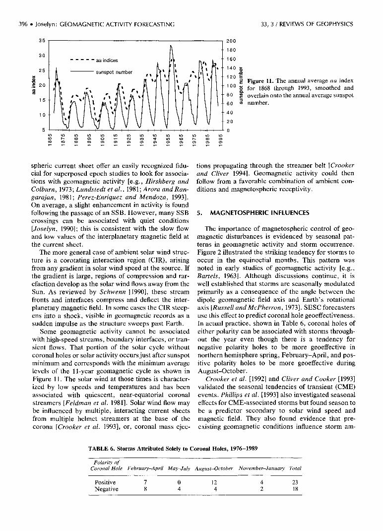
i Figure 11. The annual average a a index100 g. for 1868 through 1993, smoothed and80 g overlain onto the annual average sunspot60

40

20

in in00 05O5 O5

number.

spheric current sheet offer an easily recognized fidu-cial for superposed epoch studies to look for associa-tions with geomagnetic activity [e.g., Hirshberg andColburn, 1973; Lundstedt et al., 1981; Arora andRan-garajan, 1981; Perez-Enriquez, and Mendoza, 1993].On average, a slight enhancement in activity is foundfollowing the passage of an SSB. However, many SSBcrossings can be associated with quiet conditions[Joselyn, 1990]; this is consistent with the slow flowand low values of the interplanetary magnetic field atthe current sheet.

The more general case of ambient solar wind struc-ture is a corotating interaction region (CIR), arisingfrom any gradient in solar wind speed at the source. Ifthe gradient is large, regions of compression and rar-efaction develop as the solar wind flows away from theSun. As reviewed by Schwenn [1990], these streamfronts and interfaces compress and deflect the inter-planetary magnetic field. In some cases the CIR steep-ens into a shock, visible in geomagnetic records as asudden impulse as the structure sweeps past Earth.

Some geomagnetic activity cannot be associatedwith high-speed streams, boundary interfaces, or tran-sient flows. That portion of the solar cycle withoutcoronal holes or solar activity occurs just after sunspotminimum and corresponds with the minimum averagelevels of the 11-year geomagnetic cycle as shown inFigure 11. The solar wind at those times is character-ized by low speeds and temperatures and has beenassociated with quiescent, near-equatorial coronalstreamers [Feldman et al. 1981]. Solar wind flow maybe influenced by multiple, interacting current sheetsfrom multiple helmet streamers at the base of thecorona [Crooker et al. 1993], or, coronal mass ejec-

tions propagating through the streamer belt [Crookerand Cliver 1994]. Geomagnetic activity could thenfollow from a favorable combination of ambient con-ditions and magnetospheric receptivity.

5. MAGNETOSPHERIC INFLUENCES

The importance of magnetospheric control of geo-magnetic disturbances is evidenced by seasonal pat-terns in geomagnetic activity and storm occurrence.Figure 2 illustrated the striking tendency for storms tooccur in the equinoctial months. This pattern wasnoted in early studies of geomagnetic activity [e.g.,Bartels, 1963]. Although discussions continue, it iswell established that storms are seasonally modulatedprimarily as a consequence of the angle between thedipole geomagnetic field axis and Earth's rotationalaxis [Russell and McPherron, 1973]. SESC forecastersuse this effect to predict coronal hole geoeffectiveness.In actual practice, shown in Table 6, coronal holes ofeither polarity can be associated with storms through-out the year even though there is a tendency fornegative polarity holes to be more geoeffective innorthern hemisphere spring, February-April, and pos-itive polarity holes to be more geoeffective duringAugust-October.

Crooker et al. [1992] and Cliver and Cooker [1993]validated the seasonal tendencies of transient (CME)events. Phillips et al. [1993] also investigated seasonaleffects for CME-associated storms but found season tobe a predictor secondary to solar wind speed andmagnetic field. They also found evidence that pre-existing geomagnetic conditions influence storm am-

TABLE 6. Storms Attributed Solely to Coronal Holes, 1976-1989

Polarity ofCoronal Hole February-April May-July August-October November-January Total

PositiveNegative

124

2318


plitude: except for the strongest storms, more dis-turbed preexisting conditions correlate with strongerstorms. Is this a magnetospheric effect? Quantitativeguidance is lacking.

6. DISCUSSION

The effects of geomagnetic activity on technologicalsystems are becoming more important as componentsare miniaturized and as operating margins thin. Thereis also an increasing dependence on systems residentin space, where the levels of fluctuation in the ambientenvironment, primarily in association with geomag-netic activity, may change by orders of magnitude(e.g., energetic electron fluxes at geosynchronous or-bit). Increased demands for appropriate descriptionsand accurate predictions of geomagnetic disturbancesare emerging. This need can be addressed in severalways:

Present data and knowledge can be reformulated inmore applicable forms. For example, the SESC hasbegun expressing forecasts in terms of the probabilityof expected outcomes [Balch, 1990]. In addition to thevalue of the expected Fredericksburg A index fortomorrow, the likelihood of occurrence of active con-ditions, a minor storm, or a large (i.e., major or severe)storm is also given. This formulation has the advan-tage of informing the user that a storm may occur,even when the prudent forecast calls only for unsettledor active conditions. It also provides operators whouse cost-loss decision methods more quantitative in-formation with which to work.

Another way to be more effective in using ourcurrent data and knowledge is by developing "speci-fication" or nowcasting models that enable synthesisand vizualization of the space environment as a sys-tem. An example is the MSFM, developed for use as aoperational tool [Bales et al., 1993; Freeman et al.,1993].

Another response to improving geomagnetic fore-casts is to discard present methodologies and searchfor new ones. This response is appropriate to theresearch community but is more difficult for opera-tional service organizations, which are reluctant toadopt concepts and algorithms that have not beenthoroughly tested. In addition, new concepts are oftenbased on new data that have been gathered in researchcampaigns and are not routinely available. It usually isvery expensive to acquire new sensors on new obser-vation platforms. One operationally focused way toseek new forecasting paradigms is to employ newanalysis techniques on existing data streams. An ex-ample is the application of artificial intelligence meth-odologies to solar-terrestrial data [e.g., McPherron,1993].

Finally, new observations are being sought. Onedata set that proved in the past to be valuable for

nowcasts was the plasma and magnetic field data fromISEE 3, which was available for operations in real timein 1979-1980 [Joselyn et al, 1981]. This suite of datahas again become available, for a few hours each day,with the successful launch of the NASA WIND space-craft in late 1994. The WIND data are most helpful forshort-term (i.e., 1 hour) alerts of severe geomagneticstorms but also enable forecasters to identify and chartquasi-steady structures such as high-speed streamsand the heliospheric current sheet. An Earth-directedCME monitor [e.g., Hoeksema, 1992] is now beingdiscussed. This technique would place one (or two)coronagraphs approximately 90° away from Earth, inthe plane of the ecliptic. In this way, CMEs directedtoward Earth could be seen and their velocities couldbe estimated.

7. SUMMARY

Are accurate geomagnetic forecasts, a day or sev-eral days in advance of storm onset, possible with thepresent knowledge and data? Unfortunately, presentcapabilities are limited and are often bested by simpleforecasting schemes such as climatology. However,we are making rapid progress, having learned severalimportant things. By analyzing forecast verifications,we have been able to discard a paradigm, solar flaresas the source of nonrecurrent geophysical distur-bances, that does not verify adequately. In its place, anew concept is building. We are looking above thesolar surface into the Corona for storage and release ofmass and energy and then considering how these newreleases of mass and energy act upon and merge intothe solar wind flow to produce geoeffective topologies.

Further, we now appreciate that Earth and its mag-netic field use several physical mechanisms to extractenergy. The magnetosphere responds to details of thesolar wind (specific magnetic field orientationsweighted by atypical plasma parameters, such as ex-traordinary velocity or density [e.g., Rostoker et al.,1987]. While new observations (X ray imaging, inter-planetary remote sensing, in situ measurements) arecontributing fresh insights into the dynamics of thesystem, it is difficult indeed to predict solar windparameters in precise enough detail at the position ofEarth to be able to forecast geomagnetic activity a dayor more in advance. Nearby, real-time observations ofthe solar wind offer the best opportunity for improvedgeomagnetic warnings, but only a few minutes tohours in advance.

ACKNOWLEDGMENTS. K. A. Doggett (NOAA SpaceEnvironment Laboratory) provided much of the data andanalysis of SESC forecast verifications. S.-I. Watari (HiraisoSolar Terrestrial Research Center) contributed to the analy-sis of the geoeffectivity of solar proton events.


The editor responsible for handling this paper is ThomasCravens. He thanks two technical referees, Gordon Ros-toker and Marcia Neugebauer, and the cross-disciplinaryreferee, Duncan C. Agnew.

REFERENCES

Alien, J., H. Sauer, L. Frank, and P. Reiff, Effects of theMarch 1989 solar activity, Eos Trans. AGU, 70, 1479,1989.

Arora, B. R., and G. K. Rangarajan, Temporal variation inthe geomagnetic response to IMF sector boundary pas-sage, J. Geophys. Res., 86, 3369, 1981.

Axford, W. I., The interaction between the solar wind andthe magnetosphere, in Physics of Geomagnetic Phenom-ena, vol. 1, edited by S. Matsushita and W. H. Campbell,p. 1243, Academic, San Diego, Calif., 1967.

Balch, C., A probability forecast for geomagnetic activity, inProceedings of the 1989 Solar-Terrestrial PredictionsWorkshop, vol. 2, p. 13, Natl. Oceanic and Atmos. Ad-min., Boulder Colo., 1990.

Bales, B., et al., Status of the development of the Magneto-spheric Specification and Forecast Model, in Proceedingsof the 1992 Solar-Terrestrial Predictions Workshop, vol.2, p. 467, Natl. Oceanic and Atmos. Admin., Boulder,Colo., 1993.

Bartels, J., Discussion of time variations of geomagneticactivity indices Kp and Ap, 1932-1961, Ann. Geophys.,19, 1, 1963.

Behannon, K. W., F. M. Neubauer, and H. Barnstorf, Fine-scale characteristics of interplanetary sector boundaries,J. Geophys. Res., 86, 3273, 1981.

Bird, M. K., and P. Edenhofer, Remote sensing observa-tions of the solar corona, in Physics of the Inner Helio-sphere, vol. 1, Large-Scale Phenomena, edited by R.Schwenn and E. Marsch, p. 13, Springer-Verlag, NewYork, 1990.

Bothmer, V., and R. Schwenn, Eruptive prominences assources of magnetic clouds in the solar wind, Space Sci.Rev., 70, 215, 1994.

Bravo, S., B. Mendoza, and R. Perez-Enriquez, Coronalholes as sources of large-scale solar wind disturbancesand geomagnetic perturbations, /. Geophys. Res., 96,5387, 1991.

Burlaga, L. F. E., Magnetic clouds, in Physics of the InnerHeliosphere, vol. 2, Particles, Waves and Turbulence,edited by R. Schwenn and E. Marsch, p. 1, Springer-Verlag, New York, 1991.

Burlaga, L. F., and J. H. King, Intense interplanetary mag-netic fields observed by geocentric spacecraft during1963-1975, /. Geophys. Res., 84, 6633, 1979.

Burlaga, L. F., K. W. Behannon, and L. W. Klein, Com-pound streams, magnetic clouds, and major geomagneticstorms, /. Geophys. Res., 92, 5725, 1987.

Cane, H. V., and D. V. Reames, Some statistics of solarradio bursts of spectral types II and IV, Astrophys. J.,325,901, 1988.

Cane, H. V., S. W. Kahler, and N. R. Sheeley, Jr., Inter-planetary shocks preceded by solar filament eruptions, J.Geophys. Res., 91, 13,321, 1986.

Chapman, S., Historical introduction to aurora and magneticstorms, Ann. Geophys., 24, 497, 1968.

Chapman, S., and J. Bartels, Geomagnetism, chap. 12, p. 5,Clarendon Press, Oxford, England, 1940.

Cliffswallow, W. (Ed.), Region 5395 of March 1989, NOAATech. Memo. ERL SEL-82, Space Environ. Lab., Boul-der, Colo., 1993.

Cliver, E. W., and N. U. Crooker, A seasonal dependencefor the geoeffectiveness of eruptive solar events, Sol.Phys., 145, 347, 1993.

Cilia de Gonzalez, A. L., W. D. Gonzalez, S. L. G. Dutra,and B. T. Tsurutani, Periodic variation in the geomag-netic activity: A study based on the Ap index, /. Geo-phys. Res., 98, 9215, 1993.

Crooker, N. U., and E. W. Cliver, Postmodern view ofM-regions, J. Geophys. Res., 99, 23,383, 1994.

Crooker, N. U., E. W. Cliver, and B. T. Tsurutani, Thesemiannual variation of great geomagnetic storms and thepostshock Russell-McPherron effect preceding coronalmass ejecta, Geophys. Res. Lett., 19, 429, 1992.

Crooker, N. U., G. L. Siscoe, S. Shodhan, D. F. Webb, J.T. Gosling, and E. J. Smith, Multiple heliospheric currentsheets and coronal streamer belt dynamics, J. Geophys.Res.,98, 9311, 1993.

Dodson, H. W., and E. R. Hedeman, Comments on fila-ment-disintegration and its relation to other aspects ofsolar activity, Sol. Phys., 23, 360, 1972.

Dodson, H. W., E. R. Hedeman, and O. C. Mohler, Exam-ples of "problem" flares or situations in past solar-ter-restrial observations, in Proceedings of the 1979 Solar-Terrestrial Predictions Workshop, p. 385, Natl. Oceanicand Atmos. Admin., Boulder, Colo., 1979.

Erskine, F. T., W. M. Cronyn, S. D. Shawhan, E. C. Roelof,and B. L. Gotwols, Interplanetary scintillation at largeelongation angles: Response to solar wind density struc-ture, J. Geophys. Res., 83, 4153, 1978.

Feldman, W. C., J. R. Asbridge, S. J. Bame, E. E. Feni-more, and J. T. Gosling, The solar origins of solar windinterstream flows: Near-equatorial coronal streamers, /.Geophys. Res., 86, 5408, 1981.

Feynman, J., Geomagnetic and solar wind cycles, 1900-1975, J. Geophys. Res., 87, 6153, 1982.

Feynman, J., and N. U. Crooker, The solar wind at the turnof the century, Nature, 275, 626, 1978.

Feynman, J., and P. F. Fougere, Eighty-eight year perio-dicity in solar-terrestrial phenomena confirmed, /. Geo-phys. Res., 89, 3023, 1984.

Feynman, J., and X. Y. Gu, Prediction of geomagneticactivity on time scales of one to ten years, Rev. Geo-phys., 24, 650, 1986.

Feynman, J., and S. M. Silverman, Auroral changes duringthe eighteenth and nineteenth centuries and their impli-cations for the solar wind and the long-term variation ofsunspot activity, /. Geophys. Res., 85, 2991, 1980.

Fraser-Smith, A. C., Spectrum of the geomagnetic indexAp, J. Geophys. Res., 77, 4209, 1972.

Freeman, J., A. Nagai, P. Reiff, W. Denig, S. Gussenhoven,M. A. Shea, M. Heinemann, F. Rich, and M. Hairston,The use of neural networks to predict magnetosphericparameters for input to a magnetospheric forecast model,in Proceedings of the 1993 International Workshop onArtificial Intelligence Applications in Solar-TerrestrialPhysics, p. 167, Natl. Oceanic and Atmos. Admin.,NOAA, Boulder, Colo., 1993.

Gonzalez, A. L. C., and W. D. Gonzalez, Periodicities in theinterplanetary magnetic field polarity, J. Geophys. Res.,92, 4357, 1987.

Gonzalez, W. D., and B. T. Tsurutani, Criteria of interplan-etary parameters causing intense magnetic storm (Dst <-100 nT), Planet. Space Sci., 35, 1101, 1987.

Gonzalez, W. D., J. A. Joselyn, Y. Kamide, H. W. Kroehl,G. Rostoker, B. T. Tsurutani, and V. M. Vasyliunas,What is a geomagnetic storm?, /. Geophys. Res., 99,5771, 1994.

Gosling, J. T., Coronal mass ejections and magnetic fluxropes in interplanetary space, in Physics of Magnetic


Flux Ropes, Geophys. Monogr. Ser., vol. 58, C. T. Rus-sell, E. R. Priest, and L. C. Lee, p. 343, AGU, Washing-ton, D. C., 1990.

Gosling, J. T., The solar flare myth, J. Geophys. Res., 98,18937, 1993.

Gosling, J. T., and D. J. McComas, Field line draping aboutfast coronal mass ejecta: A source of strong out-of-theecliptic interplanetary magnetic fields, Geophys. Res.Lett., 14, 355, 1987.

Gosling, J. T., E. Hildner, J. R. Asbridge, S. J. Bame, andW. C. Feldman, Noncompressive density enhancementsin the solar wind, /. Geophys. Res., 82, 5005, 1977.

Gosling, J. T., D. N. Baker, S. J. Bame, W. C. Feldman, R.D. Zwickl, and E. J. Smith, Bidirectional solar windelectron heat flux events, /. Geophys. Res., 92, 8519,1987.

Gosling, J. T., S. J. Bame, D. J. McComas, and J. L.Phillips, Coronal mass ejections and large geomagneticstorms, Geophys. Res. Lett., 17, 901, 1990.

Gosling, J. T., D. J. McComas, J. L. Phillips, and S. J.Bame, Geomagnetic activity associated with Earth pas-sage of interplanetary shock disturbances and coronalmass ejections, J. Geophys. Res., 96, 7831, 1991.

Green, C. A., The semiannual variation in the magneticactivity indices aa and Ap, Planet. Space Sci., 32, 297,1984.

Hapgood, M. A., A double solar cycle in the 27-day recur-rence of geomagnetic activity, Ann. Geophys., 11, 248,1993.

Hedin, A. E., MSIS-86 thermospheric model, J. Geophys.Res., 92, 4649, 1987.

Hirshburg, J., and D. S. Colburn, Geomagnetic activity atsector boundaries, J. Geophys. Res., 78, 3952, 1973.

Hoeksema, J. T., Solar sources of geomagnetic storms, EosTrans. AGU, 73(3), 34, 1992.

Hoeksema, J. T., Coronal and interplanetary magnetic fieldtopology, in Proceedings of the 1992 Solar-TerrestrialPredictions Workshop, vol. 2, p. 3, Natl. Oceanic andAtmos. Admin., Boulder, Colo., 1993.

Hoeksema, J. T., and X. Zhao, Prediction of magnetic ori-entation in driver gas associated —Bz events, J. Geophys.Res., 97, 3151, 1992.

Hoeksema, J. T., J. M. Wilcox, and P. H. Scherrer, Struc-ture of the heliospheric current sheet in the early portionof sunspot cycle 21, J. Geophys. Res., 87, 10,331, 1982.

Hundhausen, A. J., An interplanetary view of coronal holes,in Coronal Holes and High Speed Solar Wind Streams,edited by J. B. Zirker, p. 225, Colo. Assoc. Univ. Press,Boulder, 1977.

Hundhausen, A. J., The size and locations of coronal massejections: SMM observations from 1980 and 1984-1989,J. Geophys. Res., 98, 13,177, 1993.

Jackson, B. V., and C. Leinert, Helios images of solar massejections, J. Geophys. Res., 90, 10,759, 1985.

Jackson, B. V., G. A. Bulk, and K. V. Sheridan, in Solarand Interplanetary Dynamics, edited by M. Dryer and E.Tandberg-Hanssen, p. 379, D. Reidel, Norwell, Mass.,1980.

Jackson, B., R. Gold, and R. Altrock, The solar mass ejec-tion imager, Adv. Space Res., 77(1), 377, 1991.

Jacobs, J. A., Reversals of the Earth's Magnetic Field,Adam Hilger, Bristol, England, 1984.

Joselyn, J. A., SESC methods for short-term geomagneticpredictions in Proceedings of the 1984 Solar-TerrestrialPredictions Workshop, p. 404, Natl. Oceanic and Atmos.Admin., Boulder, Colo., 1986a.

Joselyn, J. A., Real-time prediction of global geomagneticactivity, in Solar Wind-Magneto sphere Coupling, edited

by Y. Kamide and J. A. Slavin, 127, Terra Sci. Tokyo,1986b.

Joselyn, J. A., Geomagnetic quiet day selections, Pure Appl.Geophys., 131, 333, 1989.

Joselyn, J. A., Forecasting magnetically quiet periods, inProceedings of the 1989 Solar-Terrestrial PredictionsWorkshop, vol. 1., p. 102, Natl. Oceanic and Atmos.Admin., Boulder, Colo., 1990.

Joselyn, J. A., and P. S. Mclntosh, Disappearing solar fila-ments: A useful predictor of geomagnetic activity, J.Geophys. Res., 86, 4555, 1981.

Joselyn, J. A., and B. T. Tsurutani, Geomagnetic suddenimpulses and storm sudden commencements, Eos Trans.AGU, 71, 1808, 1990.

Joselyn, J. A., J. Hirman, and G. R. Heckman, ISEE 3 inreal time, Eos Trans. AGU, 62, 617, 1981.

Joselyn, J. A., J. A. Flueck, and T. Brown, Geomagneticclimatology, Ann. Geophys., 6, 595, 1988.

Kahler, S. W., Solar flares and coronal mass ejections,Annu. Rev. Astron. Astrophys., 30, 113, 1992.

Kahler, S., A search for geomagnetic storm evidence of thereversal of the solar dipole magnetic field and interplan-etary Bz, J. Geophys. Res., 98, 3485, 1993a.

Kahler, S. W., Coronal mass ejections and long rise times ofsolar energetic particle events, J. Geophys. Res., 98,5607, 1993b.

Kahler, S. W., E. Hildner, and M. A. I. Van Hollebeke,Prompt solar proton events and coronal mass ejections,Sol. Phys., 57, 429, 1978.

Kahler, S. W., N. R. Sheeley Jr., R. A. Howard, M. J.Koomen, D. J. Michels, R. E. McGuire, T. T. vonRosenvinge, and D. V. Reames, Associations betweencoronal mass ejections and solar energetic proton events,/. Geophys. Res., 89, 9683, 1984.

Klein, L. W., and L. F. Burlaga, Interplanetary magneticclouds at 1 AU, J. Geophys. Res., 87, 613, 1982.

Lanzerotti, L. J. (Ed.), Impacts of ionospheric/magneto-spheric processes on terrestrial science and technology,in Solar System Plasma Physics, vol. Ill, edited by L. J.Lanzerotti, C. F. Kennel, and E. N. Parker, p. 317,North-Holland, New York, 1979.

Lanzerotti, L. J., C. G. Maclennan, and A. C. Fraser-Smith,Background magnetic spectra: 10~5 to 105 Hz, Geophys.Res. Lett., 17, 1593, 1990.

Legrand, J.-P., and P. A. Simon, Ten cycles of solar andgeomagnetic activity, Sol. Phys., 70, 173, 1981.

Legrand, J.-P., and P. A. Simon, A two-component solarcycle, Sol. Phys., 131, 187, 1991.

Leinbach, H., S. Ananthakrishnan, and T. R. Detman, Theutility of interplanetary scintillation maps in forecastinggeomagnetic activity: A study based on single-stationdata from Cambridge, United Kingdom, NOAA Tech.Memo. ERL SEL-83, Space Environ. Lab., Boulder,Colo., 1994.

Lincoln, J. V., Geomagnetic indices, in Physics of Geomag-netic Phenomena, vol. 1, edited by S. Matsushita and W.H. Campbell, p. 67, Academic, San Diego, Calif., 1967.

Lundstedt, H., P. H. Scherrer, and J. M. Wilcox, Geomag-netic activity and Hale sector boundaries, Planet. SpaceSci., 29, 167, 1981.

Marsden, R. G., T. R. Sanderson, C. Tranquille, K.-P.Wenzel, and E. J. Smith, ISEE 3 observations of low-energy proton bidirectional events and their relation toisolated interplanetary magnetic structures, J. Geophys.Res., 92, 11,009, 1987.

Marubashi, K., Structure of the interplanetary magneticclouds and their solar origins, Adv. Space Res., 6, 335,1986.

Matsushita, S., Solar quiet and lunar daily variation fields, in


Physics of Geomagnetic Phenomena, vol. 1, edited by S.Matsushita and W. H. Campbell, p. 302, Academic, SanDiego, Calif., 1967.

Mayaud, P. N. (Ed.), Derivation, Meaning, and Use ofGeomagnetic Indices, Geophys. Monogr. Ser., vol. 22,AGU, Washington, D. C., 1980.

McComas, D. J., J. T. Gosling, S. J. Bame, E. J. Smith, andH. V. Cane, A test of magnetic field draping induced Bzperturbations ahead of fast coronal mass ejecta, J. Geo-phys. Res., 94, 1465, 1989.

Mclntosh, P. S., Solar magnetic fields derived from hydro-gen-alpha filtergrams, Rev. Geophys., 10, 837, 1972.

McNamara, L. F., and C. S. Wright, Disappearing solarfilaments and geomagnetic activity, Nature, 299, 537,1982.

McPherron, R. L., Possible applications of expert systemsand fuzzy logic in solar terrestrial physics, in Proceedingsof the International Workshop on Artificial IntelligenceApplications in Solar-Terrestrial Physics, p. 1, Natl. Oce-anic and Atmos. Admin., Boulder, Colo., 1993.

Menvielle, M., and A. Berthelier, The /^-derived planetaryindices: Description and availability, Rev. Geophys., 29,415, 1991. (Correction, Rev. Geophys., 30, 91, 1992.)

Menvielle, M., and A. Berthelier, Correction to The #-de-rived planetary indices: Description and availability, Rev.Geophys., 30, 91, 1992.

Moore, V., and R. A. Harrison, A characterization of dis-crete solar wind events detected by interplanetary scin-tillation mapping, /. Geophys. Res., 99, 27, 1994.

Munro, R. H., J. T. Gosling, E. Hildner, R. M. MacQueen,A. I. Poland, and C. L. Ross, The association of coronalmass ejection transients with other forms of solar activ-ity, Sol. Phys., 61, 201, 1979.

Neugebauer, M., Observational constraints on solar windacceleration mechanisms, in Solar Wind Five, edited byM. Neugebauer, NASA Conf. Publ, cp2280, 135, 1983.

Neugebauer, M., The problem of associating solar and in-terplanetary events, in Solar Wind Six, edited by V. Pizzo,T. Holzer, and D. Sime, vol. 1, Tech. Note NCARITN-306+ Proc., p. 243, Natl. Cent, for Atmos. Res., Boulder,Colo., 1988.

Neupert, W. M., and V. Pizzo, Solar coronal holes assources of recurrent geomagnetic disturbances, J. Geo-phys. Res., 79, 3701, 1974.

Nolte, J. T., A. S. Krieger, A. F. Timothy, R. E. Gold, E. C.Roelof, G. Vaiana, A. J. Lazarus, J. D. Sullivan, and P.S. Mclntosh, Coronal holes as sources of solar wind, Sol.Phys.,46, 303, 1976.

Perez-Enriquez, R., and B. Mendoza, Geomagnetic re-sponse of the Earth to crossings of the heliospheric cur-rent sheet, /. Geophys. Res., 98, 19,349, 1993.

Phillips, J. L., J. T. Gosling, and D. J. McComas, Coronalmass ejections and geomagnetic storms: Seasonal varia-tions, in Proceedings of the 1992 Solar-Terrestrial Pre-dictions Workshop, vol. 3, p. 242, Natl. Oceanic andAtmos. Admin., Boulder, Colo., 1993.

Pudovkin, M. I., and A. D. Chertkov, The magnetic field ofthe solar wind, Sol. Phys., 50, 213, 1976.

Reames, D. V., Recent observations and the modeling ofsolar proton events, in Proceedings of the 1992 Solar-Terrestrial Predictions Workshop, vol. 2, p. 302, Natl.Oceanic and Atmos. Admin., Boulder, Colo., 1993.

Richardson, I. G., and H. V. Cane, Signatures of shockdrivers in the solar wind and their dependence on thesolar source location, J. Geophys. Res., 98, 15,295, 1993.

Richardson, I. G., C. J. Farrugia, and D. Winterhalter, Solaractivity and coronal mass ejections on the western hemi-sphere of the Sun in mid-August 1989: Association with

interplanetary observations at the ICE and IMP 8 space-craft, /. Geophys. Res., 99, 2513, 1994.

Rostoker, G., Geomagnetic indices, Rev. Geophys., 10, 935,1972.

Rostoker, G., S.-I. Akasofu, W. Baumjohann, Y. Kamide,and R. L. McPherron, The roles of direct input of energyfrom the solar wind and unloading of stored magnetotailenergy in driving magnetospheric substorms, Space Sci.Rev.,46, 93, 1987.

Russell, C. T., and R. L. McPherron, Semiannual variationof geomagnetic activity, J. Geophys. Res., 78, 92, 1973.

Russell, C. T., R. L. McPherron, and R. E. Burton, On thecause of geomagnetic storms, /. Geophys. Res., 79, 1105,1974.

Sanchez-Ibarra, A., and M. Barraza-Paredes, Catalogue ofCoronal Holes 1970-1991, Rep. UAG-102, World DataCent. A for Sol.-Terr. Phys., Natl. Geophys. Data Cent.,Boulder, Colo., 1992.

Sargent, H. H., Ill, The 27-day recurrence index, in SolarWind-Magneto sphere Coupling, edited by Y. Kamideand J. A. Slavin, p. 143, Terra Sci., Tokyo, 1986.

Schwenn, R., Direct correlation between coronal transientsand interplanetary disturbances, Space Sci. Rev., 34, 85,1983.

Schwenn, R., Relationship of coronal transients to interplan-etary shocks: 3D aspects, Space Sci. Rev., 44, 139, 1986.

Schwenn, R., Large-scale structures of the interplanetarymedium, in Physics of the Inner Heliosphere I, edited byR. Schwenn and E. Marsch, p. 99, Springer-Verlag, NewYork, 1990.

Sheeley, N. R., Jr., and J. W. Harvey, Coronal holes, solarwind streams, and geomagnetic disturbances during 1978and 1979, Sol. Phys., 70, 237, 1981.

Sheeley, N. R., Jr., et al., Coronal changes associated witha disappearing filament, Sol. Phys., 45, 377, 1975.

Sheeley, N. R., Jr., R. A. Howard, M. J. Koomen, and D. J.Michels, Associations between coronal mass ejectionsand soft x-ray events, Astrophys. J., 272, 349, 1983.

Sheeley, N. R., Jr., R. T. Stewart, R. D. Robinson, R. A.Howard, M. J. Koomen, and D. J. Michels, Associationsbetween coronal mass ejections and metric type II bursts,Astrophys. J., 279, 839, 1984.

Sheeley, N. R., Jr., R. A. Howard, M. J. Koomen, D. J.Michels, R. Schwenn, K. H. Muhlhauser, and H. Rosen-bauer, Coronal mass ejections and interplanetary shocks,J. Geophys. Res., 90, 163, 1985.

Tang, F., S.-I. Akasofu, E. Smith, and B. Tsurutani, Mag-netic fields on the Sun and the north-south component oftransient variations of the interplanetary magnetic field at1 AU, J. Geophys. Res., 90, 2703, 1985.

Tang, F., B. T. Tsurutani, W. D. Gonzalez, S.-I. Akasofu,and E. J. Smith, Solar sources of interplanetary south-ward Bz events responsible for major magnetic storms(1978-1979), /. Geophys. Res., 94, 3535, 1989.

Thompson, R., G. Heckman, and J. Hirman, The worldspace weather service, in Proceedings of the 1992 Solar-Terrestrial Predictions Workshop, vol. 1, p. 17, Natl.Oceanic and Atmos. Admin., Boulder, Colo., 1993.

Thomson, A. W. P., Neural networks and non-linear predic-tion of geomagnetic activity, in Proceedings of the 1993International Workshop on Artificial Intelligence Appli-cations in Solar-Terrestrial Physics, p. 133, Natl. Oceanicand Atmos. Admin., NOAA, Boulder, Colo., 1993.

Thomson, A. W. P., T. D. G. Clark, and D. J. Kerridge,Forecasting Ap in the short-term using time series anal-ysis, in Proceedings of the 1992 Solar-Terrestrial Predic-tions Workshop, vol. 3, p. 269, Natl. Oceanic and Atmos.Admin., NOAA, Boulder, Colo., 1993.

Tsurutani, B. T., W. D. Gonzalez, F. Tang, S.-I. Akasofu,


and E. J. Smith, Origin of interplanetary southward mag-netic fields responsible for major magnetic storms nearsolar maximum (1978-1979), /. Geophys. Res., 93, 8519,1988.

Wang, Y.-M., and N. R. Sheeley Jr., The solar origin oflong-term variations of the interplanetary magnetic fieldstrength, J. Geophys. Res., 93, 11,227, 1988.

Wang, Y.-M., and N. R. Sheeley Jr., Solar wind speed andcoronal flux-tube expansion, Astrophys. J., 355, 726,1990.

Watanabe, T., and R. Schwenn, Large-scale propagationproperties of interplanetary disturbances revealed fromIPS and spacecraft observations, Space Sci. Rev., 51,147, 1989.

Watari, S., The latitudinal distribution of coronal holes andgeomagnetic storms due to coronal holes, in Proceedingsof the 1989 Solar-Terrestrial Predictions Workshop, vol.1, p. 627, Natl. Oceanic and Atmos. Admin., NOAA,Boulder, Colo., 1990.

Webb, D. F., The heliospheric manifestation and geoeffec-tiveness of solar mass ejections, in Proceedings of the1992 Solar-Terrestrial Predictions Workshop, vol. 2, p.71, Natl. Oceanic and Atmos. Admin., Boulder, Colo.,1993.

Webb, D. F., and A. J. Hundhausen, Activity associatedwith the solar origin of coronal mass ejections, Sol.Phys., 108, 383, 1987.

Wilcox, J. M., and N. F. Ness, Quasi-stationary corotatingstructure in the interplanetary medium, /. Geophys. Res.,70, 5793, 1965.

Wilson, L., An evaluation of digitally derived ^-indices, J.Geomagn. Geoelectr., 39, 97, 1987.

Wilson, R. M., Geomagnetic response to magnetic clouds,Planet. Space Sci., 35, 329, 1987.

Wilson, R. M., On the behavior of the Dst geomagneticindex in the vicinity of magnetic cloud passages at Earth,J. Geophys. Res., 95, 215, 1990.

Wilson, R. M., and E. Hildner, Are interplanetary magneticclouds manifestations of coronal transients at 1 AU?, Sol.Phys., 91, 169, 1984.

Wilson, R. M., and E. Hildner, On the association of mag-netic clouds with disappearing filaments, /. Geophys.Res., 91, 5867, 1986.

Woo, R., Solar cycle variation of interplanetary distur-bances observed as Doppler scintillation transients, J.Geophys. Res., 98, 18,999, 1993.

Woo, R., and P. Gazis, Large-scale solar-wind structurenear the Sun detected by Doppler scintillation, Nature,366, 543, 1993.

Woo, R., and R. Schwenn, Comparison of Doppler scintil-lation and in situ spacecraft plasma measurements ofinterplanetary disturbances, J. Geophys. Res., 96,21,227, 1991.

Woo, R., J. W. Armstrong, N. R. Sheeley, Jr., R. A.Howard, M. J. Koomen, D. J. Michels, and R. Schwenn,Doppler scintillation observations of interplanetaryshocks within 0.3 AU, J. Geophys. Res., 90, 154, 1985.

Wright, C. S., Disappearing filaments and geomagneticstorms—The role of filament orientation, in Proceedingsof the 1984 Solar-Terrestrial Predictions Workshop, p.420, Natl. Oceanic and Atmos. Admin., Boulder, Colo.,1986.

Wright, C. S., and L. F. McNamara, The relationshipsbetween disappearing solar filaments, coronal mass ejec-tions, and geomagnetic activity, Sol. Phys., 87, 401, 1983.

Wright, C. S., and D. F. Webb, The signatures of disappear-ing filaments in the interplanetary medium at 1 AU, inProceedings of the 1989 Solar-Terrestrial PredictionsWorkshop, vol. 1, p. 664, Natl. Oceanic and Atmos.Admin., Boulder, Colo., 1990.

Zhang, G., and L. F. Burlaga, Magnetic clouds, geomagneticdisturbances, and cosmic ray decreases, /. Geophys.Res., 93, 2511, 1988.

J. A. Joselyn, NOAA Space Environment Laboratory,325 Broadway, Boulder, CO 80303. (e-mail: [email protected])

GEOMAGNETIC ACTIVITY FORECASTING: THE STATE OF THE...

Documents

Transcript of GEOMAGNETIC ACTIVITY FORECASTING: THE STATE OF THE...