MAGNETIC PULSATIONS: THEIR SOURCES AND RELATION TO SOLAR WIND AND GEOMAGNETIC ACTIVITY

Robert L. McPherron (Institute of Geophysics and Planetary Physics, University of California Los Angeles, Los Angeles, CA 90095-1567) rmcpherron@igpp.ucla.edu

Abstract ULF waves incident on the Earth are produced by processes in the magnetosphere and solar wind. These processes produce a wide variety of ULF wave types that are classified on the ground as either Pi or Pc pulsations. Waves of different frequencies and polarizations originate in different regions of the magnetosphere. The location of the projections of these regions onto the Earth depends on the solar wind dynamic pressure and magnetic field. The occurrence of various waves depends on conditions in the solar wind and in the magnetosphere. Changes in orientation of the interplanetary magnetic field or an increase in solar wind velocity can have dramatic effects on the type of waves seen on the Earth. Similarly the occurrence of a magnetospheric substorm or magnetic storm will affect which waves are seen. The properties of ULF waves seen at the ground contain information about the processes that generate them and the regions through which they have propagated. The properties also depend on the conductivity of the Earth underneath the observer. Information about the state of the solar wind and the magnetosphere distributed by the NOAA Space Disturbance Forecast Center can be used to help predict when certain types and frequencies of waves will be observed. The study of ULF waves is a very active field of space research and much has yet to be learned about the processes that generate these waves.

Introduction What are Micropulsations, Magnetic Pulsations, ULF Waves? Magnetic micropulsation is the name originally given to low frequency oscillations in the Earth’s magnetic field. The name represents the manner in which these oscillations were discovered through observation of the end of a very long compass needle with a microscope. The following quote from [Chapman and Bartels, 1962] is taken from one of the first published reports (about 1757) of such oscillations.

“From the serrated appearance of the curves, it will be seen that a force tending to increase one of the elements was generally followed after a short interval by one of the opposite description, and vice versa. The exertion of the disturbing force was thus of a throbbing or pulsatory character. The interval of time between two of these minute pulsations may be said to have varied from half a minute, or the smallest observable portion of time, up to four or five minutes. This pulsatory character of the disturbing force agrees well with the nature of its action on telegraphic wires, in which observers have noticed that the polarity of the current changes very frequently.”

The waveform of these waves was eventually recorded by reflecting a light beam onto a photographic film from a mirror on the needle. An example recording is shown in Figure 1. The peak-to-peak amplitude of the waves in this figure is about 40 nT and their period is about two minutes. As more was learned about the waves the prefix micro was dropped and these oscillations became known as magnetic pulsations. Recently the signals were renamed again as Ultra Low Frequency (ULF) waves. The international definition of this portion of the

1

electromagnetic spectrum is any wave in the frequency band 1 mHz to 1 Hz (1000 sec – 1 sec period).

Classification of ULF Waves In 1963 an IAGA committee classified ULF waves using a system dependent on waveform and wave period [Jacobs et al., 1964]. Oscillations with quasi-sinusoidal waveform were called pulsations continuous (Pc). Those with waveforms that are more irregular were called pulsations irregular (Pi). Each major type was subdivided into period bands that roughly isolate a specific type of pulsation. Today it is known that the limits of these bands are not precise, and that more than one process produces waves in a particular band. The definitions of these frequency bands are shown in Figure 2.

Figure 1: An example of a photographic recording of magnetic oscillations of a compass needle. Vertical lines denote half hour intervals. The vertical scale is shown in both minutes of arc and nanoTesla (γ) units. The pulsation packet at about 0900 UT (GMT) is called a giant pulsation [Chapman and Bartels, 1962].

How are ULF Waves Created? ULF waves are created by a variety of processes in magnetized plasma. Plasma is the name given to highly ionized gases threaded by a magnetic field. When the collision frequency in plasma is sufficiently low, the charged particles simply gyrate around the magnetic field and travel along it. Any force that moves the particles also moves the magnetic field and vise versa. In this situation the field and plasma are frozen together. This concept enabled Hannes Alfven to describe a simple process that creates a low frequency wave that propagates along a magnetic field line. He received the Nobel Prize for this discovery and the wave he described is now called the Alfven wave.

Alfven’s model for wave generation is summarized in Figure 3 [Alfven and Falthammar, 1963]. Consider an infinite volume of fully ionized hydrogen. As shown in the perspective view of panel (a), imagine that a force is applied to the plasma perpendicular to the field B displacing a rectangular section of plasma with velocity v. As the charges begin to move they experience a Lorentz force F = q(v x B). The electrons move to the left side of the moving slab, and the protons to the right side as illustrated in the top view panel (b). This polarization of the charges

Figure 2: ULF waves are classified into two types: pulsations continuous (Pc) and pulsations irregular (Pi). Each type is subdivided into frequency bands roughly corresponding to distinct phenomena [Jacobs et al., 1964].

2

creates an electric field E orthogonal to both v and B. If the slab were in vacuum the charges would be trapped at the edges of the column and the force of the electric field would eventually stop any further transfer of charge. At this point the electric force would be equal and opposite to the Lorentz force so that E = - V x B. However, in plasma the charges can flow through the surrounding fluid in an attempt to neutralize the polarization. This charge motion creates an electrical current J as shown in the end view of panel (c). As this current flows across the magnetic field above and below the moving slab it exerts a force on the gas, F = J x B. This force is in the same direction as the initial motion of the slab. Consequently, the plasma above and below begins to move.

Figure 3: The creation of an Alfven wave by displacing a slab of plasma threaded by a magnetic field. Panels a through f show successive steps in the production of a pair of pulses that propagate along a magnetic field line [Alfven and Falthammar, 1963].

The same argument can now be applied to these two moving slabs. They become polarized driving currents that cause slabs further above and below the initial slab to start moving as seen in panel (d). Clearly, the initial disturbance is propagating in both directions along the field away from the initial disturbance. As illustrated in the side view of panel (e) the displacement of the slab distorts the magnetic field that is frozen into the plasma. As the field bends, tension develops creating a restoring force that brings the slab to a stop and then returns it towards its initial location. As this happens the moving slabs above and below the initial slab distort the field line in the same way so that two pulses appear to propagate away from the origin. These pulses are Alfven waves.

Solutions of the MHD Wave Equation The Alfven wave is only one of the wave modes that can propagate in plasma. Maxwell’s equations for the electric and magnetic fields have two independent solutions. In addition, a gas also supports sound waves or pressure fluctuations in the density. In magnetized plasma the two electromagnetic waves are coupled to the sound wave by the frozen in field and there are three solutions to the basic equations. A low frequency approximation

Figure 4: The diagram shows the speed of the fast, intermediate (Alfven), and slow waves as a function of the angle of propagation relative to the background field B0. VA is the Alfven speed, cs is the sound speed, and cms is the magnetosonic speed, a combination of the Alfven and sound speed [Baumjohann and Treumann, 1996].

3

to the basic equations is called magnetohydrodynamics or MHD. The wave solutions to these equations are called MHD waves.

There is a variety of names for the three MHD waves, but the most common are fast, intermediate, and slow waves. These names are based on the speed of the wave along the magnetic field. The fast wave is a combination of pressure and field fluctuations. When the fast wave propagates perpendicular to the background field it is seen as alternating compressions and rarefactions of both the field and density. The intermediate speed wave is the Alfven wave just described. It consists of bends in the field that do not change the density. The slow wave is closest to being a pure sound wave. Each of these waves has unique polarization properties with the electric, magnetic, and plasma velocity fluctuations being oriented in different directions relative to the direction of wave propagation and background field.

Figure 5: Boundaries of various regions of the magnetosphere are projected into the magnetic equatorial plane. They include the bow shock, magnetopause, plasmapause, and inner edge of the plasma sheet. The circle around the Earth at 6.6 Re is synchronous orbit.

The dependence of wave speed on direction of propagation for the three wave modes is shown in Figure 4. The fast mode and Alfven mode propagate with the Alfven velocity along the field. This velocity is given by 2

0A µ ρ=V B where B is the field strength and ρ the plasma density. Perpendicular to the field the fast mode speed is a combination of the Alven and sound speeds,

2ms s Ac c= + 2v The Alfven mode speed is zero, i.e. does not propagate in this direction. Parallel

to the field the slow mode moves at the sound speed s Bc k Tγ= im and like the Alfven wave, does not propagate perpendicular to the field. In general, the ULF waves seen at the ground originate in space as either fast mode, or intermediate mode, or a combination of the two. They propagate along or across the magnetic field until they reach the ionosphere. At the ionosphere they drive electrical currents that radiate pure electromagnetic waves into the neutral atmosphere. Thus magnetic pulsations measured on the ground are MHD waves converted to purely electromagnetic waves in the ionosphere.

ULF waves measured on the ground are produced in various regions of the magnetosphere by a variety of physical processes. To understand what type of waves will be seen at particular latitudes one must know which region of the magnetosphere the local field line passes through. Unfortunately, the magnetosphere is highly dynamic and the magnetic projections of these regions change with the level of magnetic activity. There are two main solar wind parameters that determine the locations of these regions, the dynamic pressure, ρV2, and the rate of transport

4

of southward magnetic flux, VBs. Increases in dynamic pressure compress the magnetosphere shrinking its size. Southward magnetic field erodes magnetic flux from the day side allowing the solar wind to transport this flux to the night side where it accumulates in the lobes of the magnetic tail. All of the boundaries and regions play important roles in determining the type of ULF waves seen on the ground [McPherron, 1991; McPherron et al., 1973].

An equatorial view of the solar wind and magnetosphere Figure 5 shows an equatorial cross section of the magnetosphere for a low solar wind dynamic pressure of 0.8 nP. The outer limit of the Earth’s magnetic field is called the magnetopause. The magnetopause is a layer of current that confines the Earth’s field inside the boundary. At the nose of the magnetosphere this boundary is usually at a distance of about 10 Re. On the flanks, it is 15 Re away, and far down the tail, it is at a distance of 25-30 Re from the center. Upstream of the magnetopause is the bow shock. The shock is typically about 3 Re upstream of the magnetopause. The shock exists because the solar wind is typically moving at about eight times the speed of the fast mode wave, i.e. the solar wind is super magnetosonic. The shock must slow down the solar wind enough that fast waves travel faster than the flow so that they can carry pressure information upstream. The waves set up a pressure distribution that deflects the flow around the magnetopause.

Figure 6: A projection of the magnetosphere into the noon-midnight meridian plane at equinox when the dipole axis is orthogonal to the Earth-Sun line. The Sun is to the left and the magnetic tail to the right. The shaded region behind the Earth along the Earth-Sun line is the plasma sheet. The bow shock, magnetopause, inner edge of the plasma sheet, upper and lower edges of the plasma sheet and the tail lobes are depicted in the drawing. Field lines in the solar wind are purely southward and interacting with the Earth’s field producing a magnetic configuration open to the solar wind [McPherron, 1987].

Figure 7: Projection of magnetospheric regions onto the Earth. A cross denotes the magnetic pole. The polar cap is the region poleward of the auroral oval. The plasma trough equatorward of the oval, but poleward of the plasmasphere [Vasyliunas, 1983].

On the nightside a thick layer of plasma separates the two lobes of the magnetic field (see Figure 6). In Figure 5 there is an inner edge to this sheet of plasma that roughly corresponds to the first closed drift path around the Earth for hot electrons from the tail. Inside of this boundary is the plasmapause, a sharp boundary

5

in plasma density. The plasmapause is created by electric fields in the magnetosphere and is highly dynamic moving inward with increasing magnetic activity, and outward with decreasing activity. In steady state the plasmapause is a separatrix between cold particle drift paths that are open to the magnetopause and those that are closed around the Earth. Cold particles from the ionosphere fill the plasmasphere. The extension of the separatrix into the tail is shown in the diagram.

A noon-midnight meridian view of the magnetosphere The intersections of the various magnetospheric boundaries with the noon-midnight meridian plane are shown in Figure 6. This projection shows the shape of the Earth’s magnetic field as distorted by its interaction with the solar wind. On the day side the magnetic field typically ends at about 10 Re. The regions separating field lines that pass through the dayside equator, and those that are swept back into the tail, are called the northern and southern polar cusps. The cusps provide openings for particles and waves in the magnetosheath to easily enter the magnetosphere.

Figure 8: The electron and ion foreshocks are produced by particles reflected from the bow shock. As the particles move upstream along the tangent field line they interact with the solar wind producing waves. The type of waves depends on the distribution of particles that reach a certain point [Russell and Hoppe, 1983].

Note that the magnetopause does not completely contain the field when the solar wind magnetic field is southward. This orientation allows the solar wind field to merge with the Earth’s field at the nose creating an ‘x-line’ field configuration. The solar wind then transports the interconnected field lines over the Earth’s poles and stretches them into a long tail on the night side. Far behind the Earth at the center of the tail is another x-line were the field lines come back together and reconnect. The newly reconnected field lines then move up the tail towards the Sun, flowing around the Earth.

Figure 9: Streamline in the solar wind at the left pass through the bow shock into the magnetosheath. Only streamlines close to the subsolar point of the bow shock (bottom left) come close to the magnetopause. Disturbances on streamlines near the top of the diagram pass around the Earth far from the magnetopause [Spreiter and Stahara, 1985].

6

Note that there are three types of field lines in this drawing: Solar wind field lines connected to the Sun; open field line connected to the Sun at one end and to one pole of the Earth at the other; closed field lines that connect to the Earth at each end. This field geometry projects disturbances in the magnetosphere onto the Earth.

Projection of the magnetosphere onto the Earth’s surface Figure 7 presents a north polar view of the Earth identifying various projected regions. Intuition based on the properties of the dipole field does not work well in this projection because of the extreme distortion of the outer parts of the magnetic field. A roughly circular region around the north magnetic pole is called the polar cap. Field lines from this region pass outward into the north lobe of the magnetic tail. They eventually pass through the magnetopause becoming solar wind field lines. Because these field lines are open to the solar wind, they provide easy access to certain types of particles coming from the Sun.

Figure 10: Alfven waves in the solar wind magnetic field (left axis) and flow velocity (right axis). The traces of B and V are virtually indistinguishable. Note the absence of variations in total field and density [Barnes, 1983].

Figure 11: The magnetic field variations observed at the Earth’s bow shock. The top panel shows a quasi-perpendicular shock (ΘBN = 62°) (see text), and the bottom panel shows a parallel shock (ΘBN = 26°). Both Mach number and beta are the same [Russell, 1985].

Equatorward of the polar cap is the auroral oval. On the night side the auroral oval maps into the plasma sheet. The poleward edge of the nightside oval is generally assumed to be the last closed field line that connects to the distant x-line. The equatorward edge of the auroral oval maps to the inner edge of the plasma sheet. On the day side the oval projects to the polar cusp, the region where field lines normally crossing the equator on the day side are swept back into the tail.

7

As mentioned earlier the Earth’s magnetic field lines merge with a southward solar wind magnetic field at the nose of the magnetosphere and are then dragged over the polar caps. The feet of these field line move from noon to midnight across the polar cap dragging the ionospheric plasma towards midnight. Eventually these open field lines reconnect at the distant x-line and flow Sunward in the plasma sheet passing around the Earth. The feet of these field lines leave the polar cap and travel through the auroral oval dragging the ionospheric plasma. Depending on which side of the separatrix the field lines are on they will pass around either the dawn or dusk side of the Earth. This closed system of magnetospheric and ionospheric flow is called magnetospheric and ionospheric convection.

Figure 12: Generation of a pair of field-aligned currents (FAC) by a step-like change in the diameter of the magnetopause due to a decrease of decrease in dynamic pressure. Panel (a) shows the step propagating to the left in the rest frame of the magnetosphere. Panel (b) shows the apparent flow in the rest frame of the step. The streamline indicate a vortical flow with FAC out of the equator at A and into the equator at C. In panel (c) These FAC close in the ionosphere through a Pedersen current (horizontal bars), and also generate a Hall current (thin lines) [Kivelson and Southwood, 1991a].

Somewhat equatorward of the auroral oval is the projection of the plasmapause. Under quiet conditions the ionosphere equatorward of the plasmapause is shielded from the effects of convection.

External Sources of ULF Waves Many of the waves seen at the Earth’s surface originate outside the magnetosphere [Yumoto, 1988]. The solar wind, the foreshock, the bow shock and the magnetopause are all sources of ULF waves. Many of these waves pass through the magnetopause and propagate through the magnetosphere. Internally they interact with waveguides, cavities, and field lines creating the pulsations actually seen at the surface.

Solar wind The solar wind is a source of ULF waves, particularly at low frequencies around 1 mHz [Barnes, 1983]. Some of these waves originate at the Sun and are both carried by, and propagate through, the solar wind. A typical example of these waves is presented in Figure 10. The fluctuations in the components of the field and velocity vectors are often irregular with a smooth, power-law spectrum. The individual component time series of B and V are virtually indistinguishable indicating a high correlation between the V and B perturbations. In addition, the magnitude of B and the plasma density are virtually constant. Both observations indicate that the fluctuations are caused by Alfven waves (the intermediate mode). At other times there are quasiperiodic variations in the solar wind density, and hence dynamic pressure. These pressure changes cause

8

the magnetosphere to expand and contract creating global changes in the internal magnetic field. In a recent report [Kepko et al., 2002] show that the spectrum of the dynamic pressure has multiple peaks at frequencies including f = 0.4, 0.7, 1.0, and 1.3 mHz. The simultaneous spectrum of the total field at synchronous orbit is virtually identical. The authors speculate that these waves may have originated at the Sun as pressure waves caused by granulation, and not in a magnetospheric waveguide as has sometimes been suggested [Samson et al., 1991].

Ion foreshock The ion foreshock is another source of ULF waves seen in the magnetosphere. Figure 8 shows the relation of the electron and ion foreshocks to the bow shock [Greenstadt et al., 1980]. Both foreshocks are caused by particles moving upstream along magnetic field lines tangential to the shock. As the particles travel upstream they E x B drift in the solar wind electric field. For the geometry shown, the electric field will be upward, out of the plane of the figure when the magnetic field points away from the Sun towards the Earth. Then the particle drift is orthogonal to B in the downstream direction. An oppositely directed B reverses the electric field but the drift is the same. The actual paths followed by electrons and ions are denoted by the string of – and + signs. The ion path is at a greater angle to the tangent field line because the heavier ions move along the field lines more slowly than the electrons.

As the ions move upstream they interact with the solar wind producing waves with frequencies that depend on the strength of the solar wind magnetic field [Russell and Fleming, 1976; Russell and Hoppe, 1983]. These waves propagate very slowly relative to the speed of the solar wind so they are swept downstream towards the bow shock. The properties of the waves depend on the nature of the ion distributions [Hoppe et al., 1982; Thomsen, 1985]. Close to the ion foreshock the ions are field aligned and produce small amplitude 1 Hz waves. At larger angles the distributions are more spread out around the field direction (intermediate distributions), and produce larger amplitude, lower frequency waves. At still larger angles the ion distributions become diffuse rings around the field and produce waves that steepen into miniature shocks.

The processes that produce the various ion distributions are not fully understood. In addition, the plasma instabilities that generate the waves have not all been identified. The precise nature of the ion distributions depends on the geometry of the solar wind magnetic field, and whether reconnection is occurring at the magnetopause.

Bow shock The bow shock is a fast mode wave standing in the solar wind [Russell, 1985; Spreiter and Stahara, 1985]. As a sharp discontinuity in space, it is made up of waves with many different frequencies. For the normal spiral orientation of the solar wind magnetic field shown in Figure 8, the field will be tangential to the shock on the afternoon side. In this region the solar wind magnetic field is orthogonal to the shock normal producing a perpendicular shock. On the morning side the shock normal and magnetic field are parallel producing a parallel shock [Greenstadt, 1984; Greenstadt and Fredericks, 1979]. The difference between the two shocks is illustrated in Figure 11. The top panel shows a quasi-perpendicular shock where the angle between the field and shock normal, ΘBN, is 62°. Because the field is parallel to the shock front the waves creating the shock cannot escape and it becomes a sharp discontinuity. The bottom panel shows a quasi-parallel shock (ΘBN = 26°). In this case the waves escape from the shock front along field line producing a highly turbulent transition. The parallel shock is a source of

9

ULF waves that propagate downstream and under certain circumstances can enter the magnetosphere.

Penetration of solar wind waves, upstream waves, and bow shock waves into the magnetosphere depends on the cone angle of the solar wind magnetic field relative to the Earth-Sun line. The most common situation is a magnetic field oriented at the spiral angle as shown in Figure 8 where the cone angle is 45°. Then the upstream waves and the parallel shock are located on the dawn side of the Earth. Waves from this region will be swept downstream through the shock and into the magnetosheath generally following streamlines as illustrated in Figure 9. In the case shown the waves will miss the magnetopause. However, if the solar wind magnetic field rotates to a radial direction, then upstream waves, and the parallel shock will be located immediately in front of the Earth and the stagnation field line will contain many fluctuations that impact the magnetopause and enter the magnetosphere [Greenstadt et al., 1979b; Takahashi et al., 1981].

Figure 13: The north (H), east (E) and downward (Z) components of the magnetic field observed by a latitude chain of magnetometers (north at top) on the west coast of Greenland during a sequence of traveling convection vortices [Ridley, 2000].

Magnetopause The magnetopause is a source of several types of ULF waves. One type is produced by oscillatory dynamic pressure fluctuations in the solar wind as discussed above [Kepko et al., 2002]. As the pressure increases the magnetopause current strengthens and moves closer to the Earth globally increasing the magnetic field inside. As the pressure decreases the current moves out and weakens, reducing the internal field.

Another type of wave is caused by steplike changes in the dynamic pressure [Kivelson and Southwood, 1991b]. For example, a sudden pressure

Figure 14: An equivalent ionospheric flow diagram obtained from Figure 13 by rotating the horizontal magnetic perturbation vectors at each station 90° counterclockwise. Time runs from right to left and latitude increases towards the top of the diagram. Circles denote the direction of ionospheric flow around the centers of successive vortices. Dots and X’s denote field aligned currents out of, and into, the ionosphere [Ridley et al., 1998].

10

change will cause a ring-shaped distortion around the magnetopause that moves downstream with the flow. Behind the step the magnetopause has a different diameter than it does ahead of the step. The boundary perturbation will be "s-shaped" when projected in the equatorial plane. The vorticity produced by this step generates a pair of oppositely directed field-aligned currents connected to the magnetosphere as illustrated in Figure 12. The field-aligned currents close in the ionosphere through a Pedersen current that shields the ground from the effects of the field-aligned currents[Fukushima, 1969]. A solenoidal Hall current is also generated and circulates in the ionosphere around the pair of currents creating a vortex of current flow. Magnetic effects of this Hall current are seen on the ground as a magnetic impulse that propagates across a station array. An example of data from a high latitude chain of magnetometers on the west coast of Greenland at local noon [Ridley et al., 1998] is presented in Figure 13. The three panels show the X, Y, and Z components of the perturbation field with the northernmost station at the top of the panels. A sequence of pulses with amplitude exceeding 100 nT is evident in all components.

Figure 15: The probability of observing Pc 3 magnetic pulsations at synchronous orbit is shown as a function of the velocity of the solar wind and the angle between the Earth-Sun line (x-axis) and the direction of the field. Note very high probability when the velocity is high and the field is radial [Takahashi et al., 1981].

The cause of these disturbances is more evident when the data are plotted as equivalent ionospheric convection as is done in Figure 14. At each time point the horizontal field perturbation vectors are rotated 90° counter clockwise and plotted along a time line scaled so that the direction of the vector indicates the north and east components of the ionospheric flow. In the diagram time is plotted from right to left, and latitude from bottom to top. Since east-west time delays show that the disturbances are propagating eastward, successive vertical lines show the perturbation profiles that will move across the array as time increases. For example, the disturbance centered on 13:50 UT is a counter clockwise convection vortex produced by an outward field-aligned current. The Hall current causing the ground perturbations is everywhere opposite to the direction of convection. All together, four vortices formed and crossed the array in the interval shown in the figure. [Ridley et al., 1998] use data from other stations to show that the vortices do not usually live long enough for more than one to be present at a time. They show that the vortices were born at about 10 local time, propagated eastward across the chain located at noon, and died to the east of the chain in early afternoon.

11

Although the ionospheric form of the vortices in Figure 14 is identical to those expected from the mechanism described by [Southwood and Kivelson, 1989], other data suggest a different process caused this event. The authors note that there were no pressure fluctuations in the solar wind, but that the solar wind magnetic field was southward and reconnecting to the Earth’s field at the subsolar point. In addition, during the event the By component of the solar wind was oscillating causing ionospheric flows near noon to change direction. They speculate that these vortices were caused by a change in field-aligned current associated with these oscillations in By. Other authors have suggested additional causes of traveling convection vortices. For example, [McHenry et al., 1990] provided evidence that many vortices are created inside the magnetopause near the inner edge of the low latitude boundary layer. During strong convection this interface is a large shear in the plasma velocity between field line moving tailward in the boundary layer and other field lines returning to the day side, hence it may be unstable to the Kelvin-Helmholtz instability. Recently [Yahnin and Moretto, 1996] have used low-altitude particle measurement to take issue with the earlier work and argue that “ …TCVs map to regions inside the plasma sheet which are well separated from the LLBL/Mantle region by BPS type precipitation”. Thus, they suggest that it is unlikely that any of the three mechanisms previously postulated (pressure pulses, Kelvin-Helmholtz instability, reconnection) can account for the observations. Regardless of the eventual outcome of this controversy, traveling convection vortices are a continual source of magnetic disturbance at very high latitudes (~75° magnetic).

Transmission of ULF Waves through the Magnetopause Waves created outside the magnetosphere must pass through the magnetopause to be seen at the ground. How well they can do this is not known. Attempts have been made to measure the transfer function of the magnetopause for ULF waves, but with little success [Engebretson et al., 1987; Engebretson et al., 1991; Greenstadt et al., 1983; Lin, 1991]. The main problem is getting two spacecraft on opposite sides of the boundary near the same meridian for a sufficient length of time to determine the transfer function. Despite these difficulties, it is clear that considerable ULF wave energy does enter the magnetosphere. Figure 15 demonstrates that the probability of observing Pc 3 pulsations at synchronous orbit depends on the solar wind conditions [Takahashi et al., 1981]. Synchronous Pc 3 pulsations occur with very high probability when the solar wind velocity is high and the solar wind magnetic field is radial. A number of studies show that the amplitude of Pc 3 pulsations on the ground depends on these same parameters [Greenstadt et al., 1979a; Greenstadt et al., 1979b; Singer et al., 1977].

The ULF waves seen at the ground are not usually the same wave that enters the magnetosphere from the solar wind. The wave energy is transformed and amplified by processes inside the magnetosphere as discussed in the following section.

Internal Amplification of ULF Waves Two processes transform the ULF wave energy that enters the magnetosphere from outside. One is called field line resonance and the other cavity resonance. Magnetic field lines behave like stretched strings [Southwood and Hughes, 1983]. The cavities between various boundaries act like resonant cavities or waveguides [Kivelson et al., 1984]. The two processes interact with each other. Standing waves in the cavities feed energy to the field line resonances. Many of the pulsations seen at the ground are radiated from the ends of field lines set into motion by a

12

complex process involving coupling of the propagating waves to resonant cavities, and these in turn coupling to field line resonances.

Field line resonances Field lines of the Earth’s dipole behave like vibrating strings as illustrated in Figure 16. The ends of the field lines are frozen in the conducting ionosphere and can’t move although they can bend. In their equilibrium positions there is no force orthogonal to the lines. However, if some process displaces a field line, a tension force develops that tries to restore it to its equilibrium shape. However, because the field line is loaded with gyrating particles it picks up momentum that causes it to overshoot the equilibrium. The field line thus oscillates until other processes damp it.

There are two primary modes of oscillation of a dipole field line [Southwood and Hughes, 1983]. The toroidal mode is a displacement in the azimuthal direction creating an azimuthal magnetic perturbation as shown in the right panels of Figure 16. The poloidal mode is a radial displacement with radial magnetic perturbations as shown in the middle panels. Either mode may oscillate with different harmonics. The fundamental harmonic depicted in the top row contains an odd number (one) of half wavelengths between the ends of a field line. The second harmonic in the bottom row contains an even number (2) of half wavelengths. Many different harmonics may be simultaneously excited when the field line is excited by a broadband source.

The toroidal mode of field line resonances is most commonly observed in space. The reason is that azimuthal perturbations do not change the field magnitude or cause plasma density changes. In addition, field lines azimuthally adjacent to the vibrating line have nearly the same resonant frequency and so can vibrate in phase with the initially disturbed line. In fact, these properties identify this mode as the Alfven wave. The poloidal mode is harder to excite because field lines are oscillating in a radial direction and radially adjacent field lines have different frequencies. Inevitably, adjacent field lines will oscillate out of phase and there will be compressions and rarefactions of the field. This mode of field line resonance corresponds to the fast mode.

The simplest approximation to the fundamental frequency of a field line is obtained by integrating the Alfven travel delay dt = ds/VA along a field line. The local delay depends on both the field strength and the plasma density through VA. Longer field lines have longer resonant periods (lower frequencies). Field lines with more, or heavier particles will

Figure 16: The field lines of a dipole (middle panels) may be approximated as stretched strings (left panels). The dipole lines may be displaced and oscillate in two orthogonal directions – radial (center panels) and azimuthal (right panels). The oscillation may consist of odd (top row) or even (bottom row) harmonics. The field lines are anchored at the ends (ionosphere) and are nodes of field line displacement, but antinodes of the magnetic perturbation.

13

also have longer periods. This behavior of Alfven velocity and resonant period is shown in Figure 17 taken from[Waters et al., 2000].. In the simple model used to obtain these curves, the magnetopause is located at 10 Re, the plasmapause at 5 Re, and the ionosphere at 1.1 Re. The sudden decrease in velocity and frequency at about five Re is caused by the increase in plasma density across the plasmapause. The decrease close to the ionosphere is caused by the presence of oxygen ions in the upper ionosphere. The slow increase in resonant frequency from 3 mHz at the magnetopause to 20 mHz at the plasmapause, and a much larger increase inside the plasmapause, are caused mainly by a rapid increase in field strength and a decrease in field line length. Although the plasma density increases inward, this change is too slow to overcome the effects of the magnetic field.

Figure 17: The radial profile of Alfven velocity and field line resonance frequency in the magnetosphere. In this model the magnetopause is located at 10 Re, the plasmapause at 5 Re, and the ionosphere at about 1.1 Re. Note the increase in density at the plasmapause causes the Alfven velocity and resonant frequency to decrease sharply. The decrease near the ionosphere is caused by a rapid increase in the density of oxygen [Waters et al., 2000].

Any process that displaces a field line can excite field line resonances. The most common source is ULF waves propagating through the magnetosphere after having been transmitted through the magnetopause. Another source is waves created at the magnetopause that are evanescent inside the magnetosphere (spatially damped). A third source is sudden changes in magnetospheric plasma flow velocity such as those that occur in substorms. Another source is internal plasma instabilities as discussed below.

Latitude Profiles of The Amplitude and Phase of Resonant Pulsations Because the most common source of ULF wave energy on the ground is field line resonances, it is important to understand the structure of a resonance in space, and how the ionosphere alters this structure. The amplitude and phase of the electric field of a resonant auroral zone field line measured by radar in the auroral zone is displayed in Figure 18 [Walker and Greenwald, 1980]. The amplitude shows the expected structure of a resonance with peak amplitude at fixed latitude [Southwood, 1974]. The phase profile is also typical of a resonance, lagging the resonant signal on one side and leading on the other. Ideally the phase changes by 180 across a resonance. In this example the half width for this change is less than a degree or about 100 km. Clearly, the phase of this wave on the ground changes rapidly in the north-south direction.

In the example shown in Figure 18 only one shell of field lines was excited, hence, only one frequency was observed on the ground. More typically, the spectrum of the source that excites the resonant shell of field lines is broadband and multiple harmonics are generated on a single shell [Takahashi and McPherron, 1982]. In addition, adjacent shells will also be excited and exhibit the same type of resonant behavior, but peaked at slightly different latitudes. The result on the ground is a complex, broadband spectrum in which it is nearly impossible to detect

14

resonant peaks in amplitude or phase reversals unless one uses special techniques [Chi and Russell, 2001].

Effects of the Ionosphere The ionosphere has a variety of effects on the waves seen at the ground [Hughes, 1974]. First it should be understood that the signal seen at the ground is an electromagnetic wave radiated from currents induced in the ionosphere, and not the hydromagnetic wave that was incident. Second the ionosphere can have a strong effect on the polarization of the wave. For example, an incident toroidal mode will have its magnetic polarization in the east west direction. As shown schematically in Figure 19 the field-aligned current (FAC) driven by the Alfven wave will close both north and south of the resonant shell via Pedersen currents. These currents produce ground perturbations that cancel the ground perturbations of the FAC [Fukushima, 1969]. The J x B force from the Pedersen closure drives a vortical flow in the ionosphere. Because the ions suffer more collisions than the electrons, there is a Hall current in the opposite direction (shown by dashed lines). Magnetic effects of the Hall current are seen on the ground as a magnetic perturbation that has been rotated 90° CCW relative to the field of the incident wave. Thus, toroidal modes in the magnetosphere will have N-S polarization on the ground. If the width of the resonance is less than the height of the ionosphere (100 km) the signal on the ground will be significantly attenuated by spatial filtering effects [Hughes, 1983]. Also, if the size of the ULF wave source in the ionosphere is limited there will be strong vertical components observed on the ground [Southwood and Hughes, 1978].

Figure 18: Properties of the electric field of a resonant field line in the auroral zone as measured by radar [Walker and Greenwald, 1980]. The top panel shows the signal amplitude as a function of latitude, the bottom panel shows the phase. The solid line are the values expected at the ground from theory.

Figure 19: The ionospheric currents driven by a toroidal resonance. The incident wave is an Alfven wave with east-west polarization and field-aligned current. The FAC close N-S via Pedersen currents. These currents cancel the magnetic effects of the FAC. A Hall current created by the J x B forces of the wave produces the magnetic field seen at the surface that is rotated 90° CCW.

A third effect of the ionosphere is a consequence of a resonant cavity. The rapid increase in molecular weight from the top of the ionosphere down causes a reduction in Alfven velocity from magnetospheric values. Then, at the bottom of the ionosphere the rapid decrease in electron and

15

ion density causes an increase in Alfven velocity up to the speed of light. Together these effects create a low velocity layer with thickness of order 100 km that resonants to waves with frequency near 1.0 Hertz [Lysak, 1988]. This region of the ionosphere is known as the ionospheric wave-guide and it plays a major role in the ducting of Pc 1 pulsations from high to low latitudes. It should be noted that since the Pc 1 waves are propagating towards the equator from the auroral zone the Earth’s surface is not a surface of constant phase.

Cavity resonances We mentioned above that the boundaries within the magnetosphere form cavities that may also resonate in response to external excitation. If we approximate the magnetosphere as a spherical cavity then it is obvious that the region between the magnetopause and the plasmapause forms a complex, doughnut-shaped cavity. We might expect this cavity to have normal modes with waves standing both radially and azimuthally, as well as along the field lines. However, because of the tail the magnetosphere is more like a wave-guide than a cavity. Waves can stand radially, but will propagate azimuthally and be lost down the tail.

Numerous authors have studied this problem and obtained analytic solutions for various simplified geometries [Allan et al., 1991; Kivelson et al., 1984; Radoski, 1971; Rankin et al., 1995; Samson et al., 1992; Walker, 1998]. Others have using numerical methods to simulate magnetospheres that are more realistic [Ding et al., 1995; Keller and Lysak, 2001; Lee and Lysak, 1989; Lee and Lysak, 1991; Mann et al., 1995; Rickard and Wright, 1995; Samson et al., 1991; Samson et al., 1995; Waters et al., 2000]. The real magnetosphere is extremely complex because of the asymmetric magnetic field with strong gradients in field and plasma in every direction. In addition, its dimensions are continually changing in response to the solar wind so the cavity properties are always changing. These facts have made it difficult to conclusively demonstrate the existence of cavity modes experimentally [Crowley et al., 1987; Kivelson et al., 1997; Radoski, 1971; Samson et al., 1991]. There is, however, some indirect evidence discussed next that they exist and are an important factor in determining the properties of ground ULF waves.

Figure 20: A 1-D model of the magnetospheric cavity near local noon. The ionosphere is at the left and the magnetopause at the right. The top panel indicates that the field lines have been straightened placing the northern and southern ionospheres at the top and bottom of the box and that the field strength decreases outward. The bottom panel shows the field line resonant frequency (dashed line) and the turning points of the differential equation as a function of radial distance. Regions (a)-(c) are discussed in text. [Waters et al., 2000].

16

To illustrate the nature of cavity resonances we review a recent paper by [Waters et al., 2000] who have solved a 1-D cavity model of the magnetosphere. The two diagrams in Figure 20 summarize the model. In the top panel, dipole field lines are straightened and fixed in conducting ionospheres at the top and bottom of the box. The strength of the field decreases as the inverse cube of distance from the ionosphere on the left to the magnetopause on the right. In addition, the plasma density varies with distance to simulate the natural radial variation. From the magnetopause inward, the density gradually increases until the plasmapause where it st eps up be a factor of about 100. The density then again gradually increases until the top of the ionosphere where the average mass begins to increase rapidly as the plasma density falls. Finally at the bottom of the ionosphere the plasma density vanishes allowing the velocity to increase to that of em waves in a neutral gas. These assumptions produce the Alfven velocity profile shown by a solid line in Figure 17. Dashed curves in Figure 17 and the bottom panel of Figure 20 denote the field line resonance frequency associated with this profile. There are two cavities in the radial direction. Waves can stand radially between the magnetopause and the plasmapause, and between the inner side of the plasmapause and the ionosphere.

In this 1-D box model it is assumed that waves will stand both along field lines and radially, but propagate azimuthally. To more closely simulate the circular structure of the Earth’s field the azimuthal wavelength of the propagating wave was chosen to increase proportional to radial distance, i.e. from left to right. The model assumes that cavity modes couple energy into the field line resonances, and that the field line resonances are damped by the conductivity of the ionosphere. The inner boundary at the ionosphere is taken to be a rigid boundary that does not allow radial displacement of field lines. However to drive the system, the outer boundary at the magnetopause is displaced radially with a spectrum inversely proportional to frequency.

The radial displacement of the boundary by an azimuthally propagating wave produces a disturbance inside the magnetosphere that stands in the radial direction while propagating in the azimuthal direction. Since the cavity is open in the azimuthal direction, these waves are better called waveguide modes. At a radial distance called the turning point, the wave ceases to stands in the radial direction and becomes exponentially damped. The turning point is effectively the inner boundary of the radially standing wave, although there is evanescent penetration further in. The turning point is a function of frequency as shown by the solid line in the bottom panel of Figure 20. For a given frequency, the turning point is always radially outside the location of a field line resonance of the same frequency. Thus, the only way to couple the standing wave to the field line resonance is through its evanescent tail.

Since the waves must stand in the radial direction there are only discrete frequencies at which this is possible. Although the input spectrum is continuous, the radial magnetic perturbation inside the magnetosphere grows to significant amplitude only at the discrete frequencies of the harmonics of the radially standing waves. Each harmonic of the cavity mode then couples to a field line resonance of the same frequency some where in its evanescent tail. At the coupling point the azimuthal component of the magnetic perturbation will grow to large amplitude because energy from the cavity mode is fed into the field line resonance. At high latitudes the model indicates that this field line resonance may have an amplitude ten times as large as the cavity mode. Because of the complex Alfven velocity profile the harmonics do not fit a simple pattern of integer multiples of some fundamental frequency. The lowest frequency mode is about 6 mHz, with higher harmonics separated by about 3-4 mHz. The ground spectrum produced by

17

the coupling of cavity modes to field line resonances is very complex with many closely spaced peaks.

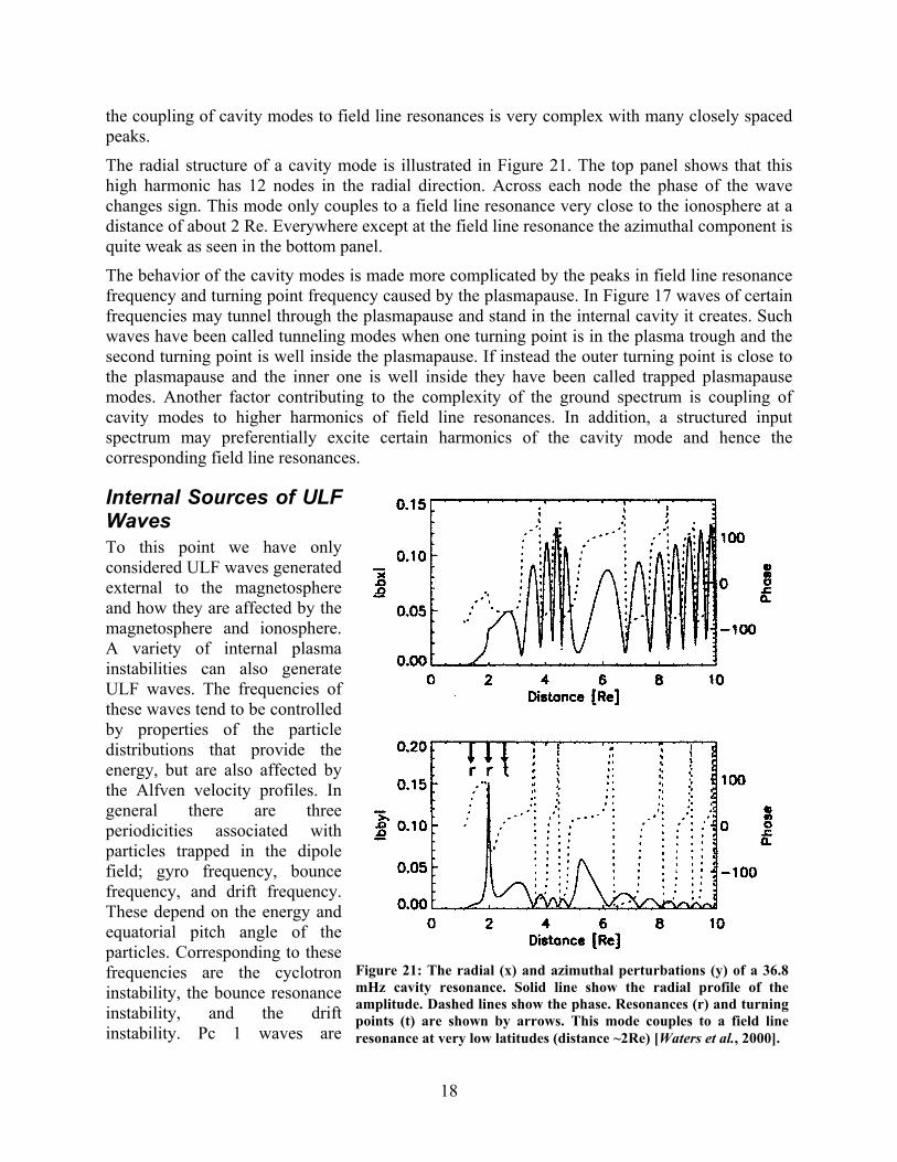
The radial structure of a cavity mode is illustrated in Figure 21. The top panel shows that this high harmonic has 12 nodes in the radial direction. Across each node the phase of the wave changes sign. This mode only couples to a field line resonance very close to the ionosphere at a distance of about 2 Re. Everywhere except at the field line resonance the azimuthal component is quite weak as seen in the bottom panel.

The behavior of the cavity modes is made more complicated by the peaks in field line resonance frequency and turning point frequency caused by the plasmapause. In Figure 17 waves of certain frequencies may tunnel through the plasmapause and stand in the internal cavity it creates. Such waves have been called tunneling modes when one turning point is in the plasma trough and the second turning point is well inside the plasmapause. If instead the outer turning point is close to the plasmapause and the inner one is well inside they have been called trapped plasmapause modes. Another factor contributing to the complexity of the ground spectrum is coupling of cavity modes to higher harmonics of field line resonances. In addition, a structured input spectrum may preferentially excite certain harmonics of the cavity mode and hence the corresponding field line resonances.

Internal Sources of ULF Waves To this point we have only considered ULF waves generated external to the magnetosphere and how they are affected by the magnetosphere and ionosphere. A variety of internal plasma instabilities can also generate ULF waves. The frequencies of these waves tend to be controlled by properties of the particle distributions that provide the energy, but are also affected by the Alfven velocity profiles. In general there are three periodicities associated with particles trapped in the dipole field; gyro frequency, bounce frequency, and drift frequency. These depend on the energy and equatorial pitch angle of the particles. Corresponding to these frequencies are the cyclotron instability, the bounce resonance instability, and the drift instability. Pc 1 waves are

Figure 21: The radial (x) and azimuthal perturbations (y) of a 36.8 mHz cavity resonance. Solid line show the radial profile of the amplitude. Dashed lines show the phase. Resonances (r) and turning points (t) are shown by arrows. This mode couples to a field line resonance at very low latitudes (distance ~2Re) [Waters et al., 2000].

18

created by the ion cyclotron instability. Some Pc 4 waves are created by a bounce resonance. Pc 5 waves can be created by a drift resonance.

Other processes also produce ULF waves. For example, bursty Earthward flows are often seen in the plasma sheet on the nightside of the Earth during geomagnetic activity. These flows radiate Alfven waves that travel to the auroral ionosphere where they are reflected and travel back to interact with the flow. This process is though to create Pi 2 waves. High frequency components of these waves may resonate in the ionospheric cavity producing Pi 1 waves. In the following, I briefly describe several of the most common processes illustrating how ULF waves are internally generated.

Gryo resonance Gryo resonance or cyclotron resonance are names applied to the situation where a circularly polarized wave and a particle rotate about the magnetic field at the same frequency. Because the electric field of the wave and the particle velocity maintain a constant angle with respect to each other, the field is able to exert a force on the charge for a long interval. This allows energy transfer to occur [Brice, 1964]. Which direction the energy flows depends on the relative angle. In the magnetosphere cyclotron resonance between a left circularly polarized wave and protons is the mechanism that creates Pc 1 magnetic pulsations (.5 – 5 Hz). This physical process is briefly described in the following paragraphs.

Figure 22: The ion cyclotron resonance occurs when a left circularly polarized Alfven wave appears to a moving ion to have a Doppler shifted frequency equal to its gyrofrequency. For these conditions the particle and wave can interchange energy either amplifying or damping the wave depending on the angle between velocity and electric field.

At frequencies close to the ion gyrofrequency, the positive ions present in plasma significantly affect the phase velocity of an Alfven wave. The wave becomes left circularly polarized and its velocity decreases to zero as the wave frequency approaches the ion gyrofrequency. Above the gyrofrequency, this wave does not propagate. Suppose a wave with frequency ω is traveling along a magnetic field line B with phase velocity VA from the equator towards the northern hemisphere as illustrated in Figure 22. Next suppose a proton is traveling in the opposite direction towards the equator with a parallel velocity V||. In the reference frame of the proton the source of the wave will appear to be approaching so that the wave frequency will be Doppler shifted to a higher frequency ω′

1A

VVω ω ′ = +

Provided the ion has finite perpendicular velocity V⊥, it will be gyrating about the field in a left-handed sense with the ion gyrofrequency Ωi. When the Doppler shifted wave frequency is the same as the ion gyrofrequency the electric field and ion velocity will be in resonance. If the wave electric field is antiparallel to the ion velocity the particle will be slowed down and the wave will

19

gain energy. In the process the pitch angle of the ion (angle between velocity vector and magnetic field) must decrease to conserve total energy.

The wave is equally likely to loose energy as gain energy when the ions are not bunched in phase. It would seem therefore that the net effect would be no change in wave energy. However, if the pitch angle distribution of the ions is peaked at large pitch angles, i.e. they have more perpendicular energy than parallel energy, then on the average the wave gains energy from the ions [Cornwall, 1965]. The reason for this is diffusion in pitch angle. Each interaction that damps the wave must increase the pitch angle of an ion, while interactions that grow the wave decrease the pitch angle. Pitch angle distributions in the magnetosphere are usually peaked at 90° so that there are more ions that can move to smaller pitch angle energizing the wave, than there are ions of low pitch angle that can move to large pitch angles.

Two processes in the magnetosphere create the necessary pitch angles distributions. The first is particle precipitation to the atmosphere. Any particle whose pitch angle gets too small will mirror in the atmosphere and will be lost. Thus, there is always a hole in the pitch angle distribution near zero degrees. This hole helps maintain the gradient responsible for pitch angle diffusion and wave growth.

The second process is magnetospheric convection discussed in a later section. Particles generally enter the magnetosphere in the tail and are transported Sunward as part of a two-celled convection pattern. As the charged particles approach the Earth, they begin to gradient and curvature drift across the electric field created by the convection. This drift moves them in the direction of the convection electric field so they gain perpendicular energy. They also gain parallel energy due to the shortening of field lines, but not as rapidly, so the pitch angle distribution becomes peaked at 90°.

There are two main type of Pc 1 seen on the ground near the auroral zone. These are called Pearl Pulsations (PP) and IPDP (intervals of pulsations diminishing in period). Both are created by the ion cyclotron instability but under different circumstances. PP are created by a wave packet bouncing back and forth between opposite ionospheres. Each time the wave packet passes through the equatorial region it interacts with protons stimulating them to emit waves of the same frequency that amplify the initial signal. The process depends on good reflection at the ionosphere, and a proton distribution with the right energy and pitch angle distribution. The Alfven wave is dispersive near the gyro frequency with high frequencies traveling slower than low frequencies. Because of this the wave packet becomes dispersed. Dynamic spectra of these pulsations typically exhibit a sequence of rising tones that repeat with the bounce frequency of the wave, and whose slopes decrease with time as the wave packet becomes more dispersed. The process is the same as in a laser and is sometimes called a “hazer”.

The IPDP pulsations are observed in the auroral zone soon after a substorm expansion has occurred at midnight. Protons are injected rapidly in a narrow sector of local time near midnight and subsequently drift westward. As they reach the dusk meridian they drift into the plasmasphere where the Alfven velocity is low enough to allow cyclotron resonance with the drifting ions. The most energetic ions arrive first and because of their high parallel velocity are Doppler shifted to low frequencies. As time progresses, lower energies arrive and resonate at successively higher frequencies. In a dynamic spectrum the signal rises in frequency from about 0.1 Hz to as high as 1 Hz over a period of about 20 minutes.

20

Drift and Bounce resonance An important internal source of ULF waves is the drift-bounce resonance mechanism. This instability allows particle distributions to give up some of their energy through the generation of waves. The nature of the interaction responsible for this instability is illustrated in Figure 23. The figure displays a flat projection of an azimuthal shell of dipole field lines. The field lines have been straightened so the northern ionosphere is at the top and the southern ionosphere at the bottom. West is to the left and east to the right. In panel (a) the plus signs show the sign of the azimuthal electric field of a fundamental mode wave standing along the field and propagating westward with a wavelength short compared to the distance around the drift shell. Plus signs indicate eastward electric field and minus signs westward field. The diagram is moving westward with the azimuthal phase velocity of the wave so the wave field does not appear to change with time. However, at a fixed point in the Earth’s magnetic field the diagram will sweep from right to left across an observer causing the electric field to oscillate. For the situation illustrated the magnetic perturbation is radial. Normally this would be the fast mode wave, but it can be shown that the assumption of a short azimuthal wavelength allows one to neglect the compressional component and treat the wave as an Alfven wave.

The solid and dashed lines represent the trajectories of two ions drifting westward as they bounce between mirror points in the north and south. The trajectories represent ions of a specific equatorial pitch angle and energy chosen so that they complete one full bounce (N-S-N) in the moving frame in exactly two wavelengths. The solid line represents an ion that happens to pass through the center of the eastward electric field at its most intense point. During this time the ion E x B0 drifts radially outward, loosing energy due to inductive effects in the main field B0. As this ion approaches the mirror points it encounter westward electric field and drifts inward gaining energy. However, since the electric field of the fundamental is weaker at the mirror points than at the equator, the ion gains less energy than it looses. Thus the ion moves outward and its energy decreases with time. The energy lost by the particle is given to the wave.

The dashed trajectory shows an ion ¼ wavelength ahead of the first ion. It passes through the equatorial node of the wave and experiences weak eastward electric field at one mirror point and weak westward field at the other. The radial motion averages to zero for this ion and it neither gains nor looses energy. An ion starting ¼ wavelength still later will move inward and gain energy on each bounce damping the wave. If the ions are not bunched in azimuth, and there are equal numbers inside and outside the drift shell, then the net effect will be no change in the wave or particles. However, if there are more particles close to the Earth than further out, the waves will cause a net outward diffusion and the waves will gain energy from the particles. This process is the drift-bounce instability and it is a major source of ULF waves in the magnetosphere.

Panel (b) of Figure 23 shows the situation for a second harmonic bounce resonance. For even harmonics the equator is a node of the electric field and peaks in the electric field appear above and below the equator with opposite polarity in the two hemispheres. For this case the resonance requirement in the rest frame of the wave is that the ion drifts one azimuthal wavelength in one bounce. The ion trajectory shown by the solid line has a small equatorial pitch angle and will sample the large westward fields at successive mirror points. This ion will experience net inward drift from the electric field and will gain energy. The ion shown by a dashed line has a larger equatorial pitch angle and hence a mirror point closer to the equator. It will experience weaker

21

Figure 23: The azimuthal electric field of a wave is shown in the rest frame of the wave. The wave is standing along the field (N-S) but is propagating azimuthally westward (W-E). Panel (a) depicts a fundamental harmonic with maximum field at the equator while panel (b) shows a second harmonic. Solid lines are trajectories of ions bouncing between mirror points at the ends of the field lines and drifting westward across the phase fronts of the wave.

electric fields and not drift as far or gain as much energy as the small pitch angle particle. Again, whether the waves grow or damp depends on the radial distribution of the ions.

The drift bounce resonance condition can be formulated mathematically quite simply. We suppose the wavelength λ is such that m cycles of the wave fit in a circular shell of radius r around the Earth. Then λ = 2πr/m. The azimuthal phase velocity of the wave is the ratio of the wavelength to period vφ = λ/T = λf =λ(ω/2π) = rω/m. Now transform to the rest frame of the wave. The drift velocity of the ion in the wave frame is wherev rϕ′ = ϕ is its angular velocity. Then dv v vφ′ = −

2 / 2(2T vλ π′= =

substituting we obtain where is the ion angular drift velocity in the Earth’s frame. The condition for fundamental bounce resonance can then be written as the ion bounce time equals the time to drift two wavelengths in the rest frame of the wave, thus T

/dwφ = −

=

ϕ

mω

2 /b π ω

dω

bb = T2λ. The bounce period is given by T where ωb is the angular bounce frequency. The time to drift 2λ in the wave frame is given by

. Equating and simplifying we obtain .

Transforming back to the Earth’s frame by substituting for 2 / ) /( ) 4 /r m rλ φ π= m 2 bmφ ω=

φ we find that . 2d bω−mω ω− =

The formula for the second harmonic resonance differs only by a factor of two on the right hand side. Both situations are special cases of the general formula where N is a positive or negative integer. Clearly there is a wide variety of possible drift–bounce resonances.

dm Nω ω ω− = b

Earthward Directed Plasma Flows Another source of waves in the magnetosphere are the Earthward directed flows that occur in the plasma sheet during substorms. Apparently, these flows are created by bursts of magnetic

22

reconnection at an x-line in the tail. The flows are transient with durations of a few minutes and localized in azimuth to a few Earth radii. The flows transport plasma and magnetic field Earthward. As they approach the Earth (8-15 Re), the pressure gradients in the midnight region slow the flow and divert it around the Earth. As soon as these flow are created the channel becomes polarized in exactly the manner described earlier for the creation of Alfven waves. The duskward point electric field produced by this polarization is propagated to the ionosphere by an Alfven wave. In the ionosphere the electric field drives a westward current. The J x B force exerted on the ionosphere by this current accelerates the ionospheric plasma equatorward. Because of inertia the ionosphere does not move as fast as the electric field would expect so the wave is reflected, reducing the total electric field. The wave reverberates between the equator and the ionosphere several times. The signal measured on the ground has the form of a short train of waves with duration about 10 minutes and period about 100 seconds. These are called Pi 2 bursts. These ULF waves are always associated with the onset of substorms, pseudo breakups, and intensifications of an ongoing substorm. An example taken from the work of [Kepko et al., 2001] is shown in Figure 24. This correlation suggests that bursty flows play an essential role in the generation of substorms.

Figure 24: A comparison of X component of flow at Geotail with the LANL magnetometer H component showing relation of Pi 2 pulses to pulses in the flow. The same Pi 2 was seen at synchronous GOES-9 and other ground stations [Kepko et al., 2001]

When the Earthward flow bursts impact the inner magnetosphere they radiate compressional waves that travel across the field lines and eventually couple to field line resonances. The bursty flows are often structured with periods of order 100 seconds caused by unknown processes in the tail. The periodicity associated with the peaks in flow can structure the spectrum of compressional waves that eventually couple to Alfven waves. The velocity shear between the edges of these flow channels and stationary plasma may generate Kelvin-Helmholtz waves. Sometimes the distribution of plasma pressure and field line curvature becomes favorable to the growth of the interchange instability or the ballooning mode.

Modulation of the electrojet Another source of ULF wave activity at high latitudes on the night side is particle precipitation. As discussed above, the cyclotron instability can scatter particles into the atmosphere causing aurora, and creating waves. When electrons are involved, it is the electron cyclotron frequency and VLF waves (~1836 times higher frequency) that are created. The impact of these particles on the ionosphere increases the conductivity and alters the strength and direction of the electrojets.

23

These changes in current cause magnetic variations on the ground that are indistinguishable from those of ULF waves. An example of this mechanism is Ps 6 pulsations (pulsations substorm).

Ps 6 are fluctuations with periods of 10-40 minutes. They are seen primarily in the east component in the post midnight sector during the recovery phase of substorms and during steady magnetospheric convection. They are associated with auroral torches or omega bands [Robinson et al., 1995]. Torches are tongues of auroral luminosity that drift eastward from midnight towards dawn. The torches are rooted at the equatorward edge of the auroral zone and project poleward towards a second band of luminosity at the poleward edge of the oval. The dark regions between torches are called omega bands because the dark regions have the shape of inverted letter omega. The magnetic fluctuations are caused by a diversion of the electrojet into a field-aligned current system [Amm, 1996]. Current comes down into the poleward portion of the tongue and exits near the equatorward edge. A southward directed current in the ionosphere creates the east-west fluctuations on the ground. The cause of the torches is not known.

Relation of ULF Waves to Magnetospheric Substorms and Magnetic Storms Many of the ULF waves generated internally in the magnetosphere are associated with either substorms or magnetic storms. The reason is that these processes create distributions of particle pressure, energy, and pitch angle that are unstable to the creation of various types of waves. To conclude this review we briefly describe these two fundamental processes.

Magnetospheric Substorm The magnetospheric substorm is a systematic response of the magnetosphere to an increase in coupling between the solar wind and the Earth’s magnetic field [McPherron, 1991]. A substorm typically lasts around three hours and occurs 3-6 times per day. During a substorm a large amount of energy is extracted from the solar wind and is dumped into the magnetosphere and ionosphere. The substorm is characterized by three phases: growth, expansion, and recovery. The growth phase begins when the solar wind magnetic field turns southward and magnetic reconnection begins at the subsolar magnetopause. Magnetic field lines of the solar wind merge with the Earth’s field and are carried over the polar caps and stretched into a long tail behind the Earth. As open magnetic field lines accumulate in the tail lobes they exert increasing pressure on the plasma sheet causing it to thin. In reaction to the increased drag on the tail, the tail current moves Earthward and strengthens to correspond to the increased magnetic field in the lobes. At the same time, plasma and magnetic field begin to flow up the tail towards the x-line at the front of the magnetosphere to replace field lines removed by reconnection. This flow is diverted around both sides of the Earth creating a two-celled convection system within the magnetosphere. This process continues until the plasma sheet becomes too thin at midnight about 20 Re behind the Earth. A new x-line is created in a limited local time sector about 3 Re west of midnight [Nagai and Machida, 1998]. This signals the beginning of the expansion phase. The duration of the growth phase is typically one hour.

During the growth phase the size of the polar cap grows as more magnetic field lines are connected to the solar wind. The open field lines enable the solar wind electric field that points from dawn to dusk to be transmitted to the ionosphere. The electric field drives a Pedersen current down field lines on the morning side, across the polar cap, and up field lines on the dusk side. In addition, some of the dawnside current flows equatorward to the plasmapause where it

24

closes upward along field lines. This portion of the current continues around the nightside equator as a partial ring current. Near dusk and in the late afternoon it is diverted downward near the plasmapause, attaching to a poleward current in the dusk oval. The current merges with the current coming across the polar cap and flows out along field lines. This complex current system is nearly invisible on the ground! However, the electric field also drives a Hall current in the ionosphere. It flows along the auroral oval towards midnight. On the dawn side this portion of the current is called the westward electrojet. On the dusk side it is called the eastward electrojet. Near midnight the currents meet and flow poleward across the polar cap diverging into the electrojets at the dayside auroral oval. Magnetic disturbances seen on the ground during the growth phase are due to this DP-2 (disturbance polar -type 2) current system.

In the first stage of the expansion phase the x-line reconnects closed field lines in the plasma sheet creating a bubble of closed magnetic flux called a plasmoid [Baker et al., 1996]. Eventually the reconnection reaches the last closed field lines that form the boundary of the plasma sheet. These field lines are normally connected to an inactive, distant x-line located beyond 100 Re down the tail. The second stage of the expansion begins when reconnection reaches open field lines in the lobe. At this time the plasmoid is no longer held to the Earth by closed field lines. It is ejected down the tail by a combination of forces including momentum of plasma injected in the bubble by reconnection in the first stage, magnetic tension of field lines connected only to the solar wind and bent around the bubble, and dynamic pressure of the flow from reconnection in the second stage.

Reconnection also drives plasma and magnetic flux Earthward from the near-Earth x-line. As this flow impacts the inner magnetic field, it causes disturbances that project to the Earth at the equatorward edge of the auroral oval near midnight. With time, more flow piles up in this region and a compression front moves backwards in the tail. The region Earthward of this front projects to the ionosphere as a region of bright, active aurora. With time this region expands both poleward and azimuthally creating what is called the auroral bulge. Some of the plasm flowing Sunward from the x-line is diverted around the Earth. The pressure gradients, vorticity, and magnetic shear caused by this diversion create a field-aligned current system called the substorm current wedge [Birn and Hesse, 1996]. Current previously flowing across the tail close to the Earth is diverted down field lines on the morning side to flow westward across the bulge and close upward from the west side of the bulge. The ground magnetic disturbance associated with this current is called DP-1. This process continues for about 30-40 minutes until the x-line begins to move down the tail. This signals the beginning of the recovery phase

In the recovery phase the magnetosphere returns to its presubstorm configuration of field and plasma. Magnetic flux accumulated in the tail lobes is closed and returned to the dayside. The inner edge of the tail current moves more tailward. The plasma sheet thickens. The x-line retreats to about 100 Re and remains fixed at this location. Sporadic, weak bursts of reconnection at this line create poleward boundary intensifications in the auroral oval as flow bursts travel Earthward from the reconnection site.

Many ULF waves are created by changes in field and plasmas during substorms. The Pi 2 pulsations are related to flow bursts. Pi-1 is created by some process in the ionospheric waveguide. IPDP are generated by protons energized and injected near midnight by the substorm expansion. As explained earlier convection preferentially energizes particles at large pitch angles setting up the conditions for instability. These protons also create Pc 4-5 waves near the dusk meridian through drift-mirror instability. However, these waves are not seen on the ground

25

because they have such small azimuthal wavelengths. Drifting electrons are precipitated in early morning hours by some unknown process that causes patches of aurora pulsating with about 1-30 second period. The auroral torches are formed near midnight and drift eastward diverting current along field lines and creating ground fluctuations of long period (Ps 6).

Magnetic Storms A magnetic storm is an interval of several days duration during which there is a large reduction in the horizontal component of the surface magnetic field [Gonzalez et al., 1994]. A classic magnetic storm begins with a sudden commencement and a prolonged initial phase. These are caused by a sudden increase is the dynamic pressure of the solar wind as high speed and high-density plasma from the Sun suddenly arrive at the Earth. The magnetopause is pushed Earthward strengthening its current and its positive effect on the ground. The sudden commencement is a packet of waves triggered by the sudden displacement of the field lines in the magnetosphere that resonate in response to the change. The initial phase lasts from a few minutes to many hours, and is usually followed by a rapid decrease in the surface field. This decrease is called the main phase of the magnetic storm. A weak storm consists of only a 50 nT decrease, a moderate storm about 150 nT, a strong storm up to 300 nT, and a great storm more than 500 nT. The main phase may last from a few hours to as many as 12 hours. Eventually the magnetic field begins to recover. A typical recovery is exponential in form with a time constant of about eight hours. The recovery phase is usually over within one to two days.

The main phase is caused by the growth of a ring current around the Earth. This is traditionally though to be a doughnut shaped region around the Earth containing a strong westward current. This current is primarily created by ions including protons, helium, and oxygen drifting westward around the Earth from midnight towards dusk and onward. This current acts much like a large solenoid around the Earth producing a magnetic disturbance that is southward along the Earth’s dipole axis. The recovery phase of the storm is caused by the loss of these ions. Until recently it was thought that the main loss process for the ions was charge exchange. As the ions approach the atmosphere in their bounce motion there is a high probability of interaction with an atmospheric neutral atom. An electron from the cold atmospheric atom is exchanged with the hot ion. The hot ion becomes an energetic neutral atom that is no longer confined by the field. The cold atom is transformed into a cold ion that contributes little to the current.

The creation of the ring current is caused by a prolonged interval of strong southward magnetic field and high solar wind velocity. These are precisely the conditions that cause magnetic reconnection on the dayside and intense convection in the magnetosphere. The ions creating the current are brought in from the tail and energized by the magnetospheric electric field associated with convection. There is growing evidence that most of these ions simply drift through the magnetosphere and exit through the dayside boundary [Liemohn et al., 2001]. Only after the recovery phase begins do some of these ions come onto closed drift paths that circle the Earth. There is also growing evidence that ion cyclotron waves may play an important role in ring current decay. As described earlier these waves scatter ions in pitch angle towards the loss cone. This allows the ions to come closer to the atmosphere where the probability of interacting with a neutral is higher.

There is no type of ULF wave that has been identified as specifically created by a storm-time ring current. The instabilities that can occur in a cloud of drifting protons also occur during

26

intervals that are not strong enough to be called storms. Every magnetic storm includes many substorms and these are probably the cause of the ULF waves occurring during storms.

Conclusions The scientific study of micropulsations, magnetic pulsations, and ULF waves has a long history. Modern instruments and satellite observations have revealed a very complex taxonomy of waves that reach the Earth’s surface. These waves are generated by processes as far away as the Sun and as close as the ionosphere. There are many sources of waves both external and internal to the magnetosphere. The magnetosphere itself is a resonant cavity and waveguide for waves that propagate through the system. These cavities respond to broadband sources by resonating at discrete frequencies. These cavity modes couple to field line resonances that drive currents in the ionosphere. These currents reradiate the energy as electromagnetic waves that propagate to the ground. Because of these resonances there are very rapid variations in wave phase at the Earth’s surface. It is almost never correct to assume that plane ULF waves are incident on the Earth from outer space.

Many of the waves now have accepted explanations in terms of physical processes in the solar wind or magnetosphere. Knowledge of the wave characteristics and the current state of space weather can give one a good idea of what waves are likely to be occurring at any particular latitude and local time. The waves are diagnostic of the conditions in space. Measurements on the ground can be used to remotely sense the conditions in the magnetosphere and solar wind. They can also be used to probe the subsurface conductivity structure of the Earth as those at this meeting are well aware.

Acknowledgments The author would like to acknowledge support for this work derived from several grants including NSF ATM 98-19935, NSF ATM 99-72069, and Los Alamos National Laboratory LANL #1001R. He also thanks Dr. R. Clauer, Dr. M. Kivelson, Dr. A. Ridley, and Dr. C. Waters for help in understanding their earlier work.

References Alfven, H., and C.-G. Falthammar, Cosmical Electrodynamics: Fundamental Principles, 228

pp., Clarendon Press, Oxford, 1963.

Allan, W., J.R. Manuel, and E.M. Poulter, Magnetospheric cavity modes: some nonlinear effects, J. Geophys. Res. , 96(A7), 11461-73, 1991.

Amm, O., Improved electrodynamic modeling of an omega band and analysis of its current system, J. Geophys. Res., 101(A2), 2677-83, 1996.

Baker, D.N., T.I. Pulkkinen, V. Angelopulos, W. Baumjohann, and R.L. McPherron, Neutral line model of substorms: Past results and present view, J. Geophys. Res., 101(A6), 12,875-13,010, 1996.

Barnes, A., Hydromagnetic waves, turbulence, and collisionless processes in the interplanetary medium, in Solar-Terrestrial Physics: Principles and Theoretical Foundations, edited by R.L. Carovillano, and J.M. Forbes, pp. 155-199, D. Reidel Publishing Company, Dordrecht, 1983.

27

Baumjohann, W., and R.A. Treumann, Basic Space Plasma Physics, 329 pp., Imperial College Press, London, 1996.

Birn, J., and M. Hesse, Details of current disruption and diversion in simulations of magnetotail dynamics, J. Geophys. Res., 101(A7), 15,345-15,358, 1996.

Brice, N., Fundamentals of very low frequency emission generation mechanisms, 69(21), 4515-4522, 1964.

Chapman, S., and J. Bartels, Geomagnetism, Vol 1, Clarendon Press, Oxford, 1962.

Chi, P., and C.T. Russell, Two methods using magnetometer-array data for studying magnetic pulsations, TAO, 12(4), 649-662, 2001.

Cornwall, J.M., Cyclotron instabilities and electromagnetic emissions in the ultra low frequency and velry low frequency ranges, J. Geophys. Res. , 70(1), 61-69, 1965.

Crowley, G., W.J. Hughes, and T.B. Jones, Observational evidence of cavity modes in the Earth's magnetosphere, J. Geophys. Res. , 92(A11), 12233-40, 1987.

Ding, D.Q., R.E. Denton, M.K. Hudson, and R.L. Lysak, An MHD simulation study of the poloidal mode field line resonance in the Earth's dipole magnetosphere, J. Geophys. Res. , 100(A1), 63-77, 1995.

Engebretson, M., L.J. Zanetti, T.A. Potemra, W. Baumjohann, H. Luhr, and M.H. Acuna, Simultaneous observation of Pc3-4 pulsations in the solar wind and in the Earth's magnetosphere, J. Geophys. Res. , 92, 10053, 1987.

Engebretson, M.J., N. Lin, W. Baumjohann, H. Luehr, B.J. Anderson, L.J. Zanetti, T.A. Potemra, R.L. McPherron, and M.G. Kivelson, A comparison of ULF fluctuations in the solar wind magnetosheath, and dayside magnetosphere. 1. Magnetosheath morphology, J. Geophys. Res. , 96(A3), 3441-54, 1991.

Fukushima, N., Equivalence in ground geomagnetic effect of Chapman-Vestine's and Birkeland-Alfven's electric current system for polar magentic subtorms, Rep. Ionos. Space Res. Jpn., 23, 219-227, 1969.

Gonzalez, W.D., J.A. Joselyn, Y. Kamide, H.W. Kroehl, G. Rostoker, B.T. Tsurutani, and V.M. Vasyliunas, What is a geomagnetic storm?, J. Geophys. Res., 99(A4), 5771-5792, 1994.

Greenstadt, E.W., Oblique, parallel, and Quasi-parallel morphology of collisionness shocks., 1984.

Greenstadt, E.W., and R.W. Fredericks, Shock Systems in Collisionless Space Plasmas, in Solar System Plasma Physics, edited by L.J. Lanzerotti, C.F. Kennel, and E.N. Parker, North-Holland Publishing Co., 1979.

Greenstadt, E.W., M.M. Mellott, R.L. McPherron, C.T. Russell, H.J. Singer, and D.J. Knecht, Transfer of pulsation-related wave activity across the magnetopause observations of corresponding spectra by ISEE-1 and ISEE-2, Geophys. Res. Lett. (USA), 10(8), 659-62, 1983.

Greenstadt, E.W., J.V. Olson, P.D. Loewen, H.J. Singer, and C.T. Russell, Correlation of Pc 3, 4, and 5 activity with solar wind speed, J. Geophys. Res. , 84(A11), 6694-6, 1979a.

28

Greenstadt, E.W., C.T. Russell, and M. Hoppe, Magnetic field orientation and suprathermal ion streams in the earth's foreshock, J. Geophys. Res. , 85(A7), 3473-3479, 1980.

Greenstadt, E.W., H.J. Singer, C.T. Russell, and J.V. Olson, IMF orientation, solar wind velocity, and Pc 3-4 signals: a joint distribution, J. Geophys. Res. , 84(A2), 527-32, 1979b.

Hoppe, M.M., C.T. Russell, T.E. Eastman, and L.A. Frank, Characteristics of the ULF waves associated with upstream ion beams, J. Geophys. Res. , 87(A2), 643-50, 1982.

Hughes, W.J., The effect of the atmosphere and ionosphere on long period magnetospheric micropulsations, Planet. Space Sci., 22, 1157, 1974.

Hughes, W.J., Hydromagnetic waves in the magnetosphere, in Solar-Terrestrial Physics: Principles and Theoretical Foundations, edited by R.L.a.F. Carovillano, J.M., pp. 453-477, D. Reidel Publishing Company, Dordrecht, 1983.

Jacobs, J.A., Y. Kato, S. Matsushita, and V.A. Troitskaya, Classification of Geomagnetic Micropulsatiions, J. Geophys. Res., 69(1), 180-181, 1964.

Keller, K.A., and R.L. Lysak, MHD simulation of magnetospheric waveguide modes, J. Geophys. Res. , 106(A5), 8447-54, 2001.

Kepko, L., M.G. Kivelson, and K. Yumoto, Flow bursts, braking, and Pi2 pulsations, J. Geophys. Res. , 106(A2), 1903-15, 2001.

Kepko, L., H.E. Spence, and H. Singer, ULF waves in the solar wind as direct drivers of magnetospheric pulsations, Geophys. Res. Lett. (USA), 29(8), 2002.

Kivelson, M., and D.J. Southwood, Ionospheric traveling vortex generation by solar wind buffeting of the magnetosphere, J. Geophys. Res. , 96(A2), 1661-1667, 1991a.

Kivelson, M.G., M. Cao, R.L. McPherron, and R.J. Walker, A possible signature of magnetic cavity mode oscillations in ISEE spacecraft oscillations, J. Geomag. Geoelectr., 49, 1079-1098, 1997.

Kivelson, M.G., J. Etcheto, and J.G. Trotignon, Global compressional oscillations of the terrestrial magnetosphere: The evidence and a model, J. Geophys. Res. , 89(11), 9851-9856, 1984.

Kivelson, M.G., and D.J. Southwood, Ionospheric traveling vortex generation by solar wind buffeting of the magnetosphere, J. Geophys. Res., 96(A2), 1661-1667, 1991b.

Lee, D.H., and R.L. Lysak, Magnetospheric ULF wave coupling in the dipole model: the impulsive excitation, J. Geophys. Res. , 94(A12), 17097-103+3 plates, 1989.

Lee, D.H., and R.L. Lysak, Monochromatic ULF wave excitation in the dipole magnetosphere, J. Geophys. Res. , 96(A4), 5811-17, 1991.

Liemohn, M.W., J.U. Kozyra, M.F. Thomsen, J.L. Roeder, G. Lu, J.E. Borovsky, and T.E. Cayton, Dominant role of the asymmetric ring current in producing the stormtime Dst*, J. Geophys. Res., 106(A6), 10883-904, 2001.

Lin, N.M.J.E., B.J. Anderson, R.L. McPherron, M. G. Kivelson, W. Baumjohann, H. Luehr, T.A. Potemera, L.J. Zanetti, A comparison of ULF wave fluctuations in the solar wind, magnetosheath, and dayside magnetosphere, 2. Field and plasma conditions in the magnetosheath, J. Geophys. Res., 96(A3), 3455-3464, 1991.

29

Lysak, R.L., Theory of auroral zone PiB pulsation spectra, J. Geophys. Res. , 93(A6), 5942-6, 1988.

Mann, I.R., A.N. Wright, and P.S. Cally, Coupling of magnetospheric cavity modes to field line resonances: a study of resonance widths, J. Geophys. Res. , 100(A10), 19441-56, 1995.

McHenry, M.A., C.R. Clauer, E. Friis-Christensen, P.T. Newell, and J.D. Kelly, Ground observations of magnetospheric boundary layer phenomena, J. Geophys. Res. , 95(A9), 14995-5005, 1990.

McPherron, R.L., The EARTH: Its properties, composition and structure, in Encyclopedia Britannica, pp. 545-558, 1987.

McPherron, R.L., Physical Processes Producing Magnetospheric Substorms and Magnetic Storms, in Geomagnetism, edited by J. Jacobs, pp. 593-739, Academic Press, London, 1991.

McPherron, R.L., C.T. Russell, and M. Aubry, Satellite studies of magnetospheric substorms on August 15, 1978, 9. Phenomenological model for substorms, J. Geophys. Res., 78(16), 3131-3149, 1973.

Nagai, T., and S. Machida, Magnetic reconnection in the near-earth magnetotail, in New Perspectives on the EArth's Magnetotail, edited by A. Nishida, D.N. Baker, and S.W.H. Cowley, pp. 211-224, American Geophysical Union, Washington, DC, 1998.

Radoski, H.R., A note on the problem of hydromagnetic resonances in the magnetosphere, Planet. Space Sci., 19, 1012, 1971.

Rankin, R., P. Frycz, V.T. Tikhonchuk, and J.C. Samson, Ponderomotive saturation of magnetospheric field line resonances, Geophys. Res. Lett. (USA), 22(13), 1741-4, 1995.

Rickard, G.J., and A.N. Wright, ULF pulsations in a magnetospheric waveguide: comparison of real and simulated satellite data, J. Geophys. Res. , 100(A3), 3531-7, 1995.

Ridley, A., Estimation of the uncertainity in timing the relationship between magnetospheric and solar wind processes, JASTP, 2000.

Ridley, A.J., T. Moretto, P. Ernstrom, and C.R. Clauer, Global analysis of three traveling vortex events during the November 1993 storm using the assimilative mapping of ionospheric electrodynamics technique, J. Geophys. Res. , 103(A11), 26349-58, 1998.

Robinson, R.M., D.L. Chenette, D.W. Datlowe, T.L. Schumaker, R.R. Vondrak, P.F. Bythrow, T.A. Potemra, J.R. Sharber, and J.D. Winningham, Field-aligned currents associated with spatially periodic X-ray structures in the morningside auroral oval, J. Geophys. Res. , 100(A12), 23945-52, 1995.

Russell, C.T., Planetary bow shock, in Collisionless Shocks in the Heliosphere: Reviews of Current Research, edited by B.T. Tsurutani, and R.G. Stone, pp. 109-130, American Geophysical Union, Washington, D.C., 1985.

Russell, C.T., and B.K. Fleming, Magnetic pulsations as a probe of the interplanetary magnetic field: A test of the Borok B index, J. Geophys. Res. , 81(34), 5882-5886, 1976.

Russell, C.T., and M.M. Hoppe, Upstream waves and particles, Space Sci. Rev., 34(2), 155-72, 1983.

30

Samson, J.C., R.A. Greenwald, J.M. Ruohoniemi, T.J. Hughes, and D.D. Wallis, Magnetometer and radar observations of magnetohydrodynamic cavity modes in the Earth's magnetosphere, Canadian Journal of Physics, 69(8-9), 929-37, 1991.

Samson, J.C., B.G. Harrold, J.M. Ruohoniemi, R.A. Greenwald, and A.D.M. Walker, Field line resonances associated with MHD waveguides in the magnetosphere, Geophys. Res. Lett. (USA), 19(5), 441-4, 1992.

Samson, J.C., C.L. Waters, F.W. Menk, and B.J. Fraser, Fine structure in the spectra of low latitude field line resonances, Geophys. Res. Lett. (USA), 22(16), 2111-14, 1995.

Singer, H., C.T. Russell, M. Kivelson, E.W. Greenstadt, and J. Olson, Evidence for the control of Pc 3,4 magnetic pulsations by the solar wind velocity, Geophys. Res. Lett. (USA), 4(9), 377-379, 1977.

Southwood, D.J., Some features of field line resonances in the magnetosphere, Planetary Space Science, 22(3), 483-491, 1974.

Southwood, D.J., and W.J. Hughes, Source induced vertical components in geomagnetic pulsation signals, Planet. Space Sci., 26, 715, 1978.

Southwood, D.J., and W.J. Hughes, Theory of hydromagnetic waves in the magnetosphere, Space Sci. Rev., 35, 301-366, 1983.

Southwood, D.J., and M.G. Kivelson, Ionospheric traveling vortex generation by solar wind buffeting of the magnetosphere, J. Geophys. Res. , submitted, September, 1989.

Spreiter, J.R., and S.S. Stahara, Magnetohydrodynamic and gasdynamic theories for planetary bow waves, in Collisionless Shocks in the Heliosphere: Reviews of Current Research, edited by B.T. Tsurutani, and R.G. Stone, pp. 85-107, American Geophysical Union, Washington DC, 1985.

Takahashi, K., and R.L. McPherron, Harmonic structure of Pc 3-4 pulsations, J. Geophys. Res. , 87(A3), 1504-16, 1982.

Takahashi, K., R.L. McPherron, and E.W. Greenstadt, Factors controlling the occurrence of Pc 3 magnetic pulsations at synchronous orbit, J. Geophys. Res. , 86(A7), 5472-84, 1981.

Thomsen, M.F., Upstream suprathermal ions, in Collisionless Shocks in the Heliosphere: Reviews of Current Research, edited by B.T. Tsurutani, and R.G. Stone, pp. 253-270, American Geophysical Union, Washington DC, 1985.

Vasyliunas, V.M., Large-scale morphology of the magnetosphere, in Solar-Terrestrial Physics: Principles and Theoretical Foundations, edited by R.L.a.F. Carovillano, J.M., pp. 243-254, D. Reidel Publishing Company, Dordrecht, 1983.

Walker, A.D.M., Excitation of magnetohydrodynamic cavities in the magnetosphere, J. Atmos. Sol.-Terr. Phys. , 60(13), 1279-93, 1998.

Walker, A.D.M., and R.A. Greenwald, Pulsation structure in the ionosphere derived from auroral radar data, J. Geomagn. Geoelectr. (Japan), 32(suppl.2), 111-27, 1980.

Waters, C.L., B.G. Harrold, F.W. Menk, J.C. Samson, and B.J. Fraser, Field line resonances and waveguide modes at low latitudes. 2. A model, J. Geophys. Res. , 105(A4), 7763-74, 2000.

31

Yahnin, A., and T. Moretto, Travelling convection vortices in the ionosphere map to the central plasma sheet, Ann. Geophys. (Germany), 14(10), 1025-31, 1996.

Yumoto, K., External and internal sources of low-frequency MHD waves in the magnetosphere-a review, J. Geomagn. Geoelectr. (Japan), 40(3), 293-311, 1988.

32