GEOHYDROLOGY OF TEST WELL USW H-3, YUCCA MOUNTAIN,

NYE COUNTY, NEVADA

By William Thordarson 1 , F. E. Rush 1 , and S. J. Waddell 2

U.S. GEOLOGICAL SURVEY

Water-Resources Investigations Report 84-4272

Prepared in cooperation with the

U.S. DEPARTMENT OF ENERGY

^.S. Geological Survey, Denver, Colorado

2Fenix & Scisson, Inc., Mercury, Nevada

Lakewood, Colorado

1985

UNITED STATES DEPARTMENT OF THE INTERIOR

WILLIAM P. CLARK, Secretary

GEOLOGICAL SURVEY

Dallas L. Peck, Director

For additional information write to:

Chief, Nuclear Hydrology Program Water Resources Division U.S. Geological Survey Box 25046, Mail Stop 416 Denver Federal Center Lakewood, CO 80225

Copies of this report can be purchased from:

Open-File Services Section Western Distribution Branch U.S. Geological Survey Box 25425, Federal Center Lakewood, CO 80225 Telephone: (303) 236-7476

CONTENTSPage

Abstract------------------------------------------------------------------ 1Introduction-------------------------------------------------------------- 1

Purpose and scope---------------------------------------------------- 2Location of the well------------------------------------------------- 2Drilling procedures and well construction---------------------------- 2Geohydrologic setting------------------------------------------------ 2

Lithology----------------------------------------------------------------- 4Geophysical log interpretations------------------------------------------- 6Borehole-flow survey------------------------------------------------------ 9Water-level monitoring---------------------------------------------------- 9Hydraulic testing--------------------------------------------------------- \\

Pumping tests-------------------------------------------------------- 14Injection tests------------------------------------------------------ 17Swabbing tests------------------------------------------------------- 31

Comparison of testing and borehole-flow survey results--------------- 31Discussion of well-site geohydrology-------------------------------------- 35Conclusions--------------------------------------------------------------- 36References cited---------------------------------------------------------- 37

ILLUSTRATIONSPage

Figure 1. Map showing location of test well USW H-3--------------------- 3

2. Chart showing distribution of porous rock in the well, asdetermined from geophysical logs---------------------------- 7

3-20. Graphs showing:3. Borehole-flow survey for test well USW H-3---- -- 104. Analysis of water-level recovery following second cycle

of pumping of the interval from 754 to 1,219 meters, using the straight-line method-------------------------- 15

5. Analysis of the pumping test of the interval from 754 to 1,219 meters, using Brown's method for a cyclically pumped well--------------------------------------------- 15

6. Analysis of water-level drawdown of the interval from822 to 1,219 meters, using the Theis method- -- 16

7. Wellbore-storage effects during injection tests of theintervals from 792 to 850, 851 to 917, 1,063 to 1,124,and 1,126 to 1,219 meters 20

8. Wellbore-storage effects during injection tests of theintervals from 911 to 972 and 972 to 1,219 meters- -- 21

9. Relation of pressure and injection rate during injectiontests 22

10. Velocity of water in tubing during injection tests of the intervals from 792 to 850, 851 to 917, 1,063 to 1,124, and 1,126 to 1,219 meters ---- ---- -- -- 23

111

ILLUSTRATIONS--ContinuedPage

Figures 3-20. Graphs showing Continued:11. Velocity of water in tubing during injection tests of

the intervals from 911 to 972 and 972 to 1,219 meters------------------------------------------------- 24

12. Relation of specific capacity and time during injectiontests 25

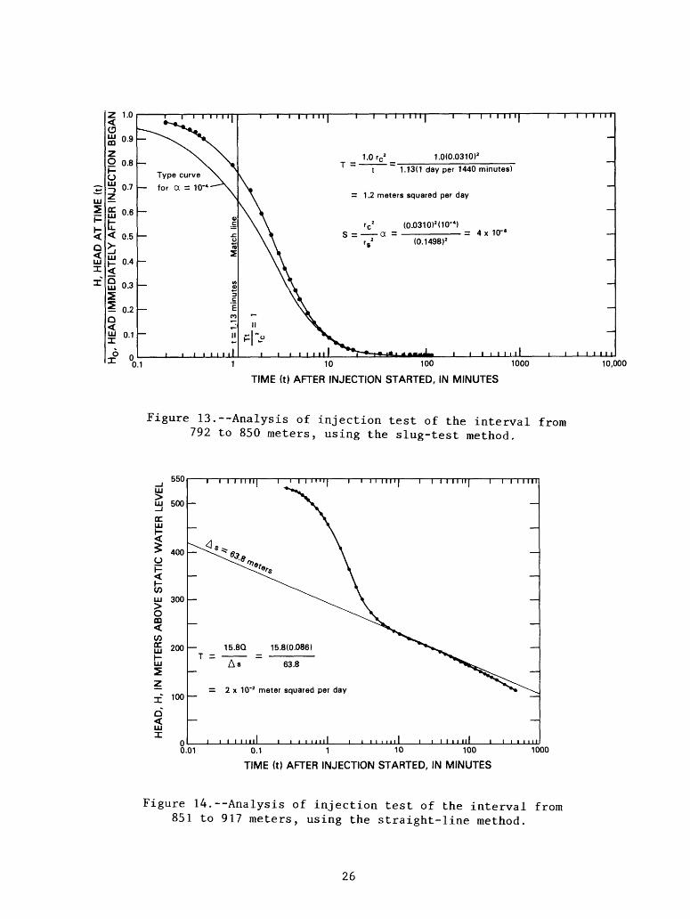
13. Analysis of injection test of the interval from 792to 850 meters, using the slug-test method-------------- 26

14. Analysis of injection test of the interval from 851to 917 meters, using the straight-line method---------- 26

15. Analysis of injection test of the interval from 911 to 972 meters, using straight-line and slug-test methods------------------------------------------------ 27

16. Analysis of injection test of the interval from 972 to 1,219 meters, using straight-line and slug-test methods 28

17. Analysis of injection test of the interval from 1,063 to 1,124 meters, using straight-line and slug-test methods - -- 29

18. Analysis of injection test of the interval from 1,126to 1,219 meters, using the straight-line method-------- 30

19. Analysis of recovery of water level during swabbingtest of the interval from 792 to 1,219 meters---------- 31

20. Analysis of recovery of water level during swabbingtest of the interval from 1,063 to 1,124 meters-------- 32

TABLESPage

Table 1. Generalized lithologic log for test well USW H-3-- -- 52. Summary of test results----------------------------------------- 133. Distribution of apparent transmissivity and hydraulic

conductivity based on the borehole-flow survey---------------- 334. Comparison of transmissivity values resulting from three types

of tests---------------------- ---------- ------------------ 34

IV

GEOHYDROLOGY OF TEST WELL USW H-3, YUCCA MOUNTAIN NYE COUNTY, NEVADA

By William Thordarson, F. E. Rush, and S. J. Waddell

ABSTRACT

Test well USW H-3 is one of several test wells drilled in the southwest­ ern part of the Nevada Test Site in cooperation with the U.S. Department of Energy for investigations related to the isolation of high-level radioactive wastes. All rocks penetrated by the well to a total depth of 1,219 meters are volcanic tuff of Tertiary age.

The composite hydraulic head in the zone 751 to 1,219 meters was 733 meters above sea level, and at a depth below land surface of 751 meters. Below a depth of 1,190 meters, the hydraulic head was 754 meters above sea level or higher, suggesting an upward component of ground-water flow at the site.

The most transmissive part of the saturated zone is in the upper part of the Tram Member of the Crater Flat Tuff in the depth interval from 809 to 841 meters, with an apparent transmissivity of about 7X10" 1 meter squared per day. The remainder of the penetrated rocks in the saturated zone, 841 to 1,219 meters, has an apparent transmissivity of about 4xlO-1 meter squared per day. The most transmissive part of the lower depth interval is in the bedded tuff and Lithic Ridge Tuff, in the depth interval from 1,108 to 1,120 meters. The apparent hydraulic conductivity of the rocks in the lower depth interval from 841 to 1,219 meters commonly ranges from about 10" 1 to 10~ 4 meter per day.

INTRODUCTION

The U.S. Geological Survey has been conducting investigations at Yucca Mountain, Nevada, to evaluate the hydrologic and geologic suitability of this site for storing high-level nuclear waste in a geologic mined repository. These investigations are part of the Nevada Nuclear Waste Storage Investiga­ tions project conducted in cooperation with the U.S. Department of Energy, Nevada Operations Office, under Interagency Agreement DE-AI08-78ET44802. Test drilling has been a principal method of investigation. This report presents hydrologic information on test well USW H-3, one of several exploratory wells drilled into tuff in or near the southwestern part of the Nevada Test Site. The data used for the interpretations in this report are contained in a report by Thordarson and others (1984).

Purpose and Scope

The primary purpose of this study is to define hydrologic characteristics of tuff in the southwestern part of the Nevada Test Site that may be useful in determining the suitability of tuffs for isolating toxic nuclear wastes. This report presents detailed hydraulic-testing data, supporting geological and geophysical information, and hydrological interpretations for the rocks penetrated in drilling the well, one of a series of test wells designed to obtain data principally for the saturated zone.

Location of the Well

Test well USW H-3 is approximately 140 km northwest of Las Vegas in southern Nevada (fig. 1). The well site is on the main north-south oriented ridge of Yucca Mountain, northwest of Jackass Flats and 2 km west of the Nevada Test Site boundary. The well is approximately 4 km south-southwest of test well USW H-l, at Nevada State Central Zone Coordinates N 756,542 and E 558,452. Altitude of the land surface at the well site is 1,483.4 m above sea level. Test well USW H-l was the first well in the series to be drilled; this well (USW H-3) was the second.

Drilling Procedures and Well Construction

Drilling of the well started on January 21, 1982; total depth of 1,219 m was reached on February 28, 1982. The rotary-drilling fluid was air foam consisting of air, detergent, and water obtained from supply well J-13 (fig. 1). About 1,200 m 3 of detergent and water were used (Thordarson and others, 1984). Drilling was completed without much difficulty; however, circulation was lost between a depth of 392 and 817 m, and caving occurred between depths of 38 and 308 m. The well did not deviate more than 2.75 degrees from the vertical; the bottom of the well is 25 m west-northwest of the starting point at land surface. Additional well-construction details are presented by Thordarson and others (1984). In July 1982, after injection and swabbing tests were completed, but before the pumping test, the well casing was perforated below the static water level, from a depth of 754 m to the bottom of the casing at 792 m; vertical spacing of perforations is about 15 cm.

Geohydrologic Setting

The rocks exposed in the vicinity of the Nevada Test Site consist princi­ pally of various sedimentary rocks of Precambrian and Paleozoic age, volcanic and sedimentary rocks of Tertiary age, and alluvial and playa deposits of Quaternary age (Winograd and Thordarson, 1975; Byers and others, 1976). The rocks of Precambrian and Paleozoic age have a total thickness of approximately 11,000 m; they are predominantly limestone and dolomite, but include marble, quartzite, argillite, shale, and conglomerate. The rocks of Paleozoic age have been intruded by granitic stocks of Mesozoic and Tertiary age, and by basalt dikes of Tertiary and Quarternary age. The bulk of the rocks of Tertiary age consist of welded, vitric, and zeolitic tuffs and rhyolite flows

36°45' -

Area of nap i

LaslVegas

Base from U.S. Geological Survey 1:250 000, Death Valley, Cali­ fornia; Nevada,1970

10 15 KILOMETERS

5 MILES

Figure 1.--Location of test well USW H-3

of Miocene age that were extruded from the Timber Mountain-Oasis Valley caldera complex, 20 km north of the test well. The alluvium consists princi­ pally of detritus deposited in the intermontane basins, much of it as fan deposits.

Tuffs underlie Yucca Mountain from land surface to some undetermined depth in excess of 1,219 m. The pre-Tertiary lithology is unknown, but it is most likely either granite or sedimentary rocks of Paleozoic age.

Surface drainage is indirectly toward the Amargosa Desert (fig. 1). Jackass Flats (fig. 1), at an altitude of about 1,000 m above sea level, receives an average annual precipitation of about 100 mm (Hunt and others, 1966, p. B5-B7). The mountain receives more precipitation because of its higher altitude; winter and spring are the seasons with the greatest precipi­ tation, when frontal storms move across the area from the west. During the summer, widely scattered, intense thundershowers are common in the region.

Infrequent runoff that results from rapid snowmelt or from summer showers flows into ephemeral streams along the canyons and washes. Commonly, the beds of the washes are a mix of sand, gravel, and boulders, that rapidly absorb the infrequent flows. Most infiltrated water is returned to the atmosphere by evaporation and transpiration shortly after runoff ceases, but small quanities percolate to depths beyond which evaporation and transpiration are effective. This water ultimately recharges the ground-water system. A much larger proportion of the water in the ground-water flow system is recharged from precipitation northwest of the Yucca Mountain area. This water flows lateral­ ly to and beneath Yucca Mountain (Blankennagel and Weir, 1973, pi. 3; Winograd and Thordarson, 1975, pi. 1; and Rush, 1970, pi. 1). Migration of ground water from the area may be eastward locally, but ultimately is southward toward the Amargosa Desert.

Sass and Lachenbruch (1982, p. 16-25) concluded from geothermal data from wells at Yucca Mountain that water percolates with a downward component of flow through the unsaturated and saturated zones. They also concluded from calculated heat flows that the downward volumetric flow rate in the saturated zone may be about 1 to 10 mm/a, and the average water-particle velocity may be about 40 mm/a, assuming a porosity of 20 percent. Using an empirical method, Rush (1970, p. 15) used a precipitation-recharge rate for Yucca Mountain (computed from data for Jackass Flats, table 3 of this report) less than 5 mm/a. Rates for the horizontal component of flow were not estimated.

LITHOLOGY

Rocks penetrated by the well are mostly ash-flow tuff with various degrees of welding (table 1), as determined from bit cuttings and from geophysical-log correlations with nearby test well USW G-3 (fig. 1). The principal exceptions in the tuff sequence are four thin, poorly lithified, bedded, or reworked tuffs at the bases of several stratigraphic units.

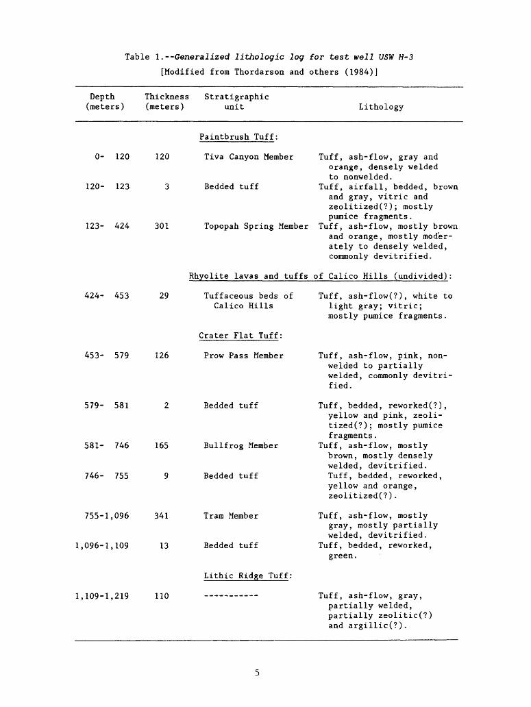
Table 1.--Generalized lithologic log for test well USW H-3

[Modified from Thordarson and others (1984)]

Depth Thickness Stratigraphic (meters) (meters) unit Lithology

424- 453

453- 579

579- 581

581- 746

746- 755

755-1,096

1,096-1,109

1,109-1,219

120

Paintbrush Tuff:

Tiva Canyon Member Tuff, ash-flow, gray andorange, densely welded to nonwelded.

Bedded tuff Tuff, airfall, bedded, brownand gray, vitric and zeolitized(?); mostly pumice fragments.

Topopah Spring Member Tuff, ash-flow, mostly brownand orange, mostly moder­ ately to densely welded, commonly devitrified.

0- 120

120- 123

123- 424 301

29

126

165

341

13

110

Rhyolite lavas and tuffs of Calico Hills (undivided):

Tuffaceous beds of Calico Hills

Crater Flat Tuff:

Prow Pass Member

Bedded tuff

Bullfrog Member

Bedded tuff

Tram Member

Bedded tuff

Lithic Ridge Tuff:

Tuff, ash-flow(?), white to light gray; vitric; mostly pumice fragments.

Tuff, ash-flow, pink, non- welded to partially welded, commonly devitri- fied.

Tuff, bedded, reworked(?), yellow and pink, zeoli- tized(?); mostly pumice fragments.

Tuff, ash-flow, mostly brown, mostly densely welded, devitrified. Tuff, bedded, reworked, yellow and orange, zeolitized(?).

Tuff, ash-flow, mostly gray, mostly partially welded, devitrified.

Tuff, bedded, reworked, green.

Tuff, ash-flow, gray, partially welded, partially zeolitic(?) and argillic(?).

The Tiva Canyon Member, the Topopah Spring Member of the Paintbrush Tuff, and the Bullfrog Member of the Crater Flat Tuff have the greatest degree of welding and are characterized as having mostly moderate-to-dense welding. The least welded tuffs are the Prow Pass Member of the Crater Flat Tuff, the Tram Member of the Crater Flat Tuff, the Lithic Ridge Tuff, and, perhaps, the Tuffaceous beds of Calico Hills, which are nonwelded to partially welded. A summary of welding characteristics and a detailed lithologic log of the penetrated rock are presented by Thordarson and others (1984).

Two geologic factors related to fracturing of the rock penetrated by the well are: (1) Older rocks would be expected to be more fractured because they have been exposed to more periods of mechanical stresses; and (2) densely welded rock is more brittle than less welded rock, and would be expected to break (rather than bend) from mechanical stress. The second factor probably dominates, in that the densely welded lithologic units probably are intensely fractured (Rush and others, 1984, p. 7). In the remainder of this report, stratigraphic members are referred to without reference to the formation of which they are a part; these relationships are given in table 1.

GEOPHYSICAL LOG INTERPRETATIONS

Sixteen types of geophysical logs were run in the well for a variety of purposes, including: (1) Defining lithology; (2) correlating with logs of other wells; (3) obtaining data for porosity, fractures, and permeability; (4) locating fluid level, casing perforations, and casing cement; and (5) gaging the diameter of the open-hole part of the well. Some of these uses are not discussed here because they do not directly contribute to characterization of the geohydrology of the penetrated stratigraphic units. However, they were useful in designing hydraulic tests for the well. A summary of the geophysi­ cal logs run in the well is given by Thordarson and others (1984).

Density, neutron, and 3-D velocity logs were used to determine the distribution of rock porosity, based on techniques described by Schlumberger Limited (1972, p. 37-55) and Birdwell Division (1973, p. OF90-OF188). The 3-D velocity log responds to matrix porosity. Borehole-compensated density and neutron logs respond both to matrix and fracture porosity. For the purpose of defining the general distribution of rock with greater-than-average porosity (that is, rock having porosity greater than the middle of the range indicated by the logs), the penetrated-rock sequence was divided into 80 equal-depth intervals, each about 15 m thick. Using the three types of logs, each depth interval was evaluated for percentage of relatively porous rock (that is, rock having porosity greater than the average for the entire sequence of rocks penetrated by the well). The three logs each produced results that were very similar, except for the interval 1,052 to 1,097 m in the lower part of the Tram Member, which had some differences between logs. The following conclu­ sions are made from the resulting graph (fig. 2): (l) The Tuffaceous beds of Calico Hills, the lower part of the Tram Member, and the penetrated part of the Lithic Ridge Tuff are above average in porosity; (2) the four bedded tuffs are above average in porosity; and (3) thick intervals in the Topopah Spring and Bullfrog Members and the upper part of the Tram Member are below average in porosity.

200

O 400

LL. CCD CO

600

CO COccKf 800

1000

1200

1400

Bottom of casing at 38 meters Tiva Canyontti^ttti-K-frKtt-K-mm^^ Member

Bedded tuff

Topopah

Spring

Member

Tuffaceous beds of Calico Hills

Prow Pass

Member

Bedded tuff

Bullfrog

Member

Bedded tuff :

Tram

Member

Bedded tuff

Lithic

Ridge

Tuff

0 20 40 60 80

PERCENTAGE OF POROUS ROCK100

Figure 2.--Distribution of porous rock in the well, as determined fromgeophysical logs.

Porosity at shallow depth probably represents both matrix porosity and fractures. However, the volume of fracture porosity at greater depths proba­ bly is much less because of greater overburden pressure; therefore, the porosity represented there is largely or entirely matrix porosity.

The neutron log also can be used to determine the position of the water table. On February 19, 1982, while the well had a depth of 808 m and the slowly rising water level in the well was measured at a depth of 777 m, the water table could not be identified from the log. This may have been the result of the fracture and matrix porosity being so low that saturated rock below the water table had very little more water content than the overlying unsaturated rock, and the log could not measure the difference.

On July 23, 1982, 5 months after total depth was reached in test well USW H-3, a temperature log was made in the well under static logging conditions; that is, no stresses were applied to the well or the penetrated rock during the logging period and the water level was near static. However, effects of past drilling and testing stresses may have remained. A summary follows of some of the thermal conditions logged, or estimated from the log: (1) The estimated average ambient land-surface temperature at the well site was 25.3°C and the maximum recorded temperature in the well, at a depth of 1,211 m, was 43.3°C; (2) a temperature reversal occurred in the geothermal gradient, as recorded in the depth interval from 0 to 126 m, in the unsaturated Tiva Canyon Member; the lowest temperature in the well, 22.5°C, was at the base of this interval; and (3) the geothermal gradients in the unsaturated zone, 17.0°C/km, and in the sa crated zone, 16.9°C/km, were very similar, suggesting that the difference n water content between the saturated and unsaturated zones was small.

The acoustic televiewer log, an acoustic traveltime log, was made to record borehole-wall texture in the liquid-filled part of the hole from the bottom of the casing at a depth of 792 m to a depth of 1,210 m. Such features as fractures and bedding planes were detected. Because the log is direction- ally oriented, the dip of inclined lineations was identified. Horizontal or nearly horizontal linear features were identified from the logs; they probably are either bedding planes or fractures. Steeply inclined linear features are more likely to be fractures. In the depth interval from 821 to 929 m, in­ clined linear features with mostly southwestward dips were identified. These features, probably fractures, had dips ranging from 60° to 80°. In the interval 1,029 to 1,107 m, another set of inclined linear features generally has dips to the northeast and east between 70° and 85°. Separating these two sets is an interval of 100 m of no detectable lineations. A listing of linear features is presented by Thordarson and others (1984).

Caliper logs were made during and after the drilling period to determine the open-hole diameter distribution with well depth. Erosion from drilling activity was the cause of the enlargement in well diameter. Erosion probably was caused by poor lithification, abundant fractures, and perhaps other unknown factors. Enlarged borehole zones that possibly were fracture con­ trolled were identified by Thordarson and others (1984) from caliper logs as zones with irregular enlargement. The principal fracture-controlled zones are: (1) A thick interval (9 to 101 m) in the Tiva Canyon Member, and (2) a thick interval (169 to 358 m) in the Topopah Spring Member.

A television-camera log was made in the well before casing the well to a depth of 792 m. Open-hole conditions were logged from a depth of 38 m to the water level in the well at that time, 767 m. Features observed were frac­ tures, hole enlargement, lithologic features, and a water seep. The fractures were observed at many depths, but mostly in the Tiva Canyon Member and the upper part of the Topopah Spring Member; they are listed by Thordarson and others (1984). Water was observed seeping from fractures, above static water level, at a depth of 277 m. Slickensides with lateral displacement were observed at a depth of 216 m in the upper part of the Topopah Spring Member.

BOREHOLE-FLOW SURVEY

A borehole-flow survey using a radioactive tracer (Blankennagel, 1967 and 1968) was used to measure vertical flow rates in the well, while water was pumped into the well at a rate of 2.7 L/s and with constant head. From this measurement, the zones through which the water flowed from the well and estimated flow rates for the zones were identified. The survey was made after the well had been cased to a depth of 792 m and had a total depth of 1,219 m. The units tested included the saturated lower 308 m of the Tram Member and the penetrated underlying units (fig. 3).

Conclusions from the survey, assuming no significant hydraulic-head loss in the wellbore are:

1. In the 31.9-m interval from 809 to 840.9 m, about 7 percent of the surveyed interval received 63 percent of the injected water. This interval is in the upper part of the Tram Member.

2. The second greatest injection rate was for the interval from 1,060 to 1,120.4 m, about 14 percent of the surveyed interval, extending from the lower part of the Tram Member through bedded tuff and into the upper part of the Lithic Ridge Tuff. This interval received 30 percent of the flow.

3. The small remaining part of the total flow mostly entered the inter­ val from 840.9 to 933 m of the Tram Member. The other intervals received little, if any, of the flow.

In a later section of this report, these survey results are used in conjunc­ tion with hydraulic tests to assign values of transmissivity and hydraulic conductivity to 28 intervals within the saturated zone.

WATER-LEVEL MONITORING

Water-level observations and measurements in the well were made during the drilling period, as part of hydraulic tests, and after testing was-com­ pleted. The purposes of these observations and measurements were: (1) To locate any perched-water zones above the water table, (2) to identify the depth at which water saturation occurs, (3) to determine the composite hydrau­ lic head in the well, (4) to identify hydraulic heads in various water-bearing zones, and (5) to determine the existence of artesian or water-table conditions.

DE

PT

H,

IN M

ETE

RS

B

ELO

W L

AN

D S

UR

FA

CE

H-

OC C o>

LO i i to

o o>H

O

sr M

o n>

H i

CU

H

) 05

(

'i-S

O

CO

%

o y co e

05

hi

13

<CL

ro

o n-

H)

cr o

n>

hjCO

ft

- o> CO

i-»

ri-

oo c c/i s: tn C

O 3

o CL

H-

H>

H-

CD

O.

o

o -

O O

o

o

o

O

5~CD

-

~O

CD

II

CO

n

i-*'

Q.

CO

CDs

src

o

During drilling of the interval from 744 to 753 m, either perched ground water or returning drilling fluid entered the well from the rock. If it was ground water, the likely source was ash-flow tuff at the base of the Bullfrog Member. This unit overlies a bedded tuff, depth interval from 746 to 755 m. Later, the composite-hydraulic head in the well stabilized at a depth of 750.7 ± 0.2 m below land surface (Thordarson and others, 1984). Below the bedded tuff, the Tram Member and all underlying units were saturated and possibly under artesian conditions in the vicinity of the well, similar to conditions at test well USW H-l (Rush and others, 1984).

To obtain information on the vertical distribution of hydraulic head at the well, a packer was installed at a depth of 1,190 m. On November 3, 1983, the hydraulic head in the rocks above the packer was at 732.9 m above sea level; below the packer, the head in those rocks was at 754.0 m above sea level and rising slowly toward static conditions. These results indicate that the lower zone had a composite head at least 21.1 m higher than the upper zone.

HYDRAULIC TESTING

This section of the report includes descriptions of pumping-, injection-, and swabbing-test results. The tests were made following the drilling of the well to final depth. Test results are discussed separately in subsequent sections of the report. Following these sections, results from the three types of tests are compared, differences reconciled, and representative values selected for various depth intervals in the penetrated part of the saturated zone.

According to Bredehoeft and Maini (1981, p. 293-294), definition of ground-water flow and the parameters that control flow through typical porous media sand, gravel, sandstone are well understood. In contrast, flow through a fractured-rock mass, such as tuffs beneath Yucca Mountain, is much less understood. Neither the theory nor the field technology required to measure flow characteristics of a ground-water system in a fractured medium is very advanced; thus, uncertainties in predictions are great in both time and space. As a result, in the following paragraphs, a conceptual model of the ground-water system beneath Yucca Mountain is presented and a solution to the theory and field-technology dilemma is proposed.

To define ground-water parameters for the flow system at this well site, a conceptual model is desired. The principal elements of the model are those of Rush and others (1984):

1. The rock is nearly homogeneous and isotropic. Primary porosity is intergranular and controlled in ash-flow tuffs principally by degree of welding and degree of alteration.

2. Secondary porosity is controlled by fractures. These fractures generally are vertical or at a steep angle and may be spatially random in the saturated zone (Baecher, 1983, p. 329), and are the result of tensional and shear failure during mechanical deformation during tectonic activity or fracturing during cooling. The volume of water stored in fractures is rela­ tively small in comparison to that stored in the matrix porosity. On a small

11

scale, the tectonic fracture permeability is anisotropic. However, the fracture permeability due to cooling joints probably would be isotropic in plan view, as well as homogeneous, because only random fracture strikes would be observed (Scott and others, 1983, p. 315).

3. Both primary and secondary porosity may be decreased by precipitation of minerals.

4. Flow to the well is through the fracture network only; however, flow probably occurs between pores and fractures. Hydraulic conductivity of fractures is several orders of magnitude larger than hydraulic conductivity of the matrix.

5. Distances between fractures are small in comparison with the dimen­ sions of the ground-water system under consideration.

6. In ash-flow tuffs, zones of approximately the same degree of welding have approximately the same density of fracturing (Scott and others, 1983, p. 309). Sufficiently dense fracture spacing probably results in the fractured ash-flow tuffs functioning in a hydraulically similar fashion to a granular porous medium (Freeze and Cherry, 1979, p. 73).

Based on the conceptual model, homogeneous porous-media solutions can be used to define general ground-water parameters and ground-water flow in fractured media, using late-time test data to define this dual-porosity system (Warren and Root, 1963; Odeh, 1965; Kazemi, 1969; Kazemi and Seth, 1969; Wang and others, 1977, p. 104; and Najurieta, 1980, p. 1242). However, early-time test data will yield parameters that apply only to the fractured part of the system. Data used for computing apparent transmissivity for all types of tests in this well probably are early-time data, as concluded by Rush and others (1984) for test well USW H-l, and therefore apply only to the fractured part of the system. The earliest hydraulic-head-change data may be dependent partly on nonrepresentative, near-well hydraulics (Wang and others, 1977, p. 103), on wellbore storage, and on skin effects. During pumping, skin effect is the pressure drop at the wellface in addition to the normal transient pressure drop in the ground-water system resulting from damage or improvement of the rock's ability to transmit water at the wellface (Earlougher, 1977, p. 57). Commonly, the damage or improvement is the result of well drilling.

Witherspoon and others (1980, p. 26-28), in their hydrologic work in crystalline rock, have assumed that, in general, a fracture system can be treated as a slightly different form of porous medium, measuring equivalent porous-media properties. The porous-media solutions will not yield correct porosity and hydraulic-conductivity values for each matrix or fracture porosi­ ty type in this dual-porosity system beneath Yucca Mountain, but rather average values for the zones tested. As a result, hydraulic conductivity, aperture, and volume of specific fractures or effective pore volume of the matrix are not determined.

The degree of reliability of the conceptual model is related to the degree to which the model approximates the actual fracture-flow ground-water system beneath Yucca Mountain, for the purposes intended and for the time during which the data are valid. The departure of test data is a measure of how far conditions are from the ideal (Ferris and others, 1962, p. 102). Departure from ideal for each test has been evaluated and is described in the following sections where testing results are presented and in table 2.

12

Table 2.--Summary of test results

Test interval (meters)

Transmissivity Storage Departure(meters squared coeffi- of data

per day) cient from ideal Remarks

754-1,219 (fig- 4)

754-1,219(fig. 5)

1 822-1,219(fig. 6)

792- 850(fig. 13)

851- 917(fig. 14)

911- 972(fig. 15)

972-1,219 (fig. 16)

1,063-1,124 (fig. 17)

1,126-1,219 (fig. 18)

792-1,219 (fig. 19)

1,063-1,124 (fig. 20)

SxlO' 1

4X10" 1

1.0

1.2

2xlO~ 2

3xlO~2

IxlO' 1 3xlO~ 2

3xlO~ 2

IxlO' 1

lxlO~ 2

1.1

1x10-1

PUMPING TESTS

----- Small Using second cycleof pumping.

----- Small Using all cyclesof pumping.

----- Small Long-term test.

INJECTION TESTS

4xlO~6 Moderate Using slug-testmethod of analysis.

------ Small Using straight-linemethod of analysis.

------ Large Do.6xlO~ 6 Moderate Using slug-test

method of analysis.

7xlO~ 6 Moderate Do.------ Large Using straight-line

method of analysis.

------ Large Used straight-linemethod of analysis

7xlO~ 6 Large Used slug-testmethod of analysis

------ Small Used straight-linemethod of analysis.

SWABBING TESTS

------ Small Used straight-linemethod of anal­ ysis .

------ Small Do.

1Pumping zone below a packer.

13

Pumping Tests

The well was initially and briefly pumped for several cycles of drawdown and recovery, using a submersible pump. The well could not sustain the yield of several liters per second. The brief drawdowns and recoveries of the water level were measured to determine transmissivity of the part of the saturated zone penetrated by the well (figs. 4 and 5). Later, a smaller pump was used, which discharged at a rate of 0.16 L/s (fig. 6). Because a large volume of water was not pumped from the well, no representative samples of ground water were collected for chemical analyses.

The methods used to analyze the data were the straight-line method (Cooper and Jacob, 1946; Ferris and others, 1962, p. 100), Brown's method (Ferris and others, 1962, p. 122), and the Theis method (Lohman, 1972, p. 15). Method assumptions are discussed in the cited references. Results of these and other tests are discussed and summarized in table 2.

For the straight-line method of analysis of the recovery in a pumped well, residual drawdown, s', was plotted against time after pumping started, divided by time after pumping stopped, t/t' , on semilogarithmic-coordinate scale. After values of time became sufficiently large, and after testing conditions were met (as described earlier in this report), the measured data plotted along a straight line. The slope of this line for one log cycle, As', was used in the following equation:

T = 1J ' os; , (1)As'

where

T is transmissivity, in meters squared per day;Q is constant rate of discharge of the well, in liters per second; and

s* is residual drawdown for one log cycle, in meters.

A transmissivity of 5*10"* m2 /d was computed in figure 4 using a single cycle of the initial pumping period.

For Brown's method, drawdown and recovery, s, were plotted against time after pumping started, t, on arithmetic-coordinate paper. Then, the intervals of time between the start of pumping in each cycle and the end of the final recovery period were calculated, resulting in values for tj through t$. The intervals of time between the end of the recovery period in each cycle and the end of the final recovery period were calculated, resulting in values for t'j through t' 5 . Then, these values of t and t' were substituted into Brown's equation:

T = 15.8Q (2)

14

CO DC LU

Z

DC Q

gCOLU DC

10

20

30

T =15.8Q 15.8(3.13 liters per second)

As' 108.1 meters

= 5 x 10~ 1 meter squared per dey

2 345

TIME (t) SINCE SWABBING STARTED

10

TIME It') SINCE SWABBING STOPPED

Figure 4.--Analysis of water-level recovery following second cycle of pumping of the interval from 754 to 1,219 meters, using the straight-line method.

I i i i i i i i i

i i i i i i i i6 8 10 12 14

TIME (t) AFTER PUMPING STARTED, IN HOURS

16 18

T =- 15.8(2.84 liters per second)

11.1 meters « 643.4 minutes\/483.4\/355.8\/236.8\/108.5\\ _

628.4 minutes K466.4y\^344.8y\226.3Jy98.2 JJ ~ 4 x 10~1 meter squared per day

Figure 5.--Analysis of the pumping test of the interval from 754 to 1,219 meters, using Brown's method for a cyclically pumped well.

15

10

cc in UJ ,52 Z o Q QC

Q

Mat

ch p

oint

Thei

s ty

pe c

urve

TYP

E C

UR

VE

MA

TCH

PO

INT

CO

OR

DIN

ATE

S

W(u

) =

1

1/u

=

1

t

1 m

inut

e

s

1.1

met

ers

T =

6.88

Q

W(u

) _

6.

88 x

0.1

6 lit

er p

er s

econ

d s

1.1

met

ers

= 1 .

0 m

eter

squ

ared

per

day

0.01

10

100

1000

TIM

E (

t) A

FTE

R P

UM

PIN

G S

TA

RT

ED

, IN

MIN

UT

ES

10,000

100,000

Figure 6.--Analysis of water-level drawdown of

th

e interval fr

om 82

2 to

1,219

mete

rs,

using the

Theis

meth

od.

where

T is transmissivity, in meters squared per day; Q is constant rate of discharge, in liters per second; and

55 is net drawdown at the end of the fifth cycle, the last cycle used, in meters.

A transmissivity of 4X10" 1 m2 /d was computed in figure 5 using multiple cycles of the initial pumping period.

For the Theis method, drawdown, s, was plotted against time after pumping started, t, on logarithmic-coordinate paper. The data curve then was superim­ posed on a type curve to obtain the best fit of the data to the type curve. An arbitrary match-point was selected anywhere on the overlapping part of the sheets, and the four coordinates of common point on the two sheets were determined. The following equation then was used:

T= ^|?-fi W(M ), (3)

where

T is transmissivity, in meters squared per day; Q is constant rate of discharge, in liters per second;

W(|j) is well function, a match-point coordinate; ands is drawdown in meters, another match-point coordinate.

Later, in January 1984, a long-term, small-discharge-rate pumping test was made testing the interval from a packer installed at a depth of 822 m to a depth of 1,219 m. The resulting data (fig. 6) yields a transmissivity of about 1.0 m2 /d. This interval is 85 percent of the penetrated part of the saturated zone, the packer being set about 71 m below the composite static- water level. The data curve strongly resembled the results of pumping test 2, zone from 687 to 1,829 m in test well USW H-l (Rush and others, 1984, fig. 12), farther north on Yucca Mountain (fig. 1). The departure of the data curve from the type curve at time 2,500 minutes indicates leaky aquifer conditions, that a recharging boundary had been reached by the cone of depres­ sion caused by pumping, or that the transition from early time to late time was reached. The discharge rate was about 0.16 L/s and the maximum drawdown was 8.12 m for the 20,520-minute pumping period. Pumping-test results ana­ lyzed in figures 4, 5, and 6 have only small departures from ideal.

Injection Tests

Injection tests were made in selected depth intervals by using inflatable packers in the well to isolate the test zones. Injection-test data were analyzed by the straight-line method described for pumping tests earlier in this report and the slug-test method described by Cooper and others (1967) and Papadopulos and others (1973). The assumptions are discussed in the cited references. Six tests were successfully completed.

17

For the slug-test method of analysis, the ratio of hydraulic head at a given time to hydraulic head at time zero, H/H , was plotted against time after injection started, t, on semilogarithmic-coordinate paper. H/H was plotted on the arithmetic scale; time was plotted on the logarithmic scale. A family of type curves was used to determine transmissivity and storage coeffi­ cient. A match point was selected on the logarithmic scale of the type-curve graph, with a value of 1.0. The corresponding time, t, match point on the logarithmic scale of the data graph was determined. The following equation then was used to calculate transmissivity:

T =1.0 r 2

c(4)

where

T is transmissivity, in meters squared per day;r is radius of the tubing used in the packer assembly, in meters; and

t is the match-point time, in days.

To estimate the coefficient of storage, S, the following equation was used:

S = (5)

where

a is the recorded matching curves value; and r is the radius of the open hole, in meters.

Use of early injection-test data to determine aquifer properties will give erroneous results because of wellbore-storage effects and hydraulic- fracturing effects. These effects are discussed in the following paragraphs.

Wellbore-storage effects were prominent during the early parts of the injection tests as a result of a gradually changing rate of injection at the formation face. During the early part of the injection, the large injection rate into the formation probably represents water being released from storage in the tubing; the later part of the injection, when the injection pressure and rate were less, represents more accurately the rate of injection at the formation face. During wellbore-storage domination, a full logarithmic plot of change of pressure versus change in time shows a unit slope of one cycle of pressure change per one cycle of time change; this unit slope represents data that cannot be used to analyze formation properties (Earlougher, 1977).

18

Effects of wellbore storage that were prominent during early parts of the injection tests were identified by drawing a unit-slope straight line on log-log plot of Ap and t, as shown in figures 7 and 8 (Earlougher, 1977). This plot shows the dominance of wellbore-storage effects during the first 3 minutes of the tests. The data following departure from unit slope are analyzed for transmissivity.

Hydraulic-fracturing effects probably occurred during the early parts of the injection tests because of the large hydraulic head exerted. Effects of probable widening of fractures during the first 5 to 6 minutes were found in the double-humped curves for the injection tests in figures 14 to 18 presented later in this section. However, the test for the interval from 792 to 850 m showed a more normal S-shaped curve as presented in figure 13 later in this section. The brief widening of fractures was caused by the great height of the column of water in the tubing, amounting to about 750 m above the static water level. At a pressure gradient of 9.80 kPa/m for fresh water, a column of 750 m exerted a total instantaneous bottom-hole pressure of 7.4xl0 3 kPa, a pressure that exceeds the pressure that is needed to produce vertical frac­ tures in a tectonically relaxed geologic environment (Hubbert and Willis, 1972). For example, pressure needed to produce hydraulic fractures in dolomites in New York is only 6.6xl0 3 kPa (Waller and others, 1978, p. 29). A plot of pressure versus injection rate for the tests in test well USW H-3 is presented in figure 9 to show the nearly flat slope that is indicative of hydraulic widening of fractures, a method used for the fractured dolomites in New York. Injection-test data generally show a nearly flat slope from approx­ imately 2 to 5 minutes, except for the injection test for the interval from 792 to 850 m. That test shows a more normal inclined slope. The nearly flat slopes are attributed to widening of fractures with associated transient increases in transmissivity.

Possible fracture widening from hydraulic pressure also is indicated by plots of velocity of the injection of water versus time shown in figures 10 and 11, and specific capacity versus time, as shown in figure 12. The plots of velocity versus time in figures 10 and 11 have steep slopes for tests with hydraulic-fracture widening; after 10 to 18 minutes the velocity decreases to less than 2.2 m per minute, a velocity below which turbulent flow in the tubing probably ends. This velocity may indicate when the turbulence in the fracture changes to laminar flow. The plot of specific capacity versus time (fig. 12) indicates fracture widening between 2 to 5 minutes by the very steep slope of the curve. Specific capacity becomes more uniform and unchanging after approximately 7 to 9 minutes for injection tests with fracture widening, and after 70 minutes for the test of the interval 792 to 850 m, which does not show fracture widening; the data are analyzed best after the specific capacity becomes more uniform.

The data for injection tests shown in figures 13 through 18 are very much affected by wellbore-storage and fracturing effects. These effects are present in the early-time data during the first 5 to 7 minutes; as a result, this part of the data curve will give erroneous results if used in calculating hydraulic properties.

19

1000

Stra

ight

lin

e of

uni

t sl

ope

792-

850

met

ers

851

-91

7 m

eter

s A

1063

-112

4 m

eter

s «

1126

-121

9 m

eter

s

- -

A

1 10

10

0

TIM

E f

t) A

FTE

R I

NJE

CT

ION

ST

AR

TE

D,

IN M

INU

TE

S

1000

Figure 7.--Wellbore-storage ef

fect

s during injections te

sts

of th

e intervals

from 792

to 85

0, 851

to 917, 1,

063

to 1,

124,

and

1,12

6 to 1,219

mete

rs.

1000

ro

Stra

ight

lin

e of

uni

t sl

ope

0.1

1 10

10

0

TIM

E (

t) A

FTE

R I

NJE

CT

ION

ST

AR

TE

D,

IN M

INU

TE

S1000

Figure 8.--Wellbore-storage effects du

ring

injection te

sts

of th

e intervals

from 911

to 97

2 and

972

to 1,

219

mete

rs.

7000

N)

Dir

ectio

n o

f in

crea

sing

tim

e du

ring

tes

ts

1000

792-

850

met

ers

851-

917

met

ers

&

911-

972

met

ers

m-

972-

1219

met

ers

*

1063

-112

4 m

eter

s 4

-

1126

-121

9 m

eter

s O

A *

34

56

7

INJE

CT

ION

RA

TE,

IN L

ITE

RS

PER

SE

CO

ND

Figure 9.--Relation of

pressure and

injection rate during injection te

sts

T I

I T

I I

\\

ro OJ

792-

850

met

ers

851-

917

met

ers

£r-

-

1063

-112

4 m

eter

s *

1126

-121

9 m

eter

s O

-o

1 10

10

0

TIM

E (

t) A

FTE

R I

NJE

CT

ION

ST

AR

TE

D,

IN M

INU

TE

S

Figure 10.--Velocity of water in tubing du

ring

injection te

sts

of th

e intervals

from

792

to 850, 851

to 917, 1,063

to 1,

124,

and

1,126

to 1,

219

mete

rs.

120

100

Sj2

£1"

(T

in U_

QC

O

UJ

>-

UJ

g LU

60 40 20

~l I

I I

I-i

i

i i

i i

i i

911-

972

met

ers

-----

972-

1219

met

ers

A- -

A

0.1

\

\ \ \

1 10

10

0

TIM

E (

t) A

FTE

R I

NJE

CT

ION

ST

AR

TE

D,

IN M

INU

TE

S10

00

Figure 11.--Velocity of water in tubing during injection te

sts

of the

intervals

from

911

to 97

2 an

d 97

2 to 1,

219

mete

rs.

SPECIFIC CAPACITY, IN GALLONS PER MINUTE PER FOOT OF HYDRAULIC HEAD

00

1-5

2.--Relat

CL

H-

00

H-

ft)nrtH- O P

fD Wft w

RJ * ^ 2 «2 _^ - <i, <ow j^ -» M ->j a<° * ? 3 3 3i 1 I § I I (? » ? W W Ww w

1" *

i..O

p op oM

SPECIFIC CAPACITY, IN LITERS PER SECOND PER METER OF HYDRAULIC HEAD

uu

p

t 1.13(1 day per 1440 minutes)

= 1.2 meters squared per day

(0.0310)2 (10'4 )

1 10 100 1000

TIME (t) AFTER INJECTION STARTED, IN MINUTES

10,000

Figure 13.--Analysis of injection test of the interval from 792 to 850 meters, using the slug-test method.

CC. UU

oI(/) uuOCD

CC.uu

IQ

uuX

A s 63.8

= 2 x 10'J meter squared per day

0.01 0.1 1 10 100 TIME (t) AFTER INJECTION STARTED, IN MINUTES

1000

Figure 14.--Analysis of injection test of the interval from 851 to 917 meters, using the straight-line method.

26

Straight line

As 51.2

= 3 x 10~2 meter squared per day

0.01 0.1 1 10 100

TIME (t) AFTER INJECTION STARTED, IN MINUTES

Slug test

LLJ

P

ScQ

IDI

0.1

T1.0r, 1.0(0.0310)2

t 22.5(1 day per 1440 minutes)

= 6 x 10~2 meter squared per day

(0.0310)J (lO-«)

(0.1280I2

Type curve for ex = 10"*

1 10 100 1000

TIME (t) AFTER INJECTION STARTED, IN MINUTES

10,000

Figure 15.--Analysis of injection test of the interval from 911 to 972 meters, using straight-line and slug-test methods.

27

Straight line

As 48.0

= 3 x 10"2 meter squared per day

0.01 0.1 1 10 100

TIME (t) AFTER INJECTION STARTED, IN MINUTES

1000

Slug test

T = V° rc ' -

t 9.70(1 day per 1440 minutes)

= 1 x 10' 1 meter squared per day

(0.0310)2 (10-4 )

.0.1208)'

T i i i i i n| i r

1.0(0.0310)'

1 10 100 1000

TIME (t) AFTER INJECTION STARTED, IN MINUTES

10,000

Figure 16.--Analysis of injection test of the interval from 972 to 1,219 meters, using straight-line and slug-test methods.

28

550

500

400

Straight line

O

C/5LU 300

O CO

C/)£ 200

100

01I

T =15.8Q 15.8(0.11)

As 62.0

= 3 x 10"z meter squared per day

0.01 0.1 1 10 100

TIME (t) AFTER INJECTION STARTED, IN MINUTES

1000

11.8(1 day per 1440 minutes)

= 1 x 10"1 meter squared per day

(0.0310) 2 (10-

1 10 100 1000

TIME (t) AFTER INJECTION STARTED, IN MINUTES

10,000

Figure 17.--Analysis of injection test of the interval from 1,063 to 1,124 meters, using straight-line and slug-test methods.

29

650_iLU> 600LU

<r LU< 500

o

j* 400COLU§CO 300<COocLU

u) 200

x 100a

As 83.4

= 1 x 10~2 meter squared per day

0.01 0.1 1 10 100

TIME (t) AFTER INJECTION STARTED, IN MINUTES1000

Figure 18.--Analysis of injection test of the interval from 1,126 to 1,219 meters, using the straight-line method.

In addition to the constraint on the use of early-time data for the injection tests, a second constraint needs to be considered for straight-line method of analysis of the test data. Constant rate of injection and values of M less than 0.01 are requirements to use the method of analysis correctly. The straight-line method was used on five of the six injection tests that show a straight line after about 8 minutes on the semilogarithmic plots. The injection rate of water was nearly constant during the middle part of the semilogarithmic straight line where this rate was within 2 to 22 percent of the average injection rate, as determined from the decline of water within the tubing. Therefore, the analysis was limited to the^middle part of the data plots. The values of transmissivity range from lxlO~ 2 to 1.2 m2 /d using both the slug-test and straight-line methods (table 2).

The storage-coefficient values computed in figures 13, 15, 16, and 17 indicate that the tested zones were under artesian conditions. Based on estimates for storage coefficients by Lohman (1972, p. 8), the values listed in table 2 were very small, but probably were reasonable in magnitude. The values of storage coefficients range from 4xiO~ 6 to 7xiO~ 6 (table 2). For the injection tests, departure from ideal was variable; these departures are

listed in table 2.

30

Swabbing Tests

Swabbing tests consisted of multiple swabbing runs in the open uncased part of the well and between two inflatable straddle packers. Swabbing tests were analyzed using the straight-line method that was described previously in the section on pumping tests.

Analyses of the two swabbing tests are presented in figures 19 and 20. For the test interval from 792 to 1,219 m (fig. 19), the calculated value of transmissivity was 1.1 m 2 /d. The other test, for the interval from 1,063 to 1,124 m (fig. 20), had a calculated value of IxlO" 1 m2 /d. Both sets of data had only small departures from ideal.

Comparison of Testing and Borehole-Flow Survey Results

In the preceding sections of this report, values of transmissivity and storage coefficient were calculated from pumping, injection, and swabbing tests; results are summarized in table 2. In table 2, two values for transmissivity for the interval 792 to 1,219 m are listed: (1) Values from a swabbing test (fig. 19) of 1.1 m 2 /d, and (2) a value calculated from four injection tests spanning the surveyed interval (figs. 13-16), 1.4 m 2 /d. A slightly smaller interval, from 822 to 1,219 m, produced a slightly smaller value, 1.0 m 2 /d, from the long-term pumping test (fig. 6). The swabbing-test results appear to have the smaller departure of data from the ideal; as a result, the value from the swabbing test of 1.1 m 2 /d was selected as the more representative value for the interval (table 3).

ocD CO

oUJ CO

COoc

760

770

780

790

800

tQ 810

V I I I

T =15.8Q _ 15.8(0.83 liter per second)

As' 12.0 meters

= 1.1 meters squared per day

10 20 30 40 50 60 70 80 90 100

TIME (t) SINCE SWABBING STARTED TIME It') SINCE SWABBING STOPPED

Figure 19.--Analysis of recovery of water level during swabbing test of the interval from 792 to 1,219 meters.

31

Ul 750

a: COQZ

760

Ul 770 00CO OC Ul

ui5 780

OC Ul

£ 790

e i8*o0i

T =15.8Q 15.8(0.46 liter per second)

As' 61.0 meters

= 1 x 10"' meter squared per day

2 3 4 56789 10

TIME (t) SINCE SWABBING STARTED TIME (t') SINCE SWABBING STOPPED

Figure 20.--Analysis of recovery of water level during swabbing test of the interval from 1,063 to 1,124 meters.

Based on the above-selected value of transmissivity for the interval 792 to 1,219 m and the borehole-flow survey for the same interval, apparent transmissivity was distributed throughout the interval in table 3. From the apparent transmissivity values, values for apparent average horizontal hydrau­ lic conductivity were calculated.

Transmissivity values were calculated from pumping tests (table 2) for the test interval from 754 to 1,219 m, an interval that includes the smaller interval of the borehole-flow survey. The larger interval would be expected to have a similar or larger value for transmissivity, but smaller values were calculated (SxlO" 1 m 2 /d and 4x10"* m2 /d) in figures 4 and 5. The departure of data from ideal for these two tests seemed to be about the same as for the above-discussed swabbing test; therefore, the selected representative value of transmissivity for the penetrated part of the saturated zone, interval from 754 to 1,219 m, was computed as the average of the three values at about 0.7 ±0.3 m2 /d. Therefore, the values of transmissivity and hydraulic conductivity listed in table 3 should be considered maximum estimated values because they were based on a slightly higher transmissivity value.

An additional comparison of transmissivity values for a selected interval is presented in table 4. Although the three depth intervals are not identi­ cal, the overlap is about 95 percent. Conclusions drawn from the table are that the three tests produced similar results of the same order of magnitude and that the selected representative value for the interval from 1,063 to 1,124 m is about IxlO' 1 m 2 /d.

32

Table 3.--Distribution of apparent transmissivity and hydraulic conductivity based on the borehole-flow survey

[Computations based on a transmissivity of 1.1 meters squared per day;<, less than]

Depth interval (meters)

1,083 -1,106.1

1,106.1-1,108.3

1,108.3-1,113.7

Apparenttransmissivity, T(meters squared

per day)

Apparent averagehorizontal hydraulic

conductivity, K(meters per day)

TRAM MEMBER

i ?92

800 -809 -823 -831.5-

832.1-839 -840.3-840.9-847 -

858 -872 -889 -933 -960 -984 -994 -1

1,009 -11,060 -1

800809823831.5832.1

839840.3840.9847858

872889933960984994,009,060,083

<2xlO-2

<2xlO~ 23x103x104x10

<2xlO<2xlO4x10

<2xlO2x10

<2xlO<2xlO5x10<2xlO<2xlO<2xlO<2xlO<2xlO8x10

-1

-1

~*

-2

-2

-2

-2

~ 2

-2

-2

-2

-2

-2

-2

-2

-2

~ 2

<3xlO~<2xlO~2x10"3x10"7x10"

<3xlO~<2xlO~7x10"

<3xlO"2x10"

<lxlO-<lx!0~1x10"

<7xlO"<8xlO~<2xlO~<lx!0"<4xlO~2x10"

3

3

2

2

2

3

2

2

3

3

3

3

3

4

4

3

3

4

3

TRAM MEMBER AND BEDDED TUFF

2X10' 1

BEDDED TUFF

<2xlO~ 2

BEDDED TUFF AND LITHIC RIDGE TUFF

4x10-2

7x10-3

<9xlO

7x10

33

Table 3. --Distribution of apparent transmissivity and hydraulic conductivity based on the borehole-flow survey--Continued

Depth interval (meters)

Apparenttransmissivity, T(meters squared

per day)

Apparent averagehorizontal hydraulic

conductivity, K(meters per day)

LITHIC RIDGE TUFF

111111

,113,116,120,120,197,200

.7-1

.2-1

.1-1

.4-1

.9-1

.9-1

,116,120,120,197,200,219

.2

.1

.4

.9

.9

<2xlO<2xlO~7xlO~

<2xlO~<2xlO~<2xlO~

2

2

2

2

2

2

<8xlO<5xlO2x10

<3xlO<7xlO<lxlO

-3

~ 3

-1

-4

-3

-3

cased to 792 meters.

Table 4.- -Comparison of transmissivity values resulting from threetypes of tests

[<, less than]

Depth interval (meters)

1,063-1,124

1,063-1,124 1,060-1,120.4

Transmissivity (meters squared Type of

per day) test

IxlO" 1 Injection

IxlO" 1 Swabbing <4xlO~ 1 Borehole-

flowsurvey

Remarks

Using value from table

for interval 2 with least

departure from ideal. From table 2. Sum of values for seven

intervals, table 3.

Values of transmissivity and hydraulic conductivity determined from the tests are very small, but are several orders of magnitude larger than those determined from tests of test well USW H-l (Rush and others, 1984, table 14). To illustrate the low magnitude of the values, using a method by Theis (1963), if the well were pumped at a constant rate for 24 hours and the resulting drawdown were 100 m, the required well yield would be less than 1 L/s.

34

DISCUSSION OF WELL-SITE GEOHYDROLOGY

In the previous sections of this report, results of the analyses of various sets of data are presented. In this section, all results are consid­ ered and data conflicts are resolved to develop a composite geohydrologic interpretation of each stratigraphic unit in the saturated-zone conceptual model and the units in the overlying unsaturated zone.

The Tiva Canyon Member crops out at the well site and has a thickness of 120 m (table 1). It is a densely welded to nonwelded ash-flow tuff with a thin bedded tuff at the base. The unit probably is fractured, with fractures extending from a depth of 9 m to 101 m. The unit probably is able readily to absorb percolating water from infiltration of infrequent runoff in the area. Runoff is from infrequent, localized, but commonly intense thundershowers during the spring and summer, and occasionally is from rapid snowmelt. The small quantity of water that is not returned to the atmosphere by evapotranspiration before it reaches a depth of about 15 m will continue percolating toward the regional water table, through this unit, and through several underlying units.

Underlying the Tiva Canyon Member and bedded tuff is the 301-m-thick Topopah Spring Member, a moderately to densely welded ash-flow tuff (table 1). The unit generally has abundance of rock that have less-than-average porosity. Fractures probably are common in the interval from 169 to 358 m. Slickensides were observed at a depth of 216 m, and a small water seep was identified at a depth of 277 m.

Tuffaceous beds of Calico Hills are a 29-m-thick unit of probably nonwelded ash-flow tuff (table 1). The unit has an abundance of rock having greater-than-average porosity. No fractures were observed with the down-hole television camera.

The Prow Pass Member is 126 m of nonwelded to partially welded ash-flow tuff overlying a thin-bedded tuff (table 1). Similar to the overlying unit, no fractures were observed by the television survey.

The Bullfrog Member is 165 m thick (table 1), at a depth of 581 to 746 m. It is an ash-flow tuff, mostly densely welded. Rock having greater-than- average porosity is not abundant in the member (fig. 2). During the drilling period, water was produced from the lower 2 m (744 to 746 m) of the unit; however, the water table was at 750.7 m in the underlying bedded tuff, from 746 to 755 m. Water in the Bullfrog Member may be perched above the bedded tuff, or it may only be water introduced during drilling.

The Tram Member is mostly a 341-m-thick, mostly partially welded, ash- flow tuff, underlain by a 13-m-thick bedded tuff (table 1). The entire unit and penetrated underlying units are saturated. Like the Bullfrog Member, the upper one-half of the unit does not have an abundance of rock having greater- than-average porosity; the lower one-half has more porous rock (fig. 2). Only minor fractures were observed, in the upper 13 m of the unit.

35

Two sets of linear features, probably fractures, were identified in the Tram Member from the acoustic-televiewer log. In the interval from 821 to 929 m, lineations dipping about 60° to 80° to the southwest were common. At a greater depth the interval from 1,029 to 1,107 m--lineations dipping 70° to 85° to the northeast and east were logged. Because the principal conductive zone for the well is from 809 to 840.9 m (table 3), most of these probable fractures do not conduct significant amounts of ground water.

Beneath the Tram Member and the thin, underlying bedded tuff, the well penetrated 110 m of Lithic Ridge Tuff. It is a partially welded, relatively porous ash-flow tuff (table 1). A thin interval from 1,120.1 to 1,120.4 m was more conductive than the remainder of the unit (table 3).

All the saturated rocks have very small apparent, average horizontal hydraulic conductivity (table 3). The order of magnitude of hydraulic conduc­ tivity generally ranges from 10~ 2 to 10~ 4 m/d. The calculated values of storage coefficient are very small also, ranging from 4xlO~ 6 to 7xlO~ 6 for four tests (table 2). Transmissivity of the penetrated part of the saturated zone, mostly rocks of the Tram Member, is no greater than about 1 m2 /d.

CONCLUSIONS

At the site of this well, results of hydraulic tests, hydrologic monitor­ ing, and geophysical log interpretations indicate that:

1. The Bullfrog Member and the overlying stratigraphic units commonly have intervals that are intensively fractured and relatively porous. They generally are unsaturated and are permeable to downward percolating water recharging the ground-water system from precipitation and runoff. However, the quantity of recharge from precipitation and runoff is very small because of the water-availability limits imposed by the desert climate.

2. The water table is at a depth of 750.7 m in the bedded tuff underly­ ing the Bullfrog Member. In the 2-m-thick interval at the base of the Bull­ frog Member, perched water or drilling fluids may be present. All saturated strata to the total depth of the well have very small permeability.

3. The most transmissive part of the saturated zone is in the upper part of the Tram Member, the interval from 809 to 840.9 m. The penetrated part of the saturated zone has an apparent horizontal transmissivity of about 1 m2 /d or less.

4. The conceptual model presented in this report is a reasonable repre­ sentation of the actual fracture-flow system near the test well.

36

REFERENCES CITED

Baecher, G. B., 1983, Statistical analysis of rock mass fracturing: Mathematical Geology, v. 15, no. 2, p. 329-348.

Birdwell Division, 1973, Geophysical well log interpretation: Tulsa, Seismo­ graph Service Corporation, 188 p.

Blankennagel, R. K., 1967, Hydraulic testing techniques of deep drill holes at Pahute Mesa, Nevada Test Site: U.S. Geological Survey Open-File Report, 50 p.

____1968, Geophysical logging and hydraulic testing, Pahute Mesa, Nevada Test Site: Ground Water, v. 6, no. 4, p. 24-31.

Blankennagel, R. K., and Weir, J. E., Jr., 1973, Geohydrology of the easternpart of Pahute Mesa, Nevada Test Site, Nye County, Nevada: U.S. Geologi­ cal Survey Professional Paper 712-B, 35 p.

Bredehoeft, J. D., and Maini, Tidu, 1981, Strategy for radioactive wastedisposal in crystalline rocks: Science, v. 213, no. 4505, p. 293-296.

Byers, R. M., Jr., Carr, W. J., Orkild, P. P., Quinlivan, W. D., and Sargent, K. A., 1976, Volcanic suites and related calderas of Timber Mountain- Oasis Valley caldera complex, southern Nevada: U.S. Geological Survey Professional Paper 919, 70 p.

Cooper, H. H., Jr., Bredehoeft, J. D., and Papadopulos, S. S., 1967, Response of a finite-diameter well to an instantaneous charge of water: Water Resources Research, v. 3, no. 1, p. 263-269.

Cooper, H. H., Jr., and Jacob, C. E., 1946, A generalized graphical method for evaluating formation constants and summarizing well-field history: American Geophysical Union Transactions, v. 27, no. 4, p. 526-534.

Earlougher, R. C., 1977, Advances in well test analysis: Dallas, Society of Petroleum Engineers of America Institute of Mining, Metallurgical, and Petroleum Engineers, Inc., 264 p.

Ferris, J. G., Knowles, D. B., Brown, R. H., and Stallman, R. W., 1962, Theory of aquifer tests: U.S. Geological Survey Water-Supply Paper 1536-E, 174 p.

Freeze, R. A., and Cherry, J. A., 1979, Groundwater: Englewood Cliffs, New Jersey, Prentice-Hall, Inc., 604 p.

Hubbert, M. K., and Willis, D. G., 1972, Mechanics of hydraulic fracturing, in Cook, T. D., ed., Underground waste management and environmental implica­ tions: Tulsa, Oklahoma, American Association of Petroleum Geologists Memoir 18, p. 238-257.

Hunt, C. B., Robinson, T. W., Bowles, W. A., and Washburn, A. L., 1966, Hydrologic basin, Death Valley, California: U.S. Geological Survey Professional Paper 494-B, 138 p.

Kazemi, Hossein, 1969, Pressure transient analysis of naturally fractured reservoirs with uniform distribution: Society of Petroleum Engineers Journal, v. 9, no. 4, p. 451-462.

Kazemi, Hossein, and Seth, M. S., 1969, The interpretation of interferencetests in naturally fractured reservoirs with uniform fracture distribu­ tion: Society of Petroleum Engineers Journal, v. 9, no. 4, p. 463-472.

Lohman, S. W., 1972, Ground-water hydraulics: U.S. Geological Survey Profes­ sional Paper 708, 70 p.

Najurieta, H. L., 1980, A theory for pressure transient analysis in naturally fractured reservoirs: Journal of Petroleum Technology, July, p. 1241-1250.

37

Odeh, A. S., 1965, Unsteady-state behavior of naturally fractured reservoirs:Society of Petroleum Engineers Journal, v. 5, no. 1, p. 60-65.

Papadopulos, S. S., Bredehoeft, J. D., and Cooper, H. H., Jr., 1973, On theanalysis of "slug test" data: Water Resources Research, v. 9, no. 4, p.1087-1089.

Rush, F. E., 1970, Regional ground-water systems in the Nevada Test Site area,Nye County, Lincoln, and Clark Counties, Nevada: Nevada Department ofConservation and Natural Resources, Division of Water Resources, WaterResources Reconnaissance Series Report 54, 25 p.

Rush, F. E., Thordarson, William, and Pyles, D. G., 1984, Geohydrology of testwell USW H-l, Yucca Mountain, Nye County, Nevada: U.S. Geological SurveyWater-Resources Investigations Report 84-4032, 56 p.

Sass, J. H., and Lachenbruch, A. H., 1982, Preliminary interpretation ofthermal data from the Nevada Test Site: U.S. Geological Survey Open-FileReport 82-973, 30 p.

Schlumberger Limited, 1972, Log interpretation, volume l--Principles: NewYork, 113 p.

Scott, R. B., Spengler, R. W., Diehl, Sharon, Lappin, A. R., and Chornack, M.P., 1983, Geologic character of tuffs in the unsaturated zone at YuccaMountain, southern Nevada, in Role of the unsaturated zone in radioactiveand hazardous waste disposal, Ann Arbor Science Publishers, Ann Arbor,Michigan, p. 289-335.

Theis, C. V., 1963, Chart for the computation of drawdown in the vicinity of adischarging well, in Bentall, Ray, compiler, Shortcuts and specialproblems in aquifer tests: U.S. Geological Survey Water-Supply Paper1545-C, p. C10-C15.

Thordarson, William, Rush, F. E., Spengler, R. W., and Waddell, S. J., 1984,Geohydrologic and drill-hole data for test well USW H-3, adjacent toNevada Test Site, Nye County, Nevada: U.S. Geological Survey Open-FileReport 84-149, 28 p.

Waller, R. M., Turk, J. T., and Dingman, R. J., 1978, Potential effects ofdeep-well waste disposal in western New York: U.S. Geological SurveyProfessional Paper 1053, 39 p.

Wang, J. S. Y., Narasimhan, T. N., Tsang, C. F., and Witherspoon, P. A., 1977,Transient flow in tight fractures, in Division of Geothermal Energy, U.S.Department of Energy and Earth Science Division, Lawrence BerkeleyLaboratory, Invitational well-testing symposium proceedings: October19-21, 1977, 103-116.

Warren, J. E., and Root, P. J., 1963, The behavior of naturally fracturedreservoirs: Society of Petroleum Engineers Journal, v. 3, no. 3,p. 245-255.

Winograd, I. J., and Thordarson, William, 1975, Hydrologic and hydrochemicalframework, south-central Great Basin, Nevada-California, with a specialreference to the Nevada Test Site: U.S. Geological Survey ProfessionalPaper 712-C, 126 p.

Witherspoon, P. A., Cook, N. G. W., and Gale, J. E., 1980, Progress withfield investigations and Stripa: University of California, LawrenceBerkeley Laboratory, Earth Science Division Technical Information ReportNo. 27, 50 p.

U.S. GOVERNMENT PRINTING OFFICE: 1985 577-991/25138 REGION NO. 8

38