Graduate Theses and Dissertations Iowa State University Capstones, Theses andDissertations

2012

Genome-wide prediction of breeding values andmapping of quantitative trait loci in stratified andadmixed populationsAli Shaarbaf ToosiIowa State University

Follow this and additional works at: https://lib.dr.iastate.edu/etd

Part of the Genetics Commons

This Dissertation is brought to you for free and open access by the Iowa State University Capstones, Theses and Dissertations at Iowa State UniversityDigital Repository. It has been accepted for inclusion in Graduate Theses and Dissertations by an authorized administrator of Iowa State UniversityDigital Repository. For more information, please contact digirep@iastate.edu.

Recommended CitationShaarbaf Toosi, Ali, "Genome-wide prediction of breeding values and mapping of quantitative trait loci in stratified and admixedpopulations" (2012). Graduate Theses and Dissertations. 12756.https://lib.dr.iastate.edu/etd/12756

Genome-wide prediction of breeding values and mapping of

quantitative trait loci in stratified and admixed populations

by

Ali S. Toosi

A dissertation submitted to the graduate faculty

in partial fulfillment of the requirements for the degree of

DOCTOR OF PHILOSOPHY

Major: Animal Breeding and Genetics (Quantitative Genetics)

Program of Study Committee:

Rohan L. Fernando, Major Professor

Jack Dekkers

James Reecy

Alicia Carriquiry

Dan Nettleton

Iowa State University

Ames, Iowa 2012

Copyright © Ali S. Toosi, 2012. All rights reserved.

ii

Tribute to my late father …

To my mother …

To Nahid …

And To Saba and Yasmin

iii

TABLE  OF  CONTENTS  

LIST  OF  TABLES  ..............................................................................................................................  VIII  

LIST  OF  FIGURES  ...............................................................................................................................  X  

ACKNOWLEDGEMENTS  ....................................................................................................................  XII  

ABSTRACT  ....................................................................................................................................  XIV  

CHAPTER  1.  GENERAL  INTRODUCTION  .....................................................................................  1  

1.1  INTRODUCTION  .........................................................................................................................  1  

1.2  RESEARCH  OBJECTIVES  ................................................................................................................  8  

1.3  THESIS  ORGANISATION  .........................................................................................................  8  

1.4  LITERATURE  CITED  ..............................................................................................................  10  

CHAPTER  2.  LITERATURE  REVIEW  ...........................................................................................  13  

2.1  LINKAGE  ANALYSIS  ...................................................................................................................  13  

2.1.1  LA  of  complex  traits  .................................................................................................................................  14  

2.1.2  LA  mapping  resolution  ............................................................................................................................  15  

2.2  POPULATION-­‐BASED  ASSOCIATION  STUDY  ....................................................................................  17  

2.2.1  Linkage  disequilibrium  ............................................................................................................................  18  

2.2.2  Measures  of  LD  ........................................................................................................................................  19  

2.2.3  Linkage,  LD  and  Hardy-­‐  Weinberg  disequilibrium  ...................................................................................  20  

2.3  FACTORS  AFFECTING  LD  ...........................................................................................................  21  

2.3.1  Mutation  .................................................................................................................................................  22  

2.3.2  Selection  ..................................................................................................................................................  22  

2.3.3  Random  genetic  drift  ...............................................................................................................................  23  

2.3.4  Non-­‐random  mating  ................................................................................................................................  24  

2.4  POPULATION  STRATIFICATION  ....................................................................................................  25  

2.4.1  Measures  of  PS  ........................................................................................................................................  26  

iv

2.4.2  Impact  of  PS  on  statistical  inferences  in  population  genetics  .................................................................  28  

2.4.3  Population  admixture  ..............................................................................................................................  31  

2.4.4  Difference  between  PS  and  population  admixture  .................................................................................  32  

2.4.5  Confounding  due  to  PS  and  admixture  ...................................................................................................  33  

2.5  TESTS  OF  GENETIC  ASSOCIATIONS  IN  PBA  STUDIES  ........................................................................  36  

2.5.1  Tests  of  independence  or  contingency  tables  for  binomial  traits  ...........................................................  37  

Pearson’s  χ2-­‐test  ..............................................................................................................................................  37  

2.5.2  Alleles  test  ...............................................................................................................................................  38  

2.5.3  Fisher’s  exact  test  ....................................................................................................................................  38  

2.5.4  Cochran-­‐Armitage    trend  test  .................................................................................................................  39  

2.5.5  Log-­‐Likelihood  ratio  test  ..........................................................................................................................  40  

2.5.6  Test  of  hypothesis  of  no  association  in  the  presence  of  PS  ....................................................................  40  

2.5.7  Tests  of  associations  for  quantitative  traits  ............................................................................................  42  

2.5.8  M-­‐sample  and  non-­‐parametric  tests  of  association  for  a  quantitative  trait  ...........................................  42  

2.5.9  Generalized  linear  model  ........................................................................................................................  43  

2.5.10  Logistic  regression  .................................................................................................................................  44  

2.6  ANALYTICAL  CHALLENGES  OF  HIGH-­‐DIMENSIONAL  GWAS  DATA  ......................................................  46  

2.6.1  Control  of  false-­‐positives  in  GWAS  ..........................................................................................................  46  

2.6.1.1  Family-­‐wise  error  rate  ..........................................................................................................................  47  

2.6.1.2  False  discovery  rate  ..............................................................................................................................  47  

2.6.1.3  Bonferroni  correction  for  multiple  comparisons  .................................................................................  49  

2.6.1.4  Effective  number  of  tests  .....................................................................................................................  49  

2.6.2  Model  selection  in  GWAS  ........................................................................................................................  51  

2.7  LITERATURE  CITED  ..............................................................................................................  52  

2.8  FIGURES  .................................................................................................................................  59  

2.9  TABLES  ..................................................................................................................................  63  

CHAPTER  3.  GENOMIC  SELECTION  IN  ADMIXED  AND  CROSSBRED  POPULATIONS  ...............  65  

v

3.1  SUMMARY  .............................................................................................................................  65  

3.2  INTRODUCTION  .......................................................................................................................  66  

3.3  MATERIALS  AND  METHODS  .......................................................................................................  67  

3.3.1  Population  ...............................................................................................................................................  68  

3.3.2  Genome  ...................................................................................................................................................  69  

3.3.3  Phenotypes  .............................................................................................................................................  70  

3.3.4  Estimation  of  marker  effects  ...................................................................................................................  71  

3.3.5  Validation  of  genomic  prediction  ............................................................................................................  72  

3.3.6  Linkage  disequilibrium  and  between  breed  diversity  .............................................................................  73  

3.4  RESULTS  ................................................................................................................................  74  

3.4.1  Accuracy  of  genomic  selection  ................................................................................................................  74  

3.4.2  Marker  density  ........................................................................................................................................  75  

3.4.3  The  effect  of  time  since  divergence  of  breeds  ........................................................................................  75  

3.4.4  Extent  of  linkage  disequilibrium  and  differentiation  between  breeds  ...................................................  76  

3.5  DISCUSSION  ...........................................................................................................................  77  

3.5.1  Accuracy  of  genomic  selection  ................................................................................................................  77  

3.5.2  Extent  of  linkage  disequilibrium  ..............................................................................................................  78  

3.5.3  Marker  density  ........................................................................................................................................  80  

3.5.4  Persistence  of  linkage  disequilibrium  phase  ...........................................................................................  81  

3.5.5  Divergence  of  the  breeds  ........................................................................................................................  84  

3.5.6  The  effect  of  time  since  divergence  of  breeds  ........................................................................................  85  

3.5.7  Effect  of  selection  ....................................................................................................................................  85  

3.6  CONCLUSIONS  ........................................................................................................................  87  

3.7  ACKNOWLEDGEMENTS  .............................................................................................................  89  

3.8  LITERATURE  CITED  ...................................................................................................................  89  

3.9  TABLES  ..................................................................................................................................  93  

3.10  FIGURES  ...............................................................................................................................  97  

vi

CHAPTER  4.  GENOME-­‐WIDE  MAPPING  OF  QTL  IN  ADMIXED  POPULATIONS  .........................  103  

4.1  ABSTRACT  .........................................................................................................................  103  

4.2  INTRODUCTION  ................................................................................................................  104  

4.3  LITERATURE  REVIEW  ...............................................................................................................  105  

4.4  METHODS  ............................................................................................................................  112  

4.5  RESULTS  ............................................................................................................................  120  

4.6  DISCUSSION  ......................................................................................................................  121  

4.7  LITERATURE  CITED  .................................................................................................................  132  

4.8  FIGURES  ...............................................................................................................................  139  

4.9  TABLES  ................................................................................................................................  141  

CHAPTER  5.  GENERAL  DISCUSSION  AND  CONCLUSION  .........................................................  145  

LITERATURE  CITED  .......................................................................................................................  148  

APPENDIX  1.  GENOMIC  SELECTION  OF  PUREBREDS  FOR  CROSSBRED  PERFORMANCE  ..........  149  

A1.1  ABSTRACT  ..........................................................................................................................  149  

Background  ....................................................................................................................................................  149  

Results  ............................................................................................................................................................  150  

Conclusion  ......................................................................................................................................................  150  

A1.2  INTRODUCTION  ...................................................................................................................  150  

A1.3  METHODS  .........................................................................................................................  152  

A1.3.1  Simulation  ...........................................................................................................................................  152  

A1.3.2  Statistical  Models  ................................................................................................................................  154  

A1.4  RESULTS  ............................................................................................................................  155  

A1.5  DISCUSSION  .......................................................................................................................  158  

A1.6  ACKNOWLEDGEMENTS  .........................................................................................................  164  

vii

A1.7  LITERATURE  CITED  ...............................................................................................................  164  

A1.8  FIGURES  ............................................................................................................................  166  

A1.9  TABLES  ............................................................................................................................  168  

APPENDIX  2.  APPLICATION  OF  WHOLE-­‐GENOME  PREDICTION  METHODS  FOR    

GENOME-­‐WIDE  ASSOCIATION  STUDIES:  A  BAYESIAN  APPROACH………………………………….…….173  

A2.1  SUMMARY  .........................................................................................................................  173  

A2.3  METHODS  .........................................................................................................................  178  

A2.4  DISCUSSION  .......................................................................................................................  191  

A2.5  ACKNOWLEDGEMENTS  .........................................................................................................  201  

A2.6  LITERATURE  CITED  ...............................................................................................................  201  

A2.7  FIGURES  ............................................................................................................................  204  

 

viii

LIST  OF  TABLES  

Table 2.1 A 2x3 contingency table for marker-trait association test in a case-control

study..………………………………………………………………………………………..62

Table 2.2 Possible outcomes of multiple hypotheses testing of an experiment with m

markers……………………………………………………………………………………….63

Table 3.1 – The parameters used for the simulation program……………………………….92

Table 3.2- Average accuracy of estimated breeding values in the validation dataset

(purebred B) from genomic selection with different training ………………….....................93

Table 3.3 - The impact of time since divergence of breeds on the accuracy of genomic

selection when training in different datasets with 5 markers …………………………..……94

Table 3.4- Average distance (in cM) between adjacent markers with r2 greater than 0.1,

0.4 or 0.7 in different training datasets…...……………………………………………..…...95

Table 4.1- QTL positions (Morgan), Mean, Standard deviation, Minimum and

Maximum of h2QTL across 32 simulated datasets………………………………………..….140

Table 4.2- Accuracy, Power, Prob. Of Type I Error and Positive Predictive Value (PPV)

for SMA and MLM analysis with NCHR method of finding thresholds in the ADMX

population…………………………………………………………………………………..141

ix

Table 4.3- Accuracy, Power, Prob. Of Type I Error and Positive Predictive Value

(PPV) for SMA and MLM analysis with SLIDE method of finding thresholds in the

ADMX population……………………………………………………………………..…..142

Table 4.4- Accuracy, Power, Prob. Of Type I Error (FPR) and Positive Predictive

Value (PPV) for BMR analysis in the ADMX population..…………………………….…143

Table A1.1 Accuracy (SE) of breeding values in pure breed predicted based on

two-breed cross data using ASGM or BSAM for three different………...……………..…167

Table A1.2 Accuracy (SE) of breeding values in pure breed predicted based on

three-breed cross data using ASGM or BSAM for three different………...………………168

Table A1.3 Accuracy (SE) of breeding values in pure breed predicted based on

four-breed cross data using ASGM or BSAM for three different scenarios…………….....169

Table A1.4 Accuracy of breeding values in pure breed predicted based on performance

in the same pure breed using ASGM……………………………………………………....170

Table A1.5 Accuracy of breeding values in pure breed predicted based on crossbred

data when the breeds are closely related for a simulated genome of………………………171

x

LIST  OF  FIGURES  

Figure 2.1 Percentage of individuals with diabetes disease in Gila Indian River

population along with frequency of Gm haplotype in subpopulations with different

Indian heritage ancestry… ...................................................................................................... 58

Figure 2.2 An effect mediator is in the causal pathway between the genotype and

the trait under study .. ............................................................................................................. 60  

Figure 2.3 False association at a marker locus due to population stratification in

a case–control study.. .............................................................................................................. 61  

Figure 2.4 Stratified analysis of case-control studies, based on either genotypes or

allele counts ............................................................................................................................ 62

Figure 3.1 Schematic representation of the simulated population history

(Ne = effective population size) and the different types of crossbred and admixed

populations that were simulated.. ............................................................................................ 96

Figure 3.2 Average linkage disequilibrium as measured by of r2 against distance

(cM) in different training populations …………………………………………………….....97

Figure 3.3 Average distance (cM) between adjacent markers in different training

populations at various levels of linkage disequilibrium (r2) ................................................... 98

Figure 3.4 Average level of linkage disequilibrium as a function of marker density

(# of markers per cM) and type of training population………………………………………99

Figure 3.5 Correlation of r between each pair of training and validation populations,

as a function of marker density (in 1 cM)…………...… …………………………………..100

Figure 3.6 Plot of accuracy against between breeds variance of true breeding values…….101

Figure 4.1 – Scatter plots of the first two principal components of the genome-wide

xi

markers in the admixed (left) and the purebred (right) populations….……………………138

Figure 4.2- Q-Q plots of the observed distribution of –log10 (P-values) on the null

chromosomes, with different analysis approaches, vs. their expected ………..…………...139

Figure A1.1 Frequency of SNP alleles for purebreds A and B in generation

1050 for unrelated breeds…………………………………………………………………..165

Figure A1.2 Difference in average genotypic values of two breeds against the

accuracy of breeding values predicted based on their crossbred data...................................166

Figure A2.1 Illustration of composite genomic window W consisting of central

window W! and flanking windows W! and W!……………………………………………203

Figure A2.2 Relationship between window posterior probability of association

(WPPA) and the actual frequency of simulated QTL in analyses where ……………….....204

Figure A2.3 Relationship between posterior probability of association (PPA) of

individual markers and the actual frequency of simulated QTL in analyses …...………….205

Figure A2.4 Relationship between window posterior probability of association

(WPPA) and the actual frequency of simulated QTL…………...………………………….206

Figure A2.5 Relationship between window posterior probability of association

(WPPA) and the actual frequency of simulated QTL………………...…………………….207

Figure A2.6 Relationship between posterior probability that variance of the central

window W! exceeds 1/1,000 of total variance and corresponding ………..……………….208

xii

ACKNOWLEDGEMENTS  

I would like to offer my greatest thanks to Dr. Rohan Fernando who gave me the honor of

doing my PhD under his supervision. I am deeply indebted to him for his encouragements,

patience and support and the learning opportunities that he provided me with. Without him, I

could not have this job done. Also, I would like to express my sincerest gratitude to Dr. Jack

Dekkers. Without his innovative ideas and brilliant solutions this research could not have

been accomplished. Dr. Jim Reecy has been always a reliable academic support for me; he

has done everything that he could to make my research more productive. I have been very

fortunate to have Dr. Alicia Carriquiry and Dr. Dan Nettleton in my program of study

committee. I appreciate very much their insightful inputs to my research program. I greatly

appreciate the time they spent to answer my questions despite their very busy schedules any time

that I needed it.

Also, I would like to express my gratitude to Drs. Fields Gunsett, Fabiano Pitta and

Archie Clutter, who have been my managers during my four-year of internship in Newsham

Choice Genetics Co. Further, I appreciate the financial support of NCG during my PhD

program.

I am totally speechless when it comes to acknowledge my family’s support. No words

can explain how much they supported me during these years. I am deeply indebted to my

wife for her unconditional love, support and patience. Without her sacrifice I was never able

to do my PhD. I would like to express my heartfelt gratitude to my beautiful daughters,

whom I could not have spent much time with them while I was a graduate student.

Further, I would like to thank all postdocs and fellow graduate students whom I have

been lucky to share my thoughts with them and learn from their experience. Lastly, I would

xiii

like to offer my final gratitude to my dear friend, Dr. M.R. Nassiri whose support and

friendship has been with me during the past several years.

xiv

ABSTRACT  

Ideally genome-wide association studies require homogenous samples originating from

randomly mating populations with minimal pedigree relationship. However, in reality such

samples are very hard to collect. Non-random mating combined with artificial selection has

created complex pattern of population structure and relationship in commercial crop and

livestock populations. This requires proper modeling of population structure and kinship a

necessary step of all genome-wide association studies. Otherwise, the risk of both false-

positives (declaring a marker as significant without it be linked to a QTL) and false-negatives

(markers linked to a QTL declared as non-significant) increases dramatically.

In this thesis, we first applied genomic selection (GS) approach to develop equations for

prediction of breeding values of purebred candidates based on a model trained on an admixed

or crossbred population. In this approach all markers effects are treated as random and are

fitted simultaneously. It was hypothesized that given a high-density marker data and using

the GS approach; training in a crossbred or admixed population could be as accurate as

training in a purebred population that is the target of selection. In a stochastic simulation

study, it was shown that both crossbred and admixed populations could predict breeding

values of a purebred population, without the need for explicitly modeling of breed

composition and pedigree relationship. However, accuracy of GS was greatly reduced when

genes from the target pure breed were not included in the admixed or crossbred training

population. In addition, it was shown that the accuracy of GS depends on the genetic distance

between the training and validation population, the closer the relationship between the two

the higher was the prediction accuracy. Further, increasing of marker density improved the

accuracy of prediction especially when a crossbred population has been used as the training

xv

dataset. Considering haplotypes with weak linkage disequilibrium (LD), the crossbreds

showed extensive LD, whereas the LD in the purebreds was confined to smaller segments. In

contrast, examination of the length of haplotypes with strong LD indicated that these

haplotypes are much shorter in crossbreds than that in purebreds. Our results showed that in

crossbred populations the number of haplotypes with strong LD is less than that in the

purebred populations. The findings of this research suggested that the crossbred populations

are more suitable for QTL fine mapping than the purebreds.

In addition, in another simulation study we compared power, false-positive rate, accuracy

and positive predictive value of QTL mapping in an admixed population with and without

modeling of breed composition. The performance of ordinary least square (OLS) and mixed

model methods (MLM), both fitting one-marker-at-a-time, were compared to that of a

Bayesian multiple-regression (BMR) method that fitted all markers simultaneously. The OLS

method showed the highest rate of false-positives due to ignoring breed composition and

pedigree relationship. The MLM approach showed spurious false-positives when breed

composition was not accounted for. The BMR outperformed both OLS and MLM

approaches. It was shown that BMR could mitigate the confounding effects of breed

composition and relationship without compromising its power. In contrast to the MLM where

fitting of breed composition reduced both its power and false-positive rates, when breed

composition was considered in the BMR it resulted in loss of power without a change of

false-positive rate. It was concluded that the BMR is able to self-correct for the effects of

population structure and relatedness.

1

CHAPTER  1.  GENERAL  INTRODUCTION   1

  2

1.1  INTRODUCTION   3

The field of commercial plant and livestock improvement has experienced considerable 4

advances over the past 60 years. This has been made possible through the application of 5

quantitative genetic theory and artificial selection based on phenotypic measurements 6

(DEKKERS and HOSPITAL 2002). Despite the tremendous achievements made, selection based 7

on phenotypes and pedigree has several shortcomings: (1) the phenotype of interest might be 8

an imperfect predictor of an individual’s true breeding value (BV); this is most relevant for 9

lowly heritable traits, (2) some phenotypes are difficult and / or expensive to measure or are 10

expressed late in an individual’s life, or even not expressed in one gender, i.e. the so-called 11

sex-limited traits, (3) sometimes the real genetic potential of an individual is masked by the 12

epistatic interaction among different genes or by the unfavorable association between genes 13

contributing to the trait (DEKKERS and HOSPITAL 2002). In contrast, scores based on non- 14

functional DNA polymorphisms, known as DNA markers, such as the single nucleotide 15

polymorphism (SNP): (1) are stable and more reliable than phenotypic scores, because they 16

are not influenced by environmental factors and are perfectly heritable, i.e., their heritability 17

is one. Thus the error margins of a marker score tends to be much narrower than that of a 18

phenotypic assay (PELEMAN et al. 2005), (2) can be assessed at any age, and hence they are 19

very advantageous for evaluating traits that are expressed subsequent to reproductive age or 20

at a point when selection decision is being made (DEKKERS and HOSPITAL 2002; PELEMAN et 21

2

al. 2005), (3) can significantly save on the cost of specialized breeding program (HAYES and 22

GODDARD 2003; SCHAEFFER 2006). 23

The first step of marker assisted selection (MAS), that is selection of genetically elite 24

individual using molecular markers rather than phenotypic scores, is identification of markers 25

that are linked to quantitative trait loci (QTL) (MALOSETTI et al. 2007). A successful genetic 26

association study leads to the identification of two sets of genetic loci that can be used 27

towards a MAS program: functional polymorphisms or causal mutations (so-called direct 28

association) and flanking non-functional genetic markers that are highly correlated with QTL 29

(indirect association) (CLAYTON 2008; DEKKERS and HOSPITAL 2002). The resource 30

population for such studies could be a specialized one, such as an F2, a back-cross, a 31

recombinant-inbred population or a natural population (PELEMAN et al. 2005). 32

The success of a genome-wide association (GWA) study that is based on the indirect 33

association depends on the magnitude of the covariance or linkage disequilibrium (LD) that 34

exist between the marker being tested and the unobserved QTL affecting the trait of interest. 35

The magnitude of the LD is determined by biological factors like population history and 36

distance between the two loci. While we are especially interested in the LD that is due to 37

close linkage, we want to exclude confounding factors such as selection, kinship and 38

population stratification (PS) from contributing to the association signal (SILLANPAA and 39

BHATTACHARJEE 2005). A GWA study with samples from a randomly mating population 40

with minimal relatedness typically has the greatest statistical power (VISSCHER et al. 2008; 41

YU et al. 2006). A statistical association between the marker being tested and the trait of 42

interest in such a population might imply a physical linkage because LD between unlinked 43

loci dissipates very rapidly with time (PRITCHARD and ROSENBERG 1999). However, in the 44

3

presence of PS any marker that has different allele frequencies across population strata will 45

be in LD with other loci across the genome and thus might show an association with the 46

phenotype of interest (PRITCHARD and ROSENBERG 1999). A spurious association, i.e., an 47

association without linkage, due to PS occurs if both of these conditions are met: First, allele 48

frequencies of the marker being tested must differ among subpopulations. Second, the mean 49

trait value of interest must vary across subpopulations (CHAKRABORTY and WEISS 1988; 50

DENG 2001; OCHIENG et al. 2007; PRITCHARD and ROSENBERG 1999). The spurious 51

association occurs simply because many markers throughout the genome are likely to be 52

slightly informative of an individual’s subpopulation of origin; therefore, they could be 53

predictive of any phenotype that varies across subpopulations (ASTLE and BALDING 54

2009). 55

Admixture is the presence of several genetically distinct subgroups within a population 56

(WANG et al. 2005). A well-know example of population admixture is a sample consisting of 57

a mixture of breeds (GODDARD and HAYES 2009). A more subtle example of admixture is 58

relatedness of individuals within a sample (GODDARD and HAYES 2009). Admixture not only 59

creates new LD between loci but also alters the extent of it for loci that were in LD in the 60

parental populations (CHAKRABORTY and WEISS 1988; DU et al. 2007). In addition, it may 61

cause highly significant LD between polymorphisms that are fairly apart from each other 62

(e.g., KAPLAN et al. 1998) or even are located on different chromosomes (FLINT-GARCIA et 63

al. 2003; GODDARD and MEUWISSEN 2005; HIRSCHHORN and DALY 2005; PFAFF et al. 2001; 64

RABINOWITZ and LAIRD 2000). Therefore, admixture and PS can seriously elevate the false- 65

positive rates of GWA studies, the extent of which depends on the degrees of population 66

differentiation and admixture (DENG 2001). Unequal relatedness within a sample can result 67

4

in increased false-positive rates in two ways: first, regions where QTL are residing may be 68

co-inherited with regions devoid of QTL (GODDARD and MEUWISSEN 2005; PAYSEUR and 69

PLACE 2007) and second, genotype correlations within larger families can have a larger 70

impact on the association results compared to the smaller ones (GODDARD and MEUWISSEN 71

2005; PRYCE et al. 2010). In essence, PS and relationship are two different aspects of the 72

same factor, i.e., the large unobserved pedigree (ASTLE and BALDING 2009). Relatedness is 73

concerned with having a “common ancestor” in the recent past and PS represents having a 74

“common ancestor” in the distant past (CLAYTON 2008). Therefore, association analysis 75

approaches that model these two factors in a unified way are expected to be better in 76

controlling of false-positive rates compared to approaches that treat them separately (KANG 77

et al. 2010; ZHANG et al. 2010). 78

The effect sizes of QTL contributing to complex traits are relatively small (VISSCHER et 79

al. 2008). The magnitude of signals from these QTL may be comparable to confounding 80

signals from PS and thus, the risk of false-positives for such traits might be higher than that 81

for monogenic traits (TEO et al. 2009). A plethora of approaches have been developed over 82

the past decades to overcome the confounding effect of PS and unequal relatedness. These 83

methods have been mainly built on the single marker association analyses (SMA), i.e., fitting 84

one-marker-at-a-time (INGVARSSON and STREET 2011). When we employ SMA to conduct a 85

GWA study on a complex trait, the problem of PS might be better thought as incorrectly 86

modeling of the trait (ATWELL et al. 2010). The SMA model simply ignores the multi- 87

factorial background of the phenotypic variance and implicitly assumes that a single QTL is 88

causing all the variation (ATWELL et al. 2010). 89

5

One of the main concerns with SMA is that it ignores the information contained in the 90

joint distribution of all markers (BALDING 2006; ZHANG et al. 2011). This would not be an 91

issue if markers were widely spaced such that they could be considered literally independent 92

or a very dense marker array was available so that every QTL could have been on the chip 93

(BALDING 2006). However, with the current genotyping densities and a polygenic trait it is 94

very unlikely that all QTL are included on the marker chip. For complex traits there are 95

possibly multiple genes across the genome that each have a small effect picked up by 96

markers adjacent to them; therefore, a multi-marker association (MMA) model better 97

explains the true underlying genetic architecture of the trait than a SMA model (CHAPMAN 98

and WHITTAKER 2008; FRIDLEY 2009; HE and LIN 2011). 99

SMA has several major drawbacks: (1) For most complex polygenic traits SMA only 100

detects a very small proportion of genetic variation and might lack enough power to detect 101

weaker associations, which are being penalized through adjustments for multiple 102

comparisons (CHO et al. 2010; GU et al. 2009; HAN and PAN 2010; HOGGART et al. 2008; 103

SHRINER and VAUGHAN 2011; ZHANG et al. 2011). (2) Performance of SMA largely depends 104

on the magnitude of LD between the marker being tested and the potential QTL, hence this 105

method could be underpowered if the LD is low (PAN 2009). (3) SMA tends to under- 106

estimate marker effects, because the effects of marker alleles are marginalized over all 107

genetic and environmental effects (SHRINER and VAUGHAN 2011). (4) SMA not only fails to 108

characterize complex network of gene-by-gene interactions (PAN 2009) but also it lacks 109

power and precision to identify GxE interactions (LI et al. 2010). (5) It cannot distinguish 110

between the set of markers in LD with each other (PUNIYANI et al. 2010) and tends to miss 111

causal signals that are marginally uncorrelated with the phenotype (HE and LIN 2011). 112

6

Considering these limitations, most statisticians would prefer to run GWA studies in a 113

multiple linear regression (MLR) framework in order to see predictors in concert (WU et al. 114

2009). However, MLR might not be powerful enough for large-scale GWA studies with 115

hundreds of thousands of markers being tested due to its large degrees of freedom cost and 116

the collinearity that might exist between marker genotypes (SHRINER and VAUGHAN 2011; 117

WANG and ABBOTT 2008; ZHANG et al. 2011). The main difficulty when the number of 118

predictors is much larger than the number of observations is to decide which set of predictors 119

should be kept in the joint prediction model and which ones should be dropped (HE and LIN 120

2011). In the second chapter of this thesis, we will briefly discuss this issue in the context of 121

the model selection. 122

Compared to homogenous purebred populations, heterogeneous multi-breed populations 123

offer some advantages. For the initial QTL mapping steps, without any loss of power, they 124

require a lot less marker density relative to the purebred populations due to their long-range 125

LD (GABRIEL et al. 2002). The improved power and accuracy of QTL mapping using multi- 126

population datasets have been shown in several studies (GUO et al. 2008; KIM et al. 2005). 127

Fine mapping in a multi-population sample will yield better result if the structure of LD 128

varies significantly across the sub-populations (TEO et al. 2009). A multi-population dataset, 129

e.g., a multi-breed sample has potentially more informative recombination events and shorter 130

haplotype length due to narrower LD distances across breeds. Thus, QTL mapping in such 131

populations might be more accurate (GODDARD and HAYES 2009; PARKER et al. 2007; TOOSI 132

et al. 2010). 133

Genomic selection (GS) (MEUWISSEN et al. 2001) is a form of marker-assisted selection 134

that uses marker genotypes and phenotypes in a training population to simultaneously 135

7

estimate effects of a large number of markers across the genome for the purpose of predicting 136

breeding values (BV) of selection candidates based on their marker genotypes. In animal 137

breeding, crossbred and multi-breed populations are usually the target of selection for genetic 138

improvement of purebreds (DEKKERS 2007). PS and selection both are inherent in livestock 139

populations and generate LD between unlinked markers (ATWELL et al. 2010). A plausible 140

concern about GS and QTL mapping in such populations has been the extent and magnitude 141

of LD in such populations and its impact on the accuracy of predictions and the precision and 142

power of QTL mapping. Interestingly, studies of human populations have shown that the 143

strengths of short-range LD in admixed African-Americans is quite similar to that in Africans 144

(GABRIEL et al. 2002). The admixed and multi-breed populations are vulnerable to the 145

spurious associations due to their variation in ancestry. Therefore, the subject of this 146

dissertation is to investigate the extent and the magnitude of LD in different crossbred and 147

admixed populations and to examine the effects of PS and admixture on the accuracy of 148

prediction and false-positive rates of GWA studies. 149

150

151

152

8

1.2  RESEARCH  OBJECTIVES   153

The work presented in this thesis investigates the possibility of using admixed and multi- 154

breed populations for QTL mapping and predicting breeding values of selection candidates 155

using the genomic selection approach and compares the distribution of LD in different 156

crossbred populations with that in a purebred population. The objective of applying genomic 157

selection in admixed and structured populations is described in the third chapter. The goal of 158

association mapping in multi-breed populations is explained in chapter four. The overall 159

objective of this thesis is to evaluate the feasibility of using the genomic selection approach 160

in admixed and different types of crossbred populations for prediction and association 161

mapping purposes. 162

1.3  THESIS  ORGANISATION   163

The aim of the second chapter is to provide a general background on some topics of 164

population-based association studies that are relevant to the subject of this thesis. This 165

includes principles and concepts of genome-wide association studies and the impact of 166

population stratification on their results. A review of literature on the most common 167

approaches for controlling false-positives due to population stratification is included in 168

chapter 4, thus is not discussed in Chapter 2. 169

Chapter 3 consists of the paper “Genomic selection in admixed and crossbred 170

populations”. This paper was published in the Journal of Animal Science 88:32-46 (2010) 171

and was conducted by Ali S. Toosi under the direction of Drs. Rohan L. Fernando and Jack 172

C.M. Dekkers. 173

9

Chapter 4 consists of the paper “Genome-wide QTL mapping of quantitative traits in 174

admixed populations”. This paper will be submitted to Genetics and was conducted by Ali S. 175

Toosi under direction of Drs. Rohan L. Fernando and Jack C.M. Dekkers. 176

Chapter 5 provides general discussion and conclusions based on the findings of projects 177

described in this thesis. 178

Appendix 1 consists of the paper “Genomic selection of purebreds for crossbred 179

performance”. This paper was published in Genetics Selection Evolution 41:12 (2009) and 180

the authors are Noelia Ibánẽz-Escriche, Rohan L. Fernando, Ali S. Toosi and Jack C.M. 181

Dekkers. This paper compared prediction accuracy of a model with breed-specific SNP 182

effects to that of the usual model that assumes SNP effects are the same across breeds. Ali S. 183

Toosi was involved in the simulation of various scenarios of genomic selection designed for 184

this study. 185

Appendix 2 consists of the paper “Application of whole-genome prediction methods for 186

genome-wide association studies: a Bayesian approach”. This paper has been submitted to 187

Animal Genetics. This paper compares various approaches of controlling false-positive rates 188

in GWA studies. The authors are Rohan L. Fernando, Ali S. Toosi, Dorian Garrick and Jack 189

C.M. Dekkers. Under direction of Drs. Rohan L. Fernando and Jack C.M. Dekkers, Ali S. 190

Toosi conducted extensive simulations to study the properties of inference based on the 191

posterior probabilities. These simulations set the direction for the study reported in this 192

paper. 193

194

10

1.4  LITERATURE  CITED   195

ASTLE, W., and D. J. BALDING, 2009 Population Structure and Cryptic Relatedness in 196 Genetic Association Studies. Statist. Sci. Volume 24: 451-471. 197

ATWELL, S., Y. S. HUANG, B. J. VILHJALMSSON, G. WILLEMS, M. HORTON et al., 2010 198 Genome-wide association study of 107 phenotypes in Arabidopsis thaliana inbred 199 lines. Nature 465: 627--631. 200

BALDING, D. J., 2006 A tutorial on statistical methods for population association studies. Nat 201 Rev Genet 7: 781-791. 202

CHAKRABORTY, R., and K. M. WEISS, 1988 Admixture as a tool for finding linked genes and 203 detecting that difference from allelic association between loci. Proceedings of the 204 National Academy of Sciences 85: 9119-9123. 205

CHAPMAN, J., and J. WHITTAKER, 2008 Analysis of multiple SNPs in a candidate gene or 206 region. Genetic Epidemiology 32: 560-566. 207

CHO, S., K. KIM, Y. J. KIM, J.-K. LEE, Y. S. CHO et al., 2010 Joint Identification of Multiple 208 Genetic Variants via Elastic-Net Variable Selection in a Genome-Wide Association 209 Analysis. Annals of Human Genetics 74: 416-428. 210

CLAYTON, D., 2008 Population Association, pp. 1216-1237 in Handbook of Statistical 211 Genetics. John Wiley & Sons, Ltd. 212

DEKKERS, J. C., 2007 Prediction of response to marker-assisted and genomic selection using 213 selection index theory. J Anim Breed Genet 124: 331-341. 214

DEKKERS, J. C. M., and F. HOSPITAL, 2002 The use of molecular genetics in the improvement 215 of agricultural populations. Nat Rev Genet 3: 22--32. 216

DENG, H.-W., 2001 Population Admixture May Appear to Mask, Change or Reverse Genetic 217 Effects of Genes Underlying Complex Traits. Genetics 159: 1319-1323. 218

DU, F.-X., A. C. CLUTTER and M. M. LOHUIS, 2007 Characterizing linkage disequilibrium in 219 pig populations. Int J Biol Sci 3: 166--178. 220

FLINT-GARCIA, S. A., J. M. THORNSBERRY and E. S. BUCKLER, 2003 Structure of linkage 221 disequilibrium in plants. Annu Rev Plant Biol 54: 357-374. 222

FRIDLEY, B. L., 2009 Bayesian variable and model selection methods for genetic association 223 studies. Genetic Epidemiology 33: 27-37. 224

GABRIEL, S. B., S. F. SCHAFFNER, H. NGUYEN, J. M. MOORE, J. ROY et al., 2002 The 225 Structure of Haplotype Blocks in the Human Genome. Science 296: 2225-2229. 226

GODDARD, M. E., and B. J. HAYES, 2009 Mapping genes for complex traits in domestic 227 animals and their use in breeding programmes. Nat Rev Genet 10: 381--391. 228

GODDARD, M. E., and T. H. E. MEUWISSEN, 2005 The use of linkage disequilibrium to map 229 quantitative trait loci. Australian Journal of Experimental Agriculture 45: 837--845. 230

GU, X., R. F. FRANKOWSKI, G. L. ROSNER, M. RELLING, B. PENG et al., 2009 A modified 231 forward multiple regression in high-density genome-wide association studies for 232 complex traits. Genet Epidemiol 33: 518-525. 233

GUO, Y. M., G. J. LEE, A. L. ARCHIBALD and C. S. HALEY, 2008 Quantitative trait loci for 234 production traits in pigs: a combined analysis of two Meishan x Large White 235 populations. Anim Genet 39: 486-495. 236

HAN, F., and W. PAN, 2010 Powerful multi-marker association tests: unifying genomic 237 distance-based regression and logistic regression. Genetic Epidemiology 34: 680-688. 238

11

HAYES, B., and M. E. GODDARD, 2003 Evaluation of marker assisted selection in pig 239 enterprises. Livestock Production Science 81: 197-211. 240

HE, Q., and D.-Y. LIN, 2011 A variable selection method for genome-wide association 241 studies. Bioinformatics 27: 1-8. 242

HIRSCHHORN, J. N., and M. J. DALY, 2005 Genome-wide association studies for common 243 diseases and complex traits. Nat Rev Genet 6: 95--108. 244

HOGGART, C. J., J. C. WHITTAKER, M. DE IORIO and D. J. BALDING, 2008 Simultaneous 245 analysis of all SNPs in genome-wide and re-sequencing association studies. PLoS 246 Genet 4: e1000130. 247

INGVARSSON, P. K., and N. R. STREET, 2011 Association genetics of complex traits in plants. 248 New Phytologist 189: 909-922. 249

KANG, H. M., J. H. SUL, S. K. SERVICE, N. A. ZAITLEN, S. Y. KONG et al., 2010 Variance 250 component model to account for sample structure in genome-wide association 251 studies. Nat Genet 42: 348-354. 252

KAPLAN, N. L., E. R. MARTIN, R. W. MORRIS and B. S. WEIR, 1998 Marker selection for the 253 transmission/disequilibrium test, in recently admixed populations. Am J Hum Genet 254 62: 703--712. 255

KIM, J.-J., M. F. ROTHSCHILD, J. BEEVER, S. RODRIGUEZ-ZAS and J. C. M. DEKKERS, 2005 256 Joint analysis of two breed cross populations in pigs to improve detection and 257 characterization of quantitative trait loci. J Anim Sci 83: 1229--1240. 258

LI, J., K. DAS, G. FU, R. LI and R. WU, 2010 The Bayesian Lasso for Genome-wide 259 Association Studies. Bioinformatics. 260

MALOSETTI, M., C. G. VAN DER LINDEN, B. VOSMAN and F. A. VAN EEUWIJK, 2007 A mixed- 261 model approach to association mapping using pedigree information with an 262 illustration of resistance to Phytophthora infestans in potato. Genetics 175: 879--889. 263

MEUWISSEN, T. H., B. J. HAYES and M. E. GODDARD, 2001 Prediction of total genetic value 264 using genome-wide dense marker maps. Genetics 157: 1819--1829. 265

OCHIENG, J. W., A. W. T. MUIGAI and G. N. UDE, 2007 Localizing genes using linkage 266 disequilibrium in plants: integrating lessons from the medical genetics. African 267 Journal of Biotechnology 6: 650-657. 268

PAN, W., 2009 Asymptotic tests of association with multiple SNPs in linkage disequilibrium. 269 Genetic Epidemiology 33: 497-507. 270

PARKER, H. G., A. V. KUKEKOVA, D. T. AKEY, O. GOLDSTEIN, E. F. KIRKNESS et al., 2007 271 Breed relationships facilitate fine-mapping studies: a 7.8-kb deletion cosegregates 272 with Collie eye anomaly across multiple dog breeds. Genome Res 17: 1562-1571. 273

PAYSEUR, B. A., and M. PLACE, 2007 Prospects for association mapping in classical inbred 274 mouse strains. Genetics 175: 1999--2008. 275

PELEMAN, J. D., A. P. SØRENSEN and J. R. VAN DER VOORT, 2005 Breeding by Design: 276 Exploiting Genetic Maps and Molecular Markers through Marker-Assisted Selection, 277 pp. 109-129 in The Handbook of Plant Genome Mapping. Wiley-VCH Verlag GmbH 278 & Co. KGaA. 279

PFAFF, C. L., E. J. PARRA, C. BONILLA, K. HIESTER, P. M. MCKEIGUE et al., 2001 Population 280 structure in admixed populations: effect of admixture dynamics on the pattern of 281 linkage disequilibrium. Am J Hum Genet 68: 198--207. 282

12

PRITCHARD, J. K., and N. A. ROSENBERG, 1999 Use of unlinked genetic markers to detect 283 population stratification in association studies. Am J Hum Genet 65: 220-228. 284

PRYCE, J. E., S. BOLORMAA, A. CHAMBERLAIN, P. BOWMAN, K. SAVIN et al., 2010 A 285 validated genome-wide association study in 2 dairy cattle breeds for milk production 286 and fertility traits using variable length haplotypes. J. Dairy Sci. 93: 3331–3345. 287

PUNIYANI, K., S. KIM and E. P. XING, 2010 Multi-population GWA mapping via multi-task 288 regularized regression. Bioinformatics 26: i208-i216. 289

RABINOWITZ, D., and N. LAIRD, 2000 A unified approach to adjusting association tests for 290 population admixture with arbitrary pedigree structure and arbitrary missing marker 291 information. Hum Hered 50: 211-223. 292

SCHAEFFER, L. R., 2006 Strategy for applying genome-wide selection in dairy cattle. J Anim 293 Breed Genet 123: 218--223. 294

SHRINER, D., and L. VAUGHAN, 2011 A unified framework for multi-locus association 295 analysis of both common and rare variants. BMC Genomics 12: 89. 296

SILLANPAA, M. J., and M. BHATTACHARJEE, 2005 Bayesian association-based fine mapping 297 in small chromosomal segments. Genetics 169: 427--439. 298

TEO, Y. Y., K. S. SMALL, A. E. FRY, Y. WU, D. P. KWIATKOWSKI et al., 2009 Power 299 consequences of linkage disequilibrium variation between populations. Genet 300 Epidemiol 33: 128-135. 301

TOOSI, A., R. L. FERNANDO and J. C. M. DEKKERS, 2010 Genomic selection in admixed and 302 crossbred populations. J Anim Sci 88: 32--46. 303

VISSCHER, P., T. ANDREW and D. NYHOLT, 2008 Genome-wide association studies of 304 quantitative traits with related individuals: little (power) lost but much to be gained. 305 Eur J Hum Genet 16: 387-390. 306

WANG, K., and D. ABBOTT, 2008 A principal components regression approach to multilocus 307 genetic association studies. Genetic Epidemiology 32: 108-118. 308

WANG, W. Y. S., B. J. BARRATT, D. G. CLAYTON and J. A. TODD, 2005 Genome-wide 309 association studies: theoretical and practical concerns. Nat Rev Genet 6: 109-118. 310

WU, T. T., Y. F. CHEN, T. HASTIE, E. SOBEL and K. LANGE, 2009 Genome-wide association 311 analysis by lasso penalized logistic regression. Bioinformatics 25: 714-721. 312

YU, J. M., G. PRESSOIR, W. H. BRIGGS, I. V. BI, M. YAMASAKI et al., 2006 A unified mixed- 313 model method for association mapping that accounts for multiple levels of 314 relatedness. Nature Genetics 38: 203-208. 315

ZHANG, F., X. GUO and H.-W. DENG, 2011 Multilocus Association Testing of Quantitative 316 Traits Based on Partial Least-Squares Analysis. PLoS ONE 6: e16739. 317

ZHANG, Z., E. ERSOZ, C.-Q. LAI, R. J. TODHUNTER, H. K. TIWARI et al., 2010 Mixed linear 318 model approach adapted for genome-wide association studies. Nat Genet 42: 355- 319 360. 320

321 322

323

324

13

CHAPTER  2.  LITERATURE  REVIEW   325

2.1  LINKAGE  ANALYSIS     326

Genetic mapping is the localization of genes contributing to phenotypes based on the 327

correlation with DNA variation, without a prior knowledge about their biological function 328

(ALTSHULER et al. 2008). In its simplest form it was started by Sturtevant for fruit flies in 329

1913 (ALTSHULER et al. 2008). Linkage analysis (LA) involves crosses between parents that 330

differ at a Mendelian trait and many segregating markers (ALTSHULER et al. 2008). In this set 331

up, any marker that shows co-segregation (“linkage”) with the trait is inferred to be linked to 332

the gene contributing to the trait (ALTSHULER et al. 2008). Based on the Mendel’s law of 333

independent assortment two independent loci show a recombination rate (θ) of ½, hence in 334

LA two loci are said to be linked if their θ < ½ (LAIRD and LANGE 2011). LA traces 335

transmission of genetic material from parents to offspring across a few generations. With 336

such time frame, only a limited number of recombinations can occur between linked loci, and 337

as a result only a few markers are needed to cover a large region. This property was a major 338

advantage for LA in the early days of genetic mapping when genotyping of more than 20-40 339

marker loci per chromosome would have been very costly and practically infeasible for most 340

of research groups. LA approach proved to be successful for localizing genes affecting 341

simple Mendelian disorders such as cystic fibrosis and Huntington’s disease in human 342

(MORRIS and CARDON 2008). Thus, the number of disorders tied to a specific gene grew 343

from nearly 100 in the late 1980s to more than 22,000 in 2008 (ALTSHULER et al. 2008). 344

Genes conferring susceptibility to such diseases, so called monogenic disorders (ORR and 345

CHANOCK 2008), are typically classified as major genes. These genes have low population 346

14

frequencies but are highly penetrant and their severe phenotypic consequences make them 347

good targets for LA (COLLINS 2007). 348

2.1.1  LA  of  complex  traits   349

Although LA of complex traits successfully was conducted in experimental organisms in 350

the late 1980s there was not such success in human populations (ALTSHULER et al. 2008). In 351

fact, LA yielded equivocal results when it was applied for genetic mapping of complex 352

diseases like type 2 diabetes, cancer and heart disease in humans (ALTSHULER et al. 2008; 353

MORRIS and CARDON 2008). For such diseases it is difficult to define disease status from 354

multiple intermediate phenotypes and hence there is not a one-to-one relation between 355

phenotype and the underlying causative mutation(s) (DARVASI 1998). In addition, individuals 356

with complex diseases are less concentrated within families and affected family members are 357

less likely to share the same variants at the underlying functional polymorphisms than that 358

for Mendelian disorders (MORRIS and CARDON 2008). 359

In most domesticated animals, crosses were made between pairs of divergent breeds due 360

to the lack of purebred lines (ANDERSSON et al. 1994). For complex traits like growth rate 361

and fatness in pigs (e.g., ANDERSSON et al. 1994), milk production in dairy cattle (e.g., 362

GEORGES et al. 1995), carcass traits in beef cattle (e.g., KEELE et al. 1999) and growth and 363

carcass traits in chicken (e.g., VAN KAAM et al. 1999) hundreds of QTL were identified. An 364

excellent review of the state of QTL mapping in different farm animals can be found in 365

COCKETT and KOLE (2008). Complex multi-factorial or quantitative phenotypes result from 366

the collective action of numerous, possibly interacting, genes and environment (DEKKERS 367

and HOSPITAL 2002). An important lesson from extensive research on quantitative traits of 368

importance in animal breeding was that to identify QTL underlying variation of such traits 369

15

often requires a series of experiments (HAYES et al. 2004). The detection of a mutation 370

responsible for a large proportion of the genetic variation in milk-fat percentage in dairy 371

cattle exemplifies the required steps (GRISART et al. 2002). GRISART et al. (2002) identified a 372

point mutation in the DGAT1 gene, which is responsible for nearly 43% of the genetic 373

variation of fat percentage. The first step in identifying the mutation was a genome-wide LA 374

undertaken in 1995 by Georges et al. They found that a region of chromosome 14 contains a 375

QTL with a large effect on fat percentage. In the next step, location of the QTL was 376

narrowed down from a large confidence interval of 20-40 cM to a 3 cM region by taking 377

advantage of association mapping (RIQUET et al. 1999). The DGAT1 gene was identified as a 378

strong candidate in this region, and subsequent sequencing revealed a single base pair 379

mutation in the gene (HAYES et al. 2004). Eventually, the study of THALLER et al. (2003) 380

proved that the mutation is associated with major effects on milk yield and composition. 381

2.1.2  LA  mapping  resolution       382

The precision of positioning of a putative QTL is the accuracy with which a QTL is 383

mapped along a chromosome and typically is expressed as a confidence interval (CI) with a 384

certain significance level (HAYES et al. 2004). CI resulted from LA typically are of the order 385

of 20-40 cM long, which is equivalent to ~20-40 million base pairs or 200 to 400 genes in 386

mammals (GEORGES 2007). Thus, the task of narrowing down the predicted QTL location 387

from a few hundred to a short list of several genes still is formidable (GEORGES 2007). 388

Increasing of marker density is a natural, and by today’s technology a trivial way of 389

improving the QTL position resolution (e.g., GEORGES 2007; HAYES et al. 2004) but the 390

effectiveness of this strategy is limited with linkage mapping because a very large number of 391

recombinations between closely spaced markers is needed to get a refined QTL position 392

16

(HAYES et al. 2004). Another method of getting a higher resolution for QTL position is 393

increasing the crossover density (GEORGES 2007; HAYES et al. 2004). Recombinant 394

chromosomes are the only source of mapping information (GEORGES 2007) and the most 395

straightforward way of increasing crossover density is to generate more progeny (GEORGES 396

2007; HAYES et al. 2004). However, for a linkage mapping study that needs to limit the QTL 397

position to a 1-3 cM interval, the number of progeny required is often beyond the 398

reproductive capacity of the target species or practically infeasible (HAYES et al. 2004). For 399

example, in an F2 or backcross (BC) linkage mapping experiment nearly 5000 progeny are 400

needed to provide a mapping resolution of 5 cM or less (GEORGES 2007). Another possibility 401

for increasing the crossover density is to employ advanced intercross lines (AIL), i.e., F3, F4, 402

…, Fn generations (DARVASI and SOLLER 1995). AIL are produced by random crossing of 403

progeny produced from an F2 or BC experiment. AIL differs from recombinant inbred lines 404

(RIL) in that the subsequent generations following F2 or BC are not created via selfing or sib- 405

breeding, rather they are produced via semi-random crossing to avoid inbreeding (DARVASI 406

1998). The accumulation of crossovers in RILs is limited due to the fact that each generation 407

inbreeding makes the recombining chromosomes more and more similar to each other, as a 408

result meiosis stops generating new recombinant haplotypes (FLINT-GARCIA et al. 2003; 409

ROCKMAN and KRUGLYAK 2008). The CI for the QTL is reduced by a factor of nearly 2 𝑛 410

when an Fn AIL is compared with that in an F2 population of the same size, where n is the 411

number of generations of intercrossing (GEORGES 2007). Nonetheless, given the long 412

generation interval and housing cost, AIL remains a costly alternative way of increasing the 413

QTL location resolution for most domestic animal species (GEORGES 2007). A natural 414

alternative for fine-mapping of a QTL, which is now taking the lead is GWA mapping 415

17

(GEORGES 2007). GWA builds on of the historical recombinations which have accumulated 416

over numerous generations preceding the genotyped generation (e.g., HAYES et al. 2004). 417

2.2  POPULATION-­‐BASED  ASSOCIATION  STUDY   418

Compared to conventional bi-parental mapping populations, population-based 419

association (PBA) studies have several advantages: (1) PBA studies are usually conducted on 420

a much larger population and hence are more powerful than studies based on the LA, given 421

that the causative mutations underlying the phenotype are not very rare (e.g., MORRIS and 422

CARDON 2008). In addition, there is less chance of an overestimation of QTL effects and 423

more refined estimates of QTL locations, (2) Evaluation of the genotype by environment 424

interactions via PBA study is more precise than that in a designed mapping experiment 425

conducted in limited number of locations and / or environmental conditions and exposures, 426

so the results of the PBA studies are applicable to a wider range of conditions, (3) 427

Germplasm diversity and genetic variability is much higher in a PBA study than that in a bi- 428

parental population such as an F2. The amount of segregating genetic variance within 429

traditional crossbred mapping populations is limited, because per locus at most two alleles 430

can segregate in a diploid species, (4) Unlike LA which requires specific pedigree 431

relationships, an attractive property of PBA studies is that they do not need specially 432

designed crosses, instead they can be applied to any collection of genotypes with arbitrary 433

and even unknown relationship between them (GEORGES 2007; MALOSETTI et al. 2007; 434

PARISSEAUX and BERNARDO 2004), (5) PBA study takes advantage of the effect of historical 435

recombination, i.e., the cumulative effects of tens or hundreds past generations of 436

recombination, to achieve fine-scale gene localization. However, a major difficulty is that 437

past historical events, like admixture, random drift, multiple mutations and selection can 438

18

disturb the relationship between LD and physical distance (JORDE 2000). While linkage 439

refers to the correlated inheritance of alleles at different loci due to their physical proximity, 440

LD only refers to dependence of alleles at different loci in a population and does not convey 441

any information about their physical linkage (FLINT-GARCIA et al. 2003; JANNINK and 442

WALSH 2002; MALOSETTI et al. 2007). 443

2.2.1  Linkage  disequilibrium   444

Linkage disequilibrium refers to the non-random association or the correlation of alleles 445

at two or more loci due to shared ancestry among individuals in a population (e.g., FLINT- 446

GARCIA et al. 2003; MORRIS and CARDON 2008). Alternatively, it can be said that two 447

markers A and B with alleles A/a and B/b, are in linkage disequilibrium (LD) if: 448

𝒑(𝑨|𝑩) ≠ 𝒑(𝑨|𝒃) [1]

where 𝑝(𝐴|𝐵) is the frequency of allele A among gametes that contain allele B. This means 449

that two gametes that are alike at marker B, have a higher chance of being identical at marker 450

A compared to two random gametes (GODDARD and MEUWISSEN 2005). This is only possible 451

if the two gametes share a ‘recent’ common ancestor at both markers (GODDARD and 452

MEUWISSEN 2005). Note that by ‘recent’ we mean more recent than expected for markers A 453

and B in two random gametes, as based on coalescence theory there is always a common 454

ancestor for two loci (GODDARD and MEUWISSEN 2005). If this is not the case, then alleles at 455

the two loci assort independently in accordance with Mendel’s second law (GODDARD and 456

MEUWISSEN 2005). 457

458

19

2.2.2  Measures  of  LD     459

Consider the pair of markers A and B on haplotype h and let X = 1 if h carries allele A at 460

the first locus (X = 0, otherwise) and Y =1 if h carries allele B at the second locus (Y = 0, 461

otherwise). Then, following CHAPMAN and THOMPSON (2001): 462

𝑫 = 𝝈𝑿,𝒀 = 𝒑𝑨𝑩 − 𝒑𝑨𝒑𝑩 [2]

where 𝑝!", 𝑝! and 𝑝! refer to the relative frequencies of haplotype AB, alleles A and B in the 463

population, respectively. Under gametic-phase equilibrium (LE), 𝑝!" is equal to 𝑝!𝑝! and 464

hence D = 0. Now, if we standardize D we will get the standard measure of correlation of 465

allelic states at locus A and B as (CHAPMAN and THOMPSON 2001): 466

𝒓 = 𝒄𝒐𝒓𝒓 𝑿,𝒀 =𝑫

𝒑𝑨𝒑𝒂𝒑𝑩𝒑𝒃 [3]

which is Pearson’s correlation between two binary variables. There are two commonly used 467

measures of LD (e.g., MORRIS and CARDON 2008): 468

𝒓𝟐 =𝑫𝟐

𝒑𝑨𝒑𝒂𝒑𝑩𝒑𝒃

[4]

And 469

𝑫! =

𝑫𝐦𝐚𝐱  (−𝒑𝑨𝒑𝑩  ,𝒑𝒂𝒑𝒃

  , 𝒊𝒇  𝑫 < 𝟎

𝑫! =𝑫

𝐦𝐢𝐧  (𝒑𝑨𝒑𝒃  ,𝒑𝒂𝒑𝑩)   , 𝒊𝒇  𝑫 ≥ 𝟎

[5]

470

Both measures range between 0 and 1. When there is complete LD between two loci, i.e., at 471

least one of the four possible haplotype has a population frequency of zero, 𝐷! will be equal 472

to 1. This means that no recombination has occurred between the two loci since the mutations 473

generating the polymorphisms occurred (MORRIS and CARDON 2008). On the other hand, in 474

presence of perfect LD, i.e., when genotypes at one locus can be used as proxies for the 475

20

genotypes at the second locus, 𝑟! will be equal to 1 (MORRIS and CARDON 2008). An 476

observed association between a marker and the phenotype of interest suggests that there is 477

LD between the marker and a QTL contributing to the trait. This simple idea is the basis of 478

association mapping (LAIRD and LANGE 2011). It is important to note that both linkage 479

mapping and association mapping strategies rely on LD between marker and QTL. Linkage 480

mapping only considers LD that exists within a finite pedigree, whereas association mapping 481

is based on the LD that exists between a marker and a QTL at the level of population (HAYES 482

et al. 2004). Genetic markers that are very close to each other have either the same or similar 483

ancestral origin, and this induces the correlation of allele states at different loci (PRITCHARD 484

and PRZEWORSKI 2001). Whereas, loci that are more distantly apart might have different 485

ancestral origin due to recombination. Hence, the strength of LD between a pair of marker 486

depends on the genetic distance between them (PRITCHARD and PRZEWORSKI 2001). The 487

power of an association study is directly related to the strength of marker-QTL LD as 488

measured by 𝑟! (PRITCHARD and PRZEWORSKI 2001). 489

2.2.3  Linkage,  LD  and  Hardy-­‐  Weinberg  disequilibrium   490

LD always exists between linked loci within a family (DEKKERS and HOSPITAL 2002), 491

but is usually not referred so because the term LD is a population concept (GODDARD and 492

MEUWISSEN 2005). In a randomly mating population, LD originates in the same way as 493

linkage, i.e., through a recent common ancestor except that the common ancestor is before 494

the recorded pedigree (if the common ancestor is within the recorded pedigree we would call 495

it linkage rather than LD) (GODDARD and MEUWISSEN 2005). LD measures the population 496

probability that two alleles at two different loci appear together on the same parental 497

haplotype. In this respect, LD is comparable to Hardy- Weinberg disequilibrium (HWD) 498

21

which is the population probability of two alleles at the same locus appear together in an 499

individual’s genotype. Similar to HWD, LD can be originated from different sources, 500

including mutation, close linkage and population structure (LAIRD and LANGE 2011). We 501

describe each of these factors in detail in next section. 502

2.3  FACTORS  AFFECTING  LD   503

In a randomly mating population and in the absence of forces that change gene frequency 504

(i.e., mutation, selection, migration and drift) polymorphic loci will be in LE. The 505

distribution of LD, i.e., the level and extent of LD, varies across populations and genomic 506

regions and it might change dramatically between different pairs of adjacent loci. Some of 507

the factors influencing LD variance are population specific, like random drift, inbreeding and 508

admixture. Some others are genomic regions specific, e.g., recombination rate, gene 509

conversion and selection (SHIFMAN et al. 2003). LD might exist between pairs of loci on the 510

same chromosome (intra-chromosomal LD) or on different chromosomes (inter- 511

chromosomal LD). Recombination is the driving factor that weakens the former, whereas 512

independent assortment breaks down the later (FLINT-GARCIA et al. 2003). In a closed 513

random mating population, LD between unlinked loci is halved every generation, but LD 514

between linked loci dissipates much more slowly per generation and it might not disappear 515

even after hundreds of generations (FALCONER and MACKAY 1996). Several evolutionary 516

forces can generate LD between alleles at different loci of which only recombination is 517

correlated with physical distance between loci (KAPLAN et al. 1995). High levels of LD 518

might be result of tight linkage (FLINT-GARCIA et al. 2003). The number of markers and the 519

experimental design needed for an association study is determined by the rate of decay of 520

LD, or the distance over which LD persists (JORDE 1995). The mapping of genes based on 521

22

LD might not be successful if the process involved in creation of LD is ignored. Because, a 522

strong LD detected between a pair of loci may be result of a recent occurrence of LD rather 523

than the close proximity of the two loci (WU and ZENG 2001). 524

2.3.1  Mutation     525

LD is the result of mutation and transmission of the mutant allele in subsequent 526

generations (ZÖLLNER 2001). With introduction of a new mutation in a population, it 527

necessarily resides on a single chromosome (the founder chromosome) and thus on a single 528

haplotype. As a result, all of the loci on the founder chromosome are in complete LD with 529

the new allele, i.e., there are only two haplotypes present in the population, one carrying the 530

mutant and another one carrying the wild-type allele. Over generations, LD between the 531

mutant allele and the set of linked markers decays gradually (JORDE 1995). With the spread 532

of the new allele in the population, the halpotype carrying the new allele will became more 533

frequent. In the absence of recombination, all haplotypes carrying the new allele are identical 534

by descent (IBD). However, in reality over time the IBD region of the founder chromosome 535

reduces in size until it gets narrowed down to a tiny region around the locus carrying the new 536

allele (ZÖLLNER 2001). 537

2.3.2  Selection     538

Selection changes allele frequencies of favorable QTL and hence creates LD between the 539

selected allele and linked loci, in a process called hitchhiking (e.g., MACKAY and POWELL 540

2007). In addition, it may result in LD between unlinked loci (FLINT-GARCIA et al. 2003; 541

GODDARD and MEUWISSEN 2005; KAPLAN et al. 1998; LANDE and THOMPSON 1990; 542

OCHIENG et al. 2007; REMINGTON et al. 2001). If there is a favorable (or unfavorable) 543

epistatic interaction between alleles at two loci, then selection can changes the frequency of 544

23

the favorable haplotypes and hence generate new LD despite the fact that the two loci might 545

not physically be linked (e.g., FLINT-GARCIA et al. 2003; LANDE and THOMPSON 1990; XU 546

2010). As a result of the Bulmer effect (BULMER 1971), negative LD will occur between loci 547

affecting a phenotype under stabilizing or directional selection. In contrast, positive LD will 548

be generated between loci affecting a trait under disruptive selection (XU 2010). If mutation 549

creates a new allele that has some selective advantages, then its frequency in the population 550

will increase rapidly (selection sweep). In this case, the LD between the new allele and loci 551

linked to it can extend over large distances, because there has been a short amount of time for 552

recombination to break down this LD (ZÖLLNER 2001). It is important to note that LD 553

resulting from a selection sweep is localized to the parts of the genome that contain QTL for 554

the trait under selection, whereas population structure affects the pattern of LD over the 555

whole genome (BRESEGHELLO and SORRELLS 2006). Selection creates correlation between 556

the QTL affecting the trait subject to selection, and hence a marker that is linked with one of 557

the QTL is likely to be in LD with all others (PLATT et al. 2010). 558

2.3.3  Random  genetic  drift     559

Random drift refers to stochastic changes in allele and halpotype frequencies over time. 560

In small populations, drift results in the consistent loss of rare haplotypes which increase 561

levels of LD (FLINT-GARCIA et al. 2003; GODDARD and MEUWISSEN 2005; LANDE and 562

THOMPSON 1990; LAZZERONI 2001; REMINGTON et al. 2001). The larger the population, the 563

smaller will be the variance of allele frequency across generation. Thus, in small populations 564

drift can have a large impact on allele frequencies and hence plays a major role in generating 565

LD. It can create LD, even if all loci start in mutual LE (TERWILLIGER et al. 1998). 566

Moreover, drift can generate LD through sudden population bottlenecks. This is because only 567

24

limited allelic combinations are passed on to future generation due to rapid changes of 568

population size (FLINT-GARCIA et al. 2003; OCHIENG et al. 2007). It has been hypothesized 569

that the extensive LD between micro-satellite markers in the Dutch black and white dairy 570

cattle population is due to the bottlenecks resulted from the globalization of semen trading 571

(FLINT-GARCIA et al. 2003). In a randomly mating population with effective size of Ne, it is 572

expected that random drift to produce substantial association between polymorphic loci with 573

recombination rates of 𝜃 <   !!!!

(HILL and ROBERTSON 1968). The expected value of LD, as 574

measured based on r2, under equilibrium between random drift and recombination is: 575

𝑬 𝒓𝟐 =  𝟏

𝟏+ 𝟒𝑵𝒆𝒄 [6]

where c is the recombination rate between the two sites (SVED 1971). 576

2.3.4  Non-­‐random  mating     577

Non-random mating is mating of individuals who are more (or less) closely related than 578

those drawn by chance from a random mating population (HEDRICK 2005). For example, 579

assortative mating is mate selection based on the phenotypic characteristics. Non-random 580

mating can strongly affect LD. In general, LD decays faster in outcrossing species as 581

compared to self-mating species. Individuals are more likely to be homozygous in a self- 582

mating population; hence recombination is less effective in such populations (FLINT-GARCIA 583

et al. 2003). When a hybrid population is formed by crossing of two large genetically 584

diverged populations, substantial LD may exist between selectively neutral loci with 585

recombination rates θ < !! , where T is the number of generations past parental populations 586

mating (KIMURA and OHTA 1971). In such populations, substantial LD between a pair of 587

loci is expected if recombination rate between them is less than 588

25

𝜽∗ = 𝐦𝐚𝐱  (𝟏 𝑻 ,𝟏𝟒𝑵𝒆

) [7]

In domesticated populations, T is usually smaller than 4Ne. Therefore, crossbreeding is more 589

effective in creating LD than random drift (LANDE and THOMPSON 1990). We will discuss in 590

more detail about the consequences of non-random mating when we introduce some basic 591

concepts of population genetics. 592

2.4  POPULATION  STRATIFICATION   593

Natural populations usually are not represented by a single panmictic entity where 594

individuals mate at random across the entire population, rather they are subdivided into 595

smaller units, which can be arranged in space, time (e.g., age groups (LI 1972)), ecology or 596

otherwise (EXCOFFIER 2007). There might be different levels of population divisions, 597

sometimes arranged in a hierarchical order. Therefore, a population can be divided into 598

groups or regions and each of them again may be subdivided into smaller units and so on 599

until they reach to a basic unit, called ‘deme’, which might be regarded as a homogenous 600

group. However, even within a deme often individual show inbreeding and there exits excess 601

of homozygosity due to some shared ancestry and finite deme size (EXCOFFIER 2007). A 602

natural population almost always shows differences in allele and genotype frequencies from 603

one geographical region to another (HARTL and CLARK 1989). Several factors, including 604

genetic bottlenecks, random genetic drift, natural or artificial selection and mating system 605

can lead to diversified subpopulations (SNELLER et al. 2009; YU et al. 2006). Population 606

stratification (PS) exits when a sample of individuals is subdivided into several mutually 607

exclusive strata with different allele frequencies. Typically these strata represent different 608

racial, ethnic and/or geographical subgroups in human populations (LAIRD and LANGE 2011). 609

26

Broadly speaking, PS can be defined as any deviation from random mating (MCVEAN 610

2001; PRITCHARD and ROSENBERG 1999). This agrees with (REDDEN and ALLISON 2006) 611

who found that assortative mating in a homogeneous population can lead to PS. Even in a 612

randomly mating population, which is expected to be of devoid of any PS (WRIGHT 1951), 613

PS could exist if some recent ancestors are heavily represented in the current population 614

(GODDARD and MEUWISSEN 2005). Perhaps, it makes more sense if we define PS as the 615

variation in the degree of relationship among individuals in the entire population. In a 616

complex population, whenever some individuals are more closely related than what is 617

expected under random mating PS exists (SNELLER et al. 2009). In Wright’s (1951) point of 618

view PS referrers to the entire pattern of relatedness among individuals in a population, both 619

within and across population subdivisions (SNELLER et al. 2009). 620

2.4.1  Measures  of  PS     621

It is clear that when there is population subdivision, individuals do not mate at random 622

and mating between individuals from the same strata is more likely than mating between two 623

individuals from different strata. This departure from panmixia creates a correlation between 624

homologous genes of uniting gametes relative to a pair of genes taken at random from the 625

population (EXCOFFIER 2007). Wright’s F statistic is a measure of such a correlation. If we 626

define ‘inbreeding’ as any type of mating that increases homozygosity, there are two distinct 627

processes that are able to do so: mating among relatives and PS (DEVLIN and ROEDER 1999). 628

Hence, it is convenient to measure the extent of PS using F statistics (HARTL and CLARK 629

1989). A subdivided population has three distinct levels: individual organisms (I), 630

subpopulations (S), and the total population (T) (HARTL and CLARK 1989). Before we show 631

27

how to calculate Wright’s fixation index (FST) we need to define different levels of 632

heterozygosity in a population as below (HARTL and CLARK 1989): 633

HI: is the heterozygosity of an individual in a subpopulation, and can be interpreted as the 634

average heterozygosity of all genes in an individual. If Hi is the heterozygosity in 635

subpopulation i, then for the case of k subpopulations, 636

𝑯𝑰 =

𝑯𝒊𝒌

𝒌

𝒊!𝟏

[8]

HS: is the expected heterozygosity of an individual in an equivalent randomly mating 637

subpopulation. It represents the expected level of heterozygosity that would be found in a 638

subpopulation if it were undergoing random mating. If pi,k is the frequency of the ith allele in 639

population s, then the expected HW heterozygosity in subpopulation s is: 640

𝑯𝒔 = 𝟏− 𝒑𝒊,𝒔𝟐

𝒌

𝒊!𝟏

[9]

HT: is the expected heterozygosity of an individual in an equivalent randomly mating total 641

population. It is the level of heterozygosity at the whole population if the subpopulations 642

were pooled together and mated at random. If 𝑝! is the frequency of allele i averaged over 643

the subpopulations, then 644

𝑯𝑻 = 𝟏− 𝒑𝒊𝟐

𝒌

𝒊!𝟏

[10]

The effects of population subdivision are measured by Wright’s fixation index (EXCOFFIER 645

2007; HARTL and CLARK 1989) defined as below: 646

𝑭𝑺𝑻 =

𝑯𝑻 −𝑯𝑺

𝑯𝑻 [11]

28

Wright defined two other F statistics as: 647

𝑭𝑰𝑺 =

𝑯𝑺 −𝑯𝑰

𝑯𝑺 [12]

And 648

𝑭𝑰𝑻 =𝑯𝑻 −𝑯𝑰

𝑯𝑻 [13]

All three statistics are measures of inbreeding but they differ according to the reference 649

populations. FIS measures the reduction in an individual’s heterozygosity within population 650

and is affected by non-random mating within subpopulations. Whereas, FIT measure 651

individual’s inbreeding relative to total population. FIT is the overall inbreeding of an 652

individual and includes a contribution due to non-random mating within subpopulations (FIS) 653

and another (FST) due to population subdivision itself (HARTL and CLARK 1989). 654

2.4.2  Impact  of  PS  on  statistical  inferences  in  population  genetics       655

In the presence of undetected PS almost any test of hypothesis on population’s 656

characteristics would be invalidated. For example, the goodness-of-fit test of Hardy- 657

Weinberg proportions is dramatically affected by inclusion of individuals from different 658

strata (HARTL and CLARK 1989). PS affects both the variance of the allele frequency 659

estimates and the distribution of test statistics that are based on the allele frequencies. In 660

addition, PS can affect the distribution of genotypes in the population (LAIRD and LANGE 661

2011). We start with a randomly mating population and consider locus A with alleles A/a. 662

Let’s consider X as the count of the favorable allele in an individual. Then, let’s take 663

𝑝 = 𝑃(𝐴) and define 𝑃 𝑋 = 0 = 𝑝!!, 𝑃 𝑋 = 1 = 𝑝!", and 𝑃 𝑋 = 2 = 𝑝!! 664

It follows by definition that: 665

𝑬 𝑿 = 𝟐𝒑𝑨𝑨 + 𝒑𝑨𝒂 = 𝟐𝒑 [14]

29

and 666

𝑽𝒂𝒓 𝑿 = 𝟒𝒑𝑨𝑨 + 𝒑𝑨𝒂 − 𝟒𝒑𝟐 [15]

Assuming that the population is at HWE with respect to this locus, then following (LAIRD 667

and LANGE 2011): 668

𝑽𝒂𝒓 𝑿 = 𝟐𝒑𝒒 [16]

Now, suppose the population is subdivided into t strata and locus A is under HWE in all 669

strata. The frequency of heterozygotes in the population as a whole will be (LAIRD and 670

LANGE 2011): 671

𝑷 𝑿 = 𝟏 = 𝟐 𝒔𝒌𝒑𝒌𝒒𝒌

𝒕

𝒌!𝟏

= 𝟐 𝒔𝒌𝒑𝒌 𝟏− 𝒑𝒌

𝒕

𝒌!𝟏= 𝟐𝒑− 𝟐𝑬 𝒑𝒌𝟐 + 𝟐𝒑𝟐 − 𝟐𝒑𝟐  = 𝟐𝒑𝒒− 𝟐𝝈𝒑𝟐= 𝟐𝒑𝒒(𝟏− 𝑭)

[17]

where 𝑠! is the proportion of individuals form stratum k in the whole population, F is the 672

inbreeding coefficient and 673

𝒑 = 𝒔𝒌𝒑𝒌

𝒕

𝒌!𝟏

[18]

In the same way the frequency of homozygote genotypes will be: 674

𝑷 𝑿 = 𝟎 = 𝒑𝒂𝒂 + 𝝈𝒑𝟐 = 𝑭𝒒+ (𝟏− 𝑭)𝒒𝟐 [19]

And 675

𝑷 𝑿 = 𝟐 = 𝒑𝑨𝑨 + 𝝈𝒑𝟐 = 𝑭𝒑+ (𝟏− 𝑭)𝒑𝟐 [20]

Similarly following LAIRD and LANGE (2011) and based on equation [14], we have: 676

30

𝑽𝒂𝒓 𝑿 = 𝟐𝒑𝒒+ 𝟐𝝈𝒑𝟐 = 𝟐𝒑𝒒(𝟏+ 𝑭) [21]

which shows that in a stratified population the Var (X) is inflated relative to that in a 677

population under HWE. Obviously, if 𝜎!!=0, i.e., the allele frequencies stays stable across 678

strata, Var (X) reduces to the binomial variance and is equal to that in the population at 679

HWE. The HWE defines the relationship between genotype- and allele-frequencies in an 680

infinitely large random mating population (FOULKES 2009). As it can be seen from equations 681

[17], [19] and [20] when undetected PS exists, the pooled population departs from HWE 682

because there is an excess of homozygote and a deficiency of heterozygote genotypes in the 683

population (CHAPMAN and THOMPSON 2001; EXCOFFIER 2007; FOULKES 2009). The deficit 684

of heterozygotes relative to a population at HWE, due to undetected PS is called Wahlund 685

effect. Statistical tests or models that are rely on the assumption of HWE are invalid in the 686

presence of the Wahlund effect (HARTL and CLARK 1989; LAIRD and LANGE 2011). 687

Departure from HWE for the locus under consideration implies associations between 688

alleles at the locus. Let’s see how the concept of HWE is related to the correlation of allelic 689

state of two uniting gametes at the same locus. Considering locus A, let X = 1 if the maternal 690

gamete carries allele A (X = 0, otherwise) and similarly let Y = 1 if the paternal gamete 691

carries allele A (Y = 0, otherwise). Then in an infinitely large population where matings 692

occur between individuals whose coefficient of kinship is f , following CHAPMAN and 693

THOMPSON (2001) we have: 694

𝝆 = 𝒄𝒐𝒓𝒓 𝑿,𝒀 =𝒑𝑨𝑨 − 𝒑𝑨𝟐

𝒑𝑨𝒑𝒂=𝒑𝑨𝒇+ 𝒑𝑨𝟐 𝟏− 𝒇 − 𝒑𝑨𝟐

𝒑𝑨𝒑𝒂= 𝒇 [22]

Note that how the above equation relates 𝜌, a measure of identical by state (IBS), to f a 695

measure of identical by descent (IBD). Under HWE the correlation of allelic states at one 696

31

locus (𝜌) is zero, in other words there is no association between the two alleles at the same 697

locus. Now, let’s see how PS can lead to allelic association. Based on equations [17] and [19] 698

we can calculate the measure of allelic association for a stratified population as follows 699

(CHAPMAN and THOMPSON 2001): 700

𝝆 =𝒑𝑨𝑨 − 𝒑𝑨𝟐

𝒑𝑨(𝟏− 𝒑𝒂)=𝒑𝟐 + 𝝈𝒑𝟐 − 𝒑𝟐

𝒑(𝟏− 𝒑) =𝝈𝒑𝟐

𝒑(𝟏− 𝒑) [23]

We already noticed that the whole population is not in HWE as a result of the Wahlund 701

effect. In addition, the above equation demonstrate that with PS and allele frequency 702

differences over strata, that is 𝜎!! ≠ 0, there is an association between alleles at a single 703

locus, even though for each of the k subpopulations HWE conditions might hold. 704

2.4.3  Population  admixture     705

Population admixture refers to a situation where individuals in a population have 706

different ancestries as a result of mixing of several genetically distinct populations (LAIRD 707

and LANGE 2011; REDDEN and ALLISON 2006). Typically, admixed populations are the result 708

of migration (LAIRD and LANGE 2011). African-American or European-American 709

populations are the well-known examples of admixed populations (PARRA et al. 1998; PFAFF 710

et al. 2001). A famous example in animal breeding literature is the crosses made between the 711

two cattle subspecies, Bos Taurus (Taurine) and B. indicus (FREEMAN et al. 2006). The 712

former were domesticated in the Middle East, Anatolia, and perhaps Africa ~10,000 years 713

ago and now can be found across northern Eurasia and some parts of Africa. The B. indicus 714

or Zebu cattle, originated from a different variant of wild cattle ancestors, were domesticated 715

on the Indian subcontinent (FREEMAN et al. 2006). Given the allele frequency differences 716

32

among the original ancestral populations, the probability that a given individual carries a 717

specific allele depends on the individual’s mixture of ancestry (LAIRD and LANGE 2011). 718

2.4.4  Difference  between  PS  and  population  admixture     719

PS and admixture are usually occurring together and the same statistical models are used 720

to describe these two phenomena. However, this does not mean that they are necessarily the 721

same (FOULKES 2009; MCKEIGUE 2008). Admixture between genetically divergent 722

populations creates gametes consisting of a mosaic of segments inherited from each of the 723

parental populations. The key point about admixture is that it generates LD that decays with 724

map distance, whereas PS creates LD between loci irrespective of their linkage status 725

(MCKEIGUE 2008; PFAFF et al. 2001). Consider two loci A and B being carried on a gamete 726

generated by a parent with mixed ancestry. The likelihood of the loci A and B being 727

originated from the same ancestral sub-population is proportional to their map distance. 728

Therefore, the age of the admixture process might be inferred based on marker data from a 729

sample of admixed individuals (CHAKRABORTY and WEISS 1988; MCKEIGUE 2008). 730

Admixed populations might be used for linkage mapping by conducting tests of 731

associations conditional on the parental sub-populations admixture proportions to eliminate 732

bias resulting from admixture (e.g., PARRA et al. 1998; PFAFF et al. 2001). This approach, 733

known as Mapping by Admixture Linkage Disequilibrium (MALD), was first introduced by 734

(CHAKRABORTY and WEISS 1988) and was extended by others (see PARRA et al. 1998; and 735

references there in). “MALDsoft” (MONTANA and PRITCHARD 2004) is one of the software 736

specifically developed for QTL mapping in admixed populations. 737

Mapping in an admixed population is both a challenge and an opportunity (MONTANA 738

and PRITCHARD 2004). It is an opportunity because of the existence of long-range LD across 739

33

the genome, of the order of 10-20 cM in human populations for example (KAPLAN et al. 740

1998; PARRA et al. 1998), only a fraction of the markers needed for a typical whole-genome 741

association study would be enough (MONTANA and PRITCHARD 2004; PARRA et al. 1998). 742

The caveat with MALD is that it requires populations that are highly diverged from each 743

other. If this is the case, then the power of MALD is larger than the LA and is comparable to 744

the PBA study (MONTANA and PRITCHARD 2004). However, the admixed populations are 745

prone to the cofounding due to variation in ancestry (MONTANA and PRITCHARD 2004). 746

2.4.5  Confounding  due  to  PS  and  admixture       747

In the previous section we showed how PS leads to a deficit in the number of 748

heterozygote genotypes relative to their expected number under HWE and also noticed that 749

the variance of the genotypic distribution being inflated. If an association study is conducted 750

in such populations without properly accounting for the effect of PS on the genotypic 751

distribution, the variance of association tests might be underestimated. This would lead to a 752

remarkable increase in the number of false-positive findings relative to the number that is 753

expected based on the specified significance level (LAIRD and LANGE 2011). 754

A well-known example that clearly shows the confounding effect of PS on association 755

study results is the study of KNOWLER et al. (1988) who conducted an association study in 756

American Indians with genetic admixture. In their study, the authors observed a very strong 757

negative association between the Gm haplotype Gm3;5,13,14 , which is located on a locus of the 758

human immunoglobulin G gene, and type-2 diabetes mellitus. The population under study 759

had different degrees of American Indian and European Hispanic history. Figure 2.1 shows 760

the distribution of the Gm haplotype and the prevalence of diabetes disease across different 761

levels of Indian ancestry. As it can be seen from the figure, for persons with the highest level 762

34

of Indian ancestry the frequency of the Gm haplotype is nearly zero, whereas the opposite is 763

true for those with no Indian ancestry in their pedigree. The risk of the disease varies 764

inversely with the degree of Indian admixture, even though that the direct role of the Gm 765

haplotype on diabetes susceptibility is known to be very unlikely (KNOWLER et al. 1988). 766

Markers like Gm haplotype, which are indicator of population subtypes, are called Ancestry 767

Informative Markers (AIM) (e.g., MONTANA and PRITCHARD 2004). In the study of the 768

European genetic contribution to several populations of African descent in the United States, 769

PARRA et al. (1998) identified several population-specific markers that were ancestry 770

informative. This example represents a common problem in genetic epidemiology studies 771

known as cofounding due to population stratification (e.g., CORDELL and CLAYTON 2005; 772

LAIRD and LANGE 2011; MCKEIGUE 2008). As an example, consider a study aiming at 773

determining whether there is an association between a single genetic polymorphism and lung 774

cancer. If the polymorphism being tested increases the chance of an individual to smoke, and 775

in turn it is known that smoking causes lung cancer then the marker is in the causal pathway 776

to the disease or is an effect mediator (See Figure 2.2). It is important to know that a 777

confounding factor like PS is associated with both the marker and the trait but is not within 778

the causal pathway of the trait (FOULKES 2009). 779

As we noticed, in the study of KNOWLER et al. (1988) the confounding factor, i.e., the 780

genetic ancestry was associated with both the genotypes at the marker and disease risk. 781

Figure 2.3 depicts confounding due to PS in a case-control association study (DEWAN et al. 782

2007). As it can be seen, there is an undetected population structure in the sample and the 783

two sub-populations vary in the tested marker genotype frequencies. The frequency of 784

alleles A and B are higher in sub-populations 1 and 2, respectively. Owing to the fact that 785

35

more cases have been selected from sub-population 2, the disease status is misleadingly 786

associated with the genotypes at this marker. This indicates that the cases and controls have 787

not been matched with respect to their ancestry carefully, although they should (DEWAN et 788

al. 2007). 789

The coupling of allele frequency heterogeneity to the disease prevalence heterogeneity 790

(or, in case of a quantitative phenotype, the trait mean) across the sub-populations, confounds 791

the disease-marker association. To avoid such confounding, the case-control association 792

studies are often conducted in a single race or ethnicity group, or at least the data is analyzed 793

within each stratum (EPSTEIN et al. 2007). CAMPBELL et al. (2005) demonstrated the effect of 794

population stratification on human height in a sample of European-American individuals. 795

They created a case-control study in a sample of adult individuals ranked as tall and short in 796

height. All the individuals were US born and were self-described as “white” or “Caucasian”, 797

but their grandparents were either born in the US or Europe. The authors knew that height 798

varies across European populations. Thus, their purpose was that to determine whether 799

matching of the cases and controls by age, country of birth (US) and self-described ethnicity 800

is sufficient to protect their findings against PS or not. A highly significant (P < 10-6) 801

association was found between the tall/short status and a marker located within the lactase 802

genet (LCT), which had a frequency that varied considerably from northern to southern 803

Europe. However, when they repeated the association test conditional on the grandparental 804

ancestry a much weaker signal was found (P < 0.005). Additional dataset from Poland and 805

Scandinavia (P > 0.05) proved that the LCT association was a false-positive (CAMPBELL et 806

al. 2005). 807

36

2.5  TESTS  OF  GENETIC  ASSOCIATIONS  IN  PBA  STUDIES   808

Like any other type of statistical association analysis, the purpose of a genetic association 809

test is to establish an association between, or examine independence of, two variables: a trait 810

of interest and a genetic marker (FOULKES 2009; LAIRD and LANGE 2011). If the marker 811

being tested is known to be a neutral locus without any known effects on DNA coding, then 812

the LD between the marker and a QTL affecting the trait could be a valid reason for the 813

observed association (LAIRD and LANGE 2011). Before we start discussing different tests of 814

association, first we show how LD between a marker and a QTL induces marker-trait 815

association. Following LAIRD and LANGE (2011) we consider a disease susceptibility locus 816

(DSL) D with alleles D and d (disease allele and non-disease allele, respectively), in a case- 817

control study that consists of equal number of individuals in the two groups. Let P(D|Cases) 818

and P(D|Controls) be the frequency of allele D in cases and controls, respectively. Then a 819

test of association between the DSL and the disease can be stated as below: 820

𝑯𝟎:  ∆𝑫= 𝑷 𝑫 𝑪𝒂𝒔𝒆𝒔 − 𝑷 𝑫 𝑪𝒐𝒏𝒕𝒓𝒐𝒍𝒔 = 𝟎 [24]

Since we usually do not observe the DSL, we genotype all individuals at a marker locus B 821

with alleles B/b, instead. In the same way, we have 822

∆𝐁= 𝐏 𝐁 𝐂𝐚𝐬𝐞𝐬 − 𝐏 𝐁 𝐂𝐨𝐧𝐭𝐫𝐨𝐥𝐬 = 𝟎 [26]

It can be argued that conditional of the DSL genotype, 𝑃(𝐷𝑖𝑠𝑒𝑎𝑠𝑒)  is independent of the 823

marker genotype. Therefore, according to PRITCHARD and PRZEWORSKI (2001): 824

∆𝑩= ∆𝑫(𝑷 𝑩 𝑫 − 𝑷 𝑩 𝒅 ) [27]

It is clear that in the absence of LD between the two loci, 𝑃 𝐵 𝐷 = 𝑃 𝐵 𝑑 = 𝑃(𝐵) and 825

hence ∆!= 0 (LAIRD and LANGE 2011). This simple derivation shows that unless the marker 826

37

and the causative mutation alleles are in LD with each other, there will be no association 827

between the marker being tested and the trait of interest (LAIRD and LANGE 2011). 828

Now we briefly introduce some simple and popular statistical measures and tests of 829

associations for binary and quantitative traits, respectively. The choice of the proper 830

statistical procedure to examine the marker-trait association depends on the nature of the data 831

and the hypothesis being tested (FOULKES 2009). In addition, the parameter estimation and 832

the hypothesis testing might be based on pre-adjusted or un-adjusted data for the nuisance 833

variables, e.g., confounding effects, and involves either univariate or multivariate statistical 834

methods (FOULKES 2009). 835

2.5.1  Tests  of  independence  or  contingency  tables  for  binomial  traits     836

There are several well-known tests commonly used in the case-control association 837

studies, such as the Pearson’s χ2-test and the Fisher’s exact test (e.g., FOULKES 2009). The 838

former sometimes is referred to the score test as well (CLAYTON 2008; MORRIS and CARDON 839

2008; ZHU and ZHANG 2010). 840

Pearson’s  χ2-­‐test     841

FISHER (1925) developed test of independence or contingency table to examine the 842

association of two variables each categorized into several levels. To start, consider a sample 843

of unrelated cases, showing the trait of interest and their corresponding controls with the 844

opposite form of the trait. Having all individuals typed at marker A, we could establish the 845

contingency table as Table 2.1. Then the Pearson’s χ2 statistic is calculated as (e.g., MORRIS 846

and CARDON 2008; SIEGMUND and YAKIR 2007): 847

𝝌𝟐 = [

𝒓𝒊 − 𝑬[𝒓𝒊] 𝟐

𝑬[𝒓𝒊]+(𝒔𝒊 − 𝑬[𝒔𝒊])𝟐

𝑬[𝒔𝒊])

𝒊!𝟎,𝟏,𝟐

  [28]

38

where 𝐸 𝑟! = !!!!

and 𝐸 𝑠! = !!!!

848

Under the null hypothesis of independence of the rows and columns (i.e., no association 849

between marker genotypes and the binary trait) the χ2 statistic has an approximate 850

𝜒! !!! (!!!) distribution, where r and c are number of rows and columns of the contingency 851

table (MORRIS and CARDON 2008; SIEGMUND and YAKIR 2007). 852

2.5.2  Alleles  test       853

If the genotype frequencies satisfy the HWE condition, the test of marker genotypes and 854

the trait association can be replaced by the alleles test (DEWAN et al. 2007; LAIRD and 855

LANGE 2011). To run the test the number of A1 alleles for the marker being tested is counted 856

and then the association test is conducted based on a 2x2 contingency table. LAIRD and 857

LANGE (2011) derived an equivalent expression of the alleles test which is very similar to the 858

trend test statistics (see below). The null hypothesis of no marker-trait association can be 859

formulated as 860

𝑯𝟎:𝑷 𝑨𝟏 𝑪𝒂𝒔𝒆𝒔 = 𝑷 𝑨𝟏 𝑪𝒐𝒏𝒕𝒓𝒐𝒍𝒔 = 𝒑𝑪𝒂𝒔𝒆𝒔 − 𝒑𝑪𝒐𝒏𝒕𝒓𝒐𝒍𝒔= 𝟎

[29]

and the test statistic is: 861

𝒁𝑨𝑻 =

𝟐 𝒓𝒔(𝒑𝑪𝒂𝒔𝒆𝒔 − 𝒑𝑪𝒐𝒏𝒕𝒓𝒐𝒍𝒔)𝟐𝒏𝒑(𝟏− 𝒑)

[30]

where 𝑝 is the frequency of allele A1 in the whole sample. Under the null hypothesis, 862

ZAT ~  𝑁(0,1) and 𝑍!"! ~𝜒!! (LAIRD and LANGE 2011) 863

2.5.3  Fisher’s  exact  test       864

When at least 20% of the expected cell counts in the contingency table are small, 865

39

(𝐸 𝑛!" < 5), the asymptotic assumptions of the χ2-test are violated (FOULKES 2009; 866

VITTINGHOFF et al. 2005). FISHER (1925) derived the required exact p-values for a 2x2 867

contingency table based on the hyper-geometric distribution. Fisher’s exact test is preferred 868

over the χ2-test although it is computationally more demanding, but it has been implemented 869

in R and other software (BALDING 2006; VITTINGHOFF et al. 2005). 870

2.5.4  Cochran-­‐Armitage    trend  test     871

The C-A trend test is a common test of association in case-control studies, especially 872

when the additive gene action is assumed as the mode of inheritance for the trait under study 873

(FOULKES 2009; LAIRD and LANGE 2011). Considering the bi-allelic marker A, and the same 874

null hypothesis as in [29] the test statistic can be formulated as: 875

𝒁𝑻 =

𝟐 𝒓𝒔(𝒑𝑪𝒂𝒔𝒆𝒔 − 𝒑𝑪𝒐𝒏𝒕𝒓𝒐𝒍𝒔)𝟒𝒏𝟐 + 𝒏𝟏 − 𝟒𝒏𝒑𝟐

[31]

Under H0 of equal frequency of allele A1 in both cases and controls, the ZT is approximately 876

𝑁(0,1) and 𝑍!! is approximately 𝜒!! (LAIRD and LANGE 2011). If the trait of interest is 877

disease status then the trend test is basically evaluating whether the probability of disease 878

changes linearly with the marker genotype (FOULKES 2009; LAIRD and LANGE 2011). The C- 879

A trend test has the advantage of not relying on the HWE assumption compared to the alleles 880

test and hence it is preferred (LAIRD and LANGE 2011). 881

Comparing the ZAT and ZT defined above reveals that: the test of hypothesis of no association 882

is essentially proportional to the allele frequency differences between the cases and control 883

and more importantly shows that the two tests are only differ in their denominators, i.e., 884

variances (DEVLIN and ROEDER 1999; LAIRD and LANGE 2011). In fact, the two tests are 885

different in their assumption regarding independence of the uniting gametes. The alleles test 886

40

is based on the allele counts and hence relies on the assumption of HWE (e.g., BALDING 887

2006), in other words it assumes that the uniting gametes of an individual are independent 888

(LAIRD and LANGE 2011). DEVLIN and ROEDER (1999) showed that the ratio of ZAT to ZT is 889

approximately equal to (1+F), which is the variance of allele frequencies across sub- 890

populations relative to that in a population in HWE (see equations [16] and [21]). They 891

concluded that unlike the alleles test, the trend test automatically accounts for the extra 892

binomial variance induced by correlation of the uniting gametes. Nevertheless, the trend test 893

does not account for the correlation of uniting gametes across individuals; instead it assumes 894

that the genotypes of individuals are independent. This assumption is not valid when 895

population stratification exists or if individuals within the strata are related and leads to 896

spurious false-positives associations (DEVLIN and ROEDER 1999). 897

2.5.5  Log-­‐Likelihood  ratio  test   898

Similar to the χ2-test, the LRT is another standard asymptotic test of hypothesis of no 899

association (CLAYTON 2008; LIN and ZHAO 2010). For our example marker shown in Table 900

2.1, the LRT test statistics can be calculated as: 901

𝑳𝑹𝑻 = 𝟐 (𝒓𝒊𝒍𝒐𝒈𝒓𝒊

𝑬[𝒓𝒊]+ 𝒔𝒊𝒍𝒐𝒈

𝒔𝒊𝑬[𝒔𝒊]

)𝒊!𝟎,𝟏,𝟐

[32]

Under the null hypothesis LRT is approximately distributed as 𝜒!!. The LRT is more difficult 902

to calculate than the score test or the χ2-test because it is based on the iterative computation 903

of the ML estimates of the common odd-ratio (CLAYTON 2008). 904

2.5.6  Test  of  hypothesis  of  no  association  in  the  presence  of  PS       905

For simplicity, consider a population consisting of two distinct but undetected sub- 906

populations and a Mendelian disorder, scored as case or control with prevalence v1 and v2 in 907

41

the sub-populations, respectively. Also, consider marker A, with alleles A/a and frequency of 908

p1 and p2 in the sub-populations, that is not in LD with any trait locus. Further, let’s assume 909

that within each stratum there is random mating (SIEGMUND and YAKIR 2007). Again, our 910

null hypothesis is that the frequency of A1 is the same in cases and controls. As we 911

demonstrate below, when 𝑝! ≠ 𝑝! and 𝜈! ≠ 𝜈! our test of hypothesis may result in a positive 912

association (CLAYTON 2008; LAIRD and LANGE 2011; SIEGMUND and YAKIR 2007), despite 913

the fact that marker A is not in LD with any trait locus. Let c designate the proportion of the 914

cases and d the proportion of controls falling into the first sub-population. Then, following 915

SIEGMUND and YAKIR (2007): 916

𝒑𝑪𝒂𝒔𝒆𝒔 = 𝒄𝒑𝟏 + (𝟏− 𝒄)𝒑𝟐 [33] and 917

𝒑𝑪𝒐𝒏𝒕𝒓𝒐𝒍𝒔 = 𝒅𝒑𝟏 + (𝟏− 𝒅)𝒑𝟐 [34]

Then, 918

𝒑𝑪𝒂𝒔𝒆𝒔 − 𝒑𝑪𝒐𝒏𝒕𝒓𝒐𝒍𝒔 = 𝒑𝟏 𝒄− 𝒅 + 𝒑𝟐 𝟏− 𝒄 − 𝟏− 𝒅= 𝒑𝟏 − 𝒑𝟐 𝒄− 𝒅 [35]

LAIRD and LANGE (2011) showed that 919

𝑬 𝒄− 𝒅 =

𝑺𝟏𝑺𝟐(𝝂𝟏 − 𝝂𝟐)𝝂(𝟏− 𝝂) [36]

where 𝜈  is the disease prevalence in the whole population and S1 and S2 are the proportion of 920

subjects in sup-populations 1 and 2, respectively. 921

Remember that both the alleles test and the C-A trend test (equations [30] and [31]) had 922

𝑝!"#$# − 𝑝!"#$%"&' in their numerator. Thus, the numerator of both test statistic will have a 923

non-zero expectation unless either 𝑝! = 𝑝! or 𝜈! = 𝜈!. One should note the problem of 924

spurious association gets worse as the sample size increases (SIEGMUND and YAKIR 2007). 925

42

Obviously, if the sub-populations are identified, a natural remedy to avoid spurious 926

association will be a stratified association analysis (CLAYTON 2008; LAIRD and LANGE 927

2011). As the term suggest, by stratified analysis we mean analyzing the data within each 928

level of the PS (Figure 2.4). A common caveat to this approach is the lack of sufficient power 929

to detect association signals (CLAYTON 2008). 930

2.5.7  Tests  of  associations  for  quantitative  traits     931

It is interesting that the vast majority of QTL have been identified using simple statistical 932

methods (GEORGES 2007). For a quantitative trait, usually the hypothesis can be formulated 933

as whether the genotypic variation at a randomly selected neutral marker in a population 934

could account for some of the phenotypic variation of the trait. A positive answer to such 935

question might imply linkage between the marker and a QTL affecting the trait (HAYES et al. 936

2004). Common statistical methods like linear regression of phenotypes on marker genotypes 937

or the analysis of variance (ANOVA) can be used for test of association for quantitative traits 938

(e.g., BALDING 2006; BROMAN and SEN 2009; GEORGES 2007; JANNINK et al. 2001; WU et 939

al. 2007). 940

2.5.8  M-­‐sample  and  non-­‐parametric  tests  of  association  for  a  quantitative  trait     941

A two-sample t-test might be used to test the hypothesis of 𝐻!:  𝜇! −  𝜇!, where 𝜇!and 𝜇! 942

are the trait population means for the two genotype groups of interest (e.g., AA and Aa vs. 943

aa). The t-statistic, assuming equal variance between the two genotype groups is calculated 944

as: 945

𝒕 =  𝒚𝟏 − 𝒚𝟐

𝒔𝒑𝟐[𝟏 𝒏𝟏 +𝟏 𝒏𝟐]

[37]

43

where 𝑦!and 𝑦! are the sample means of the quantitative trait for the genotypes groups with 946

samples sizes of 𝑛! and 𝑛!, respectively and 𝑠!! is the pooled estimate of the residual 947

variance. Under the null hypothesis, the t-statistic has a t-distribution with 𝑛! +  𝑛! − 2 948

degrees of freedom (FOULKES 2009; WU et al. 2007). A problem with using the t-statistic is 949

that it does not have the usual Student t-distribution under H0 because the underlying 950

distribution of the response variable is a mixture distribution (WU et al. 2007). One way to 951

get around with this issue is to use permutation test which gives the distribution of the test 952

statistic given the null hypothesis is true (WU et al. 2007). 953

Alternatively, if the trait is not normally distributed or the sample size is small a non- 954

parametric test known as the Wilcoxon rank-sum test (also called the Mann-Whitney U-test) 955

can be applied to the data (FOULKES 2009). ANOVA and Kruskal-Wallis (K-W) tests are the 956

M-sample extensions of the two-sample t-test and the Wilcoxon rank test, respectively 957

(FOULKES 2009). If sample size is small to the extent that the assumption of normality of the 958

response variable is not reasonable, the K-W test is a better choice than the ANOVA 959

(FOULKES 2009). 960

2.5.9  Generalized  linear  model   961

A difficulty with the regular C-A trend test or the 𝜒!-test is that consideration of 962

additional covariates, such as age or sex, in the model is not straightforward. Alternatively, 963

regression models have the advantage of allowing to simultaneously controlling for several 964

confounding factors (FOULKES 2009). The general linear model (GLM) can be expressed in 965

matrix notations as: 966

𝒈 𝑬 𝒀|𝑿 =  𝑿𝜷 [38]

44

where 𝐸 𝒚 is the expected value of Y, 𝑔(. ) is the link function and X is the design matrix. In 967

case of a quantitative trait, the link function is the identity link, for example (FOULKES 2009). 968

Thus, for a normally distributed phenotype the GLM is: 969

𝒈 𝑬 𝒀 𝑿 =  𝑬 𝒀 =  𝑿𝜷 , with 𝜷 = (𝜷𝟎,𝜷𝟏)′ [39]

or equivalently 970

𝒀 = 𝑿𝜷+  𝜺 [40]

For a single marker association analysis, the linear model can be written in scalar form as: 971

𝒚𝒊 = 𝜷𝟎 + 𝜷𝟏 + 𝝐𝒊 [41]

Then, the null hypothesis of no association between the marker locus and the trait of interest 972

will be: 973

𝑯𝟎:  𝜷𝟏 = 𝟎 [42]

The above model assumes that the residuals are independently and identically distributed 974

with 0 mean (FOULKES 2009). 975

2.5.10  Logistic  regression   976

Logistic regression can be viewed as an extension of the standard regression analysis 977

(CHRISTENSEN 1997). Consider the random variable X as the number of A1 alleles in an 978

individual’s genotype, and take Y as a dichotomous phenotype (affected and non-affected, 979

for example). Unlike the case of quantitative trait, to build a model that relates the disease 980

status to the marker genotypes we need to establish a link function between the two 981

(ANDERSEN and SKOVGAARD 2010). To do this, let’s first define the penetrance function as 982

the conditional probability of an individual’s phenotype given its genotype as 𝜋 =  𝑃(𝑌|𝑋). 983

If the marker locus under the test is not associated with the phenotype, then the penetrance 984

probabilities of all genotypes at the marker locus will be equal irrespective of the individual’s 985

45

genotype at the marker (LAIRD and LANGE 2011). The penetrance function can be 986

equivalently expressed as 𝐸(𝑌|𝑋). We may think of modeling the relation between the 987

outcome and the predictor linearly as: 988

𝑬 𝒀 𝑿 =  𝜷𝟎 + 𝜷𝟏𝒙+ 𝜺 [43]

Note that the right–hand side of the above equation is bounded between 0 and 1. The 989

ordinary least square (OLS) is not suitable for a bounded response variable because it will 990

produce fitted values outside of the permitted range (WEISBERG 2005). Therefore, for a 991

binary outcome we typically assume that some function of the basic parameter (here 𝐸 𝑌 𝑋 ) 992

depends linearly on X, rather than the parameter itself. This function is called the link 993

function (ANDERSEN and SKOVGAARD 2010). For binary traits, the link function is typically 994

log or logistic link (LAIRD and LANGE 2011). The logit link is defined as: 995

𝒍𝒐𝒈𝒊𝒕(𝝅) = 𝐥𝐧  (𝝅

𝟏− 𝝅) =  𝜷𝟎 + 𝜷𝟏𝑿+  𝜺   [44]

where 𝝅 = 𝜋!,𝜋!, . . ., 𝜋! !, for a sample of size n individuals, 996

and 𝜋! = Pr  (𝑦! = 1|𝑥!) = 𝐸(𝑌|𝑋)(ANDERSEN and SKOVGAARD 2010; FOULKES 2009). Note 997

that the ratio !!!!  !!

is the odds of the success (affection, in our example), hence the above 998

model assumes that the log-odds are a function of the predictor x (marker genotype) 999

(CASELLA and BERGER 2002). The above equation can be rewritten in scalar formulation as: 1000

𝝅𝒊 =

𝒆𝜷𝟎!𝜷𝟏𝒙𝒊𝟏+ 𝒆𝜷𝟎!𝜷𝟏𝒙𝒊

[45]

Parameters of the model can be estimated using maximum likelihood. As the OLS here 𝛽! is 1001

the change in the log-odds of success corresponding to a one-unit increase in x (CASELLA and 1002

BERGER 2002). 1003

46

2.6  ANALYTICAL  CHALLENGES  OF  HIGH-­‐DIMENSIONAL  GWAS  DATA   1004

Based on the large-scale sequencing and genotyping projects conducted over the last few 1005

years, it has been estimated that there are 10-15 SNPs with MAF > 1% in the human genome 1006

(DEWAN et al. 2007). The high-throughput genotyping technology that generate a huge 1007

amount of high-dimensional data poses a series of statistical challenges as well (DEWAN et 1008

al. 2007). Studies involving a large number of genetic markers that are potentially 1009

informative are faced with two analytical difficulties: (1) the multiplicity of statistical tests, 1010

i.e., the inflation of the Type I Error due to multiple-testing. Under this condition, 1011

significance of association of a single marker is meaningless without appropriately adjusting 1012

for multiple comparisons (FOULKES 2009; FREIMER and SABATTI 2005), (2) the complex, 1013

generally unknown relationships among the genetic markers under consideration (FOULKES 1014

2009). 1015

2.6.1  Control  of  false-­‐positives  in  GWAS       1016

We briefly describe some of the common methods of multiple-testing adjustments in this 1017

section. A comprehensive discussion on the current methods with implementation in R and 1018

SAS can be found in DUDOIT and VAN DER LAAN (2008). Following SABATTI (2007) here we 1019

assume that false-positives are potentially due to random chance, i.e., all confounding factors 1020

have been properly accounted for by study design or statistical model. To start with, let’s 1021

assume that we have conducted a whole-genome association study and are testing the 1022

association of the m markers with a phenotype of interest. Let m be the number of tests, with 1023

𝑻 = (𝑻𝟏,𝑻𝟐,… ,𝑻𝒎) test statistic calculated to examine whether any of the null hypotheses 1024

of 𝑯𝟎 = (𝑯𝟎𝟏,𝑯𝟎

𝟐,… ,𝑯𝟎𝒎) is true. In such a study, we are often deal with two questions 1025

(LEHMANN and ROMANO 2005; SABATTI 2007): (1) Can H0 be rejected? In other words, 1026

47

based on the sample data we collected can we reject the hypothesis that there is no genetic 1027

basis for the trait? and (2) If H0 is not rejected, nothing needs to be done but if it was rejected 1028

one would ask which of the 𝑯𝟎𝒊 should be rejected? This is more relevant to the identification 1029

of the genomic regions declared as associated with the trait. The statistical technique used to 1030

answer the first question is called global test, whereas the one addressing the second question 1031

are titled the multiple-testing procedure (SABATTI 2007). One might think of ANOVA 1032

procedure a global test and the step following the rejection of null hypothesis, i.e., finding 1033

which treatment means are different from the other, as the multiple-testing step, for example 1034

(Foulkes 2009). To deal with the multiple-testing issue, a new measure of the Type I Error 1035

needs to be defined. Let’s consider Table 2.2. Much of the literature on methods for adjusting 1036

for multiple-testing describes controlling one or two error rates: the family-wise error rates 1037

and the false discovery rate (FOULKES 2009; SABATTI 2007). 1038

2.6.1.1  Family-­‐wise  error  rate   1039

The FWER is the probability of committing at least one false rejection: 1040

𝑭𝑾𝑬𝑹 = 𝐏𝐫  (𝑽 > 𝟎) [46]

This is a quite stringent threshold and is typically applicable when the costs of making a 1041

wrong decision are really high (SABATTI 2007). 1042

2.6.1.2  False  discovery  rate   1043

The FDR was introduced by BENJAMINI and HOCHBERG (1995). It is defined as the expected 1044

proportion of null hypotheses that are true (V) among those that are declared significant 1045

(V+S). Thus, defining Q as 1046

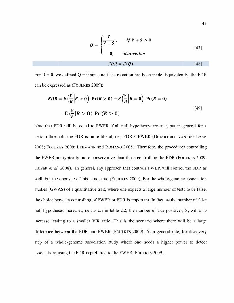
48

𝑸 =  

𝑽𝑽+ 𝑺   , 𝒊𝒇  𝑽+ 𝑺 > 𝟎

𝟎, 𝒐𝒕𝒉𝒆𝒓𝒘𝒊𝒔𝒆

[47]

𝐹𝐷𝑅 = 𝐸 𝑄 [48]

For R = 0, we defined Q = 0 since no false rejection has been made. Equivalently, the FDR 1047

can be expressed as (FOULKES 2009): 1048

𝑭𝑫𝑹 = 𝑬𝑽𝑹 𝑹 > 𝟎 .𝐏𝐫 𝑹 > 𝟎 + 𝑬

𝑽𝑹 𝑹 = 𝟎 .𝐏𝐫 𝑹 = 𝟎

= E (𝑽

𝑹𝑹 > 𝟎 .𝐏𝐫  (𝑹 > 𝟎)

[49]

Note that FDR will be equal to FWER if all null hypotheses are true, but in general for a 1049

certain threshold the FDR is more liberal, i.e., FDR ≤ FWER (DUDOIT and VAN DER LAAN 1050

2008; FOULKES 2009; LEHMANN and ROMANO 2005). Therefore, the procedures controlling 1051

the FWER are typically more conservative than those controlling the FDR (FOULKES 2009; 1052

HUBER et al. 2008). In general, any approach that controls FWER will control the FDR as 1053

well, but the opposite of this is not true (FOULKES 2009). For the whole-genome association 1054

studies (GWAS) of a quantitative trait, where one expects a large number of tests to be false, 1055

the choice between controlling of FWER or FDR is important. In fact, as the number of false 1056

null hypotheses increases, i.e., m-m0 in table 2.2, the number of true-positives, S, will also 1057

increase leading to a smaller V/R ratio. This is the scenario where there will be a large 1058

difference between the FDR and FWER (FOULKES 2009). As a general rule, for discovery 1059

step of a whole-genome association study where one needs a higher power to detect 1060

associations using the FDR is preferred to the FWER (FOULKES 2009). 1061

49

2.6.1.3  Bonferroni  correction  for  multiple  comparisons   1062

Bonferroni correction is a single-step procedure and perhaps the most straightforward 1063

adjustment to apply. The procedure suggests that testing each hypothesis at the level α/m 1064

controls FWER at the level α (DUDOIT and VAN DER LAAN 2008; SABATTI 2007). The 1065

Bonferroni procedure does not take into account the dependency between tests. Consider the 1066

scenario that someone has conducted k identical tests and wants to control FWER at the level 1067

α for each test, in this case he simply can use level α for each single test (SABATTI 2007). 1068

This shortcoming of the test makes it overly conservative, because in GWAS we expect that 1069

adjacent markers to be correlated to each other due to the background LD across the genome 1070

(GAO et al. 2008; LI and JI 2005; MORRIS and CARDON 2008; SABATTI and RISCH 2002). 1071

2.6.1.4  Effective  number  of  tests     1072

Proper modeling of the correlation structure of markers in a large-scale GWAS that 1073

examines tens of thousands markers is important because the appropriate correction for 1074

multiple-testing should be based on the possible number of independent tests, rather than the 1075

actual number of tests being carried out (FREIMER and SABATTI 2004). Simply stated, if 𝐻!! = 1076

(𝐻!!,𝐻!!,… ,𝐻!!) is the complete set of tests and 𝐻!! is a subset of it comprising of S 1077

independent tests, then the Bonferroni adjustment would have been α/S rather than α/m. This 1078

has motivated development of the idea of the effective number of tests (Meff) (CHEVERUD 1079

2001; HAN et al. 2009; LI and JI 2005; MOSKVINA and SCHMIDT 2008; NYHOLT 2004; PE'ER 1080

et al. 2008). 1081

Consider a set of M traits and their corresponding correlation matrix. If one calculates the 1082

eigenvalues (𝜆𝑠) of the correlation matrix, then the variance of these eigenvalues (𝑉!"#$) can 1083

be used to measure the total correlation among the traits (CHEVERUD 2001). The higher the 1084

50

correlation among the traits the larger is 𝑉!"#$. For instance, if the correlation between all 1085

pairs of traits is zero, then all the 𝜆𝑠 are equal to one and thus 𝑉!"#$ = 0. On the other hand, 1086

if all traits are maximally correlated the first 𝜆 is equal to the number of traits and the 1087

remaining 𝜆𝑠 are all zero. This situation generates the maximum 𝑉!"#$ that is equal to M 1088

(CHEVERUD 2001). Thus, 𝑉!"#$ varies between 0 and M depending on the strength of the 1089

correlation among the variables represented in the correlation matrix (CHEVERUD 2001). The 1090

proportional reduction in the number of tests due to correlation is 𝑉!"#$ 𝑀 (CHEVERUD 1091

2001). Thus the effective number of tests can be calculated as (CHEVERUD 2001; NYHOLT 1092

2004): 1093

𝑴𝒆𝒇𝒇 = 𝟏+ 𝑴− 𝟏 𝟏−  𝑽𝝀𝑶𝒃𝒔𝑴 [50]

Note that if all markers are perfectly correlated then 𝑉!"#$ = 𝑀 and 𝑀!"" = 1. Whereas, 1094

when they are all independent, 𝑉!"#$ = 0 and 𝑀!"" = 𝑀. Once the effective number of tests 1095

has been determined, then the Bonferroni adjusted significance threshold will be (FOULKES 1096

2009): 1097

𝜶!! = 𝟏− 𝟏− 𝜶𝟏𝑴𝒆𝒇𝒇 ≈

𝜶𝑴𝒆𝒇𝒇

[51]

Several different alternatives have been proposed for the correlation matrix among the set of 1098

markers being tested, ranging from the matrix of the Pearson’s correlation between markers 1099

genotypes (coded 0, 1, and 2) (CHEVERUD 2001), to the one based on the pair-wise LD 1100

between markers (r2) (NYHOLT 2004), for example (FOULKES 2009). 1101

51

2.6.2  Model  selection  in  GWAS       1102

The primary objective of QTL mapping is to identify a set of loci that contribute most to 1103

the observed phenotype. Therefore, QTL mapping is best viewed as a model selection or 1104

variable selection problem (BROMAN and SEN 2009; WANG et al. 2005). A model selection 1105

procedure for QTL mapping has at least two main parts: a model search algorithm and a 1106

model comparison criterion (BROMAN and SEN 2009). For model searching, we need a 1107

method that explores the model space to identify the good ones, recognizing the fact that we 1108

are only able to visit a very small fraction of the model space. On the other hand, model 1109

comparison is a procedure that balances between model complexity and quality of fit. 1110

Considering an additive QTL model and assuming that markers are on the top of QTL, then 1111

for a GWAS with only 100 markers genotyped the number of possible models is 2100≈ 1030 1112

(BROMAN and SEN 2009). Hence, for a typical GWAS consisting of a couple of thousands 1113

subjects and hundreds of thousands of markers genotyped, it is impossible to analyze the data 1114

using traditional multivariate regression (LI et al. 2010). 1115

Alternative approaches, therefore, have been developed, including ridge regression 1116

(HOERL and KENNARD 1970), least absolute shrinkage and selection operator (LASSO) 1117

(TIBSHIRANI 1994), and the Bayesian variable selection (e.g., GEORGE and MCCULLOCH 1118

1993). Ridge regression is classified as a model-selection-free approach or shrinkage 1119

estimator, because it keeps all potential model effects in the model but the estimated effects 1120

are forced to shrink toward zero (WANG et al. 2005). WHITTAKER et al. (2000) implemented 1121

the ridge regression in the context of MAS to improve the accuracy of selection. The method 1122

has been applied to genomic selection as well (HABIER et al. 2007; MEUWISSEN et al. 2001; 1123

XU 2003). The difficulty of ridge regression is its simplifying assumption of equal and fixed 1124

52

marker effect variances which can lead to over-shrinkage of large effects (HEFFNER et al. 1125

2009). Bayesian methods have relaxed this assumption and allow a marker-specific variance 1126

is estimated for each marker. Different aspects of these methods have been fully discussed 1127

elsewhere (e.g., GIANOLA et al. 2009; HABIER et al. 2011; HEFFNER et al. 2009; HOGGART et 1128

al. 2008). 1129

1130

2.7  LITERATURE  CITED   1131

ALTSHULER, D., M. J. DALY and E. S. LANDER, 2008 Genetic Mapping in Human Disease. 1132 Science 322: 881-888. 1133

ANDERSEN, P. K., and L. T. SKOVGAARD, 2010 Regression with Linear Predictors. Springer 1134 Science+Business Media, LLC. 1135

ANDERSSON, L., C. S. HALEY, H. ELLEGREN, S. A. KNOTT, M. JOHANSSON et al., 1994 1136 Genetic mapping of quantitative trait loci for growth and fatness in pigs. Science 263: 1137 1771-1774. 1138

BALDING, D. J., 2006 A tutorial on statistical methods for population association studies. Nat 1139 Rev Genet 7: 781-791. 1140

BENJAMINI, Y., and Y. HOCHBERG, 1995 Controlling the false discovery rate: a practical and 1141 powerful approach to multiple testing. J. Royal Statist. Soc. B 57: 289–300. 1142

BRESEGHELLO, F., and M. E. SORRELLS, 2006 Association Analysis as a Strategy for 1143 Improvement of Quantitative Traits in Plants. Crop Sci. 46: 1323-1330. 1144

BROMAN, K. W., and S. SEN, 2009 A Guide to QTL Mapping with R/qtl. Springer 1145 Science+Business Media, USA. 1146

BULMER, M. G., 1971 The Effect of Selection on Genetic Variability. The American 1147 Naturalist 105: 201-211. 1148

CAMPBELL, C. D., E. L. OGBURN, K. L. LUNETTA, H. N. LYON, M. L. FREEDMAN et al., 2005 1149 Demonstrating stratification in a European American population. Nat Genet 37: 868- 1150 872. 1151

CASELLA, G., and R. L. BERGER, 2002 Statistical inference. Thomson Learning. 1152 CHAKRABORTY, R., and K. M. WEISS, 1988 Admixture as a tool for finding linked genes and 1153

detecting that difference from allelic association between loci. Proceedings of the 1154 National Academy of Sciences 85: 9119-9123. 1155

CHAPMAN, N. H., and E. A. THOMPSON, 2001 Linkage disequilibrium mapping: the role of 1156 population history, size, and structure. Adv Genet 42: 413-437. 1157

CHEVERUD, J. M., 2001 A simple correction for multiple comparisons in interval mapping 1158 genome scans. Heredity 87: 52--58. 1159

CHRISTENSEN, R., 1997 Log-Linear Models and Logistic Regression. Springer-Verlag, USA. 1160 CLAYTON, D., 2008 Population Association, pp. 1216-1237 in Handbook of Statistical 1161

Genetics. John Wiley & Sons, Ltd. 1162

53

COCKETT, N. E., and C. KOLE, 2008 Genome Mapping and Genomics in Domestic Animals 1163 Springer-Verlag New York, LLC. 1164

COLLINS, A. R., 2007 Linkage Disequilibrium and Association Mapping: An Introduction, 1165 pp. 1-15 in Linkage Disequilibrium and Association Mapping : Analysis and 1166 Applications, edited by A. R. COLLINS. Humana Press Inc., Totowa, NJ. 1167

CORDELL, H. J., and D. G. CLAYTON, 2005 Genetic association studies. Lancet 366: 1121- 1168 1131. 1169

DARVASI, A., 1998 Experimental strategies for the genetic dissection of complex traits in 1170 animal models. Nat Genet 18: 19-24. 1171

DARVASI, A., and M. SOLLER, 1995 Advanced intercross lines, an experimental population 1172 for fine genetic mapping. Genetics 141: 1199--1207. 1173

DEKKERS, J. C. M., and F. HOSPITAL, 2002 The use of molecular genetics in the improvement 1174 of agricultural populations. Nat Rev Genet 3: 22--32. 1175

DEVLIN, B., and K. ROEDER, 1999 Genomic control for association studies. Biometrics 55: 1176 997-1004. 1177

DEWAN, A., R. J. KLEIN and J. HOH, 2007 Linkage Disequilibrium Mapping for Complex 1178 Disease Genes, pp. 85-107 in Linkage Disequilibrium and Association Mapping : 1179 Analysis and Applications, edited by A. R. COLLINS. Humana Press Inc., Totowa, NJ. 1180

DUDOIT, S., and M. J. VAN DER LAAN, 2008 Multiple Testing Procedures with Applications to 1181 Genomics. Springer Science+Business Media LLC, USA. 1182

EPSTEIN, M. P., A. S. ALLEN and G. A. SATTEN, 2007 A simple and improved correction for 1183 population stratification in case-control studies. Am J Hum Genet 80: 921-930. 1184

EXCOFFIER, L., 2007 Analysis of Population Subdivision, pp. 980-1020 in Handbook of 1185 Statistical Genetics, edited by D. J. BALDING, M. BISHOP and C. CANNINGS. John 1186 Wiley & Sons, L td., England. 1187

FALCONER, D. S., and T. F. C. MACKAY, 1996 Introduction to quantitative genetics. 1188 Longman Group Ltd. 1189

FISHER, R. A., 1925 Statistical Methods for Research Workers, pp. 354. Originally published 1190 in Edinburgh by Oliver and Boyd., Electronically published by York University, 1191 Toronto, Ontario.URL:http://psychclassics.yorku.ca/Fisher/Methods/index.htm, 1192 Accessed: March 20, 2012. 1193

FLINT-GARCIA, S. A., J. M. THORNSBERRY and E. S. BUCKLER, 2003 Structure of linkage 1194 disequilibrium in plants. Annu Rev Plant Biol 54: 357-374. 1195

FOULKES, A. S., 2009 Applied Statistical Genetics with R: For Population-based Association 1196 Studies. Springer Science+Business Media, LLC, USA. 1197

FREEMAN, A. R., C. J. HOGGART, O. HANOTTE and D. G. BRADLEY, 2006 Assessing the 1198 Relative Ages of Admixture in the Bovine Hybrid Zones of Africa and the Near East 1199 Using X Chromosome Haplotype Mosaicism. Genetics 173: 1503-1510. 1200

FREIMER, N., and C. SABATTI, 2004 The use of pedigree, sib-pair and association studies of 1201 common diseases for genetic mapping and epidemiology. Nat Genet 36: 1045-1051. 1202

FREIMER, N. B., and C. SABATTI, 2005 Guidelines for association studies in Human 1203 Molecular Genetics. Human Molecular Genetics 14: 2481-2483. 1204

GAO, X., J. STARMER and E. R. MARTIN, 2008 A multiple testing correction method for 1205 genetic association studies using correlated single nucleotide polymorphisms. Genetic 1206 Epidemiology 32: 361-369. 1207

54

GEORGE, E. I., and R. E. MCCULLOCH, 1993 Variable Selection Via Gibbs Sampling. Journal 1208 of the American Statistical Association 88: 881-889. 1209

GEORGES, M., 2007 Mapping, fine mapping, and molecular dissection of quantitative trait 1210 Loci in domestic animals. Annu Rev Genomics Hum Genet 8: 131--162. 1211

GEORGES, M., D. NIELSEN, M. MACKINNON, A. MISHRA, R. OKIMOTO et al., 1995 Mapping 1212 quantitative trait loci controlling milk production in dairy cattle by exploiting progeny 1213 testing. Genetics 139: 907-920. 1214

GIANOLA, D., G. DE LOS CAMPOS, W. G. HILL, E. MANFREDI and R. FERNANDO, 2009 1215 Additive genetic variability and the Bayesian alphabet. Genetics 183: 347--363. 1216

GODDARD, M. E., and T. H. E. MEUWISSEN, 2005 The use of linkage disequilibrium to map 1217 quantitative trait loci. Australian Journal of Experimental Agriculture 45: 837--845. 1218

GRISART, B., W. COPPIETERS, F. FARNIR, L. KARIM, C. FORD et al., 2002 Positional 1219 candidate cloning of a QTL in dairy cattle: identification of a missense mutation in 1220 the bovine DGAT1 gene with major effect on milk yield and composition. Genome 1221 Res 12: 222-231. 1222

HABIER, D., R. L. FERNANDO and J. C. M. DEKKERS, 2007 The impact of genetic relationship 1223 information on genome-assisted breeding values. Genetics 177: 2389--2397. 1224

HABIER, D., R. L. FERNANDO, K. KIZILKAYA and D. J. GARRICK, 2011 Extension of the 1225 bayesian alphabet for genomic selection. BMC Bioinformatics 12: 186. 1226

HAN, B., H. M. KANG and E. ESKIN, 2009 Rapid and Accurate Multiple Testing Correction 1227 and Power Estimation for Millions of Correlated Markers. PLoS Genet 5: e1000456. 1228

HARTL, D. L., and A. G. CLARK, 1989 Principles of Population Genetics. Sinauer Associates, 1229 Sunderland, MA. 1230

HAYES, B. J., B. P. KINGHORN and A. RUVINSKY, 2004 Genome Scanning for Quantitative 1231 Trait Loci, pp. 507-538 in Mammalian Genomics, edited by A. RUVINSKY and J. M. 1232 GRAVES. CABI. 1233

HEDRICK, P. W., 2005 Genetics of populations. Jones and Bartlett Publishers, Sudbury, MA 1234 USA. 1235

HEFFNER, E. L., M. E. SORRELLS and J.-L. JANNINK, 2009 Genomic Selection for Crop 1236 Improvement. Crop Sci. 49: 1-12. 1237

HILL, W. G., and A. ROBERTSON, 1968 The effects of inbreeding at loci with heterozygote 1238 advantage. Genetics 60: 615--628. 1239

HOERL, A., and R. KENNARD, 1970 Ridge Regression: Biased Estimation for Nonorthogonal 1240 Problems. Technometrics 12: 55-67. 1241

HOGGART, C. J., J. C. WHITTAKER, M. DE IORIO and D. J. BALDING, 2008 Simultaneous 1242 analysis of all SNPs in genome-wide and re-sequencing association studies. PLoS 1243 Genet 4: e1000130. 1244

HUBER, W., A. VON HEYDEBRECK and M. VINGRON, 2008 Analysis of Microarray Gene 1245 Expression Data, pp. 201-230 in Handbook of Statistical Genetics. John Wiley & 1246 Sons, Ltd. 1247

JANNINK, J.-L., M. C. A. M. BINK and R. C. JANSEN, 2001 Using complex plant pedigrees to 1248 map valuable genes. Trends in plant science 6: 337-342. 1249

JANNINK, J.-L., and B. WALSH, 2002 Association mapping in plant populations, pp. 59-68 in 1250 Quantitative Genetics, Genomics and Plant Breeding, edited by M. S. KANG. CABI, 1251 Wallingford, UK. 1252

55

JORDE, L. B., 1995 Linkage disequilibrium as a gene-mapping tool. Am J Hum Genet 56: 11- 1253 -14. 1254

JORDE, L. B., 2000 Linkage disequilibrium and the search for complex disease genes. 1255 Genome Res 10: 1435--1444. 1256

KAPLAN, N. L., W. G. HILL and B. S. WEIR, 1995 Likelihood methods for locating disease 1257 genes in nonequilibrium populations. Am J Hum Genet 56: 18--32. 1258

KAPLAN, N. L., E. R. MARTIN, R. W. MORRIS and B. S. WEIR, 1998 Marker selection for the 1259 transmission/disequilibrium test, in recently admixed populations. Am J Hum Genet 1260 62: 703--712. 1261

KEELE, J. W., S. D. SHACKELFORD, S. M. KAPPES, M. KOOHMARAIE and R. T. STONE, 1999 1262 A region on bovine chromosome 15 influences beef longissimus tenderness in steers. 1263 Journal of Animal Science 77: 1364-1371. 1264

KIMURA, M., and T. OHTA, 1971 Theoretical Aspects of Population Genetics. Princeton 1265 University Press, , Princeton, NJ USA. 1266

KNOWLER, W. C., R. C. WILLIAMS, D. J. PETTITT and A. G. STEINBERG, 1988 Gm3;5,13,14 and 1267 Type 2 Diabetes Mellitus: An Association in American Indians with Genetic 1268 Admixture. Am. J. Hum. Genet. 43: 520-526. 1269

LAIRD, N. M., and C. LANGE, 2011 The Fundamentals of Modern Statistical Genetics, pp. 1270 223 in Statistics for Biology and Health, edited by M. GAIL, K. KRICKEBERG, J. M. 1271 SAMET, A. TSIATIS and W. WONG. Springer Science+Business Media. 1272

LANDE, R., and R. THOMPSON, 1990 Efficiency of marker-assisted selection in the 1273 improvement of quantitative traits. Genetics 124: 743--756. 1274

LAZZERONI, L. C., 2001 A chronology of fine-scale gene mapping by linkage disequilibrium. 1275 Stat Methods Med Res 10: 57--76. 1276

LEHMANN, E. L., and J. P. ROMANO, 2005 Testing statistical hypotheses. Springer. 1277 LI, C. C., 1972 Population subdivision with respect to multiple alleles. Ann Hum Genet. 33: 1278

23-29. 1279 LI, J., K. DAS, G. FU, R. LI and R. WU, 2010 The Bayesian Lasso for Genome-wide 1280

Association Studies. Bioinformatics. 1281 LI, J., and L. JI, 2005 Adjusting multiple testing in multilocus analyses using the eigenvalues 1282

of a correlation matrix. Heredity 95: 221-227. 1283 LIN, S., and H. ZHAO (Editors), 2010 Handbook on Analyzing Human Genetic Data. Springer 1284

Heidelberg Dordrecht London New York. 1285 MACKAY, I., and W. POWELL, 2007 Methods for linkage disequilibrium mapping in crops. 1286

Trends Plant Sci 12: 57--63. 1287 MALOSETTI, M., C. G. VAN DER LINDEN, B. VOSMAN and F. A. VAN EEUWIJK, 2007 A mixed- 1288

model approach to association mapping using pedigree information with an 1289 illustration of resistance to Phytophthora infestans in potato. Genetics 175: 879--889. 1290

MCKEIGUE, P. M., 2008 Population Admixture and Stratification in Genetic Epidemiology, 1291 pp. 1190-1215 in Handbook of Statistical Genetics. John Wiley & Sons, Ltd. 1292

MCVEAN, G., 2001 Population structure, pp. 1-16, 1293 URL:http://www.stats.ox.ac.uk/~mcvean/notes7.pdf, Accessed Mar. 1, 2012. 1294

MEUWISSEN, T. H., B. J. HAYES and M. E. GODDARD, 2001 Prediction of total genetic value 1295 using genome-wide dense marker maps. Genetics 157: 1819--1829. 1296

56

MONTANA, G., and J. K. PRITCHARD, 2004 Statistical tests for admixture mapping with case- 1297 control and cases-only data. Am J Hum Genet 75: 771-789. 1298

MORRIS, A. P., and L. R. CARDON, 2008 Whole Genome Association, pp. 1238-1263 in 1299 Handbook of Statistical Genetics. John Wiley & Sons, Ltd. 1300

MOSKVINA, V., and K. M. SCHMIDT, 2008 On multiple-testing correction in genome-wide 1301 association studies. Genetic Epidemiology 32: 567-573. 1302

NYHOLT, D. R., 2004 A Simple Correction for Multiple Testing for Single-Nucleotide 1303 Polymorphisms in Linkage Disequilibrium with Each Other. American journal of 1304 human genetics 74: 765-769. 1305

OCHIENG, J. W., A. W. T. MUIGAI and G. N. UDE, 2007 Localizing genes using linkage 1306 disequilibrium in plants: integrating lessons from the medical genetics. African 1307 Journal of Biotechnology 6: 650-657. 1308

ORR, N., and S. CHANOCK, 2008 Chapter 1 Common Genetic Variation and Human Disease, 1309 pp. 1-32 in Advances in Genetics, edited by C. H. JEFFREY. Academic Press. 1310

PARISSEAUX, B., and R. BERNARDO, 2004 In silico mapping of quantitative trait loci in 1311 maize. Theor Appl Genet 109: 508-514. 1312

PARRA, E. J., A. MARCINI, J. AKEY, J. MARTINSON, M. A. BATZER et al., 1998 Estimating 1313 African American Admixture Proportions by Use of Population-Specific Alleles. 1314 American journal of human genetics 63: 1839-1851. 1315

PE'ER, I., R. YELENSKY, D. ALTSHULER and M. J. DALY, 2008 Estimation of the multiple 1316 testing burden for genomewide association studies of nearly all common variants. 1317 Genetic Epidemiology 32: 381-385. 1318

PFAFF, C. L., E. J. PARRA, C. BONILLA, K. HIESTER, P. M. MCKEIGUE et al., 2001 Population 1319 structure in admixed populations: effect of admixture dynamics on the pattern of 1320 linkage disequilibrium. Am J Hum Genet 68: 198--207. 1321

PLATT, A., B. J. VILHJÁLMSSON and M. NORDBORG, 2010 Conditions Under Which Genome- 1322 Wide Association Studies Will be Positively Misleading. Genetics 186: 1045-1052. 1323

PRITCHARD, J. K., and M. PRZEWORSKI, 2001 Linkage disequilibrium in humans: models and 1324 data. Am J Hum Genet 69: 1--14. 1325

PRITCHARD, J. K., and N. A. ROSENBERG, 1999 Use of unlinked genetic markers to detect 1326 population stratification in association studies. Am J Hum Genet 65: 220-228. 1327

REDDEN, D., and D. ALLISON, 2006 The Effect of Assortative Mating upon Genetic 1328 Association Studies: Spurious Associations and Population Substructure in the 1329 Absence of Admixture. Behavior Genetics 36: 678-686. 1330

REMINGTON, D. L., J. M. THORNSBERRY, Y. MATSUOKA, L. M. WILSON, S. R. WHITT et al., 1331 2001 Structure of linkage disequilibrium and phenotypic associations in the maize 1332 genome. Proc Natl Acad Sci U S A 98: 11479--11484. 1333

RIQUET, J., W. COPPIETERS, N. CAMBISANO, J. J. ARRANZ, P. BERZI et al., 1999 Fine- 1334 mapping of quantitative trait loci by identity by descent in outbred populations: 1335 application to milk production in dairy cattle. Proc Natl Acad Sci U S A 96: 9252- 1336 9257. 1337

ROCKMAN, M. V., and L. KRUGLYAK, 2008 Breeding designs for recombinant inbred 1338 advanced intercross lines. Genetics 179: 1069-1078. 1339

57

SABATTI, C., 2007 Avoiding False Discoveries in Association Studies, pp. 195-211 in 1340 Linkage Disequilibrium and Association Mapping : Analysis and Applications, edited 1341 by A. R. COLLINS. Humana Press Inc., Totowa, NJ. 1342

SABATTI, C., and N. RISCH, 2002 Homozygosity and linkage disequilibrium. Genetics 160: 1343 1707--1719. 1344

SHIFMAN, S., J. KUYPERS, M. KOKORIS, B. YAKIR and A. DARVASI, 2003 Linkage 1345 disequilibrium patterns of the human genome across populations. Hum Mol Genet 12: 1346 771-776. 1347

SIEGMUND, D., and B. YAKIR, 2007 Association Studies, pp. 279-308 in The Statistics of 1348 Gene Mapping, edited by M. GAIL, K. KRICKEBERG, J. SAMET, A. TSIATIS and W. 1349 WONG. Springer Science + Business Media, LLC, USA. 1350

SNELLER, C. H., D. E. MATHER and S. CREPIEUX, 2009 Analytical Approaches and 1351 Population Types for Finding and Utilizing QTL in Complex Plant Populations. Crop 1352 Sci. 49: 363-380. 1353

SVED, J. A., 1971 Linkage disequilibrium and homozygosity of chromosome segments in 1354 finite populations. Theor Popul Biol 2: 125-141. 1355

TERWILLIGER, J. D., S. ZOLLNER, M. LAAN and S. PAABO, 1998 Mapping genes through the 1356 use of linkage disequilibrium generated by genetic drift: 'drift mapping' in small 1357 populations with no demographic expansion. Hum Hered 48: 138--154. 1358

THALLER, G., W. KRAMER, A. WINTER, B. KAUPE, G. ERHARDT et al., 2003 Effects of 1359 DGAT1 variants on milk production traits in German cattle breeds. J Anim Sci 81: 1360 1911-1918. 1361

TIBSHIRANI, R., 1994 Regression Shrinkage and Selection Via the Lasso. Journal of the 1362 Royal Statistical Society, Series B 58: 267-288. 1363

VAN KAAM, J., M. GROENEN, H. BOVENHUIS, A. VEENENDAAL, A. VEREIJKEN et al., 1999 1364 Whole genome scan in chickens for quantitative trait loci affecting carcass traits. 1365 Poultry Science 78: 1091-1099. 1366

VITTINGHOFF, E., S. C. SHIBOSKI, D. V. GLIDDEN and C. E. MCCULLOCH, 2005 Regression 1367 methods in biostatistics : linear, logistic, survival, and repeated measures models. 1368 Springer Science+Business Media, Inc. 1369

WANG, H., Y.-M. ZHANG, X. LI, G. L. MASINDE, S. MOHAN et al., 2005 Bayesian shrinkage 1370 estimation of quantitative trait loci parameters. Genetics 170: 465--480. 1371

WEISBERG, S., 2005 Applied Linear Regression. John Wiley & Sons, Inc., Hoboken, New 1372 Jersey. 1373

WHITTAKER, J. C., R. THOMPSON and M. C. DENHAM, 2000 Marker-assisted selection using 1374 ridge regression. Genet Res 75: 249--252. 1375

WRIGHT, S., 1951 The genetical structure of populations. Ann. Eugen. 15: 323-354. 1376 WU, R., G. CASELLA and C.-X. MA, 2007 Statistical Genetics of Quantitative Traits: 1377

Linkage, Maps, and QTL. Springer Science + Business Media, LLC, New York, NY 1378 WU, R., and Z. B. ZENG, 2001 Joint linkage and linkage disequilibrium mapping in natural 1379

populations. Genetics 157: 899--909. 1380 XU, S., 2003 Estimating polygenic effects using markers of the entire genome. Genetics 163: 1381

789--801. 1382 XU, Y., 2010 Molecular Plant Breeding. CAB International, Oxfordshire, UK. 1383

58

YU, J. M., G. PRESSOIR, W. H. BRIGGS, I. V. BI, M. YAMASAKI et al., 2006 A unified mixed- 1384 model method for association mapping that accounts for multiple levels of 1385 relatedness. Nature Genetics 38: 203-208. 1386

ZHU, X., and S. ZHANG, 2010 Population-Based Association Studies, pp. 171-190 in 1387 Handbook on Analyzing Human Genetic Data, edited by S. LIN and H. ZHAO. 1388 Springer-Verlag Berlin Heidelberg. 1389

ZÖLLNER, S., 2001 Population History and Linkage Disequilibrium in eLS. John Wiley & 1390 Sons, Ltd. 1391

1392 1393

1394

59

2.8  FIGURES   1395

Figure 2.1 Percentage of individuals with diabetes disease in Gila Indian River population 1396 along with frequency of Gm haplotype in subpopulations with different Indian heritage 1397 ancestry1 1398

1399

1400 1. The X axis is the number of great grandparents with Indian heritage in an individual’s 1401 pedigree. Data adopted from (KNOWLER et al. 1988). 1402 1403

0  

10  

20  

30  

40  

50  

60  

70  

0   4   8  

Prevalen

ce  (%

)  

Indian  Heritage  

Gm3  Allele  

Diabetes  

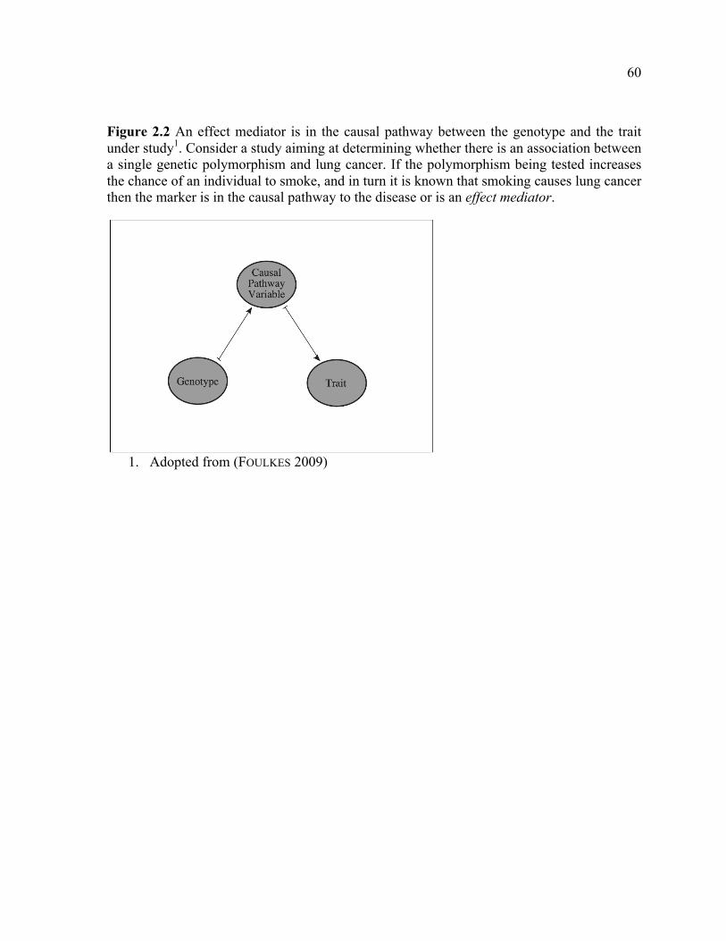
60

1404 Figure 2.2 An effect mediator is in the causal pathway between the genotype and the trait 1405 under study1. Consider a study aiming at determining whether there is an association between 1406 a single genetic polymorphism and lung cancer. If the polymorphism being tested increases 1407 the chance of an individual to smoke, and in turn it is known that smoking causes lung cancer 1408 then the marker is in the causal pathway to the disease or is an effect mediator. 1409

1410 1. Adopted from (FOULKES 2009) 1411 1412

1413

1414

1415

61

Figure 2.3 False association at a marker locus due to population stratification in a case– 1416 control study1. The schematic shows the underlying problem of PS in a case-control study. 1417 The allele frequency of the marker of interest is not the same in the two sub-populations. 1418 Because more cases are falling into the sub-population 2, it would appear as if there is an 1419 association between the disease and the marker. However, this happens due to the fact that 1420 the marker has different frequencies in the two sub-populations. 1421

1422 1. Adopted from (DEWAN et al. 2007) 1423

62

Figure 2.4 Stratified analysis of case-control studies, based on either genotypes or allele 1424 counts1 1425

1426 1. Adopted from (CLAYTON 2008) 1427

1428

63

2.9  TABLES   1429

Table 2.1 A 2x3 contingency table for marker-trait association test in a case-control study 1430

Phenotype # A1 alleles Total 0 1 2

Case r0 r1 r2 r Control s0 s1 s2 s Total n0 n1 n2 n

1431 1432

1433

64

Table 2.1 Possible outcomes of multiple hypotheses testing of an experiment with m markers 1434

No. Not Rejected

No. Rejected

Total

H0 is True U   V   m0  H0 is false T   S   m1  Total m-­‐R   R   m  

1435 1436

1437

65

CHAPTER  3.  GENOMIC  SELECTION  IN  ADMIXED  AND  CROSSBRED   1438

POPULATIONS   1439

1440

A paper published in Journal of Animal Science (2010) 88:32-46 1441

1442

Ali Toosi*, Rohan L. Fernando*1, and Jack C.M. Dekkers* 1443

*Department of Animal Science and Center for Integrated Animal Genomics, Iowa State 1444

University, Ames, IA 50011 USA 1445

  1446

3.1  SUMMARY   1447

In livestock, genomic selection (GS) has primarily been investigated by simulation of 1448

purebred populations. Traits of interest are, however, often measured in crossbred or mixed 1449

populations with uncertain breed composition. If such data are used as the training data for 1450

GS without accounting for breed composition, estimates of marker effects may be biased due 1451

to population stratification and admixture. To investigate this, a genome of 100 cM was 1452

simulated with varying marker densities (5 to 40 segregating markers per cM). After 1000 1453

generations of random mating in a population of effective size 500, four lines with effective 1454

size 100 were isolated and mated for another 50 generations to create 4 pure breeds. These 1455

breeds were used to generate combined, F1, F2, three- and four-way crosses, and admixed 1456

training data sets of 1000 individuals with phenotypes for an additive trait controlled by 100 1457

segregating QTL and heritability of 0.30. The validation data set was a sample of 1000 1458 1  Corresponding  author:  Rohan  Fernando,  237  Kildee  Hall,  Department  of  Animal  Science,  Iowa  State  

University,  Ames  IA  50011,  USA  Phone:  +1  515  294  5348,  Fax:  +1  515  294  9150,  e-­‐mail:  rohan@iastate.edu  

66

genotyped individuals from one pure breed. Method Bayes-B was used to simultaneously 1459

estimate the effects of all markers for breeding value estimation. With 5 (40) markers per 1460

cM, the correlation of true with estimated breeding value of selection candidates (accuracy) 1461

was highest, 0.79 (0.85), when data from the same pure breed was used for training. When 1462

the training dataset consisted of crossbreds, the accuracy ranged from 0.66 (0.79) to 0.74 1463

(0.83) for the two marker densities, respectively. The admixed training dataset resulted in 1464

nearly the same accuracies as when training was in the breed to which selection candidates 1465

belonged. However, accuracy was greatly reduced when genes from the target pure breed 1466

were not included in the admixed or crossbred population. This implies that, with high- 1467

density markers, admixed and crossbred populations can be used to develop GS prediction 1468

equations for all pure breeds that contributed to the population, without a substantial loss of 1469

accuracy compared to training on purebred data, even if breed origin has not been implicitly 1470

taken into account. In addition, using GS based on high-density marker data, purebreds can 1471

be accurately selected for crossbred performance without the need for pedigree or breed 1472

information. Results also showed that haplotype segments with strong linkage disequilibrium 1473

are shorter in crossbred and admixed populations than in purebreds, providing opportunities 1474

for QTL fine mapping. 1475

Key words: Genomic Selection, Marker-Assisted Selection, Admixture, 1476

Crossbreeding 1477

3.2  INTRODUCTION   1478

Genomic selection (GS) (MEUWISSEN et al. 2001) is a form of marker-assisted selection 1479

that uses marker genotypes and phenotypes in a training population to simultaneously 1480

estimate effects of a large number of markers across the genome for the purpose of predicting 1481

67

breeding values (BV) of selection candidates based on their marker genotypes. The accuracy 1482

of GS depends on the amount of linkage disequilibrium (LD) between QTL and markers and 1483

the number of records available to estimate marker effects. Most commercial beef cattle 1484

populations consist of animals with different and often unknown breed compositions. 1485

Presence of unknown population structure have raised concerns about using admixed or 1486

crossbred populations as training data for GS, yet these are the populations that are most 1487

relevant as the target for genetic improvement of purebreds (DEKKERS 2007). Admixture is 1488

the presence of multiple genetically distinct subgroups within a population (WANG et al. 1489

2005). Numerous studies (GODDARD and MEUWISSEN 2005; HIRSCHHORN and DALY 2005; 1490

PFAFF et al. 2001; RABINOWITZ 1997) have reported that admixture can produce spurious 1491

associations and seriously elevate false discovery rates in QTL detection. Several methods 1492

have been proposed to address this problem (e.g., KENNEDY et al. 1992; MEUWISSEN et al. 1493

2002; PRICE et al. 2006; PRITCHARD et al. 2000; SPIELMAN et al. 1993; YU et al. 2006). 1494

Ideally, however, if all QTL that explain genetic variation in the trait of interest were 1495

included in the model, it would not be necessary to explicitly account for pedigree or breed 1496

composition in the analysis. Thus, provided high-density SNPs are used and analyzed 1497

simultaneously, as in GS, pedigree and breed composition need not be explicitly modeled. 1498

The objective of this work, therefore, was to evaluate accuracy of GS with high-density 1499

markers for predicting BV of purebred animals based on estimates of marker effects in a 1500

crossbred or admixed population, without explicitly accounting for pedigree or breed 1501

composition. 1502

3.3  MATERIALS  AND  METHODS   1503

No live animals were used for this study. 1504

68

3.3.1  Population     1505

A base population of unrelated individuals was stochastically simulated and used as the 1506

ancestral population of four pure breeds that were used to create admixed and crossbred 1507

populations (Figure 3.1). The base population was randomly mated for 1000 generations, 1508

including selfing, with an effective size (Ne) of 500. To simulate the four purebred 1509

populations (referred to as breeds A, B, C and D hereafter), at generation 0 four independent 1510

random samples of 100 animals were drawn from the base population, and each was 1511

randomly mated (including selfing) for another 53 generations, with Ne of 100. Breeds A and 1512

B were then crossed to produce an F1 (AB) population. Mating (AB) with breeds A and B 1513

created backcrosses (AB)A and (AB)B, which were again backcrossed to either A or B to 1514

create crossbred populations ((AB)A)A, ((AB)A)B, ((AB)B)A, and ((AB)B)B. An F2 1515

population, (AB)2, was created by inter-mating the (AB) F1s. Similarly, breeds C and D were 1516

used to create corresponding crossbred populations. 1517

In beef cattle, commercial animals are often produced by mating purebred sires to 1518

crossbred dams of heterogeneous breed composition. In order to simulate such a population, 1519

an admixed population of two breeds ((Adm_AB)B) was created by first putting dams from 1520

breed A and all crossbreds involving breeds A and B in the same group and then mating them 1521

to sires from breed B. An admixed population of four breeds ((Adm_ABCD)B) was formed 1522

by mating dams from all breeds, excluding breed B, and all of the crosses involving the four 1523

breeds to sires from breed B. Further, three-way and four-way crosses were made by crossing 1524

(AB) with C and (AB) with (CD). To create the combined population, two random samples 1525

of equal size from purebreds A and B were put together into a single population. In the 1526

remainder, this latter population will be referred to as the combined_AB population, in 1527

69

contrast to the admixed populations described in the previous, which include purebreds and 1528

their crosses. 1529

Each of the purebreds A and B, the (AB), (AB)2, (AC), (AB)C, (AB)(CD) crossbreds, 1530

combined_AB and admixed datasets was used as a training population consisting of 1000 1531

animals for estimating marker effects. These animals were created by mating randomly 1532

sampled individuals from the appropriate parental lines, each of size 100. Thus, on the 1533

average each sire (and dam) had 10 offspring in the training data set. Because the objective 1534

was to determine how well marker effects estimated in the various training populations 1535

predicted BVs of purebred individuals, a separate generation of purebred population B was 1536

used for validation. To generate the validation population of size 1000, in generation 50 a 1537

sample of 1000 animals was drawn from breed B and randomly mated for another 4 1538

generations (BVal in Figure 3.1). 1539

For evaluating the impact of breed differences on the accuracy of GS, a second scenario 1540

was also considered, in which breeds were separated in generation 25 rather than generation 1541

0 (Figure 3.1), such that breeds were diverged for only 25 instead of 50 generations. In order 1542

to maintain the same level of LD, effective population size was reduced from 500 to 100 in 1543

generation 0, as before. 1544

3.3.2  Genome     1545

To make the simulation computationally feasible, a genome consisting of one 1546

chromosome of 100 cM with 100 segregating QTL and different marker densities was 1547

simulated (Table 3.1). To end up with the required number of segregating loci after 1000 1548

generations, about three times as many biallelic loci were simulated with starting allele 1549

frequencies of 0.5 and a reversible random mutation rate of 2.5*10-5. Each locus was either a 1550

70

marker locus or a QTL. A binomial map function was used to simulate recombination and 1551

interference was allowed by setting the maximum number of uniformly and independently 1552

distributed crossovers on the chromosome to be 4 (KARLIN 1984). To make a marker panel, 1553

500, 1000, 2000, or 4000 marker loci were drawn at random from segregating loci, MAF1≥ 1554

0.10, at generation 53 after pooling all four breeds into a single cohort. As a result, markers 1555

were not evenly dispersed along the chromosome and some of them may not be segregating 1556

in all training populations. 1557

3.3.3  Phenotypes       1558

To create phenotypic values for each training population, 100 QTL were randomly 1559

picked from the set of segregating QTL in that population. This was done in generation 54 1560

for breed B, (AB), and combined_AB, in generation 56 for (AB)2, three- and four-way cross 1561

datasets and in generation 57 for the admixed training data sets (Figure 3.1). Note that QTL 1562

with MAF1 < 0.10 in each breed will have an intermediate allele frequency in the 1563

combined_AB, crossbreds or admixed training populations. The QTL were additive and their 1564

effects were sampled from a gamma distribution with shape and scale parameters of 0.4 and 1565

1/1.66, respectively. This provides us with an L-shaped distribution of QTL effects which 1566

(MEUWISSEN et al. 2001) suggest is close to the real distribution of the QTL effects. With 1567

equal probability, one of the two alleles was chosen to be positive or negative. To keep the 1568

genetic variance constant across training populations, the effect of each QTL was scaled in 1569

each replicate. This was done to ensure that each training dataset had the same genetic 1570

variance, such that this could not contribute to differences between training datasets. 1571

The scaled QTL effects then were summed over all QTL genotypes for each individual to 1572

1  Minor  allele  frequency    

71

compute its true BV. With this setting, each training population received a different set of 1573

QTL affecting phenotypes, although the number of segregating QTL and the genetic variance 1574

were the same for all training populations. Finally, a standard normal deviate was added to 1575

each true BV to provide the phenotype of an individual for a quantitative trait with 1576

heritability 0.30. 1577

It should be mentioned that here the whole genetic variance is assigned to a single 1578

chromosome, whereas in reality the total genetic variance is distributed to all chromosomes 1579

(30 chromosomes in case of cattle, for instance). In this study, a short genome was chosen to 1580

reduce computational costs. An additional data set with a total of 5000 markers and 100 QTL 1581

on five chromosomes, each of length 1 M, was simulated to examine the impact of genome 1582

size on our results. The analysis was run for the training populations of purebred B, 1583

((Adm_ABCD)B), combined_AB and four-way crossbred only, with 96 replicates. 1584

3.3.4  Estimation  of  marker  effects       1585

Method Bayes-B of (MEUWISSEN et al. 2001) was used to estimate effects of markers in 1586

the training data using the model: 1587

𝒚 = 𝟏𝝁+ 𝐱𝒊𝒊

𝒈𝒊 + 𝒆 [52]

where y is the vector of phenotypic values of individuals in the training data, µ is a single 1588

unknown population mean, 1 is a vector of ones, xi is a column vector containing the 1589

genotypes (0,1 or 2) of each individual at locus i, 𝑔! is the random unknown allele effect for 1590

marker i, with 𝑔!~𝑁(0,𝜎!!! ) and e is a random vector of unknown residuals with 1591

𝑒!~𝑁(0,𝜎!!). In method Bayes-B the informative prior for locus specific genetic variance 1592

(𝜎!!! ) has a mixture distribution (SOLBERG et al. 2008). Following (MEUWISSEN et al. 2001), 1593

72

it was postulated that with probability π, 𝜎!!! = 0, and with probability (1 - π), it follows an 1594

inverted chi-square distribution with known parameters ν = 4.234 and S = 0.0429. In 1595

practice, when 𝜎!!! = 0, 𝑔! is also set to zero. 1596

The probability π is assumed known. Based on preliminary analyses with several 1597

different π values, π was set equal to 0.95, except for a density of 40 markers per cM, for 1598

which π was increased to 0.975. An MCMC chain of length 10,000 cycles with a burn in 1599

period of 1000 cycles was conducted. Convergence of the MCMC chain was examined using 1600

the R package CODA (PLUMMER et al. 2006). 1601

3.3.5  Validation  of  genomic  prediction       1602

Once estimates of marker effects were obtained from the training dataset (posterior 1603

means from the MCMC chain), the estimated BV of individual k (GEBVk) in the validation 1604

dataset (generation 54 of population Bval) was computed as 1605

𝑮𝑬𝑩𝑽𝒌 = 𝐱𝒊𝒌𝒈𝒊𝒎

𝒊 [53]

1606

where 𝐱!" and 𝑔! are the genotype and the estimated effect of genotype at locus i, 1607

respectively, and m is the total number of markers. Accuracy was calculated as the 1608

correlation between the estimated and true BV of individuals in the validation data. This 1609

accuracy was used to compare performance of the different scenarios and training 1610

populations. All scenarios were replicated 160 times and results were averaged across 1611

replicates. Mean accuracies from alternate training populations were compared by the LSD 1612

test using the JMP software package (JMP, Version 7.0.1, SAS Institute Inc., Cary, NC, 1613

1989-2007). 1614

73

3.3.6  Linkage  disequilibrium  and  between  breed  diversity       1615

To evaluate the extent and magnitude of linkage disequilibrium in the training

populations and its impact on accuracy, LD between pairs of SNP markers were estimated

using r2 (HILL and ROBERTSON 1968). Only markers with a MAF ≥ 0.1 were considered in

this analysis. The power to detect LD between two loci is minimum when at least one of

them has an extreme allele frequency (GODDARD et al. 2000). Further, to evaluate the

persistence of LD phase across training and validation populations, the correlations of r

between the two populations were calculated for different distances between loci (GODDARD

et al. 2006).

To assess and compare the decline of LD with distance in different training populations, a 1616

non-linear regression model was fitted to the observed r2 between marker pairs in each 1617

training population. The model used was based on the (SVED 1971) equation: 1618

𝒓𝒊𝒋𝟐 =𝟏

𝟏+ 𝟒𝒃𝒅𝒊𝒋+ 𝒆𝒊𝒋

[54]

where 𝑟!"! is the observed LD between markers i and j in the training data, b is a 1619

coefficient that describes the decline of LD with distance in the training data, 𝑑!" is distance 1620

in Morgans between markers i and j, and 𝑒!" is the random residual that was assumed 1621

normally distributed. 1622

The level of genetic diversity present in the simulated breeds was investigated using 1623

Wright’s F-statistics (WRIGHT 1965b) FIT, FST and FIS, as implemented in the program Fstat 1624

(GOUDET 2001). Genotypes at 200 loci from a random sample of 100 individuals from each 1625

of the four simulated breeds from generation 53 were used to estimate F-statistics. 1626

Significance levels for the F-statistics and related variance components were obtained from 1627

74

20,000 permutations and from jackknife over loci (with different loci as re-sampling units), 1628

as provided by the Fstat program. 1629

3.4  RESULTS   1630

3.4.1  Accuracy  of  genomic  selection     1631

Correlations between estimated and true BVs for individuals in the validation dataset 1632

(population Bval, Figure 3.1) for different training populations and marker densities are 1633

shown in Table 3.2. Training in the same breed as the validation population (B54) resulted in 1634

the highest accuracy in all cases. Accuracies tended to be lower if populations other than the 1635

validation breed were used for training but reductions in accuracy were not significant in 1636

some cases and depended on the breed composition of the training population. Based on 1637

differences in accuracies, the training populations can be divided into four groups: (1) 1638

purebred B and admixed populations, (2) two-breed combined_AB and crossed populations, 1639

(3) three- and four-way crosses, and (4) purebred A and AC. Training in the admixed 1640

populations resulted in similar accuracies as training in the purebred B population (group 1). 1641

The largest drop in accuracy compared to group 1 was for training populations in group 4, 1642

which included no contribution from the validation breed B. Averaged over all marker 1643

densities, relative to the accuracy of training and validating in the same breed, accuracy 1644

dropped by 46% when validation was in a different breed, whereas training in crossbred AC 1645

and validating in breed B resulted in a drop in accuracy of 35%. Populations in groups 2 and 1646

3 had accuracies intermediate to those of groups 1 and 4. Comparing accuracies for 1647

populations in groups 2 and 3, as the number of breeds contributing to the training population 1648

increased, the accuracy dropped more. While training in group 2 populations resulted in a 6% 1649

decrease of accuracy, the decrease in accuracy when using the three- and four-way crosses 1650

75

for training was on average about 10%. Interestingly, within group 2, differences in accuracy 1651

were not practically significant. Comparing groups 1, 2 and 3, the three- and four-way 1652

crossbred training populations showed the lowest accuracy of prediction. 1653

3.4.2  Marker  density   1654

Accuracy generally increased with marker density (Table 3.2). The increase was most 1655

noticeable when training in A, AC and in the three-way and four-way crosses. Thus, the 1656

effect of marker density was more pronounced when the training population had a lower 1657

contribution of the breed that comprised the validation population (breed B in this case). 1658

Increasing marker density from 5 to 20 markers per cM, improved accuracy by 35, 20, 10 1659

and 10 percent for groups 4, 3, 2 and 1, respectively. However, increasing marker density 1660

from 20 to 40 per cM did not improve accuracy as much; except for group 4 training datasets 1661

that showed an additional increase of 11% in the accuracy. Table 3.2 shows that with the 1662

level of LD and the amount of breed divergence simulated in this study, marker densities as 1663

low as 5 markers per cM were sufficient for accurate prediction of BV without explicitly 1664

accounting for pedigree or breed composition in the crossbred and admixed training 1665

populations, as long as the target breed contributed to the training population. 1666

3.4.3  The  effect  of  time  since  divergence  of  breeds       1667

Table 3.3 shows the effect of the number of generations of random mating after isolation 1668

(referred to as Time Since Divergence, TSD) on the accuracy of GEBV. As expected, TSD 1669

did not significantly affect accuracy when the purebred B population was used as training 1670

data, but accuracies significantly increased for all other training datasets when TSD was 1671

reduced from 50 to 25. The maximum increase in accuracy was observed when using group 4 1672

populations (A or (AC)) for training to predict breed B, for which accuracies increased by 1673

76

62% and 42%, respectively. Considering both Tables 3.2 and 3.3, for both values of TSD, 1674

training in the admixed populations (group 1) resulted in a higher accuracy than training in 1675

the crossbred populations (groups 2 and 3). 1676

The above results were based on one chromosome of 1 M to make the simulation 1677

computationally feasible. To determine if the simulated genome size affects the main 1678

conclusions, an additional data set with a total of 5000 markers and 100 QTL on five 1679

chromosomes, each of length 1 M, was simulated. The analysis was run for the training 1680

populations of purebred B, ((Adm_ABCD)B) , combined_AB and four-way crossbred only. 1681

The corresponding accuracies for this scenario were 0.80, 0.77, 0.72 and 0.71, respectively. 1682

These values are comparable to the accuracies presented in the Table 3.2 for the scenario of 1683

10 markers per cM. 1684

3.4.4  Extent  of  linkage  disequilibrium  and  differentiation  between  breeds     1685

To explain the differences in accuracy between the groups described earlier and shown in 1686

Table 3.2, LD in the different training populations was examined by comparing the average 1687

distances between flanking markers at different levels of r2 (Table 3.4). There were 1688

significant differences in the extent of LD between the training populations. Figure 3.2 1689

depicts how LD decayed with distance in different training populations and shows significant 1690

differences in the rate of breakdown of LD between the populations. Note that for all training 1691

datasets average LD was between the expected LD based on Sved’s (1971) formula for 1692

effective population sizes of 100 and 500. The slowest and the steepest rates of decline of LD 1693

were in the purebred and the four-way cross training populations, respectively. The 1694

combined_AB and the two-way crosses had a slower rate of decay of LD than the three-way 1695

crosses. Non-linear regression was used to estimate a coefficient that describes the rate of 1696

77

decay of LD with distance in each training population, based on the Sved (1971) formula. 1697

Resulting estimates of rate of decay of LD are shown in Table 3.4. In Sved (1971), the rate of 1698

decay constant was an estimate of the effective population size but this assumes a closed 1699

random mating population with constant historical effective population size. The 1700

interpretation is not valid for the populations analyzed here, because effective population size 1701

was not constant for the purebred population and the other populations also represented 1702

crosses and admixtures. Nevertheless, the estimated constants give a good indication that the 1703

effective number of founders, and therefore, the extent and decline of LD with distance 1704

differed substantially between populations. 1705

Wright’s F-statistics were used to quantify the amount of divergence between the 1706

simulated breeds in generation 53. The estimated FIT, FST and FIS were 0.240 (SE = 0.011), 1707

0.236 (SE = 0.011) and 0.005 (SE = 0.004), respectively, when breed separation was in 1708

generation 0. 1709

3.5  DISCUSSION   1710

Training datasets consisting of a purebred, a two-breed combined, several crossbreds and 1711

admixed populations were compared for their ability to accurately predict true BVs of 1712

selection candidates in a purebred population using genomic selection. The main focus will 1713

be on crossbred, combined and admixed populations. 1714

3.5.1  Accuracy  of  genomic  selection       1715

In Table 3.2, all types of training populations performed remarkably well, except when 1716

another pure breed was used for training, or when the training data consisted of a cross that 1717

did not include the target breed (AC). The admixed training populations resulted in nearly the 1718

78

same accuracies as when training was in the breed to which selection candidates belonged 1719

(breed B). 1720

3.5.2  Extent  of  linkage  disequilibrium       1721

Based on results presented in Table 3.4, when considering the average distance between 1722

pairs of adjacent markers that had r2 ≥ 0.1, there was more extensive LD in the crossbred, 1723

combined_AB and admixed populations than in the purebred population. The extent of LD is 1724

proportional to the age of the LD generating event (REICH et al. 2001). In a subdivided or a 1725

crossbred population, like the combined_AB and the F1 training populations, LD is 1726

composed of two parts (LO et al. 1993; NEI and LI 1973). The first part is the average LD 1727

that existed within the parental populations, referred to as ‘old’ LD, and the second part is 1728

LD generated in the cross as a result of difference in gene frequencies between the parental 1729

breeds, referred to as ‘new’ LD, because it is created by a recent phenomenon. While the 1730

‘old’ LD is confined to shorter distances due to the accumulation of recombination events, 1731

the ‘new’ LD extends over longer intervals. The combined_AB training population was 1732

composed of breeds A and B with equal proportion; as a result, the distribution of LD in this 1733

population was the same as in the F1 training population. Figure 3.3, depicts the average 1734

distance between pairs of markers at various levels of LD. 1735

Table 3.4, on the other hand, shows that haplotype with strong LD (r2 ≥ 0.70) are 1736

significantly shorter in the admixed and the crossbred populations compared to the purebred 1737

population. The average distance between pairs of markers with strong LD is three times 1738

larger in the purebred than in the admixed and four-way crossbred populations (Table 3.4 and 1739

Figure 3.3c). This very narrow region of strong LD in the crossbred training populations 1740

might explain the high accuracy obtained with these populations (Table 3.2). In the same way 1741

79

that LD limited to short distances is beneficial in QTL fine mapping by providing a more 1742

accurate estimate of the QTL position (AERTS et al. 2007), it can also result in higher 1743

accuracy of genomic selection because only markers that are very close to the QTL will 1744

explain a high proportion of the QTL variance and this association will not rapidly erode 1745

over generations by recombination. 1746

In a human genetics study, (SHIFMAN and DARVASI 2001) compared the average level of 1747

LD between SNP markers for distances below and over 200 kb in an outbred population 1748

(CEPH) with that in several isolated populations (Finnish, Ashkenazi, and Sardinian). Their 1749

findings showed that at short intervals the amount of LD in the outbred population was 1750

comparable to that in the isolated populations, whereas at long intervals (>200 kb) there was 1751

up to six times more LD in the isolated populations than that in the outbred population. In 1752

another study, (SHIFMAN et al. 2003) compared an admixed, an outbred and an isolated 1753

population (African Americans, Caucasians and Ashkenazi Jews, respectively). They found 1754

that the average LD declined with distance between loci more rapidly in the admixed 1755

population. This is in accordance with our results, which also showed that the average level 1756

of LD was higher and extended over longer intervals in the purebred population compared to 1757

crossbred and admixed populations (see Figures 3.2, 3.3c and 3.4). In a crossbred population, 1758

individuals are more “distantly” related to each other, i.e., the mean time to a common 1759

ancestor is longer, thus LD haplotypes in the population are narrower than that in a purebred 1760

population. Results of the canine genome project have also shown that haplotype blocks are 1761

several Mb long within a breed but they are much shorter across breeds, extending only to 1762

tens of kb (LINDBLAD-TOH et al. 2005). The ancient domestic dog diverged from wolves 1763

15,000-100,000 years ago, while most of the new breeds of dog were formed within the past 1764

80

few hundred years (LINDBLAD-TOH et al. 2005). 1765

Figure 3.2, illustrates that LD in all training populations fell between the expected LD 1766

based on the Sved (1971) formula for effective population sizes of 100 and 500. As can be 1767

seen from the figure, LD at short distances followed the expectation based on Ne = 500, 1768

whereas at larger distances it tended towards its expectation based on Ne = 100. LD at short 1769

intervals is a function of Ne in the distant past, whereas LD at longer intervals reflects Ne in 1770

the recent past (HAYES et al. 2003). 1771

3.5.3  Marker  density     1772

As it is evident from Table 3.4, the frequency with which strong LD haplotypes occur 1773

differs substantially between the training populations. Consider the difference of accuracies 1774

(Table 3.2) when the training population is purebred B or a four-way crossbred population, 1775

for example. While the high LD signals are restricted to very short distances in the four-way 1776

crossbred population, there are about three times as many markers with strong LD in the 1777

purebred B population (Table 3.4). This might describe why the three- and four-way 1778

crossbred populations were much more affected by marker density compared to the purebred 1779

training population. Increasing marker density is expected to raise the level of LD between 1780

markers and QTL because the average distance between adjacent loci is inversely related to 1781

marker density and recombination is less likely to erode associations between tightly linked 1782

loci. Figure 3.4 illustrates the relationship between marker density and the level of LD 1783

between markers. The higher the LD between a pair of loci (in fact a marker and QTL), the 1784

larger is the variance that is associated with the marker (LUO et al. 1997). 1785

The effect of marker density on the accuracy of GS has been discussed in some recent 1786

studies (CALUS et al. 2008; MUIR 2007; SOLBERG et al. 2008). Solberg et al. (2008) 1787

81

simulated SNP markers with several densities. In their study, where both training and 1788

validation populations were purebreds, accuracies of GS using SNP markers with densities of 1789

1, 2, 4 and 8 markers per cM, were found 0.69, 0.79, 0.84 and 0.86, respectively (with 1000 1790

QTL on the genome). For the density of 4 SNP per cM, their accuracy of 0.84 is roughly 1791

comparable to our estimate of 0.79 (Table 3.2), keeping in mind that we had 5 SNP per cM. 1792

The higher heritability of the trait (0.5 vs. 0.30) considered in Solberg et al. (2008) study 1793

might be a reason for the difference in accuracies obtained in the two studies. With a lower 1794

heritability, markers explain a lower proportion of additive genetic variance and a lower 1795

accuracy will be obtained (GODDARD and HAYES 2007). Thus, to get accurate estimates of 1796

marker effects a larger sample size is required. The level of LD between markers and QTL 1797

and the sample size used to estimate the QTL effects are the two factors driving the accuracy 1798

of marker assisted selection and the power of QTL detection (HAYES et al. 2007; LANDE and 1799

THOMPSON 1990). 1800

3.5.4  Persistence  of  linkage  disequilibrium  phase   1801

Markers in LD with putative QTL are valuable for marker-assisted selection if the 1802

marker-QTL linkage-phase and extent of LD is consistent between the population used for 1803

estimation and the population where selection is to be practiced (DEKKERS and HOSPITAL 1804

2002; GODDARD et al. 2006). Figure 3.5 shows the persistence of LD phase between 1805

adjacent markers in the training and validation populations, as measured by the correlation of 1806

r between the two populations. A higher correlation implies that the marker-marker (and 1807

most probably the marker-QTL) linkage phase is more consistent between the two 1808

populations. This figure shows that the correlation of r increased with marker density and 1809

was lower if the training and validation populations were more different, e.g. when training 1810

82

and validation was in different breeds versus in the same breed. This relationship between 1811

persistence of LD phase and divergence between breeds agrees with other reports 1812

(ANDREESCU et al. 2007; DE ROOS et al. 2008; GAUTIER et al. 2007). Obviously, the shorter 1813

the length of a haplotype, the higher is the chance of its similarity across populations. In the 1814

same way, as distance in time between two sub-populations increases, there is a higher 1815

chance for recombination to break down the LD that was present in the ancestral population 1816

and drift to create new LD within each sub-population (GODDARD et al. 2006; HILL and 1817

ROBERTSON 1968). 1818

In a study of extent and persistence of LD phase in Holstein-Friesian, Jersey and Angus 1819

cattle, de Roos et al. (2008) reported a correlation close to 1 of r between two breeds for pairs 1820

of markers that were <10 kb apart and a decline of this correlation as distance between 1821

markers or divergence between breeds increased. Considering marker loci that were less than 1822

10 kb apart, Gautier et al. (2007) reported correlations of 0.54 to 0.93 (0.77, on the average) 1823

of r for pairs of European cattle breeds, which again reflects how the degree of relationship 1824

between two breeds changes the correlation of r. In our simulations, marker densities were 1825

not greater than 40 per cM (a distance of ≈ 25 kb between adjacent markers). For pairs of 1826

markers with such average distance, the correlation of r for across breeds GS, was 0.81 (see 1827

Figure 3.5). In order for the LD correlation between two breeds to be high, tight LD between 1828

a pair of loci should exist in the ancestral population before divergence of the two breeds 1829

such that recombination cannot erode it (GODDARD et al. 2006). 1830

The high correlation of r for the admixed training populations compared to the crossbred 1831

training populations, reveals a closer relationship between these populations and breed B, as 1832

the admixed populations had a higher proportion of breed B genes. Correlation of r between 1833

83

two populations can be used as a good estimate of relationship between the two populations 1834

(ANDREESCU et al. 2007). This could explain why the admixed populations resulted in higher 1835

accuracy of selection than the crossbred training populations. The greater accuracy obtained 1836

when training in the AC population versus in the A purebred population (Table 3.2) might be 1837

explained as follows. The use of AC cross forces the model to look only at ancestral LD that 1838

was already present at the time of separation of breeds, rather than using the ‘new’ LD. 1839

Ancestral LD is more likely to be present in breed B as well. This explains why the 1840

correlation of r between the AC and breed B was higher than the correlation of r between 1841

breeds A and B (data not shown). The correlation of r between two populations may be used 1842

as an indication of the required marker density to ensure marker-QTL linkage-phase persists 1843

across the populations (GODDARD et al. 2006). 1844

In a simulation study, (IBÁNEZ-ESCRICHE et al. 2009) applied genomic selection to select 1845

purebreds for crossbred performance. In their work, they compared the performance of a 1846

model with breed-specific effects to a model with the same effects across breeds. It was 1847

shown that for two unrelated breeds, where correlation of r between the two breeds was zero, 1848

the across-breed model was as accurate as the breed-specific model in prediction of BVs. The 1849

breed-specific model resulted in a lower accuracy of prediction when the marker density 1850

increased compared to the across-breed model (IBÁNEZ-ESCRICHE et al. 2009). More effects 1851

might need to be estimated in a multi-breed population. When alternative alleles are fixed in 1852

different breeds, there are almost twice as many effects to be estimated compared to the 1853

purebred population. Thus, one may need a larger sample size in a multi-breed population to 1854

get an accuracy that is comparable to the accuracy in a purebred population. 1855

84

3.5.5  Divergence  of  the  breeds       1856

Wright’s F-statistics are inbreeding coefficients that differ in the “reference” population 1857

that is used (HARTL and CLARK 1989). FIT is the broadest measure of inbreeding in that it 1858

takes into account both the effects of nonrandom mating within the sub-populations (FIS) and 1859

the effects of population subdivision (FST) (HARTL and CLARK 1989). The estimate of FIS of 1860

0.005 implies only a minor deficit of heterozygosity within breeds. Because individuals in 1861

each breed were randomly mated, a significant divergence from the Hardy-Weinberg 1862

proportions within each breed is not expected. The expected value of FIS is 1/(2Ne), which 1863

with Ne = 100 in each breed agrees with the results and indicates negligible levels of 1864

inbreeding within the breeds. The expected value of FST under the conditions of an idealized 1865

population with subdivision (FALCONER and MACKAY 1996) is [1− 1− !!!!

!], which with 1866

t = 53 generations is equal to 0.233 and is in close agreement with our estimate based on 1867

marker data of 0.236. This value of FST shows that about 24 percent of the total genetic 1868

variability in the whole population can be attributed to the difference among breeds (e.g., 1869

CANON et al. 2001), or that about 24% of shared allelic diversity was lost within each breed 1870

since they were separated. Thus, the breeds had significantly diverged from each other. With 1871

FIS = 0, FST and FIT are expected to be equal, because (1- FIS)(1 - FST) = (1 - FIT) (WRIGHT 1872

1965a). Recently, (MCKAY et al. 2008) published estimated pairwise and global FST values 1873

for several cattle breeds, based on a panel of 2641 SNPs. Their estimated global FST when 1874

they considered both Bos taurus and Bos indicus breeds was 0.29. However, the estimated 1875

global FST reduced to 0.17 when they excluded the Bos indicus breeds from their analysis 1876

85

(MCKAY et al. 2008). Therefore, our simulated breeds had enough divergence to represent 1877

current breeds of beef cattle. 1878

3.5.6  The  effect  of  time  since  divergence  of  breeds   1879

The accuracies for the scenarios of TSD = 25 and 50 (Table 3.3) were compared. As 1880

expected, no effect of TSD on accuracy was observed for the scenario of training and 1881

validating in the same breed (B), because there was no divergence within the same breed. 1882

The minimum (4%) and the maximum (62%) increase in accuracies were observed for the 1883

admixed training populations and when training and validating in different breeds, 1884

respectively, when TSD changed from 50 to 25 generations. Again, this reflects the fact that 1885

the more distantly two populations are related, the higher is the chance of recombination to 1886

break down the shared ancestral halpotypes (and even reverse the LD phase) across the 1887

populations. This might explain why accuracy of GS was reduced for training populations 1888

other than breed B when TSD changed from 25 to 50 (Table 3.3). The more time elapsed 1889

since separation of two subpopulations, the higher is the loss of shared allelic diversity 1890

between them (MCKEIGUE 2005). 1891

3.5.7  Effect  of  selection       1892

In this simulation only LD generated by mutation and drift was considered. In reality, 1893

livestock populations have been under selection for a long time and breeds may have been 1894

under varying intensities and directions of selection. To assess the impact of differential 1895

selection of breeds on the validity of our results, the relationship, across replicates, between 1896

the accuracy of GS and the difference in the mean true breeding value of the breeds that were 1897

crossed or admixed was evaluated. Although any breed differences in the simulations were 1898

the result of mutation and drift, rather than directed selection, selection can be viewed as 1899

86

‘directed random drift’. Therefore, the accuracy of genomic selection against the variance of 1900

the mean true BV of the breeds that are crossed was plotted for the 160 replicates of our 1901

simulation (Figure 3.6). This did not reveal any significant association of accuracy with the 1902

extent of the diversity of breeds contributing to the cross. Considering figure 3.6a, for 1903

example, although breeds A and B showed quite a range of different true genetic means for 1904

the trait of interest, this difference did not affect the accuracy of selection. 1905

Traditionally, GS studies by simulation have only considered additive QTL effects 1906

(MEUWISSEN et al. 2001). However, in reality QTL contribute to total genetic variation 1907

either by themselves or by interacting with other QTL (CARLBORG et al. 2006). Interaction 1908

among loci might result in a biased estimate of the effect of each locus (CARLBORG and 1909

HALEY 2004). In a recent study, Carlborg et al. (2006) identified a genetic network of several 1910

interacting loci that significantly contributed to body weight at 56 days of age in chicken. 1911

Their results showed that the power of QTL mapping experiment in identifying loci whose 1912

effect is dependent on the genotype at another locus improves when the inter- and intra-locus 1913

interactions are included in their statistical model. Thus, dominance and epistatic QTL effects 1914

might need to be considered in GS studies where the objective is improvement of purebreds 1915

for their crossbred progeny performance. 1916

In this study our focus was on purely additive gene effects, however, there might be the 1917

question of how accurate will be GS predictions in the presence of heterosis. In an F1 1918

population, where the population is homogenous in terms of breed composition we think 1919

ignoring the effects of heterosis does not bias the prediction of marker effects. However, in 1920

an admixed population, because individuals have different breed compositions the 1921

dominance effects must be explicitly accounted for. 1922

87

Another question might be the choice of training population when the selection 1923

candidates are crossbred themselves. In a recent simulation study, (ODEGARD et al. 2009) 1924

investigated introgression of favorable alleles from an inferior donor line into a superior 1925

recipient line using dense marker genotyping and genomic selection. Their proposed method 1926

of combining backcrossing and GS increased the frequency of favorable QTL alleles at the 1927

expense of unfavorable ones (irrespective of origin) across the entire genome, without any 1928

specific effort to reduce the linkage drag from the donor line (ODEGARD et al. 2009). 1929

In a recent study with real data, (HARRIS et al. 2008) compared the accuracy of genomic 1930

selection of purebred Jersey (J), purebred Holstein-Friesian (HF), and crossbred J-HF bulls 1931

using the BovineSNP50 BeadChip. The training data sets were either one of the two breeds (J 1932

or HF) or a combined data set of both breeds. Training in one breed and validating in another 1933

breed resulted in an accuracy of -0.10 to 0.3. Accuracy of genomic selection of crossbred J- 1934

HF bulls was 5 -10% higher when training was done in the combined data set compared to 1935

when training was in J or HF breeds (HARRIS et al. 2008). Assuming that the validation 1936

population is a crossbred, we compared the accuracy of GS when the training population was 1937

either purebred or crossbred (F1). Training in the crossbred population increased accuracy of 1938

GS in crossbred population by 11% compared to training in the purebred (data not shown). 1939

1940

3.6  CONCLUSIONS   1941

A population that is a crossbred or an admixture of different breeds can be used as a 1942

training data set for GS and can provide reasonably accurate estimates of true BVs of 1943

purebred selection candidates. This also implies that, with GS using high-density SNP 1944

markers, marker estimates obtained from crossbred populations can be used to select 1945

88

purebreds for crossbred performance, as suggested by (DEKKERS 2007), and examined by 1946

(IBÁNEZ-ESCRICHE et al. 2009). Our results showed that in crossbred and admixed 1947

populations halpotypes with strong LD are much shorter than in purebred populations. Thus, 1948

crossbred or admixed populations are more suitable for QTL fine mapping than purebred 1949

populations, provided marker density is sufficient. 1950

Further, as haplotype segments with strong LD in crossbred and admixed populations are 1951

narrower; markers in such segments are expected to have more consistent associations with 1952

QTL across the training and validation populations. Therefore, the decline of accuracy of GS 1953

over generations that has been observed in simulation studies (e.g., HABIER et al. 2007) 1954

might be slower when admixed or crossbred populations are used for training than when 1955

purebred populations are used. By combining two pure breeds into a single training 1956

population, one can take advantage of a larger sample size for simultaneous estimation of 1957

marker effects and thus improve the accuracy of GS. In our simulation, when the size of the 1958

training population for the combined_AB training population was doubled, a 7% increase of 1959

the accuracy resulted (data not shown). In addition, by combining breeds into a single 1960

training population, versus making certain crosses like an F1, a lot of time and effort can be 1961

saved. More importantly, there is a higher chance of segregation of breed-specific QTL in a 1962

multi-breed training population. 1963

In the present study, while dealing with admixed populations, the population structure or 1964

additive genetic relationships were not explicitly modeled, which might be regarded as the 1965

standard method to limit the false discoveries due to population admixture in marker- 1966

phenotype association studies. Nevertheless, GS using high-density markers proved to be 1967

efficient enough to distinguish between true signals of association from spurious signals, at 1968

89

least under the idealized population structures that were used in the simulations. Whether this 1969

could provide an alternative methodology for association studies in populations with cryptic 1970

structures or extensive genealogical relationships requires further research. 1971

3.7  ACKNOWLEDGEMENTS   1972

This research was motivated by a question by R.L. Quaas at a meeting of the statistical 1973

methods group of the National Beef Cattle Evaluation Consortium. Funding for this research 1974

was provided by Newsham Choice Genetics, the United States Department of Agriculture, 1975

National Research Initiative grant USDA-NRI-2007-35205-17862, and the Iowa Agricultural 1976

and Home Economics Experiment Station, Ames, IA. 1977

  1978

3.8  LITERATURE  CITED   1979

AERTS, J., H. J. MEGENS, T. VEENENDAAL, I. OVCHARENKO, R. CROOIJMANS et al., 2007 1980 Extent of linkage disequilibrium in chicken. Cytogenet Genome Res 117: 338--345. 1981

ANDREESCU, C., S. AVENDANO, S. R. BROWN, A. HASSEN, S. J. LAMONT et al., 2007 Linkage 1982 disequilibrium in related breeding lines of chickens. Genetics 177: 2161--2169. 1983

CALUS, M. P., T. H. MEUWISSEN, A. P. DE ROOS and R. F. VEERKAMP, 2008 Accuracy of 1984 genomic selection using different methods to define haplotypes. Genetics 178: 553- 1985 561. 1986

CANON, J., P. ALEXANDRINO, I. BESSA, C. CARLEOS, Y. CARRETERO et al., 2001 Genetic 1987 diversity measures of local European beef cattle breeds for conservation purposes. 1988 Genetics Selection Evolution 33: 311 - 332. 1989

CARLBORG, O., and C. S. HALEY, 2004 Epistasis: too often neglected in complex trait 1990 studies? Nat Rev Genet 5: 618-625. 1991

CARLBORG, O., L. JACOBSSON, P. AHGREN, P. SIEGEL and L. ANDERSSON, 2006 Epistasis and 1992 the release of genetic variation during long-term selection. Nat Genet 38: 418-420. 1993

DE ROOS, A. P. W., B. J. HAYES, R. J. SPELMAN and M. E. GODDARD, 2008 Linkage 1994 disequilibrium and persistence of phase in Holstein-Friesian, Jersey and Angus cattle. 1995 Genetics 179: 1503--1512. 1996

DEKKERS, J. C. M., 2007 Marker-assisted selection for commercial crossbred performance. J 1997 Anim Sci 85: 2104--2114. 1998

DEKKERS, J. C. M., and F. HOSPITAL, 2002 The use of molecular genetics in the improvement 1999 of agricultural populations. Nat Rev Genet 3: 22--32. 2000

FALCONER, D. S., and T. F. C. MACKAY, 1996 Introduction to quantitative genetics. 2001 Longman Group Ltd. 2002

90

GAUTIER, M., T. FARAUT, K. MOAZAMI-GOUDARZI, V. NAVRATIL, M. FOGLIO et al., 2007 2003 Genetic and Haplotypic Structure in 14 European and African Cattle Breeds. Genetics 2004 177: 1059-1070. 2005

GODDARD, K. A., P. J. HOPKINS, J. M. HALL and J. S. WITTE, 2000 Linkage disequilibrium 2006 and allele-frequency distributions for 114 single-nucleotide polymorphisms in five 2007 populations. Am J Hum Genet 66: 216-234. 2008

GODDARD, M. E., and B. J. HAYES, 2007 Genomic selection. J Anim Breed Genet 124: 323-- 2009 330. 2010

GODDARD, M. E., HAYES BJ, MCPARTLAN HC and C. AT, 2006 Can the same genetic 2011 markers be used in multiple breeds?, pp. 14-22 in Proceedings of the 8th World 2012 Congress on Genetics Applied to Livestock Production, Belo Horizonte, Brazil. 2013

GODDARD, M. E., and T. H. E. MEUWISSEN, 2005 The use of linkage disequilibrium to map 2014 quantitative trait loci. Australian Journal of Experimental Agriculture 45: 837--845. 2015

GOUDET, J., 2001 FSTAT, a program to estimate and test gene diversities and fixation indices 2016 (version 2.9.3). Available from http://www.unil.ch/izea/softwares/fstat.html. Updated 2017 from Goudet ( 1995), pp. 2018

HABIER, D., R. L. FERNANDO and J. C. M. DEKKERS, 2007 The impact of genetic relationship 2019 information on genome-assisted breeding values. Genetics 177: 2389--2397. 2020

HARRIS, B. L., D. L. JOHNSON and R. J. SPELMAN, 2008 Genomic selection in New Zealand 2021 and the implications for national genetic evaluation, pp. 16-19 in Proceedings of the 2022 Interbull Meeting, Niagra Falls, USA. 2023

HARTL, D. L., and A. G. CLARK, 1989 Principles of Population Genetics. Sinauer Associates, 2024 Sunderland, MA. 2025

HAYES, B. J., A. J. CHAMBERLAIN, H. MCPARTLAN, I. MACLEOD, L. SETHURAMAN et al., 2026 2007 Accuracy of marker-assisted selection with single markers and marker 2027 haplotypes in cattle. Genet Res 89: 215--220. 2028

HAYES, B. J., P. M. VISSCHER, H. C. MCPARTLAN and M. E. GODDARD, 2003 Novel 2029 multilocus measure of linkage disequilibrium to estimate past effective population 2030 size. Genome Res 13: 635--643. 2031

HILL, W. G., and A. ROBERTSON, 1968 Linkage disequilibrium in finite populations. TAG 2032 Theoretical and Applied Genetics 38: 226-231. 2033

HIRSCHHORN, J. N., and M. J. DALY, 2005 Genome-wide association studies for common 2034 diseases and complex traits. Nat Rev Genet 6: 95--108. 2035

IBÁNEZ-ESCRICHE, N., R. L. FERNANDO, A. TOOSI and J. C. DEKKERS, 2009 Genomic 2036 selection of purebreds for crossbred performance. Genet Sel Evol 41: 12. 2037

KARLIN, S., 1984 Theoretical aspects of genetic map functions in recombination processes. , 2038 pp. 209-228 in Human Population Genetics: The Pittsburgh Symposium, edited by A. 2039 CHAKRAVARTI. Van Nostrand Reinhold, New York, NY. 2040

KENNEDY, B. W., M. QUINTON and J. A. VAN ARENDONK, 1992 Estimation of effects of 2041 single genes on quantitative traits. Journal of Animal Science 70: 2000-2012. 2042

LANDE, R., and R. THOMPSON, 1990 Efficiency of marker-assisted selection in the 2043 improvement of quantitative traits. Genetics 124: 743--756. 2044

LINDBLAD-TOH, K., C. M. WADE, T. S. MIKKELSEN, E. K. KARLSSON, D. B. JAFFE et al., 2045 2005 Genome sequence, comparative analysis and haplotype structure of the 2046 domestic dog. Nature 438: 803-819. 2047

91

LO, L. L., R. L. FERNANDO and M. GROSSMAN, 1993 Covariance between relatives in 2048 multibreed populations: additive model. TAG Theoretical and Applied Genetics 87: 2049 423-430. 2050

LUO, Z. W., R. THOMPSON and J. A. WOOLLIAMS, 1997 A population genetics model of 2051 marker-assisted selection. Genetics 146: 1173--1183. 2052

MCKAY, S., R. SCHNABEL, B. MURDOCH, L. MATUKUMALLI, J. AERTS et al., 2008 An 2053 assessment of population structure in eight breeds of cattle using a whole genome 2054 SNP panel. BMC Genetics 9: 37. 2055

MCKEIGUE, P. M., 2005 Prospects for admixture mapping of complex traits. Am J Hum 2056 Genet 76: 1-7. 2057

MEUWISSEN, T. H., B. J. HAYES and M. E. GODDARD, 2001 Prediction of total genetic value 2058 using genome-wide dense marker maps. Genetics 157: 1819--1829. 2059

MEUWISSEN, T. H. E., A. KARLSEN, S. LIEN, I. OLSAKER and M. E. GODDARD, 2002 Fine 2060 mapping of a quantitative trait locus for twinning rate using combined linkage and 2061 linkage disequilibrium mapping. Genetics 161: 373--379. 2062

MUIR, W. M., 2007 Comparison of genomic and traditional BLUP-estimated breeding value 2063 accuracy and selection response under alternative trait and genomic parameters. J 2064 Anim Breed Genet 124: 342--355. 2065

NEI, M., and W.-H. LI, 1973 LINKAGE DISEQUILIBRIUM IN SUBDIVIDED 2066 POPULATIONS. Genetics 75: 213-219. 2067

ODEGARD, J., M. H. YAZDI, A. K. SONESSON and T. H. MEUWISSEN, 2009 Incorporating 2068 desirable genetic characteristics from an inferior into a superior population using 2069 genomic selection. Genetics 181: 737-745. 2070

PFAFF, C. L., E. J. PARRA, C. BONILLA, K. HIESTER, P. M. MCKEIGUE et al., 2001 Population 2071 structure in admixed populations: effect of admixture dynamics on the pattern of 2072 linkage disequilibrium. Am J Hum Genet 68: 198--207. 2073

PLUMMER, M., N. BEST, K. COWLES and K. VINES, 2006 CODA: Convergence Diagnosis 2074 and Output Analysis for MCMC. R News 6: 7-11. 2075

PRICE, A. L., N. J. PATTERSON, R. M. PLENGE, M. E. WEINBLATT, N. A. SHADICK et al., 2076 2006 Principal components analysis corrects for stratification in genome-wide 2077 association studies. Nat Genet 38: 904-909. 2078

PRITCHARD, J. K., M. STEPHENS, N. A. ROSENBERG and P. DONNELLY, 2000 Association 2079 mapping in structured populations. Am J Hum Genet 67: 170--181. 2080

RABINOWITZ, D., 1997 A transmission disequilibrium test for quantitative trait loci. Hum 2081 Hered 47: 342--350. 2082

REICH, D. E., M. CARGILL, S. BOLK, J. IRELAND, P. C. SABETI et al., 2001 Linkage 2083 disequilibrium in the human genome. Nature 411: 199-204. 2084

SHIFMAN, S., and A. DARVASI, 2001 The value of isolated populations. Nat Genet 28: 309- 2085 310. 2086

SHIFMAN, S., J. KUYPERS, M. KOKORIS, B. YAKIR and A. DARVASI, 2003 Linkage 2087 disequilibrium patterns of the human genome across populations. Hum Mol Genet 12: 2088 771-776. 2089

SOLBERG, T., A. SONESSON, J. WOOLLIAMS and T. MEUWISSEN, 2008 Genomic selection 2090 using different marker types and densities. J Anim Sci. 2091

92

SPIELMAN, R. S., R. E. MCGINNIS and W. J. EWENS, 1993 Transmission test for linkage 2092 disequilibrium: the insulin gene region and insulin-dependent diabetes mellitus 2093 (IDDM). Am J Hum Genet 52: 506-516. 2094

SVED, J. A., 1971 Linkage disequilibrium and homozygosity of chromosome segments in 2095 finite populations. Theor Popul Biol 2: 125-141. 2096

WANG, W. Y. S., B. J. BARRATT, D. G. CLAYTON and J. A. TODD, 2005 Genome-wide 2097 association studies: theoretical and practical concerns. Nat Rev Genet 6: 109-118. 2098

WRIGHT, S., 1965a, pp. 295 in Evolution and the genetics of populations. University of 2099 Chicago Press, Chicago. 2100

WRIGHT, S., 1965b The Interpretation of Population Structure by F-Statistics with Special 2101 Regard to Systems of Mating. Evolution 19: 395-420. 2102

YU, J. M., G. PRESSOIR, W. H. BRIGGS, I. V. BI, M. YAMASAKI et al., 2006 A unified mixed- 2103 model method for association mapping that accounts for multiple levels of 2104 relatedness. Nature Genetics 38: 203-208. 2105

2106 2107

2108

93

3.9  TABLES   2109

Table 3.1 – The parameters used for the simulation program 2110 Genome size Number of chromosomes Marker density per cM Number of segregating QTL Mutation rate of QTL or marker locus Minor allele frequency Distribution of additive QTL effects Prior distribution for σ2

gi , when δi = 1 π4 Population size Generations -1000 to 0 Generations 0 to 53 Generation >= 54 Heritability Residual variance

100 cM 1 5, 10, 20 or 40 100 2.5*10-5 >= 0.10 Gamma (Shape = 0.4; Scale = 1 / 1.66) χ-2 (v = 4.234, S = 0.0429) 0.950 for marker density <=20 and 0.975 for marker density of 40 per cM Ne

1 = 500 Ne = 100 N2 = 1000 0.30 1.00

1 Effective population size 2111 2 Number of phenotypic and or genotypic records 2112 3 Variance of the marker genotype effects (σ2

gi) 2113 4  π  is  Prob.  (σ2

gi  =  0)  for  Bayes-­‐B  method   2114 2115

2116

2117

2118

2119

2120

2121

2122

2123

94

Table 3.2- Average accuracy of estimated breeding values in the validation dataset (pure 2124 breed B) from genomic selection with different training datasets and marker densities 2125 (number of SNPs per cM)1, 2 2126

Marker density 5/cM 10/cM 20/cM 40/cM Group Training dataset

1 B 0.79 a 0.83 a 0.84 a 0.85 a 1 (Adm_AB)B 0.77 ab 0.81 ab 0.84 a 0.84 ab 1 (Adm_ABCD)B 0.76 bc 0.80 ab 0.84 a 0.84 ab 2 (A + B) 0.71 e 0.76 de 0.80 cd 0.79 d

2 (AB) 0.74 cd 0.78 cd 0.82 b 0.82 c 2 (AB) 2 0.72de 0.77 d 0.81 bc 0.83 bc 3 (AB)C 0.66 f 0.75 ef 0.77 e 0.79 d 3 (AB)(CD) 0.67 f 0.72 f 0.79 de 0.79 d 4 A 0.34 h 0.45 h 0.48 g 0.54 f 4 (AC) 0.43 g 0.50 g 0.58 f 0.64 e

2127 1 Values with different letters within a column are significantly different (P<0.05). Based on 2128 160 replicates 2129 2 B is the purebred B; (Adm_AB)B and (Adm_ABCD)B are admixture of 2 and 4 breeds; 2130 (A+B) is the combined_AB; (AB) is the F1; (AB)2 is the F2; (AB)C is the three-way cross; 2131 (AB)(CD) is the four-way crossbred; A is purebred A; and (AC) is cross of breeds A and C 2132 2133

95

Table 3.3 - The impact of time since divergence of breeds on the accuracy of genomic 2134 selection when training in different datasets with 5 markers per cM on a 1 M genome 1, 2 2135

Training data set Time since divergence

25 50 B 0.80 ab 0.80 ab (Adm_AB)B 0.80 a 0.77 bcd (Adm_ABCD)B 0.79 abc 0.76 de (A + B) 0.76 cde 0.71 g (AB) 0.77 bcd 0.74 ef

(AB) 2 0.78 abcd 0.72 fg (AB)C 0.73 efg 0.66 h (AB)(CD) 0.75 def 0.67 h A 0.55 j 0.34 l (AC) 0.61 i 0.43 k 1 Values with different letters within and across columns are significantly different (P<0.05). 2136 Based on 160 replicates 2137 2 B is the purebred B; (Adm_AB)B and (Adm_ABCD)B are admixture of 2 and 4 breeds; 2138 (A+B) is the combined_AB; (AB) is the F1; (AB)2 is the F2; (AB)C is the three-way cross; 2139 (AB)(CD) is the four-way crossbred; A is purebred A; and (AC) is cross of breeds A and C 2140

2141

2142

2143

2144

2145

2146

2147

2148

2149

96

Table 3.4- Average distance (in cM) between adjacent markers with r2 greater than 0.1, 0.4 2150 or 0.7 in different training datasets, with the percentage of such marker pairs out of all 2151 adjacent pairs with r2 greater than 0 in brackets. Estimated coefficients of LD decline (Beta 2152 estimate) are shown in the third row of the table. 1, 2, 3, 4 2153 Training population

B (AB) (A + B) (AB)2 (AB)C Adm_4br

(AB)(CD)

Beta estimate 151 262 263 269 349 355 440

Minimum r2

0.7

0.31 a (0.42)

0.21 b (0.21)

0.21 b (0.21)

0.16 c (0.22)

0.12 d (0.17)

0.10 e (0.17)

0.09 f (0.14)

0.4 0.75 c (1.0)

2.21 a (0.58)

2.17 b (0.58)

0.50 d (0.55)

0.56 e (0.41)

0.32 f (0.41)

0.21 g (0.33)

0.1 3.22 g (5.7)

15.12 a (7.2)

15.05 b (7.2)

4.34 e (4.4)

10.5 c (4.1)

7.39 d (3.4)

4.41 f (2.3)

1 Values with different letters within each row are significantly different (P<0.05) 2154 2 B is the purebred B training population; (AB) is the F1; (A+B) is the combined_AB, (AB)C 2155 is the three-way cross, Adm4br is the admixture of four breeds and (AB)(CD) is the four-way 2156 crossbred training population 2157 3 Based on 60 replicates; in each replicate distances were averaged across adjacent pairs that 2158 met the minimum r2 value, resulting in at least 100,000 pairs per replicate) 2159 4 All Beta estimates had SE of less than 1 2160

2161

2162

97

3.10  FIGURES  

Figure 3.1 – Schematic representation of the simulated population history (Ne = effective population size) and the different types of crossbred and admixed populations that were simulated1,2 Generation -1000 Random mating (Ne = 500) Line separation (Ne = 100) Generation 0 Line A0 Line B0 Line C0 Line D0 Generation 50 Breed A Breed B Breed C Breed D Generation 53 A53 B53 C53 D53 Generation 54 A54, AB, (A+B), B54, BVal, C54, CD , D54 Generation 55 (AB)2 , (AB)A , (AB)B , (AB)C , (AB)(CD) , (CD)2 Generation 56 ((AB)A)A , ((AB)A)B , ((AB)B)A , ((AB)B)B Generation 57 ((Adm_AB)B) , ((Adm_ABCD)B)

1 A54 and B54 represent pure breed training populations; AB is an F1 training population; A+B is a training population consisting of individuals from breeds A and B; (AB)2 is an F2 training population; (AB)A, (AB)B, ((AB)A)A, ((AB)A)B, ((AB)B)A and ((AB)B)B are different back-cross populations; (Adm_AB)B) and (Adm_ABCD)B) are admixed training populations of two and four breeds; BVal is the validation population; 2 As of generation 54, arrows are not shown for simplicity of the picture.

98

Figure 3.2 - Average linkage disequilibrium as measured by of r2 against distance (cM) in different training populations 1,2, 3, 4

1 Sved_Ne100 and Sved_Ne500 are expectations based on Sved (1971) E(r2) ≈ 1 / (1+4Nec), where Ne = 100 or 500 and c is recombination rate calculated as 0.5(1-exp(-2*map distance); Pure breed is the purebred B training population; (AB) is the F1; Adm4br is the admixture of four breeds and (AB)(CD) is the four-way crossbred training population 2 The graph is based on 60 replicates; average r2 over all replicates are plotted against distance 3 Lines in the graph are in the order as shown in the legend. The top line is Sved_Ne100, second line is purebred, third line is (AB), fourth line is Adm4br, fifth line is (AB)(CD) and the last line is Sved_Ne500 4 Other training populations are not shown for clarity of the picture.

99

Figure 3.3 - Average distance (cM) between adjacent markers in different training populations at various levels of linkage disequilibrium (r2) 1, 2, 3

a) b)

c)

1 B is the purebred B, F1 is the (AB), F2 is the (AB)2, ABC is the three-way crossbred, ADMIX is the admixture of 4 breeds and ABCD is the four-way cross training population 2 Based on 60 replicates, results were averaged over distances with certain amount of LD and over replicates. Note to the different scales of the graphs. a) Minimum r2 between 0.10 and 0.30, b) Minimum r2 between 0.40 and 0.60, c) Minimum r2

between 0.70 and 0.90

100

Figure 3.4 - The average level of linkage disequilibrium as a function of marker density (# of markers per cM)1,2 and type of training population

1 B is the purebred B, F1 is the (AB), F2 is the (AB)2 , ABC is the three-way crossbred, ADMX is the admixture of 4 breeds, and ABCD is the four-way crossbred training population. Other training populations are not shown, because they showed the same trend and magnitude of LD. 2 The graph is based on 60 replicates, for each training population average r2 of all replicates for marker distances of 0.025, 0.05, 0.10 and 0.20 cM was calculated.

0

0.1

0.2

0.3

0.4

0.5

0.6

0.7

0.8

40 20 10 5

r2

Marker density (# of markers per cM)

B F1 F2 ABC ADMX ABCD

101

Figure 3.5 - Correlation of r between each pair of training and validation populations2, as a function of marker density (in 1 cM)3

1 r is the correlation coefficient 2 B is training and validating in breed B; A is training in breed A and validating in breed B; A+B is training in combined_AB and validating in B; AB is training in AB and validating in breed B; F2 is training in (AB)2 and validating in B; (AB)C is training in the three-way cross and validating in B; (AB)(CD) is training in a four-way cross and validating in B; and Adm4Br is training in the admixture of 4 breeds and validating in breed B. 3 Based on 60 replicates

0.50 0.55 0.60 0.65 0.70 0.75 0.80 0.85 0.90 0.95 1.00

5 10 20 40

Cor

rela

tion

of

r

Marker density (# markers per cM)

B

A

F2

(AB)C (AB)(CD) Adm4br

102

Figure 3.6 - Plot of accuracy against between breeds variance of true breeding values1 a) b)

c)

a) Plot of accuracy when training in an F1 versus between breeds [A and B] variance of true breeding values. b) Plot of accuracy when training in a three-way cross [(AB)C] versus between breeds (A, B and C) variance of true breeding values c) Plot of accuracy when training in a four-way cross [(AB)(CD)] versus between breeds (A, B, C and D) variance of true breeding values. In all plots, the black line shows the regression of accuracy on between breeds variance of true breeding values.

103

CHAPTER  4.  GENOME-­‐WIDE  MAPPING  OF  QUANTITATIVE  TRAITS  

LOCI  IN  ADMIXED  POPULATIONS  

In preparation to be submitted to Genetics

Ali Toosi3, Rohan L. Fernando1,4 and Jack C.M. Dekkers1

4.1  ABSTRACT  

Population stratification and cryptic relationship have been the main sources of excessive

false-positives and false-negatives in population-based association studies. A plethora of

methods have been developed to model these confounding factors and minimize their impact

on the results of the genome-wide association studies. In majority of these studies, a two-

stage approach has been applied where: (1) methods are used to determine if there is a

population structure in the sample dataset and (2) correcting for the effects of population

structure either by properly modeling it or by running a separate analysis within each sub-

population.

We conducted genome-wide QTL mapping study in a stochastically simulated admixed

population. Genome was composed of six chromosomes each with 1000 equally spaced

markers. Fifteen segregating QTL contributed to the genetic variation of a quantitative trait

with heritability of 0.30. To model kinship and breed composition three approaches were

evaluated: (1) Single marker simple regression, (2) Single marker mixed linear model and (3)

3  Dept.  of  Animal  Science,  Iowa  State  University,  Ames  IA  USA  4  Corresponding  author,  rohan@iastate.edu  

104

Bayesian multiple-regression. Each of the methods was fitted with and without breed

composition. Accuracy, power, false-positive rate and positive predictive value of each

method was calculated and used for comparison. Models (1) and (3), both without breed

composition, were ranked as the worst and the best performing approaches, respectively. Our

results showed that while implicit modeling of kinship and breed composition is a must for

models (1) and (2), model (3) can disregard them without a significant effect on its power

and false-positive rate. Modeling of breed composition as a fixed effect resulted in some loss

of power of QTL detection when model (3) was emploied. In conclusion, this study showed

that Bayesian multiple-regression method is robust to population structure and kinship

among study subjects and its performance is comparable to that of a linear mixed model

approach.

Keywords: Population structure, kinship, Bayesian multiple regression, Association

study

4.2  INTRODUCTION  

The ideal condition in a genome-wide association study (GWAS) is that the correlation,

i.e., linkage disequilibrium (LD), between a polymorphism and the trait of interest to be high

if and only if the polymorphism itself is a causative mutation (Quantitative Trait Loci, QTL)

or it is closely linked to a QTL (PLATT et al. 2010). This requires a panmictic population to

be used for the study. Unfortunately, except in population genetics theory, this type of

populations probably does not exist (TIWARI et al. 2008; ZHANG et al. 2006). Widespread

prevalence of non-random mating (e.g., assortative mating) in livestock and crop populations

has resulted in complex patterns of population stratification (PS) and kinship in them

(CROSSA et al. 2007; FLINT-GARCIA et al. 2003; GODDARD and HAYES 2009; NORDBORG et

105

al. 2005; YU et al. 2006). Without properly accounting for these factors, GWAS in such

populations could lead to spurious false-positives (FP) (markers declared as significant but

not closely linked to a QTL) and false-negatives (FN) (markers closely linked to a QTL but

not being declared as significant) due to extensive LD between systenic and non-systenic loci

(ARANZANA et al. 2005; ATWELL et al. 2010; BRACHI et al. 2010; DADD et al. 2009;

GODDARD and HAYES 2009; GU et al. 2009; HOGGART et al. 2003; IWATA et al. 2007; KANG

et al. 2008; LANDER and SCHORK 1994; MICLAUS et al. 2009; PALMER and CARDON 2005;

PRITCHARD et al. 2000; PRYCE et al. 2010; ROSENBERG et al. 2010; SETAKIS et al. 2006; YU

et al. 2006; ZHAO et al. 2007). Compared to simple monogenic traits, complex polygenic

phenotypes are more vulnerable to the elevated FP rates in GWAS, where the magnitude of

signals from multiple QTL may be comparable to those resulting from PS (TEO et al. 2009).

4.3  LITERATURE  REVIEW  

Plenty of approaches have been developed to account for PS and relatedness in a

population-based GWAS. In the following section we briefly explain properties of some of

the most popular ones, and then discuss how the power of a GWAS might be improved by

combining data from different population and simultaneous analysis of all markers.

4.3.1 Genomic Control

GC (BACANU et al. 2000; and 2002; DEVLIN and ROEDER 1999; DEVLIN et al. 2001) is

concerned with the effect of PS and admixture on the variance of the 𝜒! test statistic. At the

first step, the variance of the 𝜒! test statistic is empirically estimated using a set of null

markers, assuming that the effect of PS is uniform across the genome. The null markers are

non-functional random markers scattered across the genome that are known to be

independent of the phenotype. Then this variance is compared with that of the 𝜒! distribution

106

to estimate an inflation factor (λ). Finally, the inflation factor is used to scale the observed

variance of the test statistics at the marker loci of interest (LAIRD and LANGE 2011).

Assuming a set of L null markers has been genotyped, λ can be estimated as (LAIRD and

LANGE 2011):

𝜆 =0.4549

𝑚𝑒𝑑𝑖𝑎𝑛(𝜒!!,… ,𝜒!!)

where the value of 0.4549 corresponds to the median of the chi-square distribution with 1 df.

Then the scaled test statistic for the marker of interest k can be calculated as: 𝜒!"! = 𝜆  .𝜒!!

which is asymptotically distributed as 𝜒! with 1 df. With no doubt, the method is simple and

fast and even is applicable to pooled DNA samples (ZHU and ZHANG 2010). Although GC

conserves the type I error rate in the presence of PS, but this comes at the price of loosing its

power for detection of true associations (CLAYTON 2008). Estimate of λ is based on the

assumption of ‘exchangeability’ of markers and hence applying GC for an association study

in a selected population, where the distribution of the test statistic could be different for loci

linked to a favorable QTL compared to the rest of the genome, might lead to high FP rates

(CLAYTON 2008; ZHANG et al. 2003). GC has lower power if compared to its rivals

especially in samples with complex pattern of kinship and extensive PS (ASTLE and BALDING

2009; BACANU et al. 2000; BALDING 2006; MARCHINI et al. 2004; PRICE et al. 2010; SETAKIS

et al. 2006; WANG et al. 2012; YU et al. 2006; ZHANG et al. 2008).

4.3.2 Structured Associations

In SA approach (ALEXANDER et al. 2009; FALUSH et al. 2003; HOGGART et al. 2003;

PRITCHARD and ROSENBERG 1999; PRITCHARD et al. 2000; THORNSBERRY et al. 2001) a set

of null markers are first used to infer PS information of each individual in the sample and

107

then association tests are done within each stratum or the stratification information are

modeled as covariates in the association models (GAO and EDWARDS 2001).

The idea behind the approach is to use a set of null markers to quantify the background

level of PS and then proceed to test marker-trait association conditional on the estimated

ancestries (CARDON and PALMER 2003). Most popular SA methods assume that the ancestry

of each individual is drawn from one or more discrete sub-populations (the so-called

“islands” model) (ASTLE and BALDING 2009; MYLES et al. 2009), an assumption that is not

supported with real data (see NOVEMBRE et al. 2008, for an example). By default, these

methods assume that all allelic associations between markers has been originated from an

admixture or stratification event, therefore, they require a minimum spacing between markers

(CARDON and PALMER 2003), for example around 1 cM within the European-ancestry

populations (MCKEIGUE 2008). STRACTURE, the popular software developed based on a

Bayesian model-based clustering algorithm (PRITCHARD et al. 2000) assigns individuals to

different subpopulations (k) based on their genome-wide marker data. Of the three different

models implemented in the program (FALUSH et al. 2003), the ‘linkage’ model seems to be

more applicable for animal and plant breeding samples, because it has fewer restrictive

assumptions compared to other models. This model accounts for ‘mixture LD’ (LD due to

variation in ancestry) and ‘admixture LD’ (LD due to admixture), but ignores ‘background

LD’ (LD due to drift) (FALUSH et al. 2003). With continuous selection applied to livestock

and plant populations there is always a chance that some allelic combinations to be over-

represented in a sample; this could create misleading results if ‘linkage model’ is used.

Therefore, one need to make sure that the marker panel is dense enough to allow for

admixture LD and yet is sparse enough that allows ignoring of background LD (FALUSH et

108

al. 2003). STRACTURE results are sensitive to the prior assumption on k (GAO and

EDWARDS 2001; GARNIER-GÉRÉ and CHIKHI 2001; ZHANG et al. 2010). Even when the

program successfully detects PS it might not fully protect against it (ATWELL et al. 2010;

ZHAO et al. 2007) and its success rate may vary depending on the trait (ARANZANA et al.

2005; ZHAO et al. 2007). SA methods have been shown to be suboptimal in protecting

against FP in commercial crop or model organism populations (ARANZANA et al. 2005;

ATWELL et al. 2010; KANG et al. 2008; MALOSETTI et al. 2007; MYLES et al. 2009; WANG et

al. 2012; WEI et al. 2010; YU et al. 2006; ZHANG et al. 2008; ZHAO et al. 2007). Lastly, the

algorithm is computationally intensive and not applicable for high-density marker data (e.g.,

ZHU and ZHANG 2010).

4.3.3 Principal Components Analysis

Based on a set of null markers PCA, a multivariate dimension reduction technique,

derives axes of variation (eignvalues) that can be used as covariates to calculate ancestry

adjusted phenotype and genotypes (PATTERSON et al. 2006; PRICE et al. 2006). These

ancestries adjusted phenotypes and genotypes then are used to calculate association test

statistic (PRICE et al. 2006). Alternatively, the top eignvalues or principal components (PCs)

can be used either as covariates in a multiple regression model or used to match the cases and

controls in a case-control association study (LAIRD and LANGE 2011; ZHU and ZHANG 2010).

The method is fast, makes none of the assumptions made by SA methods and also unlike SA

(which is sensitive to the number of inferred strata) is robust to the number of modeled PCs

(SNELLER et al. 2009). The idea of PC-adjustment for protecting against PS is valid under an

island model; however, this might not be the case when there is a sample with complex PS.

PCA may produce artifactual PCs in the presence of outliers (ZHANG 2010), long-range LD

109

on the genome (ASTLE and BALDING 2009; LAURIE et al. 2010; NOVEMBRE et al. 2008;

PRICE et al. 2010; TIAN et al. 2008) and family structure or cryptic relatedness in the sample

(ASTLE and BALDING 2009; PATTERSON et al. 2006). The success of PC adjustment to

control FP is conditional on whether sufficient number of PCs are included in the model or

not (ASTLE and BALDING 2009). While inclusion of insufficient number of PCs may reduce

the chance of controlling FP, inclusion of extra PCs could undermine power of the

association study (ZHANG 2010; ZHU and ZHANG 2010). Pruning of markers has been

suggested (ASTLE and BALDING 2009) and applied as an ad-hoc procedure for reducing the

correlation between adjacent markers (e.g., PAUSCH et al. 2011) before applying PCA.

However, this could lead to loss of some subpopulation differences, as the partially

independent markers might not optimally reflect the underlying genetic heterogeneity among

individuals in a population (MICLAUS et al. 2009). On the other hand, if some of the SNPs

that are truly associated with the trait of interest fall in the pruned regions then adjusting for

PCs is counterproductive (LAURIE et al. 2010). Overall, still there is an uncertainty on the

proper method of PC adjustment and the optimal criteria for selecting PCs to be retained in

the model (PELOSO and LUNETTA 2011; SHRINER 2011).

4.3.4 Mixed Linear Models

Approaches described so far might be identified as two-stage methods of correcting for

PS. These methods could eliminate the true association signals whenever the strength of

association due to PS is comparable to that of a QTL. In such cases, simultaneously inferring

PS and testing association has the advantage of being able to separate the true and false

signals from each other (ARANZANA et al. 2005; PLATT et al. 2010). Methods like MLM

(ATWELL et al. 2010; KANG et al. 2008; KENNEDY et al. 1992; LISTGARTEN et al. 2010;

110

WANG et al. 2012; YU et al. 2006; ZHANG et al. 2010) that explicitly model population and

pedigree structure in a unified way have been shown to perform better than the others in

controlling FP rates (ARANZANA et al. 2005; ASTLE and BALDING 2009; ATWELL et al. 2010;

KANG et al. 2008; LISTGARTEN et al. 2010; MALOSETTI et al. 2007; WANG et al. 2012; YU et

al. 2006; ZHANG et al. 2008; ZHANG et al. 2010). The MLM approach, however, is

computationally expensive if applied to large dataset (ZHANG et al. 2010). On the other hand,

the success of MLM in finding associations might depend on markers MAF5. In fact using

MLM strong phenotypic associations are easier to detect when the MAF is low (BERGELSON

and ROUX 2010).

4.3.5 Multiple regression methods

In principle, PS simply can be adjusted for by including in the model a set of ancestry-

informative or null markers as covariates. These markers or a function of them can

effectively serve as proxies for the underlying PS (BALDING 2006; LAIRD and LANGE 2011;

SETAKIS et al. 2006; WANG et al. 2005; ZHU and ZHANG 2010). VALDAR et al. (2009)

suggested modeling PS explicitly in a multi-marker association analysis (MMA) framework.

Comparing single-marker association (SMA) with MMA model, they showed that family

structure needed to be considered in the former model to get a reasonable power, whereas the

later model could safely ignore pedigree relationship without loosing power. However, in

their study when the sample was highly structured the MMA model had the risk of more FP.

PIKKUHOOKANA AND SILLANPAA (2009) compared two scenarios of correcting for and

ignoring of pedigree relationship in a Bayesian multiple regression (BMR) using empirical

simulation and real data. For the empirical simulation they used marker genotypes of 52

5  Minor  Allele  Frequency  

111

SNPs located on 8 chromosomes from 210 individual from 15 different families and for the

real dataset they used 58 individuals from 4 families. The authors found that Bayesian MMA

analysis without correction for kinship was capable of self-correcting for residual

dependencies and did not produce spurious associations. In a comprehensive simulation

study, SETAKIS et al. (2006) using logistic regression for association study of a binary trait

were able to account for PS without explicitly modeling it.

4.3.6 Multi-population association studies

Recently, PUNIYANI (2010) proposed a multi-task regression-based technique for GWAS

in a multi-population dataset. The joint analysis allowed them to filter out weak signals

shown up in some populations, thus reducing the overall FP rates. In another recent study,

ZAITLEN et al. (2010) showed that by taking advantage of the between-populations genetic

variance the success rate of mapping QTL could be improved relative to a single-population

association study. Their study indicated that the average power of QTL detection would be

higher in combined analyses compared to single population analyses. Pooling of data from

several populations may intensify the QTL signal because markers strongly linked to a QTL

in one population might not be so in another population (EASTON et al. 2007; ZAITLEN et al.

2010). The study of ZAITLEN et al. (2010) demonstrated that a sample from a single

homogeneous population with the maximum genetic diversity is not always the optimal

choice, especially at the fine-mapping stage.

The significance of implicit modeling of PS when MMA is used has been subject of

several studies (GU et al. 2009; IWATA et al. 2007 and 2009; PIKKUHOOKANA and SILLANPAA

2009; VALDAR et al. 2009) with somewhat contradictory findings regarding the proper way

of accounting for PS (see discussion for more details). In the last few years, genomic

112

selection (GS) (MEUWISSEN et al. 2001) has shown promising results for predicting breeding

values of selection candidates (see GODDARD and HAYES (2009); HAYES et al. (2009)

and references therein). In this approach, the whole-genome marker effects are first estimated

in a reference population (training dataset) and then these estimates are used to predict the

breeding values of individuals in an independent dataset (validation dataset). Simulation

studies of GS in multi-breed admixed populations (IBÁNEZ-ESCRICHE et al. 2009; KIZILKAYA

et al. 2010; TOOSI et al. 2008; TOOSI et al. 2010) showed that the estimated marker effects in

such samples might accurately predict the BV of purebred animals in a validation dataset,

provided that marker density is sufficient to capture the shared ancestral LD across breeds.

These results suggest that the performance of QTL mapping in an admixed population, using

a Bayesian multiple-regression approach with high-density markers, may not be hampered by

the spurious FP when breed composition and relatedness have not been explicitly accounted

for. Therefore, the purpose of this study was to evaluate the performance of genome-wide

QTL mapping in a highly structured admixed population typical of animal and plant breeding

datasets using the BMR and compare that with the performance of a MLM approach, which

has been the current method of choice for many recent GWAS.

4.4  METHODS  

4.4.1 Population

A base population of unrelated individuals was stochastically simulated and used as the

ancestral population of four pure breeds that were used to create admixed and crossbred

populations. The base population was randomly mated for 1000 generations, including

selfing, with an effective size (Ne) of 1000. To simulate the four purebred populations

(referred to as breeds A, B, C and D hereafter), at generation 0 four independent random

113

samples of 100 animals were drawn from the base population, and each was randomly mated

(including selfing) for another 50 generations, with Ne of 100. A previous study (TOOSI et al.

2010) showed that this setting is successful for creating genetically diversified breeds.

In generation 1051, pure breed population sizes were increased to N = 1000. Each

population was composed of 50 half-sib families with average size of 20 offspring per family

created by random mating of sires and dams from the previous generation. No attempt was

made to keep family sizes equal. These breeds were then crossed to create (AB), (AB)A,

(AB)C and (AB)(CD) populations. This created 8 different populations (including the four

pure breeds) of size 1000. To create an admixed population, first a quarter of each of the

populations was sampled and then all samples were pooled together. The final population

was a random sample of size 1000 from such population. This was done to ensure unequal

representation of different breeds in the admixed population. The pure breed A and admixed

datasets were used as the resource populations for QTL mapping, at generation 1053

(referred to as the training generation here after). In this study PCA based on the whole-

genome marker genotypes was used to verify the population structure in the simulated

admixed dataset.

4.4.2 Genome

A genome of size 600 cM composed of six chromosomes with 1000 equally spaced

segregating markers on each was simulated. Markers were bi-allelic with starting allele

frequency of 0.5 and a reversible random mutation rate of 2.5*10-5. A binomial map function

was used to simulate recombination and interference was allowed by setting the maximum

number of uniformly and independently distributed crossovers on the chromosome to be 4

(KARLIN 1984).

114

4.4.3 Phenotypes

At the training generation, 15 segregating markers (MAF > 0.02) that were the closest to

certain positions (on chromosomes 1 to 3, Table 4.1) and also had at least one segregating

marker adjacent to them were chosen to represent the QTL with an assigned effect. Fifteen

other markers with similar positions on chromosomes 4 to 6 (to be referred as null

chromosomes herein) were also chosen to represent QTL but they did not contributed to the

simulated phenotype. Markers that surrogate for QTL were removed from the marker panel

before association analysis. To keep the genetic variance constant across the simulated

datasets, the allelic substitution effects of the QTL were standardized such that each of them

explained a predefined percentage of the total genetic variance of the admixed population.

Only additive effects were simulated. With equal probability, one of the two alleles was

chosen to be positive or negative. The scaled QTL effects then were summed over all QTL

genotypes for each individual to compute an individual’s true BV. Finally, a standard normal

deviate was added to each true BV to provide the phenotype of an individual for a

quantitative trait with heritability 0.30. Following some preliminary analyses, each dataset

was replicated 20 times to minimize the variation of the results from a given dataset. Overall,

32 different datasets were simulated that differed in their QTL minor allele frequencies and,

to a lesser extent, QTL positions.

4.4.4 Association mapping methods

The following models were used to analyze the simulated datasets.

4.4.4.1 Single marker association analysis (SMA) - Simple regression analysis was used

to examine association of each marker’s genotype with individual’s phenotypic value.

Markers were fitted one-at-a-time using the following linear model:

115

𝒚 = 𝟏𝜇 +𝒘𝑎 + 𝒆 [1]

where 𝒚 is the vector of phenotypic values of size n, 𝟏 is a vector of ones of length n, 𝜇 is the

population mean, 𝒘 is a vector of the genotypic values at a marker locus (0, 1 or 2; number

of copies of an arbitrary allele at the locus being tested), 𝑎 is the fixed marker genotype

effect and 𝒆 is the vector of random residual errors. The model assumes that

𝒚~𝑁(𝟏𝜇 +𝒘𝑎, 𝑰𝜎!!). Obviously, with our admixed population data, the residuals are not

independently, identically distributed (iid). This model was only used for comparison

purpose and to access how the type I error rate is affected due to the violation of the

underlying assumptions of association tests. Association analysis was done using the PLINK

software package with its assoc option (PURCELL et al. 2007). To examine H0: β1 =0 versus

H1:β1 ≠0 the Wald test as implemented in PLINK was used.

4.4.4.2 Single marker association analysis with breed composition (SMABC) -The

second model explicitly considered breed composition in the admixed population.

𝒚 = 𝟏𝜇 + 𝑿𝜷+𝒘𝑎 + 𝒆 [2]

where X is the n×q incidence matrix relating observations to breed composition, and β is the

fixed vector of breed composition. It was assumed that breed composition is known without

error. Further, it is assumed that 𝒚~𝑁(𝟏𝜇 + 𝑿𝜷+𝒘𝑎, 𝑰𝜎!!). All other parameters and

assumptions were the same as model [1]. ASReml (GILMOUR et al. 2009) was used for

association analysis. The Wald test as implemented in the software was used for significance

tests of the maker-trait association and breed composition effects. Both models mentioned

above are inadequate at least in the sense that they do not account for additive relationship in

116

the population. As a result, the assumptions under which the null hypothesis is being tested

might not be valid.

4.4.4.3 Single marker mixed linear model (MLM) - Conventional mixed model analysis

with fitting one marker at a time was applied as below:

𝒚 = 𝟏𝜇 + 𝒁𝒖+𝒘𝑎 + 𝒆 [3]

where Z is the incidence matrix relating observations to the corresponding random effect and

u is the vector of random additive genetic effects or BVs. It was assumed that

𝒚~𝑁(𝟏𝜇 +𝒘𝑎,𝒁𝑮𝒁! + 𝑹) and u|𝜎!!~𝑁(0,𝑮) , where 𝑮 =  𝑨𝜎!! and 𝑹 = 𝑰𝜎!!. Here 𝑨 is

the matrix of additive genetic relationships, where 𝑎!" is twice the coefficient of coancestry

between individuals i and j, and 𝜎!! is the additive genetic variance. Other parameters were as

introduced before. ASReml was used for analysis and testing of marker effect was based on

the Wald test implemented in the software.

4.4.4.4 Single marker mixed linear model with breed composition (MLMBC) - The

following mixed linear model was used for association analysis with fitting markers one at a

time:

𝒚 = 𝟏𝜇 + 𝑿𝜷+ 𝒁𝒖+𝒘𝑎 + 𝒆 [4]

It was assumed that 𝒚~𝑁(𝟏𝜇 + 𝑿𝜷+𝒘𝑎,𝒁𝑮𝒁! + 𝑹). All other assumptions and parameters

used were as mentioned before.

4.4.4.5 Bayesian multiple regression (BMR) – Stochastic search variable selection

(SSVS) is a hierarchical Bayesian model which stochastically searches for ‘promising’

subsets of predictors (GEORGE and MCCULLOCH 1993). Properties of such models have been

117

discussed in detail elsewhere (GILKS et al. 1996; O'HARA and SILLANPAA 2009). We used the

BayesCπ method of HABIER et al. (2011).

𝑦 = 𝟏𝜇 + 𝛾!𝒘!𝛼! + 𝒆

!

[5]

where 𝒘! is a column vector of marker genotypes at locus k and 𝛾! is a latent 0/1 variable

showing absence or presence of marker k in the model. Note that π determines the sparsity of

the model. Here 𝛼! is the random substitution effect of marker k and is priori assumed

independently distributed as

𝛼!|𝜋,𝜎!!! =

0,                            with  probability  𝜋~𝑁 0,𝜎!!

! ,            with  probability  (1− 𝜋)

where 𝜎!!! are a priori assumed iid scaled inverted chi-square variables with scale and shape

parameters of 𝑆!!  and  𝜈! , respectively. In addition, it was assumed that the residuals are iid

and 𝑒~𝑁(0,𝜎!!). Further, a priori it was assumed that 𝜎!! follows a scaled inverted chi-square

distribution with parameters 𝑆!!  and  𝜈!, respectively. A deterministic approach was used to

find the hyperparameters of the prior distribution of the 𝜎!!! . A Gibbs sampler was used to

generate a MCMC chain of 100,000 samples with a burn-in period of length 10,000.

Convergence of the chain was examined using the R software package CODA (PLUMMER et

al. 2006) and visual inspection of the chain plots. The posterior inclusion probability (PIP) of

a marker, Pr  (𝛾! = 1|𝑦), was calculated as the average of all post burn-in values of 𝛾!.

4.4.4.6 Bayesian multiple-regression with breed composition (BMRBC) - This model

was similar to model [5] except that breed composition was also included as a fixed effect.

4.4.5 Estimation of thresholds

118

To estimate the thresholds required for hypothesis testing each of the null chromosomes

was divided to non-overlapping bins of 40 markers. For each bin, the minimum P-values for

the non-Bayesian approaches (or the maximum PIP values for the Bayesian approaches) were

recorded. For each dataset that was composed of 20 replicates, the set of these values for all

bins on the null chromosomes were combined and then were used to determine the 5% (or

the 95% for the Bayesian approaches) quantile of their distribution using the quantile

function in R (R DEVELOPMENT CORE TEAM 2011). We refer to this approach that is based on

the empirical distribution of P- or PIP-values on the null chromosomes, as NCHR method of

finding threshold. This method might not be applicable to real datasets, but used here to

make comparison between the non-Bayesian and the Bayesian approaches feasible (SAHANA

et al. 2010). Therefore, for the non-Bayesian approaches an alternative method for finding

thresholds was also used. SLIDE, (a Sliding-window approach for Locally Inter-correlated

markers with asymptotic Distribution Errors corrected) was developed by HAN et al. (2009)

as an alternative to permutation testing. The program first estimates the effective number of

tests (𝑀!"") using a sliding window Monte-Carlo approach. The Bonferroni threshold then

can be calculated by dividing the nominal p-values by the 𝑀!"". The sliding window MCMC

approach approximates the asymptotic multivariate normal distribution of test statistic and

accounts for all correlation among markers within a sliding window. We ran SLIDE with a

window of size 40 markers and applied 100k cycles of MCMC chain. The program estimated

the 𝑀!"" and then this number was used as the actual number of markers (rather than 5970

markers that were actually on the panel) for calculating the Bonferroni adjusted P-values.

Quantile-Quantile plots (WILK and GNANADESIKAN 1968) were used to characterize the

119

extent to which the distribution of P-values on the null chromosomes deviates from their

expected distribution, when using different association analysis methods.

4.4.6 QTL detection and power calculation

For each replicate of a dataset, a QTL was declared detected if any of the markers within

an interval of ±2 cM of it (40 markers) had a P-value smaller than the 5% threshold P-value

(for the non-Bayesian analysis), or a PIP value larger than the 95% threshold PIP value (for

the Bayesian analysis). Power was defined as the proportion of times that a QTL was

detected out of 20 replicates in that dataset.

Type I error rates (FPR), Accuracy and positive prediction values (PPV) – Excluding the

±2 cM intervals harboring the QTL, the remaining parts of the chromosomes 1 to 3 were

divided into segments of length 4 cM as intervals where the null hypothesis was correct. In

any of these regions if a marker was declared significant it was regarded a false-positive.

FPR was the proportion of false-positives across the genome and then averaged over all

replicates of a single dataset. Comparing power of methods that have different FPR could be

misleading because positive results might be due to PS as well. Therefore, two other

measurements, Accuracy and PPV were also calculated for evaluating the performance of

different models (ZHANG et al. 2008). Positive and negative results falling in the H1 regions

(interval where H0 has to be rejected) were counted as true-positive (TP) and false-negatives

(FN), respectively. The same way, positive and negative results in H0 regions were regarded

as false-positives (FP) and true-negatives (TN). Then accuracy and PPV were defined as

below.

𝐴𝑐𝑐𝑢𝑟𝑎𝑐𝑦 =  𝑇𝑃 + 𝑇𝑁

𝑇𝑃 + 𝑇𝑁 + 𝐹𝑃 + 𝐹𝑁

120

𝑃𝑃𝑉 =𝑇𝑃

𝑇𝑃 + 𝐹𝑃

All performance measures, i.e., accuracy, power, FPR and PPV, were calculated on a per

dataset basis and then averaged across all datasets. Also, instead of reporting three separate

measurements for each QTL size, i.e., large, medium and small QTL, we decided to combine

all three into one single statistic by taking a weighted average over all QTL (1 large, 4

medium and 10 small QTL).

4.5  RESULTS  

4.5.1 Population stratification

PCA of the marker data for the purebred and admixed populations revealed that there are

distinct clusters of related animals within the admixed population as opposed to the purebred

one (Figure 4.1). In addition, the effect of breed composition was highly significant in all of

our non-Bayesian analyses where this term was in the model. This makes proper modeling of

population structure a must in order to conserve the type I error rate.

4.5.2 Distribution of P-values on the null chromosomes

Examination of the Q-Q plots of P-values of the markers on null chromosomes showed

spurious FP in association analysis of both the purebred and the admixed populations when

relationship and/or breed composition were not modeled properly (Figure 4.2). As it was

expected, the SMA of the admixed (ADMX) population showed an incredibly high rate of

spurious associations. For the purebred (PB) population, MLM was able to control FPR,

whereas for the ADMX population it failed to do so (see MLM ADMX and MLMBC ADMX

Q-Q plots in Figure 4.2).

121

4.5.3 Single marker regression

Results of SMA and MLM analysis of the ADMX population are shown in Tables 4.2

and 4.3. As it was expected, the SMA model ended up with the lowest accuracy and PPV and

the highest FPR among the four tested models. With the NCHR method of finding thresholds

(Table 4.2), modeling of breed composition increased power of QTL detection and PPV by

60% and 20-30%, respectively, at the cost of inflation of FPR by nearly 20%. Whereas,

accuracy of QTL detection did not change regardless of the method used for the analysis. On

the other hand, modeling breed composition dramatically improved accuracy, FPR and PPV

when the SLIDE method was used for finding thresholds (Table 4.3). The accuracies of

models accounting for breed composition were 30-60% higher than those that did not. Also,

modeling of breed composition improved PPV by 300%. However, modeling of breed

composition resulted in loss of power by more than 50% when SLIDE method was used.

4.5.4 Bayesian Multiple regression

Table 4.4, shows the results of the Bayesian association analysis in the ADMX

population. With density of 10 markers per cM adding breed composition as a fixed effect to

the model reduced both power and FPR by 11% and 13%, respectively. However, accuracy

and PPV of QTL detection remained nearly unchanged.

4.6  DISCUSSION  

In this simulation study, we compared three different methods of GWAS in an admixed

population: single marker simple regression, single marker mixed model and Bayesian

multiple regression models. In each of the methods, two scenarios were compared: ignoring

and fitting of breed composition. Our results showed that with the traditional single marker

association analysis, modeling of both the pedigree relationship and breed composition

122

improves the performance of the model. Whereas, with the Bayesian multiple-regression

association analysis, it was shown that modeling of breed composition not only does not

improve the accuracy and the positive predictive values- but also it reduces the power of

GWAS. Overall, the multi-marker association models outperformed the single marker

association models.

The PCA showed that there is a distinct PS in the ADMX dataset. In a study by TOOSI et

al. (2010) who simulated different breeds using the same scenario as described here, the

between breeds genetic distance was nearly 24% as measured by the Wright’s FST statistic. In

other words, the breed differences could explain nearly 24% of the total genetic variance of

the ADMX population. PS will be a source of spurious associations if both allele frequencies

and mean phenotypic values of a certain trait vary across the sub-populations (HIRSCHHORN

and DALY 2005). The effect of breed composition was found to be highly significant

(P<0.001) for both SMA and MLM analysis (data not shown).

The effectiveness of accounting for breed composition can be seen from Figure 4.2. The

PB dataset showed spurious FP due to the pedigree relationship that existed in the sample,

when all the sample individuals regarded as unrelated to each other. Unequal relatedness

within a sample can result in increased FP rates in two ways: first, regions where QTL are

residing may be co-inherited with regions completely devoid of QTL (PAYSEUR and PLACE

2007) and second, genotype correlations within larger families can have a larger impact on

the association results compared to the smaller families (PEIRCE et al. 2008). KENNEDY et al.

(1992) showed that for both randomly mated and selected populations with complex

pedigrees the use of MLM approach provides unbiased estimates and exact tests of

associations, whereas the ordinary least squares does not. If dependencies among study

123

subjects are not accounted for many statistical tests of association are not strictly valid

(NEWMAN et al. 2001). For the PB dataset, the MLM approach was able to control FPR at the

nominal level on the null chromosomes, as it is evident from Figure 4.2, but it failed to do so

for the ADMX dataset when breed composition was ignored. The extent of FPR is a function

of the extent to which the population is structured (ARANZANA et al. 2005), therefore, for the

highly divergent breeds simulated in our study modeling of breed composition is necessary

for controlling of FPR.

In a recent GWAS in a massively structured population consisted of 1800 bulls of the

German Fleckvieh breed, PAUSCH et al. (2011) applied the same SMA model as we used here

and observed extensive significant association signals possibly due to the variation of the

relatedness between and within the families in the sample. Very recently, WANG et al. (2012)

conducted a GWAS of several morphological and agronomic traits in a highly structured

population of barley cultivars. When they used a similar SMA model an excessive number of

significant associations were found.

Comparing the different analytical models for the ADMX population, the best model in

term of conserving FPR was the MLM approach that explicitly modeled breed composition.

This has been the preferred method in GWAS with multi-breed datasets (MUJIBI et al. 2011;

SNELLING et al. 2010; SNELLING et al. 2011). Even though the MLM approach without

modeling breed composition performed better than its corresponding SMA approach, it

showed spurious associations, implying that some of the markers that were not associated

with any QTL were picking up breed differences. In this situation, an arbitrary marker that

has different allele frequencies across different breeds shows association with the phenotype

under study.

124

The changes in the performance of SMA models when fitting and not fitting breed

composition were most evident with the SLIDE method of finding thresholds (Tables 4.2 and

4.3). While modeling of breed composition with the NCHR method improved the power of

QTL detection, this was not the case when SLIDE method was applied. On the other hand,

for SMABC model reduced FPR dramatically compared to the SMA model. This result agrees

with the result of IWATA et al. (2007) who made a similar comparison. Care should be taken

when comparing the power of two methods that have different FPR. Positive results could be

due to both true QTL signals and PS (ZHANG et al. 2008). This is evidenced by the high FPR

of models not fitting breed composition (compared to those fitting it), when SLIDE method

was used for hypothesis testing. Further, modeling of BC sharply improved both the accuracy

and the PPV of QTL detection. The SMABC models performed similar to the MLMBC, even

thought that SMABC did not fully account for the relatedness in the sample. It might be

argued that correcting for the breed composition effects (or, PS in general) is an indirect way

of correcting for relatedness among individuals in the sample and hence less spurious

associations are expected (MALOSETTI et al. 2007).

While there were no difference between accuracies of the SMA and MLM or the SMA

and the SMABC when the NCHR method was used, there was a noticeable difference

between them when SLIDE method was applied. As an example for the SMA and SMABC

methods, consider their accuracy (0.58 and 0.92, respectively), power (0.72 and 0.30,

respectively) and FPR (0.44 and 0.007, respectively). It is evident that many of the

significant results of the SMA have been FP. Also, the difference between their accuracy

implies that modeling of BC has dramatically increased the number of TN. Preventing the

confounding effect of PS comes at a cost, however. Explicit modeling of PS introduces some

125

FN (ANDERSEN et al. 2005; BERGELSON and ROUX 2010; BRACHI et al. 2010; INGVARSSON

and STREET 2011). Adjusting for PS may cancel out the effect of QTL that contribute to

phenotypic differences between breeds (SNELLER et al. 2009). ANDERSON et al. (2007)

conducted a GWAS on 32 lines of European inbred maize with different line origins.

Comparing a model that adjusted for line origin versus the one that did not, they showed that

several true QTL remained undetected when the former model was used, because these

polymorphisms were confounded with the line origin. This confounding is especially

important for traits that have experienced adaptive selection and thus their variation may

coincide with PS (BRACHI et al. 2010; VEYRIERAS et al. 2007).

When the sample under study is not heavily structured (e.g., PS is due to a very recent

genetic drift) but still is composed of related individuals, using of MLM without considering

breed composition (by fitting PC covariates, for example) has been suggested as the preferred

analytical approach (PRICE et al. 2010). Obviously, this was not the case in our simulation, as

evidenced by the comparison of the performances of MLM methods with and without fitting

BC. In our study, fitting of BC resulted in a considerable drop of power of QTL detection

when SLIDE method was used, but this was compensated for with a significant drop in FPR.

Further inspection showed that in most instances it was the smallest QTL effects that were

missed. This finding agrees with IWATA et al. (2009) who showed that smaller QTL effects

have larger FN rates.

To control family-wise type I error rate, SMA requires methods like Bonferroni

correction for multiple testing. Such adjustments are usually too conservative, especially in

large scale SMA with a lot of LD between linked markers, and thus they may cause true

associations to be missed (GU et al. 2009; STACEY et al. 2010; UDLER et al. 2009; ZHANG et

126

al. 2011). That is why for most complex polygenic traits SMA only detects a very small

proportion of genetic variation (CHO et al. 2010; HOGGART et al. 2008). Comparison of the

performance of the BMR models with and without fitting BC (Table 4.4) indicates that in the

MMA framework controlling the confounding effects of PS and kinship might be

unnecessary. The BMR model performed much better than the MLM and MLMBC. While

modeling of BC in the MLM approach improved power of association (Table 4.2), it resulted

in loss of power when BMR was used.

As it was expected, the FPR of the MMA methods were less than that of the SMA

methods. One major concern with SMA is that it ignores the information contained in the

joint distribution of all markers (BALDING 2006; PARKER et al. 2007; ZHANG et al. 2011). A

marker’s marginal effect might be different with its effect when it is considered jointly with

some other markers. MMA models that decide whether to add or skip adding a marker to the

set of pre-existing markers in the model have the advantage of lowering FPR over a SMA

model. In fact, once the marker with the strongest marginal correlation with the phenotype is

in the model, other markers that are in LD with this marker but do not provide additional

information about the phenotype are automatically discarded (GU et al. 2009; HE and LIN

2011; PUNIYANI et al. 2010). MMA analysis also improves performance over SMA tests, first

because a weak signal may be more apparent when other QTL are already accounted for, and

second because a false signal may be weakened by inclusion in the model of a stronger signal

from a real QTL (HOGGART et al. 2008).

For complex traits there are possibly multiple genes across the genome that each have a

small effect picked up by markers in LD with them; therefore, a MMA model better explains

the true underlying genetic architecture of the trait than a SMA model (CHAPMAN and

127

WHITTAKER 2008; FRIDLEY 2009; HE and LIN 2011). ATWELL et al. (2010) in a GWAS of

more than 100 phenotypes in inbred lines of Arabidopsis thaliana showed that GWAS yields

unambiguous results for monogenic (or mostly controlled by a single major gene) characters,

regardless of whether they correct for PS or not. As the authors concluded, the reason was

not because there were no confounding effects, but it was because the true signals were

showing the strongest associations. PLATT et al. (2010) showed that for a simply inherited

trait with sufficient sample size, the most significant results are expected to be real QTL, or if

they are not present on the marker panel, the marker with the strongest LD with them.

Therefore, ATWELL et al. (2010) suggested the problem of confounding due to PS in GWAS

of quantitative traits might be better thought as a model misspecification. That is, modeling

of a polygenic trait using a SMA that ignores the multi-factorial background of the trait and

implicitly assumes that a single QTL is causing all the phenotypic variation (ATWELL et al.

2010). When we attempt to model traits that are in fact result of the collective action of

multiple factors, that might be correlated and/or epistatically interacting with each other,

using single-locus models our results could be severely biased. Not only we do get spurious

false-positives across the genome, but also we may find the strongest associations on

chromosomes that are completely devoid of QTL (PLATT et al. 2010). Therefore, PLATT et

al. (2010) suggested that the real goal of GWAS in controlling of PS effects should be

accounting for the confounding effects of multiple QTL rather than modeling of PS per se.

Our results agree with SETAKIS et al. (2006), IWATA et al. (2007), IWATA et al. (2009),

PIKKUHOOKANA and SILLANPAA (2009) and VALDAR et al. (2009) who demonstrated that

unlike SMA models, the MMA models are able to self-correct for family structure. However,

with a highly structured sample MMA model of VALDAR et al. (2009) showed more FPR.

128

Therefore, they suggested that the MMA model should be applied after major structural

variations in the population have been corrected for (VALDAR et al. 2009). IWATA et al.

(2007) proposed a Bayesian MMA for an empirical GWA analysis in a rice germplasm

collection. Analysis of simulated data based on real marker genotypes revealed that their

model could successfully conserve both FP and FN over SMA models. Comparing a MMA

model that fitted PS with a model that did not; they noticed that the former model was

slightly better in controlling FN and FP (IWATA et al. 2007). In a SMA framework, YU et al.

(2006) and ZHAO et al. (2007) compared FPR of a MLM model that fitted both PS (Q) and

polygenic effects (based on a marker-derived relationship matrix, K) versus a model that

fitted only polygenic effects. Their results showed a small advantage of the Q + K model

over the K only model. In a very recent GWAS in a highly structured population of barely

cultivars, WANG et al. (2012) compared the performance of the Q + K model with the K only

model, GC, SA and PCA models. The K only model outperformed all the other rivals. In

fact, the K matrix already contains all the information on PS and hence the strict modeling of

PS might not be necessary, given high-density marker data (ASTLE and BALDING 2009;

GODDARD and MEUWISSEN 2005). Nonetheless, the presence of PS term in the model might

provide a low dimensional summary of the key features of the relationship in the population

(ASTLE and BALDING 2009). This might describe why the Q + K model, in case of SMA

analysis, or the MMA models of IWATA et al. (2007) and VALDAR et al. (2009) had some

advantage over models that did not fit PS implicitly.

The studies of VALDAR et al. (2009) and IWATA et al. (2007) had barely enough markers.

It seems that when marker density is sufficient, each marker explains a part of the effects of

kinship and PS such that the overall effects of variation of relatedness between and within

129

sub-populations are diluted. This argument agrees with SILLANPÄÄ (2011) point of view that

states in MMA models variable selection is done simultaneously with the effect estimation

and thus, the large number of markers considered jointly might account for many types of

variations.

Perhaps, our results are most comparable to those of GU et al. (2009) who applied a

modified forward multiple regression (MFMR) approach based on maximum order statistics

in an empirical GWAS. Their simulation was based on a 115k Affymetrix SNP marker panel

and a dataset that was mainly composed of Caucasians, Blacks, and Hispanics races. They

picked up three independent SNPs that were significantly correlated with race to surrogate

for QTL. With comparing the results of SMA and MFMR analysis they showed that FPR of

MFMR approach was not influenced by PS. This implies that once the QTL that is correlated

with PS is included in the multiple regression model, the effect of PS has been accounted for

(GU et al. 2009). PIKKUHOOKANA and SILLANPAA (2009) who used a BMR model for a

clinical QTL study in a sample with family structure, showed that regardless of having a

correction term for PS in the model the MMA fits a few extra small effects markers. As a

result, the MMA model was able to conserve both FP- and FN-rates. Another interesting

finding in GU et al. (2009) that agrees with our result, was that fitting of PS in the MFMR

model reduced power without changing of the FPR. Whenever we attempt to control FPR in

a GWAS some FN are inevitable (BERGELSON and ROUX 2010; INGVARSSON and STREET

2011; ZHAO et al. 2007). If the distribution of a QTL is highly correlated with PS, the effect

of the allele may be absorbed in the population effects and the QTL will be obscured

(ANDERSEN et al. 2007; BRACHI et al. 2010; INGVARSSON and STREET 2011; IWATA et al.

2009; KANG et al. 2010; ZHAO et al. 2007).

130

An important feature of using a multi-population sample is that it makes the detection of

QTL causing between-population differences possible. A combined analysis of data from

several populations (or breeds, races) takes the advantage of using the between-population

genetic variability and hence is more powerful than single-population association study (GUO

et al. 2008; PARKER et al. 2007; ROSENBERG et al. 2010; ZAITLEN et al. 2010). A pooled

sample of populations has potentially more informative recombination events and shorter

haplotype length due to narrower LD distances across breeds (GODDARD et al. 2006; PARKER

et al. 2007; TOOSI et al. 2010). Hence, association mapping in such populations is much

more accurate, although this comes at a cost: a much higher maker density is needed

(GODDARD and HAYES 2009; HAMBLIN et al. 2011; HAYES et al. 2009; TOOSI et al. 2010). In

addition, inferring GxE interactions without a multi-population dataset is difficult, if not

impossible (GUO et al. 2008). The advantages of using a multi-population sample might get

offset when a SMA is used for GWAS. As we showed in this study and in agreement with

studies of GU et al. (2009) and ZHAO et al. (2007), explicit accounting for PS results in some

FN. In fact, any method that effectively eliminates confounding due to PS will also

effectively removes QTL that are highly correlated with PS (ZHAO et al. 2007). This might

be more of a problem with the more subtle QTL effects typical of quantitative traits and the

small sample sizes usually available for GWAS in animal breeding. Whereas, the BMR

method as shown here not only is capable of reducing FN due to explicit modeling of PS but

also it reduces FN resulted from the highly conservative multiple-test correction methods like

Bonferroni.

TEO et al. (2009) showed that in the presence of opposing LD between populations, i.e.,

change of LD phase between a marker and a QTL across populations, might have a negative

131

impact on power in case-control or family-trio association studies. We think by fitting all

markers simultaneously we might overcome this problem. It is unlikely that all markers that

are in LD with a specific QTL change their LD phase especially if they are close enough to

the QTL. In a multi-population sample, markers in strong LD with QTL have less distance to

the QTL compared to that in a single-population sample (TOOSI et al. 2010). In contrast, the

SMA models that use GC, SA or PCA for controlling the confounding effect of PS, might not

be able to correct for the LD differences that reduces the power in a multi-population

association study (TEO et al. 2009). Several studies have shown that leveraging the LD

differences across populations may amplify the signal of QTL, because markers strongly

liked to a QTL in one population may not be even segregating in another population (EASTON

et al. 2007; UDLER et al. 2009; ZAITLEN et al. 2010).

As the GS approaches are gaining popularity, some recent GWAS in animal breeding

dealing with multi-breed datasets have used methods similar to the BMR method we used

here (MUJIBI et al. 2011; SNELLING et al. 2011). In these studies, breed composition has been

added as a fixed effect to the model. If breed composition is fully confounded with

contemporary group effects (e.g., slaughter date or geographical region) adding it as a fixed

effect in the BMR model might be necessary. This will suppress association signals that are

due to the correlation of the phenotype with the contemporary group effect and thus reduces

FP. However, if breed composition is not confounded with any other effect and a MMA

model like what we used is applied, then the cost of implicit accounting for it might be

increase of FN.

In conclusion, our results showed the superiority of MMA models over SMA models.

More specifically, our study confirms that MMA models are capable of automatically

132

suppressing the confounding effects of relationship and population structure in genome-wide

association studies without compromising their power of QTL detection.

4.7  LITERATURE  CITED  

ALEXANDER, D. H., J. NOVEMBRE and K. LANGE, 2009 Fast model-based estimation of ancestry in unrelated individuals. Genome Res 19: 1655-1664.

ANDERSEN, J., I. ZEIN, G. WENZEL, B. KRÜTZFELDT, J. EDER et al., 2007 High levels of linkage disequilibrium and associations with forage quality at a Phenylalanine Ammonia-Lyase locus in European maize (Zea mays L.) inbreds. TAG Theoretical and Applied Genetics 114: 307-319.

ANDERSEN, J. R., T. SCHRAG, A. E. MELCHINGER, I. ZEIN and T. LÜBBERSTEDT, 2005 Validation of Dwarf8 polymorphisms associated with flowering time in elite European inbred lines of maize (Zea mays L.). TAG Theoretical and Applied Genetics 111: 206-217.

ANDERSON, C. A., D. L. DUFFY, N. G. MARTIN and P. M. VISSCHER, 2007 Estimation of variance components for age at menarche in twin families. Behav Genet 37: 668--677.

ARANZANA, M. J., S. KIM, K. ZHAO, E. BAKKER, M. HORTON et al., 2005 Genome-wide association mapping in Arabidopsis identifies previously known flowering time and pathogen resistance genes. PLoS Genet 1: e60.

ASTLE, W., and D. J. BALDING, 2009 Population Structure and Cryptic Relatedness in Genetic Association Studies. Statist. Sci. Volume 24: 451-471.

ATWELL, S., Y. S. HUANG, B. J. VILHJALMSSON, G. WILLEMS, M. HORTON et al., 2010 Genome-wide association study of 107 phenotypes in Arabidopsis thaliana inbred lines. Nature 465: 627--631.

BACANU, S. A., B. DEVLIN and K. ROEDER, 2000 The power of genomic control. Am J Hum Genet 66: 1933-1944.

BACANU, S. A., B. DEVLIN and K. ROEDER, 2002 Association studies for quantitative traits in structured populations. Genet Epidemiol 22: 78-93.

BALDING, D. J., 2006 A tutorial on statistical methods for population association studies. Nat Rev Genet 7: 781-791.

BERGELSON, J., and F. ROUX, 2010 Towards identifying genes underlying ecologically relevant traits in Arabidopsis thaliana. Nat Rev Genet 11: 867-879.

BRACHI, B., N. FAURE, M. HORTON, E. FLAHAUW, A. VAZQUEZ et al., 2010 Linkage and association mapping of Arabidopsis thaliana flowering time in nature. PLoS Genet 6: e1000940.

CARDON, L. R., and L. J. PALMER, 2003 Population stratification and spurious allelic association. Lancet 361: 598-604.

CHAPMAN, J., and J. WHITTAKER, 2008 Analysis of multiple SNPs in a candidate gene or region. Genetic Epidemiology 32: 560-566.

133

CHO, S., K. KIM, Y. J. KIM, J.-K. LEE, Y. S. CHO et al., 2010 Joint Identification of Multiple Genetic Variants via Elastic-Net Variable Selection in a Genome-Wide Association Analysis. Annals of Human Genetics 74: 416-428.

CLAYTON, D., 2008 Population Association, pp. 1216-1237 in Handbook of Statistical Genetics. John Wiley & Sons, Ltd.

CROSSA, J., J. BURGUENO, S. DREISIGACKER, M. VARGAS, S. A. HERRERA-FOESSEL et al., 2007 Association analysis of historical bread wheat germplasm using additive genetic covariance of relatives and population structure. Genetics 177: 1889-1913.

DADD, T., M. E. WEALE and C. M. LEWIS, 2009 A critical evaluation of genomic control methods for genetic association studies. Genet Epidemiol 33: 290-298.

DEVLIN, B., and K. ROEDER, 1999 Genomic control for association studies. Biometrics 55: 997-1004.

DEVLIN, B., K. ROEDER and L. WASSERMAN, 2001 Genomic control, a new approach to genetic-based association studies. Theor Popul Biol 60: 155-166.

EASTON, D. F., K. A. POOLEY, A. M. DUNNING, P. D. P. PHAROAH, D. THOMPSON et al., 2007 Genome-wide association study identifies novel breast cancer susceptibility loci. Nature 447: 1087-1093.

FALUSH, D., M. STEPHENS and J. K. PRITCHARD, 2003 Inference of population structure using multilocus genotype data: linked loci and correlated allele frequencies. Genetics 164: 1567-1587.

FLINT-GARCIA, S. A., J. M. THORNSBERRY and E. S. BUCKLER, 2003 Structure of linkage disequilibrium in plants. Annu Rev Plant Biol 54: 357-374.

FRIDLEY, B. L., 2009 Bayesian variable and model selection methods for genetic association studies. Genetic Epidemiology 33: 27-37.

GAO, X., and T. L. EDWARDS, 2001 Population Stratification, Adjustment for in eLS. John Wiley & Sons, Ltd.

GARNIER-GÉRÉ, P. H., and L. CHIKHI, 2001 Genetics of Large Populations and Association Studies in eLS. John Wiley & Sons, Ltd.

GEORGE, E. I., and R. E. MCCULLOCH, 1993 Variable Selection Via Gibbs Sampling. Journal of the American Statistical Association 88: 881-889.

GILKS, W. R., S. RICHARDSON and D. J. SPIEGELHALTER (Editors), 1996 Markov chain Monte Carlo in practice. Chapman & Hall/CRC Interdisciplinary Statistics, USA.

GILMOUR, A. R., B. J. GOGEL, B. R. CULLIS and R. THOMPSON, 2009 ASReml User Guide Release 3.0. VSN International Ltd, Hemel Hempstead, HP1 1ES, UK.

GODDARD, M. E., and B. J. HAYES, 2009 Mapping genes for complex traits in domestic animals and their use in breeding programmes. Nat Rev Genet 10: 381--391.

GODDARD, M. E., HAYES BJ, MCPARTLAN HC and C. AT, 2006 Can the same genetic markers be used in multiple breeds?, pp. 14-22 in Proceedings of the 8th World Congress on Genetics Applied to Livestock Production, Belo Horizonte, Brazil.

GODDARD, M. E., and T. H. E. MEUWISSEN, 2005 The use of linkage disequilibrium to map quantitative trait loci. Australian Journal of Experimental Agriculture 45: 837--845.

GU, X., R. F. FRANKOWSKI, G. L. ROSNER, M. RELLING, B. PENG et al., 2009 A modified forward multiple regression in high-density genome-wide association studies for complex traits. Genet Epidemiol 33: 518-525.

134

GUO, Y. M., G. J. LEE, A. L. ARCHIBALD and C. S. HALEY, 2008 Quantitative trait loci for production traits in pigs: a combined analysis of two Meishan x Large White populations. Anim Genet 39: 486-495.

HABIER, D., R. L. FERNANDO, K. KIZILKAYA and D. J. GARRICK, 2011 Extension of the bayesian alphabet for genomic selection. BMC Bioinformatics 12: 186.

HAMBLIN, M. T., E. S. BUCKLER and J.-L. JANNINK, 2011 Population genetics of genomics-based crop improvement methods. Trends Genet 27: 98--106.

HAN, B., H. M. KANG and E. ESKIN, 2009 Rapid and Accurate Multiple Testing Correction and Power Estimation for Millions of Correlated Markers. PLoS Genet 5: e1000456.

HAYES, B. J., P. J. BOWMAN, A. J. CHAMBERLAIN and M. E. GODDARD, 2009 Invited review: Genomic selection in dairy cattle: progress and challenges. J Dairy Sci 92: 433-443.

HE, Q., and D.-Y. LIN, 2011 A variable selection method for genome-wide association studies. Bioinformatics 27: 1-8.

HIRSCHHORN, J. N., and M. J. DALY, 2005 Genome-wide association studies for common diseases and complex traits. Nat Rev Genet 6: 95--108.

HOGGART, C. J., E. J. PARRA, M. D. SHRIVER, C. BONILLA, R. A. KITTLES et al., 2003 Control of confounding of genetic associations in stratified populations. Am J Hum Genet 72: 1492--1504.

HOGGART, C. J., J. C. WHITTAKER, M. DE IORIO and D. J. BALDING, 2008 Simultaneous analysis of all SNPs in genome-wide and re-sequencing association studies. PLoS Genet 4: e1000130.

IBÁNEZ-ESCRICHE, N., R. L. FERNANDO, A. TOOSI and J. C. DEKKERS, 2009 Genomic selection of purebreds for crossbred performance. Genet Sel Evol 41: 12.

INGVARSSON, P. K., and N. R. STREET, 2011 Association genetics of complex traits in plants. New Phytologist 189: 909-922.

IWATA, H., K. EBANA, S. FUKUOKA, J. L. JANNINK and T. HAYASHI, 2009 Bayesian multilocus association mapping on ordinal and censored traits and its application to the analysis of genetic variation among Oryza sativa L. germplasms. Theor Appl Genet 118: 865-880.

IWATA, H., Y. UGA, Y. YOSHIOKA, K. EBANA and T. HAYASHI, 2007 Bayesian association mapping of multiple quantitative trait loci and its application to the analysis of genetic variation among Oryza sativa L. germplasms. Theor Appl Genet 114: 1437-1449.

KANG, H. M., J. H. SUL, S. K. SERVICE, N. A. ZAITLEN, S. Y. KONG et al., 2010 Variance component model to account for sample structure in genome-wide association studies. Nat Genet 42: 348-354.

KANG, H. M., N. A. ZAITLEN, C. M. WADE, A. KIRBY, D. HECKERMAN et al., 2008 Efficient Control of Population Structure in Model Organism Association Mapping. Genetics 178: 1709-1723.

KARLIN, S., 1984 Theoretical aspects of genetic map functions in recombination processes. , pp. 209-228 in Human Population Genetics: The Pittsburgh Symposium, edited by A. CHAKRAVARTI. Van Nostrand Reinhold, New York, NY.

KENNEDY, B. W., M. QUINTON and J. A. VAN ARENDONK, 1992 Estimation of effects of single genes on quantitative traits. Journal of Animal Science 70: 2000-2012.

135

KIZILKAYA, K., R. L. FERNANDO and D. J. GARRICK, 2010 Genomic prediction of simulated multibreed and purebred performance using observed fifty thousand single nucleotide polymorphism genotypes. J Anim Sci 88: 544--551.

LAIRD, N. M., and C. LANGE, 2011 The Fundamentals of Modern Statistical Genetics, pp. 223 in Statistics for Biology and Health, edited by M. GAIL, K. KRICKEBERG, J. M. SAMET, A. TSIATIS and W. WONG. Springer Science+Business Media.

LANDER, E. S., and N. J. SCHORK, 1994 Genetic Dissection of Complex Traits. Science 265: 2037-2048.

LAURIE, C. C., K. F. DOHENY, D. B. MIREL, E. W. PUGH, L. J. BIERUT et al., 2010 Quality control and quality assurance in genotypic data for genome-wide association studies. Genetic Epidemiology 34: 591-602.

LISTGARTEN, J., C. KADIE and D. HECKERMAN, 2010 Correction for hidden confounders in the genetic analysis of gene expression. Proceedings of the National Academy of Sciences.

MALOSETTI, M., C. G. VAN DER LINDEN, B. VOSMAN and F. A. VAN EEUWIJK, 2007 A mixed-model approach to association mapping using pedigree information with an illustration of resistance to Phytophthora infestans in potato. Genetics 175: 879--889.

MARCHINI, J., L. R. CARDON, M. S. PHILLIPS and P. DONNELLY, 2004 Reply to "Genomic Control to the extreme". Nat Genet 36: 1131-1131.

MCKEIGUE, P. M., 2008 Population Admixture and Stratification in Genetic Epidemiology, pp. 1190-1215 in Handbook of Statistical Genetics. John Wiley & Sons, Ltd.

MEUWISSEN, T. H., B. J. HAYES and M. E. GODDARD, 2001 Prediction of total genetic value using genome-wide dense marker maps. Genetics 157: 1819--1829.

MICLAUS, K., R. WOLFINGER and W. CZIKA, 2009 SNP selection and multidimensional scaling to quantify population structure. Genet Epidemiol 33: 488-496.

MUJIBI, F. D. N., J. D. NKRUMAH, O. N. DURUNNA, P. STOTHARD, J. MAH et al., 2011 Accuracy of genomic breeding values for residual feed intake in crossbred beef cattle. Journal of Animal Science 89: 3353-3361.

MYLES, S., J. PEIFFER, P. J. BROWN, E. S. ERSOZ, Z. ZHANG et al., 2009 Association mapping: critical considerations shift from genotyping to experimental design. Plant Cell 21: 2194--2202.

NEWMAN, D. L., M. ABNEY, M. S. MCPEEK, C. OBER and N. J. COX, 2001 The importance of genealogy in determining genetic associations with complex traits. Am J Hum Genet 69: 1146-1148.

NORDBORG, M., T. T. HU, Y. ISHINO, J. JHAVERI, C. TOOMAJIAN et al., 2005 The pattern of polymorphism in Arabidopsis thaliana. Plos Biology 3: 1289-1299.

NOVEMBRE, J., T. JOHNSON, K. BRYC, Z. KUTALIK, A. R. BOYKO et al., 2008 Genes mirror geography within Europe. Nature 456: 98-101.

O'HARA, R. B., and M. J. SILLANPAA, 2009 A Review of Bayesian Variable Selection Methods: What, How and Which. Bayesian Analysis 4: 85-118.

PALMER, L. J., and L. R. CARDON, 2005 Shaking the tree: mapping complex disease genes with linkage disequilibrium. Lancet 366: 1223-1234.

PARKER, H. G., A. V. KUKEKOVA, D. T. AKEY, O. GOLDSTEIN, E. F. KIRKNESS et al., 2007 Breed relationships facilitate fine-mapping studies: a 7.8-kb deletion cosegregates with Collie eye anomaly across multiple dog breeds. Genome Res 17: 1562-1571.

136

PATTERSON, N., A. L. PRICE and D. REICH, 2006 Population Structure and Eigenanalysis. PLoS Genet 2: e190.

PAUSCH, H., K. FLISIKOWSKI, S. JUNG, R. EMMERLING, C. EDEL et al., 2011 Genome-wide association study identifies two major loci affecting calving ease and growth-related traits in cattle. Genetics 187: 289-297.

PAYSEUR, B. A., and M. PLACE, 2007 Prospects for association mapping in classical inbred mouse strains. Genetics 175: 1999--2008.

PEIRCE, J. L., K. W. BROMAN, L. LU, E. J. CHESLER, G. ZHOU et al., 2008 Genome Reshuffling for Advanced Intercross Permutation (GRAIP): simulation and permutation for advanced intercross population analysis. PLoS ONE 3: e1977.

PELOSO, G. M., and K. L. LUNETTA, 2011 Choice of population structure informative principal components for adjustment in a case-control study. BMC Genet 12: 64.

PIKKUHOOKANA, P., and M. J. SILLANPAA, 2009 Correcting for relatedness in Bayesian models for genomic data association analysis. Heredity 103: 223-237.

PLATT, A., B. J. VILHJÁLMSSON and M. NORDBORG, 2010 Conditions Under Which Genome-Wide Association Studies Will be Positively Misleading. Genetics 186: 1045-1052.

PLUMMER, M., N. BEST, K. COWLES and K. VINES, 2006 CODA: Convergence Diagnosis and Output Analysis for MCMC. R News 6: 7-11.

PRICE, A. L., N. J. PATTERSON, R. M. PLENGE, M. E. WEINBLATT, N. A. SHADICK et al., 2006 Principal components analysis corrects for stratification in genome-wide association studies. Nat Genet 38: 904-909.

PRICE, A. L., N. A. ZAITLEN, D. REICH and N. PATTERSON, 2010 New approaches to population stratification in genome-wide association studies. Nat Rev Genet 11: 459-463.

PRITCHARD, J. K., and N. A. ROSENBERG, 1999 Use of unlinked genetic markers to detect population stratification in association studies. Am J Hum Genet 65: 220-228.

PRITCHARD, J. K., M. STEPHENS, N. A. ROSENBERG and P. DONNELLY, 2000 Association mapping in structured populations. Am J Hum Genet 67: 170--181.

PRYCE, J. E., S. BOLORMAA, A. CHAMBERLAIN, P. BOWMAN, K. SAVIN et al., 2010 A validated genome-wide association study in 2 dairy cattle breeds for milk production and fertility traits using variable length haplotypes. J. Dairy Sci. 93: 3331–3345.

PUNIYANI, K., S. KIM and E. P. XING, 2010 Multi-population GWA mapping via multi-task regularized regression. Bioinformatics 26: i208-i216.

PURCELL, S., B. NEALE, K. TODD-BROWN, L. THOMAS, M. FERREIRA et al., 2007 PLINK: a toolset for whole-genome association and population-based linkage analysis. American Journal of Human Genetics 81: 559–575.

R DEVELOPMENT CORE TEAM, 2011 R: A Language and Environment for Statistical Computing, pp. R Foundation for Statistical Computing, Vienna, Austria.

ROSENBERG, N. A., L. HUANG, E. M. JEWETT, Z. A. SZPIECH, I. JANKOVIC et al., 2010 Genome-wide association studies in diverse populations. Nat Rev Genet 11: 356-366.

SAHANA, G., B. GULDBRANDTSEN, L. JANSS and M. S. LUND, 2010 Comparison of association mapping methods in a complex pedigreed population. Genet Epidemiol 34: 455-462.

SETAKIS, E., H. STIRNADEL and D. J. BALDING, 2006 Logistic regression protects against population structure in genetic association studies. Genome Res 16: 290-296.

137

SHRINER, D., 2011 Investigating population stratification and admixture using eigenanalysis of dense genotypes. Heredity 107: 413-420.

SILLANPÄÄ, M. J., 2011 Overview of techniques to account for confounding due to population stratification and cryptic relatedness in genomic data association analyses. Heredity 106: 511-519.

SNELLER, C. H., D. E. MATHER and S. CREPIEUX, 2009 Analytical Approaches and Population Types for Finding and Utilizing QTL in Complex Plant Populations. Crop Sci. 49: 363-380.

SNELLING, W. M., M. F. ALLAN, J. W. KEELE, L. A. KUEHN, T. MCDANELD et al., 2010 Genome-wide association study of growth in crossbred beef cattle. J Anim Sci 88: 837-848.

SNELLING, W. M., M. F. ALLAN, J. W. KEELE, L. A. KUEHN, R. M. THALLMAN et al., 2011 Partial-genome evaluation of postweaning feed intake and efficiency of crossbred beef cattle. Journal of Animal Science.

STACEY, S. N., P. SULEM, C. ZANON, S. A. GUDJONSSON, G. THORLEIFSSON et al., 2010 Ancestry-Shift Refinement Mapping of the <italic>C6orf97-ESR1</italic> Breast Cancer Susceptibility Locus. PLoS Genet 6: e1001029.

TEO, Y. Y., K. S. SMALL, A. E. FRY, Y. WU, D. P. KWIATKOWSKI et al., 2009 Power consequences of linkage disequilibrium variation between populations. Genet Epidemiol 33: 128-135.

THORNSBERRY, J. M., M. M. GOODMAN, J. DOEBLEY, S. KRESOVICH, D. NIELSEN et al., 2001 Dwarf8 polymorphisms associate with variation in flowering time. nature genetics 28: 286-289.

TIAN, C., R. KOSOY, A. LEE, M. RANSOM, J. W. BELMONT et al., 2008 Analysis of East Asia Genetic Substructure Using Genome-Wide SNP Arrays. PLoS ONE 3: e3862.

TIWARI, H. K., J. BARNHOLTZ-SLOAN, N. WINEINGER, M. A. PADILLA, L. K. VAUGHAN et al., 2008 Review and evaluation of methods correcting for population stratification with a focus on underlying statistical principles. Hum Hered 66: 67--86.

TOOSI, A., R. L. FERNANDO and J. C. M. DEKKERS, 2008 Genomic selection of purebreds using data from admixed populations. J. Anim. Sci. 86: 361.

TOOSI, A., R. L. FERNANDO and J. C. M. DEKKERS, 2010 Genomic selection in admixed and crossbred populations. J Anim Sci 88: 32--46.

UDLER, M. S., K. B. MEYER, K. A. POOLEY, E. KARLINS, J. P. STRUEWING et al., 2009 FGFR2 variants and breast cancer risk: fine-scale mapping using African American studies and analysis of chromatin conformation. Human Molecular Genetics 18: 1692-1703.

VALDAR, W., C. C. HOLMES, R. MOTT and J. FLINT, 2009 Mapping in structured populations by resample model averaging. Genetics 182: 1263-1277.

VEYRIERAS, J.-B., L. CAMUS-KULANDAIVELU, B. GOUESNARD, D. MANICACCI and A. CHARCOSSET, 2007 Bridging Genomics and Genetic Diversity: Linkage Disequilibrium Structure and Association Mapping in Maize and Other Cereals. Crop Sci. 47: S-60-S-71.

WANG, M., N. JIANG, T. JIA, L. LEACH, J. COCKRAM et al., 2012 Genome-wide association mapping of agronomic and morphologic traits in highly structured populations of barley cultivars. Theor Appl Genet 124: 233-246.

138

WANG, Y., R. LOCALIO and T. R. REBBECK, 2005 Bias correction with a single null marker for population stratification in candidate gene association studies. Hum Hered 59: 165-175.

WEI, X., P. A. JACKSON, S. HERMANN, A. KILIAN, K. HELLER-USZYNSKA et al., 2010 Simultaneously accounting for population structure, genotype by environment interaction, and spatial variation in marker–trait associations in sugarcaneThis article is one of a selection of papers from the conference “Exploiting Genome-wide Association in Oilseed Brassicas: a model for genetic improvement of major OECD crops for sustainable farming”. Genome 53: 973-981.

WILK, M. B., and R. GNANADESIKAN, 1968 Probability plotting methods for the analysis of data. Biometrika 55: 1-17.

YU, J. M., G. PRESSOIR, W. H. BRIGGS, I. V. BI, M. YAMASAKI et al., 2006 A unified mixed-model method for association mapping that accounts for multiple levels of relatedness. Nature Genetics 38: 203-208.

ZAITLEN, N., B. PA_ANIUC, T. GUR, E. ZIV and E. HALPERIN, 2010 Leveraging Genetic Variability across Populations for the Identification of Causal Variants. American journal of human genetics 86: 23-33.

ZHANG, F., X. GUO and H.-W. DENG, 2011 Multilocus Association Testing of Quantitative Traits Based on Partial Least-Squares Analysis. PLoS ONE 6: e16739.

ZHANG, F., Y. WANG and H.-W. DENG, 2008 Comparison of Population-Based Association Study Methods Correcting for Population Stratification. PLoS ONE 3: e3392.

ZHANG, J., 2010 Ancestral Informative Marker Selection and Population Structure Visualization Using Sparse Laplacian Eigenfunctions. PLoS ONE 5: e13734.

ZHANG, L., B. MUKHERJEE, M. GHOSH and R. L. WU, 2006 Bayesian modeling for genetic association in case-control studies: accounting for unknown population substructure. Statistical Modelling 6: 352-372.

ZHANG, S., X. ZHU and H. ZHAO, 2003 On a semiparametric test to detect associations between quantitative traits and candidate genes using unrelated individuals. Genet Epidemiol 24: 44--56.

ZHANG, Z., E. ERSOZ, C.-Q. LAI, R. J. TODHUNTER, H. K. TIWARI et al., 2010 Mixed linear model approach adapted for genome-wide association studies. Nat Genet 42: 355-360.

ZHAO, K., M. J. ARANZANA, S. KIM, C. LISTER, C. SHINDO et al., 2007 An Arabidopsis example of association mapping in structured samples. PLoS Genet 3: e4.

ZHU, X., and S. ZHANG, 2010 Population-Based Association Studies, pp. 171-190 in Handbook on Analyzing Human Genetic Data, edited by S. LIN and H. ZHAO. Springer-Verlag Berlin Heidelberg.

139

4.8  FIGURES  

Figure 4.1 – Scatter plots of the first two principal components of the genome-wide markers in the admixed (left) and the purebred (right) populations. Numbers in brackets show the percentage of variances explained by corresponding PCs. Different colors represent various breed compositions.

140

Figure 4.2- Q-Q plots of the observed distribution of –log10 (P-values) on the null chromosomes, with different analysis approach, vs. their expected distribution; PB = Purebred population, ADMX = Admixed population, SMA = Single Marker Association, SMA_BC: SMA with Breed Composition, MLM = Mixed Linear Model association, MLM_BC = MLM with Breed Composition.

141

4.9  TABLES  

Table 4.1- QTL positions (Morgam), Mean, Standard deviation, Minimum and Maximum of h2

QTL across 32 simulated datasets Chrom. QTL Position Mean (h2

QTL) SD Min. Max. 1 1 0.150 0.06 0.011 0.030 0.08 1 2 0.600 0.01 0.002 0.010 0.02 1 3 0.610 0.01 0.003 0.004 0.02 1 4 0.750 0.03 0.005 0.020 0.04 1 5 0.950 0.01 0.003 0.010 0.02 2 6 1.200 0.03 0.008 0.010 0.04 2 7 1.210 0.01 0.003 0.003 0.02 2 8 1.550 0.01 0.003 0.004 0.02 2 9 1.600 0.01 0.002 0.010 0.02 2 10 1.800 0.03 0.007 0.010 0.04 3 11 2.050 0.01 0.003 0.003 0.02 3 12 2.150 0.01 0.003 0.003 0.02 3 13 2.250 0.01 0.002 0.010 0.02 3 14 2.400 0.01 0.002 0.010 0.02 3 15 2.700 0.03 0.006 0.010 0.04

142

Table 4.2- Accuracy, Power, Prob. Of Type I Error and Positive Predictive Value (PPV) for SMA and MLM analysis with NCHR method of finding thresholds in the ADMX population1 SMA SMABC MLM MLMBC Accuracy 0.86 (0.003) 0.87 (0.005) 0.86 (0.005) 0.87 (0.004)

Power 0.40 (0.027) 0.63 (0.038) 0.40 (0.049) 0.64 (0.035) Type I error rate 0.08 (0.003) 0.10 (0.007) 0.08 (0.006) 0.11 (0.006)

PPV 0.34 (0.016) 0.43 (0.014) 0.36 (0.031) 0.43 (0.012)

1. Numbers in brackets are SE of means.

143

Table 4.3- Accuracy, Power, Prob. Of Type I Error and Positive Predictive Value (PPV) for SMA and MLM analysis with SLIDE method of finding thresholds in the ADMX population1 SMA SMABC MLM MLMBC Accuracy 0.58 (0.047) 0.92 (0.003) 0.69 (0.078) 0.92 (0.002) Power 0.72 (0.034) 0.30 (0.026) 0.63 (0.063) 0.27 (0.021) Type I error rate 0.44 (0.056) 0.007 (0.001) 0.30 (0.096) 0.004 (0.001) PPV 0.25 (0.030) 0.85 (0.018) 0.34 (0.057) 0.90 (0.017) 1. Numbers in brackets are SE of means.

144

Table 4.4- Accuracy, Power, Prob. Of Type I Error (FPR) and Positive Predictive Value (PPV) for BMR analysis in the ADMX population1 BMR BMRBC Accuracy 0.89 (0.002) 0.89 (0.002) Power 0.65 (0.016) 0.58 (0.017) Type I error rate 0.08 (0.001) 0.07 (0.001) PPV 0.51 (0.007) 0.51 (0.008) 1. Numbers in brackets are SE of means.

145

CHAPTER  5.  GENERAL  DISCUSSION  AND  CONCLUSION  

This thesis presents an investigation of how the nature of linkage disequilibrium in

purebred, crossbred and admixed populations affects the accuracy of genomic prediction and

the performance of genome-wide association studies. It was shown that the rate of decay of

LD with distance between loci varies significantly across these populations, with the steepest

rate of decay of LD observed in a four-way crossbred and the slowest in a purebred

population. In addition, it was observed that weak LD (𝑟! ≥ 0.10) extends farther in

admixed and crossbreds (up to 15 cM in an F1 population) than in purebred populations (less

than 4 cM). This is in agreement with the practice of using crossbred populations for QTL

mapping when the marker density is low. In contrast, an important finding of this research is

that strong LD (𝑟! ≥ 0.70, for example) extends farther in purebreds than in crossbred and

admixed populations. It was found that the length of segments with strong LD is inversely

related to the number of breeds contributing to the cross. Results of the canine genome

project have also shown that haplotype blocks are several Mb long within a breed but they

are much shorter across breeds, extending only to tens of kb (LINDBLAD-TOH et al. 2005).

The shared haplotype between several breeds that have been isolated for many generations

traces back to a common haplotype in their ancestral population. These haplotypes must be

very narrow in order to remain intact following the large number of meiosis events that

separates the breeds. This agrees with our finding that a training population of crossbred AC,

predicts breeding values of breed B more accurately than a population of the same size but

consisting of only breed A or C. That is the use of crossbred AC forced the model to pick the

shared haplotype between A and C, rather than the breed-specific haplotypes present in A or

C. The shared haplotype between A and C is more likely to be present in breed B as well.

146

Obviously, the shorter the length of a haplotype, the higher is the chance of its similarity

across populations. In the same way, as distance in time between two sub-populations

increases, there is a higher chance for recombination to break down the LD that was present

in the ancestral population and drift to create new LD within each sub-population (GODDARD

et al. 2006; HILL and ROBERTSON 1968).

In summary the above results confirm that while the purebreds are suitable for fine-

mapping, multi-breed populations, which have larger effective population sizes, are preferred

for an ultra fine-mapping step (EASTON et al. 2007; HAYES et al. 2009a; HAYES et al. 2009b;

PARKER et al. 2007; ZAITLEN et al. 2010).

Another important finding of this research is that training in crossbred or admixed

populations can be used for GS of purebreds with little or no drop in accuracy compared to

training in purebreds. When training is in a cross between breeds A and B, for example, the

results can be applied for GS in both breeds with a high accuracy. However, when results of

training in breed A are applied for GS of breed B the accuracy would be much lower. This is

an advantage of training in a crossbred or admixed population. The high accuracy of GS of

purebreds with training in crossbred or admixed populations implies that this accuracy stems

from the short segments with strong LD rather than from the longer segments with weak LD.

The longer segments with weak LD are not expected to contribute to the accuracy of GS

because meioses between the training and validation populations are expected to break up

these longer segments. However, a higher marker density is needed for training in a

crossbred population compared to training in a purebred population. The reason for this is, as

observed in here, that short haplotypes with strong LD are more frequent in purebreds than in

crossbred populations.

147

In this thesis we have also demonstrated that with Bayesian multiple-regression explicit

modeling of breed composition and pedigree structure is not necessary. Numerous studies

have shown that population structure such as breed composition or pedigree relationship, are

sources of cofounding in GWAS. Therefore, at the first glance the need for accounting for

breed composition and pedigree relationships in the analysis seems to be necessary.

However, when a Bayesian multiple-regression model was used, fitting of breed composition

did not have an impact on the false-positive rate and slightly reduced the power of QTL

mapping. In contrast, when each marker was fitted separately using ordinary least square or a

mixed model approach, the results showed that fitting of population structure was required

for controlling of false-positives as it has been emphasized in numerous studies.

It seems that when fitting all markers simultaneously, each maker absorbs part of the

effects of population structure and relatedness, but because these effects are distributed

across many markers none of them might be individually significant (SETAKIS et al. 2006).

Alternatively, if all QTL were included in the model then breed differences do not provide

any additional information. Thus, in this case population structure does not have to be

explicitly accommodated in the model. This would also be the case, when all QTL are not in

the model but the marker density is sufficiently high to account for all genetic variability due

to QTL.

148

LITERATURE  CITED  

EASTON, D. F., K. A. POOLEY, A. M. DUNNING, P. D. P. PHAROAH, D. THOMPSON et al.,

2007 Genome-wide association study identifies novel breast cancer susceptibility loci. Nature 447: 1087-1093.

GODDARD, M. E., HAYES BJ, MCPARTLAN HC and C. AT, 2006 Can the same genetic markers be used in multiple breeds?, pp. 14-22 in Proceedings of the 8th World Congress on Genetics Applied to Livestock Production, Belo Horizonte, Brazil.

HAYES, B. J., P. J. BOWMAN, A. C. CHAMBERLAIN, K. VERBYLA and M. E. GODDARD, 2009a Accuracy of genomic breeding values in multi-breed dairy cattle populations. Genet Sel Evol 41: 51.

HAYES, B. J., P. J. BOWMAN, A. J. CHAMBERLAIN, K. SAVIN, C. P. VAN TASSELL et al., 2009b A validated genome wide association study to breed cattle adapted to an environment altered by climate change. PLoS One 4: e6676.

HILL, W. G., and A. ROBERTSON, 1968 Linkage disequilibrium in finite populations. TAG Theoretical and Applied Genetics 38: 226-231.

LINDBLAD-TOH, K., C. M. WADE, T. S. MIKKELSEN, E. K. KARLSSON, D. B. JAFFE et al., 2005 Genome sequence, comparative analysis and haplotype structure of the domestic dog. Nature 438: 803-819.

MCKEIGUE, P. M., 2005 Prospects for admixture mapping of complex traits. Am J Hum Genet 76: 1-7.

PARKER, H. G., A. V. KUKEKOVA, D. T. AKEY, O. GOLDSTEIN, E. F. KIRKNESS et al., 2007 Breed relationships facilitate fine-mapping studies: a 7.8-kb deletion cosegregates with Collie eye anomaly across multiple dog breeds. Genome Res 17: 1562-1571.

SETAKIS, E., H. STIRNADEL and D. J. BALDING, 2006 Logistic regression protects against population structure in genetic association studies. Genome Res 16: 290-296.

ZAITLEN, N., B. PA_ANIUC, T. GUR, E. ZIV and E. HALPERIN, 2010 Leveraging Genetic Variability across Populations for the Identification of Causal Variants. American journal of human genetics 86: 23-33.

149

APPENDIX  1.  GENOMIC  SELECTION  OF  PUREBREDS  FOR  CROSSBRED  

PERFORMANCE  

A paper published in Genetics Selection Evolution (2009) 41:12

Noelia Ibánẽz-Escriche1, Rohan L Fernando2, Ali Toosi2 and Jack CM Dekkers2

1Genètica i Millora Animal- Centre IRTA Lleida, 25198 Lleida, Spain 2 Department of Animal Science, Iowa State University, Ames 50011-3150, USA

A1.1  ABSTRACT  

Background  

One of the main limitations of many livestock breeding programs is that selection is in

pure breeds housed in high-health environments but the aim is to improve crossbred

performance under field conditions. Genomic selection (GS) using high-density genotyping

could be used to address this. However in crossbred populations, 1) effects of SNPs may be

breed specific, and 2) linkage disequilibrium may not be restricted to markers that are tightly

linked to the QTL. In this study we apply GS to select for commercial crossbred performance

and compare a model with breed-specific effects of SNP alleles (BSAM) to a model where

SNP effects are assumed the same across breeds (ASGM). The impact of breed relatedness

(generations since separation), size of the population used for training, and marker density

were evaluated. Trait phenotype was controlled by 30 QTL and had a heritability of 0.30 for

crossbred individuals. A Bayesian method (Bayes-B) was used to estimate the SNP effects in

the crossbred training population and the accuracy of resulting GS breeding values for

commercial crossbred performance was validated in the purebred population.

150

Results  

Results demonstrate that crossbred data can be used to evaluate purebreds for commercial

crossbred performance. Accuracies based on crossbred data were generally not much lower

than accuracies based on pure breed data and almost identical when the breeds crossed were

closely related breeds. The accuracy of both models (ASGM and BSAM) increased with

marker density and size of the training data. Accuracies of both models also tended to

decrease with increasing distance between breeds. However the effect of marker density,

training data size and distance between breeds differed between the two models. BSAM only

performed better than AGSM when the number of markers was small (500), the number of

records used for training was large (4000), and when breeds were distantly related or

unrelated.

Conclusion  

In conclusion, GS can be conducted in crossbred population and models that fit breed-

specific effects of SNP alleles may not be necessary, especially with high marker density.

This opens great opportunities for genetic improvement of purebreds for performance of their

crossbred descendents in the field, without the need to track pedigrees through the system.

A1.2  INTRODUCTION  

One of the main limitations of many livestock breeding programs is that selection is in

purebred nucleus lines or breeds that are housed in high-health environments but the goal of

selection is to improve crossbred performance under field conditions. Due to genetic

differences between purebreds and crossbreds and environmental differences between

nucleus and field conditions, performance of purebred parents can be a poor predictor of

performance of their crossbred descendants [1]. Furthermore, some important traits such as

151

disease resistance cannot be measured in nucleus lines. In order to avoid these problems, it

has been proposed to select purebred relatives based on crossbred performance using

combined crossbred and purebred selection or CCPS [2-6]. This approach can increase

response to selection for crossbred performance relative to the classical method of selection

on purebred performance [7]. It has, however, not been extensively implemented in livestock

due mainly to the difficulty and cost of routine collection of phenotypic and pedigree data

from crossbreds in the field [1]. In addition, using CCPS increases the rate of inbreeding [8]

and makes it difficult to accommodate non-additive gene action [6]. As an alternative to

CCPS, Dekkers [1] proposed to select purebreds for commercial crossbred performance

using genomic selection.

In livestock, genomic selection is becoming increasingly feasible because of the

availability of massive numbers of single nucleotide polymorphism (SNP) markers. This

approach consists of predicting breeding values on the basis of a larger number of SNPs [9-

11], utilizing linkage disequilibrium (LD) between SNPs and the QTL. Genomic selection of

purebreds for crossbred performance involves estimating effects of SNPs on crossbred

performance, using phenotypes and SNP genotypes evaluated on crossbreds, and applying

the resulting estimates to SNP genotypes obtained on purebreds (Dekkers 2007). Genomic

selection for crossbred performance has three main advantages over CCPS: 1) it does not

require pedigree information on crossbreds, 2) after estimates of SNP effects are obtained

using genotype and phenotype data, prediction can continue for several generations without

additional phenotypes [9], 3) it reduces the rate of inbreeding [12], and 4) it makes

accommodating non-additive gene action easier [1]. The success of genomic selection

depends mainly on the prediction accuracy of the estimated breeding values (GEBVs).

152

Several authors have studied the accuracy of these predictions by computer simulation

[9,13,14]. However, these studies have focused on pure breeds. In crossbred populations,

effects of SNPs may be breed specific because the extent of LD between SNPs and QTL can

differ between breeds. Moreover, the LD may not be restricted to markers that are tightly

linked to the QTL. Both these problems could be addressed by using a model with breed-

specific effects of SNP alleles. Toosi et al. [15] evaluated simulated training populations

consisting of crosses or mixtures of breeds and found the accuracy of genomic selection to be

lower compared to using purebred data for training, but not by a large degree. They,

however, used a genomic selection model in which SNP allele effects were assumed the

same in all breeds. Thus, the objective of this study was to compare by computer simulation

the accuracy of genomic selection of purebreds for commercial crossbred performance, using

either the classical genomic selection model with across-breed effects of SNP genotypes

(ASGM) or a model with breed-specific effects of SNP alleles (BSAM).

A1.3  METHODS  

A1.3.1  Simulation  

In all simulations, the genome consisted of one chromosome of 1 Morgan with 6000

SNPs and 30 biallelic QTL. A gamma distribution with shape and scale parameters equal to

0.4 and 1/1.66 was used to sample the absolute value of effects of the QTL. The sign of the

QTL effect was sampled to be positive or negative with probability 0.5. Effects were rescaled

to result in a genetic variance equal to 1.0. The phenotypic trait was simulated under additive

gene action. Dominance and epistatic effects were not simulated but would be captured to the

extent that they are incorporated in allele substitution effects (see discussion).

153

In the base population, SNP and QTL alleles were sampled from a Bernoulli distribution

with frequency 0.5. A mutation rate of 2.5 × 10-5 per generation was applied in the following

generations for all loci, where mutations switched the allele state from 1 to 2 or from 2 to 1.

Recombinations on a chromosome were modeled according to a binomial map function [16].

Three scenarios for breed history were considered in this study. In the first two scenarios,

the breeds were assumed to have a common origin either 50 or 550 generations ago. In the

third scenario, the breeds did not have a common origin. These scenarios will be referred to

as having closely related breeds, distantly related breeds, and unrelated breeds, respectively.

In all cases LD was simulated by drift and mutation in two periods. In the first period of 1000

generations, random mating was simulated in an effective population of size 500. In the

second period of 50 generations, random mating continued after reducing the effective

population size to 100. In generation 1051 the population size was expanded to 1000 or 4000

individuals simulating more matings and seven more generations of random mating with the

expanded population size were produced. Also, in generation 1051 three different

commercial crossbred lines were generated with 1000 or 4000 individuals. These crossbred

lines were an AxB two-breed cross, an ABxC three-breed cross, and an ABxCD four-breed

cross. The crossbred lines in generation 1051 were used for "training" with phenotype and

genotype data, and the purebred lines in generation 1058 for validation with only genotype

data. Either 500 or 2000 segregating SNPs (minor allele frequency > 0.05) from the

crossbred population were chosen for analysis. Some of these segregating SNPs in the

crossbred populations were fixed in the purebred populations. Heritability of the quantitative

trait was set to 0.3 by rescaling QTL effects in the training population. The method to

estimate SNP effects was Bayes-B [9], which is described further in the following. The

154

criterion to compare models was the accuracy of estimated breeding values for the purebred

validation population, calculated as the correlation between true and estimated breeding

values. Each simulated data set and analysis was replicated 40 times.

A1.3.2  Statistical  Models  

The statistical models used for the analyses are described here. The across-breed SNP

genotype model (ASGM) is:

𝛾! = 𝜇 + 𝑋!"𝛽!𝛿! + 𝑒!!

[1]

where 𝛾! is the phenotype of i, 𝜇 is the overall mean, 𝑋!" (0, 1, or 2) is the genotype of i at

marker locus j, 𝛽! is the across-breed allele substitution effect of locus j in the training

population, 𝛿! is a 0/1 indicator variable that specifies if locus j is included in the model or

not, and 𝑒! is the residual of i. The breed-specific SNP allele model (BSAM) is:

𝛾! = 𝜇 + 𝐴!"#! 𝛽!"! 𝛿!! + 𝐴!"#! 𝛽!"!𝛽!"! + 𝑒!!

[3]

where 𝐴!"#! (0,1) is the SNP allele at locus j, of breed origin k that i received from its

sire, 𝛽!"! is the breed-specific substitution effect for allele 𝐴!"#! . If the sire of i is a

purebred, k takes the same value for all alleles, e.g. k = 1 if the sire is purebred A. On the

other hand, if the sire is crossbred, AxB for example, k can take values 1 or 2, indicating

whether the SNP allele received for the sire originated from breed A or B.

The variable, 𝛿!!, is a 0/1 indicator that specifies if the sire allele is included in the model

for locusj.

155

Similarly, 𝐴!"#! , 𝛽!"!, and 𝛽!"! are defined for the SNP allele at locus j, of

origin l that i received from its dam. Breed origin of alleles was assumed to be known

without error in the analyses.

The Bayes-B method described by Meuwissen et al. [9] was used to estimate the across-

breed additive effects in ASGM and the breed-specific additive effects in BSAM. The prior

probability for a locus to be included in the model was set to 0.05, i.e., Pr(δj = 1) = 0.05. A

previous study of prior sensitivity was performed to validate that it did not influence in the

model results. For loci in the model, the locus effects were assumed to be normal with null

mean and locus specific variance σ2βj in ASGM, and locus and breed-origin specific

variance σ2βSjk and σ2βDjl for BSAM. Following Meuwissen et al. [9], the prior for these

variance components was an inverse chi-square with 4.234 degrees of freedom and scale

parameter S = 0.0429. The prior for the σ2e was an inverse chi-square distribution with four

degrees of freedom and scale parameter S = 0.4, and a flat prior was used for µ. A difference

between the Bayes-B implementation of Meuwissen et al.[9] and that used here is that we

fitted effects of SNP genotypes and alleles rather than of haplotypes. After some exploratory

analyses, a single chain of 100,000 samples was used, with a burn-in period of 1000.

Convergence was tested for all dispersion parameters separately using the Raftery and Lewis

[17] method and a visual check of the chain plots.

A1.4  RESULTS  

Accuracy of prediction of breeding values in the purebred lines using ASGM and BSAM

are in Tables 1, 2 and 3. Results when the AxB two-breed cross was used as training

population are in Table A1.1. In this table, the accuracy of both models (ASGM and BSAM)

increased with marker density and size of the training data. Accuracies of both models also

156

tended to decrease with increasing distance between breeds. The effect of marker density,

training data size and distance between breeds, however, differed between the two models,

which resulted in the model with the highest accuracy to differ between scenarios. Given the

differences in marker-QTL LD, we would have expected the model that fitted breed-specific

SNP allele effects (BSAM) to have greater accuracy. However, that was the case only when

the number of markers was small (500), the number of records used for training was large

(4000), and when breeds were distantly related or unrelated. When the number of markers

was increased to 2000, ASGM gave better results when breeds were closely related, and the

difference in accuracy was significant in the simulation with 1000 records. For distant or

unrelated breeds, BSAM had accuracies that were equal to or better than those with ASGM.

Accuracies of the best model in the cross are, however, lower for distant and unrelated

breeds. Results when the ABxC three-breed cross was used as the training population are in

Table A1.2. In this scenario, 50% of the alleles in the training population are from breed C

but only 25% are from either breed A or B. Thus, accuracies are given in this table for

predicting breeding values of B and C purebred animals. In all cases and for both models,

accuracies were lower for breed B than for breed C, as expected. Also, general trends in

accuracies for a given model with changes in marker density, data size, and breed distance

were similar as observed for the two-way cross in Table A1.1. The relative performance of

the two models, however, differed from what was observed for the two-way cross. For the

three-way cross (Table A1.2), with closely related breeds, ASGM gave better results when

1000 records were used, and with the exception of predicting purebred B animals using 500

markers, all these differences were significant. For close breeds, when 4000 records were

used for training, ASGM was significantly better only for predicting purebred C animals

157

using 2000 markers. For distant or unrelated breeds, ASGM was significantly better than

BSAM for predicting purebred C animals using 2000 markers and 1000 records for training.

When the number of records for training was increased to 4000, BSAM was significantly

better for predicting purebred B animals using 500 markers in scenario 2, but ASGM was

better for predicting purebred B animals using 500 markers in scenario 3 and for predicting

purebred C animals using 2000 markers in scenarios 2 and 3.

Results when the ABxCD four-breed cross was used as the training population are in

Table A1.3. Because the same accuracy is expected for all breeds, since all contribute 25% to

the cross, only accuracy for one breed is shown. Here, BSAM was significantly better when

500 markers were used with 4000 records for training for distant or unrelated breeds.

However, ASGM was significantly better when 2000 markers were used with 1000 records

for training for close breeds and with 4000 records for training for unrelated breeds. Figure

A1.1 shows the frequency of SNP alleles for purebreds A and B in generation 1050 for

unrelated breeds. This figure shows that a large number of loci that were segregating in one

of the purebred lines were fixed in the other purebred line. For these loci that are fixed in one

of the purebred lines, ASGM and BSAM are equivalent. This partially explains why

differences between ASGM and BSAM were small for unrelated breeds.

To further investigate the impact of the genetic difference between breeds on the

accuracy of genomic selection based on crossbred data, Figure A1.2 plots the difference in

average genotypic values of the two breeds against the accuracy of breeding values predicted

based on their crossbred data. Each point represents one replicate for the scenario with

distantly related breeds, 2000 SNPs, and 1000 records. Although in general high accuracies

were obtained for genotype differences smaller than 4 sd, the small number of samples with

158

breed differences greater than 4 sd was not enough to disclose a clear relationship between

breed difference and accuracy.

The results presented above were based on a simulated genome consisting of only 1

chromosome of 1 M. To compare these results with a more realistic situation, we simulated

the scenario for closely related breeds with a genome of 10 chromosomes with a total

genome size of 10 M, 60,000 SNPs and 1,000 QTL. For the statistical analysis we chose

20,000 segregating SNPs from the crossbred population. The analysis of this data showed a

25% drop in of accuracy relative to the results with 1 chromosome. However, the relationship

between training in a purebred line or crossbred line did not change (Table A1.5).

A1.5  DISCUSSION  

The objective of this study was to compare the accuracy of genomic selection of

purebreds for commercial crossbred performance using either ASGM or BSAM. Alleles in a

crossbred line originate from one of the purebred parental lines. If these purebred lines are

not closely related, the effect of SNP alleles will depend on their line of origin. Thus, a model

with breed-specific effects of SNP alleles (BSAM) was used to estimate the effects of alleles

in purebreds for crossbred performance. These estimated effects and the SNP genotypes of

purebred candidates for selection were then used to predict their breeding values for

crossbred performance. The accuracy of prediction was quantified by the correlation of the

predicted and true breeding values. This accuracy was compared to that obtained using the

classical model with across breed effects of SNP genotypes (ASGM).

Due to the genetic differences among the pure lines, BSAM with breed-specific effects of

SNP alleles was expected to perform better. Contrary to expectation, however, accuracy of

prediction with ASGM often was equal to or higher than with BSAM. In addition to the

159

relationship between the purebred parental lines, there are two other factors that contribute to

the difference in accuracy of prediction using ASGM and BSAM in our simulations. Marker

density is one of these, and the other is the number of records used in training. Marker

density affects the difference between ASGM and BSAM in two ways. The first is that as

marker density increases the model will include markers that are closer to the QTL. In a

finite population, marker alleles that are closer to the QTL will more accurately reflect the

state of the QTL alleles. Thus, as the marker density increases the need for BSAM is

reduced. The second is that BSAM has, relative to ASGM, twice as many effects that need to

be estimated in a two-breed cross, three times as many in a three-breed cross, and four times

as many in a four-breed cross. Thus, due to the greater number of effects that need to be

estimated, BSAM is at a disadvantage over ASGM, and this disadvantage increases with

marker density. On the other hand, as the number of records used for training increases more

information becomes available to estimate the effects of markers and, given sufficient

records for training, even small differences in breeds will make BSAM advantageous. So,

BSAM will give better results only when breed differences are big enough to compensate for

the additional breed-specific effects in the model, given the number of records used for

training. Note that in the absence of epistasis, there are no breed differences for effects at the

QTL. Thus, as the marker density increases, breed differences of markers effects decreases

while the number of extra parameters in BSAM increases.

In Table A1.1, BSAM had greater accuracy when 500 markers were used, but when the

number of markers was increased to 2000, this advantage disappeared except when breeds

were unrelated and, thus, breed differences were greatest. The effect of increasing the

number of records used for training can be seen from Tables A1.1, A1.2, A1.3, where given

160

the same number of markers, increasing the number of records used tended to favor BSAM.

In Table A1.2, for example, the difference in accuracy between ASGM and BSAM was not

significant with 500 markers for distantly related breeds when 1000 records were used for

training, but when the number of records for training was increased to 4000, BSAM was

significantly more accurate, with the difference in accuracies between ASGM and BSAM

changing from 0.02 to -0.11. Our results include several such examples where increasing the

number of records favors BSAM (Tables 1, 2,3), but none that goes in the opposite direction.

This demonstrates that BSAM will have an advantage provided sufficient information is

available for estimating the additional breed-specific effects.

In livestock, production animals often are either from a three-breed or four-breed cross.

When an ABxC three-breed cross was used for training, the accuracy of prediction of

purebred C animals was about the same as the accuracy of prediction of purebred B animals

with training in an AxB two-breed cross. This is because 50% of the alleles in the ABxC

cross are from purebred line C. On the other hand, only 25% of the alleles in ABxC are from

purebred line B. Thus, the accuracy of prediction for line B animals was significantly lower.

The same was true in a four-breed cross, where only 25% of the alleles in the crossbreds are

from any particular parental line. Thus, the accuracy of prediction of purebred B animals

with training in an ABxCD cross was similar in accuracy to that for purebred B animals with

training in an ABxC cross (Tables 2 and 3). It is interesting that the accuracy of prediction

with training in a four-breed cross using 4000 records was about the same as that with

training in a purebred line with 1000 records (Tables 3 and 4).

The results in Table A1.5 show that, given the same number of records used for training,

when marker effects from 10 chromosomes were included in the model, the accuracy of

161

prediction dropped. Table A1.1 showed that when the model included 2000 markers from

one chromosome, ASMG was significantly more accurate than BSAM. When the model

includes 20,000 markers from 10 chromosomes, the difference in accuracy became smaller

but remained significant (Table A1.5).

Dominance and epistatic effects were not considered in the present study. However, the

genomic selection methods for crossbred performance do not require absence of non-additive

effects. If non-additive effects are present, the marker effects estimated by the genomic

selection methods are allele substitution effects, which incorporate the additive components

of dominance and epistatic effects [18]. Thus, by estimating allele substitution effects based

on crossbred phenotypes, the effects of purebred alleles will be estimated against the genetic

background that they will be expressed in. Thus, genomic selection on SNP effects estimated

on crossbred data is equivalent to practicing reciprocal recurrent selection.

The simulation model also assumed absence of genotype by environment interactions.

Such interactions could, however, be present when comparing performance in nucleus and

field environments and contribute to the low genetic correlations between purebred and

crossbred performance that have been estimated in literature. However, similar to non-

additive effects, allele substitution effects estimated based on phenotypes collected in the

field would allow the effects of purebred alleles to be estimated under the environment in

which they will be expressed.

Although genomic selection models accommodate non-additive effects to the extent that

they are captured by allele substitution effects, presence of non-additive effects can reduce

the accuracy of GEBV compared to those obtained here, and also affect the comparison

between the ASGM and BSAM models. The reason is that non-additive effects will increase

162

differences in breed-specific allele substitution effects because breeds are expected to differ

in allele frequencies at QTL. Specifically, with dominance, the QTL allele substitution effect

for breed A on performance of AxB crossbreds is equal to a+d(1-2pB), where pB is the QTL

allele frequency in breed B and a and d are the additive and dominance effects at the QTL

[19]. Thus, if breeds that are being crossed have different QTL allele frequencies, they will

have different allele substitution effects at the QTL and, therefore also at markers that are in

LD with the QTL. Epistatic effects also contribute to allele substitution effects, depending on

allele frequencies. Thus, if epistatic effects are present, allele substitution effects will further

differ between breeds. These additional differences in breed-specific SNP effects compared

to what was simulated here will likely increase the accuracy of the BSAM model that

includes breed-specific allele effects compared to the ASGM model. The accuracy of the

ASGM model will likely decrease slightly, as the average allele effects across breeds will

tend to be reduced when differences in breed-specific allele effects are greater. Further work

is needed to investigate these scenarios. Presence of genotype by environment interactions

for the nucleus versus field environment are not expected to affect the accuracy of either the

ASGM or BSAM model because allele effects are evaluated in the target environment for

both models.

In this study, divergence between breeds was created by drift only. In practice, in

addition to drift, breeds will have diverged as a result of different selection pressures

imposed upon them through either artificial or natural selection. The potential impact of

differential artificial selection on the trait being evaluated is indirectly evaluated in Figure

A1.2 by considering breed pairs that have drifted apart to differing degrees for average

genotypic values for the trait. As shown in the Figure, this did not have a discernible effect

163

on the accuracy of genomic selection. The same is expected to hold for breeds that have been

differentially selected for other characteristics.

Results from this study show the potential for genomic selection of purebreds for

commercial crossbred performance. This would enable genetic improvement of purebreds for

performance of their crossbred descendents in the field, without the need to track pedigrees

through the system. Further, these results indicate that a model with breed-specific effects of

alleles may not be necessary, especially when the marker density is high. It is obvious that

ASGM would be better when breeds are not very different. However, in some cases ASGM

was significantly better even when the breeds did not have any common origin (Table A1.3).

The reason for this can be seen from figure A1.1. There are three types of loci in this figure:

1) those that are segregating in both lines, 2) those that are segregating only in one line, and

those that are fixed in both lines. Loci of the first type would favor BSAM, those of the

second type would contribute equally to both models, and those of the third type would not

contribute to either. Crosses of highly inbred lines that were separated in the distant past will

have only a few loci of the first type and thus, would not favor BSAM over ASGM. So, even

in this extreme case, ASGM can do well. Using ASGM has the advantage that it does not

require tracing alleles from crossbreds in the field to their purebred ancestors in nucleus

lines. In this study, we assumed that alleles could be traced from the crossbreds to the

purebred parents without error. Given very high density marker information, it may be

possible to trace alleles to ancestors very accurately [20], but some errors may be inevitable.

Thus, in practice, ASGM may even perform relatively better than in this study.

164

Authors' contributions

NIE participated in the design of the study, carried out the simulation studies, performed

the statistical analyses, and drafted the manuscript. AT participated in the design of the study

and helped with the simulation studies. RLF and JCMD conceived of the study, oversaw its

design and execution, and helped to revise and finalize the manuscript. RLF also assisted

with development of the simulation and analysis programs. All authors read and approved the

final manuscript.

A1.6  ACKNOWLEDGEMENTS  

Financial support from Spain's Ministerio de Educacion y Ciencia (Programa movilidad

Jose Castillejo)for NEI, and from Newsham Choice Genetics for AT is gratefully

acknowledge. RLF and JCMD are supported by the United States Department of Agriculture,

National Research Initiative grant USDA-NRI-2007-35205-17862 and by Hatch and State of

Iowa funds through the Iowa Agricultural and Home Economics Experiment Station, Ames,

IA.

A1.7  LITERATURE  CITED  

1. Dekkers JCM: Marker-assisted selection for commercial crossbred performance. J Anim Sci 2007, 85(9):2104-2114. 2. Wei M, Steen H: Comparison of reciprocal recurrent selection with pure-line selection systems in animal breeding (a review). Anim Breed Abstr 1991, 59:281-298. 3. Wei M: Combined crossbred and purebred selection in animal breeding. PhD thesis. Wageningen Agricultural Univ. The Netherlands; 1992. 4. Lo LL, Fernando RL, Grossman M: Covariance between relatives in multibreed populations: Additive model. Theor Appl Genet 1993, 87:423-430. 5. Lo LL, Fernando RL, Cantet RJC, Grossman M: Theory for modelling means and covariances in a two-breed population with dominance inheritance. Theor Appl Genet 1995, 90:49-62. 6. Lo LL, Fernando RL, Grossman M: Genetic evaluation by BLUP in two-breed terminal crossbreeding systems under dominance inheritance. J Anim Sci 1997, 75:2877-2884. 7. Bijma P, van Arendonk JAM: Maximizing genetic gain for the sire line of a crossbreeding scheme utilizing both purebred and crossbred information. Anim Sci 1998, 66(2):529-542.

165

8. Bijma P, Woolliams J, van Arendonk J: Genetic gain of pure line selection and combined crossbred purebred selection with constrained inbreeding. Anim Sci 2001, 72:225-232. 9. Meuwissen T, Hayes B, Goddard M: Prediction of Total Genetic Value Using Genome-Wide Dense Marker Maps. Genetics 2001, 157(4):1819-1829. 10. Gianola D, Perez-Enciso M, Toro M: On Marker-Assisted Prediction of Genetic Value Beyond the Ridge. Genetics 2003, 163:347-365. 11. Xu S: Estimating Polygenic Effects Using Markers of the Entire Genome. Genetics 2003, 163(2):789-801. 12. Daetwyler HD, Villanueva B, Bijma P, Woolliams JA: Inbreeding in genome-wide selection. J Anim Breed Genet 2007, 124(6):369-376. 13. Habier D, Fernando R, Dekkers J: The Impact of Genetic Relationship Information on Genome-Assisted Breeding Values. Genetics 2007, 177(4):2389. 14. Calus MPL, et al.: Accuracy of Genomic Selection Using Different Methods to Define Haplotypes. Genetics 2008, 178:553. 15. Toosi A, Fernando R, Dekkers J, RL Q: Genomic selection of purebreds using data from admixed populations. ASAS/ADSA annual meeting, 407, Indianapolis 2008. 16. Karlin S: Theoretical aspects of genetic map functions in recombination processes. Human Population Genetics: The Pittsburgh Symposium, New York 1984, 209-228. 17. Raftery A, Lewis S: The number of iterations, convergence diagnostics and generic Metropolis algorithms. Practical Markov Chain Monte Carlo 1995. 18. Falconer DS, Mackay TFC: Values and Means. In An Introduction to Quantitative Genetics. 4th edition. Edited by Logman, Essex, UK: Harrow; 1996:108-121. 19. Dekkers JCM, Chakraborty R: Optimizing purebred selection for crossbred performance using QTL. Genet Sel Evol 2004, 36:297-324. 20. Meuwissen T, Goddard M: Multipoint identity-by-descent prediction using dense markers to map quantitative trait loci and estimate effective population size. Genetics 2007, 176(4):2551-60.

166

A1.8  FIGURES  

Figure A.1.1 Frequency of SNP alleles for purebreds A and B in generation 1050 for unrelated breeds

 

167

Figure A1.2 Difference in average genotypic values of two breeds against the accuracy of breeding values predicted based on their crossbred data. Each point represents one replicate for the scenario with distantly related breeds, 2000 SNPs, and 1000 records.

168

A1.9  TABLES  

Table A1.1 Accuracy (se) of breeding values in pure breed predicted based on two-breed cross data using ASGM or BSAM for three different scenarios (40 replicates)

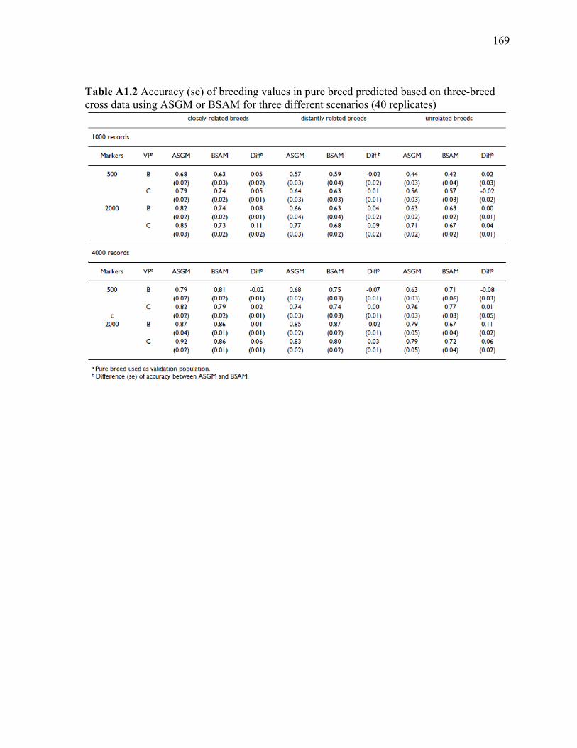
169

Table A1.2 Accuracy (se) of breeding values in pure breed predicted based on three-breed cross data using ASGM or BSAM for three different scenarios (40 replicates)

170

Table A1.3 Accuracy (se) of breeding values in pure breed predicted based on four-breed cross data using ASGM or BSAM for three different scenarios (40 replicates)

171

Table A1.4 Accuracy of breeding values in pure breed predicted based on performance in the same pure breed using ASGM (40 replicates)

172

Table A1.5 Accuracy of breeding values in pure breed predicted based on crossbred data when the breeds are closely related for a simulated genome of 10 chromosomes of 1 M each (40 replicates)

173

APPENDIX  2.  APPLICATION  OF  WHOLE-­‐GENOME  PREDICTION  

METHODS  FOR  GENOME-­‐WIDE  ASSOCIATION  STUDIES:  A  BAYESIAN  

APPROACH  

A paper submitted to Animal Genetics

Rohan Fernando, Ali Toosi, Dorian Garrick, Jack Dekkers

Department of Animal Science and Center for Integrated Animal Genomics,

Iowa State University, Ames, Iowa, 50011-3150, USA

A2.1  SUMMARY  

Data that are collected for whole-genome prediction can also be used for genome-wide

association studies (GWAS). This paper discusses how Bayesian multiple-regression

methods that are used for whole-genome prediction can be adapted for GWAS. It is argued

here that controlling the posterior type I error rate (PER) is more suitable than controlling the

genome-wise error rate (GER) for controlling false positives in GWAS. It is shown here that

under ideal conditions, PER can be controlled by using Bayesian posterior probabilities that

are easy to obtain. Computer simulation was used to examine the properties of this Bayesian

approach when the ideal conditions were not met. Results indicate that even then useful

inferences can be made.

 

 

174

A2.2  INTRODUCTION

High-density SNP genotypes are currently being used in livestock for whole-genome

prediction (VanRaden et al., 2009; Hayes et al., 2009; Habier et al.,2010b; Wolc et al., 2011).

This requires obtaining genotypes and phenotypes on several thousand animals in a training

population to estimate effects of the SNP genotypes on the traits of interest. These estimated

SNP effects are then used to predict the breeding values of selection candidates that may not

have any phenotypes recorded but have been genotyped (Meuwissen et al., 2001). The

genotype and phenotype data obtained for whole-genome prediction can also be used for

genome-wide association studies (GWAS) to locate causal variants (QTL) for traits of

economic importance.

Many GWAS for quantitative traits are based on testing one SNP at a time using simple

regression models or using a mixed model with a fixed substitution effect of the SNP

genotype included, along with a polygenic effect correlated according to pedigree

relationships to capture the effects of all the other genes. Such GWAS have been successful

in detecting many associations, but the established associations typically explain only a small

fraction of the genetic variability of quantitative traits (Maher, 2008; Manolio et al., 2009;

Visscher et al., 2010). On the other hand, when whole-genome selection models that

simultaneously fit all SNPs as random effects are used, the SNPs jointly explain a large

proportion of the genetic variance (Onteru et al., 2011; Hayes et al., 2010; Fan et al., 2011).

In these analyses, however, any given SNP may have only a weak association even with a

close QTL. The reason for this is that in multiple-regression, the association of a SNP with

the phenotype is a partial association conditional on all the other SNPs. Further, in a high-

density SNP panel, many SNP genotypes within a narrow genomic region are expected to be

175

highly correlated with each other and with any QTL that are close to them. So, any one SNP

may contribute only a little more to explain the variability of the QTL in addition to the other

SNPs in the neighborhood. On the other hand, even if each SNP in a neighborhood is only

weakly associated with a QTL, the SNPs in the neighborhood may jointly explain much more

of the variability of a QTL than any SNP by itself. Therefore in multiple-regression models,

SNPs in a genomic window should be used to locate QTL (Onteru et al., 2011; Sahana et al.,

2010; Hayeset al., 2010; Fan et al., 2011). Inferences on genomic windows by frequentist

methods, however, are computationally very challenging because they require repeated

analyses of the data with bootstrap or permuted samples to obtain significance levels for tests

(Onteru et al., 2011; Hayes et al., 2010; Fan et al., 2011). It can be shown that Bayesian

posterior probabilities obtained from a single analysis can be used to make inferences on

genomic windows. This approach to inference is related to the frequentist approach of

controlling the posterior type I error rate (PER), which is the conditional probability of a

false positive (type I error) given a positive (significant) result (Morton, 1955). It is PER that

traditionally has been used in human genetics to control false positives in linkage analyses of

monogenic traits (Elston, 1997) rather than the usual type I error rate, which is the

conditional probability of a false positive result given that the null hypothesis is true.

A requirement for controlling PER is knowledge of the distribution of the test statistic

under the null hypothesis of no association, which is also required to control the usual type I

error rate. In addition to this requirement, controlling PER requires knowing the proportion 𝜋

of SNPs for which the null hypothesis is true and the average power of the test, which is the

average probability of rejecting the null hypothesis when it is not true. These quantities are

176

almost never known in a GWAS of a quantitative trait, and thus PER cannot be controlled in

the sense that the usual type I error rate can be controlled (Elston, 1997).

In a QTL mapping study, Soller and colleagues were the first to show that 𝜋 can be

estimated from a histogram of p-values (Mosig et al., 2001). In this multiple test setting, they

showed how the estimate of 𝜋 can be used to obtain an adjusted false discovery rate (FDR)

(Benjamini & Hochberg, 1995) that results in increased power to detect QTL. Their seminal

paper also showed how to estimate the average power of tests (Mosig et al., 2001). Such

estimates of 𝜋 and average power can also be used to estimate PER for a test with a specified

significance level (type I error rate). However, when the resulting estimates of PER are used

for inference, the estimates of 𝜋 and average power are treated as known values because it is

not straightforward to incorporate the errors in these estimates into the calculations. In

contrast to frequentist methods, when the Bayesian multiple-regression models (Meuwissen

et al., 2001) that are used for whole-genome prediction are applied to GWAS, posterior

probabilities that are similar to PER can be obtained even without the requirement of

knowing the null distribution of any test statistic. Further, in Bayesian analyses, 𝜋 and the

partial regression coefficients of markers, which determine average power, can be formally

treated as unknowns such that their uncertainty is incorporated in the inference.

It can be shown that using PER or related posterior probabilities for inference has the

following advantage. Suppose PER is controlled, for example, at 0.05 for each of many tests,

which may be dependent. Then, among the positive results that accumulate over many

independent experiments the proportion of false positives will converge to 0.05 (Section 2.2).

As a result, regardless of the number of tests in an experiment and their interdependence, the

proportion of false positives that accumulate in the literature can be controlled by controlling

177

the PER for individual tests. It has been shown that controlling PER for individual tests in an

experiment is related to controlling FDR or its close relatives pFDR (Storey, 2002) or PFP

(Southey & Fernando, 1998; Fernando et al., 2004) for the collection of tests from the

experiment.

Posterior probabilities that are related to PER are still not widely used for inference in

GWAS by animal geneticists. One reason for this is that to manage false positives in a

GWAS controlling the genome-wise error rate (GER) is better accepted than controlling the

PER for individual tests or FDR for the experiment. A second reason is that the relationship

between PER and the Bayesian posterior probabilities for inference in GWAS has not been

studied in a realistic setting. A third reason for preferring GER over PER is given by Chen &

Storey (2006). Their reasoning can be interpreted as follows. In linkage analysis, a QTL is in

principle linked to every marker on the same chromosome, and this makes the null

hypothesis that a marker is not linked to a QTL false for every marker on a chromosome that

has even a single QTL. Then, a marker with a significant linkage signal on a chromosome

that has a QTL will be a true positive even if the marker is not close to the QTL. This makes

controlling the proportion of false positives among significant results meaningless (Chen &

Storey, 2006). They refer to this problem as signal dependence. Thus, the objective of this

paper are to: 1) address the problem of signal dependence and review the advantages of

managing false positives in GWAS by controlling PER or related measures such as FDR or

PFP rather than by controlling the GER, 2) discuss the theoretical relationship between

Bayesian posterior probabilities and PER, and 3) use computer simulation to examine this

relationship in a realistic GWAS setting.

178

In Section 2.1 the problem of signal dependence are addressed and the advantages of

managing false positives by controlling PER rather than GER are reviewed. Section 2.2

provides the justification for using PER in a multiple test setting and gives its relationship to

FDR and related measures. Section 2.3 describes the calculation of Bayesian posterior

probabilities that are useful for inference in GWAS, and Section 2.4 shows how these

posterior probabilities are related to PER. A computer simulation that was used to study the

properties of the Bayesian approach is described in Section 2.5. Results are discussed and

summarized in Section 3.

A2.3  METHODS  

A2.3.1 Controlling False Positives

Many papers have discussed the advantages of controlling FDR and related measures

rather than controlling GER (Benjamini & Hochberg, 1995; Storey, 2002; Fernando et al.,

2004; Stephens & Balding, 2009). Chen & Storey (2006), however, have argued that

measures such as FDR that control the proportion of false positives among significant results

are not suitable for controlling false positives in QTL studies. The essence of their argument

stems from the implicit assumption that the linkage signal from a QTL spans the whole

chromosome. Thus, the null hypothesis that a marker is not linked to a QTL is equivalent to

that of no QTL on the same chromosome as the marker. Then, rejection of the null

hypothesis does not imply that the marker is close to a QTL. To address this problem others

have employed multiple-regression models where the signal from a QTL is localized to a

relatively narrow segment of the chromosome (Zeng, 1993, 1994; Southey & Fernando,

1998).

179

Suppose data are available from a backcross population derived from two completely

homozygous lines. In such a population, the following multiple-regression model can be used

to test the null hypothesis that a chromosomal segment with a central marker 𝐶 bracketed by

two markers 𝐿 on the left and 𝑅 on the right does not contain any QTL:

𝑌!  =  𝛽!  +  𝑋!"𝛽!  + 𝑋!"𝛽! +  𝑋!"𝛽! + 𝜖! ,                                                            [1]

where 𝑌! is the trait value, 𝛽! is the intercept, 𝛽!, 𝛽! , and 𝛽! are regression coefficients

for three markers 𝐿, 𝐶 and 𝑅, respectively, and 𝑋!",  𝑋!" and 𝑋!"  are 0 or 1 depending on

whether the marker genotype is heterozygous or homozygous. It can be shown that 𝛽! is non-

null if only if the chromosomal segment bracketed by 𝐿 and 𝑅 contains a QTL (Zeng, 1993).

Thus with this multiple-regression model, the signal from the trait gene is localized to a

chromosomal segment of, for example, 10 cM in length, and testing the null hypothesis that

such a segment does not contain a QTL is meaningful in a QTL study. In this setting, we will

consider the difference between controlling GER and PER.

A hypothetical example is used next to show why controlling PER is more meaningful

than controlling GER in a QTL study. Suppose only one chromosomal segment is tested.

Then, GER is identical to the type I error rate for the single test, but PER can be much

higher, depending on the probability 𝜋 that the null hypothesis is true for a randomly chosen

segment and on the power of the test. To calculate PER, assume the trait is controlled by a

single gene, the genome consists of 30 chromosomes each of length 1 Morgan, and the

segment length is 10 cM. Then, the probability the null hypothesis is true that the

chromosomal segment does not contain a QTL for a randomly chosen segment is 𝜋 = !""!""

.

180

Further, we assume that if the null hypothesis is not true, the power of the test is 𝑝  = 90%

when a significance level of 𝛼 = 0.05 is used. Now, with GER at the usual 0.05, PER is

PER =απ

απ+ p 1− π

                                                     =0.05× 299300

0.05× 299300+ 0.9×1300

                                                                 [2]

                                                                                                                                     = 0.94,

where the numerator of (2) is the joint probability that the null hypothesis is true and it is

rejected, and the denominator is the marginal probability of rejecting the null hypothesis.

Thus, although we have controlled GER at 0.05, a significant result will be a false positive

with probability of over 90%! In other words, among significant results over 90% will be

false positives. If we want PER to be 0.05, 𝛼 must be reduced to 0.0001584 even for a single

test. Thus, controlling GER does little to control PER.

Suppose now a chromosomal segment of 10 cM is chosen at random from each of the 30

chromosomes. For each of these segments, the probability 𝜋 that the null hypothesis is true

remains !""!""

. So, if the significance level is kept at 𝛼 = 0.0001584, the PER will be 0.05 for

the results from each chromosome. In other words, if results are accumulated over repetitions

of the experiment, the proportion of false positives among the significant results would

remain 0.05. Thus, the proportion of false positives in the collection of significant results

from all chromosomes will also be 0.05. A proof of this result is given in the next section.

Given that the 30 tests are independent, the GER can be calculated (Sidak, 1967) as

GER = 1− 1− 0.0001584 !"

= 0.004742.                                                                                                                                        [3]

181

Note that as the number of tests increased GER also increased from 0.0001584 for one

test to 0.004742 for 30 tests while PER stayed constant at 0.05. So, if GER is used, as the

number of tests increases, the significance level for individual tests has to be decreased to

keep GER at 0.05, and this will result in lower power. This is not the case with PER. Thus, it

is more suitable for GWAS that involve very large numbers of tests.

A2.3.2 Relationship of PER to FDR, pFDR and PFP

In this section we provide the justification for using PER to control false positives in a

multiple test setting where the tests may be dependent such as in a GWAS. Furthermore, we

will show how controlling PER for individual tests is related to measures such as FDR that

attempt to control false positives in the collection of tests from an experiment.

In order to describe this relationship between PER that is defined for an individual test

and measures such as FDR, pFDR and PFP that are defined for a collection of tests, for test 𝑗

of experiment 𝑖, 𝑉!" and 𝑅!" are defined as follows: 𝑉!" = 1 if 𝐻! is falsely rejected (false

positive) and else 𝑉!" = 0;  𝑅!" = 1 if 𝐻! is rejected (positive) and else 𝑅!" = 0. Now using

this notation, PER for test 𝑗 in experiment 𝑖 is

PER = Pr 𝑉!" = 1 𝑅!" = 1 ,                                                                                [4]

which according the frequentist definition of probability is the limiting value of the

relative frequency:

𝑉!"!!

𝑅!"!!

                                                                                                                             [5]

as 𝑁 the number of independent experiments tends to infinity. Thus, controlling PER for

a test is equivalent to controlling the proportion of false positive results that accumulate in

182

the literature for that test. Now, the relationship of PER with PFP is used to justify its use to

control false positives in a multiple test setting.

In Fernando et al. (2004), PFP was defined as

PFP =E(𝑉!)E(𝑅!)

,

where 𝑉! = 𝑉!"! and 𝑅! = 𝑅!"! . Let 𝑆!"  =  1 denote that 𝐻! is true and 𝑆!"  =  0 that

it is false for test 𝑗 in experiment 𝑖. When 𝑆!" is considered fixed, they showed that PER for a

randomly chosen test is equal to PFP for the collection of tests that may be dependent

(Fernando et al., 2004). Further, they showed that the limiting value of the frequency of false

positives relative to the total number of positives across tests, which may be dependent, and

across 𝑁 independent experiments:

𝑉!"!!!

𝑅!"!!!

                                                                                                                             [6]

is equal to PFP as 𝑁 tends to infinity [property 2 of PFP in Fernando et al. (2004)]. Thus,

in this case, PER for a random test is equal to the limiting value of (6).

In Bayesian analyses, 𝑆!" is considered random, and for this case we show here that if

PER ≤ (1− 𝑡) for each test, then for the collection of tests that may be dependent  PFP ≤

(1− 𝑡). First note that PER can be written as

         PER = Pr 𝑉!" = 1 𝑅!" = 1

=Pr  (𝑉!" = 1)Pr  (𝑅!" = 1)

=E 𝑉!"E 𝑅!"

                                                                                                                                       [7]

183

Now, if PER ≤ (1− 𝑡) for each test, using (7), PFP for the collection of tests from

experiment 𝑖 becomes

PFP =E 𝑉!"!

E 𝑅!"!

                 =E 𝑉!"!

E 𝑅!"!

                                                                       =E 𝑅!" E 𝑉!"! E 𝑅!"

R 𝑉!"!

                                                 ≤E 𝑅!"! 1− 𝑡

R 𝑉!"!

 = 1− 𝑡 ,                                                                                                                      [8]

where in going from line three to four of (8) we have used the result (7) that

E 𝑉!" E 𝑅!" = PER and the condition that PER ≤ (1− 𝑡). This proves that if PER ≤ (1−

𝑡) for each test then PFP ≤ (1− 𝑡), for the collection of tests. Combining this result with

property 2 of PFP from Fernando et al. (2004), we have that if PER ≤ (1− 𝑡) for each test,

the limiting value of (6) ≤ (1− 𝑡).

The above result justifies using PER to control false positives in a multiple test setting

where the tests may be dependent as in a GWAS, because as we have shown above, if

PER ≤ (1− 𝑡) for each test in an experiment, then as results accumulate over 𝑁 independent

experiments, among all positive results the proportion of false positives (6) will converge to a

value that is ≤ (1− 𝑡).

When tests are independent or have a certain type of dependence, Storey (2003) has

shown that pFDR, which is defined as

184

pFDR = E𝑉!𝑅!

𝑅! > 0 ,                                                                                      [9]

is equal to PFP and to PER for an individual test. FDR (Benjamini & Hochberg, 1995) on

the other hand, defined as

pFDR = E𝑉!𝑅!

𝑅! > 0 Pr 𝑅! > 0 ,                                                      [10]

can be quite different from pFDR, PFP or PER even when the tests are independent if

Pr  (𝑅! > 0) is not close to one (Zaykin et al., 2000; Storey, 2003). Further, both pFDR and

FDR can be quite different from PFP when tests are not independent as demonstrated by a

hypothetical example in Fernando et al. (2004).

A2.3.3 Bayesian Multiple Regression

Here we will explain how multiple-regression models that were developed for whole-

genome prediction can be used for GWAS. In these models, inference is based on posterior

probabilities that, as will be shown in Section 2.4, are similar to PER.

Following Meuwissen et al. (2001), consider the mixed linear model

𝒚 = 𝑿𝜷+ 𝒛!𝛼!

!

!!!

+ 𝒆,                                                                                [11]

where 𝒚 is the vector of trait phenotypes, 𝑿 is an incidence matrix relating the vector of

non-genetic, fixed effects 𝜷 to 𝒚, 𝒛! is a vector of genotype covariates (coded as 0, 1 or 2) for

SNP j, 𝛼! is the random, partial regression coefficient for SNP j, and 𝒆 is a vector of

residuals. In this model, the fixed effects are assumed to have a constant prior, the 𝛼! are a

priori assumed independently distributed as

𝛼!|𝜋,𝜎!!! =

0,                                                                                  with  probability  𝜋~N 0,𝜎!!

! ,                        with  probability   1− 𝜋 ,                                        [12]

185

where the 𝜎!!! are a priori assumed independently and identically distributed (iid) scaled

inverse chi-square variables with scale 𝑆!! and degrees of freedom 𝜈!. The residuals are

assumed iid normal with null mean and variance 𝜎!!, with a scaled inverse chi-square prior

for 𝜎!! with scale 𝑆!! and degrees of freedom 𝜈!. Inferences on the unknowns in the model are

made from their marginal posterior distributions, using Markov Chain Monte-Carlo (MCMC)

methods (Meuwissen et al., 2001; Habier et al., 2010a).

Although this model was first proposed for whole-genome prediction (Meuwissen et al.,

2001), it can also be used to locate genomic regions that contain QTL (Yi et al., 2003; Sun et

al., 2011; Fan et al., 2011). Consider a model where 𝜋 is close to one, i.e., a model where

most regions of the genome do not have markers that are associated with the trait. This is the

model called BayesB by Meuwissen et al. (2001). Given such a model, the posterior

probability that 𝛼! is non-zero for at least one SNP j in a window or region can be used to

make inferences on the presence of QTL in that region. We will refer to this probability as

the window posterior probability of association (WPPA). The underlying assumption here is

that if a genomic window contains a QTL, one or more SNPs in that window will have non-

zero 𝛼!. Thus, WPPA, which is estimated by counting the number of MCMC samples in

which 𝛼! is non-zero for at least one SNP j in the window, can be used as a proxy for the

posterior probability that the genomic window contains a QTL.

It is possible, however, that SNPs in a window that does not contain any QTL are in

association with a QTL outside the window, which is what has been called signal dependence

(Chen & Storey, 2006). Fortunately, the linkage signal from LD extends over only short

distances compared to that from cosegregation, and as described below, when all SNPs are

186

fitted simultaneously, signal dependence is further reduced. Let 𝑊! denote the window for

which WPPA is estimated. Let 𝑊! and 𝑊! be windows of length 𝑘 cM to the left and right of

𝑊! as illustrated in Figure A2.1. A high window WPPA for 𝑊! is taken as evidence of a

QTL in the “composite” window 𝑊 comprising of 𝑊!, 𝑊! , and 𝑊!. Because WPPA for 𝑊!

is a partial association conditional on all other SNPs in the model, including those in the

flanking windows 𝑊! and 𝑊!, the inuence of QTL from outside the composite window on

the WPPA signal for 𝑊! will be inversely related to the length 𝑘 of the flanking windows. In

other words, as the number of markers between a QTL and 𝑊! increases, the influence of the

QTL on the WPPA signal for 𝑊! will decrease. Thus, as shown in more detail in the next

section, WPPA computed for 𝑊! can be used to locate QTL.

A2.3.4 Relationships of Posterior Probabilities to PER

Here, we show that Bayesian posterior probabilities such as WPPA are related to PER,

and therefore they can be used to control false positives in a multiple test setting. The

relationship of WPPA to PER is most straightforward when the priors used in the Bayesian

analysis have a frequentist interpretation. This would be the case in a simulation study where

data are generated and analyzed as follows. Suppose SNP genotypes are available on 𝑛

individuals at 𝐾 markers. Then, phenotypes for these 𝑛 individuals can be generated

according to model (11) by taking the matrix 𝑿 to be a vector of ones and the vector 𝜷 to be

any constant (for example 0), sampling the partial regression coefficients, 𝛼!, according to

(12), and sampling the residuals from a normal distribution with null mean and variance 𝜎!!.

Now, in the Bayesian analysis of the simulated data, suppose the distributions used to

simulate the partial regression coefficients and the residuals are used as priors. Then, the

187

WPPA calculated in the analysis for a genomic window, 𝑊! , is the conditional probability of

a true association (i.e., a QTL) within that window (in this case, where the QTL are included

in the marker panel, the QTL signal should stay within its own window) given the data. The

frequentist interpretation of this probability is as follows. Suppose the simulation and

analysis described above are repeated many times. Then, among all genomic windows with

WPPA equal to 𝑞, a proportion 𝑞 is expected to contain one or more SNPs with a true

associations with the trait.

Recall that PER is associated with the test of a hypothesis. The null hypothesis 𝐻! in this

case is that the genomic window 𝑊! does not contain any SNPs associated with the trait.

Using this notation, WPPA is the conditional probability that 𝐻! is false given the observed

data, while PER is the conditional probability that 𝐻! is true given that 𝐻! has been rejected

based on some statistical test. Suppose the test is based on WPPA and 𝐻! is rejected

whenever WPPA is larger than some value 𝑡. Then, PER is the probability that 𝐻! is true

given WPPA is larger than 𝑡, and it can be written as:

         PER = Pr 𝐻!  is  true WPPA > 𝑡

=1− 𝑞 𝑓(𝑞)d𝑞!

!

𝑓(𝑞)d𝑞!!

                                 = E 1−WPPA WPPA > 𝑡

≤ 1− 𝑡,                                                                                                                                                  [13]

where 𝑓(𝑞) is the density function of WPPA. Thus in hypothetical repetitions of the

analysis, for any interval with WPPA > t the proportion of false positives among significant

results will be ≤ 1− 𝑡.

188

One of the advantages of inference based on posterior probabilities such as WPPA is that

derivation of the distribution of the test statistic is not required. Further, the posterior

probabilities of interest are easily obtained from the MCMC samples from the Bayesian

analysis. Consider for example the situation where interest is in detecting regions that explain

more than some proportion 𝑣 of the total genetic variance (𝜎!!) (Hayes et al., 2010; Fan et al.,

2011). The variance that is attributed to a genomic region or window is defined as follows.

First, the component of the genotypic value that corresponds to genomic window 𝑊! is

defined as

𝒈! = 𝒁!𝜶! ,                                                                                                  [14]

where 𝒁! is the matrix of genotype covariates and 𝜶! is the vector of partial regression

coefficients for SNPs in the window 𝑊! . In other words, 𝒈! is the sum of the genotypic

values for SNPs in window 𝑊! . Then, the window variance is defined as the sample variance

of the components of 𝒈!. In most Bayesian multiple-regression analyses, samples of the

partial regression coefficients are drawn from their posterior distribution, and these samples

can be used to compute window variances. The posterior probability that the window

variance is larger than 𝑣𝜎!! can be estimated by counting the number of MCMC samples

where the window variance is larger than 𝑣𝜎!!.

In this section, the relationship between WPPA and PER was discussed in the context of

Bayesian analysis of simulated data, where the distributions used in the generation of the data

were used as priors in the Bayesian analysis. In analysis on real data, the distribution of

unobservables quantities such as the partial regression coefficients and residuals are not

known. Thus, based on available knowledge of the problem, priors that lead to

189

computationally efficient algorithms are used. Computer simulation will be used here to

study the impact of such priors on the relationship between WPPA and PER in a realistic

GWAS setting. As the amount of data that are combined with the priors increases, the impact

of the priors on the posterior distributions is expected to decrease.

A2.3.5 Computer Simulation

The simulation described here was used to test if WPPA can be used to control false

positives in GWAS, where the tests are dependent. Actual SNP genotypes of purebred Angus

bulls were used to simulate QTL and phenotypes as described in Kizilkaya et al. (2010).

Exactly 100 data sets with 1,000 observations and another 100 with 3,570 observations were

simulated, using genotypes at 52,910 SNP loci on 3,570 purebred Angus bulls. The 1,000

bulls were randomly sampled without replacement for inclusion in the data sets with 1,000

observations, whereas all bulls were used in the data sets with 3,570 observations.

In each of the 200 data sets, SNP effects of markers were sampled according to the prior

of the BayesC model of Habier et al. (Habier et al., 2011) with 𝜋 = 0.995, where a proportion

𝜋 of the loci have null effects and the remaining loci have normally distributed effects with

null mean and common variance 𝜎!! of SNP effects. The value of the common variance of

SNP effects was chosen as in Kizilkaya et al. (2010) such that the additive genetic variance

for the trait was 0.9. The average number of QTL in the data sets was about 260. The residual

variance for the trait was set at 0.1 to give a heritability of 0.9.

The data sets with 1,000 observations were analyzed with and without including the

SNPs that represent the QTL in the marker panel. The data sets with 3,570 observations were

only analyzed without including the QTL in the marker panel. Posterior inferences were

based on 10,000 MCMC samples after a burn-in of 1,000 samples.

190

In all analyses, the genome was divided into 2,676 one cM intervals according to the

bovine map. The WPPA and window variance was computed for each such window, 𝑊! , as

explained previously. In order to study the relationship between WPPA and the true

probability of a QTL, each genomic window, 𝑊! , was classified into one of 10 WPPA

classes of length 0.1 between 0 and 1. For example, all windows with WPPA between 0 and

0.1 were be classified into the first class, and those with WPA between 0.1 and 0.2 to the

second class. The true probability of a QTL for a WPPA class was estimated by the observed

frequency as follows. Let 𝑄!" denote the observed number of windows 𝑊! belonging to

WPPA class j or windows 𝑊! or 𝑊! flanking 𝑊! with one or more QTL from data set i, and

let 𝑅!" denote the total number of genomic windows that belong to WPPA class j from data

set i. Then, the actual frequency of a simulated QTL for WPPA class j was computed as

𝑓! =𝑄!"!""

!

𝑅!"!""!

.                                                                                          [15]

BayesC with 𝜋 = 0.995 or 𝜋 = 0.999 was used for the analyses where the QTL were

included in the marker panel. Recall that the prior of BayesC with 𝜋 = 0.995 was used in the

simulation of SNP effects. Thus, with 𝜋 = 0.995, WPPA is expected to agree well with the

actual frequency of the QTL. The relationship between WPPA and the actual frequency of

QTL for these analyses are given for flanking windows of length k = 0, 1, or 2 cM in Figure

A2.2.

Further, for these analyses with QTL included in the marker panel, each marker was

classified into ten posterior probability of association (PPA) classes as described above for

WPPA. Figure A2.3 shows the relationship between the PPA classes and the actual

frequency of QTL among markers that belong to each class.

191

BayesC and BayesB with 𝜋 = 0.995, and BayesC𝜋, where 𝜋 is treated as an unknown,

were used to analyze the data sets with 1,000 observations without including the QTL in the

marker panel. The relationship between WPPA and the actual frequency of QTL for these

analyses are given in Figure A2.4.

BayesC𝜋 was used to analyze the data sets with 3,570 observations without including the

QTL in the marker panel (Figure A2.5). In addition to computing WPPA for each genomic

window, 𝑊! , the posterior probability that the window variance (𝜎!!) exceeds 1/1,000 of the

posterior mean of the total variance (𝜎!!) was computed and grouped into 10 equally spaced

posterior probability classes. For each such class, the actual frequency of a QTL in 𝑊! or in

the flanking windows having a variance (𝑣!) that exceeds 1/1,000 of the total QTL variance

(𝑉!) was also computed. The relationships between these probabilities and corresponding

actual frequencies are given in Figure A2.6 using BayesC𝜋.

A2.4  DISCUSSION  

There are two main approaches to control false positives in genome-wide association

studies. The most widely used approach is based on controlling the genomewise type I error

rate (GER). The other is controlling the proportion of false positives among significant

results, which as we have shown here, is equivalent to controlling the posterior type I error

rate (PER) (Morton, 1955) for each test.

The longstanding practice of using a LOD score of three for declaring linkage between a

monogenic disease locus and a random marker is based on control of PER to about 0.05

(Elston, 1997). The examples given in section 2.1 show that a test can have very different

GER and PER values. If only one marker is tested, controlling GER to 0.05 will result in a

192

much larger value for PER, i.e., among significant results a large proportion would be false

positives (94% in the example). Thus, to control PER to 0.05, a more stringent significance

threshold has to be used (0.0001584 in the example). Now, suppose several markers are

tested with the same stringent significance threshold each with the same prior probability of

linkage to a QTL and power of test. Then for each test, PER would be 0.05, even when the

tests are not independent. Thus, provided the prior probability of linkage and power are

constant, the same significance threshold can be used to control PER regardless of the

number of tests. This is not true for GER, which for a given significance threshold increases

with the number of tests.

To control PER, however, it is required to know the value of 𝜋, which is the probability

that the null hypothesis is true for a test, and the power of the test. Mosig et al. (2001) have

shown how to estimate these quantities, and these estimates can be used to estimate PER. On

the other hand, in Bayesian analyses, these quantities can be treated as unknowns and an

upper bound for PER can be obtained from Bayesian posterior probabilities as described in

Section 2.4. For example, the PER for the test of a QTL in a genomic window, 𝑊, is

obtained as 1 – WPPA, where WPPA is estimated by counting the number of MCMC

samples in which 𝛼! is non-zero for any SNP j in 𝑊! , the central window of 𝑊 (Figure

A2.1).

In Section 2.2 we discussed the relationship of PER to FDR, pFDR and PFP. The

relationship between PER and PFP was used there to show that controlling PER for

individual tests is equivalent to controlling the relative frequency given by (6) of false

positives among all positives that accumulate across tests, which may be dependent, and

across independent experiments. It is this property of PER, which does not depend on the

193

number of tests or their dependence structure, that makes it a desirable measure for

controlling false positives in a GWAS and not its relationship to FDR, pFDR or PFP. Further,

when PER is used for inference there is no multiple-test penalty (Stephens & Balding, 2009).

We have argued here that by using multiple-regression models the linkage signal can be

localized to relatively short segments of the genome and thereby avoid the problem of signal

dependence raised by Chen & Storey (2006). In model (1), assuming no interference,

segregation of alleles at locus C are conditionally independent of the segregation of alleles at

loci to the left of locus L and to the right of locus R given the segregation events at L and R.

Thus, this model can be used to test the null hypothesis of no QTL between loci L and R in a

linkage analysis, where the signal for QTL detection comes from the cosegregation of alleles

at markers and QTL. In an association analysis, the signal for QTL detection comes from LD

between markers and QTL, which is the non-independence between the allele states at these

loci. Unfortunately, even under the assumption of no interference, allele states at locus C

may not be conditionally independent of allele states at loci to the left of locus L and to the

right of locus R given the allele states at loci L and R. However, the LD signal, depending on

the effective population size, decays much faster with distance between loci than that due to

cosegregation. Further, in the Bayesian multiple-regression models that we have used here,

all SNPs are used in the analysis. Thus, in association analyses signal dependence is less of a

problem than in linkage analysis, and when multiple regression models are used with high-

density SNP markers, the signal from a QTL is expected to be almost completely explained

by the markers within a narrow genomic window containing it. If the QTL is at the edge of a

window, however, its signal may bleed into the next window. Thus, we considered using a

194

composite window (Figure A2.1). The signal is measured only in the central window to test

the null hypothesis of no QTL in the composite window.

In this study, posterior probabilities of association were computed for genomic windows

of 1cM (WPPA). When the QTL were included in the marker panel used in the analysis and

the distribution used to simulate the QTL effects was used as the prior for marker effects in

the Bayesian analysis, Figure A2.2 (plot A) shows good agreement between WPPA for a

1cM window and the frequency of QTL in that window (k = 0). For example, among

genomic windows with WPPA between 0 and 0.1, about 5% contained one or more QTL,

and among windows with WPPA between 0.9 and 1.0, about 95% contained QTL.

Figure A2.2A also shows the frequency of QTL in composite windows consisting of a

1cM central window and left and right flanking windows of length k = 0, 1, or 2 cM. In all

three curves, WPPA was computed for the central window, but the actual QTL frequency

was computed for either a 1, 3, or 5 cM window centered at the window for which WPPA

was computed. Windows with WPPA between 0 and 0.1 had actual QTL frequencies of 0.06,

0.22, or 0.35 for windows of length 1, 3 or 5 cM. Given that about 260 QTL were simulated

and uniformly placed in 2,676 genomic windows, the prior probability that a composite

window would contain one or more QTL is 0.09, 0.25 or 0.38 for k = 0, 1 or 2. Thus, the

actual frequencies were reduced from the prior values towards the WPPA of 0.05. This is

most evident when k = 0, where the actual frequency was 0.06, indicating that in this case,

the WPPA is mainly influenced by the presence or absence of QTL in the central window. In

windows where WPPA was between 0.45 and 0.85, the actual frequency of QTL for k = 0

was about 0.05 lower than WPPA. This indicates that the WPPA is slightly inflated by the

presence of QTL outside 𝑊! whose signal bleeds into the signal observed for 𝑊! .

195

Figure A2.2 (plot B) shows the same relationships when the Bayesian analysis used 𝜋 =

0.999 although 𝜋 = 0.995 was used in the simulation (QTL were included in the marker

panel). The high value for 𝜋 makes it difficult for a locus to be included in the model, and

this can explain why WPPA was lower than the actual QTL frequencies for k = 0 and WPPA

between 0.15 and 0.55. On the other hand, for values of WPPA between 0.65 and 0.85, the

agreement between WPPA and the actual QTL frequencies for k = 0 was better in plot B of

Figure A2.2 with 𝜋 = 0.999 than in plot A with 𝜋 = 0.995, which was used in the simulation.

A possible explanation is that when 𝜋 = 0.999, loci with a strong signal are favored for

entering the model relative to those with weaker signals. Thus, in this analysis where QTL

were included in the marker panel, QTL with large effects will be favored relative to markers

that are in high LD with these QTL. When 𝜋 = 0.995 was used, markers in high LD with the

QTL may have entered the model and prevented the actual QTL from coming in. This

indicates a mixing problem given the 10,000 MCMC samples used for inference in the

simulation. If that is the case, use of a longer chain would give better results with 𝜋 = 0.995

for the entire range of WPPA. Also, it may indicate that alternative sampling strategies to

improve mixing should be investigated.

Figure A2.3 shows the relationships between PPA for each marker and the actual

frequency that the corresponding marker is a QTL (QTL were included in the marker panel).

Here, the actual frequencies of QTL were even lower than in plot A of Figure A2.2 for

WPPA between 0.45 and 0.85. Again, this may be due to a mixing problem. In plot A of

Figure A2.2, the overestimation of the QTL frequency for k = 0 was thought to be due to

markers from adjacent windows in high LD with the QTL entering the model and preventing

the actual QTL from coming in. In Figure A2.3, this can even happen with markers in the

196

window that contains the QTL. Thus, the observation that QTL frequencies are lower in

Figure A2.3 than in plot A of Figure A2.2 is consistent with the expectation that markers

within the QTL window would have higher LD with the QTL than markers from adjacent

windows.

In the remaining analyses, the QTL were not included in the marker panel. Figure A2.4

presents results from three analyses of the 100 data sets with 1,000 observations, and Figures

A2.5 and A2.6 gives results for the 100 data sets with 3,570 observations. In these analyses

that did not have the QTL included in the marker panels, in genomic windows of 1cM and k

= 0 WPPA for 𝑊! substantially overestimated the frequency of QTL in the window 𝑊! when

WPPA greater than about 0.15. For example, in plot B of Figure A2.4, which shows the

relationship between WPPA and the frequency of QTL for BayesC with 𝜋 = 0.995, in

genomic windows of 1cM with WPPA between 0.9 and 1.0 the frequency of QTL was about

0.72 and in genomic windows of 1cM with WPPA between 0.8 and 0.9 the frequency of

QTL was only about 0.5. When the QTL were included in the analysis, the comparable QTL

frequencies were 0.97 and 0.81 (plot A of Figure A2.2). Thus, when the QTL were not in the

panel, WPPA overestimated the frequency of QTL in 𝑊! . Following are two possible

reasons for this. The first is that the prior used for marker effects does not agree with the

actual distribution of effects. When the QTL are not included in the marker panel, only

markers that are in complete LD with the QTL will have effects that are distributed as the

QTL. In Angus, the average LD between adjacent markers for the 50k SNP panel is about 0.2

(Goddard & Hayes, 2009). Thus, the distribution of marker effects may be quite different

from that of the QTL and this may have an impact on the relationship between WPPA for a

genomic interval and the frequency of QTL in that interval even when the distribution used

197

to generate the QTL effects is used as the prior for marker effects as in the BayesC analysis

with 𝜋 = 0.995. The second reason is violation of the assumption that WPPA is equivalent to

the posterior probability that 𝑊! contains a QTL (WPPQ). Recall that WPPA is the posterior

probability that a marker in window 𝑊! has a non-zero effect on the trait. When the QTL are

included in the panel, WPPA is also the posterior probability of a QTL in 𝑊! because QTL

by definition have non-zero effects on the trait. However, when the QTL are not included in

the panel, WPPA is not equivalent to probability of a QTL in 𝑊! . A marker in 𝑊! may have

a non-zero effect even when 𝑊! does not contain any QTL due to it being in LD with a QTL

in an adjacent window. This would cause WPPA to be higher than the QTL frequency, which

is consistent with our results.

It can be argued that both of the reasons given above played a role in the observed over

estimation of QTL frequencies in 𝑊! by WPPA. Violation of the assumption that WPPA is

equivalent to WPPQ, however, seems to have played a greater role. The three plots in Figure

A2.4 were obtained using three different priors. Plot A is from a BayesB analysis with 𝜋 =

0.995, where a central t distribution with four degrees of freedom was used as the prior for

marker effects. Plot B is from BayesC with 𝜋 = 0.995, where a normal distribution is used for

marker effects, and plot C is from BayesC𝜋, where 𝜋 is treated as unknown with a uniform

prior between 0 and 1 and a normal prior for marker effects. The results from these three

analyses being very similar indicates that with 1,000 observations these differences in priors

had a negligible effect on the relationships between WPPA and QTL frequencies. Further, if

the overestimation of QTL frequencies by WPPA was due to the prior for marker effects not

being appropriate, then better results would be expected in the data sets with 3,570

observations. However, this was not the case. Overestimation was even greater with the

198

bigger data sets (Figure A2.5). On the other hand, if the observed overestimation of QTL

frequencies was due to markers in 𝑊! being in LD with QTL in adjacent windows, it is

possible that with more data associations with even more distant QTL could further inflate

WPPA. Comparison of QTL frequencies in plot C of Figure A2.4 with those in Figure A2.5

for genomic windows with WPPA between 0.8 and 0.9 and k = 0, 1, and 2 suggests that with

the bigger data sets more distant QTL contributed to the WPPA value calculated for 𝑊! .

In these analyses that did not include the QTL in the marker panel, there was good

agreement between WPPA and the actual frequency of the QTL in the composite window W

with k = 2 when WPPA was larger than 0.8. At lower values of WPPA, WPPA

underestimated the QTL frequency for k = 2. In genomic windows with WPPA between 0

and 0.1, the QTL frequency with k = 0 was almost 0.05, agreeing very well with WPPA. This

is because the QTL in these windows have only very small effects. Thus, only the QTL from

𝑊! contribute to WPPA. As mentioned previously, with k = 2, the prior probability of a QTL

in 𝑊 is 0.38. The actual value for windows with WPPA between 0 and 0.1 was 0.3 for k = 2,

which is lower than the prior value of 0.38. Genomic windows with higher values of WPPA,

for example, between 0.2 and 0.3, consists of a mixture of windows containing QTL of

moderate size in the flanking windows which affect WPPA computed for 𝑊! and smaller

QTL that do not affect WPPA computed in the central window 𝑊! . As WPPA gets higher,

most windows contain large QTL that contribute to the high value of WPPA.

Figure A2.6 shows the relationship between the posterior probability that the window

variance (PPWV) exceeds 1/1,000 of the total variance and the corresponding actual

frequency for the QTL variance. PPWV are especially useful for GWAS using models such

199

as BayesA (Meuwissen et al., 2001) and Bayesian Lasso (de los Campos et al., 2009) where

all markers are assumed to have non-null effects and, thus WPPA is always 1.

Here, we will use window variances to examine the signal from the flanking windows. In

the BayesC𝜋 analyses (Figures A2.4 and A2.5), the actual frequencies of QTL were in good

agreement with WPPA for WPPA values larger than 0.85 and k = 2. However, when k = 0

the actual frequencies were much lower than WPPA. This indicates that the high values of

WPPA are due partly to strong signals from the flanking windows. This can be tested by

examining the QTL signal in the central and flanking windows for segments with

PPWV=0.95 in comparison to the corresponding signal in segments with PPWV=0.05. In

segments with PPWV=0.95, the QTL in the central window (k = 0) had a mean that was

1.1% of the total variance, and those in the flanking windows (k = 2) had a mean that was

1.3% of the total variance. In segments with PPWV=0.05, the QTL in the central window

had a mean that was 0.1% of the total variance, and those in the flanking windows had a

mean that was 0.3% of the total variance. Thus, in segments with PPWV=0.95, there was a

QTL with a strong signal in the central window or one with even a stronger signal in the

flanking windows. These simulation results show that there is good agreement between

posterior probabilities and the actual frequencies for the corresponding events when the

priors used for the analysis represent the actual distribution of the marker effects. When the

QTL are not included in the marker panel, the distribution of marker effects is not known

even for simulated data. In analysis of real data, this will be even more of a problem. When

the “correct” prior was not used in the analysis, there was good agreement between the

posterior probabilities and the actual frequencies for low values of the posterior probabilities

and k = 0 and at high values of the posterior probabilities and k = 2. The width of the

200

genomic interval that gives good agreement between the posterior probabilities and the actual

frequencies may depend on the distribution of the QTL effects, the LD structure between the

markers and the QTL, and the amount of data. However, based on these simulation results it

is expected that genomic windows with a high values for WPPA or PPWV would have

equally high frequencies of large QTL in 𝑊! of close to it.

The simulation of QTL genotypes and trait phenotypes, and the Bayesian analyses

presented here were based on version 4.0 of the GenSel program (Fernando & Garrick). A

web version of this program is available at: http://bigs.ansci.iastate.edu/bigsgui/login.html.

In summary, we have argued here that PER is more suitable for controlling false positives

in GWAS than GER. Controlling PER at individual tests results in control of false positives

for the collection of tests that may be dependent. Further, we have shown the relationship

between PER and WPPA under the ideal situation where the “correct” prior is known.

Computer simulation was used to examine the impact of not knowing the “correct” prior. If a

high value of WPPA or PPWV is used to detect QTL, among the positive results that

accumulate over many experiments the proportion of false positives can be expected to be

low. Further, use of multiple regression models allows inference on the presence or absence

of QTL to be specific to relatively narrow regions of the genome. Thus, the problem of signal

dependence (Chen & Storey, 2006) is to a large degree avoided. Further research is needed to

determine the optimum size of the central and flanking window sizes, which may depend on

the nature of LD, the number of observations, heritability of the trait and possibly other

factors such as the number of QTL which may be unknown.

201

A2.5  ACKNOWLEDGEMENTS  

Authors are grateful to Dr. Soller for his instruction and research that has been a source

of inspiration for much of our work.

A2.6  LITERATURE  CITED  

Benjamini Y. & Hochberg Y. (1995) Controlling the false discovery rate: a practical and powerful approach to multiple testing. J. R. Statist. Soc. B 57, 289–300. Chen L. & Storey J.D. (2006) Relaxed significance criteria for linkage analysis. Genetics 173, 2371–2381. doi:10.1534/genetics.105.052506. de los Campos G., Naya H., Gianola D., Crossa J., Legarra A., Manfredi E., Weigel K. & Cotes J.M. (2009) Predicting quantitative traits with regression models for dense molecular markers and pedigree. Genetics 182, 375–385. doi:10.1534/genetics.109.101501. Elston R.C. (1997) 1996 William Allan Award Address: Algorithms and inferences: The challenges of multifactorial diseases. Am. J. Hum. Genet. 60, 225–262. Fan B., Onteru S.K., Du Z.Q., Garrick D.J., Stalder K.J. & Rothschild M.F. (2011) Genome-wide association study identifies loci for body composition and structural soundness traits in pigs. PLoS ONE 6, e14726. doi:10.1371/ journal.pone.0014726. Fernando R. & Garrick D. (2009) User manual for a portfolio of genomic selection related analyses. Iowa State University, Ames, Iowa, 2nd edition. Fernando R.L., Nettleton D., Southey B., Dekkers J., Rothschild M. & Soller M. (2004) Controlling the proportion of false positives in multiple dependent tests. Genetics 166. Goddard M.E. & Hayes B.J. (2009) Mapping genes for complex traits in domestic animals and their use in breeding programmes. Nat Rev Genet 10, 381–391. doi:10.1038/nrg2575. Habier D., Fernando R., Kizilkaya K. & J. G.D. (2010a) Extension of the Bayesian alphabet for genomic selection. In Proc. 9th World Congress on Genet. Appl. Livest. Prod., volume 9, page 468. Habier D., Fernando R.L., Kizilkaya K. & Garrick D. (2011) Extension of the Bayesian alphabet for genomic selection. BMC Bioinformatics 12, 186. Habier D., Tetens J., Seefried F.R., Lichtner P. & Thaller G. (2010b) The impact of genetic relationship information on genomic breeding values in German Holstein cattle. Genetics Selection Evolution 42, 5. 1297-9686. doi:10.1186/1297-9686-42-5.

202

Hayes B., Bowman P., Chamberlain A., Verbyla K. & Goddard M. (2009) Accuracy of genomic breeding values in multi-breed dairy cattle populations. Genetics Selection Evolution 41, 51. ISSN 1297-9686. doi:10.1186/1297-9686-41-51. Hayes B.J., Pryce J., Chamberlain A.J., Bowman P.J. & Goddard M.E. (2010) Genetic architecture of complex traits and accuracy of genomic prediction: Coat colour, milk-fat percentage, and type in Holstein cattle as contrasting model traits. PLoS Genet 6, e1001139. doi:10.1371/journal.pgen.1001139. Kizilkaya K., Fernando R.L. & Garrick D.J. (2010) Genomic prediction of simulated multibreed and purebred performance using observed fifty thousand single nucleotide polymorphism genotypes. J Anim Sci 88, 544–551. doi:10.2527/jas.2009-2064. Maher B. (2008) The case of the missing heritability. Nature 456, 18–21. Manolio T.A., Collins F.S., Cox N.J., Goldstein D.B., Hindorff L.A., Hunter D.J., McCarthy M.I., Ramos E.M., Cardon L.R., Chakravarti A., Cho J.H.,Guttmacher A.E., Kong A., Kruglyak L., Mardis E., Rotimi C.N., Slatkin M., Valle D., Whittemore A.S., Boehnke M., Clark A.G., Eichler E.E., Gibson G., Haines J.L., Mackay T.F., McCarroll S.A. & Visscher P.M. (2009) Finding the missing heritability of complex diseases. Nature 461, 747–753. doi:10. 1038/nature08494. Meuwissen T.H.E., Hayes B.J. & Goddard M.E. (2001) Prediction of total genetic value using genome-wide dense marker maps. Genetics 157, 1819–1829. Morton N. (1955) Sequential tests for the detection of linkage. Am. J. Hum. Genet. 7, 277–318. Mosig M., Lipkin E., Khutoreskaya G., Tchourzyna E., Soller M. & Friedmann A. (2001) A whole genome scan for QTL affecting milk protein percent in Israel-Holstein cattle by means of selective milk pooling in a daughter design, using an adjusted false discovery rate criterion. Genetics 157, 1683–1698. Onteru S.K., Fan B., Nikkila M.T., Stalder K.J. & andm M. F. Rothschild G.D.J. (2011) Whole-genome association analyses for lifetime reproductive traits in the pig. J. Anim. Sci. 89. Sahana G., Guldbrandtsen B., Janss L. & Lund M.S. (2010) Comparison of association mapping methods in a complex pedigreed population. Genetic Epidemiology 34, 455–462. Sidak Z. (1967) Rectangular confidence regions for the means of multivariate normal distributions. J. Am. Stat. Assoc. 62, 626–633.

203

Southey B.R. & Fernando R.L. (1998) Controlling the proportion of false positives among significant results in QTL detection. In Proc. 6th Wld. Cong. Genet. App. Liv. Prod., volume 26, pages 221–224. Armidale, Australia. Stephens M. & Balding D.J. (2009) Bayesian statistical methods for genetic association studies. Nat Rev Genet 10, 681–690. doi:10.1038/nrg2615. Storey J.D. (2002) A direct approach to false discovery rates. Journal of the Royal Statistical Society, Series B 64, 479–498. Storey J.D. (2003) The positive false discovery rate: Bayesian interpretation and the Q-value. The Annals of Statistics 31. Sun X., D. Habier, R.L Fernando, Garrick D. & J.C.M. Dekkers (2011) Genomic breeding value prediction and QTL mapping of QTLMAS2010 data using Bayesian methods. BMC proceedings (In press). VanRaden P.M., Van Tassell C.P., Wiggans G.R., Sonstegard T.S., Schnabel R.D., Taylor J.F. & Schenkel F.S. (2009) Invited review: reliability of genomic predictions for north American Holstein bulls. J Dairy Sci 92, 16–24. doi:10.3168/jds.2008-1514. Visscher P.M., Yang J. & Goddard M.E. (2010) A commentary on 'common SNPs explain a large proportion of the heritability for human height' by Yang et al. (2010). Twin Res Hum Genet 13, 517–524. doi:10.1375/twin.13.6.517. Wolc A., Stricker C., Arango J., Settar P., Fulton J., O'Sullivan N., Preisinger R., Habier D., Fernando R., Garrick D., Lamont S. & Dekkers J. (2011) Breeding value prediction for production traits in layer chickens using pedigree or genomic relationships in a reduced animal model. Genetics Selection Evolution 43, 5. ISSN 1297-9686. doi:10.1186/1297-9686-43-5. Yi N., George V. & Allison D.B. (2003) Stochastic search variable selection for identifying multiple quantitative trait loci. Genetics 164, 1129–1138. Zaykin D.V., Young S. & Westfall P.H. (2000) Using the false discovery rate approach in genetic dissection of complex traits: a response to Weller et al. Genetics 154, 1917–1918. Zeng Z.B. (1993) Theoretical basis of separation of multiple linked gene effects on mapping quantitative trait loci. Proc. Natl. Acad. Sci. USA 90, 10972–10976. Zeng Z.B. (1994) Precision mapping of quantitative trait loci. Genetics 136, 1457–1468.

204

A2.7  FIGURES    

Figure A2.1 Illustration of composite genomic window 𝑊 consisting of central window 𝑊! and flanking windows 𝑊! and 𝑊!. To test the null hypothesis of no QTL in 𝑊, window PPA (WPPA) is computed by counting the number of MCMC samples in which 𝛼! is non-zero for at least one SNP in the central window 𝑊! .

205

Figure A2.2 Relationship between window posterior probability of association (WPPA) and the actual frequency of simulated QTL in analyses where the QTL were included in the marker panel. WPPA was computed for each 1cM window (𝑊!) of the genome and grouped into 10 WPPA classes (x-axis). For each WPPA class, the actual frequency of simulated QTL in the composite window consisting of 𝑊! and the flanking windows of k cM (k = 0, 1, or 2) in length is given in the y-axis. Results are for BayesC with 𝜋 = 0.995 (plot A) and BayesC with 𝜋 = 0.999 (plot B) from 100 data sets of 1,000 observations.

206

Figure A2.3 Relationship between posterior probability of association (PPA) of individual markers and the actual frequency of simulated QTL in analyses where the QTL were included in the marker panel. PPA was computed for each marker in the panel and grouped into 10 PPA classes (x-axis). For each PPA class, the actual frequency of markers in that class being a QTL is given in the y-axis. Results are for BayesC with 𝜋 = 0.995 from 100 data sets each with 1,000 observations.

207

Figure A2.4 Relationship between window posterior probability of association (WPPA) and the actual frequency of simulated QTL. WPPA was computed for each 1cM window (𝑊!) of the genome and grouped into 10 WPPA classes (x-axis). For each WPPA class, the actual frequency of simulated QTL in the composite window consisting of 𝑊! and the flanking windows of k cM (k = 0, 1, or 2) in length is given in the y-axis. Results are for BayesB with 𝜋 = 0.995 (plot A), BayesC with 𝜋 = 0.995 (plot B), and BayesC𝜋 (plot C) from from 100 data sets each with 1,000 observations. The QTL were not included in the marker panel.

208

Figure A2.5 Relationship between window posterior probability of association (WPPA) and the actual frequency of simulated QTL. WPPA was computed for each 1cM window (𝑊!) of the genome and grouped into 10 WPPA classes (x-axis). For each WPPA class, the actual frequency of simulated QTL in the composite window consisting of 𝑊! and the flanking windows of k cM (k = 0, 1, or 2) in length is given in the y-axis. Results are for BayesC𝜋 from 100 data sets each with 3,570 observations. The QTL were not included in the marker panel.

209

Figure A2.6 Relationship between posterior probability that variance of the central window 𝑊! exceeds 1/1,000 of total variance and corresponding actual frequency of the simulated QTL variance for the composite window 𝑊. The posterior probability that the window variance (𝜎!!) exceeded 1/1,000 of the posterior mean of the total variance (𝜎!!) was computed for each 1cM window (𝑊!) of the genome and grouped into 10 posterior probability classes (x-axis). For each such class, the actual frequency of simulated QTL in the composite window consisting of 𝑊! and the anking windows of k cM (k = 0, 1, or 2) in length having a variance (𝑣!) that exceeds 1/1,000 of the total QTL variance (𝑉!) is given in the y-axis. Results are for BayesC𝜋 from 100 data sets each with 3,570 observations. The QTL were not included in the marker panel.