Generate Inundation Map using Sentinel-1 GRD with S1TBX
14
27 November 2018 v.1.1 | 1 UAF is an AA/EO employer and educational institution and prohibits illegal discrimination against any individual: www.alaska.edu/nondiscrimination Generate Inundation Map using Sentinel-1 GRD with S1TBX Adapted from the United Nations Platform for Disaster Management and Emergency Response - UN-SPIDER program In this document you will find: A. System Requirements B. Background C. Materials List D. Steps to Generate Inundation Map E. Sample Image A) System Requirements Many of the steps within this data recipe will take some time to process. We recommend the following: At least 16GB memory (RAM) Close other applications if possible while using S1TBX Do not use the computer during processing to avoid crashes B) Background The Sentinel-1 system consists of two satellites: Sentinel-1A and Sentinel-1B, each carrying C-band synthetic aperture radar (SAR) sensors. Sentinel-1A was launched on 3, April 2014 and Sentinel-1B on 25, April 2016. They orbit 180° apart, together imaging the entire Earth every six days. In addition, this radar imagery is sensitive to standing water, making it an ideal tool for mapping the extent of floodwater covering an area. Sentinel-1A passed over Houston, Texas on August 29 th , making it possible to create a map that highlights water and flood inundation on the surface. Harvey's extreme slow movement Aug. 26-30 kept an onslaught of moisture in southeast Texas and Louisiana for days, resulting in catastrophic flooding.
Transcript of Generate Inundation Map using Sentinel-1 GRD with S1TBX
27 November 2018 v.1.1 | 1
UAF is an AA/EO employer and educational institution and prohibits illegal discrimination against any individual: www.alaska.edu/nondiscrimination
Generate Inundation Map using Sentinel-1 GRD with S1TBX Adapted from the United Nations Platform for Disaster Management and Emergency Response -
UN-SPIDER program
In this document you will find:
A. System Requirements
B. Background
C. Materials List
D. Steps to Generate Inundation Map
E. Sample Image
A) System Requirements
Many of the steps within this data recipe will take some time to process. We recommend the following:
At least 16GB memory (RAM)
Close other applications if possible while using S1TBX
Do not use the computer during processing to avoid crashes
B) Background
The Sentinel-1 system consists of two satellites: Sentinel-1A and Sentinel-1B, each
carrying C-band synthetic aperture radar (SAR) sensors. Sentinel-1A was launched on
3, April 2014 and Sentinel-1B on 25, April 2016. They orbit 180° apart, together imaging
the entire Earth every six days. In addition, this radar imagery is sensitive to standing
water, making it an ideal tool for mapping the extent of floodwater covering an area.
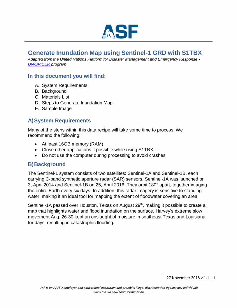
Sentinel-1A passed over Houston, Texas on August 29th, making it possible to create a
map that highlights water and flood inundation on the surface. Harvey's extreme slow
movement Aug. 26-30 kept an onslaught of moisture in southeast Texas and Louisiana
for days, resulting in catastrophic flooding.
27 November 2018 v.1.1 | 2
UAF is an AA/EO employer and educational institution and prohibits illegal discrimination against any individual: www.alaska.edu/nondiscrimination
Figure 1: Footprint of Sentinel-1 GRD Product
Figure 2: Houston flooding as a result of Hurricane Harvey; Credit: CNN

27 November 2018 v.1.1 | 3
UAF is an AA/EO employer and educational institution and prohibits illegal discrimination against any individual: www.alaska.edu/nondiscrimination
C) Materials List
Windows, OS X, Unix
Sentinel-1 GRD product downloaded from Vertex or use this sample granule:
o S1A_IW_GRDH_1SDV_20170829T002620_20170829T002645_018131_
01E74D_D734
Sentinel-1 Toolbox (latest version)
D) Steps to Generate Inundation Map Step 1: Data preparation
A. Download the sample granule from Section C or download your own granule
using Vertex (Do not unzip)
B. Open the Sentinel-1 Toolbox (S1TBX)
C. In S1TBX, use the Open Product button to add your Sentinel-1 GRD product
D. Navigate to the Sentinel-1 GRD product, select the .zip file, and click Open
E. In the Product Explorer window on the left, double-click on the Product to
expand its information, which includes Metadata, Tie-points grid, and Bands.
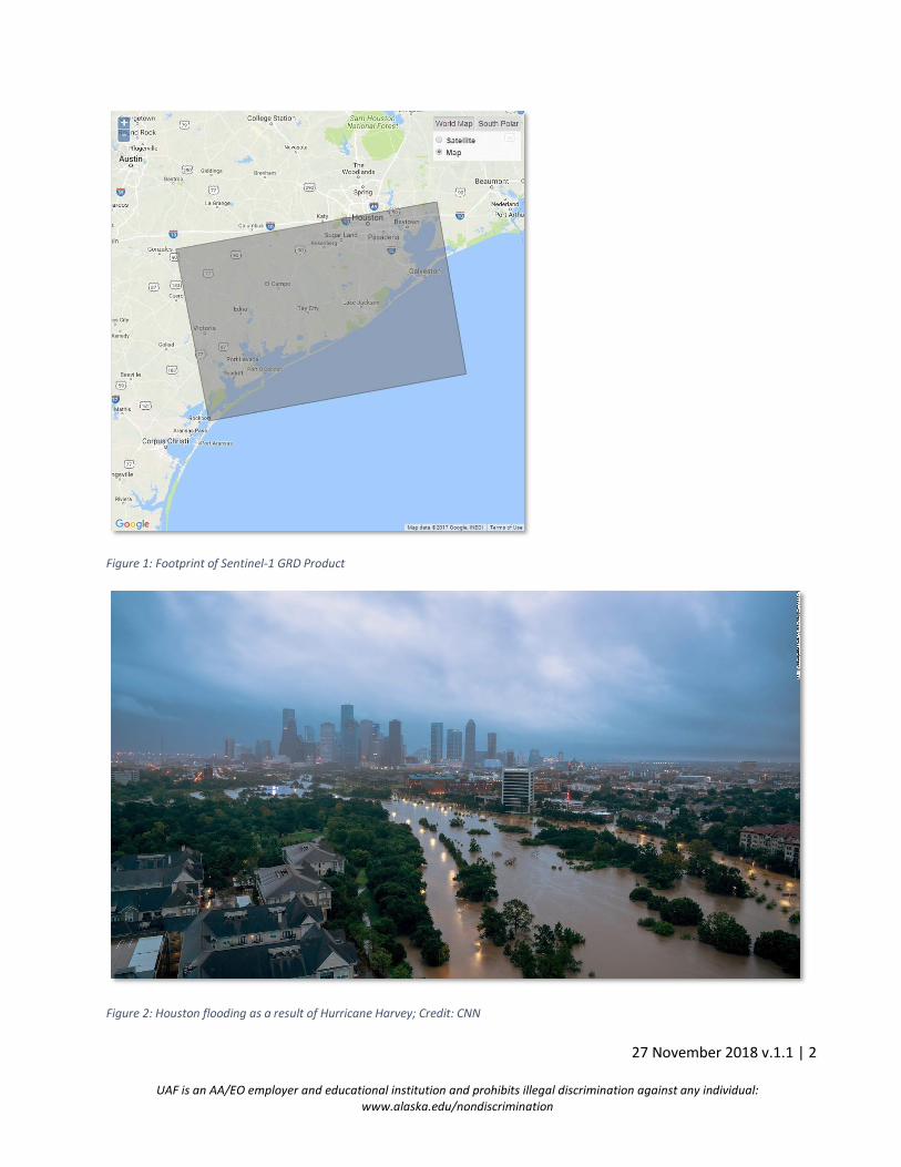
F. View a band by expanding the Bands folder (Figure 3). For each polarization
recorded, there are two bands: Amplitude and Intensity. (The Intensity band is a
virtual one. It is the square of the amplitude). Double-click on either the
Amplitude or Intensity to view the image.
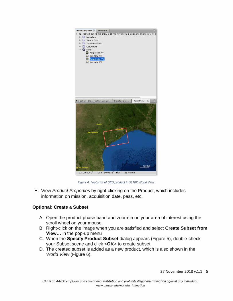
G. In the bottom left corner, the World View shows the footprint of the selected
scene (Figure 4).
27 November 2018 v.1.1 | 4
UAF is an AA/EO employer and educational institution and prohibits illegal discrimination against any individual: www.alaska.edu/nondiscrimination
Figure 3: Amplitude band of Sentinel-1 GRD Product
27 November 2018 v.1.1 | 5
UAF is an AA/EO employer and educational institution and prohibits illegal discrimination against any individual: www.alaska.edu/nondiscrimination
Figure 4: Footprint of GRD product in S1TBX World View
H. View Product Properties by right-clicking on the Product, which includes
information on mission, acquisition date, pass, etc.
Optional: Create a Subset
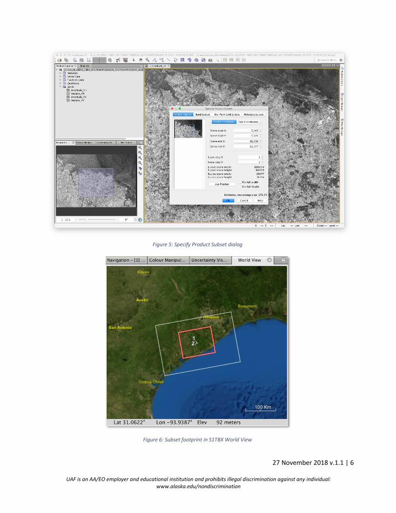
A. Open the product phase band and zoom-in on your area of interest using the scroll wheel on your mouse.
B. Right-click on the image when you are satisfied and select Create Subset from View… in the pop-up menu
C. When the Specify Product Subset dialog appears (Figure 5), double-check your Subset scene and click <OK> to create subset
D. The created subset is added as a new product, which is also shown in the World View (Figure 6).
27 November 2018 v.1.1 | 6
UAF is an AA/EO employer and educational institution and prohibits illegal discrimination against any individual: www.alaska.edu/nondiscrimination
Figure 5: Specify Product Subset dialog
Figure 6: Subset footprint in S1TBX World View

27 November 2018 v.1.1 | 7
UAF is an AA/EO employer and educational institution and prohibits illegal discrimination against any individual: www.alaska.edu/nondiscrimination
Step 2: Pre-processing – Calibration
1. In S1TBX, select the Sentinel-1 GRD product in the Product Explorer. If you
created a subset, select the subset, instead.
2. Navigate to Radar > Radiometric > Calibrate from the Menu panel
3. A Calibration window will open (Figure 7). In the I/O Parameters tab, specify
Target Product name and output directory. By default, the Target Product name
will be appended with “_Cal” if you do not create a custom file name.
Figure 7: Calibration dialog with VV selected
4. In the Processing Parameters tab, select the “VV” polarization. This will
create a new product with calibrated values of the backscatter coefficient.
5. Leave all other parameters as default and click <Run> to calibrate.
Step 3: Pre-processing – Speckle filtering
In this step, we will filter out the speckle noise that exists in SAR imagery due to random
interference between returns and the scatterers present on a surface. Speckle noise is
a critical pre-processing step for detection/classification optimization. In this example,
27 November 2018 v.1.1 | 8
UAF is an AA/EO employer and educational institution and prohibits illegal discrimination against any individual: www.alaska.edu/nondiscrimination
we will be using a standard “Lee” speckle filter; however, you may experiment with the
other speckle filters within S1TBX.
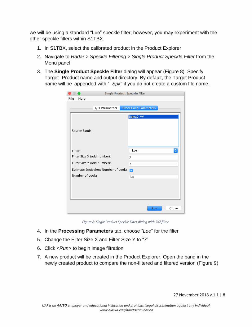
1. In S1TBX, select the calibrated product in the Product Explorer
2. Navigate to Radar > Speckle Filtering > Single Product Speckle Filter from the
Menu panel
3. The Single Product Speckle Filter dialog will appear (Figure 8). Specify
Target Product name and output directory. By default, the Target Product
name will be appended with “_Spk” if you do not create a custom file name.
Figure 8: Single Product Speckle Filter dialog with 7x7 filter
4. In the Processing Parameters tab, choose “Lee” for the filter
5. Change the Filter Size X and Filter Size Y to “7”
6. Click <Run> to begin image filtration
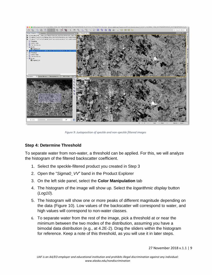
7. A new product will be created in the Product Explorer. Open the band in the
newly created product to compare the non-filtered and filtered version (Figure 9)
27 November 2018 v.1.1 | 9
UAF is an AA/EO employer and educational institution and prohibits illegal discrimination against any individual: www.alaska.edu/nondiscrimination
Figure 9: Juxtaposition of speckle and non-speckle filtered images
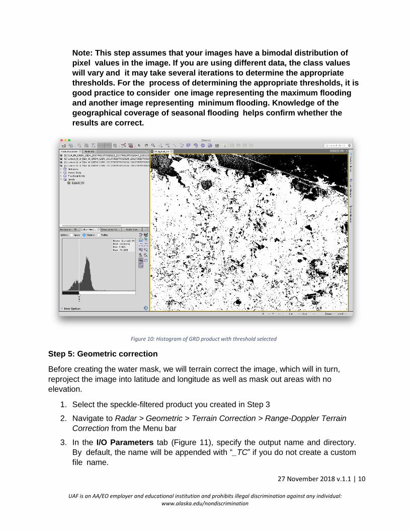
Step 4: Determine Threshold
To separate water from non-water, a threshold can be applied. For this, we will analyze
the histogram of the filtered backscatter coefficient.
1. Select the speckle-filtered product you created in Step 3
2. Open the “Sigma0_VV” band in the Product Explorer
3. On the left side panel, select the Color Manipulation tab
4. The histogram of the image will show up. Select the logarithmic display button
(Log10).
5. The histogram will show one or more peaks of different magnitude depending on
the data (Figure 10). Low values of the backscatter will correspond to water, and
high values will correspond to non-water classes.
6. To separate water from the rest of the image, pick a threshold at or near the
minimum between the two modes of the distribution, assuming you have a
bimodal data distribution (e.g., at 4.2E-2). Drag the sliders within the histogram
for reference. Keep a note of this threshold, as you will use it in later steps.
27 November 2018 v.1.1 | 10
UAF is an AA/EO employer and educational institution and prohibits illegal discrimination against any individual: www.alaska.edu/nondiscrimination
Note: This step assumes that your images have a bimodal distribution of
pixel values in the image. If you are using different data, the class values
will vary and it may take several iterations to determine the appropriate
thresholds. For the process of determining the appropriate thresholds, it is
good practice to consider one image representing the maximum flooding
and another image representing minimum flooding. Knowledge of the
geographical coverage of seasonal flooding helps confirm whether the
results are correct.
Figure 10: Histogram of GRD product with threshold selected
Step 5: Geometric correction
Before creating the water mask, we will terrain correct the image, which will in turn,
reproject the image into latitude and longitude as well as mask out areas with no
elevation.
1. Select the speckle-filtered product you created in Step 3
2. Navigate to Radar > Geometric > Terrain Correction > Range-Doppler Terrain
Correction from the Menu bar
3. In the I/O Parameters tab (Figure 11), specify the output name and directory.
By default, the name will be appended with “_TC” if you do not create a custom
file name.

27 November 2018 v.1.1 | 11
UAF is an AA/EO employer and educational institution and prohibits illegal discrimination against any individual: www.alaska.edu/nondiscrimination
Figure 11: Range-Doppler Terrain Correction dialog
4. In the Processing Parameters tab leave the default settings and click <Run> to begin correction.
5. A new product will be created and will appear in the Product Explorer
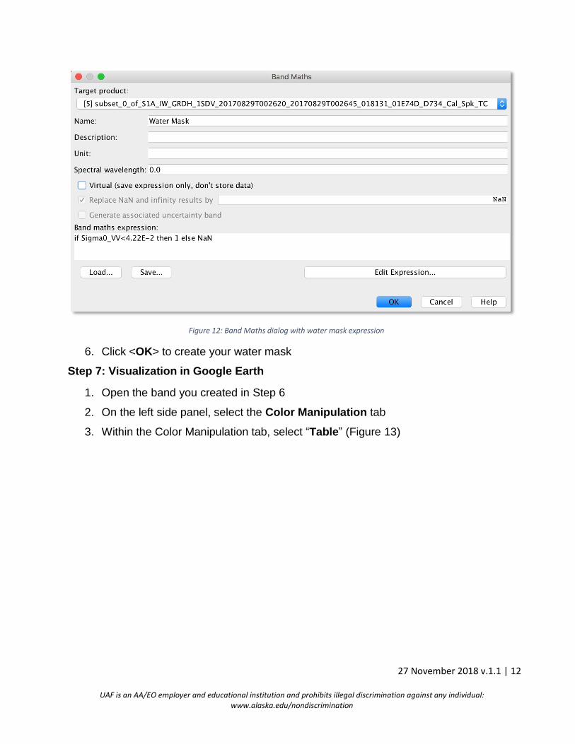
Step 6: Binarization
1. Select the terrain corrected image created in Step 5 and open the band
2. Using the determined binary threshold in Step 4, right-click on the band and
select “Band Maths…” from the pop-up menu
3. The Band Maths window will open. Type a name for the new band, for example,
“Water Mask”.
4. Uncheck the Virtual Band option
5. In the Band Maths Expression box, enter the following formula (Figure 12):
if Sigma0_VV<4.22E-2 then 1 else NaN
27 November 2018 v.1.1 | 12
UAF is an AA/EO employer and educational institution and prohibits illegal discrimination against any individual: www.alaska.edu/nondiscrimination
Figure 12: Band Maths dialog with water mask expression
6. Click <OK> to create your water mask
Step 7: Visualization in Google Earth
1. Open the band you created in Step 6
2. On the left side panel, select the Color Manipulation tab
3. Within the Color Manipulation tab, select “Table” (Figure 13)

27 November 2018 v.1.1 | 13
UAF is an AA/EO employer and educational institution and prohibits illegal discrimination against any individual: www.alaska.edu/nondiscrimination
Figure 13: Water mask with Color Manipulation: Table adjusted to blue
4. Click on the third Color box and change to a color of your choice (e.g., blue)
5. In the Product View, right-click on the image and select “Export View as
Google Earth KMZ”
6. In the Export dialog, specify a name and directory to output your KMZ file
7. Once saved, open your new image in Google Earth for visualization (Figure 14)

27 November 2018 v.1.1 | 14
UAF is an AA/EO employer and educational institution and prohibits illegal discrimination against any individual: www.alaska.edu/nondiscrimination
D) Sample Image
Figure 14: Water mask of the Houston area overlain in Google Earth; Contains modified Copernicus Sentinel data 2017; processed by ESA