Generalized Secretary Problems

7/31/2019 Generalized Secretary Problems

http://slidepdf.com/reader/full/generalized-secretary-problems 1/20

On Generalized Secretary Problems

J. Neil Bearden and Ryan O. MurphyThe University of Arizona

2000/04/29

Abstract. This paper is composed of two related parts. In the first, we present adynamic programming procedure for finding optimal policies for a class of sequentialsearch problems that includes the well-known “secretary problem.” In the second,we propose a stochastic model of choice behavior for this class of problems and testthe model with two extant data sets. We conclude that the previously reported biasfor decision makers to terminate their search too early can, in part, be accountedfor by a stochastic component of their search policies.

Keywords: sequential search, secretary problem, optimization

JEL Codes:D83, C44, C61

1. Introduction and Overview

The secretary problem has received considerable attention by appliedmathematicians and statisticians (e.g., Ferguson, 1989; Freeman, 1983).Their work has been primarily concerned with methods for determin-

ing optimal search policies, the properties and implications of thosepolicies, and the effects of introducing constraints on the search pro-cess (e.g., by adding interview costs). More recently, psychologists andexperimental economists have studied how actual decision makers (DMs)perform in these sorts of sequential search tasks (e.g., Bearden, Rapoport,and Murphy, 2004; Corbin, et al., 1975; Seale and Rapoport, 1997, 2000;Zwick, et al., 2003).

The current paper is composed of two main parts. First, we present aprocedure for computing optimal policies for a large class of sequentialsearch problems that includes the secretary problem. It is hoped thatthe accessibility of this procedure will encourage additional experi-mental work with this class of search problems. Second, we presenta descriptive model of choice for the search problems, describe someof its properties, and test the model with two extant data sets. Weconclude with a cautionary note on the difficulties researchers mayface in drawing theoretical conclusions about the cognitive processesunderlying search behavior in sequential search tasks.

c 2004 Kluwer Academic Publishers. Printed in the Netherlands.

TDDocument.tex; 16/11/2004; 15:08; p.1



2 J. Neil Bearden

2. Secretary Problems

2.1. The Problems

The Classical Secretary Problem (CSP) can be stated as follows:

1. There is a fixed and known number n of applicants for a singleposition who can be ranked in terms of quality with no ties.

2. The applicants are interviewed sequentially in a random order (withall n! orderings occurring with equal probability).

3. For each applicant j the DM can only ascertain the relative rank of the applicant, that is, how valuable the applicant is relative to the

j − 1 previously viewed applicants.

4. Once rejected, an applicant cannot be recalled. If reached, the nthapplicant must be accepted.

5. The DM earns a payoff of 1 for selecting the applicant with abso-

lute rank 1 (i.e., the overall best applicant in the population of napplicants) and 0 otherwise.

The payoff maximizing strategy for the CSP, which simply maxi-mizes the probability of selecting the best applicant, is to interviewand reject the first t − 1 applicants and then accept the first applicantthereafter with a relative rank of 1 (Gilbert and Mosteller, 1966). Fur-

ther, they proved that t converges to n/e as n goes to infinity. In thelimit, as n → ∞, the optimal policy selects the best applicant withprobability 1/e. The value of t and the selection probability convergefrom above.

Consider a variant of the secretary problem in which the DM earns apositive payoff π(a) for selecting an applicant with absolute rank a, andassume that π(1) ≥ . . . ≥ π(n). Mucci (1973) proved that the optimalsearch policy for this problem has the same threshold form as that of the CSP. Specifically, the DM should interview and reject the first t1 −1applicants, then between applicant t1 and applicant t2 − 1 she shouldonly accept applicants with relative rank 1; between applicant t2 andapplicant t3 − 1 she should accept applicants with relative ranks 1 or2; and so on. As she gets deeper into the applicant pool her standardsrelax and she is more likely to accept applicants of lower quality.

We obtain what we call the Generalized Secretary Problem (GSP)by replacing 5 in the CSP, which is quite restrictive, with the moregeneral objective function:

TDDocument.tex; 16/11/2004; 15:08; p.2



Secretary Problem 3

5’. The DM earns a payoff of π(a) for selecting an applicant withabsolute rank a where π(1) ≥ . . . ≥ π(n).

Clearly, the CSP is a special case of the GSP in which π(1) = 1 and

π(a) = 0 for all a > 1. Results for other special cases of the GSP haveappeared in the literature. For example, Moriguti (1993) examined aproblem in which a DM’s objective is to minimize the expected rankof the selected applicant. This problem is equivalent to maximizingearnings in a GSP in which π(a) increases linearly as (n − a) increases.

2.2. Finding Optimal Policies for the GSP

We will begin by introducing some notation. The orderings of the napplicants’ absolute ranks is represented by a vector a =

a1, . . . , an

,

which is just a random permutation of the integers 1, . . . , n. The relative

rank of the jth applicant, denoted r j, is the number of applicants from1, . . . , j whose absolute rank is smaller than or equal to a j. A policy

is a vector s =

s1, . . . , sn

of nonnegative integers in which s j ≤ s j+1

for all 1 ≤ j < n. The policy dictates that the DM stop on the firstapplicant for which r j ≤ s j. Therefore, the probability that the DMstops on the jth applicant, conditional on reaching this applicant, iss j/j; we will denote this probability by Q j. A DM’s cutoff for selectingan applicant with a relative rank of r, denoted tr, is the smallest value

j for which r ≤ s j . Hence, a policy s can also be represented by avector t = (t1, . . . , tn). Sometimes, the cutoff representation will bemore convenient. Again, a DM’s payoff for selecting an applicant withabsolute rank a is given by π(a).

Given the constraint on the nature of the optimal policy for theGSP proved by Mucci (1973), optimal thresholds can be computedstraightforwardly by combining numerical search methods with those of dynamic programming. We will describe below a procedure for doing so.A similar method was outlined in Lindley (1961) and briefly describedby Yeo and Yeo (1994).

The probability that the jth applicant out of n whose relative rankis r j has an absolute (overall) rank of a is given by (Lindely, 1961):

P r

A = a|R = r j

=

a−1r−1

n−a j−r

n j

, (1)

when r j ≤ a ≤ r j + (n − j); otherwise P r(A = a|R = r j) = 0. Thus,the expected payoff for selecting an applicant with relative rank r j is:

E

π j |r j

=n

a=rj

P r

A = a|R = r j

π(a). (2)

TDDocument.tex; 16/11/2004; 15:08; p.3



4 J. Neil Bearden

The expected payoff for making a selection at stage j for some stage jpolicy s j > 0 is:

E

π j|s j

=

s j−1

sji=1

E

π j|r j = i

; (3)

otherwise, when s j = 0, E

π j|s j

= 0. Now, denoting the expectedpayoff for starting at stage j + 1 and then following a fixed thresholdpolicy (s j+1, . . . , sn) thereafter by v j+1, the value of v j for any s j ≤ jis simply:

v j = Q jE

π j|s j

+

1 − Q j

v j+1. (4)

Since the expected earnings of the optimal policy at stage n are vn =n−1

na=1 π(a), we can easily find an s j for each j ( j = n − 1, . . . , 1)

that maximizes v j by searching through the feasible s j; the expectedearnings of the optimal threshold s j∗ we denote by v j∗. These compu-tations can be performed rapidly, and the complexity of the problemis just linear in n.1 From the monotonicity constraint on the s j, thesearch can be limited to 0 ≤ s j ≤ s j+1. Thus, given vn∗, starting atstage n−1 and working backward, the dynamic programming procedurefor finding optimal policies for the GSP can be summarized by:

s j∗ = arg maxs∈{0,...,sj+1∗}

v j. (5)

The expected payoff for following a policy s, then, is:

E (π|s) =n

j=1

j−1i=0

1 − Qi

Q jE

π j|s j

= v1, (6)

where Q0 = 0. The optimal policy s∗ is the policy s that maximizesEq. 6. Denoting the applicant position at which the search is terminatedby m, the probability that the DM stops on the ( j < n)th applicant is:

P r (m = j) =

j−1i=0

1 − Qi

Q j, (7)

and the expected stopping position is (Moriguti, 1993):

E (m) = 1 +n−1 j=1

ji=1

1 − Qi

. (8)

1 More elegant solutions can be used for special cases of the GSP. The methoddescribed here can be easily implemented for all special cases of the GSP.

TDDocument.tex; 16/11/2004; 15:08; p.4



Secretary Problem 5

Optimal cutoffs for several GSPs are presented in Table I. In the firstcolumn, we provide a shorthand for referring to these problems. Thefirst one, GSP1, corresponds to the CSP with n = 40. The optimal pol-icy dictates that the DM should search through the first 15 applicantswithout accepting any and then accept the first one thereafter with arelative rank of 1. GSP2 corresponds to another CSP with n = 80. Inboth, the DM should search through roughly the first 37% and thentake the first encountered applicant with a relative rank of 1. These twospecial cases of the CSP have been studied experimentally by Seale andRapoport (1997). GSPs 3 and 4 were discussed in Gilbert and Mosteller(1966), who presented numerical solutions for a number of problems inwhich the DM earns a payoff of 1 for selecting either the best or secondbest applicant and nothing otherwise. GSPs 5 and 6 correspond to thosestudied by Bearden, Rapoport, and Murphy (2004) in Experiments 1and 2, respectively. In the first, the DM searches through the first 13

applicants without accepting any; then between 14 and 28 she stopson applicants with relative rank of 1; between 29 and 36, she takesapplicants with relative rank 1 or 2; etc. Finally, GSP7 correspondsto the rank-minimization problem studied by Moriguti (1993). Theresults of our method are in agreement with all of those derived byother methods.

When inexperienced and financially motivated decision makers areasked to play the GSP in the laboratory, they have no notion of how tocompute the optimal policy. Why then should one attempt to test thedescriptive power of the optimal policy? One ma jor reason is that testsof the optimal policies for different variants of the GSP (e.g. Bearden,

Rapoport, and Murphy, 2004; Seale and Rapoport, 1997, 2000; Zwick,et al., 2003) may provide information on the question of whether DMssearch too little, just enough, or too much. This question has moti-vated most of the research in sequential search in economics (e.g., Hey,1981, 1982, 1987) and marketing (e.g., Ratchford and Srinivasan, 1993;Zwick, et al.). However, tests of the optimal policy do not tell us whatalternative decision policies subjects may be using in the GSP. Andbecause they prescribe the same fixed threshold values for all subjects,they cannot account for within-subject variability across iterations of the sequential search task or between-subject variability in the stoppingbehavior.

Seale and Rapoport (1997, 2000) have proposed and tested three

alternative decision policies in their study of two variants of the CSP.These decision policies (descriptive models) are not generalizable intheir present form to the GSP. Moreover, because all of them are deter-ministic, they cannot account for within subject variability in stoppingtimes across trials. Rather than attempting to construct more com-

TDDocument.tex; 16/11/2004; 15:08; p.5



6 J. Neil Bearden

T a b l e I . O p t i m

a l p o l i c i e s f o r s e v e r a l G S P s .

G S P

n

π =

( π ( 1 ) , . . . , π ( n ) )

t ∗

=

( t ∗ 1

, . . . , t ∗ n )

E ( π |

s ∗

)

E ( m )

1

4

0

( 1 ,

0 , . . . ,

0 )

( 1 6 ,

4 0 , . . . ,

4 0 )

. 3 8

3 0 . 0

3

2

8

0

( 1 ,

0 , . . . ,

0 )

( 3 0 ,

8 0 , . . . ,

8 0 )

. 3 7

5 8 . 7

5

3

2

0

( 1 ,

1 ,

0 , . . . ,

0 )

( 8 ,

1 4 ,

2 0 , . . . ,

2 0 )

. 6 9

1 4 . 1

5

4

1

0 0

( 1 ,

1 ,

0 , . . . ,

0 )

( 3 5 ,

6 7 ,

1 0 0 , . . . ,

1 0 0 )

. 5 8

6 8 . 4

7

5

4

0

( 1 5 ,

7 ,

2 ,

0 , . . . ,

0 )

( 1 4 ,

2 9 ,

3 7 ,

4 0 , . . . ,

4 0 )

6 . 1

1

2 7 . 2

1

6

6

0

( 2 5 ,

1 3 ,

6 ,

3 ,

2 ,

1 ,

0 , . . . ,

0 )

( 2 1 ,

4 3 ,

5 3 ,

5 7 ,

5 8 ,

5 9 ,

6 0 , . . . , 6

0 )

1 2 . 7

3

4 1 . 0

4

7

2

5

( 2 5 ,

2 4 ,

2 3 , . . . ,

1 )

( 8 ,

1 4 ,

1 7 ,

1 9 ,

2 1 ,

2 2 ,

2 3 ,

2 3 ,

2 4 ,

2 4 ,

2 4 ,

2 5 , . . . ,

2 5 )

2 2 . 8

8

1 4 . 4

6

TDDocument.tex; 16/11/2004; 15:08; p.6



Secretary Problem 7

plicated deterministic choice models for the GSP, with a considerableincrease in the number of free parameters, we propose an alternativestochastic model of choice for the GSP. Next, we describe the modeland discusses its main properties. Then we summarize empirical resultsfrom some previous studies of the GSP and use them to test the model.Finally, we conclude by discussing some problems that arise in drawingtheoretical conclusions about choice behavior in the GSP and relatedsequential search tasks.

3. A Stochastic Model of Choice in Secretary Problems

3.1. Background

Stochastic models have a long history in psychological theories. As early

as 1927, L. L. Thurstone posited that observed responses are a func-tion of an underlying (unobservable) component together with randomerror (Thurstone, 1927a, 1927b). For reviews of the consequences of Thurstone’s ideas, see Bock and Jones (1968) and Luce (1977, 1994).

More recently, theorists have shown that unbiased random errorin judgment processes can produce seemingly biased judgments. Forexample, Erev et al. (1994) have shown that symmetrically distributedrandom error can produce confidence judgments consistent with over-confidence even when the underlying (unperturbed) judgments are well-calibrated (see also, Juslin, et al., 1997; Pfeifer, 1994; Soll, 1996).

In related work, Bearden, Wallsten, and Fox (2004) have shown

that unbiased random error in the judgment process is sufficient toproduce subadditive judgments. Suppose we have an event X thatcan be partitioned into k mutually exclusive and exhaustive subeventsX =

ki=1 X i. Denote a judge’s underlying (or true) probability esti-

mate for X by C (X ) and her overt expression of the probability of X by R(X ). Bearden et al. assumed that R(X ) = f (C (X ), e), wheree is a random error component that is just as likely to be above asbelow C (X ). They proved that under a range of conditions R(X ) isregressive, i.e., it will be closer than C (X ) to .50. As a result, the overt

judgment for X can be smaller than the sum of the judgments for theX i, even when C (X ) =

i C (X i). Put differently, the overt judgments

can be subadditive even when the underlying judgments are themselvesadditive. A considerable body of research has focused on finding high-level explanations such as availability for subadditive judgments (e.g.,Rottenstreich and Tversky, 1997; Tversky and Koehler, 1994). Beardenet al. simply demonstrated that unbiased random error in the responseprocess is sufficient to account for the seemingly biased observed judg-

TDDocument.tex; 16/11/2004; 15:08; p.7



8 J. Neil Bearden

ments. One need not posit higher-level explanations. We follow this lineof research and look at the effects of random error in the GSP.

Empirical research on the GSP has consistently shown that DMsexhibit a bias to terminate their search too soon (Bearden, Rapoport,and Murphy, 2004; Seale and Rapoport, 1997, 2000). At the level of description, this observation is undeniable. However, researchers havegone beyond this observation by offering psychological explanationsto account for the bias. In a paper on the CSP, Seale and Rapoport(1997) suggested that the bias results from an endogenous search cost:Because search is inherently costly (see, Stigler, 1961), the DM’s payoff increases in the payoff she receives for selecting the best applicant butdecreases in the amount of time spent searching. Therefore, early stop-ping may be the result of a (net) payoff maximizing strategy. Bearden,Rapoport, and Murphy (2004) offered a different explanation. They hadDMs estimate the probability of obtaining various payoffs for selecting

applicants of different relative ranks in different applicant positions.Based on their findings, they argued that the bias to terminate thesearch too soon in a GSP results from DMs overestimating the payoffsthat would result from doing so.

In Section 3.2 we present a simple stochastic model of search inthe secretary problem and show that it produces early stopping be-havior even when DMs use decision thresholds that are symmetrically

distributed about the optimal thresholds.

3.2. The Model

Recall that under the optimal policy for the GSP, the DM stops onsome applicant j if and only if the applicant’s relative rank does notexceed the DM’s threshold for that stage (i.e., when r j ≤ s j∗). Exper-imental results, however, conclusively show that DMs do not strictlyadhere to a deterministic policy of this sort. Rather, we posit thatDMs’ thresholds can be modelled as random variables. Each time theDM experiences an applicant with a relative rank r, she is assumed tosample a threshold from her distribution of thresholds for applicantswith relative rank r; then, using the sampled threshold, she makes astopping decision.2 Denoting the sampled threshold σr, she stops onan applicant with relative rank r j if and only if r j ≤ σr. (Note that ateach stage j, the DM samples from a distribution that depends on the

relative rank of the applicant observed at that stage. The distribution is

2 The thresholds are, of course, unobservable. The model specified here as an as-if one: We are merely suggesting that the DM’s observed behavior is in accord withher acting as if she is randomly sampling thresholds subject to the constraints of the model we propose.

TDDocument.tex; 16/11/2004; 15:08; p.8



Secretary Problem 9

not conditional only on the stage; it is only conditional on the relativerank of the observed applicant at that stage.) We assume that theprobability density function for the sampled threshold is given by:

f (σr) =e−(σr−µr)/β r

β r1 + e−(σr−µr)/β r

2 . (9)

Consequently, conditional on being reached, the probability that anapplicant with relative rank r j is selected is:

P r

r j ≤ σr

=

1

1 + e−( j−µr)/β r. (10)

We assume that µ1 ≤ . . . ≤ µn and β 1 ≥ . . . ≥ β n. This is based on the

constraint of the GSP that payoffs are nonincreasing in the absoluterank of the selected applicant. Hence, it seems reasonable to assumethat P r

r j ≤ σr

≥ P r

r j ≤ σr

whenever r ≤ r. That is, the DM

should be more likely to stop on any given j whenever the relative rankof the observed applicant decreases. The constraints on the ordering of µ and β do not guarantee this property but do encourage it.3

Note that the model approaches a deterministic model as β r → 0for each r. Further, the optimal policy for an instance of a GSP obtainswhen β r is small (near 0) and t∗r − 1 < µr < t∗r for each r.

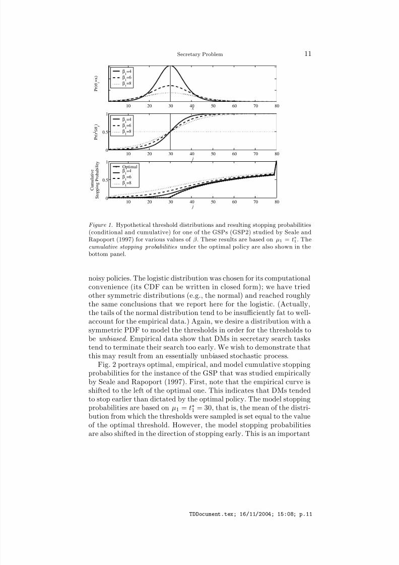
Examples of the distributions of thresholds and resulting stoppingprobabilities for a possible DM are exhibited in Fig. 1 for the GSP2 (i.e.,for a CSP with n = 80). In all cases shown in the figure, µ1 = t∗1; that

is, all of the threshold distributions are centered at the optimal cutoff point for the problem. The top panel shows the pdf of the thresholddistribution. The center panel shows that for j < µ1 the probabilityof selecting a candidate (i.e., an applicant with a relative rank of 1)increases as β increases; however, for j > µ1, the trend is reversed.The bottom panel shows the probability of stopping on applicant j orsooner for the model and also for the optimal policy. Most importantly,in this example we find that the propensity to stop too early increasesas the variance of the threshold distribution (β ) increases, and in noneof the model instances do we observe late stopping.

Under the model, the probability that the DM stops on the ( j < n)th

applicant, given that she has reached him, is:

3 Adding the strong constraint that Prrj ≤ σr

≥ Pr

rj ≤ σr

for all r ≤ r

makes dealing with the model too difficult. The numerical procedures used belowto derive maximum likelihood estimates of the model’s parameters from data wouldbe infeasible under the strong constraint.

TDDocument.tex; 16/11/2004; 15:08; p.9



10 J. Neil Bearden

Table II. Expected stopping times under the model for the GSP2 for different valuesof β 1 and µ1. Keep in mind that E (m) = 58.75 under the optimal policy and t∗1 = 30.The average value of m for this problem in Seale and Rapoport (1997) is 43.61.

β 1 E (m|µ1 = 25) E (m|µ1 = 29.5) E (m|µ1 = 30) E (m|µ1 = 35)

.01 53.83 58.74 59.24 63.80

1 53.72 58.65 59.15 63.73

2 53.29 58.32 58.83 63.48

4 51.08 56.72 57.29 62.33

8 41.46 48.54 49.27 55.94

10 36.63 43.55 44.29 51.27

12 32.62 39.03 39.74 46.59

16 26.86 32.04 32.63 38.57

Q j = j

rj=1

1

jP r

r j ≤ σr

. (11)

Replacing Q j in Eq. 8 with Q j, we can easily compute the model ex-

pected stopping position . Some examples of model expected stoppingpositions for various values of µ1 and β 1 for the GSP2 are presented inTable II. Several features of the E (m) are important. First, wheneverµ1 < t∗1, the expected stopping position under the model is smaller thanthe expectation under the optimal policy. Second, even when µ1 ≥ t∗1

and β 1 is non-negligible, we find that the model tends to stop soonerthan the optimal policy. Also, when t∗1 − 1 < µ1 < t∗1 (that is, whenthe mean of the model threshold distribution is just below the optimalcutoff), the expected stopping position under the model is always lessthan under the optimal. Finally, as β increases, the expected stoppingposition decreases. In other words, as the variance of the thresholddistribution increases, the model predicts that stopping position movetoward earlier applicants. This general pattern of results obtains forthe other GSPs as well.

The optimal policies for the GSP are represented by integers, but weare proposing a model in which the thresholds are real valued (and caneven be negative); hence, some justification is in order. Using Eq. 10 tomodel choice probabilities has a number of desirable features. First, wecan allow for shifts in both the underlying thresholds (or the means of the threshold distributions) by varying µr, and we can control the steep-ness of the response function about a given µr by β r. As stated above,this can (in the limit) allow us to model both deterministic policies and

TDDocument.tex; 16/11/2004; 15:08; p.10



Secretary Problem 11

10 20 30 40 50 60 70 80 x

P r ( σ r =

x )

10 20 30 40 50 60 70 800

0.5

1

j

P r ( r

j ≤ σ r )

10 20 30 40 50 60 70 800

0.5

1

j

C u m u l a t i v e

S

t o p p i n g P r o b a b i l i t y

Optimalβ

1=4

β1

=6

β1

=8

β1

=4

β1

=6

β1

=8

β1

=4

β1

=6

β1

=8

Figure 1. Hypothetical threshold distributions and resulting stopping probabilities(conditional and cumulative) for one of the GSPs (GSP2) studied by Seale andRapoport (1997) for various values of β . These results are based on µ1 = t∗1. Thecumulative stopping probabilities under the optimal policy are also shown in thebottom panel.

noisy policies. The logistic distribution was chosen for its computationalconvenience (its CDF can be written in closed form); we have tried

other symmetric distributions (e.g., the normal) and reached roughlythe same conclusions that we report here for the logistic. (Actually,the tails of the normal distribution tend to be insufficiently fat to well-account for the empirical data.) Again, we desire a distribution with asymmetric PDF to model the thresholds in order for the thresholds tobe unbiased . Empirical data show that DMs in secretary search taskstend to terminate their search too early. We wish to demonstrate thatthis may result from an essentially unbiased stochastic process.

Fig. 2 portrays optimal, empirical, and model cumulative stoppingprobabilities for the instance of the GSP that was studied empiricallyby Seale and Rapoport (1997). First, note that the empirical curve isshifted to the left of the optimal one. This indicates that DMs tendedto stop earlier than dictated by the optimal policy. The model stoppingprobabilities are based on µ1 = t∗1 = 30, that is, the mean of the distri-bution from which the thresholds were sampled is set equal to the valueof the optimal threshold. However, the model stopping probabilitiesare also shifted in the direction of stopping early. This is an important

TDDocument.tex; 16/11/2004; 15:08; p.11



12 J. Neil Bearden

1 10 20 30 40 50 60 70 800

0.1

0.2

0.3

0.4

0.5

0.6

0.7

0.8

0.9

1

j

C u m u l a t i v e S t o p p i n g P r o b a b i l i t y

OptimalEmpiricalModel

Figure 2. Cumulative stopping probabilities for the GSP2 for the optimal andstochastic model policies and also for the empirical data reported by Seale andRapoport (1997). The model probabilities are based on µ1 = t∗1 = 30 and β 1 = 10.

observation: In this example, the stochastic thresholds are distributedsymmetrically about the optimal threshold and stopping behavior is

biased toward early stopping. For example, it is just as likely that aDM’s threshold will be 4 units above as below the optimal threshold,corresponding to too early and a too late thresholds, respectively; yetstopping behavior is biased toward early stopping.

The reason for early stopping under the stochastic model can bestated quite simply. First, there is a nonzero probability that a DMwill stop sometime before it is optimal to do so; as a consequence, shewill not have the opportunity to stop on time or stop too late. Secondly,though the threshold distribution itself is symmetric, the unconditionalstopping probabilities are not. The probability of observing a givenrelative rank r j ≤ j decreases in j. Consider r j = 1. When j = 1,the probability of observing a relative rank of 1 is 1; when j = 2, theprobability is 1/2; and in general it is 1/j. Thus, for a given σr, theprobability of stopping on applicant j is strictly decreasing in j. There-fore, properties of the problem itself can entail early stopping under themodel. Researchers should, therefore, be cautious in attributing earlystopping to general psychological biases.

TDDocument.tex; 16/11/2004; 15:08; p.12




Thus far we have only discussed the theoretical consequences of the stochastic model. Next, we evaluate the model using some of theempirical data reported in Seale and Rapoport (1997) and in Bear-den, Rapoport, and Murphy (2004). We ask: Can the observed earlystopping in these experiments be explained by unbiased stochasticthresholds?

3.3. Parameter Estimation

We estimated the model parameters for the stochastic choice modelfor individual subjects from two previous empirical studies of the GSP.Seale and Rapoport (1997) had 25 subjects play the GSP2 for 100 trialsunder incentive-compatible payoffs. They reported that their subjectsexhibited a tendency to terminate their searches too early, and ex-plained this by a deterministic cutoff rule of the same form as the

optimal policy but whose cutoff was shifted to the left of the opti-mal cutoff. They evaluated alternative deterministic decision policiesand concluded that the alternatively parameterized cutoff rule bestaccounted for the data. To determine a subject’s cutoff—t1, in ournotation—they found the value of 1 ≤ t1 ≤ 80 that maximized thenumber of selection decisions compatible with the cutoff. For the GSP2,t∗1 = 30; Seale and Rapoport estimated that the modal cutoff for theirsubjects was 21.

Bearden, Rapoport, and Murphy (2004) had 61 subjects performthe GSP6 for 60 trials under incentive-compatible payoffs. They, too,concluded that their subjects terminated search too early, and that the

stopping behavior was most compatible with a threshold stopping rule.For the GSP6, t∗1 = 21, t∗2 = 43, t∗3 = 53, t∗4 = 57, t∗5 = 58, and t∗6 = 59;for their subjects, they estimated that the mean thresholds were t1 =12, t2 = 22, t3 = 28, t4 = 35, t5 = 40, and t6 = 44. In both Seale andRapoport and Bearden et al., the authors (implicitly) assumed thatthe subjects used deterministic or fixed thresholds. Hence, for a givensubject, they could not account for stopping decisions inconsistent withthat subject’s estimated threshold.

In the current paper, we assume that the subjects’ thresholds arerandom variables (whose pdf is given by Eq. 9) and use maximumlikelihood procedures to estimate the parameters of the distributionfrom which the thresholds are sampled. For each set of data that weexamine, the researchers reported learning across early trials of play,but in both, the choice behavior seems to have stabilized by the 20thtrial. Hence, for the tests below, we shall eliminate the first 20 trialsfrom each data set from the analyses, and we will assume that thechoice probabilities are i.i.d..

TDDocument.tex; 16/11/2004; 15:08; p.13



14 J. Neil Bearden

For a given trial of a GSP problem, the DM observes a sequence of applicants and their relative ranks, and for each applicant she decides toeither accept or continue searching. Denoting a decision function for ap-plicant j by δ r j, we let δ r j = 0 if the DM does not stop on applicant

j and δ

r j

= 1 if she does stop. Hence, decisions for a particular trial kcan be represented by a vector ∆k =

δ

r1

, . . . , δ (rm)

= (0, 0, . . . , 1),where m denotes the position of the selected applicant. Under thestochastic model, if m < n, the likelihood of ∆k can be written as:

L

∆k|µ, β

=

m−1i=1

P r

ri > σr

P r (rm ≤ σr) . (12)

When m = n (i.e., when the DM reaches the last applicant, which shemust accept), we simply omit the final term in Eq. 12 since the DM’schoice is determined. Assuming independence, the likelihood of a DM’s

choice responses over K trials of the GSP is just:

L

∆1, . . . , ∆K

|µ, β

=K k=1

L

∆k|µ, β

. (13)

Due to the small numbers involved, it is convenient to work with thelog of the likelihood, rather than the likelihood itself. Taking the log of Eq. 13, we get:

∆1, . . . , ∆K

|µ, β

=K k=1

ln

L

∆k|µ, β

. (14)

For each subject we computed the parameters µ and β that max-imized Eq. 14 under different constraints. We only estimated the pa-rameters for relative ranks that can entail positive payoffs. For theGSP2, we restrict estimates to r = 1, and for the GSP6 to 1 ≤ r ≤ 6.Therefore, we omit from the analyses trials on which the DM chose tostop on the applicants whose relative rank could not entail a positivepayoff. Very likely these were errors. Fewer than 2% of the trials wereomitted.

We are primarily interested in testing the following:

Optimal But Stochastic Threshold Hypothesis: µr = t∗r for allr.

If this hypothesis is supported, the bias toward early stopping be-havior could be the result of the stochastic nature of the thresholds.We evaluate the Optimal But Stochastic Threshold Hypothesis(OBSTH) using standard likelihood ratio tests. Under the constrained

TDDocument.tex; 16/11/2004; 15:08; p.14




model , we impose that µr = t∗r for all r and allow the β r to freely vary;under the unconstrained model we allow both the µr and β r to freelyvary. Denoting the maximum log-likelihood of the constrained modelc

(based on Eq. 15) and of the unconstrained model u

, the likelihoodratio is:

LR = (c − u) . (15)

The statistic −2LR is χ2 distributed with degrees of freedom (df )equal to the number of additional free parameters in the unconstrainedmodel. Hence, for the Seale and Rapoport (1997), df = 1; and forBearden, Rapoport, and Murphy (2004), df = 6.

A few words about estimating the model parameters are in order.To estimate the model parameters we used a constrained optimizationprocedure (fmincon) in Matlab. We imposed the constraint that µr ≤

µr whenever r ≤ r, and imposed the corresponding constraint on the β parameters. For each subject, we used a large number of initial startingvalues. We are confident that the estimated parameters provide globallyoptimal results for each subject.

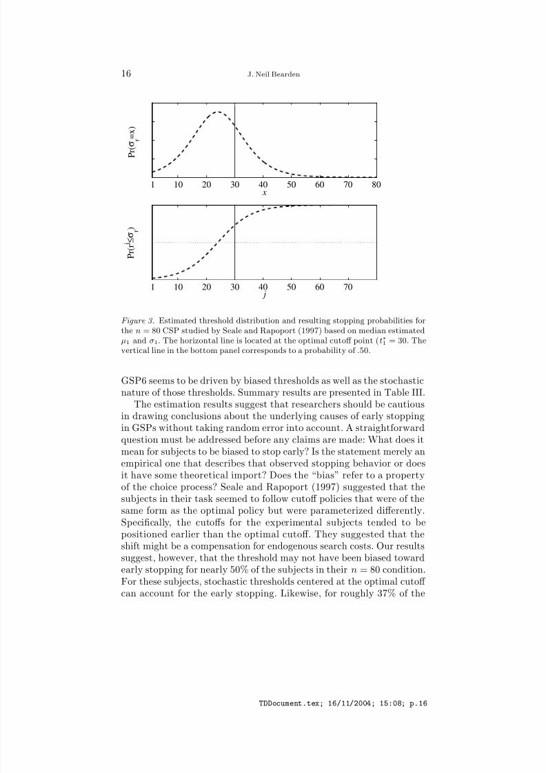
Seale and Rapoport Data . Based on the likelihood ratio test withdf = 1, the OBSTH could not be rejected for 12 of the 25 experimen-tal subjects at the α = .01 level. Seale and Rapoport concluded that21 of their 25 subjects had thresholds below the optimal cutoff. Ouranalyses suggest that they overestimated the number of subjects withbiased thresholds. Fig. 3 shows a distribution of thresholds (σ1) thatis based on the median estimated values of µ1 and β 1 from the 25 ex-

perimental subjects. We find that the distribution of thresholds (basedon the aggregate data) is, indeed, shifted to the left of the optimalcutoff, consistent with the observed early stopping behavior. Further,we find that the variance of the threshold distribution is considerablygreater than 0. Thus, early stopping in Seale and Rapoport may be dueboth to thresholds that tend to be biased toward early stopping andalso to stochastic variability in placement of the thresholds. Summarystatistics from the MLE procedures are displayed in Table III.

Bearden, Rapoport, and Murphy Data . The corresponding thresholdsfrom Bearden, Rapoport, and Murphy (2004) are displayed in Fig. 4.For these data, the OBSTH could not be rejected for 23 of the 61subjects (i.e., for 37%). We find that the distribution of thresholds forr = 1 tends to be centered rather close to the optimal cutoff. Likewisefor the r = 6 threshold. For r = 2, . . . , 5, the thresholds tend to beshifted toward early stopping. The variances of the threshold distribu-tions tend to decrease quite rapidly in r, but are all away from 0. Thus,as with the Seale and Rapoport (1997) data, the early stopping in the

TDDocument.tex; 16/11/2004; 15:08; p.15



16 J. Neil Bearden

1 10 20 30 40 50 60 70 80 x

P r ( σ

r = x )

1 10 20 30 40 50 60 70 j

P r ( r

j ≤ σ

r )

Figure 3. Estimated threshold distribution and resulting stopping probabilities forthe n = 80 CSP studied by Seale and Rapoport (1997) based on median estimatedµ1 and σ1. The horizontal line is located at the optimal cutoff point (t∗1 = 30. Thevertical line in the bottom panel corresponds to a probability of .50.

GSP6 seems to be driven by biased thresholds as well as the stochasticnature of those thresholds. Summary results are presented in Table III.

The estimation results suggest that researchers should be cautiousin drawing conclusions about the underlying causes of early stoppingin GSPs without taking random error into account. A straightforwardquestion must be addressed before any claims are made: What does itmean for subjects to be biased to stop early? Is the statement merely anempirical one that describes that observed stopping behavior or doesit have some theoretical import? Does the “bias” refer to a propertyof the choice process? Seale and Rapoport (1997) suggested that thesubjects in their task seemed to follow cutoff policies that were of thesame form as the optimal policy but were parameterized differently.Specifically, the cutoffs for the experimental subjects tended to bepositioned earlier than the optimal cutoff. They suggested that theshift might be a compensation for endogenous search costs. Our resultssuggest, however, that the threshold may not have been biased towardearly stopping for nearly 50% of the subjects in their n = 80 condition.For these subjects, stochastic thresholds centered at the optimal cutoff can account for the early stopping. Likewise, for roughly 37% of the

TDDocument.tex; 16/11/2004; 15:08; p.16




1 5 10 15 20 25 30 35 40 45 50 55 600

0.5

1

1.5

x

P r ( σ

r = x )

1 5 10 15 20 25 30 35 40 45 50 55 600

0.5

1

j

P r ( r

j ≤ σ

r )

Figure 4. Estimated threshold distribution and resulting stopping probabilities forthe GSP6 studied by Bearden, Rapoport, and Murphy (2004). The curves are basedon median estimated µr and σr (r = 1, . . . , 6), and are ordered from left (r = 1) toright (r = 6). Note that the variances of the Pr (σr = x) distributions for r = 1, 2, 3relative to the variance of the r = 6 distribution are quite small, making the resultingdistributions rather flat and difficult to see.

subjects in Experiment 1 of Bearden, Rapoport, and Murphy (2004),

we can account for early stopping by the OBSTH.We do not argue that early stopping is not driven by some gen-uine choice or judgment bias (e.g., by overestimating the probabilityof obtaining good payoffs for selecting early applicants). Rather, wesimply wish to demonstrate that the effects of random error shouldbe taken into consideration before drawing sharp conclusions aboutthe magnitude of the effects of these potential biases on the stoppingbehavior.

4. Conclusions

We began this paper by presenting a simple dynamic programmingprocedure for computing optimal policies for a large class of sequentialsearch problems with rank-dependent payoffs. The generality of thepermissible payoff schemes allows a number of realistic (especially in

TDDocument.tex; 16/11/2004; 15:08; p.17



18 J. Neil Bearden

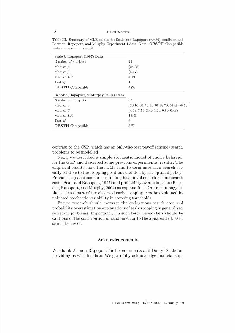
Table III. Summary of MLE results for Seale and Rapoport (n=80) condition andBearden, Rapoport, and Murphy Experiment 1 data. Note: OBSTH Compatibletests are based on α = .01.

Seale & Rapoport (1997) DataNumber of Subjects 25

Median µ (24.08)

Median β (5.97)

Median LR 4.19

Test df 1

OBSTH Compatible 48%

Bearden, Rapoport, & Murphy (2004) Data

Number of Subjects 62

Median µ (23.16, 34.71, 43.96, 48.70, 54.49, 58.53)

Median β (4.13, 3.56, 2.49, 1.24, 0.69, 0.43)

Median LR 18.38Test df 6

OBSTH Compatible 37%

contrast to the CSP, which has an only-the-best payoff scheme) searchproblems to be modelled.

Next, we described a simple stochastic model of choice behaviorfor the GSP and described some previous experimental results. Theempirical results show that DMs tend to terminate their search tooearly relative to the stopping positions dictated by the optimal policy.Previous explanations for this finding have invoked endogenous searchcosts (Seale and Rapoport, 1997) and probability overestimation (Bear-den, Rapoport, and Murphy, 2004) as explanations. Our results suggestthat at least part of the observed early stopping can be explained byunbiased stochastic variability in stopping thresholds.

Future research should contrast the endogenous search cost andprobability overestimation explanations of early stopping in generalizedsecretary problems. Importantly, in such tests, researchers should becautious of the contribution of random error to the apparently biasedsearch behavior.

Acknowledgements

We thank Amnon Rapoport for his comments and Darryl Seale forproviding us with his data. We gratefully acknowledge financial sup-

TDDocument.tex; 16/11/2004; 15:08; p.18




port by a contract F49620-03-1-0377 from the AFOSR/MURI to theDepartment of Systems and Industrial Engineering and the Departmentof Management and Policy at the University of Arizona.

References

Bearden, J. N., Rapoport, A., and Murphy, R. O. (2004) Sequential oberservationand selection with rank-dependent payoffs: An experimental test. Unpublishedmanuscript.

Bearden, J. N., Wallsten, T. S., and Fox, C. R. (2004) A stochastic model of subadditivity. Unpublished manuscript.

Bock, R. D., and Jones, L. V. (1968). The measurement and prediction of judgment

and choice. San Francisco: Holden-Day.Corbin, R. M., Olson, C. R., and M. Abbondanza, M. (1975) Context effects in

optimal stopping rules. Behavior and Human Performance, 14, 207-216.Erev, I., Wallsten, T. S., and Budescu, D. V. (1994) Simulataneous over- and

underconfidence: The role of error in judgment processes. Psychological Review ,101, 519-528.

Ferguson, T. S. (1989). Who solved the secretary problem? Statistical Science, 4,282-296.

Freeman, P. R. (1983). The secretary problem and its extensions: A review.International Statistical Review , 51, 189-206.

Gilbert, J. and Mosteller, F. (1966). Recognizing the maximum of a sequence.Journal of the American Statistical Association , 61, 35-73.

Hey, J. D. (1981). Are optimal search rules reasonable? And vice versa? Journal of

Economic Behavior and Organization, 2 , 47-70.Hey, J. D. (1982). Search for rules of search. Journal of Economic Behavior and

Organization, 3 , 65-81.

Hey, J. D. (1987). Still Searching. Journal of Economic Behavior and Organization,8 , 137-144.

Juslin, P., Olsson, H., and Bjorkman, M. (1997). Brunswikian and Thurstonianorigins of bias in probability assessment: On the interpretation of stochasticcomponents of judgmen. Journal of Behavioral Decision Making , 10, 189-209.

Lindley, D. V. (1961). Dynamic programming and decision theory. Applied Statistics,10, 39-51.

Luce, R. D. (1977). Thurstone’s discriminable process fifty years later. Psychome-

trika , 42, 461-489.Luce, R. D. (1994). Thurstone and sensory scaling: Then and now. Psychological

Review , 101, 271-277.Moriguti, S. (1993). Basic theory of selection by relative rank with cost. Journal of

the Operations Research Society of Japan , 36, 46-61.Mucci, A. G. (1973). Differential equations and optimal choice problems. Annals of

Statistics, 1, 104-113.Pfeifer, P. E. (1994). Are we overconfident in the belief that probability forecasters

are overconfident. Organizational Behavior and Human Decision Processes, 58,203-213.

Ratchford, B. T., and Srinivasan, N. (1993). An empirical investigation of return tosearch. Marketing Science,, 12, 73-87.

TDDocument.tex; 16/11/2004; 15:08; p.19



20 J. Neil Bearden

Rottenstreich, Y. and Tversky, A. (1997). Unpacking, repacking, and anchoring:Advances in support theory. Psychological Review , 104, 406-415.

Seale, D. A. and Rapoport, A. (1997). Sequential decision making with relativeranks: An experimental investigation of the secretary problem.. Organizational

Behavior and Human Decision Processes, 69, 221-236.Seale, D. A. and Rapoport, A. (2000). Optimal stopping behavior with rela-

tive ranks: The secretary problem with unknown population size. Journal of

Behavioral Decision Making , 13, 391-411.Stein, W. E., Seale, D. A., and Rapoport, A. (2003). Analysis of heuristic solutions to

the best choice problem. European Journal of Operational Research , 51, 140-152.Soll, J. B. (1996). Determinants of overconfidence and miscalibration: The roles

of random error and ecological structure. Organizational Behavior and Human

Decision Processes, 65, 117-137.Stigler, G. L. (1961). The economics of information. Journal of Political Ecnonomy ,

69, 213-225.Thurstone, L. L. (1927a). A law of comparative judgment. Psychological Review ,

34, 273-286.Thurstone, L. L. (1927b). Psychophysical analysis. American Journal of Psychology ,

38, 368-389.Tversky, A., and Koehler, D. (1994). Support theory: A nonextensional representa-

tion of subjective probability. Psychological Review , 101, 547-567.Yeo, A. J. and Yeo, G. F. (1994). Selecting satisfactory secretaries. Australian

Journal of Statistics, 36, 185-198.Zwick, R, Rapoport, A., Lo, A. K. C., and Muthukrishnan, A. V. (2003). Consumer

sequential search: Not enough or too much? Marketing Science, 22, 503-519.

Address for Offprints:

J. Neil BeardenUniversity of ArizonaDepartment of Management and Policy405 McClelland Hall

Tucson, AZ 85721Phone: 520-603-2092Fax: 520-325-4171Email: [email protected]

TDDocument.tex; 16/11/2004; 15:08; p.20

Generalized Secretary Problems

Documents

Transcript of Generalized Secretary Problems