Generalized nonlinear models in R: an overview of the...
41
Generalized nonlinear models in R: an overview of the gnm package Heather Turner and David Firth * University of Warwick, UK For gnm version 0.8-5 , 2006-07-25 Contents 1 Introduction 2 2 Generalized Linear Models 2 2.1 Preamble .......................................................... 2 2.2 Diag and Symm ....................................................... 2 2.3 Topo ............................................................. 3 2.4 The wedderburn family .................................................. 4 2.5 termPredictors ...................................................... 5 3 Nonlinear Terms 5 3.1 Multiplicative Interaction Terms using Mult ........................................ 6 3.2 Other Nonlinear Terms using Nonlin ........................................... 6 3.2.1 MultHomog ..................................................... 6 3.2.2 Dref ........................................................ 7 3.2.3 Custom Plug-in Functions ............................................. 7 4 Controlling the Fitting Procedure 9 4.1 Basic control parameters .................................................. 9 4.2 Using start ........................................................ 9 4.3 Using constrain ...................................................... 10 4.4 Using eliminate ...................................................... 12 5 Methods and Accessor functions 14 5.1 Methods ........................................................... 14 5.2 ofInterest and pickCoef ................................................ 16 5.3 checkEstimable ...................................................... 16 5.4 getContrasts, se ..................................................... 17 5.5 residSVD .......................................................... 18 6 Examples 19 6.1 Row-column Association Models .............................................. 19 6.1.1 RC(1) model .................................................... 19 6.1.2 RC(2) model .................................................... 21 6.1.3 Homogeneous effects ................................................ 22 6.2 Diagonal Reference Models ................................................ 23 6.3 Uniform Difference (UNIDIFF) Models .......................................... 30 6.4 Generalized Additive Main Effects and Multiplicative Interaction (GAMMI) Models .................. 32 6.5 Biplot Models ........................................................ 33 6.6 Stereotype Model ...................................................... 36 A User-level Functions 40 * This work was supported by the Economic and Social Research Council (UK) through a Professorial Fellowship. 1
-
Upload
nguyentuyen -
Category
Documents
-
view
223 -
download
0
Transcript of Generalized nonlinear models in R: an overview of the...
Generalized nonlinear models inR: an overview of thegnm package
Heather Turner and David Firth∗
University of Warwick, UK
For gnm version 0.8-5 , 2006-07-25
Contents1 Introduction 2
2 Generalized Linear Models 22.1 Preamble . . . . . . . . . . . . . . . . . . . . . . . . . . . . . . . . . . . . . . . . . . . . . . . . . . . . . . . . . . 22.2 Diag andSymm . . . . . . . . . . . . . . . . . . . . . . . . . . . . . . . . . . . . . . . . . . . . . . . . . . . . . . . 22.3 Topo . . . . . . . . . . . . . . . . . . . . . . . . . . . . . . . . . . . . . . . . . . . . . . . . . . . . . . . . . . . . . 32.4 Thewedderburn family . . . . . . . . . . . . . . . . . . . . . . . . . . . . . . . . . . . . . . . . . . . . . . . . . . 42.5 termPredictors . . . . . . . . . . . . . . . . . . . . . . . . . . . . . . . . . . . . . . . . . . . . . . . . . . . . . . 5
3 Nonlinear Terms 53.1 Multiplicative Interaction Terms usingMult . . . . . . . . . . . . . . . . . . . . . . . . . . . . . . . . . . . . . . . . 63.2 Other Nonlinear Terms usingNonlin . . . . . . . . . . . . . . . . . . . . . . . . . . . . . . . . . . . . . . . . . . . 6
3.2.1 MultHomog . . . . . . . . . . . . . . . . . . . . . . . . . . . . . . . . . . . . . . . . . . . . . . . . . . . . . 63.2.2 Dref . . . . . . . . . . . . . . . . . . . . . . . . . . . . . . . . . . . . . . . . . . . . . . . . . . . . . . . . 73.2.3 Custom Plug-in Functions . . . . . . . . . . . . . . . . . . . . . . . . . . . . . . . . . . . . . . . . . . . . . 7
4 Controlling the Fitting Procedure 94.1 Basic control parameters . . . . . . . . . . . . . . . . . . . . . . . . . . . . . . . . . . . . . . . . . . . . . . . . . . 94.2 Usingstart . . . . . . . . . . . . . . . . . . . . . . . . . . . . . . . . . . . . . . . . . . . . . . . . . . . . . . . . 94.3 Usingconstrain . . . . . . . . . . . . . . . . . . . . . . . . . . . . . . . . . . . . . . . . . . . . . . . . . . . . . . 104.4 Usingeliminate . . . . . . . . . . . . . . . . . . . . . . . . . . . . . . . . . . . . . . . . . . . . . . . . . . . . . . 12
5 Methods and Accessor functions 145.1 Methods . . . . . . . . . . . . . . . . . . . . . . . . . . . . . . . . . . . . . . . . . . . . . . . . . . . . . . . . . . . 145.2 ofInterest andpickCoef . . . . . . . . . . . . . . . . . . . . . . . . . . . . . . . . . . . . . . . . . . . . . . . . 165.3 checkEstimable . . . . . . . . . . . . . . . . . . . . . . . . . . . . . . . . . . . . . . . . . . . . . . . . . . . . . . 165.4 getContrasts, se . . . . . . . . . . . . . . . . . . . . . . . . . . . . . . . . . . . . . . . . . . . . . . . . . . . . . 175.5 residSVD . . . . . . . . . . . . . . . . . . . . . . . . . . . . . . . . . . . . . . . . . . . . . . . . . . . . . . . . . . 18
6 Examples 196.1 Row-column Association Models . . . . . . . . . . . . . . . . . . . . . . . . . . . . . . . . . . . . . . . . . . . . . . 19
6.1.1 RC(1) model . . . . . . . . . . . . . . . . . . . . . . . . . . . . . . . . . . . . . . . . . . . . . . . . . . . . 196.1.2 RC(2) model . . . . . . . . . . . . . . . . . . . . . . . . . . . . . . . . . . . . . . . . . . . . . . . . . . . . 216.1.3 Homogeneous effects . . . . . . . . . . . . . . . . . . . . . . . . . . . . . . . . . . . . . . . . . . . . . . . . 22
6.2 Diagonal Reference Models . . . . . . . . . . . . . . . . . . . . . . . . . . . . . . . . . . . . . . . . . . . . . . . . 236.3 Uniform Difference (UNIDIFF) Models . . . . . . . . . . . . . . . . . . . . . . . . . . . . . . . . . . . . . . . . . . 306.4 Generalized Additive Main Effects and Multiplicative Interaction (GAMMI) Models . . . . . . . . . . . . . . . . . . 326.5 Biplot Models . . . . . . . . . . . . . . . . . . . . . . . . . . . . . . . . . . . . . . . . . . . . . . . . . . . . . . . . 336.6 Stereotype Model . . . . . . . . . . . . . . . . . . . . . . . . . . . . . . . . . . . . . . . . . . . . . . . . . . . . . . 36
A User-level Functions 40∗This work was supported by the Economic and Social Research Council (UK) through a Professorial Fellowship.
1

1 Introduction
The gnm package provides facilities for fittinggeneralized nonlinear models, i.e., regression models in which the link-transformed mean is described as a sum of predictor terms, some of which may be non-linear in the unknown parameters.Linear and generalized linear models, as handled by thelm andglm functions inR, are included in the class of generalizednonlinear models, as the special case in which there is no nonlinear term.
This document gives an extended overview of thegnm package, with some examples of applications. The primarypackage documentation in the form of standard help pages, as viewed inR by, for example,?gnm or help(gnm), issupplemented rather than replaced by the present document.
We begin below with a preliminary note (Section 2) on some ways in which thegnm package extendsR’s facilitiesfor specifying, fitting and working with generalizedlinear models. Then (Section 3 onwards) the facilities for nonlinearterms are introduced, explained and exemplified.
The gnm package is installed in the standard way for CRAN packages, for example by usinginstall.packages.Once installed, the package is loaded into anR session by
> library(gnm)
2 Generalized Linear Models
2.1 Preamble
Central to the facilities provided by thegnm package is the model-fitting functiongnm , which interprets a model formulaand returns a model object. The user interface ofgnm is patterned afterglm (which is included inR’s standardstatspackage), and indeedgnm can be viewed as a replacement forglm for specifying and fitting generalized linear models.In general there is no reason to prefergnm to glm for fitting generalized linear models, except perhaps when the modelinvolves a large number of incidental parameters which are treatable bygnm ’s eliminatemechanism (see Section 4.4).
While the main purpose of thegnm package is to extend the class of models to include nonlinear terms, some of thenew functions and methods can be used also with the familiarlm andglm model-fitting functions. These are: three newdata-manipulation functionsDiag, Symm andTopo, for setting up structured interactions between factors; a newfamilyfunction,wedderburn, for modelling a continuous response variable in [0,1] with the variance functionV(µ) = µ2(1−µ)2
as in Wedderburn (1974); and a new generic functiontermPredictors which extracts the contribution of each term tothe predictor from a fitted model object. These functions are briefly introduced here, before we move on to the mainpurpose of the package, nonlinear models, in Section 3.
2.2 Diag and Symm
When dealing withhomologousfactors, that is, categorical variables whose levels are the same, statistical models ofteninvolve structured interaction terms which exploit the inherent symmetry. The functionsDiag andSymm facilitate thespecification of such structured interactions.
As a simple example of their use, consider the log-linear models ofquasi-independence, quasi-symmetryandsymmetryfor a square contingency table. Agresti (2002), Section 10.4, gives data on migration between regions of the USA between1980 and 1985:
> count <- c(11607, 100, 366, 124, 87, 13677, 515, 302, 172, 225,+ 17819, 270, 63, 176, 286, 10192)> region <- c("NE", "MW", "S", "W")> row <- gl(4, 4, labels = region)> col <- gl(4, 1, length = 16, labels = region)
The comparison of models reported by Agresti can be achieved as follows:
> independence <- glm(count ~ row + col, family = poisson)> quasi.indep <- glm(count ~ row + col + Diag(row, col), family = poisson)> symmetry <- glm(count ~ Symm(row, col), family = poisson)> quasi.symm <- glm(count ~ row + col + Symm(row, col), family = poisson)> comparison1 <- anova(independence, quasi.indep, quasi.symm)> print(comparison1, digits = 7)
2
Analysis of Deviance Table
Model 1: count ~ row + colModel 2: count ~ row + col + Diag(row, col)Model 3: count ~ row + col + Symm(row, col)Resid. Df Resid. Dev Df Deviance
1 9 125923.292 5 69.51 4 125853.783 3 2.99 2 66.52
> comparison2 <- anova(symmetry, quasi.symm)> print(comparison2)
Analysis of Deviance Table
Model 1: count ~ Symm(row, col)Model 2: count ~ row + col + Symm(row, col)Resid. Df Resid. Dev Df Deviance
1 6 243.5502 3 2.986 3 240.564
TheDiag andSymm functions also generalize the notions of diagonal and symmetric interaction to cover situationsinvolving more than two homologous factors.
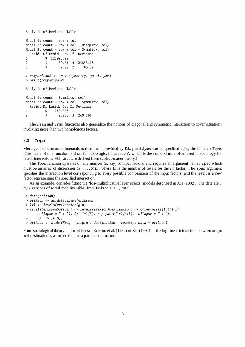
2.3 Topo
More general structured interactions than those provided byDiag andSymm can be specified using the functionTopo.(The name of this function is short for ‘topological interaction’, which is the nomenclature often used in sociology forfactor interactions with structure derived from subject-matter theory.)
TheTopo function operates on any number (k, say) of input factors, and requires an argument namedspec whichmust be an array of dimensionL1 × . . . × Lk, whereLi is the number of levels for theith factor. Thespec argumentspecifies the interaction level corresponding to every possible combination of the input factors, and the result is a newfactor representing the specified interaction.
As an example, consider fitting the ‘log-multiplicative layer effects’ models described in Xie (1992). The data are 7by 7 versions of social mobility tables from Erikson et al. (1982):
> data(erikson)> erikson <- as.data.frame(erikson)> lvl <- levels(erikson$origin)> levels(erikson$origin) <- levels(erikson$destination) <- c(rep(paste(lvl[1:2],+ collapse = " + "), 2), lvl[3], rep(paste(lvl[4:5], collapse = " + "),+ 2), lvl[6:9])> erikson <- xtabs(Freq ~ origin + destination + country, data = erikson)
From sociological theory — for which see Erikson et al. (1982) or Xie (1992) — the log-linear interaction between originand destination is assumed to have a particular structure:
3
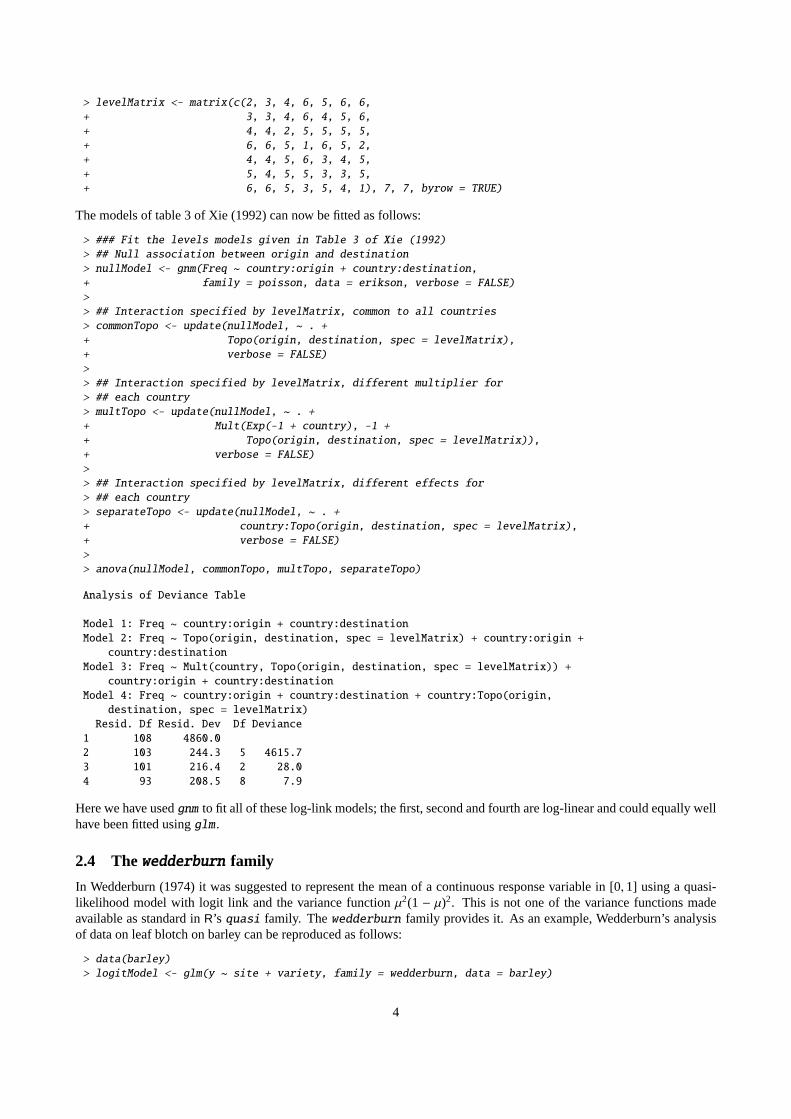
> levelMatrix <- matrix(c(2, 3, 4, 6, 5, 6, 6,+ 3, 3, 4, 6, 4, 5, 6,+ 4, 4, 2, 5, 5, 5, 5,+ 6, 6, 5, 1, 6, 5, 2,+ 4, 4, 5, 6, 3, 4, 5,+ 5, 4, 5, 5, 3, 3, 5,+ 6, 6, 5, 3, 5, 4, 1), 7, 7, byrow = TRUE)
The models of table 3 of Xie (1992) can now be fitted as follows:
> ### Fit the levels models given in Table 3 of Xie (1992)> ## Null association between origin and destination> nullModel <- gnm(Freq ~ country:origin + country:destination,+ family = poisson, data = erikson, verbose = FALSE)>> ## Interaction specified by levelMatrix, common to all countries> commonTopo <- update(nullModel, ~ . ++ Topo(origin, destination, spec = levelMatrix),+ verbose = FALSE)>> ## Interaction specified by levelMatrix, different multiplier for> ## each country> multTopo <- update(nullModel, ~ . ++ Mult(Exp(-1 + country), -1 ++ Topo(origin, destination, spec = levelMatrix)),+ verbose = FALSE)>> ## Interaction specified by levelMatrix, different effects for> ## each country> separateTopo <- update(nullModel, ~ . ++ country:Topo(origin, destination, spec = levelMatrix),+ verbose = FALSE)>> anova(nullModel, commonTopo, multTopo, separateTopo)
Analysis of Deviance Table
Model 1: Freq ~ country:origin + country:destinationModel 2: Freq ~ Topo(origin, destination, spec = levelMatrix) + country:origin +
country:destinationModel 3: Freq ~ Mult(country, Topo(origin, destination, spec = levelMatrix)) +
country:origin + country:destinationModel 4: Freq ~ country:origin + country:destination + country:Topo(origin,
destination, spec = levelMatrix)Resid. Df Resid. Dev Df Deviance
1 108 4860.02 103 244.3 5 4615.73 101 216.4 2 28.04 93 208.5 8 7.9
Here we have usedgnm to fit all of these log-link models; the first, second and fourth are log-linear and could equally wellhave been fitted usingglm .
2.4 Thewedderburn family
In Wedderburn (1974) it was suggested to represent the mean of a continuous response variable in [0,1] using a quasi-likelihood model with logit link and the variance functionµ2(1 − µ)2. This is not one of the variance functions madeavailable as standard inR’s quasi family. Thewedderburn family provides it. As an example, Wedderburn’s analysisof data on leaf blotch on barley can be reproduced as follows:
> data(barley)> logitModel <- glm(y ~ site + variety, family = wedderburn, data = barley)
4
> fit <- fitted(logitModel)> print(sum((barley$y - fit)^2/(fit * (1 - fit))^2))
[1] 71.17401
This agrees with the chi-squared value reported on page 331 of McCullagh and Nelder (1989), which differs slightly fromWedderburn’s own reported value.
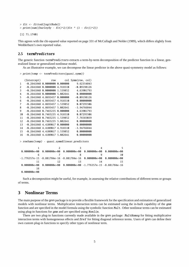
2.5 termPredictors
The generic functiontermPredictors extracts a term-by-term decomposition of the predictor function in a linear, gen-eralized linear or generalized nonlinear model.
As an illustrative example, we can decompose the linear predictor in the above quasi-symmetry model as follows:
> print(temp <- termPredictors(quasi.symm))
(Intercept) row col Symm(row, col)1 -0.2641848 0.0000000 0.000000 9.623548432 -0.2641848 0.0000000 4.918310 -0.091981263 -0.2641848 0.0000000 1.539852 4.639017934 -0.2641848 0.0000000 5.082641 0.000000005 -0.2641848 4.8693457 0.000000 -0.091981266 -0.2641848 4.8693457 4.918310 0.000000007 -0.2641848 4.8693457 1.539852 0.072955068 -0.2641848 4.8693457 5.082641 -3.947668449 -0.2641848 0.7465235 0.000000 4.6390179310 -0.2641848 0.7465235 4.918310 0.0729550611 -0.2641848 0.7465235 1.539852 7.7658303912 -0.2641848 0.7465235 5.082641 0.0000000013 -0.2641848 4.4109017 0.000000 0.0000000014 -0.2641848 4.4109017 4.918310 -3.9476684415 -0.2641848 4.4109017 1.539852 0.0000000016 -0.2641848 4.4109017 5.082641 0.00000000
> rowSums(temp) - quasi.symm$linear.predictors
1 2 3 4 50.000000e+00 0.000000e+00 0.000000e+00 0.000000e+00 0.000000e+00
6 7 8 9 10-1.776357e-15 -8.881784e-16 -8.881784e-16 0.000000e+00 0.000000e+00
11 12 13 14 150.000000e+00 0.000000e+00 0.000000e+00 -1.776357e-15 -8.881784e-16
160.000000e+00
Such a decomposition might be useful, for example, in assessing the relative contributions of different terms or groupsof terms.
3 Nonlinear Terms
The main purpose of thegnm package is to provide a flexible framework for the specification and estimation of generalizedmodels with nonlinear terms. Multiplicative interaction terms can be estimated using the in-built capability of thegnmfunction and are specified in the model formula using the symbolic functionMult. Other nonlinear terms can be estimatedusing plug-in functions forgnm and are specified usingNonlin.
There are two plug-in functions currently made available in thegnm package:MultHomog for fitting multiplicativeinteraction terms with homogeneous effects andDref for fitting diagonal reference terms. Users ofgnm can define theirown custom plug-in functions to specify other types of nonlinear term.
5
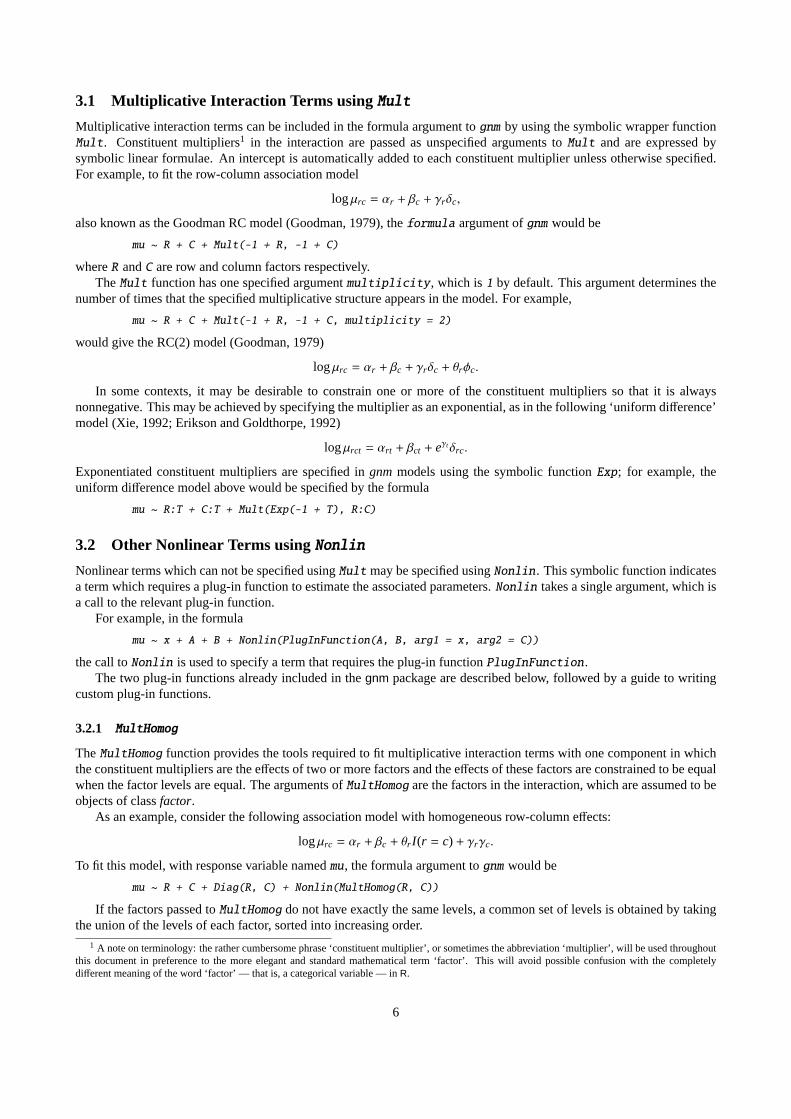
3.1 Multiplicative Interaction Terms using Mult
Multiplicative interaction terms can be included in the formula argument tognm by using the symbolic wrapper functionMult. Constituent multipliers1 in the interaction are passed as unspecified arguments toMult and are expressed bysymbolic linear formulae. An intercept is automatically added to each constituent multiplier unless otherwise specified.For example, to fit the row-column association model
logµrc = αr + βc + γrδc,
also known as the Goodman RC model (Goodman, 1979), theformula argument ofgnm would be
mu ~ R + C + Mult(-1 + R, -1 + C)
whereR andC are row and column factors respectively.TheMult function has one specified argumentmultiplicity, which is1 by default. This argument determines the
number of times that the specified multiplicative structure appears in the model. For example,
mu ~ R + C + Mult(-1 + R, -1 + C, multiplicity = 2)
would give the RC(2) model (Goodman, 1979)
logµrc = αr + βc + γrδc + θrφc.
In some contexts, it may be desirable to constrain one or more of the constituent multipliers so that it is alwaysnonnegative. This may be achieved by specifying the multiplier as an exponential, as in the following ‘uniform difference’model (Xie, 1992; Erikson and Goldthorpe, 1992)
logµrct = αrt + βct + eγtδrc.
Exponentiated constituent multipliers are specified ingnmmodels using the symbolic functionExp; for example, theuniform difference model above would be specified by the formula
mu ~ R:T + C:T + Mult(Exp(-1 + T), R:C)
3.2 Other Nonlinear Terms usingNonlin
Nonlinear terms which can not be specified usingMult may be specified usingNonlin. This symbolic function indicatesa term which requires a plug-in function to estimate the associated parameters.Nonlin takes a single argument, which isa call to the relevant plug-in function.
For example, in the formula
mu ~ x + A + B + Nonlin(PlugInFunction(A, B, arg1 = x, arg2 = C))
the call toNonlin is used to specify a term that requires the plug-in functionPlugInFunction.The two plug-in functions already included in thegnm package are described below, followed by a guide to writing
custom plug-in functions.
3.2.1 MultHomog
TheMultHomog function provides the tools required to fit multiplicative interaction terms with one component in whichthe constituent multipliers are the effects of two or more factors and the effects of these factors are constrained to be equalwhen the factor levels are equal. The arguments ofMultHomog are the factors in the interaction, which are assumed to beobjects of classfactor.
As an example, consider the following association model with homogeneous row-column effects:
logµrc = αr + βc + θr I (r = c) + γrγc.
To fit this model, with response variable namedmu, the formula argument tognm would be
mu ~ R + C + Diag(R, C) + Nonlin(MultHomog(R, C))
If the factors passed toMultHomog do not have exactly the same levels, a common set of levels is obtained by takingthe union of the levels of each factor, sorted into increasing order.
1 A note on terminology: the rather cumbersome phrase ‘constituent multiplier’, or sometimes the abbreviation ‘multiplier’, will be used throughoutthis document in preference to the more elegant and standard mathematical term ‘factor’. This will avoid possible confusion with the completelydifferent meaning of the word ‘factor’ — that is, a categorical variable — inR.
6
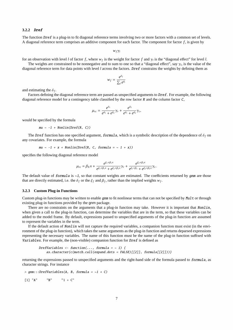
3.2.2 Dref
The functionDref is a plug-in to fit diagonal reference terms involving two or more factors with a common set of levels.A diagonal reference term comprises an additive component for each factor. The component for factorf , is given by
wfγl
for an observation with levell of factor f , wherewf is the weight for factorf andγl is the “diagonal effect” for level l.The weights are constrained to be nonnegative and to sum to one so that a “diagonal effect”, sayγl , is the value of the
diagonal reference term for data points with levell across the factors.Dref constrains the weights by defining them as
wf =eδ f∑i eδi
and estimating theδ f .Factors defining the diagonal reference term are passed as unspecified arguments toDref . For example, the following
diagonal reference model for a contingency table classified by the row factorR and the column factorC,
µrc =eδ1
eδ1 + eδ2γr +
eδ2
eδ1 + eδ2γc,
would be specified by the formula
mu ~ -1 + Nonlin(Dref(R, C))
TheDref function has one specified argument,formula, which is a symbolic description of the dependence ofδ f onany covariates. For example, the formula
mu ~ -1 + x + Nonlin(Dref(R, C, formula = ~ 1 + x))
specifies the following diagonal reference model
µrc = βXx+eξ1+β1x
eξ1+β1x + eξ2+β2xγr +
eξ2+β2x
eξ1+βx + eξ2+β2xγc.
The default value offormula is ~1, so that constant weights are estimated. The coefficients returned bygnm are thosethat are directly estimated, i.e. theδ f or theξ f andβ f , rather than the implied weightswf .
3.2.3 Custom Plug-in Functions
Custom plug-in functions may be written to enablegnm to fit nonlinear terms that can not be specified byMult or throughexisting plug-in functions provided by thegnm package.
There are no constraints on the arguments that a plug-in function may take. However it is important thatNonlin,when given a call to the plug-in function, can determine the variables that are in the term, so that these variables can beadded to the model frame. By default, expressions passed to unspecified arguments of the plug-in function are assumedto represent the variables in the term.
If the default action ofNonlin will not capture the required variables, a companion function must exist (in the envi-ronment of the plug-in function), which takes the same arguments as the plug-in function and returns deparsed expressionsrepresenting the necessary variables. The name of this function must be the name of the plug-in function suffixed withVariables. For example, the (non-visible) companion function forDref is defined as
DrefVariables <- function(..., formula = ~ 1) {as.character(c(match.call(expand.dots = FALSE)[[2]], formula[[2]]))}
returning the expressions passed to unspecified arguments and the right-hand side of the formula passed toformula, ascharacter strings. For instance
> gnm:::DrefVariables(A, B, formula = ~1 + C)
[1] "A" "B" "1 + C"
7

from whichNonlin will know thatA , B andC need to be added to the model frame.The call to the plug-in function is evaluated in the environment of the model frame and in the enclosing environment
of the parent frame of the call tognm . This should ensure that variables passed directly to the plug-in function can befound. However, to evaluate variables within the plug-in function, it may be necessary to access the model frame, whichcan be obtained using the functiongetModelFrame.
For example, the factors in aDref term are passed directly to unspecified arguments, so the dummy variables forthese factors can be found as follows:
# get design matrices for Dref factorsdesignList <- lapply(list(...), class.ind)
But any covariates on which the weights depend are only represented symbolically in theformula argument, so thedesign matrix for these variables must be found in the context of the model frame:
## get design matrix for local structuregnmData <- getModelFrame()local <- model.matrix(formula, data = gnmData)
The plug-in function should return a list with at least the following three components:
labels a character vector of labels for the parameters (to whichgnm will prefix the call to the plug-in function).
predictor a function which takes a vector of parameter estimates and returns either a vector of fitted values or a matrixwhose columns are additive components of the fitted values.
localDesignFunction a function which takes the specified argumentscoef (a vector of parameter estimates) andpredictor (the result of the predictor function), and returns the local design matrix. If the plug-in function doesnot return astart component (see below), thelocalDesignFunction must also take the argumentind , whichspecifies the index of a column to be returned instead of the full matrix.
and optionally one further component,
start a vector of default starting values for the parameters.NA may be used to indicate parameters which may be treatedas linear for the purpose of finding starting values, given the non-NA values. See Section 4.2 for details of howthese starting values will be used if provided and the starting procedure for nonlinear parameters that will be usedotherwise.
As an example of astart component,Dref returns
c(runif(nLocal) - 0.5, rep(0.5, nGlobal))
wherenLocal is the number of weight parameters (parameters which are “local” to a specific factor) andnGlobal is thenumber of diagonal effects (“global” level effects across factors). The randomness in the starting values for the weightparameters ensures that arbitrariness of the final parameterization is emphasised.
TheMultHomog function provides a simple example of apredictor component:
predictor <- function(coef) {do.call("pprod", lapply(designList, "%*%", coef))}
which computes the product of the vectors found by multiplying the design matrix for each factor in the interaction (held indesignList) by the homogeneous coefficients (incoef ). This function takes advantage oflexical scoping: designListis an object defined inMultHomog, whichpredictor is able to find becausepredictor is also defined inMultHomogand henceMultHomog is the enclosing environment ofpredictor.
ThelocalDesignFunction created byMultHomog is slightly more complicated:
localDesignFunction <- function(coef, ind = NULL, ...) {X <- 0vList <- lapply(designList, "%*%", coef)for (i in seq(designList)) {
if (is.null(ind))X <- X + designList[[*]] * drop(do.call("pprod", vList[-i]))
elseX <- X + designList[[]][, ind] *
drop(do.call("pprod", vList[-i]))}X}
8

Since the result of the predictor function is not needed here, the local design function does not have the specified argumentpredictor, but allows such an argument to be passed to the function by the use of the special argument ‘...’. SinceMultHomog does not return astart component, the local design function can optionally return a single column of thelocal design matrix as specified byind . This functionality is required by the default starting procedure for nonlinearparameters.
4 Controlling the Fitting Procedure
Thegnm function has a number of arguments which affect the way a model will be fitted. Basic control parameters canbe set using the argumentstolerance, iterStart anditerMax. Starting values for the parameter estimates can be setby start and parameters can be constrained to zero by specifying aconstrain argument. Parameters of a stratificationfactor can be handled more efficiently by specifying the factor in aneliminate argument. These options are describedin more detail below.
4.1 Basic control parameters
The argumentsiterStart anditerMax control respectively the number of starting iterations (where applicable) and thenumber of main iterations used by the fitting algorithm. The progress of these iterations can be followed by setting eitherverbose or trace to TRUE. If verbose is TRUE andtrace is FALSE, which is the default setting, progress is indicatedby printing the character “.” at the beginning of each iteration. Iftrace is TRUE, the deviance is printed at the beginningof each iteration (over-riding the printing of “.” if necessary). Wheneververbose is TRUE, additional messages indicateeach stage of the fitting process and diagnose any errors that cause that cause the algorithm to restart.
The fitting algorithm will terminate before the number of main iterations has reachediterMax if the convergencecriteria have been met, with tolerance specified bytolerance. Convergence is judged by comparing the squared com-ponents of the score vector with corresponding elements of the diagonal of the Fisher information matrix. If, for allcomponents of the score vector, the ratio is less thantoleranceˆ2, or the corresponding diagonal element of the Fisherinformation matrix is less than 1e-20, the algorithm is deemed to have converged.
4.2 Usingstart
In some contexts, the default starting values may not be appropriate and the algorithm will fail to converge, or perhaps onlyconverge after a large number of iterations. Alternative starting values may be passed on tognm by specifying astartargument. This should be a numeric vector of length equal to the number of parameters (or possibly the non-eliminatedparameters, see Section 4.4), however missing starting values (NAs) are allowed.
If there is no user-specified starting value for a parameter, the default value is used. This feature is particularly usefulwhen adding terms to a model, since the estimates from the original model can be used as starting values, as in thisexample:
model1 <- gnm(mu ~ R + C + Mult(-1 + R, -1 + C))model2 <- gnm(mu ~ R + C + Mult(-1 + R, -1 + C, multiplicity = 2),
start = c(coef(model1), rep(NA, 10))
Thegnm call can be made withmethod = "coefNames" to identify the parameters of a model prior to estimation, toassist with the specification of arguments such asstart.
The starting procedure used bygnm is as follows
1. Generate starting valuesθi for all parametersi = 1, . . . , p from the Uniform(−0.1, 0.1) distribution. Shift thesevalues away from zero as follows
θi =
θi − 0.1 if θi < 1
θi + 0.1 otherwise
2. Replace generic starting values with default starting values set by plug-in functions, where applicable.
3. Replace default starting values with any starting values specified by thestart argument ofgnm .
4. Compute theglm estimate of any parameters that may be treated as linear (i.e. those in linear terms or those witha default starting value ofNA set by a plug-in function), offsetting the contribution to the predictor of any termsspecified bystart or a plug-in function.
9
5. Run starting iterations: update one at a time any remaining nonlinear parameters not specified bystart or a plug-infunction, updatingall parameters that may be treated as linear after each round of updates.
Note that no starting iterations (step 5) will be run if all parameters are linear, or if all nonlinear parameters are specifiedby start or a plug-in function.
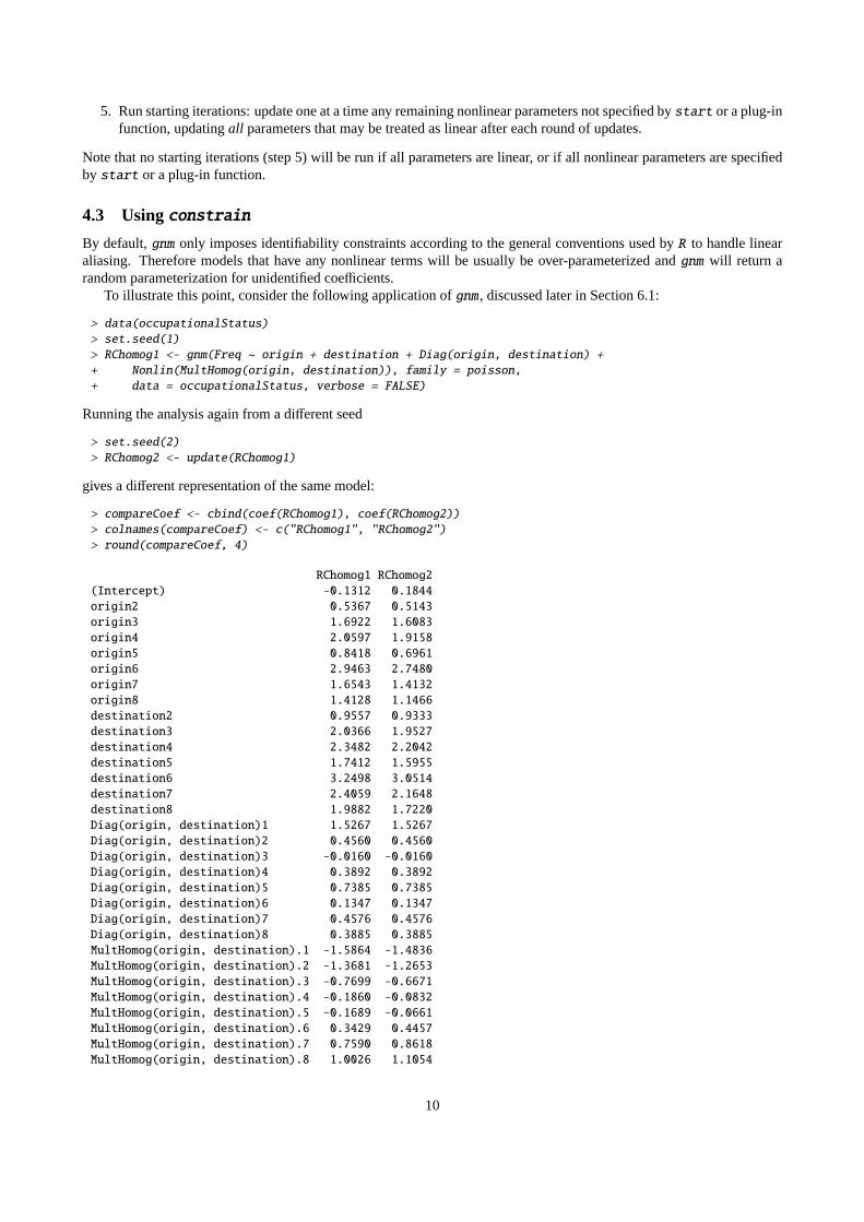
4.3 Usingconstrain
By default,gnm only imposes identifiability constraints according to the general conventions used byR to handle linearaliasing. Therefore models that have any nonlinear terms will be usually be over-parameterized andgnm will return arandom parameterization for unidentified coefficients.
To illustrate this point, consider the following application ofgnm , discussed later in Section 6.1:
> data(occupationalStatus)> set.seed(1)> RChomog1 <- gnm(Freq ~ origin + destination + Diag(origin, destination) ++ Nonlin(MultHomog(origin, destination)), family = poisson,+ data = occupationalStatus, verbose = FALSE)
Running the analysis again from a different seed
> set.seed(2)> RChomog2 <- update(RChomog1)
gives a different representation of the same model:
> compareCoef <- cbind(coef(RChomog1), coef(RChomog2))> colnames(compareCoef) <- c("RChomog1", "RChomog2")> round(compareCoef, 4)
RChomog1 RChomog2(Intercept) -0.1312 0.1844origin2 0.5367 0.5143origin3 1.6922 1.6083origin4 2.0597 1.9158origin5 0.8418 0.6961origin6 2.9463 2.7480origin7 1.6543 1.4132origin8 1.4128 1.1466destination2 0.9557 0.9333destination3 2.0366 1.9527destination4 2.3482 2.2042destination5 1.7412 1.5955destination6 3.2498 3.0514destination7 2.4059 2.1648destination8 1.9882 1.7220Diag(origin, destination)1 1.5267 1.5267Diag(origin, destination)2 0.4560 0.4560Diag(origin, destination)3 -0.0160 -0.0160Diag(origin, destination)4 0.3892 0.3892Diag(origin, destination)5 0.7385 0.7385Diag(origin, destination)6 0.1347 0.1347Diag(origin, destination)7 0.4576 0.4576Diag(origin, destination)8 0.3885 0.3885MultHomog(origin, destination).1 -1.5864 -1.4836MultHomog(origin, destination).2 -1.3681 -1.2653MultHomog(origin, destination).3 -0.7699 -0.6671MultHomog(origin, destination).4 -0.1860 -0.0832MultHomog(origin, destination).5 -0.1689 -0.0661MultHomog(origin, destination).6 0.3429 0.4457MultHomog(origin, destination).7 0.7590 0.8618MultHomog(origin, destination).8 1.0026 1.1054
10

Even though the linear terms are constrained, the parameter estimates for the main effects oforigin anddestinationstill change, because these terms are aliased with the higher order multiplicative interaction, which is unconstrained.
Standard errors are only meaningful for identified parameters and hence the output ofsummary.gnm will show clearlywhich coefficients are estimable:
> summary(RChomog2)
Call:gnm(formula = Freq ~ origin + destination + Diag(origin, destination) +
Nonlin(MultHomog(origin, destination)), family = poisson,data = occupationalStatus, verbose = FALSE)
Deviance Residuals:Min 1Q Median 3Q Max
-1.659e+00 -4.297e-01 -4.463e-08 3.862e-01 1.721e+00
Coefficients:Estimate Std. Error z value Pr(>|z|)
(Intercept) 0.18438 NA NA NAorigin2 0.51428 NA NA NAorigin3 1.60827 NA NA NAorigin4 1.91578 NA NA NAorigin5 0.69610 NA NA NAorigin6 2.74796 NA NA NAorigin7 1.41324 NA NA NAorigin8 1.14664 NA NA NAdestination2 0.93329 NA NA NAdestination3 1.95269 NA NA NAdestination4 2.20421 NA NA NAdestination5 1.59552 NA NA NAdestination6 3.05144 NA NA NAdestination7 2.16483 NA NA NAdestination8 1.72202 NA NA NADiag(origin, destination)1 1.52667 0.44658 3.419 0.00063 ***Diag(origin, destination)2 0.45600 0.34595 1.318 0.18747Diag(origin, destination)3 -0.01598 0.18098 -0.088 0.92965Diag(origin, destination)4 0.38918 0.12748 3.053 0.00227 **Diag(origin, destination)5 0.73852 0.23329 3.166 0.00155 **Diag(origin, destination)6 0.13474 0.07934 1.698 0.08945 .Diag(origin, destination)7 0.45764 0.15103 3.030 0.00245 **Diag(origin, destination)8 0.38847 0.22172 1.752 0.07976 .MultHomog(origin, destination).1 -1.48357 NA NA NAMultHomog(origin, destination).2 -1.26528 NA NA NAMultHomog(origin, destination).3 -0.66711 NA NA NAMultHomog(origin, destination).4 -0.08323 NA NA NAMultHomog(origin, destination).5 -0.06606 NA NA NAMultHomog(origin, destination).6 0.44570 NA NA NAMultHomog(origin, destination).7 0.86184 NA NA NAMultHomog(origin, destination).8 1.10541 NA NA NA---Signif. codes: 0 '***' 0.001 '**' 0.01 '*' 0.05 '.' 0.1 ' ' 1
(Dispersion parameter for poisson family taken to be 1)
Std. Error is NA where coefficient has been constrained or is unidentified
Residual deviance: 32.561 on 34 degrees of freedomAIC: 414.9
Number of iterations: 7
11
Additional constraints may be specified through theconstrain andconstrainTo arguments ofgnm . These argu-ments specify respectively parameters that are to be constrained in the fitting process and the values to which they shouldbe constrained. Parameters may be specified by a regular expression to match against the parameter names, a numericvector of indices, a character vector of names, or, ifconstrain = "[?]" they can be selected through aTk dialog. Thevalues to constrain to should be specified by a numeric vector; ifconstrainTo is missing, constrained parameters willbe set to zero.
In the case above, constraining one level of the homogeneous multiplicative factor is sufficient to make the parametersof the nonlinear term identifiable, and hence all parameters in the model identifiable. For example, setting the last level ofthe homogeneous multiplicative factor to zero,
> multCoef <- coef(RChomog1)[pickCoef(RChomog1, "Mult")]> set.seed(1)> RChomogConstrained1 <- update(RChomog1, constrain = 31, start = c(rep(NA,+ 23), multCoef - multCoef[8]))> set.seed(2)> RChomogConstrained2 <- update(RChomogConstrained1)> identical(coef(RChomogConstrained1), coef(RChomogConstrained2))
[1] TRUE
gives the same results regardless of the random seed set beforehand.It is not usually so straightforward to constrain all the parameters in a generalized nonlinear model. However use of
constrain in conjunction withconstrainTo is usually sufficient to make coefficients of interest identifiable . The func-tionscheckEstimable or getContrasts, described in Section 5, may be used to check whether particular combinationsof parameters are estimable.
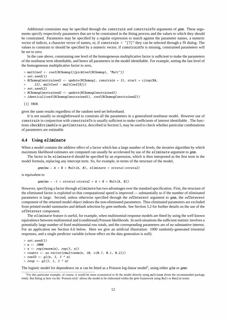
4.4 Usingeliminate
When a model contains the additive effect of a factor which has a large number of levels, the iterative algorithm by whichmaximum likelihood estimates are computed can usually be accelerated by use of theeliminate argument tognm .
The factor to beeliminate-d should be specified by an expression, which is then interpreted as the first term in themodel formula, replacing any intercept term. So, for example, in terms of the structure of the model,
gnm(mu ~ A + B + Mult(A, B), eliminate = strata1:strata2)
is equivalent to
gnm(mu ~ -1 + strata1:strata2 + A + B + Mult(A, B))
However, specifying a factor througheliminate has two advantages over the standard specification. First, the structure ofthe eliminated factor is exploited so that computational speed is improved — substantially so if the number of eliminatedparameters is large. Second, unless otherwise specified through theofInterest argument tognm , the ofInterestcomponent of the returned model object indexes the non-eliminated parameters. Thus eliminated parameters are excludedfrom printed model summaries and default selection bygnmmethods. See Section 5.2 for further details on the use of theofInterest component.
Theeliminate feature is useful, for example, when multinomial-response models are fitted by using the well knownequivalence between multinomial and (conditional) Poisson likelihoods. In such situations the sufficient statistic involves apotentially large number of fixed multinomial row totals, and the corresponding parameters are of no substantive interest.For an application see Section 6.6 below. Here we give an artificial illustration: 1000 randomly-generated trinomialresponses, and a single predictor variable (whose effect on the data generation is null):
> set.seed(1)> n <- 1000> x <- rep(rnorm(n), rep(3, n))> counts <- as.vector(rmultinom(n, 10, c(0.7, 0.1, 0.2)))> rowID <- gl(n, 3, 3 * n)> resp <- gl(3, 1, 3 * n)
The logistic model for dependence onx can be fitted as a Poisson log-linear model2, using eitherglm or gnm :
2For this particular example, of course, it would be more economical to fit the model directly usingmultinom (from the recommended packagennet). But fitting as here via the ‘Poisson trick’ allows the model to be elaborated within thegnm framework usingMult or Nonlin terms.
12

> ## Timings on a Pentium M 1.6GHz, under Linux> system.time(temp.glm <- glm(counts ~ rowID + resp + resp:x,
family = poisson))[1]
[1] 116.8
> system.time(temp.gnm <- gnm(counts ~ resp + resp:x, eliminate = rowID,family = poisson, verbose = FALSE))[1]
[1] 22.0
> c(deviance(temp.glm), deviance(temp.gnm))
[1] 2462.556 2462.556
Here the use ofeliminate causes thegnm calculations to run more quickly thanglm . The speed advantage3 increaseswith the number of eliminated parameters (here 1000). Since the default behaviour has not been over-ridden by anofInterest argument, the eliminated parameters do not appear in printed model summaries:
> summary(temp.gnm)
Call:
gnm(formula = counts ~ resp + resp:x, eliminate = rowID, family = poisson,verbose = FALSE)
Deviance Residuals:Min 1Q Median 3Q Max
-2.852038 -0.786172 -0.004534 0.645278 2.755013
Coefficients of interest:Estimate Std. Error z value Pr(>|z|)
resp2 -1.9614483 0.0340074 -57.68 <2e-16resp3 -1.2558460 0.0253589 -49.52 <2e-16resp1:x 0.0001049 NA NA NAresp2:x -0.0155083 NA NA NAresp3:x 0.0078314 NA NA NA
(Dispersion parameter for poisson family taken to be 1)
Std. Error is NA where coefficient has been constrained or is unidentified
Residual deviance: 2462.6 on 1996 degrees of freedomAIC: 12028
Number of iterations: 3
As usual,gnm has worked here with an over-parameterized representation of the model. The parameterization used byglm can be seen from
> coef(temp.glm)[-(1:1000)]
resp2 resp3 resp1:x resp2:x resp3:x-1.96145 -1.25585 -0.00773 -0.02334 NA
(we will not print the full summary oftemp.glm here, since it gives details of all 1005 parameters!), which easily can beobtained, if required, by usinggetContrasts:
> getContrasts(temp.gnm, ofInterest(temp.gnm)[5:3])
3In facteliminate is, in principle, capable of much bigger time savings than this: its implementation in the current version ofgnm is really just aproof of concept, and it has not yet been optimized for speed.
13
estimate SE quasiSE quasiVarresp3:x 0.00000 0.00000 0.02163 0.000468resp2:x -0.02334 0.03761 0.03077 0.000947resp1:x -0.00773 0.02452 0.01154 0.000133
Theeliminate feature as implemented ingnm extends the earlier work of Hatzinger and Francis (2004) to a broaderclass of models and to over-parameterized model representations.
5 Methods and Accessor functions
5.1 Methods
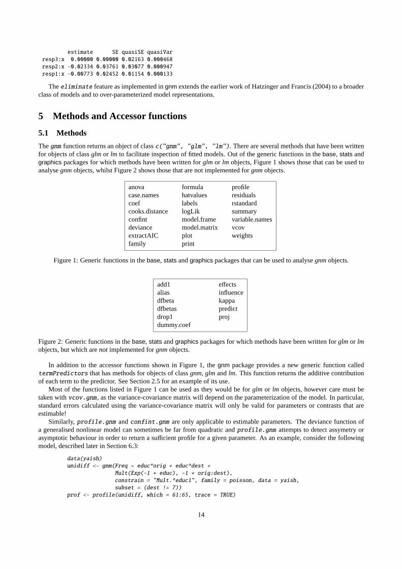
Thegnm function returns an object of classc("gnm", "glm", "lm"). There are several methods that have been writtenfor objects of classglm or lm to facilitate inspection of fitted models. Out of the generic functions in thebase, stats andgraphics packages for which methods have been written forglm or lm objects, Figure 1 shows those that can be used toanalysegnmobjects, whilst Figure 2 shows those that are not implemented forgnmobjects.
anova formula profilecase.names hatvalues residualscoef labels rstandardcooks.distance logLik summaryconfint model.frame variable.namesdeviance model.matrix vcovextractAIC plot weightsfamily print
Figure 1: Generic functions in thebase, stats andgraphics packages that can be used to analysegnmobjects.
add1 effectsalias influencedfbeta kappadfbetas predictdrop1 projdummy.coef
Figure 2: Generic functions in thebase, stats andgraphics packages for which methods have been written forglm or lmobjects, but which arenot implemented forgnmobjects.
In addition to the accessor functions shown in Figure 1, thegnm package provides a new generic function calledtermPredictors that has methods for objects of classgnm, glm andlm. This function returns the additive contributionof each term to the predictor. See Section 2.5 for an example of its use.
Most of the functions listed in Figure 1 can be used as they would be forglm or lm objects, however care must betaken withvcov.gnm , as the variance-covariance matrix will depend on the parameterization of the model. In particular,standard errors calculated using the variance-covariance matrix will only be valid for parameters or contrasts that areestimable!
Similarly, profile.gnm andconfint.gnm are only applicable to estimable parameters. The deviance function ofa generalised nonlinear model can sometimes be far from quadratic andprofile.gnm attempts to detect assymetry orasymptotic behaviour in order to return a sufficient profile for a given parameter. As an example, consider the followingmodel, described later in Section 6.3:
data(yaish)unidiff <- gnm(Freq ~ educ*orig + educ*dest +
Mult(Exp(-1 + educ), -1 + orig:dest),constrain = "Mult.*educ1", family = poisson, data = yaish,subset = (dest != 7))
prof <- profile(unidiff, which = 61:65, trace = TRUE)
14
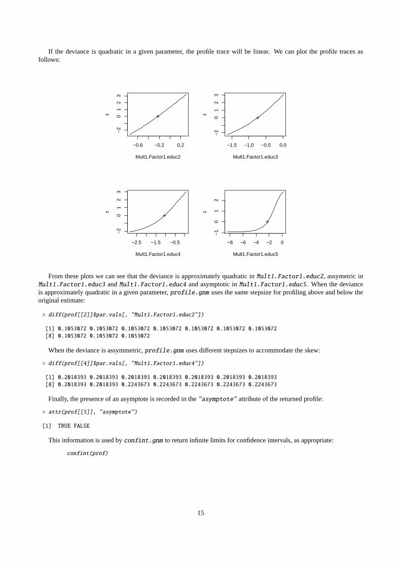
If the deviance is quadratic in a given parameter, the profile trace will be linear. We can plot the profile traces asfollows:
−0.6 −0.2 0.2
−2
01
23
Mult1.Factor1.educ2
z
−1.5 −1.0 −0.5 0.0
−2
01
23
Mult1.Factor1.educ3
z
−2.5 −1.5 −0.5
−2
01
23
Mult1.Factor1.educ4
z
−8 −6 −4 −2 0
−1
01
2
Mult1.Factor1.educ5
z
From these plots we can see that the deviance is approximately quadratic inMult1.Factor1.educ2, assymetric inMult1.Factor1.educ3 andMult1.Factor1.educ4 and asymptotic inMult1.Factor1.educ5. When the devianceis approximately quadratic in a given parameter,profile.gnm uses the same stepsize for profiling above and below theoriginal estimate:
> diff(prof[[2]]$par.vals[, "Mult1.Factor1.educ2"])
[1] 0.1053072 0.1053072 0.1053072 0.1053072 0.1053072 0.1053072 0.1053072[8] 0.1053072 0.1053072 0.1053072
When the deviance is assymmetric,profile.gnm uses different stepsizes to accommodate the skew:
> diff(prof[[4]]$par.vals[, "Mult1.Factor1.educ4"])
[1] 0.2018393 0.2018393 0.2018393 0.2018393 0.2018393 0.2018393 0.2018393[8] 0.2018393 0.2018393 0.2243673 0.2243673 0.2243673 0.2243673 0.2243673
Finally, the presence of an asymptote is recorded in the"asymptote" attribute of the returned profile:
> attr(prof[[5]], "asymptote")
[1] TRUE FALSE
This information is used byconfint.gnm to return infinite limits for confidence intervals, as appropriate:
confint(prof)
15

5.2 ofInterest and pickCoef
It is quite common for a statistical model to have a large number of parameters, but for only a subset of these parametersbe of interest when it comes to interpreting the model. An example of this has been seen in Section 4.4, where a factoris required in the model in order to represent a structural aspect of the data, but the estimated factor effects have nosubstantive interpretation. Even for models in which all parameters correspond to variables of potential interest, thesubstantive focus may still be on a subset of parameters.
TheofInterest argument tognm allows the user to specify a subset of the parameters which are of interest, so thatgnmmethods will focus on these parameters. In particular, printed model summaries will only show the parameters ofinterest, whilst methods for which a subset of parameters may be selected will by default select the parameters of interest,or where this may not be appropriate, provide aTk dialog for selection from the parameters of interest. Parameters maybe specified to theofInterest argument by a regular expression to match against parameter names, by a numeric vectorof indices, by a character vector of names, or, ifofInterest = "[?]" they can be selected through aTk dialog.
The information regarding the parameters of interest is held in theofInterest component ofgnmobjects, which isa named vector of numeric indices, orNULL if all parameters are of interest. This component may be accessed or replacedusingofInterest or ofInterest<- respectively.
ThepickCoef function provides a simple way to obtain the indices of coefficients from any model object. It takes themodel object as its first argument and has an optionalregexp argument. If a regular expression is passed toregexp, thecoefficients are selected by matching this regular expression against the coefficient names. Otherwise, coefficients may beselected via aTk dialog.
So, returning to the example from the last section, if we had setofInterest to index the education multipliers asfollows
ofInterest(unidiff) <- pickCoef(unidiff, "Mult1.*educ")
then it would not have been necessary to specify thewhich argument ofprofile as these parameters would have beenselected by default.
5.3 checkEstimable
ThecheckEstimable function can be used to check the estimability of a linear combination of parameters. For non-linear combinations the same function can be used to check estimability based on the (local) vector of partial derivatives.The checkEstimable function provides a numerical version of the sort of algebraic test described in Catchpole andMorgan (1997).
Consider the following model, that is described later in Section 6.3:
> data(cautres)> doubleUnidiff <- gnm(Freq ~ election:vote + election:class:religion ++ Mult(Exp(election - 1), religion:vote - 1) + Mult(Exp(election -+ 1), class:vote - 1), family = poisson, data = cautres)
InitialisingRunning start-up iterations..Running main iterations..........Done
The effects of the first constituent multiplier in the first multiplicative interaction are identified when the estimate of oneof these effects is constrained to zero, say for the effect of the first level. The parameters to be estimated are then thedifferences between each effect and the effect of the first level. These differences can be represented by a contrast matrixas follows:
> coefs <- names(coef(doubleUnidiff))> contrCoefs <- coefs[grep("Mult1.Factor1", coefs)]> nContr <- length(contrCoefs)> contrMatrix <- matrix(0, length(coefs), nContr, dimnames = list(coefs,+ contrCoefs))> contr <- contr.sum(contrCoefs)> contr <- rbind(contr[nContr, ], contr[-nContr, ])> contrMatrix[contrCoefs, 2:nContr] <- contr> contrMatrix[contrCoefs, 2:nContr]
16
Mult1.Factor1.election2 Mult1.Factor1.election3Mult1.Factor1.election1 -1 -1Mult1.Factor1.election2 1 0Mult1.Factor1.election3 0 1Mult1.Factor1.election4 0 0
Mult1.Factor1.election4Mult1.Factor1.election1 -1Mult1.Factor1.election2 0Mult1.Factor1.election3 0Mult1.Factor1.election4 1
Then their estimability can be checked usingcheckEstimable
> checkEstimable(doubleUnidiff, contrMatrix)
Mult1.Factor1.election1 Mult1.Factor1.election2 Mult1.Factor1.election3NA TRUE TRUE
Mult1.Factor1.election4TRUE
which confirms that the effects for the other three levels are estimable when the parameter for the first level is set to zero.However, applying the equivalent constraint to the second constituent multiplier in the interaction is not sufficient to
make the parameters in that multiplier estimable:
> coefs <- names(coef(doubleUnidiff))> contrCoefs <- coefs[grep("Mult1.Factor2", coefs)]> nContr <- length(contrCoefs)> contrMatrix <- matrix(0, length(coefs), length(contrCoefs), dimnames = list(coefs,+ contrCoefs))> contr <- contr.sum(contrCoefs)> contrMatrix[contrCoefs, 2:nContr] <- rbind(contr[nContr, ], contr[-nContr,+ ])> checkEstimable(doubleUnidiff, contrMatrix)
Mult1.Factor2.religion1:vote1 Mult1.Factor2.religion2:vote1NA FALSE
Mult1.Factor2.religion3:vote1 Mult1.Factor2.religion4:vote1FALSE FALSE
Mult1.Factor2.religion1:vote2 Mult1.Factor2.religion2:vote2FALSE FALSE
Mult1.Factor2.religion3:vote2 Mult1.Factor2.religion4:vote2FALSE FALSE
5.4 getContrasts, se
To investigate simple “sum to zero” contrasts such as those above, it is easiest to use thegetContrasts function, whichchecks the estimability of the contrasts and returns the parameter estimates with their standard errors. Returning to theexample of the first constituent multiplier in the first multiplicative interaction term, the differences between each electionand the first can be obtained as follows:
> myContrasts <- getContrasts(doubleUnidiff, pickCoef(doubleUnidiff,+ "Mult1.Factor1"))> myContrasts
estimate SE quasiSE quasiVarMult1.Factor1.election1 0.0000000 0.0000000 0.09803075 0.009610029Mult1.Factor1.election2 -0.0878181 0.1136832 0.05702819 0.003252214Mult1.Factor1.election3 -0.2615200 0.1184134 0.06812239 0.004640660Mult1.Factor1.election4 -0.3283459 0.1221302 0.07168290 0.005138439
Visualization of estimated contrasts using ‘quasi standard errors’ (Firth, 2003; Firth and de Menezes, 2004) is achievedby plotting the resulting object:
17

> plot(myContrasts, main = "Relative strength of religion-vote association, log scale",+ xlab = "Election", levelNames = 1:4)
1 2 3 4
−0.
4−
0.2
0.0
0.2
Relative strength of religion−vote association, log scale
Election
estim
ate
●
●
●
●
For more general linear combinations of parameters than contrasts, the lower-levelse function (which is called inter-nally bygetContrasts and by thesummary method) can be used directly. Seehelp(se) for details.
5.5 residSVD
Sometimes it is useful to operate on the residuals of a model in order to create informative summaries of residual variation,or to obtain good starting values for additional parameters in a more elaborate model. The relevant arithmetical operationsare weighted means of the so-calledworking residuals.
TheresidSVD function facilitates one particular residual analysis that is often useful when considering multiplicativeinteraction between factors as a model elaboration: in effect,residSVD provides a direct estimate of the parameters ofsuch an interaction, by performing an appropriately weighted singular value decomposition on the working residuals.
As an illustration, consider the biplot model described in Section 6.5 below. We can proceed by fitting a smallermodel, then useresidSVD to obtain starting values for the parameters in the bilinear term:
> emptyModel <- gnm(y ~ -1, family = wedderburn, data = barley)> biplotStart <- residSVD(emptyModel, barley$site, barley$variety,+ d = 2)> biplotModel <- gnm(y ~ -1 + Mult(-1 + site, -1 + variety, multiplicity = 2),+ family = wedderburn, data = barley, start = biplotStart)
Running main iterations...........................................................................................................................................Done
In this instance, the use of purposive (as opposed to the default, random) starting values had little effect: the fairly largenumber of iterations needed in this example is caused by a rather flat (quasi-)likelihood surface near the maximum, not bypoor starting values. In other situations, the use ofresidSVD may speed the calculations dramatically (see for exampleSection 6.4), or it may be crucial to success in locating the MLE (for example seehelp(House2001), where the numberof multiplicative parameters is in the hundreds).
18

TheresidSVD result in this instance provides a crude approximation to the MLE of the enlarged model, as can beseen in the following plot:
●●
● ●●●
●
●
●
●●●●
●●
●
●●
●
●
●
●
●●
●
●
●
●
●
●
●●
●
●
●
●
●
●
−2 0 2 4
−1.
5−
1.0
−0.
50.
00.
51.
01.
5
Comparison of residSVD and MLEfor a 2−dimensional biplot model
coef(biplotModel)
bipl
otS
tart
6 Examples
This section provides some examples of the wide range of models that may be fitted using thegnm package. Sections6.1, 6.2 and 6.3 consider various models for contingency tables; Section 6.4 considers AMMI and GAMMI models whichare typically used in agricultural applications, and Section 6.6 considers the stereotype model, which is used to model anordinal response.
6.1 Row-column Association Models
There are several models that have been proposed for modelling the relationship between the cell means of a contingencytable and the cross-classifying factors. The following examples consider the row-column association models proposed byGoodman (1979). The examples shown use data from two-way contingency tables, but thegnm package can also be usedto fit the equivalent models for higher order tables.
6.1.1 RC(1) model
The RC(1) model is a row and column association model with the interaction between row and column factors representedby one component of the multiplicative interaction. If the rows are indexed byr and the columns byc, then the log-multiplicative form of the RC(1) model for the cell meansµrc is given by
logµrc = αr + βc + γrδc.
We shall fit this model to thementalHealth data set taken from Agresti (2002) page 381, which is a two-way con-tingency table classified by the child’s mental impairment (MHS) and the parents’ socioeconomic status (SES). Althoughboth of these factors are ordered, we do not wish to use polynomial contrasts in the model, so we begin by setting thecontrasts attribute of these factors totreatment:
19

> set.seed(1)> data(mentalHealth)> mentalHealth$MHS <- C(mentalHealth$MHS, treatment)> mentalHealth$SES <- C(mentalHealth$SES, treatment)
Thegnmmodel is then specified as follows, using the poisson family with a log link function:
> RC1model <- gnm(count ~ SES + MHS + Mult(-1 + SES, -1 + MHS),+ family = poisson, data = mentalHealth)
InitialisingRunning start-up iterations..Running main iterations........Done
> RC1model
Call:
gnm(formula = count ~ SES + MHS + Mult(-1 + SES, -1 + MHS), family = poisson,data = mentalHealth)
Coefficients:(Intercept) SESB3.831281 -0.067413
SESC SESD0.109959 0.404969
SESE SESF0.025257 -0.200685MHSmild MHSmoderate0.712969 0.204987
MHSimpaired Mult1.Factor1.SESA0.251749 0.340495
Mult1.Factor1.SESB Mult1.Factor1.SESC0.343267 0.114885
Mult1.Factor1.SESD Mult1.Factor1.SESE-0.006284 -0.305574
Mult1.Factor1.SESF Mult1.Factor2.MHSwell-0.551460 0.935600
Mult1.Factor2.MHSmild Mult1.Factor2.MHSmoderate0.094793 -0.056941
Mult1.Factor2.MHSimpaired-0.755299
Deviance: 3.570562Pearson chi-squared: 3.568088Residual df: 8
The row scores (parameters 10 to 15) and the column scores (parameters 16 to 19) of the multiplicative interaction can benormalized as in Agresti’s eqn (9.15):
> rowProbs <- with(mentalHealth, tapply(count, SES, sum)/sum(count))> colProbs <- with(mentalHealth, tapply(count, MHS, sum)/sum(count))> rowScores <- coef(RC1model)[10:15]> colScores <- coef(RC1model)[16:19]> rowScores <- rowScores - sum(rowScores * rowProbs)> colScores <- colScores - sum(colScores * colProbs)> beta1 <- sqrt(sum(rowScores^2 * rowProbs))> beta2 <- sqrt(sum(colScores^2 * colProbs))> assoc <- list(beta = beta1 * beta2, mu = rowScores/beta1, nu = colScores/beta2)> assoc
20

$beta[1] 0.1664874
$muMult1.Factor1.SESA Mult1.Factor1.SESB Mult1.Factor1.SESC Mult1.Factor1.SESD
1.11233090 1.12143715 0.37107612 -0.02702946Mult1.Factor1.SESE Mult1.Factor1.SESF
-1.01036153 -1.81823284
$nuMult1.Factor2.MHSwell Mult1.Factor2.MHSmild Mult1.Factor2.MHSmoderate
1.6775144 0.1403989 -0.1369924Mult1.Factor2.MHSimpaired
-1.4136910
6.1.2 RC(2) model
The RC(1) model can be extended to an RC(m) model withmcomponents of the multiplicative interaction. For example,the RC(2) model is given by
logµrc = αr + βc + γrδc + θrφc.
Extra instances of the multiplicative interaction can be specified by themultiplicity argument ofMult, so the RC(2)model can be fitted to thementalHealth data as follows
> RC2model <- gnm(count ~ SES + MHS + Mult(-1 + SES, -1 + MHS,+ multiplicity = 2), family = poisson, data = mentalHealth)
InitialisingRunning start-up iterations..Running main iterations............Done
> RC2model
Call:
gnm(formula = count ~ SES + MHS + Mult(-1 + SES, -1 + MHS, multiplicity = 2),family = poisson, data = mentalHealth)
Coefficients:(Intercept) SESB
3.85530 -0.06444SESC SESD
0.11140 0.38457SESE SESF
0.01081 -0.18462MHSmild MHSmoderate0.69860 0.16975
MHSimpaired Mult1.Factor1.SESA0.22876 0.95047
Mult1.Factor1.SESB Mult1.Factor1.SESC0.99597 0.33932
Mult1.Factor1.SESD Mult1.Factor1.SESE-0.17292 -0.91634
Mult1.Factor1.SESF Mult1.Factor2.MHSwell-1.39376 0.35782
Mult1.Factor2.MHSmild Mult1.Factor2.MHSmoderate0.03795 -0.02129
Mult1.Factor2.MHSimpaired Mult2.Factor1.SESA-0.28029 -0.17762
Mult2.Factor1.SESB Mult2.Factor1.SESC
21
-0.25156 -0.16614Mult2.Factor1.SESD Mult2.Factor1.SESE
0.28993 0.22675Mult2.Factor1.SESF Mult2.Factor2.MHSwell
-0.45554 0.30776Mult2.Factor2.MHSmild Mult2.Factor2.MHSmoderate
0.09804 -0.25536Mult2.Factor2.MHSimpaired
0.06769
Deviance: 0.5225353Pearson chi-squared: 0.523331Residual df: 3
6.1.3 Homogeneous effects
If the row and column factors have the same levels, or perhaps some levels in common, then the row-column interactioncould be modelled by a multiplicative interaction with homogeneous effects, that is
logµrc = αr + βc + γrγc.
For example, theoccupationalStatus data set from Goodman (1979) is a contingency table classified by the occupa-tional status of fathers (origin) and their sons (destination). Goodman (1979) fits a row-column association model withhomogeneous effects to these data after deleting the cells on the main diagonal. Equivalently we can account for thediagonal effects by a separateDiag term:
> data(occupationalStatus)> RChomog <- gnm(Freq ~ origin + destination + Diag(origin, destination) ++ Nonlin(MultHomog(origin, destination)), family = poisson,+ data = occupationalStatus)
InitialisingRunning start-up iterations..Running main iterations........Done
> RChomog
Call:gnm(formula = Freq ~ origin + destination + Diag(origin, destination) +
Nonlin(MultHomog(origin, destination)), family = poisson,data = occupationalStatus)
Coefficients:(Intercept) origin2-0.67122 0.57207origin3 origin41.82441 2.28650origin5 origin61.07137 3.25871origin7 origin82.03415 1.83204
destination2 destination30.99108 2.16883
destination4 destination52.57493 1.97078
destination6 destination73.56218 2.78575
destination8 Diag(origin, destination)12.40741 1.52667
Diag(origin, destination)2 Diag(origin, destination)3
22
0.45600 -0.01598Diag(origin, destination)4 Diag(origin, destination)5
0.38918 0.73852Diag(origin, destination)6 Diag(origin, destination)7
0.13474 0.45764Diag(origin, destination)8 MultHomog(origin, destination).1
0.38847 -1.74831MultHomog(origin, destination).2 MultHomog(origin, destination).3
-1.53001 -0.93185MultHomog(origin, destination).4 MultHomog(origin, destination).5
-0.34797 -0.33080MultHomog(origin, destination).6 MultHomog(origin, destination).7
0.18096 0.59710MultHomog(origin, destination).8
0.84068
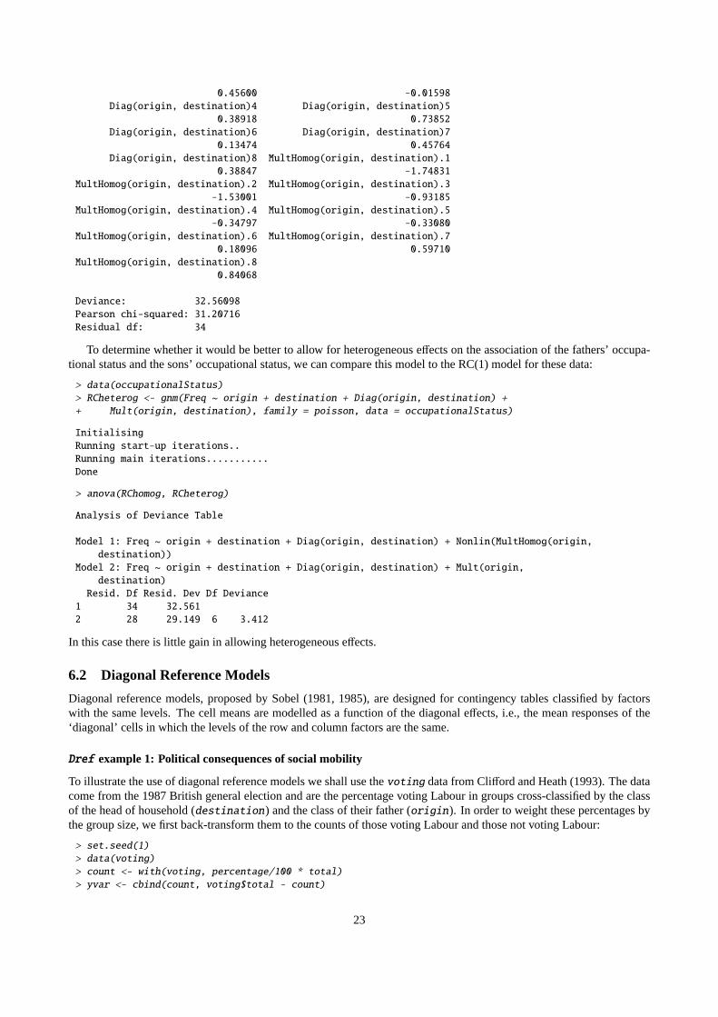
Deviance: 32.56098Pearson chi-squared: 31.20716Residual df: 34
To determine whether it would be better to allow for heterogeneous effects on the association of the fathers’ occupa-tional status and the sons’ occupational status, we can compare this model to the RC(1) model for these data:
> data(occupationalStatus)> RCheterog <- gnm(Freq ~ origin + destination + Diag(origin, destination) ++ Mult(origin, destination), family = poisson, data = occupationalStatus)
InitialisingRunning start-up iterations..Running main iterations...........Done
> anova(RChomog, RCheterog)
Analysis of Deviance Table
Model 1: Freq ~ origin + destination + Diag(origin, destination) + Nonlin(MultHomog(origin,destination))
Model 2: Freq ~ origin + destination + Diag(origin, destination) + Mult(origin,destination)
Resid. Df Resid. Dev Df Deviance1 34 32.5612 28 29.149 6 3.412
In this case there is little gain in allowing heterogeneous effects.
6.2 Diagonal Reference Models
Diagonal reference models, proposed by Sobel (1981, 1985), are designed for contingency tables classified by factorswith the same levels. The cell means are modelled as a function of the diagonal effects, i.e., the mean responses of the‘diagonal’ cells in which the levels of the row and column factors are the same.
Dref example 1: Political consequences of social mobility
To illustrate the use of diagonal reference models we shall use thevoting data from Clifford and Heath (1993). The datacome from the 1987 British general election and are the percentage voting Labour in groups cross-classified by the classof the head of household (destination) and the class of their father (origin). In order to weight these percentages bythe group size, we first back-transform them to the counts of those voting Labour and those not voting Labour:
> set.seed(1)> data(voting)> count <- with(voting, percentage/100 * total)> yvar <- cbind(count, voting$total - count)
23

The grouped percentages may be modelled by a basic diagonal reference model, that is, a weighted sum of the diagonaleffects for the corresponding origin and destination classes. This model may be expressed as
µod =eδ1
eδ1 + eδ2γo +
eδ2
eδ1 + eδ2γd.
See Section 3.2.2 for more detail on the parameterization.The basic diagonal reference model may be fitted usinggnm as follows
> classMobility <- gnm(yvar ~ Nonlin(Dref(origin, destination)),+ family = binomial, data = voting)
InitialisingRunning main iterations........Done
> classMobility
Call:
gnm(formula = yvar ~ Nonlin(Dref(origin, destination)), family = binomial,data = voting)
Coefficients:(Intercept) Dref(origin, destination).origin-1.34325 -0.30736
Dref(origin, destination).destination Dref(origin, destination).1-0.05501 -0.83454
Dref(origin, destination).2 Dref(origin, destination).30.21066 -0.61159
Dref(origin, destination).4 Dref(origin, destination).50.76500 1.38370
Deviance: 21.22093Pearson chi-squared: 18.95311Residual df: 19
and the origin and destination weights can be evaluated as below
> prop.table(exp(coef(classMobility)[2:3]))
Dref(origin, destination).origin Dref(origin, destination).destination0.4372469 0.5627531
These results are slightly different from those reported by Clifford and Heath (1993). The reason for this is unclear: weare confident that the above results are correct for the data as given in Clifford and Heath (1993), but have not been ableto confirm that the data as printed in the journal were exactly as used in Clifford and Heath’s analysis.
Clifford and Heath (1993) suggest that movements in and out of the salariat (class 1) should be treated differentlyfrom movements between the lower classes (classes 2 - 5), since the former has a greater effect on social status. Thus theypropose the following model
µod =
eδ1
eδ1 + eδ2γo +
eδ2
eδ1 + eδ2γd if o = 1
eδ3
eδ3 + eδ4γo +
eδ4
eδ3 + eδ4γd if d = 1
eδ5
eδ5 + eδ6γo +
eδ6
eδ5 + eδ6γd if o , 1 andd , 1
To fit this model we define factors indicating movement in (upward) and out (downward) of the salariat
24
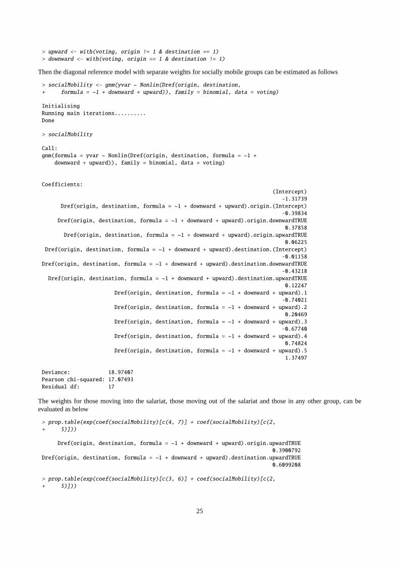
> upward <- with(voting, origin != 1 & destination == 1)> downward <- with(voting, origin == 1 & destination != 1)
Then the diagonal reference model with separate weights for socially mobile groups can be estimated as follows
> socialMobility <- gnm(yvar ~ Nonlin(Dref(origin, destination,+ formula = ~1 + downward + upward)), family = binomial, data = voting)
InitialisingRunning main iterations..........Done
> socialMobility
Call:gnm(formula = yvar ~ Nonlin(Dref(origin, destination, formula = ~1 +
downward + upward)), family = binomial, data = voting)
Coefficients:(Intercept)-1.31739
Dref(origin, destination, formula = ~1 + downward + upward).origin.(Intercept)-0.39834
Dref(origin, destination, formula = ~1 + downward + upward).origin.downwardTRUE0.37858
Dref(origin, destination, formula = ~1 + downward + upward).origin.upwardTRUE0.06225
Dref(origin, destination, formula = ~1 + downward + upward).destination.(Intercept)-0.01158
Dref(origin, destination, formula = ~1 + downward + upward).destination.downwardTRUE-0.43218
Dref(origin, destination, formula = ~1 + downward + upward).destination.upwardTRUE0.12247
Dref(origin, destination, formula = ~1 + downward + upward).1-0.74021
Dref(origin, destination, formula = ~1 + downward + upward).20.20469
Dref(origin, destination, formula = ~1 + downward + upward).3-0.67740
Dref(origin, destination, formula = ~1 + downward + upward).40.74824
Dref(origin, destination, formula = ~1 + downward + upward).51.37497
Deviance: 18.97407Pearson chi-squared: 17.07493Residual df: 17
The weights for those moving into the salariat, those moving out of the salariat and those in any other group, can beevaluated as below
> prop.table(exp(coef(socialMobility)[c(4, 7)] + coef(socialMobility)[c(2,+ 5)]))
Dref(origin, destination, formula = ~1 + downward + upward).origin.upwardTRUE0.3900792
Dref(origin, destination, formula = ~1 + downward + upward).destination.upwardTRUE0.6099208
> prop.table(exp(coef(socialMobility)[c(3, 6)] + coef(socialMobility)[c(2,+ 5)]))
25
Dref(origin, destination, formula = ~1 + downward + upward).origin.downwardTRUE0.6044394
Dref(origin, destination, formula = ~1 + downward + upward).destination.downwardTRUE0.3955606
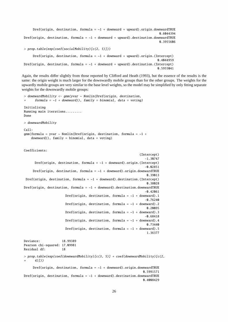
> prop.table(exp(coef(socialMobility)[c(2, 5)]))
Dref(origin, destination, formula = ~1 + downward + upward).origin.(Intercept)0.4044959
Dref(origin, destination, formula = ~1 + downward + upward).destination.(Intercept)0.5955041
Again, the results differ slightly from those reported by Clifford and Heath (1993), but the essence of the results is thesame: the origin weight is much larger for the downwardly mobile groups than for the other groups. The weights for theupwardly mobile groups are very similar to the base level weights, so the model may be simplified by only fitting separateweights for the downwardly mobile groups:
> downwardMobility <- gnm(yvar ~ Nonlin(Dref(origin, destination,+ formula = ~1 + downward)), family = binomial, data = voting)
InitialisingRunning main iterations.........Done
> downwardMobility
Call:gnm(formula = yvar ~ Nonlin(Dref(origin, destination, formula = ~1 +
downward)), family = binomial, data = voting)
Coefficients:(Intercept)-1.30747
Dref(origin, destination, formula = ~1 + downward).origin.(Intercept)-0.02851
Dref(origin, destination, formula = ~1 + downward).origin.downwardTRUE0.39013
Dref(origin, destination, formula = ~1 + downward).destination.(Intercept)0.38028
Dref(origin, destination, formula = ~1 + downward).destination.downwardTRUE-0.42061
Dref(origin, destination, formula = ~1 + downward).1-0.76240
Dref(origin, destination, formula = ~1 + downward).20.20095
Dref(origin, destination, formula = ~1 + downward).3-0.68418
Dref(origin, destination, formula = ~1 + downward).40.73440
Dref(origin, destination, formula = ~1 + downward).51.36377
Deviance: 18.99389Pearson chi-squared: 17.09981Residual df: 18
> prop.table(exp(coef(downwardMobility)[c(3, 5)] + coef(downwardMobility)[c(2,+ 4)]))
Dref(origin, destination, formula = ~1 + downward).origin.downwardTRUE0.5991571
Dref(origin, destination, formula = ~1 + downward).destination.downwardTRUE0.4008429
26

> prop.table(exp(coef(downwardMobility)[c(2, 4)]))
Dref(origin, destination, formula = ~1 + downward).origin.(Intercept)0.3992031
Dref(origin, destination, formula = ~1 + downward).destination.(Intercept)0.6007969
Dref example 2: Conformity to parental rules
Another application of diagonal reference models is given by van der Slik et al. (2002). The data from this paper are notpublicly available4, but we shall show how the models presented in the paper may be estimated usinggnm .
The data relate to the value parents place on their children conforming to their rules. There are two response variables:the mother’s conformity score (MCFM) and the father’s conformity score (FCFF). The data are cross-classified by twofactors describing the education level of the mother (MOPLM) and the father (FOPLF), and there are six further covariates(AGEM, MRMM, FRMF, MWORK, MFCM and FFCF).
In their baseline model for the mother’s conformity score, van der Slik et al. (2002) include five of the six covariates(leaving out the father’s family conflict score, FCFF) and a diagonal reference term with constant weights based on thetwo education factors. This model may be expressed as
µrc = β1x1 + β2x2 + β3x3 + β4x4 + β5x5 +eδ1
eδ1 + eδ2γr +
eδ2
eδ1 + eδ2γc.
The baseline model can be fitted as follows:
> set.seed(1)> A <- gnm(MCFM ~ -1 + AGEM + MRMM + FRMF + MWORK + MFCM ++ Nonlin(Dref(MOPLM, FOPLF)), family = gaussian, data = conformity,+ verbose = FALSE)> A
Call:gnm(formula = MCFM ~ -1 + AGEM + MRMM + FRMF + MWORK + MFCM +
Nonlin(Dref(MOPLM, FOPLF)), family = gaussian, data = conformity,verbose = FALSE)
Coefficients:AGEM MRMM FRMF
0.06364 -0.32425 -0.25324MWORK MFCM Dref(MOPLM, FOPLF).MOPLM
-0.06430 -0.06043 -0.33730Dref(MOPLM, FOPLF).FOPLF Dref(MOPLM, FOPLF).1 Dref(MOPLM, FOPLF).2
-0.02507 4.95123 4.86328Dref(MOPLM, FOPLF).3 Dref(MOPLM, FOPLF).4 Dref(MOPLM, FOPLF).5
4.86458 4.72343 4.43516Dref(MOPLM, FOPLF).6 Dref(MOPLM, FOPLF).7
4.18873 4.43379
Deviance: 425.3389Pearson chi-squared: 425.3389Residual df: 576
The coefficients of the covariates are not aliased with the parameters of the diagonal reference term and thus the basicidentifiability constraints that have been imposed are sufficient for these parameters to be identified. The diagonal effectsdo not need to be constrained as they represent contrasts with the off-diagonal cells. Therefore the only unidentifiedparameters in this model are the weight parameters. This is confirmed in the summary of the model:
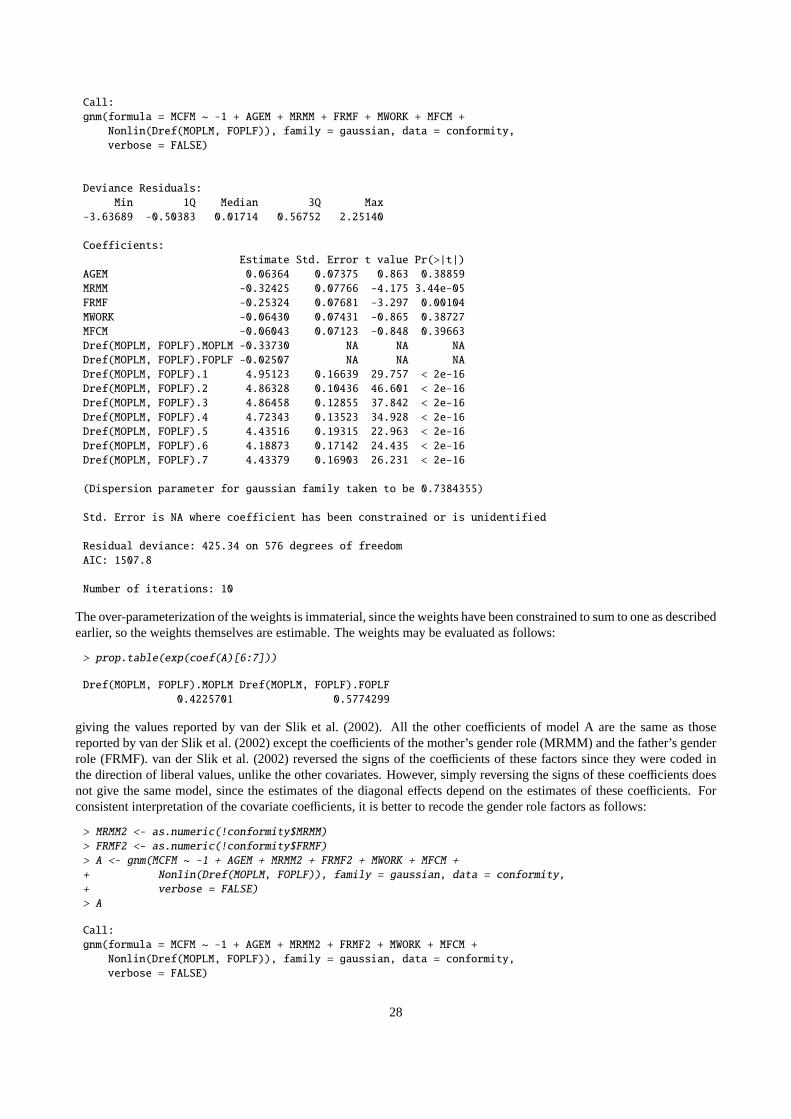
> summary(A)
4 We thank Frans van der Slik for his kindness in sending us the data.
27
Call:gnm(formula = MCFM ~ -1 + AGEM + MRMM + FRMF + MWORK + MFCM +
Nonlin(Dref(MOPLM, FOPLF)), family = gaussian, data = conformity,verbose = FALSE)
Deviance Residuals:Min 1Q Median 3Q Max
-3.63689 -0.50383 0.01714 0.56752 2.25140
Coefficients:Estimate Std. Error t value Pr(>|t|)
AGEM 0.06364 0.07375 0.863 0.38859MRMM -0.32425 0.07766 -4.175 3.44e-05FRMF -0.25324 0.07681 -3.297 0.00104MWORK -0.06430 0.07431 -0.865 0.38727MFCM -0.06043 0.07123 -0.848 0.39663Dref(MOPLM, FOPLF).MOPLM -0.33730 NA NA NADref(MOPLM, FOPLF).FOPLF -0.02507 NA NA NADref(MOPLM, FOPLF).1 4.95123 0.16639 29.757 < 2e-16Dref(MOPLM, FOPLF).2 4.86328 0.10436 46.601 < 2e-16Dref(MOPLM, FOPLF).3 4.86458 0.12855 37.842 < 2e-16Dref(MOPLM, FOPLF).4 4.72343 0.13523 34.928 < 2e-16Dref(MOPLM, FOPLF).5 4.43516 0.19315 22.963 < 2e-16Dref(MOPLM, FOPLF).6 4.18873 0.17142 24.435 < 2e-16Dref(MOPLM, FOPLF).7 4.43379 0.16903 26.231 < 2e-16
(Dispersion parameter for gaussian family taken to be 0.7384355)
Std. Error is NA where coefficient has been constrained or is unidentified
Residual deviance: 425.34 on 576 degrees of freedomAIC: 1507.8
Number of iterations: 10
The over-parameterization of the weights is immaterial, since the weights have been constrained to sum to one as describedearlier, so the weights themselves are estimable. The weights may be evaluated as follows:
> prop.table(exp(coef(A)[6:7]))
Dref(MOPLM, FOPLF).MOPLM Dref(MOPLM, FOPLF).FOPLF0.4225701 0.5774299
giving the values reported by van der Slik et al. (2002). All the other coefficients of model A are the same as thosereported by van der Slik et al. (2002) except the coefficients of the mother’s gender role (MRMM) and the father’s genderrole (FRMF). van der Slik et al. (2002) reversed the signs of the coefficients of these factors since they were coded inthe direction of liberal values, unlike the other covariates. However, simply reversing the signs of these coefficients doesnot give the same model, since the estimates of the diagonal effects depend on the estimates of these coefficients. Forconsistent interpretation of the covariate coefficients, it is better to recode the gender role factors as follows:
> MRMM2 <- as.numeric(!conformity$MRMM)> FRMF2 <- as.numeric(!conformity$FRMF)> A <- gnm(MCFM ~ -1 + AGEM + MRMM2 + FRMF2 + MWORK + MFCM ++ Nonlin(Dref(MOPLM, FOPLF)), family = gaussian, data = conformity,+ verbose = FALSE)> A
Call:gnm(formula = MCFM ~ -1 + AGEM + MRMM2 + FRMF2 + MWORK + MFCM +
Nonlin(Dref(MOPLM, FOPLF)), family = gaussian, data = conformity,verbose = FALSE)
28

Coefficients:AGEM MRMM2 FRMF2
0.06364 0.32425 0.25324MWORK MFCM Dref(MOPLM, FOPLF).MOPLM
-0.06430 -0.06043 -0.08270Dref(MOPLM, FOPLF).FOPLF Dref(MOPLM, FOPLF).1 Dref(MOPLM, FOPLF).2
0.22955 4.37372 4.28579Dref(MOPLM, FOPLF).3 Dref(MOPLM, FOPLF).4 Dref(MOPLM, FOPLF).5
4.28708 4.14593 3.85766Dref(MOPLM, FOPLF).6 Dref(MOPLM, FOPLF).7
3.61123 3.85629
Deviance: 425.3389Pearson chi-squared: 425.3389Residual df: 576
The coefficients of the covariates are now as reported by van der Slik et al. (2002), but the diagonal effects have beenadjusted appropriately.
van der Slik et al. (2002) compare the baseline model for the mother’s conformity score to several other models inwhich the weights in the diagonal reference term are dependent on one of the covariates. One particular model theyconsider incorporates an interaction of the weights with the mother’s conflict score as follows:
µrc = β1x1 + β2x2 + β3x3 + β4x4 + β5x5 +eξ1+β1x
eξ1+β1x + eξ2+β2xγr +
eξ2+β2x
eξ1+β1x + eξ2+β2xγc.
This model can be fitted as below, using the original coding for the gender role factors for ease of comparison to theresults reported by van der Slik et al. (2002),
> F <- gnm(MCFM ~ -1 + AGEM + MRMM + FRMF + MWORK + MFCM ++ Nonlin(Dref(MOPLM, FOPLF, formula = ~ 1 + MFCM)), family = gaussian,+ data = conformity, verbose = FALSE)> F
Call:gnm(formula = MCFM ~ -1 + AGEM + MRMM + FRMF + MWORK + MFCM +
Nonlin(Dref(MOPLM, FOPLF, formula = ~1 + MFCM)), family = gaussian,data = conformity, verbose = FALSE)
Coefficients:AGEM
0.05818MRMM
-0.32701FRMF
-0.25772MWORK
-0.07847MFCM
-0.01694Dref(MOPLM, FOPLF, formula = ~1 + MFCM).MOPLM.(Intercept)
0.79413Dref(MOPLM, FOPLF, formula = ~1 + MFCM).MOPLM.MFCM
-2.51751Dref(MOPLM, FOPLF, formula = ~1 + MFCM).FOPLF.(Intercept)
-0.27618Dref(MOPLM, FOPLF, formula = ~1 + MFCM).FOPLF.MFCM
2.03673Dref(MOPLM, FOPLF, formula = ~1 + MFCM).1
4.82477
29
Dref(MOPLM, FOPLF, formula = ~1 + MFCM).24.88066
Dref(MOPLM, FOPLF, formula = ~1 + MFCM).34.83969
Dref(MOPLM, FOPLF, formula = ~1 + MFCM).44.74849
Dref(MOPLM, FOPLF, formula = ~1 + MFCM).54.42019
Dref(MOPLM, FOPLF, formula = ~1 + MFCM).64.17956
Dref(MOPLM, FOPLF, formula = ~1 + MFCM).74.40819
Deviance: 420.9022Pearson chi-squared: 420.9022Residual df: 575
In this case there are two sets of weights, one for when the mother’s conflict score is less than average (coded as zero) andone for when the score is greater than average (coded as one). These can be evaluated as follows:
> prop.table(exp(coef(F))[c(6,8)])
Dref(MOPLM, FOPLF, formula = ~1 + MFCM).MOPLM.(Intercept)0.7446574
Dref(MOPLM, FOPLF, formula = ~1 + MFCM).FOPLF.(Intercept)0.2553426
> prop.table(exp(coef(F)[c(7,9)] + coef(F)[c(6,8)]))
Dref(MOPLM, FOPLF, formula = ~1 + MFCM).MOPLM.MFCM0.02977308
Dref(MOPLM, FOPLF, formula = ~1 + MFCM).FOPLF.MFCM0.97022692
giving the same weights as in Table 4 of van der Slik et al. (2002).
6.3 Uniform Difference (UNIDIFF) Models
Uniform difference models (Xie, 1992; Erikson and Goldthorpe, 1992) use a simplified three-way interaction to providean interpretable model of contingency tables classified by three or more variables. For example, the uniform differencemodel for a three-way contingency table, also known as the UNIDIFF model, is given by
µi jk = αik + β jk + exp(δk)γi j .
Theγi j represent a pattern of association that varies in strength over the dimension indexed byk, and exp(δk) representsthe relative strength of that association at levelk.
This model can be applied to theyaish data set (Yaish, 1998, 2004), which is a contingency table cross-classified byfather’s social class (orig), son’s social class (dest) and son’s education level (educ). In this case, we can consider theimportance of the association between the social class of father and son across the education levels. We omit the sub-tablewhich corresponds to level 7 ofdest, because its information content is negligible:
> set.seed(1)> data(yaish)> unidiff <- gnm(Freq ~ educ * orig + educ * dest + Mult(Exp(-1 ++ educ), -1 + orig:dest), ofInterest = "Mult1.Factor1", family = poisson,+ data = yaish, subset = (dest != 7))
InitialisingRunning start-up iterations..Running main iterations.............................................Done
30

> coef(unidiff)
Coefficients of interest:Mult1.Factor1.educ1 Mult1.Factor1.educ2 Mult1.Factor1.educ3 Mult1.Factor1.educ4
-0.8242673 -1.0496391 -1.5676909 -1.8632059Mult1.Factor1.educ5
-3.0737699
TheofInterest component has been set to index the multipliers of the association between the social class of fatherand son. We can contrast each multiplier to that of the lowest education level and obtain the standard errors for theseparameters as follows:
> getContrasts(unidiff, ofInterest(unidiff))
estimate SE quasiSE quasiVarMult1.Factor1.educ1 0.0000000 0.0000000 0.09757438 0.00952076Mult1.Factor1.educ2 -0.2253718 0.1611874 0.12885847 0.01660450Mult1.Factor1.educ3 -0.7434236 0.2335083 0.21182123 0.04486823Mult1.Factor1.educ4 -1.0389386 0.3434256 0.32609379 0.10633716Mult1.Factor1.educ5 -2.2495026 0.9453763 0.93560641 0.87535936
Four-way contingency tables may sometimes be described by a “double UNIDIFF” model
µi jkl = αil + β jkl + exp(δl)γi j + exp(φl)θik,
where the strengths of two, two-way associations with a common variable are estimated across the levels of the fourthvariable. Thecautres data set, from Cautres et al. (1998), can be used to illustrate the application of the double UNIDIFFmodel. This data set is classified by the variables vote, class, religion and election. Using a double UNIDIFF model, wecan see how the association between class and vote, and the association between religion and vote, differ between themost recent election and the other elections:
> set.seed(1)> data(cautres)> doubleUnidiff <- gnm(Freq ~ election * vote + election * class *+ religion + Mult(Exp(-1 + election), religion:vote) + Mult(Exp(-1 ++ election), class:vote), family = poisson, data = cautres)
InitialisingRunning start-up iterations..Running main iterations..........Done
> getContrasts(doubleUnidiff, rev(pickCoef(doubleUnidiff, "Mult1.Factor1")))
estimate SE quasiSE quasiVarMult1.Factor1.election4 0.00000000 0.00000000 0.07168290 0.005138439Mult1.Factor1.election3 0.06682585 0.09906916 0.06812239 0.004640660Mult1.Factor1.election2 0.24052778 0.09116479 0.05702819 0.003252214Mult1.Factor1.election1 0.32834588 0.12213023 0.09803075 0.009610029
> getContrasts(doubleUnidiff, rev(pickCoef(doubleUnidiff, "Mult2.Factor1")))
estimate SE quasiSE quasiVarMult2.Factor1.election4 0.00000000 0.0000000 0.10934798 0.011956980Mult2.Factor1.election3 0.08754435 0.1446833 0.09475938 0.008979340Mult2.Factor1.election2 0.31990726 0.1320022 0.07395886 0.005469913Mult2.Factor1.election1 -0.36183013 0.2534754 0.22854400 0.052232362
31

6.4 Generalized Additive Main Effects and Multiplicative Interaction (GAMMI) Models
Generalized additive main effects and multiplicative interaction models, or GAMMI models, were motivated by two-waycontingency tables and comprise the row and column main effects plus one or more components of the multiplicativeinteraction. The singular value corresponding to each multiplicative component is often factored out, as a measure of thestrength of association between the row and column scores, indicating the importance of the component, or axis.
For cell meansµrc a GAMMI-K model has the form
g(µrc) = αr + βc +
K∑k=1
σkγkrδkc,
in which g is a link function,αr andβc are the row and column main effects,γkr andδkc are the row and column scoresfor multiplicative componentk andσk is the singular value for componentk. The number of multiplicative components,K, is less than or equal to the rank of the matrix of residuals from the main effects.
The row-column association models discussed in Section 6.1 are examples of GAMMI models, with a log link andpoisson variance. Here we illustrate the use of an AMMI model, which is a GAMMI model with an identity link and aconstant variance.
We shall use thewheat data set taken from Vargas et al. (2001), which gives wheat yields measured over ten years.First we scale these yields and create a new treatment factor, so that we can reproduce the analysis of Vargas et al. (2001):
> set.seed(1)> data(wheat)> yield.scaled <- wheat$yield * sqrt(3/1000)> treatment <- interaction(wheat$tillage, wheat$summerCrop, wheat$manure,+ wheat$N, sep = "")
Now we can fit the AMMI-1 model, to the scaled yields using the combined treatment factor and the year factor fromthewheat dataset. We will proceed by first fitting the main effects model, then usingresidSVD (see Section 5.5) for theparameters of the multiplicative term:
> mainEffects <- gnm(yield.scaled ~ year + treatment, family = gaussian,+ data = wheat)
Linear predictor - using glm.fit
> svdStart <- residSVD(mainEffects, year, treatment, 3)> bilinear1 <- update(mainEffects, . ~ . + Mult(year - 1, treatment -+ 1), start = c(coef(mainEffects), svdStart[, 1]))
Running main iterationsDone
We can compare the AMMI-1 model to the main effects model,
> anova(mainEffects, bilinear1)
Analysis of Deviance Table
Model 1: yield.scaled ~ year + treatmentModel 2: yield.scaled ~ year + treatment + Mult(year - 1, treatment -
1)Resid. Df Resid. Dev Df Deviance
1 207 2795152 176 128383 31 151133
giving the same results as in Table 1 of Vargas et al. (2001) (up to error caused by rounding).
32
6.5 Biplot Models
Biplots are used to display two-dimensional data transformed into a space spanned by linearly independent vectors, suchas the principal components or singular vectors. The plot represents the levels of the two classifying factors by their scoreson the two axes which show the most information about the data, for example the first two principal components.
A rank-n model is a model based on the firstn components of the decomposition. In the case of a singular valuedecomposition, this is equivalent to a model withn components of the multiplicative interaction.
To illustrate the use of biplot models, we shall use thebarley data set which describes the incidence of leaf blotchover ten varieties of barley grown at nine sites (Wedderburn, 1974; Gabriel, 1998). The biplot model is fitted as follows:
> data(barley)> set.seed(1)> biplotModel <- gnm(y ~ -1 + Mult(site, variety, multiplicity = 2),+ family = wedderburn, data = barley)
InitialisingRunning start-up iterations..Running main iterations...................................................................................................................................Done
using thewedderburn family function introduced in Section 2. Matrices of the row and column scores for the first twosingular vectors can then be obtained by:
> barleySVD <- svd(matrix(biplotModel$predictors, 10, 9))> A <- sweep(barleySVD$v, 2, sqrt(barleySVD$d), "*")[, 1:2]> B <- sweep(barleySVD$u, 2, sqrt(barleySVD$d), "*")[, 1:2]> A
[,1] [,2][1,] 4.1948212 -0.39186806[2,] 2.7642419 -0.33951298[3,] 1.4250456 -0.04654256[4,] 1.8463067 0.33365981[5,] 1.2704091 0.15776743[6,] 1.1562916 0.40048225[7,] 1.0172048 0.72727990[8,] 0.6451366 1.46162702[9,] -0.1470898 2.13234195
> B
[,1] [,2][1,] -2.0673655 -0.97420449[2,] -3.0599788 -0.50683009[3,] -2.9598021 -0.33190618[4,] -1.8086251 -0.49758487[5,] -1.5579480 -0.08444513[6,] -1.8939998 1.08460534[7,] -1.1790432 0.40687015[8,] -0.8490092 1.14671353[9,] -0.9704664 1.26558193[10,] -0.6036790 1.39655898
These matrices are essentially the same as in Gabriel (1998). From these the biplot can be produced, for sitesA . . . I andvarieties 1. . . 9,X:
> plot(rbind(A, B), pch = c(levels(barley$site), levels(barley$variety)),+ xlim = c(-4, 4), ylim = c(-4, 4), main = "Biplot for barley data")
33
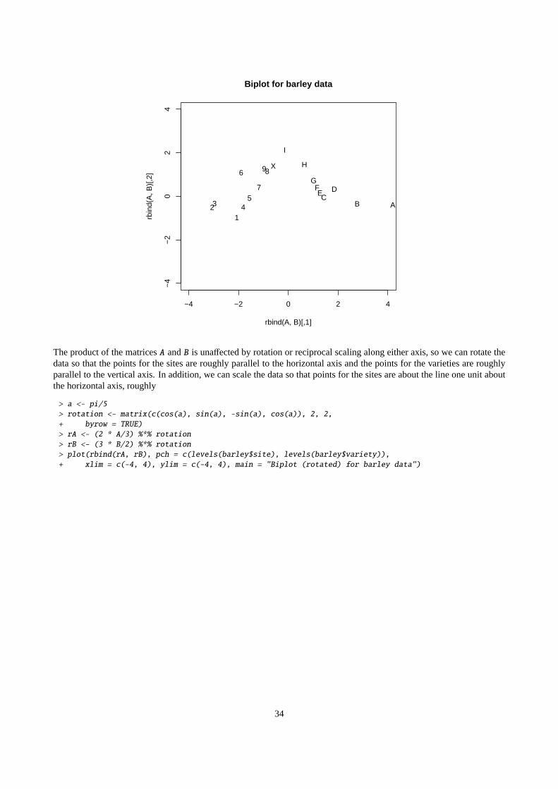
ABC
DEF
G
H
I
123 4
5
6
7
89X
−4 −2 0 2 4
−4
−2
02
4
Biplot for barley data
rbind(A, B)[,1]
rbin
d(A
, B)[
,2]
The product of the matricesA andB is unaffected by rotation or reciprocal scaling along either axis, so we can rotate thedata so that the points for the sites are roughly parallel to the horizontal axis and the points for the varieties are roughlyparallel to the vertical axis. In addition, we can scale the data so that points for the sites are about the line one unit aboutthe horizontal axis, roughly
> a <- pi/5> rotation <- matrix(c(cos(a), sin(a), -sin(a), cos(a)), 2, 2,+ byrow = TRUE)> rA <- (2 * A/3) %*% rotation> rB <- (3 * B/2) %*% rotation> plot(rbind(rA, rB), pch = c(levels(barley$site), levels(barley$variety)),+ xlim = c(-4, 4), ylim = c(-4, 4), main = "Biplot (rotated) for barley data")
34

A
BCD
EFGHI
123
4
5
6 7
89X
−4 −2 0 2 4
−4
−2
02
4
Biplot (rotated) for barley data
rbind(rA, rB)[,1]
rbin
d(rA
, rB
)[,2
]
In the original biplot, the co-ordinates for the sites and varieties were given by the rows of A and B respectively, i.e
αTi =
√(d)(u1i ,u2i)
βTj =
√(d)(v1 j , v2 j)
The rotated and scaled biplot suggests the simpler model
αTi = (γi ,1)
βTj = (δ j , τ j)
which implies the following model for the logits of the leaf blotch incidence:
αTi β j = γiδ j + τ j .
Gabriel (1998) describes this as a double additive model, which we can fit as follows:
> variety.binary <- factor(match(barley$variety, c(2, 3, 6), nomatch = 0) >+ 0, labels = c("rest", "2,3,6"))> doubleAdditive <- gnm(y ~ variety + Mult(site, variety.binary),+ family = wedderburn, data = barley)
InitialisingRunning start-up iterations..Running main iterations...........................Done
Comparing the chi-squared statistics, we see that the double additive model is an adequate model for the leaf blotchincidence:
> biplotModChiSq <- sum(residuals(biplotModel, type = "pearson")^2)> doubleAddChiSq <- sum(residuals(doubleAdditive, type = "pearson")^2)> c(doubleAddChiSq - biplotModChiSq, doubleAdditive$df.residual -+ biplotModel$df.residual)
[1] 9.513782 15.000000
35

6.6 Stereotype Model
The stereotype model was proposed by Anderson (1984) for ordered categorical data. It is a linear logistic model, inwhich there is assumed to be a common relationship between the response and the covariates in the model, but the scaleof this association varies between categories and there is an additional category main effect or category-specific intercept:
logµic = β0c + γc
∑r
βr xir .
This model can be estimated by re-expressing the categorical data as counts and using agnmmodel with a log link andpoisson variance function. Thegnm package includes the utility functionexpandCategorical to facilitate the requireddata processing.
For example, thebackPain data set from Anderson (1984) describes the progress of patients with back pain. Thedata set consists of an ordered factor quantifying the progress of each patient, and three prognostic variables. These datacan be re-expressed as follows:
> set.seed(1)> data(backPain)> backPain[1:2, ]
x1 x2 x3 pain1 1 1 1 same2 1 1 1 marked.improvement
> backPainLong <- expandCategorical(backPain, "pain")> backPainLong[1:12, ]
x1 x2 x3 pain count id1 1 1 1 worse 0 11.1 1 1 1 same 1 11.2 1 1 1 slight.improvement 0 11.3 1 1 1 moderate.improvement 0 11.4 1 1 1 marked.improvement 0 11.5 1 1 1 complete.relief 0 12 1 1 1 worse 0 22.1 1 1 1 same 0 22.2 1 1 1 slight.improvement 0 22.3 1 1 1 moderate.improvement 0 22.4 1 1 1 marked.improvement 1 22.5 1 1 1 complete.relief 0 2
We can now fit the stereotype model to these data:
> oneDimensional <- gnm(count ~ pain + Mult(pain - 1, x1 + x2 ++ x3 - 1), eliminate = id, family = "poisson", data = backPainLong)
InitialisingRunning start-up iterations..Running main iterations................Done
> oneDimensional
Call:gnm(formula = count ~ pain + Mult(pain - 1, x1 + x2 + x3 - 1),
eliminate = id, family = "poisson", data = backPainLong)
Coefficients of interest:painsame painslight.improvement16.1578 15.6848
painmoderate.improvement painmarked.improvement12.4556 19.9140
36
paincomplete.relief Mult1.Factor1.painworse21.6653 -0.3351
Mult1.Factor1.painsame Mult1.Factor1.painslight.improvement1.9154 1.7941
Mult1.Factor1.painmoderate.improvement Mult1.Factor1.painmarked.improvement1.2622 2.4625
Mult1.Factor1.paincomplete.relief Mult1.Factor2.x12.9238 -1.6484
Mult1.Factor2.x2 Mult1.Factor2.x3-0.9455 -0.8324
Deviance: 303.1003Pearson chi-squared: 433.3727Residual df: 493
specifying theid factor througheliminate so that the 101id effects are estimated more efficiently and are excludedfrom printed model summaries by default. This model is one dimensional since it involves only one function ofx =(x1, x2, x3). We can compare this model to one with category-specific coefficents of thex variables, as may be used for aqualitative categorical response:
> threeDimensional <- gnm(count ~ pain + pain:(x1 + x2 + x3), eliminate = id,+ family = "poisson", data = backPainLong)
InitialisingRunning main iterations..........Done
> threeDimensional
Call:gnm(formula = count ~ pain + pain:(x1 + x2 + x3), eliminate = id,
family = "poisson", data = backPainLong)
Coefficients of interest:painsame painslight.improvement36.0994 35.7186
painmoderate.improvement painmarked.improvement32.6011 39.8017
paincomplete.relief painworse:x142.2498 10.6708
painsame:x1 painslight.improvement:x1-2.8855 -2.5559
painmoderate.improvement:x1 painmarked.improvement:x1-2.2924 -4.1156
paincomplete.relief:x1 painworse:x2-4.6275 0.4189
painsame:x2 painslight.improvement:x2-2.2551 -2.1325
painmoderate.improvement:x2 painmarked.improvement:x2-1.2531 -2.4249
paincomplete.relief:x2 painworse:x3-2.8561 -1.7476
painsame:x3 painslight.improvement:x3-2.9031 -3.0397
painmoderate.improvement:x3 painmarked.improvement:x3-2.4938 -3.4391
paincomplete.relief:x3-4.6883
Deviance: 299.0152Pearson chi-squared: 443.0043Residual df: 485
37

This model has the maximum dimensionality of three (as determined by the number of covariates). To obtain the log-likelihoods as reported in Anderson (1984) we need to adjust for the extra parameters introduced to formulate the modelsas Poisson models. We write a simple function to do this and compare the log-likelihoods of the one dimensional modeland the three dimensional model:
> logLikMultinom <- function(model) {+ object <- get(model)+ if (inherits(object, "gnm")) {+ l <- logLik(object) + object$eliminate+ c(nParameters = attr(l, "df") - object$eliminate, logLikelihood = l)+ }+ else c(nParameters = object$edf, logLikelihood = -deviance(object)/2)+ }> t(sapply(c("oneDimensional", "threeDimensional"), logLikMultinom))
nParameters logLikelihoodoneDimensional 12 -151.5501threeDimensional 20 -149.5076
which show that theoneDimensional model is adequate.To obtain estimates of the category-specific multipliers in the stereotype model, we need to constrain both the location
and the scale of these parameters. The latter constraint can be imposed by fixing the slope of one of the covariates in thesecond multiplier to1, which may be achieved by specifying the covariate as an offset:
> summary(oneDimensional)
Call:gnm(formula = count ~ pain + Mult(pain - 1, x1 + x2 + x3 - 1),
eliminate = id, family = "poisson", data = backPainLong)
Deviance Residuals:Min 1Q Median 3Q Max
-0.9708 -0.6506 -0.4438 -0.1448 2.1385
Coefficients of interest:Estimate Std. Error z value Pr(>|z|)
painsame 16.1578 NA NA NApainslight.improvement 15.6848 6.5274 2.403 0.01626 *painmoderate.improvement 12.4556 NA NA NApainmarked.improvement 19.9140 6.4976 3.065 0.00218 **paincomplete.relief 21.6653 NA NA NAMult1.Factor1.painworse -0.3351 NA NA NAMult1.Factor1.painsame 1.9154 NA NA NAMult1.Factor1.painslight.improvement 1.7941 NA NA NAMult1.Factor1.painmoderate.improvement 1.2622 NA NA NAMult1.Factor1.painmarked.improvement 2.4625 NA NA NAMult1.Factor1.paincomplete.relief 2.9238 NA NA NAMult1.Factor2.x1 -1.6484 NA NA NAMult1.Factor2.x2 -0.9455 NA NA NAMult1.Factor2.x3 -0.8324 NA NA NA---Signif. codes: 0 '***' 0.001 '**' 0.01 '*' 0.05 '.' 0.1 ' ' 1
(Dispersion parameter for poisson family taken to be 1)
Std. Error is NA where coefficient has been constrained or is unidentified
Residual deviance: 303.1 on 493 degrees of freedomAIC: 731.1
Number of iterations: 16
38

> oneDimensional <- gnm(count ~ pain + Mult(pain - 1, offset(x1) ++ x2 + x3 - 1), eliminate = id, family = "poisson", data = backPainLong)
InitialisingRunning start-up iterations..Running main iterations..............Done
> summary(oneDimensional)
Call:gnm(formula = count ~ pain + Mult(pain - 1, offset(x1) + x2 +
x3 - 1), eliminate = id, family = "poisson", data = backPainLong)
Deviance Residuals:Min 1Q Median 3Q Max
-0.9708 -0.6506 -0.4438 -0.1448 2.1385
Coefficients of interest:Estimate Std. Error z value Pr(>|z|)
painsame 16.1578 6.5741 2.458 0.013980 *painslight.improvement 15.6848 6.5274 2.403 0.016265 *painmoderate.improvement 12.4555 6.4312 1.937 0.052777 .painmarked.improvement 19.9140 6.4975 3.065 0.002178 **paincomplete.relief 21.6653 6.5571 3.304 0.000953 ***Mult1.Factor1.painworse 1.3694 NA NA NAMult1.Factor1.painsame -2.3404 NA NA NAMult1.Factor1.painslight.improvement -2.1403 NA NA NAMult1.Factor1.painmoderate.improvement -1.2636 NA NA NAMult1.Factor1.painmarked.improvement -3.2422 NA NA NAMult1.Factor1.paincomplete.relief -4.0025 NA NA NAMult1.Factor2.x2 0.5736 0.2178 2.633 0.008451 **Mult1.Factor2.x3 0.5050 0.2431 2.077 0.037807 *---Signif. codes: 0 '***' 0.001 '**' 0.01 '*' 0.05 '.' 0.1 ' ' 1
(Dispersion parameter for poisson family taken to be 1)
Std. Error is NA where coefficient has been constrained or is unidentified
Residual deviance: 303.1 on 493 degrees of freedomAIC: 731.1
Number of iterations: 14
The location of the category-specific multipliers can constrained by setting one of the parameters to zero, either throughtheconstrain argument ofgnm or with getContrasts:
> getContrasts(oneDimensional, pickCoef(oneDimensional, "Mult.*pain"))
estimate SE quasiSE quasiVarMult1.Factor1.painworse 0.000000 0.000000 1.7797287 3.1674342Mult1.Factor1.painsame -3.709725 1.825561 0.4281331 0.1832980Mult1.Factor1.painslight.improvement -3.509685 1.791725 0.4024680 0.1619805Mult1.Factor1.painmoderate.improvement -2.632931 1.669250 0.5518544 0.3045433Mult1.Factor1.painmarked.improvement -4.611584 1.895233 0.3133219 0.0981706Mult1.Factor1.paincomplete.relief -5.371842 1.999651 0.4919552 0.2420199
giving the required estimates.
39

A User-level Functions
We list here, for easy reference, all of the user-level functions in thegnm package. For full documentation see the packagehelp pages.
Model Fitting
gnm fit generalized nonlinear models
Model Specification
Diag create factor differentiating diagonal elementsSymm create symmetric interaction of factorsTopo create ‘topological’ interaction factorsMult specify a multiplicative interaction in agnm formulaExp specify an exponentiated constituent multiplier in aMult termNonlin specify a special nonlinear term in agnm formulaDref gnm plug-in function to fit diagonal reference termsMultHomog gnm plug-in function to fit multiplicative interactions with homogeneous effectswedderburn specify the Wedderburn quasi-likelihood family
Methods and Accessor Functions
confint.gnm compute confidence intervals ofgnmparameters based on the profiled devianceconfint.profile.gnm compute confidence intervals of parameters from aprofile.gnmobjectprofile.gnm profile deviance for parameters in agnmmodelplot.profile.gnm plot profile traces from aprofile.gnmobjectsummary.gnm summarizegnmfitsresidSVD multiplicative approximation of model residualsexitInfo print numerical details of last iteration whengnm has not convergedofInterest extract theofInterest component of agnmobjectofInterest<- replace theofInterest component of agnmobjectparameters get model parameters from agnm object, including parameters that were con-
strainedpickCoef get indices of model parametersgetContrasts estimate contrasts and their standard errors for parameters in agnmmodelcheckEstimable check whether one or more parameter combinations in agnmmodel is identifiedse get standard errors of linear parameter combinations ingnmmodelstermPredictors (generic) extract term contributions to predictor
Auxiliary Functions
asGnm coerce an object of classlm or glm to classgnmexpandCategorical expand a data frame by re-expressing categorical data as countsgetModelFrame get the model frame in use bygnmMPinv Moore-Penrose pseudoinverse of a real-valued matrixqrSolve Minimum-length solution of a linear system
40

References
Agresti, A. (2002).Categorical Data Analysis(2nd ed.). New York: Wiley.
Anderson, J. A. (1984). Regression and ordered categorical variables.J. R. Statist. Soc. B 46(1), 1–30.
Catchpole, E. and B. Morgan (1997). Detecting parameter redundancy.Biometrika 84, 187–196.
Cautres, B., A. F. Heath, and D. Firth (1998). Class, religion and vote in Britain and France.La Lettre de la MaisonFrançaise 8.
Clifford, P. and A. F. Heath (1993). The political consequences of social mobility.J. Roy. Stat. Soc. A 156(1), 51–61.
Erikson, R. and J. H. Goldthorpe (1992).The Constant Flux. Oxford: Clarendon Press.
Erikson, R., J. H. Goldthorpe, and L. Portocarero (1982). Social fluidity in industrial nations: England, France andSweden.British Journal of Sociology 33, 1–34.
Firth, D. (2003). Overcoming the reference category problem in the presentation of statistical models.SociologicalMethodology 33, 1–18.
Firth, D. and R. X. de Menezes (2004). Quasi-variances.Biometrika 91, 65–80.
Gabriel, K. R. (1998). Generalised bilinear regression.Biometrika 85, 689–700.
Goodman, L. A. (1979). Simple models for the analysis of association in cross-classifications having ordered categories.J. Amer. Statist. Assoc. 74, 537–552.
Hatzinger, R. and B. J. Francis (2004). Fitting paired comparison models in R. Technical Report 3, Department ofStatistics and Mathematics, Wirtschaftsuniversität Wien.
McCullagh, P. and J. A. Nelder (1989).Generalized Linear Models (Second Edition). Chapman & Hall Ltd.
Sobel, M. E. (1981). Diagonal mobility models: A substantively motivated class of designs for the analysis of mobilityeffects.Amer. Soc. Rev. 46, 893–906.
Sobel, M. E. (1985). Social mobility and fertility revisited: Some new models for the analysis of the mobility effectshypothesis.Amer. Soc. Rev. 50, 699–712.
van der Slik, F. W. P., N. D. de Graaf, and J. R. M. Gerris (2002, 4). Conformity to parental rules: Asymmetric influencesof father’s and mother’s levels of education.Europ. Soc. Rev. 18, 489–502.
Vargas, M., J. Crossa, F. van Eeuwijk, K. D. Sayre, and M. P. Reynolds (2001). Interpreting treatment by environmentinteraction in agronomy trials.Agronomy Journal 93, 949–960.
Wedderburn, R. W. M. (1974). Quasi-likelihood functions, generalized linear models, and the Gauss-Newton method.Biometrika 61, 439–447.
Xie, Y. (1992). The log-multiplicative layer effect model for comparing mobility tables.American Sociological Review 57,380–395.
Yaish, M. (1998). Opportunities, Little Change. Class Mobility in Israeli Society, 1974–1991. Ph. D. thesis, NuffieldCollege, University of Oxford.
Yaish, M. (2004).Class Mobility Trends in Israeli Society, 1974-1991. Lewiston: Edwin Mellen Press.
41