Generalized nonlinear models in R: An overview of the...
53
Generalized nonlinear models in R: An overview of the gnm package Heather Turner and David Firth * University of Warwick, UK For gnm version 0.9-3 , 2007-09-10 Contents 1 Introduction 2 2 Generalized linear models 2 2.1 Preamble .......................................................... 2 2.2 Diag and Symm ....................................................... 2 2.3 Topo ............................................................. 3 2.4 The wedderburn family .................................................. 4 2.5 termPredictors ...................................................... 5 2.6 Const ............................................................ 5 3 Nonlinear terms 6 3.1 Basic mathematical functions of predictors ......................................... 6 3.2 MultHomog ......................................................... 7 3.3 Dref ............................................................ 7 3.4 instances ......................................................... 8 3.5 Custom nonlin functions .................................................. 8 3.5.1 General description ................................................. 8 3.5.2 Example: a logistic function ............................................ 9 3.5.3 Example: MultHomog ............................................... 9 3.6 Using custom plug-ins to fit nonlinear terms ........................................ 10 4 Controlling the fitting procedure 10 4.1 Basic control parameters .................................................. 10 4.2 Using start ........................................................ 10 4.3 Using constrain ...................................................... 11 4.4 Using eliminate ...................................................... 13 5 Methods and accessor functions 15 5.1 Methods ........................................................... 15 5.2 ofInterest and pickCoef ................................................ 17 5.3 checkEstimable ...................................................... 18 5.4 getContrasts, se ..................................................... 19 5.5 residSVD .......................................................... 19 6 gnm or (g)nls? 20 7 Examples 21 7.1 Row-column association models .............................................. 21 7.1.1 RC(1) model .................................................... 22 7.1.2 RC(2) model .................................................... 23 7.1.3 Homogeneous effects ................................................ 24 7.2 Diagonal reference models ................................................. 25 7.3 Uniform difference (UNIDIFF) models ........................................... 32 * This work was supported by the Economic and Social Research Council (UK) through Professorial Fellowship RES-051-27-0055. 1
Transcript of Generalized nonlinear models in R: An overview of the...
Generalized nonlinear models in R: An overview of the gnm package
Heather Turner and David Firth∗
University of Warwick, UK
For gnm version 0.9-3 , 2007-09-10
Contents1 Introduction 2
2 Generalized linear models 22.1 Preamble . . . . . . . . . . . . . . . . . . . . . . . . . . . . . . . . . . . . . . . . . . . . . . . . . . . . . . . . . . 22.2 Diag and Symm . . . . . . . . . . . . . . . . . . . . . . . . . . . . . . . . . . . . . . . . . . . . . . . . . . . . . . . 22.3 Topo . . . . . . . . . . . . . . . . . . . . . . . . . . . . . . . . . . . . . . . . . . . . . . . . . . . . . . . . . . . . . 32.4 The wedderburn family . . . . . . . . . . . . . . . . . . . . . . . . . . . . . . . . . . . . . . . . . . . . . . . . . . 42.5 termPredictors . . . . . . . . . . . . . . . . . . . . . . . . . . . . . . . . . . . . . . . . . . . . . . . . . . . . . . 52.6 Const . . . . . . . . . . . . . . . . . . . . . . . . . . . . . . . . . . . . . . . . . . . . . . . . . . . . . . . . . . . . 5
3 Nonlinear terms 63.1 Basic mathematical functions of predictors . . . . . . . . . . . . . . . . . . . . . . . . . . . . . . . . . . . . . . . . . 63.2 MultHomog . . . . . . . . . . . . . . . . . . . . . . . . . . . . . . . . . . . . . . . . . . . . . . . . . . . . . . . . . 73.3 Dref . . . . . . . . . . . . . . . . . . . . . . . . . . . . . . . . . . . . . . . . . . . . . . . . . . . . . . . . . . . . 73.4 instances . . . . . . . . . . . . . . . . . . . . . . . . . . . . . . . . . . . . . . . . . . . . . . . . . . . . . . . . . 83.5 Custom nonlin functions . . . . . . . . . . . . . . . . . . . . . . . . . . . . . . . . . . . . . . . . . . . . . . . . . . 8
3.5.1 General description . . . . . . . . . . . . . . . . . . . . . . . . . . . . . . . . . . . . . . . . . . . . . . . . . 83.5.2 Example: a logistic function . . . . . . . . . . . . . . . . . . . . . . . . . . . . . . . . . . . . . . . . . . . . 93.5.3 Example: MultHomog . . . . . . . . . . . . . . . . . . . . . . . . . . . . . . . . . . . . . . . . . . . . . . . 9
3.6 Using custom plug-ins to fit nonlinear terms . . . . . . . . . . . . . . . . . . . . . . . . . . . . . . . . . . . . . . . . 10
4 Controlling the fitting procedure 104.1 Basic control parameters . . . . . . . . . . . . . . . . . . . . . . . . . . . . . . . . . . . . . . . . . . . . . . . . . . 104.2 Using start . . . . . . . . . . . . . . . . . . . . . . . . . . . . . . . . . . . . . . . . . . . . . . . . . . . . . . . . 104.3 Using constrain . . . . . . . . . . . . . . . . . . . . . . . . . . . . . . . . . . . . . . . . . . . . . . . . . . . . . . 114.4 Using eliminate . . . . . . . . . . . . . . . . . . . . . . . . . . . . . . . . . . . . . . . . . . . . . . . . . . . . . . 13
5 Methods and accessor functions 155.1 Methods . . . . . . . . . . . . . . . . . . . . . . . . . . . . . . . . . . . . . . . . . . . . . . . . . . . . . . . . . . . 155.2 ofInterest and pickCoef . . . . . . . . . . . . . . . . . . . . . . . . . . . . . . . . . . . . . . . . . . . . . . . . 175.3 checkEstimable . . . . . . . . . . . . . . . . . . . . . . . . . . . . . . . . . . . . . . . . . . . . . . . . . . . . . . 185.4 getContrasts, se . . . . . . . . . . . . . . . . . . . . . . . . . . . . . . . . . . . . . . . . . . . . . . . . . . . . . 195.5 residSVD . . . . . . . . . . . . . . . . . . . . . . . . . . . . . . . . . . . . . . . . . . . . . . . . . . . . . . . . . . 19
6 gnm or (g)nls? 20
7 Examples 217.1 Row-column association models . . . . . . . . . . . . . . . . . . . . . . . . . . . . . . . . . . . . . . . . . . . . . . 21
7.1.1 RC(1) model . . . . . . . . . . . . . . . . . . . . . . . . . . . . . . . . . . . . . . . . . . . . . . . . . . . . 227.1.2 RC(2) model . . . . . . . . . . . . . . . . . . . . . . . . . . . . . . . . . . . . . . . . . . . . . . . . . . . . 237.1.3 Homogeneous effects . . . . . . . . . . . . . . . . . . . . . . . . . . . . . . . . . . . . . . . . . . . . . . . . 24
7.2 Diagonal reference models . . . . . . . . . . . . . . . . . . . . . . . . . . . . . . . . . . . . . . . . . . . . . . . . . 257.3 Uniform difference (UNIDIFF) models . . . . . . . . . . . . . . . . . . . . . . . . . . . . . . . . . . . . . . . . . . . 32
∗This work was supported by the Economic and Social Research Council (UK) through Professorial Fellowship RES-051-27-0055.
1
7.4 Generalized additive main effects and multiplicative interaction (GAMMI) models . . . . . . . . . . . . . . . . . . . 347.5 Biplot models . . . . . . . . . . . . . . . . . . . . . . . . . . . . . . . . . . . . . . . . . . . . . . . . . . . . . . . . 357.6 Stereotype model for multinomial response . . . . . . . . . . . . . . . . . . . . . . . . . . . . . . . . . . . . . . . . 387.7 Lee-Carter model for trends in age-specific mortality . . . . . . . . . . . . . . . . . . . . . . . . . . . . . . . . . . . 437.8 Exponential and sum-of-exponentials models for decay curves . . . . . . . . . . . . . . . . . . . . . . . . . . . . . . 46
7.8.1 Example: single exponential decay term . . . . . . . . . . . . . . . . . . . . . . . . . . . . . . . . . . . . . . 477.8.2 Example: sum of two exponentials . . . . . . . . . . . . . . . . . . . . . . . . . . . . . . . . . . . . . . . . . 48
A User-level functions 51
1 IntroductionThe gnm package provides facilities for fitting generalized nonlinear models, i.e., regression models in which the link-transformed mean is described as a sum of predictor terms, some of which may be non-linear in the unknown parameters.Linear and generalized linear models, as handled by the lm and glm functions in R, are included in the class of generalizednonlinear models, as the special case in which there is no nonlinear term.
This document gives an extended overview of the gnm package, with some examples of applications. The primarypackage documentation in the form of standard help pages, as viewed in R by, for example, ?gnm or help(gnm), issupplemented rather than replaced by the present document.
We begin below with a preliminary note (Section 2) on some ways in which the gnm package extends R’s facilitiesfor specifying, fitting and working with generalized linear models. Then (Section 3 onwards) the facilities for nonlinearterms are introduced, explained and exemplified.
The gnm package is installed in the standard way for CRAN packages, for example by using install.packages.Once installed, the package is loaded into an R session by
> library(gnm)
2 Generalized linear models
2.1 PreambleCentral to the facilities provided by the gnm package is the model-fitting function gnm , which interprets a model formulaand returns a model object. The user interface of gnm is patterned after glm (which is included in R’s standard statspackage), and indeed gnm can be viewed as a replacement for glm for specifying and fitting generalized linear models.In general there is no reason to prefer gnm to glm for fitting generalized linear models, except perhaps when the modelinvolves a large number of incidental parameters which are treatable by gnm’s eliminate mechanism (see Section 4.4).
While the main purpose of the gnm package is to extend the class of models to include nonlinear terms, some of thenew functions and methods can be used also with the familiar lm and glm model-fitting functions. These are: three newdata-manipulation functions Diag, Symm and Topo, for setting up structured interactions between factors; a new familyfunction, wedderburn, for modelling a continuous response variable in [0, 1] with the variance function V(µ) = µ2(1−µ)2
as in Wedderburn (1974); and a new generic function termPredictors which extracts the contribution of each term tothe predictor from a fitted model object. These functions are briefly introduced here, before we move on to the mainpurpose of the package, nonlinear models, in Section 3.
2.2 Diag and SymmWhen dealing with homologous factors, that is, categorical variables whose levels are the same, statistical models ofteninvolve structured interaction terms which exploit the inherent symmetry. The functions Diag and Symm facilitate thespecification of such structured interactions.
As a simple example of their use, consider the log-linear models of quasi-independence, quasi-symmetry and symmetryfor a square contingency table. Agresti (2002), Section 10.4, gives data on migration between regions of the USA between1980 and 1985:
> count <- c(11607, 100, 366, 124, 87, 13677, 515, 302, 172, 225,+ 17819, 270, 63, 176, 286, 10192)> region <- c("NE", "MW", "S", "W")
2
> row <- gl(4, 4, labels = region)> col <- gl(4, 1, length = 16, labels = region)
The comparison of models reported by Agresti can be achieved as follows:
> independence <- glm(count ~ row + col, family = poisson)> quasi.indep <- glm(count ~ row + col + Diag(row, col), family = poisson)> symmetry <- glm(count ~ Symm(row, col), family = poisson)> quasi.symm <- glm(count ~ row + col + Symm(row, col), family = poisson)> comparison1 <- anova(independence, quasi.indep, quasi.symm)> print(comparison1, digits = 7)
Analysis of Deviance Table
Model 1: count ~ row + colModel 2: count ~ row + col + Diag(row, col)Model 3: count ~ row + col + Symm(row, col)Resid. Df Resid. Dev Df Deviance
1 9 125923.292 5 69.51 4 125853.783 3 2.99 2 66.52
> comparison2 <- anova(symmetry, quasi.symm)> print(comparison2)
Analysis of Deviance Table
Model 1: count ~ Symm(row, col)Model 2: count ~ row + col + Symm(row, col)Resid. Df Resid. Dev Df Deviance
1 6 243.5502 3 2.986 3 240.564
The Diag and Symm functions also generalize the notions of diagonal and symmetric interaction to cover situationsinvolving more than two homologous factors.
2.3 Topo
More general structured interactions than those provided by Diag and Symm can be specified using the function Topo.(The name of this function is short for ‘topological interaction’, which is the nomenclature often used in sociology forfactor interactions with structure derived from subject-matter theory.)
The Topo function operates on any number (k, say) of input factors, and requires an argument named spec whichmust be an array of dimension L1 × . . . × Lk, where Li is the number of levels for the ith factor. The spec argumentspecifies the interaction level corresponding to every possible combination of the input factors, and the result is a newfactor representing the specified interaction.
As an example, consider fitting the ‘log-multiplicative layer effects’ models described in Xie (1992). The data are 7by 7 versions of social mobility tables from Erikson et al. (1982):
> data(erikson)> erikson <- as.data.frame(erikson)> lvl <- levels(erikson$origin)> levels(erikson$origin) <- levels(erikson$destination) <- c(rep(paste(lvl[1:2],+ collapse = " + "), 2), lvl[3], rep(paste(lvl[4:5], collapse = " + "),+ 2), lvl[6:9])> erikson <- xtabs(Freq ~ origin + destination + country, data = erikson)
From sociological theory — for which see Erikson et al. (1982) or Xie (1992) — the log-linear interaction between originand destination is assumed to have a particular structure:
3
> levelMatrix <- matrix(c(2, 3, 4, 6, 5, 6, 6,+ 3, 3, 4, 6, 4, 5, 6,+ 4, 4, 2, 5, 5, 5, 5,+ 6, 6, 5, 1, 6, 5, 2,+ 4, 4, 5, 6, 3, 4, 5,+ 5, 4, 5, 5, 3, 3, 5,+ 6, 6, 5, 3, 5, 4, 1), 7, 7, byrow = TRUE)
The models of table 3 of Xie (1992) can now be fitted as follows:
> ### Fit the levels models given in Table 3 of Xie (1992)> ## Null association between origin and destination> nullModel <- gnm(Freq ~ country:origin + country:destination,+ family = poisson, data = erikson, verbose = FALSE)>> ## Interaction specified by levelMatrix, common to all countries> commonTopo <- update(nullModel, ~ . ++ Topo(origin, destination, spec = levelMatrix),+ verbose = FALSE)>> ## Interaction specified by levelMatrix, different multiplier for> ## each country> multTopo <- update(nullModel, ~ . ++ Mult(Exp(country), Topo(origin, destination, spec = levelMatrix)),+ verbose = FALSE)>> ## Interaction specified by levelMatrix, different effects for> ## each country> separateTopo <- update(nullModel, ~ . ++ country:Topo(origin, destination, spec = levelMatrix),+ verbose = FALSE)>> anova(nullModel, commonTopo, multTopo, separateTopo)
Analysis of Deviance Table
Model 1: Freq ~ country:origin + country:destinationModel 2: Freq ~ Topo(origin, destination, spec = levelMatrix) + country:origin +
country:destinationModel 3: Freq ~ Mult(country, Topo(origin, destination, spec = levelMatrix)) +
country:origin + country:destinationModel 4: Freq ~ country:origin + country:destination + country:Topo(origin,
destination, spec = levelMatrix)Resid. Df Resid. Dev Df Deviance
1 108 4860.02 103 244.3 5 4615.73 101 216.4 2 28.04 93 208.5 8 7.9
Here we have used gnm to fit all of these log-link models; the first, second and fourth are log-linear and could equally wellhave been fitted using glm .
2.4 The wedderburn familyIn Wedderburn (1974) it was suggested to represent the mean of a continuous response variable in [0, 1] using a quasi-likelihood model with logit link and the variance function µ2(1 − µ)2. This is not one of the variance functions madeavailable as standard in R’s quasi family. The wedderburn family provides it. As an example, Wedderburn’s analysisof data on leaf blotch on barley can be reproduced as follows:
> data(barley)> logitModel <- glm(y ~ site + variety, family = wedderburn, data = barley)> fit <- fitted(logitModel)> print(sum((barley$y - fit)^2/(fit * (1 - fit))^2))
4
[1] 71.17401
This agrees with the chi-squared value reported on page 331 of McCullagh and Nelder (1989), which differs slightly fromWedderburn’s own reported value.
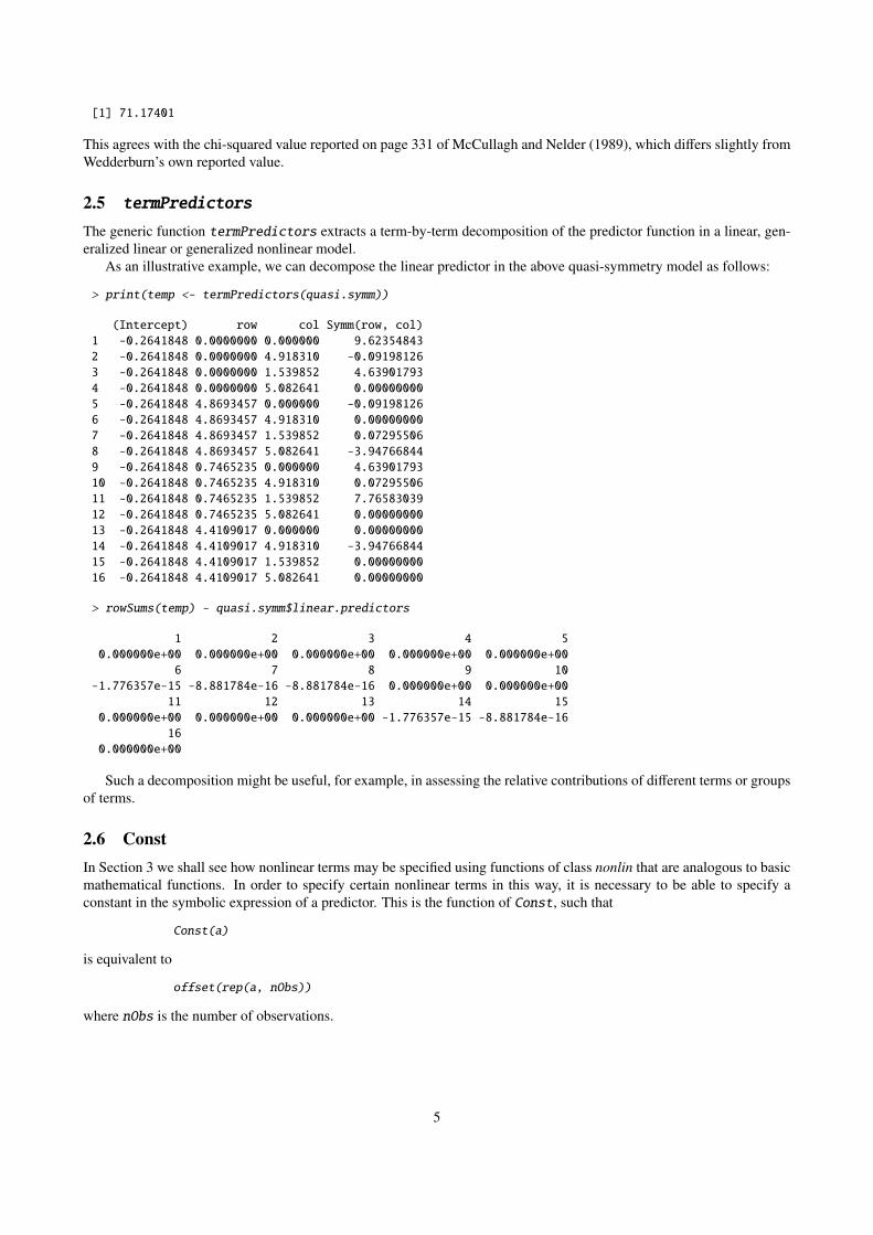
2.5 termPredictors
The generic function termPredictors extracts a term-by-term decomposition of the predictor function in a linear, gen-eralized linear or generalized nonlinear model.
As an illustrative example, we can decompose the linear predictor in the above quasi-symmetry model as follows:
> print(temp <- termPredictors(quasi.symm))
(Intercept) row col Symm(row, col)1 -0.2641848 0.0000000 0.000000 9.623548432 -0.2641848 0.0000000 4.918310 -0.091981263 -0.2641848 0.0000000 1.539852 4.639017934 -0.2641848 0.0000000 5.082641 0.000000005 -0.2641848 4.8693457 0.000000 -0.091981266 -0.2641848 4.8693457 4.918310 0.000000007 -0.2641848 4.8693457 1.539852 0.072955068 -0.2641848 4.8693457 5.082641 -3.947668449 -0.2641848 0.7465235 0.000000 4.6390179310 -0.2641848 0.7465235 4.918310 0.0729550611 -0.2641848 0.7465235 1.539852 7.7658303912 -0.2641848 0.7465235 5.082641 0.0000000013 -0.2641848 4.4109017 0.000000 0.0000000014 -0.2641848 4.4109017 4.918310 -3.9476684415 -0.2641848 4.4109017 1.539852 0.0000000016 -0.2641848 4.4109017 5.082641 0.00000000
> rowSums(temp) - quasi.symm$linear.predictors
1 2 3 4 50.000000e+00 0.000000e+00 0.000000e+00 0.000000e+00 0.000000e+00
6 7 8 9 10-1.776357e-15 -8.881784e-16 -8.881784e-16 0.000000e+00 0.000000e+00
11 12 13 14 150.000000e+00 0.000000e+00 0.000000e+00 -1.776357e-15 -8.881784e-16
160.000000e+00
Such a decomposition might be useful, for example, in assessing the relative contributions of different terms or groupsof terms.
2.6 ConstIn Section 3 we shall see how nonlinear terms may be specified using functions of class nonlin that are analogous to basicmathematical functions. In order to specify certain nonlinear terms in this way, it is necessary to be able to specify aconstant in the symbolic expression of a predictor. This is the function of Const, such that
Const(a)
is equivalent to
offset(rep(a, nObs))
where nObs is the number of observations.
5
3 Nonlinear termsThe main purpose of the gnm package is to provide a flexible framework for the specification and estimation of generalizedmodels with nonlinear terms. The facility provided with gnm for the specification of nonlinear terms is designed to becompatible with the symbolic language used in formula objects. Primarily, nonlinear terms are specified in the modelformula as calls to functions of the class nonlin. There are a number of nonlin functions included in the gnm package.Some of these specify simple mathematical functions of predictors: Exp, Mult, and Inv. Others specify more specializednonlinear terms, in particular MultHomog specifies homogeneous multiplicative interactions and Dref specifies diagonalreference terms. Users may also define their own nonlin functions.
In previous versions of gnm, specialized nonlinear terms were implemented using plug-in functions and users coulddefine custom plug-in functions as described in Section 3.6. Such functions still work in the current version of gnm, butas plug-in functions are less user-friendly than nonlin functions, support for plug-in functions is likely to be withdrawn infuture versions.
3.1 Basic mathematical functions of predictorsMost of the nonlin functions included in gnm are basic mathematical functions of predictors:
Exp: the exponential of a predictor
Inv: the reciprocal of a predictor
Mult: the product of predictors
Predictors are specified by symbolic expressions that are interpreted as the right-hand side of a formula object, except thatan intercept is not added by default.
The predictors may contain nonlinear terms, allowing more complex functions to be built up. For example, supposewe wanted to specify a logistic predictor with the same form as that used by SSlogis (a selfStart model for use with nls— see section 6 for more on gnm vs. nls):
Asym1 + exp((xmid − x)/scal)
.
This expression could be simplified by re-parameterizing in terms of xmid/scal and 1/scal, however we shall continue withthis form for illustration. We could express this predictor symbolically as follows
~ -1 + Mult(1, Inv(Const(1) + Exp(Mult(1 + offset(-x), Inv(1)))))
However, this is rather convoluted and it may be preferable to define a specialized nonlin function in such a case. Section3.5 explains how users can define custom nonlin functions, with a function to specify logistic terms as an example.
One family of models usefully specified with the basic functions is the family of models with multiplicative interac-tions. For example, the row-column association model
log µrc = αr + βc + γrδc,
also known as the Goodman RC model (Goodman, 1979), would be specified as a log-link model (for response variableresp, say), with formula
resp ~ R + C + Mult(R, C)
where R and C are row and column factors respectively. In some contexts, it may be desirable to constrain one or moreof the constituent multipliers1 in a multiplicative interaction to be nonnegative . This may be achieved by specifying themultiplier as an exponential, as in the following ‘uniform difference’ model (Xie, 1992; Erikson and Goldthorpe, 1992)
log µrct = αrt + βct + eγtδrc,
which would be represented by a formula of the form
resp ~ R:T + C:T + Mult(Exp(T), R:C)
1 A note on terminology: the rather cumbersome phrase ‘constituent multiplier’, or sometimes the abbreviation ‘multiplier’, will be used throughoutthis document in preference to the more elegant and standard mathematical term ‘factor’. This will avoid possible confusion with the completelydifferent meaning of the word ‘factor’ — that is, a categorical variable — in R.
6
3.2 MultHomog
MultHomog is a nonlin function to specify multiplicative interaction terms in which the constituent multipliers are theeffects of two or more factors and the effects of these factors are constrained to be equal when the factor levels are equal.The arguments of MultHomog are the factors in the interaction, which are assumed to be objects of class factor.
As an example, consider the following association model with homogeneous row-column effects:
log µrc = αr + βc + θrI(r = c) + γrγc.
To fit this model, with response variable named resp, say, the formula argument to gnm would be
resp ~ R + C + Diag(R, C) + MultHomog(R, C)
If the factors passed to MultHomog do not have exactly the same levels, a common set of levels is obtained by takingthe union of the levels of each factor, sorted into increasing order.
3.3 Dref
Dref is a nonlin function to fit diagonal reference terms involving two or more factors with a common set of levels. Adiagonal reference term comprises an additive component for each factor. The component for factor f is given by
w fγl
for an observation with level l of factor f , where w f is the weight for factor f and γl is the “diagonal effect” for level l.The weights are constrained to be nonnegative and to sum to one so that a “diagonal effect”, say γl, is the value of the
diagonal reference term for data points with level l across the factors. Dref specifies the constraints on the weights bydefining them as
w f =eδ f∑i eδi
where the δ f are the parameters to be estimated.Factors defining the diagonal reference term are passed as unspecified arguments to Dref . For example, the following
diagonal reference model for a contingency table classified by the row factor R and the column factor C,
µrc =eδ1
eδ1 + eδ2γr +
eδ2
eδ1 + eδ2γc,
would be specified by a formula of the form
resp ~ -1 + Dref(R, C)
The Dref function has one specified argument, delta, which is a formula with no left-hand side, specifying thedependence (if any) of δ f on covariates. For example, the formula
resp ~ -1 + x + Dref(R, C, delta = ~ 1 + x)
specifies the generalized diagonal reference model
µrci = βxi +eξ01+ξ11 xi
eξ01+ξ11 xi + eξ02+ξ12 xiγr +
eξ02+ξ12 xi
eξ01+ξ11 xi + eξ02+ξ12 xiγc.
The default value of delta is ~1, so that constant weights are estimated. The coefficients returned by gnm are those thatare directly estimated, i.e. the δ f or the ξ. f , rather than the implied weights w f . However, these weights may be obtainedfrom a fitted model using the DrefWeights function, which computes the corresponding standard errors using the deltamethod.
7

3.4 instances
Multiple instances of a linear term will be aliased with each other, but this is not necessarily the case for nonlinear terms.Indeed, there are certain types of model where adding further instances of a nonlinear term is a natural way to extend themodel. For example, Goodman’s RC model, introduced in section 3.1
log µrc = αr + βc + γrδc,
is naturally extended to the RC(2) model, with a two-component interaction
log µrc = αr + βc + γrδc + θrφc.
Currently all of the nonlin functions in gnm except Dref have an inst argument to allow the specification of multipleinstances. So the RC(2) model could be specified as follows
resp ~ R + C + Mult(R, C, inst = 1) + Mult(R, C, inst = 2)
The convenience function instances allows multiple instances of a term to be specified at once
resp ~ R + C + instances(Mult(R, C), 2)
The formula is expanded by gnm , so that the instances are treated as separate terms. The instances function may beused with any function with an inst argument.
3.5 Custom nonlin functions3.5.1 General description
Users may write their own nonlin functions to specify nonlinear terms which can not (easily) be specified using the nonlinfunctions in the gnm package. A function of class nonlin should return a list of arguments for the internal functionnonlinTerms. The following arguments must be specified in all cases:
predictors: a list of symbolic expressions or formulae with no left hand side which represent (possibly nonlinear)predictors that form part of the term.
term : a function that takes the arguments predLabels and varLabels, which are labels generated by gnm for thespecified predictors and variables (see below), and returns a deparsed mathematical expression of the nonlinearterm. Only functions recognised by deriv should be used in the expression, e.g. + rather than sum .
Intercepts are added by default to predictors that are specified by formulae. If predictors are named, these names are usedas a prefix for parameter labels or as the parameter label itself in the single-parameter case.
The following arguments of nonlinTerms should be specified as necessary:
variables: a list of expressions representing variables in the term (variables with a coefficient of 1).
common: a numeric index of predictors with duplicated indices identifying single factor predictors for which ho-mologous effects are to be estimated.
The arguments below are optional:
call: a call to be used as a prefix for parameter labels.
match : (if call is non-NULL) a numeric index of predictors specifying which arguments of call the predictorsmatch to — zero indicating no match. If NULL, predictors will be matched sequentially to the arguments of call.
start: a function which takes a named vector of parameters corresponding to the predictors and returns a vector ofstarting values for those parameters. This function is ignored if the term is nested within another nonlinear term.
Predictors which are matched to a specified argument of call should be given the same name as the argument.Matched predictors are labelled using “dot-style” labelling, e.g. the label for the intercept in the first constituent multi-plier of the term Mult(A, B) would be "Mult(. + A, 1 + B).(Intercept)". It is recommended that matches arespecified wherever possible, to ensure parameter labels are well-defined.
The arguments of nonlin functions are as suited to the particular term, but will usually include symbolic representationsof predictors in the term and/or the names of variables in the term. The function may also have an inst argument to allowspecification of multiple instances (see 3.4).
8
3.5.2 Example: a logistic function
As an example, consider writing a nonlin function for the logistic term discussed in 3.1:
Asym1 + exp((xmid − x)/scal)
.
We can consider Asym, xmid and scal as the parameters of three separate predictors, each with a single intercept term.Thus we specify the predictors argument to nonlinTerms as
predictors = list(Asym = 1, xmid = 1, scal = 1)
The term also depends on the variable x, which would need to be specified by the user. Suppose this is specified toour nonlin function through an argument named x. Then our nonlin function would specify the following variablesargument
variables = list(substitute(x))
We need to use substitute here to list the variable specified by the user rather than the variable named “x” (if it exists).Our nonlin function must also specify the term argument to nonlinTerms. This is a function that will paste together
an expression for the term, given labels for the predictors and the variables:
term = function(predLabels, varLabels) {paste(predLabels[1], "/(1 + exp((", predLabels[2], "-",varLabels[1], ")/", predLabels[3], "))")
}
We now have all the necessary ingredients of a nonlin function to specify the logistic term. Since the parameterizationdoes not depend on user-specified values, it does not make sense to use call-matched labelling in this case. The labels forour parameters will be taken from the labels of the predictors argument. Since we do not anticipate fitting models withmultiple logistic terms, our nonlin function will not specify a call argument with which to prefix the parameter labels.We do however, have some idea of useful starting values, so we will specify the start argument as
start = function(theta){theta[3] <- 1theta
}
which sets the initial scale parameter to one.Putting all these ingredients together we have
Logistic <- function(x){list(predictors = list(Asym = 1, xmid = 1, scal = 1),
variables = list(substitute(x)),term = function(predLabels, varLabels) {
paste(predLabels[1], "/(1 + exp((", predLabels[2], "-",varLabels[1], ")/", predLabels[3], "))")
},start = function(theta){
theta[3] <- 1theta
})}class(Logistic) <- "nonlin"
3.5.3 Example: MultHomog
The MultHomog function included in the gnm package provides a further example of a nonlin function, showing how tospecify a term with quite different features from the preceding example. The definition is
MultHomog <- function(..., inst = NULL){dots <- match.call(expand.dots = FALSE)[["..."]]list(predictors = dots,
9

common = rep(1, length(dots)),term = function(predLabels, ...) {
paste("(", paste(predLabels, collapse = ")*("), ")", sep = "")},call = as.expression(match.call()),match = rep(0, length(dots)))
}class(MultHomog) <- "nonlin"
Firstly, the interaction may be based on any number of factors, hence the use of the special “...” argument. The use ofmatch.call is equivalent to the use of substitute in the Logistic function: to obtain expressions for the factors asspecified by the user.
The returned common argument specifies that homogeneous effects are to be estimated across all the specified factors.The term only depends on these factors, but the term function allows for the empty varLabels vector that will be passedto it, by having a “...” argument.
Since the user may wish to specify multiple instances, the call argument to nonlinTerms is specified, so thatparameters in different instances of the term will have unique labels (due to the inst argument in the call). However asthe expressions passed to “...” may only represent single factors, rather than general predictors, it is not necessary touse call-matched labelling, so a vector of zeros is returned as the match argument.
3.6 Using custom plug-ins to fit nonlinear termsPrior to the introduction of nonlin functions, nonlinear terms that could not be specified and estimated using the in-builtcapability of gnm had to be fitted using plug-in functions. The plug-in functions previously distributed with gnm havenow been implemented as nonlin functions, however user-specified plug-in functions may still be used with the currentversion of gnm as documented in ?Nonlin. Nevertheless, support for plug-in functions is likely to be withdrawn in futureversions, in favour of the simpler nonlin functions.
4 Controlling the fitting procedureThe gnm function has a number of arguments which affect the way a model will be fitted. Basic control parameters canbe set using the arguments tolerance, iterStart and iterMax. Starting values for the parameter estimates can be setby start and parameters can be constrained via constrain and constrainTo arguments. Parameters of a stratificationfactor can be handled more efficiently by specifying the factor in an eliminate argument. These options are describedin more detail below.
4.1 Basic control parametersThe arguments iterStart and iterMax control respectively the number of starting iterations (where applicable) and thenumber of main iterations used by the fitting algorithm. The progress of these iterations can be followed by setting eitherverbose or trace to TRUE. If verbose is TRUE and trace is FALSE, which is the default setting, progress is indicatedby printing the character “.” at the beginning of each iteration. If trace is TRUE, the deviance is printed at the beginningof each iteration (over-riding the printing of “.” if necessary). Whenever verbose is TRUE, additional messages indicateeach stage of the fitting process and diagnose any errors that cause that cause the algorithm to restart.
The fitting algorithm will terminate before the number of main iterations has reached iterMax if the convergencecriteria have been met, with tolerance specified by tolerance. Convergence is judged by comparing the squared com-ponents of the score vector with corresponding elements of the diagonal of the Fisher information matrix. If, for allcomponents of the score vector, the ratio is less than toleranceˆ2, or the corresponding diagonal element of the Fisherinformation matrix is less than 1e-20, the algorithm is deemed to have converged.
4.2 Using startIn some contexts, the default starting values may not be appropriate and the algorithm will fail to converge, or perhaps onlyconverge after a large number of iterations. Alternative starting values may be passed on to gnm by specifying a startargument. This should be a numeric vector of length equal to the number of parameters (or possibly the non-eliminatedparameters, see Section 4.4), however missing starting values (NAs) are allowed.
10

If there is no user-specified starting value for a parameter, the default value is used. This feature is particularly usefulwhen adding terms to a model, since the estimates from the original model can be used as starting values, as in thisexample:
model1 <- gnm(mu ~ R + C + Mult(R, C))model2 <- gnm(mu ~ R + C + instances(Mult(R, C), 2),
start = c(coef(model1), rep(NA, 10)))
The gnm call can be made with method = "coefNames" to identify the parameters of a model prior to estimation, toassist with the specification of arguments such as start.
The starting procedure used by gnm is as follows
1. Begin with all parameters set to NA .
2. Replace NA values with any starting values set by nonlin functions or plug-in functions.
3. Replace current values with any (non-NA) starting values specified by the start argument of gnm .
4. Set any values specified by the constrain argument to the values specified by the constrainTo argument (seeSection 4.3).
5. Categorise remaining NA parameters as linear or nonlinear, treating non-NA parameters as fixed. Initialise thenonlinear parameters by generating values θi from the Uniform(−0.1, 0.1) distribution and shifting these valuesaway from zero as follows
θi =
θi − 0.1 if θi < 1θi + 0.1 otherwise
6. Compute the glm estimate of the linear parameters, offsetting the contribution to the predictor of any terms fullydetermined by steps 2 to 5.
7. Run starting iterations: update nonlinear parameters one at a time, jointly re-estimating linear parameters after eachround of updates.
Note that no starting iterations (step 7) will be run if all parameters are linear, or if all nonlinear parameters are specifiedby start, constrain or a plug-in function.
4.3 Using constrainBy default, gnm only imposes identifiability constraints according to the general conventions used by R to handle linearaliasing. Therefore models that have any nonlinear terms will be usually be over-parameterized and gnm will return arandom parameterization for unidentified coefficients.
To illustrate this point, consider the following application of gnm , discussed later in Section 7.1:
> data(occupationalStatus)> set.seed(1)> RChomog1 <- gnm(Freq ~ origin + destination + Diag(origin, destination) ++ MultHomog(origin, destination), family = poisson, data = occupationalStatus,+ verbose = FALSE)
Running the analysis again from a different seed
> set.seed(2)> RChomog2 <- update(RChomog1)
gives a different representation of the same model:
> compareCoef <- cbind(coef(RChomog1), coef(RChomog2))> colnames(compareCoef) <- c("RChomog1", "RChomog2")> round(compareCoef, 4)
11

RChomog1 RChomog2(Intercept) 0.1281 -0.0753origin2 0.5184 0.5329origin3 1.6237 1.6777origin4 1.9422 2.0349origin5 0.7228 0.8167origin6 2.7843 2.9121origin7 1.4574 1.6128origin8 1.1954 1.3669destination2 0.9374 0.9519destination3 1.9681 2.0221destination4 2.2306 2.3234destination5 1.6222 1.7161destination6 3.0878 3.2156destination7 2.2090 2.3644destination8 1.7708 1.9423Diag(origin, destination)1 1.5267 1.5267Diag(origin, destination)2 0.4560 0.4560Diag(origin, destination)3 -0.0160 -0.0160Diag(origin, destination)4 0.3892 0.3892Diag(origin, destination)5 0.7385 0.7385Diag(origin, destination)6 0.1347 0.1347Diag(origin, destination)7 0.4576 0.4576Diag(origin, destination)8 0.3885 0.3885MultHomog(origin, destination)1 1.5024 -1.5686MultHomog(origin, destination)2 1.2841 -1.3504MultHomog(origin, destination)3 0.6860 -0.7522MultHomog(origin, destination)4 0.1021 -0.1683MultHomog(origin, destination)5 0.0849 -0.1511MultHomog(origin, destination)6 -0.4268 0.3606MultHomog(origin, destination)7 -0.8430 0.7768MultHomog(origin, destination)8 -1.0866 1.0203
Even though the linear terms are constrained, the parameter estimates for the main effects of origin and destinationstill change, because these terms are aliased with the higher order multiplicative interaction, which is unconstrained.
Standard errors are only meaningful for identified parameters and hence the output of summary.gnm will show clearlywhich coefficients are estimable:
> summary(RChomog2)
Call:gnm(formula = Freq ~ origin + destination + Diag(origin, destination) +
MultHomog(origin, destination), family = poisson, data = occupationalStatus,verbose = FALSE)
Deviance Residuals:Min 1Q Median 3Q Max
-1.659e+00 -4.297e-01 -2.107e-08 3.862e-01 1.721e+00
Coefficients:Estimate Std. Error z value Pr(>|z|)
(Intercept) -0.07530 NA NA NAorigin2 0.53285 NA NA NAorigin3 1.67773 NA NA NAorigin4 2.03492 NA NA NAorigin5 0.81670 NA NA NAorigin6 2.91210 NA NA NAorigin7 1.61278 NA NA NAorigin8 1.36691 NA NA NAdestination2 0.95187 NA NA NAdestination3 2.02215 NA NA NAdestination4 2.32335 NA NA NA
12
destination5 1.71612 NA NA NAdestination6 3.21558 NA NA NAdestination7 2.36438 NA NA NAdestination8 1.94228 NA NA NADiag(origin, destination)1 1.52667 0.44658 3.419 0.00063 ***Diag(origin, destination)2 0.45600 0.34595 1.318 0.18747Diag(origin, destination)3 -0.01598 0.18098 -0.088 0.92965Diag(origin, destination)4 0.38918 0.12748 3.053 0.00227 **Diag(origin, destination)5 0.73852 0.23329 3.166 0.00155 **Diag(origin, destination)6 0.13474 0.07934 1.698 0.08945 .Diag(origin, destination)7 0.45764 0.15103 3.030 0.00245 **Diag(origin, destination)8 0.38847 0.22172 1.752 0.07976 .MultHomog(origin, destination)1 -1.56865 NA NA NAMultHomog(origin, destination)2 -1.35035 NA NA NAMultHomog(origin, destination)3 -0.75219 NA NA NAMultHomog(origin, destination)4 -0.16831 NA NA NAMultHomog(origin, destination)5 -0.15114 NA NA NAMultHomog(origin, destination)6 0.36062 NA NA NAMultHomog(origin, destination)7 0.77676 NA NA NAMultHomog(origin, destination)8 1.02033 NA NA NA---Signif. codes: 0 '***' 0.001 '**' 0.01 '*' 0.05 '.' 0.1 ' ' 1
(Dispersion parameter for poisson family taken to be 1)
Std. Error is NA where coefficient has been constrained or is unidentified
Residual deviance: 32.561 on 34 degrees of freedomAIC: 414.9
Number of iterations: 7
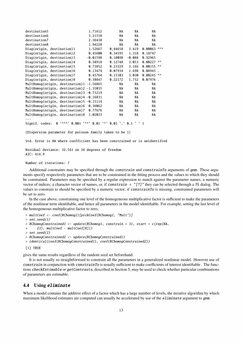
Additional constraints may be specified through the constrain and constrainTo arguments of gnm . These argu-ments specify respectively parameters that are to be constrained in the fitting process and the values to which they shouldbe constrained. Parameters may be specified by a regular expression to match against the parameter names, a numericvector of indices, a character vector of names, or, if constrain = "[?]" they can be selected through a Tk dialog. Thevalues to constrain to should be specified by a numeric vector; if constrainTo is missing, constrained parameters willbe set to zero.
In the case above, constraining one level of the homogeneous multiplicative factor is sufficient to make the parametersof the nonlinear term identifiable, and hence all parameters in the model identifiable. For example, setting the last level ofthe homogeneous multiplicative factor to zero,
> multCoef <- coef(RChomog1)[pickCoef(RChomog1, "Mult")]> set.seed(1)> RChomogConstrained1 <- update(RChomog1, constrain = 31, start = c(rep(NA,+ 23), multCoef - multCoef[8]))> set.seed(2)> RChomogConstrained2 <- update(RChomogConstrained1)> identical(coef(RChomogConstrained1), coef(RChomogConstrained2))
[1] TRUE
gives the same results regardless of the random seed set beforehand.It is not usually so straightforward to constrain all the parameters in a generalized nonlinear model. However use of
constrain in conjunction with constrainTo is usually sufficient to make coefficients of interest identifiable . The func-tions checkEstimable or getContrasts, described in Section 5, may be used to check whether particular combinationsof parameters are estimable.
4.4 Using eliminateWhen a model contains the additive effect of a factor which has a large number of levels, the iterative algorithm by whichmaximum likelihood estimates are computed can usually be accelerated by use of the eliminate argument to gnm .
13
The factor to be eliminate-d should be specified by an expression, which is then interpreted as the first term in themodel formula, replacing any intercept term. So, for example, in terms of the structure of the model,
gnm(mu ~ A + B + Mult(A, B), eliminate = strata1:strata2)
is equivalent to
gnm(mu ~ -1 + strata1:strata2 + A + B + Mult(A, B))
However, specifying a factor through eliminate has two advantages over the standard specification. First, the structure ofthe eliminated factor is exploited so that computational speed is improved — substantially so if the number of eliminatedparameters is large. Second, unless otherwise specified through the ofInterest argument to gnm , the ofInterestcomponent of the returned model object indexes the non-eliminated parameters. Thus eliminated parameters are excludedfrom printed model summaries and default selection by gnm methods. See Section 5.2 for further details on the use of theofInterest component.
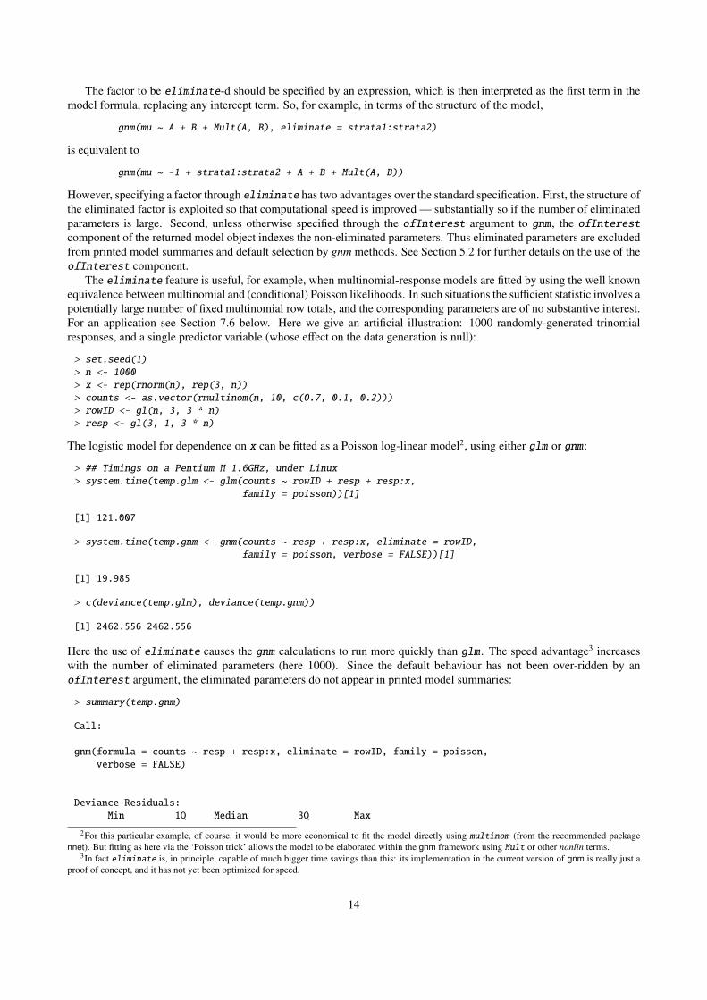
The eliminate feature is useful, for example, when multinomial-response models are fitted by using the well knownequivalence between multinomial and (conditional) Poisson likelihoods. In such situations the sufficient statistic involves apotentially large number of fixed multinomial row totals, and the corresponding parameters are of no substantive interest.For an application see Section 7.6 below. Here we give an artificial illustration: 1000 randomly-generated trinomialresponses, and a single predictor variable (whose effect on the data generation is null):
> set.seed(1)> n <- 1000> x <- rep(rnorm(n), rep(3, n))> counts <- as.vector(rmultinom(n, 10, c(0.7, 0.1, 0.2)))> rowID <- gl(n, 3, 3 * n)> resp <- gl(3, 1, 3 * n)
The logistic model for dependence on x can be fitted as a Poisson log-linear model2, using either glm or gnm :
> ## Timings on a Pentium M 1.6GHz, under Linux> system.time(temp.glm <- glm(counts ~ rowID + resp + resp:x,
family = poisson))[1]
[1] 121.007
> system.time(temp.gnm <- gnm(counts ~ resp + resp:x, eliminate = rowID,family = poisson, verbose = FALSE))[1]
[1] 19.985
> c(deviance(temp.glm), deviance(temp.gnm))
[1] 2462.556 2462.556
Here the use of eliminate causes the gnm calculations to run more quickly than glm . The speed advantage3 increaseswith the number of eliminated parameters (here 1000). Since the default behaviour has not been over-ridden by anofInterest argument, the eliminated parameters do not appear in printed model summaries:
> summary(temp.gnm)
Call:
gnm(formula = counts ~ resp + resp:x, eliminate = rowID, family = poisson,verbose = FALSE)
Deviance Residuals:Min 1Q Median 3Q Max
2For this particular example, of course, it would be more economical to fit the model directly using multinom (from the recommended packagennet). But fitting as here via the ‘Poisson trick’ allows the model to be elaborated within the gnm framework using Mult or other nonlin terms.
3In fact eliminate is, in principle, capable of much bigger time savings than this: its implementation in the current version of gnm is really just aproof of concept, and it has not yet been optimized for speed.
14
-2.852038 -0.786172 -0.004534 0.645278 2.755013
Coefficients of interest:Estimate Std. Error z value Pr(>|z|)
resp2 -1.9614483 0.0340074 -57.68 <2e-16resp3 -1.2558460 0.0253589 -49.52 <2e-16resp1:x 0.0001049 NA NA NAresp2:x -0.0155083 NA NA NAresp3:x 0.0078314 NA NA NA
(Dispersion parameter for poisson family taken to be 1)
Std. Error is NA where coefficient has been constrained or is unidentified
Residual deviance: 2462.6 on 1996 degrees of freedomAIC: 12028
Number of iterations: 3
As usual, gnm has worked here with an over-parameterized representation of the model. The parameterization used byglm can be seen from
> coef(temp.glm)[-(1:1000)]
resp2 resp3 resp1:x resp2:x resp3:x-1.96145 -1.25585 -0.00773 -0.02334 NA
(we will not print the full summary of temp.glm here, since it gives details of all 1005 parameters!), which easily can beobtained, if required, by using getContrasts:
> getContrasts(temp.gnm, ofInterest(temp.gnm)[5:3])
estimate SE quasiSE quasiVarresp3:x 0.00000 0.00000 0.02163 0.000468resp2:x -0.02334 0.03761 0.03077 0.000947resp1:x -0.00773 0.02452 0.01154 0.000133
The eliminate feature as implemented in gnm extends the earlier work of Hatzinger and Francis (2004) to a broaderclass of models and to over-parameterized model representations.
5 Methods and accessor functions
5.1 MethodsThe gnm function returns an object of class c("gnm", "glm", "lm"). There are several methods that have been writtenfor objects of class glm or lm to facilitate inspection of fitted models. Out of the generic functions in the base, stats andgraphics packages for which methods have been written for glm or lm objects, Figure 1 shows those that can be used toanalyse gnm objects, whilst Figure 2 shows those that are not implemented for gnm objects.
In addition to the accessor functions shown in Figure 1, the gnm package provides a new generic function calledtermPredictors that has methods for objects of class gnm, glm and lm. This function returns the additive contributionof each term to the predictor. See Section 2.5 for an example of its use.
Most of the functions listed in Figure 1 can be used as they would be for glm or lm objects, however care must betaken with vcov.gnm , as the variance-covariance matrix will depend on the parameterization of the model. In particular,standard errors calculated using the variance-covariance matrix will only be valid for parameters or contrasts that areestimable!
Similarly, profile.gnm and confint.gnm are only applicable to estimable parameters. The deviance function ofa generalized nonlinear model can sometimes be far from quadratic and profile.gnm attempts to detect assymetry orasymptotic behaviour in order to return a sufficient profile for a given parameter. As an example, consider the followingmodel, described later in Section 7.3:
15

anova formula profilecase.names hatvalues residualscoef labels rstandardcooks.distance logLik summaryconfint model.frame variable.namesdeviance model.matrix vcovextractAIC plot weightsfamily print
Figure 1: Generic functions in the base, stats and graphics packages that can be used to analyse gnm objects.
add1 effectsalias influencedfbeta kappadfbetas predictdrop1 projdummy.coef
Figure 2: Generic functions in the base, stats and graphics packages for which methods have been written for glm or lmobjects, but which are not implemented for gnm objects.
data(yaish)unidiff <- gnm(Freq ~ educ*orig + educ*dest + Mult(Exp(educ), orig:dest),
constrain = "[.]educ1", family = poisson, data = yaish,subset = (dest != 7))
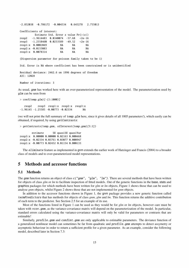
prof <- profile(unidiff, which = 61:65, trace = TRUE)
If the deviance is quadratic in a given parameter, the profile trace will be linear. We can plot the profile traces asfollows:
From these plots we can see that the deviance is approximately quadratic in Mult(Exp(.), orig:dest).educ2, as-symetric in Mult(Exp(.), orig:dest).educ3 and Mult(Exp(.), orig:dest).educ4 and asymptotic in Mult(Exp(.),orig:dest).educ5. When the deviance is approximately quadratic in a given parameter, profile.gnm uses the samestepsize for profiling above and below the original estimate:
> diff(prof[[2]]$par.vals[, "Mult(Exp(.), orig:dest).educ2"])
[1] 0.1053072 0.1053072 0.1053072 0.1053072 0.1053072 0.1053072 0.1053072[8] 0.1053072 0.1053072 0.1053072
When the deviance is assymmetric, profile.gnm uses different stepsizes to accommodate the skew:
> diff(prof[[4]]$par.vals[, "Mult(Exp(.), orig:dest).educ4"])
[1] 0.2018393 0.2018393 0.2018393 0.2018393 0.2018393 0.2018393 0.2018393[8] 0.2018393 0.2018393 0.2243673 0.2243673 0.2243673 0.2243673 0.2243673
Finally, the presence of an asymptote is recorded in the "asymptote" attribute of the returned profile:
> attr(prof[[5]], "asymptote")
[1] TRUE FALSE
This information is used by confint.gnm to return infinite limits for confidence intervals, as appropriate:
confint(prof)
16
−0.6 −0.2 0.2−
20
12
3
Mult(Exp(.), orig:dest).educ2
z
−1.5 −1.0 −0.5 0.0
−2
01
23
Mult(Exp(.), orig:dest).educ3
z
−2.5 −1.5 −0.5
−2
01
23
Mult(Exp(.), orig:dest).educ4
z
−8 −6 −4 −2 0−
10
12
Mult(Exp(.), orig:dest).educ5
z
Profile traces for the multipliers of the orig:dest association
Figure 3: Profile traces for the multipliers of the orig:dest association
5.2 ofInterest and pickCoefIt is quite common for a statistical model to have a large number of parameters, but for only a subset of these parametersbe of interest when it comes to interpreting the model. An example of this has been seen in Section 4.4, where a factoris required in the model in order to represent a structural aspect of the data, but the estimated factor effects have nosubstantive interpretation. Even for models in which all parameters correspond to variables of potential interest, thesubstantive focus may still be on a subset of parameters.
The ofInterest argument to gnm allows the user to specify a subset of the parameters which are of interest, so thatgnm methods will focus on these parameters. In particular, printed model summaries will only show the parameters ofinterest, whilst methods for which a subset of parameters may be selected will by default select the parameters of interest,or where this may not be appropriate, provide a Tk dialog for selection from the parameters of interest. Parameters maybe specified to the ofInterest argument by a regular expression to match against parameter names, by a numeric vectorof indices, by a character vector of names, or, if ofInterest = "[?]" they can be selected through a Tk dialog.
The information regarding the parameters of interest is held in the ofInterest component of gnm objects, which isa named vector of numeric indices, or NULL if all parameters are of interest. This component may be accessed or replacedusing ofInterest or ofInterest<- respectively.
The pickCoef function provides a simple way to obtain the indices of coefficients from any model object. It takes themodel object as its first argument and has an optional regexp argument. If a regular expression is passed to regexp, thecoefficients are selected by matching this regular expression against the coefficient names. Otherwise, coefficients may beselected via a Tk dialog.
So, returning to the example from the last section, if we had set ofInterest to index the education multipliers asfollows
ofInterest(unidiff) <- pickCoef(unidiff, "[.]educ")
then it would not have been necessary to specify the which argument of profile as these parameters would have beenselected by default.
17

5.3 checkEstimable
The checkEstimable function can be used to check the estimability of a linear combination of parameters. For non-linear combinations the same function can be used to check estimability based on the (local) vector of partial derivatives.The checkEstimable function provides a numerical version of the sort of algebraic test described in Catchpole andMorgan (1997).
Consider the following model, that is described later in Section 7.3:
> data(cautres)> doubleUnidiff <- gnm(Freq ~ election:vote + election:class:religion ++ Mult(Exp(election), religion:vote) + Mult(Exp(election),+ class:vote), family = poisson, data = cautres)
InitialisingRunning start-up iterations..Running main iterations...........Done
The effects of the first constituent multiplier in the first multiplicative interaction are identified when the estimate of oneof these effects is constrained to zero, say for the effect of the first level. The parameters to be estimated are then thedifferences between each effect and the effect of the first level. These differences can be represented by a contrast matrixas follows:
> coefs <- names(coef(doubleUnidiff))> contrCoefs <- coefs[grep(", religion:vote", coefs)]> nContr <- length(contrCoefs)> contrMatrix <- matrix(0, length(coefs), nContr, dimnames = list(coefs,+ contrCoefs))> contr <- contr.sum(contrCoefs)> contr <- rbind(contr[nContr, ], contr[-nContr, ])> contrMatrix[contrCoefs, 2:nContr] <- contr> contrMatrix[contrCoefs, 2:nContr]
Mult(Exp(.), religion:vote).election2Mult(Exp(.), religion:vote).election1 -1Mult(Exp(.), religion:vote).election2 1Mult(Exp(.), religion:vote).election3 0Mult(Exp(.), religion:vote).election4 0
Mult(Exp(.), religion:vote).election3Mult(Exp(.), religion:vote).election1 -1Mult(Exp(.), religion:vote).election2 0Mult(Exp(.), religion:vote).election3 1Mult(Exp(.), religion:vote).election4 0
Mult(Exp(.), religion:vote).election4Mult(Exp(.), religion:vote).election1 -1Mult(Exp(.), religion:vote).election2 0Mult(Exp(.), religion:vote).election3 0Mult(Exp(.), religion:vote).election4 1
Then their estimability can be checked using checkEstimable
> checkEstimable(doubleUnidiff, contrMatrix)
Mult(Exp(.), religion:vote).election1 Mult(Exp(.), religion:vote).election2NA TRUE
Mult(Exp(.), religion:vote).election3 Mult(Exp(.), religion:vote).election4TRUE TRUE
which confirms that the effects for the other three levels are estimable when the parameter for the first level is set to zero.However, applying the equivalent constraint to the second constituent multiplier in the interaction is not sufficient to
make the parameters in that multiplier estimable:
18

> coefs <- names(coef(doubleUnidiff))> contrCoefs <- coefs[grep("[.]religion", coefs)]> nContr <- length(contrCoefs)> contrMatrix <- matrix(0, length(coefs), length(contrCoefs), dimnames = list(coefs,+ contrCoefs))> contr <- contr.sum(contrCoefs)> contrMatrix[contrCoefs, 2:nContr] <- rbind(contr[nContr, ], contr[-nContr,+ ])> checkEstimable(doubleUnidiff, contrMatrix)
Mult(Exp(election), .).religion1:vote1 Mult(Exp(election), .).religion2:vote1NA FALSE
Mult(Exp(election), .).religion3:vote1 Mult(Exp(election), .).religion4:vote1FALSE FALSE
Mult(Exp(election), .).religion1:vote2 Mult(Exp(election), .).religion2:vote2FALSE FALSE
Mult(Exp(election), .).religion3:vote2 Mult(Exp(election), .).religion4:vote2FALSE FALSE
5.4 getContrasts, seTo investigate simple “sum to zero” contrasts such as those above, it is easiest to use the getContrasts function, whichchecks the estimability of the contrasts and returns the parameter estimates with their standard errors. Returning to theexample of the first constituent multiplier in the first multiplicative interaction term, the differences between each electionand the first can be obtained as follows:
> myContrasts <- getContrasts(doubleUnidiff, pickCoef(doubleUnidiff,+ ", religion:vote"))> myContrasts
estimate SE quasiSEMult(Exp(.), religion:vote).election1 0.0000000 0.0000000 0.09803075Mult(Exp(.), religion:vote).election2 -0.0878181 0.1136832 0.05702819Mult(Exp(.), religion:vote).election3 -0.2615200 0.1184134 0.06812239Mult(Exp(.), religion:vote).election4 -0.3283459 0.1221302 0.07168290
quasiVarMult(Exp(.), religion:vote).election1 0.009610029Mult(Exp(.), religion:vote).election2 0.003252214Mult(Exp(.), religion:vote).election3 0.004640660Mult(Exp(.), religion:vote).election4 0.005138439
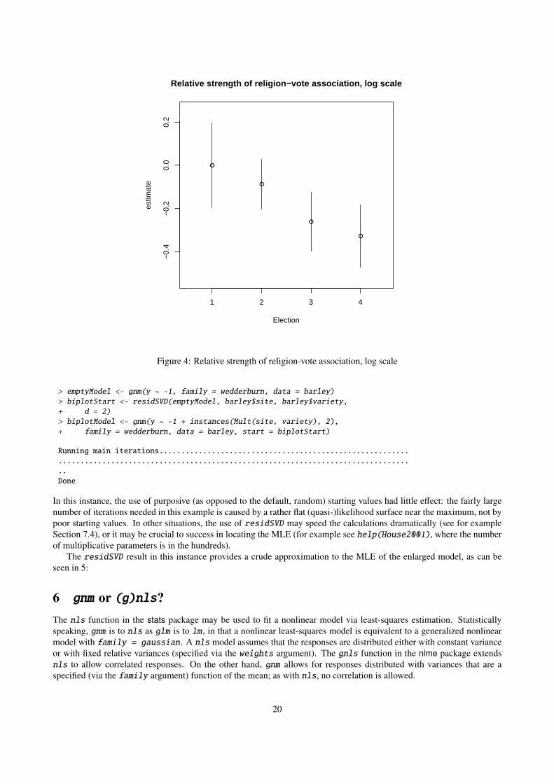
Visualization of estimated contrasts using ‘quasi standard errors’ (Firth, 2003; Firth and de Menezes, 2004) is achievedby plotting the resulting object:
> plot(myContrasts, main = "Relative strength of religion-vote association, log scale",+ xlab = "Election", levelNames = 1:4)
For more general linear combinations of parameters than contrasts, the lower-level se function (which is called inter-nally by getContrasts and by the summary method) can be used directly. See help(se) for details.
5.5 residSVD
Sometimes it is useful to operate on the residuals of a model in order to create informative summaries of residual variation,or to obtain good starting values for additional parameters in a more elaborate model. The relevant arithmetical operationsare weighted means of the so-called working residuals.
The residSVD function facilitates one particular residual analysis that is often useful when considering multiplicativeinteraction between factors as a model elaboration: in effect, residSVD provides a direct estimate of the parameters ofsuch an interaction, by performing an appropriately weighted singular value decomposition on the working residuals.
As an illustration, consider the biplot model described in Section 7.5 below. We can proceed by fitting a smallermodel, then use residSVD to obtain starting values for the parameters in the bilinear term:
19
1 2 3 4
−0.
4−
0.2
0.0
0.2
Relative strength of religion−vote association, log scale
Election
estim
ate
●
●
●
●
Figure 4: Relative strength of religion-vote association, log scale
> emptyModel <- gnm(y ~ -1, family = wedderburn, data = barley)> biplotStart <- residSVD(emptyModel, barley$site, barley$variety,+ d = 2)> biplotModel <- gnm(y ~ -1 + instances(Mult(site, variety), 2),+ family = wedderburn, data = barley, start = biplotStart)
Running main iterations...........................................................................................................................................Done
In this instance, the use of purposive (as opposed to the default, random) starting values had little effect: the fairly largenumber of iterations needed in this example is caused by a rather flat (quasi-)likelihood surface near the maximum, not bypoor starting values. In other situations, the use of residSVD may speed the calculations dramatically (see for exampleSection 7.4), or it may be crucial to success in locating the MLE (for example see help(House2001), where the numberof multiplicative parameters is in the hundreds).
The residSVD result in this instance provides a crude approximation to the MLE of the enlarged model, as can beseen in 5:
6 gnm or (g)nls?The nls function in the stats package may be used to fit a nonlinear model via least-squares estimation. Statisticallyspeaking, gnm is to nls as glm is to lm , in that a nonlinear least-squares model is equivalent to a generalized nonlinearmodel with family = gaussian. A nls model assumes that the responses are distributed either with constant varianceor with fixed relative variances (specified via the weights argument). The gnls function in the nlme package extendsnls to allow correlated responses. On the other hand, gnm allows for responses distributed with variances that are aspecified (via the family argument) function of the mean; as with nls, no correlation is allowed.
20

●●
● ●●●
●
●
●
●●●●
●●
●
●●
●
●
●
●
●●
●
●
●
●
●
●
●●
●
●
●
●
●
●
−2 0 2 4
−1.
5−
1.0
−0.
50.
00.
51.
01.
5
Comparison of residSVD and MLE for a 2−dimensional biplot model
coef(biplotModel)
bipl
otS
tart
Figure 5: Comparison of residSVD and the MLE for a 2-dimensional biplot model
The gnm function also differs from nls/gnls in terms of the interface. Models are specified to nls and gnls in termsof a mathematical formula or a selfStart function based on such a formula, which is convenient for models that have asmall number of parameters. For models that have a large number of parameters, or can not easily be represented by amathematical formula, the symbolic model specification used by gnm may be more convenient. This would usually be thecase for models involving factors, which would need to be represented by dummy variables in a nls formula.
When working with artificial data, gnm has the minor advantage that it does not fail when a model is an exact fit tothe data (see help(nls)). Therefore it is not necessary with gnm to add noise to artificial data, which can be useful whentesting methods.
7 ExamplesThis section provides some examples of the wide range of models that may be fitted using the gnm package. Sections7.1, 7.2 and 7.3 consider various models for contingency tables; Section 7.4 considers AMMI and GAMMI models whichare typically used in agricultural applications, and Section 7.6 considers the stereotype model, which is used to model anordinal response.
7.1 Row-column association modelsThere are several models that have been proposed for modelling the relationship between the cell means of a contingencytable and the cross-classifying factors. The following examples consider the row-column association models proposed byGoodman (1979). The examples shown use data from two-way contingency tables, but the gnm package can also be usedto fit the equivalent models for higher order tables.
21

7.1.1 RC(1) model
The RC(1) model is a row and column association model with the interaction between row and column factors representedby one component of the multiplicative interaction. If the rows are indexed by r and the columns by c, then the log-multiplicative form of the RC(1) model for the cell means µrc is given by
log µrc = αr + βc + γrδc.
We shall fit this model to the mentalHealth data set taken from Agresti (2002) page 381, which is a two-way con-tingency table classified by the child’s mental impairment (MHS) and the parents’ socioeconomic status (SES). Althoughboth of these factors are ordered, we do not wish to use polynomial contrasts in the model, so we begin by setting thecontrasts attribute of these factors to treatment:
> set.seed(1)> data(mentalHealth)> mentalHealth$MHS <- C(mentalHealth$MHS, treatment)> mentalHealth$SES <- C(mentalHealth$SES, treatment)
The gnm model is then specified as follows, using the poisson family with a log link function:
> RC1model <- gnm(count ~ SES + MHS + Mult(SES, MHS), family = poisson,+ data = mentalHealth)
InitialisingRunning start-up iterations..Running main iterations........Done
> RC1model
Call:gnm(formula = count ~ SES + MHS + Mult(SES, MHS), family = poisson,
data = mentalHealth)
Coefficients:(Intercept) SESB SESC
3.84143 -0.06741 0.10999SESD SESE SESF
0.40502 0.02535 -0.20055MHSmild MHSmoderate MHSimpaired0.70380 0.19416 0.23331
Mult(., MHS).SESA Mult(., MHS).SESB Mult(., MHS).SESC-0.41864 -0.42216 -0.13207
Mult(., MHS).SESD Mult(., MHS).SESE Mult(., MHS).SESF0.02183 0.40198 0.71429
Mult(SES, .).MHSwell Mult(SES, .).MHSmild Mult(SES, .).MHSmoderate-0.73671 -0.07475 0.04471
Mult(SES, .).MHSimpaired0.59453
Deviance: 3.570562Pearson chi-squared: 3.568088Residual df: 8
The row scores (parameters 10 to 15) and the column scores (parameters 16 to 19) of the multiplicative interaction can benormalized as in Agresti’s eqn (9.15):
> rowProbs <- with(mentalHealth, tapply(count, SES, sum)/sum(count))> colProbs <- with(mentalHealth, tapply(count, MHS, sum)/sum(count))> rowScores <- coef(RC1model)[10:15]> colScores <- coef(RC1model)[16:19]> rowScores <- rowScores - sum(rowScores * rowProbs)> colScores <- colScores - sum(colScores * colProbs)
22
> beta1 <- sqrt(sum(rowScores^2 * rowProbs))> beta2 <- sqrt(sum(colScores^2 * colProbs))> assoc <- list(beta = beta1 * beta2, mu = rowScores/beta1, nu = colScores/beta2)> assoc
$beta[1] 0.1664874
$muMult(., MHS).SESA Mult(., MHS).SESB Mult(., MHS).SESC Mult(., MHS).SESD
-1.11233093 -1.12143720 -0.37107614 0.02702955Mult(., MHS).SESE Mult(., MHS).SESF
1.01036159 1.81823273
$nuMult(SES, .).MHSwell Mult(SES, .).MHSmild Mult(SES, .).MHSmoderate
-1.6775143 -0.1403989 0.1369924Mult(SES, .).MHSimpaired
1.4136910
7.1.2 RC(2) model
The RC(1) model can be extended to an RC(m) model with m components of the multiplicative interaction. For example,the RC(2) model is given by
log µrc = αr + βc + γrδc + θrφc.
Extra instances of the multiplicative interaction can be specified by the multiplicity argument of Mult, so the RC(2)model can be fitted to the mentalHealth data as follows
> RC2model <- gnm(count ~ SES + MHS + instances(Mult(SES, MHS),+ 2), family = poisson, data = mentalHealth)
InitialisingRunning start-up iterations..Running main iterations..............Done
> RC2model
Call:gnm(formula = count ~ SES + MHS + instances(Mult(SES, MHS), 2),
family = poisson, data = mentalHealth)
Coefficients:(Intercept) SESB
3.81539 -0.06452SESC SESD
0.11327 0.38762SESE SESF
0.01619 -0.17718MHSmild MHSmoderate0.72796 0.22209
MHSimpaired Mult(., MHS, inst = 1).SESA0.27738 -0.19609
Mult(., MHS, inst = 1).SESB Mult(., MHS, inst = 1).SESC-0.23247 -0.10207
Mult(., MHS, inst = 1).SESD Mult(., MHS, inst = 1).SESE0.15618 0.23954
Mult(., MHS, inst = 1).SESF Mult(SES, ., inst = 1).MHSwell0.03515 -1.00815
Mult(SES, ., inst = 1).MHSmild Mult(SES, ., inst = 1).MHSmoderate-0.04298 -0.21716
23
Mult(SES, ., inst = 1).MHSimpaired Mult(., MHS, inst = 2).SESA1.11729 0.39218
Mult(., MHS, inst = 2).SESB Mult(., MHS, inst = 2).SESC0.25985 0.01665
Mult(., MHS, inst = 2).SESD Mult(., MHS, inst = 2).SESE0.68097 0.05502
Mult(., MHS, inst = 2).SESF Mult(SES, ., inst = 2).MHSwell-1.75425 0.32550
Mult(SES, ., inst = 2).MHSmild Mult(SES, ., inst = 2).MHSmoderate0.05297 -0.07626
Mult(SES, ., inst = 2).MHSimpaired-0.17352
Deviance: 0.5225353Pearson chi-squared: 0.523331Residual df: 3
7.1.3 Homogeneous effects
If the row and column factors have the same levels, or perhaps some levels in common, then the row-column interactioncould be modelled by a multiplicative interaction with homogeneous effects, that is
log µrc = αr + βc + γrγc.
For example, the occupationalStatus data set from Goodman (1979) is a contingency table classified by the occupa-tional status of fathers (origin) and their sons (destination). Goodman (1979) fits a row-column association model withhomogeneous effects to these data after deleting the cells on the main diagonal. Equivalently we can account for thediagonal effects by a separate Diag term:
> data(occupationalStatus)> RChomog <- gnm(Freq ~ origin + destination + Diag(origin, destination) ++ MultHomog(origin, destination), family = poisson, data = occupationalStatus)
InitialisingRunning start-up iterations..Running main iterations.........Done
> RChomog
Call:gnm(formula = Freq ~ origin + destination + Diag(origin, destination) +
MultHomog(origin, destination), family = poisson, data = occupationalStatus)
Coefficients:(Intercept) origin2-1.55466 0.62373origin3 origin42.01762 2.61788origin5 origin61.40681 3.71525origin7 origin82.58917 2.44470
destination2 destination31.04274 2.36204
destination4 destination52.90631 2.30623
destination6 destination74.01873 3.34077
destination8 Diag(origin, destination)13.02008 1.52667
24

Diag(origin, destination)2 Diag(origin, destination)30.45600 -0.01598
Diag(origin, destination)4 Diag(origin, destination)50.38918 0.73852
Diag(origin, destination)6 Diag(origin, destination)70.13474 0.45764
Diag(origin, destination)8 MultHomog(origin, destination)10.38847 -1.98495
MultHomog(origin, destination)2 MultHomog(origin, destination)3-1.76665 -1.16849
MultHomog(origin, destination)4 MultHomog(origin, destination)5-0.58461 -0.56744
MultHomog(origin, destination)6 MultHomog(origin, destination)7-0.05568 0.36046
MultHomog(origin, destination)80.60403
Deviance: 32.56098Pearson chi-squared: 31.20716Residual df: 34
To determine whether it would be better to allow for heterogeneous effects on the association of the fathers’ occupa-tional status and the sons’ occupational status, we can compare this model to the RC(1) model for these data:
> data(occupationalStatus)> RCheterog <- gnm(Freq ~ origin + destination + Diag(origin, destination) ++ Mult(origin, destination), family = poisson, data = occupationalStatus)
InitialisingRunning start-up iterations..Running main iterations.........Done
> anova(RChomog, RCheterog)
Analysis of Deviance Table
Model 1: Freq ~ origin + destination + Diag(origin, destination) + MultHomog(origin,destination)
Model 2: Freq ~ origin + destination + Diag(origin, destination) + Mult(origin,destination)
Resid. Df Resid. Dev Df Deviance1 34 32.5612 28 29.149 6 3.412
In this case there is little gain in allowing heterogeneous effects.
7.2 Diagonal reference modelsDiagonal reference models, proposed by Sobel (1981, 1985), are designed for contingency tables classified by factorswith the same levels. The cell means are modelled as a function of the diagonal effects, i.e., the mean responses of the‘diagonal’ cells in which the levels of the row and column factors are the same.
Dref example 1: Political consequences of social mobility
To illustrate the use of diagonal reference models we shall use the voting data from Clifford and Heath (1993). The datacome from the 1987 British general election and are the percentage voting Labour in groups cross-classified by the classof the head of household (destination) and the class of their father (origin). In order to weight these percentages bythe group size, we first back-transform them to the counts of those voting Labour and those not voting Labour:
25

> set.seed(1)> data(voting)> count <- with(voting, percentage/100 * total)> yvar <- cbind(count, voting$total - count)
The grouped percentages may be modelled by a basic diagonal reference model, that is, a weighted sum of the diagonaleffects for the corresponding origin and destination classes. This model may be expressed as
µod =eδ1
eδ1 + eδ2γo +
eδ2
eδ1 + eδ2γd.
See Section 3.3 for more detail on the parameterization.The basic diagonal reference model may be fitted using gnm as follows
> classMobility <- gnm(yvar ~ Dref(origin, destination), family = binomial,+ data = voting)
InitialisingRunning main iterations........Done
> classMobility
Call:gnm(formula = yvar ~ Dref(origin, destination), family = binomial,
data = voting)
Coefficients:(Intercept) Dref(origin, destination)delta1-1.34325 -0.30736
Dref(origin, destination)delta2 Dref(., .).origin|destination1-0.05501 -0.83454
Dref(., .).origin|destination2 Dref(., .).origin|destination30.21066 -0.61159
Dref(., .).origin|destination4 Dref(., .).origin|destination50.76500 1.38370
Deviance: 21.22093Pearson chi-squared: 18.95311Residual df: 19
and the origin and destination weights can be evaluated as below
> DrefWeights(classMobility)
$originweight se
0.43724694 0.03996404
$destinationweight se
0.56275306 0.03996404
These results are slightly different from those reported by Clifford and Heath (1993). The reason for this is unclear: weare confident that the above results are correct for the data as given in Clifford and Heath (1993), but have not been ableto confirm that the data as printed in the journal were exactly as used in Clifford and Heath’s analysis.
Clifford and Heath (1993) suggest that movements in and out of the salariat (class 1) should be treated differentlyfrom movements between the lower classes (classes 2 - 5), since the former has a greater effect on social status. Thus they
26

propose the following model
µod =
eδ1
eδ1 + eδ2γo +
eδ2
eδ1 + eδ2γd if o = 1
eδ3
eδ3 + eδ4γo +
eδ4
eδ3 + eδ4γd if d = 1
eδ5
eδ5 + eδ6γo +
eδ6
eδ5 + eδ6γd if o , 1 and d , 1
To fit this model we define factors indicating movement in (upward) and out (downward) of the salariat
> upward <- with(voting, origin != 1 & destination == 1)> downward <- with(voting, origin == 1 & destination != 1)
Then the diagonal reference model with separate weights for socially mobile groups can be estimated as follows
> socialMobility <- gnm(yvar ~ Dref(origin, destination, delta = ~1 ++ downward + upward), family = binomial, data = voting)
InitialisingRunning main iterations..........Done
> socialMobility
Call:gnm(formula = yvar ~ Dref(origin, destination, delta = ~1 + downward +
upward), family = binomial, data = voting)
Coefficients:(Intercept)
-1.3211Dref(origin, destination, delta = ~ . + downward + upward).delta1(Intercept)
0.2753Dref(origin, destination, delta = ~ 1 + . + upward).delta1downwardTRUE
0.2122Dref(origin, destination, delta = ~ 1 + downward + .).delta1upwardTRUE
0.1474Dref(origin, destination, delta = ~ . + downward + upward).delta2(Intercept)
0.6620Dref(origin, destination, delta = ~ 1 + . + upward).delta2downwardTRUE
-0.5986Dref(origin, destination, delta = ~ 1 + downward + .).delta2upwardTRUE
0.2076Dref(., ., delta = ~ 1 + downward + upward).origin|destination1
-0.7365Dref(., ., delta = ~ 1 + downward + upward).origin|destination2
0.2084Dref(., ., delta = ~ 1 + downward + upward).origin|destination3
-0.6737Dref(., ., delta = ~ 1 + downward + upward).origin|destination4
0.7519Dref(., ., delta = ~ 1 + downward + upward).origin|destination5
1.3787
Deviance: 18.97407Pearson chi-squared: 17.07493Residual df: 17
The weights for those moving into the salariat, those moving out of the salariat and those in any other group, can beevaluated as below
27
> DrefWeights(socialMobility)
$origindownward upward weight se
1 FALSE FALSE 0.4044959 0.059181412 TRUE FALSE 0.6044393 0.123710323 FALSE TRUE 0.3900792 0.08134359
$destinationdownward upward weight se
1 FALSE FALSE 0.5955041 0.059181412 TRUE FALSE 0.3955607 0.123710323 FALSE TRUE 0.6099208 0.08134359
Again, the results differ slightly from those reported by Clifford and Heath (1993), but the essence of the results is thesame: the origin weight is much larger for the downwardly mobile group than for the other groups. The weights for theupwardly mobile group are very similar to the base level weights, so the model may be simplified by only fitting separateweights for the downwardly mobile group:
> downwardMobility <- gnm(yvar ~ Dref(origin, destination, delta = ~1 ++ downward), family = binomial, data = voting)
InitialisingRunning main iterations.........Done
> downwardMobility
Call:gnm(formula = yvar ~ Dref(origin, destination, delta = ~1 + downward),
family = binomial, data = voting)
Coefficients:(Intercept)-1.31336
Dref(origin, destination, delta = ~ . + downward).delta1(Intercept)-0.04679
Dref(origin, destination, delta = ~ 1 + .).delta1downwardTRUE0.58421
Dref(origin, destination, delta = ~ . + downward).delta2(Intercept)0.36199
Dref(origin, destination, delta = ~ 1 + .).delta2downwardTRUE-0.22653
Dref(., ., delta = ~ 1 + downward).origin|destination1-0.75650
Dref(., ., delta = ~ 1 + downward).origin|destination20.20684
Dref(., ., delta = ~ 1 + downward).origin|destination3-0.67829
Dref(., ., delta = ~ 1 + downward).origin|destination40.74029
Dref(., ., delta = ~ 1 + downward).origin|destination51.36966
Deviance: 18.99389Pearson chi-squared: 17.09981Residual df: 18
> DrefWeights(downwardMobility)
$origindownward weight se
28
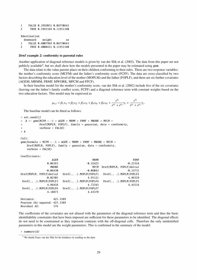
1 FALSE 0.3992031 0.047506432 TRUE 0.5991569 0.11951340
$destinationdownward weight se
1 FALSE 0.6007969 0.047506432 TRUE 0.4008431 0.11951340
Dref example 2: conformity to parental rules
Another application of diagonal reference models is given by van der Slik et al. (2002). The data from this paper are notpublicly available4, but we shall show how the models presented in the paper may be estimated using gnm .
The data relate to the value parents place on their children conforming to their rules. There are two response variables:the mother’s conformity score (MCFM) and the father’s conformity score (FCFF). The data are cross-classified by twofactors describing the education level of the mother (MOPLM) and the father (FOPLF), and there are six further covariates(AGEM, MRMM, FRMF, MWORK, MFCM and FFCF).
In their baseline model for the mother’s conformity score, van der Slik et al. (2002) include five of the six covariates(leaving out the father’s family conflict score, FCFF) and a diagonal reference term with constant weights based on thetwo education factors. This model may be expressed as
µrci = β1x1i + β2x2i + β3x3i + β4x4i + β5x5i +eδ1
eδ1 + eδ2γr +
eδ2
eδ1 + eδ2γc.
The baseline model can be fitted as follows:
> set.seed(1)> A <- gnm(MCFM ~ -1 + AGEM + MRMM + FRMF + MWORK + MFCM ++ Dref(MOPLM, FOPLF), family = gaussian, data = conformity,+ verbose = FALSE)> A
Call:gnm(formula = MCFM ~ -1 + AGEM + MRMM + FRMF + MWORK + MFCM +
Dref(MOPLM, FOPLF), family = gaussian, data = conformity,verbose = FALSE)
Coefficients:AGEM MRMM FRMF
0.06363 -0.32425 -0.25324MWORK MFCM Dref(MOPLM, FOPLF)delta1
-0.06430 -0.06043 -0.33731Dref(MOPLM, FOPLF)delta2 Dref(., .).MOPLM|FOPLF1 Dref(., .).MOPLM|FOPLF2
-0.02505 4.95121 4.86329Dref(., .).MOPLM|FOPLF3 Dref(., .).MOPLM|FOPLF4 Dref(., .).MOPLM|FOPLF5
4.86458 4.72343 4.43516Dref(., .).MOPLM|FOPLF6 Dref(., .).MOPLM|FOPLF7
4.18873 4.43378
Deviance: 425.3389Pearson chi-squared: 425.3389Residual df: 576
The coefficients of the covariates are not aliased with the parameters of the diagonal reference term and thus the basicidentifiability constraints that have been imposed are sufficient for these parameters to be identified. The diagonal effectsdo not need to be constrained as they represent contrasts with the off-diagonal cells. Therefore the only unidentifiedparameters in this model are the weight parameters. This is confirmed in the summary of the model:
> summary(A)
4 We thank Frans van der Slik for his kindness in sending us the data.
29
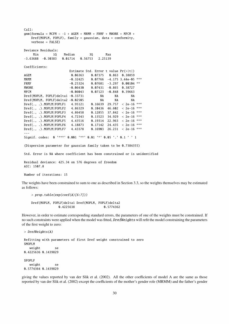
Call:gnm(formula = MCFM ~ -1 + AGEM + MRMM + FRMF + MWORK + MFCM +
Dref(MOPLM, FOPLF), family = gaussian, data = conformity,verbose = FALSE)
Deviance Residuals:Min 1Q Median 3Q Max
-3.63688 -0.50383 0.01714 0.56753 2.25139
Coefficients:Estimate Std. Error t value Pr(>|t|)
AGEM 0.06363 0.07375 0.863 0.38859MRMM -0.32425 0.07766 -4.175 3.44e-05 ***FRMF -0.25324 0.07681 -3.297 0.00104 **MWORK -0.06430 0.07431 -0.865 0.38727MFCM -0.06043 0.07123 -0.848 0.39663Dref(MOPLM, FOPLF)delta1 -0.33731 NA NA NADref(MOPLM, FOPLF)delta2 -0.02505 NA NA NADref(., .).MOPLM|FOPLF1 4.95121 0.16639 29.757 < 2e-16 ***Dref(., .).MOPLM|FOPLF2 4.86329 0.10436 46.602 < 2e-16 ***Dref(., .).MOPLM|FOPLF3 4.86458 0.12855 37.842 < 2e-16 ***Dref(., .).MOPLM|FOPLF4 4.72343 0.13523 34.929 < 2e-16 ***Dref(., .).MOPLM|FOPLF5 4.43516 0.19314 22.963 < 2e-16 ***Dref(., .).MOPLM|FOPLF6 4.18873 0.17142 24.435 < 2e-16 ***Dref(., .).MOPLM|FOPLF7 4.43378 0.16903 26.231 < 2e-16 ***---Signif. codes: 0 '***' 0.001 '**' 0.01 '*' 0.05 '.' 0.1 ' ' 1
(Dispersion parameter for gaussian family taken to be 0.7384355)
Std. Error is NA where coefficient has been constrained or is unidentified
Residual deviance: 425.34 on 576 degrees of freedomAIC: 1507.8
Number of iterations: 15
The weights have been constrained to sum to one as described in Section 3.3, so the weights themselves may be estimatedas follows:
> prop.table(exp(coef(A)[6:7]))
Dref(MOPLM, FOPLF)delta1 Dref(MOPLM, FOPLF)delta20.4225638 0.5774362
However, in order to estimate corresponding standard errors, the parameters of one of the weights must be constrained. Ifno such constraints were applied when the model was fitted, DrefWeights will refit the model constraining the parametersof the first weight to zero:
> DrefWeights(A)
Refitting with parameters of first Dref weight constrained to zero$MOPLMweight se
0.4225636 0.1439829
$FOPLFweight se
0.5774364 0.1439829
giving the values reported by van der Slik et al. (2002). All the other coefficients of model A are the same as thosereported by van der Slik et al. (2002) except the coefficients of the mother’s gender role (MRMM) and the father’s gender
30
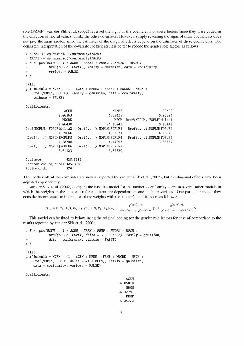
role (FRMF). van der Slik et al. (2002) reversed the signs of the coefficients of these factors since they were coded inthe direction of liberal values, unlike the other covariates. However, simply reversing the signs of these coefficients doesnot give the same model, since the estimates of the diagonal effects depend on the estimates of these coefficients. Forconsistent interpretation of the covariate coefficients, it is better to recode the gender role factors as follows:
> MRMM2 <- as.numeric(!conformity$MRMM)> FRMF2 <- as.numeric(!conformity$FRMF)> A <- gnm(MCFM ~ -1 + AGEM + MRMM2 + FRMF2 + MWORK + MFCM ++ Dref(MOPLM, FOPLF), family = gaussian, data = conformity,+ verbose = FALSE)> A
Call:gnm(formula = MCFM ~ -1 + AGEM + MRMM2 + FRMF2 + MWORK + MFCM +
Dref(MOPLM, FOPLF), family = gaussian, data = conformity,verbose = FALSE)
Coefficients:AGEM MRMM2 FRMF2
0.06363 0.32425 0.25324MWORK MFCM Dref(MOPLM, FOPLF)delta1
-0.06430 -0.06043 0.08440Dref(MOPLM, FOPLF)delta2 Dref(., .).MOPLM|FOPLF1 Dref(., .).MOPLM|FOPLF2
0.39666 4.37371 4.28579Dref(., .).MOPLM|FOPLF3 Dref(., .).MOPLM|FOPLF4 Dref(., .).MOPLM|FOPLF5
4.28708 4.14593 3.85767Dref(., .).MOPLM|FOPLF6 Dref(., .).MOPLM|FOPLF7
3.61123 3.85629
Deviance: 425.3389Pearson chi-squared: 425.3389Residual df: 576
The coefficients of the covariates are now as reported by van der Slik et al. (2002), but the diagonal effects have beenadjusted appropriately.
van der Slik et al. (2002) compare the baseline model for the mother’s conformity score to several other models inwhich the weights in the diagonal reference term are dependent on one of the covariates. One particular model theyconsider incorporates an interaction of the weights with the mother’s conflict score as follows:
µrci = β1x1i + β2x2i + β3x3i + β4x4i + β5x5i +eξ01+ξ11 x5i
eξ01+ξ11 x5i + eξ02+ξ12 x5iγr +
eξ02+ξ12 x5i
eξ01+ξ11 x5i + eξ02+ξ12 x5iγc.
This model can be fitted as below, using the original coding for the gender role factors for ease of comparison to theresults reported by van der Slik et al. (2002),
> F <- gnm(MCFM ~ -1 + AGEM + MRMM + FRMF + MWORK + MFCM ++ Dref(MOPLM, FOPLF, delta = ~ 1 + MFCM), family = gaussian,+ data = conformity, verbose = FALSE)> F
Call:gnm(formula = MCFM ~ -1 + AGEM + MRMM + FRMF + MWORK + MFCM +
Dref(MOPLM, FOPLF, delta = ~1 + MFCM), family = gaussian,data = conformity, verbose = FALSE)
Coefficients:AGEM
0.05818MRMM
-0.32701FRMF
-0.25772
31
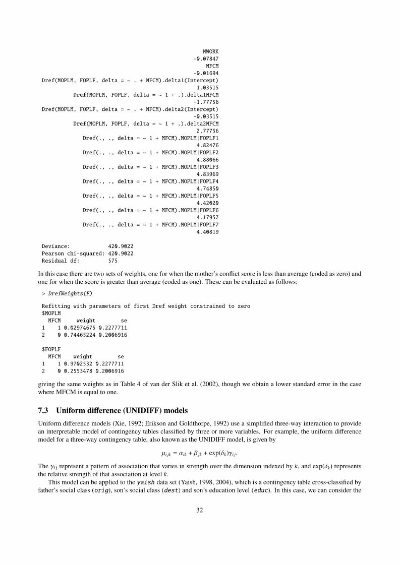
MWORK-0.07847
MFCM-0.01694
Dref(MOPLM, FOPLF, delta = ~ . + MFCM).delta1(Intercept)1.03515
Dref(MOPLM, FOPLF, delta = ~ 1 + .).delta1MFCM-1.77756
Dref(MOPLM, FOPLF, delta = ~ . + MFCM).delta2(Intercept)-0.03515
Dref(MOPLM, FOPLF, delta = ~ 1 + .).delta2MFCM2.77756
Dref(., ., delta = ~ 1 + MFCM).MOPLM|FOPLF14.82476
Dref(., ., delta = ~ 1 + MFCM).MOPLM|FOPLF24.88066
Dref(., ., delta = ~ 1 + MFCM).MOPLM|FOPLF34.83969
Dref(., ., delta = ~ 1 + MFCM).MOPLM|FOPLF44.74850
Dref(., ., delta = ~ 1 + MFCM).MOPLM|FOPLF54.42020
Dref(., ., delta = ~ 1 + MFCM).MOPLM|FOPLF64.17957
Dref(., ., delta = ~ 1 + MFCM).MOPLM|FOPLF74.40819
Deviance: 420.9022Pearson chi-squared: 420.9022Residual df: 575
In this case there are two sets of weights, one for when the mother’s conflict score is less than average (coded as zero) andone for when the score is greater than average (coded as one). These can be evaluated as follows:
> DrefWeights(F)
Refitting with parameters of first Dref weight constrained to zero$MOPLMMFCM weight se
1 1 0.02974675 0.22777112 0 0.74465224 0.2006916
$FOPLFMFCM weight se
1 1 0.9702532 0.22777112 0 0.2553478 0.2006916
giving the same weights as in Table 4 of van der Slik et al. (2002), though we obtain a lower standard error in the casewhere MFCM is equal to one.
7.3 Uniform difference (UNIDIFF) modelsUniform difference models (Xie, 1992; Erikson and Goldthorpe, 1992) use a simplified three-way interaction to providean interpretable model of contingency tables classified by three or more variables. For example, the uniform differencemodel for a three-way contingency table, also known as the UNIDIFF model, is given by
µi jk = αik + β jk + exp(δk)γi j.
The γi j represent a pattern of association that varies in strength over the dimension indexed by k, and exp(δk) representsthe relative strength of that association at level k.
This model can be applied to the yaish data set (Yaish, 1998, 2004), which is a contingency table cross-classified byfather’s social class (orig), son’s social class (dest) and son’s education level (educ). In this case, we can consider the
32

importance of the association between the social class of father and son across the education levels. We omit the sub-tablewhich corresponds to level 7 of dest, because its information content is negligible:
> set.seed(1)> data(yaish)> unidiff <- gnm(Freq ~ educ * orig + educ * dest + Mult(Exp(educ),+ orig:dest), ofInterest = "[.]educ", family = poisson, data = yaish,+ subset = (dest != 7))
InitialisingRunning start-up iterations..Running main iterations..................................................Done
> coef(unidiff)
Coefficients of interest:Mult(Exp(.), orig:dest).educ1 Mult(Exp(.), orig:dest).educ2
-0.2364828 -0.4618546Mult(Exp(.), orig:dest).educ3 Mult(Exp(.), orig:dest).educ4
-0.9799063 -1.2754212Mult(Exp(.), orig:dest).educ5
-2.4859851
The ofInterest component has been set to index the multipliers of the association between the social class of fatherand son. We can contrast each multiplier to that of the lowest education level and obtain the standard errors for theseparameters as follows:
> getContrasts(unidiff, ofInterest(unidiff))
estimate SE quasiSE quasiVarMult(Exp(.), orig:dest).educ1 0.0000000 0.0000000 0.09757438 0.00952076Mult(Exp(.), orig:dest).educ2 -0.2253718 0.1611874 0.12885847 0.01660450Mult(Exp(.), orig:dest).educ3 -0.7434235 0.2335083 0.21182122 0.04486823Mult(Exp(.), orig:dest).educ4 -1.0389385 0.3434256 0.32609377 0.10633714Mult(Exp(.), orig:dest).educ5 -2.2495024 0.9453762 0.93560622 0.87535900
Four-way contingency tables may sometimes be described by a “double UNIDIFF” model
µi jkl = αil + β jkl + exp(δl)γi j + exp(φl)θik,
where the strengths of two, two-way associations with a common variable are estimated across the levels of the fourthvariable. The cautres data set, from Cautres et al. (1998), can be used to illustrate the application of the double UNIDIFFmodel. This data set is classified by the variables vote, class, religion and election. Using a double UNIDIFF model, wecan see how the association between class and vote, and the association between religion and vote, differ between themost recent election and the other elections:
> set.seed(1)> data(cautres)> doubleUnidiff <- gnm(Freq ~ election * vote + election * class *+ religion + Mult(Exp(election), religion:vote) + Mult(Exp(election),+ class:vote), family = poisson, data = cautres)
InitialisingRunning start-up iterations..Running main iterations...........Done
> getContrasts(doubleUnidiff, rev(pickCoef(doubleUnidiff, ", religion:vote")))
33
estimate SE quasiSEMult(Exp(.), religion:vote).election4 0.00000000 0.00000000 0.07168290Mult(Exp(.), religion:vote).election3 0.06682585 0.09906916 0.06812239Mult(Exp(.), religion:vote).election2 0.24052778 0.09116479 0.05702819Mult(Exp(.), religion:vote).election1 0.32834589 0.12213023 0.09803075
quasiVarMult(Exp(.), religion:vote).election4 0.005138439Mult(Exp(.), religion:vote).election3 0.004640660Mult(Exp(.), religion:vote).election2 0.003252214Mult(Exp(.), religion:vote).election1 0.009610029
> getContrasts(doubleUnidiff, rev(pickCoef(doubleUnidiff, "[.]religion")))
Mult(Exp(election), .).religion4:vote2 Mult(Exp(election), .).religion3:vote2NA FALSE
Mult(Exp(election), .).religion2:vote2 Mult(Exp(election), .).religion1:vote2FALSE FALSE
Mult(Exp(election), .).religion4:vote1 Mult(Exp(election), .).religion3:vote1FALSE FALSE
Mult(Exp(election), .).religion2:vote1 Mult(Exp(election), .).religion1:vote1FALSE FALSE
Note: not all of the specified contrasts in this set are estimableEstimate Std. Error
Mult(Exp(election), .).religion4:vote2 0 0
7.4 Generalized additive main effects and multiplicative interaction (GAMMI) modelsGeneralized additive main effects and multiplicative interaction models, or GAMMI models, were motivated by two-waycontingency tables and comprise the row and column main effects plus one or more components of the multiplicativeinteraction. The singular value corresponding to each multiplicative component is often factored out, as a measure of thestrength of association between the row and column scores, indicating the importance of the component, or axis.
For cell means µrc a GAMMI-K model has the form
g(µrc) = αr + βc +
K∑k=1
σkγkrδkc,
in which g is a link function, αr and βc are the row and column main effects, γkr and δkc are the row and column scoresfor multiplicative component k and σk is the singular value for component k. The number of multiplicative components,K, is less than or equal to the rank of the matrix of residuals from the main effects.
The row-column association models discussed in Section 7.1 are examples of GAMMI models, with a log link andpoisson variance. Here we illustrate the use of an AMMI model, which is a GAMMI model with an identity link and aconstant variance.
We shall use the wheat data set taken from Vargas et al. (2001), which gives wheat yields measured over ten years.First we scale these yields and create a new treatment factor, so that we can reproduce the analysis of Vargas et al. (2001):
> set.seed(1)> data(wheat)> yield.scaled <- wheat$yield * sqrt(3/1000)> treatment <- interaction(wheat$tillage, wheat$summerCrop, wheat$manure,+ wheat$N, sep = "")
Now we can fit the AMMI-1 model, to the scaled yields using the combined treatment factor and the year factor fromthe wheat dataset. We will proceed by first fitting the main effects model, then using residSVD (see Section 5.5) for theparameters of the multiplicative term:
> mainEffects <- gnm(yield.scaled ~ year + treatment, family = gaussian,+ data = wheat)
Linear predictor - using glm.fit
34

> svdStart <- residSVD(mainEffects, year, treatment, 3)> bilinear1 <- update(mainEffects, . ~ . + Mult(year, treatment),+ start = c(coef(mainEffects), svdStart[, 1]))
Running main iterationsDone
We can compare the AMMI-1 model to the main effects model,
> anova(mainEffects, bilinear1)
Analysis of Deviance Table
Model 1: yield.scaled ~ year + treatmentModel 2: yield.scaled ~ year + treatment + Mult(year, treatment)Resid. Df Resid. Dev Df Deviance
1 207 2795152 176 128383 31 151133
giving the same results as in Table 1 of Vargas et al. (2001) (up to error caused by rounding).
7.5 Biplot modelsBiplots are used to display two-dimensional data transformed into a space spanned by linearly independent vectors, suchas the principal components or singular vectors. The plot represents the levels of the two classifying factors by their scoreson the two axes which show the most information about the data, for example the first two principal components.
A rank-n model is a model based on the first n components of the decomposition. In the case of a singular valuedecomposition, this is equivalent to a model with n components of the multiplicative interaction.
To illustrate the use of biplot models, we shall use the barley data set which describes the incidence of leaf blotchover ten varieties of barley grown at nine sites (Wedderburn, 1974; Gabriel, 1998). The biplot model is fitted as follows:
> data(barley)> set.seed(1)> biplotModel <- gnm(y ~ -1 + instances(Mult(site, variety), 2),+ family = wedderburn, data = barley)
InitialisingRunning start-up iterations..Running main iterations......................................................................................................................................Done
using the wedderburn family function introduced in Section 2. Matrices of the row and column scores for the first twosingular vectors can then be obtained by:
> barleySVD <- svd(matrix(biplotModel$predictors, 10, 9))> A <- sweep(barleySVD$v, 2, sqrt(barleySVD$d), "*")[, 1:2]> B <- sweep(barleySVD$u, 2, sqrt(barleySVD$d), "*")[, 1:2]> A
[,1] [,2][1,] 4.1948224 -0.39186730[2,] 2.7642412 -0.33951379[3,] 1.4250454 -0.04654265[4,] 1.8463067 0.33365988[5,] 1.2704088 0.15776724[6,] 1.1562913 0.40048201[7,] 1.0172048 0.72727987[8,] 0.6451366 1.46162701[9,] -0.1470898 2.13234201
> B
35
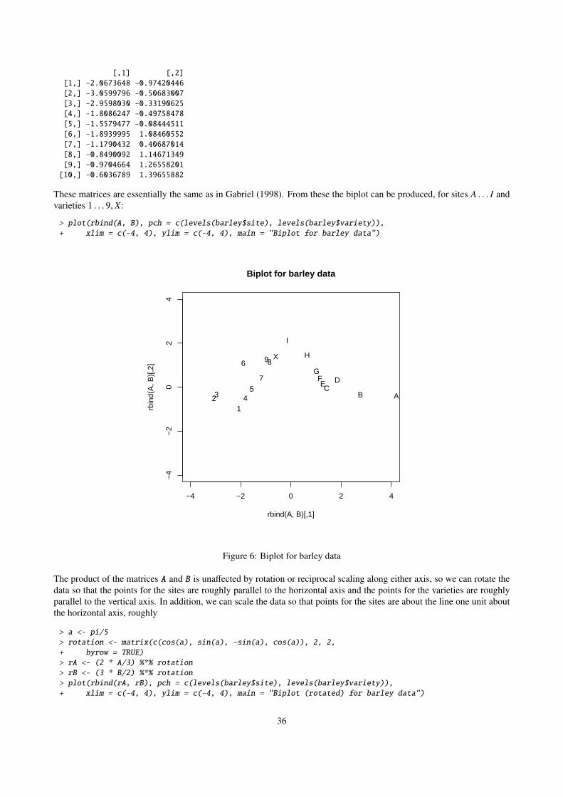
[,1] [,2][1,] -2.0673648 -0.97420446[2,] -3.0599796 -0.50683007[3,] -2.9598030 -0.33190625[4,] -1.8086247 -0.49758478[5,] -1.5579477 -0.08444511[6,] -1.8939995 1.08460552[7,] -1.1790432 0.40687014[8,] -0.8490092 1.14671349[9,] -0.9704664 1.26558201[10,] -0.6036789 1.39655882
These matrices are essentially the same as in Gabriel (1998). From these the biplot can be produced, for sites A . . . I andvarieties 1 . . . 9, X:
> plot(rbind(A, B), pch = c(levels(barley$site), levels(barley$variety)),+ xlim = c(-4, 4), ylim = c(-4, 4), main = "Biplot for barley data")
ABC
DEF
G
H
I
123 4
5
6
7
89X
−4 −2 0 2 4
−4
−2
02
4
Biplot for barley data
rbind(A, B)[,1]
rbin
d(A
, B)[
,2]
Figure 6: Biplot for barley data
The product of the matrices A and B is unaffected by rotation or reciprocal scaling along either axis, so we can rotate thedata so that the points for the sites are roughly parallel to the horizontal axis and the points for the varieties are roughlyparallel to the vertical axis. In addition, we can scale the data so that points for the sites are about the line one unit aboutthe horizontal axis, roughly
> a <- pi/5> rotation <- matrix(c(cos(a), sin(a), -sin(a), cos(a)), 2, 2,+ byrow = TRUE)> rA <- (2 * A/3) %*% rotation> rB <- (3 * B/2) %*% rotation> plot(rbind(rA, rB), pch = c(levels(barley$site), levels(barley$variety)),+ xlim = c(-4, 4), ylim = c(-4, 4), main = "Biplot (rotated) for barley data")
36
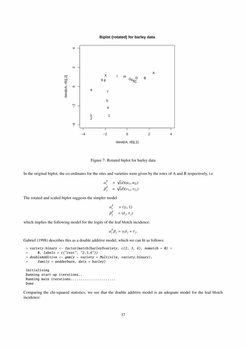
A
BCD
EFGHI
123
4
5
6 7
89X
−4 −2 0 2 4
−4
−2
02
4
Biplot (rotated) for barley data
rbind(rA, rB)[,1]
rbin
d(rA
, rB
)[,2
]
Figure 7: Rotated biplot for barley data
In the original biplot, the co-ordinates for the sites and varieties were given by the rows of A and B respectively, i.e
αTi =
√(d)(u1i, u2i)
βTj =
√(d)(v1 j, v2 j)
The rotated and scaled biplot suggests the simpler model
αTi = (γi, 1)βT
j = (δ j, τ j)
which implies the following model for the logits of the leaf blotch incidence:
αTi β j = γiδ j + τ j.
Gabriel (1998) describes this as a double additive model, which we can fit as follows:
> variety.binary <- factor(match(barley$variety, c(2, 3, 6), nomatch = 0) >+ 0, labels = c("rest", "2,3,6"))> doubleAdditive <- gnm(y ~ variety + Mult(site, variety.binary),+ family = wedderburn, data = barley)
InitialisingRunning start-up iterations..Running main iterations.......................Done
Comparing the chi-squared statistics, we see that the double additive model is an adequate model for the leaf blotchincidence:
37

> biplotModChiSq <- sum(residuals(biplotModel, type = "pearson")^2)> doubleAddChiSq <- sum(residuals(doubleAdditive, type = "pearson")^2)> c(doubleAddChiSq - biplotModChiSq, doubleAdditive$df.residual -+ biplotModel$df.residual)
[1] 9.513774 15.000000
7.6 Stereotype model for multinomial responseThe stereotype model was proposed by Anderson (1984) for ordered categorical data. It is a linear logistic model, inwhich there is assumed to be a common relationship between the response and the covariates in the model, but the scaleof this association varies between categories and there is an additional category main effect or category-specific intercept:
log µic = β0c + γc
∑r
βr xir.
This model can be estimated by re-expressing the categorical data as counts and using a gnm model with a log link andpoisson variance function. The gnm package includes the utility function expandCategorical to facilitate the requireddata processing.
For example, the backPain data set from Anderson (1984) describes the progress of patients with back pain. Thedata set consists of an ordered factor quantifying the progress of each patient, and three prognostic variables. These datacan be re-expressed as follows:
> set.seed(1)> data(backPain)> backPain[1:2, ]
x1 x2 x3 pain1 1 1 1 same2 1 1 1 marked.improvement
> backPainLong <- expandCategorical(backPain, "pain")> backPainLong[1:12, ]
x1 x2 x3 pain count id1 1 1 1 worse 0 11.1 1 1 1 same 1 11.2 1 1 1 slight.improvement 0 11.3 1 1 1 moderate.improvement 0 11.4 1 1 1 marked.improvement 0 11.5 1 1 1 complete.relief 0 12 1 1 1 worse 0 22.1 1 1 1 same 0 22.2 1 1 1 slight.improvement 0 22.3 1 1 1 moderate.improvement 0 22.4 1 1 1 marked.improvement 1 22.5 1 1 1 complete.relief 0 2
We can now fit the stereotype model to these data:
> oneDimensional <- gnm(count ~ pain + Mult(pain, x1 + x2 + x3),+ eliminate = id, family = "poisson", data = backPainLong)
InitialisingRunning start-up iterations..Running main iterations..............Done
> oneDimensional
38

Call:gnm(formula = count ~ pain + Mult(pain, x1 + x2 + x3), eliminate = id,
family = "poisson", data = backPainLong)
Coefficients of interest:painsame16.1578
painslight.improvement15.6848
painmoderate.improvement12.4556
painmarked.improvement19.9140
paincomplete.relief21.6653
Mult(., x1 + x2 + x3).painworse0.3950
Mult(., x1 + x2 + x3).painsame-3.0297
Mult(., x1 + x2 + x3).painslight.improvement-2.8450
Mult(., x1 + x2 + x3).painmoderate.improvement-2.0356
Mult(., x1 + x2 + x3).painmarked.improvement-3.8622
Mult(., x1 + x2 + x3).paincomplete.relief-4.5641
Mult(pain, . + x2 + x3).x11.0832
Mult(pain, x1 + . + x3).x20.6213
Mult(pain, x1 + x2 + .).x30.5470
Deviance: 303.1003Pearson chi-squared: 433.3727Residual df: 493
specifying the id factor through eliminate so that the 101 id effects are estimated more efficiently and are excludedfrom printed model summaries by default. This model is one dimensional since it involves only one function of x =
(x1, x2, x3). We can compare this model to one with category-specific coefficents of the x variables, as may be used for aqualitative categorical response:
> threeDimensional <- gnm(count ~ pain + pain:(x1 + x2 + x3), eliminate = id,+ family = "poisson", data = backPainLong)
InitialisingRunning main iterations...........Done
> threeDimensional
Call:gnm(formula = count ~ pain + pain:(x1 + x2 + x3), eliminate = id,
family = "poisson", data = backPainLong)
Coefficients of interest:painsame painslight.improvement36.3326 35.9518
painmoderate.improvement painmarked.improvement32.8344 40.0350
paincomplete.relief painworse:x1
39
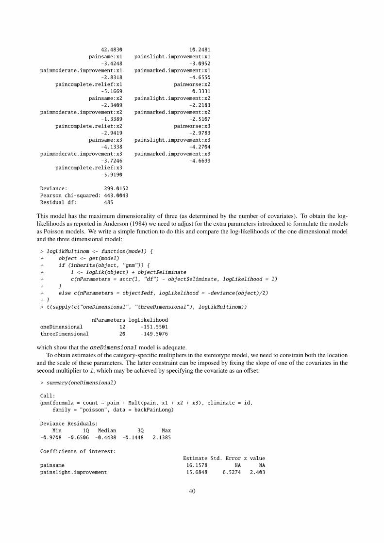
42.4830 10.2481painsame:x1 painslight.improvement:x1
-3.4248 -3.0952painmoderate.improvement:x1 painmarked.improvement:x1
-2.8318 -4.6550paincomplete.relief:x1 painworse:x2
-5.1669 0.3331painsame:x2 painslight.improvement:x2
-2.3409 -2.2183painmoderate.improvement:x2 painmarked.improvement:x2
-1.3389 -2.5107paincomplete.relief:x2 painworse:x3
-2.9419 -2.9783painsame:x3 painslight.improvement:x3
-4.1338 -4.2704painmoderate.improvement:x3 painmarked.improvement:x3
-3.7246 -4.6699paincomplete.relief:x3
-5.9190
Deviance: 299.0152Pearson chi-squared: 443.0043Residual df: 485
This model has the maximum dimensionality of three (as determined by the number of covariates). To obtain the log-likelihoods as reported in Anderson (1984) we need to adjust for the extra parameters introduced to formulate the modelsas Poisson models. We write a simple function to do this and compare the log-likelihoods of the one dimensional modeland the three dimensional model:
> logLikMultinom <- function(model) {+ object <- get(model)+ if (inherits(object, "gnm")) {+ l <- logLik(object) + object$eliminate+ c(nParameters = attr(l, "df") - object$eliminate, logLikelihood = l)+ }+ else c(nParameters = object$edf, logLikelihood = -deviance(object)/2)+ }> t(sapply(c("oneDimensional", "threeDimensional"), logLikMultinom))
nParameters logLikelihoodoneDimensional 12 -151.5501threeDimensional 20 -149.5076
which show that the oneDimensional model is adequate.To obtain estimates of the category-specific multipliers in the stereotype model, we need to constrain both the location
and the scale of these parameters. The latter constraint can be imposed by fixing the slope of one of the covariates in thesecond multiplier to 1, which may be achieved by specifying the covariate as an offset:
> summary(oneDimensional)
Call:gnm(formula = count ~ pain + Mult(pain, x1 + x2 + x3), eliminate = id,
family = "poisson", data = backPainLong)
Deviance Residuals:Min 1Q Median 3Q Max
-0.9708 -0.6506 -0.4438 -0.1448 2.1385
Coefficients of interest:Estimate Std. Error z value
painsame 16.1578 NA NApainslight.improvement 15.6848 6.5274 2.403
40
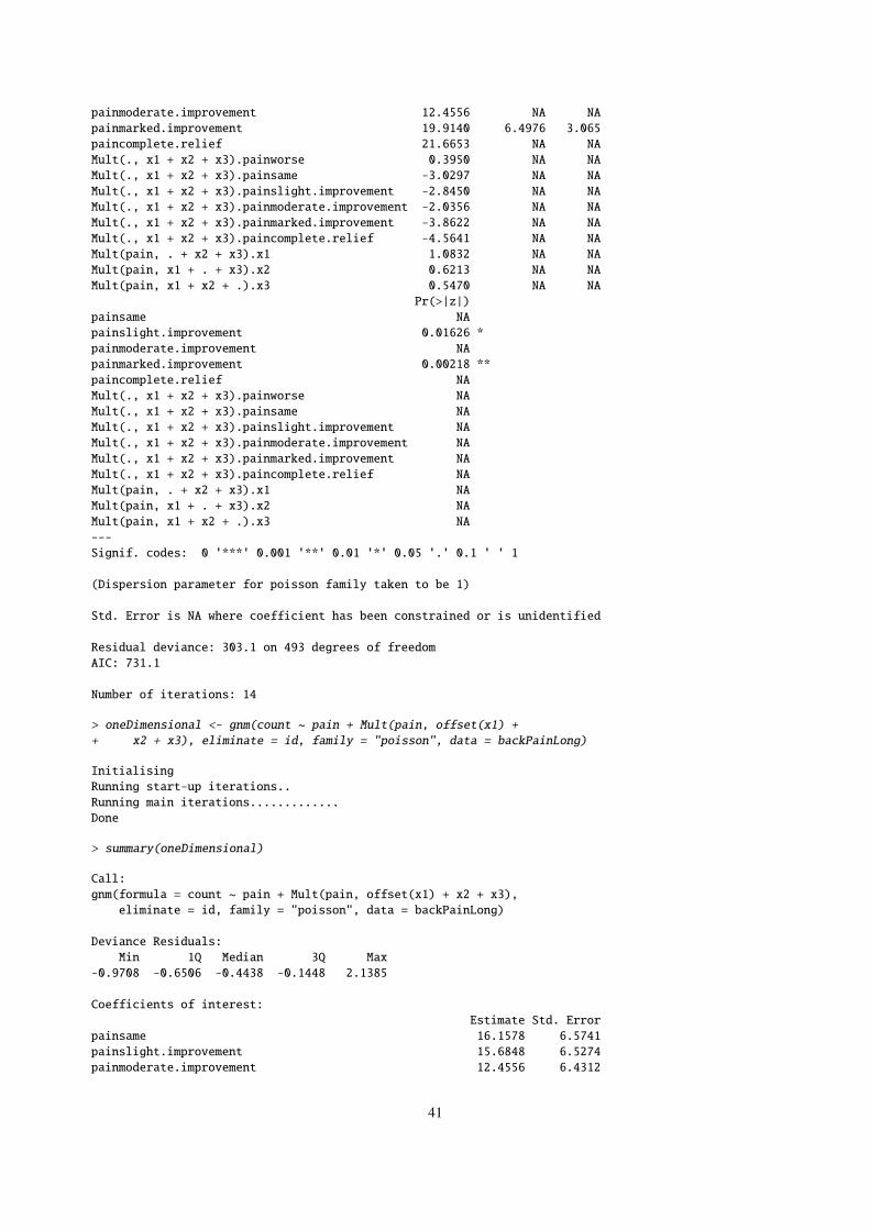
painmoderate.improvement 12.4556 NA NApainmarked.improvement 19.9140 6.4976 3.065paincomplete.relief 21.6653 NA NAMult(., x1 + x2 + x3).painworse 0.3950 NA NAMult(., x1 + x2 + x3).painsame -3.0297 NA NAMult(., x1 + x2 + x3).painslight.improvement -2.8450 NA NAMult(., x1 + x2 + x3).painmoderate.improvement -2.0356 NA NAMult(., x1 + x2 + x3).painmarked.improvement -3.8622 NA NAMult(., x1 + x2 + x3).paincomplete.relief -4.5641 NA NAMult(pain, . + x2 + x3).x1 1.0832 NA NAMult(pain, x1 + . + x3).x2 0.6213 NA NAMult(pain, x1 + x2 + .).x3 0.5470 NA NA
Pr(>|z|)painsame NApainslight.improvement 0.01626 *painmoderate.improvement NApainmarked.improvement 0.00218 **paincomplete.relief NAMult(., x1 + x2 + x3).painworse NAMult(., x1 + x2 + x3).painsame NAMult(., x1 + x2 + x3).painslight.improvement NAMult(., x1 + x2 + x3).painmoderate.improvement NAMult(., x1 + x2 + x3).painmarked.improvement NAMult(., x1 + x2 + x3).paincomplete.relief NAMult(pain, . + x2 + x3).x1 NAMult(pain, x1 + . + x3).x2 NAMult(pain, x1 + x2 + .).x3 NA---Signif. codes: 0 '***' 0.001 '**' 0.01 '*' 0.05 '.' 0.1 ' ' 1
(Dispersion parameter for poisson family taken to be 1)
Std. Error is NA where coefficient has been constrained or is unidentified
Residual deviance: 303.1 on 493 degrees of freedomAIC: 731.1
Number of iterations: 14
> oneDimensional <- gnm(count ~ pain + Mult(pain, offset(x1) ++ x2 + x3), eliminate = id, family = "poisson", data = backPainLong)
InitialisingRunning start-up iterations..Running main iterations.............Done
> summary(oneDimensional)
Call:gnm(formula = count ~ pain + Mult(pain, offset(x1) + x2 + x3),
eliminate = id, family = "poisson", data = backPainLong)
Deviance Residuals:Min 1Q Median 3Q Max
-0.9708 -0.6506 -0.4438 -0.1448 2.1385
Coefficients of interest:Estimate Std. Error
painsame 16.1578 6.5741painslight.improvement 15.6848 6.5274painmoderate.improvement 12.4556 6.4312
41

painmarked.improvement 19.9140 6.4975paincomplete.relief 21.6653 6.5571Mult(., x2 + x3 + offset(x1)).painworse 1.3471 NAMult(., x2 + x3 + offset(x1)).painsame -2.3626 NAMult(., x2 + x3 + offset(x1)).painslight.improvement -2.1626 NAMult(., x2 + x3 + offset(x1)).painmoderate.improvement -1.2858 NAMult(., x2 + x3 + offset(x1)).painmarked.improvement -3.2645 NAMult(., x2 + x3 + offset(x1)).paincomplete.relief -4.0247 NAMult(pain, . + x3 + offset(x1)).x2 0.5736 0.2178Mult(pain, x2 + . + offset(x1)).x3 0.5050 0.2431
z value Pr(>|z|)painsame 2.458 0.013980 *painslight.improvement 2.403 0.016265 *painmoderate.improvement 1.937 0.052777 .painmarked.improvement 3.065 0.002178 **paincomplete.relief 3.304 0.000953 ***Mult(., x2 + x3 + offset(x1)).painworse NA NAMult(., x2 + x3 + offset(x1)).painsame NA NAMult(., x2 + x3 + offset(x1)).painslight.improvement NA NAMult(., x2 + x3 + offset(x1)).painmoderate.improvement NA NAMult(., x2 + x3 + offset(x1)).painmarked.improvement NA NAMult(., x2 + x3 + offset(x1)).paincomplete.relief NA NAMult(pain, . + x3 + offset(x1)).x2 2.633 0.008451 **Mult(pain, x2 + . + offset(x1)).x3 2.077 0.037807 *---Signif. codes: 0 '***' 0.001 '**' 0.01 '*' 0.05 '.' 0.1 ' ' 1
(Dispersion parameter for poisson family taken to be 1)
Std. Error is NA where coefficient has been constrained or is unidentified
Residual deviance: 303.1 on 493 degrees of freedomAIC: 731.1
Number of iterations: 13
The location of the category-specific multipliers can constrained by setting one of the parameters to zero, either throughthe constrain argument of gnm or with getContrasts:
> getContrasts(oneDimensional, pickCoef(oneDimensional, "Mult.*pain"))
Mult(., x2 + x3 + offset(x1)).painworseNA
Mult(., x2 + x3 + offset(x1)).painsameTRUE
Mult(., x2 + x3 + offset(x1)).painslight.improvementTRUE
Mult(., x2 + x3 + offset(x1)).painmoderate.improvementTRUE
Mult(., x2 + x3 + offset(x1)).painmarked.improvementTRUE
Mult(., x2 + x3 + offset(x1)).paincomplete.reliefTRUE
Mult(pain, . + x3 + offset(x1)).x2FALSE
Mult(pain, x2 + . + offset(x1)).x3FALSE
Note: not all of the specified contrasts in this set are estimableestimate SE
Mult(., x2 + x3 + offset(x1)).painworse 0.000000 0.000000Mult(., x2 + x3 + offset(x1)).painsame -3.709726 1.825562Mult(., x2 + x3 + offset(x1)).painslight.improvement -3.509687 1.791726
42
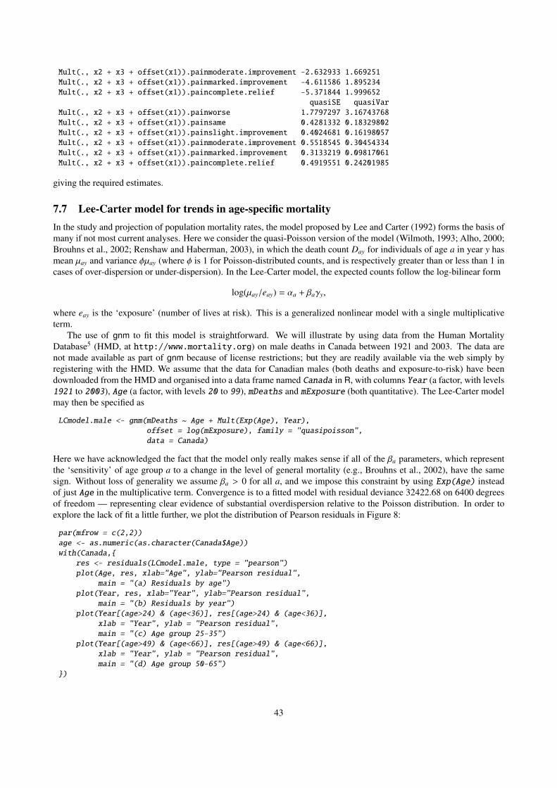
Mult(., x2 + x3 + offset(x1)).painmoderate.improvement -2.632933 1.669251Mult(., x2 + x3 + offset(x1)).painmarked.improvement -4.611586 1.895234Mult(., x2 + x3 + offset(x1)).paincomplete.relief -5.371844 1.999652
quasiSE quasiVarMult(., x2 + x3 + offset(x1)).painworse 1.7797297 3.16743768Mult(., x2 + x3 + offset(x1)).painsame 0.4281332 0.18329802Mult(., x2 + x3 + offset(x1)).painslight.improvement 0.4024681 0.16198057Mult(., x2 + x3 + offset(x1)).painmoderate.improvement 0.5518545 0.30454334Mult(., x2 + x3 + offset(x1)).painmarked.improvement 0.3133219 0.09817061Mult(., x2 + x3 + offset(x1)).paincomplete.relief 0.4919551 0.24201985
giving the required estimates.
7.7 Lee-Carter model for trends in age-specific mortalityIn the study and projection of population mortality rates, the model proposed by Lee and Carter (1992) forms the basis ofmany if not most current analyses. Here we consider the quasi-Poisson version of the model (Wilmoth, 1993; Alho, 2000;Brouhns et al., 2002; Renshaw and Haberman, 2003), in which the death count Day for individuals of age a in year y hasmean µay and variance φµay (where φ is 1 for Poisson-distributed counts, and is respectively greater than or less than 1 incases of over-dispersion or under-dispersion). In the Lee-Carter model, the expected counts follow the log-bilinear form
log(µay/eay) = αa + βaγy,
where eay is the ‘exposure’ (number of lives at risk). This is a generalized nonlinear model with a single multiplicativeterm.
The use of gnm to fit this model is straightforward. We will illustrate by using data from the Human MortalityDatabase5 (HMD, at http://www.mortality.org) on male deaths in Canada between 1921 and 2003. The data arenot made available as part of gnm because of license restrictions; but they are readily available via the web simply byregistering with the HMD. We assume that the data for Canadian males (both deaths and exposure-to-risk) have beendownloaded from the HMD and organised into a data frame named Canada in R, with columns Year (a factor, with levels1921 to 2003), Age (a factor, with levels 20 to 99), mDeaths and mExposure (both quantitative). The Lee-Carter modelmay then be specified as
LCmodel.male <- gnm(mDeaths ~ Age + Mult(Exp(Age), Year),offset = log(mExposure), family = "quasipoisson",data = Canada)
Here we have acknowledged the fact that the model only really makes sense if all of the βa parameters, which representthe ‘sensitivity’ of age group a to a change in the level of general mortality (e.g., Brouhns et al., 2002), have the samesign. Without loss of generality we assume βa > 0 for all a, and we impose this constraint by using Exp(Age) insteadof just Age in the multiplicative term. Convergence is to a fitted model with residual deviance 32422.68 on 6400 degreesof freedom — representing clear evidence of substantial overdispersion relative to the Poisson distribution. In order toexplore the lack of fit a little further, we plot the distribution of Pearson residuals in Figure 8:
par(mfrow = c(2,2))age <- as.numeric(as.character(Canada$Age))with(Canada,{
res <- residuals(LCmodel.male, type = "pearson")plot(Age, res, xlab="Age", ylab="Pearson residual",
main = "(a) Residuals by age")plot(Year, res, xlab="Year", ylab="Pearson residual",
main = "(b) Residuals by year")plot(Year[(age>24) & (age<36)], res[(age>24) & (age<36)],
xlab = "Year", ylab = "Pearson residual",main = "(c) Age group 25-35")
plot(Year[(age>49) & (age<66)], res[(age>49) & (age<66)],xlab = "Year", ylab = "Pearson residual",main = "(d) Age group 50-65")
})
43
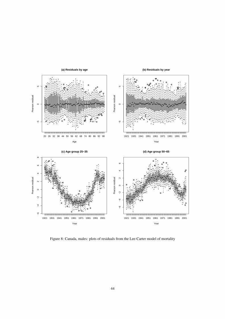
●●
● ●
●
●●
●
●
●
●●
●●
●
●
●
●
●
●●
●
●
●
●
●
●
●
●●
●●
●●
●
20 26 32 38 44 50 56 62 68 74 80 86 92 98
−5
05
(a) Residuals by age
Age
Pea
rson
res
idua
l
●
●●
●
●
●
●
●
●
●
●
●●
●●●
●
●●
●
●●
●
●●
●
●
●●●
1921 1931 1941 1951 1961 1971 1981 1991 2001
−5
05
(b) Residuals by year
Year
Pea
rson
res
idua
l
●●
●●
●
●
●
●
●
●
●
●
●●
●
●
●
●
●
●
●
●
●
●
1921 1931 1941 1951 1961 1971 1981 1991 2001
−6
−4
−2
02
46
8
(c) Age group 25−35
Year
Pea
rson
res
idua
l
●
●
●
●
●
●
●
●
●
●●
●
●
●
● ●
●
●
●
●
●
●
●
●
●
●
●
1921 1931 1941 1951 1961 1971 1981 1991 2001
−6
−4
−2
02
46
(d) Age group 50−65
Year
Pea
rson
res
idua
l
Figure 8: Canada, males: plots of residuals from the Lee-Carter model of mortality
44
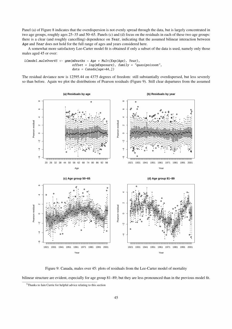
Panel (a) of Figure 8 indicates that the overdispersion is not evenly spread through the data, but is largely concentrated intwo age groups, roughly ages 25–35 and 50–65. Panels (c) and (d) focus on the residuals in each of these two age groups:there is a clear (and roughly cancelling) dependence on Year, indicating that the assumed bilinear interaction betweenAge and Year does not hold for the full range of ages and years considered here.
A somewhat more satisfactory Lee-Carter model fit is obtained if only a subset of the data is used, namely only thosemales aged 45 or over:
LCmodel.maleOver45 <- gnm(mDeaths ~ Age + Mult(Exp(Age), Year),offset = log(mExposure), family = "quasipoisson",data = Canada[age>44,])
The residual deviance now is 12595.44 on 4375 degrees of freedom: still substantially overdispersed, but less severelyso than before. Again we plot the distributions of Pearson residuals (Figure 9). Still clear departures from the assumed
●
●
●
●
●●
●●
●●●
●
●
●●
●
●
●
●
●●
●
●
●
●●
●
●
●
●
●
●
●●
●●●●
●
●●
●
●
20 26 32 38 44 50 56 62 68 74 80 86 92 98
−6
−4
−2
02
46
8
(a) Residuals by age
Age
Pea
rson
res
idua
l
●●
●
●
●
●
●
●●
●
●
●
●
●
●
●
●
●
●
●
●●
●● ●●
●
●
●●●●
●
●
●
●
●
●●
●●
●
●
●
●
●
●
●
●●
●●●
●
●
●
●
●
●
●
●
●
●
●
●
●●
●
1921 1931 1941 1951 1961 1971 1981 1991 2001
−6
−4
−2
02
46
8
(b) Residuals by year
Year
Pea
rson
res
idua
l
●●
●
●
●
●
●
●
●
●
●
●
●●
●
●
●
●
●
●
●
●
●
●
●
●
●
●
1921 1931 1941 1951 1961 1971 1981 1991 2001
−6
−4
−2
02
46
(c) Age group 50−65
Year
Pea
rson
res
idua
l
●
●
●
●
●
●
●●
●
●
●
●
●
●
●
●
●
●
●
●
●
●
●
●
●
●
●
●
●
●●
●
●●
●
●
●
●
●●
●
●
●
●
●
1921 1931 1941 1951 1961 1971 1981 1991 2001
−4
−2
02
4
(d) Age group 81−89
Year
Pea
rson
res
idua
l
Figure 9: Canada, males over 45: plots of residuals from the Lee-Carter model of mortality
bilinear structure are evident, especially for age group 81–89; but they are less pronounced than in the previous model fit.
5Thanks to Iain Currie for helpful advice relating to this section
45
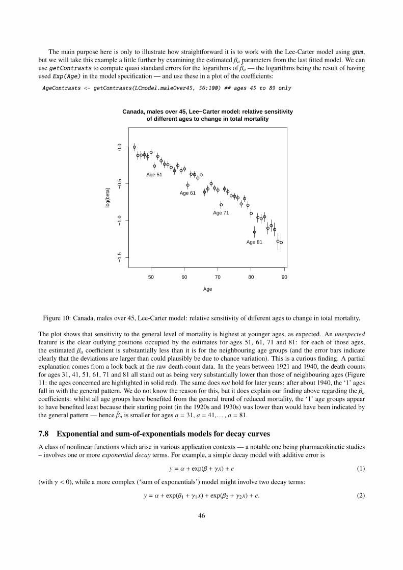
The main purpose here is only to illustrate how straightforward it is to work with the Lee-Carter model using gnm ,but we will take this example a little further by examining the estimated βa parameters from the last fitted model. We canuse getContrasts to compute quasi standard errors for the logarithms of βa — the logarithms being the result of havingused Exp(Age) in the model specification — and use these in a plot of the coefficients:
AgeContrasts <- getContrasts(LCmodel.maleOver45, 56:100) ## ages 45 to 89 only
●
● ● ●●
●
●
●
●● ●
●●
●
●●
●
● ●●
●
●●
●
●●
●
●●
● ●●
●
●
●
●
●
● ●●
●●
●
● ●
50 60 70 80 90
−1.
5−
1.0
−0.
50.
0Canada, males over 45, Lee−Carter model: relative sensitivity
of different ages to change in total mortality
Age
log(
beta
)
Age 81
Age 71
Age 61
Age 51
Figure 10: Canada, males over 45, Lee-Carter model: relative sensitivity of different ages to change in total mortality.
The plot shows that sensitivity to the general level of mortality is highest at younger ages, as expected. An unexpectedfeature is the clear outlying positions occupied by the estimates for ages 51, 61, 71 and 81: for each of those ages,the estimated βa coefficient is substantially less than it is for the neighbouring age groups (and the error bars indicateclearly that the deviations are larger than could plausibly be due to chance variation). This is a curious finding. A partialexplanation comes from a look back at the raw death-count data. In the years between 1921 and 1940, the death countsfor ages 31, 41, 51, 61, 71 and 81 all stand out as being very substantially lower than those of neighbouring ages (Figure11: the ages concerned are highlighted in solid red). The same does not hold for later years: after about 1940, the ‘1’ agesfall in with the general pattern. We do not know the reason for this, but it does explain our finding above regarding the βa
coefficients: whilst all age groups have benefited from the general trend of reduced mortality, the ‘1’ age groups appearto have benefited least because their starting point (in the 1920s and 1930s) was lower than would have been indicated bythe general pattern — hence βa is smaller for ages a = 31, a = 41,. . . , a = 81.
7.8 Exponential and sum-of-exponentials models for decay curvesA class of nonlinear functions which arise in various application contexts — a notable one being pharmacokinetic studies– involves one or more exponential decay terms. For example, a simple decay model with additive error is
y = α + exp(β + γx) + e (1)
(with γ < 0), while a more complex (‘sum of exponentials’) model might involve two decay terms:
y = α + exp(β1 + γ1x) + exp(β2 + γ2x) + e. (2)
46
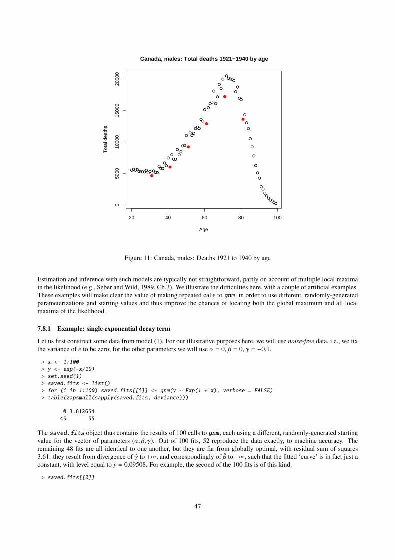
●●●●●●●●
●●●
●
●●●
●●●
●●
●
●
●
●●
●
●●
●●
●
●
●●
●
●●●
●●
●
●
●
●●
●
●
●
●
●
●
●
●●●●●
●
●
●●
●
●
●
●
●
●
●
●
●
●
●●
●●
●●●●●
20 40 60 80 100
050
0010
000
1500
020
000
Canada, males: Total deaths 1921−1940 by age
Age
Tot
al d
eath
s
Figure 11: Canada, males: Deaths 1921 to 1940 by age
Estimation and inference with such models are typically not straightforward, partly on account of multiple local maximain the likelihood (e.g., Seber and Wild, 1989, Ch.3). We illustrate the difficulties here, with a couple of artificial examples.These examples will make clear the value of making repeated calls to gnm , in order to use different, randomly-generatedparameterizations and starting values and thus improve the chances of locating both the global maximum and all localmaxima of the likelihood.
7.8.1 Example: single exponential decay term
Let us first construct some data from model (1). For our illustrative purposes here, we will use noise-free data, i.e., we fixthe variance of e to be zero; for the other parameters we will use α = 0, β = 0, γ = −0.1.
> x <- 1:100> y <- exp(-x/10)> set.seed(1)> saved.fits <- list()> for (i in 1:100) saved.fits[[i]] <- gnm(y ~ Exp(1 + x), verbose = FALSE)> table(zapsmall(sapply(saved.fits, deviance)))
0 3.61265445 55
The saved.fits object thus contains the results of 100 calls to gnm , each using a different, randomly-generated startingvalue for the vector of parameters (α, β, γ). Out of 100 fits, 52 reproduce the data exactly, to machine accuracy. Theremaining 48 fits are all identical to one another, but they are far from globally optimal, with residual sum of squares3.61: they result from divergence of γ to +∞, and correspondingly of β to −∞, such that the fitted ‘curve’ is in fact just aconstant, with level equal to y = 0.09508. For example, the second of the 100 fits is of this kind:
> saved.fits[[2]]
47
Call:gnm(formula = y ~ Exp(1 + x), verbose = FALSE)
Coefficients:(Intercept) Exp(. + x).(Intercept) Exp(1 + .).x9.508e-02 -1.424e+03 1.377e+01
Deviance: 3.612654Pearson chi-squared: 3.612654Residual df: 99
The use of repeated calls to gnm , as here, allows the local and global maxima to be easily distinguished.
7.8.2 Example: sum of two exponentials
We can conduct a similar exercise based on the more complex model (2):
> x <- 1:100> y <- exp(-x/10) + 2 * exp(-x/50)> set.seed(1)> saved.fits <- list()> for (i in 1:100) saved.fits[[i]] <- suppressWarnings(gnm(y ~+ Exp(1 + x, inst = 1) + Exp(1 + x, inst = 2), verbose = FALSE))> round(unlist(sapply(saved.fits, deviance)), 4)
[1] 0.1589 0.1589 0.0000 0.0000 0.1589 41.6439 0.1589 0.0000 41.6439[10] 0.0000 0.1589 0.1589 0.0000 41.6439 0.1589 0.1589 41.6439 0.1589[19] 0.1589 0.1589 0.1589 0.0000 0.1589 0.1589 0.1589 0.1589 0.1589[28] 0.0000 0.0000 0.0000 0.1589 41.6439 0.1589 0.0000 0.1589 0.1589[37] 0.1589 0.1589 0.1589 41.6439 0.0000
In this instance, only 37 of the 100 calls to gnm have successfully located a local maximum of the likelihood: in theremaining 63 cases the starting values generated were such that numerical problems resulted, and the fitting algorithmwas abandoned (giving a NULL result). Among the 37 ‘successful’ fits, it is evident that there are three distinct solutions(with respective residual sums of squares equal to 0.1589, 41.64, and essentially zero — the last of these, the exact fit tothe data, having been found 12 times out of the above 37). The two non-optimal local maxima here correspond to thebest fit with a single exponential (which has residual sum of squares 0.1589) and to the fit with no dependence at all on x(residual sum of squares 41.64), as we can see by comparing with:
> singleExp <- gnm(y ~ Exp(1 + x), start = c(NA, NA, -0.1), verbose = FALSE)> singleExp
Call:gnm(formula = y ~ Exp(1 + x), start = c(NA, NA, -0.1), verbose = FALSE)
Coefficients:(Intercept) Exp(. + x).(Intercept) Exp(1 + .).x
0.25007 0.93664 -0.03465
Deviance: 0.1589496Pearson chi-squared: 0.1589496Residual df: 97
> meanOnly <- gnm(y ~ 1, verbose = FALSE)> meanOnly
Call:gnm(formula = y ~ 1, verbose = FALSE)
Coefficients:(Intercept)
0.9511
48

Deviance: 41.6439Pearson chi-squared: 41.6439Residual df: 99
> plot(x, y, main = "Two sub-optimal fits to a sum-of-exponentials curve")> lines(x, fitted(singleExp))> lines(x, fitted(meanOnly), lty = "dashed")
●
●
●
●
●
●
●●●●●●●●●●●●●●●●●●●●●●●●●●●●●●●●●●●●●●●●●●●●●●●●●●●●●●●●●●●●●●●●●●●●●●●●●●●●●●●●●●●●●●●●●●●●●●
0 20 40 60 80 100
0.5
1.0
1.5
2.0
2.5
Two sub−optimal fits to a sum−of−exponentials curve
x
y
Figure 12: Two sub-optimal fits to a sum-of-exponentials curve
In this example, it is clear that even a small amount of noise in the data would make it practically impossible todistinguish between competing models containing one and two exponential-decay terms.
In summary: the default gnm setting of randomly-chosen starting values is useful for identifying multiple local maximain the likelihood; and reasonably good starting values are needed if the global maximum is to be found. In the presentexample, knowing that γ1 and γ2 should both be small and negative, we might perhaps have tried
> gnm(y ~ instances(Exp(1 + x), 2), start = c(NA, NA, -0.1, NA,+ -0.1), verbose = FALSE)
Call:gnm(formula = y ~ instances(Exp(1 + x), 2), start = c(NA, NA,
-0.1, NA, -0.1), verbose = FALSE)
Coefficients:(Intercept) Exp(. + x, inst = 1).(Intercept)1.844e-12 -3.639e-12
Exp(1 + ., inst = 1).x Exp(. + x, inst = 2).(Intercept)-1.000e-01 6.931e-01
Exp(1 + ., inst = 2).x-2.000e-02
Deviance: 1.520732e-24
49

Pearson chi-squared: 1.520732e-24Residual df: 95
which reliably yields the (globally optimal) perfect fit to the data.
50

A User-level functionsWe list here, for easy reference, all of the user-level functions in the gnm package. For full documentation see the packagehelp pages.
Model Fitting
gnm fit generalized nonlinear models
Model Specification
Diag create factor differentiating diagonal elementsSymm create symmetric interaction of factorsTopo create ‘topological’ interaction factorsConst specify a constant in a gnm model formulaDref specify a diagonal reference term in a gnm model formulaMult specify a product of predictors in a gnm formulaMultHomog specify a multiplicative interaction with homogeneous effects in a gnm formulaExp specify the exponential of a predictor in a gnm formulaInv specify the reciprocal of a predictor in a gnm formulaNonlin specify a special nonlinear term in a gnm formula (using external plug-in function)wedderburn specify the Wedderburn quasi-likelihood family
Methods and Accessor Functions
confint.gnm compute confidence intervals of gnm parameters based on the profiled devianceconfint.profile.gnm compute confidence intervals of parameters from a profile.gnm objectprofile.gnm profile deviance for parameters in a gnm modelplot.profile.gnm plot profile traces from a profile.gnm objectsummary.gnm summarize gnm fitsresidSVD multiplicative approximation of model residualsexitInfo print numerical details of last iteration when gnm has not convergedofInterest extract the ofInterest component of a gnm objectofInterest<- replace the ofInterest component of a gnm objectparameters get model parameters from a gnm object, including parameters that were con-
strainedpickCoef get indices of model parametersgetContrasts estimate contrasts and their standard errors for parameters in a gnm modelcheckEstimable check whether one or more parameter combinations in a gnm model is identifiedse get standard errors of linear parameter combinations in gnm modelsDref estimate weights and corresponding standard errors for a diagonal reference term
in a gnm modeltermPredictors (generic) extract term contributions to predictor
Auxiliary Functions
asGnm coerce an object of class lm or glm to class gnmexpandCategorical expand a data frame by re-expressing categorical data as countsgetModelFrame get the model frame in use by gnmMPinv Moore-Penrose pseudoinverse of a real-valued matrixqrSolve Minimum-length solution of a linear system
51
ReferencesAgresti, A. (2002). Categorical Data Analysis (2nd ed.). New York: Wiley.
Alho, J. M. (2000). Discussion of Lee (2000). North American Actuarial Journal 4, 91–93.
Anderson, J. A. (1984). Regression and ordered categorical variables. J. R. Statist. Soc. B 46(1), 1–30.
Brouhns, N., M. Denuit, and J. K. Vermunt (2002). A poisson log-bilinear regression approach to the construction ofprojected lifetables. Insurance Mathematics and Economics 31, 373–393.
Catchpole, E. and B. Morgan (1997). Detecting parameter redundancy. Biometrika 84, 187–196.
Cautres, B., A. F. Heath, and D. Firth (1998). Class, religion and vote in Britain and France. La Lettre de la MaisonFrançaise 8.
Clifford, P. and A. F. Heath (1993). The political consequences of social mobility. J. Roy. Stat. Soc. A 156(1), 51–61.
Erikson, R. and J. H. Goldthorpe (1992). The Constant Flux. Oxford: Clarendon Press.
Erikson, R., J. H. Goldthorpe, and L. Portocarero (1982). Social fluidity in industrial nations: England, France andSweden. British Journal of Sociology 33, 1–34.
Firth, D. (2003). Overcoming the reference category problem in the presentation of statistical models. SociologicalMethodology 33, 1–18.
Firth, D. and R. X. de Menezes (2004). Quasi-variances. Biometrika 91, 65–80.
Gabriel, K. R. (1998). Generalised bilinear regression. Biometrika 85, 689–700.
Goodman, L. A. (1979). Simple models for the analysis of association in cross-classifications having ordered categories.J. Amer. Statist. Assoc. 74, 537–552.
Hatzinger, R. and B. J. Francis (2004). Fitting paired comparison models in R. Technical Report 3, Department ofStatistics and Mathematics, Wirtschaftsuniversität Wien.
Lee, R. D. and L. Carter (1992). Modelling and forecasting the time series of US mortality. Journal of the AmericanStatistical Association 87, 659–671.
McCullagh, P. and J. A. Nelder (1989). Generalized Linear Models (Second Edition). Chapman & Hall Ltd.
Renshaw, A. and S. Haberman (2003). Lee-carter mortality forecasting: a parallel generalized linear modelling approachfor England and Wales mortality projections. Applied Statistics 52, 119–137.
Seber, G. A. F. and C. J. Wild (1989). Nonlinear Regression. Wiley.
Sobel, M. E. (1981). Diagonal mobility models: A substantively motivated class of designs for the analysis of mobilityeffects. Amer. Soc. Rev. 46, 893–906.
Sobel, M. E. (1985). Social mobility and fertility revisited: Some new models for the analysis of the mobility effectshypothesis. Amer. Soc. Rev. 50, 699–712.
van der Slik, F. W. P., N. D. de Graaf, and J. R. M. Gerris (2002, 4). Conformity to parental rules: Asymmetric influencesof father’s and mother’s levels of education. Europ. Soc. Rev. 18, 489–502.
Vargas, M., J. Crossa, F. van Eeuwijk, K. D. Sayre, and M. P. Reynolds (2001). Interpreting treatment by environmentinteraction in agronomy trials. Agronomy Journal 93, 949–960.
Wedderburn, R. W. M. (1974). Quasi-likelihood functions, generalized linear models, and the Gauss-Newton method.Biometrika 61, 439–447.
Wilmoth, J. R. (1993). Computational methods for fitting and extrapolating the Lee-Carter model of mortality change.Technical report, Department of Demography, University of California, Berkeley.
52

Xie, Y. (1992). The log-multiplicative layer effect model for comparing mobility tables. American Sociological Review 57,380–395.
Yaish, M. (1998). Opportunities, Little Change. Class Mobility in Israeli Society, 1974–1991. Ph. D. thesis, NuffieldCollege, University of Oxford.
Yaish, M. (2004). Class Mobility Trends in Israeli Society, 1974-1991. Lewiston: Edwin Mellen Press.
53