
Generalized Event Tree Algorithm and Software for Dam Safety Risk
135
Utah State University DigitalCommons@USU All Graduate eses and Dissertations Graduate Studies, School of 12-1-2008 Generalized Event Tree Algorithm and Soſtware for Dam Safety Risk Analysis Anurag Srivastava Utah State University is esis is brought to you for free and open access by the Graduate Studies, School of at DigitalCommons@USU. It has been accepted for inclusion in All Graduate eses and Dissertations by an authorized administrator of DigitalCommons@USU. For more information, please contact [email protected]. Recommended Citation Srivastava, Anurag, "Generalized Event Tree Algorithm and Soſtware for Dam Safety Risk Analysis" (2008). All Graduate eses and Dissertations. Paper 32. hp://digitalcommons.usu.edu/etd/32
-
Upload
tonykallada -
Category
Documents
-
view
51 -
download
0
Transcript of Generalized Event Tree Algorithm and Software for Dam Safety Risk
Utah State UniversityDigitalCommons@USU
All Graduate Theses and Dissertations Graduate Studies, School of
12-1-2008
Generalized Event Tree Algorithm and Software forDam Safety Risk AnalysisAnurag SrivastavaUtah State University
This Thesis is brought to you for free and open access by the GraduateStudies, School of at DigitalCommons@USU. It has been accepted forinclusion in All Graduate Theses and Dissertations by an authorizedadministrator of DigitalCommons@USU. For more information, pleasecontact [email protected].
Recommended CitationSrivastava, Anurag, "Generalized Event Tree Algorithm and Software for Dam Safety Risk Analysis" (2008). All Graduate Theses andDissertations. Paper 32.http://digitalcommons.usu.edu/etd/32

GENERALIZED EVENT TREE ALGORITHM AND SOFTWARE
FOR DAM SAFETY RISK ANALYSIS
by
Anurag Srivastava
A thesis submitted in partial fulfillment of the requirements for the degree
of
MASTER OF SCIENCE
in
Civil and Environmental Engineering Approved: Dr. David S. Bowles Dr. Loren R. Anderson Major Professor Committee Member Dr. Sanjay S. Chauhan Dr. Terry F. Glover Committee Member Committee Member
Dr. Byron R. Burnham
Dean of Graduate Studies
UTAH STATE UNIVERSITY Logan, Utah
2008

ii
ABSTRACT
Generalized Event Tree Algorithm and Software for
Dam Safety Risk Analysis
by
Anurag Srivastava, Master of Science
Utah State University, 2008
Major Professor: Dr. David S. Bowles Department: Civil and Environmental Engineering
Event tree analysis is a most commonly used method in dam safety risk analysis
modeling. Available software tools for performing event tree analyses lack the flexibility
to efficiently address many important factors in dam safety risk analysis. As a result of
these practical limitations, spreadsheets have been used, sometimes including Visual
Basic macros, to perform these analyses. However, this approach lacks generality and
can require significant effort to apply to a specific dam or to modify the event tree
structure. In response to these limitations, here a generalized event tree analysis tool,
DAMRAE (DAM safety Risk Analysis Engine), has been developed. It includes a
graphical interface for developing and populating an event tree, and a tool for calculating
and post-processing an event tree risk model for dam safety risk assessment in a highly
flexible manner. This thesis describes the underlying theoretical and computational logic
employed in the current version of DAMRAE, and provides a detailed example of the

iii
calculations in the current version of DAMRAE for an application to a US Army Corps
of Engineers (USACE) dam. The thesis closes with some conclusions about the
capabilities of DAMRAE and a summary of plans for its further development.
(134 pages)

iv
ACKNOWLEDGMENTS
I express my sincere gratitude to my advisor, Dr. David Bowles, for his guidance,
invaluable ideas, intellectual support, and motivation throughout my graduate studies.
I am grateful to Dr. Sanjay Chauhan for his precious suggestions and intellectual
inputs in developing this work.
I thank my committee members, Drs. Loren Anderson and Terry Glover, for their
active interest and involvement.
The support of the U.S. Army Corps of Engineers and the Utah Water Research
Laboratory at Utah State University in funding this research and development work on
DAMRAE is gratefully acknowledged.
Anurag Srivastava

v
CONTENTS
Page
ABSTRACT........................................................................................................................ ii
ACKNOWLEDGMENTS ................................................................................................. iv
LIST OF TABLES............................................................................................................ vii
LIST OF FIGURES ........................................................................................................... ix
CHAPTER I. INTRODUCTION ................................................................................... 1
Dam Safety Risk Analysis .............................................................. 1 Application of ETA in Dam Safety Risk Analysis ......................... 2 Available ETA Software Tools....................................................... 3 Objectives of Research ................................................................... 5 Organization of the Thesis .............................................................. 7
II. LITERATURE REVIEW......................................................................... 9
Introduction..................................................................................... 9
Failure modes and effects analysis (FMEA)...........................9 Fault tree analysis (FTA) ......................................................10 Event tree analysis (ETA).....................................................10
Event Tree..................................................................................... 12
Event tree structure ...............................................................15 Event tree construction .........................................................18 Probability and consequences assignment ............................19 The mathematics of event trees.............................................20
Proprietary Software Tools for ETA............................................. 25
III. THEORETICAL DEVELOPMENT OF DAMRAE.............................. 28
Introduction................................................................................... 28 Branch Attributes .......................................................................... 28 Branch Identifiers.......................................................................... 30
vi
Calculation of State, Branch Probability, Exposure, and Consequences Values................................................................. 30
Types of Branches......................................................................... 31 Collapsed Nodes ........................................................................... 34
IV. COMPUTATIONAL METHODOLGY OF DAMRAE........................ 37
Introduction................................................................................... 37 Event Tree Algorithm ................................................................... 38
Step 1. Event tree diagram and inputs ..................................39 Step 2. Branch state value assignment and branch probability calculation .......................................................46
Step 3. Branch and annualized consequences Calculation .........................................................................47
Step 4. Post-processing .........................................................47
V. DAMRAE DEMONSTRATION........................................................... 49
Introduction................................................................................... 49 Success Dam: A Dam Safety Risk Analysis Study ...................... 49 Flood Event Tree........................................................................... 50
Event tree structure ...............................................................50 Event tree Inputs ...................................................................53 Risk analysis output ..............................................................58
Earthquake Event Tree.................................................................. 59
Event tree structure ...............................................................59 Event tree inputs ...................................................................62 Risk analysis output ..............................................................79
Post-processing ............................................................................. 80 Discussion ..................................................................................... 82
VI. SUMMARY, CONCLUSION, AND FUTURE WORK ....................... 83
Summary....................................................................................... 83 Conclusion .................................................................................... 84 Future Work .................................................................................. 85
REFERENCES ................................................................................................................. 86
APPENDIX....................................................................................................................... 90

vii
LIST OF TABLES
Table Page
1 Flood loading input table: peak reservoir stage versus AEP .................................53
2 Wave erosion SRP for the Main Dam....................................................................54
3 Piping SRP for the Main Dam ...............................................................................55
4 Overtopping SRP for the Main Dam .....................................................................56
5 Wave erosion SRP for the Frazier Dike.................................................................56
6 Piping SRP for the Frazier Dike ............................................................................56
7 Overtopping SRP for the Frazier Dike...................................................................57
8 Economic consequence values for the Main Dam.................................................58
9 Life-loss consequence values for the Main Dam...................................................58
10 Flood event tree failure probabilities and annualized economic and life-loss. ........................................................................................................................59
11 Earthquake loading: PGA - annual exceedance probability relationships.............63
12 PGA values for specifying the earthquake loading intervals.................................64
13 Stage-duration relationship ....................................................................................64
14 Pool elevation interval values ................................................................................64
15 Pool elevation vs. discharge relationship...............................................................65
16 Tabular interpolation approach for estimating vertical deformation for M 5.75.........................................................................................................................67
17 Tabular interpolation approach for estimating vertical deformation for M 8.0...........................................................................................................................68
18 Tabular interpolation approach for estimating horizontal deformation at M 5.75.........................................................................................................................70

viii
19 Tabular interpolation approach for estimating horizontal deformation at M 8.0...........................................................................................................................72
20 Two-dimensional relationship of time to failure after earthquake and pool elevation for estimating SRP .................................................................................73
21 Two-dimensional relationship of horizontal deformation and pool elevation for estimating the SECF probabilities ....................................................73
22 Economic consequences input table ......................................................................75
23 Success consequence center Life-loss input tables ................................................76
24 Tulare center life-loss input tables.........................................................................77
25 Tulare center life-loss supplement input tables .....................................................77
26 King county center life-loss input tables ...............................................................78
27 Earthquake event tree failure probabilities and annualized economic and life-loss...................................................................................................................80

ix
LIST OF FIGURES
Figure Page
1 Hierarchical nature of FMEA. ...............................................................................11
2 Fault tree for failure of an emergency spillway generator to start. ........................12
3 Generic earthquake event tree for PRA of Fort Worth District Dams...................14
4 Event tree terminology...........................................................................................17
5 An example levee overtopping event tree: top showing dichotomous representation of river stage branches; bottom showing continuous representation of river stages. ................................................................................18
6 Steps in constructing an event tree.........................................................................21
7 Steps 1 and 2: event tree, input relationships and branch probability calculation flowchart..............................................................................................41
8 Steps 3 and 4: branch consequences calculation and post-processing flowchart. ...............................................................................................................42
9 An example event tree structure. ...........................................................................43
10 DAMRAE-assigned branch labels for the example event tree shown in Figure 9. .................................................................................................................44
11 Connectivity and pedigree matrices for the example event tree shown in Figure 9. .................................................................................................................45
12 Success Dam flood event tree. ...............................................................................51
13 DAMRAE representation of the Success Dam flood event tree, displaying event tree branch levels at the top..........................................................................52
14 Success Dam earthquake event tree. ......................................................................60
15 DAMRAE version of the Success Dam earthquake event tree (M 5.75), including exposure and consequences branches. ...................................................61
16 Vertical crest settlement at M 5.75 as a function of pool elevation and PGA........................................................................................................................66

x
17 Estimated position of knee in Figure 16. ...............................................................66
18 Vertical crest settlement at M 8.0 as a function of pool elevation and PGA.........67
19 Estimated position of knee in Figure 18. ...............................................................68
20 Horizontal deformation at M 5.75 as a function of pool elevation and PGA........................................................................................................................69
21 Estimated position of knee in Figure 20. ...............................................................70
22 Horizontal deformation at M 8.0 as a function of pool elevation and PGA. .........71
23 Estimated position of knee in Figure 22. ...............................................................71
24 ANCOLD F-N plot for combined outputs from flood and earthquake event trees. .......................................................................................................................81
25 Flood and earthquake event tree output on the USBR Portrayal of risks plot. ........................................................................................................................81
26 Menu bar options. ..................................................................................................92
27 Menu bar icons.......................................................................................................93
28 New event tree analysis project window. ..............................................................94
29 Project information window. .................................................................................95
30 Open event tree analysis project window. .............................................................95
31 DAMRAE interface displaying the window for drawing the event tree structure..................................................................................................................96
32 Create branch window displaying the inputs required to draw a branch on the DAMRAE interface. ........................................................................................96
33 Consequences calculation window for assigning the number of consequence centers and their names. ...................................................................98
34 DAMRAE interface displaying the probability calculation progress bar and the output matrices window. .........................................................................100
35 Consequence table window displaying the embedded economic and life-loss consequences buttons....................................................................................100

xi
36 Failure probabilities and consequence output window........................................101
37 Add external text data file window......................................................................102
38 Event tree drawing window displaying the node-right-click menu options. .......105
39 Discrete branch input window. ............................................................................109
40 User-specified constant value input window for a discrete branch group. ..........109
41 Discrete branch input window including the option for tabular interpolation and a user-specified function..........................................................110
42 Tabular interpolation input window for a discrete branch...................................112
43 Continuous branch input and continuous branch tabular interpolation windows. ..............................................................................................................113
44 State function input and state function user-specified function windows. ..........114
45 Failure branch input and failure branch user-specified function input windows. ..............................................................................................................116
46 Consequence branch input window. ....................................................................117
47 Intervention branch input. ....................................................................................117
48 Intervention branch combination window displaying different possible ‘with’ and ‘without’ intervention cases for two intervention branch pairs in the event tree. .......................................................................................................118
49 Project summary window used in the post-processing step.................................122
50 Event tree project file input window....................................................................122
51 Append project sub-window displaying the failure modes of a selected event tree project..................................................................................................123

CHAPTER I
INTRODUCTION
Dam Safety Risk Analysis
Dams are considered as an essential infrastructure in a country. They are essential
because they contribute in economic, environmental, and social development. Some of
their benefits are recreation, flood control, water supply, hydroelectric power, waste
management, river navigation, and wildlife habitat. But, history is the evidence that dams
have also been a potential source of catastrophes in the world. Their possible failure
poses great risks to social life and valuable property. Therefore, the safety of a dam
structure is critical to realizing the benefits of dams and to the people and property
surrounding the structure. Generally agencies, lawmakers, public and many others are
concerned about dam safety but it is a legal and moral responsibility of the dam owner to
ensure the safe operation of a dam.
Of the total 76,926 dams listed in the US national inventory (based on the 1998-
1999 data), private business, citizens, and state and local governments own a large
majority. To spread the awareness of dam safety, to improve the state of the practice in
dam safety management, and to educate individual dam owners many organizations [e.g.
Association of State Dam Safety Officials (ASDSO), National Performance of Dam
Programs, US Society on Dams (USSD), etc.] are working in the field of dam safety.
Also, researchers are consistently attempting to enhance the engineering aspect of dam
safety approach. The traditional dam safety approach uses the periodic examinations and
project specific modifications to dams. But, in 1979, after the failure of Teton Dam, the

2
Federal Guidelines for Dam Safety introduced the risk-based analysis as an additional
tool to combine with the benefits of the time-tested traditional approach to dam safety.
The implementation of risk-based analysis serves as a dam safety tool to improve the
effectiveness and efficiency of dam safety efforts. Risk-based analysis is becoming more
widely used as method to supplement traditional approaches to dam safety decision-
making.
The overall risk-based analysis includes risk analysis as an essential step for
providing inputs to decision making. Risk analysis can provide insights into the
performance of the dam system and its safety issues. In the present state of the practice,
the risk analysis step is performed to identify the potential failure modes, to make
quantitative estimates of the probabilities of each failure mode and their associated
consequences, and also, to address the uncertainty issues inherent in the dam structural
behavior and the consequences of failure.
Application of ETA in Dam Safety Risk Analysis
Event trees can be used to obtain quantitative estimates of the probability of dam
failure and its associated consequences. This can be done for an existing dam or for
various risk reduction measures. Event trees can also serve as qualitative or
diagrammatic representations of failure modes, their associated outcomes (system
effects), and their consequences for various types of initiating events.
The series of events, represented by an event tree, begins with an initiating event
and continue with the events that can lead to the outcomes of normal operation or various
modes of dam failure (i.e. an uncontrolled release of the reservoir contents). Partial

3
failure and specified non-failure damage states (incidents) may also be defined as
outcomes of interest. No-failure outcomes are of interest for flood events if the
incremental consequences due to dam failure are to be calculated.
The initiating event may be external to the dam-foundation-abutments-reservoir-
spillway system (referred to as the “dam system” hereafter), such as the loading
associated with a flood or an earthquake. Alternatively, the initiating event can be
internal to the dam system, such as the development of a sink hole in an embankment
dam. The series of events represented by the event tree describe the various responses of
the dam system to the initiating event. A divergent event tree structure is formed by
branching at each chance node where there is more than one possible result from the
precursor event.
For dam safety risk assessment, event trees often include a representation of
various exposure scenarios that affect the estimated magnitude of consequences,
especially for life loss. In addition, human interventions, such as emergency measures to
lower a reservoir following discovery of a sink hole, or to repair a jammed spillway gate
during a flood, can also be incorporated into event trees.
In dam safety risk assessment, it is important that the results obtained from ETA
can be used to perform risk evaluations against tolerable risk guidelines, such as those of
ANCOLD (2003).
Available ETA Software Tools
Event Tree Analysis comprises the following four phases: (a) initial conception,
(b) construction, (c) quantification, and (d) post-processing and report generation. In any

4
field, initial conception is always a matter of the analyst’s experience and knowledge but
the other three phases of ETA are amenable to a generalized systematic approach. Thus,
a number of commercially and government-funded computerised tools have been
developed to streamline the process of drafting, quantifying and reporting in ETA. All
these software tools have the functionalities to fulfill some of the requirements of a
particular application in a particular field but none provides a complete solution to the
issues an analyst is required to handle while performing a dam safety risk assessment. For
example, various software tools are available for business risk analysis applications but
all of these are ill-suited for use in dam safety risk assessment. Saphire is a very
sophisticated software package developed by the US Department of Energy’s Idaho
National Engineering and Environmental Laboratory (INEEL) for the nuclear industry.
Some other examples of this type of software are DATA (TreeAge Software),
DecisionPro (Vanguard Software Cooperation), DPL (ADA Decision System) and
Precision Tree (Palisade Cooperation).
Although most of these software tools could be applied to dam safety risk
assessment, they generally lack the flexibility to deal with initiating events such as floods
and earthquakes for which it is desirable to use variable computational step sizes to
achieve numerical precision in ETA calculations. They also lack the capability to readily
assign system response probabilities (SRPs) and consequences to event tree branches
considering the interdependencies among the variables in the event tree. In some
software tools output is available only as expected values or annualized estimates of risk
with poor flexibility to obtain breakdowns of total risk estimates. In addition, there is
often no straightforward way to track and obtain probability-consequence pairs with their

5
associated state values so that they can be presented in graphical and tabular forms,
including F-N charts. Most software tools provide user-friendly ways to construct
graphical representations of event tree diagrams, although they do not contain all the
options needed for dams safety applications, such as common-cause adjustment for non-
mutually exclusive failure modes (Bowles, Anderson, and Chauhan, 2001) and handing
continuous events such as flood and earthquake initiating events. It is typically tedious to
construct the full event tree and is sometimes awkward to modify. In addition, the full
event tree diagram can be difficult to readily understand.
Some software tools provide the option of developing the risk model as an
influence diagram, which can be converted to an event tree by the software. However, no
unique inverse transformation is available from event trees to influence diagrams.
In dam safety risk assessment practice these significant limitations have been
addressed through the use of spreadsheets, sometimes including Visual Basic macros to
facilitate looping over the range of initiating events with variable step sizes, input of SRP
and consequences relationships, and post processing for reporting and risk evaluation
(e.g. Chauhan and Bowles, 2001; Hill et al., 2003). @Risk and Crystal Ball have been
linked to these spreadsheet models to perform uncertainty analysis (e.g. Chauhan and
Bowles, 2003). However, the spreadsheet approach lacks generality and can require
significant effort to apply to a specific dam or to modify the event tree structure.
Objectives of Research
The objective of this thesis is to develop a general computational routine for
developing event trees applied to the dam safety risk analysis and performing the

6
associated computations and some aspects of post processing such as applying some
tolerable risk guidelines. This objective is addressed from the following perspectives: (a)
specific computational requirements of event tree analysis (b) solution to all analysis
requirements, and (c) ease of event tree analysis. As mentioned above, several proprietary
software packages exist, and these are particularly suited for various business risk
analysis applications but none is in itself well suited to performing dam safety risk
analysis. So the other facet of this thesis objective includes presenting the computational
routine in a flexible user-friendly graphics-based software format, which can be easily
used for any dam safety risk analysis. To facilitate the applicability of the tool, the
following design objectives were established for the tool:
a) Stand-alone GUI based software,
b) Interactive event tree construction,
c) Graphical display of event trees on screen,
d) Capability to add or remove of any event tree branch at any time,
e) Immediate update on the screen as changes are mode,
f) Capability to perform calculations for different forms of input methods,
g) Capability to plot input data tables,
h) No restriction on the size of event tree or the number of downstream impact
centers,
i) Capability to perform dam risk evaluation specific calculations on
probabilities and consequences,
j) Capability to store the event tree structure and all calculated values for future
modification or completion,

7
k) Interactive display of failure probabilities and consequences, and
l) Capability to perform post processing
With above-listed functionalities and a generalized computational algorithm,
efforts to fulfill the thesis objective have been focused on developing a general
independent dam safety event tree modeling tool. To ensure the validity of the
computational logics and also, to demonstrate the capabilities of the developed software,
an important part of this thesis has been to compare the results with those from a
completed and verified dam risk analysis model.
Organization of the Thesis
This thesis describes the development process and functionalities of an
independent software tool, DAMRAE (DAM safety Risk Analysis Engine), developed for
performing dam safety risk analysis using event tree analyses and some aspects of risk
evaluation. This report is organized into six chapters as follows. Chapter I begins with the
past and the present state-of-the-art in dam safety techniques and proceeds with
discussing the importance and requirements of event tree analysis, as the most prevalent
method in risk analysis. Chapter II presents a literature review of the construction and
computational algorithm for event tree analysis and includes some discussion of the
existing software tools for performing event tree calculations. Chapter III provides the
definitions and descriptions of the terminology used as a basis for the generalized
software development. To present the computational efforts and programming steps
employed in DAMRAE, a detailed description of computational logic has been included
in Chapter IV. For demonstrating the major capabilities and potential application of

8
DAMRAE, an example application to Success Dam is included in Chapter V based on a
completed risk assessment by Bowles et al. (2004). Chapter VI summarizes the research
conclusions and lists some topics for future research. Finally, an appendix has been
attached containing a user manual guide for using the DAMRAE software.

9
CHAPTER II
LITERATURE REVIEW
Introduction
The risk-based dam safety management process is an enhanced system safety
approach that incorporates the following four fundamental steps: (a) risk analysis, (b) risk
evaluation, (c) risk assessment, and (d) risk control (Bowles et al., 1999; Hartford and
Baecher, 2004). These four well-defined steps are implemented in sequence to support
better decision-making by contributing to a greater insight into risks including their
consequences. The first three steps deal with identifying the threats that can potentially
affect a given dam and assessing the resulting risk. The last step involves taking actions
to reduce either the likelihood or consequences dimensions of the risk of the dam failure
or strengthening management actions in support of dam safety risk management.
The principal methods, most commonly used to analyze the risk of dam failure, as
adapted from the Canadian Standards Association’s (1991) Risk Analysis Requirements
and Guidelines, are as follows: (1) failure modes and effect analysis (FMEA), and
associated methods, (2) fault tree analysis (FTA), and (3) event tree analysis (ETA).
Failure modes and effects analysis (FMEA)
FMEA is a logic diagram based inductive methodology used to identify potential
failure modes, determine their effect on the safe operation of the dam, and identify
actions to mitigate the failures (Hartford and Baecher, 2004). In the analysis process, a
dam system is broken down into its individual elements and the failure modes of each

10
element are identified and analyzed. FMEA is used during the design stage of a dam and
is continued throughout the life of the dam. An example of FMEA used to illustrate the
relationship between failure mode, failure cause and failure effect is shown in Figure 1.
Fault tree analysis (FTA)
Hartford and Baecher (2004) define FTA as a quantitative or qualitative technique
to deductively identify the conditions and factors that can contribute to a specified
undesired event. FTA can also be defined as “a top-down approach to failure analysis
starting with an undesirable called a top event, such as a failure or malfunction and then
determining all the ways it can happen” (Hartford and Baecher, 2004). An example of a
fault tree for the failure of an emergency spillway generator to start is illustrated in Figure
2.
Event tree analysis (ETA)
ETA is a commonly-used approach for understanding, analyzing and
communicating dam safety risk and for supporting decision making (Bowles and
McClelland, 2000; Hartford and Baecher, 2004). According to Turney and Pitblado
(1996), ETA is a process which beings with an initiating event and depicts the possible
sequences of events, which can lead to an accident. In dam safety applications, ETA can
also be extended to the representation of possible series of event that link the occurrence
of a dam failure (or accident) or even normal operations especially in the case of flood
operation, to the realization of consequences (Bowles and McClelland, 2000).
Given the occurrence of an initiating event, ETA also serves as a logical method
to quantify the consequences resulting from a given initiating event. ETA requires a mix

11
of both inductive and deductive logics to construct the dam failure event tree and to
calculate the total risk posed by the dam failure (Bowles and McClelland, 2000).
Figure 1. Hierarchical nature of FMEA (Hartford and Baecher, 2004).
Water retaining sub-system failure
Failure cause level
Next highest failure effect
level
Ultimate Failure effect
Next highest failure effect
level
Next highest failure effect
level
Next highest failure effect
level
Immediate failure effect
level
Failure mode level
To root cause
Downstream Consequences
DAM FAILURE
Earth dam sub-system failure
Concrete dam sub-system failure
Flow control Sub-system failure
Gate operation sub-system failure
Gate actuator Sub-system failure
Mechanical lift sub-system failure
Primary pump and pressure switch failure
Primary pump and backup pump failure
Gate structure Sub-system failure
Chosen level of FEMA
Failure cause level
Failure mode level
Immediate failure effect level
Next highest level of FEMA
Water remaining system level
Main water remaining sub system level
To ultim
ate failure effect
Increasin
g System
Deco
mpositio
n

12
Figure 2. Fault tree for failure of an emergency spillway generator to start (Hartford and Baecher, 2004).
Event Tree
The essential component of an Event Tree Analysis is the event tree. An event
tree is a visual representation of all the events which can occur in a system, with a precise
mathematical representation associated with it. According to Bedford and Cooke (2001),
event tree is a basic modeling technique which provides an effective method of dissecting
the operation of an arbitrary system or process into critical events which can then be
assigned probabilities of success or failure. In the context of the dam safety risk
assessment, Bowles and McClelland (2000) describe an event tree as a series of events,

13
which begins with an initiating event and continues with a series of events that can lead
to the outcomes of normal operation or various types of dam failure (Figure 3). For dam
safety risk assessment, the series of events represented by an event tree describe the
various responses of the dam system to the initiating event, which are triggered in a
cascading fashion and failure, partial failure, and no-failure states are generally defined as
desired outcomes in the event tree. Event trees are also extended to include various
exposure scenarios that affect the estimated magnitude of consequences, especially life
loss and different human interventions, such as emergency measures to lower a reservoir,
or to remove a jammed spillway gate, during a flood (Bowles and McClelland, 2000).
Quantification of the event tree diagram helps in predicting the frequency of each
of the outcomes. The outcome event consequences, usually expressed in terms of
fatalities, are then combined with the frequency of occurrence to produce an F-N curve to
help assess the acceptability of the response to hazards (Andrews and Dunnett, 2000).
The Event Tree method was first used by the US Nuclear Regulatory Commission
in 1960 to perform risk assessments for nuclear power plants (Rasmussen, 1975). After
that, event tree analysis was used to study system risk in various contexts arising in both
the public and private sectors. A survey by Sherali, Desai, and Glickman (2006) shows
that these studies include steam generator tube ruptures (Zhang and Yan, 1999), water
resources planning (Beim and Hobbs, 1997), fusion-fission hybrid reactor failures (Yang
and Qiu, 1993), electrical accident counter-measure system for mines (Collins and
Cooley, 1983), failure of temporary structures (Hadipriono, Lim, and Wong, 1986),
reliability analysis of high voltage transmission systems (Ohba et al., 1984), and

14
emergency response in the event of chemical hazard or spills (Raman, 2004; Zhang et al.,
2004) .
The use of event trees in dam safety issues came into the picture in 1979, after the
failure of Teton dam, when a committee of Federal agency representatives appointed by
the President developed the Federal Guidelines for Dam Safety to promote prudent and
Figure 3. Generic earthquake event tree for PRA of Fort Worth District Dams (Bowles et al., 2006).
a1 - a2
.
.
.
LegendExpanded Chance Node
Collapsed Chance Node
Consequences Node
a2 - a3
an-1 - an
> an
.
.
.
Peak GroundAcceleration
No
LiquefactionNo
Deformation
No Failure
Deformation
(Newmark type)No
Overtopping
No Failure
SEC Failure
(Seepage Erosion through Cracks)
Overtopping Failure
Foundation
Liquefaction
No Breach
Breach
No
Stability Failure
Slope Stability
Failure
No Failure

15
reasonable dam safety practices among Federal agencies. At present, event trees have
become a prevalent method used in risk-based system safety analysis in many industries
and businesses. The basic three attributes that make an event tree a valuable tool in risk
analysis are as follows: (1) it is graphic; (2) it provides qualitative insight to a system:
and (3) it can be used to quantitatively to estimate a system’s reliability (Hartford and
Baecher, 2004).
Event tree structure
Paté-Cornell (1984) refers an event tree as a graph without loops. The risk
analysis literature for power plants, aircrafts and other mechanical equipment suggests
that the events within the event tree are usually limited to binary outcomes (McCormick,
1981; Levenson, 1995). These kinds of event trees are known as Bernoulli event tree and
they use binary branching to illustrate that either that the system succeeds or fails at each
system logic branching node. Since in dam safety cases events may have many possible
discrete outcomes or even have continuous outcomes, event trees are not necessarily
binary (Hartford and Baecher, 2004).
An event tree serves as a model of the physical dam system in which each node
represents an identifiable behavior of the dam or its physical components and each event
should be something that happens in space or time (Hartford and Baecher, 2004). An
event tree begins with a single initiating branch on the left hand side and progress toward
more detailed events to the right hand side. Starting with an initiating event branch (e.g. a
severe flood, an earthquake or other natural or human caused hazards), each node is
divided at various nodes to generate all possible subsequent events. Each node is an

16
origin of possible subsequent events and each branch is a possible event that is a logical
consequence of the one before it, and a necessary precursor of the one that follows. As
the number of events increases, the structure fans outs like the branches of a tree until
each event tree chain comes to a terminal branch. Terminal branches are the system
outcome or system effect of an initiating event which leads to adverse consequences or
failure of the system completely or partially. The tree may be extended to represent the
economic damages and life-loss consequences associated with the terminal branches.
Since the first event tree applications in the 1960s many studies have been done
using event trees related to the fields of nuclear industry, chemical processing, offshore
oil and gas production, and transportation. In the past, various authors have investigated
the role of event trees in dam failure risk assessment but recently, Bowles and
McClelland (2000), and Hartford and Baecher (2004) have presented detailed
descriptions of the event tree structures in context of the dam risk safety management. As
adapted from their literature, a brief description of the terminology used in event tree
structures has been presented as follows (Figure 4):
Initiating event. Initiating events are the first level branches in an event tree that
precede the subsequent chain of the events leading to failure. Initiating events can be
external to the dam system (e.g. flood, earthquakes and upstream dam failure) or they can
be internal to the dam system (e.g. piping and slope instability).
Branch. A branch graphically links the sequence of one system state to the
subsequent system state. In its simplest form, a branch represents a real physical event
but in advance analyses, a branch can also be used to represent the process whereby the
system transitions from one state to another. In case of discrete nature of the event (i.e.

17
the number of states of an event is finite), branch is designated by a line segment but in
case of continuous nature of the event (i.e. the number of possible states of an event is
infinite), branch is displayed as a fan originating from the node (Figure 5).
Chance node. Chance node is a branching point at which a new random variable
(event) is introduced in the event tree (Pate-Cornell, 1984). It represents transitions from
one system state to one or more new states.
Terminal point. Terminal point is a unique end-state of one of the events
associated with the last level of branches in an event tree. Alternatively, the terminal
point could be associated with the consequences of the final system state.
Branch probability. Branch probability is the likelihood of the occurrence of an
event (branch), conditional on the occurrence of the preceding events (branches).
Pathway. Pathway is a chain of events in an event tree beginning from an
initiating event to an event of interest. Pathway probability is the joint probability of
occurrence of an intersection of events belonging to the chain of events.
Critical pathway. Critical pathway is a pathway that leads to system failure or
some other outcome of interest.
Figure 4. Event tree terminology (Hartford and Baecher, 2004).
Consequence
Terminal Point
Chance Node
Initiating event
Branch

18
Figure 5. An example levee overtopping event tree: top showing dichotomous representation of river stage branches; bottom showing continuous representation of river stages (Hartford and Baecher, 2004).
Failure mode. Failure mode is a characterization of the way that can cause the
failure of the sub-system or system. It includes all critical pathways of same type of
events at each level of branches that results in a common failure outcome.
Consequences. Consequences are the impacts in the downstream, as well as other,
areas resulting from failure of the dam or its appurtenances. Generally, economic and
life-loss consequences are of most interest in the dam safety risk analysis.
Event tree construction
There is no unique event tree for a dam subjected to a particular initiating event
(Baird, 1989). The construction of an event tree for a dam safety risk assessment depends
on the scope and objectives of risk assessment and the nature and functional

19
characteristics of the dam. Based on what the event tree is required to represent (physical
system, joint probabilities of events; or system information, knowledge, and beliefs),
different rules and considerations can be applied for an event tree construction, but as an
event tree is logic based graphical statement of a system, it should be logically consistent
and mathematically valid (Hartford and Baecher, 2004). Figure 6 depicts the general
steps applied to an event tree construction process but a detailed study on the rules and
logic and mathematical considerations employed in dam-safety related event tree
construction is discussed in Bowles and McClelland (2000), and Hartford and Baecher
(2004) literatures.
Probability and consequences assignment
The quantitative aspect of an event tree analysis comprises the inclusion of
numerical probabilities and consequences values into the event tree. As per the defined
definition, risk is a combination of probabilities and consequences. So, in order to assess
the risk represented in an event tree, it is essential to quantify the probabilities of a set of
undesired events and the consequences should those events occur.
Probability assignment for different initiating events such as extreme floods or
earthquakes is done by using an appropriate statistical model and typically includes some
reliance on subjective expert judgments. These are usually expressed as annual
exceedance probabilities (AEP). Probability values for the system response branches
(events) which are usually expressed as system response probabilities (SRPs) are
conditional on all preceding events in the tree leading to the node from which they

20
emanate, and their sum over all the branches emerging from the same node equals one.
Various approaches for obtaining SRPs have been summarized by Fell et al. (2000).
Loss of life and economic losses are typically quantified as consequences values
in an event tree analysis for dam safety. These values are based on the available data,
models and experience. Based on the locations of impact areas or some other criteria,
consequences values are aggregated into “consequence centers” (Bowles and
McClelland, 2000). To calculate the “incremental consequences” i.e. the difference
between failure and no-failure consequences, it is required to enter both failure and no-
failure values into the event tree analysis.
The mathematics of event trees
The basic mathematical concept of event trees is reasonably straightforward and
has not changed since its conception in the 1960’s when this approach was successfully
used in the WASH 1400 study (Andrews and Dunnett, 2000). After drawing the structure
and assigning the probabilities and consequences values to an event tree, a simple
multiplication of branch probabilities along any pathway yields the probability associated
with that terminal node. The probability associated with a terminal node times the
consequences value is often calculated as an estimate of the annualized risk associated
with that terminal node. This seemingly simple mathematical multiplication becomes a
cumbersome calculation when the event tree size is large or when the event tree has to be
re-quantified several times. To quantify an event tree in an efficient and accurate manner
several theories have been proposed by different authors.

21
Figure 6. Steps in constructing an event tree (Hartford and Baecher, 2004).
To highlight the inherent conceptual and computational aspect of event tree
analysis, Kaplan (1982) formulated the theory of replicating an event tree using transition
matrices. Matrix theory formalism by Kaplan (1982) was a significant contribution in
building up the basis for structuring event tree analysis as an automated computer
program. Considering the nature of large event tree calculations, Takaragi et al. (1983)
Define the system including all “pre-existing states of nature
Define hazard (System demand)
Construct logic tree
Identify relevant system response states and failure modes
Develop influence diagram
Develop initial (basic) event tree
Account for timing and sequential and conditional dependencies
Develop complete event tree
Reduce event tree by collapsing and pruning

22
proposed a theory for estimating an upper-bounding approximation of failure
probabilities. This theory was based on eliminating a few basic events from the event tree
using minimum cut/prime implicant sets. For transforming the event tree structure and
the associated branch probabilities into a computer programming compatible numerical
form input, Unwin (1984) suggested a compact numerical representation method for
event trees. To strengthen the concept of automated computer assisted event tree
construction and evaluation technique, Papazoglou (1998) developed a mathematical
representation method for event trees based on basic concepts of set theory and
probability theory. Papazoglou (1998) defined the event tree as a graphical representation
of the outcome space of an event base where each path of the event tree corresponds to an
element of the outcome space. The concept of outcome space enables the generation of
the event tree in its reduced form to facilitate the formal quantification of the event tree.
Some other authors such as, Andrews and Dunnett (2000) and Xu and Dugan (2004)
discussed the relationship of event trees and fault trees while Kenarangui (1991), Patra,
Soman, and Misra (1995), Huang, Chen, and Wang (2001), Dumitrescu, Ulmeanu, and
Munteanu (2002), and Jin, Yan, and Zhou (2003), addressed the uncertainty issues
involved in an event tree analysis using the fuzzy set-based approach. Apart from these
system-specific or generic event tree construction and evaluation oriented literatures,
Bowles and McClelland (2000), and Hartford and Baecher (2004) reported the basic
mathematical concepts for event tree analysis applied specifically to the dam safety risk
assessment. As adapted from their literature a brief description of basic event tree
calculations can be summarized as follows:

23
Pathway probability. Pathway probability is the product of the probability of the
initiating event and all conditional probabilities along the pathway. If the event tree
branches along a given pathway are serially identified as A, B, C … M, N, beginning
with the initiating event, A, then their joint probability is given as follows:
)()/(),/(
...,...),,/(),...,,,/(
/,/
,...,,/,...,,,/
aPabPbacP
cbamPmcbanP
AABBAC
CBAMMCBAN
The units of pathway probability are same as those of the initiating events.
Typically for dam safety event tree analyses “per year” units are used.
Probability of failure. Joint probabilities of all mutually exclusive and collectively
exhaustive pathways, which lead to an identical terminal outcome is summed together to
calculate the total probability of that terminal outcome occurring given the initiating
event. The total probability of failure for a particular initiating event can be calculated by
summing the pathway probabilities of all the critical (failure) pathways. Alternatively,
only those critical pathways that involve a particular system response (e.g. spillway gate
failure) could be summed to calculate the failure probability associated with that system
response and initiating event.
Common-cause adjustment (CCA). Common-cause failures (CCF) are failures
that can occur simultaneously at a single dam section or multiple dam sections due to a
single, shared cause. In case of CCF, failure modes (events) emanating from a common
chance node are not mutually exclusive which contrasts the typical condition of event
tree calculation. To adjust the event tree calculation for the non-mutually exclusive
events, Hill et al. (2003) proposed the theory of common-cause adjustment (CCA).

24
Common-cause adjustment can be performed using one of the two approaches (Uni-
model bounds theorem and physical dominance) described in their literature.
Annualized incremental consequences. Annualized incremental consequences are
calculated as the expected value of consequences by summing the incremental
consequences ( iC∆ ) times the pathway probability ( ip ) over the n pathways of interest,
as follows:
iCni
iip ∆∑
=
=1
The units of annualized incremental consequences are typically $/year for
economic losses and lives/year for life loss.
Post processing. Post processing is performed, (a) to interpret the evaluated event
tree results in terms of prescribed guidelines by different dam safety associated agencies,
and (b) to arrange the results in a presentable manner which is easily adaptable for
making decisions. There can be several possible ways for post-processing calculations
and graphical displays that can be developed from an event tree analysis but most
common and simple methods can be categorized as follows:
a) Annualized Risk Measures – Separate estimate of probability of dam
failure, incremental risk cost and annualized incremental life loss can be
generated based on the types of initiating events, types of failure modes, or,
some other pattern of interest such as parts of the overall range of initiating
events.
b) Range of Incremental Consequences – The range of incremental
economical damages can be represented by the minimum and maximum

25
incremental damages over the failure pathways and the range of incremental
life loss can be represented by the minimum and maximum incremental life
loss over the failure pathways.
c) Societal Risk Measures – can be represented by cumulative frequency (F)
versus life-loss severity (N) chart which is usually referred as F-N plot. In F-N
plot, F-N pair values are obtained by sorting f (pathway probabilities)-N pairs
in descending order of life-loss severity and then cumulating f values in order
corresponding from largest to smallest N values.
Proprietary Software Tools for ETA
Due to the concern of public’s safety, several industries are required to ensure the
very high reliability of their safety and control systems. Generally, safety systems used in
various industries involve large numbers of components, much redundancy, and have
very small failure probabilities (Koren, Rothbart, and Putney 1984). With the enhanced
knowledge of event tree structures for most of these systems and also, in desire to assess
the best estimate of failure probability and associated consequences, the use of much
detailed and complex event tree analyses has become prevalent. According to Koren,
Rothbart, and Putney (1984), in the past, event trees were small and often, quantitative
results were not needed but at present, these trees are very large and quantitative results
are more useful. In order to simplify the process of drafting, quantifying and reporting the
result of event tree analyses, Koren, Rothbart, and Putney (1984) developed an event tree
modeling software written in BASIC computer language. This tool was a graphics based
user-friendly program but it was developed to run on the IBM Personal Computers only.

26
In 1989, Idaho National Laboratory (INL) released a modified version of its basic
software, IRRAS, with the capability to draw, edit, and analyze graphical event trees. The
current SAPHIRE software is an advanced version of IRRAS software, which was
originally developed for the U.S. Nuclear Regulatory Commission (NRC) activities. In
1992, EC (Event Consequence) Tree software was developed by members of the
Advanced Technology Group of SAIC in New York to facilitate the rapid generation of
event trees for application to event based risk analyses, specifically for use in short
turnaround assessments to estimate the risk and reliability of space flight missions. This
software was a product for the specific use in NASA’s Integrated Modeling and
Simulation Program and it was developed using Microsoft Excel and Visual Basic (Sen et
al., 2006). The ever-growing interest in ETA-based risk management procedures has
always spurred the software analyst to come up with more delicate and more user-
friendly software to ease the tedious task of algebraic manipulation employed in event
tree analysis. Also, Webb (1997) states, “The whole subject of risk analysis and
management within the context of engineering projects has grown in significance over
the last few years. This trend has not escaped the attention of the software developers
who have produced a range of packages, but each tends to be confined to a particular
aspect of the problem.”
Some of the more commonly used ETA software tools, as named by Bowles and
McClelland (2000), are DATA, DecisionPro, DPL, Precision Tree, and Saphire. These
software packages provide very nice user-friendly ways for the graphical representation
of any event tree diagram but Bowles and McClelland (2000) observation shows that all
of these software packages lack the flexibility to handle the computational variation used

27
in a specific dam safety event tree from other general event trees. Based on their
experience on risk assessment for several dam cases, Bowles and McClelland (2000)
found that the use of Microsoft Excel with Visual Basic macro is most efficient to
facilitate looping over the range of initiating events with variable step sizes, input from
SRP and consequences protocols, post processing, and uncertainty analysis employed in
dam safety risk assessment.

28
CHAPTER III
THEORETICAL DEVELOPMENT OF DAMRAE
Introduction
This chapter summarizes some theoretical concepts for DAMRAE in the
following subsections: branch attributes; branch identifiers; calculation of state, branch
probability, exposure and consequences values; types of branches; and collapsed nodes.
We have made some refinements to traditional ETA terminology to develop a generalized
event tree algorithm that is readily adaptable for a computational processing in dam
safety risk analysis.
Branch Attributes
The following three types of Branch Attributes are important properties of
branches or events in the quantification of an event tree:
1. State Value. This is also referred to the ‘State’ of a branch. It can be
defined as a condition (e.g. “liquefaction occurs” or “liquefaction does not occur” to an
extent sufficient to be of interest in a potential failure mode), a point value (e.g. $500m in
economic losses), or a range of values (e.g. peak reservoir pool elevations associated with
extreme flood events between 645 m and 647 m) that are used to describe a situation or
variable of interest in a risk analysis (Hartford and Baecher, 2004). The state value can
be assigned by the user or it can be calculated as a function of other preceding (i.e.
located to the left in the event tree) state variables, as described in the next subsection.

29
2. Branch Probability. The likelihood that a branch has a particular state
value. A branch probability can be a user-specified value or it can be calculated as a
function of the state values of the branch or other preceding branches. Thus, it is typically
a conditional probability, often referred to as a system response probability (SRP), unless
the branch is in the first level of branching representing an initiating event, in which case
it is typically a maximum annual event probability. The conditional branch probabilities
across all branches in a group, which emanate from a chance node, must sum to 1.0.
3. Exposure Weight: The fraction of the time that the exposure case occurs,
where an exposure case is a time period over which the size of the PAR that is exposed to
the dam failure hazard varies or the PAR is exposed in different ways such as differences
in the effectiveness of warning systems at day or at night. For example, if life-loss is
estimated in four six-hour intervals to represent variations in the magnitude and exposure
conditions of the PAR over a 24-hour period, then each of the four Exposure Branches
would be assigned an equal weight value of 0.25, which is treated the same as a
probability in the event tree calculations.
4. Consequence Value. It shows the impacts in the downstream and other
areas resulting from failure of the dam or its appurtenances (Hartford and Baecher, 2004).
Generally, economic and life-loss consequences are of most interest in the dam safety
risk analysis. Values can be assigned by the user or they can be calculated as a function
of other preceding state variables. Life-loss consequence values are also influenced by
the exposure state(s), such as time of day, weekday/weekend and season of the year. In
the case of flood initiating events, no-failure consequences can be considered on no-
failure branches so that incremental consequences can be calculated.

30
Branch Identifiers
The following three types of identifiers are used in DAMRAE to assign a unique
identity to each branch. These unique identifiers are used in the computational algorithm,
plotting and reporting wherever it is required to access the input data or calculated values
associated with a branch.
1. Branch Variable Name: This is a brief description of the event that is
represented by a branch. It is input by the user and used in reporting but it is not used by
the DAMRAE computational algorithm.
2. Branch Variable Code: This code is used by the DAMRAE computational
algorithm and by the user when defining functional and probabilistic dependencies to
calculate state values, probabilities and consequences for a branch as a function of the
state values or probabilities of the branch or other branches. This code is input by the
user and should be chosen so that the event that it represents can be readily interpreted
from the code.
3. Branch Level Number: This number is assigned by DAMRAE and
represents the position of a branch from left to right in the event tree with the initiating
branch being Level 1.
Calculation of State, Branch Probability, Exposure, and Consequences Values
The user can select from the following three methods to calculate the state, branch
probability, exposure, and consequence values associated with each branch in DAMRAE:

31
1. User-specified Input: A specific numerical value input by the user is
assigned to the state probability or consequence; or it can be an alpha-numeric value in
the case of state or exposure values (e.g. “liquefaction occurs” or “liquefaction does not
occur”; “day” or “night”).
2. Tabular Interpolation: The numerical value is interpolated from a table of
dependent and independent values input by the user. Tabular interpolation can be a one-
way interpolation (i.e. one dependent variable and one independent variable) or it can be
two-way interpolation (i.e. one dependent variable and two independent variables). Based
on the relationship between the dependent and independent variables, the interpolation
method can be linear, logarithmic or semi-logarithmic. Interpolation can also be done
between a dependent variable and z-variate of the independent variable.
3. Relational Equation. Functional relationships input by the user can be used
to calculate the values from an algebraic equation that is a function of the state value of
the branch or preceding branches. Equations can be imbedded in tables.
Types of Branches
To facilitate the event tree calculations in DAMRAE, the following seven types of
branches or branch groups have been defined, each with unique properties in the
DAMRAE algorithm:
1. Discrete Branch Group: Represents a discrete random variable that can
take on only a finite number of state values, where each value is represented by a branch.
Thus, the number of branches is selected to match the number of discrete values that the
variable can take on. Each discrete branch is assigned a user-specified state value and the

32
probability that the value will occur. The state value and probability are calculated by
one of the three methods described in the previous subsection.
2. Continuous Branch Group: Represents a continuous random variable that
can take on an infinite number of state values in an interval defined by user-specified
lower and upper values. Continuous branches can be used to represent flood (e.g. peak
reservoir pool elevation) or earthquake [e.g. peak ground acceleration (PGA)] loading
variables, for example. DAMRAE divides the interval over which the continuous
random variable is defined into a user-specified number discrete computational branches,
which can be varied to achieve numerical precision in the resulting risk estimates. Each
of these computational branches is assigned a calculated interval of state values and the
probability that this interval of state values will occur. The state value and probability are
calculated by any of the three methods described in the previous subsection.
3. State Function Branch: Represents a deterministic variable, which
therefore has a probability of 1 of occurring conditioned on the preceding branches, but
which is included in the event tree so that its state value can be used to calculate the
probabilities or state values in succeeding branches to its right. State functions can be
used to represent deterministic relationships between variables in the event tree such as:
stage-discharge; stage-duration; and vertical and horizontal deformations as a function of
earthquake magnitude, PGA, and reservoir pool elevation (Bowles et al., 2006).
4. Failure Branch Group: Represents no failure and one or more failure
modes. These branches are characterised by their state values, which are the failure mode
names assigned to each branch and the SRPs that each failure mode will occur
conditioned on one or more preceding branch(es). By defining failure modes in one or

33
more failure branch group(s), DAMRAE allows the user to readily develop reports
displaying the estimated risk associated with each failure mode or with groups of failure
modes defined by the user as illustrated in the application at the end of this paper.
5. Exposure Branch Group: Represents different exposure cases (e.g.
summer and winter; or day and night). This type of branch is characterised by the state
value, which is the branch name that is assigned to the branch and an exposure weight,
which is the fraction of the time that the exposure case occurs. For example, if life loss is
estimated in four six-hour intervals to represent variations in the size and exposure
conditions of the PAR over a 24-hour period, then the Exposure Branch Group would
comprise four branches with equal weights of 0.25.
6. Intervention Branch Group: Represents human interventions, such as
emergency measures to lower a reservoir when signs of piping, instability or a sink hole
are observed, or to repair a jammed spillway gate during a flood event. The two discrete
intervention branches represent the events of successful intervention and unsuccessful
intervention. The branches are labeled by their Branch Variable Names (i.e. “Successful
intervention” and “Unsuccessful intervention”) and the probability of each occurring is
calculated using one of the three methods in the previous subsection. By defining one or
more Intervention Branch Groups, the user can readily perform sensitivity analysis to
explore the degree of dependency on successful intervention.
7. Consequences Branch Group: Represents the economic or the life-loss
consequences for various types of initiating events, failure modes, exposure conditions or
other preceding event combinations. Consequence branches are characterized by the
branch variable code.

34
The discrete, failure and exposure types of branch groups must have at least two branches
connected to a single preceding node. The number of branches for the intervention
branch group is also currently limited to two. The state function type of branch group
always has only one branch. The consequences type of branch group is shown in the
event tree diagram as having only one branch to keep the event tree compact and readily
understandable (see discussion in the next subsection on “Collapsed Nodes”), but in
reality it has as many computational branches as the user defines to achieve numerical
precision.
Collapsed Nodes
Event trees can become very large if they are fully developed for all state values
at all levels of the event tree. Although a full development is necessary to complete the
event tree calculations, the full tree can be difficult to understand1 and tedious to
construct. In fact, the latter limitation of event trees is one of the drivers behind the
development of DAMRAE. To assist in understanding of the event tree structure and to
reduce the effort required to construct the event tree diagram, DAMRAE includes a
collapsed nodes feature. Collapsed nodes (referred to as “Host Nodes”) take on the sub
tree structure and the input relationships of another node (referred to as the “Donor
Node”). There are two types of collapsed nodes used in DAMRAE as described below:
1. Copied Collapsed Node: When the entire succeeding sub tree branch
structure connected to a node (chance or deterministic) is identical to or similar to the
succeeding sub tree structure of another node located above in the same branch level
1 To paraphrase a popular expression, "It is difficult to see the tree for the branches.”

35
(referred to as the “Donor Node”), the sub tree structure and all user-defined input
relationships for state variables, probabilities, exposure weights and consequences can be
copied from the Donor Node to the other node (referred to as the “Host Node”). This
saves time and effort in constructing the Copied sub tree. At the time of copying,
references in input relationships in the Donor sub tree to branches on its left are modified
in the Copied sub tree to refer to the corresponding branches to the left of the Host Node.
Following copying, the structure and the calculation relationships in the Copied sub tree
can be changed by the user with no effect on the Donor sub tree. The DAMRAE event
tree diagram shows a copy of the Donor Node’s succeeding branch structure appended to
the Host Node.
2. Cloned Collapsed Node: When the entire succeeding event sub tree branch
structure connected to a node and all user-defined input relationships are identical to the
succeeding sub tree structure of another node located above in the same branch level
(“Donor Node”), the sub tree structure and all user-defined input relationships can be
associated with the other node (“Host Node”) in addition to the Donor Node. This saves
time and effort in constructing the Cloned sub tree. Like copying, at the time of cloning
references in input relationships in the Donor sub tree to branches on its left are modified
in the Copied sub tree to refer to the corresponding branches to the left of the Host Node.
Following cloning, the structure, and the calculation relationships in the Cloned sub tree
cannot be changed because they will continue to be identical to those in the Donor sub
tree. Also, if the Donor sub tree structure or its input relationships are changed by the
user, the same changes will be associated with the Cloned sub tree. In the DAMRAE
event tree diagram, the Host Node references the Donor Node, but the Cloned sub tree is

36
not displayed to reduce the complexity of the diagram. However, the event tree diagram
contains a hidden image of the Donor sub tree structure and refers to the user-specified
input relationships in the Donor sub tree.

37
CHAPTER IV
COMPUTATIONAL METHODOLGY OF DAMRAE
Introduction
DAMRAE has been developed as independent software using the VB.NET
environment and some dynamic-link library (dll) files for performing the graphical and
database functions. Intermediate calculation files and output data are stored in MS
Access and using .xml files. The event tree structure and input data are stored in an MS
Access file but all output matrices (pedigree, branch code, etc.) are stored in .xml files.
The major capabilities included in the prototype version of the model are as follows:
1. Event tree construction, which is conducted graphically and includes
flexible options to update the event tree by, for example, inserting or deleting branches.
The event tree and other inputs are stored in a database. The event tree can comprise
discrete, continuous and other types of branches described in the previous chapter.
2. Input of probability, consequences and state variable relationships, which
can be in the form of assigned numerical values, equations or tables for interpolation. In
the latter two cases, values can be calculated or interpolated for a particular branch as a
function of the state value in that branch or state variables that are located to the left of
the variable to be calculated in the event tree.
3. Event tree calculations, which are structured based on the event tree
graphic that is built on the screen. This involves generating the pedigree matrix to track
pathways, that is every level of branching, that is passed through to reach an end node. In
addition to making the probability calculation possible with all the different conditional

38
probability relationships that can exist, the pedigree is stored in the database to facilitate
obtaining information about the contributions of different factors to the overall risk
during post processing. The pedigree and the branch connectivity concepts are the keys
to implementing this flexible approach to event tree modeling for dam safety risk
analysis.
4. Basic risk calculations, which commence with the assignment of state
variable values, probabilities and consequences to branches in the event tree and continue
with the calculation of branch probabilities, annualized life loss and annualized economic
loss (risk cost). In addition, although “probability-consequences pairs” are also stored in
the data base for post processing. Probability calculations are structured in a general
form that includes the common-cause adjustment for non-mutually exclusive failure
events following the approach developed by Bowles, Anderson, and Chauhan (2001).
5. Post processing of the basic risk calculations, which results includes
tabular and graphical outputs with flexibility in formatting based on the event tree
structure and user needs.
Event Tree Algorithm
The DAMRAE computational process can be subdivided into the following four
major steps:
1. Draw the Event Tree Diagram and assign the inputs to branches;
2. Calculate branch state values and branch probabilities for all branches;
3. Calculate branch and annualized consequences for all branches; and
4. Post process to generate summary tables and plots.

39
The four steps must be performed in sequence. Each step is described using
examples in the following subsections.
Figure 7 is a flowchart for the first and second steps of the computational process.
It begins with the construction of the event tree diagram in the DAMRAE interface and
continues with the user assigning the necessary branch attributes and identifiers, which
are described in the subsection on Step 1, below. The user can opt to input tabular
relationships by importing text files (e.g. SRP data tables). This flowchart ends at the
bottom of Figure 7 with branch probabilities being calculated for all branches in the
entire event tree, including all intervals of continuous branches and all branches
associated with copied collapsed nodes and hidden branches for cloned collapsed nodes.
These are passed to Step 3 in the flowchart shown in Figure 8 as indicated by the symbol
‘E’ in Figures 7 and 8. In addition, branch inputs, a Pedigree (explained in the next
subsection for Step 1), a Branch Code and a State Value for all branches, contained in
separate matrices (labeled as ‘A’ ‘B’, ‘C’ and ‘D’, respectively) are passed to Step 3 in
the flowchart shown in Figure 8.
Figure 8 is a flowchart for Steps 3 and 4 of the computational process in which
the branch consequences are calculated and the primary results are post-processed.
Step 1. Event tree diagram and inputs
The event tree structure is drawn by the user on the DAMRAE interface screen.
Simultaneously, relationships for branch identifiers and relationships for calculating state,
branch probability, exposure and consequences values are input by the user. There are
flexible options to update the event tree by, for example, inserting or deleting branches.

40
The user-generated event tree diagram and input relationships are stored in a database for
computational processing.
Event tree calculations are dynamically structured in the DAMRAE
computational algorithm to match the form of the event tree diagram built by the user on
the screen. To communicate the structure of the event tree diagram to the DAMRAE
computational algorithm, connectivity and pedigree matrices are generated by
DAMRAE. The connectivity matrix is a row-cell display of the program-assigned branch
labels arranged according to their connections with other nodes. These branch labels are
assigned to match the identity of the branch that is located immediately to its left in event
tree.
The pedigree matrix uniquely identifies the pathways to all terminal nodes in the
event tree. In addition to making the probability calculation possible with all the different
conditional probability relationships that can exist, the pedigree matrix is stored in the
database to facilitate obtaining information about the contributions of different failure
modes or loading ranges to the total risk during post processing.
The pedigree and the branch connectivity concepts are the keys to implementing
the flexible approach to event tree modeling for dam safety risk analysis in DAMRAE.
The connectivity and pedigree matrices are explained below through an example event
tree shown in Figure 9.

41
Figure 7. Steps 1 and 2: event tree, input relationships and branch probability calculation flowchart.
Event Tree Structure
Pedigree
Matrix
YES Non-Mutually Exclusive
Failure Modes?
B
NO
Probability Matrix
Common-cause Adjustment
A
Failure Mode Probability
State
Value
D
E
Failure M
odes
Identification
Branch Inputs
Connectivity Matrix
Calculation
Branch Code Matrix
Population
Pedigree Matrix
Calculation
State Value Matrix
Population
State Value Calculation
Probability Matrix
Population
SRP Calculation
SRP Tables
Br Code
Matrix
C
Step 1
Step 2

42
Figure 8. Steps 3 and 4: branch consequences calculation and post-processing flowchart.
Figure 9 shows an event tree with the initiating branch as a single discrete branch
in the first branch level. The second level of the event tree is a group of two discrete
branches. The first branch in this group leads to a continuous branch, which contains a
total of i loading intervals. The second branch leads to a state function branch in the third
level of the event tree structure, with a “dummy” discrete branch (treated automatically
by DAMRAE as a state function branch with no defined state value and a conditional
probability of 1.0) connecting it at the second level. In the fourth level of the event tree,
two failure branches are connected to all the loading intervals of the continuous branch,
although DAMRAE only shows these connected to the first branch in the continuous
A B C D
Economic Consequence Calculation
Life Loss Consequence Calculation
Consequences Matrix Population
Annualized Consequences Calculation
Annualized Incremental Consequences Calculation
Failure Mode Consequences Calculation
Post-processing (Summary Table, F-N Plot, USBR Plot)
Failure M
odes
Identification
E
Step 4
Step 3

43
branch group because the other (i-1) branches are collapsed; which is indicated in this
diagram by the solid black circle for the Host Node and an open circle for the Donor
Node. A state function branch at the fourth level is connected with the third level state
function branch at the bottom of the event tree in Figure 9. All branches emanating from
a node are numbered within each group starting at the top of the event tree diagram in
Figure 9. These are referred to as branch index numbers. They represent the order of a
branch within each group of branches. For a continuous branch group, the branch index
numbers depend on the number of loading computational intervals or branches that the
user has specified to be used in the DAMRAE event tree computations. For the example,
in Figure 9, the continuous branch group has three computational branches (i.e. i = 3),
and these branches are assigned the branch index numbers 1, 2, and 3.
Figure 9.An example event tree structure.
1 2 3 4
Branch i
Branch i-1
Branch 1
Discrete Discrete Continuous Failure
Branch 2
Branch 1 Branch 1
Branch 2
Branch 1
Branch 1 Branch 1
State F State F
Branch Type:
Event Tree Structure (With Branch Indices)
Branch Type:
Branch Level:

44
Figure 10.DAMRAE-assigned branch labels for the example event tree shown in Figure 9.
The example event tree structure from Figure 9 is shown in Figure 10 in the form
that it would have on the DAMRAE interface. The DAMRAE representation in Figure
10 is similar to the representation in Figure 9, except that the loading branches in the
continuous branch group are lumped together and represented by a single “segment-
shaped” symbol. Figure 10 also shows DAMRAE-assigned branch labels for these
branches. These labels are ASCII characters.2 For a particular branch, DAMRAE forms
the branch identifier by concatenating the letters assigned to each preceding connected
branch. This method of assigning the branch labels enables DAMRAE to locate the order
of a branch in a group of branches and to identify the identifier of the preceding
connected branch so that the connectivity matrix can be developed. For the example
event tree shown in Figure 9, the connectivity matrix is shown in Figure 11 (a). The
number of columns in the connectivity matrix corresponds to the number of branch levels
in the event tree and the number of columns corresponds to the number of pathways in
the event tree in the form shown in Figure 10.
2 Up to 95 unique ASCII characters.
1 2 3 4
Discrete Discrete Continuous Failure
State F State F
Branch Type:
Event Tree Structure (With Program Assigned Labels)
Branch Type:
Branch Level:
AAAA A AAA
AB
AA
AAAB
ABAA ABA

45
a.
A AA AAA AAAA
A AA AAA AAAB
A AB ABA ABAA
b.
1121
2311
1311
2211
1211
2111
1111
Figure 11.Connectivity and pedigree matrices for the example event tree shown in Figure 9.
Beginning with the terminal branch labels in the right column of the connectivity
matrix, the next column immediately to the left is filled with the branch labels for the
branches that are linked to each terminal branch in Figure 10. This process continues
until all columns in the connectivity matrix are populated.
The connectivity matrix is combined with the branch index numbers to produce
the pedigree matrix. The number of columns in the pedigree matrix corresponds to the
number of branch levels in the event tree and the number of rows corresponds to the
number of terminal nodes or branches in the complete event tree with all continuous
branches and all collapsed nodes fully expanded. Using this convention, the pedigree
matrix for the event tree shown in Figure 9 can be generated as shown in Figure 11(b) for
the example of i = 3. The pedigrees shown in each row of Figure 11(b), starting on the
right side and moving to the left, can be related to the original event tree diagram in
Figure 9 by noting that they are simply the branch index numbers for each pathway in the
Connectivity Matrix
Pedigree Matrix

46
event tree that one’s finger would trace from a terminal branch on the extreme right side
of the event tree back to the first branch level on the extreme left side of the event tree.
Using the connectivity and pedigree matrices with the user-assigned branch
variable codes, a branch code matrix is produced. The branch code matrix has the same
dimensionality as the pedigree matrix but its entries are the branch variable codes, which
are the user-assigned branch identifiers, instead of the branch index numbers, which are
assigned internally by the program.
Step 2. Branch state value assignment and branch probability calculation
For each branch in the event tree, state and branch probability values are assigned
or calculated based on the user-assigned input relationships. These state and branch
probability matrices are populated with the state and branch probability values,
respectively. These matrices follow the same form as the pedigree matrix described in the
previous subsection for Step 1. The probability matrix is then used to calculate the total
probabilities of failure for each different failure mode identified from the state value
matrix and based on the event tree structure originally defined by the user. If non-
mutually exclusive failure events are included in the event tree, then DAMRAE
automatically applies a common-cause adjustment method developed by Bowles,
Anderson, and Chauhan (2001) and also described by Hill et al. (2003). The adjustments
are applied to the entries in the probability matrix before the total failure probabilities for
each failure mode are calculated; but unadjusted probabilities are also saved for use in the
preparation of sensitivity analysis outputs during post-processing.

47
Step 3. Branch and annualized consequences calculation
Consequence values for each consequences branch are calculated based on the
user-specified input and calculation method. These calculated values are placed in the
consequence matrices for economic losses and life loss. These matrices have the same
number of rows as the pedigree and branch code matrices but separate columns for each
different consequences center.
The consequences are calculated as incremental consequences (i.e. the difference
between failure and no-failure consequences for flood-induced failure modes), although
total consequences can be obtained by defining no-failure consequences as zero.
Annualized (incremental) consequences are calculated for each row in the consequences
matrix, corresponding to each terminal branch or unique event tree pathway. Total
annualized (incremental) consequences for each failure mode are calculated by summing
over each column for different consequences centers and exposure scenarios for life loss
in the consequence matrices.
Step 4. Post-processing
This step is performed to generate the final output summary table containing
estimates of the failure probabilities and associated annualized consequences. Using the
failure modes defined in the event tree by the user, DAMRAE displays the list of failure
modes by their user-defined names. The user can then select which failure modes to
display in the summary table, including grouping some together to show subtotals and
total in a flexible user-defined arrangement.

48
In addition, an F-N Chart can be developed from the probability and
consequences matrices to evaluate the dam against the ANCOLD (2003) societal risk
guidelines and the Reclamation (2003) Portrayal of Risks Chart can be developed to
evaluate the dam against the Reclamation Public Protection Guidelines.

49
CHAPTER V
DAMRAE DEMONSTRATION
Introduction
The prototype version of DAMRAE was verified and demonstrated using risk
analysis studies for four dams that have been completed using independently verified
spreadsheet calculation. To demonstrate the generality of computational structure and
associated calculation logic, the flood and earthquake event trees for these risk four dams
were redrawn and requantified using DAMRAE. One of these four studies, a risk-based
evaluation of operating restrictions to reduce the risk of earthquake-induced dam failure
of Success Dam is presented here to demonstrate the features of the present version of
DAMRAE.
Success Dam: A Dam Safety Risk Analysis Study
Bowles et al. (2004) performed the risk assessment of Success Dam for the
Sacramento District of the U.S. Army Corps of Engineers. This study comprises the flood
and earthquake induced dam failure risk analysis for the Main Dam and the Frazier Dike
located on the Lake Success. Although, the main focus of this study was to examine the
seismic performance of the dam, Flood (i.e. overtopping and wave erosion) and Flood-
internal (i.e. piping and slope instability) failure modes were included so that tolerable
risk guidelines could be fully implemented. For the demonstration of DAMRAE, both the
earthquake and flood event trees were implemented in DAMRAE and results obtained
were compared with those obtained from the original study. Along with describing the

50
original event tree structures and their inputs, the following sections also present details
of the event trees and inputs in the form used in DAMRAE.
Flood Event Tree
The original flood event tree for Success Dam is shown in Figure 12 and the
DAMRAE version of shown in Figure 13. Figure 12 includes the initial loading, failure
and exposure branches while the DAMRAE version also includes the economic and life-
loss consequences and other state function branches as needed in DAMRAE.
Event tree structure
The first level of branching in the original flood event tree (Figure 12) represents
the peak reservoir loading intervals as initiating branches. The second level of branches
includes the no failure and other failure branches for the Main Dam and the Frazier Dike.
The subsequent branch levels (shown as A and B) represent the seasonal and day/night
exposure branches.
The DAMRAE version of the flood event tree comprises seven branch levels. The
first branch level includes the peak reservoir elevation loading intervals as a continuous
branch (PRE). In the second level, a state function branch (OTD) has been added to
calculate the overtopping depth of the reservoir from the peak reservoir elevation and the
dam crest elevation. Level 3 includes the no-failure and eight failure branches. Levels 4
and 5 represents the seasonal and day/night exposure scenarios, respectively, and the
economic loss and life-loss consequences branches have been added as Levels 6 and 7,
respectively.
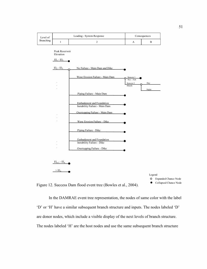
51
Figure 12. Success Dam flood event tree (Bowles et al., 2004).
In the DAMRAE event tree representation, the nodes of same color with the label
‘D’ or ‘H’ have a similar subsequent branch structure and inputs. The nodes labeled ‘D’
are donor nodes, which include a visible display of the next levels of branch structure.
The nodes labeled ‘H’ are the host nodes and use the same subsequent branch structure
El2 - El3
.
.
.
Eln-1 - Eln
> Eln
Legend
Expanded Chance Node
Collapsed Chance Node
El1 - El2
Wave Erosion Failure - Dike
No Failure - Main Dam and Dike
.
.
.
Piping Failure - Main Dam
Wave Erosion Failure - Main Dam
Peak ReservoirElevation
.
.
.
Embankment and FoundationInstability Failure - Main Dam
Embankment and FoundationInstability Failure - Dike
Piping Failure - Dike
Overtopping Failure - Dike
Overtopping Failure - Main Dam
Night
Day
Season 1
Nov - Feb
Season 2
March
Level ofBranching
1 2 BA
Loading - System Response Consequences

52
Figure 13. DAMRAE representation of the Success Dam flood event tree, displaying event tree branch levels at the top.

53
and inputs as the donor node with the same color and which is located above them in the
same level of the event tree.
Event tree Inputs
The assignment of inputs to different branches of the event tree in DAMRAE is
described below for each branch level. The basis for estimating the probability and
consequences inputs is described in Bowles et al. (2004).
Level 1: The Level 1 continuous branch is assigned the branch variable code,
‘PRE’. The ‘probability’ input option is selected for this branch and the ‘tabular
interpolation’ method for calculating state variables is selected. The input file for this
branch is shown in Table 1. A one-way linear interpolation method using z-variates is
used for estimating the peak stage for the 21 values of annual exceedance probabilities
(AEP) values obtained in a range of 0.0309185 and 0.0000001.
Table 1. Flood loading input table: peak reservoir stage versus AEP
Peak Stage(ft MSL) AEP(/yr)
652.50 0.0309185
658.33 0.0169082
663.00 0.0100000
667.75 0.0050000
672.50 0.0020000
675.25 0.0010000
689.40 0.0000100
691.50 0.0000044
700.66 0.0000001

54
Level 2: this branch level is a state function branch with the assigned branch
variable code, ‘OTD’. The calculation method for estimating the overtopping depth is
selected as the ‘user-specified function’. For Success Dam the dam crest elevation is
691.5 ft, so that the overtopping depth is calculated using the function, ‘PRE-691.5’.
Level 3: this branch level contains all eight flood-induced failure mode branches.
The first branch in this failure branch group is the no-failure branch and the remaining
branches represent the different failure modes. There is no input assignment for the no-
failure branch since the no-failure probability is calculated by the program as (1- sum of
failure probabilities). The inputs for the failure branches are as follows:
1. WaveErosion (MD): this failure branch represents the wave erosion failure
mode for the Main Dam. The system response probability for this branch is calculated
from Table 2 using a one-way linear interpolation method based on PRE.
2. Piping (MD): this failure branch represents the piping failure mode for the
Main Dam. The one-way linear interpolation method is used to calculate the SRP for this
failure branch from PRE using Table 3.
Table 2. Wave erosion SRP for the Main Dam
PRE Main Dam
Wave Erosion SRP
686.5 0
691.5 0.01
691.6 0.01

55
Table 3. Piping SRP for the Main Dam
PRE Main Dam Piping SRP
652.50 0
662.25 3.0195E-07
680.75 2.6775E-06
691.50 4.0873E-06
700.50 4.0873E-06
3. Instability (MD): this branch represents the slope instability failure mode
for the Main Dam. To estimate the SRP for this branch, an internal failure mode
calculation function, ‘InternalFM’ is used. This internal failure mode calculation
function is defined as follows:
),,3,2,1( PREDCEkkkInternalFM
The k1, k2 and k3 constants in this function are 0.302007, 1 and 0, respectively.
The dam crest elevation (DCE) is 691.5 ft and peak reservoir elevation (PRE) value is
branch variable ‘PRE’, which is assigned in the Level 1 branches.
4. Overtopping (MD): this branch represents the overtopping failure mode of
the Main Dam. The one-way linear interpolation method is applied to Table 4 for the
overtopping depth versus failure probability table to estimate the overtopping failure
system response probability.
5. WaveErosion (D): similar to wave erosion failure mode branch for the
Main Dam, the Frazier Dike wave erosion failure branch uses the one-way linear
interpolation method in the PRE versus SRP relationship shown in Table 5.

56
Table 4. Overtopping SRP for the Main Dam
OTD Main Dam Overtopping SRP
0 0
1 0.25
2 1.00
10 1.00
Table 5. Wave erosion SRP for the Frazier Dike
PRE Frazier Dike Wave Erosion SRP
679.5 0
691.5 0.1
691.6 0.1
Table 6. Piping SRP for the Frazier Dike
PRE Frazier Dike Piping SRP
660 0
662.25 0.000030195
680.75 0.00026775
691.5 0.000408729
700.5 0.000408729
6. Piping (D): the piping failure mode branch for the Frazier Dike uses the
one-way linear interpolation method in the piping SRP relationship shown in Table 6.
7. Instability (D): similar to the Main Dam instability failure mode function,
this failure branch uses the following internal failure mode function:
),5.691,0,1,302007.0( PREInternalFM

57
8. Overtopping (D): the overtopping failure mode branch for the Frazier Dike
uses the one-way linear interpolation method in the overtopping SRP relationship in
Table 7.
At this level, to account for the non-mutually exclusive failure modes, an option
to perform the common-cause adjustment (CCA) to all eight flood-induced failure modes
was selected.
Level 4: this branch level shows the seasonal exposure branches. The fixed
exposure factors values assigned to the ‘Season1’ and ‘Season2’ exposure branches are
0.33 and 0.67, respectively.
Level 5: this branch level contains the day and night exposure branches. The day
and night exposure branches connected with ‘Season1’ in previous branch level are
assigned fixed exposure factor values of 0.46 and 0.54, respectively, and those connected
with ‘Season2’ are assigned as 0.67 and 0.33, respectively.
Levels 6 and 7 branches are consequence branches. These branches represent
economic and life-loss consequences for three consequence centers, which are assigned
the following names: Success, Tulare, and King County.
Table 7. Overtopping SRP for the Frazier Dike
OTD Frazier Dike Overtopping Failure SRP
0 0
0.5 0.25
1 1.00
10 1.00

58
Level 6: Level 6 branches are the economic consequence branches. All the
branches in this level have fixed user-specified values as input. Table 8 shows the no-
failure and the Main Dam failure economic consequence values for the three centers.
Economic consequence values for the Frazier Dike failure are assigned as 0 for all three
centers.
Level 7: This branch level is the life-loss consequence branches. These
consequence branches also have user-specified fixed values, which are shown in Table 9
for the Main Dam. The Frazier Dike failure life-loss branches are assigned as 0 life loss.
Risk analysis output
The DAMRAE calculation for the above mentioned inputs produces six data
matrices (Pedigree, Branch Code, Probability, State Value, Economic Consequence, and
Life Loss Consequence) as output. It also estimates the final failure probability values for
all the failure modes and associated consequences values as shown in Table 10. Table 10
also shows the results of event tree simulation performed by Bowles et al. (2004).
Table 8. Economic consequence values for the Main Dam
Success Tulare KingCounty
No Failure 0 529 0.9
Failure 0 1051 3.2
Table 9. Life-loss consequence values for the Main Dam
Success Tulare King County
No Failure 1.00E-12 12.03 0.78
Failure 1.00E-12 25.95 1.56

59
Table 10. Flood event tree failure probabilities and annualized economic and life-loss
Probability of Failure Incremental Risk Cost Annualized Incremental
Life Loss
DAMRAE
(/yr)
Bowles et al.2004 (/yr)
DAMRAE ($/yr)
Bowles et al.2004 ($/yr)
DAMRAE (lives/yr)
Bowles et al.2004 (lives/yr)
WaveErosion (MD) 1.06E-07 1.05E-07 55.5 55 1.56E-06 1.55E-06
Piping (MD) 1.42E-08 1.42E-08 7.45 7 2.09E-07 2.09E-07
Instability (MD) 1.45E-05 1.40E-05 7614.17 7352 2.13E-04 2.06E-04
Overtopping (MD) 1.42E-06 1.00E-06 743 529 2.08E-05 1.48E-05
WaveErosion (D) 6.99E-06 6.75E-06
Piping (D) 1.22E-06 1.21E-06
Instability (D) 1.45E-05 1.40E-05
Overtopping (D) 1.82E-06 2.30E-06
Earthquake Event Tree
Figure 14 shows the event tree structure used by Bowles et al. (2004) in the
seismic risk analysis of Success Dam. This event structure is composed of six branching
levels where third level has been subdivided as 3a and 3b. Exposure and consequences
branches are not displayed in the Figure. The DAMRAE version of this event tree
structure is shown in Figure 15. This Figure includes the required state function branches
and also the exposure and consequence branches.
Event tree structure
The earthquake event tree model developed by Bowles et al. (2004) begins with
two initiating branches. These branches represent the earthquake magnitudes of 5.75 and
8.0. In the DAMRAE implementation, these two earthquake magnitudes are shown
separately in two different event tree drawings. Figures 14 and 15 show the event tree

60
structure beginning with the M 5.75 earthquake as an initiating branch. To analyze the M
8.0 earthquake, a separate drawing with the same event tree structure but with different
inputs was used. Although, multiple initiating branches can be handled in DAMRAE, to
ease the process of drawing and also to verify the results separately for M 5.75 and M
8.0, two event trees are developed and analyzed separately.
The DAMRAE version of the earthquake event tree comprises fourteen branch
levels. The first level is an initiating branch for earthquake magnitude, which is displayed
with ‘M 5.75” as the branch variable code in Figure 15. The second and third level
branches are continuous branches for peak ground acceleration (PGA) and pool elevation
(PE), respectively. Levels 4, 5 and 6 are state function branches for estimating the dam
failure peak discharge rate (Q), and the vertical deformation (VD) and horizontal
deformation (HD) of the dam, respectively. Level 7 is an overtopping failure mode
.
.
.
LegendExpanded Chance Node
Collapsed Chance Node
No FailurePGA ReservoirElevation
SEC Failure
(Seepage Erosion
through Cracks)
No
Overtopping
Deformation
near Outlet Works
(Sta. 28+50)
M 5.75
Magnitude
M 8.0
Overtopping Failure
Time from
EQ
Loading - System Response
1 2 3a 3b 4 5 6
Figure 14. Success Dam earthquake event tree (Bowles et al., 2004).

61
Figure 15. DAMRAE version of the Success Dam earthquake event tree (M 5.75), including exposure and consequences branches.
Figure 15. DAMRAE version of the Success Dam
earthquake event tree (M 5.75), including exposure and
consequences branches.

62
branch group with no-failure as the first branch and the overtopping failure mode (OTF)
as the second branch. Level 8 contains a continuous branch, which is connected to the no-
failure branch in Level 7, for the time from the occurrence of the earthquake until dam
failure (TEQ). The lowest branch in Level 9 (marked as ‘Transfer1’), which is connected
to the failure branch in Level 7, is a dummy discrete branch. It has no contribution in the
failure probabilities and is used to make the event tree structure even at each level. Level
9 includes the seepage erosion through cracks failure (SECF) branch group and the
lowest branch in this level (marked as ‘Transfer2’) is again a dummy discrete branch.
Seasons and day/night exposure scenarios are included in the Levels 10 and 11,
respectively. All the branches in Level 12 are state function branches. These branches
(marked as Wi, where i = 1, 2, 3…) represent the warning time, which is a function of
TEQ. Levels 13 and 14 represent the economic and life-loss consequence branches,
respectively. As mentioned above, nodes with same color and labeled ‘D’ or ‘H’ carry the
same following branch structure and associated inputs.
Event tree inputs
Inputs assigned to different branches in each event tree branch level are described
in the following subsections.
Level 1: Level 1 is a discrete branch with branch variable code ‘M 5.75’ and a
fixed user-specified probability value of 1.0. In case of M 8.0 earthquake, a branch
variable name ‘M 8.0’ is assigned to this branch and the assigned probability value is the
same as 1.0.

63
Level 2: Level 2 is a continuous branch with the branch variable code ‘PGA’. The
user-specified input for this branch is selected as ‘State Value’ and ‘Tabular
Interpolation’ method for calculating probabilities was chosen. The one-way log-log
interpolation method is used to estimate the annual exceedance probability for 20
earthquake loading intervals. Tables 11 (a) and (b) show the PGA - annual exceedance
probability input tables for M 5.75 and M 8.0, respectively. For M 5.75 and M 8.0, the
modified 21 PGA values used to divide the assigned range into 20 intervals, are shown in
Tables 12 respectively.
Level 3: Level 3 is the pool elevation (PE) continuous branch. With user-specified
input as ‘State Value’, the one-way linear interpolation method is used for the
relationship in Table 13 to calculate the probabilities for each of 32 pool elevation
intervals. The pool elevation values assigned to divide the pool elevation range in 32
intervals are shown in Table 14.
Table 11. Earthquake loading: PGA - annual exceedance probability relationships
PGA AEP
0.0250 0.218522
0.0500 0.0369878
0.1000 0.0060653
0.1500 0.0020033
0.2000 0.0008701
0.2500 0.0004299
0.3000 0.0002301
0.4000 0.0000787
0.5000 0.000032
0.6000 0.0000148
0.6500 0.0000098
PGA AEP
0.0250 0.08426
0.0500 0.01627
0.1000 0.00131
0.1500 0.00018
0.2000 0.00002
(a) M 5.75 (b) M 8.0

64
Table 12. PGA values for specifying the earthquake loading intervals
PGA 0.1 0.11 0.12 0.13 0.14 0.15 0.16 0.17 0.18 0.19 0.2
M 5.75
PGA 0.21 0.22 0.23 0.3 0.37 0.44 0.51 0.58 0.65 0.65
PGA 0.04 0.045 0.05 0.06 0.06 0.07 0.07 0.08 0.08 0.085 0.9
M 8.0
PGA 0.1 0.1 0.105 0.11 0.128 0.15 0.16 0.18 0.2 0.2
Table 13. Stage-duration relationship
Stage Percent Stage Percent
576.39 1 629.59 0.25
579.12 0.997 635.03 0.19
580.1 0.99 636.48 0.18
581.9 0.98 638.73 0.16
583.45 0.97 639.63 0.15
586.83 0.94 641.42 0.13
588.15 0.92 643.65 0.1
589.03 0.9 644.86 0.09
593.08 0.82 648.82 0.06
594.88 0.77 651.55 0.0375
601.25 0.6 652.41 0.0175
608 0.51 656.12 0.003472
610.05 0.48 656.4 0.002003
613.49 0.43 656.51 0.000467
623.95 0.32 658.33 6.68E-05
Table 14. Pool elevation interval values
589 591 593 595 597 599 601 603 605
607 609 611 613 615 617 619 621 623
625 627 629 631 633 635 637 639 641 PE
643 645 647 649 651 654

65
Table 15. Pool elevation vs. discharge relationship
PE Q
590 60466
630 362481
634 425264
652.5 684805
Level 4: this branch level includes a state function branch to estimate the dam
failure peak discharge rate (Q) from the reservoir. The calculation method for this branch
is selected as ‘Tabular Interpolation’ with one-way linear interpolation used to calculate
the estimated dam failure peak discharge rate values from the Table 15.
Level 5: this branch level is used to obtain estimates the vertical crest settlement
using a state function branch ‘VD’. Bowles et al. (2004) provided a parametric vertical
crest settlement (Figures 16 and 18) for calculating the vertical deformation state values
for given pool elevations, earthquake magnitude and PGA. In DAMRAE, these
relationships and the plots in Figures 17 and 19 are included in tabular formats as shown
in Table 16 and 17.
Tables 16 and 17 are used as the ‘VD’ state function branch input tables for the
earthquake event trees for M 5.75 and M 8.0, respectively. The interpolation method
selected for these tables is two-way linear interpolation and the two variables assigned for
the interpolation are ‘PGA’ (denoted as X) and ‘PE’ (denoted as ‘Y). ‘LInterP’ is a linear
interpolation routine, which is built into DAMRAE to take an independent variable
(shown as ‘Y’) and interpolation table (shown as ‘VST’) as functional arguments.

66
Figure 16. Vertical crest settlement at M 5.75 as a function of pool elevation and PGA.
(a) PGA at knee (b) Deformation at knee
Figure 17. Estimated position of knee in Figure 16.

67
Table 16. Tabular interpolation approach for estimating vertical deformation for M 5.75
PGA VD
0 0
0.03 0
(0.156-0.036*(Y-590)/62) (1.4-0.43*(Y-590)/62)
LInterP(Y,VST) (2586.8-8.0957*Y+0.0063902*Y*Y)
0.65 (2586.8-8.0957*Y+0.0063902*Y*Y)
a. PGA vs. VD table for M 5.75 transformed from the Figure 16
PGA PE
590 0.221
619 0.192
635 0.154
652.5 0.154
b. VST table used in (a)
Figure 18. Vertical crest settlement at M 8.0 as a function of pool elevation and PGA.
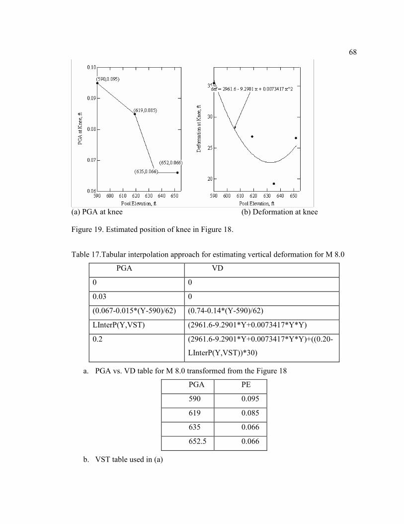
68
(a) PGA at knee (b) Deformation at knee
Figure 19. Estimated position of knee in Figure 18.
Table 17.Tabular interpolation approach for estimating vertical deformation for M 8.0
PGA VD
0 0
0.03 0
(0.067-0.015*(Y-590)/62) (0.74-0.14*(Y-590)/62)
LInterP(Y,VST) (2961.6-9.2901*Y+0.0073417*Y*Y)
0.2 (2961.6-9.2901*Y+0.0073417*Y*Y)+((0.20-
LInterP(Y,VST))*30)
a. PGA vs. VD table for M 8.0 transformed from the Figure 18
PGA PE
590 0.095
619 0.085
635 0.066
652.5 0.066
b. VST table used in (a)

69
Level 6: this branch level is similar to Level 5, but is to estimate the horizontal
deformation values (HD) instead of the vertical deformation (VD) values. Tables 18 and
19 are used for M 5.75 and M 8.0 earthquakes, respectively. These tables are transformed
from Figures 20 and 22, respectively.
Level 7: Level 7 includes the no-failure and overtopping failure (OTF) branches.
For estimating the overtopping failure probabilities user specified function is assigned as
),,5.691( PEVDTrig
‘Trig’ is a program inbuilt function that uses the crest elevation, vertical
deformation and pool elevation values to calculate the overtopping system response
probability (Bowles et al., 2004).
Figure 20. Horizontal deformation at M 5.75 as a function of pool elevation and PGA.

70
(a) PGA at knee (b) Deformation at knee
Figure 21.Estimated position of knee in Figure 20.
Table 18.Tabular interpolation approach for estimating horizontal deformation at M 5.75
PGA HD
0 0
0.1 0
0.156-0.044*(Y-590)/62 8.3-6.2*(Y-590)/62
LInterP(Y,HST) 7853.8-24.735*Y+0.01956*Y*Y
0.65 7853.8-24.735*Y+0.01956*Y*Y
a. PGA vs. HD table for M 5.75 transformed from the Figure 20
PGA PE
590 0.221
619 0.198
635 0.154
652.5 0.154
b. HST table used in (a)
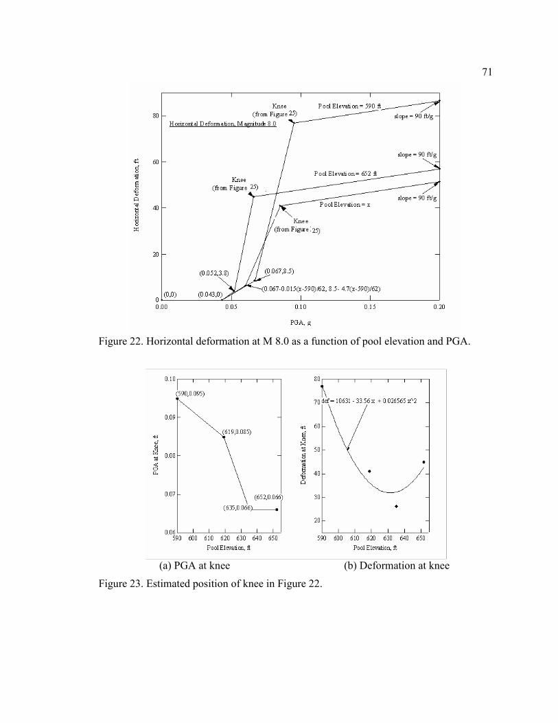
71
Figure 22. Horizontal deformation at M 8.0 as a function of pool elevation and PGA.
(a) PGA at knee (b) Deformation at knee
Figure 23. Estimated position of knee in Figure 22.

72
Table 19.Tabular interpolation approach for estimating horizontal deformation at M 8.0
PGA HD
0 0
0.043 0
(0.067-0.015*(Y-590)/62) 8.5-4.7*(Y-590)/62
LInterP(Y,HST) 10631-33.56*Y+0.026565*Y*Y
0.2 (10631-33.56*Y+0.026565*Y*Y)+((0.20-
LInterP(Y,HST))*90)
a. PGA vs. HD table for M 8.0 transformed from the Figure 22
PGA PE
590 0.095
619 0.085
635 0.066
652.5 0.066
b. HST table used in (a)
Level 8: user specified input for the continuous branch ‘TEQ’ in Level 8 is
selected as state value and two-way linear interpolation method is used to estimate the
probability values for 20 equally spaced intervals of time to failure ranging from 30 hr to
315 hr. Table 20 is used as input for this branch and ‘TEQ’ state values and ‘PE’ values
are assigned as independent variables for the interpolation.
The other branch in this level (labeled as ‘Transfer1’) is a discrete branch with
user assigned probability value of 1.
Level 9: failure branch group connected with the ‘TEQ’ continuous branch
represents the no-failure and seepage erosion through cracks failure mode. For estimating
the ‘SECF’ branch probabilities, two-way linear interpolation method is used with ‘HD’

73
and ‘PE’ as assigned independent variables. The input table for this branch is shown in
Table 21.
Table 20. Two-dimensional relationship of time to failure after earthquake and pool elevation for estimating SRP
Time to
Failure (hr)
590 630 652.5
30 0 0 0
315 0 0 0.43
360 0 0.02 0.5
600 0 0.13 0.55
900 0 0.26 0.61
1440 0 0.5 0.71
2880 0.33 0.67 1
3600 0.5 0.75 1
Table 21. Two-dimensional relationship of horizontal deformation and pool elevation for estimating the SECF probabilities
HD 590 592 614 638 662
0 0 0 0 0 0
2 0 0 0 0 0
10 0 0 0 0.23 0.44
20 0 0 0.15 0.51 1
24 0 0 0.21 0.63 1
30 0 0.02 0.3 0.8 1
40 0 0.04 0.45 0.83 1
50 0 0.07 0.6 0.86 1
100 0 0.20 0.82 1 1
140 0 0.3 1 1 1

74
The other branch in this branch level (labeled as ‘Transfer2’) is again a discrete
branch with user assigned probability value of 1.
Level 10: this branch level shows the season exposure branches. The fixed
probability value assigned to ‘Season1’ exposure branch is 0.33 and ‘Season2’ exposure
branch is 0.67.
Level 11: this branch level shows the day and night exposure branches. The day
and night exposure branches connected with ‘Season1’ in previous branch level are
assigned fixed probability values of 0.46 and 0.54 respectively and those connected with
‘Season2’ are assigned as 0.67 and 0.33, respectively.
Level 12: all the branches in this level represent the warning time state function
branch. Input function for calculating the warning time linked with the day exposure
branch is assigned as 60−TEQ and for branches linked with the night exposure it is
assigned as 90−TEQ .
Levels 13 and 14 branches are consequences branches. These branches represent
economic and life-loss consequences for three consequence centers, which are assigned
the following names: Success, Tulare, and King County.
Level 13: this branch level contains the economic consequence branches. Inputs
for no-failure consequence branches are assigned fixed user-specified values of 0. For
other branches, the interpolation input tables contained in Table 22 are used for various
exposure seasons and consequences centers. One-way linear interpolation is used with
dam failure peak discharge rate (‘Q’) as the independent variable.

75
Table 22. Economic consequences input table
Q Economic Losses
60466 0
362481 0
684805 0
Q Economic Losses
60466 0
362481 0
684805 0
(a) Success Center for Season1 (b) Success Center for Season2
Q Economic Losses
60466 0
362481 0
684805 0
Q Economic Losses
60466 0
362481 0
684805 0
(c) Tulare Center for Season1 (d) Tulare Center for Season2
Q Economic Losses
60466 0
362481 0
684805 0
Q Economic Losses
60466 0
362481 0
684805 0
(e) King County Center for Season1 (f) King County Center for Season2
Level 14: this branch level represents the life-loss consequence branches.
Branches linked with no-failure branches have 0 life loss. For other branches, the
appropriate life-loss input table is entered based on the seasonal and day/night exposures.
Input interpolation tables for different centers are given in Tables 23 to 26. The main
interpolation input table uses the two-way linear interpolation method with ‘Q’ and ‘Wi’
(where i = 1, 2, 3…) as the independent variables to calculate the life-loss values. The
input table includes a function ‘TWLinear’, which is a two-way linear interpolation
routine that is built into DAMRAE. The ‘TWLinear’ function uses ‘Q’ values (denoted as
‘X’) and warning time ‘Wi’ (denoted as ‘Y’) and an interpolation table as functional
arguments.

76
Table 23. Success consequence center life-loss input tables
Q LL
60466 TWLinear(X,Y,SSDT)
362481 TWLinear(X,Y,SSDT)
425264 TWLinear(X,Y,SSDT)
684805 TWLinear(X,Y,SSDT)
a. Success consequence center life-loss input.
WT
Q
60466 362481 425264 684805
-30 1.00E-12 1.00E-12 1.00E-12 0.0028
-15 1.00E-12 1.00E-12 1.00E-12 1.00E-12
0 1.00E-12 1.00E-12 1.00E-12 1.00E-12
15 1.00E-12 1.00E-12 1.00E-12 1.00E-12
30 1.00E-12 1.00E-12 1.00E-12 1.00E-12
45 1.00E-12 1.00E-12 1.00E-12 1.00E-12
60 1.00E-12 1.00E-12 1.00E-12 1.00E-12
75 1.00E-12 1.00E-12 1.00E-12 1.00E-12
90 1.00E-12 1.00E-12 1.00E-12 1.00E-12
105 1.00E-12 1.00E-12 1.00E-12 1.00E-12
120 1.00E-12 1.00E-12 1.00E-12 1.00E-12
135 1.00E-12 1.00E-12 1.00E-12 1.00E-12
150 1.00E-12 1.00E-12 1.00E-12 1.00E-12
165 1.00E-12 1.00E-12 1.00E-12 1.00E-12
180 1.00E-12 1.00E-12 1.00E-12 1.00E-12
195 1.00E-12 1.00E-12 1.00E-12 1.00E-12
210 1.00E-12 1.00E-12 1.00E-12 1.00E-12
225 1.00E-12 1.00E-12 1.00E-12 1.00E-12
240 1.00E-12 1.00E-12 1.00E-12 1.00E-12
b. SSDT interpolation table used in Table (a)

77
Table 24. Tulare center life-loss input tables
Q LL
60466 TWLinear(X,Y,TSD1T)
362481 TWLinear(X,Y,TSD1T)
425264 TWLinear(X,Y,TSD1T)
684805 TWLinear(X,Y,TSD1T)
Q LL
60466 TWLinear(X,Y,TSD2T)
362481 TWLinear(X,Y,TSD2T)
425264 TWLinear(X,Y,TSD2T)
684805 TWLinear(X,Y,TSD2T)
a. Day b. Night
Table 25. Tulare center life-loss supplement input tables
WT
Q
60466 362481 425264 684805
-30 9.43 9.72 9.78 325.94
-15 9.43 9.72 9.78 309.92
0 9.43 9.72 9.78 293.91
15 9.43 9.72 9.78 277.89
30 9.43 9.72 9.78 261.87
45 9.43 9.72 9.78 245.85
60 9.43 9.72 9.78 229.84
75 9.43 9.72 9.78 213.82
90 9.43 9.72 9.78 197.8
105 9.43 9.72 9.78 179.78
120 9.43 9.72 9.78 161.76
135 9.43 9.72 9.78 143.74
150 9.43 9.72 9.78 125.72
165 9.43 9.72 9.78 107.7
180 9.43 9.72 9.78 89.68
195 9.43 9.72 9.78 71.66
210 9.43 9.72 9.78 17.6
225 9.43 9.72 9.78 17.6
240 9.43 9.72 9.78 17.6
a. TSD1T interpolation table used in Table 24(a)

78
WT
Q
60466 362481 425264 684805
-30 9.43 9.72 9.78 614.67
-15 9.43 9.72 9.78 563.73
0 9.43 9.72 9.78 512.79
15 9.43 9.72 9.78 461.84
30 9.43 9.72 9.78 410.9
45 9.43 9.72 9.78 359.96
60 9.43 9.72 9.78 309.02
75 9.43 9.72 9.78 258.07
90 9.43 9.72 9.78 207.13
105 9.43 9.72 9.78 188.18
120 9.43 9.72 9.78 169.22
135 9.43 9.72 9.78 150.27
150 9.43 9.72 9.78 131.32
165 9.43 9.72 9.78 112.37
180 9.43 9.72 9.78 93.41
195 9.43 9.72 9.78 74.46
210 9.43 9.72 9.78 55.51
225 9.43 9.72 9.78 36.55
240 9.43 9.72 9.78 17.6
b. TSD2T interpolation table used in Table 24 (b)
Table 26. King county center life-loss input tables
Q LL
60466 TWLinear(X,Y,KSDT)
362481 TWLinear(X,Y,KSDT)
425264 TWLinear(X,Y,KSDT)
684805 TWLinear(X,Y,KSDT)
a. King county life-loss input tables

79
WT
Q
60466 362481 425264 684805
-30 1E-12 0.18 0.22 1.31
-15 1E-12 0.18 0.22 1.31
0 1E-12 0.18 0.22 1.31
15 1E-12 0.18 0.22 1.31
30 1E-12 0.18 0.22 1.31
45 1E-12 0.18 0.22 1.31
60 1E-12 0.18 0.22 1.31
75 1E-12 0.18 0.22 1.31
90 1E-12 0.18 0.22 1.31
105 1E-12 0.18 0.22 1.3
120 1E-12 0.18 0.22 1.28
135 1E-12 0.18 0.22 1.27
150 1E-12 0.18 0.22 1.25
165 1E-12 0.18 0.22 1.24
180 1E-12 0.18 0.22 1.22
195 1E-12 0.18 0.22 1.21
210 1E-12 0.18 0.22 1.16
225 1E-12 0.18 0.22 1.16
240 1E-12 0.18 0.22 1.16 b. KSDT interpolation table used in table (a)
Risk analysis output
The final output failure probabilities and consequence values obtained in two
separate runs for the M 5.75 and M 8.0 earthquake event tree models are summarized in
Table 27 for the DAMRAE runs and from the original Bowles et al. (2004) study.

80
Table 27. Earthquake event tree failure probabilities and annualized economic and life-loss
Probability of Failure Incremental Risk Cost Annualized Incremental Life Loss
DAMRAE (/yr)
Bowles et al. 2004 (/yr)
DAMRAE ($/yr)
Bowles et al. 2004 ($/yr)
DAMRAE (lives/yr)
Bowles et al. 2004 (lives/yr)
SECF 9.49E-04 8.29E-04 6020796 543457.84 2.55E-02 2.75E-02 M 5.75 OTF 0 0 0 0 0 0
SECF 3.03E-03 2.67E-03 1958169.5 1760752 8.42E-02 9.12E-02 M 8.0 OTF 7.40E-07 7.36E-07 543.1 545.89 3.12E-04 3.88E-04
Post-processing
The user can summarize the results by combining individual failure mode result
for wave erosion and overtopping results to obtain the total flood failure probability and
by combining results for piping and slope instability results to obtain the total flood-
internal failure probability. Similarly, the failure probabilities obtained from the two
earthquake magnitude event trees can be combined as a total earthquake failure
probability over all earthquake-related failure modes. Post processing of all three event
trees together produces the ANCOLD (2003) F-N plot and the USBR Portrayal of Risks
plot as shown in Figures 24 and 25, respectively.

81
Figure 24. ANCOLD F-N plot for combined outputs from flood and earthquake event trees.
Figure 25. Flood and earthquake event tree output on the USBR Portrayal of risks plot.

82
Discussion
The implementation of the Success Dam flood and earthquake event trees in
DAMRAE shows that the developed tool has flexible functionalities for drafting,
quantifying and reporting a complex dam safety event tree analysis. The comparable
results obtained from the event tree analyses verify the credibility of the employed
computational logics. The slight difference in obtained results from the Bowles et al.
(2004) study can be justified as follows:
1) In the Bowles et al. (2004) study, the event tree models were developed
using the MS Excel and a VB macro. MS Excel has its own inbuilt function for
estimating the z-variate while an approximate algorithm has been used in
DAMRAE to calculate the z-variate. Since the flood event tree analysis uses the
z-variate method for interpolation, the functional difference in performing the z-
variate interpolation account for the differences in the values of flood failure
probabilities obtained in DAMRAE.
2) In the Bowles et al. (2004) study, the number of intervals the for time after
earthquake continuous branch are different for each different PGA loading while
in the DAMRAE implementation same number of intervals are used for all PGA
loading intervals. This difference appears to be the source of variation in seepage
erosion through cracks probabilities obtained in earthquake event tree analysis
performed using DAMRAE.

83
CHAPTER VI
SUMMARY, CONCLUSION, AND FUTURE WORK
Summary
Event tree analysis is a well-established method for risk analysis in the nuclear,
chemical and aerospace industries. It has also become the most commonly-used tool for
risk analysis in the field of dam safety. To facilitate event tree analysis, several software
tools have been developed. However, all these tools are dedicated to some specific
applications and unfortunately they are somewhat cumbersome to use for dam safety
event tree analysis. Most commonly spreadsheet-based approach have been used for dam
safety risk analyses and in some cases VB macros and other Excel add-ons have made
these use more efficient. This thesis points out the shortcomings of existing event tree
modeling tools and techniques. It also emphasizes the need for generalized software for
efficient processing in practical dam safety event tree analysis. To highlight the
differences in the details of the applications of the mathematical calculations employed in
dam safety risk analysis from other risk analysis fields, this thesis describes the standard
event tree structure and propose some differences in calculation details that are better
suited to the dam safety risk analysis.
The development process for a new dam safety event tree analysis tool has been
divided in two parts: its theoretical development and its computational development. The
theoretical development includes the refined event tree terminology and additional
variables. The computational development includes the computational logic involved in

84
DAMRAE. Finally, the capabilities of the developed tool have been demonstrated using
the Success Dam case study by Bowles et al. (2004).
Conclusion
The purpose of designing and building DAMRAE is to enable users to rapidly
develop and quantify event trees. The present version of DAMRAE has been built using
Visual Basic.NET and can be executed on any windows-based operating system. Unlike
other existing dam safety event tree modeling tools, DAMRAE is stand-alone software
and is easy and intuitive to use. The underlying concept of transforming the event tree
structure into a computationally-adapted matrix form is a novel idea of this work. Based
on this structure-transformed-matrix or Connectivity Matrix, branch probabilities and
consequences can be calculated. Standard methods have been incorporated to calculate
and assign the state values, SRPs, exposure weights and consequence values to each
branch. DAMRAE also includes the functionality to perform the common-cause
adjustment in case of non-mutually exclusive failure events. Failure modes are identified
from the event tree graphics and for each of these failure modes, failure probabilities and
associated annualized consequences are displayed such that reports can be generated
interactively using a flexible post-processing functionality. The present version of
DAMRAE has been developed as a prototype to prove the concept of the generalized
algorithm for dam safety event tree analysis. It effectively addresses all the limitations
identified in the “Introduction” chapter of this thesis.

85
Future Work
Application of DAMRAE to Corps of Engineers risk assessments is planned to
begin in 2008. However, continued development is planned after that initial deployment.
These future developments are planned to include uncertainty and sensitivity analysis
options, along with providing some enhanced graphics options, additional reporting
capabilities, and code optimisation to improve program performance and memory usage.
An automatic feature for selecting the number of computational branches for continuous
branches, such as initiating events or loading events, will be developed based on user-
specified error criteria similar to those used in other types of numerical models.
A facility for importing standard event tree templates and adapting them for
application to a specific dam will be added.
Database aspects will be enhanced to facilitate the consideration of risk reduction
measures. A capability for performing sensitivity and scenarios analyses will be
developed, together with post-processing to support these capabilities, including features
needed for the prioritisation of risk reduction measures and investigations in portfolio
applications.
A capability similar to that for invention branch groups will be developed to
calculate the contributions of spillway gate reliability and spillway plugging by debris on
estimates of failure risks, including the combined effects of intervention.
DAMRAE will be tested and evaluated for additional some dams, including some
that will be selected because of unique and complex aspects to their event tree structures.

86
REFERENCES
ANCOLD (Australian National Committee on Large Dams). 2003. Guidelines on risk assessment. Australian National Committee on Large Dams, Sydney, New South Wales, Australia.
Andrews, J. D., and S. J. Dunnett. 2000. Event-Tree analysis using binary decision diagrams, IEEE Transactions on Reliability 49(2): 230-238.
Baird, Bruce F. 1989. Managerial decisions under uncertainty: An introduction to the analysis of decision making. John Wiley & Sons, Inc., New York. 544 p.
Bedford, T., and R. Cooke. 2001. Probabilistic Risk Analysis. Cambridge University Press, Cambridge. 414 p.
Beim, G. K., and B. F. Hobbs. 1997. Event tree analysis of lock closure risks. Journal of Water Resources Planning and Management-ASCE 123(3): 169-178.
Bowles, D. S., L. R. Anderson, T. F. Glover, and S. S. Chauhan. 1999. Understanding and managing the risk of aging dams: principals and case studies. 19th USCOLD Annual Meeting and Lecture, May 16-21, 1999, Atlanta, Georgia.
Bowles, D. S., L. R. Anderson, and S. S. Chauhan. 2001. Approaches to the common Cause adjustment in event trees used in dam safety risk analysis. Working paper, Institute for Dam Safety Risk Management, Utah State University, Logan, Utah.
Bowles, D.S., L. R. Anderson, T. F. Glover, S. S. Chauhan, and J. Bay. 2004. Risk-based evaluation of operating restrictions for Lake Success. RAC Engineers & Economists technical consulting final report to the Sacramento District, U.S. Army Corps of Engineers, Sacramento, California.
Bowles, D.S., L. R. Anderson, T. F. Glover, and S. S. Chauhan. 2006. Fort Worth district portfolio risk assessment. RAC Engineers & Economists technical consulting report to the U.S. Army Corps of Engineers.
Bowles, D.S., and D. McClelland. 2000. Event Tree Analysis. Working paper prepared for the Canadian Electricity Association Dam Safety Interest Group. Institute for Dam Safety Risk Management, Utah State University, Logan, Utah, March 2006.
Canadian Standards Association. 1991. Risk Analysis Requirements and Guidelines. Toronto, Canada, CAN/CSA-Q634-91.
Chauhan, S. S., and D. S. Bowles. 2001. Incorporating Uncertainty into Dam Safety Risk Assessment. Proceedings on Risk Analysis in Dam Safety, at Third International Conference on Dam Safety Evaluation. Goa, India. December 2001.

87
Chauhan, S. S., and D. S. Bowles. 2003. Dam safety risk assessment with uncertainty analysis. Australian Committee on Large Dams Risk Workshop, Launceston, Tasmania, Australia, October 2003.
Collins, E. W. and W. L. Cooley. 1983. Use of event tree analysis to optimize electrical accident counter-measure systems for metal/nonmetal mines. Conference Record - IAS Annual Meeting (IEEE Industry Applications Society), Piscataway, NJ. p.139-151.
Dumitrescu, M., A. P. Ulmeanu, and T. Munteanu. 2002. Fuzzy logic systems for fuzzy event tree computing. IEEE Symposium “Intelligent Systems”, Elsevier Science Limited, September 2002, 0-7803-7134-8/02.
Fell, R., D.S. Bowles, L.R. Anderson, and G. Bell. 2000. The status of estimation of the probability of failure of dams for use in quantitative risk assessment. Proceedings of the 20th International Commission on Large Dams (ICOLD) Congress, Beijing, China, September. p. 213.
Hadipriono, F. C., C. Lim, and K. Wong. 1986. Event tree analysis to prevent failures in temporary structures. Journal of Construction Engineering and Management – ASCE 12(4): 500-513.
Hartford, D.N.D., and G. B. Baecher. 2004. Risk and uncertainty in dam safety. Thomas Telford, Ltd, London. 391 p.
Hill, P., D. Bowles, P. Jordan, and R. Nathan. 2003. Estimating overall risk of dam failure: practical considerations in combining failure probabilities. Australian National Committee on Large Dams, Bulletin 127: 63-72.
Huang, D., Chen, T. and Wang, M. J. 2001. Fuzzy set approach for event tree analysis. Fuzzy Sets and Systems 118(1):153-165.
Jin, C. L., J. Yan, and S. Zhou. 2003. Application of event tree analysis based on fuzzy sets in risk analysis. Journal of Dalian University of Technology 43(1): 97-100
Kaplan, S. 1982. Matrix theory formalism for event tree analysis: Application to nuclear-risk analysis. Risk Analysis 2(1): 9-18.
Kenarangui, R. 1991. Event-tree analysis by fuzzy probability. IEEE Transactions on Reliability 40(1): 120-124.
Koren, J. M., G. B. Rothbart, and B. F. Putney. 1984. Event tree modeling on a small computer. Annual Reliability and Maintainability Proceedings, IEEE. p. 330.
Levenson, N. 1995. SafeWare: System safety and computers. Addison-Wesley, Reading, MA. 704 p.

88
McCormick, N.J. 1981. Reliability and risk analysis: Methods and nuclear power applications. Academic Press, New York. 466 p.
Ohba, Y., T. Hayashi, Y. Yoshida, and K. Takahashi. 1984. Reliability analysis of ultra-high voltage DC transmission system by event tree analysis. Electrical Engineering in Japan 104(1): 118-128.
Papazoglou, I.A. 1998. Mathematical foundations of event trees. Reliability Engineering and System Safety 61: 169-183.
Patra, S., K. P. Soman, and R. B. Misra. 1995. Event tree analysis of a power system using Bayesian and fuzzy set approach. Journal of the Institution of Engineers (India), Part Et: Electronics and Telecommunication Engineering Division 76: 11-18.
Paté-Cornell, M.E. 1984. Fault trees vs. Event Trees in Reliability Analysis. Risk Analysis 4(3):177-186.
Raman, R. 2004. Accounting for dynamic processes in process emergency response using event tree modeling. Center for Chemical Process Safety, 19th Annual International Conference - Emergency Planning Preparedness, Prevention, and Response. p.197-213.
Rasmussen, N.C. 1975. Reactor Safety Study: An assessment of accident risks in US. Commercial Nuclear Power Plants, Nuclear Regulatory commission.
Reclamation (U.S. Bureau of Reclamation). 2003. Guidelines for achieving public protection in dam safety decisionmaking. Dam Safety Office, Department of the Interior, Denver, Colorado. p.19.
Sen, D.K., Banks, J.C., Maggio, G., and Railsback, J. 2006. Rapid development of event tree modeling tool using COTS Software, IEEEAC #1647.
Sherali, H.D., J. Desai, and T.S. Glickman. 2006. Event tree optimization for the management of cascading risks. https://filebox.vt.edu/users/jidesai/Event%20Tree%20Optimization.pdf
Takaragi, K., R. Sasaki, and S. Shingai. 1983. Algorithm for obtaining simplified prime implicant sets in fault tree and event tree analysis, IEEE Transactions on Reliability. 4: 386-390.
Turney, R., and R. Pitblado. 1996. Risk Assessment in the process industries. Second edition, Institute of Chemical Engineers, Rugby, Warwickshire, UK. 177 p.
Unwin, S. D. 1984. Binary event string analysis: A compact numerical representation of the event tree. Society for Risk Analysis 4(2): 83-87.

89
Webb, A. 1997. Software for risk analysis in business projects. Engineering Management Journal 7(1): 33-42.
Xu, H., and J. B. Dugan. 2004. Combining dynamic fault tree and event trees for probabilistic risk assessment, reliability and maintainability, IEEE Annual Symposium, 2004. p. 214-219.
Yang, Y., and L. Qiu. 1993. Event tree analysis for the system of hybrid reactor. Nuclear Power Engineering 14(6): 516-522.
Zhang, X. and S. Yan. 1999. Event-tree analysis of steam generator tube ruptures. Nuclear Power Engineering 20(2): 169-173.
Zhang, Z., C. Wu, T. Xia, B. Zhang, and A. Li. 2004. Chemical hazards assessing and accidents estimation by event tree modeling. Proceedings of the 2004 International Symposium on Safety Science and Technology, 4 - Part B: 1753-1758.

90
APPENDIX
(DAMRAE USER MANUAL)

91
Introduction
DAMRAE has been developed as independent software using the VB.NET
environment. The executable file of the developed software RiskManagement.exe can
be run on any windows platform independent of the requirement to install the Microsoft
Visual Studio.NET. Other than the inbuilt programming code, the software also uses
some dynamic-link library (dll) files. These external files are Interop.ADODB,
Interop.MSScriptControl, Interop.Scripting, and NPlot. They are required to be placed in
the same folder with the software’s executable file. Upon creating an event tree project,
the program generates several text, MS Access and XML files. The MS Access file
stores the event tree structure information and the text and XML files store the
intermediate calculation values and final output values. A detailed description of the
steps involved in developing and computing an event tree project is included in this
Appendix
Menu Bar Description
Upon running the software executable file, the program displays a Dam Safety
Risk Analysis Engine (DAMRE) tool bar on the screen. This tool bar includes several
options as shown in Figures 26 and 27.
A. New Project
The first step in developing an event tree model in DAMRAE is to establish the
directory in which you wish to work in and to enter a title for the new project. The
default directory is the location of the executable file of this software. To start a new

92
project, either use the File menu on the toolbar and select the New Project option or
click the icon A from the toolbar menu icons. This will bring up a New Event Tree
Analysis Project window as shown in Figure 28.
The user is required to enter a proper filename for the new project and to save it in
the desired directory. The filename should be alphanumeric and should not include any
special characters, such as decimals, commas or question marks, etc. The program creates
a folder with the user-assigned name in the selected directory and within that folder a file
with extension “.eap” is generated. This “.eap” file is the main project file and its name
or extension should not be changed by the user.
Figure 26. Menu bar options.

93
Figure 27. Menu bar icons.
After saving the project file, the next window that comes up is the Project Info
window, which is shown in Figure 29. This window has preliminary information input
options related to the project. These inputs are completely optional. None of these is
used in the event tree calculation; and hence they can be left blank if desired. To proceed
to the next step, click the Enter Input button, or if you wish to cancel the project, click
the Cancel button.
B. Open Project
To open an existing Event Tree Analysis Project (EAP), select the Open Project
option from the File menu, or click the icon B in the menu bar icons. This brings up an
Open Event Tree Analysis Project window, as shown in the Figure 30. To open an
existing project, go to the appropriate directory and select the project name file with an
extension “.eap”. If the Open project option is chosen, it will bring up the Project Info
A B C D E F G H I J K
A. New Project B. Open Project C. Draw Event Tree D. Draw Consequences E. Save Event Tree F. Run Probability Calculation G. Show Probability Tables H. Run Consequences Calculation I. Show Consequences Tables J. Failure Probability and Consequence
Values K. Add External Data File

94
window. The Project Info window shows the information that was saved while creating
the project. These inputs can be changed, and then to proceed to next step Enter Input
button should be clicked.
C. Draw Event Tree
After entering the project information inputs, the next step is to draw the event
tree structure. Event tree drawing can be initiated by selecting the Draw Event Tree
option under the Event Tree menu or by using the icon C.
The Draw Event Tree window (Figure 31) has two checkboxes. If the event tree
structure initiates with a discrete branch, such as for a certain magnitude of earthquake
loading, then select the option Start Event Tree with Discrete Branch and if event tree
starts with a continuous branch, for example, flood loading, then select the option Start
Event Tree with Continuous Branch.
Figure 28. New event tree analysis project window.

95
Figure 29. Project information window.
Figure 30. Open event tree analysis project window.

96
Figure 31. DAMRAE interface displaying the window for drawing the event tree structure.
Figure 32. Create branch window displaying the inputs required to draw a branch on the DAMRAE interface.
When the desired initiating branch option is selected, it brings up a Create
Branch window, as shown in Figure 32. This window includes different branch inputs,
which are described in the following subsections. After assigning all the appropriate
required inputs, the OK button should be clicked to draw the initiating branch on the

97
DAMRAE interface, or otherwise Cancel button can be clicked to cancel the initiating
branch selection.
After drawing the initiating branch, subsequent branches can be added by using
the right click menu of the previous branch node. A detailed description of the different
types of branch inputs and the node-right-click-menu is given under the Drawing Details
subsection below.
D. Draw Consequences Branches
Before economic and life-loss consequences branches can be added to an event
tree structure, it is required to define the number of consequence centers for which the
consequence analysis is being done. The number of centers and their names can be
defined by using the Draw Consequence option under the Event Tree menu, or by using
the icon D. This option brings up a window as shown in Figure 33.
To add the number of consequence centers and their names into the program
database, it is required to transfer the names of centers to the data grid. Names can be
transferred to data gird one by one by entering the name in the Name of Centers input
box and then clicking the Add button. A name can be removed from the data grid by
selecting the desired row in the data grid and then using the Remove button. The number
of Names in the data grid should be same as the number of consequence centers in the
Number of Centers input box. After entering all the names, the OK button should be
clicked. After this step, the consequence branches can be added to the event tree using
the node-right-click-menu.

98
Figure 33. Consequences calculation window for assigning the number of consequence centers and their names.
E. Save Event Tree
This option provides the facility to save the event tree graphic into the program
database at any time. Although all the graphics details and input values are automatically
saved to the database when the user exits the program, it is a good idea to save the
graphics frequently while creating the event tree structure and inputs.
F. Run Probability Calculation
After completing the event tree structure and entering all the inputs for each
branch, either Probability Calculation under the Calculation menu, or the icon F, can
be used to perform the event tree calculation. This calculation generates four matrices
namely, the Pedigree, Branch Code, Probability and State Value matrices. The details
of these matrices have been included under the Output Details subsection below.
The Probability Calculation option brings up a window containing four buttons
to select each type of output matrix and a progress bar displaying the percentage

99
completion of the calculation. A screenshot of the DAMRAE interface with the matrices
output window and progress bar is shown in Figure 34. After completion, the calculation
output matrices can be viewed by clicking the corresponding tab to select each matrix.
G. Show Probability Calculation
Although, the Probability Calculation option displays the probability calculation
output tables, to reopen the window either the Probability Tables option under teh
Calculation menu or the icon G must be used.
H. Run Consequences Calculation
The consequence calculation is performed to assign the consequence values to
each loading interval for each consequence center and to calculate the annualized
incremental risk cost and life loss associated with each failure mode. The consequence
calculation can be performed using the Consequence Calculation option under the
Calculation menu or by using the icon H. These will option bring up a Consequence
Table window, as shown in Figure 35. Upon completion of the calculation, economic
and life-loss consequences tables can be viewed using the buttons imbedded in this
window.
I. Show Consequences Tables
Although the Consequence Calculation displays the consequence table window,
to reopen this window, the Consequence Table under the Calculation menu or the icon
I must be used.
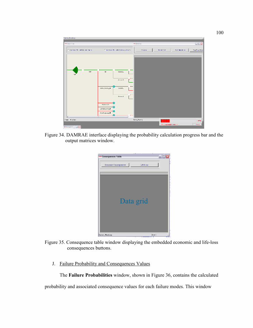
100
Figure 34. DAMRAE interface displaying the probability calculation progress bar and the output matrices window.
Figure 35. Consequence table window displaying the embedded economic and life-loss consequences buttons.
J. Failure Probability and Consequences Values
The Failure Probabilities window, shown in Figure 36, contains the calculated
probability and associated consequence values for each failure modes. This window
Data grid

101
Figure 36. Failure probabilities and consequence output window
contains a list box displaying the failure modes and a combo box displaying consequence
types. To find out the probability and consequence value for a failure mode, check the
failure mode in the list box and select the consequence type in the combo box, and the
use the Probability and Consequences buttons to view the output values.
The Failure Probabilities window also contains a ‘Cumulative Failure
Probability Plot’, which contains a plot of the cumulative probability for the selected
failure mode vs. the pedigree row number.
K. Add External Data File
To add an external interpolation text file, the icon H can be used. This option
brings up an Add ASCII File window, as shown in Figure 37. To find the file location,
use the browse folder button and type in the name of the file in the input box. To transfer
the content of the file into the program database, click the Add button. The added
content of the file are displayed in the data grid.

102
Figure 37. Add external text data file window.
Drawing Details
The construction of the event tree is sequential with the usual convention being
from left to right. The construction process begins with an initiating event, for example a
range of magnitudes of large flood peak water levels in the reservoir, and the sequence of
subsequent events that might lead to dam failure are drawn, typically in the order that
they occur. To draw the initiating event branch, one of the two check boxes should be
selected, as appropriate. If the initiating branch represents a discrete value of the
initiating event, select the Start Event Tree with Discrete Branch. If the initiating
branch represents a range of values for the initiating event, then select the Start Event
Tree with Continuous Branch. As the appropriate initiating branch type is selected a
Create Branch window is displayed, as shown in Figure 32. This window contains the

103
inputs required for drawing the branch on the software interface. The descriptions of
these inputs are present in the following subsections.
Branch Variable Name: This is assigned for the branch identification. This name
is not used by the program in any calculation so it can be any length depending upon the
user’s choice.
Branch Variable Code: This represents the variable name for a branch which is
used to access the probability or state value of that branch. Other than this, Branch
Variable Code is also used in generating the Branch Code Matrix. So, it is required to
assign a short unique name to each branch (or group of branches in case of a discrete
branch, failure branch or exposure branch).
Branch Number: This denotes the branch level starting from the left side of the
event tree with the initiating branch as Level 1. The branch number is assigned by the
program and hence the input window is disabled.
State Value Unit: Not functioning in the current version of DAMRAE.
Types of Branches: Based on the functionality of different events that are useful
in dam safety event trees, DAMRAE includes seven types of branches from which an
event tree structure can be built. Typically, the initiating branch is either a discrete branch
or a continuous branch.
Number of Branches: Next to the each of type of branch, there is an input box for
assigning the required number of branches. For the discrete, failure and exposure types of
branch, multiple branches can be added under the same branch variable name and branch
variable code. The default branch number for these branches, assigned by the program, is
2; but the actual number can be changed by the user as required. The state function,

104
consequence and intervention types of branches have a fixed number of branches and
hence, for these types of branches, the numbers of branches in the input boxes are
disabled.
User Specified Input: This option is enabled for discrete, continuous and exposure
branch types. For these branch types, the user has a choice to input the probability values
or the state values for the branch.
State Function Calculation Method: This option is enabled for the state function
and failure types of branches. For a state function branch, the state value can be
computed either by selecting the tabular interpolation option or by entering a user-
specified function. The tabular interpolation option requires the appropriate text file
input containing the related branch variable codes as the heading of columns in the text
file. The user-specified function option requires defining the functional relationship
between the state value in the state function branch and state values in preceding
branches with the equation written using their branch variable codes. The equation of
functional relationship could be an algebraic equation or it could be a predefined function
included in the program.
After drawing the initiating branch on the DAMRAE interface branches can be
added to the event tree moving from left to right by using the options available in the
node-right-click menu, as shown in Figure 38. A detailed description of the node-right-
click menu, which can be accessed from each branch node is present in the next
subsection.
Node-Right-Click Menu Options: The first level of right click menu includes the
following three options:-

105
Figure 38. Event tree drawing window displaying the node-right-click menu options.
1. Branch: This option provides the facility to add, insert or delete the next
level of branch to a node. The second level of this menu, following this Branch option
includes four options, as follows:
a) Add: To add the subsequent event branches to an initiating branch, the
ADD option next to the branch right click menu is used. The next level of
the ADD menu includes different options for each branch type. To add a
new branch, select the desired branch type, and enter all the required
inputs in the Create Branch window that will appear.
b) Insert: To insert a new branch between two existing branches the ADD
option cannot be used. To do so, the INSERT option must be used.
Similar to the ADD option, the next level of the INSERT option includes
the same branch type options and requires the same steps as for the ADD
option.

106
c) Delete: This option is used to delete a branch from the last branch level. If
this option is selected for a branch level other than the last branch level,
the selected branch and all other subsequent branches connected to the
selected branch will be deleted.
d) Delete All: This option deletes all the branches from the program database
and also clears the entire draw event tree window. To restart the event
tree drawing, select the desired branch type option for the initiating branch
and continue as before.
2. Node: The next level of right click menu attached to the Node option
includes the Copied Collapsed Node and Cloned Collapsed Node options. If it is
desired to copy the sub tree following a particular node to an underlying node, the
Copied Collapsed Node option should be used. If, in addition to copying the sub tree it
is desired to use the same inputs in the new location, the Cloned Collapsed Node option
should be used. The node from which the sub tree is copied is known as a ‘Donor Node’
and the ‘copied collapsed node’ or a ‘cloned collapsed node’ is known as a ‘Host Node’.
To set a node as a ‘copied collapsed node’ or a ‘cloned collapsed node’ the appropriate
option must be selected, which brings up a message box with a command for the user to
click on the ‘Donor Node’. As the user clicks on the ‘Donor Node’, the program asks the
user to confirm the location of the ‘Donor Node’. If the selected node is the desired
‘Donor Node’, click the Yes button on the message box, otherwise click the No button.
If at this stage the user decides not to set the node as a ‘Host Node’ the Cancel button
must be clicked. If the ‘copied collapsed node’ option is selected for a node, as Yes
button is clicked on the message box, the sub tree branch structure of the ‘Donor Node’

107
is copied to the ‘Host Node’. This copied branch structure has all the inputs from the
donor node sub tree but any changes must be made separately in the donor and host
nodes sub trees. If the ‘cloned collapsed node’ option is selected, upon clicking the Yes
button, the program marks the ‘Donor Node’ with a label ‘D’ and the ‘Host Node’ with
a label ‘H’. As a ‘cloned collapsed node’ has the same following branch structure and
associated inputs as its ‘Donor Node’, the program does not make a copy of the branch
structure on the interface and the user is not required to assign inputs in the cloned sub
tree because the inputs in the donor sub tree will continue to be used in the host sub tree.
Some requirements for the ‘Donor Node’ and ‘Host Node’ are that a ‘Host Node’ and its
‘Donor Node’ must be in the same branch level and the Donor Node must be above the
‘Host Node’ in that level of the event tree. A node can be a ‘Donor Node’ for multiple
‘Host Nodes’ and it is preferred not to set a ‘Host Node’ as a ‘Donor Node’ for some
other nodes.
3. Input: Input for a branch can be entered using the right-click-menu of the
node attached to the end of that branch. Inputs can be filled simultaneously while
creating the event tree structure or after completing the event tree drawing. Upon
selecting the Input option, the appropriate input window comes up based on the type of
branch. Details of inputs for different branch types are described in the following
subsection.
Input Details
In general, the branch inputs for calculating the probabilities or state values can be
assigned in any of the following three ways: (a) User-specified Constant Values, (b)

108
Tabular Interpolation, or (c) a User-specified Function. All the three options are
available only for the discrete, exposure, and consequence types of branches. For the
state function and failure types of branches either the Tabular Interpolation or User-
Specified Function method can be used. If a failure branch is assigned a fixed user-
specified value, it can be assigned as a User-specified Function input. For the
intervention branch, the user only has the option to enter the fixed probability value for
the successful intervention and the unsuccessful probability value is calculated as the
complement of the successful intervention value. A detailed description of input
assignment for different types of branches is included in the following subsections.
Discrete Branch Input
Upon selecting the Input option for a discrete branch, an input window, as shown
in Figure 39, shows up. User-Specified Input can be either a Probability or a State
Value; but the present version of the DAMRAE has only been tested for the probability
option. The Method for Calculating State Value/ Probability has the following three
options:
1. User-specified Constant Values: To enter a user-specified value of a
probability or a state value, the first option must be checked. Upon clicking the OK
button, another window, as shown in Figure 40, comes up and includes the discrete
branch labels and branch values in a data grid. Discrete branches included in the data
grid are the branches that emerge from a common preceding node. If the event tree starts
with a discrete branch group, all the discrete branches will be included in the data grid.

109
Figure 39. Discrete branch input window.
Figure 40. User-specified constant value input window for a discrete branch group.
The default branch name for a discrete branch is ‘Branch (index)’, where the
index is the number of the branch. The user can reassign both the branch name and the
branch value in the data grid. To save the data in the program database, click the OK
button. If a new name is assigned for a branch, the event tree drawing on the interface
displays the new name for that branch.
2. Tabular Interpolation: If a single discrete branch or a discrete branch in a
group of discrete branches, which are linked with a common preceding node, will use the
tabular interpolation calculation method, the user should select the second Tabular
Interpolation check box. Upon clicking the OK button, a Discrete Branch Input
window, as shown in Figure 41, comes up. This window contains a data grid, which

110
Figure 41. Discrete branch input window including the option for tabular interpolation and a user-specified function.
includes the names of the discrete branches connected to a common preceding node. To
enter the input for a branch, check the desired option from the data grid columns and
highlight the branch name in Input Branch combo box.
If the Tabular Interpolation option is checked for a discrete branch, upon clicking
the button, a Tabular Interpolation input window, as shown in Figure 42, comes up. This
window includes several inputs that are required to compute the probability or state value
for a discrete branch, as follows:
a. File location: Use the browse folder icon to locate the path of the desired
interpolation text file. The text file columns should be tab separated and the first row of
the text file should contain the heading each columns, which must match the appropriate
branch variable codes. If the file format and the file location are correct, the input file
content is displayed in the data grid.

111
b. Interpolation routine: If the input interpolation file has two columns, select
the one-way interpolation routine. In this routine, the first column of the input text file is
treated as the input value column for the interpolation and the second column is the
output value column. The names of both columns must match the appropriate branch
variable codes. If the input text file has three variables and more than two columns,
select the two-way interpolation routine. The first column of the text file is the input
column and its heading must match the appropriate branch variable code. The other
columns are the output value columns, which must have headings that correspond to the
appropriate numerical values of the third variable.
c. Interpolation method: The interpolation method can be linear, log-log or
semi-log. In the present version of the DAMRAE only linear and log-log interpolation
methods are functional. Select the desired interpolation method from the combo box.
d. Variables: This combo box shows the list of available branch variable
codes which have been defined by the user and which are therefore available to be used
as the columns heading in the input text file.
e. Functional relation: To incorporate the dependencies of a probability or a
state values on different variables, this input box displays a relationship as Probability or
state value = f (Input Branch Variable Code or Codes), where the user is required to
assign the input branch variable codes.
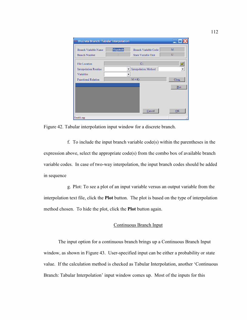
112
Figure 42. Tabular interpolation input window for a discrete branch.
f. To include the input branch variable code(s) within the parentheses in the
expression above, select the appropriate code(s) from the combo box of available branch
variable codes. In case of two-way interpolation, the input branch codes should be added
in sequence
g. Plot: To see a plot of an input variable versus an output variable from the
interpolation text file, click the Plot button. The plot is based on the type of interpolation
method chosen. To hide the plot, click the Plot button again.
Continuous Branch Input
The input option for a continuous branch brings up a Continuous Branch Input
window, as shown in Figure 43. User-specified input can be either a probability or state
value. If the calculation method is checked as Tabular Interpolation, another ‘Continuous
Branch: Tabular Interpolation’ input window comes up. Most of the inputs for this

113
Figure 43. Continuous branch input and continuous branch tabular interpolation windows.
window are similar to the discrete branch tabular interpolation input window as described
above except for a few additional inputs, as described below.
a. Data Range: It is required to assign the minimum and maximum values of
the input variable in the data range input boxes. By default, the minimum and maximum
value assigned to these boxes are the first and last values of the input data column in the
data grid but these values can be reassigned by the user.
b. Number of Levels: This represents the number of intervals for the input
variable data range. After entering the number of intervals, click the ‘+’ button. This
will divide the data range into the assigned number of intervals with equal spacing.
These values of the input variable will be added to the data grid. To change the spacing
of the input variable values, values can be modified in the data grid.

114
c. z-Variate Method: This option is checked to use the z-variates of the input
variable in interpolation.
d. Include the probability lesser than the Min Range Value: Sometimes,
when the minimum data range value does not has a probability of 1.0, it may be desired
to include the probability that values lower than the assigned minimum data range value
will occur.
State Function Input
The State Function Input window for a state function branch is shown in Figure
44. If the User-specified Function option is checked, upon clicking the OK button,
another window for State Function Input comes up.
Figure 44. State function input and state function user-specified function windows.

115
To calculate the state value of a state function branch, an algebraic equation or a
predefined program functions can be used. The variables used in the functional relation
should be in terms of the available branch variable codes. A list of available branch codes
can be seen in the ‘Available Branch Variable Code’ combo box.
Failure Branch Input
The failure branch input window, shown in Figure 45, is similar to a discrete
branch input window, shown in Figure 41. The first row in the data grid is always ‘NF’
(i.e. the no-failure branch) and the other rows of the data grid display the name for each
of the other failure modes. Since the probability for a no-failure branch is always (1- sum
of failure branches) so there is no need to enter any input for a no-failure branch. For the
failure branches, either tabular interpolation or the user-specified method can be selected.
For the selected calculation method, the input is assigned in the same way as described
for the discrete branch tabular interpolation, above.
When failure modes are not mutually exclusive, the total probability of failure can
be calculated based on the common-cause adjustment approach (Hill et. al, 2003). In
order to perform the common-cause adjustment (CCA) for the failure modes, a check box
option added at the bottom of the failure branch input window must be selected.
Exposure Branch Input
Exposure branch inputs assignment is similar to a discrete branch inputs
assignment, which is described above.

116
Figure 45. Failure branch input and failure branch user-specified function input windows.
Consequence Branch Input
The consequence branch input window, shown in Figure 46, is similar in format
as a discrete branch input window, shown in Figure 40, except for a few differences. The
first column of the data grid shows the name of the consequence centers, which were
entered by the user before starting the drawing of the consequence branches. Before
inputs can be entered for these centers, it is required to select the Consequence Type
from the combo box. It is necessary to assign the same consequence type to all the
consequence branches in the same branch level.

117
Figure 46. Consequence branch input window.
Figure 47. Intervention branch input.
Intervention Branch Input
The Input option for an intervention branch brings the window shown in Figure
47. As mentioned above, the intervention branch is a pair of branches representing
successful intervention and unsuccessful intervention. This input window has input
boxes for both the branches in the pair. The user can specify a fixed probability value for

118
Figure 48. Intervention branch combination window displaying different possible ‘with’ and ‘without’ intervention cases for two intervention branch pairs in the event tree.
the successful intervention branch and the unsuccessful intervention branch probability is
calculated by the program as (1- successful intervention probability).
Event Tree Evaluation
After the completion of the event tree drawing and assigning the inputs to all the
nodes on the DAMRAE interface, the next step is to calculate the event tree for
estimating the failure probabilities and associated consequences. The event tree
calculation is performed in two steps: (a) probability calculation, and (b) consequence
calculation. The probability calculation is performed using the Probability Calculation
option and then consequences are calculated using the Consequence Calculation as
described under the heading of menu bar details.
If an event tree structure includes an intervention branch pair, upon selecting the
Probability Calculation option from the menu bar, the program displays an

119
Intervention Branch Combination window, as shown in Figure 48. For an intervention
branch pair it is typically desired to evaluate the event tree with and without the inclusion
of the intervention branch pair in the event tree structure. For the ‘with intervention’
case, the actual successful intervention probability value assigned by the user is used in
calculating the event tree. In case of the ‘without intervention’ case, the program uses a
fixed zero probability value for the successful intervention. The program provides a
flexible facility for the user to calculate the event tree either for the ‘with intervention’
case, or for the ‘without intervention’ case, or for both. In case of more than one
intervention branch pairs in the event tree structure, the Intervention Branch
Combination window shows the ‘with intervention’ and ‘without intervention’
combinations for different intervention branch pairs. In Figure 48, four rows of possible
combinations for the two intervention branch pairs are shown, where ‘Y’ denotes the
‘with intervention’ case and ‘N’ denotes the ‘without intervention’ case for the respective
column headings. The column headings include the branch variable codes for the
intervention branches. The user is required to select the check boxes for the desired
combination of different intervention branch pairs. Upon clicking the OK button, the
program performs the probability calculations for the selected number of cases. After the
probability calculation, when the Consequence Calculation option is selected, the
program performs the consequence calculation for the same number of cases as they were
selected for the probability calculation.

120
Output Details
The program outputs are divided into three parts: (a) probability matrices output,
(b) consequence matrices output, and (c) failure probability and consequence values
output. As mentioned above, the probability matrices can be viewed using either the
Probability Tables option under the Calculation menu or the icon G shown in Figure
27. The probability matrices output includes the ‘Pedigree’, ‘Branch Code’, ‘Probability’
and ‘State Value’ matrices. The consequence matrices output can be accessed using
either the Consequence Table option under the Calculation menu or the icon I, shown
in Figure 27. This output includes the economic and life-loss consequence values for each
consequence centers in two separate tables. These tables have different columns based on
the number of consequence centers and each column shows the respective consequence
value for all the pedigree rows. The last column in the economic consequence table
shows the total annualized incremental economic consequence values for all the rows and
the last column in the life-loss table shows the total annualized incremental life-loss
values for all the rows. The failure probability and consequence value outputs are
accessed using the output window, shown in Figure 36. This output window lists the
name of all the failure modes. The probability of occurrence of the selected failure
modes and the annualized consequence values associated with that failure mode can be
printed in the text boxes. The output window also shows the plot for the cumulative
probability of occurrence of the selected failure mode vs. the pedigree row index.

121
Post-processing Details
The post-processing step can be initiated by using the Append Project option
under the Post Process menu bar tab, shown in Figure 26. Upon selecting this option,
the program opens a separate Project Summary window, shown in Figure 49. This new
window contains the Post Process option in the menu bar. For appending an already-
calculated event tree project into the post-processing step, the user is required to select
the Append Project sub-menu option under the Post Process menu bar option. This
option brings up the window shown in Figure 50. Using the browse folder icon, the user
can point to the location of the desired event tree project. After including the name of the
desired event tree project in the project file input box, the OK button must be clicked to
display the window, shown in Figure 51, which displays all the failure modes present in
the selected event tree project. These failure modes are displayed under the heading of
the Calculated Failure Modes. Using the four arrow buttons available in this window,
the user can include or exclude selected failure modes in the summary table. The
selected failure modes and their probability and associated consequences values are then
displayed in the bottom data grid of the Project Summary window.

122
Figure 49. Project summary window used in the post-processing step.
To create a brief summary table by combining the probabilities and associated
consequences for some different failure modes, the user can select the desired rows in the
bottom data grid by using the <ctrl + click> and then using the Transport To Brief
Summary Table button available in the center of the Project Summary window. Upon
clicking the Transport To Brief Summary Table button, the user is required to assign a
name for each group of combined failure modes.
Figure 50. Event tree project file input window.

123
Figure 51. Append project sub-window displaying the failure modes of a selected event tree project.
To include more than one event tree projects in the same summary table, the user
is required to repeat all the steps described above from the beginning.
After creating the brief summary table, the user can use the F-N plot and USBR
Criteria buttons to plot the ANCOLD F-N plot and USBR Portrayal of Risks plot for the
selected event tree projects.