1

GENERAL SUPERSTRUCTURE AND GLOBAL OPTIMIZATION FOR THE

DESIGN OF INTEGRATED PROCESS WATER NETWORKS

Elvis Ahmetović1, Ignacio E. Grossmann

2,*

1Department of Process Engineering, University of Tuzla, 75000 Tuzla, Bosnia and Herzegovina

2Department of Chemical Engineering, Carnegie Mellon University, Pittsburgh, PA 15213, United States

Abstract

In this paper, we propose a general superstructure and a model for the global optimization for the design of

integrated process water networks. The superstructure consists of multiple sources of water, water-using

processes, wastewater treatment and pre-treatment operations. The unique features are first, that all feasible

interconnections are considered between them, including water re-use, water regeneration and re-use, water

regeneration recycling, local recycling around process and treatment units. Second, multiple sources of water

of different quality that can be used in the various operations are included. Third, the superstructure

incorporates both mass transfer and non-mass transfer operations. The proposed model of the integrated water

network is formulated as a Nonlinear Programming (NLP) and as a Mixed Integer Nonlinear Programming

(MINLP) problem for the case when 0-1 variables are included to model the cost of piping and/or selection of

technologies for treatment. The MINLP model can be used to find optimal network designs with different

number of streams in the piping network. In this work, we propose to represent the bounds on the variables as

general equations obtained by physical inspection of the superstructure and using logic specifications needed

for solving the model. We also incorporate the cut proposed by Karuppiah and Grossmann (2006) to

significantly improve the strength of the lower bound for the global optimum. The proposed model is tested on

the several illustrative examples, including large-scale problems.

Keywords: Integrated water networks; Superstructure optimization; Nonconvex NLP and MINLP model.

1. Introduction

The process industry consumes a large amount of water. For instance, water is used for washing

operations, separation processes, steam and power generation, cooling, etc. These processes in turn

generate wastewater, which is usually processed in treatment units before discharge to the

environment. The shortage of freshwater, its increasing cost and the one of treatment processes, as

well as strict environmental regulations on the industrial effluents, provide a strong motivation for

developing approaches and techniques to design more efficient process water networks.

*Corresponding author. Tel.: +1 412 268 2230; fax: +1 412 268 7139.

E-mail address: grossmann@cmu.edu (I.E. Grossmann).

2

The two major approaches for the optimal design of water network systems are water pinch

technology and mathematical programming. A comprehensive review of these approaches as well as

systematic methods of chemical process design are given by Rossiter (1995), El-Halwagi (1997),

Biegler, Grossmann and Westerberg (1997), Mann and Liu (1999), Bagajewicz (2000), Ježowski

(2008), Bagajewicz and Faria (2009), and Foo (2009).

Water pinch technology relies on graphic representations and it is based on an extension of pinch

analysis technique for heat integration (Linnhoff and Hindmarsh 1983). The first authors, who

introduced the notion of synthesizing mass-exchange networks (MEN’s), were El-Halwagi and

Manousiouthakis (1989; 1990). They considered mass exchange between the rich and the lean

process streams. After that, a targeting approach for minimum freshwater consumption was

developed by Wang and Smith (1994a; 1994b; 1995) and later extended and improved by a number

of researchers (Dhole, Ramchandani, Tainsh & Wasilewski, 1996; Doyle & Smith, 1997; Kuo &

Smith, 1997; Castro, Matos, Fernandes & Nunes, 1999; Sorin & Bedard, 1999; Polley & Polley,

2000; Hallale, 2002; Bandyopadhyay, Ghanekar & Pillai, 2006; Foo, Kazantzi, El-Halwagi & Abdul

Manan, 2006; Foo, 2009).

The mathematical programming approach is based on the optimization of a superstructure. The

seminal paper addressed a mathematical programming formulation of water network was given by

Takama, Kuriyama, Shiroko & Umeda (1980). They considered a total system consisting of water-

using and wastewater-treating units. In addition to this, they generated a superstructure of all possible

re-use and regeneration opportunities and formulated the problem of optimal water allocation in a

petroleum refinery as a nonlinear programming problem. After their paper the solution of the

mathematical programming formulation for this problem was not addressed for many years

(Bagajewicz, 2000). In many papers, the total water network is decomposed into two parts (network

with water-using operations and wastewater treatment network) which are solved separately. For

example, Kuo and Smith (1997) presented an extension of the methodology for the design of

distributed effluent treatment systems previously given by Wang and Smith (1994b). They presented

an improved method for targeting the treatment flowrate and the distribution of load between multiple

treatment processes. In addition to this, Galan and Grossmann (1998) addressed the optimal design of

distributed wastewater network where multiple contaminants are considered. They proposed a

heuristic search procedure based on the successive solution of a relaxed linear model and the original

nonconvex nonlinear model. Their procedure has the capability of finding global or near global

optimum solutions. In addition, the model was extended for selecting different treatment technologies

3

for handling membrane separation modules. Savelski and Bagajewicz (2000; 2003) developed

necessary optimality conditions (maximum outlet concentrations from water-using units and

concentration monotonicy) for single and multiple water allocation systems in refineries and process

plants. They used these conditions to eliminate the nonlinearities in the water network models arising

in the mass balance equations in the form of bilinear terms (concetration times flowrate). According

to this, they showed that the nonlinear model of water networks for single component can be

linearized. Quesada and Grossmann (1995) proposed a rigorous procedure for the global optimization

of bilinear process networks with multicomponent streams. Their procedure is based on a

reformulation-linearization technique applied to nonlinear models in order to obtain a relaxed linear

programming formulation that provides a valid lower bound to the global optimum. Castro, Teles and

Novais (2009) proposed the two-stage solution strategy for the optimal design of distributed

wastewater networks with multiple contaminants. In the first stage, a decomposition method is

employed that replaces the nonlinear program by a succession of linear programs, one for each

treatment unit. In the second, stage, the resulting network is used as a starting point for the solution of

the nonlinear model with a local optimization solver.

The problem of designing the total water networks has been addressed in relatively few papers

(Ježovski, 2008). Doyle and Smith (1997) proposed a method based on nonlinear programming for

targeting maximum water reuse in processing systems. To overcome the difficulties associated with

the nonlinear optimization model, they used a linear model to provide an initialization for the

nonlinear model. Alva-Argáez, Kokossis and Smith (1998) proposed an integrated methodology for

the design of industrial water systems. Their decomposition strategy is based on a recursive procedure

where the original Mixed-Integer Nonlinear Problem (MINLP) problem is replaced by a sequence of

Mixed-Integer Linear Problems (MILPs). Huang, Chang, Ling, and Chang (1999) proposed a

mathematical model for determining the optimal water usage and treatment network in any chemical

plant. They presented a modified version of the superstructure proposed by Takama, Kuriyama,

Shiroko, and Umeda (1980) and included in the model design equations of all wastewater treatment

facilities and all units which utilize either process or utility water so that better integration on a plan-

wide scale can be achieved. Feng and Seider (2001) proposed a network structure in which internal

water mains are utilized. Their structure simplifies the piping network as well as the operation and

control of large plants involving many water-using processes. Gunaratnam, Alva-Argaez, Kokossis,

Kim, and Smith (2005) presented an automated design of total water systems where the optimal

distribution of water to satisfy process demands and optimal treatment of effluent streams are

4

considered simultaneously. They used a two-stage optimization approach to solve the MINLP model

involving an MILP in the first stage to initialize the problem. In the second stage, the design is fine-

tuned using MINLP. In addition to this, the network complexity is controlled by specifying the

minimum permissible flowrates in the network. Their methodology provides a robust technique but it

does necessarily yield the global optimum.

Karuppiah and Grossmann (2006) addressed the problem of optimal synthesis of an integrated

water system consisting of water-using processes and water treatment operations. In contrast to

previous work, they proposed a spatial branch and contract algorithm for the rigorous global

optimization of the nonlinear program of the integrated water system. In their algorithm, tight lower

bounds on the global optimum are obtained by solving a relaxation of the original problem obtained

by approximating the nonconvex terms in the NLP model with piecewise linear estimators. Li and

Chang (2007) developed an efficient initialization strategy to solve the NLP and MINLP models for

water network with multiple contaminants. In the MINLP model they formulated structural

constraints to manipulate structural complexity, but global optimality is not guaranteed. Also, they

reported that the optimum solution obtained by the initialization strategy is at least as good as results

reported in the literature but with less computation time to achieve convergence. In the same year,

Alva-Argaez, Kokossis, and Smith (2007) proposed a systematic approach to address water reuse in

oil refineries. The methodology is based on the water-pinch decomposition. Their approach simplifies

the challenges of the optimization problem making systematic use of water-pinch insights to define

successive projections in the solution space.

Putra and Amminudin (2008) proposed an alternative solution strategy for solving the total water

system design problem by utilizing the MILP and NLP in a two-step optimization approach. Their

approach, which is not guaranteed to find the global optimum, has the capability of generating

multiple optimal solutions and to handle practical considerations, as well as to provide users with the

ability to control water network during the optimization process. Luo and Uan (2008) presented a

superstructure-based method for the optimization of integrated water systems with the heuristic

Particle Swarm Optimization (PSO) algorithm. Karuppiah and Grossmann (2008) presented a

formulation for representing and optimizing integrated water networks operating under uncertain

conditions of the contaminant loads in the process units and contaminant removals of the treatment

units. They formulated a multi-scenario nonconvex MINLP model for globally optimizing an

integrated water network operating under uncertainty. Further, they proposed a spatial branch and cut

5

algorithm combining the concepts of Lagrangean relaxation and convex relaxation in order to

generate strong bounds for the global optimum.

Notice that in the previously mentioned papers the vast majority are based on linearization of the

nonlinear models, or use linear models to provide an initialization for the nonlinear models, which are

solved with local optimization solvers. Moreover, a number of authors replace the MINLP problems

by a sequence of the MILPs. Bagajewicz and Faria (2009) and Faria and Bagajewicz (2009) presented

the evolution of the water network allocation problem given by Takama, Kuriyama, Shiroko &

Umeda (1980). In addition, they included the water pre-treatment subsystem in the network and

discussed the end-of-pipe wastewater treatment and the complete water integration.

It should be mentioned that the problem of designing total water networks has been addressed in

relatively few papers due to its complexity (Ježovski, 2008). The main complexity in the nonlinear

model appears due to the bilinear terms in the mass balance equations (flowrate times concentration)

and the concave cost terms in the objective function with which the solution for the total water

network is not guaranteed to be the global optimum. In addition to this, it is worth pointing out that in

the majority of the published papers all possible options are not considered in the total water network

such as all feasible interconnections in the network, multiple sources of water of different quality,

pre-treatment of the water, mass transfer and non-mass transfer water-using operations. Moreover, in

many papers the cost of water pumping through pipes and the investment cost for pipes are not

included in the objective function.

The main objective of this paper is to propose a general superstructure and a global optimization

approach for the design of integrated process water networks. The superstructure consists of multiple

sources of water, water-using (mass transfer and non-mass transfer) processes, water treatment

operations and all feasible interconnections in the network. We propose nonconvex NLP and MINLP

models for the integrated water network. We also develop bounds on the variables as general

equations obtained by physical inspection of the superstructure and use logic specifications that have

the capability of reducing the feasible region, and helping global the NLP and MINLP solvers to find

more efficiently the global optimum. In the MINLP model we include the costs of piping and the

costs of water pumping through pipes. With the proposed model we can also control the complexity

of the piping network. For large-scale industrial MINLP problems, we propose a two-stage solution

method in which we first solve the NLP model in order to fix a subset of 0-1 variables to zero so as to

solve a reduced size MINLP. We also update the bounds to tighten the reduced MINLP model.

Several examples, including large-scale industrial problems, are presented in the paper to illustrate

6

the proposed method. We use the general purpose global optimization solvers BARON (Sahinidis,

1996) and LINDOGlobal to solve the proposed models to global optimality.

The outline of the paper is as follows. First, we present the problem statement. We then introduce

the general water network superstructure, followed by its mathematical formulation. Further, we

present two-stage solution methods for solving large-scale industrial MINLP problems. The

computational results and discussion are given in the following section. Finally, in the last section we

present general conclusions.

2. Problem statement

The problem addressed in this paper can be stated as follows. Given is a set of single/multiple

water sources with/without contaminants, a set of water-using units and wastewater treatment

operations, fixed water demands of process units, maximum concentrations of contaminants in inlet

streams at process units, mass loads of contaminants in process units, the costs of water sources and

wastewater treatment units, % removal for each contaminant in treatment units and the maximum

contaminant concentrations in the discharge effluent to the environment. The problem consists in

determining the interconnections, flowrates and contaminants concentration of each stream in the

water network, the freshwater consumption and wastewater generation, and the total annual cost of

the water network (costs of freshwater consumption, wastewater treatment, piping network, pumping

water through pipes in the network).

The proposed model is based on the following assumptions: the number of water sources is fixed,

the number of water-using and water treatment operations is fixed, the flowrates through the water-

using wastewater treatment operations are fixed, the network operates under isothermal condition and

isobaric conditions.

3. Superstructure of the integrated process water network

The proposed model of the integrated water network relies on the superstructure given in Figure 1.

The superstructure, which is an extension and generalization of the one given by Karuppiah and

Grossmann (2006), consists of one or multiple sources of water of different quality, water-using

processes, and wastewater treatment operations. The unique feature is that all feasible connections are

considered between them, including water re-use, water regeneration and re-use, water regeneration

recycling, local recycling around process and treatment units and pre-treatment of feedwater streams.

Multiple sources of water include water of different quality that can be used in the various operations,

7

and which may be sent first for pre-treatment. The superstructure incorporates both the mass transfer

and non-mass transfer operations. According to this, it can be used to represent separate subsystems

as well as an integrated total system. Furthermore, it enables modeling different types of water

network optimization problems as will be shown later in the paper.

Figure 1. Generalized superstructure for the design of integrated process water networks.

4. Basic conceptual options of models

The mathematical model of integrated process water networks consists of mass balance equations

for water and the contaminants for every unit in the network. The model is formulated as a

nonconvex nonlinear programming (NLP), and as a nonconvex mixed-integer nonlinear programming

(MINLP) for the case when 0-1 variables are included to model the cost of piping and/or selection of

technologies for treatment. The nonlinearities in the models appear in the mass balance equations in

8

the form of bilinear terms (concentration times flowrate). In addition to this, nonlinearities appear in

the objective function as concave terms of the cost functions for the water-treatment operations.

Hence, the water network models are nonconvex, and in most cases lead to multiple local solutions

making difficult to obtain the global or a near-global optimal solution. The basic options of the

proposed water network optimization model are shown in Figure 2.

Figure 2. The basic options of the proposed optimization model.

9

First of all, the model enables the choice of a single or multiple sources of water that are available

for the network plant operation. Second, water sources can be clean water without contaminants or

water with multiple contaminants. Water with higher quality is more expensive and the total cost will

be minimized at the expense of lower quality water as shown later in illustrative examples. Water

with contaminants on the other hand may be directly sent to treatment units before using it for water-

using operations. Third, the water network can consist only of the water-using operations or

wastewater treatment operations. In addition, it can be an integrated water network including both

water-using operations and wastewater treatment operations. Fourth, all feasible interconnections are

possible in the network for every option mentioned before. Fifth, it is possible to choose local

recycles around the water-using operations or the wastewater treatment operations. Local recycling

(Wang & Smith, 1995) can be used to satisfy the flowrate constraints and in these cases it is possible

to have an additional reduction in water consumption as is shown later in an illustrative example.

Sixth, as industrial water network systems usually consist of different types of water-using operations

that can be classified as mass-transfer operations and non-mass transfer operations (Mann & Liu,

1999), both types of these operations are included in the superstructure. In addition to this, in many

processes there is loss of water that is not available for re-use in a water-using operation. Hence, this

unit involves water demand unit and is a water sink. Moreover, from some water-using operations

water is available for re-use in other operations and they represent sources of water. In all the above

mentioned options, the number of contaminants, water sources, water-using operations and

wastewater treatment operations is fixed. The proposed model enables modeling and optimization of

any of the above mentioned options of the water network superstructure.

4.1. Mathematical model

In this section we propose an MINLP model for the superstructure given in Figure 1.

Nomenclature

Sets and Indices

j contaminant

DU set of demand units

d demand unit

PU set of process units

p process unit

10

SU set of source units

r source unit

SW set of freshwater sources

s freshwater source

TU set of treatment units

t treatment unit

Parameters

AR annualized factor for investment for treatment units

CFWs cost of freshwater from source s

CP

fixed cost for each individual pipe in the network

in

dFDU

mass flowrate of inlet water stream in demand unit d

in

pFPU

mass flowrate of inlet water stream in process unit p

out

rFSU

mass flowrate of outlet water stream from source unit r

sFWW

mass flowrate of freshwater source s

H hours of plant operation per annum

tIC

investment cost coefficient for treatment unit t

IP

variable cost for each individual pipe in the network

LPUp,j load of contaminant j in process unit p

Nmax maximum number of streams for the network

OCt operating cost coefficient for treatment unit t

PM

operating cost coefficient for pumping water through each pipe in the network

Rp, Rt local recycle around process unit p and treatment unit t (Rp=0 and Rt=0 does not exist,

Rp=1 and Rt=1 if exists)

jtRR , % removal for contaminant j in treatment unit t

max,out

jx

maximum concentration of contaminant j in discharge stream to the environment

max,

.

in

jdxDU

maximum concentration of contaminant j in inlet stream into demand unit d

max,

.

in

jpxPU

maximum concentration of contaminant j in inlet stream into process unit p

out

jrxSU . concentration of contaminant j in outlet stream from source unit r

11

in

jsxW . concentration of contaminant j in freshwater source s

cost exponent for treatment units (0 ≤ ≤ 1)

TUt, j 1-(RRt, j /100)

cost exponent for pipes (0 ≤ ≤ 1)

Continuous variables

outF

mass flowrate of outlet wastewater stream from final mixer

dsFID , mass flowrate of water stream from freshwater source s to demand unit d

sFIF

mass flowrate of water stream from freshwater source s to final mixer

psFIP , mass flowrate of water stream from freshwater source s to process unit p

tsFIT , mass flowrate of water stream from freshwater source s to treatment unit t

ppFP ,' mass flowrate of water stream from process unit p’ to process unit p

dpFPD , mass flowrate of water stream from process unit p to demand unit d

pFPO

mass flowrate of water stream from process unit p to final mixer

tpFPT , mass flowrate of water stream from process unit p to treatment unit t

out

pFPU

mass flowrate of outlet water stream from process unit p

drFSD , mass flowrate of water stream from source unit r to demand unit d

rFSO

mass flowrate of water stream from source unit r to final mixer

prFSP , mass flowrate of water stream from source unit r to process unit p

trFST , mass flowrate of water stream from source unit r to treatment unit t

ttFT ,' mass flowrate of water stream from treatment unit t’ to treatment unit t

dtFTD , mass flowrate of water stream from treatment unit t to demand unit d

tFTO

mass flowrate of water stream from treatment unit t to final mixer

ptFTP , mass flowrate of water stream from treatment unit t to process unit p

in

tFTU

mass flowrate of inlet water stream in treatment unit t

out

tFTU

mass flowrate of outlet water stream from treatment unit t

sFW

mass flowrate of water for freshwater source s

12

out

jx

concentration of contaminant j in discharge stream to the environment

in

jdxDU , concentration of contaminant j in inlet stream into demand unit d

in

jpxPU , concentration of contaminant j in inlet stream into process unit p

out

jpxPU , concentration of contaminant j in outlet stream from process unit p

out

jtxSPU , concentration of contaminant j in outlet stream from splitter process unit p

out

jtxSTU , concentration of contaminant j in outlet stream from splitter treatment unit t

in

jtxTU ,

concentration of contaminant j in inlet stream into treatment unit t

out

jtxTU , concentration of contaminant j in outlet stream from treatment unit t

Binary variables

dsFIDy,

existence of pipe between freshwater source s and demand unit d

sFIFy

existence of pipe between freshwater source s and final mixer

psFIPy,

existence of pipe between freshwater source s and process unit p

tsFITy,

existence of pipe between freshwater source s and treatment unit t

ppFPy',

existence of pipe between process unit p’ and process unit p

dpFPDy,

existence of pipe between process unit p and demand unit d

pFPOy

existence of pipe between process unit p and final mixer

tpFPTy,

existence of pipe between process unit p and treatment unit t

drFSDy,

existence of pipe between source unit r and demand unit d

rFSOy

existence of pipe between source unit r and final mixer

prFSPy,

existence of pipe between source unit r and process unit p

trFSTy,

existence of pipe between source unit r and treatment unit t

ttFTy',

existence of pipe between treatment unit t’ and treatment unit t

dtFTDy,

existence of pipe between treatment unit t and demand unit d

tFTOy

existence of pipe between treatment unit t and final mixer

13

ptFTPy,

existence of pipe between treatment unit t and process unit p

Subscripts/superscripts

FX fixed bound for the variable

in inlet stream

L lower bound for the variable

max maximal

out outlet stream

U upper bound for the variable

4.2. Initial splitters

The feedwater of an initial splitter SIs (shown in Figure 3) for freshwater source sSW can be

clean water without contaminants or water with single/multiple contaminants. Freshwater from the

initial splitter can be directed to the mixer process unit, the mixer treatment unit, the mixer demand

units, or the final mixer. The connection between the initial splitter and the mixers in the network

depends of the special network case that is considered. For instance, if we consider only multiple

wastewater feeds and the wastewater distribution subsystem there will be connections between the

initial splitter and the final mixer. However, in an integrated system consisting of water-using units

and wastewater treatment units, connections between the initial splitter and the final mixer do not

exist because it would lead to a loss of freshwater.

Figure 3. Initial splitter.

The overall material balance for the initial splitter is given by Eq. (1):

SWsFITFIDFIPFIFFWTUt

ts

DUd

ds

PUp

psss

,,, (1)

For each of the corresponding flowrates, upper and lower bound constraints are formulated in

terms of the binary variables that denote the existence of the pipes or these streams.

14

SWsyFIFFIFyFIFss FIF

U

ssFIF

L

s (2)

PUpSWsyFIPFIPyFIPpsps FIP

U

pspsFIP

L

ps ,,, ,,, (3)

DUdSWsyFIDFIDyFIDdsds FID

U

dsdsFID

L

ds ,,, ,,, (4)

TUtSWsyFITFITyFITtsts FIT

U

tstsFIT

L

ts ,,, ,,, (5)

4.3. Mixer process units

The mixer process unit MPUp, shown in Figure 4, consists of a set of inlet streams from the splitter

source unit, the splitter treatment unit, the initial splitter, and the splitter process unit. An outlet

stream from the mixer process unit is directed to the process unit.

Figure 4. Mixer process unit.

The overall material balance for the mixer process unit is given by Eq. (6) and the mass balance

for each contaminant j by Eq. (7), which involves bilinear terms:

PUpFPFPFIPFTPFSPFPU

pp RPUp

pp

RppPUp

pp

SWs

ps

TUt

pt

SUr

pr

in

p

,

1'

,'

0,''

,',,, (6)

jPUpxSPUFPxSPUFP

xWFIPxSTUFTPxSUFSPxPUFPU

out

jp

RPUp

pp

out

jp

RppPUp

pp

in

js

SWsTUt

out

jtpt

out

jr

SUr

pr

in

jp

in

p

pp

,,,'

1'

,','

0,''

,'

,,,,,,

(7)

4.4. Process units

The process unit PUp, shown in Figure 5, consists of an inlet stream FPUpin

from the mixer process

unit and an outlet stream FPUpout

from the process unit. In the mass transfer process unit there is

direct contact, usually countercurrent, between a contaminant-rich process stream and a contaminant-

lean water stream. These units can be represented as a “true” contaminant-rich process streams. In

15

this case during the mass-transfer process the contaminants LPUp, j (pollutants) are transferred from

the process streams to the water. The contaminant concentration in the process stream is reduced,

while the contaminant concentration increases in the water stream (Mann and Liu 1999).

Figure 5. Process unit.

The inlet and outlet water flows for the process unit are equal. The overall material balance is

given by Eq. (8) and the mass balance equation for each contaminant j by Eq. (9):

PUpFPUFPU out

p

in

p (8)

jPUpxPUFPULPUxPUFPU out

jp

out

pjp

in

jp

in

p ,10 ,

3

,, (9)

The outlet concentrations in the flows from the process units and the inlet concentrations to the

splitter process units are the same as shown in Eq. (10):

jPUpxSPUxPU in

jp

out

jp ,,, (10)

4.5. Splitter process units

The splitter process unit SPUp shown in Figure 6 consists of an inlet stream from the process unit,

and a set of outlet streams directed to the final mixer, the mixer treatment unit, the mixer demand

unit, and the mixer process unit. The overall material balance for the splitter process unit is given by

Eq. (11):

PUpFPFPFPDFPTFPOFPU

pp RPUp

pp

RppPUp

pp

DUd

dp

TUt

tpp

out

p

1'

,'

0,''

,',, (11)

Figure 6. Splitter process unit.

16

The contaminant concentration of every stream leaving the splitter is equal to the contaminant

concentration of the inlet stream and this equality is given by Eq. (12):

jPUpxSPUxSPU in

jp

out

jp ,,, (12)

The lower and upper bound constraints that relate the 0-1 variables with the flows between the

splitter process units and all mixers in the network are given as follows.

PUpyFPOFPOyFPOpp FPO

U

ppFPO

L

p (13)

TUtPUpyFPTFPTyFPTtptp FPT

U

tptpFPT

L

tp ,,, ,,, (14)

DUdPUpyFPDFPDyFPDdpdp FPD

U

dpdpFPD

L

dp ,,, ,,, (15)

0,',',,',' ,',',' pFP

U

ppppFP

L

pp RppPUpPUpyFPFPyFPpppp

(16)

1,',',,',' ,',',' pFP

U

ppppFP

L

pp RppPUpPUpyFPFPyFPpppp

(17)

4.6. Demand and source process units

In many processes there is loss of water that cannot be re-used in a water-using operation. This

unit represents a water demand unit or water sink. Cooling towers are typical process units where

water is lost by evaporation. The demand process unit is shown in Figure 7.

Figure 7. Demand process unit.

The mixer demand unit MDUd unit shown in Figure 7 consists of a set of inlet streams from the

splitter treatment unit, the splitter source unit, initial splitter, and the splitter process unit. An outlet

stream from the mixer demand unit is directed to the demand unit. The overall material balance for

the mixer demand unit is given by Eq. (18) and the mass balance for each contaminant j by Eq. (19):

DUdFPDFIDFSDFTDFDUPUp

dp

SWs

ds

SUr

dr

TUt

dt

in

d

,,,, (18)

17

jDUdxSPUFPD

xWFIDxSUFSDxSTUFTDxSDUFDU

out

jp

PUp

dp

in

js

SWs

ds

out

jr

SUr

dr

out

jt

TUt

dt

in

jd

in

d

,,,

,,,,,,,

(19)

Additionally, the contaminant concentration at the demand inlet has to be less or equal to the

maximum allowed contaminant concentration:

jDUdxSDUxSDU in

jd

in

jd ,max,

,, (20)

From some water-using operations water is available for re-use in other operations. These units

represent water sources or gains of water. The splitter source unit SSUr unit shown in Figure 8

consists of an inlet stream from the source unit and a set of outlet streams directed to the mixer

process unit, the final mixer, the mixer treatment unit, and the mixer demand unit.

Figure 8. Source process unit.

The overall material balance for the splitter source unit is given by Eq. (21). Notice, that the

contaminant concentration at the outlet of the source unit and the outlet of the splitter source unit is

the same.

SUrFSDFSTFSOFSPFSUDUd

dr

TUt

trr

PUp

pr

out

r

,,, (21)

The lower and upper bound constraints that relate the flows and 0-1 variables for the streams

between the splitter source units and all mixers in the network are given as follows.

PUpSUryFSPFSPyFSPprpr FSP

U

prprFSD

L

pr ,,, ,,, (22)

SUryFSOFSOyFSOrr FSO

U

rrFSO

L

r (23)

TUtSUryFSTFSTyFST

trtr FST

U

trtrFST

L

tr ,,, ,,, (24)

DUdSUryFSDFSDyFSDdrdr FSD

U

drdrFSD

L

dr ,,, ,,, (25)

18

4.7. Mixer treatment units

The mixer treatment unit MTUt shown in Figure 9 consists of a set of inlet streams from the splitter

source unit, the initial splitter, the splitter process unit, and the splitter treatment unit.

Figure 9. Mixer treatment unit.

The overall material balance for the mixer that is placed in front of the treatment unit is given by

Eq. (26) and the mass balance for each contaminant j by Eq. (27):

TUtFTFTFPTFITFSTFTU

tt RTUt

tt

RttTUt

tt

PUp

tp

SWs

ts

SUr

tr

in

t

1'

,'

0,''

,',,, (26)

jTUtxSTUFTxSTUFT

xSPUFPTxWFITxSUFSTxTUFTU

out

jt

RTUt

tt

out

jt

RttTUt

tt

out

jp

PUp

tp

W

js

SWs

ts

out

jr

SUr

tr

in

jt

in

t

TUTU

,,

1'

,',

0,''

,'

,,,,,,,

(27)

4.8. Treatment units

The treatment unit TUt, shown in Figure 10, consists of an inlet stream from the mixer treatment

unit, and an outlet stream from the treatment unit. The inlet and outlet flows for a treatment unit are

equal and the overall material balance is given by Eq. (28).

TUtFTUFTU out

t

in

t (28)

Figure 10. Treatment unit.

19

The mass balance equation for each contaminant j for the treatment unit tTU is assumed to be a

linear function given by Eq. (29).

jTUtxTUxTU in

jtjtTU

out

jt ,,,, (29)

where βTU t,j = (1-RRt,j/100) for tTU, j .

4.9. Splitter treatment units

The splitter treatment unit STUt shown in Figure 11 consists of an inlet stream from the treatment

unit and a set of outlet streams directed to the mixer demand unit, the mixer process unit, the final

mixer and the mixer treatment unit.

Figure 11. Splitter treatment unit.

The overall material balance for the splitter process unit is given by equation Eq. (30) and the

equality of concentrations at the treatment unit and the splitter treatment unit by Eq. (31):

TUtFTFTFTOFTPFTDFTU

tt RTUt

tt

RttTUt

ttt

PUp

pt

DUd

dt

out

t

1'

,'

0,''

,',, (30)

jTUtxTUxSTU out

jt

out

jt ,,, (31)

The lower and upper bound constraints that relate the flows and 0-1 variables for streams between

the splitter treatment units and all mixers in the network are given as follows.

DUdTUtyFTDFTDyFTDdtdt FTD

U

dtdtFTD

L

dt ,,, ,,, (32)

PUpTUtyFTPFTPyFTPptpt FTP

U

ptptFTP

L

pt ,,, ,,,

(33)

TUtyFTOFTOyFTO

tt FTO

U

ttFTO

L

t (34)

0,',',,',' ,',',' tFT

U

ttttFT

L

tt RttTUtTUtyFTFTyFTtttt

(35)

1,',

,',' ,',',' tFT

U

ttttFT

L

tt RTUtTUtyFTFTyFTtttt

(36)

20

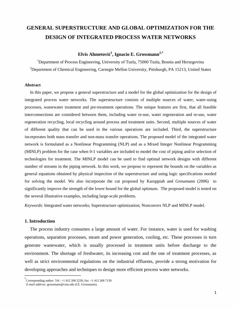
4.10. Final mixer

The final mixer unit MF shown in Figure 12 consists of a set of inlet streams from the initial

splitter, the splitter process unit, the splitter treatment unit, and the splitter source unit.

Figure 12. Final mixer.

The overall material balance for the final mixer is given by Eq. (37) and the mass balance equation

for each contaminant j by Eq. (38):

SUr

r

TUt

t

PUp

p

SWs

s

out FSOFTOFPOFIFF (37)

jxSUFSO

xSTUFTOxSPUFPOxWFIFxF

out

jr

SUr

r

out

jt

TUt

t

out

jp

PUp

p

in

js

SWs

s

out

j

out

,

,,,

(38)

Using the binary variables for the existence of pipe connections, the specification for a maximum

number of these connections in the network is given by Eq. (39). Using this constraint it is possible to

control the complexity of the piping network.

max

1'

0,''

1'

0,''

,,

,,,,

,,',',

,',',,

Nyy

yyyyy

yyyyy

yyyyyy

SUr PUp

FSP

SUr TUt

FST

SUr

FSO

SUr DUd

FSD

TUt DUd

FTD

PUp DUd

FPD

SWs DUd

FID

TUt PUp

FTP

TUt

FTO

RTUt TUt

FT

RttTUt TUt

FT

PUp TUt

FPT

RPUp PUp

FPO

PUp

FP

RppPUp PUp

FP

SWs

FIF

SWs TUt

FIT

SWs PUp

FIP

prtr

rdrdtdpds

ptt

t

tt

t

tttp

PU

ppp

p

ppstsps

(39)

4.11. Objective function of the NLP and MINLP model

When binary variables are excluded with their corresponding lower and upper bound constraints,

the MINLP model in the previous section reduces to an NLP. The objective function of the NLP

water network problems can simply be formulated to minimize the total consumption of freshwater

21

for network plant operation and the total amount of wastewater treated in treatment operations for an

integrated system (Karuppiah & Grossmann, 2006).

TUt

out

t

SWs

s FTUFWZmin (40)

For separate subsystems consisting of water-using or wastewater treatment operations the

objective function is to either minimize the total consumption of freshwater or the total amount of

wastewater treated in treatment operations, respectively.

SWs

sFWZmin (41)

TUt

out

tFTUZmin (42)

A more accurate objective function is to minimize the total network cost consisting of the cost of

freshwater, the cost of investment on treatment units and the operating cost for the treatment units.

This type of objective function is used in many papers to optimize the water network problems.

TUt

out

tt

TUt

out

tts

SWs

s FTUOCHFTUICARCFWFWHZ

min (43)

Furthermore, in the case of separate subsystems consisting of water-using or wastewater treatment

operations the objective function is to minimize the total cost of water, or the total cost of investment

on treatment units and operating cost for the treatment units:

s

SWs

s CFWFWHZ

min (44)

TUt

out

tt

TUt

out

tt FTUOCHFTUICARZ

min (45)

In most papers, the cost of the network piping and the cost of water pumping through pipes are not

considered. Here, we introduce these costs in the objective function when the water network problem

is formulated as an MINLP problem. The objective function is to minimize the total network cost

given by Eq. (46):

pipespumpingwatertreatmenttreatmentwater ICOCOCICCZ min

(46)

Here Cwater is the yearly cost of water for the network plant operation; ICtreatment is the investment cost

for treatment units; OCtreatment is the yearly operating cost for treatment units; OCpumping is the yearly

operating cost for pumping water through pipes in the network; ICpipes is the investment cost of the

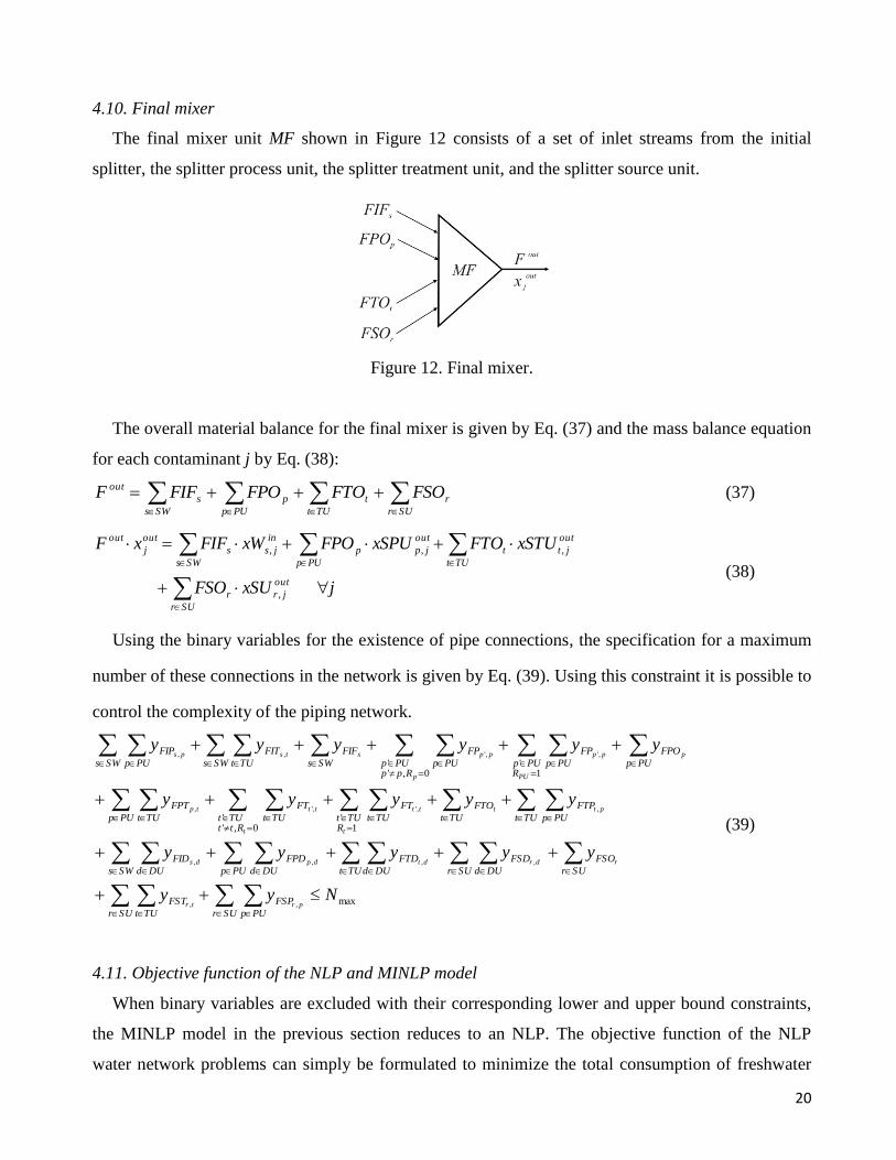
pipes in the network. The annualized costs are expressed for each term in Eq. (46) as follows.

s

SWs

swater CFWFWHC

(46a)

22

TUt

out

tttreatment FTUICARIC

(46b)

TUt

out

tttreatment FTUOCHOC (46c)

SUr SUr

rr

TUt

ttr

SUr PUp

ppr

SUr DUd

ddr

TUt DUd

ddt

PUp DUd

ddp

SWs DUd

dds

RttTUt TUt

ttt

RTUt TUt

ttt

TUt

tt

PUp

pp

PUp TUt

ptp

RppPUp PUp

ppp

RPUp PUp

ppp

TUt PUp

tpt

SWs TUt

tts

SWs PUp

ppspumping

PMFSOPMFST

PMFSPPMFSDPMFTD

PMFPDPMFIDPMFT

PMFTPMFTOPMFPO

PMFPTPMFPPMFP

PMFTPPMFITPMFIPHOC

TU

t

pp

,

,,,

,,

0,''

','

1'

','

,

0,''

','

1'

','

,,,

(46d)

SUr PUp

prpFSPp

SUr TUt

trtFSTt

SUr

rrFSOr

SUr DUd

drdFSDd

TUt DUd

dtdFTDd

PUp DUd

dsdFPDd

SWs DUd

dsdFIDd

SWs TUt

tstFITt

SWs PUp

pspFIPp

RttTUt TUt

tttFTt

RTUt TUt

tttFTt

TUt

ttFTOt

PUp

ppFPOp

PUp TUt

tppFPTp

RppPUp PUp

pppFPp

RPUp PUp

pppFPp

TUt PUp

pttFTPtpipes

FSPIPyCP

FSTIPyCPFSOIPyCP

FSDIPyCPFTDIPyCP

FPIPyCPFIDIPyCP

FITIPyCPFIPIPyCP

FTIPyCPFTIPyCP

FTOIPyCPFPOIPyCP

FPTIPyCPFPIPyCP

FPIPyCPFTPIPyCPARIC

pr

trr

drdt

dpds

tsps

TU

tt

t

tt

tp

tp

p

pp

p

pppt

)((

))(())((

))(())((

))(())((

))(())((

(46e)))(())((

))(())((

))(())((

))(())((

,

,

,,

,,

,,

0,''

,'''

1'

,'''

,

0,''

,'''

1'

,''',

,

,

,,

,,

,,

,','

,,'

,',

23

5. Solution strategy

The proposed model presented in the previous section corresponds to a nonconvex NLP or

nonconvex MINLP problem. This problem is modeled in GAMS (Brooke, Kendrick et al. 1988). In

this paper, the BARON (Sahinidis, 1996) and LINDOGlobal solvers are used for solving all water

network problems to global optimality.

To significantly improve the strength of the lower bound for the global optimum we incorporate

the cut proposed by Karuppiah and Grossmann (2006). The bound strengthening in the nonlinear

model corresponds to the contaminant flow balances for the overall water network system and is

given by equation:

jxDUFDUxF

xTUFTUxSUFSULPUxWFW

in

jd

DUd

in

d

out

j

out

in

jt

TUt

in

tjtTU

out

jr

SUr

out

r

PUp

jp

in

js

SWs

s

,

,,,

3

,, )1(10

(47)

where bilinear terms are involved for the treatment units and final mixing points. It is also worth

pointing out that when solving nonconvex water network problems by the previously mentioned

global optimization solvers, it is important to specify good variable bounds for all flowrates and

concentrations in the water network. The reason is that these bounds are used in the convex envelopes

for under and overestimating the nonconvexities (eg. secant for concave function or McCormick

envelopes for bilinear terms). In the proposed model the bounds on the variables are represented as

general equations as shown in the Appendix. They are obtained by physical inspection of the

superstructure and by using logic specifications. Using the proposed model with the cuts by

Karuppiah and Grossmann (2006) and the bounds in the Appendix we can effectively solve the NLP

water network problems for different levels of complexity with multiple sources of water, multiple

contaminants and more process and treatment units (large-scale problems). Also, the MINLP water

network problems with a modest number of process units, treatment units, and contaminants can be

effectively solved using the proposed model. However, for large-scale MINLP problems the global

optimization solvers cannot find the optimal solution in reasonable computational time.

To circumvent this problem, we propose a solution strategy that can be used for solving large-scale

industrial water network problems. The basic idea is shown in Figure 13. When the objective is to

minimize the total network cost given by Eq. (43) without specifying a maximum number of piping

connections, we solve the NLP problem in which the 0-1 variables and the upper and lower bound

constraints are excluded. Once we obtain the solution of the NLP, we fix all zero flowrates in the

network and update the variable bounds before solution of reduced the MINLP. In the case when we

24

specify a maximum number of pipe segments, we solve first the relaxed MINLP problem. The 0-1

variables of the streams in the network with zero value we fix at zero and then solve the reduced

MINLP. With this solution method we can control the complexity of the water network. After solving

the MINLP problem we can solve it again by restricting the number of piping connections. It that

case, we assign to the model a new number of piping connections using the equation

NNN MINLP

streams

MINLP

streams . Here N is the number of piping connections for simplifying the network. Both,

the NLP and reduced MINLP models are solved by a global optimization solver. While the rigorous

global optimum cannot be guaranteed with the two-stage solution strategy, in our experience the

global optimum is still obtained in most cases

Figure 13. Two-stage solution strategy for solving the MINLP problems.

25

6. Examples

In this section we present several examples to illustrate the proposed optimization models. All

examples were implemented in GAMS 23.0 (Brooke, Kendrick, Meeraus, & Raman, 1988) and

solved on a HP Pavilion Notebook PC with 4 GB RAM memory, and Intel Core Duo 2 GHz

processor. The general purpose global optimization solver BARON (Sahinidis, 1996) or

LINDOGlobal are used for solving the examples to global optimality. Model statistics, problems sizes

and computational times are reported at the end of the six example problems.

6.1. Example 1

In this example we illustrate the advantage of using local recycles around the process units in the

network. Moreover, it is shown how the complexity of the water networks can be controlled by

restricting the number of piping connections. The water network superstructure for this example is

shown in Figure 14. It consists of two process, two treatment units and a single source of water.

Figure 14. Water network superstructure for Example 1.

Data of process units, treatment units and contaminants are given in Tables 1 and 2, respectively

and are taken from Karuppiah and Grossmann (2006).

Table 1. Data of process units.

Unit Flowrate (t/h) Discharge load

(kg/h)

Maximum inlet

concentration (ppm)

A B A B

PU1 40 1 1.5 0 0

PU2 50 1 1 50 50

26

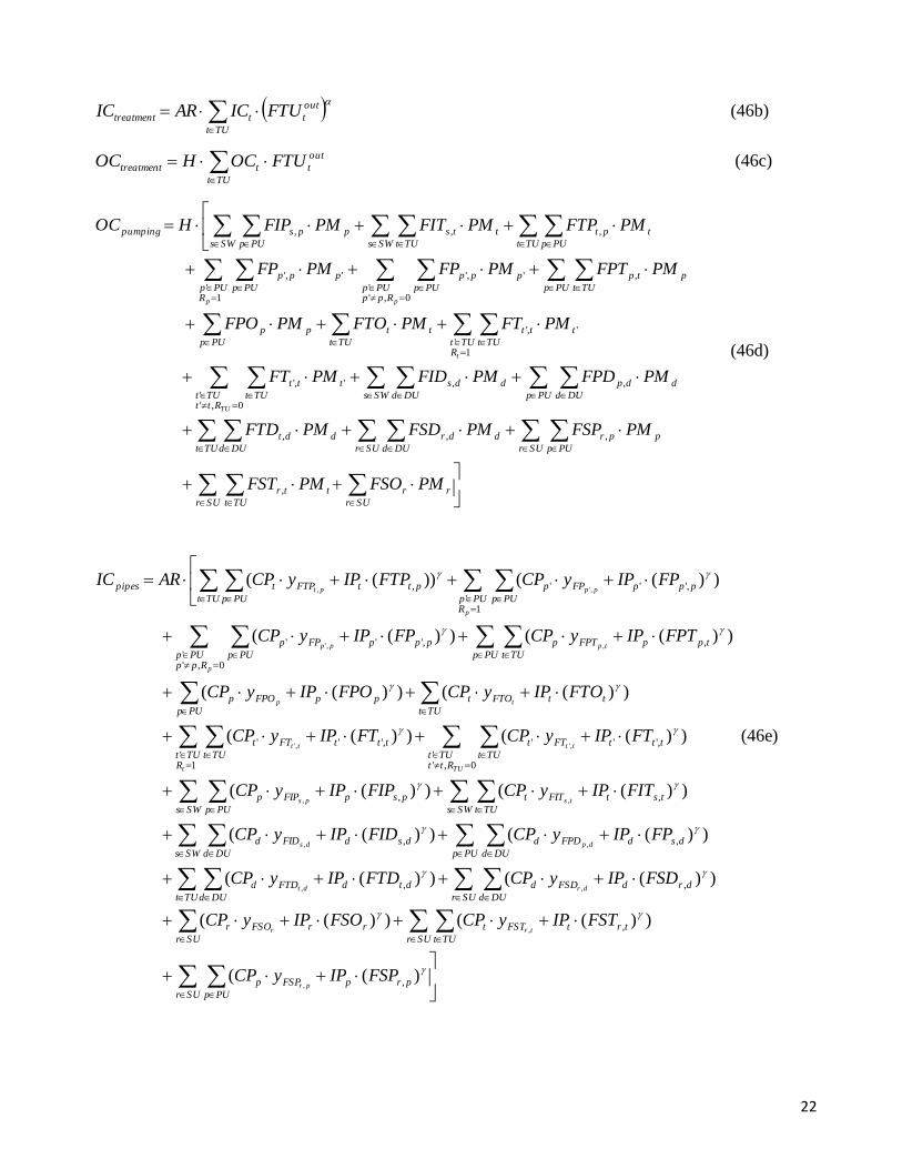
Table 2. Data of treatment units.

Unit % removal for

contaminant

IC (Investment

cost coefficient)

OC (Operating

cost coefficient)

A B

TU1 95 0 16800 1 0.7

TU2 0 95 12600 0.0067 0.7

Each treatment unit can remove only one contaminant. The environmental discharge limit for

contaminant A and contaminant B is 10 ppm. The freshwater cost is assumed to be $1/ton, the

annualized factor for investment on the treatment units is taken to be 0.1, and the total time for the

network plant operation in a year is assumed to be 8000 h. We formulated the problem as the

nonconvex Nonlinear Programming (NLP) where the objective function is to minimize the total

network cost given by equation (43). The global optimization results are given in Table 3.

Table 3. Optimization results for the NLP water network problem.

Without recycle With recycle

Freshwater cost $320,000 $320,000

Investment cost of treatment units $37,440 $33,585.3

Operating costs of treatment units $238,723.6 $230,431.6

Total cost $596,163.6 $584,016.9

With the local recycle around the process unit it is possible to meet both flowrate and contaminant

constraints at the process unit inlets and have lower total network cost ($584,016.9/year) compared to

the case without local recycle ($596,163.6/year).

In addition to this, we solved the same example for the case when the investment cost for piping

and the operating cost for pumping water inside pipes are included in the objective function (see

equation 46). In this example, the fixed cost pertaining to the pipes is assumed to be $6, the variable

cost for each individual pipe $100, and operating cost coefficient for pumping water through pipes

$0.006/ton (Karuppiah and Grossmann 2008). The global optimization results are given in Table 4.

27

Table 4. Optimization results for the MINLP water network problem.

Without recycle With recycle

Freshwater cost $320,000 $320,000

Investment cost on pipes $540.69 $546.3

Operating cost for pumping water $10,056.26 $9,427.84

Investment cost of treatment units $37,440.01 $33,585.32

Operating costs of treatment units $238,723.59 $230,431.64

Total cost $606,760.55 $593,991.1

It should be noted, that both the NLP and MINLP problem with or without local recycles have the

same optimal design of water network as shown in Figures 15 and 16.

Figure 15. Optimal solution for the NLP and MINLP problem without local recycle.

Figure 16. Optimal solution for the NLP and MINLP problem with local recycle.

As can be seen from Figures 15 and 16 the number of removable piping connections (streams

between all splitters and mixers in the network) for the NLP and MINLP problem without local

recycle is 8 and with local recycle it is 9. In addition, removable connections are shown in Figure 14

28

as dashed lines that can be actually deleted from the superstructure. According to this, it is useful for

the designer to have a tool which can be used to control network complexity. For the water networks

given in Figures 15 and 16, and the same data for the MINLP problem, the results of the optimization

by restricting the number of piping connections are shown in Table 5.

Table 5. Results of controlling the piping network complexity.

Solver

Total cost ($/year) Number of removable streams in the

network

Without local

recycle

With local

recycle

Without local

recycle

With local

recycle

BARON

- 593,991.11 - 9

606,760.55 596,012.94 8 8

620,857.57 613,610.77 7 7

695,456.90 691,610.36 6 6

The optimal network cost for the option without local recycle is $606,760.55/year, and with local

recycle $593,991.11/year. In the first case the number of removable connections is 8 and in the

second it is 9. In order to simplify the network we assigned to the design constraint Eq. (39) a new

number of removable streams as shown in Figure 13. Figure 17 shows the results of the water

network optimization for different number of removable streams.

Figure 17. Controlling the network complexity by restricting number of removable connections.

0.58

0.60

0.62

0.64

0.66

0.68

0.70

6 7 8 9

To

tal n

etw

ork

co

st (

10

6$/y

ear)

Number of removable piping connections in the network

wo/ Recycle w/ Recycle

29

For instance, we can greatly simplify the water network with 6 removable piping connections as

shown in Figures 18 and 19, while we still keep the freshwater consumption at 40 t/h.

Figure 18. Water network with 6 removable streams and without local recycle.

Figure 19. Water network with 6 removable streams and with local recycle.

As can be seen from Table 5 the total network cost for the option without local recycle is a little

higher compared to the case with local recycle. The main reason is the higher wastewater flowrate

(50 t/h) which must be treated in treatment unit TU2.

6.2. Example 2

The main goal of this example is to demonstrate the capability of the proposed model to solve

water network problems of different complexity to global optimality and to compare results with the

ones reported in the literature. Data for this example is taken from the literature (Example 1-4 given

by Karuppiah and Grossmann, 2006). The relative optimality tolerance in all examples was set to

0.01. Here we used the general purpose optimization software BARON (Sahinidis, 1996) to solve all

the problems. The optimization results reported in the paper given by Karuppiah and Grossmann

(2006) and the results obtained with the proposed model in this paper are shown in Table 6.

30

Table 6. Comparison of optimization results for NLP problems different complexity.

Problem

No units

(Karuppiah and Grossmann, 2006) Proposed NLP method

Global optimum Total time (s) Global optimum Total time (s)

1 2PU-2TU 117.05 t/h 37.72 101.57 0.36

2 3PU-3TU $381,751.35 13.21 $381,751.35 0.34

3 4PU-2TU $874,057.37 0.90 $874,057.37 0.11

4 5PU-3TU $1,033,810.95 231.37 $1,033,810.95 16.15

The first problem involves a water network with 2 process units (PU) and 2 treatment (TU) units.

The objective function was to minimize the total sum of the freshwater consumption and total

flowrate of wastewater treated inside of treatment units (Eq. 40). Karuppiah and Grossmann (2006)

reported the optimal solution 117.05 t/h. However, they did not consider local recycle around the

process unit which leads to a 13 % reduction in the objective function as seen in Table 6.

In addition, as can be also seen in Table 6, we solved water network problems with 3 process and 3

treatment units, 4 process and 2 treatment units, 5 process and 3 treatment units. For these examples

the values of the objective function (minimum total network cost) obtained by the proposed model in

this paper are the same as the ones reported by Karuppiah and Grossmann (2006), while the

computational time is smaller in all cases. The main reasons for improved performance are good

variable bounds for all flowrates and concentrations, incorporating the cut proposed by Karuppiah

and Grossmann (2006) and a faster computer.

6.3. Example 3

This example demonstrates the capability of the proposed model to solve water network problems

with both mass transfer and non mass transfer operations. The case study, a Specialty Chemical Plant,

is taken from Wang and Smith (1995). The process flowsheet is given in Figure 20, which has a

consumption of 165 t/h freshwater. It should be noted that the water entering the process is greater

than the wastewater flow in the exit since some water leaves the process with the product. Table 7

gives limiting process data for water-using operations in the process and its utility system.

31

Table 7. Limiting process data for Specialty Chemical Plant (Wang and Smith, 1995).

Operation Water in

(t/h)

Water out

(t/h)

cin

(ppm)

cout

(ppm)

Reactor 80 20 100 1,000

Cyclone 50 50 200 700

Filtration 10 40 0 100

Steam System 10 10 0 10

Cooling System 15 5 10 100

Water-using operations such as the reactor, filtration and cooling tower have different water

flowrates at their inlets and outlets. In the case of the reactor and the cooling tower there are losses of

water. However, in the case of filtration process there is gain of water. Water flowrates of these

operations can be divided in two parts. The first part is considered to be unchanged through the

process, while the second part involves loss or gain of water (Wang and Smith, 1995). According to

this, the modified process data for this example are given in Table 8.

32

Figure 20. Flowsheet for Specialty Chemical Plant with its utility systems.

33

Table 8. Modified limiting process data for Specialty Chemical Plant.

Operation Water in

(t/h)

Water out

(t/h)

cin

(ppm)

cout

(ppm)

Reactor I 20 20 100 1,000

Reactor II 60 0 100 -

Cyclone 50 50 200 700

Filtration I 10 10 0 100

Filtration II 0 30 - 100

Steam System 10 10 0 10

Cooling System I 5 5 10 100

Cooling System II 10 0 10 -

According to the flowsheet in Figure 20, the operations that can be considered as the water

sink/demand units are reactor and cooling tower. The water source unit is filtration. Representation of

these units and their flowrates is shown in Figures 21 and 22, respectively.

Figure 21. Representation of flowrates of the water demand unit.

34

Figure 22. Representation of flowrates of the water source unit.

The optimal solution of the water network with reuse for the data in Table 8 is given in Figure 23.

The optimization was performed with the global optimization BARON solver and the selected

optimality tolerance was zero. The objective function was to minimize the total consumption of

freshwater for network. The new water network design yields a reduction in freshwater consumption

of about 45% (from 165 t/h to 90.64 t/h) and wastewater generation of about 59% (from 125 t/h to

50.64 t/h) . It is worth to mention that the values of water consumption and wastewater generation are

the same as the ones reported by Wang and Smith (1995) and Bandyopadhyay, Ghanekar, and Pillai

(2006).

35

Figure 23. Optimal design of water network for Specialty Chemical Plant.

36

In addition to this, Bandyopadhyay, Ghanekar, and Pillai (2006) solved the same problem using

their proposed method for targeting minimum effluent treatment flowrate satisfying the minimum

freshwater requirement. In their paper the water allocation network incorporates two treatment units.

They assumed the % removal for each contaminant in treatment units to be 90, and maximum

allowable concentration of contaminants in the discharge effluent to the environment to be 50 ppm.

We solved the same problem by sequential optimization of water-using and water treatment units.

The objective function for optimization of water using operations is to minimize the sum of

freshwater consumption and the objective function for optimization of treatment operations is to

minimize the sum of water flowrates going to treatment units. The optimal network design is the

same as reported by Bandyopadhyay, Ghanekar, and Pillai (2006) (freshwater consumption of 90.64

t/h). However, we also optimized simultaneously the same problem as an integrated network with the

water-using operations and water treatment operations. We assumed to have two treatment units with

the same % removal for contaminant in the treatment units (90%). Also, we considered the options

with/without local recycle around process units. In both cases the new design yields a reduction in

freshwater consumption of about 73% (from 165 t/h to 45 t/h) and wastewater generation of about

96% (from 125 t/h to 5 t/h) compared to the base case. Moreover, we assumed to have two treatment

units for wastewater treatment, but only one is selected by the optimization. The optimal solution of

the water network design with recycle around process unit is given in Figure 24.

37

Figure 24. Optimal design of water network for Specialty Chemical Plant by simultaneous optimization with local recycle.

38

6.4. Example 4

In the process industry water-using operations can have different maximum allowed

concentrations at their inlets. Therefore, water sources of different quality can be used to satisfy

water-using concentration and flowrate demands. The higher quality water is more expensive

than the lower quality water. The objective of this example is to illustrate that the proposed

method can be applied to a complex industrial water network consisting of four sources of water,

six water-using operations, three water treatment operations and three contaminants. Data for

water sources, water-using operations, and treatment units are given in Tables 9, 10 and 11.

Table 9. Data for water sources for Example 4.

Water

source

Cost of water

source ($/t)

Concentration of

contaminants (ppm)

A B C

SW1 1.00 0 0 0

SW2 0.50 25 35 35

SW3 0.20 45 40 40

SW4 0.15 50 50 50

Table 10. Data for process units for Example 4.

Process

unit

Flowrate

(t/h)

Discharge load

(kg/h)

Maximum inlet concentration

(ppm)

A B C A B C

PU1 40 1 1.5 1 25 25 25

PU2 50 1 1 1 50 50 50

PU3 60 1 1 1 50 50 50

PU4 70 2 2 2 50 50 50

PU5 80 1 1 0 25 25 25

PU6 90 1 1 0 10 10 10

39

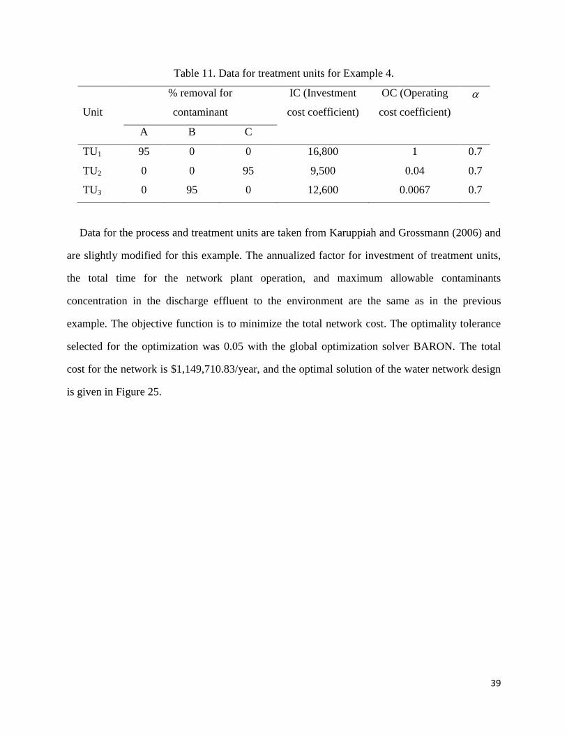
Table 11. Data for treatment units for Example 4.

Unit

% removal for

contaminant

IC (Investment

cost coefficient)

OC (Operating

cost coefficient)

A B C

TU1 95 0 0 16,800 1 0.7

TU2 0 0 95 9,500 0.04 0.7

TU3 0 95 0 12,600 0.0067 0.7

Data for the process and treatment units are taken from Karuppiah and Grossmann (2006) and

are slightly modified for this example. The annualized factor for investment of treatment units,

the total time for the network plant operation, and maximum allowable contaminants

concentration in the discharge effluent to the environment are the same as in the previous

example. The objective function is to minimize the total network cost. The optimality tolerance

selected for the optimization was 0.05 with the global optimization solver BARON. The total

cost for the network is $1,149,710.83/year, and the optimal solution of the water network design

is given in Figure 25.

40

Figure 25. Optimal design of the integrated process network for Example 4.

It should be noticed that the freshwater source 4 is not selected. In addition, pure water from

source 1, which has the highest cost, is minimized at the expense of using more of the lower

quality water.

6.5. Example 5

The objective of this example is to illustrate the application of the proposed MINLP solution

method on a large-scale industrial network consisting of five water-using units, three wastewater

treatment units and three contaminants (A, B, C). Data for this example are given in Tables 12

and 13 (Karuppiah and Grossmann 2006). The water network superstructure is given in Figure

26. It includes all feasible connections between units in the network.

41

Table 12. Data for s for Example 5.

Process

unit

Flowrate

(t/h)

Discharge load

(kg/h)

Maximum inlet

concentration (ppm)

A B C A B C

PU1 40 1 1.5 1 0 0 0

PU2 50 1 1 1 50 50 50

PU3 60 1 1 1 50 50 50

PU4 70 2 2 2 50 50 50

PU5 80 1 1 0 25 25 25

Table 13. Data for treatment units for Example 6.

Uni

t

% removal for

contaminant

IC (Investment

cost coefficient)

OC (Operating

cost coefficient)

A B C

TU1 95 0 0 16,800 1 0.7

TU2 0 0 95 9,500 0.04 0.7

TU3 0 95 0 12,600 0.0067 0.7

The annualized factor for investment of the treatment units, the total time for the network

plant operation, and maximum allowable contaminants concentration in the discharge effluent to

the environment are the same as in the previous example. The objective function is to minimize

the total network cost. We used the BARON and LINDOGlobal solvers in this example.

42

Figure 26. Water network superstructure for Example 5.

The MINLP model for this example is solved using the proposed solution approach. In the

first step, we solved the NLP model of the network shown in Figure 26 and obtained the global

solution. Then, we fixed all zero flowrates, and update bounds before solution of reduced the

MINLP. The total network cost of the MINLP model was $1,062,700.53/year and the number of

removable piping connections in the network was 22. In order to control the piping complexity

we restricted the number of connections in the network and solved the corresponding MINLP

problems. Results of the optimization are given in Figure 27, which shows the costs of the water

networks for different number of removable connections. It is interesting to note that the

freshwater consumption in all cases was the same (40 t/h). In addition, it should be mentioned

that the greatly simplified water network shown in Figure 28 has 13 removable connections, and

the total network cost $1,223,698.7/year which is about 15% increase in the value of objective

function compared to the optimal base case ($1,062,700.5/year) with 22 removable connections.

43

Figure 27. The costs of the water networks for different number of removable connections.

Figure 28. Optimal design of the simplified water network with 13 removable connections.

1.04

1.06

1.08

1.10

1.12

1.14

1.16

1.18

1.20

1.22

1.24

12 13 14 15 16 17 18 19 20 21 22 23

Tota

l net

work

cost

(10

6 $

/yea

r)

Number of removable piping connections in the network

44

6.6. Example 6

This example illustrates the different possibilities for reducing of the water consumption and

the total costs for the network consists of the water pre-treatment subsystem, the water-using

subsystem, and the wastewater treatment subsystem. Moreover, we present results of the

complete water integration, and zero liquid discharge cycles when all feasible interconnections

between previously mentioned subsystems are allowed in the network.

Table 14 shows the data for this example that involves two process units (PU1, PU2), two

water pre-treatment units (TU1, TU2), one wastewater treatment unit (TU3), and four

contaminants.

Table 14. Data of process units.

Unit Flowrate

(t/h)

Discharge load

(kg/h)

Maximum inlet

concentration (ppm)

A B C D A B C D

PU1 40 1 1.5 1 1 0 0 0 0

PU2 50 1 1 1 1 50 50 50 50

Data for the operating cost and the investment cost of the water pre-treatment (TU1 and TU2)

and the wastewater treatment (TU3) units are given in Table 15 and they are taken from Faria and

Bagajewicz (2009).

Table 15. Data of pre-treatment and treatment units.

Unit IC (Investment

cost coefficient)

OC (Operating

cost coefficient)

TU1 (Pre-treatment 1) 10,000 0.10 0.7

TU2 (Pre-treatment 2) 25,000 1.15 0.7

TU3 (Wastewater treatment) 30,000 1.80 0.7

There is one freshwater source with four contaminants (100 ppm A, 100 ppm B, 100 ppm C,

and 100 ppm D). The freshwater cost is assumed to be $0.1/ton. The annualized factor for

investment of the treatment units is assumed to be 0.1, and the total time for the network

operation in a year 8600 h. The environmental discharge limit for all contaminants (A, B, C, and

45

D) concentration is 10 ppm. In addition, the maximum inlet contaminants concentration of the

water pre-treatment unit TU1 is 100 ppm and TU2 10 ppm. We assume that the water pre-

treatment units can purify the freshwater to the water quality down to 10 ppm for each

contaminant (TU1) and down to 0 ppm (TU2). The percent removal for contaminants in the

wastewater treatment unit (TU3) was 95%. We used the BARON to solve the MINLP in this

example.

Figure 29 shows the optimal design of water network when the recycling water from the

water-using subsystem and the wastewater treatment subsystem to the water pre-treatment

subsystem is not allowed. The freshwater consumption is 50 t/h and the total network cost

$1,244,299.7 /year.

Figure 29. Recycling water from the water-using /wastewater treatment subsystem to the water

pre-treatment subsystem is not allowed

In the next case shown in Figure 30, we assume that recycling water from the water-using and

the wastewater treatment subsystem to the water pre-treatment subsystem is allowed. Note that

the freshwater consumption is reduced to 40 t/h compared to the previous case. In addition, the

total network cost is lower, $1,223,838.0/year.

Figure 30. Recycling water from the water-using /wastewater treatment subsystem to the water

pre-treatment subsystem is allowed

As can be seen from Figure 30, the network has the recycles from the water-using unit 2 (1.5

t/h) and from the wastewater treatment unit 3 (8.5 t/h) to the water pre-treatment unit 2. In

addition, both types of freshwater (10 ppm and 0 ppm) are used in the network.

46

The optimal design of water network with local recycle is shown in Figure 31. The total

network cost is $1,057,659.3/year and the freshwater consumption is the same (40 t/h) as in

Figure 30, while the wastewater flowrate of treatment unit 3 is reduced from 42.5 t/h to 32.28 t/h.

Figure 31. Optimal design of water network with local recycle.

It is worth pointing out that water networks can have zero liquid discharge cycles when all

connections between the subsystems in the network are allowed (the complete water integration).

In Figure 32, we present the optimal network designs with zero liquid discharge cycles for this

example. The total network cost for option without local recycle is $1,157,863.5/year and for

option with local recycle $971,320.7/year. Note that we assumed to have two pre-treatment units,

but just one (TU2) is selected by the optimization. Note also that although the use of freshwater

has been eliminated the cost of treatment in Figure 32a is higher due to its higher flowrate

(43.77t/h vs 32.28t/h).

a) without local recycle

b) with local recycle

Figure 32. Optimal design of water network with zero liquid discharge cycles.

47

7. Model sizes and computational times for Examples 1-6

Table 16 shows the sizes and computational times for the examples presented in the previous

section. As can be seen from this table we solved NLP and MINLP problems of different sizes

and complexity. The optimality tolerance selected for optimization in the first, third, fifth, and

sixth example was 0.0 and in the second and fourth 0.01 and 0.05. All MINLP examples shown

in Table 16 are solved with the proposed two-stage solution. To solve the water network

examples to global optimality we used the BARON and LINDOGlobal solvers. The

computational times, for problems with no constraints on the removable streams were reasonable

in all cases (see Table 16), although, it should be mentioned that by increasing size of the

MINLP problems computational time increases and in these cases available optimization solvers

cannot find an optimal solution in several hours. However, by applying the two-stage strategy as

shown in Figure 13 it was possible to solve the corresponding problems in much less time.

Table 16. Model statistics and computational results for Examples 1-6.

*Option with local recycles

It should be mentioned that the computational time for Example 5 with no constraints on

removable streams (i.e. 22 removable connections) was 10.3 CPUs (BARON) and 56.3 CPUs

(LINDOGlobal). We greatly simplified the water network when no more than 13 removable

Example Number of units Continuous

variables

Discrete

variables

Constraints CPU time

(s)

1 2PU-2TU 55 - 44 < 0.5

57* - 44 < 1.0

75 20 85 < 0.5

79* 22 89 < 0.5

2 2PU-2TU 57* - 44 < 0.5

3PU-3TU 92 - 62 < 0.5

4PU-2PU 91 - 62 < 0.5

5PU-3TU 161 - 106 16.2

3 5PU 82 - 41 < 0.5

5PU-2TU 119 - 53 2.9

126* - 53 < 0.5

4 6PU-3TU 223 - 121 2.0

232*

- 121 1.4

5 5PU-3TU 233 72 251 10.3

6 2PU-3TU 135

145*

30

35

148

158

< 1.0

< 1.0

48

connections are used as shown in Figure 28. The computational time for this problem was 153.3

CPUs (BARON) and 159 CPUs (LINDOGlobal). For other limits on the number of removable

connections the (20, 18, 16, 15, 14) the computational times were significantly higher (up to 600

CPUs (LINDOGlobal)). In addition, the LINDOGlobal solver could not find any solution for 14

removable connections. Finally, it is worth to point that in all other cases of removable

connections the optimal solution was the same for both solvers.

8. Conclusions

In this paper, we have presented a general superstructure and a global optimization strategy

for the design of integrated process water network as well as its separate subsystems. The

superstructure includes all feasible interconnections in the network, mass transfer and non-mass

transfer water-using processes, wastewater treatment operations, single and multiple sources of

water with/without contaminants, and their possible pre-treatment. On the basis of this

superstructure, we have formulated nonconvex NLP and MINLP models. The cost of piping and

the cost of pumping water are included in the MINLP model. To expedite the global optimization

search we have represented the bounds on the variables as general equations obtained by

physical inspection of the superstructure. Furthermore, we proposed a two-stage procedure for

solving large-scale models.

From the examples it is clear that the proposed approach can be successfully used for solving

industrial water network problems as well as for controlling the complexity of water networks.

The capabilities of the proposed method were illustrated on several examples, including large-

scale water network problems. All the examples were solved to global optimality with reasonable

computational time using BARON and LINDOGlobal.

Acknowledgments

The authors would like to express their gratitude to the Fulbright Visiting Scholar Program

and the Center for Advanced Process Decision-making, Department of Chemical Engineering at

Carnegie Mellon University for support throughout this work.

49

Appendix

Variable bounds for the proposed model

In the proposed NLP/MINLP optimization model the bounds on the variables are represented

as general equations in this appendix.

Initial Splitter

The upper bound of water flowrate at the initial splitter can be determined on the basis of

fixed flowrates for all process and demand units.

0,

pSWsFDUFPUFWDUd

in

d

PUp

in

p

U

s (A1)

The lower bound of the water flowrate at the initial splitter has a minimum fixed flowrate for

a process unit if one external source of water exists in the network. If there are more sources of

water in the network, the lower bound is set to be zero because it is possible that some sources of

water will not be selected by the optimization model.

1,0,)(min spSWsFPUFW in

pp

L

s (A2)

The upper bound for flowrates going from the initial splitter to the mixer treatment units can

be determined on the basis of fix flowrates for all process units.

0,,,

pTUtSWsFPUFITPUp

in

p

U

ts (A3)

In the case that water network consists only of treatment units (number of process units is set

to be zero), then wastewater feed flowrates are fixed and the upper bounds of flowrates from the

initial splitter to the mixer treatment units and the final mixer are given as follows.

0, pSWsFWWFW in

s

FX

s (A4)

0,,, pTUtSWsFWWFIT in

s

U

ts (A5)

0, pSWsFWWFIF in

s

U

s (A6)

The upper bound of water flowrate going from the initial splitter to the process units depends

of the fixed flowrate in particular process units.

PUpSWsFPUFIP in

p

U

ps ,, (A7)

50

Process Units

The process units can be considered as part of the integrated water network, as well as a

separate water-using subsystem. The inlet and outlet flowrates of the process unit are the same.

The outlet flowrate of the process unit has fixed value and depends of the inlet flowrate.

PUpFPUFPU in

p

FXout

p (A8)

The upper and lower bounds for contaminants concentration at the process unit inlets and

outlets are given as follows.

jPUpxPUxPU in

jp

Uin

jp ,max,

., (A9)

jPUpFPULPUxPU in

pjp

Lin

jp ,/10 ,

3

, (A10)

jPUpFPULPUFPUxPUxPU in

pjp

in

p

in

jp

Uout

jp ,/)10( ,

3max,

,, (A11)

Splitter Process Units

The splitter process units streams can be directed to any mixer process units so the upper

bounds of these flowrates depend of the fixed flowrates in a particular process unit. Notice that

the outlet contaminants concentration of the process unit and the splitter process unit are the

same.

PUpPUpFPUFPUifFPUFP in

p

in

p

in

p

U

pp ,'',' (A12)

PUpPUpFPUFPUifFPUFP in

p

in

p

in

p

U

pp ,'',' (A13)

jPUpxPUxSPU out

jp

Uout

jp ,,, (A14)

The upper bounds for flowrates going from the splitter process units to the mixer treatment

units and the final mixer depend of the fixed flowrates of process units.

TUtPUpFPUFPT in

p

U

tp ,, (A15)

PUpFPUFPO in

p

U

p (A16)

51

Treatment Units

The treatment units can be considered as part of the integrated water network, as well as a

separate wastewater subsystem. According to this, the upper bounds for flowrates and

contaminants concentration of the treatment units are given as follows.

0,

pTUtFPUFTUPUp

in

p

Uin

t (A17)

0,

pTUtFWWFTUSWs

in

s

Uin

t (A18)

0,

pTUtFPUFTUPUp

in

p

Uout

t (A19)

0,

pTUtFWWFTUSWs

in

s

Uout

t (A20)

0,,/)10(max ,

3max,

,,

pjTUtFPULPUFPUxPUxTU in

pjp

in

p

in

jpPUp

Uin

jt (A21)

0,,)(max ,,

pjTUtxWxTU in

jsSWs

Uin

jt (A22)

jTUtxTURRxTUUin

jtjt

Uout

jt ,)100/1( ,,, (A23)

Splitter Treatment Units

The streams from splitter process units can be directed to any mixer in the network. The upper

bounds of these streams are given as follows.

0,,','

pTUtTUtFPUFTPUp

in

p

U

tt (A24)

0,,','

pTUtTUtFWWFTSWs

in

s

U

tt (A25)

PUpTUtFPUFTP in

p

U

pt ,, (A26)

0,

pTUtFPUFTOPUp

in

p

U

t (A27)

0,

pTUtFWWFTOSWs

in

s

U

t (A28)

jTUtxTUxSTUUout

jt

Uout

jt ,,, (A29)

52

Source and Demand Units

It should be noted that inlet and outlet flowrates of water-using operations can have different

values. In that case, they can be divided in two parts. The first part can be considered unchanged

through process, and the second part can account for the loss of water or the gain of water.

According to this, the upper bounds of flowrates and contaminants concentrations are given as

follows.

DUdSWsFDUFID in

d

U

ds ,, (A30)

jDUdxDUxDU in

jd

in

jd

U

,max,

,, (A31)

DUdPUpFDUFPD in

d

U

dp ,, (A32)

DUdTUtFDUFTD in

d

U

dt ,, (A33)

TUtSUrFPUFSTPUp

in

p

U

tr

,, (A34)

SUrFSUFSO out

r

U

r (A35)

DUdSUrFDUFSD in

d

U

dr ,, (A36)

jSUrxSUxSU in

jr

in

jr

U

,max,

,, (A37)

Final Mixer

The lower bound of the discharge flowrate to the environment has a minimum value of the

fixed flowrates in the process units. However, if the network consists only of treatment units then

it has a minimum value of wastewater streams of the initial splitters.

0)(min

pFPUF in

pPUp

Lout (A38)

0)(min

pFWWF in

sSWs

Lout (A39)

The upper bounds of the discharge flowrate and contaminants concentration are given as follows.

0

pFPUFPUp

in

p

Uout (A40)

53

0

pFWWFSWs

in

s

Uout (A41)

jxx out

j

Uout

j max, (A42)

0,/)10(max ,

3max,

,

tjFPULPUFPUxPUx in

pjp

in

p

in

jpPUp

Uout

j (A43)

References

Alva-Argaez, A., Kokossis, A. C. & Smith, R. (2007). The design of water-using systems in

petroleum refining using a water-pinch decomposition. Chemical Engineering Journal,

128(1), 33-46.

Alva-Argáez, A., Kokossis, A. C. & Smith, R. (1998). Wastewater minimisation of industrial

systems using an integrated approach. Computers & Chemical Engineering, 22(Supplement

1), S741-S744.

Bagajewicz, M. (2000). A review of recent design procedures for water networks in refineries

and process plants. Computers & Chemical Engineering, 24(9-10), 2093-2113.

Bagajewicz, J. & Faria D. C. (2009). On the appropriate architecture of the water/wastewater

allocation problem in process plants. In J. Ježovski & J. Thullie (Editors), 19th

European

Symposium on Computer Aided Process Engineering – ESCAPE19. Elsevier.

Bandyopadhyay, S., Ghanekar, M. D. & Pillai, H. K. (2006). Process water management.

Industrial & Engineering Chemistry Research, 45(15), 5287-5297.

Biegler, L. T., Grossmann, I. E. & Westerberg, A. W. (1997). Systematic methods of chemical

process design. New Jersey, USA: Prentice-Hall.

Brooke, A., Kendrick, D., Meeraus, A. & Raman, R. (1988). GAMS: A user’s guide, release

2.50. GAMS Development Corporation.

Castro, P., Matos, H., Fernandes, M. C. & Nunes, C. P. (1999). Improvements for mass-

exchange networks design. Chemical Engineering Science, 54(11), 1649-1665.

Castro, P., Teles, J. P. & Novais, A. (2009). Linear program-based algorithm for the optimal

design of wastewater treatment systems. Clean Technologies and Environmental Policy,

11(1), 83-93.

Dhole, V. R., Ramchandani, N., Tainsh, R. A. & Wasilewski, M. (1996). Make Your Process

Water Pay for Itself. Chemical Engineering, 103, 100.

54

Doyle, S. J. & Smith, R. (1997). Targeting water reuse with multiple contaminants. Process

Safety and Environmental Protection, 75(3), 181-189.

El-Halwagi, M. M. (1997). Pollution prevention through process integration. Systematic design

tools. San Diego, USA: Academic Press.

El-Halwagi, M. M. & Manousiouthakis, V. (1989). Synthesis of mass exchange networks.

AIChE Journal, 35(8), 1233-1244.

El-Halwagi, M. M. & Manousiouthakis, V. (1990). Automatic synthesis of mass-exchange

networks with single-component targets. Chemical Engineering Science, 45(9), 2813-2831.

Faria D. C. & Bagajewicz, J. (2009). On the appropriate modeling of process plant water

systems. (http://www.ou.edu/class/che-design/).

Feng, X. & Seider, W. D. (2001). New structure anddesign methodology for water networks.

Industrial & Engineering Chemistry Research, 40(26), 6140-6146.

Foo, D. C. Y., Kazantzi, V., El-Halwagi, M. M. & Abdul Manan, Z. (2006). Surplus diagram and

cascade analysis technique for targeting property-based material reuse network. Chemical

Engineering Science, 61(8), 2626-2642.

Foo, D. C. Y. (2009). State-of-the-Art Review of Pinch Analysis Techniques for Water Network

Synthesis. Industrial & Engineering Chemistry Research, 489(11), 5125-5159.

Galan, B. & Grossmann, I. E. (1998). Optimal design of distributed wastewater treatment

networks. Industrial & Engineering Chemistry Research, 37(10), 4036-4048.

Gunaratnam, M., Alva-Argaez, A., Kokossis, A., Kim, J.-K. & Smith, R. (2005). Automated

Design of Total Water Systems. Industrial & Engineering Chemistry Research, 44(3), 588-

599.

Hallale, N. (2002). A new graphical targeting method for water minimisation. Advances in

Environmental Research, 6(3), 377-390.

Huang, C.-H., Chang, C.-T. Ling, H.-C. & Chang, C.-C. (1999). A Mathematical Programming

Model for Water Usage and Treatment Network Design. Industrial & Engineering Chemistry

Research, 38(8), 3190-3190.

Ježowski, J. (2008). Review and analysis of approaches for designing optimum industrial water

networks. Chemical and Process Engineering, 29, 663-681.

Karuppiah, R. & Grossmann, I. E. (2006). Global optimization for the synthesis of integrated

water systems in chemical processes. Computers & Chemical Engineering, 30(4), 650-673.

55

Karuppiah, R. & Grossmann, I. E. (2008). Global optimization of multiscenario mixed integer

nonlinear programming models arising in the synthesis of integrated water networks under

uncertainty. Computers & Chemical Engineering, 32(1-2), 145-160.

Kuo, W.C. J. & Smith, R. (1997). Effluent treatment system design. Chemical Engineering

Science, 52(23), 4273-4290.

Li, B.-H. & Chang, C.-T. (2007). A Simple and Efficient Initialization Strategy for Optimizing

Water-Using Network Designs. Industrial & Engineering Chemistry Research, 46(25), 8781-

8786.

Linnhoff, B. & Hindmarsh, E (1983). The pinch design method for heat exchanger networks.

Chemical Engineering Science, 38(5), 745-763.

LINDOGlobal: A Global Optimization Solver from Lindo Systems, Inc.

Luo, Y. & Uan, X (2008). Global Optimization for the Synthesis of Integrated Water Systems

with Particle Swarm Optimization Algorithm. Chinese Journal of Chemical Engineering,

16(1),11-15.

Mann, J. G. & Liu, Y. A. (1999). Industrial water reuse and wastewater minimization. New

York, USA: McGraw-Hill.

Polley, G. T. & Polley, H. L. (2000). Design Better Water Networks. Chem. Eng. Progress, 96,

47.

Putra, Z. A. & Amminudin, K. A. (2008). Two-Step Optimization Approach for Design of A

Total Water System. Industrial & Engineering Chemistry Research, 47(16), 6045-6057.

Quesada, I. & Grossmann, I. E. (1995). Global optimization of bilinear process networks with

multicomponent flows. Computers & Chemical Engineering, 19(12), 1219-1242.

Rossiter, A. P. (1995). Waste minimization through process design. New York, USA: McGraw-

Hill.

Sahinidis, N. V. (1996). BARON: A general purpose global optimization software package.

Journal of Global Optimization 8(2): 201-205.

Savelski, M. & Bagajewicz, M. (2003). On the necessary conditions of optimality of water

utilization systems in process plants with multiple contaminants. Chemical Engineering

Science, 58(23-24), 5349-5362.

56

Savelski, M. J. & Bagajewicz, M. J. (2000). On the optimality conditions of water utilization

systems in process plants with single contaminants. Chemical Engineering Science, 55(21),

5035-5048.

Sorin, M. & Bedard, S. (1999). The global pinch point in water reuse networks. Process Safety

and Environmental Protection, 77(B5), 305-308.

Takama, N., Kuriyama, T., Shiroko, K. & Umeda, T. (1980). Optimal water allocation in a

petroleum refinery. Computers & Chemical Engineering, 4(4), 251-258.

Wang, Y. P. & Smith, R. (1994a). Wastewater minimisation. Chemical Engineering Science,

49(7), 981-1006.

Wang, Y.P. & Smith, R. (1994b). Design of distributed effluent treatment systems. Chemical

Engineering Science, 49(18), 3127-3145.

Wang, Y. P. & Smith, R. (1995). Wastewater Minimization with Flowrate Constraints. Chem.

Eng. Res. Des., 73, 889.