2021-08 STRUCTURAL OPTIMIZATION OF SUPERSTRUCTURE ...

DSpace Institution

DSpace Repository http://dspace.org

Geotechnical Engineering Thesis

2021-08

STRUCTURAL OPTIMIZATION OF

SUPERSTRUCTURE PARAMETER OF

EXTRADOSED CABLE STAYED

BRIDGE USING GENETIC

ALGORITHM, As A CASE STUDY ON

ABAY RIVER BRIDGE

ABEBA, LAMESGIN SIMEGN

http://ir.bdu.edu.et/handle/123456789/12573

Downloaded from DSpace Repository, DSpace Institution's institutional repository

BAHIR DAR UNIVERSITY

BAHIR DAR INSTITUTE OF TECHNOLOGY

SCHOOL OF RESEARCH AND POSTGRADUATE STUDIES

FACULTY OF CIVIL AND WATER RESOURCE ENGINEERING

STRUCTURAL ENGINEERING

MSc. Thesis

On

STRUCTURAL OPTIMIZATION OF SUPERSTRUCTURE

PARAMETER OF EXTRADOSED CABLE STAYED BRIDGE

USING GENETIC ALGORITHM, As A CASE STUDY ON ABAY

RIVER BRIDGE

By

ABEBA LAMESGIN SIMEGN

Aug. 2021

Bahir Dar, Ethiopia

i


BAHIR DAR INSTITUTE OF TECHNOLOGY

FACULTY OF CIVIL AND WATER RESOURCES ENGINEERING

Structural Optimization of Superstructure Parameter of Extradosed

Cable- Stayed Bridge Using Genetic Algorithm, As A Case Study On

Abay River Bridge

By

Abeba Lamesgin Simegn

A thesis submitted

in Partial Fulfillment of the Requirements for the Degree of

Master of Science in Structural Engineering

Advisor: Eng. Ghulam Rasool

Co-Advisor: Eng. Wubishet Jemanenh

Aug. 2021

Bahir Dar, Ethiopia

©2021 Abeba Lamesgin Simegn

ii

© Copyright by Abeba Lamesgin Simegn

Aug. 04, 2021. All Rights Reserve

iii

DECLARATION

This is to certify that the thesis entitled ―Structural Optimization of Superstructure

Parameter of Extradosed Cable-Stayed Bridge using Genetic Algorithm, as a Case

study on Abay River Bridge” submitted in partial fulfillment of the requirements for

the degree of Master of Science in Structural Engineering under Faculty of Civil and

Water Resources Engineering, Bahir Dar Institute of Technology , is a record of

original work carried out by me and has never been submitted to this or any other

institution to get any other degree or certificates. The assistance and help I received

during the course of this investigation have been duly acknowledged.

Abeba Lamesgin Simegn ______ 03/08/2021

Name of the Candidate Signature Date

iv


BAHIR DAR INSTITUTE OF TECHNOLOGY-

SCHOOL OF RESEARCH AND GRADUATE STUDIES

FACULTY OF CIVIL AND WATER RESOURCE ENGINEERING

APPROVAL OF THESIS FOR DEFENSE

I hereby certify that I have supervised, read, and evaluated this thesis titled ―Structural

Optimization of Superstructure Parameter of Extradosed Cable-Stayed Bridge

using Genetic Algorithm, as a Case study on Abay River Bridge prepared by Abeba

Lamesgin under my guidance. I recommend the submission of the thesis for oral

defense.

Ghulam Rasool (Eng) 22/06/2021

Advisor’s name Signature Date

vi

DEDICATION

To my family and my uncle

vii

ACKNOWLEDGEMENTS

First of all, I would like to thank ―The Almighty‖ for giving me the time, courage,

patience, initiation, and determination of doing the research.

I would like to express my thankfulness to structural engineering department head Mr.

Alemayehu Golla for his commitment, valuable guidance, and willingness to share his

knowledge from beginning of research up to end of the research work.

I would like to express my gratitude to my thesis supervisors Eng. Ghulam Rasool, Eng

Fkre silassie worku and Eng. Wubeshet Jemaneh for their proper guidance, invaluable

advice and support throughout this research period.

I would also like to express my appreciation to Botek Head of Structural Department of

Amir Reza Poorbakhshaie, and all structural department members for their willingness

to answer questions for any aspect of conventional design work of Abay bridge.

I would also like to express my thanks to Dr. Hanibal Lemma and Dr. Abrham Gebre

who have helped me through my thesis work.

Also, I would like to express my appreciation to ―China Communication Construction

Company‖ for their willingness to giving any aspect of conventional design output Abay

bridge.

A special thanks to my family, outstandingly to my uncle, my mother, and my father, for

all their unconditional support.

viii

ABSTRACT

Weight of post-tensioning prestressing extradosed cable-stay bridge superstructure part

formed from concrete, non-prestressing reinforcement, and prestressing reinforcement

and stay cable tendon weight. Main load-carrying members, which are, girder, stayed-

cable, and pylon are considered to apply structural optimization techniques in the

superstructure component of the extradosed cable-stayed bridge. This research paper

evaluated the optimum depth of the girder with pylon height, angle of stay cable, and

effect of concrete grade in the three main parameters of an extradosed cable-stay bridge.

Then identification of significant and insignificant design variables using sensitivity

analysis by considering cable stiffness, girder weight, and stay cable tension. Structural

optimization was carried out by taking the minimization of the total material weight of

girders, pylon, and angle of stayed-cable as an objective function and all requirements of

strength, stability, serviceability, and fatigue as constraint functions. As a case study

Abay‘s extradosed cable-stayed bridge first design by China Communication

Construction Company. It has two twin box girders with 24.7m width and a length of

380m. The width of the top of the box girder is 24.7m, and the width of the bottom plate

gradually changes from 9m to the end fulcrum. The main tower adopts a double-column

tower, the tower beam is consolidated. The tower root size is 4m x2m (lateral), and the

tower top dimension is 3mx2m as respectively. The bridge is subject to five main load

cases, dead, live, wind, settlement, and temperature loads. This paper gives an optimum

cross-section of the superstructure main component of the Abay bridge by using the

fixed load parameter that has already been defined by the designer company. Effects of

girder depth, angle of cable-stayed, and pylon height with the effect of concrete grade on

the optimum weight were investigated. The results of structural optimization indicate

that optimum girder depth is 5.129m at pier level and 2.62m at span. The optimum pylon

height was found to be 24.827m. And optimum stay cable length was reduced from

conventional design output length by 10% from total values. Optimum design of pylon

height reduced weight of conventional design by 20.03% and optimum design of box

girder reduced girder weight by 19.47%. Paper gives the more reduced weight of bridge

by 49.47% from conventional design output by using same material grade.

Keywords: Box girder depth, Height of Pylon, Stay cable angle, and Concrete

grade, Sensitivity analysis

ix

ABBREVIATIONS

AASHTO America Association of State Highway and Transportation Officials

ASTM American Society for Testing and Materials,

ERA Ethiopia Road Authority

FEM Finite Element Method

GA Genetic Algorithm

SLS Serviceability limit state

ULS Ultimate limit state

CCCC China Communication Construction Company

AWS American Welding Society,

IM Dynamic load allowance or impact factor

M Multiple presence factors

LRFD load resistance factor design

x

NOTATIONS

cp- Tensile strain in the concrete at the level of the tendon at decompression stage.

o -Compressive strain at the extreme top fiber at service load stage

oc- Compressive strain in the concrete at the level of the tendon

s - Tensile strain in the reinforcing steel at working loads

A - Cross-sectional area of concrete (mm2 )

a - Depth of equivalent rectangular stress block (mm)

a‘- Distance from the left support to the point of truckload for which deflection is to be

computed.

Ac - Area of concrete cross-section (mm2 )

Act - Area of the cracked transformed section under service limit state (mm2

)

At - Effective tension area of concrete surrounding one bar (mm2)

Ap- Area of prestressing steel (mm2 )

As- Area of non-prestressed steel tension reinforcement (mm2 )

As‘- Area of non-prestressed steel compression zone reinforcement (mm2 )

Av- Cross-sectional area of shear reinforcement within a distance S (mm2)

be -Width of compression face of the section of exterior girder (mm)

bi -Width of compression face of the section of interior girder (mm)

bw -Web width of the cross-section (mm)

C -Resultant compressive force in the compression zone of concrete (N)

c - Depth of the neutral axis (mm)

Cn - Compressive force in the compression zone of concrete used to reduce the resultant

Compressive force C when NA depth exceeds flange thickness (N)

Wp - Weight of prestressing Reinforcement steel (Kg/m3)

Ws - Weight of non-prestressing Reinforcement steel (Kg/m3)

d- Distance from extreme compression fiber to centroid of non-prestressed tension

xi

reinforcement (mm)

dc -Thickness of concrete cover measured from extreme tension fiber to centroid of the

closest bar (mm)

de - Depth from extreme compression fiber to centroid of tensile force (mm)

dp - Depth from extreme compression fiber to centroid of prestressing steel (mm)

ds‘- Distance from extreme compression fiber to centroid of non-prestressed compression

zone reinforcement (mm)

dv - Effective depth of shearing force (N)

dz-Depth from extreme compression fiber to centroid of resultant compression

force(mm)

dzn -Depth from extreme compression fiber to centroid of compression force Cn (mm)

e - Eccentricity of prestressing force from the centroid of the section (mm)

Ec- Modulus of elastic of concrete (N/mm2 )

Ep- Modulus of elastic of prestressing steel (N/mm2 )

Es Modulus of elastic of reinforcing steel (N/mm2 )

fbr Stress range at the extreme bottom fiber(N/mm2 )

fc‘ Specified cylindrical compressive strength of concrete (N/mm2 )

fcpe -Compressive stress in concrete due to effective pre-stress forces only (N/mm2 )

fct - Maximum allowable compressive stress in concrete at initial pre-stress (N/mm2 )

fcw -Maximum allowable compressive stress in concrete at service load (N/mm2 )

ffp - Stress range in prestressing steel due to fatigue load (N/mm2 )

ffs - Stress range in reinforcing steel due to fatigue load (N/mm2 )

finf - Stress at the extreme bottom fiber for a given eccentricity e (N/mm2 )

fmin- Minimum live load stress where there is stress reversal (N/mm2 )

fp - Total stress in prestressing tendons at the application of service loads (N/mm2 )

fpe- Effective stress in prestressing steel (N/mm2 )

xii

fps - Average stress in prestressing steel (N/mm2 )

fpu - Ultimate tensile strength of prestressing steel (N/mm2

)

fpy- Yield strength of prestressing steel (N/mm2 )

fr - Modulus of rupture (N/mm2 )

fs Stress in steel reinforcement at the application of service loads (N/mm2 )

ftr Stress range at the extreme top fiber (N/mm2 )

ftt -Maximum allowable tensile stress in concrete at initial prestress (N/mm2 )

ftw - Maximum allowable tensile stress in concrete at service load (N/mm2 )

Fx - Forces acting in the horizontal direction (N)

Fy - Yield strength of non-prestressed steel tension reinforcement (N/mm2 )

fy‘ -Yield strength of non-prestressed steel compression zone reinforcement (N/mm2 )

gs - Girder spacing (mm)

h - Height of the deformation (mm)

h - Prestress loss factor

h - Overall depth of the section (mm)

h1 - Distance from the centroid of tensile steel to NA depth (mm)

h2 - Depth from extreme compression fiber to the depth of NA (mm)

hf - Thickness of the flange (mm)

I - Second moment of area or moment of inertia of concrete cross-section (mm4 )

Ict - Moment of inertia of cracked transformed section under service limit state (mm4

)

Ie - Effective moment of inertia of the section (mm4 )

L- Span length of the girder (mm)

M3- Working moment at service limit state III (Nmm)

Mcr- Cracking moment (Nmm)

Md- Ultimate factored design moment due to all loads (Nmm)

Mf - Maximum fatigue load moment (Nmm)

xiii

Mg - Total un-factored dead load moment (Nmm)

Mmin - Minimum moment due to self-weight or during handling of the member (Nmm)

Mn -Nominal moment of resistance (Nmm)

Mr -Total factored moment of resistance of the section (Nmm)

Mw- Working moment at service limit state I (Nmm)

np- Modular ratio of prestressing steel

ns- Modular ratio of reinforcing steel P Prestressing force (N)

r -Base radius of the deformation (mm) and S Spacing of stirrups (mm)

Tp -Tension force in the prestressing steel at service limit state (N)

Ts -Tension force in the reinforcing steel at service limit state (N)

Vc -Shear resisting force due to tensile stress in the concrete (N)

Vn -Nominal shear resistance (N)

Vp - Component of prestressing force in the direction of shearing force (N)

Vs- Shear resisting force due to tensile stress in traverse reinforcement (N)

Vu- Factored design shearing forced distance from the face of support (N)

who - Width of overhang (mm)

Wstr- Weight of stirrups (g)

x -Distance from left support to a point at which maximum service load moment occurs.

y - NA depth of the cracked section under service limit state (mm)

yb- Depth from extreme bottom fiber to centroid of the section (mm)

yct- Depth from extreme compression fiber to centroid of cracked section (mm)

yt - Depth from extreme top fiber to centroid of the section (mm)

Zb- Section modulus of the extreme bottom fiber (mm3

)

Zc -Section modulus for the extreme fiber of the composite section where tensile stress is

caused by externally applied loads (mm3

)

Znc- Section modulus for the extreme fiber of monolithic or non-composite section

xiv

where tensile stress is caused by externally applied loads (mm3 ) that is Zb

Zt- Section modulus of the extreme top fiber (mm3).

Δall - Allowable deflection for the live load (mm)

Δd - Total long term deflection due to dead load (mm)

Δdi- Immediate deflection due to dead load (mm)

Δkl - Deflection due to truckload (mm)

ΔLL- Deflection due to living load (mm)

ΔLn - Deflection due to design lane load (mm)

Δp - Upward deflection due to prestressing force (mm)

Φ- Resistance factor

1 - Stress block factor s Density of reinforcement steel

κ - Correction factor for closely spaced anchorages

aeff -Lateral dimension of the effective bearing area measured parallel to the larger

dimension of the cross-section (mm)

beff- Lateral dimension of the effective bearing area measured parallel to the smaller


Pw - Width of bearing plate or pad (mm)

L- Length of bearing pad (mm)

de -Effective depth from extreme compression fiber to centroid of tensile force (mm)

t - Member thickness (mm)

s - Center-to-center spacing of anchorages (mm)

n - Number of anchorages in a row

ℓc -Longitudinal extent of confining reinforcement of the local zone but not more than

the larger of 1.15 aeff or 1.15 beff (mm)

Ag - Gross area of the bearing plate calculated following the requirements herein (mm2 )

xv

Ab - Effective net area of the bearing plate calculated as the area Ag, minus the area of

openings in the bearing plate (mm2 )

f ′ci - Nominal concrete strength at the time of application of tendon force (Mpa)

A - Maximum area of the portion of the supporting surface that is similar to the loaded

area and concentric with it and does not overlap similar areas for adjacent anchorage

devices (mm2 )

Tburst -Tensile force in the anchorage zone acting ahead of the anchorage device and

transverse to the tendon axis (N)

Pu -Factored tendon force (N)

dburst -Distance from anchorage device to the centroid of the bursting force, Tburst(mm)

a - Lateral dimension of the anchorage device or group of devices in the direction

considered (mm)

e -Eccentricity of the anchorage device or group of devices concerning the centroid of

the cross-section; always taken as positive (mm)

h- Lateral dimension of the cross-section in the direction considered (mm)

α - Angle of inclination of a tendon force concerning the centerline of the member;

positive for concentric tendons or if the anchor force points toward the centroid of the

section; negative if the anchor force points away from the centroid of the section.

1 - The basic partial coefficient for steel for the fatigue test of the stay cables

2 - The partial coefficient taking into account the effect of grouping (fatigue tests carried

out on separated wires or strands or the full size of the stay cable)

3 - The partial coefficient taking into account the conversion of the fatigue test values

into characteristic values

Fi -Required re-stressing or de-stressing force for the stay cable no. i

Fi-∞-0 -Change of the stay cable force between the time infinity and the time of the

construction completion

.Li - Shortening length of stay cable no. i

Mi - Change of the bending moment at the anchorage point of stay cable no. i or at the

xvi

intermediate support of a continuous beam

i - Change of vertical deflection at the anchorage point of stay cable no. i

11- Vertical deflections for construction method no. 1 in the first stage

41- Vertical deflections for construction method no. 4 in the first stage

12- Vertical deflections for construction method no. 1 in the second stage

42 - Vertical deflections for construction method no. 4 in the second stage

m1 -Vertical deflection at point m1 due to the combination of the dead load and the

stay cable forces

s1 -Vertical deflection at point s1 due to the combination of the dead load and stay

cable forces

per - Permissible stress variation

L -Stress variation due to living load

-Test Stress variation considered in the fatigue test

, el - Strain(mm) and Elastic strain(mm) respectively

C-cr - Strain of concrete due to the creep effect

C-sh - Strain of concrete due to the shrinkage effect

- Ratio between the side span and main span lengths

I - Angle of the stay cable no. i with the horizontal line

- Ratio between the uniform live and dead loads acting on the deck L Partial length of

the deck

- Allowable stress in the stay cable under SLS loads

w - Axial stress in the stay cable due to dead load

q - Axial stress in the stay cable due to living load

UTS - Ultimate tensile stress of the stay cable material

I - Creep coefficient of the beam elements in span no. i

xvii

TABLE OF CONTENTS

DECLARATION ......................................................................................................... iii

APPROVAL OF THESIS FOR DEFENSE ................................................................. iv

DEDICATION .............................................................................................................. vi

ACKNOWLEDGEMENTS ......................................................................................... vii

ABBREVIATIONS ...................................................................................................... ix

LIST OF FIGURES .................................................................................................... xxi

LIST OF TABLES .................................................................................................... xxiv

1. INTRODUCTION .................................................................................................. 1

Background ............................................................................................... 1 1.1

Problem Statement .................................................................................... 2 1.2

Objective of Study .................................................................................... 3 1.3

1.3.1 General Objective ..................................................................................... 3

1.3.2 Specific Objectives ................................................................................... 3

Significance of the Study .......................................................................... 3 1.4

Scope and limitation of the study.............................................................. 4 1.5

2. LITERATURE REVIEW ....................................................................................... 5

2.1 Extradosed cable-stayed bridge ................................................................ 5

2.1.1 Advantages of extradosed cable-stayed bridge ......................................... 5

2.1.2 The disadvantage of extradosed cable-stayed bridge ................................ 6

2.2 Structural Optimization Techniques ......................................................... 6

2.2.1 Linear programming ................................................................................. 7

2.2.2 Nonlinear Programming............................................................................ 7

2.3 Forms of Structural Optimization ............................................................. 8

2.3.1 Shape Optimization ................................................................................... 8

2.3.2 Size optimization. ..................................................................................... 8

2.3.3 Topology Optimization ............................................................................. 8

xviii

2.4 Genetic Algorithm .................................................................................... 9

2.4.1 The major advantage of Genetic Algorithm ............................................. 9

2.4.2 The major disadvantage of Genetic Algorithm ......................................... 9

2.4.3 Application of Genetic Algorithm .......................................................... 10

2.4.4 Sensitivity analysis for design variable................................................... 10

2.5 Optimization Problem Formulation ........................................................ 11

2.6 Objective Function .................................................................................. 11

2.7 Design Variables ..................................................................................... 11

2.8 Design Constraints .................................................................................. 11

2.8.1 Stayed cable force design constraint values............................................ 12

2.8.2 Cast-in-Place Post-Tensioned Concrete Box Girder............................... 31

2.8.3 Pylon design ............................................................................................ 60

2.8.4 Need of optimization............................................................................... 67

3. METHODOLOGY ............................................................................................... 68

3.1 General .................................................................................................... 68

3.2 Method of Structural Analysis ................................................................ 68

3.3 Method of Design Optimization ............................................................. 68

3.4 Materials Used ........................................................................................ 69

3.4.1 Prestressed Reinforcement ...................................................................... 70

3.4.2 Reinforcement ......................................................................................... 70

3.5 Optimization Procedure with GA in Matlab ........................................... 71

3.5.1 Running the model .................................................................................. 75

3.6 Study Variables ....................................................................................... 75

3.6.1 Independent variables ............................................................................. 75

3.6.2 Dependent variables ................................................................................ 76

3.7 Load Analysis ......................................................................................... 76

3.7.1 Load Cases and Load Combinations ....................................................... 76

xix

3.7.2 Design Truck Load ................................................................................. 77

3.7.3 Braking force .......................................................................................... 77

3.7.4 Wind Load .............................................................................................. 77

3.7.5 Load Combination and Load Factors ...................................................... 88

3.8 Design Philosophy .................................................................................. 89

3.9 Optimization Problem Formulation ........................................................ 89

3.10 Numerical Model .................................................................................... 90

3.10.1 Numerical modeling of prestressing box girder extradosed cable-

stayed Bridge ........................................................................................................ 90

3.10.2 Numerical modeling of stay cable extradosed stayed- Cable

Bridge..……. ........................................................................................................ 91

3.10.3 Numerical modeling of pylon parameter of extradosed cable-stayed

Bridge………… ................................................................................................... 92

3.11 Fixed Design Variables ........................................................................... 93

3.12 Design Variables ..................................................................................... 93

3.13 Objective Function .................................................................................. 94

3.14 Constraint Function ................................................................................. 95

3.15 Sensitivity Analysis of Optimum Section of Extradosed Cable Stay

Bridge………….. ..................................................................................................... 95

4. RESULTS AND DISCUSSIONS ........................................................................ 96

4.1 Effect of depth of box girder of on optimum weight of extradosed cable-

stayed bridge ............................................................................................................ 96

4.2 Effect of Concrete Grades of on optimum the weight bridge and the

depth of girder of extradosed cable-stayed bridge ................................................... 97

4.3 Effect of the unit cost of Concrete grade on the optimum weight of the

bridge…… .............................................................................................................. 100

4.4 The optimum height of the pylon.......................................................... 102

4.5 Effect of concrete grade on the optimum height of the pylon .............. 103

xx

4.6 Optimum angle of Cables Stay ............................................................. 104

4.7 Effect of concrete grade on the angle of the stayed cable ..................... 106

4.8 Comparison of the conventional and optimal design approach ............ 106

4.8.1 Comparison of conventional versus optimal design of box girder ....... 107

4.8.2 Comparison of conventional and optimal design of pylon ................... 109

4.8.3 Comparison of Conventional versus optimal design of cable .............. 110

4.9 Analysis of parametric sensitivity ......................................................... 112

4.9.1 Parametric sensitivity of girder weight. ................................................ 113

4.9.2 Parametric sensitivity of cable stiffness. ............................................... 118

4.9.3 Parametric sensitivity of cable tension ................................................. 121

5 CONCLUSION AND RECOMMENDATION ................................................. 124

5.1 Conclusion ............................................................................................ 124

5.2 Recommendation .................................................................................. 125

REFERENCE ............................................................................................................. 126

APPENDIX ................................................................................................................ 130

Annex 1 Extradosed Cable-Stayed Bridge structural modeling............................. 130

Annex 2 Design calculation process of the pylon .................................................. 130

Annex 3 Design Optimization Code using GA in Matlab for angle of stay cables 130

Annex 4 Design Optimization Code using GA in Matlab for box girder .............. 140

Annex 5 Design Optimization Code Using GA in Matlab for Pylon of Extradosed

Bridge ..................................................................................................................... 155

Appendix 6 Design Optimization Validation in Excel spreadsheet for stay cable of

extradosed cable-stayed bridge .............................................................................. 161

Appendix 7 Design Optimization Validation in Excel spreadsheet for box girder for

extradosed cable-stayed bridge .............................................................................. 163

xxi

LIST OF FIGURES

Figure 2.8-1 an inclined stay-cable layout and its component (Chen & Duan, 2000b)

...................................................................................................................................... 13

Figure 2.8-2 Determination of cable force corresponding to a specified distribution of

dead load moments adopted (Niels J.Gimsing, 2012) ................................................. 15

Figure 2.8-3 extradosed bridge with a deck of variable depth under the variable dead

load W(x) and the equivalent vertical stay cable forces wc (Dipl.-Ing. & Ägypten,

2013). ........................................................................................................................... 16

Figure 2.8-4Dead load and the moment of inertia of the deck cross-section change to

constant along the entire length of the deck (Dipl.-Ing. & Ägypten, 2013) ................ 16

Figure 2.8-5 dead load moment distribution(Dipl.-Ing. & Ägypten, 2013). ............... 16

Figure 2.8-6 Ms1(x) due to a unit vertical load acting at s1. ...................................... 17

Figure 2.8-7 Mm1(x) due to the vertical load acting at m1 ........................................... 18

Figure 2.8-8 Bending moment due to unit load on s1(Dipl.-Ing. & Ägypten, 2013) .. 19

Figure 2.8-9Bending moment for unit vertical load act on m1 .................................... 20

Figure 2.8-10 Prestressing configurations for extradosed bridges (Dipl.-Ing. &

Ägypten, 2013). ........................................................................................................... 21

Figure 2.8-11 Fp and Mf place due to bottom straight tendons at the middle of the

main span (Dipl.-Ing. & Ägypten, 2013) ..................................................................... 23

Figure 2.8-12 Place of Fp and Ms due to top straight tendons at the pylons (Dipl.-Ing.

& Ägypten, 2013). ....................................................................................................... 24

Figure 2.8-13Fp and Mo due to bottom straight tendons in the side spans (Dipl.-Ing.

& Ägypten, 2013). ....................................................................................................... 24

Figure 2.8-14 Weq, P and Fp due to draped tendons at the middle of the main

span(Dipl.-Ing. & Ägypten, 2013). .............................................................................. 24

Figure 2.8-15Forces of P, Weq, and Fp due to draped tendons in the side spans (Dipl.-

Ing. & Ägypten, 2013). ................................................................................................ 25

Figure 2.8-16 Basic systems with cable support (left) stay cable alone ( right) stay

cable +pylon(Niels J.Gimsing, 2012) .......................................................................... 26

Figure 2.8-17 Chord force T and chord length c of stay cable(Niels J.Gimsing, 2012)

...................................................................................................................................... 28

Figure 2.8-18 Two conditions for horizontal stay cable with chord forces T1 and T2,

respectively(Niels J.Gimsing, 2012). ........................................................................... 29

xxii

Figure 2.8-19 The vertical sag kv and relative sag kc of a horizontal stay cable(Niels

J.Gimsing, 2012) .......................................................................................................... 30

Figure 2.8-20 Cross section of trapezoidal box girder ............................................... 32

Figure 2.8-21A flange section at normal moment capacity state(Chen & Duan, 2000a)

...................................................................................................................................... 35

Figure 2.8-22 Cracked Transformed Section (Mast, 1998). ........................................ 44

Figure 2.8-23 Anchorage set loss model(F. Abebe, 2016). ......................................... 57

Figure 2.8-24 Limited longitudinal displacements of the pylon top in a system with a

fixed bearing under the deck (Niels J.Gimsing, 2012). ............................................... 65

Figure 2.8-25 linear variation of the cross-sectional area of the pylon above the

deck(Niels J.Gimsing, 2012)........................................................................................ 66

Figure 3.4-1Working flow genetic algorithm for optimization ................................... 75

Figure 3.6-1 Characteristics of the Design Truck adopted from AASHTO Bridge

Design Specification 2010 ........................................................................................... 77

Figure 3.7-2 Cross section of pylon and wind direction .............................................. 78

Figure 3.6-3Wind direction on bridge deck (Fig 8.2 EN 1991-1-4) ............................ 81

Figure 3.7-4 Positive Vertical Temperature Gradient(Load and Resistance Factor

Design., 2015) .............................................................................................................. 88

Figure 3.10-1 Cross-section of the bridge deck ........................................................... 91

Figure 3.10-2 Cables number and geometry of the Abay extradosed stay cable bridge

...................................................................................................................................... 91

Figure 4.2-1 Effect of grades of Concrete on Optimum weight of the bridge ............. 99

Figure 4.2-2 Concrete specified compressive strength of concrete versus with

optimum depth and optimum weight. ........................................................................ 100

Figure 4.3-1 Effect of the unit cost of concrete grade on the optimum weight of the

bridge ......................................................................................................................... 102

Figure 4.5-1Effect of concrete grade on height and weight of pylon ........................ 104

Figure 4.8-1Weight Comparison of Optimum and Conventional Design box section

.................................................................................................................................... 108

Figure 4.8-2Comparison cumulative conventional design output and optimum design

output of bridge girders section ................................................................................. 109

Figure 4.8-3Weight comparison of the two design outputs of the pylon................... 110

Figure 4.8-4Comparison of conventional and optimum stay cable length and the

reduced amount .......................................................................................................... 112

xxiii

Figure 4.9-1Variation of girder deflection due to dead load when the weight of girder

decreasing 3.5% ......................................................................................................... 115

Figure 4.9-2 Variation of girder deflection due to live load when the weight of girder

decreasing 3.5% ......................................................................................................... 116

Figure 4.9-3 Variation of cable force when the weight of girder decreasing 3.5% ... 117

Figure 4.9-4 Variation of girder stress when the weight of girder decrease 3.5% .... 118

Figure 4.9-5Variation of girder stress when Modulus change through the length of the

bridge ......................................................................................................................... 121

Figure 4.9-6 Stay cable force from mid-span to pier ................................................. 122

Figure 4.9-7Stay cable tension force from side-span to pier ..................................... 123

xxiv

LIST OF TABLES

Table 2.8-1values of k(AASHTO LRFD 2010 BridgeDesignSpecifications 5th

Ed..Pdf, 2010) .............................................................................................................. 36

Table 3.4-1reinforcement steel strength (China Communication Construction

Campany Limited, 2020) ............................................................................................. 70

Table 3.7-1 Braking force values ................................................................................. 77

Table 3.7-2 Pylon Wind Load Calculation .................................................................. 79

Table 3.6-3 Pylon Wind Load Calculation ................................................................. 80

Table 3.6-4Wind Load Calculation Table ................................................................... 81

Table 3.7-5Beam Vertical Wind Load Calculation ..................................................... 82

Table 3.7-6 Side span cable base frequency fn calculation .......................................... 83

Table 3.7-7 Middle span Cable base frequency fn calculation ..................................... 83

Table 3.7-8 for calculating critical wind speed of wake vibration of side span cable . 85

Table 3.6-9 Calculation table of critical wind speed of wake vibration of mid-span

cable ............................................................................................................................. 85

Table 3.7-10 If calculation table of the flutter stability index ...................................... 86

Table 3.7-11 Uf table for flutter critical wind speed .................................................... 86

Table 3.7-12 Flutter stability list ................................................................................. 86

Table 3.7-13 Calculation table of vortex-induced resonance amplitude YMAX of stay

cable ............................................................................................................................. 87

Table 3.7-14 Temperature ranges ................................................................................ 87

Table 3.7-15 Basis for temperature gradients .............................................................. 88

Table 3.7-16 Load combination ................................................................................... 89

Table 3.10-1 Coding of design related to box girder variables .................................... 91

Table 3.10-2 Designation of Design Variables ............................................................ 91

Table 3.10-3Coding of design related to cable-stay variables ..................................... 92

Table 3.10-4Designation of Design Variables ............................................................. 92

Table 3.10-5Coding of design related to pylon variables ............................................ 92

Table 3.10-6 Designation of Design Variables ........................................................... 92

Table 3.11-1 Material property .................................................................................... 93

Table 4.1-1effect of depth of box girder of on optimum weight of extradosed cable

stayed bridge ................................................................................................................ 97

Table 4.2-1 Effect of grades of concrete on the optimum weight ............................... 98

xxv

Table 4.2-2Cumulative optimum weight of box girder in grade concrete 35 up to

75(Mpa)........................................................................................................................ 99

Table 4.3-1Unit price cost of concrete grade(Votorantim Cimentos & St. Marys CBM,

2021)and (Peng et al., 2019) ...................................................................................... 101

Table 4.3-2 Unit cost effect of concrete grade on optimum weight box girder ......... 101

Table 4.5-1Effect of concrete grade on the optimum height and weight of pylon .... 103

Table 4.6-1Optimum angle of stay cable for fixed span length for side span ........... 105

Table 4.6-2Optimum angle of stay cable for fixed span length for Mid-span ........... 105

Table 4.7-1Effect of Concrete Grades on Optimum angle of stay cable ................... 106

Table 4.8-1Comparison of conventional versus optimal design of box girder .......... 107

Table 4.8-2 Cumulative mass of 90m bridge segment .............................................. 108

Table 4.8-3 Conventional weight of pylon and optimum weight of pylon with the

reduced amount of weight .......................................................................................... 109

Table 4.8-4Comparison of Conventional stays cable length with optimum length side

span stay cable ........................................................................................................... 111

Table 4.8-5Comparison of Conventional stays cable length with optimum length

middle span stay cable ............................................................................................... 111

Table 4.8-6Cumulative conventional stay cable length and optimum stay cable length

and reduced length ..................................................................................................... 112

Table 4.9-1Variation of girder deflection due to dead load when the weight of girder

decreasing 3.5% ......................................................................................................... 114

Table 4.9-2Variation of girder deflection due to live load though the length of the

bridge when the weight of girder decreasing 3.5% .................................................... 115

Table 4.9-3 Variation of cable force when the weight of girder decreasing 3.5%

before and after Shrinkage and creep ......................................................................... 117

Table 4.9-4 Variation of girder tension stress when Modulus changes through the

length of the bridge .................................................................................................... 120

Table 4.9-5Stay cable force from mid-span to pier ................................................... 121

Table 4.9-6 Stay cable tension force from side-span to pier ...................................... 122

1

1. INTRODUCTION

Background 1.1

The extradosed bridge is a relatively new type of structure that has been developed

since the 1990s. The first such structure was the Odawara Blue way bridge, which

was designed and constructed in Japan (Shirono, Y., Takuwa, I., Kasuga, A., and

Okamoto, 1993). The extradosed concept precursors are Ganter Bridge in Switzerland

and the bridge in Rzuchów in Poland, both built-in 1980. Nevertheless, Jacques

Mathivat is most commonly credited as an inventor of extradosed terminology and its

design concepts by publishing his ideas in 1988 (Miskiewicz & Pyrzowski, 2018a).

The extradosed bridge can be defined as the structure being between the girder bridge

and the cable-stayed bridge (Mermigas & A, 2008). The extradosed prestressed bridge

in essence provides a transition structure type between conventional prestressed girder

bridges and cable-stayed bridges(Stroh, 2012). The feature of the extradosed bridges

is the larger girder stiffness in comparison to that of the cable-stayed bridges. Stay-

cables in the extradosed bridges can be stressed to a relatively high level, similar to

use in prestressed girder structures since the stress variation under live loads in stay

cable is usually lower in comparison with the cable-stayed bridges (Jerzy Onysyk,

Wojciech Barcik, 2017).

Currently the world's longest extradosed bridge, according to structurae.net, is

ArrahChhapra Bridge in India with 1920 m of total main bridge length (16 spans, 120

m each), built in 2017. In turn, the longest span world record belongs to KisoGawa

Bridge in Japan, 275 m long. The European bridges reach lower achievements.

However, one of the records belongs to a Polish structure. It started in 2013 when the

extradosed bridge was completed in Kwidzyn over the Vistula River. This structure,

with its main span length of 204 m, became the record holder in this category in

Europe (Biliszczuk et al., 2017). Recently, at the end of 2017, the bridge MS-3

construction was finished along the road DK-16 near Ostróda. The longest European

span length achievement has (Miskiewicz & Pyrzowski, 2018b).

The first extradosed concrete box girder deck and pylons bridge in Ethiopia is

renaissance bridge has 4m Girder depth at pier point and main span 145m and 78m

each side up to abutment.

2

The overall bridge length is 303m. This bridge opened at 2008 E.C(Kaljima

Corporation, 2019). The second prestressing concrete extradosed cable-stayed bridge

is the Abay Bridge. It has 380m in length .main span is 180m and the side span is

100m.

Problem Statement 1.2

The target of the research is on weight minimization of superstructure components of

extradosed cable-stayed bridges. The use of the conventional design method leads to

oversize structural members. Because large iterations by the conventional method are

so tedious and time consumes. Therefore traditional design methods have mostly had

non-optimal structural members in terms of size, shape, and topology. Besides, the

practice of structural optimization has been overlooked in civil engineering. But in the

world, there is a Limited resource of construction material. In extradosed cable-stayed

bridge to apply optimization, consider the main parameters of the superstructure.

Because this type of bridge has hybrid nature; bridges have significant additional

complexity and oversizing of structure(Tejashree G. Chitari1 & 1ME, 2019). The

existing extradosed cable-stayed bridges have high self-weighted and the effect of

concrete grade is high affects the weight of the bridge.

Thesis fills the gap of optimum design parameters of superstructure components of

extradosed cable-stayed bridge. The parameters of the study were the depth of box

girder, the height of the pylon, angle of cables stay, and effect of concrete of grade on

those three main parameters as independent variables and as dependent variables,

dimension of side cantilever, bottom width of slab, and prestressing reinforcement,

and non-prestressing reinforcing concerning the weight of the bridge. Therefore the

study is about structural optimization of superstructure main components of the

extradosed cable-stayed bridge on Abay River. The paper answers the optimum value

of the main load-carrying component parameter in extradosed bridge by considering

the concrete grade and sensitivity analysis of parameter that concerned the structure.

The previous research work gap was no one was the study about optimum box girder

depth with the height of pylon and angle of cable-stay in extradosed cable-stay bridge

with fixed span length (Tejashree G. Chiari*1 & ME, 2019). Therefore this paper

answers the optimum value of the main load-carrying component parameter that has

not been done so far.

3

Objective of Study 1.3

1.3.1 General Objective

The main objective of the research is weight optimization of superstructure main

component of extradosed cable-stayed bridge by using genetic algorithm.

1.3.2 Specific Objectives

To analyze the effect of depth of box girder extradosed cable-stayed bridge on

optimum weight.

To determine concrete grade effect on the optimum weight of bridge and depth of

girder of extradosed cable-stayed bridge.

To determine unit cost concrete grade effect on the optimum weight of box girder

To investigate the optimum angle of stayed cable.

To examine concrete grade on the optimum angle of the stayed cable

To compute the optimum height of the pylon

To examine concrete grade on the optimum height of the pylon

To compare the conventional and optimal design of superstructure components of

extradosed cable-stayed bridge.

Significance of the Study 1.4

The research specified on weight minimization of extradosed cable-stay bridge

structures facilitates the use of structural optimization methods in structural design

practice. The purpose of this thesis is to contribute to the close gap between

conventional design and optimum design works by implementing weight optimization

in practical works. The significance of structural optimize of the superstructure of

extradosed cable-stayed bridge is important not only weight reduction and also

economically, but it also gives better economical section and aesthetic appearance. Its

uses for the structural engineers and for the student to create familiarity about

structural optimization with any civil structure design work with regarding the

reducing structural weight.

As a case study, any decision-maker of the Ethiopian government can use this paper

to build these extradosed cable-stay bridges in other places of the country. Because

paper gives optimum dimension and weight of extradosed cable-stay bridge.

4

The weight minimization use for the bridge to reduced settlement and self-weight and

for the owner of the bridge used by minimizes the cost of the material.

Scope and limitation of the study 1.5

Consider the superstructure part as a case study on the Abay River Bridge to minimize

the weight of the bridge. The literature review and the case study focus on structural

optimization of extradosed cable-stay bridges of superstructure main components. The

superstructure component of different parametric consider case by case and subjected

to routine iterations of optimization by genetic algorithm to find the optimum weight

of the bridge. For Abay bridge construction, materials use prestressing strands for

girder prestressing reinforcement will be uncoated, low-relaxation, seven-wire strand,

Type 1x7 (d15.2mm), complying with AASHTO M 203/M (ASTM A 416/A 416M),

Type 1860Mpa(Grade 270) with the tensile strength of 1860Mpa use. The

optimization process uses two codes AASHTO Bridge Design Specification 2010 and

ERA 2013 Bridge Design Manual. Any ultimate and serviceability check is based on

these two codes. This paper, considering live load as per AASHTO LRFD Load and

ERA Bridge Design Manual 2013. The models are analyses by applying dead load,

live load, wind load, temperature, and settlement according to ERA 2013.

5

2. LITERATURE REVIEW

2.1 Extradosed cable-stayed bridge

The concept of an extradosed bridge is based on a combination of post-tensioned

girder bridges and cable-stay bridges. In some situations, bridges with higher ratios of

span-to-depth arrangement, beyond the capacity of internal post-tensioning, are

required. To achieve this requirement, higher eccentricity/load balancing is needed

from the post-tensioning tendons(Özel et al., n.d.).

An extradosed bridge has the characteristics of a lower tower, a more rigid main

beam, and a more concentrated cable layout. Cable force layout and corresponding

tower height will have crucial impacts on the structural performance of extradosed

bridge(Chang-Huan Kou1, a Tsung-Ta Wu2, b, Pei-Yu Lin3, 2014). It has two

different structural systems, the cable suspension system and the stiff deck bending

system. By reducing the deck stiffness, the bridge has the behavior like a cable-stayed

bridge; on the other hand, by increasing the deck stiffness it will behave more like the

traditional box-girder bridge. It was estimated that an extradosed bridge has a stiffness

ratio of around 30%(Tejashree G. Chiari*1 & ME, 2019). The pre-stressing force will

improve the stress performance of the main beam, therefore, the cable force layout

and corresponding tower height will have crucial impacts on the structural

performance of extradosed bridge(Kou et al., 2014). Tower height affects how the

loads are shared between the cables and the girder. Mainly how live loads are carried,

and how much change in live load, or fatigue, the cable is subjected to(Mermigas &

A, 2008). The reduced cable inclination in an extradosed bridge leads to an increase in

the axial load in the deck and a decrease in the vertical component of force at the

cable anchorages. Thus, the function of the extradosed cables is also to prestress the

deck, not only to provide vertical support as in a cable-stayed bridge(Mermigas & A,

2008). The estimated sizes of the stay cables should then be checked for compliance

with the requirements of the fatigue limit state and the strength limit state. This

process should be repeated until the minimum size/weight of stay cables is reached.

2.1.1 Advantages of extradosed cable-stayed bridge

1. A shallow structural depth below the roadway is preferable, either to meet

clearance requirements.

6

2. Tall piers over a deep valley do not permit a cable-stayed tower to be

aesthetically pleasing when the portion of the tower above the deck is around

half of the height between the deck and the ground.

3. There are height restrictions imposed by a nearby airport that limit the height of

the towers overhead.

4. The cross-section of the approach spans on a long viaduct can be made to span

further with extradosed pre-stressing. Extradosed prestressing can be kept to a

minimum by using as many internal and external tendons in the girder of the

extradosed span as in the approach spans(Mermigas & A, 2008).

2.1.2 The disadvantage of extradosed cable-stayed bridge

I. It has many uncertainty behaviors. Due to their hybrid nature can lead to

significant additional complexity in their design, as the response of the bridge

to applied loads (Tejashree G. Chitari1 & 1ME, 2019).

II. In extradosed prestressed bridges, the prestressing tendons in the negative

moment region over supports are moved outside the box girder to increase

their eccentricity (Saad, 2000).

III. For extradosed bridges with concrete decks, a combination of the stay cable

forces and the Prestressing forces inside the deck section may be selected to

eliminate the bending moment due to dead load along the entire length of the

deck(Dipl.-Ing. & Ägypten, 2013).

2.2 Structural Optimization Techniques

Structural optimization is the subject of making an assemblage of materials that

sustains loads in the best way. To fix ideas, think of a situation where a load is to be

transmitted from a region in space to a fixed support. To find the structure that

performs this task in the best possible way(Klarbring &An, 2008). In using the

mathematical programming methods, the process of optimization begins with an

acceptable design point. A new point is selected suitably to minimize the objective

function. The search for another new point is continued from the previous point until

the optimum point is reached. There are several well-established techniques for

selecting a new point and proceeding towards the optimum point, depending upon the

nature of the problem, such as linear and nonlinear programming( J. Abebe wubishet,

2018).

7

2.2.1 Linear programming

In a linear programming problem, the objective function and constraints are linear

functions of the design variables, and the solution is based on the elementary

properties of systems of linear equations. The properties of systems of proportionality,

additively, divisibility, and deterministic features are utilized in the mathematical

formulation of the linear programming problem. A linear function in three-

dimensional spaces is a plane representing the locus of all design points. In n-

dimensional space, the surface so defined is a hyperplane. In these cases, the

intersections of the constraints give solutions which are the simultaneous solutions of

the constraint equations meeting at that point (Rechenberg, 1973).

2.2.2 Nonlinear Programming

In nonlinear programming problems, the objective function and the constraints are

nonlinear functions of the design variables. Several techniques have been developed

for the solution of nonlinear programming problems (Rechenberg, 1973). Some of the

prominent techniques are

1. The method of feasible direction can be grouped under the direct methods of

approach on general nonlinear Inequality constrained optimization problems.

From starting from an initial feasible point, the nearest boundary is reached and a

new feasible direction is found. An appropriate step is taken along this feasible

direction to get the new design point. The procedure is repeated until the optimum

design point is reached(Gladwell, 1991).

2. In the sequential unconstrained minimization technique, the constrained

minimization problem is converted into an unconstrained one by introducing an

interior or exterior penalty function(Gladwell, 1991).

3. In sequential linear programming, the nonlinear objective function and

constraints are linearized in the vicinity of the starting point and a new design

point is obtained by solving the linear programming problem. The sequence of

linearizing in the neighborhood and solving by linear programming is continued

from the new point till the optimum is reached(Gladwell, 1991).

4. Dynamic programming which is widely applied in operations research and

economics is a mathematical approach for multi-stage decision problems.

8

This approach is well suited to the optimal design of certain kinds of structures,

in general, those in which the interaction between different parts is rather simple.

The main limitation of dynamic programming is that it does not lend itself to the

construction of general-purpose computer programs suitable for a wide range of

distinct problems(Gladwell, 1991).

2.3 Forms of Structural Optimization

2.3.1 Shape Optimization

Shape optimization is performed similarly to topology optimization. The main

difference is in how the design variables are defined. Design variables are the

coordinates of the boundary. The process of shape optimization consists of three

modules. Geometrical representation, structural analysis, and optimization algorithms.

Select a geometrical representation is the first step in the shape optimization process,

The nodal coordinates are chosen as design variables (Prashant Kumar Srivastava1*,

Simant2 & 1Asst., 2017).

2.3.2 Size optimization.

Sizing optimization is the simplest form of structural optimization. The shape of the

structure is known and the objective is to optimize the structure by adjusting the sizes

of the components. Here the design variables are the sizes of the structural elements

(Prashant Kumar Srivastava1*, Simant2 & 1Asst., 2017).

2.3.3 Topology Optimization

Topology optimization is the most general structural optimization technique and it is

mainly considered in a conceptual design stage. By topology optimization, we

understand finding a structure without knowing its final form beforehand. Only the

environment, optimality criteria, and constraints are known. The major Civil

Engineering representatives serve as a decision tool in selecting an appropriate static

scheme of the desired structure. They are mostly applied to the pin-jointed structures,

where the nodal coordinates of joints are optimization variables. Based on the position

of supports and objective functions, several historically well-known schemes can be

discovered.

9

The typical example of this optimization form within the reinforced concrete area is

the placement of steel reinforcing bars into a concrete block. In other words, search

for the most suitable strut-and-tie model(Bendsøe, M. P. and Sigmund, 2003).

2.4 Genetic Algorithm

Genetic Algorithms are global optimization techniques developed by John Holland in

1975(S.N.Sivanandam, 2008). They belong to the family of evolutionary algorithms

that search for solutions to optimization problems by "evolving" better and better

solutions. Thus this search is based on Darwin‘s theory of survival of the fittest.

Genetic algorithms are ideally suited for unconstrained optimization problems. As the

present problem is a constrained optimization one, it is necessary to transform it into

an unconstrained problem to solve it using Genetic Algorithms. Transformation

methods achieve this by either using exterior or interior penalty functions. This

method is shown to be highly advantageous in practical structural design

problems(Kirsch, 1993). Hence, traditional transformations using penalty or barrier

functions are not appropriate for genetic algorithms. A formulation based on the

violations of normalized constraints is proposed in this paper.

2.4.1 The major advantage of Genetic Algorithm

It doesn‘t have many mathematical requirements for the optimization problem.

Due to its evolutionary nature, the genetic algorithm will search for the solution

without regard to the specific inner working.

Genetic Algorithm can handle any kind of objective function and any kind of

constraint( i.e. linear or nonlinear) defined on discrete, continuous

It provides us great flexibility to hybridize with domain-dependent heuristics to

make an efficient implementation for a specific problem (Parsaei, 1997).

2.4.2 The major disadvantage of Genetic Algorithm

A genetic algorithm is an unconstraint optimization method. We must provide

an external penalty function for structural optimization

GA requires less information about the problem, but designing an objective

function and getting the representation and operators right can be difficult.

GA implementation is still an art.

10

2.4.3 Application of Genetic Algorithm

Genetic Algorithms are the heuristic search and optimization techniques that

mimic the process of natural evolution(Bhattacharjya, 2015).

Structural design- Size, Shape, Topology optimization

Control Gas- pipeline, missile evasion

Design -Aircraft design, keyboard configuration, communication networks

Security- Encryption and Description(Parsaei, 1997).

2.4.4 Sensitivity analysis for design variable

Sensitivity analysis is conducted to evaluate the dependence of structural

performances on design or imperfection parameters. As stated in the Preface,

dependent on parameters to be employed, sensitivity analysis in structural stability

can be classified as follows. In the design sensitivity analysis, employed as

parameters are design variables, such as member stiffness‘s and geometrical variables.

The sensitivity (differential) coefficients of structural responses, such as

displacements, stresses, and buckling loads, concerning these parameters are obtained.

These coefficients, in turn, are put to use in gradient-based optimization

algorithms(Introduction to Design Sensitivity Analysis, 2015). The main purpose of

global sensitivity analysis is to identify the most significant model parameters

affecting a specific model response. This helps engineers to improve the model

understanding and provides valuable information to reduce computational effort in

structural optimization. Structural optimization is characterized by a set of design

parameters, constraints, and objective functions formulated on basis of model

responses. The computational effort of a structural optimization depends besides the

complexity of the computational model heavily on the number of design parameters.

However, in many cases, an objective function is dominated only by a few design

parameters. The result of global sensitivity analysis may be used to select the most

significant design parameters from several potential candidates and thereby reduce

optimization problems by insignificant ones(Reuter & Liebscher, 2009).

11

2.5 Optimization Problem Formulation

Optimization problem formulation is started by defining all elements that need for any

constraints function. The ingredients of a structural optimization computer code

include finite element analysis, sensitivity analysis, and optimization. . Each of these

is now avail- able, but is seldom contained in a single computer code. Notably,

sensitivity analysis must often be calculated as a post-processing operation to the

finite element analysis. These various aspects of structural optimization are dis-

cussed, with emphasis on sensitivity calculations. Examples are given to demonstrate

the present state of the art. It is argued that, while experts in the field can now create

this capability by combining existing software, this is still a major task.

2.6 Objective Function

A function is used to classify designs. For every possible design, f returns a number

that indicates the goodness of the design. Usually, we choose f such that a small value

is better than a large one (a minimization problem). Frequently f measures weight,

displacement in a given direction, effective stress, or even cost of

production(Klarbring & An, 2008).

2.7 Design Variables

A function or vector that represents the design, and which can be changed during

optimization. It may represent geometry or a choice of material. When it describes

geometry, it may relate to a sophisticated interpolation of shape or it may simply be

the area of a bar, or the thickness of a sheet(Klarbring & An, 2008).

2.8 Design Constraints

Design constraints are conditions that need to happen for a project to be

successful. Design constraints help narrow choices when creating a project. Design

constraints can feel like a negative thing, but they help shape the project to fit the

exact needs of the client. Any set of values for the design variables represents a design

of the structure. Some designs are useful solutions to the optimization problem, but

others might be inadequate in terms of function, behavior, or other considerations. If a

design meets all the requirements placed on it, it will be called a feasible design. The

restrictions that must be satisfied to produce a feasible design are called constraints

(Kirsch, 1993).

12

2.8.1 Stayed cable force design constraint values

1. Equivalent Modulus of Elasticity for Stay Cables

Stay cable carry the load of the girder and transfer it to the tower. The cables in an

extradosed cable-stayed bridge are all inclined shown in Figure 2.8-1.

Equivalent elastic modulus of inclined cables

( )

2.1

Where

Eeq -The equivalent elastic modulus of inclined cables

E - The cable effective elastic modulus ((205Gpa Modulus of elasticity)

L0 - The horizontal projected length of the cable;

γ - The weight per unit volume of cable (87 kN/m³ for strand)

f - The cable tensile stress (Mpa)

The actual stiffness of an inclined cable varies with the inclination angle

* ( )+

2.2

Where

G - Total cable weight

Cable tension force (N)

Aeff - Cross-sectional area of the cable (mm2)

E - Young‘s modulus single cable (N/mm2)

If the cable tension T changes from T1 to T2, the equivalent cable stiffness state in

equation 2.3(Chen & Duan, 2000b).

* ( ) (

)+

2.3

13

Figure 2.8-1 an inclined stay-cable layout and its component (Chen & Duan, 2000b)

2. Preliminary Design of Stay Cables at the Serviceability Limit States

(Setral, 2002) limit the allowable stress of a stay cable fa to between 0.46 and 0.60 of

the guaranteed ultimate tensile strength fpu, for a maximum axial stress range due to

living load at SLS ΔσL between 140 Mpa and 50 Mpa(Dipl.-Ing. & Ägypten, 2013).

(

)

2.4

{

(

)

}

2.5

Where

- Allowable stress of a stay cable

fpu - Ultimate tensile strength

- Stress variation due to SLS live loads

Ultimate stress at SLS for the stay cables

- Allowable axial stress at SLS for the stay cables

3. Verification of Stay Cables at the Fatigue Limit State

PTI, (2001) fatigue load consists of a single design truck, in a single lane, and the load

effect is then increased by a Dynamic Load Allowance of 15% and by a factor of 1.4

to account for longer spans of cable-stayed bridges.

( ) ( ) ( )

( ) ( )

( )

14

Where

γ - The load factor of 0.75.

(ΔF) - The stress range due to the passage of the fatigue load

(ΔF)TH - The constant amplitude fatigue threshold (taken as 110 Mpa for parallel

strands)

4. Verification of Stay Cables at the Ultimate Limit States

SETRA (2001), material resistance factor for extradosed cables is 0.75 if the cables

have been mechanically tested to ensure ultimate and fatigue strength, 0.67 if they

have not been tested.

5. The cable forces due to dead load

The cable forces, Ti, can be found from the dead load moments and dead load moment

distribution through the following equation(Niels J.Gimsing, 2012).

4

( )

5

2.6

Where

Ti - Cable forces

Dead load moments at the cable anchor points (and at the pylons)

Length of bridge between cable anchorage

- The intensity of the deck dead load between each anchor point

- The angle of stay cable inclination

Where

W -Total dead load of the deck

Wc - Equivalent vertical stay cable forces

L - Main span length of the bridge

- Ratio between side span to the main span

15

Figure 2.8-2 Determination of cable force corresponding to a specified distribution of dead

load moments adopted (Niels J.Gimsing, 2012)

6. Calculation of the desired equivalent vertical stay cable forces wc

Extradosed cable-stay Bridge has a deck of variable depth under the variable dead

load W(x) and the equivalent vertical stay cable forces wc is shown in Figure 2.8-3.

Vertical components of the stay cable forces wc are calculated by assuming that

deflection of the deck at the points s1, m1, m3 and s2 are equal to zero (i.e. deck

under dead load will behave as a continuous beam on 8-supports at the points s1, m1,

m3, and s2, in addition to the already existing rigid supports at points 1 to 4.

Accordingly, using the virtual work method, the following two equations may be

written for the structure Figure 2.8-3. Equal/symmetrical stay cable forces on both

sides of the pylon are needed to avoid bending or rotation of the pylon under dead

load.

∫ ( ) ( )

( )

( )

-∫

( ) ( )

( )

( )

0 2.7

∫ ( ) ( )

( )

( )

, ∫

( ) ( )

( )

( )

2.8

Zs1 - Vertical deflection of the deck at s1 due to the combination of w(x) and wc

Zm1 - Vertical deflection of the deck at m1 due to the combination of w(x) and wc

ms1(x) - The bending moment at any point, along the entire length of the deck, due to

a vertical unit load F=1 acting at s1

16

Mm1(x) - The bending moment at any point, along the entire length of the deck, due to

a vertical unit load F=1 acting at m1

I(x) - Moment of inertia of the deck cross-section at any point along the length

- The ratio between the side span and the main span length

Figure 2.8-3 extradosed bridge with a deck of variable depth under the variable dead load

W(x) and the equivalent vertical stay cable forces wc (Dipl.-Ing. & Ägypten, 2013).

Figure 2.8-4Dead load and the moment of inertia of the deck cross-section change to constant

along the entire length of the deck (Dipl.-Ing. & Ägypten, 2013)

Figure 2.8-5 dead load moment distribution(Dipl.-Ing. & Ägypten, 2013).

M(x) evaluate in 11-zones as follows(Dipl.-Ing. & Ägypten, 2013).

17

( )

{

( )

( )

( ) ( )

(

)

( ) ( )

( )

( )

( )

( )

( )

( )

( )

( )

( )

( )

( )

( )

( ) ( ) }

2.9

Figure 2.8-6 Ms1(x) due to a unit vertical load acting at s1.

Figure 2.8-6 represent may be written for 4-zones as follows

( )

{

( )

( ) ( )

( )

( ) ( ) }

2.10

18

Figure 2.8-7 Mm1(x) due to the vertical load acting at m1

In Figure 2.8-7 Mm1(x), calculated Mm1(x) may be written for 4- zones from the

bridge as

( )

{

( )

( )

( ) ( ) }

2.11

Where

R1 -The reaction force at the support (1) for the structure

M2 - The bending moment at the support (2)

f -An unknown factor depending only on the parameter

( )

( )

.

/

2.12

(

)

( )

2.13

2.14

Where

R2 - The reaction force at support (2) and calculated by using equation 2.13.

R3 - Reaction force at support (3) and it is equal to R2 due to structural symmetry.

Q2r - The shear force and it.

Q3r - The shear forces on the support (3)

19

( )

2.15

( )

( )

2.16

( )

2.17

( )

2.18

Where

Q2rs1 - The shears force on the right-hand side of the support (2)

Q3rs1 - The shear force on the right-hand side of the support (3) for the structure

shown in Figure 2.8-8

R1s1, M2s1, and M3s1 – The reaction force at the support (1) and bending moments at

supports (2) and (3) respectively.

R4s1, R3s1, R2s1- The reaction forces at the support (4), (3), and (2).

Figure 2.8-8 Bending moment due to unit load on s1(Dipl.-Ing. & Ägypten, 2013)

,

( )

( ) 2.19

( ) 2.20

( )

2.21

( )

2.22

20

2.23

Where

R1m1- The reaction force at the support (1).

M2m1 and M3m1 - The bending moments at the supports (2) and (3) respectively for the

structure.

R4m1, R3m1, and R2m1 - The reaction forces at the support (4), (3), and (2)

Q2rm1 - The shear force on the right-hand side of the support (2) for the structure

Q3rm1 - The shear forces on the right-hand side of the support (3) for the structure and

calculated by using equation 2.23

Figure 2.8-9Bending moment for unit vertical load act on m1

1. Desired stay cable force for each stay cable FDI under dead load

After calculating wc. Desired stay cable force for each stay cable FDi under dead load

was determined, by using equation 2.24

( )

2.24

wc- Equivalent cable-stayed force

n- Number of stay cable

Ɵ- Angle between stay cable and horizontal distance

Stay cables in extradosed bridges carry approximately 70% of the dead load of the

bridge in extradosed bridges (Stroh, 2012).

( )

( )

2.25

21

2. Stay cable force of the cable no. i under shortening/re-stressing of any stay

cable by the forces Fi.

Stay cable force of the cable no. i under the effect of the dead load before the

shortening/re-stressing of any stay cable by the forces Fi.

( )

( )

2.26

The force F1 is dependent on the ―e‖. By rearrangement of equation

( )

.

( )/

2.27

Where

L- Main span length of the bridge

W- A dead load of the deck

Ɵ- Angle between stay cable and horizontal decks

e- Eccentricity

3. Effect of prestressing cable on the stayed-cable force in extradosed bridges

Prestressing cable is applied to the girder. Bending moment distribution allows the

possible use of draped tendons within the side and main spans of extradosed bridges.

The value of stay cable forces that get from dead load decrease by prestressing force

effect(Dipl.-Ing. & Ägypten, 2013).

Figure 2.8-10 Prestressing configurations for extradosed bridges (Dipl.-Ing. & Ägypten,

2013).

22

The forces resulting from the bottom straight tendons at the middle of the main span

Figure 2.8-11(Dipl.-Ing. & Ägypten, 2013).

Mf = - Fp eb, , M2= -3 Mf

2.28

R1f = - R2f =

= -3

2.29

When the forces resulting from the top straight tendons at the pylons (Dipl.-Ing. &

Ägypten, 2013).

= = .

( ) / 2.30

= - = - .

( ) / 2.31

When the forces resulting from the bottom straight tendons in the side spans (Dipl.-

Ing. & Ägypten, 2013).

= Fpeb , M2 =

. /

( ) = = -R2o =

2.32

The forces resulting from draped tendons at the middle of the main span Figure

2.8-14(Dipl.-Ing. & Ägypten, 2013).

=

Fb , P =

. ( )

( )

/

.

/

2.33

=

, =

( )(

)

( )

2.34

R1p = - ( ), M2p = R1pƞL , M2 = M2w + M2p 2.35

The forces resulting from draped tendons in the side span. The forces due to the

equivalent uniform load alone can be determined by using the equations

= weq Lo

. /

, = weq Lo

. /

2.36

23

(

+

(r1 λ L – r2(ƞ L – λ L - ))

+

+

( – )

( )

= M2w

L.

/

2.37

= -

. /

( )

2.38

The final forces resulting from the equivalent uniform loads and the 2x2

vertical nodal loads P can be determined then by superposition (Dipl.-Ing. & Ägypten,

2013).

∑

( ( )( ) ( ) ( )

( )

( )

2.39

2.40

( ) , 2.41

Figure 2.8-11 Fp and Mf place due to bottom straight tendons at the middle of the main span

(Dipl.-Ing. & Ägypten, 2013)

24

Figure 2.8-12 Place of Fp and Ms due to top straight tendons at the pylons (Dipl.-Ing. &

Ägypten, 2013).

Figure 2.8-13Fp and Mo due to bottom straight tendons in the side spans (Dipl.-Ing. &

Ägypten, 2013).

Figure 2.8-14 Weq, P and Fp due to draped tendons at the middle of the main span(Dipl.-Ing.

& Ägypten, 2013).

25

Figure 2.8-15Forces of P, Weq, and Fp due to draped tendons in the side spans (Dipl.-

Ing. & Ägypten, 2013).

4. Stay cable force under prestressing force

[ ( .

/ )

( ( )

( )

]

2.42

5. Total stay cable force for each cable in two directions

2.43

6. Quantity of cable steel

Quantity of cable steel Qcb,1 for a single cable with length lcb and axial force Tcb is

defined by:

2.44

26

Where

fcbd - The design stress (allowable cable stress) and

The density of the cable material.

For a cable system composed of n cable elements, the theoretical quantity for the total

system is found by a summation.

∑

∑

2.45

Quantity of stay cable material is expressed by

4

5

2.46

hopt=λ i.e stay cable inclination corresponding to an angle 45o

in Figure 2.8-16

vertical deflection at the lower stay cable anchorage can be expressed:

4

5

2.47

Figure 2.8-16 Basic systems with cable support (left) stay cable alone ( right) stay cable

+pylon(Niels J.Gimsing, 2012)

The minimum tension in the anchor cable occurs for traffic load in the side spans

expressing equation 2.48 (Niels J.Gimsing, 2012).

∑ ∑ ( )

2.48

Where

n - The number of loading points in one main span half and

27

m - The number of loading points in the side span.

The minimum tension in the anchor cable

The maximum tension max Tac in the anchor cable occurs for traffic load in the main

state in Equation 2.49 (Niels J.Gimsing, 2012)

∑ ( ) ∑ (

2.49

The stress ratio kac = min ac/max ac =minTac/max Tac in the anchor cable is then

determined by(Niels J.Gimsing, 2012)

∑ ∑ ( )

∑ ( ) ∑ (

2.50

With a specified value of kac and a given main span length, this expression can be

used to determine the side span length. For a continuous system with the uniform load

as shown in the expression for kac in equation 2.51(Niels J.Gimsing, 2012).

( )

( )

2.51

For a bridge with kac=0.4 and p=0.25g, corresponding to a typical road bridge

situation, la/lm becomes 0.38 so that in this case the side span length could amount to

almost 40% of the main span length without(Niels J.Gimsing, 2012)

7. Stay cables resist only tensile forces

-The specified minimum tensile resistance=

D=Diameter of the stay cable

2.52

According to AASHTO LRFD [2007], the maximum deflection of bridge deck under

live load should satisfy the following constraint

28

2.53

Maximum deflection limit of bridge deck due to living load

The allowable deflection limit prescribed by AASHTO LRFD [2007]

L-The total length of the bridge

8. Axial stress in stay cable due to dead load

2.54

9. Axial stress in stay cable due to dead load

Stay cable resist (25- 30) % of live load in extradosed stay cable bridge(Tejashree G.

Chitari*1 & ME, 2019).

= 2.55

10. Stay cable under varying chord force

Cables are subjected to axial tension the most relevant deformational characteristic is

the relationship between the chord force T and the chord length c. With the cable dead

load distributed uniformly along the curve, the correct cable curve is a catenary. Two

conditions, characterized by the chord forces T1 and T2, are considered

Figure 2.8-17 Chord force T and chord length c of stay cable(Niels J.Gimsing, 2012)

29

Figure 2.8-18 Two conditions for horizontal stay cable with chord forces T1 and T2,

respectively(Niels J.Gimsing, 2012).

In Condition 1 the equation of the catenary is given by(Niels J.Gimsing, 2012)

6 4

(

)5 (

)7

2.56

Cable two

8 [

(

)] 4

( )

59

2.57

Where

Gcb - The cable dead load per unit length

d - The cable elongation

The cable lengths s1 and s2 are determined by(Niels J.Gimsing, 2012).

( ( )

)

( (

)

2.58

The total elongation from the unstressed condition are found from

[ (

)

]

[ (

)

] 2.59

If , s2 expressing

.

/ .

/

The equation of state for cable now leads to the following

expression for shown that equation 2.60

30

( )

0

.

/

.

/1

0 .

/ .

/1

.

/

.

/

2.60

Introducing T1=A, T2=A2 and gcb=Acb

( )

0

.

/

.

/1

0 .

/ .

/1

.

/

2.61

Where

s1 -The cable stress in Condition 1,

s2 - The cable stress in Condition 2, and

gcb -The density (weight per unit volume) of the cable material

Figure 2.8-19 The vertical sag kv and relative sag kc of a horizontal stay cable(Niels

J.Gimsing, 2012)

The vertical sag k of a horizontal stay cable is determined by:

2.62

It appears that the relative sag k/c is proportional to the cable length c. So that the

relative sag k/c remains below 1/100 for cable lengths up to 400 m. For an inclined

stay cable, the sag kc perpendicular to the chord is given by

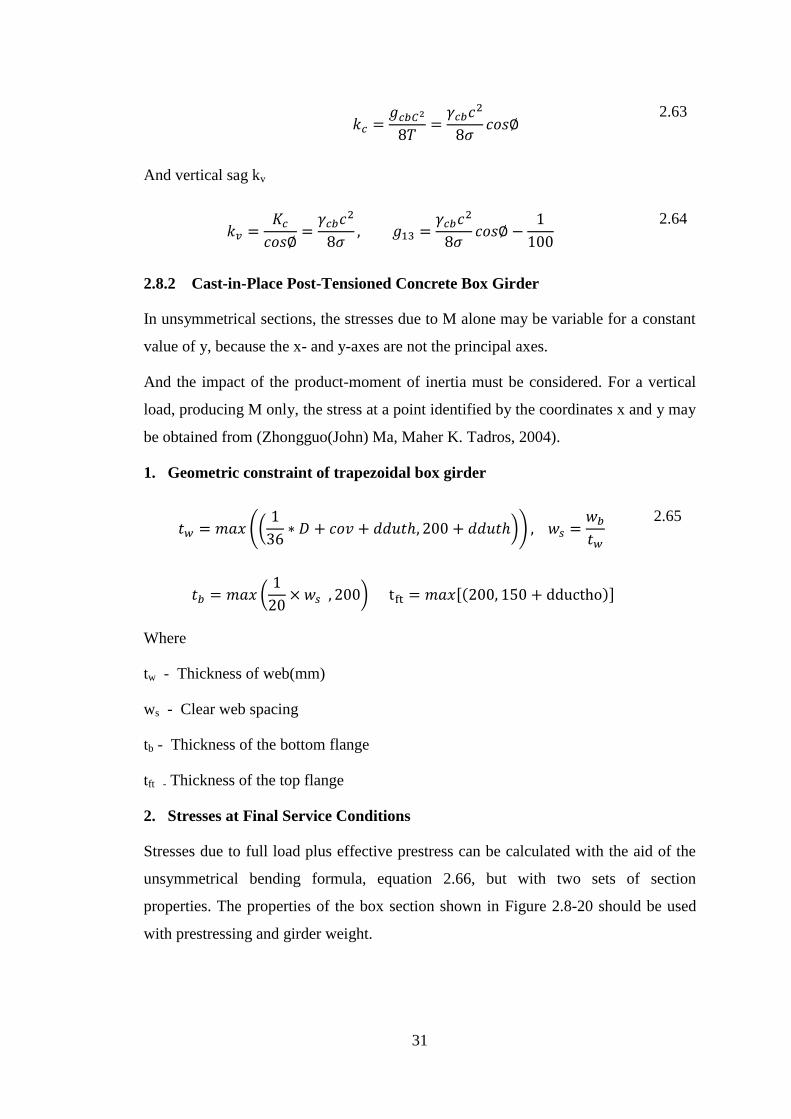
31

2.63

And vertical sag kv

2.64

2.8.2 Cast-in-Place Post-Tensioned Concrete Box Girder

In unsymmetrical sections, the stresses due to M alone may be variable for a constant

value of y, because the x- and y-axes are not the principal axes.

And the impact of the product-moment of inertia must be considered. For a vertical

load, producing M only, the stress at a point identified by the coordinates x and y may

be obtained from (Zhongguo(John) Ma, Maher K. Tadros, 2004).

1. Geometric constraint of trapezoidal box girder

4(

)5

2.65

(

) ,( )-

Where

tw - Thickness of web(mm)

ws - Clear web spacing

tb - Thickness of the bottom flange

tft - Thickness of the top flange

2. Stresses at Final Service Conditions

Stresses due to full load plus effective prestress can be calculated with the aid of the

unsymmetrical bending formula, equation 2.66, but with two sets of section

properties. The properties of the box section shown in Figure 2.8-20 should be used

with prestressing and girder weight.

32

Figure 2.8-20 Cross section of trapezoidal box girder

Top fiber subjected to tension at stress transfer stage:

+

2.66

2.67

Bottom fiber subjected to compression at stress transfer.

2.68

Top fiber subjected to compression at service loads:

(

)

(

)

2.69

Bottom fiber subjected to tension at service loads:

(

)

(

)

2.70

< . ( )

/ ( ) ( ) .

/

( ) .

/

( )

=

( ) ( ) ( ) .

/

33

[

( ) ( ) . ( )

/

( ) .

/ .

( ) ( )/

( ) .

/ .

( ) ( ) ( )

/

( ) ( ) ( ) .

/

]

( )

( ) (

)

(

)

( )

( )

4 ( )

5

4 ( ) ( )

5 ( ) ( )

( ( ))

( )

(

)

[

( )

( ) .

( )

/

4( ( )

5

( ) ( ( )

)

.

/ ( ( ) )

( ( )

) ( ( ) )

4 ( ) ( ( )

) 5

4( ) ( )

5

(

( ( )

( ))

( ( ) ) ( ( )

)

( ( ) ) (

( )

4 ( ) ( )

( )

(

)5

)

)

]

.

/

( ) .

/

+

( ) .

( ) ( )/

34

Where

y2 –height of opening of box girder

y3-width of opening of box girder

Stresss at point P1 due to self-weight moment Mdx=

=

2.71

The stress at bottom due to prestressing force at release is

,

(

)

2.72

Stress at Point P1 due to superimposed dead load moment (kN-m) and live load

moment (kN-m) is:

,

(

) 2.73

3. Live load

Live-load stresses are mostly determined by the evaluation of influence lines.

However, the stress at a given location in a cable-stayed bridge is usually a

combination of several force components. The stress, f, of a point at the bottom

flange(Chen & Duan, 2000b)

⁄

⁄ K

Where

A - The cross-sectional area,

I - The moment of inertia,

y - The distance from the neutral axis, and

35

c - A stress influence coefficient due to the cable force

K -Anchored in the vicinity.

P - The axial force and

M - The bending moment.

The above equation can be rewritten as

2.74

Where

a1, a2, and a3- Depend on the effective width, location of the point, and other global

and local geometric configurations.

f- Combined influence line obtained by adding up the three terms multiplied by the

corresponding constants a1, a2, and a3, respectively.

4. Flexural Strength

For members with bonded tendons, strain is linearly distributed across a section. Non-

prestressed reinforcement reaches the yield strength, and the corresponding stresses in

the prestressing tendons are compatible based on plane section assumptions. For a

member with a flanged section Figure 2.8-21 subjected to uniaxial bending, the

equations of equilibrium are used to give a nominal moment resistance(Chen & Duan,

2000a).

Figure 2.8-21A flange section at normal moment capacity state(Chen & Duan, 2000a)

NA axis depth for evaluation at the strength limit state is given by AASHTO LRFD

Equation 5.7.3.1-3. If

( )

………T

36

section else

……… rectangular section. For rectangular or

T sections where , average stress in Prestressing steel is given by

AASHTO LRFD Equation (

) (

)

(

) for

Table 2.8-1values of k(AASHTO LRFD 2010 BridgeDesignSpecifications 5th Ed..Pdf, 2010)

Type of Tendon Value of k

Low relaxation strand 0.9 0.28

Stress-relieved strand and Type 1 high-strength bar 0.85 0.38

Type 2 high-strength bar 0.8 0.48

Effective depth from extreme compression fiber to centroid of tensile force, de is

given by AASHTO LRFD Equation 5.7.3.3.1-2

Depth of equivalent rectangular stress block, a=1.c, and the nominal moment of

resistance Mn is given by AASHTO LRFD Equation 5.7.3.2.2-1 stated as follows.

If

.

/ .

/

.

/

( )(

) .

/ .

/

.

/

2.75

Where

fpe -Compressive stress in concrete due to effective pre-stresses(N/mm2

)

fd -Stress due to un-factored self-weight(N/mm2

)

fpe and fd - Stress at extreme fiber where tensile stresses are produced by externally

applied loads. (N/mm2

)

Ap – Area of prestressing steel (mm2)

fpe– Effective stress in prestressing steel (N/mm2

)

37

fpu – Ultimate tensile strength of prestressing steel (N/mm2 )

fpy – Yield strength of prestressing steel (N/mm2

fps – Average stress in prestressing steel (N/mm2 )

dp –Distance from extreme compression fiber to centroid of prestressing tendons(mm)

de – Depth from extreme compression fiber to centroid of tensile force (mm)

As – Area of non-prestressed steel tension reinforcement (mm2)

fy – Yield strength of non-prestressed steel tension reinforcement (N/mm2 )

d – Distance from extreme compression fiber to centroid of non-prestressed tension

reinforcement (mm)

As‘ – Area of non-prestressed steel compression zone reinforcement (mm2)

fy‘ – Yield strength of steel compression zone reinforcement (N/mm2 )

ds‘ – Distance from extreme compression fiber to centroid of non-prestressed

compression zone reinforcement (mm)

fc‘ – Specified cylindrical compressive strength of concrete (N/mm2 )

b – Width of the cross-section in compression zone (mm)

bw – Web width of the cross-section (mm)

1 – Stress block factor, 1 = 0.85 for fc‘ = 28Mpa and reduced by 0.05 for each

7Mpa increment of fc‘ and 1 ≥ 0.65

hs – Depth of the deck slab or flange thickness (mm)

c – Depth of the neutral axis (mm)

a – Depth of equivalent rectangular stress block (mm)

Md – Ultimate factored design moment due to all loads (Nmm)

Mn – Nominal moment of resistance (Nmm)

Φ – Resistance factor

Aeff- Area of the concrete section

Ap - Area of prestressed tension reinforcement

b -Top flange width of box girder

38

d- Distance from extreme compression fiber to centroid of tension reinforcement

f -Concrete stress

f1 to f7- Concrete stress at critical checking Points 1 to 7

f’c- Specified compressive strength of concrete

f - Specified compressive strength of concrete at the transfer of prestress

f‘ - Ultimate strength of prestressing steel

fsu* -Stress in prestressing steel at ultimate load

Ix, Iy, Ixy-Second moments of inertia about x- and y axes of cross-section

5. Estimate Crack Angle θ

The LRFD method of shear design involves several cycles of iteration. The first step

is to estimate a value of ζ, the angle of inclination of diagonal compressive stress, ζ =

26.5 degrees. This simplifies the equation somewhat by setting coefficient 0.5 cotζ =

1.0.

6. Shear Strength

The shear resistance is contributed by the concrete, the transverse reinforcement, and

the vertical component of prestressing force. The modified compression field theory-

based shear design strength was adopted by the AASHTO-LRFD and has the

formula(AASHTO LRFD 2010 BridgeDesignSpecifications 5th Ed..Pdf, 2010). Thus

nominal shear resistance,

4

5

:

⁄;

2-76

For 2-77

Where

de- Effective shear depth is given by AASHTO LTRFD Article 5.8.2.9

- The effective depth between the resultants of the tensile and compressive forces

due to flexure.

39

- The effective web width is determined by subtracting the diameters of un-grouted

ducts or one half the diameters of grouted ducts

- Nominal shear resistance

- The shear resistance is contributed by the concrete

- The shear resistance is contributed by the transverse reinforcement

- The shear resistance is contributed by the vertical component of prestressing force

5. Required Vertical Reinforcement, Vs

( )

2.78

( )

2.79

,

√

√

2.80

Then from this, we have the following

2.81

2.82

Where

bv -The effective web width determined by subtracting the diameters of un-grouted

ducts or one half the diameters of grouted ducts;

dv - The effective depth between the resultants of the tensile and compressive forces

due to flexure.

Av - The area of transverse reinforcement within distance s;

s - The spacing of stirrups;

α The angle of inclination of transverse reinforcement to the longitudinal axis;

40

-Factor indicating the ability of diagonally cracked concrete to transmit tension;

ζ - The angle of inclination of diagonal compressive stresses

Shear stress v and strain εx in the reinforcement on the flexural tension side of the

member is determined by

2.83

Where

Mu - Factored moment

Nu - Axial force (taken as positive if compressive)

fpo- Stress in prestressing steel when the stress in the surrounding concrete is zero

fpe -Effective stress after losses

When the value of εx calculated from the above equation is negative, its absolute value

shall be reduced by multiplying by the factor Fε, taken as

Where

Es, Ep, and Ec- Modulus of elasticity for reinforcement, prestressing steel, and

concrete, respectively

Ac-The area of concrete on the flexural tension side of the member Minimum

transverse reinforcement

√

Maximum spacing of transverse reinforcement

For 2

41

2.84

For 2

whereasfci=fc‘

2.85

7. Longitudinal reinforcement

At each section, the tensile capacity of the longitudinal reinforcement on the flexural

tension side of the member shall satisfy the following requirement.

+.⌊

⌋ /

take Ɵ=45 =1

=

⌊

⌋-0.5min0

1 2.86

Where,

Nd – Factored longitudinal tension force (N)

Md- Factored moment for Action (kN.m)

Longitudinal reinforcement on the flexural tension side should satisfy the following

conditions, AASHTO LRFD Article 5.8.3.5:

.

/ Assume =45, cot=1

2.87

Minimum spacing of traverse reinforcement, S

√

√

2.88

Maximum spacing of transverse reinforcement, S

if ⌈

⌉

2

2

2.89

42

Else, for 2

whereas fci=fc‘

2

2.90

Where;

Vu – Factored design shearing force d distance from the face of support (N)

Vn – Nominal shear resistance (N)

Vc - Shear resisting force due to tensile stress in the concrete (N)

Vs – Shear resisting force due to tensile stress in traverse reinforcement (N)

Vp – Component of prestressing force in the direction of shearing force (N)

S – Spacing of stirrups (mm)

Av- Cross-sectional area of shear reinforcement within a distance S (mm2)

dv - Effective depth of shearing force (N) in (mm)

8. Limits of reinforcement (AASHTO LRFD Article 5.7.3.3)

Maximum reinforcement limit

=

0 2.91

Minimum reinforcement limit

Where as

( )

Where

φ- Flexural resistance factor 1.0 for prestressed concrete and 0.9 for reinforced

concrete

Mcr -The cracking moment strength

Mn- Nominal flexural resistance

43

9. The minimum amount of reinforcement

The amount of prestressed and non-prestressed tensile reinforcement shall be

adequate to develop factored flexural resistance Mr which shall not be the lesser of 1.2

times cracking moment and 1.33 times factored design moment as equated below.

Cracking moment, ( ) (

)

For monolithic section substitute for then, ( )

, .

/ And

2.92

2.93

As per ACI-318 1989 minimum area of flexural reinforcement shall not be less than

0.4% of ( )

2.94

Where,

fcpe – Compressive stress in concrete due to effective prestress forces (N/mm2 )

Mg – Total un-factored dead load moment (Nmm)

Md – Total factored design moment (Nmm)

Mr – Total factored moment of resistance of the section (Nmm)

Mcr – Cracking moment (Nmm)

Zc – Section modulus for the extreme fiber of the composite section where tensile

stress is caused by externally applied loads (mm3)

Znc – Section modulus for the extreme fiber of monolithic or non-composite section

where tensile stress is caused by externally applied loads (mm3) that is Zb

fr – Modulus of rupture (N/mm2

)

44

10. Permissible stresses in the reinforcement steels

The stress and forces acting on a cracked post-tension prestressed concrete section

subjected to a moment a working or service load moment of Mw over the cracking

moment Mcr is shown in Figure 2.8-22 below(Mast, 1998).

Figure 2.8-22 Cracked Transformed Section (Mast, 1998).

From the cracked section analysis we have the following equations.

a. On application of Mw or at stage (1) stress in the prestressing tendons is

b. Consider a fictitious load stage (2) corresponding to complete decompression of

the concrete, at which there is zero concrete strain throughout the entire depth as

shown in Figure 2.8-22 compatibility of deformation of concrete and steel

requires that changes in strain in the tendon are the same as that in the concrete at

that level and the stress in tendon due to this stain is given by:

0

1From which 0

1

c. During the application of Mw, the concrete compressive strain in the bottom fiber

reduces to zero and then becomes tensile. With Mw acting the tensile strain in the

reinforcing steel is s and the strain in the concrete at the level of the tendon have

changed from a compression oc to a tension of cp( wubishet J. Abebe, 2018).

From the linearity of strain distribution, these strains can be defined in terms of

the neutral axis depth y and top fiber strain o. Let the extreme top fiber strain be

45

o and NA depth y, and then from strain compatibility one can drive the strains

and stresses in reinforcing steel and prestressing tendons at their respective depths.

Once the strains are evaluated the corresponding stresses can be obtained from the

stress-strain relationship as shown in the following steps. The strain in reinforcing

steel at a depth is d is

and the corresponding stress.

; Similarity the tensile strain in concrete at the level of

prestressing steel or a depth is =

; the Prestressing tendons undergo.

This strain and thus the stress in the tendons are

and

stress in concrete at extreme top fiber is . The Prestressing steel undergoes

the stress of [ ] during the application of Mw so that the total tensile stress in

the tendon is . Tensile force in Prestressing and reinforcing steel

respectively. . In the concrete compressive zone, the

resultant compressive force is; by which is acting at a depth

. This

equation is valid if the neutral axis lies in the flange that is and if , the

force C shall be reduced Cn given by; ( )( )

which can be

regarded as negative. Force and acting at a depth,

the incremental

strain, sought as loading passes from the stage (2) to stage (3) can be defined in

terms of neutral axis depth, y as;

( )

( ( ) .

/) 4 .

/ .

/5

This equation is for the flanged section so that substitute bw by b if y is less than or

equal to hf. From equilibrium of moments have

If 2.95

2.96

Since Mw is known to solve for the strain co and NA depth y and then the equilibrium

of x (horizontal of forces should be checked).

46

∑

2.97

Location of the centroid of the cracked transformed section from extreme top fiber, yct

is given

If

( )

( ) by else

The cross-sectional area of the cracked transformed section, Act will be; if

( )

The second moment of area or moment of inertia of the cracked transformed section,

Ict is; if

.

/

( )

( ) 4

5

( ) ( )

.

/

( ) ( )

If then 2.98

Where,

fp1 – Incremental stress in prestressing tendons before the application of service loads

or at stage (1) (N/mm2)

fp2 – Incremental stress in prestressing tendons as the section passes from before the

application of service loads stage (1) to decompression stage (2) (N/mm2)

fp3 – Incremental stress in prestressing tendons due to change of stress from

compression to tension in the concrete located at the level of the tendon (N/mm2)

fco – Stress in extreme top fiber during application of service load moment(N/mm2 )

fs – Stress in steel reinforcement at the application of service loads (N/mm2)

fp – Total stress in prestressing tendons at the application of service loads (N/mm2 )

47

oc– Compressive strain in the concrete at the level of the tendon(mm)

cp – Tensile strain in the concrete at the level of the tendon(mm)

o –compressive strain at the extreme top fiber (mm)

s – Tensile strain in the reinforcing steel at working loads

np – Modular ratio of prestressing steel

ns – Modular ratio of reinforcing steel

Ec –modulus of elasticity of concrete (N/mm2)

Es – Modulus of elastic of reinforcing steel (N/mm2)

Ep – Modulus of elastic of prestressing steel (N/mm2)

Fx – Forces acting in the horizontal direction (N)

Ts – Tension force in the reinforcing steel at service limit state (N)

Tp – Tension force in the prestressing steel at service limit state (N)

C – Resultant compressive force in the compression zone of concrete (N)

Cn – Compressive force in the compression zone of concrete used to reduce the

resultant compressive force C when NA depth exceeds flange thickness (N)

y – NA depth of the cracked section under service limit state (mm)

dz – Depth from extreme compression fiber to centroid of resultant compression force

C (mm)

dzn – Depth from extreme compression fiber to centroid of compression force Cn

(mm)

yct – Depth from extreme compression fiber to centroid of cracked section (mm)

Act – Area cracked transformed section under service limit state (mm2)

Ict – Moment of inertia of cracked transformed section under service limit state (mm4)

11. Deflection control (ASHTO LRFD Article 5.7.3.6)

Deflection and camber calculations shall consider dead load, live load, prestressing,

erection loads, concrete creep and shrinkage, and steel relaxation.

48

Immediate or instantaneous deflection is computed by taking the effective moment of

inertia, the effective moment of inertia used to calculate the instantaneous deflection

is given by

{.

/

( .

/

)

}

And =0.63

Where,

Ie- Effective moment of inertia (mm4)

Mck – Cracking moment (Nmm)

frk – Modulus of rupture of concrete (N/mm2)

12. Deflection due to dead loads and prestressing force

Instantaneous deflection for permanent loads calculation, i

Instantaneous deflection due to dead load, di=∬ ( )

Additional long-term deflection d1= . di λ 8

9

Thus total deflection to dead load, . For parabolic tendon profile with

central anchor upward deflection due to prestress is

2.99

13. Deflection due to living loads

When investigating the maximum absolute deflection, all of the design lanes should

be loaded. For live load deflection evaluation, design vehicular live load of AASHTO

HL-93 where the vehicle load includes the impact factor IM and the multiple presence

factor m. In general, the deflection at the point of maximum moment, x due to each

design truckload at a distance a, from the left support is given by live load deflection

due to design truckload will be

For x=a,

. For

( ) individual truckload

deflection. Thus total design truck deflection will be ∑ .

49

Deflection due to each design lane load

where

In the computation of live load deflection design truckload alone or design lane load

plus 25% of design truckload whichever is the greater as stated in AASHTO article

3.6.1.3.2. Thus live load deflection is, {

. Allowable live load

deflection,

. Thus limit live load deflection,

Hence

2.100

Where:

Ie – Effective moment of inertia of the section (mm4)

Δdi – Immediate deflection due to dead load (mm)

Δd – Total long term deflection due to dead load (mm)

Δp – Upward deflection due to prestressing force (mm)

Δkl – Deflection due to truckload (mm)

ΔLn – Deflection due to design lane load (mm)

ΔLL – Deflection due to living load (mm)

Δall – Allowable deflection for the live load (mm)

x – Distance from left support to a point at which maximum service load moment

occurs.

a – Distance from the left support to the point of truckload for which deflection is to

be computed.

b – Distance from the right support to the point of truckload for which deflection is to

be computed.

14. Limit of the crack width

For dry air or protective membrane (class I) exposure conditions, and assumed

allowable crack width is 0.41mm. The expressions that have figured prominently in

the development of the crack control provisions in the ACI code. These equations are

respectively.

50

( )

( ) 2

3 2.101

Where,

fs - Service load stress in non prestressed steel (Mpa)

h1 – Distance from the centroid of tensile steel to NA depth (mm)

h2 – Depth from extreme compression fiber to depth of NA (mm)

dc Thickness of concrete cover from extreme tension fiber to centroid (mm)

Act – Effective tension area of concrete surrounding one bar (mm2)

15. Fatigue limit state (AASHTO LRFD Article 5.5.3)

The stress range in reinforcing steel resulting from fatigue load is ( )

And stress range in prestressing steel resulting from fatigue load is

( )

. The allowable stress range in reinforcing steel is given by

.

/ by setting

Where,

r/h– Ratio of base radius-to-height of rolled-on transverse deformation (a value of 0.3

can be used in the absence of specific data). Allowable stress range in prestressing

tendons with the radius of curvature larger than 9000mm shall be less than 125Mpa.

Thus, the following constraints stated;

2.102

2.103

Where,

fffs – Stress range in reinforcing steel due to fatigue load (N/mm2 )

fffp – Stress range in prestressing steel due to fatigue load (N/mm2 )

Mf – Maximum fatigue load moment (Nmm)

51

fmin – Minimum live load stress where there is stress reversal (N/mm2 )

r – Base radius of the deformation (mm) and

h –The height of the deformation (mm)

16. Torsion

Calculation of torsion resistance by formula（5.8.2.1-4） in《AASHTO Bridge

Design Specification 2010》. . In which

4

5

2.104

Where:

Tu- Factored torsional moment (Nmm)

Tcr - Torsional cracking moment (Nmm)

Acp-Total area enclosed by the outside perimeter of concrete cross-section (mm2)

Pc -The length of the outside perimeter of the concrete section (mm)

17. Longitudinal Reinforcement due to torsion

The provisions of Article 5.8.3.5 shall apply as amended, herein, to include torsion.

The longitudinal reinforcement in solid sections shall be proportioned to satisfy Eq.

5.8.3.6.3-1:

+ √.⌈

⌉ /

.

/

In the box girder sections, longitudinal reinforcement for torsion, in addition to that

required for flexure, shall not be less than

+ √.⌈

⌉ /

.

/

( )

2.105

Where:

52

ph - Perimeter of the centerline of closed transverse torsion reinforcement (mm)

18. Minimum Area of Interface Shear Reinforcement

The cross-sectional area of the interface shear reinforcement, Avf, crossing the

interface area, Acv, shall satisfy the equation of 5.8.4.4 in AASHTO

. Amount needed to resist 1.33Vui /φ as determined using Eq.5.8.4.1-3

2.106

Where

Avf- The cross-sectional area of the interface shear reinforcement

Acv- Crossing the interface area

19. Torsional Reinforcement

Where a consideration of torsional effects is required by Article 5.8.6.3, torsion

reinforcement shall be provided.

The nominal torsional resistance from transverse reinforcement shall be based on a

truss model with 45-degree diagonals and shall be computed as:

.

The minimum additional longitudinal reinforcement for torsion, Aℓ , shall satisfy:

2.107

Where:

Av - Area of transverse shear reinforcement (mm2)

Aℓ - Total area of longitudinal torsion reinforcement in the exterior web of the box

girder (mm2)

Tu -Applied factored torsional moment (Nmm)

53

Ph - Perimeter of the polygon defined by the centroids of the longitudinal chords of

the space truss resisting torsion.

Ao- Area enclosed by shear flow path, including the area of holes, if any (mm2)

fy -Yield strength of additional longitudinal

20. Edge Tension Forces

The longitudinal edge tension force may be determined from an analysis of a section

located at one-half the depth of the section away from the loaded surface taken as a

beam subjected to combined flexure and axial load. The force may be taken as equal

to the longitudinal edge tension force but not less than that specified in (AASHTO

LRFD 2010 BridgeDesignSpecifications 5th Ed..Pdf, 2010) in Article 5.10.9.3.2)

21. Bursting Forces

This calculation is checked by (AASHTO LRFD 2010 BridgeDesignSpecifications

5th Ed..Pdf, 2010). Calculation of bursting forces by formula（5.10.9.6.3-1and（

5.10.9.6.3-2 ） in(AASHTO LRFD 2010 BridgeDesignSpecifications 5th Ed..Pdf,

2010).

∑ .

/ 0∑ 1

The location of the bursting force, dburst, may be taken as:

( ) 2.108

Where:

Tburst -Tensile force in the anchorage zone acting ahead of the anchorage device and

transverse to the tendon axis (N)

Pu - Factored tendon force (N)

dburst -Distance from anchorage device to the centroid of the bursting force(m.)

a -Lateral dimension of anchorage device or group of devices in direction (mm)

e -Eccentricity of the anchorage device (mm)

h - Lateral dimension of the cross-section in the direction considered (mm)

α - Angle of inclination of a tendon force concerning the centerline of the member

54

22. Bursting Forces Results of End Beam Prestressed reinforcement

∑ .

/ ,∑ -The location of the bursting force, dburst,

may be taken as:

( ) 2.109

23. Bursting Forces Results of Tooth Block

∑ .


may be taken as:

( ) 2.110

24. Bursting Forces Results of Stay Cables

∑ .


may be taken as:

( ) 2.111

25. Compressive Stress of Concrete in Front of Anchor Head

Calculation of Compressive Stress of Concrete in Front of Anchor Head by formula（

5.10.9.6.2-1）and（5.10.9.6.2-2）in(AASHTO LRFD 2010

BridgeDesignSpecifications 5th Ed..Pdf, 2010).

In which if ; then (

) .

/

Ifs ; then k=1, fca< 0.7φf'ci

2.112

Where:

κ -Correction factor for closely spaced anchorages

aeff -Lateral dimension of the effective bearing area measured parallel to the larger


55

beff - Lateral dimension of the effective bearing area measured parallel to the smaller


Pu -Factored tendon force (N)

t- Member thickness (mm)

s - Center-to-center spacing of anchorages (mm)

n - Number of anchorages in a row

ℓc - Longitudinal extent of confining reinforcement of the local zone but not more

than the larger of 1.15 aeff or 1.15 beff (mm)

Ab- Effective bearing area (mm2)

The effective bearing area, Ab, in Eq. 5.10.9.6.2-1 shall be taken as the larger of the

anchor bearing plate area; Aplate; or the bearing area of the confined concrete in the

local zone,

Aconf, with the following limitations:

• If Aplate controls,

A plate shall not be taken larger than 4/πAconf.

• If Aconf controls, the maximum dimension of Aconf shall not be more than twice the

maximum dimension of Aplate or three times the minimum dimension of A plate. If any

of these limits are violated, the effective bearing area, Ab, shall be based on Aplate.

Deductions shall be made for the area of the duct in the determination of Ab. If a

group of anchorages is closely spaced in two directions, the product of the correction

factors, κ, for each direction shall be used, as specified in Eq. 5.10.9.6.2-1.

26. Punching Shear

=0.125√ ( ) 2.113

Where:

f ′c- Specified strength of concrete at 28 days (Mpa)

W- Width of bearing plate or pad as shown in Figure 5.13.2.5.4-1 (mm)

L- Length of bearing pad as shown in Figure 5.13.2.5.4-1 (mm)

de -Effective depth from extreme compression fiber to centroid of tensile force(mm)

56

27. Losses of Pre-stress

Pre-stress losses can be divided into two categories:

i. Instantaneous losses

Including losses due to anchorage set (fpA), friction between tendons and

surrounding materials (∆fpF), and elastic shortening of concrete (fpES) during the

construction stage. Time-dependent losses including losses due to shrinkage (fpSR),

creep (fpsR), and relaxation of the steel (fpR) during the service life(F. Abebe, 2016).

The total pre-stress loss (fpT) is dependent on the pre-stressing methods.

For post-tensioned members

ii. Anchorage Set Loss

The anchorage set loss changes linearly within the length (LpA), the effect of

anchorage set on the cable stress can be estimated by the following formula:

0

1,

√

( )

Where

∆L - The thickness of anchorage set;

E - The modulus of elasticity of anchorage set;

∆f - The change in stress due to anchor set;

LPa - The length influenced by anchor set;

LpF - The length to a point where loss is known; and

x - The horizontal distance from the jacking end to the point considered

57

Figure 2.8-23 Anchorage set loss model(F. Abebe, 2016).

iii. Friction Loss

For a post-tensioned member, friction losses are caused by the tendon profile

curvature effect and the local deviation in tendon profile wobble effects. AASHTO-

LRFD specifies the following formula:

( ( )

Where

fpj - Stress in the prestressing steel at jacking (Mpa)

K - Wobble friction coefficient (per ft of the tendon)

µ - Curvature friction coefficient

x - Length of a prestressing tendon from the jacking end (mm)

α - Sum of absolute values of angular change of prestressing steel path from jacking

end, (o)

e - Base of Napierian logarithms

iv. Elastic Shortening Loss ∆fpES

Equation for calculation of elastic shortening in the LRFD Commentary(AASHTO

LRFD 2010 BridgeDesignSpecifications 5th Ed..Pdf, 2010).

( ) (

)

( )

( )

58

v. Time-Dependent Losses

AASHTO-LRFD provides the approximate lump sum estimation of time-dependent

losses ∆fpTM resulting from shrinkage and creep of concrete and relaxation of

prestressing steel(AASHTO LRFD 2010 BridgeDesignSpecifications 5th Ed., 2010).

vi. Refined Estimation

d. Shrinkage loss. Shrinkage loss can be determined

e. Creep loss: creep loss can be predicted by

2.114

Where

fcgp -Concrete stress at the center of gravity of prestressing steel at transfer, and

∆fcdp - Concrete stress change at the center of gravity of prestressing steel due to

permanent loads, except the load acting at the time the prestressing force

vii. Relaxation Loss:

The total relaxation loss (∆fpR) includes two parts: relaxation at the time of transfer

∆fpR1 and after transfer ∆fpR2. For low relaxation strands, the relaxation in the pre-

stressing strands equals 30% of the equation shown below:

( )

{

6

7

6

7

For stress-relieved strands

[ ( ) for post-tensioning

Where

t - The time estimated in days from testing to transfer.

- Loss due to elastic shortening (Mpa)

- Loss due to creep of concrete (Mpa)

59

-Loss due to shrinkage (Mpa)

viii. Post-Tensioned Members

The loss due to elastic shortening in post-tensioned members, other than slab systems,

maybe 5.9.5.2.3b(AASHTO LRFD 2010 BridgeDesignSpecifications 5th Ed..Pdf,

2010).

Where

N - Number of identical prestressing tendons

fcgp - Sum of concrete stresses at the center of gravity of prestressing tendons due to

the prestressing force after jacking and the self-weight of the member (Mpa)

fcgp - Values may be calculated using steel stress reduced below the initial value by a

margin dependent on elastic shortening, relaxation, and friction effects.

The loss is due to elastic shortening in post-tensioned members, other than slab

systems determined by the following alternative equation 2.115.

( )

( )

2.115

Where:

Aps- Area of prestressing steel (mm2)

Ag -Gross area of section (mm2)

Eci- Modulus of elasticity of concrete at transfer (N/mm2)

Ep - Modulus of elasticity of prestressing tendons (N/mm2)

em - Average eccentricity at mid-span (mm)

fpbt - Stress in prestressing steel immediately before transfer as specified (Mpa)

Ig - Moment of inertia of the gross concrete section (mm4)

Mg - Mid-span moment due to member self-weights (Nmm.)

N - Number of identical prestressing tendons

fpj - Stress in the prestressing steel at jacking (Mpa)

60

ix. Creep Losses

The equation for creep follows:

2.116

Where

Δfcdp -Equals the change in concrete stress due to externally applied dead loads

excluding self-weight.

2.8.3 Pylon design

The primary function of the pylon is to transmit the forces arising from anchoring the

stays cable. The pylon should ideally carry these forces by axial compression where

possible such that any eccentricity of loading is minimized(Nippon Koei Co., 2005).

The tower height is a particularly important parameter because it influences how the

loads are shared between the stay-cables and the girder. Specifically how they live

loads are carried, and how much change in live load, or fatigue, the cable is subjected

to (Stroh, 2012). When investigating the buckling of the pylon simple support at the

top and a fixed base, provided the column is subjected to the axial load Npt, the

relevant angular change Df at the bottom, as well as the longitudinal wind load. The

resistance of the pylon top against horizontal displacements due to elongation of the

anchor cable depends on the ratio between the axial force Npt and the critical force

Ncr(Niels J.Gimsing, 2012).

The pylon is linearly tapered with cross-sectional shapes of k (=4)-sided regular

polygons with circum radii r measured from the centroid to a vertex at any coordinate

x.

( )

Where

E - The material modulus of elasticity

I - Moment inertia of the prismatic column,

γcr - The buckling load factor depends on the ratio of moment inertia and support

condition of the column(Dharma & Suryoatmono, 2019).

61

Fw = γA, 2.117

Where

γ - The weight density of the column material.

The cross-sectional area of the plane area at x

I - Second moment of the plane area at x

The pylon is subjected to an external compressive load P at the head end and its own

self-weight W (= γV). When P increases and reaches the buckling load Pcr, the

column with a buckling length l buckles and forms the buckled-mode shape

represented by the solid curve(Lee & Lee, 2021). Taper pylon function of r at x

expressing mathematically in the equation

Where

n -Taper ratio

rh - Head radius

rt - Toe radius is introduced.

Linear taper function, r is expressed in terms of x as follows. Where n1 = n − 1. The

variable functions of A and I for the 4-sided regular polygon at x can be gained as

equation 2.118(Lee & Lee, 2021).

2.118

Where C1 and C2 are

.

/ .

/

.

/ .

/ 0 .

/1

Where

k ( ) is integer side number and k= for the circular cross-section. The column

volume V is determined as

∫

∫

,

( ) 2.119

62

Where

l - The buckling length of the column subjected to an external buckling load B

W (= γV) - self-weight

rt- can be obtained in terms of V as √

A and I can be obtained in terms of V as

,

The self-weight intensity Fw at x caused by the γ value of the column material is given

by

The axial force N at x is obtained as

∫

.

/ ,

2.120

Where

γV – The equal to the total column weight W.

Pcr- The buckling load

Fw- The self-weight intensity

The bending moment M is given by the relationship between load and deformation

based on the small deflection theory as

2.121

Differentiating Equation 2.121 twice yields

2.122

After substituting equations the equation yields

[ (

)]

2.123

From the equation, the first and second derivatives of I are determined, respectively:

63

, 2.124

Substituting equation 2.131 equation 2.130

[ (

)]

2.125

Following the system, parameters are cast into non-dimensional forms equation 2.126

;,

;

;

2.126

0.

/1

+

2.127

√

6

(

)

7

2.128

Where

(ξ, ε)-Non-dimensional Cartesian coordinates,

β- The buckling load parameter, and

λ - The self-weight parameter.

-The self-weight buckling length for which the column buckles

In particular, the self-weight buckling length L and self-weight buckling stress σ

caused only by the self-weight W with P = 0 are obtained using Equations 2.129

respectively.

√

.

/

2.129

Cables that are passed through saddles must be dimensioned to account for the

bending stress due to curvature fc determined as follows (Mermigas& A, 2008).

64

2.130

Therefore, the total stress in the cable is:

2.131

Where

E - The elastic modulus of the wire or strand;

r - The radius of the wire, strand, or bundle

R - The radius of the saddle bend.

As a case study, Abay extradosed cable-stayed bridge has a cross-sectional area of the

pylon that varies linearly from 3*2 at the top to the value 2*4 at deck level. The force

Npt acting at the pylon top will be the resultant of all vertical components of the cable

forces at the supporting point. Horizontal equilibrium between the two-chord forces

TA and TC, the axial force RT acting on the pylon will be the resultant of these two

forces(Niels J.Gimsing, 2012).

2.132

As the pylon is fixed at the base and longitudinally supported at the top by the anchor

cable, the effective column length will be approximately 0.7hpl.

2.133

Conversely, the horizontal restraint offered by the anchor cable implies that the force

Npt from the cable system does not have to stay vertical but might turn into an

inclined direction. Under longitudinal wind load, the anchor cable renders support to

the pylon. When investigating buckling of the pylon it can generally be assumed that

the anchor cable constitutes fixed support in the longitudinal direction. Thus, the

analysis should be based on investigating a column fixed at the base and simply

supported at the top, and subjected to an axial force Npt, a top displacement dh, and a

longitudinal wind load(Niels J.Gimsing, 2012).

65

Figure 2.8-24 Limited longitudinal displacements of the pylon top in a system with a fixed

bearing under the deck (Niels J.Gimsing, 2012).

2.134

If a linear analysis is performed, then the distinction between forces directed towards

a fixed point or remaining vertical becomes unimportant and the forces from each

cable system can then be represented by a single force equal to the resultant of all

tangential cable forces. Fixing of column-type pylons to piers, longitudinal restraint of

the pylon top can be achieved by fixing the pylon to the substructure, but this will

require a substantial increase of the cross-sectional dimensions to achieve equally

small displacements as those found in a system with an anchor cable. For the

horizontal displacement of the pylon tops, the following expressions can be derived:

2.135

2.136

Which

ac - The tensile stress in the anchor cable;

- The modulus of the elasticity for the cable;

pb - The bending stress in the lower part of the pylon; and

- The modulus of elasticity for the material used in the pylon

-The height of the pylon above the deck

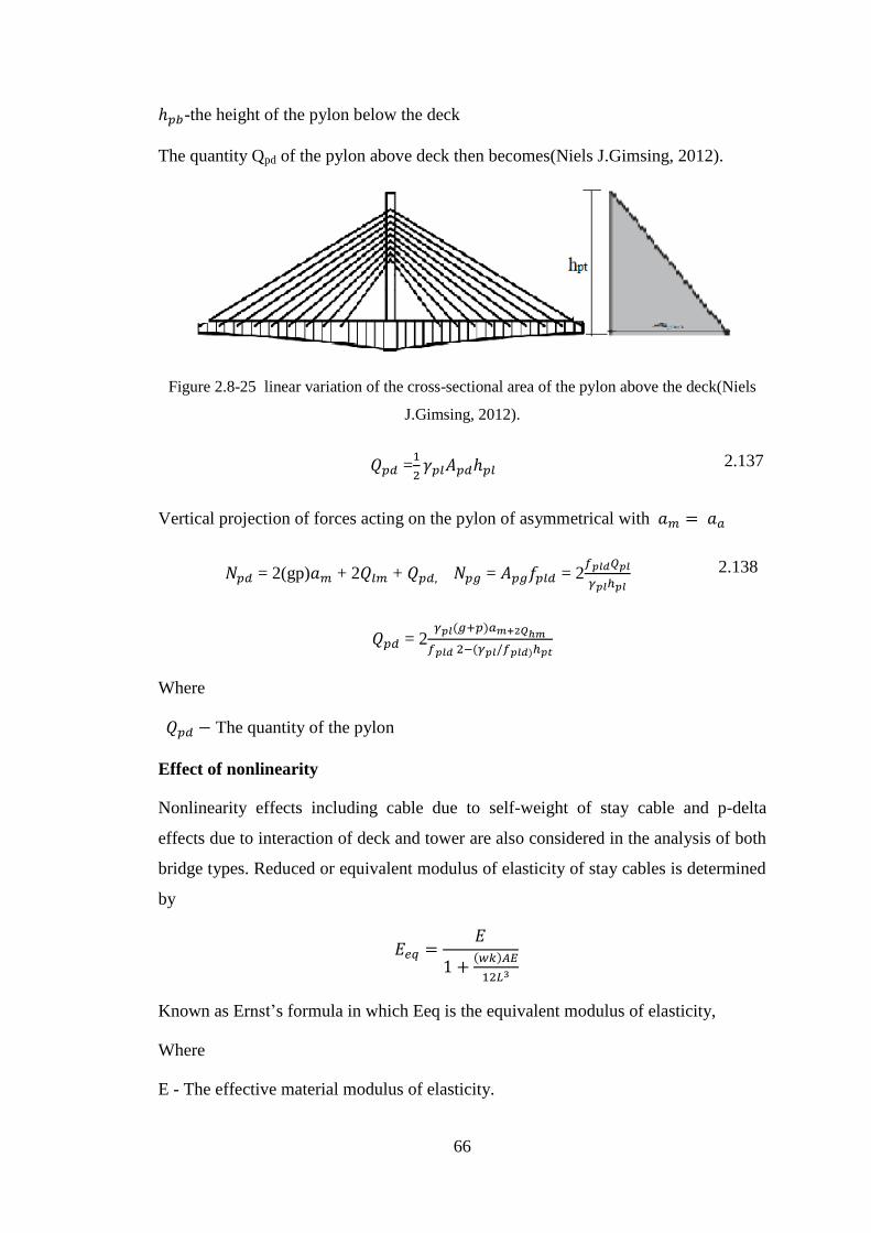
66

-the height of the pylon below the deck

The quantity Qpd of the pylon above deck then becomes(Niels J.Gimsing, 2012).

Figure 2.8-25 linear variation of the cross-sectional area of the pylon above the deck(Niels

J.Gimsing, 2012).

=

2.137

Vertical projection of forces acting on the pylon of asymmetrical with

= 2(gp) + 2 + = = 2

2.138

= 2 ( )

( )

Where

The quantity of the pylon

Effect of nonlinearity

Nonlinearity effects including cable due to self-weight of stay cable and p-delta

effects due to interaction of deck and tower are also considered in the analysis of both

bridge types. Reduced or equivalent modulus of elasticity of stay cables is determined

by

( )

Known as Ernst‘s formula in which Eeq is the equivalent modulus of elasticity,

Where

E - The effective material modulus of elasticity.

67

A - The cross-sectional area of stay cable,

w - Cable weight per unit length,

L -Horizontal projected length and

T - The tensile force in stay cable

2.8.4 Need of optimization

The major need for structural optimization is to review and enhance the current

state of structural design techniques and to show possibilities of these methods in

structural work( wubishet J. Abebe, 2018).

structural optimization needs to determine the most suitable combination of design

variables, so to achieve the satisfactory performance of the structure subject to the

behavioral and geometric constraints impose, with the goal of optimality being

defined by the objective function for specified loading or environmental

conditions(Klarbring & An, 2008).

It allows a better manipulation of material, thus decreasing structure self-weight

and saving material costs(AN, n.d.).

Also, give the structure a higher aesthetic value. Therefore structural optimization

is important for any design to get the most economical output.

68

3. METHODOLOGY

3.1 General

Structural optimization is the subject of making an assemblage of materials that

sustains loads in the best way. Term best to make the structure as light as possible, to

make the structure as stiff as possible, and to make it as insensitive to buckling or

instability as possible. Maximizations or minimizations cannot be performed without

any constraints. Quantities that are usually constrained in structural optimization

problems are stresses, displacements, and/or geometry (Klarbring & An, 2008).

Nonlinear constraint value is used for structural optimization of extradosed cable-stay

bridge. Because any civil design has its own restriction or limit values. So extradosed

cable-stay bridge has its restriction for each element design of the bridge for the

pylon, stay cable, and for post-tensioning box girder. Each limit values takes as

constraint for optimization.

3.2 Method of Structural Analysis

The method of structural analysis with the use of simplified load distribution factors

for distributing the loads among between box girders, stay cable. Abay bridge was

built in an earthquake-free zone in Bahir Dar(EBCS EN- 8 Part 1, 2014). But wind

load and vehicle load are investigated as dynamic load. MIDAS CIVIL 2019 use for

Structural analysis and model of extradosed cable-stay bridge. Worst load effects

were investigated under applicable load combinations was given in design. All load

effect is considering in structural analysis of the bridge. After analysis, take the

moment and shear value of the section then finding the optimum section of the bridge.

3.3 Method of Design Optimization

In this research design, optimization problems were handled with the use of an

evolutionary or genetic algorithm (GA) after it has been tested under simple manually

solved optimization problems. Recent advances in the field of computational

intelligence led to several promising optimization algorithms. These algorithms have

the potential to find optimal or nearly optimal solutions to complex problems within a

reasonable time frame. Structural optimization is a research field where algorithms are

applied to optimally design structures. It is essentially the combination of two

research fields, structural mechanics and computational intelligence.

69

In these thesis objectives, the concrete grade effect on the weight of girder, pylon, and

angle of stay cable have been considered case by case to compare the weight of

parameter and recommend for practical use.

After testing by simple optimization problem, the present problem had connected to

the optimizer, the optimization of superstructure parameter the such as depth of

girder, the height of the pylon, angle of stay cable, concrete grade, bottom slab width,

and side cantilever dimension with constant span 380m with constant carriage width

of 24.7m and Fe-420 grade of steel were carried out. Worst load effects are

investigated under applicable load combinations and then the results are input into GA

optimization code prepared within the built-in MATLAB R2016a software. After that,

the code was run to generate the outputs and the validity of the result was verified by

exporting it into an excel spreadsheet.

GA based optimization depends on three important aspects:

Coding of design variables.

Evaluation of fitness of each solution string.

Application of genetic parameters (selection, cross-over, and mutation) to

generate the next generation of solution strings.

Geometry to fulfill all the requisites from the ULS and SLS as well as to provide

minimized the total weight of the structure subject to constraints on deflection and

stresses in the structure under a given load.

3.4 Materials Used

The cable passes through the pylon through the embedded steel conduit and is

tensioned on the main beam. By standard, a stay cable consists of a prestressed strand

with high strength and low relaxation. The stay cables are made in a factory. C1~C3

is composed of 43- 15.2 (1x7) strands and C4~C9 is composed of 55-15.2 (1x7)

strands. The steel strand is galvanized (China Communication Construction Company

Limited, 2020).

70

3.4.1 Prestressed Reinforcement

For post-tension prestressing strand:

I. The strand should be low-relaxation, seven-wire, Type 1x7 (d15.2mm), with the

tensile strength of 1860Mpa (Grade 270), complying with AASHTO M 203/M

(ASTM A 416/A 416M).

II. The properties of the anchorages should be according to ERA 2013 standard.

III. The prestressing strand should be tensioned with 4296.6KN (75% specified

strength) +friction of the anchorage and jack for M15-22, 3710.7KN (75%

specified strength) +friction of the anchorage, and jack for M15-19, 3320.1KN

(75% specified strength) +friction of the anchorage and jack for M15-17.

IV. The strength of the grouting materials should be no less than 55Mpa and comply

with the corresponding specifications

V. The properties of the duct should comply with corresponding specifications, and

connecting of the ducts should be done with one size bigger and minimum length

should be no less than 30cm. The reinforcement welding procedures and

requirements should comply with AWS D1.4/D1.4M:2018 structural welding

code—steel reinforcing bars, during welding, the minimum overlap length should

be 20cm, the welding length should be minimum 5d or 10cm(take the bigger

value) for double side welding, minimum 10d for single-side welding, and in one

location, the welding joint percentage should not more than 50%, and the stagger

distance should be minimum 35d or 500mm((take the bigger value) (China

Communication Construction Company Limited, 2020).

3.4.2 Reinforcement

The steel bars used in the design of the beam are of high yield strength as shown in

Table 3.4-1

Table 3.4-1reinforcement steel strength (China Communication Construction Campany

Limited, 2020)

Grade of Steel Min. yield strength, fy [Mpa] Modulus of Elasticity, Es [Mpa] Dia.

Grade 420 420 2x105

>=D12

(Max.D32)

71

3.5 Optimization Procedure with GA in Matlab

Procedures involved in design optimization by GA in Matlab were given in the

following steps.

Step 1: Define fitness function. (i.e. define weight function as objective). Open

Matlab and HOME menu click the New Script button. The new script edit field is

displayed under the EDITOR menu. Use % symbol to write a comment for readers in

which Matlab could not read. It is used for defining code for users.

If % appears before any statement. The new script starts to type the fitness function

and give it its original name, in this case, let it be Extramaincompfun(x) to denote

the objective function of extradosed box girder parameter of the main load-carrying

component.

Move in other weight parameters before stating the objective function as follows and

list the weight function. The objective function must write as end letter fun.

Now define the weight function as specified below

72

And save it suppressing ―CTRL+S‖ to file folder, it must save by the same name of

objective function ‗Extramaincompfun‘ which is the name of objective function

defined earlier.

Step 2. Define the constraint function.

Then add a new script and type the constraint functions as follows. Next enter

parameters of constrained functions. Note C and Ceq stands for nonlinear inequality

and equality constrained functions respectively.

After defining all parameters in terms of design variables, next state the constraint

functions as follows.

73

Step 3. Define the main function and develop GA.

Add a new script and define the boundaries of design variables in the main file

74

Next call GA with the following syntax to solve the problem. Save this file with a

name, let it be ‗maincodeBG.m’ for this case.

Step 4: Run the code. Generate optimization results. After the end of development,

GA runs it. The program prompts to change the folder so that click change folder.

Unless the current folder is active or being opened by the program, Matlab couldn‘t

understand the newly developed code and solve it.

If all constraints are fulfilled print the outputs the optimum values of the design

variable and if not adjust lower and upper bounds and repeat it

75

3.5.1 Running the model

Workflow of structural optimization by MATLAB by genetic algorithm(Chessa,

2020)

3.6 Study Variables

Study variables have two parts that are independent variables and dependent

variables.

3.6.1 Independent variables

Depth of girder.

Define constant geometry value

Generate initial number of samples in the population

(NPOP);

Decoding of design variables

Evaluate constraints, objective function and

penalized objective function

Apply genetic operators

(reproduction, crossover and

mutation)

Print

optimum

solution

No

Yes

Check

convergenc

Figure 3.5-1Working flow genetic algorithm for optimization

76

Height of pylon

Stay cable angle.

Concrete grade

Sensitivity analysis

3.6.2 Dependent variables

Weight optimization of prestressed post-tension superstructure part of extradosed

cable-stay Bridge. The weight component of the bridge contains the optimum weight

of non-prestressing reinforcement, torsional reinforcement, concrete and prestressing

reinforcement.

3.7 Load Analysis

The structural model of Abay Bridge was done by MIDAS CIVIL 2019. Linear static

structural analysis was made using distribution factors for shear and moment given

under AASHTO Article 4.4.2.2. In the analysis of loads, a dynamic load allowance or

impact factor (IM) of 15% for fatigue and fracture limit state and 33% for all other

limit states was considered as stated in AASTO Article 3.6.2.1. These factor accounts

for hammering when riding surface discontinuities exist, and long undulations when

the settlement or resonant excitation occurs. Depending on the number of lanes loaded

multiple presence factors (m) specified under AASHTO Article 3.6.1.1.2 were used to

modify the vehicular live loads for the probability that vehicular live loads occur

together in a fully loaded state.

3.7.1 Load Cases and Load Combinations

Live loads are forces that act momentarily on structures due to moving loads. The

following Live loads are considered in the design of Abay bridge structures 《

AASHTO Bridge Design Specification 2010》3.6.1.1.6 Pedestrian Loads Pedestrian

and Bicycle of 3.6 m/10-3

. These are Traffic Loads due to trucks and Lorries. For the

new bridge design, the vehicular live load considered was《AASHTO Bridge Design

Specification 2010》 . This comprises the Design Truck or Design Tandem and

Design Lane Load.

77

3.7.2 Design Truck Load

The total design truckload is 325kN distributed between 3 axles the front axle load

being 35 KN and two rear axle loadings being145 KN each. The relative spacing of

the three axles is illustrated in 《AASHTO Bridge Design Specification 2010》.

Figure 3.7-1 Characteristics of the Design Truck adopted from AASHTO Bridge Design

Specification 2010

3.7.3 Braking force

The longitudinal displacement of the car when it is broken on the bridge and the beam

body causes the bridge to be stressed. According to the 《AASHTO Bridge Design

Specification 2010》, 3.6.4 adopts 5% of the designed truck plus lane load or 5% of

the designed series plus lane load, selects the maximum braking force of the truck,

and arranges 3 lanes. The uniform braking force on the 380m bridge length.

Table 3.7-1 Braking force values

Braking force Axle

weight(kN）

Bridge

length(

m）

Uniform

force(N/mm)

Single

lane

coefficient

Three lane

reduction

factor

Uniform

force

(kN/m)

Truck 320.3 0.05

1.29

Design tandem 222.4 0.05 1.26

Lane 380 9.3 3534 0.05

3.7.4 Wind Load

In the case of footbridges, the height of the moving load is to be taken as 2 meters

throughout the length of the span.

78

The wind pressure effect is considered as a horizontal force acting in such a direction

that resultant stresses in the member under consideration are the maximum. The

nature of the wind load is dynamic. This means that its magnitude varies concerning

time and space.

1. Horizontal Wind Pressure

The design wind speed is based on the formula in the ERA Road Design Manual

(3.8.1.1-1).

[

] [

]

3.1

Where

V0 (m/s) - The average maximum wind speed for 10 minutes in the condition of flat

open ground, a terrain clearance of 10m and a return period of 10, 50 or 100 years

The V0 friction coefficient is 17.6km/hr. according to the urban and suburban

coefficients;

V10=105km/hr. according to C3.8.1.1;

VB=160km/hr.;

Z -The height from ground or horizontal plane, value is=16m;

Z0=1m.

VDZ=22.2m/s.

The calculation process of horizontal wind load of the pylon. The calculation process

is as follows.

Figure 3.7-2 Cross section of pylon and wind direction

79

Table 3.7-2 Pylon Wind Load Calculation

Node

No V10

(km/h)

V0

(km/hr)

Vb

(km/hr

)

Z

(M)

Vdz

(km/hr

)

Vdz

(m/s)

PB

(Mpa)

PD(Mpa

)

Width of

Pylon

(m)

1 105 17.6 160 12.8 73.6 20.4 0.0024 0.0005 2.00

2 105 17.6 160 13.3 74.7 20.8 0.0024 0.0005 2.00

3 105 17.6 160 13.8 75.8 21.1 0.0024 0.0005 2.00

4 105 17.6 160 14.3 76.8 21.3 0.0024 0.0006 2.00

5 105 17.6 160 14.8 77.8 21.6 0.0024 0.0006 2.00

6 105 17.6 160 15.3 78.8 21.9 0.0024 0.0006 2.00

7 105 17.6 160 15.8 79.7 22.1 0.0024 0.0006 2.00

8 105 17.6 160 16.3 80.6 22.4 0.0024 0.0006 2.00

9 105 17.6 160 16.8 81.5 22.6 0.0024 0.0006 2.00

10 105 17.6 160 17.3 82.3 22.9 0.0024 0.0006 2.00

11 105 17.6 160 17.8 83.1 23.1 0.0024 0.0006 2.00

12 105 17.6 160 18.3 83.9 23.3 0.0024 0.0007 2.00

13 105 17.6 160 18.8 84.7 23.5 0.0024 0.0007 2.00

14 105 17.6 160 19.3 85.5 23.7 0.0024 0.0007 2.00

15 105 17.6 160 19.8 86.2 23.9 0.0024 0.0007 2.00

16 105 17.6 160 20.3 86.9 24.1 0.0024 0.0007 2.00

17 105 17.6 160 20.8 87.6 24.3 0.0024 0.0007 2.00

18 105 17.6 160 21.3 88.3 24.5 0.0024 0.0007 2.00

19 105 17.6 160 21.8 89.0 24.7 0.0024 0.0007 2.00

20 105 17.6 160 22.3 89.6 24.9 0.0024 0.0008 2.00

21 105 17.6 160 22.8 90.3 25.1 0.0024 0.0008 2.00

22 105 17.6 160 23.3 90.9 25.3 0.0024 0.0008 2.00

23 105 17.6 160 23.8 91.5 25.4 0.0024 0.0008 2.00

24 105 17.6 160 24.3 92.1 25.6 0.0024 0.0008 2.00

25 105 17.6 160 24.8 92.7 25.8 0.0024 0.0008 2.00

26 105 17.6 160 25.3 93.3 25.9 0.0024 0.0008 2.00

27 105 17.6 160 25.8 93.9 26.1 0.0024 0.0008 2.00

28 105 17.6 160 26.3 94.4 26.2 0.0024 0.0008 2.00

29 105 17.6 160 26.8 95.0 26.4 0.0024 0.0008 2.00

30 105 17.6 160 27.3 95.5 26.5 0.0024 0.0009 2.00

31 105 17.6 160 27.9 96.1 26.7 0.0024 0.0009 2.00

32 105 17.6 160 28.5 96.7 26.9 0.0024 0.0009 2.00

33 105 17.6 160 29.1 97.3 27.0 0.0024 0.0009 2.00

34 105 17.6 160 29.7 97.9 27.2 0.0024 0.0009 2.00

35 105 17.6 160 30.3 98.5 27.4 0.0024 0.0009 2.00

80

Table 3.7-3 Pylon Wind Load Calculation

Node

No

V10

(km/h)

V0

(km/hr) Vb(km/hr) Z (M) Vdz(km/hr) Vdz(m/s) PB(Mpa) PD(Mpa)

Width of

Pylon(m)

36 105 17.6 160 30.9 99.1 27.5 0.0024 0.0009 2

37 105 17.6 160 31.5 99.6 27.7 0.0024 0.0009 2

38 105 17.6 160 32.1 100.2 27.8 0.0024 0.0009 2

39 105 17.6 160 32.7 100.7 28 0.0024 0.001 2

35 105 17.6 160 33.3 101.2 28.1 0.0024 0.001 2

36 105 17.6 160 33.9 101.7 28.3 0.0024 0.001 2

38 105 17.6 160 34.5 102.2 28.4 0.0024 0.001 2

39 105 17.6 160 35.1 102.7 28.5 0.0024 0.001 2

40 105 17.6 160 35.7 103.2 28.7 0.0024 0.001 2

41 105 17.6 160 36.3 103.7 28.8 0.0024 0.001 2

42 105 17.6 160 36.9 104.2 28.9 0.0024 0.001 2

43 105 17.6 160 37.5 104.7 29.1 0.0024 0.001 2

44 105 17.6 160 38.1 105.1 29.2 0.0024 0.001 2

45 105 17.6 160 38.7 105.6 29.3 0.0024 0.001 2

46 105 17.6 160 29.7 97.9 27.2 0.0024 0.0009 2

47 105 17.6 160 30.3 98.5 27.4 0.0024 0.0009 2

48 105 17.6 160 30.9 99.1 27.5 0.0024 0.0009 2

49 105 17.6 160 31.5 99.6 27.7 0.0024 0.09 2.0

2. Wind Pressure on Structures

[

]

3.2

Where

PB =0.0024MPa；

- The design wind speed when calculating at height z

PD-The wind pressure on structure values of PD= 0.0006Mpa,

Vb- The design benchmark wind speed when calculating height is z

Zo=1 (m),

Wl=basic wind pressure, value=1.46 N/mm

Structural wind = beam height + guardrail height * PD

Wind load on the pier is calculated by, Wind Load= Width of Pier* Pd*1000(kN/m).

81

Table 3.7-4Wind Load Calculation Table

Nod

e

No

V10(km/h

r)

V0(km/h

r)

Vb(km/h

r)

Z(M

)

Vdz(km/h

r)

Vdz(m/

s)

Pd(Mpa

)

Width

of

Pier(

M)

Wind

Load(kN/

m)

1 105 17.6 160 28 96.2 26.7 0.00087 9.3 8.03

3 105 17.6 160 13 74.1 20.6 0.00051 9.1 4.69

5 105 17.6 160 12 71.8 19.9 0.00048 9 4.35

7 105 17.6 160 11 69.2 19.2 0.00045 8.9 3.99

9 105 17.6 160 10 66.5 18.5 0.00041 8.8 3.63

11 105 17.6 160 9 63.4 17.6 0.00038 8.6 3.26

12 105 17.6 160 8 60 16.7 0.00034 8.5 2.88

13 105 17.6 160 7 56.2 15.6 0.0003 2.49

3. Vertical Wind Load on the beam

In EN 1991-1-4, wind load on bridge decks are considered to be coming from the

longitudinal (y-direction) or transverse (x-direction) axes and these actions generate

stresses in the x, y, x directions of the bridge deck. During analysis, the wind must be

considering only one direction (either x or y direction) for each load combination. In

the case of the Abay bridge During the construction process, the main beam on one

side of the pylon is considered to bear 1 time of vertical wind load, and the main beam

on the other side bears 0.5 times vertical wind load.

Figure 3.7-3Wind direction on bridge deck (Fig 8.2 EN 1991-1-4)

82

According to《ERA 2013 Bridge Design Manual》,PD=0.00096Mpa. The calculation

process is as follows.

Table 3.7-5Beam Vertical Wind Load Calculation

PD(Mpa) Width of Beam(M) Wind Load (kN/m)

0.000960 24.70 23.71

4. Wind Pressure on Vehicles

According to 3.8.1.3 of 《AASHTO Bridge Design Specification 2010》, the moving

force is 1.46kN/m, and this force is 1.8m on the bridge. The vehicle wind is

2.63kN/m.

5. Symmetric vertical curved fundamental frequency fb.

For Extradosed Bridge without auxiliary piers, fb value is 0.611Hz according to the

empirical formula. According to the calculation results of the overall bridge model, fb

is 0.937Hz.

6. Symmetric vertical curved fundamental frequency fb

The symmetric vertical bending fundamental frequency fb of this bridge is calculated

as 0.937Hz according to the overall model. AASHTO Bridge Design Specification

2010.

7. Symmetric torsional fundamental ft

The value of ft is 1.043Hz according to the empirical formula

8. Cable base frequency fn

The calculation table of cable base frequency fn is as follows: m1=63 kg/m from (C1-

C4)

(

)

3.3

Where

m2=mass per length of each stay cable, value 63 Kg/m from (C1-C3) and 78Kg/m

from (C4-C9)

n=1 for all cable l -length

83

Table 3.7-6 Side span cable base frequency fn calculation

Side-span

Cable Number Fn (Hz) M (kg/m) F(N) L (m) N

C1 5.16 63 5059000 27.480 1

C2 4.23 63 5215000 33.980 1

C3 3.58 63 5352000 40.685 1

C4 2.86 78 5704000 47.358 1

C5 2.52 78 5820000 54.264 1

C6 2.25 78 5902000 61.217 1

C7 2.02 78 5947000 68.204 1

C8 1.84 78 5955000 75.215 1

C9 1.67 78 5909000 82.245 1

Table 3.7-7 Middle span Cable base frequency fn calculation

Middle-span

Cable Number Fn (Hz) M (kg/m) F (N) L (M) N

C1 5.17 63 5041000 27.356 1

C2 4.24 63 5179000 33.837 1

C3 3.59 63 5320000 40.527 1

C4 2.86 78 5675000 47.188 1

C5 2.52 78 5800000 54.080 1

C6 2.25 78 5894000 61.021 1

C7 2.03 78 5955000 67.996 1

C8 1.85 78 5982000 74.995 1

C9 1.69 78 5962000 82.012 1

9. Galloping stability

Galloping is an aeroelastic self-excited phenomenon, characterized by low

frequencies and high amplitudes. It was observed for the first time on ice-covered

power lines subject to strong wind. Galloping is a typical instability induced by the

coupling of aerodynamic forces, which affect the structure along with its vibration.

The vibration of the structure periodically changes the angle of attack of wind.

Changes in the angle of attack induce change in aerodynamic forces affecting the

structure, changing the structure‘s response(Jafari, 2019). The first simplified criterion

(assuming the model of a single-degree-of-freedom system) concerning the instability

connected with galloping was introduced by Glauert-Den Hartog and is as follows.

84

(

) 3.4

Where

α - The angle of attack,

CL and CD-Aerodynamic coefficients of the lift force and drag force, respectively.

A necessary condition for galloping to take place (as part of quasi-steady theory) is

the occurrence of negative aero-elastic damping in the system. Cable with circular

cross-section cannot gallop, because of its geometrical symmetry (

⁄ )

unless the cross-section is changed. Ice accumulation on a cable causes changes in its

cross-section and, as a result, it leads to the cable‘s aerodynamic instability.

10. Wake galloping for groups of cables

Wake galloping is an elliptical motion caused by the variability of forces that affects

cables that are in the wake of other structural elements (e.g. pylons or other cables).

This phenomenon occurs at high wind velocities and is associated with high vibration

amplitudes. Cooper has proposed an approximate global stability criterion in the form

of minimum critical wind velocity above which wake galloping can be expected.

Minimum critical velocity is proportional to a square root of the Scruton number,

frequency of cable‘s vibration, and diameter. At small distances between cables (from

2 to 6 x cable diameters), leeward cables move along an almost circular orbit; for

larger distances, the orbit becomes elliptical, with the main axis of the ellipsis situated

approximately in the same direction as the wind direction. These types of vibration

have been observed on overhead power lines, with amplitudes around 20 x cable

diameters and with cables arranged with a span between them of 10 to 20 x diameters

(Golebiowska & Peszynski, 2018). The main beam and cable tower of the bridge are

made of concrete structure with large damping and no galloping effect.

11. Wake galloping

The minimum longitudinal spacing of the stay cables of this bridge is about 3m,

which appears near the main tower end of C1 ~ C4. The diameter of the stay cables is

0.24m, and the wake gallop vibration test should be carried out for the stay cables.

85

:

⁄

⁄ ;

3.5

Where

δs=0.001,

ρ-The constant related to the density of air, value =1.25 kg/m3,

Dc=0.24

Table 3.7-8 for calculating critical wind speed of wake vibration of side span cable

Side-span

Cable

Number

Uwg (m/s) Cwg Fn (Hz) M (kg/m) δs Ρ (kg/m3) Dc (m)

C1 92.6 80 5.16 63 0.001 1.25 0.24

C2 76.0 80 4.23 63 0.001 1.25 0.24

C3 64.3 80 3.58 63 0.001 1.25 0.24

C4 57.1 80 2.86 78 0.001 1.25 0.24

C5 56.6 90 2.52 78 0.001 1.25 0.24

C6 50.5 90 2.25 78 0.001 1.25 0.24

C7 50.6 100 2.02 78 0.001 1.25 0.24

C8 45.9 100 1.84 78 0.001 1.25 0.24

C9 41.8 100 1.67 78 0.001 1.25 0.24

Table 3.7-9 Calculation table of critical wind speed of wake vibration of mid-span cable

Middle-span

Cable

Number Uwg(m/s) Cwg Fn(Hz) M(kg/m) δs Ρ(kg/m

3) Dc(M)

C1 92.9 80 5.17 63 0.001 1.25 0.24

C2 76.1 80 4.24 63 0.001 1.25 0.24

C3 64.4 80 3.59 63 0.001 1.25 0.24

C4 57.1 80 2.86 78 0.001 1.25 0.24

C5 56.7 90 2.52 78 0.001 1.25 0.24

C6 50.6 90 2.25 78 0.001 1.25 0.24

C7 50.8 100 2.03 78 0.001 1.25 0.24

C8 46.1 100 1.85 78 0.001 1.25 0.24

C9 42.1 100 1.69 78 0.001 1.25 0.24

86

It can be seen from the above table that the minimum critical wind speed of the wake

gallop of the stay cable is 41.8m, the design reference wind speed of the stay cable is

26.7m/s, and the partial coefficient of the wake gallop stability is 1.2,

41.8＞26.7 * 1.2 = 32.1

12. Flutter stability

Table 3.7-10 If calculation table of the flutter stability index

If Ks Μ Ud(m/s) ft(Hz) B(M) M(kg/m) Ρ(kg/m3)

1.79 12 114.8 20.6 1.043 12.35 68714 1.25

As can be seen from the above table, the flutter stability index If =0.9＜2.Therefore,

the Uf table of the critical flutter wind speed of this bridge is as follows:

Table 3.7-11 Uf table for flutter critical wind speed

Uf(m/s) εs Ηα Uco(m/s) Μ ft(Hz) B(m) b(m) R(M)

160.5 0.9 0.7 254.7 114.8 1.043 24.7 12.35 1.68

Table 3.7-12 Flutter stability list

Uf (m/s) εf εt εα Ud(m/s) εf εtεαUd (m/s)

160.5 1.4 1.33 1 20.6 38.4

The critical wind velocity Uf is much higher than the f t Ud, and the bridge flutter

meets the design requirements.

Uf> Ud 3.6

13. Structural vortex-induced resonance

Both the main beam and cable tower of this bridge adopt concrete structure, with

large damping. Aerodynamic negative damping is not enough to overcome structural

damping, and no vorticity resonance effect is generated.

87

14. Stay cable vortex-induced resonance

Table 3.7-13 Calculation table of vortex-induced resonance amplitude YMAX of stay cable

ymax (M) St Sc Dc(M) σCl M(kg/m) δs Ρ(kg/m3)

0.02 0.2 1.08 0.24 0.45 78 0.001 1.25

The vortex-induced amplitude of the stay cable meets the design requirements.

15. Temperature force

1. Temperature Load

Temperature loads are forces due to temperature change. The following temperature

loads are considered in the design of structures.

2. Uniform Temperature

According to the ERA Bridge Design Manual provision 3.12.2, the ranges of

temperature shall be as specified in ERA Bridge Design Manual Table 3.12.2-1. The

difference between the extended lower or upper boundary and the base construction

temperature assumed in the design shall be used to calculate thermal deformation

effects.

Table 3.7-14 Temperature ranges

Steel or Aluminium Concrete Wood

-5° to 50°C 5° to 35°C 0° to 35°C

-5° to 50°C 5° to 35°C 0° to 35°C

16. Temperature Gradient

According to the ERA Bridge Design Manual provision 3.12.3, positive temperature

values shall be taken as specified for various deck surface conditions in ERA Bridge

Design Manual Table 3.12.3-1. Negative temperature values shall be obtained by

multiplying the values specified in ERA Bridge Design Manual Table 3.12.3-1 by -

0.30 for plain concrete decks and -0.20 for decks with an asphalt overlay.

88

Table 3.7-15 Basis for temperature gradients

Zone T1 (°C) T2 (°C) T3 (°C)

1 (Lowland, below +1 500 m level) 30 8 0

2 (Highland, above +1 500 m level) 35 10 5

Positive Vertical Temperature Gradient in Concrete and Steel Superstructures

Figure 3.7-4 Positive Vertical Temperature Gradient(Load and Resistance Factor Design.,

2015)

17. Settlement

The settlement position of the support is selected according to the position of the main

beam support to simulate the position of the main beam center point. The settlement

of the main pier support is calculated by -0.5cm.

3.7.5 Load Combination and Load Factors

Structural components shall be proportioned to satisfy the requirements at all

appropriate service and strength limit states. The load factors and load combination

were specified in 《AASHTO Bridge Design Specification 2010》.

89

Table 3.7-16 Load combination

Load Combination Limit State Participation in portfolio projects and coefficients

DC DW LL

Strength I 1.25 1.5 1.75

Strength V 1.25 1.5 1.35

Service I 1 1 1

Service III 1 1 0.8

3.8 Design Philosophy

The design philosophy used in this thesis is the AASHTO load and resistance factor

design (LRFD) approach stated in Article 1.3.2 is given below.

∑

3.7

Where,

i – Load modifier as per ODOT recommendation is a value of 1.05 used.

j – Load factor, statically based multipliers applied to force effects.

Φ – Resistance factor, statically based multipliers applied to nominal resistance; a

value of 0.90 is used for both shear and flexure as given in AASHTO LRFD Article

5.5.4.

Qi – Force effects.

Rn – Nominal resistance.

3.9 Optimization Problem Formulation

In this thesis, problem formulation was based on linear elastic analysis and ultimate

strength method of design with the consideration of serviceability constraints as per

AASHTO LRFD 2010 code was used. Optimization problem algorithm develops by

GA. In GA, the population is a collection of candidate solutions. An important feature

of a population, especially in the early generation of its evolution, is its genetic

diversity. The too-small population size may lead to a scarcity of genetic diversity.

90

It may result in a population dominated by almost equal chromosomes and then, after

decoding the genes and evaluating the objective function it converges quickly but

leads to a local optimum. On the other hand, if there is too large a population, the

overabundance of genetic diversity can lead to the clustering of individuals around

different local optimal. But the mating of individuals belonging to different clusters

can produce children lacking the good genetic part of either of the parents. In

addition, the manipulation of large populations is excessively expensive in terms of

computer time(S.N.Sivanandam, 2008). Thus the proper selection of population size

is extremely important.

The formulation of the optimization problem had been made by utilizing the interior

penalty function method as an optimization method to minimize the objective

function representing the weight of the superstructure component.

3.10 Numerical Model

Modeling is a way to create a virtual representation of a real-world system that

includes software and hardware. If the software components of this model are driven

by mathematical relationships, it can simulate this virtual representation under a wide

range of conditions to see how it behaves. Numeric models are the

basic numeric representation of linear systems or components of linear systems. In

this paper extradosed stay cable bridge superstructure component numerical model in

Matlab.

3.10.1 Numerical modeling of prestressing box girder extradosed cable-stayed

Bridge

In numerical modeling of prestressing post-tensioning box girder extradosed stayed-

Cable Bridge. Abay extradosed stay cable has an Unsymmetrical post-tensioning

prestressing girder. Design variables prestressing box girder include overall depth,

Area of non Prestressing reinforcement, Area of Prestressing reinforcement, the width

of bottom deck, spacing of traverse reinforcement (m), and NA depth of the cracked

transformed section (m). These variables are listed in Table 3.10-1.

91

Figure 3.10-1 Cross-section of the bridge deck

Table 3.10-1 Coding of design related to box girder variables

No Description Notation

1 Overall depth (D) D

2 Width of side cantilever(m) W1

3 Bottom slab width(m) W2

4 Fulcrum Section area(mm2) Acp

5 Area of non Prestressing reinforcement (mm2) As

6 Area of Prestressing reinforcement (mm2) Ap

7 NA depth of the cracked transformed section(m) Y

8 spacing of traverse reinforcement(m) S

Table 3.10-2 Designation of Design Variables

Variable Designation D W2 W1 At As Ap Y S

Matlab code Designation x(1) x(2) x(3) x(4) x(5) x(6) x(7) x(8)

3.10.2 Numerical modeling of stay cable extradosed stayed- Cable Bridge

Figure 3.10-2 Cables number and geometry of the Abay extradosed stay cable bridge

92

Table 3.10-3Coding of design related to cable-stay variables

No Descriptions Notations

1 The angle of stay cable A

2 The ratio between equivalent stay cable force and dead load wc/w

3 Length of stay cable Lcb

4 Number of stay cable N

5 Horizontal length of between pier and first anchorage point HL

6 cable stayed spacing on pylon Sv

7 cable Stayed spacing on girder Sh

Table 3.10-4Designation of Design Variables

Variable Designation A R Lcb N HL Sv Sh

Matlab code

Designation x(1) x(2) x(3) x(4) x(5) x(6) x(7)

3.10.3 Numerical modeling of pylon parameter of extradosed cable-stayed

Bridge

The main parameter related to pylon height is the numerical model. This parameter

must be an independent variable. If one variable expressing by other parameters the

variables must be removed from the model. Pylon is one of the main loading

components it transferred cable force into the pier.

Table 3.10-5Coding of design related to pylon variables

No Description Notations

1 Height of pylon above deck H

2 Area of non prestressing reinforcement

bars(mm2)

As

Table 3.10-6 Designation of Design Variables

Variable Designation H As

Matlab code Designation x(1) x(2)

93

3.11 Fixed Design Variables

In the case study of structural optimization of Abay extradosed stayed cable bridge,

the width of the deck including the distance between barriers, the thickness of deck,

length of span, number of lanes, tower height below deck, cross-section, and shape of

the tower are kept constant as they are governed by the traffic requirement. The cross-

section of the tower is assumed to be a solid reinforced concrete box. Weight of

anchorage also fixed load in the bridge.

Also, reinforcement steel grade, modulus of elasticity, and unit weight of concrete and

reinforcement, the magnitude of dead and live loads were assumed to be fixed or pre-

assigned parameters. Consequently, the total weight of the structure was calculated

using fixed parameters of the density of the unit volume of concrete and the unit

weight of reinforcement. Values of fixed parameters and the defined materials

property are given in Table 3.11-1.

Table 3.11-1 Material property

Items Properties Values

Modulus of Elasticity of Concrete Ec 27660 N/mm2

Modulus of Elasticity of prestressing steel Ep 195000 N/mm2

Modulus of Elasticity of non-prestressing steel Es 200000 N/mm2

Specified compressive strength of concrete girder Fc 55 N/mm2

Specified compressive strength of concrete pylon

50N/mm2

Yield strength of reinforcing bars Fy 420 N/mm2

Ultimate tensile strength of prestressing steel Fpu 1860 N/mm2

The density of reinforcement steel 7.850x109

3.12 Design Variables

The formulations of an optimization problem begin with noticing the underlying

geometric design variables.

94

These variables should be independent of each other. If one of the design variables

can be expressed in terms of the other variable then that variable can be removed from

the numerical model.

3.13 Objective Function

In structural design, the dominant objective was to minimize the structural weight (i.e.

it minimized cost). There can be multi-objective functions such as minimizing cost,

maximize performance and maximize reliability. But generally, it is avoided by

choosing the most important objective as the objective function and the other

objective functions were included as constraints by restricting their values within a

certain range. In this research minimization of the initial weight of bridge girders,

pylon, and stayed cable was carried out. So the total weight is the weight of concrete

and the weight of non Prestressing reinforcement and prestressing steel and the weight

of stay cable. The function below defines the total weight of extradosed superstructure

components in terms of weight of concrete, stay cable, Prestressing reinforcement,

and non Prestressing reinforcement.

( )

(( )

)

( )

)

( )

3.8

Where

c- Concrete density (g/mm3)

S-Density non-prestressing reinforcement bar (g/mm3)

p -Density of Prestressing reinforcement bar (g/mm3)

Cab-Stay cable bar density (g/mm3)

Aeff – Area of concrete cross-section (mm2)

As – Area of longitudinal reinforcement (mm2)

Ap – Area of prestressing tendons (mm2)

L – Span length of the girder (mm)

Wstr– Weight of stirrups (g)

95

vp- Total volume of pylon(mm3)

vs- Volume of non Prestressing reinforcement (mm3)

3.14 Constraint Function

The constraints reflect design requirements in the optimization problem. In other

words, they limit the range of acceptable designs in the problem. In this research, the

constraints relevant to the design of Prestressing post-tensioning box girder, stay cable

angle and pylon height are applied using a penalty function. Generally, structural

design is required to conform to the number of inequality constraints related to

stresses, deflection, dimensional relationships, and other code requirements. The

constraint functions formulated were constrained nonlinear programming problems

for numerical solutions of post-tension box girders and stay cable angle and pylon.

These formulations were coded in the script for constraint function definition in GA

packages of Matlab software.

3.15 Sensitivity Analysis of Optimum Section of Extradosed Cable Stay

Bridge

Sensitivity analysis is conducted to evaluate the dependence of structural

performances on design or imperfection parameters. As stated in the Preface,

dependent on parameters to be employed, sensitivity analysis in structural stability.

Sensitivity analysis is a promising way to provide a tuned analytical model and assess

the actual dynamic characteristics of superstructures such as extradosed cable-stayed

bridges. Sensitivity analysis is a technique to determine the influence of different

properties, such as deflection of bridge, stress of bottom and top girder due to

variation of elastic modulus, stress after and before loss of shrinkage and creep loss

and geometrical parameters and stay cable tension. For sensitivity analysis of

optimization output done by Microsoft excel and JMP Pro 14 used.

96

4. RESULTS AND DISCUSSIONS

The main load-carrying component of extradosed cable-stay bridge was considering

in the structural optimization process. Structural optimization applies to the parameter

of the box girder, the parameter of pylon height, and the parameter of the angle of stay

cable on the optimum weight of extradosed cable-stayed bridge using a genetic

algorithm. The formulated optimization problem was coded into Matlab R2016b

software to run the optimization genetic algorithm. The various parameters such as

effect of concrete grades on optimum weight, optimum girder depth, and optimum

height of the pylon, and optimum angle of stay cable and comparisons of conventional

design and optimum output have been studied by using GA and evaluate sensitivity

analysis of girder weight, cable stiffness and stay cable tension. All result of

parameters was discussed as follows.

4.1 Effect of depth of box girder of on optimum weight of extradosed

cable-stayed bridge

By considering all relevant loads of the bridge the optimum design output of bridge

girder depth was done. Optimization for girder depth of Abay extradosed cable-stayed

bridge did form point of pier up to the mid-span of the bridge. It has 90m in length.

Because this span represents the whole girder of the bridge. The nature of the bridge

depth girder is parabolic shape because of that the depth was optimized in every 10m

section of the bridge by using maximum moment and shear at that point. Maximum

moment and shear of the bridge at different sections obtained from analysis finite

element MIDAS CIVIL 2019 software. The optimum depth of extradosed cable-

stayed bridge was done by considering all parameters that were affected by the depth

of girders such as prestressing reinforcement, non- prestressing reinforcement,

torsional reinforcement, spacing of transverse reinforcement, and neutral axis depth

were optimized other‘s parameters are fixed.

97

Table 4.1-1effect of depth of box girder of on optimum weight of extradosed cable stayed

bridge

Span

Length

h opt

(mm) At(mm

2) As(mm

2) Ap(mm

2) Y(mm) S(mm)

Wop

use (T)

0 5129 5.64E+03 1.68E+08 3.90E+04 2166.6 100 5.47E+03

10 4971 7.15E+03 1.62E+08 3.76E+04 2106.6 120 5.11E+03

20 4571 2.58E+03 7.99E+07 2.38E+03 2056.6 150 4.92E+03

30 4418 7.31E+03 8.19E+07 2.40E+03 1866.6 200 3.97E+03

40 3818 4.92E+03 8.47E+07 4.99E+03 1766.6 220 3.63E+03

50 3516 7.04E+03 1.11E+08 9.99E+03 1666.6 230 3.32E+03

60 3511 3.78E+03 1.28E+08 1.65E+04 1566.6 250 2.98E+03

70 3506 4.36E+03 1.20E+08 1.03E+04 1466.6 260 2.69E+03

80 3131 9.97E+03 6.51E+03 7.97E+04 1366.6 270 2.47E+03

90 2620 3.75E+03 1.05E+09 7.02E+04 1166.6 275 2.31E+03

The result shows that at the point of the pier the girder depth of is 5.129 and at the

point of mid-span and abutment 2.62m. This result closed to the recommended depth

of box girder of extradosed cable-stay bridge that is the depth of girder L/34 at point

of the pier and point of mid-span and point of abutment depth of girder must greater

L/70 (Mermigas, 2008) and (fib Guidance for good bridge design (2000)). The result

obtained from this finding was fall in the range recommended by (Bujnak et al., 2013)

4.2 Effect of Concrete Grades of on optimum the weight bridge and the

depth of girder of extradosed cable-stayed bridge

Effect of concrete grade on the optimum weight of extradosed cable-stay bridge was

given below in Table 4.2-1. Recommended value of concrete grade for long-span

bridge 35 up to 70 Mpa in extradosed cable-stayed bridge. It can be noted from this

value of the table. The relation between the concrete grade and the weight of the

bridge is reversed, with the concrete grade increasing with decreasing weight of the

bridge. Due to the use of high strength concrete effect of concrete grade, not the same

relation when moves from C-35 up to C-75 concrete grade.

98

Table 4.2-1 Effect of grades of concrete on the optimum weight

Section

of

bridge

Optimum weight of bridge in (T)

C-35 C-40 C-45 C-50 C-55 C-60 C-65 C-70 C-75

0 5500 5497 5490 5480 5470 5460 5450 5435 5430

10 5210 5199 5190 5110 5110 5010 4980 4964 4960

20 4930 4927 4920 4920 4910 4900 4880 4860 4860

30 4000 3997 3989 3983 3970 3960 3950 3940 3940

40 3370 3368 3360 3360 3320 3310 3300 3280 3280

50 3659 3650 3650 3630 3630 3620 3600 3560 3560

60 2990 2989 2980 2980 2980 2960 2950 2930 2930

70 2690 2691 2690 2690 2690 2670 2650 2630 2630

80 2500 2490 2480 2480 2470 2450 2430 2410 2410

90 2380 2369 2360 2360 2310 2280 2260 2240 2240

Cumulative optimum weight showed that at lower concrete grade mass large. For high

strength, the concrete optimum weight of the bridge decreased. Because the high

quality of concrete reduced the size of the box girder.

99

Table 4.2-2Cumulative optimum weight of box girder in grade concrete 35 up to 75(Mpa)

Specified Compressive strength of

concrete ,fc, Mpa

Cumulative Mass box girder of extradosed cable-

stay bridge(Ton)

C-35 37229

C-40 37187

C-45 37098

C-50 36993

C-55 36860

C-60 36620

C-65 36450

C-70 36249

C-75 36140

The optimum mass versus the specified compressive strength of concrete draws

graphically as shown in Figure 4.2-1. The graph shows that the effect of concrete

grades on the optimum weight of the bridge is like decreasing graph. It shows

maximum weight at concrete grade C-35 up to C-45. But at concrete strength

increased weight of the bridge is decreasing.

Figure 4.2-1 Effect of grades of Concrete on Optimum weight of the bridge

Effect of concrete grade on optimum weight and optimum depth of box girder at point

of the pier is shown in Figure 4.2-2.

35600

35800

36000

36200

36400

36600

36800

37000

37200

37400

C-40 C-45 C-50 C-55 C-60 C-65 C-70 C-75

Op

tim

um

wei

gh

t(T

)

Specified Compressive Strength of Concrete, fc, Mpa

Optimum

weight(T)

100

At the point of the pier, the load is maximum, there is no support cable. Load resist

and transfer to pier only by box girder. Because of that maximum cross-section of the

box girder appeared at the pier. A graph represents optimum weight and depth have

directly related.

Figure 4.2-2 Concrete specified compressive strength of concrete versus with optimum depth

and optimum weight.

4.3 Effect of the unit cost of Concrete grade on the optimum weight of the

bridge

The weight of the bridge is decreasing when the specified compressive strength of

concrete is increasing from 35Mpa to 75Mpa. But due to using of high-quality

ingredients for higher strength concrete grade cost is highly increase, so it is

impossible to select the optimum concrete grade for Abay Bridge by only considering

the weight of the bridge. Therefore investigating unit cost effect on the bridge is very

essential for selecting optimum concrete grade for Abay Bridge. To determine the unit

costs of each concrete grade first determine the mixing ratio of concrete grade. The

mix design ratio of concrete grade C-35 is up to the C-75 grade list in Table 4.3-1.

There is no fixed mixing ratio like standard concrete grade. The mixing ratio depends

on the quality of cement and types of admixtures.

4900

5000

5100

5200

5300

5400

5500

5600

C-35 C-40 C-45 C-50 C-55 C-60 C-65 C-70 C-75

Opti

mum

wei

ght(

T)

Specified Compressive Strength of Concrete, fc, Mpa

optimum

depth(m)

Optimum

weight(T)

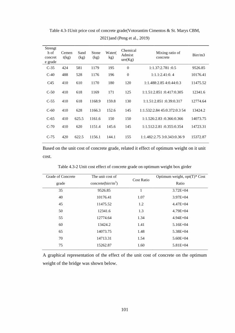
101

Table 4.3-1Unit price cost of concrete grade(Votorantim Cimentos & St. Marys CBM,

2021)and (Peng et al., 2019)

Strengt

h of

concret

e grade

Cemen

t(kg)

Sand

(kg)

Stone

(kg)

Water(

kg)

Chemical

Admixt

ure(Kg)

Mixing ratio of

concrete Birr/m3

C-35 424 581 1179 195 0 1:1.37:2.781 :0.5 9526.85

C-40 488 528 1176 196 0 1:1.1:2.41:0. 4 10176.41

C45 410 610 1170 180 120 1:1.488:2.85 4:0.44:0.3 11475.52

C-50 410 618 1169 171 125 1:1.51:2.851 :0.417:0.305 12341.6

C-55 410 618 1168.9 159.8 130 1:1.51:2.851 :0.39:0.317 12774.64

C-60 410 628 1166.3 152.6 145 1:1.532:2.84 45:0.372:0.3 54 13424.2

C-65 410 625.5 1161.6 150 150 1:1.526:2.83 :0.366:0.366 14073.75

C-70 410 620 1151.4 145.6 145 1:1.512:2.81 :0.355:0.354 14723.31

C-75 420 622.5 1156.1 144.1 155 1:1.482:2.75 3:0.343:0.36 9 15372.87

Based on the unit cost of concrete grade, related it effect of optimum weight on it unit

cost.

Table 4.3-2 Unit cost effect of concrete grade on optimum weight box girder

Grade of Concrete

grade

The unit cost of

concrete(birr/m3)

Cost Ratio Optimum weight, opt(T)* Cost

Ratio

35 9526.85 1 3.72E+04

40 10176.41 1.07 3.97E+04

45 11475.52 1.2 4.47E+04

50 12341.6 1.3 4.79E+04

55 12774.64 1.34 4.94E+04

60 13424.2 1.41 5.16E+04

65 14073.75 1.48 5.38E+04

70 14713.31 1.54 5.60E+04

75 15262.87 1.60 5.81E+04

A graphical representation of the effect of the unit cost of concrete on the optimum

weight of the bridge was shown below.

102

Figure 4.3-1 Effect of the unit cost of concrete grade on the optimum weight of the bridge

The unit cost of concrete grade ratio time‘s optimum weight gives the effect of cost of

concrete on box girder depth. The graph represents the unit cost of concrete grade

effect on the optimum weight of the bridge. As the graph show effect of the unit cost

of concrete grade changes the graph direction from o right. Because high strength

concrete achieved its strength by using admixture and jelly in addition to other

concrete gradients. These lend cost effect is higher than the weight effect when we

move from C-35 to C-75 concrete grade. Therefore based on the value of the table

and graph concrete grade from C-45 up to C-55 is the optimal concrete grade for the

box girder of Abay Bridge. The graph in this range gives intermediate point less

weight and less cost. Using concrete grade from C-45 up to C-55 is not having much

effect. So for Abay extradosed cable-stayed bridge using C-45 concrete grade is more

economical than C-55 concrete grade.

4.4 The optimum height of the pylon

A pylon is a tapered column that is connected to all cables and transmits cable forces

to the pier. The result of optimum pylon height is 24.43m for a fixed span length. As

the grade of concrete increases pylon height and weight are decreased. By optimizing

the height of the column, it will also change the inclination of the cable. Also, stay

cable force depend on the height of the pylon. As pylon height is more optimized

vertical stay cable force reduces. It acts likes prestressing force on decks.

0.00E+00

1.00E+04

2.00E+04

3.00E+04

4.00E+04

5.00E+04

6.00E+04

7.00E+04

35 40 45 50 55 60 65 70 75

Op

tim

um

Wei

gh

t,(T

)

Specified Compressive Strength of Concrete, fc', Mpa

unit cost of

concrete

grade(birr/m3)

103

The value of pylon height getting from optimization is in the range that

recommended values of tower height ratios from a H/L range of 1/7 to 1/13 (Stroh,

2012). The population of existing extradosed cable-stay bridges has not followed

Mathivat‘s original suggestion that a 1/15 height/span ratio would be the optimal

value. Based on existing bridges tower heights that have been used are slightly taller

than recommended by Mathivat‘s(Stroh, 2012).

4.5 Effect of concrete grade on the optimum height of the pylon

Pylon is a vertical member and it acts as a compressive member. Concrete grade

affects the height of the pylon and the optimum weight of the pylon. Effect of

concrete grade on pylon is like same that box girder effect. The optimization of pylon

height above the deck is done by taking the fixed force of stayed cable. And pylon is

fixed connected to piers. Effect of concrete grade on the optimum height of pylon and

weight are the list Table 4.5-1.

Table 4.5-1Effect of concrete grade on the optimum height and weight of pylon

Grades of Concrete, Mpa Optimum height pylon(m) Optimum pylon weight of bridge(T)

C-75 23.02 436.47

C-70 23.12 437.47

C-65 23.65 438.47

C-60 23.88 439.47

C-55 24.43 440.48

C-50 25.37 441.5

C-45 26.98 442.51

C-40 27.5 443.89

C-35 27.9 445.9

104

Figure 4.5-1Effect of concrete grade on height and weight of pylon

4.6 Optimum angle of Cables Stay

The angle of stay cable is one of the most critical factors in the design of extradosed

cable-stayed bridges. Using a small angle of stay cables leads to large prestressing

cable forces in the deck, and lends a small vertical cable force component. It also

affects the length of stay cable tendon. As the angle of stay cable increase length of

stay cable increases and weight also increase. Excessive cable forces also increase the

stress concentrations at the anchorage points in both the pylon and the deck. A large

angle of stay cable increases the vertical force of stay cables this lends increasing

pylon height. Optimization of the angle of stay cable of extradosed cable-stay bridge

done by considering 60%- 85% dead load and 30% of the live load (approximately

10% dead load) resisted by supporting stay cable. In the optimization process

minimum, dead load resisted by stay cables is 79%. Effect of stay cable force will

improve the stress performance of the main beam; therefore, the cable force layout

and corresponding tower height have critical impacts on the structural performance of

extradosed bridge.

430

435

440

445

450

0

5

10

15

20

25

30

C-75 C-70 C-65 C-60 C-55 C-50 C-45 C-40 C-35

Op

tim

um

p

ylo

n w

eigh

t o

f b

rid

ge(

T)

Opti

mum

hei

ght

pylo

n (

m)

specificied compressive strength of concrete, fc', Mpa

Optimum height pylon(m) Optimum pylon weight of bridge(T)

105

Table 4.6-1Optimum angle of stay cable for fixed span length for side span

Stay cable number optimum Angle of stay

cable(o)

optimum Length of stay

cable (m)

Side-span

C1 30.99 26.37

C2

26.46 32.27

C3

24.01 38.27

C4

22.24 44.31

C5

20.89 50.38

C6

19.83 56.48

C7

18.97 62.59

C8

18.27 68.72

C9 17.69 74.85

Table 4.6-2Optimum angle of stay cable for fixed span length for Mid-span

Stay cable number optimum Angle of stay

cable(o)

optimum Length of stay

cable (m)

Mid-span

C1 30.98 26.37

C2

26.46 32.27

C3

24.01 38.27

C4

22.24 44.31

C5

20.89 50.38

C6

19.83 56.48

C7

18.97 62.59

C8

18.27 68.72

C9 17.69 74.85

106

Values of stay cable angle getting in the range that recommended by (Stroh, 2012)

angle of extradosed cable-stay bridge must greater than 15o.

4.7 Effect of concrete grade on the angle of the stayed cable

When the grade of concrete decreased the amount of dead load is increased. The

angle of supported cable also increases as the dead load is increased because stay

cable in extradosed cable bridge carries at least 70% of total dead load and 30% of

live load. As the angle of the stay cable increases the amount of vertical reaction in

the stay cable is increasing. As used minimum stay cable angle most of the load is

resisted by girder. Effect of concrete grade with stay cable angle in reverse but the

effect on each cable angle is minimum. Effect of Concrete grade on the angle of stay

cable was list in tabular form Table 4.7-1.

Table 4.7-1Effect of Concrete Grades on Optimum angle of stay cable

Stay cable

number

stay cable angle for different concrete grade

C-45 C-50 C-55 C-60 C-65 C-70 C-75

a. Side span cables

C1 32.13 31.01 30.99 30.02 30.01 29.99 29.11

C2 28.12 27.21 26.46 26.01 26.36 26 25.86

C3 27.91 25.98 24.01 23.51 23.01 22.98 21.01

C4 23.04 22.89 22.24 21.98 21.44 21.24 21.21

C5 21.86 21.02 20.89 20.13 20.09 19.89 19.19

C6 19.83 19.83 19.83 19.63 19.13 18.83 19.13

C7 19.97 19.37 18.97 18.67 18.32 18.07 17.97

C8 19.52 18.97 18.27 18.21 18.1 17.89 17.27

C9 18.99 18.61 17.69 17.64 17.02 16.99 16.69

b. Middle span cables

C1 32.13 31.01 30.98 30.02 30.01 39.99 29.11

C2 28.12 27.21 26.46 26.01 26.36 26 25.86

C3 27.91 25.98 24.01 23.51 23.01 22.98 21.01

C4 23.04 22.89 22.24 21.98 21.44 21.24 21.21

C5 21.86 21.02 20.89 20.13 20.09 19.89 19.19

C6 19.83 19.83 30.99 19.63 19.13 18.83 19.13

C7 19.97 19.37 26.46 18.67 18.32 18.97 17.97

C8 19.52 18.97 24.01 18.21 18.1

17.89 17.27

C9 18.99 18.61 22.24 17.64 17.02

16.99 16.69

4.8 Comparison of the conventional and optimal design approach

Conventional design of Abay extradosed cable stays bridge. It models by software

finite element software MIDAS CIVIL 2019.

107

Conventional design output gives more weight than optimal design. Because during

conventional design not done many iterations like optimization design in Matlab. It

tests 5000 population size in a single iteration. The optimal design of the Abay

extradosed cable-stay bridge gives more reducing weight than conventional ones.

Summary of comparison of the weight of optimum design and conventional design

output of the three main superstructures parameters were discussed.

4.8.1 Comparison of conventional versus optimal design of box girder

The weight at the point of the pier is maximum. Because there is a maximum moment

and shear at the point of the pier. It needs more cross-sections. In the two designs

output weight is maximum at pier point. But by comparing conventional weight with

the optimum weight of the bridge deck optimum design given more reduced weight. It

reduced weight by 19.47% of the conventional design output of box girder weight.

This reduced weight was important for the bridge by reducing settlement and for the

owner of the bridge saving material usage. The amount of weight in each section of

the bridge was discussed as follows in Figure 4.8-1.

Table 4.8-1Comparison of conventional versus optimal design of box girder

Section

Bridge(m)

Conventional weight of

bridge(T)

Optimum Weight of

Bridge(T) Reduced Weight(T)

0 6800 5470 1420

10 5790 5110 680

20 5690 4910 777

30 5040 3970 1070

40 4810 3320 1490

50 4440 3310 1130

60 4200 2980 1220

70 3970 2690 1280

80 3690 2470 1220

90 3500 2310 1190

Total weight 38500 31100 7400

Weight Comparison of Optimum and Conventional Design output of box girder

graphed below in Figure 4.8-1.

108

Figure 4.8-1Weight Comparison of Optimum and Conventional Design box section

Bar graph representation of conventional design with optimum design output and

reduced weight of box girder was represented by graph using the cumulative mass of

bridge segment.

Table 4.8-2 Cumulative mass of 90m bridge segment

Conventional bridge weight(T) optimum bridge weight(T) Reduced weight(T)

38500 31100 7400

Bar graphs simply show the decreasing amount of weight by comparing the optimum

design with the conventional one.

0.00E+00

1.00E+03

2.00E+03

3.00E+03

4.00E+03

5.00E+03

6.00E+03

7.00E+03

8.00E+03

0 10 20 30 40 50 60 70 80 90

Conventional weight

of bridge(T)

Optimum Weight of

Bridge(T)

109

Figure 4.8-2Comparison cumulative conventional design output and optimum design output

of bridge girders section

4.8.2 Comparison of conventional and optimal design of pylon

By comparing the conventional weight of pylon with an optimum weight of pylon,

optimum design output gives more reduced weight. It reduces the amount of material

by 20.03% from the conventional weight of pylon.

Table 4.8-3 Conventional weight of pylon and optimum weight of pylon with the reduced

amount of weight

Conventional pylon weight (T) Optimum pylon weight (T) Reducing pylon of weight t(T)

552.04 441.48 110.56

0.00E+00

5.00E+03

1.00E+04

1.50E+04

2.00E+04

2.50E+04

3.00E+04

3.50E+04

4.00E+04

4.50E+04

Conventional

bridge weight(T)

optimum bridge

weight(T)

Reduced

weight(T)

Conventional

bridge weight(T)

optimum bridge

weight(T)

Reduced

weight(T)

110

Weight reduction represents by a bar graph as shown in Figure 4.8-3

Figure 4.8-3Weight comparison of the two design outputs of the pylon

4.8.3 Comparison of Conventional versus optimal design of cable

Abay extradosed cable-stayed bridge has 9 cables in the single pylon. Bridge support

twin pylon. So that at point of pier 18 cable is support girder. Consider half-bridge

width for a single pylon. Cables carry 70% dead load and 30% of live load. Stay cable

design takes 10% of a dead load of deck equal to live load. By considering load effect

for stay cable-stay optimum length and conventional length are shown.

0

100

200

300

400

500

600

Conv. pylon wt.

(Ton)

Opt. pylon wt.

(Ton)

Redu. pylon of

wt. (Ton)

Conv. pylon wt.

(Ton)

Opt. pylon wt. (Ton)

Redu. pylon of wt.

(Ton)

111

Table 4.8-4Comparison of Conventional stays cable length with optimum length side span

stay cable

Cable position Actual length(m) The optimum length of

stay cable (m) Reduced length, (%)

Side span cables

C1 29.13 26.37 9.49

C2 35.63 32.27 9.42

C3 42.34 38.27 9.62

C4 49.01 44.31 9.59

C5 55.91 50.38 9.88

C6 62.87 57.48 8.57

C7 69.85 63.59 8.96

C8 76.87 69.72 9.3

C9 83.89 75.85 9.58

Table 4.8-5Comparison of Conventional stays cable length with optimum length middle span

stay cable

Cable position Actual

length(m)

The optimum length of stay

cable (m) Reduced length, (%)

Middle span cables

C1 29.01 26.87 7.39

C2 35.49 32.27 9.06

C3 42.18 38.27 9.28

C4 48.84 44.31 9.28

C5 55.73 50.38 9.59

C6 62.67 56.48 9.87

C7 69.65 63.59 8.69

C8 76.64 69.72 9.03

C9 83.66 75.85 9.33

To compare conventional stay cable length and optimum stay cable length, optimum

length is more economical it reduced the length by 10% of conventional design output

of cable length.

112

Table 4.8-6Cumulative conventional stay cable length and optimum stay cable length and

reduced length

Convectional Length of Stay

Cable(m)

Optimum Stay Cable

Length(m) Reduced Stay Cable Length (%)

1009.37 908.49 10

Figure 4.8-4Comparison of conventional and optimum stay cable length and the reduced

amount

4.9 Analysis of parametric sensitivity

In this paper, three design parameters are selected: the main girder weight, cable

stiffness, and cable tension. Each parameter is modified separately to different scales

while the other two parameters are unchanged, then the structural analysis is

conducted to obtain the variation on girder deflection, cable force, and stress at the

control section of the main girders. Therefore, primary sensitive parameters and

secondary sensitive parameters are identified according to how they rate in terms of

their effect quantity.

1009.37(m)

908.5(m)

100.87

0

200

400

600

800

1000

1200

1

Convetional Length of Stay Cable Optimum Stay Cable Length

Reduced Stay Cable Length

113

4.9.1 Parametric sensitivity of girder weight.

The Abay River Highway Bridge is a 380m span prestressing post-tension extradosed

cable-stayed bridge. Bridge divide 1050 node and 153 elements. For construction

used cantilever casting method, its effect on the girder deflection due to dead load and

live load, cable force, and stress at the control section of the main girders is analyzed

on the completed bridge state and the results are presented in Figure 4.9-1, Figure

4.9-2 and Figure 4.9-3. All data of in each node and element getting from finite

element MIDAS CIVIL 2019.

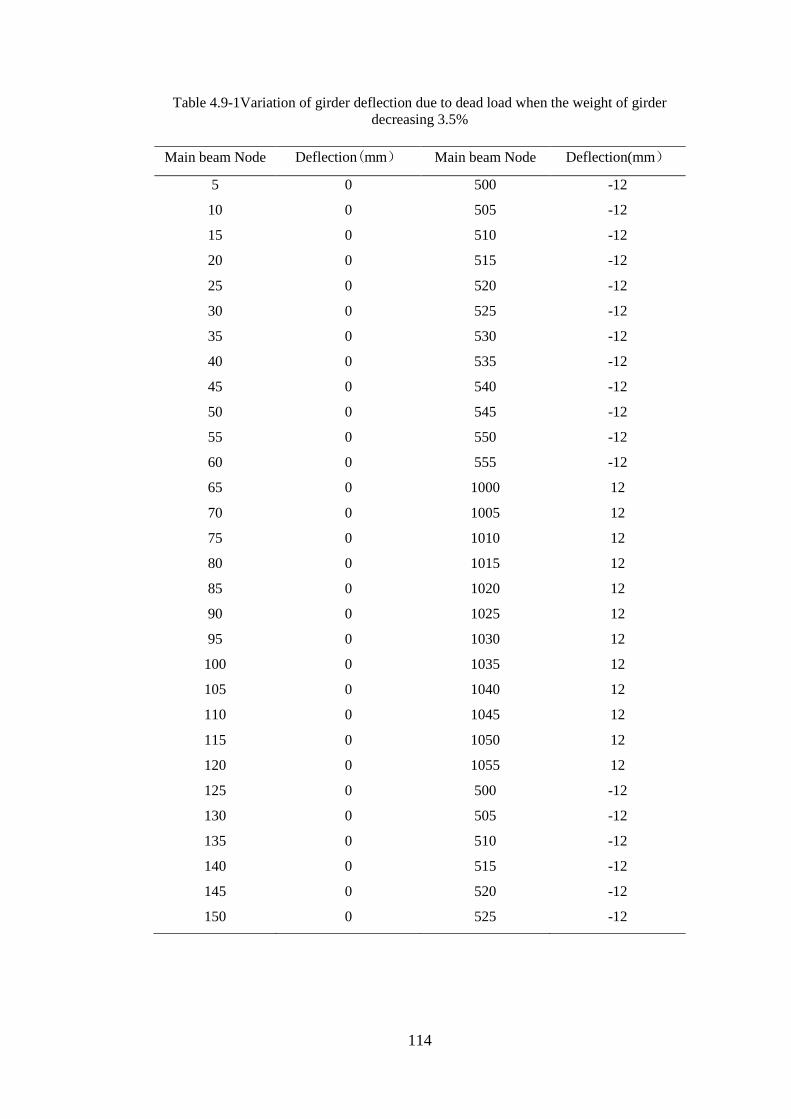
114

Table 4.9-1Variation of girder deflection due to dead load when the weight of girder

decreasing 3.5%

Main beam Node Deflection(mm） Main beam Node Deflection(mm）

5 0 500 -12

10 0 505 -12

15 0 510 -12

20 0 515 -12

25 0 520 -12

30 0 525 -12

35 0 530 -12

40 0 535 -12

45 0 540 -12

50 0 545 -12

55 0 550 -12

60 0 555 -12

65 0 1000 12

70 0 1005 12

75 0 1010 12

80 0 1015 12

85 0 1020 12

90 0 1025 12

95 0 1030 12

100 0 1035 12

105 0 1040 12

110 0 1045 12

115 0 1050 12

120 0 1055 12

125 0 500 -12

130 0 505 -12

135 0 510 -12

140 0 515 -12

145 0 520 -12

150 0 525 -12

115

Figure 4.9-1Variation of girder deflection due to dead load when the weight of girder

decreasing 3.5%

Limit of deflection due to live to load （L/800）=225.00 mm for construction of bridge.

Table 4.9-2Variation of girder deflection due to live load though the length of the bridge

when the weight of girder decreasing 3.5%

Node DZ (mm) Node DZ (mm)

1 1.79 80 69.19

5 17.65 85 66.39

10 42.41 90 59.28

15 58.55 95 51.31

20 63.10 100 41.11

25 60.44 105 26.95

30 48.61 110 10.57

35 34.21 115 9.81

40 3.98 120 38.58

45 14.79 125 52.51

50 30.81 130 60.79

55 41.70 135 62.59

60 53.69 140 55.45

65 61.49 145 41.46

70 66.61 150 11.26

75 69.45 153 1.80

-15

-10

-5

0

5

10

15

0 200 400 600 800 1000 1200

Dis

pla

cem

ent(

mm

)

Main beam Node

116

Figure 4.9-2 Variation of girder deflection due to live load when the weight of girder

decreasing 3.5%

0.00

10.00

20.00

30.00

40.00

50.00

60.00

70.00

80.00

0 50 100 150 200

Def

lect

ion o

f dec

k d

eck f

or

live

load

(m

m)

Node

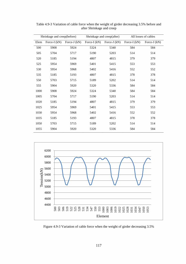
117

Table 4.9-3 Variation of cable force when the weight of girder decreasing 3.5% before and

after Shrinkage and creep

Shrinkage and creep(before) Shrinkage and creep(after) All losses of cables

Elem Force-I (kN) Force-J (kN) Force-I (kN) Force-J (kN) Force-I (kN) Force-J (kN)

500 5908 5924 5324 5340 584 584

505 5704 5717 5190 5203 514 514

520 5185 5194 4807 4815 379 379

525 5954 5969 5401 5415 553 553

530 5954 5968 5402 5416 552 552

535 5185 5193 4807 4815 378 378

550 5703 5715 5189 5202 514 514

555 5904 5920 5320 5336 584 584

1000 5908 5924 5324 5340 584 584

1005 5704 5717 5190 5203 514 514

1020 5185 5194 4807 4815 379 379

1025 5954 5969 5401 5415 553 553

1030 5954 5968 5402 5416 552 552

1035 5185 5193 4807 4815 378 378

1050 5703 5715 5189 5202 514 514

1055 5904 5920 5320 5336 584 584

Figure 4.9-3 Variation of cable force when the weight of girder decreasing 3.5%

4400

4600

4800

5000

5200

5400

5600

5800

6000

6200

500

503

506

519

522

525

528

531

534

547

550

553

100

0

100

3

100

6

101

9

102

2

102

5

102

8

103

1

103

4

104

7

105

0

105

3

Ten

sion(k

N)

Element

118

Figure 4.9-4 Variation of girder stress when the weight of girder decrease 3.5%

The above figures show that when the concrete box girder weight decrease by 3%-5%

from the pier to mid-span, the effect on the main beam elevation and the cable force

of the bridge completed state is greater. While the stress dispersion of negative

moment is generated at the control section of the beam, in the light of the above

passage, can get that the effect on the bridge completed state is great when the beam

weight is increased, so should control the cubic amount of concrete strictly in the

construction.

4.9.2 Parametric sensitivity of cable stiffness.

In the case of the same length of structural members, structural stiffness depends on

the elastic modulus and the geometric properties of A and I, and the support

conditions of the elastic state of the material. For the extradosed cable-stayed bridge,

on the premise that the support condition simulation accuracy, the stiffness depends

on the E, A, and I of the beam, tower, and cable. As a result of limited space, only the

cable stiffness sensitivity analysis was operated, the stiffness error of cable mainly

comes from modulus E and area A of steel wire, which under normal circumstances,

the production of steel have high accuracy, so the error of its area A is limited, while

the elastic modulus of high strength steel is generally more stable.

-2

-1

0

1

2

3

4

5

6

7

1 3 5 7 9 11 13 15 17 19 21 23 25 27 29 31 33 35

Stre

sss(

N/m

m2

)

Element

Top

Stress(N/mm^2)

Bottom

stress(N/mm^2)

119

So these two errors are relatively small, but because the span of the extradosed cable-

stayed bridge is generally relatively large, the cable sag effect will cause the axial

stiffness of cable down, usually, through the conversion of the elastic modulus to

modify, this paper analyzes the impact on the bridge state when cable elastic modulus

E increase by 3 %. Girder tension stress in variation of elastic modulus in top stress

tension (FTL)and bottom stress tension( FBL) of box girder in each element of bridge

length is state in Table 4.9-4.

120

Table 4.9-4 Variation of girder tension stress when Modulus changes through the length of

the bridge

Elem FTL

(N/mm^2)

FBL

(N/mm^2)

1 -1.06 -0.29

2 0.79 8.95

3 1.16 6.88

4 1.30 6.34

5 1.52 5.40

6 1.68 4.62

7 1.75 3.94

8 2.09 2.69

9 2.14 1.91

10 1.25 4.50

11 3.19 1.32

12 3.07 1.41

13 2.83 1.57

14 2.59 1.69

15 2.51 1.70

16 2.48 1.69

17 2.48 1.68

18 2.47 1.67

19 2.48 1.66

20 2.47 1.65

21 2.46 1.67

22 2.42 1.72

23 2.44 1.75

24 2.52 1.74

25 2.74 1.62

26 0.62 6.57

27 1.31 4.11

28 1.97 2.49

29 1.97 2.82

30 1.71 4.13

31 1.61 4.71

32 1.47 5.43

33 1.26 6.33

34 1.23 6.99

121

Figure 4.9-5Variation of girder stress when Modulus change through the length of the bridge

4.9.3 Parametric sensitivity of cable tension

All the cables of Abay Bridge take repeatedly stretching method. In this paper; the

last tension of every stay-cable is increased by 2% when doing tension sensitivity

analysis. Its effect on the girder deflection, cable force, and stress at the control

section of the main girders on the completed bridge state is analyzed.

Table 4.9-5Stay cable force from mid-span to pier

Side-span

Cable Number F （N）

C1 5059000

C2 5215000

C3 5352000

C4 5704000

C5 5820000

C6 5902000

C7 5947000

C8 5955000

C9 5909000

-2

0

2

4

6

8

10

FTL(N/mm^2)

FBL(N/mm^2)

122

Figure 4.9-6 Stay cable force from mid-span to pier

Table 4.9-6 Stay cable tension force from side-span to pier

Middle-span

Cable Number F (N)

C1 5041000

C2 5179000

C3 5320000

C4 5675000

C5 5800000

C6 5894000

C7 5955000

C8 5982000

C9 5962000

5000

5100

5200

5300

5400

5500

5600

5700

5800

5900

6000

6100

0 2 4 6 8 10

Ten

sio

n F

orc

e(K

N)

Cable No

Cable Tension(KN)

Cable Tension(KN)

123

Figure 4.9-7Stay cable tension force from side-span to pier

4800

5000

5200

5400

5600

5800

6000

6200

0 2 4 6 8 10 12

Ten

sio

n f

orc

e(K

N)

Cable No

Cable Tension(KN)

Cable Tension(KN)

124

5 CONCLUSION AND RECOMMENDATION

5.1 Conclusion

The goal of this research was to optimize the superstructure weight of prestressed

post-tensioning extradosed cable-stayed bridge by considering the depth of girder

with the height of pylon and angle stay cable. Those three parameters are the main

loading carrying components of the bridge. This paper state that saves material

amount by considering these three main superstructure parameters. The amount of

material described in terms of prestressing reinforcement, concrete, and reinforcement

bar by comparing conventional design out of Abay extradosed cable-stayed bridge

that builds in Abay River. The following conclusions were drawn from the present

work.

1. The result indicates that the bridge has unwanted mass. As comparing between

conventional depth and optimum depth, optimum depth given more reducing

weight. This gives the minimum weight of concrete, prestressing reinforcement,

and non-prestressing reinforcement for each section of the bridge. The result

shows that at the point of pier depth of girder is 5.129m and at point of mid-span

and abutment 2.62m.

2. Concrete grade and weight of bridge have an inverse relation

3. As a study of the effect unit cost of the concrete grade on optimal weight was

given that the optimal grade of concrete for prestressing posts tensioning

extradosed cable-stay bridge is form C-45 up to C-55 concrete grade is optimal.

4. The optimum height of the pylon above the deck is 24.43m for a fixed span length

of 180m.

5. As result shows that amount of stay cable parameter depends on the weight of the

girder and the amount of prestressing force applies on decks. As the amount of

stay cable force increase with increasing dead load amount. For stay cable angle

optimization considering prestressing force.

6. The effect of concrete grade on the angle of stay cable is less because it more

depends on prestressing force on deck. Because of using fixed prestressing force

in deck change angle less.

7. To compare the conventional and optimal design of box girder, pylon, and stayed

cable length using by weight of the bridge, the optimal design gives less weight.

125

The total reducing amount is 10% from stay cable length and 20.03% from pylon

weight and 19.47% % from box girder weight. Generally, 49.47% of the weight is

reduced from conventional design output. So that for the design of extradosed

cable-stayed bridge design use optimization techniques gives the best result.

8. Based on the parameters sensitivity analysis of the weight of girder, the stiffness

and tension of cable the influences of the weight of girder and the tension of cable

are noticeable and need amended as the main design parameters when the bridge

model are being calculated. Through the parameters sensitivity analysis of

structure, the bridge model can be optimized. Combining the optimization with

the technology of model amended can guarantee the accuracy of bridge

construction control.

5.2 Recommendation

In this study, the effect of box girder on optimum weight, effect of concrete grades on

the weight of three main parameters (box girder pylon and angle of stay cable), pylon

height, and angle of stay cable were investigated.

It is recommended to use 5.129m girder depth at the pier and 2.62m at mid-span

for a 180m main span length.

It is recommended to use C-45 concrete grade for box girder of extradosed bridge.

Use the height of pylon 24.43m for a 180m span length.

Using the optimum angle of stay cable 32.13o for using optimum grade of

concrete C-45 in girder.

For extradosed cable-stayed bridge, optimum superstructure value is 5.129m

depth of girder at point of the pier and 2.62m at point of mid-span and optimum

height of pylon is 24.43m and optimum first stay cable angle is 32.13o for using

optimum concrete grade C-45.

For using the optimum output of superstructure parameter of Abay Bridge, must

consider optimization on substructure component of bridge.

The parameters sensitivity analysis of structure is useful for parameter

recognition and correct for error adjustment in the construction process.

126

REFERENCE

Abebe, wubishet J. (2018). Optimization of PC Girders for Bridge Design_by

WubishetJ.pdf. Jimma University.

Abebe, F. (2016). Department of Civil and Environmental Engineering Design of

Precast Pre-Stressed Concrete Girder Bridges As an Economical Solution for

Congested Urban Areas Design of Precast Pre-Stressed Concrete Girder

Bridges As an Economical Solution For Congested Urb. Addis Ababa Institute

Of Technology.

An, Y. F. (N.D.). An Optimization Index To Identifyidentify The Optimal Design

Solution Of Bridges. University Of Trento Department.

Introduction to Design Sensitivity Analysis, (2015).

Bendsøe, M. P. and Sigmund, O. (2003). Topology Optimization: Theory, Methods

and Applications. Springer-Verlag.

Bhattacharjya, R. K. (2015). Genetic Algorithms.pdf.

Biliszczuk, J., Onysyk, J., Barcik, W., Toczkiewicz, R., & Tukendorf, A. (2017).

Extradosed Bridges in Poland—Design and Construction. Frontiers in Built

Environment, 2(January), 1–9. https://doi.org/10.3389/fbuil.2016.00037

Bujnak, J., Odrobinak, J., & Vican, J. (2013). Extradosed bridge - Theoretical and

experimental verification. Procedia Engineering, 65, 327–334.

https://doi.org/10.1016/j.proeng.2013.09.050

Chang-Huan Kou1, a, Tsung-Ta Wu2, b, Pei-Yu Lin3, C. (2014). Optimization of

Cable Force of Extradosed Bridges. Vols 587-5.

Chen, E. W., & Duan, L. (2000a). Bridge Engineering Handbook.

Chen, E. W., & Duan, L. (2000b). Cable-Stayed Bridges Man-Chung. In Bridge

Engineering.

Chessa, J. (2002). matlab_fem.pdf.

China Communications Construction Company Limited. (2020). Bahirdarabay River

Bridge And Approach Roaddesign-Build Project: Lot 1 - Abay River Bridge And

127

Adjacent Concrete Structures.

Dharma, A. P., & Suryoatmono, B. (2019). Non-Linear Buckling Analysis of Axially

Loaded Column with Non-Prismatic. 5(3).

Dipl.-Ing., vorgelegt von, & Ägypten, E. A. E. S. aus. (2013). Form Finding For

Cable-Stayed And Extradosed Bridges. der Technischen Universität Berlin zur.

EBCS EN- 8 Part. (2014). EBCS- 8 Part 1 Design of Structures R for (Issue

December).

Gladwell, G. M. . (1991).

f i i i h f f f.

Golebiowska, I., & Peszynski, K. (2018). Cable vibration caused by wind. EPJ Web

of Conferences, 180, 1–6. https://doi.org/10.1051/epjconf/201818002031

Load and Resistance Factor Design., 18 Engineering Journal 74 (2015).

Jafari, M. (2019). Aerodynamic-load identification and prediction of wind-induced

vibration of structural / power-line cables and traffic signal structures.

Jerzy Onysyk,Wojciech Barcik, R. T. and A. T. (2017). Extradosed bridges in

poland-design and construction. 1–11.

Kaljima Corporation. (2019). Ethiopia‘s First Extradosed Bridge to Span the Blue

Nile Gorge. 35(May 2006), 30. https://doi.org/10.36621/0397-004-998-003

Kirsch, P. U. (1993).

Structural_Optimization_Fundamentals_and_Applications_by_Prof_Uri.pdf.

Klarbring, P. W. C. · A., & An. (2008).

An_Introduction_to_Structural_Optimization_by_Peter_W_Christensen.pdf.

Kou, C., Wu, T., & Lin, P. (2014). Optimization of Cable Force of Extradosed

Bridges. 589, 1577–1580. https://doi.org/10.4028/www.scientific.net/AMM.587-

589.1577

Lee, B. K., & Lee, J. K. (2021). Buckling of Tapered Heavy Columns with Constant

Volume. 1–14.

128

Mast, R. F. (1998). Analysis of cracked prestressed concrete sections: A practical

approach. PCI Journal, 43(4), 80–90.

https://doi.org/10.15554/pcij.07011998.80.91

Mermigas, by K. K., & A. (2008). Behaviour and Design of Extradosed Bridges.

University of Toronto ©.

Miskiewicz, M., & Pyrzowski, L. (2018a). Load test of new European record holder

in span length among extradosed type bridges. E3S Web of Conferences, 63, 1–2.

https://doi.org/10.1051/e3sconf/20186300006

Miskiewicz, M., & Pyrzowski, L. (2018b). Load test of new European record holder

in span length among extradosed type bridges. E3S Web of Conferences, 63, 1–6.

https://doi.org/10.1051/e3sconf/20186300006

Niels J.Gimsing, C. T. G. (2012). Cable Supported Bridges- Concept and Design .pdf.

Technical University of Denmark.

Nippon Koei Co., L. (2005). The Feasibility Study of Padma Bridge Final Report.

AASHTO LRFD 2010 BridgeDesignSpecifications 5th Ed..pdf, (2010).

Özel, C. N., Özkul, Ö., Erdoğan, E., Ergüner, K., & Görgülü, G. (n.d.). The First

x B i g i  : D ig f h A Ç ı B i g . 1–8.

PARSAEI, H. R. (1997).

Genetic_Algorithms_and_Engineering_Design_by_Mitsuo_Gen,_Runwei.pdf.

Peng, S., Rong, C., Cheng, H., Wang, X., Li, M., Tang, B., & Li, X. (2019).

Mechanical Properties of High-Strength High-Performance Reinforced Concrete

Shaft Lining Structures in Deep Freezing Wells. Advances in Civil Engineering,

2019. https://doi.org/10.1155/2019/2430652

Prashant Kumar Srivastava1*, Simant2, S. S., & 1Asst. (2017). Structural

Optimization Methods: A General Review. International Journal of Innovative

Research in Science, 6(9,), 3.

PTI. (2001). 3. Recommendations for stay cable design, testing and installation.pdf.

Rechenberg, I. (1973). . Evolution strategy: Optimization of technical systems by

129

means of biological evolution. Fromman-Holzboog, Stuttgart.

Reuter, U., & Liebscher, M. (2009). Global Sensitivity Analysis in Structural

Optimization. 7th European LS-DYNA Conference, Salzburg.

http://www.dynamore.de/dynamore/documents/papers/euro2009/f-i-03.pdf

S.N.Sivanandam. (2008).

Introduction_to_Genetic_Algorithms_by_S_N_Sivanandam,_S_N_Deepa.pdf.

Saad, F. (2000). Structural Optimization of Extradosed Bridges.

Setral. (2002). 2. Cable stays.pdf.

Shirono, Y., Takuwa, I., Kasuga, A., and Okamoto, H. (1993). The design of an

extradosed prestressed concrete bridge – the Odawara Port Bridge.

Stroh, S. L. (2012). On The Development Of The Extradosed Bridge Concept (Issue

January). University of South Florida.

Tejashree G. Chitari*1, T. N. N., & ME. (2019). The Study of Pylon Height Variation

for Cost Optimization of Extradosed Bridge.

Tejashree G. Chitari1, T. N. N., & 1ME. (2019). Cost Optimization of Extradosed

Bridge by varying Cable Position Tejashree.

Votorantim Cimentos, & St. Marys CBM. (2021). 2021 General Contractors Price

List. http://www.canadabuildingmaterials.com/en-ca/Pages/Products and

Services/GTA-Pricelist.aspx

Zhongguo(John) Ma, Maher K. Tadros, C. S. P. (2004). Prestressed Concrete Box

Girders Made from Precast Concrete Unsymmetrical Sections.pdf.

130

APPENDIX

Annex 1 Extradosed Cable-Stayed Bridge structural modeling

Table 1 Maximum moment and shear value of Abay extradosed cable-stayed bridge(China

Communications Construction Company Limited, 2020)

Item Strength(KN.m) Action (KN.m)

Bending

moment

Mid span 566323 333176

Support -1901784 -886238

Item Strength(kN) Action(kN)

Max 73587 40500

Min 73587 -40500

Annex 2 Design calculation process of the pylon

Table 2 Value Axial force and bending moment of pylon under different load combination

Loads ULS

Strength Ⅰ Strength Ⅱ Strength Ⅲ

DC 1.25 1.25 1.25

DW 1.5 1.5 1.5

LL 1.75 1.35 1.5

WS 1.4

FR 1 1 1

Axial Force(kN) 1357.3 1053.1 823

Moment(kN.m) 16683.5 13179.8 1387.1

Force(kN) Shear 58847.8 62836.9 59607.8

Annex 3 Design Optimization Code using GA in Matlab for angle of stay

cables

1) Stay cable design

Fitness Function for Stay Cable in Extradosed Cable Stay Bridge

Function Y = staycableobjfun(x)

% weight parameter for stay cable

%pc = 0.0848; % unit weight (N/mm3)

yca=0.0023; % density of the cable material low relaxation strand

dca=15.2; % diameter of stay cable

131

n=46; % number of cable in single tendon

Aca=pi*dca^2/4; % area of one bar in cable tendon

av =n*Aca*x(3); % area of f16mm for shear reinforcement within a

distance S (mm2)

% weight function of stay cable

Y= x (4)*yca*av; % weight function of stay cable of extradosed

cable-stay bridge component

Nonlinear Constraint Functions Definition for Stay Cable for

Extradosed Cable-Stay Bridge

Function [C,ceq] = Extracableconst(x)

% Material properties

fc = 45; % cylindrical compr.strength for box girder (N/mm2)

fpu = 1860; % specified tensile strength of prestressing

reinforcement (Mpa)(fpu = 270,000 psi (low-relaxation strand;)

Eca= 190e3; % typical modulus of elasticity of stay cable (N/mm^2)

Qult=1.6e3; %Ultimate tensile stress of the stay cable material

% stress limits in concrete

fcbd =0.6*fpu; % for stays cable are designed to a maximum

allowable tensile strength(fcbd is the design stress (allowable

cable stress)

Qa=0.45*Qult; % Allowable stress in the stay cable under SLS loads

ftw = 0.5.*sqrt(fc); % Allowable tensile stress at working loads

Ec=27660; % Young’s modulus of concrete (N/mm2)

Mw= 40218.79e6*0.3; % Service limit state-I bending moment (Nmm)

w=3.3727E+11+(0.1*3.3727E+11); % total load that apply on girder

(dead load + live load)

%% section properties of box girder

Re=24700; % total width of roadway (mm)

Angle=45; % angle of external web inclination (o)

dduth=32; % diameter of duct(mm_)

Cov=50; % concrete cover of box girder (mm)

z1=90000; % half bridge length of bridge (mm)

w1=0.03404*z1+2.2e3;

tb=min([1/20*w1, 200]); % thickness of bottom flange

w2=2.315e3; % optimum side width of cantilever

w3=0.0645*z1+9e3; % optimum bottom width of box girder

132

tw=max([1/36*w1+cov + dduth, 200+dduth]); % thickness of web(mm)

%% equations for effective depth of reinforcing steel

db = 32; % assumed diam. of bar assume it (mm).

Agg = 25; % maximum aggregate size (mm)

Sh = max ([1.5*db, 1.5*Agg, 38]); % clear spacing of parallel bars

(horizontal) (mm)

Sv = max ([25, db]); % clear spacing between layers of bars

(vertically) (mm)

tft=max([200, 150+dductho]); % thickness of top flange

as = pi*db^2/4; % area of a single reinf. Bar (mm2)

nb =As/as; % Number of bars

npr = min([(tw+Sh-124)/(Sh+db), nb]); % Number of bars per a row

nr = nb/npr; % Number of reinforcement rows

hr = nr*db+ Sv*(nr-1); % Height of reinforcement rows

dst = 62+hr/2; % depth from extreme tension fiber to centroid of

reinf. Steel (mm)

d = w1-dst; % effective depth of reinforcement steel (mm)

% effective depth of prestressing steel

dsrd = 15.2; % assumed diam. of prestressing low relaxation strand

(mm)

Nspt = 31; % number of strands per tendon

ap = 0.77.*pi.*dsrd.^2./4; % steel area of a single strand

(mm2)(using a reduction factor of 77 % of nominal area of the

strand)

dduct = 125; % diameter of duct, (mm)

Sduct = 38; % clear vertical and horizontal spacing of ducts (mm)

nst = w4/ap ; % number of strands required

nt = nst/Nspt; % Number of tendons

ntr = min([(tw+Sduct-200)/(dduct+Sduct),nt]); % Number of tendons

per a row

nrt = nt/ntr; % Number of rows of prestressing tendons

hrt = dduct.*nrt+Sduct*(nrt-1); % height of rows of prestressing

tendons

dpt = 50+12+Sduct+25+hr+hrt./2; % Depth from extreme tension fiber

to centroid of prestressing tendons (mm)

133

dp = w1-dpt; % Depth from extreme top fiber to centroid of

prestressing steel (mm)

d1 =5129; % optimum depth of box girder (mm)

W1= 2135; % optimum side cantilever width (mm)

W2 = 8650; % optimum bottom slab width (mm)

n=3; % number of opening cell

Gs=(x (3)-(n+1)*tw)/(n+1); % spacing between web or internal girder

Aeff=Re*tft+x (3)*tb+ (d1-tb-tft)*tw*(n-1)+(d1-tb-tft)/sin…

(43.9)*tw*2; % total area of concrete

yt=(W2)*tb^2/2+Re*tft*(d 1-tft/2)+(d1-tb-tft)*tw*(n-1)*(d1-tb…

-tft)/2+ (d1-tb-tft)/sin (43.9)*tw*1/3*(d1-tb-tft)/sin…

(43.9)*2)/Aeff; % depth from c.g of section to extreme bottom

fiber(mm)

yb = d1-yt; % depth from c.g of section to extreme top fiber (mm)

Iy=W2*tft^3/12+W2*tft*(yt-tft/2)^2+tw*(x(1)-tb-tft)^3/12*(n-

1)+tw*(x(1)-tb-tft)*((x(1)-tb-tft)/2-yt)^2+tw*((x(1)-tb-

tft)/sin(43.9))^3/12+tw*(x(1)-tb-tft)/sin(43.9)*(((x(1)-tb-

tft)/sin(43.9))*1/3-yt)+Re*tft^3/12+Re*tft*(tft/2-yt)^2; % Gross

moment of inertia of concrete in y axis

Zb=Iy/yb; % section modulus of the extreme bottom fiber (mm3)

Zt=Iy/yt; % section modulus of the extreme top fiber (mm3)

xb=((Re.*(Re/2).*tft)+W2*tb*(W1+(d1-tb-tft)/tan(43.9)+W2/2)+(d1-tb-

tft)/sin(43.9)*tw*(W1+(d1-tb-tft)/tan(43.9)*2/3)+(d1-tb-

tft)/sin(43.9)*tw*(W1+(d1-tb-tft)/tan(43.9)+W2+(d1-tb-

tft)/tan(43.9)*1/3)+(d1-tb-tft)*tw*(W1+(d1-tb-

tft)/tan(43.9)+Gs)+(d1-tb-tft)*tw*( W1+(d1-tb-tft)/tan(43.9)+(n-

1)*Gs))/Aeff; % depth from c.g of section to extreme bottom fiber

in x- axis(mm)

Ixeff=tft*Re^3/12+tft*Re*(Re/2-xb)^2+tb*W2^3/12+tb*W2*(W1+ (d1+tb….

-tft)/tan (43.9) +W2/2-xb) ^2+ ((d1-tb-tft)/tan (43.9))*tw^3/12…

+ ((d1-tb-tft)/tan (43.9))*tw*(x(2)+(d1-tb-tft)/tan (43.9)*2/3…

-xb)^2+(d1-tb-tft)/sin (43.9)*tw^3/12+ (d1-tb-tft)/sin(43.9)*tw…

*(W1+W2+(d1-tb-tft)/tan (43.9)+(d1-tb-tft)/tan(43.9)*1/3-xb)^2…

+(d1-tb-tft)*tw^3/12+ (d1-tb-tft)*tw*(W1+ (d1-tb-tft)/tan (43.9)....

+Gs-xb) ^2+ (d1-tb-tft)*tw^3/12+(d1-tb-tft)*tw*(W1+((d1-tb…

-tft)/tan (43.9) +2*Gs-xb) ^2);

134

Ixy=xb.*yb.*Aeff;

finf = ftw/0.85+Mw/(0.85*Zb); % extreme bottom fiber stress, finf

developed at a given eccentricity e (N/mm2)

e = yb-dpt; % possible maximum eccentricity of prestressing force

from c.g.c (mm)

P = Aeff*finf*Zb/(Zb+Aeff*e); % minimum prestressing force at a

known eccentricity, e(N)

%% Geometric properties

r=0.555; % Ratio of main span and side span

L=180e3; % Length main span length of bridge (mm)

% total stress in the cable

dca=15.2; % diameter of wire

wc =x(2)*w; % desired equivalent vertical stay cable forces

% initial tension loading in stay cable

E=205e3; % modulus of elasticity for stay cable (Gpa)

yca=0.0023; % density of the cable material

f=0.6*fpu; % cable tensile stress

Eeq=E/(1+(x(3)*yca)^2/12*f^3); % equivalent modulus of elasticity

fn=0.00346884; %unknown factor depending only on the parameter 0.65

M2= (-w*L^2*(1+0.65^3)+wc*L^2*(62/125+24*fn)/(8*0.65+12)); %bending

moment at the support (2) for the structure

M3=M2; %bending moment at the support (2) for the structure

R1= (M2-w*(0.6*L)^2/2-6*wc*L^2/100)/r*L; % reaction force at the

support (1) for the structure

R2= (w*(L+2*0.65*L)-0.8*L*wc-2*R1)/2=R3; % reaction force at the


Q2r=-R1+w*r*L-0.2*L*wc-R2; % shear force on the right hand side of

the support (2) for the structure

Q3r=Q2r+w.*L-0.4*L.*wc-R3; % shear force on the right hand side of


M3s1=-0.01633; % bending moments at the supports (3) (kN.m)

M2s1=-2*(0.65+1)*M3s1; % bending moments at the supports (3) (kN.m)

Rlsl= (M2s1-0.3*L)/(r*L);

R4s1=M3s1/0.65*L;

R3s1= (M2s1-R4s1*((r+1)*L)^2/L);

R2s1= (M3s1-(Rlsl*(r+1)*L-1.3*L)/L);

135

Q2rs1=-Rlsl-R2s1-1; % the shears force on the right-hand side of the

support (2)

Q3rs1=-Rlsl-R2s1-1-R3s1; % the shear force on the right-hand side of


M2m1= (0.714*(1+r)-0.273)/(4*(1+r)^2-1)*L; %bending moment at

support (2)

R1ml= (M2m1)/(r*L);

M3m1=0.357*L-2*(1.65)*M2m1;

R4m1=M3m1/0.65*L;

R2m1= (M3m1-R1ml*((1+r)*L-0.7*L)/L);

R3m1= (M2m1-R4m1*((1+r)*L-0.3*L)/L); %

Q2m1=-R1ml-R2m1; % shear force on the right hand side of the support

(2) for the structure

Q3m1=-R1ml-R2m1-1-R3m1; % shear force on the right hand side of the


% M(x) calculation in 11 zones

z=38e3; % section distance on bridge (moment determine every z

section)

if (-r*L<=z<=0.4*L) ; % first section distance of bridge

M(z) =R1*(r*L+z)-w*(r*L+z)^2/2; % bending moment in first section

elseif(-0.4*L<=z<=0.2*L)

M(z) =R1*(r*L+z)-w*((r*L+z)^2)/2+wc*((0.4*L+z))^2/2; % bending

moment in second section

elseif(-0.2*L<z<=0)

M(z) =R1*(r*L+z)-w(r*L+z)^2/2+0.2*L*wc* (0.3*L+z); %bending moment

in third section

elseif (0<z<=0.2*L)

M(z)=M2-(w*((z)^2)/2)-(Q2r*(z)); %bending moment in fourth section

else if(0.2*L<z<=0.4*L)

M (z) =M2-w*((z)^2)/2-Q2r*(z)-wc*(z-0.2*L)^2/2; %bending moment in

fifth section

elseif(0.4*L<z<0.6*L)

M (z) =M2-w*(z^2)/2-Q2r*(z) +0.2*L*wc*(z-0.3*L); %bending moment in

sixth section

elseif 0.6*L<z<=0.8*L

136

M(z)=M2-w*(z^2)/2-Q2r*(z)+0.2*L*wc*(z-0.3*L)+wc*(z-0.6*L)^2/2;

%bending moment in seventh section

elseif(0.8*L<=z)&&(z<=L)

M(z)=M2-w*(z^2)/2-Q2r*(z)+0.4*L*wc*(z-0.5*L); %bending moment in

eight section

elseif L<z<=1.2*L

M(z)= M3-w*((z-L)^2/2)-Q3r(z-L); % bending moment in ninth section

elseif 1.2*L<z<=1.4*L

M(z) = M3-w*((z-L)^2)/2-Q3r*(z-L)+wc*(z-1.2*L)^2/2; %bending moment

in tenth section

elseif 1.4*L<z<=(1+r)

M(z) = M3-w*((w-L)^2)/2-Q3r*(z)+0.2*L*wc*(z-1.3*L); %bending moment

in eleventh section

% the bending moment at any point, the entire length of the deck,

due to a vertical unit load F=1 acting at s1

if(-r*L<=z<0.3*L)

Ms1 (z) = Rlsl*(r*L+z);

elseif -3*L<z<=0

Ms1 (z) = Rlsl*((r*L+z) + (0.3*L+z));

elseif 0<z<=0.3*L

Ms1(z) = M2s1-Q2rs1*z;

elseif (L<z<=(r+1)*L)

Ms1(z) = M3s1-Q3rs1*(z-L);

% the bending moment at any point, along the entire length of the

deck, due to a vertical unit load F=1 acting at m1

if(-r*L<z<=0)

Mm1 (z) =R1ml*(r*L+z);

Elseif (0<z<=0.3*L)

Mm1 (z) =M2m1-Q2m1*z;

elseif(0.3*L<z<=L)

Mm1 (z) =M2m1-Q2m1*z+ (z-0.3*L);

elseif (L<z<=(1+r)*L)

Mm1 (z) =M3m1-Q3m1*(z-L);

H=x (3) ^2-22e3^2;

FDi= (0.2*wc*L/(2*x (4)*sin(x(1)))); % desired stay cable force for

each stay cable FDi under dead load may be determined,

137

%the forces resulting from the bottom straight tendons at the middle

of the main span

xb=24.7e2/2;

eb=5.129e3./2-xb-cov;

Mf=-Fp.*eb; % moment of prestressing force in decks

M21=-3*Mf*Lf/L* (1/(3+2*r)); % bending moment at support two

R1f=M21/(r*L); % reaction at support 1 and 2

R2f=-(-0.3*Mf*Lf/(r*L^2)*1/(3+2*r)); %the forces resulting from the

top straight tendons at the pylons

et=w1/2-Zt-cov;

Ls=100e3; % from center to center of cable stayed

Ms=Fp*et;

M22=Ms*(1-(24*Ls*r*L-3*Ls^2)/(12*r*L^2*(1+r)-4*r^2*L^2));

R1s=-Ms*(1-(24*Ls*r*L-3*Ls^2)/(12*r^2*L^3*(1+r)-4*r^3*L^3));

R2s=-R1s;

%the forces resulting from the bottom straight tendons in the side

spans

Mo=-Fp*eb;

Lamda=0.03;

Lo=63e3;

M23=-6*Mo*Lo*(lamda*L+Lo/2)/(3*r*L^2*(r+1)-r^2*L^2);

R1o=M23/(r*L);

M23=R1o*r*L;

R2o=-M23/(r*L);

R1o=-R2o;

%the forces resulting from draped tendons at the middle of the main

span

Weq=8.*eb*Fp./L.^2;

Tc1=-4*eb/Lf*Fp;

M2w=Weq*Lf/48*(3*(L-Lf) ^2+6.*Lf.*(L-Lf) +2*Lf.^2/L.* (r/3+1/2));

R1w=M2w/r*L;

R2w1=-Weq*Lf/2-R1w;

R2p1=3*P*r*L*(2*r*L+L+Lf)*(r*L+ (L-Lf)/2)-2*P*r^3*L^3/

(6*r^2*L^3*(r+1)-2*r^3*L^2);

R1p=-(R2p1+Tc1);

M2p=R1p*r*L;

138

M24=M2w+M2p;

% the forces resulting from draped tendons in the side spans

%the forces due to the equivalent uniform load Weq alone, can be

determined by using the equations

Weq= (8*eb/Lo^2)*Fp;

r1= (Lo*(r*L-lamda*L-Lo/2)/ (0.55*L))*Weq;

r2=Weq*Lo*(lamda*L+Lo/2)/r*L; % where r1 and r2 are supplementary

variables and will be used below to determine M2w

%1/3*lamda^3/r*L^2*r1+Lo*r2*(r*L-lamda*L- Lo)*((lamda*L+Lo/2)/r*L)…

+ 1/2*Lo*(r1*lamd*L-r2*(r*L-lamda*L-Lo))*(lamda*L+Lo/3)/(r*L)…

+ 1/12*Weq*Lo^3*(y*L+Lo/2)/(r*L)+1/2*r2*(r*L-y*L-Lo)^2*(r*L…

-2/3*(r*L-y*L-Lo)/(r*L))=M2w*L*(1/2+r/3);

M2w=1/3*lamda^3/r*L^2*r1+Lo*r2*(r*L-lamda*L-

Lo)*((lamda*L+Lo/2)/r*L)+1/2*Lo.*(r1.*lamda*L-r2*(r*L-lamda*L-

Lo))*(lamda*L+Lo/3)/(r*L)+1/12*Weq*Lo^3*(lamda*L+Lo/2)/(r*L)+1/2*r2*

(r*L-lamda*L-Lo)^2*(r*L-2/3*(r*L-lamda*L-Lo)/(r*L))/(L*(1/2+r/3)); %

R1w1=-(Weq*Lo*(r*L-lamda*L-Lo/2)-M2w)/(r.*L);

R2w2=-(Weq*Lo+R1w1);

%The final forces resulting from the equivalent uniform loads Weq

and the 2x2 vertical nodal loads P, can be determined then by

superposition.

P1=-(4*eb)/Lf*Fp;

Ls1=(r*L-lamda*L-Lo);

Ls2= (r.*L-lamda.*L);

Lsi=Ls1:Ls2;

R2p2=symsum((-P1*(3*r*L*(r*L+L+Lsi)*(r*L-Lsi)-(r*L…

-Lsi)^2*(r*L+2*Lsi)-3*Lsi^2*(r*L-Lsi))/(3*r^2*L^3*(r+1)-r.^3…

*L.^3)), i, 1, 2);

R1p1=-2.*P1-R2p2;

M2p=R1p*r*L+P1*(Ls1+Ls2);

M25=M2-(M24+M22+M2p);

FPTi= (R2f+R2s+R2o+R2w1+R2p1+R2w2+R2p2)/(2*(x(4)*sin(x (1))))…

-(R1f+R1s+R1o+R1w+R1p+R1w1+R1p1)/(2*(x(4)*sin(x(1))));

Fi=3*w*L/(x(4)*sin(x(1))*1/(1+3/2*e/L*cot(x (1)))); % stay cable

force of the cable no. i under the effect of the dead load prior to

the shortening/re-stressing of any stay cable by the forces Fi

139

yca=0.0023; % density of the cable material

% x (2); % horizontal length of stay cable position

FDI= (FDi-Fi-FPTi+Pcb);

H=x (5)*tan(x(1));

H1=H+x (6);

y=x(5)+x(7);

d= (fcbd/Eeq*(H1+y^2/H));

%H= (24.6e3-8*1.1e3):1.1e3:24.6e3; %vertical height of stay cable

position

%Qsptc=(yca/fcbd*(FDI)*x(3),1, 9); % total cable steel quantity

Qcb=x(3)*yca/fcbd*(H+x(5)^2/H)*(FDI); % quantity of cable material

d= (fcbd/Eeq)*(H+(x(5)^2/H)); % vertical deflection d at the lower

stay cable anchorage

FDI=Qcb*fcbd/yca/((H+(22e3^2/H)));

Tc=pi*dca^2/4*Qult;

Aca=53*pi*15.262/2;

Qw=FDI/Qcb; % Axial stress in the stay cable due to dead load

fb=0.937; %(Hz)

m= (Aca*yca*x(3)/x(3)); % mass per length of stay cable (kg/m)

ft=1.043; % Symmetric torsional fundamental(HZ)

fn=n/2* (I*((FDI/m)^2)); % Cable base frequency

%Nonlinear inequality constraints [c] written of the form gi(xi)<= 0

% stay cable force limit

g1=0.7-4*wc*56e3/w* (2*r*L+L);

g2=Zs1+ (M (z)*Ms1 (z))/ ((Ec)*Ixeff); % the vertical deflection of

deck at s1 due to the combination of w(x) and wc

g3=Zm1+M (z)*Mm1 (z)/ (Ec*Ixeff); % the vertical deflection of deck

at m1 due to the combination of W(x) and WC

g4= (fn-ft)*I5;

g5= (fn-fb)*I5;

g6=FDI-0.55*Tc; %Stay cables tensile forces limit

g7= (800*d/L-1)*I5; % allowable stay cable deflections

g8= (4*22e3*8*6e3/ (w*2*r*L+L))*I5;

g9=Qw-Qa;

C=[g1;g2;g3;g4;g5;g6;g7;g8;g9;g10;g11;g12];

Main Code for Running the Genetic Algorithm

140

% Problem parameters

% x(1) = a; x(2)=n ; x(3)=Lcb; x(4)=N x(5)=HL, x(6)=Sv, x(7)=Sh

objfcn=@staycableobjfun;

% set boundary values of variables

lb =[15 0.9 1e3 14 13e3 1e3 5e3]

ub=[35 1.9 90e3 18 24.9e3 1.4e3 7e3]

consfcn= @Extracableconst;

%% set ga options

Options = optimoptions(@ga,...

'PopulationSize', 5000...

'MaxGenerations', 100,...

'EliteCount',1,...

'Maxstallgeneration',100 ,...

'FitnessScalingFcn',@fitscalingprop,...

'NonlinearConstraintAlgorithm','auglag',...

'InitialPenalty',10,...

'PenaltyFactor',100,...

'FunctionTolerance', 1e-10, ...

'ConstraintTolerance', 1e-10,...

'PlotFcn',@gaplotbestf);

%Call |ga| to solve the Problem

% we can now call |ga| to solve the problem.

rng(1,'twister') % random number generator for reproducibility

[xbest,fbest,exitFlag] =

ga(@staycableobjfun,nvars,Aineq,bineq,Aeq,beq,lb,ub,@Extracableconst

, 1:3,options);

% _Analyze the Results

Display (xbest)

%% return optimal value

fprintf ('\n Y function returned by ga = %g\n', fbest)

Annex 4 Design Optimization Code using GA in Matlab for box girder

% this is fitness function for Extradosed main loading carrying

component

function z = Extramaincompfun(x)

% weight parameters box girder

141

pc = 0.0024; % density of concrete(g/mm3)

ps= 0.00785; % density of steel_prestressing strands and

reinforcing bars (g/mm3)

pp= 0.0023; % density of steel_prestressing strands and reinforcing

bars (g/mm3)

tb=min([1/36*x(1), 200]); %thickness of bottom flange

L=5000%length of half span of main span bridge (mm)

dduth=32; % diameter of duct

dductho=dduth+10;% diameter of duct hole

Asb = 0.004*tfb*((NG-1)*x(5)+x(2))*L+0.005*tfb*((NG-1)*x(5)+tw); %

total area of bottom slab reinf.

NL = 4; % number of legs of vertical stirrups

dsh = 16; % diam. of shear rebar (mm)

av = NL*pi*dsh^2/4; % area of f12mm for shear reinforcement within a

distance S (mm2)

tft =max([200, 150+dductho]); %thickness of top flange

Re=24700; % width of roadway (mm)

A1= Re*tft; % concrete cross sectional area of the top slab of box

girder (mm^2)

Ag= ((Re-2*x (2))/2-(x(3)/2))*((x(1)-tb))+(x(3)*(x(1)-tb)); % gross

cross sectional area of concrete (mm2)

ddut=32; % diameter of duct

dduth=ddut+10;% diameter of duct hole

cov=50; % concrete cover of box girder

n=3; number of opening cell

tw=max([1/36*x(1)+(cov+dduth),(200+dduth)]); % thickness of web(mm)

y2=x(1)-tb-30;% height of opening

y3=x (3)/3-(3-1)*tw; % width of opening

Ag= (1/2)*((Re-(2*x(2)))+x(3))*(x(1)-tb); % gross cross sectional

area of concrete (mm2)

y2=x (1)-tb-300; % height of opening

y3=x (3)/3-((3-1)*tw); % width of opening

Aho=3*(y3*y2)+(y3*y2); % area of opening cell (mm2)

Aeff = A1+Ag-Aho; % effective cross sectional area of concrete (mm2)

VAsb = 0.004*tb*((NG-1)*x(3)+tw)*L+0.005*tb.*((NG-1)*x (3) +tw) ^2;

% volume of bottom slab reinf (mm3)

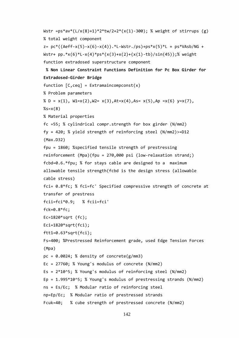
142

Wstr =ps*av*(L/x(8)+1)*2*tw/2+2*(x(1)-300); % weight of stirrups (g)

% total weight component

z= pc*((Aeff-x(5)-x(6)-x(4)).*L-Wstr./ps)+ps*x(5)*L + ps*VAsb/NG +

Wstr+ pp.*x(6)*L-x(4)*ps*(x(3)+x(2)+(x(1)-tb)/sin(45));% weight

function extradosed superstructure component

% Non Linear Constraint Functions Definition for Pc Box Girder for

Extradosed-Girder Bridge

function [C,ceq] = Extramaincompconst(x)


% D = x(1), W1=x(2),W2= x(3),At=x(4),As= x(5),Ap =x(6) y=x(7),

%s=x(8)

% Material properties

fc =55; % cylindrical compr.strength for box girder (N/mm2)

fy = 420; % yield strength of reinforcing steel (N/mm2)>=D12

(Max.D32)

fpu = 1860; %specified tensile strength of prestressing

reinforcement (Mpa)(fpu = 270,000 psi (low-relaxation strand;)

fcbd=0.6.*fpu; % for stays cable are designed to a maximum

allowable tensile strength(fcbd is the design stress (allowable

cable stress)

fci= 0.8*fc; % fci=fc' Specified compressive strength of concrete at

transfer of prestress

fcii=fci*0.9; % fcii=fci'

fck=0.8*fc;

Ec=1820*sqrt (fc);

Eci=1820*sqrt(fci);

ftt1=0.63*sqrt(fci);

Fs=400; %Prestressed Reinforcement grade, used Edge Tension Forces

(Mpa)


Ec = 27760; % Young's modulus of concrete (N/mm2)

Es = 2*10^5; % Young's modulus of reinforcing steel (N/mm2)

Ep = 1.995*10^5; % Young's modulus of prestressing strands (N/mm2)

ns = Es/Ec; % Modular ratio of reinforcing steel

np=Ep/Ec; % Modular ratio of prestressed strands

Fcuk=40; % cube strength of prestressed concrete (N/mm2)

143

% stress limits in concrete

fci = 0.8.*fc; % Specified compressive strength of concrete at

transfer of prestress

fct = 0.6*fci; % Allowable compressive stress at transfer of

prestress

% Compressive Stress Check of the Main Beam at SLS

PHicwatsupport=0.93; % compressive stress check factor for mid-span

PHiwamidspan=0.98; % compressive stress check factor for support

ftt2=0.6*pHiwamidspan*fci; %compressive strength of girder at top

fiber

fcw = 0.45*fc; % Allowable compressive stress at working loads

ftw = 0.5.*sqrt(fc); % Allowable tensile stress at working loads

% loading box girder

Md =-886238e6; % design moment at support due to Action (kN.m)

%Md=333176e6; % design moment at mid-span due to Action (kN.m)

Vd =-73587e3; % max shear due to Action (N)

Tu = 131.8; % maximum torsion due to action (N)

Pa=1980.3e3; % axial force (N)

Mw = 1880218.79e6; % Service limit state-I bending moment (Nmm)

M3 = 1696825.33e6; Service limit state-III bending moment (Nmm) for

tension control

Mf=5888.69e6; % fatigue load design bending moment (Nmm)

Mg=-1901784e6; %moment due to dead load at support point

%% Geometric properties

tb=min([1/36.*x(1), 200]); % thickness of bottom flange

%% section properties of box girder

Gs=(x(3)-(n+1)*tw)/(n+1);% spacing of interior girder tb=max([140,(gs-x(2))/30]);

be = min([L/4,12*x(3)+x(2),gs]);% effec.width for int. girder

bb=be;

Re=24700; % total width of roadway (mm)

wsup = 4000; % width of support pier(mm)

Angle=43.9; % angle of external web inclination ()

dduth =32; % diameter of duct

cov=50;% concrete cover of girder mm

Ao=201; % area enclosed by shear path, including the area of holes

144

dductho=dduth+10; % diameter of duct hole

Acp=x(3)+2*x(2)+(x(1)-tb)/sin (43.39); %Fulcrum Section area for

torsion (mm2)

tw=max([1/36.*x(1)+cov + dduth, 200+dduth]); % thickness of web(mm)

Ao=201; % area enclosed by shear path, including area of holes

dductho=dduth+10;% diameter of duct hole

tft=max([200, 150+dductho]); %thickness of top flange

tw=max([1/36.*x(1)+cov + dduth, 200+dduth]); % thickness of web(mm)

Gs=(x (3)-(n+1)*tw)/(n+1); % number of cell of box girder

Aeff=Re*tft+x (3)*tb+(x (1)-tb-tft)*tw*(n-1)…

+(x (1)-tb-tft)/sin (43.9)*tw*2;

yt=(x(3)*tb^2/2+Re*tft*(x(1)-tft/2)+(x(1)-tb-tft)*tw*(n-1)*(x(1)…

-tb-tft)/2+(x(1)-tb-tft)/sin(43.9)*tw*1/3*(x(1)-tb…

-tft)/sin(43.9)*2)/Aeff;

yb = x(1)- yt; % depth from c.g of section to extreme top fiber (mm)

Iy=x (3)*tft^3/12+x (3)*tft*(yt-tft/2) ^2+tw*(x (1)-tb-tft)

^3/12*(n-1)+tw*(x (1)-tb-tft)*((x (1)-tb-tft)/2-yt) ^2+tw*((x(1)…

-tb-tft)/sin (43.9)) ^3/12+tw*(x (1)-tb-tft)/sin (43.9)…

*(((x (1)-tb-tft)/sin (43.9))*1/3-yt)…

+Re*tft^3/12+Re*tft*(tft/2-yt)^2;

Zb=Iy/yb;

Zt=Iy/yt;

xb=((Re.*(Re/2).*tft)+x(3)*tb*(x(2)+(x(1)-tb-

tft)/tan(43.9)+x(3)/2)+(x(1)-tb… tft)/sin(43.9)*tw*(x(2)+(x(1)-tb-

tft)/tan(43.9)*2/3)+(x(1)-tb-tft)/sin(43.9)*tw*(x(2)+(x(1)…

-tb-tft)/tan(43.9)+x(3)+(x(1)-tb-tft)/tan(43.9)*1/3)+(x(1)-tb…

-tft)*tw*(x(2)+(x(1)-tb-tft)/tan(43.9)+Gs)+(x(1)-tb…

-tft)*tw*(x(2)+(x(1)-tb-tft)/tan(43.9)+(n-1)*Gs))/Aeff;

Ix=tft*Re^3/12+tft*Re*(Re/2-xb)^2+tb*x(3)^3/12+tb*x(3)*(x(2)…

+(x(1)+tb-tft)/tan(43.9)+x(3)/2-xb)^2+((x(1)-tb…

-tft)/tan(43.9))*tw^3/12+((x(1)-tb-tft)/tan (43.9))*tw*(x(2)…

+(x(1)-tb-tft)/tan (43.9)*2/3-xb)^2+(x (1)-tb…

-tft)/sin(43.9)*tw^3/12+(x(1)-tb-tft)/sin(43.9)*tw*(x(2)+x(3)+(x(1)…

-tb-tft)/tan(43.9)+(x(1)-tb-tft)/tan (43.9)*1/3-xb) ^2+(x (1)-tb…

-tft)*tw^3/12+(x (1)-tb-tft)*tw*(x(2) +(x(1)-tb-tft)/tan (43.9)…

+Gs-xb) ^2+(x (1)-tb-tft)*tw^3/12+(x (1)-tb-tft)*tw*(x(2)+((x(1)…

145

-tb-tft)/tan (43.9) +2*Gs-xb) ^2);

Ixy=xb*yb*Aeff;

%% equations for effective depth of reinforcing steel

db = 32; % assumed diam. of bar assume it (mm).

Agg = 25; % maxim aggregate size (mm)

Sh = max ([1.5*db, 1.5*Agg, 38]); % clear spacing of parallel bars

(horizontal) (mm)

Sv = max ([25, db]); % clear spacing between layers of bars

(vertically) (mm)

tft=max([200, 150+dductho]);%thickness of top flange

as = pi*db^2/4 ; % area of a single reinforcement bar (mm2)

nb = x(5)/as; % Number of bars

npr = min([(tw+Sh-124)/(Sh+db),nb]);% Number of bars per a row

nr = nb/npr; % Number of reinforcement rows

hr = nr*db+ Sv*(nr-1); % Height of reinforcement rows

dst =62+hr./2;%depth from extreme tension fiber to centroid of

reinforcement steel (mm)

d = x(1)-dst; % effective depth of reinforcement steel (mm)

% effective depth of prestressing reinforcement steel

dsrd =15.2;% assumed diameter of prestressing low relaxation strand

(mm)

Nspt = 31; % number of strands per tendon

ap = 0.77.*pi.*dsrd.^2./4; % steel area of a single strand

(mm2)(using a reduction factor of 77 % of nominal area of the

strand)

dduct = 125; %diameter of duct, (mm)

Sduct = 38; %clear vertical and horizontal spacing of ducts (mm)

nst = x(6)/ap;% number of strands required

nt = nst/Nspt; % Number of tendons

ntr= min([(tw+Sduct-200)/(dduct+Sduct),nt]); %Number of tendons per

a row

nrt = nt/ntr; % Number of rows of prestressing tendons

hrt = dduct*nrt+Sduct.*(nrt-1); %height of rows of prestressing

tendons

dpt = 50+12+Sduct+25+hr+hrt./2;%Depth from extreme tension fiber to

centroid of prestressing tendons (mm)

146

dp = x(1)-dpt;% Depth from extreme top fiber to centroid of

prestressing steel (mm)

% shear reinforcement steel

NL = 4; % No. of legs of vertical stirrups

dsh = 16; % diam. of bar for shear reinforcement (mm)

av = NL*pi*dsh^2/4;%area of shear reinforcement within a distance S

(mm2)

% NA depth c from equivalent stress block analyses

co = ((x(6)*fpu+x(5)*fy-0.85^2*fc*(be-tw)*tft)/(0.85^2*fc*tw)…

+(0.28*fpu)*x(6)./dp);

if (co > tft)

c = co; % NA depth for T section (mm)

c = (x (6)*fpu+x (5)*fy)/(0.85^2*fc*be+0.28*x(6)*fpu/dp); % NA depth

for rectangular section (mm)

fps = fpu*(1-0.28*c/dp); % Average stress in prestressing steel

(N/mm2)

de = (x(6)*fps*dp+x(5)*fy*d)/(x(6)*fps+(x(5)*fy)); % effective depth

from extreme compression fiber to centroid of tension force (mm)

a = 0.85*c; % depth of equivalent stress block (mm)

% Nominal flexural resistance, Mn

if(c>tft)

Mn = x (6)*fps*(dp-a/2) +x (5)*fy*(d-a/2) +0.85^2*fc*tft*(be-

tw)*(a/2-tft/2); % Mn for T section (mm)

Mn = x (6)*fps*(dp-a/2) +x (5)*fy*(d-a/2)-(x (5)*fy)*(ds'-a/2); % Mn

for rectangular section (mm)

%% extreme fiber stresses for computing Prestressing force

% total prestressing force at release

%% fsup = ftt-Mg/Zt; % extreme bottom fiber stress, finf developed

at a given eccentricity e (N/mm2)

finf = ftw/0.85+Mw/(0.85*Zb); % extreme bottom fiber stress, finf

developed at a given eccentricity e (N/mm2)

e = yb-dpt; % possible maximum eccentricity of prestressing force

from c.g (mm)

P = Aeff*finf*Zb/(Zb+Aeff*e); % x(5)*fpt; minimum prestressing force

at a known eccentricity, e (N)

% shearing force parameters

147

dv = max([0.9.*de,0.72*x(1),de-a/2]); % effective shear depth

Vu = Vd*(L/2-wsup/2-d)/L/2; % ultimate design shear force at a

distance d from face of support (N)

Vc = 0.083*2*sqrt (fc)*tw*dv; % shear capacity of concrete

% Shear Force Due To Required Vertical Reinforcement, Vs

teta=45; %Crack Angle

Vs = av*fy*dv*cot(teta)/(x(8)); % shear capacity of non prestressing

reinforcement

Vp = 0.85*P*(4*e/L); % shear capacity of non prestressing

reinforcement

bv=(Vu/0.9-Vp)/(0.25*dv*fc);

Vn = min ([(Vc+Vs+Vp),(0.25*fc*bv*dv+Vp)]); % nominal shear

resistance

% limits of longitudinal reinforcement

fcpe = 0.85*P*(1/Aeff+e/Zb); % compressive stress in concrete due to

effective prestress forces only (N/mm2)

fr = 0.97*sqrt(fc); % modulus of rupture (N/mm2)

Mcr = (fcpe+fr)*Ixeff/yt; % cracking moment (Nmm)

% limits of maximum reinforcement

% a). Using reinforcement index omega-om

Asn = 0;

rhp = x(5)/(be*d);

rhn = Asn/(be*d);

rhpr = x(6)/(be*dp);

Omp = rhp*fy/fc;

Omn = rhn*fy/fc;

Ompr = rhpr*fps/fc;

% b). Using imperic.

c/de <= 0.42

% cracked section analysis

fp1 = 0.85*P/Aeff; % stress in the prestressing tendons prior to the

application of Mw (N/mm2)

fp2 = 0.85*np*P*(e.^2/Ixeff+1/Aeff); % stress in prestressing

tendons due to decompression (N/mm2)

% incremental strain during the appl. of Mw

% let NA depth of cracked section be y = x (7)

148

if(x(7)> tft)

eo = (x(6)*(fp1+fp2))/(0.5*Ec*(tw*x(7)+(be-tw)*tft*(1+(x (7)-tft)/x

(7)))-(Es*x (5)*(d-x (7))/x (7) +Ep*x (6)*(dp.*x (7))/x (7)));

eo = (x(6))*(fp1+fp2)/(0.5*Ec*be*(x(7))-(Es*(x(5))*(d.)…

*(x(7)))/(x(7)+Ep.*(x(6))*(dp-x(7)/x (7)))));

fco = eo*Ec; % stress in concrete at service limit state (N/mm2)

fs = Es*eo*(d-x(7))/x(7); % tensile stress in reinforcing steel at

service stage (N/mm2)

fp3 = Ep*eo*(dp-x(7)/x(7); % tensile stress in prestressing steel at


fpk = fp1+fp2+fp3; % total tensile stress in prestressing steel at


Ts = x (5)*fs; % tension force in reinforcing steel at service limit

state (N)

Tp = x (6)*fpk; % tension force in prestressing steel at service

limit state (N)

Ca = 0.5*fco*be*x (7); % total compression force in concrete (N)

Cn = 0.5*fco*(be-tw)*(x (7)-tft)^2/x(7); % a force used to reduce

if x(7)>tft

dz = x(7)/3; % location of centroid of comp. force C from top (mm)

dzn = tft+(x(7)-tft)/3; % location of centroid of comp. force Cn

from top (mm)

% section properties of cracked transformed section

% --------------moment of inertia of cracked section---------------%

if(x(7)>tft)

Ict = tw.*x(7).^3./3+((be-tw).*tft.^3/12)+(be-tw).*tft*(x(7)…

-tft./2).^2+np.*x(6)*(dp-x(7))^2+ns.*x(7)*(d-x(7))^2; % 2nd moment

of area of cracked transformed section (mm4)

Ict = be*x(7)^3/3+np*x(6)*(dp-x(7))^2+ns*x(5)*(d-x(7))^2; % 2nd

moment of area of cracked transformed section (mm4)

% ---------------------deflection parameters----------------------%

frk = 0.63*sqrt(fc); % modulus of rupture for Ie computation (N/mm2)

Mck = frk*Ixeff/yb;%cracking moment for deflection computation (Nmm)

Ie = min([(Mck./Md).^2*(Mck./Md)*Ixeff…

+(1-(Mck./Md)^2*(Mck./Md).*(Ict),Ixeff]); %effective moment of

inertia for deflection calculation (mm4)

149

defD = (1.708E+19)./(Ec.*Ie); % total dead load deflection including

long term effects (mm)

defLL = (5.45E+17)/(Ec*Ie); % maximum live load deflection (mm)

defP = (0.85*5*L^2*e*P/(48*Ec*Ie)); % total effec. Prestressing

load deflection (mm)

% maximum crack width

cw1 = (fs - 40)*1e-3; % CEB-FIP-1970, crack width eq. (mm)

h1 = d-x (7)-dst; % depth from steel centroid to NA (mm)

h2 = d-x (7); % depth from NA ~ tension face (mm)

dc = 62+db./2; % concrete cover to closest bar layer (mm)

Atc = tw*2*dst/nb; % effective tension area of concrete per bar

(mm2)

cw2 = 0.076*(h2/h1)*fs*(dc*Atc)^(1/3)*1e-3*0.1451; % Gergely Lut2-

1968 crack equation (mm)

cw = max([cw1, cw2]); % maximum of the crack width given by the

above eqns.

cwa = 0.41; % allowable crack width for moderate exposure condition

%% fatigue stress ranges

ffs = ns* Mf.*(d-x(7))/Ict; % fatigue stress range in reinforcing

steel(N/mm2)

ffp = np* Mf.*(dp-x(7))/Ict; % fatigue stress range in prestressing

steel (N/mm2)

%% torsion resistance

Pc= (x (3) +2*(x (1)-tb)/tan (angle) +2*x (2)); % the length of the

outside perimeter of the concrete section

fpc=0.25*sqrt(fc);

Tcr=(0.125*sqrt(fc')*Acp^2)./Pc.*sqrt(1+fpc/(0.125*sqrt(fci)));

%% Axial force and moment capacity check

% Prmax=Nsp;

% Shear force capacity check

%% factored flexural resistance

Mr=0.9*Mn;

Mu=Vu*dv; % factored shear force

%% Stress Limits for Prestressing Tendons

fpj=0.8*fpu; % jacking stress for Low Relaxation Strand

150

fpt = 0.7*fpu; % Post-tensioning at anchorages and couplers

immediately after anchor set

fpy = 0.9*fpu; % Yield strength of Prestressing Strand

fpe = 0.8*fpy; % Allowable stress in tendons at working loads(stress

limitation)

%% Temporary Concrete Stress Limits at Jacking State before Losses

due to Creep and Shrinkage

% Fully Prestressed Components

fccj =0.55*(fci); % compressive stress limit of post tension

fctj=0.58*sqrt(fci); % tension stress limit of post tension---Area

with bonded reinforcement which is sufficient to resist 120% of the

tension force in the cracked concrete computed on the basis of

uncracked section

fsa=0.8*fr; %

dzn= tft+(x(7)-tft)/3;

% Bursting Forces Results of End Beam Prestressed reinforcement

As=201;

a1=309.64; %( mm)

alphab1=17; % angle of inclination of a tendon force with respect to

the centerline of the member;

rnb1=40; % Root number

Pub1=1395*19*139*1.2; % top and bottom--factored tendon force (N)

T=rnb1*As*Fs*phib;

Tburst=0.25*sum (Pub1.*(1-a1/x (2) +0.5*sum (Pub1*sin (alphab1))));

%Compression zone assumed in the strength limit state to the depth

of the actual compression zone stress block.


g1 = ftt2-P*(1/Aeff+e./Zt)-Mg/Zt; % Top fiber subjected to tension

at stress transfer stage

g2 = ftt1-(1/Aeff)*P+Mx*(yb*Iyeff-xb*Ixy)/(Ixeff*Iyeff-

(Ixy)^2)+My*(xb*Ixeff-yb*Ixy)/(Ixeff*Iyeff-(Ixy)^2); % Top fiber

subjected to tension at stress transfer stage

g3= P*(1/Aeff+e./Zb)-Mg/Zb-fct; % Bottom fiber subjected to

compression at stress transfer:

g4=fct-P/Aeff-Mx.*(yb.*Iyeff-xb.*Ixy)./(Ixeff.*Iyeff…

151

-(Ixy).^2)+My.*(xb.*Ixeff-yb.*Ixy)/(Ixeff*Iyeff-(Ixy)^2);% Bottom

fiber subjected to compression at stress transfer

g5=ftt2-P/Aeff-Mx*(yb*Iyeff-xb*Ixy)/(Iyeff*Ixeff+Ixy^2)…

+ My*(xb*Ixeff-yb*Ixy/ (Iyeff*Ixeff+Ixy^2)); % Top fiber subjected

to tension at stress transfer stage

g6= 0.85*P.*(1/Aeff-e/Zt) +Mw/Zt-fcw;

g7= ftw-0.85.*P.*(1./Aeff+e./Zb) +M3 /Zb;

g8=fct-Pa/Aeff+Md*yb/2*Ixeff+c*k; % live load stress limit

g9 = (Md-0.9.*Mn); % flexural strength required

g10= Vu-0.9.*Vn; % shear strength required

g11= Vu/0.9-(0.25*fc*dv)-Vp; % web requirement for shear

% limits of flexural reinf.

g12= abs(Md)/(0.9*dv)+abs(Vu/0.9-Vp)-0.5*min([Vu/0.9,Vs])-x(5)*fy-

x(6)*fps; % longitudinal reinf.

g13 = Vu/0.9-(0.5*Vs)-Vp-(x (5)*fy)-x (6)*fps; % min. longitudinal

reinf.

g14= (Md/dv+0.5*Pa+0.5*Vu*cot (angle)-x (6)*fpu)/ (Es*x (5) +Ep*x

(6)); %strain in reinforcement on flexural tension side

g15 = 1.2*Mcr; % minimum flexural reinf. Requirement

g16 = 0.004*tw*yb-x (5)-x (6); % minimum flexural reinforcement

required

g17 = (Omp+Ompr-Omn-0.3);

g18 = (c/de-0.42); % maximum flexural reinforcement required

bv=tw-dduct;

g19=Vu-0.1*fci*bv*dv*x (8); % maximum spacing of transverse

reinforcement

% limits of traverse reinforcement

g20= (x (8)-fy*av/ (0.083*tw*sqrt (fc))); % shear reinforcement

if (abs(Vu-0.9.*Vp)/(0.9*dv*tw) < 0.125*fc)

g21 = (x (8)-0.8.*dv); % spacing of shear reinf.

g21 = x (8)-min ([0.4*dv, 300]); % spacing of shear reinf.

% service load stress limit

g22 = P - x (6)*fpt; % stress limit in tendons at transfer

g23 = fs- min ([206, 0.6*fy]); % stress limit in reinforcing steel

at service limit state

% deflection limit

152

radd = 0;

tol = 1e-6;

confcnvald = defD-defP-radd;

g24 = confcnvald-tol; % camber due to prestressing shall counter

balanced by dead load deflection

g25= -confcnvald-tol;

g26= defLL-L/10000; % limit of vehicular live load deflection

% Crack width

g27= (cw-cwa); % spacing of longitudinal bars for crack control

% fatigue stress limit

g28 = (ffs-161.5); % limit on fatigue stress limit in reinforcing

steel

g29= (ffp-125); % limit on fatigue stress limit in prestressing

steel

% service load degree of prestress

g26=1-Mdec/Mw;

% check equilibrium conditions

% summations of internal couple must equal to working moment

if x(8) >tb

rad = Mw;

dz=x(1)./2-cov;

tol = 1e-6;

confcnvalm =Ts*d+Tp*dp+Cn-Ca*(dz)-rad;

g30 = confcnvalm-tol;%sum of service load moments when NA depth y>hf

g31 = -confcnvalm-tol;

rad = Mw;

tol = 1e-6;

confcnvalm = Ts*d+Tp*dp-Ca.*(dz)-rad;

g32 = confcnvalm-tol;%sum of service load moments when NA depth y<hf

g33= -confcnvalm-tol;

if x(8) > tft

radf = 0;

tol = 1e-6;

confcnvalf = Ts+Tp+Cn-Ca-radf;

g34= confcnvalf-tol; %sum of service load moments when NA depth y>hf

g35 = -confcnvalf-tol;

153

radf = 0;

tol = 1e-6;

confcnvalf = Ts+Tp-Ca-radf;

g36= confcnvalf-tol; %sum of service load moments when NA depth y<hf

g37 = -confcnvalf-tol;

O=0.9; % torsional resistance factor

g38=0.25*O.*Tcr-(Tu); % torsional resistance

g39 = (0.20*x (1)-x (7));

g40 = (x (8) - 0.75*x (1));

g41= (L/800); % deflection limit of bridge

% Compressive Stress Check of the Main Beam at SLS

Factor =0.93; % phi*watsupport

g42= (0.6*factor*fck); % Under the SLS combination I, the

compressive stress limit of the main beam

%Tensile Stress Check of the Main Beam at SLS

g43= (0.25*sqrt (fc)); %for segmental- constructed bridge, the

tensile stress limit of the joint is 0.25*fc under the SLS

combination III,

% Cable Stress limitation Check

g44=0.55*fpk; % cable stress meet the specifications requirements

g45=Tu*Pc/(2*0.9*Ao*fy)-x (4); % torsional reinforcement limit

g46= (fccj-0.6*phiw*fci); % Compressive Stress Limits in Prestressed

Concrete at Service Limit State after Losses, Fully Prestressed

Components

g47= (fctj-3*sqrt(fci)); % tension Stress Limits in Prestressed

Concrete at Service Limit State after Losses, Fully Prestressed

Components

g48=Vd-Vn; % constraint of shear force

g49=Tburst-O*T; % bursting force checks

g50=Vu/0.9-0.5*Vs-Vp-x (5)*fs-x (6)*fpu;

g51=x (8)-(av*fy)/ (0.083*bv*sqrt (fc));

%Minimum amount of reinforcement

g52=1.2*Mcr-0.9*Mn;

g53=1.33*Md-0.9*Mn;

g54= Mu/(dv*0.9)+(Vu/0.9-Vp)-0.5*min([Vu/0.9,(x(5)*fy*dv)/x(8)])-

((x(5)*fy+x(6)*fpu));% limit of longitudinal reinforcement

154

g55=Md/O*dv+0.5*Pa/O+ cot (angle*sqrt ((Vu/O-Vp)-0.5*Vs) ^2+

(0.45*Pc*Tu))-(x (6)*fps+x (5)*fy); % longitudinal reinforcement due

to torsion

% nonlinear equality const. functions defn.

C=[g1;g2;g3;g4;g5;g6;g7;g8;g9;g10;g11;g12;g13;g14;g15;g16;g17;g18;g1

9;g20;g21;g22;g23;g24;g25;g26;g27;g28;g29;g30;g31;g32;g33;g34;g35;g3

6;g37;g38;g39;g40;g41;g42;g43;g44;g45;g46;g47;g48;g49;g50;g51;g52;g5

3;g54;g55;g56,g57,g58;]; % nonlinear inequality const. functions

defn.

%% Main Code for Running the GA Algorithm


% D= x(1), W1= x(2), W2 = x(3),M= x(4), As = x(5),% Ap = x6, y=x7,

s=x(8)

objfcn=@Extramaincompfun; % calling fitness function

consfcn= @Extramaincompconst; % calling constraint Function


lb =[4551 1350 7800 100 1*10^3 1*10^3 900 100];

ub=[7818*10^3 3350 9500 10000 1*10^9 1*10^8 2000 400];

%% Develop Genetic algorithm for optimization

options = optimoptions(@ga,...

'PopulationSize',5000, ...

'MaxGenerations',1000, ...

'EliteCount',10,...

'Maxstallgeneration',1000,...

'FitnessScalingFcn',@fitscalingprop, ...

'NonlinearConstraintAlgorithm','auglag', ...

'InitialPenalty',1.5,...

'PenaltyFactor',1, ...


'ConstraintTolerance', 1e-10,...

'PlotFcn',@gaplotbestf)

%Call |ga| to solve the Problem

rng(1,'twister') % random number generator for reproducibility

[xbest, fbest, exitFlag] = ga (@Extramaincompfun, nvars, Aineq,

bineq, Aeq,…. Beq, lb, ub,@Extramaincompconst, 1:3, options);


155

display (xbest)


fprintf ('\n z function returned by ga = %g\n', fbest)

Annex 5 Design Optimization Code Using GA in Matlab for Pylon of

Extradosed Bridge

% this is fitness function for Pylon of Extradosed Bridge

Function Q = pylonobjfun(x)

% weight parameter for pylon


ps= 0.00785; % density of steel_prestressing strands and

reinforcing bars (g/mm3)

NL = 4; % number of legs of vertical stirrups

dsh = 16; % diam. of shear rebar (mm)

av = NL*pi*dsh^2/4; % area of f16mm for shear reinforcement within a

distance S (mm2)

Wstr = pc*av*(x(1)/x(3)+1); % weight of stirrups (mm3)

%Wstr= pc*av*(x (1)/x(2)+1)*2*(x(1)/2+2*(x(1)-280));

%pp= 0.0023; % density of steel_prestressing strands and reinforcing

bars (g/mm3)

Ap1=2000*3000; % area at top of pylon (mm^2)

Ap2= 2000*4000; % area at bottom of pylon (m^2)

vp=(Ap1+Ap2)*x(1); % concrete volume of pylon (mm^3)

% weight function of pylon for extradosed bridges

Q= pc*((vp-x (3)*x (1))-Wstr/ps) + ps*x (3)*x (1) + Wstr; % weight

function extradosed superstructure component

% Non Linear Constraint Functions Definition for Pylon for

Extradosed Cable- Stay Bridge

Function [C,ceq] = pylonconst(x)

% material properties

fyk = 420; % standard strength non prestressed reinforcement

fyd=fyk/1.15; % yield strength of steel reinforcement

fc = 50; % cylindrical compr.strength for pylon (N/mm2)

fcd=0.8*0.85.*fc/1.5;

fci=0.8*fc;


156

Ec = 0.043*pc*sqrt (fc); % Young's modulus of concrete (N/mm2) ----

pc density of concrete

Es = 2*10^5; % Young's modulus of reinforcing steel (N/mm2)

ns = Es/Ec; % Modular ratio of reinforcing steel

%% pylon section properties

z=1.195e3;

rh=1.5e3; % head radius

rt=2e3; % toe radius

n=rh/rt; % taper ratio

n1=n-1;

h=25e3;

F1=n1*h/x(1);

r=rt*F1; % To express the taper function of r at x mathematically

k=4; % number of side of pylon cross section

c1=k*sin(pi/k)*cos(pi/k);

c2=k/12*sin (pi/k)*(cos^3*(pi/k)*(3+tan^2*(pi/k)));

c3=1/3*(n^2+n+1);

I=c2*r^4; %second moment of the plane area at x

A=c1*r^2; %cross-sectional area

V=c1*c3*rt ^2*x (1); %The column volume V

rt =sqrt((V/(c1*c3*x(1))));

A= (V/(c3*x (1)))*F1^2;

I= (c2*V^2)/ (c1^2*c3^2*x (1) ^2)* F1^4; % moment of inertial of

tapered column

Fw=pc*A; % self-weight of pylon

F2=(n1^2)/3*(z^3/x(1)^3) +n1*z^2/x(1)^2 +z/x(1);

%N=Pcr+pc*V-integral (Fw, 0, x)*dx

Pcr=N-pc*V(1-F2/c3);

Q=diff (M,x)-N *diff(y,x);

%diff(Q,x)=diff(M,x,2)-diff(N,x)*diff(y,x)-N*(diff(y,x,2));

%diff(y,x,4)=-2/I*diff(I,x)*(diff(y,x,3)…

-1/I*(diff(I,x,2)*I*diff(y,x,2)-1./Ec*I*(B+pc*V(1-F2/c3

))*(diff(y,x,2)+pc*V/(c3*x(1))*(F1^2)/Ec*I*diff(y,x))));

Fw=pc*V/ (c3*x (1))*F1^2;

%M=-EI (diff(y, x, 2));

157

%diff(M,x,2)=-Ec*(diff(I,x,2)-(diff(y,x,2)-

2*Ec*diff(I,x)*(diff(y,x,3)-Ec*I(diff(y,x,4)))));

%diff(I,x)=(4*n1*c2*V^2)/(c1^2*c3^2*x(1)^3)* F1^3;

za=z/x(1);% non-dimensional Cartesian coordinates

f1=n1*za+1;

%diff(y,x,4)=-(8*n1/(x(1)*f1))*diff(y,x,3)-(12*n1^2/(x(1)^2*F1^2))*

diff(y,x,2)-(c1^2*c3^2)/(c2)*((x(1)^2)/(E*V^2)* (Pcr+pc*V(1-F2/c3 )*

1/(F1^4 )*(diff(y,x,2)

+(c1^2*c3*pc*x(1))/(c2*E*V)*1/(F1^2)*diff(y,x))));

beta=(Pcr*x(1)^4)/(Ec*V^2'); % buckling load parameter,

Pcr= (beta/x (1))^4*Ec*V^2; % buckling load

ba=y/x(1)'; % non-dimensional Cartesian coordinates

lamda=(pc.*x(1)^4)./Ec.*V';%self-weight parameter.

f2= (n1^2)/3*za^3+n1*za^2+za;

%diff(ba,za,4)=-(8*n1/F1*(diff(ba,za,3)-

(12*n1^2/f1.^2*(diff(ba,za,2))-(c1^2*c3^2)/c2*(beta+lamda.*(1-

f2/c3))*1/(f1^4)*(diff(ba,za,2)

+(c1^2*c3)/c2)*lamda/(f1^2)*diff(ba,za'))));

%diff (ba, za, 3) + (c1^2*c3^2)/ (n^4*c2)*diff (ba, za)*beta=0;

J= (pc*x (1)^4)/(E.*V'); %buckling self-weight parameter for P = 0

%diff(ba,za,4)=(-(8*n1/f1*diff(ba,za,3)-

(12*n1^2/(f1^2)*diff(ba,za,2)-(c1^2*c3^2)/c2*J*(1-

f2/c3)*1/(f1^4)*(diff(ba,za,2)+(c1^2*c3)/c2*J/(f1^2)*diff(ba,za'))))

;% L is the self-weight buckling length for which the column buckles

under self-weight alone

x (1)=nthroot((E*V^2)/Pcr,4)*beta;

L=nthroot (EV/pc, 4)*J;

Stress= (c3*Ec*V)/x(1)^3*(1-f2/c3)*J/(f1^2); %self-weight buckling

stress

E=1.995.*10 ^5; % elastic modulus of wire or strand

r= 99; % radius of strand

R= 150; %radius of saddle bend

f=E*r/R+P/A;

g11=stress-f;

hpl=24.5e3;

g12=L-0.7*hpl;

158

% loading

Tc=[5600e3;5600e3;5600e3;5800e3;5800e3;5800e3;5800e3;5800e3;5800e3];

% initial tension force for stay cable

Nsd=1357.3e18; % maximum axial force of pylon in strength I(N)

angle=[32.13; 28.12; 27.91; 23.04; 21.86; 19.83; 19.97;19.52;18.99];

Npt=2*Tc(1)*cos(angle(1))+2*Tc(2)*cos(angle(2))+2*Tc(3)…

*cos(angle(3))+2*Tc(4)*cos(angle(4))+2*Tc(5)*cos(angle(5))+2*Tc(6)*c

os(angle(6))+2*Tc(7)*cos(angle(7))+2*Tc(8)*cos(angle(8))+2*Tc(9)*cos

(angle(9));

Vu=62836.93e18;% maximum sheer force of pylon in strength I

% Axial ultimate load resistance (squash load) of a column (NRd)

Nrd= (Apt-x (3))*fcd+ x(3)*fyd; %Design Axial Load(N)

Vn=Nrd/((L1*L2)*fcd);

%critical load for buckling

Le=x (2)*1;

EIe=max (0.2*Ec*Ic+Es*Is, 0.4*Ec*Ic);

Ncr=pi*EIe/Le ^2;

c=pi^2/8*(x (1)*Pcr); % resistance of pylon against horizontal

displacement

% axial loads

pu=Tc.*2+Wpylon;

Mcy=324000; Mcz=0; Mc=x (3)*fyd;

% axial load and moment’s capacity check

Pr=1.9e8; %N) concentric max axial load pr-max

%checks whether the column is slender or not:

k=0.77; Lu=x (1);

r=120;

ph=240442;% axial load

vuy =7653.98;% design shear value in y direction

vuz =7653.98;% design shear value in z direction


g1=Nsd/Ncr-0.1;

g2=pu/pr-1;

g3=Mcy/Mc-1;

g4=Mcz/Mc-1;

%shear force capacity check

159

g5=ph/vuy-1;

g6=ph/vuz-1;

g7=Vu./ph./Vn-1;

g8=pu-Nrd;

g9=34-k.*lu./r;

g10=Npt-Pcr; % limit of deflection state of pylon

C =[g1;g2;g3;g4;g5;g6;g7;g8;g9,g10;g11;g12];% nonlinear inequality

const. functions defn.

ceq = [];

%% MAIN CODE FOR RUNNING THE GA ALGORITHIM FOR PYLON DESIGN


% H= x (2), As = x (7)


lb = [24e3 200 1e2 ];

ub = [30e3 3000 2e5];

objfcn=@pylonobjfun; % call objective of pylon

consfcn=@pylonconst;% call constraint function of pylon

%% set ga options

opts = optimoptions(@ga, ...

'PopulationSize',5000, ...

'CreationFcn', @gacreationlinearfeasible, ...

'MaxGenerations',1000, ...

'EliteCount',10,...

'Maxstallgeneration', 1000, ...

'FitnessScalingFcn',@fitscalingprop, ...

'NonlinearConstraintAlgorithm','auglag', ...

'InitialPenalty',10,...

'PenaltyFactor',1000, ...


'Constraint Tolerance', 1e-10,...

'PlotFcn', @gaplotbestf)

% _Call |ga| to solve the Problem_

rng (1,'twister') % random number generator for reproducibility

[xbest, fbest,

exitFlag]=ga(@pylonobjfun,nvars,[],[],[],[],lb,ub,@pylonconst,1:3,

opts);

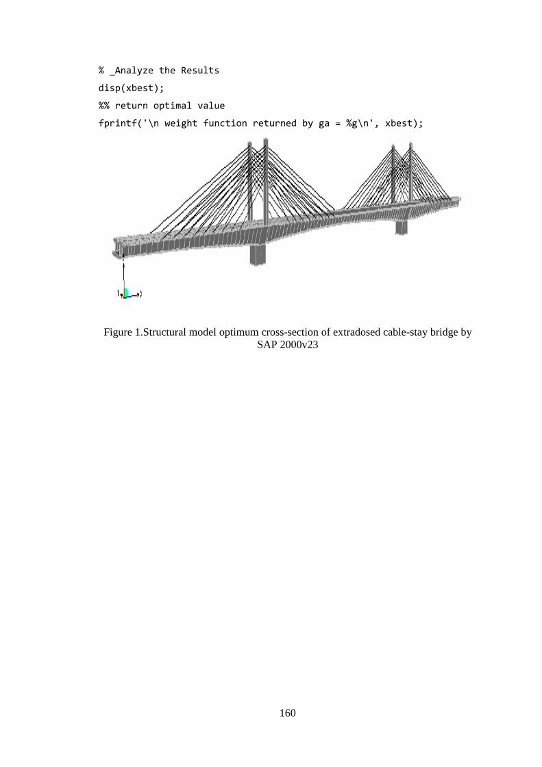
160


disp(xbest);


fprintf('\n weight function returned by ga = %g\n', xbest);

Figure 1.Structural model optimum cross-section of extradosed cable-stay bridge by

SAP 2000v23

161

Appendix 6 Design Optimization Validation in Excel spreadsheet for stay

cable of extradosed cable-stayed bridge

gca 0.00 angle ratio length(m) number Lh(m) sv(m) sh(m)

Eca 190000.00 x(1) x(2) x(3) x(4) x(5) x(5) x(6)

da 15.20 30 1 26.37 18 19.282 1.132 5.3

Aca 181.37

av 4782.63 lu 15 0.6 14 1E+01 1 4

fpu 1860.00 ub 40 1 20 8E+01 1.4 7

Qult 1600.00

fc 55.00

fcbd=0.6*fpu 1116.00

173690400

QL 140.00 4570.8

Qa=0.45*Qult 720.00

Ec=4500*sqrt(fc) 4.34565763

L 180000.00 4781.92077

Mw 421879.00 135904574

ftw=0.5sqrt(fc) 3.71 0.48113347

et 4781.92

Ls 100000.00 -12154067.6

Lf 22000.00 135904574

r 0.55 6.4988E+11

lamda=0.03; 0.03 6.4988E+11

Lo=63e3; 63000.00 6.4988E+11

Mo=-Fp.*eb; 135904573.93

M2w 2000.00 -25945418.7

Weq=8*eb*Fp./L.^2 0.03 -262.074936

Tc1=-4.*eb./Lf.*Fp 0.00 -262.074936

Ls1=(r.*L-lamda.*L-Lo); 30600.00

w 45708.00 1.4726E+12

e 60.00 -12154067.6

H= x(5).*tan(x(1)) 11.13 587068.568

E 205000.00 -122.768359

n 1.00 14874933.3

I 1.00 -14875302.4

fpk= 1302.00 159089297

(ΔF)TH 110.00 -159089297

R2w1=-Weq.*Lf/2-R1w;

R2p1=3*P*r*L*(2*r*L+L+Lf)*(r*L+(L-Lf)/2)-2*P*r^3*L^3/(6*r^2*L^3*(r+1)-2*r^3*L^2);

R1p=-(R2p1+Tc1)

Check up of validity of Optim. Outputs for stay cables

%The forces resulting from the bottom straight tendons in the side spans

R1o=M23./(r*L);

R2o=-M23/(r*L), R1o=-R2o;

%The forces resulting from draped tendons at the middle of the main span

R1w=M2w/r.*L;

M23=-6*Mo*Lo*(lamda*L+Lo/2)/(3*r*L.^2*(r+1)-r.^2*L.^2);

M2w=Weq.*Lf/48*(3*(L-Lf)^2+6.*Lf.*(L-Lf)+2.*Lf.^2/L.*(r./3+1./2))

R2f=-(-3.*Mf.*Lf/(r.*L.^2)*1/(3+2.*r));

R1f=M21/(r*L)

extreme fiber stresses for computing Prestressing force

ql=0.1qd

M21=-3.*Mf.*Lf./L.*(1/(3+2.*r))

e = yb - dpt

M21=-3.*Mf.*Lf./L.*(1/(3+2.*r))

Ms=Fp.*et;

M22=Ms*(1-(24.*Ls.*r.*L-3*Ls^2)/(12*r*L^2*(1+r)-4*r^2*L^2))

R1s=-Ms*(1-(24*Ls*r*L-3*Ls^2)/(12*r^2*L^3*(1+r)-4*r^3*L^3))=-R2s

Possible use of concordant cable profiles for the extradosed bridges

Eeq=E./(1+(x(3).*yca)^2./12.*f̂ 3);

Fp=P = Aeff.*finf.*Zb./(Zb+Aeff.*e)

Mf=-Fp.*eb

Material Properties optim. Output variable

Desired stay cable force for each stay cable FDi under dead load

w=Aeff*ycon;

FDi=0.2*x(2).*w*L./(9.*sin(x(1)))

stress limits in concrete(Mpa)

stress limit in stay cable(Mpa)

finf = ftw/0.85+Mw/(0.85.*Zb)

162

14873607.2

-14875721.3

-24709.9225

-88596169

-183212979

9.00376606

2903578412

-1364944011

-3.79E+06

-2477429.55

103288.047

-1.6334E+10

2.90E+05

1270.51724

-1.45E-04

9.37E+18

2.92218965

1.0909E+17

-1.2047619 OK

-511 OK

-23067 OK

-9.2609E+18 OK

-9.2609E+18 OK

-1.37E+09 OK

458.057986 OK

0.46672156 OK

-7.20E+02 OK

-4.2555E+10 OK

-1.7699E+10 OK

-0.2 OK

-511 OK

d=(fcbd/Eeq).*(H+(x(5)^2./H))

FDI1=Qcb*fcbd/yca/((H+(x(5)^2/H)))

Tc=pi*dca^2/4.*Qult

%The forces due to the equivalent uniform load Weq alone, can be determined by using the equations

R1w1=-(Weq.*Lo.*(r*L-lamda.*L-Lo/2)-M2w)./(r.*L);

%% To calculate the wind resistance

fb=0.937

m=(Aca*yca)

fn=n./2.*(I.*((FDI./m).^2))

Aca=53*pi*15.262/2

FPTi=(R2f+R2s+R2o+R2w1+R2p1+R2w2+R2p2)./(9*sin(x(1)))-(R1f+R1s+R1o+R1w+R1p+R1w1+R1p1)./(9*sin(x(1)));

Fi=3.*w.*L./(8.*sin(x(1)).*1./(1+3./2.*e./L.*cot(x(1))))

FDI=(FDi-Fi-FPTi)./2

Ai=FDI/Qa*sin(x(1))

Qcb=x(3)*yca./fcbd.*(H+x(5)^2./H).*(FDI)

R2w2=-(Weq*Lo+R1w1);

%The final forces resulting from the equivalent uniform loads Weq and the 2x2 vertical nodal loads

P1=-(4.*eb)./Lf.*Fp;

R2p2=symsum((-P1.*(3.*r.*L.*(r.*L+L+Lsi).*(r.*L-Lsi)-(r.*L-Lsi).^2.*(r.*L+2.*Lsi)-

3.*Lsi.^2.*(r.*L-Lsi))/(3.*r.^2.*L.^3.*(r+1)-r.^3.*L.^3)),i,1,2)

R1p1=-2.*P1-R2p2;

g12=ql/qd-0.3

g13=QL-0.55*fpk

g9=Qw-Qa;

g10=18*FDI/tan(x(1));

g11=FDI-FDI1;

g4=(fn-ft)

g5=(fn-fb)

g6=FDI-0.55.*Tc

g7=(800*d/L-1)

g8=(4.*22e3*8.*6e3./(w.*2.*r.*L+L))*I5

%% nonlinear constraint function

g1=0.7-4.*wc.*56e3/w*(2.*r*L+L)

g2=QL-0.55*fpk

g3=Zm1+M(z)*Mm1(z)./(Ec.*Ixeff);

Qw=FDI./(Qcb*Ai);

163

Appendix 7 Design Optimization Validation in Excel spreadsheet for box

girder for extradosed cable-stayed bridge

D W1 W2 At As Ap y s

5129 2350 9000 5.64E+03 1.68E+08 39000 3900 350

fc= 55 x(1) x(2) x(3) x(4) x(5) x(6) x(7) x(8)

Ec = 27660

Es= 200000 lb 4.50E+03 2350 9000 1.00E+02 1*10^3 2*10^3 1500 100

Ep= 199500 ub 7000 2350 9000 1.00E+04 2*10^9 8*10^4 4500 400

fc= 55

ns= 7.23065799

np= 0.9975 5000 3500 1402 2 20689 15678 3578

fy 420 4 b

L= 10000 16 av 803.84 bex

N 3 bb

tw 200 tb

tft 250

vd -40500000

Md 8.86E+11

Mw 4021879 diam. Of bar,db 32 dia.strand dsrd 15.24

M3 -3.96E+10 area of single baras 803.84 140

Mf 1.39E+09 max. agg size,Agg 25

Tu 3.12E+02

Mg 1.90E+10 clc spacing of //bars sh 48 duct diam,DD 125

Ec.Ic.defDL dr spacing of bars layerssv 32 38

Ec.Ic.defLL no bars nb 25.7377 68.68

nr bars per row,npr 5.29 35

fci=0.8*fc 44 no of row of barnr 4.86535 1.9622857

fct=0.6*fci 26.4 Height of reint rowshr 279.382 2.07

ftt=0.63sqrt(fci) 4.178947236 d' dst 172.62 0.9479641

fcw=0.45*fc 24.75 d 4827.38 116.51815

ftw=0.5sqrt(fc) 3.708099244 dpt 466.64157

dp 4533.3584

fpu 1860 Pa 1.98E+06

fpy=0.9*fpu 1674 Ao 201

fpt=0.74*fpu 1376.4 o 0.9

fpe=0.8*fpy 216 y2 2951

fpk 1302 y3 700

Mx=xb.*P; 4.75712E+14

My=P.*yb; 5337426.572 Aho 8262800

A1 49400000 Ag 47139500

be 3.00E+03 300 tb

check up of validity of optim, outputs for box girder

Input fixed variab.

Concrete stress limit(Mpa)

Optimum output variable box girder

prestressing steel stress limits(Mpa)

optimum output variable box girder

number of leg of vertical strirups

dia. Of strirup

effec. depth of reinf. Steel

area of single strand,ap

dr [email protected] spcg,SD

No. strands,nsrd

no strand per tendon

No.of Tdn,nT

No,Tdn/row,ntr

effective depth of prestressing steel

no of. Rows, nrt

ht of rows of Tdn,hrt

164

88276700

2.4859781

5248.514

1.6E+15

2.046E+13

1.579E+15

30087.968

6.352E+14

4.678E+11

4.747E+13

2.405E+11

4.723E+13

2.167E+23

161.62209

4781.8725

1016.9405

7.06E+10

5107054.5

-8.11E+09

4.83E+03

4340996.3

-1.53E+17

16290.491

250

3692.88

-385722

909252.75

31968.296

1653.3792

942874.43

2.079E+14

6.4520927

-0.000838

yb=x1 - ytIgx=(2.*((x(2).*(tb.^3))./12+x(2)*tb.*((yb-tb./2)).^2+ (Re.*(tb).^3)/12+Re.*tb.*((yb-

tb/2)).^2+(x1-tb)./tan(43.9).*((x1-tb)^3).*1/18+((x1-tb)/tan(45)).*(x1-tb).*(2/3.*(x1-tb)-

yt).^2+(x3.*(x1-tb)^2/12

+x3.*(x1-tb).*(x1-tb-yt).^2)))

Iho=(y3.*((y2.^3)./12+y3*y2*(y2-yt)*(y2-yt)+(y3.*y2.^3)/18+(2/3.*(y2-yt).^2)))

Ixeff=Igx-Iho

Aeff=Re*tb+(1/2).*((Re-(2.*x2))+x3).*(x1-tb)-(x4.*(y3.*y2)+(y3.*y2))

yt= (Re.*tb.*(x1-tb./2)+x3.*(x1-tb).*((x1-tb)./2)+((x1-tb).*((x1-tb)./tan(43.9)).*2/3.*(x1-

tb)))./(Re.*tb)+(x3.*(x1-tb)+(x1-tb)+(x1-tb).*((x1-tb)./tan(angle)))

Section Properties

de = (x(6)*fps*dp+x(4)*fy*d)/(x(5)*fps+x(4)*fy) =

e = yb - dpt

P = Aeff.*finf.*Zb./(Zb+Aeff.*e)

co = ((x6.*fpu+x5.*fy-(x5'.*fy')-0.85^2.*fc.*(be-tw).*tft)./(0.85^2.*fc*tw)+

(0.28.*fpu).*x6./dp)

c =(if(co > tft,co,c = (x6.*fpu+x5.*fy)./(0.85.^2.*fc.*be+0.28.*x6.*fpu./dp))

fps = fpu.*(1-0.28.*c./dp)

Flexural reisitance

Minimum flexural reinf

a = 0.85*c =

wsup

Shear force resistance

Mn =if(c>hf), x(5)*fps*(dp-a/2)+x(4)*fy*(d-a/2)+0.85^2*fc*x(3)*(be-x(2))*(a/2-x(3)/2),

else, Mn = x(5)*fps*(dp-a/2)+x(4)*fy*(d-a/2)

dv = max([0.9*de,0.72*x(1),de-a/2])

Vu = Vd*(L/2-wsup/2-d)/(L/2) =

Vc = 0.083*2*sqrt(fc)*tw*dv =

Vs = fy*dv*av/(x(6)) =

Vp = 0.85*P*(4*e/L)

Vn = min([(Vc+Vs+Vp),(0.25*fc*tw*dv+Vp)])

fcpe = 0.85*P*(1/Ac+e/Zb)

fr = 0.97*sqrt(fc) =

Mcr = (fcpe+fr)*I/yb

xb=(Re.*(Re/2).*tb)+x(3).*(x(1)-tb).*(x(2)+(x(1)-tb)./tan(angle)+x(3)./2)+1/2.*(x(1)-

tb).*((x(1)-tb)./tan(angle).*(1/3.*(x(1)-tb)+x(2))+1/2.*(x(1).*tb).*((x(1)-

Zt = Ixeff./yt

Zb = Ixeff./yb

finf = ftw/0.85+Mw/(0.85.*Zb)

extreme fiber stresses for computing Prestressing force

Ixy=xb*yb*Aeff

Iyeff=Igy-Ihy

Ihy=(y2.*(y3.^3)./12+(y2*y3)*(xb-y3/2)^2+(y2.*(y3^3)/18+1/2*(y2*y3)*(xb-(3.*y3-

x2).^2+(y2.*(y3.^3)./18+1./2.*(y2.*y3).*(xb-y3./3-x2-x3.^2)))))

Igy=(x2.^3.*tb)./12+x2.*tb.*((xb-x2)./2).^2+(((Re-2.*x2^3.*tb)./12)+(Re-2.*x2).*tb.*(xb-

x2)-(Re-2.*x2/2).^2+(((x1-tb)./tan(RADIANS(angle))).^3.*(x1-tb ))./18+1/2.*((x1-

Pc= (x(3)+2*(x(1)-tb)/tan(angle)+2*x(2))

165

1058.0012

0

174.00743

0

0.0430145

1328.784

0

1.4546711

1330.2387

9.792E-06

9.767E-06

-5.01E+11

-2.38E+16

-2.38E+16

-2.38E+16

-1.38E+16

-1.34E+20

72540000

-5.4E+21

-6.62E+22

1300

7300

1.10E+15

4.672205

9.828E+11

2.167E+23

2.002E-12

7.182E-15

4.387E-13

-2.38E+13

754.76

927.38

78

2682.7563

-2.25E+16

0.0084343

0.0007946

15713121

ffs = ns* Mf*(d-y)/Ict

ffp = np* Mf*(dp-y)/Ict =

Prestressing indices

Mdec = x(5)*(fp1+fp2)*e =

h2 = d-x(7)

dc = 62+db/2

Atc = tw*2*dst/nb =

cw2 = 0.076*(h2/h1)*fs*(dc*Atc)^(1/3)*1e-3*0.1451 = 0

j). Fatigue stress limit

defP = 0.85*5*P*e*L^2/(48*Ec*Ie)

defLL = 2.63e15/(Ec*Ie) =

cw1 = (fs - 40)*1e-3 =

h1 = d-x(7) - dst =

h). Deflection limit

frk = 0.63*sqrt(fc)

Mck = frk*I/yb

Ie = min([(Mck/Mw)^3*I+(1-(Mck/Mw)^3)*Ict, I]) =

defD = 2.26e16/(Ec*Ie) =

C = 0.5*fco*be*x(7)

Cn = 0.5*fco*(be-x(2))*(x(7)-x(3))^2/x(7

dz = x(7)/3

dzn = x(3)+(x(7)-x(3))/3 =

Ict =if(y>hf)= tw*y^3/3+(be-tw)*tft^3/12+ (be-tw)*tft*(y-tft/2)^2+np*x(6)*(dp-y)^2+

ns*x(6)*(d-y)^2, else, Ict = be*y^3/3+np*x(6)*(dp-y)^2+ ns*x(5)*(d-y)^2

fp3 = Ep*eo*(dp-x(7))/x(7)

fp = fp1+fp2+fp3

fco = eo*Ec

Ts = x(5)*fs

Tp = x(6)*fp

Maximum limits of reinf.

a. c/de

Asn

rhp = x(4)/(be*d) =

rhn = Asn/(be*d)

rhpr = Ap/(be*dp)

fp1 = 0.85*P/Ac =

fp2 = 0.85*np*P*(e^2/I+1/Ac) = 1

eo =if(y>hf) =eo = (x(6)*(fp1+fp2))/(0.5.*Ec*(tw*x(7)+(be-tw)*tft* (1+(x(7)-tft)/x(7)))-

(Es*x(5)*(d-x(7))/x(7)+Ep*x(6)*(dp.*x(7))/x(7)));,else,

eo = (x(6)).*(fp1+fp2)./(0.5.*Ec.*be.*(x(7))-(Es.*(x(5)).*(d.*(x(7)))./(x(7)+Ep.*(x(6)).*(dp-

x(7)./x(7)))))

fs = Es*eo*(d-x(7))/x(7)

Omp = rhp*fy/fc =

Omn = rhn*fy/fc

Ompr = rhpr*fps/fc =

Omp+Ompr - Omn =

Cracked section analysis

166

-4.18E+00 OK

-1022.564 OK

-1026.742 OK

-2.69E+03 OK

-1.35E+04 OK

-1.32E+06 OK

-7.35E+02 OK

-1.38E+17 OK

-1234309 OK

-481010.5 OK

-7.04E+10 OK

-7.05E+10 OK

-4.43E-03 OK

-0.001006 OK

-1.68E+08 OK

-1330.209 OK

-1.12E+18 OK

75 OK

OK

-435016.5 OK

-296285.5 OK

-3.25E+03 OK

OK

-2.25E+16 OK

OK

-157.3211 OK

OK

-7.03E+10 OK

-2874.2 OK

-100.62 OK

-5.61E+03 OK

4.00E+24 OK

-4067274 OK

-1.38E+17 OK

-1.38E+17 OK

-60890 OK

-41442874 OK

-2390 OK

g5 = 0.85.*P.*(1./Aeff-e./Zt)+Mw./Zt-fcw;

g6 = ftw-0.85.*P.*(1./Aeff+e./Zb)+M3./Zb;

g7=fct-Pa/Aeff-Md*yb/2*Ixeff+c*k

g8= (Md-0.9.*Mn);

Non linear inequality constraints [c] written of the form gi(xi)<= 0

g1 = ftt-P.*(1./Aeff+e./Zt)-Mg./Zt

g2=ftt-P/Aeff-Mx*(yb*Iyeff-xb*Ixy)/(Iyeff*Ixeff+Ixy^2)+My*(xb*Ixeff-yb*Ixy/(Iyeff*Ixeff+Ixy^2))

g3=P/Aeff-Mx.*(yb.*Iyeff-xb.*Ixy)./(Ixeff.*Iyeff-(Ixy).^2)+My.*(xb.*Ixeff-yb.*Ixy)./(Ixeff.*Iyeff-(Ixy).^2)-fct

g4 = P.*(1./Aeff+e./Zb)-Mg./Zb-fct;

% Crack width

g21 = (cw-cwa);

g9= Vu-0.9.*Vn;

g10 = Vu./0.9-(0.25*fc*dv)-Vp;

g11 = abs(Md)/(0.9*dv)+abs(Vu/0.9-Vp)-0.5*min([Vu/0.9,Vs])-x(5)*fy-x(6)*fps;

g9 = Vu./0.9-(0.5.*Vs)-Vp-(x(5).*fy)-x(6).*fps;

g12=(Md/dv+0.5*Pa+0.5*Vu*cot(angle)-x(6)*fpu)/(Es*x(5)+Ep*x(6));

g13 = 1.2.*Mcr;

g14 = 0.004.*tw.*yb-x(5)-x(6

g15 = (Omp+Ompr-Omn-0.3);

%Minimum amount of reinforcement

g30=1.2*Mcr-0.9*Mn;

g31=1.33*Md-0.9*Mn;

g32= Mu/(dv*0.9)+(Vu/0.9-Vp)-0.5*min([Vu/0.9,(x(5)*fy*dv)/x(8)])-((x(5)*fy+x(6)*fpu));

g39=Vd-Vn

g40=Tburst-O*T

% fatigue stress limit

g22 = (ffs-161.5);

g23 = (ffp-125);

g24=Md/O*dv+0.5*Pa/O+cot(angle*sqrt((Vu/O-Vp)-0.5*Vs)^2+(0.45*Pc*Tu))-(x(6)*fps+x(5)*fy);

g25 = (0.20.*x(1)-x(7));

g26 = (x(7)- 0.75*x(1));

g27=Tu*Pc/(2*0.9*Ao*fy)-x(4);

g28=Vu/0.9-0.5*Vs-Vp-x(5)*fs-x(6)*fpu;

g29=x(8)-(av*fy)/(0.083*bv*sqrt(fc));

g16 =(c./de-0.42);

bv=tw-dduct;

% limits of traverse reinforcement

g17 = (x(7)-fy*av/(0.083*tw*sqrt(fc)))

g18= P - x(6).*fpt

g20 = fs- min([206,0.6.*fy])

2021-08 STRUCTURAL OPTIMIZATION OF SUPERSTRUCTURE ...

Documents

Transcript of 2021-08 STRUCTURAL OPTIMIZATION OF SUPERSTRUCTURE ...