General Relativity and Cosmology

Steven BalbusVersion: March 7, 2021

1

These notes are intended for classroom use. I believe that there is little here that is original, but itis possible that a few results are. If you would like to quote from these notes and are unable to findan original literature reference, please contact me by email first. Conversely, if you find errors inthe text, I would be grateful to have these brought to my attention. I thank those readers who havealready done so: T. Acharya, V. Alimchandani, C. Arrowsmith, J. Bonifacio, Y. Chen, M. Elliot,L. Fraser-Taliente, G. Johnson, A. Orr, J. Patton, V. Pratley, W. Potter, T. Surawy-Stepney, andH. Yeung.

Thanks to the reader in advance for his/her cooperation.

Steven Balbus

2

Welcome to B5, General Relativity, Hilary Term 2021.

This set of notes is substantially revised from HT20, with the inclusion of a significantamount of new material. This is primarily in Chapter 11 in the form of SupplementaryTopics. All of Chapters 7 and 11 is off-syllabus and non-examinable. It is included as awork in progress, toward the preparation of a textbook, for students who would like to beintroduced to more advanced material. Your comments and questions are welcome.

The examinable material for HT21 is Chapters 1-6, 8.1–8.5, 9, 10.1–10.6.

3

Recommended TextsHobson, M. P., Efstathiou, G., and Lasenby, A. N. 2006, General Relativity: An Introductionfor Physicists, (Cambridge: Cambridge University Press) Referenced as HEL06.

A very clear, very well-blended book, admirably covering the mathematics, physics, andastrophysics of GR. Excellent presentation of black holes and gravitational radiation. Theexplanation of the geodesic equation and the affine connection is very clear and enlightening.A little thin on physical cosmology, though a nice introduction to the physics of inflationand the early universe. Overall, my favourite text on this topic. (The metric has a differentsign convention in HEL06 compared with Weinberg 1972 & MTW [see below], as well asthese notes. Be careful.)

Weinberg, S. 1972, Gravitation and Cosmology. Principles and Applications of the GeneralTheory of Relativity, (New York: John Wiley) Referenced as W72.

This is a classic reference, but in many ways it has become very dated. A paucity of materialon (and a disparaging view of) black holes, an awkward treatment of gravitational radiation,and an unsatisfying development of the geometrical interpretation of the equations are alldrawbacks. The author could not be more explicit in his aversion to anything geometrical. Inthis view, gravity is a field theory with a mere geometrical “analogy.” From the Introduction:“[A] student who asked why the gravitational field is represented by a metric tensor, or whyfreely falling particles follow geodesics, or why the field equations are generally covariantwould come away with the impression that this had something to do with the fact that space-time is a Riemannian manifold.” Well...yes, actually. There is simply no way to understandthe equations of gravity without immersing oneself in geometry, and this point-of-view hasled to many deeply profound advances. (Please do come away from this course with theimpression that space-time is something very like a Riemannian manifold.) The detailedsections on what is now classical physical cosmology are the text’s main strength, and theseare very fine indeed. Weinberg also has a more recent graduate-level text on cosmology perse, (Cosmology 2007, Oxford: Oxford University Press). While comprehensive in coverage,the level is advanced and not particularly user-friendly.

Misner, C. W., Thorne, K. S., and Wheeler, J. A. 1973, Gravitation, (New York: Freeman)Reprinted 2017 by Princeton University Press. Referenced as MTW.

At 1280 pages, don’t drop this on your toe, not even the paperback version. MTW, as it isknown, is often criticised for its sheer bulk and seemingly endless meanderings. Having saidthat, it is truly a monumental achievement. In the end, there is a lot wonderful materialhere, much that is difficult to find anywhere else, and it has all aged very well. Here, wefind geometry is front and centre from start to finish, with lots of very detailed black holeand gravitational radiation physics, half-a-century on more timely than ever. I heartilyrecommend its deeply insightful discussion of gravitational radiation, now part of the coursesyllabus. There is a “Track 1” and “Track 2” for aid in navigation; Track 1 contains theessentials. A new hardbook edition was published in October 2017 by Princeton UniversityPress. The core text is unchanged, but there is interesting new prefatory material, whichreviews developments since the 1970s.

Hartle, J. B. 2003, Gravity: An Introduction to Einstein’s General Theory of Relativity, (SanFrancisco: Addison-Wesley)

This is GR Lite, at a very different level from the previous three texts, though written bya major contributor. For what it is meant to be, it succeeds very well. Coming into the

4

subject cold, this is not a bad place to start to get the lay of the land, to understand theissues in their broadest context, and to be treated to a very accessible presentation. GeneralRelativity is a demanding subject. There will be times in your study of GR when it will bedifficult to see the forest for the trees, when you will feel overwhelmed with the calculations,drowning in a sea of indices and Riemannian formalism. Everything will be all right: justspend some time with this text.

Ryden, Barbara 2017, Introduction to Cosmology, (Cambridge: Cambridge University Press)

Very recent, and therefore up-to-date, second edition of an award-winning text. The style isclear and lucid, the level is right, and the choice of topics is excellent. Less GR and moreastrophysical in content, but with a blend appropriate to the subject matter. Ryden is alwaysvery careful in her writing, making this a real pleasure to read. Warmly recommended.

A few other texts of interest:

Binney J., and Temaine, S. 2008, Galactic Dynamics, (Princeton: Princeton UniversityPress) Masterful text on galaxies with an excellent introduction to cosmology in the ap-pendix. Very readable, given the high level of mathematics.

Carroll, S. M. 2019, Spacetime and Geometry. An Introduction to General Relativity, (Cam-brige: Cambridge University Press) An up-to-date text with good coverage of many modernadvanced topics such as differential geometry, singularity theorems, and field theory in curvedspacetime. The treatment is very mathematical compared with HEL06, and there is alsoa tendency to state results without laying sufficient groundwork, which can be frustratingwhen encountering material for the first time. Still, the motivated student will find much ofinterest here after mastering the material in this course.

Landau, L., and Lifschitz, E. M. 1962, Classical Theory of Fields, (Oxford: Pergamon)Classic advanced text; original and interesting treatment of gravitational radiation. Somematerial here can’t be found elsewhere. Again, best after you’ve completed this course;otherwise dedicated students only!

Longair, M., 2006, The Cosmic Century, (Cambridge: Cambridge University Press) Excel-lent blend of observations, theory and the history of cosmology. This is a good generalreference for anyone interested in astrophysics more generally, a very lucid and informativeread.

Peebles, P. J. E. 1993, Principles of Physical Cosmology, (Princeton: Princeton UniversityPress) Authoritative and advanced treatment by the leading cosmologist of the 20th century,but (in my view) a difficult and sometimes frustrating read. A better reference than text.

Shapiro, S., and Teukolsky S. 1983, Black Holes, White Dwarfs, and Neutron Stars, (Wiley:New York) A text I grew up with. Very clear, with a nice summary of applications of GRto compact objects and very good physical discussions. Level is appropriate to this course.Highly recommended.

5

Notational Conventions & Miscellany

• Spacetime dimensions are labelled 0, 1, 2, 3 or (Cartesian) ct, x, y, z or (spherical) ct, r, θ, φ.Time is always the 0-component. Beware of extraneous factors of c in 0-index quan-tities, present in e.g. T 00 = ρc2, dx0= cdt, but absent in e.g. g00 = −1. (That is onereason why some like to set c = 1 from the start.)

• Repeated indices are summed over, unless otherwise specified. (Einstein summationconvention.)

• The Greek indices κ, λ, µ, ν etc. are used to represent arbitrary spacetime componentsin all general relativity calculations.

• The Greek indices α, β, etc. are used to represent arbitrary spacetime components inspecial relativity calculations (Minkowski spacetime).

• The Roman indices i, j, k are used to represent purely spatial components in any space-time.

• The Roman indices a, b, c, d are used to represent fiducial spacetime components formnemonic aids, and in discussions of how to perform index-manipulations and/or per-mutations, where Greek indices may cause confusion.

• ∗ is used to denote a generic dummy index, always summed over with another ∗.• The tensor ηαβ is numerically identical to ηαβ with −1, 1, 1, 1 corresponding to the

00, 11, 22, 33 diagonal elements. Other texts use the sign convention 1,−1,−1,−1. Becareful.

• Viewed as matrices, the metric tensors gµν and gµν are always inverses. The respectivediagonal elements of diagonal gµν and gµν metric tensors are therefore reciprocals.

• c almost always denotes the speed of light. It is occasionally used as an (obvious)tensor index. c as the velocity of light is only occasionally set to unity in these notesor in the problem sets; if so it is explicitly stated. (Relativity texts often set c = 1 toavoid clutter.) Newton’s G is never unity, no matter what. And don’t you dare eventhink of setting 2π to unity.

• It is “Lorentz invariance,” but “Lorenz gauge.” Not a typo, two different blokes.

6

Really Useful Numbers

c = 2.99792458× 108 m s−1 (Speed of light, exact.)

c2 = 8.9875517873681764× 1016 m2 s−2 (Exact!)

h = 6.62607015× 10−34 J s (Planck’s constant, exact.)

aγ = 7.56573325...× 10−16 J m−3 K−4 (Blackbody radiation constant, exact.)

G = 6.67384× 10−11 m3 kg−1 s−2 (Newton’s G.)

M = 1.98855× 1030 kg (Mass of the Sun.)

r = 6.955× 108 m (Radius of the Sun.)

GM = 1.32712440018 × 1020 m3 s−2 (Solar gravitational parameter; much more accuratethan either G or M separately.)

2GM/c2 = 2.9532500765× 103 m (Solar Schwarzschild radius.)

GM/c2r = 2.1231× 10−6 (Solar relativity parameter.)

M⊕ = 5.97219× 1024 kg (Mass of the Earth)

r⊕ = 6.371× 106 m (Mean Earth radius.)

GM⊕ = 3.986004418× 1014 m3 s−2(Earth gravitational parameter.)

2GM⊕/c2 = 8.87005608× 10−3 m (Earth Schwarzschild radius.)

GM⊕/c2r⊕ = 6.961× 10−10 (Earth relativity parameter.)

1 AU = 1.495978707 × 1011m (1 Astronomical Unit, exact.)

1pc = 3.085678× 1016 m (1 parsec.)

H0 = 100h km s−1 Mpc−1 (Hubble constant. h ' 0.7. H−10 = 3.085678h−1 × 1017s=

9.778h−1 × 109 yr.)

For diagonal gab,

Γaba = Γaab =1

2gaa

∂gaa∂xb

(a = b permitted, NO SUM)

Γabb = − 1

2gaa

∂gbb∂xa

(a 6= b, NO SUM)

Γabc = 0, (a, b, c distinct)

Ricci tensor:

Rµκ =1

2

∂2 ln g

∂xκ∂xµ− 1√

g

∂√g Γλµκ∂xλ

+ ΓηµλΓλκη (FULL SUMMATION, g = |det gµν |)

7

Contents

1 An overview 13

1.1 The legacy of Maxwell . . . . . . . . . . . . . . . . . . . . . . . . . . . . . . 13

1.2 The legacy of Newton . . . . . . . . . . . . . . . . . . . . . . . . . . . . . . . 14

1.3 The need for a geometrical framework . . . . . . . . . . . . . . . . . . . . . . 14

2 The toolbox of geometrical theory: Minkowski spacetime 18

2.1 4-vectors . . . . . . . . . . . . . . . . . . . . . . . . . . . . . . . . . . . . . . 18

2.2 Transformation of gradients . . . . . . . . . . . . . . . . . . . . . . . . . . . 21

2.3 Transformation matrix . . . . . . . . . . . . . . . . . . . . . . . . . . . . . . 22

2.4 Tensors . . . . . . . . . . . . . . . . . . . . . . . . . . . . . . . . . . . . . . 24

2.4.1 The energy-momentum stress tensor . . . . . . . . . . . . . . . . . . 24

2.5 Electrodynamics . . . . . . . . . . . . . . . . . . . . . . . . . . . . . . . . . 25

2.5.1 4-currents and 4-potentials . . . . . . . . . . . . . . . . . . . . . . . . 25

2.5.2 Electromagnetic field tensor . . . . . . . . . . . . . . . . . . . . . . . 27

2.6 Conservation of Tαβ . . . . . . . . . . . . . . . . . . . . . . . . . . . . . . . 27

3 The effects of gravity 31

3.1 The Principle of Equivalence . . . . . . . . . . . . . . . . . . . . . . . . . . . 31

3.2 The geodesic equation . . . . . . . . . . . . . . . . . . . . . . . . . . . . . . 33

3.3 The metric tensor . . . . . . . . . . . . . . . . . . . . . . . . . . . . . . . . . 35

3.4 The relationship between the metric tensor and affine connection . . . . . . . 35

3.5 Variational calculation of the geodesic equation . . . . . . . . . . . . . . . . 37

3.6 The Newtonian limit . . . . . . . . . . . . . . . . . . . . . . . . . . . . . . . 38

4 Tensor Analysis 43

4.1 Transformation laws . . . . . . . . . . . . . . . . . . . . . . . . . . . . . . . 43

4.2 The covariant derivative . . . . . . . . . . . . . . . . . . . . . . . . . . . . . 45

4.2.1 Contravariant vectors . . . . . . . . . . . . . . . . . . . . . . . . . . . 45

4.2.2 Transformation of the affine connection . . . . . . . . . . . . . . . . . 46

4.2.3 Covariant vectors . . . . . . . . . . . . . . . . . . . . . . . . . . . . . 47

4.2.4 Tensors of arbitrary rank . . . . . . . . . . . . . . . . . . . . . . . . . 48

4.2.5 Going from special to general relativity . . . . . . . . . . . . . . . . . 49

4.3 The affine connection and basis vectors . . . . . . . . . . . . . . . . . . . . . 49

4.4 Volume element . . . . . . . . . . . . . . . . . . . . . . . . . . . . . . . . . . 51

4.5 Covariant div, grad, curl, and all that . . . . . . . . . . . . . . . . . . . . . . 52

8

4.6 Hydrostatic equilibrium . . . . . . . . . . . . . . . . . . . . . . . . . . . . . 54

4.7 Covariant differentiation and parallel transport . . . . . . . . . . . . . . . . . 55

5 The curvature tensor 57

5.1 Commutation rule for covariant derivatives . . . . . . . . . . . . . . . . . . . 57

5.2 Parallel transport . . . . . . . . . . . . . . . . . . . . . . . . . . . . . . . . . 58

5.3 Algebraic identities of Rσνλρ . . . . . . . . . . . . . . . . . . . . . . . . . . . 61

5.3.1 Remembering the curvature tensor formula. . . . . . . . . . . . . . . 61

5.3.2 Rλµνκ: fully covariant form . . . . . . . . . . . . . . . . . . . . . . . . 61

5.3.3 How many independent components does the curvature have? . . . . 63

5.4 The Ricci tensor . . . . . . . . . . . . . . . . . . . . . . . . . . . . . . . . . 64

5.5 Curvature and Newtonian gravity . . . . . . . . . . . . . . . . . . . . . . . . 65

5.6 The Bianchi Identities . . . . . . . . . . . . . . . . . . . . . . . . . . . . . . 65

5.7 The Einstein field equations . . . . . . . . . . . . . . . . . . . . . . . . . . . 67

6 Schwarzschild black holes 71

6.1 Schwarzschild metric . . . . . . . . . . . . . . . . . . . . . . . . . . . . . . . 71

6.2 Schwarzschild metric in Cartesian coordinates . . . . . . . . . . . . . . . . . 76

6.3 The Schwarzschild Radius . . . . . . . . . . . . . . . . . . . . . . . . . . . . 77

6.4 Why does the determinant of gµν not change with M? . . . . . . . . . . . . . 79

6.5 Working with Schwarzschild spacetime. . . . . . . . . . . . . . . . . . . . . . 80

6.5.1 Radial photon geodesic . . . . . . . . . . . . . . . . . . . . . . . . . . 80

6.5.2 Orbital equations . . . . . . . . . . . . . . . . . . . . . . . . . . . . . 81

6.6 The deflection of light by an intervening body. . . . . . . . . . . . . . . . . . 83

6.7 The advance of the perihelion of Mercury . . . . . . . . . . . . . . . . . . . . 86

6.7.1 Newtonian orbits . . . . . . . . . . . . . . . . . . . . . . . . . . . . . 86

6.7.2 The relativistic orbit of Mercury . . . . . . . . . . . . . . . . . . . . . 89

6.8 General solution for Schwarzschild orbits . . . . . . . . . . . . . . . . . . . . 90

6.8.1 Formulation . . . . . . . . . . . . . . . . . . . . . . . . . . . . . . . . 90

6.8.2 Solution . . . . . . . . . . . . . . . . . . . . . . . . . . . . . . . . . . 92

6.9 Gravitational Collapse . . . . . . . . . . . . . . . . . . . . . . . . . . . . . . 93

6.10 Shapiro delay: the fourth protocol . . . . . . . . . . . . . . . . . . . . . . . . 95

7 Kerr Black Holes 97

7.1 Rotating spacetime: Kerr-Schild metric . . . . . . . . . . . . . . . . . . . . . 97

7.2 Boyer-Lindquist coordinates . . . . . . . . . . . . . . . . . . . . . . . . . . . 98

7.3 Kerr geometry . . . . . . . . . . . . . . . . . . . . . . . . . . . . . . . . . . . 100

9

7.3.1 Singularities . . . . . . . . . . . . . . . . . . . . . . . . . . . . . . . . 100

7.3.2 Stationary limit surface: g00 = 0 . . . . . . . . . . . . . . . . . . . . . 101

7.3.3 Event horizon: grr = 0 . . . . . . . . . . . . . . . . . . . . . . . . . . 102

8 Self-Gravitating Relativistic Hydrostatic Equilibrium 104

8.1 Historical Introduction . . . . . . . . . . . . . . . . . . . . . . . . . . . . . . 104

8.2 Fundamentals . . . . . . . . . . . . . . . . . . . . . . . . . . . . . . . . . . . 106

8.3 Constant density stars . . . . . . . . . . . . . . . . . . . . . . . . . . . . . . 108

8.4 White Dwarfs . . . . . . . . . . . . . . . . . . . . . . . . . . . . . . . . . . . 109

8.5 Neutron Stars . . . . . . . . . . . . . . . . . . . . . . . . . . . . . . . . . . . 113

8.6 Pumping iron: the physics of neutron star matter . . . . . . . . . . . . . . . 118

9 Gravitational Radiation 122

9.1 The linearised gravitational wave equation . . . . . . . . . . . . . . . . . . . 124

9.1.1 Come to think of it... . . . . . . . . . . . . . . . . . . . . . . . . . . . 129

9.2 Plane waves . . . . . . . . . . . . . . . . . . . . . . . . . . . . . . . . . . . . 130

9.2.1 The transverse-traceless (TT) gauge . . . . . . . . . . . . . . . . . . . 130

9.3 The quadrupole formula . . . . . . . . . . . . . . . . . . . . . . . . . . . . . 132

9.4 Radiated Energy . . . . . . . . . . . . . . . . . . . . . . . . . . . . . . . . . 134

9.4.1 A useful toy problem . . . . . . . . . . . . . . . . . . . . . . . . . . . 134

9.4.2 A conserved energy flux for linearised gravity . . . . . . . . . . . . . 135

9.5 The energy loss formula for gravitational waves . . . . . . . . . . . . . . . . 138

9.6 Gravitational radiation from binary stars . . . . . . . . . . . . . . . . . . . . 141

9.7 Detection of gravitational radiation . . . . . . . . . . . . . . . . . . . . . . . 144

9.7.1 Preliminary comments . . . . . . . . . . . . . . . . . . . . . . . . . . 144

9.7.2 Indirect methods: orbital energy loss in binary pulsars . . . . . . . . 146

9.7.3 Direct methods: LIGO . . . . . . . . . . . . . . . . . . . . . . . . . . 149

9.7.4 Direct methods: Pulsar timing array . . . . . . . . . . . . . . . . . . 152

10 Cosmology 155

10.1 Introduction . . . . . . . . . . . . . . . . . . . . . . . . . . . . . . . . . . . . 155

10.1.1 Newtonian cosmology . . . . . . . . . . . . . . . . . . . . . . . . . . . 155

10.1.2 The dynamical equation of motion . . . . . . . . . . . . . . . . . . . 157

10.1.3 Cosmological redshift . . . . . . . . . . . . . . . . . . . . . . . . . . . 158

10.2 Cosmology models for the impatient . . . . . . . . . . . . . . . . . . . . . . . 159

10.2.1 The large-scale spacetime metric . . . . . . . . . . . . . . . . . . . . 159

10.2.2 The Einstein-de Sitter universe: a useful toy model . . . . . . . . . . 160

10

10.3 The Friedmann-Robertson-Walker Metric . . . . . . . . . . . . . . . . . . . . 163

10.3.1 Maximally symmetric 3-spaces . . . . . . . . . . . . . . . . . . . . . . 164

10.4 Large scale dynamics . . . . . . . . . . . . . . . . . . . . . . . . . . . . . . . 167

10.4.1 The effect of a cosmological constant . . . . . . . . . . . . . . . . . . 167

10.4.2 Formal analysis . . . . . . . . . . . . . . . . . . . . . . . . . . . . . . 168

10.4.3 The Ω0 parameter . . . . . . . . . . . . . . . . . . . . . . . . . . . . . 171

10.5 The classic, matter-dominated universes . . . . . . . . . . . . . . . . . . . . 172

10.6 Our Universe . . . . . . . . . . . . . . . . . . . . . . . . . . . . . . . . . . . 174

10.6.1 Prologue . . . . . . . . . . . . . . . . . . . . . . . . . . . . . . . . . . 174

10.6.2 A Universe of ordinary matter and vacuum energy . . . . . . . . . . . 175

10.7 Radiation-dominated universe . . . . . . . . . . . . . . . . . . . . . . . . . . 176

10.8 Observational foundations of cosmology . . . . . . . . . . . . . . . . . . . . . 179

10.8.1 The first detection of cosmological redshifts . . . . . . . . . . . . . . 179

10.8.2 The cosmic distance ladder . . . . . . . . . . . . . . . . . . . . . . . . 180

10.8.3 The parameter q0 . . . . . . . . . . . . . . . . . . . . . . . . . . . . . 182

10.8.4 The redshift–magnitude relation . . . . . . . . . . . . . . . . . . . . . 183

10.9 The Cosmic Microwave Background Radiation (CMB) . . . . . . . . . . . . 186

10.9.1 Overview . . . . . . . . . . . . . . . . . . . . . . . . . . . . . . . . . 186

10.9.2 An observable cosmic radiation background: the Gamow argument . 188

10.9.3 The cosmic microwave background (CMB): subsequent developments 191

10.10Thermal history of the Universe . . . . . . . . . . . . . . . . . . . . . . . . . 192

10.10.1 Prologue . . . . . . . . . . . . . . . . . . . . . . . . . . . . . . . . . . 192

10.10.2 Classical cosmology: helium nucleosynthesis . . . . . . . . . . . . . . 194

10.10.3 Neutrino and photon temperatures . . . . . . . . . . . . . . . . . . . 196

10.10.4 Ionisation of hydrogen . . . . . . . . . . . . . . . . . . . . . . . . . . 198

11 Supplemental Topics 200

11.1 The Oppenheimer-Snyder problem . . . . . . . . . . . . . . . . . . . . . . . 200

11.2 Particle production and event horizons . . . . . . . . . . . . . . . . . . . . . 204

11.2.1 Minkowski and Rindler metrics . . . . . . . . . . . . . . . . . . . . . 205

11.2.2 Scalar field equation . . . . . . . . . . . . . . . . . . . . . . . . . . . 206

11.2.3 Review of quantum field theory . . . . . . . . . . . . . . . . . . . . . 207

11.2.4 Bogoliubov formalism . . . . . . . . . . . . . . . . . . . . . . . . . . . 208

11.2.5 Invariant inner product . . . . . . . . . . . . . . . . . . . . . . . . . . 209

11.2.6 Minkowski and Rindler vacuums . . . . . . . . . . . . . . . . . . . . . 211

11.2.7 The Hawking effect . . . . . . . . . . . . . . . . . . . . . . . . . . . . 213

11

11.2.8 Hawking luminosity and Bekenstein-Hawking entropy . . . . . . . . . 214

11.3 The Raychaudhuri equation . . . . . . . . . . . . . . . . . . . . . . . . . . . 215

11.4 Effects of electric charge . . . . . . . . . . . . . . . . . . . . . . . . . . . . . 218

11.4.1 The Reissner-Nordstrom metric . . . . . . . . . . . . . . . . . . . . . 218

11.4.2 Singular metric structure: worm holes and white holes . . . . . . . . 220

11.4.3 Naked singularities . . . . . . . . . . . . . . . . . . . . . . . . . . . . 221

11.5 The growth of density perturbations in an expanding universe . . . . . . . . 222

11.6 Inflationary Models . . . . . . . . . . . . . . . . . . . . . . . . . . . . . . . 224

11.6.1 “Clouds on the horizon” . . . . . . . . . . . . . . . . . . . . . . . . . 224

11.6.2 The stress energy tensor of a scalar field . . . . . . . . . . . . . . . . 225

11.6.3 Effective Potentials in Quantum Field Theory . . . . . . . . . . . . . 230

11.6.4 The slow roll inflationary scenario . . . . . . . . . . . . . . . . . . . . 232

11.6.5 Inflated expectations . . . . . . . . . . . . . . . . . . . . . . . . . . . 233

11.6.6 A final word . . . . . . . . . . . . . . . . . . . . . . . . . . . . . . . . 236

12

Most of the fundamental ideas of

science are essentially simple, and

may, as a rule, be expressed in a

language comprehensible to everyone.

— Albert Einstein

1 An overview

1.1 The legacy of Maxwell

We are told by the historians that the greatest Roman generals would have their mostimportant victories celebrated with a triumph. The streets would line with adoring crowds,cheering wildly in support of their hero as he passed by in a grand procession. But theRomans astutely realised the need for a counterpoise, so a slave would ride with the general,whispering in his ear, “All glory is fleeting.”

All glory is fleeting. And never more so than in theoretical physics. No sooner is a triumphhailed, but unforseen puzzles emerge that could not possibly have been anticipated beforethe breakthrough. The mid-nineteenth century reduction of all electromagnetic phenomenato four equations, the Maxwell Equations, is very much a case in point.

The 1861 synthesis provided by Maxwell’s equations united electricity, magnetism, andoptics, showing them to be different manifestations of the same field. The theory accountedfor the existence of electromagnetic waves, explained how they propagated, and showedthat the propagation velocity is 1/

√ε0µ0 (ε0 is the permitivity, and µ0 the permeability, of

free space). This combination is precisely equal to the speed of light. Light is a form ofelectromagnetic radiation! The existence of electromagnetic raditation was later verified bybrilliant experiments carried out by Heinrich Hertz in 1887, in which the radiation was bothgenerated and detected.

But when one probed, Maxwell’s theory, for all its success, had disquieting features.For one, there seemed to be no provision in the theory for allowing the velocity of lightto change with the observer’s velocity. The speed of light is aways 1/

√ε0µ0. A related

point is that simple Galilean invariance is not obeyed, i.e. absolute velocities appear toaffect the physics, something that had not been seen before. Lorentz and Larmor in the latenineteenth century discovered that Maxwell’s equations in fact had a simple mathematicalvelocity transformation that did leave them invariant, but it was not Galilean, and mostbizarrely, it involved changing the time. The non-Galilean character of the transformationequation relative to the “aetherial medium” hosting the waves was put down, a bit vaguely,to electromagnetic interactions between charged particles that truly changed the length ofthe object. In other words, the non-Galilean transformation was somehow electrodynamicalin origin. As to the time change...well, one would just have to put up with it as an aetherialformality.

All was resolved in 1905 when Einstein showed how, by adopting as postulates (i) thespeed of light is constant in all frames (as had already been indicated by a body of verycompelling experiments, most notably the famous Michelson-Morley investigation); and (ii)the truly essential Galilean notion that relative uniform velocity cannot be detected by anyphysical experiment, that the “Lorentz transformations” (as they had become known) mustfollow. In the process, electromagnetic radiation in vacuo took on a reality all its own: it nolonger need be viewed as some sort of aetherial displacement. The increasingly problematic

13

aether host medium could be abandoned: the waves were “hosted” by the vacuum itself. Moststunningly, all equations of physics, not just electromagnetic phenomena, had to be invariantin form under the kinematic Lorentz transformations, even with the peculiar relative timevariable. The transformations themselves really had nothing to do with electrodynamics.They were far more general. It just so happened that the Maxwell equations was the firstsuch set to adhere to correct transformation laws. The others had to be fixed up!

These ideas, and the consequences that ensued collectively from them (e.g., the equiva-lence of energy and inertia) became known as relativity theory, in reference to the invarianceof form with respect to relative velocities. The relativity theory that arose from the dis-internment of the Lorrentz transformations from within the Maxwell equations is rightlyregarded as one of the crown jewels of 20th century physics. In other words, a triumph.

1.2 The legacy of Newton

Another triumph, another problem. If indeed all of physics had to be compatible withrelativity, what of Newtonian gravity? By the early twentieth century it had been verifiedwith great precision, even predicting the existence of a new distant planet (Neptune) in thesolar system. But Newtonian gravity is manifestly not compatible with relativity, becausethe governing Poisson equation

∇2Φ = 4πGρ (1)

implies instantaneous transmission of changes in the Φ field from source to observer. (Here Φis the Newtonian potential function, G the Newtonian gravitational constant, and ρ the massdensity.) Wiggle the density locally, and throughout all of space there must instantaneouslybe a wiggle in Φ, as given by equation (1).

In Maxwell’s theory, the electrostatic potential also satisfies its own Poisson equation,but the appropriate time-dependent potential obeys a wave equation:

∇2Φ− 1

c2

∂2Φ

∂t2= − ρ

ε0, (2)

and solutions of this equation do not propagate instantaneously throughout all space. Theypropagate at the speed of light c. At least in retrospect, this is rather simple. Might it notbe the same for gravity?

Alas, no. The problem is that the source of the signals for the electric potential field, i.e.the charge density, behaves differently from the source for the gravity potential field, i.e. themass density. The electrical charge of an individual bit of matter does not change when thematter is in motion, but the mass does: mass, as a source of gravity, depends upon velocity.This deceptively simple detail complicates everything. It leads immediately to the realisationthat in a relativistic theory, energy, like matter, must also be a source of a gravitational field,and this includes the distributed energy of the gravitational field itself. On other words, anyrelativistic theory of gravity would have to be nonlinear. In such a time-dependent theoryof gravity, it is not even clear a priori what the appropriate mathematical objects should beon either the right side or the left side of the wave equation. Come to think of it, should webe using a wave equation at all?

1.3 The need for a geometrical framework

In 1908, the mathematician Hermann Minkowski presented a remarkable insight. He arguedthat one should view the Lorentz transformations not merely as a set of rules for how

14

space and time coordinates change from one constant-velocity reference frame to another.Minkowski’s idea was that these coordinates should be regarded as living in their own sortof pseudo-Euclidian geometry—a spacetime, if you will: Minkowski spacetime. There waseven a ready-made mathematical structure at hand to be used: hyperbolic geometry.

To understand the motivation for this, start simply. We know that in ordinary Euclidianspace we are free to choose any set of Cartesian coordinates we like, and it can make nodifference to the description of the space itself, e.g., in measuring how far apart objects are.If (x, y) is a set of Cartesian coordinates for the plane, and (x′, y′) another coordinate setrelated to the first by a rotation, then

dx2 + dy2 = dx′2 + dy′2 (3)

i.e., the distance between two closely spaced points is the same number, regardless of thecoordinates used. The quantity dx2 + dy2 is said to be an “invariant” under rotationaltransformations.

Now, an abstraction. From a mathematical viewpoint, there is nothing special aboutthe use of dx2 + dy2 as our so-called metric. Imagine a space in which the metric invariantwas dy2 − dx2. From a purely formal point-of-view, we needn’t worry about the plus/minussign. An invariant is an invariant. Indeed, the hyperbolic geometry arising from this formof invariant had been studied by Bolyai and Lobachevsky (and was known to Gauss) longbefore. With dy2 − dx2 as our invariant, we are in fact describing a hyperbolic Minkowskispace, with dy = cdt and dx a space interval as before. Under the simplest form of theLorentz transformations, c2dt2 − dx2 emerges as an invariant quantity, which is preciselywhat is needed to guarantee that the speed of light is always constant...an invariant. Withthis formulation, the interval c2dt2 − dx2 always vanishes for light propagation along the xdirection, in any coordinates (i.e., “observers”) related by a Lorentz transformation. Theobvious generalisation

c2dt2 − dx2 − dy2 − dz2 = 0 (4)

will guarantee the same is true in any spatial direction. Our Universe is one of four di-mensions, but its hyperbolic geometry picks out one of these dimensions to appear with adifferent sign in formulating the invariant interval. This dimensional separation therefore hasa different character to the other three, and is experienced by our consciousness in a verydifferent way. We feel the need to separate this one particular form of dimensional separationfrom the other three, and give it its own name: time. Minkowski thus took a kinematicalrequirement—that the speed of light be a universal constant—and gave it a geometrical in-terpretation in terms of an invariant quantity (a “quadratic form” as it is sometimes called)in Minkowski space. Rather, Minkowski spacetime.

Pause. And so what? Call it whatever you like. Who needs obfuscating mathematicalpretence? Eschew obfuscation! One could argue that lots of things add together quadrati-cally, and it is not particularly helpful to regard them as geometrical objects. The Lorentztransform stands on its own! I like my way! That was very much Einstein’s initial take onMinkowski’s pesky mathematical meddling with his theory.

However, as the reader has no doubt sensed, it is the geometrical viewpoint that is trulythe more fundamental, a perspective that time (our fourth dimension) has vindicated. InMinkowski’s 1908 tour-de-force paper, we find more than just a simple analogy or math-ematical pretence. We find the first presentation of relativistic 4-vectors and tensors, ofthe Maxwell equations in manifestly covariant form, and the remarkable realisation that themagnetic vector and electrostatic potentials combine seamlessly to form their own 4-vector.Gone are the comforting kinematical tools, the clocks, the rods and the quaint Swiss trams ofEinstein’s 1905 relativity paper. This is no mere “uberflussige Gelehrsamkeit” (superfluouserudition), Einstein’s dismissive term for the whole business.

15

It was not until 1912 that Einstein finally changed his view. Five years earlier, he hadhad the seed of a very important idea, but had been unable to build upon it. In 1912,Einstein discovered what it was that he had discovered. His great 1912 revelation was thatthe effect of the presence of matter (or its equivalent energy) throughout the Universe is todistort Minkowski’s spacetime, and that this embedded geometrical distortion manifests itselfas the gravitational field. Minkowski spacetime is not some mere mathematical formalism,it is physical stuff, you can mess with it. The spacetime distortions of which we speakmust become, when sufficiently weak, familiar Newtonian gravitational theory. You thoughtgravity was a dynamical force? No. Gravity is a purely geometrical phenomenon.

Now that is one big idea. It is an idea that physicists are still taking in. How did Einsteinmake this leap? What was the path that led him to change his mind? Where did the notionof a gravity-geometry connection come from?

It came from that “important idea” he had in 1907, a year before Minkowski publishedhis geometrical interpretation of relativity. In a freely falling elevator, or more safely in anexpertly piloted aircraft executing a ballistic parabolic arch, one feels “weightless.” That is,the effect of gravity can be made to disappear locally in the appropriate reference frame—i.e., the right coordinates. Let that sit. The physics of gravity must be intimately associatedwith coordinate transformations! This is because gravity has exactly the same effect on alltypes of mass, regardless of bulk or elemental composition. In 1912 Einstein grasped thatthis is precisely what would naturally emerge from a theory in which objects were respondingto background geometrical distortions instead of to an applied force. In a state of free-fall,gravity is in effect absent, and we locally return to the environment of an undistorted (“flat,”in mathematical parlance) Minkowski spacetime, much as a flat Euclidian tangent plane isan excellent local approximation to the surface of a curved sphere. It is easy to be fooledinto thinking that the earth is flat, if your view is too local. “Tangent plane coordinates”on small-scale road maps locally eliminate spherical geometry complications, but if we areflying from Oxford to Hong Kong, the Earth’s curvature is important. Einstein’s notionthat the effect of gravity is to cause a geometrical distortion of an otherwise flat Minkowskispacetime, but that it is always possible to find coordinates in which local distortions maybe eliminated to leading local order, is the foundational insight of general relativity. It isknown as the Equivalence Principle. We will have more to say on this topic.

Spacetime. Spacetime. Bringing in time, you see, is everything. Who would have thoughtof doing that in a geometrical theory? Non-Euclidean geometry, as developed by the greatmathematician Bernhard Riemann, begins with just the notion we’ve been discussing, thatany distorted space looks locally flat. Riemannian geometry is the natural language ofgravitational theory, and Riemann himself had the notion that gravity might arise from a non-Euclidian curvature in a space of three or more dimensions! He got nowhere, because timewas not part of his geometry. He was thinking only of space. It was the genius of Minkowski,who by showing how to incorporate time into a purely geometrical theory, allowed Einstein totake the crucial next step, freeing himself to think of gravity in geometrical terms, withouthaving to agonise over whether it made any sense to have time as part of a geometricalframework. In fact, the Newtonian limit is reached not from the leading order curvatureterms in the spatial part of the geometry, but from the leading order “curvature” (if that isthe word) of the time dimension. And that is why Riemann failed.

In brief: Riemann created the mathematics of non-Euclidian geometry. Minkoswki re-alised that the natural language of the Lorentz transformations was neither electrodynamical,nor even kinematic, it was really geometrical. But you need to include time as a componentof the geometrical interpretation! Einstein took the great leap of realising that the force wecall gravity arises from the distortions of Minkowski’s flat spacetime which are created bythe presence of mass/energy.

Well done. You now understand the conceptual framework of general relativity, and that

16

is itself a giant leap. From here on, it is just a matter of the technical details. But then, youand I also can draw like Leonardo da Vinci.

It is just a matter of the technical details.

17

From henceforth, space by itself and

time by itself, have vanished into the

merest shadows, and only a blend of

the two exists in its own right.

— Hermann Minkowski

2 The toolbox of geometrical theory: Minkowski space-

time

In what sense is general relativity “general?” In the sense that, as we are dealing with atrue spacetime geometry, the essential mathematical description must be the same in anycoordinate system at all, not just among those related by constant velocity reference frameshifts, nor even just among those coordinate transformations that make tangible physicalsense as belonging to some observer or another. Any mathematically proper coordinates atall, however unusual. Full stop.

We need coordinates for our description of the structure of spacetime, but somehow theessential physics (and other mathematical properties) must not depend on which coordinateswe use, and it is no easy business to formulate a theory which satisfies this restriction. Weowe a great deal to Bernhard Riemann for coming up with a complete mathematical theoryfor these non-Euclidian geometries. The sort of geometrical structure in which it is alwayspossible to find coordinates in which the space looks locally smooth is known as a Riemannianmanifold. Crudely speaking, manifolds are smooth surfaces in n dimensions. A circle is amanifold, a spherical surface is a manifold, an egg shell is a manifold, but a tetrahedronis not. Mathematicians would say that an n-dimensional manifold is homeomorphic to n-dimensional Euclidian space. Actually, since our local invariant interval c2dt2 − dx2 is nota simple sum of squares, but contains that notorious minus sign, the manifold is said to bepseudo-Riemannian. Pseudo or no, the descriptive mathematical machinery is the same.

The objects that geometrical theories work with are scalars, vectors, and higher ordertensors. You have certainly seen scalars and vectors before in your other physics courses,and you may have encountered tensors as well. We will need to be very careful how we definethese objects, and very careful to distinguish them from objects that look like vectors andtensors (because they have many components and index labels with perfect Greek lettering)but are actually imposters. Their credentials are fake.

To set the stage, we begin with the simplest geometrical objects of Minkowski spacetimethat are not just simple scalars: the 4-vectors.

2.1 4-vectors

In their most elementary guise, the familiar Lorentz transformations from “fixed” laboratorycoordinates (t, x, y, z) to moving frame coordinates (t′, x′, y′, z′) take the form

ct′ = γ(ct− vx/c) = γ(ct− βx) (5)

x′ = γ(x− vt) = γ(x− βct) (6)

y′ = y (7)

18

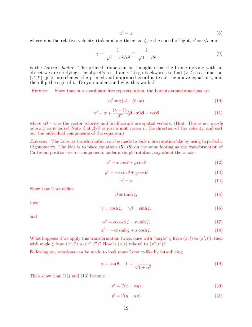
z′ = z (8)

where v is the relative velocity (taken along the x axis), c the speed of light, β = v/c and

γ =1√

1− v2/c2≡ 1√

1− β2(9)

is the Lorentz factor. The primed frame can be thought of as the frame moving with anobject we are studying, the object’s rest frame. To go backwards to find (x, t) as a function(x′, t′), just interchange the primed and unprimed coordinates in the above equations, andthen flip the sign of v. Do you understand why this works?

Exercise. Show that in a coordinate free representation, the Lorentz transformations are

ct′ = γ(ct− β · x) (10)

x′ = x+(γ − 1)

β2(β · x)β − γctβ (11)

where cβ = v is the vector velocity and boldface x’s are spatial vectors. (Hint: This is not nearlyas scary as it looks! Note that β/β is just a unit vector in the direction of the velocity, and sortout the individual components of the equation.)

Exercise. The Lorentz transformation can be made to look more rotation-like by using hyperbolictrigonometry. The idea is to place equations (5)–(8) on the same footing as the transformation ofCartesian position vector components under a simple rotation, say about the z axis:

x′ = x cos θ + y sin θ (12)

y′ = −x sin θ + y cos θ (13)

z′ = z (14)

Show that if we defineβ ≡ tanh ζ, (15)

thenγ = cosh ζ, γβ = sinh ζ, (16)

andct′ = ct cosh ζ − x sinh ζ, (17)

x′ = −ct sinh ζ + x cosh ζ. (18)

What happens if we apply this transformation twice, once with “angle” ζ from (x, t) to (x′, t′), thenwith angle ξ from (x′, t′) to (x′′, t′′)? How is (x, t) related to (x′′, t′′)?

Following on, rotations can be made to look more Lorentz-like by introducing

α ≡ tan θ, Γ ≡ 1√1 + α2

(19)

Then show that (12) and (13) become

x′ = Γ(x+ αy) (20)

y′ = Γ(y − αx) (21)

19

Thus, while a having a different appearance, the Lorentz and rotational transformations havemathematical structures that are similar. The Universe has both timelike and spacelike dimensionalextensions; what distinguishes a timelike extension from a spacelike extension is the symmetryit exhibits. Spacelike extensions exhibit rotational (ordinary trigonometric) symmetry amongstthemselves. Timelike extensions exhibit Lorentzian (hyperbolic trigonometric) symmetry with aspacelike extension, and probably nothing with another possible timelike extension. Maybe theneed for internal symmetry between all of the dimensional extensions is self-consistently why therecan only be one timelike dimension in the Universe. The fundamental imperative for symmetry isoften a powerful constraint in physics.

Of course lots of quantities besides position are vectors, and it is possible (indeed de-sirable) just to define a quantity as a vector if its individual components satisfy equations(12)–(14). Likewise, we find that many quantities in physics obey the transformation laws ofequations (5–8), and it is therefore natural to give them a name and to probe their proper-ties more deeply. We call these quantities 4-vectors. They consist of an ordinary vector V ,together with an extra component —a “time-like” component we will designate as V 0. (Weuse superscripts for a reason that will become clear later.) The“space-like” components arethen V 1, V 2, V 3. The generic form for a 4-vector is written V α, with α taking on the values0 through 3. Symbolically,

V α = (V 0,V ) (22)

We have seen that (ct,x) is one 4-vector. Another, you may recall, is the 4-momentum,

pα = (E/c,p) (23)

where p is the ordinary momentum vector and E is the total energy. Of course, we speak ofrelativistic momentum and energy:

p = γmv, E = γmc2 (24)

where m is a particle’s rest mass. Just as

(ct)2 − x2 (25)

is an invariant quantity under Lorentz transformations, so too is

E2 − (pc)2 = m2c4 (26)

A rather plain 4-vector is pα without the coefficient of m. This is the 4-velocity Uα,

Uα = γ(c,v) (27)

Note that in the rest frame of a particle, U0 = c (a constant) and the ordinary 3-velocitycomponents U = 0. To get to any other frame, just use (“boost with”) the Lorentz transfor-mation along the v direction. (Be careful with the sign of v). We don’t have to worry thatwe boost along one axis only, whereas the velocity has three components. If you wish, justrotate the axes as you like after we’ve boosted. This sorts out all the 3-vector componentsand leaves the time (“0”) component untouched.

Humble in appearance, the 4-velocity is a most important 4-vector. Via the simple trickof boosting, the 4-velocity may be used as the starting point for constructing many otherimportant physical 4-vectors. Consider, for example, a charge density ρq in a fluid at rest.We may create a 4-vector which, in this rest frame, has only one component: ρ0c is the lonelytime component and the ordinary spatial vector components are all zero. It is just like Uα,only with a different normalisation constant. Now boost! The resulting 4-vector is denoted

Jα = γ(cρ0,vρ0) (28)

20

The time component gives the charge density in any frame, and the 3-vector components arethe corresponding standard current density J . This 4-current is the fundamental 4-vectorof Maxwell’s theory. As the source of the fields, this 4-vector source current is the basis forMaxwell’s electrodynamics being a fully relativistic theory. J0 is the source of the electricfield potential function Φ, and J is the source of the magnetic field vector potential A.Moreover, as we will later see,

Aα = (Φ,A) (29)

is itself a 4-vector1. From here, we can generate the electromagnetic fields themselves fromthe potentials by constructing a tensor...well, we are getting a bit ahead of ourselves.

2.2 Transformation of gradients

We have seen how the Lorentz transformation express x′α as a function of the x coordinates.It is a simple linear transformation, and the question naturally arises of how the partialderivatives, ∂/∂t, ∂/∂x transform, and whether a 4-vector can be constructed from thesecomponents. This is a simple exercise. Using

ct = γ(ct′ + βx′) (30)

x = γ(x′ + βct′) (31)

we find∂

∂t′=∂t

∂t′∂

∂t+∂x

∂t′∂

∂x= γ

∂

∂t+ γβc

∂

∂x(32)

∂

∂x′=∂x

∂x′∂

∂x+

∂t

∂x′∂

∂t= γ

∂

∂x+ γβ

1

c

∂

∂t(33)

In other words,1

c

∂

∂t′= γ

(1

c

∂

∂t+ β

∂

∂x

)(34)

∂

∂x′= γ

(∂

∂x+ β

1

c

∂

∂t

)(35)

and for completeness,∂

∂y′=∂

∂y(36)

∂

∂z′=∂

∂z. (37)

This is not the Lorentz transformation (5)–(8); it differs by the sign of v. By contrast,coordinate differentials dxα transform, of course, just like xα:

cdt′ = γ(cdt− βdx), (38)

dx′ = γ(dx− βcdt), (39)

dy′ = dy, (40)

dz′ = dz. (41)

1We are using relativistic esu units, in which A and Φ have the same dimensions, which is natural.

21

This has a very important consequence:

dt′∂

∂t′+ dx′

∂

∂x′= γ2

[(dt− βdx

c)

(∂

∂t+ βc

∂

∂x

)+ (dx− βcdt)

(∂

∂x+ β

1

c

∂

∂t

)], (42)

or simplifying,

dt′∂

∂t′+ dx′

∂

∂x′= γ2(1− β2)

(dt∂

∂t+ dx

∂

∂x

)= dt

∂

∂t+ dx

∂

∂x(43)

Adding y and z into the mixture changes nothing. Thus, a scalar product exists between dxα

and ∂/∂xα that yields a Lorentz scalar, much as dx · ∇, the ordinary complete differential, isa rotational scalar. It is the fact that only certain combinations of 4-vectors and 4-gradientsappear in the equations of physics that allows these equations to remain invariant in formfrom one reference frame to another.

It is time to approach this topic, which is the mathematical foundation on which specialand general relativity is built, on a firmer and more systematic footing.

2.3 Transformation matrix

We begin with a simple but critical notational convention: repeated indices are summed over,unless otherwise explicitly stated. This is known as the Einstein summation convention,invented to avoid tedious repeated use of the summation sign Σα. For example:

dxα∂

∂xα= dt

∂

∂t+ dx

∂

∂x+ dy

∂

∂y+ dz

∂

∂z(44)

I will often further shorten this to dxα∂α. This brings us to another important notationalconvention. I was careful to write ∂α, not ∂α, which differs from the former by the sign ofits time (0) component. Superscripts will be reserved for vectors, like dxα, which transformaccording to (5) through (8) from one frame to another, with the x′ axis moving at a velocityv relative to the x axis. Subscripts will be used to indicate vectors that transform as thegradient components in equations (34)–(37). Superscipt vectors like dxα are referred toas contravariant vectors; their subscripted counterparts are covariant. (These names willacquire significance later.) The co- contra- difference is a very important distinction ingeneral relativity, and we begin by respecting it in special relativity.

Notice that we can write equations (38) and (39) as

[−cdt′] = γ([−cdt] + βdx) (45)

dx′ = γ(dx+ β[−cdt]) (46)

so that the 4-vector (−cdt, dx, dy, dz) is covariant, just like a gradient! We therefore have

dxα = (cdt, dx, dy, dz) (47)

dxα = (−cdt, dx, dy, dz) (48)

It is simple to go between covariant and contravariant forms in special relativity: flip thesign of the time component. We are motivated to formalise this by introducing a matrix ηαβ,which is defined as

ηαβ =

−1 0 0 00 1 0 00 0 1 00 0 0 1

(49)

22

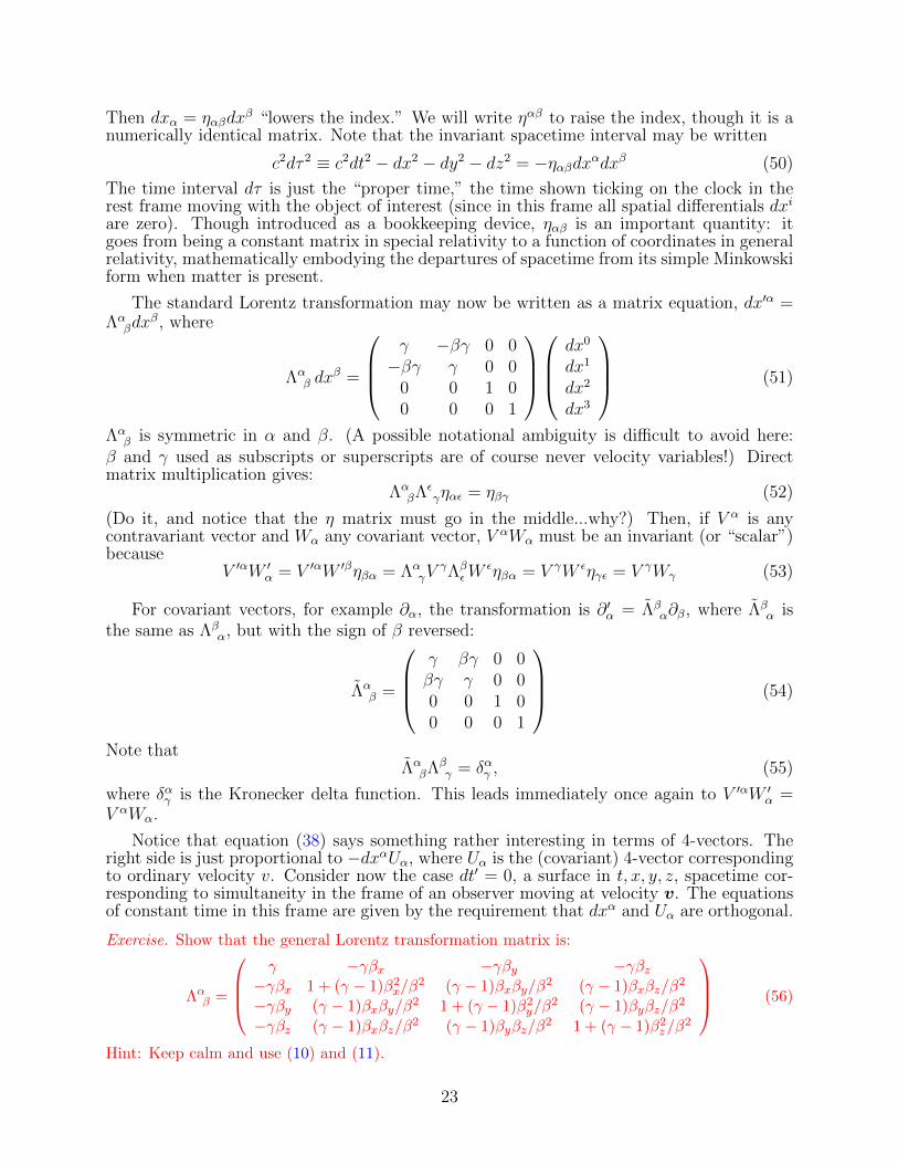
Then dxα = ηαβdxβ “lowers the index.” We will write ηαβ to raise the index, though it is a

numerically identical matrix. Note that the invariant spacetime interval may be written

c2dτ 2 ≡ c2dt2 − dx2 − dy2 − dz2 = −ηαβdxαdxβ (50)

The time interval dτ is just the “proper time,” the time shown ticking on the clock in therest frame moving with the object of interest (since in this frame all spatial differentials dxi

are zero). Though introduced as a bookkeeping device, ηαβ is an important quantity: itgoes from being a constant matrix in special relativity to a function of coordinates in generalrelativity, mathematically embodying the departures of spacetime from its simple Minkowskiform when matter is present.

The standard Lorentz transformation may now be written as a matrix equation, dx′α =Λα

βdxβ, where

Λαβ dx

β =

γ −βγ 0 0−βγ γ 0 0

0 0 1 00 0 0 1

dx0

dx1

dx2

dx3

(51)

Λαβ is symmetric in α and β. (A possible notational ambiguity is difficult to avoid here:

β and γ used as subscripts or superscripts are of course never velocity variables!) Directmatrix multiplication gives:

ΛαβΛε

γηαε = ηβγ (52)

(Do it, and notice that the η matrix must go in the middle...why?) Then, if V α is anycontravariant vector and Wα any covariant vector, V αWα must be an invariant (or “scalar”)because

V ′αW ′α = V ′αW ′βηβα = Λα

γVγΛβ

εWεηβα = V γW εηγε = V γWγ (53)

For covariant vectors, for example ∂α, the transformation is ∂′α = Λβα∂β, where Λβ

α isthe same as Λβ

α, but with the sign of β reversed:

Λαβ =

γ βγ 0 0βγ γ 0 00 0 1 00 0 0 1

(54)

Note thatΛα

βΛβγ = δαγ , (55)

where δαγ is the Kronecker delta function. This leads immediately once again to V ′αW ′α =

V αWα.

Notice that equation (38) says something rather interesting in terms of 4-vectors. Theright side is just proportional to −dxαUα, where Uα is the (covariant) 4-vector correspondingto ordinary velocity v. Consider now the case dt′ = 0, a surface in t, x, y, z, spacetime cor-responding to simultaneity in the frame of an observer moving at velocity v. The equationsof constant time in this frame are given by the requirement that dxα and Uα are orthogonal.

Exercise. Show that the general Lorentz transformation matrix is:

Λαβ =

γ −γβx −γβy −γβz−γβx 1 + (γ − 1)β2

x/β2 (γ − 1)βxβy/β

2 (γ − 1)βxβz/β2

−γβy (γ − 1)βxβy/β2 1 + (γ − 1)β2

y/β2 (γ − 1)βyβz/β

2

−γβz (γ − 1)βxβz/β2 (γ − 1)βyβz/β

2 1 + (γ − 1)β2z/β

2

(56)

Hint: Keep calm and use (10) and (11).

23

2.4 Tensors

2.4.1 The energy-momentum stress tensor

There is more to relativistic life than vectors and scalars. There are objects called tensors,which carry several indices. But possessing indices isn’t enough! All tensor components musttransform in the appropriate way under a Lorentz transformation. To play off an examplefrom Prof. S. Blundell, I could make a matrix of grocery prices with a row of dairy products(a11 = milk, a12 = butter), and a row of vegetables (a21 = carrots, a22 = spinach). If I putthis collection in my shopping cart and push the cart at some velocity v, I shouldn’t expectthe prices to change by a Lorentz transformation!

A tensor Tαβ must transform according to the rule

T ′αβ = ΛαγΛ

βεT

γε, (57)

whileT ′αβ = Λγ

αΛεβTγε, (58)

and of courseT ′αβ = Λα

γΛεβT

γε , (59)

You get the idea. Contravariant superscript use Λ, covariant subscript use Λ.

Tensors are not hard to find. Remember equation (52)? It works for Λαβ as well, since it

doesn’t depend on the sign of β (or its magnitude for that matter):

ΛαβΛε

γηαε = ηβγ (60)

So ηαβ is a tensor, with the same components in any frame! The same is true of δαβ , a mixedtensor (which is the reason for writing its indices as we have), that we must transform asfollows:

ΛεγΛ

αβδ

γα = Λε

γΛγβ = δεβ. (61)

Here is another tensor, slightly less trivial:

Wαβ = UαUβ (62)

where the U ′s are 4-velocities. This obviously transforms as tensor, since each U obeys itsown vector transformation law. Consider next the tensor

Tαβ = ρr〈uαuβ〉 (63)

where the 〈 〉 notation indicates an average of all the 4-velocity products uαuβ taken over awhole swarm of little particles, like a gas. (An average of these 4-velocity products preservesits tensor properties: the linear average of all the little particle tensors must itself be atensor.) ρr is a local rest density, a scalar number. (Here, r is not an index.)

The component T 00 is just ρc2, the energy density of the swarm, where ρ (without ther) includes both a rest mass energy and a thermal contribution. (The thermal part comesfrom averaging the “swarming” γ factors in the u0 = γc.) Moreover, if, as we shall assume,the particle velocities are isotropic, then Tαβ vanishes if α 6= β. Finally, when α = β 6= 0,then T ii (no sum!) is by definition the pressure P of the swarm. (Do you see how this works

24

out with the γ factors when the ui are relativistic?) Hence, in the frame in which the swarmhas no net translational bulk motion,

Tαβ =

ρc2 0 0 00 P 0 00 0 P 00 0 0 P

(64)

This is, in fact, the most general form for the so-called energy-momentum stress tensor foran isotropic fluid in the rest frame of the fluid.

To find Tαβ in any frame with 4-velocity Uα we could adopt a brute force method, boostaway, and apply the Λ matrix twice to the rest frame form, but what a waste of effort thatwould be! Here is a better idea. If we can find any true tensor that reduces to our resultin the rest frame, then that tensor is the unique stress tensor. Proof: if a tensor is zero inany frame, then it is zero in all frames, as a trivial consequence of the transformation law.Suppose the tensor I construct, which is designed to match the correct rest frame value, maynot be (you claim) correct in all frames. Hand me your tensor, the one you think is thecorrect choice. Now, the two tensors by definition match in the rest frame. I’ll subtract onefrom the other to form the difference between my tensor and your tensor. The differenceis also a tensor, but it vanishes in the rest frame by construction. Hence this “differencetensor” must vanish in all frames, so your tensor and mine are identical after all! Corollary:if you can prove that the two tensors are the same in any one particular frame, then theyare the same in all frames. This is a very useful ploy.

The only two tensors we have at our disposal to construct Tαβ are ηαβ and UαUβ, andthere is only one linear superposition that matches the rest frame value and does the trick:

Tαβ = Pηαβ + (ρ+ P/c2)UαUβ (65)

This is the general form of the energy-momentum stress tensor appropriate to an ideal fluid.

2.5 Electrodynamics

2.5.1 4-currents and 4-potentials

The vacuum Maxwell equations for the electric field E and magnetic field B produced by acharge density ρq and vector current J may be written:

∇·E = 4πρq (66)

∇×E = −1

c

∂B

∂t(67)

∇·B = 0 (68)

∇×B =4π

cJ +

1

c

∂E

∂t(69)

We have used gaussian esu units rather than SI. The former is the natural choice for rela-tivistic field applications (see Jackson 1999 for an interesting discussion on the topic of unitsin electrodynamics).

25

To cast these equations into a Lorentz invariant form, we first introduce the standardvector potential A, so that if

B =∇×A (70)

equation (68) is automatically satisfied in full generality. Then, equation (67) becomes

∇×(E +

1

c

∂A

∂t

)= 0 (71)

This means that the bracketed combination is derivable from a gradient, leading to

E = −∇Φ− 1

c

∂A

∂t(72)

where Φ is the standard electrostatic potential with its conventional minus sign.

The Lorentz invariant properties of Maxwellian electrodynamics become more apparentwhen we write the sourced equations (66) and (69) in terms of Φ and A:

− 1

c2

∂2Φ

∂t2+∇2Φ +

1

c

∂

∂t

(∇·A+

1

c

∂Φ

∂t

)= −4πρq (73)

− 1

c2

∂2A

∂t2+∇2A−∇

(∇·A+

1

c

∂Φ

∂t

)= −4π

cJ (74)

We have alread noted in §(2.1), equation (28), that the combination

Jα = γ(cρ0,vρ0) = (cρq,vρq) (75)

is a relativistic 4-vector, provided that ρq is identified with the “boosted” rest frame chargedensity ρ0. This leads immediately to a relativistic formulation of (73) and (74) potentials.We combine these two equations into a single, relativistically invariant, 4-vector equation:

∂α∂αAβ − ∂β(∂αA

α) = −4π

cJβ (76)

whereAα = (Φ,A) (77)

must itself be a 4-vector, because that is the only kind of object that will transform properlyfrom one frame to another, given the 4-vector Jβ on the right side of the equation. It isstraightforward to show that the physical E and B fields remain unchanged if we add a4-gradient of a scalar function Λ to Aα:

Aα → Aα + ∂αΛ, (78)

an important property of the Maxwell equations known as gauge invariance. Among otherconsequences, it means that we are free to choose, via an appropriate choice of Λ, whatevervalue of ∂αA

α is convenient for the task at hand. In particular, if we work in the so-calledLorenz gauage (note spelling!):

∂αAα = 0, (79)

then equation (76) takes on the elegant form

∂α∂αAβ = −4π

cJβ, (80)

26

a set of uncoupled classical wave equations with sources, and the starting point for mosttreatments of classical electrodynamical radiation theory.

Finally, we note that the 4-divergence of equation (76) gives zero identically on the leftside of that equation, leading to an equation of charge conservation,

∂αJα = 0, (81)

a constraint that is very clear in the Lorenz gauge wave equation (80).

2.5.2 Electromagnetic field tensor

The natural extension of the equation B = ∇×A leads us to define the electromagneticfield tensor:

Fαβ = ∂αAβ − ∂βAα, (82)

which is manifestly antisymmetric in its indices. We then have for the electric and magenticfield components, Ei, Bi:

Fi0 = ∂iA0 − ∂0Ai = − ∂Φ

∂xi− 1

c

∂Ai∂t

= Ei (83)

andFij = ∂iAj − ∂jAi ≡ εijkB

k (84)

where εijk = εijk is the Levi-Civita symbol, defined to be +1 when ijk is an even permutationof 123, equal to −1 for an odd permutation, and 0 when any index repeats. The indices ofFαβ are raised and lowered in the usual way, by contraction with ηαβ.

Equation (76) becomes:

∂αFαβ = −4π

cJα. (85)

It is now a straightforward exercise to show that the remaining two unsourced Mawell equa-tions (67, 68) may be combined into a single equation expressing the vanishing of the cyclicderivative combination

∂αFβγ + ∂γF

αβ + ∂βFγα = 0. (86)

Exercise. Verify equation (86) and show that it may also be written in terms of the fourdimensional Levi-Civita symbol εαβγδ as εαβγδ∂βF

γδ = 0.

2.6 Conservation of T αβ

One of the most salient properties of Tαβ is that, in the absence of designated sources, it isconserved, in the sense of

∂Tαβ

∂xα= 0 (87)

Since gradients of Lorentz tensors transform as tensors, this must be true in all Lorentzframes. What, exactly, are we conserving?

First, the time-like 0-component of this equation is

∂

∂t

[γ2

(ρ+

Pv2

c4

)]+∇·

[γ2

(ρ+

P

c2

)v

]= 0 (88)

27

which is the relativistic version of mass conservation,

∂ρ

∂t+∇·(ρv) = 0. (89)

Elevated in special relativity, this becomes a statement of energy conservation. So one ofthe things we are conserving is energy. This is good.

The spatial part of the conservation equation reads

∂

∂t

[γ2

(ρ+

P

c2

)vi

]+

(∂

∂xj

)[γ2

(ρ+

P

c2

)vivj

]+∂P

∂xi= 0 (90)

You may recognise this as Euler’s equation of motion, a statement of momentum conserva-tion, upgraded to special relativity. Conserving momentum is also good.

Now do the following Exercise:

Exercise. By using the explicit form (65) of Tαβ and contracting equation (87) with Uβ, prove theinteresting identity:

0 =∂(ρc2Uα)

∂xα+ P

∂Uα

∂xα.

(Remember that UαUα = −c2, a constant.) What is the physical interpretation of this equation?If we use this result back in equation (87), show that takes a more familiar form:(

ηαβ +UαUβ

c2

)∂P

∂xα+

(ρ+

P

c2

)Uα

∂Uβ

∂xα= 0

This is recognisable as the standard equation of motion with relativistic corrections of order v2/c2.

What if there are other external forces? These forces are included in this formalism byexpressing them in terms of the divergence of their own associated stress tensors. Then, itis the summed total of the Tαβ that is conserved.

An important example which follows this description is the Maxwellian electromagneticstress tensor. To construct this, Begin with the following contracted form of the relativisticMaxwell equation (85):

1

4πFα

γ∂βFβγ = −1

cJγFα

γ. (91)

In particular, the 0 component of the right side of this equation reads:

− 1

cJiF

0i = −1

cJ · E (92)

This is immediately recognisable as minus the rate at which the fields do work on theirsources, with a lead 1/c factor. (This factor is present for dimensional reasons, and is ineffect compensated by a 1/c factor in the x0 = ct time-coordinate partial derivative.) It isnatural, then, to expect the left side of (91) to be expressible as the divergence of the Tα0

(energy) component of a full, symmetric electromagnetic stress tensor for the fields, Tαβem . Inother words, we seek an explicit form for the mathematical object Tαβem such that the equation

1

4πFα

γ∂βFβγ = ∂βT

αβem (93)

28

is satisfied.

Start with an integration by parts:

Fαγ∂βF

βγ = ∂β(FαγF

βγ)− F βγ∂βFαγ. (94)

The first term on the right is now an explicit divergence, which is part of what we want.The second term may be written

Fβγ∂βFαγ = −Fβγ∂βF γα = −Fβγ∂γFαβ, (95)

where the second equality follows from switching the dummy indices γ and β and usingantisymmetry twice, once on each F -tensor. Therefore,

Fβγ∂βFαγ = −1

2Fβγ(∂

βF γα + ∂γFαβ + ∂αF βγ) +1

2Fβγ∂

αF βγ (96)

The first group of three terms has been constructed so that it explicitly vanishes by equation(86), the cyclic identity for the sourceless Maxwell equations. We therefore conclude that

Fβγ∂βFαγ =

1

2Fβγ∂

αF βγ =1

4ηαβ∂β(FδγF

δγ). (97)

Putting together equations (91), (93), (94) and (97), we arrive the equation

∂βTαβem = −1

cJγFα

γ, (98)

where

Tαβem =1

4π

(Fα

γFβγ − 1

4ηαβ(FδγF

δγ)

)(99)

This is our desired electromagnetic stress energy tensor. The right side of equation (98) is infact expressible as minus the divergence of the stress energy tensor for the particle sources,for whom the electromagnetic field is an external disturbance (see W72). Thus, the totalstress tensor for the sum of the particles and fields is conserved. We shall make explicit useof equation (99) in our discussion of electrically charged black holes in Chapter 10.

Exercise. Verify that the trace Tem ≡ ηαβTαβem = 0. This means that if we tried to make

a scalar relativistic field theory for gravity of the form ∂α∂αΦ = 4πGT ββ, it would failimmediately. Why?

Exercise. Show that:

T 00em =

1

8π(E2 +B2),

T 0iem =

1

4π(E×B)·ei,

where ei is a unit vector in the i direction, and

T ijem = − 1

4π

[EiEj +BiBj −

1

2δij(E

2 +B2)

].

29

Finally, show that Tem = 0 implies 3Prad = ρradc2 where Prad and ρrad represent radiation

pressure and energy density respectively.

The reader perhaps may be gaining a sense of the difficulty in constructing a theory ofgravity compatible with relativity. The mass-energy density ρ is but a single component ofa stress tensor, and it is the entire stress tensor from all possible contributors, fields andparticles alike, that would have to be the source of what we identify as the gravitationalpotential field. Recall that electromagnetic theory starts with electrostatics and Coulomb’slaw, but in the ultimate Maxwellian theory it is the entire 4-current Jα that is the source ofelectromangetic fields. We should expect something similar here. Relativistic theories mustwork with scalars, vectors and tensors to preserve their invariance properties from one frameto another. This simple insight is already an achievement: we can, for example, expectpressure to play a role in generating gravitational fields. Would you have guessed that?Perhaps our relativistic gravity equation ought to look something like:

∇2Gµν − 1

c2

∂2Gµν

∂t2= T µν , (100)

where Gµν is some sort of, I don’t know, conserved tensor guy for the...spacetime geome-try and stuff? In Maxwell’s theory we had a 4-vector (Aα) operated on by the so-called“d’Alembertian operator” −∇2 + (1/c)2∂2/∂t2 on the left side of the equation and a sourceproportional to (Jα) on the right. So now we just need to find a Gµν tensor to go with T µν .Right?

Actually, this is not a bad guess. It is more-or-less correct for weak fields, and most ofthe time gravity is a weak field. But...well...patience. One step at a time.

30

Then there occurred to me the

‘glucklichste Gedanke meines Lebens,’

the happiest thought of my life, in the

following form. The gravitational field

has only a relative existence in a way

similar to the electric field generated

by magnetoelectric induction. Because

for an observer falling freely from the

roof of a house there exists—at least

in his immediate surroundings—no

gravitational field.

— Albert Einstein

2

3 The effects of gravity

The central idea of general relativity is that presence of mass (more precisely the presenceof any stress-energy tensor component) causes departures from flat Minkowski spacetimeto appear, and that other matter (or radiation) responds to these distortions in some way.There are then really two questions: (i) How does the affected matter/radiation move inthe presence of a distorted spacetime?; and (ii) How does the stress-energy tensor distortthe spacetime in the first place? The first question is purely computational, and fairlystraightforward to answer. It lays the groundwork for answering the much more difficultsecond question, so let us begin here.

3.1 The Principle of Equivalence

We have discussed the notion that by going into a frame of reference that is in free-fall, theeffects of gravity disappear. In this era in which space travel is common, we are all familiarwith astronauts in free-fall orbits, and the sense of weightlessness that is produced. Thismanifestation of the Equivalence Principle is so palpable that hearing total mishmasheslike “In orbit there is no gravity” from an over-eager science correspondent is a commonexperience. (Our own BBC correspondent in Oxford Astrophysics, Prof. Christopher Lintott,would certainly never say such a thing.)

The idea behind the equivalence principle is that the m in F = ma and the m in theforce of gravity Fg = mg are the same m and thus the acceleration caused by gravity, g,is invariant for any mass. We could imagine, for example, that F = mIa and Fg = mgg,where mg is some kind of gravity-related “massy” property that might vary from one typeof body to another with the same inertial bulk mass mI . In this case, the acceleration a ismgg/mI , i.e., something that varies with the ratio of inertial to gravitational mass from onebody to another. How well can we actually measure this ratio, or posing the question moreaccurately, how well do we know that this ratio is truly a universal constant for all types ofmatter?

The answer is very, very well indeed. We don’t of course do anything as crude as directlymeasure the rate at which objects fall to the ground any more, a la Galileo and the tower of

2With apologies to any readers who may actually have fallen off the roof of a house—safe space statement.

31

cg

Earth

Figure 1: Schematic diagram of the Eotvos experiment. (Not to scale!) A barbell-shapedmass, the red object above, is hung from a pendulum on the surface of a rotating Earth. Itstwo end-masses are of different of material, say copper and lead. Each mass is affected bygravity (g), pulling it to the centre of the earth with a force proportional to a gravitationalmass mg, and by a centrifugal force (c) proportional to the inertial mass mI , due to theearth’s rotation. Forces are shown as blue arrows, rotation axis as a maroon arrow. Fromthe combined g and c forces, a difference between the inertial to gravitational mass ratioin the different composition end-masses will produce an unbalanced torque about the axisof the suspending fibre of the barbell.

Pisa. As with all classic precision gravity experiments (including those of Galileo!) we use apendulum. The first direct measurement of the gravitational to inertial mass ratio actuallypredates relativity, the so-called Eotvos experiment, after Baron Lorand Eotvos (1848-1919).(Pronouced “otvosh” with o as in German schon.)

The idea is shown in schematic form in figure [1]. Hang a pendulum from a string, butinstead of hanging a big mass, hang a rod, and put two masses of two different types ofmaterial at either end. There is a force of gravity toward the center of the earth (g in thefigure), and a centrifugal force (c) due to the earth’s rotation. The net force is the vectorsum of these two, and if the components of the acceleration perpendicular to the stringof each mass do not precisely balance—and they won’t if mg/mI is not the same for bothmasses—there will be a net torque twisting the masses about the string (a quartz fibre in theactual experiment). The fact that no such twist is measured is an indication that the ratiomg/mI does not, in fact, vary. In practise, to achieve high accuracy, the pendulum rotateswith a tightly controlled period, so that the rotating masses would be sometimes hinderedby any putative torque, and sometimes pushed forward. This would imprint a frequencydependence onto the motion, and the resulting signal component at a particular frequencycan be very sensitively constrained. Experiment shows that the ratio between any differencein the twisting accelerations on either mass and the average acceleration must be less than

32

a few parts in 1012 (Su et al. 1994, Phys Rev D, 50, 3614). With direct laser rangingexperiments to track the Moon’s orbit, it is possible, in effect, to use the Moon and Earthas the masses on the pendulum as they rotate around the Sun! This gives an accuracy anorder of magnitude better, a part in 1013 (Williams et al. 2012, Class. Quantum Grav., 29,184004), an accuracy comparable to measuring the distance from the Earth to the Sun towithin the size of your thumbnail.

There are two senses in which the Equivalence Principle may be used, a strong sense andweak sense. The weak sense is that it is not possible to detect the effects of gravity locally ina freely falling coordinate system, that all matter responds identically to a gravitational fieldindependent of its composition. Experiments can test this form of the Principle directly.The strong, much more powerful sense, is that all physical laws, whether gravitational ornot, behave in a freely falling coordinate system just as they do in Minkowski spacetime. Inthis sense, the Principle is a postulate which appears to be true.

If going into a freely falling frame eliminates gravity locally, then going from an inertialframe to an accelerating frame reverses the process and mimics the effect of gravity—again,locally. After all, if in an inertial frame

d2x

dt2= 0, (101)

and we transform to the accelerating frame x′ by x = x′+ gt2/2, where g is a constant, then

d2x′

dt2= −g, (102)

which the reader will agree looks an awful lot like motion in a gravitational field.

One immediate consequence of this realisation is of profound importance: gravity affectslight. In particular, if we are in an elevator of height h in a gravitational field of localstrength g, then locally the physics is exactly the same as if we were accelerating upwardsat g. But the effect of kinematic acceleration of an observer on the measured frequency oflight is easily analysed: a photon released upwards reaches a detector at height h in a timeh/c, at which point the detector is moving at a velocity v = gh/c relative to the bottom ofthe elevator at the time of release. The photon is measured to be redshifted by an amountv/c = gh/c2, or Φ/c2 with Φ the gravitational potential per unit mass at h. This is theclassical gravitational redshift, the simplest nontrivial prediction of general relativity. Thegravitational redshift was first measured accurately using changes in gamma ray energies(RV Pound & JL Snider 1965, Phys. Rev., 140 B, 788).

The gravitational redshift is the critical link between Newtonian theory and generalrelativity. Despite all those popular pictures of deformed rubber membranes (one of whichgraces the cover of these notes), it is not, after all, a distortion of space that gives rise toNewtonian gravity at the level we are familiar with. It is a distortion of the flow of time.

3.2 The geodesic equation

We denote by ξα our freely falling inertial coordinate frame in which the effects of gravityare locally absent. The local ξ coordinates are erected at a particular point in the spacetime,and are generally not the most convenient to calculate with, but all we need to know forpresent purposes is that they exist. They serve as a foothold to get to a formulation validfor arbitrary coordinates.

33

In the ξ frame, the equation of motion for a particle is

d2ξα

dτ 2= 0, (103)

withc2dτ 2 = −ηαβdξαdξβ (104)

serving as the invariant time interval. (If we are doing light, then dτ = 0, but ultimately itdoesn’t really matter. Either take a smooth limit from finite dτ , or use any other parameteryou fancy, like what you personally measure on your own wristwatch. In the end, for photonswe won’t need τ , but we may well use your watch, if that’s OK, if you are a nice quiet observerat infinity.) Next, write this equation in any other set of coordinates you like, and call themxµ. Our inertial coordinates ξα will be some function or other of the xµ so

0 =d2ξα

dτ 2=d

dτ

(∂ξα

∂xµdxµ

dτ

)(105)

where we have used the chain rule to express dξα/dτ in terms of dxµ/dτ . Carrying out thedifferentiation,

0 =∂ξα

∂xµd2xµ

dτ 2+

∂2ξα

∂xµ∂xνdxµ

dτ

dxν

dτ(106)

where now the chain rule has been used on ∂ξα/∂xµ. This may not look very promising.But if we multiply this equation by ∂xλ/∂ξα, and remember to sum over α now, then thechain rule in the form

∂xλ

∂ξα∂ξα

∂xµ= δλµ (107)

rescues us. (We are using the chain rule repeatedly and will certainly continue to do so,again and again. Make sure you understand this, and that you understand what variablesare being held constant when the partial derivatives are taken. Deciding what is constant isjust as important as doing the differentiation!) Our equation becomes

d2xλ

dτ 2+ Γλµν

dxµ

dτ

dxν

dτ= 0, (108)

where

Γλµν =∂xλ

∂ξα∂2ξα

∂xµ∂xν(109)

is known as the affine connection, and is a quantity of central importance in the study ofRiemannian geometry and relativity theory in particular. You should be able to prove, usingthe chain rule of partial derivatives, an inverse identity for the second derivatives of ξα thatwe will use shortly:

∂2ξα

∂xµ∂xν=∂ξα

∂xλΓλµν (110)

(How does this work out when used in equation [106]?)

No need to worry, despite the intimidating notation. (Early editions of relativity textsliked to use gothic font Tλµν for the affine connection, which must have imbued it with a

nice steampunk terror.) There is nothing especially mysterious about the affine connection.You use it all the time, probably without realising it. For example, in cylindrical (r, θ)

34

coordinates, when you use the combinations r−rθ2 or rθ+2rθ for your radial and tangentialaccelerations, you are using the affine connection and the geodesic equation. In the first case,Γrθθ = −r; in the second, Γθrθ = 1/r. (What happened to the 2?)

Exercise. Prove the last statements using ξx = r cos θ, ξy = r sin θ. (In an ordinary, non-distortedflat space, the “local” ξ coordinates are valid everywhere.)

Exercise. On the surface of a unit-radius sphere, choose any point as your North Pole, work incolatitude θ and azimuth φ coordinates, and show that locally near the North Pole ξx = θ cosφ,ξy = θ sinφ. It is in this sense that the ξα coordinates are tied to a local region of the space nearthe North Pole point. In our freely-falling inertial coordinate system, the local coordinates aretied to a point in spacetime, and in general are valid only in the neighbourhood of this point: ina distorted space, local coordinates are just that, valid only locally. Of course, “local” can seempretty extensive to tiny human beings like us. If you want to experience the effects of a local inertialcoordinate system in the Earth’s gravitational field, just hop. (Sitting in your chair you may feelquite inert, but your frame, alas, is noninertial!)

3.3 The metric tensor

In our locally inertial coordinates, the invariant spacetime interval is

c2dτ 2 = −ηαβdξαdξβ, (111)

so that in any other coordinates, dξα = (∂ξα/∂xµ)dxµ and

c2dτ 2 = −ηαβ∂ξα

∂xµ∂ξβ

∂xνdxµdxν ≡ −gµνdxµdxν (112)

where

gµν = ηαβ∂ξα

∂xµ∂ξβ

∂xν(113)

is known as the metric tensor. The metric tensor embodies the information of how coordinatedifferentials combine to form the invariant interval of our spacetime, and once we know gµν ,we know everything, including (as we shall see) the affine connections Γλµν . The object ofgeneral relativity theory is to compute gµν for a given distribution of mass (more precisely,a given stress energy tensor), and for now our key goal is to find the field equations thatenable us to do so.

3.4 The relationship between the metric tensor and affine connec-tion

Because of their explicit reliance on the local freely falling inertial coordinates ξα, the gµνand Γλµν quantities are awkward to use in their present formulation. Fortunately, there

is a direct relationship between Γλµν and the first derivatives of gµν that will free us oflocal bondage, permitting us to dispense with the ξα altogether. As we have emphasised,while their existence is crucial to formulate the mathematical structure of curved space, thepractical necessity of the ξ’s to carry out calculations is minimal.

35

Differentiate equation (113):

∂gµν∂xλ

= ηαβ∂2ξα

∂xλ∂xµ∂ξβ

∂xν+ ηαβ

∂ξα

∂xµ∂2ξβ

∂xλ∂xν(114)

Now use (110) for the second derivatives of ξ:

∂gµν∂xλ

= ηαβ∂ξα

∂xρ∂ξβ

∂xνΓρλµ + ηαβ

∂ξα

∂xµ∂ξβ

∂xρΓρλν (115)

All remaining ξ derivatives may be absorbed as part of the metric tensor, leading to

∂gµν∂xλ

= gρνΓρλµ + gµρΓ

ρλν (116)

It remains only to unweave the Γ’s from the cloth of indices. This is done by first adding∂gλν/∂x

µ to the above (switch λ and µ), then subtracting the same but with indices µ andν reversed:

∂gµν∂xλ

+∂gλν∂xµ

− ∂gλµ∂xν

= gρνΓρλµ +gµρΓ

ρλν + gρνΓ

ρµλ +gρλΓ

ρµν −gρµΓρνλ −gρλΓ

ρνµ. (117)

Remembering that Γ is symmetric in its bottom indices, only the gρν terms survive, leaving

∂gµν∂xλ

+∂gλν∂xµ

− ∂gλµ∂xν

= 2gρνΓρµλ (118)

Our last step is to multiply by the inverse matrix gνσ, defined by

gνσgρν = δσρ , (119)

leaving us with the pretty result

Γσµλ =gνσ

2

(∂gµν∂xλ

+∂gλν∂xµ

− ∂gλµ∂xν

). (120)

Notice that there is no mention of the ξ’s. The affine connection is completely specified bygµν and the derivatives of gµν in whatever coordinates you like. In practise, the inverse matrixis not difficult to find, as we will usually work with metric tensors whose off-diagonal termsvanish. (Gain confidence once again by practising the geodesic equation with cylindricalcoordinates grr = 1, gθθ = r2 and using [120.]) Note as well that with some very simpleindex relabeling, equation (118) leads directly to the mathematical identity

gρνΓρµλ

dxµ

dτ

dxλ

dτ=

(∂gµν∂xλ

− 1

2

∂gλµ∂xν

)dxµ

dτ

dxλ

dτ. (121)

We’ll use this in a moment.

Exercise. Prove that gνσ is given explicitly by

gνσ = ηαβ∂xν

∂ξα∂xσ

∂ξβ

Exercise. Prove the identities on page 6 of the notes for a diagonal metric gab,

Γaba = Γaab =1

2gaa

∂gaa∂xb

(a = b permitted, NO SUM)

Γabb = − 1

2gaa

∂gbb∂xa

(a 6= b, NO SUM)

Γabc = 0, (a, b, c distinct)

36

3.5 Variational calculation of the geodesic equation

The physical significance of the relationship between the metric tensor and affine connectionmay be understood by a variational calculation. Off all possible paths in our spacetime fromsome point A to another B, which path leaves the proper time an extremum (in this case, amaximum)?

The motivation for this formulation is obvious. “The shortest distance between twopoints is a straight line,” and in Cartesian coordinates the equations for this line-geodesicare d2ξi/ds

2 = 0. This is an elementary property of Euclidian space. We may also pose thequestion of what is the shortest distance between two points in a more general curved spaceas well, and this naturally lends itself to a variational approach. What is less obvious is thatthis mathematical machinery, which was fashioned for generalising the spacelike straight lineequation d2ξi/ds2 = 0 to more general non-Euclidian geometries, also works for generalisinga dynamical equation of the form d2ξi/dτ 2 = 0, where now we use invariant timelike intervals,to geodesics embedded in distorted Minkowski geometries.

We must pay particular attention to our endpoints in spacetime, say A and B. Thesepoints cannot be defined by τ itself, since the integral over τ from A to B would be B −A,and there is nothing to vary. Rather, A and B are specified by some other scalar p, knownas an affine parameter. As the path is varied, the endpoints remain fixed for all paths interms of their p values, but the elapsed value of τ will generally change. For present purposesthe parameter p need not precisely specified. Think of it as the time elapsed on your ownpersonal clock if you wish, and τ is then the time measured by a clock strapped to the objectmoving through spacetime. Then the proper time from A to B is

TAB =

∫ B

A

dτ

dpdp =

1

c

∫ B

A

(−gµν

dxµ

dp

dxν

dp

)1/2

dp (122)

Next, vary xλ to xλ + δxλ (we are regarding xλ as a function of p remember), with δxλ

vanishing at the end points A and B. We find

δTAB =1

2c

∫ B

A

(−gµν

dxµ

dp

dxν

dp

)−1/2(−∂gµν∂xλ

δxλdxµ

dp

dxν

dp− 2gµν

dδxµ

dp

dxν

dp

)dp (123)

(Do you understand the final term in the integral?)

Since the leading inverse square root in the integrand is just dp/dτ along the unperturbedpath, δTAB simplifies to

δTAB =1

2c

∫ B

A

(−∂gµν∂xλ

δxλdxµ

dτ

dxν

dτ− 2gµν

dδxµ

dτ

dxν

dτ

)dτ, (124)

and p has vanished from sight. Notice that equation (124) is, up to an overall multiplicativeconstant, exactly what we would have found by formally viewing

L = gµνdxµ

dτ

dxν

dτ(125)

as our starting Langrangian, and then carrying out a simple first-order variation in δxλ. Theultimate Euler-Lagrange equation associated with this procedure,

d

dτ

(∂L∂xρ

)− ∂L∂xρ

= 0, (126)

37

provides the simplest, most direct method for calculating the geodesic equations of motion.

Next, we integrate the second term in equation (124) by parts, noting that the contribu-tion from the endpoints has been specified to vanish. Remembering that

dgλνdτ

=dxσ

dτ

∂gλν∂xσ

, (127)

we find

δTAB =1

c

∫ B

A

(−1

2

∂gµν∂xλ

dxµ

dτ

dxν

dτ+∂gλν∂xσ

dxσ

dτ

dxν

dτ+ gλν

d2xν

dτ 2

)δxλ dτ (128)

or

δTAB =1

c

∫ B

A

[(−1

2

∂gµν∂xλ

+∂gλν∂xµ

)dxµ

dτ

dxν

dτ+ gλν

d2xν

dτ 2

]δxλ dτ (129)

Finally, using equation (121), we obtain

δTAB =1

c

∫ B

A

[(dxµ

dτ

dxσ

dτΓνµσ +

d2xν

dτ 2

)gλν

]δxλ dτ (130)

Thus, if the geodesic equation (108) is satisfied, δTAB = 0 is satisfied, and the propertime is an extremum. The name “geodesic” is used in geometry to describe the path ofminimum distance between two points in a manifold, and it is therefore gratifying to seethat there is a correspondence between a local “straight line” with zero curvature, and thelocal elimination of a gravitational field with the resulting zero acceleration, along the linesof the first paragraph of this section. In the first case, the proper choice of local coordinatesresults in the second derivative with respect to an invariant spatial interval vanishing; in thesecond case, the proper choice of coordinates means that the second derivative with respectto an invariant time interval vanishes, but the essential mathematics is the same.

Finally, we re-emphasize that the very practical side to working with the variationalmethod: it is much easier to obtain the equations of motion for a given gµν this way, asopposed to first calculating the Γλµν explicitly. Simply use equations (125) and (126). Aby-product of the variational method is that it automatically generates all the nonvanishingaffine connection components: just read them off as the coefficients of (dxµ/dτ)(dxν/dτ).The Γλµν are then available for whatever task is at hand.

3.6 The Newtonian limit

In classical mechanics, we know that the equations of motion may be derived from a La-grangian variational principle of least action, an integral involving the difference betweenkinetic and potential energies. This does not seem very geometrical. What is the connec-tion with the relativistic Lagrangian (125)? More generally, how can we make contact withNewtonian mechanics from the geodesic equation?

We consider the case of a slowly moving mass (“slow” of course means relative to c, thespeed of light) in a weak gravitational field (GM/rc2 1). Since cdt |dx|, the geodesicequation greatly simplifies:

d2xµ

dτ 2+ Γµ00

(cdt

dτ

)2

= 0. (131)

Now

Γµ00 =1

2gµν(∂g0ν

∂(cdt)+

∂g0ν

∂(cdt)− ∂g00

∂xν

)(132)

38

In the static Newtonian limit (meaning the time variations of the field are nonrelativistic),the largest of the g derivatives are contained in the final term. This leads to3:

Γµ00 ' −1

2gµν

∂g00

∂xν. (133)

Since the gravitational field is weak, gµν differs very little from its Minkoswki limiting value:

gµν = ηµν + hµν , hµν 1. (134)

Neglecting the difference between t and τ in this limit, the spatial components of the geodesicequation are therefore

d2x

dt2− c2

2∇h00 = 0. (135)

Isaac Newton would say:d2x

dt2+∇Φ = 0, (136)

with Φ being the classical gravitational potential. The two views are perfectly consistent if

h00 ' −2Φ

c2, g00 ' −

(1 +

2Φ

c2

)(137)

In other words, the gravitational potential force emerges as a sort of centripetal term, similarin structure to the centripital force in the standard radial equation of motion. This is aremarkable result. It is by no means obvious that a purely geometrical geodesic equationcan serve the role of a Newtonian gravitational potential gradient force equation, but itcan. Moreover, it teaches us that the Newtonian limit of general relativity is all in the timecomponent, h00. It is now possible to measure directly the differences in the rate at whichclocks run at heights separated by a few meters on the Earth’s surface.

The quantity h00 is a dimensionless number of order v2/c2, where v is a velocity typicalof the system, an orbital speed or just the square root of a potential. Note that h00 isdetermined by the dynamical equations only up to an additive constant. Here we havechosen the constant to make the geometry Minkowskian at large distances from any matter.

For self-consistency of the t ' τ assumption, let us check the µ = 0 geodesic equation inthe static Newtonian limit. Only the Γ0

0i,Γ0i0 terms contribute, where i is a spatial coordinate.

This leads tod2t

dτ 2− ∂h00

∂xidxi

dτ

dt

dτ= 0, (138)

summed over i. Since∂h00

∂xidxi

dτ=dh00

dτ,

this is just a first order ordinary differential equation for dt/dτ . The solution is

dt

dτ= C exp(h00),

3Notice that, going from Cartesian to polar coordinates, the steps we are following would lead to theradial centrifugal force. In this view, gravity is the centrifugal force emerging from time “curving around abend.”

39

where C is a constant of integration. Assuming that h00 vanishes at large distances from thesource, C may be chosen to be 1. With h00 1, the leading order correction term is

dt ' (1 + h00)dτ. (139)

This ∼ v2/c2 correction justifies our approximation of setting dτ = dt is the spatial geodesicequation of motion.

At the surface of a spherical object of mass M and radius R,

h00 '2GM

Rc2' 4.2× 10−6

(M

M

)(RR

)(140)

where M is the mass of the sun (about 2× 1030 kg) and R is the radius of the sun (about7× 108 m). The gravitational redshift fraction is half this number. As an exercise, you maywish to look up masses of planets and other types of stars and evaluate h00. What is itsvalue at the surface of a white dwarf (mass of the sun, radius of the earth)? What abouta neutron star (mass of the sun, radius of Oxford)? How many decimal points are neededto see the time difference in two digital clocks with a one metre separation in height on theearth’s surface?

We are now able to relate the geodesic equation to the principle of least action in classicalmechanics. In the Newtonian limit, our variational integral becomes∫ [

c2(1 + 2Φ/c2)dt2 − d|x|2]1/2

dt (141)

(Remember our compact notation: dt2 ≡ (dt)2, d|x|2 = (d|x|)2.) Expanding the square root,∫c

(1 +

Φ

c2− v2

2c2+ ...

)dt (142)

where v2 ≡ (d|x|/dt)2. Thus, minimising the Lagrangian (kinetic energy minus potentialenergy) is the same as maximising the proper time interval! What an unexpected andbeautiful connection.

What we have calculated in this section is nothing more than our old friend the gravi-tational redshift, with which we began our formal study of general relativity. The invariantspacetime interval dτ , the proper time, is given by

c2dτ 2 = −gµνdxµdxν (143)

For an observer at rest at location x, the time interval registered on a clock will be

dτ(x) = [−g00(x)]1/2dt (144)

where dt is the time interval registered at infinity, where −g00 → 1. (Compare: the “properlength” on the unit sphere for an interval at constant θ is sin θdφ, where dφ is the lengthregistered by an equatorial observer.) If the interval between two wave crest crossings isfound to be dτ(y) at location y, it will be dτ(x) when the light reaches x and it will be dtat infinity. In general,

dτ(y)

dτ(x)=

[g00(y)

g00(x)

]1/2

, (145)

40

and in particulardτ(R)

dt=ν(∞)

ν= [−g00(R)]1/2 (146)

where ν = 1/dτ(R) is, for example, an atomic transition frequency measured at rest at thesurface R of a body, and ν(∞) the corresponding frequency measured a long distance away.Interestingly, the value of g00 that we have derived in the Newtonian limit is, in fact, theexact relativistic value of g00 around a point mass M ! (A black hole.) The precise redshiftformula from a source at rest at r = R is

ν∞ =

(1− 2GM

Rc2

)1/2

ν (147)

The redshift as measured by wavelength becomes infinite from light emerging from radiusR = RS = 2GM/c2, the so-called Schwarzschild radius (about 3 km for a central point withthe mass of the entire Sun).

In its infancy, general relativity theory was supported empirically by the reported detec-tion of a gravitational redshift in a spectral line observed from the surface of the white dwarfstar Sirius B in 1925 by W.S. Adams. It “killed two birds with one stone,” as the leadingastrophysicist of his time, A.S. Eddington remarked. For it proved not only the existenceof white dwarf stars (at the time controversial since the mechanism of pressure support wasunknown), the measurement also confirmed an early and important prediction of generalrelativity theory: the spectral redshift of light due to a gravitational field.

Alas, the modern consensus is that these measurements were flawed. Adams knew whathe was looking for, and he found it, a case of “confirmation bias.” Though premature,the activity this apparently positive observation imparted to the study of white dwarfs andrelativity theory turned out to be very fruitful indeed. But we were lucky! Well-regardedbut incorrect single-investigator astronomical observations have often caused much confusionand needless wrangling, as well as years of wasted effort.

The first definitive test for gravitational redshift came much later, and it was purely ter-restrial: the 1959 Pound and Rebka experiment performed at Harvard University’s JeffersonTower measured the frequency shift of a 14.4 keV gamma ray falling (if that is the wordfor a gamma ray) 22.6 m. Pound & Rebka were able to measure the shift in energy—justa few parts in 1014—by what was at the time the new and novel technique of Mossbauerspectroscopy. In 1976, an experiment using rocket-borne hydrogen masers measured thegravitational redshift by comparing clocks at an altitude of 10,000 km with ground-basedclocks, and found agreement with Einstein’s prediction to one part in 104.

Exercise. A novel application of the gravitational redshift is provided by Bohr’s refutation ofan argument put forth by Einstein purportedly showing that an experiment could in principle bedesigned to bypass the quantum uncertainty relation ∆E∆t ≥ h. The idea is to hang a boxcontaining a photon by a spring suspended in a gravitational field g. At some precise time ashutter is opened and the photon leaves. You weigh the box before and after the photon. There isin principle no interference between the arbitrarily accurate change in box weight and the arbitrarilyaccurate time at which the shutter is opened. Or is there?

1.) Show that the box apparatus satisfies an equation of the form

Mx = −Mg − kx

where M is the mass of the apparatus, x is the displacement, and k is the spring constant. Beforerelease, the box is in equilibrium at x = −gM/k.

41

2.) Show that the momentum of the box after a short time interval ∆t from when the photonescapes is

δp =gδm

ωsin(ω∆t) ' gδm∆t

where δm is the (uncertain!) photon mass and ω2 = k/M . With δp ∼ gδm∆t, the uncertaintyprinciple then dictates an uncertain location of the box position δx given by gδmδx∆t ∼ h. Butthis is location uncertainty, not time uncertainty.

3.) Now the gravitational redshift comes in! The flow of time depends upon location. Show that ifthere is an uncertainty in position δx, there is an uncertainty in the time of release: δt ∼ (gδx/c2)∆t.

4.) Finally use this in part (2) to establish δE δt ∼ h with δE = δmc2.

Why does general relativity come into nonrelativistic quantum mechanics in such a fundamen-tal way? Because the gravitational redshift is relativity theory’s point-of-contact with classicalNewtonian gravitational mechanics, and Newtonian mechanics when blended with the uncertaintyprinciple is the start of nonrelativistic quantum mechanics.

A final thought

We Newtonian beings, with our natural mode of thinking in terms of forces and responses,would naturally say “How interesting, the force of gravity distorts the flow of time.” Thisis the way I have been describing the gravitational redshift throughout this chapter. ButEinstein has given us a more profound insight. It is not that gravity distorts the flow of time.An Einsteinian being, brought up from the cradle to be comfortable with a spacetime point-of-view, would, upon hearing this comment, cock their head and say: “What are you talkingabout? Newtonian gravity is the distortion of the flow of time. It is a simple geometricdistortion that is brought about by the presence of matter.” Equation (131), which may bewritten (with x ≡ dx/dτ)

xi + Γi00(x0)2 = 0,

should be compared with the standard flat space, ordinary time, radial centrifugal forceequation in affine connection form:

r + Γrφφ(φ)2 = 0

The analogy is unmistakable. Newtonian gravity is a centrifugal force arising from the flowof time going around a bend in space. Close to a source, the effect of weak gravity appearsas a distortion predominantly in the structure of time. Far from a source, weak gravitygenerally takes the form of gravitational radiation, and this, we shall see, may be mostnaturally thought of as a distortion of the structure of space.

42

4 Tensor Analysis

Further, the dignity of the science

seems to require that every possible

means be explored itself for the solution

of a problem so elegant and so cele-

brated.

— Carl Friedrich Gauss

A mathematical equation is valid in the presence of general gravitational fields when

i.) It is a valid equation in the absence of gravity and respects Lorentz invariance.

ii.) It preserves its form, not just under Lorentz transformations, but under any coordinatetransformation, x→ x′.

What does “preserves its form” mean? It means that the equation must be written in termsof quantities that transform as scalars, vectors, and higher ranked tensors under generalcoordinate transformations. From (ii), we see that if we can find one coordinate system inwhich our equation holds, it will hold in any set of coordinates. But by (i), the equationdoes hold in locally freely falling coordinates, in which the effect of gravity is locally absent.The effect of gravity is strictly embodied in the two key quantities that emerge from thecalculus of coordinate transformations: the metric tensor gµν and its first derivatives in Γλµν .This approach is known as the Principle of General Covariance, and it is a very powerfultool indeed.

4.1 Transformation laws

The simplest vector one can write down is the ordinary coordinate differential dxµ. If x′µ =x′µ(x), there is no doubt how the dx′µ are related to the dxµ. It is called the chain rule, andit is by now very familiar:

dx′µ =∂x′µ

∂xνdxν (148)

Be careful to distinguish between the coordinates xµ, which are almost always mere vectorimposters and can be pretty much anything, and their differentials dxµ, which are true vec-tors. Indeed, any set of quantities V µ that transforms in this way is known as a contravariantvector:

V ′µ =∂x′µ

∂xνV ν (149)

The contravariant 4-velocity, which is a 4-vector, is simply V µ = dxµ/dτ , a generalisation ofthe special relativistic dξα/dτ . A covariant vector, by contrast, transforms as

V ′µ =∂xν

∂x′µVν (150)

“CO LOW, PRIME BELOW.” (Sorry. Maybe you can do better.) These definitions ofcontravariant and covariant vectors are consistent with those we first introduced in ourdiscussions of the Lorentz matrices Λα

β and Λβα in Chapter 2, but now generalised from

specific linear transformations to arbitrary transformations.

43

The simplest covariant vector is the gradient ∂/∂xµ of a scalar Φ. Once again, the chainrule tells us how to transform from one set of coordinates to another—we’ve no choice:

∂Φ

∂x′µ=∂xν

∂x′µ∂Φ

∂xν(151)

The generalisation to tensor transformation laws is immediate. A contravariant tensor T µν

transforms as

T ′µν =∂x′µ

∂xρ∂x′ν

∂xσT ρσ (152)

a covariant tensor Tµν as

T ′µν =∂xρ

∂x′µ∂xσ

∂x′νTρσ (153)

and a mixed tensor T µν as

T ′µν =∂x′µ

∂xρ∂xσ

∂x′νT ρσ (154)

Notice that direct products of vectors V µV ν transform as a tensor T µν , and thus are tensors.This can be a useful way to think of tensorial indices. The generalisation of the transforma-tion laws to mixed tensors of arbitrary rank is self-evident.

By this definition the metric tensor gµν really is a covariant tensor, just as its notationwould lead you to believe, because

g′µν ≡ ηαβ∂ξα

∂x′µ∂ξβ

∂x′ν= ηαβ

∂ξα

∂xλ∂ξβ

∂xρ∂xλ

∂x′µ∂xρ

∂x′ν≡ gλρ

∂xλ

∂x′µ∂xρ

∂x′ν(155)

and the same for the contravariant gµν . (How else could it be? dxµdxν is clearly a con-travariant tensor, and gµνdx

µdxν is by construction a scalar, which works only if gµν is acovariant tensor.) However, the gradient of a vector is not, in general, a tensor or a vector:

∂A′λ

∂x′µ=

∂

∂x′µ

(∂x′λ

∂xνAν)

=∂x′λ

∂xν∂xρ

∂x′µ∂Aν

∂xρ+

∂2x′λ

∂xρ∂xν∂xρ

∂x′µAν (156)

The first term is just what we would have wanted if we were searching for a tensor trans-formation law. But oh, those pesky second order derivatives—the final term spoils it all.This of course vanishes when the coordinate transformation is linear (as when we found thatvector derivatives are perfectly good tensors under the Lorentz transformations), but alasnot in general. We will show in the next section that while the gradient of a vector is ingeneral not a tensor, there is an elegant solution around this problem.

Tensors can be created and manipulated in many ways. For example, direct products oftensors always transform as tensors:

W µνρσ = T µνSρσ. (157)

A linear combination of tensors of the same rank multiplied by scalars is obviously a tensorof unchanged rank. A tensor can lower its index by multiplying by gµν or raise it with gµν :

T ′ ρµ ≡ g′µνT′νρ =

∂xσ

∂x′µ∂xλ

∂x′ν∂x′ν

∂xκ∂x′ρ

∂xτgσλT

κτ =∂xσ

∂x′µ∂x′ρ

∂xτgσκT

κτ =∂xσ

∂x′µ∂x′ρ

∂xτT τσ (158)

which indeed does transform as a tensor of mixed second rank, T ρµ . Multiplying T µν by any

covariant tensor Sρµ of course generates a mixed tensor M νρ , but we adopt the very useful

44

convention of keeping the name T νρ when multiplying by Sρµ = gρµ, and thinking of the

index as “being lowered.” (And of course index-raising for multiplication by gρµ.)

Mixed tensors can “contract” to scalars. Start with T µν . Then consider the transforma-tion of T µµ:

T ′µµ =∂x′µ

∂xν∂xρ

∂x′µT νρ = δρνT

νρ = T νν (159)

i.e., T µµ is a scalar T (just like V µVµ). Exactly the same type of calculation shows that T µνµ isa vector T ν , and so on. Remember always to contract “up–down:” T µµ = T , never T µµ = T .

The generalisation of the familiar scalar dot product between vectors Aµ and Bµ isAµBµ = gµνA

µBν . We are often interested in just the spatial part of 4-vectors, the 3-vectorAi. Then, in a non-Euclidian 3-space, the cosine of the angle ∆θ between two vectors maybe written as the ratio

cos ∆θ =AiBi

(AjAj BkBk)1/2=

gijAiBj

(gklAkAl gmnBmBn)1/2(160)

the analogue of A ·B/(|A||B|). If we are given two parameterised curves, perhaps twoorbits xi(p) and yi(p), and wish to know the angle between them at some particular point,this angle becomes

cos ∆θ =xiyi

(xjxj ykyk)1/2=

gijxiyj

(gklxkxl gmnymyn)1/2

where the dot notation denotes d/dp. Do you see why this is so?

4.2 The covariant derivative

4.2.1 Contravariant vectors

Knowing the general form of the transformation law for a vector allows us to understandmore fully the content of the geodesic equation. With V ′α = dξα/dτ , the geodesic equationactually tells us the proper form of the vector quantity to use for dV ′α/dτ that is valid inany coordinate system. To see this clearly, consider the derivative of any vector dA′α/dτ ,expressed here in local inertial coordinates ξα, and in these coordinates this is the rightform of the derivative. Then, exactly the same manipulations we used to derive the geodesicequation yield, upon going to arbitrary coordinates xµ and vector Aµ:

dA′α

dτ=d

dτ

(∂ξα

∂xµAµ)

=∂ξα

∂xµdAµ

dτ+

∂2ξα

∂xµ∂xνAµ

dxν

dτ.

(This is of course always valid, whether dA′α/dτ happens to vanish or not.) Multiplying by∂xλ/∂ξα, we find

∂xλ

∂ξαdA′α

dτ=dAλ

dτ+ ΓλµνA

µdxν

dτ. (161)

The left hand side is now precisely the formal transformation law of dA′α/dτ from localinertial to general coordinates. The right side tells us what that expression is, expressedin these general coordinates. Evidently, the combination on the right of this equation is ageneral vector quantity unto itself!

45

We will return to this very useful result when we discuss the important concept of paralleltransport, but for now, let us further note that, with V ν = dxν/dτ , the vectorial right sideof (161) may be written as

V ν

[∂Aλ

∂xν+ ΓλµνA

µ

](162)

Since V ν is a vector and Aλ is arbitrary, the expression in square brackets must be a mixedtensor of rank two: it contracts with a contravariant vector V ν to produce another con-travariant vector. Recall that Γλµν vanishes in local inertial coordinates, in which we knowthat simple partial derivatives of vectors are valid tensors. So this prescription tells us howto upgrade the notion of a partial derivative of a vector to the status of a full tensor: tomake a tensor out of a plain partial derivative of a vector, form the quantity

∂Aλ

∂xµ+ ΓλµνA

ν ≡ Aλ;µ (163)

the so called covariant derivative. Following convention, we use a semicolon to denote co-variant differentiation. (Some authors use a comma for partial derivatives (e.g Aν, µ), but itis literally more clear to use full partial derivative notation [or ∂µ], and we shall abide bythis practise in these notes.) We now have a generalisation of the standard partial derivativeto tensor form4.

4.2.2 Transformation of the affine connection

Let us check our result in detail, and in the process learn how the non-tensor Γλµν changes un-der general coordinate transformations. In the following section, we will see how to constructthe covariant derivative of covariant vectors, and of yet more general tensors.5

We begin with the transformation law for Γλµν . This is just repeated application of thechain rule:

Γ′λµν ≡∂x′λ

∂ξα∂2ξα

∂x′µ∂x′ν=∂x′λ

∂xρ∂xρ

∂ξα∂

∂x′µ

(∂xσ

∂x′ν∂ξα

∂xσ

)(164)

Carrying through the derivative,

Γ′λµν =∂x′λ

∂xρ∂xρ

∂ξα

(∂xσ

∂x′ν∂xτ

∂x′µ∂2ξα

∂xτ∂xσ+

∂2xσ

∂x′µ∂x′ν∂ξα

∂xσ

)(165)

Cleaning up, and recognising an affine connection when we see one, helps get rid of thesemeddlesome ξ’s:

Γ′λµν =∂x′λ

∂xρ∂xτ

∂x′µ∂xσ

∂x′νΓρτσ +

∂x′λ

∂xρ∂2xρ

∂x′µ∂x′ν(166)

Because of the presence of the final term, this is not the transformation law of any sortof tensor. But consider now a differential change in the affine connection, δΓλµν , which arisesfrom a variation in the metric tensor itself, δgµν . This might be physically caused by apropagating wave or it may just be part of a formal mathematical calculation. The point

4Gauge-covariant derivatives in quantum field theories are a closely related concept.5Notice the use of the word “covariant” in two very different senses. This is awkward, but completely

standard, mathematical nomenclature.

46

is that the coordinate systems xµ and x′µ in equation (166) are unchanged by the variationδgµν . Under these conditions the transformation law for δΓλµν is

δΓ′λµν =∂x′λ

∂xρ∂xτ

∂x′µ∂xσ

∂x′νδΓρτσ, (167)

because the final term involves only the unchanged coordinates, and thus vanishes when thedifferential is calculated. Hence, δΓλµν is a true tensor, with all the privileges that entails.

Equation (166) may also be written

Γ′λµν =∂x′λ

∂xρ∂xτ

∂x′µ∂xσ

∂x′νΓρτσ −

∂xρ

∂x′ν∂xσ

∂x′µ∂2x′λ

∂xσ∂xρ(168)

Do you see why? (Hint: Either integrate ∂/∂x′µ by parts or differentiate the identity

∂x′λ

∂xρ∂xρ

∂x′ν= δλν .)

Hence

Γ′λµνA′ν =

(∂x′λ

∂xρ∂xτ

∂x′µ∂xσ

∂x′νΓρτσ −

∂xρ

∂x′ν∂xσ

∂x′µ∂2x′λ

∂xρ∂xσ

)∂x′ν

∂xηAη, (169)

and spotting some tricky sums over ∂x′ν that turn into Kronecker delta functions,

Γ′λµνA′ν =

∂x′λ

∂xρ∂xτ

∂x′µΓρτσA

σ − ∂xσ

∂x′µ∂2x′λ

∂xρ∂xσAρ (170)

Finally, adding this to (156), the unwanted terms cancel just as they should. We thus obtain

∂A′λ

∂x′µ+ Γ′λµνA

′ν =∂x′λ

∂xν∂xρ

∂x′µ

(∂Aν

∂xρ+ ΓνρσA

σ

), (171)

as desired. This combination really does transform as a tensor.

4.2.3 Covariant vectors

It is now a one-step process to deduce how covariant derivatives work for covariant vectors.With V λ arbitrary, consider the contraction

VλAλ;µ = Vλ

∂Aλ

∂xµ+ ΓλµνA

νVλ (172)

which is a perfectly good covariant vector. Integrating by parts the first term on the right,and then switching dummy indices λ and ν in the final term, this expression is identical to

∂(AλVλ)

∂xµ− Aλ

[∂Vλ∂xµ− ΓνµλVν

]. (173)

Since the first term is the covariant gradient of a scalar, and the entire expression must bea proper covariant vector, the term in square brackets must itself be a covariant tensor of

47

rank two. We have very quickly found our generalisation for the covariant derivative of acovariant vector:

Vλ;µ =∂Vλ∂xµ− ΓνµλVν (174)

That this really is a vector can also be directly verified via a calculation exactly similar toour previous one for the covariant derivative of a contravariant vector.

I hope that after all these examples, you will not make the cardinal sin of believingthat if V µ is a vector, then so must be its mathematical differential dV µ. Can you seehow to instantly destroy that belief using the transformation law for a vector? By contrast,coordinate differentials dxµ certainly are vectors; it is the coordinates xµ themselves that arenot!

4.2.4 Tensors of arbitrary rank

Covariant derivatives of tensors are now simple to deduce, since they have exactly the trans-formation properties of direct products of vectors. We have noted that a tensor T λκ, forexample, must formally transform like a direct product AλV κ. Well, in local inertial coordi-nates the covariant derivative of this is just the ordinary derivative

∂(AλV κ)

∂xµ= Aλ

∂V κ

∂xµ+∂Aλ

∂xµV κ.

But we already know how to generalise the partial vector derivatives on the right to arbitrarycoordinates! This leads immediately to

(AλV κ);µ =∂(AλV κ)

∂xµ+ ΓκνµA

λV ν + ΓλµνAνV κ (175)

We know that this will transform as a mixed tensor of rank 3, which means that we mayreplace the direct product AλV κ with any second rank contrariant tensor T λκ in the aboveformula:

T λκ;µ =∂T λκ

∂xµ+ ΓλµνT

νκ + ΓκνµTλν (176)

Identical reasoning leads to

Tλκ;µ =∂Tλκ∂xµ

− ΓνλµTνκ − ΓνκµTλν (177)

and of course

T λκ;µ =∂T λκ∂xµ

+ ΓλνµTνκ − ΓνµκT

λν (178)

The generalisation to tensors of arbitrary rank should now be self-evident. To generate theaffine connection terms, freeze all indices in your tensor, then “unfreeze” them one-by-one,treating each unfrozen index as either a covariant or contravariant vector, depending uponwhether it is down or up. Practise this drill until it is second-nature.

48

4.2.5 Going from special to general relativity

We now can give a precise rule for how to take an equation that is valid in special relativity,and upgrade it to the general relativistic theory of gravity. Work exclusively with scalars,4-vectors and 4-tensors. Replace ηαβ with gµν. Replace standard partial derivatives and withcovariant derivatives. Voila: your equation is set for the presence of gravitational fields.This, by the way, is not merely a presecription to do general relativity: it is the way to turnany set of properly framed mathematical equations written in Cartesian coordinates into thecorresponding equations valid in any coordinates you fancy.

It will not have escaped your attention, I am sure, that applying (177) to gµν produces

gµν;λ =∂gµν∂xλ

− gρνΓρµλ − gµρΓρνλ = 0 (179)

where equation (116) has been used for the last equality. The covariant derivatives of gµνvanish. This is exactly what we would have predicted, since the partial derivatives of ηαβvanish in special relativity, and thus the tensorial covariant derivative of gµν must alsovanish in the presence of gravitational fields. It’s just the general relativistic upgrade of∂ηαβ/∂x

γ = 0.

Here are two important technical points that are easily shown. (You should do so explic-itly.)

• The covariant derivative obeys the Leibniz rule for products. For example:

(T µνUλκ);ρ = T µν;ρ Uλκ + T µνUλκ;ρ,

(AµVµ);ν = Aµ(Vµ);ν + Vµ(Aµ);ν = Aµ∂Vµ∂xν

+ Vµ∂Aµ

∂xν(Γ′s cancel!)

This means that you can interchange the order of lowering or raising an index andcovariant differentiation; hence

• The operation of contracting two tensor indices commutes with covariant differentia-tion. It does not matter which you do first. Try it in the second example above byconsidering the covariant derivative of V µVν first before, then after, contracting theindices.

4.3 The affine connection and basis vectors

The reader may be wondering how this all relates to our notions of, say, spherical or polargeometry and their associated sets of unit vectors and coordinates. The answer is: verysimply. Our discussion will be straightforward and intuitive, rather than rigorous.

A vector V may be expanded in a set of basis vectors,

V = V aea (180)

where we sum over the repeated a, but a here on a bold-faced vector refers to a particularvector in the basis set. The V a are the usual vector contravariant components: old friends,just numbers. Note that the sum is not a scalar formed from a contraction! We’ve usedroman letters here to help avoid that pitfall.

49

The covariant components are associated with what mathematicians are pleased to calla dual basis:

V = Vbeb (181)

Same V mind you, just different ways of representing its components. If the e’s seem alittle abstract, don’t worry, just take them at a formal level for the moment. You’ve seensomething very like them before in elementary treatments of vectors.

The basis and the dual basis are related by a dot product rule,

ea·eb = δba. (182)

This dot product rule relates the vectors of orthonormal bases. The basis vectors transformjust as good old vectors should:

e′a =∂xb

∂x′aeb, e′a =

∂x′a

∂xbeb. (183)

Note that the dot product rule gives

V ·V = V aVbea·eb = V aVbδba = V aVa, (184)

as we would expect. On the other hand, expanding the differential line element ds,

ds2 = eadxa·ebdxb = ea·ebdxadxb (185)

so that we recover the metric tensor

gab = ea·eb (186)

Exactly the same style calculation gives

gab = ea·eb (187)

These last two equations tell us first that gab is the coefficient of ea in an expansion of thevector eb in the usual basis:

eb = gabea, (188)

and tell us second that gab is the coefficient of ea in an expansion of the vector eb in the dualbasis:

eb = gabea (189)

We’ve recovered the rules for raising and lowering indices, in this case for the entire basisvector.

As with any vector field, basis vectors will generally change with coordinate position. Wedefine an thrice-indexed object Γbac by

∂ea∂xc

= Γbaceb (190)

so thatΓbac = eb·∂cea ≡ ∂c(ea·eb)− ea·∂ceb = −ea·∂ceb. (191)

(Remember the shorthand notation ∂/∂xc = ∂c.) The last equality implies the expansion

∂eb

∂xc= −Γbace

a (192)

50

Consider ∂cgab = ∂c(ea·eb). Using (190),

∂cgab = (∂cea)·eb + ea·(∂ceb) = Γdaced·eb + ea·Γdbced, (193)

or finally∂cgab = Γdacgdb + Γdbcgad, (194)

exactly what we found in (116)! This leads, in turn, precisely to (120), the equation for theaffine connection in terms of the g partial derivatives. We now have a more intuitive under-standing of what the Γ’s really represent: they are expansion coefficients for the derivativesof basis vectors, which is how we are used to thinking of the extra acceleration terms innon Cartesian coordinates when we first encounter them in our first mechanics courses. InCartesian coordinates, the Γbac just go away.

Finally, consider

∂a(Vbeb) = (∂aV

b)eb + V b∂aeb = (∂aVb)eb + V bΓcabec (195)

Taking the dot product with ed:

ed·∂a(V beb) = ∂aVd + V bΓdab ≡ V d

;a, (196)

just the familiar covariant derivative of a contravariant vector. This one you should be ableto do yourself:

ed·∂a(Vbeb) = ∂aVd − VbΓbad ≡ Vd;a, (197)

the covariant derivative of a covariant vector. This gives us some understanding as to whythe true tensors formed from the partial derivatives of a vector V are not simply ∂aV

d

and ∂aVd, but rather ed·∂a(V beb) and ed·∂a(Vbeb) respectively. The Γ-terms then emergeas derivatives of the e basis vectors. Our terse, purely coordinate notation avoids the useof the e bases, but at a cost of missing a deeper and ultimately simplifying mathematicalstructure. We can see an old maxim of mathematicians in action: good mathematics startswith good definitions.

4.4 Volume element

The transformation of the metric tensor gµν may be thought of as a matrix equation:

g′µν =∂xκ

∂x′µgκλ

∂xλ

∂x′ν(198)

Remembering that the determinant of the product of matrices is the product of the deter-minants, we find

g′ =

∣∣∣∣ ∂x∂x′∣∣∣∣2 g (199)

where g is the determinant of gµν (just the product of the diagonal terms for the diagonalmetrics we will be using), and the notation |∂x′/∂x| indicates the Jacobian of the transfor-mation x → x′. The significance of this result is that there is another quantity that alsotransforms with a Jacobian factor: the volume element d4x.

d4x′ =

∣∣∣∣∂x′∂x

∣∣∣∣ d4x. (200)

51

This means √−g′ d4x′ =

√−g∣∣∣∣ ∂x∂x′

∣∣∣∣ ∣∣∣∣∂x′∂x

∣∣∣∣ d4x =√−g d4x. (201)

In other words,√−g d4x is the invariant volume element of curved spacetime. The minus

sign is used merely as an absolute value to keep the quantities positive. In flat Minkowskispace time, d4x is invariant by itself.

Euclidian example: in going from Cartesian (g = 1) to cylindrical polar (g = R2) tospherical coordinates (g = r4 sin2 θ), we have dx dy dz = RdRdz dφ = r2 sin θ dr dθ dφ. Youknew that. For a diagonal gµν , our formula gives a volume element of√

|g11g22g33g00|dx1 dx2 dx3 dx0,

just the product of the proper differential intervals. That also makes sense.

4.5 Covariant div, grad, curl, and all that

Ordinary partial derivatives of a scalar transform as covariant vectors, so in the case of asimple gradient there is no distinction between a covariant and standard partial derivative.Another result ithat is easily adpated is the covariant curl,

Vµ;ν − Vν;µ =∂Vµ∂xν− ∂Vν∂xµ

. (202)

(The affine connection terms are symmetric in the two lower indices, so they cancel.) Some-what more interesting is

V µ;µ =

∂V µ

∂xµ+ ΓµµλV

λ (203)

where by definition

Γµµλ =gµρ

2

(∂gρµ∂xλ

+∂gρλ∂xµ

− ∂gµλ∂xρ

). (204)

Now the lead factor gµρ is symmetric in its indices, whereas the last two g derivatives com-bined are antisymmetric in the same indices, so that combination disappears when summedover µρ. We are left with

Γµµλ =gµρ

2

∂gρµ∂xλ

. (205)

In this course, we will be dealing entirely with diagonal metric tensors, in which µ = ρ fornonvanishing entries, and gµρ is the reciprocal of gµρ. In this simple case,

Γµµλ =1

2

∂ ln |g|∂xλ

, (206)

where g is as usual the determinant of gµν , here just the product of the diagonal elements.Though this result has only been derived for diagonal gµν , W72 pp. 106-7, shows that thisresult is true for any gµν .

6

6Sketchy proof for the mathematically inclined: For matrix M , trace Tr, differential δ, to first orderin δ we have δ ln detM = ln det(M + δM) − ln detM = ln detM−1(M + δM) = ln det(1 + M−1δM) =ln(1 + TrM−1δM) = TrM−1δM . Can you supply the missing details?

52

The covariant divergence (203) becomes

V µ;µ =

1√|g|∂(√|g|V µ)

∂xµ(207)

a neat and tidy result. Note that the vanishing of the scalar integral∫ √|g|d4xV µ

;µ = 0, (208)

if V µ vanishes sufficiently rapidly at infinity.

Exercise. Apply our divergence formula (207) to the case of standard spherical coordinatesin three dimensions and compare with the usual formula for the divergence. What do younotice about the terms involving V θ and V φ? What needs to be done to get agreement?Explain.

Another Γ-contraction of interest is

Γσ ≡ gµλΓσµλ = gµλgνσ

2

(∂gµν∂xλ

+∂gλν∂xµ

− ∂gλµ∂xν

)(209)

The first two sums on the right are identical because of the µλ symmetry, so focus on thefirst one. Using (justify!):

gµλ∂gµν∂xλ

= −gµν∂gµλ

∂xλ,

we multiply by gνσ, so that a Kronecker δσµ conveniently appears on the right. This gives

−∂λgσλ as the sum of the first two terms on the right side of (209). The final term on theright side of this equation is now recognisable as our new friend (focus on µλ):

−gµλ gνσ

2

∂gλµ∂xν

= −gνσΓµµν = −gνσ

2

∂ ln |g|∂xν

,

to whom we have been introduced in (206). Adding this to −∂λgσλ, we finally have

Γσ = gµλΓσµλ = − 1√|g|

∂

∂xν

(√|g|gνσ

)(210)

We cannot leave the topic of covariant derivatives without discussing T µν;µ, the covariantdivergence of T µν . (And similarly for the divergence of T µν .) Conserved stress tensors are,after all, general relativity’s “coin of the realm.” We have:

T µν;µ =∂T µν

∂xµ+ ΓµµλT

λν + ΓνµλTµλ, or T µν;µ =

∂T µν∂xµ

+ ΓµµλTλν − ΓλµνT

µλ (211)

and using (206), we may condense this to

T µν;µ =1√|g|∂(√|g|T µν)∂xµ

+ ΓνµλTµλ, or T µν;µ =

1√|g|∂(√|g|T µν)∂xµ

− ΓλµνTµλ. (212)

53

For an antisymmetric contravariant tensor, call it Aµν , the last term of the first equalitydrops out because Γ is symmetric in its lower indices:

Aµν;µ =1√|g|∂(√|g|Aµν)∂xµ

if Aµν antisymmetric. (213)

Exercise. Don’t give up if T µν is symmetric. Prove that if T µν is symmetric in its indicesand the metric tensor is independent of coordinate xν , then

T µν;µ =1√|g|∂(√|g|T µν)∂xµ

.

Black holes, for example, have spacetime geometries independent of φ, and an ideal gas hasa symmetric stress tensor T µν , so this equation is very useful for astrophysicists.

Exercise. Define Γσµν = gσλΓλµν . Find an explicit expression for Γσµν and prove that∑

σµν

Γσµν =∑σµν

∂σgµν

where the sum is over the three even permutations of σµν.

4.6 Hydrostatic equilibrium

You have been patient and waded through a sea of indices, and it is time to be rewarded.We will do our first real physics problem in general relativity: hydrostatic equilibrium.

In Newtonian mechanics, you will recall that hydrostatic equilibrium represents a balancebetween a pressure gradient and the force of gravity. In general relativity this is completelyencapsulated in the condition

T µν;µ = 0

applied to the energy-momentum stress tensor (65), upgraded to fully covariant status:

T µν = Pδµν + (ρ+ P/c2)UµUν (214)

(The expression for the mixed T µν is actually unchaged from special relativity. Otherwise,one simply changes η’s to g’s.) Our conservation equation is

0 = T µν;µ =∂P

∂xν+[(ρ+ P/c2)UµUν

];µ

(215)

where we have made use of the Leibniz rule for the covariant derivative of a product, andthe fact that the δµν covariant derivative vanishes. Using (212):

0 =∂P

∂xν+

1

|g|1/2∂

∂xµ[|g|1/2(ρ+ P/c2)UµUν

]− Γµνλ(ρ+ P/c2)UµU

λ (216)

In static equilibrium, all the U components vanish except U0. To determine this, we use

UµUµ = −c2, (217)

54

in essence the upgraded version of special relativity’s ηαβUαUβ = −c2. Thus,

U0U0 = −c2, (218)

and with

Γ0ν0 =

1

2

∂ ln |g00|∂xν

, (219)

a vanishing second term on the right of equation (216), we then find

0 =∂P

∂xν+(ρc2 + P

) ∂ ln |g00|1/2∂xν

(220)

This is the general relativistic equation of hydrostatic equilibrium. Compare this with theNewtonian counterpart:

∇P + ρ∇Φ = 0 (221)

The difference for a static problem is the replacement of ρ by ρ+ P/c2 for the inertial massdensity, and the appearance of ln |g00|1/2 as the relativistic generalisation of the potential(note the agreement in the Newtonian limit).

If P = P (ρ) (a function of energy density only), then with P ′ ≡ dP/dρ, equation (220)may be formally integrated:∫

P ′(ρ) dρ

P (ρ) + ρc2+ ln |g00|1/2 = constant. (222)

Exercise. Solve the GR equation of hydrostatic equilibrium exactly for the case |g00| = (1 −2GM/rc2)1/2 (e.g., near the surface of a neutron star) and P = Kργ for γ ≥ 1.

Exercise. Show that equation (216) may be quite generally written

0 =∂P

∂xν+

1

|g|1/2∂

∂xµ

[|g|1/2(ρ+ P/c2)UµUν

]+ (ρ+ P/c2)Uµ

∂Uµ

∂xν(223)

Show that this is consistent with equation (220). If you do this exercise now, you will save yourselfsome effort on a Problem Set!

4.7 Covariant differentiation and parallel transport

Recall the geodesic equation,d2xλ

dτ 2+ Γλµν

dxµ

dτ

dxν

dτ= 0. (224)

Writing the vector dxλ/dτ as V λ this becomes

dV λ

dτ+ Γλµν

dxµ

dτV ν = 0, (225)

a covariant formulation of the statement that the vector V λ is conserved along a geodesicpath. But the covariance property of this statement has nothing to do with the specificidentity of V λ with dxλ/dτ . We have seen that the left-side of this equation is a genuine

55

vector for any V λ as long as V λ itself is a bona fide contravariant vector. The right sidesimply tells us that the fully covariant left side expression happens to vanish. Therefore,just as we “upgrade” from special to general relativity the partial derivative,

∂V α

∂xβ→ ∂V λ

∂xµ+ ΓλµνV

ν ≡ V λ;µ (226)

we upgrade the derivative along a path x(τ) in the same way by multiplying by dxµ/dτ andsumming over the index µ:

dV α

dτ→ dV λ

dτ+ Γλµν

dxµ

dτV ν ≡ DV λ

Dτ(227)

DV λ/Dτ is a true vector; the transformation

DV ′λ

Dτ=∂x′λ

∂xµDV µ

Dτ(228)

may be verified directly. (The inhomogeneous contributions from the Γ transformation andthe derivatives of the derivatives of the coordinate transformation coefficients cancel in amanner exactly analogous to our original covariant partial derviative calculation.)

Exactly the same reasoning is used to define the covariant derivative for a covariantvector, which follows from (174):

dVλdτ− Γνµλ

dxµ

dτVν ≡

DVλDτ

. (229)

The same is true for tensors, e.g.:

dT σλdτ

+ Γσµνdxν

dτT µλ − Γµλν

dxν

dτT σµ ≡

DT σλDτ

. (230)

As you might expect, the Leibniz rule holds for the covariant derivative along a path, e.g.

D(V µVµ)

Dτ= V µDVµ

Dτ+ Vµ

DV µ

Dτ,

with affine connection terms always cancelling when they need to.

When a vector or tensor quantity is carried along a path, and the object does not change ina locally inertial reference frame (d/dτ = 0), this condition becomes, in arbitrary coordinates,D/Dτ = 0. We expressing the same physical result in a covariant language. (Once again,this works because the two statements agree in the inertial coordinate frame, and then thiszero difference is zero in any coordinate frame.) The condition D/Dτ = 0 is known asparallel transport. A steady vector, for example, may always point along the y axis as wemove it around in the xy plane, but its r and θ components will have to change in orderto keep this true! The prescription for how those components change is the content of theparallel transport equation.

Suppose that we do a complete round trip following the rule of parallel transport, andwe come back to our exact starting point. Does a vector/tensor have to have the same valueit began with? You might think that the answer must be yes, but it turns out to be morecomplicated than that. Indeed, it is a most interesting question...

The stage is now set to introduce the key tensor embodying the gravitational distortionof spacetime.

56

5 The curvature tensor

The properties which distinguish space

from other conceivable triply-extended

magnitudes are only to be deduced

from experience...At every point the

three-directional measure of curvature

can have an arbitrary value if only the

effective curvature of every measurable

region of space does not differ notice-

ably from zero.

— G. F. B. Riemann

5.1 Commutation rule for covariant derivatives

The covariant derivative shares many properties with the ordinary partial derivative: it is alinear operator, it obeys the Leibniz rule, and it allows true tensor status to be bestowed uponpartial derivatives (or derivatives with respect to a scalar parameter) in any coordinates. Anatural question arises. Ordinarily, partial derivatives commute: the order in which they aretaken does not matter, provided that appropriate smoothness conditions are present. Doesthe same commutation work for covariant derivatives? Does V µ

;σ;τ equal V µ;τ ;σ?

Just do it.

V µ;σ =

∂V µ

∂xσ+ ΓµνσV

ν ≡ T µσ (231)

Then

T µσ;τ =∂T µσ∂xτ

+ ΓµντTνσ − ΓνστT

µν , (232)

or

T µσ;τ =∂2V µ

∂xτ∂xσ+

∂

∂xτ(ΓµλσV

λ)

+ Γµντ

(∂V ν

∂xσ+ ΓνλσV

λ

)− Γνστ

(∂V µ

∂xν+ ΓµλνV

λ

)(233)

The first term and the last group (proportional to Γνστ ) are manifestly symmetric in σ andτ , and so will vanish when the same calculation is done with the indices reversed and thensubtracted off. A bit of inspection shows that the same is true for all the remaining termsproportional to any partial derivative of V µ. The residual terms from taking the covariantderivative commutator are then

T µσ;τ − T µτ ;σ =

[∂Γµλσ∂xτ

− ∂Γµλτ∂xσ

+ ΓµντΓνλσ − ΓµνσΓνλτ

]V λ, (234)

which we may write as

V µ;σ;τ − V µ

;τ ;σ = T µσ;τ − T µτ ;σ = RµλστV

λ (235)

Now, both sides of this equation must be tensors, and V λ is itself some arbitrary vector.(Good thing those partial derivatives of V λ cancelled out.) This means that the quantity

57

Rµλστ must transform its coordinate indices as a tensor. That it actually does so may also be

verified explicitly in a nasty calculation (if you really want to see it spelt out in detail, seeW72 pp.132-3). We conclude that

Rµλστ =

∂Γµλσ∂xτ

− ∂Γµλτ∂xσ

+ ΓµντΓνλσ − ΓµνσΓνλτ (236)

is a true tensor. It is known as the Riemann curvature tensor. In fact, it may be shown(W72 p. 134) that this is the only tensor that is linear in the second derivatives of gµν , andcontains only its first and second derivatives.

Why do we refer to this peculiar mixed tensor as the “curvature tensor?” We may begin toanswer this by noting that it vanishes in ordinary flat Minkowski spacetime—simply chooseCartesian coordinates to do the calculation. Then, because Rµ

λστ is a tensor, if it is zeroin one set of coordinates, it is zero in all. Commuting covariant derivatives makes sense inthis case, since they amount to ordinary derivatives. Evidently, distortions from Minkowskispace are essential for a nonvanishing curvature tensor, an intuition we will strengthen inthe next section.

Exercise. What is the (much simpler) form of Rµλστ in local inertial coordinates? It is often

convenient to work in such coordinates to prove a result, and then generalise it to arbitrarycoordinates using the fact that Rµ

λστ is a tensor.

5.2 Parallel transport

We move on to the yet more striking example of parallel transport. Consider a vector Vλwhose covariant derivative along a curve x(τ) vanishes. Then,

dVλdτ

= Γµλνdxν

dτVµ (237)

Consider next a tiny round trip journey over a closed path on which Vλ is changing by theabove prescription. If we remain in the neighbourhood of some point Xρ, with xρ passingthrough Xρ at some instant τ0, xρ(τ0) = Xρ, we Taylor expand as follows:

Γµλν(x) = Γµλν(X) + (xρ −Xρ)∂Γµλν∂Xρ

+ ... (238)

Vµ[x(τ)] = Vµ(X) + dVµ + ... = Vµ(X) + (xρ −Xρ)Γσµρ(X)Vσ(X) + ... (239)

(where xρ −Xρ is dxρ from the right side of the parallel transport equation), whence

Γµλν(x)Vµ(x) = ΓµλνVµ + (xρ −Xρ)Vσ

(∂Γσλν∂Xρ

+ ΓσµρΓµλν

)+ ... (240)

where all quantities on the right (except x!) are evaluated at X. Integrating

dVλ = Γµλν(x)Vµ(x) dxν (241)

around a tiny closed path∮

, and using (241) and (240), we find that there is a change inthe starting value ∆Vλ arising from the term linear in xρ given by

∆Vλ =

(∂Γσλν∂Xρ

+ ΓσµρΓµλν

)Vσ

∮xρ dxν (242)

58

The integral∮xρdxν certainly doesn’t vanish. (Try integrating it around a unit square in

the xy plane.) But it is antisymmetric in ρ and ν. (Integrate by parts and note that theintegrated term vanishes, being an exact differential.) That means the only part of the ΓΓand ∂Γ/∂X terms that survives the ρν summation is the part that is antisymmetric in (ρ, ν).Since any object depending on two indices, say A(ρ, ν), can be written as a symmetric partplus an antisymmetric part,

1

2[A(ρ, ν) + A(ν, ρ)] +

1

2[A(ρ, ν)− A(ν, ρ)],

we find

∆Vλ =1

2Rσ

λνρVσ

∮xρ dxν (243)

where

Rσλνρ =

(∂Γσλν∂Xρ

−∂Γσλρ∂Xν

+ ΓσµρΓµλν − ΓσµνΓ

µλρ

)(244)

is precisely the curvature tensor. Parallel transport of a vector around a closed curve doesnot change the vector, unless the enclosed area has a nonvanishing curvature tensor. In fact,“the enclosed area” can be given a more intuitive interpretation if we think of integratingaround a very tiny square in the ρν plane. Then the closed loop integral is just the directedarea dxρdxν :

∆Vλ =1

2Rσ

λνρVσdxρ dxν . (245)

The conversion of a tiny closed loop integral to an enclosed surface area element reminds usof Stokes theorem, and it will not be surprising to see that there is an analogy here to theidentity “divergence of curl equals zero”. We will make good use of this shortly.

Exercise. A laboratory demonstration. Take a pencil and move it round the surfaceof a flat desktop without rotating the pencil. Do the same on a cylinder, something like amailing tube. (Avoid the endcap!) Moving the pencil around a closed path, always parallelto itself, will in either case not change its orientation. Now do the same on the surface of aspherical globe. Take a small pencil, pointed poleward, and move it from the equator alongthe 0 meridian through Greenwich till you hit the north pole. Now, once again parallel toitself, move the pencil down the 90E meridian till you come to the equator. Finally, onceagain parallel to itself, slide the pencil along the equator to return to the starting point atthe prime meridian.

Has the pencil orientation changed from its initial one? Explain.

Curvature7, or more precisely the departure of spacetime from Minkowski structure,reveals itself through the existence of the curvature tensor Rσ

λνρ. If spacetime is Minkowski-flat, every component of the curvature tensor vanishes. An important consequence is thatparallel transport around a closed loop can result in a vector or tensor not returning toits original value, if the closed loop encompasses matter (or its energy equivalent). Anexperiment was proposed in the 1960’s to measure the precession of a gyroscope orbiting theearth due to the effects of the spacetime curvature tensor. This eventually evolved into asatellite known as Gravity Probe B, a $750,000,000 mission, launched in 2004. Alas, it wasplagued by technical problems for many years, and its results were controversial because ofunexpectedly high noise levels (due to solar activity). A final publication of science results in

7“Curvature” is one of these somewhat misleading mathematical labels that has stuck, like “imaginary”numbers. The name implies an external dimension into which the space is curved or embedded, an unnec-essary complication. The space is simply distorted.

59

2011 claims to have verified the predictions of general relativity to high accuracy, includingan even smaller effect known as “frame dragging” from the earth’s rotation, but my senseis that there is lingering uneasiness in the physics community regarding the handling of thenoise. Do an internet search on Gravity Probe B and judge for yourself!

When GPB was first proposed in the early 1960’s, tests of general relativity were veryfew and far between. Any potentially observable result was novel and worth exploring.Since that time, experimental GR has evolved tremendously. We now live in a world ofgravitational lensing, exquisitely sensitive Shapiro time delays, and stunning confirmationsof gravitational radiation, first via the binary pulsar system PSR1913+16, and more recentlythe direct signal detection of a number of sources via advanced LIGO. All of these will bediscussed in later chapters. At this point it borders on ludicrous to entertain serious doubtthat the crudest leading order general relativity parallel transport prediction is correct. (Infact, it looks like we have seen this effect directly in close binary pulsar systems.) Elaboratelyengineered artificial gyroscopes, precessing by teeny-tiny amounts in earth orbit, don’t seemvery exciting any more to 21st century physicists.

The curvature tensor also appears when we calculate the difference δxµ in geodesic space-time paths executed by two closely-spaced curves, xµ(t) and x′µ(t) = xµ(t) + δxµ(t). Thecovariant derivative of δxµ satisfies (cf. [227]:

Dδxµ

Dτ=dδxµ

dτ+ Γµνλ

dxν

dτδxλ (246)

Applying the D/Dτ operator to Dδxµ/Dτ itself then gives

D2δxµ

Dτ 2=d2δxµ

dτ 2+∂Γµνλ∂xρ

dxρ

dτ

dxν

dτδxλ + ... (247)

where the ... notation indicates terms with at least one power of a Γ present. We will workin local inertial coordinates so that these Γ’s vanish, but we must be careful to retain theΓ-derivatives, which do not!

To evaluate d2δxµ/dτ 2, we use the fact that both xµ(τ) and x′µ(τ) = xµ(τ) + δxµ(τ)satisfy the geodesic equation. The difference between these two separate geodesic equationsis, to first order in δxµ,

0 =d2δxµ

dτ 2+∂Γµνλ∂xρ

δxρdxν

dτ

dxλ

dτ+ ... (248)

where once again ... denotes the additional terms that are proportional to Γ factors andtherefore vanish in inertial coordinates. If we now swap the ρ and λ indices in (248) andcombine this with (247), we obtain

D2δxµ

Dτ 2=

(∂Γµνλ∂xρ

− ∂Γµνρ∂xλ

)dxρ

dτ

dxν

dτδxλ + ... = Rµ

νλρ

dxρ

dτ

dxν

dτδxλ (249)

The final equality, which is exact, follows because the surviving Γ derivatives combine to formprecisely the curvature tensor in these inertial coodinates. But this is a vector equation, andso this must be true in any other coordinate system as well! The presence of curvatureimplies that nearby geodesics will deviate from another, or conversely, that the existence ofsuch deviations mean that true spacetime curvature is present. The principle of equivalencetells us that while we have no way of measuring the gravitational field locally as we are allfalling along our common geodesic, the very small, higher order, geodesic deviations can infact reveal an ambient gravitational field. In the Newtonian limit, these are just the familiartidal forces! We will see this more explicitly in the next section, but only if you work theExercise.

60

5.3 Algebraic identities of Rσνλρ

5.3.1 Remembering the curvature tensor formula.

It is helpful to have a mnemonic for generating the curvature tensor. The hard part iskeeping track of the indices. Remember that the tensor itself is just a sum of derivatives ofΓ, and quadratic products of Γ. That part is easy to remember, since the curvature tensorhas “dimensions” of 1/x2, where x represents a coordinate. To remember the coordinatejuggling of Ra

bcd start with:∂Γabc∂xd

+ Γ∗bcΓad∗

where the first abcd ordering is simple to remember since it follows the same placement inRa

bcd, and ∗ is a dummy variable. For the second ΓΓ term, remember to just write outthe lower bcd indices straight across, making the last unfilled space a dummy index ∗. Thecounterpart dummy index that is summed over must then be the upper slot on the other Γ,since there is no self-contracted Γ in the full curvature tensor. There is then only one placeleft for upper a. To finish off, just subtract the same thing with c and d reversed. Think ofit as swapping your CD’s. We arrive at:

Rabcd =

∂Γabc∂xd

− ∂Γabd∂xc

+ Γ∗bcΓad∗ − Γ∗bdΓ

ac∗ (250)

5.3.2 Rλµνκ: fully covariant form

The fully covariant form of the stress tensor can be written so that it involves only second-order derivatives of gµν and products of Γs, with no Γ partial derivatives. The second-orderg-derivatives, which are linear terms, will be our point of contact with Newtonian theoryfrom the full field equations. But hang on, we have a bit of heavy weather ahead.

We defineRλµνκ = gλσR

σµνκ (251)

or

Rλµνκ = gλσ

[∂Γσµν∂xκ

− ∂Γσµκ∂xν

+ ΓηµνΓσκη − ΓηµκΓ

σνη

](252)

Remembering the definition of the affine connection (120), the right side of (252) is

gλσ2

∂

∂xκ

[gσρ(∂gρµ∂xν

+∂gρν∂xµ

− ∂gµν∂xρ

)]− gλσ

2

∂

∂xν

[gσρ(∂gρµ∂xκ

+∂gρκ∂xµ

− ∂gµκ∂xρ

)]+ gλσ

(ΓηµνΓ

σκη − ΓηµκΓ

σνη

)(253)

The xκ and xν partial derivatives will operate on the gσρ term and the g-derivative terms.Let us begin with the second group, the ∂g/∂x derivatives, as it is simpler. With gλσg

σρ = δρλ,the terms that are linear in the second order g-derivatives are

1

2

(∂2gλν∂xκ∂xµ

− ∂2gµν∂xκ∂xλ

− ∂2gλκ∂xν∂xµ

+∂2gµκ∂xν∂xλ

)(254)

61

If you can sense the beginnings of the classical wave equation lurking in these linear secondorder derivatives, which are the leading terms when gµν departs only a little from ηµν , thenyou are very much on the right track.

We are not done of course. We have the terms proportional to the xκ and xν derivativesof gσρ, which certainly do not vanish in general. But the covariant derivative of the metrictensor gλσ does vanish, so invoke this sleight-of-hand integration by parts:

gλσ∂gσρ

∂xκ= −gσρ∂gλσ

∂xκ= −gσρ (Γηκλgησ + Γηκσgηλ) (255)

where in the final equality, equation (177) has been used. By bringing gσρ out from thepartial derivative, it recombines with the first order g-derivatives to form affine connectionsonce again. All the remaining terms of Rλµνκ from (253) are now of the form gΓΓ:

− (Γηκλgησ +Γηκσgηλ) Γσµν + (Γηνλgησ +Γηνσgηλ) Γσµκ + gλσ(ΓηµνΓ

σκη −ΓηµκΓ

σνη

), (256)

It is not obvious at first, but with a little colour coding and index agility to help, you shouldbe able to see four of these six gΓΓ terms cancel out— the second group with the fifth, thefourth group with the sixth—leaving only the first and third terms:

gησ(ΓηνλΓ

σµκ − ΓηκλΓ

σµν

)(257)

Adding together the terms in (254) and (257), we arrive at

Rλµνκ =1

2

(∂2gλν∂xκ∂xµ

− ∂2gµν∂xκ∂xλ

− ∂2gλκ∂xν∂xµ

+∂2gµκ∂xν∂xλ

)+ gησ

(ΓηνλΓ

σµκ − ΓηκλΓ

σµν

)(258)

Exercise. What is Rλµνκ in local inertial coordinates? Why is this the same form as emergesin the Newtonian limit? Show that for a static potential Φ, the equation of geodesic deviation(249) for a Cartesian spatial component in the Newtonian limit reduces to

d2δxi

dt2= − ∂2φ

∂xi∂xjδxj

(Hint: Note that you may raise indicies with ηαβ [why?], and that only the Rλ0ν0 termsurvives from Rλµνκ [why?].) Give a physical interpretation of this equation as a tidal forcemanifestation.

Note the following important symmetry properties for the indices of Rλµνκ. Because eachof these identities may be expressed as a vanishing tensor equation (left side minus right sideequals zero), they may be established generally by choosing any particular coordinate framewe like. We choose a simple locally flat frame in which the Γ vanish. These results may thenbe verified just from the terms linear in the g derivatives in (258):

Rλµνκ = Rνκλµ (symmetry) (259)

Rλµνκ = −Rµλνκ = −Rλµκν = Rµλκν (antisymmetry) (260)

Rλµνκ +Rλκµν +Rλνκµ = 0 (cyclic) (261)

62

5.3.3 How many independent components does the curvature have?

Note: This section is off-syllabus and non-examinable.

To count the number of independent components of Rλµνκ in n dimensions, start with thesimple observation that an antisymmetric tensor Aµν has n(n−1)/2 independent componentsin n dimensions: there are n choices for µ, only n− 1 choices for ν (since the tensor vanishesif µ = ν), and we must divide by 2 since Aµν = −Aνµ. There are n(n + 1)/2 independentcomponents of a symmetric tensor, say Sµν , since we simply add back in the n diagonalelements which are now present, but that we neglected in the component counting of Aµν .Next, we mentally group the indicies of the covariant form of the curvature tensor as R(λµ)(νκ).By equation (260), there are then n(n− 1)/2 combinations allowed each for λµ or κν. With(λµ) or (κν) each viewed as a sort of mega-index unto itself, the symmetry of equation (259)now tells us there are

1

2

[n(n− 1)

2

] [n(n− 1)

2+ 1

]≡ N (262)

ways to list the components of R(λµ)(νκ).

Wait. We are not yet finished, because we have not yet taken into account equation (261),the cyclic sum. How many constraints does this represent? In n = 4 dimensions it is onlyone constraint. To see this, set λµνκ = 1234. If we start with any other combination, theconstraint equation is either identical to the first, or just multiplied by an overall factor of −1.In n > 4 dimensions, we therefore have exactly one equation for each unique combination ofλµνκ with no index repeats. This is just the number of combinations of 4 items, taken froma larger set of n items with distinct members. This is

n!

(n− 4)!4!=

1

24n(n− 1)(n− 2)(n− 3). (263)

The total number of independent components of Rλµνκ is therefore

N − 1

24n(n− 1)(n− 2)(n− 3) =

1

12n2(n2 − 1). (264)

In one dimension there are zero components: R1111 vanishes by antisymmetry. Is acurved line really not curved? Indeed it is not, because the casual use of the word “curved”is not the same as the mathematical sense of a distortion from Euclidian (or Minkowski!)spatial structure. You can use a piece of string to measure distances accurately along flator “curved” surfaces equally well. There is simply no escape from a Euclidian metric in onedimension, it is all just a change of variable: the metric f(x)dx ≡ dX, where X =

∫f(x) dx.

In two dimensions, there is one component of the curvature tensor, R1212. This was firstidentified by Gauss in his study of the mathematics of curved surfaces.

In three dimensions, there are 6 components, but we shall later see that this is notenough for a theory of gravity! It is only with at least four dimensions, with its 20 differentcomponents of the curvature tensor, that we have enough freedom to support a gravitationalfield from an external source (a tidal force actually) in empty space.

63

5.4 The Ricci tensor

The Ricci tensor is the curvature tensor contracted on its (raised) first and third indices,Ra

bad. In terms of the covariant curvature tensor:

Rµκ = gλνRλµνκ = gλνRνκλµ (by symmetry) = gνλRνκλµ = Rκµ (265)

so that the Ricci tensor is symmetric. From equation (236) we have explicitly:

Rµκ =∂Γλµλ∂xκ

− ∂Γλµκ∂xλ

+ ΓηµλΓλκη − ΓηµκΓ

λλη. (266)

The Ricci tensor is of fundamental importance in general relativity. Indeed, we shallvery soon see that Rµν = 0 is Einstein’s Laplace equation. There is enough informationhere to calculate the deflection of light by a gravitating body, the advance of a planet’sorbital perihelion, or the spacetime geometry of a black hole. What is tricky is to guess thegeneral relativistic version of the Poisson equation, and no, it is not Rµν proportional to thestress energy tensor Tµν . (That wouldn’t be very tricky then, would it?) Notice that, whileRλ

µνκ = 0 implies that the Ricci tensor vanishes, the converse does not follow: Rµν = 0 doesnot necessarily mean that the full curvature tensor (covariant or otherwise) vanishes. If itdid, there would be no gravitational field in empty space.

Exercise. The expression given with the “Really Useful Numbers” on page 6 of these noteshas a somewhat different form of the Ricci tensor to the one above. Can you show that thetwo expressions are actually one and the same?

Next show thatRµκ = −gλνRµλνκ = −gλνRλµκν = gλνRµλκν ,

and that gλµRλµνκ = gνκRλµνκ = 0. Why does this mean that Rµκ is the only second rankcovariant tensor that can be formed from contracting Rλµνκ?

We are not quite through contracting. We may also form the Ricci (or curvature) scalar

R ≡ Rµµ, (267)

another fundamentally important quantity in general relativity.

Exercise. The curvature scalar is unique. Prove that

R = gνλgµκRλµνκ = −gνλgµκRµλνκ

and thatgλµgνκRλµνκ = 0.

Justify the title of this exercise.

Finally, it will be of interest later, in the course of a variational calculation, to have athand a formula for δRµκ, the change in the Ricci tensor due to a change δgµν in the metrictensor. This is given by:

δRµκ = (δΓλµλ);κ − (δΓλµκ);λ (268)

where the δΓ are the corresponding changes in the affine connections. The easiest way tosee this is to note that in local inertial coordinates (with vanishing affine connection), weneed retain only the first two partial derivative terms on the right side of equation (266).The result for general coordinates then follows by simply turning the partial derivatives intocovariant derivatives, since both δRµκ and δΓλµν are true tensors.

64

5.5 Curvature and Newtonian gravity

That curvature should be at the heart of our understanding of gravity is perhaps not toosurprising if we think carefully about the Poisson equation:

∇2Φ = 4πGρ (269)

where Φ is the usual gravitational potential, and ρ the mass density. Second derivativesof functions are generally associated with curvature. If you have an old-fashioned enoughbook on fluid dynamics available (I like An Introduction to Fluid Dynamics by G. Batchelor)you will come across a formula that relates the ∇2 operator directly to the curvature of anordinary 2D surface:

∂2ζ

∂x2+∂2ζ

∂y2=

1

R1

+1

R2

(270)

where ζ is the (assumed small) displacement of the surface from planar, and the R’s arethe two “principal radii of curvature.” (Pick a point and think of fitting as smoothly aspossible, into the deformed surface, arcs of two circles at right angles to one another. TheR′s are the radii of these circles.) So the Laplacian operator is, on its own, quite literallya measure of spatial curvature. Moreover, if we have a surface membrane with a pressurediscontinuity ∆P (x, y) across it, then the displacement satisfies the dynamical force balance(Young-Laplace equation):

γ

(∂2ζ

∂x2+∂2ζ

∂y2

)= ∆P, (271)

where γ is the assumed constant surface tension of the membrane (dimensions of energy perarea). This is identical to the 2D Poisson equation. So, at least in a two-dimensional world,we can think of the Newtonian potential Φ as the displacement of a surface membrane and ρas the applied pressure difference. In this analogy, that makes 1/(4πG) equal to the surfacetension!

The origins of Riemannian Geometry began with Gauss trying to describe the mathe-matics of two-dimensional surfaces with arbitrary curvature. Riemann then worked out thenotion of curvature in its full generality. It is of some interest, therefore, to see geometricalcurvature already built into 2D Newtonian gravity at a fundamental level.

5.6 The Bianchi Identities

The fully covariant curvature tensor obeys a very important set of differential identities,analogous to div(curl)=0. These are the Bianchi identities. We shall prove the Bianchiidentities in our favourite freely-falling inertial coordinates with Γ = 0, and since we will beshowing that a tensor is zero in these coordinates, it must be zero in all coordinate systems.In Γ = 0 coordinates,

Rλµνκ;η =1

2

∂

∂xη

(∂2gλν∂xκ∂xµ

− ∂2gµν∂xκ∂xλ

− ∂2gλκ∂xµ∂xν

+∂2gµκ∂xν∂xλ

)(272)

The Bianchi identities follow from cycling κ goes to ν, ν goes to η, η goes to κ. Leave λ andµ alone. Repeat. Add the original Rλµνκ;η and the two cycled expressions together. You willfind that this gives

Rλµνκ;η +Rλµην;κ +Rλµκη;ν = 0 (273)

65

An easy way to check the bookkeeping on this is just to focus upon the g’s: once you’vepicked a particular value of ∂2gab in the numerator, the other ∂xc indices downstairs areunambiguous, since as coordinate derivatives their order is immaterial. The first term in(273) is then as shown: (gλν ,−gµν ,−gλκ, gµκ). Cycle to get the second group for the secondBianchi term, (gλη,−gµη,−gλν , gµν). The final term then is (gλκ,−gµκ,−gλη, gµη). Look:every gab has its opposite when you add these all up, so the sum is clearly zero.

We would like to get equation (273) into the form of a single vanishing covariant tensordivergence, for reasons that will soon become very clear. Toward this goal, contract λ withν, remembering the symmetries in (260). (E.g., in the second term on the left side of [273],swap ν and η before contracting, changing the sign.) We find

Rµκ;η −Rµη;κ +Rνµκη;ν = 0. (274)

Next, contract µ with κ:R;η −Rµ

η;µ −Rνη;ν = 0 (275)

(Did you understand the manipulations to get that final term on the left? First set things up with:

Rνµκη;ν = gνσRσµκη;ν = −gνσRµσκη;ν

Now it is easy to raise µ and contract with κ:

−gνσRµσµη;ν = −gνσRση;ν = −Rνη;ν)

Cleaning things up, our contracted identity (275) becomes:

(δµηR− 2Rµη);µ = 0. (276)

Raising η (we are allowed, of course, to bring gνη inside the covariant derivative to do this—why?), and dividing by −2 puts this identity into its classic “zero-divergence” form:(

Rµν − gµνR2

);µ

= 0 (277)

The generic tensor combination Aµν − gµνA/2 will appear repeatedly in our study of gravi-tational radiation.

Einstein did not know equation (277) when he was struggling mightily with his theory.But to be fair, neither did most mathematicians! The identities were actually first discoveredby the German mathematician A. Voss in 1880, then independently in 1889 by Ricci. Theseresults were then quickly forgotten, even, it seems, by Ricci himself. Bianchi then redis-covered them on his own in 1902, but they were still not widely known in the mathematicscommunity in 1915. This was a pity, because the Bianchi identities streamline the derivationof the field equations. Indeed, they are referred to as the “royal road to the GravitationalField Equations ” by Einstein’s biographer, A. Pais. It seems to have been the great math-ematician H. Weyl who in 1917 first recognised the importance of the Bianchi identities forrelativity, yet the particular derivation we have followed was not formulated until 1922, byHarward. A messy legacy.

The reason for the identities’ importance is precisely analogous to Maxwell’s penetratingunderstanding of the mathematical restrictions that the curl operator imposes on the typeof field it generates from the source vector: why does the displacement current need to beadded to the equation ∇×B = µ0J? Because taking the divergence of this equation inthis form gives zero identically on the left—the divergence of the curl is zero—so the right

66

hand source term must also have a vanishing divergence. In other words, it must become astatement of some sort of physical conservation law. Maxwell needed and invoked a physical“displacement current,” (1/c2)∂E/∂t, adding it to the right side of the equation, because∇·J is manifestly not always zero. The ensuing physical conservation law correspondedto the conservation of electric charge, now built directly into the fundamental formulationof Maxwell’s Equations. Here, we shall use the Bianchi identities as the analogue (and itreally is a precise mathematical analogue) of “the divergence of the curl is zero,” a geometricalconstraint that ensures that the Gravitational Field Equations have conservation of the stressenergy tensor automatically built into their fundamental formulation, just as Maxwell’s FieldEquations have charge conservation built into their underlying structure. What is good forMaxwell is good for Einstein.

5.7 The Einstein field equations

We will now apply the principle of general covariance to the gravitational field itself. Whatis the relativistic analogue of ∇2Φ = 4πGρ? We have now built up a sufficiently strongmathematical arsenal from Riemannian geometry to be able to give a satisfactory answer tothis question.

We know that we must work with vectors and tensors to maintain general covariance, andthat the Newton-Poisson source, ρ, is a only one component of a more general stress-energytensor Tµν (in its covariant form) in relativity. We expect, therefore, that the gravitationalfield equations will take the form

Gµν = CTµν (278)

where C is a constant, and Gµν is some tensor that is comprised of gµν and its secondderivatives, or quadratic products of the first derivatives of gµν . We guess this since i) weknow that in the Newtonian limit the derivative of g00 ' −1 − 2Φ/c2 enters directly intothe dynamics; ii) in the same limit, we need to recover the Poisson equation, which involvesa Laplacian of g00; and iii) we are assuming that our theory of gravity does not change itsbehaviour with length scale: it has no characteristic length associated with it where the fieldproperties change fundamentally. In other words, we need exclusively “1/r2” scaling on theleft side.

The last condition may strike you as a bit too restrictive. Hey, who ordered that? Well,umm...OK, we now know this is actually wrong. It is wrong when applied to the Universe asa whole. But it is the simplest assumption that we can make that will satisfy all the basicrequirements of a good theory. Let’s come back to the general relativity updates once wehave version GR1.0 installed.

Next, we know that the stress energy tensor is conserved in the sense of T µν;ν = 0. Wealso know from our work with the Bianchi identities of the previous section that this willautomatically be satisfied if we take Gµν to be proportional to the particular linear combi-nation

Gµν ∝ Rµν −gµνR

2(As always, there is no difficulty shifting indices up or down as considerations demand:the index shifters gµν and gµν all have vanishing covariant derivatives.) We have thereforedetermined the field equations of gravity up to an overall normalisation:

Rµν −gµνR

2= CTµν (279)

The final step is to recover the Newtonian limit. In this limit, Tµν is dominated by T00, andgµν can be replaced by ηαβ when shifting indices. The leading order derivative of gµν that

67

enters into the field equations comes from

g00 ' −1− 2Φ

c2

where Φ is the usual Newtonian potential. In what follows, we use i, j, k to indicate spatialindices, and 0 will always be reserved for time.

The trace of equation (279) reads (raise µ, contract with ν):

R− 4×R2

= −R = CT. (280)

Substituting this for R back in the original equation leads to

Rµν = C

(Tµν −

gµνT

2

)≡ CSµν (281)

which defines the so-called source function, a convenient grouping we shall frequently use:

Sµν = Tµν − gµνT/2. (282)

The 00 component of (281) is

R00 = C

(T00 −

g00T

2

)(283)

In the Newtonian limit, the trace T ≡ T µµ is dominated by the 0 term, T 00, and raising and

lowering of the indices is done by the ηµν weak field limit of gµν .

R00 = C

(T00 −

η00T00

2

)= C

(T00 −

T00

2

)= C

T00

2= C

ρc2

2, (284)

where ρ is the Newtonian mass density. Calculating R00 explicitly,

R00 = Rν0ν0 = ηλνRλ0ν0 (285)

We need only the linear part of Rλµνκ in the weak field limit:

Rλµνκ =1

2

(∂2gλν∂xκ∂xµ

− ∂2gµν∂xκ∂xλ

− ∂2gλκ∂xν∂xµ

+∂2gµκ∂xν∂xλ

), (286)

and in the static limit with µ = κ = 0, only the final term on the right side of this equationsurvives:

Rλ0ν0 =1

2

∂2g00

∂xν∂xλ. (287)

Finally,

R00 = ηλνRλ0ν0 =1

2ηλν

∂2g00

∂xλ∂xν=

1

2∇2g00 = − 1

c2∇2Φ =

Cρc2

2(288)

This happily agrees with the Poisson equation if C = −8πG/c4. Hello Isaac Newton. AsEinstein himself put it: “No fairer destiny could be allotted to any physical theory, than that

68

it should of itself point out the way to the introduction of a more comprehensive theory, inwhich it lives on as a limiting case.” We therefore arrive at the Einstein Field Equations:

Gµν ≡ Rµν −1

2gµνR = −8πG

c4Tµν (289)

The field equations first appeared in Einstein’s notes on 25 November 1915, just over ahundred years ago, after an inadvertent competition with the mathematician David Hilbert,triggered by an Einstein colloquium at Gottingen. (Talk about being scooped! Hilbertactually derived the field equations first, by a variational method, but rightly insisted ongiving Einstein full credit for the physical theory. Incidentally, in common with Einstein,Hilbert didn’t know the Bianchi identities.)

It is useful to also exhibit these equations explicitly in source function form. Contractingµ and ν,

R =8πG

c4T, (290)

and the field equations become

Rµν = −8πG

c4

(Tµν −

1

2gµνT

)≡ −8πG

c4Sµν (291)

where as before,

Sµν = Tµν −1

2gµνT, (292)

a “Bianchified form” of the stress tensor. In vacuo, the field equations reduce to the analogueof the Laplace Equation:

Rµν = 0. (293)

One final point. If we allow the possibility that gravity could change its form on differentscales, it is always possible to add a term of the form ±Λgµν to Gµν , where Λ is a constant,without violating the conservation of Tµν condition. This is because the covariant derivativesof gµν vanish identically, so that Tµν is still conserved. Einstein, pursuing the consequencesof a cosmological theory, realised that his field equations did not produce a static universe.This is bad, he thought, and Nature is not bad. Everyone knows the Universe is static. Thisis good. So he sought a source of static stabilisation, adding an offsetting positive Λ term tothe right side of the field equations:

Rµν −1

2gµνR = −8πG

c4Tµν + Λgµν , (294)

and dubbed Λ the cosmological constant. Had he not done so, he could have made a spec-tacular prediction: the Universe is dynamic, a player in its own game, and must be eitherexpanding or contracting.8 With the historical discovery of an expanding univese, Einsteinretracted the Λ term, calling it “the biggest mistake of my life.”

Surprise. We now know that this term is, in fact, present on the largest cosmologicalscales, and on these scales it is no small effect. It mimics (and may well be) an energydensity of the vacuum itself. It is measured to be 70% of the effective energy density in

8Even within the context of straight Euclidian geometry and Newtonian dynamics, uniform expansion ofan infinite space avoids the self-consistency problems associated with a static model. I’ve never understoodwhy this simple point is not emphasised more.

69

the Universe, and it certainly doesn’t make the Universe static! It is to be emphasisedthat Λ must be taken into account only on the largest scales, scales over which the locallymuch higher baryon and dark matter inhomogeneities are lowered by effective smoothing.Λ is otherwise completely negligible. The so-called biggest mistake of Einstein’s life was,therefore, quadratic in amplitude: one factor of error for introducing Λ for the wrong reason,the second factor for retracting Λ for the wrong reason! Except for cosmological problems,we will always assume Λ = 0.

Always remember that because they have been constructed to admit a new solutionby a transformation of coordinates, there is no unique solution to the field equation. Tomake this point as clear as possible, imagine that we have worked hard, solved for themetric gµν , and it turns out to be plain old Minkowski space.9 We have the usual time tcoordinate for index 0, and let us say α, β, γ for the three spatial dimensions. Even if werestrict ourselves to diagonal gµν , we might have found that the four diagonal entries are(−1, 1, 1, 1) or (−1, 1, α2, 1) or (−1, 1, α2, α2 sin2 β) depending upon whether we happen to beusing Cartesian (x, y, z), cylindrical (R, φ, z), or spherical (r, θ, φ) spatial coordinate systems.The upside is that we always have the freedom to work with coordinates that simplify ourequations, that make physical properties of our solutions more transparent, or that joinsmoothly on to a favourite flat space coordinates at large distances from a source. Thedownside is that in a complicated problem, it is far from easy to know the best coordinatesto be using.

9Don’t smirk. If we’re using awkward coordinates, it can be very hard to tell. You’ll see.

70

As you see, the war treated me kindly

enough, in spite of the heavy gunfire,

to allow me to get away from it all and

take this walk in the land of your ideas.

— Martin Schwarzschild writing to

Albert Einstein, 1915

6 Schwarzschild black holes

6.1 Schwarzschild metric

The first exact solution to the nonlinear equations of general relativity was found by KarlSchwarzschild in 1915, a month after the appearance of Einstein’s epochal paper. Thesolution is the relativistic analgoue to the Newtonian “1/r” point mass solution for thepotential function. The Schwarzschild solution has been central to the development of generalrelativity. Its first order departure from Newtonian theory gives rise to a readily measurableperhelion advance of Mercury’s orbit, while the strong field form is the foundation of ourunderstanding of black holes.

The mathematical problem is to determine the form of the metric tensor gµν for thespacetime surrounding a nonrotating point mass M by solving the field equations in theRicci form Rµν = 0, subject to the appropriate boundary conditions. We will choose to workwith coordinates that look as much as possible like standard spherical coordinates, goingover to the standard r, θ, φ variables at large distances from the source.

Because the spacetime is static and spherically symmetric, we expect the invariant lineelement to take the form

− c2dτ 2 = −B c2dt2 + Adr2 + C dΩ2 (295)

where dΩ is the (undistorted) solid angle,

dΩ2 = dθ2 + sin2 θ dφ2

and A, B, and C are all functions of the radial variable. We may choose our coordinates sothat C is defined to be r2 everywhere. (If it is not already, do a coordinate transformationr′2 = C(r) and then drop the ′). A and B will then be some unknown functions of r to bedetermined. Our metric is now in “standard form:”

− c2dτ 2 = −B(r) c2dt2 + A(r) dr2 + r2 (dθ2 + sin2 θ dφ2) (296)

We may read off the components of gµν :

gtt = −B(r) grr = A(r) gθθ = r2 gφφ = r2 sin2 θ (297)

and its inverse gµν ,

gtt = −B−1(r) grr = A−1(r) gθθ = r−2 gφφ = r−2(sin θ)−2 (298)

71

The determinant of gµν is −g, where

g = r4AB sin2 θ (299)

We have seen that the affine connection for a diagonal metric tensor will be of the form

Γaab = Γaba =1

2gaa

∂gaa∂xb

no sum on a, with a = b permitted; or

Γabb = − 1

2gaa

∂gbb∂xa

no sum on a or b, with a and b distinct. The nonvanishing components follow straightfor-wardly:

Γttr = Γtrt =B′

2B

Γrtt =B′

2AΓrrr =

A′

2AΓrθθ = − r

AΓrφφ = −r sin2 θ

A

Γθrθ = Γθθr =1

rΓθφφ = − sin θ cos θ

Γφφr = Γφrφ =1

rΓφφθ = Γφθφ = cot θ (300)

where A′ = dA/dr, B′ = dB/dr.

Next, we need the Ricci Tensor:

Rµκ ≡ Rλµλκ =

∂Γλµλ∂xκ

− ∂Γλµκ∂xλ

+ ΓηµλΓλκη − ΓηµκΓ

λλη (301)

Remembering equation (206), this may be written

Rµκ =1

2

∂2 ln g

∂xκ∂xµ− ∂Γλµκ

∂xλ+ ΓηµλΓ

λκη −

Γηµκ2

∂ ln g

∂xη≡ ∂2 ln

√g

∂xκ∂xµ− 1√

g

∂(√g Γλµκ)

∂xλ+ ΓηµλΓ

λκη (302)

Right. First Rtt. Remember, static fields.

Rtt = −∂Γrtt∂r

+ ΓηtλΓλtη −

Γηtt2

∂ ln |g|∂xη

= − ∂∂r

(B′

2A

)+ ΓttrΓ

rtt + ΓrttΓ

ttr −

Γrtt2

∂ ln g

∂r

= −(B′′

2A

)+B′A′

2A2+

B′2

4AB+

B′2

4AB− B′

4A

(A′

A+

B′

B+

4

r

)This gives

Rtt = −B′′

2A+B′

4A

(B′

B+A′

A

)− B′

rA(303)

72

Next, Rrr:

Rrr =1

2

∂2 ln g

∂r2− ∂Γrrr

∂r+ ΓηrλΓ

λrη −

Γrrr2

∂ ln g

∂r

=1

2

∂

∂r

(A′

A+B′

B+

4

r

)−

∂

∂r

(A′

2A

)+ ΓηrλΓ

λrη −

A′

4A

(A′

A+B′

B+

4

r

)=B′′

2B− 1

2

(B′

B

)2

− 2

r2+(Γtrt)2

+ (Γrrr)2 +

(Γθrθ)2

+(

Γφrφ

)2

− 1

4

(A′

A

)2

− A′B′

4AB− A′

rA

=B′′

2B− 1

2

(B′

B

)2

−2

r2+B′2

4B2+

A′2

4A2+

1

r2+

1

r2−

1

4

(A′

A

)2

− A′B′

4AB− A′

rA

so that finally we arrive at

Rrr =B′′

2B− 1

4

B′

B

(A′

A+B′

B

)− A′

rA(304)

Tired? Well, here is a spoiler: all we will need for the problem at hand is in Rtt and Rrr,so you can now skip right now to the end of the section. For the true fanatics, we are justgetting warmed up. On to Rθθ—have at it!

Rθθ =∂Γλθλ∂θ− ∂Γλθθ∂xλ

+ ΓηθλΓλθη − ΓηθθΓ

λλη

=1

2

∂2 ln g

∂θ2− ∂Γrθθ

∂r+ ΓηθλΓ

λθη − ΓrθθΓ

λλr

=d(cot θ)

dθ+d

dr

( rA

)+ ΓηθλΓ

λθη +

r

2A

∂ ln g

∂r

= − 1

sin2 θ+

1

A− rA′

A2+ ΓrθλΓ

λθr + ΓθθλΓ

λθθ + ΓφθλΓ

λθφ +

r

2A

(A′

A+B′

B+

4

r

)= − 1

sin2 θ+

3

A− rA′

2A2+ ΓrθθΓ

θθr + ΓθθrΓ

rθθ +

(Γφθφ

)2

+rB′

2AB

= − 1

sin2 θ+

3

A− rA′

2A2− 2

A+ cot2 θ +

rB′

2AB

The trigonometric terms add to −1. We finally obtain

Rθθ = −1 +1

A+

r

2A

(−A

′

A+B′

B

)(305)

Rφφ is the last nonvanishing Ricci component. No whining now! The first term in (301)vanishes, since nothing in the metric depends on φ. Then,

Rφφ = −∂Γλφφ∂xλ

+ ΓηφλΓλφη −

Γηφφ2

∂ ln |g|∂xη

= −∂Γrφφ∂r−∂Γθφφ∂θ

+ ΓrφλΓλφr + ΓθφλΓ

λφθ + ΓφφλΓ

λφφ −

1

2Γrφφ

∂ ln |g|∂r

− 1

2Γθφφ

∂ ln |g|∂θ

73

=∂

∂r

(r sin2 θ

A

)+∂

∂θ(sin θ cos θ) + ΓrφφΓφφr + ΓθφφΓφφθ + ΓφφrΓ

rφφ + ΓφφθΓ

θφφ

+1

2sin θ cos θ

∂ ln sin2 θ

∂θ+

1

2

(r sin2 θ

A

)(A′

A+B′

B+

4

r

)=

sin2 θ

A−rA

′ sin2 θ

A2+

cos2 θ−sin2 θ−

sin2 θ

A−

cos2 θ−sin2 θ

A−

cos2 θ+cos2 θ+

r sin2 θ

2A

(A′

A+B′

B+

4

r

)= sin2 θ

[r

2A

(−A

′

A+B′

B

)+

1

A− 1

]= sin2 θRθθ

The fact that Rφφ = sin2 θRθθ and that Rµν = 0 if µ and ν are not equal are consequencesof the spherical symmetry and time reversal symmetry of the problem respectively. If thefirst relation did not hold, or if Rij did not vanish when i and j were different spatialcoordinates, then an ordinary rotation of the axes would change the relative form of thetensor components, despite the spherical symmetry. This is impossible. If Rti ≡ Rit werenon-vanishing (i is again a spatial index), the coordinate transformation t′ = −t wouldchange the components of the Ricci tensor. But a static Rµν must be invariant to this formof time reversal coordinate change. (Why?) Note that this argument is not true for Rtt.(Why not?)

Learn to think like a mathematical physicist in this kind of a calculation, taking intoaccount the symmetries that are present, and you will save a lot of work.

Exercise. Self-gravitating masses in general relativity. We are solving in this sectionthe vacuum equations Rµν = 0, but it is of great interest for stellar structure and cosmologyto have a set of equations for a self-gravitating spherical mass. Toward that end, we recallequation (291):

Rµν = −8πG

c4Sµν ≡ −

8πG

c4

(Tµν −

gµν2T λλ

)Let us evaluate Sµν for the case of an isotropic stress energy tensor of an ideal gas in its restframe. With

gtt = −B, grr = A, gθθ = r2, gφφ = r2 sin2 θ,

the stress-energy tensorTµν = Pgµν + (ρ+ P/c2)UµUν ,

where Uµ is the 4-velocity, show that, in addition to the trivial condition

Ur = Uθ = Uφ = 0,

we must have Ut = −c√B (remember equation [217]) and that

Stt =B

2(3P + ρc2), Srr =

A

2(ρc2 − P ), Sθθ =

r2

2(ρc2 − P )

We will develop the solutions of Rµν = −8πGSµν/c4 shortly.

Enough. We have more than we need to solve the problem at hand. To solve the equationsRµν = 0 is now a rather easy task. Two components will suffice (we have only A and B tosolve for after all), all others then vanish identically. In particular, work with Rrr and Rtt,both of which must separately vanish, so

Rrr

A+Rtt

B= − 1

rA

(A′

A+B′

B

)= 0 (306)

74

whence we findAB = constant = 1 (307)

where the constant must be unity since A and B go over to their Minkowski values at largedistances. The condition that Rtt = 0 is now from (303) simply

B′′ +2B′

r= 0, (308)

which means that B is a linear superposition of a constant plus another constant times 1/r.But B must approach unity at large r, so the first constant is one, and we know from long agothat the next order term at large distances must be 2Φ/c2 in order to recover the Newtonianlimit. Hence,

B = 1− 2GM

rc2, A =

(1− 2GM

rc2

)−1

(309)

The Schwarzschild Metric for the spacetime around a point mass is exactly

−c2dτ 2 = −(

1− 2GM

rc2

)c2dt2 +

(1− 2GM

rc2

)−1

dr2 + r2dθ2 + r2 sin2 θ dφ2 (310)

This remarkable, simple and critically important exact solution of the Einstein Field Equa-tion was obtained in 1915 by Karl Schwarzschild from the trenches of World War I. Tragi-cally, Schwarzschild did not survive the war,10 dying from a skin infection five months afterfinding his marvelous solution. He managed to communicate his result fully in a letter toEinstein. His final correspondence to Einstein was dated 22 December 1915, 28 days afterthe formulation of the field equations.

Exercise. The Tolman-Oppenheimer-Volkoff Equation. Let us strike again while theiron is hot. (If you do this now, you will be ahead of the game when we discuss neutron stars.)Referring back to the previous exercise, we revisit a portion of our Schwarzschild calculation,but with the source terms Sµν retained. Form a familiar combination once again:

Rrr

A+Rtt

B= − 1

rA

(A′

A+B′

B

)= −8πG

c4

(SttB

+SrrA

)= −8πG

c4(P + ρc2)

Show now that adding 2Rθθ/r2 eliminates the B dependence:

Rrr

A+Rtt

B+

2Rθθ

r2= − 2A′

rA2− 2

r2+

2

Ar2= −16πGρ

c2.

Solve this equation for A and show that the solution with A(0) = 1 at the centre of the staris

A(r) =

(1− 2GM(r)

c2r

)−1

, M(r) =

∫ r

0

4πρ(r′) r′2 dr′

Why is this the correct boundary condition?

10The senseless WWI deaths of Karl Schwarzschild for the Germans and Oxford’s Henry Moseley for theBritish were incalculable losses for science. Schwarzschild’s son Martin, a 4-year-old at the time of his father’sdeath, also became a great astrophysicist, developing much of the modern theory of stellar evolution.

75

Finally, use the equation Rθθ = −8GπSθθ/c4 together with hydrostatic equilibrium (220)

(for the term B′/B in Rθθ) to obtain the celebrated Tolman-Oppenheimer-Volkoff equationfor the interior structure of general relativistic stars:

dP

dr= −GM(r) ρ

r2

(1 +

P

ρc2

)(1 +

4πr3P

M(r) c2

)(1− 2GM(r)

rc2

)−1

Note: this is a rather long, but completely straightforward, exercise.

Students of stellar structure will recognise the classical equation hydrostatic equilibriumequation for a Newtonian star, with three correction terms. The final factor on the right ispurely geometrical, the radial curvature term A from the metric. The corrective replacementof ρ by ρ + P/c2 arises even in the special relativistic equations of motion for the inertialdensity; for inertial purposes P/c2 is an effective density. Finally the modification of thegravitatingM(r) term (toM(r)+4πr3P/c2) also includes a contribution from the pressure,as though an additional effective mass density 3P (r)/c2 were spread throughout the interiorspherical volume within r, even though P (r) is just the local pressure. Note that in massivestars, this pressure could be radiative!

6.2 Schwarzschild metric in Cartesian coordinates

Note: This section is off-syllabus and non-examinable.

It is useful for a number of applications to have a form of the Schwarzschild metric inCartesian coordinates xi = (x, y, z). We shall be particularly interested in the differencebetween the Schwarzschild and Minkowski metrics, hµν = gµν − ηµν . It is not difficult toswitch from spherical to Cartesian coordinate differentials in equation (310). This leadsdirectly to:

− c2dτ 2 = ηµνdxµdxν +

(2GM

rc2

)c2dt2 +

(2GM/c2

r − 2GM/c2

)ninjdx

idxj, (311)

whereni = xi/r and xidx

i = rdr. (312)

(Note that the subscript position is unimportant in Cartesian xi coordinates.) In particularfor r 2GM/c2, the leading order departures from Minkowski spacetime are

h00 =2GM

rc2, h0i = 0, hij =

2GMninjrc2

. (313)

If we now go on to make a formal t-coordinate change

cdt = cdt− 2GM/c2

r − 2GM/c2dr, (314)

the metric becomes

− c2dτ 2 = ηµνdxµdxν +

2GM

rc2

(cdt− nidxi

)2, (315)

76

where it is now understood that η00dx0dx0 = −(cdt)2 in the first term on the right. A little

further rearranging shows that this is of the form

− c2dτ 2 = (ηµν + λlµlν)dxµdxν (316)

where

λ =2GM

rc2, lµ = (1, ni), lν = ηµνl

µ, dx0 = cdt, ηµνlµlν = 0. (317)

The Schwarzschild metric tensor has now been decomposed into the Minkowski metrictensor, plus a second component orthogonal to the Minkowski tensor: lµ is a null vectorwith respect to ηµν . In 1963, the New Zealand mathematician Roy Kerr was investigat-ing the question of whether the were any vacuum metrics, other than Schwarzschild, withthis particular Minkowski-plus-null-tensor form of equation (316). This somewhat ad hocassumption simplified (somewhat!) the otherwise extremely complicated nonlinar partialdifferential equations that emerged from the general field equations. Kerr was indeed able tofind a second exact solution of the field equations. This remarkable achievement ultimatelyallowed explicit solutions to be found for the most general vacuum black hole solutions possi-ble, including the effects of rotation and electrical charge, and their uniqueness to be proved.The Kerr metric is the topic of Chapter 7.

6.3 The Schwarzschild Radius

It will not have escaped the reader’s attention that at

r =2GM

c2≡ RS (318)

the metric becomes singular in appearance. RS is known as the Schwarzschild radius. Nu-merically, normalising M to one solar mass M,

RS = 2.95 (M/M) km, (319)

which is well inside any normal star! The Schwarzschild radius is part of the external vacuumspacetime only for black holes. Indeed, it is what makes black holes black. At least it wasthought to be the feature that made black holes truly black, until Hawking came along in1974 and showed us that quantum field theory changes the behaviour of black holes. But asusual, we are getting ahead of ourselves. Let us stick to classical theory.

I have been careful to write “singular in appearance” because in fact, the spacetimeis perfectly well behaved at r = RS. It is only the coordinates that become strained atthis point, and these coordinates have been introduced, you will recall, so that they wouldbe familiar to us, we few, we happy band of observers at infinity, as ordinary sphericalcoordinates. The curvature scalar R, for example, remains zero without so much as a rippleas we pass through r = RS. We can see this coordinate effect staring at us if we start withthe ordinary metric on the unit sphere,

ds2 = dθ2 + sin2 θ dφ2,

and change coordinates to x = sin θ:

ds2 =dx2

1− x2+ x2dφ2.

77

This looks horrible at x = 1, but in reality nothing is happening. Since x is just the distancefrom the z-axis to spherical surface (i.e. cylindrical radius), the “singularity” simply reflectsthe fact that at the equator x has reached its maximum value 1. So, dx must be zero at thispoint. x is just a bad coordinate at the equator. But then φ is a bad coordinate at the poles,θ = 0 or θ = π, or for that matter x = 0. Bad coordinates happen to good spacetimes. Getover it.

The physical interpretation of the first two terms of the metric (310) is that the propertime interval at a fixed spatial location external to RS, is given by

dt

(1− RS

r

)1/2

(proper time interval at fixed location r > RS). (320)

The proper radial distance interval at a fixed angular location and time, also external to RS,is

dr

(1− RS

r

)−1/2

(proper radial distance interval at fixed time & angle r > RS). (321)

But a strange things happens to the r and t coordinates inside of r = RS. The signs of theircontributing terms in the metric gµνdx

µdxν flip. The distinction between space and time isnot defined by the r and t characters of the roman alphabet, it is defined by which of thesecoordinate variables collaborates with the spacelike solid angle differential r2dΩ2 by addingto it positively, and which stands alone, flaunting its hyperbolic minus sign. The physicalinterpretation of the first two terms of the metric is now,

dr

(RS

r− 1

)−1/2

(proper time interval at fixed location r < RS). (322)

dt

(1− RS

r

)(proper radial distance interval at fixed time & angle r < RS). (323)

While nonsingular, the location r = RS is evidently not without interest. We explore thenature of the Schwarzschild radius further in §6.5.

Exercise. Getting rid of the Schwarzschild coordinate singularity. A challengeproblem for the adventurous student. Consider the rather unusual coordinate trans-formation found by Martin Kruskal. Start with our standard spherical coordinates t, r, θ, φand introduce new coordinates u and v as follows. When r > RS,

u = (r/RS − 1)1/2 exp(r/2RS) cosh(ct/2RS)

v = (r/RS − 1)1/2 exp(r/2RS) sinh(ct/2RS)

and when r < RS,u = (1− r/RS)1/2 exp(r/2RS) sinh(ct/2RS)

v = (1− r/RS)1/2 exp(r/2RS) cosh(ct/2RS)

Show that in all regions the Schwarzschild metric transforms to

−c2dτ 2 =4R3

S

re−r/RS(−dv2 + du2) + r2dΩ2

78

The coordinate singularity at r = RS is gone, while the true singularity at r = 0 remains.Here, r should be regarded as a function of u and v given implicity by

(r/RS − 1)er/RS = u2 − v2.

(An explicit form for r(u2− v2) may be found in terms of the Lambert W -function, r/RS =1+W [(u2−v2)/e], available in most standard software packages.) This means that v2−u2 = 1is the r = 0 singularity. But that can happen at two locations, v = ±(1 + u2)1/2. Twosingularities, not one. Moreover, from their definitions u and v can both be positive, or onepositive and the other negative, but apparently not both negative. What is with that? Therelationship between Schwarzschild coordinates and Kruskal coordinates turns out to be moresubtle than you might have guessed; more care needs to be taken with negative square rootsin u and v coordinates. In the end, not only do we need to keep all negative roots, if we are tofully understand the true nature of Schwarzschild spacetime, we also need to be careful aboutwhat is spacelike and what is timelike when r < RS. The classical Schwarzschild solutionin spherical coordinates turns out to be only part of the story: standard Schwarzschildcoordinates don’t cover all of the spacetime geometry!

Kruskal coordinates are also strange in the limit RS → 0, i.e. when the central massvanishes. The metric does not docilely cooperate by going over to Minkowski space. Instead,it becomes defiantly singular: all u and v structure is lost! Kruskal coordinates only makesense in the spacetime geometry of a Schwarzschild black hole, and not at all in Minkowskispace. By contrast, standard Schwarzschild spherical coordinates work fine in the limit ofvanishing M , but (it turns out) not quite so well with finite M . If you would like to pursuethese topics further, see the very nice discussion in MTW, pp. 823–836 for advanced butfascinating reading.

6.4 Why does the determinant of gµν not change with M?

Note: This section is off-syllabus and non-examinable.

The reader will have noticed that the metric coefficients A and B are reciprocals, sothat the absolute value of the metric tensor determinant ABr4 sin2 θ is independent of themass M , even as the mass completely vanishes. In other words, the 4-volume elementdt dr r2 sin2 θ dθdφ remains unchanged when a central mass is added. This is very interesting.Had we known this in advance, we could have carried out our calculation for the Schwarzschildmetric, not in the two unknown functions A and B, but with just B alone, using A = 1/B.That would have been much easier.

The answer to our posed section question lies with the curvature tensor, Rλµνκ, and itsrelation to the Ricci tensor Rµκ. The Ricci tensor is the superposition gλνRλµνκ. If there areat least as many independent components of Rµκ as there are of Rλµνκ, then it is possible toinvert this expansion, and express the full curvature tensor as a superposition of Ricci terms.For example, from equation (264) we note that in three dimensions there are six independentcomponents of Rλµνκ, and since there are also six independent components of Rµκ we canindeed express the curvature tensor as a superposition of the Ricci tensor components. It isgiven explicitly by:

Rλµνκ = gλνRλκ − gλκRµν − gµνRλκ + gµκRλν −R

2(gλνgµκ − gλκgµν) (324)

where, as usual R = gµνRµν . It is easy to verify that this expression has all the correctsymmetry properties of the curvature tensor indicies, and that contraction of λ with ν

79

returns the Ricci tensor Rµκ on both sides of the equation. It is not very much more difficultto show that this formula is explicitly correct in locally orthogonal coordinates (for whichgµν is diagonal), and being a tensor, must then hold in any coordinate frame. (See W72,page 144.)

Now, if a simple Ricci superposition like equation (324) also held in our Universe offour dimensions, we would be in trouble, since Schwarzschild geometry satisfies Rµκ = 0,and there would be no curvature tensor at all! We would be back to Minkowski spacetime.Instead, the general expression for the curvaure tensor in n ≥ 3 dimensions is

Rλµνκ =1

n− 2(gλνRλκ−gλκRµν−gµνRλκ+gµκRλν)−

R

(n− 1)(n− 2)(gλνgµκ−gλκgµν)+Cλµνκ

(325)where Cλµνκ is now an additional tensor component known as the Weyl tensor. The twocoefficients depending on n ensure that contracting on λν returns the proper Ricci tensor,because the Weyl tensor is defined to be traceless (i.e. it vanishes) on contraction of any twoindices. When n = 4, as in our beloved Universe, it is OK that Rµκ = 0: the curvaturetensor then consists entirely of a nonvanishing Weyl tensor, so curvature does exist. Butnow the curvature tensor is traceless! That means it cannot be associated with any change involume associated with distortion in space. All volume distortions are contained in the Riccitensor components, whereas the Weyl tensor embodies only volume conserving distortions.

The unchanging determinant of the standard Schwarzschild metric is a reflection of thisproperty of the curvature tensor. The 4-volume element r2 sin θ dr dθdφ is preserved for theseparticularly simple and symmetric coordinates. Yet more striking, the metric determinantalso does not change for a Kerr (spinning) black hole in its standard coordinates, despite thegreat complexity of the metric. Both geometries satisfy Rµκ = 0, and have only the Weylcontribution to the full curvature tensor. But be careful. Because the determinant is not acoordinate invariant, we cannot conclude the inverse is true: that a change in the determinantwith mass necessarily implies a nonvanishing Ricci tensor. Look at the Schwarzschild metricin Kruskal coordinates from the above Exercise for a nice counter example.

6.5 Working with Schwarzschild spacetime.

6.5.1 Radial photon geodesic

The gravitational redshift recorded by an observer at infinity relative to a location r in theexternal Schwarzschild spacetime is given (we now know) precisely by

dt =dτ

(1− 2GM/rc2)1/2(Exact), (326)

so that at r → RS, signals arrive at a distant observer’s post infinitely redshifted. Whatdoes this mean?

Comfortably sitting in the Clarendon Labs, monitoring the radio signals my hardworkinggraduate student is sending to me whilst engaged on a perfectly reasonable thesis missionto take measurements of the r = RS tidal forces in a nearby black hole, I grow increasinglyimpatient. Not only are the incessant complaints becoming progressively more torpid anddrawn out, the transmission frequency keeps shifting to longer and longer wavelengths, slip-ping out of my receiver’s bandpass! Most irritating. Eventually, all contact is lost. (Typical.)I never receive any signal of any kind from inside of r = RS. RS is said to be the locationof the event horizon. The singularity at r = 0 is present in the spacetime, but completely

80

hidden from the outside world at R = RS within an event horizon. Roger Penrose has aptlynamed this “cosmic censorship.”

The time coordinate change for light to travel from rA to rB along a radial geodesic pathis given by setting

−(1− 2GM/rc2)c2dt2 + dr2/(1− 2GM/rc2) = 0,

and then computing

tAB =

∫ B

A

dt =1

c

∫ rB

rA

dr

(1− 2GM/rc2)=rB − rA

c+RS

cln

(rB −RS

rA −RS

). (327)

This will be recognised as the Newtonian time interval plus a logarithmic correction pro-portional to the Schwarzschild radius RS. Note that our expression becomes infinite whena path endpoint includes RS. When RS may be considered small over the entire integrationpath, to leading order we have

tAB 'rB − rA

c+RS

cln

(rArB

)=rB − rA

c

(1 +

RS ln(rA/rB)

rB − rA

). (328)

A GPS satellite orbits at an altitude of 20,200 km, and the radius of the earth is 6370 km.RS for the earth is only 9mm! (Make a fist. Squeeze the entire earth inside it. You’re noteven close to making a black hole.) Then, the general relativistic correction factor is

RS

rB − rA' 9× 10−3

(20, 200− 6370)× 103= 6.5× 10−10

This level of accuracy, about a part in 109, is needed for determining positions on the surfaceof the earth to a precision of less than a few meters (as when your GPS intones “Turn rightonto the Lon-don Road.”). How does the gravitational effect compare with the second orderkinematic time dilation due to the satellite’s motion? You should find them comparable.

6.5.2 Orbital equations

Formally, we wish to solve the geodesic equation for the orbits around a point mass. Wewrite the equation not as a function of τ , but of some other parameter p:

d2xλ

dp2+ Γλµν

dxµ

dp

dxν

dp= 0 (329)

We will assume that τ is just p multiplied by some constant, but that the constant is zerofor a photon. That way, we don’t have to worry anything singular happening when dτ = 0for a photon. We use some other scalar dp, a differential that is finite for both ordinarymatter and photon orbits. Don’t worry about what p is for now, we’ll see how that all worksmathematically in a moment. If you’re still bothered, just think of dp as the time you view aselapsed on your own personal Casio (whatever) wristwatch. That’s a perfectly good scalar!

The orbital equations themselves are most easily derived by starting with the Euler-Lagrange Equations for the Lagrangian

L = gµνdxµ

dp

dxν

dp= −B(r)c2t2 + A(r)r2 + r2φ2 (330)

81

where the dot now represents d/dp, just as we learned at the end of section 3.5, page 37,using τ . (Remember dp and dτ are just proportional to one another.) Here, we have fixedthe orbital plane to θ = π/2, so that dθ/dp vanishes identically. A and B depend explicitlyon r, and implicitly on p via r = r(p). Recall that for large r, A and B approach unity. TheEuler-Lagrange equation for time t is simple, since there is no ∂L/∂t:

d

dp

(∂L∂t

)= −2c2 d

dp

(B

dt

dp

)= 0, (331)

and the same holds true analogously for the φ equation:

d

dp

(∂L∂φ

)= 2

d

dp

(r2dφ

dp

)= 0. (332)

These equations are both very easy to solve. Since p can be always be multiplied by somearbitrary factor, it is handy to choose the integration constant of (331) in such a way thatp goes over to the time t at large r distances. Then, t is given by the equation:

dt

dp= B−1. (333)

(Note that this equation is perfectly consistent with identifying dp with the time interval onyour wristwatch, as long as you don’t move.) General relativity also conserves angular mo-mentum for an axisymmetric spacetime, just like ordinary mechanics. The angular variableφ is given by the simple differential equation:

r2dφ

dp= J (constant.) (334)

We could now proceed with the formal Euler-Lagrange equation for r, but there is a muchmore direct option available to us. Just write down the line element for (dτ/dp)2, and usethe last two derived results for dt/dp and dφ/dp. This gives:

A

(dr

dp

)2

+J2

r2− c2

B= −c2

(dτ

dp

)2

≡ −E (constant), (335)

where we have introduced our mysterious proportionality factor linking dτ and dp via c2dτ 2 =Edp2; i.e. p and τ differ only by the proportionality constant E. (Notice the flexibility wehave: had we chosen a different integration constant in (333), we could now just absorb itinto our definition E.) For ordinary matter, E > 0, while E = 0 for photons. On an orbitfar from the Schwarzschild radius of the point mass source, to leading Newtonian order thefinal term on the left (−c2/B) dominates over the two preceding. With B ∼ 1, we then findE ' c2, which is just the rest mass energy per unit mass. The small difference between Eand c2 is proportional to the Newtonian energy. Explicitly substituting for B in (335), wefind that the extremal (maximum and minimum) values of orbital radius r for a bound orbit(when r = 0) are solutions of(

1− 2GM

rc2

)(J2

r2+ E

)− c2 = 0 (336)

for ordinary matter, and of (1− 2GM

rc2

)J2

r2− c2 = 0 (337)

82

for photons. (A bound photon orbit can only be circular, and the orbit is actually unstable.)

The radial equation of motion may be written for either dr/dτ , dr/dt, or dr/dφ respec-tively (we use AB = 1): (

dr

dτ

)2

+Bc2

(1 +

J2

Er2

)=c4

E(338)(

dr

dt

)2

+B3

(E +

J2

r2

)= B2c2 (339)(

dr

dφ

)2

+ r2B

(1 +

Er2

J2

)=c2r4

J2(340)

From here on, it is only a matter of evaluating a (perhaps complicated) integral over r toobtain the explicit solution for the orbit. We can always do this task numerically. Whenwe are looking only for small perturbations from Newtonian theory, as discussed in the nextsection of classical tests of general relativity, practical analytic progress is possible.

Exercise. A case where it is possible to solve the orbital equations explicitly is that of radialinfall, J = 0. Show the solution to equation (338) for the comoving time τ just reduces to theclassical Newtonian problem! For the simple orbit corresponding formally to zero velocityat infinite distance, show that the infall solution is

cτ

RS

= constant − 2

3

(r

RS

)3/2

,

the constant determined by where we place the zero of τ . The important point is that aninfalling radial particle reaches RS in a finite comoving time from a finite external radius.By contrast, show that the solution to the t-equation (339) is given by

ct

RS

= constant − 2

3

(r

RS

)3/2

− 2

(r

RS

)1/2

+ ln

∣∣∣∣(r/RS)1/2 + 1

(r/RS)1/2 − 1

∣∣∣∣ .Take the limit r → RS and demonstrate that

r/RS − 1→ constant × exp(−ct/RS),

so that an infinite amount of coordinate time—the time on a distant observer’s clock—mustpass before the test mass reaches RS from any finite external radius.

6.6 The deflection of light by an intervening body.

The first measurable, new-physics prediction made by general relativity was that starlightpassing by the limb of the sun would be deflected by the gravitational field. This type ofoptical measurement can only be done, of course, when the sun is completely eclipsed by themoon. Fortunately, the timing of the appearance of Einstein’s theory with an eclipse wasideal. One of the longest total solar eclipses of the 20th century happened to occur on 29May 1919. The path of totality extended along a narrow band starting in South Americaand continuing to central Africa. An expedition headed by Arthur Eddington observed theeclipse from the island of Principe, just off the west coast of Africa. Measurements of theangular shifts of thirteen stars confirmed, not only that gravity affected the propagation of

83

b

𝝙𝜑

γ γ

Sun

δ 𝜑 = 0 𝜑 = π

Figure 2: Bending of light by the gravitational field of the sun. In flat spacetimethe photon γ travels the straight line from ϕ = 0 to ϕ = π along the pathr sinϕ = b. In the presence of spacetime curvature, a photon starting at angleϕ = −δ would finish its passage at ϕ = π + δ. The deflection angle is thus∆ϕ = 2δ.

84

light, but that it did so by an amount in much better accord with general relativity theorythan with an ad hoc Newtonian “corpuscular theory,” one with a test mass velocity set equalto c. (The latter gives a deflection angle only half as large as GR, in essence because the2GM/rc2 terms in both the dt and dr metric coefficients contribute equally to the photondeflection, whereas in the Newtonian limit only the modification in the dt metric coefficientis retained.) This success earned Einstein press coverage that today is normally reserved forrock stars and international athletes. Everybody knew who Albert Einstein was!

Today, not only mere deflection, but “gravitational lensing” and actual image formation(across the electromagnetic spectrum) are standard astronomical techniques used to probeintervening matter in all of its forms, from small planets to huge, diffuse cosmological agglom-erations of dark matter. The weak lensing caused by the presence of the latter is a powerfuldiagnostic tool, and the motivaton behind the Euclid space-based telescope mission, to belaunched in 2021.

Let us return to the classic 1919 light-deflection test. As in Newtonian dynamics, it turnsout to be easier to work with u ≡ 1/r, in which case(

du

dφ

)2

=1

r4

(dr

dφ

)2

. (341)

Equation (340) with E = 0 for a photon may be written

1

r4

(dr

dφ

)2

+B

r2=c2

J2= constant. (342)

In terms of u: (du

dφ

)2

+ u2

(1− 2GMu

c2

)=c2

J2. (343)

Differentiating with respect to φ (du/dφ ≡ u′) leads quickly to

u′′ + u =3GM

c2u2 ≡ 3εu2. (344)

Treating ε ≡ GM/c2 as a small parameter, we expand u as u = u0 +u1, with u1 = O(εu0)u0 (read “u1 is of order ε times u0 and much smaller than u0”). Then, terms of order unitymust obey the equation

u′′0 + u0 = 0, (345)

and the terms of order ε must obey the equation

u′′1 + u1 = 3εu20. (346)

To leading order (u = u0), nothing happens: the photon moves in a straight line. If theradius of closest approach is the impact parameter b, then the equation for a straight line isr sinφ = b, or

u0 =sinφ

b(347)

which is the unique solution to equation (345) with boundary conditions r = ∞ at φ = 0and φ = π. (Note that b is the radius of the body for a grazing encounter.)

85

At order ε, there is a deflection from a straight line due to the presence of u1:

u′′1 + u1 = 3εu20 =

3ε

b2sin2 φ =

3ε

2b2(1− cos 2φ) (348)

We therefore search for solutions of the form u1 = U+V cos 2φ, where U and V are constants.Substituting this form into (348), we straightforwardly find U = 3ε/2b2 and V = ε/2b2. Oursolution is then then

1

r= u0 + u1 =

sinφ

b+

3ε

2b2+ε cos 2φ

2b2(349)

With ε = 0, the solution describes a straight line, r sinφ = b. The first order effects ofincluding ε incorporate the tiny deflections from this straight line. The ε = 0 solution sendsr off to infinity at φ = 0 and φ = π. We may compute the leading order small changes tothese two “infinity angles” by using φ = 0 and φ = π in the correction ε cos 2φ term. Thenwe find that r goes off to infinity not at φ = 0 and π, but at the slightly corrected valuesφ = −δ and φ = π + δ where

δ =2ε

b(350)

(See figure [2].) In other words, there is now a total deflection angle ∆φ from a straight lineof 2δ, or

∆φ =4GM

bc2= 1.75 arcseconds for the Sun. (351)

Happily, arcsecond deflections were just at the limit of reliable photographic methods ofmeasurement in 1919. Those arcsecond deflections unleashed a truly revolutionary paradigmshift. For once, the word is not an exaggeration.

In more recent times, very long baseline radio interferometry (VLBI) can measure thedeflection of radiation from pointlike extragalactic radio sources. Agreement with generalrelativity is at the level of 0.02% accuracy.

6.7 The advance of the perihelion of Mercury

For Einstein personally, the revolution had started earlier, even before he had his fieldequations. The vacuum form of the Field Equations is, as we know, sufficient to describe thespacetime outside the gravitational source bodies themselves. Working with the equationRµν = 0, Einstein found, and on 18 November 1915 presented, the explanation of a 60-year-old astronomical puzzle: what was the cause of Mercury’s excess perihelion advanceof 43′′ per century? (See figure [3].) The directly measured perihelion advance is actuallymuch larger than this, but after the interactions from all the planets are taken into account,the excess 43′′ per century is an unexplained residual of 7.5% of the total. According toEinstein’s biographer A. Pais, the discovery that this precise perihelion advance emergedfrom general relativity was

“...by far the strongest emotional experience in Einstein’s scientific life, perhaps in all his life.Nature had spoken to him. He had to be right.”

6.7.1 Newtonian orbits

Interestingly, the first-order GR calculation of the perihelion advance is not much moredifficult than a straight Newtonian perturbation calculation would be. GR introduces a1/r2 term in the effective gravitational potential, but there is already a 1/r2 term from the

86

Figure 3: Departures from a 1/r gravitational potential cause elliptical orbits notto close. In the case of Mercury, the perihelion advances by 43 seconds of arc percentury. The effect is shown here, greatly exaggerated.

centrifugal term! Other corrections do not add substantively to the difficulty. We thus beginwith a detailed review of the Newtonian problem, and we will play off this solution for theGR perihelion advance.

Conservation of energy isv2r

2+J2

2r2− GM

r= E (352)

where J is the (constant) specific angular momentum r2dφ/dt and E is the constant energyper unit mass. (In this Newtonian case, when the two bodies have comparable masses, M isactually the sum of the individual masses, and r the relative separation of the two bodies.)This is just the low energy limit of (338), whose exact form we may write as

1

2

(dr

dτ

)2

+c2

E

(J2

2r2

)− GM

r

(1 +

J2

r2E

)=

(c2 − E

2E

)c2. (353)

We now identify E with c2 to leading order, and to next order (c2 − E)/2 with E (i.e. themechanical energy above and beyond the rest mass energy). The Newtonian equation maybe written

vr =dr

dφ

dφ

dt=J

r2

dr

dφ= ±

(2E +

2GM

r− J2

r2

)1/2

(354)

and thence separated: ∫J dr

r2

(2E +

2GM

r− J2

r2

)1/2= ±φ (355)

87

With u = 1/r, ∫du(

2EJ2

+2GMu

J2− u2

)1/2= ∓φ (356)

or ∫du[

2EJ2

+G2M2

J4−(u− GM

J2

)2]1/2

= ∓φ (357)

Don’t be put off by all the fluff. The integral is standard trigonometric,∫dy/√A2 − y2 = − cos−1(y/A),

giving us:

cos−1

u− GM

J2(2EJ2

+G2M2

J4

)1/2

= ±φ (358)

In terms of r = 1/u this equation unfolds and simplifies down to

r =J2/GM

1 + ε cosφ, ε2 ≡ 1 +

2EJ2

G2M2(359)

With E < 0, we find that ε < 1, and that (359) is just the equation for a classical ellipticalorbit of eccentricity ε. More generally, this is the classic equation for a conic section, withhyperbolic (ε > 1), parabolic (ε = 1) and elliptical (ε < 1) solutions.

For the elliptical orbits, we may identify the semilatus rectum (r at φ = π/2):

L = J2/GM, (360)

the perihelion (radius of closest approach) r− and aphelion11 (radius of farthest extent) r+,

r− =L

1 + ε, r+ =

L

1− ε,1

L=

1

2

(1

r+

+1

r−

), (361)

and the semi-major axis

a =1

2(r+ + r−), whence L = a(1− ε2). (362)

Notice that the zeros of the denominator in the integral (357) occur at u− = 1/r− andu+ = 1/r+, corresponding in our arccosine function to φ equals 0 and π respectively.

Exercise.) A shortcut. Show that with u = 1/r, the orbital equation is simply

u′′ + u = GM/J2

11The terms perihelion and aphelion refer specifically to a planetary orbit about the Sun. More generally,one speaks of periastron and apastron.

88

where u′ = dy/dφ. Up to an arbtrary zero for φ, the solution is clearly u = ε cosφ+GM/J2, whereε is an integration constant of the equation. This is completely consistent with (359, but withoutmore work we don’t know how ε depends upon the energy and angular momentum of the orbit!The method in the text provides us with this information.

Exercise.) The Shows must go on. Show that the semi-minor axis of an ellipse is b = a√

1− ε2.Show that the area of an ellipse is πab. Show that the total energy of a two-body bound system(masses m1 and m2) is −Gm1m2/2a, independent of ε. With M = m1 +m2, show that the period

of a two-body bound system is 2π√a3/GM , independent of ε. (There is a very simple way to do

the latter!)

6.7.2 The relativistic orbit of Mercury

Equation (340) may be written in terms of u = 1/r as(du

dφ

)2

+

(1− 2GMu

c2

)(u2 +

E

J2

)=c2

J2. (363)

Now differentiate with respect to φ and simplify. The resulting equation (see the aboveExercise!) is:

u′′ + u =GME

c2J2+

3GMu2

c2' GM

J2+

3GMu2

c2, (364)

since E is very close to c2 for a nonrelativistic Mercury, and the difference here is immaterial.The Newtonian limit (u ≡ uN) corresponds to dropping the final term on the right side ofthe equation; the resulting solution is that of §(6.7.1):

u ≡ uN =GM

J2(1 + ε cosφ), (365)

where ε is an arbitrary constant of eccentricity.

On the right side of equation (364), 3GMu2/c2 is tiny. We therefore view this as a smallcorrection, and to leading order shall use the Newtonian solution u2

N in this term for u2.Writing u = uN + δu, the differential equation becomes

d2δu

dφ2+ δu =

3GM

c2u2N =

3(GM)3

c2J4(1 + 2ε cosφ+ ε2 cos2 φ). (366)

In Problem Set 2, you will be asked to solve this equation. The resulting solution foru = uN + δu may be written

u ' GM

J2(1 + ε cos[φ(1− α)]) (367)

where α = 3(GM/Jc)2. Thus, the perihelion occurs not with a φ-period of 2π, but with aslightly longer period of

2π

1− α ' 2π + 2πα, (368)

i.e. an advance of the perihelion by an amount

∆φ = 2πα = 6π

(GM

Jc

)2

= 6π

(GM

c2L

)= 2.783× 10−6

(1010m

L

)(369)

89

in units of radians per orbit. With L = 5.546 × 1010 m, the measured semilatus rectumfor Mercury’s orbit, this value of ∆φ works out to be precisely 42.98 seconds of arc percentury. (There are 415.2 orbits of Mercury per century.) Einstein confided to a colleaguethat when he found that his result (369) agreed so precisely with observations, he felt asthough something inside him actually snapped...

From the year of its discovery in 1915, until the 1982 gravitational radiation measurementof the binary pulsar 1913+16, the very precise accord of this theoretical prediction with theobserved Mercury perihelion advance was regarded as general relativity’s greatest observa-tional success. By using radar ranging techniques (see §6.10 below), it is now possible tomeasure the perihelion advance to 0.001% accuracy. The measured value is 42.98(1±0.001).

6.8 General solution for Schwarzschild orbits

Note: This section is off-syllabus and non-examinable.

6.8.1 Formulation

An explicit solution for the orbits in a Schwarzschild metric may be found in terms of whatis known as an elliptic integral, or more precisely, an “elliptic integral of the first kind.”Today, it is is part of any modern software package of special functions, like MATLAB orMathematica, and not especially complicated. The function is denoted as F (φ\α), and isgiven by

F (φ\α) =

∫ φ

0

dθ√1− (sin2 α) sin2 θ

. (370)

With all quantitites real, this is a perfectly well-behaved, monotonically increasing functionfor 0 ≤ φ < π/2. If sin2 α < 1 this is well-defined for any φ. It would all be rather dull,except that when α = π/2, there is a logarithmic singularity for φ → π/2. An alternativeformulation of this function, one that is particularly useful here, is obtained by changingvariables to t = sin θ. It is customary when using this form to write m = sin2 α andx = sinφ:

F (φ|m) =

∫ x

0

dt√(1− t2)(1−mt2)

= F (sin−1 x|m) (371)

Note the use of a bar (|) here, rather than a backslash (\) . This is all purely a matterof convention. We have thus far followed the notation of the standard reference Handbookof Mathematical Functions, by Abramowitz and Stegun12. From here on we will use the“sin−1 x” formulation of F , and reserve the φ notation exclusively for the orbital azimuthalangle.

The orbital equation in its most general form may be taken directly from equation (363):

(u′)2 =2GM

c2u3 − u2 +

2GME

c2J2u+

c2 − EJ2

, (372)

where u = 1/r. Writing u = RSu, in dimensionless form this equation becomes

(u′)2 = u3 − u2 +ER2

S

J2u+

(c2 − E)R2S

J2︸ ︷︷ ︸2ER2

S/J2

. (373)

12Now available as an App: search for Book of Mathematical Functions.

90

p1 p2 p3

Figure 4: Representative graph of u cubic polynomial from equation (373)for the case of a bound orbit. The dimensionless radius r/RS varies be-tween 1/p2 and 1/p1. (Numerical values chosen for ease of plotting.)

p1 p2 p3

Figure 5: Similar to figure (4), but for the case of unbound orbits. In thiscase, 1/p2 corresponds to the radius of closest approach.

91

In the Newtonian limit, the final three terms on the right side of this equation are allcomparable and very small; the u3 term is an asymptotic order in RS/r yet smaller. It hasbeen noted that in this limit E → c2, and c2−E ≡ 2E , which reduces to twice the standardNewtonian energy per unit mass. (Remember that E is negative for a bound orbit. ) Forthe parameter space of interest, the cubic polynomial on the right side of equation (373) hasthree real roots, p1 ≤ p2 ≤ p3. The p1 root may be positive or negative according to the signof E ; p2 and p3 are always positive. If E ≥ 0 then p1 ≤ 0 and the test mass may escape toinfinity with non-negative energy. In Newtonian systems, the root p2 is also very small (i.e.it corresponds to a radius large compared with RS), while p3 is always of order unity. Whenu > 1, the mass is inside of RS and headed for r = 0. When E < 0, the roots p1 and p2,both small and positive, define the inner and outer orbital radii respectively.

For photon orbits, which is also the asymptotic limit of any extremely relativistic motionpresent at large distances from the origin, E = 0. Our equation then reduces to:

(u′)2 = u3 − u2 +c2R2

S

J2(photon orbits) (374)

6.8.2 Solution

We shall restrict the analysis to those cases in which equations (373) or (374) may be writtenwith the cubic on the right side in factored form, with three real roots, p1 ≤ p2 ≤ p3:

(u′)2 = (u− p1)(u− p2)(u− p3) (375)

These are quasi-Newtonian orbits: p1 ≤ 0 corresponds to unbound orbits, p1 > 0 to boundorbits. (See figures [4] and [5].) This differential equation separates cleanly, and may beintegrated:

φ+ φ(0) =

∫ u2

u1

du√(u− p1)(u− p2)(u− p3)

, (376)

where φ(0) is an initial phase constant which may be chosen for later convenience (which iswhy we leave the integral on the right in generic form for now). The + sign for the squareroot has been selected, assuming that the orbital motion corresponds to φ increasing withtime. Next, change variables in the integral to y = u− p1. There results∫ u2

u1

du√(u− p1)(u− p2)(u− p3)

=

∫ y2

y1

dy√y(y + p1 − p2)(y + p1 − p3)

(377)

Finally, set y = (p2 − p1)t2. After simplification, the integral becomes

2√p3 − p1

∫ x

0

dt√(1− t2)(1−mt2)

, m ≡ p2 − p1

p3 − p1

, x =

√u− p1

p2 − p1

. (378)

We have now made our choice of integration bounds. The value of x shown follows straight-forwardly from our change of variable path from u through t. Note that x,m ≤ 1. It is notby accident that the above integral now has exactly the same form as that of equation (371).Therefore, our final solution for the orbital φ angle as a function of r becomes

φ+ π =2√

p3 − p1

F

(sin−1

√RS/r − p1

p2 − p1

∣∣∣∣∣ p2 − p1

p3 − p1

). (379)

92

We have chosen the phase φ(0) = π in order to reproduce the form of our Newtonian equation(359) for classical elliptical orbits. This is the closed-form solution relating φ to r for orbitsin a Scharzschild geometry.

Exercise. Verify the Newtonian limit of (379), solving to leading order for p1, p2, p3. Notethat for small m, the integral in equation (378) reduces to sin−1 x, and the F -function toF (X|m) ' X.

6.9 Gravitational Collapse

The relativistic theory of gravitational collapse begins with the calculation of a sphericaldistribution of matter evolving toward a black hole end state. This was first developed ina seminal study by Oppenheimer and Snyder (1939). They considered a spherical cloud of“dust,” i.e., pressureless matter, evolving under the evolution of its own self-gravity. Thiswork marks the first direct confrontation the theorists had with the concept of the formationof a singularity in general relativity from nonsingular initial conditions.

Let us call calculate the redshift observed, by a distant stationary observer, due to emis-sion from the surface of the sphere. We use the fact that from the point-of-view of anunfortunate comoving observer perched upon the outer radius of the dust cloud, the entireunderyling spherical distribution of matter may just as well be replaced with a Schwarzschildblack hole right from the very start of the game. This is no different from the Newtoniantheorem that an extended spherical distribution of matter exerts exactly the same force onan exterior test mass that it would as a singular mass point concentrated at the origin. Ina collapse calculation, the comoving observer is always just barely exterior to the sphere ofmatter, so the mass enclosed beneath their feet is constant, and may be regarded as act-ing at the centre of the sphere. This general relativistic upgrade of the classic Newtoniantheorem was first proved by Birkhoff in 1923: any spherical distribution of matter, static ornot, produces the Schwarzschild metric exterior to the mass. The Newtonian “empty shelltheorem” also holds: any spherical distribution of matter exterior to an observer produces nospacetime distortion within the spherical cavity. These two results are collectively known asBirkhoff’s Theorem. This theorem allows us the treat the redshift calculation as an exercisein Schwarzschild radial orbits. (It also justifies a Newtonian treatment of cosmology, as weshall see.)

We begin by relating an infalling student’s comoving (proper) time τ to the time t of theirdistant supervisor, who is safely off at infinity, filling out a lengthy online Risk AssessmentForm for the project. (We use the notation t, instead of the more usual t, for compatibilitywith the metric calculation of Chapter 11.) We now understand that the time conversionis just a matter of solving the standard dynamical equations for a J = 0 radial orbit inSchwarzschild geometry. For ease of reference, the equation for dr/dτ with J = 0 is:(

dr

dτ

)2

+Bc2 =c4

E(380)

With help from equations (333) and (335), the ratio of time intervals for the distant observerand infalling observer is

dt

dτ≡ dt

dp

dp

dτ=

c/√E

(1− 2GM/c2r)=

√1−RS/a

(1−RS/r)(381)

where we have evaluated c/√E by using equation (380) at the start of the orbit r =

a, dr/dτ = 0, and use the notation RS = 2GM/c2.

93

We are not quite done yet; this is not quite the redshift factor. A photon emitted at timeτ by the infalling clock at the surface of the sphere at radius r(τ), actually arrives at timet′, by the clock of distant observer located at r′, after an additional light transit time givenby:

t′ = t(τ) +1

c

∫ r′

r(τ)

du

1−RS/u. (382)

We must not forget to add in the time along a Schwarzschild null geodesic after the photonis emitted, because that is not just an additive constant but will change from one photon tothe next. The desired redshift z is then given by

1 + z ≡ dt′

dτ=dt

dτ− dr/dτ

c(1−RS/r)=

√1−RS/a− (1/c)dr/dτ

(1−RS/r). (383)

We have dr/dτ = −c√

(RS/a)(a/r − 1) from (380) (remember that we know E = c2/B atr = a; note the − sign choice for dr/dτ). Therefore :

1 + z = (1−RS/r)−1(√

1−RS/a+√

(RS/a) (a/r − 1)). (384)

This is our formal result.

It is of great interest to consider the explicit time dependence as r → RS. If, as we shallassume, a RS, then

1 + z → 2RS

r −RS

, and dr/dτ → −c (limit r → RS) (385)

In this limit, the dependence of r on t′ is simple, given by:

dt′

dr=dt′

dτ

dτ

dr= (1 + z)×−1

c= − 2RS

c(r −RS). (386)

Solving this simple ordinary differential equation, we have

r −RS = constant× exp (−ct′/2RS) , r → RS. (387)

Then, combining (385) with (387), we find that the redshift z explodes exponentially asr → RS:

z ∝ exp (ct′/2RS) , as r → RS. (388)

The qualitatively history of gravitational collapse then unfolds as follows, assuming RS a. For a few free-fall times of order

√a3/GM , the small measured redshift z grows slowly,

as√RS/r. This is just the first order v/c, nearly Newtonian Doppler shift. But once the

Schwarzschild radius RS is approached, matters change abruptly. In a few light crossingtimes (∼ RS/c), the redshift erupts exponentially! If we are talking about the mass andradius of the Sun, the free fall time is about 20 minutes, while the final exponential spurtis measured in tens of microseconds. From the point of view of the distant observer, thecollapsing object suddenly just disappears, all emergent radiation explosively redshifted outof the bandpass of any detector!

94

6.10 Shapiro delay: the fourth protocol

For many years, the experimental foundation of general relativity consisted of the threetests we have described that were first proposed by Einstein: the gravitational red shift, thebending of light by gravitational fields, and the advance of Mercury’s perihelion. In 1964,nearly a decade after Einstein’s passing, a fourth test was proposed: the time delay by radioradar signals when passing near the sun in the inner solar system. The idea, proposed andcarried out by Irwin Shapiro, is that a radio signal is sent from earth, bounces off eitherMercury or Venus, and returns. One does the experiment when the inner planet is at itsclosest point to the earth, then repeats the experiment when the planet is on the far side ofits orbit. There should be an additional delay of the pulses when the planet is on the farside of the sun because of the traversal of the radio waves across the sun’s Schwarzschildgeometry. It is this delay that is measured.

Recall equation (339), using the “ordinary” time parameter t for an observer at infinity,with E = 0 for radio waves: (

dr

dt

)2

+B3J2

r2= B2c2 (389)

It is convenient to evaluate the constant J in terms of r0, the point of closest approach tothe sun. With dr/dt = 0, we easily find

J2 =r2

0c2

B0

(390)

where B0 ≡ B(r0). The differential equation then separates and we find that the time t(r, r0)to traverse from r0 to r (or vice-versa) is

t(r, r0) =1

c

∫ r

r0

dr

B

(1− B

B0

r20

r2

)1/2. (391)

Expanding to first order in RS/r0 with B(r) = 1−RS/r:

1− B

B0

r20

r2' 1−

[1 +RS

(1

r0

− 1

r

)]r2

0

r2. (392)

This may now be rewritten as:

1− B

B0

r20

r2'(

1− r20

r2

)(1− RSr0

r(r + r0)

)(393)

Using this in our time integral for t(r0, r) and expanding,

t(r0, r) =1

c

∫ r

r0

dr

(1− r2

0

r2

)−1/2(1 +

RS

r+

RS

2r(r + r0)

)(394)

The required integrals are

1

c

∫ r

r0

r dr

(r2 − r20)1/2

=1

c(r2 − r2

0)1/2 (395)

95

Figure 6: Radar echo delay from Venus as a function of time, fit withgeneral relativistic prediction.

RS

c

∫ r

r0

dr

(r2 − r20)1/2

=RS

ccosh−1

(r

r0

)=RS

cln

(r

r0

+

√r2

r20

− 1

)(396)

RSr0

2c

∫ r

r0

dr

(r + r0)(r2 − r20)1/2

=RS

2c

√r − r0

r + r0

(397)

Thus,

t(r, r0) =1

c(r2 − r2

0)1/2 +RS

cln

(r

r0

+

√r2

r20

− 1

)+RS

2c

√r − r0

r + r0

(398)

We are interested in 2t(r1, r0) ± 2t(r2, r0) for the path from the earth at r1, reflected fromthe planet (at r2), and back. The ± sign depends upon whether the signal passes throughr0 while enroute to the planet, i.e. on whether the planet is on the far side or the near sideof the sun.

It may seem straightforward to plug in values appropriate to the earth’s and the planet’sradial location, compute the “expected Newtonian time” for transit (a sum of the first terms)and then measure the actual time for comparison with our formula. In practise, to know whatthe delay is, we would have to know what the Newtonian transit time is to fantastic accuracy!In fact, the way this is done is to treat the problem not as a measurement of a single delaytime, but as an entire function of time given by our solution (398) with r = r(t). Figure (6)shows such a fit near the passage of superior conjunction (i.e. the planet on the distant sideof its orbit relative to Earth, near the sun seen in projection), in excellent agreement withtheory. There is further discussion of this in W72 pp. 202–207, and an abundance of verytopical information on the internet under “Shapiro delay.” In 2003, it was reported thatradio communication links with the Cassini spacecraft, on its voyage to Saturn, establishedthe Shapiro delay with an agreement with general relativity to an accuracy of 0.0012%.

Modern applications of the Shapiro delay will use pulsars as signal probes, not terrestrialradar equipment. In this modern application, the time passage of a signal is altered bynothing so crude and dramatic as an entire star, but by the presence of low frequencygravitational waves sprinkled through the galaxy. Such is the accuracy of contemporarytime measurement.

96

Black holes have no hair.

— John A. Wheeler

7 Kerr Black Holes

This chapter is off-syllabus and non-examinable. At present it is incomplete, a work inprogress. Input from interested students is welcome; no obligation implied.

7.1 Rotating spacetime: Kerr-Schild metric

The remarkably prompt 1916 discovery of the Schwarzschild black hole solution was madepossible because its one-dimensional spherical symmetry reduced the mathematical complex-ity of Einstein’s field equations to a level of simplicity whereby the nonlinear complicationsbecame tractable. Departures from spherical symmetry, combined with nonlinearity, de-layed the discovery of any other exact vacuum solution to the field equations for nearly halfa century.

In 1963, Roy Kerr discovered such a solution. We first present the metric in what areknown as Kerr-Schild coordinates, which are quasi-Cartesian. Begin with the equation foran oblate spheroid in coordinates x, y, z:

x2 + y2

r2 + a2+z2

r2= 1 (399)

Here, a is an arbitrary oblateness parameter and r a second parameter, but one that we shallview as defined by this equation, i.e., r is a function of the coordinates and the constant a.As a → 0, r clearly goes over to the standard Euclidian radius. The Kerr-Schild metric isthen just of the form (316), which we first encountered in our study of the Schwarzschildmetric, now however with the time coordinate dx0 given by a modification of equation (314):

dx0 = ct = cdt− 2GM/rc2

1− 2GM/rc2 + a2dr. (400)

The invariant line element once again takes the form

− c2dτ 2 = (ηµν + λlµlν)dxµdxν , (401)

with

λ =2GM/rc2

1 + a2z2/r4, (402)

and lµ is a null vector by the Minkowski metric ηµν , which is used to raise and lower thel-indices. We define lµ with the aid of the following two-dimensional, Euclidian, orthogonal(x, y) vectors:

σ = (r, a) σ⊥ = (−a, r) (403)

Then, denoting σ, σ⊥ for unit vectors and setting R = (x, y) ,

lµ = (1, σ ·R, σ⊥ ·R, z/r) (404)

97

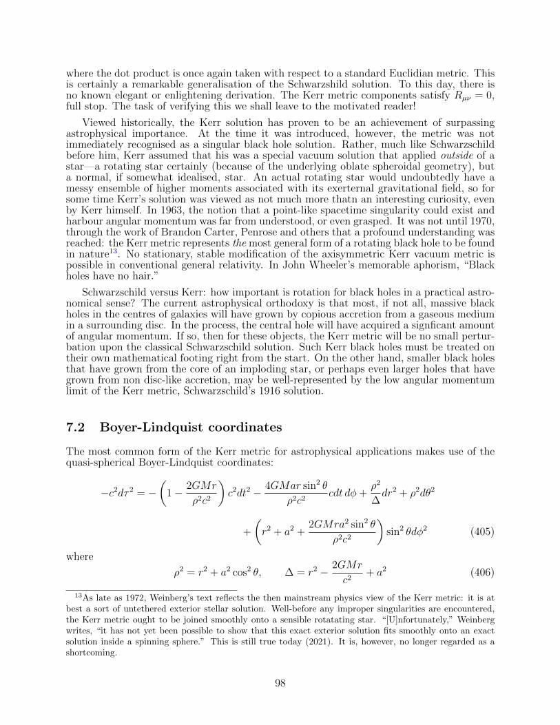
where the dot product is once again taken with respect to a standard Euclidian metric. Thisis certainly a remarkable generalisation of the Schwarzshild solution. To this day, there isno known elegant or enlightening derivation. The Kerr metric components satisfy Rµν = 0,full stop. The task of verifying this we shall leave to the motivated reader!

Viewed historically, the Kerr solution has proven to be an achievement of surpassingastrophysical importance. At the time it was introduced, however, the metric was notimmediately recognised as a singular black hole solution. Rather, much like Schwarzschildbefore him, Kerr assumed that his was a special vacuum solution that applied outside of astar—a rotating star certainly (because of the underlying oblate spheroidal geometry), buta normal, if somewhat idealised, star. An actual rotating star would undoubtedly have amessy ensemble of higher moments associated with its exerternal gravitational field, so forsome time Kerr’s solution was viewed as not much more thatn an interesting curiosity, evenby Kerr himself. In 1963, the notion that a point-like spacetime singularity could exist andharbour angular momentum was far from understood, or even grasped. It was not until 1970,through the work of Brandon Carter, Penrose and others that a profound understanding wasreached: the Kerr metric represents the most general form of a rotating black hole to be foundin nature13. No stationary, stable modification of the axisymmetric Kerr vacuum metric ispossible in conventional general relativity. In John Wheeler’s memorable aphorism, “Blackholes have no hair.”

Schwarzschild versus Kerr: how important is rotation for black holes in a practical astro-nomical sense? The current astrophysical orthodoxy is that most, if not all, massive blackholes in the centres of galaxies will have grown by copious accretion from a gaseous mediumin a surrounding disc. In the process, the central hole will have acquired a signficant amountof angular momentum. If so, then for these objects, the Kerr metric will be no small pertur-bation upon the classical Schwarzschild solution. Such Kerr black holes must be treated ontheir own mathematical footing right from the start. On the other hand, smaller black holesthat have grown from the core of an imploding star, or perhaps even larger holes that havegrown from non disc-like accretion, may be well-represented by the low angular momentumlimit of the Kerr metric, Schwarzschild’s 1916 solution.

7.2 Boyer-Lindquist coordinates

The most common form of the Kerr metric for astrophysical applications makes use of thequasi-spherical Boyer-Lindquist coordinates:

−c2dτ 2 = −(

1− 2GMr

ρ2c2

)c2dt2 − 4GMar sin2 θ

ρ2c2cdt dφ+

ρ2

∆dr2 + ρ2dθ2

+

(r2 + a2 +

2GMra2 sin2 θ

ρ2c2

)sin2 θdφ2 (405)

where

ρ2 = r2 + a2 cos2 θ, ∆ = r2 − 2GMr

c2+ a2 (406)

13As late as 1972, Weinberg’s text reflects the then mainstream physics view of the Kerr metric: it is atbest a sort of untethered exterior stellar solution. Well-before any improper singularities are encountered,the Kerr metric ought to be joined smoothly onto a sensible rotatating star. “[U]nfortunately,” Weinbergwrites, “it has not yet been possible to show that this exact exterior solution fits smoothly onto an exactsolution inside a spinning sphere.” This is still true today (2021). It is, however, no longer regarded as ashortcoming.

98

Note that we have returned to “standard time” t in (405), rather than t. The spatial Boyer-Lindquist coordinates are related to their Kerr-Schild counterparts by:

x = σ · r′, y = σ⊥ · r′, z = r cos θ (407)

withdφ′ = dφ− (a/∆)dr, r′ = (sin θ cosφ′, sin θ sinφ′, cos θ), (408)

and the dot products are Euclidian. Note that r = 0 corresponds to the surface x2 + y2 =a2 sin2 θ, not to a point, and that (r, θ, φ) become standard spherical coordinates at largeradial distances from the central singularity, where the space is asymptotically flat.

In the limit M → 0, the metric becomes

− c2dτ 2 = −c2dt2 +ρ2

r2 + a2dr2 + ρ2dθ2 +

(r2 + a2

)sin2 θdφ2 (409)

This is simply Minkowski space in oblate spheroidal coordinates, whose Cartesian counter-parts obey equation (399) and are given by:

x =√r2 + a2 sin θ cosφ, y =

√r2 + a2 sin θ sinφ, z = r cos θ. (410)

Apart from its evident complexity, the Kerr metric’s most striking feature is the appear-ance of the off-diagonal components

gφ0 = g0φ = −2GMar sin2 θ

ρ2c2. (411)

The presence of such terms results in a remarkable feature of Kerr spacetime: “dragging”of inertial frames in the sense of the rotation of the black hole. To see this most clearly,consider the fate of a test particle dropped into a Kerr a black hole following a geodesic path,with a 4-velocity component Uφ = 0 (i.e. radial) initially. In Problem Set 1, you showedthat

dUρdτ

=1

2

∂gµν∂xρ

UµUν , (412)

so that Uφ is a constant of the motion: the Kerr metric is axisymmetric. This is, of course,just the Newtonian angular momentum constant. We conclude that following the geodesic,Uφ will remain zero. With off-diagonal metric components present however, we cannotconclude that dφ/dt = 0! Indeed, with Uφ = 0 we find:

dφ

dτ= Uφ = gφ0U0,

cdt

dτ= U0 = g00U0, (413)

ordφ

dt=gφ0

g00. (414)

The components of the (inverse) contravariant metric gµν are not especially difficult to cal-culate, since gµν may be written in block form, and only a (symmetric) 2× 2 matrix for the0 and φ components need be inverted:(

g00 g0φ

gφ0 gφφ

)−1

≡(g00 g0φ

gφ0 gφφ

)=

1

D

(gφφ −gφ0

−g0φ g00

)(415)

99

where D is the determinantD = g00gφφ − gφ0g0φ. (416)

Carrying through the calculations, we find:

D = −∆ sin2 θ, gφφ =∆− a2 sin2 θ

∆ρ2 sin2 θ, g0φ = gφ0 = −2GMar

ρ2c2∆, (417)

and

g00 = −ρ2(r2 + a2) + 2GMra2 sin2 θ/c2

∆ρ2 sin2 θ. (418)

The grr and gθθ components are simple reciprocals:

grr =1

grr=

∆

ρ2, gθθ =

1

gθθ=

1

ρ2. (419)

The geodesic equation becomesdφ

dt=gφ0

g00= −gφ0

gφφ. (420)

Dropped inward on an initially radial trajectory, a test particle acquires an azimuthal angularvelocity in the same sense as the black hole angular momentum. In other words, a freelyfalling inertial frame, with a fixed vanishing angular momentum, finds itself dragged by thespacetime geometry and forced to follow the rotation of the hole: a rotating, but inertial,zero angular momentum frame!

Exercise. In Problem Set 1, you learned how to calculate the spatial metric γij from a generalmetric gµν . Show that the spatial interval dl2 for the Kerr spacetime is given by

dl2 =ρ2

∆dr2 + ρ2 dθ2 +

∆ sin2 θ

1− 2GMr/ρ2c2dφ2

Verify that in the limit a→ 0, the Schwarzschild spatial interval is recovered.

7.3 Kerr geometry

7.3.1 Singularities

The Schwarzschild geometry featured a true singularity at r = 0 and a coordinate-singularityevent horizon at r = RS = 2GM/c2. The Kerr geometry is considerably richer. There issingular structure in the Kerr metric when either ∆ or ρ vanishes. The vanishing of ∆correponds to r = RS, a coordinate singularity, when a is small, and this suggests a corre-sponding coordinate singularity. This may directly investigated by calculating the curvaturescalar RµνρσRµνρσ and checking for singular behaviour; there is none. (Why is not possibleto use the Ricci scalar R?) By contrast, the r = 0 true Schwarzschild singularity correspondsto ρ = 0 for the Kerr metric:

r2 + a2 cos2 θ = 0, (421)

which requires both r = 0 and θ = π/2. Based on the results of §(7.2), this restrictivecombination of requirements corresponds to

x2 + y2 = a2, z = 0, (422)

100

which is a circular ring, not a single point. This raises the interesting issue of what liesinterior to the ring, a question to which we shall return below.

The infinite grr coordinate singularity condition ∆ = 0 occurs when

r2 − 2rrg + a2 = 0, (423)

where we have defined rg = GM/c2, the gravitational radius. We denote the solutions r+

and r−, where

r± = rg ±√r2g − a2. (424)

There is also a coordinate singularity when ρ2 = 2GMr/c2, corresponding to g00 = 0. Thisoccurs at radial coordinate locations r′±:

r′± = rg ±√r2g − a2 cos2 θ, (425)

which match with r± at θ = 0 and θ = π. The unique r = RS Schwarzschild-geometrycoordinate singularity g00 = 1/grr = 0, which corresponds to the location of both an eventhorizon and a surface of infinite redshift, splits into no less than four distinct radii in Kerrspacetime! The physical interpretation of these locations requires some care.

7.3.2 Stationary limit surface: g00 = 0

Consider the purely azimuthal photon null geodesics in Kerr geometry. These satisfy

g00c2dt2 + 2g0φcdt dφ+ gφφdφ

2 = 0 (426)

This may be regarded as a quadratic equation for dφ/dt:

dφ

dt=|g0φ|gφφ±√g2

0φ

g2φφ

− g00

gφφ. (427)

(Recall that g0φ < 0.) In the limit g00 → 0−, the two solutions may be written

dφ+

dt= 2|g0φ|gφφ

,dφ−dt

= −|g00|2gφφ

, (428)

The (+) solution corresponds to a photon launched near the surface g00 = 0 which takes offwith twice the angular velocity of the dragged inertial frame, moving in the same sense. The(−) photon solution is barely making any progress at all in the opposite sense of rotation,facing into the fierce “headwind” of the dragged frame! At the surface of vanishing g00

itself, the (−) azimuthal-headed photon remains fixed in these coordinates. Therefore, anymaterial particle, no matter how powerfully it is driven, will be dragged back in the senseof the spacetime rotation caused by the hole’s angular momentum. The 4-velocity of whatwould be a stationary object is constrained by g00(U0)2 = −c2, which is impossible to satisfywhen g00 passes through zero. The g00 surface is thus known as the stationary limit.

While the vanishing of g00 implies that signals sent from this location become infinitelyredshifted, unlike the Schwarzschild case, this is not an event horizon. One may cross thissurface, rotate with the hole, and recross the surface in the opposite direction and return todescribe the adventure. In Schwarzschild geometry, the time to reach the g00 = 0 surfaceis logarithmically infinite as measured by a distant observer. In Kerr geometry, the time toreach the vanishing g00 stationary surface measured by a distant observer is finite, becausethe relevant time integral is only square root unbounded, and therefore integrable.

101

Figure 7: Spacetime structure of exterior null geodesics (light cones), near thesurface r = RS = 1 (in the displayed units) for a Schwarzschild black hole. Thetangentially collapsed light cones define the surface by sheathing it. This is thehallmark of an event horizon. r = RS is a null surface, on which dxµdxµ = 0.

7.3.3 Event horizon: grr = 0

To understand the physical nature of the two surfaces associated with the singular denom-inator of grr in the Kerr metric, we must first sharpen our understanding of what definesan event horizon. Figure (7) shows the light cones in a spacetime diagram near the surfacer = RS for a Schwarzschild black hole. Future time is upward. The defining feature ofthe event horizon is that the light cones have collapsed onto the surface and lie tangentiallyalong it in spacetime, rather like the weave of a wicker basket. The event horizon is thus aglobal null surface, on which any differential coordinate vector dxµ obeys dxµdxµ = 0. If wenow define this same surface by an equation of the form f(xµ) = 0, then it must also be truethat on these constant-f surfaces,

df ≡ dxµ ∂µf = 0. (429)

Since dxµ is a null vector, so must be ∂µf , because f is a scalar function. We therefore takethe definition of a null surface to be one that satisfies

(∂µf) ∂µf = 0 (430)

on f(xµ) = 0. In problems with symmetry, for which f is a function of only one coordinate,as in the present problem with f depending only upon r, the null surface condition is

grr(∂rf)2 = 0. (431)

This will in general require grr = 0, or equivalently (for the Kerr metric), grr becominginfinite.

We shall now summarise the singular behaviour structure of the Kerr metric, shownschematically in fig. (8). The reader is cautioned that a complete understanding of thespacetime structure in the vicinity of the Kerr singularity has not yet been achieved.

102

Moving radially inward in the equatorial plane from a region external to all singularities,we first cross the stationary limit surface r = r′+ (labelled I in the diagram), a surface ofinfinite redshift from the point-of-view of an external observer. Causal contact with theexterior is not lost. The next surface to be encountered, r = r+, is an event horizon (IIin the figure). Along the rotation axis of the black hole the r′+ and r+ surfaces coincide,but in general there will be a well-defined gap between them. This gap-region is known asthe ergosphere, because (as shown by Penrose) it is possible to extract energy and angularmomentum from the black hole by entering and leaving the gap. More specifically, if aparticle enters the ergosphere, splits in two, and only one of the decay products emerges,then it is possible for the emergent particle to have more energy coming out than its parentparticle had going in. In other words, via this Penrose process, the mass M and angularmomentum parameter a of the hole both decrease, with the excess taken up by the particlethat has reemerged from within the ergosphere.

Passing through surface II, we cross an event horizon moving inward, and thus enter aspacetime region that is causally cut-off from the exterior. This is similar to the r < RS

region of a standard Schwarzschild hole, with the addition of frame-dragging effects. Whena second event horizon is crossed at surface III, however, g00 becomes once again negativeand timelike. This is in principle another ergosphere condition for the metric, but withoutthe means to extract any energy from the hole: the event horizon passages have cut thatoff! Finally, passing through surface IV, the metric returns to the g00 < 0, grr > 0 signconvention it has in the asymptotically flat region lying exterior to the outer stationaryr′+ surface. Watch how you go, however: the equator of surface IV is a true spacetimesingularity! Recall that this corresponds to the coordinate conditions r = 0 or x2 + y2 = a2.Now x2 + y2 < a2 is certainly an allowed region of spacetime. But we have used up all of ourpostive r allocation in reaching the singularity! The point is that r is simply a mathematicalcoordinate defined by equation (399), and not a proper radius. Indeed, it may be shownthat allowing r to become negative, analytically continues the spacetime structure right upthrough r → −∞. But this comes at a price: when r is small and negative, gφφ < 0(timelike!) and g00 > 0 (spacelike). With the spacelike variables dt = dr = dθ = 0, θ = π/2,and r small and negative,

c2dτ 2 =

(2GMa2

|r|c2

)dφ2 (432)

In other words, the proper time consists of closed timelike curves as φ advances from 0 to 2π,two identical points in the spacetime manifold. A time machine? Does nature really allowthis? At present, we have no basis for excluding this type of structure.

End of Kerr notes 1 January 2021.

103

I II IIIIV

V

Figure 8: Schematic structure of the Kerr geometry. Surfaces II and III cor-respond to event horizons; I and IV to stationary surfaces. See text for furtherdetails.

[T]he probable effect of deviations from

the Fermi equation of state suggests that

actual stellar matter after the exhaustion

of thermonuclear energy sources will, if

massive enough, contract indefinitely,

although more and more slowly, never

reaching true equilibrium.

— J. R. Oppenheimer & G. Volkoff

8 Self-Gravitating Relativistic Hydrostatic Equilibrium

8.1 Historical Introduction

For most of the stars in the Universe, general relativity is utterly unimportant. This is true ofstars going through the normal course of core nuclear burning, and it is true of low mass starseven after nuclear burning has ceased. These low mass stars become white dwarfs. In a whitedwarf star, the fundamental force balance is between the inward directed force of gravityand the outward directed force of the pressure gradient arising from electrons following adegenerate Fermi-Dirac distribution of energies. The vast majority of stars in the Universeare low mass stars, and will become white dwarfs. Although the (degeneracy) pressure ina white dwarf can become relativistic, ordinary Newtonian gravity works perfectly well inthis regime. The point is that even when the electrons are relativistic, the baryons andthe gravitational potential they generate are both classical. In the late 1930’s, J. RobertOppenheimer and his colleagues G. Volkoff and R. Tolman developed a physical theory foranother type of degenerate star, which was based upon an idea of the Soviet theoreticalphysicist Lev Davidovich Landau. Landau had earlier suggested that neutron degeneracy

104

pressure could provide the dynamical support at the cores of stars quite generally, in additionto serving as the luminosity source (by accretion onto the degenerate surface). Even thoughhydrogen fusion had been (correctly) proposed by Eddington as early as 1920, in the late1930’s the source of stellar energy was still viewed as far from certain. The richly detailedthermonuclear theory of Hans Bethe, which would thoroughly vindicate Eddington, was justabout to arrive on the scene, but had not yet done so.

The neutron was discovered in 1932 by Chadwick. Very shortly thereafter, the remarkableobservational astronomers Baade and Zwicky proposed that a degeneracy pressure, muchlarger than that provided by electrons, would be available to support a hypothetical starcomposed of neutrons. They went on to propose (correctly!) that these unusual stars couldform as the remnant of a supernova event. Such a self-supporting“neutron star” would havea radius of about 10 km, far smaller than the planetary scale 104 km typical of a white dwarf.With a mass somewhat larger than that of the sun, the density of such an object would becomparable to that of an atomic nucleus: some 1017 kg per cubic metre. Landau then wenton to boldly propose that all ordinary stars contain neutron cores as their energy source,with energy liberated via the break up of nuclei as they accrete onto the core!

Does this idea hold together? Are the permitted masses of neutron cores in the rightrange for this to work? Just how small could a self-consistent neutron core be and, conversely,is there an upper limit to its mass? To answer these questions properly would require thefull machinery of general relativistic gravity.

In 1939 Oppenheimer and Volkoff published a paper in which, for the first time, therelativistic equation of the balance of stellar hydrostatic equilibrium was written down.This work established the basis of modern neutron star theory in particular, and of gen-eral relativistic internal stellar dynamics more broadly. Because it built on preliminarymathematical groundwork laid down by R. C. Tolman, the equation is known today as theTolman-Oppenheimer-Volkoff (TOV) equation.

Oppenheimer and Volkoff found that a fully degenerate ideal gas of neutrons could notform a stable self-gravitating body with a mass in excess of 0.7 M. Work of Chandrasekharhad earlier shown that white dwarf stars can exist with masses up to about 1.4M (the precisenumber depends somewhat upon chemical composition), so the smaller limit for a neutronstar was disappointing. However, subsequent analyses, using a more realistic equation ofstate appropriate to these very high neutron densities, showed that self-gravitating neutronstar masses can exist which are closer to 2M. We should therefore expect to find neutronstars in the narrow mass range between 1.4 and ∼ 2 M. Modern astrophysics has brilliantlyconfirmed this very tight prediction.

What of stellar cores with masses in excess of 2M? We now know that nothing canprevent their collapse to a black hole. Again in 1939, Oppenheimer, in collaboration withHartland Snyder (another student), published the first general relativistic calculation ofa gravitational collapse of ordinary matter to a black hole singularity. Many regard Op-penheimer, who went on to direct the Atomic Bomb Manhatten Project of WWII, as thefounding father of neutron star and black hole theory. Sadly, Oppenheimer died in 1967 atthe relatively young age of 62, just before the spectacular 1968 discovery of the Crab NebulaPulsar, which provided the “smoking gun” evidence for the existence of neutron stars 14 Theradius of a neutron star is only slightly larger than its Schwarzschild radius, so if neutronstars were real, black holes were not far away. Throughout Oppenheimer’s lifetime, neutronstars and black holes had been mere theoretical constructs—some would have said toys—and were simply not taken very seriously by astronomers. We now know neutron stars and

14Oppenheimer’s close colleague Hans Bethe, the father of nuclear astrophysics, died in 2005 at the re-markable age of 99, active and intellectually acute until the very end. Bethe was “present at the creation,”playing lead roles in the explosive development of both quantum mechanics and modern astrophysics.

105

black holes to be present throughout the Universe, and they are the focus of much of presentday high energy astrophysics. We have witnessed both types of objects literally smashingand merging into one another, and measured the electromagnetic and gravitational radiationthat emerged. This is truly a propitious time to be studying the general relativistic theoryof self-gravitating stars.

8.2 Fundamentals

If you have not done the exercise on page (73), now is the moment to do so. In fact, we shallstart our discussion with the results derived there. We write the field equations in “sourcefunction form”

Rµν = −8πG

c4Sµν ≡ −

8πG

c4

(Tµν −

gµνT

2

), (433)

and with the stress tensor Tµν that of an ideal static fluid:

Tµν = Pgµν + (ρc2 + P )UµUν , Ui = 0, (i = 1, 2, 3).

The metric is spherically symmetric, which we represent as usual as

− c2dτ 2 = −Bc2dt2 + Adr2 + r2dθ2 + r2 sin2 θdφ2. (434)

The only component of a static 4-velocity is U t = c/√B, and Ut = −c

√B. The Ricci tensor

components have been worked out in §5.4. The fundamental equations take the form:

Rtt = −B′′

2A+B′

4A

(B′

B+A′

A

)− B′

rA= −8πG

c4Stt = −4πGB

c4(3P + ρc2), (435)

Rrr =B′′

2B− B′

4B

(B′

B+A′

A

)− A′

rA= −8πG

c4Srr =

4πGA

c4(P − ρc2), (436)

Rθθ = −1 +1

A+

r

2A

(−A

′

A+B′

B

)= −8πG

c4Sθθ =

4πGr2

c4(P − ρc2). (437)

As usual, the prime ′ stands for d/dr. We may eliminate B completely from our equationsby forming the following combination:

Rtt

B+Rrr

A+

2Rθθ

r2= − 2A′

rA2− 2

r2+

2

Ar2= −16πGρ

c2. (438)

This may be written ( rA

)′= 1− 8πGρr2

c2. (439)

Integrating this equation from r = 0, the centre of our star, to some (interior) radius r,

1

A= 1− 2GM(r)

rc2+

(C

r

), (440)

where C is an integration constant and M(r) is the mass-like quantity

M(r) = 4π

∫ r

0

ρr′2 dr′. (441)

106

(The r′ notation is of course just a dummy integration variable, not a derivative!) Were Cnot to vanish, then A would have vanish at r = 0, and the metric would be singular, whichis not physical: with all the mass exterior to the origin and a finite pressure at the centre,the metric must be regular. Hence C = 0 and

A =

(1− 2GM(r)

rc2

)−1

. (442)

Equation (441) certainly looks at first sight like a good definition for “mass within r”,but remember that the space inside the star has curvature! Where, for example, is A(r),the metric coefficient needed for proper radial intervals: A1/2dr? When the upper limit rexceeds the outer radius of the star R, thenM must be the constant M in the Schwarzschildsolution. This “M” includes what we would think of as the Newtonian mass plus the effectivecontribution from the energy of the gravitational field. Interestingly, the purely Newtonianmass expression, with its compounded errors of neglecting curved space and the variedrelativistic contributions to the gravitational field energy, is correct after all! The errors,evidently, are offsetting.

Our next step is to return to equation (437), using the hydrostatic equilibrium equationfor B′:

B′

B= − 2P ′

ρc2 + P. (443)

Upon substitution for A and B in (437), this leads to:

dP

dr= −

(GM(r)

r2+

4πGPr

c2

)(ρ+

P

c2

)(1− 2GM(r)

rc2

)−1

. (444)

This is known as the Tolman-Oppenheimer-Volkoff, or TOV, equation. We use the TOVequation, together with equation (441) in differential form,

dMdr

= 4πρr2 (445)

as the governing, self-contained, pair of equations for relativistic hydrostatic equilibrium.

Students of stellar structure should recognise the TOV equation as the equation of New-tonian stellar equilibrium,

dP

dr= −GM(r)ρ

r2(446)

with some notable relativistic additions. We replace ρ by ρ + P/c2, a combination thatincludes the pressure contribution to the inertial energy density, and occurs repeatedly inour study of relativity. Perhaps somewhat less intuitively, the gravitating mass within rM has an additional contribution of 4πPr3/c2 because the pressure is a source all on itsown for the gravitational field. Later in these notes, we will see this same term appear inthe cosmological equations for a homogeneous universe. As to the final factor, which is justA(r), that we can make “disappear.” Watch carefully now, and write the TOV equation inthe following simpler form:

grrdP

dr= −4πGr

3

(ρ(r) +

3P

c2

)(ρ+

P

c2

)(447)

107

where grr is the rr component of the gµν metric tensor (i.e. 1/A), and ρ(r) is the averagedensity within radius r. The gradient ∂r operator acting on the scalar P is the radialcomponent of a covariant tensor; the factor grr changes it to a standard contravariant tensorradial component. The right side of the equation must then itself be proportional to theradial component of a standard gravitational acceleration contravariant vector, let us sayar. While this grr coefficient is manifestly geometrical and ensures that a contravariantform of the gradient appears, it can also be thought of more physically as embodying thecontribution to gravity arising from curvature itself: “the gravity of gravity.” In generalrelativity, the effects of gravity act geometrically, showing up in the metric terms or theirderivatives. By contrast, the density and pressure modifications act dynamically: they comedirectly from the stress tensor source.

We are not quite finished, because we need to determine B(r) to complete the solutionof our metric. This is a simple matter of combining equations (443) and (444):

B′

B=

(2GM(r)

r2+

8πGPr

c2

)(1− 2GM(r)

rc2

)−1

(448)

We use the boundary condition that B = 1 at r = ∞, the Minkowski space limit far fromthe star. Then our solution may be written

lnB = −∫ ∞r

(2GM(r′)

r′2+

8πGPr′

c2

)(1− 2GM(r′)

r′c2

)−1

dr′ (449)

The integral takes on a more familiar form when r > R, i.e., when we are outside the star.Then M(r′) is just the constant M , the total mass of the star, and the pressure P = 0.

lnB = −∫ ∞r

2GM

r′2

(1− 2GM

r′c2

)−1

dr′ = ln

(1− 2GM

rc2

)(450)

In other words,

B(r > R) = 1− 2GM

rc2. (451)

We recover the Schwarzschild solution in the vacuum outside the spherical star, as we must.

8.3 Constant density stars

An exact, but relatively simple, mathematical solution of the TOV equation is that for a starof constant energy density ρc2. The Newtonian case is very simple. WithM(r) = 4πGρr3/3,the solution to (446) is:

P

ρ=

2πGρ

3(R2 − r2) (452)

where R is the outer radius, the location at which the pressure P vanishes. The centralpressure Pc is then just

Pc =2πGρ2

3R2 (453)

In the TOV case, the differential equation is more complicated, but does separate nicely:

dP

(ρ+ 3P/c2)(ρ+ P/c2)= −4πGr

3

(1− 8πGρr2

3c2

)−1

dr. (454)

108

The solution with P (R) = 0 is obtained via a partial fraction expansion on the left side ofthis equation, then standard logarithmic integrals over P . On the right side, we have anexact derivative (up to a constant factor). Carrying out the integrations, we find:

ρ+ 3P/c2

ρ+ P/c2=

(1− 8πGρr2/3c2

1− 8πGρR2/3c2

)1/2

. (455)

Now this is a very interesting solution. With mass M = 4πρR3/3, by demanding thatthe solution make physical sense at r = 0 we find the restriction(

1

1− 2GM/Rc2

)1/2

=ρ+ 3P/c2

ρ+ P/c2≡ 3− 2ρ

ρ+ P/c2< 3. (456)

This condition can be fulfilled only if

R >9GM

4c2=

9RS

8, (457)

which states that the actual radius of a constant density star must always be larger than9RS/8, not RS itself as you might have expected. What if the density is not constant? Ifthe matter is compressible, it doesn’t help at all. The constant density case is actually anabsolute upper limit to the M/R ratio in any star. If the stellar material can be compressed,then for a given mass M , you will have to distribute the material over a larger radius Rto prevent inward gravitational collapse. (Collapse is clearly easier to trigger when theself-gravitating matter is softer!) We therefore have a very powerful result:

All stable stars must be larger in radius than 9GM/4c2.

Note as well that equation (456) states that the maximum observed-to-emitted frequencyratio possible (the largest redshift) for radiation emerging from the surface of any kind ofstar is 3.

Exercise. Show that the inequality (457) is actually an upper bound on R for a given density,and therefore, the maximum mass of a constant density star is

Mmax =4

27

√3

π

c3

G3/2ρ1/2,

corresponding to infinite central density. For a density of ρ ' 2 × 1015 g cm−3, what isMmax in solar masses? (Answer: 2.1M.) The assumption of a constant density is much toocrude a model to provide an accurate physical upper limit for real stars, but the calculationillustrates an important point of principle: an upper mass limit exisits.

8.4 White Dwarfs

The existence of an upper bound to the mass of a white dwarf star may be understood bysimple dimensional scaling arguments.

The potential energy of a (nonrelativistic) star is always a number that is of order−GM2/R, where M is the mass and R the radius of the star. For a fixed mass, this behaves

109

as 1/R, so shrinking the star always lowers the gravitational energy (more negative). In thecase of a pressure-free body (“dust”), we could in principle shrink the mass down to zeroradius and attain a state of arbitrarily low energy. Stars exist in nature because this doesnot happen, pressure fights back. The thermal energy of the star generally grows rapidlyas it shrinks, and the star effectively resists the gravitational collapse. Too small a radiuswould provide too much of a push-back, and the star would reexpand. But too large a radiuswould make pressure inefficient, and the star could once again lower its gravitational energyby contraction, so there is a happy medium that minimises the total energy, the sum of thepotential plus thermal energies. This minimum energy state is where the star lives. This isstellar equilibrium.

The thermal energy of the star is of order PR3, some sort of average pressure times thestellar volume. The argument we outined above works both for ordinary matter, as well asfor degenerate matter, which obeys an equation of state of the form P ∝ ρ5/3: the pressureis proportional to the 5/3 power of the density and nothing else. This is the equation ofstate for a nonrelativistic white dwarf supported by electron degeneracy pressure. Then

PR3 ∼ ρ5/3R3 ∼M5/3/R2 (458)

At fixed mass but variable R, we see that the thermal energy dominates at small radius(pushing back) and gravitational potential energy wins at large radius (pulling in). Asoutlined above, there is always a stable equilbrium somewhere in between. This holds forany mass at all, so if this were always the correct equation of state, a white dwarf star couldhave any mass.

An upper mass limit arises, in fact, because of the following interesting behaviour. Wehave seen that stellar equilibrium is achieved when the potential and thermal energies arecomparable. For a nonrelativistic white dwarf, this means that the balance is

M5/3/R2 ∼M2/R, (459)

which leads immediately to the scaling relation R ∼M−1/3: the more massive a degeneratestar is, the smaller it is! This is in stark contrast to ordinary stars (and ordinary people),whose radius increases with mass. For nondegenerate stars, R grows close to linearly withM . (This is related to a more-or-less constant internal temperature regulated by a nuclearburning thermostat. Why does this lead to R ∼ M?) The point here is that at larger andlarger mass, the density M/R3 rises as M2, the electrons become ever more tightly packed,and their kinetic energy (of order their Fermi energy) must enter the relativistic regime.Then the equation of state is no longer P ∝ ρ5/3, but P ∝ ρ4/3. Under these circumstances,the thermal energy scales as

PR3 ∼ ρ4/3R3 ∼M4/3/R. (460)

In other words, both the thermal and potential energies scale (at fixed mass) in the same waywith radius, as 1/R. Moreover, the potential energy is proportional to M2, versus M4/3 forthe thermal energy, so that at large enough mass the star can always lower its total energyby collapsing, like dust, down to R = 0. Thus, the properties of relativistic electron degen-eracy lead directly to the existence of a maximum mass, beyond which degenerate electronscannot prevent gravitational collapse. This is known as the Chandrasekhar Mass, after theastrophysicist who first calculated its value accurately. (He did this as a student!) DenotedMCh, its value is close to 1.42M for a typical abundance of elements. For astronomers, thisis really not a very big mass at all.

It is most instructive to work out the precise value of MCh. Begin with the Newtonianequation of stellar equilibrium, in which the gravitational force is written as the gradient of

110

a potential function Φ:

1

ρ

dP

dr= −dΦ

dr, Φ = −

∫ ∞r

GM(r′)

r′2dr′ (461)

Then, taking the divergence in spherical coordinates gives

1

r2

d

drr2

[1

ρ

dP

dr

]= − 1

r2

d

dr

(r2dΦ

dr

)= −4πGρ, (462)

where the final equality uses the spherical Poisson equation ∇2Φ = 4πGρ. Given an equationof state in form of the function P = P (ρ), this is a self-contained second-order differentialequation, which may be solved (at least by numerical methods).

Recall that a fully degenerate gas has one fermion per available energy state, up to theFermi energy, εF . With a density of states per unit volume of 8πp2dp/h3 (this includes twospin states at each level; h is Planck’s constant), the total number of electrons per unitvolume is

ne =

∫ pF

0

8πp2dp

h3=

(8π

3

)(p3F

h3

)(463)

where pF is the Fermi momentum associated with εF . The total pressure, calculated mosteasily as the momentum per unit time per unit volume imparted to an imaginary wall in xyplane is (note that we now explicity integrate over θ in spherical momentum coordinates):

P = 2×∫ pF

0

∫ π

0

vz(2pz)× (1/2) 2πp2 sin θ dθdp

h3=

8π

3h3

∫ pF

0

v p3dp (464)

where we have used vz = v cos θ and similarly for pz. (The various factors of 2 are present forspin, for twice pz imparted with each elastic collsion to the wall, with a 1/2 because only halfthe particles are moving toward the wall. The 2π is from the φ integration.) The θ integralis 2/3. This expression, as written, is valid both relativistically and nonrelativistically. Forthe nonrelativistic case, v = p/me (me is the electron mass), and

P =8πp5

F

15meh3(nonrelativistic) (465)

With mp the proton mass and µemp the total mass per electron in the gas (µe would be veryclose to 2 for equal proton and neutron numbers), we then have

P =

[h2

20me(mpµe)5/3

](3

π

)2/3

ρ5/3 ≡ K1 ρ5/3 (nonrelativistic) (466)

Numerically, K1 = 3.123× 106 in SI units. An important characteristic density at which pFis given by mec is

ρchar =8π

3

m3ec

3

h3µemp = 0.97µe × 109 kg m−3. (467)

When the mass density is comparable to or exceeds ρchar, the gas enters the relativisticregime.

For the extreme relativistic case, v = c in the rightmost integral of equation (464) and

P =2πcp4

F

3h3(extreme relativistic) (468)

111

or

P =

[hc

8(mpµe)4/3

](3

π

)1/3

ρ4/3 ≡ K2 ρ4/3 (extreme relativistic) (469)

Numerically, K2 = 4.887× 109 in SI units.

Let us next consider equation (462) for the general so-called polytropic equation of state,P = Kργ. Substituting this expression for P leads to

1

r2

d

drr2

[dργ−1

dr

]= −4πG(γ − 1)

γKρ (470)

Let ρ0 be the central density of the star. If we now make the substitutions,

n =1

γ − 1, ρ = ρ0θ

n, r =

[K(n+ 1)ρ

(1/n)−10

4πG

]1/2

ξ ≡ Aξ (471)

the equation takes the form of what is known as the Lane-Emden equation,

1

ξ2

d

dξξ2

[dθ

dξ

]= −θn. (472)

The original Newtonian equation of hydrostatic equilibrium may be written in an invertedform as

M(r) = −r2

ρ

dP

dr= −

[K3(n+ 1)3

4πG3

]1/2

ρ(3−n)/2n0 ξ2dθ

dξ. (473)

Thus, we may read off the mass of the star as given by the above formula, with the finalLane-Emden terms evaluated at the location for which θ = 0, the dimensionless stellar radius.

The boundary conditions to be applied for the solution of (472), integrating outwardfrom the centre r = 0, are

θ(0) = 1,dθ

dξ≡ θ′(0) = 0. (474)

The vanishing derivative condition follows from (473) and the fact that the mass containedwithin a very small ξ neighbourhood of ξ = 0 goes likeM(r) ∼ ξ3. For example, an exactlysoluble solution to the Lane-Emden equation is available for the case n = 1,

θ =sin ξ

ξ, n = 1 (475)

The surface of the star for this solution corresponds to ξ = π, and at this point θ′ = −1/π.Equation (473) then gives for the mass of the star

M = ρ0

[2πK3

G3

]1/2

. (476)

More generally, the equation must be solved by numerical methods, which is a straightforwardtask.

112

The cases n = 1.5 and n = 3, corresponding to an ordinary white dwarf and a relativisticdegenerate white dwarf, are the most interesting for astrophysics. With n = 1.5,

M = −[

125K31

32πG3

]1/2

ρ1/20 ξ2dθ

dξ(477)

For the given numerical value of K1, µe = 2, a central density of 109 kg per cubic metreand the numerical result −ξ2θ′ = 2.7, this gives a mass of 0.48M, a typical low mass whitedwarf.

Yet more interesting is the relativistic equation of state, n = 3. Then,

M = −[

16K32

πG3

]1/2

ξ2dθ

dξ, (478)

which is independent of the central density ρ0, and depends only upon fundamental constantsof physics. From the solution of the Lane-Emden equation, −ξ2θ′ = 2.02, conveniently veryclose to 2. For µe = 2, this gives a numerical value of M = 1.43M. It is known as theChandrasekhar mass, MCh, and it is the fundamental upper mass limit to a white dwarf star.It is a sufficiently important quantity to be written down on its own, expressed in terms offundamental constants of nature. Replacing, for the sake of elegance, 2.02 with 2, we have

MCh = 8

[K3

2

πG3

]1/2

=

(3

8π2

)1/2(1

µemp

)2(hc

G

)3/2

(479)

(Purists may wish to multiply this by a factor of 2.018/2 = 1.009 for accuracy.)

With this explicit solution in hand, let us recall why this mass is a true upper masslimit. Imagine a sequence of white dwarf models with ever increasing total mass. In thenon-relativistic regime, the central density ρ0 increases as M2. The effective adiabatic index,at first fixed at n = 1.5, starts to rise toward n = 3 as the growing central density compelsthe electrons into the relativistic regime of their equation of state. As M continues to rise,n closes in on 3, and the central density now scales as the mass M to the power 6/(3− n),becoming infinite at M = MCh. At this point, there is nothing to prevent gravitationalcollapse to either a neutron star or, failing that, a black hole.

Exercise. What is the actual physical radius of an n = 1.5 white dwarf? Use ρ0 = 109 kgper m3, and the fact that θ vanishes at ξ = 3.65.

8.5 Neutron Stars

We have seen that a massive stellar core or a white dwarf that has accreted enough matterto bring its total mass above MCh is in deep trouble. Such a body will rapidly collapse. Asthe core density shoots up, the inverse of the classical beta-decay reaction

p+ e− → n+ νe

induces electrons (e−) to recombine with protons (p) to form a sea of neutrons (n). In theprocess, electron neutrinos (νe) escape from the initial implosion, which is thought thento immediately rebound as a supernova explosion. This is a fascinating topic unto itself,controversial and far from well-understood, but our interest here is in the neutrons, thedominant majority species left behind. The normal beta-decay of free neutrons (typically

113

10 minutes) is halted by a small residual population (typically a few percent) of protonsand electrons, which fill their respective “Fermi seas.” This keeps the forward and backwardbeta reaction rates in balance. The neutrons accordingly have one last chance to avoid thefate of complete collapse into a black hole: their degeneracy pressure can resist gravity atthese ultra high densities, just as electrons do in a white dwarf. For such a neutron star, thecharacteristic density equation (467) becomes

ρchar =8π

3

m4nc

3

h3= 6.11× 1018 kg m−3 = 6.11× 1015 g cm−3. (480)

We have replaced the typical Fermi momentum condition of a white dwarf, pF ∼ mec, withpF ∼ mnc. (mn is the neutron mass, differing very little from mp.) Neutron stars have, notby coincidence, densities characteristic of atomic nuclei.

The question immediately arises as to whether there is an upper limit to the mass of aneutron star analogous to that of MCh for a white dwarf. That this is to be expected followsfrom the fact that both the pressure and the gravitational field itself act as sources of self-gravity: a bigger self-attraction for the same amount of mass/energy. If anything, it shouldbe even more difficult to stave off collapse in the case of a neutron star as compared witha white dwarf. This is indeed the case, as found in a classical calculation by Oppenheimerand Volkoff, at least for an ideal Fermi gas of neutrons.

Exercise. Show that relativistic parameter GM/Rc2 is of order me/mp for a white dwarf,and of order unity for a neutron star. Use the appropriate ρchar in each case.

In the case of a white dwarf, the energy density ρc2 is completely dominated by thenonrelativistic nucleon rest mass. This is no longer so for a neutron star, and the equationof state must take this into account. In particular, for a fully degenerate relativistic gas ofneutrons, ρc2 is given by

ρc2 =

∫ pF

0

8π

h3p2(p2c2 +m2

nc4)1/2dp = 3ρcharc

2

∫ pF /mnc

0

u2(1 + u2)1/2du (481)

The pressure is given now by equation (464), with v ≡ pc2/E (E here is the particle energy),as

P =8c2π

3h3

∫ pF

0

p4 dp

(p2c2 +m2nc

4)1/2= ρcharc

2

∫ pF /mnc

0

u4 du

(1 + u2)1/2(482)

The integrals may be evaluated explicitly (with x = pF/mnc):∫ x

0

u2(1 + u2)1/2du =1

8

(x(1 + 2x2)

√1 + x2 − sinh−1 x

), (483)

∫ x

0

u4

(1 + u2)1/2du =

1

8

(x(2x2 − 3)

√1 + x2 + 3 sinh−1 x

), (484)

Equations (483) and (484) may be written in much more elegant forms, which are alsoconvenient for numerical computation. If we substitute in (483) α = sinh−1 x, the right handside (RHS) becomes

RHS =1

32(sinh 4α− 4α), (485)

where we have made use of the hyperbolic trig identities (prove, if they are not familiar!)

1 + sinh2 α = cosh2 α, 2 coshα sinhα = sinh 2α, 1 + 2 sinh2 α = cosh 2α.

114

Figure 9: The equation of state for a relativistic neutron gas, via the parametricsolution of equations (483) and (484). At small pF/mnc, the nonrelativisticP = K1ρ

5/3 relation is recovered. At large pF/mnc, the extreme relativisticequation of state P = ρc2/3, analogous to radiation, is recovered. (Notation:rho∗ = ρ/ρchar, P

∗ = P/ρcharc2.)

With t ≡ 4α (using the t-notation of Oppenheimer and Volkoff), we may parameterise ρ bythe compact equation:

ρ(t) =3ρchar

32(sinh t− t), t = 4 sinh−1(pF/mnc). (486)

Using exactly the same tricks for the pressure integral produces the slick result

P (t) =ρcharc

2

32[sinh t− 8 sinh(t/2) + 3t] =

c2

3[ρ(t)− 8ρ(t/2)]. (487)

With explicit forms for ρ(t) and P (t) at hand, the differential equations to be solved consistof the mass equation for dM/dr,

dMdr

= 4πr2ρ, (488)

and the TOV equation, now written as an equation for dt/dr:

1

P

dP

dr=dt

dr= − 1

P

(GMr2

+4πGPr

c2

)(ρ+

P

c2

)(1− 2GM

rc2

)−1

, (489)

where P = dP/dt, and both ρ and P are explicit functions of t, equations (486) and (487).The boundary conditions at r = 0 are M = 0 and t = t0 where t0 is implicitly defined for agiven central density ρ0 by the equation

ρ0 =3ρchar

32(sinh t0 − t0). (490)

115

An explicit equation of state of the form P = f(ρ) is shown in Fig. (9). The actual f(ρ)functional relation is remarkably simple in appearance, changing smoothly from one powerlaw to another.

When the central density of the star ρ0 is much less than ρchar, the entire star behavesexactly like an n = 1.5 white dwarf, but with mn substituting for µemp in the formulae. Themass of this type of low mass neutron star can be written down directly from the relevantsolution of the Lane-Emden equation, something we now know how to do. The answer turnsout to be

M = 2.71(ρ0/ρchar)1/2M (491)

If ρ0/ρchar = 0.03, say, this is 0.47M.

When ρ0 ρchar, the equation of state becomes P = ρc2/3, very much like a gas ofphotons. Then, the TOV equation (444) is

dρ

dr= −4GM(r)ρ

r2c2

(1 +

4πρr3

3M(r)

)(1− 2GM(r)

rc2

)−1

(492)

Surely it is obvious that an exact solution is

ρ =3c2

56πGr2! (493)

(Try it out. Start with M(r) = 3rc2/14G and go from there.) This simple inverse squarelaw is in fact the correct asymptotic local behaviour near the origin of the true physicalsolution in the limit ρ0 →∞. Note that the integrated mass does not diverge, but remainsfinite near r = 0. An equilibrium solution that vanishes at some finite r and has a well-defined finite mass may be found numerically. This was first attempted by Oppenheimerand Volkoff, but the details of their reported large density behaviour are not quite right.Given the cumbersome technology of 1930’s hand calculators, we should not judge them tooharshly! By the early 1960’s, matters had been resolved.

A plot15 of the stellar mass as a function of central density ρ0 is given in figure (10).The limiting mass as ρ0 → ∞ is 0.42M. (The oscillatory manner in which this valueis approached is surprising, and can be related to underlying stability properties of thestar.) But equation (491) shows that neutron stars in the Lane-Emden low ρ0 regime, inwhich M is rising with increasing ρ0, clearly includes stellar masses exceeding this value.There must therefore be a maximum mass somewhere between the high and low densityregimes, and figure (10) bears this out. There is a maximum mass of 0.71M and a radius of9.6km (correctly calculated by Oppenheimer and Volkoff), the classic upper limit for a gasof degenerate neutrons This occurs for t0 very close to 3, ρ0 = .66ρchar = 4× 1015 g cm−3.

If the ideal Fermi neutron gas were the whole story, there probably would not be verymany neutron stars in the Universe. Stars would become white dwarfs with masses up toabout 1.4M. Beyond this value, only black holes would be possible. Perhaps an implodingwhite dwarf might throw off enough mass to get below the Oppenheimer-Volkoff limit andbecome a neutron star, but this is hardly certain. In fact, at ultrahigh densities, neutronsinteract via the strong nuclear force, and the ideal gas equation of state used by Oppen-heimer and Volkoff is not a good approximation. (White dwarf electrons experience no suchcomplication.) There has long been great uncertainty regarding the proper equation of stateto use for calculating the maximum mass for a neutron star. Recent (2017) data from the

15I am grateful to L. Fraser-Taliente, R. McDonald and A. Morris, all of whom flawlessly carried out thiscalculation as an optional exercise for this course in 2019. Prior to their work, I was unaware that theoriginal Oppenheimer-Volkoff mass calculation was inaccurate at large densities.

116

107 1010 1013 1016 1019 1022

central density, ρ0, g/cm3

0.0

0.1

0.2

0.3

0.4

0.5

0.6

0.7

M,s

olar

mas

sesM

ρ0 →∞

NumericalLow-ρ limit

Figure 10: Computed mass M of a model neutron star for an ideal Fermi gas equation ofstate. The x-axis is central density ρ0, in units of g cm−3, on a logarithmic scale. At lowρ0, the mass rises as the square root of the density, like a white dwarf star (dotted line).At higher densities, M reaches a maximum of 0.71M. M then decreases, oscillatingwith decreasing amplitude, approaching 0.42M as ρ0 → ∞. (Figure credit: L. Fraser-Taliente.)

117

Figure 11: Neutron star (NS) masses from binary systems, de-termined by precise orbital timing measurments. The dottedlines show a spread of white dwarf upper mass limits, allowingfor variation in composition. Left pointing arrows are observa-tional upper limits for the NS mass . NS masses cluster near thewhite dwarf upper limit.

merger of two actual neutron stars, in the form of what the post-collision debris did anddid not do, has been used to constrain the parameter space allowed for a proper equationof state. These data suggest an upper mass limit of 2.17 M, more than a factor of 3 largerthan the original Oppenheimer-Volkoff value.

Our modern view of neutron stars is therefore somewhat different. There is a range ofmasses between 1.4M and 2.17M where a star appears to be able to reside happily as aneutron star. A white dwarf in a binary system that has accreted enough matter to bring itsmass just above the Chandrasekhar mass can form a neutron star after implosion, withoutlosing a significant fraction of its mass in the process. We would expect, therefore, to findmany neutron stars with masses near the Chandrasekhar value of 1.4M. That is indeedwhat observations show (Fig. 11).

8.6 Pumping iron: the physics of neutron star matter

To understand the behaviour of neutron stars in their proper context, we follow the physicistJohn Wheeler (mentor of, among other notables, Richard Feynman and Kip Thorne) whoin the 1950s computed the equation of state for matter in a massive star at the end ofall nuclear processing. This corresponds to pure iron nuclei, since iron has the greatest(negative) binding energy per nucleon of any atomic nucleus. It is not possible to extractenergy from an iron nucleus either by fusing it with other particles or by breaking it apart.Wheeler worked with B. Harrison on this project, and the result is known as the Harrison-Wheeler (HW) equation of state, the first of its kind for calculating neutron star interiors.In this section, we will give a qualitative description of how iron, upon steadily increasingcompression, makes the transition from ordinary matter to the stuff of neutron stars. Ourdiscussion in this section will be largely descriptive.

118

In our description we shall refer both to the quantity γ = d lnP/d ln ρ, the adiabaticindex of the matter, as well as to the physical density. For ordinary iron (ρ = 7.6g per cubiccm), γ is huge. This is why such a solid feels hard: to achieve a tiny density compressionrequires a vast exertion of pressure. As we keep squeezing, γ actually plummets, becaused lnP = dP/P drops very rapidly with the sharply rising P . The internal electrons, for theirpart, congregate more and more tightly around their parent nuclei, resisting the compressionby standard electron degeneracy pressure. The applied external pressure changes the spacingof the internal energy levels in the atoms, but not the number of electrons per level. Thatis fixed by degeneracy, and it is what makes this squeezing process an adiabatic one. Thisstate of affairs persists for compression factors of up to 104, i.e. up to densities of ∼ 105 gcm−3. That may seem impressively high, but we are still very far from a neutron star.

Next, we enter the white dwarf regime. At densities in excess of 105 g cm−3, the forcesof degeneracy pressure start to dominate over the electrical attraction of the iron nuclei. Asa consequence, the confining atomic orbitals cease to exist, and something much more like ametal appears, in which the electrons are free to roam between the nuclei. This is true whitedwarf matter. The adiabatic index is now easy to understand: γ = 5/3. As we continueto increase the pressure and density, the confined electron degeneracy motions approach thespeed of light. At a density of ρ = 107 g cm−3, γ has dropped to 4/3. This is the relativisticwhite dwarf regime of the Chandrasekhar limit.

We remain in the γ = 4/3 phase as the density compression rises through a factor 40,000.Then, at a density of 4 × 1011 g cm−3, the next transition occurs: the electrons no longerhave any space between the nuclei! The minimum energy state is one in which they areabsorbed by the nuclear protons. This enriches the neutron content of the matter by inversebeta decay (proton plus electron goes to neutron plus electron neutrino):

p+ e− → n+ νe

The loss of electron degeneracy pressure at these densities causes γ to drop well below unity.This is a global minimum for the adiabatic index.

As the density continues to rise, it become energetically more favourable for the neutronrich nuclei to “drip neutrons” back out into the ambient surroundings, where densities (andthus the degeneracy pressure) are lower. As the compression continues and the overall densityclimbs, the dripped-out neutrons start to resist back with their own degeneracy pressure.Finally, by 4×1012 g cm−3, the nuclei have broken apart, and we have a gas of free, degenerateneutrons. This is the stuff from which an Oppenheimer-Volkoff neutron star is made.

This was as far as Harrison and Wheeler could go in the 1950’s. This was enough,however, to show that there were no stable stars in the density gap between white dwarfsand neutron stars. In the following decades, work by many individuals on the equation ofstate for ultrahigh densities showed a greater resistance and thus a stiffer equation of statethan a simple extrapolation of the ideal gas equation of state used by Oppenheimer andVolkoff. It is this added stiffness that is the basis for our understanding of how neutron starscan exist with masses in excess of the Oppneheimer-Volkoff upper limit of 0.7M.

Figure (12), taken from the semi-popular text of Kip Thorne, Black Holes & Time Warps:Einstein’s Outrageous Legacy (1994), shows how the scenario we have just outlined translatesmore generally into equilibrium masses for actual gravitating bodies. (I apologise for thedifficulty in reading some of the numbers.) The figure is a plot of Stellar Mass (in units of theSun’s mass) as a function of circumference in kilometres (a quantity less distorted by curva-ture than radius itself) for pure iron. The km-circumference tick points are 101, 102, ...107.The solid line plots the equilibrium mass value (or possible multiple values!) for a particularcircumference. In the region that is shaded by heavy lines, pressure is larger than gravity; inthe white region gravity is larger than pressure forces. The solid line marks the equilibriumboundary. The powers of 10 in the figure that are shown pointing with wiggly arrows to

119

Figure 12: Equilibrium mass as a function of circumference for self-gravitating iron. (Cir-cumference is easier to work with radius since it is not directly affected by curvature.) Onlythe branches labelled ‘White dwarfs’ and ‘Neutron stars’ are stable. See text for a detaileddescription. (Figure from Thorne, modified for clarity by L. Fraser-Taliente.)

the equilibrium mass curve indicate the corresponding central density in units of grams percubic cm.

It is very important to note that not every value of stellar mass along the equilibrium curveis actually realisable in nature. Only the portions of the mass curve which are monotonicallydecreasing with circumference are physically stable! Consider, for example, the curve portionlabelled “White Dwarfs.” Move slightly to the right, off the curve into the white region. Themass boundary is extended, and the pressure has dropped while the gravity has gone up: themass feels a net force that returns it back toward equilibrium. Similarly, move leftward intothe shaded zone from the same White Dwarf line. Now contraction drives up the pressurerelative to the gravity, and once again the body experiences a return stabilising force.

Contrast this behaviour with the “unstable” branch, say the uppermost between densitiesof 109 and 1011. On this side of the equilibrium curve, a move to right puffing up star leadsto pressure dominating over gravity and further puffing! Similarly, a move to the left—acontraction—leads to gravity dominance, and further collapse.

The two stable portions of the equilibrium curve, at circumferences of roughly 60,000 and60 km, correspond to white dwarf and neutron stars respectively. The dotted line within theshaded portion of the neutron star section corresponds to the classical Oppenheimer-Volkoffcalculation with an upper mass limit of 0.7M. The solid curve is based on a much bettercalculation, taking account of a modern nuclear equation of state. The current most massiveneutron star actually measured (as of September 2019) weighs in at 2.14M, and there isgood reason to believe that this is very close to the maximum mass a neutron star can havebefore imploding to a black hole. (The black hole region of this diagram is clearly visible onthe left.)

Three real stars are shown, contracting leftward toward their fates: the Sun, Procyon,and Sirius. (The latter two are actually binary systems with white dwarf companions. We

120

refer in our diagram to the bright “normal star.”) Normal stars are not on the equilibriumcurve because they are not cold iron supported by degeneracy presure! But at the end oftheir nuclear burning they will eventually contract and move to the left in the diagram. TheSun will find solace on the white dwarf branch. Procyon is too massive to end up as a whitedwarf, but will catch the stable neutron star branch. For poor Sirius, unless it manages toshed some mass, its fate will be complete gravitational collapse to a black hole.

To go deeper into the topic of the equation of state at ultrahigh densities would take ustoo far afield from our primary interest in general relativity. The reader who would like topursue this topic in more detail, starting with the basic physics, should begin by consultingChapter 2 of the text by Shapiro and Teukolsky for a clear exposition and a number ofexcellent exercises.

121

They are not objective, and (like abso-

lute velocity) are not detectable by any

conceivable experiment. They are merely

sinuosities in the co-ordinate system, and

the only speed of propagation relevant to

them is “the speed of thought.”

— A. S. Eddington, writing in 1922 of

Einstein’s suspicions.

On September 14, 2015, at 09:50:45 UTC

the two detectors of the Laser Interfer-

ometer Gravitational Wave Observatory

simultaneously observed a transient grav-

itational wave signal. The signal sweeps

upwards from 35 to 250 Hz with a peak

gravitational wave strain of 1 × 10−21. It

matches the waveform predicted by general

relativity for the inspiral and merger of a

pair of black holes and the ringdown of the

resulting single black hole.

— B. P. Abbott et al., 2016, Physical

Review Letters, 116, 061102

9 Gravitational Radiation

Gravity is spoken in the three languages. First, there is traditional Newtonian potentialtheory, the language used by most practising astrophysicists. Then, there is the languageof Einstein’s General Relativity, the language of Riemannian geometry that we have beenstudying. Finally, there is the language of quantum field theory: gravity arises from theexchange of spin 2 particles, gravitons, much as electromagnetism arises from the exchangeof spin 1 photons. Just as the starting point of quantum electrodynamics is the classicalradiation theory of Maxwell, the starting point of quantum gravity must be a classicalradiation theory of gravity. However, unlike quantum electrodynamics, the most accuratephysical theory ever created, there is no quantum theory of gravity at present, and there isnot even a consensus approach. Quantum gravity is very much an active area of ongoingresearch. For the theorist, this is reason enough to study the theory of gravitational radiationin general relativity. But there are now good reasons for the practical astrophysicist toget involved. In Februrary 2016, the first detection of gravitational waves was announced.The event signal had been received and recorded earlier, on September 14, 2015, and isdenoted G[ravitational]W[ave]150914. The detection was so clean, and matched the waveform predictions of general relativity in such detail, there can be no doubt that the detectionwas genuine. A new way to probe the most impenetrable parts of the Universe is at hand.

122

In the limit when gµν is very close to ηµν , the theory of general relativity is a classical the-ory of gravitational radiation (not just Newtonian theory), in the same way that MaxwellianElectrodynamics is a classical electromagnetic radiation theory. The field equations for thesmall difference tensor hµν = gµν − ηµν become, in this weak field limit, a set of rather or-dinary looking linear wave equations with source terms, completely analogous to Maxwell’sEquations. The principal difference is that electrodynamics is sourced by a vector currentJµ, whereas gravitational fields in general relativity are sourced by a tensor quantity Tµν .This becomes a major difference when we relax the condition that the gravitational field beweak: the gravitational radiation makes a contribution to its own source, something electro-magnetic radiation cannot do. This is not completely unprecedented in wave theories. Wehave seen this sort of thing before, in a purely classical context: sound waves can themselvesgenerate acoustical disturbances, and one of the consequences is a shock wave, or sonic boom.While a few somewhat pathological mathematical solutions for exact gravitational radiationwaves are known, in general theorists either work in the weak field limit or resort to numericalsolutions of the field equations. Even with powerful computers, however, precise numericalsolutions of the field equations for astrophysically interesting problems—like merging blackholes—have long been a major technical challenge. In the last decade, a practical mathe-matical breakthrough has occurred, and it is now possible to compute highly accurate waveforms for these kinds of problems, with important predictions to guide the new generationof gravitational wave detectors.

As we have noted, astrophysicists now have perhaps the most important reason of allto understand gravitational radiation: we are on the verge of what will surely be a goldenage of gravitational wave astronomy. That gravitational radiation well and truly exists wasestablished in the years following 1974, when a close binary system (7.75 hour period) with aneutron star and a pulsar (PSR 1913+16) was discovered and analysed by Hulse and Taylor.So much orbital information could be extracted from this remarkable system that it was pos-sible to predict, then measure, the rate of orbital decay (the gradual shortening of the periodof the pulsar’s decaying orbit) caused by the energy loss in gravitational waves. Though tinyin any practical sense, the period change was large enough to be cleanly measured. Generalrelativity turned out to be exactly correct (Taylor & Weisberg, ApJ, 1982, 253, 908), andthe 1993 Nobel Prize in Physics was duly awarded to Hulse and Taylor for this historicalachievement.

The September 2015 gravitational wave detection pushed back the envelope dramatically.It established that i) the direct reception and quantitative analysis of gravitational wavesis technically feasible and will become a widely-used probe of the universe; ii) black holesexist beyond any doubt whatsoever, this truly is the proverbial “smoking-gun”; iii) the fulldynamical content of strong field general relativity, on time and length scales characteristicof stellar systems, is correct. This achievement is an historical milestone in physics16. Somehave speculated that its impact on astronomy will rival Galileo’s introduction of the telescope.Perhaps Hertz’s 1887 detection of electromagnetic radiation in the lab is another, more apt,comparison. (Commercial exploitation of gravity waves is probably some ways off. Maybeit will be licenced someday as a revenue source.)

There will be more to come. In the near future, it is anticipated by many that extremelydelicate pulsar timing experiments, in which arrival times of pulses are measured to fantasticprecision, will detect distortions in interstellar space. In essence, this is a measure of theShapiro delay, caused neither by the sun nor by a star, but by the passage of a large scalegravitational wave between us and the pulsar probes!

The subject of gravitational radiation is complicated and computationally intensive. Eventhe basics will involve some effort on your part. I hope you will agree that the effort is well

16Update: This was recognised with the 2017 Nobel Prize in Physics, awarded to Barish, Thorne, andWeiss for the detection of gravitational radiation by the LIGO facility.

123

rewarded.

9.1 The linearised gravitational wave equation

Summary: The linearised gravitational wave equation of general relativity takes on the formof a standard wave equation when written in what are known as “harmonic” coordinates.These coordinates are very important for the study of gravitational radiation.

We begin with the assumption that the spacetime metric is close to Minkowski. Let usintroduce the quantity hµν , the (small) departure in the metric tensor gµν from its Minkowskiηµν limit:

gµν = ηµν + hµν (494)

To leading order, when we raise and lower indices we may do so with ηµν . But be carefulwith gµν itself. Don’t just lower the indices in the above equation willy-nilly! Instead, notethat

gµν = ηµν − hµν (495)

to ensure gµνgνκ = δκµ. (You can raise the index of g with η only when approximating gµν as

its leading order value, which is ηµν .) Note that

ηµνhνκ = hµκ, ηµν∂

∂xν=

∂

∂xµ, (496)

so that we can slide dummy indices “up-down” as follows:

∂hµν∂xµ

= ηµρ∂hρν∂xµ

=∂hρν∂xρ

≡ ∂hµν∂xµ

. (497)

The story begins with the Einstein Field Equations cast in a form in which the “linearisedRicci tensor” is isolated on the left side of our working equation. Specifically, we write

Rµν = R(1)µν +R(2)

µν + ...etc. (498)

and

G(1)µν = R(1)

µν − ηµνR(1)

2(499)

where R(1)µν is all the Ricci tensor terms linear in hµν , R

(2)µν all terms quadratic in hµν , and so

forth. The linearised affine connection is

Γλµν =1

2ηλρ(∂hρν∂xµ

+∂hρµ∂xν

− ∂hµν∂xρ

)=

1

2

(∂hλν∂xµ

+∂hλµ∂xν

− ∂hµν∂xλ

). (500)

In terms of hµν and h = hµµ, from contracting the linear-in-g terms of equation (258) onpage 62, we explicitly find

R(1)µν =

1

2

(∂2h

∂xµ∂xν− ∂2hλµ∂xν∂xλ

− ∂2hλν∂xµ∂xλ

+ 2hµν

)(501)

124

where

2 ≡ ∂2

∂xλ∂xλ= ∇2 − 1

c2

∂2

∂t2(502)

is the d’Alembertian (clearly a Lorentz invariant), making a most welcome appearance intothe proceedings. Contracting µ with ν, we find that

R(1) = 2h− ∂2hµν

∂xµ∂xν(503)

where we have made use of∂hλµ∂xµ

=∂hλµ

∂xµ.

Assembling G(1)µν , we find

G(1)µν =

1

2

[∂2h

∂xµ∂xν− ∂2hλµ∂xλ∂xν

− ∂2hλν∂xλ∂xµ

+ 2hµν − ηµν(

2h− ∂2hλρ

∂xλ∂xρ

)]. (504)

The full, nonlinear field equations may then formally be written

G(1)µν = −

(8πGTµνc4

+Gµν −G(1)µν

)≡ −8πG(Tµν + τµν)

c4, (505)

where

τµν =c4

8πG(Gµν −G(1)

µν ) ' c4

8πG

(R(2)µν − ηµν

R(2)

2

)(506)

Though composed of geometrical terms, the quantity τµν is written on the right side of theequation with the stress energy tensor Tµν , and is interpreted as the stress energy contributionof the gravitational radiation itself. We shall have more to say on this in §9.4. In linear theory,τµν is neglected in comparison with the ordinary matter Tµν , and the equation is

∂2h

∂xµ∂xν− ∂2hλµ∂xλ∂xν

− ∂2hλν∂xλ∂xµ

+ 2hµν − ηµν(

2h− ∂2hλρ

∂xλ∂xρ

)= −16πGTµν

c4(507)

Exercise. Show that, in terms of the source function Sµν = Tµν − ηµνT/2, the linear fieldequation is

∂2h

∂xµ∂xν− ∂2hλµ∂xλ∂xν

− ∂2hλν∂xλ∂xµ

+ 2hµν = −16πG

c4Sµν

Recover the static Poisson equation limit, as per our more general treatment in Chapter 6.

This is all a bit disappointing to behold. Even the linearised field equations look to bea mess! But then, you may have forgotten that the raw Maxwell wave equations for thepotentials are no present, either. You will permit me to remind you. Here are the equationsfor the scalar potential Φ and vector potential A:

∇2Φ +1

c

∂

∂t(∇·A) = −4πρ (508)

∇2A− 1

c2

∂2A

∂t2−∇

(∇·A+

1

c

∂Φ

∂t

)= −4π

cJ (509)

125

(Note: I have used esu units, which are much more natural for relativity. Here ρ is theelectric charge density.) Do the following exercise!

Exercise. In covariant notation, with Aα = (Φ,A) and Jα = (ρ,J/c) representing respec-tively the potential and source term 4-vectors, the original general equations look a bit morepresentable. The only contravariant 4-vectors that we can form which are second order inthe derivatives of Aα are 2Aα and ∂α∂βA

β. Show that if ∂αJα = 0 identically, then our

equation relating Aα to Jα must be of the form

2Aα − ∂α∂βAβ = CJα

where C is a constant to be determined, and that this equation remains unchanged whenthe transformation Aα → Aα + ∂αΛ in made. This property is known as gauge-invariance.We will shortly see something very analogous in general relativity. In the meantime, how dowe determine C?

Do you remember the way forward from here? Work in the “Lorenz gauge,” which we arealways free to do:

∇·A+1

c

∂Φ

∂t= 0 (510)

In covariant 4-vector language, this is simply a vanishing divergence condition, ∂αAα = 0.

Then, the dynamical equations simplify:

∇2Φ− 1

c2

∂Φ

∂t2= 2Φ = −4πρ (511)

∇2A− 1

c2

∂2A

∂t2= 2A = −4π

cJ (512)

This is much nicer. Physically transparent Lorentz-invariant wave equations emerge. Mightsomething similar happen for the Einstein Field Equations?

That the answer might be YES is supported by noticing that G(1)µν can be written entirely

in terms of the Bianchi-like quantity

hµν = hµν −ηµνh

2, or hµν = hµν −

δµνh

2. (513)

Using this in (504), the linearised field equation becomes

2G(1)µν ≡ 2hµν −

∂2hλµ∂xν∂xλ

− ∂2hλν∂xµ∂xλ

+ ηµν∂2hλρ

∂xλ∂xρ= −16πGTµν

c4. (linearised) (514)

(It is easiest to verify this by starting with (514), substituting with (513), and showing thatthis leads to (504).)

Interesting. Except for 2hµν , every term in this equation involves the divergence ∂µhµν

or ∂µhµν . Hmmm. Shades of Maxwell’s ∂αA

α. In the Maxwell case, the freedom of gaugeinvariance allowed us to pick the gauge in which ∂αA

α = 0. Does equation (514) have agauge invariance that will allow us to do the same for gravitational radiation, so that we canset these h-divergences to zero?

It does. Go back to equation (504) and on the right side, change hµν to h′µν , where

h′µν = hµν −∂ξν∂xµ− ∂ξµ∂xν

, h′ = h− 2∂ξµ

∂xµ(515)

126

and the ξµ represent any vector function. You will find that the form of the equationis completely unchanged, i.e., the ξµ terms cancel out identically! This is a true gaugeinvariance.

Exercise. Show that under a gauge transformation,

h′µν = hµν −∂ξν∂xµ− ∂ξµ∂xν

+ ηµν∂ξρ

∂xρ,

∂h′µν∂xµ

=∂hµν∂xµ

−2ξν .

Show as well that equation (514) may be written

∂Θλµν

∂xλ= −16πG

c4T µν ,

whereΘλµν = ∂λhµν − ∂µhλν + ηµν∂ρh

λρ − ηλν∂ρhµρ

and that Θλµν = −Θµλν . This is the gravitational analogue to the Maxwell equation (85).Is Θλµν gauge invariant on its own?

Note that if we replace T µν on the right with T µν + τµν , following equations (505) and(506), the Θ-equation becomes an exact statement of energy-momentum conservation forthe combined fields arising from material and gravitational sources.

What is manifesting as gauge invariance is actually invariance to coordinate transforma-tions, which acts to leading linear order as a gauge transformation. To see this, consider theinfinitesimal coordinate transformation,

x′µ = xµ + ξµ(x), or xµ = x′µ − ξµ(x′) (to leading order). (516)

Then

g′µν = η′µν + h′µν =∂xρ

∂x′µ∂xσ

∂x′νgρσ =

(δρµ −

∂ξρ

∂xµ

)(δσν −

∂ξσ

∂xν

)(ηρσ + hρσ) (517)

Notice that for the derivatives of ξρ, we may use x instead of x′, since the difference isquadratic in ξ. With η′ identical to η, to leading order in ξ we must have

h′µν = hµν −∂ξν∂xµ− ∂ξµ∂xν

, (518)

as we found earlier. Though closely related, don’t confuse general covariance under coordi-nate transformations with this gauge transformation. Unlike general covariance, the gaugetransformation is implemented without actually changing the coordinates! We keep the samex’s and add a group of certain functional derivatives to the hµν , analogous to adding a gra-dient ∇Λ to A in Maxwell’s theory. We find that the equations remain identical, just as wewould find if we took ∇×(A+∇Λ) in the Maxwell case.

Pause for a moment. In general relativity, don’t we actually need to change the coor-dinates when we...well, when we change the coordinates? What is going on here? Keepingthe coordinates is not an option, is it? Change the hµν tensor components as though wewere changing coordinates, but then leave the coordinates untouched? Why should thatwork? The answer is that the additional terms that we pick up when we elect to do the fullcoordinate transformation are of higher order than the purely linear (in ∂µξν) terms thatcome from merely changing the components of hµν . Remember that hµν is itself already

127

infinitesimal! The additional terms that we are ignoring here are of quadratic order, productterms like ∂λξσ contracted with ∂λ∂σhµν . The terms that we retain are of linear order, ∂µξνalone. This is the right and proper thing to do. We are, after all, only working to linearorder in our overall formulation of the problem.

Understanding the gauge invariant properties of the gravitational wave equation was verychallenging in the early days of the subject. The opening “speed-of-thought” quotation ofthis chapter by Eddington is taken somewhat out of context. What he really said in hisfamous paper (Eddington A.S. 1922 Proc. Roy. Soc. A, 102, 716, 268) is the following:

“Weyl has classified plane gravitational waves into three types, viz.: (1) longitudinal-longitudinal;(2) longitudinal-transverse; (3) transverse-transverse. The present investigation leads to the con-clusion that transverse-transverse waves are propagated with the speed of light in all systems ofco-ordinates. Waves of the first and second types have no fixed velocity—a result which rousessuspicion as to their objective existence. Einstein had also become suspicious of these waves (inso far as they occur in his special co-ordinate system) for another reason, because he found theyconvey no energy. They are not objective and (like absolute velocity) are not detectable by anyconceivable experiment. They are merely sinuosities in the co-ordinate system, and the only speedof propagation relevant to them is the ‘speed of thought.’ ”

[Note that “longitudinal” refers to the direction parallel to the propagation of the wave;“transverse” to the axes at right angles to this direction.]

The final line of the quotation is often taken to be dismissive of the entire notion ofgravitational radiation, which it clearly is not. Rather, it is directed toward those solutionswhich we would now say are gauge-dependent (either type [1] or type [2] waves, whichinvolve at least one longitudinal component in an h-index) and those which are gauge-independent (type [3], which is completely transverse). Physical waves must ultimately begauge independent. Matters would have been quite clear to anyone who bothered to examinethe components of the Riemann curvature tensor! The first two types of waves would haveproduced an identically zero Rλ

µνκ. They produce no curvature; they are indeed “merelysinuosities in the co-ordinate system,” and they are in fact unphysical.

Back to our problem. Just as the Lorenz gauge ∂αAα = 0 was useful in the case of

Maxwell’s equations, so now is the so-called harmonic gauge:

∂hµν∂xµ

=∂hµν∂xµ− 1

2

∂h

∂xν= 0 (519)

In this gauge, the Field Equations (514) take the “wave-equation” form

2hµν = −16πGTµνc4

(520)

How we can be sure that, even with our gauge freedom, we can find the right ξµ to get intoa harmonic gauge and ensure the emergence of (520)? Well, if we have been unfortunateenough to be working in a gauge in which equation (519) is not satisfied, then follow equation(518) and form a new improved h′µν , with the stipulation that our new gauge is harmonic:∂h′µν /∂x

µ = (1/2)∂h′/∂xν . We find that this implies the ξν must satisfy

2ξν =∂hµν∂xµ

, (521)

a wave equation for ξν identical in form to (520). For this equation, a solution certainlyexists. Indeed, our experience with electrodynamics has taught us that the solution to the

128

fundamental radiation equation (520) takes the form

hµν(r, t) =4G

c4

∫Tµν(r

′, t−R/c)R

d3r′, R ≡ |r − r′| (522)

and hence a similar solution exisits for (521). The hµν , like their electrodynamic counterparts,are determined at time t and location r by a source intergration over r′ taken at the retardedtimes t′ ≡ t − R/c. In other words, disturbances in the gravitational field travel at a finitespeed, the speed of light c.

Exercise. Show that for a source with motions near the speed of light, like merging blackholes, hµν (or hµν for that matter) is of order RS/r, where RS is the Schwarzschild radiusbased on the total mass of the system in question and r is the distance to the source. If youwant to know how big hµν is going to be in your detector when black holes merge, simplycount the number of expected Schwarzschild radii to the source and take its reciprocal.With M tot

equal to the total mass measured in solar masses, show that hµν ∼ 3M tot /rkm,

measuring r in km. We are pushing our weak field approximation here, but to this order itworks fine. We’ll give a sharper estimate shortly.

9.1.1 Come to think of it...

You may not have actually seen the solution (522) before, or maybe, you know, you justneed a little reminding. It is important. Let’s derive it.

Consider the equation

− 1

c2

∂2Ψ

∂t2+∇2Ψ = −4πf(r, t) (523)

We specialise to the Green’s function solution

− 1

c2

∂2G

∂t2+∇2G = −4πδ(r)δ(t) (524)

Of course, our particular choice of origin is immaterial, as is our zero of time, so that weshall replace r by R ≡ r − r′ (R ≡ |R|), and t by τ ≡ t− t′ at the end of the calculation,with the primed values being fiducial reference points. The form of the solution we find herewill still be valid with the shifts of space and time origins.

Fourier transform (524) by integrating over∫eiωtdt and denote the Fourier transform of

G by G:k2G+∇2G = −4πδ(r) (525)

where k2 = ω2/c2. Clearly G is a function only of r, hence the solution to the homogeneousequation away from the origin,

d2(rG)

dr2+ k2(rG) = 0,

is easily found to be G = e±ikr/r. Although we haven’t done anything to deserve this favour,the singular delta function behaviour is actually already included here! This may be seen bytaking the static limit k → 0, in which case we recover the correctly normalised 1/r potentialof a point charge at the origin. The back transform gives

G =1

2πr

∫ ∞−∞

e±ikr−iωt dω =1

2πr

∫ ∞−∞

e−iω(t∓r/c) dω (526)

129

which we recognise as a Dirac delta function (remember ω/k = c):

G =δ(t∓ r/c)

r→ δ(t− r/c)

r→ δ(τ −R/c)

R. (527)

We have selected the retarded time solution t− r/c as a nod to causality, and moved thenceto (τ , R) variables for an arbitary time and space origin. The solution shows that a flashoccurring at t = t′ and r = r′, produces an effect at a distance R from the flash at a timeR/c later. The general solution constructed from a superposition of our Green’s function is

Ψ(r, t) =

∫f(r′, t′)

Rδ(t− t′ −R/c)dt′dr′ =

∫f(r′, t−R/c)

Rdr′. (528)

Remember that R depends on both r and r′.

9.2 Plane waves

Summary: Linear gravitational radiation comes in only two independent modes of plane wavepolarisation. In what are known as “transverse-traceless” (TT) coordinates, a plane wavetravelling in the z direction has one mode with hxx = −hyy and all others zero; the other modehas hxy = hyx and all others zero. In contrast to harmonic coordinates, which are generallyavailable, the TT gauge is available only for plane wave solutions. These coordindates arethe most widely used for studying linear gravitational radiation.

To understand more fully the solution (522), consider the problem in which Tµν has anoscillatory time dependence, e−iωt

′. Since we are dealing with a linear theory, this isn’t

particularly restrictive, since any well-behaved time dependence can be represented by aFourier sum. The source, say a binary star system, occupies a finite volume. We seek thesolution for hµν at distances huge compared with the scale of the source itself, i.e. r r′.Then,

R ' r − er · r′ (529)

where er is a unit vector in the r direction, and

hµν(r, t) 'ei(kr−ωt)

r

4G

c4

∫Tµν(r

′) exp(−ik · r′) d3r′, (530)

with k = (ω/c)er, a wavenumber in the radial direction. Since r is large, this has theasymptotic form of a plane wave. Hence, both hµν and hµν take on the form of simple planewaves, travelling in the radial outward direction, at great distances from the generatingsource. These plane waves have simple and important polarisation properties, which we nowdiscuss.

9.2.1 The transverse-traceless (TT) gauge

Consider a traveling plane wave for hµν , orienting our z axis along k, so that

k0 = ω/c, k1 = 0, k2 = 0, k3 = ω/c and k0 = −ω/c, ki = ki (531)

where as usual we raise and lower indices with ηµν , or its numerically identical dual ηµν .Then hµν takes the form

hµν = eµνa exp(ikρxρ) (532)

130

where a is an amplitude and eµν = eνµ a symmetric polarisation tensor, again with the η’sraising and lowering subscripts. Thus

eij = eij = eij (533)

e0i = −e i0 = e0

i = −e0i (534)

e00 = e00 = −e00 (535)

The harmonic constraint∂hµν∂xµ

=1

2

∂hµµ∂xν

(536)

implieskµe

µν = kνe

µµ/2. (537)

This leads to several linear dependencies between the eµν . For example, when ν = 0 thismeans

k0e00 + k3e

30 = k0(eii + e0

0)/2, (538)

or, with k3 = −k0,− (e00 + e30) = (eii − e00)/2. (539)

When ν = j (a spatial index),

k0e0j + k3e

3j = kj(eii − e00)/2. (540)

The j = 1 and j = 2 cases reduce to

e01 + e31 = e02 + e32 = 0, (541)

while j = 3 yieldse03 + e33 = (eii − e00)/2 = −(e00 + e03). (542)

Equations (541) and the first=last equality of (542) yield

e01 = −e31, e02 = −e32, e03 = −(e00 + e33)/2. (543)

Using the above expression for e03 in the first=second equality of (542) then gives

e22 = −e11. (544)

Of the 10 independent components of the symmetric eµν the harmonic condition (536) thusenables us to express e0i and e22 in terms of e3i, e00, and e11. These latter 5 components plusa sixth, e12, remain unconstrained for the moment.

But wait! We have not yet used the gauge freedom of equation (518) within the harmonicconstraint. We can still continue to eliminate components of eµν . In particular, let us choose

ξµ(x) = iεµ exp(ikρxρ) (545)

where the εµ are four constants to be chosen, and we will do so to make the calculationas simple as possible. This satisfies 2ξµ=0, and therefore keeps the harmonic coordinatecondition, ∂µh

µν = 0, intact. Following the prescription of (518), we now generate a new, but

physically equivalent polarisation tensor,

e′µν = eµν + kµεν + kνεµ. (546)

131

By choosing the εµ appropriately, we can actually eliminate all of the e′µν , except for e′11,e′22 = −e′11, and e′12. In particular, using (546),

e′11 = e11, e′12 = e12 (547)

both remain unchanged. But, with k = ω/c,

e′13 = e13 + kε1, e′23 = e23 + kε2, e′33 = e33 + 2kε3, e′00 = e00 − 2kε0, (548)

so that these four components may be set to zero by a simple choice of the εµ. When workingwith plane waves we may always choose this gauge, which is transverse (since the only eijcomponents that are present are transverse to the z direction of propagation) and traceless(since e11 = −e22). Oddly enough, this gauge is named the transverse-traceless (TT) gauge.Notice that in the TT gauge, hµν vanishes if any of its indices are 0, whether raised orlowered, and gravitational waves propagate to leading order only as distortions in space, notin time.

We thus see that there are only two independent modes of polarisation for a gravitationalwave. The first, with only e11 and e22 = −e11 present, is known as the “+” mode. The second,with only e12 = e21 present, is the cross or “×” mode. All linear gravitational radiation is asuperposition of these two modes.

9.3 The quadrupole formula

Summary: hij is given by a very simple formula in harmonic coordinates (not just the TTgauge), and is directly proportional to the second time derivative of the classical moment ofinertia tensor, I ij. The latter requires use of only the T 00 component of the stress tensor.

In the limit of large r (“compact source approximation”), equation (522) is:

hµν(r, t) =4G

rc4

∫T µν(r′, t′)d3r′, (549)

where t′ = t − r/c is the retarded time. Moreover, for the TT gauge, we are interested inthe spatial ij components of this equation, since all time indices vanish. (Also, because hµνis traceless, we need not distinguish between h and h.) The integral over Tij may be cast ina very convenient form as follows. Start with the identity

0 =

∫∂(x′jT ik)

∂x′kd3r′ =

∫ (∂T ik

∂x′k

)x′j d3r′ +

∫T ij d3r′, (550)

where the first equality follows because the first integral reduces to a surface integration ofx′jT ik at infinity, where it is presumed to vanish. Thus∫

T ij d3r′ = −∫ (

∂T ik

∂x′k

)x′j d3r′ =

∫ (∂T i0

∂x′0

)x′j d3r′ =

1

c

d

dt′

∫T i0x′j d3r′ (551)

where the second equality uses the conservation of T µν . Remember that t′ is the retardedtime. As Tij is symmetric in its indices,

d

dt′

∫T i0x′j d3r′ =

d

dt′

∫T j0x′i d3r′ (552)

132

Continuing in this same spirit,

0 =

∫∂(T 0kx′ix′j)

∂x′kd3r′ =

∫ (∂T 0k

∂x′k

)x′ix′j d3r′ +

∫(T 0ix′j + T 0jx′i) d3r′ (553)

Using exactly the same reasoning as before,∫(T 0ix′j + T 0jx′i) d3r′ =

1

c

d

dt′

∫T 00x′ix′j d3r′ (554)

Differentiating with respect to t′, and using (552) and (551) gives an elegant result:∫T ij d3r′ =

1

2c2

d2

dt′2

∫T 00x′ix′j d3r′. (555)

Inserting this in (549), we obtain the quadrupole formula for gravitational radiation:

hij =2G

c6r

d2I ij

dt′2(556)

where I ij is the quadrupole-moment tensor of the energy density:

I ij =

∫T 00x′ix′j d3r′ (557)

To estimate this numerically, we write

d2I ij

dt′2∼Ma2c2ω2 (558)

where M is the characteristic mass of the rotating system, a an internal separation, and ωa characteristic frequency, an orbital frequency for a binary say. Then

hij ∼ 2GMa2ω2

c4r' 7× 10−22(M/M)(a2

11ω27/r100) (559)

where M/M is the mass in solar masses, a11 the separation in units of 1011 cm (about aseparation of one solar radius), ω7 the frequency associated with a 7 hour orbital period(similar to PSR193+16) and r100 the distance in units of 100 parsecs, some 3× 1020 cm. Atypical rather large h one might expect at earth from a local astronomical source is then oforder 10−21.

What about the LIGO source, GW150914? How does our formula work in this case? Thedistance in this case is cosmological, not local, with r = 1.2 × 1022 km, or in astronomicalparlance, about 400 megaparsecs (Mpc). In this case, we write (559) as

hij ∼ 2GMa2ω2

c4r=

(2.9532

rkm

)(M

M

)(aωc

)2

' 1× 10−22M/MrGpc

(aωc

)2

, (560)

since 2GM/c2 is just the Sun’s Schwarzschild radius. (One Gpc=103Mpc = 3.0856 ×

1022km.) The point is that (aω/c)2 is a number not very different from 1 for a relativisticsource, perhaps 0.1 or so. Plugging in numbers with M/M = 60 and (aω/c)2 = 0.1, we findhij = 1.5× 10−21, just about as observed at peak amplitude.

Exercise. Prove that hij given by (556) is an exact solution of 2hij = 0, for any r, even if r is notlarge.

133

9.4 Radiated Energy

Overall Section Summary: The energy flux at infinity carried off by gravitational radiationis given in the TT gauge is given by −(c4/32πG)∂th

µν∂ihµν. This is needed to understandhow the orbits of binary systems evolve due to the emission of gravitational radiation.

9.4.1 A useful toy problem

We have yet to make the link between hµν and the actual energy flux that is carried off bythese time varying metric coefficients. Relating metric coefficients to energy is not trivial.To see how to do this, start with a simpler toy problem. Imagine that the wave equation forgravitational radiation looked like this:

− 1

c2

∂2Φ

∂t2+∇2Φ = 4πGρ. (561)

This is what a relativistic theory would look like if the source ρ were just a simple scalarquantity, rather than a component of a stress tensor. To turn this into an energy equation,multiply by (1/4πG)∂Φ/∂t, integrate (∂Φ/∂t)∇2Φ by parts and regroup. This leads to

− 1

8πG

∂

∂t

[1

c2

(∂Φ

∂t

)2

+ |∇Φ|2]

+∇·(

1

4πG

∂Φ

∂t∇Φ

)= ρ

∂Φ

∂t. (562)

But

ρ∂Φ

∂t=∂(ρΦ)

∂t− Φ

∂ρ

∂t=∂(ρΦ)

∂t+ Φ∇·(ρv) =

∂(ρΦ)

∂t+∇·(ρvΦ)− ρv·∇Φ, (563)

where v is the velocity, and the mass conservation equation

∂ρ

∂t+∇·(ρv) = 0

has been used in the second “=” sign from the left. Combining (562) and (563), and rear-ranging the terms a bit leads to

∂

∂t

[ρΦ +

1

8πG

(1

c2

(∂Φ

∂t

)2

+ |∇Φ|2)]

+∇·(ρvΦ− 1

4πG

∂Φ

∂t∇Φ

)= ρv·∇Φ. (564)

The right side is just minus the rate at which work is being done on the sources per unitvolume. (Recall that the force per unit volume is −ρ∇Φ.) For those cases of interest whenthe source ρ vanishes outside a certain radius, the left side of the equation may then beinterpreted as a far-field wave energy density of

E = [(∂tΦ/c)2 + |∇Φ|2]/8πG, (Scalar gravity energy density) (565)

and a wave energy flux of

F = −(∂tΦ)∇Φ/4πG. (Scalar gravity energy flux) (566)

(Is the sign of the flux sensible for outgoing waves?) Does an analogous procedure work onthe more involved linear wave equation of tensorial general relativity? The answer is YES,but we have to set things up properly. And needless to say, it is a bit more messy.

134

9.4.2 A conserved energy flux for linearised gravity

Summary: We identify the energy flux for gravitational radiation in the TT gauge by showingthat its 4-divergence is equal to the rate of doing work by a suitable Newtonian potential onthe material sources.

Start with equation (514):

2hµν −∂2hλµ∂xν∂xλ

− ∂2hλν∂xµ∂xλ

+ ηµν∂2hλρ

∂xλ∂xρ= −16πGTµν

c4. (567)

To facilitate the construction of a conserved flux, we need to rewrite the final term on theleft side of this equation and the source term in the right. Begin by contracting on µν: thefirst term on the left becomes 2h, the second and third each become −∂λ∂ρhλρ, while thefinal contraction turns ηµν into a factor of 4. (Why?) This leads us to

2h+ 2∂2hλρ

∂xλ∂xρ= −κT, (568)

where we have written κ = 16πG/c4. Using this relation to substitute for ∂λ∂ρhλρ, we may

recast our original equation as

2hµν −∂2hλµ∂xν∂xλ

− ∂2hλν∂xµ∂xλ

− ηµν2

2h = −κSµν , (569)

where we have once again made use of the source function

Sµν = Tµν −ηµνT

2. (570)

Equation (569) is in fact the fourth form of the linearised field equation we have encountered(one of which is in the Exercises), depending upon whether the fields are expressed in termsof hµν or hµν , and the source in terms of Tµν or Sµν . For ease of reference, these have beencollected and shown in figure (13).

Now, and only now, may we proceed with the same technique we used successfully forour toy problem. Contract (569) with ∂hµν/∂xσ, summing over µ and ν as usual but keepingσ free. We want to fold everything on the left side into a divergence. The first term on theleft becomes

∂hµν

∂xσ2hµν =

∂hµν

∂xσ∂2hµν∂xρ∂xρ

=∂

∂xρ

(∂hµν∂xρ

∂hµν

∂xσ

)− ∂hµν

∂xρ∂2hµν

∂xρ∂xσ

=∂

∂xρ

(∂hµν∂xρ

∂hµν

∂xσ

)− ∂hµν

∂xρ∂

∂xσ∂h

µν

∂xρ=

∂

∂xρ

(∂hµν∂xρ

∂hµν

∂xσ

)− ∂

∂xσ

(1

2

∂hµν∂xρ

∂hµν

∂xρ

)(571)

Do you understand why the final equality is valid for the ∂/∂xσ exact derivative? Here, itdoesn’t matter which group of µν’s (or ρ′s) on the h’s (or the ∂/∂x) is the up group andwhich is the down group.

Now that you’ve seen the tricks of the trade, you should be able to juggle the indiceswith me and recast every single term on the left side of the equation as an exact divergence.The second term on the left of (569) is

− ∂2hλµ∂xν∂xλ

∂hµν

∂xσ= − ∂2hλµ

∂xν∂xλ∂hµν∂xσ

= − ∂

∂xν

(∂hλµ

∂xλ∂hµν∂xσ

)+∂hλµ

∂xλ∂2hµν∂xσ∂xν

.

135

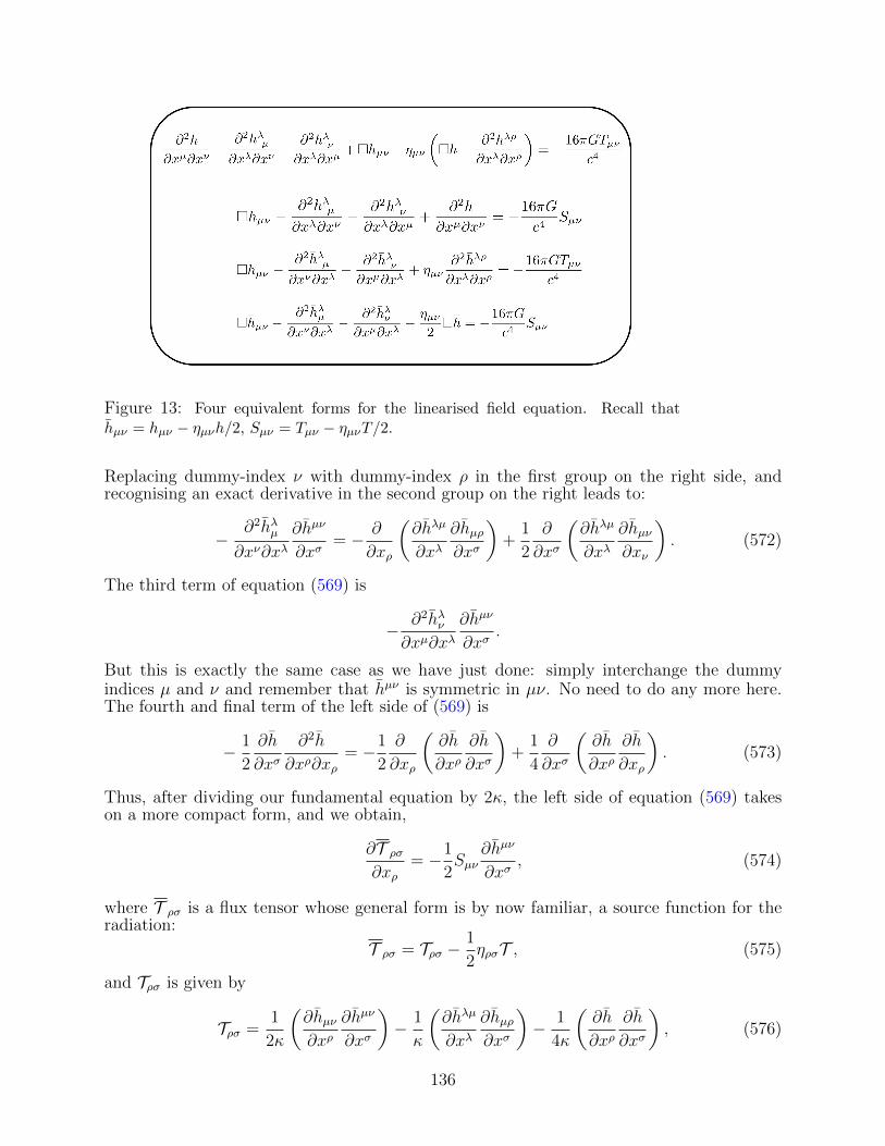
Figure 13: Four equivalent forms for the linearised field equation. Recall thathµν = hµν − ηµνh/2, Sµν = Tµν − ηµνT/2.

Replacing dummy-index ν with dummy-index ρ in the first group on the right side, andrecognising an exact derivative in the second group on the right leads to:

− ∂2hλµ∂xν∂xλ

∂hµν

∂xσ= − ∂

∂xρ

(∂hλµ

∂xλ∂hµρ∂xσ

)+

1

2

∂

∂xσ

(∂hλµ

∂xλ∂hµν∂xν

). (572)

The third term of equation (569) is

− ∂2hλν∂xµ∂xλ

∂hµν

∂xσ.

But this is exactly the same case as we have just done: simply interchange the dummyindices µ and ν and remember that hµν is symmetric in µν. No need to do any more here.The fourth and final term of the left side of (569) is

− 1

2

∂h

∂xσ∂2h

∂xρ∂xρ= −1

2

∂

∂xρ

(∂h

∂xρ∂h

∂xσ

)+

1

4

∂

∂xσ

(∂h

∂xρ∂h

∂xρ

). (573)

Thus, after dividing our fundamental equation by 2κ, the left side of equation (569) takeson a more compact form, and we obtain,

∂T ρσ∂xρ

= −1

2Sµν

∂hµν

∂xσ, (574)

where T ρσ is a flux tensor whose general form is by now familiar, a source function for theradiation:

T ρσ = Tρσ −1

2ηρσT , (575)

and Tρσ is given by

Tρσ =1

2κ

(∂hµν∂xρ

∂hµν

∂xσ

)− 1

κ

(∂hλµ

∂xλ∂hµρ∂xσ

)− 1

4κ

(∂h

∂xρ∂h

∂xσ

), (576)

136

with T ≡ T ρρ.We consider exclusively vacuum plane waves, which in fact form a Fourier basis for any

disturbance. If we choose an harmonic gauge to work in, then from the linearised formof Rµν = 0 it follows that we must have kµkµ = 0. The scalar T manifestly vanishes inan harmonic gauge. It can be shown, though we will not do so here, that for plane wavesolutions Tρσ, and therefore its scalar trace T are both gauge invariant. Hence, T mustvanish in general. Moreover, the tensor Tρσ − Tσρ must also be gauge invariant, vanishesfor an harmonic gauage, and so must vanish in any gauge. Hence, despite appearances,T ρσ = Tρσ for plane wave solutions, and may be replaced by its symmetrised form:

Tρσ =1

2κ

(∂hµν∂xρ

∂hµν

∂xσ

)− 1

2κ

(∂hλµ

∂xλ∂hµρ∂xσ

+∂hλµ

∂xλ∂hµσ∂xρ

)− 1

4κ

(∂h

∂xρ∂h

∂xσ

). (577)

Finally, for the TT gauge of choice, matters simplify yet more dramatically, and we find theelegant result

Tρσ =c4

32πG

(∂hµν∂xρ

∂hµν

∂xσ

)(TT gauge). (578)

Why did we choose to divide by 2κ for our overall normalisation constant? Why not justκ, or for that matter, 4κ? It is the right side of our energy equation that answers this. Thisis

− 1

2Sµν

∂hµν

∂xσ= −1

2

(Tµν −

ηµν2T)(∂hµν

∂xσ− ηµν

2

∂h

∂xσ

)= −1

2Tµν

∂hµν

∂xσ. (579)

Choose σ = 0, the time component. We work in the Newtonian limit h00 ' −2Φ/c2, whereΦ is a Newtonian gravitational potential. In the µν summation on the right side of theequation, we are then dominated by the 00 components of both hµν and Tµν . Next, we do twointegrations by parts, in which we shall ignore the exact derivative. Why? Because the exactderivative of a bounded periodic function (and everything here is periodic) must oscillateaway to zero on average. It is not a sustained energy source for the waves. By contrast,the product of two periodic functions need not oscillate to zero; for example the average ofcos2(ωt) = 1/2. This is a sustained source. (If cos2(ωt) is expressed as the derivative of afunction, that function contains a decidedly nonperiodic growing term proportional to t andis not bounded.) We therefore keep product terms only when they are not exact derivatives.Then, using the right arrow → notation to mean “integrate by parts and ignore the purederivatives,” we perform the following manipulations on the right side of equation (579):

− 1

2T00

∂h00

∂x0→ 1

2

∂T00

∂x0h00 = −1

2

∂T 0i

∂xih00 → 1

2T 0i∂h

00

∂xi' −ρv

c·∇Φ, (580)

where the first equality follows from ∂νT0ν = 0. We have therefore arrived at an expression

for the rate at which the effective Newtonian potential does net work on the matter. The 1/cfactor cancels out with the same factor on the left (flux) side of the original equation. Theexpression is overall negative if the force −ρ∇Φ is oppositely directed to the velocity, so thatthe source is losing energy by generating outgoing waves. Our harmonic gauge expression(578) for T0i is also negative for an outward flowing wave that is a function of the argument(r − ct), r being spherical radius and t time. By contrast, T 0i would be positive, as befitsan outward moving wave energy flux.

The fact that division by 2κ produces a source corresponding to the rate at which work isdone on the Newtonian sources (when σ = 0) means that our overall normalisation is indeed

137

correct. The σ = 0 energy flux of (578) is the true TT gauge energy flux of gravitationalradiation in the weak field limit:

F i = Fi = c T i0 = −c Ti0 = − c4

32πG

(∂hµν∂xi

∂hµν

∂t

)(TT gauge). (581)

9.5 The energy loss formula for gravitational waves

Summary: Einstein’s classic formula for the total gravitational energy radiated by a sourceis G/(5c9)

...J ij

...J ij, where Jij is the traceless form of the source’s moment of inertia tensor:

Jij = Iij − δijIkk/3.

Our next step is to evaluate the transverse and traceless components of hij, denotedhTTij , in terms of the transverse and traceless components of Iij. Begin with the tracelesscomponent, denoted Jij:

Jij = Iij −δij3I (582)

where I is the trace of Iij. Next, we address the transverse property. The projection of avector v onto a plane perpendicular to a unit direction vector n is accomplished simply byremoving the component of v along n. Denoting the resulting projected vector as w,

w = v − (n · v)n (583)

orwj = (δij − ninj)vi ≡ Pijvi (584)

where we have introduced the projection tensor

Pij = δij − ninj,

which has the easily shown properties

niPij = njPij = 0, PijPjk = Pik, Pii = 2. (585)

Notice that PijPjk = Pik simply states that if you project something that is already projected,nothing is changed! Projection operators are idempotent: applying them twice is the sameas applying them once.

Projecting tensor components presents no difficulties,

wij = PikPjlvkl → niwij = njwij = 0, (586)

nor does the extraction of a projected tensor that is both traceless and transverse:

wTTij =

(PikPjl −

1

2PijPkl

)vkl → wTTii = (PikPil − Pkl)vkl = (Pkl − Pkl)vkl = 0. (587)

Using the properties of Pij given in (585), it is a straightforward calculation to show thatthe analogue of PijPjk = Pik for the traceless transverse operator is:

(PikPjl −1

2PijPkl)(PimPjn −

1

2PijPmn) = (PmkPnl −

1

2PklPmn). (588)

138

Again, an informal way to say this is that if you take the transverse-traceless part of a tensorthat is already transverse and traceless, you don’t change anything. The transverse-tracelessprojection operator, like all projection operators, is idempotent. Recognising this simplemathematical fact in advance will save a great deal of calculational effort.

Let us define

JTTij =

(PikPjl −

1

2PijPkl

)Jkl. (589)

Now do the following exercise.

Exercise. Prove that JTTij is also given by

JTTij =

(PikPjl −

1

2PijPkl

)Ikl,

so that nothing is changed by using only the traceless form of Iij in our calculations, Jij.Yet another ploy to save computational effort.

Notice now that (Jij − JTTij )JTTij is the contraction of the part of Jij that has no transversecomponent with the part that is completely transverse. This ought to vanish, if there is anyjustice. Happily, it does:

(Jij − JTTij )JTTij = JijJTTij − Jkl(PikPjl −

1

2PijPkl)(PimPjn −

1

2PijPmn)Jmn (590)

Following (588), the right side of this is just

JijJTTij − Jkl(PmkPnl −

1

2PklPmn)Jmn = JijJ

TTij − JklJTTkl = 0 (591)

This will come in handy in a moment.

Next, we write down the traceless-transverse part of the quadrupole formula:

hTTij =2G

c6r

d2JTTijdt′2

. (592)

Recalling that t′ = t− r/c and the JTT ’s are functions of t′ (not t!),

∂hTTij∂t

=2G

c6r

d3JTTijdt′3

,∂hTTij∂r

= −2G

c7r

d3JTTijdt′3

(593)

where, in the second expression we retain only the dominant term in 1/r. The radial flux ofgravitational waves is then given by (581):

Fr =G

8πr2c9

d3JTTijdt′3

d3JTTijdt′3

(594)

The 1/c9 dependence ultimately translates into a 1/c5 dependence for Newtonian sources,since each of the J ’s carries a c2 factor.

The final step is to write out JTTij in terms of the Jij via the TT projection operator. Itis here that the fact that Jij is traceless is a computational help.(

PikPjl −1

2PijPkl

)= (δik − nink)(δjl − njnl)−

1

2(δij − ninj)(δkl − nknl) (595)

139

With Jkl traceless, we may work this through to find

JTTij =

(PikPjl −

1

2PijPkl

)Jkl = Jij +

1

2(δij + ninj)nknlJkl − ninkJjk − njnkJik (596)

Now, ...JTTij

...JTTij = [

...J ij + (

...JTTij −

...J ij)]

...JTTij . (597)

But we’ve seen in (591) that

(...JTTij −

...J ij)

...JTTij = 0,

so we are left with

...JTTij

...JTTij =

...J ij

...JTTij ≡

...J ij(

...J ij +

1

2(δij + ninj)nknl

...J kl − nink

...J jk − njnk

...J ik) =

...J ij

...J ij − 2njnk

...J ij

...J ik +

1

2ninjnknl

...J ij

...J kl (598)

Remember, the vector n is just the unit vector pointing in the direction of spherical anglesθ and φ. In Cartesian coordinates:

n = (nx, ny, nz) = (sin θ cosφ, sin θ sinφ, cos θ).

The total gravitational wave luminosity is an integration of the distribution (598) overall solid angles,

LGW =

∫r2Fr dΩ =

G

8πc9

∫...JTTij

...JTTij dΩ. (599)

To evaluate this, you will need ∫ninj dΩ =

4π

3δij. (600)

This is pretty simple: if the two components ni and nj of the unit normal vector are notthe same, the integral vanishes by symmetry (e.g. the average of xy over a sphere is zero).That means the integral is proportional to a delta function, say Cδij. To get the constant ofproportionality C, just take the trace of both sides:

∫dΩ = 4π = 3C, so C = 4π/3. Much

more scary-looking is the other identity you’ll need:∫ninjnknl dΩ =

4π

15(δijδkl + δikδjl + δilδkj). (601)

For example, the combination nxnxnynz would be sin3 θ cos θ cos2 φ sinφ. But keep calm andthink. The only way the integral cannot vanish is if two of the indices agree with one anotherand the remaining two indices also agree with one another. Maybe the second agreeing pairis just the same as the first, maybe not. (The nxnxnynz example provided clearly vanisheswhen integrated over solid angles, as you can easily show.) This pairwise index agreementrule is precisely what the additive combination of delta functions ensures, symmetricallysummed over the three different ways by which the pairwise index agreement can occur. Toget the 4π/15 factor, simply set i = j and k = l, then sum. The integral on the left is thentrivially

∫nininlnl dΩ ≡

∫dΩ = 4π. The combination of delta functions is 9 + 3 + 3 = 15.

Hence the normalisation factor 4π/15. Putting this all together via (594), (598), (600) and

140

(601), remembering Jii = 0, and carrying out the angular integral, the total gravitationalluminosity is thus given by

LGW =G

8πc9×[4π − 2× 4π

3+

1

2× 4π

15× (0 + 1 + 1)

]...J ij

...J ij,

which amounts to:

LGW =G

5c9

...J ij

...J ij =

G

5c9

(...I ij

...I ij −

1

3

...I ii

...I jj

). (602)

The calculation has not been easy. But the endpoint is a beautifully simple formula, aclassical result first derived by Albert Einstein17 in 1918. Indirect verification of this formulacame in about 1980 with the analysis of the binary pulsar, some 25 years after Einstein’sdeath. Direct verification with LIGO came in 2015, almost exactly one century after theepochal relativity paper.

9.6 Gravitational radiation from binary stars

Summary: This section contains more advanced material not on the syllabus, and is optional.Later, we will make use of the results for a circular orbit (equation 617 below), but you willbe provided with the formula.

Despite an initial burst of optimism surrounding an erroneous detection in 1968 (see§9.7), until relatively recently the direct detection of gravitational radiation seemed to mostphysicists a very distant possibility, at best. The coverage of the topic in Weinberg’s classictext emphasises the possibility that rapidly rotating neutron stars might be a viable source.Alas, for this to occur the neutron star would have to possess a sizeable and rapidly varyingquadrupole moment, and this is not an observed property of neutron stars. Even whenrotating rapidly as pulsars, neutron stars would not develop a quadrupole moment thatchanges with time; rotation maintains strict axisymmetry.

By contrast, the possibility that Keplerian orbits might be interesting for measuringgravitational radiation is examined in some detail in MTW. Ordinary orbits involving ordi-nary stars are not a very promising source of observable gravitational radiation. But a closebinary with two compact objects was discovered within two years of the textbook’s publica-tion, a system presciently considered by these authors. The binary, PSR 1913+16, was anunusual double neutron star system, with an orbital period of 7.75 hours. Compact objectbinaries have become the central focus of modern-day gravitational wave research. As notedin the Introduction, the first indirect confirmation of the existence of gravitational radiationcame from radio observations of PSR 1913+16, in which a change in orbital period (fromthe loss of mechanical orbital energy into gravitational radiation energy) was inferred viathe diminishing interval between arrival times of the pulsar’s signal. The amplitude of thegravitational waves was itself well-below the threshold of any direct detection. In the rangeof emitted frequencies, it remains so even today. Over long enough time scales, however,a tight compact object binary will lose enough energy through gravitational radiation thatthe resulting inspiral goes all the way to completion, and the system either coalesces (e.g.two black holes) or explodes (e.g., GW170817: two neutron stars). This end state scenariois observable. Predictions suggest that there are enough merging binaries in the universeto produce a rather high detection rate: several per year at a minimum. The final frenzied

17Actually, Einstein found a coefficient of 1/10, not 1/5. Eddington put matters right a few years later.Tricky business, this gravitational radiation.

141

seconds before coalescence produce detectable gravitational wave signatures rich in physicalcontent, at frequencies for which LIGO has been specifically designed. Through the endof 2020, there have been 20 rigorously confirmed binary merger gravitational wave events,and dozens of candidate signals under active consideration. Black hole merger waveformscan now be determined by high precision numerical calculation (but only since relativelyrecently: see, e.g., F. Pretorius 2005, Phys. Rev. Lett. 95, 121101).

Let us apply equation (602) to the case of two point masses in a classical Keplerianorbit. There is of course no contradiction between assuming a classical Newtonian orbitand calculating its leading order gravitational energy loss. We are working in the regime inwhich the losses exert only the most tiny change on the orbit over one period, and the masses,though very close to one another by ordinary astronomical standards, are still separated by adistance well beyond their respective Schwarzschild radii. (The numerical calculations makeno such restriction, faithfully calculating the orbital evolution all the way down to the finalmerger of two black holes into one.)

The Newtonian orbital elements are defined on page 88. The separation r of the twobodies is given as a function of azimuth φ as

r =L

1 + ε cosφ, (603)

where L is the semilatus rectum and ε the orbital eccentricity. With M being the totalmass of the individual objects, M = m1 + m2, l the constant specific angular momentum(we forego the symbol J for angular momentum to avoid confusion with Jij), and a thesemi-major axis, we have

r2dφ

dt= l, L =

l2

GM= a(1− ε2), (604)

and thus

dφ

dt=

(GM

a3(1− ε2)3

)1/2

(1 + ε cosφ)2 dr

dt=

(GM

a(1− ε2)

)1/2

ε sinφ (605)

The distance of each body from the center-of-mass is denoted r1 and r2 respectively. Writingthese as vector quantities,

r1 =m2r

M, r2 = −m1r

M. (606)

Thus, the xy coordinates in the orbital plane are

r1 =m2r

M(cosφ, sinφ), r2 =

m1r

M(− cosφ,− sinφ). (607)

The nonvanishing moment tensors Iij are then

Ixx =m1m

22 +m2

1m2

M2r2 cos2 φ = µr2 cos2 φ (608)

Iyy = µr2 sin2 φ (609)

Ixy = Iyx = µr2 sinφ cosφ (610)

Iii = Ixx + Iyy = µr2 (611)

142

where µ is the reduced mass m1m2/M . (Notice that if m1 and m2 are very different, it is thesmaller of the two masses that determines µ.) It is a now lengthy, but utterly straightforwardtask to differentiate each of these moments three times. If you choose to verify these results,you may wish to begin with the relatively easy ε = 0 case in the course of reproducing theformulae below:

d3Ixxdt3

= α(1 + ε cosφ)2(2 sin 2φ+ 3ε sinφ cos2 φ), (612)

d3Iyydt3

= −α(1 + ε cosφ)2[2 sin 2φ+ ε sinφ(1 + 3 cos2 φ)], (613)

d3Ixydt3

=d3Iyxdt3

= −α(1 + ε cosφ)2[2 cos 2φ− ε cosφ(1− 3 cos2 φ)], (614)

where

α2 ≡ 4G3m21m

22M

a5(1− ε2)5(615)

Equation (602) yields, after some assembling:

LGW =32

5

G4

c5

m21m

22M

a5(1− ε2)5(1 + ε cosφ)4

[(1 + ε cosφ)2 +

ε2

12sin2 φ

](616)

Our final step is to average LGW over an orbit. This is not simply an integral over dφ/2π.

We must integrate over time, i.e., over dt = dφ/φ, and then divide by the orbital period

2π√a3/GM to produce a time average. The answer is (Peters and Mathews 1963):

〈LGW 〉 =32

5

G4

c5

m21m

22M

a5f(ε) = 1.00× 1025 m2

1m22M(a)−5 f(ε) Watts, (617)

where

f(ε) =1 + (73/24)ε2 + (37/96)ε4

(1− ε2)7/2, (618)

and indicates solar units of mass (1.99×1030 kg) and length (one solar radius is 6.955×108

m). Something that is of order v/c is considered to be Newtonian, like a standard kinematicDoppler shift. At order v2/c2, we are in the regime of relativity (e.g. gravitational redshift),and measurements are traditionally quite difficult. Equation (617) tells us that LGW is anumber of order EΩ(v/c)5, where E is the Keplerian orbital energy, Ω the orbital frequency,and v a typical orbital velocity. No wonder gravitational radiation is so hard to measure!

Exercise. Show that following the procedure described above, the time-averaged luminosity〈LGW 〉time is given by the expression

〈LGW 〉time =32

5

G4

c5

m21m

22M

a5(1− ε2)7/2

⟨(1 + ε cosφ)2

[(1 + ε cosφ)2 +

ε2

12sin2 φ

]⟩angle

,

where the 〈 〉 angular average on the right is over 2π angles in φ. Use the fact that theangular average of cos2 φ is 1/2 and the average of cos4 φ is 3/8 to derive equation (617).

Exercise. By way of comparison, we calculate the average electromagnetic power when twoequal and opposite charges, e and −e, are in an elliptical orbit about one another. Thelowest order electromagnetic dipole radiation is given by Larmor’s formula

LEM =2

3c3didi

143

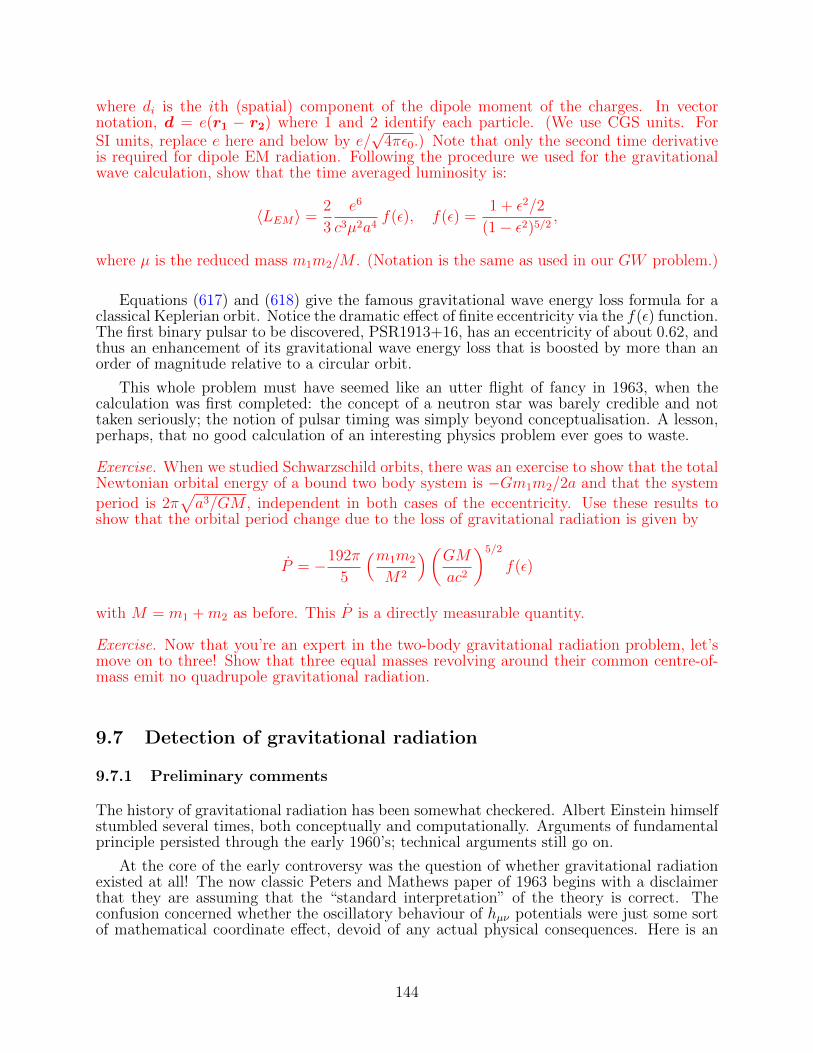
where di is the ith (spatial) component of the dipole moment of the charges. In vectornotation, d = e(r1 − r2) where 1 and 2 identify each particle. (We use CGS units. ForSI units, replace e here and below by e/

√4πε0.) Note that only the second time derivative

is required for dipole EM radiation. Following the procedure we used for the gravitationalwave calculation, show that the time averaged luminosity is:

〈LEM〉 =2

3

e6

c3µ2a4f(ε), f(ε) =

1 + ε2/2

(1− ε2)5/2,

where µ is the reduced mass m1m2/M . (Notation is the same as used in our GW problem.)

Equations (617) and (618) give the famous gravitational wave energy loss formula for aclassical Keplerian orbit. Notice the dramatic effect of finite eccentricity via the f(ε) function.The first binary pulsar to be discovered, PSR1913+16, has an eccentricity of about 0.62, andthus an enhancement of its gravitational wave energy loss that is boosted by more than anorder of magnitude relative to a circular orbit.

This whole problem must have seemed like an utter flight of fancy in 1963, when thecalculation was first completed: the concept of a neutron star was barely credible and nottaken seriously; the notion of pulsar timing was simply beyond conceptualisation. A lesson,perhaps, that no good calculation of an interesting physics problem ever goes to waste.

Exercise. When we studied Schwarzschild orbits, there was an exercise to show that the totalNewtonian orbital energy of a bound two body system is −Gm1m2/2a and that the system

period is 2π√a3/GM , independent in both cases of the eccentricity. Use these results to

show that the orbital period change due to the loss of gravitational radiation is given by

P = −192π

5

(m1m2

M2

)(GMac2

)5/2

f(ε)

with M = m1 +m2 as before. This P is a directly measurable quantity.

Exercise. Now that you’re an expert in the two-body gravitational radiation problem, let’smove on to three! Show that three equal masses revolving around their common centre-of-mass emit no quadrupole gravitational radiation.

9.7 Detection of gravitational radiation

9.7.1 Preliminary comments

The history of gravitational radiation has been somewhat checkered. Albert Einstein himselfstumbled several times, both conceptually and computationally. Arguments of fundamentalprinciple persisted through the early 1960’s; technical arguments still go on.

At the core of the early controversy was the question of whether gravitational radiationexisted at all! The now classic Peters and Mathews paper of 1963 begins with a disclaimerthat they are assuming that the “standard interpretation” of the theory is correct. Theconfusion concerned whether the oscillatory behaviour of hµν potentials were just some sortof mathematical coordinate effect, devoid of any actual physical consequences. Here is an

144

example of how you might get into trouble. We calculate the affine connection Γµνλ and applythe geodesic equation,

d2xµ

dτ 2+ Γµνλ

dxν

dτ

dxλ

dτ= 0 (619)

and ask what happens to a particle initially at rest with dxν/dτ = (c,0). The subsequentevolution of the spatial velocity components is then

d2xi

dτ 2+ Γi00c

2 = 0 (620)

But equation (500) clearly shows that Γi00 = 0 since any h with a zero index vanishes forour TT plane waves. The particle evidently remains at rest. Is there really no effect ofgravitational radiation on ordinary matter?!

Coordinates, coordinates, coordinates. The point, once again, is that coordinates bythemselves mean nothing, any more than does the statement “My house is located at thevector (2, 1.3).” By now we should have learned this lesson. We picked our gauge tomake life simple, and we have indeed found a very simple coordinate system that remainsfrozen to the individual particles! That does not mean that the particles don’t physicallybudge. The proper spatial separation between two particles with coordinate separation dxi

is ds2 = (ηij + hij)dxi dxj, and that separation surely is not constant because h11, h22, and

h12 = h21 are wiggling even while the dxi are fixed. Indeed, to first order in hij, we maywrite

ds2 = ηij(dxi + hikdx

k/2)(dxj + hjmdxm/2).

This makes the physical interpretation easy: the passing wave increments the initially undis-turbed spatial interval dxi by an amount δl = hikdx

k/2. It was Richard Feynman who in1955 seems to have given the simplest and most convincing argument for the existence ofgravitational waves. If the separation is between two beads on a rigid stick and the beadsare free to slide, they will oscillate with the tidal force of the wave. If there is now a tinybit of stickiness, the beads will heat the stick. Where did that energy come from? It couldonly be the wave. The “sticky bead argument” became iconic in the relativity community.

Recall that the two independent states of linear polarisation of a gravitational wave arethe + and × modes, “plus” and “cross.” They behave similarly, just rotated by 45. The+ wave (e11 = −e22) causes a prolate extension along the vertical part of the plus sign as itpasses, then squeezes down along the vertical axis and oblate outward along the horizontalaxis, then once again squeezes inward from oblate to vertical prolate. The ×mode (e21 = e12)shows the same oscillation pattern along a rotation pattern rotated by 45. (An excellentanimation is shown in the Wikipedia article Gravitational Wave.) These are the actual truephysical distortions caused by the tidal force of the gravitational wave.

In 1968, in the midst of what had been intensively theoretical investigations and debatesurrounding the nature of gravitational radiation, a physicist named Joseph Weber calmlyannounced that he had detected gravitational radiation experimentally in his basement lab,coming in prodigious amounts from the centre of the Milky Way Galaxy, thank you verymuch. His technique was to use what are now called “Weber bars”, giant cylinders of alu-minium fitted with special piezoelectric devices that can convert tiny mechanical oscillationsinto electrical signals. The gravitational waves distorted these great big bars by a tiny, tinyamount, and the signals were picked up. At least that was the idea. The dimensionlessrelative strain δl/l of a bar of length l due to passing wave would be of order hij, or 10−21

by our optimistic estimate. To make a long, rather sad story very short, Weber was inerror in several different ways, and ultimately his experiment was completely discredited.Yet his legacy was not wholly negative. The possibility of actually detecting gravitationalwaves hadn’t really been taken very seriously up to this point. Like Adams’s false detection

145

of a white dwarf gravitational redshift forty years before, an incorrect measurement caughtthe attention of the community. Post Weber, theorists and observers began to considervery seriously how one might go about detecting these signals properly, and what physicsmight be learnt from an unambiguous detection. Gravitational radiation detection becamepart of the physics mainstream, with leading figures in relativity becoming directly involved.The detection of gravitational radiation is not a task for a lone researcher, however clever,working in the basement of university building, any more than was finding the Higgs boson.Substantial resources of the National Science Foundation in the US and an internationalresearch team numbering in the thousands were needed for the construction and testing ofviable gravitational wave receptors. (In the UK, the University of Glasgow played a criticalLIGO design role.) Almost fifty years after Weber, the LIGO facility cleanly detected theexquisitely gentle tensorial strains of gravitational waves at the level of h ∼ 10−21. The LIGOmirrors may not have crack’d from side-to-side, but they did flutter in the tidal breeze. Thistruly borders on magic: using an effective length of LIGO’s interferometer arm of l = 10km, then δl is 10−15 cm, one percent of the radius of a proton!

The next exercise is strongly recommended.

Exercise. Weaker than weak interactions. Imagine a gravitational detector of twoidentical masses m separated by a distance l symmetrically about the origin and constrainedto move along the x-axis. Along comes a plane wave gravitational wave front, propagatingalong the z-axis, with hxx = −hyy = Axx cos(kz−ωt) and no other components. The massesvibrate in response. Show that, to linear order in Axx,

...I xx =

1

2mc2ω3l2Axx sinωt,

that there are no other...I ij, and that the masses radiate an average gravitational wave

luminosity of

〈LGW 〉 =G

60c5m2ω6l4A2

xx

Next, show that the average energy flux for our incoming plane wave radiation is, fromequation (581),

F =c3ω2A2

xx

32πG.

The cross section for gravitational interaction (dimensions of area) is defined to be the ratioof the average luminosity to the average incoming flux. Why is this a good definition for thecross section? Show that this ratio is

σ =8πG2m2ω4l4

15c8=

2π

15R2S

(ωl

c

)4

where RS = 2Gm/c2 is the Schwarzschild radius of each mass. Evaluate this numerically form = 10kg, l = 10m, ω = 20 rad s−1 (motivated by GW150914). Compare this with a typicalweak interaction cross section of 10−48m2. Just how weak is gravitational scattering?

9.7.2 Indirect methods: orbital energy loss in binary pulsars

In 1974, a remarkable binary system was discovered by Hulse and Taylor (1975, ApJ Letters,195, L51). One of the stars was a pulsar with a pulse period of 59 milliseconds, i.e., a neutron

146

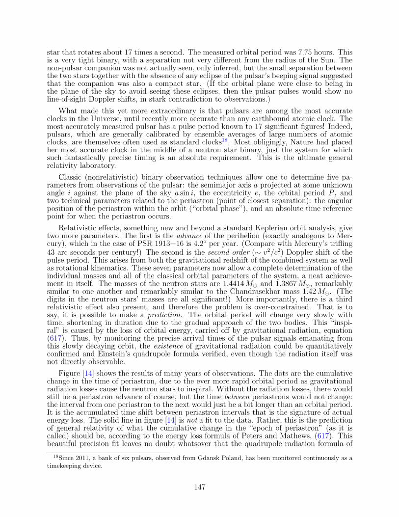
star that rotates about 17 times a second. The measured orbital period was 7.75 hours. Thisis a very tight binary, with a separation not very different from the radius of the Sun. Thenon-pulsar companion was not actually seen, only inferred, but the small separation betweenthe two stars together with the absence of any eclipse of the pulsar’s beeping signal suggestedthat the companion was also a compact star. (If the orbital plane were close to being inthe plane of the sky to avoid seeing these eclipses, then the pulsar pulses would show noline-of-sight Doppler shifts, in stark contradiction to observations.)

What made this yet more extraordinary is that pulsars are among the most accurateclocks in the Universe, until recently more accurate than any earthbound atomic clock. Themost accurately measured pulsar has a pulse period known to 17 significant figures! Indeed,pulsars, which are generally calibrated by ensemble averages of large numbers of atomicclocks, are themselves often used as standard clocks18. Most obligingly, Nature had placedher most accurate clock in the middle of a neutron star binary, just the system for whichsuch fantastically precise timing is an absolute requirement. This is the ultimate generalrelativity laboratory.

Classic (nonrelativistic) binary observation techniques allow one to determine five pa-rameters from observations of the pulsar: the semimajor axis a projected at some unknownangle i against the plane of the sky a sin i, the eccentricity e, the orbital period P , andtwo technical parameters related to the periastron (point of closest separation): the angularposition of the periastron within the orbit (“orbital phase”), and an absolute time referencepoint for when the periastron occurs.

Relativistic effects, something new and beyond a standard Keplerian orbit analysis, givetwo more parameters. The first is the advance of the perihelion (exactly analogous to Mer-cury), which in the case of PSR 1913+16 is 4.2 per year. (Compare with Mercury’s trifling43 arc seconds per century!) The second is the second order (∼ v2/c2) Doppler shift of thepulse period. This arises from both the gravitational redshift of the combined system as wellas rotational kinematics. These seven parameters now allow a complete determination of theindividual masses and all of the classical orbital parameters of the system, a neat achieve-ment in itself. The masses of the neutron stars are 1.4414M and 1.3867M, remarkablysimilar to one another and remarkably similar to the Chandrasekhar mass 1.42M. (Thedigits in the neutron stars’ masses are all significant!) More importantly, there is a thirdrelativistic effect also present, and therefore the problem is over-constrained. That is tosay, it is possible to make a prediction. The orbital period will change very slowly withtime, shortening in duration due to the gradual approach of the two bodies. This “inspi-ral” is caused by the loss of orbital energy, carried off by gravitational radiation, equation(617). Thus, by monitoring the precise arrival times of the pulsar signals emanating fromthis slowly decaying orbit, the existence of gravitational radiation could be quantitativelyconfirmed and Einstein’s quadrupole formula verified, even though the radiation itself wasnot directly observable.

Figure [14] shows the results of many years of observations. The dots are the cumulativechange in the time of periastron, due to the ever more rapid orbital period as gravitationalradiation losses cause the neutron stars to inspiral. Without the radiation losses, there wouldstill be a periastron advance of course, but the time between periastrons would not change:the interval from one periastron to the next would just be a bit longer than an orbital period.It is the accumulated time shift between periastron intervals that is the signature of actualenergy loss. The solid line in figure [14] is not a fit to the data. Rather, this is the predictionof general relativity of what the cumulative change in the “epoch of periastron” (as it iscalled) should be, according to the energy loss formula of Peters and Mathews, (617). Thisbeautiful precision fit leaves no doubt whatsover that the quadrupole radiation formula of

18Since 2011, a bank of six pulsars, observed from Gdansk Poland, has been monitored continuously as atimekeeping device.

147

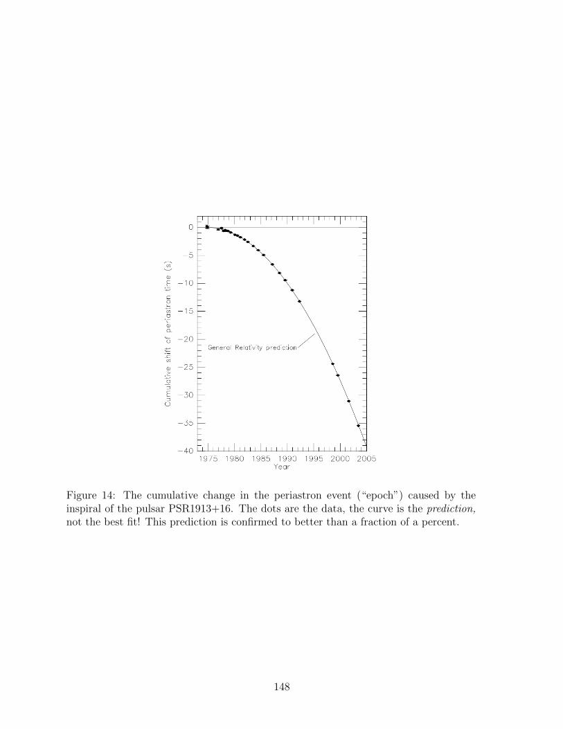
Figure 14: The cumulative change in the periastron event (“epoch”) caused by theinspiral of the pulsar PSR1913+16. The dots are the data, the curve is the prediction,not the best fit! This prediction is confirmed to better than a fraction of a percent.

148

Einstein is correct. For this achievement, Hulse and Taylor won a well-deserved Nobel Prizein 1993. (It must be just a coincidence that 1993 is about the time that the observationaldata points become noticeably more sparse.)

Direct detection of gravitational waves is a very recent phenomenon. There are twotypes of gravitational wave detectors currently in operation. The first is based on a classic19th century laboratory apparatus, a Michelson interferometer. The second makes use ofpulsar emissions—specifically the arrival times of pulses—as a probe of the hµν inducedby gravitational waves as these waves propagate across our line of site to the pulsar. Theinterferometers are designed for wave frequencies from ∼ 10 Hz to 1000’s of Hz. These havebeen detetecting sources since 2015. By contrast, the pulsar measurements are sensitive tofrequencies of tens to hundreds of micro Hz—a very different range, produced by systemswith much larger distance scales. This technique has yet to be demonstrated. The highfrequency interferometers measure the gravitational radiation from stellar-mass black holesor neutron star binaries merging together. The low frequency pulsar timing will also inprinciple measure black holes merging, but with masses of order 109 solar masses. These arethe masses of black holes that live in the cores of active galaxies.

9.7.3 Direct methods: LIGO

LIGO, or Laser Interferometer Gravitational-Wave Observatory, detects gravitational wavesas described in figure [15]. In the absence of a wave, the arms are set to destructivelyinterfere, so that no light whatsoever reaches the detector. The idea is that a gravitationalwave passes through the apparatus, each period of oscillation slightly squeezing one arm,slightly extending the other. With coherent laser light traversing each arm, when this lightre-superposes at the centre, the phase will become ever so slightly out of precise cancellation,and therefore photons will appear in the detector. In practise, the light makes many passagesback and forth along a 4 km arm before analysis. There are two such interferometers, onein Livingston, Louisiana, the other in Hanford, Washington, a separation of 3000 km. For asignal to be verified, both detectors must show a simultaneous wave passage (“simultaneous”after taking into account an offset of 10 milliseconds for the speed of light travel time!)

This is a highly simplified description, of course. A vast amount of ingenious amplifica-tion, noise suppression, and (especially) laser frequency stabilisation techniques19 have goneinto this project, which is designed to measure induced strains at the astronishing level of onepart in 1023. Wave detection is possible at all only because gravitational attennae measure,not the time-averaged flux of radiation, which would have a 1/r2 dependence with distancer to the source, but the time-explicit amplitude hij(t), which has a 1/r dependence.

Exercise. Following the above description, show that if one arm of the inteferometer hasits phase increased by φ1(t) due to the passage of a gravitational wave, and the other has aphase shift of φ2(t), then the lowest order signal detected will be

(φ2 − φ1) sin(ωct+ δ)

where ωc is the “carrier frequency” of the laser and δ is an arbitrary constant phase. Thephases φ1 and φ2 will generally have opposite signs. Why?

Figure [16] shows a match of an accurate numerical simulation to the processed LIGOevent GW150914. I have overlaid three measured wave periods P1, P2, and P3, with each oftheir respective lengths given in seconds. (These were measured with a plastic ruler directlyfrom the diagram!) The total duration of these three periods is 0.086 s. Throughout this

19The feedback system maintaining the utterly stable frequency requirements for the LIGO lasers wereimplemented by Ronald Drever, who passed away shortly before the LIGO Nobel Prize was announced.

149

Figure 15: A schematic interferometer. Coherent light enters from the laser at the left.Half is deflected 45 upward by the beam splitter, half continues on. The two halvesreflect from the mirrors. The beams re-superpose at the splitter, interfere, and arepassed to a detector at the bottom. If the path lengths are identical or differ by anintegral number of wavelengths they interfere constructively; if they differ by an oddnumber of half-wavelengths they cancel one another. In “null” mode, the two armsare set to destructively interfere so that no light whatsoever reaches the detector. Apassing gravity wave just barely offsets this ultra-precise destructive interference andcauses laser photons to appear in the detector.

150

time the black holes are separated by a distance in excess of of 4 RS, so we are barely at thelimit for which we can trust Newtonian orbit theory. Let’s give it a try for a circular orbit.(Circularity is not unexpected for the final throes of coalescence.)

Using the zero eccentricity orbital period decrease formula from the final exercise of §9.6,but remembering that the orbital period P is twice the gravitational wave period PGW ,

PGW = −96π

5

(m1m2

M2

)(GMac2

)5/2

We eliminate the semi-major axis a in favour of the measured period PGW ,

P 2 =4π2a3

GM, whence P 2

GW =π2a3

GM

This gives

PGW = −96π8/3

5c5

(GMc

PGW

)5/3

(621)

where we have introduced what is known as the “chirp mass” Mc,

Mc =(m1m2)3/5

M1/5(622)

The chirp mass (so-named because if the gravitational wave were audible at these samefrequencies, it would indeed sound like a chirp!) is the above combination of m1 and m2,which is directly measurable from PGW and its derivative. It is easy to show (try it!) thatM = m1 +m2 is a minimum when m1 = m2, in which case

m1 = m2 ' 1.15Mc.

Putting numbers in (621), we find

Mc = 5.522× 103PGW (−PGW )3/5, (623)

where Mc is the chirp mass in solar masses and PGW is measured in seconds. From theGW150914 data, we estimate

PGW 'P3 − P1

P1 + P2 + P3

=−0.0057

0.086= −0.0663,

and for PGW we use the midvalue P2 = 0.0283. This yields

Mc ' 30.7 (624)

compared with “Mc ' 30M” in Abbot et al. (2016). I’m sure this remarkable level ofagreement is somewhat (but not entirely!) fortuitous. Even in this, its simplest presentation,the wave form presents a wealth of information. The “equal mass” coalescing black holesystem comprises two 35M black holes, and certainly at that mass a compact object canonly be a black hole!

The two masses need not be equal of course, so is it possible that this is something otherthan a coalescing black hole binary? We can quickly rule out any other possibility, withouta sophisticated analysis. It cannot be any combination of white dwarfs or neutron stars,

151

because the chirp mass is too big. Could it be, say, a black hole plus a neutron star? Witha fixed observed Mc = 30M, and a neutron star of at most ∼ 2M, the black hole wouldhave to be some 1700M. So? Well, then the Schwarzschild radius would have to be verylarge, and coalescence would have occurred at a separation distance too large for any of theobserved high frequencies to be generated! There are frequencies present toward the end ofthe wave form event in excess of 75 Hz. This is completely incompatible with a black holemass of this magnitude.

A sophisticated analysis using accurate first principle numerical simulations of gravita-tional wave from coalescing black holes tells an interesting history, one rather well-capturedby even our naive efforts. Using a detailed match to the waveform, the following can bededuced. The system lies at a distance of some 400 Mpc, with significant uncertainties hereof order 40%. At these distances, the wave form needs to be corrected for cosmologicalexpansion effects, and the masses in the source rest frame are 36M and 29M, with ±15%uncertainties. The final mass, 62M is definitely less than the sum of the two, 65M: some3Mc

2 worth of energy has disappeared in gravitational waves! A release of 5 × 1047J is, Ibelieve, the largest explosion of any kind every recorded. A billion years later, some of thatenergy, in the form of ripples in space itself, tickles the interferometer arms in Louisiana andWashington. It is, I believe, at 10−15 cm, the smallest amplitude for mechanical motion everrecorded.

What a story.

9.7.4 Direct methods: Pulsar timing array

Pulsars are, as we have noted, fantastically precise clocks. Within the pulsar cohort, thosewith millisecond periods are the most accurate of all. The period of PSR1937+21 is knownto be 1.5578064688197945 milliseconds, an accuracy of one part in 1017. (That is equivalentto knowing the age of the Universe to within a few seconds!) One can then predict thearrival time of a pulse to this level of accuracy as well. By constraining variations in pulsearrival times from a single pulsar, we can set an upper limit to amount of gravitationalradiation that the signal has traversed. But we don’t just have one pulsar. So why settlefor one pulsar and mere constraints? We know of many pulsars, distributed more or lessuniformly through the galaxy. If the arrival times from this “pulsar timing array” (PTA)started to vary but the variations were correlated with one another in a mathematicallypredictable manner, this would be a direct indication of the deformation of space causedby the passage of a gravitational wave (fig. [17]). This technique is sensitive to very longwavelength gravitational radiation, light-years in extent. This is very difficult to do becauseall other sources introducing a spurious correlation must be scrupulously eliminated. LIGOtoo has noise issues, but unlike pulsar blips propagating through the interstellar medium,LIGO’s signal is very clean and all hardware is accessible. Thus, PTA has its share ofskeptics. At the time of this writing (January 2021), there are only upper limits from thePTA measurements.

152

Figure 16: From Abbott et al. (2016). The upper diagram is a schematic rendering of theblack hole inspiral process, from slowly evolution in a quasi-Newtonian regime, to a stronglyinteracting regime, followed by a coalescence and “ring-down,” as the emergent single blackhole settles down to its final, nonradiating geometry. The middle figure is the gravitationalwave strain, overlaid with three identified periods discussed in the text. The final bottom plotshows the separation of the system and the relative velocity as a function of time, from insprialjust up to the moment of coalescence.

153

Figure 17: A schematic view of a gravitational wave passing through an array of pulsar probes,inducing regular variations in arrival times of pulses.

154

Despite its name, the big bang theory is

not really a theory of a bang at all. It is

really only a theory of the aftermath of a

bang.

— Alan Guth

10 Cosmology

10.1 Introduction

Summary. When carefully applied, local Newtonian mechanics in a background of outwardly-expanding matter provides a surprisingly good (indeed, unreasonably good) description ofmuch of basic cosmology. Expansion is essential for mathematical self-consistency. Photonspropagating in such an expanding space are observed to be redshifted relative to their restframe: the wavelength increases, as the photon propagates, in proportion to the size of theUniverse.

10.1.1 Newtonian cosmology

The subject of the origin of the Universe is irresistible to the scientist and layperson alike.What went bang? Where did the Universe come from? What happened along the way?Where are we headed? The theory of general relativity, with its rigorous mathematicalformulation of the large-scale geometry of spacetime, provides both the conceptual andtechnical apparatus to understand the structure and evolution of the Universe. We arefortunate to live in an era in which many precise answers to these great questions are athand. Moreover, while we need general relativity to put ourselves on a properly rigorousfooting, we can get quite far using very simple ideas and hardly any relativity at all! Not onlycan, we absolutely should begin this way. Let us start with some very Newtonian dynamicsand see what there is to see. Then, knowing a bit of what to expect and where we areheaded, we will be in a much better position to revisit “the problem of the Universe” on afully relativistic basis.

A plausible, if somewhat naive, first model of the Universe might be one in which spaceis an ordinary static Euclidian geometry, and the galaxies fill up this space uniformly (onaverage) everywhere out to infinity. Putting aside the question of the origin of such astructure (let’s say it has existed for all time) and the problem that the cumulative lightreceived at any location would be infinite (“Olber’s paradox”–that’s tougher to get around:let’s say maybe we turned on the galaxies at some finite time in the past20), the staticEuclidian model is not even mathematically self-consistent.

Consider the analysis from figure [18]. In the figure on the left, we note that there aretwo observers, one at the centre of the sphere 1, the other at the centre of sphere r2. Eachcalculates the expected acceleration at the location of the big black dot, which is a point onthe surface of each of the spheres. Our model universe is spherically symmetric about r1,but it is also spherically symmetric about r2! Hence the following conundrum:

20See W72, pp. 611-13.

155

!!!!!!!!!!!!!!!Homogeneous,!Euclidian!!!!!!!!!!!!!!!sta2c!universe!

r1#r2#

1!

2!

!!!!!!!!!!!!!!!Homogeneous,!Euclidian!!!!!!!!!!!!!!!sta2c!universe!

a1!≠!a2$$

a1$ a2$1!

2!

Figure 18: In a static homogeneous Euclidian universe, an observer at thecenter of sphere 1 would calculate a different gravitational acceleration forthe dot to that of an observer at the centre of sphere 2: a1 6= a2. But ifwe take into account the actual relative acceleration of the two observers,each considers the other to be in a noninertial frame, and the calculationbecomes self-consistent with this non-inertial “fictitious” force. (See text.)

The observer at the centre of sphere 1 ignores the effect of the spherically symmetricmass exterior to the black point and concludes that the acceleration at the dot’s location is

a1 =GM(within r1)

r21

=4πGρr1

3, (625)

directed toward the centre of the r1 sphere. (Here ρ is meant to be the average uniform massdensity of the Universe.) But the observer at the origin of the r2 sphere claims, by identicalreasoning, that the acceleration must be a2 = 4πGρr2/3 directed toward the centre of r2!This is shown in the bottom diagram of figure [18]. Both cannot be correct.

What if the Universe is dynamically active? Then we must put in the gravitationalacceleration, in the form of a noninertial reference frame, from the very start of the cal-culation. If the observers at the centres of r1 and r2 are actually accelerating relative toone another, there is no reason to expect that their separate calculations for the black dotacceleration to agree, because the observers are not part of the same inertial frame! Can wemake this picture self-consistent somehow for any two r1 and r2 observers? Yes, providedthat the Universe is allowed to expand (or contract!) and Newtonian mechanics is appliedself-consistently.

Here is how it works. The observer at the centre of sphere 1 measures the acceleration ofthe black dot to be −4πGρr1/3 as above, with r1 pointing from the centre of sphere 1 to thesurface dot. The same sphere-1 observer finds that the acceleration of the centre of sphere

156

2 is −4πGρ(r1 − r2)/3, where r2 is the position vector oriented from the sphere 2 centretoward the big dot. Defined this way, these particular r1 and r2 vectors are colinear. Thus,the person at the centre of sphere 1 finds that the acceleration of the big dot, as measured byan observer moving in the (noninertial) centre of sphere 2 frame is the sphere-1 accelerationof −4πGρr1/3 minus the acceleration of the observer at the centre of sphere 2:

− 4πGρr13

− −4πGρ(r1 − r2)

3= −4πGρr2

3(626)

Lo and behold, this is the acceleration that the observer at the centre of sphere 2 would findself-consistently in the privacy of their own study, without worrying about what anyone elsethinks might be going on. A Euclidian, “linearly accelerating” universe is therefore perfectlyself-consistent. The expansion process itself is a Newtonian requirement, not, as originallythought at the time of its discovery, a mysterious effect of general relativity. Naively, therate of expansion ought to be slowing, since this is what gravity does: an object thrownfrom the surface of the earth slows down as its upward displacement increases. This is whatastronomers assumed for 70 years. It turns out however, that our Universe is a bit moredevious than that. There is some mystery here beyond the realm of the purely Newtonian!

10.1.2 The dynamical equation of motion

A simple way to describe the internal acceleration of the Universe is to begin with thespatially homogeneous but time-dependent relative expansion between two locations. Theseparation between two arbitrary points separated by a distance r(t) may be written

r(t) = R(t)l (627)

where l is a comoving coordinate that labels a fixed radial distance from us in the space—fixed in the sense of being fixed to the expanding space, like latitude and longitude wouldbe on the surface of an inflating globe. It is natural to take l to have dimensions of length,in which case R(t) is a dimensionless function of time alone, a scale factor that embodiesthe dynamical behaviour of the Universe. The velocity v = dr/dt ≡ r of a comoving pointexpanding with space is then

v(t) = Rl = (R/R)r. (628)

We should emphasise the vector character of this relationship:

v(t) = (R/R)r (629)

where r is a vector pointing outward from our arbitrarily chosen origin. Then, the accelera-tion is

a(t) =dv

dt= (R/R)r. (630)

(Why didn’t we differentiate r(t)/R(t)?) This kinematic relative acceleration between twopoints is, by Newtonian gravitation theory, given by equation [625]):

a(t) = −4πGρ

3r. (631)

Hence,

− 4πGρ

3=R

R. (632)

157

Notice how l disappears: this is an equation for the scale factor R, and the scale factordepends not on where you are, but on when you are. Next, multiply this equation by RRand integrate, assuming that ordinary mass is conserved in the ordinary way, i.e. ρR3 isconstant. We then obtain

R2 − 8πGρR2

3= 2E, (633)

where E is an energy-like integration constant. This, in a simple, apparently naive Euclidian-Newtonian approach, would be our fundamental dynamical cosmological equation for theevolution of the Universe. Amazingly, providing that we are prepared to allow the massdensity ρ is to be upgraded to an energy density (divided by c2) that includes all contributions(in particular radiation and vacuum energy), this innocent little equation turns out to be farmore general: it is exactly correct in full relativity theory! More on this anon.

10.1.3 Cosmological redshift

The expansion of the Universe leads to a very important kinematic effect known as thecosmological redshift. Since the Universe is expanding, a travelling photon is constantlyovertaking more distant observers that are moving away from the original source. If thephoton had a measured wavelength λ at location r, then when the photon passes an observera distance dr = cdt away from r, who is moving at a relative velocity R dr/R, this observermeasures a Doppler change in wavelength dλ determined by equation (629):

dλ

λ=v

c=

R

cRdr =

R

Rdt, (634)

or in other words1

λ

dλ

dt≡ λ

λ=R

R. (635)

Solving for λ, we find that it is linearly proportional to R. It is as though the wavelengthstretches out with the rest of the Universe. This is a very general kinematic result, aproperty of any cosmological model that is symmetrically expanding. (Even if there isspatial curvature, the “differential proper distance” is always cdt for a travelling photon.)

This result means that the frequency of a photon goes down as 1/R. But the frequencyof a photon is proportional to its energy, hence the radiation temperature Tγ ∝ 1/R. Theenergy density in radiation (fourth power in Tγ) decreases as 1/R4. Evidently the totalenergy in a comoving volume R3 decreases as 1/R: energy is not conserved by the expansionof the Universe! By contrast, the entropy density in the radiation is proportional to T 3

γ ,

and (TγR)3 is therefore constant. The radiation entropy, which is just proportional to thenumber of photons, is conserved. Photons are neither created nor destroyed by the act ofexpansion. This makes perfect sense.

We are free, and it is customary, to choose our coordinates in such a way that the currentvalue of R is 1, with R becoming smaller and smaller as we go back in time. If a photon isemitted with a wavelength λe at some time t in the past, the wavelength (λ0) we would nowmeasure at time t0 is formally expressed as

λ0 = λe(1 + z) (636)

where z is defined by this equation and known as the redshift parameter. Therefore,

λ0

λe= 1 + z =

R(t0)

R(t)=

1

R(t). (637)

158

The advantage to using z, as opposed to the more geometrical quantity R, is that z isdirectly observed by astronomers. But the two quantities are mathematically equivalent viathis completely general equation, R = 1/(1 + z). In any symmetric cosmological model, ifyou measure a redshift of 2, it has come from a time when the Universe had one-third of itscurrent size.

10.2 Cosmology models for the impatient

Summary. The concept of a spacetime metric is needed even in Newtonian cosmology. Ametric allows us to describe the paths of photons as they move through an expanding space,and to determine from which comoving coordinate location l they emerged, given a measuredredshift z. Because different cosmologies produce different functions for this l(z), this quantityis a key observational tool which in principle allows us to determine what kind of Universewe live in.

10.2.1 The large-scale spacetime metric

Because the Newtonian approach works remarkably well, here is a brief reminder as to whywe really do need relativity in our study of the large scale structure of the Universe.

First, we require a Riemannian metric structure to ensure that the proper speed oflight is a universal constant c, especially when traversing a dynamically evolving spacetimebackground. It is easy to see what the form of this metric must be in a simple model ofan expanding Euclidian Universe. Symmetry demands that time must flow identically forall observers comoving with the universal expansion, and we can always choose time to bea linear function of the time coordinate. Space is uniformly expanding at the same rateeverywhere. If space itself is Euclidian, the spacetime metric practically leaps out of thepage,

− c2dτ 2 = −c2dt2 +R2(dx2 + dy2 + dz2), (638)

where we have used the usual (x, y, z) Cartesian coordinates, and R satisfies equation (633).Note that x, y, z are comoving with the expansion, with an embedded Euclidian comovingspatial interval dl given by

dx2 + dy2 + dz2 = dl2.

In particular, a photon heading directly towards us satisfies the equation:

Rdl

dt= −c (639)

where dl is the change of radial comoving coordinate induced by the photon’s passage. Amechanical analogue is an ant, moving at a constant velocity c, crawling from the pole to theequator along the surface of an expanding sphere. In this case, dl correspond to the changein the ant’s latitude.

Second, we must allow for the theoretical possibility of non-Euclidian spatial structure.Now, equation (638) really does appear to be the true form of the spacetime metric for ourUniverse. Space happens to be very nearly, or perhaps even precisely, Euclidian. But as apurely mathematical point, this need not be the case even if we demand perfect symmetry,any more than the requirement of a perfectly symmetric two-dimensional surface demandsa flat Euclidian plane. We could preserve our global maximal spatial symmetry and be ina curved space, like the surface of sphere. This surface, in common with a flat plane, issymmetric about every point, but its spatial properties are clearly distorted relative to a

159

plane. (E.g. the Pythagorean theorem does not hold, and the sum of the angles of a triangleon the surface exceeds 180 degrees.) The case of a two-dimensional spherical surface is readilygrasped because we can easily embed it in three dimensions to form a mental image—or justlook at a globe. The surface is finite in area and is said to be positively curved. There isalso a perfectly viable, flaring, negatively curved two-dimensional surface. A saddle beginsto capture its essence, but not quite, because the curvature of a saddle is not uniform. Thecase of a uniformly negatively curved two-dimensional surface cannot actually be embeddedin three Euclidian dimensions, so it is very hard to picture in your mind’s eye! (At least,it is for me.) There are positively and negatively curved fully three-dimensional spaces aswell, all perfectly symmetric, all logically possible alternative structures for the space of ourUniverse. They just happen not to fit the data. It is fortunate for us that the real Universeseems also to be mathematically the simplest. For now, we shall confine our attention tothis expanding, good old flat Euclidian space.

Third, we need relativity in the form of the Birkhoff theorem to justify properly theargument neglecting exterior contributions from outside the arbitrarily chosen spheres weused in section 10.1. The Newtonian description strictly can’t be applied to an infinitesystem, whereas nothing prevents us from using Birkhoff’s theorem applied to an unboundedsymmetric spacetime.

Fourth, we need a relativistically valid argument to arrive at equation (633). Nothingin the Newtonian derivation even hints at this level of generality. We shall return to thiscarefully in section 10.3.

Finally, we need relativity theory to relate the energy constant E to the geometry of ourspace. For now, we restrict ourselves to the case E = 0, which will turn out to be the onlysolution consistent with the adoption of a flat Euclidian spatial geometry, our own Universe.

10.2.2 The Einstein-de Sitter universe: a useful toy model

Consider equation (633) for the case E = 0 in the presence of ordinary matter, whichmeans that ρR3 is a constant. Remember that we are free to choose coordinates in whichR = R0 = 1 at the present time t = t0. We may then choose the constant ρR3 to be equalto ρ(t0) = ρM0, the mass density at the current epoch. Equation (633) becomes

R1/2R =

(8πGρM0

3

)1/2

. (640)

Integrating,

2

3R3/2 =

(8πGρM0

3

)1/2

t, (641)

where the integration constant has been set to zero under the assumption that R was verysmall at early times. This leads to

R =

(3H0t

2

)2/3

, (642)

where we have introduced an important structural constant of the Universe, H0, the valueof R/R at the current time t0. (The current growth rate.) This is known as the Hubbleconstant,

H0 = R(t0) =

(8πGρM0

3

)1/2

→ R = H0R−1/2. (643)

160

More generally, the Hubble parameter is defined by

H(t) =R

R(644)

for any time t. The solution (642) for the scale factor R is known for historical reasons asthe Einstein-de Sitter model.

Exercise. Show that H(t) = H0(1 + z)3/2 for our simple model R = (t/t0)2/3.

The Hubble constant is in principle something that we may observe directly by measuringthe distances to nearby galaxies as well as their redshift, and then using equation (629)locally. As a problem in observational astronomy, this is hardly straighforward! On thecontrary, it is a very difficult task because we cannot be certain that the motion of thesenearby galaxies comes from cosmological expansion alone. But astronomers have persevered,obtaining good distance measurments to ever more distant galaxies, and the bottom line isthat the measured value of H0 and the measured value of the density of ordinary matter ρM0

do not satisfy (643) in our Universe. There is not enough ordinary matter ρM0 to accountfor the measured H0. On the other hand, equation (633) does seem to be precisely valid,with E = 0. As the energy density of radiation in the contemporary Universe is much lessthan 3H2

0/8πG, how is all this possible?

The answer is stunning. While the energy density of ordinary matter most certainlydominates over radiation, it is not the dominant contributor to the energy density of theUniverse. There is now strong evidence of an additional energy density associated with thevacuum of spacetime itself! This energy density, ρV , is the dominant energy density of thereal Universe on cosmological scales, though not at present overwhelmingly so: ρV is about69% of the total energy budget, whereas matter (the familiar baryons plus whatever“darkmatter” is) comes in at about 31%. However, because ρV remains constant as the Universeexpands, at later times vacuum energy will completely dominate the expansion: ρM dropsoff as 1/R3, and the constant ρV takes up the slack.

What does this imply for the expansion of the Universe? With an effective vacuumHubble parameter of

HV ≡(

8πGρV3

)1/2

, (645)

equation (633) at later times takes the form

R = HVR (646)

orR ∝ exp(HV t). (647)

The Universe will expand exponentially! In other words, rather than gravity slowly deceler-ating the expansion by the mutual attractive force of Newtonian gravity, the vacuum energydensity will actively drive an ever more vigorous expansion via a repulsive force. The con-verse of this is that an exponential Universe would be expanding less rapidly in the past thanin the present. It is this “less rapidly than expected” earlier history of cosmic expansionthat has led to our current understanding of the remarkable dynamical state of our Universe.The Nobel Prize in Physics was awarded to Perlmutter, Schmidt and Riess in 2011 for theiruse of distant supernovae as a tool for unravelling the dynamics of the Universe from earlyto modern times. We currently live in the epoch where exponential expansion happens tobe taking over.

Let us return to the Einstein-de Sitter Universe. Equations (637), (639) and (643) maybe combined to answer the following question. If we measure a photon of redshift z, from

161

what value of l did it originate? This is an important question because it provides thelink between astronomical observations and the geometry of the Universe. With R(t) =(t/t0)2/3 = (3H0t/2)2/3, equation (639) may be integrated over the path of the photon fromits emission at l at time t:∫ l

0

dl′ = −c∫ t

t0

dt′

R= c

∫ 1

R

dR

RR=

2c

H0

(1−√R)

=2c

H0

(1− 1√

1 + z

)≡ l(z) (648)

Note that as z → ∞, l → 2c/H0, a constant. The most distant photons—and thereforethe most distant regions of the Universe that may causally influence us today—come froml = 2c/H0. This quantity is known as the horizon, denoted lH . Beyond the horizon, we candetect—and be influenced by—nothing. This particular value of lH = 2c/H0 is associatedwith the Einstein–de Sitter model, but the existence of a horizon is a general feature of manycosmologies and on dimensional grounds it will generally be of order c/H0. Do not confusethis cosmological horizon, sometimes called a “particle horizon” with the event horizon ofa black hole. The particle horizon is the radial extent throughout which cosmological-scalecausality may be exerted. The event horizon is a surface enveloping a black hole, withinwhich no causal contact with the outside world is possible.

Physical distances are given not by l, but by Rl. Since R = 1 currently, 2c/H0 is thecurrent physical scale of the horizon as well. There is nothing special about now, however.We could be doing this analysis at any time t, and the physical size of the horizon at time t inthe E-de S model would then be 2c/H(t) = 2c/[H0(1 + z)3/2]. So here is another interestingquestion. As a practical matter, the farthest back in time that we can see is to a redshift ofabout z = 1100. At higher redshifts, the Universe was completely opaque to photons. Justas in viewing the Sun we can see only down to its opaque photosphere, not into its interior,so can we also only see back in cosmological time to an era when the Universe itself wasbecoming similarly opaque. What would be the subtended angular size of the horizon ΘH

at z = 1100, as we measure it today on the sky? This is an important question becausewe would not expect the Universe to be very smooth or regular or correlated in any way onangular scales bigger than this. (The E-dS model doesn’t actually hold during the radiationdominated phase, but it will serve to make our point; greater numerical accuracy doesn’thelp the problem!) The angular size of the horizon at a redshift z is given by the followingexpression:

ΘH(z) =2c

H0(1 + z)3/2× 1

R(z)l(z)=

2c

H0(1 + z)1/2l(z)=

1√1 + z − 1

(649)

The first equality sets the horizon angle equal to the actual physical size of the horizon atredshift z, divided by d = R(z)l(z), the distance to redshift z at precisely the same earliertime corresponding to redshift z (not now!). This d is the relevant proper distance to thephoton source at the moment of the radiation emission when the proper size was 2c/H(t).The Universe was a smaller place then, and it would be inconsistent to compute the angleΘH(z) using the current proper distance R0l(z) = l(z), with the old proper horizon size. Ifyou plug in z = 1100 into (649) and convert ΘH to degrees, you’ll find ΘH = 1.8, about3 times the diameter of the full moon. But the Universe looks very regular on much, muchlarger angular scales, indeed we know that the radiation temperature over the entire skyis unchanging to one part in 105. Even if our E-dS model is only crude, it highlights animportant problem. Simply put, how does the Universe know about itself in a globally,given that it takes signals, even signals travelling at the speed of light, so long to cross it?What we’ve got here is a failure to communicate. We will see later in this course how moderncosmology can address this puzzle and facilitate communication.

By the way, the fact that the Universe was “on top of us” at early times has anothersurprising consequence. Assuming that the average physical size of a galaxy isn’t changing

162

very much with time, if we calculate the average angular size of a galaxy, we find that atlow redshift, all is normal: the more distant galaxies appear to be smaller. But then, atprogressively higher redshifts, the galaxies appear to be growing larger on the sky! Why?Because at large z, the Universe was, well, on top of us. The proper distance to redshift zformula is (for E-dS models):

l(z)R(z) =2c

H0(1 + z)3/2

(√1 + z − 1

)(650)

At low z, this is increasing linearly with z, which is intuitive: bigger redshift, more distant.But at large z this declines as 1/z, since the Universe really was a smaller place.

Exercise. At what redshift would the average galaxy appear to be smallest in this model?(Answer: z = 5/4.)

10.3 The Friedmann-Robertson-Walker Metric

Summary. The form of the metric for an expanding space time that is homogeneous andisotropic about every point, but allows for curvature to be present, is known as the Friedmann-Robertson-Walker (FRW) metric. A uniformly expanding Euclidian space is a particularinstance of the FRW metric, one that seems to describe our Universe. The form of theFRW can be found with simple mathematics, from the notion of a curved spherical surface inmultidimensional Euclidian spaces. The FRW is required to establish the relationship betweenthe redshift of a photon and its comoving coordinate of origin.

We begin with an important notational shift. The variable r will henceforth denote acomoving radial coordinate. To avoid any confusion, we will no longer use l as a comovingcoordinate.

The Friedmann-Robertson-Walker, or FRW, metric is the most general metric of a ho-mogeneous isotropic cosmology. To understand its mathematical form, let us start simply.The ordinary metric for a planar two-dimensional space (“2-space”) without curvature maybe written in cylindrical coordinates as

ds2 = d$2 +$2dφ2 (651)

where the radial $ and angular φ polar coordinates are related to ordinary Cartesian x andy coordinates by the familiar formulae:

x = $ cosφ, y = $ sinφ (652)

As we have noted, this flat 2-space is not the most general globally symmetric 2-spacepossible. The space could, for example, be distorted like the 2-surface of a sphere, yet retainthe symmetry of every point being mathematically equivalent. The metric for a sphericalsurface is

ds2 = a2dθ2 + a2 sin2 θdφ2, (653)

where a is the radius of the sphere. We know how to relate cylindrical polar and sphericalcoordinates: set $ = a sin θ. This may be viewed as a purely formal transformation ofcoordinates, but in our mind’s eye we can picture θ in simple geometrical terms as thecolatitude angle measured downward from the z axis, so that this $ is actually the samecylindrical radius $ seen in equation (651). But don’t expect to get back to (651) from (653)via this simple coordinate change sin θ = $/a. Instead, we find that the spherical surfacemetric becomes:

ds2 =d$2

1−$2/a2+$2dφ2, (654)

163

an entirely different space from the flat planar surface (651). The space of (654) is the sameoriginal spherical surface space we started with by any other name; the metric resemblesequation (651) for a plane only in the limit a→∞. Changing coordinates does not changethe geometry. In particular, a coordinate change cannot alter any curvature scalar, whichremains invariant to coordinate transformation.

Let’s stretch ourselves a bit and consider at a formal level the closely related two-dimensional metric

ds2 =d$2

1 +$2/a2+$2dφ2, (655)

which upon substituting sinhχ = $/a reverts to

ds2 = a2dχ2 + a2 sinh2 χdφ2 (656)

the fundamental symmetry properties of the metric are unaffected by the ±$2/a2 sign flip.The flip in denominator sign simply changes the sign of the constant curvature from positive(convex, think sphere) to negative (flaring, think saddle). This characteristic form of theradial metric tensor component, g$$ = 1/(1±$2/a2), will reappear when we go from curved2-space to curved 3-space.

Exercise. Show that the Ricci scalar R for the spherical metric (653) is −2/a2, and for thesaddle metric (656) is 2/a2. These are constants of equal magnitudes across their respectivesurfaces, but with opposite signs. The underlying homogeneous and isotropic symmetry isthe same in both cases.

10.3.1 Maximally symmetric 3-spaces

It is best to begin with the conclusion, which ought not to surprise you. The most generalform of the three dimensional metric tensor that is maximally symmetric—homogeneous andisotropic about every point—takes the form

− c2dτ 2 = −c2dt2 +R2(t)

(dr2

1− r2/a2+ r2dθ2 + r2 sin2 θ dφ2

)(657)

where we allow ourselves the liberty of taking the curvature constant a2 to be either positiveor negative.

The derivation of the metric for the three-dimensional hypersurface of a four-dimensionalsphere is not difficult. The surface of such a “4-ball” (Cartesian coordinates w, x, y, z) is givenby

w2 + x2 + y2 + z2 = a2 = constant. (658)

Thus, on the three-dimensional surface (“3-sphere”), a small change in w2 is restricted tosatisfy:

d(w2) = −d(x2 + y2 + z2) ≡ −d(r2), whence dw = −rdr/w (659)

with r2 ≡ x2 + y2 + z2. Therefore,

(dw)2 =r2(dr)2

w2=r2(dr)2

a2 − r2(660)

The line element in Cartesian 4-space is

ds2 = dx2 + dy2 + dz2 + dw2 = dr2 + r2dθ2 + r2 sin2 θ dφ2 + dw2. (661)

164

Adding together dr2 and (dw)2 as given by (660), there follows immediately the desired lineelement restricted to the 3-sphere of a 4-ball, analogous to our expression for the ordinaryspherical surface metric (653):

ds2 =dr2

1− r2/a2+ r2dθ2 + r2 sin2 θdφ2, (662)

just as we see in equation (657).

An alternative form for (662) is sometimes useful without the singular denominator. Setr = a sinχ. Then

ds2 = a2dχ2 + a2 sin2 χdθ2 + a2 sin2 χ sin2 θdφ2 (663)

Exercise. Show that the 3-sphere (surface) of a 4-ball with radius a has a “volume” π2a3.

Exercise. Would you care to hazard a guess as to what the line element of the 4-sphere of a5-ball looks like either in the form of (662) or (663)?

What if we began, not with the 3-sphere of a Euclidian 4-ball, but with the 3D surfaceof a 4D hyperboloid,

x2 + y2 + z2 − w2 = a2 = constant (664)

in a flat Minkowski-like space? The line element is

ds2 = dx2 + dy2 + dz2 − dw2. (665)

Why not? Special relativity is not the only venue for hyperbolic geometry.

An identical calculation restricting dw to stay on the 3D surface yields in this case

(dw)2 =r2(dr)2

w2=r2(dr)2

a2 + r2. (666)

The constrained four-dimensional Minkowski metric (665) within our 3D surface now takesthe form

ds2 = dx2 + dy2 + dz2 − dw2 =dr2

1 + r2/a2+ r2dθ2 + r2 sin2 θdφ2, (667)

This is the corresponding negatively curved (saddle-like) 3D surface, and with r = a sinhχ,its alternative form is

ds2 = a2dχ2 + a2 sinh2 χdθ2 + a2 sinh2 χ sin2 θ dφ2. (668)

For our Universe, a appears to be immeasurably large (but with χ compensatingly smallso that aχ finite). In other words, space is neither positively nor negatively curved. Spaceis very close to flat.

It is customary in some textbooks to set a to be a positive constant, use r′ = r/a asa rescaled radial variable, and then absorb the factor of a into the definition of what youmean by the scale factor R(t). In effect, one introduces a new scale factor R′ = aR. Thiseliminates a entirely from the metric! If you choose this route, however, you give up on theconvenience of setting the current value of R′ equal to 1. Dropping the ′ on r′ and R′, thisgeneral FRW metric, with a absorbed, is written:

− c2dτ 2 = −c2dt2 +R2(t)

(dr2

1− kr2+ r2dθ2 + r2 sin2 θ dφ2

), (669)

165

where the constant k is +1 for a positively curved space, −1 for a negatively curved space,and 0 for a flat space. This particular line element with

g00 = −1, grr = R2(t)/(1− kr2), gθθ = R2(t)r2, gφφ = R2(t)r2 sin2 θ. (670)

is often what people mean when they write “the FRW metric.” Because a is absent in thisformulation, this can be mathematically convenient in calculations. In my view, the form(657) is more physically transparent.

Be careful. In (669), R has dimensions of length, and r is dimensionless. In (657), R isdimensionless and it is r that carries dimensions of length. For k = 0, we may stick to Rbeing dimensionless and r carrying dimensions of length, as there is no need to “absorb a.”In all cases, r is a comoving coordinate.

A few final words on practical uses of the FRW metric. I will use the metric in the form(657). In flat Euclidian space, the integrated comoving distance to coordinate r is just ritself. (The proper distance is then found by multiplying by the scale factor R(t) at theappropriate time.) Otherwise, the comoving radial distance associated with coordinate r is∫ r

0

dr′√1− r′2/a2

= a sin−1(r/a) (a2 > 0), or |a| sinh−1(r/|a|) (a2 < 0).

(In the above, a is positive when a2 > 0, and |a| is the positive norm when a2 < 0.)

By way of a specific example, let us rework equation (648) in our current notation forthe case of positive curvature. The comoving coordinate of a photon arriving with redshiftz when the scale factor was R is given by

a sin−1(r/a) = c

∫ t0

t

dt′

R(t′)= c

∫ 1

R

dR

RR= c

∫ z

0

dz

(1 + z)R(z)≡ a sin−1(r[z]/a)

We’ve been a bit casual with notation to avoid a clutter, using R as dummy variable insidethe integral and also as an integration limit. (The same with z.) But the meaning shouldbe clear. Note that we have used R = 1/(1 + z), so that the current value of R is 1, which isappropriate for the form of the metric in equation (657). R is given by equation (633) quitegenerally, but we need to relate E and a. That requires general relativity. In §10.4, we showthat 2E = −c2/a2.

Let’s look at a flat, pure vacuum universe, but one with finite ρV and HV so that wehave something to work with! Then R = HVR and

r = c

∫ 1

R

dR

RR=

c

HV

∫ 1

R

dR

R2=

c

HV

(1

R− 1

)=

cz

HV

(671)

How interesting. There is no horizon in such a universe. As z → ∞, r → ∞. An earlyphase of exponential growth (“inflation”) has in fact been proposed as a means to avoid thehorizon problem. We’ve learnt something very important already.

Next, the volume in a maximally symmetric space within redshift zm is formally givenby

V = 4π

∫ r

0

R3 r′2dr′√1− r′2/a2

, (672)

a function of r and thus ultimately of redshift. But what do we use for R inside this integral?That depends on the question. If we are interested in the current net volume of, let us say,

166

a prescribed group of photon sources, then R = R0, a constant, and life is simple. If we areinterested in the net volume occupied of the sources at the time of the photon emission, thenwe would need first to find R as a function of r to do the integral, then we need to find r(zm)to get back to redshift z. That can be complicated! As an easier example, however, thecurrent net volume V for sources out to a maximum redshift zm with a2 > 0 is (R = R0 = 1)

V = 4π

∫ r

0

r′2dr′√1− r′2/a2

= 2π

(a3 sin−1 r

a− a2r

√1− r2

a2

). (673)

You should be able to show that this reduces to the more familiar 4πr3/3 when a is large.In that case, for an E-dS universe the volume to redshift z is (show!):

V (z) =32π

3

(c

H0

)3(1− 1√

1 + z

)3

. (674)

10.4 Large scale dynamics

Summary. The day of reckoning can be put off no longer, as the field equations of generalrelativity are confronted. We show that our Newtonian dynamical equation for R is validunder all circumstances, and that 2E from this equation is equal to −c2/a2 where a is fromthe FRW metric. The field equations can be modified by the addition of what is known asthe cosmological constant, a term whose effect is very important on the largest scales. Thiscosmological constant is mathematically identical to the effect of a vacuum energy density.We may therefore, without loss of generality, keep the original form of the field equations, butallow for the possibility that the energy density ρc2 contains a contribution from the vacuum.

The student should read and study subsections 10.4.1 and 10.4.3, but may regard therather heavy 10.4.2 as optional (off syllabus). Remember, however, the identification of 2Ewith −c2/a2!

10.4.1 The effect of a cosmological constant

Begin first with the Field Equations including the cosmological constant, equation (294):

Rµν −gµν2R = −8πG

c4Tµν + Λgµν (675)

Recall the stress energy tensor for a perfect fluid:

Tµν = Pgµν + (ρ+ P/c2)UµUν . (676)

We may arrange the right side source term of (675) as follows:

− 8πG

c4Tµν + Λgµν = −8πG

c4

[P gµν +

(ρ+

P

c2

)UµUν

], (677)

where

P = P − c4Λ

8πG, ρ = ρ+

c2Λ

8πG(678)

167

In other words, the effect of a cosmological constant is to leave the left side of the FieldEquations untouched and to leave the right side of the Field Equations in the form of astress tensor for a perfect fluid, but with the density acquiring a constant additive termc2Λ/8πG and the pressure acquiring a constant term of the opposite sign, −c4Λ/8πG!

This is simple, almost trivial, mathematics, but profound physics. The effect of a cosmo-logical constant is as if the vacuum itself had an energy density EV = ρV c

2 = c4Λ/8πG anda pressure PV = −c4Λ/8πG. Does it make sense that the vacuum has a negative pressure,equal to its energy density but opposite in sign? Yes! If the vacuum volume expands by dV ,the change in energy per unit volume of expansion is just dE/dV ≡ ρV c

2. By the first lawof thermodynamics, this must be −PV . Yet more fundamentally, if we recall the form of thestress energy tensor of the vacuum, but without assuming PV = −ρV c2, then

Tµν (V ) = PV gµν + (ρV + PV /c2)UµUν , (679)

and the last group of terms would change the form of the vacuum stress energy going fromone constant velocity observer to another. In other words, you could tell if you were movingrelative to the vacuum. That is absolutely forbidden! The vacuum stress must always beproportional to gµν , and to gµν alone. The only way this can occur is if PV = −ρV c2.

An early general relativity advocate, Sir Arthur Eddington was particularly partial to acosmological constant, and famously commented that “To drop the cosmical constant wouldbe to knock the bottom out of space.” At the time, this was probably viewed as Eddingtonin his customary curmudgeon mode. Today, his insight seems quite prescient. Contemporaryphysicists think less in terms of a cosmological constant, placing greater conceptual emphasison the notion of a vacuum energy density. What is the reason for its existence? Why doesit have the value that it does? If ρV is not strictly constant, there is new physics to bediscovered. Are the best observational data supportive of a truly constant value for ρV ?The value of ρV probably emerged from the same type of “renormalisation process” that hasproduced finite values for the masses for the fundamental particles. How do we calculatethis? These are some of the most difficult questions in all of physics.

Moving forward, we must place these fascinating issues to the side, and continue our devel-opment of large scale models of the Universe without the formal appearance of a cosmologicalconstant, but with the understanding that we may add the appropriate contributions to thedensity ρ and pressure P to account precisely for the effects of Λ.

10.4.2 Formal analysis

We shall use the field equations in terms of the source function Sµν = Tµν − gµνT/2,

Rµν = −8πG

c4Sµν , (680)

and the FRW metric in the form of equation (670). We shall lose no generality in so doing, aswe may always set k = 1/a2 at the end of the calculation here, without invalidating any stepalong the way. In our comoving coordinates, the only component of the covariant 4-velocityUµ that does not vanish is U0 = −c (from the relations g00(U0)2 = −c2 and U0 = g00U

0).The nonvanishing components of Tµν are then

T00 = ρc2, Tij = Pgij. (681)

Which meansT 0

0 = −ρc2, T ij = δijP, T = T µµ = −ρc2 + 3P (682)

168

We shall need

S00 = T00 −g00

2T =

1

2(ρc2 + 3P ), Sij =

1

2gij(ρc

2 − P ) (683)

To calculate R00, begin with our expression for the Ricci tensor, (302):

Rµκ =1

2

∂2 ln |g|∂xκ∂xµ

− ∂Γλµκ∂xλ

+ ΓηµλΓλκη −

Γηµκ2

∂ ln |g|∂xη

where g is the determinant of the metric tensor gµν given by (670). Defining

f(r) = 1/(1− kr2),

we have|g| = R6(t) r4 f(r) sin2 θ (684)

For diagonal metrics, Γaab = ∂b(ln gaa)/2 and Γbaa = −(∂bgaa)/2gbb (no sum on a). ThereforeΓλ00 = 0, and our expression for R00 simplifies to

R00 =1

2

∂2 ln |g|∂x0∂x0

+ Γη0λΓλ0η =

1

2

∂2 ln |g|∂x0∂x0

+ Γr0rΓr0r + Γθ0θΓ

θ0θ + Γφ0φΓφ0φ (685)

With1

2

∂2 ln |g|∂x0∂x0

=3R

Rc2− 3R2

R2c2, Γr0r = Γθ0θ = Γφ0φ =

R

Rc, (686)

the 00 component of (680) becomes

R = −4πGR

3

(ρ+

3P

c2

)(687)

which differs from our Newtonian equation (632) only by an additional, apparently verysmall, term of 3P/c2 as an effective source of gravitation. However, during the time whenthe Universe was dominated by radiation, this term was important, and even now it turnsout to be not only important, but negative as well! During the so-called inflationary phase,3P/c2 was hugely important. We will have much more to say about all of this later.

The rr component of the Field Equations is a bit more involved. Ready? With f ′ ≡df/dr, we prepare a working table in advance of all the results we will need:

Rrr =1

2

∂2 ln |g|∂r2

− ∂Γλrr∂xλ

+ ΓηrλΓλrη −

1

2Γηrr

∂ ln |g|∂xη

(688)

Γrrr =1

2grr

∂grr∂r

=f ′

2f, Γ0

rr = − 1

2cg00

∂grr∂t

=fRR

c, Γr0r =

1

2cgrr

∂grr∂t

=R

Rc(689)

Γφφr =1

2gφφ

∂gφφ∂r

= Γθθr =1

2gθθ

∂gθθ∂r

=1

r(690)

∂ ln |g|∂r

=f ′

f+

4

r,

1

2

∂2 ln |g|∂r2

=1

2

f ′′

f− 1

2

(f ′)2

f 2− 2

r2,

∂Γ0rr

∂x0=

1

c2

(fR2 + fRR

)(691)

∂ ln |g|∂t

=6R

R,

∂Γrrr∂r

=f ′′

2f− (f ′)2

2f 2(692)

169

Putting it all together:

Rrr =1

2

∂2 ln |g|∂r2

− ∂Γrrr∂r− ∂Γ0

rr

∂x0+ (Γrrr)

2 +(

Γθθr

)2+(

Γφφr

)2+ 2Γ0

rrΓrr0 −

Γrrr2

∂ ln |g|∂r

− Γ0rr

2c

∂ ln |g|∂t

=f ′′

2f−(f ′)2

2f2−2

r2−[f ′′

2f−(f ′)2

2f2

]− 1

c2

(fR2 + fRR

)+

(f ′)2

4f2+2

r2+

2fR2

c2− f ′

4f

(f ′

f+

4

r

)− 3fR2

c2

Thus, with f ′/f = 2krf ,

Rrr = −2fR2

c2− fRR

c2− 2kf = −8πG

c4Srr = −4πG

c4grr(ρc

2 − P ) = −4πR2Gf

c4(ρc2 − P )

or2R2 +RR + 2kc2 = 4πGR2(ρ− P/c2) (693)

Notice that r has disappeared, as it must! (Why must it?) Eliminating R from (693) viaequation (687) and simplifying the result leads to

R2 − 8πGρR2

3= −kc2 (694)

This is exactly the Newtonian equation (633) with the constant 2E identified with −kc2.But be careful. The Newtonian version (633) was formulated with R dimensionless. If we usethe standard FRW convention that k is either 1, 0, or −1, then remember that R has beenrescaled to have dimensions of length in equation (694). To recover the Newtonian formis just a matter of replacing k by 1/a2, with dimensions of an inverse length squared. Wethen have 2E = −c2/a2, with the same dimensions of R2 or 1/t2. Remember that we mustallow a2 < 0 in the case of negative curvature. The important point is that equation (633)is valid in full general relativity. The dynamical Newtonian energy constant is therefore tobe identified with the geometrical curvature of the space.

One final item in our analysis. We have not yet made explicit use of the equation for theconservation of energy-momentum, based on (212) and the Bianchi Identities:

T µν;µ =1√|g|∂(√|g|T µν)∂xµ

+ ΓνµλTµλ = 0. (695)

This constraint is of course already built into the field equations themselves, and so in thissense adds no new information to our problem. But we may ask whether use of this equationfrom the start might have saved us some labour in getting to (694): it was a long derivationafter all. The answer is an interesting YES and NO.

The ν = 0 component of (695) reads

T µ0;µ =

1√|g|∂(√|g|T 00)

∂x0+ Γ0

µλTµλ = 0. (696)

Only affine connections of the form Γ0ii (spatial index i, no sum) are present, and with

Γ0ii = − 1

2g00

∂gii∂x0

=1

2

∂gii∂x0

, T 00 = ρc2, T ii = Pgii =P

gii, (NO i SUMS)

170

equation (696) becomes:

1

R3

∂(R3ρc2)

∂t+ 3P

R

R= 0→ ρ+ 3

(ρ+

P

c2

)R

R= 0. (697)

This is simply the relativistic form of the first law of thermodynamics, dE = −PdV , whichreverts to mass conservation in the nonrelativistic limit.

Exercise. Justify the last statement, and show that a pure vacuum energy density universetrivially satisfies (697).

If we now use (697) to substitute for P in (687), after a little rearranging we easily arriveat the result

d

dt

(R2)

=8πG

3

d

dt

(ρR2

)(698)

which in turn immediately integrates to (694)! This is surely a much more efficient route to(694), except...except that we cannot relate the integration constant that emerges from (698)to the spatial curvature constant k. True, we have a faster route to our final equation. Butwe only have dynamical content. Equation (694) is, after all, just a statement of energy con-servation. Without explicitly considering the Ricci Rrr component, we lose the geometricalconnection between Newtonian E (an untethered integration constant) and −kc2 (a geomet-rical curvature constant). We therefore have consistency between the energy conservationand Ricci approaches, but not true equivalence. A subtle and interesting distinction.

10.4.3 The Ω0 parameter

We work with the dynamical cosmological equation in its Newtonian form, with no loss ofgenerality,

R2 − 8πGρR2

3= 2E, (699)

where E is an energy integration constant. This constant may be determined, using directlyobservable quantities, by using the convention that R = 1 at the current time t0. We write2E in terms of H0, the Hubble constant R0 and ρ0c

2, the current average value of the totalenergy density of the Universe:

H20

(1− 8πGρ0

3H20

)≡ H2

0 (1− Ω0) = 2E = − c2

a2, (700)

where the parameter Ω0 is

Ω0 =8πGρ0

3H20

. (701)

The Universe is therefore positively curved (closed) or negatively curved (open) accordingto whether the measured value of Ω0 is larger or smaller than unity. Defining the criticalmass density ρc by

ρc =3H2

0

8πG, (702)

and the critical energy density in the Universe is then ρcc2. The parameter Ω(t) is defined

just as Ω0, with ρ(t) and H(t) replacing their current t0 values.

171

A puzzle associated with classical cosmologies that were based on the assumption thatthe Universe is comprised of standard matter, was that the measured value of Ω0 seemedto be about 0.05. This is disquieting because the two terms on the left side of equation(699) are then neither very close, nor hugely different from one another. Just different.But over the lifetime of the Universe, this interval of just being different is a mere fleetinginstant of time. In the early Universe, the two terms were both large and remained veryclose in magnitude, like an Einstein-de Sitter model. Thereafter, the R term dominates ina continuously expanding Universe, with Ω(t) 1 over almost all time. So why are weprivileged to live in a very special epoch in which Ω(t) just happens to be in transition fromunity to miniscule?

It is now understood that the components can, and do, involve a the energy density of thevacuum. The currently best measured value of H0 (in standard astronomical units) is 67.6 kms−1 Mpc−1,21 or H0 ' 2.2× 10−18 s−1. This number implies a critical density of 8.6× 10−27

kg (about 5 hydrogen atoms) per cubic meter, far less than what is actually observed inmatter22. The best so-called “concordance models” all point to an Ω0 = 1, E = 0 Universe,but only if ∼ 70% of ρ0c

2 comes from the vacuum! About 25% comes from dark matter,which is matter that is not luminous but whose presence is inferred from its gravitationaleffects, and just 5% comes from ordinary baryonic matter in the form of gas and stars. Wewill denote the current vacuum contribution to Ω0 as ΩV 0 and the matter contribution asΩM0. In addition, there is a contribution from radiation, Ωγ0, and while it is quite negligiblenow, in the early universe (z ≥ 5500) it was completely dominant. The Universe went firstthrough a radiation-dominated phase, followed by a matter-dominated phase, and then atabout a redshift of 0.3, it started to switch to its current vacuum-dominated phase. Thislatter transition is still ongoing.

While an Ω = 1 Universe remains an Ω = 1 Universe throughout all time, the relativecontribution from each of constituents changes, and the question of fine-tuning has not quitedisappeared. We now just happen to be in the extended neighbourhood of an inflection pointwhere Einstein-de Sitter behaviour is giving rise to exponential growth. It is not obviouswhat, if anything, to make of that.

10.5 The classic, matter-dominated universes

Summary. Matter-dominated models of the Universe dominated cosmological thought through-out the 20th century. If the matter density is high, these universes all have a closed geometryand recollapse after a finite time. By contrast, low density, open geometry models expandforever, the scale factor eventually increasing linearly with time. A unique critical densitydivides these two cases. In this unique case the geometry is flat (Euclidian) and the expan-sion rate is ever diminishing: the scale factor is proportional to t2/3 at all times t. This isthe Einstein-de Sitter solution. All three types of solution may be studied analytically.

Let us return to the good old days, when the idea that the Universe was driven by “theenergy density of the vacuum” was the stuff of Star Trek conventions, not something that

21One “megaparsec,” or Mpc is one million parsecs. One parsec (“pc”) is the distance from the solar systemat which the Earth–Sun semi-major axis would subtend an angle of one arcsecond: 1 pc = 3.0856×1013 km,1 Mpc = 3.0856× 1019 km. Stars are typically separated by 1 pc in galaxies, galaxies from one another byabout 1Mpc.

22 The absolute value of the pressure in the vacuum is some 5.4× 10−10 Pa (for “Pascals”, the SI pressureunit). This would be an ultra-vacuum in a terrestrial lab, but is rather substantial by astronomical standards:in magnitude, it is roughly the ordinary gas pressure in the core of a molecular cloud in the interstellarmedium.

172

serious-minded physicists dwelt upon. The expansion dynamics of the Universe was thoughtto be dominated by matter, pure and simple, after a brief early phase when it was radiation-dominated. Matter obeys the constraint that ρ(t)R3(t) remains constant with time. WithR0 = 1, this constant must be the current mass density ρM0. The dynamical equation of theUniverse may then be written

R2 = 2E +8πGρR2

3= H2

0

(1− ΩM0 +

ΩM0

R

)(703)

or ∫ R

0

dR′√1− ΩM0 + (ΩM0/R′)

=

∫ R

0

R′1/2dR′√(1− ΩM0)R′ + ΩM0

= H0t (704)

The nature of the integral depends upon whether ΩM0 is less than, equal to, or greater than,1. The case ΩM0 = 1 is trivial and leads immediately to

R =

(3H0t

2

)2/3

(705)

our Einstein-de Sitter solution (642). According to (699) with E = 0, the average density isthen given explicitly by

ρ =R2

R2

3

8πG=

1

6πGt2(706)

Consider next the case ΩM0 > 1, that of a Closed Universe. Then (704) may be written:∫ R

0

R′1/2dR′√1− (1− Ω−1

M0)R′= Ω

1/2M0H0t (707)

Set(1− Ω−1

M0)R′ = sin2 θ′ (708)

Then (707) becomes

2

(1− Ω−1M0)3/2

∫ θ

0

sin2 θ′ dθ′ =1

(1− Ω−1M0)3/2

∫ θ

0

(1− cos 2θ′) dθ′ = Ω1/2M0H0t (709)

or2θ − sin 2θ

2(1− Ω−1M0)3/2

= Ω1/2M0H0t (710)

With η = 2θ, our final solution is in the form of a parameterisation:

R =1− cos η

2(1− Ω−1M0)

, H0t =η − sin η

2√

ΩM0(1− Ω−1M0)3

(711)

Some readers may recognise these equations for R and H0t as the parameterisation of acycloid, which is the path taken by a fixed point on the circumference of a wheel as thewheel rolls forward. (See the curve labelled “Closed” in figure [19].) Precisely analogousexpressions emerge for the case ΩM0 < 1, which are easily verified from (704):

R =cosh η − 1

2(Ω−1M0 − 1)

, H0t =sinh η − η

2√

ΩM0(Ω−1M0 − 1)3

(712)

173

This is the solution for negative curvature, an Open Universe.

Exercise. Show that for either equation (711) or (712),

dη

dt=

c

aR

where a is interpreted as√| ± a2|. We will use this in the Problem Set!

Exercise. Show that the equations analogous to (705), (711) and (712) for the FRW metricin the form (669) are respectively

R = ω1/3t2/3 (Einstein− deSitter)

R =ω

c2

(1− cos η

2

), ct =

ω

c2

(η − sin η

2

)(closed)

R =ω

c2

(cosh η − 1

2

), ct =

ω

c2

(sinh η − η

2

)(open)

where ω = 8πGρM0R30/3. Show that cdt = Rdη for the last two cases.

Exercise. Show that as η → 0, both (711) and (712) reduce to R = Ω1/30 [3H0t/2]2/3 (the

same of course as [705] for Ω0 = 1), and at late times (712) becomes the “coasting” solution,

R =√

1− Ω0H0t. This means that a plot of all possible solutions of R(t) versus Ω1/20 H0t

would converge to exactly same solution at early times, regardless of Ω0. Figure (10) showsthis behaviour quite clearly.

What if Ω0 = 0? Show then that R = H0t for all times. Wait. Can a universe really beexpanding if there is nothing in it? Expanding with respect to exactly what, please? SeeProblem Set.

10.6 Our Universe

10.6.1 Prologue

Throughout most the 20th century, the goal of cosmology was to figure out which of thethree standard model scenarios actually holds: do we live in an open, closed, or criticaluniverse? Solutions with a cosmological constant were relegated to the realm of disreputablespeculation, perhaps the last small chapter of a textbook, under the rubric of “AlternativeCosmologies.” If you decided to sneak a look at this, you would be careful to lock youroffice door. All of that changed in 1998-9, when the results of two cosmological surveys ofsupernovae (Perlmutter et al. 1998 ApJ, 517, 565; Riess et al. 1999 Astron J., 116, 1009)produced compelling evidence that the rate of expansion of the Universe is increasing withtime, and that the spatial geometry of the Universe was flat (k = 0), even with what hadseemed to be an under density of matter.

Though at the time this was a shocking result, for years there had been mounting evidencethat something was seriously amiss with standard cosmological models. Without a processto increase the rate of the Universe’s expansion, the large measured value of H0 consistentlygave an embarrassingly short lifetime for the Universe, less than the inferred ages of theoldest stars! (The current stellar record holder is HE 1523-0901, coming in at a spry 13.2billion years.) People were aware that a cosmological constant could fix this, but to get

174

an observationally reasonable balance between the energy density of ordinary matter and avacuum energy density seemed like a desperate appeal to “it-just-so-happens” fine-tuning.But the new millenium brought with it unambiguous evidence that this is the way thingsare: our Universe is about 30% non-relativistic matter, 70% vacuum energy, and boasts aEuclidian spatial geometry. So right now it just so happens that there is a bit more thantwice as much energy in the vacuum as there is in ordinary matter. Nobody has the foggiestidea why.

10.6.2 A Universe of ordinary matter and vacuum energy

It is perhaps some consolation that we can give a simple mathematical function for the scalefactor R(t) of our Universe. With E = 0 for a Euclidian space, (699) is

R =

(8πGρ

3

)1/2

R (713)

The energy density ρc2 is a combination of nonrelativistic matter ρM , for which ρR3 is aconstant, and a vacuum energy density ρV which remains constant. With ρM0 the currentvalue of ρM and R0 = 1, ρM = ρM0/R

3 and therefore

ρR2 = ρVR2 +

ρM0

R(714)

Substituting (714) into (713) leads to

R1/2 dR√ρM0 + ρVR3

=

√8πG

3dt. (715)

Integration then yields∫R1/2 dR√ρM0 + ρVR3

=2

3

∫d(R)3/2√ρM0 + ρVR3

=2

3

1√ρV

sinh−1

(√ρVρM0

R3/2

)=

√8πG

3t (716)

Equation (716) then tells us:

R3/2 =

√ρM0

ρVsinh

(3

2

√8πGρV

3t

). (717)

In terms of the Ω parameters, we have

ΩM =8πGρM0

3H20

, ΩV =8πGρV

3H20

, (718)

henceforth dropping the 0 subscript on the Ω’s with the understanding that these parametersrefer to current time. The dynamical equation of motion (713) at the present epoch tells usdirectly that

ΩM + ΩV = 1. (719)

In terms of the observationally accessible quantity ΩM , the scale factorR becomes

R =1

(Ω−1M − 1)1/3

sinh2/3

(3

2

√1− ΩM H0t

), (720)

175

or, with ΩM = 0.31,R = 0.7659 sinh2/3(1.246H0t). (721)

This gives a current age of the Universe t0 of

H0t0 =2 sinh−1(

√Ω−1M − 1)

3√

1− ΩM

=sinh−1[(0.7659)−3/2]

1.246= 0.9553, (722)

i.e., t0 = 1 is rather close to 1/H0: t0 ' 13.8 billion years. (This calculation ignores the briefperiod of the Universe’s history when it was radiation dominated.)23

Exercise. Show that the redshift z is related to the time t since the big bang by

z = 1.306 sinh−2/3

(1.19t

t0

)− 1

If a civilisation develops 5 billion years after the big bang and we detect their signals(!), atwhat redshift would they be coming from?

Figure [20] is a comparison of a classical open model, with ΩM0 = 0.31, with our vacuum-dominated Universe for the same value of ΩM0. Notice how the extended transition fromconcave to convex temporal growth causes our Universe to grow nearly linearly with timeover much of its history. The open model is some 12% younger than the now acceptedvacuum-dominated model, and would not be old enough to accommodate the oldest knownstars.

Figure [21] summarises the ΩV − ΩM parameter space. Accelerating/decelerating andopen/closed boundaries are also shown. The pioneering supernova data have now been su-perceded by statistical analyses of the cosmic microwave radiation background (discussed inmore detail in later sections). These more recent results both confirm the original supernovadate interpretation, and tightly constrain the allowed parameter range.

Figure [22] is a plot of equation (722) showing that age of vacuum/matter universes as afunction of ΩM . The smaller ΩM is, the older the inferred age of the universe. As ΩM → 0,H0t0 approaches −(ln ΩM)/3, a phenomenon that Sir Arthur Eddington, an early proponentof such models on philosopical grounds, dubbed the “logarithmic eternity.”

10.7 Radiation-dominated universe

The early stages of the Universe were dominated by radiation, which includes very relativisticparticles along with photons. We denote the energy density of radiation as ργc

2. In such auniverse,

ργ ∝ 1/R4.

This follows from the fact that the equilibrium energy density of radiation is proportional toT 4γ , where Tγ is the radiation temperature. The temperature Tγ has the same R-scaling as a

photon with energy hν: both the frequency ν as well as Tγ (which measures average energyper particle) decrease as 1/R. In these early times, the dynamical equation of motion (699)is dominated by the two terms on the left side of the equation, both of which are very large

23Possible notational confusion: sinh−1 always denotes the inverse hyperbolic sine function, whereassinh±2/3 denotes the hyperbolic sine function to the +2/3 or −2/3 power.

176

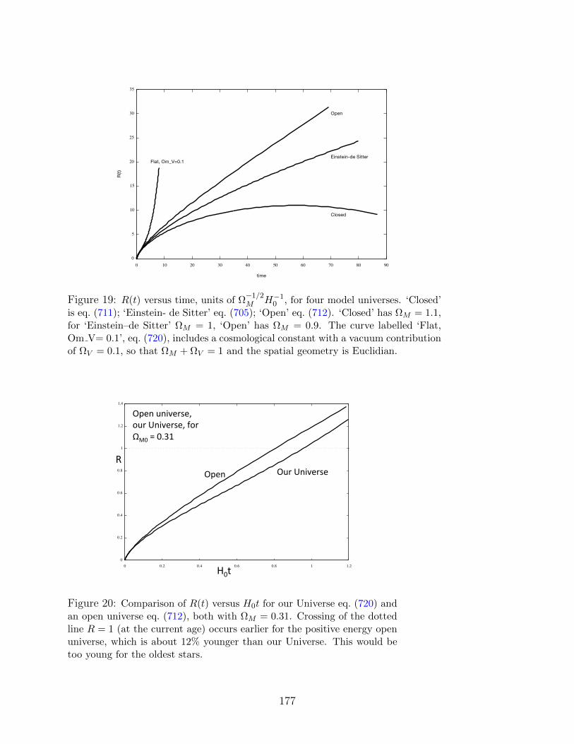
Figure 19: R(t) versus time, units of Ω−1/2M H−1

0 , for four model universes. ‘Closed’is eq. (711); ‘Einstein- de Sitter’ eq. (705); ‘Open’ eq. (712). ‘Closed’ has ΩM = 1.1,for ‘Einstein–de Sitter’ ΩM = 1, ‘Open’ has ΩM = 0.9. The curve labelled ‘Flat,Om V= 0.1’, eq. (720), includes a cosmological constant with a vacuum contributionof ΩV = 0.1, so that ΩM + ΩV = 1 and the spatial geometry is Euclidian.

Open Our Universe R

H0t

Open universe, our Universe, for ΩM0 = 0.31

Figure 20: Comparison of R(t) versus H0t for our Universe eq. (720) andan open universe eq. (712), both with ΩM = 0.31. Crossing of the dottedline R = 1 (at the current age) occurs earlier for the positive energy openuniverse, which is about 12% younger than our Universe. This would betoo young for the oldest stars.

177

SNe

CMB

Figure 21: Parameter plane of ΩV versus ΩM assuming no radiation contribution.Regions of open/closed geometry and currently accelerating/decelerating dynamicsare shown. Also shown are approximate zones of one standard deviation uncertaintiesfor the distant supernova data (SNe) and—you have to squint—for fluctuations inthe cosmic microwave background radiation (CMB), which came a decade later.Note the powerful constraint imposed by the latter: we no longer depend on theSNe data. That the Universe is accelerating is beyond reasonable doubt.

Figure 22: The current age of the Universe H0t0 as a function of ΩM for flat,matter plus vacuum energy models with negligible radiation, equation (722). AsΩM approaches unity, the model recovers the Einstein–de Sitter value H0t0 = 2/3;as ΩM → 0, H0t0 becomes proportional to − ln ΩM (Show!), and we recover the“logarithmic eternity” that was first highlighted by Sir Arthur Eddington.

178

(becoming infinite as t → 0) compared with the constant on the right side. Then, usingργR

4 = constant, the dynamical equation of motion at early times may then be written

R2R2 =8πGργR

4

3= (constant). (723)

This leads to a simple power law time dependence for the scale factor:

R(t) ∝ t1/2 (radiation dominated universe). (724)

Knowing only that R ∼ t1/2, if we now return to the dynamical equation of motion, we maysolve explicitly for ργc

2:

ργc2 =

3c2

8πG

(R2

R2

)=

3c2

32πGt2. (725)

We then have an exact expression for what the total energy density in all relativistic particlesmust be, even if we don’t know how many relativistic species there are. (In practise, we havea good idea of this number from other physics!)

This is a rather neat result. At a time of one second, we know that the Universe had anenergy density of 4×1025 J m−3, and that is that. Moreover, since the total energy density isfixed, the greater the number of relativistic particle populations that were present in the earlyUniverse (e.g., the various neutrino species), the smaller the temperature at a given time.During the epoch when hydrogen was being fused into helium and a few other low atomicnumber nuclei, the production rate of these latter isotopes was sensitive to temperature. (Bycontrast, helium production is not so temperature sensitive, which makes a prediction of itsabundance rather robust.) This temperature sensitivity of the light isotopes, combined withtheir observationally-determined abundances, has been used to limit the number of differenttypes of neutrinos that could have been present during the era of nucleosynthesis.

10.8 Observational foundations of cosmology

10.8.1 The first detection of cosmological redshifts

To me, the name of Vesto Melvin Slipher has always conjured up images of some 1930’s J.Edgar Hoover FBI G-man in a fedora who went after the bad guys. But Vesto was a mild-mannered, careful astronomer. If we allow that Edwin Hubble was the father of modernobservational cosmology, then Slipher deserves the title of grandfather.

In 1912, using a 24-inch reflecting telescope, Slipher was the first person to measure theredshifts of external galaxies. He didn’t know that that was what he had done, becausethe notion of galaxies external to our own was not one that was well-formed at the time.Nebular spectroscopy was hard, tedious work, spreading out the light from the already veryfaint, low surface brightness smudges of spiral nebulae through highly dispersive prisms.Slipher worked at Lowell Observatory, a small, isolated, private outpost in Flagstaff, Arizona.Percival Lowell, Slipher’s boss, was at the time obsessed with mapping what he thought werethe Martian canals!

Slipher toiled away, far removed from the great centres of astronomical activity. By1922, he had accumulated 41 spectra of spiral nebulae, of which 36 showed a shift towardthe red end of the spectrum. But he had no way of organising these data to bring out thelinear scaling of the redshift with distance for a very simple reason: he hadn’t any idea

179

what the distances to the nebulae were. Other observations were at this time showing anapparent trend of greater redshift with fainter nebulae, but the decisive step was takenby Edwin Hubble. With the aid of Milton Humason, Hubble found a linear relationshipbetween galactic distance and redshift (E. Hubble 1929, PNAS, 15, 168.) How did Hubblemanage to determine the distances to the nebulae? Using the new 100-inch telescope on MtWilson, Hubble had earlier resolved individual Cepheid variables stars in the outer arms ofthe Andromeda spiral galaxy, as we shall henceforth refer to it. For in obtaining the distancesto the “nebulae,” Hubble also showed that they must be galaxies in their own right.

Cepheid variable stars were at the time already well-studied in our own galaxy. Cepheidsoscillate in brightness with periods ranging from days to months. What makes them animportant candle for observational astronomers is that they have a well-defined relationshipbetween their oscillation time period and their absolute mean luminosity. To measure adistance, one proceeds as follows. Find a Cepheid variable. Measure its oscillation period.Determine thereby its true luminosity. Measure the star’s flux, which is the energy per unitarea per unit time crossing your detector—this is all that can actually be measured. The fluxis the absolute luminosity L divided by 4πr2, where r is the distance to the star. Therefore,by measuring the flux and inferring L from the oscillation period, one may deduce r, thedistance to the star. Simple—if you just happen to have a superb quality, 100-inch telescopehandy. To such an instrument, only Hubble and a small handful of other astronomers hadaccess24.

10.8.2 The cosmic distance ladder

As observations improved through the 1930’s the linear relation between velocity and dis-tance, which became known as the Hubble Law, v = H0r, became more firmly established.There are two major problems with collecting data in support of the Hubble expansion.

First, galaxies need not be moving with the Hubble expansion (or “Hubble flow”): theirmotions are affected by neighbouring masses. The best known example of this is the An-dromeda galaxy, whose redshift is in fact a blueshift! It is approaching our own Milky WayGalaxy at about 300 km per second. The redshift measurement problem is greatest for anearby galaxy whose “peculiar velocity” (deviation from Hubble flow) is a large fraction ofits Hubble recession velocity. Second, it is very difficult to establish distances to cosmologicalobjects. We can establish distances to relatively nearby objects relatively easily, but thesegalaxies are precisely the ones affected by large peculiar velocities. Those galaxies unaffectedby large peculiar velocities are just the ones whose distances are difficult to establish!

But observational astronomers are resourceful, and they have come up with a number ofingenious techniques which have served them well. The idea is to create a cosmic “distanceladder” (perhaps better described as a linked chain). You start with direct measurementson certain objects, and then use those measurements to calibrate the distances to other,somewhat more distant, objects. Then repeat. Here is how it actually works.

Start with our solar system. These days, we can bounce radar signals off planets andmeasure the time of flight (even testing general relativity in the process, as we have seen)to get extremely accurate distances. Next, we make use of our precise knowledge of theastronomical unit (denoted AU) thus obtained to use the classic technique of trigonometricparallax. The earth’s motion around the sun creates a baseline of about 2 AU, which

24Much later, in 1952, Hubble’s quantitative results were found to be inaccurate. It turns out that Cepheidscome in two quite separate populations, with very different Period-Luminosity relations! This was discoveredby W. Baade, who was then motivated to introduce the concept of distinct stellar populations (differing byages) into astronomy. This also revised the whole extragalactic distance scale, though it kept intact thelinearity of the redshift-distance relation.

180

allows us to have a different perspective on nearby stars as we orbit. We see nearby starsshift in angular position on the sky relative to their much more distant counterparts. Theobserved angular shift is inversely proportional to the distance of the nearer star from thesolar system. We define the unit of distance known as a parsec (pc) as the distance at whicha separation of 1 AU subtends 1 second of arc. We can turn this definition around and saythat the parallax angle, perversely denoted as π in the astronomical literature and measuredin arc seconds, corresponds to a distance to a measured star of 1/π parsecs. (One parsec is' 3.085678...× 1016 m. Because 1 AU is now a defined exact quantity, so is 1 pc.)

The next rung up the ladder is known as spectroscopic parallax. There is no actualparallax angle in this case, it is just an analogous name. The idea is that you first usethe method of direct trigonometric parallax to obtain distances to stars of a given spectraltype. Knowing the distance to a star of a given spectral type and measuring its flux, youalso know the intrinsic luminosity L, since F = L/4πr2 where F is the measured flux andr the measured distance to the star. Now you see a star with precisely the same spectrum,but much fainter and therefore more distant. You cannot measure its parallax, it is toofar away. But the detailed agreement between spectra means this is the same type of staryou’ve already measured, with the same mass and same luminosity. You then measure thenew star’s flux F , and deduce its distance!

Keep going. Distances to Cepheid variables can be calibrated by spectroscopic parallax,and these bright stars have, as we have explained, a well-defined period-luminosity rela-tionship. They are bright enough that they can be seen individually in external galaxies.Measure, thereby, the distances to these external galaxies.

Keep going. In studying the properties of external galaxies, Tully and Fisher showed thatthe rotation velocities of spiral galaxies (measured by the Doppler shifts in the combinedspectra of moving stars) was tightly correlated with the intrinsic luminosity of the galaxy.This is not terribly surprising in itself: the larger the stellar mass of a galaxy the largerthe luminosity, and the larger the binding mass the larger the rotational velocity. Tullyand Fisher crafted this notion into a widely used tool for establishing the distances to verydistant galaxies. Elliptical galaxies, which are supported by the dispersion of stellar velocitiesrather than their systematic rotation were also turned into useful distance indicators. Herethe correlation between luminosity and velocity dispersion is known as the Faber-Jacksonrelation.

The final step in the cosmic distance ladder involves Type Ia supernovae. Type Ia super-novae are thought to occur when a white dwarf in a tight binary system accretes just enoughmatter from its companion to tip itself over the “Chandrasekhar mass.” (This mass is themaximum possible mass a white dwarf can sustain by electron degeneracy pressure, about1.4 times the mass of the sun.) When this mass is exceeded, the white dwarf implodes, over-whelmed by its now unsupportable self-gravitational attraction. In the process, carbon andoxygen nuclei are converted to 56Ni, triggering a thermonuclear explosion that can be seenquite literally across the Universe. What is nice about type Ia supernovae, from an astro-nomical perspective, is that they always occur in a white dwarf of the same mass. Thereforethere is little variation in the absolute intrinsic luminosity of the supernova explosion. Tothe extent that there is some variation, it is reflected not just in the luminosity, but in therise and decay times of the emission, the “light curve.” The slower the decline, the largerthe luminosity. So you can correct for this. This relation has been well calibrated in manygalaxies with well-determined distances.

The Type Ia supernova data were the first to provide compelling evidence that the Uni-verse was expanding. To understand how this was obtained we need to return to our formulafor the flux, F = L/4πr2, and understand how this changes in an expanding, possibly curved,spatial geometry.

181

10.8.3 The parameter q0

Observational astronomers often work with distances where the time it has taken light toreach us, measured from the present, is small compared with the age of the Universe. Thegoal is to measure small changes from conditions at the current epoch, t = t0. Under thesecircumstances, it is mathematically convenient to expand our basic cosmological functionsR(t) and H(t) to leading order in a Taylor series in t−t0. For example, the Hubble parameterR/R may be expanded in time:

H(t) =R

R= H0 + (t− t0)

(R0

R0

−H20

)+ ... (726)

since R2/R2 at the present time t0 is H20 . (Remember t < t0 for observed sources.) This

may also be writtenH(t) = H0 +H2

0 (t0 − t)(1 + q0) (727)

where we have defined the deceleration parameter q0 by

q0 ≡ −R0R0

R20

→ − R0

H20

for R0 = 1. (728)

This is important observational quantity because it embodies the observed evolution of theHubble parameter. Next, use (1 + z)R(t) ≡ 1 and expand R(t) in a similar Taylor seriesaround t0. Then, to leading order in z, we obtain z = H0(t0 − t), and then (727) becomes

H(z) = H0[1 + z(1 + q0)]. (729)

For the classical matter-dominated cosmological models, q0 is defined in such a way that itought be a positive quantity. If q0 < 0, the Universe would be accelerating, a seeminglyoutlandish possibility not taken seriously until after 1998. Consider the integral for thecomoving coordinate of a photon, r =

∫cdt/R(t). With R0 = 1 and t − t0 ≡ δt, carry out

the Taylor expansion in δt of

1 + z =1

R(t)=

1

R(t0 + δt)= 1− δtR0 + (δt)2(R2

0 −R0

2) + ... (730)

To linear order this gives δt = −z/R0 = −z/H0. Using this result in the small quadraticcorrection term in (δt)2 in (730), the next order refinement is

− δt = t0 − t =1

H0

[z −

(1 +

q0

2

)z2]. (731)

Using our expansion for 1/R we find,

l(z) ≡ c

∫ t0

t

dt′

R= c(t0 − t) +

cH0

2(t− t0)2 + ... (732)

and substituting with the help of (731) through order z2:

l(z) =c

H0

[z − z2

2(1 + q0) + ...

](733)

Equation (733) is general for any FRW model. q0 embodies the leading order deviationsfrom a simple Euclidian model in which l(z) ∝ z.

182

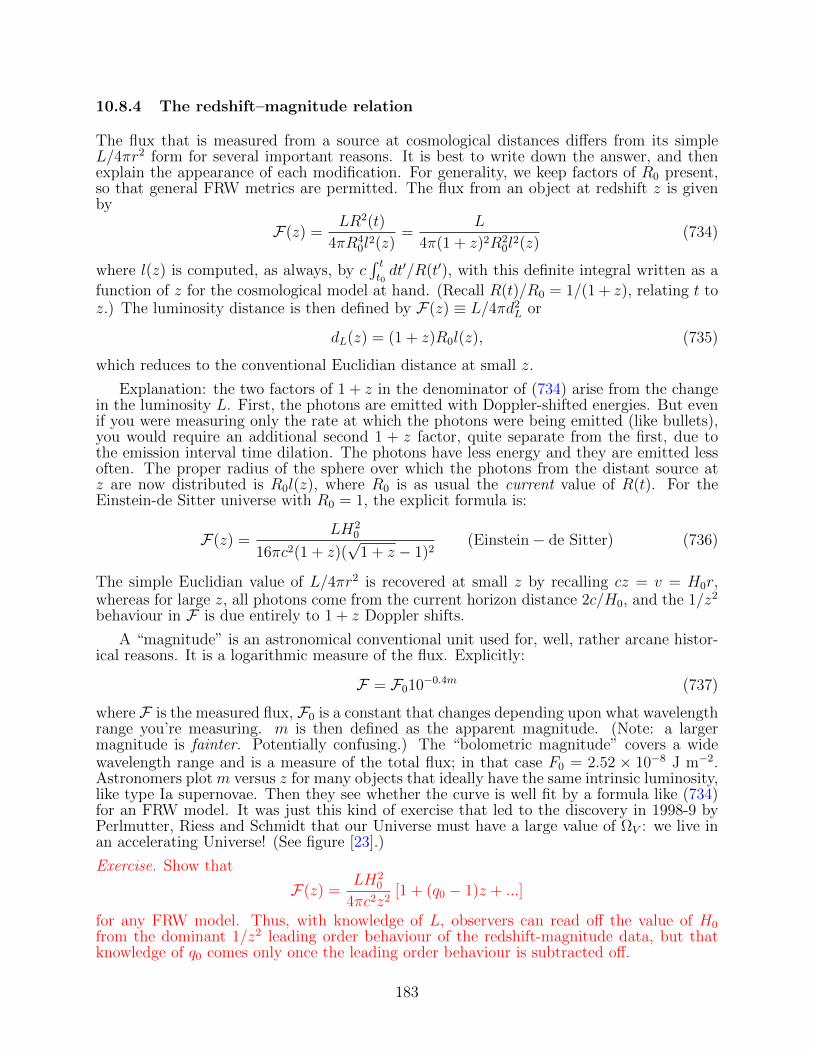
10.8.4 The redshift–magnitude relation

The flux that is measured from a source at cosmological distances differs from its simpleL/4πr2 form for several important reasons. It is best to write down the answer, and thenexplain the appearance of each modification. For generality, we keep factors of R0 present,so that general FRW metrics are permitted. The flux from an object at redshift z is givenby

F(z) =LR2(t)

4πR40l

2(z)=

L

4π(1 + z)2R20l

2(z)(734)

where l(z) is computed, as always, by c∫ tt0dt′/R(t′), with this definite integral written as a

function of z for the cosmological model at hand. (Recall R(t)/R0 = 1/(1 + z), relating t toz.) The luminosity distance is then defined by F(z) ≡ L/4πd2

L or

dL(z) = (1 + z)R0l(z), (735)

which reduces to the conventional Euclidian distance at small z.

Explanation: the two factors of 1 + z in the denominator of (734) arise from the changein the luminosity L. First, the photons are emitted with Doppler-shifted energies. But evenif you were measuring only the rate at which the photons were being emitted (like bullets),you would require an additional second 1 + z factor, quite separate from the first, due tothe emission interval time dilation. The photons have less energy and they are emitted lessoften. The proper radius of the sphere over which the photons from the distant source atz are now distributed is R0l(z), where R0 is as usual the current value of R(t). For theEinstein-de Sitter universe with R0 = 1, the explicit formula is:

F(z) =LH2

0

16πc2(1 + z)(√

1 + z − 1)2(Einstein− de Sitter) (736)

The simple Euclidian value of L/4πr2 is recovered at small z by recalling cz = v = H0r,whereas for large z, all photons come from the current horizon distance 2c/H0, and the 1/z2

behaviour in F is due entirely to 1 + z Doppler shifts.

A “magnitude” is an astronomical conventional unit used for, well, rather arcane histor-ical reasons. It is a logarithmic measure of the flux. Explicitly:

F = F010−0.4m (737)

where F is the measured flux, F0 is a constant that changes depending upon what wavelengthrange you’re measuring. m is then defined as the apparent magnitude. (Note: a largermagnitude is fainter. Potentially confusing.) The “bolometric magnitude” covers a widewavelength range and is a measure of the total flux; in that case F0 = 2.52 × 10−8 J m−2.Astronomers plot m versus z for many objects that ideally have the same intrinsic luminosity,like type Ia supernovae. Then they see whether the curve is well fit by a formula like (734)for an FRW model. It was just this kind of exercise that led to the discovery in 1998-9 byPerlmutter, Riess and Schmidt that our Universe must have a large value of ΩV : we live inan accelerating Universe! (See figure [23].)

Exercise. Show that

F(z) =LH2

0

4πc2z2[1 + (q0 − 1)z + ...]

for any FRW model. Thus, with knowledge of L, observers can read off the value of H0

from the dominant 1/z2 leading order behaviour of the redshift-magnitude data, but thatknowledge of q0 comes only once the leading order behaviour is subtracted off.

183

Figure 23: Evidence for an accelerating Universe from type Ia supernovae. The topfigure shows a redshift-magnitude plot for three different FRW models, ΩM0 = 1,ΩV = 0, an Einstein-de Sitter model, in magenta; ΩM0 = 0.2, ΩV = 0, an openmodel, in black; and ΩM0 = 0.3, ΩV = 0.7 an accelerating model, in blue. Thebottom panel shows the same with the inverse square slope removed. The data aremuch better fit by the accelerating model.

184

With the determination of ΩV , the classical problem of the large scale structure of theUniverse has been solved. There were 6 quantities to be determined:

• The Hubble constant, H0 = R/R at the present epoch.

• The age of the Universe, t0.

• The curvature of the Universe, in essence the integration constant 2E = −c2/a.

• The ratio Ω0 of the current mass density ρ0 to the critical mass density 3H20/8πG.

• The value of the cosmological constant or equivalently, the ratio ΩV of the vacuumenergy density ρV c

2 to the critical energy density.

• The value of the q0 parameter.

Within the context of FRW models, these parameters are not completely independent,but are related by the dynamical equations for R (687) and R2 (699). A quick summary:

• H0 ' 67.6 km s−1 Mpc−1.

• t0 ' 13.8 billion years

• E ' 0

• ΩM0 ' 0.31

• ΩV ' 0.69.

• q0 = Ω0/2− ΩV ' −0.54

Exercise. Derive the last result on this list.

This brief list of values hardly does justice to the century-long effort to describe our Uni-verse with precision. Because astronomers were forced to use galaxies as “standard candles”(the colloquial term for calibrated luminosity sources), their measuring tools were fraughtwith uncertainties that never could be fully compensated for. It was only the combination ofestablishing a truly standard candle via the type Ia supernovae, together with the technicalcapabilities of high receiver sensitivity and automated search techniques that allowed theprogramme (“The Supernova Cosmology Project”) to succeed.

Since the 1998/9 breakthrough, cosmologists have not been idle. The development ofextremely sensitive receivers and sophisticated modelling techniques have turned the remnantmicrowave radiation “noise” from the big bang itself into a vast treasure trove of information.In particular, the nature of the tiny fluctuations that are present in the radiation intensity—more specifically the radiation temperature—allow one to set very tight constraints on thethe large scale parameters of our Universe. Not only are these measurements completelyconsistent with the supernova data, the results of the missions known as WMAP and Planckrender this same data all but obsolete! Figure [21] speaks for itself.

185

10.9 The Cosmic Microwave Background Radiation (CMB)

10.9.1 Overview

The Universe is expanding, and expanding systems cool adiabatically. That means if wefollow history backwards, the compressing Universe becomes hot and dense. We have seenthat the energy density of a radiation scales as 1/R4, whereas the energy density of matter(dominated by its rest mass) scales as 1/R3. The Universe must, at some point in the past,have become radiation dominated. This, we shall see, occurred at a redshift z ∼ 1000.

You should now be thinking of the radiation as actual photons; electrons and positrons(and probably neutrinos as well) are relativistic only at the very earliest times. At redshiftslarger than 1000, not only was radiation dominant, the photons were also “well-coupled” toordinary matter. That means that photons would scatter many times off of electrons duringthe time it took the Universe to ∼ double in size. These collisions kept the radiation in astate of complete thermodynamic equilibrium, the radiation temperature did not differ fromthe matter temperature. In thermodynamic equilibrium, the number density of photons isfixed, given by the Planck function associated with a blackbody spectrum:

n(ν, T ) dν =(8πν2/c3)dν

exp(hν/kTγ)− 1(738)

Recall that if radiation is in thermal equilibrium with matter, there is no choice of how manyphotons there are at a given frequency. Mother Nature determines that precisely. It is worthdwelling on this point. Unlike a gas bag of atoms in thermal equilibrium, whose density canbe whatever we like, a gas bag of photons has its number density completely determinedby its temperature! The spectrum may be directly proportional a Planck function, butif the total number density is not given exactly by (738), the photons are simply not inthermal equilbrium with their surroundings, and their numbers will change as this thermalequilibrium is inevitably approached. So does the unavoidable decline in photon numberdensity with ogoing, universal expansion mean that we lose a thermal equilibrium distributionfor the radiation?

At about the time that the radiation became subdominant relative to matter, the photonsalso lost good coupling with the matter. Thermal equilibrium could then no longer bemaintained via photon-electron collisions or induced exchanges with atoms. Imagine now asituation in which the photons “move along” with the expansion of the Universe, but areotherwise unaffected by interactions. You might guess that while the overall shape of thefrequency spectrum would be maintained, the photon number density would be diluted belowthat of a true blackbody. (Rather like sunlight reaching the earth.) Not so. In fact, thenumber density and effective temperature of the photons together vary in just the right wayto maintain an exact blackbody distribution! The ever decreasing number density is alwaysexactly the correct one for a true thermal Planck spectrum for the concurrently evolving andever-cooling photon temperature.

To see this, start with the spectrum (738) at the time t of last scattering, by whichwe mean the last moment thermal equilibrium was maintained by collisions. We follow agroup of photons with frequency ν and small disperson dν as these photons evolve with theUniverse. Now, it is some much later time t′. The t′ number density n(ν ′, t′, T ′) is diluted byan overall (volume) factor of R3(t)/R3(t′) relative to the original blackbody number densityat the time of last scattering t. In addition, each photon at t′ that we now observe atfrequency ν ′ must have come from a frequency way back at time t given by ν = R′ν ′/R(where R′ ≡ R(t′)), in the original blackbody distribution. Therefore, to determine the latertime t′ spectrum, follow this rule: take the original time-t blackbody distribution, dilute it

186

by R3/R′3, and then replace ν everywhere in the Planck formula by R′ν ′/R. Carrying thisthrough,

n(ν ′, t′)dν ′ =R3

R′3n(ν, t)dν =

R3

R′3(8π/c3)(R′ν ′/R)2d(ν ′R′/R)

exp(hR′ν ′/RkTγ)− 1=

8πν ′2 dν ′/c3

exp(hν ′/kT ′γ)− 1(739)

where T ′γ = TγR/R′, a cooler temperature. The remarkable point is that the distribution

(739) is still a blackbody at time t′, but with a new temperature T ′γ that has cooled inproportion to 1/R with the expansion. The reason this is remarkable is that there is nothingto maintain this thermal equilibrium! In fact, you can see that this scaling result followsmathematically for any number spectrum of the form ν2F (ν/T ) dν, where F is an arbitraryfunction.

Might we just be playing a mathematical game? What if, in the real Universe, otherinteractions scatter photons and change their frequencies in the process? For many years,there were arguments as to whether the actual cosmic radiation spectrum was truly a pre-cise blackbody. Adding to the confusion, there were puzzling observations, largely based onstrikingly un-blackbody spectra obtained from rocket-borne instruments. Now, to signifi-cantly change the radiation spectrum of the entire Universe would take a vast amount ofenergy. From whence would that have come? Theorists tied themselves into knots trying tocome up with explanations. All doubts were finally erased in 1992 when the COBE (COsmicBackground Explorer) satellite was launched. This satellite had (submillimetre) detectorsof unprecedented accuracy, no rocket exhaust, and it was established beyond any questionthat the background radiation was almost a perfect blackbody at Tγ = 2.725K. Figure [24]summarises the data. The error bars are shown at 400 times their actual value, just to bevisible! (The earlier rocket observations had by this time been retracted.)

You may have noticed that I wrote “almost a perfect blackbody.” The photon distributionis in fact not exactly a blackbody for two very interesting reasons. The first is that the earthis not at rest relative to the CMB frame. In fact, the local group of galaxies seems to bemoving at about 630 km s−1 relative to the CMB, a surprisingly large value. This translatesto a measured radiation temperature that is about 2× 10−3K warmer in one direction, andthe same amount cooler in the opposite direction. This induces no change in the overallenergy of the radiation.

The second reason is much deeper in its physics. The objects that comprise our Uni-verse collapsed out of an expanding gaseous background, forming great clusters of galaxiesand ultimately individual galaxies and stars. The seeds to form these structures could nothave appeared recently, after the last scattering event. There simply hasn’t been enoughtime for them to have grown from tiny seeds, collapse, and then form the objects we seethroughout the Universe today. The seeds must already have been present during the erawhen the Universe was radiation-dominated, the same era when matter and radiation werestill interacting strongly with one another. This interaction would have left its imprint, atthe time of last scattering, in the form of temperature fluctuations in the microwave back-ground radiation. Scrunch the matter, you also compress the radiation, and therefor heat itup a bit. Some places are little hotter, others a bit cooler (where there has been dilation).The simplest calculations suggested that the relative temperature fluctuation ∆T/T shouldhave been at least ∼ 10−3, in order for these initially tiny compressions to be able to formnonlinear structures by the current epoch.

COBE found the temperature fluctuations (figure [25]). But when COBE (and latersatellites in yet greater detail) did find them, they were an order of magnitude smaller thanexpected. So how does structure form in the Universe? The consensus answer is that there ismore matter in the Universe than the usual atomic nuclei and electrons that we know about.The Universe is also pervaded by what is known as “dark matter,” which turns out to be

187

Figure 24: COBE satellite data showing a perfect fit to a blackbody at 2.725 K. Tobe visible, the error bars are shown at 400 times their actual value! When shownat an American Astronomical Society Meeting, this plot triggered a spontaneousstanding ovation. Units of ν are cm−1, i.e., the wavelength in cm is the reciprocalof the number on the x axis.

most of the so-called ordinary matter, and apparently leaves only a gravitational imprint onthe microwave background. Dark Matter feels the force of gravity, and so far as in known,nothing else,. It had been postulated long before COBE as something that was needed tohold galaxies together. (Were visible light truly representative of the bulk of the matter,internal stellar motions in galaxies would be far too large to be keep the stars gravitationallybound.) COBE offered another compelling reason to believe in Dark Matter.

The directors of the COBE project, John Mather and George Smoot, won the 2006 NobelPrize in Physics for their work.

10.9.2 An observable cosmic radiation background: the Gamow argument

The idea that the Universe had a residual radiation field left over from its formation, andthat this radiation is potentially observable, seems to have originated with George Gamowin the 1940s. Gamow was a theoretical physicist with a brilliant common sense instinct thatallowed him to make contributions to a wide variety of important problems, from the theoryof radioactivity to how DNA coding works. He spent many years developing, and makingrespectable, what has become known as the Big Bang theory25.

Gamow drew attention to the fact that helium, with about 25% of the mass of the ob-servable Universe, is neither an overwhelming nor a tiny constituent. Gamow was convinced,we now know correctly, that helium was made during a brief interval of nucleosynthesis inthe early Universe. (Gamow thought all the other elements were made this way as well, butthat bit turns out to be false. Heavier elements are made over the course of stellar evolution,

25The name was coined by Fred Hoyle, a rival cosmologist who meant the description to be a disparagingmoniker. But proponents of the theory loved the name and adopted it as their own.

188

Figure 25: COBE temperature fluctuations. Top: Temperature dipole variationdominated by motion of the galaxy. Middle: Residual with kinematic dipole sub-tracted off. Bottom: Further residual with galactic foreground subtracted off. Theserepresent primordial fluctuations in the CMB.

and also possibly in neutron star mergers as well.) The 25% number implies that at the timeof nucleosynthesis, the expansion rate of the Universe and the nuclear reaction rate couldnot have been very different. Too rapid an expansion, there is no helium made. Too slowan expansion rate, all the protons get fused into helium, and there is no hydrogen left over.The delicate balance turns out to be a remarkably tight constraint, leading to a predictionthat there should today be an observable residual radiation field of about 10 K. Let’s seehow it works.

At some point early in its history, the Universe’s temperature passes downward throughthe range of ∼ 109 K. When that happens, neutrons n and protons p can begin to combineto form Deuterium (a proton p plus a neutron n ) nuclei. The reaction is pretty simple:

n+ p→ D + γ

where γ is a gamma ray. Helium synthesis follows rapidly thereafter. Gamow assumedequal numbers of protons, neutrons and electrons. As we have emphasised, in order to geta 25% yield of helium, the reaction rate and the age of the Universe (which is of orderthe expansion time to double in size) should be comparable. Denote the cross section forDeuterium formation to be σ (units of area). Then, the reaction rate per proton due toan incoming flux nv of neutrons is nvσ (units of pure number per time). At the time ofnucleosynthesis t, roughly speaking, about one reaction per proton should have occurred.This is because of the order unity mass fraction of helium that is now observed. This is theheart of the Gamow argument:

nvσt ∼ 1, (740)

where t is the age of the Universe at the time of nucleosynthesis. How simple!

189

The product σv is just a laboratory number nearly independent of v (because the crosssection σ depends inversely on v), and, as Gamow knew from nuclear physics experiments, isequal to about 4.6×10−26 m3 s−1. As for the time t, we are interested in the epoch when thetemperature Tγ ∼ 109K. Using equation (725) for the density of relativistic particles, andfollowing Gamow by assuming (not quite correctly, but let it go) that this was all radiationwith energy density aγT

4γ (aγ is the standard blackbody radiation constant), the time of

interest t is

t =c

T 2γ

(3

32πGa

)1/2

(741)

which amounts to 230 s for Tγ = 109K. This gives n very close to 1023 m−3. Next, Gamowestimated a present day average particle density of about 0.1 per cubic meter based onastronomical estimates and observations, so that the Universe had expanded by a factor of108 in the scale factor R. (Recall that the factor 108 reduces n by 1024.) But an expansionof a factor of 108 in R means that the current Tγ should be near 109/108 = 10 K! Themillimeter wave detectors that would have been required for this wavelength of observationwere just at the leading edge of technology in the late 1940s, a by-product of the developmentof radar during the Second World War (which was instrumental to winning the Battle ofBritain). Gamow could have, but did not, pursue this result aggressively, and the predictionwas gradually forgotten. Thus, the CMB might have been detected in the late 1940s, as partof the great postwar flowering of physics. But it wasn’t.

The argument would be put slightly differently now, but in essence it is correct, a brilliantpiece of intuitive reasoning.

Exercise. Repeat the Gamow argument with modern cosmological numbers. Keep Tγ = 109Kand the σv value, but note that relativistic species present at the time include not onlyphotons but three types of neutrinos and three types of antineutrinos, each neutrino-antineutrino combination contributing (7/8)aγT

4γ to the background energy density. We can

neglect e+ and e− pairs in our relativistic fermion population. Why? The 7/8 factor arisesbecause the neutrinos obey Fermi statistics. Recall from your statistical physics that theoccupation number for a state with momentum p is

n± =1

exp(pc/kT )± 1

where the + sign is for bosons (e.g. photons) and the − sign for fermions (e.g. neutrinos).The density of states (per unit volume) is the same for both types of particles: 4πp2dp/h3,where h is the Planck’s constant. The energy is the same for each type of particle, pc.Therefore, the difference in the total energy densities of a population of bosons or fermionscomes down to the difference in two simple integrals:∫ ∞

0

x3 dx

ex + 1=

7

8

∫ ∞0

x3 dx

ex − 1

Can you prove this mathematically without doing either integral explicitly? (Hint: considerthe difference

1

ex − 1− 1

ex + 1,

and integrate x3 times the residual.) Note that for each neutrino specie the factor is actually7/16, because only one spin helicity is present, as opposed to two spin states for photons.But then the neutrinos get back up to 7/8 with their antiparticle cousins...which the photons

190

lack! You may take the current density in ordinary baryons to be 5% of the critical density3H2

0/8πG.

Almost 20 years later, in 1965, the problem of determining the current Tγ attracted theattention of an impressive team of physicists at Princeton University. They rediscovered forthemselves the Gamow argument. The senior investigator, Robert Dicke, a very talentedphysicist (both theoretical and experimental), realised that there was likely to be a measur-able background radiation field that survived to the present day. Moreover, it could be easilydetected by an instrument, the Dicke radiometer, that he himself had invented twenty yearsbefore! (A Dicke radiometer is a device that switches its view 100 times per second, lookingbetween the sky source and a carefully calibrated thermal heat bath of liquid helium. Thisimprints a 100Hz Fourier component on the desired signal, and thereby reduces nuisancevariability occurring on longer time scales.)

The A-Team assembled: Dicke, the scientific leader; J. Peebles, the brilliant young the-orist who would become the world’s leading cosmologist in the decades ahead, and P. Rolland D. Wilkinson, superb instrument builders who designed and built the contemporaryDicke radiometer. The were all set up to do the observation from the roof of their Princetonoffice building(!), when a phone call came from nearby Bell Telephone Laboratories. Tworadio engineers named Arno Penzias and Robert Wilson had found a weird extraneous signalin their own detector! Their device was designed to receive long range signals relayed bysome of the first commercial television satellites. (The Telstar series.) Naturally, they weretrying to chase down all possible sources of background confusion. The “effective radiationtemperature” of the nuisance diffuse signal was about 3 K. Penzias and Wilson had no ideawhat to make of it, but they were advised by a colleague to give the Dicke team at Princetona call. Those guys are very clever you know, they might just be able to help.

The 1978 Nobel Prize in Physics went to Penzias and Wilson for the discovery of thecosmic microwave background radiation. In 2019, Jim Peebles received his own Nobel forhis many contributions to modern comology.

10.9.3 The cosmic microwave background (CMB): subsequent developments

The initial observations of the CMB were at one wavelength: 7 cm. Needless to say, a singlepoint does not establish an entire spectrum! The task of establishing the broader spectrumwas fraught with difficulties, however, with many disputed and ultimately withdrawn claimsof large deviations from a blackbody, as we have noted. Recall that in 1992, matters werefinally lain to rest when the COBE satellite returned its dramatically undramatic findingthat the CMB is, very nearly, but not exactly, a blackbody. There are small fluctuations inthe temperature, the largest of which amount to a few parts in 104. This value is smallerthan first expected, but ultimately of the order needed to account for the nonlinear structurein the Universe that we see today, provided that there is a healthy component of dark matterthat does not react with the radiation. This unseen, and perhaps unseeable, dark mattercomponent had been invoked, long before the COBE results, for a very different reason: toaccount for the large stellar velocities measured in galaxies and within clusters of galaxies.These velocities are unsustainable unless most of the gravitating mass of the galaxy or clusteris in the form of dark, non-light-emitting matter. The COBE results are yet further evidencefor the presence of dark matter in the Universe.

Following COBE, the next important CMB probe was the Wilkinson Microwave AnisotropyProbe, or WMAP. This is named for David Wilkinson, the same Princeton researcher whohad been instrumental in the earliest CMB studies. With the launch of WMAP in 2003,cosmology truly became a precision science. WMAP revealed the structure of the tempera-ture fluctuations in such exquisitely fine angular resolution on the sky, it became possible todetermine all the key physical parameters of the Universe: H0, ΩM0, ΩV , t0 and many others,

191

WMAP%

Planck%

Figure 26: WMAP (top) and Planck (bottom) temperature fluctuations, with dif-ferent colour scales. Think of these as the Universe’s baby pictures. Note the muchhigher angular resolution compared with COBE; Planck is another factor of 3 betterthan WMAP. The angular information encoded on these small scales is valuable asa means of tightly constraining cosmological parameters.

to an excellent level of accuracy. WMAP was followed by the Planck satellite, launched in2009, which provided a further shrinking of the error bars, higher angular resolution coverageof the CMB on the sky, broader frequency coverage (very important for subtracting off theeffects of the Milky Way Galaxy), and better constraints on null results (absence of CMBpolarisation, for example). But somewhat disappointingly, there were no qualitatively newphysical findings. The current story remains essentially the one revealed by WMAP (figure[26]).

Think of the evolution of the maps and globes of the Earth, from ancient to moderntimes. Gross inaccuracies in basic geometry gradually evolved to Googlemap standard overa period of thousands of years. Contrast this with the observation that, well within theprofessional careers of currently active researchers, serious models of the Universe went fromfundamental misconceptions to three-significant-figure accuracy in structural parameters.By any measure, this is one of the great scientific achievements of our time. As with anygreat scientific advance, its full meaning and implications will take many years to elucidate.

10.10 Thermal history of the Universe

10.10.1 Prologue

The recorded history of civilisation began when Sumerian merchants inscribed their graininventories on clay tablets. (BTW, the concept of a “grain inventory” would not have beenpossible without the invention of large scale agriculture, which would not have been possible

192

without the invention of astronomy. Stick with this for a moment: despite what you’rethinking, I am on-message...) Etched in the matrix of clay, these markings were frozen intime because the clay, once dried, remained unaltered and intact. It turns out that theUniverse has its own gigantic clay tablet, which allowed inscriptions first to be imprinted,then to be preserved, pretty much unaltered for 13.8 billion years. We know these inscriptionsas temperature fluctuations, and the clay tablet is the cosmic microwave background.

The temperature fluctuations trace the initial density fluctuations, which are coupled tothe radiation by electron-photon scattering, also known as Thompson scattering. While thisscattering remained vigorous, the CMB dutifully recorded and re-recorded the ever evolvingchanges in the density. Then, matter and radiation suddenly became decoupled. The patternimprinted on the CMB abruptly stopped being recorded. The CMB instead retained only thevery last pattern that happened to be imprinted upon it, at the time of the “last scattering.”It is this pattern that we receive, redshifted by the enormous subsequent expansion of theUniverse, in our detectors today. Think of this either as an ancient inscription passed onthrough the aeons, or more congenially as the Universe’s baby picture.

Exercise. Let σT be the Thompson cross section for a photon to collide with an electron,a constant number equal to 6.7 × 10−29 m2. When an electron has moved relative to thephoton gas a distance l such that the swept-out volume lσT captures a single photon, l issaid to be one mean free path (mfp): the average distance between scatterings.

Justify this definition, and show that the scattering rate per electron is nγcσT = c/l. (Whatis nγ here?) In a radiation-dominated Universe, show that the ratio of the photon scattering

mfp to the horizon size grows like√t, and that the mfp relative to the scale factor R grows

like t. (t as usual is time.)

Exactly how to decipher the ancient CMB inscriptions and turn them into a model of theUniverse is a very complicated business. While it is a local Oxford Astrophysics speciality, itis one that we will be able to treat only very superficially in this course. We shall go aboutthis in two stages. In the first, we will describe what I will call the “classical theory” of thethermal history of the Universe: how matter and radiation behaved in each other’s presencefrom temperatures of 1012 K through 3000K, the time when hydrogen ions recombine withelectrons to form neutral H atoms. In the second stage, in Chapter 11, which the reader mayregard as optional “off-syllabus” material, we will discuss a more modern theory of the veryearly Universe. This puts a premium on the notion of inflation, a period in the history ofthe Universe in which it seems to have undergone a very rapid (exponential!) growth phase.First put forth in 1980, this idea has been the single most important theoretical advance inmodern cosmology in recent decades. There are very good theoretical reasons for invokingthe process of inflation, even if the mechanism is not well-understood (not an unusual stateof affairs in science), and there is by now compelling observational support for it. To mymind, one of the best arguments for inflation is that we have in fact entered another, albeitfar more mild, inflationary stage of the Universe’s history.

In what follows, the reader should bear in mind the characteristic physical quantities onwhat is known as the “Planck scale.” These are the scales set by the three fundamentaldimensional constants of physics: Newton’s G, Planck’s h, and the speed of light c. Thereare unique dimensional combinations to form a mass mP , a length lP and a time tP fromthese constants:

mP =

(hc

G

)1/2

= 5.456× 10−8 kg (742)

lP =

(hG

c3

)1/2

= 4.051× 10−35 m (743)

193

tP = lP/c =

(hG

c5

)1/2

= 1.351× 10−43 s (744)

With these three quantities, we can form any other dimensional quantity we like. Theseare, in some sense, the limits of our knowledge, for it is on these scales that we may expectquantum gravity effects to be important, a theory of which we remain quite ignorant. Wecannot expect to have anything like a classical picture of the early Universe for time t < tP ,or for horizon scales c/H < lP . The Planck mass may not, at first glance, appear remarkable,but remember the natural comparison is with elementary particle masses. An electron, forexample, is close to 5×10−4 GeV in rest energy; the Planck mass energy is mP c

2 = 3.06×1019

GeV. By these Planckian standards, we will always be working with very low mass particles,very large distances, and very long times.

10.10.2 Classical cosmology: helium nucleosynthesis

Let us begin the story when the temperature of the Universe is just under 1012K. This isvery early on, only about 10−4s after the big bang. At this stage, the Universe consists of arelativistic cocktail of photons, neutrinos and their antiparticles, muons and their antipar-ticles and electrons and their antiparticles (positrons). This cocktail is well-mixed (shaken,not stirred). Even the neutrinos are in complete thermal equilibrium, freely created anddestroyed.26 There is also a population of protons and neutrons, which are energeticallyunimportant at these temperatures. But keep track of them in the inventory! They aregoing to make the Universe we know as home.

Once the temperature slips below 1012 K, the muons and antimuons can annihilate,but there isn’t enough energy for muon production from the other relativistic populationspresent. The energy from the photons and e+e− pairs produced in the annihilation is sharedout amongst all the other populations. Everyone is heated and takes part, including, atthese ultra high densities, the normally elusive neutrinos.

The Universe continues to expand, the temperature falls. To understand the next im-portant phase, recall that neutrons and protons do not have quite the same mass. Moreprecisely, with mp the proton mass and mn the neutron mass,

∆mc2 ≡ (mn −mp)c2 = 1.293 MeV = 2.072× 10−13 J. (745)

This is very small compared with either mnc2 or mpc

2. Except when we are specificallyconcerned with the mass difference or doing very accurate calculations, there is normally noneed to distinguish mn for mp. Textbooks on statistical mechanics tells us that the ratio ofthe probabilities for finding a system in some state i or j depends only on the energies Eiand Ej of these states, and nothing else. In particular, the ratio of the probability of findingthe system in i to the probability of finding it in j is given by the Boltzmann equation:

PiPj

=gigj

exp

[−(Ei − EjkT

)](746)

where the g’s are known as the statistical weights, a fancy name for how many distinct statesthere are with energy Ei or Ej. (If you’ve forgotten this, don’t have a statistical mechanicstextbook handy, and you are curious, see the Exercise below for a quick justification.) Below1011K, the so-called Boltzmann factor exp(−∆mc2/kT ) starts to differ noticeably from unity,and as we approach 1010 it becomes rather small. Since neutrons are more massive than

26By using the word “freely,” we ignore the particle rest masses.

194

protons, the former become more scarce at cooler temperatures. The critical temperaturecorresponding to kT = ∆mc2 is 1.5 × 1010K. (By way of comparison, for electrons andpositrons, mec

2/k = 5.9× 109K.)

Exercise. Let the probability of finding a system in state i be f(Ei), where Ei is the energyof the state. The ratio of the probability of finding the system in state i versus j is thenf(Ei)/f(Ej). But this ratio must be a function only of the difference of the energies, becausea constant additive constant in energy can’t affect the physics! The potential energy is alwaysdefined only up to such a constant. Hence, with F an arbitrary function,

f(Ei)

f(Ej)= F (Ei − Ej).

If Ei = Ej + δ, show that if this equation is to hold even to first order in δ, that

f(E) ∝ exp(−βE)

where β is an as yet undetermined constant. We can determine β by physics, e.g. bydemanding that the ideal gas equation of state be satisfied, pressure P equals nkT , wheren is the number density and k is the Boltzmann constant and T the temperature. Then itfollows (show!) β = 1/kT .

The reactions that determine the neutron n proton p balance are (ν means “antineu-trino”):

n+ ν ↔ p+ e

n+ e+ ↔ p+ ν

n↔ p+ e+ ν

The reaction rates for the two body processes are about 0.1 per second per nucleon atT = 1010K. However, this rate drops rapidly as the thermometer falls. Below 1010K, thereactions can’t keep up with the expansion rate of the Universe, they simply don’t take placefast enough. Once this occurs, whatever the ratio of n/p happens to be, it remains “frozen”with time, since the Universe is too cold to keep the reactions cooking! At T = 1010K, theUniverse is about 1 s old. The n/p ratio at this temperature is exp(−∆mc2/kT ) ' 0.2, andit remains stuck at this value, frozen in.

Exercise. Show that the early Universe “temperature clock” is given conveniently by

t ' 1/T 210,

where t is the time in seconds and T10 the temperature in 1010K. Assume a Universe ofphotons, electrons and positrons, and three neutrinos and anti-neutrinos.

This figure of 20% is interesting, because it is neither close to unity nor tiny (a coincidencerelated to the 25% helium mass fraction!). Without further production of neutrons, they willdecay in minutes by the third reaction channel. If all the neutrons had decayed into protonsand electrons and antineutrinos, there would have been no cosmological nucleosynthesis.But just as the neutrons start to decay as we approach 109K, the remaining neutrons aresalvaged by being safely packed into stable 4He nuclei. Helium nuclei are environmentallysound, perfectly safe, radioactive containment vehicles. Here neutron decay is absolutelyforbidden, in essence because the statistical phase space within the realm of the nuclearpotential is degenerate. “Degenerate” means that when the neutrons are confined to thenuclear potential, there are no available states for them to decay into. They are already

195

occupied by protons. It is rather like trying to use Oxford public transportation on a veryrainy day: SORRY, BUS FULL.

Back to our story. The neutrons are scarfed up into He nuclei. This offers a firm predictionfor the observed mass fraction of the Universe, since later stellar nucleosynthesis does notchange the helium number significantly. (By sharp contrast, almost all of the heavier elementabundances, collectively not much more than one percent of the total, are indeed dominatedby stellar nucleosynthesis.) From what we have just seen, we may estimate the mass fractionin helium to be

4mp × (n/2)

mp(n+ p)=

2

1 + p/n' 0.33. (747)

Much more detailed, time-dependent calculations (pioneered by Peebles in 1965) give anumber close to 0.27 (a slight refinement of the 25% figure mentioned above), but the essentialphysics is captured by our simple estimate. There is not very much wiggle room here. Wecannot use the precise value of this abundance to determine retrospectively what sort ofUniverse (open, closed, critical) we live in. The curse and strength of the calculation is thatthe results are essentially the same for any FRW model. The Big Bang Theory predictssomething close to 27% of the mass of the Universe is in the form of helium, and that isthat. Happily, this turns out to be very close to what observations reveal.

10.10.3 Neutrino and photon temperatures

This subsection is non-examinable.

As the temperature slides from 5×109 K to below 109, the electron positron pairs annihilateinto photons,

e+e− → 2γ

The falling temperature means that the photons cannot maintain an equilibrium populationof these e+e− pairs. In other words, there is a conversion of electrons and positrons intophotons. However, it is not possible to just add photons and keep the temperature thesame. In thermal equilibrium, the number of photons at a given temperature is fixed. Ifyou add more via e+e− annihilation, the extra photons force a new thermal equilibrium,one at a higher temperature that is compatible with the increased photon number. Thephotons are, in effect, heated. By contrast, the relativistic neutrinos that are also presentjust march blithely along, enjoying the expansion of the Universe without a care, obliviousto everything. (When it was the muons that annihilated, the Universe was so dense thateven the neutrinos took part in the thermal collisions, but not this time!) This means thatpresent day background neutrinos are cooler than the CMB photons. The question is, byhow much?

This turns out to be a relatively simple problem, because if we fix our attention on acomoving volume of the Universe, the entropy in this volume is conserved by the conversionof electron-positron pairs into photons. For photons or relativistic electrons/positrons, theentropy per unit volume is a function only of the temperature. It is most easily calculatedfrom a standard thermodynamic identity,

E + PV − TS +µN = 0,

for a gas with zero chemical potential µ. The latter is true of a relativistic gas that freelycreates and annihilates its own particles. So for the entropy per unit volume s,

s ≡ S

V=

E

V T+P

T(748)

196

With ρc2 denoting the energy per unit volume and P = ρc2/3 for a relativistic gas,

s =4ρc2

3T(749)

With a relativistic energy density always proportional to T 4, the entropy per unit volumeis proportional to T 3, and the entropy in a comoving volume R3 is proportional to (TR)3.It is conserved with the expansion, in essence because the entropy and particle number areproportional to one another, and particle number is conserved.

Before the e+e− annihilation, the entropy in volumeR3 in photons, electrons and positronsis

sR3 =4aγ(TR)3

3

(1 + 2× 7

8

)=

11aγ(TR)3before

3(750)

Afterwards, and after the reestablishment of thermal equilibrium, it is all photons:

sR3 =4aγ(TR)3

after

3(751)

Since the number of photons produced is equal to the number of relativistic electrons andpositrons that annihilated, this process conserves entropy, sR3. It is reversible: one couldrecompress the adiabatic expansion backwards to produce anew the pairs. In other words,

4(TR)3after

3=

11(TR)3before

3(752)

Now for an interesting point of physics. Recall that the muon-antimuon annihilation heatedall relativistic populations, because the reaction rates demand this at these earlier times,when the Universe was so very dense. But the e+e− annihilation we are now consideringignores the neutrinos. This is because the density has now fallen to a level at which theneutrinos pass through everything, so that their TR value does not increase during the e+e−

annihilation. This process must therefore produce different cosmic background photon andneutrino temperatures. The ratio of neutrino temperature Tν to photon temperature Tγ nowfollows from:

Tν (after) = Tν (before) = Tγ (before) =

(4

11

)1/3

Tγ (after) = 0.7138 Tγ (after). (753)

This would correspond to a current value of Tν = 1.95 K — if the neutrinos remained a µ = 0relativistic population for all time. (We now know they do not—at least not quite.) At onetime, people wondered whether there was any possible way to measure this temperaturedifference. But a temperature of 1.95K corresponds to an energy kT of 1.7 × 10−4 eV,whereas the average mass per neutrino species (the best we can measure at the currenttime) is about 0.1 eV, with a corresponding temperature of 1160 K. Neutrinos thus became“cold” at a redshift of z ∼ 400. As we shall see, this is well after hydrogen recombined, butprobably before galaxies formed. These neutrinos are a part, but only a very small part, ofthe dark matter in galaxies. Even if it had turned out that neutrinos had zero rest mass, itwould have been impossible with present technology to measure a 2K neutrino background!Nevertheless, the physics of this problem is enlightening, and the formal difference in neutrinoand photon temperatures surprising.

197

10.10.4 Ionisation of hydrogen

Between the time of helium synthesis, a few minutes into the baby Universe’s life, and afew hundred thousand years, almost nothing happens. Radiation remains the dominantsource of energy and pressure, and the Universe simply expands with R scaling like t1/2.The matter and the radiation remain tightly coupled, so that density fluctuations in thematter correspond also to energy fluctuations in the radiation. But finally at some point,the Universe cools enough that hydrogen recombines and the matter ceases to be an ionisedplasma, becoming a neutral gas. At what temperature does this occur? To answer thisquestion, we need to use an interesting sort of variation of the Boltzmann equation, knownas the Saha equation. It tells us the ionisation fraction of an atomic element as a functionof T .

Recall the Boltzmann equation. The probability Pi for an atom to be in state i relativeto the probability Pj to be in state j is

PiPj

=gigj

exp

(−Ei − Ej

kT

)(754)

where Ei, Ej are the energies of the states, and gi, gj are the statistical weights (i.e. thenumber of states at each level). For simplicity, we will consider a gas of pure hydrogen, andinterpret this equation as follows. State j is the ground state of hydrogen with one electron,the 1s state. Let’s set j equal to 0 so we think of neutrality. State i is then the ionised statewith a bare proton and a free electron with kinetic energy between E and E + dE. Set iequal to 1. Whether bound or free, the electron has two spin states available to it, so thisfactor of 2 appears in both numerator and denominator, cancelling in the process. Theng0 is unity. We think of g1 as the number of states available to the electron with energyin the range dE. Do you remember how to do this odd-sounding calculation? In terms ofmomentum p (a scalar magnitude here), the number of states per electron around a shell ofthickness dp in momentum space is

4πp2

neh3dp

where the factor 1/ne represents the volume per electron and h is Planck’s constant. Thisis derived in any standard text on statistical mechanics, but if this is not familiar, now isa good time to have a look at Blundell and Blundell, Concepts of Thermal Physics. Theconcept comes from the stratagem of putting the electrons in big cube of volume V , countingthe eigenstates (now discrete because of the box walls) for each electron, and then noticingthat the artificial box appears in the calculation only as a volume per electron, which isjust 1/ne. Drawing these threads together, (754) becomes, upon adding up all possible freeelectron states,

nenpn0

= exp

(− Φ

kT

)4π

h3

∫ ∞0

p2 e−p2/2mekT dp (755)

where Φ is the ionisation potential of hydrogen, me the electron mass, np the proton densityand n0 the neutral hydrogen density. Note that we have replaced the ratio of relativeprobabilities of the ionised H state (or p) to the neutral H state (subscript 0) by theirnumber densities np and n0. Now∫ ∞

0

p2 e−p2/2mekT dp = (2mekT )3/2

∫ ∞0

x2e−x2

dx = (2mekT )3/2 × π1/2

4(756)

The Saha equation becomes

nenpn0

=

(2πmekT

h2

)3/2

exp

(− Φ

kT

)(757)

198

The final step is to note that for pure hydrogen, ne = np and thus ne + n0 is the totalhydrogen density nH . This remains unchanged regardless of the ionisation state: if ne goesup by 1, n0 has gone down by 1. With x = ne/nH , our equation therefore becomes

x2

1− x =1

nH

(2πmekT

h2

)3/2

exp

(− Φ

kT

)=

(2.415× 1021T 3/2

nH

)exp

(−1.578× 105

T

)(758)

in SI units. The value x = 0.5 is attained at a redshift of about 1400, a temperature of 3800K. (This is naturally close to the formal decoupling redshift, z ' 1100.) This is remarkable,because it is much less than the formal Boltzmann ionisation temperature of 1.58×105K. Atredshifts much less than 1400, the Universe becomes transparent to photons, and the energydensity is already dominated by matter. Interestingly, the intergalactic medium seems tohave been reionised shortly after galaxies were able to form at z ∼ 10, presumably by theradiation produced by the accretion process that gave rise to these galaxies. Alas, to pursuethis active area of current astrophysical research would take us too far afield at this point.

199

“Curiouser and curiouser!” cried Alice

...“now I’m opening out like the largest

telescope that ever was!”

— Alice’s Adventures in Wonderland,

by L. Carroll

11 Supplemental Topics

This chapter contains additional material on several advanced topics in general relativity.It is off-syllabus and non-examinable. I hope you will pick and choose material that is ofinterest you. This is work in preparation, and your critical comments are welcome.

11.1 The Oppenheimer-Snyder problem

In section (6.9), we presented a calculation of the redshift coming from the surface of acollapsing spherical dust cloud, en route to forming a black hole, as measured by a distantobserver. The collapse problem is a more comprehensive investigation carried out by Op-penheimer and Snyder in 1939, which included an explicit solution for the global form ofthe metric, both interior and exterior to the dust cloud. This calculation relies on conceptsdeveloped for cosmology, as well as for Schwarzschild black holes.

Consider a self-gravitating sphere whose surface is at radial coordinate a at time t = 0.The sphere encloses a uniform energy density ρ(t)c2, and is subject only to its own internalgravitational forces. In particular, there is no pressure: this is a cloud of noninteractingdust particles. The metric describing the interior of such a dust sphere is easy to writedown, by application of Birkhoff’s theorem. The trick is to imagine adding an infinite,spherically symmetric dust envelope exterior to our collapsing dust sphere. This envelopecontracts uniformly and continuously with the interior sphere, and does not affect the sphere’sinternal dynamics. There is, in effect, no gravitational field inside the interior sphere due tothe exterior envelope. But the metric for this combined extended mass distribution is clearlyjust a standard FRW cosmology, which we write in the following form:

− c2dτ 2 = −c2dt2 +R2(t)

(dr2

1−Kr2/c2+ r2dθ2 + r2 sin2 θdφ2

)(759)

where K > 0 is a constant, with units of (time)−2. This metric must be the interior solutionfor the dust sphere in isolation as well. Recall that r and t are comoving coordinates in(759), and R is a dimensionless scale factor.

The equation for the rate of change of the scale factor R is the usual dynamical equationof cosmology:

R2 − 8πGρR2

3= −K (760)

We choose the origin of time t = 0 to coincide with the start of the collapse, when thesphere’s surface has radial coordinate a. (Note: this is not the same as the proper radius.

200

Why not?) With R(0) = 1, R(0) = 0, this fixes the constant K:

K =8πGρ(0)

3=

2GM

a3=c2RS

a3≡ ε

c2

a2, (761)

where we have defined ε = RS/a and

Mc2 ≡ 4πρ(0)c2a3

3(762)

is the (conserved) total energy of the sphere. The Schwarzschild radius RS is defined usingthis value of M . ε is a small quantity for an initial Newtonian-scale cloud radius a largecompared to RS, but in what follows we shall not assume this, except when explicitly noted.Using ρ(t)R3 = ρ(0), equation (760) becomes

R2 = K(R−1 − 1) = ε(c2/a2)(R−1 − 1) (763)

with R < 0.

Exterior to the dust sphere, Birkhoff’s theorem once again comes into play. Since thetotal mass of this spherical distribution is not changing with time, the only possible radialmetric is the static Schwarzschild solution:

− c2dτ 2 = −c2dt2(1− 2GM/rc2

)+(1− 2GM/rc2

)−1dr2 + r2dθ2 + r2 sin2 θdφ2 (764)

We use the notation t, r, etc. to distinguish these fixed coordinates, which go over to standardspherical Minkowski coordinates at large distances from the sphere, from the comoving t, rcoordinates of (759). The problem now is to find a single set of coordinates for both theinterior and exterior of the sphere, valid at all times. We shall do this by expressing theinterior sphere metric (759) in terms of the exterior coordinates of (764).

The metric at the surface of the sphere follows from continuity arguments: it must havethe form of a standard Schwarzschild metric at the time the instantaneous radius of thesphere, aR(t) passes through a given fixed radial coordinate r. Writing the metric in termsof ε, we have:

− c2dτ 2 = −c2dt2 (1− ε/R) +dr2

1− ε/R + r2dθ2 + r2 sin2 θdφ2 (surface metric) (765)

At the surface of the sphere, the relationship between t and t is exactly that given byequation (381) from §6.9, which relates the time interval dt of an observer at infinity to thetime interval dt of an observer at the surface. Here, dt here replaces dτ , and aR replaces r:

dt

dt=

√1− ε

1− ε/R (766)

It is useful to incorporate the time implicitly via the function R(t):

dt

dR=

1

R

dt

dt= − a/c

1− ε/R

√1− ε

ε(R−1 − 1). (767)

In integral form this is:

t =a

c

√1− εε

∫ 1

R

x

x− εdx√

x−1 − 1(768)

201

where the integration constant has been determined by demanding that t = 0 at the start ofthe collapse, when R = 1. The goal now is to generalise this result so that it is a functionalrelationship valid not only between t and the surface radius r = a, but for any interiorradius r as well. Finding the interior metric in t, r coordinates reduces to implementing thecoorindate transformation.

Formally, we require the functions f and g, where

r = f(r, t), t = g(r, t). (769)

The spherical angles θ = θ and φ = φ are unaffected. It is then obvious that

r = f(r, t) = rR(t) (770)

so that the coefficient of solid angle terms matches. We therefore require only the functiong(r, t), knowing its value at r = rR via equation (768).

Next, we use the relations (769) in the metric (759) and enforce the symmetry-maintainingconstraint that there be no term proportional to dr dt in the interior metric. We have

dr = Rdr + rRdt, dt = ∂rg dr + ∂tg dt (771)

Solving for dr, dt:

dr = (∂tg dr − rR dt)/D, dt = (Rdt− ∂rg dr)/D, D = (R∂tg − rR∂rg) (772)

Substituting these relations into (759), and demanding that the coefficient of dr dt vanish,leads to the equation

∂g

∂t− c2 −Kr2

rRR

∂g

∂r= 0, (773)

a linear partial differential equation for g. The solution to this class of equation is that thefunction g(r, t) is constant along r = r(t) paths in the rt plane defined by

dr

dt= −c

2 −Kr2

rRR, g = g(r(t), t). (774)

These paths are known as characteristics. Note that g need not be the same constant fromone path to another, but g must remain constant along each individual characteristic path.To prove this claim, note that

dg ≡ dt

[∂g

∂t+dr

dt

∂g

∂r

], (775)

so that if equation (773) is enforced along the r(t) paths defined by (774), then g is indeedconstant (dg = 0) along a characteristic. Another way to state the same thing is that g(r, t)depends only upon the combination of r and t that constitutes the integration constant ofthe characteristic path of the ordinary differential equation (774).

The characteristic ordinary differential equation may be written in terms of R = R(t):

dr

dR=

1

R

dr

dt= −c

2 −Kr2

rRR2= − c2 −Kr2

rK(1−R)= −(a2 − εr2)

εr(1−R), (776)

202

whence it is readily solved:

(1− εr2/a2)1/2(1−R) = constant. (777)

We next implicitly define the function F (r, t) by

(1− εr2/a2)1/2(1−R) = (1− ε)1/2(1− F ) (778)

Then F = R(t) at the surface r = a for all time. Moreover, off this surface, F will have byexplicit construction the correct (r, t) dependence to be a constant of the motion along eachcharacteristic. Therefore, we may choose the time transformation to depend solely upon F :t(r, t) = g(F ). In particular, if we simply replace R by F in equation (768):

t = g(r, t) = g(F ) =a

c

√1− εε

∫ 1

F (r,t)

x

x− εdx√

x−1 − 1, (779)

we arrive at precisely the function we are seeking. It agrees for all t with t at the surface ofthe sphere, and has the proper (r, t) dependence in the interior. The integral may in fact beexplictly evaluated:

ct

a=

√1− εε

[(1 + 2ε) cos−1

√F +

√ε3

1− ε ln

∣∣∣∣1 + Y

1− Y

∣∣∣∣+√F (1− F )

](780)

where

Y 2 =ε

F

1− F1− ε (781)

When ε 1 with no further approximations, then to leading order in ε we have the simpleexpressions,

F −R ' − ε2

(1−R)(1− r2/a2), F (1− F )−R(1−R) ' ε

2(1− r2/a2). (782)

Using equations (770) and (779) for r and t, it is now a straightforward, if somewhatcumbersome, procedure to transform the interior metric (759 into t, r, θ, φ coordinates. Theinterior metric then takes the form

− c2dτ 2 = −Bc2dt2 + Adr2 + r2(dθ2 + dφ2) (783)

where

B =R

F

√1− εr2/a2

1− ε(1− ε/F )2

1− εr2/a2R(784)

andA = (1− εr2/a2R)−1 (785)

The derivation of A and B is left as a problem for the reader.

Formally, this solves our problem. The t coordinate does not, however, cover all ofspacetime! First, there is a logarithmic singularity at F = ε. If we treat this by takinga principal value for the divergent integral, then two different values of t are mapped tothe same t. Yet worse, once F < 0 (e.g., when R = ε2 and ε 1), t is not defined atall. These regions of spacetime are of course perfectly viable, and well-decribed in interior(r, t) coordinates. A complete description of space time may be constructed by using (r, t)coordinates exterior to the cloud and continuously through a small neighbourhood near thesurface. The coodinate transformation (779) then patches smoothly to (r, t) coordinates,which are valid until the surface reaches the r = 0 singularity.

203

11.2 Particle production and event horizons

In our opening discussion in Chapter 9 on gravitational radiation, we noted that there iscurrently no formulation of gravitation that is fully compatible with quantum field theory.When studying the quantum theory of electromagnetic radiation, it is helpful to begin witha semi-classical approach in which an atom interacting with an external radiation field istreated via quantum theory, but the field is viewed as a classical continuum rather than as anensemble of photons. The equivalent approach for general relativistic gravity was first carriedout in 1974 by Stephen Hawking, who showed that quantum field theory, in the presence ofa classical Schwarzschild geometry, predicts that particles will be spontaneously produced atthe the event horizon. More precisely, the vacuum expectation value of the particle numberoperator at the event horizon is identical to that of a population in thermal equilibrium: theevent horizon has a finite, well-defined temperature! This calculation, controversial for manyyears, is now regarded as one of the landmark achievements of twentieth-century theoreticalphysics. Its implications for fundamental physics are still being understood, and are verymuch a topic of current research.

In the wake of Hawking’s achievement, researchers attempted to study quantum fieldtheory in more simple spacetimes for the insights that may afford into the nature of particleproduction by spacetime curvature. Event horizons do not require an anchoring black holefor their existence. They can arise even in ordinary Minkowski space, if the metric is writtenin coordinates appropriate to a uniformly accelerating observer.27 Do such flat-space eventhorizons also result in particle production? In 1976 Unruh showed that they do.

The concept of Unruh radiation is just as remarkable as, and (in this author’s view) yetmore fundamental than, Hawking radiation. Begin with empty Minkowski space. Thereis no radiation of course, or it wouldn’t be empty Minkowski space. Perform a coordinatetransformation to accelerating coordinates. Suddenly, thermal radiation is present. Wait. Ifthe stress energy tensor Tµν vanishes to start with, a coordinate transformation should notcreate a Tµν : a zero tensor in one coordinate system transforms to zero in another. Right?

The issue here is far from trivial or settled. The received explanation is that it allcomes down to the radiation detector (Birrell & Davies 1982). If a tree falls in a forestand no one is present, is there sound? Does radiation exist without a detector to detect it?While the coordinate change appears to bring about the radiation field, it is the detector—the observer—that is key to the argument. An accelerating observer detects the radiationproduced by the event horizon his motion creates. But if there is an accelerating detectorpresent, then for a nonaccelerating observer, it is the detector itself that is producing theradiation. In this view, the horizon radiation has no independent existence outside of thepresence of a detector to measure it! Neither, for that matter, would the leptons and quarks,which are calculated to be produced as well. The entwining of observer and detector bringsus to the heart of quantum mechanics. It is the observer that conjures reality into being.In our analogy, the falling tree in the forest produces compressional waves in the air withor without a conscious registration of sound, but it is the very notion of the existence ofparticles that is at issue here. Nowhere is this dilemma more clear than in Unruh radiation.The final word on this fascinating problem is yet to come.

The heart of the mathematical Unruh calculation is that, in a rather formal sense, theinertial vacuum state of a constant velocity observer and the so-called Rindler vacuum stateof the accelerating observer are not the same superposition of states in the vector space inwhich these vacua live: the multi-particle Fock space. In short, the reason that particles areseen by an acclerating observer is that, in order to express his Rindler vacuum in terms ofthe Minkowski Fock space states, the superposition requires the appearance of multi-particle

27It may seem surprising that a photon travelling at c can never overtake a fleeing accelerating observeralways travelling at less than c, but it is so. The gap shrinks as t→∞, but never quite reaches zero.

204

vector states. In our calculation, we shall not proceed along such formal lines, however.Rather, we shall fix the vacuum state right at the start, and instead focus upon the particleoperators. We invoke the creation and annihilation operators from separate Rindler andMinkowski bases to produce the particles. In relating these bases to one another, thecalculation will come down to a well-defined, if somewhat delicate, Fourier integral.

11.2.1 Minkowski and Rindler metrics

In this Chapter, c = 1.

We will need several different coordinate representations of Minkowski spacetime. Start withthe standard Minkowski metric in Cartesian coordinates:

− dτ 2 = −dt2 + dx2 + dy2 + dz2 (786)

Introducing outgoing and ingoing photon coordinates,

u = t− x, v = t+ x, (787)

the Minkowski metric may also be written as

− dτ 2 = −dudv + dy2 + dz2. (788)

Transform now to accelerating observer (′) coordinates (Problem Set 1):

x = x′ cosh(at′), t = x′ sinh(at′) (789)

the metric (786) becomes

− dτ 2 = −(ax′)2dt′2 + dx′2 + dy′2 + dz′2 (790)

Note the coordinate (not structural) singularity at x′ = 0, corresponding to the location ofan observer-dependent event horizon. The character of the spacetime has not changed fromMinkowski, but we shall henceforth follow custom and refer to these as Rindler coordinatesand the Rindler metric.

The final set of coordinates required are known a Lass coordinates. These are defined bythe transform x′ → X ′ via

x′ = eaX′/a, (791)

with t′ untouched. The corresponding null Lass coordinates are

u′ = t′ −X ′, v′ = t′ +X ′. (792)

Note that the X ′ Lass coordinate covers only part of the spacetime: x′ > 0, hence x > 0.

The respective metrics are

− dτ 2 = e2aX′(−dt′2 + dX ′2) + dy′2 + dz′2 (Lass), (793)

and− dτ 2 = −ea(v′−u′)du′dv′ + dy′2 + dz′2 (null Lass). (794)

The simple coordinate transformation

u = −e−au′/a, v = eav′/a↔ u′ = − ln(−au)/a, v′ = ln(av)/a (795)

takes us back to the null (unaccelerated) Minkowski metric, −dudv+dy2 +dz2. But in goingfrom u′, v′ back to Minkowski, once again only part of the spacetime is covered, namely−∞ < u < 0, and 0 < v <∞.

205

11.2.2 Scalar field equation

Our study of particle production will be restricted to the simplest case of a massles, scalar(spin 0) field Φ. In ordinary Minkowski spacetime, the behaviour of such fields is by nowwell-understood. However, in the presence of an event horizon, notably an horizon in Rindlerspacetime, the behaviour of quantum fields is currently an active area of research.

In standard Cartesian Minkowski space, the field Φ satisfies the Klein-Gordon equation

∂µ∂µΦ = 0. (796)

In either curved spacetimes or general coordinates, this becomes

gµν(∂µΦ);ν =1√g∂µ√g (gµν∂νΦ) = 0, (797)

where g is, as usual, | det gµν |. We will use the notation 2Φ to indicate the operator inequation (797).

In Cartesian Minkowski coordinates xµ, the equation 2Φ = 0 has classical solutions ofthe form

Φ = A exp(±ikµxµ) (798)

where the wave four-vector kµ takes the form

kµ = (ω, kx, ky, kz), ω2 = (k2x + k2

y + k2z) ≡ k2 (799)

where ω > 0 is an angular frequency. Remarkably, in Lass coordinates the field equation takeson precisely the same form, even though the metric (793) is quite different, a consequenceof the metric’s conformal structure. We may regard solutions of the form exp(±ikµX ′µ), asharmonic excitations in the Lass vacuum, particles in their on right, on an equal footingwith those in the Minkowski vacuum. We are, in effect, describing the same underlying fieldwith a different set of basis functions.

We consider next Rindler coordinates. Assuming an eiωt′

time dependence and choosingthe x′ axis to coincide with the direction of the spatial wavevector ki, the field equation forthe spatial amplitude Φ(x′) takes the form

ω2

a2x′Φ +

d

dx′x′dΦ

dx′= 0, (800)

with solution

Φ(x′) = constant× (x′)±iω/a ∼ exp(±iω ln(x′)/a) ∼ exp(±iωX ′). (801)

These solutions thus correspond to exp(±iωu′) and exp(±iωv′), a result consistent with the2Φ = 0 field equation,

∂u′∂v′Φ = 0, (802)

as well as with our above conclusions for the Lass basis functions. An identical equation ofcourse also holds in standard Minkowski (u, v) coordinates, with solutions exp(±iωu) andexp(±iωv). The branch cut singularity evinced in (801) at x′ = 0 is at this point purelyformal, since the domain of x′ is x′ > 0. Nevertheless, the distinct mathematical form ofthese field solutions is in fact crucial to the emergence of particles from the vacuum, as weshall presently see.

206

11.2.3 Review of quantum field theory

The Bogoliubov formalsim allows us to go between two different bases in a quantised fieldtheory, by expressing the creation and destruction of one in terms of the another.

We begin with a brief review of the foundations of quantum fields. (See the text ofSchwarz 2017 for a thorough treatment.) In classical theory, any real solution to the standardMinkowski field equation may be written as a Fourier superposition over wavenumbers:

Ψ = aj exp(ikµj xµ) + a∗j exp(−ikuj xµ) (classical) (803)

where, as usual, we employ the convention that the repeated j index is summed over unlessotherwise stated. (Here j is a label for the wavenumber mode, not a spatial index. µ is aspacetime coordinate index.) The Fourier coefficient a∗j is the complex conjugate of aj. Inquantum field theory (QFT), these same coefficients are upgraded to creation and annihila-tion operators. The formalism of creation and annihilation operators is possible, includingan explicit representation of the operators, because the classical field theory correspnds tothe continuum limit of a collection of harmonic operators: in effect, masses on springs. QFTis simply the quantum mechanics of this collection of harmonic oscillators, with Heisenberg’sraising and lowering operators taken over directly. The lowest excited state of the oscillatorsis a field particle, higher excited states are many field particles. Creation and destructionof these field particles corresponds to respective applications of the raising and loweringoperators, as shown by Dirac in his famous 1928 photon paper.

In QFT, the Fourier amplitude aj becomes a destruction operator, lowering an excitedstate by the removal of a particle of wavenumber kµj . The Fourier ampliude a∗j becomes acreation operator, creating a particle of the same wavenumber from a lower state. Since thisamplitude is now an operator, the complex conjugate becomes a hermitian conjugate and iswritten a†. The a-operators satisfy the commutation relation

[ ai, a†j ] ≡ aia

†j − a†jai = δij (804)

All aj commute with all other aj, and the same for the a†j.

The field Ψ, now a formal operator, needs to have objects to operate upon. Theseobjects are close analogues to the familar state vectors in Hilbert space one encountersin the formalism of ordinary quantum mechanics. Here these states are “upgraded” tomany-particle states in a Fock space. We use Dirac bra and ket notation: the vacuumstate is denoted |0〉, the state with nj particles of wavenumber kµj is |nj〉, the state withni particles with wavenumber kµi and nj particles with wavenumber kµj is |ni, nj〉, and soforth, throughout the entire multiparticle Fock space. Then the creation and annihilationoperators must behave in such a way that

a†|nj〉 = C+|nj + 1〉, a|nj〉 = C−|nj − 1〉, (805)

where C+ and C− are constants to be determined.

We require an operator Nj that returns the number of particles in wavenumber state j.This is simply

Nj ≡ a†jaj = aja†j − 1. (806)

To see how this works, note first that Nj returns zero when applied to the vaccum state |0〉.Dropping the j subscript, if we assume that N |n〉 = n|n〉, then application of N to the state

a†|n〉 = C+|n+ 1〉

207

gives,Na†|n〉 = a†aa†|n〉 = a†(1 + a†a)|n〉 = (n+ 1)a†|n〉, (807)

which proves our claim inductively. It is now a simple matter to determine C+:

C2+ = 〈n+ 1|C2

+|n+ 1〉 = 〈n+ 1|aa†|n+ 1〉 = 〈n+ 1|1 + a†a|n+ 1〉,= n+ 1 (808)

and the reader should now have little difficulty showing that a similar calculation on |n− 1〉gives

C2− = n. (809)

To reiterate: the vaccum state is not unique, not all vacuums are the same. Differentobservers will interpret the vacuum differently even within the same classical spacetimemanifold. We shall henceforth denote the Minkowski vacuum state by |0〉M and the vacuumof an accelerating observer described by Rindler coordinates as |0〉R.

11.2.4 Bogoliubov formalism

The equationΨ = (e−ik

µj xµa†j + eik

µj xµaj)|0〉M (810)

states that the Ψ field is a superpostion of particles states, labeled by a summed fiducialindex j, that are created and destroyed from the vacuum state |0〉. The destruction operatorsaj acting on the vacuum return a value of zero of course, which is not very interesting, butwe use this example to establish notation.

The Rindler vacuum has its own accelerating observer’s X ′ coordinates, which are notthe same as x, but are just as valid, satisfying the same harmonic oscillator field equation,2Φ = 0:

Ψ = (e−ik′µj X

′µb†j + eik

′µj X

′µbj)|0〉R. (811)

We use a distinct b notation for the Rindler creation and annihilation operators becausethey are distinct operators. The essence of the Bogoluibov approach is that ai and bi areexpressible as superpositions of one another:

ai = αijbj + βikb†k, a†i = α∗ijb

†j + β∗ikbk. (812)

Note the possibility that a creation (annihilation) operator in one vacuum contains an an-nihilation (creation) operator from another! One observer’s vacuum may thereby containparticles as measured by another observer.

The Rindler number operator for particles with momentum state i in a state n is

Ni(n) = R〈n|b†ibi|n〉R. (813)

If we apply the number operator a†iai to the Minkowski vacuum |0〉M , it will of course vanish.But what if we apply this number operator to the Rindler vacuum |0〉R? Does

R〈0|a†iai|0〉R = 0 ? (814)

We may answer this question by expressing the a′s (Minkowski) in terms of the b′s (Rindler)

via (812). In the cross multiplication of Ni = a†iai (no sum i), the only possible survivingterm on the Rindler vacuum expectation is

R〈0|β∗ijβikbjb†k|0〉R = R〈0|β∗ijβik(δjk + b†kbj)|0〉R = R〈0|β∗ijβij|0〉R = β∗ijβij (815)

208

as all other terms (b†b, bb, b†b†) are eliminated. The vacuum expectation value for the particleoccupation number is then equal to (summed over j, not i):

Ni(0)R = R〈0|a†iai|0〉R = β∗ijβij ≡∑j

|βij|2 (816)

The presence of β-mixing coefficients are critical. These are present when one vacuum’s pureannihilation operator contains a piece of another’s creation operator. When this occurs, theso-called vacuum will not be a state of zero particle number.

11.2.5 Invariant inner product

To determine the individual contributions from a superposition of basis functions, an in-variant inner product operation must be defined. For functions f1 and f2 which satisfy the(covariant) KG equation, a suitable formal inner product is:

(f1, f2) = −i∫ √

γ d3xnµ[f1(f ∗2 );µ − f ∗2 (f1);µ] (817)

where the integration is over a spacelike hypersurface Σ, and the overall −i phase factoris chosen for convenience. The inner product is constructed so that it is independent ofthe particular choice for Σ. nµ is a unit vector normal to Σ (nµnνgµν = −1), and γ is theabsolute value of the determinant of the spacelike metric for Σ.

Here, we shall be interested in metrics for which g0i = 0 vanish, in which case we maychoose a purely timelike normal nµ = (n0, 0, 0, 0), and µ then takes on only its 0 time index.The nµ normalisation condition implies n0 = 1/

√−g00. To motivate this formulation for theinner product, consider the 4-current Jµ defined in terms of the scalar fields ψ and φ by

Jµ = ψ∗∂µφ− φ∂µψ∗, (818)

where φ, ψ and their complex conjugates all satisfy the covariant KG equation. Then,

Jµ;µ =1√g∂µ(√gJµ) = (∂µψ

∗)∂µφ− (∂µφ)∂µψ∗ + ψ∗(∂µφ);µ − φ(∂µψ∗);µ = 0, (819)

because the first two terms on the right cancel and the last two term vanish by the KGequations. This means

∂t

∫ √|g|J0d3x = −

∫∞

√|g|J jnjdS → 0, (820)

where the integral on the right is taken over a surface at infinity (j here is a spatial index!). Inthis sense, the J0 integral is an invariant conserved quantity. With our g0i = 0 assumption,it is easy to see that g = |g00γ|. (In fact, this determinant relationship is true more generallyas we showed in Problem Set 1.) Hence, the integrand beomes

|g|1/2J0 = |g00γ|1/2g00J0 = −|γ/g00|1/2J0 = −|γ|1/2n0J0. (821)

Up to an unimportant overall phase, −∫d3x|γ|1/2n0J0 is the same invariant inner product

of equation (817).

209

Consider now how plane wave solutions to the KG equation behave in the inner product.We have

f1 = eikµ1 xµ , f2 = eik

µ2 xµ , ∂tf

∗2 = iω2e

−ikµ2 xµ , ∂tf1 = −iω1eikµ1 xµ (822)

f1∂tf∗2 = iω2e

i(kµ1−kµ2 )xµ , f ∗2∂tf1 = −iω1e

i(kµ1−kµ2 )xµ , (823)

f1∂tf∗2 − f ∗2∂tf1 = i(ω1 + ω2)e−i(k

µ1−k

µ2 )xµ . (824)

This leads to

(f1, f2) = (eikµ1 xµ , eik

µ2 xµ) = (ω1 + ω2)ei(ω1−ω2)t(2π)3δ3(k1 − k2). (825)

Using this result, it is convenient to renormalise the f -functions to unit norm:

fi ≡eik

µi xµ

√16π3ωi

(renormalised) (826)

Note that(e−ik

µ1 xµ , eik

µ2 xµ) = (ω1 − ω2)ei(ω1+ω2)t(2π)3δ3(k1 + k2) (827)

Since the ω > 0, the above must vanish. It is now straightforward to show that, with fidefined as in (826),

(fi, fj) = −(f ∗i , f∗j ) = δij, (fi, f

∗j ) = 0 (828)

Note the sign change between the f and f ∗ inner products.

If we now form a second orthonormal g-basis from a superposition of f -basis functions,

gi = αikfk + βikf∗k (829)

then by equation (828) the α and β coefficients are

(gi, fj) = αij, (gi, f∗j ) = −βij. (830)

Therefore, using the inner product rules (828):

(gi, gj) = δij =∑k

(αikfk + βikf∗k , αjlfl + βjlf

∗l ),

=∑k

αik[(fk, fl)α∗jl + βik(f

∗k , f

∗l )β∗jl]

orδij =

∑k

(αikα∗jk − βikβ∗jk). (831)

Setting i = j, we obtain the important result

1 =∑k

(|αik|2 − |βik|2)→∫ (|αωω′|2 − |βωω′|2|

)dω′ (832)

where the expression following the arrow corresponds to associating the label k with a con-tinuous frequency distribution. Following equation (816), we anticipate that if their is arelation between α and β which takes the form |αωω′|2 = n2|βωω′ |2 where n2 is a constantother than unity, then (832) implies:

Ni(0) = R〈0|a†iai|0〉R =

∫|βωω′|2dω′ = 1

n2 − 1(833)

In other words, the vacuum expectation value for the particle number operator would befinite! (More typically, β vanishes for the vacuum state and n2 is formally infinite.) Let ussee how a finite n2 arises between the Rindler and Minkowski bases functions.

210

11.2.6 Minkowski and Rindler vacuums

In Minkowski coordinates, the one-dimensional outgoing basis functions are proportional toe−iωu; in Rindler coordinates, the outgoing basis functions correspond to e−iωu

′:

fω′ =eik

′µxµ

√2πω′

=e−iω

′u

√2πω′

(Minkowski) (834)

gω =eik

µX′µ

√2πω

=e−iωu

′

√2πω

(Rindler) (835)

The Bogoliuobov coefficients are:

αωω′ = (gω, fω′), βωω′ = −(gω, f∗ω′), (836)

The integrations are carried out in Minkowski coordinates, so that the integration variableis u, not x, and u depends upon time as well as x. An effective way to handle this is to dothe original integral over δ(t− t0)dx dt, where t0 is simply a fiducial time. Then∫

δ(t− t0)dx dt =

∫δ

(u+ v

2− t0

) ∣∣∣∣ ∂(x, t)

∂(u, v)

∣∣∣∣ du dv =

∫du (837)

where |∂(x, t)/∂(u, v)| is the full Jacobian. The Jacobian is just 1/2, and the delta functionintegration over v returns a factor of 2 and nothing else, so this is all simply reduces to du!Finally:

∂t = ∂tu ∂u + ∂tv ∂v = ∂u, (838)

since ∂tu is unity and nothing depends on v. Note that while u′ ranges from +∞ to −∞,the variable u runs from −∞ to 0 (equation [795]).

Expressions for αωω′ , βωω′ are:

αωω′ = −i∫ 0

−∞[gω ∂uf

∗ω′ − f ∗ω′ ∂ugω]du = −2i

∫ 0

−∞gω ∂uf

∗ω′ du, (839)

βωω′ = i

∫ 0

−∞[gω ∂ufω′ − fω′ ∂ugω]du = 2i

∫ 0

−∞gω ∂ufω′du, (840)

where we have integrated the second term by parts in each case. With

gω∂uf∗ω′ = i

eiω′u−iωu′

2π

√ω′

ω(841)

gω∂ufω′ = ie−iω

′u−iωu′

2π

√ω′

ω(842)

we see that βωω′ = ±iα(ω) (−ω′). (The sign ambiguity is present because we must choose abranch of the square root, and we do so below. It is not a concern if we are interested onlyin the modulus.) Thus, to obtain βωω′ , we need only calculate the αωω′ coefficient. This isgiven by (795), (839) and (841):

αωω′ =1

π

√ω′

ω

∫ 0

−∞e−iωu

′+iω′udu =1

π

√ω′

ω

∫ 0

−∞eiω ln(−ua)/aeiω

′udu (843)

211

Rearranging the integral a bit, with x = −u,

αωω′ =aiω/a

π

√ω′

ω

∫ ∞0

eiω ln(x)/ae−iω′xdx =

aiω/a

π

√ω′

ω

∫ ∞0

xiω/ae−iω′xdx (844)

Finally, with y = ω′x,

αωω′ =aiω/a

π

√ω′

ω(ω′)−1−iω/a

∫ ∞0

yiω/ae−iydy (845)

To calculate the βωω′ coefficient, substitute ω′ → −ω′ into the above, noting that the integral(which is a complex-valued Γ-function) does not change. It is the single factor ω′−iω/a thatmakes the calculation interesting, since none of the other terms change the modulus when ω′

changes its sign. The integral (844) defines an analytic function only in the lower complexplane, which determines the appropriate branch of −ω′ = e−iπω′. Hence

|βωω′|2 = |α(ω)(−ω′)|2 = e−2πω/a|αωω′ |2. (846)

Returning to equation (833), the particle occupation number is found to be

Ni(0) =1

e2πω/a − 1. (847)

Astonishingly, the is the particle occupation number of a thermal population of scalar par-ticles! Putting c back in the equation and identifying the argument of the exponent with~ω/kBTU , defines the “Boltzmann-Unruh temperature TU” of the particle distribution:

TU =~a

2πkBc= 4.055× 10−21a K, (848)

where a is expressed in m s−2. (~ and kB are the Planck and Boltzmann constants). Weconclude that in an otherwise empty Minkwoski space, an accelerating observer would mea-sure a thermal background of particles due to the presence of an horizon at x′ = 0. Thetemperature is barely above absolute zero for accelerations significantly below ∼ 1020m s−2.Nevertheless, there are currently proposals for measuring the Unruh-effect radiation in thelaboratory via the quantum mechanical Berry phase28.

Let us recap our earlier discussion, now that the calculation is complete. The interpre-tation of the Unruh effect is at the time of this writing not entirely free of controversey,with some authors questioning whether radiation is actually produced. The detector itselfis key, bringing to the fore the ontological entanglement between quantum physics and thepresence of an observer. The current consensus is that the accelerated Rindler observer reg-isters thermal particle absorption on their detector, whereas the inertial Minkowski observerviews this as an emission from the detector with an accompanying radiation reaction. Moregenerally, the Unruh effect is conceptually linked to, and its initial investigation motivatedby, particle production at event horizons, to which we now turn.

28 Martin Martinez, E.; Fuentes, I.; Mann, R. B. (2011), “Using Berry’s Phase to Detect the Unruh Effectat Lower Accelerations,” Physical Review Letters, 107 (13): 131301

212

11.2.7 The Hawking effect

We shall restrict our attention to the Hawking effect in its simplest form, the production ofmassless scalars particles at the event horizon of a Schwarzschild black hole. We begin withthe geodesic equation for a radially moving, freely-falling observer ( §6.5.2). It is identicalto the Newtonian case:

d2r

dτ 2= −GM

r2(849)

Consider next a static observer just outside the event horizon at r = RS = 2GM/c2. Theproper acceleration felt by a stationary observer is d2l/dτ 2, where the proper length dl isgiven by

dl =dr

(1−RS/r)1/2,

and thusd2l

dτ 2=

1

(1−RS/r)1/2

d2r

dτ 2,

since the dr/dτ terms vanish for a stationary observer. In order to ensure that the second-order τ derivative also vanishes, an additional external forcing of +GM/r2 must be addedto the right side of the coordinate equation (849) for d2r/dτ 2, which then translates to aproper counter-accleration of

a(r) =d2l

dτ 2=

GM

R2S (1−RS/r)

1/2=

c4

4GM (1−RS/r)1/2

(850)

Hence, a static observer hovering just above the event horizon feels a proper physical acceler-

ation, not of GM/R2S, but of (1−RS/r)

−1/2 times this value, which becomes huge near RS.(If the static observer could stand on a scale, this is the weight that would be shown.) Moresignificantly for our purposes, an inertial, freely-falling, inward-moving observer passing thesame location would perceive the static observer accelerating upward at this rate. To thislocally Minkowski observer, this looks just like the Unruh problem! Hence, the detector ofsuch a static observer would record a thermal spectrum with Unruh temperature

TU =~a(r)

2πkc=

~c3

8πkGM (1−RS/r)1/2. (851)

This, however, is the local radiation temperature, not the radiation temperature detected byan observer at infinity. The latter radiation, received at large distances, is redshifted by anoffsetting factor of √−g00 = (1−RS/r)

1/2 .

In other words, the so-called Hawking temperature of particle radiation observed by a detectoran infinite distance from a Schwarzschild black hole is

TH =~c3

8πkBGM= 6.17× 10−8

(MM

)K (852)

This is Hawking’s celebrated 1974 result: a black hole radiates particles with a thermalspectrum at this temperature when viewed in the far field of its event horizon. Energy is,of course, not spontaneously generated at a black hole event horizon. The source is theblack hole energy itself, Mc2. The emission of a particle of energy ~ω is accompanied by areduction of Mc2 by an identical amount. That is to say, black holes evaporate.

213

11.2.8 Hawking luminosity and Bekenstein-Hawking entropy

Let us assume that the thermal luminosity of a black hole’s event horizon is dominated byspin 1 photons as opposed to the simple massless spin 0 particles of our calculation. Theemitted luminosity from the event horizon of a Schwarzschild black hole would then be

LH = 4πR2SσT

4H =

~c6

15360πG2M2, (853)

where σ is the Stefann-Boltzmann constant. In the real Universe, there is thermal back-ground of photons at 2.3K, which means that any known black hole would actually be fartoo cold to emit, but would instead grow by the net absorption of cosmic microwave back-grounds photons alone! (To exceed a Hawking temperature of 2.7K, the black hole masswould need to be below 4.5 × 1022kg, about 60% of the Earth’s moon.) Let us ignore thispracticality, and assume that the black hole is radiating into a vacuum at absolute zero. Theevaporation time is then straightforward to calculate, a task we shall leave to the reader:

tev =5120πG2M3

~c4= 2.1× 1067

(M

M

)3

y, (854)

some 57 orders of magnitude greater than the age of the Universe! One would need a mass lessthan ∼ 1.7×1011 kg, about the size of a large mountain, with a correspnding TH = 7×1011K,to bring the evaporation lifetime of a black hole within the age of the Universe. There isno known mechanism to produce such a small mass black hole in the course of stellar orgalactic evolution, but gravitational collapse in the early Universe may, in principle, leadto such tiny black hole masses. If this occurred, such sources would today be approachingthe M → 0 limit, and therefore radiating high energy gamma rays explosively, according toequations (852) and (853). Astronomical gamma ray sources are, in fact, routinely observed,but none to date exhibit the spectral properties that would make them suitable candidatesfor evaporating primordial black holes.

Accompanying this finite temperature there must be a finite entropy, which may befound from the first law of thermodynamics, dE = TdS. Applied to a black hole of mass M ,E = Mc2 and T = TH , so that a vast amount of energy is associated with a tiny temperature.Hence, the entropy is

S =

∫dE

T=

8πkBG

~c

∫MdM =

4πkGM2

~c=kAc3

4G~. (855)

where A is the area of the event horizon, 4πR2S. Hawking (1971) had already established

that, during dynamical black hole interactions, the total area of all event horizons mustalways increase, never decrease (e.g., by the emission of gravitational radiation). This must-always-increase property is curiously reminscent of entropy in thermodynamic interactions.Motivated by this finding, Bekenstein (1972) argued that the area/entropy correspondencewas no mere “analogy,” there really was a true black hole entropy, and it was directlyproportional to the event horizon surface area! On dimensional grounds, the dimensionlessentropy S/kB must then be proportional to Ac3/g~, but neither Bekenstein nor anyone elsecould deduce the proportionality constant in the absence of any theory. But it didn’t takelong. Stephen Hawking’s classic 1974 paper did just that. Equation [855] is often referredto as the Bekenstein-Hawking entropy, hereafter SBH.

In dimensionless form,

SBH

k=Ac3

4G~=

A

4l2P= 1.05× 1077

(M

M

)2

(856)

214

where lP = (c3/G~)1/2 is the Planck length. This is a huge number. By way of comparison,the dimensionless Sackur-Tetrode entropy for the sun is about 3.5 × 1058, a factor of ∼10−18.5 smaller than the Hawking entropy associated with a black hole formed from the Sun!The entropy of the Universe appears to be utterly dominated by the event horizons of itsconstituent black holes.

The concept of entropy was introduced into physics in the course of the developmentof thermodynamics by Clausius in the mid-nineteenth century. Later (1877), an underylingand profound statistical interpretation of entropy was advanced by Boltzmann via his famousstatistical formula S = k ln Ω, where Ω is the number of internal microstates that give rise toa specified macrostate. We have just seen that there is a thermodynamic entropy associatedwith black holes. Is there an underlying statistical interpretation associated with this entropyin the form of counting internal microstates? The fact that SBH/kB is, up to a factor oforder unity, the area of the event horizon area measured in square Planck lengths, is verysuggestive.

In 1996, Strominger and Vafa showed that, provided one is willing to work in five di-mensions, and with a rather extreme manifestation of black hole (one carrying electric anda more exotic “axion” charge), string theory provides the required mathematical frameworkfor carrying out just such a statistical calculation. This is done by counting the degeneracyof the relevant solution of the governing field equations for such a black hole. Because of thespecial symmetries evinced by this extreme black hole solution, it the simplest possible prob-lem of its class. The Boltzmann-like statistical entropy that emerges from such a calculationagrees precisely with the Bekenstein-Hawking entropy (856). It is widely believed that theentropy of less extreme astrophysical black holes has an analogous statistical basis, althoughat the time of this writing, only the Strominger-Vafa case has been explicitly calculated.

The association of event horizons and accelerated observers with thermal particle pro-duction, the understanding that the quantum vacuum is a thermal state, the well-definedand enormous entropy of black holes, the underlying statistical basis for Hawking entropy instring theory—these are results of enormous significance from late twentieth-century physicsToday, the quest to understand the behaviour of quantum fields in curved spacetimes isvery much at the forefront of modern physics. There are many unanswered questions. Isquantum information destroyed at the event horizon of a black hole, in contradiction to afoundational principle of quantum mechanics? A rigorous answer to this question will likelyrequire a fully-developed theory of quantum gravity, whose beginnings perhaps may havebeen previewed by the black hole-entropy connection we have been begun to explore here.

11.3 The Raychaudhuri equation

In 1955, A. K. Raychaudhuri derived a very general and elegant equation describing how the4-velocity field of a test particles evolves as they move through spacetime. More precisely,the Raychaudhuri equation (RE) describes how the 4-velocity divergence, θ ≡ Uµ

;µ, changeswith time in the presence of shear, vorticity and spacetime curvature. The equation itself is apurely mathematical statement for any spacetime. In general relativity theory, the curvaturemay in turn be directly expressed related to components of the stress energy tensor. Byconstruction, the 4-divergence measures how a comoving 4-volume of particles changes withtime. The power of the RE is its generality: it places no restrictions upon the symmetry ofthe flow, and only very weak restrictions upon the equation of state. The equation plays acentral role in the Penrose-Hawking singularity theorems of general relativity, in essence bydemanding that if all future-directed geodesics are converging in the spacetime (in particularthe null geodesics), they can never subsequently diverge. Indeed, the area of the hypersurfacepierced by a bundle of such converging geodesics will vanish in a finite amount of time. And

215

that is what leads to a singularity.

We start our derivation by recalling equation (235), which defines the curvature tensorRµ

λσκ in terms of the commutator of the covariant derviatives.

Uµ;σ;κ − Uµ

;κ;σ = RµλσκU

λ (857)

Here, Uµ is taken to be a timelike vector, which we are free to think of as a 4-velocity.Contracting µ and σ, and multiplying by Uκ gives

Uκθ;κ − UκUµ;κ;µ = RλκU

λUκ, (858)

orUκθ;κ − (UκUµ

;κ);µ + Uκ;µU

µ;κ = RλκU

λUκ. (859)

We write this more compactly as

θ − (Uµ);µ + Uκ;µU

µ;κ = RλκU

λUκ, (860)

where we have identified the standard covariant time derivative D/Dτ along the 4-velocitycurve using the dot notation X = UµX;µ. (Here, X is a tensor of arbitrary rank, indices

suppressed). Notice that this equation for θ is purely geometrical: we have have not yet usedgeneral relativity.

We next introduce two important spacelike tensors, σµν and ωµν , which are a measureof the flow shear and vorticity, respectively. Both are linear in the space and time covariantderivatives of Uµ, and in fact reduce to standard expressions for the shear and vorticity (e.g.Landau & Lifschitz 1959) in the local rest frame. While their interpretation in terms of flowproperties enhances our understanding of the equations to follow, this is not at all essentialto our formal results. These tensors are defined as follows:

σµν =1

2(Uµ;ν + Uν;µ) +

1

2

(UµUν + UνUµ

)− θ

3(gµν + UµUν) (861)

ωµν =1

2(Uµ;ν − Uν;µ) +

1

2

(UµUν − UνUµ

)(862)

The tensor σµν is constructed so that i) it is linear in the first order velocity derivatives;ii) it is symmetric in its indices; iii) its trace vanishes; and iv) it satisfies Uµσµν = 0. Upto an overall arbitrary normalisation, these four constraints uniquely determine σµν . Notethat σ0ν = σν0 = 0 in the local rest frame of the flow, and in this frame σµν reduces to thestandard, purely spacelike shear tensor σij.

The tensor ωµν follows along similar lines. It is constructed so that i) it is linear in thevelocity derivatives; ii) it is anti-symmetric in its indices; iii) its trace vanishes; and iv) itsatisfies Uµωµν = 0. Up to an overall arbitrary normalisation, these four constraints uniquelydetermine ωµν . In common with σµν , all 0-indexed components of ωµν vanish in a local restframe, and ωµν then reduces to the standard spatial vorticity tensor ωij.

It is easily shown that

σµν + ωµν = Uµ;ν + UµUν −θ

3(gµν + UµUν), (863)

σµν − ωµν = Uν;µ + UνUµ −θ

3(gµν + UµUν), (864)

216

and therefore the product

(σµν + ωµν)(σµν − ωµν) = σµνσ

µν − ωµνωµν (865)

may be evaluated by direct multiplication. Note in particular the direct terms,

(Uµ;ν + UµUν)(Uν;µ + UνUµ) = Uµ;νU

ν;µ,

θ2

9(gµν + UµUν)(g

µν + UµUν) =θ2

3,

and the cross terms,

−θ3

(gµν + UµUν)(Uν;µ + UνUµ) = −θ

3(Uµ;ν + UµUν)(g

µν + UµUν) = −θ2

3.

(In arriving at these results, we have made repeated use of the constancy of UµUµ.) Therefore,

σµνσµν − ωµνωµν = Uµ;νU

ν;µ − θ2

3. (866)

Using this in (860) brings us to the RE in its most general form:

θ = −(σµνσµν − ωµνωµν)−

θ2

3+ (Uµ);µ +RλκU

λUκ (867)

Next, we introduce the physics of general relativity by relating the Ricci tensor Rλκ tocomponents of a local stress-energy source tensor. The Einstein field equation is, in its sourcefunction form,

Rλκ ≡ −8πG(Tλκ − gλκT/2) = −8πGSλκ. (868)

For an ideal fluid, the stress-energy tensor is

Tλκ = Pgλκ + (P + ρ)UλUκ, Sλκ = (ρ− P )gλκ/2 + (P + ρ)UλUκ, (869)

andSλκU

λUκ = (ρ+ 3P )/2, (870)

thus the RE becomes:

θ = −(σµνσµν − ωµνωµν)−

θ2

3− 4πG(ρ+ 3P ) + (Uµ);µ. (871)

For an ideal fluid, the term SλκUλUκ is generally positive definite. More generally, fluids for

whichSλκt

λtκ > 0, (872)

where tκ is any timelike vector, are said to satisfy the Strong Energy Condition. (See CarrollCh. [4] for a discussion of other energy conditions used in general relativity.) It is possible, inprinciple, to violate such a constraint: a purely vacuum energy density, for example, satisfiesρ+ 3P = −2ρ. The collapse of the vacuum not being the focus of the present investigation,we shall assume that the material in question satisfies the Strong Energy Criterion, and thusSλκU

λUκ > 0.

217

To understand the crucial role of the RE in the singularity theorems of general relativity,consider a region of neighbouring geodesics, known as a congruence, which by definitionsatisfy Uµ = 0. The congruence is constructed so that the Uµ are orthogonal to well-definedhypersurfaces in the spacetime manifold, which means in essence that Uµ is a gradientflow. Under these conditions ωµν vanishes, for the same reason that the curl of a gradientvanishes. There is no vorticity associated with gradient flow. Using this hypersurface-orthogonal congruence to probe the spacetime, the RE becomes:

θ = −σµνσµν −θ2

3− 8πGSλκU

λUκ. (873)

Since σµν is a symmetric, spacelike tensor, σµνσµν must be nonnegative (it may be zero).(It is the sum of the squares of the spatial diagonal elements in the appropriate rest frame,and it is frame-independent.) Hence,

θ < −θ2

3(874)

This inequality may be integrated:

θ <θ0

1 + τθ0/3(875)

where θ0 is the integration constant corresponding to θ at τ = 0. If this is negative, thegeodesics are always converging, and θ becomes infinite in a finite amount of time! In otherwords, a caustic forms.

This is the intuitive heart of the singularity theorems, though there is still a technicalgap to fill from the formation of caustics in a congruence to an actual singularity in thespacetime manifold. There is also a RE for null geodesics, which is very similar in formto (867), but with only two spatial dimensions entering the calculation. Then, the factorof 1/3 is replaced by 1/2 with no other formal changes. (The null RE also requires asomewhat weaker energy constraint for convergence of geodesics.) Null geodesic causticsonce again form according to (875), but with the factor of 3 replaced by 2. Setting up aninitial condition of converging geodesics, Penrose introduced the notion of a trapped surface,from which all all future-directed null geodesics point inwards29. This occurs, for example,in the spherical Oppenheimer-Snyder collapse problem within those regions of spacetime forwhich the cloud radius is less than 2GM/c2. The work of Penrose, Hawking and othersshowed that once such a trapped surface forms, the RE combined with more technical globalarguments lead to the conclusion that such a spacetime must be incomplete. In this sense,singularities are inevitable. With this establishment of this powerful result in the 1960’s,black holes permanently entered the domains of observational astronomy and fundamentalphysics alike.

11.4 Effects of electric charge

11.4.1 The Reissner-Nordstrom metric

The Schwarzschild metric is not the only spherically symmetric black hole solution to thefield equations. If an electric charge q is swallowed by the hole, its effect is not lost from

29A trapped surface does not require exceptionally high densities if the volume is large. A gas with thedensity of Earth’s sea level atmosphere spread throughout a sphere the size of the outer solar system wouldform a trapped surface at its boundary.

218

the universe. There is the direct electric field which is retained, but more subtly, the chargealters the form of the spacetime metric. An electromagnetic stress tensor Tµν from the chargeis everywhere present, permeating the spacetime and determining, with the hole’s mass, theexternal geometry. The presence of the stress tensor means that the metric is not a vacuumsolution to the Einstein field equations. Rather, the metric is a solution to the full, inhomo-geneous form of the field equations, and is known as the Reissner-Nordstrom (RN) metric. Itwas discovered in the very early days of general relativity (Reissner 1916, Nordstrom 1918),not long after Schwarzschild’s great contributions. In practise, such solutions are not rele-vant for observational astronomy, since a charged black hole would rapidly neutralise in anyactual astrophysical environment. The metric, however, evinces structure that is physicallyinteresting in its own right.

The mathematical calculation for the RN metric is a rather straightforward extension ofthe Schwarzschild case. The general form of the metric tensor is the same as equation (296):

− c2dτ 2 = −B(r)c2dt2 + A(r)dr2 + r2(sin2 θ dθ2 + dφ2) (876)

where B and A are functions to be determined from the field equations. The electromagneticfield tensor Fµν is defined in terms of of vector potential Aµ (not be confused with A(r)) by

Fµν = ∂µAν − ∂νAµ. (877)

(See §2.5.2, and recall that the covariant curl may calculated with standard partial deriva-tives.) The black hole of interest has a mass M and a static charge q. Absent a magneticvector potential, there is only one independent component of the field tensor:

Frt = ∂rAt = −∂rAt = Er = −Ftr = −F rt = F tr, (878)

(Be careful with signs.) We require the divergence of the electric field to vanish outside thehole. Self-consistently, this must be done with the RN metric itself. Using the covariantform of equation (85),

1√g

∂(√gF µν)

∂xν= 0 =

1√g

∂(√gF tr)

∂r= 0, (879)

where g is, as usual, the absolute value of the determinant of gµν , or r4AB. We find

F tr =q

r2√AB

, (880)

with A and B to be determined.

Our next task is to find a suitable form for the electromagnetic stress tensor T µνem . Thismay be obtained from equation (99), replacing ηαβ with gµν :

T µνem =1

4π

(F µ

γFνγ − 1

4gµν(FδγF

δγ)

)(881)

For ease of index manipulation, we henceforth drop the “em” subscript. Then,

4πT tt = grr(Ftr)2 − 1

2gttgttgrr(F

tr)2 =A

2(F tr)2 (882)

219

Lowering indices and using (880), we find

Ttt =q2B

8πr4. (883)

A very similar calculation yields

Trr = − q2A

8πr4. (884)

These are the only two components required to findA andB, as we know from the Schwarzschildcalculation.

Because the trace T µµ vanishes, the feld equations take the form

Rµν = −8πG

c4Tµν (885)

The Ricci tensor components Rtt and Rrr are given by equations by (303) and (304). Notethat even with the sources (883) and (884) present,

Rrr

A+Rtt

B= 0, (886)

just as for a Schwarzschild black hole. This leads once again to AB = 1, and equation (880)then shows that the electric field outside the hole is unchanged from its Minkowski form inthese quasi-spherical coordinates.

The tt field equation may be written:

− ARtt =B′′

2+B′

r=Gq2

c4r4. (887)

The solution of this simple differential equation consists of the solution to the homogeneousequation (i.e., with zero on the right side), plus a particular solution of the inhomogeneousequation. The homogeneous solution is 1 − RS/r, where RS is the Schwarzschild radius2GM/c2, since this behaviour must be recovered in the limit q → 0. The particular solutionis easily found to be Gq2/(c4r2). Hence

B(r) = 1− 2GM

c2r+Gq2

c4r2. (888)

Therefore, the Reissner-Nordstrom metric for a charged black hole is

− c2dτ 2 = −(

1− 2GM

c2r+Gq2

c4r2

)c2dt2 +

dr2

1− 2GM/c2r +Gq2/c4r2+ r2(sin2 θ dθ2 + dφ2)

(889)(To return to SI units, simply replace the charge q with q/

√4πε0.)

11.4.2 Singular metric structure: worm holes and white holes

In common with Schwarzschild geometry, the RN metric exhibits a coordinate singularitywhen

B(r) =1

A= 1− 2GM

c2r+Gq2

c4r2= 0. (890)

220

It is convenient to introduce two characteristic radii: the gravitational radius rg = GM/c2 =RS/2, and the charge radius rq = qG1/2/c2. Then, there are singularities in the RN metricat the locations

r± = rg ±√r2g − r2

q . (891)

There are now potentially two event horizons!

When rq rg and the hole is only slightly charged, then r+ reduces to the familiarSchwarzschild radius RS = 2GM/c2, and r− = r2

q/RS. Crossing from r > r+ to r < r+ is nodifferent from the Schwarzschild experience. The role of the space r and time t coordinatesare reversed. A test mass must move inexorably in the direction of future time, which meanscontinuing smoothly toward smaller r. The mass can pause at fixed t, but not at fixed r.

However, when the inward transition into the domain r < r− occurs, a very differentgeometry materialises. The metric reverts back to “normal form,” with r the space variableand t the time variable. The r = 0 singularity is once again a place, not a future time. Itcan be avoided. One could make a life for oneself in r < r− land. Should the urge to travelproves irresistable, however, there is nothing to stop a return journey into r > r− land. Butbe careful of the change in time zone! Now r is the time variable once again, and future timeis toward increasing r, one’s unavoidable destiny. This includes an outward ejection fromr+, once that boundary is reached.

Back into a normal, asymptotically flat spacetime? How can that possibly be? Thereis no returning from within an event horizon, which sounds very much like what has justbeen described. The resolution of this apparent contradiction is that the asymptotically flatspacetime the test mass has emerged into is not the original spacetime domain from whenceit fell into the RN black hole, but a different domain altogether. The original RN quasi-spherical coordinates are an incomplete coverage of the manifold, just as we found to be thecase in our discussion of Kruskal coordinates for the Schwarzschild geometry. The outwardrecrossings of (first) the r− boundary, and (second) the r+ boundary occur in regions ofspacetime different from those of initial ingress. The phenomenon we have just described isknown as a white hole, a sort of inverted black hole from which matter can only escape, neverenter. The bridging structure between the black and white holes is known as a worm hole.We are certainly at the speculative edge of physics! There is as yet no astronomical evidencethat is supportive of the existence of white holes, in sharp contrast to the now overwhelmingcase that can be made for black holes. Moreover, as we have noted, charged black holes arenot thought to be possible in practise. As a matter of principle however, is this senario onethat the laws of physics permits? We currently have no basis for its prohibition.

11.4.3 Naked singularities

If rq > rg, the character of the metric changes completely. There are now no coordinatesingularities at all in the metric, though of course the true singularity at r = 0 remains.No coordinate singularities means no event horizons. Thus one may approach, in principle,arbitraily close to the true singularity, and return to the comfort of asymptotically flatspacetime. This type of black hole is known as a naked singularity.

How large a charge does this involve? Setting rg = rq and using SI units, we obtain forthe formal critical charge qc,

qc =√

4πGε0M (892)

which translates to about 1020 Coulombs for a 1M black hole. This is an enormous amountof charge by any standard! The electric field at the Schwarzschild radius 2GM/c2 (simply afiducial reference here, not an event horizon) would be 1023 V/m. By way of comparison, the

221

physicist Julian Schwinger showed in 1951 that a static electric field would spontaneouslycreate a current of e+ e− pairs out of the vacuum, once the strength surpassed 1018 V/m.Thus, our result is a breakdown of self-consistency as well as of the integrity of the vacuuum.Roger Penrose has conjectured that naked singularities simply cannot exist, full stop. Thisis not for practical reasons of construction, but because the laws of physics, when properlyapplied, will not allow a self-consistent solution under any circumstances. Penrose’s con-jecture is known as the Cosmic Censorship Hypothesis: naked spacetime singularities areforbidden. They must be veiled by an event horizon.

Further discussion of such matters is consigned to the problems. We need say nothingmore.

11.5 The growth of density perturbations in an expanding uni-verse

This section is optional and off-syllabus.

The Universe is expanding and the density of nonrelativistic matter decreasing as 1/R3.In such an expanding background, as the reservoir of material to form condensed objectsdiminishes so quickly, does gravity even result in the sort of runaway collapse we think ofwhen we envision a star or a galaxy forming?

Determining the fate of a small overdensity or underdensity of nonrelativistic matter in anFRW universe is a problem that can be approached via an analysis of how small disturbancesbehave in a uniformly expanding background. We require two fundamental equations. Thefirst expresses the conservation of ordinary matter. The mass within a volume V ,

∫Vρ dV is

changed only if matter flows into or out from the boundaries of V . The flux of mass (massper square meter per second) is ρv. Hence

d

dt

∫V

ρ dV =

∫V

∂ρ

∂tdV = −

∫∂V

ρv · dA = −∫V

∇·(ρv) dV

where ∂V is the volume’s boundary, and we have used the divergence theorem. The volumeV is arbitrary, so we must have

∂ρ

∂t+∇·(ρv) = 0 (893)

which is the equation of mass conservation. Newton’s equation of motion states that if amass element of fluid ρdV is accelerating, then it is acted on by a gravitational force given by−ρdV∇Φ, where Φ is the associated potential function. In other words, the force equationreads after cancellation of ρdV , [

∂

∂t+ (v · ∇)

]v = −∇Φ (894)

Note that the acceleration measured relative to a fixed space-time coordinate backgroundmeans that the “total time derivative” must be used, ∂t + vi∂i in index notation.

The local time behaviour of the density is entirely Newtonian. The expansion of theuniverse is described by

v =R

Rr (895)

222

a familiar Hubble law. The mass equation then becomes

∂ρ

∂t+

1

r2

∂

∂r

(r3ρ

R

R

)= 0 (896)

With the background ρ independent of position,

d ln ρ

dt+

3R

R= 0 (897)

whence ρR3 is a constant, as we know. As for the force equation, a straightforward calculationyields

∂v

∂t+ (v · ∇)v =

R

Rr (898)

and, as the discussion of §10.1.1 shows that R/R = −4πGρ/3, our solution for the back-ground expansion is correct. The Poisson equation

∇2Φ =1

r

∂2(rΦ)

∂r2= 4πGρ (899)

is likewise solved by our solution. (Try Φ = 2πGρr2/3.)

We are interested in the fate of small disturbances δρ, δv and δΦ expressed as smalladditions to this background:

ρ→ ρ+ δρ, v → v + δv, Φ→ Φ + δΦ (900)

Using our fundamental equations, we replace our dynamical variables as shown, and becausethe δ-quantities are small, we retain them only through linear order. We ignore quadraticand higher order tems. The mass equation is then

∂δρ

∂t+∇·(ρδv) +∇·(vδρ) = 0 (901)

Note that the gradient of ρ vanishes and that the equilibrium v satisfies ∇·v = −∂t ln ρ.It is then straightforward to show that the perturbed linearised mass conservation equationsimplifies to [

∂

∂t+ (v · ∇)

]δρ

ρ+∇·δv = 0 (902)

The linearised equation of motion[∂

∂t+ v · ∇

]δv + (δv · ∇)v = −∇δΦ (903)

becomes [∂

∂t+ v · ∇

]δv +

R

Rδv = −∇δΦ (904)

Next, we change to comoving coordinates. This is straightforward. Let r = R(t′)r′ andt = t′. Then r′ (or x′i in index notation) is a comoving spatial coordinate. The partialderivative transformation is (sum over repeated i):

∂

∂t=∂

∂t′+∂x′i∂t

∂

∂x′i, ∇ =

1

R∇′, ∂x′i

∂t= − xi

R2R = −vi

R, (905)

223

so that∂

∂t+ (v · ∇) =

∂

∂t′, (906)

which is a time derivative following a fluid element of the unperturbed expansion. Then, ourtwo equations for mass conservation and dynamics are

∂

∂t′δρ

ρ+

1

R∇′·δv = 0 (907)

∂δv

∂t′+R

Rδv = − 1

R∇′δΦ (908)

Taking ∇′· of (908) and using (907) leads to

∂2

∂t′2δρ

ρ+

2R

R

∂

∂t′δρ

ρ=

1

R2∇′2δΦ = 4πGρ

(δρ

ρ

)(909)

where the last equality is the linearised Poisson equation ∇2δφ = 4πGδρ. For an Einstein-deSitter univese, recall that ρ = 1/6πGt2 and R/R = 2/3t, where we have dropped the primes.

Using the notation δ = δρ/ρ and a dot δ for a time derivative, our differential equation forthe growth of small perturbations in an Einstein de-Sitter universe takes on a very elegantform:

δ +4

3tδ − 2

3t2δ = 0 (910)

This differential equation has two very simple linearly independent solutions, one where δdecays as 1/t, the other where it grows as t2/3. (Show!) The important point is that becauseof the background expansion, the pertubations display none of the rapid growth one usuallyfinds against a static background. The growing solution of the small perturbation is t2/3,growing no faster than the universe itself expands. This is a pretty torpid tempo. For themusically inclined, think adagio.

How our Universe grew both its large and small scale structures has long been a greatmystery, one that remains far from well-understood. To make things grow in the barren soilof the Universe, one needs to start out with very healthy-sized seeds30. The questions ofwhere those might come from are the topics of the next section.

11.6 Inflationary Models

11.6.1 “Clouds on the horizon”

We begin by posing two profound mysteries associated with classical FRW universes: thehorizon problem and the flatness problem.

We have already encountered the first, the horizon problem, on page (162). The CMB ishomogeneous to 1 part in 104 on all angular scales, yet the angular size of the horizon at theredshift of hydrogen recombination is of the order of the diameter of the full moon. How canwe possibly understand this degree of homogeneity between regions that have never been incausal contact?

30One also needs a great deal of Dark Matter, a topic we must alas leave untouched.

224

The second problem is known as the flatness problem. Consider the dynamical equationof motion in the form

1− 8πGρ

H2≡ 1− Ω =

2E

R2(911)

Now if E happens to be zero, Ω is unity for all time. Fair enough. But the measured value ofΩ, at least in terms of ordinary matter, was thought to be a number of order 25%, includingunseen dark matter, with only 5% for ordinary baryons. This is decidedly smaller than unity,but not infinitesimally small. Now normally either Ω is very close to unity if E is small and Rlarge, or Ω is very small indeed, proportional to 1/RR2 throughout most of the vast historyof a matter dominated universe. But Ω passes though through “a number less than but notvery different from unity” during a tiny, fleeting moment of a universe’s history. And this isthe period we just so happen to be observing it? That certainly is a coincidence. We don’tlike coincidences like that.

To see how the concept of inflation can resolve both of these problems, consider theintegral that is done on page (162) to calculate the horizon distance. The problem is thatthe horizon length at cosmic time t is very finite, of order c/H(t). Formally, this distance isproportional to ∫ t

0

dt′

R(t′)=

∫ R

0

dR

RR(912)

Imagine that at very small R, the dominant behaviour of R is R ∼ Rp, where p is somenumber. If p ≥ 0, then the integral diverges like lnR or R−p at small R, and in this casedivergence is good: it is what we want. Then the horizon problem goes away because thehorizon is unbounded! In essence a small patch of universe, small enough to communicatewith itself completely, can rapidly grow to encompass an arbitrarily large segment of sky.With p ≥ 0, then R ≥ 0 at small R so that the universe would be accelerating (or justnot decelerating). The problem with standard models is that they are radiation-dominated,p = −1, and highly decelerating. A matter-dominated universe, p = −1/2, is no help.

What instead appears to have happened is that the Universe, early in its history, wentthrough a phase of exponential expansion with R ∼ R, p = +1. As we have seen, the Universehas begun such an inflationary period recently, at redshifts of order unity. Exponentialexpansion is the hallmark of a vacuum energy density ρV , with a corresponding pressurePV = −ρV c2. This rapid expansion makes an entire Universe from a once very tiny regionthat was in complete causal self-contact31. The rapid large expansion also has the effect ofkilling off the 2E/R term in equation (911). In other words it resolves the flatness problem by,well, flattening the Universe! Think of being on patch of sphere and then having the radiusexpand by an enormous factor. The new surface would look very flat indeed. Dynamically,(911) shows us that Ω must then be equal to unity to great accuracy. This is just whatobservations show.

11.6.2 The stress energy tensor of a scalar field

Can we make a case for early inflation? If we are to understand the physics of the vacuumquantitatively, we need to learn a little about quantum field theory, the domain of physicswhere the vacuum makes a centre-stage appearance in a leading role.

31Note that the rest of the original universe is still hanging around! Inflationary models therefore leadnaturally to the concept of a “multiverse,” which in itself would help us to understand many otherwisemysterious cooperations between physical scales.

225

We start simply, with spin 0 particles. Spin 0 particles, so-called scalar fields (“scalar”because they have only one component), satisfy the Klein-Gordon equation. In Minkowskispacetime, this is

2Φ− µ2Φ = 0, µ2 = (mc/~)2 (913)

where as usual 2 = ∂α∂α, m is the mass of the particle (the “quantum of the field”), and ~is Planck’s constant over 2π. To solve the Einstein Field Equations, an explicit form for thestress energy tensor T µν is of course needed. For ordinary matter, this is not a problem:

T µν = Pgµν + (ρ+ P/c2)UµUν

The question is, what is T µν for a quantum field obeying equation (913)? Is there somethingwe can identify as the energy density? The pressure? Once we have a T µν from a fieldequation, it should be treated on an equal footing with the standard T µν given above, andused as a source term in the Einstein Field Equations.

We are not entirely in the dark on how to proceed. Indeed, there is light. Literally.Electrodynamics is a field theory. There is both an energy density in the electromagneticfield and a corresponding pressure. In short, there is a perfectly good stress tensor availablefor whatever legitimate use we would like. We may certainly use the radiation stress tensorof §2.6 on the right side of the Einstein Field Equations. To remind the reader, we definethe field tensor Fαβ in terms of the 4-potential Aµ:

Fαβ =∂Aβ∂xα

− ∂Aα∂xβ

. (914)

The stress tensor is then

Tαβ =1

4π

(Fα

γFβγ − 1

4ηαβFγδF

γδ

). (915)

(Jackson [1998] or W72 are good references if further details are needed. Beware of differentsign conventions for the metric tensor and normalisation factors in different texts.) Thisis the only conserved tensorial combination that is quadratic in the derivatives of the 4-potential, and in principle one may derive the stress tensor directly this way. The overallnormalisation constant of Tαβ can then be determined by identifying the interaction termbetween the fields and the particles via the Lorentz equation of motion. (More precisely, byidentifying the rate at which work is done by the fields upon the particle sources.) A truetensor that is quadratic in the derivatives of the potentials and is conserved: these are theessential features we seek in our stress tensor.

With this thought in mind, it is a rather simple matter to find the Tαβ for the Klein-Gordon field, and even to pick out its corresponding ρ and P . Multiply (913) by ∂βΦ.For future convenience, we write the µ2Φ term in terms of the derivative of a potentialfunction V (Φ), and set dV (Φ)/dΦ = µ2Φ, the potential derivative. For the K-G equation,V = µ2Φ2/2. We will shortly consider other forms, as well. Our field equation becomes:

∂Φ

∂xβ∂2Φ

∂xα∂xα=dV (Φ)

dΦ

∂Φ

∂xβ=∂V

∂xβ=∂(ηαβV )

∂xα. (916)

Integrate the left side by parts:

∂Φ

∂xβ∂2Φ

∂xα∂xα=

∂

∂xα

(∂Φ

∂xα∂Φ

∂xβ

)− ∂Φ

∂xα∂2Φ

∂xβ∂xα. (917)

226

The final term of (917) is

− ∂Φ

∂xα∂2Φ

∂xβ∂xα= −1

2

∂

∂xα

(ηαβ

∂Φ

∂xγ∂Φ

∂xγ

). (918)

Putting the last three equations together:

∂Tαβ∂xα

= 0, where Tαβ = −ηαβ[

1

2

∂Φ

∂xγ∂Φ

∂xγ+ V (Φ)

]+

(∂Φ

∂xα∂Φ

∂xβ

), (919)

with frame-independent trace T = −(∂αΦ)(∂αΦ)− 4V . T00 may now be read off directly:

T00 = “ρc2” =1

2c2Φ2 +

1

2|∇Φ|2 + V, (920)

which really does look like an energy density, but corresponds to the true rest frame ρc2

only in the rest frame of the field! The first term is a kinetic energy density (the dot asusual means time derivative), the second is the effective potential energy density from thespring-like coupling that produces the simple harmonic motion of Φ, and the final term isthe external potential from an external driver. In textbooks on quantum fields, Chapter 1often begins by a discussion of the quantum mechanics of a collection of masses on springs,because that problem is not just similar to, but is practically identical with, the problem ofthe excitation of massless spin 0 particles. The Hamiltonian density found for this analoguemechanical problem is precisely our expression (920), where Φ corresponds to the massdisplacement.

To extract a field rest frame energy density and pressure, begin by noting that thecoefficient of ηαβ is by definition the rest frame pressure associated with the Φ field:

P = −(

1

2∂γΦ∂γΦ + V (Φ)

)(921)

To obtain the rest frame energy density ρ, note that the scalar trace Tαα of the stress tensorfor an ideal fluid is 3P −ρc2, which we identify with the trace of the field stress tensor (919):

Tαα = 3P − ρc2 = − ∂Φ

∂xα∂Φ

∂xα− 4V (Φ) (922)

With P taken from (921), it is now a simple matter to solve for ρc2 and ρ+ P/c2:

ρc2 = −(

1

2∂αΦ∂αΦ− V (Φ)

), ρ+

P

c2= − 1

c2∂αΦ∂αΦ (923)

The latter equality then allows us to directly read the 4-velocity tensor UαUβ of the fieldfrom the final term in (919):

UαUβ = −c2∂αΦ ∂βΦ

∂γΦ ∂γΦ(924)

Does this make sense in terms of field momenta divided by a mass-like quantity?

In thinking about these interesting results, remember that the expressions for P and ρare the rest frame pressure and the rest frame energy density expressed in a form that isvalid for any frame, similar to calculating the rest energy (squared) as E2 − p2c2 using E

227

and p from any inertial frame. Notice, for example, the difference between T00 in (920) andρc2 in (923). When do the two expressions agree with one another?

The idea now is to upgrade from ηαβ to gµν as per the usual GR prescription, and proceedsemi-classically: use this quantum field form of Tµν in the classical spacetime cosmologicalequations during the earliest phase of the Universe. But why did we go through the troubleof explicitly identifying ρ and P? Why not just work directly with the stress tensor itself?The reason for explicitly identifying ρ and P is that it becomes a relatively easy matter toanalyse the “quantum cosmological field equations” by direct analogy to the classical case.

The fundamental dynamical equation of the Universe, when curvature may be neglected,is

H2 =8πGρ

3, (925)

where as usual H = R/R. We also need a second equation to know how ρ and P dependupon R. This is the energy conservation equation, (697):

ρ+ 3H

(ρ+

P

c2

)= 0. (926)

This equation comes from ∂µTµν = 0. This, however, amounts to solving the Klein-Gordonequation itself, since the way we formed our stress tensor (919) was precisely by contractingthe K-G equation with a 4-gradient of Φ. So all the relevant equations are embodied in (925)and (926), with (923) for Φ. We assume that Φ depends only upon time, so that in commonwith classical homogeneous cosmologies, the 4-velocity has only a U0 component.

What is this V (Φ)? It helps to have a concrete mechanical model. If I have a one-dimensional line of masses on springs (we can even make the masses out of concrete), andφn is the displacment of mass n, the equation of motion is:

φn = −k(φn − φn−1)− k(φn − φn+1), (927)

where k is the spring constant. When n is very large and the masses are closely spaced witha small separation ∆x, one may take the limit

φn − φn−1 ' ∆xφ′n−1/2,

so that− k(φn − φn−1)− k(φn − φn+1)→ −k∆x(φ′n−1/2 − φ′n+1/2), (928)

where the spatial x derivative φ′ is formally assigned a label halfway between the integer n’s.A second use of this limit brings us to

− k∆x(φ′n−1/2 − φ′n+1/2) = k(∆x)2φ′′n (929)

or∂2φ

∂t2= c2∂

2φ

∂x2(930)

where c2 = k(∆x)2 becomes the velocity of a propagating φ disturbance as k gets large and∆x small. A three-dimensional extension of this argument would introduce nothing new, sothis is a mechanical analogue of the standard wave equation. But this is not yet the K-Gequation: where is V ?

228

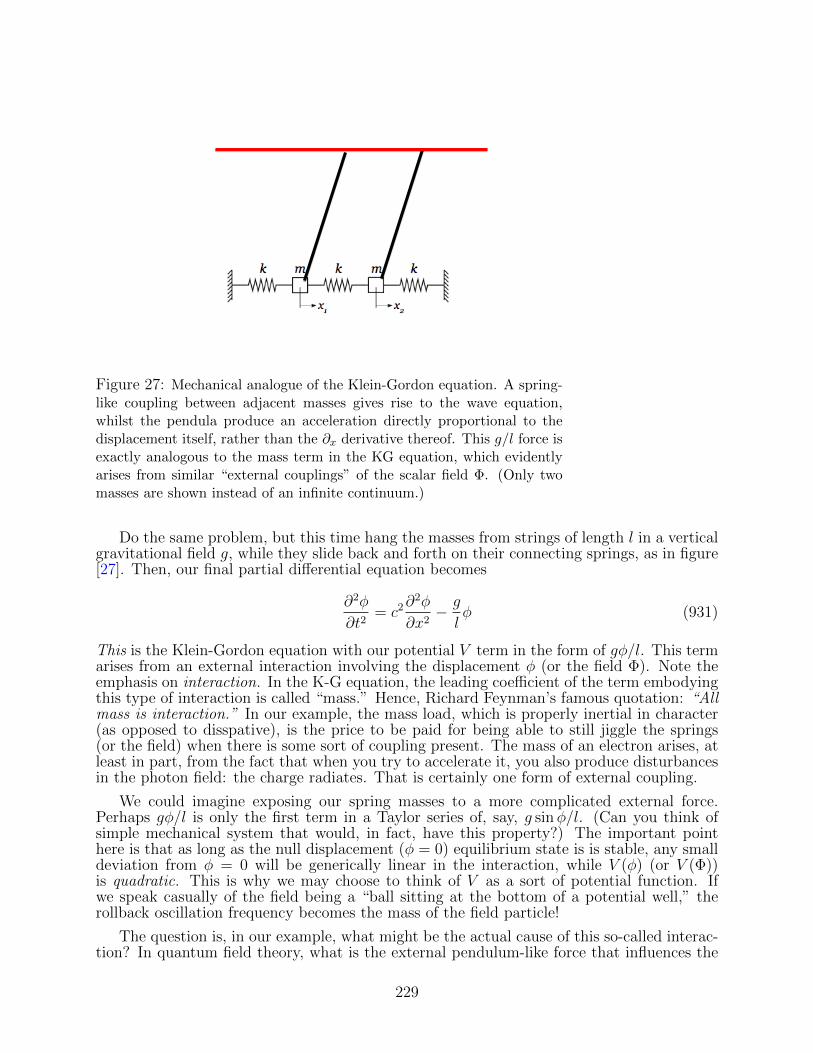
Figure 27: Mechanical analogue of the Klein-Gordon equation. A spring-like coupling between adjacent masses gives rise to the wave equation,whilst the pendula produce an acceleration directly proportional to thedisplacement itself, rather than the ∂x derivative thereof. This g/l force isexactly analogous to the mass term in the KG equation, which evidentlyarises from similar “external couplings” of the scalar field Φ. (Only twomasses are shown instead of an infinite continuum.)

Do the same problem, but this time hang the masses from strings of length l in a verticalgravitational field g, while they slide back and forth on their connecting springs, as in figure[27]. Then, our final partial differential equation becomes

∂2φ

∂t2= c2∂

2φ

∂x2− g

lφ (931)

This is the Klein-Gordon equation with our potential V term in the form of gφ/l. This termarises from an external interaction involving the displacement φ (or the field Φ). Note theemphasis on interaction. In the K-G equation, the leading coefficient of the term embodyingthis type of interaction is called “mass.” Hence, Richard Feynman’s famous quotation: “Allmass is interaction.” In our example, the mass load, which is properly inertial in character(as opposed to disspative), is the price to be paid for being able to still jiggle the springs(or the field) when there is some sort of coupling present. The mass of an electron arises, atleast in part, from the fact that when you try to accelerate it, you also produce disturbancesin the photon field: the charge radiates. That is certainly one form of external coupling.

We could imagine exposing our spring masses to a more complicated external force.Perhaps gφ/l is only the first term in a Taylor series of, say, g sinφ/l. (Can you think ofsimple mechanical system that would, in fact, have this property?) The important pointhere is that as long as the null displacement (φ = 0) equilibrium state is is stable, any smalldeviation from φ = 0 will be generically linear in the interaction, while V (φ) (or V (Φ))is quadratic. This is why we may choose to think of V as a sort of potential function. Ifwe speak casually of the field being a “ball sitting at the bottom of a potential well,” therollback oscillation frequency becomes the mass of the field particle!

The question is, in our example, what might be the actual cause of this so-called interac-tion? In quantum field theory, what is the external pendulum-like force that influences the

229

Φ field? The answer is that the interaction arises from the vacuum itself. Seriously.

11.6.3 Effective Potentials in Quantum Field Theory

One thing you have to understand about the quantum vacuum: it is a jungle out there.

The vacuum, yes even the vacuum, is full of ground state fluctuations in the motley col-lection of harmonic oscillators that we are pleased to call particles. There are circumstancesin which a simple K-G equation, which would represent free, massive scalar particles, maynot capture the dynamics of the field in question. The K-G scalar field may interact withall these other fields, and since this interaction gives rise to what we call “mass,” the in-teraction gives rise to a new mass coefficient. Imagine, in our mass-and-springs problem, ageneric nonlinear pendulum of some sort coupling to the oscillating fields. (Let us say thelength of the string depends upon the displacement.) Then, the orginal mass coefficient µ2

is not a constant, but actually depends on the field strength Φ. In the simplest case, µ2

would depend additively upon Φ2, so that only the magnitude of Φ, not its sign, affects thedistortion of µ2. The resulting modified potential V (Φ) would then take the form

V (Φ) = µ2Φ2/2 + βΦ4. (932)

This µ2 is once again just a constant, as is β. Decades before the notion of the cosmologicalinflation became popular, precisely this generic model for a modified field potential had beenin wide use amongst particle physicists, for completely different reasons. The key idea is thatif, despite appearances, µ2 is for some reason negative in our new model, and β positive, thenΦ = 0 is not a stable vacuum solution to our equation: a small departure from Φ = 0 doesnot oscillate in time, it grows exponentially! The actual stable vacuum state would have tobe the global minimum, Φ2 = |µ2/4β|. The Φ = 0 symmetry is broken. The potential looksnicely quadratic when locally perturbed about this new, stable minimum. We are then backto the K-G Equation, at least to leading order. But now the mass coefficient of our newlyperturbed field has changed! This is, in essence, the formal mechanism by which the Higgsboson acquires its mass. It is all about interactions and “spontaneous symmetry breaking.”

For understanding the dynamics of the early Universe, it is not the value of Φ of thenew equilibrium that is important, it is the wild, exponential journey we take to reach it:down the hill of an extended, rolling potential. It is this scenario upon which cosmologicalinflation was orginally based. It assumes, of course, that we start off somewhere near thetop of the slide!

Sound a bit woolly? Try not to be put off. This is forefront physics, and we must grope tosome extent. Physicists continue to argue about inflation scenario amongst themselves. Myown view borrows from Mark Twain’s famous comment upon Wagnerian music: it is betterthan it sounds. The V (Φ)’s of the early universe were likely to be complicated functions(embodying lots of interactions at high energies), but it would not have taken long beforethe fields sorted themselves out, landing in their respective stable local parabolic V -minima.Perhaps one of these fields may have taken a long time (in quantum terms) to get there. Soto modern physicists, we denizens of the displaced vacuum, local field disturbances now lookdeceptively, Klein-Gordonly, simple. It is OK to grope in the dark a bit to try to understandwhat new physics might in principle lie beyond the standard theories, and then see what themost robust predictions might be. Our current theories are incomplete, we have to grope!(Einstein in 1912 was groping: what if Minkowski space was only a first approximation andcould be distorted?) All within reason, of course. As long as certain ground rules like Lorentzinvariance are respected, there is considerable freedom in choosing the form of an interactionpotential V (φ). As noted, the type of quartic potential seen in (932) was already well-knownto particle physicists, and very much in play at the time it was culturally-appropriated by the

230

Figure 28: V (Φ) potential functions of the form (932). Theupper curve corresponds to µ2 > 0, the lower to µ2 < 0. Ifthere is a scalar field described by the µ2 < 0 potential in theearly Universe, it could trigger an episode of inflation. Beforecosmological applications, these potential functions were used todescribe ferromagnets, and to explain how symmetry is brokenin fundamental particle physics.

cosmologists. The particle physicists had, for their part, already borrowed it from condensedmatter physicists, who had been using it (in the form of a thermodynamic potential) todescribe ferromagnets. The “broken symmetry” approach has been enormously fruitful inparticle physics. Physicists groped, struggled, argued, predicted, and then ultimately foundthe Higgs boson. Just as a ferromagnet can spontaneously magnetise itself, so too can certaintypes of particles spontaneously acquire mass. Physically different processes often share avery similar mathematical heritage.

A few digressive words on the ferromagnet problem may be useful. In a ferromagnet,the equilibrium state minimises the Gibbs Free Energy G, a requirement for thermodynamicsystems at fixed temperature and pressure. G is a function of the magnetisation M , andtypically is modelled to follow the form of (932):

G = αM2 + βM4. (933)

A ferromagnet is spontaneously magnetised at low temeperatures, minimising G, with dipolemoments all alligned in a minimum energy state. On the other hand, at high temperatures,G is minimised at maximum entropy, with unalligned dipoles. This is captured in equation(933) by demanding that above some critical temperature Tc, both α and β are positive.Below Tc, α passes through zero and changes sign. It then becomes more favourable —G attains a smaller value—when M2 is finite and equal to −α/2β. The system, in otherwords, is spontaneously magnetised. Yet another, very similar, mathematical arrangementof interactions also produces the phenomenon of superconductivity. We have seen that inparticle physics this is the core of the argument for how a class of fields acquires mass. Thecosmologists, a little late to the party, have at last embraced spontaneous symmetry breakingas a key concept in their quest to explain the gross features of our Universe.

231

11.6.4 The slow roll inflationary scenario

The essence of the slow roll inflationary model is now easily grasped. Start by using (923)in (925) and (926). This leads to the equations

H2 =8πG

3c2

(V +

Φ2

2c2

)(934)

and

Φ + 3HΦ + c2dV

dΦ= 0 (935)

The idea is that the gross form of the governing interaction potential V (Φ) changes as theUniverse expands and cools, evolving from the top form of figure [28] early on, to the bottomform as things cool, much as a ferromagnet’s free energy does when the temperature changesfrom T > Tc to T < Tc. Moreover, if V is very flat, so that dV/dΦ is small, then Φ is alsosmall by equation (935) and there is an extended period when (934) is simply

H =R

R'√

8πGV0

3c2(936)

where V0 is the (approximately) constant of V (Φ). R grows exponentially,

R ∝ exp

(√8πGV0

3c2t

)(937)

and the Universe enters its inflationary phase. Φ meanwhile grows slowly, but it does grow,and eventually, after many e-foldings, the inflation stops when the minimum of V (Φ) isreached. It was Alan Guth, a particle physicist, who, motivated by earlier lectures of RobertDicke and Steven Weinberg, put together this picture in 1981 and brought to the fore theconcept of inflation as a phase of the early history of the Universe. In particular, Guthexplicitly argued that certain model potentials, then in widespread use to understand ferro-magnets and symmetry-breaking in particle physics, might also be relevant to fundamentalproblems in cosmology.

Exercise. The slow roll equations of inflationary cosmology, from (934) and (935), are

H2 =

(R

R

)2

=8πGV

3c2, Φ = −

(c6

24πGV

)1/2dV

dΦ.

Under what conditions are these equations valid? Next, consider a potential of the form

V (Φ) = V0(1− ε2Φ2)2,

where ε is small and V0 constant. Plot V as a function of Φ. Show that this V satisfies theslow-roll constraints, and solve the above differential equations for R(t) and Φ(t) with nofurther approximations.

The theoretical arguments for the mechanism of inflation are not (yet) based on funda-mental theory. They are phenomenological. The task is to carry through a detailed mathe-matical exploration of a candidate theory to see how naturally it leads to the behaviour inquestion. Perhaps the theory will explain something it wasn’t specifically designed to do.

232

That is when you know you are on the right track. Inflation models have this property,which is why there are considered attractive by many.

Here is an example. During the period of inflation, small density fluctuations go throughtwo types of behaviour in sequence. In their very earliest development, fluctuations oscillatelike a sound wave. But as the Universe rapidly expands, at some point the peak and thetrough of the same wave find themselves outside of one other’s horizons! A wave can’tpossibly oscillate coherently under those conditions. The disturbance remains “frozen,”stretched by the expansion.

But the rapid inflation eventually slows while the Universe is still very much a newbornbaby. Then, the expansion no longer is accelerating, but decelerating, and it does not takevery long before the ever-expanding horizon scale once again is able to enclose a wavelength.In the parlance of cosmology, the wave “enters” the horizon, and the oscillation behaviourcan then restart. Consider the case in which between this (very early) moment of restartwhen the oscillation starts off with zero velocity, and the time of hydrogen recombination(several hundred thousand years later, when we see the imprint of the fluctuation in theradiation), there is precisely one full contraction of the oscillation. (Or one full expansion,if the disturbance starts on its expanding phase.) This half-period of oscillation correpondsto a particular wavelength disturbance, and for this particular wavelength we would expectto see a peak when we plot the spectrum of fluctuations as a function of wavelength. Andthen another peak for the shorter wavelength that would allow a compression followed by acomplete expansion in the same time period. And so on. The so-called power spectrum32

(figure [29]) shows a sequence of peaks on certain angular scales on the sky. In order to existas well-defined entities, instead of just a smear, these peaks need to have their oscillationsstart up at a well-defined, coordinated beginning time. This is possible only because ofinflation. During inflation, the rapid expansion prevents the random oscillations that wouldotherwise be present. It then allows the oscillation dance to begin again, choreographed tostart from zero velocity. This moment happens very early on, once the exponential expansionhas slowed and the oscillations enter the horizon. The orchestrated release at only slightlydifferent (shorter wavelengths enter the horizon a tiny bit sooner!) early times is what makeswell-defined peaks possible in the first place. Their very existence is powerful evidence forthe concept of inflation.

11.6.5 Inflated expectations

The concept of an early inflationary period of the Universe explains both why there is suchuniformity in the CMB temperature across the sky and why the Universe is flat. It explainswhy there is an FRW metric at all. But there is subtlety as well in the predictions ofinflation, including predictions of where the power spectrum should have its peaks. Thereis so much more that, unfortunately, we don’t have time to go into in this course. Thereare, for example, firm predictions for how large scale structure in the Universe evolves—how galaxies cluster—from initial seed fluctuations. This is from highly inhomogeneous,spontaneous quantum fluctuations that become inflated to macroscopic scales, and grow (itis believed) into the large scale structure we see today. The power spectrum of the densityfluctations that result from the fluctuating quantum inflation field can actually be predictedfrom theory: it is close to (but not exactly!) linear in wavenumber k. The fluctuations leavean imprint in the CMB that can be measured. What do the recent (2015) results from thePlanck satellite show? A power-law power spectrum, with index a little bit less than unity(0.96). This is remarkable agreement with theory.

32If T (θ, φ) is the CMB temperature as a function of angle (angular separation), and T is the usual Fouriertransform in wavenumber space, the power spectrum is |T |2.

233

Figure 29: The temperature power spectrum of fluctuations (known as “TT spec-trum” in the literature) as a function of angular scale from recent Planck data. (Thebottom plot is a measure of the discrepancy between the data and a model, and doesnot concern us here.) The excellent model fit in the top plot is strong evidence forinflation.

234

To form real galaxies and real clusters, it is necessary for what is known as Cold DarkMatter to take part in the gravitational response to the initial seeds laid down by the quantumfield. Cold Dark Matter (CDM) is cold in the sense that it responds readily to gravitationalperturbations, forming in the process the bulk of the mass distribution in galaxies andclusters. These are extended dark matter haloes. Though we don’t know very much aboutCDM (another theory dominated by phenemonology), there are reasons to think that itmay be some kind of weakly interacting massive particle that pervades the Universe. Thereare searches underway to try to detect such particles via their more easily found decayproducts33. But it is hard to escape the notion that it all must have begun with some kindof inflationary process. There really is no other explanation for how vast stretches of theUniverse could ever have been in causal contact. Inflation is a powerful, unifying conceptwithout which it is difficult to make sense of even the most basic cosmological observations.And don’t forget: the Universe is inflating right now. We are living through mild inflationthat will, with time, become much more dramatic.

But from whence inflation? Is it inevitable? What is the underlying imperative to inflate,and then how do we exit gracefully from inflation? While there are some promising ideasafoot, we still don’t really know why inflation occurred. Maybe somebody reading thesenotes will settle the matter.34

33Update: No luck so far with the searches! An alternative view that black holes may be the dark matteris now starting to be taken seriously. We’ll see.

34I couldn’t be more serious: given the historical track record, when this problem is solved, and it will be,it would not be at all surprising if the solver spent their formative years as an Oxford undergraduate.

235

11.6.6 A final word

Astrophysics can be a very messy and speculative business. But every once and a while,something truly outstanding is accomplished. We began this course by talking about the tri-umphs of theoretical physics. The development of a theory for stellar structure and evolutionis one such triumph. This led to a new field of science: nuclear astrophysics, and ultimately aprecision theory for the origin of all the chemical elements. We now understand where atomscome from, and even how to make new ones ourselves, a stunning achievement. Anothermilestone is the coming of age of the theory of black holes, brilliantly confirmed in the lastfew years by the LIGO detections of gravitational radiation from a number of merging blackhole binaries. (A real “two birds with one stone” triumph for general relativity: both blackholes and gravitational radiation exist beyond a shadow of doubt.) Surely the developmentof precision cosmology, the discovery and construction of a rigorous model of the Universe,must also rank as one of the great historical advances in science. I view this on a par withthe Rutherford nuclear atom, Godel’s theorem, or the Crick-Watson DNA model: not justan important technical advance, but a transformative understanding. We have taken themeasure of the entire Universe, and you know what? The vacuum is on board, a full payingclient. What we reckoned a generation ago as the stuff of the Universe is just foam on asea, less than 5% of the true stuff of the Universe. The Universe started out dominated byits vacuum, and it will spend most of its life dominated by its vacuum. Let that sink in. Itis not about atomic ensembles like us. It is about the vacuum. The time when matter andradiation have much of a say in telling the Universe what to do will be a fleeting instant inits history, one from which we are only just now emerging. We ensembles of ordinary matterare merely soot from the fumes of the Universe’s exhaust vapour, waste products of thevacuum-driven engine. Even that doesn’t begin to capture our insignificance. The conceptof inflation suggests that an incomprehensibly vast multiverse is a viable description of thetrue reality.

But we can take heart, all is not bleak. Important questions remain for us, we tiny restlesspieces of a Universe that has produced a recursive understanding of itself. Thank goodnessfor that. Along the way, we have deduced our true age, something of our dynamics, and agreat deal of our history. I think it very unlikely that very many universes are fortunateenough to have internal bits that are able to justify such a remarkable and outlandish claim.

End of notes March 7, 2021.

236

Bibilography

Binney, J. & Tremaine, S. 2008, Galactic Dynamics, 2nd ed. (Princeton Univ.: Princeton)

Birrell, N. D. & Davies, P. C. W. 1982, Quantum Fields in Curved Space, (CambriddgeUniv.: Cambridge)

Carroll, S. M. 2019, Spacetime and Geometry. An Introduction to General Relativity, (Cam-bridge Univ.: Cambridge)

Einstein, A. 1952, The Principle of Relativity: A Collection of Original Papers on the Specialand General Theory of Relativity (Dover: New York)

Hartle, J. B. 2003, Gravity: An Introduction to Einstein’s General Theory of Relativity,(Addison-Wesley: San Francisco)

Hobson, M. P., Efstathiou, G. & Lasenby, A. N. 2006, General Relativity: An Introductionfor Physicists, (Cambridge Univ.: Cambridge)

Jackson, J. D. Classical Electrodynamics, 3rd ed. (John Wiley & Sons: Hoboken)

Landau, L. D. & Lifshitz, E. M. 1975, Classical Theory of Fields, 4th English ed. (Elsevier:Oxford)

Longair, M., 2006, The Cosmic Century, (Cambridge Univ.: Cambridge)

Misner, C. W., Thorne, K. S., & Wheeler, J. A. 1973, Gravitation, (Freeman: New York)

Pais, A. 1982, ‘Subtle is the Lord...’, (Oxford Univ.: Oxford)

Peebles, P. J. E. 1993, Principles of Physical Cosmology, (Princeton Univ.: Princeton)

Ryden, B. 2003, Introduction to Cosmology, (Cambridge Univ.: Cambridge)

Schwartz, M. D. 2014, Quantum Field Theory and the Standard Model, (Cambridge Univ.:Cambridge)

Shapiro, S. L. & Teukolsky, S. A. 1983, Black Holes, White Dwarfs and Neutron Stars(Wiley–Interscience: New York)

Thorne, K. 1994, Black Holes and Time Warps: Einstein’s Outrageous Legacy, (Norton:New York)

Tolman, R. C. 1987, Relativity, Thermodynamics and Cosmology, (Dover: New York)

Weinberg, S. 1972, Gravitation and Cosmology, (John Wiley & Sons: New York)

Weinberg, S. 2008, Cosmology, (John Wiley & Sons: New York) (Oxford Univ.: Oxford)

Zeldovich, Ya. B. & Novikov, I. D. 1971, Stars and Relativity, (Dover: Mineola)

237