GENERAL RELATIVITY COSMOLOGY - Niels Bohr Institutet
107
Transcript of GENERAL RELATIVITY COSMOLOGY - Niels Bohr Institutet
GENERAL RELATIVITY
AND
COSMOLOGY
Lecture notes
Poul Olesen
The Niels Bohr Institute
Blegdamsvej ��
DK ���� Copenhagen �
Denmark
Autumn ����
Preface
The following lecture notes on general relativity and cosmology grew out of a onesemester course on these topics and classical gauge theory by Jan Ambj�rn and the presentauthor� Subsequently semesters were abandoned and replaced by �Blocks� which havean extension of approximately only two months� Therefore the classical eld theory part�which anyhow strongly needed a revision� was dropped and the general relativity andcosmology chapters were revised�
These lecture notes are introductory and do not in any way pretend to be comprehen sive� Several important topics have been left out� For example gravitational radiationis not discussed at all� There are two reasons for the brevity of the notes� the allotedtime was short �a couple of months four hours a week� and it was hoped that by makingthe notes equally short there is a bigger chance of getting through that general relativityand cosmology are exciting subjects� Sometimes the trouble with exposing the beauty ofphysics is that one has to walk a very long way so people start to feel that they ratherwalk in a desert than in a beautiful garden� Students hungry for more comprehensivestudies are referred to the enormous literature�
Poul Olesen
Contents
� General relativity ���� The principle of equivalence � � � � � � � � � � � � � � � � � � � � � � � � � � ���� Gravitation and geometry � � � � � � � � � � � � � � � � � � � � � � � � � � � ���� Motion in an arbitrary gravitational eld � � � � � � � � � � � � � � � � � � � ���� The Newton limit � � � � � � � � � � � � � � � � � � � � � � � � � � � � � � � � ���� The principle of general covariance � � � � � � � � � � � � � � � � � � � � � � ���� Contravariant and covariant tensors � � � � � � � � � � � � � � � � � � � � � � ���� Di�erentiation � � � � � � � � � � � � � � � � � � � � � � � � � � � � � � � � � � ����� A property of the determinant of g�� � � � � � � � � � � � � � � � � � � � � � ����� Some special derivatives � � � � � � � � � � � � � � � � � � � � � � � � � � � � ������ Some applications to physics � � � � � � � � � � � � � � � � � � � � � � � � � � ������ Curvature � � � � � � � � � � � � � � � � � � � � � � � � � � � � � � � � � � � � ������ Parallel transport and curvature � � � � � � � � � � � � � � � � � � � � � � � � ������ Properties of the curvature tensor � � � � � � � � � � � � � � � � � � � � � � � ������ The energy momentum tensor � � � � � � � � � � � � � � � � � � � � � � � � � ������ Einstein�s eld equations for gravitation � � � � � � � � � � � � � � � � � � � ������ The time dependent spherically symmetric metric � � � � � � � � � � � � � � ������ A digression� A simpler method for computing ���� � � � � � � � � � � � � � ������ The Christo�el symbols for the time dependent spherically symmetric metric ������ The Ricci tensor � � � � � � � � � � � � � � � � � � � � � � � � � � � � � � � � ������ The Schwarzschild solution � � � � � � � � � � � � � � � � � � � � � � � � � � � ������ Birkho��s theorem � � � � � � � � � � � � � � � � � � � � � � � � � � � � � � � ������ The general relativistic Kepler problem � � � � � � � � � � � � � � � � � � � � ������ De�ection of light by a massive body � � � � � � � � � � � � � � � � � � � � � ������ Black holes � � � � � � � � � � � � � � � � � � � � � � � � � � � � � � � � � � � ������ Kruskal coordinates � � � � � � � � � � � � � � � � � � � � � � � � � � � � � � � ������ Painlev�e�s version of the Schwarzschild metric � � � � � � � � � � � � � � � � ������ Tidal forces and the Riemann tensor � � � � � � � � � � � � � � � � � � � � � ������ The Tidal force from the Schwarzschild solution � � � � � � � � � � � � � � � ������ The energy momentum tensor for electromagnetism � � � � � � � � � � � � � ������ The Reissner Nordstr�om solution � � � � � � � � � � � � � � � � � � � � � � � ������ The spherically symmetric solution in ��� dimensions � � � � � � � � � � � � ������ Cosmic strings � � � � � � � � � � � � � � � � � � � � � � � � � � � � � � � � � � ��
� Cosmology ����� The cosmological problem � � � � � � � � � � � � � � � � � � � � � � � � � � � ����� The cosmological standard model � � � � � � � � � � � � � � � � � � � � � � � ��
�
� CONTENTS
��� A geometric interpretation of the Robertson Walker metric � � � � � � � � � ����� Hubble�s law � � � � � � � � � � � � � � � � � � � � � � � � � � � � � � � � � � � ����� Higher order correction to Hubble�s law � � � � � � � � � � � � � � � � � � � � ����� Einstein�s equations and the Robertson Walker metric � � � � � � � � � � � � ����� The Big Bang � � � � � � � � � � � � � � � � � � � � � � � � � � � � � � � � � � ��
����� Existence of the big bang �the initial singularity� � � � � � � � � � � ������� The age of the Universe according to Big Bang � � � � � � � � � � � � ������� Discussion of the fate of the Universe � � � � � � � � � � � � � � � � � ��
��� Fitting parameters to observations � � � � � � � � � � � � � � � � � � � � � � ����� The cosmic microwave radiation background � � � � � � � � � � � � � � � � � ������ The matter dominated era � � � � � � � � � � � � � � � � � � � � � � � � � � � ��
������ The closed Universe �� � � � � � � � � � � � � � � � � � � � � � � � � �������� The �at Universe �� � � � � � � � � � � � � � � � � � � � � � � � � � � �������� The open universe �� � � � � � � � � � � � � � � � � � � � � � � � � � �������� Inclusion of the cosmological constant � � � � � � � � � � � � � � � � � �������� Discussion of the life time of the Universe � � � � � � � � � � � � � � ��
���� Causality structure of the big bang �The horizon problem� � � � � � � � � � ������ In�ation � � � � � � � � � � � � � � � � � � � � � � � � � � � � � � � � � � � � � ������ Observational evidence for the cosmological constant � � � � � � � � � � � � ������ The end of cosmology� � � � � � � � � � � � � � � � � � � � � � � � � � � � � � ������ An inhomogeneous universe without � � � � � � � � � � � � � � � � � � � � � ��
� Problems ��
� Some constants ���
� Some literature ���
Chapter �
General relativity
��� The principle of equivalence
Einstein�s general theory of relativity is a beautiful piece of art which connects gravita tional elds with geometry of space and time and thus provides a scheme in which ouruniverse can be discussed�
Einstein�s starting point was the principle of equivalence which can be understood inthe context of Newton�s mechanics� We have the general equation of motion
�F � mi��x �����
where ��x is the acceleration and mi is the inertial mass ! for a given force the accelerationis smaller the larger the mass is i�e� the body is more inert the larger mi is�
In a constant gravitational eld the force is given by
�Fg � mg �g �����
where �g and mg are constants� It is clear that a priori the parameter mg is not related tothe inertial mass� Newton made experiments where the period of oscillation of a pendulummade up from di�erent materials were studied and he found no variation with mi�mg�Later on many very precise experiments were made which showed that mi � mg to a highaccuracy and this was accepted to such an extent that most text books today �and atEinstein�s time� do not bother to put any indices on the masses�
Let us consider a constant gravitational eld� Withmi � mg � m one has the equationof motion
��x � �g �����
Thus if we introduce the coordinate
�y � �x� �
��gt� �����
we get��y � � �����
Therefore we conclude that an observer living in the y system sees no e�ect of the gravi tational eld because eq� ����� shows that particles move in straight lines as if there wasno force� On the other hand eq� ����� shows that the observer is freely falling ��
��gt� is just
�
� GENERAL RELATIVITY
the displacement pertinent to a free fall�� All this is true irrespective of any mass becausemi � mg� If mi �� mg the coordinate transformation ����� would have to be replaced by
�y � �x� �
�
mg
mi�g t� �����
and hence the �y system would depend on which material we consider through the ratiomg�mi�
When mg � mi the transformation ����� is universal and is easily seen to eliminatethe gravitational eld also if other forces �e�g� electrostatic forces� are at work� If thegravitational eld varies in space we can apply the transformation ����� in a su"cientlysmall domain�
In Newtonian mechanics we therefore know that an observer in a su"ciently smallfreely falling elevator is unable to detect a gravitational eld� Einstein�s principle ofequivalence generalizes this to any physical phenomena� In any arbitrary gravitationaleld it is possible at each spacetime point to select locally inertial systems�freely falling small elevators� such that the laws of physics in these are thesame as in special relativity�
One can use this statement to obtain some insight into the way in which gravityin�uences other physical phenomena by writing down in each of the small elevators somelaw of physics and then transform it to a general coordinate system� In the next sectionwe shall consider the simplest example namely a particle which is freely falling in anarbitrary gravitational eld�
Some remarks on the history of the Einsteinian version of the equivalence principle��
After having nished the special theory of relativity Einstein thought about the prob lem of how Newton gravity should be modied in order to t in with special relativity� Atthis point Einstein experienced what he called the �happiest thought of my life� namelythat an observer falling from the roof of a house experiences no gravitational eld#
��� Gravitation and geometry
Let us consider a particle which moves under the in�uence of a gravitational eld only�Thus in each of the �innitely many� freely falling systems of inertia we can apply specialrelativity with no forces acting on the particle�
In special relativity an event is described by a four vector y� � �y�� �y� where y� is thetime� Since the elevators are a priori small we need however to consider an innitesimalfour vector dy� � �dy�� d�y�� The proper time�
d� � � �dy��� � �d�y�� �����
is an invariant i�e� if we make a Lorentz transformation from y� to y�� then
d� � � �dy��� � �d�y�� � �dy���� � �d�y ��� �����
�Most of the historical remarks in these notes are taken from MacTutor History of Mathematics�http���www�history�mcs�st �andrews�ac�uk�HistTopics�General relativity�html�� where much more infor�mation can be found�
�Here d�� means �d���� This convention of leaving out the bracket in the square of innitesimalquantities will be used in the following� unless it leads to confusion�
��� GRAVITATION AND GEOMETRY �
For light d� � � and eq� ����� says that the speed of light jd�y�dtj is equal to one inall systems �Michelson Morley�s experiment�� The proper time has the following physicalinterpretation� Let us consider a clock �or any physical system which species a time e�g�a particle which decays with a certain life time� which by denition marks time by smallintervals dt when the clock is at rest� In the rest system the velocity �v � d�y�dy� vanishes�Thus
d� � � �dy������ �v�� � �dy��� �����
in the rest system� Thus d� � dy� � the interval between two ticks on the clock �at rest��In a moving system
d� � � �dy������� �v���
which leads to the formula for the time dilatation dy��
� d��p�� v���
In four vector notation we write the proper time as
d� � � ����dy� dy� ������
where ��� � � for �� and ��� � ��� � ��� � �� ��� � ��� This convention is calledmostly positive� In eq� ������ we use the summation convention� Whenever an indexoccurs two times in a product it is to be summed� Thus eq� ������ means
d� � � ��X
���
�X���
���dy�dy� ������
To obtain the e�ect of gravity we should notice that eq� ������ is valid in any of the freelyfalling elevators� However in general the elevators are di�erent in di�erent space timepoints� If we denote the space time coordinates in an arbitrary coordinate system by x�then the y�s are functions of the x�s
y� � y��x�� ������
For an example see the Newtonian case ������ Inserting this in eq� ������ we get
d� � � ���� �y�
�x��y�
�x�dx�dx� � �g���x�dx�dx� ������
where
g���x� � ����y�
�x��y�
�x�� g���x� ������
is called the metric tensor�Eq� ������ has an almost obvious geometric interpretation� In a curved space �e�g� the
surface of a sphere� one can introduce local coordinate systems where Euclidian geometryis valid in spite of the fact that this geometry is not valid in general in curved space�The local Euclidean geometry corresponds to eq� ������ if we replace ��� by ���� where��� is the Kronecker symbol ���� � � for �� � ��� � �� for � �� d� � then meansthe distance between two points computed by the law of Pythagoras� Then eq� ������ isthe same distance written in arbitrary coordinates� Similarly in Einstein�s gravity locallyone has pseudo Euclidian�Minkowsky geometry due to the principle of equivalence butthe geometry of space is in general non pseudo Euclidean ��non Minkowskian� and the
� GENERAL RELATIVITY
deviations from ��at space� ��Minkowski space� represent the e�ects of the gravitationaleld�
Some remarks on the history of Einsteins geometrical gravity�
According to historians of physics it is not known how Einstein got the idea of relatinggravity with geometry� One hypothesis is that he was inspired by a rotating disk� Here themeasuring rods will become Lorentz contracted and hence the length of the peripheryof a circle will be di�erent from � ��radius�� This means a deviation from Euclideangeometry� In any case in papers on gravitation published in ���� he realized that theLorentz transformations will not always be applicable in a gravity theory based on theequivalence principle� Space time were dynamically in�uenced by gravity� According tothe philospher Kant Euclidean geometry should be considered as an a priori descriptionof space� Therefore the notion of space and time as dynamical quantities represented astrong break with philosophical traditions� Kant had not been right#
Einstein now remembered that as a student he had studied Gauss�s theory of surfaces�To proceed Einstein got help with the mathematical formulation of the theory of generalrelativity from his former classmate Marcel Grossmann and the latter �being a professorof descriptive geometry in Zurich� pointed out the relevance of di�erential geometry thathad previously been investigated by a number of mathematicians �Riemann Ricci Levi Civita ����� Einstein says about this period� ����in all my life I have not laboured so hardand I have become imbued with great respect for mathematics the subtler part of whichI had in my simple mindedness regarded as pure luxury until now��
��� Motion in an arbitrary gravitational �eld
We shall now apply the principle of equivalence to see how gravity in�uences space inthe simple case where there are no other forces than gravity� So let us consider a particlewhich moves under the in�uence of an arbitrary gravitational eld� In the freely fallingsystem special relativity applies and we have the equation of motion
d�y��x�
d� �� � ������
The solution to this equation is that y� is a linear function of � inside a small elevatorwhere there are no forces� This simply means straight line motion inside the elevator inaccordance with the ndings of Gallilei�
Using that the y��s depend on x� we have
� �d
d�
�dy�
d�
��
d
d�
��y�
�x�dx����
d�
�
��y�
�x�d�x�
d� ��
��y�
�x��x�dx�
d�
dx�
d�������
This looks somewhat like an equation of motion �because of d�x��d� �� with a force� Wecan remove the factor multiplying the second derivative of x� by the following trick� Bythe rules of di�erentiation we have ���� � �� for � � � � ��� � � for � �� ��
�x�
�y��y�
�x�� ��� ������
��� MOTION IN GRAVITATIONAL FIELD �
Thus multiplying eq� ������ by �x���y� and summing over we get
d�x�
d� �� ����
dx�
d�
dx�
d�� � ������
where
���� ���y�
�x��x��x�
�y�������
is called the Christo�el symbol or the a"ne connection �sometimes denoted f���g�� Wesee that the Christo�el symbol is proportional to the �gravitational force��
So far the metric and ���� have been expressed in terms of the functional relationbetween the local freely falling elevators and the arbitrary system x�� We shall now showthat the Christo�el symbol can be expressed in terms of the metric tensor�
From eq� ������ we see that ���� depends on the second derivatives of y� whereas from
eq� ������ g�� depends only on the rst derivative� Therefore let us di�erentiate g�� byuse of the denition ������
�g���x�
� �a���y�
�x��x��y�
�x�� ���
�y�
�x���y�
�x��x�������
From ������ we have
�����y�
�x��
��y�
�x��x�
��x�
�y��y�
�x�
��
��y�
�x��x�������
where we used the chain rule for di�erentiation
�x�
�y��y�
�x�� ��� ������
Thus we can express the second derivative of y in terms of � by means of eq� �������Using this in eq� ������ we get
�g���x�
� �������
�y�
�x��y�
�x�� ����
���
�y�
�x��y�
�x�
� g������ � g���
��� ������
where we used the expression ������ for the metric� Using eq� ������ we get
�g���x�
��g���x�
� �g���x�
� �g������ ������
If one wishes g�� can be thought of as a �� � matrix� One can then consider the inversewhich we denote g��
g���x�g���x� � ��� ������
The inverse exists�
g�� � ����x�
�y��x�
�y�������
because the transformations y � x and x � y are non singular coordinate transforma tions� Eq� ������ now gives the following relation between � and g
���� ��
�g��
��g���x�
��g���x�
� �g���x�
�������
� GENERAL RELATIVITY
��� The Newton limit
Eqs� ������ and ������ determine the motion of a particle in a gravitational eld providedwe know how g���x� depend on the gravitational eld� Later we shall see that the secondderivatives of g�� are determined through Einstein�s eld equations in terms of matterdistributions�
At present we shall study a much more modest problem namely the Newton limitwhere all velocities are small relative to the velocity of light jd�x�d� j �� � and where theproblem is static i�e� g�� is time independent� To the lowest non trivial approximationeq� ������ then gives �t � x��
d�x�
d� �� ����
�dt
d�
��
� � ������
Using eq� ������ and the fact that all time derivatives vanish we have
���� � ��
�g��
�g���x�
������
Since we are interested in small e�ects of gravity we write
g���x� � ��� � h���x� � jh�� j � � ������
where h�� is the correction to the constant metric tensor ��� � Then eq� ������ gives
���� � ��
����
�h���x�
������
so that ���� � � since h�� does not depend on time� Hence the � � � component of eq������� becomes simply
d�t
d� �� �
i�e�dt
d�� constant
For � � i� i � �� �� � eq� ������ becomes by use of eq� ������
d��x
d� �� �
�
�dt
d�
��
�rh����x� � � ������
and because dt is proportional to d�
d��x
dt���
��rh����x� ������
This equation can immediately be compared to Newton�s equation
d��x
dt�� ��r���x� ������
where ���x� is the gravitational potential� The Newtonian potential is determined byPoisson�s equation
r����x� � � G ���x� ������
��� THE NEWTON LIMIT �
where G i Newton�s constant �G � G�c� � ����� ����� cm$g�� For a point mass one hasthe well known result
� � �GMr
������
Comparing eqs� ������ and ������ we get h�� � constant ��� and requiring that at verylarge distances from the point mass space should be �at we get
g����x� � ��� � ����x�� ������
Thus we see that su"ciently close to a point mass space time must indeed be slightly�curved�#
The �curvature� indicated by eq� ������ can be observed� Recalling that the propertime is the time observed on a freely falling watch we have
d� � � ���� dt�falling � �g���x�dx�dx� � �g����x�dt� ������
where the last expression is valid in a gravitational eld where the clock is �approximately�at rest� Thus the time measured in this system in the point x is
dt �d�q�g���x�
������
This is not in itself an observable e�ect since all clocks and physical processes in the pointwill su�er the same e�ect� However we can compare two di�erent points� Here it isimportant to note that if e�g� an atom emits light in one point this light will travel toanother point in a constant time if the metric is time independent� This follows becaused� � � for light and the line element � � g����x�dx
�dx� can be solved for dt � dx� andsubsequently integrated over the distance between the two points �
Rdt� and the resulting
integrated travel time for light is time independent� Therefore it follows that if a wavelength is emitted in time interval dt in one point this wave length will be observed in theother point in the same time interval dt�
If the clock is a physical system with a frequency � we therefore get �� � � �dt�
�����
vuutg���x��
g���x��������
In the weak eld approximation ������ we then have
%�
���
�� � ����
� ��x��� ��x�� ������
which is an observable e�ect� Here �� is the frequency of light emitted in the point �but in accordance with what was said above this is also the frequency when this light isobserved in point � provided the metric is time independent� Now two spectra emittedfrom the same type of atom can be identied even if the spectral lines are displacedby the amount %� so we can compare an atomic spectrum emitted from the sun andobserved on earth with the same atomic spectrum emitted on earth�
If we consider light which passes from the sun to the earth we have for the sun�spotential
�� � �GM�
R�
� � ���� ���� ������
� GENERAL RELATIVITY
whereas the earth�s potential can be ignored relative to ��� In eq� ������ G should bereplaced by G�c� in ordinary units� The frequency of light from the sun is thus shiftedby ��� parts per million relative to light from earthbound sources� Taking into accountvarious other e�ects the best experimental result is ����� ���� times the predicted value�
Another experiment made ���� consists in emitting light from a tower of height ����m�The falling light is then observed on the ground� From ������ the frequency shift shouldbe
%� � �top � �bottom ����� cm�sec������� cm�
��� ���� cm�sec��� ����� ����� ������
The experimental value is������ ������ ����� ������
in excellent agreement with the prediction�
��� The principle of general covariance
So far we have studied the e�ects of gravity by use of the principle of equivalence accordingto which the physics of special relativity is valid in freely falling local systems of inertiaand the e�ects of gravity can then be obtained by transforming to an arbitrary system�Such a procedure is in general rather complicated�
Einstein introduced ������ a new principle which leads to a much more systematic wayof obtaining the physics of gravity from the physics without gravity namely the principleof general covariance� Using his own words �well translated to English� this principlestates�
The general laws of nature are to be expressed by equations which holdgood for all systems of coordinates that is are covariant �i�e� preserve theirform� with respect to any substitutions whatever ��generally covariant���
In this connection the �laws of nature� are to be understood as those which are valid inspecial relativity� It then follows that if general covariance is satised then the equivalenceprinciple is also satised� in each point there are freely falling local elevators in which thelaws of nature are those of special relativity and from general covariance they are thusvalid laws in all coordinate systems�
We need to specify precisely what we mean by �local elevators�� Clearly they shouldnot be too large because then from experience with tidal forces we know that gravita tional e�ects can be observed on a su"ciently large scale� The equation of motion in agravitational eld is given by equation ������� At each point x � x� we can select theelevator such that g���x�� � ��� �� �at Minkowski space� and in order to have localstraight line motion we can select the elevator such that
�g���x�
�x�
�����x�x�
� � ������
Because of the connection between the Cristo�el symbol ���� and g�� given by eq� ������this ensures that to lowest order near each point of space time we have no e�ect fromgravitational forces� However it should be emphasized that second derivatives of g���x�
��� TENSORS �
are not in general assumed to vanish� This amounts to saying that we only assume thate�ects of gravity can be transformed away on a scale which is small relative to the scaleof the gravitational eld�
��� Contravariant and covariant tensors
We shall now present a systematic construction of certain quantities tensors which aresuitable for applying the principle of general covariance� For tensors there exist trans formations when the coordinates are transformed �x � x��� The tensor transformationsare linear and homogeneous for the components of the tensors� Hence all components inthe x� system vanish if they vanish in the x system� A law of nature requiring that allcomponents of a tensor vanish is thus valid in all systems if it is valid in one system�Tensor laws thus follow the principle of general covariance if we ensure that they are validin special relativity� The simplest quantity is a scalar quantity which is invariant underx � x�� Numbers like �� etc� are examples� Also the proper time is an example ofan invariant� In general one can also have a scalar eld ��x� dened in each space timepoint transforming like ���x�� � ��x��
Another quantity is the coordinate di�erential dx� which transforms like
dx�� ��x��
�x�dx� ������
Any quantity which transform like ������ is called a contravariant vector i�e� U� is acontravariant vector if under a transformation x� x� one has U� � U �� with
U ���x�� ��x��
�x�U��x� ������
It should be noticed that since d� is invariant it follows from ������ that the four velocitydx��d� � �dx��d�� d�x�d�� is a contravariant vector�
In special relativity x� is a vector� It is important to realize that this is not the case ingeneral relativity where the transformation x� � x��� x�� � x� is completely arbitrary�In general relativity we can only a�ord that the coordinate di�erentials dx� are vectors�The physical reason for this di�erence is as mentioned before that in the equivalenceprinciple we must restrict ourselves to innitesimal elevators�
A covariant vector is dened by
A���x
�� ��x�
�x��A��x� ������
From ������ and ������ we can form a scalar
A���x
��U ���x�� ��x�
�x���x��
�x�A��x�U
��x� � A��x�U��x� ������
We say that by contracting the indices of two vectors we obtain an invariant�From a scalar ��x� we can form a covariant vector by di�erentiation
����x��
�x���
���x�
�x��x�
�x��������
�� GENERAL RELATIVITY
A general tensor can have arbitrarily many indices e�g� T ������n������m � Its transformation
is given by
T �������n
������m�x�� �
�x���
�x�� �x
��n
�x�n�x��
�x��� �x
�m
�x��mT ������n
������m�x� ������
A tensor with upstairs as well as downstairs indices is called a mixed tensor� The trans formation law ������ can easily be remembered by noticing that T transforms the sameway as if it had been a product of n contravariant and m covariant vectors� In otherwords a product of vectors is a tensor e�g� A�B�C� transforms as a tensor D
��� etc�
etc�The reader should be warned that the summation convention requires some care�
Suppose for example we have the two relations A � B�C� and D � E�F�� What is thenAD� Well multiplying the two relations together we apparently get AD � B�C�E
�F��This expression is however meaningless and hence wrong� The summation indices occurfour instead of two times� Before multiplying A and D together we must ensure that thesummation indices in A and D are di�erent� Thus keeping the indices in A we shoulduse a di�erent name for the indices in D e�g� D � E�F�� We then obtain the correctexpression AD � B�C�E
�F� where each summation index occurs only twice�The metric tensor g�� is a covariant tensor as is easily seen from the denition ������
g����x�� � ���
�y�
�x���y�
�x��
� ����y�
�x��y�
�x��x�
�x���x�
�x��
��x�
�x���x�
�x��g���x� ������
Also g�� is a contravariant tensor� The index of a tensor can be �raised� or �lowered�by means of g�� or g��� E�g� T�� � g��g��T
��� By going to a freely falling system we see
that the tensors T and T are the same physical object and T is denoted T � The symbol��� is easily seen to be a mixed tensor�
Often the determinant of g�� occurs
g � � det g��From the transformation law ������ which in matrix form reads �g�� � � x
x���g�T � x
x��
where �g� etc� denotes the matrix g�� and where the superscript T denotes the transposeof the matrix one obtains
g��x�� �
����� �x�x�������
g�x� ������
where j�x��x�j is the Jacobi determinant j�x��x�j � j det��x���x���j� Eq� ������ has theimportant consequence that �dx � dx�dx�dx�dx��
qg��x�� dx� �
qg��x��
������x�
�x
����� dx �qg�x� dx � invariant ������
where in the rst step we used the usual Jacobi transformation� Thus the measure ofintegration dx is not invariant but should be multiplied by
pg�
��� DIFFERENTIATION ��
Finally let us mention a few simple rules for tensors which follow from the transfor mation ������� a sum of two tensors is a tensor a product of two tensors is a new tensor�with more indices� e�g�
A��� B�
�� � T ����
�� ������
and a contraction in a tensor is a new tensor with fewer indices e�g�
T ����� � &T ��� ������
�� Dierentiation
We saw in the last section that di�erentiation of a scalar leads to a vector �see eq� ��������However in general it is not true that di�erentiation of a tensor leads to a new tensor�This is related to the fact that di�erentiation is dened by comparing the tensor intwo di�erent points �and then taking the limit where the points approach one another��However a tensor transforms di�erently in the two points as can be seen e�g� from thetransformation law �������
In the following we shall discuss the concept of di�erentiation versus covariance follow ing Einstein�s original ���� paper� To see what happens let us consider some trajectoryx����� Starting from a scalar ��x� we have
invariant �d��x�
d��
���x�
�x�dx�
d�������
where the invariance follows from the fact that d� and d� are individually invariant�However dx��d� is a vector and consequently it follows that
V��x� ����x�
�x�������
is a covariant vector� This statement has already been checked directly in eq� ������ �Now let us di�erentiate ������ once more
invariant �d��
d� ��
���
�x��x�dx�
d�
dx�
d��
��
�x�d�x�
d� �������
Next let us take the trajectory x���� to be a path for a particle which falls freely in anarbitrary gravitational eld� Then we have from the equation of motion ������
invariant �d��
d� ��
����
�x��x�� ����
��
�x�
�dx�
d�
dx�
d�������
Sincedx�
d�
dx�
d�
is a contravariant tensor and since the left hand side of ������ is an invariant it followsthat the quantity in the bracket in eq� ������ is a covariant tensor� Inserting ������ wehave that
V�� ��V��x�
� ����V� ������
�� GENERAL RELATIVITY
is a covariant tensor with indices � and �� V�� is called the covariant derivative of V��The result ������ was derived for a trajectory of a particle falling freely in some gravi
tational eld� By choosing all sorts of such elds we can however manage that the curveis completely arbitrary� Hence eq� ������ should be valid for x� being an arbitrary pointin the space time continuum� Alternatively one can use the connection ������ between���� and the metric as well as the fact that the metric g�� is a tensor to show directlythat ������ is a tensor�
If we di�erentiate a contravariant tensor V � the following quantity
V �� �
�V �
�x�� ����V
� ������
is a mixed tensor �T �� �� The concept of covariant di�erentiation can be generalized to an
arbitrary tensor� One has e�g�
C���� �
�C���
�x�� ����C
��� � �
���C
��� � ���C��
������
We leave it to the diligent reader to verify this statement�An important property of the covariant derivative is that it reduces to the ordinary
derivative in a freely falling local elevator� This follows from the denition of locality givenin ������ according to which the rst derivatives of the metric tensor can be required tovanish in a local system� Since ���� is directly related to these derivatives through eq������� it follows that
�����x� jx�x� � � ������
From this we have the very important conclusion that in spite of the notation ���� �mixedtensor notation� it is not true that ���� is a tensor because if it was a tensor thenit follows from ������ that in any point there exists a freely falling elevator where ����vanishes and consequently it should vanish in all coordinate systems� Since ���� does notvanish in general it follows that it is not a tensor� Using the transformation law for thetensor g�� and the relation ������ one can easily see that �
��� transforms as
������x�� �
�x��
�x��x�
�x���x�
�x�������x� �
�x��
�x���x�
�x���x��������
The rst term on the right hand side is what one would get if ���� was a tensor but thesecond term shows that ���� transforms in a more complicated way�
Because of ������ it follows that in the small elevators the covariant derivative is justthe ordinary derivative� This is rather satisfactory since we are supposed to use the lawsof special relativity in each elevator and these laws of course contain only the ordinaryderivatives�
From the denition ������ of a local elevator i�e� from the fact that the rst derivativesof g�� can be taken to vanish in a local elevator and from the fact �see eq� ������ � thatg�� is a tensor it follows that the covariant derivative of g�� vanishes
g��� � � ������
Finally let us consider motion along a trajectory x����� In this case one can only talkabout di�erentiation along the curve x����� We can then project the covariant derivativeto the tangent dx��d� � Eq� ������ is then replaced by
DV �
D�� dV �
d�� ����V
� dx�
d�������
�� THE DETERMINANT OF g�� ��
which is easily shown to be a contravariant vector with index �� In a local elevator itreduces to the ordinary derivative dV ��d� �
��� A property of the determinant of g��
We shall show an interesting property related to the determinant of g�� � To this endwe need to di�erentiate a determinant� Let us therefore start by considering an n � ndeterminant with elements ars� It is dened by
det a �X����P ������������n�a���a��� � � � an�n ������
where P is even �odd� for even �odd� permutations of the reference sequence �� �� � � � � n�In the sum ������ we can take an element ars outside a bracket and all the terms in������ containing the particular factor ars can then be written arsArs �no summation overr and s� where Ars is a sum of terms which consist of n � � factors� Ars is called thecomplement� Because of the construction ������ of the determinant Ars is independentof the elements in the r�th row and the s�th column �we have already picked the elementars and each term in the sum ������ has only one element from the r�th row and the s�thcolumn�� Now each of the n# products in det a contains one and only one element in ther�th row and we have �no sum over r�
ar�Ar� � ar�Ar� � � arnArn � det a ������
The n complements Ar�� � � � � Arn are all independent of the elements ar�� � � � � arn in ther�th row� Thus the quantities Ar�� � � � � Arn are unchanged if in det a we interchange theelements in the r�th row with other elements� In particular we can keep Ar�� � � � � Arn
unchanged if we replace the elements in the r�th row with the corresponding elementsas�� as�� � � � � asn in the s�th row �r �� s�� However the new determinant has the value �since two rows have the same elements i�e�
as�Ar� � as�Ar� � � asnArn � � �s �� r� ������
Eqs� ������ and ������ can be used to construct the inverse determinant or matrix� Thusthe inverse of �
BBB�a�� a�� � � � a�na�� a�� � � � a�n� � � � � � � � � � � �an� an� � � � ann
CCCA ������
is �BBB�
A��
det aA��
det a� � � An�
det aA��
det aA��
det a� � � An�
det a
A�n
det aA�n
det a� � � Ann
det a
CCCA ������
The correctness of ������ is seen by multiplying ������ and ������ together by use of ������and ������� The result is the unit matrix�
Now let us di�erentiate det a i�e� consider the variation � det a arising from �������Each term in the sum ������ has n factors and the variation is a product of n� � factors

�� GENERAL RELATIVITY
multiplied by �ars according to the usual rule for di�erentiation of a product� The n� �factors do not contain ars� Thus collecting all terms which are multiplied by �ars amountsto collecting the terms in the complement Ars� According to ������ this means that
� det a �X
Ars�ars �X�a���sr det a �ars ������
where �a���sr stands for the elements in the inverse matrix a���
From this general result let us return go g�� � With g � � det g�� we have �g�� issymmetric�
dg � g��g dg�� ������
since g�� was dened as the inverse of g��� Using ������ we have g��g�� � � i�e�
g�� dg�� � g�� dg�� � � ������
so ������ has the alternative form
dg � �g g�� dg�� ������
From ������ we have
g���g���x�
��
g
�g
�x��
� ln g
�x�������
This property turns out to be rather useful�
��� Some special derivatives
In mathematical physics the curl of a vector is dened by
curl �V �
��V��x�
� �V��x�
��V��x�
� �V��x�
��V��x�
� �V��x�
�������
For the covariant derivative of a vector V� we can similarly dene the curl to be V���V���Using the expression ������ we see that the terms involving the Christo�el symbols dropout and we just have
V�� � V�� ��V��x�
� �V��x�
������
i�e� the curl is given in terms of just the ordinary derivatives�The divergence of a vector is given by
V �� �
�V �
�x�� ����V
�� ������
Using the expression ������ we have
���� ��
�g��
��g���x�
��g���x�
� �g���x�
���
�g��
�g���x�
� ������
since the rst and the third terms are seen to be identical by interchange of the summationindices � and �� Now we can use ������ to simplify this to
���� ��
�
�
�x�ln g �
�pg
�
�x�pg ������
�� SOME SPECIAL DERIVATIVES ��
Eq� ������ can then be written in the elegant form
V �� �
�pg
�
�x��pg V �� ������
In eq� ������ we mentioned thatpgdx is invariant� Gauss� theorem in four dimensions
can then be written
Zdxpg V �
� �Zdx
�
�x��pg V �� �
Zd'�
pg V � ������
whereP
� are � �surfaces� �e�g� for � � �� d'o � dx�dx�dx��� If these surfaces are takenat innity and if V � � � at innity one has
Zdxpg V �
� � � ������
For tensors similar simplications occur� The covariant derivative of a tensor T �� is givenby
T ��� �
�T ��
�x�� ����T
�� � ����T�� ������
Thus the divergence is given by
T ��� �
�T ��
�x�� ����T
�� � ����T�� ������
Using ������ we can combine the rst two terms just like we did in eq� ������
T ��� �
�pg
�
�x��pg T ��� � ����T
�� ������
If the tensor is antisymmetric
F �� � �F �� ������
then the last term in ������ drops out �because ���� is symmetric in � and �� and we havethe simple result
F ��� �
�pg
�
�x��pg F ��� ������
The usual Laplace operator acting on a scalar equals divgrad� In our case there is asimilar result� The gradient of the scalar S is just �S��x� which when multiplied by themetric can be contravariant� We can then apply ������ to obtain
�g S � �pg
�
�x�
�pg g��
�S
�x�
�������
where �g generalizes the usual d�Alembert operator �����x���� In a local elevator �g
reduces to the d�Alembertian�
�� GENERAL RELATIVITY
��� Some applications to physics
Having developed the apparatus of tensors and generalized di�erentiation let us enjoyourselves with some applications to physics�
First let us consider again the problem of a particle which falls in a gravitationaleld g���x� but this time we apply the principle of general covariance� Thus rst wemust know what happens in special relativity� Here the particle is completely free� Itsfour velocity is given by
U� �dy�
d��
�dy�
d��d�y
d�
�������
where y� are the coordinates in special relativity� The equation of motion is simply
dU�
d�� � ������
Now we must make this equation generally covariant� This was done in eq� ������ wherewe showed that d�d� should be replaced by D�D� i�e� we have
DU�
D��
dU�
d�� ����U
�U� � � ������
This equation is correct because
�� it is valid in any freely falling local elevator ����� � � locally�
�� it is generally covariant �a vector DU��D� vanishes in one system and hence itvanishes in all systems��
From this example we see that once we have been through the somewhat tiresome proce dure of setting up tensor calculus the result ������ can be derived in a much simpler waythan by applying the equivalence principle directly�
To present another example let us consider a small gyroscope which moves in thegravitational eld g���x�� In special relativity it is thus not in�uenced by any forces� Thegyroscope taken to be at rest has an angular momentum� In the limit where it can beconsidered to be a point we say that it has a spin �S� The spin is conserved if no externalforce acts� We can then introduce the four vector S� � ��� �S� and hence
dS�d�
� � ������
Also since the gyroscope is at rest �the spin is dened in the rest frame� we have
U�S� � � ������
These equations are valid in special relativity� Under the in�uence of the gravitationaleld they become
DS�D�
� dS�d�
� ���� U�S� � � ������
S�U� � � ������
���� SOME APPLICATIONS TO PHYSICS ��
Eq� ������ for example describes the precession of a gyroscope carried in a satellitemoving in the gravitational eld from the earth� To actually utilize eq� ������ we needhowever more accurate result for the metric than the one obtained in the Newtonian limit�see eq� ��������
Newton�s equation ����� can be generalized to special relativity
mdU�
d�� f� ������
where f� is called the four force� In general relativity this becomes
mDU�
D�� F � �������
where F � is a generalized four force�We now turn to electrodynamics� The Maxwell equations can be expressed in terms
of an antisymmetric tensor F �� with F �� � B�� F�� � B�� F
�� � B� � �B is the magnetic
eld� F �� � E�� F�� � E�� F
�� � E� � �E is the electric eld�� Furthermore the current
is a four vector J� � ��� �J� where � is the charge density and �J is the current� Theequations
div �E � �r �E � � � �r� �B � curl �B �� �E
�t� �J �������
become�
�x�F �� � �J� �������
The other Maxwell equations
div �B � �r �B � � � �r� �E � ���B
�t�������
can be expressed as�
�x�F�� �
�
�x�F�� �
�
�x�F�� � � �������
where the indices are permuted cyclically� Eqs� ������� and ������� are of course validin special relativity( as a matter of fact they )or rather the equivalent eqs� ������� and�������* are the raison d�etre for special relativity�
Now we can apply our tensor apparatus to obtain the e�ects of gravitation on electro magnetism� Eq� ������� is simple to write in a generally covariant form
F ��� � �J� �������
Now F �� is antisymmetric so we can simplify as in eq� ������
�
�x��pg F ��� � �pg J� �������
To make ������� generally covariant we lower the indices
F�� � g�� g��F�� �������
�� GENERAL RELATIVITY
which is still antisymmetric� Eq� ������� then becomes
F��� � F��� � F��� � � �������
where e�g�
F��� ��F���x�
� ����F�� � ����F�� �������
Adding the three terms in ������� it is seen that the six terms containing the ��s canceland we thus get the simple result
�F���x�
��F���x�
��F���x�
� � �������
In special relativity the four current is conserved� It is easy to see that the same must betrue in general relativity� From eq� ������� we have
��
�x��x��pg F ��� � � � � �
�x��pg J�� �������
because F �� is antisymmetric� The conservation law
�
�x��pg J�� � � �������
precisely corresponds to the vanishing of the four divergence of J� )compare with eq�������* in generally covariant form�
Finally we mention that in special relativity the Lorentz force
d�p
dt� e) �E � �v � �B* �������
can be written )compare with eq� ������*
f� � eF ��dx�
d��������
In general relativity the generalized four force ������� therefore becomes
F � � e F ��dx�
d��������
where F � is a vector since F �� is a tensor and dx
��d� is a vector�
���� Curvature
The principle of equivalence �and the principle of general covariance� shows that a gravi tational eld can be represented by a metric tensor g���x� which is not everywhere con stant� The opposite is however not true� Suppose space is just �at Minkowski spaceand g���x� � ��� everywhere� Thus
d� � � ����dx� dx� �������
���� CURVATURE ��
We can however always transform the x coordinate to a di�erent system x � x� andthen ��
d� � � �g����x��dx�� dx��
g����x�� � ���
�x�
�x���x�
�x���������
In the new system it appears that the metric does not represent �at space� Howeverit is clear from the derivation that the apparent non �atness is an illusion�
The question then arises whether we can somehow avoid being fooled by somebodywho claims to have an interesting gravitational eld g�� but who has obtained this eldfrom �at space by applying some complicated mathematical transformation x � x�� Toavoid such a joke we can notice that in �at space if we di�erentiate a vector two times thederivatives commute� In curved space derivatives are replaced by covariant derivativeswhich in general do not commute� To see this let us notice that
T�� ��T���x
� ���T�� � ���T�� �������
In this equation T�� is an arbitrary tensor so we can take T�� � V�� since the covariantderivative of a vector V� is a tensor� Thus
V�� ��V���x
� ���V�� � ��� V�� �������
From this we get ���� is symmetric in � and �#�
V�� � V�� ��V���x
� �V��x�
� ���V�� � ���� V� �������
Inserting now
V�� ��V��x�
� ����V� �������
we obtain �the ordinary derivatives of V� commute and thus drop out�
V�� � V�� � �R���V� �������
where
R��� �
������x
� �����x�
� ������� � ������� �������
The quantity R��� is a mixed tensor because the left hand side of eq� ������� is a tensor
and because V� on the right hand side of ������� is a vector� R��� is called the Riemann
Christo�el curvature tensor �or just the curvature tensor��Now it is clear that nobody can fool us any longer since if space is �at it follows
that the curvature tensor vanishes in the �at system� However if a tensor vanishes in onesystem it is zero in any other system�
�Such a transformation is very often used e�g� in quantum mechanics� where the hydrogen atom is mosteasily solved in spherical coordinates� where �d�� dr��r�d���r� sin� �d��� The spherical coordinatesx� r� x� �� x� � thus look �non� at� with g�� �� g�� �x���� g�� �x����sin�x���� �gij � fori � j�� It is clear that this �non� at� metric does not represent any gravitational eld� since we also have�d�� �dx�� � �dy�� � �dz��� where x� y� z are the Cartesian coordinates
�� GENERAL RELATIVITY
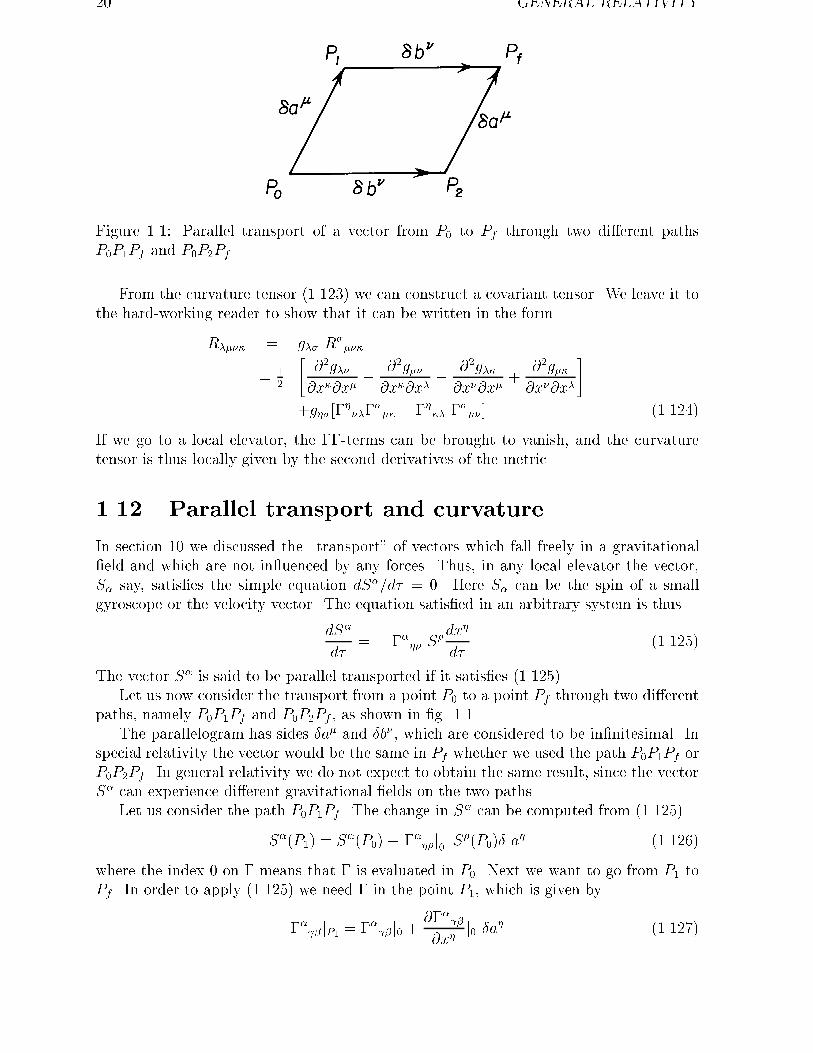
Figure ���� Parallel transport of a vector from P� to Pf through two di�erent pathsP�P�Pf and P�P�Pf
From the curvature tensor ������� we can construct a covariant tensor� We leave it tothe hard working reader to show that it can be written in the form
R��� � g�� R���
� ��
���g���x�x�
� ��g���x�x�
� ��g��x��x�
���g��x��x�
�
�g �)� ���
�� � � � ���� * �������
If we go to a local elevator the �� terms can be brought to vanish and the curvaturetensor is thus locally given by the second derivatives of the metric�
���� Parallel transport and curvature
In section �� we discussed the �transport� of vectors which fall freely in a gravitationaleld and which are not in�uenced by any forces� Thus in any local elevator the vectorS� say satises the simple equation dS��d� � �� Here S� can be the spin of a smallgyroscope or the velocity vector� The equation satised in an arbitrary system is thus
dS�
d�� � �� � S
�dx
d��������
The vector S� is said to be parallel transported if it satises ��������Let us now consider the transport from a point P� to a point Pf through two di�erent
paths namely P�P�Pf and P�P�Pf as shown in g� ����The parallelogram has sides �a� and �b� which are considered to be innitesimal� In
special relativity the vector would be the same in Pf whether we used the path P�P�Pf orP�P�Pf � In general relativity we do not expect to obtain the same result since the vectorS� can experience di�erent gravitational elds on the two paths�
Let us consider the path P�P�Pf � The change in S� can be computed from �������
S��P�� � S��P��� �� �j� S��P��� a �������
where the index � on � means that � is evaluated in P�� Next we want to go from P� toPf � In order to apply ������� we need � in the point P� which is given by
����jP� � ����j� � ������x
j� �a �������
���� THE CURVATURE TENSOR ��
From ������� we have
S��P�� P�� Pf� � S��P��� ����jP� S��P���b� �������
Inserting ������� and ������� in ������� we get to second order
S��P�� P�� Pf� � S��P�������j� � �����
�x j� �a
�nS��P��� ����j� S��P���a
�o�b�
� S��P��� ����j� S��P���b� � �����
�x j� S��P���a
�b�
�����j� ����j� S��P���a� �b� �������
Furthermore S��P�� can be expressed in terms of S��P�� through ������� so we get
S��P�� P�� Pf� � S��P��� �� �j� S��P���a � ����j� S��P���b
�
������
�x j� S��P���a
�b� � ����j� �� �j� S��P���a �b� �������
For the path P�P�Pf we can obtain S��P�� P�� Pf� from the above expression just byinterchange of �a and �b� Subtracting we nd
%S� � S��P�� P�� Pf�� S��P�� P�� Pf� � � R��� S
��P���a �b� �������
where R��� is the curvature tensor dened in eq� ��������
From eq� ������� we see that as expected if there exists a gravitational eld then ingeneral a vector which is parallel transported through two di�erent paths to the samepoint does not acquire the same value�
If on the other hand we assume that the Riemann tensor vanishes then it follows thatS� becomes independent of the path and only depends on the space time point� In otherwords S� is a eld S��x� which satises the di�erential equation �������� This equationsimply means that the covariant derivative of the eld S��x� must vanish� At one pointwe can prescribe a value of S� and the value in any other point �in a domain where R�
��
vanishes� is then obtained by integrating �������� If the curvature tensor vanishes we canalways dene everywhere inertial coordinates ���at coordinates�� by parallel transport�Thus it is necessary and su"cient for a metric g���x� to be equivalent to a �at metric��� that R
���� � � everywhere�
���� Properties of the curvature tensor
The covariant form of the curvature tensor ������� has a number of symmetries which canbe read o� from �������
R��� � � R���
��� �� � �� ��
�������
R��� � � R��� �� �� �������
R��� � � R��� �� � � � �� �������
R��� � � R��� �� �� �������
R��� �R��� �R��� � � ��� �� � permuted cyclically� �������
�� GENERAL RELATIVITY
Eq� ������� is a simple consequence of the commutation rule ������� for covariant deriva tives �the left hand side of ������� is clearly antisymmetric in � and ���
We can form the contracted curvature tensor
R� � g��R��� � R��� �������
which is called the Ricci tensor� Because of ������� it is symmetric
R� � R� �������
The contraction ������� is essentially unique� if we contracted instead the rst two indicesor the last two indices we get zero because of ������� and �������� Contraction of the otherindices leads again to R� because of ������� ������� ������� and ��������
We can make a further contraction in order to get a scalar
R � g� R� � g��g�R��� �������
Contraction of � and � and � and � gives zero because of antisymmetry in these indices�
Apart from the algebraic properties mentioned above the curvature tensor also satisesimportant di�erential identities� These are most easily derived from ������� by going toa local elevator where � vanishes� Di�erentiating R��� with respect to x
one obtainsthird derivatives on the metric as well as � ����x terms� However these terms vanishin the local system� Permuting the indices �� � and � cyclically and adding the threeexpressions one nds that this sum vanishes� In generally covariant language this means
R��� �R�� � �R�� � � � �������
This equation is valid in the local elevators where the covariant derivatives reduce toordinary derivatives and it is generally covariant and hence it holds in all systems�
Remembering that the covariant derivative of the metric tensor vanishes we nd bycontracting � and � in �������
R� � R� �R�� � � � �������
Contracting � and � we get
R �R� � � R�
� � �
and �R�
� �
��� R
��� � �������
Again since the covariant derivative of the metric vanishes we have from �������
�R�� � �
�g��R
��� � �������
It turns out that eq� ������� plays a fundamental role in the theory of general relativityas we shall soon see�
���� THE ENERGY MOMENTUM TENSOR ��
���� The energy�momentum tensor
We now turn to the essential problem facing us� Suppose we are given some distributionof matter e�g� our universe how do we determine the gravitational eld g���x� � So farwe only know how to proceed in the Newton limit �sect� �� where we found �eqs� ������and �������
r� g����x� � � � G���x� �������
where ���x� is the mass density in the limit where all velocities are small relative to thelight velocity�
Eq� ������� suggests that we should attempt to understand how ���x� can be gener alized to arbitrary relativistic velocities� If we can nd this we know how to representsome matter distribution �e�g� in our universe� in terms of special relativity�
Let us consider a simple situation where we have a �ow of matter� In special relativitythe relevant quantity is not the mass density but the energy density �remember the famousformula E � mc��� The proper density ��x� is then dened as the density measured byan observer moving with the �ow� The left hand side of eq� ������� suggests that inmore general situations it should be represented by a tensor with two indices �this tensorshould somehow at least contain second derivatives of the metric tensor�� Thus we shouldattempt to generalize the right hand side to a tensor with two indices which for smallvelocities reduce to the right hand side of eq� �������� In special relativity the �ow ofmatter is characterized by its density and the four velocity U��x� of matter at the pointx�� From this we can construct a tensor with two indices
T ���x� � ��x� U��x� U��x�� U� � dx��d� �������
Let us consider T ��
T �� � �
�dx�
d�
��
� ��
�� v��������
where v is the usual velocity �v � d�x�dx� and where we used the special relativisticrelation between d�� dx� and �v
d� � � �dx��� � �d�x�� � �dx��� ��� �v�� �������
From eq� ������� we see that in the Newton limit v �� � we get T �� � � so eq� �������becomes approximately
r� g���x� � � � G T���x� �������
Recalling that the mass of a small volume of moving material increases by a factor��p�� v� relative to the rest mass and that the volume decreases by a factor
p�� v�
we see that T �� in eq� ������� is the density measured by a xed observer who sees thematter passing by with a velocity �v� Thus T �� is simply the relativistic energy density�The other components are just
T ij � T ji � �vivj�� v�
T i� � T �i �� vi�� v�
�������
The quantity T �� is called the energymomentum tensor �of special relativity�� T �i isthe density of momentum �as seen by a xed observer� and T ij is the current of momentum�
�� GENERAL RELATIVITY
T �� has the property that for closed systems the energy and momentum are conserved�In di�erential form we just have
�T ��
�x��
�
�t
��
�� v�
�� �r
���v
�� v�
�� � �������
which expresses the conservation of a quantity of material with density �����v�� movingwith a velocity �v�x��
We also have
�T ��
�x��
�
�t
��vx�� v�
��
�
�x
��vx
�
�� v�
��
�
�y
��vxvy�� v�
��
�
�z
��vxvz�� v�
�
��
�� v�
��vx�t
� �v �rvx�
�������
where we used eq� �������� Thus
�T i�
�x��
�
�� v�
��vi
�t� �v �rvi
�� � �������
since the quantity in the bracket in eq� ������� is just the change in the velocity for anobserver following the stream of matter and in the absence of any forces this velocitycannot change� Thus we have by combining ������� and �������
�T ��
�x�� � �������
and we say that the energy momentum tensor is conserved� From ������� it follows thatthe total energy momentum P � is conserved because ������� implies that
P � �Zd�x T ����x� t� �������
and hence from �������
dP �
dt�Zd�x
�T ��
�t�Zd�x
�T ��
�x�� � �������
where we used that Zd�x
�T i�
�xi� �
if T i� vanishes at innity� From eqs� ������� and ������� it is easily veried that P �
dened by eq� ������� is indeed a four vector �remember that volume d�x decreases by afactor
p�� v��
The energy momentum tensor ������� represents an extremely simple physical system�A somewhat more useful case can be constructed by considering a perfect �uid whichis dened as a �uid characterized by a velocity eld �v�x� such that an observer movingalong with the �uid sees it as being isotropic around each point� Ideal �uids are oftenused to approximately describe our universe at large scales �much larger than the sizeof galaxies� and hence the energy momentum distribution of such �uids is of particularrelevance in the theory of gravity�
���� THE ENERGY MOMENTUM TENSOR ��
To nd the energy momentum tensor we simply use the rest frame where
�T ���rest � �
�T i��rest � �T oi�rest � �
�T ij�rest � �T ji�rest � p �ij �������
The ���� component is the same as in ������� since �v � � and the result for the �ij� component expresses the meaning of isotropy� Similarly the �i�� components must vanishdue to isotropy� In ������� � is again the proper energy density whereas p is called thepressure�
We can now express T �� in a frame where the �uid moves with velocity �v��x� t�
T �� � p ��� � �p� ��U�U� �������
To see that T �� is correct notice that it is a tensor �in special relativity� and that it reducesto ������� in the rest frame� Conservation of energy and momentum in the di�erentialform �for a closed system�
�T ��
�x�� � �������
leads to the special relativistic equations for an ideal �uid
�v
�t� �vr�v � ��� v�
p� �
�rp� v
�p
�t
�� �������
We recommend the reader to verify this result�To make the above result generally covariant we proceed as done many times before�
The conservation equation ������� becomes replaced by
T ��� � � �������
Using eq� ������ we get�pg
�
�x��pg T ��� � ����� T �� �������
where we can say that the right hand side represents a gravitational force density� Thetotal energy momentum can �tentatively� be written down in analogy with �������
P � �Zd�x
pg T �� �������
which is however not conserved due to the non vanishing of the right hand side of eq��������� Physically non conservation of P � is due to the possibility of exchanging energyand momentum between matter and gravitation� Also P � is not a contravariant vector�
The explicit form of the energy momentum tensor for an ideal �uid interacting withgravity is given by
T �� � p g�� � �p� ��U�U� �������
since T �� is a tensor and since it reduces to ������� in special relativity�The energy momentum tensors constructed above are symmetric T �� � T ��� This is
a general property assumed to be valid in the following�
�� GENERAL RELATIVITY
���� Einstein�s �eld equations for gravitation
We are now able to proceed to present Einstein�s eld equations which were �derived�by plausibility arguments in ���� ��Die Grundlage der allgemeinen Relativit�atstheorie�Annalen der Physik �Leipzig� �� ������ ����� We return to the Newtonian limit whichcan be written as in eq� ������� i�e�
r� g���x� � � � G T���x� �������
The left hand side contains the second derivative of the metric tensor whereas the right hand side is the ���� component of the energy momentum tensor� Thus it is natural togeneralize this equation to
E���x� � � � G T���x� �������
in arbitrary coordinates where the tensor E�� should depend on the metric and its rstand second derivatives� From ������� it is clear that we need to include second derivativesand the reason we do not include higher derivatives is primarily because of simplicity�However such terms would have to be multiplied by a constant with dimension of a powerof length ���g��x� terms would have to be multiplied by some constant with dimensionof length �g��x by �length�� etc��� Looking around among the fundamental constantsof nature there is only one constant with dimension of length the so called Planck length
LP lanck� �
G+h
c��������
Using G�c� � ����� ����� cm$g and +h � ���� erg �s one obtainsLP lanck � �����cm �������
It therefore follows that if the constants of dimension length to a power are present theyare incredibly small and of no relevance for large scale phenomena in our universe� Theycould be relevant in the very early universe which is supposed to be very small �big bang��Due to the occurrence of +h it is clear that quantum phenomena must be involved andhence such terms could be of relevance in quantum gravity� However here we shallproceed to consider only scales which are large relative to ����� cm�
The Einstein tensor E���x� in eq� ������� thus depends on the geometry of space timeand should be linear in the second derivatives of g��� Also it should be a tensor whichrepresents the genuine physical contents of gravitational elds� For this we have only onecandidate� namely the curvature tensor and quantities derived from it� Since E�� has twoindices it should depend on the contracted curvature tensor� Because of the symmetriesof R���� we saw in sect� �� that there is essentially only one such tensor namely R���Could we take
E�� � R�� � �������
The answer is no� In sect� �� it was shown that the energy momentum tensor satisesdi�erential conservation
T ��� � � �������
�Such terms occur in superstring theories �one of which could be the �right� theory of quantumgravity��
�Mathematicians have shown that the curvature tensor is the only tensor that can be constructedfrom the rst and second derivatives of the metric tensor� and which is linear in the second derivativesof the metric tensor�
���� EINSTEIN�S FIELD EQUATIONS ��
Going back go eq� ������� we therefore also have
E��� � � �������
From eq� ������� it follows however that R��� �� � in general� Thus eq� ������� is
wrong��However eq� ������� shows that the right answer is
E�� � c�R�� � �
�g��R� �������
which is covariantly conserved� Here c is a dimensionless constant which we shall x byrequiring that we get the correct Newton limit� In a non relativistic system the pressureterms are much smaller than the energy density so jTijj �� jT��j� Eqs� ������� and������� reduce to
c�R�� � �
�g��R� � � � G T�� �������
Since jTijj �� jT��j we also have that Eij is very small so from �������
Rij � �
�gij R �������
In the weak eld limit to the rst approximation gij � �ij� Thus
R �� Rii �R�� � �
�R �R��
i�e��
�R � R�� �������
Inserting this in ������� we get
E�� � c�R�� ��
�R� � �c R�� �������
Now R�� can be obtained from ������� where the �� terms are of higher order and hencecan be left out in the Newton limit� Thus
R��� � �
�
���g���x�x�
� ��g���x�x�
� ��g��x��x�
���g��x��x�
��������
Since all time derivatives vanish we get
R���� � � � Ri�j� � �
�
��g���xi�xj
�������
so from ������� we get
E�� � �c R�� � �c�Ri�i� � R����� � cr� g�� �������
�It is interesting that the rst eld equation that Einstein published actually was precisely ��������He was aware that it could not be generally valid�
�� GENERAL RELATIVITY
This shows that we obtain eq� ������� provided c � �� Consequently Einstein�s eldequations read
R�� � �
�g��R � � � G T�� �������
This equation can be written in a di�erent form� By contraction we get
R�� � �
���� R � R� �
� � R � �R � � � G T �
�
orR � � G T �
� �������
This can be inserted in eq� ������� and we then get
R�� � � � G�T�� � �
�g��T
��� �������
Eq� ������� is of course fully equivalent to eq� ��������In empty space T�� � � and ������� then gives the vacuum Einstein equation
R�� � � �������
Flat Minkowski space satises this equation globally and locally but in the local casethere are other non trivial solutions �due to the non linearity of eq� ���������
Eq� ������� can be generalized by adding the �cosmological term�
R�� � �
�g��R � g�� � � � G T�� �������
This is allowed from the point of view of covariant conservation of T�� since the covariantderivative of g�� vanishes� However eq� ������� does not satisfy the Newton limit� Thecosmological constant must therefore be rather small and in this chapter we shall ignoreit� However a small which seems to exist has profound cosmological e�ects as weshall see later� It should be noticed that consistency of the Einstein equation �������requires that T�� is symmetric T
�� � T ���To conclude this section we now have a non linear set of second order di�erential
equations ������� which allows one to compute the gravitational eld from a given energy momentum distribution� This is precisely the contents of Einstein�s general relativity�
Remarks on the history of Einsteins eld equations�
In ���� Einstein and Grossmann published a paper where gravity was for the rst timedescribed by the metric tensor and the Ricci tensor was introduced as an important tool�The theory was however not right� Also a later paper from ���� by Einstein containsa treatise of di�erential geometry� The contents of this paper was corrected for technicalerrors by Levi Civita� The �aw in Einstein�s ���� paper �mainly that the covariantconservation of the energy momentum tensor on the right hand side was not correctlyimplemented by the geometrical left hand side as explained above in connection with�������� was corrected in November ���� by Einstein and by the matematician Hilbertwho derived the consistent eld equation from a variational principle� On November ��Einstein submitted a paper which for the rst time gives the correct eld equation� Fivedays before Hilbert had actually submitted a paper which also contained the right eldequation�
���� SPHERICALLY SYMMETRIC METRIC ��
���� The time�dependent spherically symmetric met�
ric
In order to gain insight in Einstein�s equations we shall start by considering a time dependent spherically symmetric gravitational eld g���x�� By this we mean that themetric should be the same when the rectangular coordinates x�� x�� x� are subjected toa rotation� Intuitively this means that the proper time interval can only depend on thefollowing quantities �which are rotationally invariant�
t� r� dt� �xd�x � r dr � �d�x�� � dr� � r��d�� � sin� �d��� �������
where r �px� � y� � z�� Thus
d� � � A�r� t�dt� � B�r� t�dr� � C�r� t�drdt� D�r� t�r��d�� � sin� �d��� �������
In general relativity it is important to realize that the coordinates are arbitrary� Thuswe are free to make transformations x� � x�� in �������� In particular we can alwaystry to select such transformations in a way which simplies the expression �������� Firstthe function D can easily be removed by introducing a new radial variable
r� � rqD�r� t� �������
d� � then becomes dependent on new functions A�� B� and C � which are functions of tand r�� Dropping the primes we can write
d� � � A�r� t�dt� � B�r� t�dr� � C�r� t�drdt� r��d�� � sin� �d��� �������
The �mixed� drdt term can also be removed by resetting our clocks by use of a new timecoordinate t� which is dened by
dt��r� t� � ��r� t�)A�r� t�dt� �
�C�r� t�dr* �������
Here ��r� t� is an integrating factor dened such that ������� becomes a perfect di�erentialwith �A � �t���t���
��C � �t���r� This requires the integrability condition
�
�r���r� t�A�r� t�� � � �
�
�
�t���r� t�C�r� t�� �������
This is a rst order partial di�erential equation for � since A and C are given� Once weare given � at a certain time for all r we can compute it at any other time� Using that
�
A��dt�� � A dt� � C dtdr �
C�
�Adr� �������
the proper time ������� becomes
d� � ��
��Adt�� �
�B �
C�
�A
�dr� � r��d�� � sin� �d���
�It could happen that this transformation produces a constant r�� In the following� for simplicitywe only consider non�trivial transformations �r� const turns out to be inconsistent with the Einsteinequation��
�� GENERAL RELATIVITY
or renaming these functions
d� � � E�r� t�dt� � F �r� t�dr� � r��d�� � sin� � d��� �������
This form of the metric is called the �standard� form of the metric rst derived by Weyl�It should be noted that the transformations used above do not involve the angles andtherefore the spherical symmetry is still manifest�
The metric tensor thus has the form
grr � F � g�� � r� � g�� � r� sin� � � gtt � �E�grr �
�
F� g�� �
�
r�� g�� � �
r� sin� �� gtt � � �
E�������
whereas the determinant g isg � rEF sin� � �������
The invariant volume element is thus
r� sin �qE�r� t�F �r� t� dr d� d� dt �������
If E and F were constants this would just be the usual volume element in sphericalcoordinates�
��� A digression� A simpler method for computing
����
In order to write down the Einstein eld equations we need rst to know the Christo�elsymbols ���� for the metric �������� One method is to use eq� ������ directly i�e� to use
���� ��
�g��
��g���x�
��g���x�
� �g���x�
��������
This is a straightforward but tedious method� A somewhat simpler way consists in ob taining the ��s from a variational principle�
First let us consider some functional F � F �x�� ,x�� where ,x� � dx�����d� anddemand that the trajectory x� � x���� is obtained by requiring the minimum variationof the integral Z
F �x�� ,x��d�
i�e�
�ZF �x�� ,x��d� �
Z�F �x�� ,x��d�
�Z �
�F
�x��x� �
�F
� ,x�� ,x�
�d� � � �������
Now � ,x� � d�x��d� � Requiring that the variations vanish at the ends of the interval ofintegration we obtain by a partial integration
�ZFd� �
Z ��F
�x�� d
d�
�F
� ,x�
��x�d� � �
���� COMPUTING ���� ��
or the Euler Lagrange equationd
d�
�F
� ,x��
�F
�x��������
Now we can easily check that if we take
F � g���x�dx�
d�
dx�
d��������
then the Euler Lagrange equation becomes
�d
d�
�g���x�
dx�
d�
��
�g���x�
�x�dx�
d�
dx�
d��������
Doing the di�erentiation on the left hand side we get
�g���x�
dx�
d�
dx�
d�� g��
d�x�
d� ���
�
�g���x�
dx�
d�
dx�
d�
so after multiplication with g�� we get
d�x�
d� ���
�g��
���g���x�
� �g���x�
�dx�
d�
dx�
d�
�d�x�
d� ���
�g��
��g���x�
��g���x�
� �g���x�
�dx�
d�
dx�
d�� �� �������
where in the last step we used that the names of the summation indices are arbitrary anddx�dx� is symmetric in � and �� From ������� and ������ we see that this is preciselythe equation of motion for a freely falling particle in a gravitational eld specied by themetric g���x��
As a side!remark we mention that use of the Euler Lagrange equation ������� alsoshows that ������� can be obtained from the variational principle
�Z s
g���x�dx�
d�
dx�
d�d� � � �������
We leave it to the reader to verify this statement� Eq� ������� shows that freely fallingparticles follow a curve with the shortest �distance� since the square root times d� in������� is the distance i�e� ������� can be written �
Rd� � �� The curve followed by a
freely falling particle is therefore called a geodesic�To return to the main issue of obtaining the Christo�el symbols we see that eq� �������
ord�x�
d� �� ����
dx�
d�
dx�
d�� � �������
allows one to obtain the ��s from a variational principle using the Euler Lagrange equa tions ������� with F given by �������� In our case the line element ������� therefore leadsto the variational principle
�Z h
E ,t� � F ,r� � r� ,�� � r� sin� � ,��id� � � �������
where ,t � dt�d�� ,r � dr�d�� ,� � d��d� and ,� � d��d� �
�� GENERAL RELATIVITY
���� The Christoel symbols for the time�dependent
spherically symmetric metric
Let us start by applying eq� ������� to the case where x� in the Euler Lagrange equation������� is the time� In that case ������� gives from �������
d
d���E ,t� � ,t�
�E
�t� �F
�t,r� �������
Performing the di�erentiation on the left hand side �remember that E depends on r andt which in turn depends on ��
�E�t� �,t��E
�t� �,t ,r
�E
�r� ,t�
�E
�t� �F
�t,r�
or
�t��
�E
�E
�t,t� �
�
E
�E
�r,t ,r �
�
�E
�F
�t,r� � � �������
From this we get by comparison with ������� the following ��s �remember that mixedterms like ,t ,r occur twice in ��������
�ttt ��
�E
�E
�t
�ttr ��
�E
�E
�r� �trt
�trr ��
�E
�F
�t�������
Next let us use the Euler Lagrange equation ������� for the problem ������� when we varyx� � r
� d
d���F ,r� �
�E
�r,t� � �F
�r,r� � �r ,�� � �r sin� � ,�� �������
Proceeding as before we perform the d�d� on the left hand side and obtain
�r ��
F
�F
�t,t ,r �
�
�F
�F
�r,r� �
�
�F
�E
�r,t� � r
F,�� � r
Fsin� � ,�� � � �������
Comparing with ������� we see that
�rtr � �rrt ���F
Ft
� �rrr ��
�F
�F
�r
�rtt � ��F
Er
� �r�� � � rF
� �r�� ��r sin� �
F�������
Proceeding now with the variable � we get �since E and F are independent of ��
� d
d���r� ,�� � ��r� sin � cos � ,�� �������
which gives
�� ��
r,r ,� � sin � cos � ,�� � � �������
��� THE RICCI TENSOR ��
i�e�
��r� � ���r ��
r� ���� � � sin � cos � �������
Finally we need only to vary �
� d
d���r� sin� � ,�� � � �������
or
����
r,r ,�� �
cos �
sin �,� ,� � � �������
Hence the only remaining non vanishing Christo�el symbols become
��r� � ���r ��
r� ���� � ���� �
cos �
sin ��������
The reader can now make a psychological experiment where he$she compares the time ittakes to obtain the ��s by means of the variational principle and by the direct applicationof the expression �������� This would also provide a check of the correctness of the results������� ������� ������� and ��������
���� The Ricci tensor
In order to study the Einstein equation ������� or ������� we need to know the Riccitensor R�� � From eqs� ������ ������� ������� we have
R� ��
�
�� ln g
�x��x� ����
�x�� � �� �
� �
�
�� �
� ln g
�x �������
Inserting the ��s found in the last section as well as g given by eq� ������� we get thefollowing non vanishing components of the Ricci tensor
Rrr ��
�E
��E
�r�� �
�E�
��E
�r
��
� �
�EF
�E
�r
�F
�r
� �
rF
�F
�r� �
�E
��F
�t��
�
�E�
�E
�t
�F
�t�
�
�EF
��F
�t
��
R�� � �� � �
F� r
�F �
�F
�r�
r
�EF
�E
�r
Rtt ����F
��E
�r��
�
�F �
�E
�r
�F
�r� �
rF
�E
�r
��
�EF
��E
�r
��
��
�F
��F
�t�� �
�F �
��F
�t
��
� �
�EF
�E
�t
�F
�t
Rtr ���rF
�F
�t
R�� � sin� � R�� �������
�� GENERAL RELATIVITY
Thus given some energy momentum tensor T�� we can in principle obtain second orderdi�erential equation for the metric functions E and F by use of e�g� eq� �������
R�� � � � G �T�� � �
�g��T
��� �������
For example�
rF
�F
�t� � G Ttr �������
etc� etc�
��� The Schwarzschild solution
We shall now consider the case where space is empty except for a mass M situated atr � �� Thus except for r � � we must satisfy the vacuum Einstein equations R�� � ��Using ������� we see that this implies that the time dependence drops out� From Rtr � �we get that F is independent of time and it is then easily checked that all the timederivatives drop out of the other R�s� From the last eq� ������� it follows that we onlyneed to consider Rrr � R�� � Rtt � �� It is seen that Rrr and Rtt contain rather similarterms� Therefore we form
Rrr
F�Rtt
E���rF
��
F
�F
�r��
E
�E
�r
�� � �������
This gives� lnF
�r� �� lnE
�r�������
orE�r� t� F �r� � f�t�� �������
We now impose the boundary condition that the metric ������� should become �atMinkowski at innity so the function f�t� in ������� is xed to be � for r � andhence also for all other r�s� Thus
E�r� ��
F �r��������
Now we can take R�� and Rrr to vanish �because of ������� Rtt then vanishes auto matically�� Using the result ������� we get
R�� � �� � E�r� � rdE�r�
dr�������
Rrr ��
�E�r�
d�E�r�
dr��
�
rE�r�
dE�r�
dr
��
�rE�r�
d R���r�
dr�������
Thus if R�� � � then Rrr is automatically zero� Hence from R�� � � we get
d
dr�rE�r�� � � �������
���� BIRKHOFF�S THEOREM ��
sorE�r� � r � constant � r � C �������
From ������� we then know the functions E�r� and F �r� in terms of the constant C whichcan be xed by means of the results g�� � �� � �GM�r obtained in the Newton limitsee eqs� ������ and �������
Thus from ������� we get C � ��MG and hence
E�r� � �� �MG
r
F �r� ��
�� �MGr
�������
and the metric ������� becomes
d� � ���� �MG
r
�dt� � dr�
�� �MGr
� r��d�� � sin� �d��� �������
This is the Schwarzschild solution� The radial variable r has the property that the solutionis asymptotically �at� Furthermore the solution is singular at r � � as one would expectbecause of the presence of the mass� This singularity can be shown to be physical sincee�g� the scalar R����R
���� is singular only at r � �� For an elaboration of this featuresee sections ���� and �����
Remarks on the history of the Schwarzschild solution�
Karl Schwarzschild was a well known astronomer who had wide interests in allbranches of physics and mathematics� When the war started in August ���� he enteredmilitary service where he calculated missile trajectories in France and later in Russia�Here he worked out his solution �explained above� of the newly proposed Einstein eldequation� He send his paper to Einstein who replied� �I had not expected that onecould formulate the exact solution of the problem in such a simple way�� Schwarzschildcontracted an illness while in Russia� After having returned to Berlin in March ���� hedied two months later at the age of �� years�
���� Birkho�s theorem
We saw from Rtr � � that the function F is time independent and all time derivativesdisappeared� In principle the function E could depend on time
E�r� t� � f�t���� �MG
r
��������
but f�t� can be removed by a redenition of time t� t� where
t� �Z t q
f�t� dt �������
Thus the Schwarzschild metric ������� always results and we have Birkho��s theoremsaying that a spherically symmetric gravitational eld in empty space must be static witha metric given by the Schwarzschild solution�
�� GENERAL RELATIVITY
This theorem is similar to Newton�s result that the gravitational eld outside a spher ically symmetric mass distribution behaves af if the mass was concentrated in the centre�It is a priori far from obvious that the similar result applies in general relativity wherethe body needs not be static� A non static body can in general emit gravitational waves�However Birkho��s theorem shows that no gravitational radiation can escape from aspherical body into empty spaces�
Birkho��s theorem can also be applied if we have a spherical cavity in a spherical massdistribution� In this case there is no mass at the center and hence GM � � and themetric is just �at Minkowski� Thus if e�g� the universe was a spherical mass distributionthe metric would be �at and gravitation would have no e�ect in a spherical cavity�
���� The general relativistic Kepler problem
We shall now discuss some implications of the Schwarzschild solution ������� for the solarsystem� In ������� it appears that there is a singularity for a radius r � �MG whichis called the Schwarzschild radius� We shall discuss this phenomena later� Here we onlyremark that for the sun �M�G � ���� km which is deep in the solar interior� Hence thisapparent singularity is not relevant for the solar system since the solution ������� is onlyvalid outside the massive bodies �for the earth the Schwarzschild radius is � � cm��
In eqs� ������� ������� ������� and ������� we have written down the equations ofmotion� Using that E and F can be taken to be time independent and using the result������� we get
d
d��r� ,�� � r� sin � cos � ,�� �������
d
d��r� sin� � ,�� � � �������
d
d�
���� �MG
r
�,t�� � �������
where the dot denotes di�erentiation with respect to � � We also have an equation for �rwhich we replace by the line element �������
� ���� �MG
r
�,t� � ,r�
�� �MGr
� r�� ,�� � sin� � ,��� �������
Here we assumed that the particle is not a photon since for a photon d� � �� We shallreturn to the photon case later�
We thus have four equations for the four functions t���� r���� ����� ���� so we canstudy planetary motion by solving these equations� A great simplication occurs becausethis motion lies in a plane� It is easy to see that if we x � at some initial value of � then� will be xed to the same value for all other � �s� Taking e�g�
� �
��������
for some � � �� and ,� � � for � � �� then eq� ������� implies that this remains true forall � � Eq� ������� can then be integrated
r� ,� � H �������
���� THE KEPLER PROBLEM ��
where H is a constant of integration� Also eq� ������� gives
��� �MG
r
�,t � L �������
where L is another constant� Substituting these results into ������� we get
� �L�
�� �MGr
� ,r�
�� �MGr
� H�
r��������
In applications to orbital motion we are interested in the shape of the orbit and we wouldtherefore like to know r as a function of � instead of � � We have
r� � dr
d��
,r
,��������
From ������� we thus have
,r � ,�r� �H
r�r� �������
Inserting this in ������� we get
�� �MG
r� L� � H�
rr�� � H�
r�
��� �MG
r
��������
which is a di�erential equation for r � r����In the classical Kepler problem it is convenient to introduce the new variable
u ��
r�������
It turns out that this substitution is also convenient in general relativity� From �������we have r� � �u��u� and eq� ������� gives
�� �MGu � L� �H�u�� �H�u���� �MGu� �������
which can be solved for u�
u�� �L� � �H�
��MG
H�u� u� � �MGu� �������
This gives the exact result
� � �� �Z u
u�
duqL���H� � �MG
H� u� u� � �MGu��������
The integral is of the elliptic type and ������� gives � � ��u� so the inverse function�
provides us with u � u��� � ��r���� However in practice this elliptic integral is notvery useful� Although it can easily be evaluated numerically using e�g� Mathematica the
�One can express u or r as functions of � by inverting the integral ������� by means of Weierstrass� p�
function �� MG�r
��������const��� where the Weirstrass invariants are given by g�
���� M�G�
H� � g� �
���� M�G�
�H� � M�G�L�
�H� � For more discussion of this solution� see E� T� Whittaker� A treatise on the
analytical dynamics of particles and rigid bodies� Cambridge University Press ������� pages ��������
�� GENERAL RELATIVITY
main work is to express the constants L�H in terms of quantities that are measured bythe astronomers�
To orient ourselves in this mess let us notice that the term �MGu� under the squareroot is expected to be very small relative to e�g� the u� term since �MGu � �
���� is the
Schwarzschild radius divided by the �average� planetary radius� As a matter of fact ifwe did not have this term the result ������� would be the Newtonian result except thatthe constant H in ������� would be related to the usual time �not the proper time�� Thissuggests that we expand the integral �approximately� around the Newtonian solution�
To do this systematically we notice that in the motion around the sun the orbit reachesa maximum �minimum� distance called the aphelia �perihelia� wherer � r��r�� with dr�d� � � i�e� for u � u� we also have du�d� � �� Eq� ������� thengives
u�� �L�
H���� �MGu��� � �
H��������
which determines the integration constants L and H in terms of u� which are knownfrom astronomical observations� This is a third order equation� To simplify the analysiswe expand to second order
u�� �L�
H��� � �MGu� � �M
�G�u��� ��
H�� �� �������
Subtracting these two equations for u� and u� we get
� � �u� � u��
�u� � u� � �MG
L�
H��� � �MG�u� � u���
�
or
�MGL�
H�� u� � u�� � �MG�u� � u��
�������
The result ������� can be written
��r� � ��r�� �Z ��r
��r�
dup�� �MGu
�L�
H���� �MGu�� u� � �
H�
�� �
�
�������
where � is measured from the perihelia� To proceed we expand
�
�� �MGu� � � �MGu� �M�G�u� � � �������
so
L�
H���� �MGu�� u� � �
H�� L� � �
H���MGL�
H�u� �
�M�G�L�
H�� ��u��������
� C�u� � u��u� u��
The last form follows from the fact that the left hand side is approximately a second orderpolynomial in u which vanishes for u � u� according to eq� �������� Consider the termlinear in u in ������� with coe"cient C�u�� u��� It should equal �MG L��H� accordingto the left hand side of eq� �������� Hence
C�u� � u�� � �MGL�
H��
u� � u�� � �MG�u� � u��
���� THE KEPLER PROBLEM ��
where eq� ������� has been used� Thus
C � �� �MG�u� � u��� �������
Inserting this in ������� we get
��r�� ��r�� ��� �MG
��
r���
r�
�� Z �
r
�
r�
�� �MGu� duq�u� � u��u� u��
�������
where the constant factor outside the integral comes from expanding ��pC� The integral
can be performed trivially by making the substitution
u ��
r��
��u� � u�� �
�
��u� � u�� sin� �������
and we get
��r�� ��r�� �
�� �
�
�MG
��
r���
r�
���� �
��� �
�MG
��
r�� �
r�
�cos� �������
Now when r goes from r� to r� it follows from ������� that � goes from � � � �� to� � ��� The total charge in � per revolution is thus �j��r�� � ��r��j� For an ellipsethis equals � so the perihelia precesses an amount %� where
%� � �j��r��� ��r��j � � �������
Thus
%� � � MG
��
r���
r�
�radians$revolution� �������
For Mercury this gives %� � �������� per revolution� In each century Mercury makes ���revolutions and observations go back to ����� From general relativity we thus have
%� � ������ per century �������
whereas observational data give
�%��obs � ������ �����per century �������
This is the most important experimental verication of general relativity since it is sen sitive to the second order expansion of g��� It should be pointed out that due to pertur bations from other planets and due to the rotation of the earth Newtonian gravity alsogives a precession of Mercury
�%��Newton � �������� ����� �������
whereas the actual observation gives
�%��Totobs � �������� ����� �������
so the value ������� is obtained as the di�erence �%��obs � �%��TOTobs � �%��Newton� Onemight feel unhappy about the subtraction of two large numbers because small systematicerrors may in�uence ������� quite considerably� Some discussion of this point has beenmade in the literature� However nobody has found any convincing evidence against theresult ��������
�� GENERAL RELATIVITY
���� De�ection of light by a massive body
So far we have considered the gravitational e�ects for a massive body moving around thesun� Now we wish to nd these e�ects for light which is characterized by d� � � �i�e�velocity of light is always one in the freely falling elevators�� Therefore we cannot divideby d� as we did in the previous section�
Let us consider the free motion along a curve described by x� � x��p� where p issome parameter� Proceeding as in section ��� the equivalence principle leads to
d�x�
dp�� ����
dx�
dp
dx�
dp� �� �������
since light moves in a straight line in the freely falling elevators� Changing to anotherparameter p� q with p � p�q� and q � q�p� we obtain
d�q
dp�dx�
dq�
�d�x�
dq�� ����
dx�
dq
dx�
dq
��dq
dp
��
� � �������
Thus we see that we get again the geodesic equation of motion if and only if d�q�dp� � �i�e� if q is a linear function of p� It therefore follows that the form of the geodesicequation remains only if we make linear transformations of the parameter so we cantake d� � � constant � dp� and use p as another parameter� For a photon one then hasd��dp � � i�e� the constant of proportionality vanishes� The equations of motion in thelast section should therefore be replaced by similar equations with � replaced by p�
In most equations this change only leads to trivial alterations� However eq� �������now becomes
� ���� �MG
r
��dt
dp
��
��drdp
��� �MG
r
� r�
���d�
dp
��
� sin� �
�d�
dp
���� �������
since d� � �� Thus introducing again integration constants as in eqs� ������� and ��������with � ,�� d��dp and ,t� dt�dp respectively� we get
� � L� � H�
rr�� � H�
r�
��� �MG
r
��������
Proceeding as in sect� �� we get the solution
��r� � ��r�� �Z ��r
��r�
duqL�
H� � u���� �MGu��������
which is again a elliptic integral which should be expanded�Let us consider a light ray passing the sun� The radial variable r originates at the sun
and measures the distance to the light ray� At the point of closest approach r � r� onehas dr�d� � � �r��� has its minimum� so from ������� we get
L� �H�
r��
��� �MG
r�
��������
���� DEFLECTION OF LIGHT ��
Thus
��r� � �� � �Z ��r
�
duqu����� �MGuo�� u���� �MGu�
� �� � �Z ��r
�
duqu�� � u�
�� �MG
u�� � u�
u�� � u�
��������
Using
u�� � u�
u�� � u�� u�
u��u� � u
we get
��r� � �� � �Z ��r
�
duqu�� � u�
�� �MGu�
MGu�� � u
u�
� �
� �� � � sin���u
u�
��MGu�
����
s�� u�
u���vuut�� u�u�� � u�u�
A� �������
Now r � ��u goes from to r� and then goes from ro to � The total change in � is�j��r����� �j because of the symmetry of the problem� Half of the bending takes placebefore the passage of r � r� and the other half after the passage of this point� If therewas no de�ection this would be so the de�ection is %� � �j��r����� �j � � Hencefrom ������� we get
%� ��MG
r��������
For the sun we get with r� � the solar radius �� ����� ��� km�
%� � ����� �������
A recent observational value is ����������� in good agreement with �������� The quantity%� was rst observed in ���� and the excellent agreement with ������� brought Einstein�sgeneral relativity into the newspapers� However %� is in general very di"cult to measurewith high precision� The precession of perihelia in sect� �� is far more accurate bothfrom an experimental and a theoretical point of view�
Instead of using the sun as the lense one can obtain much more spectacular e�ects byuse of galactic lenses� We shall not discuss the details but the principle is quite simple�Suppose we consider a source which is positioned in such a way that it lies on an straightline passing through the center of a galaxy to an observer� Just like in the case of thesun light passing to the observer will be bend by the galaxy� Because of the very specialgeometry there is cylindrical symmetry� Thus if we take the source galaxy observer lineto be the z axis the bending will result in an e�ect which is rotationally invariant in the�x� y��plane� Therefore the observer will see a circle �where the maximal intensity is�around the galaxy� Such a circle is called an Einstein Ring since it was rst predictedby Einstein himself� If the geometry is not so symmetric the ring degenerates to one ormore arcs� These phenomena have been neatly observed�
�� GENERAL RELATIVITY
���� Black holes
As already mentioned the Schwarzschild solution looks singular for r � �MG� In oursolar system this seems not to be relevant� However it could be that somewhere in ouruniverse there exists an object which is so small that r � �MG could be reached� Thequestion is then what happens at the Schwarzschild radius�
We know from Birkho��s theorem shown in sect� �� that outside a �possibly time dependent� spherically symmetric object Schwarzschild�s solution is valid� Let us considerradial motion where r and t are functions of proper time � � Since ,� � � we have from������� ������� and ������� that H � � and
,t �L
�� �MGr
,r� � L� ���� �MG
r
��������
Now let us consider a particle originating at large distance r � where space is �at�Minkowski� and special relativity is valid� In the asymptotic system let the clock bechosen such that dt�d� � � for r � � Then L � � and hence
,t ��
�� �MGr
,r� ��MG
r�������
Now we have two times� the proper time � is the one measured by an observer fallingfreely in the gravitational eld and the time t is the time measured by an observer atrest at large distances where space is �at� From the second equation ������� we get sincepr ,r � �p�MG �r decreases with ��
�
�p�MG
�r��� � r���� � � �� � � �������
with r � r� for � � ��� The solution ������� is valid as long as we are outside the bodyso if the radius of the body is less than �MG it follows from ������� that the freely fallingobserver passes the Schwarzschild radius without observing any singularity� If the massis just a point mass this observer reaches r � � in a nite proper time
�r�� � �� ��
�p�MG
r���� �������
Incidentally it should be noticed that this conclusion could have been reached without anycalculations since the second equation ������� is the same as one would obtain in Newtongravity �why�� except that there proper time is replaced by Newton time� Howevermathematics does not care about the time variable it cares only about the di�erentialequation so from everyday intuition ��Newton gravity� we know that the point r � �would be reached in a nite time�
Let us now consider this motion from the point of view of the observer at rest at largedistances from the massive object� From ������� we have
dr
dt�,r,t� �
s�MG
r
��� �MG
r
��������
���� BLACK HOLES ��
This di�erential equation can be solved exactly without any problem� However it is moreinstructive to consider the two cases where r is much larger than the Schwarzschild radiusor where r � �MG� In the rst case we can use �MG�r � � and hence ������� becomesapproximately the same as the proper time result� Hence at large distances there isapproximately no di�erence between the proper time and the asymptotic time which isof course quite reasonable� For r � �MG the situation is quite di�erent� Here eq� �������gives to a good approximation
dr
dt� � �
r
s�MG
r�r � �MG� � ��
�MG�r � �MG� �������
with the solution
r � �MG � constant� e�t
�MG �������
Thus we see that from the point of view of the asymptotic observer the Schwarzschildradius is never reached �it takes an innite time to get there��
This feature can be put into perspective if we think of the asymptotic observer as ahuman being on this earth who observes a distant spherically symmetric body by sendinga test body towards it and compare this with the situation as seen by an observer insidethe test body� Seen from earth it takes an innite time for the test body to get to theSchwarzschild radius and during this time the entire evolution of the universe happens�However the observer in the test body reaches the Schwarzschild radius in a nite time�on his watch� and then he proceeds� He thus sees what happens after t � �on ourclock�#
A body which collapses to a sphere with radius equal to the Schwarzschild radius iscalled a black hole� The reason for this is that no particles �including photons� can beemitted from the surface� To give a full discussion of black holes one needs also to solvethe Einstein equations inside the mass distribution which turns out to be a relativelycomplicated task which we shall not attempt� However the blackness is clear from������� since if we reverse the time direction it follows that a particle emitted from thesurface r � �MG would require an innite time t to reach us� For light d� � � so radialmotion of light satises �
�� �MG
r
�dt� � dr�
�� �MGr
� �
i�e� �����drdt����� � �� �MG
r�r � �MG� �������
so the velocity of light seen from the asymptotic system approaches zero as r � �MG �#��Comparing with eq� ������� we see that if light should reach us from the Schwarzschildradius an innite time would be needed so this can never happen� The body is black�Thus if a body shrinks to its Schwarzschild radius it disappears from our view� Sinceg�� is zero for r � �MG it follows from the discussion ������ ������������ that there isan innite red shift� Therefore the shrinking body fades out of sight� The Schwarzschildradius is called the horizon of the black hole for obviuos reasons�
Do black holes exist� The stability of a star is determined by the balance betweenthe pull of gravity and the pressure from radiation emitted by nuclear fusion� When thelight nuclei have been used up the fusion ceases and the gravitational pull may win�

�� GENERAL RELATIVITY
This requires masses larger than the mass of our sun which will not end up as a blackhole� In some cases it can happen that the radius asymptotically approaches �MG �fromabove� and a black hole can be formed� There is now much observational evidence for theexistence of black holes� For example one can observe a star which moves around a pointfollowing Kepler�s laws� However in the point nothing is observed� This point is thereforeexpected to be a black hole� Also X ray radiation from falling charged particles has beenobserved� Quite recently ������ it seems as if the existence of the horizon has been directlyobserved near the black hole candidate Cygnus XR �� One tracks the ultraviolet emissionfrom hot clumps of gas circling XR �� In two cases the signature of the emission dimsrapidly before disappearing as it dips below the horizon� The light dims as it is stretchedby gravity to ever longer wavelengts in accordance with what we saw above� We refer tothe literature for a discussion of these interesting questions�
We end by some historical remarks� Black Holes were predicted from Newtoniangravity by Laplace �r�� in ���� in a paper entitled �Proof of the theorem that theattractive force of a heavenly body could be so large that light could not �ow out of it��The argument is quite simple� Let us consider light as consisting of particles with mass ��ultimately you can take the limit �� � since the result is independent of ��� In modernterminology we would call � the photon mass� At the time when Laplace did his workthere were the competing theories of light namely that it has a wave nature �Fresnel andothers� or it has a particle nature �Newton�� We know now that both pictures are rightin a duality sense� Anyhow consider a spherical body with mass M and let us try toshoot a particle with mass � away from this body� The condition for escape is that thekinetic energy exceeds the gravitational energy so
�
��v� � G�M�r� �������
Thus after division by � we see that the critical radius is given by
rcrit � �GM�v�� �������
Here Laplace mentions that v is the velocity on the surface of the body� In general it candepend on r but if we assume that v � c which we have taken to be one the criticalradius is just the Schwarzschild radius# Thus Laplace correctly predicted the existence ofblack holes which is a most remarkable historical fact�
���� Kruskal coordinates
The Schwarzschild radius appears as a singularity in the metric� To investigate whetherthis is a real singularity or whether it has been induced by our choice of coordi nates we should compute some invariant quantity� One obvious choice is given byR���� R���� �invariant� The diligent reader can verify that for the Schwarzschild so lution one gets R���� R
���� � ��M�G��r�� Thus this invariant is completely regular forr � �MG and is only singular for r � �� This singularity is physically reasonable sincethe point mass is situated at r � ��
Motivated by the remarks above one may then ask if it is possible to nd new coordi nates without any singularity at r � �MG but singular for r � � �in this connection itshould be remembered that in general relativity the coordinates are arbitrary�� These new
���� KRUSKAL COORDINATES ��
coordinates were found by Kruskal in ���� and we shall motivate them in the following�Since the angular coordinates are not changed we shall consider only the quantity
ds� ���� �MG
r
��B�dt� � dr���� �MG
r
�CA
���� �MG
r
��dt� dr
�� �MGr
��dt �
dr
�� �MGr
�� �������
It is natural to try to �absorb� the singular factor associated with dr� by a new variable�To this end we notice that
dr
�� �MGr
� d�r � �MG ln
�r
�MG� �
��� �������
where we have taken r � �MG� We then have
ds� ���� �MG
r
��dt� dr � �MGd ln
�r
�MG� �
���dt� dr � �MGd ln
�r
�MG� �
���
�������This suggest that we introduce new variables v� by
t� r
�MG� ln
�r
�MG� �
�� v��
t� r
�MG� � ln
�r
�MG� �
�� v�� �������
From eq� ������� it follows that the trajectory of light moving radially in a Schwarzschildblack hole is given by v� � � or v� � �� The metric in the new variables becomes
ds� � ��M�G���� �MG
r
�dv�dv�� �������
This form of the metric still has a one way membrane for r � �MG because of the bracketon the right hand side� To remove this factor by another change of coordinates we noticethat from ������� it can be written in the two forms
r
�MG� � � ev� e
t�r
�MG � ev� e�t�r
�MG � �������
Multiplying these two expressions together gives
�r
�MG� �
��� ev��v� e�
r
MG � �������
Thus ������� becomes
ds� � ��M�G�
re�
r
�MG e�
��v��v�� dv�dv�� �������
Thus the unwanted factor �� �MG�r can be removed by the substitution
�
�e�
�v�dv� � ds�� �������
�� GENERAL RELATIVITY
which amounts tov� � � ln s� �������
with �use ��������
s�s� ��
r
�MG� �
�er��MG�
s�s�
� et��MG� �������
The metric then becomes
ds� � ���M�G��
re�r��MGds�ds�� �������
which is singular only at r � � in agreement with the fact that the Riemann tensor issingular only in this point� In this metric r should be considered as a function of s��Usually this metric is written in terms of still other variables
s� � t� � r�� s� � r� � t�� �������
The metric then takes the nal form
d� � � ��M�G� �
re�r��MG�dt�� � dr���� r�r�� t����d�� � sin� �d���� �������
where
t�� � r�� � ��
r
�MG� �
�er��MG �all r��
t�
r�� tanh
t
�MG�for r � �MG��
t�
r�� coth
t
�MG�for r � �MG�� �������
as is seen from eq� �������� Here we have left it as an excersise for the reader to do theabove calculations for the case r � �MG� It turns out that the nal result is the oneexhibited in �������� Alternatively we can continue the expression ������� analyticallyfrom r � �MG to r � �MG�
In the Kruskal form of the metric ������� the variable r� in front of the angular termsis an implicit function of t�� r� given by �������� The same is true for the factor in frontof �dt�� � dr��� in ��������
From ������� we see that the lines of constant r� t are formed by a set of hyperbolasintersected by the lines t� � r� tanh�t��MG� in the t�� r� plane� The singular point r � �is mapped to the hyperbola t�� � r�� � � and the horizon is mapped to the degeneratehyperbola t���r�� � � consisting of two straight lines� It should be noticed that ������� hastwo solutions for given t� r corresponding to the two branches of the hyperbolas� Thesetwo solutions are bounded by the r � � hyperbola t�� � r�� � �� The solutions lead to thesame metric� One class of solutions can be identied with the standard asymptotically �atuniverse introduced originally in the discussion of the Schwarzschild solution� The secondclass of solutions correspond to the same metric and is a �ghost� universe� These twouniverses are related through the Kruskal variables and they are said to be �connected�by a Schwarzschild �throat�� This �connection� is not physical since once a test body isinside the horizon it will always hit the point mass�
Let us consider a light ray travelling radially in the r� coordinate� From ������� wesee that it has the equation of motion jdr��dt�j � � corresponding to a velocity of lightequal one� If we study this in the old coordinates r� t we see from ������� that the light
PAINLEVE COORDINATE ��
ray starts at some nite t with r � �MG then travels towards r � �MG correspondingto t � and crosses the line t � and goes into the interior of the horizon� In thiscontinued motion r decreases and most remarkably t also decreases� This means that tis not a good time variable inside the horizon�
If the ray is emitted from the inside of the horizon it will travel through increasing r�sbut t is decreasing� When the ray crosses the horizon t � � � The motion measuredin the asymptotic time t is thus time reversed�
���� Painlev�e�s version of the Schwarzschild metric
The Kruskal form of the Schwarzschild metric discussed in the previous section issomewhat complicated� Here we shall present a much simpler transformation of theSchwarzschild coordinates which has no singularity for r � �MG� It was originally foundby Painlev�e ������ who used these coordinates to criticize Einstein gravity for allowingthe singularities to come and go# As we know this is a result of the coordinates beeingarbitrary in general relativity so one ask for some scalar quantity ��x� where a singularitycannot be transformed away due to ���x�� � ��x� under x� x�� Such a scalar was givenin the beginning of the last section � � R���� R
���� � ��M�G��r�� This shows thatthere is no singularity in r � �MG�
To go back to Painlev�e we start from
d� � ���� �MG
r
�dt� � dr�
�� �MGr
� r�d��� �������
where d�� represents the angular part of the Schwartzschild metric which is not changedin the following� A new time t� is introduced by the equation
dt� � dt�
s�MG
r
dr
�� �MGr
� �������
The variable r is unchanged� Integrating eq� ������� we obtain
t� � t � �p�MGr � �MG ln
pr �p�MGpr �
p�MG
� �������
where r � �MG� For r � �MG a similar �real� expression is valid�Inserting eq� ������� in the metric ������� we get after some simple algebra
d� � ���� �MG
r
�dt�� � �
s�MG
rdrdt� � dr� � r�d��� �������
Thus we see that the dr��term in the new coordinates is not associated with a singularityin accordance with the fact that r � �MG is not a singularity of the theory�
We still have g�� � � for r � �GM so at the horizon light is innitely red shifted�Thus some charged matter falling towards the center and therefore emitting radiation willbe observed to produce ever increasing wave lenghts and will ultimately be unobservable�
From eq� ������� or
,t� � ,t�
s�MG
r
,r
�� �MGr
� �������
�� GENERAL RELATIVITY
where a dot means derivative with respect to proper time � we obtain by use of eq��������
,t� ��
�� �MGr
� �MG
r
�
�� �MGr
� �� �������
This shows that for a freely falling test person the proper time observed by him �equiva lence principle#� is equal to the Painlev�e time t� �plus a possible constant� t� � ��const�Measured on a �star clock� �t�� the observer will reach the horizon in a nite time however if he communicates with us by means of radiation this will get out of range forour detectors at large distance when r� �MG##
��� Tidal forces and the Riemann tensor
So far we have discussed a point observer falling towards the black hole� However ifthe observer has an extension tidal forces will occur� In this section we shall study thise�ect in details� Let us consider the separation between two nearby geodesics i�e� thetrajectories of two freely falling observers
x���� and x���� � �x����� �������
These two coordinates can be thought of as the head and feets respectively of a freelyfalling observer �assuming that this observer is quite elastic so that head and feets canmove freely�� Let us consider the covariant derivative of �x���� where this derivative wasintroduced in eq� ������ i�e�
D�x�
D��
d�x�
d�� �����x��x
� dx�
d�� �������
This is a vector since the coordinate di�erence �x� is a vector� We want to nd thetidal �force� so inspired by Newtonean mechanics we take the second derivative of thecoordinate di�erence i�e�
D
D�
D�x�
D��
D
D�
�d�x�
d�� �����x��x
� dx�
d�
�� �������
To simplify life we go to a freely falling elevator where the Christo�el symbols �but nottheir derivatives� vanish in x� so
D
D�
D�x�
D��
d
d�
�d�x�
d�� �����x��x
� dx�
d�
�� � �
d��x�
d� ��������x�
dx�
d�
dx�
d��x�� �������
The two neighbouring geodesics ��head� and �feets�� satisfy
� �d�x�
d� �� �����x����
dx�
d�
dx�
d��
d�x�
d� ��������
and
� �d��x� � �x��
d� �� �����x��� � �x����
d�x� � �x��
d�
d�x� � �x��
d�
�d�x�
d� ��d��x�
d� �� �x�
������x����
�x�dx�
d�
dx�
d��O���x���� �������
TIDAL FORCE FROM SCHWARZSCHILD ��
in the freely falling elevator in x�� Subtracting the two equations we get
d��x�
d� �� ���
����x����
�x��x����
dx�
d�
dx�
d�� �������
Inserting this in eq� ������� we obtain
D
D�
D�x�
D��
�������x�
� ������x�
�dx�
d�
dx�
d��x� � R�
���dx�
d�
dx�
d��x�� �������
Here we used the expression for the Riemann tensor in freely falling coordinates� Howevereq� ������� is valid in any coordinate system since the left hand side is a vector and theproduct of the last three factors on the right is a tensor� Hence the rst factor on theright must be the Riemann tensor in any frame of reference�
The result is thus that the tidal force on an extended observer i�e� the second deriva tive of the di�erence between head and feets is given by the Riemann tensor�
We can actually demonstrate that the acceleration ������� can be interpreted as thefour acceleration of a particle moving along the geodesic x� � �x� as seen by an observermoving along the geodesic x� so it is the acceleration of the feets seen from the head�
First we have to realize that a freely falling observer will claim that a vector eld V �
say which is dened along his geodesic �path of motion� is constant if it is carried intoitself by parallel transport i�e� if �remember that the D�D��derivative is just the d�d��derivative in the freely falling system located at x��
DV �
D�� �� �������
Thus in forming time derivatives she$he will compare the actual change �V � with thechange for a parallel transported vector and thus consider the derivative
�V � � �V �parallel transport
d��
DV �
D�� �������
Now given the position vector �x� of the neighbouring particle �the distance to the feetsseen from the head� he will dene the velocity vector �the velocity with which the feetsmove away#�
D�x�
D�� V ����� �������
and by use of ������� the acceleration of feets seen from head is therefore precisely
a���� �DV �
D��
D
D�
D�x�
D�� �������
The above result ������� is completely general� In the next section we shall see whathappens to the tidal force for a Schwarzschild black hole�
���� The Tidal force from the Schwarzschild solu�
tion
Let us consider the metric given by the Schwarzschild solution� An observer is in free falltowards the center following a geodesic t � t��� and r � r��� in the standard coordinates�
�� GENERAL RELATIVITY
At time � � �� he$she passes the point P� � �t�� r��� The coordinates in the freely fallingsystem around P� are denoted �t
�� r��� The freely falling coordinates should be Lorentzianaccording to the principle of equivalence� Using that the metric transforms as a tensorwe have the conditions
� � � gt�t��P�� �
��t
�t��P��
��
gtt�P�� �
��r
�t��P��
��
grr�P��� �������
� � gt�r��P�� ��t
�t��P��
�t
�r��P�� gtt�P�� �
�r
�t��P��
�r
�r��P�� grr�P��� �������
and
� � � gr�r��P�� �
��t
�r��P��
��
gtt�P�� �
��r
�r��P��
��
grr�P��� �������
The metric on the left hand side refers to the freely falling Lorentzian local system andthe metric g�� is the Schwarzschild metric� For later use we shall not use the explicitform of this metric until the very end of this section� Thus most of the following resultsare valid for any spherically symmetric metric�
To solve these equations we introduce the quantities
�� � �t
�t��P��
q�gtt�P��� �
� � �t
�r��P��
q�gtt�P��� �������
and
�� � �r
�t��P��
qgrr�P��� �
� � �r
�r��P��
qgrr�P��� �������
From eqs� ������� ������� these quantities should satisfy
�� � �� �
� ��� �
� �� � � � �
� ��� �
� ��� �� � �
� �
� ��� �
� �� �������
These equations are precisely the dening equations of the Lorentz transformation �seealmost any book on special relativity or solve ������� directly� so we can solve by taking
�� � �� �
� � v�� �� � v�� �
� � �� �������
where� � ��
p�� v�� �������
Here v is a parameter restricted by � � v � ��Next we can insert this solution for the �s in eqs� ������� and ������� to obtain
�t
�t��P�� �
�q�gtt�P��
��t
�r��P�� �
v�q�gtt�P��
� �������
�r
�t��P�� �
v�qgrr�P��
��r
�r��P�� �
�qgrr�P��
� �������
So far v is a free parameter and we now ask for the physical meaning of it� The fallingobserver is at rest in his own freely falling system so his actual trajectory satises
dt�
d�� � and
dx��
d�� � for � � �� �� �� �������
TIDAL FORCE FROM SCHWARZSCHILD ��
Transforming these conditions to the �r� t� coordinates we nd
dt
d��
�t
�t�dt�
d��
�q�gtt�P��
� �������
anddr
d��
�r
�t�dt�
d��
v�qgrr�P��
� �������
An observer at rest at the point P� �i�e� remaining at the value r � r� at all times�sees the freely falling observer move a distance �use the dr���� � �MG�r��term in theSchwarzschild metric#�
dl �qgrr�P��
dr
d�d� � v�d�� �������
where we used eq��������� For similar reasons this takes the time
dT � dtq�gtt�P�� � �d�� �������
So in other words this entirely xed observer sees the nearby falling observer �his feets�pass him with a velocity dl�dT � v��� � v� Thus the parameter v can be interpretedas the velocity of the freely falling observer as seen by an observer who remains xed atr � r�� So v is the velocity of the feets as seen from the head�
We shall now use the general formula ������� to an observer falling radially in thespherically symmetric metric� In the observers freely falling coordinates the accelerationbetween head and feets is
a�� � R�����
dx��
d�
dx��
d��x��� �������
This expression simplies considerably since obviously the observer is at rest in his freelyfalling system so dx���d� � � for � � �� �� �� Also dx���d� is a unit vector and g��� � ���so it follows that dt��d� � �� Therefore
a�� � R��t�t �x
��� �������
Now let us take the observer to be entirely in the radial direction with the distance hbetween head and feet� We then have
a�� � h R��trt� �������
If we are only interested in the tidal acceleration between head and feet we have � � rand consequently we only need to evaluate R�r
trt�To do this we rst use that the primed system is �at �freely falling elevator� in P� so
R�rtrt�P�� � R�
rtrt�P�� ��x�
�x�r�x�
�x�t�x�
�x�r�x�
�x�tR�����P��� �������
Here we also used the transformation formula for the Riemann tensor� From eqs� �������and ������� the transformation coe"cients can be evaluated
R�rtrt�P�� �
��t
�r��r
�t�� �r
�r��t
�t�
��
Rtrtr � ���v� � ���� Rtrtr � Rtrtr� �������
�� GENERAL RELATIVITY
NowRrtrt�P�� � grr�P�� R
rtrt�P�� �������
by use of the �diagonal� Schwarzschild metric� The Riemann tensor can be evaluated byuse of the list of non vanishing Christo�el symbols in Section ����
Rrtrt � ���
rtt
�r� ��tr�
rt� � ��tt�rr� � �
��rtt�r
� �rtt��ttr � �rrr
� �������
Here we used that �rtr � � since �F��t � �� Therefore we nd
Rrtrt � � �
�r
��
�F
�E
�r
��
�
�F
�E
�r
��
�E
�E
�r� �
�F
�E
�r
�� �������
It should be noticed that this formula is valid in any spherically symmetric metric�If we use E � ��F which is valid for the Schwarzschild metric we obtain
Rrtrt � ��
�E��E
�r�� �������
Using this in ������� and ������� we get the result
R�rtrt � ��
�
��E
�r�� �������
Here we used that grr � ��E� Also from eq� ������� we get the nal result
a�r � �h�
��E
�r�� �������
Now we can specify to the Schwarzschild metric by taking E � � � �MG�r so eq�������� gives
a�r ��MGh
r��� �������
Thus in some arbitrary point r� this is the acceleration that an observer will see his$herfeets move away �assuming that the feets fall rst towards r � ��# It is of some interest thatthis is also the result obtained in Newton gravity� The acceleration of the head is�MG�r�and the feets have acceleration �MG��r � h��� Therefore the relative acceleration is�MGh�r� where we expanded in the �assumed� small quantity h�r�
The result ������� is in units where c � �� In standard units we should rewrite �������as
a�r ��MGhc
r���������
It should be noticed that this acceleration does not behave in a special way at theSchwarzschild radius and the only singularity occurs at r� � � as expected� Note thata�r does not depend on the relative velocity v of head and feets�
If we take M to be the solar mass� then if r� is the Schwarzschild radius � ���� kmand if h � � m then
a� �h
r�Schwarzschildc� �
� m
��� ��� m�� ��� ��� m�sec�� � �� ���� m�sec�� �������
Actually our sun will not end up as a black hole� Instead the mass should be somewhat larger� perhapsa few solar masses� but this does not change the disasterous order of magnitude estimate essentially�
THE E M TENSOR FOR ELECTROMAGNETISM ��
This is a rather disastous acceleration#However if we take one of the large black holes observed in the center of several
galaxies �like the Milky Way� with masses of order ��� solar masses the accelerationwould only be
a� � h ���� m�sec�� �������
where h is measured in meters� Thus large black holes are quite friendly#
���� The energy�momentum tensor for electromag�
netism
In this section we shall construct the energy momentum tensor for electromagnetism asa preliminary for nding the solution of the Einstein equations for a point mass withcharge �the Reissner Nordstr�om solution�� We start by considering special relativity sothe metric tensor is just ��� � We assume that the reader is familiar �from the course onelectromagnetism� with the energy density
T �� ��
�� �E� � �B�� �������
and the Poynting vectorT �i � � �E � �B�i� i � �� �� �� �������
We have used that the Poynting vector is the momentum density and hence is to beidentied with T �i�
We start by reminding the reader that the antisymmetric electromagnetic eld tensorF �� can be written
F �� �
�BBB�� E� E� E�
�E� � B� �B�
�E� �B� � B�
�E� B� �B� �
CCCA � �������
Let us notice that
F ��F�� � F �iF�i � F i�Fi� � F ijFij � ��� �E� � �B��� �������
Then we can write
T �� � �E� ��
�F ��F��� �������
Now we can write �E� in a fancy way
�E� � ���F��F ��� �������
and collecting results we thus have
T �� � ���F��F �� � �
����F ��F��� �������
Next consider the Poynting vector� We have
T �� � E�B� � E�B� � F ��F �� � F ��F �� � F ��F������ �������
�� GENERAL RELATIVITY
This obviously generalizes toT �i � F ��F i����� �������
We can combine eqs� ������� and ������� to form the quantity
T �� � F ��F ����� � �
����F ��F��� �������
which is a tensor in special relativity� In general relativity one therefore has from theprinciple of covariance
T �� � F ��F ��g�� � �
�g��F ��F��� �������
We see that this energy momentum tensor is symmetric as it should be since it is thesource on the right hand side of the Einstein equations�
In a domain where there is no current J� this energy momentum tensor is conservedin special relativity and in general relativity it is covariantly conserved� If currents andcharges are present only the total energy momentum tensor is conserved� The total T ��
is given by the expression ������� above plus the energy momentum tensor of the charge current carrying particles� We leave it to the reader to work out the details �Problem ��since we shal only need this tensor outside a point charge�
��� The Reissner�Nordstr�om solution
In the case of the Schwarzschild solution we could take advantage of the fact that theenergy momentum tensor vanishes outside the spherically symmetric mass� This simpliesthe mathematics considerably since we could solve the empty space Einstein equations andtake into account the mass by suitable boundary conditions at innity� In the followingwe shall solve a somewhat more complicated problem where we have a point mass withmassM and a charge q� Since the energy momentum tensor of electromagnetism involveslong range forces we cannot use the empty space Einstein equations any longer� Therelevant electromagnetic energy momentum tensor is given by eq� ������� and can bewritten in the form
T �� � F �� F�� � �
���� F��F
��� �������
As in the case of the Schwarzschild solution the obvious spherical symmetry of the prob lem allows us to write the metric in the form
d� � � A�r� t�dt� �B�r� t�dr� � r��d�� � sin� �d���� �������
Since we have a static point charge there is no magnetic eld so F ij � �� i� j � �� �� ��The electric eld must be radial because of the spherical symmetry and hence the onlynon vanishing contravariant eld is F �r � Er � E� Similarly the only covariant eld isF�r � g��gr�F
�� � g��grrF�r � �A�r� t�B�r� t�E� From ������� we then easily obtain the
energy momentum tensor
T �� � � for � �� ��
T �� � T r
r � ��
�A�r� t�B�r� t� E�r� t���
T �� � T �
� ��
�A�r� t�B�r� t� E�r� t��� �������
THE REISSNER NORDSTROM SOLUTION ��
In particular we notice that the trace of the energy momentum tensor vanishes
T �� � �� �������
Away from the point charge it follows from ������� that
�
�x��pg F ��� � �� �������
Since g � A�r� t�B�r� t�r sin� � from ������� this leads to the two equations
�
�x�
�qA�r� t�B�r� t�F r�
�� �� �������
and�
�r
�r�qA�r� t�B�r� t�F �r
�� �� �������
We take the electric eld to be time independent�� i�e� F r� � F r��r� so from ������� weobtain
A�r� t�B�r� t� � time independent � f�r��� �������
From ������� we then obtain
Er �const�
r�qA�r� t�B�r� t�
�const�
r�f�r�� �������
From the results ������� transcribed to the metric ������� by the replacements E � Aand F � B and from T t
r � � or Ttr � � we have
��rB�r� t�
�B�r� t�
�t� �� �������
so B�r� t� is time independent� From ������� it then follows that the function A�r� t� isalso time independent i�e�
A�r� t� � A�r� and B�r� t� � B�r�� �������
To proceed we consider the Einstein equations �remember that the trace of the energy momentum tensor vanishes see ��������
Rtt � �� GT t
t and Rrr � �� GT r
r� �������
Using T tt � T r
r we therefore have Rtt � Rr
r� From ������� this means
Rtt � Rr
r ��
rA�r�B�r�
�A�r�
�r�
�
rB�r���B�r�
�r�
�
rB�r�
�� lnA�r�
�r�� lnB�r�
�r
�� ��
�������
�This assumption is not necessary� The reader can show that the electric eld is time�independent bydoing the following calculations with an a priori time dependent electric eld� and show that the resultis the same as we shall obtain� In analogy with Birkho��s theorem one nds that it is only consistentwith the Einstein equations to have A�r� t� A�r�f�t�� but f�t� can be absorbed by a redenition of t�The electric eld is then constant in time�
�� GENERAL RELATIVITY
This di�erential equation obviously has the solution lnB�r� � � lnA�r�� const� Theconstant can be determined from the boundary condition that space is �at at innity i�e�A�r�B�r�� � for r� � Therefore we have
B�r� � ��A�r� �������
as in the Schwarzschild case� The electric eld in ������� therefore simplies
Er �const�
r��
q
� r�� �������
Here we identied the constant with the electric charge� This is seen to correspond to thestandard denition of the charge by means of Gauss� law�
To nd the so far unknown function B�r� in the metric we need the Einstein equationR�
� � �� GT �� � �� GE�� In using this equation the actual long range character of
the energy momentum tensor will play a crucial role� We have
R�� �
�
r�
��rA�r�
�r� �
�� �G q�
� r� �������
where we used �������� Equation ������� leads to the simple di�erential equation
�rA�r�
�r� ��G
q�
� r�� �������
with the solution
A�r� ��
B�r�� � �
C
r�G
q�
� r�� �������
Here C is an constant of integration which we determine by requiring that we get theSchwarzschild solution for the case q � �� Thus C � ��MG and the metric �������becomes
d� � �
��� �MG
r�
Gq�
� r�
�dt� � dr�
�� �MGr� Gq�
�r�
� r��d�� � sin� �d���� �������
which is the Reissner Nordstr�om solution�The metric ������� displays the important feature that in Einstein�s theory of gravity
an electric charge in�uences the gravitational behavior� A similar feature is not true inNewton�s gravity which is completely decoupled from electromagnetism� It should beobserved that the gravitational e�ect of the charge decreases faster at large r than thepurely gravitational e�ect� However for small r the situation is just the opposite namelythat the electric contribution � ��r� dominates over pure gravity � ��r with severalinteresting consequences as we shall see in the following�
The solution ������� has the feature that if the charge is large enough there is nohorizon� In this case the singularity at r � � is called a naked singularity� This featurecan be seen by observing that the quantity
A�r� � �� �MG
r�
Gq�
� r��������
THE REISSNER NORDSTROM SOLUTION ��
in the metric goes to innity for r � � and approaches � for r � � In between thesevalues the function A�r� has a minimum� Requiring that A��r� � � we nd the value of rcorresponding to the minimum
rmin �q�
� M� �������
In this point A has the value
A�rmin� � �� � GM�
q�� �������
The minimum is positive ifq�
� M�� G� �������
Thus if this condition is satised there is no horizon� For a proton one has
q�
GM�� ���� � � � �������
so a proton does not have a horizon# However this argument should not be taken tooseriously since a proton cannot be descibed by classical physics�
If the condition ������� is violated i�e� if the charge is not so large we have a horizonlike in the Schwarzschild case� This distance where the horizon is passed is given by theequation A�r� � � which has the solutions
r� �MG
����
s�� q�
� M�G
A � �������
A freely falling observer seen from an observer at large distance passes out of view atr � r� which is the horizon� This follows because the metric ������� for photons d� � �in radial motion �� �const and � �const�� leads to the velocity of light
dr
dt� �� �MG
r�
Gq�
� r�� � for r � r�� �������
as seen by an observer far away from the charged mass� For a material particle �d� �� ��we get the equations of motion �letting the clocks run identically at innite distance�
,t � ��
��� �MG
r�
Gq�
� r�
��������
and �directly from the metric ��������
,r� ��MG
r� Gq�
� r��
r� � r�r
� r�r�r�
� �������
The last equation tells us how a freely falling observer using proper time � sees the radialfall� Like in the Schwarzschild case nothing special happens in passing the horizon r��However the rest of the fall is very di�erent because at the distance
rc �q�
� M�
r�r�r� � r�
� �������
�� GENERAL RELATIVITY
the velocity ,r vanishes� This means that the electric contribution to the metric overwhelmsthe pure gravity contribution and the combined e�ect appears repulsive� Thus althoughgravity is attractive outside the horizon we see that this does not hold inside� Thereforeit is not always true that gravity is attractive�
This distance ������� is below r� and r� as is easily seen from the last form of eq��������� This means that an observer can pass through the original asymptotically �atregion r � �MG to the region r� � r � r� and further into the region r� � r � rc wherethe motion comes to rest� The singularity at r � � is therefore never reached#
To study what happens near rc let us nd the acceleration by di�erentiating �������with respect to the proper time � � On both sides we get a factor ,r and disregarding thepoint where r is exactly equal to rc we get by dividing by ,r
�r � �r� � r��
��
r�� � rc
r�
�� �������
We see that at large distances the acceleration is negative as expected in a free fall�Coming from large distances we see that ��r increases until r � �rc� Then ��r decreasesand �r � � for r � �rc� Then �r actually becomes positive corresponding to acceleration inthe direction away from the singularity at r � �� When r approaches rc correspondingto ,r� � the acceleration has the positive value �r � r�r����r
�c�� The exciting possibilty
therefore exists that the observer can re emerge into a region with r � r�� Howeversince this observer has passed out of view the rst time she went through r � r� andthis took an innite coordinate time t the region with r � r� into which she re emergesis an asymptotically �at region which is di erent from the asymptotically �at regionin which this observer started the fall� This observer has passed through a wormhole
produced by the charge� Alternatively two observers living in di�erent asymptotically�at universes can fall freely and meet at rc� They can compare their informations butthey cannot communicate back to their original universes since they both went out ofsight for observers situated in the original universes� Unfortunately there is apparentlyno way in which an observer can travel from the original asymptotically �at universe toanother one and then back to the original universe to inform about what was seen on theother side of the wormhole�
It should be mentioned that the Reissner Nordstr�om metric actually has an innitenumber of asymptotically �at spaces with the same metric� This can be seen from thefollowing gedankenexperiment� First let the freely falling observer fall from some distanceoutside the horizon� In a nite proper time she will reach r � rc and then move outinto another asymptotically �at space� As mentioned before this space must be di�erentfrom the original one since she passed out of view �after an innite coordinate time tlike in the Schwarzschild case� as seen from the observers living in the rst asymptotically�at space� In the new space her velocity decreases as she moves outward in r and bymeans of a suitable rocket she can turn around and fall again� Repeating this procedurein su"cient �nite� proper time she will travel to an arbitrarily large number of di�erentasymptotically �at universes� Thus there exists an innite number of such universes�
For the Reissner Nordstr�om solution coordinates analogous to the Kruskal coordinateshave been found� These are more complicated due to the existence of the two �horizons�r� and two sets of coordinates are actually needed�
We end the discussion of the charged metric by calculating the tidal force in theReissner Nordstr�om solution� The rst change we have to make is notational replacing
THE SPHERICALLY SYMMETRIC SOLUTION IN ��� DIMENSIONS ��
E and F by A and B� Using that A � ��B �like in Schwarzschild� we can use equation������� which now reads
a�r � �h�
��A
�r���MGh
r�
��� �rc
r
�� �������
Here we inserted the explicit form for A�r� and introduced the critical distance given ineq� �������� We should note that this result has no analogy in Newton gravity which isunin�uenced by the charge�
The result ������� di�ers from the corresponding Schwarzschild result ������� by notbeing positive denite� For r � �rc the acceleration vanishes and for r below �rc itbecomes negative so the feet will now accelerate towards the head� Presumably theobserver will become somewhat seasick� The fall will continue from �rc to rc wherethe motion stops as mentioned before� In rc the negative acceleration acieves the value��MGh�r�c �
���� The spherically symmetric solution in ��� di�
mensions
Einstein�s eld equations look the same way in all dimensions� It is therefore of interestto show that the solutions can di�er remarkably by going to other dimensions than ����Consequently let us look for a solution analogous to the Schwarzschild solution in twospace and one time dimension� It turns out that this result is quite interesting from thepoint of view of principles and is also quite di�erent from the Schwarzschild solution sofor this reason we shall give the derivation� We start from the metric
d� � � dt� � e �r��dr� � r�d��� � dt� � e �p
x��y���dx� � dy��� �������
Here we used the notation r� � x�� y�� For a static metric the most general rotationallyinvariant � dimensional metric is A�r�dr��B�r��dr��r�d��� as can be seen as in section
����� Introducing the new variable r� � exp�R dr
r
qA�BB
one obtains the spatial part of
��������Using the Euler Lagrange variational principle we easily obtain
d
d��� ,t� � ��
d
d���e ,x� � � ,x� � ,y�� e
��
�x�
d
d���e ,y� � � ,x� � ,y�� e
��
�y� �������
The last equation follows by symmetry from the second by observing that the metric������� is symmetric in x and y� Hence all results derived from this metric must besymmetric under interchange of x and y� The Christo�el symbols can then be easily reado� by performing the ��di�erentiations� For example the second equation leads to
�x��
�
��
�x,x� � �
�
��
�x,y� �
��
�y,x ,y � �� �������
In this way we obtain
��tt � �� �t�� � �� �xxx ��
�
��
�x� �xyy � �
�
�
��
�x� �xxy �
�
�
��
�y� �������
�� GENERAL RELATIVITY
The remaining symbols follow by the symmetry between x and y
�yyy ��
�
��
�y� �yxx � �
�
�
��
�y� �yxy �
�
�
��
�x� �������
Also for the logarithm of the metric tensor we have
log g � ���qx� � y�� � ���r�� �������
We are now in the position to compute the Ricci tensor R� for which we have the generalformula
R� ��
�
�� log g
�x��x� ����
�x�� �����
�� �
�
����
� log g
�x�� �������
We then obtainRtt � �� Rti � �� i � x� y� �������
Also
Rxx ����
�x�� ���xx
�x�� ��x��
�x� � ��xx
��
�x�
����
�x�� ��xxx
�x� ��yxx
�y� ��xx�
xx� � �
�xy�
yx� � �xxx
��
�x� �yxx
��
�y
��
�
���
�x��
��
�y�
���q
x� � y��� Ryy� �������
where the last equation follows by symmetry �i�e� without doing any calculations�� Aftera few calculations we also nd
Rxy ����
�x�y� ��xxy
�x� ��yxy
�y� ��x��
�y� � �xxy
��
�x� �yxy
��
�y� �� �������
From these equations it now follows that
R � �Rtt � gxxRxx � gyyRyy � e� �p
x��y�� r���qx� � y��� �������
where the operator multiplying exp���� in the last equation is the ��at� Laplacian actingon an r�dependent function�
Let us consider a point mass M at rest in the point r � �� The corresponding energydensity is given by
� �M���x��pg� �������
Here ���x� � ��x� ��y� is the two dimensional delta function ��� Thus ������� is validonly in the x � y coordinates where g � e� �r�� The reason for the identication in eq�������� is that Z
d�xpg� �M� �������
The Einstein equation
R�� � �
�g��R � �� G T��� �������
��The reason for the ��pg in ������� is that the density should be a scalar� The delta function
satisesRd�xF �x���x� F ��� for some arbitrary function F �x�� However� d�x is not invariant� but
d�xpg is� Therefore ��x��
pg is invariant� A similar result is valid in higher dimensions�
THE SPHERICALLY SYMMETRIC SOLUTION IN ��� DIMENSIONS ��
with T�� � � and all other components T�� � � therefore gives by contraction
R � ��� G T��� �������
therefore reduces to �use that in the x� y coordinates g � e� �
r� ��r� � ��� GM ���x�� �������
It is easy to solve eq� ������� if we use that
r� log r � � ���x�� �������
which shows that log r is the Greens function for the two dimensional Laplace operator�Eq� ������� can be shown by noticing that for r �� � log r trivially satises eq� ��������In the neighbourhood of r � � we have
�
�
Zd�x r� log r �
�
�
Idn r log r � �
�
Idn
r
r��
�
�
Z ��
�d� � �� �������
as claimed in eq� �������� The Einstein equation ������� now has the solution
��r� � ��GM log r� �������
The metric ������� thus becomes
d� � � dt� � r��GM�dr� � r�d���� �������
Here r occuring in the power is measured in some arbitrary units�The surprising feature concerning the metric ������� is that it can be transformed to
a simpler form looking like �at space# We can introduce a new radial variable r� by
�dr��� � r��GMdr�� or r� � r��GM���� �GM�� �������
By this substitution we get
d� � � dt� � �dr��� � ��� �GM���r���d�� � dt� � �dr��� � �r����d����� �������
where we introduced the rescaled angle �� by
�� � ��� �GM� �� �������
It is important to notice that although this metric looks �at the angle �� is restricted by
� � �� � � ��� �GM�� �������
since the original standard angle � is of course restricted to be between � and � �Due to the form ������� of the metric it is clear that in any point �t� r�� ��� there are
no pointwise e�ects of gravity� Thus there are no local gravitational elds�However due to the fact that the variation of the angle �� is restricted to be less than
� there are global gravitational e�ects� This is illustrated in gure ��� with � � ���GM �The two points P and P � are in the same distance from the origin� In between thesepoints for � � � �� � � there is a forbidden region� A space with a forbidden region of
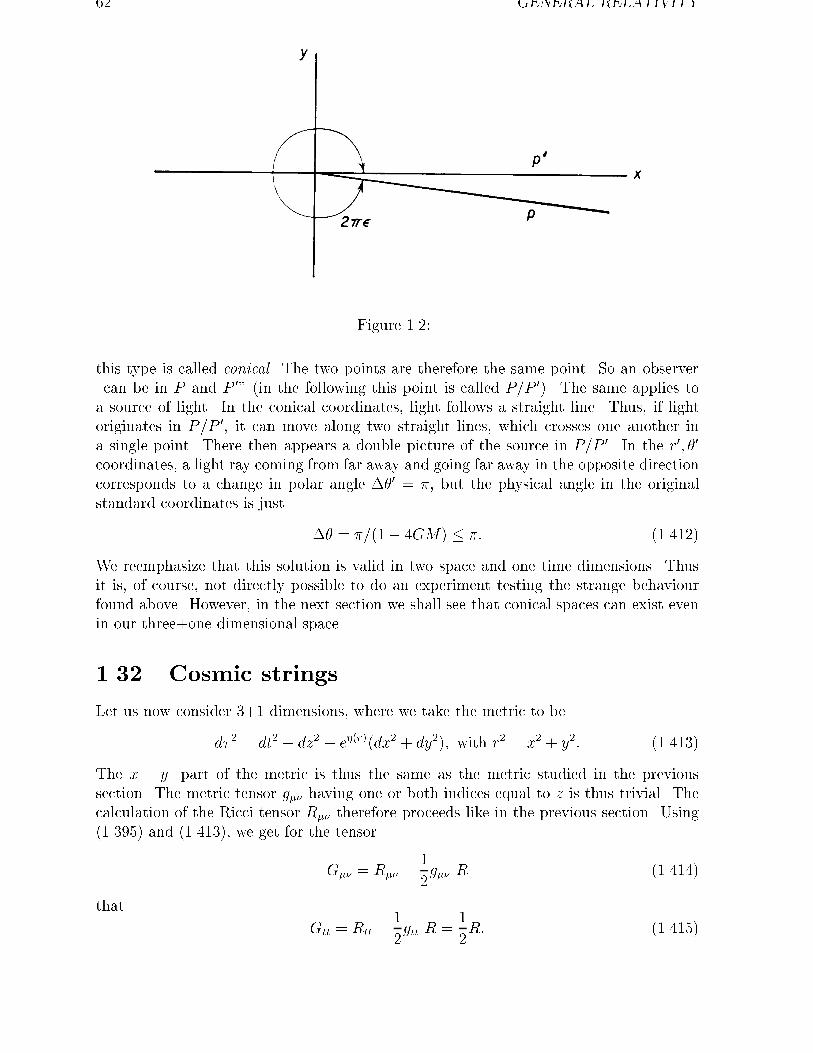
�� GENERAL RELATIVITY
Figure ����
this type is called conical� The two points are therefore the same point� So an observer�can be in P and P �� �in the following this point is called P�P ��� The same applies toa source of light� In the conical coordinates light follows a straight line� Thus if lightoriginates in P$P � it can move along two straight lines which crosses one another ina single point� There then appears a double picture of the source in P�P �� In the r�� ��
coordinates a light ray coming from far away and going far away in the opposite directioncorresponds to a change in polar angle %�� � but the physical angle in the originalstandard coordinates is just
%� � ���� �GM� � � �������
We reemphasize that this solution is valid in two space and one time dimensions� Thusit is of course not directly possible to do an experiment testing the strange behaviourfound above� However in the next section we shall see that conical spaces can exist evenin our three�one dimensional space�
���� Cosmic strings
Let us now consider ��� dimensions where we take the metric to be
d� � � dt� � dz� � e �r��dx� � dy��� with r� � x� � y�� �������
The x � y�part of the metric is thus the same as the metric studied in the previoussection� The metric tensor g�� having one or both indices equal to z is thus trivial� Thecalculation of the Ricci tensor R�� therefore proceeds like in the previous section� Using������� and ������� we get for the tensor
G�� � R�� � �
�g�� R �������
that
Gtt � Rtt � �
�gtt R �
�
�R� �������
COSMIC STRINGS ��
Also it is easily shown from the results ������� ������� and ������� that
Gxx � �� Gyy � �� Gzz � ���R� �������
while all other components of G�� vanish� From ������� we see that
R � e� �r�r���r�� with r� � ����x� � ����y�� �������
The conclusion is thus that the tensor G�� vanishes except for
Gzz � �Gtt � ���R� �������
The metric ������� is thus consistent with an energy momentum tensor of the form
Ttt � �Tzz� T�� � � for all other � and �� �������
Furthermore we take the non vanishing components of T�� to be proportional to a two dimensional delta function
Ttt � �Tzz � � ���x��pg� �������
The constant � has dimension energy$length and is called the string tension� The objectdescribed by the energy momentum tensor ������� and ������� is called a cosmic string�It is a line along the z axis with support only in the point x � y � �� The pressureis negative since Ttt by denition is positive� We shall later see that it is possible toconstruct such an object in certain eld theories� In this case the cosmic string is a�defect� i� e� an object which contains false vacuum giving rize to the negative pressure�
Proceeding as in the previous section we can now solve the Einstein equations
��r� � ��G� log r� �������
The metric ������� can now be written in the two coordinate systems
d� � � dt� � dz� � r��G��dr� � r�d��� � dt� � dz� � �dr��� � �r����d����� �������
where r� and �� are dened by
r� � r��G����� �G��� �� � ��� �G���� �������
We thus see that again there appears a conical space where the angle �� has a range whichis less than � �
The conical space leads to the occurence of double pictures of a given light sourceplaced �behind� the cosmic string seen from an observer in �front� of the string� This isshown in gures ��� and ����
In g� ��� we see the situation from the point of view of the �r� �� coordinates so thelight rays emitted from the source Q �e�g� a quasar� bend towards the observer O� In g���� we see the situation from the point of view of the conical coordinates �r�� ��� wherelight moves in straight lines� From g� ��� we get
tan�%���� � l tan� a���d� l�� where a � �G�� �������
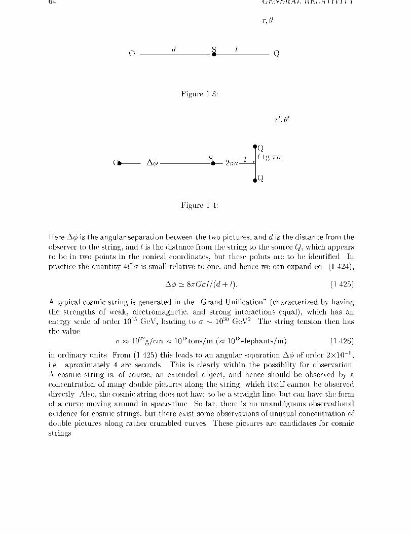
�� GENERAL RELATIVITY
��������������������
�����������������������
������������������������
���������������������������
�������������������������������
������������������������������������������
�������������������������������������������������������������������������������������������
����������������������������������������������������������������������������������������������������������������������������������������������������������������������������������������������������������������������������������������������������������������������������� u ���������������������������� �������������������������������������������������������� �������������������
��������� ������������������
������������������
��������������������
��������������������
�����������������������
����������������������
��������������������������
��������������������������������
���������������������������������������������
�����������������������������������������������������������������
��������������������������������������������������������������������������������������������������������������������������������������������������������������������������������������������������������������������������������������������������������������������������������������������������������������������������������������������������������������������������������������
�������������������������������������������������������������������������������������������������������������������������������������������������������������������������������������������������������������������������������������������������������������������������������������������������������������������������������������������������������������������������
�����������������������������������������
��������������������������������
�������������������������������������������������������������������������������������������������������������������������������������������������������������������������������������������������������������������������������������������������������������������������������������������������������������������������������������������������������������������������������������������������������������������������������������������������������������������������������������������������������������������
�����������������������������������������������������������
�������������������������������������������
������������������������������������
������������������������������
�������������������������������
�������������������������
������������������������
���������
r� �
ldO S Q
Figure ����
���������������������������
u u
u
u
����������������������������������������������������������������������
�������������������������������������������������������������������������
����������������������������������������������������������������������
����������������������������������������������������������������������
�������������������������������������������������������������������������
����������������������������������������������������������������������
�����������������������������������������������������������������������
�������������
������������������������������������������������������������������������������������������������������������������������������������������������������������������������������������������������������������������������������������������������������������������������������������������������������������������������������������������������������������������������������������������������������������������������������������������������������������������������������������������������������������������������������
����������������������������������������������������������������������������������������������������������������������������������������������������������������������������������������������������������������������������������������������������������������������������������
����������������������������������������������������������������������������������������������������������������������������������������������������������������������������������������������������������������������������������������������������������������������������������
�������������������������� � a
Q
Q
SO l
r�� ��
l tg a%�
Figure ����
Here %� is the angular separation between the two pictures and d is the distance from theobserver to the string and l is the distance from the string to the source Q which appearsto be in two points in the conical coordinates but these points are to be identied� Inpractice the quantity �G� is small relative to one and hence we can expand eq� �������
%� � � G�l��d� l�� �������
A typical cosmic string is generated in the �Grand Unication� �characterized by havingthe strengths of weak electromagnetic and strong interactions equal� which has anenergy scale of order ���� GeV leading to � � ���� GeV�� The string tension then hasthe value
� � ����g�cm � ����tons�m �� ����elephants�m� �������
in ordinary units� From ������� this leads to an angular separation %� of order ������i�e� aproximately � arc seconds� This is clearly within the possibilty for observation�A cosmic string is of course an extended object and hence should be observed by aconcentration of many double pictures along the string which itself cannot be observeddirectly� Also the cosmic string does not have to be a straight line but can have the formof a curve moving around in space time� So far there is no unambiguous observationalevidence for cosmic strings but there exist some observations of unusual concentration ofdouble pictures along rather crumbled curves� These pictures are candidates for cosmicstrings�
Chapter �
Cosmology
��� The cosmological problem
Speculations about the nature of the Universe form an integral part of the history ofmankind� Various mythologies and religions have several scenarios to o�er� In modernphysics the canonical scenario is based on astronomical observations described in terms ofEinstein�s general relativity� In physics it is always important to x a relevant scale� If wewish to describe the solar system there is no need to bother about the properties of theUniverse at intergalactic scales� If on the other hand we wish to understand the largescale structure of the Universe we do not need to be concerned with small details like oursolar system� Then we can consider even the galaxies � to be �point particles�� Now itturns out that galaxies tend to �cluster� so we have also clusters of galaxies � which ona very large scale may be considered to be particles� There are also clusters of clusters ofgalaxies � ��superclusters�� which when viewed at a large scale are also particles� Thisamount to �building up� the Universe from �particles� with diameter ������� light years�
This situation is somewhat similar to considering a gas consisting of a large number ofparticles where we do not keep track of the individual particles but rather consider thelarge scale statistical properties� It therefore also follows that in the large scale view ofthe universe we cannot assign any �center�� Every point is equivalent to any other pointin the universe� This means a radical deviation from the medieval idea that the earth isthe center of the universe� One can say that since it turned out that we do not live in thecenter of the universe we then assume that nobody else has this honor�
The idea that all points in our �large scale� universe are equivalent is called the cosmological principle� It means that the universe is assumed to be homogeneous andisotropic �because for us and hence for everybody else the universe appears to be ap proximately isotropic� around any point�
One of the rst proponents of this picture of the universe was Giordano Bruno ����� ����� who went beyond the Copernican heliocentric theory which still maintained auniverse with a sphere of xed stars� Instead Bruno made the suggestion that the universeis innite and the stars are solar systems like our own�
�With masses � ���� � ����M���With masses � ���� � ����M���With masses � ���� � ����M���When Bruno refused to retract his views he was sentenced to death� He addressed his judges� saying�
�Perhaps your fear in passing judgement on me is greater than mine in receiving it��
��
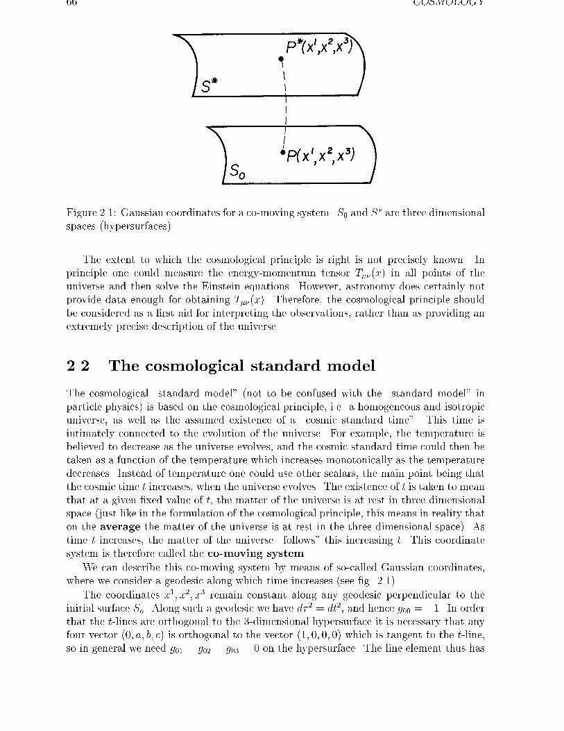
�� COSMOLOGY
Figure ���� Gaussian coordinates for a co moving system� S� and S� are three dimensional
spaces �hypersurfaces�
The extent to which the cosmological principle is right is not precisely known� Inprinciple one could measure the energy momentum tensor T���x� in all points of theuniverse and then solve the Einstein equations� However astronomy does certainly notprovide data enough for obtaining T���x�� Therefore the cosmological principle shouldbe considered as a rst aid for interpreting the observations rather than as providing anextremely precise description of the universe�
��� The cosmological standard model
The cosmological �standard model� �not to be confused with the �standard model� inparticle physics� is based on the cosmological principle i�e� a homogeneous and isotropicuniverse as well as the assumed existence of a �cosmic standard time�� This time isintimately connected to the evolution of the universe� For example the temperature isbelieved to decrease as the universe evolves and the cosmic standard time could then betaken as a function of the temperature which increases monotonically as the temperaturedecreases� Instead of temperature one could use other scalars the main point being thatthe cosmic time t increases when the universe evolves� The existence of t is taken to meanthat at a given xed value of t the matter of the universe is at rest in three dimensionalspace �just like in the formulation of the cosmological principle this means in reality thaton the average the matter of the universe is at rest in the three dimensional space�� Astime t increases the matter of the universe �follows� this increasing t� This coordinatesystem is therefore called the comoving system�
We can describe this co moving system by means of so called Gaussian coordinateswhere we consider a geodesic along which time increases �see g� �����
The coordinates x�� x�� x� remain constant along any geodesic perpendicular to theinitial surface So� Along such a geodesic we have d�
� � dt� and hence g�� � ��� In orderthat the t lines are orthogonal to the � dimensional hypersurface it is necessary that anyfour vector ��� a� b� c� is orthogonal to the vector ��� �� �� �� which is tangent to the t lineso in general we need g�� � g�� � g�� � � on the hypersurface� The line element thus has
��� THE STANDARD MODEL ��
the form
d� � � dt� � gij dxidxj �i� j � �� �� ��
xi � S� �����
Consider the equation for a geodesic
d�x�
d� �� ����
dx�
d�
dx�
d�� � �����
When d� � � dt� and the coordinates x�� x�� x� are constants along the geodesic we deducethat �i�� � � for i � �� �� �� This implies from ������ that
��g�i�t
��g���xi
�����
and since g�� � �� on any geodesic we obtain�g�i�t
� �
along the geodesic t lines� Thus the elements g��� g��� g�� of the metric tensor which arezero on the initial surface S� remain zero on all other surfaces� Thus the metric for aco moving system has the form
d� � � dt� � gij�t� x�� x�� x��dxi dxj �����
over all space� Eq� ����� is thus a consequence of the assumed existence of a cosmicstandard time�
The picture of the development of the universe presented above is thus that at a givencosmic time t the galaxies clusters of galaxies etc� are �on the average� at rest� Thuswe can construct the three dimensional space coordinates by putting numbers �x� y� z� oneach galaxy� As time increases the coordinates remain the same but all distances can bescaled with a time dependent scale factor�
Now let us consider an arbitrary but xed point in space around which we takespherical coordinates r� �� �� The requirement of isotropy in this point means that theline element has the form
d� � � dt� � f��t� r�dr� � f��t� r�r
��d�� � sin� �d��� �����
since the only rotational invariant at this point are t� r� dr� and dr��r� �d���sin� �d����The functions f� and f� only depend on t and r since a � and$or � dependence of f�and f� would destroy rotational invariance� Since we are using co moving coordinates eq������ implies that there cannot be a drdt term in eq� ����� even though it is rotationalinvariant� Thus eq� ����� is the most general form of the line element�
Now we must ensure that as time goes by the only thing that happens is that distancesare scaled� Thus the galaxies are dragging along the coordinate mesh so each galaxykeeps the same coordinates� The galaxies do move but the distance between the galaxiesmove too so the coordinates remain the same� This means that in ����� r� � and � remainthe same and the only thing which can happen is that the overall scale changes� If ata given but arbitrary time we consider two points r�� ��� �� and r�� ��� �� with d� �
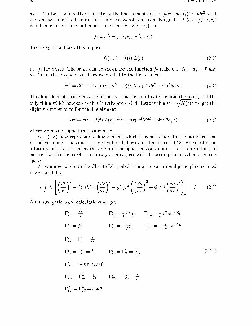
�� COSMOLOGY
d� � � at both points then the ratio of the line elements f��t� r��dr� and f��t� r��dr
� mustremain the same at all times since only the overall scale can change i�e� f��t� r���f��t� r��is independent of time and equal some function F �r�� r�� i�e�
f��t� r�� � f��t� r�� F �r�� r��
Taking r� to be xed this implies
f��t� r� � f�t� L�r� �����
i�e� f� factorizes� The same can be shown for the function f� �take e�g� dr � d� � � andd� �� � at the two points�� Thus we are led to the line element
d� � � dt� � f�t� L�r� dr� � g�t� H�r�r��d�� � sin� �d��� �����
This line element clearly has the property that the coordinates remain the same and the
only thing which happens is that lengths are scaled� Introducing r� �qH�r�r we get the
slightly simpler form for the line element
d� � � dt� � f�t� L�r� dr� � g�t� r��d�� � sin� �d��� �����
where we have dropped the prime on r�Eq� ����� now represents a line element which is consistent with the standard cos
mological model� It should be remembered however that in eq� ����� we selected anarbitrary but xed point as the origin of the spherical coordinates� Later on we have toensure that this choice of an arbitrary origin agrees with the assumption of a homogeneousspace�
We can now compute the Christo�el symbols using the variational principle discussedin section ����
�Zd�
��� dt
d�
��
� f�t�L�r�
�dr
d�
��
� g�t�r�
���d�
d�
��
� sin� �
�d�
d�
��A�� � � �����
After straightforward calculations we get�
�trr ��fL�� �t�� �
��r� ,g� �t�� �
��r� sin� � ,g
�rrr �L�
�L� �r�� � � rg
fL� �r�� � � rg
fLsin� �
�rrt � �rtr ��f
�f
��r� � ���r ��r� ���t � ��t� �
�g�g�
���� � � sin � cos ��
��r� � ���r ��r� ��t� � ���t �
�g�g
���� � ���� � cot �
������
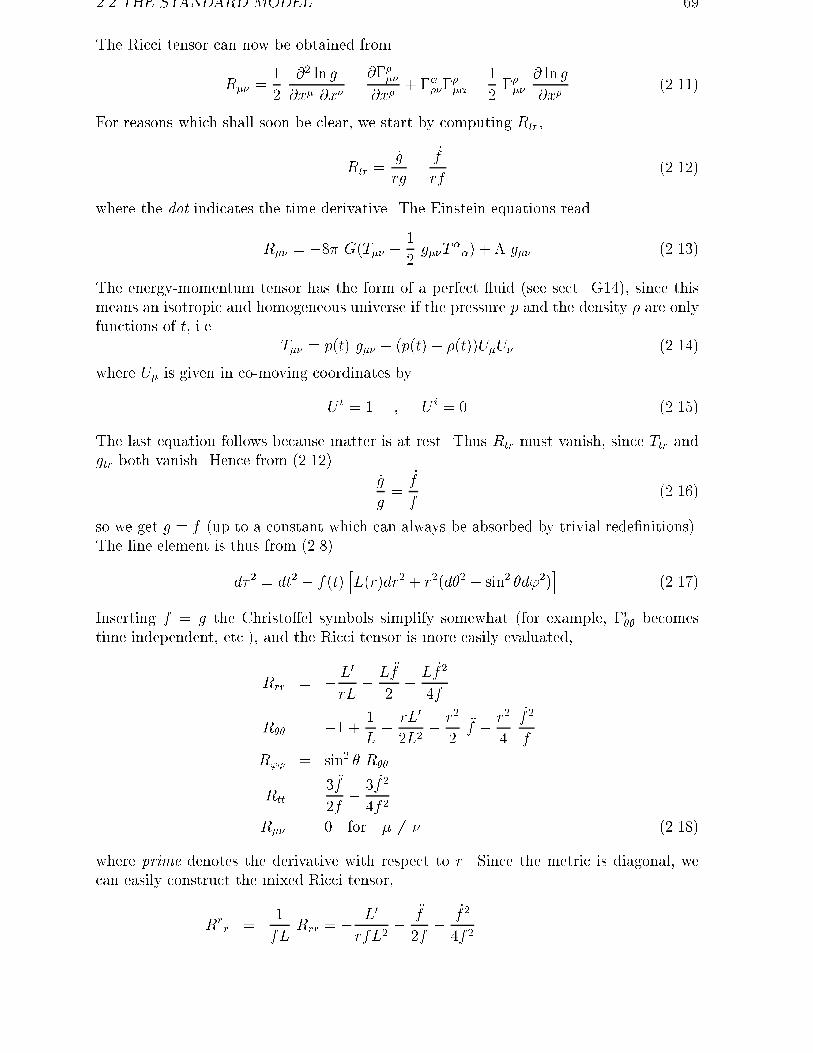
��� THE STANDARD MODEL ��
The Ricci tensor can now be obtained from
R�� ��
�
�� ln g
�x� �x�� �����
�x�� �����
��� �
�
�����
� ln g
�x�������
For reasons which shall soon be clear we start by computing Rtr
Rtr �,g
rg�
,f
rf������
where the dot indicates the time derivative� The Einstein equations read
R�� � �� G�T�� � �
�g��T
��� � g�� ������
The energy momentum tensor has the form of a perfect �uid �see sect� G��� since thismeans an isotropic and homogeneous universe if the pressure p and the density � are onlyfunctions of t i�e�
T�� � p�t� g�� � �p�t� � ��t��U�U� ������
where U� is given in co moving coordinates by
U t � � � U i � � ������
The last equation follows because matter is at rest� Thus Rtr must vanish since Ttr andgtr both vanish� Hence from ������
,g
g�
,f
f������
so we get g � f �up to a constant which can always be absorbed by trivial redenitions��The line element is thus from �����
d� � � dt� � f�t�hL�r�dr� � r��d�� � sin� �d���
i������
Inserting f � g the Christo�el symbols simplify somewhat �for example �r�� becomestime independent etc�� and the Ricci tensor is more easily evaluated
Rrr � � L�
rL� L �f
�� L ,f �
�f
R�� � �� � �
L� rL�
�L�� r�
��f � r�
�
,f �
f
R�� � sin� � R��
Rtt �� �f
�f� � ,f �
�f �
R�� � � for � �� � ������
where prime denotes the derivative with respect to r� Since the metric is diagonal wecan easily construct the mixed Ricci tensor
Rrr �
�
fLRrr � � L�
rfL��
�f
�f�
,f �
�f �
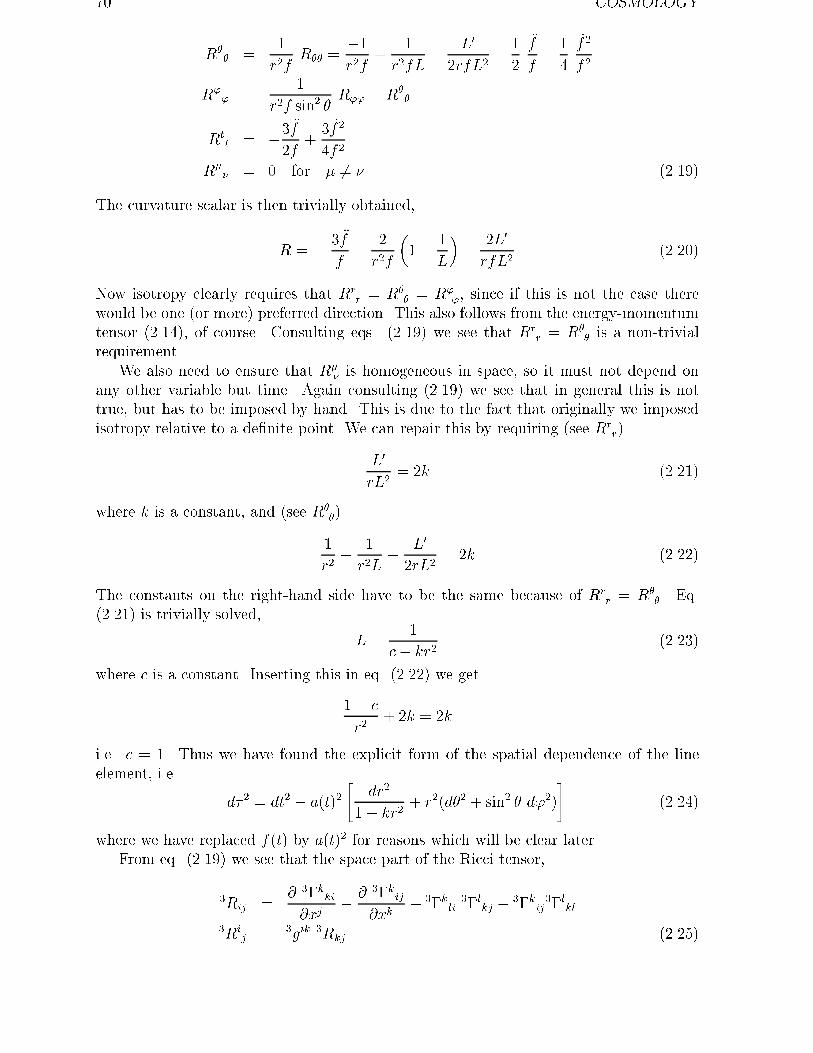
�� COSMOLOGY
R�� �
�
r�fR�� �
��r�f
��
r�fL� L�
�rfL�� �
�
�f
f� �
�
,f �
f �
R�� �
�
r�f sin� �R�� � R�
�
Rtt � ��
�f
�f�� ,f �
�f �
R�� � � for � �� � ������
The curvature scalar is then trivially obtained
R � � � �f
f� �
r�f
��� �
L
�� �L�
rfL�������
Now isotropy clearly requires that Rrr � R�
� � R�� since if this is not the case there
would be one �or more� preferred direction� This also follows from the energy momentumtensor ������ of course� Consulting eqs� ������ we see that Rr
r � R�� is a non trivial
requirement�We also need to ensure that R�
� is homogeneous in space so it must not depend onany other variable but time� Again consulting ������ we see that in general this is nottrue but has to be imposed by hand� This is due to the fact that originally we imposedisotropy relative to a denite point� We can repair this by requiring �see Rr
r�
L�
rL�� �k ������
where k is a constant and �see R���
�
r�� �
r�L�
L�
�rL�� �k ������
The constants on the right hand side have to be the same because of Rrr � R�
�� Eq������� is trivially solved
L ��
c� kr�������
where c is a constant� Inserting this in eq� ������ we get
�� c
r�� �k � �k
i�e� c � �� Thus we have found the explicit form of the spatial dependence of the lineelement i�e�
d� � � dt� � a�t���
dr�
�� kr�� r��d�� � sin� � d���
�������
where we have replaced f�t� by a�t�� for reasons which will be clear later�From eq� ������ we see that the space part of the Ricci tensor
�Rij �� ��kki�xj
� � ��kij�xk
� ��kli��lkj � ��kij
��lkl
�Rij � �gik �Rkj ������
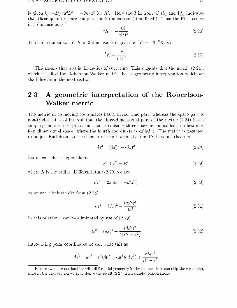
��� A GEOMETRIC INTERPRETATION ��
is given by �L��ra�L� � ��k�a� for Rrr� Here the � in front of Rij and �
klm indicates
that these quantities are computed in � dimensions �time xed#�� Thus the Ricci scalarin � dimensions is �
�R � � �k
a�t��������
The Gaussian curvature K in � dimensions is given by �R � �� �K so
�K �k
a�t��������
This means that a�t� is the radius of curvature� This suggests that the metric ������which is called the Robertson Walker metric has a geometric interpretation which weshall discuss in the next section�
��� A geometric interpretation of the Robertson�
Walker metric
The metric in co moving coordinates has a trivial time part whereas the space part isnon trivial� It is of interest that the three dimensional part of the metric ������ has asimple geometric interpretation� Let us consider three space as embedded in a ctitiousfour dimensional space where the fourth coordinate is called z� The metric is assumedto be just Euclidean so the element of length ds is given by Pythagoras� theorem
ds� � �d�x�� � �dz�� ������
Let us consider a hypersphere�x� � z� � R� ������
where R is the radius� Di�erentiating ������ we get
dz� � �z dz � �d��x�� ������
so we can eliminate dz� from ������
ds� � �d�x�� ��d�x���
�z�������
In this relation z can be eliminated by use of ������
ds� � �d�x�� ��d�x���
��R� � �x��������
Introducing polar coordinates we can write this as
ds� � dr� � r��d�� � sin� � d��� �r�dr�
R� � r�
�Readers who are not familiar with di�erential geometry in three dimensions can skip these remarks�since in the next section we shall derive the result ������ from simple considerations�
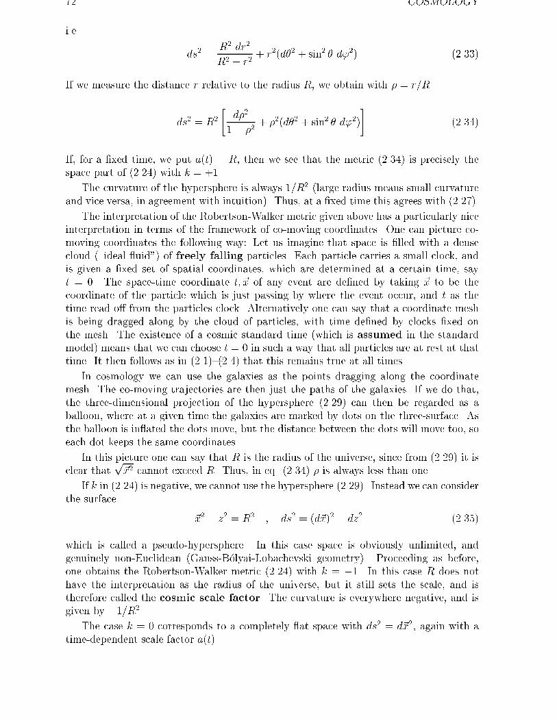
�� COSMOLOGY
i�e�
ds� �R� dr�
R� � r�� r��d�� � sin� � d��� ������
If we measure the distance r relative to the radius R we obtain with � � r�R
ds� � R�
�d��
�� ��� ���d�� � sin� � d���
�������
If for a xed time we put a�t� � R then we see that the metric ������ is precisely thespace part of ������ with k � ���
The curvature of the hypersphere is always ��R� �large radius means small curvatureand vice versa in agreement with intuition�� Thus at a xed time this agrees with �������
The interpretation of the Robertson Walker metric given above has a particularly niceinterpretation in terms of the framework of co moving coordinates� One can picture co moving coordinates the following way� Let us imagine that space is lled with a densecloud ��ideal �uid�� of freely falling particles� Each particle carries a small clock andis given a xed set of spatial coordinates which are determined at a certain time sayt � �� The space time coordinate t� �x of any event are dened by taking �x to be thecoordinate of the particle which is just passing by where the event occur and t as thetime read o� from the particles clock� Alternatively one can say that a coordinate meshis being dragged along by the cloud of particles with time dened by clocks xed onthe mesh� The existence of a cosmic standard time �which is assumed in the standardmodel� means that we can choose t � � in such a way that all particles are at rest at thattime� It then follows as in �����!����� that this remains true at all times�
In cosmology we can use the galaxies as the points dragging along the coordinatemesh� The co moving trajectories are then just the paths of the galaxies� If we do thatthe three dimensional projection of the hypersphere ������ can then be regarded as aballoon where at a given time the galaxies are marked by dots on the three surface� Asthe balloon is in�ated the dots move but the distance between the dots will move too soeach dot keeps the same coordinates�
In this picture one can say that R is the radius of the universe since from ������ it isclear that
p�x� cannot exceed R� Thus in eq� ������ � is always less than one�
If k in ������ is negative we cannot use the hypersphere ������� Instead we can considerthe surface
� �x� � z� � R� � ds� � �d�x�� � dz� ������
which is called a pseudo hypersphere� In this case space is obviously unlimited andgenuinely non Euclidean �Gauss B�olyai Lobachevski geometry�� Proceeding as beforeone obtains the Robertson Walker metric ������ with k � ��� In this case R does nothave the interpretation as the radius of the universe but it still sets the scale and istherefore called the cosmic scale factor� The curvature is everywhere negative and isgiven by ���R��
The case k � � corresponds to a completely �at space with ds� � d�x� again with atime dependent scale factor a�t��

��� HUBBLE�S LAW ��
��� Hubble�s law
We shall now investigate the frequency of light emitted by some distant object in a universedescribed by the Robertson Walker metric ������� Since light has d� � � we get for radialmotion from ������
dt� � a�t��dr�
�� kr�������
From this we get for a light wave leaving a galaxy at r � r� at time t � t� and arrivingat our galaxy r � � at time t � t�
Z t�
t�
dt
a�t��Z r�
�
drp�� kr�
�
�����sin�� r� �k � ���r� �k � ��sinh�� r� �k � ���
������
In co moving coordinates galaxies have constant coordinates �r� �� �� only the scalechanges� Thus r� is time independent� We wish to relate ������ to the frequency oflight so let the periods be �t� and �t� as measured by us and on the emitting galaxyrespectively� Thus Z t���t�
t���t�
dt
a�t��Z t�
t�
dt
a�t�������
so using that �t� is very small ����� sec for a typical light signal� we get
�t�a�t��
��t�a�t��
������
where we used the rather safe approximation a�t � ���� sec� � a�t� �i�e� the universeevolves very little in ���� sec #�� Eq� ������ then gives for the frequencies
�����
�����
�t��t�
�a�t��
a�t��������
This shows that the wave length shifts like the scale factor� The wave length is stretchedor shortened at the same rate as the universe expands or contracts�
Conventionally this relations is expressed in terms of the red shift parameter z
z ��� � ����
�a�t��
a�t��� � � a�t��� a�t��
a�t��������
where � is the wave length and where we used ����� � ����o�From eq� ������ we see that since �o is the light observed by us after a long travel
from the galaxy at r � r� then if z � � i�e� �� � �� �red shift� or if z � � �blue shift�it follows that a�t�� � a�t�� �red shift� or a�t�� � a�t�� �blue shift�� Obviously t� � t� inboth cases since we observe the light later than it was emitted� Hence we have the resultthat an expanding �contracting� universe is characterized by a red shift �blueshift� of the spectral lines� For increasing t� � t� we expect that a�t�� will increase�decrease� more and more and hence z will increase �decrease� more and more so thelarger �smaller� the value of z is the farther is the object�
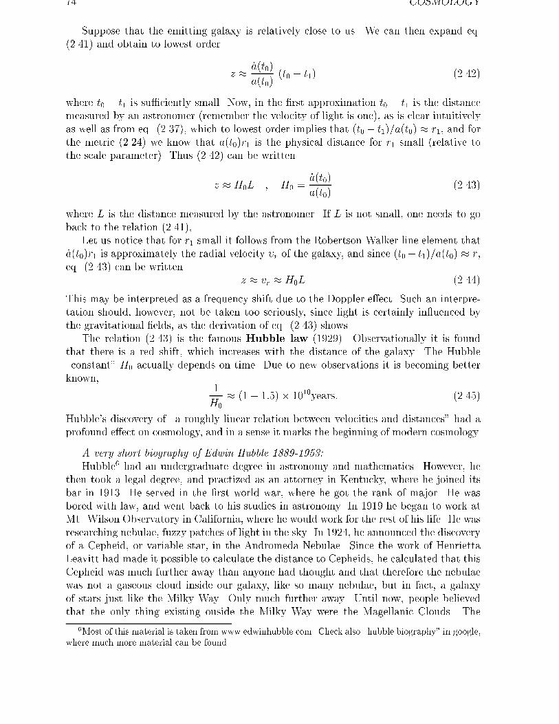
�� COSMOLOGY
Suppose that the emitting galaxy is relatively close to us� We can then expand eq������� and obtain to lowest order
z � ,a�t��
a�t���t� � t�� ������
where t� � t� is su"ciently small� Now in the rst approximation t� � t� is the distancemeasured by an astronomer �remember the velocity of light is one� as is clear intuitivelyas well as from eq� ������ which to lowest order implies that �t�� t���a�t�� � r� and forthe metric ������ we know that a�t��r� is the physical distance for r� small �relative tothe scale parameter�� Thus ������ can be written
z � H�L � H� �,a�t��
a�t��������
where L is the distance measured by the astronomer� If L is not small one needs to goback to the relation ������
Let us notice that for r� small it follows from the Robertson Walker line element that,a�t��r� is approximately the radial velocity �r of the galaxy and since �t�� t���a�t�� � req� ������ can be written
z � vr � H�L ������
This may be interpreted as a frequency shift due to the Doppler e�ect� Such an interpre tation should however not be taken too seriously since light is certainly in�uenced bythe gravitational elds as the derivation of eq� ������ shows�
The relation ������ is the famous Hubble law ������� Observationally it is foundthat there is a red shift which increases with the distance of the galaxy� The Hubble�constant� H� actually depends on time� Due to new observations it is becoming betterknown
�
H�� ��� ����� ����years� ������
Hubble�s discovery of �a roughly linear relation between velocities and distances� had aprofound e�ect on cosmology and in a sense it marks the beginning of modern cosmology�
A very short biography of Edwin Hubble ����������
Hubble� had an undergraduate degree in astronomy and mathematics� However hethen took a legal degree and practized as an attorney in Kentucky where he joined itsbar in ����� He served in the rst world war where he got the rank of major� He wasbored with law and went back to his studies in astronomy� In ���� he began to work atMt� Wilson Observatory in California where he would work for the rest of his life� He wasresearching nebulae fuzzy patches of light in the sky� In ���� he announced the discoveryof a Cepheid or variable star in the Andromeda Nebulae� Since the work of HenriettaLeavitt had made it possible to calculate the distance to Cepheids he calculated that thisCepheid was much further away than anyone had thought and that therefore the nebulaewas not a gaseous cloud inside our galaxy like so many nebulae but in fact a galaxyof stars just like the Milky Way� Only much further away� Until now people believedthat the only thing existing ouside the Milky Way were the Magellanic Clouds� The
�Most of this material is taken from www�edwinhubble�com� Check also �hubble biography� in google�where much more material can be found�
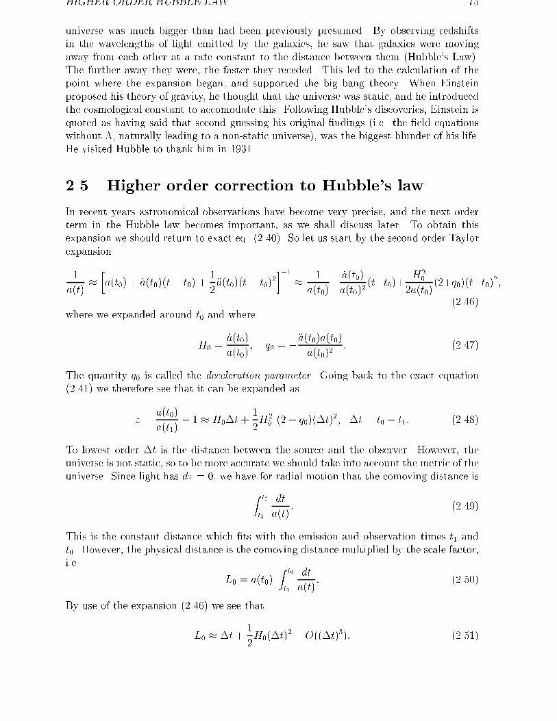
HIGHER ORDER HUBBLE LAW ��
universe was much bigger than had been previously presumed� By observing redshiftsin the wavelengths of light emitted by the galaxies he saw that galaxies were movingaway from each other at a rate constant to the distance between them �Hubble�s Law��The further away they were the faster they receded� This led to the calculation of thepoint where the expansion began and supported the big bang theory� When Einsteinproposed his theory of gravity he thought that the universe was static and he introducedthe cosmological constant to accomodate this� Following Hubble�s discoveries Einstein isquoted as having said that second guessing his original ndings �i�e� the eld equationswithout naturally leading to a non static universe� was the biggest blunder of his life�He visited Hubble to thank him in �����
��� Higher order correction to Hubble�s law
In recent years astronomical observations have become very precise and the next orderterm in the Hubble law becomes important as we shall discuss later� To obtain thisexpansion we should return to exact eq� ������� So let us start by the second order Taylorexpansion
�
a�t���a�t�� � ,a�t���t� t�� �
�
��a�t���t� t��
����
� �
a�t��� ,a�t��
a�t����t�t��� H�
�
�a�t�����q���t�t����
������where we expanded around t� and where
H� �,a�t��
a�t��� q� � ��a�t��a�t��
,a�t���� ������
The quantity q� is called the deceleration parameter� Going back to the exact equation������ we therefore see that it can be expanded as
z �a�t��
a�t��� � � H�%t �
�
�H�
� �� � q���%t��� %t � t� � t�� ������
To lowest order %t is the distance between the source and the observer� However theuniverse is not static so to be more accurate we should take into account the metric of theuniverse� Since light has d� � � we have for radial motion that the comoving distance is
Z t�
t�
dt
a�t�� ������
This is the constant distance which ts with the emission and observation times t� andt�� However the physical distance is the comoving distance multiplied by the scale factori�e�
L� � a�t��Z t�
t�
dt
a�t�� ������
By use of the expansion ������ we see that
L� � %t ��
�H��%t�
� �O��%t���� ������
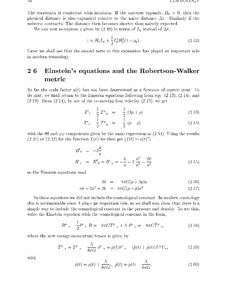
�� COSMOLOGY
The correction is consistent with intuition� If the universe expands H� � � then thephysical distance is also expanded relative to the naive distance %t� Similarly if theuniverse contracts� The distance then becomes shorter than naively expected�
We can now re express z given by ������ in terms of L� instead of %t
z � H�L� ��
�L��H
�� �� � q��� ������
Later we shall see that the second term in this expression has played an important rolein modern cosmology�
��� Einstein�s equations and the Robertson�Walker
metric
So far the scale factor a�t� has not been determined as a function of cosmic time� Todo that we shall return to the Einstein equations following from eqs� ������ ������ and������� From ������ by use of the co moving four velocity ������ we get
T tt � �
�T �
� � �����p� �� ������
T rr � �
�T �
� � ����p� �� ������
with the �� and �� components given by the same expression as ������� Using the results������ or ������ for the function L�r� we then get �f�t� � a�t���
Rtt � ���a
a
Rrr � R�
� � R�� � ��a
a� � ,a�
a�� �k
a�������
so the Einstein equations read
��a � �� G��� �p�a ������
a�a� �,a� � �k � � G��� p�a� ������
In these equations we did not include the cosmological constant� In modern cosmologythis is unreasonable since plays an important role so we shall now show that there is asimple way to include the cosmological constant in the pressure and density� To see thiswrite the Einstein equation with the cosmological constant in the form
R�� � �
��� � R � �� GT �
� � �� � � �� G &T ��� ������
where the new energy momentum tensor is given by
&T �� � T �
� �
� G�� � � &p�t��� � � �&p�t� � &��t��U�U�� ������
with
&��t� � ��t� �
� G� &p�t� � p�t��
� G� ������
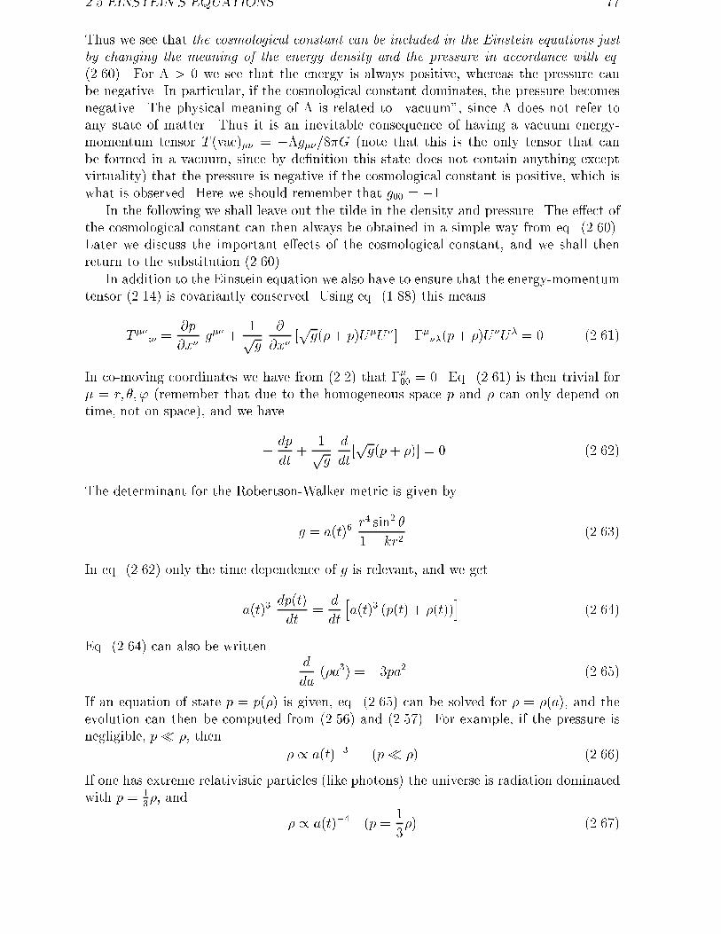
��� EINSTEIN�S EQUATIONS ��
Thus we see that the cosmological constant can be included in the Einstein equations just
by changing the meaning of the energy density and the pressure in accordance with eq�
������� For � � we see that the energy is always positive whereas the pressure canbe negative� In particular if the cosmological constant dominates the pressure becomesnegative� The physical meaning of is related to �vacuum� since does not refer toany state of matter� Thus it is an inevitable consequence of having a vacuum energy momentum tensor T �vac��� � � g���� G �note that this is the only tensor that canbe formed in a vacuum since by denition this state does not contain anything exceptvirtuality� that the pressure is negative if the cosmological constant is positive which iswhat is observed� Here we should remember that g�� � ���
In the following we shall leave out the tilde in the density and pressure� The e�ect ofthe cosmological constant can then always be obtained in a simple way from eq� �������Later we discuss the important e�ects of the cosmological constant and we shall thenreturn to the substitution �������
In addition to the Einstein equation we also have to ensure that the energy momentumtensor ������ is covariantly conserved� Using eq� ������ this means
T ��� �
�p
�x�g�� �
�pg
�
�x�)pg��� p�U�U� * � �����p� ��U�U� � � ������
In co moving coordinates we have from ����� that ���� � �� Eq� ������ is then trivial for� � r� �� � �remember that due to the homogeneous space p and � can only depend ontime not on space� and we have
� dp
dt�
�pg
d
dt)pg�p� ��* � � ������
The determinant for the Robertson Walker metric is given by
g � a�t��r sin� �
�� kr�������
In eq� ������ only the time dependence of g is relevant and we get
a�t��dp�t�
dt�
d
dt
ha�t�� �p�t� � ��t��
i������
Eq� ������ can also be writtend
da��a�� � ��pa� ������
If an equation of state p � p��� is given eq� ������ can be solved for � � ��a� and theevolution can then be computed from ������ and ������� For example if the pressure isnegligible p� � then
� � a�t��� �p� �� ������
If one has extreme relativistic particles �like photons� the universe is radiation dominatedwith p � �
�� and
� � a�t�� �p ��
��� ������
�� COSMOLOGY
We notice that the Einstein equations ������ and ������ can be simplied by eliminating�a� Thus inserting ������ in ������ we get
,a� � k �� G
��a� ������
which is called the Friedmann equation�
The functional equations in the standard model are thus the equation of state p � p���the energy conservation ������ and the Friedmann equation ������� The last two equationsare easy to remember� the quantity a� is proportional to the �volume� of the universe�for k � ��� and M � �a� is proportional to the mass of the universe� Eq� ������ canthen be written �multiply by da� dM � pdV � � which expresses energy balance duringthe evolution since dM is the change in energy balanced by pdV which is the work doneagainst the pressure forces� The Friedmann equation ������ has an �almost Newtonian�interpretation� multiply by �
�
�
�,a� �G
�� �a�
�
��
a� �k
�������
and the rst term is the Newtonian kinetic energy of a test particle with unit mass andwith coordinate proportional to the scale factor the second term �G�mass of the universe����a�� is the Newtonian potential� The sum of the �kinetic energy� and the �potentialenergy� is then the constant total energy which is negative �positive� for k � ���k � ���and vanishes for k � �� These considerations should be taken purely as an aid for thememory�
�� The Big Bang
If the pressure p is positive many features of the standard model can be understoodwithout specication of the equation of state p � p���� This is in particular true in theearly universe where it will turn out that the cosmological constant is not of importance�
To proceed we need to use the Friedmann equation ������ i�e�
�,a
a
��
�� G
��� k
a�������
and the energy conservation ������ i�e�
d
da��a�� � ��pa� ������
It is also convenient to use eq� ������
��a � �� G��� �p�a ������
which is a consequence of eqs� ������ and ������� We can now qualitatively derive thefollowing results�
�It is easy to show that eqs� ������ and ������ are implied by eqs� ������ and ������� The reason weonly have two independent equations is that T�� �� � is already contained in �R�� � �
�g��R��� ��
��� THE BIG BANG ��
Figure ���� Plot of a�t� with ,a � � and �a � �
����� Existence of the big bang �the initial singularity�
If p � � or more generally if � � �p is positive it follows from ������ that �a�a � �which means that gravity is attractive� Since we observe red shifts �and not blue shifts�it follows from the discussion in section � that at present the Hubble �constant� ������ ispositive so ,a�a � �� Thus in a plot of a�t� versus t the velocity ,a is positive but theacceleration �a is negative and we have a situation like the one shown in g� ���� It isseen that sometime in the past the function a�t� has reached zero�
Conventionally we take this time to be t � �� Clearly a vanishing scale factormeans that the Robertson Walker metric becomes singular since the three dimensionalco moving space shrinks to a single point as t � �� This singularity is the famous bigbang� Such singularities are known to occur generically in most space times under verygeneral assumptions � so it is not just a feature of the Robertson Walker metric� Theoccurrence of the singularity means that the universe starts as an explosion and a�t�increases until it reaches its present value�
����� The age of the Universe according to Big Bang
The history of the present universe is thus that it starts with a � � and a�t� increasesuntil it reaches its present value a�to� where t� is the age of the universe�
As mentioned in the last subsection �a � � when � � �p � �� Thus we have that ,a isdecreasing and therefore is smaller today than it was in the past
,a�t�� � ,a�t� for � � t � t�� ������
Using this inequality we obtain an upper limit for the age of the universe
t� �Z a�t��
�
da
,a�Z a�t��
�
da
,a�t���
a�t��
,a�t���
�
H�t��������
�See e�g� S�W� Hawking and G�F�R� Ellis�The large�scale structure of space�time� Cambridge Univ�Press� �����
�� COSMOLOGY
where H�t�� is the Hubble �constant� at present �see eq� �������� From eq� ������ we seethat the upper limit on the age of the universe is between �� and �� billion years
t� �� ���� ���� ��� yr ������
This limit is actually an important feature of the big bang model since there are argumentsbased on geology stellar evolution and the nuclear abundances which put lower boundson the age of the universe in a way which is independent of the big bang model� We shallreturn to this point later�
����� Discussion of the fate of the Universe
Having looked at the past let us now turn to the future� Suppose a�t� continues to growand ultimately a�t� � � From eq� ������ we see that if p � � the quantity �a� isconstant or decreasing� Therefore we must have �a� � � for a� and it follows that,a� � �k �at least as fast as ��a since �a� � � at least like ��a�� Thus it is only possiblefor a�t� to go to innity if k � �� or k � �� For k � �� we thus get for the �openuniverse�
a�t�� t for t� and k � �� ������
For k � � we have similarly for the ��at universe�
a�t�� slower than t for t� and k � � ������
For k � �� it is impossible for a�t� to go to innity and from ������ we see that ,a�t�becomes zero when a�t� has its maximum value amax where �a
�max � ��� G� Since �a
is always negative the scale parameter will then drop down again �with ,a negative andblue shifted spectral lines� and reach a�t� � � in a nite time t� This is the �closeduniverse��
It therefore would be quite interesting to know the sign of k to see whether the universeexpands forever or whether we shall be heading for the disastrous future singularity� Weshall discuss this in the next section�
��� Fitting parameters to observations
The general relativistic equations ������ and ������ are incomplete without the speci cation of an equation of state p � p���� In the standard model two such equations areused namely for relativistic matter relevant for the early universe and for non relativisticmatter relevant for the present universe�
Most of the matter �galaxies and clusters of galaxies� observed today appear to benon relativistic with kinetic energy much smaller than the rest energy� In the kinetic
theory of gases �here applied to galaxies� p � ����� where
p�� is the root mean square
average velocity of the gas molecules �� the galaxies�� Reintroducing the velocity of lightthe pressure in the energy momentum tensor enters like p�c� and hence p�c� � �
�����c�
and for galaxies observed now ���c� � �� Hence eq� ������ gives with p � �
� �B
a�������
��� FITTING PARAMETERS ��
where B is a constant of integration� Eq� ������ means that the energy content of aco moving volume a� remains constant when a�t� changes�
In the early universe one usually assumes the existence of a hot gas of extreme rela tivistic particles with the kinetic energy much larger than the rest energy� For a relativisticideal gas one has�
p ��
�� ������
and eq� ������ gives
� �D
a������
where D is a constant of integration� The ��a behavior is related to the fact thatrelativistically the energy in a co moving volume �red shifts� like ��a while the volumestill scales as ��a��
Now at very early times matter was very hot and as the universe expands and coolsthe kinetic energy of the matter redshifts and ultimately it becomes non relativistic�
We shall try to t the various parameters to observations� In order to t the crucialparameter k �open �at closed universe for k � ��� k � �� k � �� respectively� let ususe eq� ������ in the form
�,a
a
��� H� �
� G
��� k
a�� � G
��crit� ������
If � � �crit then the expansion is driven entirely by � and k � �� In eq� ������ H is thevalue of the Hubble �constant� at time t� From
H � h
���� yr� � � h � ��� ������
today we get�crit� � �h� � ����� g�cm� ������
Introducing � � ���crit eq� ������ becomes
k
a��� G
��crit���� �� � H���� �� ������
so � � ��� � ��� � � correspond to k � ��� k � �� k � �� respectively�Eq� ���� has a simple intuitive appeal� Suppose � is very large� Then we have a
lot of energy with a lot of gravitational attraction which will counteract the expansionmaking a closed universe� Similarly if � is very small there is very little counteractionto expansion and the universe is open�
Since �crit is given in terms of the Hubble constant and since � could in principlebe determined by �measuring� the mass density in the universe the Friedmann equation������ allows a determination of the sign of k and hence the fate of the universe�
If one considers luminous matter �stars� one nds
�lum� ��lum��crit�
� ���� ������
For a relativistic particle one has energy � jmomentumj� the factor ��� arises because statisticallyparticles can move in three directions�
�� COSMOLOGY
so � � ����� However one can also estimate the masses of dynamical systems by askingfor the gravitational forces necessary to explain the observed motions�
For a system with spherical symmetry one can use Kepler�s third law GM�r � ��where M is the mass interior to the orbit of an object �a star� with velocity � and orbitalradius r� By studying the orbital motion of stars in a galaxy at the radius where light hasessentially disappeared �this radius is called the Holmberg radius� one can measure themass of the luminous material and one gets ������� However studies of orbits of stars inspiral galaxies �for elliptic galaxies similar results do not exist perhaps because of the lackof �test bodies� i�e� stars outside luminous matter� beyond the Holmberg radius haverevealed the interesting and stunning result that � does not go as ��
pr but instead stays
approximately constant� This phenomenon is called ��at rotation curves� and it meansthat the mass M increases linearly with r even though there is essentially no luminousmatter to observe� This indicate that a large part of all matter is �dark�� For galaxiesone gets
�dyn� ��dyn��crit�
� ���� ������
so � �� ���� The discrepancy between ������ and ������ gives rise to the search �theoreti cally and experimentally� for dark matter� We shall however not enter this fascinatingsubject�
From geology stellar evolution and evolution of nuclear abundances one can makearguments which puts a lower limit of �� billion years on the age of the universe� Now �is related to the age of the universe as one can see qualitatively� If � is very large wehave a lot of gravitational interaction slowing down the expansion and thus the life timeof the universe is small� If � is very small the converse is true �if � � � there is onlyexpansion no counteraction from gravity�� This turns out to give the bound
� �� � ������
Thus using this and ������ we have
��� � � � � ������
Consequently we see that from these arguments we are not in a position to determinewhether the universe is closed �� � �� �at �� � �� or open �� � �� and we cannotsay whether the universe will eventually re contract or expand forever� However recently����� ����� new types of observations have been developed �supernovae and �uctuationsin the microwave background� which give very strong indications that the universe is �atand expanding due to a cosmological constant� This will be brie�y discussed in section�����
From eq� ������ and the bounds ������ we get
� G
� � �crit� �
k
a�� � � G
���� �crit� ������
today� This limits the three dimensional curvature k�a��
Finally we shall determine the parameter D in eq� ������� To get a bound on D weneed to consider the microwave background radiation�
�� COSMIC MICROWAVE RADIATION ��
��� The cosmic microwave radiation background
In the standard big bang model the universe starts out with a very small scale factor�Presumably the temperature is very high and the universe is lled with highly relativisticparticles� As the universe expanded the temperature dropped so matter and radiationcooled� At a temperature of around �����K �the decoupling temperature� the free elec trons joined the nuclei to bind into neutral atoms and the thermal contact betweenmatter and radiation was broken since the absence of free charged particles means thatthe interactions of photons with other matter drop o� steeply� The radiation existing atthat time has since been much redshifted but it should still ll space around us�
To describe the situation in very simple terms let us consider photons in thermalequilibrium� We found in eq� ������ that the frequency changes with the scale factoraccording to
�����
a�t��
a�t��������
Thus if t� is the time of the decoupling we can get the redshift today �t � t�� from eq�������� Also because of eq� ������ the Boltzmann factor for a photon satises
eh��kT� � e
h��kT� ������
where we have dened
T� � T�a�t��
a�t��������
If there is a thermal equilibrium we can thus absorb the scale factor in the temperature�In particular we get at the present age of the universe the Planck black body radiationdistribution of the photons
�����d�� �� h��
� d��
exp�h��kT�
� �
������
Thus the big bang predicts that there should be a thermal distribution of photons presenttoday left over from the time of the decoupling of photons from other matters� Presum ably the most signicant experimental result in cosmology since Hubble�s discovery is thatsuch a spectrum is indeed observed �Penzias and Wilson ������
In principle the temperature T� at present can be predicted from eq� ������ whichwas also done by a number of people �Gamow Alpher Herman Dicke Peebles Roll andWilkinson� before the discovery of the radiation� After the recombination the universe ismatter dominated and we have ������ i�e�
� �B
a�������
from which we get
a�t�
a�t���
���t��
��t�
����
������
Inserting the densities of baryons at t and at present ���t�� � ����g�cm�� the most carefulprediction was T� � �oK� The experiments give a nice black body radiation spectrum
�� COSMOLOGY
������ with T� � ����� ����oK in good agreement with the theoretical estimates� Recentsatellite measurements give a very precise Planck spectrum�
We can now obtain a lower bound on the constant D in eq� ������ for � in theradiation dominated early universe � � D�a� The presently observed microwave photonscontribute a relativistic component �MW to � as they did in the relativistic era� Thus
�MW �DMW
a�all times�
In the relativistic era the photons were not the only component to the energy density so
D � DMW ������
Now using Z �
�
x�dx
ex � � �
��������
we obtain by integrating ������ over the frequency
D � DMW � �MW a���today
� �kT�� �
�a
��h�
�����today
������
From ������ and the bound ������ one gets a lower bound on a�t� and inserting this weget for +h � �
D � �� ���� ������
Thus the constant D in the radiation dominated density � � D�a is huge� We shallreturn to this later�
��� The matter dominated era
We now consider the matter dominated era with negligible pressure so � � B�a�� Alsoin this section for simplicity we ignore the cosmological constant which can be taken intoconsideration at the cost of more complicated formulas� The Friedmann equation ������becomes
,a�
a���� G
�
��crit�
���
a�a� k
a���������
where we divided by a�� �a� is the scale parameter today� and used
�
����a�a
��
�������
From eq� ������ we have
k
a��� G
��crit��� �� � H���� �� �������
Using this today in eq� ������� we get
,a�
a��� H�
� ��� �� � ��a�a� �������
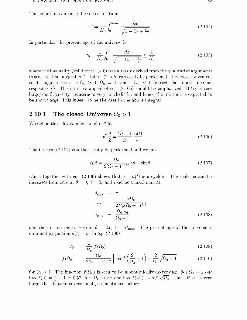
�� THE MATTER DOMINATED ERA ��
This equation can easily be solved for time
t ��
H�
Z a�a�
�
dxq�� �� �
��x
�������
In particular the present age of the universe is
t� ��
H�
Z �
�
dxq�� �� �
��x
� �
H�
�������
where the inequality �valid for �� � �� was already derived from the qualitative argumentsin sect� �� The integral in ������� or ������� can easily be performed� It is most convenientto distinguish the case �� � �� �� � � and �� � � �closed �at open universerespectively�� The intuitive appeal of eq� ������� should be emphasized� If �� is verylarge$small gravity counteracts very much$little and hence the life time is expected tobe short$large� This is seen to be the case in the above integral�
����� The closed Universe �� � �
We dene the �development angle� � by
sin��
���� � ���
a�t�
a��������
The integral ������� can then easily be performed and we get
H�t ���
���� � ����� �� � sin �� �������
which together with eq� ������� shows that a � a�t� is a cycloid� The scale parameterincreases from zero at � � �� t � � and reaches a maximum at
�max �
tmax � ��
�H���� � �����
amax ��� a��� � � �������
and then it returns to zero at � � � � t � �tmax� The present age of the universe isobtained by putting a�t� � a� in eq� �������
t� ��
H�f���� �������
f���� ���
���� � ������cos��
��
��� �
�� �
��
q�� � �
��������
for �� � �� The function f���� is seen to be monotonically decreasing� For �� � � onehas f��� � �
�� � � ���� for �� � one has f���� � ��
p��� Thus if �� is very
large the life time is very small as mentioned before�
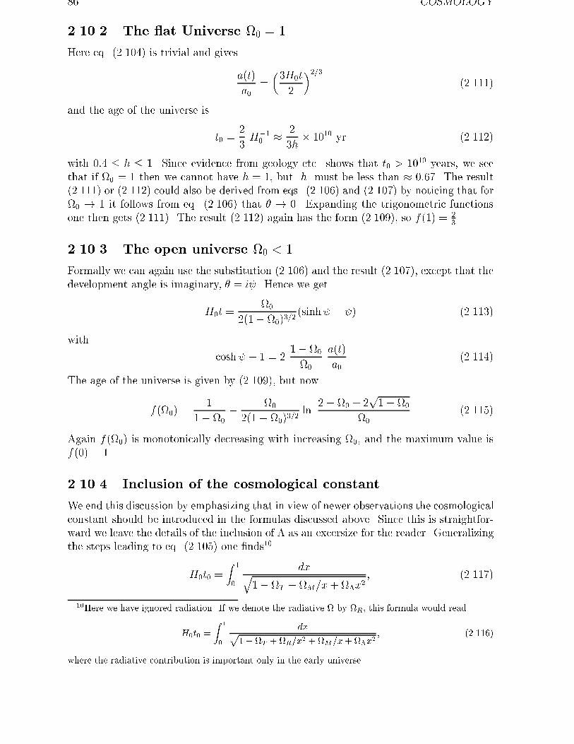
�� COSMOLOGY
����� The at Universe �� � �
Here eq� ������� is trivial and gives
a�t�
a����H�t
�
�����������
and the age of the universe is
t� ��
�H��
� � �
�h� ���� yr �������
with ��� � h � �� Since evidence from geology etc� shows that t� � ���� years we seethat if �� � � then we cannot have h � � but h must be less than � ����� The result������� or ������� could also be derived from eqs� ������� and ������� by noticing that for�� � � it follows from eq� ������� that � � �� Expanding the trigonometric functionsone then gets �������� The result ������� again has the form ������� so f��� � �
��
����� The open universe �� � �
Formally we can again use the substitution ������� and the result ������� except that thedevelopment angle is imaginary � � i�� Hence we get
H�t ���
���� �������sinh� � �� �������
with
cosh� � � � ��� ��
��
a�t�
a��������
The age of the universe is given by ������� but now
f���� ��
�� ��� ��
���� ������ln
�� �� � �p�� ��
���������
Again f���� is monotonically decreasing with increasing �� and the maximum value isf��� � ��
����� Inclusion of the cosmological constant
We end this discussion by emphasizing that in view of newer observations the cosmologicalconstant should be introduced in the formulas discussed above� Since this is straightfor ward we leave the details of the inclusion of as an excersize for the reader� Generalizingthe steps leading to eq� ������� one nds��
H�t� �Z �
�
dxq�� �T � �M�x � ��x�
� �������
�Here we have ignored radiation� If we denote the radiative � by �R� this formula would read
Ht
Z �
dxp���T ��R�x� ��M�x���x�
� �������
where the radiative contribution is important only in the early universe�
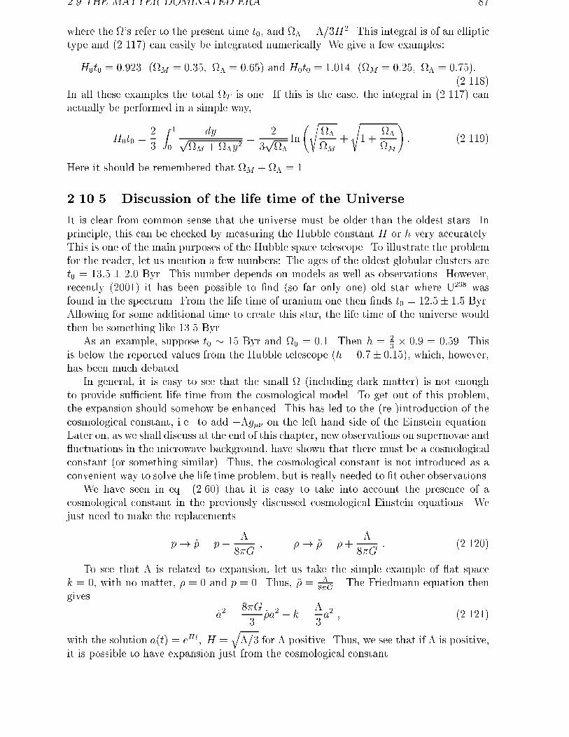
�� THE MATTER DOMINATED ERA ��
where the ��s refer to the present time t� and �� � ��H�� This integral is of an elliptictype and ������� can easily be integrated numerically� We give a few examples�
H�t� � ����� ��M � ����� �� � ����� and H�t� � ����� ��M � ����� �� � �������������
In all these examples the total �T is one� If this is the case the integral in ������� canactually be performed in a simple way
H�t� ��
�
Z �
�
dyp�M � ��y�
��
�p��
ln
�s��
�M�
s� �
��
�M
�� �������
Here it should be remembered that �M � �� � ��
����� Discussion of the life time of the Universe
It is clear from common sense that the universe must be older than the oldest stars� Inprinciple this can be checked by measuring the Hubble constant H or h very accurately�This is one of the main purposes of the Hubble space telescope� To illustrate the problemfor the reader let us mention a few numbers� The ages of the oldest globular clusters aret� � ���� � ��� Byr� This number depends on models as well as observations� Howeverrecently ������ it has been possible to nd �so far only one� old star where U��� wasfound in the spectrum� From the life time of uranium one then nds t� � ����� ��� Byr�Allowing for some additional time to create this star the life time of the universe wouldthen be something like ���� Byr�
As an example suppose t� � �� Byr and �� � ���� Then h � ��� ��� � ����� This
is below the reported values from the Hubble telescope �h � ���� ����� which howeverhas been much debated�
In general it is easy to see that the small � �including dark matter� is not enoughto provide su"cient life time from the cosmological model� To get out of this problemthe expansion should somehow be enhanced� This has led to the �re �introduction of thecosmological constant i�e� to add � g�� on the left hand side of the Einstein equation�Later on as we shall discuss at the end of this chapter new observations on supernovae and�uctuations in the microwave background have shown that there must be a cosmologicalconstant �or something similar�� Thus the cosmological constant is not introduced as aconvenient way to solve the life time problem but is really needed to t other observations�
We have seen in eq� ������ that it is easy to take into account the presence of acosmological constant in the previously discussed cosmological Einstein equations� Wejust need to make the replacements
p� &p � p�
� G� �� &� � ��
� G� �������
To see that is related to expansion let us take the simple example of �at spacek � � with no matter � � � and p � �� Thus &� � �
��G� The Friedmann equation then
gives
,a� �� G
�&�a� � k �
�a� � �������
with the solution a�t� � eHt� H �q �� for positive� Thus we see that if is positive
it is possible to have expansion just from the cosmological constant�

�� COSMOLOGY
In the older universe we see that the Friedmann equation
�,a
a
���� G
�
B
a�� k
a��
��������
implies that the di�erent terms dominate at di�erent times� In the beginning �afterrecombination� the matter term dominates then the curvature �k�a�� takes over as aincreases and ultimately the cosmological constant term dominates completely� For � �and k � �� the expansion continues forever� For � � the expansion comes to a stopsince the left hand side of the Friedmann equation is always positive� In this case thereis a maximum value of a obtained for ,a � ��
We have mentioned before that the cosmological constant does not play an importantrole in the early relativistic universe where the Friedmann equation becomes
�,a
a
���� G
�
D
a� k
a��
�� �������
When a is very small the rst term dominates entirely and the curvature ��k�a�� andthe cosmological terms are utterly unimportant� Thus our considerations on the big bangin sect� ��� are valid in spite of the fact that we did not explicitly take into account thecosmological constant�
If is introduced it is easy to solve any age problem� An example� Let t� � ����Byr and h � ���� With �� � ���� and �� � ���� these numbers t as can be seen byuse of �������� We end by remarking that the age problem has been there since Hubble�sdicovery� Using his value for H the life time of the universe was shorter than the life timeof the planet earth# This led to a disbelief in the standard cosmological model� Howeveras mentioned before there are now observations independent of the age problem whichrequires a cosmological constant� Observations seem to converge to a consistent pictureof the universe as beeing described by the standard model to a rst approximation�
���� Causality structure of the big bang �The hori�
zon problem�
The region of causal contact with a given event is determined by how far photons origi nating at that event can travel� We shall consider photons emitted at big bang and seehow far they can propagate�
For photons d� � � so the Robertson Walker metric gives dt� � a�t��dl� where dl isthe time independent distance in co moving coordinates� The physical causal distance isthus
d � a�t��l � a�t��Z t�
�
dt
a�t��������
where the time � is the big bang time that the photon was emitted whereas t� is the timeit was received�
To obtain a�t� let us consider the Friedmann equation ������
,a� �� G
��a� � k �������
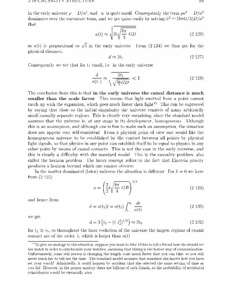
���� CAUSALITY STRUCTURE ��
In the early universe � � D�a and a is quite small� Consequently the term �a� � D�a�
dominates over the curvature term and we get quite easily by solving ,a� � �� G���D�a�
that
a�t� �vuut�t
s�
�GD �������
so a�t� is proportional topt in the early universe� From ������� we thus get for the
physical distanced � �t� �������
Consequently we see that for t� small i�e� in the early universe
d
a�t���vuut �t�q
���GD
�� � �������
The conclusion from this is that in the early universe the causal distance is muchsmaller than the scale factor� This means that light emitted from a point cannotcatch up with the expansion which goes much faster than light��� This can be expressedby saying that close to the initial singularity the universe consists of many arbitrarilysmall causally separate regions� This is clearly very surprising since the standard modelassumes that the universe is at any stage in its development homogeneous� Althoughthis is an assumption and although one is free to make such an assumption the situationdoes not appear very self consistent� From a physical point of view one would like thehomogeneous universe to be established by the contact between all points by physicallight signals so that physics in any point can establish itself to be equal to physics in anyother point by means of causal contacts� This is not the case in the early universe andthis is clearly a di"culty with the standard model� This is the causality problem alsocalled the horizon problem� The latter concept refers to the fact that Einstein gravityproduces a horizon beyond which one cannot observe�
In the matter dominated �later� universe the situation is di�erent� For k � � we havefrom �������
a �
����t
s�
�GB
A
���
�������
and hence from
d � a�t��l � a�t��Z t�
t�
dt
a�t��������
we getd � �
�t� � �t�t������
� �t� �������
for t� � t� so throughout the later evolution of the universe the largest regions of causalcontact are of the order t which is larger than a�t��
��To give an analogy to this situation� suppose you want to bike �� km to tell a friend how she should sether watch in order to synchronize your watches� assuming that biking is the fastest way of communication�Unfortunately� some evil person is changing the length scale much faster that you can bike� so you willnever reach her to tell her the time� The standard model assumes that somehow she knows how you haveset your watch� Admittedly� it could happen by accident that she selected the same setting of time asyou did� However� in the proper analogy there are billions of such friends� so the probability of accidentalcoincidences would be essentially zero�
�� COSMOLOGY
The microwave background discussed in section � is observed to be very isotropic�It turns out that the microwave photons originated in causally separate regions if theirdirections di�er by more than a few degrees� Thus the data show that a truly strikingdegree of isotropy is present in the universe and in the big bang standard model thiscould not have been produced by causal processes� In the big bang model this strikingisotropy is not explained but has to be put in �by hand� to t the observations�
Finally let us discuss another puzzle �the �atness problem�� Flat space i�e� � � �is an unstable equilibrium� If � is ever exactly equal to one it remains equal to one� Nowwe know that today � is at least ��� ��� which is not very far from �� The Friedmannequation can be rewritten
k � ,a���� ��� �������
Since k is a constant and since ,a increases if we go backward in time it follows thatin early times � must have been extraordinarily closer to � than it is today� To givesome examples� For � to be in the allowed range today it must have been equal to �to an accuracy of �� decimal places � sec after big bang �time of nucleosynthesis�� Atgrand Unication � should be equal to � to an accuracy of �� decimals� This fact is notexplained by the Standard Model�
���� In�ation
We have seen that the standard model has many successful features and gives a niceframework for discussing the rather few astronomical observations which are available� Inthe last section however we saw that certain features emerge from the standard modelwhich point to di"culties for the model if we want to understand it in more physicalterms�
The standard model is therefore to be supplemented by a new scenario called �in �ation� where many of the physical di"culties have been removed� In�ation concernsitself with the early universe where the di"culties arise � In the previous work we haveassumed that the pressure is positive� Although this seems intuitively natural it is notlogically necessary� In quantum eld theory one can have negative pressure�
We cannot give a full explanation of this since this would require the introduction ofelds� However let us give an intuitive description of what happens� Suppose at a veryearly time the system is in a metastable state called the �false vacuum�� On short timescales the energy cannot be lowered so �false� could be replaced by �temporary�� Givenenough time the false vacuum decays to a stable �true� vacuum which is the state withlowest possible energy� Also let us assume that it takes a rather long time for the falsevacuum to decay� This is in short the scenario in in�ation�
Let us call �f the energy density of the false vacuum �relative to the true vacuum��To nd the pressure of the false vacuum let us imagine that we enclose it in a cylindricalcontainer with a movable piston� So inside the cylinder and piston we have the energydensity �f � Outside we have true vacuum with � � p � �� Now move the piston outwardsadiabatically which means that there is no heat �ow into or out of the cylinder� Whenthe piston is pulled the false vacuum keeps its energy density everywhere also in the�new� volume� This is because this energy is �temporarily� the lowest possible one� Sothe change in energy dU is given by dU � �fdV where dV is the change in volume�However in the adiabatic case we always have dU � pdV � �� Hence
���� INFLATION ��
p � ��f � �� �������
i�e� the pressure is negative�You may wonder where the extra energy arising when we pull the piston comes from�
It is of course supplied by the agent pulling the piston who has to perform this workagainst negative pressure#
Another way of seeing the negative pressure related to vacuum is to ask for the energy momentum tensor for a false or true vacuum� This T �� cannot depend on velocities etc�since the vacuum does not move or carry momentum� The only relativistically invarianttensor is therefore T �� � ��g�� where � is the density of the true or false vacuum�The minus sign occurs because by denition the energy density is positive� This tensortherefore corresponds to the negative pressure p � ���
The negative pressure has profound consequences� Consider eq� ��������
�a � �� �G��� �p�a� �������
Usually this means �a � � i�e� gravity is attractive� Now during the time the false vacuumdominates
�a � ��
�G�fa �������
so gravity is now repulsive## This means that during in�ation gravity does not counteractthe expansion on the contrary because the solution of the attractive gravity equation is
a�t� � c�e�t � c�e
��t � � �
s�
�G�f �������
where c�� c� and � are constants �remember that �f is the constant energy density of thefalse vacuum�� Let us estimate �f � A simple model is to assume that it is the densityrelevant at the Grand Unication scale with temperature ���� GeV� In natural units �fhas dimension �mass� so
�f � �����GeV� �������
This is enormous# To get this density in the sun we would have to compress it to the sizeof a proton� We then get
�
�� ����sec �������
and the Hubble constant �which is now a true constant� becomes
,a
a� � � ���sec��� �������
Let us consider the density during in�ation
d
da��fa
�� � ��pa� � ��fa� � �f
da�
da�������
so d�f�da vanishes and �f is time independent as we knew beforehand� The Friedmannequation for k � � is then just
,a
a�
s�
�G�f � Hin�ation� �������
�� COSMOLOGY
Let us now modify the standard big bang so that for � � t � t� we have the usual radiationdomination �� � D��a
� for t� � t � t� we have negative pressure and the equation ofstate ������� for t� � t � td we return to the relativistic equation of state whereasfor t � td �td �time of decoupling of photons� we have the usual matter domination�� � B�a��� Then the evolution looks like�
� � t � t� radiation dominance a � pt � � D��a
t� � t � t� in�ation a � etHin�� � � const�
t� � t � td radiation dominance a � pt � � D��a
td � t matter dominance a � t��� � � B�a�
The integration constant D� and D� are now determined by requiring consistency at thetimes t� and t� so
D� � D� eHin�ation�t��t�� �������
The important feature is that even if D� is of order one then D� can be very large� IfHinfl��t��t�� � �� then one can have D� � ���� with D� � ����� Thus the large value ofD� can be obtained in a quite reasonable way from a decent value of D�� Models wherethe equation of state ������� is satised are called �in�atory� models and when a�t� blowsup exponentially the universe is said to be in�ating� As the in�ationary period proceedsall elds get red shifted away exponentially fast� The in�ationary period essentially wipesthe slate clear of primordial �uctuations �from � � t � t���
One may ask whether Hin��t� � t�� � �� is reasonable� Since � � Hin� we needt� � t� � ����� sec which is the right time for the in�ationary period� In the phasetransiton where false goes to true vacuum the energy stored in the false vacuum isreleased in the form of new particles �in thermodynamics language the released energyis the �latent heat� of the phase transition�� These new particles then come to thermalequilibrium at the temperature T � ��� GeV�
What happens to the causality problem� Start with the present universe which iscausally connected� Going backwards in time we encounter in�ation with its enormouscontraction �we go backwards#� producing an incredibly small region out of our universeof size �t� In this small region photons can maintain causal contact so there is no problem�To see this in more details let us estimate the distance d travelled by light
d � a�t��Z t�
�
dt�
a�t��� a�t��
�Z t�
�
dt�
a�t���Z t�
t�
dt�
a�t��
�� �������
where the various times are dened above� In the in�ationary time interval t� � t � t�we take
a�t� � a�t�� eH�t�t��� �������
In the interval from big bang to t� we have
a�t� � a�t��qt�t�� �������
Hence
d � ��t� � ��H� eH�t��t��� �������
���� EVIDENCE FOR THE COSMOLOGICAL CONSTANT ��
Therefore the causal distance is blown up by an exponential factor quite compatible withthe exponential blow up of the scale factor exhibited in ������� where a�t�� is the size ofa causal domain just before in�ation sets in i�e�
a�t�� � �t�� �������
It should be noticed that this scale factor is the size of a physical early universe and thatit represents a tiny part of the causally non connected early universe� Also notice thateq� ������� would not work if there is no in�ation since the resulting older universe wouldbe far too small to have anything to do with the universe we know�
After the end of in�ation the universe is radiation dominated for some time� At thisstage the causal distance is again �t�
What about �� We still have Friedmann k � ,a���� ��� During in�ation ,a increasesextremely rapidly so � is driven towards � so
�in�ation � �� �������
Finally it should be said that in�ation occurs in many versions and some of them aresomewhat di�erent from the intuitive description given above�
���� Observational evidence for the cosmological
constant
In ���� evidence for a non vanishing cosmological constant was found by observing ��� type Ia supernovae out to redshifts of order one��� The data was plotted in themagnitude redshift Hubble diagram� The main point in using distant supernovae is thatthey are considered to be very good standard candles� they are assumed to be associatedwith the nuclear detonation of white dwarfs� It is completely outside the scope of thesenotes to describe the theory of white dwarfs��� However because of the knowledge ofthe blow up mechanism the intrinsic luminosity and the observed �ux are known andhence the �luminosity� distance can be computed from the ratio of these quantities� Inparticular features of the distant sample of Ia�s appear to be similar to a nearby sample�So far there is no serious objection against Ia as a standard candle� Therefore andbecause it has become possible to observe high z objects the old uncertainty concerningthe determination of the distance in Hubble�s relation seem overcome�
For nearby galaxies it is su"cient to use the simple Hubble �law� z � vr � HL whereL is the distance and vr is the radial velocity �see eq� �������� In the standard modeldistant galaxies should have larger velocities than predicted by the simple Hubble lawbecause gravitation slows the expansion� However the supernovae observations showedprecisely the opposite# The conclusion is therefore that the expansion speeds up�
This is in contrast to the standard model without a cosmological constant� Howeverintroducing we saw in connection with eq� ������� that the evolution of the velocity ,achanges �
,a
a
���� G
��� k
a��
�� �������
��A� Riess et al�� Astrophys� J� ��� ������ �����this paper is most easily found on the net� see astro�ph��������� and B� Schmidt et al�� Astrophys� J� ��� ������ ���see astro�ph���������
��See e�g� S� Weinberg� Gravitation and Cosmology� p� ����
�� COSMOLOGY
For a positive in a late universe the two rst terms on the right hand side are subdom inant and the expansion is driven by the last term� Remembering that
�crit ��H�
� Gand H �
,a
a� �������
we obtain the following form for the Friedmann equation
k
a�� H���M � �� � ��� �������
Here �M � ���crit is the matter density and �� � ��H� is the relative density associatedwith the cosmological constant which can be interpreted as a vacuum energy since itexists irrespective of matter�
By further expansion of z � �a�t��� a�t����a�t�� in eq� ������ we obtained a general ization of the simple Hubble law
z � H�L� ��
�H�
�L���� � q��� �������
where q� is the deceleration parameter today with
q � ��aa,a�� �������
The interesting thing is that q can be expressed in terms of the ��s� In the later universewe can ignore the pressure and we have
�a � �� G�
�a �
�a � �H�aq �������
from the denition ������� of q� If we use H� � � G�crit�� and �M � ���crit eq� �������becomes
q ��
��M � �� �
�
��tot � �
���� �������
Here �tot � �M��� is the total energy �ignoring the small contribution from radiation��The name deceleration parameter refers to the expectation that q � � since �a was ex pected to be negative if there is no cosmological constant �if �� �p � ��� However if ��
is present this need no longer be true and we see that tries to change the sign of q so produces positive acceleration�
The main point is that eqs� ������� and ������� supplies astronomers with a method ofactually measuring �� if �M is known from other observations provided the distance L�
is known accurately enough� From the high z supernovae observations mentioned aboveone nds
�� � ���� �������
This is consistent with a total energy
�tot � �� �������
These numbers are of course expected to have some uncertainty� It is to be noticed thatthe last result is at least roughly consistent with in�ation� For further discussion we referto the recent reviews to be found in astro ph �http�$$xxx�lanl�gov$list$astro ph$new��
���� EVIDENCE FOR THE COSMOLOGICAL CONSTANT ��
More recently precise data have been obtained for the �uctuations in the microwavebackground� These lead again to �tot � � rougly consistent with in�ation� These dataare completely independent of the supernovae observations and are thus not subjectto any doubt concerning the mechanism behind supernovae production� Therefore theconclusion that the universe is at least approximately �at is indicated by independent setof observations�� It is of philosophical interest that even very precise future measurementswill always have an uncertainty� Thus if it turns out that � � �����������X then theexistence of X no matter how small will always prevent one from making the statementthat the universe is exactly �at� One can only say that with a high probability it is �at���
The conclusion is that the cosmological constant is necessary because of the recentobservations� Cosmology seems to converge rapidly towards a very precise science whereobservations determine the parameters� With �� � ��� and �M � ��� the �at universewill go on expanding forever��� This gives rize to the problem that we live in a protabletime from the point of view of observations because in the future astronomers will be ableto observe fewer and fewer objects� Also the cosmological constant gives rize to severalother problems� For example the matter density is of the same order as the densityassociated with � However these two densities have di�erent origins �matter versusvacuum� and behave in a di�erent way as functions of the scale parameter� Consequentlyit is not easy to nd an explanation why �matter is so close in value to �� in our time�
There are several attempts to understand the cosmological constant without reallyhaving it �for example by the use of suitable scalar theories� in such a way that thereis temporarily something which looks like a cosmological constant� In this way perhapsthe end is not an empty universe� On the other hand the simplest possible explanationof the data is a constant �
In quantum eld theory a vacuum energy emerges naturally� This is precisely whatis needed for understanding the cosmological constant� However this has not led to a of the right order of magnitude� This constitutes one of the most important problems inmodern physics�
It is the e�ort of many human beings to ask for a �meaning� �of life death theuniverse����� So in cosmology we have the opportunity to ask very precisely what is themeaning of the universe� The cosmological constant represents the vacuum i�e� �nothing��Most of the energy �� ��-� in the universe is thus empty space� So perhaps the answerto the question on the meaning of the universe is that there is no meaning#
In this connection it should be noted that the cosmological constant allowed by Ein stein gravity is considered together with the assumptions of the standard model namely ahomogeneous and isotropic universe with an evolution characterized by the cosmologicaltime� Although this may appear reasonable on an extremely large scale these assump tions are denitely not valid on shorter scales where the universe is inhomogeneous� Thismay lead to a problem because of the non linearity of the Einstein eld equations whichcan make the averaging procedure much more subtle than one might naively think� Thusthe equation ������� used to analyze the Supernovae data depends on the ��s becauseof Einstein eld equations� If we think of the various quantities in ������� as large scale
��The data from the uctuations in the microwave background actually have a statistical preferencefor a total � which is slightly larger than one� but � can be one within a standard deviation�
��This di�culty is due to the fact that � � is a borderline case� If� for example� it had turned outthat � � ���� no such problem of principles would occur�
��See� however� the previous footnote
�� COSMOLOGY
averages it is not obvious that there are no corrections coming from the non linearities�
���� The end of cosmology�
Lawrence Krauss and Robert Scherrer �see arXiv���������� where further references canbe found� have investigated some of the depressing consequences of the cosmologicalconstant� As we have seen in eq� ������� ultimately there will be an expansion drivenby the cosmological constant� In approximately ��� billion years almost all galaxies willbe invisible except the Local Group of six galaxies which are gravitationally bound anddo not participate in the large scale expansion� Observers in this �island universe� willbe fundamentaly incapable of determining the true nature of our universe as Krauss andScherrer say� Of course there will be no such observers on earth since its life time isonly of the order ��� bilion years but perhaps there are observers some other place in theMilky Way perhaps having the same DNA as us�
These observers will have absolutely no way of knowing that the universe expands andwill think that the universe is static� This was Einstein�s starting point corrected by as tronomical observations� This was also the reason for his introduction of the cosmologicalconstant#
In the island universe there is no way of recognizing that there was a Big Bang� Dueto the expansion the cosmic microwave background will disappear in the sense that thewavelenghts will be shifted and totally buried by radio noise in our galaxy� So perhapsthese observers will spend their time producing a lot of papers on why there are six �ascontrasted to any other number� galaxies in the whole universe�
Although the return of the static universe is not of immediate concen philosophicallythe situation in the island universe is interesting because the observers can have the rightphysics but are unable �no matter how good they are� to get the right cosmology becauseof lack of observational support� One may wonder if the same thing is happening today are we also beeing deceived like the islanders �or like the man who came to Casablancafor the waters��
���� An inhomogeneous universe without ��
Recently there has been much interest in the study of an inhomogeneous universe in orderto see if it is possible to avoid the cosmological constant� Of course from CMB we knowthat the early universe is to a high degree of accuracy homogeneous� Hopwever at earlytimes plays no role�
For the universe at the present epoch one basic consideration is that even thoughthe universe now appears to be homogeneous at very large scales observationally thereare voids of considerable size surrounded by clusters of galaxies� It is estimated that�� �� per cent of the present universe consists of voids with diameter of order ���h Mpc�We refer the reader to a paper by David L� Wiltshire �Phys� rev� Letters �� ������������� where further references can be found� The necessary formalism is somewhatcomplicated but the physical idea is simple� It is necessary to average over the di�erentstructures that have di�erent time rates because the time depends on the gravitationaleld� Also in the voids there is very little matter so this part of the universe has anegative curvature metric �k � ���� Therefore volumes are larger and hence densities
���� UNIVERSE WITHOUT � ��
are smaller than expected in the standard cosmological model� It then turn out that thedeceleration parameter q is given by
q � ���� f���f � � ��f � � ��f � ���� � f � �f ���
� �������
where f is the void volume fraction� Here we see that in spite of having no cosmologaicalconstant q changes sign� At early times there are no voids so f � � giving q � ����But q changes sign for f � ������ corresponding to acceleration �not due to #�� Theapparent acceleration becomes maximal for f � ������ with q � ������� At later timesq approaches zero i�e� the acceleration disappears and there will be no island universe#
�� COSMOLOGY
Chapter �
Problems
Problem �� Consider cylindrical coordinates�
x � r cos� � y � r sin� � z � z
Find the metric expressed in terms of these coordinates� Find the Laplace operator inthese coordinates�
Do the same for spherical coordinates�
x � r cos� sin � � y � r sin� sin � � z � r cos � �
Check the correctness of the resulting Laplace operator by comparing your result withsome book �e�g� on quantum mechanics��
Problem �� Let A� be a quantity consisting of four components A�� A�� A�� A�� Assumethat
A�B� � invariant
for an arbitrary vector B�� Show that then A� is a vector�Generalize this result to arbitrary tensors�The resulting theorem is called the �quotient!theorem��
Problem �� Let S�� � S�� be a symmetric tensor and A�� an antisymmetric tensorA�� � �A��� Show that S��A
�� is identically zero�Show that an arbitrary tensor with two indices can be written as the sum of a sym
metric and an antisymmetric tensor�
Problem �� Consider a two!dimensional surface of a sphere dened by
x� � y� � z� � R� �
What is the metric expressed in terms of x and y �Find the metric in spherical coordinates�
Problem �� Assume that V �� � �V ���x� � ����V
�� Then show that V� � g��V�
satises eq� �������
��
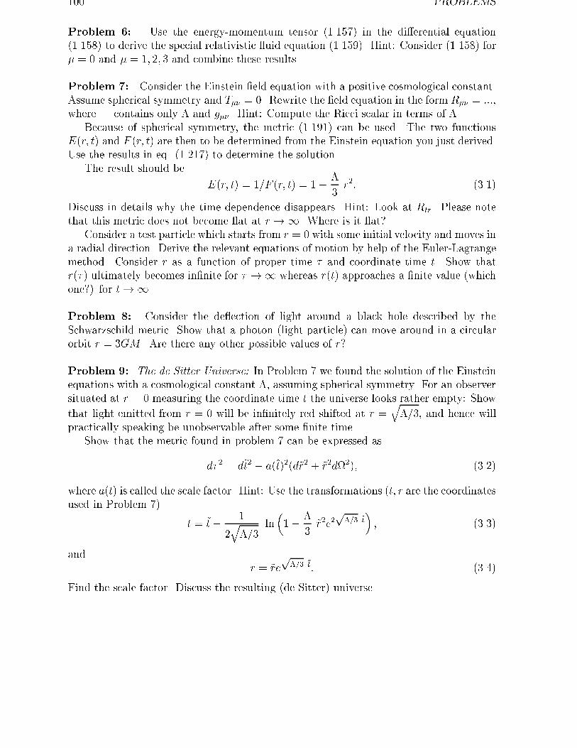
��� PROBLEMS
Problem �� Use the energy momentum tensor ������� in the di�erential equation������� to derive the special relativistic �uid equation �������� Hint� Consider ������� for� � � and � � �� �� � and combine these results�
Problem �� Consider the Einstein eld equation with a positive cosmological constant�Assume spherical symmetry and T�� � �� Rewrite the eld equation in the form R�� � ���where ��� contains only and g��� Hint� Compute the Ricci scalar in terms of �
Because of spherical symmetry the metric ������� can be used� The two functionsE�r� t� and F �r� t� are then to be determined from the Einstein equation you just derived�Use the results in eq� ������� to determine the solution�
The result should be
E�r� t� � ��F �r� t� � ��
�r�� �����
Discuss in details why the time dependence disappears� Hint� Look at Rtr� Please notethat this metric does not become �at at r� � Where is it �at�
Consider a test particle which starts from r � � with some initial velocity and moves ina radial direction� Derive the relevant equations of motion by help of the Euler Lagrangemethod� Consider r as a function of proper time � and coordinate time t� Show thatr��� ultimately becomes innite for � � whereas r�t� approaches a nite value �whichone�� for t� �
Problem �� Consider the de�ection of light around a black hole described by theSchwarzschild metric� Show that a photon �light particle� can move around in a circularorbit r � �GM � Are there any other possible values of r�
Problem �� The de Sitter Universe� In Problem � we found the solution of the Einsteinequations with a cosmological constant assuming spherical symmetry� For an observersituated at r � � measuring the coordinate time t the universe looks rather empty� Show
that light emitted from r � � will be innitely red shifted at r �q �� and hence will
practically speaking be unobservable after some nite time�Show that the metric found in problem � can be expressed as
d� � � d&t� � a�&t���d&r� � &r�d���� �����
where a�t� is called the scale factor� Hint� Use the transformations �t� r are the coordinatesused in Problem ��
t � &t� �
�q ��
ln���
�&r�e�
p��� �t
�� �����
andr � &re
p��� �t� �����
Find the scale factor� Discuss the resulting �de Sitter� universe�
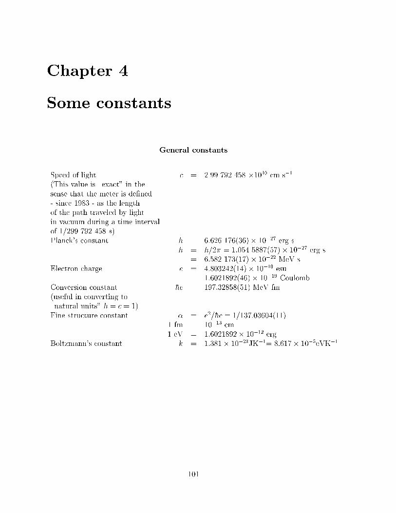
Chapter �
Some constants
General constants
Speed of light c � ���� ��� ��� ����� cm s��
�This value is �exact� in thesense that the meter is dened since ���� as the lengthof the path traveled by lightin vacuum during a time intervalof ����� ��� ��� s��Planck�s constant h � ����� �������� ���� erg s
+h � h�� � ����� ��������� ���� erg s� ����� �������� ����� MeV s
Electron charge e � ������������� ����� esu� �������������� ����� Coulomb
Conversion constant +hc � ������������� MeV fm�useful in converting to�natural units� +h � c � ��Fine structure constant � e��+hc � ���������������
� fm � ����� cm� eV � ���������� ����� erg
Boltzmann�s constant k � ������ �����JK��� ������ ����eVK��
���
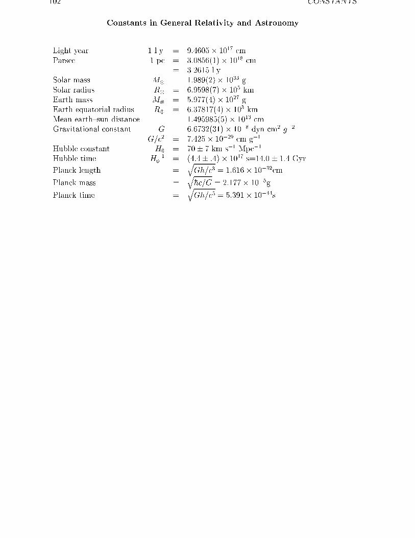
��� CONSTANTS
Constants in General Relativity and Astronomy
Light year � l�y� � ������� ��� cmParsec � pc � ���������� ���� cm
� ������ l�y�Solar mass M� � ��������� ���� gSolar radius R� � ���������� ��� kmEarth mass M� � ��������� ��� gEarth equatorial radius R� � ����������� ��� kmMean earth!sun distance ������������ ���� cmGravitational constant G � ����������� ���� dyn cm� g��
G�c� � ������ ����� cm g��
Hubble constant H� � ��� � km s�� Mpc��
Hubble time H��� � ����� ���� ��� s������ ��� Gyr
Planck length �qG+h�c� � ������ �����cm
Planck mass �q+hc�G � ������ ����g
Planck time �qG+h�c� � ������ ���s
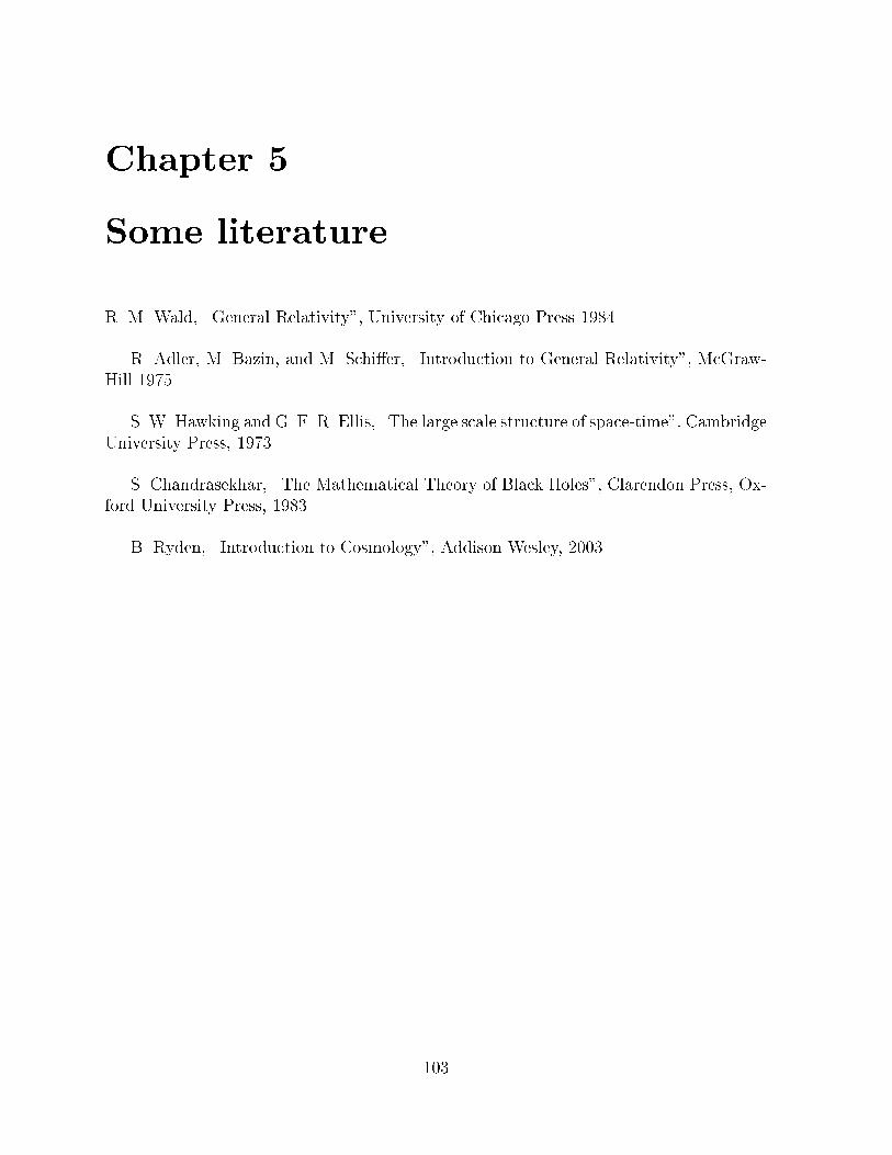
Chapter �
Some literature
R� M� Wald �General Relativity� University of Chicago Press �����
R� Adler M� Bazin and M� Schi�er �Introduction to General Relativity� McGraw Hill �����
S� W� Hawking and G� F� R� Ellis �The large scale structure of space time� CambridgeUniversity Press �����
S� Chandrasekhar �The Mathematical Theory of Black Holes� Clarendon Press Ox ford University Press �����
B� Ryden �Introduction to Cosmology� Addison Wesley �����
���