Gender Role Identity, Breadwinner Status and Psychological .../file/serps... · Gender Role...
33
Gender Role Identity, Breadwinner Status and Psychological Well-being in the Household Heather Brown Jennifer Roberts ISSN 1749-8368 SERPS no. 2014004 March 2014
Transcript of Gender Role Identity, Breadwinner Status and Psychological .../file/serps... · Gender Role...

Gender Role Identity, Breadwinner Status and Psychological Well-being in the Household Heather Brown Jennifer Roberts ISSN 1749-8368 SERPS no. 2014004 March 2014

Gender Role Identity, Breadwinner Status and Psychological
Well-being in the Household
Heather Brown1 and Jennifer Roberts2
1 Institute of Health and Society, Newcastle University, UK
2 Department of Economics, University of Sheffield, UK
Abstract
It is only recently that the psychological concept of identity has entered economic discourse. This paper is concerned with an important aspect of social identity - gender roles within couples. We explore the extent to which compliance with this identity influences individual utility. We consider gender roles and attitudes in a sample from the British Household Panel Survey, within a framework that controls for individual heterogeneity. Our work offers some support for the identity model. Women in ‘traditional’ marriages who accept this role have improved well-being. In couples with ‘modern’ views, women who earn more than their husbands and still have to do most of the domestic work, have lower well-being; this persists if they work part-time and if they report no time pressures. Men who hold traditional views have lower well-being if their wives work; and men who hold modern views on gender roles only have higher well-being if their wives are the higher earner but only work part-time. Our results have implications for the validity of traditional household bargaining models which are largely gender neutral.
D1; J16; Z13. social identity; gender roles; household; well-being; panel data.
Acknowledgements:
We would like to acknowledge the Institute for Social and Economic Research, University of Essex and the UK Data Service for the provision of the British Household Panel Survey data used in this study (University of Essex, 2010). We also thank Anita Ratcliffe and Gurleen Popli for very useful comments on an earlier version of this paper.
Gender Role Identity, Breadwinner Status and Psychological Well-Being in the Household …
2
Introduction
“ ... because identity is fundamental to behavior, choice of identity may be the most important ‘economic’
decision people make. Individuals may – more or less consciously – choose who they want to be. Limits on
this choice may also be the most important determinant of an individual’s economic well-being.” Akerlof
and Kranton (2000: 717)
This paper is concerned with an important aspect of identity, gender roles within couples, and the
extent to which complying with or diverging from this social identity can influence an individual’s
utility. We consider gender roles and attitudes in a longitudinal sample of couples from the British
Household Panel Survey (BHPS), within an analysis framework that controls for unobserved
heterogeneity across individuals. Our primary outcome is a measure of psychological well-being, which
can be understood as a proxy for cardinal utility.
It is only relatively recently that the psychological concept of identity has entered economic discourse
(Akerlof and Kranton, 2000). Traditional models of the economics of the household, such as those of
Mincer (1962) and Becker (1965), were gender neutral; they are based in a standard time allocation
framework and predict, for example, that whoever works more in the market will do less domestic
work, regardless of their gender. This seems unsatisfactory in a world where gender is such a
recognisable and universally accepted trait. To argue, for example, that the domestic division of labour
does not depend in any causal way on the gender of the individuals involved, when gender is such a
strong predictor of the existing division, seems inadequate regardless of the internal consistency of the
economic models behind these arguments.
Akerlof and Kranton (2000) draw on theories of social norms from psychology to develop an
economic theory of social identity. In their model, identity, or an individual’s sense of self, directly
enters the utility function and thus influences economic outcomes. Gender is a universally familiar
example of social identity; there are two prescribed categories, male and female, each with a set of
accepted physical attributes and behaviours. Following these prescribed behaviours affirms one’s
identity as a man or a woman, whereas violating them causes anxiety both in oneself and in others;
hence gender identity influences the pay-offs from different actions. For example, if women’s ‘female’
identity is enhanced by work inside the home she will have lower labour force attachment than men,
which can help to explain women’s historically lower participation rates, and the greater cyclical
variability in these rates.
Social norms theory is not the only way in which economic theory is becoming gendered (Bertrand,
2010). Developments in experimental economics have produced a plethora of laboratory based
research that uncovers gender differences in key psychological attributes such risk attitudes and social

Gender Role Identity, Breadwinner Status and Psychological Well-Being in the Household …
3
preferences. However, outside of the laboratory, there is much less empirical work that explores how
these differential attributes affect the economic outcomes and behaviours of men and women; also the
work that does exist has tended to focus largely on labour market outcomes (see for example: Fortin,
2005; 2008). Similarly, Akerlof and Kranton (2000) do not attempt to test the predictions of their
theoretical model of identity directly. Our study is an attempt to partially fill this gap in the empirical
work.
In contrast to the dominance of theoretical models and experimental evidence in the economics of
gender role identity, there is a related strand of work in sociology that has been largely driven by field
based empirical research. The seminal work in his area is that of Ross et al (1983) who consider the
gradual shift in marriage types from complementary, where the husband is employed and the wife cares
for the household and children, to parallel, where both spouses are employed and both are responsible
for housework. One result of this on-going process is that at any particular point in time an individual’s
role within their marriage may not be consistent with their social identity/preferences and this
disjunction, and the extent to which it is present for either or both spouses, affects psychological
outcomes. So, for example, if the wife is working but either or both spouses would prefer that she did
not, this will have consequences for the psychological well-being of each spouse. The empirical work
of Ross et al (1983) is based on a telephone survey of couples in the US in 1978. These data have three
main limitations. Firstly they are relatively old, and given the dynamic nature of social gender norms,
they do not reflect the current context of marriage and wider gender roles. Secondly, they are cross-
sectional and therefore it is not possible to account for unobserved heterogeneity across individuals in
the methods employed, hence any causal inferences may be misleading. Thirdly, women’s part-time
work is not given adequate consideration, and this is particularly relevant here because it potentially
enables women to combine dual domestic and labour market roles.
While the economic and sociological work has largely developed separately to date, our work draws on
both of these literatures to improve our understanding of gender roles within couples and the effects
on psychological well-being. We use longitudinal data for a sample of households in the UK and we
test the hypothesis that the extent that an individual’s behaviour within the household complies with
their gender role identity affects their overall psychological well-being. We explore this hypothesis for
the four couple types originally defined by Ross et al (1983); these couple types are distinguished by
whether or not the wifei undertakes market work, the shares of housework done by each spouse, and
the attitude of each spouse towards the ‘traditional’ gender roles of male breadwinner/female
homemaker. We also extend the analysis categories to consider women’s part-time work and a further
three ‘modern’ couple types defined by the fact that, within these couples, the wife is the primary wage
earner.

Gender Role Identity, Breadwinner Status and Psychological Well-Being in the Household …
4
This paper makes a number of contributions to the economic literature on gender identity. Firstly, we
use information on attitudes to ‘traditional’ gender roles as a measure of stated preferences; this allows
us to explore the extent to which observed behaviours diverge from these preferences. This is distinct
from the work of Booth and van Ours (2008, 2009, 2013) who study partnered women’s part-time
work and life satisfaction but do not account for these gender role attitudes. Secondly, our outcome
measure (an instrument for measuring psychological well-being) is a good proxy for individual utility,
and is arguably more objective than standard life satisfaction questions which are prone to reporting
biases. Thirdly, we use a panel pseudo fixed effects framework (Mundlak, 1978) to control for
unobserved heterogeneity. If there are unobservable factors, such as psychological traits for
optimism/pessimism or introversion/extraversion, that are correlated with psychological well-being
and couple type, then to the extent that these traits are time invariant our estimation method controls
for them to prevent potentially misleading inference. The longitudinal nature of our data also allows
us to explore the effects for ‘stable’ couples who remain together throughout the period, thus casting
some light on selection issues. Our work can be viewed as a test of some of the predictions arising
from Akerlof and Kranton’s (2000) work on identity. If the allocation of market work and domestic
work within couples is the optimal outcome of household bargaining, within a time allocation
framework, based on individual preferences, then we would not expect to find systematic differences
in husbands’ and wives’ psychological well-being across our couple types, once we have controlled for
other determinants of psychological well-being. Our results show that some systematic differences do
emerge and further analysis suggests that the extent to which an individual’s current situation is in line
with their gender role identity affects their psychological well-being.
In what follows, Section 1 considers the background literature on gender identity and psychological
well-being and discusses gaps in this literature which this paper attempts to address. Section 2
describes the data and variables, and our econometric method. Section 3 reports the results. Section 4
provides further discussion of these results and Section 5 concludes.
1. Background and Motivation
The traditional neoclassical models of the household, such as those of Mincer (1962) and Becker
(1965), as well as the household bargaining literature that emerged from this (e.g. Manser and Brown
1980; McElroy, 1990; Lundberg and Pollak, 1996), treat the household as a unit of production and
consumption. The allocation of time between market work, domestic work and leisure is the outcome
of an optimisation process that depends on individual preferences, the market wage and other
household income. These models are gender neutral; they do not recognise the household as an
important locus for the expression and maintenance of gender identity. In contrast while Akerlof &
Kranton (2000) rely on an essentially neoclassical utility maximization approach, their identity model

Gender Role Identity, Breadwinner Status and Psychological Well-Being in the Household …
5
(when applied to gender roles) allows for the distribution of housework and market work to depend on
gender specific utility. This utility is determined, inter alia, by the extent to which an individual’s
behaviour conforms to their prescribed gender role identity.
Akerlof and Kranton (2000) do not attempt to test their theoretical model directly, but a small number
of more recent studies have explored some of its predictions in relation to gender identity. Booth and
van Ours (2008) use data on couples from eight waves of the BHPS and find a ‘part-time work puzzle’
for women. Data on hours satisfaction and job satisfaction suggest that women prefer to work part-
time, but overall life satisfaction is unaffected by hours of work. The authors hypothesise that part-
time work allows women to combine market and domestic responsibilities more easily than full-time
work; hence women who work part-time should have higher life satisfaction. However, we would
argue that this depends on individual gender role identities; women who have strong labour market
attachment and reject the traditional female gender role, but who are constrained to part-time work
because of their domestic responsibilitiesii, will have lower life satisfaction from working part-time.
Booth and van Ours (2008) do not use information on individuals’ gender role preferences to directly
test gender identity hypotheses, but their results are inconsistent with gender neutrality and consistent
with the gender identity modeliii.
A related strand of literature has explored what has been termed the ‘doing gender’ hypothesis. The
neoclassical gender neutral resource bargaining perspective predicts that an individual’s share of
domestic work will decrease as their contribution to household income increases (Manser and Brown,
1980). An anomaly has been identified empirically in data for a number of different countries in that
when the husband’s household income share is low compared to the wife’s the husband’s share of
domestic work is reduced (Greenstein, 2000; Bittman et al, 2003; Evertsson and Nermo, 2004). The
‘doing gender’ explanation for this is that the domestic sphere can play an important role in sustaining
gender role identity when it is threatened elsewhere, so men who are not fulfilling their stereotypical
breadwinner role reduce their homework hours to prevent further deviation from the male gender
norm. However, when Kan (2008) tests this hypothesis for the UK, using the first nine waves of the
BHPS, she finds no support for it; instead for both men and women their share of housework declines
linearly as their share of household income increases, as the resource bargaining perspective would
predict.
In the only study we are aware of that explores the relationship between stated gender role preferences,
behaviours and subjective well-being, Chang (2011) estimates a two-stage model of gender identity and
happiness for a cross section sample of individuals in Taiwan is 2002. His conceptualisation of gender
role identity includes attitudes towards women’s family position, labour market status and political
participation, and he finds support for the gender identity model. The extent to which an individual’s
actions correspond to their ideal gender role is a significant determinant of their happiness. Benjamin

Gender Role Identity, Breadwinner Status and Psychological Well-Being in the Household …
6
et al (2010) have explored the effects of racial and gender identity on time and risk preference using
‘self-categorization’ as a priming condition to strengthen the salience of these norms. In a series of
experiments with subjects in the US they find that racial priming has an effect on these preferences but
gender priming does not.
In the sociological literature Ross et al (1983) study the effects of historical changes in marriage
patterns and gender roles on the incidence of depression in couples. They define four types of couple
to reflect the gradual transition from complementary to parallel marriages: (i) the traditional marriage
where the wife is not employed in market work, both partners approve of this, and she does the
majority of the housework; (ii) the wife works but both partners disapprove of this and she still does
the majority of the domestic work; (iii) the wife works and both partners approve of this, but she still
does the majority of the housework; (iv) the wife works, both partners approve of this and the
housework is shared. They study the effects of these marriage types on depression using data from a
telephone survey of 678 US couples in 1978. The results suggest that the worst couple type is (ii),
where the wife works but neither spouse thinks she should. Both the husband and wife are more
depressed than for any other couple type, and the husband is more likely to be depressed than the wife.
Couple type (iv), where the wife works but both partners approve and housework is shared, results in
the least depression for both partners. Ross et al (1983) do not look at gender role identity per se to
explain their findings but their results do appear to be consistent with a gender identity model. Couple
type (ii) involves both the wife and husband diverging from their gender role identities and
preferences; she does not want to work, he does not want her to work, hence they are both adversely
affected. Couple type (iv) suggests the least divergence from gender role identity since both partners
appear to have accepted the wife’s role in the labour market and the husband’s role in domestic work.
However, Ross et al (1983) do not consider women’s part-time work, which is an important omission
is given the fact that part-time is often a means of facilitating dual roles for women.
One important issue that has not been given adequate coverage in the economics literature, but which
may nevertheless help to explain the lack of empirical work in the area, is the difficulty in measuring,
and even defining, identity. While Akerlof and Kranton (2000) themselves do not consider this
explicitly, the concept they refer to is social identity, and this should be distinguished from personal
identity (Aguiar et al, 2010; Davis, 2006; 2007). This distinction is well-known in psychology, as Turner
(1999) points out:
“Personal identity refers to self-categories which define the individual as a unique person in terms of their individual differences from other (ingroup) persons. Social identity refers to social categorization of self and others, self-categories which define the individual in terms of his or her shared similarities with members of certain social categories in contrast to other social categories.” (p. 12)

Gender Role Identity, Breadwinner Status and Psychological Well-Being in the Household …
7
An individual can relate to multiple social identities (for example professional working woman and mother),
each of which demand different behaviours, and which may be in conflict (Russo and van Hooft, 2011;
Wichardt, 2008). Personal identity is more than just the sum of social identities; it also requires a
degree of choice (and the power to exercise that choice) over which social identity is most salient to
the individual at any particular point in time and how different social identities will be combined to
determine behavioursiv. In our analysis we do not measure personal identity, rather following Akerlof
and Kranton (2000), we measure the extent to which individuals and their spouses adhere to their
preferred gender role social identity. Gender role identity is a social construct but the amount that
diverging from it is likely to affect individual well-being is dependent on how strong individual
preferences for this identity are; thus the attitude variable that is used in our empirical analysis provides
an indication of how strongly an individual and their spouse adhere to their preferred gender roles in
their actual behaviours.
It is not the purpose of this paper to consider the origins of male and female gendered identities.
Evolutionary psychologists and biologists emphasize nature, whereby, like the physiological differences
between the sexes, the psychological differences also contribute to maximising the chances of
reproductive success and survival. In contrast nurture based explanations emphasize the role of
parents, schools and peers who treat boys and girls differently from an early age. Indeed, even within
the confines of the economic literature on this subject, it is not clear whether differences in
psychological attributes, like risk attitudes and social preferences, drive gender role identity or whether
gender norms are the cause of the psychological differences uncovered in the laboratory, whereby
individuals are behaving according to what it expected of their gender (Bertrand, 2010). Regardless of
the causes, we take gender role social identity as a given, which varies in its strength and type across
individuals, and we explore how the extent to which individuals comply with this identity affects the
psychological well-being of the men and women in couples.
2. Data and methods
We use longitudinal data from the BHPS over the period 1996 to 2008 (University of Essex, 2010).
The BHPS is a nationally representative survey which began in 1991, when it consisted of
approximately 5000 households containing around 10,000 original sample members who are followed
up annually. In 1999 and 2001 additional samples from Scotland, Wales and Northern Ireland were
recruited into the survey to improve the national representativeness of the sample across the UK. The
data include, inter alia, information on socioeconomic status, labour market outcomes, household
composition, individual preferences and opinions, education, and health.

Gender Role Identity, Breadwinner Status and Psychological Well-Being in the Household …
8
Our analysis sample is restricted to working age adults who live as a heterosexual couple; that is they
are in a cohabiting relationship or legal marriage. Women are aged between 16 and 60 years old and
men are 16 to 65 years old; retired individuals within this age range are excluded to retain an emphasis
on working status. The restrictions placed on the sample give us 22,636 individual observations across
1504 couples. The main analysis sample includes any couple that is present in at least two years of
data. Sensitivity analysis is performed where we restrict the sample to couples who are observed as
remaining together from the first year in which they are observed until the end of the sample period.
The analysis sample is further reduced by our couple classification system; in order to accurately
classify couple types according to housework shares, we require a non-missing answer from both
partners and for partners answers on housework shares to be consistent with one another’s (see
variable definitions below). Our final estimation sample comprises 9730 individual year observations
across 589 couples (see Table 3 for sample sizes for each couple type).
Variable Definitions
The main outcome variable used in our analysis is a measure of psychological well-being, the General
Health Questionnaire (GHQ) (Goldberg and Williams, 1988). This measure has been frequently used
in economic analysis (see for example Clark, 2003; Brown et al, 2005; Gardner and Oswald, 2007;
Roberts et al, 2011); and it is arguably a more objective measure of psychological well-being than
standard life satisfaction questions, such as those used in Booth and van Ours (2009), which are prone
to reporting biases as they are explicitly evaluative measures. The GHQ is part of a self-completion
questionnaire administered to all survey respondents; the version used is comprised of twelve
questions (see Appendix A) focusing on both positive and negative emotions experienced recently.
Each question has a choice of four options and answers are aggregated to produce a 36 point scale.
For ease of exposition the coding of the GHQ scores has been reversed so that a higher score means
better psychological well-being. The 36 point GHQ scale is treated as continuous following evidence
from the literature that if unobserved individual effects are controlled for in estimation, assuming
cardinality or ordinality of well-being scores has little effect on the results (Ferrer-i-Carbonell and
Frijters 2004).
In our sensitivity analyses we also consider two alternative outcome variables that measure different
aspects of psychological well-being. Firstly, a binary variable that equals one if an individual reports
suffering from anxiety and depression in the previous year and zero otherwise; this variable has the
advantage that it is very similar to the outcome variable used the original sociological work by Ross et
al (1983), thus allowing us to compare our results with theirs. The ‘anxiety and depression’ question is
part of a set of thirteen yes/no questions on specific health problems, which are administered to
respondents via the self-completion questionnaire. The second alternative outcome variable is a binary
Gender Role Identity, Breadwinner Status and Psychological Well-Being in the Household …
9
variable created from a question in the GHQ on unhappiness and depression (Question 5 in Appendix
A). This variable is equal to one if the respondent reports feeling unhappy or depressed rather more or
much more than usual and is equal to zero otherwise.
In our analysis the key variables of interest are couple type and gender; seven couple types are defined.
The first four are the same as those used in the analysis by Ross et al (1983) discussed in Section 1;
these couple types are distinguished by whether or not the female spouse undertakes market work, the
shares of housework done by each spouse, and the attitude of each spouse to traditionally prescribed
gender roles. The specific couple types are: (1) the wife does not work, both partners approve of this
and she does the majority of the housework; (2) the wife works, both spouses disapprove of this and
she does the majority of the housework; (3) the wife works, both partners approve of this and she does
the majority of the housework; (4) the wife works, both partners approve of this and the housework is
shared. These couple types were chosen by Ross et al (1983) to reflect the transition from
complementary to parallel marriages that was a result, inter alia, of growing female labour force
participation rates in the US during the 1960s and 1970s. However, social norms are dynamic and
gender roles and marriages have continued to evolve, therefore couple types (1) and (2) in particular
may be considered unusual in the UK today.
To reflect this continual process of change we extend the analysis categories to consider three ‘modern’
couple types, in which the wife not only works but is also the primary wage earner; this was chosen to
reflect the increase in the female share of household incomes that has been a feature of the UK
economy in the past two decades (Soobedar, 2011). In addition in these couples both spouses disagree
with traditional gender roles. It is not possible to consider those spouses who agree with traditional
gender roles within this female primary wage earner sub-sample because the sample sizes are too small;
and this is reflective of the fact that the perceived appropriateness of gender roles does change over
time. However, while labour market roles have undoubtedly changed, attitudes and domestic
responsibilities may not have fully kept up with this. For example, most of the 29 British families
surveyed for a recent Joseph Rowntree Foundation report agreed with the view that the father’s role
was that of "financial provider and protector" v ; despite the fact that in the majority of these
households the mother was employed (Hauari et al. 2009). In order to shed some light on this we
firstly distinguish couple types (2) to (4) above according to whether the wife works full-time or part-
time. Part-time work is often undertaken by women in the UK and one reason for this is that it allows
them to combine labour market and domestic responsibilities i.e. to fulfil a dual role (Booth and van
Ours, 2008). In addition we also classify our three modern couple types according to housework
shares. Thus in couple type (5) the wife does the majority of housework, in (6) the housework is
shared, and in (7) the husband does the majority. Our reasoning here is that regardless of the stated

Gender Role Identity, Breadwinner Status and Psychological Well-Being in the Household …
10
attitudes of each spouse, the actual division of domestic responsibilities in the home gives additional
information on gender role identity. The more housework the husband does the more this suggests he
has accepted the change of gender roles and the subsequent implications for gender role identity. The
attitudes question is stated preference measure, whereas the actual housework shares can be
interpreted as revealed preferences.
A number of variables are required in order to classify these couple types, and Table 1 summarises
how the seven couple types are constructed. Employment status is derived from reported current
labour market status, with individuals who report being employed or self-employed, characterised as
undertaking market work. Part-time work is defined as less than 30 hours per week. Earnings are
derived from the question on individual annual labour income. Our measure of gender role social
identity is taken from the individuals’ attitudes towards prescribed gender roles elicited from the
question: “A husband’s job is to earn money: a wife’s job is to look after the home and family”, where the available
responses are: Strongly Agree/ Agree/ Neither Agree or Disagree/ Disagree/ Strongly Disagreevi. We
take either of the first two responses to represent agreement with traditional gender roles, and either of
the last two to represent disagreementvii.
The amount of housework done by each individual is derived from questions on household tasks. For
the set of household tasks respondents are asked to state who spends most time on the task:
themselves, their partner, or whether the work is shared equally. The tasks include cooking, cleaning,
washing and ironing, and grocery shopping. Couples who provide responses that are inconsistent with
each other, and couples who report that the task is done by paid help or another person are excluded
from the analysis. A binary variable is created that equals one if the four household tasks are shared
equally between the couple, if partners share at least two tasks and each partner has responsibility for
the remaining two tasks, or if each partner is responsible for two tasks and is equal to zero if one
partner is solely responsible for the majority of the household tasksviii.
As an alternative in our sensitivity analyses we also use the amount of hours that each individual
reports spending on housework overall. This variable is constructed from a question that asks each
respondent: About how many hours do you spend on housework in an average week such as time spent cooking,
cleaning, and doing laundry. From this variable we construct three dummy variables controlling for
whether: the wife and husband do approximately similar levels of housework (within 7 hours of each
other): the wife does eight or more hours of housework than her husband; the husband does eight or
more hours of housework than his wife.
Gender Role Identity, Breadwinner Status and Psychological Well-Being in the Household …
11
The multivariate analysis also controls for a number of individual characteristics that are likely to affect
psychological well-being. Our choice of variables is informed by the growing economic literature on
the determinants of psychological well-being (Dolan et al 2008; Oswald and Powdtahvee, 2008). Age
and age squared are included to reflect the well-reported U-shaped relationship between age and
psychological well-being (Blanchflower and Oswald, 2008). Most of the existing literature also includes
a variable to represent the presence of children, although there is no strong evidence for its effects
Haller & Hadler (2006). We include a dummy variable to represent whether or not the couple has
children aged under 12 years; this controls for childcare responsibilities as well as any potential effects
on psychological well-being. We also include equivalised household income, highest educational
attainment and a dummy variable which equals one if the individual has a non-Caucasian ethnic
background.
Health status is measured in two ways. Firstly, we use a set of dichotomous variables on the presence
of ten specific health problems; these are generally considered to be objective measures which detect
problems with physical health. As an alternative we use the standard self-assessed health (SAH)
measure derived from the question ‘Please think back over the last 12 months about how your health has been.
Compared to people of your own age, would you say that your health has on the whole been
excellent/good/fair/poor/very poor?’ix. This is a broad measure that may reflect psychological as well as
physical health. A full list of variables included in the analysis is presented in Appendix B.
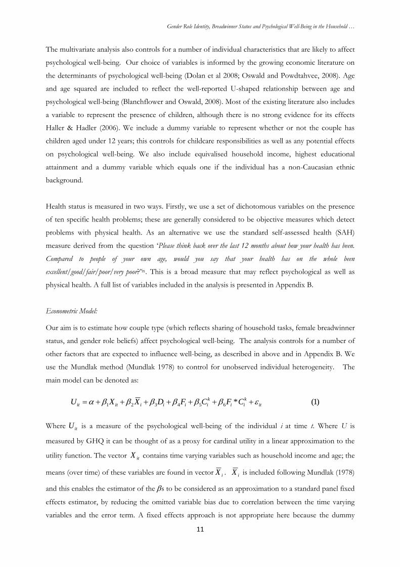
Econometric Model:
Our aim is to estimate how couple type (which reflects sharing of household tasks, female breadwinner
status, and gender role beliefs) affect psychological well-being. The analysis controls for a number of
other factors that are expected to influence well-being, as described in above and in Appendix B. We
use the Mundlak method (Mundlak 1978) to control for unobserved individual heterogeneity. The
main model can be denoted as:
)1(*654321 it
k
ii
k
iiiiitit CFCFDXXU
Where itU is a measure of the psychological well-being of the individual i at time t. Where U is
measured by GHQ it can be thought of as a proxy for cardinal utility in a linear approximation to the
utility function. The vector itX contains time varying variables such as household income and age; the
means (over time) of these variables are found in vector iX . iX is included following Mundlak (1978)
and this enables the estimator of the s to be considered as an approximation to a standard panel fixed
effects estimator, by reducing the omitted variable bias due to correlation between the time varying
variables and the error term. A fixed effects approach is not appropriate here because the dummy

Gender Role Identity, Breadwinner Status and Psychological Well-Being in the Household …
12
variables couple type ( ) and sex (Fi), which are key to our analysis, are time invariant.
The vector iD contains other time invariant variables, such as ethnicity, that are likely to affect
psychological well-being. is an interaction term between the dummy variables Fi and
. 4 is
the average effect of being female (compared to male) on psychological well-being after controlling for
the other variables; 5 is the average effect of being in couple type k on the psychological well-being
of men (compared to men not in that couple type); 654 is the average effect of being a
woman in couple type k. The error term, it is comprised of a time invariant individual effect, i and
an idiosyncratic error term, itu .
Equation (1) is estimated (seven times) for each couple type in turnx; the entire sample of couples is
used in each estimation, but in each case the dummy variable represents a different couple type k (k
= 1,2, ...,7). The models with GHQ as the dependent variable are estimated via random effects GLS,
and all estimation is done using Stata v12.
When considering a priori expectations about the effect of couple type on the psychological well-being
of each spouse the focus of our gender identity model is on the extent to which behaviours with
regards to market work and housework are consistent with the stated gender role preferences of each
spouse; if behaviours are consistent with gender role identity we expect a positive effect on well-being,
if behaviours are inconsistent we expect a negative effect. In contrast to these gender identity
predictions, if the allocation of market work and domestic work within couples is the optimal outcome
of a gender neutral household bargaining modelling based on individual preferences, then we would
not expect to find systematic differences in husbands’ and wives’ psychological well-being across our
couple types, given that we have controlled for other determinants of well-being. It is worth stressing
here that we condition on household income, so any potential material benefits from women’s
employment, which may outweigh the effects on gender role identity are already controlled forxi.
Couple type (1) is a ‘traditional’ marriage with a female homemaker and male breadwinner and both
spouses approve of this; thus behaviours are consistent with gender role identity and we would expect
a positive effect on well-being for both husband and wife. In couple type (2) the wife’s employment is
contrary to the preferences of both spouses; they both want a ‘traditional’ marriage but the wife works,
possibly due to economic necessity, so we may expect a negative effect on well-being for both husband
and wife. In couple type (3) the wife’s employment is consistent with stated gender role preferences for
both spouses but she still does most of the housework; it is therefore an empirical question as to
whether we would expect any effect on well-being. If the housework burdens are consistent with the
differential working hours of each spouse then we would expect a positive effect resulting from

Gender Role Identity, Breadwinner Status and Psychological Well-Being in the Household …
13
consistency with gender role identity, but if women’s greater responsibility for housework is a
reflection of the inconsistency of preferences and behaviours, then we may expect both spouses to be
adversely affected. In our empirical work we distinguish those women who work part-time in order to
shed further light on this. Women’s well-being may also be more adversely affected than men’s, since
they will have the added burden of dealing with possibly conflicting roles in the labour market and in
the domestic sphere. In couple type (4) behaviours are consistent with gender role identity since both
partners appear to have accepted the wife’s role in the labour market and the husband’s role in
domestic work, thus we would expect a positive effect on well-being.
For all the ‘modern’ couple types (5) to (7) the wife earns more than the husband and both spouses
disagree with traditional gender roles, but these couple types are distinguished by how much of the
housework is shared by the husband. In couple type (5) the wife is still carrying the larger domestic
burden, which suggests that despite her larger earnings contribution and their stated gender role
attitudes, traditional gender roles are to some extent still adhered to at home. One explanation for this
is the ‘doing gender’ hypothesis discussed in Section 1; in which the husband uses the home sphere to
sustain traditional gender roles because these are undermined by his wife’s labour market role. The
effects on well-being for both the husband and wife are not determined a priori; if the ‘doing gender’
hypothesis is valid we would expect a positive effect on husband’s well-being. In couple type (6) the
housework is shared thus suggesting more consistency with gender role preferences and labour market
roles, hence potentially positive effects on the well-being of both spouses. Similarly in couple type (7)
the husband’s greater responsibility for housework suggests that he has accepted the gender role swap
where his wife is the primary earner, thus we would expect a positive effects on both spouses well-
being.
We carry out a number of sensitivity analyses to explore the robustness of our results. Firstly, we use
two additional alternative measures of psychological well-being (U), both of these are dichotomous
variables; one records the presence of anxiety or depression in the previous year, and the other records
whether or not the individual reports recent strong feelings of unhappiness or depression. Where
equation (1) is estimated with these alternative dependent variables, a random effects logit specification
is used. The marginal effect for the interaction term, does not have a straightforward
interpretation in this non-linear model (Norton et al. 2004; Buis 2010). To overcome this problem we
adopt the method of Buis (2010) to estimate the marginal effects for the difference in predicted
outcome between: (i) Women not in couple type Ck compared to men not in couple type Ck; (ii)
women in couple type Ck compared to women not in couple type Ck; (iii) women in couple type Ck
compared to men in couple type Ck; (iv) men in couple type Ck compared to men not in couple type
Ck. The ‘margins’ command in Stata v.12 is used to calculate the odds of suffering from

Gender Role Identity, Breadwinner Status and Psychological Well-Being in the Household …
14
anxiety/depression (or being more unhappy) for every combination of gender and couple type. We
can then calculate the difference between the four categories above using the estimated odds.
As well as exploring alternative dependent variables we also consider alternative specifications of the
health explanatory variable. The SAH measure, defined earlier in this section, is a broad health measure
that may reflect psychological as well as physical health and hence may be endogenous in our model
for GHQ. Nevertheless it is arguably a more meaningful measure of overall health than the list of
specific physical health problems we have included, and if we condition on SAH and still find
significant effects of couple type this further supports our hypothesis that the extent of compliance
with gender role identity within the household affects overall psychological well-being. SAH is
specified as three dichotomous variables representing excellent, good and fair health, with poor health
as the baseline category (see Appendix B).
In addition we carry out two further sensitivity analyses. Firstly, because the degree of conformity to
gender identity within couples may affect the probability of a couple remaining together, we re-
estimate all of our models for the sub-sample of ‘stable’ couples; these are defined as those who
remain together from the first wave in which they are observed to the end of the sample period. It
seems reasonable to assume that the estimated negative effects of compliance with gender role identity
on psychological well-being will be smaller for the selective sample of couples who stay together, and
any estimate positive effects will be largerxii. Secondly, in relation to the classification of our couple
types, we use an alternative classification of housework sharing defined via the number of hours that
each partner contributes rather than by the number of household tasks they carry out (see variable
definitions above).
3. Results
Table 2 reports descriptive statistics for all the variables used in the analysis for men and women
separately. Women have lower GHQ scores, are more likely to report suffering from anxiety and
depression, and to have become unhappy over the past month compared to men. 92% of men are
employed compared to 76% of women, and of those women around a half work part-time compared
to only 4% of men. Women spend more than 3 times longer doing housework in a week than men,
and they are more likely to do the majority of household tasks. The most common shared task is
grocery shopping, and the task least likely to be shared is washing and ironing. There seems to be a
tendency for more men to report tasks as shared than women. Both men and women are far more
likely to hold modern views about gender roles than traditional views, but men are more (less) likely
than women to have traditional (modern) views. The incidence of physical health problems is similar

Gender Role Identity, Breadwinner Status and Psychological Well-Being in the Household …
15
across men and women, with two exceptions; women are more likely to report problems with skin and
migraines. Overall SAH is distributed very similarly for men and women.
Table 3 shows all three of our psychological well-being outcomes by gender and couple type, as well as
the proportions working part-time. The previous literature has commonly found that women report
lower levels of psychological well-being on the GHQ scale than men (see for example Clark and
Oswald, 1994). Here we see that women have significantly lower GHQ scores in couple types (3) to
(6), but for (1), (2) and (7) the scores are similar. In addition women are more likely to report anxiety
and depression than men in couples types (3) and (4), and are more likely to report being unhappy than
men in couples types (3) to (5). The proportion of part-time working sheds further light on time
allocation across couple types. In couple types (3) and (4), which are distinguished by housework
shares, the shares are consistent with the proportion of wives who work part-time; in (3) the wife does
the majority of housework and 52% work part-time, whereas in (4) housework is shared and only 32%
of wives work part-time. Only a very small proportion of men work part-time, except in couple type
(7), and this is consistent with the fact that the wife is the primary earner in this couple type and the
husband is doing the majority of housework. The most common couple type is (3) where both
partners work but the wife still does most of the housework; second is (4) where the housework is
shared. It is unusual for husbands and wives to both agree with traditional gender roles (couple types
(1) and (2)), and it is unusual for women to be the main wage earner and for their husbands to do most
of the housework (couple type (7).
Main results
The main GLS results for equation (1) with Mundlak fixed effects and GHQ as the dependent variable
are presented in Table 4. The columns show the results for couple types (1) to (7). The first point to
note is that the estimated effects of our conditioning variables are very stable across couple types.
There is a negative and significant effect of age and a positive effect of age squared, suggesting the
well-known U-shaped relationship between age and psychological well-being. The presence of
childrenxiii and has no significant effect on GHQ. For education, only being educated to degree level or
higher has a significant association with GHQ, and this is negative. While this result may appear
counterintuitive, it is not uncommon in the literature; one potential explanation is that education may
raise aspirations, which are subsequently not met (Sabates and Hammond 2008). Despite the key role
for income in economic decision making, again our finding of an insignificant effect of equivalised
household income on psychological well-being is common in this empirical literature. This is
particularly the case in models that utilise fixed effects or the Mundlak approach, as we have here,
because the levels effect of income is removedxiv. It is worth noting here that if we use individual
income instead of household income the results are largely the same. Ethnicity also has no significant
effect. For conciseness the presence of specific health problems is not presented in Table 4. Of the ten
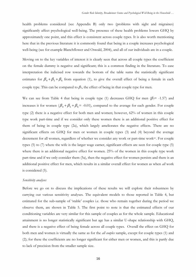
Gender Role Identity, Breadwinner Status and Psychological Well-Being in the Household …
16
health problems considered (see Appendix B) only two (problems with sight and migraines)
significantly affect psychological well-being. The presence of these health problems lowers GHQ by
approximately one point, and this effect is consistent across couple types. It is also worth mentioning
here that in the previous literature it is commonly found that being in a couple increases psychological
well-being (see for example Blanchflower and Oswald, 2004), and all of our individuals are in a couple.
Moving on to the key variables of interest it is clearly seen that across all couple types the coefficient
on the female dummy is negative and significant; this is a common finding in the literature. To ease
interpretation the italicised row towards the bottom of the table sums the statistically significant
estimates for 654 from equation (1), to give the overall effect of being a female in each
couple type. This can be compared to 5, the effect of being in that couple type for men.
We can see from Table 4 that being in couple type (1) decreases GHQ for men (5= -1.57) and
increases it for women ( 654 = -0.01), compared to the average for each gender. For couple
type (2) there is a negative effect for both men and women; however, 62% of women in this couple
type work part-time and if we consider only these women there is an additional positive effect for
them of being in couple type (2a), which largely ameliorates the negative effects. There are no
significant effects on GHQ for men or women in couple types (3) and (4) beyond the average
decrement for all women, regardless of whether we consider any work or part-time workxv. For couple
types (5) to (7) where the wife is the larger wage earner, significant effects are seen for couple type (5)
where there is an additional negative effect for women. 25% of the women in this couple type work
part-time and if we only consider them (5a), then the negative effect for women persists and there is an
additional positive effect for men, which results in a similar overall effect for women as when all work
is considered (5).
Sensitivity analyses
Before we go on to discuss the implications of these results we will explore their robustness by
carrying out various sensitivity analyses. The equivalent models to those reported in Table 4, but
estimated for the sub-sample of ‘stable’ couples i.e. those who remain together during the period we
observe them, are shown in Table 5. The first point to note is that the estimated effects of our
conditioning variables are very similar for this sample of couples as for the whole sample. Educational
attainment is no longer statistically significant but age has a similar U-shape relationship with GHQ,
and there is a negative effect of being female across all couple types. Overall the effect on GHQ for
both men and women is virtually the same as for the all couples sample, except for couple types (1) and
(2); for these the coefficients are no longer significant for either men or women, and this is partly due
to lack of precision from the smaller sample size.

Gender Role Identity, Breadwinner Status and Psychological Well-Being in the Household …
17
Most of the remainder of our additional results are not reported in tables for conciseness, but are
simply summarised here. Firstly, we use an alternative measure of health, the SAH measure defined in
Section 2; this is included (instead of specific health problems) in models equivalent to those reported
in Tables 4 and 5. It is specified as three dichotomous variables representing excellent, good and fair
health, with poor health as the baseline category. Coefficients on all three SAH variables are positive
and significant for all couple types and have the expected gradient; excellent SAH is associated with
around a 5 point increase in GHQ compared to poor health, and this is around 4 points for good
health and 3 for fair health. While there are small quantitative differences in the coefficient estimates
on the other variables the results are substantively the same as those already reported; there are no
changes in those variables that have statistically significant effects.
Secondly, in relation to the classification of our couple types (see Table 1), we define share of
housework by the number of hours that each partner contributes rather than by the number of
household tasks, this has no substantive effect on any of the results reported here. The final set of
sensitivity analyses we consider are two alternative measures of psychological well-being as defined in
Section 2; these are dichotomous variables representing the presence of anxiety and depression, and
unhappiness. The results from the random effects logit models with these outcomes as the dependent
variable are reported in Table 6. In Section 2 above we outlined the problems with the interpretation
of the marginal effect for the interaction terms in these non-linear models, and because of this we
present the results in a slightly different way to those of Tables 4 and 5. In Table 6 we report the
difference in predicted outcome for four different comparisons across the seven couple types. The
explanatory variables are the same as in Tables 4 & 5 and associated marginal effects (which are not
reported here) are also largely the same.
In the upper half of the table we see from the first row that women are around 4% more likely to
report having anxiety and depression than men. The results in the second row suggest that women in
couple types (2), (3) and (4) less likely to report anxiety and depression than women not in that couple
type. In the third row women in couple types (3), (4) and (5) are more likely to report having anxiety
and depression than men in that couple type; and in row (iv) men in couple types (3), (4) and (6) are
less likely to report having anxiety and depression than men not in that couple type. In the lower half
of Table 6 we see the equivalent results for unhappiness. Row (i) in the lower half shows that in
general women are around 12% more likely to report being unhappy than men. In row (iii) women in
couple types (3), (5) and (5a) are more likely to be unhappy than men in those couple types; and in the
last row men in couple types (1), (2) and (2a) are more likely to be unhappy than other men, and in
couple types (3) and (5a) they are less likely to be unhappy. These results are largely consistent to those
reported above with GHQ as the measure of psychological well-being, and we summarise and discuss
them further below.

Gender Role Identity, Breadwinner Status and Psychological Well-Being in the Household …
18
4. Discussion
The results presented above reveal some systematic differences in husbands’ and wives’ psychological
well-being across couple types, and this is not consistent with the predictions of gender neutral models
of the household. However, it is less clear that these results can be explained purely by the gender
identity model.
Couple type (1) is the ‘traditional’ household; the wife does not work and both partners agree with this,
she also does the majority of the housework. Our all couple results (Table 4) suggest that in terms of
GHQ score this is the best couple type to be in for women and one of the worst for men; this is
supported by the results for unhappiness in Table 6. This is only partly consistent with the gender
identity model because in this couple type the husband and wife are both fulfilling the ‘traditional’
gender role, with which they both agree, hence we would expect positive effects for both partners, not
just for the wife; the negative effect for men is hard to reconcile with the gender identity model.
However, for our stable couples (Table 5) these effects are no longer present. Our results are also
different to those of Ross et al (1983) who found that in the ‘traditional’ marriage the wife was more
likely to be depressed than the husband. This difference may be a reflection of changing social norms
and institutions; women in the 1970s may have been more constrained to this type of marriage,
whereas during the time period of our study it is more likely to be the outcome of a positive choice
(Hakim, 2000).
In couple type (2) both the husband and wife state that they believe in the ‘traditional’ male
breadwinner/female homemaker model; however, the wife does work in the market (possibly due to
economic necessity). Ross et al (1983) found this to be the worst couple type for both men and
women, but our results show that the estimated effects depend on whether or not the wife works part-
time. Where we consider all work for women there are significant negative effects on the GHQ score
of both husbands and wives. However, when we consider only those women who work part-time the
adverse effects for women disappear, but remain for men. Thus it seems that when men think they
should be the sole breadwinner, their psychological well-being is adversely effects when their wife
works, even if this work is part-time. While for women, even if they agree with traditional gender roles,
work, as long as it is part-time, has no adverse effects on their well-being.
In couple type (3) while both partners approve of the wife working she still does most of the
housework. Ross et al (1983) found that the husband was content with this but that the wife was as
likely to be depressed as in the traditional couple type (1). We find no effects on the GHQ score for
men and women (whether women’s work is part-time or not) but that both partners are less likely to
report anxiety and depression than men and women in other couple types, and for men this also
applies to unhappiness. However, within this couple type women are more likely to report anxiety and

Gender Role Identity, Breadwinner Status and Psychological Well-Being in the Household …
19
depression, and unhappiness, than men. So there is some evidence that the effects of compliance with
gender role identity are asymmetric. Traditional gender role identities are partly modified, as women
work and both partners approve, but not completely as women still do the majority of the domestic
work. This appears to be better for men’s psychological well-being than women’s. Couple type (4) is an
egalitarian type marriage where both partners work, both approve of this arrangement and they share
housework. Ross et al (1983) found this to be the best type of marriage for both the husband and wife.
To some extent our results are consistent with this; we find no effects on GHQ scores, both the men
and women in this couple type are less likely to report anxiety and depression than other men and
women. However, within this couple type women are more likely to report anxiety and depression
than men.
In our remaining ‘modern’ couple types both partners disagree with traditional gender roles and the
wife earns more than the husband. However, despite these stated attitudes towards gender roles, in
couple type (5) the wives still do most of the housework and our results reveal that this has a negative
effect on their GHQ scores. This effect persists when we consider only those women who work part-
time, and here there is an additional positive effect for men. This result is consistent with the ‘doing
gender’ hypothesis (Kan, 2008); the husbands gender role identity is threatened by his wife’s labour
market position so he uses the domestic sphere to reinforce traditional gender stereotypes and this
increases his psychological well-being. However, the positive effect for the husband may also arise
because he gains additional utility from being able to spend more time with his wife, and/or from her
greater potential contribution to household production (Stein, 1984). Where housework is shared (6)
or the husband does more (7) , we find no systematic effects on well-being for either the husband or
the wife.
A number of our results, and in particular the adverse effects for women of being in couple types (2)
and (5), where the wife is working and also carrying out most of the domestic labour, could be argued
to arise from time pressures and the practical difficulties experienced in attempting to combine dual
roles, rather than divergence from gender role identity per se. Comparing the results for couple types
(2) and (2a) seems to support this view because in (2a) the wife works part-time and the adverse effects
on her GHQ disappear. However, a number of features of our results do not support the view. Firstly,
in couple type (3) the women involved are expected to suffer the same time pressures, in fact more so
because a lower proportion of them work part-time than in couple type (2) (see Table 3); but in couple
type (3) we see no adverse effects on GHQ and these women are less likely to report anxiety and
depression than other women (Table 6). The only difference between couple types (2) and (3) is in
stated gender role attitudes, so this strong support for the identity model. In addition the negative
effects for women in couple type (5) persist in (5a) where their work is part-time. We attempt to shed
further light on the issue of time pressure by taking into account the extent to which the individuals

Gender Role Identity, Breadwinner Status and Psychological Well-Being in the Household …
20
involved are satisfied with the amount of leisure time they havexvi. Estimating the models in Table 4
and 5 only for those women who are satisfied with their leisure time (78% of the sample) results in
virtually no change in the coefficient estimates, hence there is a still a negative effect on well-being for
women in couple types (5) and (5a) even when they do not report experiencing time pressures. This
provides further support for the gender identity model; the adverse effects for women’s well-being are
caused by dealing with dual, and possibly conflicting, roles in both the labour market and in the
domestic sphere. This adverse outcome persists despite stated disagreement, on behalf of both
spouses, with traditional gender roles.
5. Conclusion
The psychological concept of social identity and its role in determining economic outcomes is a
growing issue in the economics literature. Our study has explored an important aspect of social identity
that of gender roles within couples. We have used a longitudinal sample from the BHPS to estimate
the extent to which compliance with this identity influences individual utility, proxied by the GHQ
measure of psychological well-being. Our work offers some support for Akerlof and Kranton’s (2000)
identity model. Women in ‘traditional’ (male breadwinner/female homemaker) marriages who accept
this role have improved well-being. However, in a number of couple types where behaviours and
attitudes are inconsistent we see systematic effects on well-being. Where couples have ‘traditional’
views, if the wives work this has adverse effects for both partners. However, it appears that these wives
can work part-time with no adverse effect on their own well-being, but their part-time work still
adversely affects their husbands. In couples who both state that they hold ‘modern’ views on gender
roles, and where the wives earn more than their husbands but still have to do the bulk of the domestic
work, then these wives have lower well-being even if they work part-time. However, their husbands
well-being benefits from this. We find no evidence that these results are due to time pressure, so we
conclude that they support the gender identity model and are inconsistent with the traditional gender
neutral economics of the household, and household bargaining models. A well as providing support
for the gender identity model, our results also suggest that social identity is a topic worthy of further
research to determine its effects on a broad range of economic outcomes.

Gender Role Identity, Breadwinner Status and Psychological Well-Being in the Household …
21
References:
Aguiar F, Branas-Garza P, Espinosa MP, Miller LM (2010) Personal identity: a theoretical and experimental analysis. Journal of Economic Methodology 17(3): 261-75.
Akerlof GA and Kranton RE (2000) Economics and identity. Quarterly Journal of Economics 115(3): 715-53.
Becker G (1965) A theory of the allocation of time. Economic Journal 75(299): 493-517.
Benjamin DJ, Choi JJ and Strickland J (2010) Social identity and preferences. American Economic Review 100(4): 1913-28.
Bertrand M (2010) ‘New perspectives on gender’ Ch 17 in O. Ashenfelter & D. Card (Eds.) Handbook of Labour Economics Vol 4b. North Holland: Elsevier
Bittman M, England P, Folbre N, Sayer L, Matheson G (2003) When does gender trump money? Bargaining and time in household work. American Journal of Sociology 109(1): 186-214.
Blanchflower DG and Oswald AJ (2004) Money, sex and happiness: an empirical study. Scandinavian Journal of Economics, 106(3), 393-41
Blanchflower DG and Oswald AJ (2008) Is well-being U-shaped over the life-cycle? Social Science and Medicine 66(8): 1733-49
Booth AL and van Ours JC (2008) Job satisfaction and family happiness: the part-time work puzzle. Economic Journal 118: F77-99.
Booth AL and van Ours JC (2009) Hours of work and gender identity: does part-time work make the family happier? Economica 76:176-96.
Booth AL and van Ours JC (2013) Part-time jobs: what women want? Journal of Population Economics 26: 263-83.
Brown S, Taylor K, Wheatley Price S (2005) Debt and distress: evaluating the psychological cost of credit. Journal of Economic Psychology 26(5):642-63.
Buis ML (2010) Stata tip 87: Interpretation of interactions in non-linear models. The Stata Journal 10: 305-308.
Chang W-C (2011) Identity, gender and subjective well-being. Review of Social Economy 69(1): 97-121.
Clark AE and Oswald AJ (1994) Unhappiness and unemployment. Economic Journal 104: 648-59.
Davis JB (2006) Social identity strategies in recent economics. Journal of Economic Methodology 13(3): 371-90.
Davis JB (2007) Akerlof and Kranton on identity in economics: inverting the analysis. Cambridge Journal of Economics 31:349-62.
Dolan P, Peasgood T, White M (2008) Do we really know what makes us happy? A review of the economic literature on the factors associated with subjective well-being. Journal of Economic Psychology 29(1): 94-122.
Evertsson M and Nermo M (2004) Dependence within families and the division of labour: comparing Sweden and the United States. Journal of Marriage and Family 66(5): 1272-86.
Ferrer-i-Carbonell A and Frijters P (2004). How important is methodology for the estimates of the determinants of happiness? Economic Journal 114 (497): 641-659.
Fortin N (2005) Gender role attitudes and women’s labour market outcomes across OECD countries. Oxford Review of Economic Policy 21(3):416-38.

Gender Role Identity, Breadwinner Status and Psychological Well-Being in the Household …
22
Fortin N (2008) The gender wage gap among young adults in the United States: the importance of money vs. people. Journal of Human Resources 43(4):886-920.
Gardner J and Oswald AJ (2007). Money and mental well-being: A longitudinal study of medium-sized lottery wins. Journal of Health Economics 26 (1): 49-60.
Goldberg DP and Williams P (1988). A User’s Guide to the GHQ. NFER-Nelson, Windsor.
Greenstein TN (2000) Economic dependence, gender and the division of labor in the home: a replication and extension Journal of Marriage and Family 62(2): 322-35
Hakim C (2000) Work–Lifestyle Choices in the 21st Century: Preference Theory. Oxford: Oxford University Press.
Haller M and Hadler M (2006) How social relations and structures can produce happiness and unhappiness: an international comparative analysis. Social Indicators Research, 75, 169-216
Hernandez-Quevedo C, Jones AM, Rice N (2005) Reporting bias and heterogeneity in self-assessed health: evidence from the BHPS. HEDG University of York Working Paper 05/04.
Hauari H, Hollingworth K and Thomas Corum Research Unit. (2009) Understanding fathering: Masculinity, diversity, and change. Joseph Rowntree Foundation. www.jrf.org.uk/publications/understanding-fathering
Kan MY (2008) Does gender trump money? Housework hours of husbands and wives in Britain. Work Employment and Society 22: 45-66.
Lundberg S and Pollak R (1996) Bargaining and distribution in marriage. Journal of Economic Perspectives 10: 139-58.
Manser M and Brown M (1980) Marriage and the household decision making: a bargaining analysis. International Economic Review 21: 31-44.
McElroy MB (1990) The empirical content of Nash-bargained household behaviour. Journal of Human Resources 25(4): 559-83.
Mincer J (1962) “Labor force participation of married women: a study of labor supply” in Aspects of Labor Economics. Conference No. 14 of the Universities National Bureau Committee for Economic Research. Princeton NJ: Princeton University Press.
Mundlak Y (1978) On the pooling of time series and cross-section data. Econometrica, 46: 69-85.
Norton E, Wang H and Ai C. (2004) Computing interaction effects and standard errors in logit and probit models. The Stata Journal 4: 154–167.
Oswald AJ and Powdthavee N (2008) Does happiness adapt? A longitudinal study of disability with implications for economists and judges. Journal of Public Economics 92(5-6):1061-77.
Roberts J, Hodgson R and Dolan P (2011) It's driving her mad": Gender differences in the effects of commuting on psychological health. Journal of Health Economics 30 (5): 1064 -1076.
Ross CE, Mirowsky J, Huber J (1983) Dividing work, sharing work ad in-between: marriage patterns and depression. American Sociological Review 48(6): 809-23.
Russo G and van Hooft E (2011) Identities, conflicting behavioural norms and the importance of job attributes. Journal of Economic Psychology 32:103-119.
Sabates R and Hammond C. (2008) The impact of lifelong learning on happiness and well-being. National Institute of Adult Continuing Education. www.niace.org.uk/lifelonglearninginquiry/docs/Ricardo-Wellbeing-evidence.pdf
Soobedar Z (2011). A semiparametric analysis of the rising breadwinner role of women in the UK. Review of Economics of the Household, 9(3): 415-428.

Gender Role Identity, Breadwinner Status and Psychological Well-Being in the Household …
23
Stein PJ (1984) Men in families. Marriage and Family Review, 7: 143-162.
Turner J (1999) ‘Some current issues in research on social identity and self-categorization theories’ in N. Ellemers, R. Spears, and B. Doosje (Eds) Social Identity. Oxford: Blackwell.
University of Essex (2010) British Household Panel Survey: Waves 1-18, 1991-2009. 7th Edition. Institute for Social and Economic Research. Colchester, Essex: UK Data Archive. SN: 5151.
Wichardt PC (2008) Identity and why we cooperate with those we do. Journal of Economic Psychology 29:127-39.
Zuo J and Tang S (2000) Breadwinner status and gender ideologies of men and women regarding family roles. Sociological Perspectives 43(10):29-43.

Gender Role Identity, Breadwinner Status and Psychological Well-Being in the Household …
24
Table 1: Description of the Seven Couple Types
Couple
Type
Attitude to ‘traditional’
gender roles1
Woman
works2
Partners share household
tasks3
Woman earns
more than
man4
(1) Both Agree No No (Wife does majority) N/A
(2) Both Agree Yes No (Wife does majority) N/A
(3) Both Disagree Yes No (Wife does majority) N/A
(4) Both Disagree Yes Yes N/A
(5) Both Disagree Yes No (Wife does majority) Yes
(6) Both Disagree Yes Yes Yes
(7) Both Disagree Yes No (Husband does majority) Yes
Notes:
1. Full statement is “A husband’s job is to earn money: a wife’s job is to look after the home and family”. (Dis)Agreement is derived from (Dis)Agree or Strongly (Dis)Agree.
2. Where part-time work is considered, this is taken to be less than 30 hours per week.
3. Classification based on who spends most time on four household tasks: cooking, cleaning, washing and ironing, and grocery shopping. A binary variable is created that equals one if the four household tasks are shared equally between the couple, if partners share at least two tasks and each partner has responsibility for the remaining two tasks, or if each partner is responsible for two tasks and is equal to zero if one partner is solely responsible for the majority of the household tasks. An alternative classification based on hours spent on housework was also considered; see Section 2.
4. Earnings are based on annual labour income.

Gender Role Identity, Breadwinner Status and Psychological Well-Being in the Household …
25
Table 2: Descriptive Statistics by Gender
Variable Women Men
Mean sd Mean sd
GHQ1 24.21 5.41 25.44 4.79 Anxiety/Depression 0.08 0.27 0.04 0.19 More unhappy 0.24 0.43 0.18 0.38 Age 41.06 9.71 43.25 10.05 Children Under 12 0.43 0.49 0.43 0.49 Degree 0.16 0.36 0.17 0.38 A-level 0.67 0.47 0.66 0.47 GCSE 0.27 0.44 0.19 0.39 Log Equivalised household income
9.68 0.52 9.68 0.52
Ethnic minority 0.02 0.14 0.02 0.14 Employed 0.76 0.42 0.92 0.28 Part-time work (<30 hrs) 0.52 0.49 0.04 0.20 Annual labour income 9793.12 10147.76 21601.58 16379.31 Household Chores Self grocery shops 0.56 0.50 0.11 0.32 Share grocery shop 0.38 0.48 0.34 0.47 Self cook 0.66 0.47 0.12 0.33 Shared cooking 0.23 0.42 0.26 0.44 Self clean 0.74 0.46 0.07 0.26 Share cleaning 0.21 0.41 0.25 0.43 Self irons/washing 0.82 0.39 0.05 0.22 Share Ironing/washing 0.15 0.36 0.18 0.38 Housework hours 17.19 10.90 5.18 5.26 Gender Roles Attitudes2
Traditional Views 0.09 0.28 0.12 0.32 Modern Views 0.68 0.47 0.60 0.49 Health Problems: Arms, legs, hands 0.21 0.40 0.22 0.41 Sight 0.02 0.15 0.02 0.15 Hearing 0.04 0.19 0.06 0.24 Skin condition/allergy 0.15 0.36 0.09 0.29 Chest/breathing 0.12 0.32 0.10 0.30 Heart/blood pressure 0.09 0.29 0.10 0.30 Stomach/digestion 0.06 0.24 0.06 0.24 Diabetes 0.01 0.12 0.03 0.16 Epilepsy 0.01 0.09 0.01 0.09 Migraine 0.14 0.35 0.05 0.22 SAH: SAH: excellent 0.24 0.43 0.27 0.44 SAH: good 0.52 0.50 0.51 0.50 SAH: fair 0.18 0.38 0.17 0.38
Notes:
1. GHQ scores reversed so a higher score represents better psychological health.
2. ‘Traditional’ is defined as agreeing with male breadwinner/female homemaker roles; ‘modern’
is defined as disagreeing with this.

Gender Role Identity, Breadwinner Status and Psychological Well-Being in the Household …
26
Table 3: Psychological well-being, and part-time work by gender and couple type
Couple type
GHQ1 p-value2
Anxiety/ Depression3
p-value4 Unhappy/ Depressed5
p-value4
Working Part-time (< 30 hrs/wk)
No. of couple observations
Women Men Women Men Women Men Women Men
(1) 23.91 (5.89)
24.55 (5.95)
0.50 0.08 (0.27)
0.04 (0.20)
0.37 0.20 (0.40)
0.29 (0.45)
0.20 n/a 0.07 160
(2) 22.78 (5.86)
24.55 (5.95)
0.11 0.03 (0.16)
0.04 (0.20)
0.63 0.40 (0.50)
0.29 (0.45)
0.20 0.62 0.07 134
(3) 24.64 (4.87)
25.78 (4.37)
0.00 0.06 (0.23)
0.03 (0.16)
0.00 0.24 (0.43)
0.15 (0.36)
0.00 0.52 0.03 2689
(4) 24.75 (5.19)
26.02 (4.32)
0.00 0.06 (0.24)
0.02 (0.15)
0.00 0.21 (0.41)
0.15 (0.36)
0.01 0.32 0.04 1217
(5) 24.51 (5.02)
25.72 (4.65)
0.00 0.08 (0.26)
0.06 (0.24)
0.51 0.26 (0.44)
0.15 (0.36)
0.00 0.25 0.10 582
(6) 24.88 (5.30)
25.76 (3.88)
0.06 0.07 (0.25)
0.04 (0.19)
0.17 0.18 (0.38)
0.16 (0.37)
0.70 0.19 0.10 393
(7) 25.41 (5.09)
25.88 (4.49)
0.57 0.07 (0.26)
0.09 (0.29)
0.75 0.19 (0.40)
0.15 (0.36)
0.47 0.27 0.23 135
Notes: Standard deviations in parenthesis. 1. Mean GHQ score. 2. p-value for t-test for the difference between male and female GHQ responses. 3. Proportion reporting anxiety or depression. 4. p–value for Wilcoxon-Mann-Whitney test for the difference between male and female proportions. 5. Proportion reporting being unhappy or depressed.
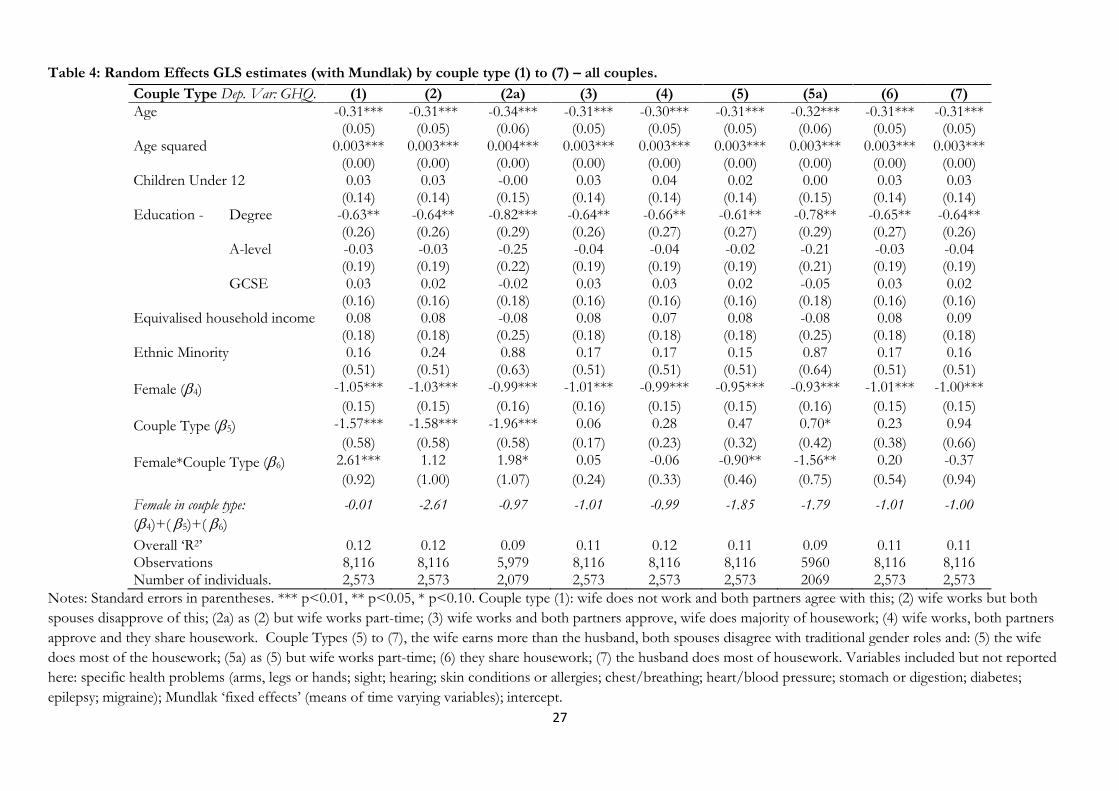
27
Table 4: Random Effects GLS estimates (with Mundlak) by couple type (1) to (7) – all couples.
Couple Type Dep. Var: GHQ. (1) (2) (2a) (3) (4) (5) (5a) (6) (7)
Age -0.31*** -0.31*** -0.34*** -0.31*** -0.30*** -0.31*** -0.32*** -0.31*** -0.31*** (0.05) (0.05) (0.06) (0.05) (0.05) (0.05) (0.06) (0.05) (0.05) Age squared 0.003*** 0.003*** 0.004*** 0.003*** 0.003*** 0.003*** 0.003*** 0.003*** 0.003*** (0.00) (0.00) (0.00) (0.00) (0.00) (0.00) (0.00) (0.00) (0.00) Children Under 12 0.03 0.03 -0.00 0.03 0.04 0.02 0.00 0.03 0.03 (0.14) (0.14) (0.15) (0.14) (0.14) (0.14) (0.15) (0.14) (0.14) Education - Degree -0.63** -0.64** -0.82*** -0.64** -0.66** -0.61** -0.78** -0.65** -0.64** (0.26) (0.26) (0.29) (0.26) (0.27) (0.27) (0.29) (0.27) (0.26) A-level -0.03 -0.03 -0.25 -0.04 -0.04 -0.02 -0.21 -0.03 -0.04 (0.19) (0.19) (0.22) (0.19) (0.19) (0.19) (0.21) (0.19) (0.19) GCSE 0.03 0.02 -0.02 0.03 0.03 0.02 -0.05 0.03 0.02 (0.16) (0.16) (0.18) (0.16) (0.16) (0.16) (0.18) (0.16) (0.16) Equivalised household income 0.08 0.08 -0.08 0.08 0.07 0.08 -0.08 0.08 0.09 (0.18) (0.18) (0.25) (0.18) (0.18) (0.18) (0.25) (0.18) (0.18) Ethnic Minority 0.16 0.24 0.88 0.17 0.17 0.15 0.87 0.17 0.16 (0.51) (0.51) (0.63) (0.51) (0.51) (0.51) (0.64) (0.51) (0.51)
Female (4) -1.05*** -1.03*** -0.99*** -1.01*** -0.99*** -0.95*** -0.93*** -1.01*** -1.00***
(0.15) (0.15) (0.16) (0.16) (0.15) (0.15) (0.16) (0.15) (0.15)
Couple Type (5) -1.57*** -1.58*** -1.96*** 0.06 0.28 0.47 0.70* 0.23 0.94
(0.58) (0.58) (0.58) (0.17) (0.23) (0.32) (0.42) (0.38) (0.66)
Female*Couple Type (6) 2.61*** 1.12 1.98* 0.05 -0.06 -0.90** -1.56** 0.20 -0.37
(0.92) (1.00) (1.07) (0.24) (0.33) (0.46) (0.75) (0.54) (0.94)
Female in couple type:
(4)+(5)+(6)
-0.01 -2.61 -0.97 -1.01 -0.99 -1.85 -1.79 -1.01 -1.00
Overall ‘R2’ 0.12 0.12 0.09 0.11 0.12 0.11 0.09 0.11 0.11 Observations 8,116 8,116 5,979 8,116 8,116 8,116 5960 8,116 8,116 Number of individuals. 2,573 2,573 2,079 2,573 2,573 2,573 2069 2,573 2,573
Notes: Standard errors in parentheses. *** p<0.01, ** p<0.05, * p<0.10. Couple type (1): wife does not work and both partners agree with this; (2) wife works but both
spouses disapprove of this; (2a) as (2) but wife works part-time; (3) wife works and both partners approve, wife does majority of housework; (4) wife works, both partners
approve and they share housework. Couple Types (5) to (7), the wife earns more than the husband, both spouses disagree with traditional gender roles and: (5) the wife
does most of the housework; (5a) as (5) but wife works part-time; (6) they share housework; (7) the husband does most of housework. Variables included but not reported
here: specific health problems (arms, legs or hands; sight; hearing; skin conditions or allergies; chest/breathing; heart/blood pressure; stomach or digestion; diabetes;
epilepsy; migraine); Mundlak ‘fixed effects’ (means of time varying variables); intercept.

28
Table 5: Random Effects GLS estimates (with Mundlak) by couple type (1) to (7) – ‘stable’ couples.
Couple Type Dep. Var: GHQ. (1) (2) (2a) (3) (4) (5) (5a) (6) (7)
Age -0.35*** -0.36*** -0.37*** -0.36*** -0.36*** -0.35*** -0.36*** -0.35*** -0.35*** (0.08) (0.08) (0.09) (0.08) (0.08) (0.08) (0.09) (0.08) (0.08) Age squared 0.004*** 0.004*** 0.004*** 0.004*** 0.004*** 0.004*** 0.004*** 0.004*** 0.004*** (0.00) (0.00) (0.00) (0.00) (0.00) (0.00) (0.00) (0.00) (0.00) Children Under 12 0.13 0.14 0.04 0.14 0.13 0.13 0.06 0.14 0.13 (0.17) (0.17) (0.18) (0.17) (0.17) (0.17) (0.19) (0.17) (0.17) Education - Degree -0.45 -0.44 -0.54 -0.45 -0.44 -0.40 -0.56 -0.45 -0.45 (0.37) (0.37) (0.40) (0.37) (0.37) (0.37) (0.40) (0.37) (0.37) A-level 0.29 0.29 0.24 0.28 0.29 0.31 0.21 0.28 0.29 (0.28) (0.28) (0.31) (0.28) (0.28) (0.28) (0.31) (0.28) (0.28) GCSE -0.25 -0.25 -0.32 -0.25 -0.25 -0.25 -0.32 -0.25 -0.25 (0.22) (0.22) (0.24) (0.22) (0.22) (0.22) (0.24) (0.22) (0.22) Equivalised household income 0.16 0.17 0.16 0.16 0.16 0.16 0.13 0.16 0.18 (0.24) (0.24) (0.32) (0.24) (0.24) (0.24) (0.32) (0.24) (0.24) Ethnic Minority 0.67 0.70 0.68 0.66 0.66 0.65 0.64 0.66 0.66 (0.65) (0.65) (0.75) (0.65) (0.65) (0.65) (0.75) (0.65) (0.65)
Female ( 4) -0.98*** -0.99*** -0.88*** -1.02*** -0.95*** -0.87*** -0.80*** -0.98*** -0.96***
(0.20) (0.20) (0.21) (0.22) (0.21) (0.20) (0.21) (0.20) (0.20)
Couple Type ( 5) -1.03 -1.03 -0.65 -0.04 0.01 0.72* 0.84* -0.19 1.12
(0.93) (0.93) (1.19) (0.22) (0.29) (0.42) (0.49) (0.48) (0.86)
Female*Couple Type (6) 2.10 2.24 2.48 0.20 -0.10 -1.52** -1.54** 0.35 -0.35
(1.75) (1.48) (2.17) (0.32) (0.41) (0.60) (0.77) (0.67) (1.21) Female in couple type:
(4)+(5)+(6)
-0.98 -0.99 -0.88 -1.02 -0.95 -1.67 -1.50 -0.98 -0.96
Overall ‘R2’ 0.11 0.11 0.09 0.10 0.10 0.11 0.09 0.10 0.11 Observations 4,526 4,526 3,479 4,526 4,526 4,526 3,479 4,526 4,526 No. of individuals 1,175 1,175 1,035 1,175 1,175 1,175 1,035 1,175 1,175
Notes: Standard errors in parentheses. *** p<0.01, ** p<0.05, * p<0.10. Other notes as for Table 4.

29
Table 6: Marginal effects from Random Effects Logit models for Alternative Outcome Variables by couple type (1) to (7).
Couple Type (1) (2) (2a) (3) (4) (5) (5a) (6) (7)
Anxiety & Depression
(i) Woman not in couple type vs. men not in couple type
0.040*** (0.009)
0.042*** (0.009)
0.031*** (0.007)
0.047*** (0.011)
0.041*** (0.009)
0.041*** (0.009)
0.046*** (0.010)
0.040*** (0.009)
0.041*** (0.009)
(ii) Women in couple type vs. women not in couple type
0.019 (0.061)
-0.050*** (0.014)
-0.021 (0.025)
-0.043*** (0.011)
-0.025** (0.012)
-0.018 (0.016)
0.127 (0.103)
-0.031 (0.023)
-0.030 (0.021)
(iii) Women in couple type vs. men in couple type
0.050 (0.065)
-0.018 (0.024)
0.017 (0.019)
0.020** (0.006)
0.031** (0.011)
0.026** (0.010)
0.020 (0.018)
0.044 (0.024)
0.013 (0.035)
(iv) Men in couple type vs. men not in couple type
0.009 (0.021)
0.009 (0.021)
0.014 (0.019)
-0.016*** (0.005)
-0.015*** (0.004)
0.005 (0.010)
0.004 (0.008)
-0.011* (0.006)
0.028 (0.035)
Unhappy
(i) Woman not in couple type vs. men not in couple type
0.129*** (0.018)
0.126*** (0.018)
0.111*** (0.019)
0.121*** (0.021)
0.127*** (0.020)
0.117*** (0.018)
0.102*** (0.019)
0.129*** (0.019)
0.123*** (0.018)
(ii) Women in couple type vs. women not in couple type
-0.078 (0.098)
0.031 (0.026)
0.107 (0.193)
-0.033 (0.029)
-0.065 (0.035)
0.057 (0.064)
0.048 (0.116)
-0.106 (0.147)
-0.009 (0.111)
(iii) Women in couple type vs. men in couple type
-0.198 (0.164)
0.183 (0.291)
-0.069 (0.238)
0.124*** (0.029)
0.099 (0.037)
0.221** (0.068)
0.190*** (0.030)
0.023 (0.061)
0 .158 (0.124)
(iv) Men in couple type vs. men not in couple type
0.249* (0.133)
0.249* (0.133)
0.286** (0.139)
-0.036** (0.018)
-0.037 (0.022)
-0.046 (0.029)
-0.087** (0.027)
0.0004 (0.042)
-0.043 (0.057)
Notes: Standard errors in parentheses. *** p<0.01, ** p<0.05, * p<0.10. Conditioning variables not reported here: age; age squared; children under 12; education – degree, A level, GCSE; equivalised household income; ethnic minority; specific health problems (arms, legs or hands; sight; hearing; skin conditions or allergies; chest/breathing; heart/blood pressure; stomach or digestion; diabetes; epilepsy; migraine); Mundlak ‘fixed effects’ (means of time varying variables); intercept. All other notes as for Table 4. Marginal effects for interaction terms in non-linear models calculated using the method of Buis (2010) – see Section 2.

30
Appendix A: The General Health Questionnaire 12 (GHQ-12)
Have you recently:
1) been able to concentrate on what you are doing?
a. Better than usual
b. Same as usual
c. Less than usual
d. Much less than usual
2) lost sleep over worry
3) felt constantly under strain
4) felt could not overcome your difficulties
5) been feeling unhappy or depressed
6) been losing confidence in yourself
7) been thinking of yourself as a worthless person
The options to the above set of questions are:
a. Not at all
b. Not more than usual
c. Rather more than usual
d. Much more than usual
8) felt that you were playing a useful part in things
9) felt capable of making decisions about things
10) been able to enjoy your day-to-day activities
11) Been able to face up to your problems
12) Been feeling reasonably happy, all things considered.
The options to the above set of questions are:
a. More than usual
b. Same as usual
c. Less so than usual
d. Much less than usual
Source: Goldberg and Williams (1988)

31
Appendix B: Variable Definitions
Variable Description
Dependent Variables GHQ 36 point measure of psychological well-being derived from General
Health Questionnaire. anxiety 0-No problems with anxiety/depression
1-Problems with anxiety/depression unhappy 0-Not more than usual/same as usual
1-Rather more than usual/much more than usual
Explanatory Variables Age Age in years Children Under 12 1= dependent children under 12 years old in the household, 0 otherwise Highest educational qualification: (baseline = non qualifications) GCSE 1=GCSE or O-level, 0 otherwise A-level 1=A-level or equivalent, 0 otherwise Degree 1=First degree or higher, 0 otherwise Household income Log of equivalised household income Ethnic Minority 1=Non-Caucasian ethnic background, 0=Caucasian ethnic background. Female 0=Male, 1=Female Self-assessed health Baseline = poor/very poor. excellent 1 = excellent health, 0 otherwise. good/very good
1 = good/very good health, 0 otherwise.
fair 1 = fair health, 0 otherwise. Health problems A set of 10 dummy variables = 1 if the respondent has a problem with:
arms, legs or hands; sight; hearing; skin conditions or allergies; chest/breathing; heart/blood pressure; stomach or digestion; diabetes; epilepsy; migraine. Baseline = no health problems.
Couple Type 1 – 7 Dummy variable for each See Table 1.

32
Footnotes
i For ease of exposition we use the terms wife and husband to denote the female and male spouse, even though in our empirical work not all of the couples in question are legally married; they are defined as ‘married or living as a couple’. ii These constraints can be reinforced by policy and institutional arrangements such as a shortage of affordable childcare. iii Booth and van Ours (2009, 2013) come to similar conclusions when they explore Dutch and Australian data. iv Davis (2007) has formalised this by making personal identity a function of individual utility, and utility a function of social identity. v The study focused on fatherhood rather than the male spouse’s role more generally. vi This variable is only asked in alternate years of the survey, so we impute for missing years using ‘last observation carried forward’. We assume that the attitudes will remain relatively stable over time and a simple cross tabulation shows persistence in attitudes across waves in the non-imputed data. vii
It is worth noting here that the interviewer records who is present in the room during each section of the interview and the data shows that respondents are large alone when the questions on gender roles and housework shares are completed. viii For example, if the wife mostly does the grocery shopping and cleaning and the husband mostly does the washing/ironing and cooking; or alternatively the couple could share the cooking and washing/ironing and the husband mostly do the grocery shopping and the wife the cleaning. ix A continuity problem arises with this 5-point SAH variable because in wave 9 (only) there was a change in the available response categories. To achieve consistency over all waves we follow the method of Hernandez-Quevedo et al., (2005). x While technically it is possible to include all couple types in one estimation (as they are mutually exclusive) the series of interaction effects required would be unwieldy for the continuous GHQ outcome variable and not appropriate for the Buis (2010) method used to estimate interaction effects for the ordinal outcomes. xi See for example Zuo and Tang (2000) who outline the threat and benefit hypotheses of how wives’ earnings may affect husbands’ gender role identity. xii We are unable to carry out any analysis on couples who split up due to inadequate sample sizes. xiii As an alternative we also included three variables for the number of children aged 0-2, 3-4 and 5-11; none of these are statistically significant, and their inclusion results in little change to the existing coefficient estimates. xiv The mean (over time) equivalised level of household income is included in the regression as part of the Mundlak method of accounting for individual effects, and this mean level is positive and statistically significant. It is worth noting that if the Mundlak fixed effects are removed the effect of household income is positive and significant; also the number of children exerts a positive effect and more of the health problems have a negative effect. xv Considering part-time rather than any work for women only makes a difference to the results for couple types (2) and (5) and we report these in Table 4 as couples (2a) and (5a). xvi Respondents are asked the extent to which they are ‘satisfied with the amount of leisure time’ they have on a scale from 1 (completely dissatisfied) to 7 (completely satisfied); we interpret responses 5 to 7 as ‘satisfied’.