Gender Gaps

and the Rise of the Service Economy∗

L. Rachel Ngai

London School of Economics

and CFM, CEPR.

Barbara Petrongolo

Queen Mary University

and CEP (LSE), CEPR.

January 2017

Abstract

This paper investigates the role of the rise in services in the narrow-

ing of gender gaps in hours and wages in recent decades. We highlight

the between-industry component of differential gender trends for the

U.S., and propose a model economy with goods, services and home pro-

duction, in which women have a comparative advantage in producing

services. The rise of services, driven by structural transformation and

marketization of home production, raises women’s relative wages and

market hours. Quantitatively, the model accounts for an important

share of the observed trends in women’s hours and relative wages.

JEL codes: E24, J22, J16.

Keywords: gender gaps, structural transformation, marketization.

∗We wish to thank Benjamin Bridgman, Berthold Herrendorf, Donghoon Lee, AlessioMoro, Richard Rogerson, Rob Shimer, and especially Alwyn Young and Chris Pissarides for

helpful discussions; as well as seminar participants at LSE, NBER Summer Institute 2014,

the Conference on Structural Change and Macroeconomics (PSE, 2014), and the Household

and Female Labor Supply Conference (Arizona State U, 2015) for constructive comments.

We also thank Benjamin Bridgman for sharing data on labor productivity in the home

sector. Financial support from the ESRC (Grant RES-000-22-4114) and hospitality from

the Institute of Advanced Studies at HKUST are gratefully acknowledged.

1

1 Introduction

One of the most remarkable changes in labor markets since World War II is the

rise in female participation in the workforce. In the U.S., the employment rate

of prime-age women has more than doubled from about 35% in 1945 to 77%

at the end of the century, and similar trends are detected in the majority of

OECD countries. These developments have generated a vast literature on the

causes, characteristics and consequences of the rise in women’s involvement

in the labor market. Existing work has indicated a number of supply-side

explanations for these trends, including human capital investment, medical

advances, technological progress in the household, and the availability of child

care, and a recent line of research emphasizes the role of social norms regarding

women’s work in shaping the observed decline in gender inequalities.1

In this paper we propose a novel, and complementary, explanation for

the observed trends in gender outcomes, based on the secular expansion of

the service economy and its role in raising the relative demand for female

work.2 Our emphasis on the evolution of the industry structure is motivated

by a few stylized facts. First, the sustained rise in female work since the late

1960s in the U.S. has been accompanied by a fall in male work, and a rise

in women’s relative wages. In 1968, women’s hours were about 37% of men’s

hours, and their wages were about 62% of male wages. By 2008, these ratios

rose to 73% and 81%, respectively. Second, the entire (net) rise in female

hours took place in the broad service sector, while the entire (net) fall in male

hours took place in goods-producing sectors, including the primary sector,

manufacturing, construction and utilities. This pattern is closely linked to

1See Goldin (2006) for a comprehensive overview of historical trends and their causes.

See (among others) Goldin and Katz (2002) and Albanesi and Olivetti (2016) for the role of

medical progress; Greenwood, Seshadri and Yorukoglu (2005) for the role of technological

progress in the household; Galor and Weil (1996) and Attanasio, Low and Sanchez-Marcos

(2008) for the role of declining fertility. See Fernandez (2013) and references therein for

theory and evidence on cultural factors.2The focus on demand forces is appealing as it has the potential to address gender

trends in both quantities and prices. Indeed the rise in female hours at a time of rising

female wages “places a strong restriction on theories explaining the increase in female labor

force participation” (Aguiar and Hurst, 2007a, p. 982).

2

the process of structural transformation, and specifically the reallocation of

labor from goods to service industries, with an expansion of the service share

from 56% in 1968 to 75% in 2008. Finally, the rise in women’s hours in the

service sector was accompanied by a strong decline in their working hours in

the household, from about 41 to 31 hours weekly, consistent with substantial

marketization of home production (Freeman and Schettkat, 2005).3

Motivated by these facts, this paper studies the role of the rise in services,

in turn driven by structural transformation and marketization, in the simul-

taneous evolution of gender outcomes in hours and wages. The interaction

between structural transformation, marketization and female work has been

largely overlooked in the literature. However there are clear reasons why these

can contribute to the rise in female market hours and relative wages.

First, the production of services is relatively less intensive in the use of

“brawn” skills than the production of goods, and relatively more intensive in

the use of “brain” skills. As men are better endowed of brawn skills than

women, the historical growth in the service sector has created jobs for which

women have a natural comparative advantage (Goldin, 2006, Galor and Weil,

1996, Rendall, 2010, Weinberg, 2000, and Fan and Lui, 2003). While the in-

troduction of brawn-saving technologies has to a large extent compensated

the female disadvantage in physical tasks, women may still retain a compara-

tive advantage in services, related to the more intensive use of communication

and interpersonal skills, which cannot be easily automated. The simultaneous

presence of producers and consumers in the provision of services makes these

skills relatively more valuable in services, and a few studies have highlighted

gender differences in the endowment and use of such traits (Borghans, Bas ter

Weel and Weinberg, 2008, 2014). In particular, Borghans, Bas ter Weel and

Weinberg (2014) show that the rise in the use of interpersonal tasks acceler-

ated between the late 1970s and the early 1990s, and that women are over-

represented in these tasks, suggesting that women are relatively more endowed

3See also the discussion in Lebergott (1993, chapter 8) on the link between marketization

and consumerism: “... by 1990 [women] increasingly bought the goods and services they

had produced in 1900”, and Bridgman (2013), documenting the rise in the ratio of services

purchased relative to home production since the late 1960s.

3

in those increasingly valuable interpersonal skills. Finally, a recent strand of

the experimental literature highlights some gender differences in other social

attitudes such as altruism, fairness and caring behavior (Bertrand, 2010; Az-

mat and Petrongolo, 2014), which may be more highly valued in service jobs,

and especially in those that involve assisting or caring for others.

Women’s comparative advantage in services is clearly reflected in the allo-

cation of women’s hours of market work. In 1968, the average working woman

was supplying three quarters of her market time to the service sector, while

the average man was supplying only one half of his market time to it. As struc-

tural transformation expands the sector in which women are over-represented,

it has potentially important consequences for the evolution of women’s hours

of market work. Indeed, in a shift-share framework, almost one third of the

rise in the share of female hours took place via the expansion of services.

The second reason is related to women’s involvement in household work.

In 1965, women spent on average 41 hours per week in home production,

while men only spent 11 hours. Household work includes child care, cleaning,

food preparation, and in general activities that have close substitutes in the

market service sector. If the expansion of the service sector makes it cheaper

to outsource these activities, one should expect a reallocation of women’s work

from the household to the market. The work allocation of men and women in

the late 1960s is thus key to understanding later developments. While women

were mostly working in home production and the service sector, and thus their

market hours were boosted by the rise in services, men were predominantly

working in the goods sector, and their working hours mostly bore the burden

of de-industrialization.

In our proposed model, market sectors produce commodities (goods and

services) that are poor substitutes for each other in consumer preferences,

while the home sector produces services that are good substitutes to services

produced in the market. Production in each sector involves a combination of

male and female work, and women have a comparative advantage in producing

services, both in the market and the home. Labor productivity growth is

4

uneven,4 reducing both the cost of producing goods, relative to services, and

the cost of producing market services, relative to home services. As goods and

services are poor substitutes, faster productivity growth in the goods sector

reallocates labor from goods to services, resulting in structural transformation.

As market and home services are good substitutes, slower productivity growth

in the home sector reallocates hours of work from the home to market services,

resulting in marketization.

The combination of consumer tastes and uneven productivity growth de-

livers two novel results. First, due to women’s comparative advantage in ser-

vices, structural transformation and marketization jointly raise women’s rela-

tive market hours and wages. In other words, gender comparative advantages

turn a seemingly gender-neutral force such as the rise in services into a de

facto gender-biased force. Second, for both men and women, market hours

rise with marketization but fall with structural transformation. Their combi-

nation is thus necessary to rationalize observed gender trends: marketization

is necessary to boost female market work while structural transformation is

needed to explain the fall in male market work.

To quantitatively assess the importance of the mechanisms described, we

calibrate our model economy to the U.S. labor market and predict trends in

gender outcomes. The calibrated marketization and structural transformation

forces predict the entire rise in the service share between 1970 and 2006, 20%

of the gender convergence in wages, one third of the rise in female market

hours and 9% of the fall in male market hours. These predictions are solely

due to between-sector forces, while no within-sector forces are at work. Al-

lowing for a within-sector increase in the relative demand for female labor

— due for example to the fall in gender discrimination and the evolution of

gender norms — improves the model’s predictions for gender-specific trends,

leaving predictions for the industry structure unchanged. A simple way to

summarize the quantitative performance of our model consists in comparing

predicted and actual changes in the overall time allocation structure for men

4Uneven labor productivity growth can be driven by uneven TFP growth or different

capital intensities across sectors.

5

and women across market goods, market services, home services and leisure.

When between-sector forces alone are at work, the model explains nearly 60%

of the variation in the time allocation structure during our sample period, and

adding within-sector forces explains a further 30%.

There exist extensive literatures that have independently studied the rise

in female labor market participation and the rise of services, respectively, but

work on the interplay between the two phenomena is relatively scant. Early

work by Reid (1934), Fuchs (1968) and Lebergott (1993) has suggested links

between them, without proposing a unified theoretical framework. One notable

exception is work by Lee and Wolpin (2006, 2010), who relate the rise in

services and female labor market outcomes to shocks to fertility and the value

of home time in a labor market equilibrium model.

Our work is related to Galor and Weil (1996) and Rendall (2010), who

illustrate the consequences of brain-biased technological progress for female

employment in a one-sector model in which females have a comparative ad-

vantage in the provision of brain inputs.5 In a similar vein, we assume that

women have a comparative advantage in producing services in a model with

two market sectors and home production, in which the rise in female market

hours and the share of services are simultaneous outcomes of uneven produc-

tivity growth. Marketization of home services, contributing to both the rise

of female market work and the services share, also features in Akbulut (2011),

Buera, Kaboski and Zhao (2013) and Rendall (2015). Our main contribution to

this strand of literature is to endogenously explain the simultaneous narrowing

of gender gaps in wages, market hours and home hours. Finally, the interplay

between the service share and female outcomes has been recently studied in an

international perspective by a few papers that relate lower female employment

in Europe to an undersized service sector relative to the U.S. (Rendall, 2015;

Olivetti and Petrongolo, 2014, 2016). In particular, Olivetti and Petrongolo

(2014) find that the between-industry component of labor demand explains

5Heathcote, Storesletten and Violante (2010) and Jones, Manuelli and McGrattan (2015)

also consider within-sector demand forces and illustrate the rise in the gender hours ratio

stemming, respectively, from gender-biased technological progress and falling gender dis-

crimination.

6

the bulk of the international variation in the gender-skill structure of labor

demand, and Olivetti and Petrongolo (2016) confirm similar qualitative con-

clusions on a longer time period and a larger set of countries.

The recent literature on structural transformation often classifies the mech-

anisms that drive the rise in services into income and relative price effects.6

With the first mechanism, income growth shifts the allocation of resources to-

wards services as long as the demand for services is more elastic to income than

the demand for goods. With the second mechanism, changes in relative prices

alter the resource allocation when the elasticity of substitution between goods

and services is not unity.7 Both channels are at work in our model. Slower

productivity growth in services raises their relative price, in turn raising the

expenditure share on services, as services and goods are poor substitutes in

consumption. Higher income elasticity of services follows from the assumption

that market services are closer substitutes to home services than goods. Un-

der this assumption, the rise in income driven by faster productivity growth

in market sectors raises the opportunity cost of home production, in turn

stimulating the demand for market services, as these are the closest available

substitute to home production.

The paper is organized as follows. Section 2 documents relevant trends in

gender work and the size of services during 1968-2008, combining data from the

Current Population Survey and several time use surveys. Section 3 develops

a model for a three-sector economy and shows predictions of uneven labor

productivity growth for relative wages, market hours, home production hours

and leisure. Section 4 presents quantitative results and Section 5 concludes.

6See Herrendorf et al (2013b) for a recent survey on the mechanisms. See (among others)

Baumol (1967), Ngai and Pissarides (2007) and Acemoglu and Guerrieri (2008) for the role

of uneven productivity or different capital intensities; Kongsamut, Rebelo and Xie (2001)

and Buera and Kaboski (2012) for the role of income effects; and Boppart (2014) for both

effects.7See also Dix-Caneiro (2014) for an alternative explanation for the decline in the relative

prices of goods due to trade liberalization, and its effects on the skill tructure of employment

and wage along the classic mechanims of the Heckscher-Ohlin trade model.

7

2 Data and stylized facts

This Section presents evidence on the evolution of market work, wages and

home production, using micro data from the March Current Population Sur-

veys (CPS) for survey years 1968 to 2008 and time use surveys for 1965-2008.8

2.1 Market work

Our CPS sample includes individuals aged 21-65, who are not in full-time

education, retired, or in the military. Annual hours worked in the market are

constructed as the product of weeks worked in the year prior to the survey year

and hours worked in the week prior to the survey week. This hours measure is

the only one continuously available since 1968 and comparable across annual

surveys. For employed individuals who did not work during the reference week,

weekly hours are imputed using the average of current hours for individuals of

the same sex in the same year. Until 1975, weeks worked in the previous year

are only reported in intervals (0, 1-13, 14-26, 26-39, 40-47, 48-49, 50-52), and to

recode weeks worked during 1968-1975 we use within-interval means obtained

from later surveys. These adjustment methods have been previously applied

to the March CPS by Katz and Murphy (1992) and Heathcote, Storesletten

and Violante (2010). Our wage concept is represented by hourly earnings,

obtained as wage and salary income in the previous year, divided by annual

hours. Survey weights are used in all calculations.

Figure 1 presents evidence on market work. Panel A plots annual hours

by gender, obtained as averages across the whole population, including the

nonemployed. Female work rises steadily from about 720 annual hours in

1968 to nearly 1200 hours in the 2000s, while male hours gradually decline

throughout the sample period, from about 2000 to 1700. These diverging

trends imply a doubling of the hours ratio,9 from about 0.36 to 0.73, with a

modest increase in total hours in the economy.

8We choose to end our sample period in 2008 to avoid unusual fluctuations in economic

activity and the industry structure linked to the onset of the Great Recession.9Throughout the paper, hours and wage ratios indicate female/male ratios.

8

We classify market hours into two broad sectors, which we define as goods

and services. The goods sector includes the primary industries, manufacturing,

construction and utilities. The service sector includes the rest of the economy.

Panel B in Figure 1 plots the proportion of hours in services overall and by

gender, and shows an increase of 19 percentage points in the share of market

hours worked by both males and females in services. For women, the service

share is substantially higher than for men, and rises from 73% to 88%, while

for men it rises from 50% to 65%. Panel C further shows that all of the (net)

increase in female hours takes place in the service sector, while Panel D shows

that all of the (net) fall in male hours takes place in the goods sector. In

summary, while women are moving - in net terms - from nonemployment into

the service sector, men are moving from the goods sector to nonemployment.

These aggregate trends are also clearly confirmed within broad skill groups,

as shown in Figure A1 in the Appendix.

Table 1 provides detailed evidence on the industry composition of total

hours and the female intensity within each industry. The 19 percentage points’

expansion in the service share is expected to boost female employment as the

female intensity in services is much higher than in the goods sector. A sim-

ilar point can be made across more disaggregated industries. The decline in

the broad goods sector is disproportionately driven by the fall in manufactur-

ing industries and, to a lesser extent, primary industries. Within the broad

service sector, several industries contribute to its expansion (retail, FIRE,

business services, personal services, entertainment, health, education, profes-

sional services and public administration). The female intensity is generally

higher in expanding service industries than in declining goods industries. A

further stylized fact to note is the rise in the female intensity in every indus-

try.10 The evidence summarized in Table 1 thus highlights both between- and

within-industry components in the rise of female hours.

We quantify between- and within-industry components of trends in female

10The fall in the female intensity in the post and telecoms industry is an exception, entirely

driven by the near disappearance of telephone operators, who were 98% female at the start

of our sample period.

9

hours by decomposing the growth in the female hours share between 1968 and

2008 into a term reflecting the change in the share of services, and a term

reflecting changes in gender intensities within either sector. Using a standard

shift-share decomposition, the change in the female hours share between year

0 and year can be expressed as

∆ =X

∆ +X

∆ (1)

where denotes the share of female hours in the economy in year , de-

notes the hours share of sector , denotes the share of female hours in

sector , and = ( + 0) 2 and = ( + 0) 2 are decomposition

weights. The first term in equation (1) represents the change in the female

hours share that is attributable to changes in sector shares, while the second

term reflects changes in the female intensity within sectors. The results of this

decomposition are reported in Table 2. The first row reports the total change

in the female hours share, which rises from 29% in 1968 to 44.4% in 2008.

The second row shows that about 30% of this change was explained by the

growth in the share of services, as measured by the first term in equation (1).

The third row performs the same decomposition on 17, as opposed to two, in-

dustries, and delivers a very similar estimate of the role of the between-sector

component. This means that, by focusing on our binary decomposition, we do

not miss important between-sector dynamics in the rise in female hours.11

We have motivated our focus on the sectoral dimension of gender develop-

ments based on gender comparative advantages, via the more intensive use of

non-physical tasks and interpersonal skills in the production of services rather

than goods. However, tasks are more directly associated to occupations than

sectors, and some sectors tend to use female labor more intensively because

11Olivetti and Petrongolo (2016) perform a similar analysis on a large panel of OECD

countries, and find that variation in the services employment share explains about 60% of

the overall variation in the share of female hours across countries since the 1970s. This

proportion rises to about 80% when using a 12-fold industry classification, as the finer

industries making up the two broad goods/service sectors vary considerably in size across

countries.

10

they use more intensively occupations in which women have a comparative

advantage. Thus the rise in female hours should have an important between-

occupation component. This is shown in the fourth row of Table 2, based on

a 4-fold occupational decomposition.12 The between-occupation component

explains about 24% of the total. This is somewhat smaller than the between-

sector component, but still sizeable.

Clearly, changes in the industry and occupation structures are not orthogo-

nal. As the distribution of occupations varies systematically across industries,

a portion of the between-occupation component of the rise in female hours may

be explained by the expansion of industries that oversample female-friendly oc-

cupations. Between-occupation changes that are not captured by changes in

the industry structure are by definition included in the within-industry com-

ponent of (1). We therefore decompose the within-industry component of (1)

into within- and between-occupation components. The full decomposition is

∆ =X

∆ +X

ÃX

∆ +X

∆

! (2)

where indexes occupations, is the share of occupation in industry ,

is the share of female hours in occupation and industry , and =

( + 0) 2 and = ( + 0) 2 The first term in (1) represents

the between-industry component, the second term represents the between-

occupation component that takes place within industries, and the last term

represents the component that takes place within industry×occupation cells.The results of this further decomposition are reported in the fifth row of Table

2, and show that only a small share (7.9%) of the growth in the female hours

share took place via the expansion of female-friendly occupations within sec-

tors. The bulk of the growth in female-friendly occupations took instead place

via the expansion of the service share. We thus focus the rest of the paper on

a binary goods/services distinction, as the decomposition results reported in

12This is the broad task-based grouping of occupations suggested by Acemoglu and Autor

(2011). Categories are: professional, managerial and technical occupations; clerical and sales

occupations; production and operative occupations; service occupations.

11

Table 2 suggest that this is a sufficient dimension for understanding relative

female outcomes.

2.2 Wages

Evidence on wages is presented in Figure 2. Panel A shows the evolution of

the wage ratio in the aggregate economy, obtained as the exponential of the

gender gap in mean log wages, unadjusted for characteristics. Women’s hourly

wages remained relatively stable at or below 65% of male wages until about

1980, and then started rising to reach about 80% of male wages at the end of

the sample period. The combined increase in female hours and wages raised

the female wage bill from 30% to two thirds of the male wage bill. When

using hourly wages adjusted for human capital (controlling for age and age

squared, ethnicity, and four education levels), the rise in the gender wage ratio

is only slightly attenuated, from 64% in 1968 to 78% in 2008 (Panel B). While

a measure of actual, rather than potential, labor market experience is not

available in the CPS, estimates by Blau and Kahn (2013) on the PSID show

that gender differences in actual experience explain about a third of the rise in

the wage ratio between 1980 and 1999. Thus there is clear evidence of closing

— but still sizeable — gender gaps even after controlling for actual labor market

experience. Note finally that the trend in the wage ratio is very similar across

market sectors.

2.3 Time use

We show evidence on the distribution of total work between market and home

production for each gender, by linking major time use surveys for the U.S.

for 1965-2008.13 As a measure of market hours we use “core” market work,

including time worked on main jobs, second jobs and overtime, but excluding

time spent commuting to/from work and time spent on ancillary activities,

13These are: 1965-1966 America’s Use of Time; 1975-1976 Time Use in Economics and

Social Accounts; 1985 Americans’ Use of Time; 1992-1994 National Human Activity Pattern

Survey; and 2003-2008 American Time Use Surveys. These surveys are described in detail

in Aguiar and Hurst (2007a).

12

e.g. meal times and breaks. This is a measure that is most closely comparable

to market hours measured in the CPS. However, no information on annual

weeks worked is available from the time use surveys, and all work indicators

presented are weekly. To obtain a measure of home production we sum hours

spent on core household chores (cleaning, preparing meals, shopping, repairing

etc.) and hours of child care.

We compute time use series adjusted for changing demographics, i.e. at

constant gender, age and education composition. Following Aguiar and Hurst

(2007a), we divide our sample into cells defined by two genders, five age groups

(21-29, 30-39, 40-49, 50-59, 60-65), and four education groups (less than high

school, high school completed, some college or more) and compute average

population shares in each of the resulting 40 cells across the sample period.

We then compute changes in hours for the whole sample as weighted averages

of cell-level changes, using as weights the fixed population shares.

Figure 3 shows trends in market and home hours for men and women since

1965. The series for market work of men and women clearly converge during

the sample period: weekly hours worked in the market rise from 19 to 24 for

women, and fall from 42 to 36 for men. The trends are similar to those detected

using the CPS in Figure 1A. The series for home production also move closer

to each other, as home hours fall from 38 to 28 for women, and rise from 11

to 16 for men. Interestingly, there are only minor gender differences in the

dynamics of total work, which falls slightly for both men and women, keeping

the ratio of total work — and therefore leisure — roughly constant.14

While gender differences in total work are relatively small and very sta-

ble, the market/home divide of total work differs sharply across genders. For

women the share of market work in total work rises from one third in 1965

to 45% in 2008, while for men this falls from 80% to 70%. The allocation of

total work between the market and the home seems therefore the key mar-

gin to understand gender trends in market hours. All trends considered are

also confirmed within two broad skill groups, as shown in Figure A2 in the

14This fact - also known as the isowork result - was noted by Aguiar and Hurst (2007a)

on the same data, and by Burda, Hamermesh and Weil (2013) in a cross-section of countries

13

Appendix.

3 The model

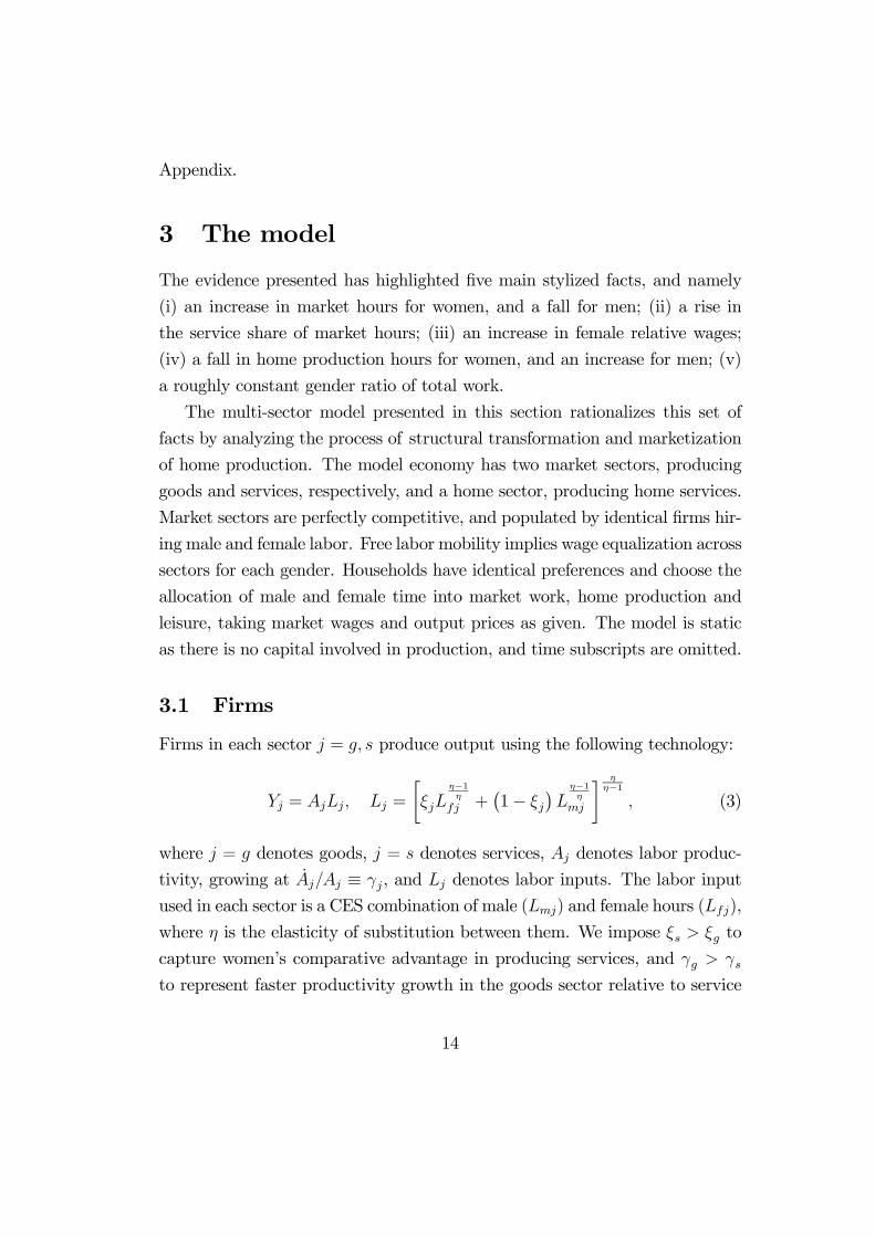
The evidence presented has highlighted five main stylized facts, and namely

(i) an increase in market hours for women, and a fall for men; (ii) a rise in

the service share of market hours; (iii) an increase in female relative wages;

(iv) a fall in home production hours for women, and an increase for men; (v)

a roughly constant gender ratio of total work.

The multi-sector model presented in this section rationalizes this set of

facts by analyzing the process of structural transformation and marketization

of home production. The model economy has two market sectors, producing

goods and services, respectively, and a home sector, producing home services.

Market sectors are perfectly competitive, and populated by identical firms hir-

ing male and female labor. Free labor mobility implies wage equalization across

sectors for each gender. Households have identical preferences and choose the

allocation of male and female time into market work, home production and

leisure, taking market wages and output prices as given. The model is static

as there is no capital involved in production, and time subscripts are omitted.

3.1 Firms

Firms in each sector = produce output using the following technology:

= =

∙

−1

+¡1−

¢

−1

¸ −1

(3)

where = denotes goods, = denotes services, denotes labor produc-

tivity, growing at ≡ , and denotes labor inputs. The labor input

used in each sector is a CES combination of male () and female hours (),

where is the elasticity of substitution between them. We impose to

capture women’s comparative advantage in producing services, and

to represent faster productivity growth in the goods sector relative to service

14

sector.15

3.2 Households

Households consists of one man and one woman, whose joint utility depends

on consumption of goods (), market services (), home services () and

leisure ():

( ) = ln + ln (4)

where denotes a bundle of goods and services:

=h

−1

+ (1− ) −1

i −1; =

h

−1

+ (1− ) −1

i −1

(5)

and denotes all services combined. Goods and services are poor substi-

tutes ( 1), while market and home services are good substitutes ( 1)

in the combined service bundle. Home services are produced with the same

technology as market services in (3), except for the level of labor productivity:

=

∙

−1

+ (1− )−1

¸ −1

(6)

where productivity growth in market services is assumed to be faster than in

the home: .

Leisure time is a CES aggregator of male and female leisure:

=

∙

−1

+ (1− )

−1

¸ −1

(7)

where 1 is imposed to indicate that male and female leisure are poor

substitutes.

Given market wages ( , ) and market prices (, ), a representative

household chooses market consumption (, ), home production time (,

15While we are assuming a simple technology directly employing male and female inputs,

Appendix A shows that specification (3) delivers equivalent results to one in which output

in each sector requires a combination of tasks, and men and women are differently endowed

of the skills necessary to perform them.

15

) and leisure time (, ) to maximize the utility function (4) subject

to (5)-(7) and the household budget constraint:

+ = ( − − ) + ( − − ) (8)

3.3 Equilibrium

A competitive equilibrium is defined by market wages ( , ), market prices

(, ), consumption (, ) and time allocation {, }= such that:

1. the representative firm maximizes profits, subject to technology (3); and

the representative household maximizes utility (4), subject to (5)-(7);

2. given the optimal choices of firms and households, market wages and

prices clear the market in each sector and the labor market for each

gender:

= = (9)

+ = − − = (10)

The Subsections that follow highlight the impact of structural transfor-

mation and marketization on the equilibrium allocation of time, and their

implications for gender gaps in employment and wages and the service share.

The full derivation of equilibrium results is provided in Appendix B.

3.4 Structural transformation and the wage ratio

Profit maximization equalizes the marginal rate of technical substitution be-

tween female and male labor to the gender wage ratio in each sector, and

perfect mobility of labor equalizes the wage ratio across sectors:

= − = (11)

16

where ≡ and

≡

1−

Women’s comparative advantage in services is captured by .

Let denote labor supply for each gender, to be determined by house-

holds’ optimization problem. Labor market clearing implies:

+ = = (12)

Combining conditions (11) and (12) for = gives the allocation of female

hours:

=1−

−

1− () (13)

Given gender comparative advantages ( ) the equilibrium condition

(13) implies that the allocation of female hours to the service sector is an

increasing function of the wage ratio. The intuition is that a higher wage ratio

induces substitution away from female labor in all sectors, but substitution

is weaker in the sector in which women have a comparative advantage. As

is proportional to due to (11), higher implies higher

and an overall lower share of hours in the goods sector.

Formally, define service employment ≡ ++++

Using (11) and

(13), service employment is positively related to the wage ratio according to:

=

³

´−³

´ ³

´1−

³

´ ∙µ

¶

+ 1

¸1

1 +

(14)

This result can be summarized in the following proposition.

Proposition 1 When women have a comparative advantage in services, a rise

in the service share is associated with a higher wage ratio (at constant relative

labor suppy, ).

Proposition 1, which is derived from profit maximization, is solely based

on the assumption of gender comparative advantages, and in particular it

17

holds independently of both product demand and the specific process driving

structural transformation.16

The result in Proposition 1 highlights the importance of considering a two-

sector economy, as gender comparative advantages turn a seemingly gender-

neutral force such as the rise in services into a de facto gender-biased force. To

see this more explicitly, consider a one-sector model with a CES production

function like (3), with technology parameter . The equilibrium wage ratio in

this economy is given by

=

1−

µ

¶1 (15)

and it can only rise following a fall in relative female labor supply () or

an increase in the female-specific parameter The rise in is typically inter-

preted as a gender-biased demand shift (Heathcote, Storesletten and Violante.,

2010), driven by a variety of factors: female friendly technological progress

(Johnson and Keane, 2007); the evolution of social norms towards women’s

work and the reduction in gender discrimination in the workplace (Goldin,

2006); or reduced distortions in the allocation of gender talents (Hsieh et al.,

2016). Our approach contributes an endogenous between-sector mechanism to

existing work to explain the rise in the relative demand for female labor, at

constant technology parameters and

3.5 Structural transformation and marketization

Utility maximization yields an expression similar to (11) for the home sector,

as the marginal rate of technical substitution must equal the gender wage ratio:

= − (16)

16As will be shown below, one outcome of structural transformation is the rise in the

relative price of services. Thus Proposition 1 is similar in spirit to the Stolper-Samuelson

theorem from international trade theory, predicting that a rise in the relative price of a good

leads to higher return to the factor that is used most intensively in the production of the

good.

18

where ≡ (1− ) Furthermore, the marginal rate of substitution across

any two commodities must equal their relative price, thus an implicit price — or

the opportunity cost — for home services can be defined as () =

Free labor mobility equalizes the value of the marginal product of labor

across home and market for each gender. Thus, using production functions

(3) and (6), relative prices for any pair of commodities are a function of the

wage ratio:

=

µ

¶ −1µ ()

()

¶ 1−1; = (17)

where () denotes the female wage bill share in sector ,

() ≡

+

=1

1 + − −1

(18)

and the equality follows from (11) and (16).

According to (17), uneven productivity growth ( ) acts as

a shifter that increases the opportunity cost of home services relative to all

market goods and services, and the price of market services relative to goods,

for any given level of the wage ratio .

3.5.1 Labor allocation across market and home services

The equilibrium allocation of time is characterized in two steps. We first solve

for the optimal allocation of service hours between the market and the home,

and next solve for the optimal allocation of total hours across market sectors.

The optimal time allocation between market and home services can be

obtained from the corresponding expenditure allocation, ≡ ()()Using the utility function (4)-(5) to equalize the marginal rate of substitution

of market and home services to their relative prices gives relative expenditure

as a function of relative prices:

=

µ

¶−1µ

1−

¶

(19)

19

This results states that a higher opportunity cost of home relative to market

services raises the relative expenditure on market services, as the two types

of services are good substitutes ( 1). Faster productivity growth in mar-

ket services thus shifts expenditure from home to market services, by making

home services relatively more expensive according to (17). This is the process

of marketization and its strength is captured by the “marketization force”,

measured by the interaction between the productivity growth differential be-

tween the market and the home and the substitutability in their respective

outputs:

≡ ( − 1) ( − ) 0 (20)

To illustrate the impact of marketization on time allocation, the home

production function (6) and the market clearing condition (9) can be combined

to express the allocation of female hours across home and market services as

a function of relative expenditures:

= ()

() (21)

Using (11), the allocation of male hours can be obtained:

=

µ

¶

(22)

By shifting expenditure from home to market services, marketization also shifts

working hours from the home to the market for both women and men, as

implied by (21) and (22), respectively.

After substituting (17) and (19) into (21), the equilibrium time allocation

between the market and the home can be expressed as a function of sector-

specific productivity and , and gender-specific parameters and :

≡ () = −1

µ

¶(−1)−1

µ ()

()

¶−−1

(23)

20

where

≡

µ

1−

¶ −1

(24)

3.5.2 Labor allocation between goods and market services

The optimal time allocation between goods and market services can be ob-

tained from the expenditure allocation, ≡ ()() having equalizedthe marginal rate of substitution between goods and market services to their

relative prices:

=

µ

¶1−µ

1−

¶

(1−)−1

µ1 +

1

¶−−1

(25)

Two mechanisms induce a decline in the relative goods expenditure. The

first is marketization, discussed above, expanding the relative expenditure for

market services, . The second is the relative price effect. Faster produc-

tivity growth in the goods sector relative to market services raises the relative

price of market services, as shown in (17). As goods and market services are

poor substitutes ( 1) a rise in the relative price of market services shifts

households’ expenditure from goods to market services as shown in (25). The

strength of this effect is captured by the “structural transformation force”,17

measured by the interaction of the productivity growth differential between

goods and market services and their poor substitutability in preferences:

≡ (1− )¡ −

¢ 0 (26)

By combining the production functions (3) and market clearing (9), the

allocation of female hours across goods and market services can be expressed

as a function of the relative expenditure:

= ()

() (27)

17We should admit a slight abuse of terminology here, as the term “structural transfor-

mation” is typically referred to the rise in the service employment and value added shares,

without reference to the underlying driving forces.

21

Using (11) gives the corresponding allocation of male hours:

=

µ

¶

(28)

By shifting expenditure from goods to market services, structural transforma-

tion shifts market hours of men and women from the goods to service sector,

as shown in (27) and (28).

Substituting (17) and (25) into (27) gives the time allocation as a function

of sector-specific productivities , and , and gender-specific parameters

and :

≡ () =

µ ()

()

¶−−1

1−

µ

¶(1−)−1

µ1 +

()

() ()

¶−−1

(29)

where

≡

µ

1−

¶ 1−

−1 (30)

The service share of employment in the market can be derived from (11):

=1

1 + ()()

()

(31)

and it rises with both marketization and structural transformation, as sum-

marized in the following Proposition:

Proposition 2 Marketization and structural transformation expand the ser-

vice share

The intuition for Proposition 2 follows directly from the forces behind rela-

tive expenditure, . Faster productivity growth in the goods sector ( )

makes market services relatively more expensive. As goods and services are

poor substitutes ( 1), the change in relative prices shifts expenditure and

working hours towards market services, expanding the service share. Further-

more, faster productivity growth in the market relative to the home ( )

22

raises the opportunity cost of home production, leading households to substi-

tute home production for market services, as these are closer substitute for

home production than goods ( ).

These two channels are related to relative price and income effects often

emphasized in the structural transformation literature (Herrendorf, Rogerson

and Valentinyi, 2013b). In our framework, income effects are generated by

nested CES preferences (5), in which the presence of home services implies non-

homothetic utility in goods and market services. Marketization thus provides a

channel whereby the income elasticity of demand is higher for market services

than for goods.18

Taken together, Propositions 1 and 2 state that marketization and struc-

tural transformation raise both the service share and the wage ratio. The

prediction about the service share is common to the structural transformation

literature. The second prediction is novel: since women have a comparative

advantage in producing services, uneven labor productivity growth acts as an

increase in relative demand for female labor, which in turn raises the equilib-

rium wage ratio.

Uneven labor productivity growth is a necessary condition to deliver a

simultaneous increase in both market services and the wage ratio. Clearly, if

productivity growth is balanced across all sectors, = = the service

share and the wage ratio are unaffected. However, these results still hold in

two special cases, = and = In the first case, only

structural transformation is present, and faster productivity growth in the

goods sector, combined with poor substitutability between goods and market

services, shifts labor from goods to services, leading to a higher service share

and wage ratio. In the second case, only marketization is present, and faster

productivity growth in market than home services, combined with their good

substitutability, pulls labor out of the household, with a corresponding increase

18The link between the income elasticity of services and home production is first noted by

Kongsamut, Rebelo and Xie (2001), who adopt a non-homothetic utility function defined

over and ( + ), where is an exogenous constant that “can be viewed as representing

home production of services”. See Moro, Moslehi and Tanaka (2017) for recent work on

this.

23

in the market service share and the wage ratio. Whenever both

mechanisms are at work.

3.6 Market hours by gender

Marketization and structural transformation have opposing effects on market

hours. While marketization drives hours out of the home sector — thereby

increasing market hours for both genders — structural transformation shifts

hours from goods into services, in turn reducing market hours for both genders,

as part of services are produced in the home. Their combination has the

potential to rationalize observed gender trends: marketization is needed to

deliver the rise in female market work while structural transformation is needed

to deliver the fall in male market work.

While the effect of structural transformation and marketization on the level

of market hours for each gender depends on leisure choices, it is possible to

learn about how they affect relative labor supply through the alloca-

tion of market hours. Using (27), the share of female market hours in services

is

=1

1 + ()

Setting this equal to (13) delivers:

=³

´ ⎡⎣1− 1−³

´1 + ()

⎤⎦−1 (32)

Recall from (29) that () falls with both marketization and structural

transformation forces as defined in (20) and (26), with a consequent increase

in relative labor supply,, which in equilibrium equals the gender ratio

of market hours. This result is summarized in the following proposition:

Proposition 3 When women have a comparative advantage in producing ser-

vices, marketization and structural transformation raise the ratio of female to

male market hours.

24

3.7 Work and leisure

Utility maximization yields an expression similar to (11) for leisure choice:

= − (33)

Comparing (33) to the corresponding condition (16) for home hours, the fol-

lowing result follows:

Proposition 4 When the wage ratio increases, relative female hours in home

production fall more than in leisure time if and only if

In particular, the gender ratio of leisure time is independent of the wage

ratio for = 0. As a corollary, the gender ratio of total work is also approxi-

mately constant for small enough . The intuition for Proposition 4 is that,

if male and female leisure hours are complements ( 1), while their home

production hours are substitutes ( 1), a higher opportunity cost of stay-

ing out of the market () mostly substitutes male to female inputs in home

production, while leaving them roughly unchanged in leisure time, as spouses

enjoy spending leisure together.

3.8 Summary of qualitative results

Our three-sector model establishes four qualitative results. First a rise in the

service share is associated to a higher gender wage ratio whenever women

have a comparative advantage in producing services (Proposition 1). Sec-

ond, uneven productivity growth raises the share of services (Proposition 2),

thereby raising the wage ratio. Third, given women’s comparative advantage

in services, structural transformation and marketization unambiguously raises

female market hours relative to men (Proposition 3). Fourth, given poor sub-

stitutability of spousal leisure time, the increase in female market hours mostly

translates into a decline in female home production hours, keeping the ratio of

total work roughly unchanged (Proposition 4). These four results rationalize

the main stylized facts presented in Section 2.

25

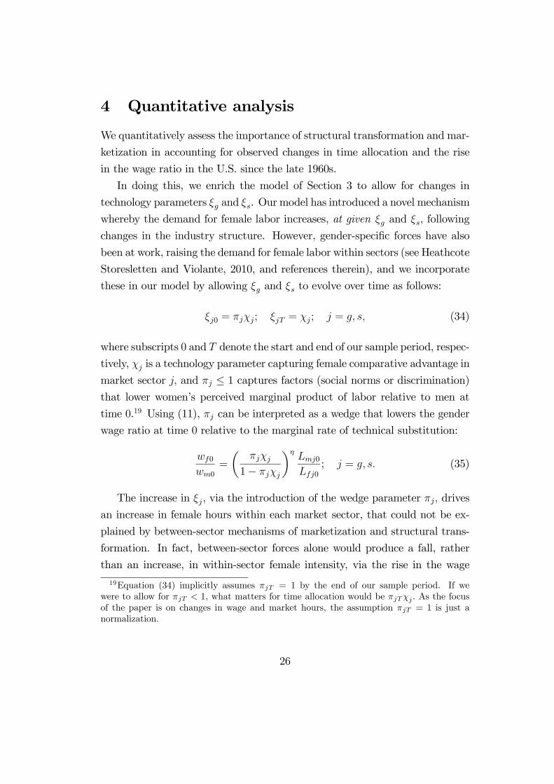
4 Quantitative analysis

We quantitatively assess the importance of structural transformation and mar-

ketization in accounting for observed changes in time allocation and the rise

in the wage ratio in the U.S. since the late 1960s.

In doing this, we enrich the model of Section 3 to allow for changes in

technology parameters and . Our model has introduced a novel mechanism

whereby the demand for female labor increases, at given and , following

changes in the industry structure. However, gender-specific forces have also

been at work, raising the demand for female labor within sectors (see Heathcote

Storesletten and Violante, 2010, and references therein), and we incorporate

these in our model by allowing and to evolve over time as follows:

0 = ; = ; = (34)

where subscripts 0 and denote the start and end of our sample period, respec-

tively, is a technology parameter capturing female comparative advantage in

market sector and ≤ 1 captures factors (social norms or discrimination)that lower women’s perceived marginal product of labor relative to men at

time 0.19 Using (11), can be interpreted as a wedge that lowers the gender

wage ratio at time 0 relative to the marginal rate of technical substitution:

0

0

=

µ

1−

¶0

0

; = (35)

The increase in via the introduction of the wedge parameter drives

an increase in female hours within each market sector, that could not be ex-

plained by between-sector mechanisms of marketization and structural trans-

formation. In fact, between-sector forces alone would produce a fall, rather

than an increase, in within-sector female intensity, via the rise in the wage

19Equation (34) implicitly assumes = 1 by the end of our sample period. If we

were to allow for 1, what matters for time allocation would be As the focus

of the paper is on changes in wage and market hours, the assumption = 1 is just a

normalization.

26

ratio, as shown in (11). Changes in thus help our model fit evidence on

both between- and within-sector changes in female hours.

4.1 Data targets

Model outcomes are related to changes in relevant data moments between the

start and the end of the sample period. We aim to account for changes in the

aggregate service share, , and its gender components ( and ), the wage

ratio , and shares of market hours () and total work ( ≡ 1−) for

each gender. The service shares are obtained from the CPS, using the sample

selection criteria and the goods/service classification described in Subsection

2.1, and are adjusted for changing demographics as we did for time use data

in Subsection 2.3. The adjusted wage ratio, , is also obtained from the CPS,

as plotted in Panel B of Figure 2. Market hours and home hours are obtained

from time use data as described in Subsection 2.3. To obtain the share of

total work, we adopt Aguiar and Hurst (2007a) narrow leisure measure, which

includes the time individuals spend socializing, in passive and active leisure,

volunteering, in pet care, and gardening.

Data on , , , and can be combined to characterize the full

time allocation across four activities (goods, market services, home services or

leisure) for each gender:

=

⎧⎪⎪⎪⎪⎨⎪⎪⎪⎪⎩

(1− ) for =

for =

−

for =

1− for =

=

Data on , ,, and for the start and the end of our sample

period are shown in Table 3 as 5-year averages for 1968-1972 and 2004-2008,

respectively. This is to smooth out short-run fluctuations that are not relevant

for model predictions, and possibly single-year outliers. For simplicity we will

refer to the start of the sample period 1968-1972 as “1970”, and to the end of

the sample period 2004-2008 as “2006”.

27

4.2 Baseline parameters

We calibrate baseline parameters to match the time allocation and wage ratio

in 1970, and then feed in the measured marketization and structural transfor-

mation forces to predict their change until 2006. The parameters needed to

match the data at baseline include the elasticity parameters ( and ),

the relative time endowment , the leisure preference parameter the

sector-specific productivity parameters ( − , − ), the gender-specific

parameters (, , and ), the wedge parameters ( ), and (0, 0)

defined in (24) and (30).

The calibration procedure is described below, and step-by-step details are

given in Appendix C. In a nutshell, , , − and − (measuring

marketization and structural transformation) are model-free, i.e. pinned down

by existing estimates of relevant magnitudes. The remaining twelve parameters

are calibrated to match the initial time allocation across the four activities for

each gender (8 data targets) and the responsiveness of the gender hours ratio

in such activities to changes in the wage ratio (4 data targets).

4.2.1 Marketization and structural transformation parameters

The driving forces of marketization and structural transformation are defined,

respectively, as ≡ ( − 1) ( − ) and ≡ (1− )¡ −

¢. To

obtain a value for , we borrow from existing estimates of the elasticity of

substitution between home and market consumption, discussed in detail by

Aguiar, Hurst and Karabarbounis (2012) and Rogerson and Wallenius (2016).

The most common approach to estimate such elasticity has used micro data

on consumer expenditure and home production hours (see e.g. Rupert, Roger-

son and Wright, 1995; Aguiar and Hurst, 2007b). More recently, Gelber and

Mitchell (2012) obtain an estimate of the elasticity of substitution between

home and market goods from the observed hours response to tax changes.

Estimates obtained typically range between 1.5 and 2.5. We use as our bench-

mark the mid-range value of this interval, = 2, which is also close to the

average of existing point estimates. Appendix D provides some sensitivity

28

analysis for .

As for the elasticity of substitution between goods and services, recent

findings in Herrendorf, Rogerson and Valentinyi (2013a) on newly-constructed

consumption value-added data and relative prices suggest very values of .

They argue that, if technology is specified as a value-added production func-

tion, as is the case in our model, the arguments of the utility function should

also be the value added components of final consumption — as opposed to final

consumption expenditures. They identify using the equilibrium condition

equating the marginal rate of substitution between (value-added consumption

in) goods and services to relative prices, and obtain an estimate of 0002, which

we use as our benchmark value. Moro, Moslehi and Tanaka (2017) extend the

framework of Herrendorf, Rogerson and Valentinyi (2013a) to allow for home

production and also find an estimate for that is not significantly different

from zero. In Appendix D we provide some sensitivity analysis for .

Labor productivity growth in market sectors is obtained from the Bu-

reau of Economic Analysis (BEA) database, delivering real labor productivity

growth in the goods and services sectors of 2.49% and 1.25% respectively, thus

− = 124% To obtain a measure of labor productivity growth in the

home sector, we follow recent BEA calculations of U.S. household production

using national accounting conventions (see Bridgman et al, 2012, and refer-

ences therein). The BEA approach consists in estimating home nominal value

added by imputing income to labor and capital used in home production, and

deflating this using the price index for the private household sector. Specifi-

cally, Bridgman (2013) obtains productivity in the home sector as:

= +

P ( + )

where denotes the wage of private household employees; denotes hours

worked in the household sector; denotes the capital inputs used (consumer

durables, residential capital, government infrastructure used for home produc-

tion), with associated returns and depreciation rates and , respectively;

and is the price index for the sector “private households with employed per-

29

sons”. This includes both the wage of private sector employees and imputed

rental services provided by owner-occupied housing. The average growth in

during our sample period is 0.45%. Thus we set − = 080% as our

baseline.

Later work has suggested slight variations on the measurement of home

productivity growth. Bridgman, Duernecker and Herrendorf (2016) construct

explicit price indexes for expenditure on close market substitutes to household

consumption, instead of using the price index the for private household sector,

and excludes residential capital from home capital. These variations deliver

estimates in home productivity growth in the range 0.12%-0.45% during our

sample period. Lower values for would deliver a stronger marketization force

than in the benchmark case = 045%. Appendix C will show the effects

of a stronger marketization force, , by varying , which has qualitatively

similar effects to reducing

4.2.2 Calibrated parameters

The relative time endowment, , is set to match the service share, noting

that this can be expressed as:

=

+

+

The implied for 1970 is 1.03.

Using equilibrium condition (16) and (33), the elasticity parameters and

are set to match the observed response in (log) gender hours ratios at

home and in market services, respectively, to changes in the (log) wage ratio.

The implied values are = 227 and = 019 respectively. As expected,

1 reflects substitutability of male and female inputs in production (see

also estimates for the US by Weinberg, 2000, and Acemoglu, Autor and Lyle,

2004), and 1 reflects complementarity of male and female leisure time

(see Goux, Maurin and Petrongolo, 2014). The low value of is unsurprising,

given the relative stability of the gender ratio of total market time.

30

Given and , the gender-specific parameters and are pinned down

by conditions (16) and (33), evaluated in 1970, giving = 050 and = 029

The wedge parameters and are set to match the observed response in

gender hours ratios in goods and services, respectively, to changes in the wage

ratio, according to condition (11) and definition (34). This gives = 084

and = 080, and thus fairly similar wedges between the marginal rate of

technical substitution and the wage ratio in the two market sectors in 1970.

Given and the gender-specific parameters and are set to match the

1970’s hours ratios in goods and services, respectively. This gives = 029

and = 043 Women’s comparative advantage is thus highest in the home

sector ( = 050), intermediate in market services ( = 043), and lowest in

goods ( = 029).

The three remaining parameters 0, 0 and are calibrated to match

the 1970’s time allocation across home and services in (23), across goods and

services in (29), and across leisure and goods.20 Note that, given the 1970

data targets and the calibrated values for 0 and 0 separate values for

(, ) and productivity levels of (0, 0, 0) are not needed to work out

predictions for the time allocation and the wage ratio.

The determination of baseline parameters is summarized as follows:

20This is derived in Appendix B:

=

()

()

⎡⎣1 + "

µ

¶ −1

µ ()

()

¶ 1−1

µ1 +

1

¶ 1−

# 1−

⎤⎦ where and are functions of the time allocation in (21) and (27).

31

Parameters Values Data or Targets

Model free parameters

− 1.2% BEA data.

− 0.8% BEA data for services and Bridgman (2013) for home sector.

2.0 Various estimates in Aguiar, Hurst and Karabarbounis (2012).

0.002 Herrendorf, Rogerson and Valentinyi (2013a).

Calibrated parameters

1.03 match service share in 1970 given

2.27, 0.19match response in hours ratio (home&leisure)

to changes in wage ratio

, 0.50, 0.29 match wage ratio and hours ratio (home&leisure) in 1970

0.84,0.80match response in hours ratio (goods&services)

to changes in wage ratio

0.29,0.43match gender wage ratio and hour ratio (goods&services)

in 1970

0 0.95 match relative hours across services and home in 1970

0 5.35 match relative hours across goods and services in 1970

0.60 match relative hours across leisure and goods in 1970

4.3 Results

Our baseline quantitative exercise takes on board both between-sector forces

of marketization and structural transformation, and within-sector forces rep-

resented by the reduction in the wedge between the marginal rate of technical

substitution and the wage ratio, via the rise in and . To assess the

sole contribution of between-sector forces, in a later exercise we shut down

within-sector forces by fixing = = 1

Table 4 reports the quantitative results of model calibrations for the service

share, the wage ratio, market hours and total work. The two top rows report

their levels in 1970 and 2006, respectively, the third row reports their per-

centage change, and rows denoted A-D report predicted changes from model

calibrations. Calibration A uses baseline parameters described in subsections

32

4.2.1 and 4.2.2, and it shows that our model almost exactly replicates the 25%

rise in the service share observed in the data (column 1) and the 24% increase

in the wage ratio (column 2), and slightly overpredicts the 51% increase in the

market hours ratio (column 5). However, model performance for each gender

separately is weaker, by overpredicting and underpredicting, respectively, the

rise in female market hours and the decline in male market hours (columns

3 and 4). Finally, the model does a relatively good job at replicating a rel-

atively stable ratio of total work, which rises by only 3% during the sample

period (column 6). This is due to poor substitutability of spousal leisure,

which constrains the reallocation of total work across genders.

Calibration B assesses the merit of between-sector forces of marketization

and structural transformation, having shut down within-sector forces by set-

ting = = 1 The prediction on the service share is spot on, indicating that

the key forces in the model can account for the rise in services. The fall in the

female wage-productivity wedges (i.e. the rise in and ) would induce a fur-

ther rise in the service share by pulling women into the market — and especially

so in the sector in which they have a comparative advantage — but quantita-

tively this effect is tiny, as shown by comparison of predictions in column 1 of

rows A and B. Between-sector forces predict a nearly 5% increase in the wage

ratio (column 2), translating into a 3 percentage points’ increase from 0.63 to

0.66, against an actual increase up to 0.78. Thus between-sector forces predict

one fifth of the observed rise in the wage ratio, i.e. (0.66-0.63)/(0.78-0.63). To

put this figure into perspective, the calibrated contribution of marketization

and structural transformation to the rise in relative female wages is quanti-

tatively similar to the contribution of the rise in women’s human capital (as

proxied by education, potential experience and ethnicity, see notes to Figure

2), as including basic human capital controls explains about 20% of wage con-

vergence over the sample period.21 Similarly, between-sector forces predict a

nearly 11% rise in relative market hours, equivalent to roughly one fifth of the

21Between 1968-72 and 2004-08, the raw wage ratio rises by about 18 percentage points

(080−062), while the adjusted wage ratio rises by about 15 percentage points (078−063).Thus basic human capital controls explain 20% of wage convergence.

33

actual increase. The shift-share analysis of Subsection 2.1 suggests that 30%

of the rise in female hours is enabled by the expansion of services22, and the

model proposed thus explains two thirds of such between-sector component.

As above, the model implies near stability in the gender ratio of total work.

Model predictions for the full time allocation across four activities and

two genders are represented graphically in Figure 4. Each panel plots combi-

nations between actual percentage changes during 1970-2006 (horizontal axis)

and predicted percentage changes (vertical axis) for each of the eight outcomes,

together with the 45 degree line for reference. Panel A plots prediction based

on calibration A, encompassing within- and between-sector forces. The full

model provides a very good fit overall of changes in the structure of time allo-

cation of men and women, as summarized by an 2 of 0.90 from a regression

of predicted on actual changes.23 Despite the very good fit overall, the model

does a better job at matching changes in hours in the goods sector and the

home, than in market services and leisure. In particular, the model predicts a

slight reduction in leisure for women, from 37% to 36% of total hours, while

this rose from 37% to 38% - though magnitudes involved are too small to be

at all meaningful. Panel B plots predictions based on calibration B, which

isolates the role of between-sector forces. The overall model fit falls to 0.57,

and in particular the shift of female and male hours out of and into the home,

respectively, are underpredicted. A further, within-sector, increase in the rel-

ative demand for female labor is thus necessary to accurately reproduce the

decline of female home hours and the rise in male home hours.

Calibrations C and D in Table 4 decompose between-sector forces into

marketization and structural transformation separately. In row C we shut

down the structural transformation channel by imposing balanced productiv-

ity growth in market sectors ( = ), and in row D we shut down the marke-

tization channel by imposing balanced productivity growth across all services

( = ). In both cases we impose = = 1. Our results show that struc-

22This result is also confirmed on the series adjusted for changing demographics.23Note that none of these outcomes are targeted directly. Two baseline parameters (

and ) are set to match the elaticity in the gender hours with respect to the wage ratio,

which is itself predicted by marketization and structural transformation.

34

tural transformation is necessary to deliver a decline in male hours (comparing

column 4 in rows C and B) and marketization is necessary to increase female

hours (comparing column 3 in rows D and B). The comparison of results from

calibrations C and D confirms Propositions 3. Market hours for both genders

fall with structural transformation and rise with marketization. But, due to

gender comparative advantages, marketization has a stronger effect on female

market hours, while structural transformation has a stronger effect on male

market hours, and they both contribute to the rise in the market hours ratio.

As expected, each force contributes to the rise in services (11% and 16.7%

increase, respectively), in line with Proposition 2. The rise in services is in

turn associated to a rise in the wage ratio, in line with Proposition 1. How-

ever, structural transformation is the key driver of relative wages, explaining

a 5.1% rise in the wage ratio, as opposed to 0.2% for marketization. Note

that structural transformation alone would predict a higher rise in the wage

ratio than both forces together (5.1% versus 4.7%), due to the strong impact

of marketization on gender relative market hours (8.3%).

5 Conclusions

The rise in female participation to the workforce is one of the main labor

market changes of the post-war period, and has been reflected in a large and

growing body of work on the factors underlying such change. The bulk of

the existing literature has emphasized gender-specific factors such as human

capital accumulation, medical advances, gender-biased technical change, cul-

tural change, and antidiscrimination interventions, which imply a rise in the

female intensity across the whole industry structure. This paper complements

existing work by proposing a gender-neutral mechanism that boosts female em-

ployment and wages by expanding the sector of the economy in which women

have a comparative advantage.

Due to gender comparative advantages in production, marketization of

home production and structural transformation, in turn driven by differential

productivity growth across sectors, jointly act as a gender-biased labor demand

35

force, generating a simultaneous increase in both women’s relative wages and

market hours. While the source of both forces is gender neutral, their combi-

nation has female friendly outcomes. Marketization draws women’s time into

the market and structural transformation creates the jobs that women are

better suited for in the market. These outcomes are consistent with evidence

on gender convergence in wages, market work, and household work. When

calibrated to the U.S. economy, inter-sector forces adequately predict the rise

in services, and explain about one fifth of the narrowing wage gap and nearly

60% of changes in the time allocation of men and women.

References

[1] Acemoglu, Daron, David Autor and David Lyle. 2004. “Women, War,

and Wages: The Effect of Female Labor Supply on the Wage Structure

at Mid-century”. Journal of Political Economy 112: 497—551.

[2] Acemoglu, Daron, and David Autor. 2011. “Skills, Tasks and Technolo-

gies: Implications for Employment and Earnings”. In O. Ashenfelter and

D. Card, eds., Handbook of Labor Economics, Volume 4B. Amsterdam:

Elsevier, North Holland, 1043—1171.

[3] Acemoglu, Daron and Veronica Guerrieri. 2008. “Capital Deepening and

Non—Balanced Economic Growth,” Journal of Political Economy 116:

467—498.

[4] Albanesi, Stefania and Claudia Olivetti. 2016. “Gender Roles and Medical

Progress.” Journal of Political Economy 124: 650—695.

[5] Attanasio, Orazio, Hamish Low and Virginia Sanchez-Marcos. 2008. “Ex-

plaining Changes in Female Labor Supply in a Life-Cycle Model.” Amer-

ican Economic Review 98: 1517—1542.

[6] Aguiar, Mark and Erik Hurst. 2007a. “Measuring Trends in Leisure: The

Allocation of Time Over Five Decades”. Quarterly Journal of Economics

122: 969—1006.

36

[7] Aguiar, Mark and Erik Hurst. 2007b. “Lifecycle Prices and Production”.

American Economic Review 97: 1533—1559.

[8] Aguiar, Mark, Erik Hurst, and Loukas Karabarbounis. 2012. “Recent De-

velopments in the Economics of Time Use.” Annual Review of Economics

4: 373—397.

[9] Akbulut, Rahsan. 2011, “Sectoral Changes and the Increase in Women’s

Labor Force Participation” Macroeconomic Dynamics 15: 240—264.

[10] Azmat, Ghazala and Barbara Petrongolo. 2014. “Gender and the La-

bor Market: What Have We Learned from Field and Lab Experiments?”

Labour Economics 30: 32—40.

[11] Baumol, William 1967. “Macroeconomics of Unbalanced Growth: The

Anatomy of Urban Crisis.” American Economic Review 57: 415—26.

[12] Bertrand, Marianne. 2011. “New Perspectivs on Gender.” In O. Ashenfel-

ter and D. Card (eds.) Handbook of Labor Economics, vol. 4B: 1545—1592.

Amsterdam: Elsevier

[13] Blau, Francine and David Kahn. 2013. “The Feasibility and Importance

of Adding Measures of Actual Experience to Cross-Sectional data Collec-

tion”. Journal of Labor Economics 31: S17—S58.

[14] Boppart, Timo. 2014. “Structural Change and the Kaldor Facts in a

Growth Model with Relative Price Effects and non-Gorman Preferences.”

Econometrica 82: 2167—2196.

[15] Borghans, Lex, Bas ter Weel, and Bruce Weinberg. 2008. “Interpersonal

Styles and Labor Market Outcomes.” Journal of Human Resources 43:

815—858.

[16] Borghans, Lex, Bas ter Weel, and Bruce Weinberg. 2014. “People Skills

and the Labor-market Outcomes of Underrepresented Groups.” Industrial

and Labor Relations Review 67: 287—334.

37

[17] Bridgman, Benjamin, Andrew Dugan, Mikhael Lal, Matthew Osborne

and Shaunda Villones. 2012. “Accounting for Household Production in

National Accounts, 1965-2010”, Survey of Current Business 92: 23—36.

[18] Bridgman, Benjamin. 2013. “Home Productivity”, Working Paper 0091,

Bureau of Economic Analysis.

[19] Bridgman, Benjamin, Georg Duernecker and Berthold Herrendorf. 2016.

“Structural Transformation, Marketization, and Household Production

around theWorld”. Mimeo, University of Arizona.

[20] Buera, Francisco and Joseph Kaboski. 2012. “The Rise of the Service

Economy.” American Economic Review 102: 2540—2569.

[21] Buera, Francisco, Joseph Kaboski, and Min Qiang Zhao. 2013. “The Rise

of Services: the Role of Skills, Scale, and Female Labor Supply.” NBER

working paper No. 19372.

[22] Burda, Michael, Daniel Hamermesh and Phillipe Weil. 2013. “Total Work

and Gender: Facts and Possible Explanations.” Journal of Population

Economics 26: 239—261.

[23] Dix-Carneiro, Rafael. 2014. “Trade Liberalization and labor Market Dy-

namics.” Econometrica 82: 825—885.

[24] Fan, Chengze Simon and Hon-Kwong Lui. 2003. “Structural change and

the narrowing gender gap in wages: Theory and evidence from Hong

Kong”. Labour Economics 10: 609—626.

[25] Fernández, Raquel. 2013. “Cultural Change as Learning: The Evolution

of Female Labor Force Participation over a Century”, American Economic

Review 103: 472—500.

[26] Freeman, Richard and Ronald Schettkat. 2005. “Marketization of House-

hold Production and the EU-US Gap in Work”, Economic Policy 41:

5—39.

38

[27] Fuchs, Victor. 1968. The Service Economy, New York: Columbia Univer-

sity Press.

[28] Galor, Oded and David Weil. 1996. “The Gender Gap, Fertility, and

Growth.” American Economic Review 86: 374—87.

[29] Gelber, Alexander and Joshua W. Mitchell. 2012. “Taxes and Time Al-

location: Evidence from Single Women and Men.” Review of Economic

Studies 79: 863—897.

[30] Goldin, Claudia. 2006. “The Quiet Revolution That Transformed

Women’s Employment, Education, and Family”. American Economic Re-

view, Papers and Proceedings 96: 1—21.

[31] Goldin, Claudia and Lawrence Katz. 2002. “The Power of the Pill: Oral

Contraceptives and Women’s Career and Marriage Decisions”. Journal of

Political Economy 100: 730—770.

[32] Greenwood, Jeremy, Ananth Seshadri and Mehmet Yorukoglu. 2005. “En-

gines of Liberation”. Review of Economic Studies 72: 109—133.

[33] Goux, Dominique, Eric Maurin and Barbara Petrongolo. 2014. “Wortime

Regulations and Spousal Labor Supply.” American Economic Review 104:

252—276.

[34] Heathcote, Jonathan, Kjetil Storesletten and Gianluca Violante. 2010.

“The Macroeconomic Implications of Rising Wage Inequality in the

United States”. Journal of Political Economy 118: 681—722.

[35] Herrendorf, Berthold, Richard Rogerson, and Ákos Valentinyi.

2013a.“Two Perspectives On Preferences and Structural Transformation.”

American Economic Review 103: 2752—2789.

[36] Herrendorf, Berthold, Richard Rogerson, and Ákos Valentinyi. 2013b.

“Growth and Structural Transformation”. In P. Aghion and S. Durlauf

(eds.) Handbook of Economic Growth. Amsterdam: Elsevier, North Hol-

land, 855—941.

39

[37] Hsieh, Chang-Tai, Erik Hurst, Chad Jones and Pete Klenow. 2016. “The

Allocation of Talent and U.S. Economic Growth”. Mimeo, Chicago Booth.

[38] Jones, Larry, Rodolfo Manuelli, Ellen McGrattan. 2015. “Why Are Mar-

ried Women Working So Much?” Journal of Demographic Economics 81:

75—114.

[39] Kongsamut, Piyabha, Sergio Rebelo, and Danyang Xie. 2001. “Beyond

Balanced Growth,” Review of Economic Studies 68: 869—882.

[40] Lebergott, Stanley. 1993. Pursuing Happiness. Princeton Univ. Press,

Princeton, NJ.

[41] Lee, Donghoon and Ken Wolpin. 2006. “Intersectoral labor mobility and

the growth of the service sector”. Econometrica 74: 1—46.

[42] Lee, Donghoon and Ken Wolpin. 2010. “Accounting for Wage and Em-

ployment Changes in the U.S. from 1968-2000: A Dynamic Model of

Labor Market Equilibrium”. Journal of Econometrics 156: 68—85.

[43] Katz Lawrence and Kevin Murphy. 1992. “Changes in Relative Wages,

1963-1987: Supply and Demand Factors”. Quarterly Journal of Eco-

nomics 107: 35—78.

[44] Moro, Alessio, Solmaz Moslehi and Satonshi Tanaka. 2017. “Does Home

Production Drive Structural Transformation?” Forthcoming in American

Economic Journal: Macroeconomics.

[45] Ngai, L. Rachel and Christopher Pissarides. 2007. “Structural Change in a

Multi-sector Model of Growth”. American Economic Review 97: 429—443.

[46] Ngai, L. Rachel and Christopher Pissarides. 2008. “Trends in Hours and

Economic Growth”. Review of Economic Dynamics 11: 239—256.

[47] Olivetti, Claudia and Barbara Petrongolo. 2014. “Gender Gaps Across

Countries and Skills: Supply, Demand and the Industry Structure”. Re-

view of Economic Dynamics 17: 842—859

40

[48] Olivetti, Claudia and Barbara Petrongolo. 2016. “The Gender Gap in

Industrialized Countries.” Annual Review of Economics 8: 405—434.

[49] Rendall, Michelle. 2010. “Brain versus Brawn: The Realization of

Women’s Comparative Advantage.” Mimeo, University of Zurich.

[50] Rendall, Michelle. 2015. “Female Market Work, Tax Regimes, and the

Rise of the Service Sector.” Mimeo, University of Zurich.

[51] Reid, Margaret. 1934. Economics of Household Production. Wiley, New

York.

[52] Rogerson, Richard and JohannaWallenius. 2016. “Retirement, Home Pro-

duction and Labor Supply Elasticities”, Journal of Monetary Economics

78: 23—34.

[53] Rupert, Peter, Richard Rogerson and Rendall Wright, 1995. “Estimat-

ing Substitution Elasticities in Household Production Models”. Economic

Theory 6: 179—193.

[54] Weinberg, Bruce 2000. “Computer Use and the Demand for Female Work-

ers”. Industrial and Labor Relations Review 53: 290—308.

41

42  

Table 1 Descriptive statistics on 17 industries, 1968-2008.

Sector share Female intensity

(1) (2) (3) (4) (5) (6)

1968 2008 Change 1968 2008 Change

Primary sector 6.2 3.3 -3.0 10.2 17.1 7.0

Construction 6.0 7.6 1.7 4.5 9.0 4.6

Manufacturing 29.7 12.7 -17.0 23.1 29.3 6.2

Utilities 1.7 1.3 -0.4 8.1 20.9 12.8

All goods 43.6 25.0 -18.6 18.1 21.1 3.0

Transportation 4.4 3.8 -0.6 8.4 21.6 13.2

Post and Telecoms 1.2 0.9 -0.3 44.1 36.4 -7.6

Wholesale trade 3.8 3.0 -0.8 15.4 28.4 13.0

Retail trade 13.6 14.0 0.4 36.2 45.1 9.0

FIRE 4.6 7.2 2.6 36.9 54.6 17.7

Business and repair services 3.1 8.4 5.3 18.3 37.3 19.0

Personal services 4.1 2.8 -1.3 64.4 69.0 4.7

Entertainment 0.9 2.1 1.2 24.7 40.8 16.1

Health 4.8 10.2 5.4 64.7 76.0 11.3

Education 7.2 10.4 3.1 56.8 70.5 13.7

Professional services 1.1 3.2 2.2 23.7 41.9 18.2

Welfare and no-profit 1.4 2.7 1.4 36.8 64.2 27.3

Public administration 6.2 6.4 0.1 25.1 43.4 18.3

All services 56.4 75.0 18.6 37.4 52.1 14.8 Notes. Columns 1 and 2 report the share of sector hours in total annual hours (×100) in 1968 and 2008, respectively, and column 3 reports their change. Columns 4 and 5 report the share of female hours in each sector (×100) in 1968 and 2008, respectively, and column 6 reports their change. The primary sector includes agriculture, forestry, fishing, mining and extraction. Source: CPS.

Table 2 Alternative decompositions of the rise in the female hours share, 1968-2008.

Notes. Row 1 corresponds to the left-hand side of equation (1) in the text. Percentages in rows 2-4 are obtained as ratios between the first term on the right-hand side of equation (1) and the left-hand side. The percentage in row 5 is obtained as the ratio between the second term on the right-hand side in equation (2) and the left-hand side.

1 Total change (×100) 44.4 – 29.0 = 15.4

2 Between sector, % of total change (goods/services)

30.4

3 Between sector, % of total change (17 categories)

28.6

4 Between occupation, % of total change (4 categories)

24.1

5 Between occupation, % of within-sector component (4 occupations, 2 sectors)

7.9

43  

Table 3 Data Targets

Estimates of model targets

Service share

Service share

(women)

Service share (men)

Wage ratio

Market hours

(women)

Market hours (men)

Total work

(women)

Total work (men)

Time / /

1968-1972 0.59 0.76 0.51 0.63 0.23 0.48 0.64 0.62

2004-2008 0.74 0.87 0.63 0.78 0.29 0.40 0.62 0.59

Source Current Population Survey Time Use Surveys

Complete time allocation

Women Men

goods Services home leisure goods services home leisure

Time / / / / / / / /

1968-1972 0.05 0.17 0.41 0.37 0.23 0.24 0.14 0.38

2004-2008 0.04 0.25 0.34 0.38 0.15 0.25 0.18 0.41

Source Current Population Survey and Time Use Surveys

44  

Table 4 Quantitative results

Service share Wage ratio Female market hours

Male market hours

Market hours ratio

Total work ratio

/ / // /

1 2 3 4 5 6

1970 data 0.59 0.63 0.23 0.48 0.47 1.03

2006 data 0.74 0.78 0.29 0.40 0.71 1.06

Percentage change 1970-2006

Data 25.4 23.8 26.9 -15.8 50.6 3.0

A. Model – baseline 27.3 22.7 44.9 -8.0 57.6 2.3

B. Model – Between-sector forces only ( 1) 26.1 4.7 9.0 -1.4 10.6 0.5

C. Model – Marketization only ( 1 and )

11.0 0.2 12.4 3.8 8.3 0.0

D. Model – Structural transformation only ( 1 and )

16.7 5.1 -4.3 -6.6 2.4 0.6

Notes. 1970 refers to the 1968-1972 average. 2006 refers to the 2004-2008 average. All parameters used are baseline values reported in Subsection 4.2, unless indicated in brackets.

45  

Figure 1 Trends in market hours, by gender.

Notes. See Table 1 for definition of the service sector. Sample: men and women aged 21-65. Source: CPS: 1968-2008.

600

800

1000

1200

1400

1600

1800

2000

1970 1975 1980 1985 1990 1995 2000 2005 2010Year

All Men Women

A: Annual hours

0

200

400

600

800

1000

1200

1400

1970 1975 1980 1985 1990 1995 2000 2005 2010Year

All Goods Services

C: Annual hours - Females

40

50

60

70

80

90

10

0

1970 1975 1980 1985 1990 1995 2000 2005 2010Year

All Men Women

B: Fraction of annual hours in services

400

600

800

1000

1200

1400

1600

1800

2000

1970 1975 1980 1985 1990 1995 2000 2005 2010Year

All Goods Services

D: Annual hours - Males

46  

Figure 2

The gender wage ratio

Notes. In panel A the wage ratio is obtained as (the exp of) the coefficient on a female dummy from yearly log wage regressions that only control for gender. In panel B the wage ratio is obtained from corresponding regressions that also control for age, age squared, education (4 categories) and ethnicity (one non-white dummy). Sample: men and women aged 21-65. Source: CPS: 1968-2008.

60

65

70

75

80

85

1970 1975 1980 1985 1990 1995 2000 2005 2010Year

A: The unadjusted wage ratio (x100)

60

65

70

75

80

85

1970 1975 1980 1985 1990 1995 2000 2005 2010Year

All Goods Services

B: Wage ratios adjusted for human capital (x100)

47  

Figure 3 Trends in market work and home production

(usual weekly hours)

Notes. Market work includes time spent working in the market sector on main jobs, second jobs, and overtime, including any time spent working at home, but excluding commuting time. Home production hours include: time spent on meal preparation and cleanup, doing laundry, ironing, dusting, vacuuming, indoor and outdoor cleaning, design, maintenance, vehicle repair, gardening, and pet care; time spent obtaining goods and services; child care. Sample: men and women aged 21-65. Source: 1965-1966 America's Use of Time; 1975-1976 Time Use in Economics and Social Accounts; 1985 Americans' Use of Time; 1992-1994 National Human Activity Pattern Survey; 2003-2008 American Time Use Surveys. All series are adjusted for changing demographics following Aguiar and Hurst (2007a).

1020

3040

5060

1965 1970 1975 1980 1985 1990 1995 2000 2005 2010year

women, market women, home women, totalmen, market men, home men, total

48  

Figure 4 Model predictions for men’s and women’s time allocation across goods, market services home services and leisure

Notes. Each point in the scatter plot represents the combination of actual and predicted changes in time allocation. In Panels A and B, predicted changes are obtained using calibrations A and B, respectively, in Table 4. The , label used for each point refers to gender , and sector (good), (market services), (home), (leisure).

(f,g)

(f,s)

(f,h)

(f,l)

(m,g)

(m,s)(m,h)

(m,l)

R2 = 0.90

-40

-20

020

4060

80Pr

edic

ted

% c

hang

e

-40 -20 0 20 40 60Actual % change

Panel A: Baseline predictions

(f,g)

(f,s)

(f,h) (f,l)

(m,g)

(m,s)

(m,h)(m,l)

R2 = 0.57

-40

-20

020

4060

80Pr

edic

ted

% c

hang

e

-40 -20 0 20 40 60Actual % change

Panel B: Predictions based on between-sector forces

Appendices

A A multisector model with tasks

Our model technology combines male and female inputs to produce output in

each sector. This Appendix provides microfoundations for the assumed tech-

nology, showing that our production function specification delivers equivalent

results to one in which output in each sector requires a combination of tasks,

and men and women are differently endowed of the skills necessary to perform

them.

Assume for simplicity that there are only two sectors in the economy, goods

and services, denoted by = , respectively, whose output is produced

combining mental and physical tasks, according to the following technology:

=

h

−1

+ (1− )−1

i −1

where and represent hours of mental and physical tasks, respectively, in

sector , is the elasticity of substitution between them, and is a technology

parameter representing the relative weight of mental inputs in sector . We

impose to capture the relatively heavier use of physical tasks in goods

than service production.

Mental and physical inputs are each described by CES aggregators of male

and female work:

=

∙

−1

+¡1−

¢

−1

¸ −1

=

∙

−1

+¡1−

¢

−1

¸ −1

where and represent gender inputs in either task and and

represent female comparative advantages. We impose to capture

female comparative advantages in mental tasks.

49

The first order condition for female wages in mental tasks is

= 1

− 1

1

− 1

which can be rearranged as

1

=

1

1− 1

=

where ≡ 1

1− 1

and inter-sector labor mobility is imposed, thus

= , = .

Total female hours in mental tasks are given by:

≡ + =

+

and similarly for physical tasks:

≡ + =

+

Total female hours in the economy are thus given by

≡ + =

+

+

+

(36)

where inter-task labor mobility is imposed, with = = .

Using expression (36) and a similar expression for total male hours the

gender wage gap can be derived:

=

Ã

+

+

+

(1− )

+ (1− )

+ (1− )

+ (1− )

!1 µ

¶1

(37)

This expression has clear similarities with result (11) for the gender wage gap

in the main model, having expressed women’s comparative advantages () as

50

a combination of their comparative advantages in mental and physical tasks

in both sectors ( and

), with weights that depend on the use of such

tasks in each sector ( and

).

To highlight the link between the share of services and the demand for

women, consider the

term at the numerator of (37), which is in turn

equal to 1

1− 1

. Given the assumptions made, a rise in services ()

raises the wage ratio via the combination of the heavier use of mental tasks in

services () and female comparative advantages in mental tasks ().

B Deriving the competitive equilibrium

B.1 Firms

Taking wages ( ) and prices ( ) as given, the representative firm in

sector = chooses©

ªto maximize profit

= − −

subject to technology:

= =

∙

−1

+¡1−

¢

−1

¸ −1

= (38)

The first order conditions for wages are

=

µ

¶1; =

¡1−

¢µ

¶1 (39)

Free mobility of labor implies equal marginal rates of technical substitution

across sectors:

= − (40)

which is equation (11) in the main text, with ≡ and ≡ (1−).Having denoted by () the female wage bill share in sector , the following

51

expression can be derived:

() ≡

+

=1

1 + − −1

(41)

which is the equation (18) in the main text. Using the production function

(38) gives:

=

−1

¡1 +

− −1

¢ −1 =

µ

()

¶ −1

(42)

Combining (42) and (39) implies

=

−1 ( ())

11− (43)

Equalizing the value of the marginal product of labor across sectors for each

gender implies:

=

µ

¶ −1µ ()

()

¶ 1−1

(44)

which is equation (17) in the main text.

Let denote labor supply for each gender (which will be determined by

the household optimization problem). Labor market clearing for each gender

implies:

+ = = (45)

Combining (45) and (40) for = gives the allocation of female hours:

=1−

−

1− () (46)

which is the equation (13) in the main text.

B.2 Households

The representative household chooses ( ) to maximize

( ) = ln + ln (47)

52

subject to

=h

−1

+ (1− ) −1

i −1; =

h

−1

+ (1− ) −1

i −1

(48)

=

∙

−1

+ (1− )−1

¸ −1

(49)

=

∙

−1

+ (1− )

−1

¸ −1

(50)

+ = ( − − ) + ( − − ) (51)

Let be the Langrangian multiplier on the budget constraint (51). The first

order conditions of the household optimization problem are

() :

= (52)

() :

= (53)

() :

= (54)

() :

= (55)

() :

= (56)

() :

= (57)

B.2.1 Home production

The first order conditions for and imply that the marginal rate of

technical substitution must equal the wage ratio:

= − (58)

53

where ≡ (1− ). Let () denote the implicit female wage bill share

in the home sector:

() ≡

+

=1

1 + − −1

(59)

Using production function (49) gives:

=

−1

¡1 +

− −1

¢ −1 =

µ

()

¶ −1

(60)

The implicit price index for home output is defined using the first order

conditions for and :

≡

; = (61)

Using (39), (49) and (60) gives

=

µ

¶ −1µ ()

()

¶ 1−1

(62)

which is equation (17) in the main text.

Equating the marginal rate of substitution across market and home services

to their relative prices using first order conditions (53) and (54), the utility

functions (48) and the definition of , (61), implies the relative demand func-

tion:

=

µ

1−

¶ µ

¶

(63)

Rearranging (63) gives relative expenditure :

≡

=

µ

¶−1µ

1−

¶

(64)

which is equation (19) in the main text. Using the relative prices (62), the

54

relative expenditure can be expressed as function of :

= −1

"µ

¶ −1µ ()

()

¶ 1−1#−1

(65)

where

≡µ

¶µ

1−

¶ −1

(66)

is growing at rate −

It is convenient to derive an expression for for developing the rest of

the model. Substituting (63) into (48) gives:

=

−1

Ã1 +

µ1−

¶µ

¶−1

! −1

=

−1

Ã1 +

µ1−

¶ µ

¶1−! −1

Finally using (64) gives:

=

−1

µ1 +

1

¶ −1

(67)

B.2.2 Expenditure on market goods and services

Equating the marginal rate of substitution across goods and market services

to their relative prices using the first order conditions (52) and (53) and utility

functions (48) gives:

(1− )

µ

¶1µ

¶ 1

=

and, rearranging:

=

µ

(1− )

µ

¶¶µ

¶−

55

Substituting using (67) gives:

=

µ

(1− )

¶µ

¶Ã

−1

µ1 +

1

¶ −1!−

which can be simplified to

=

∙µ

1−

¶

¸

(1−)−1

µ1 +

1

¶−−1

(68)

Thus relative expenditure can be obtained:

≡

=

µ

¶1−µ

1−

¶

(1−)−1

µ1 +

1

¶−−1

(69)

This is equation (25) in the main text. Using relative prices in (44), the relative

expenditure can be expressed as function of :

= −1

õ

¶ −1µ ()

()

¶ 1−1!1−µ

1 +1

¶−−1

(70)

where

≡

µ1−

¶ 1−

1− (71)

is growing at rate −

B.2.3 Leisure

The first order conditions for and imply that the marginal rate of

technical substitution must equal the wage ratio:

= − (72)

56

where ≡ (1 − ). Let’s denote by () the implicit female wage bill

share for leisure:

() ≡

+

=1

1 + − −1

(73)

Using the leisure aggregator (50) gives:

=

−1

³1 +

− −1

´ −1 =

µ

()

¶ −1

(74)

The implicit price index for leisure is defined using the first order con-

ditions for and :

≡

; = (75)

Using (39), (49) and (60) gives

=

µ

¶ −1µ ()

()

¶ 1−1

(76)

Equating the marginal rate of substitution across goods and leisure to their

relative prices using the first order conditions (52) and (56) and the utility

functions (48) and (50) gives:

µ

¶ 1

=1

(77)

Thus relative expenditure is given by:

≡

=

µ

¶ −1

(78)

Using (48):

µ

¶ −1

=

Ã1 +

1−

µ

¶ −1

!

57

Using (67) and (68):

µ

¶µ

¶=

−1

µ1 +

1

¶ −1µ

1−

¶−

(−1)−1

µ1 +

1

¶ −−1

= −1

µ1 +

1

¶ −1µ

1−

¶−

Substituting this into (78) gives:

=

"1 +

µ1−

¶

(−1)−1

µ1 +

1

¶ −1−1µ

¶1−# (79)

Substituting relative prices using (44) gives:

=

⎡⎣1 +µ1−

¶

(−1)−1

µ1 +

1

¶ −1−1Ã

µ

¶ −1µ ()

()

¶ 1−1!1−⎤⎦

which can be simplified to obtain:

=

⎡⎣1 + "

µ

¶ −1µ ()

()

¶ 1−1µ1 +

1

¶ 11−#1−⎤⎦ (80)

B.2.4 Household’s optimal decision

Given the definition of implicit prices and the budget constraint (51)

can be rewritten as X=

+ = +

Dividing through by gives:X=

=

+

58

and, rearranging:

+

=1X

=

(); () ≡

where () is a function of given (65), (70) and (80). The share of female

leisure time can be derived as a function of relative expenditures, and thus a

function of the wage ratio :

= ()

()X

=

() (81)

where () is the implicit female wage bill share in total wage income:

() ≡

+

(82)

B.3 Market clearing

The market clearing conditions for the labor and commodity markets are,

respectively:

= = (83)

+ = − − = (84)

Using market clearing conditions and the production functions, relative ex-

penditures in (64), (69) and (79) can be rewritten as:

() =

=

Using relative prices (44), (62) and (76) gives:

() =

Ã

()

! 1−1 µ

()

¶ 11−

µ

¶µ

¶

59

Using derived in (42), (60) and (74), to obtain:

= ()

() () = (85)

This gives equation (21) and (27) in the main text. Substituting it into the

female time constraint (84), a second condition for female leisure time is given

by

=1X

=

()()

()

(86)

which is also a function of the wage ratio. Together with the condition in (81),

the equilibrium wage ratio satisfies:

()X

=

()−X

=

() () = 0 (87)

Thus the gender wage ratio depends on relative expenditures in (65), (70)

and (80), which respond to gender-neutral shifts due to the effects of uneven

productivity growth through the terms and

B.4 Time allocation

B.4.1 Time allocation across market and home services

Substituting the relative expenditure (65) into (85) gives:

=

µ ()

()

¶−1

õ

¶ −1µ ()

()

¶ 1−1!−1

which simplifies to:

= () ≡ −1

µ

¶(−1)−1

µ ()

()

¶−−1

(88)

This is equation (23) in the main text.

60

B.4.2 Time allocation across goods and market services

Substituting the relative expenditure (70) into (85) gives:

=

µ ()

()

¶−1

õ

¶ −1µ ()

()

¶ 1−1!1−µ

1 +1

¶−−1

Substituting using (85) and (88) gives:

= () ≡ −1

µ ()

()

¶ −−1·µ

¶(1−)−1

µ1 +

()

() ()

¶−−1

(89)

B.4.3 Service employment share

By definition, the service employment share is = ( + )( + +

+ ). Thus:

−1 = 1 +

+ 1

+ 1

= 1 +

()

()

Substituting this into (40) gives

−1 = 1 +

()

()=⇒ =

1

1 + ()()

()

(90)

which is equation (31) in the main text.

B.4.4 Leisure

Substituting (80) in (85) gives:

1

= ()

()

⎡⎣1 + "

µ

¶ −1µ ()

()

¶ 1−1µ1 +

1

¶ 1−

1

# 1−

⎤⎦ (91)

61

C Calibration

Sixteen parameters are required to determine the wage ratio and the time al-

location by gender in the model. The paper has explained in detailed how

the time use data and the CPS data are combined to obtain the data targets

{ ; }=1 and how© − −

ªare cal-

ibrated. This section describes the step-by-step procedure of obtaining the

remaining eleven parametersn 1 0 0

osequen-

tially.

(a) Elasticity of substitution in leisure aggregator ().

As (72) needs to hold at any point in time, is set to match the response

in the (log) leisure hours ratio to the change in the wage ratio:

=ln

− ln 0

0

ln − ln0 (92)

where subscripts 0 and denote the start and end of our sample period,

respectively

(b) Elasticity of substitution in the production function ().

As (58) needs to hold at any point in time, is set to match the response

in the (log) home hours ratio to the change in the wage ratio:

=ln

− ln 0

0

ln − ln0 (93)

(c) Gender-specific parameters and

Given 00, 00 and 0, and are obtained from (58) and

(72) respectively:

1−

= 0

µ0

0

¶−1

;

1− = 0

µ0

0

¶− 1

(94)

(d) Wedge parameters and

Using definition (34) and condition (40), and are set to match the

62

response in the hours ratio in goods and services, respectively, to the change

in the wage ratio:

=0

³0

0

´− 1

1 + 0

³0

0

´− 1

1 +

³

´− 1

³

´− 1

= (95)

(e) Gender-specific parameters 1 and

Using (34) and (40), and are set to match the initial hours ratio in

goods and services:

=1

0

³0

0

´− 1

1 + 0

³0

0

´− 1

= (96)

(f) Combinations of productivity parameters, 0 and 0

From (88):

0 =

µ0

¶ −1µ0 ()

0 ()

¶ 1−1∙0

0

0 ()

0 ()

¸ 1−1

(97)

From (89):

0 =

µ00

¶ −1µ0 ()

0 ()

¶ 1−1"0

0

0 ()

0 ()

µ1 +

1

0 ()

¶−−1# 11−

(98)

where 0 () = (00) (0 () 0 ()) from (85).

(g) Leisure parameter in utility function ()

Using (91):

=

00

0()

0()

1 +

∙

³00

´ −1³0()

0()

´ 1−1³1 + 1

0()

´ 1−

0 ()

¸1− (99)

63

where 0 () = (00)(0 () 0 ()) from (85).

D Sensitivity Analysis

We perform some sensitivity analysis on parameters and , which affect

the strength of marketization and structural transformation forces, respec-

tively. The results are shown in Table A1, which reports for reference in row

A our previous calibration of between-sector forces (row B of Table 4). As the

main contribution of our calibrations is to highlight the quantitative impact of

between-sector forces, we show sensitivity analysis with respect to this bench-

mark. In rows B-D we consider lower and upper bounds for , respectively,

near the extremes of the range of variation of empirical estimates found in

the literature, and a higher value for .24 In row B we consider weaker mar-

ketization than in the baseline case ( = 15), implying lower market hours

for both genders than in row A (in which = 2). The model thus does a

better job at predicting the fall in men’s market hours, but performs worse on

women’s hours. The model also predicts a slightly stronger rise in the wage

ratio, thanks to reduced labour supply of women relative to men. In row C we

consider instead stronger marketization ( = 25), and as expected changes in

model predictions are reversed. The calibration in row D weakens structural

transformation by setting = 01, leaving the marketization force unchanged.

Model predictions slightly worsen in all dimensions, but quantitatively they

stay very close to the baseline simulation.

24Clearly could not be reduced further from the baseline calibration, in which we set

= 0002

64

65  

Appendix Tables and Figures

Table A1 Sensitivity analysis on between-sector forces

Service share Wage ratio Female market hours

Male market hours

Market hours ratio

Total work ratio

/ / // /

1 2 3 4 5 6

1970 data 0.59 0.63 0.23 0.48 0.47 1.03

2006 data 0.74 0.78 0.29 0.40 0.71 1.06

Percentage change 1970-2006

Data 25.4 23.8 26.9 -15.8 50.6 3.0

A. Model – Between-sector forces only ( 1)

26.1 4.7 9.0 -1.4 10.6 0.5

B. Model – Weaker marketization ( 1 and 1.5)

24.2 5.7 1.5 -5.1 7.0 0.6

C. Model – Stronger marketization ( 1 and 2.5)

27.6 3.8 16.5 2.1 14.0 0.4

D. Model – Weaker structural transformation ( 1 and 0.1)

24.2 4.2 9.4 -0.8 10.3 0.5

Notes. 1970 refers to the 1968-1972 average. 2006 refers to the 2004-2008 average. All parameters used are baseline values reported in Subsection 4.2, unless indicated in brackets.

66  

Figure A1. Trends in market hours, by skill

 

   

Notes. The low-skilled include high-school dropouts and high-school graduates. The high-skilled include those with some college, or college completed. See Table 1 for definition of the service sector. Sample: men and women aged 21-65. Source: CPS: 1968-2008.

0

200

400

600

800

1000

1200

1400

1600

1970 1975 1980 1985 1990 1995 2000 2005 2010Year

All Goods Services

A: Low-skill women

400

600

800

1000

1200

1400

1600

1800

2000

2200

1970 1975 1980 1985 1990 1995 2000 2005 2010Year

All Goods Services

C: Low-skill men

0

200

400

600

800

1000

1200

1400

1600

1970 1975 1980 1985 1990 1995 2000 2005 2010Year

All Goods Services

B: High-skill women

400

600

800

1000

1200

1400

1600

1800

2000

2200

1970 1975 1980 1985 1990 1995 2000 2005 2010Year

All Goods Services

D: High-skill men

67  

Figure A2

Trends in market work and home production, by skill. (usual weekly hours)

Notes. The low-skilled include high-school dropouts and high-school graduates. The high-skilled include those with some college, or college completed. Market work includes time spent working in the market sector on main jobs, second jobs, and overtime, including any time spent working at home, but excluding commuting time. Home production hours include: time spent on meal preparation and cleanup, doing laundry, ironing, dusting, vacuuming, indoor and outdoor cleaning, design, maintenance, vehicle repair, gardening, and pet care; time spent obtaining goods and services; child care. Sample: men and women aged 21-65. Source: 1965-1966 America's Use of Time; 1975-1976 Time Use in Economics and Social Accounts; 1985 Americans' Use of Time; 1992-1994 National Human Activity Pattern Survey; 2003-2008 American Time Use Surveys. All series are adjusted for changing demographics following the method of Aguiar and Hurst (2007a).

1020

3040

5060

1965 1970 1975 1980 1985 1990 1995 2000 2005 2010year

women, market women, home women, totalmen, market men, home men, total

A: Low skill

1020

3040

5060

1965 1970 1975 1980 1985 1990 1995 2000 2005 2010year

women, market women, home women, totalmen, market men, home men, total

B: High skill