GE 162 Introduction to Seismology
84
California Institute of Technology – Seismological Laboratory GE 162 Introduction to Seismology Lecture notes Jean Paul (Pablo) Ampuero – [email protected] Winter 2013 - 2016
Transcript of GE 162 Introduction to Seismology

California Institute of Technology – Seismological Laboratory
GE 162 Introduction to Seismology Lecture notes
Jean Paul (Pablo) Ampuero – [email protected] Winter 2013 - 2016
GE 162 Introduction to Seismology Winter 2013 - 2016
1
Contents 1 Overview and 1D wave equation .......................................................................................................... 5
1.1 Overview, etc ................................................................................................................................ 5
1.2 Longitudinal waves in a rod: derivation of the wave equation .................................................... 5
1.2.1 Description of the problem and kinematics.......................................................................... 5
1.2.2 Dynamics ............................................................................................................................... 6
1.2.3 Rheology ............................................................................................................................... 6
1.2.4 The 1D wave equation .......................................................................................................... 6
2 1D wave equation: solution and main properties ................................................................................ 8
2.1 General solution ............................................................................................................................ 8
2.2 Reflection at one end .................................................................................................................... 8
2.3 Fourier transform .......................................................................................................................... 9
2.4 Harmonic waves ............................................................................................................................ 9
3 Energy, reflection/transmission, normal modes ............................................................................... 11
3.1 Impedance .................................................................................................................................. 11
3.2 Energy considerations for harmonic waves ................................................................................ 11
3.3 Reflection and transmission at a material interface ................................................................... 11
3.4 Normal modes of a finite elastic rod ........................................................................................... 12
3.5 Duality between modes and propagating waves........................................................................ 13
4 Green’s function. Waves in heterogeneous media. ........................................................................... 14
4.1 Linear invariant systems, Green’s functions, convolution .......................................................... 14
4.2 Green’s function for the 1D wave equation ............................................................................... 14
4.3 Waves in heterogeneous medium (WKBJ approximation) ......................................................... 15
5 The 3D elastic wave equation ............................................................................................................. 16
5.1 Strain ........................................................................................................................................... 16
5.2 Stress ........................................................................................................................................... 16
5.3 Momentum equation .................................................................................................................. 16
5.4 Elasticity ...................................................................................................................................... 16
5.5 The seismic wave equation ......................................................................................................... 17
5.6 It’s a perturbative equation ........................................................................................................ 17
5.7 P and S waves examples ............................................................................................................. 17
5.8 General decomposition into P and S waves ................................................................................ 18
GE 162 Introduction to Seismology Winter 2013 - 2016
2
5.9 Polarization of body waves ......................................................................................................... 18
5.10 Usual characteristics of body waves ........................................................................................... 19
6 Body waves ......................................................................................................................................... 20
6.1 Spherical waves, far-field, near-field .......................................................................................... 20
6.2 Ray theory: eikonal equation, ray tracing ................................................................................... 20
6.3 Rays in depth-dependent media, Snell’s law, refraction ............................................................ 21
7 More on body waves .......................................................................................................................... 22
7.1 Layer over half-space: head waves ............................................................................................. 22
7.2 A steep transition zone ............................................................................................................... 23
7.3 A low velocity zone ..................................................................................................................... 23
7.4 Wave amplitude along a ray ....................................................................................................... 25
7.5 Ray parameter in spherically symmetric Earth ........................................................................... 25
7.6 Body waves in the Earth .............................................................................................................. 25
8 Surface waves I: Love waves ............................................................................................................... 30
8.1 Separation between SH and P-SV waves .................................................................................... 30
8.2 SH reflection and transmission coefficients at a material interface ........................................... 30
8.3 Love waves .................................................................................................................................. 32
8.4 Dispersion relation ...................................................................................................................... 32
8.5 Phase and group velocities ......................................................................................................... 34
8.6 Airy phase .................................................................................................................................... 35
9 Surface waves II: Rayleigh waves ........................................................................................................ 36
9.1 Rayleigh waves ............................................................................................................................ 36
9.2 Surface waves in a heterogeneous Earth .................................................................................... 38
9.3 Implications for tsunami waves .................................................................................................. 39
10 Normal modes of the Earth ............................................................................................................ 40
11 Attenuation and scattering ............................................................................................................. 47
11.1 Attenuation of normal modes .................................................................................................... 47
11.2 A damped oscillator .................................................................................................................... 48
11.3 A propagating wave .................................................................................................................... 48
12 Scattering ........................................................................................................................................ 50
13 Seismic sources. .............................................................................................................................. 55
13.1 Kinematic vs dynamic description of earthquake sources ......................................................... 55
GE 162 Introduction to Seismology Winter 2013 - 2016
3
13.2 Stress glut and equivalent body force ........................................................................................ 55
13.3 Equivalent body force representation of fault slip ..................................................................... 55
13.4 Moment tensor ........................................................................................................................... 56
13.5 Seismic moment and moment magnitude ................................................................................. 58
13.6 Representation theorem ............................................................................................................. 58
14 Seismic sources: moment tensor .................................................................................................... 59
14.1 Green’s function .......................................................................................................................... 59
14.2 Moment tensor wavefield .......................................................................................................... 59
14.3 Far field and radiation pattern of a double couple source ......................................................... 60
14.4 Surface waves ............................................................................................................................. 65
15 Finite sources .................................................................................................................................. 66
15.1 Kinematic source parameters of a finite fault rupture ............................................................... 66
15.2 Far-field, apparent source time function .................................................................................... 66
15.3 ASTF in the Fraunhofer approximation ....................................................................................... 66
15.4 Haskell pulse model, directivity .................................................................................................. 67
16 Scaling laws ..................................................................................................................................... 69
16.1 Circular crack model.................................................................................................................... 69
16.2 Stress drop, corner frequency, self-similarity ............................................................................. 69
16.3 Energy considerations and moment magnitude scale ................................................................ 70
16.4 Stress drop for Haskell model and break of self-similarity ......................................................... 71
17 Source inversion, near-fault ground motions and isochrone theory.............................................. 72
17.1 Fundamental limitation of far-field source imaging ................................................................... 72
17.2 Source inversion .......................................................................................................................... 72
17.3 Isochrone theory ......................................................................................................................... 73
18 Source inversion and source imaging ............................................................................................. 74
18.1 Source inversion problem ........................................................................................................... 74
18.2 Ill-conditioning of the source inversion problem ........................................................................ 74
18.3 Stacking ....................................................................................................................................... 76
18.4 Array seismology ......................................................................................................................... 76
18.5 Array response ............................................................................................................................ 79
18.6 Coherency stacking ..................................................................................................................... 79
19 Earthquake dynamics I: Fracture mechanics perspective ............................................................... 80
GE 162 Introduction to Seismology Winter 2013 - 2016
4
20 Earthquake dynamics II: Fault friction perspective ......................................................................... 80
21 Inverse problems, part 1 ................................................................................................................. 81
21.1 Earthquake location .................................................................................................................... 81
21.2 Iterative solution ......................................................................................................................... 81
21.3 Solution of inverse problems. ..................................................................................................... 81
21.4 Weighted over-determined problem .......................................................................................... 81
21.5 Uncertainties: model covariance ................................................................................................ 81
21.6 Double difference location ......................................................................................................... 81
22 Inverse problems, part 2 ................................................................................................................. 82
22.1 Travel time tomography, ill-posed problems .............................................................................. 82
22.2 SVD, minimum-norm solution .................................................................................................... 82
22.3 Resolution matrix, model covariance matrix .............................................................................. 82
22.4 Truncated SVD............................................................................................................................. 82
22.5 Regularization ............................................................................................................................. 82
22.6 Bayesian approach ...................................................................................................................... 82

GE 162 Introduction to Seismology Winter 2013 - 2016
5
1 Overview and 1D wave equation
1.1 Overview, etc • Have you ever felt an earthquake? • About me: Pablo Ampuero, office SM 359, email [email protected], research topics • About you: fill entry survey • Seismology = study of ground motions induced by seismic waves • Show a few seismograms and point to interesting features and their broader significance • Applications from traditional to recent: Earth structure (e.g. seismic tomography), search for
natural resources (exploration seismology), earthquake physics, monitoring nuclear explosions, monitoring volcanic activity, assess natural or anthropogenic hazards, mitigate hazards (early warning), helioseismology, landslides, tsunamis, icequakes, sediment transport in rivers, hydrology and brittle deformation of glaciers, …
• History and the Seismolab: Gutenberg-Richter frequency-magnitude distribution. Richter’s magnitude scale. Kanamori’s moment magnitude scale. Anderson’s PREM. From Trinet to SCSN, EEW, CSN. Analog to digital. Today: large N, big data, noise, computational seismology.
• These lectures are in two parts: basic seismology theory, and basic earthquake source theory.
• These lecture notes are a support for class, but not a replacement for it (they are terse and sometimes incomplete). Derivations in blue are not done in detail in class, you should review them at home.
• Books. Some are available as ebooks through our library. In brackets are the shorthand for references in this document. for Part 1:
i. Stein and Wysession (S&W) ii. Shearer (S)
iii. Lay and Wallace (LW) iv. More technical: Aki and Richards (AR)
for Part 2 i. Madariaga et al (M)
ii. Scholz (SZ) iii. More technical: Aki and Richards (AR), Freund (F)
• What is the most recent significant earthquake you learned about? sign up for USGS email Earthquake Notification Service follow Twitter earthquake reports via @CaltechQuake, @USGSBigQuakes, @USGSted learn about USGS-NEIC and IRIS online products
1.2 Longitudinal waves in a rod: derivation of the wave equation See also S&W 2.2.1
1.2.1 Description of the problem and kinematics [experiment: waves along a rope or slinky – or the projector cable]
Consider a solid rod with cross section S much smaller than length. [Sketch rod and cross section]
Ignore transverse expansion or contraction of the rod. Focus on longitudinal waves: transient deformations parallel to the axis of the rod.
GE 162 Introduction to Seismology Winter 2013 - 2016
6
[Sketch undeformed and deformed rod, annotate] Let 𝑥𝑥 be a location along the rod. At time 𝑡𝑡, its perturbed location is 𝑥𝑥 + 𝑢𝑢(𝑥𝑥, 𝑡𝑡). Our goal: determine the evolution of the displacement field 𝑢𝑢(𝑥𝑥, 𝑡𝑡) induced by some initial conditions (out of static equilibrium) or by some external forcing.
[discuss initial conditions and forcing]
1.2.2 Dynamics Apply 𝐹𝐹 = 𝑚𝑚𝑚𝑚 to a small portion of the rod, of length 𝑑𝑑𝑥𝑥.
[Sketch forces on an elementary segment dx. Recall first-order Taylor expansion.] Definition: on a transverse surface located at x, F(x) = force induced by the material located “to the right” (x’>x) on the material located to the left (x’<x).
𝜌𝜌𝑑𝑑𝑥𝑥 𝑆𝑆
𝜕𝜕2𝑢𝑢𝜕𝜕𝑡𝑡2
= 𝐹𝐹 �𝑥𝑥 +𝑑𝑑𝑥𝑥2� − 𝐹𝐹 �𝑥𝑥 −
𝑑𝑑𝑥𝑥2� = … ≈ 𝑑𝑑𝑥𝑥
𝜕𝜕𝐹𝐹𝜕𝜕𝑥𝑥
(𝑥𝑥) (1)
Define stress = force per unit of cross section area: 𝜎𝜎 = 𝐹𝐹𝑆𝑆
. Then:
𝜌𝜌𝜕𝜕2𝑢𝑢𝜕𝜕𝑡𝑡2
=𝜕𝜕𝜎𝜎𝜕𝜕𝑥𝑥
(2)
1.2.3 Rheology Constitutive relation: How does a material deform in response to an applied stress? Imaginary experiment: compress a rod (static).
[sketch uncompressed, compressed rod. Define notations] [discuss non linear elasticity and inelasticity, e.g. plasticity]
Linear elasticity: 𝐹𝐹 ∝ Δ𝑙𝑙, if Δ𝑙𝑙 ≪ 𝑙𝑙. Important assumption: small deformations. [experiment with rubber band]
Actually 𝐹𝐹 ∝ Δ𝑙𝑙/𝑙𝑙 = 𝜖𝜖 (strain). [experiment with stack of two rods (larger S)]
Also 𝐹𝐹 ∝ 𝑆𝑆. These properties are summarized by: 𝐹𝐹 = 𝑆𝑆𝑆𝑆 Δ𝑙𝑙/𝑙𝑙 (3)
where E is a material parameter called Young’s modulus. 𝜎𝜎 = 𝑆𝑆Δ𝑙𝑙/𝑙𝑙 (4)
Consider an elementary segment of length dx.
[sketch undeformed and deformed rod. Annotate new positions of two ends.] The length of the undeformed rod is 𝑙𝑙 = 𝑑𝑑𝑥𝑥. Stretch of the deformed rod: Δ𝑙𝑙 = 𝑢𝑢 �𝑥𝑥 + 𝑑𝑑𝑑𝑑
2� − 𝑢𝑢 �𝑥𝑥 − 𝑑𝑑𝑑𝑑
2� ≈ 𝑑𝑑𝑥𝑥 𝜕𝜕𝑢𝑢/𝜕𝜕𝑥𝑥.
Dividing by dx: Δ𝑙𝑙/𝑙𝑙 = 𝜕𝜕𝑢𝑢/𝜕𝜕𝑥𝑥 (5)
Plugging it into eq. (4): 𝜎𝜎 = 𝑆𝑆 𝜕𝜕𝑢𝑢 /𝜕𝜕𝑥𝑥 (6)
1.2.4 The 1D wave equation Combining eqs. (2) and (6):
𝜕𝜕𝜕𝜕𝑥𝑥
�𝑆𝑆𝜕𝜕𝑢𝑢𝜕𝜕𝑥𝑥� = 𝜌𝜌
𝜕𝜕2𝑢𝑢 𝜕𝜕𝑡𝑡2
(7)
Assuming E is constant
𝑆𝑆𝜕𝜕2𝑢𝑢𝜕𝜕𝑥𝑥2
= 𝜌𝜌 𝜕𝜕2𝑢𝑢 𝜕𝜕𝑡𝑡2
(8)

GE 162 Introduction to Seismology Winter 2013 - 2016
7
[dimensional analysis: determine the units of 𝑆𝑆/𝜌𝜌] Define a quantity with units of speed: 𝑐𝑐 = �𝑆𝑆/𝜌𝜌 = wave speed (celerity). We get the 1D wave equation:
𝜕𝜕2𝑢𝑢𝜕𝜕𝑥𝑥2
=1𝑐𝑐2
𝜕𝜕2𝑢𝑢 𝜕𝜕𝑡𝑡2
(9)
For transverse motions we get the same wave equation (9) but with shear wave speed 𝑐𝑐 = �𝜇𝜇/𝜌𝜌, where 𝜇𝜇 is the shear modulus. The shear stress is 𝜎𝜎 = 𝜇𝜇 𝜕𝜕𝑢𝑢 /𝜕𝜕𝑥𝑥. More on this in a later lecture.
[orders of magnitude of c]
GE 162 Introduction to Seismology Winter 2013 - 2016
8
2 1D wave equation: solution and main properties
2.1 General solution The solution comprises waves propagating in both directions at speed 𝑐𝑐, D’Alembert’s solution:
𝑢𝑢(𝑥𝑥, 𝑡𝑡) = 𝑓𝑓(𝑥𝑥 − 𝑐𝑐𝑡𝑡) + 𝑔𝑔(𝑥𝑥 + 𝑐𝑐𝑡𝑡) (10)
[Sketch waves snapshots, seismograms, characteristic lines in space-time (x,t) plane] Proof: Define new variables 𝜉𝜉 = 𝑥𝑥 − 𝑐𝑐𝑡𝑡 and 𝜂𝜂 = 𝑥𝑥 + 𝑐𝑐𝑡𝑡. Apply chain rule:
𝜕𝜕𝜕𝜕𝑥𝑥
=𝜕𝜕𝜕𝜕𝜉𝜉
𝜕𝜕𝜉𝜉𝜕𝜕𝑥𝑥
+𝜕𝜕𝜕𝜕𝜂𝜂
𝜕𝜕𝜂𝜂𝜕𝜕𝑥𝑥
=𝜕𝜕𝜕𝜕𝜉𝜉
+𝜕𝜕𝜕𝜕𝜂𝜂
𝜕𝜕𝜕𝜕𝑡𝑡
= ⋯ = −𝑐𝑐𝜕𝜕𝜕𝜕𝜉𝜉
+ 𝑐𝑐𝜕𝜕𝜕𝜕𝜂𝜂
Apply it again, then plug it into eq (9). After some algebra: 𝜕𝜕2𝑢𝑢
𝜕𝜕𝜉𝜉𝜕𝜕𝜂𝜂= 0
(11)
Integrating this equation with respect to 𝜉𝜉: 𝜕𝜕𝑢𝑢/𝜕𝜕𝜂𝜂 = 𝑔𝑔′ (𝜂𝜂)
where 𝑔𝑔′ is an arbitrary function. Integrating this with respect to 𝜂𝜂: 𝑢𝑢(𝜉𝜉, 𝜂𝜂) = 𝑓𝑓(𝜉𝜉) + 𝑔𝑔(𝜂𝜂) (12)
where 𝑓𝑓 is an arbitrary function. □ 𝑓𝑓 and 𝑔𝑔 are constrained by the initial conditions. Example: compress the rod, then suddenly release it. The initial conditions are 𝑢𝑢(𝑥𝑥, 0) = 𝑢𝑢0(𝑥𝑥) and �̇�𝑢(𝑥𝑥, 0) = 0. Considering these initial conditions and (10) we get two equations: 𝑓𝑓(𝑥𝑥) + 𝑔𝑔(𝑥𝑥) = 𝑢𝑢0(𝑥𝑥) and −𝑐𝑐𝑓𝑓′(𝑥𝑥) + 𝑐𝑐𝑔𝑔′(𝑥𝑥) = 0. From these we derive: 𝑓𝑓 = (𝑢𝑢0 + 𝐶𝐶)/2 and 𝑔𝑔 = (𝑢𝑢0 − 𝐶𝐶)/2, where 𝐶𝐶 is a constant. Finally,
𝑢𝑢(𝑥𝑥, 𝑡𝑡) =12𝑢𝑢0(𝑥𝑥 − 𝑐𝑐𝑡𝑡) +
12𝑢𝑢0(𝑥𝑥 + 𝑐𝑐𝑡𝑡)
(13)
Note that 𝐶𝐶 is undetermined but cancels out in the final solution. [Draw this solution]
2.2 Reflection at one end Apply mirror image trick to satisfy boundary conditions at the end of the rod (at 𝑥𝑥 = 0).
[Sketches explaining the mirror image trick] Case 1, fixed displacement (Dirichlet b.c.) 𝑢𝑢(0, 𝑡𝑡) = 0 achieved by an image wave with opposite amplitude:
𝑢𝑢(𝑥𝑥, 𝑡𝑡) = 𝑓𝑓(𝑥𝑥 − 𝑐𝑐𝑡𝑡) − 𝑓𝑓(−𝑥𝑥 − 𝑐𝑐𝑡𝑡) (14)
Case 2, free stress (Neumann b.c.) 𝑢𝑢′(0, 𝑡𝑡) = 0 achieved by an image with same amplitude (note the cancelation of slopes):
𝑢𝑢(𝑥𝑥, 𝑡𝑡) = 𝑓𝑓(𝑥𝑥 − 𝑐𝑐𝑡𝑡) + 𝑓𝑓(−𝑥𝑥 − 𝑐𝑐𝑡𝑡) (15)
In case 2 there is amplification at the boundary: 𝑢𝑢(0, 𝑡𝑡) = 2𝑓𝑓
GE 162 Introduction to Seismology Winter 2013 - 2016
9
2.3 Fourier transform Any “well behaved” function 𝑢𝑢(𝑡𝑡) can be decomposed as a linear superposition (weighted sum) of oscillatory functions 𝑒𝑒−𝑖𝑖𝑖𝑖𝑖𝑖 with angular frequency 𝜔𝜔:
𝑢𝑢(𝑡𝑡) =
12𝜋𝜋
� 𝑢𝑢�(𝜔𝜔)𝑒𝑒−𝑖𝑖𝑖𝑖𝑖𝑖𝑑𝑑𝜔𝜔+∞
−∞
(16)
[Sketch linear superposition. Note diversity of conventions about factor 1/2𝜋𝜋 and frequency] The frequency-dependent weights 𝑢𝑢�(𝜔𝜔) are called the spectral coefficients or Fourier coefficients and are defined by the so-called Fourier transform of 𝑢𝑢(𝑡𝑡) :
𝑢𝑢�(𝜔𝜔) = � 𝑢𝑢(𝑡𝑡)𝑒𝑒𝑖𝑖𝑖𝑖𝑖𝑖𝑑𝑑𝑡𝑡
+∞
−∞
(17)
The function 𝑢𝑢�(𝜔𝜔) is also called the spectrum of 𝑢𝑢(𝑡𝑡). Some useful Fourier transform pairs: 𝑢𝑢(𝑡𝑡) ⟷ 𝑢𝑢�(𝜔𝜔) (18)
�̇�𝑢(𝑡𝑡) ⟷−𝑖𝑖𝜔𝜔 𝑢𝑢�(𝜔𝜔) (19)
�̈�𝑢(𝑡𝑡) ⟷−𝜔𝜔2 𝑢𝑢�(𝜔𝜔) (20)
2.4 Harmonic waves Taking the Fourier transform of equation (9):
−𝜔𝜔2𝑢𝑢�(𝑥𝑥,𝜔𝜔) = 𝑐𝑐2
𝜕𝜕2𝑢𝑢�𝜕𝜕𝑥𝑥2
(21)
Solution: 𝑢𝑢�(𝑥𝑥,𝜔𝜔) = 𝐴𝐴(𝜔𝜔) 𝑒𝑒𝑖𝑖𝑖𝑖𝑑𝑑 + 𝐵𝐵(𝜔𝜔) 𝑒𝑒−𝑖𝑖𝑖𝑖𝑑𝑑 (22)
where A and B are complex valued functions of frequency, to be determined by boundary conditions, and 𝑘𝑘 is the wavenumber defined by
𝑘𝑘 = 𝜔𝜔/𝑐𝑐 (23)
Taking the inverse Fourier transform of (22) shows that 𝑢𝑢(𝑥𝑥, 𝑡𝑡) is a superposition of harmonic waves of the following form:
𝐴𝐴 𝑒𝑒𝑖𝑖(𝑖𝑖𝑑𝑑−𝑖𝑖𝑖𝑖) + 𝐵𝐵 𝑒𝑒−𝑖𝑖(𝑖𝑖𝑑𝑑+𝑖𝑖𝑖𝑖) (24)
[Sketch harmonic wave (real part) at fixed t, then at fixed x]
Some definitions: Frequency: 𝑓𝑓 = 𝜔𝜔/2𝜋𝜋 Period (temporal): 𝑇𝑇 = 2𝜋𝜋/𝜔𝜔 = 1/𝑓𝑓 Wavelength (spatial period): 𝜆𝜆 = 2𝜋𝜋/𝑘𝑘 Duality space-time:
𝜆𝜆 = 𝑐𝑐 𝑇𝑇 (25)
Short periods = high frequencies = short wavelengths. Long periods = low frequencies = long wavelengths.

GE 162 Introduction to Seismology Winter 2013 - 2016
10
The space-time duality encapsulated in equation (25) has profound implications for how seismologists infer Earth structure and earthquake processes. Long period waves are associated to long wavelengths and are not sensitive to small scale features, which limits the resolution of seismic tomography. Short period waves are associated to short wavelengths and potentially contain detailed information about small scale earthquake rupture processes, but they are also severely affected by the poorly known fine scale structure along the wave path.
GE 162 Introduction to Seismology Winter 2013 - 2016
11
3 Energy, reflection/transmission, normal modes
3.1 Impedance How is stress related to velocity? (dynamic vs kinematic quantities) Shear stress in elastic medium:
𝜎𝜎 = 𝜇𝜇 𝜕𝜕𝑢𝑢 /𝜕𝜕𝑥𝑥 Consider a wave 𝑢𝑢(𝑥𝑥, 𝑡𝑡) = 𝑓𝑓(𝑥𝑥 − 𝑐𝑐𝑡𝑡). We have 𝜕𝜕𝑢𝑢 /𝜕𝜕𝑥𝑥 = 𝑓𝑓′ and 𝜕𝜕𝑢𝑢/𝜕𝜕𝑡𝑡 = −𝑐𝑐𝑓𝑓′. Hence
𝜕𝜕𝑢𝑢 /𝜕𝜕𝑥𝑥 = −1/𝑐𝑐 𝜕𝜕𝑢𝑢/𝜕𝜕𝑡𝑡 It implies that a local measurement of velocity allows an estimate of strain. For a shear wave we find that shear stress is proportional to velocity:
𝜎𝜎 = 𝜇𝜇 𝜕𝜕𝑢𝑢 /𝜕𝜕𝑥𝑥 = −𝜇𝜇/𝑐𝑐 𝜕𝜕𝑢𝑢/𝜕𝜕𝑡𝑡 This relation defines the impedance 𝝁𝝁/𝒄𝒄 of the material.
3.2 Energy considerations for harmonic waves For a harmonic wave of the form 𝑢𝑢(𝑥𝑥, 𝑡𝑡) = 𝐴𝐴 cos(𝑘𝑘𝑥𝑥 − 𝜔𝜔𝑡𝑡) where 𝐴𝐴 is a real number: Kinetic energy density (per unit volume) 𝑒𝑒𝐾𝐾 = 𝜌𝜌�̇�𝑢2/2 Potential energy density 𝑒𝑒𝑃𝑃 = 𝜎𝜎 𝑢𝑢′/2 Making use of 𝜎𝜎 = 𝜇𝜇𝜕𝜕𝑢𝑢/𝜕𝜕𝑥𝑥, 𝜕𝜕𝑢𝑢/𝜕𝜕𝑥𝑥 = −1/𝑐𝑐 𝜕𝜕𝑢𝑢/𝜕𝜕𝑡𝑡 and 𝑐𝑐2 = 𝜇𝜇/𝜌𝜌, we can show that
𝑒𝑒𝑃𝑃 = 𝑒𝑒𝐾𝐾 = 𝜌𝜌𝜔𝜔2𝐴𝐴2sin2(𝑘𝑘𝑥𝑥 − 𝜔𝜔𝑡𝑡) Integrating over one wavelength we get the average energies, 1
𝜆𝜆 ∫ …𝑑𝑑𝑥𝑥𝑑𝑑+𝜆𝜆𝑑𝑑 :
𝜀𝜀𝐾𝐾 = 𝜀𝜀𝑃𝑃 = 𝜌𝜌𝜔𝜔2𝐴𝐴2/4 Total average energy density = 𝜀𝜀 = 𝐸𝐸
𝑆𝑆𝑑𝑑𝑑𝑑= 𝜀𝜀𝐾𝐾 + 𝜀𝜀𝑃𝑃 = 𝜌𝜌𝜔𝜔2𝐴𝐴2/2
Energy flux (per unit of cross-section surface, per unit of time) = �̇�𝑆 = 𝐸𝐸𝑆𝑆𝑑𝑑𝑖𝑖
= 𝜀𝜀 𝑑𝑑𝑑𝑑𝑑𝑑𝑖𝑖
= 𝑐𝑐 𝜀𝜀 = 𝜌𝜌𝑐𝑐 𝜔𝜔2𝐴𝐴2/2 Note that 𝜌𝜌𝑐𝑐 = 𝜇𝜇/𝑐𝑐 = impedance. For a harmonic wave of the form 𝑢𝑢(𝑥𝑥, 𝑡𝑡) = 𝐴𝐴𝑒𝑒𝑖𝑖(𝑖𝑖𝑑𝑑−𝑖𝑖𝑖𝑖) where A is a complex number:
�̇�𝑆 =12𝜇𝜇𝑐𝑐
𝜔𝜔2|𝐴𝐴|2 (26)
where |𝐴𝐴| is the modulus of 𝐴𝐴.
3.3 Reflection and transmission at a material interface Consider two semi-infinite media in welded contact at 𝑥𝑥 = 0. Medium 1 is in 𝑥𝑥 ≤ 0 and has wave speed 𝑐𝑐1 and shear modulus 𝜇𝜇1, medium 2 is in 𝑥𝑥 ≥ 0 and has wave speed 𝑐𝑐2 and shear modulus 𝜇𝜇2. Consider a harmonic shear wave incident from medium 1, of the form 𝑒𝑒𝑖𝑖(𝑖𝑖1𝑑𝑑−𝑖𝑖𝑖𝑖), with 𝑘𝑘1 = 𝜔𝜔/𝑐𝑐1.
[Sketch] In medium 1 we have the incident and reflected waves:
𝑢𝑢1(𝑥𝑥, 𝑡𝑡) = 𝑒𝑒𝑖𝑖(𝑖𝑖1𝑑𝑑−𝑖𝑖𝑖𝑖) + 𝑅𝑅 𝑒𝑒−𝑖𝑖(𝑖𝑖1𝑑𝑑+𝑖𝑖𝑖𝑖) (27)
In medium 2 we have the transmitted wave, with 𝑘𝑘2 = 𝜔𝜔/𝑐𝑐2: 𝑢𝑢2(𝑥𝑥, 𝑡𝑡) = 𝑇𝑇 𝑒𝑒𝑖𝑖(𝑖𝑖2𝑑𝑑−𝑖𝑖𝑖𝑖) (28)
Boundary conditions at 𝑥𝑥 = 0: Continuity of displacement: 𝑢𝑢1(0, 𝑡𝑡) = 𝑢𝑢2(0, 𝑡𝑡) Continuity of shear stress: 𝜇𝜇1𝜕𝜕𝑢𝑢1/𝜕𝜕𝑥𝑥(0, 𝑡𝑡) = 𝜇𝜇2𝜕𝜕𝑢𝑢2/𝜕𝜕𝑥𝑥(0, 𝑡𝑡) Combining the boundary conditions with eqs (27)-(28) yields:

GE 162 Introduction to Seismology Winter 2013 - 2016
12
1 + 𝑅𝑅 = 𝑇𝑇 (29)
1 − 𝑅𝑅 = 𝛼𝛼 𝑇𝑇 (30)
where 𝛼𝛼 = 𝜇𝜇2𝑐𝑐2
/ 𝜇𝜇1𝑐𝑐1
is the impedance ratio at the material interface. Solving this system of 2 equations
with 2 unknowns: 𝑇𝑇 = 2/(1 + 𝛼𝛼) (31)
𝑅𝑅 = (1 − 𝛼𝛼)/(1 + 𝛼𝛼) (32)
Verifications: If 𝛼𝛼 = 1 (no material contrast), then 𝑇𝑇 = 1 and 𝑅𝑅 = 0. If 𝛼𝛼 = ∞ (Dirichlet b.c.), then 𝑇𝑇 = 0 and 𝑅𝑅 = −1. If 𝛼𝛼 = 0 (Neumann b.c.), then 𝑅𝑅 = 1, but 𝑇𝑇 = 2 instead of 𝑇𝑇 = 0! Energy flux is conserved: �̇�𝑆𝑖𝑖𝑖𝑖𝑐𝑐𝑖𝑖𝑑𝑑𝑖𝑖𝑖𝑖𝑖𝑖 − �̇�𝑆𝑅𝑅 = �̇�𝑆𝑇𝑇 (1 − 𝑅𝑅2 = 𝛼𝛼𝑇𝑇2, after multiplying (29) and (30))
3.4 Normal modes of a finite elastic rod Consider a rod of finite length 𝐿𝐿.
[Discuss the vibrations of a guitar string. Sketch a standing wave.] Consider solutions of the 1D wave equation in the form of a standing wave (we seek a “separable solution” to the PDE):
𝑢𝑢(𝑥𝑥, 𝑡𝑡) = 𝑋𝑋(𝑥𝑥)𝑇𝑇(𝑡𝑡) (33)
Plugging (33) into (9) we get 𝑋𝑋 �̈�𝑇 = 𝑐𝑐2𝑋𝑋" 𝑇𝑇 and �̈�𝑇
𝑇𝑇(𝑡𝑡) = 𝑐𝑐2
𝑋𝑋"
𝑋𝑋(𝑥𝑥)
(34)
The l.h.s. is a function of 𝑡𝑡 only and the r.h.s. is a function of 𝑥𝑥 only. Both are necessarily equal to a constant. We are free to choose a name for the constant, let’s call it −𝜔𝜔2. Equation (34) leads to two separate ODEs, one for 𝑇𝑇(𝑡𝑡) and one for 𝑋𝑋(𝑥𝑥):
�̈�𝑇 = −𝜔𝜔2𝑇𝑇 (35)
𝑋𝑋" = −𝜔𝜔2/𝑐𝑐2 𝑋𝑋 = −𝑘𝑘2𝑋𝑋 (36)
Note that we have introduced the wavenumber 𝑘𝑘 = 𝜔𝜔/𝑐𝑐. Their solutions are 𝑇𝑇(𝑡𝑡) ∝ sin(𝜔𝜔𝑡𝑡 + 𝜓𝜓) (37)
𝑋𝑋(𝑥𝑥) ∝ sin(𝑘𝑘𝑥𝑥 + 𝜙𝜙) (38)
where 𝜓𝜓 and 𝜙𝜙 are constants called phase shifts. Combining them, we get a standing wave solution: 𝑢𝑢(𝑥𝑥, 𝑡𝑡) = 𝐴𝐴 sin(𝜔𝜔𝑡𝑡 + 𝜓𝜓) sin(𝑘𝑘𝑥𝑥 + 𝜙𝜙) (39)
Assume fixed displacements as boundary conditions on both ends of the rod: 𝑢𝑢(0, 𝑡𝑡) = 𝑢𝑢(𝐿𝐿, 𝑡𝑡) = 0. Applying these to (35) we get: 𝜙𝜙 = 0 and sin(𝑘𝑘𝐿𝐿) = 0. This is satisfied by a discrete set of admissible wavenumbers:
GE 162 Introduction to Seismology Winter 2013 - 2016
13
𝑘𝑘𝑖𝑖 = (𝑛𝑛 + 1) 𝜋𝜋/𝐿𝐿 (40)
with 𝑛𝑛 ∈ ℕ. The general solution is a discrete superposition of standing waves, each with a different wavenumber 𝑘𝑘𝑖𝑖 and associated frequency 𝜔𝜔𝑖𝑖 = 𝑐𝑐 𝑘𝑘𝑖𝑖 :
𝑢𝑢(𝑥𝑥, 𝑡𝑡) = �𝐴𝐴𝑖𝑖 sin(𝑘𝑘𝑖𝑖𝑥𝑥) sin(𝜔𝜔𝑖𝑖𝑡𝑡 + 𝜙𝜙𝑖𝑖)
∞
0
(41)
Each term of this sum is called a mode. The amplitude 𝐴𝐴𝑖𝑖 and phase 𝜙𝜙𝑖𝑖 are determined by initial conditions. The 𝑛𝑛-th mode has 𝑛𝑛 zero-crossings.
[Draw modes] The mode with 𝑛𝑛 = 0 is the fundamental mode. The fundamental frequency is 𝑓𝑓0 = 𝜔𝜔0/2𝜋𝜋 = 𝑐𝑐/2𝐿𝐿. The others are higher modes or overtones and correspond to higher frequencies and shorter wavelengths.
3.5 Duality between modes and propagating waves Using the trigonometric relation
2 sin 𝑚𝑚 sin 𝑏𝑏 = cos(𝑚𝑚 − 𝑏𝑏) − cos(𝑚𝑚 + 𝑏𝑏), a mode can be re-written as
𝐴𝐴𝑖𝑖2
[cos(𝑘𝑘𝑖𝑖(𝑥𝑥 − 𝑐𝑐𝑡𝑡) − 𝜙𝜙𝑖𝑖) − cos(𝑘𝑘𝑖𝑖(𝑥𝑥 + 𝑐𝑐𝑡𝑡) + 𝜙𝜙𝑖𝑖)] (42)
This is actually a superposition of two propagating waves.
[Mirror image trick, periodic functions, Fourier series.]
GE 162 Introduction to Seismology Winter 2013 - 2016
14
4 Green’s function. Waves in heterogeneous media.
4.1 Linear invariant systems, Green’s functions, convolution So far we considered the wave equation (9) without forcing term: waves induced by initial conditions. We are now interested in waves induced by a source 𝑓𝑓(𝑥𝑥, 𝑡𝑡).
𝜌𝜌
𝜕𝜕2𝑢𝑢 𝜕𝜕𝑡𝑡2
− 𝜇𝜇𝜕𝜕2𝑢𝑢𝜕𝜕𝑥𝑥2
= 𝑓𝑓(𝑥𝑥, 𝑡𝑡) (43)
A linear invariant system is defined by the following properties: Input Output 𝑓𝑓(𝑡𝑡) 𝑢𝑢(𝑡𝑡) Multiply 𝑚𝑚 𝑓𝑓(𝑡𝑡) 𝑚𝑚 𝑢𝑢(𝑡𝑡) Add 𝑓𝑓1(𝑡𝑡) + 𝑓𝑓2(𝑡𝑡) 𝑢𝑢1(𝑡𝑡) + 𝑢𝑢2(𝑡𝑡) Delay 𝑓𝑓(𝑡𝑡 − 𝑡𝑡′) 𝑢𝑢(𝑡𝑡 − 𝑡𝑡′) Over the time scales of seismic wave propagation the Earth is a linear invariant system: it is linearly elastic and its material properties (density and elastic moduli) are fixed. We define the Green’s function (aka impulse response, transfer function) as the motion induced by an impulse force 𝛿𝛿(𝑡𝑡). The motion produced by an arbitrary force 𝑓𝑓(𝑡𝑡) can be obtained from the Green’s function by an integral operation known as convolution: Input Output 𝛿𝛿(𝑡𝑡) 𝐺𝐺(𝑡𝑡) Impulse response, Green’s function 𝑚𝑚 𝛿𝛿(𝑡𝑡) + 𝑏𝑏 𝛿𝛿(𝑡𝑡 − 𝑡𝑡′) 𝑚𝑚 𝐺𝐺(𝑡𝑡) + 𝑏𝑏 𝐺𝐺(𝑡𝑡 − 𝑡𝑡′) Linear combination of impulses ∫ 𝑓𝑓(𝑡𝑡′)𝛿𝛿(𝑡𝑡 − 𝑡𝑡′)𝑑𝑑𝑡𝑡′ = 𝑓𝑓(𝑡𝑡) ∫ 𝑓𝑓(𝑡𝑡′)𝐺𝐺(𝑡𝑡 − 𝑡𝑡′)𝑑𝑑𝑡𝑡′ Continuum superposition of impulses = [𝑓𝑓 ∗ 𝛿𝛿](𝑡𝑡) = [𝑓𝑓 ∗ 𝐺𝐺](𝑡𝑡) = Convolution Important property of the Fourier transform: convolution in time domain is equivalent to multiplication in frequency domain:
𝑓𝑓 ∗ 𝑔𝑔� (ω) = 𝑓𝑓(ω) × 𝑔𝑔�(ω) (44)
Convolution is easier to compute in spectral domain. Chain of linear invariant systems: 𝑢𝑢(𝜔𝜔) = 𝐺𝐺1(𝑖𝑖) × 𝐺𝐺2(𝜔𝜔) × … × 𝑓𝑓(𝜔𝜔)
[Ex: source, path, site, instrument or building]
4.2 Green’s function for the 1D wave equation The solution of the wave equation with an impulsive point source 𝑓𝑓(𝑥𝑥, 𝑡𝑡) = 𝛿𝛿(𝑥𝑥)𝛿𝛿(𝑡𝑡) (per unit force, per second) is called the Green’s function 𝐺𝐺(𝑥𝑥, 𝑡𝑡). It is given by (displacement per unit force, per unit time):
𝐺𝐺(𝑥𝑥, 𝑡𝑡) =
𝑐𝑐/𝜇𝜇2
𝐻𝐻 �𝑡𝑡 −|𝑥𝑥|𝑐𝑐�
(45)
where 𝐻𝐻 is the Heaviside step function. [Sketch it]
Proof: The solution must comprise two symmetric waves propagating away from 𝑥𝑥 = 0, hence it must be of the form 𝐺𝐺(𝑥𝑥, 𝑡𝑡) = 𝐹𝐹(𝑡𝑡 − |𝑥𝑥|/𝑐𝑐). Plugging this into the wave equation, and noting that 𝐻𝐻′ = 𝛿𝛿, 𝜕𝜕|𝑑𝑑|𝜕𝜕𝑑𝑑
= sign(𝑥𝑥) = 2𝐻𝐻(𝑥𝑥) − 1 and 𝜕𝜕sign(𝑥𝑥)/𝜕𝜕𝑥𝑥 = 2𝛿𝛿(𝑥𝑥), we get 𝐹𝐹′ = 𝑐𝑐2𝜇𝜇𝛿𝛿, hence 𝐹𝐹 = 𝑐𝑐
2𝜇𝜇𝐻𝐻.
GE 162 Introduction to Seismology Winter 2013 - 2016
15
4.3 Waves in heterogeneous medium (WKBJ approximation) We have previously considered harmonic waves in homogeneous media:
𝑢𝑢(𝑥𝑥, 𝑡𝑡) = 𝐴𝐴𝑒𝑒𝑖𝑖(𝑖𝑖𝑑𝑑−𝑖𝑖𝑖𝑖) = 𝐴𝐴𝑒𝑒𝑖𝑖𝑖𝑖(𝑑𝑑/𝑐𝑐−𝑖𝑖) (46)
Note that 𝑥𝑥/𝑐𝑐 is the wave travel time over distance 𝑥𝑥. Let us generalize this concept, at least approximately, to smoothly heterogeneous media. We consider spatially variable material properties 𝜌𝜌(𝑥𝑥) and 𝜇𝜇(𝑥𝑥). Inspired by harmonic waves, we adopt the following ansatz:
𝑢𝑢(𝑥𝑥, 𝑡𝑡) = 𝐴𝐴(𝑥𝑥)𝑒𝑒𝑖𝑖𝑖𝑖(𝑇𝑇(𝑑𝑑)−𝑖𝑖) (47)
where the amplitude 𝐴𝐴(𝑥𝑥) (a real number) and travel time 𝑇𝑇(𝑥𝑥) are smoothly varying functions of 𝑥𝑥. Plugging this into the wave equation (7)
𝜕𝜕𝜕𝜕𝑥𝑥
�𝜇𝜇(𝑥𝑥)𝜕𝜕𝑢𝑢𝜕𝜕𝑥𝑥� = 𝜌𝜌(𝑥𝑥)
𝜕𝜕2𝑢𝑢 𝜕𝜕𝑡𝑡2
(48)
we get after some algebra: (𝜇𝜇𝐴𝐴′)′ − 𝜔𝜔2𝜇𝜇𝑇𝑇′2𝐴𝐴 + 𝑖𝑖𝜔𝜔(2𝜇𝜇𝑇𝑇′𝐴𝐴′ + (𝜇𝜇𝑇𝑇′)′𝐴𝐴) = −𝜌𝜌𝜔𝜔2𝐴𝐴 (49)
Separating the real and imaginary parts we get two equations:
𝑇𝑇′2 −1c2
=(𝜇𝜇𝐴𝐴′)′
𝜇𝜇𝐴𝐴𝜔𝜔2 (50)
2𝐴𝐴′
A+
(𝜇𝜇𝑇𝑇′)′
𝜇𝜇𝑇𝑇′= 0
(51)
In the high frequency limit, the r.h.s. of equation (50) can be neglected. This approximation is valid when the typical length scale of material heterogeneities, 𝜇𝜇/|𝜇𝜇′|, is much longer than the wavelength. We obtain then the so-called eikonal equation:
𝑇𝑇′2 −1c2
= 0 (52)
From which we derive the travel time:
𝑇𝑇(𝑥𝑥) = �𝑑𝑑𝑥𝑥′𝑐𝑐(𝑥𝑥′)
𝑑𝑑
0
(53)
Integrating equation (51), making use of 𝑇𝑇′ = 1/𝑐𝑐 and denoting by 𝑍𝑍(𝑥𝑥) = 𝜇𝜇(𝑥𝑥)/𝑐𝑐(𝑥𝑥) the local impedance, we get the wave amplitude:
𝐴𝐴(𝑥𝑥) = 𝐴𝐴(0)�𝑍𝑍(0)/𝑍𝑍(𝑥𝑥)
(54)
Note that this is a statement of conservation of energy along the wave path (see section 3.1): 𝑍𝑍(𝑥𝑥)𝐴𝐴(𝑥𝑥)2 = 𝑐𝑐𝑐𝑐𝑛𝑛𝑐𝑐𝑡𝑡𝑚𝑚𝑛𝑛𝑡𝑡.

GE 162 Introduction to Seismology Winter 2013 - 2016
16
5 The 3D elastic wave equation Notation: bold quantities are column vectors, with 3 components in 3D. See also chapters 2 and 3 of Peter Shearer’s book. See Tromp and Dahlen’s book for gravitational, Earth’s rotation and pre-stress effects (not treated here).
5.1 Strain Displacement field: 𝒖𝒖(𝒙𝒙). Deformation, related to the displacement gradient (a tensor): 𝒖𝒖(𝒙𝒙 + 𝒅𝒅𝒙𝒙) ≈ 𝒖𝒖(𝒙𝒙) + 𝛁𝛁𝒖𝒖:𝒅𝒅𝒙𝒙. Where 𝛁𝛁 = (𝜕𝜕𝑑𝑑 ,𝜕𝜕𝑦𝑦 , 𝜕𝜕𝑧𝑧) is the gradient differential operator. The displacement gradient 𝛁𝛁𝒖𝒖 = 𝛁𝛁 𝒖𝒖𝑻𝑻 is a tensor, (∇𝑢𝑢)𝑖𝑖𝑖𝑖 = 𝜕𝜕𝑖𝑖𝑢𝑢𝑖𝑖 Strain tensor = symmetric part of the displacement gradient: 𝜀𝜀 = 1
2� 𝛁𝛁𝒖𝒖 + 𝛁𝛁𝒖𝒖𝑻𝑻�, 𝜀𝜀𝑖𝑖𝑖𝑖 = 1
2(𝜕𝜕𝑖𝑖𝑢𝑢𝑖𝑖 + 𝜕𝜕𝑖𝑖𝑢𝑢𝑖𝑖).
Assumption: small perturbations relative to a static configuration, 𝜀𝜀 ≪ 1 [earthquake strain ~ slip/(rupture length) ~ m / 10 km ~0.01%]
5.2 Stress Traction 𝒕𝒕(𝒙𝒙,𝒏𝒏) is the force per unit of surface area acting on an oriented surface with normal 𝒏𝒏 centered on 𝒙𝒙.
[sketch] The dependence on 𝒏𝒏 is encapsulated in the stress tensor: 𝒕𝒕(𝒙𝒙,𝒏𝒏) = 𝜎𝜎(𝒙𝒙) ∙ 𝒏𝒏, 𝑡𝑡𝑖𝑖 = 𝜎𝜎𝑖𝑖𝑖𝑖𝑛𝑛𝑖𝑖 The i-th column of 𝜎𝜎 is the traction on a surface whose normal is the unit vector along the i-th dimension. Owing to conservation of angular momentum, 𝜎𝜎 is a symmetric tensor: 𝜎𝜎𝑖𝑖𝑖𝑖 = 𝜎𝜎𝑖𝑖𝑖𝑖
5.3 Momentum equation Apply 𝐹𝐹 = 𝑀𝑀𝑚𝑚 to a volume, and
�𝜌𝜌�̈�𝒖 𝑑𝑑𝑑𝑑 = �𝒕𝒕 𝑑𝑑𝑐𝑐 = �𝜎𝜎 ∙ 𝒏𝒏 𝑑𝑑𝑐𝑐 (55)
Applying Gauss’ theorem (aka divergence theorem; applied here to the tensor field 𝜎𝜎(𝒙𝒙)) we transform the surface integral into a volume integral:
�𝜌𝜌�̈�𝒖 𝑑𝑑𝑑𝑑 = �𝛁𝛁 ⋅ 𝜎𝜎 𝑑𝑑𝑑𝑑 (56)
where 𝛁𝛁 ⋅ 𝜎𝜎 is the divergence of 𝜎𝜎, a vector with components (𝛁𝛁 ⋅ 𝜎𝜎)𝑖𝑖 = ∂jσij This is valid for any volume, hence
𝜌𝜌�̈�𝒖 − 𝛁𝛁 ⋅ 𝜎𝜎 = 0 (57)
𝜌𝜌�̈�𝑢i − ∂jσij = 0 (58)
5.4 Elasticity We also need a constitutive equation relating stress to strain. Assumption: linear elastic material. Not valid near the source, but we assume that non-linearity occurs on length scales smaller than the wavelengths we will investigate. Hooke’s law:
𝜎𝜎 = 𝑐𝑐: 𝜀𝜀 (59)
𝜎𝜎𝑖𝑖𝑖𝑖 = 𝑐𝑐𝑖𝑖𝑖𝑖𝑖𝑖𝑖𝑖𝜀𝜀𝑖𝑖𝑖𝑖 (60)

GE 162 Introduction to Seismology Winter 2013 - 2016
17
where 𝑐𝑐 is the elastic tensor. Its components 𝑐𝑐𝑖𝑖𝑖𝑖𝑖𝑖𝑖𝑖 are material properties (elastic moduli). Assumption: isotropic elasticity
𝜎𝜎𝑖𝑖𝑖𝑖 = 𝜆𝜆𝜀𝜀𝑖𝑖𝑖𝑖𝛿𝛿𝑖𝑖𝑖𝑖 + 2𝜇𝜇𝜀𝜀𝑖𝑖𝑖𝑖 (61)
where 𝜆𝜆 and 𝜇𝜇 are the Lame coefficients.
5.5 The seismic wave equation Combining Hooke’s law with eq (57):
𝜌𝜌�̈�𝒖 − 𝛁𝛁 ⋅ (𝑐𝑐: 𝜀𝜀) = 0 (62)
For isotropic elasticity:
𝜌𝜌�̈�𝑢𝑖𝑖 = (𝜆𝜆 + 𝜇𝜇)
𝜕𝜕2𝑢𝑢𝑖𝑖𝜕𝜕𝑥𝑥𝑖𝑖𝜕𝜕𝑥𝑥𝑖𝑖
+ 𝜇𝜇𝜕𝜕2𝑢𝑢𝑖𝑖𝜕𝜕𝑥𝑥𝑖𝑖2
(63)
which can also be written as 𝜌𝜌�̈�𝒖 = (𝜆𝜆 + 𝜇𝜇)𝛁𝛁(𝛁𝛁 ⋅ 𝒖𝒖) + 𝜇𝜇𝛁𝛁𝟐𝟐𝒖𝒖 (64)
where 𝛁𝛁𝟐𝟐𝒖𝒖 = (𝛁𝛁 ⋅ 𝛁𝛁)𝒖𝒖 is the Laplacian of 𝒖𝒖.
5.6 It’s a perturbative equation So far 𝜎𝜎 and 𝒖𝒖 denote the total stress and displacement, respectively. Consider now that before seismic waves are generated by a certain source, the Earth is in static equilibrium with stress and displacement (𝜎𝜎0,𝒖𝒖0) satisfying eq (57) with zero acceleration.
−𝛁𝛁 ⋅ 𝜎𝜎0 = 0 (65)
We assume that the subsequent transient motion comprises small perturbations (𝛿𝛿𝜎𝜎, 𝛿𝛿𝒖𝒖) relative to the initial static configuration (𝜎𝜎0,𝒖𝒖0). Subtracting (65) from (57) we find that the perturbations (𝛿𝛿𝜎𝜎, 𝛿𝛿𝒖𝒖) =(𝜎𝜎,𝒖𝒖) − (𝜎𝜎0,𝒖𝒖𝟎𝟎) also satisfy
𝜌𝜌𝛿𝛿�̈�𝒖 − 𝛁𝛁 ⋅ 𝛿𝛿𝜎𝜎 = 0 (66)
The material might have a non-linear behavior, 𝜎𝜎 = 𝐹𝐹(𝜀𝜀). If the perturbations are small enough, we can linearize the constitutive relation near the initial configuration: 𝛿𝛿𝜎𝜎 = 𝐹𝐹(𝜀𝜀0 + 𝛿𝛿𝜀𝜀) − 𝐹𝐹(𝜀𝜀0) ≈ ∇𝐹𝐹: 𝛿𝛿𝜀𝜀. This has the same form as Hooke’s law but for the perturbations, 𝛿𝛿𝜎𝜎 = 𝑐𝑐: 𝛿𝛿𝜀𝜀, if we define the effective linear elastic tensor as 𝑐𝑐 = ∇𝐹𝐹. Hence the governing equation (62) also applies to the perturbations 𝛿𝛿𝒖𝒖 and 𝛿𝛿𝜀𝜀. In the remainder we will be concerned only with the perturbations, but to simplify the notations we will drop the 𝛿𝛿.
5.7 P and S waves examples Longitudinal waves (P waves): assume 𝒖𝒖(𝒙𝒙, 𝑡𝑡) = 𝑢𝑢1(𝑥𝑥, 𝑡𝑡)𝒙𝒙� (no dependence on 𝑦𝑦 or 𝑧𝑧) where 𝒙𝒙� is the unit vector in the 𝒙𝒙 direction. Plugging it into the wave equation we get:
𝜌𝜌𝜕𝜕2𝑢𝑢1𝜕𝜕𝑡𝑡2
= (𝜆𝜆 + 2𝜇𝜇) 𝜕𝜕2𝑢𝑢1 𝜕𝜕𝑥𝑥2
(67)
This is a wave equation like eq (9), with P wave speed
GE 162 Introduction to Seismology Winter 2013 - 2016
18
𝑐𝑐𝑃𝑃 = �
𝜆𝜆 + 2𝜇𝜇𝜌𝜌
(68)
Transverse waves (S waves): assume 𝒖𝒖(𝒙𝒙, 𝑡𝑡) = 𝑢𝑢3(𝑥𝑥, 𝑡𝑡)𝒛𝒛�
𝜌𝜌𝜕𝜕2𝑢𝑢3𝜕𝜕𝑡𝑡2
= 𝜇𝜇 𝜕𝜕2𝑢𝑢3 𝜕𝜕𝑥𝑥2
(69)
S wave speed:
𝑐𝑐𝑆𝑆 = �𝜇𝜇/𝜌𝜌
(70)
Rocks usually have 𝜆𝜆 ≈ 𝜇𝜇 (a Poisson solid), hence 𝑐𝑐𝑃𝑃 ≈ √3𝑐𝑐𝑆𝑆. Typically wave speeds ~ several km/s, but can be ~ 100 m/s on the shallowest layers.
5.8 General decomposition into P and S waves Let’s show that the 3D wavefield is a superposition of two types of body waves. Using the following vector identity
𝛁𝛁2𝒖𝒖 = 𝛁𝛁(𝛁𝛁 ⋅ 𝒖𝒖) − 𝛁𝛁 × 𝛁𝛁 × 𝒖𝒖 (71)
where 𝛁𝛁 × 𝒖𝒖 is the curl of 𝒖𝒖, eq (64) can be written as �̈�𝒖 = 𝑐𝑐𝑃𝑃2 𝛁𝛁(𝛁𝛁 ⋅ 𝒖𝒖) − 𝑐𝑐𝑆𝑆2 𝛁𝛁 × 𝛁𝛁 × 𝒖𝒖 (72)
The Helmholtz theorem states that any sufficiently smooth, rapidly decaying 3D vector field 𝒖𝒖 can be decomposed as the sum of a curl-free vector field and a divergence-free vector field. This decomposition can also be expressed as the sum of the gradient of a scalar potential 𝜙𝜙 and the curl of a divergence-free vector potential 𝝍𝝍 (i.e. 𝛁𝛁 ⋅ 𝝍𝝍 = 0):
𝒖𝒖 = 𝛁𝛁𝜙𝜙 + 𝛁𝛁 × 𝝍𝝍 (73)
The curl of the gradient of any 3D scalar field is always the zero vector, hence the vector field 𝛁𝛁𝜙𝜙 is curl-free (𝛁𝛁 × 𝛁𝛁𝜙𝜙 = 𝟎𝟎). The divergence of the curl of any 3D scalar field is always the zero, hence the vector field 𝛁𝛁 × 𝝍𝝍 is divergence-free (𝛁𝛁 ⋅ (𝛁𝛁 × 𝝍𝝍) = 0). Combining (73) and the divergence and curl of (72), respectively, we arrive at two partial differential equations (actually not quite, see AR for a more rigorous derivation):
�̈�𝜙 = 𝑐𝑐𝑃𝑃2∇2𝜙𝜙 (74)
�̈�𝝍 = 𝑐𝑐𝑆𝑆2 ∇2𝝍𝝍 (75)
These are two 3D wave equations for P wave and S wave potentials, respectively.
5.9 Polarization of body waves A particular solution of the 3D wave equation for the scalar potential is a plane wave:
𝜙𝜙(𝒙𝒙, 𝑡𝑡) = 𝐴𝐴𝑒𝑒𝑖𝑖(𝒌𝒌⋅𝒙𝒙−𝑖𝑖𝑖𝑖) (76)
where 𝒌𝒌 is the wave vector, which indicates the direction of propagation. [Sketch]
The phase velocity of the plane wave is 𝜔𝜔/|𝒌𝒌|. The wave equation is satisfied if
𝜔𝜔/|𝒌𝒌| = 𝑐𝑐𝑃𝑃 (77)
GE 162 Introduction to Seismology Winter 2013 - 2016
19
The P wave displacement is [show it] 𝒖𝒖𝑃𝑃 = ∇𝜙𝜙 = 𝒌𝒌𝜙𝜙 (78)
It is parallel to the direction of wave propagation 𝒌𝒌. Similarly, assuming that the vector potential 𝝍𝝍 is a plane wave one can show that the S wave displacement is
𝒖𝒖𝑺𝑺 = 𝛁𝛁 × 𝝍𝝍 = 𝒌𝒌 × 𝝍𝝍 (79)
This is perpendicular to the wave propagation direction 𝒌𝒌.
5.10 Usual characteristics of body waves P vs S:
• speed: S is slower. Typically, 𝑐𝑐𝑃𝑃/𝑐𝑐𝑆𝑆 = √3 and epicentral distance (km) ≈ 8 × P-S travel time (s) • polarization (see above). Refraction at shallow depth P vertical, S horizontal • amplitude: S is stronger • frequency content: S is often lower frequency (attenuation)
[You can guess the distance to an earthquake if you feel P and S waves.
Principle of early warning systems: P information carrier, S damage carrier.]

GE 162 Introduction to Seismology Winter 2013 - 2016
20
6 Body waves
6.1 Spherical waves, far-field, near-field We now consider the wavefield induced by an explosive (isotropic) point-source with source-time-function 𝑓𝑓(𝑡𝑡). Considering the isotropy of the problem, we seek radially symmetric solutions that derive from a scalar potential 𝜙𝜙(𝑟𝑟, 𝑡𝑡) satisfying
∇2𝜙𝜙 −1𝑐𝑐𝑃𝑃2�̈�𝜙 = −4𝜋𝜋𝛿𝛿(𝑟𝑟)𝑓𝑓(𝑡𝑡) (80)
It can be shown that the solution is 𝜙𝜙(𝑟𝑟, 𝑡𝑡) = −
1𝑟𝑟𝑓𝑓 �𝑡𝑡 −
𝑟𝑟𝑐𝑐𝑃𝑃� (81)
The displacement field, 𝒖𝒖 = ∇𝜙𝜙, is radially symmetric. Its radial component is 𝑢𝑢𝑟𝑟(𝑟𝑟, 𝑡𝑡) = 1
𝑟𝑟2𝑓𝑓 �𝑡𝑡 − 𝑟𝑟
𝑐𝑐𝑃𝑃� − 1
𝑟𝑟𝑐𝑐𝑃𝑃𝑓𝑓̇ �𝑡𝑡 − 𝑟𝑟
𝑐𝑐𝑃𝑃� (82)
The first term describes the near-field term and has the following properties: • It decays as 1/𝑟𝑟2 • A persistent source (i.e. 𝑓𝑓 ≠ 0 when 𝑡𝑡 → ∞) leaves a static residual displacement
The second term describes the far-field motion and has the following properties: • Transient, it vanishes after the passage of the wave (𝑓𝑓̇ is non-zero only over a finite interval) • 1/r decay, consistent with conservation of total energy 𝑆𝑆 ∝ 4𝜋𝜋𝑟𝑟2𝜌𝜌�̇�𝑢2 (energy density times
surface area of the spherical wavefront) The far-field term dominates over the near-field term when 𝑟𝑟 ≫ 𝑐𝑐𝑃𝑃/𝜔𝜔 = 𝜆𝜆/2𝜋𝜋, i.e. at high-frequencies / long distances. (Take the Fourier transform of 𝑢𝑢𝑟𝑟, then compare the two terms).
6.2 Ray theory: eikonal equation, ray tracing In smoothly heterogeneous media, approximate solutions of the form
𝜙𝜙(𝒙𝒙, 𝑡𝑡) = 𝐴𝐴(𝒙𝒙)𝑒𝑒𝑖𝑖𝑖𝑖(𝑇𝑇(𝑑𝑑)−𝑖𝑖) (83)
can be found at high frequencies corresponding to wavelengths much shorter than the characteristic length scales of heterogeneity of the material properties (see also LW p.72). The travel time 𝑇𝑇(𝒙𝒙) satisfies the 3D eikonal equation:
|𝛁𝛁𝑇𝑇|2 = 1/𝑐𝑐(𝒙𝒙)2 (84)
Solving this non-linear differential equation with a given origin point (𝑇𝑇(𝒙𝒙0) = 0) gives the spatial distribution of travel times. The contours of 𝑇𝑇(𝒙𝒙) are the wave fronts. The normal to these contours is parallel to 𝛁𝛁𝑇𝑇. The paths connecting these normals define rays.
[sketch wave fronts and rays] Denoting the local ray direction by the slowness vector 𝒔𝒔 = 𝛁𝛁𝑇𝑇 and defining a curvilinear coordinate 𝜉𝜉 along a ray, the ray tracing problem is formulated as: given an origin point, 𝒙𝒙(𝜉𝜉 = 0), and an initial ray direction (take-off vector), 𝒔𝒔(𝜉𝜉 = 0), compute the ray path 𝒙𝒙(𝜉𝜉) and slowness 𝒔𝒔(𝜉𝜉) by solving:
𝑑𝑑𝒙𝒙𝑑𝑑𝜉𝜉
= 𝑐𝑐(𝒙𝒙) 𝒔𝒔 (85)
𝑑𝑑𝒔𝒔𝑑𝑑𝜉𝜉
= 𝛁𝛁�1
𝑐𝑐(𝒙𝒙)� (86)
GE 162 Introduction to Seismology Winter 2013 - 2016
21
6.3 Rays in depth-dependent media, Snell’s law, refraction Consider the special case of a medium with depth-dependent material properties: 𝑐𝑐(𝒙𝒙) = 𝑐𝑐(𝑧𝑧). From the last equation we get 𝑑𝑑𝑐𝑐𝑑𝑑/𝑑𝑑𝜉𝜉 = 𝑑𝑑𝑐𝑐𝑦𝑦/𝑑𝑑𝜉𝜉 = 0: the horizontal components of the slowness vector are constant and rays remain confined on a vertical plane. The constant horizontal slowness (aka
apparent slowness) defines the ray parameter 𝑝𝑝 = �𝑐𝑐𝑑𝑑2 + 𝑐𝑐𝑦𝑦2.
Because |𝒔𝒔| = 1/𝑐𝑐, we have 𝑝𝑝 = sin𝜃𝜃 /𝑐𝑐 and 𝑐𝑐𝑧𝑧 = cos𝜃𝜃 /𝑐𝑐, where 𝜃𝜃 is the angle between the ray and the vertical axis. The constancy of the ray parameter gives Snell’s law at the interface between two materials:
𝑝𝑝 = sin𝜃𝜃1/𝑐𝑐1 = sin𝜃𝜃2 /𝑐𝑐2 (87)
Continuity of the wave front along an interface also implies Snell’s law. It can also be shown for plane waves (not restricted to high-frequency ray theory). It is also implied by Fermat’s principle: ray path is optimal, it has shortest travel time.
[Analogy: getting from A to B across a river, by running and swimming.] If wave speed increases as a function of depth, Snell’s law implies that upward rays get refracted (bent) towards the vertical. Downward rays refract towards horizontal and eventually turn up. Refraction potentially brings information back to the surface.
[Draw a downward refracted ray. Add more rays]
Wave gets reflected at the surface, so this can repeat multiple times. Rays with more vertical take-off (lower p) resurface further away. Prograde branch. Its ray parameter is 𝑝𝑝 = sin(𝜃𝜃0) /𝑐𝑐(0). At the turning point sin(𝜃𝜃) = 1. From Snell’s law, the depth of the turning point is such that 𝑝𝑝 = 1/𝑐𝑐(𝑧𝑧). [Q: what is the angle of a ray emitted by a shallow source that penetrates down to depth where S wave
speed is 3 km/s, if shallow speed is 300 m/s?]
GE 162 Introduction to Seismology Winter 2013 - 2016
22
7 More on body waves
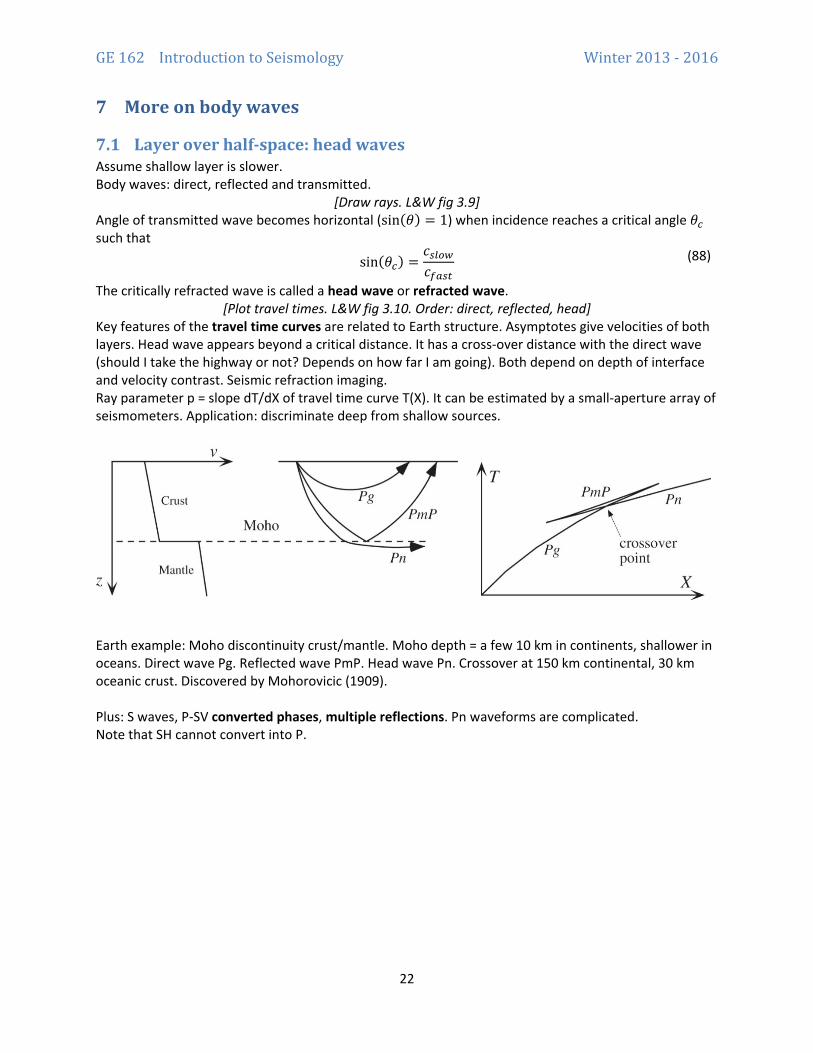
7.1 Layer over half-space: head waves Assume shallow layer is slower. Body waves: direct, reflected and transmitted.
[Draw rays. L&W fig 3.9] Angle of transmitted wave becomes horizontal (sin(𝜃𝜃) = 1) when incidence reaches a critical angle 𝜃𝜃𝑐𝑐 such that
sin(𝜃𝜃𝑐𝑐) =𝑐𝑐𝑠𝑠𝑖𝑖𝑠𝑠𝑠𝑠𝑐𝑐𝑓𝑓𝑓𝑓𝑠𝑠𝑖𝑖
(88)
The critically refracted wave is called a head wave or refracted wave. [Plot travel times. L&W fig 3.10. Order: direct, reflected, head]
Key features of the travel time curves are related to Earth structure. Asymptotes give velocities of both layers. Head wave appears beyond a critical distance. It has a cross-over distance with the direct wave (should I take the highway or not? Depends on how far I am going). Both depend on depth of interface and velocity contrast. Seismic refraction imaging. Ray parameter p = slope dT/dX of travel time curve T(X). It can be estimated by a small-aperture array of seismometers. Application: discriminate deep from shallow sources.
Earth example: Moho discontinuity crust/mantle. Moho depth = a few 10 km in continents, shallower in oceans. Direct wave Pg. Reflected wave PmP. Head wave Pn. Crossover at 150 km continental, 30 km oceanic crust. Discovered by Mohorovicic (1909). Plus: S waves, P-SV converted phases, multiple reflections. Pn waveforms are complicated. Note that SH cannot convert into P.
GE 162 Introduction to Seismology Winter 2013 - 2016
23
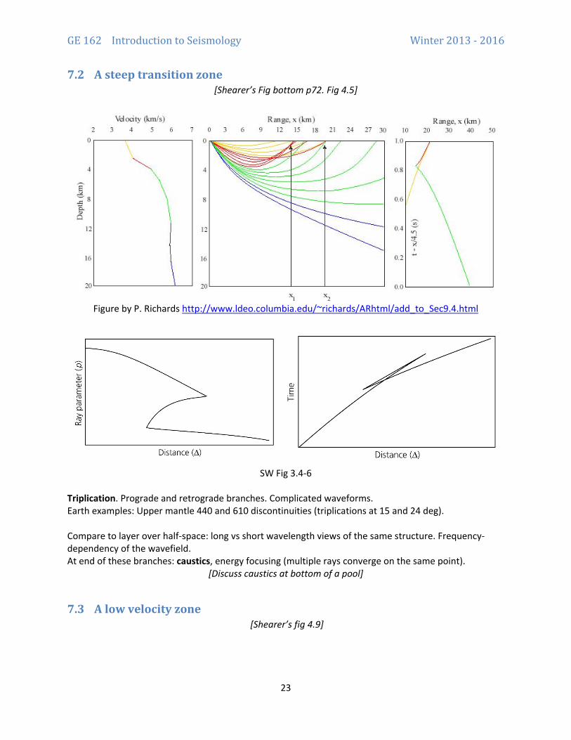
7.2 A steep transition zone [Shearer’s Fig bottom p72. Fig 4.5]
Figure by P. Richards http://www.ldeo.columbia.edu/~richards/ARhtml/add_to_Sec9.4.html
SW Fig 3.4-6
Triplication. Prograde and retrograde branches. Complicated waveforms. Earth examples: Upper mantle 440 and 610 discontinuities (triplications at 15 and 24 deg). Compare to layer over half-space: long vs short wavelength views of the same structure. Frequency-dependency of the wavefield. At end of these branches: caustics, energy focusing (multiple rays converge on the same point).
[Discuss caustics at bottom of a pool]
7.3 A low velocity zone [Shearer’s fig 4.9]

GE 162 Introduction to Seismology Winter 2013 - 2016
24
Fig by P. Richards http://www.ldeo.columbia.edu/~richards/ARhtml/add_to_Sec9.4.html
SW Fig 3.4-7
Shadow zone. Ex: vp drops at the core-mantle boundary then keeps increasing, shadow zone from 103 to 140 deg. Trapped waves (guided waves) if source is inside the LVZ.
[Shearer’s fig 4.10]
Ex: SOFAR (Sound Fixing and Ranging) channel in oceans. T waves. Less than 12 deg from horizontal. Earthquakes may induce them by diffraction at bathymetry.
[Determine the geometrical spreading of a guided wave from energy argument] Guided waves have slow geometrical spreading ∝ 1/√𝑟𝑟. Actually decay a bit faster, 1/𝑟𝑟𝑖𝑖 with 1
2< 𝑛𝑛 <
1, because of energy leakage. Nevertheless, they persist over longer distances than other body waves. Other ex: fault zone guided waves.
GE 162 Introduction to Seismology Winter 2013 - 2016
25
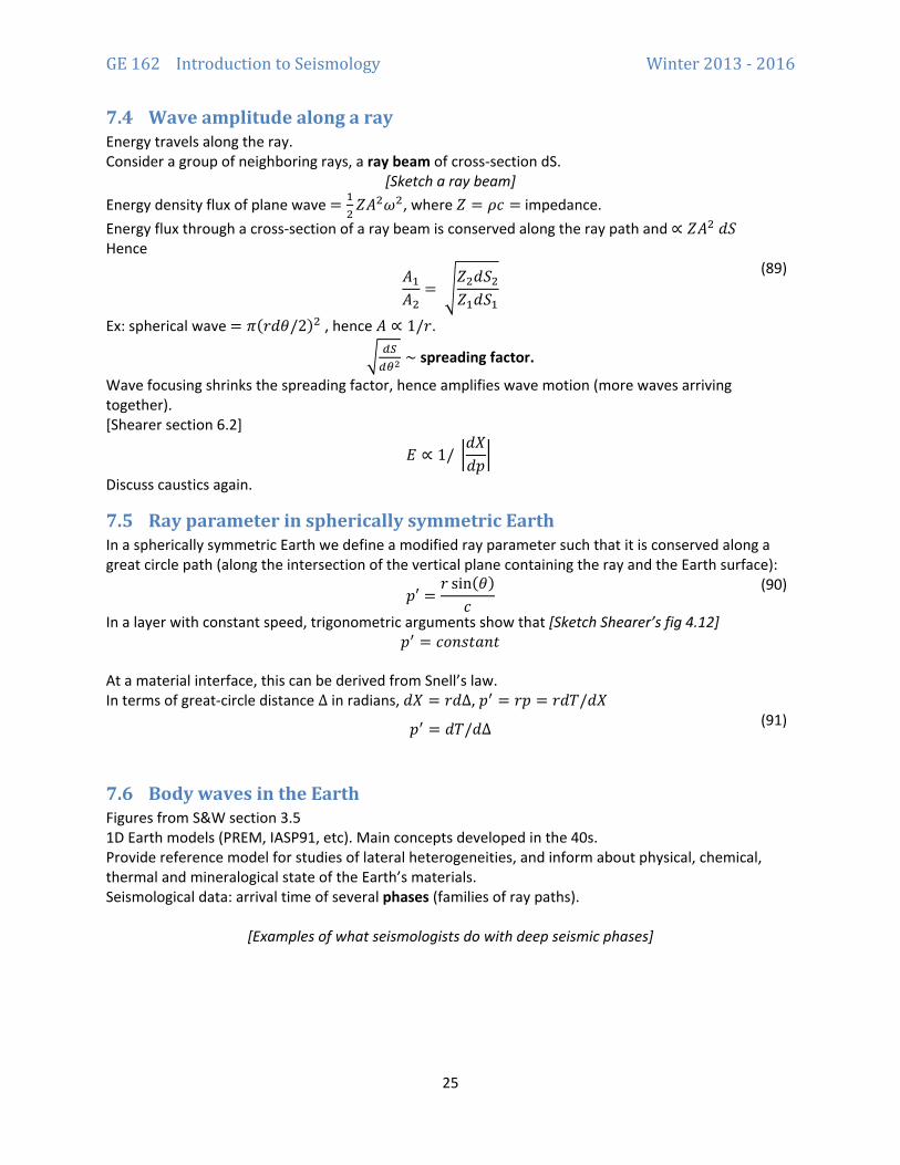
7.4 Wave amplitude along a ray Energy travels along the ray. Consider a group of neighboring rays, a ray beam of cross-section dS.
[Sketch a ray beam] Energy density flux of plane wave = 1
2𝑍𝑍𝐴𝐴2𝜔𝜔2, where 𝑍𝑍 = 𝜌𝜌𝑐𝑐 = impedance.
Energy flux through a cross-section of a ray beam is conserved along the ray path and ∝ 𝑍𝑍𝐴𝐴2 𝑑𝑑𝑆𝑆 Hence
𝐴𝐴1𝐴𝐴2
= �𝑍𝑍2𝑑𝑑𝑆𝑆2𝑍𝑍1𝑑𝑑𝑆𝑆1
(89)
Ex: spherical wave = 𝜋𝜋(𝑟𝑟𝑑𝑑𝜃𝜃/2)2 , hence 𝐴𝐴 ∝ 1/𝑟𝑟.
� 𝑑𝑑𝑆𝑆𝑑𝑑𝜃𝜃2
∼ spreading factor.
Wave focusing shrinks the spreading factor, hence amplifies wave motion (more waves arriving together). [Shearer section 6.2]
𝑆𝑆 ∝ 1/ �𝑑𝑑𝑋𝑋𝑑𝑑𝑝𝑝�
Discuss caustics again.
7.5 Ray parameter in spherically symmetric Earth In a spherically symmetric Earth we define a modified ray parameter such that it is conserved along a great circle path (along the intersection of the vertical plane containing the ray and the Earth surface):
𝑝𝑝′ =
𝑟𝑟 sin(𝜃𝜃)𝑐𝑐
(90)
In a layer with constant speed, trigonometric arguments show that [Sketch Shearer’s fig 4.12] 𝑝𝑝′ = 𝑐𝑐𝑐𝑐𝑛𝑛𝑐𝑐𝑡𝑡𝑚𝑚𝑛𝑛𝑡𝑡
At a material interface, this can be derived from Snell’s law. In terms of great-circle distance Δ in radians, 𝑑𝑑𝑋𝑋 = 𝑟𝑟𝑑𝑑Δ, 𝑝𝑝′ = 𝑟𝑟𝑝𝑝 = 𝑟𝑟𝑑𝑑𝑇𝑇/𝑑𝑑𝑋𝑋
𝑝𝑝′ = 𝑑𝑑𝑇𝑇/𝑑𝑑Δ (91)
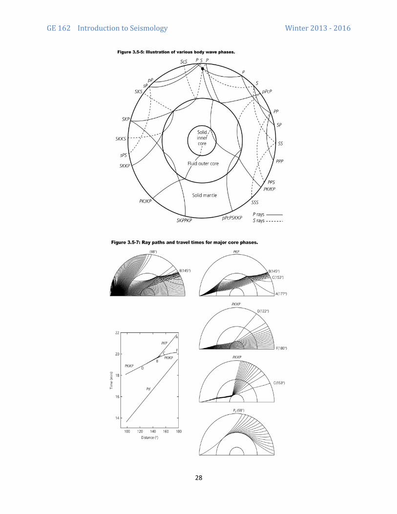
7.6 Body waves in the Earth Figures from S&W section 3.5 1D Earth models (PREM, IASP91, etc). Main concepts developed in the 40s. Provide reference model for studies of lateral heterogeneities, and inform about physical, chemical, thermal and mineralogical state of the Earth’s materials. Seismological data: arrival time of several phases (families of ray paths).
[Examples of what seismologists do with deep seismic phases]

GE 162 Introduction to Seismology Winter 2013 - 2016
26
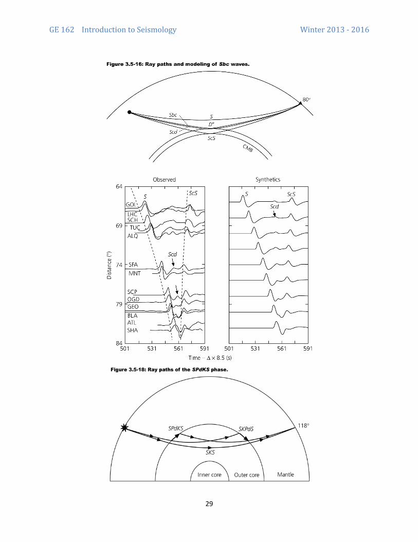
+ D’’ = region with reduced gradient above the CMB (2700-2900 km)

GE 162 Introduction to Seismology Winter 2013 - 2016
27
GE 162 Introduction to Seismology Winter 2013 - 2016
28
GE 162 Introduction to Seismology Winter 2013 - 2016
29

GE 162 Introduction to Seismology Winter 2013 - 2016
30
8 Surface waves I: Love waves
8.1 Separation between SH and P-SV waves
In depth-dependent media rays remain confined in the vertical plane of their take-off vector (see 6.3). SV waves = shear motion within the plane of the ray SH waves = shear motion normal to the plane of the ray In a depth dependent medium SH waves are decoupled from P-SV waves, i.e. the equations governing these two systems of waves are independent.
8.2 SH reflection and transmission coefficients at a material interface
Show that SH displacement field of the form 𝑢𝑢(𝑥𝑥, 𝑧𝑧, 𝑡𝑡)𝒚𝒚� satisfies a scalar wave equation with S-wave speed. Consider two materials in contact along a planar interface, with speeds 𝛽𝛽1 and 𝛽𝛽2, and an incident plane wave arriving to the interface from medium 1. Formulate the problem:
• Write the plane wave displacement field in both materials, composed of incident, reflected and transmitted waves of amplitude 1, R and T, respectively (z points down):
𝑢𝑢1(𝑥𝑥, 𝑧𝑧, 𝑡𝑡) = 𝑒𝑒𝑖𝑖𝑖𝑖(𝑝𝑝𝑑𝑑+𝜂𝜂1𝑧𝑧−𝑖𝑖) + 𝑅𝑅𝑒𝑒𝑖𝑖𝑖𝑖(𝑝𝑝𝑑𝑑−𝜂𝜂1𝑧𝑧−𝑖𝑖) 𝑢𝑢2(𝑥𝑥, 𝑧𝑧, 𝑡𝑡) = 𝑇𝑇 𝑒𝑒𝑖𝑖𝑖𝑖(𝑝𝑝𝑑𝑑−𝜂𝜂2𝑧𝑧−𝑖𝑖)
where 𝑝𝑝 = 𝑖𝑖𝑥𝑥𝑖𝑖
is the ray parameter, 𝜂𝜂1 = 𝑖𝑖𝑧𝑧1
𝑖𝑖= �
1𝛽𝛽12− 𝑝𝑝2 and 𝜂𝜂2 = 𝑖𝑖𝑧𝑧2
𝑖𝑖= �
1𝛽𝛽22− 𝑝𝑝2. If 𝑝𝑝 < 1/𝛽𝛽𝑖𝑖,
the incidence/reflection/transmission angles are well defined (real) and 𝜂𝜂𝑖𝑖 = cos 𝑗𝑗𝑖𝑖. • Write the boundary conditions: continuity of displacement and shear stress at the interface.

GE 162 Introduction to Seismology Winter 2013 - 2016
31
• Obtain a system of two linear equations with two unknowns (R and T). • Solve it (defining impedances 𝑍𝑍1 = 𝜇𝜇1/𝛽𝛽1 and 𝑍𝑍2 = 𝜇𝜇2/𝛽𝛽2):
𝑅𝑅 = 𝑍𝑍1𝜂𝜂1−𝑍𝑍2η2𝑍𝑍1η1+𝑍𝑍2η2
and 𝑇𝑇 = 2 𝑍𝑍1𝜂𝜂1𝑍𝑍1η1+𝑍𝑍2η2
If 𝑝𝑝 < 1/𝛽𝛽𝑖𝑖 we can write it as:
𝑅𝑅 = 𝑍𝑍1 cos 𝑖𝑖1−𝑍𝑍2 cos 𝑖𝑖2𝑍𝑍1 cos 𝑖𝑖1+𝑍𝑍2 cos 𝑖𝑖2
and 𝑇𝑇 = 2 𝑍𝑍1 cos 𝑖𝑖1𝑍𝑍1 cos 𝑖𝑖1+𝑍𝑍2 cos 𝑖𝑖2
If 𝛽𝛽1 < 𝛽𝛽2 there is a critical angle 𝑗𝑗𝑐𝑐 defined by
sin 𝑗𝑗𝑐𝑐 = 𝛽𝛽1/𝛽𝛽2 such that any wave with incidence angle wider than 𝑗𝑗𝑐𝑐 (post-critical) emerges parallel to the interface (𝑗𝑗2 = 𝜋𝜋/2). Post-critical reflections have |𝑅𝑅| = 1 (total reflection) and incur a phase shift. The refracted wave in the post-critical range decays exponentially with distance to the interface: this
kind of wave is called inhomogeneous or evanescent wave: if 𝑝𝑝 > 1𝛽𝛽2
, the quantity 𝜂𝜂2 = �1𝛽𝛽22− 𝑝𝑝2 is
imaginary and the displacement in the bottom half-space is 𝑢𝑢2(𝑥𝑥, 𝑧𝑧, 𝑡𝑡) = 𝑇𝑇 𝑒𝑒𝑖𝑖𝑖𝑖(𝑝𝑝𝑑𝑑−𝑖𝑖)𝑒𝑒−𝑖𝑖 𝐼𝐼𝐼𝐼(𝜂𝜂2)𝑧𝑧 . The exponential decay has a characteristic depth ∝ 1
𝐼𝐼𝐼𝐼(𝜂𝜂2)𝑖𝑖. If 𝑝𝑝 ≫ 1/𝛽𝛽2 the penetration depth is ~ 1
𝑝𝑝𝑖𝑖∝ 𝜆𝜆𝑑𝑑
In the special case of a free surface (𝑍𝑍2 = 0) we get total reflection (𝑅𝑅 = 1) at all incident angles.

GE 162 Introduction to Seismology Winter 2013 - 2016
32
8.3 Love waves Consider a soft layer of thickness h over a half space. Post-critical waves are trapped by total reflection at the surface and at the material interface.
Constructive interference between these trapped waves leads to surface waves known as Love waves, a system of post-critical waves that propagate horizontally and whose amplitude below the soft layer decays exponentially with depth (they are evanescent). The penetration depth of a surface wave is ∼ 𝜆𝜆 (horizontal wavelength).
The amplitude of surface waves decays as 1/√𝜆𝜆𝑟𝑟 where 𝑟𝑟 is horizontal propagation distance. Proof: energy is proportional to wave amplitude squared and is conserved over a ring of surface ∝ 𝜆𝜆𝑟𝑟 (as opposed to a sphere of surface ∝ 𝑟𝑟2 in the case of body waves).
8.4 Dispersion relation The longer wavelengths / lower frequencies penetrate deeper, hence probe faster speeds of the medium: hints that the Love wave speed depends on frequency, a phenomenon called dispersion. Derivation of dispersion relation:
• Write displacement fields as plane waves in each of the two media 𝑢𝑢1(𝑥𝑥, 𝑧𝑧, 𝑡𝑡) = 𝐴𝐴𝑒𝑒𝑖𝑖𝑖𝑖(𝑝𝑝𝑑𝑑+𝜂𝜂1𝑧𝑧−𝑖𝑖) + 𝐵𝐵𝑒𝑒𝑖𝑖𝑖𝑖(𝑝𝑝𝑑𝑑−𝜂𝜂1𝑧𝑧−𝑖𝑖)
𝑢𝑢2(𝑥𝑥, 𝑧𝑧, 𝑡𝑡) = 𝐶𝐶 𝑒𝑒𝑖𝑖𝑖𝑖(𝑝𝑝𝑑𝑑−𝜂𝜂2𝑧𝑧−𝑖𝑖) • Apply boundary conditions (3): zero stress at the surface (at z=0) and continuity of displacement
and shear stress at the interface (at z=h) • Obtain a homogeneous (zero right-hand-side) system of 3 linear equations with 3 unknowns (A,
B and C).

GE 162 Introduction to Seismology Winter 2013 - 2016
33
• A homogeneous system has non-trivial (non-zero) solutions only if its determinant is zero. This condition yields the following equation relating horizontal speed 𝒄𝒄 = 𝟏𝟏/𝒑𝒑 to frequency, known as a dispersion relation:
tan�ℎ𝜔𝜔𝛽𝛽1
�1 − �𝛽𝛽1𝑐𝑐�2
� =𝑍𝑍2𝑍𝑍1
��𝛽𝛽2𝑐𝑐 �2− 1
�1 − �𝛽𝛽1𝑐𝑐 �2
For any frequency 𝜔𝜔, this equation can be solved to get a speed 𝑐𝑐(𝜔𝜔). Because of the trigonometric (periodic) function on the l.h.s., solutions are not always unique; in some frequency ranges we get a set of speeds 𝑐𝑐𝑖𝑖(𝜔𝜔).

GE 162 Introduction to Seismology Winter 2013 - 2016
34
Fundamental mode. (𝑛𝑛 = 0) Penetration depth is shorter at high frequency, probes shallower part of the crust, lower velocity. Two extremes: 𝑐𝑐 ∼ 𝛽𝛽1 at high frequency, 𝑐𝑐 ∼ 𝛽𝛽2 at low frequency. General appearance of Love wave seismogram: different frequencies arrive at different times. Overtones. (𝑛𝑛 > 0) In some frequency ranges the dispersion relation has multiple solutions: the n-th higher modes (overtone) appears at frequencies higher than cutoff frequency
𝜔𝜔𝑖𝑖 =𝑛𝑛𝜋𝜋
ℎ�1𝛽𝛽12
− 1𝛽𝛽22
8.5 Phase and group velocities Consider the superposition of two harmonic waves with slightly different parameters, (𝑘𝑘1,𝜔𝜔1) = (𝑘𝑘0 +𝛿𝛿𝑘𝑘,𝜔𝜔0 + 𝛿𝛿𝜔𝜔) and (𝑘𝑘1,𝜔𝜔1) = (𝑘𝑘0 − 𝛿𝛿𝑘𝑘,𝜔𝜔0 − 𝛿𝛿𝜔𝜔):
cos(𝑘𝑘1𝑥𝑥 − 𝜔𝜔1𝑡𝑡) + cos(𝑘𝑘2𝑥𝑥 − 𝜔𝜔2𝑡𝑡) We can rewrite it as
2 cos(𝑘𝑘0𝑥𝑥 − 𝜔𝜔0𝑡𝑡) cos(𝛿𝛿𝑘𝑘𝑥𝑥 − 𝛿𝛿𝜔𝜔𝑡𝑡) Product of two terms: a fast (high-frequency) carrier modulated by a slow (low frequency) envelope.

GE 162 Introduction to Seismology Winter 2013 - 2016
35
Phase velocity = 𝑐𝑐(𝜔𝜔) = 𝑖𝑖𝑖𝑖𝑥𝑥
= propagation speed of the carrier
Group velocity = 𝑈𝑈(𝜔𝜔) = 𝛿𝛿𝑖𝑖𝛿𝛿𝑖𝑖
= propagation speed of the envelope Compare: in homogeneous media, 𝜔𝜔/𝑘𝑘 = 𝑐𝑐. Phase velocity is constant, does not depend on frequency: no dispersion. Group velocity is also = 𝑐𝑐.
8.6 Airy phase
𝑈𝑈 =𝑑𝑑𝜔𝜔𝑑𝑑𝑘𝑘
=1
𝑑𝑑 �𝜔𝜔𝑐𝑐 �𝑑𝑑𝜔𝜔
=𝑐𝑐
1 −𝜔𝜔𝑐𝑐𝑑𝑑𝑐𝑐𝑑𝑑𝜔𝜔
=𝑐𝑐
1 + 𝑇𝑇𝑐𝑐𝑑𝑑𝑐𝑐𝑑𝑑𝑇𝑇
where 𝑇𝑇 = 2𝜋𝜋𝑖𝑖
= period.
Because 𝑑𝑑𝑐𝑐𝑑𝑑𝑇𝑇
> 0, the group velocity U may have a minimum.
Surface waves with a range of frequencies close to the minimum U have very similar U, hence they arrive close together and add up to create a high amplitude phase known as Airy phase (see example in next lecture).
GE 162 Introduction to Seismology Winter 2013 - 2016
36
9 Surface waves II: Rayleigh waves
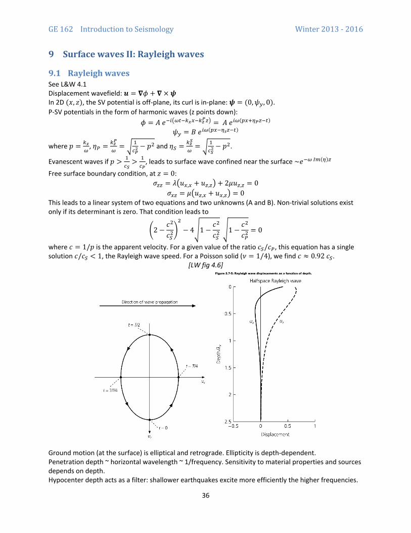
9.1 Rayleigh waves See L&W 4.1 Displacement wavefield: 𝒖𝒖 = 𝛁𝛁𝜙𝜙 + 𝛁𝛁 × 𝝍𝝍 In 2D (𝑥𝑥, 𝑧𝑧), the SV potential is off-plane, its curl is in-plane: 𝝍𝝍 = (0,𝜓𝜓𝑦𝑦, 0). P-SV potentials in the form of harmonic waves (z points down):
𝜙𝜙 = 𝐴𝐴 𝑒𝑒−𝑖𝑖�𝑖𝑖𝑖𝑖−𝑖𝑖𝑥𝑥𝑑𝑑−𝑖𝑖𝑧𝑧𝑃𝑃𝑧𝑧� = 𝐴𝐴 𝑒𝑒𝑖𝑖𝑖𝑖(𝑝𝑝𝑑𝑑+𝜂𝜂𝑃𝑃𝑧𝑧−𝑖𝑖) 𝜓𝜓𝑦𝑦 = 𝐵𝐵 𝑒𝑒𝑖𝑖𝑖𝑖(𝑝𝑝𝑑𝑑−𝜂𝜂𝑠𝑠𝑧𝑧−𝑖𝑖)
where 𝑝𝑝 = 𝑖𝑖𝑥𝑥𝑖𝑖
, 𝜂𝜂𝑃𝑃 = 𝑖𝑖𝑧𝑧𝑃𝑃
𝑖𝑖= �
1𝑐𝑐𝑃𝑃2 − 𝑝𝑝2 and 𝜂𝜂𝑆𝑆 = 𝑖𝑖𝑧𝑧𝑆𝑆
𝑖𝑖= �
1𝑐𝑐𝑆𝑆2 − 𝑝𝑝2.
Evanescent waves if 𝑝𝑝 > 1𝑐𝑐𝑆𝑆
> 1𝑐𝑐𝑃𝑃
, leads to surface wave confined near the surface ~𝑒𝑒−𝑖𝑖 𝐼𝐼𝐼𝐼(𝜂𝜂)𝑧𝑧 Free surface boundary condition, at 𝑧𝑧 = 0:
𝜎𝜎𝑧𝑧𝑧𝑧 = 𝜆𝜆�𝑢𝑢𝑑𝑑,𝑑𝑑 + 𝑢𝑢𝑧𝑧,𝑧𝑧� + 2𝜇𝜇𝑢𝑢𝑧𝑧,𝑧𝑧 = 0 𝜎𝜎𝑑𝑑𝑧𝑧 = 𝜇𝜇�𝑢𝑢𝑧𝑧,𝑑𝑑 + 𝑢𝑢𝑑𝑑,𝑧𝑧� = 0
This leads to a linear system of two equations and two unknowns (A and B). Non-trivial solutions exist only if its determinant is zero. That condition leads to
�2 −𝑐𝑐2
𝑐𝑐𝑆𝑆2�2
− 4�1 −𝑐𝑐2
𝑐𝑐𝑆𝑆2 �1 −
𝑐𝑐2
𝑐𝑐𝑃𝑃2= 0
where 𝑐𝑐 = 1/𝑝𝑝 is the apparent velocity. For a given value of the ratio 𝑐𝑐𝑆𝑆/𝑐𝑐𝑃𝑃, this equation has a single solution 𝑐𝑐/𝑐𝑐𝑆𝑆 < 1, the Rayleigh wave speed. For a Poisson solid (𝜈𝜈 = 1/4), we find 𝑐𝑐 ≈ 0.92 𝑐𝑐𝑆𝑆.
[LW fig 4.6]
Ground motion (at the surface) is elliptical and retrograde. Ellipticity is depth-dependent. Penetration depth ~ horizontal wavelength ~ 1/frequency. Sensitivity to material properties and sources depends on depth. Hypocenter depth acts as a filter: shallower earthquakes excite more efficiently the higher frequencies.
GE 162 Introduction to Seismology Winter 2013 - 2016
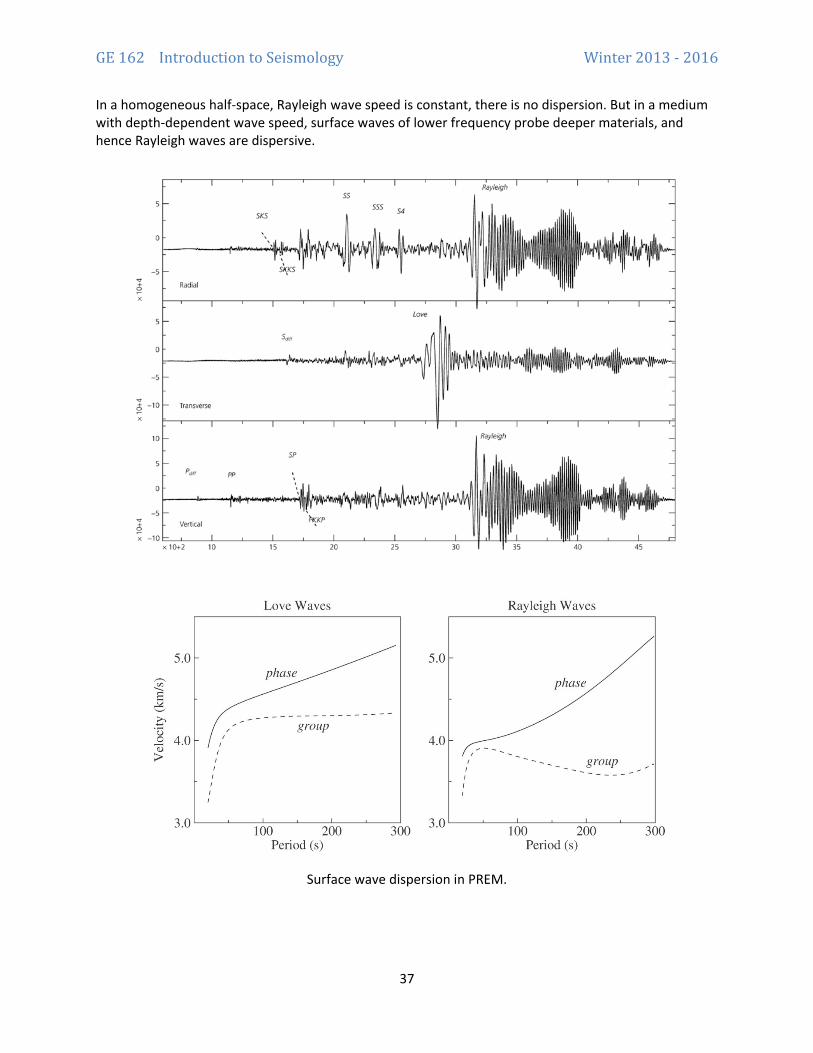
37
In a homogeneous half-space, Rayleigh wave speed is constant, there is no dispersion. But in a medium with depth-dependent wave speed, surface waves of lower frequency probe deeper materials, and hence Rayleigh waves are dispersive.
Surface wave dispersion in PREM.
GE 162 Introduction to Seismology Winter 2013 - 2016
38
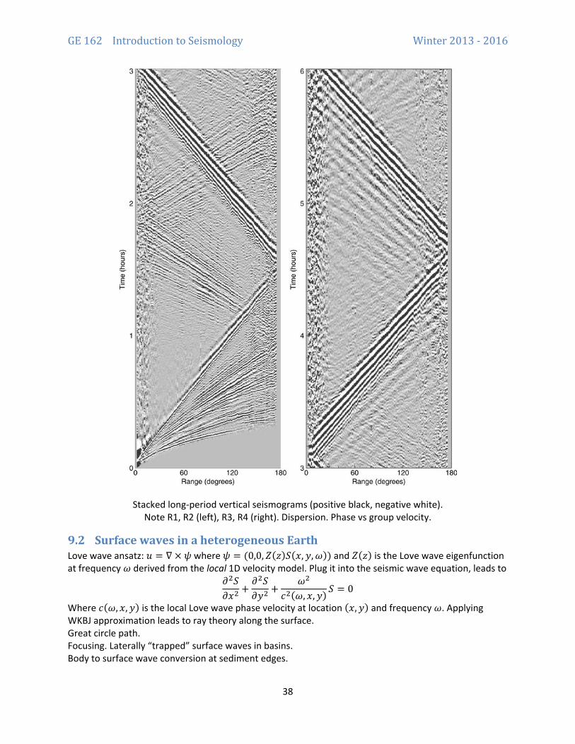
Stacked long-period vertical seismograms (positive black, negative white). Note R1, R2 (left), R3, R4 (right). Dispersion. Phase vs group velocity.
9.2 Surface waves in a heterogeneous Earth Love wave ansatz: 𝑢𝑢 = ∇ × 𝜓𝜓 where 𝜓𝜓 = (0,0,𝑍𝑍(𝑧𝑧)𝑆𝑆(𝑥𝑥,𝑦𝑦,𝜔𝜔)) and 𝑍𝑍(𝑧𝑧) is the Love wave eigenfunction at frequency 𝜔𝜔 derived from the local 1D velocity model. Plug it into the seismic wave equation, leads to
𝜕𝜕2𝑆𝑆𝜕𝜕𝑥𝑥2
+𝜕𝜕2𝑆𝑆𝜕𝜕𝑦𝑦2
+𝜔𝜔2
𝑐𝑐2(𝜔𝜔, 𝑥𝑥,𝑦𝑦) 𝑆𝑆 = 0
Where 𝑐𝑐(𝜔𝜔, 𝑥𝑥,𝑦𝑦) is the local Love wave phase velocity at location (𝑥𝑥,𝑦𝑦) and frequency 𝜔𝜔. Applying WKBJ approximation leads to ray theory along the surface. Great circle path. Focusing. Laterally “trapped” surface waves in basins. Body to surface wave conversion at sediment edges.

GE 162 Introduction to Seismology Winter 2013 - 2016
39
9.3 Implications for tsunami waves
The dispersion at short periods was explained in a homework. The derivation assumed a rigid seafloor. The dispersion at long periods is only observed for mega-earthquakes. It is due to the coupling between wave height - water pressure changes – and elastic deformation of the crust (deformable seafloor). See Tsai et al (2013).
GE 162 Introduction to Seismology Winter 2013 - 2016
40
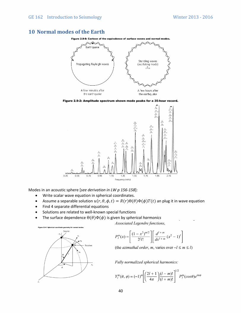
10 Normal modes of the Earth
Modes in an acoustic sphere [see derivation in LW p 156-158]:
• Write scalar wave equation in spherical coordinates. • Assume a separable solution 𝑢𝑢(𝑟𝑟,𝜃𝜃,𝜙𝜙, 𝑡𝑡) = 𝑅𝑅(𝑟𝑟)Θ(𝜃𝜃)Φ(𝜙𝜙)𝑇𝑇(𝑡𝑡) an plug it in wave equation • Find 4 separate differential equations • Solutions are related to well-known special functions • The surface dependence Θ(𝜃𝜃)Φ(𝜙𝜙) is given by spherical harmonics
GE 162 Introduction to Seismology Winter 2013 - 2016
41
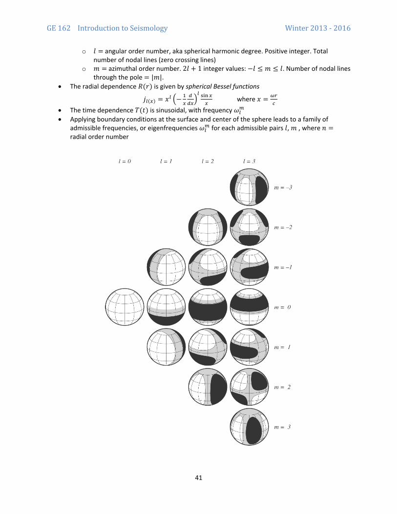
o 𝑙𝑙 = angular order number, aka spherical harmonic degree. Positive integer. Total number of nodal lines (zero crossing lines)
o 𝑚𝑚 = azimuthal order number. 2𝑙𝑙 + 1 integer values: −𝑙𝑙 ≤ 𝑚𝑚 ≤ 𝑙𝑙. Number of nodal lines through the pole = |𝑚𝑚|.
• The radial dependence 𝑅𝑅(𝑟𝑟) is given by spherical Bessel functions
𝑗𝑗𝑖𝑖(𝑑𝑑) = 𝑥𝑥𝑖𝑖 �− 1𝑑𝑑𝑑𝑑𝑑𝑑𝑑𝑑�𝑖𝑖 sin 𝑑𝑑
𝑑𝑑 where 𝑥𝑥 = 𝑖𝑖𝑟𝑟
𝑐𝑐
• The time dependence 𝑇𝑇(𝑡𝑡) is sinusoidal, with frequency 𝜔𝜔𝑖𝑖𝐼𝐼
• Applying boundary conditions at the surface and center of the sphere leads to a family of admissible frequencies, or eigenfrequencies 𝜔𝜔𝑖𝑖
𝐼𝐼 for each admissible pairs 𝑙𝑙, 𝑚𝑚 , where 𝑛𝑛 = radial order number
GE 162 Introduction to Seismology Winter 2013 - 2016
42
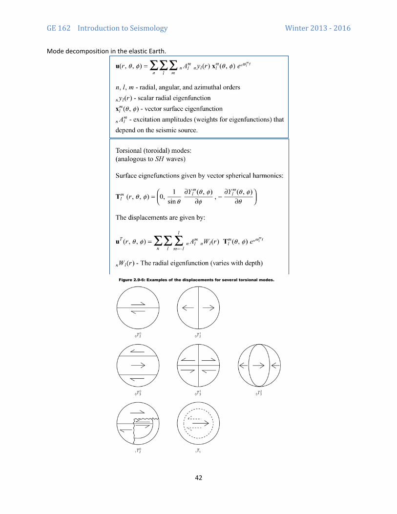
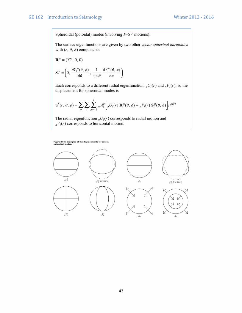
Mode decomposition in the elastic Earth.
GE 162 Introduction to Seismology Winter 2013 - 2016
43
GE 162 Introduction to Seismology Winter 2013 - 2016
44
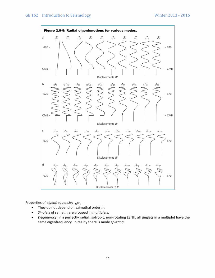
Properties of eigenfrequencies 𝜔𝜔𝑖𝑖𝑖𝑖 :
• They do not depend on azimuthal order 𝑚𝑚 • Singlets of same 𝑚𝑚 are grouped in multiplets. • Degeneracy: in a perfectly radial, isotropic, non-rotating Earth, all singlets in a multiplet have the
same eigenfrequency. In reality there is mode splitting

GE 162 Introduction to Seismology Winter 2013 - 2016
45

GE 162 Introduction to Seismology Winter 2013 - 2016
46
Duality modes – waves:
GE 162 Introduction to Seismology Winter 2013 - 2016
47
11 Attenuation and scattering
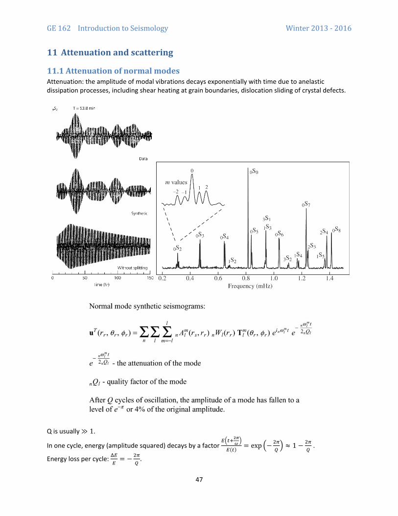
11.1 Attenuation of normal modes Attenuation: the amplitude of modal vibrations decays exponentially with time due to anelastic dissipation processes, including shear heating at grain boundaries, dislocation sliding of crystal defects.
Q is usually ≫ 1.
In one cycle, energy (amplitude squared) decays by a factor 𝐸𝐸�𝑖𝑖+2𝜋𝜋𝜔𝜔 �
𝐸𝐸(𝑖𝑖) = exp �− 2𝜋𝜋𝑄𝑄� ≈ 1 − 2𝜋𝜋
𝑄𝑄 .
Energy loss per cycle: Δ𝐸𝐸𝐸𝐸
= −2𝜋𝜋𝑄𝑄
.

GE 162 Introduction to Seismology Winter 2013 - 2016
48
11.2 A damped oscillator Mass-spring-dashpot system, single degree of freedom, subject to an impulse force:
𝑀𝑀�̈�𝑥 + 𝜂𝜂�̇�𝑥 + 𝐾𝐾𝑥𝑥 = 𝛿𝛿(𝑡𝑡) Displacement:
𝑥𝑥(𝑡𝑡) = 𝐴𝐴 exp(−𝜖𝜖𝜔𝜔0𝑡𝑡) sin (�1 − 𝜖𝜖2𝜔𝜔0𝑡𝑡) where 𝜔𝜔0 = �𝐾𝐾/𝑀𝑀 and 𝜖𝜖 = 𝜂𝜂/𝑀𝑀𝜔𝜔0 Here 𝑄𝑄 = 1/2𝜖𝜖.
In a standard linear solid, Q is not constant but depends on frequency (see LW p 111-112):
11.3 A propagating wave Consider a plane wave, 𝑢𝑢(𝑥𝑥, 𝑡𝑡) = 𝐴𝐴(𝑥𝑥) exp �−𝑖𝑖𝜔𝜔 �𝑡𝑡 − 𝑑𝑑
𝑐𝑐��, in an attenuating medium. In a frame that
tracks the wave front (“riding the wave”), wave amplitude decays with increasing travel time 𝑇𝑇:
𝐴𝐴(𝑇𝑇) = 𝐴𝐴0 exp �−𝜔𝜔𝑇𝑇2𝑄𝑄
�
or, equivalently, with increasing propagation distance 𝑥𝑥 = 𝑐𝑐𝑇𝑇:
𝐴𝐴(𝑥𝑥) = 𝐴𝐴0 exp �−𝜔𝜔𝑥𝑥2𝑐𝑐𝑄𝑄
�
Hence,
𝑢𝑢(𝑥𝑥, 𝑡𝑡) = 𝐴𝐴0exp �−𝜔𝜔𝑥𝑥2𝑐𝑐𝑄𝑄
� exp �−𝑖𝑖𝜔𝜔 �𝑡𝑡 −𝑥𝑥𝑐𝑐�� = 𝐴𝐴0 exp �−𝑖𝑖𝜔𝜔 �𝑡𝑡 −
𝑥𝑥𝑐𝑐′��
where 1𝑐𝑐′
=1𝑐𝑐
+𝑖𝑖
2𝑐𝑐𝑄𝑄
𝑐𝑐′ =𝑐𝑐
1 + 𝑖𝑖2𝑄𝑄
GE 162 Introduction to Seismology Winter 2013 - 2016
48
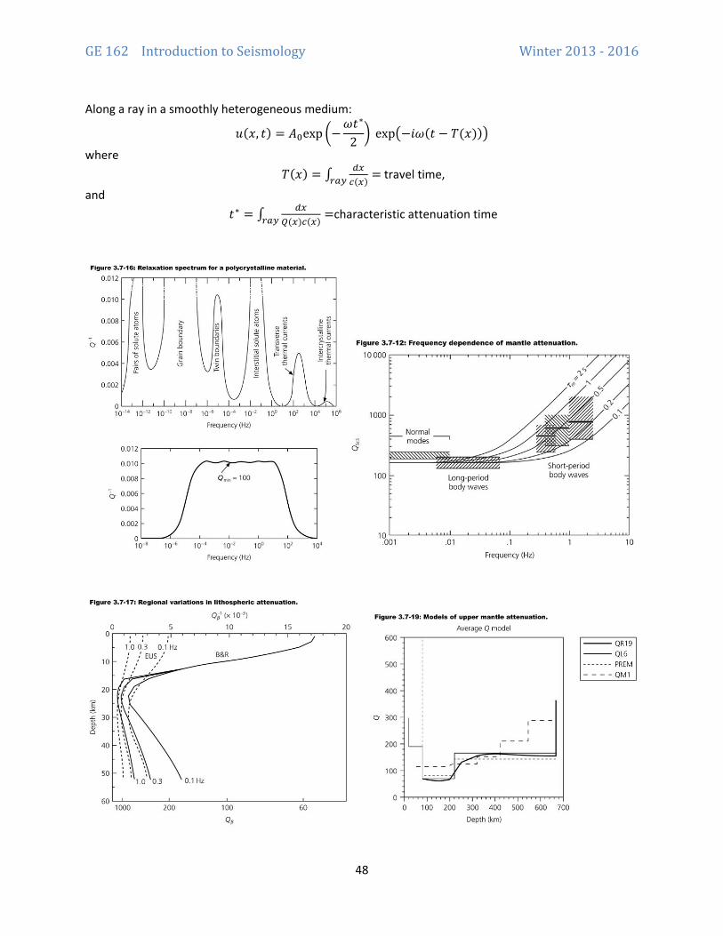
Along a ray in a smoothly heterogeneous medium:
𝑢𝑢(𝑥𝑥, 𝑡𝑡) = 𝐴𝐴0exp �−𝜔𝜔𝑡𝑡∗
2� exp�−𝑖𝑖𝜔𝜔(𝑡𝑡 − 𝑇𝑇(𝑥𝑥))�
where 𝑇𝑇(𝑥𝑥) = ∫ 𝑑𝑑𝑑𝑑
𝑐𝑐(𝑑𝑑)𝑟𝑟𝑓𝑓𝑦𝑦 = travel time,
and 𝑡𝑡∗ = ∫ 𝑑𝑑𝑑𝑑
𝑄𝑄(𝑑𝑑)𝑐𝑐(𝑑𝑑)𝑟𝑟𝑓𝑓𝑦𝑦 =characteristic attenuation time
GE 162 Introduction to Seismology Winter 2013 - 2016
49
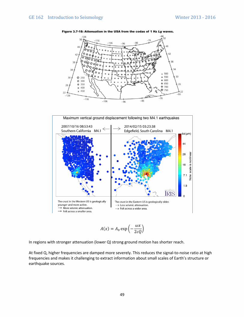
𝐴𝐴(𝑥𝑥) = 𝐴𝐴0 exp �−𝜔𝜔𝑥𝑥2𝑐𝑐𝑄𝑄
�
In regions with stronger attenuation (lower Q) strong ground motion has shorter reach. At fixed Q, higher frequencies are damped more severely. This reduces the signal-to-noise ratio at high frequencies and makes it challenging to extract information about small scales of Earth’s structure or earthquake sources.
GE 162 Introduction to Seismology Winter 2013 - 2016
50
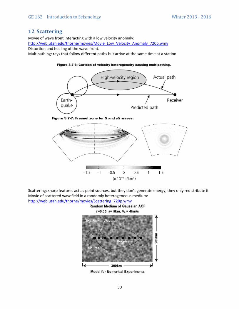
12 Scattering Movie of wave front interacting with a low velocity anomaly: http://web.utah.edu/thorne/movies/Movie_Low_Velocity_Anomaly_720p.wmv Distortion and healing of the wave front. Multipathing: rays that follow different paths but arrive at the same time at a station
Scattering: sharp features act as point sources, but they don’t generate energy, they only redistribute it. Movie of scattered wavefield in a randomly heterogeneous medium: http://web.utah.edu/thorne/movies/Scattering_720p.wmv
GE 162 Introduction to Seismology Winter 2013 - 2016
51
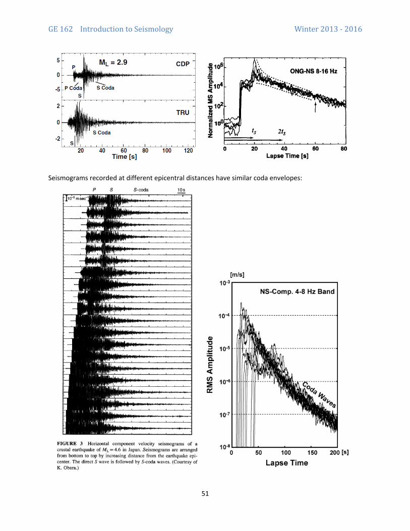
Seismograms recorded at different epicentral distances have similar coda envelopes:

GE 162 Introduction to Seismology Winter 2013 - 2016
52
Observed energy (waveform envelope squared) decays as
𝑆𝑆~ exp �−𝜔𝜔𝑡𝑡𝑄𝑄𝑐𝑐� /𝑡𝑡𝑖𝑖
where 𝑄𝑄𝑐𝑐 = coda attenuation quality factor.

GE 162 Introduction to Seismology Winter 2013 - 2016
53
Single scattering. The ellipsoids in the previous figure are isochrones: surfaces grouping positions of scattering points whose scattered waves reach the station at the same time. Waves from scattering sources in a given isochrone have same arrival time but different amplitude. For an elementary scattering volume containing a collection of scattering points, define 𝑔𝑔0 = scattering coefficient = scattered energy per unit of volume, averaged over all directions. It combines information about the “strength” of each scatterer (size, material contrast, etc) and the density of scatterers. A plane wave leaks out energy by scattering. Its energy decays as exp (−𝑔𝑔0𝑥𝑥). Defining scattering attenuation as 𝑄𝑄𝑠𝑠𝑐𝑐 = 𝜔𝜔/𝑔𝑔0𝑐𝑐, the energy decay is ∼ exp (−𝜔𝜔𝑥𝑥/𝑐𝑐𝑄𝑄𝑠𝑠𝑐𝑐). If A=source, B=scattering point and C=station, the energy scattered by point B is:
𝑆𝑆 ∝ 𝑆𝑆01𝑟𝑟𝐴𝐴𝐴𝐴2
𝑔𝑔01𝑟𝑟𝐴𝐴𝐵𝐵2
The total contribution integrated over one isochrone is
𝑆𝑆 ∝ 𝑆𝑆0 �1𝑟𝑟𝐴𝐴𝐴𝐴2
𝑔𝑔01𝑟𝑟𝐴𝐴𝐵𝐵2
𝑑𝑑𝑙𝑙𝑖𝑖𝑠𝑠𝑠𝑠𝑐𝑐ℎ𝑟𝑟𝑠𝑠𝑖𝑖𝑖𝑖(𝑖𝑖)
The amplitude of coherent waves adds up. The amplitude squared (energy) of incoherent waves add up. Travel time 𝑡𝑡 = (𝑟𝑟𝐴𝐴𝐴𝐴 + 𝑟𝑟𝐴𝐴𝐵𝐵)/𝑐𝑐. It can be shown that sufficiently long after the first arrival, when 𝑡𝑡 ≫ 𝑟𝑟/𝑐𝑐,
𝑆𝑆 ∝𝑆𝑆0𝑡𝑡2
Long after the passage of the main wave front, the scattered energy is independent on distance to the source A. In practice, a phenomenological attenuation factor (“coda Q”) needs to be included, representing energy loss of the main wave front due to scattering and intrinsic attenuation:
𝑆𝑆 ∝𝑆𝑆0𝑡𝑡2
exp−𝜔𝜔𝑡𝑡𝑄𝑄𝑐𝑐
where 1𝑄𝑄𝑐𝑐
= 1𝑄𝑄𝑖𝑖
+ 1𝑄𝑄𝑠𝑠
.
Multiple scattering.
GE 162 Introduction to Seismology Winter 2013 - 2016
54
At longer times, multiple scattering dominates over single scattering. A strong scattering process can be described by diffusion with diffusivity 𝜅𝜅 = 𝑐𝑐/3𝑔𝑔0. The total energy in the medium is given by the classical solution of the 3D diffusion equation:
𝑆𝑆𝑖𝑖𝑠𝑠𝑖𝑖~𝑆𝑆0
(4𝜋𝜋𝜅𝜅 𝑡𝑡)3/2 exp �−𝑟𝑟2
4𝜅𝜅𝑡𝑡�
An alternative approximation: energy uniformly distributed behind the direct wave front. Energy gets redistributed by scattering. The direct phase (first-arrival) loses energy to scattering, its energy decays with travel time as exp (−𝜔𝜔 𝑡𝑡/𝑄𝑄𝑠𝑠𝑐𝑐). Energy partitioning between direct and scattered field, and overall conservation:
𝑆𝑆𝑖𝑖𝑠𝑠𝑖𝑖~E0 exp �−𝜔𝜔𝑡𝑡𝑄𝑄𝑠𝑠𝑐𝑐
� +4𝜋𝜋3
(𝑐𝑐𝑡𝑡)3𝑆𝑆𝑠𝑠𝑐𝑐 = 𝑆𝑆0
Leads to
𝑆𝑆𝑠𝑠𝑐𝑐~3𝑆𝑆04𝜋𝜋
1 − 𝑒𝑒−
𝑖𝑖𝑖𝑖𝑄𝑄𝑠𝑠𝑐𝑐
(𝑐𝑐𝑡𝑡)3
In practice, both equations need to be corrected by an intrinsic attenuation factor exp (−𝜔𝜔 𝑡𝑡/𝑄𝑄𝑖𝑖) Applications Interferometry. Ex: in optical fiber. In the crust.
GE 162 Introduction to Seismology Winter 2013 - 2016
55
13 Seismic sources.
13.1 Kinematic vs dynamic description of earthquake sources Standard earthquake model: sudden slip along a pre-existing fault surface Slip = displacement discontinuity (offset) across the fault Faults: nature vs models. Slip on thin fault vs inelastic deformation inside a thick fault zone. Kinematic source model = describes what happened on the fault: space-time distribution of slip velocity Dynamic source model = describes why it happened: forces governing unstable slip (e.g. fault friction) The next few lectures will deal with kinematic sources.
13.2 Stress glut and equivalent body force See Dahlen & Tromp section 5.2 Reminder: seismic wave equation (momentum equation & constitutive “law” – elasticity)
𝜌𝜌�̈�𝑢 = ∇ ⋅ 𝜎𝜎 + 𝑓𝑓 𝜎𝜎 = 𝑐𝑐: 𝜀𝜀
where the source 𝑓𝑓 is a density of body forces (distributed in the volume). The deformation in the earthquake source region is inelastic, a departure from our usual model of elastic media. Our goal here is to derive an equivalent body-force representation of an earthquake source, so that we can still use the elastic seismic wave equation to evaluate ground motions. Momentum equation:
𝜌𝜌�̈�𝑢 = ∇ ⋅ 𝜎𝜎𝑖𝑖𝑟𝑟𝑡𝑡𝑖𝑖 = ∇ ⋅ 𝜎𝜎𝐼𝐼𝑠𝑠𝑑𝑑𝑖𝑖𝑖𝑖 + ∇ ⋅ �𝜎𝜎𝑖𝑖𝑟𝑟𝑡𝑡𝑖𝑖 − 𝜎𝜎𝐼𝐼𝑠𝑠𝑑𝑑𝑖𝑖𝑖𝑖� = ∇ ⋅ 𝜎𝜎𝐼𝐼𝑠𝑠𝑑𝑑𝑖𝑖𝑖𝑖 − ∇ ⋅ 𝜎𝜎∗
where 𝜎𝜎𝐼𝐼𝑠𝑠𝑑𝑑𝑖𝑖𝑖𝑖 is the stress given by the idealized Hooke’s law, and the mismatch between model and true stress is called stress glut:
𝜎𝜎∗ = 𝜎𝜎𝐼𝐼𝑠𝑠𝑑𝑑𝑖𝑖𝑖𝑖 − 𝜎𝜎𝑖𝑖𝑟𝑟𝑡𝑡𝑖𝑖 We define a density of body forces as
𝑓𝑓 = −∇ ⋅ 𝜎𝜎∗ Then
𝜌𝜌�̈�𝑢 = ∇ ⋅ 𝜎𝜎𝐼𝐼𝑠𝑠𝑑𝑑𝑖𝑖𝑖𝑖 + 𝑓𝑓 Example: plastic deformation. As an example of departure from Hooke’s law, consider an elasto-plastic material. Strain is partitioned into elastic and plastic components, 𝜀𝜀 = 𝜀𝜀𝑖𝑖𝑖𝑖𝑓𝑓𝑠𝑠𝑖𝑖𝑖𝑖𝑐𝑐 + 𝜀𝜀𝑝𝑝𝑖𝑖𝑓𝑓𝑠𝑠𝑖𝑖𝑖𝑖𝑐𝑐, the true stress is related by Hooke’s law to the elastic strain, 𝜎𝜎𝑖𝑖𝑟𝑟𝑡𝑡𝑖𝑖 = 𝑐𝑐: 𝜀𝜀𝑖𝑖𝑖𝑖𝑓𝑓𝑠𝑠𝑖𝑖𝑖𝑖𝑐𝑐, and the model stress is what you get by trying to apply Hooke’s law to the total strain instead, 𝜎𝜎𝐼𝐼𝑠𝑠𝑑𝑑𝑖𝑖𝑖𝑖 = 𝑐𝑐: 𝜀𝜀. Then,
𝜎𝜎∗ = 𝑐𝑐: 𝜀𝜀𝑝𝑝𝑖𝑖𝑓𝑓𝑠𝑠𝑖𝑖𝑖𝑖𝑐𝑐 Plastic deformation is a source of seismic waves. For an isotropic elastic medium:
𝜎𝜎𝑖𝑖𝑖𝑖∗ = 𝜆𝜆𝜀𝜀𝑖𝑖𝑖𝑖𝑝𝑝𝑖𝑖𝑓𝑓𝑠𝑠𝑖𝑖𝑖𝑖𝑐𝑐𝛿𝛿𝑖𝑖𝑖𝑖 + 2𝜇𝜇𝜀𝜀𝑖𝑖𝑖𝑖
𝑝𝑝𝑖𝑖𝑓𝑓𝑠𝑠𝑖𝑖𝑖𝑖𝑐𝑐 Example: explosion source, 𝜀𝜀𝑖𝑖𝑖𝑖
𝑝𝑝𝑖𝑖𝑓𝑓𝑠𝑠𝑖𝑖𝑖𝑖𝑐𝑐 = 13Δ𝑉𝑉𝑉𝑉𝛿𝛿𝑖𝑖𝑖𝑖 and we get an isotropic stress glut:
𝜎𝜎𝑖𝑖𝑖𝑖∗ = �𝜆𝜆 + 23𝜇𝜇� Δ𝑉𝑉
𝑉𝑉𝛿𝛿𝑖𝑖𝑖𝑖.
13.3 Equivalent body force representation of fault slip Consider a vertical strike-slip fault. The trace of the fault at the surface is parallel to 𝒙𝒙� (perpendicular to 𝒚𝒚�). Slip D is defined as the displacement offset across the fault. Slip is horizontal, parallel to 𝒙𝒙�, i.e. near the fault the inelastic displacement is: 𝒖𝒖 ∼ 𝐷𝐷𝐻𝐻(𝑦𝑦) 𝒙𝒙�.
GE 162 Introduction to Seismology Winter 2013 - 2016
56
The gradient tensor of the inelastic displacement, (𝛁𝛁𝒖𝒖)𝑖𝑖𝑖𝑖 = 𝜕𝜕𝑢𝑢𝑖𝑖/𝜕𝜕𝑥𝑥𝑖𝑖, has only one non-zero component: 𝜕𝜕𝑡𝑡𝑥𝑥𝜕𝜕𝑦𝑦
= 𝐷𝐷𝛿𝛿(𝑦𝑦). The only non-zero components of the inelastic strain tensor, 𝜀𝜀 = 12
(𝛁𝛁𝒖𝒖 + 𝛁𝛁𝒖𝒖𝑻𝑻), are:
𝜀𝜀𝑑𝑑𝑦𝑦 = 𝜀𝜀𝑦𝑦𝑑𝑑 = 12𝜕𝜕𝑡𝑡𝑥𝑥𝜕𝜕𝑦𝑦
= 12
𝐷𝐷𝛿𝛿(𝑦𝑦).
The only non-zero components of the associated stress glut tensor are: 𝜎𝜎𝑑𝑑𝑦𝑦∗ = 𝜎𝜎𝑦𝑦𝑑𝑑∗ = 𝜇𝜇𝐷𝐷𝛿𝛿(𝑦𝑦). If the source is localized at a point (very small fault): 𝜎𝜎𝑑𝑑𝑦𝑦∗ = 𝜎𝜎𝑦𝑦𝑑𝑑∗ = 𝜇𝜇𝐷𝐷𝛿𝛿(𝑦𝑦)𝛿𝛿(𝑥𝑥)𝛿𝛿(𝑧𝑧) = 𝜇𝜇𝐷𝐷𝛿𝛿(𝒙𝒙). Equivalent body force:
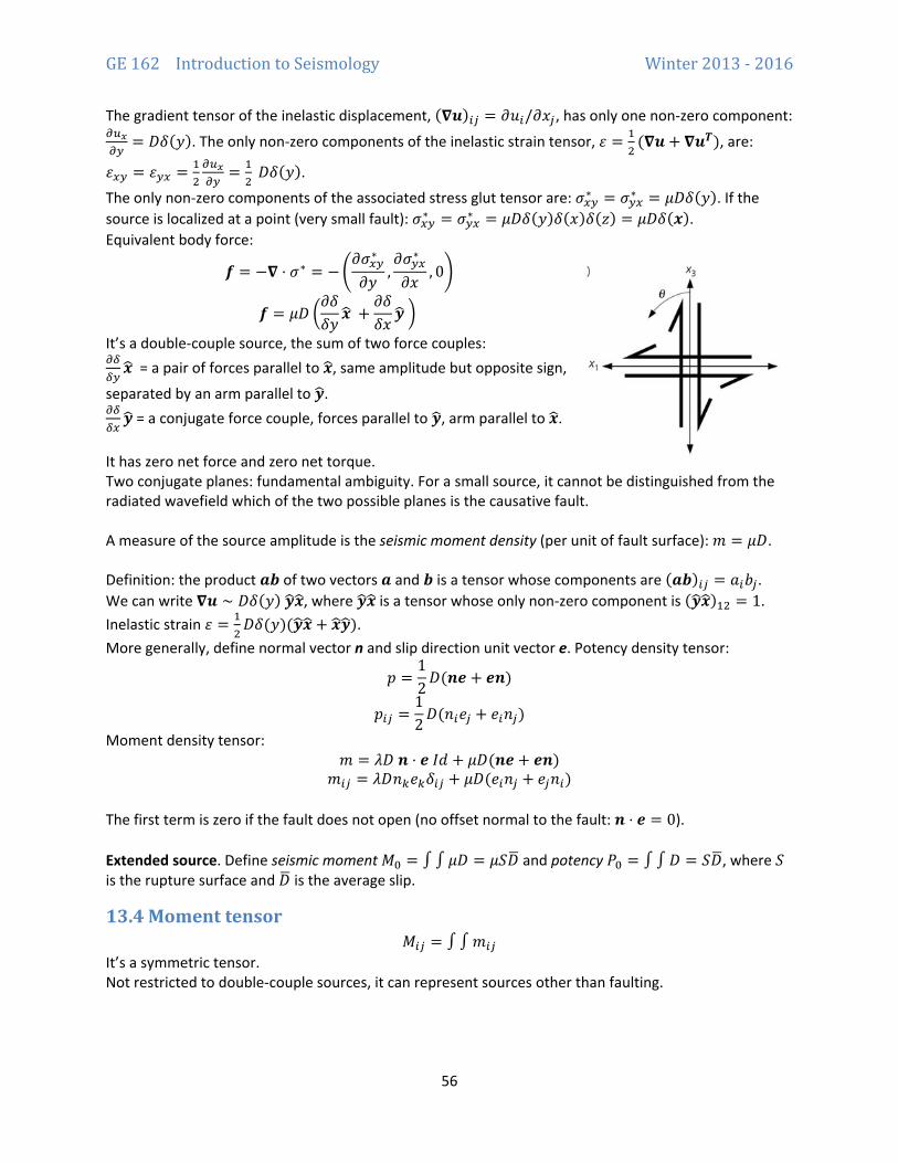
𝒇𝒇 = −𝛁𝛁 ⋅ 𝜎𝜎∗ = −�𝜕𝜕𝜎𝜎𝑑𝑑𝑦𝑦∗
𝜕𝜕𝑦𝑦,𝜕𝜕𝜎𝜎𝑦𝑦𝑑𝑑∗
𝜕𝜕𝑥𝑥, 0�
𝒇𝒇 = 𝜇𝜇𝐷𝐷 �𝜕𝜕𝛿𝛿𝛿𝛿𝑦𝑦
𝒙𝒙� +𝜕𝜕𝛿𝛿𝛿𝛿𝑥𝑥
𝒚𝒚� �
It’s a double-couple source, the sum of two force couples: 𝜕𝜕𝛿𝛿𝛿𝛿𝑦𝑦𝒙𝒙� = a pair of forces parallel to 𝒙𝒙�, same amplitude but opposite sign,
separated by an arm parallel to 𝒚𝒚�. 𝜕𝜕𝛿𝛿𝛿𝛿𝑑𝑑𝒚𝒚� = a conjugate force couple, forces parallel to 𝒚𝒚�, arm parallel to 𝒙𝒙�.
It has zero net force and zero net torque. Two conjugate planes: fundamental ambiguity. For a small source, it cannot be distinguished from the radiated wavefield which of the two possible planes is the causative fault. A measure of the source amplitude is the seismic moment density (per unit of fault surface): 𝑚𝑚 = 𝜇𝜇𝐷𝐷. Definition: the product 𝒂𝒂𝒂𝒂 of two vectors 𝒂𝒂 and 𝒂𝒂 is a tensor whose components are (𝒂𝒂𝒂𝒂)𝑖𝑖𝑖𝑖 = 𝑚𝑚𝑖𝑖𝑏𝑏𝑖𝑖. We can write 𝛁𝛁𝒖𝒖 ∼ 𝐷𝐷𝛿𝛿(𝑦𝑦) 𝒚𝒚�𝒙𝒙�, where 𝒚𝒚�𝒙𝒙� is a tensor whose only non-zero component is (𝒚𝒚�𝒙𝒙�)12 = 1. Inelastic strain 𝜀𝜀 = 1
2𝐷𝐷𝛿𝛿(𝑦𝑦)(𝒚𝒚�𝒙𝒙� + 𝒙𝒙�𝒚𝒚�).
More generally, define normal vector n and slip direction unit vector e. Potency density tensor:
𝑝𝑝 =12𝐷𝐷(𝒏𝒏𝒏𝒏 + 𝒏𝒏𝒏𝒏)
𝑝𝑝𝑖𝑖𝑖𝑖 =12𝐷𝐷(𝑛𝑛𝑖𝑖𝑒𝑒𝑖𝑖 + 𝑒𝑒𝑖𝑖𝑛𝑛𝑖𝑖)
Moment density tensor: 𝑚𝑚 = 𝜆𝜆𝐷𝐷 𝒏𝒏 ⋅ 𝒏𝒏 𝐼𝐼𝑑𝑑 + 𝜇𝜇𝐷𝐷(𝒏𝒏𝒏𝒏 + 𝒏𝒏𝒏𝒏)
𝑚𝑚𝑖𝑖𝑖𝑖 = 𝜆𝜆𝐷𝐷𝑛𝑛𝑖𝑖𝑒𝑒𝑖𝑖𝛿𝛿𝑖𝑖𝑖𝑖 + 𝜇𝜇𝐷𝐷(𝑒𝑒𝑖𝑖𝑛𝑛𝑖𝑖 + 𝑒𝑒𝑖𝑖𝑛𝑛𝑖𝑖) The first term is zero if the fault does not open (no offset normal to the fault: 𝒏𝒏 ⋅ 𝒏𝒏 = 0). Extended source. Define seismic moment 𝑀𝑀0 = ∫ ∫ 𝜇𝜇𝐷𝐷 = 𝜇𝜇𝑆𝑆𝐷𝐷� and potency 𝑃𝑃0 = ∫ ∫ 𝐷𝐷 = 𝑆𝑆𝐷𝐷�, where 𝑆𝑆 is the rupture surface and 𝐷𝐷� is the average slip.
13.4 Moment tensor 𝑀𝑀𝑖𝑖𝑖𝑖 = ∫ ∫𝑚𝑚𝑖𝑖𝑖𝑖
It’s a symmetric tensor. Not restricted to double-couple sources, it can represent sources other than faulting.
GE 162 Introduction to Seismology Winter 2013 - 2016
57
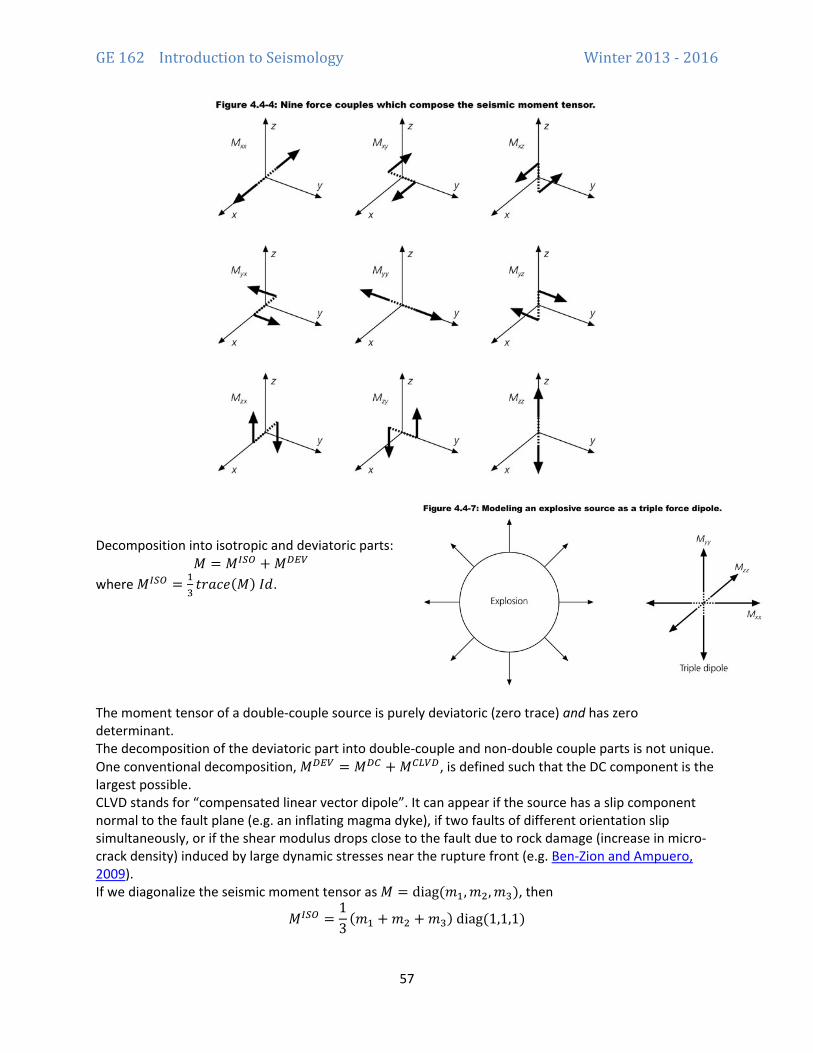
Decomposition into isotropic and deviatoric parts:
𝑀𝑀 = 𝑀𝑀𝐼𝐼𝑆𝑆𝐼𝐼 + 𝑀𝑀𝐷𝐷𝐸𝐸𝑉𝑉 where 𝑀𝑀𝐼𝐼𝑆𝑆𝐼𝐼 = 1
3𝑡𝑡𝑟𝑟𝑚𝑚𝑐𝑐𝑒𝑒(𝑀𝑀) 𝐼𝐼𝑑𝑑.
The moment tensor of a double-couple source is purely deviatoric (zero trace) and has zero determinant. The decomposition of the deviatoric part into double-couple and non-double couple parts is not unique. One conventional decomposition, 𝑀𝑀𝐷𝐷𝐸𝐸𝑉𝑉 = 𝑀𝑀𝐷𝐷𝐵𝐵 + 𝑀𝑀𝐵𝐵𝐶𝐶𝑉𝑉𝐷𝐷, is defined such that the DC component is the largest possible. CLVD stands for “compensated linear vector dipole”. It can appear if the source has a slip component normal to the fault plane (e.g. an inflating magma dyke), if two faults of different orientation slip simultaneously, or if the shear modulus drops close to the fault due to rock damage (increase in micro-crack density) induced by large dynamic stresses near the rupture front (e.g. Ben-Zion and Ampuero, 2009). If we diagonalize the seismic moment tensor as 𝑀𝑀 = diag(𝑚𝑚1,𝑚𝑚2,𝑚𝑚3), then
𝑀𝑀𝐼𝐼𝑆𝑆𝐼𝐼 =13
(𝑚𝑚1 + 𝑚𝑚2 + 𝑚𝑚3) diag(1,1,1)

GE 162 Introduction to Seismology Winter 2013 - 2016
58
𝑀𝑀𝐷𝐷𝐵𝐵 =12
(𝑚𝑚1 −𝑚𝑚3) diag(1,0,−1)
𝑀𝑀𝐵𝐵𝐶𝐶𝑉𝑉𝐷𝐷 = �𝑚𝑚2 −13
(𝑚𝑚1 + 𝑚𝑚2 + 𝑚𝑚3)� diag �−12
, 1,−12�
13.5 Seismic moment and moment magnitude Seismic moment is a scalar that quantifies the “amplitude” of a moment tensor (its norm, in N.m):
𝑀𝑀0 =1√2
�𝑀𝑀𝑖𝑖𝑖𝑖2 �
12
Moment magnitude is a logarithmic scale related to the seismic moment:
𝑀𝑀𝑠𝑠 =23
log10(𝑀𝑀0) − 6
13.6 Representation theorem Green’s function 𝐺𝐺𝑖𝑖𝑝𝑝(𝒙𝒙, 𝑡𝑡; 𝝃𝝃) is the n-th component of displacement at location 𝒙𝒙 and time t induced by a point force at location 𝝃𝝃 set at 𝑡𝑡 = 0 in the p-th direction, i.e. 𝒇𝒇 = 𝛿𝛿(𝑡𝑡)𝛿𝛿(𝒙𝒙 − 𝝃𝝃)𝒙𝒙�𝒑𝒑 Displacement induced by a point-force with arbitrary orientation and source time function 𝒇𝒇(𝑡𝑡):
𝑢𝑢𝑖𝑖(𝒙𝒙, 𝑡𝑡) = 𝐺𝐺𝑖𝑖𝑝𝑝 ∗ 𝑓𝑓𝑝𝑝 Displacement induced by an extended distribution of point-forces 𝒇𝒇(𝝃𝝃, 𝑡𝑡):
𝑢𝑢𝑖𝑖(𝒙𝒙, 𝑡𝑡) = �𝐺𝐺𝑖𝑖𝑝𝑝(𝒙𝒙, 𝑡𝑡; 𝝃𝝃) ∗ 𝑓𝑓𝑝𝑝(𝝃𝝃, 𝑡𝑡)𝑑𝑑3𝜉𝜉
For a moment tensor source, 𝑓𝑓𝑝𝑝 = −𝑚𝑚𝑝𝑝𝑖𝑖,𝑖𝑖 and
𝑢𝑢𝑖𝑖(𝒙𝒙, 𝑡𝑡) = −�𝐺𝐺𝑖𝑖𝑝𝑝 ∗ 𝑚𝑚𝑝𝑝𝑖𝑖,𝑖𝑖𝑑𝑑3𝜉𝜉
Integrating by parts:
𝑢𝑢𝑖𝑖(𝒙𝒙, 𝑡𝑡) = �𝐺𝐺𝑖𝑖𝑝𝑝 ∗ 𝑚𝑚𝑝𝑝𝑖𝑖𝑛𝑛𝑖𝑖𝑑𝑑2𝜉𝜉 + �𝐺𝐺𝑖𝑖𝑝𝑝,𝑖𝑖 ∗ 𝑚𝑚𝑝𝑝𝑖𝑖𝑑𝑑3𝜉𝜉
The surface integral (first term on r.h.s.) vanishes if the integration surface is taken sufficiently far from the source region, where 𝑚𝑚𝑝𝑝𝑖𝑖 vanishes. We obtain the representation theorem, a relation between wave field and moment tensor source:
𝑢𝑢𝑖𝑖(𝒙𝒙, 𝑡𝑡) = �𝐺𝐺𝑖𝑖𝑝𝑝,𝑖𝑖 ∗ 𝑚𝑚𝑝𝑝𝑖𝑖𝑑𝑑3𝜉𝜉
Practical significance: if we know the Green’s function, we can compute the whole wave field induced by an arbitrary moment tensor source by convolution with the gradients of the Green’s function, 𝐺𝐺𝑖𝑖𝑝𝑝,𝑖𝑖(𝒙𝒙, 𝑡𝑡; 𝝃𝝃).
GE 162 Introduction to Seismology Winter 2013 - 2016
59
14 Seismic sources: moment tensor
14.1 Green’s function Sketch of derivation: Lamé potentials of the wave field: = ∇ϕ + ∇ × 𝜓𝜓 , with ∇ ⋅ 𝜓𝜓 = 0. Decompose a point-force source 𝒇𝒇 in Helmholtz potentials: 𝒇𝒇 = ∇Φ + ∇ × Ψ with ∇ ⋅ Ψ = 0. The potentials satisfy wave equations with source terms:
�̈�𝜙 = 𝑐𝑐𝑃𝑃2∇2𝜙𝜙 + Φ/𝜌𝜌 and �̈�𝜓 = 𝑐𝑐𝑆𝑆2∇2𝜓𝜓 + Ψ/𝜌𝜌 The solutions are
𝜙𝜙(𝒙𝒙, 𝑡𝑡) = 14𝜋𝜋𝑐𝑐𝑃𝑃
2∭Φ�𝜉𝜉,𝑖𝑖− 𝑟𝑟
𝑐𝑐𝑃𝑃�
𝑟𝑟𝑑𝑑3𝜉𝜉 and 𝜓𝜓(𝒙𝒙, 𝑡𝑡) = 1
4𝜋𝜋𝑐𝑐𝑆𝑆2∭
Ψ�𝜉𝜉,𝑖𝑖− 𝑟𝑟𝑐𝑐𝑆𝑆�
𝑟𝑟𝑑𝑑3𝜉𝜉
For any vector field 𝑾𝑾 we have ∇2𝑊𝑊 = ∇(∇ ⋅ 𝑊𝑊) − ∇ × (∇ × 𝑊𝑊). Hence we can derive the force potentials from a single vector potential 𝑊𝑊 that satisfies Poisson’s equation, ∇2𝑾𝑾 = 𝒇𝒇, if Φ = ∇ ⋅ W and Ψ = −∇ × W. The solution of Poisson’s equation is 𝑊𝑊 = − 1
4𝜋𝜋∭𝑓𝑓𝑟𝑟𝑑𝑑3𝜉𝜉. For a point source: 𝑾𝑾 = −𝒇𝒇(𝑖𝑖)
4𝜋𝜋𝑟𝑟.
Knowing 𝑾𝑾, we can now evaluate Φ and Ψ, then 𝜙𝜙 and 𝜓𝜓, and finally 𝑢𝑢 (the Green’s function). For a force with source time function 𝑭𝑭(𝑡𝑡):
𝑢𝑢𝑖𝑖(𝒙𝒙, 𝑡𝑡) = 14𝜋𝜋𝜋𝜋
�3𝛾𝛾𝑖𝑖𝛾𝛾𝑖𝑖 − 𝛿𝛿𝑖𝑖𝑖𝑖�1𝑟𝑟3
∫ 𝜏𝜏𝐹𝐹𝑖𝑖(𝑡𝑡 − 𝜏𝜏)𝑑𝑑𝜏𝜏𝑟𝑟/𝑐𝑐_𝑆𝑆 𝑟𝑟/𝑐𝑐_𝑃𝑃 (near field)
+ 14𝜋𝜋𝜋𝜋𝑐𝑐𝑃𝑃
2 𝛾𝛾𝑖𝑖𝛾𝛾𝑖𝑖1𝑟𝑟
𝐹𝐹𝑖𝑖 �𝑡𝑡 −𝑟𝑟𝑐𝑐𝑃𝑃� (far-field P wave)
+ 14𝜋𝜋𝜋𝜋𝑐𝑐𝑆𝑆
2 �𝛾𝛾𝑖𝑖𝛾𝛾𝑖𝑖 − 𝛿𝛿𝑖𝑖𝑖𝑖�1𝑟𝑟
𝐹𝐹𝑖𝑖 �𝑡𝑡 −𝑟𝑟𝑐𝑐𝑆𝑆� (far-field S wave)
where 𝛾𝛾𝑖𝑖 = 𝑥𝑥𝑖𝑖/𝑟𝑟 are direction cosines.
14.2 Moment tensor wavefield The representation theorem for a moment tensor source (last lecture):
𝑢𝑢𝑖𝑖(𝒙𝒙, 𝑡𝑡) = �𝐺𝐺𝑖𝑖𝑝𝑝,𝑖𝑖 ∗ 𝑚𝑚𝑝𝑝𝑖𝑖𝑑𝑑3𝜉𝜉
involves the derivatives of the Green’s function. So, taking appropriate derivatives of the result in the previous section:
𝑢𝑢𝑖𝑖(𝒙𝒙, 𝑡𝑡) = 𝑅𝑅𝑁𝑁(𝜸𝜸)4𝜋𝜋𝜋𝜋
1𝑟𝑟4
∫ 𝜏𝜏𝑀𝑀𝑝𝑝𝑝𝑝(𝑡𝑡 − 𝜏𝜏)𝑑𝑑𝜏𝜏𝑟𝑟𝑐𝑐𝑆𝑆𝑟𝑟𝑐𝑐𝑃𝑃
(near field)
+ 𝑅𝑅𝐼𝐼𝑃𝑃(𝜸𝜸)4𝜋𝜋𝜋𝜋𝑐𝑐𝑃𝑃
21𝑟𝑟2
𝑀𝑀𝑝𝑝𝑝𝑝 �𝑡𝑡 −𝑟𝑟𝑐𝑐𝑃𝑃� + 𝑅𝑅𝐼𝐼𝑆𝑆(𝜸𝜸)
4𝜋𝜋𝜋𝜋𝑐𝑐𝑆𝑆21𝑟𝑟2
𝑀𝑀𝑝𝑝𝑝𝑝 �𝑡𝑡 −𝑟𝑟𝑐𝑐𝑆𝑆� (intermediate field, P and S)
+ 𝑅𝑅𝐹𝐹𝑃𝑃(𝜸𝜸)4𝜋𝜋𝜋𝜋𝑐𝑐𝑃𝑃
31r
�̇�𝑀𝑝𝑝𝑝𝑝 �𝑡𝑡 −𝑟𝑟𝑐𝑐𝑃𝑃� + 𝑅𝑅𝐹𝐹𝑆𝑆(𝜸𝜸)
4𝜋𝜋𝜋𝜋𝑐𝑐𝑆𝑆31r
�̇�𝑀𝑝𝑝𝑝𝑝 �𝑡𝑡 −𝑟𝑟𝑐𝑐𝑆𝑆� (far field, P and S)
Discuss properties of near-field, intermediate-field, far-field terms.
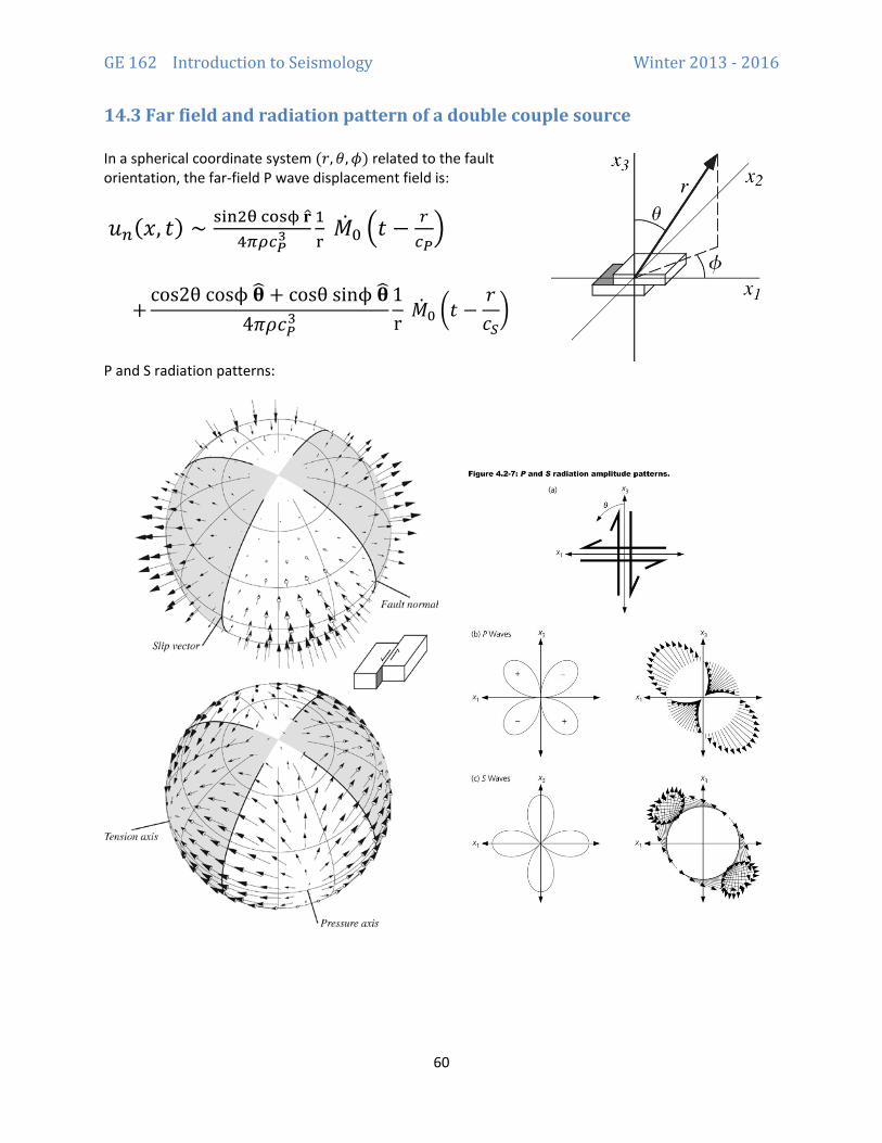
GE 162 Introduction to Seismology Winter 2013 - 2016
60
14.3 Far field and radiation pattern of a double couple source In a spherical coordinate system (𝑟𝑟,𝜃𝜃,𝜙𝜙) related to the fault orientation, the far-field P wave displacement field is:
𝑢𝑢𝑖𝑖(𝑥𝑥, 𝑡𝑡) ∼ sin2θ cosϕ 𝐫𝐫�4𝜋𝜋𝜋𝜋𝑐𝑐𝑃𝑃
31r
�̇�𝑀0 �𝑡𝑡 −𝑟𝑟𝑐𝑐𝑃𝑃�
+cos2θ cosϕ 𝛉𝛉� + cosθ sinϕ 𝛉𝛉�
4𝜋𝜋𝜌𝜌𝑐𝑐𝑃𝑃31r
�̇�𝑀0 �𝑡𝑡 −𝑟𝑟𝑐𝑐𝑆𝑆�
P and S radiation patterns:
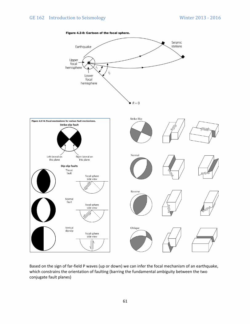
GE 162 Introduction to Seismology Winter 2013 - 2016
61
Based on the sign of far-field P waves (up or down) we can infer the focal mechanism of an earthquake, which constrains the orientation of faulting (barring the fundamental ambiguity between the two conjugate fault planes)

GE 162 Introduction to Seismology Winter 2013 - 2016
62

GE 162 Introduction to Seismology Winter 2013 - 2016
63
Focal mechanisms are a useful information for seismo-tectonic studies, for instance to infer the orientation of strain accumulation in the crust:
The far-field displacement is proportional to the seismic moment rate 𝑀𝑀0̇ (𝑡𝑡). This provides information about the temporal evolution of the rupture. Once we have determined the focal mechanism and the distance to the source, the time-integral of the far-field displacement gives an estimate of the seismic moment 𝑀𝑀0.
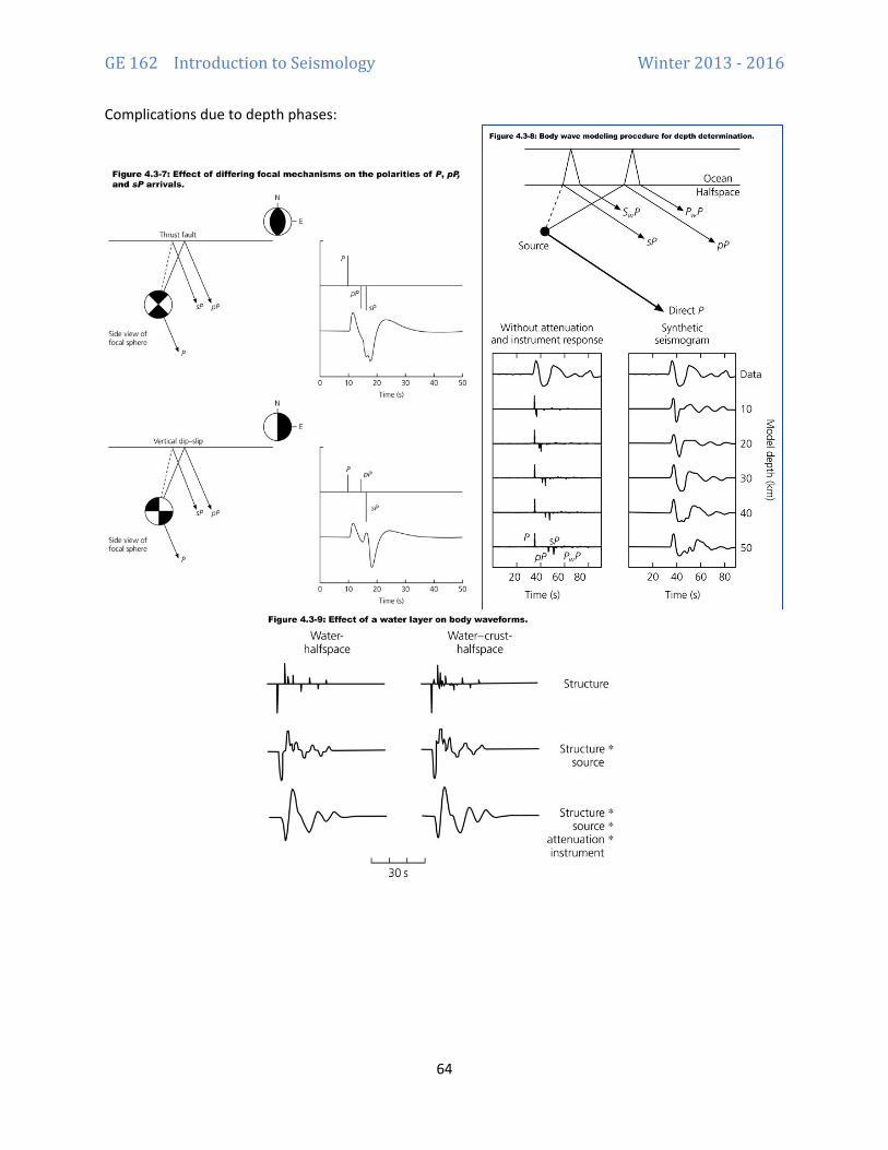
GE 162 Introduction to Seismology Winter 2013 - 2016
64
Complications due to depth phases:

GE 162 Introduction to Seismology Winter 2013 - 2016
65
14.4 Surface waves
GE 162 Introduction to Seismology Winter 2013 - 2016
66
15 Finite sources
15.1 Kinematic source parameters of a finite fault rupture Far from the source and for wavelengths longer than the rupture size, we can consider an earthquake as a point source characterized by its
• seismic moment 𝑀𝑀0 (or moment magnitude 𝑀𝑀𝑠𝑠), • moment tensor 𝑀𝑀𝑖𝑖𝑖𝑖 • source time function �̇�𝑀0(𝑡𝑡).
Close to the fault we need to describe in more detail the space-time distribution of the source: [sketch]
• Slip. • Slip velocity. • Rupture front. Rupture speed. • Rupture duration. • Healing front. Rise time (local slip duration).
15.2 Far-field, apparent source time function Far-field displacement induced by an extended source with slip rate �̇�𝐷(𝝃𝝃, 𝑡𝑡):
𝒖𝒖(𝒙𝒙, 𝑡𝑡) = �𝑅𝑅𝑃𝑃(𝜃𝜃,𝜙𝜙)
4𝜋𝜋𝜌𝜌𝑐𝑐𝑃𝑃31𝑟𝑟
𝜇𝜇�̇�𝐷Σ
�𝝃𝝃, 𝑡𝑡 −𝑟𝑟𝑐𝑐𝑃𝑃� 𝒓𝒓� 𝑑𝑑2𝜉𝜉
If the source area is small compared to the distance 𝑟𝑟 between the fault and the receiver, we can approximate the Green’s function by its value at the center of the rupture area (subscript 0):
𝒖𝒖(𝒙𝒙, 𝑡𝑡) ≈𝑅𝑅𝑃𝑃(𝜃𝜃0,𝜙𝜙0)
4𝜋𝜋𝜌𝜌𝑐𝑐𝑃𝑃3 𝒓𝒓�0𝑟𝑟0
𝜇𝜇� �̇�𝐷 �𝝃𝝃, 𝑡𝑡 −𝑟𝑟𝑐𝑐𝑃𝑃� 𝑑𝑑2𝜉𝜉
Σ
The integral term defines the apparent source time function (ASTF):
ΩP(𝒙𝒙, 𝑡𝑡) = � �̇�𝐷 �𝝃𝝃, 𝑡𝑡 −𝑟𝑟𝑐𝑐𝑃𝑃� 𝑑𝑑2𝜉𝜉
Σ
We can similarly define an ASTF for S waves, ΩS(𝒙𝒙, 𝑡𝑡). The ASTF is not only a property of the source, it depends also on the location of the observer relative to the source and on the type of wave considered (P or S). The time integral of the ASTF
�ΩP or S(𝒙𝒙, 𝑡𝑡) 𝑑𝑑𝑡𝑡 = � 𝐷𝐷(𝝃𝝃) 𝑑𝑑2𝜉𝜉Σ
= 𝑃𝑃0
is the seismic potency, which does not depend on the location of the observer nor on wave type.
15.3 ASTF in the Fraunhofer approximation Let 𝒓𝒓0 be the position of the receiver relative to a reference point on the fault, 𝒓𝒓 its position relative to an arbitrary point on the fault, and 𝝃𝝃 an arbitrary position on the fault (relative to the reference point). Far from the source, 𝜉𝜉 ≪ 𝑟𝑟0 and
𝑟𝑟 = ‖𝒓𝒓0 − 𝝃𝝃‖ = (𝑟𝑟02 − 2𝝃𝝃 ⋅ 𝒓𝒓𝟎𝟎 + 𝜉𝜉2)1/2 ≈ 𝑟𝑟0 − 𝝃𝝃 ⋅ 𝒓𝒓�0 +𝜉𝜉2 − (𝝃𝝃 ⋅ 𝒓𝒓�)2
2𝑟𝑟0+ 𝑂𝑂 �
𝜉𝜉𝑟𝑟0�3
GE 162 Introduction to Seismology Winter 2013 - 2016
67
The Fraunhofer approximation amounts to keep only the zero and first order terms: 𝑟𝑟 ≈ 𝑟𝑟0 − 𝝃𝝃 ⋅ 𝒓𝒓�0
Define the time relative to the wave arrival from the reference point, 𝜏𝜏 = 𝑡𝑡 − 𝑟𝑟0/𝑐𝑐. The simplified expression of ASTF, in the Fraunhofer approximation, is:
Ω(𝒓𝒓�𝟎𝟎, 𝜏𝜏) = � �̇�𝐷 �𝝃𝝃, 𝜏𝜏 +𝝃𝝃 ⋅ 𝒓𝒓�0𝑐𝑐
� 𝑑𝑑2𝜉𝜉Σ
The ASTF depends on the direction 𝒓𝒓�𝟎𝟎 from which we observe the source. Range of validity of the Fraunhofer approximation. Valid if the rupture size, 𝐿𝐿 = max(𝜉𝜉), is small compared to distance and wavelength:
𝐿𝐿 ≪ �𝜆𝜆𝑟𝑟02
The range of validity depends on frequency (through 𝜆𝜆). It is less restrictive than the validity condition of the point-source approximation (𝐿𝐿 ≪ 𝜆𝜆). Proof: Denote 𝑟𝑟∗ the Fraunhofer approximation of the distance 𝑟𝑟, and 𝜖𝜖 = 𝑟𝑟 − 𝑟𝑟∗ the residual of this approximation. The Fourier transform of �̇�𝐷(𝝃𝝃, 𝑡𝑡 − 𝑟𝑟/𝑐𝑐) is �̇�𝐷(𝝃𝝃,𝜔𝜔) exp(𝑖𝑖𝜔𝜔𝑟𝑟/𝑐𝑐). We can justify exp(𝑖𝑖𝜔𝜔𝑟𝑟/𝑐𝑐) ≈ exp(𝑖𝑖𝜔𝜔𝑟𝑟∗/𝑐𝑐) if 𝜔𝜔𝜖𝜖/𝑐𝑐 ≪ 𝜋𝜋/2. This leads to the quarter-wavelength rule: 𝜖𝜖 ≪ 𝜆𝜆/4.
Applying it to the residual 𝜖𝜖 ≈ 𝜉𝜉2−(𝝃𝝃⋅𝒓𝒓�)2
2𝑟𝑟0 (the third order term in the Taylor expansion of 𝑟𝑟) we get,
conservatively, 𝐿𝐿 ≪ �𝜆𝜆𝑟𝑟0/2. 2D example: let’s consider a problem with lower dimensionality, a linear (1D) fault embedded in a 2D elastic medium. Let 𝜃𝜃0 be the take-off angle of the seismic ray leaving the reference point, relative to the fault line direction.
Ω(𝜃𝜃0, 𝜏𝜏) = � �̇�𝐷 �𝜉𝜉, 𝜏𝜏 +𝜉𝜉 cos𝜃𝜃0
𝑐𝑐� 𝑑𝑑𝜉𝜉
Σ
[Sketch �̇�𝐷(𝜉𝜉, 𝑡𝑡). Construct graphically the ASTF for 𝜃𝜃0 = 0𝑠𝑠 , 90𝑠𝑠 , 180𝑠𝑠.
At 𝜃𝜃0 = 90𝑠𝑠we recover the STF. Comparing the other angles, introduce the directivity effect: the duration of the ASTF depends on 𝜃𝜃0.
Shorter duration yields larger amplitude because the time-integral of ASTF is the seismic potency, regardless of 𝜃𝜃0.]
15.4 Haskell pulse model, directivity Haskell model Consider a pulse propagating with constant slip 𝐷𝐷, rise time 𝑡𝑡𝑟𝑟𝑖𝑖𝑠𝑠 and rupture speed 𝑑𝑑𝑟𝑟 on a rectangular fault of width 𝑊𝑊 and length 𝐿𝐿. The slip rate function is assumed invariant. �̇�𝐷(𝑥𝑥, 𝑡𝑡) = 𝐷𝐷 �̇�𝑐 �𝑡𝑡 − 𝑑𝑑
𝑣𝑣𝑟𝑟� if 𝑥𝑥 ∈ [0, 𝐿𝐿] and 𝑧𝑧 ∈ [0,𝑊𝑊]
= 0 elsewhere Far-field spectrum of a Haskell source Its ASTF is
GE 162 Introduction to Seismology Winter 2013 - 2016
68
Ω(𝒓𝒓�𝟎𝟎, 𝜏𝜏) = 𝐷𝐷� �̇�𝑐 �𝜏𝜏 − 𝜉𝜉/𝑑𝑑𝑟𝑟 +𝝃𝝃 ⋅ 𝒓𝒓�0𝑐𝑐
� 𝑑𝑑𝜉𝜉 𝑑𝑑𝜂𝜂Σ
If 𝑊𝑊 is small,
Ω(𝒓𝒓�𝟎𝟎, 𝜏𝜏) = 𝐷𝐷𝑊𝑊� �̇�𝑐 �𝜏𝜏 − 𝜉𝜉/𝑑𝑑𝑟𝑟 +𝜉𝜉 cos 𝜃𝜃0
𝑐𝑐� 𝑑𝑑𝜉𝜉
𝐶𝐶
0
Its Fourier transform is
Ω(𝒓𝒓�𝟎𝟎,𝜔𝜔) = −𝑖𝑖𝜔𝜔 𝑐𝑐(𝜔𝜔)𝐷𝐷𝑊𝑊𝐿𝐿� exp�𝑖𝑖𝜔𝜔𝜉𝜉 �1𝑑𝑑𝑟𝑟−
cos 𝜃𝜃0𝑐𝑐
��𝑑𝑑𝜉𝜉𝐶𝐶
0= −𝑖𝑖𝜔𝜔 𝑐𝑐(𝜔𝜔)𝐷𝐷𝑊𝑊𝐿𝐿
sin𝑋𝑋𝑋𝑋
𝑒𝑒𝑖𝑖𝑖𝑖
where 𝑋𝑋 = 𝑖𝑖𝐶𝐶2� 1𝑣𝑣𝑟𝑟− cos𝜃𝜃0
𝑐𝑐�.
If 𝑐𝑐(𝑡𝑡) is a boxcar function with duration 𝑡𝑡𝑟𝑟𝑖𝑖𝑠𝑠, then 𝑐𝑐(𝜔𝜔) = (1 − 𝑒𝑒𝑖𝑖𝑖𝑖𝑖𝑖𝑟𝑟𝑖𝑖𝑠𝑠)/𝜔𝜔2𝑡𝑡𝑟𝑟𝑖𝑖𝑠𝑠, and
|Ω(𝒓𝒓�𝟎𝟎,𝜔𝜔)| = 𝑊𝑊𝐿𝐿𝐷𝐷 �sin𝑋𝑋𝑋𝑋
sin𝜔𝜔𝑡𝑡𝑟𝑟𝑖𝑖𝑠𝑠𝜔𝜔𝑡𝑡𝑟𝑟𝑖𝑖𝑠𝑠
�
[Plot 𝑠𝑠𝑖𝑖𝑖𝑖 𝑖𝑖
𝑖𝑖, indicate zero-crossings.
Log-log plot spectrum of ASTF.] Spectral shape and two corners frequencies The ASTF spectrum exhibits three distinct behaviors, from low to high-frequencies: flat, 1/ω and 1/ω2. These regimes are separated by corner frequencies
𝜔𝜔1(𝜃𝜃0) = 𝑣𝑣𝑟𝑟𝐶𝐶
�1 − 𝑣𝑣𝑟𝑟𝑐𝑐
cos𝜃𝜃0� and 𝜔𝜔2 = 1/𝑡𝑡𝑟𝑟𝑖𝑖𝑠𝑠 Directivity effect The directivity effect (azimuth-dependence) appears in the lower corner frequency, 𝜔𝜔1.
[Plot 𝜔𝜔1 as a function of 𝜃𝜃0]
Far-field waveform shape Displacement seismogram is a trapezoid. Velocity is made of two bumps and nothing in between: far-field radiation occurs during initiation and arrest (abrupt changes of rupture speed) but not during steady-state rupture propagation.
[Sketch: far-field displacement and velocity waveform. Indicate time scales] Directivity more intuitively: 1/𝜔𝜔1 is the duration of the ASTF.
[Sketch: relation between ASTF duration
and the arrival times of waves radiated by the two ends of a rupture]
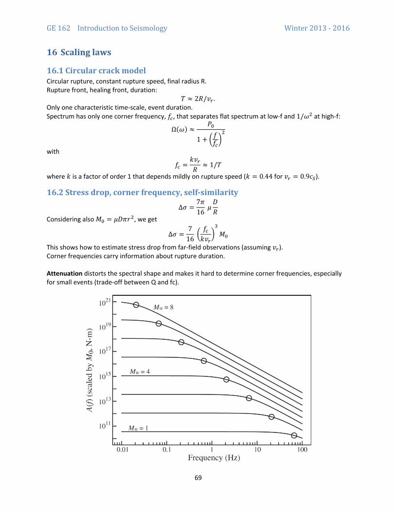
GE 162 Introduction to Seismology Winter 2013 - 2016
69
16 Scaling laws
16.1 Circular crack model Circular rupture, constant rupture speed, final radius R. Rupture front, healing front, duration:
𝑇𝑇 ≈ 2𝑅𝑅/𝑑𝑑𝑟𝑟. Only one characteristic time-scale, event duration. Spectrum has only one corner frequency, 𝑓𝑓𝑐𝑐, that separates flat spectrum at low-f and 1/𝜔𝜔2 at high-f:
Ω(𝜔𝜔) ≈𝑃𝑃0
1 + �𝑓𝑓𝑓𝑓𝑐𝑐�2
with
𝑓𝑓𝑐𝑐 =𝑘𝑘𝑑𝑑𝑟𝑟𝑅𝑅
≈ 1/𝑇𝑇
where 𝑘𝑘 is a factor of order 1 that depends mildly on rupture speed (𝑘𝑘 = 0.44 for 𝑑𝑑𝑟𝑟 = 0.9𝑐𝑐𝑆𝑆).
16.2 Stress drop, corner frequency, self-similarity
Δ𝜎𝜎 =7𝜋𝜋16
𝜇𝜇𝐷𝐷𝑅𝑅
Considering also 𝑀𝑀0 = 𝜇𝜇𝐷𝐷𝜋𝜋𝑟𝑟2, we get
Δ𝜎𝜎 =7
16 �𝑓𝑓𝑐𝑐𝑘𝑘𝑑𝑑𝑟𝑟
�3
𝑀𝑀0
This shows how to estimate stress drop from far-field observations (assuming 𝑑𝑑𝑟𝑟). Corner frequencies carry information about rupture duration. Attenuation distorts the spectral shape and makes it hard to determine corner frequencies, especially for small events (trade-off between Q and fc).

GE 162 Introduction to Seismology Winter 2013 - 2016
70
Self-similarity: if Δ𝜎𝜎 and 𝑑𝑑𝑟𝑟 do not depend on earthquake size:
𝑀𝑀0 ∝ 𝑅𝑅3 𝑇𝑇 ∝ 𝑅𝑅
𝑢𝑢(𝑡𝑡) ∝ �̇�𝑀0 ∼ 𝑀𝑀0/𝑇𝑇 ∝ 𝑅𝑅2 ∝ 𝑀𝑀02/3
�̇�𝑢(𝑡𝑡) ∝ �̈�𝑀0 ∼ 𝑀𝑀0/𝑇𝑇2 ∝ 𝑅𝑅 ∝ 𝑀𝑀01/3
16.3 Energy considerations and moment magnitude scale Energy radiated to the far-field:
𝑆𝑆 ∝ ∫ �̇�𝑢2𝑑𝑑𝑡𝑡 ∝ �̇�𝑢2 𝑇𝑇 ∝ 𝑀𝑀0 log10 𝑆𝑆 = log10 𝑀𝑀0 + ⋯
Moment magnitude:
𝑀𝑀𝑠𝑠 =23
log10(𝑀𝑀0) − 6.0
Then:
log𝑆𝑆 =32𝑀𝑀𝑠𝑠 + ⋯
One magnitude unit = 30 times more energy radiated, 30 times larger moment, 10 times larger ground displacement, 3 times larger ground velocity (ignoring attenuation) It’s also useful to have in mind relations between magnitude and earthquake size:
𝑀𝑀𝑠𝑠 = 2 log10 𝑅𝑅 + ⋯ One magnitude unit = 3 times larger rupture size, 3 times longer rupture duration. In terms of rupture surface area A:
𝑀𝑀𝑠𝑠 = log10 𝐴𝐴 + ⋯ One magnitude unit = 10 times larger rupture area.
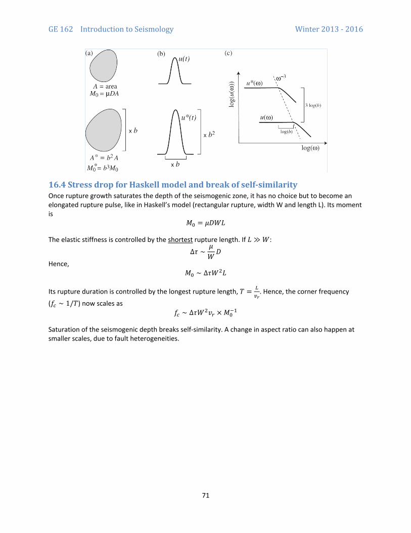
GE 162 Introduction to Seismology Winter 2013 - 2016
71
16.4 Stress drop for Haskell model and break of self-similarity Once rupture growth saturates the depth of the seismogenic zone, it has no choice but to become an elongated rupture pulse, like in Haskell’s model (rectangular rupture, width W and length L). Its moment is
𝑀𝑀0 = 𝜇𝜇𝐷𝐷𝑊𝑊𝐿𝐿
The elastic stiffness is controlled by the shortest rupture length. If 𝐿𝐿 ≫ 𝑊𝑊:
Δ𝜏𝜏 ∼𝜇𝜇𝑊𝑊𝐷𝐷
Hence, 𝑀𝑀0 ∼ Δ𝜏𝜏𝑊𝑊2𝐿𝐿
Its rupture duration is controlled by the longest rupture length, 𝑇𝑇 = 𝐶𝐶𝑣𝑣𝑟𝑟
. Hence, the corner frequency
(𝑓𝑓𝑐𝑐 ∼ 1/𝑇𝑇) now scales as 𝑓𝑓𝑐𝑐 ∼ Δ𝜏𝜏𝑊𝑊2𝑑𝑑𝑟𝑟 × 𝑀𝑀0
−1
Saturation of the seismogenic depth breaks self-similarity. A change in aspect ratio can also happen at smaller scales, due to fault heterogeneities.
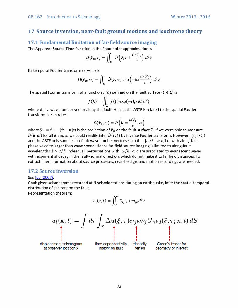
GE 162 Introduction to Seismology Winter 2013 - 2016
72
17 Source inversion, near-fault ground motions and isochrone theory
17.1 Fundamental limitation of far-field source imaging The Apparent Source Time Function in the Fraunhofer approximation is
Ω(𝒓𝒓�𝟎𝟎, 𝜏𝜏) = � �̇�𝐷 �𝝃𝝃, 𝜏𝜏 +𝝃𝝃 ⋅ 𝒓𝒓�0𝑐𝑐
� 𝑑𝑑2𝜉𝜉Σ
Its temporal Fourier transform (𝜏𝜏 → 𝜔𝜔) is
Ω(𝒓𝒓�𝟎𝟎,𝜔𝜔) = � �̇�𝐷(𝝃𝝃,𝜔𝜔) exp �−iω𝝃𝝃 ⋅ 𝒓𝒓�0𝑐𝑐
� 𝑑𝑑2𝜉𝜉Σ
The spatial Fourier transform of a function 𝑓𝑓(𝝃𝝃) defined on the fault surface (𝝃𝝃 ∈ Σ) is
𝑓𝑓(𝒌𝒌) = � 𝑓𝑓(𝝃𝝃) exp(−i 𝛏𝛏 ⋅ 𝒌𝒌)𝑑𝑑2𝜉𝜉Σ
where 𝒌𝒌 is a wavenumber vector along the fault. Hence, the ASTF is related to the spatial Fourier transform of slip rate:
Ω(𝒓𝒓�𝟎𝟎,𝜔𝜔) = �̇�𝐷 �𝒌𝒌 =𝜔𝜔𝜸𝜸�0𝑐𝑐
,𝜔𝜔�
where 𝜸𝜸�0 = 𝒓𝒓�0 − (𝒓𝒓�0 ⋅ 𝒏𝒏)𝒏𝒏 is the projection of 𝒓𝒓�0 on the fault surface Σ. If we were able to measure �̇�𝐷(𝒌𝒌,𝜔𝜔) for all 𝒌𝒌 and 𝜔𝜔 we could readily infer �̇�𝐷(𝝃𝝃, 𝑡𝑡) by inverse Fourier transform. However, |𝜸𝜸�0| < 1 and the ASTF only samples on-fault wavenumber vectors such that |𝜔𝜔/𝑘𝑘| > 𝑐𝑐, i.e. with along-fault phase velocity larger than wave speed. Hence far-field source imaging is limited to along-fault wavelengths 𝜆𝜆 > 𝑐𝑐/𝑓𝑓. Indeed, all perturbations with |𝜔𝜔/𝑘𝑘| < 𝑐𝑐 are associated to evanescent waves with exponential decay in the fault-normal direction, which do not make it to far field distances. To extract finer information about source processes, near-field ground motion recordings are needed.
17.2 Source inversion See Ide (2007). Goal: given seismograms recorded at N seismic stations during an earthquake, infer the spatio-temporal distribution of slip rate on the fault. Representation theorem:
𝑢𝑢𝑖𝑖(𝒙𝒙, 𝑡𝑡) = �𝐺𝐺𝑖𝑖𝑖𝑖,𝑖𝑖 ∗ 𝑚𝑚𝑖𝑖𝑖𝑖𝑑𝑑3𝜉𝜉
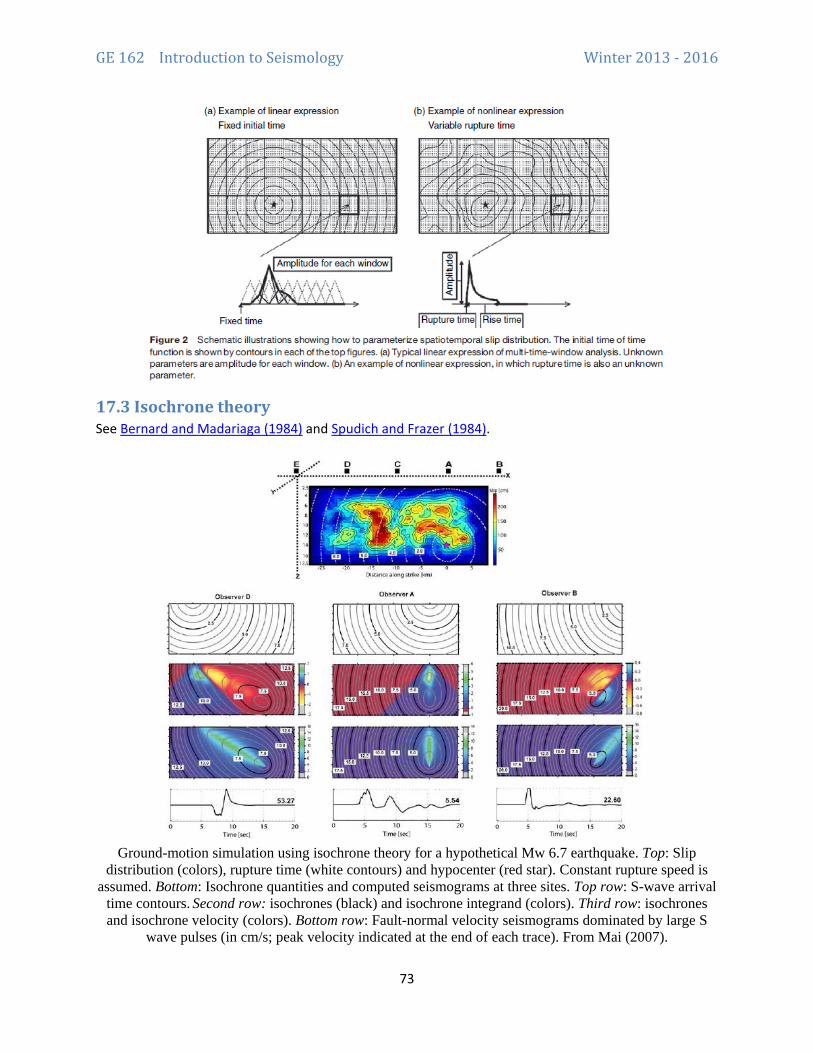
GE 162 Introduction to Seismology Winter 2013 - 2016
73
17.3 Isochrone theory See Bernard and Madariaga (1984) and Spudich and Frazer (1984).
Ground-motion simulation using isochrone theory for a hypothetical Mw 6.7 earthquake. Top: Slip
distribution (colors), rupture time (white contours) and hypocenter (red star). Constant rupture speed is assumed. Bottom: Isochrone quantities and computed seismograms at three sites. Top row: S-wave arrival
time contours. Second row: isochrones (black) and isochrone integrand (colors). Third row: isochrones and isochrone velocity (colors). Bottom row: Fault-normal velocity seismograms dominated by large S
wave pulses (in cm/s; peak velocity indicated at the end of each trace). From Mai (2007).

GE 162 Introduction to Seismology Winter 2013 - 2016
74
18 Source inversion and source imaging
18.1 Source inversion problem For given data d and design matrix G (Green’s functions), find the model m that minimizes the cost
function χ2 = �|𝑑𝑑 − 𝐺𝐺𝑚𝑚|�2 . The formal solution is 𝑚𝑚 = (𝐺𝐺𝑇𝑇𝐺𝐺)−1𝐺𝐺𝑇𝑇𝑑𝑑 = 𝐺𝐺#𝑑𝑑. Proof: set 𝑑𝑑χ2
𝑑𝑑𝐼𝐼= 0.
18.2 Ill-conditioning of the source inversion problem The Singular Value Decomposition (SVD) of matrix G is
𝐺𝐺 = 𝑈𝑈𝑈𝑈𝑉𝑉𝑇𝑇 where U[N,M] and V[M,M] are orthonormal matrices (𝑈𝑈𝑇𝑇𝑈𝑈 = 𝐼𝐼, 𝑉𝑉𝑇𝑇𝑉𝑉 = 𝐼𝐼), and 𝑈𝑈[M,M] is a diagonal matrix consisting of positive singular values 𝜆𝜆𝑖𝑖, 𝑖𝑖 = 1, . . . ,𝑀𝑀, sorted in descending order. The columns 𝑉𝑉(𝑖𝑖) of matrix V are called right-singular vectors. They are also eigenvectors of matrix 𝐺𝐺𝑇𝑇𝐺𝐺[M,M], forming an orthonormal basis system in the model space, and 𝜆𝜆𝑖𝑖2 are its eigenvalues. Columns 𝑈𝑈(𝑖𝑖) of matrix U are called left-singular vectors. They are projections of basis vectors 𝑉𝑉(𝑖𝑖) into the data space,
𝑈𝑈(𝑖𝑖) = 𝐺𝐺𝑉𝑉(𝑖𝑖) /𝜆𝜆𝑖𝑖 i.e. normalized seismograms related to the individual singular vectors. The generalized solution of the inverse problem, 𝑚𝑚 = 𝐺𝐺#𝑑𝑑 can be expressed as a linear combination of basis vectors 𝑉𝑉(𝑖𝑖):
𝑚𝑚 = ∑ 𝑚𝑚�𝑖𝑖 𝑉𝑉(𝑖𝑖)𝑀𝑀𝑖𝑖=1 where 𝑚𝑚�𝑖𝑖 = 𝑈𝑈(𝑖𝑖) ⋅ 𝑑𝑑/𝜆𝜆𝑖𝑖
Similarly, the data vector can be expressed as 𝑑𝑑 = ∑ �̃�𝑑𝑖𝑖 𝑈𝑈(𝑖𝑖)
𝑁𝑁𝑖𝑖=1 where �̃�𝑑𝑖𝑖 = 𝑈𝑈(𝑖𝑖) ⋅ 𝑑𝑑
The spectral components of data and model are thus related by 𝑚𝑚�𝑖𝑖 = �̃�𝑑𝑖𝑖/𝜆𝜆𝑖𝑖
Therefore, the smaller is the singular value 𝜆𝜆𝑖𝑖, the less sensitive is the data component to a given change of the corresponding model component; in other words, the singular value bears information about the sensitivity of the data to the particular basis function in the model space. Also, if 𝜆𝜆𝑖𝑖 is small, errors in the data or in the G matrix get amplified. Hence the components of the data associated to small eigenvalues are hardly recoverable by the inverse problem, they define an effective null space.

GE 162 Introduction to Seismology Winter 2013 - 2016
75

GE 162 Introduction to Seismology Winter 2013 - 2016
76
18.3 Stacking Stacking (adding up) seismograms enhances the signal-to-noise ratio. Central limit theorem: stacking N seismograms reduces the noise by √𝑁𝑁.
18.4 Array seismology Plane wave impinging on a linear array and 2D array:
Parameters: back-azimuth and horizontal slowness (related to wave speed and incidence angle i):
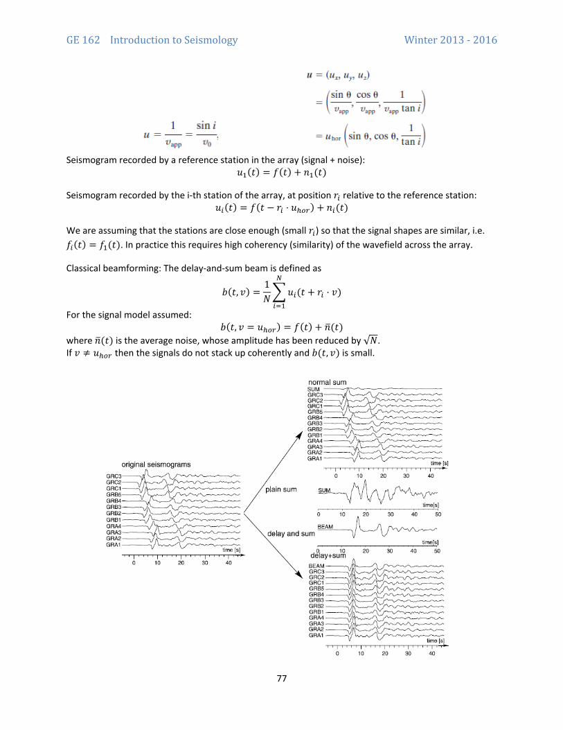
GE 162 Introduction to Seismology Winter 2013 - 2016
77
Seismogram recorded by a reference station in the array (signal + noise):
𝑢𝑢1(𝑡𝑡) = 𝑓𝑓(𝑡𝑡) + 𝑛𝑛1(𝑡𝑡)
Seismogram recorded by the i-th station of the array, at position 𝑟𝑟𝑖𝑖 relative to the reference station: 𝑢𝑢𝑖𝑖(𝑡𝑡) = 𝑓𝑓(𝑡𝑡 − 𝑟𝑟𝑖𝑖 ⋅ 𝑢𝑢ℎ𝑠𝑠𝑟𝑟) + 𝑛𝑛𝑖𝑖(𝑡𝑡)
We are assuming that the stations are close enough (small 𝑟𝑟𝑖𝑖) so that the signal shapes are similar, i.e. 𝑓𝑓𝑖𝑖(𝑡𝑡) = 𝑓𝑓1(𝑡𝑡). In practice this requires high coherency (similarity) of the wavefield across the array.
Classical beamforming: The delay-and-sum beam is defined as
𝑏𝑏(𝑡𝑡, 𝑑𝑑) =1𝑁𝑁�𝑢𝑢𝑖𝑖(𝑡𝑡 + 𝑟𝑟𝑖𝑖 ⋅ 𝑑𝑑)𝑁𝑁
𝑖𝑖=1
For the signal model assumed: 𝑏𝑏(𝑡𝑡, 𝑑𝑑 = 𝑢𝑢ℎ𝑠𝑠𝑟𝑟) = 𝑓𝑓(𝑡𝑡) + 𝑛𝑛�(𝑡𝑡)
where 𝑛𝑛�(𝑡𝑡) is the average noise, whose amplitude has been reduced by √𝑁𝑁. If 𝑑𝑑 ≠ 𝑢𝑢ℎ𝑠𝑠𝑟𝑟 then the signals do not stack up coherently and 𝑏𝑏(𝑡𝑡, 𝑑𝑑) is small.
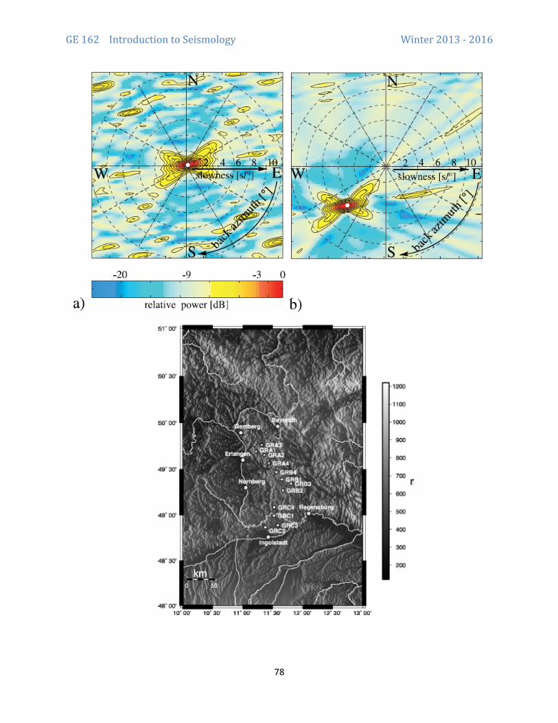
GE 162 Introduction to Seismology Winter 2013 - 2016
78

GE 162 Introduction to Seismology Winter 2013 - 2016
79
18.5 Array response
18.6 Coherency stacking …
GE 162 Introduction to Seismology Winter 2013 - 2016
80
19 Earthquake dynamics I: Fracture mechanics perspective [Hand-written notes and slides to be cleaned up] Stress intensity factor Energy release rate Crack tip equation of motion Radiated energy
20 Earthquake dynamics II: Fault friction perspective [Hand-written notes and slides to be cleaned up] Friction (laboratory, physical mechanisms, usual constitutive relations) Slip-weakening and process zone size Earthquake nucleation Fluid and thermal effects in fault weakening Cracks versus pulses Supershear rupture

GE 162 Introduction to Seismology Winter 2013 - 2016
81
21 Inverse problems, part 1
21.1 Earthquake location
21.2 Iterative solution
21.3 Solution of inverse problems.
21.4 Weighted over-determined problem
21.5 Uncertainties: model covariance
21.6 Double difference location

GE 162 Introduction to Seismology Winter 2013 - 2016
82
22 Inverse problems, part 2
22.1 Travel time tomography, ill-posed problems
22.2 SVD, minimum-norm solution
22.3 Resolution matrix, model covariance matrix
22.4 Truncated SVD
22.5 Regularization
22.6 Bayesian approach


![GE 162 Introduction to Seismology - clay/Ge162/Ge162_lecture_notes.pdfGE 162 Introduction to Seismology Winter 2013 - 2016. 6 [Sketch undeformed and deformed rod, annotate] Let 𝑥𝑥](https://static.fdocuments.in/doc/165x107/5cf7382e88c99346318ca77c/ge-162-introduction-to-seismology-clayge162ge162lecturenotespdfge-162-introduction.jpg)