Gambler’s Ruin Problem

John Boccio

October 17, 2012

Contents

1 The Gambler’s Ruin Problem 11.1 Pascal’s problem of the gambler’s ruin . . . . . . . . . . . . . 11.2 Huygen’s Approach . . . . . . . . . . . . . . . . . . . . . . . . 1

1.2.1 Digression on Probability and Expected Value . . . . . 11.3 Problem and Solution . . . . . . . . . . . . . . . . . . . . . . . 3

1.3.1 Digression to the Problem of Points . . . . . . . . . . . 31.3.2 Solving difference equations . . . . . . . . . . . . . . . 8

2 Ruin, Random Walks and Diffusion 102.1 General Orientation . . . . . . . . . . . . . . . . . . . . . . . . 102.2 The Classical Ruin problem . . . . . . . . . . . . . . . . . . . 12

2.2.1 The limiting case . . . . . . . . . . . . . . . . . . . . . 162.3 Expected Duration of the Game . . . . . . . . . . . . . . . . . 162.4 Generating Functions for the Duration of the Game and for

the First-Passage Times . . . . . . . . . . . . . . . . . . . . . 182.4.1 Infinite Intervals and First Passages . . . . . . . . . . . 20

2.5 Explicit Expressions . . . . . . . . . . . . . . . . . . . . . . . 212.6 Connection with Diffusion Processes . . . . . . . . . . . . . . 23

i

1 The Gambler’s Ruin Problem

1.1 Pascal’s problem of the gambler’s ruin

Two gamblers, A and B, play with three dice. At each throw, if the totalis 11 then B gives a counter to A; if the total is 14 then A gives a counterto B. They start with twelve counters each, and the first to possess all 24 isthe winner. What are their chances of winning?

Pascal gives the correct solution. The ratio of their respective chances ofwinning pA : pB, is

150094635296999122 : 129746337890625

which is the same as

282429536481 : 244140625

on dividing by 312.

Unfortunately it is not certain what method Pascal used to get this result.

1.2 Huygen’s Approach

However, Huygens soon heard about this new problem, and solved it in afew days (sometime between September 28,1656 and October 12, 1656). Heused a version of Pascal’s idea of value.

1.2.1 Digression on Probability and Expected Value

Many problems in chance are inextricably linked with numerical outcomes,especially in gambling and finance (where “numerical outcome” is a eu-phemism for money). In these cases probability is inextricably linked to“value”, as we now show.

To aid our thinking let us consider an everyday concrete and practical prob-lem

A plutocrat(member of a plutocracy = a government or state in which thewealthy rule) makes the following offer. She will flip a fair coin; if it shows

heads she will give you $1, if it shows tails she will give your friend Jack $1.What is the offer worth to you? That is to say, for what fair price $p, shouldyou sell it?

Clearly, whatever price $p this is worth to you, it is worth the same price $pto Jack, because the coin is fair, i.e., symmetrical (assuming he needs andvalues money just as much as you do). So,to the pair of you, this offer isaltogether worth $2p. But whatever the outcome, the plutocrat has givenaway $1. Hence $2p = $1, so that p = 1

2and the offer is worth $1

2to you.

It seems natural to regard this value p = 12

as a measure of your chance ofwinning the money. It is intuitively reasonable to make the following generalrule.

Suppose you receive $1 with probability p (and otherwise youreceive nothing). Then the value or fair price of this offer is $p.More generally, if you receive $d with probability p (and nothingotherwise) then the fair price or expected value of this offer isgiven by

expected value = pd

This simple idea turns out to be enormously important later on; for themoment we note only that it is certainly consistent with ideas about proba-bility.. For example, if the plutocrat definitely gives you $1 then this is worthexactly $1 to you, and p = 1. Likewise, if you are definitely given nothing,then p = 0 and it is easy to see that 0 ≤ p ≤ 1, for any such offers.

In particular, for the specific example above we find that the probability ofa head when a fair coin is flipped is 1

2. Likewise a similar argument shows

that the probability of a six when a fair die is rolled is 16

(simply imagine theplutocrat giving $1 to one of six people selected by the roll of the die).

The “fair price” of such offers is often called the expected value, or expecta-tion, to emphasize its chance nature.

Returning to Huygens- Huygen’s definition of value

if you are offered $x with probability p, or $y with probability q(p+ q = 1), then the value of this offer to you is (px+ qy).

2

Now of course we do not know for sure if this was Pascal’s method, but Pascalwas certainly at least as capable of extending his own ideas as Huygens was.The correct balance of probabilities indicates that he did use this method. Bylong-standing tradition this problem is always solved in books on elementaryprobability, and so we now give a modern version of the solution. Here is ageneral statement of the problem.

1.3 Problem and Solution

Two players, A and B again, play a series of independent games. Each gameis won by A with probability α, or by B with probability β; the winner ofeach game gets one counter from the loser. Initially A has m counters andB has n. The victor of the contest is the first to have all m+n counters, theloser is said to be “ruined”, which explains the name of the problem. Whatare the chances of A and B to be the victor?

Note that α + β = 1, and for the moment we assume that α 6= β.

We will need the “partition rule” for two events from probability theory:

P (A) = P (A|B)P (B) + P (A| B)P ( B)

and the “conditional partition rule” for three events

P (A|C) = P (A|B ∩ C)P (B|C) + P (A| B ∩ C)P ( B|C)

It is also helpful to discuss a different problem first.

1.3.1 Digression to the Problem of Points

“Prolonged gambling differentiates people into two groups, thoseplaying with the odds, who are following a trade or profession;and those playing against the odds, who are indulging a hobbyor pastime, and if this involves a regular annual outlay, this is nomore than what has been said about most other amusements.”

John Venn

We consider her a problem which was of particular importance in the historyand development of probability. In most texts on probability, one starts off

3

with problems involving dice, cards, and other simple gambling devices. Theapplication of the theory is so natural and useful that it might be supposedthat the creation of probability parallelled the creation of dice and cards. Infact, this is far from being the case. The greets single initial step in con-structing a theory of probability was made in response to a more obscurequestion - the problem of points.

Roughly speaking the essential question is this.

Two players, traditionally called A and B, are competing for a prize. Thecontest takes the form of a sequence of independent similar trials; as a resultof each trial one of the contestants is awarded a point. The first player toaccumulate n points is the winner; in colloquial parlance A and B are playingthe best of 2n − 1 points. Tennis matches are usually the best of five sets;n = 3.

The problem arises when the contest has to be stopped or abandoned beforeeither has won n points; in fact A needs a points (having n − a already)and B needs b points (having n− b already). How should the prize be fairlydivided? (Typically the “prize” consisted of stakes put up by A and B, andheld by the stakeholder).

For example, in tennis, sets correspond to points and men play the best offive sets. If the players were just beginning the fourth set when the courtwas swallowed up by an earthquake, say, what would be a fair division of theprize? (assuming a natural reluctance to continue the game on some nearbycourt).

This is a problem of great antiquity; it first appeared in print in 1494 in abook by Luca Pacioli, but was almost certainly an old problem even then.In his example, A and B were playing the best of 11 games for a prize of tenducats, and are forced to abandon the game when A has 5 points (needing1 more) and B has 2 points (needing 4 more). How should the prize bedivided?

Though Pacioli was a man of great talent (among many other things hisbook included the first printed account of double-entry book-keeping), hecould not solve this problem.

4

Nor could Tartaglia (who is best known for showing how to find the roots ofa cubic equation), nor could Forestani, Peverone, or Cardano, who all madeattempts during the 16th century.

In fact, the problem was finaly solved by Blaise Pascal in 1654, who, withFermat thereby officially inaugurated the theory of probability. In that year,probably sometime around Pascal’s birthday (June 19; he was 31), the prob-lem of points was brought to his attention. The enquiry was made by Cheva-lier de Mere (Antoine Gombaud) who as a man-about-town and a gambler,had a strong and direct interest in the answer. Within a very short time,Pascal had solved the problem in two different ways. In the course of a cor-respondence with Fermat, a third method of solution was found by Fermat.

Two of these methods relied on counting the number of equally likely out-comes. Pascal’s great step forward was to create a method that did not relyon having equally likely outcomes. This breakthrough came about as a resultof his explicit formulation of the idea of the value of a bet or lottery, as wediscussed above, i.e., if you have a probability p of winning $1 then the gameis worth $p to you.

It naturally follows that, in the problem of the points, the prize should bedivided in proportion to the player’s respective probabilities of winning if thegame were to be continued. The problem is therefore more precisely statedthus.

Precise problem of the points. A sequence of fair coins isflipped; A get a pony for every head, B a point for every tail.Player A wins if there are a heads before b tails, otherwise Bwinds. Find the probability that A wins.

Solution. Let α(a, b) be the probability that A wins and β(a, b) the proba-bility that B wins. If the first flip is a head, then A now needs a− 1 furtherheads to win, so the conditional probability that A wins , given a head, isα(a− 1, b). Likewise the conditional probability that A wins, given a tail isα(a, b− 1). Hence, by the partition rule,

α(a, b) = 12α(a− 1, b) + 1

2α(a, b− 1) (1)

Thus, if we know α(a, b) for small values of a and b, we can find the solutionfor any a and b by simple recursion. And of course we do know such values

5

of α(a, b), because if a = 0 and b > 0, then A has won and takes the wholeprize: that is to say

α(0, b) = 1 (2)

Likewise, if b = 0 and a > 0, then B has won, and so

α(a, 0) = 0 (3)

How do we solve (1) in general, with (2) and (3)? Recall the fundamentalproperty of Pascal’s triangle: the entries in the (row,column):

(0, 0)

(0

0

)= 1

(1, 0)

(1

0

)= 1 (1, 1)

(1

1

)= 1

(2, 0)

(2

0

)= 1 (2, 1)

(2

1

)= 2 (2, 2)

(2

2

)= 1

and so on, i.e., the entries c(j + k, k) = d(j, k) satisfy

d(j, k) = d(j − 1, k) + d(j, k − 1) (4)

You do not need to be genius to suspect that the solution α(a, b) of (1) isgoing to be connected with the solutions

c(j + k, k) = d(j, k) =

(j + k

k

)of (4). We can make the connect even more transparent by writing

α(a, b) =1

2a+bu(a, b)

Then (1) becomes

u(a, b) = u(a− 1, b) + u(a, b− 1) (5)

withu(0, b) = 2b and u(a, 0) = 0 (6)

6

There are various ways of solveng (5) with conditions (6), but Pascal had theinestimable advantage of having already obtained the solution by anothermethod. Thus, he had simply to check that the answer is indeed

u(a, b) = 2b−1∑k=0

(a+ b− 1

k

)(7)

and

α(a, b) =1

2a+b−1

b−1∑k=0

(a+ b− 1

k

)(8)

At long last there was a solution to this classic problem. We may reasonablyask why Pascal was able to solve it in a matter of weeks, when all previousattempts had failed for at least 150 years. As usual the answer lies in a com-bination of circumstances: mathematicians had become better at countingthings; the binomial coefficients were better understood; notation and thetechniques of algebra had improved immeasurably; and Pascal had a coupleof very good ideas.

Pascal immediately realized the power of these ideas and techniques andquickly invented new problems on which to use them.

The Gambler’s Ruin problem is the best known of them.

Just as in the problem of points, suppose that at some stage A has a counters(so B has m + n− a counters), and let A’s chances of victory at that pointbe v(a). If A wins the next game his chance of victory is now v(a+ 1); if Aloses the next game his chance of victory is v(a− 1). Hence by the partitionrule,

v(a) = αv(a+ 1) + βv(a− 1) , 1 ≤ a ≤ m+ n− 1 (9)

Furthermore we know that

v(m+ n) = 1 (10)

because in this case A has all the counters, and

v(0) = 0 (11)

because A then has no counters.

7

1.3.2 Solving difference equations

Any sequence (xr; r ≥ 0) in which each term is a function of its predecessors,so that

xr+k = f(xr, xr+1, ......., xr+k−1) , r ≥ 0 (12)

is said to satisfy the recurrence relation (12). When f is linear this is calleda difference equation of order k:

xr+k = a0xr + a1xr+1 + · · ·+ ak−1xr+k−1 + g(r) , a0 6= 0 (13)

When g(r) = 0, the equation is homogeneous:

xr+k = a0xr + a1xr+1 + · · ·+ ak−1xr+k−1 , a0 6= 0 (14)

Some examples to give a hint at the solutions are:

If we havepn = qpn−1

the solution is easy because

pn−1 = qpn−2 , pn−2 = qpn−3

and so on. By successive substitution we obtain

pn = qnp0

If we havepn = (q − p)pn−1 + p

this is almost as easy to solve when we notice that

pn =1

2

is a particular solution. Now writing

pn =1

2+ xn

givesxn = (q − p)xn−1 = (q − p)nx0

so that

pn =1

2+ (q − p)nx0

8

If we havepn = ppn−1 + pqpn−2 , pq 6= 0

is more difficult, but after some work which we omit, the solution turnsout to be

pn = c1λn1 + c2λ

n2 (15)

where λ1 and λ2 are the roots of

x2 + px− pq = 0

and c1 and c2 are arbitrary constants.

Having seen these special examples, one is not surprised to see the generalsoluten to the second order difference equation: let

xr+2 = a0xr + a1xr+1 + g(r) , r ≥ 0 (16)

Suppose that π(r) is any function such that

π(r + 2) = a0π(r) + a1π(r + 1) + g(r)

and suppose that λ1 and λ2 are the roots of

x2 = a0 + a1x

Then the solution of (16) is given by

xr =

{c1λ

r1 + c2λ

r2 + π(r) λ1 6= λ2

(c1 + c2r)λr1 + π(r) λ1 = λ2

where c1 and c2 are arbitrary constants. Here π(r) is called a particularsolution. One should note that λ1 and λ2 may be complex, as then may c1and c2.

The solution of higher-order difference equations proceeds along similar lines.From section 1.3.2 we know that the solution of (9) takes the form

v(a) = c1λa + c2µ

a

where c1 and c2 are arbitrary constants, and λ and µ are roots of

αx2 − x+ β = 0 (17)

9

Trivially, the roots of (17) are λ = 1 and µ = β/α 6= 1 (since we assumedthat α 6= β). Hence, using (10) and (11), we find that

v(a) =1− (β/α)a

1− (β/α)m+n(18)

In particular, when A starts with m counters,

pA = v(m) =1− (β/α)m

1− (β/α)m+n(19)

This method of solution of difference equation was unknown in 1656, soother approaches were employed. In obtaining the answer to the gambler’sruin problem, Huygens (and later workers) used intuitive induction with theproof omitted. Pascal probably did use (9) but solved it by a different route.

Finally, we consider the case when alpha = β. Now (9) is

v(a) = 12v(a+ 1) + 1

2v(a− 1) (20)

and it is easy to check that, for arbitrary constants c1 and c2

v(a) = c1 + c2a

satisfies (20). Now using (10) and (11) gives

v(a) =a

m+ n(21)

Thus, there is always a winner (hence the ruin of the loser) . Note that thisrelation is linear in a!

2 Ruin, Random Walks and Diffusion

2.1 General Orientation

Some of this discussion will be a repeat of result in section 1. Consider thefamiliar gambler who wins or loses a dollar with probability p and q, respec-tively. Let his initial capital be z and let him play against an adversary withinitial capital a − z, so that the combined capital is a. The game continuesuntil the gambler’s capital either is reduced to zero or has increased to a, that

10

is, until one of the two players is ruined. We are interested in the probabilityof the gambler’s ruin and the probability distribution of the duration of thegame. This is the classical ruin problem.

Physical applications and analogies suggest the more flexible interpretationin terms of the notion of a variable point or “particle” on the x-axis. Thisparticle starts from the initial position z, and moves at regular time intervalsa unit step in the positive or negative direction, depending on whether thecorresponding trial resulted in success or failure. The position of the particleafter n steps represents the gambler’s capital at the conclusion of the nth

trial. The trials terminate when the particle for the first time reaches either0 or a, and we describe this by saying that the particle performs a randomwalk with absorbing barriers at 0 and a. This random walk is restricted tothe possible positions 1, 2, ..., a− 1; in the absence of absorbing barriers therandom walk is called unrestricted. Physicists use the random-walk modelas a crude approximation to one-dimensional diffusion or Brownian motion,where a physical particle is exposed to a great number of molecular collisionswhich impart to it a random motion. The case p > q corresponds to a driftto the right when shocks from the left are more probable; when p = q = 1

2;

the random walk is called symmetric.

In the limiting case a→∞ we get a random walk on a semi-infinite line: Aparticle starting at z > 0 performs a random walk up to the moment whenit for the first time reaches the origin. In this formulation we recognize thefirst-passage time problem; it can be solved by elementary methods (at leastfor the symmetric case) and by the use of generating functions. The presentderivation is self-contained.

In this section we shall use the method of difference equations which servesas an introduction to the differential equations of diffusion theory. This anal-ogy leads in a natural way to various modifications and generalizations of theclassical ruin problem, a typical and instructive example being the replacingof absorbing barriers by reflecting and elastic barriers. To describe a re-flecting barrier, consider a random walk in a finite interval as defined beforeexcept that whenever the particle is at point 1 it has probability p of movingto position 2 and probability q to stay at 1. In gambling terminology thiscorresponds to a convention that whenever the gambler loses his last dollarit is generously replaced by his adversary so that the game can continue.

11

The physicist imagines a wall placed at the point 12

of the as-axis with theproperty that a particle moving from 1 toward 0 is reflected at the wall andreturns to 1 instead of reaching 0. Both the absorbing and the reflectingbarriers are special cases of the so-called elastic barrier. We define an elasticbarrier at the origin by the rule that from position 1 the particle moves withprobability p to position 2; with probability δq it stays at 1; and with proba-bility (1 − δ)q it moves to 0 and is absorbed (i.e., the process terminates).For δ = 0 we have the classical ruin problem or absorbing barriers, for δ = 1reflecting barriers. As δ runs from 0 to 1 we have a family of intermediatecases. The greater δ is, the more likely is the process to continue, and withtwo reflecting barriers the process can never terminate.

Sections 2.2 and 2.3 are devoted to an elementary discussion of the classicalruin problem and its implications. The next three sections are more technical(and may be omitted); in 2.4 and 2.5 we derive the relevant generating func-tions and from them explicit expressions for the distribution of the durationof the game, etc. Section 2.6 contains an outline of the passage to the limitto the diffusion equation (the formal solutions of the latter being the limitingdistributions for the random walk).

In section 2.7 the discussion again turns elementary and is devoted to randomwalks in two or more dimensions where new phenomena are encountered.Section 2.8 treats a generalization of an entirely different type, namely arandom walk in one dimension where the particle is no longer restricted tomove in unit steps but is permitted to change its position in jumps whichare arbitrary multiples of unity.

2.2 The Classical Ruin problem

We shall consider the problem stated at the opening of the present section.Let qz, be the probability of the gambler’s ultimate(Strictly speaking, theprobability of ruin is defined in a sample space of infinitely prolonged games,but we can work with the sample space of n trials. The probability of ruin inless than n trials increases with n and has therefore a limit. We call this limit“the probability of ruin”. All probabilities in this section may be interpretedin this way without reference to infinite spaces ruin and pz the probabilityof his winning. In random-walk terminology qz and pz are the probabilitiesthat a particle starting at z will be absorbed at 0and a, respectively. We

12

shall show that pz + qz = 1, so that we need not consider the possibility ofan unending game.

After the first trial the gambler’s fortune is either z−1 or z+1, and thereforewe must have

qz = pqz+1 + qqz−1 (22)

provided that 1 < z < a− 1. For z = 1 the first trial may lead to ruin, and(22) is to be replaced by q1 = pq2 + q. Similarly, for z = a− 1 the first trialmay result in victory, and therefore qa−1 = qqa−2. To unify our equations wedefine

q0 = 1 , qa = 0 (23)

With this convention the probability qz of ruin satisfies (22) for z = 1, 2, ..., a−1.

Systems of the form (22) are known as difference equations, and (23) repre-sents the boundary conditions on qz. We shall derive an explicit expressionfor qz by the method of particular solutions, which will also be used in moregeneral cases.

Suppose first that p 6= q. It is easily verified that the difference equations(22) admit of the two particular solutions qz = 1 and qz = (q/p)z. It followsthat for arbitrary constants A and B the sequence

qz = A+B

(q

p

)z(24)

represents a formal solution of (22). The boundary conditions (23) will holdif, and only if, A and B satisfy the two linear equations A + B = 1 andA+ b(q/p)z = 0. Thus

qz =(q/p)a − (q/p)z

(q/p)a − 1(25)

is a formal solution of the difference equation (22), satisfying the boundaryconditions (23). In order to prove that (24) is the required probability of ruinit remains to show that the solution is unique, that is, that all solutions of(22) are of the form (24). Now, given an arbitrary solution of (22), the twoconstants A and B can be chosen so that (24) will agree with it for z = 0 andz = 1. From these two values all other values can be found by substitutingin (22) successively z = 1, 2, 3, ..... Therefore two solutions which agree for

13

z = 0 and z = 1 are identical, and hence every solution is of the form (24).

Our argument breaks down if p = q = 12, for then (25) is meaningless because

in this case the two formal particular solutions qz = 1 and qz = (q/p)z areidentical. However, when p = q = 1

2we have a formal solution in qz = z,

and therefore qz = A+Bz is a solution of (22) depending on two constants.In order to satisfy the boundary conditions (23) we must put A = 1 andA+Ba = 0. Hence

qz = 1− z

a(26)

(The same numerical value can be obtained formally from (25) by findingthe limit as p→ 1

2, using L’Hospital’s rule).

We have thus proved that the required probability of the gambler’s ruin isgiven by (25) if p 6= q and by (26) if p = q = 1

2. The probability pz of the

gambler’s winning the game equals the probability of his adversary’s ruin andis therefore obtained from our formulas on replacing p, q, and z by q, p, anda− z, respectively. It is readily seen that pz + qz = 1, as stated previously.

We can reformulate our result as follows: Let a gambler with an initial capitalz play against an infinitely rich adversary who is always willing to play,although the gambler has the privilege of stopping at his pleasure. The gambleradopts the strategy of playing until he either loses his capital or increases itto a (with a net gain a−z). Then qz is the probability of his losing and 1−qzthe probability of his winning.

Under this system the gamblers ultimate gain or loss is a random variableG which assumes the values a− z and −z with probabilities 1− qz, and qz,respectively. The expected gain is

E(G) = a(1− qz)− z (27)

Clearly E(G) = 0 if, and only if, p = q. This means that, with the systemdescribed, a “fair” game remains fair, and no “unfair” game can be changedinto a “fair” one.

From (26) we see that in the case p = q a player with initial capital z = 999has a probability 0.999 to win a dollar before losing his capital. With q = 0.6,p = 0.4 the game is unfavorable indeed, but still the probability (25) of win-ning a dollar before losing the capital is about 2

3. In general, a gambler with a

14

relatively large initial capital z has a reasonable chance to win a small amounta− z before being ruined(A certain man used to visit Monte Carlo year afteryear and was always successful in recovering the cost of his vacations. Hefirmly believed in a magic power over chance. Actually his experience is notsurprising. Assuming that he started with ten times the ultimate gain, thechances of success in any year are nearly 0.9. The probability of an unbroken

sequence of ten successes is about(1− 1

2

)10 ≈ e−1 ≈ 0.37. Thus continuedsuccess is by no means improbable. Moreover, one failure would, of course,be blamed on an oversight or momentary indisposition).

Let us now investigate the effect of changing stakes. Changing the unit froma dollar to a half dollar is equivalent to doubling the initial capitals. Thecorresponding probability of ruin q∗z is obtained from (25) on replacing z by2z and a by 2a:

qz =(q/p)2a − (q/p)2z

(q/p)2a − 1= qz ·

(q/p)2a + (q/p)2z

(q/p)2a + 1(28)

For q > p the last fraction is greater than unity and q∗z > qz. We restate thisconclusion as follows: if the stakes are doubled while the initial capitals remainunchanged, the probability of ruin decreases for the player whose probabilityof success is p < 1

2and increases for the adversary (for whom the game is

advantageous. Suppose, for example, that Peter owns 90 dollars and Paul10, and let p = 0.45, the game being unfavorable to Peter. If at each trialthe stake is one dollar, table 1 shows the probability of Peter’s ruin to be0.866, approximately. If the same game is played for a stake of 10 dollars,the probability of Peter’s ruin drops to less than one fourth, namely about0.210. Thus the effect of increasing stakes is more pronounced than mightbe expected. In general, if k dollars are staked at each trial, we find theprobability of ruin from (25), replacing z by Z/k and a by a/k; the probabilityof ruin decreases as k increases. In a game with constant stakes the unfavoredgambler minimizes the probability of ruin by selecting the stake as largeas consistent with his goal of gaining an amount fixed in advance. Theempirical validity of this conclusion has been challenged, usually by peoplewho contended that every “unfair” bet is unreasonable. If this were to betaken seriously, it would mean the end of all insurance business, for the carefuldriver who insures against liability obviously plays a game that is technically“unfair”. Actually, there exists no theorem in probability to discourage sucha driver from taking insurance.

15

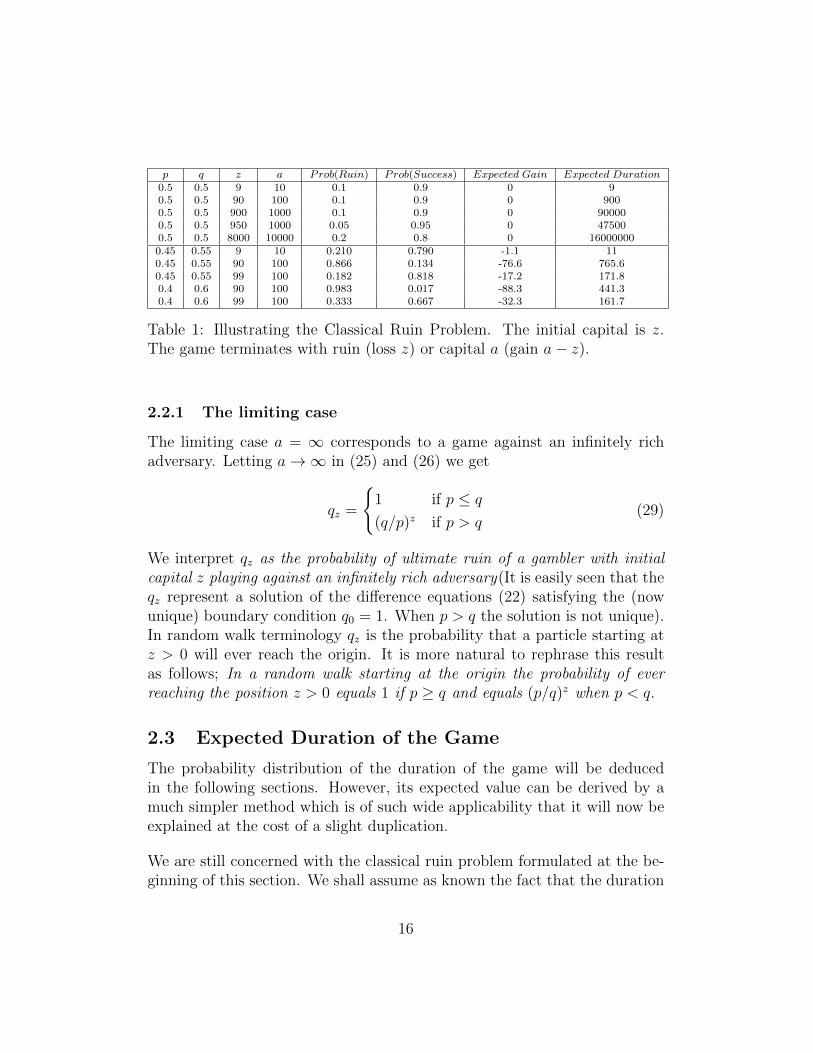
p q z a Prob(Ruin) Prob(Success) Expected Gain Expected Duration0.5 0.5 9 10 0.1 0.9 0 90.5 0.5 90 100 0.1 0.9 0 9000.5 0.5 900 1000 0.1 0.9 0 900000.5 0.5 950 1000 0.05 0.95 0 475000.5 0.5 8000 10000 0.2 0.8 0 160000000.45 0.55 9 10 0.210 0.790 -1.1 110.45 0.55 90 100 0.866 0.134 -76.6 765.60.45 0.55 99 100 0.182 0.818 -17.2 171.80.4 0.6 90 100 0.983 0.017 -88.3 441.30.4 0.6 99 100 0.333 0.667 -32.3 161.7

Table 1: Illustrating the Classical Ruin Problem. The initial capital is z.The game terminates with ruin (loss z) or capital a (gain a− z).

2.2.1 The limiting case

The limiting case a = ∞ corresponds to a game against an infinitely richadversary. Letting a→∞ in (25) and (26) we get

qz =

{1 if p ≤ q

(q/p)z if p > q(29)

We interpret qz as the probability of ultimate ruin of a gambler with initialcapital z playing against an infinitely rich adversary(It is easily seen that theqz represent a solution of the difference equations (22) satisfying the (nowunique) boundary condition q0 = 1. When p > q the solution is not unique).In random walk terminology qz is the probability that a particle starting atz > 0 will ever reach the origin. It is more natural to rephrase this resultas follows; In a random walk starting at the origin the probability of everreaching the position z > 0 equals 1 if p ≥ q and equals (p/q)z when p < q.

2.3 Expected Duration of the Game

The probability distribution of the duration of the game will be deducedin the following sections. However, its expected value can be derived by amuch simpler method which is of such wide applicability that it will now beexplained at the cost of a slight duplication.

We are still concerned with the classical ruin problem formulated at the be-ginning of this section. We shall assume as known the fact that the duration

16

of the game has a finite expectation Dz. A rigorous proof will be given in thenext section. If the first trial results in success the game continues as if theinitial position had been z + 1. The conditional expectation of the durationassuming success at the first trial is therefore Dz+1+1. This argument showsthat the expected duration Dz satisfies the difference equation

Dz = pDz+1 + qDz−1 + 1 , 0 < z < a (30)

with the boundary conditions

D0 = 0 , Da = 0 (31)

The appearance of the term 1 makes the difference equation (30) non-homogeneous.If p 6= q, then Dz = z/(q − p) is a formal solution of (30). The differ-ence ∆z of any two solutions of (30) satisfies the homogeneous equations∆z = p∆z+1 +q∆z−1, and we know already that all solutions of this equationare of the form A+B(q/p)z. It follows that when p 6= q all solutions of (30)are of the form

Dz =z

q − p+ A+B

(q

p

)z(32)

The boundary conditions (31) require that

A+B = 0 , A+B

(q

p

)q= − a

q − p

Solving for A and B, we find

Dz =z

q − p− a

q − p· 1− (q/p)z

1− (q/p)a(33)

Again the method breaks down if q = p = 12. In this case we replace z/(q−p)

by −z2, which is now a solution of (30). It follows that when q = p = 12

allsolutions of (30) are of the form Dz = −z2 +A+Bz. The required solutionDz satisfying the boundary conditions (31) is

Dz = z(a− z) (34)

The expected duration of the game in the classical ruin problem is given by(33) or (34), according as p 6= q or q = p = 1

2.

It should be noted that this duration is considerably longer than we would

17

naively expect. If two players with 500 dollars each toss a coin until one isruined, the average duration of the game is 250, 000 trials. If a gambler hasonly one dollar and his adversary 1000, the average duration is 1000 trials.Further examples are found in table 1.

As indicated at the end of the preceding section, we may pass to the limita → ∞ and consider a game against an infinitely rich adversary. Whenp > q the game may go on forever, and in this case it makes no sense to talkabout its expected duration. When p < q we get for the expected durationz(q − p)−1, but when p = q the expected duration is infinite. (The sameresult was established will be proved independently in the next section.)

2.4 Generating Functions for the Duration of the Gameand for the First-Passage Times

We shall use the method of generating functions to study the duration of thegame in the classical ruin problem, that is, the restricted random walk withabsorbing barriers at 0 and a. The initial position is z (with 0 < z < a).Let uz,n denote the probability that the process ends with the nth step at thebarrier 0 (gamblers ruin at the nth trial). After the first step the position isz + 1 or z − 1, and we conclude that for 1 < z < a− 1 and n ≥ 1

uz,n+1 = puz+1,n + quz−1,n (35)

This is a difference equation analogous to (22), but depending on the twovariables 2 and n. In analogy with the procedure of section 2.2 we wish todefine boundary values u0,n, ua,n, and uz,0 so that (35) becomes valid also forz = 1, z = a− 1, and n = 0. For this purpose we put

u0,n = ua,n = 0 when n ≥ 1 (36)

andu0,0 = 1 , uz,0 = 0 when 0 < z ≤ a (37)

Then (35) holds for all z with 0 < z < a and all n ≥ 0.

We now introduce the generating functions

Uz(s) =∞∑n=0

uz,nsn (38)

18

Multiplying (35) by sn+1 and adding for n = 0, 1, 2, ....., we find

Uz(s) = psUz+1(s) + qsUz−1(s) 0 < z < a (39)

the boundary conditions (36) and (37) lead to

U0(s) = 1 , Ua(s) = 0 (40)

The system (39) represents difference equations analogous to (22), and theboundary conditions (40) correspond to (23). The novelty lies in the cir-cumstance that the coefficients and the unknown Uz(s) now depend on thevariable s, but as far as the difference equation is concerned, s is merely anarbitrary constant. We can again apply the method of section 2.2 providedwe succeed in finding two particular solutions of (39). It is natural to inquirewhether there exist two solutions Uz(s) of the form Uz(s) = λz(s). Substi-tuting this expression into (39), we find that λ(s) must satisfy the quadraticequation

λ(s) = psλ2(s) + qs (41)

which has the two roots

λ1(s) =1 +

√1− 4pqs2

2ps, λ2(s) =

1−√

1− 4pqs2

2ps(42)

(we take 0 < s < 1 and the positive square root).

We are now in possession of two particular solutions of (39) and conclude asin section 2.2 that every solution is of the form

Uz(s) = A(s)λz1(s) +B(s)λz2(s) (43)

with A(s) and B(s) arbitrary. To satisfy the boundary conditions (40), wemust have A(s) +B(s) = 1 and A(s)λa1(s) +B(s)λa2(s) = 0, whence

Uz(s) =λa1(s)λ

z2(s)− λz1(s)λa2(s)λa1(s)− λa2(s)

(44)

Using the obvious relation λ1(s)λ2(s) = q/p, this simplifies to

Uz(s) =

(q

p

)zλa−z1 (s)− λa2(s)λa−z1 (s)− λa2(s)

(45)

19

This is the required generating function of the probability of ruin (absorptionat 0) at the nth trial. The same method shows that the generating functionfor the probabilities of absorption at a is given by

Uz(s) =λz1(s)− λz2(s)λa1(s)− λa2(s)

(46)

The generating function for the duration of the game is, of course, the sumof the generating functions (45) and (46).

2.4.1 Infinite Intervals and First Passages

The preceding considerations apply equally to random walks on the interval(0,∞) with an absorbing barrier at 0. A particle starting from the positionz > 0 is eventually absorbed at the origin or else the random walk continuesforever. Absorption corresponds to the ruin of a gambler with initial cap-ital z playing against an infinitely rich adversary. The generating functionUz(s) of the probabilities uz,n that absorption takes place exactly at the nth

trial satisfies again the difference equations (39) and is therefore of the form(43), but this solution is unbounded at infinity unless A(s) = 0. The otherboundary condition is now U0(s) = 1, and hence B(s) = 1 or

Uz(s) = λz2(s) (47)

[The same result can be obtained by letting a→∞ in (45), and rememberingthat λ1(s)λ2(s) = q/p.]

It follows from (47) for s = 1 that an ultimate absorption is certain if p ≤ q,and has probability (q/p)z otherwise. The same conclusion was reached insection 2.2.

Our absorption at the origin admits of an important alternative interpreta-tion as a first passage in an unrestricted random walk. Indeed, on movingthe origin to the position z it is seen that in a random walk on the entire lineand starting from the origin uz,n is the probability that the jirst visit to thepoint −z < 0 takes place at the nth trial. That the corresponding generatingfunction (47) is the zth power of λ2 reflects the obvious fact that the waitingtime for the first passage through −z is the sum of z independent waitingtimes between the successive first passages through −1,−2, ...,−z.

20

2.5 Explicit Expressions

The generating function Uz, of (45) depends formally on a square root but isactually a rational function. In fact, an application of the binomial theoremreduces the denominator to the form

λa1(s)− λa2(s) = s−a√

1− 4pqs2 Pa(s) (48)

where Pa is an even polynomial of degree a− 1 when a is odd, and of degreea − 2 when a is even. The numerator is of the same form except that a isreplaced by a−z. Thus Uz is the ratio of two polynomials whose degrees differat most by 1. Consequently it is possible to derive an explicit expression forthe ruin probabilities uz,n by the method of partial fractions. The result isinteresting because of its connection with diffusion theory, and the derivationas such provides an excellent illustration for the techniques involved in thepractical use of partial fractions.

The calculations simplify greatly by the use of an auxiliary variable φ definedby

cosφ =1

2√pq · s

(49)

(To 0 < s < 1 there correspond complex values of φ, but this has no effecton the formal calculations.) From (42)

λ1(s) =√q/p [cosφ+ i sinφ] =

√q/p eiφ (50)

while λ2(s) equals the right side with i replaced by −i. Accordingly,

Uz(s) = (√q/p)z

sin (a− z)φ

sin aφ(51)

The roots s1, s2, .... of the denominator are simple and hence there exists apartial fraction expansion of the form

(√q/p)z

sin (a− z)φ

sin aφ= A+Bs+

ρ1s1 − s

+ · · ·+ ρa−1sa−1 − s

(52)

In principle we should consider only the roots sv which are not roots of thenumerator also, but if sv is such a root then Uz(s) is continuous at s = svand hence ρv = 0. Such canceling roots therefore do not contribute to the

21

right side and hence it is not necessary to treat them separately.

The roots s1, s2, ......, sa−1 correspond obviously to φv = πv/a with v =1, ....., a− 1, and so

sv =1

2√pq cosπv/a

(53)

This expression makes no sense when v = a/2 and a is even, but then φvis a root of the numerator also and this root should be discarded. Thecorresponding term in the final result vanishes, as is proper.

To calculate ρv we multiply both sides in (52) by sv − s and let s → sv.Remembering that sin aφv = 0 and cos aφv = 1 we get

ρv = (√q/p)z sin zφv · lim

s→sv

s− svsin aφ

The last limit is determined by L’Hospital’s rule using implicit differentiationin (50). The result is

ρv = a−1 · 2√pq (√q/p)z sin zφv · sinφv · s2v

From the expansion of the right side in (53) into geometric series we get forn > 1

uz,n =a−1∑v=1

ρvs−n−1v = a−1 · 2√pq (

√q/p)z

a−1∑v=1

s−n+1v · sinφv · sin zφv

and hence finally

uz,n = a−12np(n−z)/2q(n+z)/2a−1∑v=1

cosn−1πv

asin

πv

asin

πzv

a(54)

This, then, is an explicit formula for the probability of ruin at the nth trial.It goes back to Lagrange and has been derived by classical authors in variousways, but it continues to be rediscovered in the modern literature.

Passing to the limit as a→∞ we get the probability that in a game againstan infinitely rich adversary a player with initial capital z will be ruined atthe nth trial.

22

A glance at the sum in (54) shows that the terms corresponding to thesummation indices v = k and v = a − k are of the same absolute value;they are of the same sign when n and z are of the same parity and cancelotherwise. Accordingly uz,n = 0 when n− z is odd while for even n− z andn > 1

uz,n = a−12n+1p(n−z)/2q(n+z)/2∑v<a/2

cosn−1πv

asin

πv

asin

πzv

a(55)

the summation extending over the positive integers < a/2. This form is morenatural than (54) because now the coefficients cos πv/a form a decreasingsequence and so for large n it is essentially only the first term that counts.

2.6 Connection with Diffusion Processes

This section is devoted to an informal discussion of random walks in whichthe length δ of the individual steps is small but the steps are spaced so closein time that the resultant change appears practically as a continuous motion.A passage to the limit leads to the Wiener process (Brownian motion) andother diffusion processes. The intimate connection between such processesand random walks greatly contributes to the understanding of both. Theproblem may be formulated in mathematical as well as in physical terms.

It is best to begin with an unrestricted random walk starting at the origin.The nth step takes the particle to the position Sn where Sn = X1 + · · ·+ Xn

is the sum of n independent random variables each assuming the values +1and −1 with probabilities p and q, respectively. Thus

E(Sn) = (p− q)n , V ar(Sn) = 4pqn (56)

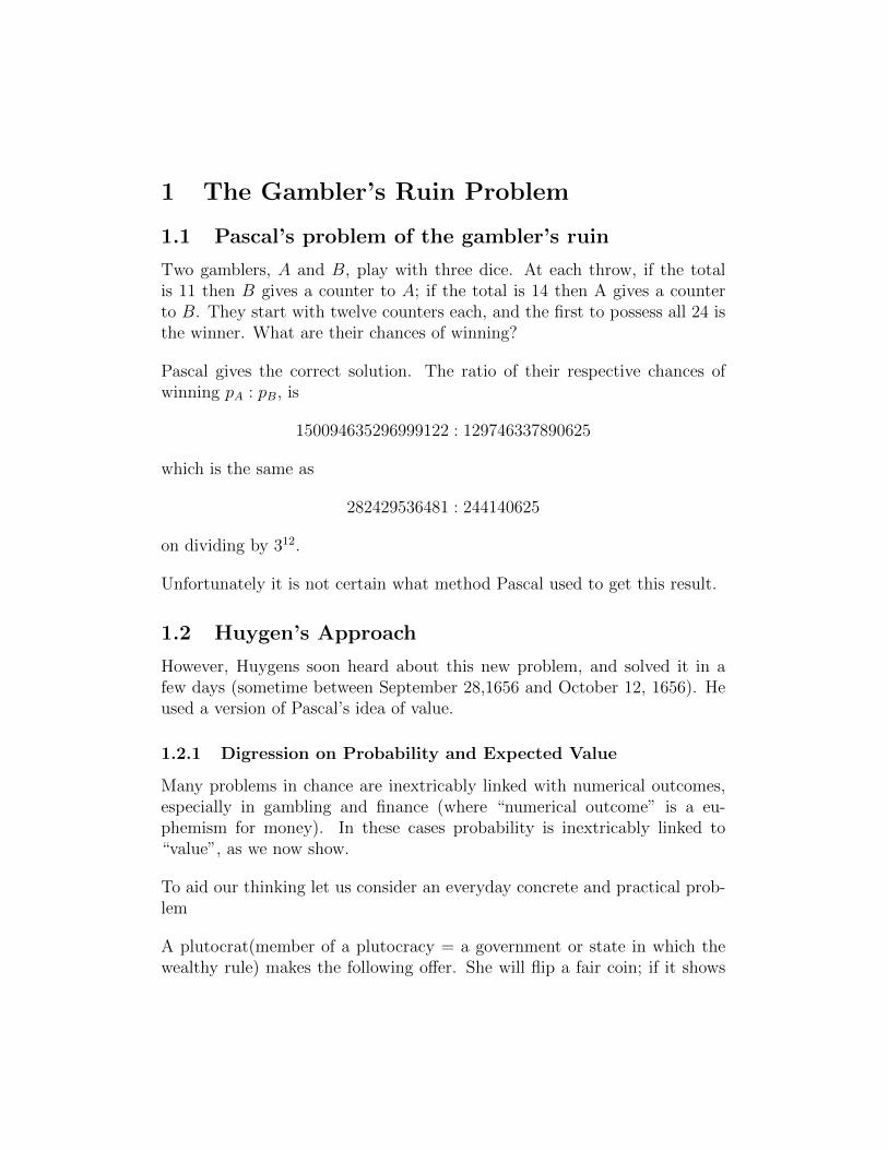
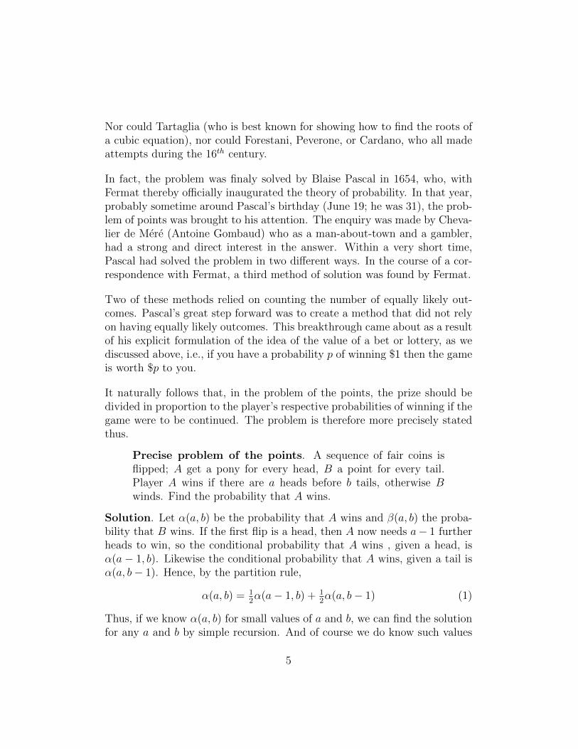
The figure below presents the first 10,000 steps of such a random walk withp = q = 1

2; to fit the graph to a printed page it was necessary to choose appro-

priate scales for the two axes. Let us now go a step further and contemplatea motion picture of the random walk. Suppose that it is to fake 1000 seconds(between 16 and 17 minutes). To present one million steps it is necessarythat the random walk proceeds at the rate of one step per millisecond, andthis fixes the time scale. What units are we to choose to be reasonably surethat the record will fit a screen of a given height?

23

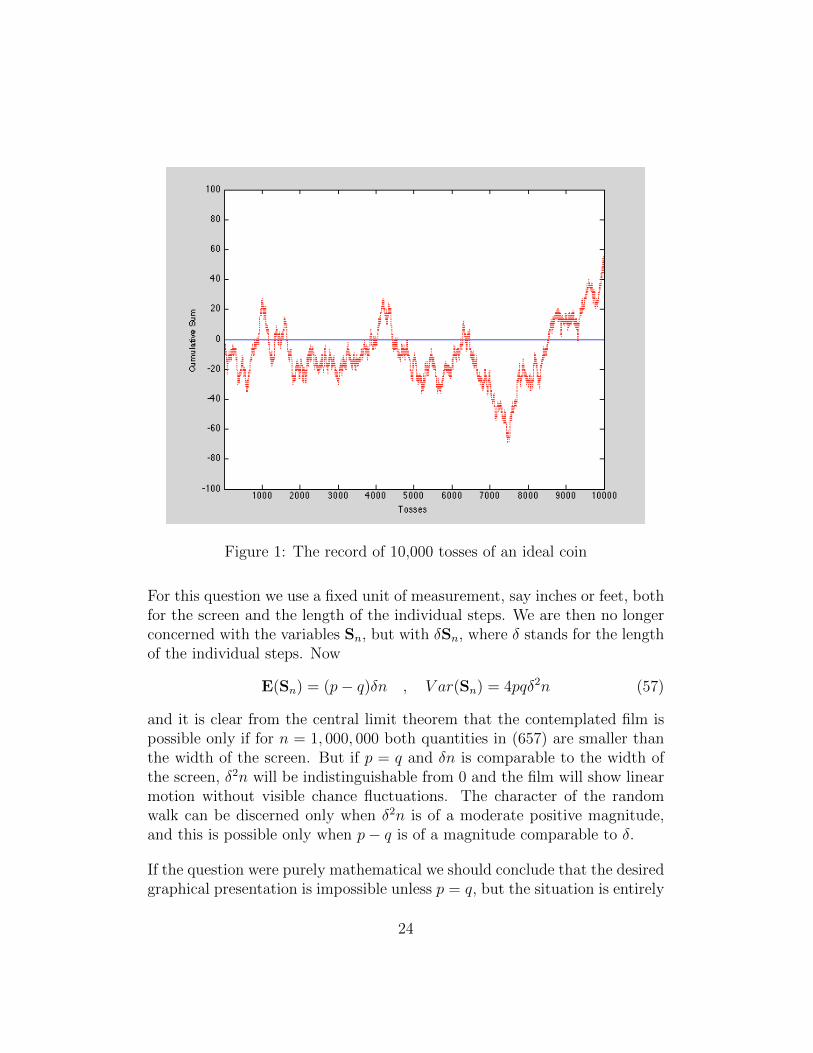
Figure 1: The record of 10,000 tosses of an ideal coin

For this question we use a fixed unit of measurement, say inches or feet, bothfor the screen and the length of the individual steps. We are then no longerconcerned with the variables Sn, but with δSn, where δ stands for the lengthof the individual steps. Now

E(Sn) = (p− q)δn , V ar(Sn) = 4pqδ2n (57)

and it is clear from the central limit theorem that the contemplated film ispossible only if for n = 1, 000, 000 both quantities in (657) are smaller thanthe width of the screen. But if p = q and δn is comparable to the width ofthe screen, δ2n will be indistinguishable from 0 and the film will show linearmotion without visible chance fluctuations. The character of the randomwalk can be discerned only when δ2n is of a moderate positive magnitude,and this is possible only when p− q is of a magnitude comparable to δ.

If the question were purely mathematical we should conclude that the desiredgraphical presentation is impossible unless p = q, but the situation is entirely

24

different when viewed from a physical point of view. In Brownian motionwe see particles suspended in a liquid moving in random fashion, and thequestion arises naturally whether the motion can be interpreted as the resultof a tremendous number of collisions with smaller particles in the liquid. Itis, of course, an over-simplification to assume that the collisions are spaceduniformly in time and that each collision causes a displacement preciselyequal to ;±δ. Anyhow, for a first orientation we treat the impacts as governedby the Bernoulli-type trials we have been discussing and ask whether theobserved motion of the particles is compatible with this picture. From actualobservations we find the average displacement c and the variance D for a unittime interval. Denote by r the (unknown) number of collisions per time unit.Then we must have, approximately,

(p− q)δr = c , 4pqδ2r = D (58)

In a simulated experiment no chance fluctuations would be observable un-less the two conditions (58) are satisfied with D > 0. An experiment withp = 0.6 and δr = 1 is imaginable, but in it the variance would be so smallthat the motion would appear deterministic: A clump of particles initiallyclose together would remain together as if it were a rigid body.

Essentially the same consideration applies to many other phenomena inphysics, economics, learning theory, evolution theory, etc., when slow fluctu-ations of the state of a system are interpreted as the result of a huge numberof successive small changes due to random impacts. The simple random-walkmodel does not appear realistic in any particular case, but fortunately thesituation is similar to that in the central limit theorem. Under surprisinglymild conditions the nature of the individual changes is not important, be-cause the observable effect depends only on their expectation and variance.In such circumstances it is natural to take the simple random-walk model asuniversal prototype.

To summarize, as a preparation for a more profound study of various stochas-tic processes it is natural to consider random walks in which the length δ ofthe individual steps is small, the number r of steps per time unit is large, andp − q is small, the balance being such that (58) holds (where c and D > 0are given constants). The words large and small are vague and must remainflexible for practical applications?(The number of molecular shocks per timeunit is beyond imagination. At the other extreme, in evolution theory one

25

considers small changes from one generation to the next, and the time sep-arating two generations is not small by everyday standards. The number ofgenerations considered is not fantastic either, but may go into many thou-sands. The point is that the process proceeds on a scale where the changesappear in practice continuous and a diffusion model with continuous timeis preferable to the random-walk model.) The analytical formulation of theproblem is as follows. To every choice of δ, r, and p there corresponds arandom walk. We ask what happens in the limit when δ → 0, r → ∞, andp→ 1

2in such a manner that,

(p− q)δr → c , 4pqδ2r → D (59)

The main procedure is to start from the difference equations governing therandom walks and the derivation of the limiting differential equations. Itturns out that these differential equations govern well defined stochastic pro-cesses depending on a continuous time parameter. The same is true of variousobvious generalizations of these differential equations, and so this methodleads to the important general class of diffusion processes.

We denote by {Sn} the standard random walk with unit steps and put

vk,n = P{Sn = k} (60)

In our random walk the nth step takes place at epoch n/r, and the positionis Snδ = kδ. We are interested in the probability of finding the particle at agiven epoch tin the neighborhood of a given point x, and so we must inves-tigate the asymptotic behavior of vk,n when k → ∞ and n → ∞ in such amanner that n/r → t and kd→ x. The event {Sn = k} requires that n andk be of the same parity and takes place when exactly (n + k)/2 among thefirst n steps lead to the right.

The approach based on the appropriate difference equations is very interest-ing. Considering the position of the particle at the nth and the (n+ 1)st trialit is obvious that the probabilities vk,n satisfy the difference equations

vk,n+1 = pvk−1,n + qvk+1,n (61)

Now vk,n is the probability of finding Snδ between kδ and (k + 2)δ, andsince the interval has length 2δ we can say that the ratio vk,n/(2δ) measureslocally the probability per unit length, that is the probability density and

26

vk,n/(2δ)→ v(t, x).

On multiplying by 2δ it follows that v(t, x) should be an approximate solutionof the difference equation

v(t+ r−1, x) = pv(t, x− δ) + qv(t, x+ δ) (62)

Since v has continuous derivatives we can expand the terms according toTaylor’s theorem. Using the first-order approximation on the left and second-order approximation on the right we get (after canceling the leading terms)

∂v(t, x)

∂t= (q − p)δr · ∂v(t, x)

∂x+

1

2δ2r

∂2v(t, x)

∂x2+ · · · (63)

In our passage to the limit the omitted terms tend to zero and (63) becomesin the limit

∂v(t, x)

∂t= −c∂v(t, x)

∂x+

1

2D∂2v(t, x)

∂x2(64)

This is a special diffusion equation also known as the Fokker-Planck equationfor diffusion. Now the function v given by

v(t, x) =1√

2πDte−

12(x−ct)2/Dt (65)

satisfies the differential equation (63). Furthermore, it can be shown that(64) represents the only solution of the diffusion equation having the prop-erties required by a probabilistic interpretation.

Thus, we have demonstrated some brief and heuristic indications of the con-nections between random walks and general diffusion theory.

As another example let take the ruin probabilities uz,n discussed earlier. Theunderlying difference equations (35) differ from (61) in that the coefficientsp and q are interchanged. The formal calculations indicated in (63) now leadto a diffusion equation obtained from (64) on replacing −c by c. Our limitingprocedure leads from the probabilities uz,n to a function u(t, ξ) which satisfiesthis modified diffusion equation and which has probabilistic significance sim-ilar to uz,n: In a diffusion process starting at the point ξ > 0 the probabilitythat the particle reaches the origin before reaching the point α > ξ and thatthis event occurs in the time interval t1 < t < t2 is given by the integral of

27

u(t, ξ) over this interval.

The formal calculations are as follows. For uz,n we have the explicit expres-sion (55). Since z and n must be of the same parity, uz,n corresponds to theinterval between n/r and (n+ 2)/r, and we have to calculate the limit of theratio uz,nr/2 when r → ∞ and δ → 0 in accordance with (59). The lengtha of the interval and the initial position z must be adjusted so as to obtainthe limits α and ξ. Thus z ∼ ξ/δ and a ∼ α/δ. It is now easy to find thelimits for the individual factors in (55).

From (59) we get 2p ∼ 1 + cδ/D, and

2q ∼ 1− cδ/D

From the second relation in (59) we see that δ2r → D. Therefore

(4pq)1/2(q/p)z/2 ∼ (1− c2δ2/D2)(rt)/2(1− 2cδ/D)ξ/(2δ)

∼ e−12t/D · e−cξ/D (66)

Similarly for fixed v(cos

vπδ

α

)n∼(

1− v2π2δ2

2α2

)tr∼ e−

12v2π2Dt/α2

(67)

Finally sin vπδ/α ∼ vπδ/α. Substitution into (55) leads formally to

u(t, ξ) = πDα−2e−12(ct+2ξ)c/D

∞∑v=1

ve−12v2π2Dt/α2

sinπξv

α(68)

(Since the series converges uniformly it is not difficult to justify the formalcalculations.) In physical diffusion theory (68) is known as Furth’s formulafor first passages.

28