
Ruin Theory
32
ELEMENTARY RUIN THEORY David Rechavel MAY 6, 2016 TOURO COLLEGE AND UNIVERSITY SYSTEM
-
Upload
david-rechavel -
Category
Documents
-
view
83 -
download
23
Transcript of Ruin Theory
0
ELEMENTARY RUIN
THEORY David Rechavel
MAY 6, 2016 TOURO COLLEGE AND UNIVERSITY SYSTEM

1
Contents Abstract ........................................................................................................................................... 2
Acknowledgements ......................................................................................................................... 2
1.The Concept of Ruin .................................................................................................................... 3
2. Basic Notation, Terminology, and Definitions ........................................................................... 4
3. The Aggregate Claims Process for Continuous Time ................................................................. 7
4. The Adjustment Coefficient, R ............................................................................................ 11
5. The Probability of Ruin, ψ(u) ................................................................................................... 15
6. Proof of Theorem 5.1 ................................................................................................................ 20
7. More General Expressions of 𝜓𝑢 ........................................................................................... 27
8. Further Reading ........................................................................................................................ 29
Works Cited .................................................................................................................................. 31

2
Abstract
The primary goal of this paper is to present the material covered in sections 13.1, 13.3,
and 13.4 of Actuarial Mathematics by Bowers, Gerber, Hickman, Jones, and Nesbitt in a more
thorough and easy-to-read manner than it is presented therein. The main topics of these sections
are the continuous-time surplus model, the adjustment coefficient, and one way of expressing the
probability of ruin, which has an exact solution for exponential claims, and in other cases results
in Lundberg’s bound. The paper will also briefly discuss some more general expressions of the
probability of ruin, and several further developments of the topic.
Acknowledgements
Thank you to Dr. Basil Rabinowitz for aiding me on this project and pointing me to the
right sources.
Thank you to Dr. Baili Min for helping me with some of the intermediary steps in some
derivations and proofs.

3
1. The Concept of Ruin1
Every business involves risks. Revenues and expenses may not always be easily
predictable, and may be highly volatile; therefore it makes sense to have tools to be able to
manage the uncertainty. This is the premise of Risk Theory, the study of how results deviate
from their expected values, and how to prevent undesirable results. More specifically, Risk
Theory attempts to model cash flows as a surplus process, a function describing how much
money the firm has at a given time (Bowers et al., 2010, XX). Of course, some types of cash
flows are easily predictable and can therefore be modeled with great precision; others, though,
are more random and are thus harder to predict.
In the specific case of an insurance company,2 the most important cash flows are of
course premiums and claims, which together form the company’s surplus. In reality, many more
factors would have to be considered to get a “full picture” – interest, dividends, taxes, etc. – but
these can be adjusted for after the basic models have been developed. This paper will focus just
on building the basic models.
One of the worst events that could happen to an insurance company is called ruin,
defined as the company’s surplus becoming negative; in other words, the collected premiums
don’t cover the customers’ claim payments. An interesting and useful question, then, is how
likely ruin is to occur, and if it happens, how severe will the deficit be? These questions provide
the basis for a specific branch of Risk Theory called Ruin Theory, the most developed modeling
theory specific to the insurance industry (Bowers et al., 2010, XX). The probability of ruin can
1 This and the next section follow section 13.1 of Actuarial Mathematics. 2 Everything in this paper would be relevant not only to a company, but also to an individual
insurance portfolio. Throughout the paper, “company” and “portfolio” are used indiscriminately.

4
be a useful signal of the company’s health in general, but more specifically, two major
applications are to reserves and reinsurance. Reserves have to do with how much cash the
company needs to have on hand to be able to meet its claim liabilities; ruin theory aids these
calculations by describing the possible results of different initial surplus conditions, i.e. what
could happen when reserves are kept at different levels. Reinsurance is the business of insuring
insurance products; clearly, a reinsurer would want to know about the riskiness of the insurance
product being reinsured, which ruin theory sheds light on.
Asmussen and Albrecher note in the preface to their book Ruin Probabilities that in
practice, simpler – but weaker - measures of risk are typically used, due to their simplicity. But
the principles of Ruin Theory still provide powerful insight into risk management and the risk
structure of insurance companies, and some results of ruin theory can be fundamental to certain
problems.
2. Basic Notation, Terminology, and Definitions
While the concept of ruin probability is simple, figuring out how to calculate it is tricky
and involves a lot of variables and notations. To make this paper easier to read, many of the
commonly used symbols have been colored.
Before we move on to discussing ruin probability, let’s start with some basic definitions.
First, we need to introduce the concept of a stochastic process. When a system develops in a non-
random manner – like insurance premiums being collected at a known rate3 - it is called a
deterministic process. For any time, we can predict with a high level of accuracy exactly how
3 As a general rule, all of the literature on ruin theory assumes a constant linear rate of premium
collection, claiming that in the real world this is generally true.

5
much money has been collected as premiums. When, though, a system evolves randomly,
representing a collection of random variables over time – like insurance claims building up - it is
called a stochastic process. The size and number of claims are random, and we will assume that
they are identically distributed as well as independent.
Now we can better describe the surplus process. As mentioned above, the surplus of an
insurance company is a sum of three basic components: aggregate premiums, aggregate claims,
and the initial surplus. Aggregate premiums can be represented as a simple linear model over
time, c(t), while aggregate claims can be viewed as a stochastic process, which we call S(t). The
initial surplus is a constant, u. Altogether, we can then write the surplus process, represented by
U(t), as
𝑈(𝑡) = 𝑢 + 𝑐(𝑡) − 𝑆(𝑡) . (2.1)
To visualize this model, we can think of a straight line starting at u at time zero and
increasing at a rate of c, representing the collection of premiums. Claims are represented by
negative jumps of random sizes at random times.
Figure 2.1, A Typical Outcome of S(t)

6
As can be seen, the surplus undergoes periods of growth interrupted by sudden jumps
downwards. The surplus drops below its initial level three times before finally becoming
negative at T, the time of ruin. We can now give more formal definitions of the time and
probability of ruin.
Definition 2.1: The time of ruin, T, is the first time that the Aggregate Surplus becomes
negative.
𝑇 ∶= min { 𝑡 ∶ 𝑡 ≥ 0 ∩ 𝑈(𝑡) < 0 }
Note that 𝑇 = ∞ implies that ruin never happens. This property leads to
Definition 2.2: The probability of ruin, ψ(u), is the probability that ruin will happen, i.e. that
T ≠ 0 .
𝜓(𝑢) ∶= Pr ( 𝑇 < ∞ )
Although using finite time would more accurately represent the reality of the business
world, it will become clear later on that that many of Ruin Theory’s major results are possible
only because of simplifications that derive from using specifically infinite time. Without these
simplifications, the formulas would be too complicated and ambiguous to be useful. In any case,
using infinite time is not very problematic since Pr ( T < ∞ ) is just the upper bound of Pr ( T <
𝑡 ). Note that 𝜓 is expressed as a function of u, since the probability of ruin clearly depends on
how big the initial surplus is.
Now that we have the basic concepts and definitions, we can start moving towards a
formula for the probability of ruin.

7
3. The Aggregate Claims Process for Continuous
Time4
In order to define an expression for the probability of ruin, we have to decide whether to
express time continuously or discretely. Each way of looking at 𝜓(𝑢) has relevant and practical
applications: a discrete model would be useful in a situation in which information is gathered or
analyzed periodically - like for an annual report. For a more general perspective, though, a
continuous model would suffice. This paper will focus on the continuous model.
The only part of U(t) that requires further analysis is S(t), since c(t) is just a simple linear
model, and 𝑢 is just a constant. Let’s remember that S(t) is a collection of individual claim-size
random variables. But the number of claims itself is unknown; it itself is a random variable
representing how many claims will be made until and including the claim that ultimately causes
ruin. We can refer to the number of claims as a process N(t) such that
𝑆(𝑡) = 𝑥1 + 𝑥2 + ⋯ + 𝑥𝑁(𝑡)−1 + 𝑥𝑁(𝑡) .
We can now think of these two processes happening simultaneously: N(t) jumps up by
one at random times 𝑡𝑖 when claims are made, and S(t), the aggregate claims, jumps up randomly
by the size of the claim 𝑥𝑖 at each 𝑡𝑖. We can see this in the below figure.
4 This section follows section 13.3 of Actuarial Mathematics.
8
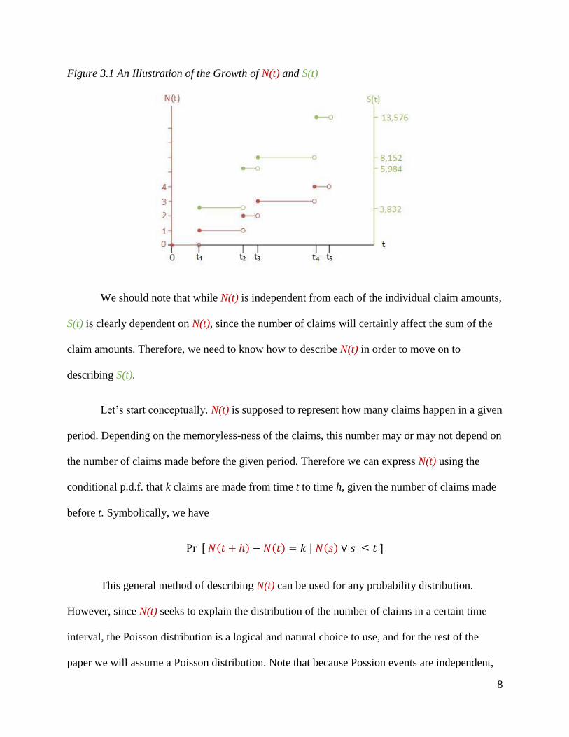
Figure 3.1 An Illustration of the Growth of N(t) and S(t)
We should note that while N(t) is independent from each of the individual claim amounts,
S(t) is clearly dependent on N(t), since the number of claims will certainly affect the sum of the
claim amounts. Therefore, we need to know how to describe N(t) in order to move on to
describing S(t).
Let’s start conceptually. N(t) is supposed to represent how many claims happen in a given
period. Depending on the memoryless-ness of the claims, this number may or may not depend on
the number of claims made before the given period. Therefore we can express N(t) using the
conditional p.d.f. that k claims are made from time t to time h, given the number of claims made
before t. Symbolically, we have
Pr [ 𝑁(𝑡 + ℎ) − 𝑁(𝑡) = 𝑘 | 𝑁(𝑠) ∀ 𝑠 ≤ 𝑡 ]
This general method of describing N(t) can be used for any probability distribution.
However, since N(t) seeks to explain the distribution of the number of claims in a certain time
interval, the Poisson distribution is a logical and natural choice to use, and for the rest of the
paper we will assume a Poisson distribution. Note that because Possion events are independent,

9
the condition of knowledge of previous claims is irrelevant. The desired probability simply
follows the p.d.f. of an individual Poisson distributed random variable with parameter 𝜆ℎ, as
follows.
Pr [ 𝑁(𝑡 + ℎ) − 𝑁(𝑡) = 𝑘 | 𝑁(𝑠) ∀ 𝑠 ≤ 𝑡 ] =
𝑒−𝜆ℎ(𝜆ℎ)𝑘
𝑘!
(3.1)
Now that we have exactly defined N(t), we can move on to expressing S(t). We see that if
N(t) is a Poisson process, S(t) is then a Compound Poisson process, meaning a stochastic process
with randomly-sized jumps that arrive according to a Poisson process. In other words, for each
claim 𝑥𝑖, S(t) jumps up by the size of 𝑥𝑖, where the 𝑥𝑖’s are identically distributed, independent
random variables, and the total number of 𝑥𝑖’s obeys a Poisson distribution. Refer back to figure
3.1 for an illustration of this.
Although more can be done to analyze S(t), what is pertinent to this paper is to express
the expected value and variance of S(t), which will be required in order to express 𝜓(𝑢). For
simplicity, we will express the expected individual claim size as 𝑝1, and the expected squared
individual claim size as 𝑝2.
To derive 𝐸[𝑆], we recall that 𝐸[𝑁] = 𝑉𝑎𝑟[𝑁] = 𝜆𝑡 (considering a time interval from 0
to t rather than t to h), and apply the identity
𝐸[𝑆] = 𝐸( 𝐸[𝑆|𝑁] )
= 𝐸 [ ∑(𝑆) Pr(𝑆 ∩ 𝑁)
Pr(𝑁)𝑆
]
= ∑ ∑ (𝑆) Pr(𝑆 ∩ 𝑁)
Pr(𝑁)𝑆
𝑁
[ Pr(𝑁) ]

10
= ∑ ∑ (𝑆) Pr(𝑆)
𝑆𝑁
[ Pr(𝑁)]
= ∑ Pr(𝑁) 𝐸[𝑆]
𝑁
= ∑ Pr(𝑁) 𝐸 [ ∑ 𝑥𝑖
𝑁
𝑖=1
]
𝑁
= ∑ Pr(𝑁) (𝑁)𝐸[𝑥𝑖]
𝑁
= 𝐸[𝑥𝑖] 𝐸[𝑁]
= 𝑝1𝐸[𝑁]
𝐸[𝑆] = 𝜆 𝑡 𝑝1 (3.2)
Similarly, to derive variance we begin with
𝑉𝑎𝑟[𝑆] = 𝐸[ 𝑉𝑎𝑟(𝑆|𝑁) ] + 𝑉𝑎𝑟[ 𝐸(𝑆|𝑁) ]
where
𝐸(𝑆|𝑁) = 𝐸 [ (∑ 𝑥𝑖 )
𝑁
𝑖=1
| 𝑁 ]
= 𝑁 𝐸[ 𝑥𝑖|𝑁 ]
= 𝑁 𝑝1
and
𝑉𝑎𝑟( 𝑆|𝑁 ) = 𝑉𝑎𝑟[𝑥1 + 𝑥2 + ⋯ + 𝑥𝑁 | 𝑁 ]
= 𝑁 𝑉𝑎𝑟[𝑥]
11
= 𝑁 ( 𝑝2 − 𝑝12 )
Plugging in, this yields
𝑉𝑎𝑟[𝑆] = 𝐸[ 𝑁 ( 𝑝2 − 𝑝12 ) ] + 𝑉𝑎𝑟[𝑁 𝑝1 ]
= 𝐸[𝑁] ( 𝑝2 − 𝑝12 ) + 𝑉𝑎𝑟[𝑁] 𝑝1
2
= 𝜆 𝑡 ( 𝑝2 − 𝑝12 + 𝑝1
2 )
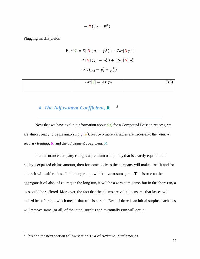
𝑉𝑎𝑟[𝑆] = 𝜆 𝑡 𝑝2 (3.3)
4. The Adjustment Coefficient, R 5
Now that we have explicit information about S(t) for a Compound Poisson process, we
are almost ready to begin analyzing 𝜓(𝑢). Just two more variables are necessary: the relative
security loading, 𝜃, and the adjustment coefficient, R.
If an insurance company charges a premium on a policy that is exactly equal to that
policy’s expected claims amount, then for some policies the company will make a profit and for
others it will suffer a loss. In the long run, it will be a zero-sum game. This is true on the
aggregate level also, of course; in the long run, it will be a zero-sum game, but in the short-run, a
loss could be suffered. Moreover, the fact that the claims are volatile ensures that losses will
indeed be suffered – which means that ruin is certain. Even if there is an initial surplus, each loss
will remove some (or all) of the initial surplus and eventually ruin will occur.
5 This and the next section follow section 13.4 of Actuarial Mathematics.

12
Obviously, firms want to prevent this from happening, so they reduce the probability of
suffering a loss by charging premiums that are larger than the expected claims. The “extra
premium” is split proportionally across all their policies, based on each policy’s expected claims
amount. This proportion is called the relative security loading, 𝜃; if a policy’s expected claims
are $100, the premium will be $(1 + 𝜃)100. Looking at the company as a whole, its total
collected premiums in one unit of time are then
𝑐 = (1 + 𝜃) 𝜆 𝑝1 (4.1)
𝜃 appears in many formulas in ruin theory, since it allows for a comparison between
claims and premiums. Note that, as explained above, if 𝜃 ≤ 0, ruin has a probability of one; the
volatility of claims ensures that ruin will happen. Therefore we assume a positive 𝜃, so that we
can write
𝑐 > 𝜆 𝑝1 . (4.2)
The adjustment coefficient R is a purely mathematical concept that that has no conceptual
meaning; nevertheless, we will see that it is essential to expressing 𝜓(𝑢), and because of its
relationship to 𝜓(𝑢), it itself is a good indicator of a company’s risk. Also, it can be calculated
explicitly for most claims distributions.6
Definition 4.1: Let (−∞, 𝛾) represent the largest open interval such that 𝑀𝑥(𝑟), the m.g.f. of
6 However, Bowers 410 points out that for some distributions R does not exist, as with, for
example, the inverse Gaussian distribution. This property will be demonstrated later on.

13
the individual claim distribution, exists. If 𝑀𝑥(𝑟) approaches infinity as r
approaches 𝛾,7 then the Adjustment Coefficient R is defined as the smallest
positive root of
𝑟 𝑐 = 𝜆 ( 𝑀𝑥(𝑟) − 1 )
For now this definition seems entirely random, but the importance of this choice of r will
become apparent in the proof of Theorem 6.1 later on. Substituting in from equation (4.1), we
have
𝑟 𝜆 𝑝1 (1 + 𝜃) = 𝜆 ( 𝑀𝑥(𝑟) − 1 )
1 + 𝑟 𝑝1 (1 + 𝜃) = 𝑀𝑥(𝑟) (4.3)
R is simply the smallest positive solution of this equation. All that needs to be known to
calculate it is the mean claim size, the distribution of claims, and the relative security loading.
We can represent R graphically by taking into account the following considerations: The
left-hand side is a positive-sloped linear function of r, and the right-hand side is also positively
sloped as long as it exists, as assumed in the definition. Also, we know that the right-hand side is
concave up, since its second derivative – the second central moment – must be positive.
In terms of the intersections of the two functions, we see that at r = 0, the left-hand side
becomes 1, and the right-hand side becomes 𝑀𝑥(0) = 1 as well. This means that one intersection
is at r = 0 (but this is not R, which must be positive by definition). Finally, we note that the
slope of the left-hand side at r = 0 is 𝑝1 (1 + 𝜃), which is greater than the slope of 𝑀𝑥(𝑟) at r =
7 as is typically the case

14
0, which is just 𝑝1, the first moment of x. Putting all of these facts together, it must follow that
the two curves obey the following general shape, with R represented as the non-zero intersection:
Figure 4.1 A Graphical Representation of R
Note that as 𝜃 increases, the slope of the line becomes steeper, but 𝑀𝑥(𝑟) is unaffected,
resulting in a larger R. In other words, charging more “extra premium” on an insurance portfolio,
results in a higher adjustment coefficient. The importance of this property will be explained later.
It must be noted that in some cases R does not exist. Based on Figure 4.1, this can be
visualized: if 𝛾 (the upper bound of the interval for which 𝑀𝑥(𝑟) exists and is increasing) is such
that 𝑀𝑥(𝑟) ceases to exist before it intersects with the line, then R will not exist. One example of
this is the inverse Gaussian distribution, which Bowers et al discuss in detail.
Bowers et al work through several examples of how to calculate R. An especially
important one is in the case of an exponential distribution with parameter 𝑝1 = 1
𝛽> 0.

15
We know that the m.g.f. of such an exponential distribution is 𝛽
𝛽−𝑟 , so using (4.3) we
obtain
1 +(1 + 𝜃)𝑟
𝛽=
𝛽
𝛽 − 𝑟
𝛽 − 𝑟 + (𝛽 − 𝑟)(1 + 𝜃)𝑟
𝛽= 𝛽
−𝑟 + (𝛽 − 𝑟)(1 + 𝜃)𝑟
𝛽= 0
−𝑟 + (1 + 𝜃)𝑟 − 𝑟(1 + 𝜃)𝑟
𝛽= 0
𝜃𝑟 = 𝑟(1 + 𝜃)𝑟
𝛽
𝑅 =𝜃𝛽
(1 + 𝜃)
Another interesting implication of equation (4.3) is that when 𝜃 approaches zero,
R also approaches zero. This can be observed from Figure 4.1: the slope of 1 + 𝑟 𝑝1 (1 + 𝜃) is
𝑝1 (1 + 𝜃), which approaches 𝑝1 as 𝜃 approaches zero. But at 𝑟 = 0, 𝑝1 is also the slope of
𝑀𝑥(𝑟)! This implies that the amount that 𝑀𝑥(𝑟) “dips” below the line becomes trivial as 𝜃 goes
to zero, which means that R must also approach zero.
5. The Probability of Ruin, ψ(u)
Finally, we have all of the necessary concepts and variables to be able to express our first
expression for ψ(u).

16
Theorem
5.18
𝜓(𝑢) = 𝑒−𝑅 𝑢
𝐸[ 𝑒−𝑅 𝑈(𝑇 ) | 𝑇 < ∞ ]
This theorem will be proved shortly, but first let’s make some observations about it. First
off, it was just explained that as 𝜃 goes to zero, R also goes to zero. Plugging this limit into
Theorem 5.1, we observe that 𝜓(𝑢) is one when θ is zero. This agrees with what was intuitively
explained earlier in the beginning of Section 4, that when the relative security loading is zero –
i.e. the company seeks a “zero sum game” between claims and premiums and therefore does not
collect “extra” claims - ruin is 100% certain at some point in the future.
Secondly, evaluating the denominator of this formula is quite complicated, since
evaluating the expected value of U(T), the surplus immediately after ruin, would require the joint
p.d.f. of 𝑇 and 𝑈(𝑇), which is beyond the scope of this paper.9 We will see shortly, though, that
for exponential claims the evaluation is straightforward. In any case, we can simplify the formula
by noting that U(T) is always negative, by definition. This means that the denominator is always
greater than one, so we can the theorem simplifies to
𝜓(𝑢) < 𝑒−𝑅 𝑢
This simple expression, known as Lundberg’s10 Bound, is one of the most profound and
useful in all of Ruin Theory, since all it involves is u – a known constant - and a simple
8 This is Theorem 13.4.1 in Actuarial Mathematics, 413. 9 Gerber and Shiu present methods of evaluating this p.d.f. See Section 8 - Further Reading. 10 Filip Lundberg, a Swedish actuary, provided the theoretical basis of Ruin Theory in his 1903
doctoral thesis “Approximations of the Probability Function/Reinsurance of Collective Risks.” In
the words of Harold Cramér, who republished the paper in 1930, “Filip Lundberg's works on risk
theory were all written at a time when no general theory of stochastic processes existed, and
when collective reinsurance methods, in the present day sense of the word, were entirely
unknown to insurance companies. In both respects his ideas were far ahead of his time, and his

17
calculation of R. A convenient implication of Lundberg’s bound is that 𝜓(𝑢) can be minimized
by maximizing 𝑅. This property is of vital importance in the reinsurance world, where a primary
goal is to minimize 𝜓(𝑢).
Likewise, we can now understand the positive relationship between R and 𝜃: when a
company charges more “extra premium”, this gives the company more financial security, and as
we should expect, this means a higher R. On the other hand, when a company charges no “extra
premium” (𝜃 = 0), then ruin is certain (𝜓(𝑢) = 1) and 𝑅 = 0. To summarize, Lundberg’s bound
demonstrates that 𝑅 is a strong and relatively tractable indicator of an insurance portfolio’s
security.
Also, in the case of exponentially distributed claims, the denominator of Theorem 5.1 can
in fact be evaluated easily: we proceed with the example used previously of exponentially
distributed claims with parameter 1
𝛽 .
The goal is to evaluate the denominator,
𝐸[ e −𝑅 𝑈(𝑇 ) | 𝑇 < ∞ ] = ∫ 𝑃𝑟 [ 𝑈(𝑇 ) = 𝑦 | 𝑇 < ∞ ] 𝑒−𝑅 𝑦 𝑑𝑦
∞
0
(5.1)
As mentioned above, we need to find the p.d.f. of U(T). To this end, we introduce a new
variable û, the surplus just before the time of ruin. If we let x denote the claim that causes ruin,
then û – x = U(T). Then U(T) < y means û – x < y, and finally x > û - y = û + | y |. (Note that y
is negative.) In words, this means that if the surplus at ruin is less than y, then the final claim that
works deserve to be generally recognized as pioneering works of fundamental importance.”
(From the abstract of “Historical Review of Filip Lundberg's Works on Risk Theory”)

18
causes ruin must be large enough to “undo” the ruin just before T - to bring the surplus to zero -
and then to bring the surplus below y. This gives us
𝑃𝑟[ 𝑈(𝑇) < 𝑦 | 𝑇 < ∞ ] = 𝑃𝑟[ 𝑥 > û − 𝑦 | 𝑥 > û ]
= 𝛽 ∫ 𝑒−𝛽 𝑥∞
û −𝑦𝑑𝑥
𝛽 ∫ 𝑒−𝛽 𝑥∞
û 𝑑𝑥
= 𝑒−𝛽 𝑥|û −y
∞
𝑒−𝛽 𝑥|û∞
= 𝑒−𝛽 ( û −y )
𝑒−𝛽 ( û )
= 𝑒 𝛽 𝑦
This is the probability that x is greater than û - y; to form a proper c.d.f., we need the
probability that x is less than û - y, which is 1 - 𝑒 𝛽 𝑦. The desired p.d.f. is then just the derivative
of this result.
𝑃𝑟 [ 𝑈(𝑇 ) = 𝑦 | 𝑇 < ∞ ] = −𝛽 𝑒𝛽 𝑦
Plugging this result back into equation (5.1), we obtain
𝐸[ e−𝑅 𝑈(𝑇 ) | 𝑇 < ∞ ] = ∫ −𝛽 𝑒𝛽 𝑦 𝑒−𝑅 𝑦 𝑑𝑦
∞
0
= −𝛽 ∫ 𝑒− 𝑦 (𝑅−𝛽 ) 𝑑𝑦
∞
0
= ( 𝛽
𝑅 − 𝛽 ) 𝑒− 𝑦 ( 𝑅−𝛽 ) |𝑦= 0
∞
= ( 𝛽
𝛽 − 𝑅 )

19
Plugging this back in for the denominator of Theorem 5.1 yields
𝜓(𝑢) = ( 𝛽 − 𝑅 ) e−𝑅 𝑢
𝛽
But this can be simplified further; we saw earlier that for exponentially distributed
claims, 𝑅 =𝜃𝛽
(1+𝜃) . Then
𝜓(𝑢) = ( 𝛽 −
𝜃𝛽
(1+𝜃)) e
−𝜃𝛽
(1+𝜃)𝑢
𝛽
= ( 1 −𝜃
(1 + 𝜃) ) e
−𝜃𝛽
(1+𝜃)𝑢
𝜓(𝑢) = ( 1
1 + 𝜃 ) 𝑒
− 𝜃 𝑢
(1+𝜃) 𝑝1
This is a remarkable result. For identical, exponentially distributed claims, the probability
of ruin depends on only three simple and known factors: the relative security loading, the mean
claim size, and the initial surplus. Additionally, if 𝑢 = 0,
𝜓(0) = (
1
1 + 𝜃 )
(5.2)
which is even more remarkable; the probability of ruin depends only on the relative security
loading. It can actually be shown that (5.2) is true for every distribution, as will be discussed in
Section 7.
20
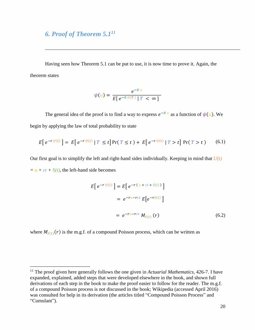
6. Proof of Theorem 5.111
Having seen how Theorem 5.1 can be put to use, it is now time to prove it. Again, the
theorem states
𝜓(𝑢) = 𝑒−𝑅 𝑢
𝐸[ 𝑒−𝑅 𝑈(𝑇 ) | 𝑇 < ∞ ]
The general idea of the proof is to find a way to express 𝑒−𝑅 𝑢 as a function of 𝜓(𝑢). We
begin by applying the law of total probability to state
𝐸[ 𝑒−𝑟 𝑈(𝑡) ] = 𝐸[ 𝑒−𝑟 𝑈(𝑡) | 𝑇 ≤ 𝑡] Pr( 𝑇 ≤ 𝑡 ) + 𝐸[ 𝑒−𝑟 𝑈(𝑡) | 𝑇 > 𝑡] Pr( 𝑇 > 𝑡 ) (6.1)
Our first goal is to simplify the left and right-hand sides individually. Keeping in mind that U(t)
= u + ct + S(t), the left-hand side becomes
𝐸[ 𝑒−𝑟 𝑈(𝑡) ] = 𝐸[ 𝑒−𝑟 ( 𝑢 + 𝑐𝑡 + 𝑆(𝑡) ) ]
= 𝑒−𝑟𝑢−𝑟𝑐𝑡 𝐸[𝑒−𝑟𝑆(𝑡) ]
= 𝑒−𝑟𝑢−𝑟𝑐𝑡 𝑀𝑆(𝑡) (𝑟) (6.2)
where 𝑀𝑆(𝑡)(𝑟) is the m.g.f. of a compound Poisson process, which can be written as
11 The proof given here generally follows the one given in Actuarial Mathematics, 426-7. I have
expanded, explained, added steps that were developed elsewhere in the book, and shown full
derivations of each step in the book to make the proof easier to follow for the reader. The m.g.f.
of a compound Poisson process is not discussed in the book; Wikipedia (accessed April 2016)
was consulted for help in its derivation (the articles titled “Compound Poisson Process” and
“Cumulant”).

21
𝑀𝑆(𝑡)(𝑟) = ∫ 𝑒𝑆 𝑟 𝑓(𝑆 = 𝑠) 𝑑(𝑆)
𝑆
= ∫ ∫ 𝑒𝑆 𝑟 𝑓 ( 𝑆 = 𝑠 | 𝑁 = 𝑛 ) 𝑓( 𝑁 = 𝑛 ) 𝑑(𝑁) 𝑑(𝑆)
𝑁𝑆
= ∫ 𝑓( 𝑁 = 𝑛 )
𝑛
∫ 𝑒𝑆 𝑟 𝑓 ( 𝑆 = 𝑠 | 𝑁 = 𝑛 )
𝑠
𝑑𝑠 𝑑𝑛
= ∫ 𝑓( 𝑁 = 𝑛 ) ∫ 𝑒(∑ 𝑥𝑖) 𝑟 𝑓 ( ∑ 𝑥𝑖 = 𝑠
𝑛
𝑖=1
)
𝑠
𝑑𝑠
𝑛
𝑑𝑛
= ∫ 𝑓( 𝑁 = 𝑛 ) ( 𝑀𝑥(𝑟) ) 𝑛 𝑑𝑛
𝑛
= ∫ 𝑓( 𝑁 = 𝑛 ) 𝑒𝑛 ln 𝑀𝑥(𝑟) 𝑑𝑛
𝑛
= 𝑀𝑁 (ln 𝑀𝑥(𝑟))
= 𝐸[ 𝑒𝑁 ln 𝑀𝑥(𝑟) ]
= 𝑒𝜆 𝑡 ln 𝑀𝑥(𝑟)
But ln 𝑀𝑥(𝑟) is known as the cumulant generating function, and it is equal to 𝑀𝑥(𝑟) − 1.
So finally we have
𝑀𝑆(𝑡) (𝑟) = 𝑒𝜆 𝑡 ( 𝑀𝑥(𝑟) − 1 ) (6.3)
Plugging this back into (6.2) yields
𝐸[ 𝑒−𝑟 𝑈(𝑡) ] = 𝑒−𝑟𝑢−𝑟𝑐𝑡+ 𝜆𝑡 ( 𝑀𝑥(𝑟) − 1 ) (6.4)
22
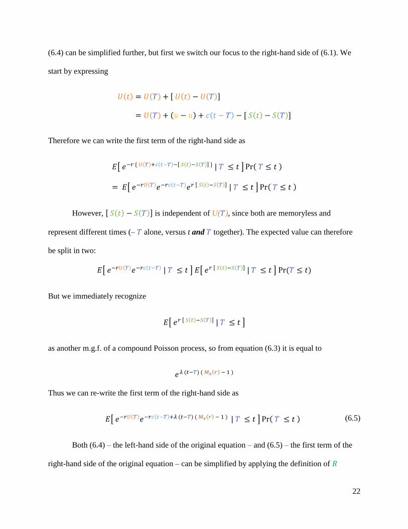
(6.4) can be simplified further, but first we switch our focus to the right-hand side of (6.1). We
start by expressing
𝑈(𝑡) = 𝑈(𝑇) + [ 𝑈(𝑡) − 𝑈(𝑇)]
= 𝑈(𝑇) + (𝑢 − 𝑢) + 𝑐(𝑡 − 𝑇) − [ 𝑆(𝑡) − 𝑆(𝑇)]
Therefore we can write the first term of the right-hand side as
𝐸[ 𝑒−𝑟 { 𝑈(𝑇)+𝑐(𝑡−𝑇)−[ 𝑆(𝑡)−𝑆(𝑇)] } | 𝑇 ≤ 𝑡 ] Pr( 𝑇 ≤ 𝑡 )
= 𝐸[ 𝑒−𝑟𝑈(𝑇)𝑒−𝑟𝑐(𝑡−𝑇)𝑒𝑟 [ 𝑆(𝑡)−𝑆(𝑇)] | 𝑇 ≤ 𝑡 ] Pr( 𝑇 ≤ 𝑡 )
However, [ 𝑆(𝑡) − 𝑆(𝑇)] is independent of U(𝑇), since both are memoryless and
represent different times (– 𝑇 alone, versus t and 𝑇 together). The expected value can therefore
be split in two:
𝐸[ 𝑒−𝑟𝑈(𝑇)𝑒−𝑟𝑐(𝑡−𝑇) | 𝑇 ≤ 𝑡 ] 𝐸[ 𝑒𝑟 [ 𝑆(𝑡)−𝑆(𝑇)] | 𝑇 ≤ 𝑡 ] Pr (𝑇 ≤ 𝑡)
But we immediately recognize
𝐸[ 𝑒𝑟 [ 𝑆(𝑡)−𝑆(𝑇)] | 𝑇 ≤ 𝑡 ]
as another m.g.f. of a compound Poisson process, so from equation (6.3) it is equal to
𝑒𝜆 (𝑡−𝑇) ( 𝑀𝑥(𝑟) − 1 )
Thus we can re-write the first term of the right-hand side as
𝐸[ 𝑒−𝑟𝑈(𝑇)𝑒−𝑟𝑐(𝑡−𝑇)+𝜆 (𝑡−𝑇) ( 𝑀𝑥(𝑟) − 1 ) | 𝑇 ≤ 𝑡 ] Pr( 𝑇 ≤ 𝑡 ) (6.5)
Both (6.4) – the left-hand side of the original equation – and (6.5) – the first term of the
right-hand side of the original equation – can be simplified by applying the definition of 𝑅

23
(indeed, this is why the adjustment coefficient is designed as it is – to allow these expressions to
simplify). Remember from Definition 4.1 that 𝑅 is the solution of the equation
𝑟 𝑐 = 𝜆 ( 𝑀𝑥(𝑟) − 1 )
This of course be re-written as
𝑟 𝑐 − 𝜆 ( 𝑀𝑥(𝑟) − 1 ) = 0,
This expression appears in both (6.4) and (6.5), and if we set it to zero, the two terms
become much easier to deal with. (6.4) becomes
𝑒−𝑟𝑢
and (6.5) becomes
𝐸[ 𝑒−𝑟𝑈(𝑇) | 𝑇 ≤ 𝑡 ] Pr( 𝑇 ≤ 𝑡 )
As we know, two solutions for r exist: one is r = 0, but this would make the simplified
versions of (6.4) and (6.5) trivial. Therefore we choose R to be the smallest positive solution.
Substituting in R, we can finally simplify our original equation to
𝑒−𝑅 𝑢 = 𝐸[ 𝑒−𝑅 𝑈(𝑇) | 𝑇 ≤ 𝑡 ] Pr( 𝑇 ≤ 𝑡 ) + 𝐸[ 𝑒−𝑅 𝑈(𝑡) | 𝑇 > 𝑡] Pr( 𝑇 > 𝑡 )
Taking the limit as t goes to ∞ yields
𝑒−𝑅 𝑢 = 𝐸[ 𝑒−𝑅 𝑈(𝑇) | 𝑇 ≤ ∞] 𝜓(𝑢) + 𝑙𝑖𝑚𝑡 → ∞
𝐸[ 𝑒−𝑅 𝑈(𝑡) | 𝑇 > 𝑡] 𝑃𝑟( 𝑇 > 𝑡 ) (6.6)
If the second half of the right-hand side equals zero, then we have arrived at the desired theorem:
𝜓(𝑢) = 𝑒−𝑅 𝑢
𝐸[ 𝑒−𝑅 𝑈(𝑇) | 𝑇 < ∞ ]

24
To show that the second term of the right-hand side does indeed equal zero, let
𝛼 = 𝑐 − 𝜆𝑝1
and
𝛽2 = 𝜆𝑝2
Previously it was shown (equations (3.2) and (3.3) )that
𝐸[ 𝑆(𝑡) ] = 𝜆𝑝1𝑡
and
𝑉𝑎𝑟[𝑆(𝑡)] = 𝜆𝑝2𝑡
Then
𝐸[ 𝑈(𝑡)] = 𝐸[ 𝑢 + 𝑐𝑡 − 𝑆(𝑡)]
= 𝑢 + 𝑐𝑡 − 𝜆𝑝1𝑡 = 𝑢 + 𝛼𝑡
and
𝑉𝑎𝑟[ 𝑈(𝑡)] = 𝑉𝑎𝑟[ 𝑆(𝑡)]
= 𝜆𝑝2𝑡 = 𝛽2𝑡
Now consider the quantity
𝑢 + 𝛼𝑡 − 𝛽𝑡2 3⁄
Note that for sufficiently large t, this quantity will always be positive. We can use this
quantity as a condition and apply the Law of Total Probability to express the right-hand side of
(6.6) as (without the limit, for simplicity)
𝐸[ 𝑒−𝑅 𝑈(𝑡) | 𝑇 > 𝑡 , 𝑈(𝑡) ≤ 𝑢 + 𝛼𝑡 − 𝛽𝑡2 3⁄ ] Pr{ 𝑇 > 𝑡 ∩ 𝑈(𝑡) ≤ 𝑢 + 𝛼𝑡 − 𝛽𝑡2 3⁄ }

25
+ 𝐸[ 𝑒−𝑅 𝑈(𝑡) | 𝑇 > 𝑡 , 𝑈(𝑡) > 𝑢 + 𝛼𝑡 − 𝛽𝑡2 3⁄ ] Pr{ 𝑇 > 𝑡 ∩ 𝑈(𝑡) > 𝑢 + 𝛼𝑡 − 𝛽𝑡2 3⁄ } (6.7)
Remember that 𝑅 is positive by definition, and since t < 𝑇, U(t) must also be positive by
definition. This implies that
0 < 𝑒−𝑅 𝑈(𝑡) ≤ 1
Then obviously
𝐸[ 𝑒−𝑅 𝑈(𝑡) | 𝑇 > 𝑡 ] ≤ 1
and
𝐸[ 𝑒−𝑅 𝑈(𝑡) | 𝑇 > 𝑡 ] Pr(𝑇 > 𝑡) ≤ 1
Since the probabilities that
𝑇 > 𝑡
and
𝑈(𝑡) ≤ 𝑢 + 𝛼𝑡 − 𝛽𝑡2 3⁄
are independent of each other, it follows from the above that the first term of (6.7) must be less than
or equal to
Pr{ 𝑈(𝑡) ≤ 𝑢 + 𝛼𝑡 − 𝛽𝑡2 3⁄ }
= Pr{𝑈(𝑡) − (𝑢 + 𝛼𝑡) ≤ − 𝛽𝑡2 3⁄ }
= Pr{𝑈(𝑡) − 𝐸[𝑈(𝑡)] ≤ − 𝑡1 6⁄ 𝑉𝑎𝑟[𝑈(𝑡)] }
Taking into account that t is positive and that variance of any random variable must also be positive, it
must be that the 𝑈(𝑡) − 𝐸[𝑈(𝑡)] being considered in this probability is negative. If so, we have
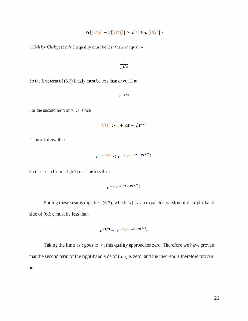
26
Pr{| 𝑈(𝑡) − 𝐸[𝑈(𝑡)] | ≥ 𝑡1 6⁄ 𝑉𝑎𝑟[𝑈(𝑡)] }
which by Chebyeshev’s Inequality must be less than or equal to
1
𝑡1 3⁄
So the first term of (6.7) finally must be less than or equal to
𝑡−1 3⁄
For the second term of (6.7), since
𝑈(𝑡) > 𝑢 + 𝛼𝑡 − 𝛽𝑡2 3⁄
it must follow that
𝑒−𝑅 𝑈(𝑡) < 𝑒−𝑅 (𝑢+ 𝛼𝑡− 𝛽𝑡2 3⁄ )
So the second term of (6.7) must be less than
𝑒−𝑅 (𝑢+ 𝛼𝑡− 𝛽𝑡2 3⁄ )
Putting these results together, (6.7), which is just an expanded version of the right-hand
side of (6.6), must be less than
𝑡−1 3⁄ + 𝑒−𝑅 (𝑢+ 𝛼𝑡− 𝛽𝑡2 3⁄ )
Taking the limit as t goes to ∞, this quality approaches zero. Therefore we have proven
that the second term of the right-hand side of (6.6) is zero, and the theorem is therefore proven.
∎
27
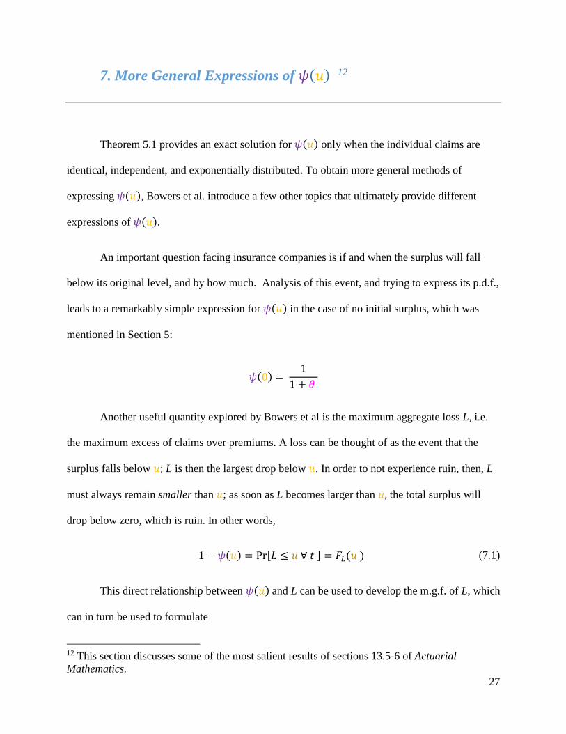
7. More General Expressions of 𝜓(𝑢) 12
Theorem 5.1 provides an exact solution for 𝜓(𝑢) only when the individual claims are
identical, independent, and exponentially distributed. To obtain more general methods of
expressing 𝜓(𝑢), Bowers et al. introduce a few other topics that ultimately provide different
expressions of 𝜓(𝑢).
An important question facing insurance companies is if and when the surplus will fall
below its original level, and by how much. Analysis of this event, and trying to express its p.d.f.,
leads to a remarkably simple expression for 𝜓(𝑢) in the case of no initial surplus, which was
mentioned in Section 5:
𝜓(0) = 1
1 + 𝜃
Another useful quantity explored by Bowers et al is the maximum aggregate loss L, i.e.
the maximum excess of claims over premiums. A loss can be thought of as the event that the
surplus falls below 𝑢; L is then the largest drop below 𝑢. In order to not experience ruin, then, L
must always remain smaller than 𝑢; as soon as L becomes larger than 𝑢, the total surplus will
drop below zero, which is ruin. In other words,
1 − 𝜓(𝑢) = Pr[𝐿 ≤ 𝑢 ∀ 𝑡 ] = 𝐹𝐿(𝑢 ) (7.1)
This direct relationship between 𝜓(𝑢) and L can be used to develop the m.g.f. of L, which
can in turn be used to formulate
12 This section discusses some of the most salient results of sections 13.5-6 of Actuarial
Mathematics.

28
∫ 𝑒𝑢𝑟 [−𝜓′(𝑢)]
∞
0
𝑑𝑢 = 1
1 + 𝜃
𝜃 [𝑀𝑥(𝑟) − 1]
1 + (1 + 𝜃)𝑝1𝑟 − 𝑀𝑥(𝑟)
While this equation seems long and intimidating, it is useful in that it doesn’t require
much information in order to be able to explicitly define 𝜓(𝑢) for certain claim distributions,
such as mixtures of exponential distributions.
An even more general expression for 𝜓(𝑢) is sought for cases when the m.g.f. of the
claim distribution (which 𝑅 depends on) is difficult to express. The method is to evaluate E[L]
using two separate strategies, and set the results equal to each other. It turns out that
𝐸[𝐿] = 𝑝2
2 𝜃 𝑝1
where 𝑝1and 𝑝2 are the first two moments of the individual claim distribution. But we also recall
that the expected value of a variable can be calculated by taking the integral of its survival
function over its domain. From equation (7.1), we see that the survival function of L is
1 − 𝐹𝐿(𝑢 ) = 𝜓(𝑢)
so
𝐸[𝐿] = ∫ 1 − 𝐹𝐿(𝑢 )
∞
0
𝑑𝑢 = ∫ 𝜓(𝑢)
∞
0
𝑑𝑢
Bowers et al show that this equality leads to the approximation
𝜓(𝑢) ≅1
1 + 𝜃 𝑒
[−2 𝜃 𝑝1 𝑢
(1+𝜃)𝑝2]

29
This approximation, the most general one discussed in Actuarial Mathematics, obviates
the need for the full m.g.f. of the individual claim distribution; all it requires is the first two
moments.
8. Further Reading
Even though it isn’t widely used in practice, Ruin Theory provides a rigorous foundation
for understanding the risk processes underlying insurance companies. Two of its tools that are
both approachable and useable in practice are the adjustment coefficient and Lundberg’s bound,
which in many cases are easy to evaluate and give a good sense of the riskiness of an insurance
portfolio: this is especially useful in reinsurance.
The point of reinsurance is for insurance companies to reduce their risk by sharing their
obligations with a reinsurer. Philip J. Boland explains in Statistical and Probabilistic Methods in
Actuarial Science that at first glance, the best way to decide the appropriate level of reinsurance
would be to maximize expected profit, like any other company would. But this is actually not a
reasonable goal for reinsurance: the whole point is to reduce risk, which most likely comes at the
expense of some profit. A more appropriate strategy is to look for the reinsurance arrangement
that minimizes the company’s ruin probability. To this end Boland uses ruin theory to develop
several models and strategies for selecting and analyzing reinsurance opportunities (Boland,
2007, 146-149).
An important topic not covered here is the discrete-time model. This paper has treated
aggregate claims process as a continuous-time process, which is not always accurate or relevant
in practice. Any analysis done on a periodic basis – such as financial reporting - may be suited

30
better by a discrete model. Bowers et al, as well as Boland and Promislow, all go into great detail
about developing the discrete model, its corresponding adjustment coefficient, and its
applications to expressing ruin probabilities (Bowers et al, 2010, 401-405; Boland, 2007, 129-
132; Promislow, 2011, 332-336).
As mentioned, Theorem 5.1 highlights the importance of the joint p.d.f. of 𝑇 and 𝑈(𝑇).
This has been studied thoroughly, and the results are summarized by Gerber and Shiu in their
1997 paper “On the Time Value of Ruin” (Bowers et al, 2010, 423). According to their paper’s
abstract, it also generalizes the classical ruin theory models by showing how to discount with
respect to 𝑇, so that the subject can be treated from a time-value-of-money perspective, lending
the paper its title. This leads to a notion called the expected discounted penalty, meaning the
expected present value of the deficit at ruin – which is due at ruin. The expected discounted
penalty is represented by a function that has become known in the literature as the Gerber-Shiu
function.
The field of Ruin Theory has been studied and developed to a great extent. In 2010, a
more-than-500-page book, Ruin Probabilities, was published that gives a full treatment of the
topic on a purely theoretical, “mathematically mature” basis, according to its Preface. Needless
to say, most of the topics discussed there are far beyond the scope of this paper, but one simple
and interesting topic explained there (and in Promislow) is to look at ruin theory from the
perspective of Martingales and Brownian motion.
Bowers et al list several more sources for further reading.

31
Works Cited
Asmussen, Soren, and Hansjorg Albrecher. 2010. Ruin Probabilities. Singapore: World
Scientific Publishing Co.
http://web.a.ebscohost.com/ehost/detail/detail/bmxlYmtfXzM3NDg3Ml9fQU41?sid=356
71356-68cb-4074-9716-
edf6cc41ce6c@sessionmgr4003&vid=0#AN=374872&db=nlebk.
Boland, Philip J. 2007. Interdisciplinary Statistics: Statistical and Probabilistic Methods in
Actuarial Science. Boca Raton: Taylor & Francis Group, LLC.
Bowers, Newton L., Jr, Hans U. Gerber, James C. Hickman, Donald A. Jones, and Cecil J.
Nesbitt. 1997. Actuarial Mathematics. Vol. 2. Schaumberg, IL: The Society of Actuaries.
Cramér, Harald. 1969. "Historical Review of Filip Lundberg's Works on Risk Theory."
Scandinavian Actuarial Journal 1969 (3): 6-12. doi:10.1080/03461238.1969.10404602.
Gerber, Hans U., and Elias S.W. Shiu. 1998. "On the Time Value of Ruin." North American
Actuarial Journal 2 (1): 48-72. doi:10.1080/10920277.1998.10595671.
Promislow, S. David. 2011. Fundamentals of Actuarial Mathematics. Vol. 2. Toronto: Wiley.