DEPARTMENT OF ECONOMICS WORKING PAPER SERIES

Understanding the Cell Phone Effect on Motor Vehicle Fatalities

Using Classical and Bayesian Methods

Gail Blattenberger

Richard Fowles

Peter D. Loeb

and

Wm. A. Clarke

Working Paper No: 2008-24

University of Utah

Department of Economics

1645 East Central Campus Dr., Rm. 308

Salt Lake City, UT 84112-9300

Tel: (801) 581-7481

Fax: (801) 585-5649

http://www.econ.utah.edu

2

Understanding the Cell Phone Effect on Motor Vehicle Fatalities

Using Classical and Bayesian Methods

Gail Blattenberger Department of Economics, University of Utah

Richard Fowles Department of Economics and Institute of Public and International Affairs, University of Utah

Peter D. Loeb Department of Economics, Rutgers University, NJ

Wm. A. Clarke Department of Economics, Bentley University, MA

Acknowledgements: Loeb gratefully acknowledges the research support of a Rutgers

University Research Council Grant. Tianda Xing and Stephanie Jensen provided

research support funded by the Departments of Economics at Rutgers University and the

University of Utah. This paper was presented at the 2009 Annual Meeting of the

Transportation and Public Utilities Group/Allied Social Sciences Meeting in San

Francisco, CA.

3

I. Introduction

Motor vehicle accidents continue to result in large numbers of fatalities each year.

In 2006, for example, there were over 42,700 fatalities associated with these accidents.1

As such, the determinants of these accidents and methods to reduce them continue to be

of great interest to economists, public health officials, and policy makers.

To date, numerous studies have been conducted to attempt to determine the

causes of motor vehicle accidents. The factors leading to such accidents are attributed

generally to the vehicles themselves, the roadways, or to drivers. More specifically, the

studies have examined the effects of speed limits, types of highways, vehicle speed,

speed variance, motor vehicle inspection, seat belt laws, minimum legal drinking age,

alcohol consumption, income, population characteristics, among many others. Just

recently, some studies have directed their attention to the impact of cell phones on motor

vehicle accidents and fatalities. Cell phones have become an issue in the literature given

the growth of their widespread use in the general public and by drivers as well. The

effects of these factors do not necessarily remain static over time which compounds the

difficulty of evaluating the marginal impact of them on fatality rates.2

Fragile and inconsistent results across studies may be due to different data sets

(either survey or non-survey data), different estimation techniques used, e.g., cross-over

analysis versus logistic analysis or OLS, as well as differences in the general model

specifications. We present in this paper econometric models using a rich set of panel data

covering the period 1980 to 2005 by state and the District of Columbia. In addition, the

panel data set allows for measurement of changes in federal speed limit laws which have

changed in 1987 and again in 1995.

Modeling the determinants of motor vehicle fatality rates is done several ways in

this study. First, a linear model is developed using classical linear regression modeling

techniques based on the work of Loeb et al. (forthcoming). This classically specified

model serves as the reference prior of the research. We recognize that classical linear

modeling, which relies on a known and well-behaved sampling distribution, may be

1 See NHTSA (2008).

2 See, for example, Keeler, who estimated that motor vehicle inspection had a life-saving effect initially,

but its effect diminished over time.

4

prone to error due to fundamental uncertainty regarding model specification. In this

paper we then address issues related to both parameter and to model uncertainty via three

Bayesian techniques.

In what follows, Section II.A develops an econometric reference model to

articulate the anticipated effects of explanatory variables on traffic fatalities. In a

Bayesian context, this serves to reference prior beliefs regarding the effects of variables.

Section II. B describes the data and defines the variables used in this paper. Section III.A

estimates this model using a classical fixed effects regression. Section III.B explores

global model fragility using Extreme Bounds Analysis. Sections III.C and III.D present

results from Bayesian Model Average and Stochastic Search Variable Selection

procedures which direct attention to the most probable models. Section III. E compares

the four estimation approaches. Section IV. provides some concluding comments

including highlights on how the classical and Bayesian methods agree and differ across

model specifications and suggests ways these data may be further examined.

II. A. The Reference Prior

Econometric models of the determinants of motor vehicle accidents often follow

the approach suggested by Peltzman (1975). One of the important contributions of

Peltzman was to examine potential offsetting behavior on the part of drivers as they

adjust their driving behavior in the face of improved safety of vehicles over time and the

imposition of safety regulations. For example, in the 1980’s seatbelt laws were being

passed in the U.S. to reduce fatalities and injuries of occupants of cars involved in

accidents. However, although there may be a benefit to the seatbelt user should there be

an accident, the probability of an accident may be increased as drivers take on riskier

driving behavior which may, among other things, put pedestrians at greater risk.

Peltzman’s paper initiated numerous studies on the determinants of automobile

accidents using various econometric techniques and data sets. There were many studies

on the effect of motor vehicle inspection on automobile accidents3, the effect of speed

3 See, for example, Keeler (1994), Loeb (1985, 1990), Loeb and Gilad (1984), and Garbacz and Kelly

(1987).

5

and speed variance on such accidents4, the effect of seatbelts and seatbelt laws on

accidents5, the effect of alcohol and related taxing policies on accidents

6, among other

factors which might have countervailing effects. Loeb, Talley, and Zlatoper (1994)

review and evaluate the impact of many of these potential determinants of accidents.

Until recently, however, most studies did not consider the impact of cell phones on motor

vehicle accidents since cell phone use in the United States became relevant, from a

practical point of view, starting in the 1980s. There were only about 340 thousand cell

phone subscribers in the United States in 1985. Since then, the number of subscribers of

cell phones has grown exponentially. By the year 2007, there were over 255 million

subscribers.7 Given this fast and large increase in cellular phone subscribership,

economists, safety experts, and policy makers have recently increased their attention to

the effect cell phones may have on motor vehicle accident rates.

Cell phone use by drivers may result in an increase in accidents and fatalities for

several reasons. Firstly, cell phone usage may have a distracting effect on the driver (as

well as pedestrians) and may impede a driver’s ability to operate a vehicle due to an

inability to do more than one thing at a time, i.e., drive a car and talk on a cell phone. In

addition, cell phone use may reduce attention spans and reaction times. With this in

mind, five states (Connecticut, New Jersey, California, New York, and Washington)

along with the District of Columbia have banned the use of hand-held phones by drivers.8

Strangely, the bans do not affect the use of hands-free devices in spite of research

indicating that such devices have a similar adverse effect on safety as do the hand-held

devices.9

It is not merely the sheer number of cell phones available to the public which has

safety researchers concerned, but also the propensity of drivers to use them. Glassbrenner

(2005) has estimated that ten percent of all drivers at any moment of time during daylight

hours were using either hand-held or hands-free phones. Furthermore, there is indication

4 See, for example, Lave (1985), Levy and Asch (1989), Fowles and Loeb (1989), among others.

5 See, for example, Cohen and Einav (2003), Evans (1996), Dee (1998), and Loeb (1993,1995,2001).

6 See, for example, Fowles and Loeb (1989), and Chaloupka et al. (1993).

7 See Cellular Telecommunications and Internet Association (2007).

8 In addition, both New Jersey and California banned text messaging by drivers in 2008.

9 See, for example, Consiglio et al. (2003).

6

that the percentage of drivers using these devices is increasing over time as well.10

Not

only are cell phones and subscribers increasing over time, but driver usage is increasing

as well and apparently at an increasing rate.

Redelmeier and Tibshirani (1997) is the most well-known study of the effects of

cell phones on automobile accidents. Using cross-over analysis, they conclude that

property-only accidents increase four-fold when cell phones are involved. They also find

that 39% of all drivers involved in these accidents make use of their cell phones to call

for assistance after the accident. McEvoy et al. (2005) also find an increase in the risk of

an accident due to cell phones using data on crashes resulting in hospital visits. Violanti

(1998) attributes an approximate nine-fold increase in fatalities when cell phones are in

use as opposed to when they are not.11

Neyens and Boyle (2007) examining teenage

drivers, found that cell phones increased the likelihood of rear-end collisions relative to

fixed-object collisions. From a different perspective, Consiglio et al. (2003), using a

laboratory environment, simulated driving conditions and found that brake reaction time

was reduced when cell phones were in use and this reduction occurred regardless of

whether the cell phones were hand-held or hands-free devices. Similarly, Beede and

Kaas (2006) using a sample of 36 college students and simulating driving conditions in a

laboratory environment also found that hands-free devices adversely effected driving

performance.

As noted above, not all research has supported the claim that cell phones are

associated with accidents and fatalities. Rather, there are studies indicating that cell

phones do not have a significant impact on motor vehicle accidents. Laberge-Nadeau et

al. (2003) using logistic-normal regression models and Canadian survey data initially

found an association between cell phone use and accidents. However, this risk was

diminished as their basic models were extended, suggesting that their results were fragile

with respect to model specification. This suggests that results from modeling may be

questioned due to issues of both model and parameter uncertainty. The life-taking effect

of cell phones was further countered by Chapman and Schofield (1998) who argue that

cell phones should be credited with saving lives as opposed to taking them. Chapman and

10

Glassbrenner (2005) has estimated that driver use of just hand-held phones increased from 5% in 2004 to

6% in 2005. 11

See Violanti (1998, p. 522).

7

Schofield found that, “Over one in eight current mobile phone users have used their

phones to report a road accident.”12

Referring to the “golden hour,” – the period of time

crucial for survivorship from various medical emergencies and accidents – they claim

that it is highly likely that many lives were saved due to cell phones.13

Similarly, Poysti,

et al. (2005) claim that, “phone-related accidents have not increased in line with the

growth of the mobile phone industry.”14

More recently, Loeb et al. (forthcoming) addresses the fragile results reported

across the various research endeavors by using econometric methods and specification

error tests to examine the potential interacting-effect of life-saving and life-taking

attributes of cell phones with regard to motor vehicle fatalities. A non-linear model is

posited and the statistical results suggest a non-monotonic relationship between cell

phone availability and motor vehicle fatalities. Initially, with low cell phone subscriber

rates, cell phones are found to be associated with net life-taking effects. As the number

of subscribers increase, the life-saving effect overwhelms the life-taking effect. This life-

saving effect may be due to sufficient numbers of cell phones being available so that a

quick response to an accident by witnesses is likely and their expeditious call for medical

help avails the victims to the benefit of the golden hour rule. Starting in the 1990s,

however, when subscribers numbered 100 million and more, the life-taking effect

overwhelmed the life-saving effect once again.15

These results were found to be

statistically significant and stable. The results are considered reliable given the outcome

of the specification error tests which paid particular attention to the structural form of the

models.16

12

See Chapman and Schofield (1998, p. 5). 13

See Chapman and Schofield (1998, p. 6). 14

See Poysti (2005, p. 50). 15

These results allow for not only driver usage of cell phones to impact on automobile related fatalities,

but for a potential beneficial externality associated with the general population having cell phones. Usage

by both drivers and the general public may offset or more than offset each other with regard to safety

effects. 16

The models presented by Loeb et al. (forthcoming) were evaluated for their conformity to the Full Ideal

Conditions associated with the error term, i.e., µ~N(0,σ2I). To examine this, a set of specification error

tests were applied to the models, i.e., the Regression Specification Error Test (RESET), the Jarque-Bera

Test, and the Durbin-Watson Test. Rejection of the null hypothesis of no specification errors by one or

more of these tests resulted in the elimination of the models from consideration. These results were

supported as well by Fowles et al. (2008) using Bayesian Extreme Bounds Analysis.

8

II. B. The Data

In order to better understand the effects of socio-economic and policy related

variables on traffic fatality rates we utilize a newly compiled, rich set of data that were

collected on 50 states and Washington, D.C. over the period from 1980 to 2005.

The choice of the measure of the dependent variable was of prime importance.

Data are available on the number of fatalities, and on four different fatality rates. Here

we examine the most commonly reported dependent variable, fatalities per 100 million

vehicle miles traveled.17

During our coverage period there were significant changes in a

host of variables. Our data cover the time of the explosive growth in cell phone

subscriptions from effectively zero to over 270 million. Because annual subscription data

are only available at the national level we imputed state level subscriptions to be

proportional to state population proportions for each year. Another major variable

change related to Federal legislation that allowed states to modify the 55 mile per hour

speed limit on Interstate highways. Our data records the highest posted urban Interstate

speed limit that was in effect during the year for each state. Within the data, per se blood

alcohol concentration (BAC) laws vary widely, even though by 2005 all states and the

District of Columbia had mandated a .08 BAC illegal per se law.18

Seat belt legislation

varies widely across states. Our data records the years in which a state mandatory

primary or secondary seat belt law came into effect. The data are organized by

geographical coding of states into eleven regions. The variables are defined and

described in Table 1 along with their expected effects (priors) on fatality rates.

17

The other fatality rate measures are fatalities per capita, fatalities per vehicle registrations, and fatalities

per licensed drivers. All measures exhibit, at the national level, a downward trend. 18

The per se law refers to legislation that makes it illegal to drive a vehicle at a blood alcohol level at or

above the specified BAC level. BAC is measured in grams per deciliter.

9

Table 1

Explanatory Variables a

Cross Sectional - Time Series Analysis of Traffic Fatality Rates

For 50 States and DC from 1980 to 2005

Name Description Expected

Sign

(Priors)

YEAR Year -

PERSELAW Dummy variable indicating the existence of a law defining

intoxication of a driver in terms of Blood Alcohol

Concentration (BAC). PERSELAW=1 indicates the

existence of such a law and PERSELAW=0 indicates the

absence of such a law. (More precisely, PERSELAW = 1

when the BAC indicating driving under the influence is 0.1 or

lower.)

-

INSPECT Indicator for annual safety inspection -

SPEED Maximum posted speed limit, urban highways +

BELT Indictor for presence of a legislated seat belt law -

BEER Per capita beer consumption (in gal) +

MLDA Minimum legal drinking age -

YOUNG Percentage of males (16-24) relative to population of age 16

and over

+

CELLPOP Imputed number of cell phone subscribers per capita

+

POVERTY Poverty rate +

UNEMPLOY Unemployment rate -

REALINC Real per household income in 2000 dollars ?

ED_HS Percent of persons with high school diploma -

ED_COL Percent of persons with a college degree -

CRIME Crime rate ?

SUICIDE Suicide rate ? a For data sources, see Appendix 1

III. A. The Classical Fixed Effects Model

We begin by specifying a linear relationship between the fatality rate – FATAL –

(vehicle fatalities per 100 million miles traveled) for the jth

state and for the ith

year. The

base model is estimated using regional dummy variables and includes the year as a trend

variable. Ordinary least squares results for the basic model are presented in Table 2. In

order to compare the effects of the variables on fatality rates among estimation methods,

10

all data are standardized to have mean zero and range 1. As mentioned, the regression

included regional dummy variables, but those estimated coefficients are omitted from the

table.19

Table 2

OLS Estimates for the Fatality Rate Model*

Variable Estimate

Standard

Error t value

YEAR -.466 .0334 -13.961

PERSELAW -.0331 .00697 -4.754

INSPECT .00775 .00544 1.425

SPEED .0333 .011 3.023

BELT .000318 .00753 0.042

BEER .0935 .0163 5.752

MLDA .0104 .00903 1.148

YOUNG .0619 .0197 3.133

CELLPOP .196 .0225 8.731

POVERTY .175 .0211 8.321

UNEMPLOY -.0561 .0232 -2.414

REALINC .154 .0384 4.01

ED_HS -.0361 .0283 -1.274

ED_COL -.269 .0311 -8.632

CRIME -.0000337 .0231 -0.001

SUICIDE .127 .0286 4.439 * Residual standard error: 0.06843 on 1300 degrees of freedom

Multiple R-squared: 0.807, Adjusted R-squared: 0.8031

F-statistic: 209.1 on 26 and 1300 DF, p-value: < 2.2e-16

There is considerable sign agreement in terms of expected and estimated effects.

Three variables are estimated with sign differences -- INSPECT, BELT, and MLDA.

Classical estimation addresses the issue of parameter uncertainty and statistical

significance in relation to the sampling distribution induced by assumptions in the linear

regression model. It may be noted that the three variables estimated with the “wrong”

sign are not statistically significant at conventional testing levels. Instead of changing

the model specification by adding or removing variables (and thus violating the principle

19

We selected the model presented in this paper for expository clarity. Additional models were estimated

which exclude some of the regressors presented and include others, such as what is referred to as a

“companion variable.” Companion variables attempt to account for factors not addressed by the time trend

and are discussed in Loeb (1995, 2001). In this case, both the crime rate and suicide rate may serve as

companion variables. Alternatively, the suicide rate may proxy to some extent the self-evaluation of the

value of life. Regardless, results remain stable and similar to those reported in Table 2 and these additional

models are available from the authors.

11

of statistical significance testing), we directly address model and parameter uncertainty

using three Bayesian econometric methods. They are Extreme Bounds Analysis (EBA),

Bayesian Model Averaging (BMA), and Stochastic Search Variable Selection (SSVS).

All three of the methods recognize that differing parameter estimates can be obtained

under varying specifications, in particular, when subsets of the 2K regressions (with K

potential explanatory variables) are considered. The next sections examine the extent to

which changes in model specifications lead to different conclusions regarding the

influences of particular explanatory variables, and to discover classes of model

specifications that have high posterior probabilities. Given that 2K is in the order of 250

million for these data, specification is non-trivial and yet is mathematically tractable for

these procedures.

III. B. Extreme Bounds Analysis

Extreme Bounds Analysis was developed by Leamer in a series of articles

beginning in 1978 (Leamer 1978, 1982, 1983, 1985, 1997). It is a methodology of global

sensitivity analysis that computes the maximum and minimum values for Bayesian

posterior means in the context of linear regression models. The extreme values are those

that could be estimated via maximum likelihood estimation when all possible linear

combinations of the explanatory variables are considered under all possible model

specifications. This method is rather draconian in the sense that all possible

specifications are considered and that very few hypotheses survive a full EBA analysis

(Mayer, 2007). Lack of survivability is seen in ranges of posterior estimates for model

parameters that cover zero. Such variables are called fragile even though associated

parameter estimates obtained via classical estimation might be seen to be statistically

significant. Fowles and Loeb (1989, 1995), and Fowles et al. (forthcoming) have

repeatedly used EBA analysis in models analyzing aggregate U.S. cross section and time

series models of traffic fatality rates.20

20

Calculations of EBA were computed in Gauss using MICRO-EBA (Fowles, 1988). The Gauss code is

available free on request.

12

A major advantage in using EBA is that prior distributions only have to be

specified for certain sets of variables, yet bounds can be computed for all variables in the

model. Following Leamer (1982) we specify a natural conjugate prior for a set of p

doubtful variables, or those variables which could plausibly be dropped from a

specification.21

In this paper, those are the regional binary variables, the remaining

variables, called free variables, are not linked to a proper prior specification. Free

variables are associated with a diffuse prior. For the normal linear regression model

Y ~ N(Xβ,σ2 I)

the prior mean on the p doubtful variables is also normal, centered at zero, with variance

matrix H*-1

. This is written as

Rβ ~ N(0, H*-1

)

where R is a pxK matrix of constants, β is a kx1 vector of parameters, 0 is a px1 zero

vector, and H* is a pxp positive definite symmetric precision matrix (the inverse of the

variance/covariance matrix). EBA obtains posterior information of dimension K based

on specification of dimension p (p < K). In particular, the extreme values of linear

functions of the posterior mean, b**, for the full Kx1 vector τ,22

τ’b** = τ’(H + R’H*R)-1

Hb

are given by

a + τ *'f ± (τ *'A-1

τ *c).5

when H*-1

is constrained to fall between positive definite matrices VL and VH and

21

Dropping a variable forces a very strong prior belief that the coefficient is exactly equal to zero with

perfect precision. 22

In this paper, τ is a vector with one 1 and k-1 zeros that corresponds with the ith

parameter of interest.

13

a = τ 'b - τ 'H-1R'(RH

-1R')

-1Rb,

τ *' = τ 'H-1R'(RH

-1R')

-1,

f = (h + VL-1

)-1

(hRb + (VL-1

– VH-1

) * (h + VH-1

)-1

hRb/2),

A = (h + VH-1

)(VL-1

– VH-1

)-1

(h + VH-1

) + (h + VH-1

),

c = (Rb)'h(h + VH-1

)-1

(VL-1

– VH-1

)(h + VL-1

)-1

hRb/4,

h = (RH-1

R')-1

,

b = (X'X)-1

X'Y,

H = s-2

X'X,

s = ((Y-Xb)'(Y-Xb)/(n-K)).5

.

Table 3 reports the maximum and minimum bounds for the posterior means for

the non-doubtful variables with the widest possible bounds corresponding with

VL = 0H*-1

and VH = ∞H*-1

. Column 1 reports the Maximum Likelihood Estimates for

the entire model. Columns 2 and 3 report the EBA minimum and maximum values for

the posterior mean when the regional variables are specified as doubtful variables. The

last two columns show the EBA minimum and maximum values that lie within a 95%

confidence ellipsoid with all variables specified as doubtful. Bounds within the 95%

ellipsoid are referred to as being data favored. This specification (zero prior mean)

corresponds with the prior specifications used for BMA and SSVS specifications that

follow in the next two sections. Using EBA, priors are minimally specified since H*, the

prior precision matrix, is only required to be positive definite symmetric.23

Results are

23

In MICRO-EBA, H* was set equal to the identity matrix, so the priors are spherically symmetric,

centered at zero.

14

only sensitive to the free-doubtful mix via the R matrix which reduces the dimensionality

for the prior space from K to p.

Table 3

Maximum Likelihood & Extreme Bounds Analysis for the Fatality Model Specification

Variable Name

Maximum

Likelihood

Estimate

EBA

Minimum

Regional

Doubtful

EBA

Maximum

Regional

Doubtful

EBA

Minimum

95%

Likelihood

All

Doubtful

EBA

Maximum

95%

Likelihood

All

Doubtful

YEAR -0.519 -0.5707 -0.3998 -0.7317 -0.2973

PERSELAW -0.0324 -0.0467 -0.0274 -0.0758 0.01149

INSPECT 0.0086 -0.0116 0.0318 -0.0256 0.0427

SPEED 0.0358 0.0124 0.0678 -0.0334 0.1045

BELT 0.0064 -0.0086 0.0246 -0.0414 0.0541

BEER 0.0886 0.0408 0.1271 -0.0138 0.1897

MLDA 0.015 -0.0005 0.0209 -0.042 0.0719

YOUNG 0.0498 0.0288 0.1376 -0.0753 0.1743

CELLPOP 0.2255 0.1785 0.2443 0.0788 0.3687

POVERTY 0.1851 0.1556 0.2561 0.0518 0.3157

UNEMPLOY -0.0628 -0.1329 -0.005 -0.2083 0.0836

REALINC 0.1704 0.0267 0.2761 -0.0722 0.4106

ED_HS -0.0154 -0.1266 0.075 -0.1949 0.1641

ED_COLLEGE -0.2837 -0.3698 -0.1685 -0.4759 -0.0872

CRIME -0.0069 -0.0436 0.1183 -0.1524 0.1386

SUICIDE 0.1228 0.0764 0.352 -0.0577 0.3016

When the regional variables are considered doubtful, non-fragile inferences are

obtained for all the explanatory variables except five: inspection (INSPECT), seat belts

(BELT), minimum legal drinking age (MLDA), high school education (ED_HS), and

crime (CRIME). When all variables are doubtful, EBA bounds necessarily cover zero.

However, the data favored extreme bounds are non-fragile for four variables: year

15

(YEAR), cell phone subscriptions (CELLPOP), poverty (POVERTY), and college

education (ED_COLLEGE).

Although EBA as discussed in this paper provides insight into the range of values

that the posterior means can take, it does not pay direct attention to the posterior

probabilities of the corresponding models. The next two procedures address this issue.

III. C. Bayesian Model Averaging

Bayesian Model Averaging was addressed extensively by Raftery, Madigan, and

Hoetling (1993) following a suggestion by Leamer (1978). By averaging across many

model specifications, especially among those with high posterior probability, BMA is

able to explicitly account for model uncertainty as it relates to parameter estimation. As

presented in Hoetling, Madigan, Raftery, and Volinsky (1999), BMA provides a

straightforward method to summarize the effects of explanatory variables as measured by

their regression coefficients as they are manifest in assorted models. In what follows, one

should keep in mind that two primary sources of uncertainty are addressed: of models and

of parameters.

Let ∆ represent a measure of interest, for example, the effect of speed laws on

motor vehicle fatality rates. The posterior distribution of ∆, conditional on data D, is a

weighted average of posterior distributions over models:

P(∆ | D) = ∑N P(∆ | MN, D) P(MN | D)

where M1, M2, … , MN are the N models under consideration. In order to calculate this,

the posterior distribution of model MN is required and is given by Bayes’ theorem as

P(MN | D) = P(D | MN)P(MN)/∑NP(D | MN)P(MN).

In the numerator, P(D|MN) represents the integrated likelihood of model MN and is

calculated as

16

P(D | MN) = ∫P(D | θN, MN)P(θN | MN)dθN

where θN is the vector of parameters of model MN. For linear regressions in this paper, θ

is the vector comprised of the β’s and σ2. The posterior mean and variance for ∆ are

calculated based on Raftery (1995) as:

E(∆ | D) = ∑N dN P(MN | D) and

V(∆ | D) = ∑N (Var[∆ | D, MN] + dN2)P(MN | D) – E(∆ | D)

2

for dN = E(∆ | D, MN), the estimated, or fitted, effect under model MN.

Note that the effects of ∆ are measured by averaging over many models with

weights that correspond to the models’ posterior probabilities. Posterior variance is

comprised of sampling and model variation. In this paper, the formidable task of

calculating the integrated likelihood function is mitigated by utilizing the fact that this

likelihood function is well-approximated by the Bayesian Information Criterion (BIC).24

Non-informative priors (uniform over models, MN) and diffuse over parameters within

models (θN) were utilized.

The following table summarizes BMA analysis for the same model presented

above (in Table 3), regressing fatality rates on the core set of explanatory variables.

Regional binary variables were included in the analysis but are not reported in Table 4.

The column headed “p!=0” gives the posterior probability that the particular variable is

included in the model. The “EV” column shows the posterior mean for the variable for

the BMA runs and “SD” is the posterior standard deviation for the variable. The best

performing model included 16 explanatory variables with a posterior probability of .279.

In that model, INSPECT, BELT, UNEMPLOY, ED_HS, MLDA, and CRIME were not

24

For this paper, BMA results are computed in R using the BMA package with bicreg. BMA procedures

were based on finding alternatives to stepwise methods based on p-value style searches. BMA calculations

can be performed using monte carlo (MC) integration to compute the integrated likelihood function. The

leaps method of selection is a fast alternative (George M. Furnival and Robert W. Wilson, 1974). The

relationship between the integrated likelihood function and the BIC score is developed in Raftery (1995).

MC methods are utilized in SSVS calculations in this paper.

17

present. BMA never chooses to include BELT or CRIME, and always includes YEAR,

PERSELAW, BEER, YOUNG, CELLPOP, POVERTY, REALINC, ED_COL, and

SUICIDE. Of these nine variables, all are non-fragile under EBA when the regional

dummy variables are considered doubtful. SPEED is the tenth explanatory variable that

was non-fragile under EBA. BMA selects this variable two-thirds of the time. As such,

there is a considerable agreement between EBA and BMA model choice.

Table 4

Bayesian Model Averages for the Fatality Rate Model Specification

Variable p!=0 EV SD

YEAR 100 -.445 0.0262

PERSELAW 100 -.0350 0.00677

INSPECT 1.5 .0000735 0.00081

SPEED 66.6 .0203 0.0168

BELT 0 0.00 0

BEER 100 .0934 0.0157

MLDA 1.4 .000138 0.00157

YOUNG 100 .0784 0.0197

CELLPOP 100 .179 0.02096

POVERTY 100 .184 0.0205

UNEMPLOY 36.8 -.0198 0.0291

REALINC 100 .161 0.0339

ED_HS 2.2 -.000827 0.00676

ED_COL 100 -.0282 0.0247

CRIME 0 0 0

SUICIDE 100 .115 0.025

18

III. D. Stochastic Search Variable Selection

Stochastic Search Variable Selection was introduced by George and McCulloch

(1993). Because it is computationally burdensome, it is one of the more recent

procedures in Bayesian analysis that takes advantage of the ability to integrate over

multidimensional spaces using Markov Chain Monte Carlo (MCMC) methods typically

found when dealing with analyses of the posterior density. This is done with a Gibbs

sampler.

All K of the explanatory variables are included at each iteration of the Markov

chain to take advantage of the application of the Gibbs sampler to a hierarchical Bayesian

model. The variable selection choice is imposed by means of a latent variable, γ. Each

model is represented by a binary vector γ = (γ1, γ2, …, γK) with γi = 1 if the explanatory

variable is to be effectively included in the model and γi = 0 if the variable is to be

effectively excluded from the model. The prior distributions on the slope parameters

(β’s) for the explanatory variables are distributed normally with mean zero and variance

ci2τi

2 when γi = 1, N(0, ci

2τi

2), and normally with mean zero and variance τi

2, N(0, τi

2)

when γi = 0 with c greater than 1.

βi|γi ~ (1-γi) N(0, τi2) + γi N(0, ci

2τi

2)

The effective exclusion of variable i is imposed by forcing βi to be close to zero.

This framework results in sets of posterior distributions for all vectors γ of dimension K

and pays attention to the relatively sharp prior distribution around zero when a variable is

not effectively included in a model compared with a more diffuse prior when a variable is

effectively included.25

Each variable is examined in random order at the end of each iteration of the

Gibbs sampler to evaluate the marginal effect of effectively including/excluding that

variable in the model. Based on this a probability of including the variable is computed

and the value of γi for the next iteration is computed stochastically based on this

25

ci and τi are choice variables. In this paper the reported results are for ci = 10 and τi=(2 log(c) (c2/(1-

c2))

.-5σ βi where the parameter σ βi is the OLS coefficient standard deviation. This choice is consistent with

George and McCulloch (1993) and follows their notation.

19

probability. Initial values of the γi are all set at 1 and the initial probabilities of inclusion

are set at 0.5. Then a stochastic iteration scheme is implemented using Gibbs sampling to

search for the models with the highest posterior densities.26

In particular, the Gibbs

sampler begins with initialized parameters γ(0), β(0)

, σ2(0)

and generates the sequence γ(1),

β(1), σ

2(1), γ(2)

, β(2), σ

2(2), …. This sequence converges to a posterior distribution which

supplies the complete posterior P(β, σ2, γ | Y). Concurrent with the iterative values of the

vector γ are iterative values of the vector p, the probability of variable inclusion, enabling

us to compute an expected value of the vector β at each iteration.

Table 5 summarizes the findings for SSVS for the linear fatality model based on

10,000 iterations.27

The first column (Mean Beta) gives the weighted average for the

sequence of slope coefficients, weighted by the probability of inclusion. The second

column (Standard Deviation) is the mean value of the weighted standard deviations of the

sequence of slope coefficients. The third column (Probability Inclusion) is the mean

value of the probability of a variable’s inclusion in the model. Column 3 of Table 5 can

easily be compared with the column labeled “p!=0” in Table 4. It should be noted that the

regional dummies were treated like any other variable. They were not singled out a priori

as being doubtful; nonetheless SSVS categorized them for exclusion.28

The five

variables with the highest values for inclusion (probability of inclusion > .95) in the

model correspond with the four EBA non-fragile variables (YEAR, POVERTY,

CELLPOP, and ED_COLLEGE) as presented in Table 3. SSVS chooses BEER almost

always, and is non-fragile under EBA when the prior specification includes BEER as a

non-doubtful variable and the regional variables as doubtful.

26

In this paper, SSVS was implemented via Markov chain Monte Carlo methods using R. This code is

available on request. 27

The first 500 iterations were deleted as a break-in period so there were a total of 9500 iterations

employed in the results reported 28

The average value of p for this set was .12.

20

Table 5

Stochastic Search Variable Selection for the Fatality Rate Model Specification

Variable Mean Beta

Standard

Deviation

Probability

Inclusion

YEAR -0.4604 0.0258 1

PERSELAW -0.0076 0.0134 0.2485

INSPECT 0.0012 0.0029 0.3696

SPEED 0.0102 0.0149 0.3386

BELT -0.0001 0.0032 0.4208

BEER 0.1069 0.0123 0.9999

MLDA 0.0034 0.0056 0.4081

YOUNG 0.0163 0.0278 0.2685

CELLPOP 0.2146 0.0186 1

POVERTY 0.1463 0.0174 0.9999

UNEMPLOY -0.0177 0.0265 0.3313

REALINC 0.0498 0.0643 0.3891

ED_HS -0.0185 0.0269 0.3732

ED_COLLEGE -0.2642 0.0299 0.9999

CRIME 0.0002 0.0108 0.4642

SUICIDE 0.0244 0.0441 0.2436

21

III. E. Comparing OLS, EBA, BMA, and SSVS Estimation

The four procedures discussed above shed insight on the relative importance of a

variable’s contribution in explaining fatality rates. Not surprisingly, there are agreements

between OLS, EBA, BMA, and SSVS findings. This section highlights the results which

are summarized graphically in Figure 1.29

Figure 1

Posterior Means for the Fatality Rate Model

EBA Extreme Bounds, BMA and SSVS Average Values

Regional Variables Doubtful

-0.8

-0.6

-0.4

-0.2

0

0.2

0.4

YEAR

PERSE

LAW

INSP

ECT

SPEE

DLO

BELT

BEER

MLD

A

YOUNG

CELLPO

P

POVERTY

UNEM

PLO

Y

REA

LINC

ED_H

S

ED_C

OLLE

GE

CRIM

E

SUIC

IDE

Variable

Po

ste

rio

r M

ean

SSVS

EBAHI

EBALOW

BMA

29

Figure 2 in Appendix 2 highlights the findings when all variables are doubtful and presents data favored

EBA bounds.

22

Figure 1 compares EBA, BMA, and SSVS results in a graphical way. The solid

lines (like whiskers in a box and whisker plot) plot the high and low values for the

posterior mean for each explanatory variable as computed by EBA. If these lines do not

cross zero, these variables are considered non-fragile. The BMA slope coefficient

averages are plotted as triangles, “∆,” and the SSVS averages are plotted as squares, “□.”

Box width reveals the difference between the BMA and SSVS means. For example,

there is almost no disparity between the BMA and SSVS means for variables such as

inspection (INSPECT) or minimum legal drinking age (MLDA) and some differences for

real income (REALINC), and the suicide rate (SUICIDE). There is sign agreement

between BMA and SSVS for all variables in the model.

Because the data are standardized we can assess the relative importance of each

explanatory variable. The foremost variable is YEAR; clearly there has been a

downward trend in motor vehicle fatality rates over time. College education is the

second most important variable followed by cell phone per capita and the poverty rate. It

is interesting to note that the OLS results provide the same results.

Table 6 below compares the results of the three Bayesian procedures and OLS.

With respect to the OLS column, we indicate the estimated coefficient with an asterisk

(*) indicating significance with a t-statistic of 2.00 or more (in absolute value). The EBA

column reflects the sign of the coefficients associated with columns 2 and 3 of Table 3

where the regional variables are doubtful and when the coefficients are non-fragile, i.e.

robust. In addition it indicates if the variable coefficient is fragile. The BMA column

indicates the posterior mean for the variable followed by a “1” if the variable is always

selected by BMA and “.666” if it is selected two-thirds of the time. Hence, this column

reflects the basic results of Table 4. The SSVS column reflects the basic results of Table

5, indicating the “Mean Beta” for the five variables with the highest probability for

inclusion (with probability of .95 or greater). This allows for the comparison of results

similar to Figure 1 and can be viewed together. However, in what follows, we make use

of the criterion established above in Table 6 and then supported by Figure 1. That is, we

consider a variable more certain to impact the fatality rate based on a combination of

non-fragile EBA results and inclusion of the variable by BMA and/or SSVS as well as

classical significance.

23

The variables which appear not to have an effect by any of the estimation

techniques include: INSPECT, BELT, MLDA, ED_HS, and CRIME. From the Bayesian

perspective, the results are fragile using EBA and not included via the BMA criterion or

by SSVS. Figure 1 shows the Bayesian results centering consistently on the zero line.

The OLS results dovetail with these results, given that they provide statistically

insignificant results. These findings are consistent with other studies. For example,

Keeler (1994) has found the effect of seatbelt laws has diminished over time. Other

studies dealing with seatbelt laws have generally suggested that seat belt laws provide net

benefits, but the results have been mixed. For example, Loeb (1995) found that seatbelt

laws were effective in reducing fatality and injury rates in Texas. However, when

examining seatbelt laws in Maryland, Loeb (2001) found the results varied in

significance depending on single vehicle versus multiple vehicle accidents.

What might be called a weak effect is noted with: PERSELAW, SPEED, and

UNEMPLOY. None of these were selected by SSVS. However, they were found non-

fragile by EBA and selected by BMA except for UNEMPLOY. The results once again

dovetail with the OLS results. In addition, most of these results are consistent with the

literature. PERSELAW was found to be significant and non-fragile by Fowles et al.

(forthcoming) as well as by Loeb et al. (forthcoming). However, the later study found the

significance of the coefficient associated with BACLAW using time-series data was

dependent on model specification. SPEED, like others in this group, does not have a

large associated coefficient, but is consistent with a good deal of the literature which

argues that higher speed limits are associated with motor vehicle accidents. Some counter

arguments are to be found in the literature as well as discussed by Loeb et al. (1994).30

Both YOUNG, REALINC, and SUICIDE have relatively strong results with all

methods of estimation but are somewhat attenuated by SSVS based on the criterion used

in Table 6 and supported by Figure 1. Clearly the percentage of males aged between 16-

24 have an increasing effect on motor vehicle fatality rates. Part of this may be attributed

to inexperience in decision making, including decisions pertaining to driving situations,

along with potentially higher risk taking associated with youth. SUICIDE has been

30

Lave (1985), Fowles and Loeb (1989), and Levy and Asch (1989), among others, have examined the

effect of speed versus speed variance as well. Data on average speed and the 85% speed are no longer

collected by USDOT and as such speed and speed variance could not be investigated in the current study.

24

included as a “companion variable” to measure the potential effect of excluded variables

not addressed by the time trend (YEAR). However, it has a strong positive influence on

motor vehicle fatality rates. One speculates that SUICIDE may proxy a measure of self

worth in society. As such, if self worth diminishes, suicides may increase as well as

behavior associated with additional risk taking.

The most consistently strong results across all methods of estimation (based again

on the criteria in Table 6 and nested in Figure 1) pertain to the variables: YEAR, BEER,

CELLPOP, POVERTY, and ED_COLLEGE. All these variables have signs consistent

with a priori expectations. YEAR may proxy technological changes over time and

permanent income31

. We expect safety to increase with technology and hence lower

fatality rates, assuming that drivers don’t compensate by taking on additional risks. In

addition, to the extent that YEAR serves as a proxy for permanent income, one would

expect fatality rates to diminish with increases in such income should it be a measure of

long-run income.32

The effect of alcohol has been long studied and has been found to

have an increasing effect on fatality rates. This has led to policy recommendations of

increasing the minimum legal drinking age as well as tax policies so as to reduce demand

for alcohol, especially among youths.33

Poverty is expected to potentially have an

increasing effect on fatality rates, given that individuals with low incomes have lower

opportunity costs associated with risky driving. Similarly, college education is an

investment in human capital and as such would enhance the value of life. This may then

result in life-protecting behavior, given the higher potential opportunity costs associated

with risky driving (and other risky activities). Finally, the strong results associated with

CELLPOP are consistent with the findings of Fowles et al. (forthcoming) and Loeb et al.

(forthcoming) as opposed to Chapman and Shofield (1998), Poysti et al. (2005), and to

some extent by Laberge-Nadeau et al. (2003). Clearly, cell phones have a net life-taking

effect when considering motor vehicle fatality rates.

31

As suggested by Peltzman (1975). 32

See Loeb et al. (1994) for a discussion. 33

See Loeb et al. (1994).

25

Table 6

Comparison of OLS, EBA, BMA, and SSVS Results

Variable Name

OLS

Estimate

EBA

Result

Regional

Doubtful

BMA

/P(Inclusion)

SSVS

/P(Inclusion)

YEAR -.466* - -.445/1 -.4604/1

PERSELAW -.0331* - -.035/1

INSPECT .00775 Fragile

SPEED .0333* + .0203/.66

BELT .000318 Fragile

BEER .0935* + .0934/1 0.1069/.9999

MLDA .0104 Fragile

YOUNG .0619* + .0785/1

CELLPOP .196* + .179/1 0.2146/1

POVERTY .175 + .184/1 0.1463/.9999

UNEMPLOY -.0561* -

REALINC .154* + .161/1

ED_HS -.0361 Fragile

ED_COLLEGE -.269* - -.282/1 -.2642/.9999

CRIME -.000037 Fragile

SUICIDE .127* + .115/1

26

IV. Concluding Comments

This study evaluated the effect of various driving related and socioeconomic

factors on motor vehicle fatality rates using four estimation techniques. Three Bayesian

results were compared with a simple classical OLS model which may be considered as a

bench-mark. Of particular interest is the effect of cell phones on motor vehicle fatalities.

Cell phones were found to increase fatality rates regardless of the estimation technique

used. All the Bayesian methods as well as the classical regression method suggest this

outcome when making use of a large and fertile panel data set covering the period 1980

to 2005. This suggests that efforts to diminish the use of cell phones by drivers are

warranted. It supports the decision by those states which have outlawed the use of hand-

held cell phones by drivers (in five states and the District of Columbia) and suggests that

other states may want to consider such legislation as well. These results are consistent

with those of Fowles et al. (forthcoming) and Loeb et al. (forthcoming) using different

modeling approaches and data sets. Banning the use of cell phones by drivers might be

accomplished through fines and penalties. Given that experiments have concluded that

both hand-held and hands-free cell phones are risky, additional studies might be

considered to determine if legislation banning hands-free devices might be warranted.

Alcohol continues to be a major contributing factor in automobile accidents. This

fact is supported by the current study. States may reduce the effect of alcohol by

education, fines and effective penalties for driving while under the influence of alcohol,

and taxes on alcohol.34

It should be noted that the above potential policy recommendations would require

active enforcement as well. In addition, suicides have been found to track automobile

fatalities. We have used suicides as a companion variable to account for excluded factors

which have not been picked up by the time trend.35

However, from a policy perspective,

investment in public health/mental health facilities may be warranted to reduce fatalities.

This would be food for thought for future research.

34

See Chaloupka et al. (1993) on the effect of alcohol control policies. 35

See Loeb (1995, 2001) for a discussion of companion variables.

27

References

Beede, K.E. and S. J. Kass, “Engrossed in Conversation: The Impact of Cell Phones on

Simulated Driving Performance,” Accident Analysis and Prevention, 2006, 38, 415-421.

Cellular Telecommunications and Internet Association (CITA), 2007.

http://www.ctia.org.

Chaloupka, F.J., H. Saffer, and M. Grossman, “Alcohol-Control Policies and Motor

Vehicle Fatalities,” Journal of Legal Studies, 1993, 22 (1), 161-186.

Chapman, S. and W.N. Schoefield, “Lifesavers and Samaritans: Emergency Use of

Cellular (Mobile) Phones in Australia,” Accident Analysis and Prevention, 1998, 30 (6),

815-819.

Cohen, Alma and L. Einav, “The Effects of Mandatory Seat Belt Laws on Driving

Behavior and Traffic Fatalities,” The Review of Economics and Statistics, 2003, 85 (4),

828-843.

Consiglio, Wm., P. Driscoll, M. Witte, and Wm. P. Berg, “Effect of Cellular Telephone

Conversations and Other Potential Interference on Reaction Time in Braking Responses,”

Accident Analysis and Prevention, 2003, 35, 495-500.

Dee, T.S., “Reconsidering the Enforcement of Seat Belt Laws and their Enforcement

Status,” Accident Analysis and Prevention, 1998, 30 (1), 1-10.

Evans, L., “Safety-belt Effectiveness: the Influence of Crash Severity and Selective

Recruitment,” Accident Analysis and Prevention, 1996, 28 (4), 423-433.

Fowles, R, “Micro EBA,” The American Statistician, November 1988, 274.

Fowles, Richard and P.D. Loeb, “Speeding, Coordination and the 55-MPH Limit:

Comment,” The American Economic Review, 1989, 79 (4), 916-921.

Fowles, R. and P.D. Loeb, “Effects of Policy-Related Varaiables on Traffic Fatalities: An

Extreme Bounds Analysis Using Time Series Data,” The Southern Economic Journal,

1995, 62, 359-366.

Fowles, R., P.D. Loeb, and Wm. Clarke, “The Cell Phone Effect and other Determinants

of Motor Vehicle Fatalities Using Classical Techniques and Bayesian Sensitivity

Methods.” Paper presented at the Allied Social Science Associations Meeting (TPUG) in

New Orleans, 2008.

28

Furnival, George M, and R.W. Wilson, “Regression by Leaps and Bounds,”

Technometrics, 1974, 16 (4), 499-511.

Garbacz, C. and K.G. Kelly, “Automobile Safety Inspection: New Econometric and

Benefit/Cost Estimates,” Applied Economics, 1987, 19, 763-771.

George, Edward I., and R.R. McCuloch, “Variable Selection via Gibbs Sampling,”

Journal of the American Statistical Association, 1993, 88, 881-889.

Glassbrenner, D., “Driver Cell Phone Use in 2005 – Overall Results,” Traffic Safety

Facts: Research Note, 2005, NJTSA, DOT HS 809967.

<http://www.nrd.nhtsa.dot.gov/pdf/nrd-30/NCSA/RNotes/2005/809967.pdf>

Hoetling, Jennifer A., D.M. Madign, A.E. Raftery, and C.T. Volinskly, “Bayesian Model

Averaging: A Tutorial,” Statistical Science, 1999, 14 (3), 382-417.

Keeler, Theodore, E., “Highway Safety, Economic Behavior, and Driving Environment.”

The American Economic Review, June 1994, 84(3), pp. 684-693.

Laberge-Nadeau, C.U. Maag, F. Bellavance, S.D. Lapiere, D. Desjardins, S. Messier, and

A. Saidi, “Wireless Telephones and Risk of Road Crashes,” 2003, <doi:10:1016/S0001-

4575(02)00043-X>

Lave, C.A., “Speeding, Coordination and the 55 MPH Limit,” American Economic

Review, 1985, 75, 1159-1164.

Leamer, E., Specification Searches: Ad Hoc Inference with Non-Experimental Data, New

York: Wiley & Sons, 1978.

Leamer, E. E., “Sets of Posterior Means with Bounded Variance Priors,” Econometrica,

1982, 725-736.

Leamer, E., “Let’s Take the Con out of Econometrics,” The American Economic Review.

1983, 73 (1), 31-43.

Leamer, E. E., “Sensitivity Analyses Would Help,” American Economic Review, 1985,

75 (3), 308-313.

Leamer, E. E. "Revisiting Tobin's 1950 Study of Food Expenditure", Journal of Applied

Econometrics, 1997, 12, 5, 533-553.

Levy, D.T. and P. Asch, “Speeding, Coordination, and the 55 MPH Limit: Comment,”

American Economic Review, 1989, 79 (4), 913-915.

29

Loeb, Peter D., “The Efficacy and Cost-Effectiveness of Motor Vehicle Inspection Using

Cross-Sectional Data – An Econometric Analysis,” Southern Economic Journal, 1985,

52, 500-509.

Loeb, Peter D., “Automobile Safety Inspection: Further Econometric Evidence,” Applied

Economics, 1990, 22, 1697-1704.

Loeb, Peter D., “The Effectiveness of Seat-Belt Legislation in Reducing Various Driver-

Involved Injury Rates in California,” Accident analysis and Prevention, 1993, 25 (2),

189-197.

Loeb, Peter D., “The Effectiveness of Seat-Belt Legislation in Reducing Injury Rates in

Texas,” American Economic Review – Papers and Proceedings, 1995, 88 (2), 81-84.

Loeb, Peter D., “The Effectiveness of Seat Belt Legislation in Reducing Driver-Involved

Injury Rates in Maryland,” Transportation Research: Part E, 2001, 37 (4), 297-310.

Loeb, P.D. and Wm. Clarke, “The Cell Phone Effect on Pedestrian Fatalities,”

Transportation Research: Part E, forthcoming.

Loeb, P.D., Wm. Clarke, and R. Anderson, “The Impact of Cell Phones on Motor Vehicle

Fatalities,” Applied Economics, forthcoming.

Loeb, Peter D. and B. Gilad, “The Efficacy and Cost-Effectiveness of Vehicle Inspection

– A State Specific Analysis Using Time Series Data,” Journal of Transport Economics

and Policy, 1984, 18, 145-164.

Loeb, P.D., W.K. Talley, and T.J. Zlatoper, Causes and Deterrents of Transportation

Accidents: An Analysis by Mode, 1994, Westport, CT, Quorum Books.

Mayer, Thomas, “The Empirical Significance of Econometric Models,” in Measurement

in Economics: A Handbook, 2007, Marcel Boumans, London.

McEvoy, S.P., M.R. Stevenson, A.T. McCartt, M. Woodward, C. Haworth, P. Palamara,

and R. Cercarelli, “Role of Mobile Phones in Motor Vehicle Crashes Resulting in

Hospital Attendance: A Case-Crossover Study,” British Medical Journal, July 12, 2005.

<BMJ:doi: 10.1136/bmj.38537.397512.55>

NHTSA, “2007 Traffic Safety Annual Assessment – Highlights,” Traffic Safety Facts:

Crash Stats, 2008, DOT HS 811 017.

http://www.-nrd.nhtsa.dot.gov/Pubs/811017.PDF

Neyens, D.M. and L.N. Boyle, “The Effect of Distractions on the Crash Types of

Teenage Drivers,” Accident Analysis and Prevention, 2007, 39, 206-212.

30

Peltzman, S., “The Effect of Automobile Regulation,” Journal of Political Economy,

1975, 93 (4), 677-725.

Poysti, L., S. Rajalin, and H. Summala, “Factors Influencing the Use of Cellular (Mobile)

Phone During Driving and Hazards While Using It,” Accident Analysis and Prevention,

2005, 37 (1), 47-51.

Raftery, A.E., “Bayesian Model Selection in Social Research,” Sociological

Methodology, 1995, 25, 111-163.

Raftery, A.E., D. Madigan, and J.A. Hoetling, “Model Selection and Accounting for

Model Uncertainty in Linear Regression Models,” Technical Report no. 262, 1993,

Department of Statistics, University of Washington.

Redelmeier, D.A. and R.J. Tibshirani, “Association Between Cellular-Telephone Calls

and Motor Vehicle Collisions,” The New England Journal of Medicine, 1997, 336 (7),

453-458.

Violanti, J.M., “Cellular Phones and Fatal Traffic Collisions,” Accident Analysis and

Prevention, 1998, 30 (4), 519-524.

31

Appendix 1: Data Sources

Name Data Source

FATAL Highway Statistics (various years), Federal Highway Administration,

Traffic Safety Facts (various years), National Highway Traffic Safety

Administration

PERSELAW Digest of State Alcohol-Highway Safety Related Legislation (various

years), Traffic Laws Annotated 1979, Alcohol and Highway Safety

Laws: A National Overview 1980, National Highway Traffic Safety

Administration

INSPECT Highway Statistics (various years), Federal Highway Administration

SPEED Highway Statistics (various years), Federal Highway Administration

BELT Traffic Safety Facts (various years), National Highway and Traffic

Safety Administration

BEER U.S. Census Bureau, National Institute on Alcohol Abuse and

Alcoholism

MLDA A Digest of State Alcohol-Highway Safety Related Legislation (various

years), Traffic Laws Annotated 1979, Alcohol and Highway Safety

Laws: A National Overview of 1980, National Highway Traffic Safety

Administration, U.S. Census Bureau

YOUNG State Population Estimates (various years), U.S. Census Bureau

http://www.census.gov/population/www/estimates/statepop.html

CELLPOP Cellular Telecommunication and Internet Association Wireless Industry

Survey, International Association for the Wireless Telecommunications

Industry.

POVERTY Statistical Abstract of the United States (various years), U.S. Census

Bureau website http://www.census.gov/hhes/poverty/histpov19.html

UNEMPLOY Statistical Abstract of the United States (various years), U.S. Census

Bureau

REALINC State Personal Income (various years), Bureau of Economic Analysis

website http://www.bea.doc.gov/bea/regional/spi/dpcpi.htm

ED_HS Digest of Education Statistics (various years), National Center for

Education Statistics, Educational Attainment in the United States

(various years), U.S. Census Bureau

32

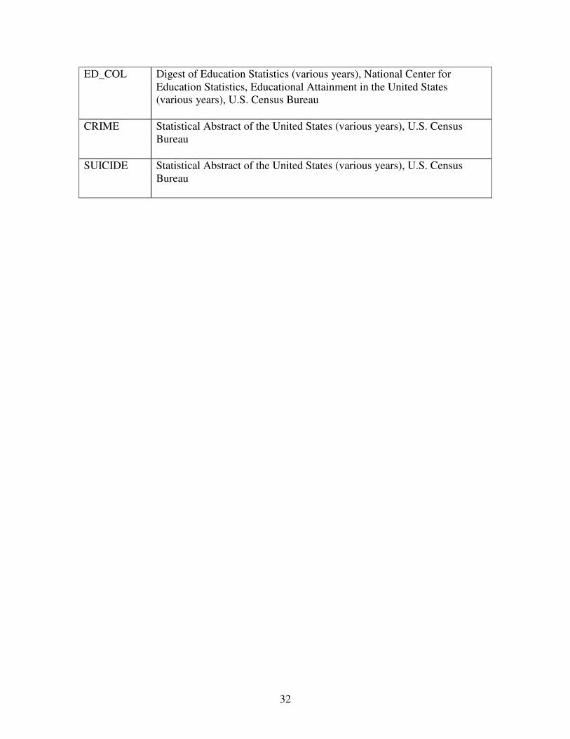
ED_COL Digest of Education Statistics (various years), National Center for

Education Statistics, Educational Attainment in the United States

(various years), U.S. Census Bureau

CRIME Statistical Abstract of the United States (various years), U.S. Census

Bureau

SUICIDE Statistical Abstract of the United States (various years), U.S. Census

Bureau

33

Appendix 2: Alternative Presentation of Bayesian Models

Figure 2

Posterior Means for the Fatality Rate Model

EBA Extreme Bounds, BMA and SSVS Average Values

-0.8

-0.6

-0.4

-0.2

0

0.2

0.4

0.6

YEAR

PERSELA

W

INSPECT

SPEEDLO

BELT

BEER

MLD

A

YOUNG

CELLP

OP

POVE

RTY

UNEM

PLO

Y

REALIN

C

ED_H

S

ED_C

OLLE

GE

CRIM

E

SUIC

IDE

Variable

Po

ste

rio

r M

ean

SSVS

EBAHI

EBALOW

BMA