FX SpotTradingand Risk ManagementfromA MarketMaker ...
101
FX Spot Trading and Risk Management from A Market Maker’s Perspective by Mu Yang A thesis presented to the University of Waterloo in fulfilment of the thesis requirement for the degree of Master of Quantitative Finance Waterloo, Ontario, Canada, 2011 c Mu Yang 2011
Transcript of FX SpotTradingand Risk ManagementfromA MarketMaker ...

FX Spot Trading and Risk Management from A
Market Maker’s Perspective
by
Mu Yang
A thesis
presented to the University of Waterloo
in fulfilment of the
thesis requirement for the degree of
Master of Quantitative Finance
Waterloo, Ontario, Canada, 2011
c© Mu Yang 2011

Author’s Declaration
I hereby declare that I am the sole author of this thesis. This is a true copy of
the thesis, including any required final revisions, as accepted by my examiners. I
understand that my thesis may be made electronically available to the public.
ii

Abstract
Due to the rapid development of computing technology and faster growth of fi-
nancial industry, Foreign Exchange high-frequency trading has become substantially
more prominent to today’s market players, especially to bankers and market makers.
This research aims at introducing today’s FX high-frequency trading structure and
discussing how a market maker can effectively reduce downside risk when market
faces a huge upward or downward stress. An Exponential Moving Average operator
is introduced and implemented using a Matlab software for tick-by-tick data analy-
sis. Simulation framework for market high-frequency data and client trading flow is
also introduced and implemented using the Matlab software. Real-time P&L calcula-
tion is introduced and used to determine the performance of a proposed risk hedging
strategy. On the other hand, due to the financial crisis we experienced in 2007, 2008,
and 2009, we analyze the tail risk of foreign exchange market. Extreme Value The-
ory (EVT) has been applied to real EUR/USD data, which contains eight-year daily
closing exchange rate. An extension of from EVT to Value-at-Risk (VaR) calcula-
tion is introduced. We also consider the volatility clustering issue in asset returns
and demonstrate how GARCH model can be applied for VaR calculation. Lastly, we
propose a method of using VaR as a high-frequency risk measure for risk hedging
strategies during intra-day trading.
iii

Acknowledgements
I am grateful to Professor Tony Wirjanto from the School of Accounting and
Finance at the University of Waterloo, who supervised and encouraged me in finishing
this thesis by providing a lot of insightful ideas and guidance. I would also like to
thank my readers Professor Don McLeish from the Department of Statistics and
Actuarial Science and Professor Allen Huang from the School of Accounting and
Finance, who helped me polishing this document through their important and helpful
suggestions. All your guidance was key to finish this thesis. Finally, I would also like
to express my gratitude to my family and friends for their supports and inspirations.
iv

Contents
Author’s Declaration ii
Abstract iii
Acknowledgements iv
List of Figures viii
List of Tables x
1 Introduction and Selected Literature Review 1
1.1 Motivation and Introduction . . . . . . . . . . . . . . . . . . . . . . . 1
1.2 Foreign Exchange Market . . . . . . . . . . . . . . . . . . . . . . . . 2
1.3 FX Spot Exchange Rate . . . . . . . . . . . . . . . . . . . . . . . . . 5
1.4 FX Market Participants . . . . . . . . . . . . . . . . . . . . . . . . . 6
1.5 Interbank Market and Market Making . . . . . . . . . . . . . . . . . 8
1.6 Electronic Broking System . . . . . . . . . . . . . . . . . . . . . . . . 10
1.7 FX High-Frequency Trading . . . . . . . . . . . . . . . . . . . . . . . 13
2 Exponential Moving Average 16
2.1 Market Data . . . . . . . . . . . . . . . . . . . . . . . . . . . . . . . . 16
2.2 Exponential Moving Average . . . . . . . . . . . . . . . . . . . . . . . 20
2.3 Application of the EMA Operator . . . . . . . . . . . . . . . . . . . . 24
v

3 Simulation Framework 28
3.1 Motivation . . . . . . . . . . . . . . . . . . . . . . . . . . . . . . . . . 28
3.2 Poisson Process . . . . . . . . . . . . . . . . . . . . . . . . . . . . . . 29
3.3 Geometric Brownian Motion . . . . . . . . . . . . . . . . . . . . . . . 30
3.4 Simulation of Market Data . . . . . . . . . . . . . . . . . . . . . . . . 31
3.5 Simulation of Client Trades . . . . . . . . . . . . . . . . . . . . . . . 33
4 Risk Hedging 39
4.1 Hedging Strategy . . . . . . . . . . . . . . . . . . . . . . . . . . . . . 39
4.2 Implementation of the Hedging Strategy . . . . . . . . . . . . . . . . 41
4.3 Scenario Analysis . . . . . . . . . . . . . . . . . . . . . . . . . . . . . 42
4.3.1 Balanced Client Buying and Selling Flows under Flat Market
Condition . . . . . . . . . . . . . . . . . . . . . . . . . . . . . 44
4.3.2 Intensive Client Selling Flow under Downward Market Condition. 47
4.3.3 Intensive Client Buying Flow under Upward Market Condition. 48
5 Tail Risk Analysis 54
5.1 Overview of Extreme Value Theory . . . . . . . . . . . . . . . . . . . 54
5.2 Maximum Likelihood Methods for EVT . . . . . . . . . . . . . . . . . 58
5.3 Empirical Analysis on EVT . . . . . . . . . . . . . . . . . . . . . . . 60
5.4 Value-at-Risk (VaR) . . . . . . . . . . . . . . . . . . . . . . . . . . . 64
5.5 An Extreme Value Approach to VaR . . . . . . . . . . . . . . . . . . 65
5.6 Considering Volatility Clustering . . . . . . . . . . . . . . . . . . . . 68
5.6.1 GARCH (p, q) Model . . . . . . . . . . . . . . . . . . . . . . . 69
5.6.2 Conditional Quantile . . . . . . . . . . . . . . . . . . . . . . . 69
5.6.3 Empirical Analysis on GARCH(1,1) . . . . . . . . . . . . . . . 70
6 VaR for A Trading Strategy 76
6.1 Ideas . . . . . . . . . . . . . . . . . . . . . . . . . . . . . . . . . . . . 76
6.2 Methodology and Example . . . . . . . . . . . . . . . . . . . . . . . . 77
vi

7 Conclusions and Future Work 84
Bibliography 86
Appendix 89
A Proof of EMA Iteration Formula for t Starting from −∞ 89
B Proof of EMA Iteration Formula for t Starting at Zero 90
vii
List of Figures
1.1 FX Daily Trading Volume Distribution . . . . . . . . . . . . . . . . . . . . 4
1.2 Reuters Dealing and EBS Trading Screens . . . . . . . . . . . . . . . . . . . 12
2.1 Number of Quote Updates for Different Inter-arrival Time on 2010/05/31 . . . . 17
2.2 Average Number of Quote Updates per Minute for Each 30-Minute Period on
2010/05/31 . . . . . . . . . . . . . . . . . . . . . . . . . . . . . . . . . 17
2.3 USD/CAD Spot Rate from 00:00 a.m. to 23:59 p.m. on 2010/05/31 . . . . . . 19
2.4 USD/CAD Spot Rate from 10:00 a.m. to 12:00 p.m. on 2010/05/31 . . . . . . 19
2.5 USD/CAD Spot Rate from 11:00 a.m. to 11:10 a.m. on 2010/05/31 . . . . . . . 20
2.6 EMA Weight Functions with Different Range Values . . . . . . . . . . . . . . 22
2.7 Time Series of Mid Price and Its EMA Values with Different Values of Range λ . 25
2.8 Mean Squared Errors of EMA estimates with Different Values of Range λ . . . . 26
3.1 Histogram of Simulation for USD/CAD Market Data Inter-Arrival Time . . . . 33
3.2 Sample Paths of USD/CAD Bid and Ask Prices by an Ito Process . . . . . . . 34
3.3 Sample Paths of Market Maker’s Base and Counter Currency Wealth Processes . 37
3.4 Sample Path of Market Maker’s P&L . . . . . . . . . . . . . . . . . . . . . 38
4.1 Sample Paths of Market Maker’s AW1(TCk) and AW2(TCk
) . . . . . . . . . . 42
4.2 Sample Path of Market Maker’s P&L(t) and PLA(t) . . . . . . . . . . . . . . 43
4.3 P&L Without Risk Hedging in Flat Market with Balanced Client Flow . . . . . 45
4.4 P&L With Risk Hedging in Flat Market with Balanced Client Flow . . . . . . . 45
4.5 P&L Differences in Flat Market with Balanced Client Flow . . . . . . . . . . . 46
viii

4.6 Sharp Ratio Comparison in Flat Market with Balanced Client Flow . . . . . . . 46
4.7 P&L Without Risk Hedging in Downward Trend Market with Intensive Client Sell 49
4.8 P&L With Risk Hedging in Downward Trend Market with Intensive Client Sell . 49
4.9 P&L Differences in Downward Trend Market with Intensive Client Sell . . . . . 50
4.10 Sharp Ratio Comparison in Downward Trend Market with Intensive Client Sell . 50
4.11 P&L Without Risk Hedging in Upward Trend Market with Intensive Client Buy . 52
4.12 P&L With Risk Hedging in Upward Trend Market with Intensive Client Buy . . 52
4.13 P&L Differences in Upward Trend Market with Intensive Client Buy . . . . . . 53
4.14 Sharp Ratio Comparison in Upward Trend Market with Intensive Client Buy . . 53
5.1 Density Functions for Frechet, Weibull, and Gumbel when α = 1.5 . . . . . . . 57
5.2 EUR/USD Day-End Price . . . . . . . . . . . . . . . . . . . . . . . . . . 61
5.3 Q-Q Plot of EUR/USD Daily Loss . . . . . . . . . . . . . . . . . . . . . . 61
5.4 EUR/USD Maximum Daily Loss for Each Month . . . . . . . . . . . . . . . 62
5.5 Empirical and Theoretical CDF Comparison for Maximum Daily Loss in Monthly
Block . . . . . . . . . . . . . . . . . . . . . . . . . . . . . . . . . . . . 63
5.6 Autocorrelation Function of EUR/USD Daily Loss . . . . . . . . . . . . . . . 71
5.7 Inferred Innovations, Standard Deviations, and Original Time Series . . . . . . 72
5.8 Autocorrelation Function of Innovations . . . . . . . . . . . . . . . . . . . . 73
6.1 Simulated P&L Sample Path for a 30-hour Trading Period . . . . . . . . . . . 79
6.2 P&L Increments for a 30-hour Trading Period . . . . . . . . . . . . . . . . . 80
6.3 Q-Q Plot for P&L Increments for A 30-hour Trading Period . . . . . . . . . . 81
6.4 Maximum 2-Minute Loss in Hourly Block for A 30-Hours Period . . . . . . . . 82
6.5 Empirical and Theoretical CDF Comparison for Maximum 2-Minute Loss in Hourly
Block . . . . . . . . . . . . . . . . . . . . . . . . . . . . . . . . . . . . 83
ix

List of Tables
1.1 ISO 4217 Code for G10 Currencies . . . . . . . . . . . . . . . . . . . 5
1.2 Top 10 FX Market Participants by % of Overall Market Volume . . . 9
5.1 MLE Estimates for Generalized Extreme Value Distribution with Dif-
ferent Block Size . . . . . . . . . . . . . . . . . . . . . . . . . . . . . 63
5.2 AR(1)-GARCH(1,1)Parameter Estimates given by MLE with Normal
Innovations . . . . . . . . . . . . . . . . . . . . . . . . . . . . . . . . 72
5.3 AR(1)-GARCH(1,1)Parameter Estimates given by MLE with Student
t Innovations . . . . . . . . . . . . . . . . . . . . . . . . . . . . . . . 74
5.4 Parameter Estimates for GJR-GARCH(1,1,1) . . . . . . . . . . . . . 75
x
Chapter 1
Introduction and Selected
Literature Review
1.1 Motivation and Introduction
The motivation of conducting this research is to provide an overview of today’s FX
market marking business and its risk management.
The first chapter contains introductions to current structure of global FX mar-
ket. We introduce the market by its segment and participants. We also introduce
the FX interbank market, market making business model, and Electronic Broking
System for FX trading. In Chapter 2, we introduce the exponential moving average
method and its application in FX high-frequency data cleaning. In Chapter 3, we
propose a simulation framework for both client trading and FX market rate simula-
tion in Matlab. A Poisson process and Geometric Brownian Motion will respectively
be applied in the simulation of an event arrival process and asset price movements.
In Chapter 4, we implement a position limit risk hedging strategy based on simulated
client trading process. Definitions of market maker’s wealth process and P&L mea-
sures will be defined and calculated. In order to accomplish this objective, we need
to assume that the market maker has the ability to access liquidity, which means
1
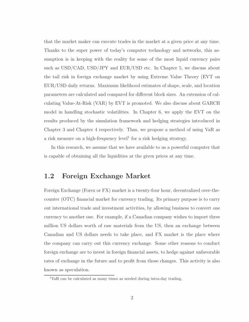
that the market maker can execute trades in the market at a given price at any time.
Thanks to the super power of today’s computer technology and networks, this as-
sumption is in keeping with the reality for some of the most liquid currency pairs
such as USD/CAD, USD/JPY and EUR/USD etc. In Chapter 5, we discuss about
the tail risk in foreign exchange market by using Extreme Value Theory (EVT on
EUR/USD daily returns. Maximum likelihood estimates of shape, scale, and location
parameters are calculated and compared for different block sizes. An extension of cal-
culating Value-At-Risk (VAR) by EVT is promoted. We also discuss about GARCH
model in handling stochastic volatilities. In Chapter 6, we apply the EVT on the
results produced by the simulation framework and hedging strategies introduced in
Chapter 3 and Chapter 4 respectively. Thus, we propose a method of using VaR as
a risk measure on a high-frequency level1 for a risk hedging strategy.
In this research, we assume that we have available to us a powerful computer that
is capable of obtaining all the liquidities at the given prices at any time.
1.2 Foreign Exchange Market
Foreign Exchange (Forex or FX) market is a twenty-four hour, decentralized over-the-
counter (OTC) financial market for currency trading. Its primary purpose is to carry
out international trade and investment activities, by allowing business to convert one
currency to another one. For example, if a Canadian company wishes to import three
million US dollars worth of raw materials from the US, then an exchange between
Canadian and US dollars needs to take place, and FX market is the place where
the company can carry out this currency exchange. Some other reasons to conduct
foreign exchange are to invest in foreign financial assets, to hedge against unfavorable
rates of exchange in the future and to profit from those changes. This activity is also
known as speculation.
1VaR can be calculated as many times as needed during intra-day trading.
2

According to [16], FX market is the largest and most liquid financial market in
the world in terms of daily trading volume. Based on the numbers published by Bank
for International Settlements (BIS)2, the FX total trading volume increased by 38%
between April 2005 and April 2006 and has increased more than two-folds since 2001.
In 2010, the average daily turnover was reported to be $3.98 trillion, of which $1.49
trillion was traded in FX spot market, $475 billion in the forward market, $1.765
trillion in FX swaps, $43 billion in currency swaps, and $207 billion in options and
other derivatives. Geographically, 36.7% of the total trading volume was made in
London, while 17.9% in New York City, and 6.2% in Tokyo. The dramatic increase
in trading volume is mainly due to the growing importance of FX as an asset class in
fund management, particularly in hedge funds and pension funds. For the FX daily
trading volume distribution by product types and geographic locations, see Figure 1.1.
The price quotation for currencies generally follows the ISO convention, and is
the three-letter code used to identify a currency , such as USD for US dollar and
GBP for British sterling. For the list of ISO codes of G10 currencies, see Table 1.1.
Currencies are always traded against one anther. The activity of buying one currency
is tpically accompanied by the activity of selling another currency. Thus, when a
price is quoted, it is always quoted for a currency pair, and is labeled as XXXYYY or
XXX/YYY. The first three letters (XXX) represent the base currency that is quoted
against the second currency (YYY), which is called the counter currency or quoted
currency. In practice, the rate convention is to quote everything in terms of one
unit of the US dollar. For instance, the US dollar and Swiss franc rate is quoted as
USD/CHF, and is the number of Swiss franc to one US dollar. The exceptions are
for euro and sterling, which are quoted respectively as GBP/USD and EUR/USD,
the number of US dollar to one pound and one euro.
2Source: 2010 Triennial Central Bank Survey, Bank for International Settlements
3

Figure 1.1: FX Daily Trading Volume Distribution
4

Table 1.1: ISO 4217 Code for G10 Currencies
USD US Dollar
CAD Canadian Dollar
JPY Japanese Yen
AUD Australian Dollar
NZD New Zealand Dollar
GBP British Pound
EUR EURO
CHF Swiss Franc
SEK Swedish Krona
NOK Norwegian Krona
1.3 FX Spot Exchange Rate
A spot FX trade is a purchase or sale of one currency against another one, with
delivery in two business days after the trade date. Non-business days are not included
in the count, so a trade on a Friday is settled on the following Tuesday. There are
some exceptions to this. For example trading of a US dollar against a Canadian dollar
are settled on the next working day. A settlement date that falls on a public holiday in
the country of one of the two currencies is delayed for settlement by one day. An FX
transaction is possible between any two currencies. However, to reduce the number of
quotes that need to be made, the market generally quotes only against the US dollar
or occasionally against the sterling or euro, so that the exchange rate between two
non-dollar currencies is calculated from the rate for each currency against the dollar.
The resulting exchange rate is known as the cross-rate. Cross-rates themselves are
also traded between banks in addition to dollar-based rates. This is usually because
the relationship between any two rates is closer than that of either one against the
dollar, for example the Swiss franc moves more closely in line with the euro than it
does against the dollar; so in practice one observes that the USD/CHF rate is more
or less a function of the EUR/CHF rate.
5

The spot FX quote is a two-way bid-offer price. The bid indicates the rate at
which a bank is prepared to buy the base currency against the counter currency; it
is the lower rate. The other side of the quote is called the offer, which is the rate
at which the bank is prepared to sell the base currency against the counter currency.
For example, USD/CAD = 1.2324/26 tells that the bid and offer prices for 1 USD are
at 1.2324 and 1.2326 CAD. In other words, this expresses the willingness of a bank to
buy 1 USD at 1.2324 CAD and to sell 1 USD at 1.2326 CAD. The difference between
bid and offer prices, called the spread, can be viewed as the risk of making one unit
currency transaction. It is the (raw) profit that a market maker can generate upon
trading with clients for one unit of the base currency. In this example, the spread
for USD/CAD is 0.0002, which is also quoted as “2 pips” (where 0.0001 = 1 pip for
USD/CAD). For G10 currencies exclude JPY and GBP, pip resolutions for exchange
rates are set at the fourth decimal place. For JPY and GBP, the pip resolutions
are set at the third and fifth decimal places respectively. Spread is often used as a
measure of the liquidity of the currency pair. In particular, the smaller the spread
is, the more liquid the currency pair is. For some of the most liquid currency pairs
such as EUR/USD, EUR/GBP, and USD/CAD, the spreads are usually very small,
at 0.5 or 1 pip during intra-day busy trading hours. For some of the currencies that
are lack of liquidity, the bid-offer spread can be as large as 20 or 30 pips. An example
of such currencies is MXN/TRY (Mexican peso and Turkish lira).
1.4 FX Market Participants
The participants in the FX market include central banks, commercial and investment
banks, funds, corporations, and individuals. Unlike the stock market, access to FX
market is divided into several levels. The top tier access level is the interbank market,
which is made up of the largest commercial banks and securities dealers. They are
responsible for 53% of the global transactions. The next tier is composed of large
6

hedge funds, pension funds, insurance companies, and multi-national corporations
who may need to execute an FX trading for the purpose of hedging currency risk,
speculating, foreign asset investment and payment of imports, etc. The third tier is
the group of individual investors (both long-term and short-term), who constitute a
growing segment of the market and mostly participates indirectly through brokers or
market makers.
FX market participants operate with varying perspectives. Each perspective car-
ries a different attitude, goal, investment horizon, risk appetite, and market impact
with it. According to [22], these participants can be categorized into five groups
according to their perspectives. Active Hedgers, who are mostly corporations, are
long-term players who seek a profit protection through treasury management. Market
Disruptors, who are usually governments, are long-term enablers of national, regional,
or global economic goals. Risk Avoiders, which are usually investment fund special-
ists, are long-term trend followers with high levels of skills, resources, knowledge,
and commitments. Risk Takers, who are usually individual traders, are short-term
system followers with a wide range of skills, knowledge, resources, and commitment.
Lastly, Market Makers, who are usually banks and dealers, are the credit suppliers to
corporations, governments, funds, other banks, and individual traders.
The key difference among these market participants is their levels of sophistication
which include: money management techniques, profit objectives, technologies, quan-
titative abilities, research abilities, and discipline. In terms of regulation, individual
traders have the least amount of external governance; whereas governments, banks,
corporations, and investment funds must adhere to a maximum amount of financial
regulations and restrictions. Individual traders fall into two groups: sophisticated
traders and un-sophisticated traders. In [22], the author states that “In the zero-sum
game of the FX trading, the sophisticated traders impose self-disciplines and use tools
and strategies that emulate those of the highly sophisticated institutional participants
to extract profits from the novice participants. In the end it is only the sophisticated
7

participants who have the ability to extract positive returns from the FX markets”.
1.5 Interbank Market and Market Making
FX market is a decentralized market. In a centralized market such as New York
Stock Exchanges (NYSE) or the Chicago Board of Trade, each transaction is recorded
according to price dealt and size traded. There is usually a central physical place back
to which all trades can be traced. The FX market, however, is a decentralized market,
where there are more than one “exchanges” that record every trade. Instead, each
market maker records his or her own transactions and keeps it as his/her proprietary
information. According to [26], the primary market makers who make bid and offer
prices in the FX market are the largest banks in the world. They deal with each
other constantly either on behalf of themselves or their customers. This is why
the market on which banks conduct transactions is called the Interbank Market.
See Table 1.2 for the list of top 10 FX market participants by the market trading
volume3. The competition between banks ensures tight spreads and fair pricing.
Most individuals are unable to access the pricing available on the interbank market
because the interbank participants tend to include the largest mutual funds and hedge
funds in the world as well as large multinational corporations who operates in millions
(if not billions) of dollars.
Market making simply means being a buyer and a seller at the same time. A
FX market maker (usually a bank) is looking for opportunities to buy low and sell
high with as many clients as possible. A customer, can be a tourist walking into
a local branch or a hedge fund manager calling into the FX sales desk and makes
FX trading deals with the market maker. As the counter party of the customer, the
market maker is using its own capital to trade with the customer at a certain rate
that is agreed between the two parties. From [17] and [2], we know that in order
3Source: Euromoney FX survey, FX Poll 2010. The Euromoney FX survey is the largest globalpoll of FX services providers.
8

Table 1.2: Top 10 FX Market Participants by % of Overall Market Volume
Deutsche Bank 18.06%
UBS AG 11.30%
Barclays Capital 11.08%
Citi 7.69%
Royal Bank of Scotland 6.50%
JPMorgan 6.35%
HSBC 4.55%
Credit Suisse 4.44%
Goldman Sachs 4.28%
Morgan Stanley 2.91%
to facilitate market making business, each bank is structured differently, but most
banks will have a separate group known as the Foreign Exchange Sales and Trading
Department. This group is responsible for making prices for the bank’s clients and
for offsetting that risk with other banks. Within the foreign exchange group, there
is a sales desk and a trading desk. The sales desk is generally responsible for taking
the orders from the clients, getting a quote from the spot trader and relaying the
quote to the clients to see if they want to deal on it. This three-step process in the
industry is quite common because even though online foreign exchange trading is
available, many of the large clients, such as pension funds or big corporations, who
deal anywhere from $10 million to $100 million at a time (cash on cash), believe
that they can get better pricing by dealing over the telephone than over the trading
platform. This is because most on-line platforms offered by banks will have a trading
size limit due to the desire of the bank to be able to offset the risk.
As the market maker, bank dealers determine their prices based upon a variety
of factors including: the current market rate, how much volume is available at the
current price level, their views on where the currency pair is headed to and their
current inventory positions. If they think that the euros is moving upwards, they
may be willing to offer a more competitive rate to clients who want to sell euros
9

because they believe that once they are given the euros, they can hold onto them for
a while for the price to increase. On the other hand, if they think that the euro is
headed toward a lower value and the client is giving them euros, they may offer a
lower price because they are not sure if they can sell the euro back to the market at
the same level at which it would be given to them.
To offset the risk, the bank dealers will turn to the interbank market and try
to flatten their positions by putting orders into the market. There are two primary
electronic platforms that interbank traders use to put their orders. One is offered by
Reuters Dealing and the other is offered by the Electronic Broking Services (EBS),
which will be introduced in section 1.6. The interbank market is a credit-approved
system in which banks trade based solely on the credit relationships they have es-
tablished with other banks. All of the banks can see the best market rates currently
available; however, each bank must have a specific credit relationship with another
bank in order to trade at the rates being offered. The bigger the bank is, the more
credit relationships it can have and the better pricing it will be able to access. The
same is true for clients such as retail FX brokers. The larger the retail FX broker in
terms of the available capital, the more favorable pricing it can get from the interbank
market. If a client or a bank is relatively small, it is usually restricted to dealing with
only a selected number of larger banks and tends to get less favorable pricing.
1.6 Electronic Broking System
Nowadays, over 90% the FX spot transactions goes through automated electronic
order-matching systems. Electronic brokers collect orders from tens of thousands
of market players globally by connecting to their networks and match their orders
automatically. As such, they are perfectly suited to a decentralized market in need
of efficient matching. The foreign exchange market, with its decentralized structure
and quickly growing volumes, was one of the earliest adopters of electronic brokers.
10

Subsequently, many equity markets also adopted electronic brokers.
According to [26], the most popular electronic broker systems are Reuters Dealing
2000 and Electronic Broking Services (EBS) in the FX interbank market. The first,
Reuters Dealing 2000-2, was introduced by Reuters in April 1992. A year later, in
April 1993, Minex was launched by Japanese banks, with EBS following in September
1993. The EBS Partnership was established by several major market making banks
to counter the dominant role of Reuters, and EBS acquired Minex in December 1995
and thereby gained a significant market share in Asia.
The electronic brokers work with the goal of matching the buyer and the seller as
efficiently as possible. When a limit order 4 is entered, there is first a price priority to
ensure that it is always the best prices that are traded on and then a time priority
(price-time priority). Market orders5 are given priority according to time of entry,
and the system matches the counter-parties automatically. The entry of orders is
anonymous, but both parties see the counter-party’s identity immediately after the
trade. Figure 1.2 is borrowed from [26] and shows the trading screens of both Reuters
Dealing and EBS.
Part a of Figure 1.2 shows both Reuters Dealing 2000-1 and Dealing 2000-2. The
middle panel contains the D2000-1 system for direct bilateral trading, and the upper
panel is the D2000-2 electronic broker. From the D2000-1 panel, we can see that the
dealer has been contacted for a quote for USD 4 million against DEM. The dealer
replies with the quote “ 05 08 ”, which is understood to be bid 1.8305 and ask 1.8308.
The contacting dealer responds with “ I BUY ”, and the system automatically fills in
the line “ TO CONFIRM AT 1.8308 I SELL 4 MIO USD ”. In the lower right corner
of the screen, the dealer can see the price and direction of the last trades through the
D2000-2 system.
Part b of Figure 1.2 shows the EBS screen. The left half of the EBS screen shows
4A limit order is an order to buy a specified quantity up to a maximum price or sell subject to aminimum price.
5A market order involves buying or selling a specified quantity at the best prevailing price.
11

Figure 1.2: Reuters Dealing and EBS Trading Screens
12

the bid and offer (ask) prices. The dealer chooses which exchange rates to display
(the base currency is written first). The prices shown are either the best prices in the
market or the best available ones (from credit-approved banks only). The upper part
of the right half of the screen shows the dealer’s own trade. The lower part shows
the price and direction of all trades through the system for selected exchange rates.
GIVEN means that it was traded at the bid price, and PAID means it was traded
at the ask price. The intuition for this is that the limit order dealer is given the base
currency (buys).
More discussions about dealer behaviors (for both electronic and traditional voice
brokers), liquidity, transaction costs on electronic FX trading can be found in [26]
and [15].
1.7 FX High-Frequency Trading
In general, high-frequency trading (HFT) involves the execution of computerized
trading strategies characterized by unusually very short position-holding periods, in
many cases taking advantage from microstructure inefficiency. In high-frequency
trading, programs analyze market data and utilize trading opportunities that may
open up for only a fraction of a second to several hours. High-frequency trading,
uses quantitative models and computer programs to hold short-term positions in
equities, options, futures, ETFs, currencies, and other financial instruments that
possess electronic trading capability. High-frequency traders compete on a basis of
speed with other high frequency traders, who are not long-term investors (that is,
who typically look for opportunities over a period of weeks, months, or years), and
compete with each other for very small, consistent profits.
According to the article [6], there are several reasons why the FX market is viewed
as the most attractive place for high-frequency trading. First, in the FX market, the
spreads are extremely low (at about 1 pip) for most liquid currency pairs such as
13
EUR/USD, EUR/GBP, etc. If we assume a trader has perfect foresight and can take
advantage of every small price spike, he/she can earn (without taking on any leverage)
approximately 2 percent of return everyday, or approximately 500 percent during one
year. If a trader can not trade at high frequency (but, for example, only once a day),
then the annual return potential is only 125 percent. Other things being equal, going
to HFT enhances the return potential of an investment strategy because a trader
can take advantage of many more price strikes. For those sophisticated investment
managers equipped with appropriate computing power and know-how, this is seen
as great enticement. Secondly, FX market is evolving at a much faster speed than
other markets such as equities or futures. Unlike equity and futures markets, where
algorithmic trading is developed as a response to a lack of liquidity, the high levels
of liquidity access in the FX market allow the market participants to focus more on
generating alphas.
To build a solid FX high-frequency trading environment is an extremely chal-
lenging exercise. A HFT engine usually contains the following components: liquidity
aggregation, trading strategies manager, execution strategies manager, and risk ana-
lytic. Liquidity aggregation involves the utilization of today’s advanced network and
computer technologies to extend the connections to as many market participants and
liquidity venues as possible. Aggregating liquidities from different sources, a HFT
engine will have a great view of FX market movements at a very low latency. In-
formation about changes in price, volume, and volatility, etc. are coming in on a
millisecond basis. And, as a result, better trading decisions and execution results can
be achieved with better liquidity aggregation. Thus, access to the liquidity pool is
very crucial in FX trading.
Trading strategies manager is the central brain of a high-frequency trading engine,
which contains the strategies that are developed by traders and quantitative modelers.
These strategies are usually built based on statistical data analysis, pervious trading
experiences, and alpha research, etc. It is the trading strategies that conduct all
14
the real-time market data analysis and make trading decisions on buy or sell certain
amounts of currency pairs at certain prices. Execution strategies manager is designed
to manage different types of orders (for example, IOC6 and GTC7, etc.) and place
orders into the market smartly and efficiently to achieve a high successful rate in its
execution. It is very important for a HFT engine to be able to catch the best timing
for its execution in this milliseconds competition. Risk analytic calculates the real-
time risk exposures and measures of the high-frequency trading activities. It is the
tool for traders to monitor auto-trading processes that are initiated by the hedging
strategies. Traders rely on risk analytic in terms of performing human-intervening
for the high-frequency trading engine.
6IOC: Immediate Or Cancel type of order7GOC: Good Till Cancel type of order
15

Chapter 2
Exponential Moving Average
2.1 Market Data
We begin the discussion in this subsection by considering a real example of FX high-
frequency time series. The data series is the USD/CAD spot tick-by-tick bid and
ask prices on 2010/05/31. The series starts at 00:00:00.2591 EST, which is the time
stamp of the first quote of the day, and ends at 23:59:58.210 EST, which is the time
stamp of the last quote update of the day. Each quote update contains a time stamp
with accuracy at 1 millisecond, and size and price for both bid and ask sides at
that moment. The data is obtained by aggregating feeds of USD/CAD spot from
four different venues, which are Reuters, EBS, HotSpot, and Currenex. A series of
data cleaning processes needs to be applied to the original raw data set to obtain a
“cleaned” version of the data that can be analyzed. A typical data cleaning processes
usually includes steps of removing inverted quotes and removing staled and expired
quotes.
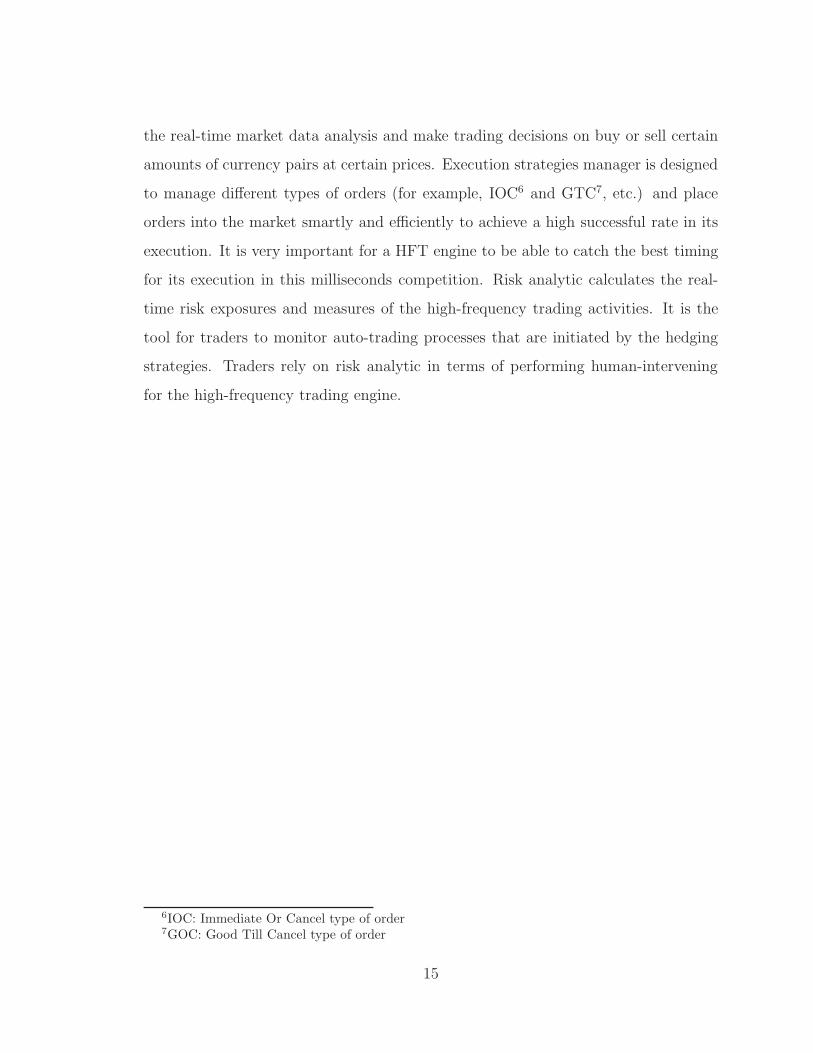
Figures 2.1 and 2.2 show two different ways of viewing quote updating frequencies
for our sample data set.
1The last three digits of the time stamp are in the unit of milliseconds. It is at 259 millisecondfor this time stamp.
16
Figure 2.1: Number of Quote Updates for Different Inter-arrival Time on 2010/05/31
Figure 2.2: Average Number of Quote Updates per Minute for Each 30-Minute Period on
2010/05/31
17

In particular Figure 2.1 shows the number of quote updates for each different
length of Inter-Arrival Time, which is defined as the time space between two con-
secutive quote updates. There are in total 36,979 quote updates during the day of
2010/05/31. Among them, there are 4,549 quote updates with inter-arrival time less
than and equal to 10 milliseconds, 17,631 quote updates with inter-arrival time less
than and equal to 100 milliseconds, and 5,031 quote updates with inter-arrival time
between 100 and 200 milliseconds. Thus, about two-thirds of the total number of
quote updates happen at inter-arrival time less than 200 milliseconds. Next Fig-
ure 2.2 shows the average number of quote updates per minute for each 30-minute
period during the day. We can see that during the North American trading hours
(from 7:00 a.m. to 17:00 p.m.), the average number of quote updates ranges from
about 20 to 60 per minute, except for a dramatic spike of hitting almost 200 per
minute between 15:00 p.m. and 15:30 p.m. In addition, there are also big numbers
recorded at 7:00 a.m., 13:00 p.m., and 22:30 p.m., which are the beginning hours of
North American morning and afternoon trading sessions and the busy hour in Asia.
So, we can see that quote updating can happen at a millisecond level. Frequency of
updating can also be different for different periods of time during the day. For ex-
ample, quote updating speed for USD/CAD between 7:00 a.m. to 11:00 a.m. (busy
hours in North America and Europe trading) can be multiple times faster than in the
period from 4 p.m. to 5 p.m. Other reasons for a dramatic change in the quote up-
dating frequency include new releases and the announcement of important economic
numbers.
Figures 2.3, 2.4, and 2.5 are the time series plots of USD/CAD tick-by-tick prices
at different magnitudes of time intervals. Figure 2.3 is the plot of the entire time series
(for a 24-hour period) of USD/CAD bid and ask prices. Figure 2.4 is the USD/CAD
bid and ask prices for a two-hour period from 10:00 a.m. to 12:00 p.m., during which
there are 2,331 quote updates. Figure 2.5 is the plot of bid and ask prices for a
ten-minute period from 11:00 a.m. to 11:10 a.m., during which there are 202 quote
18

0 1 2 3 4 5 6 7 8 9
x 104
1.04
1.045
1.05
1.055
Time Stamp in Second
US
D/C
AD
USD/CAD Spot Rate from EST 00:00 a.m. to 23:59 p.m.
ASKBID
Figure 2.3: USD/CAD Spot Rate from 00:00 a.m. to 23:59 p.m. on 2010/05/31
3.6 3.7 3.8 3.9 4 4.1 4.2 4.3 4.4
x 104
1.048
1.0485
1.049
1.0495
1.05
1.0505
1.051
Time Stamp in Second
US
D/C
AD
USD/CAD Spot Rate from EST 10:00 a.m. to 12:00 p.m.
ASKBID
Figure 2.4: USD/CAD Spot Rate from 10:00 a.m. to 12:00 p.m. on 2010/05/31
19

3.96 3.97 3.98 3.99 4 4.01 4.02
x 104
1.0498
1.0499
1.05
1.0501
1.0502
1.0503
1.0504
1.0505
1.0506
Time Stamp in Second
US
D/C
AD
USD/CAD Spot Rate from EST 11:00 a.m. to 11:10 p.m.
ASKBID
Figure 2.5: USD/CAD Spot Rate from 11:00 a.m. to 11:10 a.m. on 2010/05/31
updates. The first thing that we observe from these plots is that high-frequency
data series is a time series with irregular time space, which is referred to as inho-
mogeneous time series. Thus, methods and tools for analyzing homogeneous (regular
time-spaced) time series need to be modified to handle inhomogeneous high-frequency
data analysis. The second thing is that price movements can vary dramatically in
a very short period of time, which renders it difficult to make good trading deci-
sions. A market participant has to be very watchful of the fact that both buying and
selling decisions need to be made within a few minutes or even seconds. Thus, a mar-
ket participant must be equipped with both advanced technology and smart trading
strategies in order to capture short-term market inefficiency in this high-frequency
market.
2.2 Exponential Moving Average
Amoving average process is a widely used in conducting technical analysis on financial
data. It is often applied to time series data to smooth out short-term fluctuations
20

and highlight long-term trends or cycles.
For a continuous function x(t), its moving average at time tn is defined as an
integral
MAx,ω =
∫ tn
−∞ω(tn − t)x(t)dt
∫ tn
−∞ω(tn − t)dt
, (2.1)
where ω(t) is the weighting function defined on non-zero arguments.
The range of a moving average is defined as
R =
∫∞
0tω(t)dt∫∞
0ω(t)dt
. (2.2)
Specifically, Exponential Moving Average (EMA) is a moving average process with
the weighting function specified as
ω(t) =1
λe−
1λt, (2.3)
where λ is the range of the weight function. This weight function declines exponen-
tially with the time distance of the past observations starting from the present time.
The choice of the range value of λ is very important for the exponential moving aver-
age operation on time series because it controls the distribution of weights onto past
data values. Figure 2.6 shows the EMA weight functions with different range values.
We can see that the smaller the range value of λ is, the heavier the weights being
assigned to more recent observations, and the faster the weight function decays into
past.
If we apply the weight function (2.3) into equation (2.1), we can define the expo-
nential moving average of value x at time point tn as
EMAx(λ, tn) =
∫ tn
−∞1λe−
1λ(tn−t)x(t)dt
∫ tn
−∞1λe−
1λ(tn−t)dt
=
∫ tn
−∞
1
λe−
1λ(tn−t)x(t)dt (2.4)
Based on equation (2.4), EMA can be computed by a recursive method found in
[20] and [21]. Unfortunately, the formula, as presented in [20] and [21], are incorrect.
Here, we provide a correct version of the formula. In this study, we adopt similar
notations as those used in the text book [21]. Let Z(tj) represent a raw series with
21

0 5 10 15 20 25 30 35 40 45 500
0.02
0.04
0.06
0.08
0.1
0.12
0.14
0.16
0.18
0.2
0 ≤ t ≤ 50
Wei
ght ω
(t)
range λ = 5range λ = 10range λ = 20range λ = 30range λ = 40
Figure 2.6: EMA Weight Functions with Different Range Values
22

irregular time spaces at arrival times tj where j = 0, 1, 2, 3, ... The sequence of arrival
times is required to be monotonically increasing such that tj > tj−1. For a time point
t∗ such that tn−1 ≤ t∗ < tn, the exponential moving average value of time series Z(tj)
at time t∗ can be obtained by the following recursive formula:
EMAZ(λ, t∗) = µ1EMAZ(λ, tn−1) + (ν1 − µ1)Z(tn−1) + (1− ν1)Z(tn) (2.5)
with µ1 = e−1λ(t∗−tn−1) and value of ν1 depending on the chosen interpolation scheme
for Z(t∗), where
ν1 =
1 for the previous tick method
1− t∗ − tn−1
tn − tn−1for the linear interpolation method.
This recursive formula of calculating EMA can be applied to both homogeneous
and inhomogeneous time series. It is easy to show that 0 < µ1 < 1 and 0 ≤ ν1 < 1
given tn−1 < t∗ ≤ tn. The values of µ1 can be viewed as the weight assigned to the
EMA value of the time series at time point tn−1. Values of ν1 − µ1 and 1− ν1 can be
viewed as the weights assigned to Z(tn−1) and Z(tn). Appendix A gives the proof of
the above recursive formula. The derivation of this formula assumes the time series
to start from time −∞, which is not realistic. For practical purpose, here we list an
analogous form of the recursive equation that assumes the time series to start from
time zero instead.
We let Z(tj) with j = 0, 1, 2, 3, ... be the raw inhomogeneous time series starting
at time point t0 = 0. For a time point t∗ such that tn−1 ≤ t∗ < tn, the exponential
moving average value of time series Z(tj) at time t∗ can be obtained by the following
recursive formula:
EMAZ(λ, t∗) = µ2EMAZ(λ, tn−1) + (ν2 − µ2)Z(tn−1) + (1− ν2)Z(tn) (2.6)
with µ2 = e−
1λ(t∗−tn−1)−e
−1λt∗
1−e−
1λt∗
and value of ν2 depending on the chosen interpolation
23

scheme for Z(t∗), where
ν2 =
1 for the previous tick method
1− 1
1− e−1λt∗
t∗ − tn−1
tn − tn−1for the linear interpolation method.
The derivation of this formula is provided in Appendix B. EMA can be regarded as
an operator that transforms one time series into another one:
EMA : Z(tn) 7−→ EMAZ(λ, tn). (2.7)
Due to this recursive formula, the integration need not be computed in practice;
instead only few multiplications and additions need to be done for each tick. In this
research, we apply the above recursive formula to our FX data.
2.3 Application of the EMA Operator
The EMA operator is implemented in matlab according to equation (2.6). For the
analysis, we consider a 15-minute (from 10:00 a.m. to 10:15 a.m.) subset of the high-
frequency data series on 2010/05/31 as a starting point. Let Z(tk) for k = 0, 1, 2, ..., n
denote n mid-prices2 being calculated during this 15-minute time interval. We choose
the first observation of the time series as the starting value of the recursive formula.
That is, we set Z(t0) = EMAZ(λ, t0). Then, the EMA values of the mid-prices at
each time stamp tk for 1 ≤ k < n are calculated iteratively.
Figure 2.7 shows the original data series of the mid prices and their EMA val-
ues with different values of the range of λ (set at 20, 100, 200, and 600 seconds
respectively).
For a value of λ = 20 (seconds), we see a small discrepancy between the original
data series and the EMA series at the very beginning portion of the plot. Then, the
two series merges into almost an identical one, which means that the EMA operator
2Mid-price = (Ask price + Bid price)/2
24

0 100 200 300 400 500 600 700 800 9001.0494
1.0495
1.0496
1.0497
1.0498
1.0499
1.05λ = 20
EMA
Z(20, t)
Z(t)
0 100 200 300 400 500 600 700 800 9001.0494
1.0496
1.0498
1.05
1.0502
1.0504λ = 100
EMAZ(100, t)
Z(t)
0 100 200 300 400 500 600 700 800 9001.0494
1.0496
1.0498
1.05
1.0502
1.0504
1.0506
1.0508
1.051λ = 200
EMA
Z(200, t)
Z(t)
0 100 200 300 400 500 600 700 800 9001.049
1.0495
1.05
1.0505
1.051
1.0515
1.052
1.0525
1.053λ = 600
EMA
Z(600, t)
Z(t)
Figure 2.7: Time Series of Mid Price and Its EMA Values with Different Values of Range λ
25

generates estimation very closed to real values. By looking at the other three plots,
we can see that as the range of value of λ gets bigger, the discrepancy between the
values of the original data and the EMA values are getting bigger, and the longer it
takes for the two series to get closed enough to each other. Thus, no matter what
value of λ we choose, a built-up time period is necessary for the EMA operator to
produce accurate enough values. Empirically, the bigger the range value of λ is, the
longer the built-up period is needed for the EMA to produce accurate enough results.
This conforms with the rule of thumb given on page 57 in [21]: “the heavier the tail
of the kernel, the longer the required build-up is needed.”
To get a better picture of how well the EMA operator performs, Figure 2.8 shows
the mean square errors (MES) between the true market values and their EMA esti-
mates with different range values of λ. No surprise that we see EMA estimates with
larger value of λ has larger MSE values. For each value of λ, MSE starts to decrease
and converges after an enough number of observations being made. The larger the λ
is, the more observations we need to see MSE starting to decreasing.
0 100 200 300 400 500 600 700 800 9000
0.5
1
1.5
2
2.5x 10
−6
Time Stamp in Second
MS
E
MSE of Exponential Moving Average Estimates with Different Range Values
λ = 20λ = 100λ = 200λ = 600
Figure 2.8: Mean Squared Errors of EMA estimates with Different Values of Range λ
26

One possible explanation that Exponential Moving Average is very accurate in
estimating high-frequency data is because the time period between two consecutive
quote updates is so short that the quote jump is not significant enough to deviate
the quote far from its EMA estimate. With EMA operator, a market maker can at
least estimate market movements for a very short period (measured in milliseconds)
ahead into future. A game of issuing and canceling limit orders within millisecond
time intervals can be performed.
27
Chapter 3
Simulation Framework
3.1 Motivation
Trading as the counter-party of clients is the core business model of a market maker
because client margin spreads (used to) contribute to majority part of profit. As
the evolving of advanced technology and market transparency, more and more so-
phisticated investors start to trade in FX market with access to fast information and
liquidity. Market makers can never make money the same way they did 20 years ago.
Buying from one client then selling to another one at a higher price can not be done
as easily as before. Smart risk hedging strategies must be implemented to help the
market maker trade “profitably”. In our opinion, we believe that the hedging strategy
should be subjective to client trading flows. This is saying that under different client
trading flows, different hedging strategies (or different parameter values for one hedg-
ing strategy) should be applied to optimize risk-adjusted returns. According to [1], a
market maker should carefully study his/her client trading flows so that non-public
information can be extracted from it. For example, client trades can be categorized
into different groups such as hedge funds, banks, institutional investors, and retail
flows. Transactions done with hedge fund clients provides more useful information
than transactions done with retail clients. If a speculative trader from a hedge fund
28

is buying Eruos and selling Dollars, we reach a very different conclusion about the
future direction of EUR/USD than if the buying of EUR came from a US importer.
Due to the lack of historical high-frequency data and client trading information,
we build a basic simulation frame work for market data and client trades in this
chapter. Poisson process and Geometric Brownian motion are the natural starting
points for event arrival process and asset price simulations.
3.2 Poisson Process
A counting processes deals with the number of various outcomes of an experiment
over a period of time. According to [27], a counting process is defined as a stochastic
process{N(t), t ≥ 0
}that has the following properties:
1. N(t) ≥ 0.
2. N(t) is an integer.
3. If s < t, then N(s) ≤ N(t). In other words, N(t) is non-decreasing.
4. If s < t, then N(t)−N(s) is the number of events occurred during time interval
(s, t).
A Poisson process is a special example of the counting process. A Poisson Process
with a rate of λ is defined as a continuous-time counting process{N(t), t ≥ 0
}such
that:
1. N(t) = 0 for t = 0.
2. The process has Independent Increments, which means that the numbers of
occurrences counted in disjoint intervals are independent from each other.
3. The process has Stationary Increments. which means that the probability distri-
bution of the number of occurrences counted in any time interval only depends
on the length of the interval.
29

4. The probability of k events occurred during a time period of length t is given
by P(N(t + s)− P (N(s) = k)
)= e−λt
(λt)k
k!.
The Poisson process is widely used in practice to model events such as the arrival
process of incoming calls to a call centre, customer arrival process of a restaurant,
the number of cars reaching at a traffic light, etc. A Poisson process with a rate of λ
implies that the inter-arrival time between two consecutive events are independently
and identically distributed exponential random variables with mean 1/λ. An expo-
nentially distributed random variable T with a mean value 1/λ has the cumulative
density function given by
F (t) = 1− e−λt, ∀t ≥ 0. (3.1)
Thus, a simulation of a Poisson process is equivalent to a simulation of series of
exponentially distributed inter-arrival time. In this research, we will use it to model
both the client trading arrival process and the market data arrival process.
3.3 Geometric Brownian Motion
Geometric Brownian Motion (GMB) has been applied widely in modelling asset price
movements in both academic and industry research. In [30], the author assumes the
fundamental value of the securities follows a Brownian motion, reflecting the fact
that in absence of any trades, the mid-quote price may change due to news about the
fundamental value of the security. In section 3.4, we will adopt Geometric Brownian
Motion to the high-frequency FX spot exchange rate simulation. Let us lay out the
basic framework of modeling an asset price by using GMB.
According to [29], let{W (t), t ≥ 0
}be a Brownian motion. Let
{F (t), t ≥ 0
}be
an associated filtration, and let{α(t), t ≥ 0
}and
{σ(t), t ≥ 0
}be adapted processes.
An Ito Process X(t) can be defined as
X(t) =
∫ t
0
σ(s)dW (s) +
∫ t
0
(α(s)− 1
2σ2(s)
)ds, (3.2)
30
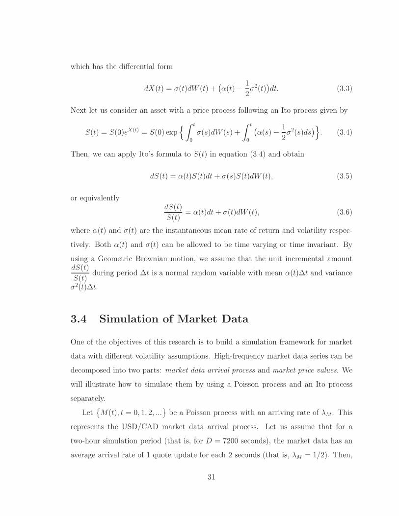
which has the differential form
dX(t) = σ(t)dW (t) +(α(t)− 1
2σ2(t)
)dt. (3.3)
Next let us consider an asset with a price process following an Ito process given by
S(t) = S(0)eX(t) = S(0) exp{∫ t
0
σ(s)dW (s) +
∫ t
0
(α(s)− 1
2σ2(s)ds
)}. (3.4)
Then, we can apply Ito’s formula to S(t) in equation (3.4) and obtain
dS(t) = α(t)S(t)dt+ σ(s)S(t)dW (t), (3.5)
or equivalentlydS(t)
S(t)= α(t)dt+ σ(t)dW (t), (3.6)
where α(t) and σ(t) are the instantaneous mean rate of return and volatility respec-
tively. Both α(t) and σ(t) can be allowed to be time varying or time invariant. By
using a Geometric Brownian motion, we assume that the unit incremental amountdS(t)
S(t)during period ∆t is a normal random variable with mean α(t)∆t and variance
σ2(t)∆t.
3.4 Simulation of Market Data
One of the objectives of this research is to build a simulation framework for market
data with different volatility assumptions. High-frequency market data series can be
decomposed into two parts: market data arrival process and market price values. We
will illustrate how to simulate them by using a Poisson process and an Ito process
separately.
Let{M(t), t = 0, 1, 2, ...
}be a Poisson process with an arriving rate of λM . This
represents the USD/CAD market data arrival process. Let us assume that for a
two-hour simulation period (that is, for D = 7200 seconds), the market data has an
average arrival rate of 1 quote update for each 2 seconds (that is, λM = 1/2). Then,
31

we can simulate a series of inter-arrival time which is exponentially distributed with
mean 1/λM = 2 seconds by applying equation (3.1) and the Inverse Transformation
Method 1. The process can be stated as follows:
1. Calculate the estimated number of arrival times for period D by nM = DλM
2. Calculate a series of estimated inter-arrival time ∆t ={∆t1,∆t2, ...,∆tnM
}
by calculating ∆tk = 1λM
log(U(0, 1)
), where U(0, 1) is a uniform [0, 1] random
variable for each k = t1, t2, ..., tnM.
3. The Kth market data arrival time stamp can be obtained as TK =∑k=K
k=1 ∆tk
for K ≤ nM , and the series of market data arrival time is then given by T ={T1, T2, ..., TnM
}.
Now we have the simulation results of the market data arrival process. The
histogram of simulated inter-arrival time series ∆t is shown in Figure 3.1. There are
in total 3,572 inter-arrival time being simulated with about 2,200 of them are between
0 to 2 seconds.
The next step is to simulate the USD/CAD market mid-price value at each market
data arrival time (simulated above) by an Ito process. Equation (3.5) is implemented
in matlab as a function with five inputs: the initial asset mid-price Pmid(0), a fixed
value of drift α per unit of time, a fixed value of volatility σ per unit of time, a series
of simulated inter-arrival time ∆t, and a series of N(0, 1) distributed scores. Then, at
each market data arrival time stamp TK for K = 1, 2, ..., nM , we calculate the market
mid-price as
Pmid(TK) = Pmid(0) exp{ K∑
k=1
σZ(0,∆tk) +
K∑
k=1
(α− 1
2σ2)∆tk
}, (3.7)
where Pmid(0) is the starting value of the process and Z(0,∆tk) is a normal random
variable with mean 0 and variance ∆tk. If we assume that the market spread value
1Inverse Transformation Method: if Y has a uniform distribution on [0, 1] and if X has a cumu-lative distribution denoted as FX , then the cumulative distribution function of the random variableis given by F−1
X(Y ) is FX
32

0 2 4 6 8 10 12 14 16 18 200
500
1000
1500
2000
2500
Inter−Arrival Time in Seconds
Cou
nt
Histogram of Simulation Results of Market Data Inter−Arrival Time
Total number of 3,572 simulated inter−arrival time
Figure 3.1: Histogram of Simulation for USD/CAD Market Data Inter-Arrival Time
during the simulation period is fixed at δ, then the Market bid and ask prices can be
obtained as
Pbid(TK) = Pmid(TK)− 0.5δ (3.8)
Pask(TK) = Pmid(TK) + 0.5δ. (3.9)
Let us assume that the initial mid-price Pmid(0) of USD/CAD is at 1.1212, the drift
and volatility for the two-hour simulation period are at 0.01 and 0.5 pips each unit
of time (in minute) respectively, and the spread is fixed at 0.5 pips. Given the series
of inter-arrival time ∆t, the sample paths of USD/CAD bid and ask prices for a
two-hour period can be obtained and shown in Figure 3.2.
3.5 Simulation of Client Trades
Similar to the market data process, a client trading process can also be decomposed
into two parts: client trading arrival process and client trading amounts. We again
33

0 20 40 60 80 100 1201.1208
1.1209
1.121
1.1211
1.1212
1.1213
1.1214
1.1215
1.1216
1.1217
Sample Paths of USD/CAD Bid and Ask Prices Simulated by Ito Process
Time in Minute
US
D/C
AD
Pric
es
Bid PriceAsk Price
Figure 3.2: Sample Paths of USD/CAD Bid and Ask Prices by an Ito Process
apply a Poisson process in the simulation of client trading arrival process. For the
client trading amount, we assume for simplicity that it follows a modified version of
the normal distribution with fixed values of mean and standard deviation.
In order to increase the flexibility of the model, we simulate the client buying
and selling trading processes separately. Let{N1(t), t = 0, 1, 2, ...
}and
{N2(t), t =
0, 1, 2, ...}be two Poisson processes with arriving rates of λN1 and λN2 respectively
to represent the USD/CAD client buying and selling trades arrival processes. Let
us assume that for the two-hour simulation period, the client buying and selling
trading arrival processes have an average arrival rate of 1 buying trade and 1 selling
trade for each 2-minute interval (that is, we set λN1 = λN2 = 1/120). Then, by
the same methodology used in the simulation of market data arrival process, we
obtain the series of client buying trades arrival time and selling trades arrival time
as TB = (TB1 , TB2 , ..., TBn1) and TS = (TS1 , TS2, ..., TSn2) respectively, where n1 and n2
are the numbers of client buying and selling trades happening during the simulation
34

period.
The next step is to simulate the client buying and selling amounts at each client
trading arrival time listed in TB and TS. We assume two random variables Y1 and
Y2 to represent client buying and selling amounts in terms of base currency2 such
that Y1 = |X1| and Y2 = |X2|, where X1 ∼ N(µX1, σ2X1) and X2 ∼ N(µX2, σ
2X2). By
applying the absolute values onto random variables X1 and X2, we simply enlarge
the probability density for far-tail values if µX1 and µX2 are enough far from 0. This
is a reasonable assumption because we believe that the client trading amount has
a distribution with heavier tails than normal distribution. Thus, for the FX spot
trading, the market maker’s Base Currency Wealth Process of trading as the counter-
party of its clients at time t can be defined as
W1(t) = W1(0)−∑
TBi≤t
Y1(TBi) +
∑
TSi≤t
Y2(TSi), (3.10)
where W1(0) = 0 is the initial value of the wealth in the base currency. Since currency
trading is always in pair, buying one currency comes with selling another currency
and vice versa. Then, given the market bid and ask prices as equations (3.8) and (3.9),
the Counter Currency Wealth Process W2(t) can be defined as
W2(t) = W2(0) +∑
TBi≤t
Y1(TBi)[Pask(TBi
) + δC ]−∑
TSi≤t
Y2(TSi)[Pbid(TSi
)− δC ], (3.11)
where W2(0) = 0 is the initial value of the counter currency wealth process and δC ≥ 0
represents client margin. As the market maker, we quote price Pask(TBi) + δC to the
client who wants to sell us the base currency, and quote price Pbid(TSi) − δC to the
clients who want to buy the base currency from us. Client margins are different by
client types and requested trading amounts. Usually the larger the requested amount
is, the large the client margin is. Processes W1(t) and W2(t) illustrates how a market
maker’s position changes according to pure client trading.
2For a currency pair XXX/YYY, the client trading amounts are always quoted in the amount ofcurrency XXX.
35

On the other hand, we can combine the two series of client buying and selling
arrival time TB = (TB1 , TB2 , ..., TBn1) and TS = (TS1 , TS2, ..., TSn2) and sort them
into one monotonically increasing series TC = (TC1 , TC2 , ..., TC(n1+n2)), which is the
time series of client trading arrival time regardless of buying or selling activities.
Then, at each client trading arrival time TCkfor k = 1, 2, ..., (n1 + n2), we can re-
write equations (3.10) and (3.11), Base and Counter Currency Wealth Processes, into
recursive formulas as follows:
W1(TCk) = W1(TCk−1
)− Y1(TCk)I[Y1(TCk
) > 0] + Y2(TCk)I[Y2(TCk
) > 0] (3.12)
and
W2(TCk) = W2(TCk−1
) + Y1(TCk)[Pask(TCk
) + δC ]I[Y1(TCk) > 0]
− Y2(TCk)[Pbid(TCk
)− δC ]I[Y2(TCk) > 0] (3.13)
with starting values ofW1(TC0) = 0 andW2(TC0) = 0. Indicator functions I[Y1(TCk) >
0] and I[Y2(TCk) > 0] tell us if it is a client buying or selling trade at time TCk
. In
our research, we assume that only one event of either client buying or selling trade
can happen at each time stamp. Thus events {Y1(TCk) > 0} and {Y2(TCk
) > 0} are
complement of each other.
The market maker’s real-time P&L 3 of trading as the counter party with clients
can be calculated as
PL(t) = W2(t) +W ∗2 (t), (3.14)
where
W ∗2 (t) =
W1(t)Pbid(t) if W1(t) ≥ 0
W1(t)Pask(t) if W1(t) < 0.
(3.15)
Note that symbol t in above equations for P&L calculation can be substituted by
symbol TCkfor k = 1, 2, ..., (n1+n2). P&L is measured in the unit of counter currency.
3P&L is an abbreviation term for Profit and Loss.
36

If we set the parameter values µX1 = µX2 = 500, 000, σ2X1 = σ2
X2 = 1, 000, 000,
δC = 0.00005, and use the simulation results of market bid and ask prices for
USD/CAD in the previous section 3.4, then we obtain sample paths of market
maker’s Base and Counter Currency Wealth Processes W1(TCk) and W2(TCk
) for
k = 1, 2, ..., (n1+n2). Figure 3.3 shows the simulation results ofW1(TCk) andW2(TCk
).
There is no surprise that these two paths are nearly mirrors of each other. The P&L
values PL(TCk) for k = 1, 2, ..., (n1+n2) are also calculated and shown in Figure 3.4.
0 20 40 60 80 100 120−6
−4
−2
0
2
4
6
8x 10
6 Market Maker Base and Counter Currency Wealth Processes
Time Stamp in Minutes
Wea
lth P
roce
ss V
alue
s
W1(T
Ck) in USD
W2(T
Ck) in CAD
Figure 3.3: Sample Paths of Market Maker’s Base and Counter Currency Wealth Processes
37

0 20 40 60 80 100 1200
1000
2000
3000
4000
5000
6000
7000Market Maker P&L Process
Time Stamp in Minutes
P&
L
PL(t) in CAD
Figure 3.4: Sample Path of Market Maker’s P&L
38

Chapter 4
Risk Hedging
4.1 Hedging Strategy
In Section 1.5, we explained how a market maker trades with clients by both buying
and selling with its own capital. The most ideal situation would be buying from one
client at market bid and selling the same amount to another client at market offer
at the same time. But this is rarely the case in practice because it is very hard to
get two clients to request the same amount of trades on each side at the same time.
Thus, a market maker will have to hold positions (positive or negative) for a period
of time, and this introduces a substantial amount of market risk to market maker’s
portfolio. Therefore it is important for a market maker to actively trade during the
day for an effective risk management.
In this chapter, we introduce a basic risk hedging strategy that generates trades
based on the market maker’s Base Currency Wealth Process{W1(Ck), k = 1, 2, ..., (n1+
n2)}. The intuition underlying this strategy is that a market maker is usually unwill-
ing to hold very big positions at any time due to a market risk exposure. Note that
the definition of “big” is subjective to market maker’s risk tolerance. This can be
determined by many factors such as client trading flows, accessibility to liquidities, ef-
ficiency in risk management, etc. For example, a global market player with advanced
39

technologies to access deep liquidities and smart risk hedging strategies may allow its
EUR position staying at 100 million during the day; but a second-tier market player,
who does not have the same level of technologies and strategies, may only allow its
trader to hold the amount of EUR less than 10 million.
Let two amounts UB and UN be such that UB > 0 and UN < 0 respectively
represent the maximum allowable positive and negative amounts in the base currency
of the trading pair that the market maker can hold. Then, once the market maker
has its Base Currency Wealth Process breaches UP or UN , a risk hedging trade will
be issued to off-load the risk to a lower level. This is pre-defined by the market maker
based on his/her risk tolerance. Let us define the two lower levels LP and LN such
that UP > LP > 0 and UN < LN < 0. Then, at each client trading arrival time TCk
for k = 1, 2, 3, ..., (n1 + n2), the market maker’s Risk Adjusted Base Currency Wealth
Process AW1(TCk) can be defined as a recursive formula as
AW1(TCk) = AW1(T
−Ck) +H(TCk
)I[H(TCk) 6= 0], (4.1)
where
AW1(T−Ck) = AW1(TCk−1
)− Y1(TCk)I[Y1(TCk
) > 0] + Y2(TCk)I[Y2(TCk
) > 0] (4.2)
and the Risk Hedging Trading Amount being
H(TCk) =
LP − AW1(T−Ck) if AW1(T
−Ck) > UP
LN − AW1(T−Ck) if AW1(T
−Ck) < UN
0 otherwise.
(4.3)
The starting value of the process is AW1(TC0) = 0, and the indicator function
I[H(TCk) 6= 0] equals to 1 when the Risk Hedging Trading Amount is non-zero.
Similar to market maker’s Counter Currency Wealth Process W2(TCk), the market
maker’s Risk Adjusted Counter Currency Wealth Process AW2(TCk) can be defined
40

as
AW2(TCk) = AW2(T
−Ck)+H(TCk
)
{Pask(TCk
)I[H(TCk) > 0]+Pbid(TCk
)I[H(TCk) < 0]
},
(4.4)
where
AW2(T−Ck) = AW2(TCk−1
) + Y1(TCk)[Pask(TCk
) + δC ]I[Y1(TCk) > 0]
− Y2(TCk)[Pbid(TCk
)− δC ]I[Y2(TCk) > 0] (4.5)
and function H(TCk) is given by equation (4.3).
Market maker’s Risk Adjusted P&L measured in the counter currency can be
calculated as
PLA(t) = AW2(t) + AW ∗2 (t), (4.6)
where
AW ∗2 (t) =
AW1(t)Pbid(t) if AW1(t) ≥ 0
AW1(t)Pask(t) if AW1(t) < 0.
(4.7)
Again, the symbol t in above equations can be substituted by the symbol TCkfor
k = 1, 2, ..., (n1 + n2). In fact, one crucial assumption we have made about this
hedging strategy is that the FX market is liquid enough so that the market maker can
successfully execute the risk hedging trade of amount H(TCk) defined by equation 4.3
at time TCkwith no market impact. For the market makers with relatively small risk
tolerance, this assumption is reasonable.
4.2 Implementation of the Hedging Strategy
The hedging strategy introduced in the previous section 4.1 is implemented in matlab.
To carry out the test, we apply this strategy to the client trading process obtained
from the simulation exercise conducted in section 3.5. Figure 4.1 shows the market
maker’s Risk Adjusted Wealth Processes AW1(TCk) and AW2(TCk
) when we assume
Up = 4, 000, 000, Lp = 2, 000, 000, UN = −4, 000, 000, and LN = −4, 000, 000. This
41

means that whenever the client trade leads the wealth process to go beyond ±4
million USD, the hedging strategy will issue a hedging trade to bring its position
back to ±2 million USD. We can see that the Risk Adjusted Base Currency Wealth
Process AW1(TCk) is bounded between ±4 million USD.
0 20 40 60 80 100 120−4
−3
−2
−1
0
1
2
3
4
5x 10
6 Market Maker Risk Adjusted Base and Counter Currency Wealth Processes
Time Stamp in Minutes
Wea
lth P
roce
ss V
alue
s
AW1(T
Ck) in USD
AW2(T
Ck) in CAD
Figure 4.1: Sample Paths of Market Maker’s AW1(TCk) and AW2(TCk
)
Figure 4.2 shows the comparison between the P&L with and without risk hedging.
At about 80th minute, we start to see discrepancies between the P&Ls. This is because
that there is no risk hedging trade happening before that time. This plot also shows
that our current risk hedging strategy does not necessarily produce better P&L. But
at least this gives us something to start with.
4.3 Scenario Analysis
After a risk hedging strategy is introduced, the first question would be “What impact
could it have on the market maker’s P&L?” In order to answer this question, we will
42

0 20 40 60 80 100 1200
1000
2000
3000
4000
5000
6000
7000Market Maker P&L Process With And Without Risk Adjustment
Time Stamp in Minutes
P&
L
PLA(t) in CAD
PL(t) in CAD
Figure 4.2: Sample Path of Market Maker’s P&L(t) and PLA(t)
run the simulation exercise for the market data process and client trading process
under three different scenarios as follows:
1. Balanced client buying and selling flows under flat market condition.
2. Intensive client selling flow under downward market condition.
3. Intensive client buying flow under upward market condition.
Scenarios 2 and 3 are more like stress tests for our strategy. For each scenario, we
calculate P&L values (equations (3.14) and (4.6)) before and after risk hedging for
each sample path, and compare their difference. Sharp ratios are also calculated to
compare the returns before and after risk hedging. It is a measure of the excess return
per unit of risk in an investment asset or a trading strategy. In [28], it is defined as
S =E[R− Rf
]√
V AR[R− Rf
] , (4.8)
43

where R and Rf are the asset return and risk-free return respectively. In our situation,
we let Rf equal to 0 since we are looking at absolute return.
4.3.1 Balanced Client Buying and Selling Flows under Flat
Market Condition
In this subsection, we assume that we are under a flat market condition. Then, given
a pre-defined client flow, which contains balanced client buying and selling trades,
we compute and compare the P&L with and without risk hedging on 5,000 different
market data paths. For a five-hour trading horizon, we use the following parameter
assumptions for the pre-defined client trading flow:
1. For client buying trades, we assume Poisson arrival process with rate λN1 =
1/120, µX1 = 500K, and σ2X1 = 500K.
2. For client selling trades, we assume Poisson arrival process with rate λN2 =
1/120, µX2 = 500K, and σ2X2 = 500K.
3. Client margin δC = 0.5 pip.
For each of the 5,000 sample paths of market (mid-price) data process, we assume
Poisson arrival process with rate λM = 1/2. Its value follows a geometric Brownian
motion given by equation (3.7) with initial value Pmid(0) = 1.1212, drift α = 0 pip
per minute, and volatility σ2 = 0.5 pip per minute. Market bid-ask spread remains
at δ = 1 pip. For risk hedging strategy, we set the risk barriers values of UP = 4M ,
LP = 1M , UN = −4M , and LN = −1M .
Figures 4.3 and 4.4 show the simulation results of market maker’s P&L without
and with risk hedging respectively. Figure 4.5 shows the difference between them, and
Figure 4.6 shows the comparison of sharp ratio values before and after risk hedging.
44

Figure 4.3: P&L Without Risk Hedging in Flat Market with Balanced Client Flow
Figure 4.4: P&L With Risk Hedging in Flat Market with Balanced Client Flow
45

Figure 4.5: P&L Differences in Flat Market with Balanced Client Flow
0 50 100 150 200 250 3002
3
4
5
6
7
8
9
Time Stamp in Minutes
Sha
rp R
atio
Sharp Ratio Before and After Risk Hedging
Before Risk HedgingAfter Risk Hedging
Flat Market Condition With Balanced Client Trading Flows
Figure 4.6: Sharp Ratio Comparison in Flat Market with Balanced Client Flow
46

From inspecting Figure 4.5 alone, it is difficult to tell that using an active risk
hedging strategy generates more revenue for the market maker than not hedging. For
the 5,000 sample paths, we see that about 50% of the time that the risk hedging
strategy generates less revenue than the un-hedging strategy. The amounts of out-
performance and under-performance almost cancel each other. But if we compare
figure 4.3 and figure 4.4, we can see that the P&L process without the risk hedging
strategy has a much wider range than the P&L process with the risk hedging strategy
does during the simulation horizon. At the end of the period, the P&L process
without the risk hedging strategy has its range from −5, 000CAD to 28, 000CAD,
while the P&L process with the risk hedging strategy has its range from 5, 000CAD
to 19, 000CAD. Figure 4.6 shows that the sharp ratio of risk-hedging P&L starts
perform better once the first risk-hedging trade is initiated. The better sharp ratio
values are mainly resulted from return variance reduction. This tells us that being
active in risk hedging is not necessarily more superiors than being in non-risk hedging,
but it substantially reduce the probability of getting very low (or even negative) P&L
in trading with the clients. This makes sense because more risk taking imposes more
chances in both winning in a big way and losing in a big way. The risk hedging strategy
is helpful if the market maker is seeking stability in his/her revenue generating.
4.3.2 Intensive Client Selling Flow under Downward Market
Condition.
In this subsection, we assume that we are facing a downward market condition and
experiencing intensive client selling trades during the trading horizon. P&Ls are
calculated on 5,000 simulation paths for risk hedging and un-hedging. For the five-
hour trading horizon, we use the following parameter assumptions for the predefined
client trading flow:
1. For client buying trades, we assume a Poisson arrival process with the rate of
47

λN1 = 1/120, µX1 = 500K, and σ2X1 = 500K.
2. For client selling trades, we assume a Poisson arrival process with a rate of
λN2 = 1/60, µX2 = 1M , and σ2X2 = 1M .
3. Client margin δC = 0.5 pip.
For each of the 5,000 sample paths of market (mid-price) data process, we assume
a Poisson arrival process with a rate of λM = 1/2. Its value is assumed to follow
a geometric Brownian motion given by equation (3.7) with initial value Pmid(0) =
1.1212, drift α = −0.5 pip per minute (negative drift means downward market), and
volatility σ2 = 1 pip per minute. Market bid-ask spread remains at δ = 1 pip. For
the risk hedging strategy, we set the risk barriers values of UP = 4M , LP = 1M ,
UN = −4M , and LN = −1M .
Figure 4.7 shows the market maker’s P&L results when the risk hedging strategy
is not applied. Since this is in a downward trend market, and client selling trades
are arriving with large amounts at twice the speed of buying trades, the market
maker is loosing a large amount of money. Figure 4.8 shows the simulation results of
market maker’s P&L with risk hedging, and Figure 4.9 shows the difference of P&L
between hedging and un-hedging. We can see that by imposing a hedging strategy,
we substantially reduce the probability of loosing money. Nearly half of the sample
paths end up in the positive region of P&L. Even if the P&L is negative, it is much
less negative than the P&L without a risk hedging strategy. By figure 4.10, we see
that the sharp ratio of risk-hedging P&L is contained at a certain level around −1,
while the sharp ratio of non-risk hedging P&L is with a big downward slope.
4.3.3 Intensive Client Buying Flow under Upward Market
Condition.
In this subsection, we assume that we face an upward market condition and experience
intensive client buying trades during the trading horizon. This represents the opposite
48

Figure 4.7: P&L Without Risk Hedging in Downward Trend Market with Intensive Client Sell
Figure 4.8: P&L With Risk Hedging in Downward Trend Market with Intensive Client Sell
49

Figure 4.9: P&L Differences in Downward Trend Market with Intensive Client Sell
0 50 100 150 200 250 300−8
−7
−6
−5
−4
−3
−2
−1
0
1
2
Time Stamp in Minutes
Sha
rp R
atio
Sharp Ratio Before and After Risk Hedging
Before Risk HedgingAfter Risk Hedging
Downward Trend Market with Intensive Client Selling Trade Flows
Figure 4.10: Sharp Ratio Comparison in Downward Trend Market with Intensive Client Sell
50

scenario to the scenario used in the pervious section. P&Ls are calculated on 5,000
simulation paths for risk hedging and un-hedging strategies. For the five-hour trading
horizon, we use the following parameter assumptions for the predefined client trading
flow:
1. For client buying trades, we assume a Poisson arrival process with a rate of
λN1 = 1/90, µX1 = 1.5M , and σ2X1 = 1M .
2. For client selling trades, we assume a Poisson arrival process with a rate of
λN2 = 1/120, µX2 = 500K, and σ2X2 = 500K.
3. Client margin δC = 0.5 pip.
For each of the 5,000 sample paths of market (mid-price) data process, we assume
a Poisson arrival process with a rate of λM = 1/2. Its value is assumed to follow
a geometric Brownian motion given by equation (3.7) with initial value Pmid(0) =
1.1212, drift α = 0.3 pip per minute (positive drift means upward market), and
volatility σ2 = 1 pip per minute. The market bid-ask spread is set to remain at
δ = 1 pip. For the risk hedging strategy, we set the risk barriers values of UP = 4M ,
LP = 1M , UN = −4M , and LN = −1M .
There is no surprise that we obtain similar results as the ones obtained in the
previous section. Figures 4.11 and 4.12 show the simulation results of market maker’s
P&L without and with a risk hedging strategy respectively, and Figure 4.13 shows
the difference between them. We can see that without any risk hedging strategy, the
market maker suffers huge losses when the upward market rally happens with intensive
client buying trades. Once the risk hedging strategy is imposed, the probability of
getting negative P&L is substantially reduced. P&L differences between the risk
hedging and un-hedging strategies are positive for all sample paths. Figure 4.14 shows
that the risk-hedging P&L achieved positive sharp ratios while non-risk hedging P&L
has a negative and decreasing sequence of sharp ratios.
51

Figure 4.11: P&L Without Risk Hedging in Upward Trend Market with Intensive Client Buy
Figure 4.12: P&L With Risk Hedging in Upward Trend Market with Intensive Client Buy
52

Figure 4.13: P&L Differences in Upward Trend Market with Intensive Client Buy
0 50 100 150 200 250 300−5
−4
−3
−2
−1
0
1
2
3
Time Stamp in Minutes
Sha
rp R
atio
Sharp Ratio Before and After Risk Hedging
Before Risk HedgingAfter Risk Hedging
Upward Trend Market Condition with Intensive Client Buying Trade Flows
Figure 4.14: Sharp Ratio Comparison in Upward Trend Market with Intensive Client Buy
53

Chapter 5
Tail Risk Analysis
5.1 Overview of Extreme Value Theory
The last years of 2007, 2008, and 2009 have seen the greatest financial crisis since the
Great Depression 1929. This has led to numerous criticisms about the existing risk
management systems and motivated the search for more appropriate methodologies
able to cope with rare events that have heavy consequences. The typical question one
would like to answer is: “If things go wrong, how wrong can they go?” The problem is
then to model the rare phenomena that lie outside the range of available observations.
Extreme value theory (EVT) provides a framework to formalize the study of behavior
in the tails of a distribution. Critical questions relating to the probability of a market
crash or boom require an understanding of the statistical behavior expected in the
tails. EVT allows us to use extreme observations to measure the density in the
tail. This measure can be extrapolated to parts of the distribution that have yet to
be observed in the empirical data. It can also be mapped onto distributions with
specific tail behavior. In this way we can simulate a theoretical process that captures
the extreme features of the empirical data and improve the accuracy of estimated
probabilities of extraordinary market movements. Extreme Value Theory has been
well established in many fields such as insurance and engineering. Text books [25]
54

and [7] gives introduction of Extreme Value Theory from its basic foundation to its
applications in insurance and finance industries.
This chapter is composed by two parts. In the first part, we draw down the
foundation work of Extreme Value Theory, and introduce the empirical estimation
methods for its shape, location, and scale parameters. A dataset of EUR/USD ex-
change rates with five-minute frequency with be applied for the empirical estimation.
In the second part of this chapter, we will introduce the concept of Value-at-Risk
(VaR), which is the most popular and important quantity for risk management. We
will discuss an approach to VaR calculation using the Extreme Value Theory.
Firstly, let’s introduce the basics of Extreme Value Theory. Assume that a series of
random variables Xk for k = 1, 2, 3, ..., n are independent and identically distributed
with a common cumulative distribution function (c.d.f) F (x). The range of random
variables Xk for k = 1, 2, 3, ..., n is [l, u]. For Xk being log returns, we have l = −∞and u = ∞. Let Mn = max{X1, X2, ..., Xn} be the maximum of the random sample
of size n. Then, the c.d.f. of Mn is given by
Fn(x) = Pr(Mn ≤ x)
=n∏
j=1
Pr(Xj ≤ x)
= [F (x)]n
= F n(x). (5.1)
In practice, the c.d.f. F (x) is unknown and, hence the c.d.f. F n(x) of Mn is
unknown. However, as n → ∞, F n(x) → 0 if x < u and F n(x) → 1 if x ≥ u, where
u is the upper boundary of the range. Therefore, the limiting distribution of F n(x)
is degenerate. To deal with this, we need to normalize F n(x). Suppose there exists a
sequence of constants an > 0 and bn ∈ R such that:
P (Mn − bn
an≤ z) = F n(anz + bn), (5.2)
55

then the limiting distribution of F n(anz + bn) is given by
limn→∞
F n(anz + bn) = G(z). (5.3)
Finding the limiting distribution G(z) is called the Extremal Limit Problem. Find-
ing the F (x) that have sequences of constants as described above leading to G(z) is
called the Domain of Attraction Problem. In articles [10] and [24], authors gave the
limiting law for the maxima Mn with n being the sample size. The theorem is as
follows: let M in be a sequence of i.i.d. random variables for i = 1, 2, .... If there exist
constants an > 0, bn ∈ R, and some non-degenerate distribution function G such that
Z i =M i
n − bnan
d→ G, (5.4)
then G belongs to one of the three standard extreme value distributions:
Frechet : Φα(z) =
0 for z ≤ 0 and α > 0
e−z−α
for z > 0 and α > 0
(5.5)
Weibull : Ψα(z) =
e−(−z)α for z ≤ 0 and α > 0
1 for z > 0 and α > 0
(5.6)
Gumbel : Λ(z) = e−e−z
for z ∈ R (5.7)
where parameter α > 0 is the shape parameter, which captures the weights of the tail
in the distribution of the parent random variable X. This theorem is known as the
Fisher-Tippet Theorem. Constants an > 0 and bn ∈ R are referred to as scale
parameter and location parameter respectively.
Intuitively, these three standard extreme value distributions represent three possi-
bilities for the decay of the density function in the tail. Frechet distribution represents
tails that decay by a power, as in the cases of the stable Paretian, Cauchy and Student
t distributions. They are no longer integrable when weighted by the tail probabilities,
hence leading to ”fat tails”. Weibull represents tails that can decay with a finite tail
56

index; this will be a thin tailed distribution with a finite upper endpoint. Gumbel
represents tails that can decay exponentially with all finite moments; these are stan-
dard cases of Normal, Lognormal, Gamma, etc. Figure 5.1 shows the shapes of the
probability density functions for standard Frechet , Weibull , and Gumbel distributions
when shape parameter α = 1.5.
Figure 5.1: Density Functions for Frechet, Weibull, and Gumbel when α = 1.5
In article [13], Jenkinson and Von Mises suggested an one-parameter representa-
tion given by
Gξ(z) =
e−(1+ξz)
−1ξ
if ξ 6= 0
e−e−z
if ξ = 0
(5.8)
for these three standard distributions, with x such that 1+ξx > 0. This generalization
is known as the Generalized Extreme Value (GEV) distribution, and is obtained by
setting ξ = α−1 for Frechet distribution, ξ = −α−1 for Weibull distribution, and by
interpreting the Gumbel distribution as the limiting case for ξ = 0. We can obtain the
probability density function (p.d.f.) of the Generalized Extreme Value distribution
57

by differentiating the above c.d.f. (5.8), which gives
gξ(z) =
(1 + ξz)−( 1
ξ+1)e−(1+ξz)
−1ξ
if ξ 6= 0
ex−e−z
if ξ = 0.
(5.9)
This generalized representation is very useful when maximum likelihood estimates
have to be computed when we do not know the type of limiting distribution of the
sample maxima in advance.
5.2 Maximum Likelihood Methods for EVT
From the previous section, we know that the Generalized Extreme Value distribution
contains three parameters ξ, an > 0, and bn ∈ R, which are referred to as shape,
scale, and location parameter respectively. In this section, we explain how to use
maximum likelihood estimate method in estimating the three parameters.
For one given sample, there is only one minimum value or maximum value ob-
served. We can not estimate these three parameters with only one extreme obser-
vation. An alternative approach that has been applied is to divide the sample into
non-overlapping sub-samples and apply the extreme value theory to the sub-samples.
This approach has been applied in literatures such as [11] and [24]. For a sample of
size T , we divide the sample into k non-overlapping sub-samples each with n obser-
vations, assuming for simplicity that T = nk. That is, we divide the sample
{x1, x2, ..., xT}
into
{x1, ..., xn, |xn+1, ..., x2n, |......|x(k−1)n+1, ..., xnk}.
We can write the observation value as xin+j, where 1 ≤ j ≤ n and i = 0, 1, ..., k−1.
This tells us that observation xin+j is the jth observation of ith sub-sample. When the
size of each sub-sample is sufficiently large, we hope that the Extreme Value Theory
58
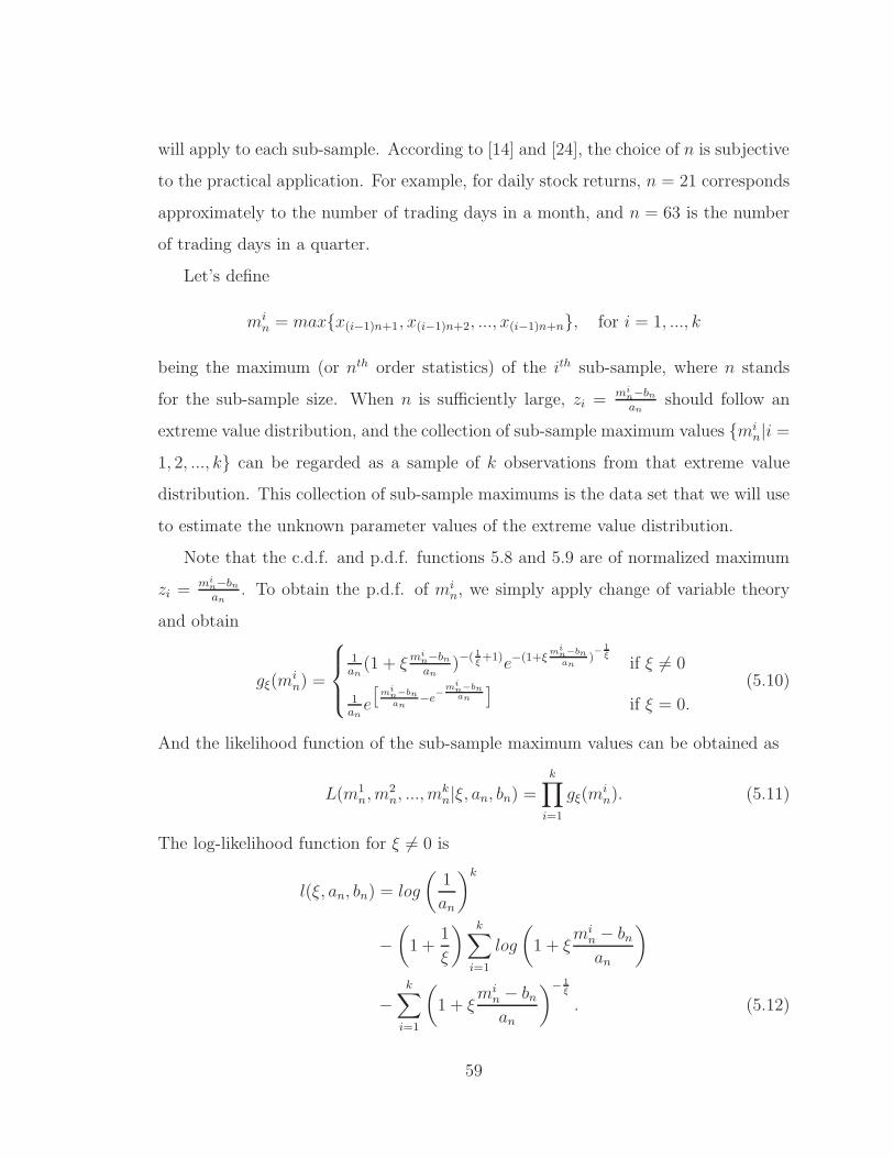
will apply to each sub-sample. According to [14] and [24], the choice of n is subjective
to the practical application. For example, for daily stock returns, n = 21 corresponds
approximately to the number of trading days in a month, and n = 63 is the number
of trading days in a quarter.
Let’s define
min = max{x(i−1)n+1, x(i−1)n+2, ..., x(i−1)n+n}, for i = 1, ..., k
being the maximum (or nth order statistics) of the ith sub-sample, where n stands
for the sub-sample size. When n is sufficiently large, zi =mi
n−bnan
should follow an
extreme value distribution, and the collection of sub-sample maximum values {min|i =
1, 2, ..., k} can be regarded as a sample of k observations from that extreme value
distribution. This collection of sub-sample maximums is the data set that we will use
to estimate the unknown parameter values of the extreme value distribution.
Note that the c.d.f. and p.d.f. functions 5.8 and 5.9 are of normalized maximum
zi =mi
n−bnan
. To obtain the p.d.f. of min, we simply apply change of variable theory
and obtain
gξ(min) =
1an(1 + ξmi
n−bnan
)−( 1ξ+1)e−(1+ξ
min−bnan
)−
1ξ
if ξ 6= 0
1ane
[mi
n−bnan
−e−
min−bnan
]if ξ = 0.
(5.10)
And the likelihood function of the sub-sample maximum values can be obtained as
L(m1n, m
2n, ..., m
kn|ξ, an, bn) =
k∏
i=1
gξ(min). (5.11)
The log-likelihood function for ξ 6= 0 is
l(ξ, an, bn) = log
(1
an
)k
−(1 +
1
ξ
) k∑
i=1
log
(1 + ξ
min − bnan
)
−k∑
i=1
(1 + ξ
min − bnan
)− 1ξ
. (5.12)
59
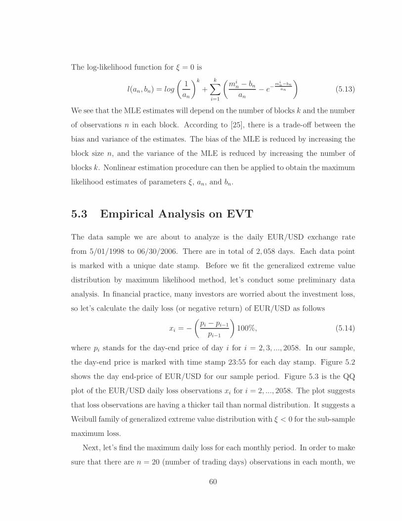
The log-likelihood function for ξ = 0 is
l(an, bn) = log
(1
an
)k
+
k∑
i=1
(mi
n − bnan
− e−mi
n−bnan
)(5.13)
We see that the MLE estimates will depend on the number of blocks k and the number
of observations n in each block. According to [25], there is a trade-off between the
bias and variance of the estimates. The bias of the MLE is reduced by increasing the
block size n, and the variance of the MLE is reduced by increasing the number of
blocks k. Nonlinear estimation procedure can then be applied to obtain the maximum
likelihood estimates of parameters ξ, an, and bn.
5.3 Empirical Analysis on EVT
The data sample we are about to analyze is the daily EUR/USD exchange rate
from 5/01/1998 to 06/30/2006. There are in total of 2, 058 days. Each data point
is marked with a unique date stamp. Before we fit the generalized extreme value
distribution by maximum likelihood method, let’s conduct some preliminary data
analysis. In financial practice, many investors are worried about the investment loss,
so let’s calculate the daily loss (or negative return) of EUR/USD as follows
xi = −(pi − pi−1
pi−1
)100%, (5.14)
where pi stands for the day-end price of day i for i = 2, 3, ..., 2058. In our sample,
the day-end price is marked with time stamp 23:55 for each day stamp. Figure 5.2
shows the day end-price of EUR/USD for our sample period. Figure 5.3 is the QQ
plot of the EUR/USD daily loss observations xi for i = 2, ..., 2058. The plot suggests
that loss observations are having a thicker tail than normal distribution. It suggests a
Weibull family of generalized extreme value distribution with ξ < 0 for the sub-sample
maximum loss.
Next, let’s find the maximum daily loss for each monthly period. In order to make
sure that there are n = 20 (number of trading days) observations in each month, we
60
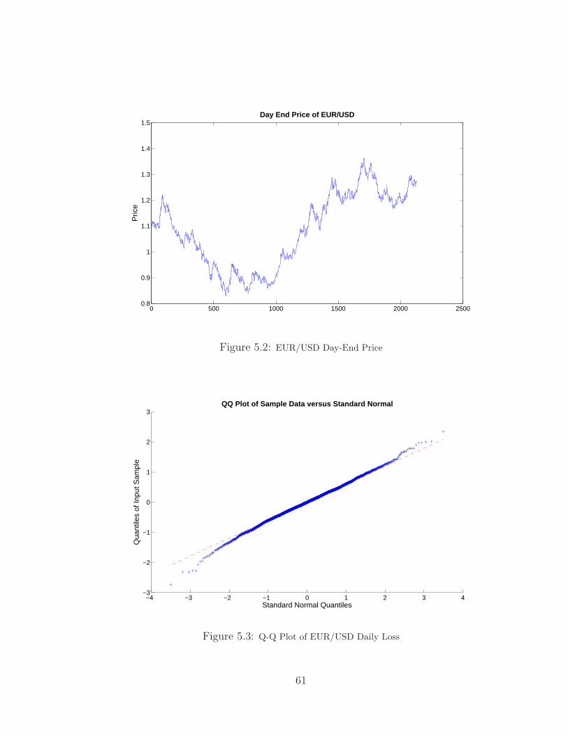
0 500 1000 1500 2000 25000.8
0.9
1
1.1
1.2
1.3
1.4
1.5Day End Price of EUR/USD
Pric
e
Figure 5.2: EUR/USD Day-End Price
−4 −3 −2 −1 0 1 2 3 4−3
−2
−1
0
1
2
3
Standard Normal Quantiles
Qua
ntile
s of
Inpu
t Sam
ple
QQ Plot of Sample Data versus Standard Normal
Figure 5.3: Q-Q Plot of EUR/USD Daily Loss
61

will count the first one or two days of the next month into this month if there is only
a number of 18 or 19 days available for this month. We will also use the first 20 days
data if the month has more than 20 trading days. This gives us in total of k = 98
observations. Figure 5.4 shows maximum daily loss in each monthly block. We see
that the largest daily loss in a monthly block is 2.34% in 2000 September.
Figure 5.4: EUR/USD Maximum Daily Loss for Each Month
Then, we can calculate the Maximum Likelihood Estimates for the parameters of
the generalized extreme value distribution by using these 98 monthly block maxima
daily loss on EUR/USD. By inputting the data into MATLAB, we get the estimates
of shape parameter ξ = −0.132, scale parameter an = 0.3513, and location parameter
bn = 1.0108. Since the shape parameter ξ < 0, the monthly maximum daily loss fol-
lows a Weibull distribution. Figure 5.5 compares the empirical cdf for the sample and
the theoretical cdf of the generalized extreme distribution with estimated parameters.
Now We can apply the same procedures with different combinations of n and k.
Thus, we can see the effects of number of observations on MLE estimates. Table 5.1
62

shows the MLE estimates for the generalized extreme value distribution of the daily
maximum loss with different block sizes. We can see that shape and location parame-
ters ξ and bn are quite sensitive to the number of observations in each block, whereas
the scale parameter an is less sensitive compare to the other two.
0 0.5 1 1.5 2 2.50
0.1
0.2
0.3
0.4
0.5
0.6
0.7
0.8
0.9
1
x
F(x
)
Comparison of Empirical and Theoretical CDF
EmpiricalTheoretical
Figure 5.5: Empirical and Theoretical CDF Comparison for Maximum Daily Loss in Monthly
Block
Table 5.1: MLE Estimates for Generalized Extreme Value Distribution with Different
Block Size
Frequency # of Obs # of Blocks ξ an bn
Bi-Weekly n = 10 k = 196 −0.1323 0.3689 0.7856
Monthly n = 20 k = 98 −0.1320 0.3513 1.0108
Quarterly n = 60 k = 32 −0.0039 0.2643 1.3087
Semi-Annually n = 120 k = 16 −0.1257 0.2647 1.5467
Annually n = 240 k = 8 −0.3158 0.2767 1.7597
63

5.4 Value-at-Risk (VaR)
Value-at-Risk (VaR) is a widely used risk measure in today’s financial industry. It
is an attempt to provide a single number to summarize the total risk in a portfo-
lio of financial assets. It is an accepted methodology used by corporate treasurers,
fund managers, and financial institutions. Central banks regulators also use VaR in
determining the capital a bank is required to keep to reflect the market risk it is
bearing.
The definitions and concepts of VaR can be found in many books and literatures
such as [12] and [4]. In [4], VaR is defined as the maximum loss which can occur with
X% confidence over a holding period of n days for a portfolio. Thus, when using
VaR as a measure of risk, we are interested in making a statement of the following
form: “We are X percent certain that we will not lose more than V dollars in the
next N days for a certain portfolio.” The variable V is the VaR of the portfolio. For
example, if a daily VaR is stated as $100, 000 with a 95% level of confidence for a
portfolio, it means that we are 95% confident that the portfolio will not lose more
than $100, 000 during a day. We can see that VaR is a very important risk measure
in helping banks to set up capital requirements for preventing extreme market risk
events. According to [12], the Basel Committee on Bank Supervision, (the committee
of world’s bank regulators), requires VaR to be calculated with N = 10 and X = 99
for the bank’s trading book on a daily basis. The capital it requires the bank to hold
is the multiplier k times the VaR measure. k is chosen on a bank-by-bank basis by
the regulators and must be at least 3.0.
Now let’s define VaR under a probabilistic framework. Since investors usually
would like to think of risk from a loss perspective, we let a continuous random variable
X represent the loss (or negative return) of a financial instrument during a certain
period of time h with c.d.f. Fh. Thus, a VaR value with p level of confidence for a
period of h can be defined as the (pth quantile of the distribution function Fh. That
64

is
VaRh,p = F−1h (p), (5.15)
where F−1 is the inverse function of the distribution function F . Equivalently, we
have
P (X > VaRh,p) = 1− Fh(VaRh,p) = 1− p. (5.16)
To quote a valid VaR statement, we must include three components: a time period,
a confidence level, and a loss amount. According to [4], calculation of VaR involves
the following factors in its practical applications:
1. The confidence level p such as p = 95% or p = 99%.
2. The time horizon h. This might be set by a regulatory committee such that
h = 1 day or h = 10 days.
3. The frequency of the data, which might not be the same as the time horizon h.
Daily observations are often used.
4. The c.d.f. Fh(x) for the return random variable.
5. The amount of the financial position or the mark-to-market value of the port-
folio.
Among these factors, it is the c.d.f. Fh(x) that draws most research attentions.
The most commonly used VaR models assume that random variable X , asset return
(or log-return) follows a normal distribution. This assumption itself is a huge risk to
those practitioners who use it because reality suggests that returns of most financial
products are fat-tailed.
5.5 An Extreme Value Approach to VaR
In this section, we discuss an approach to VaR calculation using the Extreme Value
Theory. In section 5.2, we derived the maximum likelihood function for estimating
65
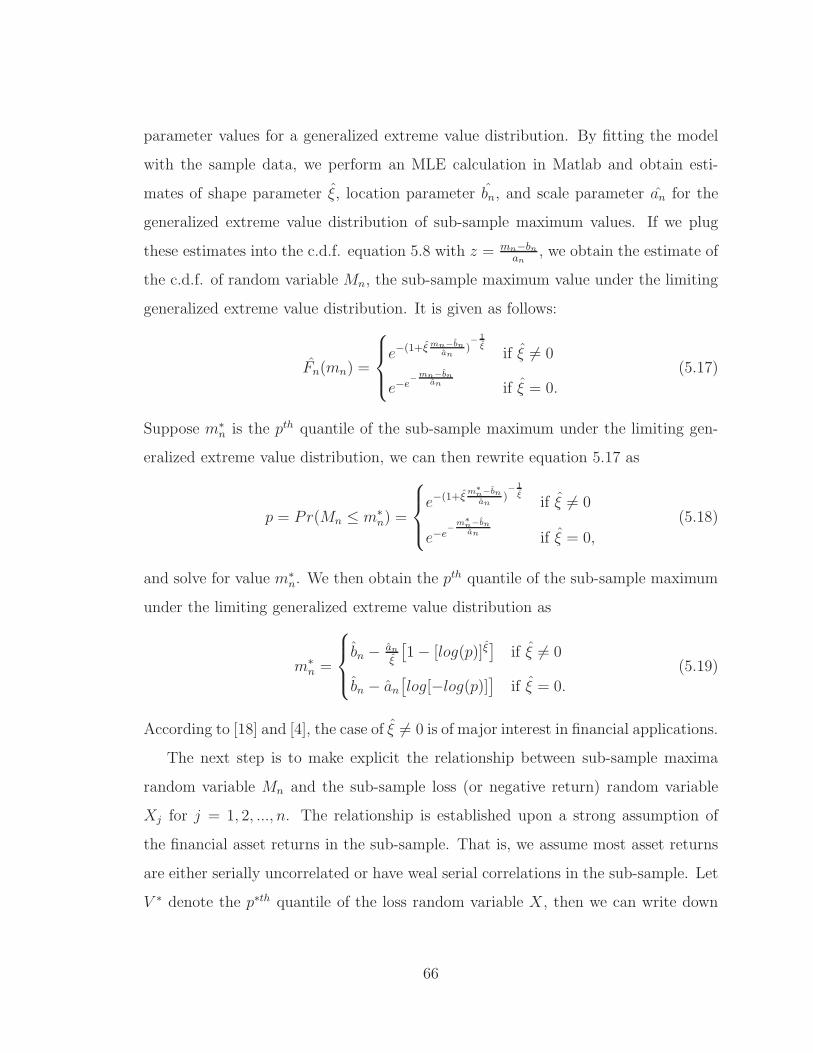
parameter values for a generalized extreme value distribution. By fitting the model
with the sample data, we perform an MLE calculation in Matlab and obtain esti-
mates of shape parameter ξ, location parameter bn, and scale parameter an for the
generalized extreme value distribution of sub-sample maximum values. If we plug
these estimates into the c.d.f. equation 5.8 with z = mn−bnan
, we obtain the estimate of
the c.d.f. of random variable Mn, the sub-sample maximum value under the limiting
generalized extreme value distribution. It is given as follows:
Fn(mn) =
e−(1+ξmn−bn
an)−
1ξ
if ξ 6= 0
e−e−
mn−bnan if ξ = 0.
(5.17)
Suppose m∗n is the pth quantile of the sub-sample maximum under the limiting gen-
eralized extreme value distribution, we can then rewrite equation 5.17 as
p = Pr(Mn ≤ m∗n) =
e−(1+ξm∗
n−bnan
)−
1ξ
if ξ 6= 0
e−e−
m∗
n−bnan if ξ = 0,
(5.18)
and solve for value m∗n. We then obtain the pth quantile of the sub-sample maximum
under the limiting generalized extreme value distribution as
m∗n =
bn − an
ξ
[1− [log(p)]ξ
]if ξ 6= 0
bn − an[log[−log(p)]
]if ξ = 0.
(5.19)
According to [18] and [4], the case of ξ 6= 0 is of major interest in financial applications.
The next step is to make explicit the relationship between sub-sample maxima
random variable Mn and the sub-sample loss (or negative return) random variable
Xj for j = 1, 2, ..., n. The relationship is established upon a strong assumption of
the financial asset returns in the sub-sample. That is, we assume most asset returns
are either serially uncorrelated or have weal serial correlations in the sub-sample. Let
V ∗ denote the p∗th quantile of the loss random variable X , then we can write down
66

following equation
[p∗]n = [Pr(X ≤ V ∗)]n
=n∏
j=1
Pr(Xj ≤ V ∗)
= Pr(Mn ≤ V ∗)
=
e−(1+ξ V ∗
−bnan
)−
1ξ
if ξ 6= 0
e−e−
V ∗−bnan if ξ = 0.
(5.20)
The 2nd equal sign in the above equation is based on assuming that asset returns are
i.i.d. The last equal sign is given by replacing m∗n by V ∗ in equation (5.18). By taking
power of 1non both sides of the above equation, we obtain
p∗ = Pr(X ≤ V ∗)
=
e−
1n(1+ξ V ∗
−bnan
)−
1ξ
if ξ 6= 0
e−1ne−
V ∗−bnan if ξ = 0.
(5.21)
Then, the p∗th quantile of the loss random variable X can be obtained by solving the
above equation for V ∗ as follows:
V ∗ =
bn − an
ξ
[1− [−nlog(p∗)]−ξ
]if ξ 6= 0
bn − an[log[−nlog(p∗)]
]if ξ = 0.
(5.22)
Consequently, if X is the loss amount random variable over a time period h, V ∗ is
the VaR with p∗ confidence level for a period of time h. By MLE estimates given
in Table 5.1, we can calculate the VaR value with 95% confidence level for the next
h = 10 days period as follows:
VaR10day, 0.95 = 0.7856− 0.3689
−0.1323
[1− [−10log(0.95)]0.1323
]
= 1.021318.
If one holds a long position of 1, 000, 000 EURUSD, the estimated VaR with 95%
confidence level and 10 days period is equal to 100, 000 × 0.01021318 = 10, 213.18
67

EUR. This is saying that in the next 10 days, we have 95% confidence level to say
that our daily loss will not exceed 10, 213.18 EUR if we hold 1 Million EUR.
Similarly, a VaR value with 99% confidence level with h = 20 days can be calcu-
lated as
VaR20day, 0.99 = 1.0108− 0.3513
−0.1320
[1− [−20log(0.99)]0.1320
]
= 1.518747.
As expected, with higher confidence level and longer time period, we obtained a bigger
VaR value.
5.6 Considering Volatility Clustering
Volatility has been a crucial ingredient in modeling financial time series, designing
trading strategies and implementing risk management. In empirical finance, it is often
found that asset return volatility is highly persistent in the sense that periods of high
volatility tend to be followed by high volatility and periods of low volatility tend to
be followed by low volatility. This behavior is well-known as heteroskedasticity.
There are many articles providing empirical supports for the argument, such as such
as [9], [23], and [19]. In this section, we will extend our tail risk estimation to include
a stochastic volatility structure for the asset loss (or equivalently, negative return).
In 1982, Article [8] proposed ARCH (autoregressive conditional heteroscedasticity) to
model volatility dynamics by taking weighted averages of past squared forecast errors.
In 1986, article [3] introduced a generalization method (GARCH), which extended
the original ARCH model to allow lagged conditional variances enter as well.
In this section, we will calculate the tail risk measurement VaR with stochastic
volatility dynamics being modeled by GARCH. According to [19], research shows that
econometric models of volatility dynamics that assume conditional normality, such as
GARCH models, do yield VaR estimates reflecting the current volatility background.
68

5.6.1 GARCH (p, q) Model
LetXt for all t ∈ N be a strictly stationary1 time series representing daily observation
of loss on a financial asset. Then, Xt is said to be a GARCH(p, q) process if it satisfies
equation
Xt = µt + σtZt (5.23)
with
σ2t = ω +
p∑
i=1
αi(Xt−i − µt−i)2 +
q∑
j=1
βjσ2t−j , (5.24)
where ω > 0, αi > 0, βj > 0 for all i and j ∈ N . Parameters µt and σt are the
conditional mean and conditional variance of Xt based on past information
Ft−1, which is the σ-field up to time t − 1. Process {Zt for all t ∈ N} is a series of
independent and identically distributed random variable with mean 0 and variance 1.
The (p, q) in parentheses is a standard notation in which the first number p refers
to how many past squared error terms are included, while the second number q refers
to how many moving average lags of past conditional variance terms are included. If
we let q = 0, we obtained ARCH(p) model. In this research, we will consider the case
where p = q = 1, which gives the mostly applied GARCH(1, 1) model.
5.6.2 Conditional Quantile
Let FX and FZ denote the marginal distribution functions of random variable Xt and
Zt respectively. For a future horizon of h days, we let Yh = Xt+1 +Xt+2 + ... +Xt+h
represent the total loss random variable for the next h days. Then, FYh|Ft(x) is the
predictive conditional distribution of loss random variable over next h day given the
information of losses up to and including current day t. Then, the pth conditional
quantile of the predictive conditional distribution for the loss over the next h days
1A process is called strictly stationary if none of its finite moments depend on time.
69

is obtained by
yph = inf{y ∈ R : FYh|Ft
(y) ≤ p}
= inf{y ∈ R : FXt+1+Xt+2+...+Xt+h|Ft
(y) ≤ p}. (5.25)
If we let h = 1 day, we can obtain
FY1(y) = FXt+1|Ft(y)
= Pr (µt+1 + σt+1Zt+1 ≤ y|Ft)
= Pr
(Zt+1 ≤
y − µt+1
σt+1|Ft
)
= Pr
(Zt+1 ≤
y − µt+1
σt+1
)
= FZ
(y − µt+1
σt+1
)(5.26)
since {Zt, for all t ∈ N} is a series of i.i.d. random variables.
Then, the pth conditional quantile for the 1-step predictive conditional distribution
for the loss over 1 day is given by
yp1 = µt+1 + σt+1zp, (5.27)
where zp is the pth quantile of the marginal distribution of Zt+1.
5.6.3 Empirical Analysis on GARCH(1,1)
In this section, we will conduct empirical analysis on EUR/USD daily closing rate
by GARCH(1, 1) model. Autocorrelation plot is most commonly used tool to visu-
alize non-independency of the observations in a time series. Figure 5.6 shows the
autocorrelation of EUR/USD daily loss at different time lags. The two horizontal
lines are the 95% confidence level lower and upper bounds. For the time lags with
autocorrelation value locating beyond the bounds, the null hypothesis that there is
no autocorrelation at and beyond these time lags is rejected at a confidence level of
95%.
70

0 2 4 6 8 10 12 14 16 18 20−0.2
0
0.2
0.4
0.6
0.8
Lag
Sam
ple
Aut
ocor
rela
tion
Sample Autocorrelation Function for EUR/USD Daily Loss
Figure 5.6: Autocorrelation Function of EUR/USD Daily Loss
The next step is to calculate the parameter values µt+1 and σt+1. We consider
that EUR/USD daily loss time series is a realization of an AR(1) - GARCH(1,1)
process. This means that the conditional mean being modeled by an AR(1) model
and the conditional variance being modeled by the GARCH(1,1) model. Hence, we
can obtain the following equations for conditional mean and conditional variance:
µt = φ1Xt−1 + φ0, (5.28)
and
σ2t = ω + α1(Xt−1 − µt−1)
2 + β1σ2t−1 (5.29)
where ω > 0, α1 > 0, and β1 > 0. Then we can fit the AR(1) - GARCH(1,1)
model by Maximum Likelihood method with EUR/USD data, and assume that the
innovations (or residuals) Zt has a standard normal distribution. In Matlab, given the
original time series of EUR/USD daily loss observations {x1, x2, ...xn} for n = 2057,
we can specify the model and obtain the parameter estimates{φ0, φ1, ω, α1, β1
}.
Table 5.2 gives the estimates of these parameter values, and figure 5.7 shows the
71

plots of Innovations being inferred from the original series, the standard deviations,
and the original EUR/USD daily loss series. To see the model effect, figure 5.8 gives
the plot of autocorrelation functions of the innovations. We can clearly see that up to
20-day lags, there is no autocorrelation locating outside the lower and upper bounds.
Table 5.2: AR(1)-GARCH(1,1)Parameter Estimates given by MLE with Normal In-
novations
φ0 φ1 ω α1 β1
−0.0119 −0.0358 0.0041 0.0177 0.9722
0 500 1000 1500 2000−4
−2
0
2
4
Innovations
Inno
vatio
n
0 500 1000 1500 2000 25000.4
0.6
0.8
1Conditional Standard Deviations
Sta
ndar
d D
evia
tion
0 500 1000 1500 2000 2500−5
0
5Loss
Loss
Figure 5.7: Inferred Innovations, Standard Deviations, and Original Time Series
Now we can calculate the conditional mean and conditional variance for day t+1
by applying equations
µt+1 = φ0 + φ1xt (5.30)
72

0 2 4 6 8 10 12 14 16 18 20−0.2
0
0.2
0.4
0.6
0.8
Lag
Sam
ple
Aut
ocor
rela
tion
Sample Autocorrelation Function for Innovations
Figure 5.8: Autocorrelation Function of Innovations
and
σ2t+1 = ω + α1 (xt − µt)
2 + β1σ2t . (5.31)
We will obtain µt+1 = 0.001407 and σ2t+1 = 0.299724.
Given the assumption that innovations Zt are i.i.d. standard normal variables,
the pth quantile of Z can be obtained by zp = Ψ−1(p), where Ψ−1 is the inverse of
standard normal distribution function. Then, for our EUR/USD daily loss data, we
can get the 99% conditional quantile for the 1-step predictive conditional distribution
for the loss over 1 day as
y0.991 = µt+1 + z0.99σt+1
= 0.001407 + 2.326√0.299724
= 1.275014.
This is also the 1-day VaR of the EUR/USD loss with 99% confidence level.
Another standard approach is to assume that the innovations have a leptokurtic
73

distribution such as Student’s t−distribution (scaled to have variance 1). An AR(1)
- GARCH(1,1) model with t-innovations can also be fitted with maximum likelihood
and an additional parameter ν (degree of freedom) can be obtained. By specifying
the model in Matlab, we obtain following estimates for parameter values (given in
Table 5.3) with assumption of t-innovations.
Table 5.3: AR(1)-GARCH(1,1)Parameter Estimates given by MLE with Student t
Innovations
φ0 φ1 ω α1 β1 ν
−0.0076 −0.0420 0.0031 0.0177 0.9747 14
We then obtain estimation values for conditional mean and conditional variance
as µt+1 = 0.008011 and σt+1 = 0.299551, and consequently get the 99% conditional
quantile for the 1-step predictive conditional distribution for the EUR/USD loss over
1 day as
y0.991 = µt+1 + z0.99σt+1
= 0.008011 + 2.624√0.299551
= 1.444159.
In above equation, z0.99 = 2.624 is the 99th quantile of a Student’s t-distribution with
degrees of freedom ν = 14. As expected, we obtain a higher value for the conditional
quantile of Student’s t−distribution than Standard Normal.
Next, we assume the conditional variance has dynamics given by another forms
of GARCH: GJR-GARCH. It consider one more quantity than the GARCH model
in previous sections. That is, the asymmetric innovations. According to [5], GJR-
GARCH is a more generic process of the evolution of the conditional variance given
by
σ2t = ω +
p∑
i=1
αi(εt−i)2 +
o∑
k=1
γk(εt−k)2I[εt−k<0]
q∑
j=1
βjσ2t−j , (5.32)
74
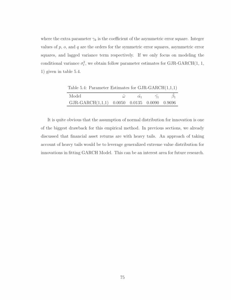
where the extra parameter γk is the coefficient of the asymmetric error square. Integer
values of p, o, and q are the orders for the symmetric error squares, asymmetric error
squares, and lagged variance term respectively. If we only focus on modeling the
conditional variance σ2t , we obtain follow parameter estimates for GJR-GARCH(1, 1,
1) given in table 5.4.
Table 5.4: Parameter Estimates for GJR-GARCH(1,1,1)
Model ω α1 γ1 β1
GJR-GARCH(1,1,1) 0.0050 0.0135 0.0090 0.9696
It is quite obvious that the assumption of normal distribution for innovation is one
of the biggest drawback for this empirical method. In previous sections, we already
discussed that financial asset returns are with heavy tails. An approach of taking
account of heavy tails would be to leverage generalized extreme value distribution for
innovations in fitting GARCH Model. This can be an interest area for future research.
75

Chapter 6
VaR for A Trading Strategy
6.1 Ideas
This chapter will link the connection between Chapter 4 and Chapter 5 by using VaR
as a performance measure of a risk trading strategy. Same as measuring the tail risk
of a financial product, VaR can also be used to measure the tail risk of a portfolio’s
real-time P&L process. If the portfolio is managed by a specific risk trading strategy,
measuring VaR of the portfolio’s tail risk is equivalent in measuring the performance
of a risk trading strategy. In previous chapters from 1 to 4, we explained the FX
market making business process by its two major components: client trading and
risk hedging. During busy market hours, live FX quotes come into the system in
milliseconds, and client trades also come in at a higher frequency than during normal
condition market. This leads to the real-time P&L process given by equations 3.14
and 4.6 to be updated at a much higher frequency, which will produce a large sample
size of the P&L numbers in a very short time period, and it motives the idea of
calculating real-time VaR during the intra-day as a performance measure for the
trading strategy. So, the question that we ask will be ”What is the extreme loss that
the P&L process can have for the next 10 minutes trading period by using current
trading strategy given a 99% level of confidence?”
76

6.2 Methodology and Example
The method we are going to apply is very similar to the method given in sections 5.2
5.5, and 5.3. We will apply generalized extreme value distribution to the block max-
ima of the P&L process, calculate the MLE estimates of the underlying parameters,
and apply equation 5.22 to calculate VaR.
For regulation purpose, VaR is calculated on a daily basis with a time period
of h = 1 or 10 days. For our purpose, h is more likely to be set at 5, 10, or 30
minutes depending on our preference. As the live rate updates are with un-equal
time intervals, the first step is to apply linear interpolation method to produce a
homogeneous time series of the P&L values. The choice of length for each time
interval of the homogeneous time series is subject to the length of the period h of
which VaR is quoted on. The short the h, the finer the time interval we need for linear
interpolation in order to have a big enough sample for each block. The choice of h is
really up to the user’s preference. But a user should keep in mind that for non-busy
trading hours, h is better to be a long interval than short. The reason is that the rate
updates may be very slow during the non-busy hour compare to the busy ones. So
does the P&L process. Thus, a very short h for a non-busy hour may contain only few
real observations before applying linear interpolation. Another key point that affects
the confidence in VaR calculation is the length of the history of the strategy. The
longer the strategy runs, the more observations we have, hence the more confidence we
have in the VaR calculation. If we decide to use only current intra-day data for VaR
calculation, then we need a built-up time period before reaching a high confidence
level in our estimation. By denoting each element of the homogeneous time series
of P&L process by {x1, x2, ..., xT}, where T is the total sample size, we can apply
exactly the same method as mentioned in sections 5.2, 5.5, and 5.3 to calculate VaR.
To given an example, let’s run our Limit Position Trading Strategy, which was
introduced in chapter 4, to simulate one P&L sample path for a 30-hour trading
period for USD/CAD. During this 30-hour period, each of the first, second, and third
77

10-hour period is with the same assumption values of the three scenarios in section
4.3, which are scenarios of Balanced Client Buying and Selling Flows under Flat
Market Condition, Intensive Client Selling Flow under Downward Market Condition,
and Intensive Client Buying Flow under Upward Market Condition respectively.
The simulation result provides a sample with a number of 2,131 observations. Each
is at the time stamp of an incoming client trade. Since we assume our risk hedging
trades can be executed immediately in the market without any delay, the time stamps
of risk hedging trades are identical to the time stamps of those client trades which hit
the position limit and trigger the auto-hedging trades1. The time series of the sample
observations is a non-homogeneous one, which has the time interval from 0 to 1,800
minutes. This mean that on average we have more than one observations per minute.
Thus, we apply linear interpolation method to transfer the original non-homogeneous
time series into a homogeneous one with time interval of 2-minute period between
two consecutive points. Figure 6.1 shows the original and the interpolated time series
with 2-minute interval period.
The ultimate objective for a market maker is to realize positive increments in
the P&L process over a portfolio. Given the homogeneous time series of the P&L
observations {y1, y2, ..., yN}2, we will perform the extreme value theory analysis and
VaR calculation on the time series {x1, x2, ..., xN−1} for which xk = yk+1 − yk for
k = 1, 2, ...N − 1. Figure 6.2 shows the P&L increment time series {x1, x2, ..., xN−1},and figure 6.3 is the Q-Q plot of these observations, which suggests that the P&L
increment has a heavy tail distribution.
Then we perform exactly the same procedures as in section 5.3 to model the block
maxima by generalized extreme value distribution and to calculate the MLE estimates
of parameters. Since we have in total of 30-hour trading history and a homogeneous
time series of P&L increments with 2-minute time interval between two consecutive
1For the client trades simulation, we didn’t apply any client spread in price. Thus, the P&Lsample path doesn’t contain client margin
2The interpolated time series with 2-minute interval period between two consecutive observations.
78

0 200 400 600 800 1000 1200 1400 1600 1800−5
−4
−3
−2
−1
0
1
2x 10
4
Time in Minute
P&
L
Simulated P&L Process for 30−Hour Trading Period
OriginalInterpolation with 2−Minute Interval
Figure 6.1: Simulated P&L Sample Path for a 30-hour Trading Period
79
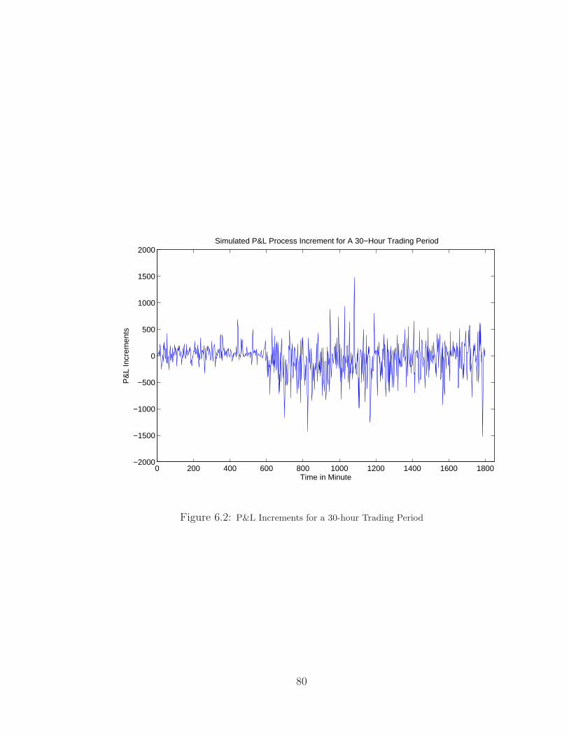
0 200 400 600 800 1000 1200 1400 1600 1800−2000
−1500
−1000
−500
0
500
1000
1500
2000Simulated P&L Process Increment for A 30−Hour Trading Period
Time in Minute
P&
L In
crem
ents
Figure 6.2: P&L Increments for a 30-hour Trading Period
80

−4 −3 −2 −1 0 1 2 3 4−2000
−1500
−1000
−500
0
500
1000
1500
Standard Normal Quantiles
Qua
ntile
s of
Inpu
t Sam
ple
Q−Q Plot of P&L Increments for A 30−Hour Trading Period
Figure 6.3: Q-Q Plot for P&L Increments for A 30-hour Trading Period
81

points, we divide the P&L increment time series into k = 30 blocks with n = 30
observations in each block. Figure 6.4 shows the maximum 2-minute loss (or negative
P&L increment) in each hourly block.
Figure 6.4: Maximum 2-Minute Loss in Hourly Block for A 30-Hours Period
By fitting the maximum block loss observations to the generalized extreme value
distribution, we obtain the maximum likelihood estimates of shape parameter ξ =
−0.1070, scale parameter an = 337.2511, and location parameter bn = 471.8377.
Figure 6.5 compares the empirical cdf for the sample and the theoretical cdf of the
generalized extreme distribution with estimated parameters.
Then, according to equation 5.22, we can calculate
VaR1hour, 0.95 = 471.8377− 337.2511
−0.1070
[1− [−30log(0.95)]0.1070
]
= 323.0779.
This tells us that with a 95% confidence level that 2-minute P&L loss will not exceed
323.0779 in the next one-hour trading period.
With this method, it is possible to use VaR on a high-frequency level as a risk mea-
82

0 200 400 600 800 1000 1200 1400 16000
0.1
0.2
0.3
0.4
0.5
0.6
0.7
0.8
0.9
1
x
F(x
)
Comparison of Empirical and Theoretical CDF
EmpiricalTheoretical
Figure 6.5: Empirical and Theoretical CDF Comparison for Maximum 2-Minute Loss in Hourly
Block
surement for a high-frequency trading strategy. As the sample size increases during
the trading period, the MLE estimations will be more and more accurate. Moreover,
VaR can be calculate on a real-time basis so that it provides a good indication on
how the strategy performs. If the VaR value is getting bigger and bigger, this may
be a signal for us to shut down the strategy or at least to be cautious in operations.
The choice of the block interval size can also be adjusted to serve different purposes
of different groups. For traders, they may want the block interval to be as small as
possible such as 5-minute, 3-minute, or even 1-minute. For regulators, they may only
care about the 1-day or 10-day VaR.
83

Chapter 7
Conclusions and Future Work
In this research paper, we looked into literatures about global foreign exchange market
in terms of its structure, product type, participants, and evolvements. We also looked
into the FX high-frequency data structure, and implemented the Exponential Moving
Average operator in matlab for processing the tick-by-tick data. Empirical analysis
on the real data showed that a built-up period was needed for the EMA operator to
produce accurate enough estimates. The bigger the range value of the operator had,
the long the built-up period was needed.
In the second part of this research, we investigated how a market maker could
effectively manage real-time risk as the counter-party of clients trading. In order
to conduct the analysis, we introduced a framework for market high-frequency data
simulation and client trading flow simulation. By using a Poisson process and a
Geometric Brownian motion, we simulated the market data arrival process and the
market data value respectively. The client trading flow can be simulated by a Poisson
process and a modified Gaussian distribution. Then, market maker’s Base Currency
Wealth Process and Counter Currency Wealth Process were successfully defined with
client trading amounts and market prices. In Chapter 4, we introduced a basic risk
hedging strategy, which limits the position that a market maker can take during the
trading horizon. Simulation results showed that when we set the risk limit at a static
84

level, the risk hedging strategy did not necessarily generate more revenue than a non-
risk hedging strategy, but it helped reducing the downside risk substantially when
the market faced am upward or downward rally.
In the third part of this research, we looked into the Extreme Value Theory and
its extension to Value-at-Risk Calculation. By using eight years daily EUR/USD
exchange rate data, we performed Maximum Likelihood Estimation methods to cal-
culate estimates for shape, scale, and location parameters. Different estimates were
obtained for different combinations of number of blocks and block sizes. Then, we
extend the generalized extreme value distribution to VaR calculation based on the
assumption that financial product has independent daily returns. Lastly, we applied
GARCH(1,1) method for modeling volatility dynamics and calculated conditional
quantile for the predictive conditional distribution function of asset loss.
One interesting avenue for future work is to identify links among risk limits, client
trading flow, and market movements. Then, the risk limit can be dynamically ad-
justed according to a real-time market event and client flows so that optimal risk-
adjusted returns can be obtained. For example, we can fix a client trading flow, and
to search for the relationship between the risk limits and market volatility. Another
interesting direction is to apply the Exponential Moving Average operator in risk
hedging strategy. For example, we can use EMA operator to estimate where the mar-
ket will be in the next couple of seconds or milliseconds, so that when we place risk
hedging trades, we can place limit orders rather than market orders to avoid paying
market spreads. The third interesting area is to leverage generalized extreme value
distribution for innovations in fitting GARCH Model. This will be very helpful in
removing the assumption that the underlying innovations are normally distributed.
85

Bibliography
[1] M. Austin. Adaptive systems for foreign exchange trading. Quantitative Finance,
pages 37–45, August 2004.
[2] E. C. Bank. Review of the Foreign Exchange Market Structure. First edition,
March.
[3] T. Bollerslev. Generalized autoregressive conditional heteroscedasticity. Journal
of Econometrics, pages 307–327, 1986.
[4] J. Danielsson. Value at risk and extreme returns. Working Paper, page London
School of Economics, January 2000.
[5] J.-C. Duan. Approximating the gjr-garch and egarch option pricing models an-
alytically. Working Paper, February 2004.
[6] eFOREX. High frequency fx trading: Technology, techniques and data.
eFOREX, pages 1–4, July 2007.
[7] K. C. Embrechts, P. Modelling Extremal Events for Insurance and Finance.
Application of Mathematics. Springer, second edition, 1997.
[8] R. Engle. Autoregressive conditional heteroscedasticity with estimates of the
variance of united kingdom inflation. Econometrica, pages 987–1007, 1982.
[9] R. Engle. Garch 101, the use of arch/garch models in applied econometrics.
Journal of Economic Perspectives, pages 157–168, 2001.
86

[10] B. Gnedenko. Sur la distribution limite du terme maximum of d’une serie aleato-
rie. Annals of Mathematics, pages 423–453, 1943.
[11] S. Grimshew. Computing the maximum likelihood estimates for the generalized
pareto distribution to data. Technometrics, pages 185–191, 1993.
[12] J. Hull. Options, Futures, and Other Derivatives. Prentice Hall, six edition, June
2005.
[13] A. Jenkinson. The frequency distribution of the annual maximum (or minimum)
of meteorological elements. Quarterly Journal of the Royal Meteorological society,
pages 158–171, 1955.
[14] K. G. Koedijk. The tail index of exchange rate returns. Journal of International
Economics, pages 93–108, 1990.
[15] J. Labuszewski. Fx market growth and trends. CME Research & Product De-
velopment, 2006.
[16] M. Levinson. The Economist: Guide to Financial Markets. Profile Books Ltd,
fourth edition, 2006.
[17] K. Lien. The Foreign Exchange Interbank Market. Investopedia Online, 2008.
[18] F. M. Login. From value at risk to stress testing: the extreme value approach.
Working Paper, pages Centre for Economic Policy Research, London, UK, 1999.
[19] A. J. McNeil. Estimation of tail-related risk measure for heteroscedastic financial
time series, an extreme value approach. Journal of Empirical Finance, pages
271–300, 2000.
[20] U. Muller. Specially weighted moving averages with repeated aplication of the
ema operator. Dec 2000.
87

[21] R. Olsen. An Introduction to High-Frequency Finance. Academic Press, first
edition, 2001.
[22] S. Owens. The six forces of forex. The Forex Report, pages 22–37, July 2004.
[23] A. Pagan. The econometrics of financial markets. Journal of Empirical Finance,
pages 15–102, 1996.
[24] F. R. and T. L.H.C. Limiting forms of the frequency distribution of largest
or smallest member of a sample. Proceedings of the Cambridge Philosophical
Society, pages 180–190, 1928.
[25] R. Reiss and M. Thomas. Statistical Analysis of Extreme Values with Appli-
cations to Insurance, Finance, Hydrology and Other Fields. Birkhauser Verlag,
Basel, first edition, 1997.
[26] D. Rime. New electronic trading systems in foreign exchange markets. New
Economy Handbook, pages 469–504, 2003.
[27] S. Ross. Introduction to Probability Models. Academic Press, eighth edition, Dec
2002.
[28] W. Sharp. Mutual fund performance. Journal of Business, pages 119–138, 1996.
[29] S. Shreve. Stochastic Calculus for Finance II: Continuous-Time Models.
Springer-Verlag, first edition, 2007.
[30] J. Wang. Optimal trading strategy and supply/demand dynamics. National
Bureau of Economic Research, April 2006.
88

Appendix A
Proof of EMA Iteration Formula for t Starting from −∞
By equation (2.4), for a time point t∗ such that tn−1 < t∗ ≤ tn, we can write
EMAZ(λ, t∗) =
∫ t∗
−∞
1
λe−
1λ(t∗−t)Z(t)dt
=
∫ tn−1
−∞
1
λe−
1λ(t∗−t)Z(t)dt+
∫ t∗
tn−1
1
λe−
1λ(t∗−t)Z(t)dt
=
∫ tn−1
−∞
1
λe−
1λ(tn−1−t)e−
1λ(t∗−tn−1)Z(t)dt+
1
λe−
1λ(t∗−t)λZ(t)|t∗t=tn−1
= e−1λ(t∗−tn−1)
∫ tn−1
−∞
1
λe−
1λ(tn−1−t)Z(t)dt+ Z(t∗)− e−
1λ(t∗−tn−1)Z(tn−1)
= µ1EMAZ(λ, tn−1) + (ν1 − µ1)Z(tn−1) + (1− ν1)Z(tn)
(A.1)
with µ1 = e−1λ(t∗−tn−1) and value of ν1 depending on the chosen interpolation scheme
for Z(t∗), where
ν1 =
1 for the previous tick method
1− t∗ − tn−1
tn − tn−1for the linear interpolation method.
89

Appendix B
Proof of EMA Iteration Formula for t Starting at Zero
By the general definition of moving average, which is given by (2.1), for a time point
t∗ such that tn−1 < t∗ ≤ tn, we can write
EMAZ(λ, t∗) =
∫ t∗
01λe−
1λ(t∗−t)Z(t)dt
∫ t∗
01λe−
1λ(t∗−t)dt
=
∫ tn−1
01λe−
1λ(t∗−t)Z(t)dt
∫ t∗
01λe−
1λ(t∗−t)dt
+
∫ t∗
tn−1
1λe−
1λ(t∗−t)Z(t)dt
∫ t∗
01λe−
1λ(t∗−t)dt
=e−
1λ(t∗−tn−1)
∫ tn−1
01λe−
1λ(tn−1−t)Z(t)dt
∫ tn−1
01λe−
1λ(tn−1−t)dt
∫ t∗
01λe−
1λ(t∗−t)
dt∫ tn−10
1λe−
1λ(tn−1−t)
dt
+
∫ t∗
tn−1
1λe−
1λ(t∗−t)Z(t)dt
∫ t∗
01λe−
1λ(t∗−t)dt
=e−
1λ(t∗−tn−1) − e−
1λt∗
1− e−1λt∗
∫ tn−1
01λe−
1λ(tn−1−t)Z(t)dt
∫ tn−1
01λe−
1λ(tn−1−t)dt
+Z(t∗)− e−
1λ(t∗−tn−1)Z(tn−1)
1− e−1λt∗
=e−
1λ(t∗−tn−1) − e−
1λt∗
1− e−1λt∗
EMAZ(λ, tn−1) +Z(t∗)− e−
1λ(t∗−tn−1)Z(tn−1)
1− e−1λt∗
= µ2EMAZ(λ, tn−1) + (ν2 − µ2)Z(tn−1) + (1− ν2)Z(tn)
(B.1)
90

with µ2 = e−
1λ(t∗−tn−1)−e
−1λt∗
1−e−
1λt∗
and value of ν2 depending on the chosen interpolation
scheme for Z(t∗), where
ν2 =
1 for the previous tick method
1− 1
1− e−1λt∗
t∗ − tn−1
tn − tn−1for the linear interpolation method.
91