September 12, 2002

Fuzzy PI Control Design

for an Industrial Weigh Belt Feeder

by

Yanan Zhao and Emmanuel G. Collins, Jr.Department of Mechanical Engineering

Florida A&M University - Florida State UniversityTallahassee, FL 32310

yzhao@eng.fsu.edu, ecollins@eng.fsu.edu

Abstract

An industrial weigh belt feeder is used to transport solid materials into a manufacturing process

at a constant feedrate. It exhibits nonlinear behavior because of motor friction, saturation, and

quantization noise in the sensors, which makes standard autotuning methods difficult to implement.

This paper proposes and experimentally demonstrates two types of fuzzy logic controllers for an

industrial weigh belt feeder. The first type is a PI-like fuzzy logic controller (FLC). A gain scheduled

PI-like FLC and a self-tuning PI-like FLC are presented. For the gain scheduled PI-like FLC the

output scaling factor of the controller is gain scheduled with the change of setpoint. For the self-

tuning PI-like FLC, the output scaling factor of the controller is modified on-line by an updating

factor whose value is determined by a rule-base with the error and change of error of the controlled

variable as the inputs. A fuzzy PI controller is also presented, where the proportional and integral

gains are tuned on-line based on fuzzy inference rules. Experimental results show the effectiveness

of the proposed fuzzy logic controllers. A performance comparison of the three controllers is also

given.

Keywords: fuzzy logic control, PI control, weigh belt feeder, gain scheduling, self-tuning

This research was supported in part by the National Science Foundation under Grant CMS-9802197.

1. Introduction

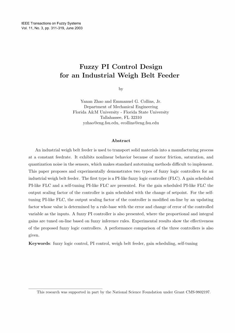
The industrial weigh belt feeder (see Figure 1) used in this research is a product of Merrick

Industries, Inc. of Lynn Haven, Florida. It is a process feeder designed to transport solid materials

into a manufacturing process (e.g., a food, chemical or plastics manufacturing process) at a constant

feedrate, usually in kilograms or pounds per second. To ensure a constant feedrate in industrial

operation, a PI control law is designed and implemented in the Merrick controller. In current

practice the PI tuning process is performed manually by an engineering technician. However,

automated PI tuning is desired for better and more consistent quality [1].

Figure 1: The Merrick Weigh Belt Feeder

The weigh belt feeder exhibits nonlinear behavior because of motor friction, motor saturation,

and quantization noise in the measurement sensors. The dynamics of the weigh belt feeder are

dominated by the motor. To protect the motor, the control signal is restricted to lie in the interval

[0,10] volts. The motor also has significant friction. In addition, the sensors exhibit significant

quantization noise [1]. To design a controller in the presence of plant friction, most friction com-

pensation methods use an observer-based friction scheme which requires selecting a friction model

and adding a feedforward friction observer in the loop. The control signal is then composed of both

the signal for the linear system, which results from neglecting the friction, and the signal to remove

the friction [2]. This kind of model-based compensation has limitations since the characteristics

of friction are difficult to predict and analyze due to their complexity and dependence on param-

eters that vary during the process [3, 4]. However, fuzzy logic control has been found particularly

useful for controller design when the plant model is unknown or difficult to develop. It does not

need an exact process model and has been shown to be robust with respect to disturbances, large

uncertainty and variations in the process behavior [5, 6].

Different approaches exists in the area of automated controller tuning for a nonlinear system

using fuzzy logic. A parallel distributed compensation algorithm first approximates a nonlinear

1

system with a fuzzy model, then a model-based fuzzy controller is designed for each rule of the fuzzy

model [7]. Conventional PID controller tuning using an adaptive-network-based fuzzy inference

system is presented in [8]. Fuzzy PID control has been widely studied and various types of fuzzy

PID (including PI and PD) controllers have been proposed. A function-based evaluation approach

for a systematic study of fuzzy PID controllers is presented in [9].

Fuzzy PID controllers can be classified into two major categories according to their construc-

tion [10]. One category of “fuzzy PID controllers” consists of typical fuzzy logic controllers (FLCs)

constructed as a set of heuristic control rules. The control signal or the incremental change of

control signal is built as a nonlinear function of the error, change of error and acceleration error,

where the nonlinear function includes fuzzy reasoning. There are no explicit proportional, integral

and derivative gains; instead the control signal is directly deduced from the knowledge base and

the fuzzy inference. They are referred to as fuzzy PID-like controllers because their structure is

analogous to that of the conventional PID controller. Most of the research on fuzzy logic control

design belongs to this category [3, 5, 11, 12, 13, 14]. To be consistent with the nomenclature of [15],

and to distinguish from the 2nd category of fuzzy PID controllers (given below), in the following

we will call FLCs in this category PID-like (PI-like, PD-like) FLCs.

Another category of “fuzzy PID controllers” is composed of the conventional PID control system

in conjunction with a set of fuzzy rules (knowledge base) and a fuzzy reasoning mechanism to tune

the PID gains on-line [16, 17, 18]. By virtue of fuzzy reasoning, these types of fuzzy PID controllers

can adapt themselves to varying environments. To use this category of fuzzy PID control, both [16]

and [17] require the ultimate gain and the ultimate period of the plant, while [18] requires the

initial value of proportional and integral gain obtained by a traditional tuning method. Thus,

design of this category of fuzzy PID controllers requires more experimental experience with the

plant. Below, PID (PI, PD) FLC refers exclusively to this type of controller.

Among the three main types of PID-type (i.e., PID-like or PID) FLCs (i.e., PI, PD and PID),

the PI-type FLC is known to be more practical than the PD-type FLC for setpoint tracking because

it is difficult for the PD-type to remove steady state error. The PI-type FLC, however, sometimes

gives poor transient response performance due to the internal integrating operation. However,

PID-type FLCs need three inputs, which greatly expands the rule-base. PID-type FLCs are also

difficult to design because an expert generally does not sense acceleration terms of the error at

every instance in his or her control action [12, 19, 20].

In the process of designing PID (including PI and PD) FLCs, once the membership functions

and the rule-bases are constructed, the next issue is the tuning. Scaling factors can dramatically

2

influence the dynamics of the overall closed-loop system, and hence there have been many studies

to determine effective means of tuning the scaling factors [11, 12, 13, 21, 22]. While self-tuning

FLCs modify the fuzzy set definitions or the scaling factors, self-organizing FLCs adjust or learn the

rules during the process of control [15]. That is, to cope with changing operation conditions and to

adjust for an ill-defined control rule-base, membership functions and/or scaling factors and/or the

rule-base are adapted by self-tuning or self-organizing algorithms according to previous responses

until a desired control performance is achieved. Various forms of self-tuning and self-organizing

fuzzy logic controllers have been reported [3, 11, 12, 13, 22, 23]. To achieve improved performance

and increased robustness, neural networks and genetic algorithms have recently been used in tuning

such controllers [24, 25, 26, 27, 28].

The objective of the weigh belt feeder control is to keep a constant feedrate; thus steady state

error is unacceptable. In this research, we first designed a PI-like FLC. The performance of the

controller was increased by first adjusting the output scaling factor by gain scheduling and then by

a fuzzy self-tuning mechanism. Next, a PI FLC was designed for the weigh belt feeder.

The paper is organized as follows. Section 2 describes the proposed gain scheduled and self-

tuning PI-like FLCs and compares their performance at different setpoints. Section 3 describes the

PI FLC and compares its performance with that of the self-tuning PI-like FLC. Section 4 presents

some discussions. Finally, Section 5 presents conclusions.

2. PI-like Fuzzy Logic Control

In this section, the design of gain scheduled and self-tuning PI-like FLCs is presented. Also,

the performance comparison of the two kinds of controllers is given.

2.1. The General PI-like FLC Controller

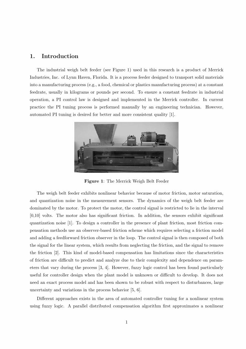
A block diagram of the general PI-like FLC system is shown in Figure 2. The FLC has two

inputs, the error e(k) and change of error △e(k), which are defined by e(k) = r(k)− y(k), △e(k) =

e(k) − e(k − 1), where r and y denote the applied setpoint input and plant output, respectively.

Indices k and k − 1 indicate the present state and the previous state of the system, respectively.

The output of the FLC is the incremental change in the control signal △u(k). The control signal

is obtained by u(k) = u(k − 1) + △u(k). Here w represents the load disturbance.

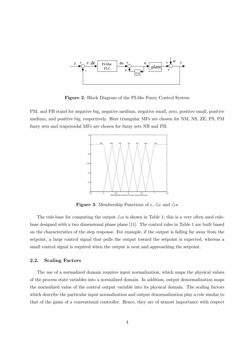
All membership functions of the FLC inputs, e and △e, and the output, △u, are defined on

the common normalized domain [-1,1] as shown in Figure 3. The characters NB, NM, NS, ZE, PS,

3

PI-likeFLC plant

r +

-

e∆e u y+

+1/z

u∆ w

+

+

Figure 2: Block Diagram of the PI-like Fuzzy Control System

PM, and PB stand for negative big, negative medium, negative small, zero, positive small, positive

medium, and positive big, respectively. Here triangular MFs are chosen for NM, NS, ZE, PS, PM

fuzzy sets and trapezoidal MFs are chosen for fuzzy sets NB and PB.

−1.5 −1 −0.5 0 0.5 1 1.50

0.2

0.4

0.6

0.8

1

1.2

Membership Functions for e(k), ∆ e(k) and ∆ u(k)

µ

NB NM NS ZE PS PM PB

Figure 3: Membership Functions of e, △e and △u

The rule-base for computing the output △u is shown in Table 1; this is a very often used rule-

base designed with a two dimensional phase plane [11]. The control rules in Table 1 are built based

on the characteristics of the step response. For example, if the output is falling far away from the

setpoint, a large control signal that pulls the output toward the setpoint is expected, whereas a

small control signal is required when the output is near and approaching the setpoint.

2.2. Scaling Factors

The use of a normalized domain requires input normalization, which maps the physical values

of the process state variables into a normalized domain. In addition, output denormalization maps

the normalized value of the control output variable into its physical domain. The scaling factors

which describe the particular input normalization and output denormalization play a role similar to

that of the gains of a conventional controller. Hence, they are of utmost importance with respect

4

e(k)\△e(k) NB NM NS ZE PS PM PB

NB NB NB NB NM NS NS ZENM NB NM NM NM NS ZE PSNS NB NM NS NS ZE PS PMZE NB NM NS ZE PS PM PBPS NM NS ZE PS PS PM PB

PM NS ZE PS PM PM PM PBPB ZE PS PS PM PB PB PB

Table 1: Fuzzy Rules for Computation of △u

to controller stability and performance. They are the source of possible instabilities, oscillation

problems and deteriorated damping effects [15].

The relationship between the scaling factors (Ge, G△e, G△u) and the input and output variables

of the FLC is eN = Ge × e,△eN = G△e × △e,△u = G△u × △uN . Adjusting the scaling factors

can alter the corresponding regions of the fuzzy sets. For example, an error equal to 0.1 may

belong to PS more than to ZE as its scaling factor is increased. Selection of suitable values of Ge,

G△e, G△u are made based on expert knowledge about the process to be controlled, and through

trial and error. Adjustment rules have been developed for the scaling factors by evaluating control

results (e.g. the characteristics of the step response and heuristics) [15, 21, 22]. The evaluation

performance measures are “overshoot”(OV), “reaching time”(RT), “amplitude”(AM) and “delay

time”(L), as shown in Figure 4. The adjustment rules are good reference for manual tuning by

human operators. Recently numerous papers have explored the integration of genetic algorithms

or neural networks with fuzzy systems in so-called genetic fuzzy or neural fuzzy systems. Many

publications are concerned with the design of FLCs by tuning the rule bases, membership functions

and scaling factors [24, 25, 26, 27, 28].

It has been experimentally observed that a conventional FLC with constant scaling factors and

a limited number of IF-THEN rules may have limited performance for a highly nonlinear plant.

(This was found to be true for the weigh belt feeder.) As a result, there has been significant research

on tuning of FLCs where either the input or output scaling factors or the definitions of the MFs and

sometimes the control rules are tuned to achieve the desired control objectives [11, 13, 18, 22]. In

the following, we concentrate only on the tuning of output scaling factor due to its strong influence

on the performance and stability of the system.

5

RT

OVr

L

t

y

AM

Figure 4: Performance Measures of Step Response

2.3. Gain Scheduling of the Fuzzy PI-like Controller

The weigh belt feeder is normally operated within a setpoint range of [0, 5] volts, and 5 volts is

the maximum possible value of the reference command. Controllers were designed for setpoints of

1 volt, 2 volts, ..., 5 volts, where 1 volt corresponds to a belt speed of 5.08× 10−3m/sec (1 ft/min).

Considering that the desired feedrate of the weigh belt feeder is a constant value, controller design

for variable magnitude step references was not considered in this research. In the FLC design

fixed Ge and G△e were chosen and their values were tuned based on the adjustment rules in

Refs. [15, 21, 22]. A constant output scaling factor was first used for the 5 different setpoints, with

Ge = 0.2, G△e = 2 and G△u = 0.4. Figure 5 shows the resulting experimental results at setpoints of

1 volt and 5 volts. (Please refer to [1] for detailed description of the weigh belt feeder experimental

system.) While the performance of the FLC is fine with a setpoint of 1 volt, the FLC leads to

increasingly large overshoots as the setpoint increased. Thus, the proposed FLC with a constant

output scaling factor for different setpoints had degraded performance at the higher setpoints due

to the nonlinearity of the feeder. To remedy this problem, reduced control effort is needed for the

higher setpoints.

Based on the above observations, we proposed tuning the scaling factor G△u by gain scheduling

it at different setpoints. The design algorithm uses a coefficient γ to adjust G△u as follows:

G△u,sp = G△u,0 · γ (1)

where sp stands for setpoint and G△u,0 is some reference value of G△u. The value of γ is determined

by γ = 1/(1+0.1×sp), which implies that γ and thereafter G△u,sp decrease with increasing setpoint.

6

Thus, the control effort will be reduced as the setpoint increases. Figure 6 shows the block diagram

illustrating this process.

0 5 10 15 20 25 30 35 400

1

2

3

4

5

6

7

8

TIME(SEC)

BE

LT S

PE

ED

(FE

ET/

MIN

)

BELT SPEED AT SETPOINT=1 VBELT SPEED AT SETPOINT=5 V

Figure 5: Performance of PI-like FLC with Constant Output Scaling Factor at Setpoint=1 and 5V

The general desired performance of the closed-loop system for the weigh belt feeder is small

or no overshoot, no steady-state error and fast rise time. There is no specific performance index

defined for the weigh belt feeder. Figure 7 illustrates the experimental results of the proposed gain

scheduled FLC at setpoints of 1 volt and 5 volts; the results at the other setpoints are similar.

The scaling factors are chosen as Ge = 0.2, G△e = 2, G△u,0 = 0.4 while G△u,sp is gain scheduled as

discussed above. It is seen that with the use of gain scheduled PI-like FLC, the performance of the

closed-loop system at different setpoints is generally acceptable.

2.4. Self-tuning of Fuzzy PI-like Controller

Developing a generalized tuning method for FLCs is a very difficult task because the computa-

tion of the optimal values of tunable parameters needs the required control objectives as well as a

fixed model for the controller. A self-tuning PI-like FLC (STFLC) was proposed for the tuning of

output scaling factor [11]. The block diagram of the proposed self-tuning FLC is shown in Figure

8.

Based on this self-tuning mechanism, the incremental change in controller output △u is obtained

by the following equation:

△u = (α · G△u) · △uN . (2)

Thus the gain of the self-tuning FLC does not remain fixed while the controller is in operation;

rather it is modified at each sampling time by the gain updating factor α, where (as detailed below)

α is obtained on-line based on fuzzy logic reasoning using the error and change of error at each

sampling time. Later we will show that this on-line updating factor will change the output surface

7

PI-likeFLC

r +

-e∆

u+

1/z

Nu∆Ge

G

eG

Gain scheduling

+u∆

e∆plant

y

+

+w

Figure 6: Closed-loop System with the Gain Scheduled PI-like FLC

0 5 10 15 20 25 30 35 400

1

2

3

4

5

6

TIME(SEC)

BE

LT S

PE

ED

(FE

ET/

MIN

)

BELT SPEED AT SETPOINT=1 VBELT SPEED AT SETPOINT=5 V

Figure 7: Performance of the Gain Scheduled PI-like FLC at Setpoint=1 and 5 V

of the FLC, and thus make the controller perform better than the gain scheduled PI-like FLC.

2.4.1. Membership Functions

Reference [11] chose 7 fuzzy sets for each of the fuzzy logic reasoning inputs, e and △e, and the

output, α, and thus has 49 fuzzy rules for the computation of α. To make implementation possible

with limited processor throughput, this research focused on reducing the number of fuzzy rules.

Here, the MFs of e and △e are defined on the common normalized domain [-1,1], where each has

3 fuzzy sets, as shown in Figure 9. The MFs for α are defined with 3 fuzzy sets, but with different

domains for different setpoints. This is to better take into account the high nonlinearity of the

weigh belt feeder. (Fixed universe of discourse of α at different setpoints has limited ability to

adapt to the setpoint changes.) The MFs of α are with domain [0.2, 0.8] for a setpoint of 5 volts.

The universe of discourse was shifted by 0.1 in the positive direction with each unit decrease of the

setpoint; hence the domain for a setpoint of 1 volt is [0.6, 1.2] as illustrated in Figure 10, where the

solid lines represent the MFs for a setpoint of 5 volts and the dotted lines represent the MFs for a

setpoint of 1 volt. Hence, the overall output scaling factor (α ·G△u) and thus the control effort will

increase with decreasing setpoint, which remedies the problems encountered by a constant output

scaling factor. Each of the MFs uses a triangular function.

8

PI-likeFLC

r +

-e∆

u+

1/z

Nu∆Ge

G

eG

Fuzzy reasoning

+u∆

e∆plant

y

+

+w

Figure 8: Closed-loop System with the Self-tuning PI-like FLC

−1.5 −1 −0.5 0 0.5 1 1.50

0.2

0.4

0.6

0.8

1

1.2

Membership Functions for e(k) and ∆ e(k)

µ

ZE N P

Figure 9: Membership Functions of e and △e for the Updating Factor

2.4.2. The Rule-bases

The rule-base for the computation of α is shown in Table 2. The rules are dependent on the

controller rule-base in Table 1. When the state is far away from the setpoint, the gain should be

large; this may be achieved by rules such as: if both the error and change of error are negative (or

positive), then α is big. When the state is close to the steady state, the gain should be medium;

this may be achieved by the rules such as: if either the error or the change of error is zero, then

α is medium. At steady state, the gain should be very small; this may be achieved by the rule: if

both the error and change of error are zero, then α is small.

e(k)\△e(k) N ZE P

N B M SZE M S MP S M B

Table 2: Fuzzy Rules for Computation of α

9

0.2 0.4 0.6 0.8 1 1.20

0.2

0.4

0.6

0.8

1

Tuning of Membership Functions for α

µ

S M B

Figure 10: Membership Functions of α for Setpoint=1 and Setpoint=5 V

2.4.3. Experimental Results

For both the two fuzzy reasoning systems, the input scaling factors chosen here are Ge = 0.2

and G△e = 2. For the fuzzy reasoning block generating signal △u, the output scaling factor is

G△u = 0.58. G△u = 0.58 is bigger than the corresponding value of the gain scheduled FLC because

a large portion of the universal discourse of α is smaller than 1. For the fuzzy reasoning block

generating α, the output scaling factor is taken as 1. This choice is reasonable because α itself

plays a role in adjusting the output scaling factor of the other fuzzy reasoning block. Figure 11

shows the experimental results of the proposed self-tuning fuzzy PI-like controller at setpoints of 1

volt and 5 volts; the performance at the other setpoints is similar.

0 5 10 15 20 25 30 35 400

1

2

3

4

5

6

TIME(SEC)

BE

LT S

PE

ED

(FE

ET/

MIN

)

BELT SPEED AT SETPOINT=1 VBELT SPEED AT SETPOINT=5 V

Figure 11: Performance of the Self-tuning PI-like FLC at Setpoint=1 and 5 V

10

2.5. Comparison of the Gain Scheduled and Self-tuning FLCs

For both the gain scheduled and self-tuning FLCs proposed above, focus was made on fine-

tuning the output scaling factor to improve the performance of the system. The update of the

output scaling factor is equivalent to changing the universe of discourse of the output signal.

For the gain scheduled FLC, the shape of the output surface of the fuzzy inference system does

not change as the output scaling factor is varied. The coefficient γ can only change the range of

the output variable. For the self-tuning FLC, the updating factor α not only changes the range of

the output variable, but also the shape of the output surface. Figures 12 shows the output surface

of α at setpoint of 1 volt. When this surface is applied to the original output surface of FLC, both

the range and the shape of the output surface of the FLC will be changed.

−1

−0.5

0

0.5

1

−1

−0.5

0

0.5

10.75

0.8

0.85

0.9

0.95

1

1.05

error

Output Surface of the Updating Factor with Setpoint=1

derivative of error

upda

ting

fact

or

Figure 12: Output Surface of Updating Factor at Setpoint=1 V

Table 3 shows the performance comparison of the two types of the FLC based on IAE (integral

of the absolute value of the error), ISE (integral of the squared error), ITAE (integral of the time-

weighted absolute error) and ISTE (integral of the time-weighted squared error) indices [29]. All of

them were computed over the time interval of [0, 40] sec, which is the time period of the previous

experiments. The ISE criterion tends to place a greater penalty on large errors than the IAE or

ITAE criteria. The ITAE criterion penalizes errors that persist for long periods of time. In general,

ITAE is the preferred integral error criterion since it results in the most conservative controller

settings. For all five setpoints the indices of the self-tuning FLC are better than that of the gain

scheduled FLC. However, the implementation of the gain scheduled FLC is much simpler than that

of the self-tuning FLC. Instead of using a set of inference rules for the updating factor, as in the

self-tuning FLC, the gain scheduled FLC only adopts a simple gain scheduling formula to lead to

acceptable performance. Thus it is more practical in terms of the ease of implementation.

11

SP Type IAE ISE ITAE ITSE

1 GS 523.8 372.2 3251.4 811.6ST 456.0 303.2 3114.4 585.3

2 GS 755.1 1032.0 4200.5 1625.4ST 689.6 883.6 4161.0 1241.6

3 GS 1071.1 2192.9 5172.5 3132.6ST 948.5 1952.1 4223.3 2440.7

4 GS 1399.5 4075.6 5496.9 5867.2ST 1395.9 3974.4 5186.7 5608.5

5 GS 1789.7 6482.2 7151.5 9498.5ST 1751.6 6354.6 6659.6 9137.8

Table 3: Comparison of the Performance of the Gain Scheduled (GS) and Self-tuning (ST) PI-likeFLCs

3. PI Fuzzy Logic Control

In this section detailed design of a PI controller whose gains are tuned on-line by fuzzy logic

reasoning [16] is given. It is called a PI FLC because the outputs of the fuzzy logic reasoning are

the proportional and integral gain instead of the incremental control signal. The control signal

is generated according to the on-line tuning of the proportional and integral gains based on the

transfer function,

H(z) = Kp + KiTs

z

z − 1= Kp(1 +

Ts

Ti

z

z − 1), (3)

where Kp is the proportional gain, Ki is the integral gain, Ti = Kp/Ki is the integral time constant

and Ts is the sampling period.

Reference [16] designed a fuzzy PID controller, where each of the proportional, integral and

derivative gains were tuned based on 49 fuzzy rules respectively. In this research the number of

fuzzy tuning rules was reduced to 9, which was a dramatic decrease in complexity. In addition, new

tuning schemes for the range of proportional gain Kp and the integral time constant Ti at different

setpoints were developed.

3.1. The Proposed PI FLC

Figure 13 shows the PI FLC system. There are two fuzzy logic reasoning systems included in

the design. One of them has two inputs e(k) and △e(k) and output Kp; the other one has the

same inputs but with output Ti. Thus Ki was obtained by Kp/Ti. It is assumed that Kp is in the

prescribed range [Kp,min, Kp,max]; the appropriate range is determined experimentally.

Let N, ZE, P, B, M and S denote negative, zero, positive, big, medium and small, respectively.

12

r +

-e∆

uGe

G

e

Fuzzy reasoning

e∆

Fuzzy reasoning

PI Controller

iT

pKplant

yw

+

+

Figure 13: Closed-loop System with Fuzzy PI controller

The three MFs of e(k) and △e(k), corresponding to the fuzzy sets, N, ZE and P, are the same as

shown in Figure 9. The two MFs of Kp, corresponding to the fuzzy sets S and B, are shown in

Figure 14. The MFs of Ti corresponding to the singleton fuzzy sets S, M, and B, are shown in

Figure 15. (Solid lines represent the MFs at a setpoint of 5 volts.)

Tables 4 and 5 show the fuzzy tuning rules for Kp and Ti respectively. The very simple inference

rules are effective and greatly reduce the computational burden for real-time implementation of the

controller.

−0.5 0 0.5 1 1.50

0.2

0.4

0.6

0.8

1

1.2

Membership Functions for Kp

µ

Big Small

Figure 14: Membership Functions of Kp Gain

e(k) \△e(k) N ZE P

N B B BZE S B SP B B B

Table 4: Fuzzy Rules for Computation of Kp

The control rules in Tables 4 and 5 are based on the desired characteristics of the step responses.

For example, at the beginning of the control action, a big control signal is needed in order to achieve

13

0 0.5 1 1.5 2 2.5 3 3.5 40

0.2

0.4

0.6

0.8

1

Tuning of Membership Functions for Ti

µ

S M B

Figure 15: Membership Functions of Ti for Setpoint=1 and 5 V

a fast rise time. Thus, the PI controller should have a large proportional gain and a large integral

gain. When the step response reaches the setpoint, a small control signal is needed to avoid a large

overshoot. Thus the PI controller should have a small proportional gain and a small integral gain.

e(k) \ △e(k) N ZE P

N S S SZE B M BP S S S

Table 5: Fuzzy Rules for Computation of Ti

3.2. Tuning Algorithm for the PI FLC

Here, scaling factors of Ge = 0.1 and G△e = 1 were chosen. There are two other tuning

algorithms used for the PI FLC design. Due to the nonlinearity of the feeder, to avoid high

overshoot at higher setpoints, it is necessary to suitably reduce both the proportional gain and the

integral gain. Hence, we chose a gain scheduling coefficient ρ = 1/(1 + 0.2 × sp), where sp stands

for setpoint. This coefficient was used for the on-line tuning of both the range of Kp and the MFs

of Ti. For different setpoints the range of the proportional gain was chosen as [0, Kp,max], where

Kp,max = ρ × Kp,max0, and Kp,max0 = 3.2 was chosen according to experimental experience. It is

clear that ρ and at the same time Kp,max will decrease as the setpoint increases, which means the

proportional gain for a higher setpoint is generally lower than that for a lower setpoint.

The singleton membership function of Ti was adjusted on-line along with the setpoint, mf =

mf0/ρ. That is the singleton membership function values will decrease as the setpoint decreases.

(That is the integral gain Ki will increase.) As shown in Figure 15, these MFs shift right as the

14

setpoint increases, while they shift left as the setpoint decreases, where the solid lines represent

the MFs at setpoint of 5 volts and the dotted lines represent the MFs at setpoint of 1 volt. The

coefficient ρ plays a role similar to γ of the gain-scheduled PI-like FLC. Sugeno-type inference was

used for the fuzzy reasoning of Ti.

3.3. Experimental Results and Comparison

Figure 16 shows the experimental results for the PI FLC implemented at setpoints of 1 volt and

5 volts. Table 6 details the performance of the PI FLC and compares it with that of the self-tuning

PI-like FLC. Considering the IAE criterion, the PI FLC improved at least 15% from that of the

self-tuning PI-like controller. Also notice that each value in Table 6 corresponding to the PI FLC

is smaller than the corresponding value for the self-tuning PI-like FLC except ITAE at a setpoint

of 4 volts. This is caused by a significant deviation from the mean response of the output signal at

about 32 sec for the PI FLC, which is largely a result of sensor noise. Comparing Figures 16 with

Figure 11, it is seen that the PI FLC leads to a faster response and a smaller overshoot than the

self-tuning PI-like FLC. The reason is that the PI-like FLC obtains the control signal incrementally

starting from zero, while the PI FLC obtains the control signal directly from the initial PI controller

which has a larger output during startup. The disadvantage of this FLC design method is that it

is more model-dependent, since it requires human experience with controlling the plant to define

the range of the proportional gain.

0 5 10 15 20 25 30 35 400

1

2

3

4

5

6

TIME(SEC)

BE

LT S

PE

ED

(FE

ET/

MIN

)

BELT SPEED AT SETPOINT=1 VBELT SPEED AT SETPOINT=5 V

Figure 16: Step Responses of the PI FLC at Setpoint=1 and 5 V

Figures 17 shows the changes of proportional and integral gains of the fuzzy PI controller at

setpoint of 1 volt. (The curves are similar for the other setpoints.) It is seen that the gains

converge very fast in the first few seconds, and are subsequently only finely tuned around the mean

steady-state values. This demonstrates that the fuzzy PI controller quickly adjusts to the current

environment.

15

SP Type IAE ISE ITAE ITSE

1 PI 317.6 149.8 2619.8 239.4ST 456.0 303.2 3114.4 585.3

2 PI 501.6 590.6 2943.5 591.0ST 689.6 883.6 4161.0 1241.6

3 PI 759.6 1522.1 3798.5 1592.1ST 948.5 1952.1 4223.3 2440.7

4 PI 1141.3 3114.7 5468.7 3735.8ST 1395.9 3974.4 5186.7 5608.5

5 PI 1488.6 5173.6 5327.6 6324.5ST 1751.6 6354.6 6659.6 9137.8

Table 6: Comparison of the Performance of the PI FLC and the Self-tuning (ST) PI-like FLC

0 5 10 15 20 25 30 35 400.4

0.6

0.8

1

1.2

1.4

1.6

1.8

TIME(SEC)

Kp

and

Ki G

AIN

S

Fuzzy PI Controller with Setpoint=1

Kp GAINKi GAIN

Figure 17: Proportional and Integral Gains of PI FLC at Setpoint=1 V

4. Discussions

Comparing the tuning mechanisms of the three kinds of FLCs proposed in this research, it is

observed the gain scheduled FLC is the simplest. It has one fuzzy reasoning block generating the

incremental change in the control command △u, and one tuning coefficient γ adjusting the output

scaling factor. Self-tuning PI-like FLC has two fuzzy reasoning blocks, one with output △u and

the other with output α. Also, the universe of discourse of α is adjusted at different setpoints to

improve the performance of the FLC at different operating conditions. The PI FLC also has two

fuzzy reasoning blocks to obtain the proportional gain and integral gain on-line. For this kind of

FLC, a coefficient ρ is used to adjust the range of both gains at different setpoints.

The performance comparison shows the PI FLC is the best among the three, and the perfor-

mance of the self-tuning PI-like FLC is better than that of gain scheduled PI-like FLC. Certainly,

the improved performance is at the cost of increased implementation effort. From this point of

view, there is no design that is uniformly “the best.”

16

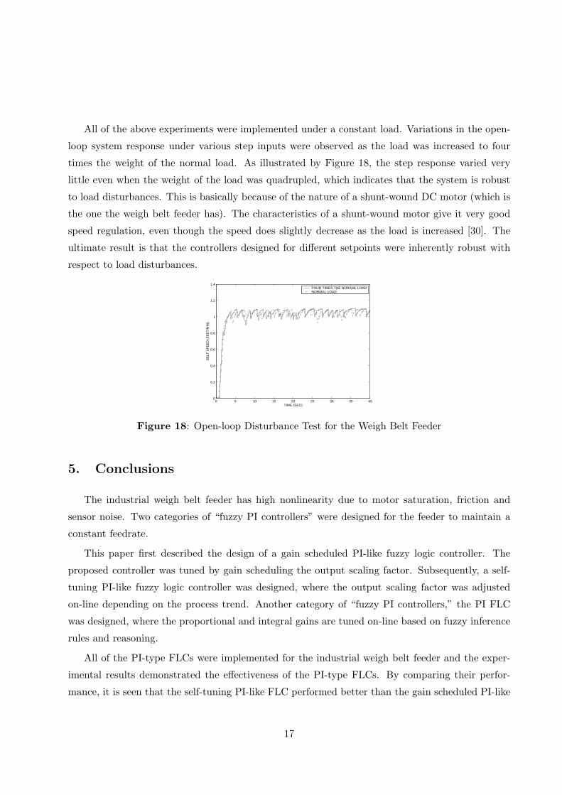
All of the above experiments were implemented under a constant load. Variations in the open-

loop system response under various step inputs were observed as the load was increased to four

times the weight of the normal load. As illustrated by Figure 18, the step response varied very

little even when the weight of the load was quadrupled, which indicates that the system is robust

to load disturbances. This is basically because of the nature of a shunt-wound DC motor (which is

the one the weigh belt feeder has). The characteristics of a shunt-wound motor give it very good

speed regulation, even though the speed does slightly decrease as the load is increased [30]. The

ultimate result is that the controllers designed for different setpoints were inherently robust with

respect to load disturbances.

0 5 10 15 20 25 30 35 400

0.2

0.4

0.6

0.8

1

1.2

1.4

TIME (SEC)

BE

LT S

PE

ED

(FE

ET/

MIN

)

FOUR TIMES THE NORAML LOADNORMAL LOAD

Figure 18: Open-loop Disturbance Test for the Weigh Belt Feeder

5. Conclusions

The industrial weigh belt feeder has high nonlinearity due to motor saturation, friction and

sensor noise. Two categories of “fuzzy PI controllers” were designed for the feeder to maintain a

constant feedrate.

This paper first described the design of a gain scheduled PI-like fuzzy logic controller. The

proposed controller was tuned by gain scheduling the output scaling factor. Subsequently, a self-

tuning PI-like fuzzy logic controller was designed, where the output scaling factor was adjusted

on-line depending on the process trend. Another category of “fuzzy PI controllers,” the PI FLC

was designed, where the proportional and integral gains are tuned on-line based on fuzzy inference

rules and reasoning.

All of the PI-type FLCs were implemented for the industrial weigh belt feeder and the exper-

imental results demonstrated the effectiveness of the PI-type FLCs. By comparing their perfor-

mance, it is seen that the self-tuning PI-like FLC performed better than the gain scheduled PI-like

17

FLC, but needs a set of inference rules for the on-line tuning of updating factor. This requires

significantly more implementation effort than the gain scheduled PI-like FLC. Also, the PI FLC

performed significantly better than the two kinds of PI-like FLCs, but the PI FLC relies on prior

experience to determine the range of the proportional gain. This demonstrates that as more user

knowledge is incorporated into the controller design, the performance of the FLC increases.

Both the gain scheduling scheme and the fuzzy rules used for the tuning of updating factor of

the PI-like FLC are very simple. The fuzzy reasoning rules proposed for the tuning of proportional

gain and integral time constant of the PI FLC are also very simple. This simplicity will make the

implementation of these methods simpler and more cost efficient in an industrial environment.

18

References

[1] E. G. Collins, Jr., Y. Zhao and R. Millett, “A genetic search approach to unfalsified PI control

design for a weigh belt feeder,”International Journal of Adaptive Control and Signal Processing,

Vol. 15, No. 5, pp. 519-534, 2001.

[2] H. Olsson, K. J. Astrom, C. Canudas de Wit, M. Gafvert and P. Lischinsky, “Friction models

and friction compensation,” European Journal of Control, Vol. 4, No. 3, pp. 176-195, 1998.

[3] S. Jee and Y. Koren, “Self-organizing fuzzy logic control for friction compensation in feed

drives,” Proceedings of the American Control Conference, pp. 205-209, Seattle, WA, June

1995.

[4] J. T. Teeter, M. Chow and J.J. Brickley, “Novel fuzzy friction compensation approach to im-

prove the performance of a DC motor control system,” IEEE Trans. on Industrial Electronics,

Vol. 43, No. 1, pp. 113-120, 1996.

[5] W. Li and X. Chang, “Application of hybrid fuzzy logic proportional plus conventional integral-

derivative controller to combustion control of stoker-fired boilers,” Fuzzy Sets and Systems, Vol.

111, No. 2, pp. 267-284, 2000.

[6] J. Fonseca, J. L. Afonso, J. S. Martins and C. Couto, “Fuzzy logic speed control of an induction

motor,” Microprocessors and Microsystems, Vol. 22, No. 9, pp. 523-534, 1999.

[7] H. O. Wang, K. Tanaka and M. Griffin, “Parallel distributed compensation of nonlinear systems

by Takagi-Sugeno fuzzy model,” Proceedings of the 4th IEEE International Conference on

Fuzzy Systems, pp. 531-538, Yokohama, Japan, March, 1995.

[8] J. C. Shen, “Fuzzy neural networks for tuning PID controller for plant with underdamped

responses,” IEEE Trans. on Fuzzy Systems, Vol. 9, No. 2, pp. 333-342, 2001.

[9] B. Hu, G. K. I. Mann, and R. G. Gosine, “A systematic study of fuzzy PID controllers -

function-based evaluation approach,” IEEE Trans. on Fuzzy Systems, Vol. 9, No. 5, pp. 699-

712, 2001.

[10] J. Xu, C. C. Hang and C. Liu, “Parallel structure and tuning of a fuzzy PID controller,”

Automatica, Vol. 36, No. 5, pp. 673-684, 2000.

[11] R. K. Mudi and N. K. Pal, “A self-tuning fuzzy PI controller,” Fuzzy Sets and Systems, Vol.

115, No. 2, pp. 327-338, 2000.

[12] C. T. Chao and C. C. Teng, “A PD-like self-tuning fuzzy controller without steady-State

error,” Fuzzy Sets and Systems, Vol. 87, No. 2, pp. 141-154, 1997.

[13] Z. W. Woo, H.Y. Chung and J. J. Lin, “A PID type fuzzy controller with self-tuning scaling

factors,” Fuzzy Sets and Systems, Vol. 115, No. 2, pp. 321-326, 2000.

[14] J. Carvajal, G. Chen and H. Ogmen, “Fuzzy PID controller: design, performance evaluation,

and stability analysis,” Information Sciences, Vol. 123, No. 3, pp. 249-270, 2000.

[15] D. Driankov, H. Hellendoorn and M. Reinfrank, An Introduction to Fuzzy Control. Berlin,

Heidelberg: Springer-Verlag, 1993.

[16] Z. Z. Zhao, M. Tomizuka and S. Isaka,“Fuzzy gain scheduling of PID controller,” IEEE Trans.

on Systems, Man, and Cybernetics, Vol. 23, No. 5, pp. 1392-1398, 1993.

[17] S. Z. He, S. Tan and F. L. Xu, “Fuzzy self-tuning of PID controller,” Fuzzy Sets and Systems,

Vol. 56, No. 1, pp. 37-46, 1993.

[18] R. Bandyopadhyay and D. Patranabis , “A fuzzy logic based PI controller,” ISA Transactions,

Vol. 37, No. 3, pp. 227-235, 1998.

[19] J. H. Lee, “On methods for improving performance of PI-type fuzzy logic controllers,” IEEE

Trans. on Fuzzy Systems, Vol. 1, No. 4, pp. 298-301, 1993.

[20] H. X. Li, “Enhanced methods of fuzzy logic control,” Proceedings of the IEEE International

Conference on Fuzzy Systems, pp. 331-336, Yokohama, Japan, March 1995.

[21] W. C. Daugherity, B. Rathakrishnan and J. Yen, “Performance evaluation of a self-tuning

fuzzy controller,” Proceedings of the IEEE International Conference on Fuzzy Systems, pp.

389-397, San Diego, CA, March 1992.

[22] M. Maedo and S. Murakami, “A self-tuning fuzzy controller”, Fuzzy Sets and Systems, Vol.

51, No. 1, pp. 29-40, 1992.

[23] Y. P. Singh, “A modified Self-organizing controller for real-time process control application,”

Fuzzy Sets and Systems, Vol. 96, No. 2, pp. 147-159, 1998.

[24] J. R. Jang, “ANFIS: adaptive-network-based fuzzy inference system,” IEEE Trans. on Sys-

tems, Man and Cybernetics, Vol. 23, No. 3, pp. 665-685, 1993.

[25] A. Nurnberger, D. Nauck and R. Kruse, “Neuro-fuzzy control based on the NEFCON-model:

recent development,” Soft Computing, Vol. 2, No. 4, pp. 168-182, 1999.

[26] A. Arslan and M. Kaya, “Determination of fuzzy logic membership functions using genetic

algorithms,” Fuzzy Sets and Systems, Vol. 118, No. 2, pp. 297-306, 2001.

[27] K. Warwick and Y. H. Kang,“Self-tuning proportional, integral and derivative controller based

on genetic algorithm least squares,” Journal of Systems and Control Engineering, Vol. 212,

No. 16, pp. 437-448, 1998.

[28] A. Homafier, M. Bikdash and V. Gopalan, “Design using genetic algorithms of hierarchical

hybrid Fuzzy-PID controllers of two-link robotic arms,” Journal of Robotic Systems, Vol. 14,

No. 6, pp. 449-463, 1997.

[29] K. Astrom and T. Hagglund, PID Controller: Theory, Design and Tuning, 2nd edition. In-

strument Society of America, 1995.

[30] R. Krishnan, Electric Motor Drives. Upper Saddle River, NJ: Prentice Hall, 2001.