PDF generated using the open source mwlib toolkit. See http://code.pediapress.com/ for more information.PDF generated at: Wed, 10 Nov 2010 00:16:57 UTC

Fundamentals ofTransportation

ContentsArticles

Fundamentals of Transportation 1Fundamentals of Transportation/About 2Fundamentals of Transportation/Introduction 3Transportation Economics/Introduction 6Fundamentals of Transportation/Geography and Networks 11Fundamentals of Transportation/Trip Generation 20Fundamentals of Transportation/Trip Generation/Problem 26Fundamentals of Transportation/Trip Generation/Solution 27Fundamentals of Transportation/Destination Choice 28Fundamentals of Transportation/Destination Choice/Background 34Fundamentals of Transportation/Mode Choice 40Fundamentals of Transportation/Mode Choice/Problem 49Fundamentals of Transportation/Mode Choice/Solution 50Fundamentals of Transportation/Route Choice 52Fundamentals of Transportation/Route Choice/Problem 61Fundamentals of Transportation/Route Choice/Solution 61Fundamentals of Transportation/Evaluation 64Fundamentals of Transportation/Planning 77Fundamentals of Transportation/Operations 81Fundamentals of Transportation/Queueing 85Fundamentals of Transportation/Queueing/Problem1 93Fundamentals of Transportation/Queueing/Solution1 93Fundamentals of Transportation/Queueing/Problem2 94Fundamentals of Transportation/Queueing/Solution2 94Fundamentals of Transportation/Queueing/Problem3 95Fundamentals of Transportation/Queueing/Solution3 95Fundamentals of Transportation/Traffic Flow 96Fundamentals of Transportation/Traffic Flow/Problem 104Fundamentals of Transportation/Traffic Flow/Solution 104Fundamentals of Transportation/Queueing and Traffic Flow 105Fundamentals of Transportation/Shockwaves 111Fundamentals of Transportation/Shockwaves/Problem 115Fundamentals of Transportation/Shockwaves/Solution 115Fundamentals of Transportation/Traffic Signals 116

Fundamentals of Transportation/Traffic Signals/Problem 125Fundamentals of Transportation/Traffic Signals/Solution 126Fundamentals of Transportation/Design 127Fundamentals of Transportation/Sight Distance 129Fundamentals of Transportation/Sight Distance/Problem 135Fundamentals of Transportation/Sight Distance/Solution 135Fundamentals of Transportation/Grade 136Fundamentals of Transportation/Grade/Problem 142Fundamentals of Transportation/Grade/Solution 143Fundamentals of Transportation/Earthwork 144Fundamentals of Transportation/Earthwork/Problem 149Fundamentals of Transportation/Earthwork/Solution 149Fundamentals of Transportation/Horizontal Curves 150Fundamentals of Transportation/Horizontal Curves/Problem 157Fundamentals of Transportation/Horizontal Curves/Solution 158Fundamentals of Transportation/Vertical Curves 159Fundamentals of Transportation/Vertical Curves/Problem 165Fundamentals of Transportation/Vertical Curves/Solution 166Transportation Economics/Pricing 167Fundamentals of Transportation/Conclusions 179Transportation Economics/Decision making 180

ReferencesArticle Sources and Contributors 187Image Sources, Licenses and Contributors 189

Article LicensesLicense 191

Fundamentals of Transportation 1

Fundamentals of Transportation

Table of contents

Market Street, San Francisco

Introductory Material

• /About/• /Introduction/

/Planning/

• /Decision Making/• /Modeling/• /Geography and Networks/• /Land Use Forecasting/• /Trip Generation/• /Destination Choice/• /Mode Choice/• /Route Choice/• /Evaluation/

/Operations/• /Queueing/• /Traffic Flow/• /Queueing and Traffic Flow/• /Shockwaves/• /Traffic Signals/• /Traffic Control Devices/• /Analogs/

/Design/• /Sight Distance/• /Grade/• /Earthwork/• /Horizontal Curves/• /Vertical Curves/

Fundamentals of Transportation 2

/Economics/• /Pricing/

Conclusions• /Conclusions/

Useful Off-site Resources• NSF STREET: Simulating Transportation for Realistic Engineering Education and Training [1]

• Transportation Engineering Lab Manual [2]

• Pavement Interactive [3]

References[1] http:/ / street. umn. edu[2] http:/ / www. webs1. uidaho. edu/ niatt_labmanual/[3] http:/ / pavementinteractive. org

Fundamentals of Transportation/AboutThis book is aimed at undergraduate civil engineering students, though the material may provide a useful review forpractitioners and graduate students in transportation. Typically, this would be for an Introduction toTransportation course, which might be taken by most students in their sophomore or junior year. Often this is thefirst engineering course students take, which requires a switch in thinking from simply solving given problems toformulating the problem mathematically before solving it, i.e. from straight-forward calculation often found inundergraduate Calculus to vaguer word problems more reflective of the real world.

How an idea becomes a roadThe plot of this textbook can be thought of as "How an idea becomes a road". The book begins with the generationof ideas. This is followed by the analysis of ideas, first determining the origin and destination of a transportationfacility (usually a road), then the required width of the facility to accommodate demand, and finally the design of theroad in terms of curvature. As such the book is divided into three main parts: planning, operations, and design, whichcorrespond to the three main sets of practitioners within the transportation engineering community: transportationplanners, traffic engineers, and highway engineers. Other topics, such as pavement design, and bridge design, arebeyond the scope of this work. Similarly transit operations and railway engineering are also large topics beyond thescope of this book.Each page is roughly the notes from one fifty-minute lecture.

Fundamentals of Transportation/About 3

AuthorsAuthors of this book include David Levinson [1], Henry Liu [2], William Garrison [3], Adam Danczyk, MichaelCorbett. Karen Dixon of Oregon State University has contributed Flash animations developed by herself and herstudents linked to in this book.

References[1] http:/ / nexus. umn. edu[2] http:/ / www. ce. umn. edu/ ~liu/[3] http:/ / en. wikipedia. org/ wiki/ William_Garrison_(geographer)

Fundamentals of Transportation/Introduction

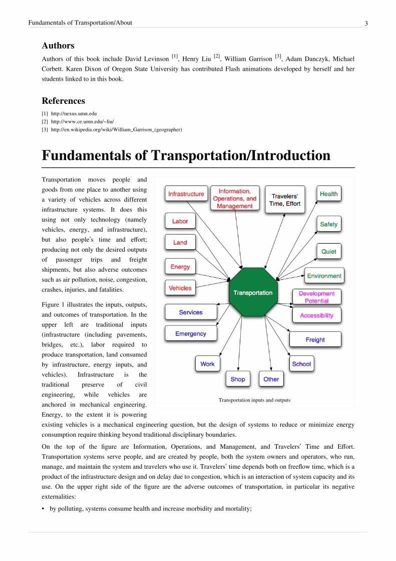
Transportation inputs and outputs

Transportation moves people andgoods from one place to another usinga variety of vehicles across differentinfrastructure systems. It does thisusing not only technology (namelyvehicles, energy, and infrastructure),but also people’s time and effort;producing not only the desired outputsof passenger trips and freightshipments, but also adverse outcomessuch as air pollution, noise, congestion,crashes, injuries, and fatalities.

Figure 1 illustrates the inputs, outputs,and outcomes of transportation. In theupper left are traditional inputs(infrastructure (including pavements,bridges, etc.), labor required toproduce transportation, land consumedby infrastructure, energy inputs, andvehicles). Infrastructure is thetraditional preserve of civilengineering, while vehicles areanchored in mechanical engineering.Energy, to the extent it is poweringexisting vehicles is a mechanical engineering question, but the design of systems to reduce or minimize energyconsumption require thinking beyond traditional disciplinary boundaries.On the top of the figure are Information, Operations, and Management, and Travelers’ Time and Effort.Transportation systems serve people, and are created by people, both the system owners and operators, who run,manage, and maintain the system and travelers who use it. Travelers’ time depends both on freeflow time, which is aproduct of the infrastructure design and on delay due to congestion, which is an interaction of system capacity and itsuse. On the upper right side of the figure are the adverse outcomes of transportation, in particular its negativeexternalities:• by polluting, systems consume health and increase morbidity and mortality;

Fundamentals of Transportation/Introduction 4

• by being dangerous, they consume safety and produce injuries and fatalities;• by being loud they consume quiet and produce noise (decreasing quality of life and property values); and• by emitting carbon and other pollutants, they harm the environment.All of these factors are increasingly being recognized as costs of transportation, but the most notable are theenvironmental effects, particularly with concerns about global climate change. The bottom of the figure shows theoutputs of transportation. Transportation is central to economic activity and to people’s lives, it enables them toengage in work, attend school, shop for food and other goods, and participate in all of the activities that comprisehuman existence. More transportation, by increasing accessibility to more destinations, enables people to better meettheir personal objectives, but entails higher costs both individually and socially. While the “transportation problem”is often posed in terms of congestion, that delay is but one cost of a system that has many costs and even morebenefits. Further, by changing accessibility, transportation gives shape to the development of land.

Modalism and IntermodalismTransportation is often divided into infrastructure modes: e.g. highway, rail, water, pipeline and air. These can befurther divided. Highways include different vehicle types: cars, buses, trucks, motorcycles, bicycles, and pedestrians.Transportation can be further separated into freight and passenger, and urban and inter-city. Passenger transportationis divided in public (or mass) transit (bus, rail, commercial air) and private transportation (car, taxi, general aviation).These modes of course intersect and interconnect. At-grade crossings of railroads and highways, inter-modal transferfacilities (ports, airports, terminals, stations).Different combinations of modes are often used on the same trip. I may walk to my car, drive to a parking lot, walkto a shuttle bus, ride the shuttle bus to a stop near my building, and walk into the building where I take an elevator.Transportation is usually considered to be between buildings (or from one address to another), although many of thesame concepts apply within buildings. The operations of an elevator and bus have a lot in common, as do a forklift ina warehouse and a crane at a port.

MotivationTransportation engineering is usually taken by undergraduate Civil Engineering students. Not all aim to becometransportation professionals, though some do. Loosely, students in this course may consider themselves in one of twocategories: Students who intend to specialize in transportation (or are considering it), and students who don't. Theremainder of civil engineering often divides into two groups: "Wet" and "Dry". Wets include those studying waterresources, hydrology, and environmental engineering, Drys are those involved in structures and geotechnicalengineering.

Transportation studentsTransportation students have an obvious motivation in the course above and beyond the fact that it is required forgraduation. Transportation Engineering is a pre-requisite to further study of Highway Design, Traffic Engineering,Transportation Policy and Planning, and Transportation Materials. It is our hope, that by the end of the semester,many of you will consider yourselves Transportation Students. However not all will.

"Wet Students"I am studying Environmental Engineering or Water Resources, why should I care about TransportationEngineering?

Transportation systems have major environmental impacts (air, land, water), both in their construction andutilization. By understanding how transportation systems are designed and operate, those impacts can be measured,managed, and mitigated.

Fundamentals of Transportation/Introduction 5

"Dry Students"I am studying Structures or Geomechanics, why should I care about Transportation Engineering?

Transportation systems are huge structures of themselves, with very specialized needs and constraints. Only byunderstanding the systems can the structures (bridges, footings, pavements) be properly designed. Vehicle traffic isthe dynamic structural load on these structures.

Citizens and TaxpayersEveryone participates in society and uses transportation systems. Almost everyone complains about transportationsystems. In developed countries you seldom hear similar levels of complaints about water quality or bridges fallingdown. Why do transportation systems engender such complaints, why do they fail on a daily basis? Aretransportation engineers just incompetent? Or is something more fundamental going on?By understanding the systems as citizens, you can work toward their improvement. Or at least you can entertain yourfriends at parties.

GoalIt is often said that the goal of Transportation Engineering is "The Safe and Efficient Movement of People andGoods."But that goal (safe and efficient movement of people and goods) doesn’t answer:Who, What, When, Where, How, Why?

OverviewThis wikibook is broken into 3 major units• Transportation Planning: Forecasting, determining needs and standards.• Traffic Engineering (Operations): Queueing, Traffic Flow Highway Capacity and Level of Service (LOS)• Highway Engineering (Design): Vehicle Performance/Human Factors, Geometric Design

Thought Questions• What constraints keeps us from achieving the goal of transportation systems?• What is the "Transportation Problem"?

Sample Problem• Identify a transportation problem (local, regional, national, or global) and consider solutions. Research the

efficacy of various solutions. Write a one-page memo documenting the problem and solutions, documenting yourreferences.

Abbreviations• LOS - Level of Service• ITE - Institute of Transportation Engineers• TRB - Transportation Research Board• TLA - Three letter abbreviation

Fundamentals of Transportation/Introduction 6

Key Terms• Hierarchy of Roads• Functional Classification• Modes• Vehicles• Freight, Passenger• Urban, Intercity• Public, Private

Transportation Economics/Introduction

Toll booth on Garden State Parkway

Transportation systems are subject toconstraints and face questions of resourceallocation. The topics of supply anddemand, as well as equilibrium anddisequilibrium, arise and give shape to theuse and capability of the system.

What is Transportation Economics?

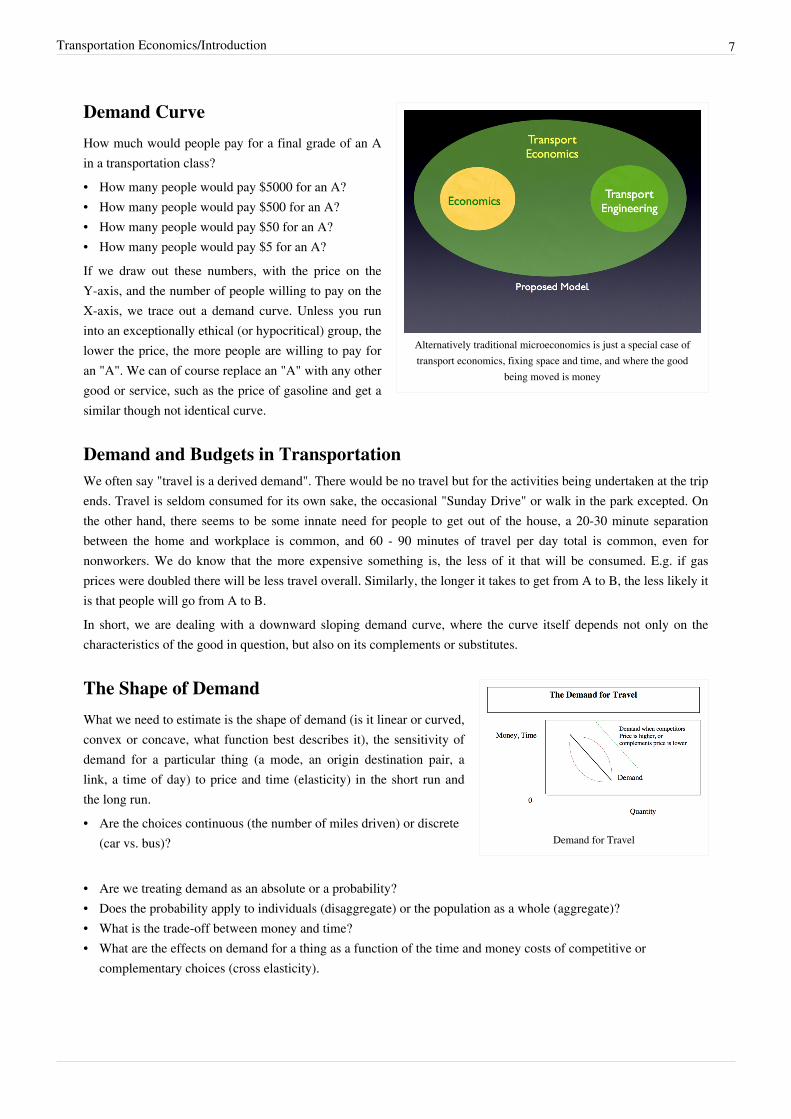
Traditionally transport economics has been thought of as located atthe intersection of microeconomics and civil engineering

Transport Economics studies the movement of peopleand goods over space and time. Historically it has beenthought of as located at the intersection ofmicroeconomics and civil engineering, as shown on theleft.However, if we think about it, traditionalmicroeconomics is just a special case of transporteconomics, fixing space and time, and where the goodbeing moved is money, as illustrated on the right.Topics traditionally associated with TransportEconomics include Privatization, Nationalization,Regulation, Pricing, Economic Stimulus, Financing,Funding, Expenditures, Demand, Production, andExternalities.

Transportation Economics/Introduction 7

Alternatively traditional microeconomics is just a special case oftransport economics, fixing space and time, and where the good

being moved is money

Demand Curve

How much would people pay for a final grade of an Ain a transportation class?• How many people would pay $5000 for an A?• How many people would pay $500 for an A?• How many people would pay $50 for an A?• How many people would pay $5 for an A?If we draw out these numbers, with the price on theY-axis, and the number of people willing to pay on theX-axis, we trace out a demand curve. Unless you runinto an exceptionally ethical (or hypocritical) group, thelower the price, the more people are willing to pay foran "A". We can of course replace an "A" with any othergood or service, such as the price of gasoline and get asimilar though not identical curve.

Demand and Budgets in TransportationWe often say "travel is a derived demand". There would be no travel but for the activities being undertaken at the tripends. Travel is seldom consumed for its own sake, the occasional "Sunday Drive" or walk in the park excepted. Onthe other hand, there seems to be some innate need for people to get out of the house, a 20-30 minute separationbetween the home and workplace is common, and 60 - 90 minutes of travel per day total is common, even fornonworkers. We do know that the more expensive something is, the less of it that will be consumed. E.g. if gasprices were doubled there will be less travel overall. Similarly, the longer it takes to get from A to B, the less likely itis that people will go from A to B.In short, we are dealing with a downward sloping demand curve, where the curve itself depends not only on thecharacteristics of the good in question, but also on its complements or substitutes.

Demand for Travel

The Shape of Demand

What we need to estimate is the shape of demand (is it linear or curved,convex or concave, what function best describes it), the sensitivity ofdemand for a particular thing (a mode, an origin destination pair, alink, a time of day) to price and time (elasticity) in the short run andthe long run.• Are the choices continuous (the number of miles driven) or discrete

(car vs. bus)?

• Are we treating demand as an absolute or a probability?• Does the probability apply to individuals (disaggregate) or the population as a whole (aggregate)?• What is the trade-off between money and time?• What are the effects on demand for a thing as a function of the time and money costs of competitive or

complementary choices (cross elasticity).

Transportation Economics/Introduction 8

Supply CurveHow much would a person need to pay you to write an A-quality 20 page term paper for a given transportation class?• How many would write it for $100,000?• How many would write it for $10,000?• How many would write it for $1,000?• How many would write it for $100?• How many would write it for $10?If we draw out these numbers for all the potential entrepreneurial people available, we trace out a supply curve. Thelower the price, the fewer people are willing to supply the paper-writing service.

Supply and Demand Equilibrium

Illustration of equilibrium between supply and demand

As with earning grades and cheating,transportation is not free, it costs both timeand money. These costs are represented by asupply curve, which rises with the amountof travel demanded. As described above,demand (e.g. the number of vehicles whichwant to use the facility) depends on theprice, the lower the price, the higher thedemand. These two curves intersect at anequilibrium point. In the example figure,they intersect at a toll of $0.50 per km, andflow of 3000 vehicles per hour. Time isusually converted to money (using a Valueof Time), to simplify the analysis.Costs may be variable and include users'time, out-of-pockets costs (paid on a per tripor per distance basis) like tolls, gasolines,and fares, or fixed like insurance or buyingan automobile, which are only borne once in a while and are largely independent of the cost of an individual trip.

Transportation Economics/Introduction 9

Equilibrium in a Negative Feedback System

Negative feedback loop

Supply and Demand comprise the economists view of transportationsystems. They are equilibrium systems. What does that mean?It means the system is subject to a negative feedback process:An increase in A begets a decrease in B. An increase B begets anincrease in A.

Example: A: Traffic Congestion and B: Traffic Demand ... morecongestion limits demand, but more demand creates more congestion.

Disequilibrium

However, many elements of the transportation system do notnecessarily generate an equilibrium. Take the case where an increase inA begets an increase in B. An increase in B begets an increase in A. Anexample where A an increase in Traffic Demand generates more Gas Tax Revenue (B) more Gas Tax Revenuegenerates more Road Building, which in turn increases traffic demand. (This example assumes the gas tax generatesmore demand from the resultant road building than costs in sensitivity of demand to the price, i.e. the investment isworthwhile). This is dubbed a positive feedback system, and in some contexts a "Virtuous Circle", where the "virtue"is a value judgment that depends on your perspective.

Similarly, one might have a "Vicious Circle" where a decrease in A begets a decrease in B and a decrease in B begetsa decrease in A. A classic example of this is where (A) is Transit Service and (B) is Transit Demand. Again "vicious"is a value judgment. Less service results in fewer transit riders, fewer transit riders cannot make as a great a claim ontransportation resources, leading to more service cutbacks.These systems of course interact: more road building may attract transit riders to cars, while those additional driverspay gas taxes and generate more roads.

Positive feedback loop (virtuous circle)

One might ask whether positive feedback systems converge or diverge.The answer is "it depends on the system", and in particular where orwhen in the system you observe. There might be some point where nomatter how many additional roads you built, there would be no moretraffic demand, as everyone already consumes as much travel as theywant to. We have yet to reach that point for roads, but on the otherhand, we have for lots of goods. If you live in most parts of the UnitedStates, the price of water at your house probably does not affect howmuch you drink, and a lower price for tap water would not increaseyour rate of ingestion. You might use substitutes if their prices werelower (or tap water were costlier), e.g. bottled water. Price might affectother behaviors such as lawn watering and car washing though.

Provision

Transportation services are provided by both the public and private sector.

Transportation Economics/Introduction 10

Positive feedback loop (vicious circle)

• Roads are generally publicly owned in the United States, though thesame is not true of highways in other countries. Furthermore, publicownership has not always been the norm, many countries had a longhistory of privately owned turnpikes, in the United States privateroads were known through the early 1900s.

• Railroads are generally private.• Carriers (Airlines, Bus Companies, Truckers, Train Operators) are

often private firms• Formerly private urban transit operators have been taken over by

local government from the 1950s in a process calledmunicipalization. With the rise of the automobile, transit systemswere steadily losing passengers and money.

The situation is complicated by the idea of contracting or franchising.Often private firms operate "public transit" routes, either under acontract, for a fixed price, or an agreement where the private firm collects the revenue on the route (a franchiseagreement). Franchises may be subsidized if the route is a money-loser, or may require bidding if the route isprofitable. Private provision of public transport is common in the United Kingdom.

London Routemaster Bus

Properties

The specific properties of highway transportation include:• Users commit a significant amount of their own time to the

consumption of the final good (a trip). While the contribution ofuser time is found in all sectors to some extent, this fact is adominant feature of highway travel.

• Links are collected into large bundles which comprise the route.Individual links may only be a small share of the bundle of links. Ifwe begin by assuming each link is “autonomous”, than the finalconsumption bundle includes a large number of (imperfect)complements.

• Highway networks have a very specialized geometry. Competition,in the form of alternative routes between origin and destination isalmost always present. Nevertheless there are large degrees ofspatial monopoly, each link uniquely occupies space, and spatiallocation affects the user contribution of time.

• There are significant congestion effects, which occur in the absence of pricing and potentially in its presence.• Users are choosing not only a route for a trip, but whether to make that trip, choose a different destination, or not

travel on the highway network (at a given time). These choices are determined by the quality of that trip and allothers.

• Individual links may serve multiple markets (origin-destination pairs). There are economies achieved by using thesame links on routes serving different markets. This is one factor leading to a hierarchy of roads.

• Quantity cannot be controlled in the short term. Once a road is deployed, it is in the network, its entire capacityavailable for use. However, roads are difficult to deploy, responses to demand are necessarily slow, and for allpractical purposes, these decisions are irrevocable.

Transportation Economics/Introduction 11

Thought questions1. Should the government subsidize public transportation? Why or why not?2. Should the government operate public transportation systems?3. Is building roads a good idea even if it results in more travel demand?

Sample ProblemProblem (Solution)

Key Terms• Supply• Demand• Negative Feedback System• Equilibrium• Disequilibrium• Public Sector• Private Sector

Fundamentals of Transportation/Geography andNetworks

Aerial view of downtown Chicago

Transportation systems have specificstructure. Roads have length, width,and depth. The characteristics of roadsdepends on their purpose.

Fundamentals of Transportation/Geography and Networks 12

Roads

Middle age road in Denmark

A road is a path connecting two points. TheEnglish word ‘road’ comes from the sameroot as the word ‘ride’ –the Middle English‘rood’ and Old English ‘rad’ –meaning theact of riding. Thus a road refers foremost tothe right of way between an origin anddestination. In an urban context, the wordstreet is often used rather than road, whichdates to the Latin word ‘strata’, meaningpavement (the additional layer or stratumthat might be on top of a path).

Modern roads are generally paved, andunpaved routes are considered trails. Thepavement of roads began early in history.Approximately 2600 BCE, the Egyptians constructed a paved road out of sandstone and limestone slabs to assistwith the movement of stones on rollers between the quarry and the site of construction of the pyramids. The Romansand others used brick or stone pavers to provide a more level, and smoother surface, especially in urban areas, whichallows faster travel, especially of wheeled vehicles. The innovations of Thomas Telford and John McAdamreinvented roads in the early nineteenth century, by using less expensive smaller and broken stones, or aggregate, tomaintain a smooth ride and allow for drainage. Later in the nineteenth century, application of tar (asphalt) furthersmoothed the ride. In 1824, asphalt blocks were used on the Champs-Elysees in Paris. In 1872, the first asphalt street(Fifth Avenue) was paved in New York (due to Edward de Smedt), but it wasn’t until bicycles became popular in thelate nineteenth century that the “Good Roads Movement” took off. Bicycle travel, more so than travel by othervehicles at the time, was sensitive to rough roads. Demands for higher quality roads really took off with thewidespread adoption of the automobile in the United States in the early twentieth century.

The first good roads in the twentieth century were constructed of Portland cement concrete (PCC). The material isstiffer than asphalt (or asphalt concrete) and provides a smoother ride. Concrete lasts slightly longer than asphaltbetween major repairs, and can carry a heavier load, but is more expensive to build and repair. While urban streetshad been paved with concrete in the US as early as 1889, the first rural concrete road was in Wayne County,Michigan, near to Detroit in 1909, and the first concrete highway in 1913 in Pine Bluff, Arkansas. By the next yearover 2300 miles of concrete pavement had been layed nationally. However over the remainder of the twentiethcentury, the vast majority of roadways were paved with asphalt. In general only the most important roads, carryingthe heaviest loads, would be built with concrete.Roads are generally classified into a hierarchy. At the top of the hierarchy are freeways, which serve entirely afunction of moving vehicles between other roads. Freeways are grade-separated and limited access, have high speedsand carry heavy flows. Below freeways are arterials. These may not be grade-separated, and while access is stillgenerally limited, it is not limited to the same extent as freeways, particularly on older roads. These serve both amovement and an access function. Next are collector/distributor roads. These serve more of an access function,allowing vehicles to access the network from origins and destinations, as well as connecting with smaller, localroads, that have only an access function, and are not intended for the movement of vehicles with neither a localorigin nor destination. Local roads are designed to be low speed and carry relatively little traffic.The class of the road determines which level of government administers it. The highest roads will generally beowned, operated, or at least regulated (if privately owned) by the higher level of government involved in roadoperations; in the United States, these roads are operated by the individual states. As one moves down the hierarchy

Fundamentals of Transportation/Geography and Networks 13

of roads, the level of government is generally more and more local (counties may control collector/distributor roads,towns may control local streets). In some countries freeways and other roads near the top of the hierarchy areprivately owned and regulated as utilities, these are generally operated as toll roads. Even publicly owned freewaysare operated as toll roads under a toll authority in other countries, and some US states. Local roads are often ownedby adjoining property owners and neighborhood associations.The design of roads is specified in a number of design manual, including the AASHTO Policy on the GeometricDesign of Streets and Highways (or Green Book). Relevant concerns include the alignment of the road, its horizontaland vertical curvature, its super-elevation or banking around curves, its thickness and pavement material, itscross-slope, and its width.

Freeways

Freeways in Phoenix

A motorway or freeway (sometimes called anexpressway or thruway) is a multi-lane dividedroad that is designed to be high-speed freeflowing, access-controlled, built to highstandards, with no traffic lights on the mainline.Some motorways or freeways are financed withtolls, and so may have tollbooths, either acrossthe entrance ramp or across the mainline.However in the United States and Great Britain,most are financed with gas or other tax revenue.Though of course there were major road networksduring the Roman Empire and before, the historyof motorways and freeways dates at least as earlyas 1907, when the first limited access automobilehighway, the Bronx River Parkway beganconstruction in Westchester County, New York(opening in 1908). In this same period, WilliamVanderbilt constructed the Long Island Parkwayas a toll road in Queens County, New York. TheLong Island Parkway was built for racing andspeeds of 60 miles per hour (96 km/hr) wereaccommodated. Users however had to pay a thenexpensive $2.00 toll (later reduced) to recover theconstruction costs of $2 million. These parkwayswere paved when most roads were not. In 1919 General John Pershing assigned Dwight Eisenhower to discover howquickly troops could be moved from Fort Meade between Baltimore and Washington to the Presidio in SanFrancisco by road. The answer was 62 days, for an average speed of 3.5 miles per hour (5.6 km/hr). While usingsegments of the Lincoln Highway, most of that road was still unpaved. In response, in 1922 Pershing drafted a planfor an 8,000 mile (13,000 km) interstate system which was ignored at the time.The US Highway System was a set of paved and consistently numbered highways sponsored by the states, withlimited federal support. First built in 1924, they succeeded some previous major highways such as the DixieHighway, Lincoln Highway and Jefferson Highway that were multi-state and were constructed with the aid ofprivate support. These roads however were not in general access-controlled, and soon became congested asdevelopment along the side of the road degraded highway speeds.

Fundamentals of Transportation/Geography and Networks 14

In parallel with the US Highway system, limited access parkways were developed in the 1920s and 1930s in severalUS cities. Robert Moses built a number of these parkways in and around New York City. A number of theseparkways were grade separated, though they were intentionally designed with low bridges to discourage trucks andbuses from using them. German Chancellor Adolf Hitler appointed a German engineer Fritz Todt Inspector Generalfor German Roads. He managed the construction of the German Autobahns, the first limited access high-speed roadnetwork in the world. In 1935, the first section from Frankfurt am Main to Darmstadt opened, the total system todayhas a length of 11,400 km. The Federal-Aid Highway Act of 1938 called on the Bureau of Public Roads to study thefeasibility of a toll-financed superhighway system (three east-west and three north-south routes). Their report TollRoads and Free Roads declared such a system would not be self-supporting, advocating instead a 43,500 km (27,000mile) free system of interregional highways, the effect of this report was to set back the interstate program nearlytwenty years in the US.The German autobahn system proved its utility during World War II, as the German army could shift relativelyquickly back and forth between two fronts. Its value in military operations was not lost on the American Generals,including Dwight Eisenhower.On October 1, 1940, a new toll highway using the old, unutilized South Pennsylvania Railroad right-of-way andtunnels opened. It was the first of a new generation of limited access highways, generally called superhighways orfreeways that transformed the American landscape. This was considered the first freeway in the US, as it, unlike theearlier parkways, was a multi-lane route as well as being limited access. The Arroyo Seco Parkway, now thePasadena Freeway, opened December 30, 1940. Unlike the Pennsylvania Turnpike, the Arroyo Seco parkway had notoll barriers.A new National Interregional Highway Committee was appointed in 1941, and reported in 1944 in favor of a 33,900mile system. The system was designated in the Federal Aid Highway Act of 1933, and the routes began to beselected by 1947, yet no funding was provided at the time. The 1952 highway act only authorized a token amount forconstruction, increased to $175 million annually in 1956 and 1957.The US Interstate Highway System was established in 1956 following a decade and half of discussion. Much of thenetwork had been proposed in the 1940s, but it took time to authorize funding. In the end, a system supported by gastaxes (rather than tolls), paid for 90% by the federal government with a 10% local contribution, on a pay-as-you-go”system, was established. The Federal Aid Highway Act of 1956 had authorized the expenditure of $27.5 billion over13 years for the construction of a 41,000 mile interstate highway system. As early as 1958 the cost estimate forcompleting the system came in at $39.9 billion and the end date slipped into the 1980s. By 1991, the final costestimate was $128.9 billion. While the freeways were seen as positives in most parts of the US, in urban areasopposition grew quickly into a series of freeway revolts. As soon as 1959, (three years after the Interstate act), theSan Francisco Board of Supervisors removed seven of ten freeways from the city’s master plan, leaving the GoldenGate bridge unconnected to the freeway system. In New York, Jane Jacobs led a successful freeway revolt againstthe Lower Manhattan Expressway sponsored by business interests and Robert Moses among others. In Baltimore,I-70, I-83, and I-95 all remain unconnected thanks to highway revolts led by now Senator Barbara Mikulski. InWashington, I-95 was rerouted onto the Capital Beltway. The pattern repeated itself elsewhere, and many urbanfreeways were removed from Master Plans.In 1936, the Trunk Roads Act ensured that Great Britain’s Minister of Transport controlled about 30 major roads, of7,100 km (4,500 miles) in length. The first Motorway in Britain, the Preston by-pass, now part of the M-6, opened in1958. In 1959, the first stretch of the M1 opened. Today there are about 10,500 km (6300 miles) of trunk roads andmotorways in England.Australia has 790 km of motorways, though a much larger network of roads. However the motorway network is nottruly national in scope (in contrast with Germany, the United States, Britain, and France), rather it is a series of localnetworks in and around metropolitan areas, with many intercity connection being on undivided and non-gradeseparated highways. Outside the Anglo-Saxon world, tolls were more widely used. In Japan, when the Meishin

Fundamentals of Transportation/Geography and Networks 15

Expressway opened in 1963, the roads in Japan were in far worse shape than Europe or North American prior to this.Today there are over 6,100 km of expressways (3,800 miles), many of which are private toll roads. France has about10,300 km of expressways (6,200 miles) of motorways, many of which are toll roads. The French motorway systemdeveloped through a series of franchise agreements with private operators, many of which were later nationalized.Beginning in the late 1980s with the wind-down of the US interstate system (regarded as complete in 1990), as wellas intercity motorway programs in other countries, new sources of financing needed to be developed. New (generallysuburban) toll roads were developed in several metropolitan areas.An exception to the dearth of urban freeways is the case of the Big Dig in Boston, which relocates the Central Arteryfrom an elevated highway to a subterranean one, largely on the same right-of-way, while keeping the elevatedhighway operating. This project is estimated to be completed for some $14 billion; which is half the estimate of theoriginal complete US Interstate Highway System.As mature systems in the developed countries, improvements in today’s freeways are not so much wideningsegments or constructing new facilities, but better managing the roadspace that exists. That improved management,takes a variety of forms. For instance, Japan has advanced its highways with application of Intelligent TransportationSystems, in particular traveler information systems, both in and out of vehicles, as well as traffic control systems.The US and Great Britain also have traffic management centers in most major cities that assess traffic conditions onmotorways, deploy emergency vehicles, and control systems like ramp meters and variable message signs. Thesesystems are beneficial, but cannot be seen as revolutionizing freeway travel. Speculation about future automatedhighway systems has taken place almost as long as highways have been around. The Futurama exhibit at the NewYork 1939 World’s Fair posited a system for 1960. Yet this technology has been twenty years away for over sixtyyears, and difficulties remain.

Layers of Networks

OSI Reference Model for the Internet

Data unit Layer Function

Hostlayers

Data 7. Application Network process to application

6. Presentation Data representation,encryption and decryption

5. Session Interhost communication

Segments 4. Transport End-to-end connections and reliability,Flow control

Medialayers

Packet 3. Network Path determination and logical addressing

Frame 2. Data Link Physical addressing

Bit 1. Physical Media, signal and binary transmission

All networks come in layers. The OSI Reference Model for the Internet is well-defined. Roads too are part of a layerof subsystems of which the pavement surface is only one part. We can think of a hierarchy of systems.• Places• Trip Ends• End to End Trip• Driver/Passenger• Service (Vehicle & Schedule)• Signs and Signals• Markings• Pavement Surface• Structure (Earth & Pavement and Bridges)

Fundamentals of Transportation/Geography and Networks 16

• Alignment (Vertical and Horizontal)• Right-Of-Way• SpaceAt the base is space. On space, a specific right-of-way is designated, which is property where the road goes.Originally right-of-way simply meant legal permission for travelers to cross someone's property. Prior to theconstruction of roads, this might simply be a well-worn dirt path.On top of the right-of-way is the alignment, the specific path a transportation facility takes within the right-of-way.The path has both vertical and horizontal elements, as the road rises or falls with the topography and turns as needed.Structures are built on the alignment. These include the roadbed as well as bridges or tunnels that carry the road.Pavement surface is the gravel or asphalt or concrete surface that vehicles actually ride upon and is the top layer ofthe structure. That surface may have markings to help guide drivers to stay to the right (or left), delineate lanes,regulate which vehicles can use which lanes (bicycles-only, high occupancy vehicles, buses, trucks) and provideadditional information. In addition to marking, signs and signals to the side or above the road provide additionalregulatory and navigation information.Services use roads. Buses may provide scheduled services between points with stops along the way. Coaches providescheduled point-to-point without stops. Taxis handle irregular passenger trips.Drivers and passengers use services or drive their own vehicle (producing their own transportation services) tocreate an end-to-end trip, between an origin and destination. Each origin and destination comprises a trip end andthose trip ends are only important because of the places at the ends and the activity that can be engaged in. Astransportation is a derived demand, if not for those activities, essentially no passenger travel would be undertaken.With modern information technologies, we may need to consider additional systems, such as Global PositioningSystems (GPS), differential GPS, beacons, transponders, and so on that may aide the steering or navigationprocesses. Cameras, in-pavement detectors, cell phones, and other systems monitor the use of the road and may beimportant in providing feedback for real-time control of signals or vehicles.Each layer has rules of behavior:• some rules are physical and never violated, others are physical but probabilistic• some are legal rules or social norms which are occasionally violated

Fundamentals of Transportation/Geography and Networks 17

Hierarchy of Roads

Hierarchy of roads

Even within each layer of the systemof systems described above, there isdifferentiation.Transportation facilities have twodistinct functions: through movementand land access. This differentiation:• permits the aggregation of traffic to

achieve economies of scale inconstruction and operation (highspeeds);

• reduces the number of conflicts;• helps maintain the desired quiet

character of residentialneighborhoods by keeping throughtraffic away from homes;

• contains less redundancy, and somay be less costly to build.

Functional Classification Types of Connections Relation to Abutting Property Minnesota Examples

Limited Access (highway) Through traffic movement betweencities and across cities

Limited or controlled access highways withramps and/or curb cut controls.

I-94, Mn280

Linking (arterial:principaland minor)

Traffic movement between limitedaccess and local streets.

Direct access to abutting property. University Avenue,Washington Avenue

Local (collector anddistributor roads)

Traffic movement in and betweenresidential areas

Direct access to abutting property. Pillsbury Drive, 17thAvenue

Model ElementsTransportation forecasting, to be discussed in more depth in subsequent modules, abstracts the real world into asimplified representation.Recall the hierarchy of roads. What can be simplified? It is typical for a regional forecasting model to eliminate localstreets and replace them with a centroid (a point representing a traffic analysis zone). Centroids are the source andsink of all transportation demand on the network. Centroid connectors are artificial or dummy links connecting thecentroid to the "real" network. An illustration of traffic analysis zones can be found at this external link for FultonCounty, Georgia, here: traffic zone map, 3MB [1]. Keep in mind that Models are abstractions.

Network• Zone Centroid - special node whose number identifies a zone, located by an "x" "y" coordinate representing

longitude and latitude (sometimes "x" and "y" are identified using planar coordinate systems).• Node (vertices) - intersection of links , located by x and y coordinates• Links (arcs) - short road segments indexed by from and to nodes (including centroid connnectors), attributes

include lanes, capacity per lane, allowable modes• Turns - indexed by at, from, and to nodes• Routes, (paths) - indexed by a series of nodes from origin to destination. (e.g. a bus route)• Modes - car, bus, HOV, truck, bike, walk etc.

Fundamentals of Transportation/Geography and Networks 18

Matrices

Scalar

A scalar is a single value that applies model-wide; e.g. the price of gas or total trips.

Total Trips

Variable T

Vectors

Vectors are values that apply to particular zones in the model system, such as trips produced or trips attracted ornumber of households. They are arrayed separately when treating a zone as an origin or as a destination so that theycan be combined into full matrices.• vector (origin) - a column of numbers indexed by traffic zones, describing attributes at the origin of the trip (e.g.

the number of households in a zone)

Trips Produced at Origin Zone

Origin Zone 1 Ti1

Origin Zone 2 Ti2

Origin Zone 3 Ti3

• vector (destination) - a row of numbers indexed by traffic zones, describing attributes at the destination

Destination Zone 1 Destination Zone 2 Destination Zone 3

Trips Attracted to Destination Zone Tj1 Tj2 Tj3

Full Matrices

A full or interaction matrix is a table of numbers, describing attributes of the origin-destination pair

Destination Zone 1 Destination Zone 2 Destination Zone 3

Origin Zone 1 T11 T12 T13

Origin Zone 2 T21 T22 T23

Origin Zone 3 T31 T32 T33

Thought Questions• Identify the rules associated with each layer?• Why aren’t all roads the same?• How might we abstract the real transportation system when representing it in a model for analysis?• Why is abstraction useful?

Abbreviations• SOV - single occupant vehicle• HOV - high occupancy vehicle (2+, 3+, etc.)• TAZ - transportation analysis zone or traffic analysis zone

Fundamentals of Transportation/Geography and Networks 19

Variables• msXX - scalar matrix• moXX - origin vector matrix• mdXX - destination vector matrix• mfXX - full vector matrix• - Total Trips• - Trips Produced from Origin Zone • - Trips Attracted to Destination Zone • - Trips Going Between Origin Zone and Destination Zone

Key Terms• Zone Centroid• Node• Links• Turns• Routes• Modes• Matrices• Right-of-way• Alignment• Structures• Pavement Surface• Markings• Signs and Signals• Services• Driver• Passenger• End to End Trip• Trip Ends• Places

External ExercisesUse the ADAM software at the STREET website [1] and examine the network structure. Familiarize yourself with thesoftware, and edit the network, adding at least two nodes and four one-way links (two two-way links), and deletingnodes and links. What are the consequences of such network adjustments? Are some adjustments better than others?

References[1] http:/ / wms. co. fulton. ga. us/ apps/ doc_archive/ get. php/ 69253. pdf

Fundamentals of Transportation/Trip Generation 20

Fundamentals of Transportation/Trip GenerationTrip Generation is the first step in the conventional four-step transportation forecasting process (followed byDestination Choice, Mode Choice, and Route Choice), widely used for forecasting travel demands. It predicts thenumber of trips originating in or destined for a particular traffic analysis zone.Every trip has two ends, and we need to know where both of them are. The first part is determining how many tripsoriginate in a zone and the second part is how many trips are destined for a zone. Because land use can be dividedinto two broad category (residential and non-residential) <joke>There are two types of people in the world, thosethat divide the world into two kinds of people and those that don't. Some people say there are three types of people inthe world, those who can count, and those who can't.</joke> we have models that are household based andnon-household based (e.g. a function of number of jobs or retail activity).For the residential side of things, trip generation is thought of as a function of the social and economic attributes ofhouseholds (households and housing units are very similar measures, but sometimes housing units have nohouseholds, and sometimes they contain multiple households, clearly housing units are easier to measure, and thoseare often used instead for models, it is important to be clear which assumption you are using).At the level of the traffic analysis zone, the language is that of land uses "producing" or attracting trips, where byassumption trips are "produced" by households and "attracted" to non-households. Production and attractions differfrom origins and destinations. Trips are produced by households even when they are returning home (that is, whenthe household is a destination). Again it is important to be clear what assumptions you are using.

ActivitiesPeople engage in activities, these activities are the "purpose" of the trip. Major activities are home, work, shop,school, eating out, socializing, recreating, and serving passengers (picking up and dropping off). There are numerousother activities that people engage on a less than daily or even weekly basis, such as going to the doctor, banking,etc. Often less frequent categories are dropped and lumped into the catchall "Other".Every trip has two ends, an origin and a destination. Trips are categorized by purposes, the activity undertaken at adestination location.

Observed trip making from the Twin Cities (2000-2001) Travel Behavior Inventory byGender

Trip Purpose Males Females Total

Work 4008 3691 7691

Work related 1325 698 2023

Attending school 495 465 960

Other school activities 108 134 242

Childcare, daycare, after school care 111 115 226

Quickstop 45 51 96

Shopping 2972 4347 7319

Visit friends or relatives 856 1086 1942

Personal business 3174 3928 7102

Eat meal outside of home 1465 1754 3219

Entertainment, recreation, fitness 1394 1399 2793

Fundamentals of Transportation/Trip Generation 21

Civic or religious 307 462 769

Pick up or drop off passengers 1612 2490 4102

With another person at their activities 64 48 112

At home activities 288 384 672

Some observations:• Men and women behave differently on average, splitting responsibilities within households, and engaging in

different activities,• Most trips are not work trips, though work trips are important because of their peaked nature (and because they

tend to be longer in both distance and travel time),• The vast majority of trips are not people going to (or from) work.People engage in activities in sequence, and may chain their trips. In the Figure below, the trip-maker is travelingfrom home to work to shop to eating out and then returning home.

Specifying ModelsHow do we predict how many trips will be generated by a zone? The number of trips originating from or destined toa purpose in a zone are described by trip rates (a cross-classification by age or demographics is often used) orequations. First, we need to identify what we think are the relevant variables.

Home-endThe total number of trips leaving or returning to homes in a zone may be described as a function of:Home-End Trips are sometimes functions of:• Housing Units• Household Size• Age• Income

Fundamentals of Transportation/Trip Generation 22

• Accessibility• Vehicle Ownership• Other Home-Based Elements

Work-endAt the work-end of work trips, the number of trips generated might be a function as below:

Work-End Trips are sometimes functions of:• Jobs• Area of Workspace• Occupancy Rate• Other Job-Related Elements

Shop-endSimilarly shopping trips depend on a number of factors:Shop-End Trips are sometimes functions of:• Number of Retail Workers• Type of Retail Available• Area of Retail Available• Location• Competition• Other Retail-Related Elements

Input DataA forecasting activity conducted by planners or economists, such as one based on the concept of economic baseanalysis, provides aggregate measures of population and activity growth. Land use forecasting distributes forecastchanges in activities across traffic zones.

Estimating ModelsWhich is more accurate: the data or the average? The problem with averages (or aggregates) is that every individual’strip-making pattern is different.

Home-endTo estimate trip generation at the home end, a cross-classification model can be used, this is basically constructing atable where the rows and columns have different attributes, and each cell in the table shows a predicted number oftrips, this is generally derived directly from data.In the example cross-classification model: The dependent variable is trips per person. The independent variables aredwelling type (single or multiple family), household size (1, 2, 3, 4, or 5+ persons per household), and person age.The figure below shows a typical example of how trips vary by age in both single-family and multi-family residencetypes.

Fundamentals of Transportation/Trip Generation 23

The figure below shows a moving average.

Non-home-endThe trip generation rates for both “work” and “other” trip ends can be developed using Ordinary Least Squares (OLS)regression (a statistical technique for fitting curves to minimize the sum of squared errors (the difference betweenpredicted and actual value) relating trips to employment by type and population characteristics.

The variables used in estimating trip rates for the work-end are Employment in Offices ( ), Retail ( ),and Other ( )A typical form of the equation can be expressed as:

Fundamentals of Transportation/Trip Generation 24

Where:• - Person trips attracted per worker in the ith zone• - office employment in the ith zone• - other employment in the ith zone• - retail employment in the ith zone• - model coefficients

NormalizationFor each trip purpose (e.g. home to work trips), the number of trips originating at home must equal the number oftrips destined for work. Two distinct models may give two results. There are several techniques for dealing with thisproblem. One can either assume one model is correct and adjust the other, or split the difference.It is necessary to ensure that the total number of trip origins equals the total number of trip destinations, since eachtrip interchange by definition must have two trip ends.The rates developed for the home end are assumed to be most accurate,The basic equation for normalization:

Sample Problems• Problem (Solution)

Variables• - Person trips originating in Zone i

• - Person Trips destined for Zone j• - Normalized Person trips originating in Zone i

• - Normalized Person Trips destined for Zone j• - Person trips generated at home end (typically morning origins, afternoon destinations)• - Person trips generated at work end (typically afternoon origins, morning destinations)• - Person trips generated at shop end• - Number of Households in Zone i• - office employment in the ith zone• - retail employment in the ith zone• - other employment in the ith zone• - model coefficients

Fundamentals of Transportation/Trip Generation 25

Abbreviations• H2W - Home to work• W2H - Work to home• W2O - Work to other• O2W - Other to work• H2O - Home to other• O2H - Other to home• O2O - Other to other• HBO - Home based other (includes H2O, O2H)• HBW - Home based work (H2W, W2H)• NHB - Non-home based (O2W, W2O, O2O)

External ExercisesUse the ADAM software at the STREET website [1] and try Assignment #1 to learn how changes in analysis zonecharacteristics generate additional trips on the network.

Additional Problems• Homework• Additional Problems

End Notes[1] http:/ / street. umn. edu/

Further Reading• Trip Generation article on wikipedia (http:/ / en. wikipedia. org/ wiki/ Trip_generation)

Fundamentals of Transportation/Trip Generation/Problem 26

Fundamentals of Transportation/TripGeneration/Problem

Problem:Planners have estimated the following models for the AM Peak Hour

Where:= Person Trips Originating in Zone

= Person Trips Destined for Zone = Number of Households in Zone

You are also given the following data

Data

Variable Dakotopolis New Fargo

10000 15000

8000 10000

3000 5000

2000 1500

A. What are the number of person trips originating in and destined for each city?B. Normalize the number of person trips so that the number of person trip origins = the number of person tripdestinations. Assume the model for person trip origins is more accurate.• Solution

Fundamentals of Transportation/Trip Generation/Solution 27

Fundamentals of Transportation/TripGeneration/Solution

Problem:Planners have estimated the following models for the AM Peak Hour

Where:= Person Trips Originating in Zone

= Person Trips Destined for Zone = Number of Households in Zone

You are also given the following data

Data

Variable Dakotopolis New Fargo

10000 15000

8000 10000

3000 5000

2000 1500

A. What are the number of person trips originating in and destined for each city?B. Normalize the number of person trips so that the number of person trip origins = the number of person tripdestinations. Assume the model for person trip origins is more accurate.

Solution:A. What are the number of person trips originating in and destined for each city?

Solution to Trip Generation Problem Part A

Households( )

OfficeEmployees( )

OtherEmployees

( )

RetailEmployees

( )

Origins Destinations

Dakotopolis 10000 8000 3000 2000 15000 16000

New Fargo 15000 10000 5000 1500 22500 20750

Total 25000 18000 8000 3000 37500 36750

B. Normalize the number of person trips so that the number of person trip origins = the number of person tripdestinations. Assume the model for person trip origins is more accurate.

Fundamentals of Transportation/Trip Generation/Solution 28

Use:

Solution to Trip Generation Problem Part B

Origins ( ) Destinations ( ) Adjustment Factor Normalized Destinations ( ) Rounded

Dakotopolis 15000 16000 1.0204 16326.53 16327

New Fargo 22500 20750 1.0204 21173.47 21173

Total 37500 36750 1.0204 37500 37500

Fundamentals of Transportation/DestinationChoiceEverything is related to everything else, but near things are more related than distant things. - Waldo Tobler's 'FirstLaw of Geography’Destination Choice (or trip distribution or zonal interchange analysis), is the second component (after TripGeneration, but before Mode Choice and Route Choice) in the traditional four-step transportation forecasting model.This step matches tripmakers’ origins and destinations to develop a “trip table”, a matrix that displays the number oftrips going from each origin to each destination. Historically, trip distribution has been the least developedcomponent of the transportation planning model.

Table: Illustrative Trip Table

Origin \ Destination 1 2 3 Z

1 T11 T12 T13 T1Z

2 T21

3 T31

Z TZ1 TZZ

Where: = Trips from origin i to destination j. Work trip distribution is the way that travel demand modelsunderstand how people take jobs. There are trip distribution models for other (non-work) activities, which follow thesame structure.

Fundamentals of Transportation/Destination Choice 29

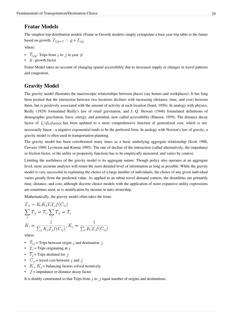
Fratar ModelsThe simplest trip distribution models (Fratar or Growth models) simply extrapolate a base year trip table to the futurebased on growth, where:

• - Trips from to in year • - growth factorFratar Model takes no account of changing spatial accessibility due to increased supply or changes in travel patternsand congestion.

Gravity ModelThe gravity model illustrates the macroscopic relationships between places (say homes and workplaces). It has longbeen posited that the interaction between two locations declines with increasing (distance, time, and cost) betweenthem, but is positively associated with the amount of activity at each location (Isard, 1956). In analogy with physics,Reilly (1929) formulated Reilly's law of retail gravitation, and J. Q. Stewart (1948) formulated definitions ofdemographic gravitation, force, energy, and potential, now called accessibility (Hansen, 1959). The distance decayfactor of has been updated to a more comprehensive function of generalized cost, which is notnecessarily linear - a negative exponential tends to be the preferred form. In analogy with Newton’s law of gravity, agravity model is often used in transportation planning.The gravity model has been corroborated many times as a basic underlying aggregate relationship (Scott 1988,Cervero 1989, Levinson and Kumar 1995). The rate of decline of the interaction (called alternatively, the impedanceor friction factor, or the utility or propensity function) has to be empirically measured, and varies by context.Limiting the usefulness of the gravity model is its aggregate nature. Though policy also operates at an aggregatelevel, more accurate analyses will retain the most detailed level of information as long as possible. While the gravitymodel is very successful in explaining the choice of a large number of individuals, the choice of any given individualvaries greatly from the predicted value. As applied in an urban travel demand context, the disutilities are primarilytime, distance, and cost, although discrete choice models with the application of more expansive utility expressionsare sometimes used, as is stratification by income or auto ownership.Mathematically, the gravity model often takes the form:

where

• = Trips between origin and destination • = Trips originating at • = Trips destined for • = travel cost between and • = balancing factors solved iteratively.• = impedance or distance decay factorIt is doubly constrained so that Trips from to equal number of origins and destinations.

Fundamentals of Transportation/Destination Choice 30

Balancing a matrix1. Assess Data, you have , , 2. Compute , e.g.

••3. Iterate to Balance Matrix

(a) Multiply Trips from Zone ( ) by Trips to Zone ( ) by Impedance in Cell ( ) for all (b) Sum Row Totals , Sum Column Totals (c) Multiply Rows by

(d) Sum Row Totals , Sum Column Totals

(e) Compare and , if within tolerance stop, Otherwise goto (f)

(f) Multiply Columns by

(g) Sum Row Totals , Sum Column Totals

(h) Compare and , and if within tolerance stop, Otherwise goto (b)

Issues

FeedbackOne of the key drawbacks to the application of many early models was the inability to take account of congestedtravel time on the road network in determining the probability of making a trip between two locations. AlthoughWohl noted as early as 1963 research into the feedback mechanism or the “interdependencies among assigned ordistributed volume, travel time (or travel ‘resistance’) and route or system capacity”, this work has yet to be widelyadopted with rigorous tests of convergence or with a so-called “equilibrium” or “combined” solution (Boyce et al.1994). Haney (1972) suggests internal assumptions about travel time used to develop demand should be consistentwith the output travel times of the route assignment of that demand. While small methodological inconsistencies arenecessarily a problem for estimating base year conditions, forecasting becomes even more tenuous without anunderstanding of the feedback between supply and demand. Initially heuristic methods were developed by Irwin andVon Cube (as quoted in Florian et al. (1975) ) and others, and later formal mathematical programming techniqueswere established by Evans (1976).

Feedback and time budgetsA key point in analyzing feedback is the finding in earlier research by Levinson and Kumar (1994) that commutingtimes have remained stable over the past thirty years in the Washington Metropolitan Region, despite significantchanges in household income, land use pattern, family structure, and labor force participation. Similar results havebeen found in the Twin Cities by Barnes and Davis (2000).The stability of travel times and distribution curves over the past three decades gives a good basis for the applicationof aggregate trip distribution models for relatively long term forecasting. This is not to suggest that there exists aconstant travel time budget.In terms of time budgets:• 1440 Minutes in a Day• Time Spent Traveling: ~ 100 minutes + or -• Time Spent Traveling Home to Work: 20 - 30 minutes + or -

Fundamentals of Transportation/Destination Choice 31

Research has found that auto commuting times have remained largely stable over the past forty years, despitesignificant changes in transportation networks, congestion, household income, land use pattern, family structure, andlabor force participation. The stability of travel times and distribution curves gives a good basis for the application oftrip distribution models for relatively long term forecasting.

Examples

Example 1: Solving for impedance

Problem:

You are given the travel times between zones, compute the impedance matrix , assuming.

Travel Time OD Matrix (

Origin Zone Destination Zone 1 Destination Zone 2

1 2 5

2 5 2

Compute impedances ( )Solution:

Impedance Matrix (

Origin Zone Destination Zone 1 Destination Zone 2

1

2

Example 2: Balancing a Matrix Using Gravity Model

Problem:

You are given the travel times between zones, trips originating at each zone (zone1 =15, zone 2=15) trips destinedfor each zone (zone 1=10, zone 2 = 20) and asked to use the classic gravity model

Fundamentals of Transportation/Destination Choice 32

Travel Time OD Matrix (

Origin Zone Destination Zone 1 Destination Zone 2

1 2 5

2 5 2

Solution:

(a) Compute impedances ( )

Impedance Matrix (

Origin Zone Destination Zone 1 Destination Zone 2

1 0.25 0.04

2 0.04 0.25

(b) Find the trip table

Balancing Iteration 0 (Set-up)

Origin Zone Trips Originating Destination Zone 1 Destination Zone 2

Trips Destined 10 20

1 15 0.25 0.04

2 15 0.04 0.25

Balancing Iteration 1 (

Origin Zone Trips Originating Destination Zone 1 Destination Zone 2 Row Total Normalizing Factor

Trips Destined 10 20

1 15 37.50 12 49.50 0.303

2 15 6 75 81 0.185

Column Total 43.50 87

Balancing Iteration 2 (

Origin Zone TripsOriginating

Destination Zone1

Destination Zone2

Row Total Normalizing Factor

Trips Destined 10 20

1 15 11.36 3.64 15.00 1.00

2 15 1.11 13.89 15.00 1.00

Column Total 12.47 17.53

Normalizing Factor 0.802 1.141

Fundamentals of Transportation/Destination Choice 33

Balancing Iteration 3 (

Origin Zone TripsOriginating

Destination Zone1

Destination Zone2

Row Total Normalizing Factor

Trips Destined 10 20

1 15 9.11 4.15 13.26 1.13

2 15 0.89 15.85 16.74 0.90

Column Total 10.00 20.00

Normalizing Factor = 1.00 1.00

Balancing Iteration 4 (

Origin Zone TripsOriginating

Destination Zone1

Destination Zone2

Row Total Normalizing Factor

Trips Destined 10 20

1 15 10.31 4.69 15.00 1.00

2 15 0.80 14.20 15.00 1.00

Column Total 11.10 18.90

Normalizing Factor = 0.90 1.06

...

Balancing Iteration 16 (

Origin Zone TripsOriginating

Destination Zone1

Destination Zone2

Row Total Normalizing Factor

Trips Destined 10 20

1 15 9.39 5.61 15.00 1.00

2 15 0.62 14.38 15.00 1.00

Column Total 10.01 19.99

Normalizing Factor = 1.00 1.00

So while the matrix is not strictly balanced, it is very close, well within a 1% threshold, after 16 iterations.

Fundamentals of Transportation/Destination Choice 34

External ExercisesUse the ADAM software at the STREET website [1] and try Assignment #2 to learn how changes in linkcharacteristics adjust the distribution of trips throughout a network.

Additional Questions• Homework• Additional Questions

Variables• - Trips leaving origin • - Trips arriving at destination • - Effective Trips arriving at destination , computed as a result for calibration to the next iteration• - Total number of trips between origin and destination • - Calibration parameter for origin • - Calibration parameter for destination • - Cost function between origin and destination

Further Reading• Background

Fundamentals of Transportation/DestinationChoice/BackgroundSome additional background on Fundamentals of Transportation/Destination Choice

HistoryOver the years, modelers have used several different formulations of trip distribution. The first was the Fratar orGrowth model (which did not differentiate trips by purpose). This structure extrapolated a base year trip table to thefuture based on growth, but took no account of changing spatial accessibility due to increased supply or changes intravel patterns and congestion.The next models developed were the gravity model and the intervening opportunities model. The most widely usedformulation is still the gravity model.While studying traffic in Baltimore, Maryland, Alan Voorhees developed a mathematical formula to predict trafficpatterns based on land use. This formula has been instrumental in the design of numerous transportation and publicworks projects around the world. He wrote "A General Theory of Traffic Movement," (Voorhees, 1956) whichapplied the gravity model to trip distribution, which translates trips generated in an area to a matrix that identifies thenumber of trips from each origin to each destination, which can then be loaded onto the network.Evaluation of several model forms in the 1960s concluded that "the gravity model and intervening opportunity modelproved of about equal reliability and utility in simulating the 1948 and 1955 trip distribution for Washington, D.C."(Heanue and Pyers 1966). The Fratar model was shown to have weakness in areas experiencing land use changes. Ascomparisons between the models showed that either could be calibrated equally well to match observed conditions,because of computational ease, gravity models became more widely spread than intervening opportunities models.

Fundamentals of Transportation/Destination Choice/Background 35

Some theoretical problems with the intervening opportunities model were discussed by Whitaker and West (1968)concerning its inability to account for all trips generated in a zone which makes it more difficult to calibrate,although techniques for dealing with the limitations have been developed by Ruiter (1967).With the development of logit and other discrete choice techniques, new, demographically disaggregate approachesto travel demand were attempted. By including variables other than travel time in determining the probability ofmaking a trip, it is expected to have a better prediction of travel behavior. The logit model and gravity model havebeen shown by Wilson (1967) to be of essentially the same form as used in statistical mechanics, the entropymaximization model. The application of these models differ in concept in that the gravity model uses impedance bytravel time, perhaps stratified by socioeconomic variables, in determining the probability of trip making, while adiscrete choice approach brings those variables inside the utility or impedance function. Discrete choice modelsrequire more information to estimate and more computational time.Ben-Akiva and Lerman (1985) have developed combination destination choice and mode choice models using a logitformulation for work and non-work trips. Because of computational intensity, these formulations tended to aggregatetraffic zones into larger districts or rings in estimation. In current application, some models, including for instancethe transportation planning model used in Portland, Oregon use a logit formulation for destination choice. Allen(1984) used utilities from a logit based mode choice model in determining composite impedance for trip distribution.However, that approach, using mode choice log-sums implies that destination choice depends on the same variablesas mode choice. Levinson and Kumar (1995) employ mode choice probabilities as a weighting factor and develops aspecific impedance function or “f-curve” for each mode for work and non-work trip purposes.

MathematicsAt this point in the transportation planning process, the information for zonal interchange analysis is organized in anorigin-destination table. On the left is listed trips produced in each zone. Along the top are listed the zones, and foreach zone we list its attraction. The table is n x n, where n = the number of zones.Each cell in our table is to contain the number of trips from zone i to zone j. We do not have these within cellnumbers yet, although we have the row and column totals. With data organized this way, our task is to fill in the cellsfor tables headed t=1 through say t=n.Actually, from home interview travel survey data and attraction analysis we have the cell information for t = 1. Thedata are a sample, so we generalize the sample to the universe. The techniques used for zonal interchange analysisexplore the empirical rule that fits the t = 1 data. That rule is then used to generate cell data for t = 2, t = 3, t = 4,etc., to t = n.The first technique developed to model zonal interchange involves a model such as this:

where:

• : trips from i to j.• : trips from i, as per our generation analysis• : trips attracted to j, as per our generation analysis• : travel cost friction factor, say = • : Calibration parameterZone i generates trips; how many will go to zone j? That depends on the attractiveness of j compared to theattractiveness of all places; attractiveness is tempered by the distance a zone is from zone i. We compute the fractioncomparing j to all places and multiply by it.The rule is often of a gravity form:

Fundamentals of Transportation/Destination Choice/Background 36

where:

• : populations of i and j• : parameters

But in the zonal interchange mode, we use numbers related to trip origins ( ) and trip destinations ( ) ratherthan populations.There are lots of model forms because we may use weights and special calibration parameters, e.g., one could writesay:

or

where:• a, b, c, d are parameters• : travel cost (e.g. distance, money, time)• : inbound trips, destinations• : outbound trips, origin

Entropy AnalysisWilson (1970) gives us another way to think about zonal interchange problem. This section treats Wilson’smethodology to give a grasp of central ideas. To start, consider some trips where we have seven people in originzones commuting to seven jobs in destination zones. One configuration of such trips will be:

Table: Configuration of Trips

zone 1 2 3

1 2 1 1

2 0 2 1

where That configuration can appear in 1,260 ways. We have calculated the number of ways thatconfiguration of trips might have occurred, and to explain the calculation, let’s recall those coin tossing experimentstalked about so much in elementary statistics. The number of ways a two-sided coin can come up is 2n, where n isthe number of times we toss the coin. If we toss the coin once, it can come up heads or tails, 21 = 2. If we toss ittwice, it can come up HH, HT, TH, or TT, 4 ways, and 2 = 4. To ask the specific question about, say, four coinscoming up all heads, we calculate 4!/4!0! =1 . Two heads and two tails would be 4!/2!2! = 6. We are solving theequation:

An important point is that as n gets larger, our distribution gets more and more peaked, and it is more and morereasonable to think of a most likely state.However, the notion of most likely state comes not from this thinking; it comes from statistical mechanics, a fieldwell known to Wilson and not so well known to transportation planners. The result from statistical mechanics is that

Fundamentals of Transportation/Destination Choice/Background 37

a descending series is most likely. Think about the way the energy from lights in the classroom is affecting the air inthe classroom. If the effect resulted in an ascending series, many of the atoms and molecules would be affected a lotand a few would be affected a little. The descending series would have a lot affected not at all or not much and onlya few affected very much. We could take a given level of energy and compute excitation levels in ascending anddescending series. Using the formula above, we would compute the ways particular series could occur, and wewould concluded that descending series dominate.That’s more or less Boltzmann’s Law,

That is, the particles at any particular excitation level, j, will be a negative exponential function of the particles in theground state, , the excitation level, , and a parameter , which is a function of the (average) energyavailable to the particles in the system. The two paragraphs above have to do with ensemble methods of calculationdeveloped by Gibbs, a topic well beyond the reach of these notes.Returning to our O-D matrix, note that we have not used as much information as we would have from an O and Dsurvey and from our earlier work on trip generation. For the same travel pattern in the O-D matrix used before, wewould have row and column totals, i.e.:

Table: Illustrative O-D Matrix with row and column totals

zone 1 2 3

zone Ti \Tj 2 3 2

1 4 2 1 1

2 3 0 2 1

Consider the way the four folks might travel, 4!/2!1!1! = 12; consider three folks, 3!/0!2!1! = 3. All travel can becombined in 12*3 = 36 ways. The possible configuration of trips is, thus, seen to be much constrained by the columnand row totals.We put this point together with the earlier work with our matrix and the notion of most likely state to say that wewant to

subject to

where:

and this is the problem that we have solved above.Wilson adds another consideration; he constrains the system to the amount of energy available (i.e., money), and wehave the additional constraint,

where C is the quantity of resources available and is the travel cost from i to j.The discussion thus far contains the central ideas in Wilson’s work, but we are not yet to the place where the readerwill recognize the model as it is formulated by Wilson.First, writing the function to be maximized using Lagrangian multipliers, we have:

where are the Lagrange multipliers, having an energy sense.

Fundamentals of Transportation/Destination Choice/Background 38

Second, it is convenient to maximize the natural log (ln) rather than w(Tij), for then we may use Stirling'sapproximation.

so

Third, evaluating the maximum, we have

with solution

Finally, substituting this value of back into our constraint equations, we have:

and, taking the constant multiples outside of the summation sign

let

we have which says that the most probable distribution of trips has a gravity model form, is proportional to trip originsand destinations. Ai, Bj, and ensure constraints are met.Turning now to computation, we have a large problem. First, we do not know the value of C, which earlier on wesaid had to do with the money available, it was a cost constraint. Consequently, we have to set to different valuesand then find the best set of values for and . We know what means – the greater the value of , the lessthe cost of average distance traveled. (Compare in Boltzmann’s Law noted earlier.) Second, the values of and depend on each other. So for each value of , we must use an iterative solution. There are computerprograms to do this.Wilson’s method has been applied to the Lowry model.

References• Allen, B. 1984 Trip Distribution Using Composite Impedance Transportation Research Record 944 pp. 118-127• Barnes, G. and Davis, G. 2000. Understanding Urban Travel Demand: Problems, Solutions, and the Role of

Forecasting, University of Minnesota Center for Transportation Studies: Transportation and Regional GrowthStudy

• Ben-Akiva M. and Lerman S. 1985 Discrete Choice Analysis, MIT Press, Cambridge MA• Boyce, D., Lupa, M. and Zhang, Y.F. 1994 Introducing “Feedback” into the Four-Step Travel Forecasting

Procedure vs. the Equilibrium Solution of a Combined Model presented at 73rd Annual Meeting ofTransportation Research Board

• Evans, Suzanne P. 1976 . Derivation and Analysis of Some Models for Combining Trip Distribution andAssignment. Transportation Research, Vol. 10, PP 37-57 1976

• Florian M., Nguyen S., and Ferland J. 1975 On the Combined Distribution-Assignment of Traffic",Transportation Science, Vol. 9, pp. 43-53, 1975

Fundamentals of Transportation/Destination Choice/Background 39

• Haney, D. 1972 Consistency in Transportation Demand and Evaluation Models, Highway Research Record 392,pp. 13-25 1972

• Hansen, W. G. 1959. How accessibility shapes land use. Journal of the American Institute of Planners, 25(2),73-76.

• Heanue, Kevin E. and Pyers, Clyde E. 1966. A Comparative Evaluation of Trip Distribution Procedures,• Levinson, D. and A. Kumar 1994 The Rational Locator: Why Travel Times Have Remained Stable, Journal of the

American Planning Association, 60:3 319-332• Levinson, D. and Kumar A. 1995. A Multi-modal Trip Distribution Model. Transportation Research Record

#1466: 124-131.• Portland MPO Report to Federal Transit Administration on Transit Modeling• Reilly, W.J. 1929 “Methods for the Study of Retail Relationships” University of Texas Bulletin No 2944, Nov.

1929.• Reilly, W.J., 1931 The Law of Retail Gravitation, New York.• Ruiter, E. 1967 Improvements in Understanding, Calibrating, and Applying the Opportunity Model Highway

Research Record No. 165 pp. 1-21• Stewart, J.Q. 1948 “Demographic Gravitation: Evidence and Application” Sociometry Vol. XI Feb.-May 1948 pp

31-58.• Stewart, J.Q., 1947. Empirical Mathematical Rules Concerning the Distribution and Equilibrium of Population,

Geographical Review, Vol 37, 461-486.• Stewart, J.Q., 1950. Potential of Population and its Relationship to Marketing. In: Theory in Marketing , R. Cox

and W. Alderson (Eds) ( Richard D. Irwin, Inc., Homewood, Illinois).• Stewart, J.Q., 1950. The Development of Social Physics, American Journal of Physics, Vol 18, 239-253• Voorhees, Alan M., 1956, "A General Theory of Traffic Movement," 1955 Proceedings, Institute of Traffic

Engineers, New Haven, Connecticut.• Whitaker, R. and K. West 1968 The Intervening Opportunities Model: A Theoretical Consideration Highway

Research Record 250 pp.1-7• Wilson, A.G. A Statistical Theory of Spatial Distribution Models Transportation Research, Volume 1, pp.

253-269 1967• Wohl, M. 1963 Demand, Cost, Price and Capacity Relationships Applied to Travel Forecasting. Highway

Research Record 38:40-54• Zipf, G.K., 1946. The Hypothesis on the Intercity Movement of Persons. AmericanSociological Review, vol. 11, Oct• Zipf, G.K., 1949. Human Behaviour and the Principle of Least Effort. Massachusetts

Fundamentals of Transportation/Mode Choice 40

Fundamentals of Transportation/Mode ChoiceMode choice analysis is the third step in the conventional four-step transportation forecasting model, following TripGeneration and Destination Choice but before Route Choice. While trip distribution's zonal interchange analysisyields a set of origin destination tables which tells where the trips will be made, mode choice analysis allows themodeler to determine what mode of transport will be used.The early transportation planning model developed by the Chicago Area Transportation Study (CATS) focused ontransit, it wanted to know how much travel would continue by transit. The CATS divided transit trips into twoclasses: trips to the CBD (mainly by subway/elevated transit, express buses, and commuter trains) and other (mainlyon the local bus system). For the latter, increases in auto ownership and use were trade off against bus use; trend datawere used. CBD travel was analyzed using historic mode choice data together with projections of CBD land uses.Somewhat similar techniques were used in many studies. Two decades after CATS, for example, the London studyfollowed essentially the same procedure, but first dividing trips into those made in inner part of the city and those inthe outer part. This procedure was followed because it was thought that income (resulting in the purchase and use ofautomobiles) drove mode choice.

Diversion Curve techniquesThe CATS had diversion curve techniques available and used them for some tasks. At first, the CATS studied thediversion of auto traffic from streets and arterial to proposed expressways. Diversion curves were also used asbypasses were built around cities to establish what percentage of the traffic would use the bypass. The mode choiceversion of diversion curve analysis proceeds this way: one forms a ratio, say:

where:cm = travel time by mode m andR is empirical data in the form:

Given the R that we have calculated,the graph tells us the percent of usersin the market that will choose transit.A variation on the technique is to usecosts rather than time in the diversionratio. The decision to use a time or costratio turns on the problem at hand.Transit agencies developed diversioncurves for different kinds of situations,so variables like income andpopulation density entered implicitly.

Diversion curves are based onempirical observations, and theirimprovement has resulted from better(more and more pointed) data. Curvesare available for many markets. It is not difficult to obtain data and array results. Expansion of transit has motivateddata development by operators and planners. Yacov Zahavi's UMOT studies contain many examples of diversioncurves.

Fundamentals of Transportation/Mode Choice 41

In a sense, diversion curve analysis is expert system analysis. Planners could "eyeball" neighborhoods and estimatetransit ridership by routes and time of day. Instead, diversion is observed empirically and charts can be drawn.

Disaggregate Travel Demand modelsTravel demand theory was introduced in the appendix on traffic generation. The core of the field is the set of modelsdeveloped following work by Stan Warner in 1962 (Strategic Choice of Mode in Urban Travel: A Study of BinaryChoice). Using data from the CATS, Warner investigated classification techniques using models from biology andpsychology. Building from Warner and other early investigators, disaggregate demand models emerged. Analysis isdisaggregate in that individuals are the basic units of observation, yet aggregate because models yield a single set ofparameters describing the choice behavior of the population. Behavior enters because the theory made use ofconsumer behavior concepts from economics and parts of choice behavior concepts from psychology. Researchers atthe University of California, Berkeley (especially Daniel McFadden, who won a Nobel Prize in Economics for hisefforts) and the Massachusetts Institute of Technology (Moshe Ben-Akiva) (and in MIT associated consulting firms,especially Cambridge Systematics) developed what has become known as choice models, direct demand models(DDM), Random Utility Models (RUM) or, in its most used form, the multinomial logit model (MNL).Choice models have attracted a lot of attention and work; the Proceedings of the International Association for TravelBehavior Research chronicles the evolution of the models. The models are treated in modern transportation planningand transportation engineering textbooks.One reason for rapid model development was a felt need. Systems were being proposed (especially transit systems)where no empirical experience of the type used in diversion curves was available. Choice models permit comparisonof more than two alternatives and the importance of attributes of alternatives. There was the general desire for ananalysis technique that depended less on aggregate analysis and with a greater behavioral content. And, there wasattraction too, because choice models have logical and behavioral roots extended back to the 1920s as well as rootsin Kelvin Lancaster’s consumer behavior theory, in utility theory, and in modern statistical methods.

Psychological roots

Early psychology work involved thetypical experiment: Here are twoobjects with weights, and ,which is heavier? The finding fromsuch an experiment would be that thegreater the difference in weight, thegreater the probability of choosingcorrectly. Graphs similar to the one onthe right result.

Louis Leon Thurstone proposed (in the1920s) that perceived weight,

,where is the true weight and israndom with

The assumption that is normally and identically distributed (NID) yields the binary probit model.

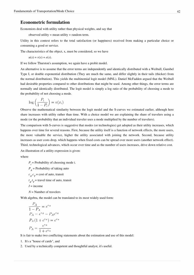
Fundamentals of Transportation/Mode Choice 42

Econometric formulationEconomists deal with utility rather than physical weights, and say that

observed utility = mean utility + random term.Utility in this context refers to the total satisfaction (or happiness) received from making a particular choice orconsuming a good or service.The characteristics of the object, x, must be considered, so we have

u(x) = v(x) + e(x).If we follow Thurston's assumption, we again have a probit model.An alternative is to assume that the error terms are independently and identically distributed with a Weibull, GumbelType I, or double exponential distribution (They are much the same, and differ slightly in their tails (thicker) fromthe normal distribution). This yields the multinomial logit model (MNL). Daniel McFadden argued that the Weibullhad desirable properties compared to other distributions that might be used. Among other things, the error terms arenormally and identically distributed. The logit model is simply a log ratio of the probability of choosing a mode tothe probability of not choosing a mode.

Observe the mathematical similarity between the logit model and the S-curves we estimated earlier, although hereshare increases with utility rather than time. With a choice model we are explaining the share of travelers using amode (or the probability that an individual traveler uses a mode multiplied by the number of travelers).The comparison with S-curves is suggestive that modes (or technologies) get adopted as their utility increases, whichhappens over time for several reasons. First, because the utility itself is a function of network effects, the more users,the more valuable the service, higher the utility associated with joining the network. Second, because utilityincreases as user costs drop, which happens when fixed costs can be spread over more users (another network effect).Third, technological advances, which occur over time and as the number of users increases, drive down relative cost.An illustration of a utility expression is given:where

Pi = Probability of choosing mode i.PA = Probability of taking autocA,cT = cost of auto, transittA,tT = travel time of auto, transitI = incomeN = Number of travelers

With algebra, the model can be translated to its most widely used form:

It is fair to make two conflicting statements about the estimation and use of this model:1. It's a "house of cards", and2. Used by a technically competent and thoughtful analyst, it's useful.

Fundamentals of Transportation/Mode Choice 43

The "house of cards" problem largely arises from the utility theory basis of the model specification. Broadly, utilitytheory assumes that (1) users and suppliers have perfect information about the market; (2) they have deterministicfunctions (faced with the same options, they will always make the same choices); and (3) switching betweenalternatives is costless. These assumptions don’t fit very well with what is known about behavior. Furthermore, theaggregation of utility across the population is impossible since there is no universal utility scale.Suppose an option has a net utility ujk (option k, person j). We can imagine that having a systematic part vjk that is afunction of the characteristics of an object and person j, plus a random part ejk, which represents tastes, observationalerrors, and a bunch of other things (it gets murky here). (An object such as a vehicle does not have utility, it ischaracteristics of a vehicle that have utility.) The introduction of e lets us do some aggregation. As noted above, wethink of observable utility as being a function:

where each variable represents a characteristic of the auto trip. The value β0 is termed an alternative specificconstant. Most modelers say it represents characteristics left out of the equation (e.g., the political correctness of amode, if I take transit I feel morally righteous, so β0 may be negative for the automobile), but it includes whatever isneeded to make error terms NID.

Econometric estimation

Turning now to some technicalmatters, how do we estimate v(x)?Utility (v(x)) isn’t observable. All wecan observe are choices (say, measuredas 0 or 1), and we want to talk aboutprobabilities of choices that range from0 to 1. (If we do a regression on 0s and1s we might measure for j a probabilityof 1.4 or -0.2 of taking an auto.)Further, the distribution of the errorterms wouldn’t have appropriatestatistical characteristics.

The MNL approach is to make amaximum likelihood estimate of this functional form. The likelihood function is:

we solve for the estimated parameters

that max L*. This happens when:

The log-likelihood is easier to work with, as the products turn to sums:

Consider an example adopted from John Bitzan’s Transportation Economics Notes. Let X be a binary variable that is gamma and 0 with probability (1- gamma). Then f(0) = (1- gamma) and f(1) = gamma. Suppose that we have 5 observations of X, giving the sample {1,1,1,0,1}. To find the maximum likelihood estimator of gamma examine

Fundamentals of Transportation/Mode Choice 44

various values of gamma, and for these values determine the probability of drawing the sample {1,1,1,0,1} If gammatakes the value 0, the probability of drawing our sample is 0. If gamma is 0.1, then the probability of getting oursample is: f(1,1,1,0,1) = f(1)f(1)f(1)f(0)f(1) = 0.1*0.1*0.1*0.9*0.1=0.00009. We can compute the probability ofobtaining our sample over a range of gamma – this is our likelihood function. The likelihood function for nindependent observations in a logit model is

where: Yi = 1 or 0 (choosing e.g. auto or not-auto) and Pi = the probability of observing Yi=1The log likelihood is thus:

In the binomial (two alternative) logit model,

, so

The log-likelihood function is maximized setting the partial derivatives to zero:

The above gives the essence of modern MNL choice modeling.

Independence of Irrelevant Alternatives (IIA)Independence of Irrelevant Alternatives is a property of Logit, but not all Discrete Choice models. In brief, theimplication of IIA is that if you add a mode, it will draw from present modes in proportion to their existing shares.(And similarly, if you remove a mode, its users will switch to other modes in proportion to their previous share). Tosee why this property may cause problems, consider the following example: Imagine we have seven modes in ourlogit mode choice model (drive alone, carpool 2 passenger, carpool 3+ passenger, walk to transit, auto driver totransit (park and ride), auto passenger to transit (kiss and ride), and walk or bike). If we eliminated Kiss and Ride, adisproportionate number may use Park and Ride or carpool.Consider another example. Imagine there is a mode choice between driving and taking a red bus, and currently eachhas 50% share. If we introduce another mode, let's call it a blue bus with identical attributes to the red bus, the logitmode choice model would give each mode 33.3% of the market, or in other words, buses will collectively have66.7% market share. Logically, if the mode is truly identical, it would not attract any additional passengers (thoughone can imagine scenarios where adding capacity would increase bus mode share, particularly if the bus was capacityconstrained.There are several strategies that help with the IIA problem. Nesting of choices allows us to reduce this problem.However, there is an issue of the proper Nesting structure. Other alternatives include more complex models (e.g.Mixed Logit) which are more difficult to estimate.

Fundamentals of Transportation/Mode Choice 45

Consumers' SurplusTopics not touched on include the “red bus, blue bus” problem; the use of nested models (e.g., estimate choicebetween auto and transit, and then estimate choice between rail and bus transit); how consumers’ surplusmeasurements may be obtained; and model estimation, goodness of fit, etc. For these topics see a textbook such asOrtuzar and Willumsen (2001).

Returning to rootsThe discussion above is based on the economist’s utility formulation. At the time MNL modeling was developedthere was some attention to psychologist's choice work (e.g., Luce’s choice axioms discussed in his IndividualChoice Behavior, 1959). It has an analytic side in computational process modeling. Emphasis is on how people thinkwhen they make choices or solve problems (see Newell and Simon 1972). Put another way, in contrast to utilitytheory, it stresses not the choice but the way the choice was made. It provides a conceptual framework for travelchoices and agendas of activities involving considerations of long and short term memory, effectors, and otheraspects of thought and decision processes. It takes the form of rules dealing with the way information is searched andacted on. Although there is a lot of attention to behavioral analysis in transportation work, the best of modernpsychological ideas are only beginning to enter the field. (e.g. Golledge, Kwan and Garling 1984; Garling, Kwan,and Golledge 1994).

Examples

Example 1: Mode Choice Model

Problem:

You are given this mode choice modelWhere:

• = cost of mode (cents) / wage rate (in cents per minute)• = travel time in-vehicle (min)• = travel time out-of-vehicle (min)• = mode specific dummies: (dummies take the value of 1 or 0)

• = driving,• = transit with walk access, [base mode]• = transit with auto access,• = carpool

With these inputs:

Fundamentals of Transportation/Mode Choice 46

'' Driving Walk Connect Transit Auto Connect Transit Carpool

t = travel time in-vehicle (min) 10 30 15 12

t0 = travel time out-of-vehicle (min) 0 15 10 3

= driving, 1 0 0 0

= transit with walk access, [base mode] 0 1 0 0

= transit with auto access, 0 0 1 0

= carpool 0 0 0 1

COST 25 100 100 150

WAGE 60 60 60 60

What are the resultant mode shares?Solution:

Outputs 1: Driving 2: Walk-connect transit 3: Auto-connect transit 4: Carpool Sum

Utilities -1.26 -2.09 -3.30 -3.58

EXP(V) 0.28 0.12 0.04 0.03

P(V) 59.96% 26.31% 7.82% 5.90% 100%

InterpretationValue of Time:

(in 1967 $, when the wage rate was about $2.85/hour)implication, if you can improve the travel time (by more buses, less bottlenecks, e.g.) for less than$1.10/hour/person, then it is socially worthwhile.

Example 2: Mode Choice Model Interpretation

Case 1

Fundamentals of Transportation/Mode Choice 47

'' Bus Car Parameter

Tw 10 min 5 min -0.147

Tt 40 min 20 min -0.0411

C $2 $1 -2.24

Car always wins (independent of parameters as long as all are < 0)Case 1

'' Bus Car Parameter

Tw 5 min 5 min -0.147

Tt 40 min 20 min -0.0411

C $2 $4 -2.24

Results -6.86 -10.51

Under observed parameters, bus always wins, but not necessarily under all parameters.It is important to note that individuals differ in parameters. We could introduce socio-economic and other observablecharacteristics as well as a stochastic error term to make the problem more realistic.

Sample Problem• Problem ( Solution )

Additional Questions• Homework• Additional Questions

Variables• - Utility of traveling from i to j by mode m• = mode specific dummies: (dummies take the value of 1 or 0)• = Probability of mode m• = cost of mode (cents) / wage rate (in cents per minute)• = travel time in-vehicle (min)• = travel time out-of-vehicle (min)• = mode specific dummies: (dummies take the value of 1 or 0)

Fundamentals of Transportation/Mode Choice 48

Abbreviations• WCT - walk connected transit• ADT - auto connect transit (drive alone/park and ride)• APT - auto connect transit (auto passenger/kiss and ride)• AU1 - auto driver (no passenger)• AU2 - auto 2 occupants• AU3+ - auto 3+ occupants• WK/BK - walk/bike• IIA - Independence of Irrelevant Alternatives

Key Terms• Mode choice• Logit• Probability• Independence of Irrelevant Alternatives (IIA)• Dummy Variable (takes value of 1 or 0)

References• Garling, Tommy Mei Po Kwan, and Reginald G. Golledge. Household Activity Scheduling, Transportation

Research, 22B, pp. 333-353. 1994.• Golledge. Reginald G., Mei Po Kwan, and Tommy Garling, “Computational Process Modeling of Household

Travel Decisions,” Papers in Regional Science, 73, pp. 99-118. 1984.• Lancaster, K.J., A new approach to consumer theory. Journal of Political Economy, 1966. 74(2): p. 132-157.• Luce, Duncan R. (1959). Individual choice behavior, a theoretical analysis. New York, Wiley.• Newell, A. and Simon, H. A. (1972). Human Problem Solving. Englewood Cliffs, NJ: Prentice Hall.• Ortuzar, Juan de Dios and L. G. Willumsen’s Modelling Transport. 3rd Edition. Wiley and Sons. 2001,• Thurstone, L.L. (1927). A law of comparative judgement. Psychological Review, 34, 278-286.• Warner, Stan 1962 Strategic Choice of Mode in Urban Travel: A Study of Binary Choice

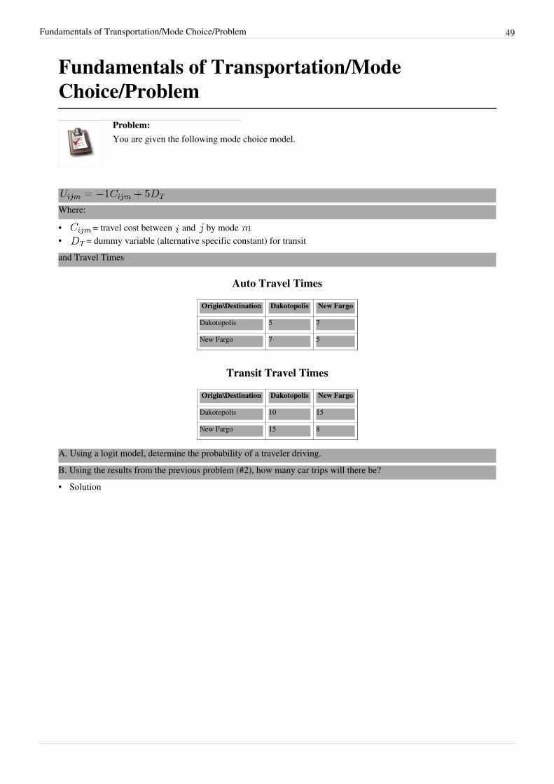
Fundamentals of Transportation/Mode Choice/Problem 49

Fundamentals of Transportation/ModeChoice/Problem

Problem:You are given the following mode choice model.

Where:

• = travel cost between and by mode • = dummy variable (alternative specific constant) for transitand Travel Times

Auto Travel Times

Origin\Destination Dakotopolis New Fargo

Dakotopolis 5 7

New Fargo 7 5

Transit Travel Times

Origin\Destination Dakotopolis New Fargo

Dakotopolis 10 15

New Fargo 15 8

A. Using a logit model, determine the probability of a traveler driving.B. Using the results from the previous problem (#2), how many car trips will there be?• Solution

Fundamentals of Transportation/Mode Choice/Solution 50

Fundamentals of Transportation/ModeChoice/Solution

Problem:You are given the following mode choice model.

Where:

• = travel cost between and by mode • = dummy variable (alternative specific constant) for transit

Auto Travel Times

Origin\Destination Dakotopolis New Fargo

Dakotopolis 5 7

New Fargo 7 5

Transit Travel Times

Origin\Destination Dakotopolis New Fargo

Dakotopolis 10 15

New Fargo 15 8

Solution:Part A

A. Using a logit model, determine the probability of a traveler driving.Solution Steps

1. Compute Utility for Each Mode for Each Cell2. Compute Exponentiated Utilities for Each Cell3. Sum Exponentiated Utilities4. Compute Probability for Each Mode for Each Cell5. Multiply Probability in Each Cell by Number of Trips in Each Cell

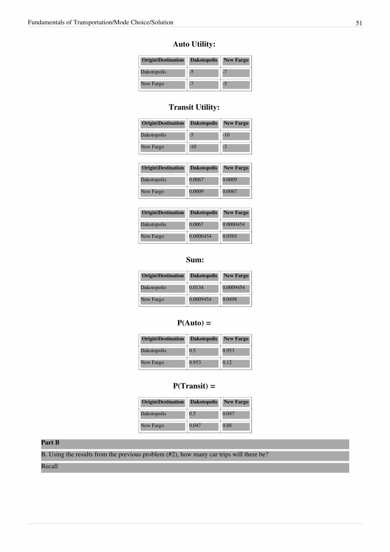
Fundamentals of Transportation/Mode Choice/Solution 51

Auto Utility:

Origin\Destination Dakotopolis New Fargo

Dakotopolis -5 -7

New Fargo -7 -5

Transit Utility:

Origin\Destination Dakotopolis New Fargo

Dakotopolis -5 -10

New Fargo -10 -3

Origin\Destination Dakotopolis New Fargo

Dakotopolis 0.0067 0.0009

New Fargo 0.0009 0.0067

Origin\Destination Dakotopolis New Fargo

Dakotopolis 0.0067 0.0000454

New Fargo 0.0000454 0.0565

Sum:

Origin\Destination Dakotopolis New Fargo

Dakotopolis 0.0134 0.0009454

New Fargo 0.0009454 0.0498

P(Auto) =

Origin\Destination Dakotopolis New Fargo

Dakotopolis 0.5 0.953

New Fargo 0.953 0.12

P(Transit) =

Origin\Destination Dakotopolis New Fargo

Dakotopolis 0.5 0.047

New Fargo 0.047 0.88

Part B

B. Using the results from the previous problem (#2), how many car trips will there be?Recall

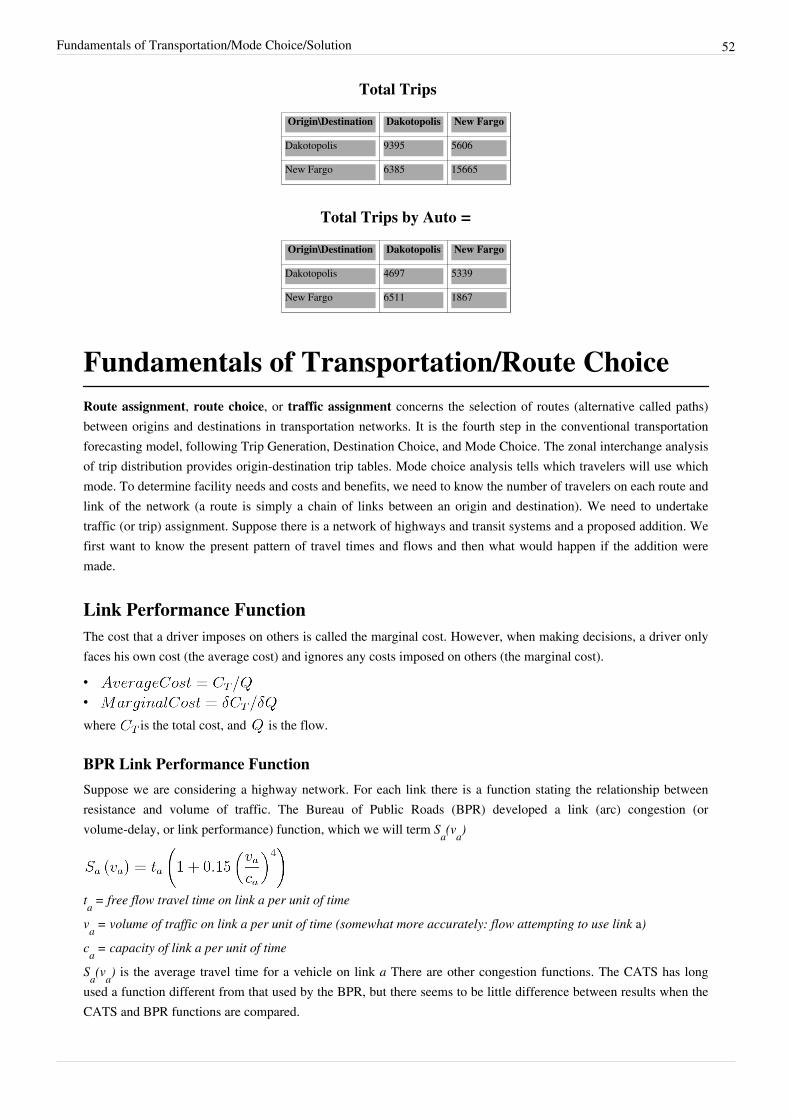
Fundamentals of Transportation/Mode Choice/Solution 52

Total Trips

Origin\Destination Dakotopolis New Fargo

Dakotopolis 9395 5606

New Fargo 6385 15665

Total Trips by Auto =

Origin\Destination Dakotopolis New Fargo

Dakotopolis 4697 5339

New Fargo 6511 1867

Fundamentals of Transportation/Route ChoiceRoute assignment, route choice, or traffic assignment concerns the selection of routes (alternative called paths)between origins and destinations in transportation networks. It is the fourth step in the conventional transportationforecasting model, following Trip Generation, Destination Choice, and Mode Choice. The zonal interchange analysisof trip distribution provides origin-destination trip tables. Mode choice analysis tells which travelers will use whichmode. To determine facility needs and costs and benefits, we need to know the number of travelers on each route andlink of the network (a route is simply a chain of links between an origin and destination). We need to undertaketraffic (or trip) assignment. Suppose there is a network of highways and transit systems and a proposed addition. Wefirst want to know the present pattern of travel times and flows and then what would happen if the addition weremade.

Link Performance FunctionThe cost that a driver imposes on others is called the marginal cost. However, when making decisions, a driver onlyfaces his own cost (the average cost) and ignores any costs imposed on others (the marginal cost).

••where is the total cost, and is the flow.

BPR Link Performance FunctionSuppose we are considering a highway network. For each link there is a function stating the relationship betweenresistance and volume of traffic. The Bureau of Public Roads (BPR) developed a link (arc) congestion (orvolume-delay, or link performance) function, which we will term Sa(va)

ta = free flow travel time on link a per unit of time

va = volume of traffic on link a per unit of time (somewhat more accurately: flow attempting to use link a)

ca = capacity of link a per unit of time

Sa(va) is the average travel time for a vehicle on link a There are other congestion functions. The CATS has longused a function different from that used by the BPR, but there seems to be little difference between results when theCATS and BPR functions are compared.

Fundamentals of Transportation/Route Choice 53

Can Flow Exceed Capacity?On a link, the capacity is thought of as “outflow.” Demand is inflow.If inflow > outflow for a period of time, there is queueing (and delay).For Example, for a 1 hour period, if 2100 cars arrive and 2000 depart, 100 are still there. The link performancefunction tries to represent that phenomenon in a simple way.

Wardrop's Principles of Equilibrium

User EquilibriumEach user acts to minimize his/her own cost, subject to every other user doing the same. Travel times are equal on allused routes and lower than on any unused route.

System optimalEach user acts to minimize the total travel time on the system.

Price of AnarchyThe reason we have congestion is that people are selfish. The cost of that selfishness (when people behave accordingto their own interest rather than society's) is the price of anarchy.The ratio of system-wide travel time under User Equilibrium and System Optimal conditions.

Price of Anarchy = For a two-link network with linear link performance functions (latency functions), Price of Anarchy is < 4/3.Is this too much? Should something be done, or is 33% waste acceptable? [The loss may be larger/smaller in othercases, under different assumptions, etc.]

Conservation of FlowAn important factor in road assignment is the conservation of flow. This means that the number of vehicles enteringthe intersection (link segment) equals the number of vehicles exiting the intersection for a given period of time(except for sources and sinks).Similarly, the number of vehicles entering the back of the link equals the number exiting the front (over a longperiod of time).

Auto assignment

Long-standing techniquesThe above examples are adequate for a problem of two links, however real networks are much more complicated.The problem of estimating how many users are on each route is long standing. Planners started looking hard at it asfreeways and expressways began to be developed. The freeway offered a superior level of service over the localstreet system and diverted traffic from the local system. At first, diversion was the technique. Ratios of travel timewere used, tempered by considerations of costs, comfort, and level of service.The Chicago Area Transportation Study (CATS) researchers developed diversion curves for freeways versus localstreets. There was much work in California also, for California had early experiences with freeway planning. Inaddition to work of a diversion sort, the CATS attacked some technical problems that arise when one works withcomplex networks. One result was the Moore algorithm for finding shortest paths on networks.

Fundamentals of Transportation/Route Choice 54

The issue the diversion approach didn’t handle was the feedback from the quantity of traffic on links and routes. If alot of vehicles try to use a facility, the facility becomes congested and travel time increases. Absent some way toconsider feedback, early planning studies (actually, most in the period 1960-1975) ignored feedback. They used theMoore algorithm to determine shortest paths and assigned all traffic to shortest paths. That’s called all or nothingassignment because either all of the traffic from i to j moves along a route or it does not.The all-or-nothing or shortest path assignment is not trivial from a technical-computational view. Each traffic zone isconnected to n - 1 zones, so there are numerous paths to be considered. In addition, we are ultimately interested intraffic on links. A link may be a part of several paths, and traffic along paths has to be summed link by link.An argument can be made favoring the all-or-nothing approach. It goes this way: The planning study is to supportinvestments so that a good level of service is available on all links. Using the travel times associated with theplanned level of service, calculations indicate how traffic will flow once improvements are in place. Knowing thequantities of traffic on links, the capacity to be supplied to meet the desired level of service can be calculated.

Heuristic proceduresTo take account of the affect of traffic loading on travel times and traffic equilibria, several heuristic calculationprocedures were developed. One heuristic proceeds incrementally. The traffic to be assigned is divided into parts(usually 4). Assign the first part of the traffic. Compute new travel times and assign the next part of the traffic. Thelast step is repeated until all the traffic is assigned. The CATS used a variation on this; it assigned row by row in theO-D table.The heuristic included in the FHWA collection of computer programs proceeds another way.• Step 0: Start by loading all traffic using an all or nothing procedure.• Step 1: Compute the resulting travel times and reassign traffic.• Step 2: Now, begin to reassign using weights. Compute the weighted travel times in the previous two loadings

and use those for the next assignment. The latest iteration gets a weight of 0.25 and the previous gets a weight of0.75.

• Step 3. Continue.These procedures seem to work “pretty well,” but they are not exact.

Frank-Wolfe algorithmDafermos (1968) applied the Frank-Wolfe algorithm [1] (1956, Florian 1976), which can be used to deal with thetraffic equilibrium problem.

Equilibrium AssignmentTo assign traffic to paths and links we have to have rules, and there are the well-known Wardrop equilibrium [2]

(1952) conditions. The essence of these is that travelers will strive to find the shortest (least resistance) path fromorigin to destination, and network equilibrium occurs when no traveler can decrease travel effort by shifting to a newpath. These are termed user optimal conditions, for no user will gain from changing travel paths once the system is inequilibrium.The user optimum equilibrium can be found by solving the following nonlinear programming problem

subject to:

Fundamentals of Transportation/Route Choice 55

where is the number of vehicles on path r from origin i to destination j. So constraint (2) says that all travel musttake place –i = 1 ... n; j = 1 ... n

= 1 if link a is on path r from i to j ; zero otherwise.So constraint (1) sums traffic on each link. There is a constraint for each link on the network. Constraint (3) assuresno negative traffic.

Transit assignmentThere are also methods that have been developed to assign passengers to transit vehicles. Some of these arediscussed in Spiess (1993) Transit Equilibrium Assignment based on Optimal Strategies [3]

Integrating travel choicesThe urban transportation planning model evolved as a set of steps to be followed and models evolved for use in eachstep. Sometimes there were steps within steps, as was the case for the first statement of the Lowry model. In somecases, it has been noted that steps can be integrated. More generally, the steps abstract from decisions that may bemade simultaneously and it would be desirable to better replicate that in the analysis.Disaggregate demand models were first developed to treat the mode choice problem. That problem assumes that onehas decided to take a trip, where that trip will go, and at what time the trip will be made. They have been used totreat the implied broader context. Typically, a nested model will be developed, say, starting with the probability of atrip being made, then examining the choice among places, and then mode choice. The time of travel is a bit harder totreat.Wilson’s doubly constrained entropy model has been the point of departure for efforts at the aggregate level. Thatmodel contains the constrainttijcij = C

where the cij are the link travel costs, tij refers to traffic on a link, and C is a resource constraint to be sized whenfitting the model with data. Instead of using that form of the constraint, the monotonically increasing resistancefunction used in traffic assignment can be used. The result determines zone-to-zone movements and assigns traffic tonetworks, and that makes much sense from the way one would imagine the system works. Zone-to-zone trafficdepends on the resistance occasioned by congestion.Alternatively, the link resistance function may be included in the objective function (and the total cost functioneliminated from the constraints).A generalized disaggregate choice approach has evolved as has a generalized aggregate approach. The large questionis that of the relations between them. When we use a macro model, we would like to know the disaggregate behaviorit represents. If we are doing a micro analysis, we would like to know the aggregate implications of the analysis.Wilson derives a gravity-like model with weighted parameters that say something about the attractiveness of originsand destinations. Without too much math we can write probability of choice statements based on attractiveness, andthese take a form similar to some varieties of disaggregate demand models.

Fundamentals of Transportation/Route Choice 56

Integrating travel demand with route assignmentIt has long been recognized that travel demand is influenced by network supply. The example of a new bridgeopening where none was before inducing additional traffic has been noted for centuries. Much research has gone intodeveloping methods for allowing the forecasting system to directly account for this phenomenon. Evans (1974)published a doctoral dissertation on a mathematically rigorous combination of the gravity distribution model with theequilibrium assignment model. The earliest citation of this integration is the work of Irwin and Von Cube, as relatedby Florian et al. (1975), who comment on the work of Evans:"The work of Evans resembles somewhat the algorithms developed by Irwin and Von Cube (“Capacity Restraint inMulti-Travel Mode Assignment Programs” H.R.B. Bulletin 347 (1962)) for a transportation study of Toronto,Canada. Their work allows for feedback between congested assignment and trip distribution, although they applysequential procedures. Starting from an initial solution of the distribution problem, the interzonal trips are assignedto the initial shortest routes. For successive iterations, new shortest routes are computed, and their lengths are used asaccess times for input the distribution model. The new interzonal flows are then assigned in some proportion to theroutes already found. The procedure is stopped when the interzonal times for successive iteration are quasi-equal."Florian et al. proposed a somewhat different method for solving the combined distribution assignment, applyingdirectly the Frank-Wolfe algorithm. Boyce et al. (1988) summarize the research on Network Equilibrium Problems,including the assignment with elastic demand.

DiscussionA three link problem can not be solved graphically, and most transportation network problems involve a largenumbers of nodes and links. Eash et al, for instance, studied the road net on DuPage County where there were about30,000 one-way links and 9,500 nodes. Because problems are large, an algorithm is needed to solve the assignmentproblem, and the Frank-Wolfe algorithm (modified a bit since first published) is used. Start with an all or nothingassignment and then follow the rule developed by Frank-Wolfe to iterate toward the minimum value of the objectivefunction. The algorithm applies successive feasible solutions to achieve convergence to the optimal solution. It usesan efficient search procedure to move the calculation rapidly toward the optimal solution. Travel times correspond tothe dual variables in this programming problem.It is interesting that the Frank-Wolfe algorithm was available in 1956. Its application was developed in 1968 and ittook almost another two decades before the first equilibrium assignment algorithm was embedded in commonly usedtransportation planning software (Emme and Emme/2, developed by Florian and others in Montreal). We would notwant to draw any general conclusion from the slow application observation, mainly because we can find counterexamples about the pace and pattern of technique development. For example, the simplex method for the solution oflinear programming problems was worked out and widely applied prior to the development of much of programmingtheory.The problem statement and algorithm have general applications across civil engineering -– hydraulics, structures,and construction. (See Hendrickson and Janson 1984).

Examples

Example 1

Problem:Solve for the flows on Links 1 and 2 in the Simple Network of two parallel links just shown if the linkperformance function on link 1:

Fundamentals of Transportation/Route Choice 57

and the function on link 2:

where total flow between the origin and destination is 1000 trips.Solution:

Time (Cost) is equal on all used routes so

And we have Conservation of flow so,

Example 2

Problem:

An example from Eash, Janson, and Boyce (1979) will illustrate the solution to the nonlinear programproblem. There are two links from node 1 to node 2, and there is a resistance function for each link(see Figure 1). Areas under the curves in Figure 2 correspond to the integration from 0 to a in equation

1, they sum to 220,674. Note that the function for link b is plotted in the reverse direction.

Show graphically the equilibrium result.Solution:

Figure 1 - Two Route Network

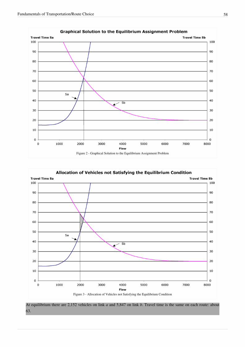
Fundamentals of Transportation/Route Choice 58

Figure 2 - Graphical Solution to the Equilibrium Assignment Problem

Figure 3 - Allocation of Vehicles not Satisfying the Equilibrium Condition

At equilibrium there are 2,152 vehicles on link a and 5,847 on link b. Travel time is the same on each route: about63.

Fundamentals of Transportation/Route Choice 59

Figure 3 illustrates an allocation of vehicles that is not consistent with the equilibrium solution. The curves areunchanged, but with the new allocation of vehicles to routes the shaded area has to be included in the solution, so theFigure 3 solution is larger than the solution in Figure 2 by the area of the shaded area.

Thought Questions• How can we get drivers to consider their marginal cost?• Alternatively: How can we get drivers to behave in a “System Optimal” way?

Sample Problem• Problem (Solution)

Variables• - total cost• - travel cost on link • - flow (volume) on link

Abbreviations• VDF - Volume Delay Function• LPF - Link Performance Function• BPR - Bureau of Public Roads• UE - User Equilbrium• SO - System Optimal• DTA - Dynamic Traffic Assignment• DUE - Deterministic User Equilibrium• SUE - Stochastic User Equilibrium• AC - Average Cost• MC - Marginal Cost

Key Terms• Route assignment, route choice, auto assignment• Volume-delay function, link performance function• User equilibrium• System optimal• Conservation of flow• Average cost• Marginal cost

Fundamentals of Transportation/Route Choice 60

External ExercisesUse the ADAM software at the STREET website [1] and try Assignment #3 to learn how changes in networkcharacteristics impact route choice.

Additional Questions• Homework• Additional Questions

References• Dafermos, Stella. C. and F.T. Sparrow The Traffic Assignment Problem for a General Network.” J. of Res. of the

National Bureau of Standards, 73B, pp. 91-118. 1969.• Florian, Michael ed., Traffic Equilibrium Methods, Springer-Verlag, 1976.• Wardrop, J. C. Some Theoretical Aspects of Road Traffic Research,” Proceedings, Institution of Civil Engineers

Part 2, 9, pp. 325-378. 1952• Eash, Ronald, Bruce N. Janson, and David Boyce Equilibrium Trip Assignment: Advantages and Implications for

Practice, Transportation Research Record 728, pp. 1-8, 1979.• Evans, Suzanne P. . "Derivation and Analysis of Some Models for Combining Trip Distribution and Assignment."

Transportation Research, Vol 10, pp 37-57 1976• Hendrickson, C.T. and B.N. Janson, “A Common Network Flow Formulation to Several Civil Engineering

Problems” Civil Engineering Systems 1(4), pp. 195-203, 1984

References[1] http:/ / en. wikipedia. org/ wiki/ Frank-Wolfe_algorithm[2] http:/ / en. wikipedia. org/ wiki/ Wardrop[3] http:/ / emme2. spiess. ch/ congtras/ congtras. html

Fundamentals of Transportation/Route Choice/Problem 61

Fundamentals of Transportation/RouteChoice/Problem

Problem:Given a flow of six (6) units from origin “o” to destination “r”. Flow on each route ab is designatedwith Qab in the Time Function. Apply Wardrop's Network Equilibrium Principle (Users EqualizeTravel Times on all used routes)

A. What is the flow and travel time on each link? (complete the table below) for Network A

Link Attributes

Link Link Performance Function Flow Time

o-p

p-r

o-q

q-r

B. What is the system optimal assignment?C. What is the Price of Anarchy?• Solution

Fundamentals of Transportation/RouteChoice/Solution

Problem:Given a flow of six (6) units from origin “o” to destination “r”. Flow on each route ab is designatedwith Qab in the Time Function. Apply Wardrop's Network Equilibrium Principle (Users EqualizeTravel Times on all used routes)

A. What is the flow and travel time on each link? (complete the table below) for Network A

Link Attributes

Link Link Performance Function Flow Time

o-p

p-r

o-q

q-r

B. What is the system optimal assignment?C. What is the Price of Anarchy?

Fundamentals of Transportation/Route Choice/Solution 62

Solution:Part A

What is the flow and travel time on each link? Complete the table below for Network A:

Link Attributes

Link Link Performance Function Flow Time

o-p

p-r

o-q

q-r

These four links are really 2 links O-P-R and O-Q-R, because by conservation of flow Qop = Qpr and Qoq=Qqr.

Link Attributes

Link Link Performance Function Flow Time

o-p-r

o-q-r

By Wardrop's Equilibrium Principle, The travel time (cost) on each used route must be equal. So .OR By the conservation of flow principle By substitution

Check Check (within rounding error)

Link Attributes

Link Link Performance Function Flow Time

o-p-r 2.84 42.01

o-q-r 3.15 42.01

or expanding back to the original table:

Link Attributes

Link Link Performance Function Flow Time

o-p 2.84 14.2

p-r 2.84 27.84

o-q 3.15 26.3

q-r 3.15 15.75

User Equilibrium: Total Delay = 42.01 * 6 = 252.06Part B

What is the system optimal assignment?

Fundamentals of Transportation/Route Choice/Solution 63

What is the system optimal assignment for the previous exampleConservation of Flow:

Analytic Solution requires minimizing total delay

And we can compute the SO travel times on each path

Note that unlike the UE solution, Total Delay = 3.04(25+ 6*3.04) + 2.96(20+7*2.96) = 131.45+120.53= 251.98Note: one could also use software such as a "Solver" algorithm to find this solution.Part C

What is the Price of Anarchy?User Equilibrium: Total Delay =252.06 System Optimal: Total Delay = 251.98Price of Anarchy = 252.06/251.98 = 1.0003 < 4/3

Fundamentals of Transportation/Evaluation 64

Fundamentals of Transportation/EvaluationA benefit-cost analysis (BCA)[1] is often required in determining whether a project should be approved and is usefulfor comparing similar projects. It determines the stream of quantifiable economic benefits and costs that areassociated with a project or policy. If the benefits exceed the costs, the project is worth doing; if the benefits fallshort of the costs, the project is not. Benefit-cost analysis is appropriate where the technology is known and wellunderstood or a minor change from existing technologies is being performed. BCA is not appropriate when thetechnology is new and untried because the effects of the technology cannot be easily measured or predicted.However, just because something is new in one place does not necessarily make it new, so benefit-cost analysiswould be appropriate, e.g., for a light-rail or commuter rail line in a city without rail, or for any road project, butwould not be appropriate (at the time of this writing) for something truly radical like teleportation.The identification of the costs, and more particularly the benefits, is the chief component of the “art” of Benefit-CostAnalysis. This component of the analysis is different for every project. Furthermore, care should be taken to avoiddouble counting; especially counting cost savings in both the cost and the benefit columns. However, a number ofbenefits and costs should be included at a minimum. In transportation these costs should be separated for users,transportation agencies, and the public at large. Consumer benefits are measured by consumer’s surplus. It isimportant to recognize that the demand curve is downward sloping, so there a project may produce benefits both toexisting users in terms of a reduction in cost and to new users by making travel worthwhile where previously it wastoo expensive.Agency benefits come from profits. But since most agencies are non-profit, they receive no direct profits. Agencyconstruction, operating, maintenance, or demolition costs may be reduced (or increased) by a new project; these costsavings (or increases) can either be considered in the cost column, or the benefit column, but not both.Society is impacted by transportation project by an increase or reduction of negative and positive externalities.Negative externalities, or social costs, include air and noise pollution and accidents. Accidents can be consideredeither a social cost or a private cost, or divided into two parts, but cannot be considered in total in both columns.If there are network externalities (i.e. the benefits to consumers are themselves a function of the level of demand),then consumers’ surplus for each different demand level should be computed. Of course this is easier said than done.In practice, positive network externalities are ignored in Benefit Cost Analysis.

Background

Early BeginningsWhen Benjamin Franklin was confronted with difficult decisions, he often recorded the pros and cons on twoseparate columns and attempted to assign weights to them. While not mathematically precise, this “moral orprudential algebra”, as he put it, allowed for careful consideration of each “cost” and “benefit” as well as thedetermination of a course of action that provided the greatest benefit. While Franklin was certainly a proponent ofthis technique, he was certainly not the first. Western European governments, in particular, had been employingsimilar methods for the construction of waterway and shipyard improvements.Ekelund and Hebert (1999) credit the French as pioneers in the development of benefit-cost analyses for government projects. The first formal benefit-cost analysis in France occurred in 1708. Abbe de Saint-Pierre attempted to measure and compare the incremental benefit of road improvements (utility gained through reduced transport costs and increased trade), with the additional construction and maintenance costs. Over the next century, French economists and engineers applied their analysis efforts to canals (Ekelund and Hebert, 1999). During this time, The Ecole Polytechnique had established itself as France’s premier educational institution, and in 1837 sought to create a new course in “social arithmetic”: “…the execution of public works will in many cases tend to be handled by a

Fundamentals of Transportation/Evaluation 65

system of concessions and private enterprise. Therefore our engineers must henceforth be able to evaluate the utilityor inconvenience, whether local or general, or each enterprise; consequently they must have true and preciseknowledge of the elements of such investments.” (Ekelund and Hebert, 1999, p. 47). The school also wanted toensure their students were aware of the effects of currencies, loans, insurance, amortization and how they affectedthe probable benefits and costs to enterprises.In the 1840s French engineer and economist Jules Dupuit (1844, tr. 1952) published an article “On Measurement ofthe Utility of Public Works”, where he posited that benefits to society from public projects were not the revenuestaken in by the government (Aruna, 1980). Rather the benefits were the difference between the public’s willingnessto pay and the actual payments the public made (which he theorized would be smaller). This “relative utility” conceptwas what Alfred Marshall would later rename with the more familiar term, “consumer surplus” (Ekelund and Hebert,1999).Vilfredo Pareto (1906) developed what became known as Pareto improvement and Pareto efficiency (optimal)criteria. Simply put, a policy is a Pareto improvement if it provides a benefit to at least one person without makinganyone else worse off (Boardman, 1996). A policy is Pareto efficient (optimal) if no one else can be made better offwithout making someone else worse off. British economists Kaldor and Hicks (Hicks, 1941; Kaldor, 1939) expandedon this idea, stating that a project should proceed if the losers could be compensated in some way. It is important tonote that the Kaldor-Hicks criteria states it is sufficient if the winners could potentially compensate the projectlosers. It does not require that they be compensated.

Benefit-cost Analysis in the United StatesMuch of the early development of benefit-cost analysis in the United States is rooted in water related infrastructureprojects. The US Flood Control Act of 1936 was the first instance of a systematic effort to incorporate benefit-costanalysis to public decision-making. The act stated that the federal government should engage in flood controlactivities if “the benefits to whomsoever they may accrue [be] in excess of the estimated costs,” but did not provideguidance on how to define benefits and costs (Aruna, 1980, Persky, 2001). Early Tennessee Valley Authority (TVA)projects also employed basic forms of benefit-cost analysis (US Army Corp of Engineers, 1999). Due to the lack ofclarity in measuring benefits and costs, many of the various public agencies developed a wide variety of criteria. Notlong after, attempts were made to set uniform standards.The U.S. Army Corp of Engineers “Green Book” was created in 1950 to align practice with theory. Governmenteconomists used the Kaldor-Hicks criteria as their theoretical foundation for the restructuring of economic anlaysis.This report was amended and expanded in 1958 under the title of “The Proposed Practices for Economic Analysis ofRiver Basin Projects” (Persky, 2001).The Bureau of the Budget adopted similar criteria with 1952’s Circular A-47 - “Reports and Budget EstimatesRelating to Federal Programs and Projects for Conservation, Development, or Use of Water and Related LandResources”.

Modern Benefit-cost AnalysisDuring the 1960s and 1970s the more modern forms of benefit-cost analysis were developed. Most analyses requiredevaluation of:1. The present value of the benefits and costs of the proposed project at the time they occurred2. The present value of the benefits and costs of alternatives occurring at various points in time (opportunity costs)3. Determination of risky outcomes (sensitivity analysis)4. The value of benefits and costs to people with different incomes (distribution effects/equity issues) (Layard and

Glaister, 1994)

Fundamentals of Transportation/Evaluation 66

The Planning Programming Budgeting System (PBBS) - 1965The Planning Programming Budgeting System (PBBS) developed by the Johnson administration in 1965 was createdas a means of identifying and sorting priorities. This grew out of a system Robert McNamara created for theDepartment of Defense a few years earlier (Gramlich, 1981). The PBBS featured five main elements:1. A careful specification of basic program objectives in each major area of governmental activity.2. An attempt to analyze the outputs of each governmental program.3. An attempt to measure the costs of the program, not for one year but over the next several years (“several” was

not explicitly defined)4. An attempt to compare alternative activities.5. An attempt to establish common analytic techniques throughout the government.

Office of Management and Budget (OMB) – 1977Throughout the next few decades, the federal government continued to demand improved benefit-cost analysis withthe aim of encouraging transparency and accountability. Approximately 12 years after the adoption of the PPBSsystem, the Bureau of the Budget was renamed the Office of Management and Budget (OMB). The OMB formallyadopted a system that attempts to incorporate benefit-cost logic into budgetary decisions. This came from theZero-Based Budgeting system set up by Jimmy Carter when he was governor of Georgia (Gramlich, 1981).

Recent DevelopmentsExecutive Order 12292, issued by President Reagan in 1981, required a regulatory impact analysis (RIA) for everymajor governmental regulatory initiative over $100 million. The RIA is basically a benefit-cost analysis thatidentifies how various groups are affected by the policy and attempts to address issues of equity (Boardman, 1996).According to Robert Dorfman, (Dorfman, 1997) most modern-day benefit-cost analyses suffer from severaldeficiencies. The first is their attempt “to measure the social value of all the consequences of a governmental policyor undertaking by a sum of dollars and cents”. Specifically, Dorfman mentions the inherent difficultly in assigningmonetary values to human life, the worth of endangered species, clean air, and noise pollution. The secondshortcoming is that many benefit-cost analyses exclude information most useful to decision makers: the distributionof benefits and costs among various segments of the population. Government officials need this sort of informationand are often forced to rely on other sources that provide it, namely, self-seeking interest groups. Finally,benefit-cost reports are often written as though the estimates are precise, and the readers are not informed of therange and/or likelihood of error present.The Clinton Administration sought proposals to address this problem in revising Federal benefit-cost analyses. Theproposal required numerical estimates of benefits and costs to be made in the most appropriate unit of measurement,and “specify the ranges of predictions and shall explain the margins of error involved in the quantification methodsand in the estimates used” (Dorfman, 1997). Executive Order 12898 formally established the concept ofEnvironmental Justice with regards to the development of new laws and policies, stating they must consider the “fairtreatment for people of all races, cultures, and incomes.” The order requires each federal agency to identify andaddress “disproportionately high and adverse human health or environmental effects of its programs, policies andactivities on minority and low-income populations.”

Fundamentals of Transportation/Evaluation 67

Probabilistic Benefit-Cost Analysis

Probability-density distribution of net present values approximated by anormal curve. Source: Treasury Board of Canada, Benefit-Cost Analysis

Guide, 1998

Probability distribution curves for the NPVs of projects A and B. Source:Treasury Board of Canada, Benefit-Cost Analysis Guide, 1998.

In recent years there has been a push for theintegration of sensitivity analyses of possibleoutcomes of public investment projects with opendiscussions of the merits of assumptions used.This “risk analysis” process has been suggested byFlyvbjerg (2003) in the spirit of encouragingmore transparency and public involvement indecision-making.

The Treasury Board of Canada’s Benefit-CostAnalysis Guide recognizes that implementation ofa project has a probable range of benefits andcosts. It posits that the “effective sensitivity” of anoutcome to a particular variable is determined byfour factors:

• the responsiveness of the Net Present Value(NPV) to changes in the variable;

• the magnitude of the variable's range ofplausible values;

• the volatility of the value of the variable (thatis, the probability that the value of the variablewill move within that range of plausiblevalues); and

• the degree to which the range or volatility ofthe values of the variable can be controlled.

It is helpful to think of the range of probableoutcomes in a graphical sense, as depicted inFigure 1 (probability versus NPV).Once these probability curves are generated, acomparison of different alternatives can also beperformed by plotting each one on the same set ofordinates. Consider for example, a comparisonbetween alternative A and B (Figure 2).In Figure 2, the probability that any specified positive outcome will be exceeded is always higher for project B thanit is for project A. The decision maker should, therefore, always prefer project B over project A. In other cases, analternative may have a much broader or narrower range of NPVs compared to other alternatives (Figure 3).Some decision-makers might be attracted by the possibility of a higher return (despite the

Fundamentals of Transportation/Evaluation 68

Probability distribution curves for the NPVs of projects A and B, whereProject A has a narrower range of possible NPVs. Source: Treasury Board

of Canada, Benefit-Cost Analysis Guide, 1998

possibility of greater loss) and therefore mightchoose project B. Risk-averse decision-makerswill be attracted by the possibility of lower lossand will therefore be inclined to choose project A.

Discount rate

Both the costs and benefits flowing from aninvestment are spread over time. While somecosts are one-time and borne up front, otherbenefits or operating costs may be paid at somepoint in the future, and still others received as astream of payments collected over a long periodof time. Because of inflation, risk, anduncertainty, a dollar received now is worth morethan a dollar received at some time in the future.Similarly, a dollar spent today is more onerousthan a dollar spent tomorrow. This reflects theconcept of time preference that we observe when people pay bills later rather than sooner. The existence of realinterest rates reflects this time preference. The appropriate discount rate depends on what other opportunities areavailable for the capital. If simply putting the money in a government insured bank account earned 10% per year,then at a minimum, no investment earning less than 10% would be worthwhile. In general, projects are undertakenwith those with the highest rate of return first, and then so on until the cost of raising capital exceeds the benefit fromusing that capital. Applying this efficiency argument, no project should be undertaken on cost-benefit grounds ifanother feasible project is sitting there with a higher rate of return.Three alternative bases for the setting the government’s test discount rate have been proposed:1. The social rate of time preference recognizes that a dollar's consumption today will be more valued than a dollar's

consumption at some future time for, in the latter case, the dollar will be subtracted from a higher income level.The amount of this difference per dollar over a year gives the annual rate. By this method, a project should not beundertaken unless its rate of return exceeds the social rate of time preference.

2. The opportunity cost of capital basis uses the rate of return of private sector investment, a government projectshould not be undertaken if it earns less than a private sector investment. This is generally higher than social timepreference.

3. The cost of funds basis uses the cost of government borrowing, which for various reasons related to governmentinsurance and its ability to print money to back bonds, may not equal exactly the opportunity cost of capital.

Typical estimates of social time preference rates are around 2 to 4 percent while estimates of the social opportunitycosts are around 7 to 10 percent.Generally, for Benefit-Cost studies an acceptable rate of return (the government’s test rate) will already have beenestablished. An alternative is to compute the analysis over a range of interest rates, to see to what extent the analysisis sensitive to variations in this factor. In the absence of knowing what this rate is, we can compute the rate of return(internal rate of return) for which the project breaks even, where the net present value is zero. Projects with highinternal rates of return are preferred to those with low rates.

Fundamentals of Transportation/Evaluation 69

Determine a present valueThe basic math underlying the idea of determining a present value is explained using a simple compound interestrate problem as the starting point. Suppose the sum of $100 is invested at 7 percent for 2 years. At the end of the firstyear the initial $100 will have earned $7 interest and the augmented sum ($107) will earn a further 7 percent (or$7.49) in the second year. Thus at the end of 2 years the $100 invested now will be worth $114.49.The discounting problem is simply the converse of this compound interest problem. Thus, $114.49 receivable in 2years time, and discounted by 7 per cent, has a present value of $100.Present values can be calculated by the following equation:

(1)

where:• F = future money sum• P = present value• i = discount rate per time period (i.e. years) in decimal form (e.g. 0.07)• n = number of time periods before the sum is received (or cost paid, e.g. 2 years)Illustrating our example with equations we have:

The present value, in year 0, of a stream of equal annual payments of $A starting year 1, is given by the reciprocal ofthe equivalent annual cost. That is, by:

(2)

where:• A = Annual PaymentFor example: 12 annual payments of $500, starting in year 1, have a present value at the middle of year 0 whendiscounted at 7% of: $3971

The present value, in year 0, of m annual payments of $A, starting in year n + 1, can be calculated by combiningdiscount factors for a payment in year n and the factor for the present value of m annual payments. For example: 12annual mid-year payments of $250 in years 5 to 16 have a present value in year 4 of $1986 when discounted at 7%.Therefore in year 0, 4 years earlier, they have a present value of $1515.

Fundamentals of Transportation/Evaluation 70

Evaluation criterionThree equivalent conditions can tell us if a project is worthwhile1. The discounted present value of the benefits exceeds the discounted present value of the costs2. The present value of the net benefit must be positive.3. The ratio of the present value of the benefits to the present value of the costs must be greater than one.However, that is not the entire story. More than one project may have a positive net benefit. From the set of mutuallyexclusive projects, the one selected should have the highest net present value. We might note that if there areinsufficient funds to carry out all mutually exclusive projects with a positive net present value, then the discount usedin computing present values does not reflect the true cost of capital. Rather it is too low.There are problems with using the internal rate of return or the benefit/cost ratio methods for project selection,though they provide useful information. The ratio of benefits to costs depends on how particular items (for instance,cost savings) are ascribed to either the benefit or cost column. While this does not affect net present value, it willchange the ratio of benefits to costs (though it cannot move a project from a ratio of greater than one to less thanone).

Examples

Example 1: Benefit Cost Application

Problem:

This problem, adapted from Watkins (1996) [2], illustrates how a Benefit Cost Analysis might beapplied to a project such as a highway widening. The improvement of the highway saves travel timeand increases safety (by bringing the road to modern standards). But there will almost certainly be

more total traffic than was carried by the old highway. This example excludes external costs and benefits, thoughtheir addition is a straightforward extension. The data for the “No Expansion” can be collected from off-the-shelfsources. However the “Expansion” column’s data requires the use of forecasting and modeling.

Table 1: Data

No Expansion Expansion

Peak

Passenger Trips (per hour) 18,000 24,000

Trip Time (minutes) 50 30

Off-peak

Passenger Trips (per hour) 9,000 10,000

Trip Time (minutes) 35 25

Traffic Fatalities (per year) 2 1

Note: the operating cost for a vehicle is unaffected by the project, and is $4.

Fundamentals of Transportation/Evaluation 71

Table 2: Model Parameters

Peak Value of Time ($/minute) $0.15

Off-Peak Value of Time ($/minute) $0.10

Value of Life ($/life) $3,000,000

What is the benefit-cost relationship?Solution:

Benefits

Figure 1: Change in Consumers' Surplus

A 50 minute trip at $0.15/minute is$7.50, while a 30 minute trip is only$4.50. So for existing users, theexpansion saves $3.00/trip. Similarlyin the off-peak, the cost of the tripdrops from $3.50 to $2.50, saving$1.00/trip.Consumers’ surplus increases both forthe trips which would have been takenwithout the project and for the tripswhich are stimulated by the project(so-called “induced demand”), as illustrated above in Figure 1. Our analysis is divided into Old and New Trips, thebenefits are given in Table 3.

Table 3: Hourly Benefits

TYPE Old trips New Trips Total

Peak $54,000 $9000 $63,000

Off-peak $9,000 $500 $9,500

Note: Old Trips: For trips which would have been taken anyway the benefit of the project equals the value of thetime saved multiplied by the number of trips. New Trips: The project lowers the cost of a trip and public responds byincreasing the number of trips taken. The benefit to new trips is equal to one half of the value of the time savedmultiplied by the increase in the number of trips. There are 250 weekdays (excluding holidays) each year and fourrush hours per weekday. There are 1000 peak hours per year. With 8760 hours per year, we get 7760 offpeak hoursper year. These numbers permit the calculation of annual benefits (shown in Table 4).

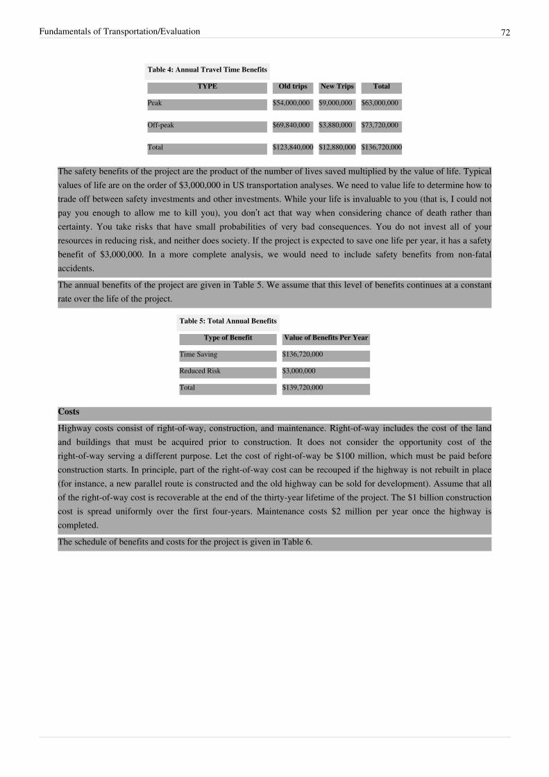
Fundamentals of Transportation/Evaluation 72

Table 4: Annual Travel Time Benefits

TYPE Old trips New Trips Total

Peak $54,000,000 $9,000,000 $63,000,000

Off-peak $69,840,000 $3,880,000 $73,720,000

Total $123,840,000 $12,880,000 $136,720,000

The safety benefits of the project are the product of the number of lives saved multiplied by the value of life. Typicalvalues of life are on the order of $3,000,000 in US transportation analyses. We need to value life to determine how totrade off between safety investments and other investments. While your life is invaluable to you (that is, I could notpay you enough to allow me to kill you), you don’t act that way when considering chance of death rather thancertainty. You take risks that have small probabilities of very bad consequences. You do not invest all of yourresources in reducing risk, and neither does society. If the project is expected to save one life per year, it has a safetybenefit of $3,000,000. In a more complete analysis, we would need to include safety benefits from non-fatalaccidents.The annual benefits of the project are given in Table 5. We assume that this level of benefits continues at a constantrate over the life of the project.

Table 5: Total Annual Benefits

Type of Benefit Value of Benefits Per Year

Time Saving $136,720,000

Reduced Risk $3,000,000

Total $139,720,000

Costs

Highway costs consist of right-of-way, construction, and maintenance. Right-of-way includes the cost of the landand buildings that must be acquired prior to construction. It does not consider the opportunity cost of theright-of-way serving a different purpose. Let the cost of right-of-way be $100 million, which must be paid beforeconstruction starts. In principle, part of the right-of-way cost can be recouped if the highway is not rebuilt in place(for instance, a new parallel route is constructed and the old highway can be sold for development). Assume that allof the right-of-way cost is recoverable at the end of the thirty-year lifetime of the project. The $1 billion constructioncost is spread uniformly over the first four-years. Maintenance costs $2 million per year once the highway iscompleted.The schedule of benefits and costs for the project is given in Table 6.

Fundamentals of Transportation/Evaluation 73

Table 6: Schedule Of Benefits And Costs ($ millions)

Time (year) Benefits Right-of-way costs Construction costs Maintenance costs

0 0 100 0 0

1-4 0 0 250 0

5-29 139.72 0 0 2

30 139.72 -100 0 2

Conversion to Present Value

The benefits and costs are in constant value dollars. Assume the real interest rate (excluding inflation) is 2%. Thefollowing equations provide the present value of the streams of benefits and costs.To compute the Present Value of Benefits in Year 5, we apply equation (2) from above.To convert that Year 5 value to a Year 1 value, we apply equation (1)

The present value of right-of-way costs is computed as today’s right of way cost ($100 M) minus the present value ofthe recovery of those costs in Year 30, computed with equation (1):

The present value of the construction costs is computed as the stream of $250M outlays over four years is computedwith equation (2):

Maintenance Costs are similar to benefits, in that they fall in the same time periods. They are computed the sameway, as follows: To compute the Present Value of $2M in Maintenance Costs in Year 5, we apply equation (2) fromabove.

To convert that Year 5 value to a Year 1 value, we apply equation (1)

As Table 7 shows, the benefit/cost ratio of 2.5 and the positive net present value of $1563.31 million indicate that theproject is worthwhile under these assumptions (value of time, value of life, discount rate, life of the road). Under adifferent set of assumptions, (e.g. a higher discount rate), the outcome may differ.

Fundamentals of Transportation/Evaluation 74

Table 7: Present Value of Benefits and Costs ($ millions)

Present Value

Benefits 2,597.21

Costs

Right-of-Way 44.79

Construction 951.93

Maintenance 37.18

Costs SubTotal 1,033.90

Net Benefit (B-C) 1,563.31

Benefit/Cost Ratio 2.5

Thought Questions

Decision CriteriaWhich is a more appropriate decision criteria: Benefit/Cost or Benefit - Cost? Why?

Is it only money that matters?Problem

Is money the only thing that matters in Benefit-Cost Analysis? Is "converted" money the only thing that matters? Forexample, the value of human life in dollars?Solution

Absolutely not. A lot of benefits and costs can be converted to monetary value, but not all. For example, you can puta price on human safety, but how can you put a price on, say, asthetics--something that everyone agrees is beneficial.What else can you think of?

Can small units of time be given the same value of time as larger units of time?In other words, do 60 improvements each saving a traveler 1 minute equal 1 improvement saving a traveler 60minutes? Similarly, does 1 improvement saving a 1000 travelers 1 minute equal the value of time of a single travelerof 1000 minutes. These are different problems, one is intra-traveler and one is inter-traveler, but related.Several issues arise.A. Is value of time linear or non-linear? To this we must conclude the value of time is surely non-linear. I am muchmore agitated waiting 3 minutes at a red light than 2, and I begin to suspect the light is broken. Studies of rampmeters show a similar phenomena[3] .B. How do we apply this in a benefit-cost analysis? If we break one project into 60 smaller projects, each with asmaller value of travel time saved, and then we added the gains, we would get a different result than the what obtainswith a single large project. For analytical convenience, we would like our analyses to be additive, not sub-additive,otherwise arbitrarily dividing the project changes the result. In particular many smaller projects will produce anundercount that is quite significant, and result in a much lower benefit than if the projects were bundled.As a practical matter, every Benefit/Cost Analysis assumes a single value of time, rather than assuming non-linearvalue of time. This also helps avoiding biasing public investments towards areas with people who have a high valueof time (the rich)

Fundamentals of Transportation/Evaluation 75

On the other hand, mode choice analyses do however weight different components of travel time differently,especially transit time (i.e. in-vehicle time is less onerous than waiting time). The implicit value of time for travelersdoes depend on the type of time (though generally not the amount of time). Using the log-sum of the mode choicemodel as a measure of benefit would implicitly account for this.

Are sunk costs sunk, is salvage value salvageable? A paradox in engineering economicsanalysisSalvage value is defined as "The estimated value of an asset at the end of its useful life." [4] Sunk cost is defined as"Cost already incurred which cannot be recovered regardless of future events."[5]

It is often said in economics that "sunk costs are sunk", meaning they should not be considered a cost in economicanalysis, because the money has already been spent.Now consider two casesIn case 1, we have a road project that costs $10.00 today, and at the end of 10 years has some economic valueremaining, let's say a salvage value of $5.00, which when discounted back to the present is $1.93 (at 10% interest).This value is the residual value of the road. Thus, the total present cost of the project $10.00 - $1.93 = $8.07. Clearlythe road cannot be moved. However, its presence makes it easier to build future roads ... the land has been acquiredand graded, some useful material for aggregate is on-site perhaps, and can be thought of as the amount that it reducesthe cost of future generations to build the road. Alternatively, the land could be sold for development if the road is nolonger needed, or turned into a park.Assume the present value of the benefit of the road is $10.00. The benefit/cost ratio is $10.00 over $8.07 or 1.23. Ifwe treat the salvage value as a benefit rather than cost, the benefit is $10.00 + $1.93 = $11.93 and the cost is $10, andthe B/C is 1.193.In 10 years time, the community decides to replace the old worn out road with a new road. This is a new project. Thesalvage value from the previous project is now the sunk cost of the current project (after all the road is there andcould not be moved, and so does not cost the current project anything to exploit). So the cost of the project in 10years time would be $10.00 - $5.00 = $5.00. Discounting that to the present is $1.93.The benefit in 10 years time is also $10.00, but the cost in 10 years time was $5.00, and the benefit/cost ratio theyperceive is $10.00/$5.00 = 2.00Aggregating the two projects• the benefits are $10 + $3.86 = $13.86• the costs are $8.07 + $1.93 = $10.00• the collective benefit/cost ratio is 1.386• the NPV is benefits - costs = $3.86One might argue the salvage value is a benefit, rather than a cost reduction. In that case• the benefits are $10.00 + $1.93 + $3.86 = $15.79• the costs are $10.00 + $1.93 = $11.93• the collective benefit/cost ratio is 1.32• the NPV remains $3.86Case 2 is an identical road, but now the community has a 20 year time horizon to start. The initial cost is $10, andthe cost in 10 years time is $5.00 (discounted to $1.93). The benefits are $10 now and $10 in 10 years time(discounted to $3.86). There is no salvage value at the end of the first period, nor sunk costs at the beginning of thesecond period. What is the benefit cost ratio?• the costs are $11.93• the benefits are still $13.86• the benefit/cost ratio is 1.16

Fundamentals of Transportation/Evaluation 76

• the NPV is $1.93.If you are the community, which will you invest in? Case 1 has an initial B/C of 1.23 (or 1.193), Case 2 has a B/C of1.16. But the real benefits and real costs of the roads are identical.The salvage value in this example is, like so much in economics (think Pareto optimality), an accounting fiction. Inthis case no transaction takes place to realize that salvage value. On the other hand, excluding the salvage valueover-estimates the net cost of the project, as it ignores potential future uses of the project.Time horizons on projects must be comparable to correctly assess relative B/C ratio, yet not all projects do have thesame benefit/cost ratio.

Sample ProblemsProblem (Solution)

Key Terms• Benefit-Cost Analysis• Profits• Costs• Discount Rate• Present Value• Future Value

External ExercisesUse the SAND software at the STREET website [1] to learn how to evaluate network performance given a changingnetwork scenario.

References[1] benefit-cost analysis is sometimes referred to as cost-benefit analysis (CBA)[2] http:/ / www. sjsu. edu/ faculty/ watkins/ cba. htm[3] Weighting Waiting: Evaluating Perception of In-Vehicle Travel Time Under Moving and Stopped Conditions[4] http:/ / www. investorwords. com/ 4372/ salvage_value. html[5] http:/ / www. investorwords. com/ 4813/ sunk_cost. html

• Aruna, D. Social Cost-Benefit Analysis Madras Institute for Financial Management and Research, pp. 124, 1980.• Boardman, A. et al., Cost-Benefit Analysis: Concepts and Practice, Prentice Hall, 2nd Ed,• Dorfman, R, “Forty years of Cost-Benefit Analysis: Economic Theory Public Decisions Selected Essays of Robert

Dorfman”, pp. 323, 1997.• Dupuit, Jules. “On the Measurement of the Utility of Public Works R.H. Babcock (trans.).” International

Economic Papers 2. London: Macmillan, 1952.• Ekelund, R., Hebert, R. Secret Origins of Modern Microeconomics: Dupuit and the Engineers, University of

Chicago Press, pp. 468, 1999.• Flyvbjerg, B. et al. Megaprojects and Risk: An Anatomy of Ambition, Cambridge University Press, pp. 207,

2003.• Gramlich, E., A Guide to Benefit-cost Analysis, Prentice Hall, pp. 273, 1981.• Hicks, John (1941) “The Rehabilitation of Consumers’ Surplus,” Review of Economic Studies, pp. 108-116.• Kaldor, Nicholas (1939) “Welfare Propositions of Economics and Interpersonal Comparisons of Utility,”

Economic Journal, 49:195, pp. 549-552.• Layard, R., Glaister, S., Cost-Benefit Analysis, Cambridge University Press; 2nd Ed, pp. 507, 1994.

Fundamentals of Transportation/Evaluation 77

• Pareto, Vilfredo., (1906) Manual of Political Economy. 1971 translation of 1927 edition, New York: Augustus M.Kelley.

• Perksy, J., Retrospectives: Cost-Benefit Analysis and the Classical Creed Journal of Economic Perspectives, 2001pp. 526, 2000.

• Treasury Board of Canada “Benefit-cost Analysis Guide”, 1998 http:/ / classwebs. spea. indiana. edu/ krutilla/v541/ Benfit-Cost%20Guide. pdf

Fundamentals of Transportation/PlanningUrban, city, and town planning integrates land use planning and transportation planning to improve the built,economic and social environments of communities. Transportation planning evaluates, assesses, designs and sitestransportation facilities.There are two approaches to planning• Planning determines the rules of the game or constitution. This is planning as regulator or referee• Planning determines the outcome of the game. This is planning as designer or player.Both are typically undertaken. In land markets, the first is often the case. In transportation, which is oftengovernment provided, the second often holds.

Rationales for Planning

Why plan?• To prepare for future contingencies, lowering the cost (in money, time, political effort) of dealing with

anticipatable future outcomes. If the forecast is for rain, it is prudent to carry an umbrella.• To establish a vision of the future to guide present action. To graduate with a Bachelor's degree in Civil

Engineering, I must take CE3201.

Why plan transportation?Transportation is, for better or worse, a public enterprise with long lasting consequences for decisions. There existeconomies of coordination which may (but not necessarily) be difficult to achieve in the absence of planning. Forinstance, we want to ensure that roads from two different counties meet at the county line.

Why plan land use?Owners of developed land have a right to service from public and private infrastructure. As infrastructure is costlyand the economics of financing it are crude (though they need not be), planning is a substitute for the market.

Economic rationalesTo invoke microeconomic theory:

In a market, equilibrium ( , ) occurs where marginal private cost equals marginal willingness to pay ordemand. However if there are externalities, costs that are not borne by the parties to the transaction (e.g. noisepollution, air pollution, and congestion), there is a marginal social cost that is higher than the marginal private cost,leading to overconsumption. The first best solution is to price goods at their marginal social cost, imposing anadditional charge. However, the same effect can be achieved by establishing a restrictive quota on demand ( ).There are other approaches to the problem besides directly increasing taxes or restricting demand. The libertarianapproach for instance is the use of lawsuits, and fear thereof, to bring about good behavior. If you create a nuisance

Fundamentals of Transportation/Planning 78

for your neighbors, they could sue you and the courts could force you to behave better. This shifts the problem fromlegislators and bureaucrats to judges and juries, which may or may not be an improvement. However, while this iseasy to do for some kinds of obvious nuisances, it poses more problems for widely distributed externalities like airpollution.The favored transportation economist solution to congestion is road pricing, charging a higher toll in the peak toprovide the right price signal to commuters about their true costs. More radical solutions include road privatization.The central issue with most externalities is the lack of well defined property rights:Ronald Coase (1992) argues that the problem is that of actions of economic agents have harmful effects on others.His theorem is restated from George Stigler (1966) as "... under perfect competition, private and social costs will beequal." This analysis extends and controverts the argument of Arthur Pigou (1920), who argued that the creator ofthe externality should pay a tax or be liable, what is now called The Polluter Pays Principle. Coase (1992) suggeststhe problem is lack of property rights, and notes that the externality is caused by both parties, the polluter and thereceiver of pollution. In this reciprocal relationship, there would be no noise pollution externality if no-one wasaround to hear. This theory echoes the Zen question ``If a tree falls in the woods and no-one is around to hear, does itmake a sound?. Moreover, the allocation of property rights to either the polluter or pollutee results in a sociallyoptimal level of production, because in theory the individuals or firms could merge and the external cost wouldbecome internal. However, this analysis assumes zero transaction costs. If the transaction costs exceed the gainsfrom a rearrangement of activities to maximize production value, then the switch in behavior won’t be made.

There are several means for internalizing these external costs. Pigou identifies the imposition of taxes and transfers,Coase (1992) suggests assigning property rights, while government most frequently uses regulation. To some extentall have been tried in various places and times. In dealing with air pollution, transferable pollution rights have beencreated for some pollutants. Fuel taxes are used in some countries to deter the amount of travel, with an addedrationale being compensation for the air pollution created by cars. The US government establishes pollution andnoise standards for vehicles, and requires noise walls be installed along highways in some areas.

Property rightsGovernment in general, and land use planning in particular, concerns itself with restricting individual property rightsfor the common good. Donald Krueckeberg (1995) [1] cites Christman who defines 9 separable kinds of propertyrights:• Possession,• Use,• Alienation,• Consumption,• Modification,• Destruction,• Management,• Exchange,• Profit Taking.Some quotes about property and government:• "The Government is Best which Governs least." -- Henry David Thoreau in Civil Disobedience• "Government is there only to do what people can't do for themselves." - Minnesota's former beloved Governor,

Jesse Ventura (paraphrased)• "Proptery is Liberty" - Pierre-Joseph Proudhoun• "When a Man assumes a public trust, he should consider himself as public property" - Thomas Jefferson• "Few rich men own their own property. The property owns them. " R. Ingersoll

Fundamentals of Transportation/Planning 79

• "What is politics after all, but the compulsion to preside over property and make other people's decisions forthem." Tom Robbins

• "Property is Theft" - all natural inheritances derive in part or whole from force and fraud. As historical fact this ishard to argue with. This forms part of the anarchist worldview. But so what if property is theft? A stable systemof property relations is necessary to have a functioning economy, to encourage long term investments. Belief thatyour property can easily be taken, or taken without recompense, will discourage long term investment.

Problems in urban land marketsWhitehead[2] identifies a number of problems in urban land markets.• Provision of public goods

• Q: Are transportation services truly public goods?• Existence of locational externalities

• Q: Why do location externalities exist?• Imperfect information on which to base individual decisions

• Q: Do planners really know better?• Unequal division of market power among economic agents

• Q: Is unequal division of market power necessary to achieve economies of scale and scope, efficiencies fromdoing things big or broadly?

• Differences between how individuals and communities value future and current benefits• Q: Do communities value anything?

Arrow's Impossibility Theorem An illustration of the problem of aggregation of social welfare functions:Three individuals each have well-behaved preferences. However, aggregating the three does not produce a wellbehaved preference function:• Person A prefers red to blue and blue to green• Person B prefers green to red and red to blue• Person C prefers blue to green and green to red.Aggregating, transitivity is violated.• Two people prefer red to blue• Two people prefer blue to green, and• Two people prefer green to red.What does society want?• Differences between individual and community risk perception

• Q: How should the economic discount rate, be computed. This rate may be lower for communities thanindividuals because communities can borrow more cheaply, they tend to be lower risk for lenders thanindividuals. But each investment, treated on its own, should have the same discount rate applied to it.

• Interdependence in utility arising from "merit goods," consumption of which by one individual benefits others• Q: Do merit goods exist? While there may be an external benefit to some things, it is rare that there is not a

much larger internal benefit. For instance, education or good housing benefit the recipients much more thansociety.

• Income redistribution• Do income redistribution schemes reduce the incentive to work? What are the long term consequences of these

schemes. While in the U.S. they have been kept manageable, these schemes have undermined the economy ofmany countries.

Fundamentals of Transportation/Planning 80

Thought questionsIs there a right to be free of pollution, noise, or nuisance of various kinds?We have seen over the past century a century of planning mistakes. One must ask "Why Plan?"F. A. Hayek, 1974 winner of the Nobel Prize in Economics, called the belief in Soviet Style socialist planning TheFatal Conceit. Planners, even if smarter than any individual in the market, cannot possibly know more than themarket as a whole. Acquiring one bit of additional data is just adding a glass of water to the ocean of informationthat the market possesses.However, even Hayek conceded the need for so-called "Piecemeal Planning" to achieve coordination in small areas,see The Constitution of Liberty. A second issue is whether that planning is more appropriately done in the public orprivate spheres.Which of the following statements is more accurate:• Hypothesis: Planning was established by the state to provide long term certainty regarding property relations and

the need for takings.• Hypothesis: Planning was established to reduce transactions and coordination costs.

Discussion QuestionsDo community decisions require government decisions? To what extent does planning require government? Forinstance, Columbia, Maryland was largely private sector (with some public provided goods).Can private arrangements substitute for government mandates? Privatopias, covenant arrangements, etc.What would transportation look like without land use planners and their plans?Using the rationales for planning, justify:• Historic preservation• Building height restrictions• Poletown Case [3]

• Subsidized housing• Subsidized transit• Subsidized roads• Public playgrounds and parks

How is planning doneThe remainder of this unit in the wikibook Fundamentals of Transportation concerns not whether planning should beundertaken, but how it is done, ideally and in practice. Sections include:• Fundamentals of Transportation/Decision Making• Fundamentals of Transportation/Modeling• Fundamentals of Transportation/Geography and Networks• Fundamentals of Transportation/Land Use Forecasting• Fundamentals of Transportation/Trip Generation• Fundamentals of Transportation/Destination Choice• Fundamentals of Transportation/Mode Choice• Fundamentals of Transportation/Route Choice• Fundamentals of Transportation/Evaluation

Fundamentals of Transportation/Planning 81

References[1] Krueckeberg, D. 1995. "The Difficult Character of Property: To Whom Do Things Belong?" Journal of the American Planning Association

61: 301-9.[2] Whitehead, Christine (1983) “The Rationale for Government Intervention.” In Urban Land Policy: Issues and Opportunities, H. Dunkerly, ed.

New York: Oxford University Press.[3] http:/ / en. wikipedia. org/ wiki/ Poletown,_Detroit

• Coase, Ronald H. (1992). "The Problem of Social Cost, and Notes on the Problem of Social Cost". The Firm, TheMarket and the Law. University of Chicago Press: Chicago..

• Krueckeberg, D.A. (1995). "The difficult character of property: to whom do things belong?". Journal of theAmerican Planning Association (Routledge) 61 (3): 301--309.

• Stigler, G. (1966). The Theory of Price. New York: Macmillan.• Pigou, A.C. (1920). The Economics of Welfare. Transaction Pub 2002 reissue.• Hayek, F.A. (2001). The Fatal Conceit: The errors of socialism. Columbia Univ Press. pp. 362.• Hayek, F.A. (1960). The Constitution of Liberty. South Bend: Gateway Editions Ltd.• Thoreau, H.D.. Civil Disobedience.

Fundamentals of Transportation/OperationsAlmost anybody can build a road. Its safety and durability would likely come into question if done by an amateur,but roads are not a difficult thing to deploy. Management of these roads, however, is something that is far fromsimple. Safety, efficiency, and sensibility are all elements that come into play when managing a road. It is seldompossible to find a managing strategy that satisifies all three of these categories, but often a "good" strategy can befound by balancing tradeoffs. This section introduces the fundamentals of traffic management and operation,discussing everything from queueing theory to traffic signals. The discussions here cover the fundamentals for trafficoperations. To this day, research is still being conducted to perfect these elements.

QueueingQueueing is the study of traffic behavior near a certain section where demand exceeds available capacity. Queuescan be seen in a variety of situations and transportation systems. Its presence is one of the causes of driver delay.

Traffic FlowTraffic Flow is the study of the movement of individual drivers and vehicles between two points and the interactionsthey make with one another. While traffic flow cannot be predicted with one-hundred percent certainty due tounpredictable driver behavior, drivers tend to behave within a reasonable range that can be representedmathematically. Relationships have been established between the three main traffic flow characteristics:• Flow• Density• Velocity

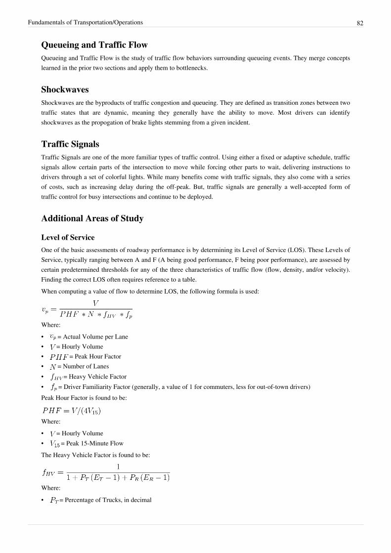
Fundamentals of Transportation/Operations 82

Queueing and Traffic FlowQueueing and Traffic Flow is the study of traffic flow behaviors surrounding queueing events. They merge conceptslearned in the prior two sections and apply them to bottlenecks.

ShockwavesShockwaves are the byproducts of traffic congestion and queueing. They are defined as transition zones between twotraffic states that are dynamic, meaning they generally have the ability to move. Most drivers can identifyshockwaves as the propogation of brake lights stemming from a given incident.

Traffic SignalsTraffic Signals are one of the more familiar types of traffic control. Using either a fixed or adaptive schedule, trafficsignals allow certain parts of the intersection to move while forcing other parts to wait, delivering instructions todrivers through a set of colorful lights. While many benefits come with traffic signals, they also come with a seriesof costs, such as increasing delay during the off-peak. But, traffic signals are generally a well-accepted form oftraffic control for busy intersections and continue to be deployed.

Additional Areas of Study

Level of ServiceOne of the basic assessments of roadway performance is by determining its Level of Service (LOS). These Levels ofService, typically ranging between A and F (A being good performance, F being poor performance), are assessed bycertain predetermined thresholds for any of the three characteristics of traffic flow (flow, density, and/or velocity).Finding the correct LOS often requires reference to a table.When computing a value of flow to determine LOS, the following formula is used:

Where:• = Actual Volume per Lane• = Hourly Volume• = Peak Hour Factor• = Number of Lanes• = Heavy Vehicle Factor• = Driver Familiarity Factor (generally, a value of 1 for commuters, less for out-of-town drivers)Peak Hour Factor is found to be:

Where:• = Hourly Volume• = Peak 15-Minute FlowThe Heavy Vehicle Factor is found to be:

Where:• = Percentage of Trucks, in decimal

Fundamentals of Transportation/Operations 83

• = Passenger Car Equivelant of Trucks (found through table)• = Percentage of Recreational Vehicles, in decimal• = Passenger car Equivelant of Recreational Vehicles (found through table)Similarly, LOS can be analyzed the anticipated speed of the corridor. The equation below produces the estimatedfree-flow speed for a strip of rural road, given certain characteristics about it:

Where:• = Estimated Free Flow Speed• = Base Free Flow Speed• = Adjustment for Lane Width (found in tables)• = Adjustment for Lateral Clearance (found in tables)• = Adjustment for Number of Lanes (found in tables)• = Adjustment for Interchange Density (found in tables)For multilane urban highways, free-flow speed is computed with a similar equation:

Where:• = Estimated Free Flow Speed• = Base Free Flow Speed• = Adjustment for Lane Width (found in tables)• = Adjustment for Lateral Clearance (found in tables)• = Adjustment for Median Type (found in tables)• = Adjustment for Access Points (found in tables)Lateral Clearance is computed:

Where:• = Total Lateral Clearance• = Lateral Clearance on the Right Side of the Travel Lanes to Obstructions• = Lateral Clearance on the Left Side of the Travel Lanes to ObstructionsOnce TLC is computed, a table can provide the value for the Lateral Clearance Adjustment.

Estimating GapsOne area of transportation operations that is still being considered is the estimation of gaps between vehicles. This isapplicable in a variety of situations, primarily dealing with arrivals of vehicles at a given intersection. Gaps can onlybe predicted through a probability, based on several known characteristics occurring at a given time or location.One of the more popular models used for predicting arrivals is the Poisson Model. This model is shown here:

Where:

• = Probability of having x vehicles arrive in time t• = Average vehicle flow or arrival rate• = Duration of the time interval over which vehicles are counted• = Number of vehicles to arrive in time t

Fundamentals of Transportation/Operations 84

Additional Questions• Homework• Additional Questions

Variables• - Actual Volume per Lane• - Hourly Volume• - Peak Hour Factor• - Number of Lanes• - Heavy Vehicle Factor• - Driver Familiarity Factor (generally, a value of 1 for commuters, less for out-of-town drivers)• - Peak 15-Minute Flow• - Percentage of Trucks, in decimal• - Passenger Car Equivelant of Trucks (found through table)• - Percentage of Recreational Vehicles, in decimal• - Passenger car Equivelant of Recreational Vehicles (found through table)• - Estimated Free Flow Speed• - Base Free Flow Speed• - Adjustment for Lane Width (found in tables)• - Adjustment for Lateral Clearance (found in tables)• - Adjustment for Number of Lanes (found in tables)• - Adjustment for Interchange Density (found in tables)• - Adjustment for Median Type (found in tables)• - Adjustment for Access Points (found in tables)• - Total Lateral Clearance• - Lateral Clearance on the Right Side of the Travel Lanes to Obstructions• - Lateral Clearance on the Left Side of the Travel Lanes to Obstructions• - Probability of having x vehicles arrive in time t• - Average vehicle flow or arrival rate• - Duration of the time interval over which vehicles are counted• - Number of vehicles to arrive in time t

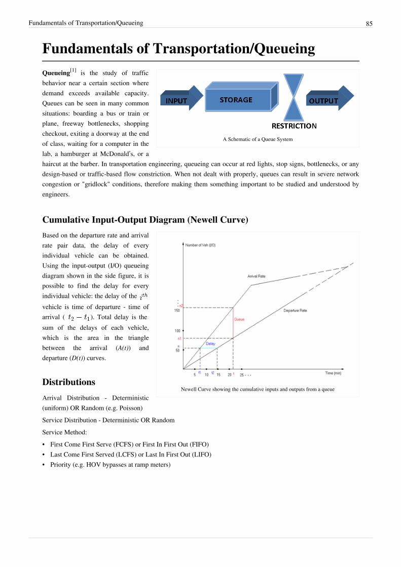
Fundamentals of Transportation/Queueing 85

Fundamentals of Transportation/Queueing

A Schematic of a Queue System

Queueing[1] is the study of trafficbehavior near a certain section wheredemand exceeds available capacity.Queues can be seen in many commonsituations: boarding a bus or train orplane, freeway bottlenecks, shoppingcheckout, exiting a doorway at the endof class, waiting for a computer in thelab, a hamburger at McDonald’s, or ahaircut at the barber. In transportation engineering, queueing can occur at red lights, stop signs, bottlenecks, or anydesign-based or traffic-based flow constriction. When not dealt with properly, queues can result in severe networkcongestion or "gridlock" conditions, therefore making them something important to be studied and understood byengineers.

Cumulative Input-Output Diagram (Newell Curve)

Newell Curve showing the cumulative inputs and outputs from a queue

Based on the departure rate and arrivalrate pair data, the delay of everyindividual vehicle can be obtained.Using the input-output (I/O) queueingdiagram shown in the side figure, it ispossible to find the delay for everyindividual vehicle: the delay of the vehicle is time of departure - time ofarrival ( ). Total delay is thesum of the delays of each vehicle,which is the area in the trianglebetween the arrival (A(t)) anddeparture (D(t)) curves.

Distributions

Arrival Distribution - Deterministic(uniform) OR Random (e.g. Poisson)Service Distribution - Deterministic OR RandomService Method:• First Come First Serve (FCFS) or First In First Out (FIFO)• Last Come First Served (LCFS) or Last In First Out (LIFO)• Priority (e.g. HOV bypasses at ramp meters)

Fundamentals of Transportation/Queueing 86

Characterizing QueuesQueue Length Characteristics - Finite or InfiniteNumber of Channels - Number of Waiting Lines (e.g. Ramps = 2, Supermarket = 12)We use the following notation:• Arrival Rate = • Departure Rate =

Utilization Rate

Degree of Saturation

Oversaturated: Undersaturated Saturated

Little's Formula

A Traffic Queue

Little's Formula: This means that the average queue size (measured in vehicles)equals the arrival rate (vehicles per unit time) multiplied by theaverage waiting time (in units of time). This result is independentof particular arrival distributions and, while perhaps obvious, is animportant fundamental principle that was not proven until 1961.See Wikipedia article [2] for more applications.

Uncapacitated Queues (M/D/1) and (M/M/1)

It has been shown that queue sizes, waiting times, and delaysdiffer between M/D/1 and M/M/1 queueing. These differences arerepresented in formulas and shown below. Note the minor differences between the two.

Comparison of M/D/1 and M/M/1 queue properties

'' M/D/1 M/M/1

Q (average queue size (#))

w (average waiting time)

t (average total delay)

Notes:• Average queue size includes customers currently being served (in number of units)• Average wait time excludes service time• Average travel time (through the queue) is (wait time + service time). This is sometimes referred to average delay

time due to the existence of the bottleneck.

Fundamentals of Transportation/Queueing 87

Uncapacitated queues (M/M/1) (random arrival and random service)In addition to the properties stated before, M/M/1 queueing have a few additional ones of which to take note.

Additional M/M/1 queue properties

'' M/M/1

Probability of n units in the system

Expected number of units in the system

Mean Queue Length

Average waiting time of arrival, including queue and service

Average waiting time in queue

Probability of spending time t or less in system

Probability of spending time t or less in queue

Probability of more than N vehicles in queue

Capacitated Queues (Finite)Capacitated queues permit a maximum number of vehicles to wait, and thus have different properties thanuncapacitated queues. For single channel undersaturated finite queues where the maximum number of units insystem is specified as and with random arrivals and departures ( ) we have:

Additional M/M/1 queue properties

'' M/M/1

Probability of n Units in System

Expected Number of Units in System

Real Life Causes of Queue GenerationFor Roads:• Geometric Bottlenecks (lane drops, hard curves, hills)• Accidents and Incidents• Traffic Signals and Intersection Controls• At-Grade Crossings with other Modes (Railroad crossings, drawbridges, etc.)• Toll Booths• Ramp Meters• "Gawker" Effect• Inclement WeatherFor Trains and Transit:• Platform Capacities

Fundamentals of Transportation/Queueing 88

• Fare Gates• Ticket Windows/Ticket Machines• Minimum Safe Separation for Trains• Security Checkpoints• Efficiency of Trains Entering and Leaving Station (number of tracks, switches, etc.)For Aviation and Airports:• Runways• Designated Minimum Safe Following Distances for Planes (by government)• Physical Minimum Safe Following Distance for Planes (creation of turbulence, etc.)• Available Airspace for Approaches and Departures• Ticketing Counters/Check-in Procedures• Security Checkpoints• Baggage Systems• Terminal Capacity for Planes• Internal Terminal Capacity for Passengers• Inclement WeatherFor Water and Maritime:• Locks and Dams• Port Capacities• Minimum "Safe" Distances (determined by government and physics)• Inclement WeatherFor Space Flight:• Launch Capacity• Minimum Spacings between Orbital Vehicles• Inclement Weather on Earth• Unfavorable Celestial Conditions

Examples

Example 1

Problem:

At the Krusty-Burger, if the arrival rate is 1 customer every minute and the service rate is 1 customerevery 45 seconds, find the average queue size, the average waiting time, and average total delay.Assume an M/M/1 process.

Solution:

To proceed, we convert everything to minutes.Service time:

per customer. Alternatively, you can say the server can handle 60/45 = 1/0.75 = 1.33customers per minute.The arrival rate is 1 customer per minute.

The utilization rate Meaning the server is busy on average 75% of the time.Average queue size (Q):

Fundamentals of Transportation/Queueing 89

(within rounding error)Average wait time:

Average delay time:Comparison:We can compute the same results using the M/D/1 equations, the results are shown in the Table below.

Comparison of M/D/1 and M/M/1 queue properties

'' M/D/1 M/M/1

Q (average queue size (#)) 1.125 2.25

w (average waiting time) 1.125 2.25

t (average total delay) 1.88 3

As can be seen, the delay associated with the more random case (M/M/1, which has both random arrivals andrandom service) is greater than the less random case (M/D/1), which is to be expected.

Example 2

Problem:

How likely was it that Homer got his pile of hamburgers in less than 1, 2, or 3 minutes?

Solution:

Example 3

Problem:

Before he encounters the “pimply faced teen” who serves burgers, what is the likelihood that Homerwaited more than 3 minutes?

Solution:

Fundamentals of Transportation/Queueing 90

Example 4

Problem:

How likely is it that there were more than 5 customers in front of Homer?

Solution:

Thought QuestionProblem

How does one minimize wait time at a queue?Solution

Cutting in line always helps, but this problem will be answered without breaking any rules. Think about going out todinner, only to find a long line at your favorite restaurant. How do you deal with that? Maybe nothing can be done atthat time, but the next time you go to that restaurant, you might pick a new time. Perhaps an earlier one to avoid thelunch or dinner rush. Similar decisions can be seen in traffic. People that are tired of being in network queues ontheir way to work may attempt to leave earlier or (if possible) later than rush hour to decrease their own travel time.This typically works well until all the other drivers figure out the same thing and shift congestion to a different time.

Sample Problems

Sample Problem 1 : Queueing at a TollboothProblem (Solution)

Sample Problem 2 : Queueing at a Ramp MeterProblem (Solution)

Sample Problem 3 : Queueing at a Ramp MeterProblem (Solution)

Variables• A(t) = λ - Arrival Rate• D(t) = μ - Departure Rate• 1/μ - service time• ρ = λ/ μ - Utilization• Q - average queue size including customers currently being served (in number of units)• w - average wait time• t - average delay time (queue time + service time)

Fundamentals of Transportation/Queueing 91

Key Terms• Queueing theory• Cumulative input-output diagram (Newell diagram)• average queue length• average waiting time• average total delay time in system• arrival rate, departure rate• undersaturated, oversaturated• D/D/1, M/D/1, M/M/1• Channels• Poisson distribution,• service rate• finite (capacitated) queues, infinite (uncapacitated) queues

External ExercisesThe assignment seeks to provide students with the opportunity to gain a better understanding of two queuingtheories: M/D/1 and M/M/1. Two preformatted spreadsheets have been made available for assistance in computingthe values sought after in this exercise. While these spreadsheets provide the computations for these results, theformula is listed below for reference:

Where:

• : Average customer delay in the queue• : Coefficient of variation (CV) of the arrival distribution• : Coefficient of variation of the departure distribution• : Standard deviation/mean; CV = (1/SqRt (mean)) for Poisson process and CV = 0 for constant distribution• : Average departure rate• : Average arrival rate• : Utilization = Arrival rate/service rate M/D/1 Queueing

Download the file for M/D/1 Queueing from the University of Minnesota's STREET website: M/D/1 QueueSpreadsheet [3]

With this spreadsheet, run 5 simulations for each of the 10 scenarios, using the arrival and departure informationlisted in the table below. In other words, program the same data into the spreadsheet 5 different times to capture achanging seed and, thus, produce slightly different answers because of the model's sensitivity. A total of 50simulations will be run.

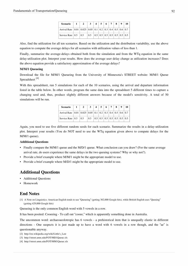
Fundamentals of Transportation/Queueing 92

Scenario 1 2 3 4 5 6 7 8 9 10

Arrival Rate 0.01 0.025 0.05 0.1 0.2 0.3 0.4 0.5 0.6 0.7

Service Rate 0.5 0.5 0.5 0.5 0.5 0.5 0.5 0.5 0.5 0.5

Also, find the utilization for all ten scenarios. Based on the utilization and the distribution variability, use the aboveequation to compute the average delays for all scenarios with utilization values of less than 1.Finally, summarize the average-delays obtained both from the simulation and from the WTq equation in the samedelay-utilization plot. Interpret your results. How does the average user delay change as utilization increases? Doesthe above equation provide a satisfactory approximation of the average delays?M/M/1 Queueing

Download the file for M/M/1 Queueing from the University of Minnesota's STREET website: M/M/1 QueueSpreadsheet [4]

With this spreadsheet, run 5 simulations for each of the 10 scenarios, using the arrival and departure informationlisted in the table below. In other words, program the same data into the spreadsheet 5 different times to capture achanging seed and, thus, produce slightly different answers because of the model's sensitivity. A total of 50simulations will be run.

Scenario 1 2 3 4 5 6 7 8 9 10

Arrival Rate 0.01 0.025 0.05 0.1 0.2 0.3 0.4 0.5 0.6 0.7

Service Rate 0.5 0.5 0.5 0.5 0.5 0.5 0.5 0.5 0.5 0.5

Again, you need to use five different random seeds for each scenario. Summarize the results in a delay-utilizationplot. Interpret your results (You do NOT need to use the WTq equation given above to compute delays for theM/M/1 queue).Additional Questions

• Finally compare the M/M/1 queue and the M/D/1 queue. What conclusion can you draw? (For the same averagearrival rate, do users experience the same delays in the two queuing systems? Why or why not?).

• Provide a brief example where M/M/1 might be the appropriate model to use.• Provide a brief example where M/D/1 might be the appropriate model to use.

Additional Questions• Additional Questions• Homework

End Notes[1] A Note on Linguistics: American English tends to use “Queueing” (getting 302,000 Google hits), while British English uses “Queuing”

(getting 429,000 Google hits)

Queueing is the only common English word with 5 vowels in a row.It has been posited: Cooeeing - To call out “cooee,” which is apparently something done in Australia.The uncommon word: archaeoaeolotropic has 6 vowels - a prehistorical item that is unequally elastic in differentdirections - One suspects it is just made up to have a word with 6 vowels in a row though, and the “ae” isquestionable anyway.[2] http:/ / en. wikipedia. org/ wiki/ Little's_Law[3] http:/ / street. umn. edu/ FOT/ MD1Queue. xls[4] http:/ / street. umn. edu/ FOT/ MM1Queue. xls

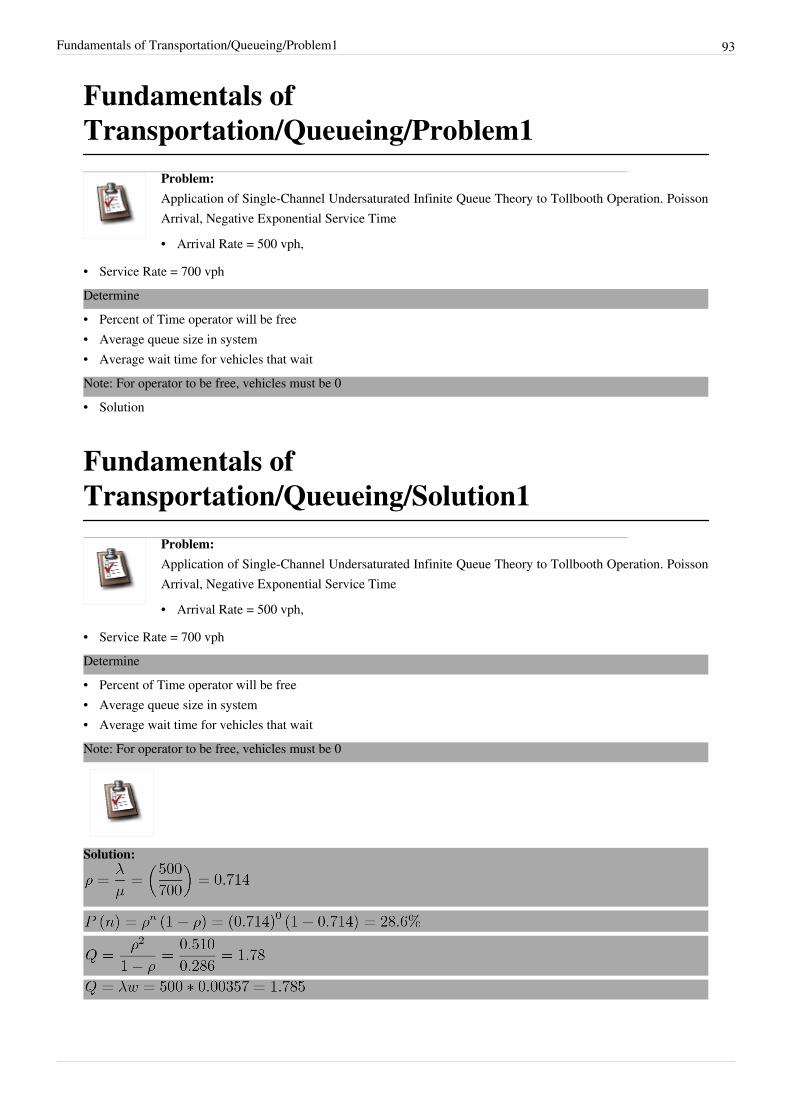
Fundamentals of Transportation/Queueing/Problem1 93

Fundamentals ofTransportation/Queueing/Problem1

Problem:Application of Single-Channel Undersaturated Infinite Queue Theory to Tollbooth Operation. PoissonArrival, Negative Exponential Service Time

• Arrival Rate = 500 vph,

• Service Rate = 700 vphDetermine• Percent of Time operator will be free• Average queue size in system• Average wait time for vehicles that waitNote: For operator to be free, vehicles must be 0• Solution

Fundamentals ofTransportation/Queueing/Solution1

Problem:Application of Single-Channel Undersaturated Infinite Queue Theory to Tollbooth Operation. PoissonArrival, Negative Exponential Service Time

• Arrival Rate = 500 vph,

• Service Rate = 700 vphDetermine• Percent of Time operator will be free• Average queue size in system• Average wait time for vehicles that waitNote: For operator to be free, vehicles must be 0

Solution:

Fundamentals of Transportation/Queueing/Solution1 94

Fundamentals ofTransportation/Queueing/Problem2

Problem:

A ramp has an arrival rate of 200 cars an hour and the ramp meter only permits 250 cars per hour,while the ramp can store 40 cars before spilling over.(A) What is the probability that it is half-full, empty, full?

(B) How many cars do we expect on the ramp?• Solution

Fundamentals ofTransportation/Queueing/Solution2

Problem:

A ramp has an arrival rate of 200 cars an hour and the ramp meter only permits 250 cars per hour,while the ramp can store 40 cars before spilling over.(A) What is the probability that it is half-full, empty, full?

(B) How many cars do we expect on the ramp?Solution:

Part (A)

What is the probability that it is half-full, empty, full?Half-fullEmpty

FullPart (B)

How many cars do we expect on the ramp?

Fundamentals of Transportation/Queueing/Problem3 95

Fundamentals ofTransportation/Queueing/Problem3

Problem:

In this problem we apply the properties of capacitated queues to an expressway ramp. Note thefollowing• Ramp will hold 15 vehicles

• Vehicles can enter expressway at 1 vehicle every 6 seconds• Vehicles arrive at ramp at 1 vehicle every 8 secondsDetermine:(A) Probability of 5 cars,(B) Percent of Time Ramp is Full,(C) Expected number of vehicles on ramp in peak hour.• Solution

Fundamentals ofTransportation/Queueing/Solution3

Problem:

In this problem we apply the properties of capacitated queues to an expressway ramp. Note thefollowing:• Ramp will hold 15 vehicles

• Vehicles can enter expressway at 1 vehicle every 6 seconds• Vehicles arrive at ramp at 1 vehicle every 8 secondsDetermine:(A) Probability of 5 cars,(B) Percent of Time Ramp is Full,(C) Expected number of vehicles on ramp in peak hour.

Solution:

Part A

Probability of 5 cars,

Fundamentals of Transportation/Queueing/Solution3 96

Part B

Percent of time ramp is full (i.e. 15 cars),Part C

Expected number of vehicles on ramp in peak hour.Conclusion, ramp is large enough to hold most queues, though 12 seconds an hour, there will be some rampspillover. It is a policy question as to whether that is acceptable.

Fundamentals of Transportation/Traffic Flow

Traffic Jam in Portugal

Traffic Flow is the study of the movementof individual drivers and vehicles betweentwo points and the interactions they makewith one another. Unfortunately, studyingtraffic flow is difficult because driverbehavior is something that cannot bepredicted with one-hundred percentcertainty. Fortunately, drivers tend tobehave within a reasonably consistent rangeand, thus, traffic streams tend to have somereasonable consistency and can be roughlyrepresented mathematically. To betterrepresent traffic flow, relationships havebeen established between the three maincharacteristics: (1) flow, (2) density, and (3)velocity. These relationships help inplanning, design, and operations of roadway facilities.

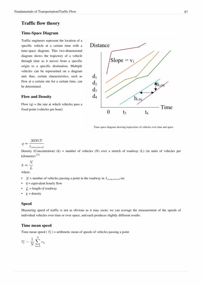
Fundamentals of Transportation/Traffic Flow 97

Traffic flow theory

Time-Space Diagram

Time-space diagram showing trajectories of vehicles over time and space

Traffic engineers represent the location of aspecific vehicle at a certain time with atime-space diagram. This two-dimensionaldiagram shows the trajectory of a vehiclethrough time as it moves from a specificorigin to a specific destination. Multiplevehicles can be represented on a diagramand, thus, certain characteristics, such asflow at a certain site for a certain time, canbe determined.

Flow and Density

Flow (q) = the rate at which vehicles pass afixed point (vehicles per hour)

Density (Concentration) (k) = number of vehicles (N) over a stretch of roadway (L) (in units of vehicles perkilometer) [1]

where:• = number of vehicles passing a point in the roadway in sec• = equivalent hourly flow• = length of roadway• = density

SpeedMeasuring speed of traffic is not as obvious as it may seem; we can average the measurement of the speeds ofindividual vehicles over time or over space, and each produces slightly different results.

Time mean speedTime mean speed ( ) = arithmetic mean of speeds of vehicles passing a point

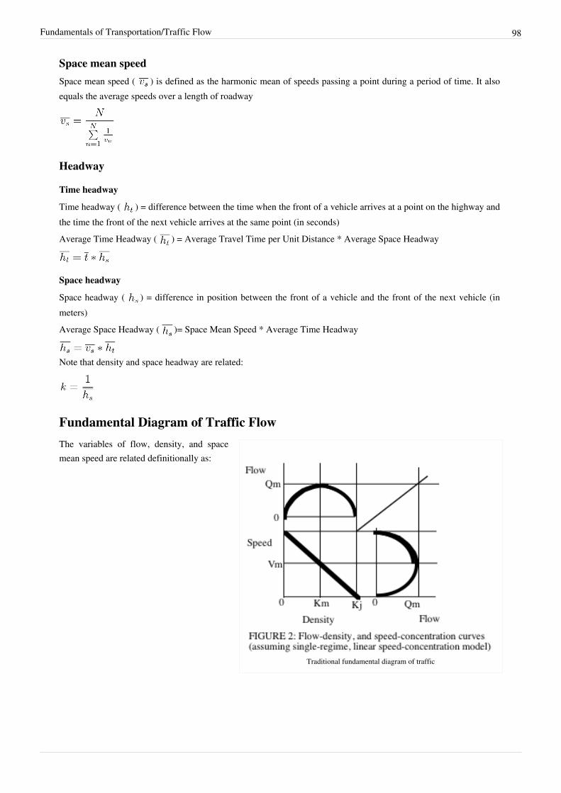
Fundamentals of Transportation/Traffic Flow 98

Space mean speedSpace mean speed ( ) is defined as the harmonic mean of speeds passing a point during a period of time. It alsoequals the average speeds over a length of roadway

Headway

Time headway

Time headway ( ) = difference between the time when the front of a vehicle arrives at a point on the highway andthe time the front of the next vehicle arrives at the same point (in seconds)Average Time Headway ( ) = Average Travel Time per Unit Distance * Average Space Headway

Space headway

Space headway ( ) = difference in position between the front of a vehicle and the front of the next vehicle (inmeters)Average Space Headway ( )= Space Mean Speed * Average Time Headway

Note that density and space headway are related:

Fundamental Diagram of Traffic Flow

Traditional fundamental diagram of traffic

The variables of flow, density, and spacemean speed are related definitionally as:

Fundamentals of Transportation/Traffic Flow 99

Flow varying by density on detector 688 (I-94 at 49th/53rd Avenue inMinneapolis) on November 1st 2000

Traditional Model (Parabolic)Properties of the traditional fundamental diagram.• When density on the highway is zero, the flow is also zero because there are no vehicles on the highway• As density increases, flow increases• When the density reaches a maximum jam density ( ), flow must be zero because vehicles will line up end to

end• Flow will also increase to a maximum value ( ), increases in density beyond that point result in reductions of

flow.• Speed is space mean speed.• At density = 0, speed is freeflow ( ). The upper half of the flow curve is uncongested, the lower half is

congested.• The slope of the flow density curve gives speed. Rise/Run = Flow/Density = Vehicles per hour/ Vehicles per km

= km / hour.

Observation (Triangular or Truncated Triangular)Actual traffic data is often much noisier than idealized models suggest. However, what we tend to see is that asdensity rises, speed is unchanged to a point (capacity) and then begins to drop if it is affected by downstream traffic(queue spillbacks). For a single link, the relationship between flow and density is thus more triangular thanparabolic. When we aggregate multiple links together (e.g. a network), we see a more parabolic shape.

Microscopic and Macroscopic ModelsModels describing traffic flow can be classed into two categories: microscopic and macroscopic. Ideally,macroscopic models are aggregates of the behavior seen in microscopic models.

Fundamentals of Transportation/Traffic Flow 100

Traffic phases in a the microscopic fundamental diagram (truncated triangular)

Traffic phases in the queueing cumulative input-output (Newell) diagram

Microscopic Models

Microscopic models predict the followingbehavior of cars (their change in speed andposition) as a function of the behavior of theleading vehicle.

Macroscropic Models

Macroscopic traffic flow theory relatestraffic flow, running speed, and density.Analogizing traffic to a stream, it hasprincipally been developed for limitedaccess roadways (Leutzbach 1988). Thefundamental relationship “q=kv” (flow (q)equals density (k) multiplied by speed (v)) isillustrated by the fundamental diagram.Many empirical studies have quantified thecomponent bivariate relationships (q vs. v, qvs. k, k vs. v), refining parameter estimatesand functional forms (Gerlough and Huber1975, Pensaud and Hurdle 1991; Ross 1991;Hall, Hurdle and Banks 1992; Banks 1992;Gilchrist and Hall 1992; Disbro and Frame1992).

The most widely used model is theGreenshields model, which posited that therelationships between speed and density islinear. These were most appropriate beforethe advent of high-powered computersenabled the use of microscopic models.Macroscopic properties like flow anddensity are the product of individual(microscopic) decisions. Yet those microscopic decision-makers are affected by the environment around them, i.e.the macroscopic properties of traffic.While traffic flow theorists represent traffic as if it were a fluid, queueing analysis essentially treats traffic as a set ofdiscrete particles. These two representations are not-necessarily inconsistent. The figures to the right show the same4 phases in the fundamental diagram and the queueing input-output diagram. This is discussed in more detail in thenext section.

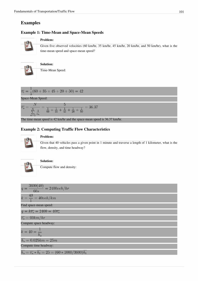
Fundamentals of Transportation/Traffic Flow 101

Examples

Example 1: Time-Mean and Space-Mean Speeds

Problem:

Given five observed velocities (60 km/hr, 35 km/hr, 45 km/hr, 20 km/hr, and 50 km/hr), what is thetime-mean speed and space-mean speed?

Solution:

Time-Mean Speed:

Space-Mean Speed:

The time-mean speed is 42 km/hr and the space-mean speed is 36.37 km/hr.

Example 2: Computing Traffic Flow Characteristics

Problem:

Given that 40 vehicles pass a given point in 1 minute and traverse a length of 1 kilometer, what is theflow, density, and time headway?

Solution:

Compute flow and density:

Find space-mean speed:

Compute space headway:

Compute time headway:

Fundamentals of Transportation/Traffic Flow 102

The time headway is 1.5 seconds.

Thought QuestionProblem

Microscopic traffic flow simulates the behaviors of individual vehicles while macroscopic traffic flow simulates thebehaviors of the traffic stream overall. Conceptually, it would seem that microscopic traffic flow would be moreaccurate, as it would be based off of driver behavior than simply flow characteristics. Assuming microscopicsimulation could be calibrated to truly account for driver behaviors, what is the primary drawback to simulating alarge network?Solution

Computer power. To simulate a very large network with microscopic simulation, the number of vehicles that neededto be assessed is very large, requiring a lot of computer memory. Current computers have issues doing very largemicroscopic networks in a timely fashion, but perhaps future advances will do away with this issue.

Sample Problem• Problem (Solution)

Variables• = distance of nth vehicle• = travel time of nth vehicle• = speed (velocity) of nth vehicle• = time headway between vehicles and • = space (distance) headway between vehicles and • = flow past a fixed point (vehicles per hour)• = number of vehicles• = time over which measurement takes place (number of seconds)• = travel time• = density (vehicles per km)• = length of roadway section (km)• = time mean speed• = space mean speed• = freeflow (uncongested speed)• = jam density• = maximum flow

Fundamentals of Transportation/Traffic Flow 103

Key Terms• Time-space diagram• Flow, speed, density• Headway (space and time)• Space mean speed, time mean speed• Microscopic, Macroscopic

Supplementary Reading• Revised Monograph on Traffic Flow Theory [2]

References• Banks, J.H. (1991). Two Capacity Phenomenon at Freeway Bottlenecks: A Basis for Ramp Metering?

Transportation Research Record 1320, pp. 83-90.• Banks, James H. (1992). “Freeway Speed-Flow-Concentration Relationships: More Evidence and Interpretations.”

Transportation Research Record 1225:53-60.• Cassidy, M.J. and R.L. Bertini (1999) Some Traffic Features at Freeway Bottlenecks. Transportation Research

Part B Vol. 33, pp. 25-42• Disbro, John E. and Frame, Michael. (1992). “Traffic Flow Theory and Chaotic Behavior.” Transportation

Research Record. 1225: 109-115.• Gerlough, Daniel L. and Huber, Matthew J. (1975). Traffic Flow Theory: A Monograph TRB Special Report 165.

Transportation Research Board, Washington DC.• Gilchrist, Robert S. and Fred L. Hall. (1992). “Three-Dimensional Relationships Among Traffic Flow Theory

Variables.” Transportation Research Record. 1225:99-108.• Hall, F.L. and K. Agyemang-Duah (1991). Freeway Capacity Drop and the Definition of Capacity. Transportation

Research Record 1320, pp. 91-98• Hall, Fred L., Hurdle, V. F., and Banks, James H. (1992). “A Synthesis of Recent Work on the Nature of

Speed-Flow and Flow-Occupancy (or Density) Relationships on Freeways”. presented at TRB 71st AnnualMeeting, Washington DC.

• Pensaud, B.N. and Hurdle, V. F. (1991). “Some New Data That Challenge Some Old Ideas About Speed-FlowRelationships.” Transportation Research Record. 1194: 191-8.

• Ross, Paul. (1991). “Some Properties of Macroscopic Traffic Models.” Transportation Research Record. 1194:129-34.

End Notes[1] Note: We use k because the word is Konzentration in German[2] http:/ / www. tfhrc. gov/ its/ tft/ tft. htm

Fundamentals of Transportation/Traffic Flow/Problem 104

Fundamentals of Transportation/TrafficFlow/Problem

Problem:

Four vehicles are traveling at constant speeds between sections X and Y (280 meters apart) with theirpositions and speeds observed at an instant in time. An observer at point X observes the four vehiclespassing point X during a period of 15 seconds. The speeds of the vehicles are measured as 88, 80, 90,

and 72 km/hr respectively. Calculate the flow, density, time mean speed, and space mean speed of the vehicles.• Solution

Fundamentals of Transportation/TrafficFlow/Solution

Problem:

Four vehicles are traveling at constant speeds between sections X and Y (280 meters apart) with theirpositions and speeds observed at an instant in time. An observer at point X observes the four vehiclespassing point X during a period of 15 seconds. The speeds of the vehicles are measured as 88, 80, 90,

and 72 km/hr respectively. Calculate the flow, density, time mean speed, and space mean speed of the vehicles.Solution:

Flow

Density

Time Mean Speed

Space Mean Speed

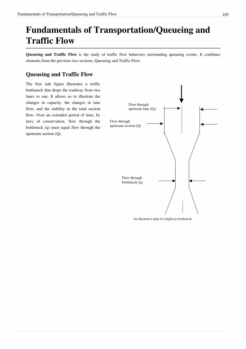
Fundamentals of Transportation/Queueing and Traffic Flow 105

Fundamentals of Transportation/Queueing andTraffic FlowQueueing and Traffic Flow is the study of traffic flow behaviors surrounding queueing events. It combineselements from the previous two sections, Queueing and Traffic Flow.

Queueing and Traffic Flow

An illustrative plan of a highway bottleneck

The first side figure illustrates a trafficbottleneck that drops the roadway from twolanes to one. It allows us to illustrate thechanges in capacity, the changes in laneflow, and the stability in the total sectionflow. Over an extended period of time, bylaws of conservation, flow through thebottleneck (q) must equal flow through theupstream section (Q).

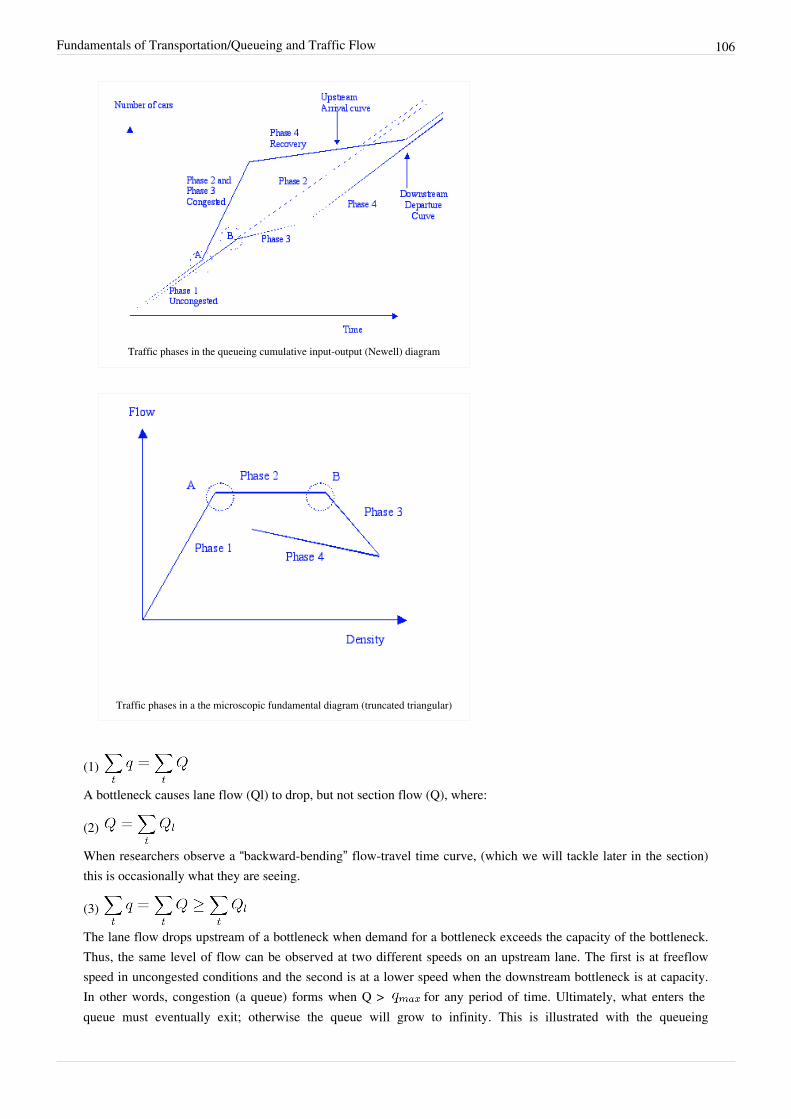
Fundamentals of Transportation/Queueing and Traffic Flow 106

Traffic phases in the queueing cumulative input-output (Newell) diagram

Traffic phases in a the microscopic fundamental diagram (truncated triangular)

(1)

A bottleneck causes lane flow (Ql) to drop, but not section flow (Q), where:

(2)

When researchers observe a “backward-bending” flow-travel time curve, (which we will tackle later in the section)this is occasionally what they are seeing.

(3)

The lane flow drops upstream of a bottleneck when demand for a bottleneck exceeds the capacity of the bottleneck. Thus, the same level of flow can be observed at two different speeds on an upstream lane. The first is at freeflow speed in uncongested conditions and the second is at a lower speed when the downstream bottleneck is at capacity. In other words, congestion (a queue) forms when Q > for any period of time. Ultimately, what enters the queue must eventually exit; otherwise the queue will grow to infinity. This is illustrated with the queueing

Fundamentals of Transportation/Queueing and Traffic Flow 107

input-output (IO) diagram shown in the second side figure. We can identify four distinct phases in traffic.• Phase 1 is the uncongested phase when there is no influence of the increasing density on the speeds of the

vehicles. The speed does not drop with the introduction of newer vehicles onto the freeway.• Phase 2 finds the freeway cannot sustain the speed with injection of newer vehicles into the traffic stream. The

density increases while speed falls, maintaining the flow.• Phase 3 shows decreased speed and decreased flows. This is caused by very low speeds cause the queue discharge

to drop (slightly) at an active bottleneck, or a queue from a downstream bottleneck may be constraining the flow.As reported by many researchers (Banks, 1991; Hall and Agyemang-Duah, 1991; Persaud and Hurdle, 1991;Cassidy and Bertini, 1999), the reduced bottleneck capacity after breakdown ranges from 0% to 8%. A majorityof papers conclude that the section capacity reduction a queue presents is negligible. (As noted above, lane flowupstream of a bottleneck does drop, but this is due to the downstream bottleneck). This is a second source of the“backward-bending” phenomenon.

• Phase 4 is the recovery phase. During this phase, the density of traffic starts decreasing and speed startsincreasing.

The circled region, ‘A’ (in the third side figure) is typically where we start observing ‘freeway breakdown’. In otherwords, this region occurs when upstream flow exceeds some critical downstream capacity at a specific point andthere is a drop in speed. In the circled region, ‘B’, flow drops are associated with very low speeds. The phenomenonis particularly evidenced by the formation of queues upstream of where the breakdown occurs and a low dischargerate of vehicles due to sustained low speeds.Traditional queues have “servers”. For example, the check-out line at the grocery store can serve one customer every5 minutes, or one item every 10 seconds, etc. A conveyor belt can serve so many packages per hour. Capacity isoften referred to as belonging to the road. However when we talk about road capacity, it is really a misnomer, ascapacity is located in the driver, more precisely in the driver’s willingness and ability to drive behind the driverahead. If drivers were willing and able to drive behind the vehicle ahead with no gap (spacing between vehicles), andthat driver was driving behind the driver ahead of him with no gap, and so on, at high speeds, many more vehiclesper hour could use the road. However, while some compression of vehicles occurs in heavy traffic, this situation isunstable because a driver will tap the brakes or even let-up on the accelerator for any number of reasons (to changelanes, to respond to someone else trying to change lanes, because he sees an object in the road, to limit the forceswhen rounding a corner, etc). This by definition lowers his speed, which in turn will lower the flow. Risk-aversedrivers behind him will slow down even more (the driver has established some unpredictability in behavior, it isreasonable for other drivers to establish an even larger gap to accommodate the unpredictable driver’s behavior,especially given there is a reaction time between the lead driver’s actions, and the following driver’s perception (leadvehicle is slowing), decision (must brake), action (tap the brakes), the vehicle’s response to the action (tighten brakeson wheel)). In this way, maximum flow possible, our capacity ( ), is a function of the drivers. The road shapesthe driver’s willingness to take risks. Drivers will slow down around curves, vehicles may have difficultyaccelerating uphill, or even from a slower speed (and even if they don’t, driver’s may provide insufficient fuel beforethey realize they are going too slow by not giving the vehicle enough gas), merges take time to avoid collision, etc.Clearly, different drivers and different vehicles (for instance racecars or taxis) could increase the maximum flowthrough the bottleneck ( ). It is better to think of capacity as a maximum sustainable flow (over an extendedperiod of time), given typical drivers’ willingness to follow (subject to highway geometrics and environmentalconditions) and their vehicles’ ability to respond to decisions. A series of aggressive drivers may exceed this‘capacity’ for a short period of time, but eventually more cautious drivers will even out the function.The IO diagram lets us understand delay in a way that the fundamental diagrams of traffic flow don’t easily allow. The first point to note about the IO diagram is that delay differs for each driver. The average delay can be measured easily (the total area in the triangle is the total delay, the average delay is just that triangle divided by the number of vehicles). The variation (or standard deviation) can also be measured with some more statistics. As the total number

Fundamentals of Transportation/Queueing and Traffic Flow 108

of vehicles increases, the average delay increases.The second point to note about the IO diagram is that the total number of queued vehicles (the length of the queue)can also be easily measured. This also changes continuously; the length of the queue rises and falls with changes inthe arrival rate (the tail of the queue edge of the shockwave, where travel speed changes suddenly). Shockwavesindicate a change in state, or speed that suddenly occurs. One such shockwave is found where vehicles reach theback of queues. The arrival rate, coupled with the queue clearance rate, will tell you where the back of the queue is.This is interesting and is where the traveler first suffers delay – but it is not the source of the delay.Only if the arrival rate exactly equals the departure rate would we expect to see a fixed length of the queue. If thequeue results from a management practice (such as ramp metering), we can control the departure rate to match thearrival rate, and ensure that the queue remains on the ramp and doesn’t spill over to neighboring arterials. Howeverthat observation suggests that congested “steady state” is likely to be a rare phenomenon, since in general the arrivalrate does not equal the service rate.Queueing analysts often make a simplifying assumption that vehicles stack vertically (queues take place at a point).This is of course wrong, but not too wrong. The resulting travel time is almost the same as if the queue weremeasured over space. The difference is that the time required to cover distance is included when we make the betterassumption, even under freeflow conditions it takes time to travel from the point where a vehicle entered the back ofthe queue to the point where it exits the front. We can make that correction, but when queueing is taking place, thattime is often small compared to the time delayed by the queue. We also assume a first-in, first-out logic, thoughagain this can be relaxed without distracting from the main point. Another assumption we will make for exposition isthat this is a deterministic process; vehicles arrive in a regular fashion and depart in a regular fashion. Howeversometimes vehicles bunch up (drivers are not uniform), which leads to stochastic arrivals and departures. Thisstochastic queueing can be introduced, and will in general increase the measured delay.

Hypercongestion

It has been observed that the same flow canbe achieved on many links at two differentspeeds. Some call this the“backward-bending” phenomenon (Hau1998, Crozet and Marlot 2001). Thequeueing analysis framework also hasimplications for “hypercongestion” or“backward-bending” flow-travel time curves,such as shown in the figure to the right.Recall we identified two sources for“backward-bending” speed-flowrelationships. The first has to do with thepoint of observation. Observing the lane flowupstream of a bottleneck gives theimpression of a backward bendingrelationship, but this disappears at thebottleneck itself. Under any given demand pattern, flow and speed are a unique pair. When demand is below thedownstream active bottleneck’s capacity, a flow on an upstream link can be achieved at high speed. When demand isabove the downstream active bottleneck’s capacity, the same flow on the upstream link can only be achieved at a lowspeed because of queueing. The second has to do with a capacity drop at the bottleneck itself under congestedconditions. However, much research reports that this drop is slight to non-existent.

Fundamentals of Transportation/Queueing and Traffic Flow 109

As in the bottleneck, we define lowercase q to be flow (vehicles per hour) departing the front of the bottleneck anduppercase Q to be flow arriving at the back of the bottleneck. We also define k to be density (vehicles per kilometer),v to be speed (kilometers per hour), and s to be service rate (seconds per vehicle). The fundamental diagrams oftraffic flow (q-k-v curves) represent a model of traffic flow as stylized in the traditional textbook representation ofthe fundamental diagram of traffic flow. The reasons why q should drop as k increases beyond a certain point at anisolated bottleneck are unclear. In other words, why should flow past a point drop just because the number ofvehicles behind that point increases? Why should leading traffic be influenced by the behavior of following traffic?If traffic behaves as a queue through a bottleneck (illustrated above), we should consider reasons why traffic flowdeparting the queue would not stay at its maximum.One reason is if the vehicles in the queue could not travel fast enough so that the front of the following car could notreach the point of the front of the leading car in the time allotted the service rate. If a lane serves 1800 vehicles perhour, it serves 1 vehicle every 2 seconds, we say there is a 2 second service rate. If there were a 10 meter spacingbetween the vehicles (including the vehicle length plus a physical gap), this implies that the service rate would beworse than 1 vehicle every 2 seconds only if it took longer than 2 seconds to travel 10 meters (i.e. speed < 18 km/hour). This is very slow traffic and may properly be called hypercongestion. Why would traffic get that slow iffreeflow speed is 120 km / hour? In general traffic departing the front of the queue won’t be traveling that slowly, asthe shockwave that reduces speed (the wave of red brake lights) has moved to the back of the queue.A second reason the bottleneck flow might drop is if the departure flow is affected by external sources, namely abottleneck further downstream spilling backwards. If the queue at a downstream bottleneck becomes sufficientlylong, it will reduce the number of vehicles that can depart the upstream bottleneck. This is because the firstbottleneck is no longer controlling, the downstream bottleneck is.A third reason that bottleneck flow might drop is if the bottleneck is not being fully served (slots for cars are goingunfilled). If vehicles are separated by large time headways, then the bottleneck might lose capacity. Thus, if vehicleschoose large gaps, the bottleneck flow might drop. However, in congested situations, vehicles tend to follow moreclosely, not less closely.For an isolated bottleneck, the departure flow remains (essentially) a constant and arrival flow varies. As morevehicles arrive at the back of the queue, the expected wait at the queue increases. All vehicles will eventually beserved. In general, there is no practical constraint on the number of vehicles arriving at the back of the queue, butthere is a maximum output flow in vehicles per unit time. Examining traffic upstream of the bottleneck is interesting,but does not get to the root of the problem – the bottleneck itself. This view of hypercongestion is thus notinconsistent with the conclusion drawn by Small and Chu (1997) that the hypercongested region is unsuitable for useas a supply curve in congestion pricing analyses.

Thought QuestionProblem

Bottlenecks are shown here to be the main cause of traffic flow congestion and queueing. The examples given are oflane drops, which are not very common (some drivers think they're more common than they actually are). Is this theonly way a bottleneck can form?Solution

Absolutely not. A bottleneck is defined as a constriction of traffic flow, where demand exceeds available capacity.Infrastructure-wise, a bottleneck would be where a lane drop is present, where lane widths decrease, or a sightobstruction lowers the natural free-flow speed. However, bottlenecks can also form because of traffic. Chaotictraffic, primarily where lane changing is occurring, is a prime source of a bottleneck. On-ramps, off-ramps, andweaving areas are the most common examples, but there are many more. Think about how often you have been stuckin standstill traffic where a lane drop is not present.

Fundamentals of Transportation/Queueing and Traffic Flow 110

Additional Questions• Additional Questions

Variables• - Flow through the bottleneck• - Flow through the upstream section• - Lane Flow• - time

Key Terms• Bottleneck• Queueing• Traffic Flow• Lane Flow• Lane Flow Drops• Flow-Travel Time Curve• "Backwards-Bending"• IO• Hypercongestion

ReferencesReferences on Queueing and Traffic Flow

• Banks, J.H. (1991). Two Capacity Phenomenon at Freeway Bottlenecks: A Basis for Ramp Metering?Transportation Research Record 1320, pp. 83-90.

• Banks, James H. (1992). “Freeway Speed-Flow-Concentration Relationships: More Evidence and Interpretations.”Transportation Research Record 1225:53-60.

• Cassidy, M.J. and R.L. Bertini (1999) Some Traffic Features at Freeway Bottlenecks. Transportation ResearchPart B Vol. 33, pp. 25-42

• Hall, F.L. and K. Agyemang-Duah (1991). Freeway Capacity Drop and the Definition of Capacity. TransportationResearch Record 1320, pp. 91-98

• Persaud, B.N. and Hurdle, V. F. (1991). “Some New Data That Challenge Some Old Ideas About Speed-FlowRelationships.” Transportation Research Record. 1194: 191-8.

• Persaud, B.N. and V.F. Hurdle (1991). Freeway Capacity: Definition and Measurement Issues. Proceedings of theInternational Symposium of Highway Capacity, A.A. Balkema press, Germany, pp.289-307

References on Hypercongestion

• Crozet, Yves Marlot, Gregoire (2001) "Congestion and Road Pricing: Where Is The 'Bug'?" 9th WorldConference on Transport Research

• Hau, T.D. (1998) “Congestion pricing and road investment”, in: K.J. Button and E.T. Verhoef, eds., Road pricing,traffic congestion and the environment: Issues of efficiency and social feasibility. Cheltenham: Edward Elgar.

• Small, Kenneth and Xuehao Chu. 1997. "Hypercongestion", Working Paper No. 96-97-11, Department ofEconomics, University of California, Irvine.

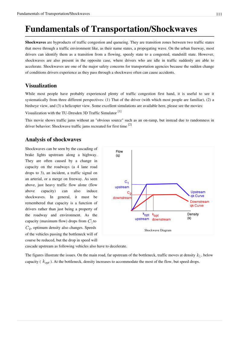
Fundamentals of Transportation/Shockwaves 111

Fundamentals of Transportation/ShockwavesShockwaves are byproducts of traffic congestion and queueing. They are transition zones between two traffic statesthat move through a traffic environment like, as their name states, a propogating wave. On the urban freeway, mostdrivers can identify them as a transition from a flowing, speedy state to a congested, standstill state. However,shockwaves are also present in the opposite case, where drivers who are idle in traffic suddenly are able toaccelerate. Shockwaves are one of the major safety concerns for transportation agencies because the sudden changeof conditions drivers experience as they pass through a shockwave often can cause accidents.

VisualizationWhile most people have probably experienced plenty of traffic congestion first hand, it is useful to see itsystematically from three different perspectives: (1) That of the driver (with which most people are familiar), (2) abirdseye view, and (3) a helicopter view. Some excellent simulations are available here, please see the movies:Visualization with the TU-Dresden 3D Traffic Simulator [1]

This movie shows traffic jams without an "obvious source" such as an on-ramp, but instead due to randomness indriver behavior: Shockwave traffic jams recreated for first time [2]

Analysis of shockwaves

Shockwave Diagram

Shockwaves can be seen by the cascading ofbrake lights upstream along a highway.They are often caused by a change incapacity on the roadways (a 4 lane roaddrops to 3), an incident, a traffic signal onan arterial, or a merge on freeway. As seenabove, just heavy traffic flow alone (flowabove capacity) can also induceshockwaves. In general, it must beremembered that capacity is a function ofdrivers rather than just being a property ofthe roadway and environment. As thecapacity (maximum flow) drops from to

, optimum density also changes. Speedsof the vehicles passing the bottleneck will ofcourse be reduced, but the drop in speed willcascade upstream as following vehicles also have to decelerate.

The figures illustrate the issues. On the main road, far upstream of the bottleneck, traffic moves at density , belowcapacity ( ). At the bottleneck, density increases to accommodate the most of the flow, but speed drops.

Fundamentals of Transportation/Shockwaves 112

Shockwave Diagram

Shockwave Math

Shockwave speed

If the flow rates in the two sections are and , then and .

Relative speedWith equal to the space mean speed of vehicles in area 1, the speed relative to the line is:

The speed of vehicles in area 2 relative to the line w is

Boundary crossingThe number of vehicles crossing line 2 from area 1 during time period is

and similarly

By conservation of flow, the number of vehicles crossing from left equals the number that crossed on the right

so:

or

which is equivalent to

Fundamentals of Transportation/Shockwaves 113

Examples

Example 1

Problem:The traffic flow on a highway is with speed of . As the result of anaccident, the road is blocked. The density in the queue is . (Jam density, vehicle length = 3.63meters).• (A) What is the wave speed ( )?• (B) What is the rate at which the queue grows, in units of vehicles per hour ( )?

Solution:

(A) At what rate does the queue increase?1. Identify Unknowns:

2. Solve for wave speed ( )

Conclusion: the queue grows against traffic(B) What is the rate at which the queue grows, in units of vehicles per hour?

Thought QuestionProblem

Shockwaves are generally something that transportation agencies would like to minimize on their respectivecorridor. Shockwaves are considered a safety concern, as the transition of conditions can often lead to accidents,sometimes serious ones. Generally, these transition zones are problems because of the inherent fallibility of humanbeings. That is, people are not always giving full attention to the road around them, as they get distracted by acolorful billboard, screaming kids in the backseat, or a flashy sports car in the adjacent lanes. If people were able togive full attention to the road, would these shockwaves still be causing accidents?Solution

Yes, but not to the same extent. While accidents caused by driver inattentiveness would decrease nearly to zero,accidents would still be occurring between different vehicle types. For example, in a case where conditions changevery dramatically, a small car (say, a Beetle) would be able to stop very quickly. A semi truck, however, is a much

Fundamentals of Transportation/Shockwaves 114

heavier vehicle and would require a longer distance to stop. If both were moving at the same speed whenencountering the shockwave, the truck may not be able to stop in time before smashing into the vehicle ahead ofthem. That is why most trucks are seen creeping along through traffic with very big gaps ahead of them.

Sample Problem• Problem (Solution)

Additional Questions• Additional Questions• Homework

Variables• - flow• - capacity (maximum flow)• - density• - speed• - relative speed (travel speed minus wave speed)• - wave speed• - number of vehicles crossing wave boundary

Key Terms• Shockwaves• Time lag, space lag

References[1] http:/ / www. vwi. tu-dresden. de/ ~treiber/ movie3d/ index. html[2] http:/ / www. youtube. com/ watch?v=Suugn-p5C1M

Fundamentals of Transportation/Shockwaves/Problem 115

Fundamentals ofTransportation/Shockwaves/Problem

Problem:

Flow on a road is , and the density of . To reducespeeding on a section of highway, a police cruiser decides to implement a rolling roadblock, and to travel in the leftlane at the speed limit ( ) for 10 km. No one dares pass. After the police cruiser joins, the platoondensity increases to 20 veh/km/lane and flow drops. How many vehicles (per lane) will be in the platoon when thepolice car leaves the highway?• Solution

Fundamentals ofTransportation/Shockwaves/Solution

Problem:

Flow on a road is , and the density of . To reducespeeding on a section of highway, a police cruiser decides to implement a rolling roadblock, and to travel in the leftlane at the speed limit ( ) for 10 km. No one dares pass. After the police cruiser joins, the platoondensity increases to 20 veh/km/lane and flow drops. How many vehicles (per lane) will be in the platoon when thepolice car leaves the highway?

Solution:

Step 0

Solve for Unknowns:Original speed

Flow after police cruiser joins

Step 1

Calculate the wave velocity:

Step 2

Determine the growth rate of the platoon (relative speed)

Fundamentals of Transportation/Shockwaves/Solution 116

Step 3

Determine the time spent by the police cruiser on the highway

Step 4

Calculate the Length of platoon (not a standing queue)

Step 5

What is the rate at which the queue grows, in units of vehicles per hour?Step 6

The number of vehicles in platoon

OR

Fundamentals of Transportation/Traffic Signals

A Traffic Light

Traffic Signals are one of the more familiar types of intersectioncontrol. Using either a fixed or adaptive schedule, traffic signalsallow certain parts of the intersection to move while forcing otherparts to wait, delivering instructions to drivers through a set ofcolorful lights (generally, of the standard red-yellow (amber)-greenformat). Some purposes of traffic signals are to (1) improve overallsafety, (2) decrease average travel time through an intersection, and(3) equalize the quality of services for all or most traffic streams.Traffic signals provide orderly movement of intersection traffic,have the ability to be flexible for changes in traffic flow, and canassign priority treatment to certain movements or vehicles, such asemergency services. However, they may increase delay during theoff-peak period and increase the probability of certain accidents,such as rear-end collisions. Additionally, when improperlyconfigured, driver irritation can become an issue. Traffic signals aregenerally a well-accepted form of traffic control for busyintersections and continue to be deployed. Other intersectioncontrol strategies include signs (stop and yield) and roundabouts.Intersections with high volumes may be grade separated.

Fundamentals of Transportation/Traffic Signals 117

Intersection QueueingAt an intersection where certain approaches are denied movement, queueing will inherently occur. Of the variousqueueing models, one of the more commons and simple ones is the D/D/1 Queueing Model. This model assumes thatarrivals and departures are deterministic (D) and one departure channel exists. D/D/1 is quite intutive and easilysolvable. Using this form of queueing with an arrival rate and a departure rate , certain useful values regardingthe consequences of queues can be computed.One important piece of information is the duration of the queue for a given approach. This time value can becalculated through the following formula:

Where:• = Time for queue to clear• = Arrival Rate divided by Departure Rate• = Red TimeWith this, various proportions dealing with queues can be calculated. The first determines the proportion of cyclewith a queue.

Where:

• = Proportion of cycle with a queue• = Cycle LenghSimilarly, the proportion of stopped vehicles can be calculated.

Where:• = Proportion of Stopped Vehicles• = Green TimeTherefore, the maximum number of vehicles in a queue can be found.

Intersection delayVarious models of intersection delay at isolated intersections have been put forward, combining queuing theory withempirical observations of various arrival rates and discharge times (Webster and Cobbe 1966; Hurdle 1985; Hagenand Courage 1992). Intersections on arterials are more complex phenomena, including factors such as signalprogression and spillover of queues between adjacent intersections. Delay is broken into two parts: uniform delay,which is the delay that would occur if the arrival pattern were uniform, and overflow delay, caused by stochasticvariations in the arrival patterns, which manifests itself when the arrival rate exceeds the service flow of theintersection for a time period.Delay can be computed with knowledge of arrival rates, departure rates, and red times. Graphically, total delay is theproduct of all queues over the time period in which they are present.

Fundamentals of Transportation/Traffic Signals 118

Similarly, average vehicle delay per cycle can be computed.

From this, maximum delay for any vehicle can be found.

Level of ServiceIn order to assess the performance of a signalized intersection, a qualitative assessment called Level of Service(LOS) is assessed, based upon quantitative performance measures. For LOS, the performance measured used isaverage control delay per vehicle. The general procedure for determining LOS is to calculate lane group capacities,calculate delay, and then make a determination.Lane group capacities can be calculated through the following equation:

Where:• = Lane Group Capacity• = Adjusted Saturation Flow Rate• = Effective Green Length• = Cycle LengthAverage control delay per vehicle, thus, can be calculated by summing the types of delay mentioned earlier.

Where:• = Average Signal Delay per vehicle (sec)• = Average Delay per vehicle due to uniform arrivals (sec)• = Progression Adjustment Factor• = Average Delay per vehicle due to random arrivals (sec)• = Average delay per vehicle due to initial queue at start of analysis time period (sec)Uniform delay can be calculated through the following formula:

Where:• = Volume/Capacity (v/c) ratio for lane group.Similarly, random delay can be calculated:

Where:• = Duration of Analysis Period (in hours)

Fundamentals of Transportation/Traffic Signals 119

• = Delay Adjustment Factor that is dependent on signal controller mode• = Upstream filtering/metering adjustment factorOverflow delay generally only applies to densely urban corridors, where queues can sometimes spill over intoprevious intersections. Since this is not very common (usually the consequence of a poorly timed intersectionsequence, the rare increase of traffic demand, or an emergency vehicle passing through the area), it is generally nottaken into account for simple problems.Delay can be calcaulated for individual vehicles in certain approaches or lane groups. Average delay per vehicle foran approach A can be calculated using the following formula:

Where:• = Average Delay per vehicle for approach A (sec)• = Average Delay per vehicle for lane group i on approach A (sec)• = Analysis flow rate for lane group iAverage delay per vehicle for the intersection can then be calculated:

Where:• = Average Delay per vehicle for the intersection (sec)• = Average Delay per vehicle for approach A (sec)• = Analysis flow rate for approach A

Critical Lane GroupsFor any combination of lane group movements, one lane group will dictate the necessary green time during aparticular phase. This lane group is called the Critical Lane Group. This lane group has the highest traffic intensity(v/s) and the allocation of green time for each phase is based on this ratio.The sum of the flow ratios for the critical lane groups can be used to calculate a suitable cycle length.

Where:• = Sum of Flow Ratios for Critical Lane Groups• = Flow Ratio for Critical Lane Group i• = Number of Critical Lane GroupsSimilarly, the total lost time for the cycle is also an element that can be used in the calculation of cycle length.

Where:• = Total lost Time for Cycle• = Total Lost Time for Critical Lane Group i

Fundamentals of Transportation/Traffic Signals 120

Cycle Length CalcuationCycle lengths are calculated by summing individual phase lengths. Using the previous formulas for assistance, theminimum cycle length necessary for the lane group volumes and phasing plan can be easily calculated.

Where:• = Minimum necessary cycle length• = Critical v/c ratio for the intersection• = Flow Ratio for Critical Lane Group• = Number of Critical Lane GroupsThis equation calculates the minimum cycle length necesary for the intersection to operate at an acceptable level, butit does not necessarily minimize the average vehicle delay. A more optimal cycle length usually exists that wouldminimize average delay. Webster (1958) proposed an equation for the calculation of cycle length that seeks tominize vehicle delay. This optimum cycle length formula is listed below.

Where:

• = Optimal Cycle Length for Minimizing Delay

Green Time AllocationOnce cycle length has been determined, the next step is to determine the allocation of green time to each phase.Several strategies for allocating green time exist. One of the more popular ones is to distribute green time such thatv/c ratios are equalized over critical lane groups. Similarly, v/c ratios can be found with predetermined values forgreen time.

Where:• = v/c ratio for lane group iWith knowledge of cycle lengths, lost times, and v/s ratios, the degree of saturation for an intersection can be found.

Where:• = Degree of saturation for an intersection cycleFrom this, the total effective green for all phases can be computed.

Fundamentals of Transportation/Traffic Signals 121

Demonstrations• Flash animation: Signal Phasing (by Karen Dixon and Thomas Wall) [1]

• Flash animation: Signal Progression (by Karen Dixon and Thomas Wall) [2]

Examples

Example 1: Intersection Queueing

Problem:

An approach at a pretimed signalized intersection has an arrival rate of 0.1 veh/sec and a saturationflow rate of 0.7 veh/sec. 20 seconds of effective green are given in a 60-second cycle. Provide analysisof the intersection assuming D/D/1 queueing.

Solution:

Traffic intensity, , is the first value to calculate.

Red time is found to be 40 seconds (C - g = 60 - 20). The remaining values of interest can be easily found.Time to queue clearance after the start of effective green:

Proportion of the cycle with a queue:

Proportion of vehicles stopped:

Maximum number of vehicles in the queue:

Total vehicle delay per cycle:

Average delay per vehicle:

Maximum delay of any vehicle:

Fundamentals of Transportation/Traffic Signals 122

Example 2: Total Delay

Problem:

Compute the average approach delay given certain conditions for a 60-second cycle lengthintersection with 20 seconds of green, a v/c ratio of 0.7, a progression neutral state (PF=1.0), and nochance of intersection spillover delay (overflow delay). Assume the traffic flow accounts for the peak

15-minute period and a lane capacity of 840 veh/hr.Solution:

Uniform Delay:

Random Delay:(from problem statement)

(for pretimed control)(isolated intersection)

Overflow Delay:Overflow delay is zero because it is assumed that there is no overflow.

Total Delay:

The average total delay is 22.22 seconds.

Example 3: Cycle Length Calculation

Problem:

Calculate the minimum and optimal cycle lengths for the intersection of Oak Street and WashingtonAvenue, given that the critical v/c ratio is 0.9, the two critical approaches have a v/s ratio of 0.3, andthe Lost Time equals 15 seconds.

Solution:

Minimum Cycle Length:

Optimal Cycle Length:

Fundamentals of Transportation/Traffic Signals 123

The minimum cycle length is 45 seconds and the optimal cycle length is 68.75 seconds.

Thought QuestionProblem

Why don't signalized intersections perform more efficiently than uncontrolled intersections?Solution

The inherent lost time that comes from each signal change is wasted time that does not occur when intersections areuncontrolled. It comes at quite a surprise to most of the Western World, where traffic signals are plentiful, but thereare intersections that perform quite well without any form of control. There is an infamous video on YouTube thatshows an uncontrolled intersection in India where drivers somehow navigate through a busy, chaotic environmentsmoothly and efficiently [3] . The video is humorous to watch, but it shows a valid point that uncontrolledintersections can indeed work and are quite efficient. However, the placement of traffic signals is for safety, asdrivers entering an uncontrolled intersection have a higher likelihood of being involved in a dangerous accident, suchas a T-bone or head-on collision, particularly at high speed.

Sample ProblemProblem (Solution)

Additional QuestionsHomework

Variables• - Time for queue to clear• - Arrival Rate divided by Departure Rate• - Red Time

• - Proportion of cycle with a queue• - Proportion of Stopped Vehicles• - Lane Group Capacity• - Adjusted Saturation Flow Rate• - Effective Green Length• - Cycle Length• - Average Signal Delay per vehicle (sec)• - Average Delay per vehicle due to uniform arrivals (sec)• - Progression Adjustment Factor• - Average Delay per vehicle due to random arrivals (sec)• - Average delay per vehicle due to initial queue at start of analysis time period (sec)• - Volume/Capacity (v/c) ratio for lane group.• - Duration of Analysis Period (in hours)

Fundamentals of Transportation/Traffic Signals 124

• - Delay Adjustment Factor that is dependent on signal controller mode• - Upstream filtering/metering adjustment factor• - Average Delay per vehicle for approach A (sec)• - Average Delay per vehicle for lane group i on approach A (sec)• - Analysis flow rate for lane group i• - Average Delay per vehicle for the intersection (sec)• - Analysis flow rate for approach A• - Sum of Flow Ratios for Critical Lane Groups

• - Flow Ratio for Critical Lane Group i• - Number of Critical Lane Groups• - Minimum necessary cycle length• - Critical v/c ratio for the intersection

• - Flow Ratio for Critical Lane Group• - Optimal Cycle Length for Minimizing Delay• - v/c ratio for lane group i• - Degree of saturation for an intersection cycle

Key Terms• Delay• Total Delay• Average Delay• Uniform Delay• Random Delay• Overflow Delay• Cycle Length• v/c ratio• v/s ratio• Saturation Flow Rate• Red Time• Effective Green• Minimum Cycle Length• Optimal Cycle Length• Critical Lane Group• Degree of Saturation• Progression Adjustment Factor• Lost Time• Queue

Fundamentals of Transportation/Traffic Signals 125

External ExercisesUse the GAME software at the STREET website [1] to learn how to coordinate traffic signals to reduce delay.Use the OASIS software at the STREET website [1] to study how signals change when given information abouttime-dependent vehicle arrivals.

References• Hagen, Lawrence T. and Courage, Kenneth. (1992). “Comparison of Macroscopic Models for Signalized

Intersection Analysis.” Transportation Research Record. 1225: 33-44.• Hurdle, V. F. (1982). “Signalized Intersections: A Primer for the Uninitiated.” Transportation Research Record

971:96-105.• Webster, F.V. (1958). Traffic Signal Settings. Road Research Technical Paper No. 39. London: Great Britain

Road Research Laboratory.• Webster, F.V. and Cobbe, B. M. (1966). Traffic Signals. Road Research Technical Paper No. 56. HMSO London

UK.

Notes[1] http:/ / street. umn. edu/ flash_signal_phasing. html[2] http:/ / street. umn. edu/ flash_signal_progression. html[3] YouTube video: India Driving http:/ / www. youtube. com/ watch?v=RjrEQaG5jPM

Fundamentals of Transportation/TrafficSignals/Problem

Problem:

An approach at a pretimed signalized intersection has an arrival rate of 500 veh/hr and a saturationflow rate of 3000 veh/hr. 30 seconds of effective green are given in a 100-second cycle. Analyze theintersection assuming D/D/1 queueing by describing the proportion of the cycle with a queue, the

maximum number of vehicles in the queue, the total and average delay, and the maximum delay.• Solution

Fundamentals of Transportation/Traffic Signals/Solution 126

Fundamentals of Transportation/TrafficSignals/Solution

Problem:

An approach at a pretimed signalized intersection has an arrival rate of 500 veh/hr and a saturationflow rate of 3000 veh/hr. 30 seconds of effective green are given in a 100-second cycle. Analyze theintersection assuming D/D/1 queueing by describing the proportion of the cycle with a queue, the

maximum number of vehicles in the queue, the total and average delay, and the maximum delay.Solution:With the statements in the problem, we know:

• Green Time = 30 seconds• Red Time = 70 seconds

• Cycle Length = 100 seconds• Arrival Rate = 500 veh/hr (0.138 veh/sec)• Departure Rate = 3000 veh/hr (0.833 veh/sec)Traffic intensity, , is the first value to calculate.

Time to queue clearance after the start of effective green:

Proportion of the cycle with a queue:

Proportion of vehicles stopped:

Maximum number of vehicles in the queue:

Total vehicle delay per cycle:

Average delay per vehicle:

Maximum delay of any vehicle:

Thus, the solution can be determined:• Proportion of the cycle with a queue = 0.84• Maximum number of vehicles in the queue = 9.66• Total Delay = 406 veh-sec

Fundamentals of Transportation/Traffic Signals/Solution 127

• Average Delay = 29.41 sec• Maximum Delay = 70 sec

Fundamentals of Transportation/DesignIn order to have a fully functional transportation system, the links that connect the various origins and destinationsneed to be designed to a level of quality that allows the safe and efficient movement of all vehicles that use them.This level of quality is reflective to the accurate installment of a geometric design. Such a design needs to takevarious elements into consideration, including number of lanes, lane width, median type, length of acceleration anddeceleration lanes, curve radii, and many more. The detailed work of design has made lifelong careers for manyengineers in the past. Today, despite advances in computer software, the basic fundamental understanding ofbuilding a highway still needs to be understood to guarantee that intuitive roads continue to be built in the future.Highway design itself is made up of a spectrum of considerations. Some of the main points are discussed below.Details can be found in their respective sections.

Sight DistanceSight Distance is the distance a driver can see from his or her vehicle. This becomes important when determiningdesign speed, as it would be unsafe to allow a driver to drive faster and not be able to stop in time for a potential,unforseen hazard. Sight distance is applied to two main categories:• Stopping Sight Distance (SSD)• Passing Sight Distance (PSD)

GradeGrade is the slope, either upward or downward, of a road. This is especially critical because the terrain on which aroad is built is seldom flat, thus requiring inherent "hills" to be present on the road to keep costs down from diggingcanyons or tunnels. However, too steep of a grade would make it difficult for vehicles to travel along that route.Since a road is built to provide a service to travelers, it is undesirable to have an impassable road.An appropriate grade is dependent on the engine power in the vehicles that are expected to use the road. This breaksdown into a force balance equation, where engine power is countered by various resistances. These include:• Aerodynamic Resistance• Rolling Resistance• Grade Resistance

Horizontal CurvesHorizontal Curves are semicircular curves designed on the horizontal plane to allow roads to weave aroundobstacles, such as towns, mountains, or lakes. They allow a smooth transition to occur between two nonparallel roadsinstead of a sharp, pointed turn. When designing horizontal curves, designers must consider the intended designspeed, as centripetal force is required to ensure that vehicles can successfully negotiate the curve. Such elements toconsider for design include:• Curve Radius• Superelevation

Fundamentals of Transportation/Design 128

Vertical CurvesVertical Curves are placed to allow the road to follow the terrain, whether it be hills or valleys. Vertical curves areprimarily designed as parabolas, using the general form of the parabolic equation with coefficients corresponding toknown elements for the road in question. Designers can design a road by adjusting these elements and minimizingcosts. These elements include:• Inbound and Outbound Grades• Curve Length• Rate of curvature

Cross SectionsRoadway cross sections are important in design primarily for drainage. If roads were flat and level, water wouldcongregate on the surface, reduce the coefficient of friction, and become a safety concern. Therefore, designersimplement a "crown" cross section, which has a high elevation along the road's centerline and then tapers off as itleads to the shoulders. This slope is generally very small and unnoticeable by drivers, but succeeds in allowing thewater to run into the ditches or storm sewers.

EarthworkEarthwork plays into highway design as primarily a budgetary concern. The movement of earth, regardless if it is toa site, away from a site, or around a site, is an expensive venture. Designers often make roadway designs with aminimal amount of necessary earthwork to keep project costs down. However, knowing how to minimize dirtmovement requires an understanding of the process.

Pavement DesignPavement design generally is not considered part of geometric design, but is still an important part of the designprocess. In order to facilitate efficient traffic flow, the road beneath the vehicles' tires needs to sturdy, stable, andsmooth. Pavement engineers are responsible for determining appropriate pavement depths necessary to allow trafficto pass on a certain road. Inadequate engineering would result in cracking, formation of potholes, and totaldegradation of the roadway surface.

External ExcercisesThe calculation and design process of roadway geometry design are often cumbersome and time consuming. TheUniversity of Minnesota has an online roadway geometry design tool that was created to assist transportationstudents in this process. This tool, titled Roadway Online Application for Design (ROAD), allows students to designa roadway on a computer screen using a contour map in the background as reference. This tool makes the designprocess more efficient and effective over the traditional paper and pencil method. It can be found on the link listedbelow, is free to use, and covers the topics discussed in the Design section. It can be found at the STREET website[1].

Fundamentals of Transportation/Design 129

Additional Questions• Additional Questions

References[1] http:/ / street. umn. edu/ ROAD_about. html

Fundamentals of Transportation/Sight DistanceSight Distance is a length of road surface which a particular driver can see with an acceptable level of clarity. Sightdistance plays an important role in geometric highway design because it establishes an acceptable design speed,based on a driver's ability to visually identify and stop for a particular, unforeseen roadway hazard or pass a slowervehicle without being in conflict with opposing traffic. As velocities on a roadway are increased, the design must becatered to allowing additional viewing distances to allow for adequate time to stop. The two types of sight distanceare (1) stopping sight distance and (2) passing sight distance.

Derivations

Stopping Sight Distance

Forces acting on a vehicle that is braking

Stopping Sight Distance (SSD) is the viewable distance required for adriver to see so that he or she can make a complete stop in the event ofan unforeseen hazard. SSD is made up of two components: (1) BrakingDistance and (2) Perception-Reaction Time.For highway design, analysis of braking is simplified by assuming thatdeceleration is caused by the resisting force of friction against skiddingtires. This is applicable to both an uphill or a downhill situation. Avehicle can be modeled as an object with mass sliding on a surfaceinclined at angle .

While the force of gravity pulls the vehicle down, the force of frictionresists that movement. The forces acting this vehicle can be simplified to:

where

• = object’s weight,• = coefficient of friction.Using Newton’s second law we can conclude then that the acceleration ( ) of the object is

Using our basic equations to solve for braking distance ( ) in terms of initial speed ( ) and ending speed ( )gives

and substituting for the acceleration yields

Fundamentals of Transportation/Sight Distance 130

Ample Stopping Sight Distance

For angles commonly encountered on roads, and , where is called theroad’s grade. This gives

Using simply the braking formula assumes that a driver reacts instantaneously to a hazard. However, there is aninherent delay between the time a driver identifies a hazard and and when he or she mentally determines anappropriate reaction. This amount of time is called perception-reaction time. For a vehicle in motion, this inherentdelay translates to a distance covered in the meanwhile. This extra distance must be accounted for.For a vehicle traveling at a constant rate, distance covered by a specific velocity and a certainperception-reaction time can be computed using simple dynamics:

Finally, combining these two elements together and incorporating unit conversion, the AASHTO stopping sightdistance formula is produced. The unit conversions convert the problem to metric, with in kilometers per hourand in meters.

A Note on Sign Conventions

We said

Use: if going downhill and if going uphill, where G is the absolute value of the grade

Passing Sight DistancePassing Sight Distance (PSD) is the minimum sight distance that is required on a highway, generally a two-lane,two-directional one, that will allow a driver to pass another vehicle without colliding with a vehicle in the opposinglane. This distance also allows the driver to abort the passing manuever if desired. AASHTO defines PSD as havingthree main distance components: (1) Distance traveled during perception-reaction time and accleration into theopposing lane, (2) Distance required to pass in the opposing lane, (3) Distance necessary to clear the slower vehicle.The first distance component is defined as:

Fundamentals of Transportation/Sight Distance 131

where• = time for initial maneuver,• = acceleration (km/h/sec),• = average speed of passing vehicle (km/hr),• = difference in speeds of passing and impeder vehicles (km/hr).The second distance component is defined as:

where• = time passing vehicle is traveling in opposing lane,• = average speed of passing vehicle (km/hr).The third distance component is more of a rule of thumb than a calculation. Lengths to complete this maneuvervary between 30 and 90 meters.With these values, the total passing sight distance (PSD) can be calculated by simply taking the summation of allthree distances.

Demonstrations• GIF animation: Stopping Sight Distance on Flat Surface (by Karen Dixon) [1]

• GIF animation: Stopping Sight Distance on Downhill Grade (by Karen Dixon) [2]

• Flash animation: Bicycle Crash Type (by Karen Dixon) [3]

Examples

Example 1: Stopping Distance

Problem:

A vehicle initially traveling at 88 km/h skids to a stop on a 3% downgrade, where the pavementsurface provides a coefficient of friction equal to 0.3. How far does the vehicle travel before coming toa stop?

Solution:

Example 2: Coefficient of Friction

Problem:

A vehicle initially traveling at 150 km/hr skids to a stop on a 3% downgrade, taking 200 m to do so.What is the coefficient of friction on this surface?

Fundamentals of Transportation/Sight Distance 132

Solution:

Example 3: Grade

Problem:

What should the grade be for the previous example if the coefficient of friction is 0.40?

Solution:

Thus the road needs to be a 4 percent uphill grade if the vehicles are going that speed on that surface and can stopthat quickly.

Example 4: Accident Reconstruction

Problem:

You are shown an accident scene with a vehicle and a light pole. The vehicle was estimated to hit thelight pole at 50 km/hr. The skid marks are measured to be 210, 205, 190, and 195 meters. A trial runthat is conducted to help measure the coefficient of friction reveals that a car traveling at 60 km/hr can

stop in 100 meters under conditions present at the time of the accident. How fast was the vehicle traveling to beginwith?

Solution:

First, Average the Skid Marks.

Fundamentals of Transportation/Sight Distance 133

Estimate the coefficient of friction.

Third, estimate the unknown velocity

Example 5: Compute Stopping Sight Distance

Problem:

Determine the Stopping Sight Distance from Example 4, assuming an AASHTO recommendedperception-reaction time of 2.5 seconds.

Solution:

Thought Question

Problem

If the coefficient of friction is 0 (zero) and the grade is 0, how long does it take a moving vehicle to stop?Solution

ForeverNote, the design conditions for roads are wet, i.e. a lower coefficient of friction

Sample ProblemProblem (Solution)

Additional Questions• Homework• Additional Questions

Variables• - stopping (sight) distance (m)• - perception reaction distance (m)• - braking distance (m)• - passing distance (m)

Fundamentals of Transportation/Sight Distance 134

• - initial speed (km/h)• - perception/reaction time (seconds)• - AASHTO stopping friction coefficient (dimensionless)• - roadway grade (dimensionless)

Key Terms• SSD : Stopping Sight Distance• PSD : Passing Sight Distance• PRT : Perception-Reaction Time

Standards and Practices

AASHTO Recommended Friction Coefficients

(km/hr) Coefficient of Skidding Friction (f)

30 0.40

40 0.38

50 0.35

60 0.33

70 0.31

80 0.30

90 0.30

100 0.29

110 0.28

120 0.28

References[1] http:/ / street. umn. edu/ flash_stop_flat. html[2] http:/ / street. umn. edu/ flash_downhill. html[3] http:/ / www. street. umn. edu/ flash_bike. html

Fundamentals of Transportation/Sight Distance/Problem 135

Fundamentals of Transportation/SightDistance/Problem

Problem:

You see a body lying across the road and need to stop. If your vehicle was initially traveling at 100km/h and skids to a stop on a 2.5% upgrade, taking 75 m to do so, what was the coefficient of frictionon this surface?

• Solution

Fundamentals of Transportation/SightDistance/Solution

Problem:

You see a a body lying across the road and need to stop. If your vehicle was initially traveling at 100km/h and skids to a stop on a 2.5% upgrade, taking 75 m to do so, what was the coefficient of frictionon this surface?

Solution:

Fundamentals of Transportation/Grade 136

Fundamentals of Transportation/Grade

Filbert Street in San Francisco (North Beach)

Road Vehicle Performance forms the basics thatmake up highway design guidelines and trafficanalysis. Roads need to designed so that thevehicles traveling upon them are accommodated.For example, the Interstate Highway system inthe United States has a maximum allowable gradethat can be used, so that the semitrucks thatfrequently use these roads would be able to travelthem without encountering grade problems.While this can pose quite a design challenge inmountainous regions like Colorado Rockies,without it those trucks would be forced to findbetter alternative routes, which costs time andmoney. The ability of a certain vehicle type to usea road is dependent on the power produced by itsmotor, as well as other road-based andenvironmental characteristics. When choosing aroad design, these elements need to beconsidered.

Illustration

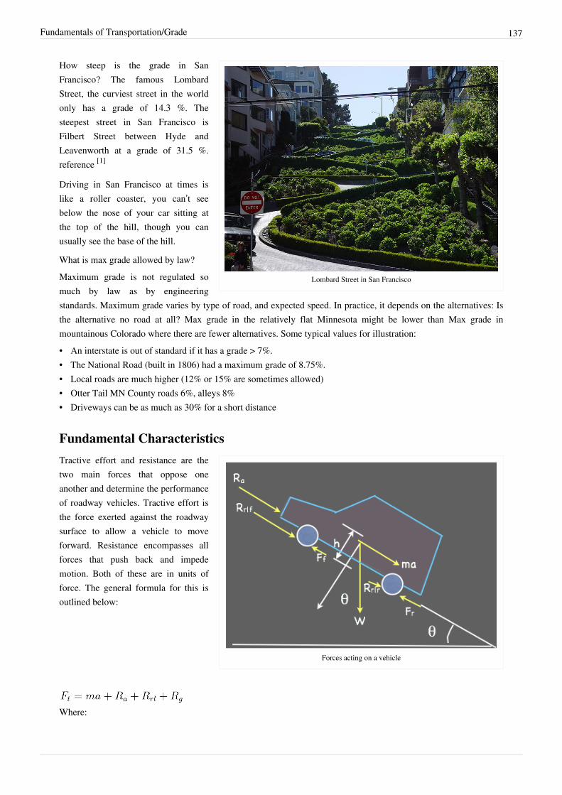
Fundamentals of Transportation/Grade 137

Lombard Street in San Francisco

How steep is the grade in SanFrancisco? The famous LombardStreet, the curviest street in the worldonly has a grade of 14.3 %. Thesteepest street in San Francisco isFilbert Street between Hyde andLeavenworth at a grade of 31.5 %.reference [1]

Driving in San Francisco at times islike a roller coaster, you can’t seebelow the nose of your car sitting atthe top of the hill, though you canusually see the base of the hill.

What is max grade allowed by law?Maximum grade is not regulated somuch by law as by engineeringstandards. Maximum grade varies by type of road, and expected speed. In practice, it depends on the alternatives: Isthe alternative no road at all? Max grade in the relatively flat Minnesota might be lower than Max grade inmountainous Colorado where there are fewer alternatives. Some typical values for illustration:• An interstate is out of standard if it has a grade > 7%.• The National Road (built in 1806) had a maximum grade of 8.75%.• Local roads are much higher (12% or 15% are sometimes allowed)• Otter Tail MN County roads 6%, alleys 8%• Driveways can be as much as 30% for a short distance

Fundamental Characteristics

Forces acting on a vehicle

Tractive effort and resistance are thetwo main forces that oppose oneanother and determine the performanceof roadway vehicles. Tractive effort isthe force exerted against the roadwaysurface to allow a vehicle to moveforward. Resistance encompasses allforces that push back and impedemotion. Both of these are in units offorce. The general formula for this isoutlined below:

Where:

Fundamentals of Transportation/Grade 138

• = Tractive Effort• = Vehicle Mass• = Acceleration• = Aerodynamic Resistance• = Rolling Resistance• = Grade ResistanceThese components are discussed in greater detail in the following sections.

Aerodynamic ResistanceAerodynamic resistance is a force that is produced by turbulent air flow around the vehicle body. This turbulence isdependent on the shape of the vehicle, as well as the friction of air passing over the vehicle's surface. A small portionof this resistance comes from air flow through vehicle components, such as interior ventilation. This resistance canbe estimated through the following formula:

Where:• = Air Density• = Frontal area of the vehicle• = Coefficient of Drag• = Speed of the vehicleAir density is a function of elevation and temperature. Frontal area and coefficient of drag are generally unique toeach vehicle or type of vehicle.

Rolling ResistanceRolling resistance is caused by a vehicle's internal mechanical friction and the interaction of tires with the roadwaysurface. Three main causes exist that create this resistance. The first is the rigidity of the tire and the roadwaysurface. The second is tire pressure and temperature. The third is vehicular operating speed. This value of rollingfriction can be calculated from a very simplified formula, given here in metric. is in meters per second.

The resistance caused by this friction will increase as weight is added to the vehicle. Therefore, rolling resistance canbe calculated.

Where:• = Vehicle Weight• = Rolling Friction

Fundamentals of Transportation/Grade 139

Grade ResistanceGrade resistance is the simplest form of resistance. It is the gravitational force acting on the vehicle. This force maynot be exactly perpendicular to the roadway surface, especially in situations when a grade is present. Thus, graderesistance can be calculated in the following formula:

Where:• = Vehicle Weight• = Grade (length/length)

Tractive EffortTractive effort is the force that allows the vehicle to move forward, subject to the resistances of the previous threeforces. The derivation of the formula comes from understanding the forces and moments that on around the varioustires. It can be summarized into a simple concept, illustrated here.For a rear-wheel drive car:

For a front-wheel drive car:

Where:• = Maximum Tractive Effort• = Coefficient of road adhesion• = Vehicle Weight• = Distance from rear axle to vehicle's center of gravity• = Distance from front axle to vehicle's center of gravity• = Coefficient of rolling friction• = Height of the center of gravity above the roadway surface• = Length of wheelbase

Grade ComputationMost of the work surrounding tractive effort is geared toward determining the allowable grade of a given roadway.With a certain known vehicle type using this road, the grade can be easily calculated. Using the force balanceequation for tractive effort, a value for grade can be separating, producing the formula below:

This calculation produces the maximum grade allowed for a given vehicle type. It assumes that the vehicle isoperating at optimal engine capacity and, thus, no acceleration can occur, dropping that element from the overallequation.

Fundamentals of Transportation/Grade 140

Examples

Example 1: Racecar Acceleration

Problem:

A racecar is speeding down a level straightaway at 100 km/hr. The car has a coefficient of drag of 0.3,a frontal area of 1.5 , a weight of 10 kN, a wheelbase of 3 meters, and a center of gravity 0.5meters above the roadway surface, which is 1 meter behind the front axle. The air density is 1.054 kg/

and the coefficient of road adhesion is 0.6. What is the rate of acceleration for the vehicle?Solution:

Use the force balancing equation to solve for .

Since the straightaway is a level one, the grade is zero, thus removing grade resistance from the general problem.

Aerodynamic resistance is computed:Rolling resistance is computed:

Tractive Effort is computed:Looking back to the force balancing equation:Divide out mass, which can be computed from weight by dividing out gravity.

Thus, divide mass from the force and acceleration can be found.

Thus, the vehicle is accelerating at a rate of 1.43 meters per second squared.

Example 2: Going Up a Hill

Problem:

Using the same case from Example 1, assume that instead the racecar encounters a steep hill that itmust travel up. It is desired that the driver maintain the 100 km/hr velocity at a very minimum. Withthat being said, what would be the maximum grade that the hill could be?

Solution:

At the steepest eligible hill, the racecar would be able to maintain 100 km/hr without any room foracceleration or deceleration. Therefore, acceleration goes to zero. All other values would stay thesame from Example 1. Using the grade formula, the maximum grade can be calculated.

The maximum allowable grade is 14.61%.

Fundamentals of Transportation/Grade 141

Thought QuestionProblem

Why is it that, in mountainous country, trucks and cars have different speed limits?Answer

Tractive effort is one of the leading reasons, as trucks have a harder time going up steep hills than typical passengercars, but it is not the only one. Safety is another leading reason, surprisingly, as big rig trucks are obviously moredifficult to control in a harsh environment, such as a mountain pass.

Sample ProblemProblem (Solution)

Additional Questions• Homework• Additional Questions

Variables• - Tractive Effort Force• - Aerodynamic resistance Force• - Rolling Resistance Force

• - Grade Resistance Force• - Vehicle Weight• - Vehicle Mass• - Acceleration• - Air Density• - Frontal area of the vehicle• - Coefficient of Drag• - Speed of the vehicle

• - Rolling Friction• - Grade• - Coefficient of road adhesion• - Distance from rear axle to vehicle's center of gravity

• - Distance from front axle to vehicle's center of gravity• - Height of the center of gravity above the roadway surface• - Length of wheelbase

Fundamentals of Transportation/Grade 142

Key Terms• Tractive Effort• Aerodynamic Resistance• Rolling Resistance• Grade Resistance

References[1] http:/ / www. sallys-place. com/ travel/ san_francisco/ pt_lombard. htm

Fundamentals of Transportation/Grade/ProblemProblem:

It has been estimated that a Tour-de-France champion could generate a sustained 510 Watts of powerwhile a healthy young human male (HYHM) can generate about 310 Watts of power. The bicyclingchampion and HYHM are going to race (on bicycles) up a hill with a 6% upgrade, that is five miles

long, and the elevation at the top of the hill is 5000 feet. Both rider/bicycle combinations weigh 170 lbs, with frontalarea 0.4m2 and coefficient of drag 0.9 (values being typical of bicyclists in crouched racing positions). Thecoefficient of rolling resistance for both bicycles is 0.01. Assume is 1.0567 kg/cubic-m. Remember, power equalsthe product of force and velocity. (1) Who gets to the top first? (2) How much longer does it take the loser to make itto the top?

• Solution

Fundamentals of Transportation/Grade/Solution 143

Fundamentals of Transportation/Grade/SolutionProblem:

It has been estimated that a Tour-de-France champion could generate a sustained 510 Watts of powerwhile a healthy young human male (HYHM) can generate about 310 Watts of power. The bicyclingchampion and HYHM are going to race (on bicycles) up a hill with a 6% upgrade, that is five miles

long, and the elevation at the top of the hill is 5000 feet. Both rider/bicycle combinations weigh 170 lbs, with frontalarea 0.4 and coefficient of drag 0.9 (values being typical of bicyclists in crouched racing positions). Thecoefficient of rolling resistance for both bicycles is 0.01. Assume is 1.0567 kg/cubic-m. Remember, power equalsthe product of force and velocity. (1) Who gets to the top first? (2) How much longer does it take the loser to make itto the top?

Solution:The winner is obvious the Tour-de-France champion, as everything between the two is equal with theexception of power. Since the champion produces more power, he, by default, would win.

We need to find the maximum steady state speed for each racer to compute the differences in arrivaltime. At the steady state speed we must have:

Where:• = Tractive Effort• = Vehicle Mass• = Acceleration• = Aerodynamic Resistance• = Rolling Resistance• = Grade ResistanceWe also know:• = 1.0567 kg/cubic-m• = 756 N• = 0.01• = 0.06• = 0.4 • = 0.9To estimate available tractive effort we can use the definition of power as time rate of work, P = FV, to get:

Substituting in the components of the individual formulas to the general one, we get:

If we compute rolling and grade resistance, we get:

Together, they add up to 52.92 N.Aerodynamic Resistance can be found to be:

Fundamentals of Transportation/Grade/Solution 144

With everything substituted into the general formula, the end result is the following formulation:

This problem can be solved iteratively (setting a default value for v and then computing through iterations) orgraphically. Either way, when plugging in 510 watts for the Tour-de-France champion, the resulting velocity is 7.88meters/second. Similarly, when plugging in 310 watts for the HYHM, the resulting velocity is 5.32 meters/second.The hill is five miles in length, which translates to 8.123 kilometers, 8,123 meters. It will take the champion 1030seconds (or 17.1 minutes) to complete this link, whereas the HYHM will take 1527 seconds (or 25.4 minutes). Theresulting difference is 8.3 minutes.

Fundamentals of Transportation/Earthwork

The equipment necessary for earthwork to occur

Earthwork is something thattransportation projects seldom avoid.In order to establish a properlyfunctional road, the terrain must oftenbe adjusted. In many situations,geometric design will often involveminimizing the cost of earthworkmovement. Earthwork is expressed inunits of volumes (cubic meters inmetric). Increases in such volumesrequire additional trucks (or more runsof the same truck), which cost money.Thus, it is important for designers to engineer roads that require very little earthwork.

Cross Sections and Volume Computation

A Roadway Cross Section on otherwise Level Ground

To determine the amount of earthworkto occur on a given site, one mustcalculate the volume. For linearfacilities, which include highways,railways, runways, etc., volumes caneasily be calculated by integrating theareas of the cross sections (slices thatgo perpendicular to the centerline) forthe entire length of the corridor. Moresimply, several cross sections can beselected along the corridor and an average can be taken for the entire length. Several different procedures exist forcalculating areas of earthwork cross sections. In the past, the popular method was to draw cross sections by hand anduse a planimeter to measure area. In modern times, computers use a coordinate method to assess earthworkcalculations. To perform this task, points with known elevations need to be identified around the cross section. Thesepoints are considered in the (X, Y) coordinate plane, where X represents the horizontal axis paralleling the groundand Y represents the vertical axis that is elevation. Area can be computed with the following formula:

Fundamentals of Transportation/Earthwork 145

Where:• = Area of Cross-Section• = Number of Points on Cross Section (Note: n+1 = 1 and 1-1=n, for indexing)• = X-Coordinate• = Y-CoordinateWith this, earthwork volumes can be calculated. The easiest means to do so would by using the average end areamethod, where the two end areas are averaged over the entire length between them.

Where:• = Volume• = Cross section area of first side• = Cross section area of second side• = Length between the two areasIf one end area has a value of zero, the earthwork volume can be considered a pyramid and the correct formulawould be:

A more accurate formula would the prismoidal formula, which takes out most of the error accrued by the averageend area method.

Where:

• = Volume given by the prismoidal formula• = Area of a plane surface midway between the two cross sections

Cut and Fill

A Typical Cut/Fill Diagram

Various sections of a roadway designwill require bringing in earth. Othersections will require earth to beremoved. Earth that is brought in isconsidered Fill while earth that isremoved is considered Cut. Generally,designers generate drawings called Cutand Fill Diagrams, which illustrate thecut or fill present at any given site.This drawing is quite standard, beingno more than a graph with site locationon the X-axis and fill being thepositive range of the Y-axis while cutis the negative range of the Y-axis.

Fundamentals of Transportation/Earthwork 146

A Typical Mass Diagram (Note: Additional Dirt is Needed in this Example)

Mass Balance

Using the data for cut and fill, anoverall mass balance can be computed.The mass balance represents the totalamount of leftover (if positive) orneeded (if negative) earth at a givensite based on the design up until thatpoint. It is a useful piece ofinformation because it can identifyhow much remaining or needed earthwill be present at the completion of aproject, thus allowing designers tocalculate how much expense will beincurred to haul out excess dirt or haul in needed additional. Additionally, a mass balance diagram, representedgraphically, can aid designers in moving dirt internally to save money.Similar to the cut and fill diagram, the mass balance diagram is illustrated on two axes. The X-axis represents sitelocation along the roadway corridor and the Y-axis represents the amount of earth, either in excess (positive) orneeded (negative).

Demonstrations• Flash animation: Shrinkage (by Karen Dixon) [1]

• Flash animation: Swell (by Karen Dixon) [2]

Examples

Example 1: Computing Volume

Problem:

A roadway is to be designed on a level terrain. This roadway is 150 meters in length. Four crosssections have been selected, one at 0 meters, one at 50 meters, one at 100 meters, and one at 150meters. The cross sections, respectively, have areas of 40 square meters, 42 square meters, 19 square

meters, and 34 square meters. What is the volume of earthwork needed along this road?Solution:

Three sections exist between all of these cross sections. Since none of the sections end with an area ofzero, the average end area method can be used. The volumes can be computed for respective sectionsand then summed together.

Section between 0 and 50 meters:

Section between 50 and 100 meters:

Section between 100 and 150 meters:

Fundamentals of Transportation/Earthwork 147

Total Volume is found to be:

Example 2: Mass Balance

Problem:

Given the following cut/fill profile for each meter along a 10-meter strip of road built on very, veryhilly terrain, estimate the amount of dirt left over or needed for the project.• 0 Meters: 3 meters of fill

• 1 Meter: 1 meter of fill• 2 Meters: 2 meters of cut• 3 Meters: 5 meters of cut• 4 Meters: 7 meters of cut• 5 Meters: 8 meters of cut• 6 Meters: 2 meters of cut• 7 Meters: 1 meter of fill• 8 Meters: 3 meters of fill• 9 Meters: 6 meters of fill• 10 Meters: 7 meters of fill

Solution:

If 'cut' is considered an excess of available earth and 'fill' is considered a reduction of available earth,the problem becomes one of simple addition and subtraction.3 cubic-meters of dirt remain in excess.

Thought QuestionProblem

If it is found that the mass balance is indeed balanced (end value of zero), does that automatically mean that no dirttransport, either out of or into the site, is needed?Solution

No. Any soil scientist will eagerly state that dirt type can change with location quite quickly, depending on theregion. So, if half a highway cuts from the earth and the other half needs fill, the dirt pulled from the first half cannotbe simply dumped into the second half, even if mathematically it balances. If the soil types are different, the exactnumbers of volume needed may be different, as different soil types have different properties (settling, water storage,etc.). In the worse case, not consulting a soil scientist could result in your road being washed out!

Fundamentals of Transportation/Earthwork 148

Sample ProblemProblem (Solution)

Additional QuestionsHomework

Variables• - Area of Cross-Section• - Number of Points on Cross Section (Note: n+1 = 1 and 1-1=n, for indexing)• - X-Coordinate• - Y-Coordinate• - Volume• - Cross section area of first side• - Cross section area of second side• - Length between the two areas• - Volume given by the prismoidal formula• - Area of a plane surface midway between the two cross sections

Key Terms• Cut• Fill• Mass Balance• Area• Volume• Earthwork• Prismoidal Volume

References[1] http:/ / street. umn. edu/ flash_earthwork_shrink. html[2] http:/ / street. umn. edu/ flash_earthwork_swell. html

Fundamentals of Transportation/Earthwork/Problem 149

Fundamentals ofTransportation/Earthwork/Problem

Problem:Given the end areas below, calculate the volumes of cut (in cubic meters) and fill between stations0+00 and 2+50. Determine the true amount of excess cut or fill to be removed.

• 0+00: Fill = 60

• 0+50: Fill = 50• 0+75: Cut = 0, Fill = 25• 1+00: Cut = 10, Fill = 5• 1+15: Cut = 15, Fill = 0• 1+50: Cut = 30• Solution

Fundamentals ofTransportation/Earthwork/Solution

Problem:Given the end areas below, calculate the volumes of cut (in cubic meters) and fill between stations0+00 and 2+50. Determine the true amount of excess cut or fill to be removed.

• 0+00: Fill = 60

• 0+50: Fill = 50• 0+75: Cut = 0, Fill = 25• 1+00: Cut = 10, Fill = 5• 1+15: Cut = 15, Fill = 0• 1+50: Cut = 30

Solution:Two different methods need to be used here to compute earthwork volumes along the five strips. Theaverage end area method can be used for non-zero sections. The pyramid method needs to be used forareas with zero ends.

For 0+00 to 0+50, use average end area:

For 0+50 to 0+75, use average end area:

For 0+75 to 1+00, use the average end area method for the fill section and the pyramid method for the cut section:

Fundamentals of Transportation/Earthwork/Solution 150

For 1+00 to 1+15, use the pyramid method for the fill section and the average end area method for the cut section:

For 1+15 to 1+50, use the average end area method:

The sums of both cut and fill can be found:• Fill = 4087.5 cubic-meters• Cut = 1058.3 cubic-metersThus, 3029.2 cubic-meters of dirt are needed to meet the earthwork requirement for this project.

Fundamentals of Transportation/HorizontalCurvesHorizontal Curves are one of the two important transition elements in geometric design for highways (along withVertical Curves). A horizontal curve provides a transition between two tangent strips of roadway, allowing a vehicleto negotiate a turn at a gradual rate rather than a sharp cut. The design of the curve is dependent on the intendeddesign speed for the roadway, as well as other factors including drainage and friction. These curves are semicirclesas to provide the driver with a constant turning rate with radii determined by the laws of physics surroundingcentripetal force.

Fundamental Horizontal Curve Properties

Physics Properties

A Horizontal Curve in Oslo, Norway

When a vehicle makes a turn, twoforces are acting upon it. The first isgravity, which pulls the vehicle towardthe ground. The second is centripetalforce, which is an external forcerequired to keep the vehicle on acurved path. For any given velocity,the centripetal force would need to begreater for a tighter turn (one with asmaller radius) than a broader one (onewith a larger radius). On a levelsurface, side friction could serve asa countering force, but it generallywould provide very little resistance.Thus, the vehicle would have to makea very wide circle in order to negotiatea turn. Given that road designs usually encounter very narrow design areas, such wide turns are generallydiscouraged.

Fundamentals of Transportation/Horizontal Curves 151

To deal with this issue, horizontal curves have roads that are tilted at a slight angle. This tilt is defined assuperelevation, or , which is the amount of rise seen on an angled cross-section of a road given a certain run,otherwise known as slope. The presence of superelevation on a curve allows some of the centripetal force to becountered by the ground, thus allowing the turn to be executed at a faster rate than would be allowed on a flatsurface. Superelevation also plays another important role by aiding in drainage during precipitation events, as waterruns off the road rather than collecting on it. Generally, superelevation is limited to being less than 14 percent, asengineers need to account for stopped vehicles on the curve, where centripetal force is not present.The allowable radius for a horizontal curve can then be determined by knowing the intended design velocity ,the coefficient of friction, and the allowed superelevation on the curve.

With this radius, practitioners can determine the degree of curve to see if it falls within acceptable standards. Degreeof curve, , can be computed through the following formula, which is given in Metric.

Where:• = Degree of curve [angle subtended by a 30.5-m (100 ft) arc along the horizontal curve

Application of Superelevation

Bristol Motor Speedway

One place you will see steep banking isat automobile racetracks. These tracksdo not operate in winter, and so canavoid the problems of banking inwinter weather. Drivers are alsoespecially skilled, though crashes arenot infrequent. For NASCAR fans, thefollowing table may be of interest.Table: Banking at US Racetracks

Track Length (miles) Banking (degrees)

Chicago Motor Speedway 1 0.00

Infineon Raceway 1.949

Watkins Glen International 2.45

Pocono Raceway 2.5 6.00

Homestead-Miami Speedway 1.5 8.00

Indianapolis Motor Speedway 2.5 9.00

Memphis Motorsports Park 0.75 11.00

Phoenix International Raceway 1 11.00

Las Vegas Motor Speedway 1.5 12.00

Fundamentals of Transportation/Horizontal Curves 152

Martinsville Speedway 0.526 12.00

New Hampshire Int'l Speedway 1.058 12.00

California Speedway 2 14.00

Kentucky Speedway 1.5 14.00

Richmond International Raceway 0.75 14.00

Kansas Speedway 1.5 15.00

Michigan International Speedway 2 18.00

Nashville Speedway USA 0.596 18.00

North Carolina Speedway 1.017 22.00

Darlington Raceway 1.366 23.00

Atlanta Motor Speedway 1.54 24.00

Dover Downs Int'l Speedway 1 24.00

Lowe's Motor Speedway 1.5 24.00

Texas Motor Speedway 1.5 24.00

Daytona International Speedway 2.5 31.00

Talladega Superspeedway 2.66 33.00

Bristol Motor Speedway 0.533 36.00

Source: Fantasy Racing Zone by FSN [1]

Geometric Properties

A Typical Horizontal Curve (Plan View)

Horizontal curves occur at locations where tworoadways intersect, providing a gradual transitionbetween the two. The intersection point of the tworoads is defined as the Point of Tangent Intersection(PI). The location of the curve's start point is defined asthe Point of Curve (PC) while the location of thecurve's end point is defined as the Point of Tangent(PT). Both the PC and PT are a distance from thePI, where is defined as Tangent Length. TangentLength can be calculated by finding the central angle ofthe curve, in degrees. This angle is equal to thesupplement of the interior angle between the two roadtangents.

Where:• = tangent length (in length units)

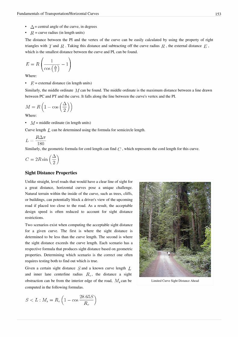
Fundamentals of Transportation/Horizontal Curves 153

• = central angle of the curve, in degrees• = curve radius (in length units)The distance between the PI and the vertex of the curve can be easily calculated by using the property of righttriangles with and . Taking this distance and subtracting off the curve radius , the external distance ,which is the smallest distance between the curve and PI, can be found.

Where:• = external distance (in length units)Similarly, the middle ordinate can be found. The middle ordinate is the maximum distance between a line drawnbetween PC and PT and the curve. It falls along the line between the curve's vertex and the PI.

Where:• = middle ordinate (in length units)Curve length can be determined using the formula for semicircle length.

Similarly, the geometric formula for cord length can find , which represents the cord length for this curve.

Sight Distance Properties

Limited Curve Sight Distance Ahead

Unlike straight, level roads that would have a clear line of sight fora great distance, horizontal curves pose a unique challenge.Natural terrain within the inside of the curve, such as trees, cliffs,or buildings, can potentially block a driver's view of the upcomingroad if placed too close to the road. As a result, the acceptabledesign speed is often reduced to account for sight distancerestrictions.Two scenarios exist when computing the acceptable sight distancefor a given curve. The first is where the sight distance isdetermined to be less than the curve length. The second is wherethe sight distance exceeds the curve length. Each scenario has arespective formula that produces sight distance based on geometricproperties. Determining which scenario is the correct one oftenrequires testing both to find out which is true.Given a certain sight distance and a known curve length and inner lane centerline radius , the distance a sightobstraction can be from the interior edge of the road, can becomputed in the following formulas.

Fundamentals of Transportation/Horizontal Curves 154

Demonstrations• Flash animation: Roadside Clear Zone (by Karen Dixon and Thomas Wall) [2]

• Flash animation: Superelevation (by Karen Dixon and Thomas Wall) [3]

Examples

Example 1: Curve Radius

Problem:

A curving roadway has a design speed of 110 km/hr. At one horizontal curve, the superelevation hasbeen set at 6.0% and the coefficient of side friction is found to be 0.10. Determine the minimum radiusof the curve that will provide safe vehicle operation.

Solution:

Example 2: Determining Stationing

Problem:

A horizontal curve is designed with a 600 m radius and is known to have a tangent length of 52 m.The PI is at station 200+00. Determine the stationing of the PT.

Solution:

Fundamentals of Transportation/Horizontal Curves 155

What is known for this problem

Example 3: Stopping Sight Distance

Problem:

A very long horizontal curve on a one-directional racetrack has 1750-meter centerline radius, two4-meter lanes, and a 200 km/hr design speed. Determine the closest distance from the inside edge ofthe track that spectators can park without impeding the necessary sight distance of the drivers. Assume

that the sight distance is less than the length of the curve, a coefficient of friction of 0.3, and a perception-reactiontime of 2.5 seconds.

Solution:

With a centerline radius of 1750 meters, the centerline of the interior lane is 1748 meters from thevertex (1750 - (4/2)). Using the stopping sight distance formula (See Sight Distance), SSD iscomputed to be 664 meters. With this, the distance from the track that spectators can be parked can

easily be found.

This gives the distance (31.43 m) to the center of the inside lane. Subtracting half the lane width (2m in this case)would give the distance to the edge of the track, 29.43 m.

Fundamentals of Transportation/Horizontal Curves 156

Thought QuestionProblem

Horizontal curves are semicircles, as to allow the driver to negotiate the curve without having to change the tilt of thewheel while passing through. However, what happens at the PC or PT, where tangent road transitions to a curve orvice versa. Is the driver expected to abruptly turn the wheel to match the curve or tangent?Solution

Generally not. Engineers employ several techniques to allow drivers to gradually turn the wheel as they enter orleave the curve. One of the more popular ways is to use Splines. Splines are polynomial curves that have changingrates of curvature. Employed at the PC and PT, Splines take away any sharp changes for the drivers and make thedrive a more pleasant one.

Sample ProblemProblem (Solution)

Additional Questions• Homework• Additional Questions

Variables• - Centerline Curve Radius• - Degree of curve [angle subtended by a 30.5-m (100 ft) arc along the horizontal curve• - tangent length (in length units)• - central angle of the curve, in degrees• - Smallest distance between the curve and PI• - Middle ordinate• - Curve Length• - Cord Length• - Sight Distance• - Acceptable distance from inner edge of road for a sight obstruction to be placed without impeding sight

distance• - Radius of innermost lane centerline

Fundamentals of Transportation/Horizontal Curves 157

Key Terms• PC: Point of Curve• PI: Point of Tangent Intersect• PT: Point of Tangent

References[1] http:/ / www. ffzone. com/ nascar/ tracks. php?sortval=atrackbanking[2] http:/ / street. umn. edu/ flash_roadside. html[3] http:/ / street. umn. edu/ flash_superelevation. html

Fundamentals of Transportation/HorizontalCurves/Problem

Problem:

A given curve was very poorly designed. The two-lane road used has a lower-than-average coefficientof friction (0.05), no superelevation to speak of, and 4-meter lanes. 900 kg vehicles tend to go aroundthis curve and are stylistically top heavy. County engineers have warned that this curve cannot be

traversed as safely as other curves in the area, but politicians want to keep the speed up to boost tourism in the area.The curves have a radius of 500 feet and a design speed of 80 km/hr. Because the vehicles using the curve are topheavy, they have a tendency to roll over if too much side force is exerted on them (the local kids often race aroundthe curve at night to get the thrill of "two-wheeling"). As an engineer, you need to prove that this curve is infeasiblebefore an accident occurs. How can you show this?• Solution

Fundamentals of Transportation/Horizontal Curves/Solution 158

Fundamentals of Transportation/HorizontalCurves/Solution

Problem:

A given curve was very poorly designed. The two-lane road used has a lower-than-average coefficientof friction (0.05), no superelevation to speak of, and 4-meter lanes. 900 kg vehicles tend to go aroundthis curve and are stylistically top heavy. County engineers have warned that this curve cannot be

traversed as safely as other curves in the area, but politicians want to keep the speed up to boost tourism in the area.The curves have a radius of 500 feet and a design speed of 80 km/hr. Because the vehicles using the curve are topheavy, they have a tendency to roll over if too much side force is exerted on them (the local kids often race aroundthe curve at night to get the thrill of "two-wheeling"). As an engineer, you need to prove that this curve is infeasiblebefore an accident occurs. How can you show this?

Solution:

The stated speed is 80 km/hr. The easiest way would be to prove that this is too high. We will look atthe innermost lane, since forces will be greater there. Using the general curve radius formula andsolving for v, we find:

80 km/hr is much greater than 56.23 km/hr, which by default means that more force is being exerted on the vehiclethan the road can counter. Thus, the curve's speed limit is dangerous and needs to be changed.

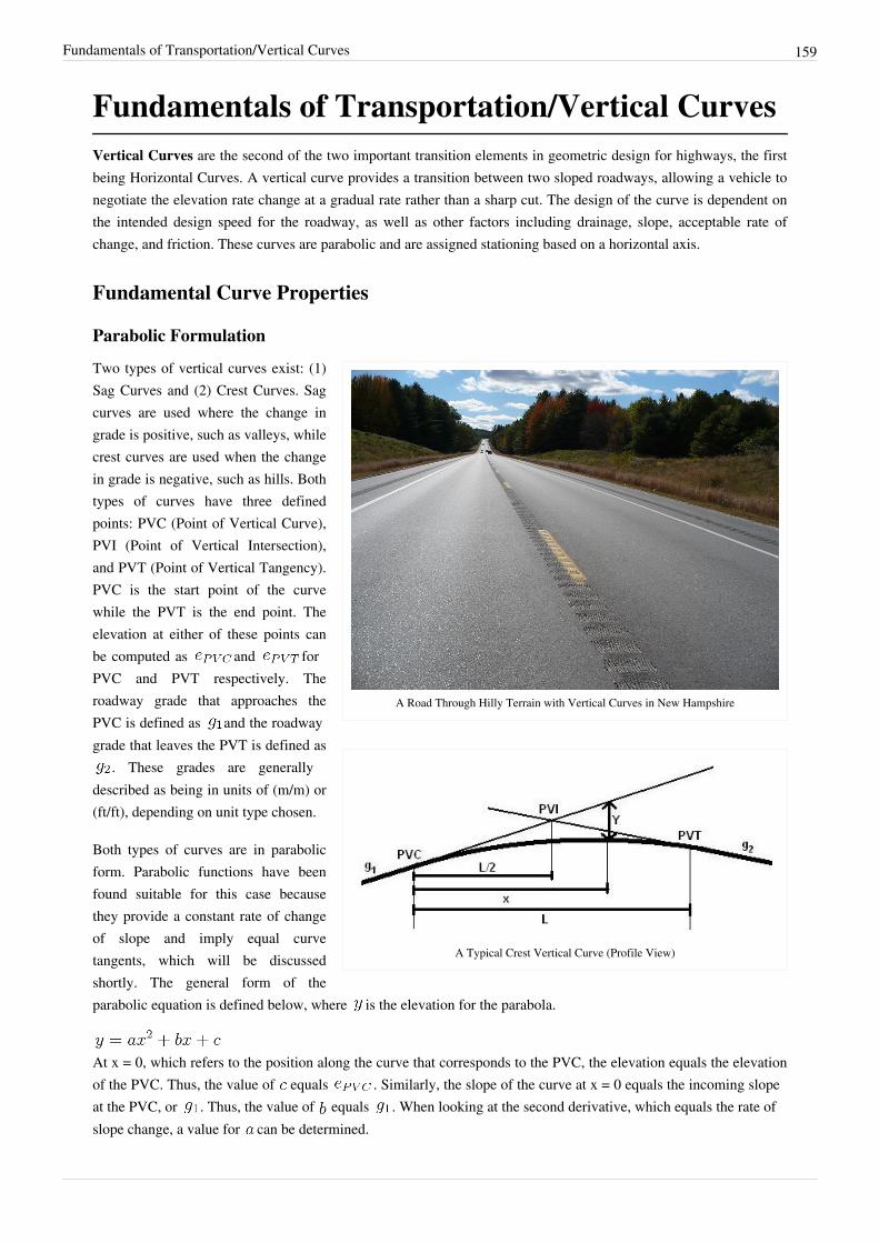
Fundamentals of Transportation/Vertical Curves 159

Fundamentals of Transportation/Vertical CurvesVertical Curves are the second of the two important transition elements in geometric design for highways, the firstbeing Horizontal Curves. A vertical curve provides a transition between two sloped roadways, allowing a vehicle tonegotiate the elevation rate change at a gradual rate rather than a sharp cut. The design of the curve is dependent onthe intended design speed for the roadway, as well as other factors including drainage, slope, acceptable rate ofchange, and friction. These curves are parabolic and are assigned stationing based on a horizontal axis.

Fundamental Curve Properties

Parabolic Formulation

A Road Through Hilly Terrain with Vertical Curves in New Hampshire

A Typical Crest Vertical Curve (Profile View)

Two types of vertical curves exist: (1)Sag Curves and (2) Crest Curves. Sagcurves are used where the change ingrade is positive, such as valleys, whilecrest curves are used when the changein grade is negative, such as hills. Bothtypes of curves have three definedpoints: PVC (Point of Vertical Curve),PVI (Point of Vertical Intersection),and PVT (Point of Vertical Tangency).PVC is the start point of the curvewhile the PVT is the end point. Theelevation at either of these points canbe computed as and forPVC and PVT respectively. Theroadway grade that approaches thePVC is defined as and the roadwaygrade that leaves the PVT is defined as

. These grades are generallydescribed as being in units of (m/m) or(ft/ft), depending on unit type chosen.

Both types of curves are in parabolicform. Parabolic functions have beenfound suitable for this case becausethey provide a constant rate of changeof slope and imply equal curvetangents, which will be discussedshortly. The general form of theparabolic equation is defined below, where is the elevation for the parabola.

At x = 0, which refers to the position along the curve that corresponds to the PVC, the elevation equals the elevationof the PVC. Thus, the value of equals . Similarly, the slope of the curve at x = 0 equals the incoming slopeat the PVC, or . Thus, the value of equals . When looking at the second derivative, which equals the rate ofslope change, a value for can be determined.

Fundamentals of Transportation/Vertical Curves 160

Thus, the parabolic formula for a vertical curve can be illustrated.

Where:• : elevation of the PVC• : Initial Roadway Grade (m/m)• : Final Roadway Grade (m/m)• : Length of Curve (m)Most vertical curves are designed to be Equal Tangent Curves. For an Equal Tangent Curve, the horizontal lengthbetween the PVC and PVI equals the horizontal length between the PVI and the PVT. These curves are generallyeasier to design.

OffsetSome additional properties of vertical curves exist. Offsets, which are vertical distances from the initial tangent tothe curve, play a significant role in vertical curve design. The formula for determining offset is listed below.

Where:• : The absolute difference between and , multiplied by 100 to translate to a percentage• : Curve Length• : Horizontal distance from PVC along curve

Stopping Sight DistanceSight distance is dependent on the type of curve used and the design speed. For crest curves, sight distance is limitedby the curve itself, as the curve is the obstruction. For sag curves, sight distance is generally only limited byheadlight range. AASHTO has several tables for sag and crest curves that recommend rates of curvature, , givena design speed or stopping sight distance. These rates of curvature can then be multiplied by the absolute slopechange percentage, to find the recommended curve length, .

Without the aid of tables, curve length can still be calculated. Formulas have been derived to determine the minimumcurve length for required sight distance for an equal tangent curve, depending on whether the curve is a sag or acrest. Sight distance can be computed from formulas in other sections (See Sight Distance).

Crest Vertical Curves

The correct equation is dependent on the design speed. If the sight distance is found to be less than the curve length,the first formula below is used, whereas the second is used for sight distances that are greater than the curve length.Generally, this requires computation of both to see which is true if curve length cannot be estimated beforehand.

Fundamentals of Transportation/Vertical Curves 161

Where:• : Minimum Curve Length (m)• : The absolute difference between and , multiplied by 100 to translate to a percentage• : Sight Distance (m)• : Height of driver's eye above roadway surface (m)• : Height of objective above roadway surface (m)

Sag Vertical Curves

Just like with crest curves, the correct equation is dependent on the design speed. If the sight distance is found to beless than the curve length, the first formula below is used, whereas the second is used for sight distances that aregreater than the curve length. Generally, this requires computation of both to see which is true if curve length cannotbe estimated beforehand.

Where:• : The absolute difference between and , multiplied by 100 to translate to a percentage• : Sight Distance (m)• : Height of headlight (m)

• : Inclined angle of headlight beam, in degrees

Passing Sight DistanceIn addition to stopping sight distance, there may be instances where passing may be allowed on vertical curves. Forsag curves, this is not an issue, as even at night, a vehicle in the opposing can be seen from quite a distance (with theaid of the vehicle's headlights). For crest curves, however, it is still necessary to take into account. Like with thestopping sight distance, two formulas are available to answer the minimum length question, depending on whetherthe passing sight distance is greater than or less than the curve length. These formulas use units that are in metric.

Where:• : The absolute difference between and , multiplied by 100 to translate to a percentage• : Passing Sight Distance (m)• : Minimum curve length (m)

Fundamentals of Transportation/Vertical Curves 162

Demonstrations• Flash animation: Stopping Sight Distance on Crest Vertical Curve (by Karen Dixon) [1]

• Flash animation: Stopping Sight Distance on Sag Vertical Curve (by Karen Dixon) [2]

Examples

Example 1: Basic Curve Information

Problem:

A 500-meter equal-tangent sag vertical curve has the PVC at station 100+00 with an elevation of 1000m. The initial grade is -4% and the final grade is +2%. Determine the stationing and elevation of thePVI, the PVT, and the lowest point on the curve.

Solution:

The curve length is stated to be 500 meters. Therefore, the PVT is at station 105+00 (100+00 + 5+00)and the PVI is in the very middle at 102+50, since it is an equal tangent curve. For the parabolicformulation, equals the elevation at the PVC, which is stated as 1000 m. The value of equals the

initial grade, which in decimal is -0.04. The value of can then be found as 0.00006.

Using the general parabolic formula, the elevation of the PVT can be found:Since the PVI is the intersect of the two tangents, the slope of either tangent and the elevation of the PVC or PVT,depending, can be used as reference. The elevation of the PVI can then be found:

To find the lowest part of the curve, the first derivative of the parabolic formula can be found. The lowest point has aslope of zero, and thus the low point location can be found:

Using the parabolic formula, the elevation can be computed for that location. It turns out to be at an elevation of993.33 m, which is the lowest point along the curve.

Example 2: Adjustment for Obstacles

Problem:

A current roadway is climbing a hill at an angle of +3.0%. The roadway starts at station 100+00 andelevation of 1000 m. At station 110+00, there is an at-grade railroad crossing that goes over the slopedroad. Since designers are concerned for the safety of drivers crossing the tracks, it has been proposed

to cut a level tunnel through the hill to pass beneath the railroad tracks and come out on the opposite side. A verticalcrest curve would connect the existing roadway to the proposed tunnel with a grade of (-0.5)%. The prospectivecurve would start at station 100+00 and have a length of 2000 meters. Engineers have stated that there must be atleast 10 meters of separation between the railroad tracks and the road to build a safe tunnel. Assume an equal tangentcurve. With the current design, is this criteria met?

Solution:

Fundamentals of Transportation/Vertical Curves 163

One way to solve this problem wouldbe to compute the elevation of thecurve at station 110+00 and then see ifit is at least 10 meters from the tangent.Another way would be to use theOffset Formula. Since A, L, and x areall known, this problem can be easilysolved. Set x to 1000 meters torepresent station 110+00.

The design DOES NOT meet the criteria.

Example 3: Stopping Sight Distance

Problem:

A current roadway has a design speed of 100 km/hr, a coefficient of friction of 0.1, and carries driverswith perception-reaction times of 2.5 seconds. The drivers use cars that allows their eyes to be 1 meterabove the road. Because of ample roadkill in the area, the road has been designed for carcasses that

are 0.5 meters in height. All curves along that road have been designed accordingly.The local government, seeing the potential of tourism in the area and the boost to the local economy, wants toincrease the speed limit to 110 km/hr to attract summer drivers. Residents along the route claim that this is a horribleidea, as a particular curve called "Dead Man's Hill" would earn its name because of sight distance problems. "DeadMan's Hill" is a crest curve that is roughly 600 meters in length. It starts with a grade of +1.0% and ends with(-1.0)%. There has never been an accident on "Dead Man's Hill" as of yet, but residents truly believe one will comeabout in the near future.A local politician who knows little to nothing about engineering (but thinks he does) states that the 600-meter lengthis a long distance and more than sufficient to handle the transition of eager big-city drivers. Still, the residents pushback, saying that 600 meters is not nearly the distance required for the speed. The politician begins a lengthycampaign to "Bring Tourism to Town", saying that the residents are trying to stop "progress". As an engineer,determine if these residents are indeed making a valid point or if they are simply trying to stop progress?

Solution:

Using sight distance formulas from other sections, it is found that 100 km/hr has an SSD of 465meters and 110 km/hr has an SSD of 555 meters, given the criteria stated above. Since both 465meters and 555 meters are less than the 600-meter curve length, the correct formula to use would be:

Since the 1055-meter minimum curve length is greater than the current 600-meter length on "Dead Man's Hill", thiscurve would not meet the sight distance requirements for 110 km/hr.This seems like a very large gap. The question becomes, was the curve even good enough at 100 km/hr? Using thesame formula, the result is:740 meters for a minimum curve length is far greater than the existing 600-meter curve. Therefore, the residents arecorrect in saying that "Dead Man's Hill" is a disaster waiting to happen. As a result, the politician, unable to holdpublic confidence by his "progress" comment, was forced to resign.

Fundamentals of Transportation/Vertical Curves 164

Thought QuestionProblem

Sag curves have sight distance requirements because of nighttime sight distance constraints. The headlights on carshave a limited angle at which they can shine with bright enough intensity to see objects far off in the distance. If thegovernment were to allow a wider angle of light to be cast out on standard car headlights, would this successfullyprovide more stopping sight distance?Solution

Yes, of course. For a single car traveling on a road with many sag curves, the design speed could be increased sincemore road could be seen. However, when additional cars were added to that same road, problems would begin toappear. With a greater angle of light being cast from headlights, drivers in opposing lanes would be severely blinded,forcing them to slow down to avoid causing an accident. Just think of the last time somebody drove by with their'brights' on and blinded you. This problem could cause more accidents and force people to slow down, thusproducing a net loss overall.

Sample ProblemProblem (Solution)

Additional Questions• Homework• Additional Questions

Variables• - Curve Length• - Elevation of designated point, such as PVC, PVT, etc.• - Grade• - Absolute difference of grade percentages for a certain curve, in percent• - Elevation of curve• - Offset between grade tangent from PVC and curve elevation for a specific station• - Height of driver's eye above roadway surface• - Height of object above roadway surface• - Height of headlight

• - Inclined angle of headlight beam, in degrees• - Sight Distance in question• - Rate of curvature• - Minimum Curve Length

Fundamentals of Transportation/Vertical Curves 165

Key Terms• PVC: Point of Vertical Curve• PVI: Point of Vertical Intersection• PVT: Point of Vertical Tangent• Crest Curve: A curve with a negative grade change (like on a hill)• Sag Curve: A curve with a positive grade change (like in a valley)

References[1] http:/ / street. umn. edu/ flash_curve_crest. html[2] http:/ / street. umn. edu/ flash_curve_sag. html

Fundamentals of Transportation/VerticalCurves/Problem

Problem:

To help prevent future collisions between cars and trains, an at-grade crossing of a rail road by acountry road is being redesigned so that the county road will pass underneath the tracks. Currently thevertical alignment of the county road consists of an equal tangents crest vertical curve joining a 4%

upgrade to a 3% downgrade. The existing vertical curve is 450 feet long, the PVC of this curve is at station48+24.00, and the elevation of the PVC is 1591.00 feet. The centerline of the train tracks is at station 51+50.00.Your job is to find the shortest vertical curve that provides 20 feet of clearance between the new county road and thetrain tracks, and to make a preliminary estimate of the cut that will be needed to construct the new curve.• Solution

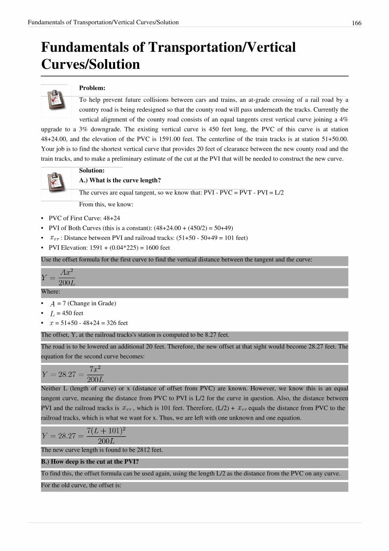
Fundamentals of Transportation/Vertical Curves/Solution 166

Fundamentals of Transportation/VerticalCurves/Solution

Problem:

To help prevent future collisions between cars and trains, an at-grade crossing of a rail road by acountry road is being redesigned so that the county road will pass underneath the tracks. Currently thevertical alignment of the county road consists of an equal tangents crest vertical curve joining a 4%

upgrade to a 3% downgrade. The existing vertical curve is 450 feet long, the PVC of this curve is at station48+24.00, and the elevation of the PVC is 1591.00 feet. The centerline of the train tracks is at station 51+50.00.Your job is to find the shortest vertical curve that provides 20 feet of clearance between the new county road and thetrain tracks, and to make a preliminary estimate of the cut at the PVI that will be needed to construct the new curve.

Solution:A.) What is the curve length?

The curves are equal tangent, so we know that: PVI - PVC = PVT - PVI = L/2From this, we know:

• PVC of First Curve: 48+24• PVI of Both Curves (this is a constant): (48+24.00 + (450/2) = 50+49)• : Distance between PVI and railroad tracks: (51+50 - 50+49 = 101 feet)• PVI Elevation: 1591 + (0.04*225) = 1600 feetUse the offset formula for the first curve to find the vertical distance between the tangent and the curve:

Where:• = 7 (Change in Grade)• = 450 feet• = 51+50 - 48+24 = 326 feetThe offset, Y, at the railroad tracks's station is computed to be 8.27 feet.The road is to be lowered an additional 20 feet. Therefore, the new offset at that sight would become 28.27 feet. Theequation for the second curve becomes:

Neither L (length of curve) or x (distance of offset from PVC) are known. However, we know this is an equaltangent curve, meaning the distance from PVC to PVI is L/2 for the curve in question. Also, the distance betweenPVI and the railroad tracks is , which is 101 feet. Therefore, (L/2) + equals the distance from PVC to therailroad tracks, which is what we want for x. Thus, we are left with one unknown and one equation.

The new curve length is found to be 2812 feet.B.) How deep is the cut at the PVI?

To find this, the offset formula can be used again, using the length L/2 as the distance from the PVC on any curve.For the old curve, the offset is:

Fundamentals of Transportation/Vertical Curves/Solution 167

For the new curve, using data found from before, the offset is:

The difference between the two offsets is 20.67 feet. This is the depth of the cut at the PVI.

Transportation Economics/PricingPricing

Rationales for PricingRoadway congestion, air pollution from cars, and the lack of resources to finance new surface transportation optionspresent challenges.  Road pricing, charging users a monetary toll in addition to the amount of time spent traveling,has been suggested as a solution to these problems.  While tolls are common for certain expensive facilities such astunnels and bridges, they are less common on streets and highways.  A  new generation of private toll roads are beingdeployed in the United States and elsewhere.  There have been a few trials of areawide pricing schemes, such as inSingapore, London, and Stockholm, and many others proposed but not implemented.In short pricing has several advantages:• Revenue• Congestion management• Off-loading costs or reallocating costs (changing who bears burden)• Changing energy supply indicates declining gas tax revenue• Encourage alternatives to drivingThere are reasons that road pricing is not more widespread. Until recently, technical issues were dominant, tollcollection added considerable delay and greatly reduced net revenue with the need for humans sitting in toll booths.However, advances in automatic vehicle identification and tolling have enabled toll collection, without humanoperators, at full speed. Other issues are fundamentally political: concerns over privacy, equity, and the perception ofdouble taxation. Privacy concerns, though political, may have a technical solution, with the use of electronic money,which is not identified with its owner, rather than credit or debit cards or automatic identification and billing ofvehicles. Equity issues, the belief that there will be winners and losers from the new system, may not be entirelyresolvable. Though it can be shown that under certain circumstances road pricing has a net benefit for society as awhole, unless a mechanism exists for making a sufficient majority of road users and voters benefit, or perceivebenefit, this concern is a roadblock to implementation. Similarly, people may believe that they have paid for roadsalready through gas taxes and general revenue, and that charging for them is akin to double taxation. Unless userscan be convinced that the revenue raised is for maintenance and expansion, or another convincing public purpose,the political sell will be difficult. Widespread road pricing may require changes in the general transportationfinancing structure and a clear accounting of the benefits will need to be provided.

Transportation Economics/Pricing 168

Objectives of Pricing Infrastructure• Economic efficiency• Cost recovery if required by the policy• Non-economic objectives

Efficient Pricing, Investment, and Cost Recoverycalls for efficient use of the existing capacity, and efficient investment on quality and capacity of infrastructure;surprisingly large benefits from efficient pricing and investment;• current pricing systems do not reflect true economic costs• poor design and capacity decisions have resulted in higher costs of use• under efficient pricing and investment decisions, the long run requisite increase in investment becomes quite

modest.

Charging for Pavement DamagePavement damage depends on vehicle weight per axle, not total vehicle weight - the damage power risesexponentially to the third power with the load per axle (e.g., a rear axle of a typical 13-ton van causes over 1000times as much damageas that of a car.In order to reflect the pavement damage costs more accurately, Small and Winston propose a "graduated per-mile taxbased on axle weight". This would give truckers (truck manufactuers) an incentive to reduce axle weights by shiftingto trucks with more axles, extending pavement life and reducing highway maintenace. The fuel tax currently in placeprovides truckers with the opposite incentives: the tax rises with a vehicle's axles, since trucks with more axlesrequire larger engines and get lower fuel economy.They pointed out that the pavement thickness guidelines of the American Association of State Highway andTransportation Officials (AASHTO) fails to incorporate economic optimization into the design procedure. Forexample, by increasing rigid concrete pavement thickness only by 2.6 inches from currently 11.2 inches to 13.8inches would more than double the life of the pavement.

Congestion Chargesare suggested as a means to allocate scarce road capacity in congested areas and peak times. The automated vehicleidentification (AVI) technology, proved as a reliable means to calculate charge congestion tolls during the HongKong experiment, the North Dallas Tollway and in New Orleans, can be used to minimize the cost of administration

Theory(based on Levinson, David (2002) Financing Transportation Networks [1] Cheltenham (UK) and Northampton (US):Edward Elgar. (Chapter 10).

Theory: Congestion Pricing Brings About Efficient Equilibrium

Transportation Economics/Pricing 169

Unpacking

The top part of Figure 2 shows schematically the travel time to a driver (short run average cost) at a bottleneck or ona capacitated link resulting from various levels of approach flow. The travel time function relates travel time (ordelay) and approach traffic flow. The greater the approach flow, the higher the travel time. At flows below capacity(level of service A (SA) or B (SB)), traffic flows smoothly, while at high approach flows, those above capacity,traffic is stop and start and is classified as level of service E (SE) or F (SF).The bottom part of Figure 2 shows schematically the implicit demand for travel on a link as a function of the traveltime. All else equal (for instance the price charged to users), demand to travel on a link at level of service A (DA) ishigher than demand at level of service F (DF). However the demand and the travel time on a link are not

Transportation Economics/Pricing 170

independent, as shown in Figure 2(A).So the implicit demand and revealed demand are not identical, rather the revealed demand is formed by projectingthe travel time at a given flow onto the implicit demand curves. So for instance, when the price charged users is high,the revealed demand coincides with the implicit demand at level of service A (DA). As the prices are lowered, therevealed demand crosses the implicit demand curve at level of service B (DB), then DC, DD, DE and finally at azero money price it crosses DF. While the actual prices that generate specific demand levels vary from place to placewith local circumstances, demand preferences, and market conditions, the general trend (higher prices gives lowerapproach flow gives better level of service) is simply an application of the law of demand from economics alongwith traffic flow theory.In other words, the change in welfare with congestion pricing depends not only on both the change in price andquantity, but also on the change in reservation price. The reservation price is the amount travelers would be willingto pay at a given level of service. And at better levels of service, travelers (and potential travelers) have a higherreservation price.

Welfare Analysis

The movement along the revealed demand curve follows the shape of the curve shown above because of therelationship between traffic flow (quantity demanded) and travel time. Assume for instance that each level of servicecategory represents a one-minute increase in travel time from the immediately better travel time. So in the graph, letthe level of service for a one minute trip be denoted SA , and for a six minute trip, SF. The amount of trafficnecessary to move from 1 minute to 2 minutes exceeds the amount to move from 2 to 3 minutes. In other words,there is a rising average (and thus marginal) cost in terms of time.The concepts in Figure 2 can be used to develop the welfare analysis shown in Figure 3. There are several areas ofinterest in Figure 3. The first is defined by the lower left triangle (the blue + green) (triangle VOZ) which is theconsumer surplus when the road is unpriced. The second is the producer surplus (profit) to the road authority whenthe road is priced, illustrated by the rectangle formed in the lower left (yellow + green) (rectangle OVWY). The thirdis the consumer surplus when the road is priced, shown in gray (triangle UVW). This consumer surplus represents ahigher reservation price than the other because the level of service is better when flow is lower.

Transportation Economics/Pricing 171

That first area needs to be compared to the sum of the second and third areas. If the sum of the second and third areas(OUWY) is larger than the first (OVZ), then pricing has higher welfare than remaining unpriced. Similarly, twoprice levels can be compared. In other words, the welfare gain from pricing is equal to the yellow + gray area(VUWX) minus the blue area (XYZ). In this particular figure, consumer’s surplus is maximized when the good isfree, but overall welfare (including producer’s surplus) is not. Whether consumer’s surplus is in fact higher in a givensituation depends on the slopes of the various demand curves.The greatest welfare is achieved by maximizing the sum of the producer’s surplus rectangle and the consumer’ssurplus “triangle” (it may not be a true triangle). This must recognize that the consumers surplus triangle’shypotenuse must follow an underlying demand curve, not the revealed demand curve. Differentiating the level ofservice (for instance, providing two different levels of service at two different prices) may result in higher overallwelfare (though not necessarily higher welfare for each individual).

Use of the RevenueHow welfare is measured and how it is perceived are two different things. If the producer’s surplus is not returned tothe users of the system somehow the users will perceive an overall welfare gain as a personal loss because it wouldbe acting as an additional tax. The money can be returned through rebates of other taxes or reinvestment intransportation. It should be noted that the entire argument can be made in reverse, where consumer and producerssurplus are measured in time rather than money, and the level of service is the monetary cost of travel. This howeverhas less practical application.

Pricing and Cost RecoveryIn low volume situations, those that are uncongested, it is unlikely that the revenue from marginal cost congestionpricing will recover long term fixed costs. This is because the marginal impacts of an additional car when volume islow is almost zero, so that additional revenue which can be raised with marginal cost pricing is also zero. Imagine aroad with one car - the car’s marginal impact is zero, a marginal cost price would also be zero, its revenue would thusbe zero, which is less than the fixed costs.Add a second car, and marginal impacts are still nearly zero - a phenomenon which remains true until capacity isapproached.

Vickery’s Types of Congestion• Simple interaction - light traffic, one car blocked by another, delay is proportional to Q^2• Multiple interaction - 0.5 < V/C < 0.9

t actual time, to freeflow time, K ~ 3-5• Bottleneck see below• Triggerneck - overflow affects other traffic• Network and Control - Traffic control devices transfer delay• General Density - high traffic level in general

Transportation Economics/Pricing 172

Marginal Cost PricingTransportation is a broad field, attracting individuals with backgrounds in engineering, economics, and planning,among others who don’t share a common model or worldview about traffic congestion. Economists look for receivedtechnological functions that can be analyzed, but risk misinterpreting them. Engineers seek basic economic conceptsto manage traffic, which they view as their own purview. These two fields intersect in the domain of congestionpricing. However many engineers view pricing with suspicion, believing that many economists are overstating itsefficacy, while the economists are frustrated with engineering intransigence, and consider engineers as lackingunderstanding of basic market principles.This section applies the microscopic model of traffic congestion that to congestion pricing, and allows us to critiquethe plausibility of several economic models of congestion that have appeared in the literature.This section uses the idea of queueing and bottlenecks to explain congestion. If there were no bottlenecks (which canbe physical and permanent such as lane drops or steep grades, or variable such as a traffic control device, ortemporary due to a crash), there would be very little congestion. Vehicles interacting on an uncongested road lead torelatively minimal delays and are not further considered (Vickery 1969, Daganzo 1995) . We define congestion, orthe congested period, to be the time when there is queueing. This exceeds the time when arrivals exceed departures,as every vehicle has to wait for all previous vehicles to depart the front of the queue before it can.A previous section developed the queueing model of congestion.

Input output diagram at level of individual vehicle

What is the implication of ourqueueing models for marginal costpricing?First, the use of hourly average timevs. flow functions such as the Bureauof Public Roads function, (which weintroduced in the discussion of routechoice (which approximates the hourlyaverage delay from a queueing model)ignores that different vehicles withinthat hour have different travel times.They are at best useful for coarsemacroscopic analyses, but shouldnever be applied to the level ofindividual vehicles.

Second, travel time for a vehicle through a bottleneck depends on the number of vehicles that have come before, butnot on the number of vehicles coming after. Similarly, the marginal delay that a vehicle imposes is only imposed onvehicles that come after. This implies that the first vehicle in the queue imposes the highest marginal delay, and thelast vehicles in the queue have the lowest marginal

Transportation Economics/Pricing 173

Marginal delay at level of individual vehicle

delay. A marginal delay function thatlooks like figure on the right (bottom)is generated from the typicalinput-output diagram shown on thefigure on the right (top). If marginalcost were equal to the marginal delay,then our pricing function would beunusual, and perhaps unstable. Theinstability might be tempered bymaking demand respond to price,rather than assuming it fixed (Raffertyand Levinson 2003), and byrecognizing the stochastic nature ofarrival and departure patterns, whichwould flatten the arrival curve to moreclosely resemble the departure curve,and thereby flatten the marginal delay curve.However, the idea that the first vehicle "causes" the delay is a controversial point. Economists will sometimes argueCoase’s position (1992) – that it takes two to have a negative externality, that there would be no congestionexternality but for the arrival of the following vehicles. Coase is, of course, correct. Moreover, they would note thatcharging a toll to the following vehicle will discourage that vehicle from coming and might also eliminate thecongestion externality. This may also be true. This would however be charging the sufferer of congestion twice(once in terms of time, a second in terms of toll), while the person with the faster trip (earlier in the queue) wouldn’tpay at all. Further, it is the followers who have already internalized the congestion externality in their decisionmaking, so tolling them is charging them twice, in contrast to charging the leaders. Given that charging either partycould eliminate the externality, it would be more reasonable to charge the delayer than the delayed, which is muchlike the “polluter pays principle” advocated by environmentalists. It would also be more equitable, in that total costs(congestion delay + toll) would now be equalized across travelers. The disadvantage of this is that the amount of thedelay caused is unknown at the time that the first traveler passes; at best it can be approximated.Implicitly, this privileges the “right to uncongested travel” over the “right to unpriced travel”. That is a philosophicalquestion, but given that there is to be some mechanism to finance highways, we can eliminate the notion of unpricedtravel altogether, the remaining issue is how to implement financing: with insensitive prices like gas taxes or flattolls or with time-dependent (or flow-dependent) congestion prices.The marginal cost equals marginal delay formulation does ignore the question of schedule delay. There are practicalreasons for not including schedule delay in a marginal cost price. Unlike delay, schedule delay is not easilymeasured. While a road administrator can tell you from traffic counts how much delay a traveler caused, theadministrator has no clue as to how much schedule delay was caused. Second, if the late (early) penalty is large, thenit dominates scheduling. Travelers can decide whether they would rather endure arriving early (without delay) orarriving on time, with some delay (or some combination of the two), presumably minimizing their associated costs.If they choose the delay, it is the lower cost alternative. That lower cost is the one they suffer, and thus that serves asa lower bound on the marginal cost to attribute to other travelers. If they choose schedule delay (which then becomesthe cost they face) and avoid the delay, they are affected as well by other travelers, but in a way that is unknown topricing authorities. They are “priced out of the market”, which happens all the time. In short, endogenizing scheduledelay would be nice, but requires more information than is actually available.

Transportation Economics/Pricing 174

Profit Maximizing PricingA realistic network of highway links is not, in the economists' terminology, perfectly competitive.  Because a linkuniquely occupies space, it attains some semblance of monopoly power. While in most cases users can switch toalternative links and routes, those alternatives will be more costly to the user in terms of travel time. Theory suggeststhat excess profits will attract new entrants into a market, but the cost of building a new link is high, indicatingbarriers to entry not easily overcome.Although roads are generally treated as public goods, they are both rivalrous when congested and in many casesexcludable.  This indicates that it is feasible to consider them for privatization.  The advantages often associated withprivatization are several: increasing the efficiency of the transportation system through road pricing, providingincentives for the facility operator to improve service through innovation and entrepreneurship, and reducing thetime and cost of building and expanding infrastructure.An issue little addressed is implementation. Most trials of road pricing suppose either tolls on a single facility, orarea-wide control. Theoretical studies often assume marginal cost pricing on links, and don't discuss ownershipstructure. However, in other sectors of the economy, central control of pricing either through government ownershipor regulation has proven itself less effective than decentralized control for serving customer demands in rapidlychanging environments. Single prices system-wide don’t provide as much information as link-specific prices. Linkswhich are priced only at marginal cost, the optimal solution in a first-best, perfectly competitive environment,constrain profit. While in the short-term, excess profit is not socially optimal, over the longer term, it attracts capitaland entrepreneurs to that sector of the economy. New capital will both invest more in existing technology to furtherdeploy it and enter the sector as competitors trying to gain from a spatial monopoly or oligopoly. Furthermore, newcapitalists may also innovate, and thereby change the supply (and demand) curves in the industry.By examining road pricing and privatization from a decentralized point of view, the issues associated with amarketplace of roads can be more fully explored, including short and long term distributional consequences andoverall social welfare. The main contribution of this research will be to approach the problem from a theoretical andconceptual level and through the conduct of simulation experiments. This analysis will identify salient empiricalfactors and critical parameters that determine system performance. To the extent that available data from recent roadpricing experiments becomes available, it may be used to compare with the results of the model.

Case 1. Simple MonopolyThe simplest example is that of a monopoly link,

The link has elastic demand :

here given by a linear equation:for all and

The objective of the link is to maximize profit .  Here we assume no congestion effects.  Profit ismaximized when the first derivative is set to zero and the second derivative is negative.

Giving the following first order conditions (f.o.c.):

Checking second order conditions (s.o.c.), we find them to be less than zero, as required for a maximum.

For this example, if and , gives , and .  This situation clearly does not maximize social welfare, defined as the sum of profit and consumer surplus.  Consumer surplus at for this demand curve is 125,000, giving a social welfare (SW) of 375,000.  Potential social welfare, maximized at (when links are costless), would be , all of

Transportation Economics/Pricing 175

which comes from consumer surplus.

Case 2. Monopolistic Perfect ComplementsIn a second simple example, we imagine two autonomous links, and , which are pure monopoliesand perfect complements, one cannot be consumed without consuming (driving on) the other. The links are in series.In this case, demand depends on the price of both links, so we can illustrate by using the following generalexpression, and a linear example : Again we assume no congestion costs.  When we profit maximize, we attain a system which produces a Nashequilibrium that is both worse off for the owners of the links, who face lower profits, and for the users of the links,who face higher collective profits, than a monopoly.  Simply put, the links do not suffer the full extent of their ownpricing policy as they would in the case of a monopoly, where the pricing externality is internalized.

f.o.c.

solving the f.o.c. simultaneously yields:

checking the s.o.c.:

At and , the solution is , which gives ,, which is less total profit than the case of the simple monopoly. This situation results in

total profit to both firms of 222,222, and a consumer surplus of 55,555, or total social welfare of 277,000, which isless than the results from the case of a simple monopoly. Similar arguments apply to three (or more) perfectcomplements, which are more and more dysfunctional if operated autonomously.  The general formula for Nautonomous perfectly complementary links, with linear demand and   , is given by:

Case 3. Duopoly of Perfect SubstitutesIn a third example, we imagine two parallel autonomous links, and , which serve the same,homogenous market.   They are perfect substitutes (operate in parallel).The optimal pricing for this case depends upon assumptions about how users distribute themselves across suppliersand the relationships between the links.  First, assume there are no congestion costs and time costs are otherwiseequal and not a factor in the decision.  Do users simply and deterministically choose the lowest cost link, or are thereother factors which shape this choice, so that a minor reduction in price will not attract all users from the other link? For this example, we assume deterministic route choice, so demand chooses the lowest cost link, or splits betweenthe links if they post the same price.  Here, demand is defined as below:

As before, let , .  Also assume that competitive links can respond instantaneously.  Assume each link can serve the entire market, so that there are no capacity restrictions. Clearly there is a (welfare maximizing) stable equilibrium at (assuming equal and zero costs for the links), the result for a competitive system.  Demonstration: Suppose each link sets price 500, and had 250 users.  If link IJ lowers its prices by one unit to 499, it attains all 501 users, and profits on link IJ increase to 249,999 from 125,000.  However profits on link KL drop to 0.  The most profitable decision for KL is to lower its price to 498, attain 502 users, and profits of 249,996.  This price war can continue until profits are eliminated.  At any point in the process raising prices by one link alone loses all demand. However it seems unlikely in the case of only two links.  Therefore, if the links could coordinate their actions they would want to.  Even in the absence of formal cartels,

Transportation Economics/Pricing 176

strategic gaming and various price signaling methods are possible.   For instance, a far sighted link KL, seeing that aprice war will ultimately hurt both firms, may only match the price cut rather than undercut in retaliation.  If IJ didnot follow with a price cut, a price will be maintained.  It has been argued (Chamberlin 1933), that the duopolywould act as a monopoly, and both links would charge the monopoly price and split the demand evenly, because thatis the best result for each since lowering prices will lead to a price war, with one link either matching or undercuttingthe other, in both cases resulting in smaller profits.

Case 4. Monopoly and CongestionThe previous three cases did not exploit any special features of transportation systems.  In this case travel time isintroduced on the network used in Case 1.  Here demand is a function of both Price ( ) and Time ( ):

For this example is given by linear form:

where travel time is evaluated with the following expression incorporating both distance effects and congestion(queuing at a bottleneck over a fixed period with steady demand):

if

if where: = freeflow travel time, = length of congested period, =

maximum flow through bottleneck.Because is a constant, and we are dealing with only a single link, it can be combined with for the analysisand won’t be considered further.  By inspection, if is large, it too does not figure into the analysis.  From Case 1,with the as given, is only important if it is less than .  For this example then, we will set at avalue less than 500, in this case assume . As before, the objective of the link is to maximize profit

. Profit is maximized when the first derivative is set to zero and the second derivative is negative.Giving the following first order conditions (f.o.c.):

Solving equations (4.2) and (4.6) simultaneously, at values:, , reflecting that the value of time for all homogenous travelers is 1 in the chosen unit

set,   , representing 1800 time units (such as seconds) of congestion, we get the following answer:.   It is thus to the advantage of the monopoly in the short term, with capacity

fixed, to allow congestion (delay) to continue, rather than raising prices high enough to eliminate it entirely.  In thelonger term, capacity expansion (which reduces delay), will allow the monopoly to charge a higher price.  In thiscase, , and .  There is a large deadweight loss to congestion, ascan be seen by comparing with Case 1.

SimulationMore complex networks are not easily analyzed in the above fashion.  Links serve as complements and substitutes atthe same time.  Simulation models address the same questions posed in the analytic model on more complexnetworks, that is, what are the performance measures and market organization under different model parameters andscenarios.  Second, we can consider market organization within the model framework, so that the question becomes:What market organization emerges under alternative assumptions, and what are the social welfare consequences ofthe organization?

Transportation Economics/Pricing 177

Competing links restrict the price that an autonomous link can charge and still maximize profits.  Furthermore, it islikely that government regulations will ultimately constrain prices, though the level of regulation may provide greatlatitude to the owners.  It is anticipated that each link will have an objective function for profit maximization.  However, depending upon assumptions of whether the firm perfectly knows market demand, and how the firmtreats the actions of competitors, the Nash equilibrium solution to the problem may not be unique, or even exist.Because the demand on a link depends on the price of both upstream and downstream links, its complements,revenue sharing between complementary links, and the concomitant coordination of prices, may better serve alllinks, increasing their profits as well as increasing social welfare. Vertical integration among highly complementarylinks is Pareto efficient.It is widely recognized that the roadway network is subject to economies of density, at least up to a point.  Thismeans that as the flow of traffic on a link increases, all else equal, the average cost of operating the link declines.   Itis less clear if links are subject to economies of scale, that it is cheaper per unit of output (for instance per  passengerkilometer traveled) to build and manage two links, a longer link, or a wider link than it is to build and manage asingle link, a shorter link, or a narrower link.   If there are such economies of scale, then link cost functions shouldreflect this.Different classes of users (rich or poor; or cars, buses, or trucks) have different values of time.  The amount of timespent on a link depends upon flow on that link, which in turn depends on price.  It may thus be a viable strategy forsome links to price high and serve fewer customers with a high value of time, and others to price low and serve morecustomers with a lower value of time.  It is hypothesized that in a sufficiently complex network, such distinct pricingstrategies should emerge from simple profit maximizing rules and limited amounts of coordination.There are a number of parameters and rules to be considered in such simulation model, some are listed below.

Parameters

Network Size and Shape.  The first issue that must be considered is the size of network in terms of  the number oflinks and nodes and how those links connect, determined by the shape of the network  (symmetric: grid, radial; asymmetric).  While the research will begin with a small network, it is possible that the equilibrium conditionsfound on limited networks may not emerge on more complex networks, giving cause for considering a more realisticsystem.Demand Size and Shape.  A second issue is the number of origin-destination markets served by the network, thelevel of demand, and the number of user classes (each with a different value of time).  Again, while the research willbegin with very simple assumptions, the results under simple conditions may be very different from those underslightly more complex circumstances.

Rules

Profit Seeking.  How do autonomous links determine the profit maximizing price in a dynamic situation?  Underlying the decision of each autonomous link is an objective function, profit maximization given certainamounts of information, and a behavioral rule which dictates the amount and direction of price changes dependingon certain factors.  Once a link has found a toll which it can neither raise nor lower without losing profit, it will betempted to stick with it. However, a more intelligent link may realize that while it may have found a local maxima,because of the non-linearities comprising a complex network, it may not be at a global maxima.  Furthermore otherlinks may not be so firmly attached to their decision, and a periodic probing of the market landscape by testingalternative prices is in order.  This too requires rules.Revenue Sharing.  It may be advantageous for complementary links to form coalitions to coordinate their action to maximize their profit.  How do these coalition form?  By the inclusion of a share of the profits of other links in one link’s objective function, that link can price more appropriately. What level of revenue sharing, between 0 and 100 percent is best?  These questions need to be tested with the model.  An interlink negotiation process will need to be

Transportation Economics/Pricing 178

developed.Cost Sharing. Similar to revenue sharing is the sharing of certain expenses that each link faces.  Links face largeexpenses periodically, such as resurfacing or snow clearance in winter, that have economies of scale.  Theseeconomies of scale may be realized either through single ownership of a great many links or through the formationof economic networks.  Just as revenue sharing between links is a variable which can be negotiated, so is costsharing.Rule Evaluation and Propagation.  A final set of considerations is the possibility of competition between rules.  Ifwe consider the rules to be identified with the firms which own links or shares of links, and set pricing policy, therules can compete.  Accumulated profits can be used by more successful rules to buy shares from less successfulrules.  The decision to sell will compare future expected profits under current management with the lump sumpayment by a competing firm.  An open market in the shares of links will need to be modeled to test these issues. Similarly, it may be possible to model rules which learn, and obtain greater intelligence iteration to iteration.

DiscussionJust as airline networks seem to have evolved a hub and spoke hierarchy, a specific geometry may be optimal in aprivate highway network.  Initial analysis indicates that there are advantages to both the private and social welfare tovertical integration of highly complementary links.  However the degree of complementarity for which integrationserves both public and private interests remains to be determined.  Other issues that are to be examined include theinfluence of substitutes and degree of competition on pricing policies through cross-elasticity of demand, economiesof scale in the provision of infrastructure, multiple classes of users with different values of time, “free” roadscompeting with toll roads, and the consequences of regulatory constraints.  Using the principles developed under theanalytic approach, a repeated game of road pricing by autonomous links learning the behavior of the system throughadaptive expectation will be developed.

Additional Problems• Homework

References• Chamberlin, E (1933) "Monopolistic competition". Harvard University Press• Coase, Ronald (1992), "The Problem of Social Cost, and Notes on the Problem of Social Cost", reprinted in The

Firm, The Market and the Law, Chicago: University of Chicago Press.• Daganzo, Carlos. (1995). An Informal Introduction To Traffic Flow Theory. University of California at Berkeley,

Institute of Transportation Studies. Berkeley, CA.• Levinson, David and Peter Rafferty (2004) Delayer Pays Principle: Examining Congestion Pricing with

Compensation [2]. International Journal of Transport Economics 31:3 295-311• Vickery, William (1969) Congestion Theory and Transport Investment. American Economic Review 59,

pp.251-260.[1] http:/ / nexus. umn. edu/ Books/ FTN. html[2] http:/ / nexus. umn. edu/ Papers/ DelayerPays. pdf

Fundamentals of Transportation/Conclusions 179

Fundamentals of Transportation/ConclusionsTransportation is multi-modal, multi-disciplinary field that requires the efforts of people from a spectrum ofbackgrounds. Planners, engineers and policy makers are the primary groups, but architects, economists, andoperations researchers serve in roles that benefit the industry. In order for an idea to become a road, it must gothrough several planning and design stages. This section serves as a conclusion for this wikibook as well as asummary of the building process for a roadway.

Connecting Places• Planning• Assessing Needs: Testing Alternatives (Hypotheses)• Predicting Demand• Trip Generation• Trip Distribution• Mode Choice• Route Assignment

Determining Road Capacity (Width)• Level of service• Design to satisfy standard• Understand implications of traffic (queues, shockwaves, congestion)

Determining Road Alignment (Length)• Properties of drivers, vehicles, roadway• Maximum grade associated with speed, vehicle type• Stopping sight distance• Vertical alignment (sags & crests)• Horizontal alignment

Determining Road Strength (Depth)• Given load on the road, how long can the road hold up.• Design pavement depth to satisfy predicted traffic.

Putting it togetherPlanning determines origin/destination demand by vehicle type … feeds into Level of Service• LOS feeds into in-depth traffic analysis and determines number of lanes• Truck demand determines maximum grade• Stopping sight distance determines horizontal and vertical curvatures.• Truck demand determines pavement thickness

Fundamentals of Transportation/Conclusions 180

ImplicationsFraction of demand (trucks) is determining design characteristics (grade, depth)Fraction of demand (peak hour traffic) is determining width.1. Financing should consider this2. Design should consider this. Maybe cars and trucks should have separate routes. (car-only highways would becheaper, separation would be safer).3. We don’t ask one building to serve all needs, why should one road?

Thought QuestionHow does an idea become a road? Explain how an idea becomes a road. Illustrate your explanation with a consistentset of examples for all of the major steps of analysis that are required (i.e. the output of one example should be theinput to the next example).

Transportation Economics/Decision makingDecision Making is the process by which one alternative is selected over another. Decision making generally occursin the planning phases of transportation projects, but last minute decision making has been shown to occur,sometimes successfully. Several procedures for making decisions have been outlined in effort to minimizeinefficencies or redundancies. These are idealized (or normative) processes, and describe how decisions might bemade in an ideal world, and how they are described in official documents. Real-world processes are not as orderly.Applied systems analysis is the use of rigorous methods to assist in determining optimal plans, designs andsolutions to large scale problems through the application of analytical methods. Applied systems analysis focusesupon the use of methods, concepts and relationships between problems and the range of techniques available. Anyproblem can have multiple solutions. The optimal solution with depend upon technical feasibility (engineering) andcosts and valuation (economics). Applied systems analysis is an attempt to move away from the engineering practiceof design detail and to integrate feasible engineering solutions with desirable economic solutions. The systemsdesigner faces the same problem as the economist, "efficient resource allocation" for a given objective function.Systems analysis emerged during World War II, especially with the deployment of radar in a coordinated way. Itspread to other fields such as fighter tactics, mission planning and weapons evaluation. Ultimately the use ofmathematical techniques in such problems came to be known as operations research, while other statistical andeconometric techniques are being applied. Optimization applies to cases where data is under-determined (fewerobservations than dependent variables) and statistics where data is over-determined (more observations thandependent variables). After World War II, techniques spread to universities. Systems analysis saw furthermathematical development and application to a broad variety of problems.It has been said of Systems Analysis, that it is:• "A coordinated set of procedures which addresses the fundamental issues of design and management: that of

specifying how men, money and materials should be combined to achieve a higher purpose" - De Neufville• "... primarily a methodology, a philosophical approach to solving problems for and for planning innovative

advances" - Baker• "Professionals who endeavor to analyze systematically the choices available to public and private agencies in

making changes in the transportation system and services in a particular region" - Manheim• "Systems analysis is not easy to write about: brief, one sentence definitions frequently are trivial" - ThomasThe most prominent decision-making process to emerge from systems analysis is rational planning, which will bediscussed next, followed by some critiques and alternatives.

Transportation Economics/Decision making 181

How does one (rationally) decide what to do?

The figure identifies three layers of abstraction. The first layer (top row) describes the high level process, which wecan summarize in six steps. A second layer details many of the components of the first layer. A third layer, identifiedby the blue box, "abstract into model or framework" depends on the problem at hand

Overview dataThe first step is observational, review and gather data about the system under consideration. An understanding of theworld around is required, including specifying the system.The problem (defined in the next step) lies within a larger system, that comprises1. Objectives - measure the effectiveness or performance2. Environment - things which affect the system but are not affected by it3. Resources - factor inputs to do the work4. Components - set of activities or tasks of the system5. Management - sets goals, allocates resources and exercises control over components6. Model of how variables in 1-5 relate to each otherthe detailed objectives are identified in the following step, and the detailed model for analysis of the problem isspecified in the step after that.For instance in the case of intercity transportation in California, data about existing demand conditions, existingsupply conditions, future demand expectations, and proposed changes to supply would be important inputs. Changesin technology and environmental conditions are important considerations for long-term projects. We would also wantto know the certainty of the forecasts, not just a central tendency, and the potential for alternative scenarios whichmay be widely different.

Transportation Economics/Decision making 182

Define the problemThe second step is to define the problem more narrowly, in a sense to identify needs.Rather than an amorphous issue (intercity transportation), we might be interested in a more detailed question, e.g.how to serve existing and future demands between two cities (say metropolitan Los Angeles and San Francisco). Theproblem might be that demand is expected to grow and outstrip supply.

Formulate goalThe third step is to formulate a goal. For major transportation projects, or projects with intense community interest,this may involve the public.In this step, the To serve future passenger demand between Los Angeles and San Francisco, quickly, safely, cleanly,and inexpensively.

The goal will need to be testable, the process below "formulate goal" in the flowchart suggests this process in moredetail.The first aspect is to operationalize the goal. We need to measure the adverbs in the goal (e.g. how do we measure"quickly", "safely", "cleanly", or "inexpensively"). Some are straight-forward. "Quickly" is a measure of travel timeor speed. But it needs to account for both the access and egress time, the waiting time, and the travel time, and thesemay not be weighted the same.The second step is identify the decision criteria. Each adverb may have a certain value, but it might be that analternative has not merely have the most points in one area, but establish at least minimum satisfactory points in allareas. So a very fast mode must meet a specific safety test, and going faster does not necessarily mean it can also bemore dangerous (despite what a rational economist might think about trade-offs).The third is to weight those criteria. E.g. how important is speed vs. safety? This is in many ways a value question,though economics can try to value each of these aspects in monetary form, enabling Evaluation. For instance, manyNegative externalities have been monetized, giving a value of time in delay, a value of pollution damages, and avalue of life.

Generate alternativesExamining, evaluating, and recommending alternatives is often the job of professionals, engineers, planners, andeconomists. Final selection is generally the job of elected or appointed officials for important projects.There are several sub-problems here, the first is to generate alternatives. This may require significant creativity.Within major alternatives, there may be many sub-alternatives, e.g. the main alternative may be mode of travel, thesub-alternatives may be different alignments. For network problems there may be many combinations of alternativealignments. If the analyst is lucky, these are separable problems, that is, the choice of one sub-alignment isindependent of the choice of alternative sub-alignments.1. Algorithms-systematic search over available alternatives

1. Analytical2. Exact numerical3. Heuristic numerical

2. Generate alternatives selectively, evaluate subjectively1. Fatal flaw analysis2. Simple rating schemes3. Delphi exercises

3. Generate alternatives judgmentally, evaluate scientifically using system model

Transportation Economics/Decision making 183

A critical issue is how many alternatives to consider. In principle, an infinite number of more or less similaralternatives may be generated, not all are practical, and some may be minor variations. In practice a stopping rule toconsider a reasonable number of alternatives is used. Major exemplars of the alternatives may be used, withfine-tuning awaiting a later step after the first set of alternatives is analyzed. The process may be iterative,winnowing down alternatives and detailing alternatives as more information is gained throughout the analysis.There are several sub-problems here, the first is to generate alternatives. This may require significant creativity.Within major alternatives, there may be many sub-alternatives, e.g. the main alternative may be mode of travel, thesub-alternatives may be different alignments. For network problemsSeveral major alternatives may be suggested, expand highways, expand air travel, or construct new high-speed railline, along with a no-build alternative.

Abstract into model or framework"All Models are Wrong, Some Models are Less Wrong than Others" -- Anonymous"All Models are Wrong, Some Models are Useful" -- George Box [1]

The term Model refers here to a mathematical representation of a system, while a Framework is a qualitativeorganizing principle for analyzing a system. The terms are sometimes used interchangeably.

Framework Example: Porter’s Diamond of Advantage

Michael Porter's Diamond of Advantage

To illustrate the idea of a framework, consider Porter'sDiamond of Advantage

Michael Porter proposes four key determinants ofcompetitiveness, which he calls the "Diamond ofAdvantage," based on cases from around the world:1. factor conditions, such as a specialized labor pool,

specialized infrastructure and sometimes selectivedisadvantages that drive innovation;

2. home demand, or local customers who pushcompanies to innovate, especially if their tastes orneeds anticipate global demand;

3. related and supporting industries, specifically internationally competitive local supplier industries, creating a highquality, supportive business infrastructure, and spurring innovation and spin-off industries; and

4. industry strategy/rivalry, involving both intense local rivalry among area industries that is more motivating thanforeign competition and as well as a local "culture" which influences individual industries' attitudes towardinnovation and competition.

Model Example: The Four-Step Urban Transportation Planning SystemWithin the rational planning framework, transportation forecasts have traditionally followed the sequential four-stepmodel or urban transportation planning (UTP) procedure, first implemented on mainframe computers in the 1950s atthe Detroit Area Transportation Study and Chicago Area Transportation Study (CATS).Land use forecasting sets the stage for the process. Typically, forecasts are made for the region as a whole, e.g., ofpopulation growth. Such forecasts provide control totals for the local land use analysis. Typically, the region isdivided into zones and by trend or regression analysis, the population and employment are determined for each.The four steps of the classical urban transportation planning system model are:

Transportation Economics/Decision making 184

• Trip generation determines the frequency of origins or destinations of trips in each zone by trip purpose, as afunction of land uses and household demographics, and other socio-economic factors.

• Destination choice matches origins with destinations, often using a gravity model function, equivalent to anentropy maximizing model. Older models include the fratar model.

• Mode choice computes the proportion of trips between each origin and destination that use a particulartransportation mode. This model is often of the logit form, developed by Nobel Prize winner Daniel McFadden.

• Route choice allocates trips between an origin and destination by a particular mode to a route. Often (for highwayroute assignment) Wardrop's principle of user equilibrium is applied, wherein each traveler chooses the shortest(travel time) path, subject to every other driver doing the same. The difficulty is that travel times are a function ofdemand, while demand is a function of travel time.

See Modeling for a deeper discussion of modeling questions.

Ascertain performanceThis is either an output of the the analytical model, or the result of subjective judgment.Sherden[2] identifies a number of major techniques for technological forecasting that can be used to ascertainexpected performance of particular technologies, but that can be used within a technology to ascertain theperformance of individual projects. These are listed in the following box:"Major techniques for technological forecasting [3]

• Delphi method: a brain-storming session with a panel of experts.• Nominal group process: a variant of the Delphi method with a group leader.• Case study method: an analysis of analogous developments in other technologies.• Trend analysis: the use of statistical analysis to extend past trends into the future.• S-curve: a form of trend analysis using an s-shaped curve to extend past trends into the future.• Correlation analysis: the projection of development of a new technology past developments in similar

technologies.• Lead-user analysis: the analysis of cading-edge users of a new technology redict how the technology will develop.• Analytic hierarchy process: the projection of a new technology by analyzing a hierarchy of forces influencing its

development.• Systems dynamics: the use of a detailed model to assess the dynamic relationships among the major forces

influencing the development of the technology.• Cross-impact analysis: the analysis of potentially interrelated future events that may affect the future development

of a technology.• Relevance trees: the breakdown of goals for a technology into more detailed goals and then assigning

probabilities that the technology will achieve these detail goals.• Scenario writing: the development of alternative future views on how the new technology could be used."

Transportation Economics/Decision making 185

Rate alternativesThe performance of each of the alternatives is compared across decision criteria, and weighted depending on theimportance of those criteria. The alternative with the highest ranking would be identified, and this information wouldbe brought forward to decision-makers.

Compute optimal decisionThe analyst is generally not the decision maker. The actual influence of the results of the analysis in actual decisionswill depend on:1. Determinacy of evaluation2. Confidence in the results on the part of the decision maker3. Consistency of rating among alternatives

Implement alternativesA decision is made. A project is constructed or a program implemented.

Evaluate outcomeEvaluating outcomes of a project includes comparing outcome against goals, but also against predictions, so thatforecasting procedures can be improved. Analysis and implementation experience lead to revisions in systemsdefinition, and may affect the values that underlay that definition. The output from this "last" step in is used as inputto earlier steps in subsequent analyses. See e.g. Parthasarathi, Pavithra and David Levinson (2010) Post-ConstructionEvaluation of Traffic Forecast Accuracy. Transport Policy [4]

Relationship to other modelsWe need a tool to "Identify Needs" and "Evaluate Options". This may be the transportation forecasting model.

Problem PRT: Skyweb ExpressThe Metropolitan Council of Governments (the region's main transportation planning agency) is examining whetherthe Twin Cities should build a new Personal Rapid Transit system in downtown Minneapolis, and they have askedyou to recommend how it should be analyzed1. What kind of model should be used. Why?2. What data should be collected.Form groups of 3 and take 15 minutes and think about what kinds of models you want to run and what data you wantto collect, what questions you would ask, and how it should be collected. Each group should have a note-taker, butall members of the group should be able to present findings to the class.

Transportation Economics/Decision making 186

Thought Questions• Is the "rational planning" process rational?• Compare and contrast the rational planning process with the scientific method?

Some Issues with Rational PlanningNevertheless, some issues remain with the rational planning model:

Problems of incomplete information• Limited Computational Capacity• Limited Solution Generating Capacity• Limited input data• Cost of Analysis

Problems of incompatible desires• Conflicting Goals• Conflicting Evaluation Criteria• Reliance on Experts (What about the People?)

Alternative Planning Decision Making Paradigms: Are They Irrational?No one really believes the rational planning process is a good description of most decision making, as it is highlyidealized. Alternatives normative and positive paradigms to the rational planning process include:Several strategies normatively address the problems associated with incomplete information:• Satisficing• Decomposition hierarchically into Strategy/Tactics/Operations.Other strategies describe how organizations and political systems work:• Organizational Process• Political BargainingSome do both:• IncrementalismThe paper Montes de Oca, Norah and David Levinson (2006) Network Expansion Decision-making in the TwinCities. Journal of the Transportation Research Board: Transportation Research Record #1981 pp 1-11 [5] describesthe actual decision making process for road construction in the Twin Cities

References[1] Box, G.E.P., Robustness in the strategy of scientific model building, in Robustness in Statistics, R.L. Launer and G.N. Wilkinson, Editors.

1979, Academic Press: New York.[2] Sherden, William (1998) The Fortune Sellers, Wiley.[3] Figure 6.4, p. 167 Major techniques for technological forecasting, in Sherden, William (1998) The Fortune Sellers, Wiley.[4] http:/ / dx. doi. org/ doi:10. 1016/ j. tranpol. 2010. 04. 010[5] http:/ / nexus. umn. edu/ Papers/ DecisionRules. pdf

Article Sources and Contributors 187

Article Sources and ContributorsFundamentals of Transportation  Source: http://en.wikibooks.org/w/index.php?oldid=1884966  Contributors: AdamD, Adrignola, Dallas1278, Darklama, DavidLevinson, Mike.lifeguard,Panic2k4, Recent Runes, Rimodo, 3 anonymous edits

Fundamentals of Transportation/About  Source: http://en.wikibooks.org/w/index.php?oldid=1613990  Contributors: AdamD, DavidLevinson, Jomegat, 2 anonymous edits

Fundamentals of Transportation/Introduction  Source: http://en.wikibooks.org/w/index.php?oldid=1701328  Contributors: AdamD, DavidLevinson, Panic2k4, QuiteUnusual, 2 anonymousedits

Transportation Economics/Introduction  Source: http://en.wikibooks.org/w/index.php?oldid=1915471  Contributors: DavidLevinson, Fishpi, MIacono

Fundamentals of Transportation/Geography and Networks  Source: http://en.wikibooks.org/w/index.php?oldid=1853200  Contributors: AdamD, DavidLevinson, 2 anonymous edits

Fundamentals of Transportation/Trip Generation  Source: http://en.wikibooks.org/w/index.php?oldid=1938135  Contributors: AdamD, DavidLevinson, Reddi, 3 anonymous edits

Fundamentals of Transportation/Trip Generation/Problem  Source: http://en.wikibooks.org/w/index.php?oldid=1238333  Contributors: AdamD, DavidLevinson

Fundamentals of Transportation/Trip Generation/Solution  Source: http://en.wikibooks.org/w/index.php?oldid=1242935  Contributors: AdamD, DavidLevinson

Fundamentals of Transportation/Destination Choice  Source: http://en.wikibooks.org/w/index.php?oldid=1938138  Contributors: AdamD, DavidLevinson, 2 anonymous edits

Fundamentals of Transportation/Destination Choice/Background  Source: http://en.wikibooks.org/w/index.php?oldid=1505583  Contributors: Adrignola, DavidLevinson

Fundamentals of Transportation/Mode Choice  Source: http://en.wikibooks.org/w/index.php?oldid=1910239  Contributors: AdamD, DavidLevinson

Fundamentals of Transportation/Mode Choice/Problem  Source: http://en.wikibooks.org/w/index.php?oldid=1238343  Contributors: AdamD, DavidLevinson

Fundamentals of Transportation/Mode Choice/Solution  Source: http://en.wikibooks.org/w/index.php?oldid=1238346  Contributors: AdamD, DavidLevinson

Fundamentals of Transportation/Route Choice  Source: http://en.wikibooks.org/w/index.php?oldid=1942988  Contributors: AdamD, Adrignola, DavidLevinson

Fundamentals of Transportation/Route Choice/Problem  Source: http://en.wikibooks.org/w/index.php?oldid=1238354  Contributors: AdamD, DavidLevinson

Fundamentals of Transportation/Route Choice/Solution  Source: http://en.wikibooks.org/w/index.php?oldid=1648165  Contributors: AdamD, DavidLevinson, Nobac001

Fundamentals of Transportation/Evaluation  Source: http://en.wikibooks.org/w/index.php?oldid=1862736  Contributors: AdamD, DavidLevinson, 1 anonymous edits

Fundamentals of Transportation/Planning  Source: http://en.wikibooks.org/w/index.php?oldid=1925405  Contributors: DavidLevinson, MIacono

Fundamentals of Transportation/Operations  Source: http://en.wikibooks.org/w/index.php?oldid=1807875  Contributors: AdamD, DavidLevinson

Fundamentals of Transportation/Queueing  Source: http://en.wikibooks.org/w/index.php?oldid=1963894  Contributors: AdamD, DavidLevinson, Panic2k4, 6 anonymous edits

Fundamentals of Transportation/Queueing/Problem1  Source: http://en.wikibooks.org/w/index.php?oldid=1238371  Contributors: AdamD, DavidLevinson

Fundamentals of Transportation/Queueing/Solution1  Source: http://en.wikibooks.org/w/index.php?oldid=1242949  Contributors: AdamD, DavidLevinson

Fundamentals of Transportation/Queueing/Problem2  Source: http://en.wikibooks.org/w/index.php?oldid=1238375  Contributors: AdamD, DavidLevinson

Fundamentals of Transportation/Queueing/Solution2  Source: http://en.wikibooks.org/w/index.php?oldid=1242950  Contributors: AdamD, DavidLevinson

Fundamentals of Transportation/Queueing/Problem3  Source: http://en.wikibooks.org/w/index.php?oldid=1238385  Contributors: AdamD, DavidLevinson

Fundamentals of Transportation/Queueing/Solution3  Source: http://en.wikibooks.org/w/index.php?oldid=1242952  Contributors: AdamD, DavidLevinson

Fundamentals of Transportation/Traffic Flow  Source: http://en.wikibooks.org/w/index.php?oldid=1616290  Contributors: AdamD, DavidLevinson, 1 anonymous edits

Fundamentals of Transportation/Traffic Flow/Problem  Source: http://en.wikibooks.org/w/index.php?oldid=1701344  Contributors: AdamD, DavidLevinson

Fundamentals of Transportation/Traffic Flow/Solution  Source: http://en.wikibooks.org/w/index.php?oldid=1701380  Contributors: AdamD, DavidLevinson, 1 anonymous edits

Fundamentals of Transportation/Queueing and Traffic Flow  Source: http://en.wikibooks.org/w/index.php?oldid=1710430  Contributors: AdamD, DavidLevinson, Wutsje, 1 anonymous edits

Fundamentals of Transportation/Shockwaves  Source: http://en.wikibooks.org/w/index.php?oldid=1807883  Contributors: AdamD, DavidLevinson, 1 anonymous edits

Fundamentals of Transportation/Shockwaves/Problem  Source: http://en.wikibooks.org/w/index.php?oldid=1238396  Contributors: AdamD, DavidLevinson

Fundamentals of Transportation/Shockwaves/Solution  Source: http://en.wikibooks.org/w/index.php?oldid=1238399  Contributors: AdamD, DavidLevinson

Fundamentals of Transportation/Traffic Signals  Source: http://en.wikibooks.org/w/index.php?oldid=1810867  Contributors: AdamD, DavidLevinson, 1 anonymous edits

Fundamentals of Transportation/Traffic Signals/Problem  Source: http://en.wikibooks.org/w/index.php?oldid=1527728  Contributors: AdamD, DavidLevinson

Fundamentals of Transportation/Traffic Signals/Solution  Source: http://en.wikibooks.org/w/index.php?oldid=1527733  Contributors: AdamD, DavidLevinson

Fundamentals of Transportation/Design  Source: http://en.wikibooks.org/w/index.php?oldid=1673917  Contributors: AdamD, DavidLevinson, 2 anonymous edits

Fundamentals of Transportation/Sight Distance  Source: http://en.wikibooks.org/w/index.php?oldid=1807866  Contributors: AdamD, DavidLevinson, 2 anonymous edits

Fundamentals of Transportation/Sight Distance/Problem  Source: http://en.wikibooks.org/w/index.php?oldid=1238406  Contributors: AdamD, DavidLevinson

Fundamentals of Transportation/Sight Distance/Solution  Source: http://en.wikibooks.org/w/index.php?oldid=1238407  Contributors: AdamD, DavidLevinson

Fundamentals of Transportation/Grade  Source: http://en.wikibooks.org/w/index.php?oldid=1807860  Contributors: AdamD, DavidLevinson, Van der Hoorn

Fundamentals of Transportation/Grade/Problem  Source: http://en.wikibooks.org/w/index.php?oldid=1238412  Contributors: AdamD

Fundamentals of Transportation/Grade/Solution  Source: http://en.wikibooks.org/w/index.php?oldid=1241907  Contributors: AdamD, Ramac

Fundamentals of Transportation/Earthwork  Source: http://en.wikibooks.org/w/index.php?oldid=1807869  Contributors: AdamD, DavidLevinson

Fundamentals of Transportation/Earthwork/Problem  Source: http://en.wikibooks.org/w/index.php?oldid=1241911  Contributors: AdamD, Ramac

Fundamentals of Transportation/Earthwork/Solution  Source: http://en.wikibooks.org/w/index.php?oldid=1241912  Contributors: AdamD

Fundamentals of Transportation/Horizontal Curves  Source: http://en.wikibooks.org/w/index.php?oldid=1807849  Contributors: AdamD, DavidLevinson, 7 anonymous edits

Fundamentals of Transportation/Horizontal Curves/Problem  Source: http://en.wikibooks.org/w/index.php?oldid=1238525  Contributors: AdamD

Article Sources and Contributors 188

Fundamentals of Transportation/Horizontal Curves/Solution  Source: http://en.wikibooks.org/w/index.php?oldid=1242971  Contributors: AdamD, Ramac

Fundamentals of Transportation/Vertical Curves  Source: http://en.wikibooks.org/w/index.php?oldid=1962509  Contributors: AdamD, Adrignola, Bacca002, DavidLevinson, GW, RecentRunes, 7 anonymous edits

Fundamentals of Transportation/Vertical Curves/Problem  Source: http://en.wikibooks.org/w/index.php?oldid=1238532  Contributors: AdamD

Fundamentals of Transportation/Vertical Curves/Solution  Source: http://en.wikibooks.org/w/index.php?oldid=1241917  Contributors: AdamD, Ramac

Transportation Economics/Pricing  Source: http://en.wikibooks.org/w/index.php?oldid=1918689  Contributors: DavidLevinson, MIacono, 1 anonymous edits

Fundamentals of Transportation/Conclusions  Source: http://en.wikibooks.org/w/index.php?oldid=1235516  Contributors: AdamD, DavidLevinson

Transportation Economics/Decision making  Source: http://en.wikibooks.org/w/index.php?oldid=1862728  Contributors: AdamD, DavidLevinson, MIacono

Image Sources, Licenses and Contributors 189

Image Sources, Licenses and ContributorsFile:MarketStreet.jpg  Source: http://en.wikibooks.org/w/index.php?title=File:MarketStreet.jpg  License: Creative Commons Attribution-Sharealike 3.0  Contributors: User:DavidLevinsonFile:100%.svg  Source: http://en.wikibooks.org/w/index.php?title=File:100%.svg  License: Public Domain  Contributors: User:SiebrandImage:TransportationInputsOutputs.png  Source: http://en.wikibooks.org/w/index.php?title=File:TransportationInputsOutputs.png  License: Creative Commons Attribution 3.0  Contributors:User:DavidLevinsonFile:Garden State Parkway Toll booth.jpg  Source: http://en.wikibooks.org/w/index.php?title=File:Garden_State_Parkway_Toll_booth.jpg  License: Public Domain  Contributors: Deadstar,JohnnyAlbert10, MitchazeniaFile:TE-Venn-1.png  Source: http://en.wikibooks.org/w/index.php?title=File:TE-Venn-1.png  License: Creative Commons Attribution-Sharealike 3.0  Contributors: DavidLevinsonFile:TE-Venn-2.png  Source: http://en.wikibooks.org/w/index.php?title=File:TE-Venn-2.png  License: Creative Commons Attribution-Sharealike 3.0  Contributors: DavidLevinsonImage:DemandForTravel.png  Source: http://en.wikibooks.org/w/index.php?title=File:DemandForTravel.png  License: Creative Commons Attribution 3.0  Contributors: User:DavidLevinsonImage:TransportationSupplyAndDemand.png  Source: http://en.wikibooks.org/w/index.php?title=File:TransportationSupplyAndDemand.png  License: Creative Commons Attribution 3.0 Contributors: User:DavidLevinsonImage:NegativeFeedback.png  Source: http://en.wikibooks.org/w/index.php?title=File:NegativeFeedback.png  License: Creative Commons Attribution 3.0  Contributors: User:DavidLevinsonImage:PositiveFeedbackVirtuous.png  Source: http://en.wikibooks.org/w/index.php?title=File:PositiveFeedbackVirtuous.png  License: Creative Commons Attribution 3.0  Contributors:User:DavidLevinsonImage:PositiveFeedbackVicious.png  Source: http://en.wikibooks.org/w/index.php?title=File:PositiveFeedbackVicious.png  License: Creative Commons Attribution 3.0  Contributors:User:DavidLevinsonImage:Routemaster.JPG  Source: http://en.wikibooks.org/w/index.php?title=File:Routemaster.JPG  License: unknown  Contributors: Dapete, KF, Kneiphof, Kotasik, LoopZilla, 1 anonymouseditsFile:Chicago Downtown Aerial View.jpg  Source: http://en.wikibooks.org/w/index.php?title=File:Chicago_Downtown_Aerial_View.jpg  License: unknown  Contributors: Adrignola,Conscious, DavidLevinson, JeremyA, Leslie, Matt314, Quasipalm, 1 anonymous editsFile:Middle Age-road.JPG  Source: http://en.wikibooks.org/w/index.php?title=File:Middle_Age-road.JPG  License: Creative Commons Attribution-Sharealike 3.0  Contributors: User:StenFile:Phoenix Freeway.JPG  Source: http://en.wikibooks.org/w/index.php?title=File:Phoenix_Freeway.JPG  License: Public Domain  Contributors: User:Adrian104Image:FOT-Planning-Hierarchy.png  Source: http://en.wikibooks.org/w/index.php?title=File:FOT-Planning-Hierarchy.png  License: Public Domain  Contributors: David LevinsonImage:HomeWorkShopEat.png  Source: http://en.wikibooks.org/w/index.php?title=File:HomeWorkShopEat.png  License: Public Domain  Contributors: User:DavidLevinsonImage:TripGeneration01.png  Source: http://en.wikibooks.org/w/index.php?title=File:TripGeneration01.png  License: Public Domain  Contributors: User:DavidLevinsonImage:TripGeneration02.png  Source: http://en.wikibooks.org/w/index.php?title=File:TripGeneration02.png  License: Public Domain  Contributors: User:DavidLevinsonImage:Evolution-tasks.png  Source: http://en.wikibooks.org/w/index.php?title=File:Evolution-tasks.png  License: GNU General Public License  Contributors: Artwork by Tuomas Kuosmanen<tigert_at_ximian.com> and Jakub Steiner <jimmac_at_ximian.com>Image:DiversionCurveMC.png  Source: http://en.wikibooks.org/w/index.php?title=File:DiversionCurveMC.png  License: Public Domain  Contributors: Original uploader was DavidLevinsonat en.wikipedia Later version(s) were uploaded by Andrew pmk at en.wikipedia.Image:ThurstonMC.png  Source: http://en.wikibooks.org/w/index.php?title=File:ThurstonMC.png  License: Public Domain  Contributors: Original uploader was DavidLevinson at en.wikipediaLater version(s) were uploaded by Andrew pmk at en.wikipedia.Image:LikelihoodMC.png  Source: http://en.wikibooks.org/w/index.php?title=File:LikelihoodMC.png  License: Public Domain  Contributors: David LevinsonImage:TwoRouteNetwork.png  Source: http://en.wikibooks.org/w/index.php?title=File:TwoRouteNetwork.png  License: Public Domain  Contributors: Original uploader was DavidLevinson aten.wikipedia Later version(s) were uploaded by Andrew pmk at en.wikipedia.Image:EquilibriumAssignment2.png  Source: http://en.wikibooks.org/w/index.php?title=File:EquilibriumAssignment2.png  License: Public Domain  Contributors: Original uploader wasDavidLevinson at en.wikipediaImage:EquilibriumAssignment3.png  Source: http://en.wikibooks.org/w/index.php?title=File:EquilibriumAssignment3.png  License: Public Domain  Contributors: Original uploader wasDavidLevinson at en.wikipedia Later version(s) were uploaded by Andrew pmk at en.wikipedia.Image:PDFNPV.PNG  Source: http://en.wikibooks.org/w/index.php?title=File:PDFNPV.PNG  License: Public Domain  Contributors: User:AdamDImage:PDF2NPV.PNG  Source: http://en.wikibooks.org/w/index.php?title=File:PDF2NPV.PNG  License: Public Domain  Contributors: User:AdamDImage:PDF3NPV.PNG  Source: http://en.wikibooks.org/w/index.php?title=File:PDF3NPV.PNG  License: Public Domain  Contributors: User:AdamDImage:ChangeInConsumersSurplus.png  Source: http://en.wikibooks.org/w/index.php?title=File:ChangeInConsumersSurplus.png  License: Public Domain  Contributors: User:DavidLevinsonImage: Queue_System.PNG  Source: http://en.wikibooks.org/w/index.php?title=File:Queue_System.PNG  License: Public Domain  Contributors: User:AdamDImage:QueueingIO.png  Source: http://en.wikibooks.org/w/index.php?title=File:QueueingIO.png  License: Creative Commons Attribution-Sharealike 3.0  Contributors: User:DavidLevinsonImage: Traffic Congestion Brasilia.jpg  Source: http://en.wikibooks.org/w/index.php?title=File:Traffic_Congestion_Brasilia.jpg  License: Creative Commons Attribution 3.0  Contributors:User:MariordoFile:Auto stoped highway.JPG  Source: http://en.wikibooks.org/w/index.php?title=File:Auto_stoped_highway.JPG  License: Creative Commons Attribution-Sharealike 2.5  Contributors:Adrignola, DavidLevinson, OsvaldoGago, Tm, Wst, ZaphodImage:TimeSpaceDiagram.png  Source: http://en.wikibooks.org/w/index.php?title=File:TimeSpaceDiagram.png  License: Creative Commons Attribution-Sharealike 3.0  Contributors:User:DavidLevinsonImage:TraditionalTrafficFlowModel.png  Source: http://en.wikibooks.org/w/index.php?title=File:TraditionalTrafficFlowModel.png  License: Creative Commons Attribution-Sharealike 3.0 Contributors: User:DavidLevinsonImage:TriangularTrafficFlowModel.png  Source: http://en.wikibooks.org/w/index.php?title=File:TriangularTrafficFlowModel.png  License: Creative Commons Attribution-Sharealike 3.0 Contributors: User:DavidLevinsonImage:TrafficPhases.png  Source: http://en.wikibooks.org/w/index.php?title=File:TrafficPhases.png  License: Creative Commons Attribution-Sharealike 3.0  Contributors: User:DavidLevinsonImage:QueueingIOPhases.png  Source: http://en.wikibooks.org/w/index.php?title=File:QueueingIOPhases.png  License: Creative Commons Attribution-Sharealike 3.0  Contributors:User:DavidLevinsonImage:Bottleneck.png  Source: http://en.wikibooks.org/w/index.php?title=File:Bottleneck.png  License: Creative Commons Attribution-Sharealike 3.0  Contributors: User:DavidLevinsonImage:BackwardBending.png  Source: http://en.wikibooks.org/w/index.php?title=File:BackwardBending.png  License: Creative Commons Attribution-Sharealike 3.0  Contributors:User:DavidLevinsonImage:ShockwaveGraphic.png  Source: http://en.wikibooks.org/w/index.php?title=File:ShockwaveGraphic.png  License: Public Domain  Contributors: David LevinsonImage:ShockwaveGraphic02.png  Source: http://en.wikibooks.org/w/index.php?title=File:ShockwaveGraphic02.png  License: Public Domain  Contributors: User:DavidLevinsonImage: Feuvert2.jpg  Source: http://en.wikibooks.org/w/index.php?title=File:Feuvert2.jpg  License: Public Domain  Contributors: User:WazouilleImage:AASHTOSSD.png  Source: http://en.wikibooks.org/w/index.php?title=File:AASHTOSSD.png  License: Creative Commons Attribution 3.0  Contributors: User:DavidLevinsonImage:I-90_floating_bridges_looking_east.JPG  Source: http://en.wikibooks.org/w/index.php?title=File:I-90_floating_bridges_looking_east.JPG  License: GNU Free Documentation License Contributors: Infrogmation, Jmabel, Ronaldino, Strangnet, Tano4595, XnatedawgxFile:SF Filbert St North Beach CA-e.jpg  Source: http://en.wikibooks.org/w/index.php?title=File:SF_Filbert_St_North_Beach_CA-e.jpg  License: Creative Commons Attribution-Sharealike 2.5 Contributors: User:DschwenFile:Lombard Street.jpg  Source: http://en.wikibooks.org/w/index.php?title=File:Lombard_Street.jpg  License: Creative Commons Attribution 2.0  Contributors: Adrignola, DavidLevinsonImage:Triaxle dump truck 2005-10-06.km.jpg  Source: http://en.wikibooks.org/w/index.php?title=File:Triaxle_dump_truck_2005-10-06.km.jpg  License: GNU Free Documentation License Contributors: AdamD, Adrignola, G®iffen, Kymacpherson, MB-one, Stefan Knauf, Wesha, 1 anonymous editsImage:Cross-section.PNG  Source: http://en.wikibooks.org/w/index.php?title=File:Cross-section.PNG  License: Public Domain  Contributors: User:AdamD

Image Sources, Licenses and Contributors 190

Image:CutFillDiagram.PNG  Source: http://en.wikibooks.org/w/index.php?title=File:CutFillDiagram.PNG  License: Public Domain  Contributors: User:AdamDImage:MassDiagram.PNG  Source: http://en.wikibooks.org/w/index.php?title=File:MassDiagram.PNG  License: Public Domain  Contributors: User:AdamDImage:Ring_3_and_E6_Oslo_Quevaal.jpg  Source: http://en.wikibooks.org/w/index.php?title=File:Ring_3_and_E6_Oslo_Quevaal.jpg  License: Creative Commons Attribution-Sharealike 2.5 Contributors: User:QuevaalFile:-88 Navy Chevrolet Monte Carlo.jpg  Source: http://en.wikibooks.org/w/index.php?title=File:-88_Navy_Chevrolet_Monte_Carlo.jpg  License: Public Domain  Contributors: U.S. Navyphoto by Mass Communications Specialist 2nd Class Kristopher WilsonImage:Horizontal_Curve.JPG  Source: http://en.wikibooks.org/w/index.php?title=File:Horizontal_Curve.JPG  License: Public Domain  Contributors: User:AdamDImage:Costal_Redwood.jpg  Source: http://en.wikibooks.org/w/index.php?title=File:Costal_Redwood.jpg  License: GNU Free Documentation License  Contributors: Ayacop, H-stt, Quadell,UrbanImage:Horizontal_Curve_Example_2.JPG  Source: http://en.wikibooks.org/w/index.php?title=File:Horizontal_Curve_Example_2.JPG  License: Public Domain  Contributors: User:AdamDImage:Centerline_Rumble_Strip.jpg  Source: http://en.wikibooks.org/w/index.php?title=File:Centerline_Rumble_Strip.jpg  License: Public Domain  Contributors: User:SayCheeeeeeseImage:Vertical_Curve.PNG  Source: http://en.wikibooks.org/w/index.php?title=File:Vertical_Curve.PNG  License: Public Domain  Contributors: User:AdamDImage:Vertical_Curve_Example_2.JPG  Source: http://en.wikibooks.org/w/index.php?title=File:Vertical_Curve_Example_2.JPG  License: Public Domain  Contributors: User:AdamDImage:TE-Pricing-EquilibriumCongestion.png  Source: http://en.wikibooks.org/w/index.php?title=File:TE-Pricing-EquilibriumCongestion.png  License: Creative CommonsAttribution-Sharealike 3.0  Contributors: User:DavidLevinsonImage:TE-Pricing-EquilbriumUnpacked.png  Source: http://en.wikibooks.org/w/index.php?title=File:TE-Pricing-EquilbriumUnpacked.png  License: Creative Commons Attribution-Sharealike3.0  Contributors: User:DavidLevinsonImage:TE-Pricing-WelfareAnalysis.png  Source: http://en.wikibooks.org/w/index.php?title=File:TE-Pricing-WelfareAnalysis.png  License: Creative Commons Attribution-Sharealike 3.0 Contributors: User:DavidLevinsonImage:CongestionPricingA.png  Source: http://en.wikibooks.org/w/index.php?title=File:CongestionPricingA.png  License: Creative Commons Attribution-Sharealike 3.0  Contributors:User:DavidLevinsonImage:CongestionPricingB.png  Source: http://en.wikibooks.org/w/index.php?title=File:CongestionPricingB.png  License: Creative Commons Attribution-Sharealike 3.0  Contributors:User:DavidLevinsonImage:TE-Systems-RationalPlanningAndDecisionMaking.png  Source: http://en.wikibooks.org/w/index.php?title=File:TE-Systems-RationalPlanningAndDecisionMaking.png  License:Creative Commons Attribution-Sharealike 3.0  Contributors: User:DavidLevinsonImage:TE-Systems-Porter's Diamond.jpg  Source: http://en.wikibooks.org/w/index.php?title=File:TE-Systems-Porter's_Diamond.jpg  License: unknown  Contributors: QuintEssence Source:Self-made using Image Tools

License 191

LicenseCreative Commons Attribution-Share Alike 3.0 Unportedhttp:/ / creativecommons. org/ licenses/ by-sa/ 3. 0/