Fundamentals of Thermodynamics and Applications

Ingo Müller · Wolfgang H. Müller

Fundamentals ofThermodynamics andApplicationsWith Historical Annotations and ManyCitations from Avogadro to Zermelo

ABC

Prof. Ingo MüllerInstitut für Prozess- und VerfahrenstechnikThermodynamik und Thermische VerfahrenstechnikTechnische Universität BerlinStr. des 17. Juni 13510623 BerlinGermanyE-mail: [email protected]

Prof. Dr. Wolfgang H. MüllerFakultät V - Verkehrs- und MaschinensystemeTechnische Universität BerlinEinsteinufer 5D-10587 BerlinGermanyE-mail: [email protected]

ISBN 978-3-540-74645-4 e-ISBN 978-3-540-74648-5

DOI 10.1007/978-3-540-74648-5

Library of Congress Control Number: 2008942041

c© 2009 Springer-Verlag Berlin Heidelberg

This work is subject to copyright. All rights are reserved, whether the whole or part of the mate-rial is concerned, specifically the rights of translation, reprinting, reuse of illustrations, recitation,broadcasting, reproduction on microfilm or in any other way, and storage in data banks. Dupli-cation of this publication or parts thereof is permitted only under the provisions of the GermanCopyright Law of September 9, 1965, in its current version, and permission for use must alwaysbe obtained from Springer. Violations are liable to prosecution under the German Copyright Law.

The use of general descriptive names, registered names, trademarks, etc. in this publication doesnot imply, even in the absence of a specific statement, that such names are exempt from the relevantprotective laws and regulations and therefore free for general use.

Typesetting: Scientific Publishing Services Pvt. Ltd., Chennai, India.Cover Design: eStudio Calamar S.L.

Printed in acid-free paper

9 8 7 6 5 4 3 2 1

springer.com

Preface

Thermodynamics is the much abused slave of many masters • physicists who love the totally impractical Carnot process, • mechanical engineers who design power stations and refrigerators, • chemists who are successfully synthesizing ammonia and are puzzled by photosynthesis, • meteorologists who calculate cloud bases and predict föhn, boraccia and scirocco, • physico-chemists who vulcanize rubber and build fuel cells, • chemical engineers who rectify natural gas and distil fer-mented potato juice, • metallurgists who improve steels and harden surfaces, • nu-trition counselors who recommend a proper intake of calories, • mechanics who adjust heat exchangers, • architects who construe – and often misconstrue – chim-neys, • biologists who marvel at the height of trees, • air conditioning engineers who design saunas and the ventilation of air plane cabins, • rocket engineers who create supersonic flows, et cetera.

Not all of these professional groups need the full depth and breadth of thermo-dynamics. For some it is enough to consider a well-stirred tank, for others a sta-tionary nozzle flow is essential, and yet others are well-served with the partial dif-ferential equation of heat conduction.

It is therefore natural that thermodynamics is prone to mutilation; different group-specific meta-thermodynamics’ have emerged which serve the interest of the groups under most circumstances and leave out aspects that are not often needed in their fields. To stay with the metaphor of the abused slave we might say that in some fields his legs and an arm are cut off, because only one arm is needed; in other circumstances the brain of the slave has atrophied, because only his arms and legs are needed. Students love this reduction, because it enables them to avoid “nonessential” aspects of thermodynamics. But the practice is dangerous; it may backfire when a brain is needed.

In this book we attempt to exhibit the complete fundament of classical thermo-dynamics which consists of the equations of balance of mass, momentum and en-ergy, and of constitutive equations which characterize the behavior of material bodies, mostly gases, vapors and liquids because, indeed, classical thermodynam-ics is often negligent of solids, – and so are we, although not entirely.

Many applications are treated in the book by specializing the basic equations; a brief look at the table of contents bears witness to that feature.

Modern thermodynamics is a lively field of research at extremely low and ex-tremely high temperatures and for strongly rarefied gases and in nano-tubes, or nano-layers, where quantum effects occur. But such subjects are not treated in this book. Indeed, there is nothing here which is not at least 70 years old. We claim, however, that our presentation is systematic and we believe that classical thermo-dynamics should be taught as we present it. If it were, thermodynamics might shed the nimbus of a difficult subject which surrounds it among students.

Even classical thermodynamics is such a wide field that it cannot be fully de-scribed in all its ramifications in a relatively short book like this one. We had to

VI Preface

resign ourselves to that fact. And we have decided to omit all discussion of • em-pirical state functions, • temperature dependent specific heats of liquids and ideal gases, and • irreversible secondary effects in engines. Such phenomena affect the neat analytical structure of thermodynamic problems, and we have excluded them, although we know full well that they are close to the hearts and minds of engi-neers who may even, in fact, consider incalculable irreversibilities of technical processes as the essence of thermodynamics. We do not share that opinion.

In the second half of the 19th century and early in the 20th century thermody-namics was at the forefront of physics, and eminent physicists and chemists like Planck, Einstein and Haber were steeped in thermodynamics; actually the formula E = m c2, which identifies energy as it were, is basically a contribution to thermo-dynamics. We have made an attempt to enliven the text by a great many mini-biographies and historical annotations which are somewhat relevant to the devel-opment of thermodynamics or, in other cases, they illustrate early misconceptions which may serve to highlight the difficult emergence of the basic concepts of the field. A prologue has been placed in front of the main chapters in order to avoid going into subjects which are by now so commonplace that they are taught in high schools.

Colleagues, co-workers, and students have contributed to this work, some sig-nificantly, others little, but all of them something:

Manfred Achenbach, Giselle Alves, Jutta Ansorg, Teodor Atanackovic, Jörg Au, Elvira Barbera, Andreas Bensberg, Andreas Bormann, Michel Bornert, Tamara Borowski, Wolfgang Dreyer, Heinrich Ehrenstein, Fritz Falk, Semlin Fu, Uwe Glasauer, Anja Hofmann, Yongzhong Huo, Oliver Kastner, Wolfgang Kitsche, Gilberto M. Kremer, Thomas Lauke, I-shih Liu, Wilson Marquez jr., Angelo Morro, Olav Müller, André Musolff, Mario Pitteri, Daniel Reitebuch, Roland Ry-dzewski, Harsimar Sahota, Stefan Seelecke, Ute Stephan, Peter Strehlow, Hen-ning Struchtrup, Manuel Torrilhon, Wolf Weiss, Krzysztof Wilmanski, Yihuan Xie, Huibin Xu, Giovanni Zanzotto.

Mark Warmbrunn has drawn the cartoons. Rudolf Hentschel and Marlies Hentschel have helped with the figures and part of the text.

Several teaching assistants have edited the text and converted it into Springer style: Matti Blume, Anja Klinnert, Volker Marhold, Christoph Menzel, Felix J. Müller.

Guido Harneit has given support with the computer.

Everyone of them deserves our sincere gratitude.

Berlin, in the summer of 2008

Ingo Müller & Wolfgang H. Müller

Contents

P Prologue on ideal gases and incompressible fluids................................... 1P.1 Thermal and caloric equations of state................................................. 1

• Ideal gases ..................................................................................... 1• Incompressible fluid ...................................................................... 1

P.2 “mol”.................................................................................................... 2P.3 On the history of the equations of state ................................................ 3P.4 An elementary kinetic view of the equations of state for ideal gases;

interpretation of pressure and absolute temperature ............................ 4

1 Objectives of thermodynamics and its equations of balance................... 7 1.1 Fields of mechanics and thermodynamics ........................................... 7

1.1.1 Mass density, velocity, and temperature........................................... 7 1.1.2 History of temperature ...................................................................... 7

1.2 Equations of balance............................................................................ 9 1.2.1 Conservation laws of thermodynamics............................................. 91.2.2 Generic equations of balance for closed and open systems .............. 91.2.3 Generic local equation of balance in regular points........................ 10

1.3 Balance of mass................................................................................. 11 1.3.1 Integral and local balance equations of mass.................................. 111.3.2 Mass balance and nozzle flow ........................................................ 11

1.4 Balance of momentum....................................................................... 12 1.4.1 Integral and local balance equations of momentum........................ 121.4.2 Pressure........................................................................................... 141.4.3 Pressure in an incompressible fluid at rest...................................... 141.4.4 History of pressure and pressure units ............................................ 151.4.5 Applications of the momentum balance ......................................... 16

• Buoyancy law of ARCHIMEDES ................................................... 16• Barometric steps in the atmosphere............................................. 17• Thrust of a rocket ........................................................................ 18• Thrust of a jet engine................................................................... 19• Convective momentum flux ........................................................ 20• Momentum balance and nozzle flow........................................... 21• Bernoulli equation ....................................................................... 23• Kutta-Joukowski formula for the lift of an airfoil ....................... 24

1.5 Balance of energy .............................................................................. 26 1.5.1 Kinetic energy, potential energy, and four types

of internal energy............................................................................ 26• Kinetic energy of thermal atomic motion. “Heat energy” ........... 26• Potential energy of molecular interaction. “Van der Waals

energy” or “elastic energy” ......................................................... 27

VIII Contents

• Chemical energy between molecules. “Heat of reaction” ........... 27• Nuclear energy ............................................................................ 29• Heat into work............................................................................. 29

1.5.2 Integral and local equations of balance of energy .......................... 291.5.3 Potential energy .............................................................................. 311.5.4 Balance of internal energy .............................................................. 321.5.5 Short form of energy balance for closed systems ........................... 331.5.6 First Law for reversible processes. The basis of “pdV -

thermodynamics”............................................................................ 341.5.7 Enthalpy and First Law for stationary flow processes.................... 341.5.8 “Adiabatic equation of state” for an ideal gas – an integral of the

energy balance ................................................................................ 361.5.9 Applications of the energy balance................................................. 37

• Experiment of GAY-LUSSAC ....................................................... 37• Piston drops into cylinder............................................................ 38• Throttling .................................................................................... 40• Heating of a room........................................................................ 40• Nozzle flow ................................................................................. 42• Fan............................................................................................... 46• Turbine ........................................................................................ 47• Chimney ...................................................................................... 48• Thermal power station................................................................. 50

1.6 History of the First Law .................................................................... 53 1.7 Summary of equations of balance ..................................................... 55

2. Constitutive equations .............................................................................. 572.1 On measuring constitutive functions ................................................. 57

2.1.1 The need for constitutive equations ................................................ 572.1.2 Constitutive equations for viscous, heat-conducting fluids,

vapors, and gas ............................................................................... 572.2 Determination of viscosity and thermal conductivity........................ 59

2.2.1 Shear flow between parallel plates. NEWTON’s law of friction ...... 592.2.2 Heat conduction through a window-pane ....................................... 61

2.3 Measuring the state functions p(υ,T) and u(υ,T) ............................... 63 2.3.1 The need for measurements ............................................................ 632.3.2 Thermal equations of state.............................................................. 632.3.3 Caloric equation of state ................................................................. 642.3.4 Equations of state for air and superheated steam............................ 662.3.5 Equations of state for liquid water.................................................. 67

2.4 State diagrams for fluids and vapors with a phase transition............. 68 2.4.1 The phenomenon of a liquid-vapor phase transition....................... 682.4.2 Melting and sublimation ................................................................. 702.4.3 Saturated vapor curve of water ....................................................... 702.4.4 On the anomaly of water................................................................. 73

Contents IX

2.4.5 Wet region and ),( υp -diagram of water........................................ 75

2.4.6 3D phase diagram ........................................................................... 752.4.7 Heat of evaporation and (h,T)–diagram of water ............................ 762.4.8 Applications of saturated steam...................................................... 77

• The preservation jar..................................................................... 77• Pressure cooker ........................................................................... 78

2.4.9 Van der Waals equation.................................................................. 792.4.10 On the history of liquefying gases and solidifying liquids ............. 81

3 Reversible processes and cycles “p dV thermodynamics” for the calculation of thermodynamic engines......................................................... 833.1 Work and heat for reversible processes ............................................. 83 3.2 Compressor and pneumatic machine. The hot air engine .................. 84

3.2.1 Work needed for the operation of a compressor ............................. 843.2.2 Two-stage compressor .................................................................... 863.2.3 Pneumatic machine......................................................................... 863.2.4 Hot air engine ................................................................................. 87

3.3 Work and heat for reversible processes in ideal gases. “Iso-processes” and adiabatic processes............................................ 88

3.4 Cycles ................................................................................................ 893.4.1 Efficiency in the conversion of heat to work .................................. 893.4.2 Efficiencies of special cycles .......................................................... 90

• Joule process ............................................................................... 90• Carnot cycle................................................................................. 91• Modified Carnot cycle................................................................. 92• Ericson cycle ............................................................................... 94• Stirling cycle ............................................................................... 96

3.5 Internal combustion cycles ................................................................ 963.5.1 Otto cycle........................................................................................ 963.5.2 Diesel cycle..................................................................................... 993.5.3 On the history of the internal combustion engine ......................... 101

3.6 Gas turbine ...................................................................................... 1023.6.1 Brayton process ............................................................................ 1023.6.2 Jet propulsion process................................................................... 1033.6.3 Turbofan engine............................................................................ 104

4. Entropy .................................................................................................... 1054.1 The Second Law of thermodynamics .............................................. 105

4.1.1 Formulation and exploitation........................................................ 105• Formulation ............................................................................... 105• Universal efficiency of the Carnot process................................ 105• Absolute temperature as an integrating factor ........................... 107

X Contents

• Growth of entropy ..................................................................... 108• ( )ST , -diagram and maximal efficiency of the

Carnot process........................................................................... 1104.1.2 Summary....................................................................................... 111

4.2 Exploitation of the Second Law ...................................................... 1134.2.1 Integrability condition .................................................................. 1134.2.2 Internal energy and entropy of a van der Waals gas and

of an ideal gas ............................................................................... 1144.2.3 Alternatives of the Gibbs equation and its integrability

conditions ..................................................................................... 1154.2.4 Phase equilibrium. Clausius-Clapeyron equation ......................... 1174.2.5 Phase equilibrium in a van der Waals gas .................................... 1194.2.6 Temperature change during adiabatic throttling. Example:

Van der Waals gas ........................................................................ 1204.2.7 Available free energies ................................................................. 1234.2.8 Stability conditions ....................................................................... 1254.2.9 Specific heat cp is singular at the critical point ............................. 126

4.3 A layer of liquid heated from below – onset of convection............. 1274.4 On the history of the Second Law ................................................... 131

5. Entropy as S=k lnW ................................................................................ 1355.1 Molecular interpretation of entropy................................................. 1355.2 Entropy of a gas and of a polymer molecule ................................... 1355.3 Entropy as a measure of disorder .................................................... 1395.4 Maxwell distribution ....................................................................... 1405.5 Entropy of a rubber rod ................................................................... 1415.6 Examples for entropy and Second Law. Gas and rubber................. 143

5.6.1 Gibbs equation and integrability condition for liquids and solids .......................................................................... 143

5.6.2 Examples for entropic elasticity ................................................... 1455.6.3 Real gases and crystallizing rubber .............................................. 1465.6.4 Free energy of gases and rubber. ( )Vp, - and ( )LP, -curves. ....... 148

5.6.5 Reversible and hysteretic phase transitions .................................. 1505.7 History of the molecular interpretation of entropy .......................... 151

6. Steam engines and refrigerators ............................................................ 1536.1 The history of the steam engine....................................................... 1536.2 Steam engines.................................................................................. 155

6.2.1 The ( )ST , -diagram....................................................................... 155

6.2.2 Clausius-Rankine process. The essential role of enthalpy............ 1556.2.3 Clausius-Rankine process in a ( )ST , -diagram............................. 157

6.2.4 The ( )sh, -diagram ....................................................................... 159

6.2.5 Steam flow rate and efficiency of a power station........................ 1616.2.6 Carnotization ................................................................................ 162

Contents XI

6.2.7 Mercury-water binary vapor cycle................................................ 1636.2.8 Combined gas-vapor cycle............................................................ 164

6.3 Refrigerator and heat pump ............................................................. 1646.3.1 Compression refrigerator .............................................................. 1646.3.2 Calculation for a cold storage room.............................................. 1656.3.3 Absorption refrigerator ................................................................. 1666.3.4 Refrigerants .................................................................................. 1676.3.5 Heat pump..................................................................................... 168

7. Heat Transfer .......................................................................................... 1717.1 Non-Stationary Heat Conduction .................................................... 171

7.1.1 The heat conduction equation ....................................................... 171 7.1.2 Separation of variables ................................................................. 171 7.1.3 Examples of heat conduction........................................................ 172

• Heat conduction of an adiabatic rod of length L ...................... 172 • Heat conduction in an infinitely long rod.................................. 175 • Maximum of temperature of the heat-pole-solution.................. 176 • Heat waves in the Earth............................................................. 177

7.1.4 On the history of non-stationary heat conduction......................... 179 7.2 Heat Exchangers.............................................................................. 179

7.2.1 Heat transport coefficients and heat transfer coefficient............... 179 7.2.2 Temperature gradients in the flow direction ................................. 181 7.2.3 Temperatures along the heat exchanger........................................ 182

7.3 Radiation ......................................................................................... 184 7.3.1 Coefficients of spectral emission and absorption ......................... 184 7.3.2 Kirchhoff’s law............................................................................. 186 7.3.3 Averaged emission coefficient and averaged

absorption number ........................................................................ 187 7.3.4 Examples of thermodynamics of radiation ................................... 190

• Temperature of the sun and its planets ...................................... 190 • A comparison of radiation and conduction................................ 192

7.3.5 On the history of heat radiation .................................................... 193 7.4 Utilization of Solar Energy.............................................................. 194

7.4.1 Availability ................................................................................... 194 7.4.2 Thermosiphon............................................................................... 195 7.4.3 Green house .................................................................................. 196 7.4.4 Focusing collectors. The burning glass......................................... 198

8. Mixtures, solutions, and alloys............................................................... 1998.1 Chemical potentials ......................................................................... 199

8.1.1 Characterization of mixtures......................................................... 1998.1.2 Chemical potentials. Definition and relation to

Gibbs free energy.......................................................................... 2008.1.3 Chemical potentials; eight useful properties................................. 2018.1.4 Measuring chemical potentials ..................................................... 203

XII Contents

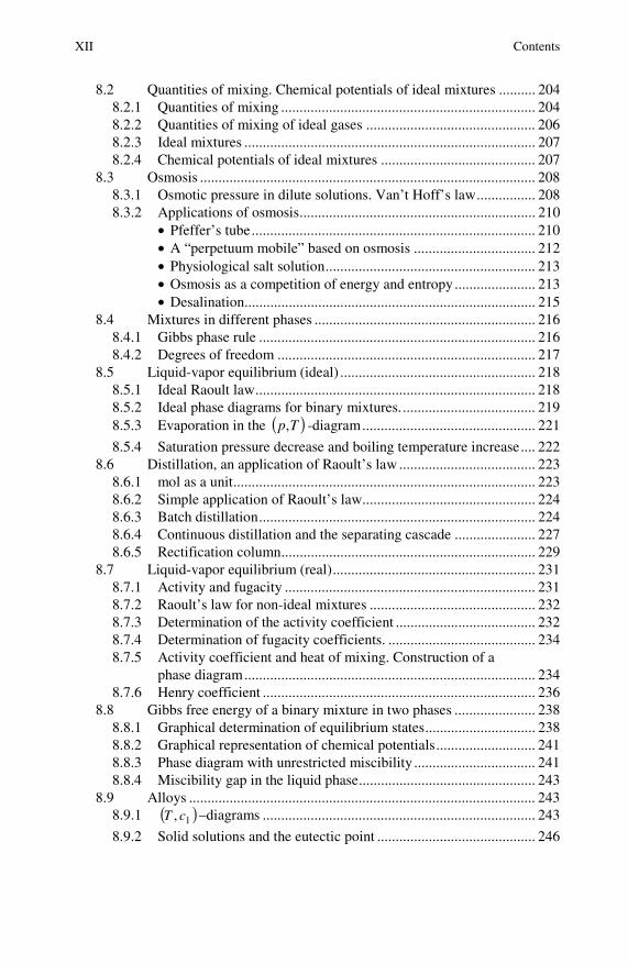
8.2 Quantities of mixing. Chemical potentials of ideal mixtures .......... 2048.2.1 Quantities of mixing ..................................................................... 2048.2.2 Quantities of mixing of ideal gases .............................................. 2068.2.3 Ideal mixtures ............................................................................... 2078.2.4 Chemical potentials of ideal mixtures .......................................... 207

8.3 Osmosis ........................................................................................... 2088.3.1 Osmotic pressure in dilute solutions. Van’t Hoff’s law................ 2088.3.2 Applications of osmosis................................................................ 210

• Pfeffer’s tube............................................................................. 210• A “perpetuum mobile” based on osmosis ................................. 212• Physiological salt solution......................................................... 213• Osmosis as a competition of energy and entropy ...................... 213• Desalination............................................................................... 215

8.4 Mixtures in different phases ............................................................ 2168.4.1 Gibbs phase rule ........................................................................... 2168.4.2 Degrees of freedom ...................................................................... 217

8.5 Liquid-vapor equilibrium (ideal) ..................................................... 2188.5.1 Ideal Raoult law............................................................................ 2188.5.2 Ideal phase diagrams for binary mixtures..................................... 2198.5.3 Evaporation in the ( )Tp, -diagram............................................... 221

8.5.4 Saturation pressure decrease and boiling temperature increase.... 2228.6 Distillation, an application of Raoult’s law ..................................... 223

8.6.1 mol as a unit.................................................................................. 2238.6.2 Simple application of Raoult’s law............................................... 2248.6.3 Batch distillation........................................................................... 2248.6.4 Continuous distillation and the separating cascade ...................... 2278.6.5 Rectification column..................................................................... 229

8.7 Liquid-vapor equilibrium (real)....................................................... 2318.7.1 Activity and fugacity .................................................................... 2318.7.2 Raoult’s law for non-ideal mixtures ............................................. 2328.7.3 Determination of the activity coefficient ...................................... 2328.7.4 Determination of fugacity coefficients. ........................................ 2348.7.5 Activity coefficient and heat of mixing. Construction of a

phase diagram............................................................................... 2348.7.6 Henry coefficient .......................................................................... 236

8.8 Gibbs free energy of a binary mixture in two phases ...................... 2388.8.1 Graphical determination of equilibrium states.............................. 2388.8.2 Graphical representation of chemical potentials........................... 2418.8.3 Phase diagram with unrestricted miscibility ................................. 2418.8.4 Miscibility gap in the liquid phase................................................ 243

8.9 Alloys .............................................................................................. 2438.9.1 ( )1, cT –diagrams .......................................................................... 243

8.9.2 Solid solutions and the eutectic point ........................................... 246

Contents XIII

8.9.3 Gibbs phase rule for a binary mixture........................................... 2478.10 Ternary Phase Diagrams.................................................................. 247

8.10.1 Representation .............................................................................. 2478.10.2 Miscibility gaps in ternary solutions............................................. 248

9. Chemically reacting mixtures ................................................................ 2519.1 Stoichiometry and law of mass action ............................................. 251

9.1.1 Stoichiometry................................................................................ 2519.1.2 Application of stoichiometry. Respiratory quotient RQ ............... 2539.1.3 Law of mass action ....................................................................... 2539.1.4 Law of mass action for ideal mixtures and mixtures of

ideal gases..................................................................................... 2549.1.5 On the history of the law of mass action....................................... 2559.1.6 Examples for the law of mass action for ideal gases .................... 256

• From hydrogen and iodine to hydrogen iodide and vice versa................................................................................... 256

• Decomposition of carbon dioxide into carbon monoxide and oxygen ................................................................................ 257

9.1.7 Equilibrium in stoichiometric mixtures of ideal gases.................. 2589.2 Heats of reaction, entropies of reaction, and absolute values of

entropies .......................................................................................... 2609.2.1 The additive constants in u and s ............................................... 2609.2.2 Heats of reaction ........................................................................... 2629.2.3 Entropies of reaction..................................................................... 2639.2.4 Le Chatelier’s principle of least constraint ................................... 264

9.3 Nernst’s heat theorem. The Third Law of thermodynamics ............ 2649.3.1 Third Law in Nernst’s formulation............................................... 2649.3.2 Application of the Third Law. The latent heat of the

transformation gray→white in tin................................................. 2659.3.3 Third Law in PLANCK’s formulation ............................................ 2669.3.4 Absolute values of energy and entropy......................................... 267

9.4 Energetic and entropic contributions to equilibrium ....................... 2679.4.1 Three contributions to the Gibbs free energy................................ 2679.4.2 Examples for minima of the Gibbs free energy ............................ 269 H2 2H .................................................................................... 269

322 NH23HN →+ Haber-Bosch synthesis of ammonia......... 270

9.4.3 On the history of the Haber-Bosch synthesis................................ 2719.5 The fuel cell..................................................................................... 272

9.5.1 Chemical Reactions ...................................................................... 2729.5.2 Various types of fuel cells ............................................................ 2739.5.3 Thermodynamics .......................................................................... 2749.5.4 Effects of temperature and pressure.............................................. 2769.5.5 Power of the fuel cell .................................................................... 2769.5.6 Efficiency of the fuel cell.............................................................. 277

XIV Contents

9.6 Thermodynamics of photosynthesis ................................................ 2789.6.1 The dilemma of glucose synthesis ................................................ 2789.6.2 Balance of particle numbers ......................................................... 2799.6.3 Balance of energy. Why a plant needs lots of water ..................... 2809.6.4 Balance of entropy. Why a plant needs air ................................... 2829.6.5 Discussion..................................................................................... 283

10. Moist air................................................................................................... 28510.1 Characterization of moist air ............................................................ 285

10.1.1 Moisture content ........................................................................... 28510.1.2 Enthalpy of moist air .................................................................... 28510.1.3 Table for moist air ........................................................................ 28610.1.4 The ( )xh x ,1+ -diagram .................................................................. 288

10.2 Simple processes in moist air .......................................................... 28910.2.1 Supply of water............................................................................. 28910.2.2 Heating ......................................................................................... 29010.2.3 Mixing .......................................................................................... 29010.2.4 Mixing of moist air with fog......................................................... 291

10.3 Evaporation limit and cooling limit................................................. 29110.3.1 Mass balance and evaporation limit.............................................. 29110.3.2 Energy balance and cooling limit ................................................. 292

10.4 Two Instructive Examples: Sauna and Cloud Base ......................... 29410.4.1 A sauna is prepared....................................................................... 29410.4.2 Cloud base .................................................................................... 295

10.5 Rules of thumb ................................................................................ 29710.5.1 Alternative measures of moisture ................................................. 29710.5.2 Dry adiabatic temperature gradient............................................... 298

10.6 Pressure of saturated vapor in the presence of air ........................... 299

11. Selected problems in thermodynamics.................................................. 301 11.1 Droplets and bubbles ....................................................................... 301

11.1.1 Available free energy.................................................................... 30111.1.2 Necessary and sufficient conditions for equilibrium .................... 30211.1.3 Available free energy as a function of radius ............................... 30211.1.4 Nucleation barrier for droplets...................................................... 30411.1.5 Nucleation barrier for bubbles ...................................................... 30511.1.6 Discussion..................................................................................... 306

11.2 Fog and clouds. Droplets in moist air.............................................. 30611.2.1 Problem......................................................................................... 30611.2.2 Available free energy. Equilibrium conditions ............................. 30711.2.3 Water vapor pressure in phase equilibrium .................................. 30811.2.4 The form of the available free energy........................................... 30811.2.5 Nucleation barrier and droplet radius ........................................... 311

11.3 Rubber balloons............................................................................... 31211.3.1 Pressure-radius relation ................................................................ 312

Contents XV

11.3.2 Stabililty of a balloon.................................................................... 31511.3.3 A suggestive argument for the stability of a balloon .................... 31711.3.4 Equilibria between interconnected balloons ................................. 320

11.4 Sound............................................................................................... 32211.4.1 Wave equation .............................................................................. 32211.4.2 Solution of the wave equation, d’Alembert method ..................... 32511.4.3 Plane harmonic waves .................................................................. 32611.4.4 Plane harmonic sound waves........................................................ 327

11.5 Landau theory of phase transitions .................................................. 32911.5.1 Free energy and load as functions of temperature and strain.. ............ Phase transitions of first and second order ................................... 32911.5.2 Phase transitions of first order ...................................................... 32911.5.3 Phase transitions of second order.................................................. 33211.5.4 Phase transitions under load ......................................................... 33411.5.5 A remark on the classification of phase transitions ...................... 334

11.6 Swelling and shrinking of gels ........................................................ 33511.6.1 Phenomenon ................................................................................. 335 11.6.2 Gibbs free energy.......................................................................... 337 11.6.3 Swelling and shrinking as function of temperature ...................... 340

12. Thermodynamics of irreversible processes........................................... 34312.1 Single fluids..................................................................................... 343

12.1.1 The laws of FOURIER and NAVIER-STOKES .................................. 34312.1.2 Shear flow and heat conduction between parallel plates .............. 34512.1.3 Absorption and dispersion of sound ............................................. 347 12.1.4 Eshelby tensor............................................................................... 349

12.2 Mixtures of Fluids ........................................................................... 35112.2.1 The laws of Fourier, Fick, and Navier-Stokes .............................. 35112.2.2 Diffusion coefficient and diffusion equation ................................ 35412.2.3 Stationary heat conduction coupled with diffusion

and chemical reaction ................................................................... 35612.3 Flames ............................................................................................. 358

12.3.1 Chapman-Jouguet equations ......................................................... 35812.3.2 Detonations and flames................................................................. 36012.3.3 Equations of balance inside the flame .......................................... 361

• Balance of fuel mass ................................................................. 362• Energy conservation .................................................................. 362

12.3.4 Dimensionless equations .............................................................. 36312.3.5 Solutions ....................................................................................... 36412.3.6 On the precarious nature of a flame.............................................. 366

12.4 A model for linear visco-elasticity .................................................. 36612.4.1 Internal variable ............................................................................ 36612.4.2 Rheological equation of state........................................................ 36812.4.3 Creep and stress relaxation ........................................................... 369

XVI Contents

12.4.4 Stability conditions ....................................................................... 37112.4.5 Irreversibility of creep .................................................................. 37112.4.6 Frequency-dependent elastic modulus and the complex elastic

modulus ........................................................................................ 37312.5 Shape memory alloys ...................................................................... 374

12.5.1 Phenomena and applications......................................................... 374 12.5.2 A model for shape memory alloys................................................ 378 12.5.3 Entropic stabilization.................................................................... 379 12.5.4 Pseudoelasticity ............................................................................ 382 12.5.5 Latent heat .................................................................................... 385 12.5.6 Kinetic theory of shape memory................................................... 387 12.5.7 Molecular dynamics ..................................................................... 391

Index .................................................................................................................. 395

P Prologue on ideal gases and incompressible fluids

P.1 Thermal and caloric equations of state

The systematic development of the thermodynamic theory and its applications be-gins in Chap. 1 of this book. Some of the applications concern ideal gases, notably air. Others concern nearly incompressible fluids, notably water. Therefore it is ap-propriate to have the equations for ideal gases and incompressible fluids available at the outset. There are two of them, the thermal equation of state and the caloric one.

The equations of state of ideal gases and of incompressible liquids are the re-sults of the earliest researches in the field of thermodynamics. Their best-known pioneers are Robert BOYLE (1627-1691), Edmé MARIOTTE (1620-1684), Joseph Louis GAY-LUSSAC (1778-1850), James Prescott JOULE (1818-1889) and William THOMSON (Lord KELVIN, 1824-1907) and their work is nowadays a popular sub-ject of the physics curricula in high schools.

Therefore in this somewhat advanced – or intermediate – book on thermody-namic we feel that we may assume those equations as known. We just list them in order to introduce notation and for future reference.

• Ideal gases

The thermal equation of state relates the pressure p of the gas to the mass density ρ and the absolute temperature T

TM

Rp ρ= , where Kmol

J314.8 ⋅=R , and molg

0m

m=M (P.1)

denote the universal ideal gas constant and the molar mass, respectively; m is the atomic mass of the gas, and 0m is a reference mass – nowadays 121 of the mass

of the most common carbon atom, the C12 isotope, so that g1067.1 270

−⋅=m holds. The caloric equation of state relates the specific internal energy u to the mass

density and temperature

( ) RR uTTM

Rzu +−= where gas. atomic

more

two

one

afor

3

25

23

⎪⎩

⎪⎨

⎧

−−−

=z (P.2)

For ideal gases u is independent of ρ , and it contains an arbitrary additive

constant Ru , representing the internal energy at an arbitrary reference temperature

RT which is usually chosen as 25°C, or 298 K.

• Incompressible fluid

Incompressibility means const.=ρ (P.3)

2 P Prologue on ideal gases and incompressible fluids

The mass density is independent of either pressure or temperature. For water,

which is incompressible to a good approximation, the value of ρ is 33

mkg10 .

The caloric equation of state reads ( ) RR uTTcu +−= , (P.4)

where c is the specific heat. For water we have approximately KkgkJ18.4 ⋅=c but,

indeed, c depends weakly on temperature, a fact which we often ignore.

P.2 “mol”

The “mol” – appearing in Section (P.1) as a unit – is a unit for the number of at-

oms or molecules. By (P.1)3 the mass of all atoms per mol is molg

0mm=M and

therefore the number of atoms per mol is equal to

molg

0

1

mm== M

A , or mol12310023.6 ⋅=A . (P.5)

This number is called AVOGADRO’s number and most often denoted by A . One mol of all substances contains that same number of particles.

For a body of mass m , volume V and particle number N we may write

V

N

V

m m==ρ ,

if the density is homogeneous throughout the body. In an ideal gas the thermal equation of state may then be expressed as

( )TRNpV gmol

0m= , and with the Boltzmann constant KJ23

gmol

0 1038.1 −⋅== mRk

NkTpV = (P.6)

This implies AVOGADRO’s law: Equal volumes of different gases at the same pressure and temperature contain equally many particles.

The mol as a unit carries all the potential for confusion as any unit for a dimensionless quantity does. Physicists and most engineers would prefer to carry on without using the mol, but chemists and chemical engineers insist on it. And so the mol is a unit by interna-tional agreement along with meter, second, Newton, Kelvin, etc.

The approximate molar masses of a few common substances are as follows

1:H , 16:O , 14:N , 12:C , 40:Ar , 5.35:Cl , 23:Na ; all in mol

g (P.7)

Air is a mixture that behaves, under normal conditions, like an ideal gas. It con-sists of * 2N%78.02 , 2O%95.02 , Ar%94.0 , 2CO%03.0 , (P.8)

so that the mean mass of an “air molecule” is:

02COAr2O2Nair 96.280003.00094.0209.07808.0 mmmmmm =+++= . (P.9)

* The percentages in (P.8) are “volume percent:” Before mixing – under the pressure p and

temperature T – the constituents occupy 0.7808, 0.209, 0.0094, and 0.0003 parts of the volume of the air after mixing.

P.3 On the history of the equations of state 3

P.3 On the history of the equations of state

Robert Boyle, son of an Irish nobleman took a strong interest in the then new natural philosophy. He worked on chemistry and physics and repeated some of GALILEO’s and GUERICKE’s experiments. He was the first chemist to produce a gas other than air, namely hydro-gen, by treating some metals with acids; but he did not name the gas. His contribution to thermodynamics is BOYLE’s law: In a gas at constant temperature the volume is inversely proportional to pres-sure.

BOYLE was a zealous religious advocate – he had met God in a particularly intense thunderstorm while traveling in Switzerland – and in his lectures he defended Christianity against “notorious infi-dels, namely atheists, theists, pagans, jews and muslims.”

Edmé Mariotte was as devout as BOYLE. He was in fact a priest and Prior of St. Martin sous Beaune. He rediscovered BOYLE’s law and he extended it by noting that, at constant pressure, the volume of a gas grows with temperature t. BOYLE had not made that observation or, anyway, he did not mention it.

In that early age of natural science most scientists did not limit their attention to a single field of research and so MARIOTTE was also a keen meteorologist and a keen physiologist. He discovered the circulation of the earth’s water supply and the “blind spot” of the eye.

Joseph Louis Gay-Lussac, about 100 years later than Mariotte, no-ticed that for a given pressure the volume of a gas is proportional to 273°C + t. This relation is also known as CHARLES’s law, but GAY-LUSSAC found out a little more: The factor of proportionality is equal for all gases. GAY-LUSSAC’s and Charles’s findings foreshad-owed the existence of a minimal temperature at t = - 273°C. Also GAY-LUSSAC found that gases combine chemically in simple vol-ume proportions; thus he complemented DALTON’s earlier observa-tion according to which many chemical processes – between any constituents – combine by simple mass proportions.

In 1804 GAY-LUSSAC ascended to a height of 6 km (!) in a hot air balloon in an effort to determine changes of atmospheric pres-sure and temperature with height. He married a shop assistant when he caught her reading a chemistry book below the counter. GAY-LUSSAC is also known for his work on alcohol-water mixtures, which led to the “degrees GAY-LUSSAC” that were used in many countries to measure, classify, and tax alcoholic beverages.


William Thomson (Lord Kelvin since 1892) completed the ther-mal equation of state of gases by suggesting the absolute tem-perature scale whose origin is put at t = - 273°C and whose de-grees we call K in honor of LORD KELVIN. He accompanied the development of thermodynamics with deep interest and intelli-gent suggestions for more than half a century, and he promoted Joule, and made Joule’s measurements of the mechanical equiva-lent of heat known to the scientific community.

KELVIN made a fortune through his connection with telegraph transmission through transatlantic cables.

James Prescott Joule was one of the pioneers of the First Law of thermodynamics. He constructed an apparatus in which a weight turned a paddle wheel immersed in water. The water became slightly warmer as a result of friction. Thus he determined the mechanical equivalent of heat: 772 foot-pounds of mechanical work raise the temperature of one pound of water by 1 degree Fahrenheit. In JOULE’s honor the unit of energy is now called 1 Joule. After CLAUSIUS had conceived of the internal energy of ideal gases as independ-ent of density or pressure, JOULE jointly with KELVIN found the Joule-Kelvin effect in air: Expanding air cools very slightly; the cooling is due to the work done to separate the molecules, and it occurs to the extent that the gas is not really ideal. GAY-LUSSAC with his cruder thermometers had missed the cooling effect.

Lorenzo Romano Amadeo Carlo Avogadro, Conte di Quarenga e di Cerreto (1776-1856) came from a distin-guished family of lawyers and he himself studied ecclesiasti-cal law and became a lawyer at the age of 16. He was, how-ever, also much interested in physics and chemistry which he studied privately and successfully so that – in 1820 – he be-came a professor of natural philosophy at the University of Torino. He was able to see a common basis for DALTON’s and GAY-LUSSAC’s observations of simple proportions – by mass and volume, respectively – in chemical reactions and he concluded that equal volumes of different gases contain equally many molecules. This became known as AVOGADRO’s law. Nowadays it is a simple corollary of the thermal equation of state.

P.4 An elementary kinetic view of the equations of state for ideal gases; interpretation of pressure and absolute temperature

P.4 An elementary kinetic view of the equations of state for ideal gases We consider a monatomic ideal gas at rest in a rectangular box. The particle num-ber density is VNn = , and we assume n to be so small that the interaction

forces between the molecules are negligible. The pressure on the walls results

P.4 An elementary kinetic view of the equations of state for ideal gases 5

from the incessant bombardment of the walls by the atoms – at a rate of 109 colli-sions per second – and we present a strongly simplified model.

Ap d− is the force of the wall element Ad on the gas. This force must be equal

to the change of momentum of the atoms which hit Ad in the time interval td . The change of momentum is calculated as follows: For simplicity we assume that all atoms have the same speed and that 61 of them fly in the 6 directions perpen-

dicular to the walls. The momentum change of one atom on the wall element Ad is then cm2− , cf. Fig. P1, and per time interval we will have 6d nAc such im-

pacts on Ad . This is to say that all atoms in the cylindrical volume Atc dd col-

lide with the wall provided they fly forward toward Ad . Their momentum change is equal to

( ) ( ) Acn

Atcc d3

1

6dd2 2ρ−=− m .

This expression must be equal to Ap d− and we obtain

2

3

1cp ρ= .

c dt

n

dA

c

Fig. P1 Atomic interpretation of the pressure in an ideal gas

Comparison with the thermal equation of state provides

2

3

1cT

M

R = or 2

22

3ckT

m= , (P.10)

so that the temperature is a measure for the kinetic energy of the atoms. The energy density uρ of the model gas is obviously also related to the atomic

kinetic energy. We have

TM

Rcnu

2

3

22 ρρ == m

. (P.11)

This compares well with the caloric equation of state (P.2) for a monatomic gas. To be sure, RT must be set to zero to make the analogy complete, and Ru must be zero as well, so that an atom at rest is assigned the energy zero.


The simple model for a gas described above was first introduced by Daniel BERNOULLI (1700-1782). He belonged to a family of eminent mathematicians. His father Johann and his uncle Jacob were both professors, and they knew that there was no money in mathematics. Therefore Daniel was destined to become a physi-cian. But the genes were stronger and he drifted to mathematics during his life. His work on the kinetic theory of gases was largely ignored and the kinetic theory had to be reinvented – and im-proved – in the nineteenth century, a hundred years after Ber-noulli. Daniel is also the author of the Bernoulli equation of fluid mechanics which we shall learn about in Paragraph 1.4.5.

In the eighteenth century scientific academies used to offer awards for the solution of certain unsolved mathematical or physi-cal problems, and Daniel Bernoulli won several of them. In one of those he competed with his father. They both won and had to share the award money. It is said that this event made Johann Ber-noulli break off relations with his son.

The equations (P.10) and (P.11) remain valid for more sophisticated gas mod-els, except that in those models c must be replaced by the mean speed c of the at-oms. The deviation of the caloric equation (P.11) from (P.2) for two- and more-atomic molecules is due to the fact that molecules can store energy in rotational motion.

A noteworthy consequence of (P.10) is the value of the (mean) speed of atoms. For helium with mol

g4≈M and K300=T the speed equals sm1360=c . For

heavier atoms it is smaller. The speed decrease is inversely proportional to M ,

so that argon atoms with molg40≈M move only about 31 as fast as helium

atoms.

1 Objectives of thermodynamics and its equations of balance

1.1 Fields of mechanics and thermodynamics

1.1.1 Mass density, velocity, and temperature

During a process the mass density, the velocity, and the temperature of a fluid are, in general, not homogeneous in space, nor are they constant in time. Therefore mass density, velocity, and temperature are called time-dependent fields.

Fluid mechanics proposes to calculate the fields of mass density ( )txi ,ρ , and

velocity ( )txw ij , in a fluid. Thermodynamics proposes to calculate the fields of

mass density ( )txi ,ρ , velocity ( )txw ij , , and temperature ( )txT i , in the fluid.

Therefore thermodynamics is more accurate than fluid mechanics: In addition to the motion of the fluid and its inertia, it takes into consideration how “hot” the fluid is.

On the interface between two bodies – the fluid and the wall of the container (say) – the temperature is continuous. This property defines temperature, it is the basis of all measurements of temperature by contact thermometers, and it is often referred to as the Zeroth Law of Thermodynamics.*

Most thermometers rely on the thermal expansion of the thermometric sub-stance, often mercury. In this book we shall usually employ the Celsius scale – or centigrade scale – but often also the absolute or Kelvin scale. Both scales use the same degree of temperature such that melting ice and boiling water at normal pressure differ by 100 degrees. The values of temperature of these fix points are 0°C and 100°C, or 273.15K and 373.15K, respectively.

1.1.2 History of temperature

The word temperature is Latin in origin: temperare means to mix and, of course, mixing of two fluids of different temperatures is the easiest method to realize intermediate tempera-tures. Our skin is fairly sensitive to hot and cold in a certain range, but it is not perfect, be-cause it cannot compensate for subjective circumstances. Therefore thermometers were de-veloped in the 17th century. Gianfrancesco SAGREDO (1571-1620), a Venetian diplomat and pupil of GALILEO GALILEI (1564-1642) experimented with a thermometer in the early 17th century and he wondered at his observation that in winter time the air can be colder than ice or snow. Also in a letter to his former teacher GALILEI he expressed his surprise that … water from a well is actually colder in winter than in summer, although our

senses judge otherwise. This is a neat example for the subjectivity of our senses. Indeed, if we bring water up

from a well in wintertime and stick our hand into it, it feels warm. If we do the same in summertime, the water feels cool.

* By the time when the basic character of the definition of temperature was fully appreciated, the

1st and 2nd Laws of Thermodynamics had already been firmly labeled.

8 1 Objectives of thermodynamics and its equations of balance

The genius of Galileo GALILEI as a physicist and mechanician is not really reflected in thermodynamics except that GALILEI categorically claimed – in his correspondence with SAGREDO – that he had invented the thermometer. There is some doubt concerning that claim although SAGREDO was enough of a diplomat to accept it. GALILEI immortalized SAGREDO in his famous narrative treatise Il Dialogo dei Massimi Sistemi which takes place in the palace of the SAGREDO family and in which SAGREDO plays the role of the intelligent dilettante. He can be seen as the central figure on the frontispiece of the book.

The introduction of scales with universally reproducible fix points ended the early phase

of speculation and hapless observation. The most widely used scale today is the centigrade scale with one hundred equal degrees between the temperatures of boiling water and melt-ing ice. This scale was introduced by Anders Cornelius CELSIUS (1701-1744) and Mårten STRÖMER (1707-1770). CELSIUS had counted downwards from boiling water at 0°C to melt-ing ice at 100°C, because he wished to avoid negative temperatures in wintertime. STRÖMER reversed this direction.

Another traditional scale is the Fahrenheit scale, named after Gabriel Daniel FAHRENHEIT (1686-1736), which also uses melting ice (32°F) and boiling water (212°F) as fix points with 180°F in-between. This scale is still used in some countries, notably in the United States of America. The transformation formulae from Fahrenheit temperature (F) to

Celsius temperature (C) and vice versa are given by ( )32FC95 −= and 32CF

59 += .

Anders Cornelius CELSIUS Mårten STRÖMER Gabriel Daniel FAHRENHEIT

FAHRENHEIT also wanted to avoid negative temperatures and therefore in his scale the

zero point occurs at -17.8°C. This is the freezing point of sea water and FAHRENHEIT may have thought that it surely would never get colder than that.

There are various quaint alternative propositions for fix points, such as • the melting point of butter, • the temperature of a deep cellar and • the temperature in the armpit of a healthy man.

A fairly complete account of the development of the thermometer, of temperature

scales, and of fix points is given in the book by W.E. Knowles MIDDLETON* to which we refer the interested reader.

* W.E. Knowles Middleton, A History of the Thermometer and its Use in Meteorology. The

Johns Hopkins Press, Baltimore, Md (1966).

1.2 Equations of balance 9 The absolute scale was proposed by William THOMSON (Lord KELVIN). It relies on the

existence of a lowest temperature which defines the zero point of the scale. The other fix point is the triple point of water which occurs at 0.01°C or 273.16 K.

1.2 Equations of balance

1.2.1 Conservation laws of thermodynamics

In order to determine the five fields ( )txi ,ρ , ( )txw ij , , and ( )txT i , we need five

field equations, and these are based on the five conservation laws of mechanics and thermodynamics, namely the

• conservation law of mass, or equation of continuity, • conservation law of momentum, or NEWTON’s Second Law, • conservation law of energy, or First Law of Thermodynamics.

Mathematically speaking all of these “laws” are balance equations. Therefore we may avoid repetition by formulating a generic equation of balance first and spe-cializing it to specific cases later.

1.2.2 Generic equations of balance for closed and open systems

In general the elements of the surface V∂ of thermodynamic systems of volume V move with the velocity ( )txu ij , which, as indicated by the variables ix and t ,

are usually different for each element and may change over time. Consequently the shape, the size and the location of the system will change.

The equation of balance for a generic quantity with the volume density ρψ –

i.e. the specific value ψ per mass – is an equation for its rate of change

∫=V

Vtt

dd

dΨd

d ρψ . (1.1)

The equation reads

( ) ( )∫∫∫∫ ++−−−=∂∂ VV

ii

V

iii

V

VAnAnuwVt

ddddd

d ζπρφρψρψ . (1.2)

The first surface integral represents the convective flux through the surface, and the second one represents the non-convective flux; in is the outer unit normal on

V∂ . The convective flux vector ( )ii uw −ρψ vanishes, if the surface moves with

the velocity iw of the fluid. iφ is the non-convective flux density vector, the best-

known example of which is the heat flux; the minus sign in front of the flux terms is chosen so that increases, if the flux densities point into V∂ . The volume inte-gral on the right hand side is taken over the production density ρπ , and the sup-

ply density ρζ . Supplies are due to external forces, such as gravitation and iner-

tial forces, and to absorption of radiation. In principle supplies may be “switched off” by taking suitable external measures. Production, however, is due to thermo-dynamic processes inside V , e.g. to internal friction or to heat conduction; in


other words, it cannot be influenced directly. To be sure, in a conservation law the production vanishes, and it is this very property that defines a conserved quantity.

The system is called closed, if ii uw = holds everywhere on V∂ . Then (1.2)

reduces to

( )∫∫∫ ++−=∂ VV

ii

V

VAnVt

dddd

d ζπρφρψ . (1.3)

The system is called open and at rest, if 0=iu holds on V∂ . In this case V is

independent of time and we may write for the left hand side in (1.2)

∫∫ ∂∂=

VV

Vt

Vt

ddd

d ρψρψ to obtain (1.4)

( ) ( )∫∫∫ +++−=∂

∂

∂ VV

iii

V

VAnwVt

ddd ζπρφρψρψ. (1.5)

By comparison of (1.3) through (1.5) we obtain

∫∫∫∂

+∂

∂=V

ii

VV

AnwVt

Vt

dddd

d ρψρψρψ . (1.6)

V on the left hand side is the time-dependent closed volume V(t), while V on the right hand side is fixed; it is equal to V(t0) (say). The relation is known as the Rey-nolds transport theorem; it is the three-dimensional analogue of the Leibniz rule for the differentiation of a one-dimensional integral between variable limits.

1.2.3 Generic local equation of balance in regular points

We recall GAUSS’s theorem for a smooth function ( )kxa . According to this theo-

rem the surface integral of the function ( ) ( )kik xnxa over a closed surface is equal

to the volume integral over the gradient field ix

a∂∂

Vx

aAan

V iV

i dd ∫∫ ∂∂=

∂

. (1.7)

If this rule is applied to the surface integral in (1.5) that equation may be written in the form

( ) ( ) 0d =⎟⎟

⎠

⎞⎜⎜⎝

⎛+−

∂+∂

+∂

∂∫V i

ii Vx

w

tζπρφρψρψ

, (1.8)

provided that ρ , ψ , iw , and iφ are all smooth functions in V. Since (1.8) must

hold for all V – even for infinitesimally small ones – the integrand itself must van-ish. Thus in regular points, where the assumed smoothness holds, we obtain the generic equation of balance as a partial differential equation of the form

( ) ( )ζπρφρψρψ +=

∂+∂

+∂

∂

i

ii

x

w

t. (1.9)

1.3 Balance of mass 11

1.3 Balance of mass

1.3.1 Integral and local balance equations of mass

In a closed system the mass is constant and therefore we have

0dd

d =∫V

Vt

ρ . (1.10)

Comparison with the generic equation (1.3) shows that in the case of the mass bal-ance the generic quantities ψ , iφ , π and ζ must be identified as shown in the

following table

Ψ ψ iφ π ζ

mass 1 0 0 0

Mass is a conserved quantity so that 0=π holds. Also there is no way to supply mass to a system except through the surface, and this is why 0=ζ holds. And,

obviously, a non-convective mass flux cannot exist on a surface which moves with the mass.

With the assignments of the table the mass balance of an open system at rest reads according to (1.5):

0dd =+∂∂

∫∫∂V

ii

V

AnwVt

ρρ, (1.11)

and the local equation (1.9) is reduced to

0=∂

∂+

∂∂

i

i

x

w

t

ρρ. (1.12)

1.3.2 Mass balance and nozzle flow

We consider a flow through a nozzle as shown in Fig. 1.1. The flow is assumed to be stationary which is to say that at each fixed point ix the density and the veloc-

ity are constant. Formally this means that 0=∂∂t holds.

The dashed line in the figure represents an open volume at rest. It consists of

two cross-sections, IA and IIA , and the mantle surface MA . The mass balance (1.11) reads

0d =∫∂V

ii Anwρ . (1.13)

iw is perpendicular to in on the mantle so that on that surface 0=iinw holds,

which means that the mantle does not contribute in (1.13). Thus the equation re-duces to

0ddIII

=+ ∫∫A

ii

A

ii AnwAnw ρρ . (1.14)


V

AI AII

x1

V∂

Fig. 1.1 Nozzle flow

In particular, if we assume one-dimensionality of the flow, meaning that ρ and

1w are homogeneous on a cross-section, we obtain from (1.14)

( ) ( ) II1

I1 AwAw ρρ = , (1.15)

since on IA the normal vector equals ( )001 ,,− , while on IIA it reads ( )001 ,, .

Thus the mass transfer rate Awm 1ρ=& (1.16)

is equal in magnitude for all cross-sections: In general ρ , 1w , and A are all dif-

ferent for the cross-sections. The product Aw1ρ , however, is a constant. It seems

that this property has given rise to the name continuity equation for the mass bal-ance, an expression which is often used in fluid mechanics.

1.4 Balance of momentum

1.4.1 Integral and local balance equations of momentum

NEWTON’s law of motion states that the momentum ∫V

j Vw dρ of a closed system

is changed by the forces acting on the system. These forces are of two types

i.) stress forces or tractions on the surface ∫∫∂∂

=V

iji

V

j AntAt dd

ii.) body forces ∫V

j Vf dρ .

At jd is the j -component of the stress force on the surface element Ad . The ele-

ment is equilibrated by the forces 11 dAt j and 22 dAt j , cf. Fig. 1.2. Thus, by

αcosdd 1 AA = and αsindd 2 AA = we have

ijijjj ntttt =+= αα sincos 21 .

1.4 Balance of momentum 13

jit is called the stress tensor. The figure illustrates the significance of the compo-

nents jit albeit – for simplicity – only in a two-dimensional case.

In general the stress tensor jit has nine different components, while the stress

force has only three. It is thus clear that the stress tensor jit at some place cannot

be determined by the stress force jt at that place; we need the stress force on the

whole surface. In most fluids – and always in this book – the stress tensor is sym-metric so that ijji tt = holds, and then it has six independent components. Excep-

tions are fluids with an intrinsic spin, such as liquid crystals.

dA

x1

t1dA

t2dAn

t11dA1

α

t22dA2

t dA

x2

t12dA2

t21dA1

dA1

dA2 Fig. 1.2 On the components 11t , 12t , 21t , and 22t of the stress tensor in two dimensions

fj is the specific body force. In all cases relevant to this book the body force is the gravitational force. And, if this force is accounted for at all*, the coordinate system is chosen such that

( )gf j −= ,, 00 , where 2sm80679.=g is the gravitational acceleration.

Thus NEWTON’s law of motion for a closed system may be written as

∫∫∫ +=∂ V

j

V

iji

V

j VfAntVwt

dddd

d ρρ . (1.17)

It has the form of an equation of balance for a closed system and the comparison with the generic equation (1.3) leads to the following assignments.

Ψ ψ iφ π ζ

momentum jwρ jit− 0 jf

The production density of momentum vanishes, because momentum is a con-served quantity, i.e. in the absence of forces – on the surface and within the body – the momentum is constant.

With the assignments of the table we obtain for an open system at rest

* The effect of gravitation on a gas or on a vapor may often be neglected because their densities

are small.


( ) ∫∫∫ =−+∂

∂

∂ V

j

V

ijiij

V

jVfAntwwV

t

wddd ρρ

ρ, (1.18)

and locally in regular points

( )

ji

jiijjf

x

tww

t

wρ

ρρ=

∂−∂

+∂

∂. (1.19)

1.4.2 Pressure

In a fluid at rest, or with a homogeneous velocity field, the stress force tjini dA on an area element dA is perpendicular to the element for all orientations of the ele-ment. This means that jiji npnt −= (1.20)

holds for all kn . p is called the pressure. By setting nk =(1,0,0), nk =(0,1,0), and

nk =(0,0,1) we conclude that the stress tensor for the fluid has the form

jiji pt δ−= , where ⎟⎟⎟

⎠

⎞

⎜⎜⎜

⎝

⎛=

100

010

001

jiδ , (1.21)

and we say that the stress tensor is isotropic. The minus sign in (1.20) and (1.21) is due to a convention by which the force of a container wall on the fluid is con-sidered positive. Thus obviously Ap d is the force exerted by the fluid on the ele-

ment Ad of the wall. If the velocity field of the fluid is not homogeneous so that velocity gradients

exist, the stress tensor does have off-diagonal elements and its diagonal compo-nents may be different. We say that jiji pt δ+ – if unequal to zero – represents the

viscous forces in a fluid.

1.4.3 Pressure in an incompressible fluid at rest

With 0=jw , jiji pt δ−= , and ( )gf j −= ,0,0 the local balance of momentum

(1.19) reduces to the three equations

01

=∂∂x

p, 0

2

=∂∂x

p, g

x

p ρ-3

=∂∂

. (1.22)

Hence p depends only on 3x and – since const=ρ holds in an incompressible fluid – we have ( ) 303 xgpxp ρ−= , (1.23)

where 0p is the pressure at 03 =x . Therefore the pressure increases linearly with

increasing depth. In water with 3m

kg310=ρ the pressure increases by 1 bar

roughly for every 10 meters of depth.

1.4 Balance of momentum 15

1.4.4 History of pressure and pressure units

Evangelista TORRICELLI (1608-1647) was GALILEI’s last pupil and he was given the prob-lem to investigate the function of a suction pump. Fig. 1.3 shows a sketch of such a pump. When the piston is lifted, the water below the piston rises along with the piston. This phe-nomenon was explained at that time by the so-called horror vacui, the perceived horror of nature of an empty space. Indeed, if the water did not follow, a vacuum would develop be-neath the piston. And yet, water could not be raised by more than about 10 m in this manner and, if that was attempted, a vacuum did appear below the piston.

TORRICELLI solved the problem. He argued that air has weight and this weight pushes on the free surface of the water everywhere adjacent to the pump. When the piston is raised, the air pressure pushes the water into the cylinder of the pump through the valve. This works until the pressure of the lifted water equals the pressure of the air.

TORRICELLI tested his theory by filling a pipe of a height of 1 m with mercury and stuck the open end vertically into a water basin. Mercury has a larger density than water –

3cm

gHg 595.13=ρ – and, indeed, some mercury flowed out of the pipe but a column of

roughly the height mm760Hg =H remained. Above the mercury column an almost empty

space had formed – now called a TORRICELLI vacuum – filled only with a minute amount of mercury vapor.

From this observation the maximum height of the water column in a suction pump could be calculated. If mercury and water exert the same pressure, (1.23) implies

O2HO2HHgHg HH ρρ = , hence m3310O2H .=H .

Fig. 1.3 Evangelista TORRICELLI. A suction pump

The weight of the mercury column of mm760 height – or of water with m33.10 height – must be equal to the weight of air on the same cross-section.

For a rough estimate of the thickness of the atmospheric shell of the earth one may as-

sume that the density of air is independent of height and equal to the value 3m

kgair 293.1=ρ

at the surface. In that way airH would follow from

airairHgHg HH ρρ = as m8000air =H .

Although the assumption of a homogeneous air density is bad, the estimate shows that the atmosphere is quite thin, at least compared to the radius of the earth.

Fundamentals of Thermodynamics and Applications · tionary nozzle flow is essential, and yet others...

Documents

Transcript of Fundamentals of Thermodynamics and Applications · tionary nozzle flow is essential, and yet others...