Week # 1

Particle Technology Fundamentals

MARTIN RHODES (2008) Introduction to Particle

Technology , 2nd Edition. Publisher John Wiley & Son,

Chichester, West Sussex, England.

Textbook

Textbook:

Introduction to Particle Technology – Second Edition; Martin Rhodes

John Wiley and Sons Ltd, ISBN: 978-0-470 -01427-1; link: https://onlinelibrary-wiley-

com.libproxy1.nus.edu.sg/doi/book/10.1002/9780470727102

Solids Handling / Particle Technology

Granular Materials

Particle ‘diameter’

1 mm 10mm 100mm 1mm 10mm 100mm

Size ranges of various granular materials.

Cohesive free-flowing

Powder granular solid

Cohesive dp < 100mm

dp < 100 mm

Considerable attractive or

cohesive forces between

particles.

CementSand

Granular Fertilizers

Polymer Pellets

Coal

Photographs of sand

(a) Ottawa standard sand

(b) Monterey sand

Particle Size Measurement - Sieve

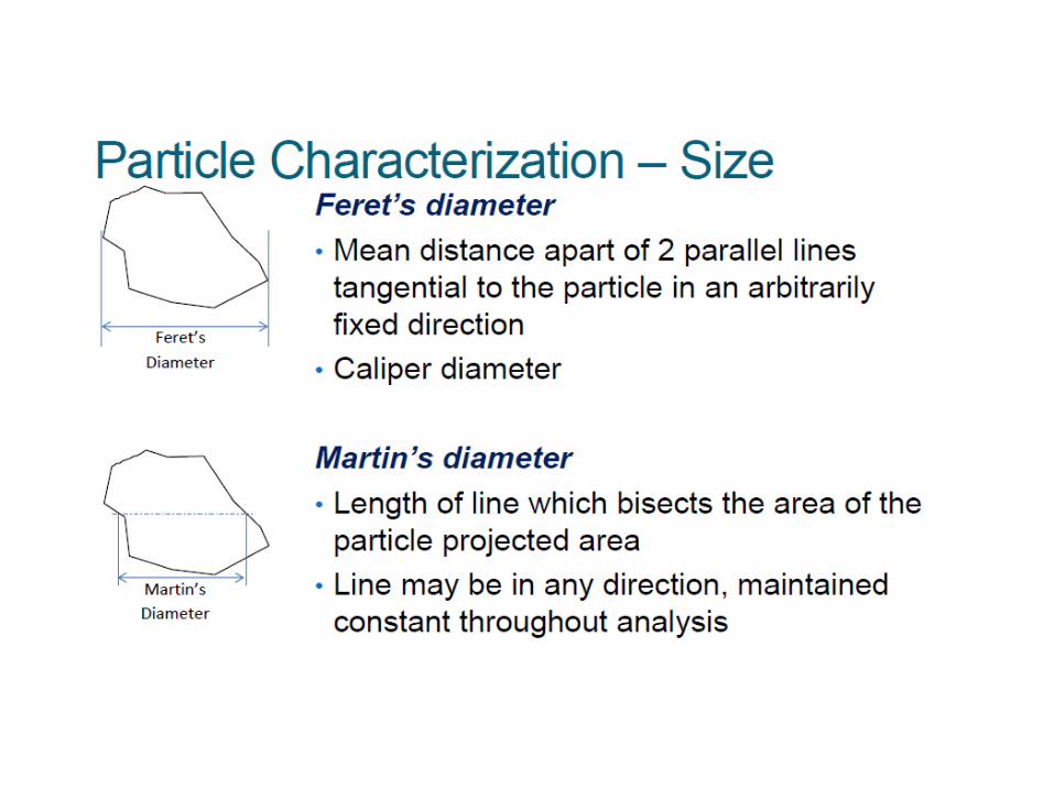
• Describing the size of a single particle. Some terminolgy about diameters used in microscopy.

• Equivalent circle diameter.

• Martin’s diameter.

• Feret’s diameter.

• Shear diameter.

Describing the size of a single particle

• Regular-shaped particles

• The orientation of the particle on the

microscope slide will affect the

projected image and consequently the

measured equivalent sphere diameter.

• Sieve measurement: Diameter of a

sphere passing through the same sieve

aperture.

• Sedimentation measurement:

Diameter of a sphere having the same

sedimentation velocity under the

same conditions.

Comparison of equivalent sphere diameters.

Comparison of equivalent diameters

• The volume equivalent sphere diameter is a commonly used equivalent

sphere diameter.

• Example: Coulter counter size measurement. The diameter of a sphere

having the same volume as the particle.

• Surface-volume diameter is the diameter of a sphere having the same

surface to volume ratio as the particle.

Shape

Cuboid

Cylinder

(Example)

Cuboid: side lengths of 1, 3, 5.

Cylinder: diameter 3 and length 1.

Description of populations of particles

• Typical differential

frequency distribution

( )dF f xdx

F: Cumulative distribution,

integral of the frequency distribution.

• Typical cumulative frequency distribution.

• Comparison between distributions

• For a given population of particles,

the distributions by mass, number

and surface can differ dramatically.

• All are smooth continuous curves.

• Size measurement methods often

divide the size spectrum into size

ranges, and size distribution becomes

a histogram.

Common methods of displaying size

distributions

Arithmetic-normal Distribution

Log-normal Distribution

logz x

Arithmetic-normal distribution with an arithmetic mean of 45 and standard deviation of 12.

z: Arithmetic mean of z, sz: standard deviation of log x

• Log-normal distribution plotted on linear coordinates

• Log-normal distribution plotted on logarithmic coordinates

Methods of particle size measurements:

Sieving

• Sieving: Dry sieving using woven wire sieves is

appropriate for particle size greater than 45 mm.

The length of the particle does not hinder it

passage through the sieve aperture.

• Most common modern sieves are in sizes such that

the ratio of adjacent sieve sizes is the fourth

root of two (e.g. 45, 53, 63, 75, 90, 107 mm).

Methods of particle size measurements:

Microscopy

• The optical microscope may be used to measure particle size down to 5 mm.

• The electron microscope may be used for size analysis below 5 mm.

• Coupled with an image analysis system, the optical and electron microscopy can give number distribution of size and shape.

• For irregular-shaped particles, the projected area offered to the viewer can vary significantly. Technique (e.g. applying adhesive to the microscope slide) may be used to ensure “random orientation”.

MR Chapter 2

• Tutorial

• MR # 2.1, 2.4.MARTIN RHODES (2008)

Introduction to Particle

Technology , 2nd Edition.

Publisher John Wiley & Son,

Chichester, West Sussex,

England.

Overview

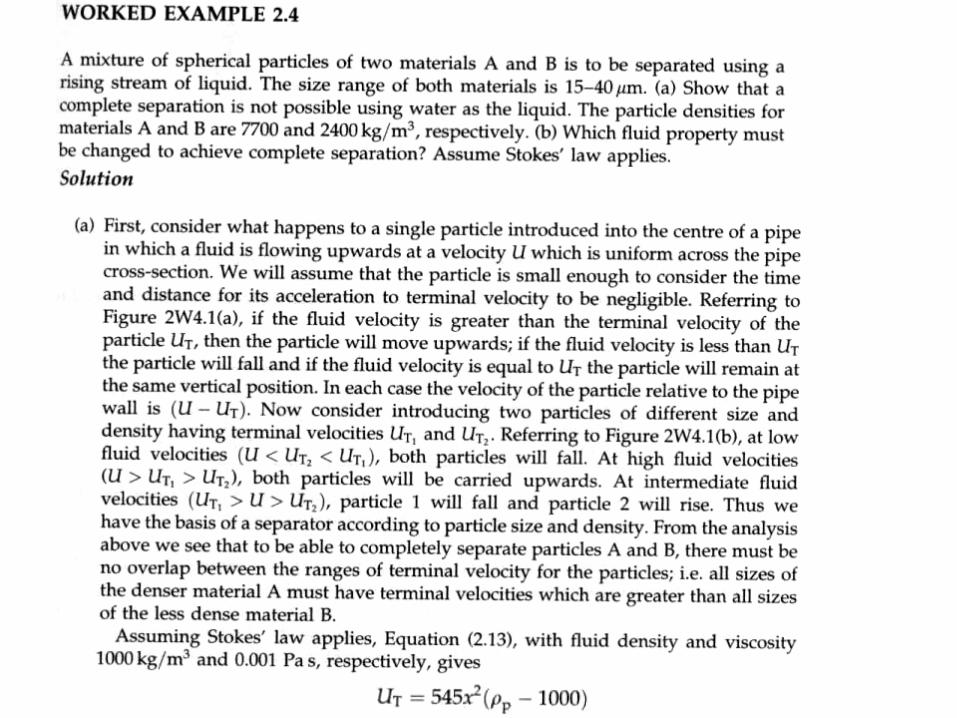
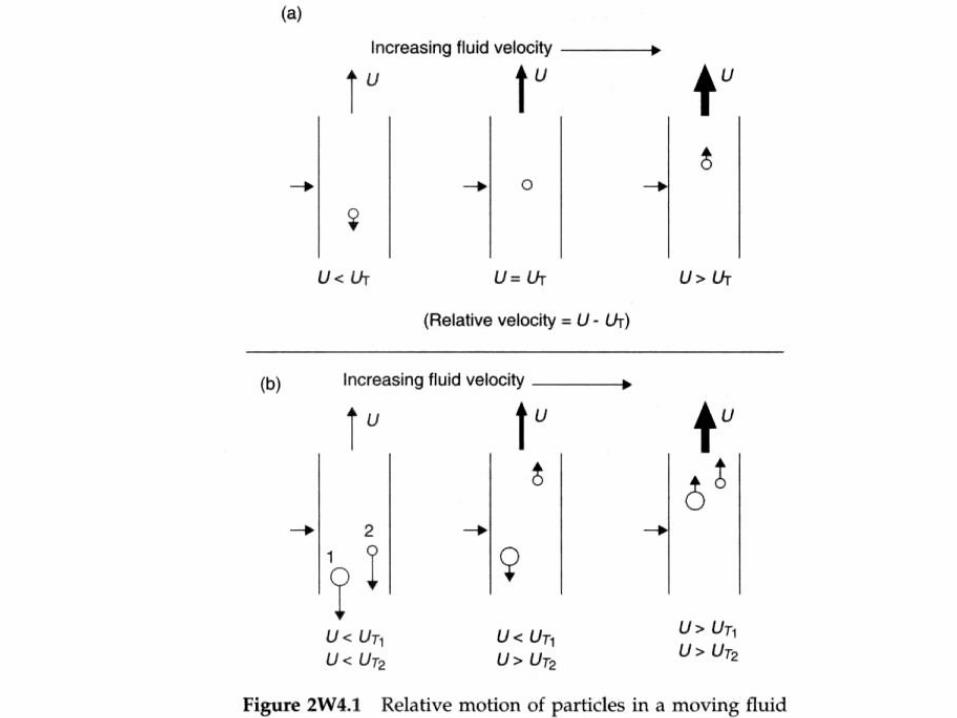
1. Motion of solid particles in a fluid

2. Standard drag curve for motion of a sphere in a fluid

3. Single Particle Terminal Velocity

4. Special Cases

5. To calculate UT and x

6. Particles falling under gravity through a fluid

7. Non-spherical particles

8. Effect of boundaries on terminal velocity

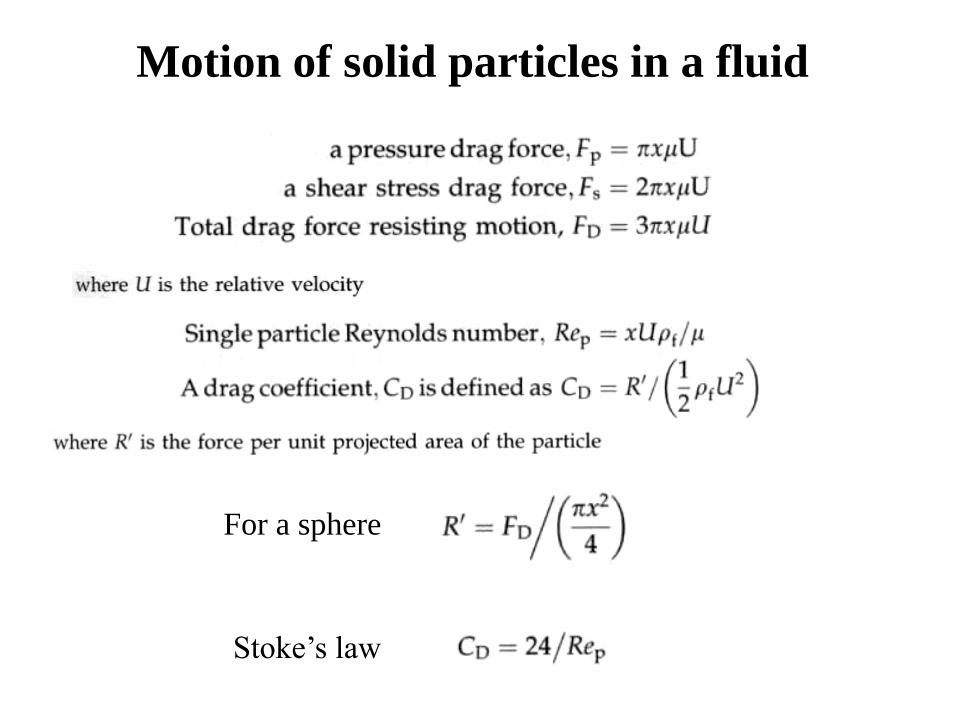
Motion of solid particles in a fluid

For a sphere

Stoke’s law

Motion of solid particles in a fluid

For a sphere

Stoke’s law

Standard drag curve for motion of a sphere in a fluid

Reynolds number ranges for single

particle drag coefficient correlations

At higher relative velocity, the inertia of fluid begins to dominate.

Four regions are identified: Stoke’s law, intermediate, newton’s law, boundary layer

separation.

Table 2.1 (Schiller and Naumann (1933) : Accuracy around 7%.

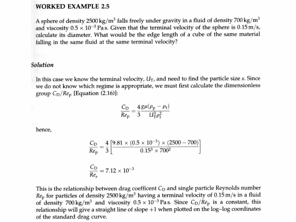
Single Particle Terminal Velocity

To calculate UT and x

• (a) To calculate UT, for a given size x,

• (b) To calculate size x, for a given UT,

3

2

2

( )4Re

3

f p f

D

x gC

m

Independent of UT

3 2

( )4

Re 3

P fD

P T f

gC

U

m

Independent of size x

Particles falling under gravity through a fluid

Method for estimating terminal velocity for a given size of particle and vice versa

Non-spherical particles

Drag coefficient CD versus Reynolds number ReP for particles of sphericity

ranging from 0.125 to 1.0

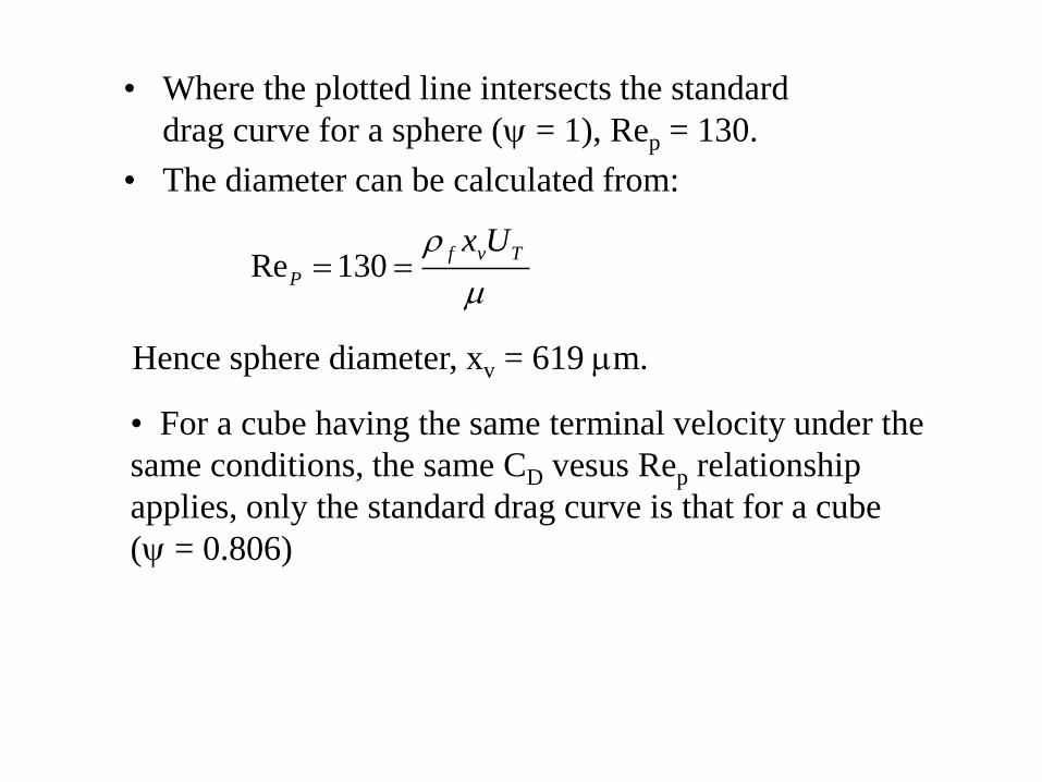
• Where the plotted line intersects the standard

drag curve for a sphere (y = 1), Rep = 130.

• The diameter can be calculated from:

Re 130f v T

P

x U

m

Hence sphere diameter, xv = 619 mm.

• For a cube having the same terminal velocity under the

same conditions, the same CD vesus Rep relationship

applies, only the standard drag curve is that for a cube

(y = 0.806)

850

Packed Beds: Ergun Equation

Pressure Drop-Flow Relation

MR Chapter 6

Fluid Flow Through a Packed Bed of Particles

• Tutorial

• MR #6.1, 6.3, 6.5, 6.7,

MARTIN RHODES (2008)

Introduction to Particle

Technology , 2nd Edition.

Publisher John Wiley & Son,

Chichester, West Sussex,

England.

Pressure drop-flow relationship

/U Ui

Tube equivalent diameter:

Hagen-Poiseuille:

Laminar flow:

2eH K H

Flow area = A; wetted perimeter = SBA;

SB: Particle surface area per unit volume of the bed.

Total particle surface area in the bed = SBAH

For packed bed, wetted perimeter = SBAH/H = SBA

Darcy (1856)

Carmen-Kozeny eq.:

Turbulent flow:

(1 )v BS S

A

Sv = 6/x

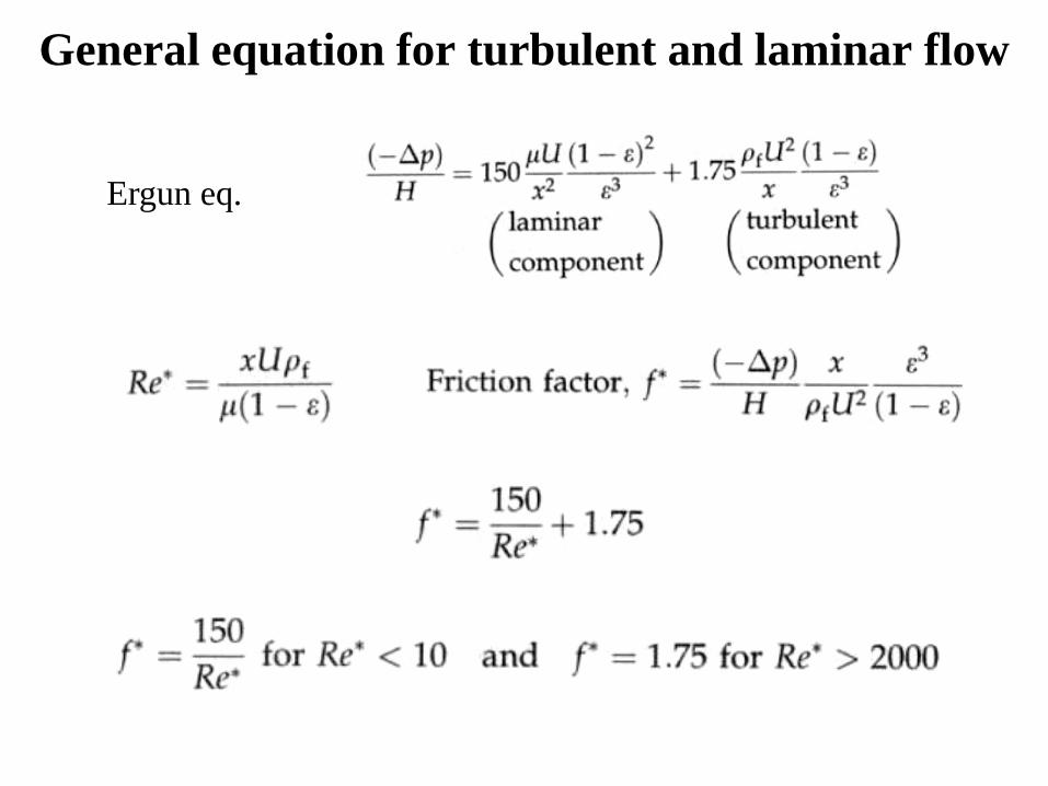
General equation for turbulent and laminar flow

Ergun eq.

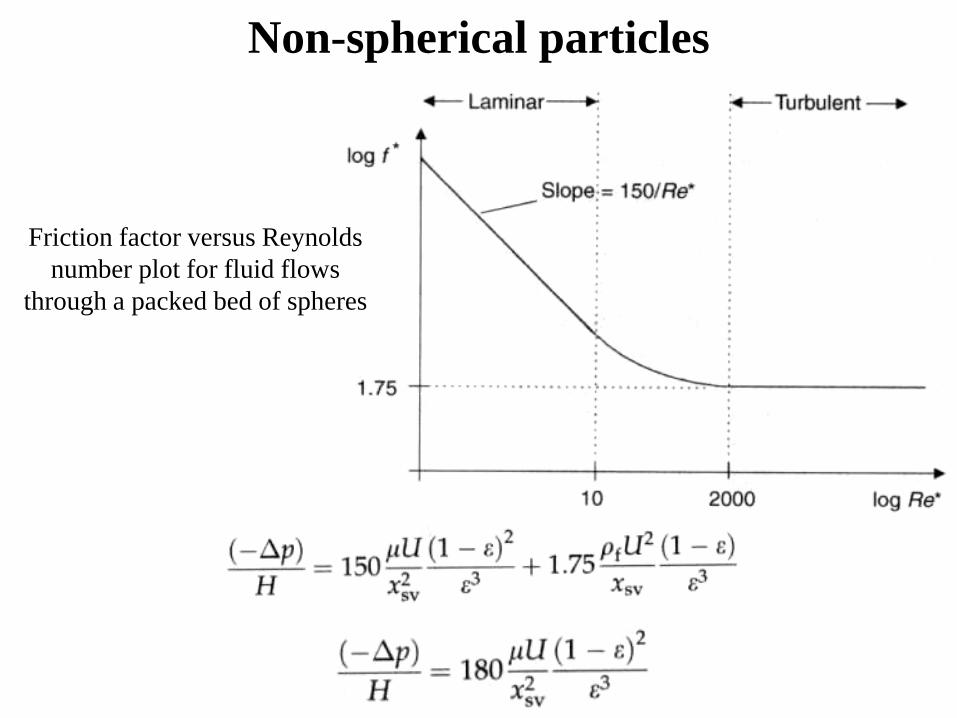
Non-spherical particles

Friction factor versus Reynolds

number plot for fluid flows

through a packed bed of spheres

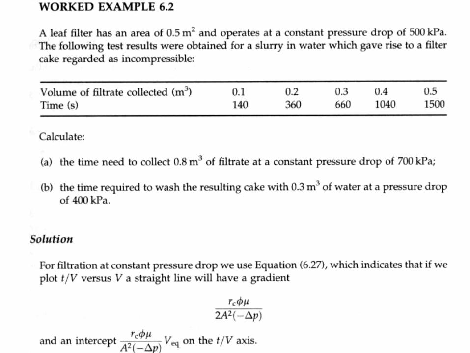
Filtration

• Incompressible cake

(Eq. 6.21, See Appendix 1

for derivation )

(From Ergun equation)

The volume of cake formed by the passage of unit

volume of filtrate.

• Constant pressure drop filtration

• Including the resistance of the filter medium

(Eq. 6.23, see Appendix

1 for derivation )

(Eq. 6.27, see Appendix 1

for derivation )

Washing the cake

Removal of filtrate during washing of the filter cake

Compressible cake

Analysis of the pressure drop-flow relationship for a compressible cake

rc = rc(ps)

xsv = 792 mm.