WP/06/149

Fundamentals-Based Estimation of Default Probabilities: A Survey

Jorge A. Chan-Lau

© 2006 International Monetary Fund WP/06/149

IMF Working Paper

Monetary and Financial Systems Department

Fundamentals-Based Estimation of Default Probabilities: A Survey1

Prepared by Jorge A. Chan-Lau

Authorized for distribution by David D. Marston

June 2006

Abstract

This Working Paper should not be reported as representing the views of the IMF. The views expressed in this Working Paper are those of the author(s) and do not necessarily represent those of the IMF or IMF policy. Working Papers describe research in progress by the author(s) and are published to elicit comments and to further debate.

This survey reviews a number of different fundamentals-based models for estimating default probabilities for firms and/or industries, and illustrates them with real applications by practitioners and policy making institutions. The models are especially useful when the firms analyzed do not have publicly traded securities or secondary market prices are unreliable because of low liquidity. JEL Classification Numbers: C5, C53, G00 Keywords: Default probabilities, econometric models, scoring models, ratings models Author(s) E-Mail Address: jchanlau@imf.org

1 This paper benefits from comments by seminar participants at the IMF, Renzo Avesani, Antonio García-Pascual, Amadou Sy, and especially André Santos. Errors and omissions are the author’s sole responsibility.

- 2 -

Contents Page I. Introduction .........................................................................................................................3 II. Macroeconomic-Based Models...........................................................................................4 A. Econometric Models with Exogenous Economic Factors ...............................................4 Example 1. A Macro-Stress Testing Model for Finland....................................................5 B. Econometric Models with Endogenous Economic Factors..............................................5 Example 2. Stress Tests of U.K. Banks .............................................................................6 C. Pros and Cons of Macroeconomic Based Models............................................................7 III. Credit Scoring (or Accounting-Based) Models ..................................................................7 A. Econometric Models ........................................................................................................9 Example 3. Moody's KMV EDFTM RiskCalcTM Model ................................................9 B. Linear Discriminant Analysis...........................................................................................9 Example 4. Altman’s Z-Score..........................................................................................10 C. Some Caveats on the Use of Accounting-Based Models...............................................11 IV. Ratings-Based Models ......................................................................................................11 A. Two Simple Models: Cohort and Duration Analyses ....................................................11 B. The Most Prudent Estimation Principle (MPEP) ...........................................................12 Example 5. A Simple Application of the MPEP..............................................................13 C. Some Caveats on the Use of Ratings-Based Models .....................................................14 V. Hybrid Models ...................................................................................................................14 Example 6. Estimating Default Probabilities Using Argentina's Credit Bureau Data.....15 Example 7. The Impact of Credit Growth on Loan Losses in Spain ...............................15 Example 8. Forecasting Default Probabilities of German Firms.....................................15 VI. Conclusions.......................................................................................................................16 References...............................................................................................................................17 Tables 1. Financial Ratios Used in Credit Scoring Models...............................................................8 2. Most Prudent Default Probabilities..................................................................................13

- 3 -

I. INTRODUCTION

Estimating default probabilities for individual obligors is the first step for assessing the credit exposure and potential losses faced by an investor or financial institutions. Default probabilities are also the basic inputs for evaluating systemic risk and stress testing financial systems at the national, regional, and global level.2 In particular, once the default probabilities of a subset of obligors are known, it is straightforward to estimate the associated loss distribution, a key ingredient for assessing risks and vulnerabilities in the corporate and financial system.3 Estimating default probabilities, however, could be challenging mainly due to limitations on data availability. Fortunately, there are number of models which allow us to overcome these limitations. These models can be broadly classified into two categories: market-based models, which rely on security prices, and fundamentals-based models, which rely on accounting, systematic market and economic factors, and ratings information. This paper reviews a number of different fundamentals-based models for estimating default probabilities for firms and/or industries.4 These models are especially useful when the firms analyzed do not have publicly traded securities or secondary market prices are unreliable because of low liquidity. In particular, the models are well suited for estimating the default probabilities associated with loans or privately held firms. Last but not least, estimation of these models only require users to be familiar with simple econometric techniques such as panel data analysis and qualitative dependent variable models such as probit and logit. These econometric techniques are readily available in most econometric software packages. The models can be classified into three main broad groups. Section II reviews the first group of models, macroeconomic-based models, which attempt to assess how default probabilities are affected by the state of the economy. Macroeconomic-based models are usually employed for estimating sectoral or industry-level default rates or default probabilities. Section III reviews the second group of models, accounting-based or credit scoring models, which generate default probabilities or credit ratings for individual firms using accounting information. Section IV presents the third group of models, ratings-based models, that can be used to infer default probabilities when ratings information is available. These models could be especially useful in countries where credit registry data for corporates and households are

2 Indeed, internal models for estimation of default probabilities are at the heart of Basel II, the revised framework for capital measurement and capital standards issued by the Basel Committee on Banking Supervision. This has prompted the rapid adoption of quantitative models of default probabilities among banks moving towards internal ratings-based (IRB) and Advanced-IRB approaches. Supervisors also need similar tools to be able to assess banks’ internal models.

3 For a comprehensive description and implementation of CreditRisk+ with a view towards stress testing, see Avesani, Liu, Mirenstean, and Salvati (2005).

4 Market-based techniques are reviewed in a companion document, Chan-Lau (2006).

- 4 -

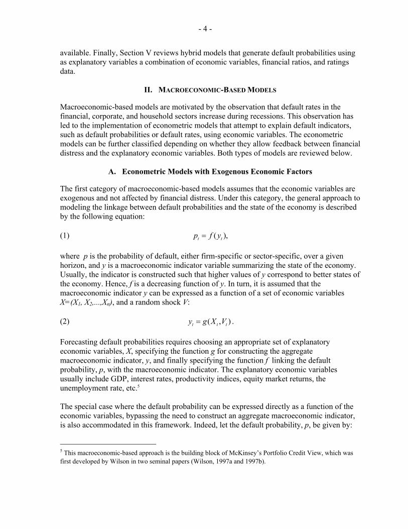
available. Finally, Section V reviews hybrid models that generate default probabilities using as explanatory variables a combination of economic variables, financial ratios, and ratings data.

II. MACROECONOMIC-BASED MODELS

Macroeconomic-based models are motivated by the observation that default rates in the financial, corporate, and household sectors increase during recessions. This observation has led to the implementation of econometric models that attempt to explain default indicators, such as default probabilities or default rates, using economic variables. The econometric models can be further classified depending on whether they allow feedback between financial distress and the explanatory economic variables. Both types of models are reviewed below.

A. Econometric Models with Exogenous Economic Factors

The first category of macroeconomic-based models assumes that the economic variables are exogenous and not affected by financial distress. Under this category, the general approach to modeling the linkage between default probabilities and the state of the economy is described by the following equation: (1) ( ),t tp f y= where p is the probability of default, either firm-specific or sector-specific, over a given horizon, and y is a macroeconomic indicator variable summarizing the state of the economy. Usually, the indicator is constructed such that higher values of y correspond to better states of the economy. Hence, f is a decreasing function of y. In turn, it is assumed that the macroeconomic indicator y can be expressed as a function of a set of economic variables X=(X1, X2,...,Xn), and a random shock V: (2) ( , )t t ty g X V= . Forecasting default probabilities requires choosing an appropriate set of explanatory economic variables, X, specifying the function g for constructing the aggregate macroeconomic indicator, y, and finally specifying the function f linking the default probability, p, with the macroeconomic indicator. The explanatory economic variables usually include GDP, interest rates, productivity indices, equity market returns, the unemployment rate, etc.5 The special case where the default probability can be expressed directly as a function of the economic variables, bypassing the need to construct an aggregate macroeconomic indicator, is also accommodated in this framework. Indeed, let the default probability, p, be given by: 5 This macroeconomic-based approach is the building block of McKinsey’s Portfolio Credit View, which was first developed by Wilson in two seminal papers (Wilson, 1997a and 1997b).

- 5 -

(3) ( , )t t tp h X ε= , whereε is a random shock. Equation (3) is a special case of equations (1) and (2) where the function g is set equal to h, and the function f is simply the identity function. Example 1. A Macro-Stress Testing Model for Finland

Virolainen (2004) develops a macro stress testing model for Finland using the framework above. In his model, the average default rate is estimated using equations (1) and (2) and historical data on default rates for the following industries: (i) agriculture, (ii) manufacturing, (iii) construction, (iv) transport and communications, (v) trade, hotels, and restaurants, and (vi) other industries. Specifically, the average default rate ,j tp for industry j at time t is given by a logistic function:

,,

11 exp( )j t

j t

py

=+

,

where ,j ty is an industry-specific macroeconomic index determined by: , ,0 ,1 1, , , ,...j t j j t j n n t j ty x xβ β β υ= + + + + , where xi, i=1,..,n are explanatory macroeconomic factors. Each macroeconomic factor, in turn, is modeled as an AR(2) process for forecasting purposes. The macroeconomic factors include real GDP, as a proxy for profits/demand for each industry, the 12-month money market interest rate, as a proxy for interest rates, and a measure of corporate indebtness in the industry, the ratio of gross debt to the value added of the industry.

B. Econometric Models with Endogenous Economic Factors

The second category of macroeconomic-based models allows feedback effects between financial distress and the business cycle. For instance, the financial accelerator theory suggests that a decline in net worth in the corporate sector raises funding costs and leads to lower aggregate investment, and in turn, to lower future output.6 Agency theory also indicates that the incentive for corporations to invest in riskier projects increases as their credit quality deteriorates. In turn, this risk-shifting behavior leads to higher output volatility. Financial distress, hence, may play an important role in exacerbating boom-and-bust cycles.

6 Bernanke and Gertler (1989).

- 6 -

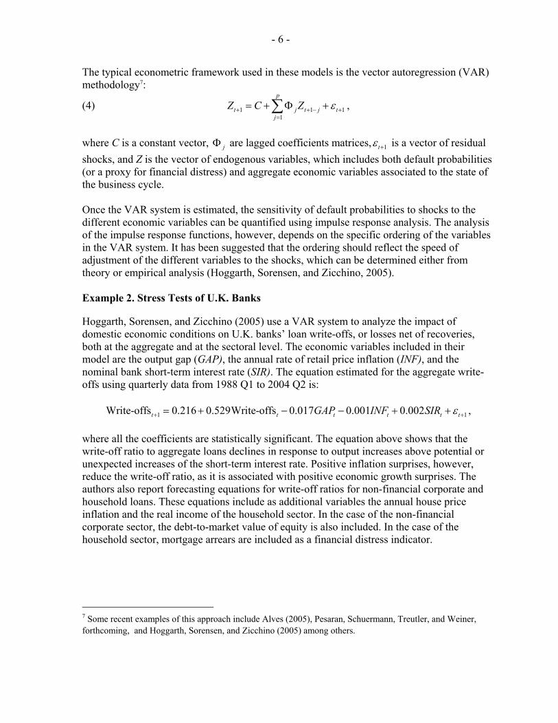
The typical econometric framework used in these models is the vector autoregression (VAR) methodology7:

(4) 1 1 11

p

t j t j tj

Z C Z ε+ + − +=

= + Φ +∑ ,

where C is a constant vector, jΦ are lagged coefficients matrices, 1tε + is a vector of residual shocks, and Z is the vector of endogenous variables, which includes both default probabilities (or a proxy for financial distress) and aggregate economic variables associated to the state of the business cycle. Once the VAR system is estimated, the sensitivity of default probabilities to shocks to the different economic variables can be quantified using impulse response analysis. The analysis of the impulse response functions, however, depends on the specific ordering of the variables in the VAR system. It has been suggested that the ordering should reflect the speed of adjustment of the different variables to the shocks, which can be determined either from theory or empirical analysis (Hoggarth, Sorensen, and Zicchino, 2005). Example 2. Stress Tests of U.K. Banks

Hoggarth, Sorensen, and Zicchino (2005) use a VAR system to analyze the impact of domestic economic conditions on U.K. banks’ loan write-offs, or losses net of recoveries, both at the aggregate and at the sectoral level. The economic variables included in their model are the output gap (GAP), the annual rate of retail price inflation (INF), and the nominal bank short-term interest rate (SIR). The equation estimated for the aggregate write-offs using quarterly data from 1988 Q1 to 2004 Q2 is: 1 1Write-offs 0.216 0.529Write-offs 0.017 0.001 0.002t t t t t tGAP INF SIR ε+ += + − − + + , where all the coefficients are statistically significant. The equation above shows that the write-off ratio to aggregate loans declines in response to output increases above potential or unexpected increases of the short-term interest rate. Positive inflation surprises, however, reduce the write-off ratio, as it is associated with positive economic growth surprises. The authors also report forecasting equations for write-off ratios for non-financial corporate and household loans. These equations include as additional variables the annual house price inflation and the real income of the household sector. In the case of the non-financial corporate sector, the debt-to-market value of equity is also included. In the case of the household sector, mortgage arrears are included as a financial distress indicator.

7 Some recent examples of this approach include Alves (2005), Pesaran, Schuermann, Treutler, and Weiner, forthcoming, and Hoggarth, Sorensen, and Zicchino (2005) among others.

- 7 -

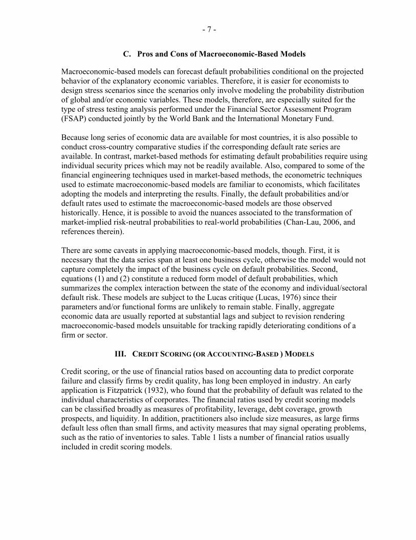
C. Pros and Cons of Macroeconomic-Based Models

Macroeconomic-based models can forecast default probabilities conditional on the projected behavior of the explanatory economic variables. Therefore, it is easier for economists to design stress scenarios since the scenarios only involve modeling the probability distribution of global and/or economic variables. These models, therefore, are especially suited for the type of stress testing analysis performed under the Financial Sector Assessment Program (FSAP) conducted jointly by the World Bank and the International Monetary Fund. Because long series of economic data are available for most countries, it is also possible to conduct cross-country comparative studies if the corresponding default rate series are available. In contrast, market-based methods for estimating default probabilities require using individual security prices which may not be readily available. Also, compared to some of the financial engineering techniques used in market-based methods, the econometric techniques used to estimate macroeconomic-based models are familiar to economists, which facilitates adopting the models and interpreting the results. Finally, the default probabilities and/or default rates used to estimate the macroeconomic-based models are those observed historically. Hence, it is possible to avoid the nuances associated to the transformation of market-implied risk-neutral probabilities to real-world probabilities (Chan-Lau, 2006, and references therein). There are some caveats in applying macroeconomic-based models, though. First, it is necessary that the data series span at least one business cycle, otherwise the model would not capture completely the impact of the business cycle on default probabilities. Second, equations (1) and (2) constitute a reduced form model of default probabilities, which summarizes the complex interaction between the state of the economy and individual/sectoral default risk. These models are subject to the Lucas critique (Lucas, 1976) since their parameters and/or functional forms are unlikely to remain stable. Finally, aggregate economic data are usually reported at substantial lags and subject to revision rendering macroeconomic-based models unsuitable for tracking rapidly deteriorating conditions of a firm or sector.

III. CREDIT SCORING (OR ACCOUNTING-BASED ) MODELS

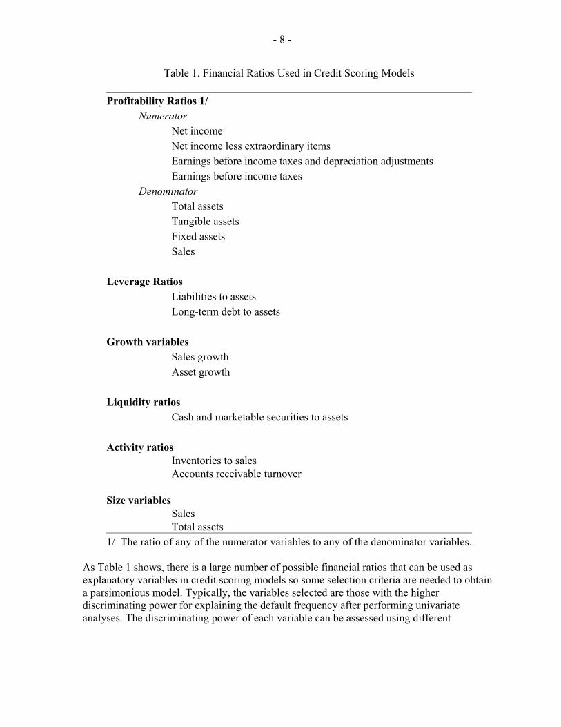
Credit scoring, or the use of financial ratios based on accounting data to predict corporate failure and classify firms by credit quality, has long been employed in industry. An early application is Fitzpatrick (1932), who found that the probability of default was related to the individual characteristics of corporates. The financial ratios used by credit scoring models can be classified broadly as measures of profitability, leverage, debt coverage, growth prospects, and liquidity. In addition, practitioners also include size measures, as large firms default less often than small firms, and activity measures that may signal operating problems, such as the ratio of inventories to sales. Table 1 lists a number of financial ratios usually included in credit scoring models.

- 8 -

Table 1. Financial Ratios Used in Credit Scoring Models Profitability Ratios 1/

Numerator Net income Net income less extraordinary items Earnings before income taxes and depreciation adjustments Earnings before income taxes

Denominator Total assets Tangible assets Fixed assets Sales

Leverage Ratios

Liabilities to assets Long-term debt to assets

Growth variables Sales growth Asset growth

Liquidity ratios

Cash and marketable securities to assets

Activity ratios Inventories to sales Accounts receivable turnover

Size variables

Sales Total assets

1/ The ratio of any of the numerator variables to any of the denominator variables. As Table 1 shows, there is a large number of possible financial ratios that can be used as explanatory variables in credit scoring models so some selection criteria are needed to obtain a parsimonious model. Typically, the variables selected are those with the higher discriminating power for explaining the default frequency after performing univariate analyses. The discriminating power of each variable can be assessed using different

- 9 -

methodologies such as the cumulative accuracy profile (CAP), the receiver-operating characteristic (ROC), and the Kolmogorov-Smirnov test among others.8 Once the variables have been selected, credit scoring models use a variety of statistical techniques for assessing the default probability of a firm, including econometric models, linear discriminant analysis, k-nearest neighbor classifier, neural networks, and support vector machine classifiers among others. This paper explains only the first two types of statistical techniques, econometric models and linear discrimination analysis.

A. Econometric Models

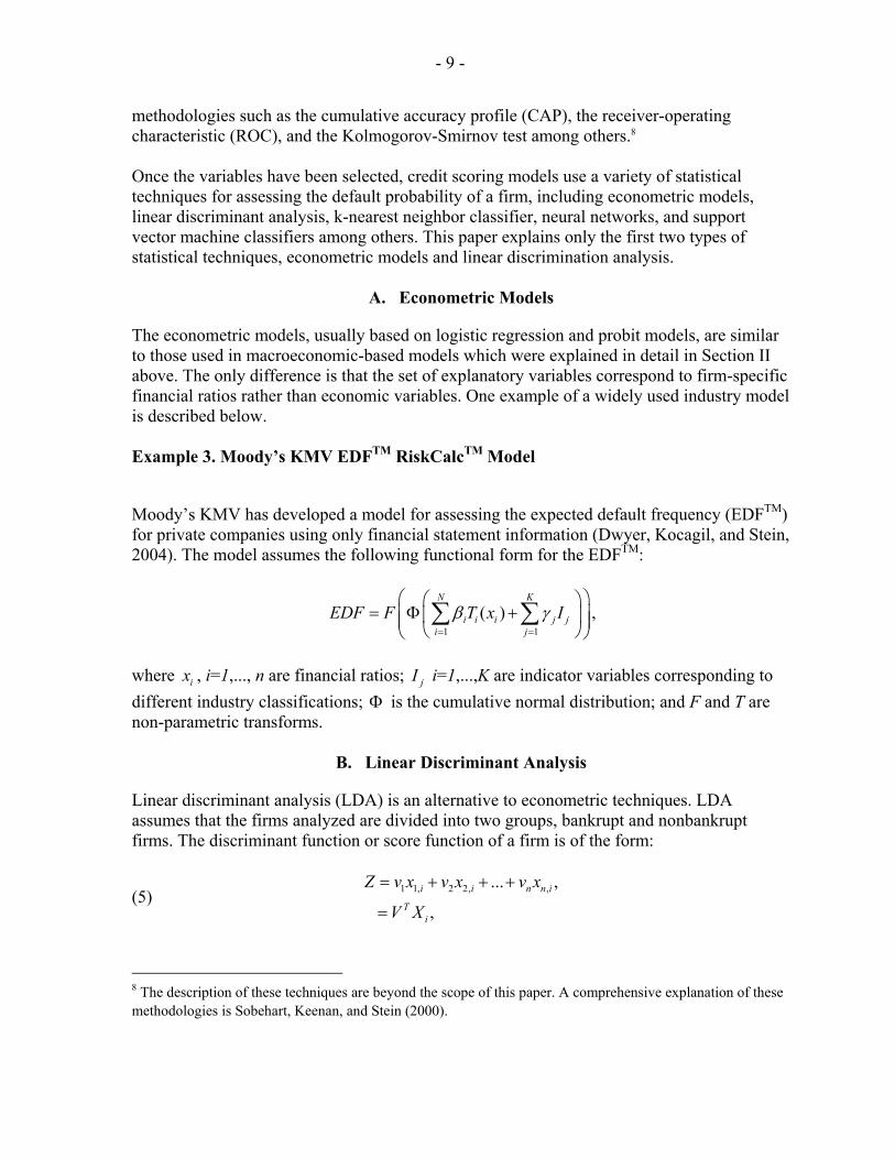
The econometric models, usually based on logistic regression and probit models, are similar to those used in macroeconomic-based models which were explained in detail in Section II above. The only difference is that the set of explanatory variables correspond to firm-specific financial ratios rather than economic variables. One example of a widely used industry model is described below. Example 3. Moody’s KMV EDFTM RiskCalcTM Model

Moody’s KMV has developed a model for assessing the expected default frequency (EDFTM) for private companies using only financial statement information (Dwyer, Kocagil, and Stein, 2004). The model assumes the following functional form for the EDFTM:

1 1

( )N K

i i i j ji j

EDF F T x Iβ γ= =

⎛ ⎞⎛ ⎞= Φ +⎜ ⎟⎜ ⎟⎜ ⎟⎝ ⎠⎝ ⎠

∑ ∑ ,

where ix , i=1,..., n are financial ratios; jI i=1,...,K are indicator variables corresponding to different industry classifications; Φ is the cumulative normal distribution; and F and T are non-parametric transforms.

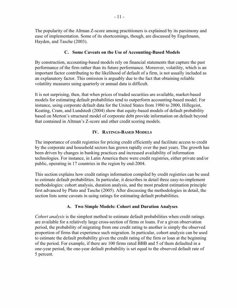
B. Linear Discriminant Analysis

Linear discriminant analysis (LDA) is an alternative to econometric techniques. LDA assumes that the firms analyzed are divided into two groups, bankrupt and nonbankrupt firms. The discriminant function or score function of a firm is of the form:

(5) 1 1, 2 2, ,... ,

,i i n n i

Ti

Z v x v x v x

V X

= + + +

=

8 The description of these techniques are beyond the scope of this paper. A comprehensive explanation of these methodologies is Sobehart, Keenan, and Stein (2000).

- 10 -

where jv , j=1,...,n, are the discriminant coefficients, and ,j ix , j=1,...,n, are the firm-specific financial ratios. The discriminant coefficients are chosen such that they maximize the following objective function:

(6) 2

( )TB NBT

VF

V Vµ µ⎡ ⎤−⎣ ⎦=

Σ,

where Bµ and NBµ are the vectors collecting the average value of the financial ratios of the bankrupt and non-bankrupt firms, respectively, and Σ is the between-class covariance matrix. Once the coefficients iv , i=1,...,n, are known, the score function is used to discriminate between bankrupt and non-bankrupt firms: if 0T

iV X α+ < for an arbitrary constant α , the firms is bankrupt. The constant α is calibrated using historical default data. The score of a specific firm given its financial ratios iX can be transformed into a bankruptcy probability,

( )B ip X , using the following formula:

(7) 1( )1 exp( )B i T

i

p XV X β

=+ +

,

where

(8) log NB

B

pp

β α⎛ ⎞

= + ⎜ ⎟⎝ ⎠

,

where Bp and NBp are the unconditional probabilities of the firm being bankrupt or not respectively. These unconditional probabilities can be proxied by their sample estimates. While the analysis here has been restricted only to two “ratings”, bankruptcy and solvency, it can be generalized to multiple ratings easily. LDA, hence, is widely used for constructing internal ratings systems. Example 4. Altman’s Z-Score

Altman’s Z-score (Altman, 1968) is arguably the most well known application of credit scoring for bankruptcy prediction. Altman includes as explanatory variables the following financial ratios: working capital to total assets ( 1X ), retained earnings to total assets ( 2X ), earnings before interest and taxes to total assets ( 3X ), the market value of equity to the book value of total liabilities ( 4X ), and sales to total assets ( 5X ). For U.S. corporations, the updated Z-score (Altman, 2000) is given by: 1 2 3 4 50.012 0.014 0.033 0.006 0.999Z X X X X X= + + + + .

- 11 -

The popularity of the Altman Z-score among practitioners is explained by its parsimony and ease of implementation. Some of its shortcomings, though, are discussed by Engelmann, Hayden, and Tasche (2003).

C. Some Caveats on the Use of Accounting-Based Models

By construction, accounting-based models rely on financial statements that capture the past performance of the firm rather than its future performance. Moreover, volatility, which is an important factor contributing to the likelihood of default of a firm, is not usually included as an explanatory factor. This omission is arguably due to the fact that obtaining reliable volatility measures using quarterly or annual data is difficult. It is not surprising, then, that when prices of traded securities are available, market-based models for estimating default probabilities tend to outperform accounting-based model. For instance, using corporate default data for the United States from 1980 to 2000, Hillegeist, Keating, Cram, and Lundstedt (2004) show that equity-based models of default probability based on Merton’s structural model of corporate debt provide information on default beyond that contained in Altman’s Z-score and other credit scoring models.

IV. RATINGS-BASED MODELS

The importance of credit registries for pricing credit efficiently and facilitate access to credit by the corporate and household sectors has grown rapidly over the past years. The growth has been driven by changes in banking practices and increased availability of information technologies. For instance, in Latin America there were credit registries, either private and/or public, operating in 17 countries in the region by end-2004. This section explains how credit ratings information compiled by credit registries can be used to estimate default probabilities. In particular, it describes in detail three easy-to-implement methodologies: cohort analysis, duration analysis, and the most prudent estimation principle first advanced by Pluto and Tasche (2005). After discussing the methodologies in detail, the section lists some caveats in using ratings for estimating default probabilities.

A. Two Simple Models: Cohort and Duration Analyses

Cohort analysis is the simplest method to estimate default probabilities when credit ratings are available for a relatively large cross-section of firms or loans. For a given observation period, the probability of migrating from one credit rating to another is simply the observed proportion of firms that experience such migration. In particular, cohort analysis can be used to estimate the default probability given the credit rating of the firm or loan at the beginning of the period. For example, if there are 100 firms rated BBB and 5 of them defaulted in a one-year period, the one-year default probability is set equal to the observed default rate of 5 percent.

- 12 -

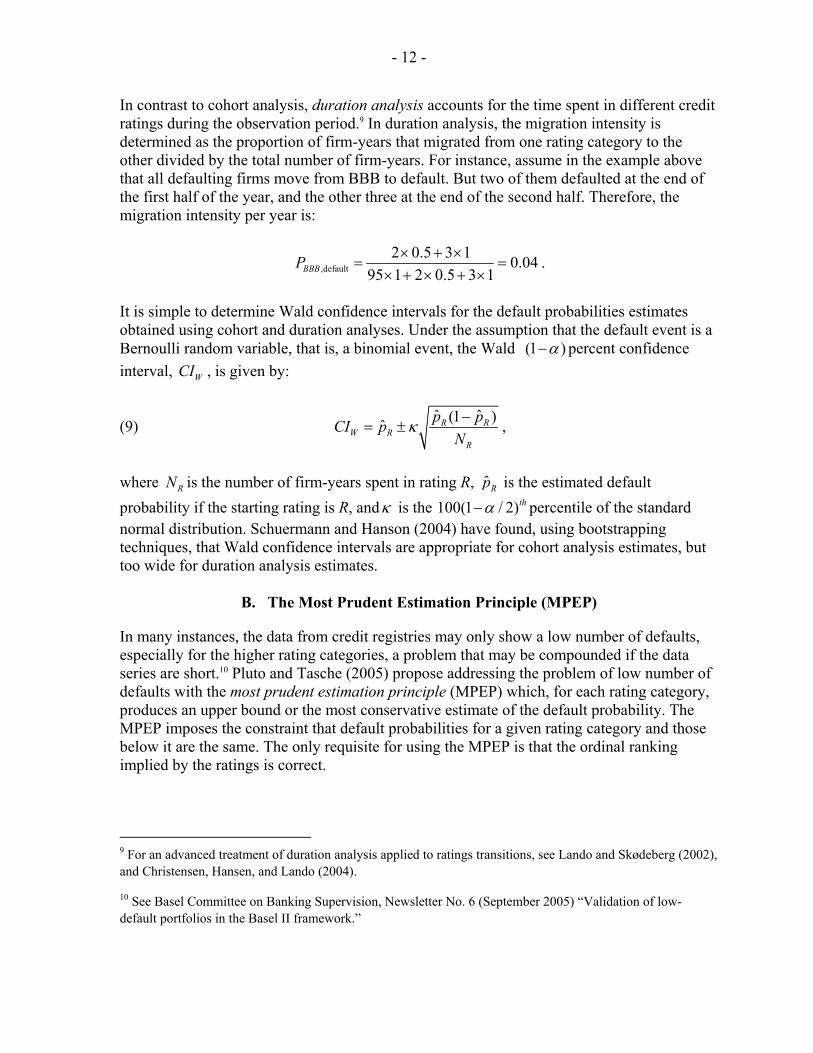
In contrast to cohort analysis, duration analysis accounts for the time spent in different credit ratings during the observation period.9 In duration analysis, the migration intensity is determined as the proportion of firm-years that migrated from one rating category to the other divided by the total number of firm-years. For instance, assume in the example above that all defaulting firms move from BBB to default. But two of them defaulted at the end of the first half of the year, and the other three at the end of the second half. Therefore, the migration intensity per year is:

,default2 0.5 3 1 0.04

95 1 2 0.5 3 1BBBP × + ×= =

× + × + ×.

It is simple to determine Wald confidence intervals for the default probabilities estimates obtained using cohort and duration analyses. Under the assumption that the default event is a Bernoulli random variable, that is, a binomial event, the Wald (1 )α− percent confidence interval, WCI , is given by:

(9) ˆ ˆ(1 )ˆ R R

W RR

p pCI pN

κ −= ± ,

where RN is the number of firm-years spent in rating R, ˆ Rp is the estimated default probability if the starting rating is R, andκ is the 100(1 / 2)thα− percentile of the standard normal distribution. Schuermann and Hanson (2004) have found, using bootstrapping techniques, that Wald confidence intervals are appropriate for cohort analysis estimates, but too wide for duration analysis estimates.

B. The Most Prudent Estimation Principle (MPEP)

In many instances, the data from credit registries may only show a low number of defaults, especially for the higher rating categories, a problem that may be compounded if the data series are short.10 Pluto and Tasche (2005) propose addressing the problem of low number of defaults with the most prudent estimation principle (MPEP) which, for each rating category, produces an upper bound or the most conservative estimate of the default probability. The MPEP imposes the constraint that default probabilities for a given rating category and those below it are the same. The only requisite for using the MPEP is that the ordinal ranking implied by the ratings is correct.

9 For an advanced treatment of duration analysis applied to ratings transitions, see Lando and Skødeberg (2002), and Christensen, Hansen, and Lando (2004).

10 See Basel Committee on Banking Supervision, Newsletter No. 6 (September 2005) “Validation of low-default portfolios in the Basel II framework.”

- 13 -

The use of the principle is illustrated for the case of independent defaults. Assume that there are K rating categories, A, B, ..., K where A is a higher rating than B and so on. Let nI and dI , I=A, ...,K be the number of firms rated I and the number of defaults for firms rated I respectively. Assume also that defaults are independent. Letγ be the desired confidence level which implies that the probability of a type I error is equal to (1-γ ). For rating category A, the most prudent default probability pA is the upper bound on the set of probabilities that solves the inequality below:

(10) ...

...

0

...1 (1 )

A KA K

d dA K n n ii

i

n np p

iγ

+ ++ + −

=

+ +⎛ ⎞− ≤ −⎜ ⎟

⎝ ⎠∑ ,

since the number of defaults follows a binomial distribution given that defaults are independent. In general, for rating category E, the most prudent default probability pE is the solution to the following program:

(11) ...

...

0

...max [0,1] such that 1 (1 )

E KE K

d dE K n n ii

E pi

n np p p p

iγ

+ ++ + −

=

⎧ + + ⎫⎛ ⎞= ∈ − ≤ −⎨ ⎬⎜ ⎟

⎝ ⎠⎩ ⎭∑

Example 5. A Simple Application of the MPEP

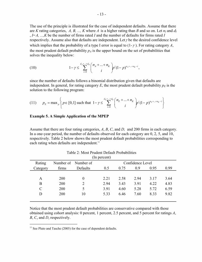
Assume that there are four rating categories, A, B, C, and D, and 200 firms in each category. In a one-year period, the number of defaults observed for each category are 0, 2, 5, and 10, respectively. Table 2 below shows the most prudent default probabilities corresponding to each rating when defaults are independent.11

Rating Number of Number ofCategory firms Defaults 0.5 0.75 0.9 0.95 0.99

A 200 0 2.21 2.58 2.94 3.17 3.64B 200 2 2.94 3.43 3.91 4.22 4.83C 200 5 3.91 4.60 5.28 5.72 6.59D 200 10 5.33 6.46 7.60 8.33 9.82

Confidence Level

Table 2: Most Prudent Default Probabilities(In percent)

Notice that the most prudent default probabilities are conservative compared with those obtained using cohort analysis: 0 percent, 1 percent, 2.5 percent, and 5 percent for ratings A, B, C, and D, respectively. 11 See Pluto and Tasche (2005) for the case of dependent defaults.

- 14 -

C. Some Caveats on the Use of Ratings-Based Models

While ratings are constructed to reflect the creditworthiness of a debtor going forward, ratings tend to assign firms to a rather broad risk bucket. Within the bucket, default probabilities can exhibit a wide dispersion. Such a dispersion is justified since some ratings models are designed to discriminate between high and low risk firms, and may perform poorly at predicting the likelihood of default. A ratings agency may weight different criteria differently when assigning a rating. For instance, the probability of default weights more on Standard and Poor’s ratings than on Moody’s Investor Services ratings. On the other hand, expected losses are more important in determining Moody’s ratings than Standard and Poor’s ratings. Hence, ratings per se do not imply a precise estimate of a debtor’s default probability, and cross-country comparisons need to take into account that ratings methodologies may differ from country to country. Another caveat when using credit ratings is that they are constructed by factoring in expected business cycle conditions, a practice known as “through-the-cycle” ratings. Due to the difficulty of predicting the business cycle, the expected business cycle conditions are those corresponding to an average business cycle scenario. This practice helps reducing the volatility of ratings changes during the business cycle, which is appropriate for buy-and-hold investors. The downside of using an average business cycle scenario, however, is that ratings may not reflect reality well if the business cycle turns very differently from the average scenario used in the analysis. This fact underlies the criticism that ratings are too slow to react to news. In addition, a number of empirical studies have found that rating transition matrices, which capture the probability of migrating from one rating to another, are not stable through time since they depend on the stage of the business cycle.12

V. HYBRID MODELS

This section describes recent approaches to estimating default probabilities using as explanatory variables economic variables, accounting data, and ratings data. Similar to macroeconomic-based models, the usual empirical framework of these models is given by the equations: ( ),t tp f y=

( , )t t ty g X V= . where p is the probability of default, either firm-specific or sector-specific, over a given horizon, and y is an indicator variable. In contrast to macroeconomic-based models, hybrid models assume that the indicator variable is a function of a set of economic, accounting, and

12 For instance, see Nickell, Perraudin, and Varotto (2000) among others.

- 15 -

ratings variables X=(X1, X2,...,Xn), and a random shock V. Three recent applications are reviewed below. Example 6. Estimating Default Probabilities Using Argentina’s Credit Bureau Data

Balzarotti, Falkenheim, and Powell (2002) propose an econometric model for estimating a loan’s probability of default using historical data from Argentina’s Central de Deudores del Sistema Financiero (CDSF), which collects data on almost every loan originated in the Argentine financial system. Namely, they use an ordered probit specification where the explanatory variables are: the borrower’s classification (or actual credit rating), the borrower’s industrial activity classification, the size of the exposure, the CAMELS rating of the lender, and the percent of the debt backed by collateral. Example 7. The Impact of Credit Growth on Loan Losses in Spain

Jiménez and Saurina (2005) studied the impact of rapid credit growth on loan losses in Spain. Their model for default probabilities is given by:

1 1 2

1 2 3

Pr( 1) (

),ijt t t jt ijt

jt t

Default F GDPG RIR LGR LOANCHAR

DREG DIND BANKCHAR

α β β γ χ

δ δ δ η+ = = + + + +

+ + + +

where 1Pr( 1)ijtDefault + = is the probability of default of loan i, in bank j, the next year after being granted, F is the logistic function, and LOANCHAR are the characteristics of the loan such as its size, maturity, and collateral. Control variables included in the equation are the region where the loan is granted (DREG), the borrower’s industry (DIND), the bank characteristics (BANKCHAR), and the bank’s loan growth rate (LGRI). The macroeconomic variables included in the analysis are GDP growth (GDPG), and the real interest rate (RIR). Using a random-effect logit model, Jiménez and Saurina find that rapid loan growth rates lead to future higher loan losses, and that lending standards decrease during lending booms, leading to higher future default probabilities. Example 8. Forecasting Default Probabilities of German Firms

Hamerle, Liebig, and Scheule (2004) propose the following one-factor model for forecasting conditional default probabilities for German firms :

0 , 1 1, , 1 1

0 , 1 1

exp( ' )( , , )

1 exp( ' )i t t t

i t i t t ti t t t

x z bfp x z f

x z bfβ β γβ β γ

− −− −

− −

+ + +=

+ + + +

%% %

%% %,

where , , 1 1( , , )i t i t t tp x z f− − is the default probability one-year ahead conditional for firm i, conditional on past realizations of firm-specific risk factors, , 1i tx − , systematic risk factors,

1tz − , and a normally distributed contemporary systematic latent factor, tf . The firm-specific factors included in the analysis are trade accounts receivable to total turnover, the ratio of

- 16 -

notes and trade accounts payable to total turnover, the capital recovery rate, the equity to assets ratio, the return on interest expenses, and the transformed total turnover. Systematic risk factors included in the model are the growth of new orders of the construction industry, the business climate index, and the unemployment rate.

VI. CONCLUSIONS

This paper has reviewed a number of different fundamentals-based models for estimating default probabilities for firms and/or industries. These models are especially useful for assessing financial distress for firms with no publicly traded securities, and estimating the default probability of individual loans. The combination of single-firm default probability estimation techniques presented here and in the companion paper (Chan-Lau, 2006) together with credit portfolio techniques (Avesani, Liu, Mirenstean, and Salvati, 2005) provides researchers and policy makers with a powerful toolkit for assessing financial sector stability.

- 17 -

REFERENCES Altman, Edward, 1968, “Financial Ratios, Discriminant Analysis and the Prediction of

Corporate Bankruptcy,” Journal of Finance 23, pp. 589 – 609. _______, 2000, “Predicting Financial Distress of Companies: Revisiting the Z-Score and

Zeta® Models” (unpublished: New York University). Alves, Iván, 2005, “Sectoral Fragility: Factors and Dynamics,” in Investigating the

Relationship Between the Financial and Real Economy, BIS Papers No. 22 (Basle: Bank for International Settlements).

Avesani, Renzo G., Kexue Liu, Alin Mirenstean, and Jean Salvati, 2005, “Credit Risk

Models for the Financial Sector Assessment Program” (unpublished; Washington: International Monetary Fund).

Balzarotti, Veronica, Michael Falkenheim, and Andrew Powell, 2002, “On the Use of

Portfolio Risk Models and Capital Requirements in Emerging Markets: The Case of Argentina,” The World Bank Economic Review 16, pp. 197–212.

Bernanke, Ben, and Mark Gertler, 1989, “Agency Costs, Net Worth, and Business

Fluctuations,” American Economic Review 79, pp. 14–31. Chan-Lau, Jorge A., 2006, “Market-Based Estimation of Default Probabilities and Its

Application to Financial Surveillance,” IMF Working Paper 06/104 (Washington: International Monetary Fund)

Christensen, Jens, Ernst Hansen, and David Lando, 2004, “Confidence Sets for Continuous-

time Rating Transition Probabilities,” Journal of Banking and Finance 28, pp 2575–2602.

Dwyer, Douglas W., Ahmet E. Kocagil, and Roger M. Stein, 2004, “The Moody’s KMV

EDFTM RiskCalcTM Model,” (Moody’s–KMV). Engelmann, Bernd, Evelyn Hayden, and Dirk Tasche, 2003, “Testing Rating Accuracy,” Risk

(January). Fitzpatrick, P., 1932, “A Comparison of Ratios of Successful Industrial Enterprises with

those of Failed Firms,” Certified Public Accountant 12, pp. 598–605. Hamerle, Alfred, Thilo Liebig, and Harald Scheule, 2004, “Forecasting Credit Portfolio

Risk,” Discussion Paper Series 2: Banking and Financial Supervision, No. 01/2004 (Frankfurt: Deutsche Bundesbank).

Hillegeist, Stephen, Elizabeth K. Keating, Donald P. Cram, Kyle G. Lundstedt, 2004,

“Assessing the Probability of Bankruptcy,” Review of Accounting Studies 9, pp. 5–24.

- 18 -

Hoggarth, Glenn, Steffen Sorensen, and Lea Zicchino, 2005, “Stress Tests of UK Banks using a VAR Approach,” Working Paper No. 282 (London: Bank of England).

Jiménez, Gabriel, and Jesús Saurina, 2005, “Credit Cycles, Credit Risk, and Prudential

Regulation,” unpublished (Madrid: Banco de España). Lando, David, and Torben Magaard Skødeberg, 2002, “Analyzing Rating Transitions and

Rating Drift with Continuous Observations,” Journal of Banking and Finance 26, pp. 423–444.

Lucas, Robert E., 1976, “Econometric Policy Evaluation: A Critique,” Carnegie-Rochester

Conference Series on Public Policy 1, pp. 19–46. Nickell, Pamela, William Perraudin, and Simone Varotto, 2000, “Stability of Rating

Transitions,” Journal of Banking and Finance 24, pp. 203–227. Pesaran, M. Hashem, Til Schuermann, Bjorn-Jakob Treutler, and Scott M. Weiner,

forthcoming, “Macroeconomic Dynamics and Credit Risk: A Global Perspective,” Journal of Money, Credit and Banking.

Pluto, Katja, and Dirk Tasche, 2005, “Thinking Coherently,” Risk (August), pp 72–79. Schuermann, Til, and Samuel Hanson, 2004, “Estimating Probabilities of Default,” Staff

Report No. 190, Federal Reserve Bank of New York. Sobehart, Jorge R,, Sean C. Keenan, and Roger M. Stein, 2000, “Benchmarking Quantitative

Default Risk Models: A Validation Methodology,” (New York: Moody’s Investor Services)

Virolainen, Kimmon, 2004, “Macro Stress Testing with a Macroeconomic Credit Risk Model

for Finland,” Bank of Finland Discussion Paper 18 (Helsinki). Wilson, Thomas C., 1997a, “Credit Portfolio Risk (I),” Risk (October). _____, 1997b, “Credit Portfolio Risk (II),” Risk (November).