Fundamentals and Applications of Microfluidics · No part of this book may be reproduced or...
512
Transcript of Fundamentals and Applications of Microfluidics · No part of this book may be reproduced or...


Fundamentals and Applicationsof Microfluidics
Second Edition

For a complete listing of recent titlesin the Artech House Integrated Microsystems Series,
turn to the back of this book.

Fundamentals and Applicationsof Microfluidics
Second Edition
Nam-Trung NguyenSteven T. Wereley
a r tec hh ous e . c o m

Library of Congress Cataloging-in-Publication DataNguyen, Nam-Trung, 1970–
Fundamentals and applications of microfluidics/Nam-Trung Nguyen, Steve Wereley.—2nd ed.p. cm.—(Artech House integrated microsystems series)Includes bibliographical references and index.ISBN 1-58053-972-6 (alk. paper)1. Fluidic devices. 2. Microfluidics. 3. Microeletromechanical systems.I. Wereley, Steven T. II. Title. III. Series: Integrated microsystems series.
TJ853.N48 2006620.1’06—dc22 2006045969
British Library Cataloguing in Publication DataNguyen, Nam-Trung, 1970–
Fundamentals and applications of microfluidics.—2nd ed.—(Artech House integrated microsystems series)1. Fluidic devices 2. MicromechanicsI. Title II. Wereley, Steven T.620.1'06
ISBN-10 1-58053-972-6ISBN-13 978-1-58053-972-2
Cover design by Igor Valdman
© 2006 ARTECH HOUSE, INC.685 Canton StreetNorwood, MA 02062
All rights reserved. Printed and bound in the United States of America. No part of this bookmay be reproduced or utilized in any form or by any means, electronic or mechanical, includ-ing photocopying, recording, or by any information storage and retrieval system, withoutpermission in writing from the publisher.
All terms mentioned in this book that are known to be trademarks or service marks havebeen appropriately capitalized. Artech House cannot attest to the accuracy of this informa-tion. Use of a term in this book should not be regarded as affecting the validity of any trade-mark or service mark.
10 9 8 7 6 5 4 3 2 1

DedicationTo my wife, Jill—my friend, my companion,and the love of my life
To our daughter Kristi, our son-in-law Bill,and our two beautiful granddaughters, Megan and Apryl

Contents
Preface xi
Acknowledgments xiii
Chapter 1 Introduction 11.1 What Is Microfluidics? 1
1.1.1 Relationships Among MEMS, Nanotechnology, and Microfluidics 11.1.2 Commercial Aspects 41.1.3 Scientific Aspects 5
1.2 Milestones of Microfluidics 61.2.1 Device Development 61.2.2 Technology Development 8
1.3 Organization of the Book 8References 9
Chapter 2 Fluid Mechanics Theory 112.1 Introduction 11
2.1.1 Intermolecular Forces 122.1.2 The Three States of Matter 142.1.3 Continuum Assumption 15
2.2 Continuum Fluid Mechanics at Small Scales 182.2.1 Gas Flows 192.2.2 Liquid Flows 232.2.3 Boundary Conditions 252.2.4 Parallel Flows 302.2.5 Low Reynolds Number Flows 332.2.6 Entrance Effects 362.2.7 Surface Tension 37
2.3 Molecular Approaches 392.3.1 MD 402.3.2 DSMC Technique 42
2.4 Electrokinetics 442.4.1 Electro-osmosis 442.4.2 Electrophoresis 472.4.3 Dielectrophoresis 49
2.5 Conclusion 51
v

vi Fundamentals and Applications of Microfluidics
Problems 52References 53
Chapter 3 Fabrication Techniques for Microfluidics 553.1 Basic Microtechniques 55
3.1.1 Photolithography 553.1.2 Additive Techniques 573.1.3 Subtractive Techniques 593.1.4 Pattern Transfer Techniques 61
3.2 Functional Materials 623.2.1 Materials Related to Silicon Technology 623.2.2 Polymers 67
3.3 Silicon-Based Micromachining Techniques 693.3.1 Silicon Bulk Micromachining 693.3.2 Silicon Surface Micromachining 76
3.4 Polymer-Based Micromachining Techniques 813.4.1 Thick Resist Lithography 823.4.2 Polymeric Bulk Micromachining 863.4.3 Polymeric Surface Micromachining 873.4.4 Microstereo Lithography 913.4.5 Micromolding 95
3.5 Other Micromachining Techniques 1003.5.1 Subtractive Techniques 1013.5.2 Additive Techniques 103
3.6 Assembly and Packaging of Microfluidic Devices 1043.6.1 Wafer Level Assembly and Packaging 1043.6.2 Device Level Packaging 106
3.7 Biocompatibility 1083.7.1 Material Response 1083.7.2 Tissue and Cellular Response 1093.7.3 Biocompatibility Tests 109
Problems 109References 110
Chapter 4 Experimental Flow Characterization 1174.1 Introduction 117
4.1.1 Pointwise Methods 1174.1.2 Full-Field Methods 118
4.2 Overview ofµPIV 1224.2.1 Fundamental Physics Considerations ofµPIV 1224.2.2 Special Processing Methods forµPIV Recordings 1384.2.3 Advanced Processing Methods Suitable for Both Micro/Macro-PIV
Recordings 1414.3 µPIV Examples 144
4.3.1 Flow in a Microchannel 1444.3.2 Flow in a Micronozzle 1464.3.3 Flow Around a Blood Cell 1494.3.4 Flow in Microfluidic Biochip 1514.3.5 Conclusions 153
4.4 Extensions of theµPIV Technique 153

Contents vii
4.4.1 Microfluidic Nanoscope 1534.4.2 Microparticle Image Thermometry 1584.4.3 InfraredµPIV 1674.4.4 Particle Tracking Velocimetry 169
Problems 172References 172
Chapter 5 Microfluidics for External Flow Control 1775.1 Velocity and Turbulence Measurement 177
5.1.1 Velocity Sensors 1775.1.2 Shear Stress Sensors 181
5.2 Turbulence Control 1895.2.1 Microflaps 1905.2.2 Microballoon 1915.2.3 Microsynthetic Jet 192
5.3 Microair Vehicles 1935.3.1 Fixed-Wing MAV 1945.3.2 Flapping-Wing MAV 1955.3.3 Microrotorcraft 1975.3.4 Microrockets 198
Problems 207References 208
Chapter 6 Microfluidics for Internal Flow Control: Microvalves 2116.1 Design Considerations 213
6.1.1 Actuators 2136.1.2 Valve Spring 2346.1.3 Valve Seat 2376.1.4 Pressure Compensation Design 238
6.2 Design Examples 2396.2.1 Pneumatic Valves 2396.2.2 Thermopneumatic Valves 2406.2.3 Thermomechanical Valves 2426.2.4 Piezoelectric Valves 2446.2.5 Electrostatic Valves 2456.2.6 Electromagnetic Valves 2476.2.7 Electrochemical and Chemical Valves 2486.2.8 Capillary-Force Valves 250
6.3 Summary 250Problems 251References 251
Chapter 7 Microfluidics for Internal Flow Control: Micropumps 2557.1 Design Considerations 256
7.1.1 Mechanical Pumps 2567.1.2 Nonmechanical Pumps 269
7.2 Design Examples 2887.2.1 Mechanical Pumps 2887.2.2 Nonmechanical Pumps 298
7.3 Summary 303

viii Fundamentals and Applications of Microfluidics
Problems 303References 304
Chapter 8 Microfluidics for Internal Flow Control: Microflow Sensors 3118.1 Design Considerations 311
8.1.1 Design Parameters 3118.1.2 Nonthermal Flow Sensors 3128.1.3 Thermal Flow Sensors 317
8.2 Design Examples 3248.2.1 Nonthermal Flow Sensors 3248.2.2 Thermal Flow Sensors 327
8.3 Summary 335Problems 336References 336
Chapter 9 Microfluidics for Life Sciences and Chemistry: Microneedles 3399.1 Design Considerations 341
9.1.1 Mechanical Design 3419.1.2 Delivery Modes 346
9.2 Design Examples 3489.2.1 Solid Microneedles 3489.2.2 Hollow Microneedles 349
9.3 Summary 352Problems 353References 353
Chapter 10 Microfluidics for Life Sciences and Chemistry: Micromixers 35710.1 Design Considerations 359
10.1.1 Parallel Lamination 36010.1.2 Sequential Lamination 36310.1.3 Sequential Segmentation 36410.1.4 Segmentation Based on Injection 36610.1.5 Focusing of Mixing Streams 36910.1.6 Formation of Droplets and Chaotic Advection 372
10.2 Design Examples 37410.2.1 Passive Micromixers 37410.2.2 Active Micromixers 383
10.3 Summary 386Problems 388References 389
Chapter 11 Microfluidics for Life Sciences and Chemistry: Microdispensers 39511.1 Design Considerations 395
11.1.1 Droplet Dispensers 39511.1.2 In-Channel Dispensers 404
11.2 Design Examples 40811.2.1 Droplet Dispensers 40811.2.2 In-Channel Dispensers 412
11.3 Summary 414Problems 415

Contents ix
References 416
Chapter 12 Microfluidics for Life Sciences and Chemistry: Microfilters and Microseparators 41912.1 Microfilters 419
12.1.1 Design Considerations 42112.1.2 Design Examples 423
12.2 Microseparator 42512.2.1 Cell and Particle Sorter 42612.2.2 Chromatography 431
12.3 Summary 438Problems 439References 439
Chapter 13 Microfluidics for Life Sciences and Chemistry: Microreactors 44313.1 Design Considerations 444
13.1.1 Specification Bases for Microreactors 44413.1.2 Miniaturization of Chemical Processes 44513.1.3 Functional Elements of a Microreactor 446
13.2 Design Examples 44913.2.1 Gas-Phase Reactors 44913.2.2 Liquid-Phase Reactors 45713.2.3 Multiphase Reactors 46413.2.4 Microreactors for Cell Treatment 46813.2.5 Hybridization Arrays 470
13.3 Summary 472Problems 472References 473
Appendix A List of Symbols 479
Appendix B Resources for Microfluidics Research 483
Appendix C Abbreviations of Different Plastics 485
Appendix D Linear Elastic Deflection Models 487
About the Authors 489
Index 491

x

Preface
As we complete the work on the second edition of this book, microfluidics is reaching a moreadvanced stage. More textbooks are appearing on the topic, journals are dedicated to microfluidics,and the number of consumer products using microfluidics is on the rise. It is an exciting field inwhich to work, with simultaneous advances being made on many fronts. Given the dynamic natureof the field of study, the materials presented in this book are intended to bring the reader to a thoroughunderstanding of the current state of the art of microfluidics, and, hopefully, to provide the readerwith the tools necessary to grow in understanding beyond the present scope of this book as thefield advances. The materials in this book have been adapted from classes that we authors havedeveloped and taught in the area, both collaboratively as well as individually. The book is intendedto be of a level of difficulty appropriate to serve as a course text for upper-level undergraduatesand graduate students in an introductory course in microelectromechanical systems (MEMS), bio-MEMS, or microfluidics. The organizational scheme for the book is clear and suitable for classroomuse. It is divided into afundamentalssection and anapplicationssection.
Fundamentals:Chapter 1 introduces the field of microfluidics including its definition and commercial and
scientific aspects.Chapter 2 discusses when to expect changes in fluid behavior as the length scale of a flow is
shrunk to microscopic sizes.Chapter 3 provides the technology fundamentals required for making microfluidic devices,
ranging from silicon-based microfabrication to alternative nonbatch techniques appropriate forsmall-scale production and prototyping.
Chapter 4 presents experimental characterization techniques for microfluidic devices with aconcentration on full-field optical techniques.
Applications:Chapter 5 describes the design of microdevices for sensing and controlling macroscopic flow
phenomena such as velocity sensors, shear stress sensors, microflaps, microballoons, microsyntheticjets, and microair vehicles.
Chapters 6, 7, and 8 present design rules and solutions for microvalves, micropumps, andmicroflow sensors, respectively.
Chapters 9 to 13 discuss a number of tools and devices for the emerging fields of life sciencesand chemical analysis in microscale, such as needles, mixers, dispensers, separators, and reactors.
xi

xii

Acknowledgments
We authors would like to express our gratitude to the many faculty colleagues, research staff,and graduate students who helped this work come together. Conversations with Carl Meinhart ofthe University of California Santa Barbara, Juan Santiago at Stanford University, Ali Beskok atTexas A&M University, Kenny Breuer at Brown University, and Ron Adrian at the University ofIllinois were especially helpful, both in this book as well as in developing microfluidic diagnostictechniques.
Nam-Trung Nguyen is grateful to Hans-Peter Trah of Robert Bosch GmbH (Reutlingen,Germany), who introduced him to the field of microfluidics almost 10 years ago. Dr. Nguyen isindebted to Wolfram Dotzel, who served as his advisor during his time at Chemnitz University ofTechnology, Germany, and continues to be his guide in the academic world. He is thankful to hiscolleagues at Nanyang Technological University, Singapore. He expresses his love and gratitude tohis wife Thuy-Mai and his two children Thuy-Linh and Nam-Tri, for their love, support, patience,and sacrifice.
Steve Wereley is particularly indebted to Richard Lueptow at Northwestern University, whoserved as his dissertation advisor and continues to offer valuable advice on many decisions, bothlarge and small. He would also like to thank his wife and fellow traveler in the academic experience,Kristina Bross. This book project has exacted many sacrifices from both of them. Certain portionsof Chapter 2 were written at the hospital while Kristina was laboring to deliver our second child.Finally, he would like to thank his parents, who nurtured, supported, and instilled in him the curiosityand motivation to complete this project.
xiii

Chapter 1
Introduction
1.1 WHAT IS MICROFLUIDICS?
mi·cro·flu·id·ics (mi ′kro f loo id′iks) n. The science and engineering of systems inwhich fluid behavior differs from conventional flow theory primarily due to the smalllength scale of the system.
1.1.1 Relationships Among MEMS, Nanotechnology, and Microfluidics
Since Richard Feynman’s thought-provoking 1959 speech “There’s Plenty of Room at the Bottom”[1], humanity has witnessed the most rapid technology development in its history—the miniatur-ization of electronic devices. Microelectronics was the most significant enabling technology of thelast century. With integrated circuits and progress in information processing, microelectronics haschanged the way we work, discover, and invent. From its inception through the late 1990s, miniatur-ization in microelectronics followed Moore’s law [2], doubling integration density every 18 months.Presently poised at the limit of photolithography technology (having a structure size less than 100nm), this pace is expected to slow down to doubling integration density every 24 to 36 months [3].Until recently, the development of miniaturized nonelectronic devices lagged behind the miniatur-ization trend in microelectronics. In the late 1970s, silicon technology was extended to machiningmechanical microdevices [4]—which later came to be known as microelectromechanical systems(MEMS). However, it is inappropriate, though common, to use MEMS as the term for the microtech-nology in use today. With fluidic and optical components in microdevices, microsystem technology(MST) is a more accurate description. The development of microflow sensors, micropumps, andmicrovalves in the late 1980s dominated the early stage of microfluidics. However, the field has beenseriously and rapidly developed since the introduction by Manz et al. at the Fifth International Con-ference on Solid-State Sensors and Actuators (Transducers ’89), which indicated that life sciencesand chemistry are the main application fields of microfluidics [5]. Several competing terms, such as“microfluids,” “MEMS-fluidics,” or “Bio-MEMS,” and “microfluidics” appeared as the name for thenew research discipline dealing with transport phenomena and fluid-based devices at microscopiclength scales [6]. With the recent emergence of nanotechnology, terms such as “nanofluidics” and“nanoflows” have also been growing in popularity. With all these different terms for basically thesame thing (i.e., flows at small scales), it makes sense to try to converge on an accepted terminologyby asking a few fundamental questions, such as:
• What does the “micro” refer to in microfluidics?
• Is microfluidics defined by the device size or the fluid quantity it can handle?
• How does the length scale at which continuum assumptions break down fit in?
1

2 Fundamentals and Applications of Microfluidics
1 m�
Figure 1.1 Size characteristics of microfluidic devices.
While for MEMS, it may be reasonable to say that the device size should be smaller than amillimeter (after all, the first “M” stands formicro), the important length scale for microfluidicsis not the overall device size but rather the length scale that determines flow behavior. Microfluidicdevices need not be silicon-based devices fabricated with conventional micromachining technology.The main advantage of microfluidics is utilizing scaling laws and continuum breakdown for neweffects and better performance. These advantages are derived from the microscopic amount of fluida microfluidic device can handle. Regardless of the size of the surrounding instrumentation andthe material of which the device is made, only the space where the fluid is processed has to beminiaturized. The miniaturization of the entire system, while often beneficial, is not a requirementof a microfluidic system. The microscopic quantity of fluid is the key issue in microfluidics. Theterm “microfluidics” is used here not to link the fluid mechanics to any particular length scale, suchas the micron, but rather to refer in general to situations in which small-size scale causes changesin fluid behavior. This use of “microfluidics” is analogous to the way that “microscope” is usedto refer both to low magnification stereo microscopes that have spatial resolutions of 100µm, aswell as to transmission electron microscopes that can resolve individual atoms. Hence, in this text“microfluidics” is a generic term referring to fluid phenomena at small length scales, and whilenanometer-scale and even molecular-scale flow phenomena are certainly discussed at length in thistext, the term “nanofluidics” is not used. The working definition of microfluidics used in this text isgiven above.
These differing points of view regarding device size and fluid quantity are to be expectedconsidering the multidisciplinary nature of the microfluidics field and those working in it. Electricaland mechanical engineers came to microfluidics with their enabling microtechnologies. Theircommon approach was shrinking down the device size, leading to the idea that microfluidics shouldbe defined by device size. Analytical chemists, biochemists, and chemical engineers, for yearsworking in the field of surface science, came to microfluidics to take advantage of the new effectsand better performance. They are interested primarily in shrinking down the pathway the chemicalstake, leading to the idea that microscopic fluid quantities should define microfluidics. To put theselength scales in context, Figure 1.1 shows the size characteristics of typical microfluidic devicescompared to other common objects.
When beginning in the field of microfluidics, one must ask whether working at microscopiclength scales is really beneficial. For example, the maximum sensitivity that a sensor can have islimited by the analyte concentration in a sample. The relation between the sample volumeV and the

Introduction 3
Figure 1.2 Concentrations of typical diagnostic analytes in human blood or other samples. (After: [7].)
analyte concentrationAi is given by [5]:
V =1
ηsNA Ai(1.1)
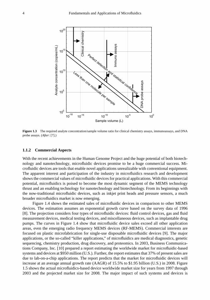
whereηs is the sensor efficiency (0< ηs < 1), NA is the Avogadro number, andAi is theconcentration of analytei. Equation (1.1) demonstrates that the sample volume or the size of themicrofluidic device is determined by the concentration of the desired analyte. Figure 1.2 illustratesthe concentrations of typical diagnostic analytes in human blood or other samples of interest.Concentration determines how many target molecules are present for a particular sample volume.Sample volumes that are too small may not contain any target molecules, and thus will be uselessfor detection purposes. This concept is illustrated in Figure 1.3. Common human clinical chemistryassays require analyte concentrations between 1014 and 1021 copies per milliliter. The concentrationrange for a typical immunoassay is from 108 to 1018 copies per milliliter. Deoxyribonucleicacid (DNA) probe assays for genomic molecules, infective bacteria, or virus particles require aconcentration range from 102 to 107 copies per milliliter [5]. Clinical chemistry with a relativelyhigh analyte concentration allows shrinking the sample volume down to femtoliter range or 1µm3
(see Figure 1.1 and Table 1.1).Immunoassays with their lower analyte concentrations require sample volumes on the order
of nanoliters. Nonpreconcentrated analysis of the DNA present in human blood requires a samplevolume on the order of a milliliter [7]. Some types of samples, like libraries for drug discovery, haverelatively high concentrations.
Table 1.1
Unit Prefixes
Atto Femto Pico Nano Micro Milli Centi Deka Hecto Kilo Mega
10−18 10−15 10−12 10−9 10−6 10−3 10−2 10 102 103 106
4 Fundamentals and Applications of Microfluidics
10-15
10-10
10-5
100
100
105
1010
1015
1020
Sample volume (L)
10-18
Lessthan
onem
oleculeper
sample
Perfect detection
andstatistical confidence
Analy
teconcentr
ation
(copie
s/m
L)
Clinic
alchem
istr
y
Imm
uno
assays
DN
Apro
be
assays
Figure 1.3 The required analyte concentration/sample volume ratio for clinical chemistry assays, immunoassays, and DNAprobe assays. (After: [7].)
1.1.2 Commercial Aspects
With the recent achievements in the Human Genome Project and the huge potential of both biotech-nology and nanotechnology, microfluidic devices promise to be a huge commercial success. Mi-crofluidic devices are tools that enable novel applications unrealizable with conventional equipment.The apparent interest and participation of the industry in microfluidics research and developmentshows the commercial values of microfluidic devices for practical applications. With this commercialpotential, microfluidics is poised to become the most dynamic segment of the MEMS technologythrust and an enabling technology for nanotechnology and biotechnology. From its beginnings withthe now-traditional microfluidic devices, such as inkjet print heads and pressure sensors, a muchbroader microfluidics market is now emerging.
Figure 1.4 shows the estimated sales of microfluidic devices in comparison to other MEMSdevices. The estimation assumes an exponential growth curve based on the survey data of 1996[8]. The projection considers four types of microfluidic devices: fluid control devices, gas and fluidmeasurement devices, medical testing devices, and miscellaneous devices, such as implantable drugpumps. The curves in Figure 1.4 show that microfluidic device sales exceed all other applicationareas, even the emerging radio frequency MEMS devices (RF-MEMS). Commercial interests arefocused on plastic microfabrication for single-use disposable microfluidic devices [9]. The majorapplications, or the so-called “killer applications,” of microfluidics are medical diagnostics, geneticsequencing, chemistry production, drug discovery, and proteomics. In 2003, Business Communica-tions Company, Inc. [10] prepared a report estimating the worldwide market for microfluidic-basedsystems and devices at $950 million (U.S.). Further, the report estimates that 37% of present sales aredue to lab-on-a-chip applications. The report predicts that the market for microfluidic devices willincrease at an average annual growth rate (AAGR) of 15.5% to $1.95 billion (U.S.) in 2008. Figure1.5 shows the actual microfluidics-based device worldwide market size for years from 1997 through2003 and the projected market size for 2008. The major impact of such systems and devices is

Introduction 5
1996 1997 1998 1999 2000 2001 2002 2003
500
1000
1500
2000
2500
3000
3500
Year
Millions
ofU
SD
ollars
Microfluidics
Pressure sensors
Inertial sensors
RF-devices
Figure 1.4 Estimated sales of microfluidic components compared to other MEMS devices. (After: [7].)
predicted to be in the $10 billion (U.S.) analytical laboratory instrumentation market. Microfluidics,and ‘labs-on-a-chip’ in particular, will help to address the high cost of drug development and thepressure to reduce the drug development cycle time. Notice that there is a discrepancy between thesize of the predicted market in Figure 1.4 and the actual market in Figure 1.5. This difference can beattributed largely to two factors: different definitions of what is a microfluidic device or system anda general slowdown in world economies around 2001.
Microfluidics can have a revolutionizing impact on chemical analysis and synthesis, similarto the impact of integrated circuits on computers and electronics. Microfluidic devices could changethe way instrument companies do business. Instead of selling a few expensive systems, companiescould have a mass market of cheap, disposable devices. Making analysis instruments, tailored drugs,and disposable drug dispensers available for everyone will secure a huge market similar to that ofcomputers today.
Consider the analogy of the tremendous calculating labors required of hundreds of people(known as computers) necessary for even a relatively simple finite element analysis at the beginningof the twentieth century, compared to the fraction of a second a personal computer needs today.Computing power is improved from generation to generation by higher operation frequency as wellas parallel architecture. Exactly in the same way, microfluidics revolutionizes chemical screeningpower. Furthermore, microfluidics will allow the pharmaceutical industry to screen combinatoriallibraries with high throughput—not previously possible with manual, bench-top experiments. Fastanalysis is enabled by the smaller quantities of materials in assays. Massively parallel analysis onthe same microfluidic chip allows higher screening throughput. While modern computers only haveabout 20 parallel processes, a microfluidic assay can have several hundred to several hundred thou-sand parallel processes. This high performance is extremely important for DNA-based diagnosticsin pharmaceutical and health care applications.
1.1.3 Scientific Aspects
In response to the commercial potential and better funded environments, microfluidics quickly at-tracted the interest of the scientific community. Scientists from almost all traditional engineering andscience disciplines have begun pursuing microfluidics research, making it a truly multidisciplinaryfield representative of the new economy of the twenty-first century. Electrical and mechanical engi-neers contribute novel enabling technologies to microfluidics. Initially, microfluidics developed as

6 Fundamentals and Applications of Microfluidics
1996 1998 2000 2002 2004 2006 20080
400
800
1200
1600
2000
Year
Mill
ions
of U
S D
olla
rs
Figure 1.5 Actual worldwide sales of microfluidic systems and devices for 1997 through 2003 and projected sales for 2008.The growth is nearly linear over the last 8 years and projected to be steady for the coming 5. (After: [10].)
a part of MEMS technology, which in turn used the established technologies and infrastructure ofmicroelectronics. Fluid mechanics researchers are interested in the new fluids phenomena possibleat the microscale. In contrast to the continuum-based hypotheses of conventional macroscale flows,flow physics in microfluidic devices is governed by a transitional regime between the continuumand molecular-dominated regimes. Besides new analytical and computational models, microfluidicshas enabled a new class of fluid measurements for microscale flows using in situ microinstruments.Life scientists and chemists also find novel, useful tools in microfluidics. Microfluidic tools allowthem to explore new effects not possible in traditional devices. These new effects, new chemicalreactions, and new microinstruments lead to new applications in chemistry and bioengineering.These reasons explain the enormous interest of research disciplines in microfluidics. Nowadays,almost all conferences of professional societies, such as the Institute of Electrical and ElectronicEngineers (IEEE), American Society of Mechanical Engineers (ASME), International Society forOptical Engineering (SPIE), and American Institute of Chemical Engineers (AIChe), have technicalsessions for microfluidics. Figure 1.6 shows an exponential increase of papers on microfluidics inrecent years.
1.2 MILESTONES OF MICROFLUIDICS
At the time of the writing of this book, microfluidics still is in an early stage. With the worldwideeffort in microfluidics research, we find ourselves in the unique position of being able to makeobservations about the short history of microfluidics research as well as about its likely future trends.Two major aspects are considered here: the applications-driven development of devices and thedevelopment of fabrication technologies.
1.2.1 Device Development
Miniaturization approachWith silicon micromachining as the enabling technology, researchershave been developing silicon microfluidic devices. The first approach for making miniaturizeddevices was shrinking down conventional principles. This approach is representative of the research

Introduction 7
1995 1996 1997 1998 1999 2000 2001 2002 2003 2004
0
20
40
60
80
100
120
140
160
180
200
Microfluidics
Micropumps
Microvalves
Microneedles
Micromixers
Years
Nu
mb
er
of
pa
pe
rs
Figure 1.6 Publication of microfluidics-related papers in international journals and conferences.
conducted in the 1980s through the mid-1990s. In this phase of microfluidics development, a numberof silicon microvalves, micropumps, and microflow sensors were developed and investigated [11].
Two general observations of scaling laws can be made in this development stage: the powerlimit and the size limit of the devices. Assuming that the energy density of actuators is independentof their size, scaling down the size will decrease the power of the device by the length scale cubed.This means that we cannot expect micropumps and microvalves to deliver the same power level asconventional devices. The surface-to-volume ratio varies as the inverse of the length scale. Largesurface area means large viscous forces, which in turn requires powerful actuators to be overcome.Often, integrated microactuators cannot deliver enough power, force, or displacement to drive amicrofluidics device, so an external actuator is the only option for microvalves and micropumps.The use of external actuators limits the size of those microfluidic devices, which can range frommillimeters to centimeters.
Exploration of new effectsSince the mid-1990s, development has been shifted to the ex-ploration of new actuating schemes for microfluidics. Because of the power and size constraintsdiscussed above, research efforts have concentrated on actuators with no moving parts and nonme-chanical pumping principles. Electrokinetic pumping, surface tension-driven flows, electromagneticforces, and acoustic streaming are effects that usually have negligible effect at macroscopic lengthscales. However, at the microscale they offer particular advantages over mechanical principles. Neweffects, which mimic the way cells and molecules function, will be the next developmental stage ofmicrofluidics. With this move, microfluidics will enter the era of nanotechnology.
Application developmentsConcurrent with the exploration of new effects, microfluidics todayis looking for further application fields beyond conventional fields, such as flow control, chemicalanalysis, biomedical diagnostics, and drug discovery. New applications utilizing microfluidics fordistributed energy supply, distributed thermal management, and chemical production are promising.

8 Fundamentals and Applications of Microfluidics
Chemical production using distributed microreactors makes new products possible. The large-scaleproduction can be realized easily by running multiple identical microreactors in parallel. Scalabilityis inherent in microfluidics, and can be approached from the point of view of “numbering up” ratherthan scaling up. In this regard, the microreactor concept mirrors potential of nanotechnology, inwhich technology imitates nature by using many small parallel processors rather than a single largerreactor.
1.2.2 Technology Development
Similar to the trends in device development, the technology of making microfluidic devices has alsoseen a paradigm shift. Starting with silicon micromachining as the enabling technology, a numberof microfluidic devices with integrated sensors and actuators were made in silicon. However, unlikemicroelectronics, which manipulates electrons in integrated circuits, microfluidics must transportmolecules and fluids in larger channels, due to the relative size difference between electrons and themore complicated molecules that comprise common fluids. This size disparity leads to much largermicrofluidic devices. Significantly fewer microfluidic devices than electronic devices can be placedon a silicon wafer. Adding material cost, processing cost, and the yield rate, microfluidic devicesbased on silicon technology are too expensive to be accepted by the commercial market, especiallyas disposable devices.
Since mid-1990, with chemists joining the field, microfabrication technology has been movingto plastic micromachining. With the philosophy of functionality above miniaturization and simplic-ity above complexity, microfluidic devices have been kept simple, sometimes only with a passivesystem of microchannels. The actuating and sensing devices are not necessarily integrated into themicrodevices. These microdevices are incorporated as replaceable elements in benchtop and hand-held tools. Batch fabrication of plastic devices is possible with many replication and forming tech-niques. The master (stamp or mold) for replication can be fabricated with traditional silicon-basedmicromachining technologies. However, a cheap plastic device with integrated sensors and actuatorsis still desirable. Complex microfluidic devices based on plastic microfabrication could be expectedin the near future with further achievements of plastic-based microelectronics. One example of thismigration from silicon to plastic fabrication is the i-STAT point-of-care blood chemistry diagnosticsystem in which only a very small fraction of the device is made using silicon microfabricationtechnologies. The bulk of the device is fabricated from two pieces of plastic that are taped together.
With new applications featuring highly corrosive chemicals, microfluidic devices fabricated inmaterials such as stainless steel or ceramics are desired. Microcutting, laser machining, microelectrodischarge machining, and laminating are a few examples of these alternative fabrication techniques.The relatively large-scale microfluidic devices and the freedom of material choice make thesetechniques serious competitors for silicon micromachining.
1.3 ORGANIZATION OF THE BOOK
This book is divided into thirteen chapters. The topic of each chapter follows.Chapter 1 introduces the field of microfluidics, including its definition and commercial and
scientific aspects. Chapter 1 also addresses the historical development of this relatively new researchfield and provides important resources for microfluidics research.
Chapter 2 discusses when to expect changes in fluid behavior as the length scale of a flowis shrunk to microscopic sizes. The appropriate means for analytically treating as well as compu-tationally simulating microflows is addressed. The theoretical fundamentals that form the basis fordesign and optimization of microfluidic devices are addressed. Several multiphysics couplings arediscussed, including thermofluid and electrofluid. Chapter 3 provides the technology fundamentals

Introduction 9
required for making microfluidic devices. Conventional MEMS technology, such as bulk microma-chining and surface micromachining, are discussed. Varieties of plastic micromachining techniquesare presented in this chapter. Alternative nonbatch techniques, which are interesting for small-scaleproduction and prototyping, are also discussed in this chapter.
Chapter 4 analyzes various experimental characterization techniques for microfluidic devices.The chapter presents a number of novel diagnostic techniques developed for investigation of fluidflow in microscale. Chapters 2 through 4 consider the fundamentals of the typical developmentprocess of microfluidic devices—from analysis to fabrication to device characterization.
Chapters 5 through 13 present design examples of microfluidic devices, which were the objectsof the worldwide microfluidics research community in the last decade. The examples are categorizedin their application fields, such as external flow control, internal flow control, and microfluidics forlife sciences and chemistry.
Chapter 5 describes the design of microdevices for controlling macroscopic flow phenomena,such as velocity sensors, shear stress sensors, microflaps, microballoon, microsynthetic jets, andmicroair vehicles.
Chapters 6, 7, and 8 present design rules and solutions for microvalves, micropumps, andmicroflow sensors, respectively. The chapters analyze in detail the operation principles, designconsiderations, and fabrication techniques of these microfluidic devices.
Chapters 9 through 13 list a number of tools and devices for the emerging fields of lifesciences and chemical analysis in microscale. Typical devices are filters, needles, mixers, reactors,heat exchangers, dispensers, and separators.
As mentioned above, the field of microfluidics is in an early, rapid development stage. Manytopics, such as new fluid effects and multiphysics effects at the microscale, are still under intensiveresearch. New applications in the fields of life sciences and chemistry are emerging at an exponentialrate. Therefore, while the materials presented in this book serve to bring the reader to a completeunderstanding of the present state of the art, the examples and the references listed at the end ofeach chapter will allow the reader to grow beyond the subject matter presented here. This book isintended to serve as a source on microfluidics.
References
[1] Feynman, R. P., “There’s Plenty of Room at the Bottom,”Journal of Microelectromechanical Systems, Vol. 1, No. 1,1992, pp. 60–66.
[2] Moore, G., “VLSI, What Does the Future Hold,”Electron. Aust., Vol. 42, No. 14, 1980.
[3] Chang, C. Y., and Sze, S. M.,ULSI Devices, New York: Wiley, 2000.
[4] Petersen, K. E., “Silicon as Mechanical Material,”Proceedings of the IEEE, Vol. 70, No. 5, 1982, pp. 420–457.
[5] Manz, A., Graber, N., and Widmer, H. M., “Miniaturized Total Chemical Analysis Systems: A Novel Concept forChemical Sensing,”Sensors and Actuators B, Vol. 1, 1990, pp. 244–248.
[6] Gravesen, P., Branebjerg, J., and Jensen, O. S., “Microfluidics—A Review,”Journal of Micromechanics and Micro-engineering, Vol. 3, 1993, pp. 168–182.
[7] Petersen, K. E., et al., “Toward Next Generation Clinical Diagnostics Instruments: Scaling and New ProcessingParadigms,”Journal of Biomedical Microdevices, Vol. 2, No. 1, 1999, pp. 71–79.
[8] System Planning Corporation, “Microelectromechanical Systems (MEMS): An SPC Market Study,” January 1999,Arlington, VA.
[9] Harrison, D. J., et al., “The Decade’s Search for the Killer Ap in m-TAS,”Micro Total Analysis Systems 2000, A. vanden Berg et al. (eds.), Kluwer Academic Publishers, 2000, pp. 195–204.
[10] Business Communications Company, Inc., “Microfluidics Technology–Updated Edition,” Publication No. RGB-226R,2003, Norwalk, CT.
[11] Shoji, S., and Esashi, M., “Microflow Devices and Systems,”Journal of Micromechanics and Microengineering, Vol.4, No. 4, 1994, pp. 157–171.

10 Fundamentals and Applications of Microfluidics

Chapter 2
Fluid Mechanics Theory
2.1 INTRODUCTION
Although everyone has an intuitive sense of what a fluid is, rigorously defining just what fluidsare is more troublesome. According toMerriam-Webster’s Collegiate Dictionary[1], a fluid is: “asubstance (as a liquid or gas) tending to flow or conform to the outline of its container.”
While this definition gives us a sense of what a fluid is, it is far removed from a technicaldefinition. It also begs the question: What is a liquid or a gas? Again, according to [1], a liquid is:“a fluid (as water) that has no independent shape but has a definite volume and does not expandindefinitely and that is only slightly compressible,” while a gas is: “a fluid (as air) that has neitherindependent shape nor volume but tends to expand indefinitely.”
These definitions are circular and ultimately rely on examples such as water and air to explainwhat a fluid is. Clearly we must look further for a good definition of what a fluid is.
According to one of the leading undergraduate textbooks in fluid mechanics [2], the definitionof a fluid is: “a substance that deforms continuously under the application of shear (tangential) stress,no matter how small that stress may be.” This definition proves to be a suitable working definitionthat we can use to determine whether some material that is not air or water is a fluid.
Consider a thought experiment wherein both a solid block of an elastic material (such asaluminum) and a layer of fluid are subjected to the same shearing force. Figure 2.1 depicts just thissituation. The block of material in Figure 2.1(a), when subjected to the shearing force, will deformfrom its equilibrium shape, indicated by the vertical solid lines, to its deformed shape, indicated bythe dashed inclined lines. If this force is released the block will return to its original, equilibriumposition. As long as the elastic limit of the solid is not exceeded, it will always behave like this.A fluid subject to a constant shearing force in Figure 2.1(b) will behave very differently. The fluidis deformed from its original position, indicated by the vertical solid lines, to another position,indicated by the first set of dashed inclined lines, by the shearing force. If the force is removed,the fluid will remain in this position, its new equilibrium position. If the force is reapplied, thefluid will deform still further to the shape indicated by the second set of dashed lines. As long asthe shear force persists, the fluid will continue deforming. As soon as the shear force is removed,the fluid will cease deforming and remain in its present position. For true fluids, this process willcontinue indefinitely and for any size of shearing force. When the shear stress (shearing force/areafluid contact) is directly proportional to the rate of strain (typically∂u/∂y) within the fluid, the fluidis said to beNewtonian. This simple demonstration also alludes to the no-slip boundary condition,which is of fundamental importance in fluid mechanics and needs to be considered on a case-by-casebasis in microscopic domains.
Flowing fluids can be characterized by the properties of both the fluid and the flow. These canbe organized into four main categories [3]:
11

12 Fundamentals and Applications of Microfluidics
ForceForce
(a) (b)
Figure 2.1 (a) A block of solid material, and (b) a fluid contained between two plates are subjected to a shearing force. Bothmaterials are shown in an original position (solid lines) and deformed positions (dashes). When the force is removed fromthe solid material, it returns from its deformed position to its original or equilibrium position. The fluid remains deformedupon removal of the force.
• Kinematic properties such as linear and angular velocity, vorticity, acceleration, and strain rate;
• Transport properties such as viscosity, thermal conductivity, and diffusivity;
• Thermodynamic properties such as pressure, temperature, and density;
• Miscellaneous properties such as surface tension, vapor pressure, and surface accommodationcoefficients.
Knowledge of these properties is necessary for quantifying the fluid’s response to some set ofoperating conditions. The kinematic properties are actually properties of the flow, but they usuallydepend on the properties of the fluid. The transport properties and thermodynamic propertiesare generally properties of the fluid, but they may depend on the properties of the flow. Themiscellaneous properties are properties that may depend on the interaction of fluid and the vessel inwhich it is flowing such as the surface tension or the surface accommodation coefficient. They canalso be constitutive properties of the fluid (or any other hard-to-classify properties of the fluid/flow).
A fluid can be modeled in one of two ways: as a collection of individual, interacting moleculesor as a continuum in which properties are defined to be continuously defined throughout space.The former approach is addressed in the introductory chapters of many fluid mechanics texts [3–5]and then ignored as either impractical or unnecessary. However, as the length scale of a systemdecreases in size, the question of whether to treat the fluid as a collection of molecules or asa continuum acquires critical significance. To use a continuum approach in a situation where amolecular approach is necessary would certainly produce incorrect results. In this chapter, these twodistinctly different approaches will be explored.
2.1.1 Intermolecular Forces
The behavior of all states of matter–solids, liquids, and gases–as well as the interaction among thedifferent states, depends on the forces between the molecules that comprise the matter. An accuratemodel of the interaction of two simple, nonionized, nonreacting molecules is given by the Lennard-Jones potential,Vi j :
Vi j (r ) = 4ε
[ci j
( r
σ
)−12− di j
( r
σ
)−6]
(2.1)
wherer is the distance separating the moleculesi and j , ci j anddi j are parameters particular tothe pair of interacting molecules,ε is a characteristic energy scale, andσ is a characteristic lengthscale. The term with ther −12 dependence is a phenomenological model of the pairwise repulsionthat exists between two molecules when they are brought very close together. The term with ther −6 dependence is a mildly attractive potential due to the van der Waals force between any twomolecules. The van der Waals forces are analytically derivable and reflect the contribution fromseveral phenomena. These are:

Fluid Mechanics Theory 13
Table 2.1
A Selection of Lennard-Jones Constants Derived from Viscosity Data [9].Note: The Boltzmann constantK is equal to
1.381× 10⁻²³J/K .
Fluid εK (K) σ (nm)
Air 97 0.362N2 91.5 0.368CO2 190 0.400O2 113 0.343Ar 124 0.342
• Dipole/dipole interactions (Keesom theory);
• Induced dipole interactions (Debye theory);
• Fundamental electrodynamic interactions (London theory).
Since (2.1) represents the potential energy between two interacting molecules, the force betweenthose two molecules is given by its derivative as:
Fi j (r ) =∂Vi j (r )
∂r=
48ε
σ
[ci j
( r
σ
)−13−
di j
2
( r
σ
)−7]
(2.2)
With an appropriate choice of the parametersci j and di j , this equation can represent the forcebetween any two molecules. The characteristic time scale for molecular interactions for whichLennard-Jones is a good model is given by:
τ = σ
√m
ε(2.3)
which is the period of oscillation about the minimum in the Lennard-Jones potential. Them is themass of a single molecule. The Lennard-Jones potential has been shown to provide accurate resultsfor liquid argon usingε/K = 120K,σ = 0.34 nm, andc = d = 1. For these parameters, the timescale works out toτ = 2.2×10⁻¹² sec—a very short time indeed [6]. Several recent articles providea more in-depth discussion of the Lennard-Jones potential and its various uses [6–8].
The values of the various parameters in (2.1) through (2.3) are available in the literature [7] fora limited number of molecules. These values are summarized in Table 2.1. The parametersci j anddi j
should be taken as unity when using the parameters from Table 2.1. These parameters should be usedonly to calculate the potential between two fluid molecules of the same species. It is also acceptableto use these parameters between molecules of the same species even if they are in different phases(e.g., liquid and solid). However, these constants should not be used to calculate the interaction of afluid molecule with a flow boundary of different molecules.
These parameter values can be used to calculate the potential energy and force between twointeracting molecules. The effect of the constants in Table 2.1 is to change themagnitudeof thepotential energy and force, but not itsgeneral shape. Figure 2.2 shows this general shape by plottingpotential energy scaled by14ε and force scaled byσ48ε versus dimensionless separation distancer/σ . Were this a dimensional figure, it would be stretched or compressed in both the horizontaland vertical directions, but the overall shape would appear the same. One important observationconcerning this force plot is that, although its magnitude decreases very quickly with distancesbeyond the location of the minimum (e.g., it drops from−0.05 at a distance of 1.2 to nearly nothing

14 Fundamentals and Applications of Microfluidics
1 1.2 1.4 1.6 1.8 2
-0.2
-0.1
0
0.1
0.2
0.3
1 1.2 1.4 1.6 1.8 2
-0.2
-0.1
0
0.1
0.2
0.3
1 1.2 1.4 1.6 1.8 2
-0.2
-0.1
0
0.1
0.2
0.3
1 1.2 1.4 1.6 1.8 2
-0.2
-0.1
0
0.1
0.2
0.3
1 1.2 1.4 1.6 1.8 2
-0.2
-0.1
0
0.1
0.2
0.3
1 1.2 1.4 1.6 1.8 2
-0.2
-0.1
0
0.1
0.2
0.3
1 1.2 1.4 1.6 1.8 2
-0.2
-0.1
0
0.1
0.2
0.3
1 1.2 1.4 1.6 1.8 2
-0.2
-0.1
0
0.1
0.2
0.3
1 1.2 1.4 1.6 1.8 2
-0.2
-0.1
0
0.1
0.2
0.3
Potential: V(r) / 4�
Force: F(r).� / 48�
Repulsive
Attractive
Dim
ensio
nle
ss
Separation Distance r/�
Figure 2.2 Generalized plot of intermolecular potential energy and force according to the Lennard-Jones model.
at 2.0), it never reaches zero. This has important implications for molecular dynamics simulations,as we will see in Section 2.3.1.
2.1.2 The Three States of Matter
All three states of matter–solids, liquids, and gases–are comprised of molecules that are all interact-ing through the Lennard-Jones force discussed earlier. The molecules in a solid are densely packedand rigidly fixed within some particular molecular arrangement. The molecules are in constant con-tact with one another with a mean intermolecular spacing of aboutσ . The molecules of the solidinteract with all of their neighbors through the Lennard-Jones force. Each molecule is held in placeby the large repulsive forces that it would experience if it were to move closer to one of its neighbors.Hence, for a molecule to leave its particular molecular neighborhood and join a nearby arrangementof molecules requires a significant amount of energy–an amount that it is unlikely to receive whenthe solid is held below its melting temperature. As the solid is heated up to and beyond its meltingtemperature, the average molecular thermal energy becomes high enough that the molecules areable to vibrate freely from one set of neighbors to another. The material is then called aliquid. Themolecules of a liquid are still relatively close together (still approximatelyσ ), which agrees withour observations that the density of a liquid just above the melting temperature is only slightly lowerthan a solid just below the melting temperature. Water is the most common exception to this ruleand is a few percent more dense as a liquid near the melting temperature than as a solid. If thetemperature of the liquid is raised, the vibration of the molecules increases still further. Eventually,the amplitude of vibration is great enough that, at the boiling temperature, the molecules jumpenergetically away from each other and assume a mean spacing of approximately 10σ (at standardconditions). The material is now called agas. The molecules interact strictly through brief, highlyenergetic collisions with their neighbors.
They are no longer in continuous contact with each other. In fact, only during these briefcollisions are the molecules close enough together that the Lennard-Jones forces become significantwhen compared with their kinetic energy. The molecules comprising the gas will expand to fillwhatever vessel contains them. These attributes of solids, liquids, and gases are summarized inTable 2.2.

Fluid Mechanics Theory 15
Table 2.2
Summary of Solid, Liquid, and Gas Intermolecular Relationships (After: [4].)
Phases Intermolecular ForcesRatio of Thermal VibrationAmplitude Compared toσ
Approach Needed
Solid Strong � 1 QuantumLiquid Moderate ∼ 1 Quantum/classicalGas Weak � 1 Classical
�
‘point
value’
Variations due to
molecular fluctuations
Sampling volume L3
Macroscopic flow variations,
e.g. shocks, temp. changes, etc.
Figure 2.3 Continuum assumption in fluids illustrated by thought experiment for measuring density. (After: [4].)
2.1.3 Continuum Assumption
The study of fluid mechanics (at conventional, macroscopic length scales) generally proceeds fromthe assumption that the fluid can be treated as a continuum. All quantities of interest such as density,velocity, and pressure are assumed to be defined everywhere in space and to vary continuously frompoint to point within a flow. We have just seen that all matter is actually comprised of quanta of mass–discrete atoms and molecules–not a uniformly distributed featureless substance. Whether assumingcontinuity of mass and other properties is reasonable at microscopic length scales depends greatlyon the particular situation being studied. If the molecules of a fluid are closely packed relative to thelength scale of the flow, the continuum assumption is probably valid. If the molecules are sparselydistributed relative to the length scale of the flow, assuming continuity of fluid and flow propertiesis probably a dangerous approach. However, even at microscopic length scales, there can still bemany thousands of molecules within a length scale significant to the flow. For example, a 10-µmchannel will have approximately 30,000 water molecules spanning it–certainly enough molecules toconsider the flow as continuous.
To illustrate this point of the molecular versus continuum nature of fluids, let us consider athought experiment in which we measure the density of a fluid at a point, as is shown in Figure2.3. Most graduate-level fluid mechanics textbooks will have an argument similar to that whichfollows [4, 5, 10]. This is not a point in the geometric sense, but rather, a small sampling volume ofspace surrounding the geometric point in which we are interested. To make this argument morestraightforward, let us consider that the molecules are frozen in space. The argument is easilyextensible to moving molecules, but this simplification separates the temporal and spatial variationsof the flow. If we consider measuring the average density of the fluid within the sampling volume,we could do it by counting the number of molecules within the sampling volume, multiplying by the

16 Fundamentals and Applications of Microfluidics
Figure 2.4 Sketches of (a) a gas, such as N2, at standard conditions, and (b) a liquid, such as H2O.
Table 2.3
Properties of a Typical Gas and Liquid at Standard Conditions (After: [10].)
Property Gas (N2) Liquid (H2O)
Molecular diameter 0.3 nm 0.3 nmNumber density 3× 1025m−3 2 × 1028m−3
Intermolecular spacing 3 nm 0.4 nmDisplacement distance 100 nm 0.001 nmMolecular velocity 500 m/s 1,000 m/s
molecular mass of each molecule, and dividing by the volume of the sampling volume according to:
ρ =N · m
L3(2.4)
where the sampling region is assumed to be a cube measuringL on a side, andN is the number ofmolecules that were found in it. The mass of a single molecule ism.
When the size of the sampling volume is very small, it will at any given time contain only afew molecules. Gradually expanding the sampling volume will at times add a new molecule to thesampling volume and at other times merely increase the volume of the sampling volume. Hence, wewould expect that, when the number of molecules in the sampling volume is small, the calculateddensity would vary rapidly, but as the volume becomes larger and larger, the calculated densitywould approach some relatively constant value. That value is called thepoint valuein continuumfluid mechanics. If the size of the sampling volume is increased beyond that necessary to achieve apoint value, spatial variations in the flow will begin to get averaged out. In the case of density, spatialvariations could be due to a shock wave or to local heating of the flow.
To make this distinction between continuous and molecular behavior, it is useful to considerconcrete examples. Figure 2.4 shows two sketches, one of a gas, which for the sake of concretenesswe will take to be diatomic nitrogen, N2, at standard conditions, as well as a liquid, water, also atstandard conditions. Table 2.3 compares the properties of the gas and the liquid.
In order that a fluid can be modeled as a continuum, all of its properties must be continuous[10]. There are different length scales for different types of properties. A fluid’s kinematic properties,such as velocity and acceleration, as well as its thermodynamic properties, such as pressure anddensity, can be treated as the point quantities in the thought experiment above. According to randomprocess theory, in order to get reasonably stationary statistics, less than 1% statistical variations,104 molecules must be used to compute an average value. Consequently, the point quantities can bethought of as continuous if the sampling volume is a cube that measures:
Lgas,pt =3
√104
3 × 1025m−3= 70× 10−9 m (2.5)

Fluid Mechanics Theory 17
and
L liquid,pt =3
√104
2 × 1025m−3= 8 × 10⁻⁹ m (2.6)
The transport quantities such as viscosity and diffusivity must also be continuous in orderfor the fluid to be treated as a continuum. The analysis of the transport quantities is somewhatdifferent from that of the point quantities where a certain number ofmoleculeswere required in orderfor the property to be treated as continuous. For the transport quantities to behave continuously,it is important that the fluid molecules interact much more often with themselves than with flowboundaries. As a somewhat arbitrary criterion, we can choose the measurement point to be a cubewhose sides are 10 times as large as the molecules’ interaction length scale. For a gas, the bestestimate of an interaction length scale is the displacement distance, also known as the mean freepath, which is on the order of 100 nm. For a liquid, the molecules are essentially in a continualstate of collision or interaction, so their displacement distance is not a good estimate of how manyinteractions will be present in some cube of space. Their molecular diameter is a much betterestimate. Hence, the transport quantities will be continuous in a cube measuring:
Lgas,tr =3√
103 × 100nm= 10−6m (2.7)
and
L liquid,tr =3
√103
2 × 1025m−3= 4 × 10⁻⁹m (2.8)
In order to be able to treat a flow as continuous, both its point quantities and its transport quantitiesmust be continuous. Hence, taking the greater of the two length scales, the length scale at whichcontinuous behavior can be expected is:
Lgas= 1µm (10−6m) (2.9)
andL liquid = 10 nm(10−8m) (2.10)
This analysis is very approximate and is meant merely to help the reader get a feel for whencontinuum behavior can be expected and when the flow must be treated as an ensemble of individualinteracting molecules.
The ultimately quantized nature of matter combined with the diminutive length scales that arethe subject of this book beg the question of why we should bother with the continuum approach atall if the downside is an incorrect analysis. Scientists and engineers had been developing the fieldof fluid mechanics since long before the atomic nature of matter was conclusively demonstratedin the late nineteenth century. The governing continuum fluid mechanics equations have existedin their present form, called the Navier-Stokes equations, when certain reasonable approximationsare used, for more than a century. Consequently, if the continuum approach is valid in a givenmicrofluidic situation, it should be used because of the tremendous body of work available forimmediate application to the flow situation. Also, describing fluids by continuously varying fieldsgreatly simplifies modeling the fluid. Using the continuum approach, many flows can be computedanalytically with no more equipment necessary than a pencil. Molecular approaches to solvingfluid mechanics problems generally consist of knowing the state (position and velocity) of eachmolecule of the fluid and then evolving that state forward in time for every single molecule.While the evolution equations might be particularly simple, for example, Newton’s second law plusthe Lennard-Jones force, it might need to be repeated excessively. Because most microflows arerelatively large compared to molecular length scales, they necessarily contain a moderate (several

18 Fundamentals and Applications of Microfluidics
thousands) to large (billions or more) number of molecules. Two of the main molecular fluidstechniques are discussed later in this chapter. These are the molecular dynamics (MD) and directsimulation Monte Carlo (DSMC) techniques. The remaining sections in this chapter explore:
• Continuum approaches to fluid mechanics at small scales (Section 2.2);
• Molecular approaches to fluid mechanics (Section 2.3);
• Electrokinetics (Section 2.4).
2.2 CONTINUUM FLUID MECHANICS AT SMALL SCALES
Even in very small devices and geometries, fluids, especially liquids, can be considered to becontinuous. Hence, well-established continuum approaches for analyzing flows can be used. Theseapproaches have been treated in great detail in a variety of fluid mechanics textbooks [2–5]and hence will only be summarized here. The three primary conservation laws that are used tomodel thermofluid dynamics problems are conservation of mass, momentum, and energy. In partialdifferential equation form, these are:
∂ρ
∂t+∂ρ
∂xi(ρui ) = 0 (2.11)
∂
∂t(ρui )+
∂
∂x j(ρu j ui ) = ρFi −
∂p
∂xi+
∂
∂x jτ j i (2.12)
∂
∂t(ρe)+
∂
∂xi(ρui e) = −p
∂ui
∂xi+ τ j i
∂ui
∂x j+∂qi
∂xi(2.13)
where repeated indices in any single term indicate a summation according to the accepted practice inindex notation (Einstein summation convention). In these equations,ui represents the flow velocity,ρ is the local density,p is the pressure,τ is the stress tensor,e is the internal energy,F is bodyforce, andq is the heat flux. Most often at large length scales, the body forceF is taken to begravity. However, because of cube-square scaling, the effect of gravity in small systems is usuallynegligible. In order to overpower the cube-square scaling, the body force needs to be some forcethat can be increased to large values—such as a magnetic body force, which can be several ordersof magnitude larger than the body force generated by gravity. These equations comprise five partialdifferential equations (one for mass, three for momentum, and one for energy) in 17 unknowns:ρ,ui , τ j i , e, andqi . Thus, they do not represent a closed system of equations. To close these equations,a necessary but not sufficient condition for their solution, we must look to constitutive relationshipsamong these unknowns—specifically to relationships between the stress tensor and the velocityfield, heat flux and temperature field, and constitutive thermodynamic properties of the fluid, suchas the ideal gas law. These relationships can be very different for gases and liquids, so they will beconsidered separately in the next sections.
One note of commonality between the continuum approach to solving fluid mechanicsproblems in gases and liquids is that computational fluid dynamics (CFD) methods have beendeveloped to solve problems in both gases and liquids, and these methods have been very successfulin large-scale problems. As long as the continuum assumption holds, there should be no particularproblems with adapting CFD to solve microscale problems. Several commercial packages presentlyare available which do just that.

Fluid Mechanics Theory 19
2.2.1 Gas Flows
2.2.1.1 Kinetic Gas Theory
As explained in Section 2.1.2, gases consist of mostly space with a few molecules colliding onlyinfrequently. Consequently, they can be described quite well by the kinetic gas theory, in which agas molecule is considered to move in a straight line at a constant speed until it strikes anothermolecule—which it does infrequently. Many of the conclusions of kinetic gas theory are presentedin this section. The equation of state for a dilute gas is the ideal gas law, which can have severalequivalent forms. Two of these forms are:
p = ρRT (2.14)
andp = nK T (2.15)
wherep is the pressure,ρ is the density of the gas,R is the specific gas constant for the gas beingevaluated,n is the number density of the gas,K is Boltzmann’s constant (K = 1.3805×10⁻²³J/K ),andT is the absolute temperature. The specific gas constantR can be found from:
R =R
MwhereR = 8.3185
kJ
kmol · K(2.16)
whereR is the universal gas constant andM is the molar mass of the gas.Using the second form of the ideal gas law, it is possible to calculate that at standard conditions
(273.15K ; 101,625Pa), the number density of any gas isn = 2.70×1025m−3. The mean molecularspacing will be important in the following analysis. Since the molecules in the gas are scatteredrandomly throughout whatever vessel contains them, the mean molecular spacingδ can be estimatedasδ = n−1/3
= 3.3 × 10⁻⁹m (at standard conditions).Comparing this value to the diameter of a typical gas molecule, say, N2 from above
δ
d=
3.3 × 10⁻⁹ m
3 × 10⁻¹⁰ m≈ 10 � 1 (2.17)
gives a measure of effective density. Gases for whichδ/d � 1 are said to bedilute gases[11], whilethose not meeting this condition are said to bedense gases. For dilute gases, the most commonmode of intermolecular interaction is binary collisions. Simultaneous multiple molecule collisionsare unlikely. Generally, values ofδ/d greater than 7 are considered to be dilute.
Several transport quantities are important in gas dynamics. These are the mean free pathλ, themean-square molecular speedc, and the speed of soundcs. The mean free path is the distance thatthe average molecule will travel before experiencing a collision. For a simple gas of hard spheres atthermodynamic equilibrium, Bird [11] gives the equation:
λ =1
√2 · πd2n
(2.18)
The mean-square molecular speed is given by Vincenti and Kruger [12] as:
c =√
3RT (2.19)
where R is the gas constant specific to the gas under consideration. The speed at which sound(infinitesimal pressure waves) travels through a gas is important in determining the type of flow that

20 Fundamentals and Applications of Microfluidics
will develop in the gas. The speed of soundcs is given by:
cs =√
k RT (2.20)
wherek is the ratio of specific heats, defined to be the ratio of the specific heat at a constant pressurecp to the specific heat at a constant volumecv. For common gases (air,N2, O2), k is generally about1.4 but can depart significantly from that value for more complicated molecules.
One last quantity of importance in gas dynamics is the viscosity of the gas. According to thekinetic theory of gases, the viscosity is given by:
ν =η
ρ=
1
2λc (2.21)
whereν is the kinematic viscosity andη is the dynamic viscosity. Bothλ andc are given as above.This equation thus relates viscosity to temperature and pressure through the mean free path andmean molecular speed. If we solve (2.21) for the dynamic viscosityη, we can find that the dynamicviscosity is not a function of pressure, because density is proportional to pressure while the meanfree path is inversely proportional to it.
In addition to these parameters, there are several dimensionless groups of parameters thatare very important in assessing the state of a fluid in motion. These are the Mach number Ma, theKnudsen number Kn, and the Reynolds number Re. The Mach number is the ratio between the flowvelocityu and the speed of soundcs, and is given by:
Ma =u
cs(2.22)
The Mach number is a measure of the compressibility of a gas and can be thought of as the ratio ofinertial forces to elastic forces. Flows for which Ma< 1 are calledsubsonicand flows for whichMa > 1 are calledsupersonic. When Ma= 1, the flow is said to besonic. The Mach number caneither be a local measure of the speed of the flow ifu is a local velocity, or it can be a global measureof the flow if the mean flow velocityuavg is used. Under certain conditions, the density of a gaswill not change significantly while it is flowing through a system. The flow is then considered tobe incompressible even though fluid, a gas, is still considered compressible. This distinction is animportant one in fluid mechanics. The analysis of an incompressible gas flow is greatly simplified,since it can be treated with the same versions of the governing equations that will be derived forliquid flows in Section 2.2.2. If the Mach number of a gas flow is greater than 0.3, the flow must betreated as a compressible flow. If the Mach number of a flow is less than 0.3, the flow may be treatedas incompressible provided some further conditions are satisfied. The Mach number of a flow beingless than 0.3 is a necessary but not sufficient condition for the flow to be treated as incompressible[8]. Gas flows in which the wall is heated locally can cause large changes in the density of the gaseven at low Mach numbers. Similarly, gas flows in long, thin channels will experience self-heatingdue to the viscous dissipation of the fluid which can cause significant changes in the gas density. Fora further discussion of these effects, see [8]. Absent effects like these, when the Mach number is lessthan 0.3, gas flows may be treated as incompressible.
The Knudsen number has tremendous importance in gas dynamics. It provides a measure ofhow rarefied a flow is, or how low the density is, relative to the length scale of the flow. The Knudsennumber is given by:
Kn =λ
L(2.23)
whereλ is the mean free path given in (2.18) andL is some length scale characteristic of the flow.

Fluid Mechanics Theory 21
The Reynolds number is given by:
Re=ρuL
η=
uL
ν(2.24)
whereu is some velocity characteristic of the flow,L a length scale characteristic of the flow,ρ isthe density,η is the dynamic viscosity, andν is the kinematic viscosity. The physical significance ofthe Reynolds number is that it is a measure of the ratio between inertial forces and viscous forces ina particular flow. The different regimes of behavior are:
• Re� 1 viscous effects dominate inertial effects (completely laminar flows);
• Re≈ 1 viscous effect comparable to inertial effects (vortices begin to appear);
• Re� 1 inertial effects dominate viscous effects (turbulence occurs).
Flow patterns will typically be functions of the Reynolds number. In channel flows, Reynoldsnumbers smaller than about 1,500 typically indicate laminar flow, while flows with Reynoldsnumbers greater than 1,500 are increasingly likely to be turbulent. These dynamics are discussedin greater detail in Section 2.2.4.3. The three dimensionless groups just presented are all related bythe expression:
Kn =
√kπ
2
Ma
L(2.25)
wherek is the ratio of specific heats. The Knudsen number is one of the main tools used to classifyhow rarefied a flow is—or how far apart the molecules of the flow are relative to the scale of theflow. There are four main regimes of fluid rarefaction. These are:
• Kn < 10−3 Navier-Stokes equation, no-slip boundary conditions;
• 10−3 < Kn < 10−1 Navier-Stokes equation, slip boundary conditions;
• 10−1 < Kn < 101 Transitional flow regime;
• Kn > 101 Free molecular flow.
Example 2.1: Gas Flow Calculation
Calculate all the significant parameters to describe a flow of diatomic nitrogen N2 at 350K and200 kPa at a speed of 100 m/s through a channel measuring 10µm in diameter.
First step: Look up properties for diatomic nitrogen gas:
• Molar mass:M = 28.013 kg/kmol
• Molecular diameter [9]:d = 3.75× 10⁻¹⁰m
Second step: Calculate the dimensional parameters for the flow:
R =8.3145 kJ/kmol· K
28.013 kg/kmol= 0.2968
kJ
kg · K
n =2 × 10⁵ N/m2
1.3805× 10⁻²³J/K × 350K·
J
Nm= 4.14× 1025 m−3
δ = n−1/3= 2.89× 10⁻⁹m
λ =
(√2πd2n
)−1=
[√
2π(3.75× 10⁻¹⁰ m
)2· 4.14× 1025 m−3
]−1
= 3.9 × 10⁻⁸m

22 Fundamentals and Applications of Microfluidics
10-10
10-8
10-6
10-4
10-2
100
102
10-8
10-6
10-4
10-2
100
102
1
Density Ratio (n / n )0
101
102
103
104
102
104
106
108
1010
��d
L/d
Kn=0.0
01
Kn=
0.1
Kn=
10Navie
r-Sto
kes
No-slip
boundary
Navie
r-Sto
kes
Slip
at boundary
Tra
nsitio
nal F
low
Free
Molecular
Flow
Significant
statistical
fluctuationsCh
ara
cte
ristic
Dim
en
sio
nL
(m)
Dilu
teG
as
De
nse
Ga
s
�/d=7
L =100��
Kn lines
Figure 2.5 Graphical representation of the relationship among the important dimensionless quantities.
c =
√3 × 0.2968
kJ
kgK× 350K× 1,000
kg m2/s2
kJ= 558 m/s
cs =
√1.4 × 0.2968
kJ
kgK× 350K× 1,000
kg m2/s2
kJ= 381 m/s
ν =1
2λc =
1
2× 3.9 × 10−8m × 558 m/s= 1.09× 10⁻⁵m2/s (2.26)
Third step: Calculate the dimensionless parameters for the flow and draw reasonable conclu-sions:
Quantity Comparison Conclusion
δd =
2.89×10⁻⁹m3.75×10−10m = 7.7 δ/d � 1 Dilute gas
Ma =ucc =
100m381m/s = 0.26 Ma< 0.3 Incompressible
Kn =λL =
3.9×10⁻⁸m10−5m = 0.004 10−3 < Kn < 10−1 N-S with slip B.C.
Re=uLν =
100m/s×10−5m1.09×10−3m = 92 Re< 1000 Not turbulent
Once these dimensionless parameters are known for a particular gas flow, it is possible to categorizethe flow and determine the best way to solve for the flow. Figure 2.5 shows the relationship amongthe three important dimensionless parameters for gas flows. The dilute gas assumption is valid to theleft of the vertical dotted line. The continuum assumption is valid above the dashed line. Below thedashed line, in the area labeled “significant statistical fluctuations,” point quantities are ill-definedand fluctuate rapidly due to an insufficient number of molecules in the sampling region. The threeKnudsen number lines quantify how rarefied the gas is, as well as demark regions where the Navier-Stokes equations can be used, both with and without slip boundary conditions, as well as areas whereother approaches must be used to treat the transitional flow and free molecular flow regimes.

Fluid Mechanics Theory 23
2.2.1.2 Governing Equations for Gas Flows
Assuming the flow of a compressible gas governed by the ideal gas law in which the fluid canbe considered Newtonian and isotropic (i.e., the same in all directions), to exhibit heat conductionaccording to Fourier’s law of heat conduction, the shear stress tensor and the flux vector can bestated as follows:
τ j i = −pδ j i + η
(∂ui
∂x j+∂u j
∂xi
)+ λ
∂uk
∂xkδ j i (2.27)
qi = −κ∂T
∂xi(2.28)
These relationships can be substituted into the mass, momentum, and energy equations to yield theclosed conservation equations:
∂ρ
∂t+
∂
∂xi(ρui ) = 0 (2.29)
ρ
(∂ui
∂t+∂u j ui
∂x j
)= ρF −
∂p
∂xi+
∂
∂xi
[η
(∂ui
∂x j+∂u j
∂xi
)+ λ
∂uk
∂xkδ j i
](2.30)
ρcv
(∂T
∂t+ ui
∂T
∂xi
)= −p
∂ui
∂xi+ φ +
∂
∂
(κ∂T
∂xi
)(2.31)
φ =1
2η
(∂ui
∂x j+∂u j
∂xi
)2
+ λ
(∂uk
∂xk
)2
(2.32)
This set of equations is now closed, and represents a system of equations that may be solved forthe velocity and thermodynamic state of a compressible gas—or a liquid for that matter—but theequations can be simplified further for an incompressible liquid. These equations are accurate forKnudsen numbers less than 0.1. For Knudsen numbers greater than 0.1, alternate methods must beused to arrive at a solution for a flow. One of these techniques is the direct simulation Monte Carlotechnique, and is described further in Section 2.3.2.
2.2.2 Liquid Flows
2.2.2.1 Behavior of Liquids
As discussed in Section 2.1.2, liquid molecules exist in a state of continual collision. Their behavioris completely different from that of gases and is significantly more complex. Consequently, themolecular theory of liquids is not as well developed as that for gases. There are no parameterssuch as the Knudsen number to help in determining the behavioral regime in which a liquid mightbe. Turning to experimental results yields no help either. Researchers have found that the apparentviscosity of a liquid flowing through a small channel is either higher than, the same as, or lower thanthe same liquid flowing through a channel of the same material but at a larger length scale. Clearly,more work needs to be done on both the theoretical and experimental sides of this issue. For a goodreview of the experiments to date, the reader is encouraged to refer to Gad-el-Hak’s recent reviewarticle [8].
As discussed in the gas dynamics case in Section 2.2.1.1, several constitutive relationships areneeded to close the conservation equations governing liquid flows. The two primary assumptions arethat the fluid is Newtonian (i.e., stress is directly proportional to strain rate), and Fourier’s law of heatconduction (i.e., heat flow is directly proportional to temperature gradient). For liquids comprised ofa single type of simple molecules (such as water), these assumptions are quite effective. Of course,there are many deviations from these assumptions for liquid mixtures, suspensions, and slurries,

24 Fundamentals and Applications of Microfluidics
each of which must be treated on an individual basis. Because of the generality of the Newtonianand Fourier relationships, those are the two that will be used exclusively here.
As mentioned above, the theory and experimental data are of little help in determining whento expect a flow to behave continuously and when to expect it to behave as a collection of individualmolecules. The argument outlined in Section 2.1.3 suggests a guideline of when to treat a liquid, thatis, the material itself, as a continuum—whenever the length scale is larger than 10 nm. However,this guideline is no help in determining ifthe flowshould be treated as continuous. There are certaindynamic situations that may cause an otherwise continuous flow to behave discontinuously. Anexample in gas flow would be the occurrence of a shock wave, where the properties of the flow (suchas velocity or acceleration) might vary discontinuously even though there are more than enoughmolecules present to treat the gas as a continuum. As mentioned above, the paucity of theoreticalwork and the contradictory nature of the experimental work in this area provide few examples toconsider.
One important situation during which a flowing liquid changes behavior due to its molecularnature is when it is sheared too much. Loose and Hess [13] showed that proportionality betweenstress and strain rate (the Newtonian assumption) breaks down when the strain rate exceedsapproximately twice the molecular interaction frequency:
γ =∂u
∂y≥
2
τ(2.33)
whereγ is the strain rate, and the molecular interaction frequency is the inverse of the characteristictime scale given in (2.3). To give the reader an idea of the magnitude of the shear, if liquid argon(properties given above) is contained between two parallel plates separated by 1µm, one of theplates fixed and one moving at a constant speed, the plate would have to be moving at 106 m/s—arelativistic speed much higher than that found in most mechanical systems. The conclusion is thatin most microflows, liquids can be regarded as continuous.
2.2.2.2 Governing Equations
When considering the flow of an incompressible, Newtonian, isotropic, Fourier conducting fluid, theprevious equations can be simplified considerably to:
∂ui
∂xi= 0 (2.34)
ρ
(∂ui
∂t+ ui
∂ui
∂x j
)= ρFi −
∂p
∂xi+
∂
∂xi
[η
(∂ui
∂x j+∂u j
∂xi
)](2.35)
ρcv
(∂T
∂t+ ui
∂T
∂xi
)=
∂
∂xi
(κ∂T
∂xi
)(2.36)
To close this set of equations, a constitutive relationship between viscosity and temperature isneeded. This type of information is available in table and equation forms from many fluid mechanicstextbooks [2].
Assuming that the flow remains at a constant temperature (a reasonable assumption in amicroscopic surface-dominated flow, provided no reacting species are present) or that the viscositydoes not depend on temperature, still further simplification is possible. The energy equation can beeliminated altogether (or at least decoupled from conservation of mass and momentum), and theconservation of mass and momentum equations can be simplified to:
∂ui
∂xi= 0 (2.37)

Fluid Mechanics Theory 25
ρ
(∂ui
∂t+ ui
∂ui
∂x j
)= ρFi −
∂p
∂xi+ η
∂2u j
∂x2j
(2.38)
2.2.3 Boundary Conditions
The proper boundary condition between a flowing fluid and the solid that bounds it has been anissue of debate since the inception of modern fluid mechanics more than 150 years ago. Generally,the complete thermomechanical state of the fluid must be known at the boundary. This meanstemperature and velocity for an incompressible liquid or temperature, pressure, and velocity fora compressible gas. The following discussion will focus on the velocity boundary condition, since ithas received the most attention, but the other boundary conditions are important as well. Goldstein[14] provides a thorough discussion of the history of fluid boundary conditions (among other topics)by the great names in fluid mechanics: Navier, Newton, Prandtl, Rayleigh, and Stokes—among manyothers. Beginning in the late 1800s through to the present day, the accepted practice at macroscopiclength scales has been to assume a no-slip velocity condition at the fluid–solid boundary (i.e.,the fluid has the same speed as the boundary). Further, the temperature of the fluid immediatelyadjacent to the wall is assumed to be the same as that of the wall itself. This boundary condition isusually called theno-temperature-jump boundary condition. The pressure is treated similarly. In thedirection normal to the wall, this velocity boundary condition amounts to ano-penetration boundarycondition in which flow is prevented from flowing through a solid boundary. In the directiontangential to the wall, this boundary condition is called theno-slip boundary conditionbecausethe fluid is assumed to stick to the wall. This no-slip boundary condition has been widely usedfor more than 100 years because it is simple and generates results in agreement with macroscopicexperiments. The emergence of microfluidics with its wall-dominated flows raises the question ofwhat is the most appropriate fluid–solid boundary condition at small length scales. There have beena large number of computational, analytical, and experimental studies of the fluid–solid boundarycondition in recent years. The reader is referred to a review of these recent activities [15], rather thansummarizing all of them here. Several different types of fluid slip are identified in the review article.In the interest of developing an accepted terminology for these different types of fluid slip, they arepresented here. They are [15]
• Phenomenon of slip: Any flow situation where the tangential fluid velocity component appearsto be different from that of the solid surface immediately in contact with it.
• Molecular slip (also intrinsic slip): The flow situation where liquid molecules immediatelyadjacent to a solid boundary “slip” past the solid molecules. Such a concept necessarilyinvolves large forces (see Section 2.2.3.2) [15, 21].
• Apparent slip: Flow situation where no-slip is enforced on a small length scale but is notevident on a large length scale. Examples of apparent slip include electrokinetics (see Section2.3.3), acoustic streaming (see Section 7.1.1.8), and a liquid flowing over a gas layer.
• Effective slip: The situation where molecular or apparent slip is estimated from a macroscopic(at least in the molecular sense) measurement or calculation. This is called effective slipbecause the source of the slip cannot be determined from this measurement alone.
One of the earliest works proposing a fluid–solid boundary condition was that of Navier [16],in which he proposed that the relative velocity at which the fluid slips along the wall1uwall isdirectly proportional to the velocity gradient at the wall—and hence the shear stress. The constantof proportionality is called the slip lengthLs because it has dimensions of length. In equation form,
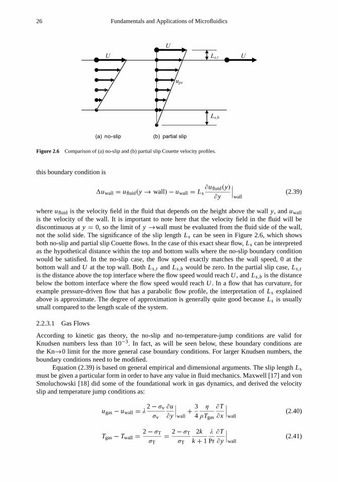
26 Fundamentals and Applications of Microfluidics
UU
U
(a) no-slip (b) partial slip
Ls,b
Ls,t
ups( )yuns( )y
ut
ub
Figure 2.6 Comparison of (a) no-slip and (b) partial slip Couette velocity profiles.
this boundary condition is
1uwall = ufluid(y → wall)− uwall = Ls∂ufluid(y)
∂y
∣∣∣wall
(2.39)
whereufluid is the velocity field in the fluid that depends on the height above the wally, anduwallis the velocity of the wall. It is important to note here that the velocity field in the fluid will bediscontinuous aty = 0, so the limit ofy →wall must be evaluated from the fluid side of the wall,not the solid side. The significance of the slip lengthLs can be seen in Figure 2.6, which showsboth no-slip and partial slip Couette flows. In the case of this exact shear flow,Ls can be interpretedas the hypothetical distance within the top and bottom walls where the no-slip boundary conditionwould be satisfied. In the no-slip case, the flow speed exactly matches the wall speed, 0 at thebottom wall andU at the top wall. BothLs,t andLs,b would be zero. In the partial slip case,Ls,t
is the distance above the top interface where the flow speed would reachU , andLs,b is the distancebelow the bottom interface where the flow speed would reachU . In a flow that has curvature, forexample pressure-driven flow that has a parabolic flow profile, the interpretation ofLs explainedabove is approximate. The degree of approximation is generally quite good becauseLs is usuallysmall compared to the length scale of the system.
2.2.3.1 Gas Flows
According to kinetic gas theory, the no-slip and no-temperature-jump conditions are valid forKnudsen numbers less than 10−3. In fact, as will be seen below, these boundary conditions arethe Kn→0 limit for the more general case boundary conditions. For larger Knudsen numbers, theboundary conditions need to be modified.
Equation (2.39) is based on general empirical and dimensional arguments. The slip lengthLsmust be given a particular form in order to have any value in fluid mechanics. Maxwell [17] and vonSmoluchowski [18] did some of the foundational work in gas dynamics, and derived the velocityslip and temperature jump conditions as:
ugas− uwall = λ2 − σv
σv
∂u
∂y
∣∣∣wall
+3
4
η
ρTgas
∂T
∂x
∣∣∣wall
(2.40)
Tgas− Twall =2 − σT
σT=
2 − σT
σT
2k
k + 1
λ
Pr
∂T
∂y
∣∣∣wall
(2.41)

Fluid Mechanics Theory 27
Table 2.4
Tangential Momentum and Thermal Accommodation Coefficients
for Various Gases Flowing Through Channels of Various Materials [19, 20]
Gas Metal σv σT
Air Aluminum 0.87–0.97 0.87–0.97Air Iron 0.87–0.96 0.87–0.93Air Bronze 0.88–0.95 n/aAr Silicon 0.80–0.90 n/aN2 Silicon 0.80–0.85 n/a
where σv and σT are the tangential momentum and temperature accommodation coefficients,respectively, and Pr is the Prandtl number. The accommodation coefficients are defined accordingto:
σv =τi − τr
τi − τwand σT =
dEi − dEr
dEi − dEw(2.42)
whereτi andτr are the tangential momentum of the incoming and reflected molecules andτw isthe tangential momentum of reemitted molecules, that is those that may have been adsorbed to thesurface, and is equal to zero for stationary walls. Similarly forσT, dEi and dEr are the energyfluxes of incoming and reflected molecules per unit time, respectively, and dEw is the energy fluxof reemitted molecules corresponding to the surface temperatureTwall. The Prandtl number is givenby:
Pr =cpη
κ(2.43)
wherecp is the specific heat at constant pressure,η is the viscosity, andκ is the thermal conductivity.The first term on the right-hand side of both (2.40) and (2.41) has the expected form insofar as
wall-normal gradients in the velocity and temperature field result in velocity and temperature jumpsat the wall. The second term on the right-hand side of (2.40) is somewhat unexpected. If the gas in achannel is stationary with no imposed external forces, but there is a temperature gradient along thewall, the gas at the wall will experience a slip velocity in the direction of the temperature gradient,that is, toward the higher temperature end of the channel. This phenomenon is calledthermal creep,and when used to move gases from one reservoir to another is called aKnudsen pump. For low speedflows or large temperature changes, the effect of thermal creep can be significant.
The accommodation coefficients have physical interpretations that make their significanceapparent. Whenσv = 0, the tangential momentum of all incident molecules equals that of thereflected molecules. Hence, the gas collisions impart no momentum to the wall. Effectively, theflow can be considered inviscid forσv = 0. This mode of molecular reflection is calledspecularreflection. Whenσv = 1, the net reflected tangential momentum is equal to zero. Hence, the gasmolecules impart all of their tangential momentum to the wall.
This mode of reflection is calleddiffuse reflection. For the case of perfect energy exchangebetween the wall and the gas,σT = 1. Table 2.4 gives the accommodation coefficients for air flowingthrough some common metals. These values are meant to be representational only. In general, theseaccommodation coefficients will depend on the temperature, pressure, and velocity of the flow, aswell as the surface finish and surface roughness of the material. Accommodation coefficients aslow as 0.2 have been observed. The only recent (i.e., MEMS-era) measurements of accommodationcoefficients are those of Arkilic [20].
In order to assess relative size of the terms that contribute to the slip velocity and temperaturejump, it is necessary to nondimensionalize (2.40) and (2.41), using a characteristic velocityu0

28 Fundamentals and Applications of Microfluidics
and temperatureT0 (see Section 2.2.5 for more details about nondimensionalization). The resultingboundary conditions are:
u∗gas− u∗
wall = Kn2 − σv
σv
∂u∗
∂y∗
∣∣∣wall
+3
2π
k − 1
k
Kn2Re
Ec
∂T∗
∂x∗
∣∣∣wall
(2.44)
= Kn2 − σv
σv
∂u∗
∂y∗
∣∣∣wall
+3
4
1T
T0
1
Re
∂T∗
∂x∗
∣∣∣wall
(2.45)
T∗gas− T∗
wall =2 − σT
σT
2k
k + 1
Kn
Pr
∂T∗
∂y∗
∣∣∣wall
(2.46)
where the superscript * denotes dimensionless quantities. The quantity Ec is the Eckert numbergiven by:
Ec =u2
0
cp1T= (k − 1)
T0
1TMa2 (2.47)
where1T = Tgas − T0. The first version of (2.45) shows that thermal creep should becomesignificant at larger Knudsen numbers, while the second version shows that thermal creep willbe more prevalent for slower flows (smaller Reynolds number) or when the relative temperaturegradient is large.
These boundary conditions are all the boundary conditions that are needed to cover theentire range for which the Navier-Stokes equations are valid. The boundary conditions in (2.45)and (2.46) are applicable for any Knudsen number less than 0.1. Of course, when the Knudsennumber is smaller than 0.001, these equations will degenerate to the no-slip and no-temperature-jump conditions.
2.2.3.2 Liquid Flows
For most microscale liquid flows, the no-slip and no-temperature-jump conditions will hold. Inequation form, this is:
uwall = uliquid
∣∣∣wall
Twall = Tliquid
∣∣∣wall
(2.48)
whereuwall is the speed of the wall, anduliquid is the speed of the liquid in contact with the wall. Asimilar interpretation holds for the temperature field. These boundary conditions are just the largelength scale (when measured in molecular diameters) approximations of the linear Navier boundarycondition introduced in Section 2.2.3.1:
1uwall = ufluid(y → wall)− uwall = LS∂ufluid(y)
∂y
∣∣∣wall
(2.49)
in which the velocity slip at the wall1uwall is approximately zero, due to the low shear rates foundin most microdevices and the relatively large length scale. The slip lengthLS is a constant for anyliquid-solid pairing but can vary significantly for different pairs of liquids and solids. Determiningthis slip length is difficult and must be done through experiments or molecular dynamics simulations.Presently, there is little data available of this type. One such source of data is the molecular dynamicssimulations of Thompson and Troian [21], in which they simulated the motion of a liquid comprisedof simple molecules between atomically flat plates comprised of simple atoms in a (111) plane ofa face-centered cubic arrangement. One of the plates was moved at a constant velocity relative tothe other—a typical Couette arrangement—in which the shear rate could be defined and controlledwell. When the spacing between the atoms comprising the wall was commensurate with the mean

Fluid Mechanics Theory 29
Table 2.5
Slip Length Properties from Thompson and Troian’s Data [21]. The characteristic energy scaleεw f and length scaleσw f of
the Lennard-Jones potential between wall atoms and the fluid molecules are given in terms of the fluid’s properties, as is the
density of the wall materialρw . The constant slip length at low shear rates isL0S, while the critical shear rate isγc.
εw f σw f ρw L0S/σ γcτ
0.6 1.0 1 0.0 n/a0.1 1.0 1 1.9 0.360.6 0.75 4 4.5 0.140.4 0.75 4 8.2 0.100.2 0.75 4 16.8 0.06
molecular spacing in the fluid, the slip length was found to be zero (i.e., the no-slip condition governsthe flow when the liquid and solid are matched in molecular spacing). However, when the latticespacing of the solid was four times the mean molecular spacing of the liquid, the slip length hadincreased to 16.8 times the mean molecular spacing in the liquid. These results are expected to begeneral for any choice of simple fluids and simple solids in the (111) plane of a face-centered cubicarrangement. Unfortunately, water is not such a simple liquid, and therefore these results should beused with caution when considering water as the liquid.
The most important conclusion of Thompson and Troian’s [21] work is that the linear Navierboundary condition, which should be independent of the velocity field and hence the shear rate, doesbreak down at large shear rates. In fact, the breakdown is quite catastrophic. They observed the sliplength to change at large values of the shear rate according to the relation:
LS = L0S
(1 −
γ
γc
)−12
(2.50)
whereLS is the slip length as a function of the shear rateγ , the shear rate at which the slip lengthbreaks downγc, andL0
S is the constant slip length found at low values of the shear rate. Anotherimportant conclusion is that this breakdown of the Navier boundary condition happens well belowthe breakdown of Newtonian behavior in the bulk of the fluid—see Section 2.2.2.1—atγc ≥ 2/τ .The last row of Table 2.5 shows that the critical shear rate occurs at approximately 3% of the valueof the breakdown of the Newtonian assumption (0.06/2 = 0.03). Significant deviations from theNavier boundary condition occur at an order of magnitude lower than the critical shear rate, wherethe slip length has already increased by 5% when compared with the low shear rate value of the sliplength. Deviations from the Navier boundary condition are significant at a shear rate that measures0.3% of that at which breakdown of Newtonian behavior occurs. In terms of the example used aboveto illustrate when to expect a breakdown of Newtonian behavior, if liquid argon (properties givenabove) is contained between two parallel plates separated by 1µm, one of the plates fixed and onemoving at a constant speed, the plate would have to be moving at 3,000 m/s—still a high speed, butone which could potentially be encountered in actual microflows.
Another exception to the Navier boundary condition is moving contact lines that require arelaxation of the no-slip assumption in order to avoid unbounded shear stresses at the point where asolid, liquid, and gas all meet. Since a liquid will “pull” itself into and through a hydrophilic channel,the point at which the solid, liquid, and gas meet must move along the wall of the channel, violatingthe no-slip assumption. The solution to this problem lies in the molecular reordering very near thepoint where the three phases come together, and thus is an example of effects at the molecular levelcausing macroscopic effects. This phenomenon will be discussed further in Section 2.2.7.

30 Fundamentals and Applications of Microfluidics
x, u1
y, u2
z, u3
Figure 2.7 Parallel flow geometry through a channel of an arbitrary cross section.
2.2.4 Parallel Flows
Many microdevices have long straight passages of constant cross sections in them. Flow throughsuch channels is thus an important flow phenomenon at small length scales. In addition, many ofthese long straight passages have cross-sectional geometries that are considerably different fromthe usual macroscopic circular pipe. As a simplification, let us consider an isothermal flow of anincompressible, isotropic, Newtonian liquid through a long channel of a constant arbitrary crosssection, as shown in Figure 2.7. Also consider that the body force is absent. Because this is a liquidflow, we will take the boundary conditions to be no-slip at the wall in the direction parallel to theflow (x) and no penetration through the wall in the directions normal to the flow(y, z).
For laminar flows in parallel geometries, the flow is purely axial—only theu1 component isnonzero—andu1 is a function ofy andz only. Under these assumptions, (2.34) and (2.35) simplifyto:
0 = −∂p
∂x+ η
(∂2u1
∂y2+∂2u1
∂z2
)(2.51)
0 =∂p
∂y=∂p
∂z(2.52)
Equation (2.52) indicates that the pressure is strictly a function ofx; that is, it is independent ofyandz. Since the pressure is strictly a function ofx and (2.51) requires that its derivative equal afunction of y andz only, notx, must be a constant. Further, it stands to reason that the flow must bein the direction of decreasing pressure, so∂p/∂x must be a negative constant.
2.2.4.1 Analytical Solutions
To proceed to a solution, we need only fix the geometry of the cross section. Solutions for severalcommon shapes (and many unusual ones) are available from Berker [22] and Shah and London [23].The details of the solutions presented here are left to the reader. The isosceles triangle is includedin the solutions presented here because an anisotropic wet etch in single crystal (100) silicon, ifallowed to self-terminate, will form an isosceles triangle cross section.
Circular cross section:
u1 =−dp/dx
4η(r 2
0 − r 2) (2.53)
Q =πr 4
0
8η
(dp
dx
)(2.54)
Rectangular cross section:
u1(y, z) =16a2
ηπ3
(−
dp
dx
) ∞∑i =1,3,5...
(−1)(i −1)/2[1 −
cosh(iπz/2a)
cosh(iπb/2a)
]cos(iπy/2a)
i 3(2.55)
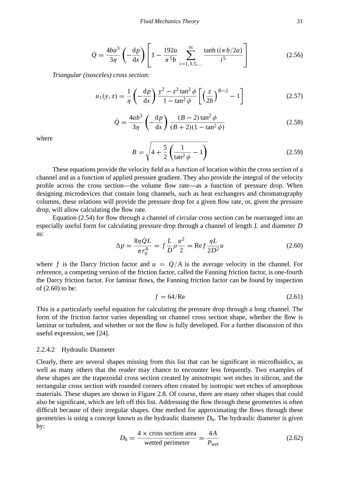
Fluid Mechanics Theory 31
Q =4ba3
3η
(−
dp
dx
) 1 −192a
π5b
∞∑i =1,3,5,...
tanh(iπb/2a)
i 5
(2.56)
Triangular (isosceles) cross section:
u1(y, z) =1
η
(−
dp
dx
)y2
− z2 tan2 φ
1 − tan2 φ
[( z
2b
)B−2− 1
](2.57)
Q =4ab3
3η
(−
dp
dx
)(B − 2) tan2 φ
(B + 2)(1 − tan2 φ)(2.58)
where
B =
√4 +
5
2
(1
tan2 φ− 1
)(2.59)
These equations provide the velocity field as a function of location within the cross section of achannel and as a function of applied pressure gradient. They also provide the integral of the velocityprofile across the cross section—the volume flow rate—as a function of pressure drop. Whendesigning microdevices that contain long channels, such as heat exchangers and chromatographycolumns, these relations will provide the pressure drop for a given flow rate, or, given the pressuredrop, will allow calculating the flow rate.
Equation (2.54) for flow through a channel of circular cross section can be rearranged into anespecially useful form for calculating pressure drop through a channel of lengthL and diameterDas:
1p =8ηQL
πr 40
= fL
Dρ
u2
2= Ref
ηL
2D2u (2.60)
where f is the Darcy friction factor andu = Q/A is the average velocity in the channel. Forreference, a competing version of the friction factor, called the Fanning friction factor, is one-fourththe Darcy friction factor. For laminar flows, the Fanning friction factor can be found by inspectionof (2.60) to be:
f = 64/Re (2.61)
This is a particularly useful equation for calculating the pressure drop through a long channel. Theform of the friction factor varies depending on channel cross section shape, whether the flow islaminar or turbulent, and whether or not the flow is fully developed. For a further discussion of thisuseful expression, see [24].
2.2.4.2 Hydraulic Diameter
Clearly, there are several shapes missing from this list that can be significant in microfluidics, aswell as many others that the reader may chance to encounter less frequently. Two examples ofthese shapes are the trapezoidal cross section created by anisotropic wet etches in silicon, and therectangular cross section with rounded corners often created by isotropic wet etches of amorphousmaterials. These shapes are shown in Figure 2.8. Of course, there are many other shapes that couldalso be significant, which are left off this list. Addressing the flow through these geometries is oftendifficult because of their irregular shapes. One method for approximating the flows through thesegeometries is using a concept known as the hydraulic diameterDh. The hydraulic diameter is givenby:
Dh =4 × cross section area
wetted perimeter=
4A
Pwet(2.62)

32 Fundamentals and Applications of Microfluidics
a
2a
2b2�
y
b
y
z
z
r0
Figure 2.8 Channel cross sections with practical applications in microsystems. (After: [13].)
Figure 2.9 Common channel shapes produced by microfabrication.
The concept of the hydraulic diameter can be used to assess flows through both completely filledchannels, as well as those that are only partially filled. The termwetted perimeterrefers to theperimeter of the channel that is in direct contact with the flow, while the area refers to the areathrough which the flow is occurring. For channels that are completely filled, the wetted perimeter issimply the perimeter of the channel and the area is the cross sectional area of the channel.
The utility of the hydraulic diameter can be demonstrated by considering the example of flowthrough a passage of circular cross section. In that case,
Dh =4 ×
π4 × d2
πd= d (2.63)
so the hydraulic diameter reduces to simply the diameter of the passage.
Example 2.2: Hydraulic Diameter
Calculate the hydraulic diameter for the shapes in Figure 2.9, assuming the shapes to exhibitleft-right reflection symmetry.
Trapezoid:
Area=h
2(a + b)
Wetted perimeter= a + b + 2
√h2 +
(a − b
2
)2
= a + b + 2h
√1 +
(a − b
2h
)2
Dh =4
[h2(a + b)
]a + b + 2h
√1 +
(a−b2h
)2=
2h
1 +2h
a+b
√1 +
(a−b2h
)2
Fluid Mechanics Theory 33
Rounded rectangle:
Area= ah +1
2πh2
Wetted perimeter= 2a + πh + 2h
Dh =
4(ah +
12πh2
)2a + πh + 2h
= 2hah +
π2
ah +
π2 + 1
Once these hydraulic diameters are known, they may be used in the expressions for flow through acircular cross section [(2.54) or (2.60)] to estimate the volume flow rate as a function of pressuregradient or conversely to estimate the expected pressure drop for a given volume flow rate.
2.2.4.3 Transition to Turbulence in Microchannels
For flows in long straight channels of constant cross section as discussed above, the Reynoldsnumber remains a good predictor of when turbulence will occur (see Section 2.2.5 for furtherexplanation of the Reynolds number), even at microscopic length scales. The Reynolds numberis given by:
Re=ρDhu
η=
Dhu
ν(2.64)
whereDh is the hydraulic diameter (as discussed above),u is some measure of the characteristicvelocity in the channel,r is the density of the fluid,η is the dynamic viscosity of the fluid, andν isthe kinematic viscosity of the fluid. In channels of circular cross section [24] as well as rectangularcross section [25], recent experiments have demonstrated no significant deviation of the transitionalReynolds number—the Reynolds number below which the flow is laminar and above which theflow is turbulent—from that typically encountered at macroscopic length scales. The transitionalReynolds number has been found to be in the range of 1,500 to 2,500. Figure 2.10 shows fullydeveloped velocity profiles for five different Reynolds numbers ranging from 238 to 2,770. Thescatter between the velocity profiles at the lower Reynolds numbers is fairly small, while the fifthprofile is considerably wider and blunter—indicating that the transition to turbulent flow has begunsomewhere between Reynolds numbers of 1,980 and 2,770. The particular Reynolds number atwhich transition will occur is a function of many parameters, such as the channel shape, aspectratio, and surface roughness, but is expected to be in the range of 1,000 to 2,000 for most situations.This conclusion is at odds with some other researchers’ findings [26, 27] in which the transitionalReynolds number has been reported to be as low as several hundred. However, those findings werelargely based on global pressure drop measurements and not confirmed with a close inspection ofthe velocity profile as a function of Reynolds number. Sharp [24] provides an excellent discussionof this topic.
2.2.5 Low Reynolds Number Flows
A great many microfluidic devices operate in regimes where the flow moves slowly—at least bymacroscopic standards. Biomedical microdevices are a good example where samples are carriedfrom one reaction chamber or sensor to the next by a flowing fluid that may be driven by an externalsyringe pump. To determine whether a flow is slow relative to its length scale, we need to scale theoriginal dimensional variables to determine their relative size. Consider a flow in some geometry

34 Fundamentals and Applications of Microfluidics
Re=2,770
Re=238
Re=1,700
Re=1,980
Re=970
0
X/D
0.1 0.2 0.3 0.4 0.5-0.1-0.2-0.3-0.4-0.5
1
0.9
0.8
0.7
0.6
0.5
0.4
0.3
0.2
0.1
U
Umax
Figure 2.10 Fully developed velocity profiles for flow through a channel with rectangular cross section (Dh = 327 mm).The highest Reynolds number exhibits the broadened profile characteristic of turbulent flow while the others agree to theparabolic profile within experimental uncertainty.
whose characteristic size is represented byD and average velocityu. We can scale the spatialcoordinates withD and the velocity field withu according to the relations:
x∗
i =xi
Dand u∗
i =ui
u(2.65)
with the inverse scaling:xi = Dx∗
i and ui = uu∗
i (2.66)
The starred quantities are then dimensionless quantities whose size varies from zero to order one.These inverse scalings can be substituted into the dimensional forms of the governing equationsgiven in (2.34) and (2.35) to arrive at a dimensionless set of governing equations. Assuming anisothermal flow of a Newtonian, isotropic fluid, the conservation of mass and momentum equationscan be simplified to:
∂u∗
i
∂x∗
i= 0 (2.67)
ρuD
η
D
u
∂u∗
i
∂t+ρuD
ηu∗
j∂u∗
i
∂x∗
j=ρD2
uηFi −
D
uη
∂p
∂x∗
i+∂2u∗
i
∂x∗2j
(2.68)
This transformation is incomplete because some of the variables in (2.68) are dimensionless whileothers remain in dimensional form. Considering the constants that multiply each term of (2.68), thefollowing scalings suggest themselves:
t∗ =t
D/uand p∗
=p
ηu/D(2.69)
Upon substituting these expressions into (2.68), the following convenient, dimensionless versions ofthe governing equations emerge:
∂u∗
i
∂x∗
i= 0 (2.70)
Fluid Mechanics Theory 35
Re(∂u∗
i
∂t∗+ u∗
j∂u∗
i
∂x∗
j−
Fi D
u2
)= −
∂p∗
∂x∗
i+∂2u∗
i
∂x∗2j
(2.71)
in which all of the variables (ui , xi , t , p) appear in dimensionless form, all of the terms aredimensionless, and the Reynolds number emerges as a key parameter. When the body forceFi
is gravity, the group of parametersFi D/u2 is the inverse of the Froude number [2]. Because ofthe nondimensionalization process, each of the groups of variables, such as∂u∗
i /∂t∗, ∂p∗/∂x∗
i , or∂u∗
i /∂t∗, has a size of order one, while the groups of parameters, namely the Reynolds number andFi D/u2, have a size determined by flow parameters. If the Reynolds number is very small, Re� 1,the entire left side of (2.71) becomes negligible, leaving only:
∂u∗
i
∂x∗
i= 0 (2.72)
0 = −∂p∗
∂x∗
i+∂2u∗
i
∂x∗2j
(2.73)
as the governing equations. Although this equation requires Re� 1 to be true, the agreement withexperiments is usually acceptable up to Re∼ 1. The momentum equation assumes the form of thePoisson equation.
Observations About (2.72) and (2.73):
• The equation islinear and thus relatively easy to solve. Tabulated solutions for many commongeometries are available in standard fluid mechanics texts [3, 4].
• If the pressure gradient is increased by some constant factor A, the entire flow field is increasedby the same factor; that is, the velocity at every point in the flow is multiplied by A. The shape(streamlines) of the flow does not change. Thus, an experiment done atoneReynolds numberis valid for predicting all low Reynolds number behaviors of a system.
• Time does not appear explicitly in the equation. Consequently, low Reynolds number flows arecompletely reversible (except for diffusion effects that are not included in the equation). Sincemany microsystems contain periodically moving boundaries such as membranes, any motionthe membrane imparts to the fluid in the first half of the membrane’s period will be exactlyreversed in the second half of the period, and sum to zero net motion.
Example 2.3: Low Reynolds Number Systems
To get an idea of what kind of systems might exhibit low Reynolds behavior, it is useful toperform a sample calculation. A typical biomedical microdevice might exhibit the followingbehavior:
Fluid properties similar to water: η = 10−3 kg/(s m),ρ = 103 kg/m3
Length scale: 10µm = 10−5 mVelocity scale: 1 mm/s= 10−3 m/sThen: Re= 10−2
Clearly low Reynolds number behavior.
As another example, consider the flow in a microchannel heat exchanger:Fluid properties similar to water: µ = 10−3 kg/(s m),ρ = 103 kg/m3
Length scale: 100µm = 10−4mVelocity scale: 10 m/sThen: Re= 103
Clearlynot low Reynolds number behavior—borderline turbulent behavior.

36 Fundamentals and Applications of Microfluidics
2.2.6 Entrance Effects
Sometimes the differences between microscale flows and larger flows are due to changes infundamental physics, such as working at size scales where the length at the wall becomes importantor there is a large electrical field, and sometimes they are due to more practical differences. A greatmany of the fabrication processes that are used to produce small-scale systems (see Chapter 3) areplanar techniques in which some pattern having anx and y dependence is effectively extruded inthez direction to produce a three-dimensional geometry. Since the geometry through which the flowis happening is independent of thez position, it might be tempting to consider the flow to be two-dimensional. However, the aspect ratio (ratio between the height of channels and the lateral featuresize) is usually near 1, meaning that the flow must definitely be considered three-dimensional.
One example where this situation can be important is in considering the entrance length effect.When a fluid flows from a large vessel or reservoir into a smaller one of a constant cross section (acommon situation in both large- and small-scale fluid mechanics), the flow profile requires a certaindistance along the flow direction to develop or adjust to the presence of the walls of the channel.Beyond the entrance length, the flow is considered fully developed and the velocity profile does notchange any further. The point at which flow adjusts to the presence of the walls most slowly is atits furthest distance from the walls—its centerline. Intuition leads us to expect that the centerlinevelocity in a very long pipe would initially rapidly approach its fully developed value, and thatfarther and farther downstream, the centerline velocity would continue to increase, albeit ever moreslowly. Consequently, an arbitrary standard needs to be set beyond which the flow is consideredclose enough to fully developed to be considered fully developed. Shah and London [23] definethe entrance lengthLe as the point where the developing centerline velocity is equal to 0.99 timesits fully developed value. A large-scale example of such a flow would be the flow out of a largereservoir through a pipe. A corresponding small-scale flow might be the flow in a microchannelheat exchanger where the flow proceeds from a plenum (or large chamber) into the microchannel.This type of geometry is most often made by a planar microfabrication technique, so that while theplenum may be large compared to the microchannel, they are both the same height. Figure 2.11depicts this situation.
As a consequence of the plenum and the microchannel having the same height in the planarmicrofabricated geometry, the flow in the plenum is uniform in the direction parallel to the topand bottom walls, but parabolic in the direction normal to the top and bottom walls, whereas inthe macroscopic reservoir, the flow in the reservoir is everywhere uniform. The implication is thatsince the flow is already partially developed in the microscopic case, the entrance length should bedecreased in the planar geometry when compared to the macroscopic situation.
For macroscopic flows where the Reynolds number is usually assumed to be relatively high,the entrance lengthLe can be accurately predicted by:
Le
Dh≈ 0.06ReDh (2.74)
where Dh is the hydraulic diameter and ReDh is the Reynolds number based on the hydraulicdiameter [2]. Since the Reynolds number scales with the length scale of a system, small-scalesystems often exhibit low Reynolds number behavior. As the Reynolds number tends towards zero,the entrance length predicted by (2.74) also tends towards zero, in disagreement with low Reynoldsnumber experiments. A better expression for low Reynolds numbers is given by:
Le
Dh≈
0.6
1 + 0.035ReDh
+ 0.056ReDh (2.75)
according to Shah and London [23]. This expression predicts that even in the limit of the Reynoldsnumber approaching zero, the entrance length is approximately 0.6 hydraulic diameters long.

Fluid Mechanics Theory 37
Fully Developed
Vertical Velocity Profile
Uniform HorizontalVelocity Profile
Uniform Vertical
Velocity Profile
Uniform Horizontal
Velocity Profile
Channel Entrance Assumed for Fluid Dynamics Theory
Typical Microchannel Entrance
Figure 2.11 (a) Typical macroscopic entrance geometry versus (b) microscopic entrance geometry as a consequence ofplanar microfabrication.
Using (2.75) to predict the entrance length provides more reasonable results at low Reynoldsnumbers. However, the problem of the different macroscopic and microscopic geometries still re-mains. Developing a better expression for entrance length in planar geometries will require many setsof spatially resolved measurements at various Reynolds numbers. Preliminary experiments demon-strating that there is a difference in the entrance length have been conducted in the microfluidicslaboratory at Purdue University [25]. Using the microparticle image velocimetry (µPIV) techniqueexplained further in Chapter 4, velocity profiles were measured in a rectangular channel (hydraulicdiameter of 327µm) being fed by a planar plenum of the same height (600µm). For a Reynoldsnumber of 1,980, the differences between the experimentally observed entrance length and thatpredicted by (2.75) are quite obvious. Figure 2.12 demonstrates this developing behavior and clearlyshows that the flow develops in approximately one-half the distance predicted by (2.75). Given thatthe convective heat transfer behavior in the developing region differs from that in the fully developedregion, and given that many microchannel heat exchangers are shorter than the entrance length of theflow, this change in the entrance length could prove significant in many cases. The shear stress at thewall in the developing region is less than that in the fully developed region, which has implicationsfor biomedical microdevices.
2.2.7 Surface Tension
Consider again the Lennard-Jones potential represented by (2.1) and shown in Figure 2.2. TheLennard-Jones potential models accurately the interaction between any two simple molecules. Asdiscussed in Section 2.1.2, molecules of a liquid have a mean spacing, such that they vibrate aroundthe zero crossing location of the force versus distance plot in Figure 2.2. The behavior of a liquidmolecule is independent of its location within the liquid as long as that location is far from anyinterfaces when measured in molecular units. Consider the oscillation of a liquid molecule thatis exactly on the interface between a liquid and a gas. As it vibrates away from its equilibriumposition toward the gas phase, it experiences the attractive van der Waals forces (ther −6 term in theLJ potential) of all of its neighboring liquid molecules. Recall that gas molecules interact through

38 Fundamentals and Applications of Microfluidics
0 2 4 6 8 10
x 104
4
5
6
7
8
9
10
y (�m)
umax
(m/s)
y = 13,878(�m)
Figure 2.12 Development of flow entering rectangular channel. The flow becomes fully developed 1.4 cm downstreamfrom the entrance, whereas (2.75) predicts 3.6 cm—a significant deviation. The square boxes are data points and the solidcurve is an exponential curve fit.
infrequent energetic collisions and are not in a state of continual interaction with their neighbors, asare liquids. Consequently, the gas will not exert any attractive force on the liquid molecule that wouldtend to pull it free from the bulk of the liquid. Hence, the molecule will experience a net attractiveforcetoward the bulk of the fluid. This behavior is generally the case at liquid-gas interfaces.
The liquid-solid interface behavior is more difficult to predict because the molecules of theliquid on the interface are continually interacting with liquid molecules in one half-space and solidmolecules in the other. Whether the liquid molecules on the interface are more attracted to the solidmolecules on the other side of the interface or the liquid molecules on their side of the interfacedepends on the particular form of the Lennard-Jones potential for liquid-liquid interactions versusthat for liquid-solid interactions. When all three phases come together at a line, the phenomenon iscalled acontact line.
Surface tension has vexed microsystem designers since they began building devices that aremeant to be filled with liquid, as well as devices that are manufactured using liquid-based processing.For example, removing a sacrificial silicon dioxide layer from under a layer of silicon (see Section3.2) should be a simple wet etch. However, once the etch is complete, the area where the sacrificiallayer used to be is filled with a liquid. The surface tension of the liquid makes it difficult to remove. Itmay even break the silicon surface because of the high pressures that can be generated by interfaceswith small radii of curvature. Clearly, it is worthwhile to know more about this phenomenon.
Figure 2.13 shows a typical contact line phenomenon where a solid, liquid, and gas all meetalong a line of contact. Because the solid is rigid, the contact line can only move left or right alongthe surface. It cannot be displaced in a vertical direction. Hence, the energy balance must be:
σsl + σlg cosθ = σsg (2.76)
whereθ is called the contact angle. When the contact angle is smaller than 90◦ (as shown in thefigure), the liquid is said towet the surface. When the contact angle is greater than 90◦, the liquid issaid to benonwetting. A surface that a liquid can wet is said to behydrophilic, and a surface that a

Fluid Mechanics Theory 39
Liquid
Gas
Solid
� �sg
�lg
�sl
Figure 2.13 Typical contact line arrangement. The contact angle is labeledθ , and the interfacial tensionsσsl, σlg, andσsgare the solid–liquid, liquid–gas, and solid–gas, respectively.
liquid cannot wet is said to behydrophobic. Because of the tension along the interfaces, there willbe a net increase or decrease in pressure upon crossing a curved interface. This pressure change1pis given by:
1p = σ
(1
R1+
1
R2
)(2.77)
whereR1 andR2 are the two radii of curvature of the interface surface [5].The most commonly used liquid in microflows is water. The surface tension of water is
predicted well by:σlg = (0.076− 0.00017T · K−1) N/m (2.78)
whereT is the temperature of the system. This expression is accurate to within 1% of tabulatedvalues over the range of 0◦C to 374◦C [3]. The surface tension of a liquid depends strongly onthe presence of contaminants such as surfactants or dirt. These contaminants can greatly changethe observed surface tension. The contact angle of water on glass is approximately 0◦. For furtherinformation about surface tension, including tables of surface energies for many liquids, please see[28].
Equations (2.76) and (2.77) can be combined to solve simple but important contact lineproblems. First, consider the case of a glass capillary of diameter 2r0 inserted vertically into areservoir of water, as in Figure 2.14. The water climbs up the inside of the capillary to someequilibrium heighth that is given by:
ρgh = 1p =2σlg cosθ
r0(2.79)
where the hydrostatic pressureρgh is equated to that encountered by crossing the air-water interface.The tendency of liquids to draw themselves into small channels comprised of materials that they wetis known ascapillarity. Capillarity makes it difficult to fill hydrophobic channels and difficult toempty hydrophilic channels.
2.3 MOLECULAR APPROACHES
As we saw in Section 2.2, the continuum assumption will fail for some range of parameters—for gas flows when the Knudsen number is larger than 0.1, and for liquid flows when the fluid issheared at a rate faster than twice the characteristic molecular interaction frequency (2/τ ). Whenthe continuum assumption fails, the continuum approach to modeling flows must also fail and anew means for modeling flows must be used. Two approaches have emerged in recent years basedon radically different methods—MD and DSMC. There have been several thorough explorationsof these techniques [6–8] to which the reader is directed for a thorough discussion of these issues.The next two sections will provide an introduction to these techniques. The reader is encouraged toconsult the works cited above for a more thorough coverage of these techniques.

40 Fundamentals and Applications of Microfluidics
h
2r0
�
gas
liquid
Figure 2.14 Capillarity of liquids filling small channels.
2.3.1 MD
The MD technique is in principle a straightforward application of Newton’s second law, in which theproduct of mass and acceleration for each molecule comprising the flow is equated to the forces onthe molecule that are computed according to a model—quite often the Lennard-Jones model. Koplikand Banavar [6] provide a thorough, accessible introduction to the technique, along with the latestresearch results in their recent review article. The technique begins with a collection of moleculesdistributed in space. Each molecule has a random velocity assigned to it, such that the distributionof velocities obeys a Boltzmann distribution corresponding to the temperature of the distribution.The molecular velocities are integrated forward in time to arrive at new molecular positions. Theintermolecular forces at the new time step are computed and used to evolve the particles forward intime again. As the user desires, the molecular positions and velocities can be sampled, averaged, andused to compute flow quantities, such as velocity, density, and viscosity. Although the algorithm isrelatively simple to explain, it is computationally intensive to implement because of the very shorttime steps needed for the integration and the extremely large number of molecules in even modestvolumes of space. Theoretically, MD can be used for any range of flow parameters from slow liquidflows to highly rarefied, hypersonic gas flows. However, the MD technique is used primarily forliquid flows because the molecules are in a continual collision state. MD is very inefficient for gasflows because collisions are infrequent. DSMC (see Section 2.3.2) is often used for gas flows.
2.3.1.1 Difficulties with MD Implementation
Even though the algorithm can be outlined in a single paragraph as above, the MD techniqueis quite complicated to implement. Chief among these complications is the sheer volume ofcalculations required to simulate a reasonably sized volume of space for a reasonable duration. Inthis instance, “reasonable” is used to mean large enough that continuum behavior can be observed.MD simulations typically consider volumes measuring 10 nm on a side—meaning approximately303
= 27,000 molecules. The characteristic molecular interaction time is 2.2 × 10⁻¹² secondsand perhaps a total of 10−9 seconds would be used for the entire simulation—just enough time forcontinuum behavior to set in.
A second problem is constructing a reasonable pairwise molecular interaction potential. Asdiscussed previously, the Lennard-Jones potential:
Vi j (r ) = 4ε
[ci j
( r
σ
)−12− di j
( r
σ
)−6]
(2.80)

Fluid Mechanics Theory 41
whereε and σ are characteristic energy and length scales, respectively, is widely used for thispurpose. The force between interacting molecules is given by the derivative of the potential as:
Fi j (r ) = −∂Vi j (r )
∂r=
48ε
σ
[ci j
( r
σ
)−13−
di j
2
( r
σ
)−7]
(2.81)
With an appropriate choice of the parametersci j and di j , this equation can represent the forcebetween any two simple molecules. With appropriate modifications, it can even represent the forcebetween more complicated molecules, like water, by considering two hydrogen atoms tethered to anoxygen atom through another potential. The characteristic time scale for molecular interactions, forwhich Lennard-Jones is a good model, is given by:
τ = σ
√m
ε(2.82)
which is the period of oscillation about the minimum in the Lennard-Jones potential. The Lennard-Jones potential has been shown to provide accurate results for liquid argon usingε/kB = 120 K,σ = 0.34 nm, andc = d = 1. For these parameters, the time scale isτ = 2.2 × 10⁻¹² seconds [6].
The Lennard-Jones potential (and the resulting force) has the inconvenient property of neverquite reaching zero, even for large distances. Consequently, every molecule in a flow will exert aforce on every other molecule. If there areN molecules in a flow, then there areN factorial possiblepairwise interactions between molecules. The number of possible interactions scales approximatelywith N2. One solution to this problem is to shift the potential by a function linear inr , such thatthe force at some cutoff distancerc is zero. Beyond that cutoff distance, the force is set to zeroidentically. One such modified Lennard-Jones force is:
Fi j ,TRUNC(r ) =
{ Fi j (r )− Fi j (rc) r < rc0 r > rc
(2.83)
The potential is modified similarly but instead of being shifted by a constant value, it isshifted by an amount linear inr . These modified potentials are plotted in Figure 2.15 along withthe difference between the modified and original Lennard-Jones expressions. The differences aremultiplied by 100 to make them apparent. In the dimensionless units of the figure, the Lennard-Jones force is shifted upward by a constant amount, approximately 2% of the maximum attractiveforce. Once the form of the pairwise potential is decided, the state (position and velocity) of all themolecules is evolved forward in time according Newton’s second law in the form:
mid2r i
dt= −
∂
∂r i
∑i = j
Vi j (|r i − r j |) (2.84)
where the mass of thei th molecule is given bymi and its vector position isr i . Any suitable finitedifference method may be used for this evolution. Macroscopic flow quantities are calculated byaverages over small volumes of space. For instance, the vector velocityu(x) in some neighborhoodB would be calculated by:
u(x) =1
N
⟨ ∑xi ∈B
dxi
dt
⟩(2.85)
whereN is the number of molecules in the neighborhood andxi is their position.Molecular dynamics has been used to investigate a great many flows, such as the investigation
into the Navier boundary condition described in Section 2.2.3.2. In practice, it is a great deal moredifficult than described in this brief introduction. The reader is referred to Koplik and Banavar’s [6]review article on the subject for a more thorough discussion, as well as a description of significantresults achieved by the technique.

42 Fundamentals and Applications of Microfluidics
1 1.2 1.4 1.6 1.8 2
-0.2
-0.1
0.0
0.1
0.2
0.3
Separation Distance r / �
Dimensionless
Potential: V(r) / 4 �
Force: F(r)�/48�
�V(r)�100
�F(r) �100
Figure 2.15 Difference between truncated and untruncated Lennard-Jones potential and force.
2.3.2 DSMC Technique
The DSMC technique was developed by Bird [29] nearly 30 years ago, and has been used success-fully by many researchers for computing gas flows. Several comprehensive review articles concern-ing the technique are available [7, 30, 31]. In Section 2.2, we saw that for Knudsen numbers largerthan 0.1, the continuum assumption will fail. Necessarily, the analytical techniques based on thecontinuum assumption will also fail for Kn> 0.1. For flows with higher Knudsen numbers, there areseveral alternatives for obtaining solutions. One is the Burnett equation [32], a continuum approachthat uses a higher order stress-strain rate model and is applicable to higher Knudsen numbers thanthe Navier-Stokes equation. Unfortunately, the Burnett equation is unwieldy and difficult to solve.Solutions are generally reached computationally.
Another approach that has been used successfully is the DSMC technique, which is a sim-ulation technique based on kinetic theory. DSMC tracks the motion of hundreds of thousands ormillions of “particles,” each of which represents a large number of molecules. DSMC uncouplesmolecular motions from intermolecular collisions. The molecular motions are treated deterministi-cally, while the collisions are treated statistically. DSMC is a very efficient method (compared to itscompetitors) to compute flows in the transitional flow regime, 0.1< Kn < 10, although technicallyit can be used in any dilute gas flow,δ/d > 10—see (2.17). This means that there is an overlapwhere both the Navier-Stokes equations can be used (Kn< 0.1) and where the DSMC techniquecan be used (δ/d > 10) to solve the same problem.
2.3.2.1 Overview of the DSMC Procedure
DSMC consists of four main steps [30, 31], which are repeated at each time step of the simulation.These are:
• Moving the particles;
• Indexing and cross-referencing the particles;
• Simulating particle collisions;
• Sampling macroscopic properties of the flow.

Fluid Mechanics Theory 43
These steps will be discussed in greater detail below.The first step in DSMC consists of evolving the position of all the particles forward in time
according to their velocity at the beginning of the time step. The length of the time step is chosento be smaller than the mean collision time1tc, which is the ratio of the mean free pathλ to therms molecular speedc. When1tc is calculated, it is usually found to be on the order of 10−10
seconds for most flows. Once the particles are advanced in space, some of them will have left thecomputational domain through inlets and exits, and some will be inside the boundaries of the flow.Hence, the boundary conditions must be applied at this point. Particles that are found to be insidewalls will be subjected to wall collisions according to the appropriate boundary conditions (2.42).
The second process is indexing and tracking the particles. For more efficient computations,the volume of the flow being simulated is divided into cells, each of which measures approximatelyone-third of the mean free path of the gas. During the first step, particles may leave one cell andenter another cell. Because potentially millions of particles are being tracked, it is important thatthis step is efficient.
The third step consists of modeling the collisions of particles within each cell. Since eachparticle represents thousands of molecules, a statistical collision model must be used. The no-time-counter technique of Bird [11] is commonly used, in which collision rates are calculated within thecells and collision pairs are selected within subcells, improving the accuracy of the collision modelby enforcing that particles collide with their nearest neighbors.
The fourth and last step is calculating macroscopic flow quantities (e.g., velocity within thecell) from the microscopic quantities (e.g., individual particle velocity) within each cell. This can bedone in a process similar to that used in MD (2.81). At this point, the simulation can conclude or canloop back to the first step. Some amount of iteration is required, even with steady flows, to reach asteady-state after the initial start-up transience.
2.3.2.2 Drawbacks and Limitations of DSMC
Beskok [30] and Oran et al. [31] identify several possible sources of error and limitations of theDSMC technique. These are:
Finite cell size:DSMC cell sizes should be chosen to be approximately one-third of the localmean free path. Cells larger than this size can result in artificial increases in gas viscosity, reducedsensitivity to macroscopic spatial gradients in the flow, and larger errors. Cells smaller than this sizewill have too few particles in them for statistically reliable collision results.
Finite time step:The time step must be smaller than the mean collision time1tc, or asignificant fraction of the collisions in the flow will be overlooked when the particles travel throughmore than one cell during the time1tc.
Ratio of simulated particles to real molecules:When each of the simulated particles representstoo many real molecules, large statistical scatter results. Typically, each particle represents 1014 to1018 molecules for a three-dimensional calculation. This ratio is too large, especially if there arecomplicated dynamics beyond simple collisions happening in each cell.
Boundary condition uncertainties:It can be challenging to provide the correct boundaryconditions for DSMC flows. For a subsonic flow, boundary conditions are usually specified at theentrance to a channel flow as number density of molecules, temperature, and mean macroscopicvelocity. At the exit, number density and temperature can be specified. The mass flow rate throughthe pipe will develop according to these boundary conditions. It is difficult to specify the mass flowrate directly.
Uncertainties in the physical parameters:These effects include the inaccuracies of simulatingcollisions of real molecules, like N2, with the variable hard sphere (VHS) and variable soft sphere(VSS) models frequently used in DSMC.

44 Fundamentals and Applications of Microfluidics
Table 2.6
Classification of Main Electrokinetic Phenomena (After: [35].)
Name Type of Movement Electrokinetic Coupling
Electrophoresis Charged surface moves relative to a stationary liquid Use an applied electric field toinduce movement
Electro-osmosis Liquid moves relative to a stationary charged surfaceStreaming potential Liquid moves relative to a stationary charged surface Use movement to create an
electric fieldSedimentation potential Charged surface moves relative to a stationary liquid
Despite these limitations, DSMC has proved to be very useful in computing rarefied gasdynamics. It has been used successfully to model the flow between hard drive read/write headsand the magnetic media—a lubrication-type flow in which the head “flies” on a cushion of air on theorder of 10-nm thick. DSMC has also been used for simple, constant cross-section microchannelflows for verifying high Knudsen number boundary condition models [30] and in complicatedmicrogeometries, such as diffusers [33] and backward-facing steps [34].
2.4 ELECTROKINETICS
Electrokinetic pumping and particle manipulation techniques are widely used to move liquids andparticles at small length scales because they are implemented through surface forces, which scalewell when length scales are reduced. Electrokinetic techniques also have the advantage of beingeasily integrable into microfluidic systems when compared to external systems such as syringepumps.
This section will provide a brief overview of the field of electrokinetics. For a thoroughdiscussion of this topic, the reader is referred to several comprehensive texts on the subject [35, 36].Several overviews of the topic have also recently appeared [24, 37] that discuss the topic in somewhatmore detail than that presented here but are more accessible than the first two sources cited.In addition, Devasenathipathy and Santiago [37] provide a thorough discussion of experimentaldiagnostic techniques that can be applied to electrokinetic flows. Probstein [35] follows Shaw’s[38] classification of electrokinetic phenomena into four main types. These are listed in Table 2.6.The discussion here will concentrate on electrophoresis and electro-osmosis—the two electrokineticphenomena that use an applied electric field to induce motion. The remaining two phenomena, thestreaming potential and the sedimentation potential, have the opposite electrokinetic coupling in thatthey use motion to produce an electric field.
2.4.1 Electro-osmosis
Electro-osmosis is a good place to begin discussions of electrokinetic effects because the geometriesinvolved can be simplified to considering a liquid in contact with a planar wall. When polar liquid,such as water, and the solid are brought into contact, the surface of the solid acquires an electriccharge. The surface charge then influences the migration of charges within the liquid near the wall.Ions in the liquid are strongly drawn toward the surface and form a very thin layer called theSternlayer in which the ions in the liquid are paired with the charges on the surface. The Stern layerthen influences the charge distribution deeper in the fluid creating a thicker layer of excess chargesof the same sign, as those in the Stern layer called thediffuseor Gouy-Chapman layer. Togetherthese two layers are called theelectric double layer(EDL). Because of the proximity of charges,

Fluid Mechanics Theory 45
Potential ��
Stern layer
Diffuse layer
0
�w
�
�D
(a) (b)
Figure 2.16 Sketch of the electric double layer showing (a) the Stern layer, and the diffuse layer and (b) the resultingpotential.
the Stern layer is fixed in place while the diffuse layer can be moved. In particular, the diffuse layerhas a net charge and can be moved with an electric field. Consequently, the boundary between theStern layer and the diffuse layer is called theshear surfacebecause of the relative motion across it.The potential at the wall is called thewall potentialφw and the potential at the shear plane is calledthezeta potentialζ . This situation is shown in Figure 2.16 and is typical of the charge distributionsobserved in many microfluidic devices. Both glass [36] and polymer-based [39] microfluidic devicestend to have negatively charged or deprotonated surface chemistries, which means that the EDL ispositively charged.
After assuming a Boltzmann distribution of the charge in the EDL and the Poisson relation-ship:
∇2φ = −
ρE
ε(2.86)
between the charge densityρE and the potentialφ, and that the electrolyte is symmetric (e.g., Na+,Cl−), the governing equation for the potential is found to be the Poisson-Boltzmann equation:
d2φ
dy2=
2Fzc∞ε
sinh
(zFφ
K T
)(2.87)
wherec∞ is the concentration of ions far from the surface,z is the charge number (valence) of eachion, ε = εrε0 is the dielectric constant, andF is Faraday’s constant. Faraday’s constant is equalto the charge of 1 mole of singly-ionized molecules—F = 9.65× 10⁴ C mol−1. This equation isclearly nonlinear and difficult to solve. However, the relative thickness of the EDL is usually smallenough in micron-sized systems, that the hyperbolic sine term can be replaced by the first term in itsTaylor series—just its argument. This approximation is called the Debye-Huckel limit of thin EDLs,and it greatly simplifies (2.87) to:
d2φ
dy2=
φ
λ2D
whereλ2D =
√εK T
2z2F2c∞
(2.88)
whereλD is called the Debye length of the electrolyte. The solution to this ordinary differentialequation is quite straightforward and found to be:
φ = φw exp
(−
y
λD
)(2.89)
Hence, the Debye length represents the decay distance for the potential as well as the electric fieldat low potentials.

46 Fundamentals and Applications of Microfluidics
Electric double layer
Negatively charged wall
Figure 2.17 Schematic representation of the flow in a constant cross-section channel subject to electro-osmosis.
This potential can be added into the Navier-Stokes equation from Section 2.2.2 to calculate theflow produced by the electro-osmotic effect. Consider the geometry shown in Figure 2.17 where theelectro-osmotic flow is established in a flow of constant cross sections. This geometry is reminiscentof the parallel flow geometry of Section 2.2.4. Hence, we can use the simplified form of the Navier-Stokes equation given in (2.51). Combining these two equations, we get:
0 = −∇ p + η∇2u + ρEEel = −∇ p + η∇2u − ε∇2φ (2.90)
where in the first equation, the force generated by the electrical field is given by the product of thecharge density and the field strength. In the second equation, the electrical force is written in termsof the potential using Poisson’s equation. In microfluidic systems, the imposed pressure is usually acondition set by the designer as is the potential. The goal of this analysis is to calculate the velocityfield that these two input conditions generate. Fortunately, (2.90) is linear, implying that the velocityfield generated by the imposed pressure field can be added to the velocity field generated by theelectrical field. Since the pressure, generated velocity field was considered above, only the effect ofthe electrical field will be considered here. The simplified equation is then:
η∇2ueof = εEel∇2φ (2.91)
where the component of the flow due to electro-osmosis is denotedueof. If, as in the parallel flowcase, we consider the flow to be fully developed, the only gradients that will be present are those inthe y direction. So the equation becomes:
ηd2ueof
dy2= εEel
d2φ2
dy2(2.92)
This differential equation can be solved by two integrations with respect toy and applicationof appropriate boundary conditions. The boundary conditions are that at the edge of the EDL, thegradients in the fluid velocity and the potential should both be zero (i.e., that outside the doublelayer, both the potential and the velocity are constant). At the wall location, the potential is set equalto the potential of the zeta potential of the wall. The final version of this equation becomes:
ueof =εEelζ
η(2.93)
This equation is known as theHelmholtz-Smoluchowskiequation, and is subject to the restriction thatthe Debye layer is thin relative to the channel dimension. This velocity field can be directly added

Fluid Mechanics Theory 47
to that obtained by imposing a pressure gradient on the flow to find the combined result of the twoforces. Obtaining solutions for the flow when the Debye length is large generally requires resortingto numerical solutions because the Debye-Huckel approximation is not valid when the Debye layeris an appreciable fraction of the channel size.
2.4.1.1 Fluid Velocity/Electric Field Similitude
Equation (2.93) can be used to find approximate electro-osmosis solutions in more complicatedchannel geometries [37, 40]. The equation can be generalized from flow in a constant cross-sectionchannel with a field aligned with the channel axis to any imposed electrical field, provided a fewconstraints are satisfied according to:
ueof(x, y, x, t) =εζ
ηEel(x, y, z, t) (2.94)
where the electrical field dependence on space and time is explicitly included. The velocity fieldis assumed to be proportional to the electrical field. This expression provides reasonably accurateresults provided:
• The zeta potential is uniform everywhere;
• The Debye length is small compared to channel geometry;
• There is no applied pressure gradient.
For the purpose of comparing the effectiveness of several different electro-osmotic chan-nel/solution combinations, the electro-osmotic mobilityµeo is defined as:
µeo =ueo
Eel(2.95)
The electro-osmotic mobility is a useful, empirical quantity that aids in predicting flow velocitiesexpected for different imposed electrical fields. In the absence of appreciable Joule heating, theproportionality is very good. The zeta potentialζ that is necessary in calculating the electro-osmoticflow is an approximate quantity. It is a quantity that should be a function of wall material and surfacechemistry. However, presently there is no method to independently determine the zeta potential otherthan to conduct electro-osmosis experiments, which presupposes the correctness of the EDL theory.
2.4.2 Electrophoresis
Electrophoresis is the manipulation of particles or molecules through the use of an electrical field,as in Figure 2.18. Capillary electrophoresis (CE) is commonly used to fractionate or separate DNAmolecules according to length—a technique that is being used widely in police forensics (e.g., theO. J. Simpson trial), as well as genetic research such as the human genome project. This phenomenonis closely related to the electro-osmosis phenomenon discussed in Section 2.4.1. Consequently, theanalysis presented in this section will be abbreviated. The reader is directed to Section 2.4.1 for amore in-depth discussion.
The analysis of particles moving in fluids necessarily includes some drag model to accountfor the effect of the fluid on the particle. Because the particles tend to be small and slow moving(at least relatively speaking), a Reynolds number based on particle diameter and relative fluid speedwould be a small number, probably significantly less than unity. Given this line of reasoning, it isreasonable to balance the viscous Stokes drag (low Reynolds number) with the electrical force for aparticle moving at a constant speed. When solving problems using the Stokes drag assumption, it isalways advisable after working the problem to check that the Reynolds number is small. The force

48 Fundamentals and Applications of Microfluidics
Eel
vep�D
Figure 2.18 Sketch of charge distribution around an electrophoretic particle.
balance on the particle then becomes:
qsEel = 6πηuepr0 (2.96)
whereuep is the electrophoretic velocity of the particle relative to the fluid,r0 is the radius of theparticle, and all other parameters are defined as above. The particle is assumed to be nonconducting.This is a reasonable assumption, even for materials that would normally be conducting, becausein many cases conducting particles will become polarized by the applied field and behave asnonconductors. Working in spherical coordinates, the relationship between the surface charge onthe particleqs and the zeta potentialζ can be found to be:
qs = −ε
(∂φ
∂r
)r =r0
= εζ
(1
r0+
1
λD
)=εζ
λD
(λD
r0+ 1
)=εζ
λD
(1 +
r0
λD
)(2.97)
whereλD is defined as in the electro-osmosis case. It is immediately obvious that there are twointeresting limits to this expression—Debye lengthsmallcompared to the particle radius, and Debyelengthlargecompared to the particle radius. These expressions now must be related to the net chargein the EDL according to:
q = 4πεr 20
(∂φ
∂r
)r =r0
= 4πεr 20ζ
(1
r0+
1
λD
)=
4πεr 20ζ
λD
(λD
r0+ 1
)= 4πεr0ζ
(1 +
r0
λD
)(2.98)
The electrophoretic motion of molecules often meets the limit of Debye length large comparedto the effective size of the molecule simply because molecules can be very small. In addition, withthe emergence of gold and titania nanoparticles, and fullerenes, this limit becomes a very importantone for nanotechnology. The expression for the electrophoretic velocityuep becomes:
uep =qsEel
6πηr0=
2
3
εζEel
η(2.99)
where the first form of the equation is well suited to molecules in which the total chargeq = qsof the molecule may be known (valence number) rather than some distributed surface charge. Thesecond form of the equation is more appropriate for very small particles for which the zeta potentialζ might be known. This form of the equation is called the Huckel equation.

Fluid Mechanics Theory 49
The limit of small Debye length compared to particle radius is an appropriate limit to considerfor particles in excess of 100 nm. Examples of these types of particles include polystyrene latexspheres used to “tag” biomolecules, as well as single-cell organisms, which tend to have diametersmeasured in microns. When the Debye length is small compared to particle radius, the EDLdynamics are approximately reduced to the flat plate scenario discussed in the case of electro-osmosis. Hence, the equation of motion becomes:
uep =εζEel
η(2.100)
which is simply the Helmholtz-Smoluchowski equation from the electro-osmosis phenomenon. Oneinteresting thing to note about (2.99) and (2.100) is that even though they are developed for oppositelimiting cases, they differ only by the constant factor 2/3. When the Debye length is neither largenor small relative to the particle radius, the dynamics of the particle motion are significantly moredifficult to calculate—beyond the scope of this text—however, (2.99) is still a reasonable estimateof particle velocity.
As with the electro-osmosis case, the effectiveness of electro-phoresis is quantified using anelectrophoretic mobility parameter defined as:
µep =uep
Eel(2.101)
whereµep can be thought of as motion produced per unit field.
2.4.3 Dielectrophoresis
Dielectrophoresis (DEP) refers to the motion of polarizable particles (or cells) suspended in anelectrolyte and subjected to a nonuniform electric field [41, 42]. Since the particles or cells aremoving in a liquid electrolyte, the DEP force is balanced by the viscous drag on the particle.Following the notation of Ramos [42], the DEP force for a homogeneous dielectric particle in anaqueous solution can be written as:
FDEP =1
2<
[(m(ω) • ∇ E∗
el
)](2.102)
where< represents the real component,E∗
el is the complex conjugate of the electrical fieldEel, andm(ω) is the dipole moment that can be written as:
m(ω) = 4πεmr 30 K (ω)E (2.103)
for a spherical particle of radiusr0 and a solution of permittivityεm, with ω being the angular fieldfrequency (radians per second). The parameterK (ω) is the Clausius-Mossotti factor, which is givenby:
K (ω) =εp − εm
εp + 2εm(2.104)
where εp and εm are the complex permittivities of the particle and solution, respectively. For anisotropic homogeneous dielectric, the complex permittivity is:
ε = ε −kel
ωi (2.105)
whereε is the permittivity andkel is the conductivity of the dielectric, andi is the square root of−1 (also denoted byj , depending on the source). For real electrical fields [i.e.,Eel = <(Eel)], the

50 Fundamentals and Applications of Microfluidics
Table 2.7
Positive and Negative DEP Force Classifications and Particle Behavior
Positive DEP<[K (ω)] > 0 DEP force is toward higher electrical fields Particles collect at electrodeedges
Negative DEP<[K (ω)] < 0 DEP force is toward lower electrical fields Particles are repelled fromelectrode edges
�m
Figure 2.19 (a) Image of particles captured by DEP force while flowing through microfluidic device, and (b) velocityfluctuations (arbitrary units) as the particles flow into and out of regions of high DEP force at a voltage lower than thatneeded for particle capture.
DEP force can be found by substituting (2.103) through (2.105) into (2.102), averaging in time, andsimplifying to get:
〈FDEP(t)〉 = 2πεmr 30<[K (ω)]∇|Erms|
2 (2.106)
where∇|Erms|2 is the gradient of the square of the root-mean-square (rms) electrical field. The
dependence of the DEP force on the various parameters is clear except in the case of theK (ω)parameter. The limits on this parameter are:
−1
2< <[K (ω)] < 1 (2.107)
The exact value of the parameter varies with the frequency of the applied field and the complexpermittivity of the medium. The DEP force is classified as either positive or negative depending onthe sign of the real part ofK . The classifications are given in Table 2.7.
The effect of the DEP force is shown in Figure 2.19, which is based on recent work at PurdueUniversity [43]. Figure 2.19(a) shows particles being collected at the edges of electrodes—positiveDEP—as they flow through a chamber with interdigitated electrodes patterned on its bottom. Thereare five fingers in each electrode, with each finger measuring 70µm wide and 10µm from itsneighboring electrode. The beads are polystyrene, 2.38µm in diameter, and are captured with afield produced by a sinusoidal voltage of 10-V amplitude, and a frequency of 1 MHz. Figure 2.19(b)shows the mean velocity (arbitrary units) of the particles as they flow through the device along ahorizontal line from left to right at a voltage slightly lower than that needed to capture the particles.The velocities were measured using theµPIV technique described in Chapter 4. The wavelength ofoscillations in the speed directly correspond to the pitch of the electrodes in the device.

Fluid Mechanics Theory 51
2.5 CONCLUSION
Gases and liquids, though very different in nature, together comprise the class of matter calledfluids. In this chapter we have explored the range of parameters for which various types of fluidflow analysis are accurate. For both gas and liquid flows of moderate size and flow parameters, thestandard continuum analysis as taught in most fluid mechanics courses is sufficient. However, withboth gases and liquids in microscopic domains, flow behavior can often deviate from that expectedaccording to macroscopic intuition. When and in what manner gases and liquids deviate from typicalmacroscopic behavior depends strongly on whether the fluid is a gas or a liquid. The behavior forgases and liquids can be summarized as follows:
For gases, the Knudsen number is the parameter that predicts how the gas will flow whenacted upon by some external force.
• When the Knudsen number is smaller than 0.001, a traditional continuum approach yieldssufficient accuracy for most situations. The assumption that the flow sticks to the wall (i.e., theno-slip condition) is reasonably accurate.
• When the Knudsen number is larger than 0.001 but smaller than 0.1, the gas still behaves as acontinuumawayfrom the flow boundaries.Near the flow boundaries, the molecular nature ofthe gas becomes apparent as the molecules begin to slip along the surface of the flow boundaryand no longer assume the temperature of the boundary. A model is presented that relates thedegree of velocity slip and temperature jump at the wall to the velocity gradient, mean freepath, accommodation coefficients, and temperature gradients. With this boundary conditionmodification, the traditional continuum analysis can be used for these Knudsen numbers.
• When the Knudsen number is larger than 0.1 and smaller than 10, the gas is in a transitionalregime where it does not behave as a continuum, even in the bulk of the gas, and it may stillhave too many collisions to be regarded as a free molecular flow. For this range of parameters,the flow can be analyzed by a computational method called the DSMC technique.
• When the Knudsen number is larger than 10, the gas can be considered to be a free molecularflow in which the collision of two gas molecules is rare. The solution of these types of problemsis not addressed in this chapter.
For liquids, the situation is somewhat more complicated. There is no parameter for liquidscomparable to the Knudsen number for gases to use as a basis for determining how the liquid willrespond to external forces.
• In most cases, a liquid will behave as a continuum and observe no-slip and no-temperature-jump at a boundary because of the tight spacing of the liquid’s molecules. The typicalcontinuum analysis can be used except when special circumstances exist as described in thenext few points.
• An argument is presented based on having a population of molecules sufficiently large toprevent noticeable statistical variations in point quantities. When the length scale of a flowof simple molecules is larger than about 10 nm, the liquid should behave as a continuum. Formore complicated molecules, the argument should be modified based on the types of moleculesbeing considered.
• When the liquid is sheared especially vigorously—at shear rates greater than twice themolecular interaction frequency—it will cease to behave as a Newtonian fluid. At that point,only computational means can be used to analyze the flow.

52 Fundamentals and Applications of Microfluidics
• MD simulations show that the correct boundary condition for liquid flows is the constant sliplength Navier boundary condition, where the slip length, measured in molecular diameters, istoo small to be noticed (i.e., on the scales of microns).
• The MD simulations also show that the Navier boundary condition will begin to break downand allow slip lengths at the wall as the shear rate is increased beyond a value about two ordersof magnitude smaller than that at which the Newtonian approximation breaks down.
Small scale domains also have plenty of advantages. Liquid flows can be manipulated by electricalfields when the liquid and channel have the correct chemical composition to form an EDL at the wallof the channel. If the EDL exists, it can be manipulated by an applied electric field to accomplishelectro-osmotic pumping. A similar phenomenon occurs for particles immersed in liquids when theparticle and the liquid have the correct chemical relationship. They can be moved using the EDL andan electrical field in a process called electrophoresis. Even if the surface chemistry for a particularcombination of liquid and particle is not favorable for the formation of an EDL, if the particles arepolarizable, they can be manipulated by an ac electric field in a process called dielectrophoresis.
Problems
2.1 At what separation distance can one molecule influence another molecule? Provide proof ofyour statement. Plot the intermolecular potential and force versus separation distance for N2.
2.2 Calculate all the significant parameters to describe a flow of diatomic nitrogen N2 at 350K and200 kPa at a speed of 100 m/s through a two-dimensional slot measuring 100 mm in heightand infinite in depth. Classify the type of flow you will have based on these parameters andhow you would solve this problem.
2.3 Develop a spreadsheet containing the formulae used in Problem 2.2. Using this spreadsheet,repeat the analysis in Problem 2.2 for channel dimensions of 10 mm, 1 mm, 100 nm, 10 nm,and 1 nm. Classify the types of flows encountered for these operating parameters.
2.4 Consider a flow of diatomic nitrogen N2 at 350K and 200 kPa at a speed of 100 m/s through atwo-dimensional slot measuring 1 mm in height and infinite in depth. Calculate the slip lengthat the wall.
2.5 Consider that the flow in the slot from Problem 2.4 is not moving—the pressure gradient hasbeen set to zero. Instantaneously, the wall temperature is modified so that it varies from 100Kto 1,000K within the space of 1 mm. What is the slip velocity at the wall at the instant the flowbegins moving?
2.6 Compute the velocity profiles for the conditions in Problem 2.4 given the two channel heightsof 100 mm and 1 mm. What is the slip velocity at the wall in each case?
2.7 Consider a simple liquid such as water. At what shear rates do the no-slip condition and theNewtonian assumption break down? Working in terms of variables, develop expressions forthe electrophoretic particle velocity of both a small and large particle in a channel that exhibitselectro-osmotic flow. Assume that the channel and particle can be made of different materials.
2.8 Develop an expression for the velocity profile in an electro-osmotic flow in a long, two-dimensional slot in which both ends are blocked. Assume that you are looking at the flowfar from the blocked ends. Hint: The blocked ends imply the existence of a pressure gradientthat causes the net flow across any cross section to be zero.

Fluid Mechanics Theory 53
References
[1] On-line dictionary available at http://www.m-w.com/.
[2] Fox, R. W., and McDonald, A. T.,Introduction to Fluid Mechanics, New York: Wiley, 1999.
[3] White, F. M.,Viscous Fluid Flow, Boston, MA: McGraw-Hill, 1991.
[4] Batchelor, G. K.,An Introduction to Fluid Dynamics, Cambridge, U.K.: Cambridge University Press, 2000.
[5] Panton, R. L.,Incompressible Flow, New York: Wiley, 1996.
[6] Koplik, P. J., and Banavar, J. R., ”Continuum Deductions from Molecular Hydrodynamics,”Annu. Rev. Fluid Mech.1995, Vol. 27, pp. 257-292.
[7] Karniadakis, G. E., and Beskok, A.,Microflows, New York: Springer, 2002.
[8] Gad-el-Hak, M., Flow Physics, in M. Gad-el-Hak (ed.),The MEMS Handbook, Boca Raton, FL: CRC Press, 2002.
[9] Hirschfelder, J., Gurtiss, C., and Bird, R.,Molecular Theory of Gases and Liquids, New York: Wiley, 1954.
[10] Deen, W. M.,An Analysis of Transport Phenomena, Oxford, U.K.: Oxford University Press, 1998.
[11] Bird, G. A.,Molecular Gas Dynamics and the Direct Simulation of Gas Flows, Oxford, U.K.: Clarendon Press, 1994.
[12] Vincenti, W., and Kruger, C.,Introduction to Physical Gas Dynamics, Huntington, NY: Robert E. Krieger PublishingCompany, 1977.
[13] Loose, W., and Hess, S., “Rheology of Dense Fluids via Nonequilibrium Molecular Hydrodynamics: Shear Thinningand Ordering Transition,”Rheologica Acta, Vol. 28, 1989, pp. 91–101.
[14] Goldstein, S., “Fluid mechanics in first half of this century“Ann. Rev. Fluid Mech., Vol. 1, 1969, pp. 1-28.
[15] Lauga, E., Brenner, M. P., and Stone, H. A., “Microfluidics: The No-Slip Boundary Condition,” inHandbook ofExperimental Fluid Dynamics, edited by J. F. Foss, C. Tropea, and A. Yarin (Springer, New York, in press).
[16] Navier, C. L. M. H, “Memoire sur les lois du mouvement des fluides,”Mem. Acad. Roy. Sci. Inst. France, Vol. 1,1823, pp. 389-440.
[17] Maxwell, J. C., “On Stresses in Rarefied Gases Arising from Inequalities of Temperature,”Philosophical Transactionsof the Royal Society Part 1, Vol. 170, 1879, pp. 231–256.
[18] Smoluchowski, von M., “Uber Warmeleitung in verdunnten Gasen,”Annalen der Physik und Chemie, Vol. 64, 1898,pp. 101–130.
[19] Seidl, M., and Steinheil, E., “Measurement of Momentum Accomodation Coefficients on Surfaces Characterizedby Auger Spectroscopy, SIMS and LEED,”Proceedings of the Ninth International Symposium on Rarefied GasDynamics, 1974, pp. E9.1–E9.2.
[20] Arkilic, E., ”Measurement of the Mass Flow and Tangential Momentum Accommodation Coefficient in Silicon Micro-machined Channels,” Ph.D. thesis, Massachusetts Institute of Technology, 1997.
[21] Thompson, P. A., and Troian, S. M., “A General Boundary Condition for Liquid Flow at Solid Surfaces,”Nature,Vol. 389, 1997, pp. 360–362.
[22] Berker, A. R., “Integration desequations du movement d’un fluide visqueux incompressible,” in S. Flgge (ed.),Encyclopedia of Physics, Vol. 8, No. 2, Berlin: Springer, 1963, pp. 1–384.
[23] Shah, R. K., and London, A. L.,Laminar Flow Forced Convection in Ducts, New York: Academic, 1978.
[24] Sharp, K. V., et al., “Liquid Flows in Microchannels,” in M. Gad-el-Hak (ed.),The MEMS Handbook, Boca Raton,FL: CRC, 2001.
[25] Lee, S. Y., et al., “Microchannel Flow Measurement Using Micro-PIV,”Proceedings of IMECE2002 ASME In-ternational Mechanical Engineering Congress & Exposition, New Orleans, Louisiana, November 17–22, 2002,IMECE2002-33682.
[26] Wu, P., and Little, W. A., “Measurement of Friction Factors for the Flow of Gases in Very Fine Channels Used forMicrominiature Joule-Thomson Refrigerators,”Cryogenics, Vol. 23, 1983, pp. 273-277.
[27] Peng, X. F., Peterson, G. P., and Wang, B. X., “Frictional Flow Characteristics of Water Flowing Through RectangularMicrochannels,”Exp. Heat Transfer, Vol. 7, 1994, pp. 249-264.
[28] Israelachvili, J.,Intermolecular & Surface Forces, London: Academic Press, 1992.
[29] Bird, G.,Molecular Gas Dynamics, Oxford, U.K.: Clarendon Press, 1976.

54 Fundamentals and Applications of Microfluidics
[30] Beskok, A., “Molecular-Based Microfluidic Simulation Models,” in Gad-el-Hak (ed.),The MEMS Handbook, BocaRaton, FL: CRC Press, 2002.
[31] Oran, E. S., Oh, C. K., and Cybyk, B. Z., “Direct Simulation Monte Carlo: Recent Advances and Applications,”Annu.Rev. Fluid Mech., Vol. 30, 1998, pp. 403–441.
[32] Agarwal, R. K., and Yun, K. Y., “Burnett Simulations of Flows in Microdevices,” in Gad-el-Hak (ed.),The MEMSHandbook, Boca Raton, FL: CRC Press, 2002.
[33] Piekos, E. S., and Breuer, K. S., “Numerical Modeling of Micromechanical Devices Using the Direct SimulationMonte Carlo Method,”J. Fluids Eng., Vol. 118(3), 1996, pp. 464–469.
[34] Beskok, A., and Karniadakis, G.E., “Modeling Separation in Rarefied Gas Flows,”28th AIAA Fluid DynamicsConference, AIAA 97-1883, Snowmass Village, CO, June 29–July 2, 1997.
[35] Probstein, R. F.,Physicochemical Hydrodynamics: An Introduction, 2nd ed., New York: Wiley, 1994.
[36] Hunter, R. J.,Zeta Potential in Colloid Science, London: Academic Press, 1981.
[37] Devasenathipathy, S., and Santiago, J. G., “Diagnostics for Electro-Osmotic Flows,” in Breuer (ed.),MicroflowDiagnostics, New York: Springer, 2002.
[38] Shaw, D. J.,Introduction to Colloid and Surface Chemistry, 3rd ed., London: Butterworth’s, 1980.
[39] Roberts, M. A., et al.,Analytical Chemistry, Vol. 69, 1997, pp. 2035–2042.
[40] Cummings, E. B., et al., “Conditions for Similitude Between the Fluid Velocity and Electric Field in electro-osmoticFlow,” Anal. Chem., Vol. 72, 2000, pp. 2526–2532.
[41] Pohl, H.,Dielectrophoresis, Cambridge, U.K.: Cambridge University Press, 1978.
[42] Ramos, A., et al., “AC Electrokinetics: A Review of Forces in Microelectrode Structures,”J. Phys. D: Appl. Phys.,Vol. 31, 1998, pp. 2338–2353.
[43] Gomez, R. et al., “Microfabricated Device for Impedance-Based Detection of Bacterial Metabolism,”MaterialsResearch Society Spring 2002 Meeting, San Francisco, CA, April 1-5, 2002.

Chapter 3
Fabrication Techniques for Microfluidics
3.1 BASIC MICROTECHNIQUES
This section aims to provide the readers an overview of basic microtechniques, which are notonly used for microfluidics but also for microelectronics and MEMS. Refer to [1] for an excellentreference describing all these techniques in detail.
3.1.1 Photolithography
Lithography is the most important technique for fabricating microscale structures. Depending on thetype of energy beam, lithography techniques can be further divided into photolithography, electronlithography, X-ray lithography, and ion lithography [2]. Photolithography and X-ray lithographyfor LIGA1-technique (see Section 3.3.1.1) are the most relevant techniques for the fabrication ofmicrofluidic devices. The patterning process with photolithography is limited to two-dimensional,lateral structures. This technique uses a photosensitive emulsion layer called resist, which transfersa desired pattern from a transparent mask to the substrate. The mask is a transparent glass platewith metal (chromium) patterns on it. For microfluidic applications with relatively large structures,a mask printed on a plastic transparency film by high-resolution imagesetter is an option for low-costand fast prototyping. Photolithography consists of three process steps:
• Positioning process:Lateral positioning of the mask and the substrate, which is coated with aresist, adjusting the distance between mask and substrate.
• Exposure process:Optical or X-ray exposure of the resist layer, transferring patterns to thephotoresist layer by changing properties of exposed area.
• Development process:Dissolution (for negative resist) or etching (for positive resist) of theresist pattern in a developer solution.
Generally, photolithography is categorized as contact printing, proximity printing, and projectionprinting. In the first two techniques, the mask is brought close to the substrate. Contact printing letsthe mask even touch the photoresist layer. The resolutionb depends on the wavelengthλ and thedistances between the mask and the photoresist layer [2]:
b = 1.5√λs (3.1)
1 German acronym of “Lithographie, Galvanoformung, Abformung.”
55

56 Fundamentals and Applications of Microfluidics
Table 3.1
Spectrum of Mercury Lamps
Types I-line H-line G-line E-line — — —
Wavelength (nm) 365.0 404.7 435.8 546.1 577.0 579.1 623.4
Example 3.1: Resolution of Proximity PhotolithographyA resist layer at the bottom of a 5-mm-deep channel and a 20-mm-deep channel is to bepatterned. The photoresist is exposed to ultraviolet (UV) light of a 400-nm wavelength.Compare the resolutions at the bottom of the two channels.Solution. Following (3.1), the resolutions at the bottom of the two channels can be estimatedas:
b1 = 1.5√λs1 = 1.5
√0.4 × 5 = 2.1 µm
b2 = 1.5√λs2 = 1.5
√0.4 × 20 = 4.2 µm
Deeper channels cause larger distances and “blurrier” images.
The resolution of projection printing system is estimated as:
b =λ
2NA(3.2)
where NA is the numerical aperture of the imaging lens system. While contact printing andprojection printing offer a resolution on the order of 1µm, proximity printing has a lower resolutionon the order of several microns. Depth of focus of projection printing (0.1 to 0.25µm) is poorcompared to proximity printing (around 5µm). Most photolithography systems use a mercury lampas a light source, which has a spectrum as listed in Table 3.1.
Photolithography of thick resists has a big impact in the fabrication of microfluidic devices.Microfluidic devices use thick resists directly as functional material or as a template for polymermolding as well as electroplating of metals. In this case, the lithography process should offer a highaspect ratio, which is the ratio of resist thickness and the smallest structure dimension.
Because of the thickness and the required high aspect ratio, special resists such as SU-8 orhigh-energy beam such as X-ray should be used. Section 3.3 on polymeric micromachining willdiscuss these techniques in detail. Thick resist layers can be achieved with multiple spin-coatingsteps or with viscous resist at a slower spinning speed. Because the best depth of focus offeredby proximity printing is on the order of 5µm, a resist layer thicker than this depth may degradethe resolution. Three is the rule-of-thumb number for the aspect ratio between resist thickness andresolution.
The resolution of photolithography is limited by the wavelength. For the fabrication ofnanostructures with size on the order of tens of nanometers, the interferometric effect can be utilized.This technique is calledinterferometric lithography(IL). IL is a simple process, where two coherentlight beams interfere to generate a standing wave. The gratings have a spatial period of one-half thewavelength of interfering light. If ultraviolet laser is used, structures smaller than 100 nm can becreated by IL.

Fabrication Techniques for Microfluidics 57
3.1.2 Additive Techniques
3.1.2.1 Chemical Vapor Deposition
Chemical vapor deposition (CVD) is an important technique for creating material films on asubstrate. In a CVD process, gaseous reactants are introduced into a reaction chamber. Reactionsoccur on heated substrate surfaces, resulting in the deposition of the solid product. Other gaseousreaction products leave the chamber. Depending on the reaction conditions, CVD processes arecategorized as:
• Atmospheric pressure chemical vapor deposition (APCVD);
• Low-pressure chemical vapor deposition (LPCVD);
• Plasma-enhanced chemical vapor deposition (PECVD).
APCVD and LPCVD involve elevated temperatures ranging from 500◦C to 800◦C. These temper-atures are too high for metals with low eutectic temperature with silicon, such as gold (380◦C) oraluminum (577◦C). For APCVD or LPCVD processes, some metals such as tungsten are suitable.PECVD processes have a part of their energy in the plasma; thus, lower substrate temperature isneeded, typically on the order of 100◦C to 300◦C.
3.1.2.2 Thermal Oxidation
Although silicon dioxide can be deposited with CVD, thermal oxidation is the simplest techniqueto create a silicon dioxide layer on silicon. In silicon-based microfluidic devices, thermal oxidationcan be used for adjusting gaps such as filter pores or channel width with submicron accuracy. Basedon the type of oxidizer, thermal oxidation is categorized as dry oxidation or wet oxidation.
In dry oxidation, pure oxygen reacts with silicon at high temperatures from about 800◦C to1,200◦C:
Si + O2 → SiO2 (3.3)
In wet oxidation, water vapor reacts with silicon at high temperatures:
Si + 2H2O → SiO2 + H2 ↑ (3.4)
Based on the densities of silicon and silicon dioxide and their molecular masses, one canestimate the amount of consumed silicon for a certain oxide film, as illustrated in the followingexample.
Example 3.2: Thickness of Oxide Layer of Thermal OxidationThe density of silicon and silicon dioxide are 2,330 kg/m3 and 2,200 kg/m3, respectively.Molecular masses of silicon and oxygen are 28.09 kg/kmol and 15.99 kg/kmol, respectively.Determine the consumed silicon thickness for a silicon dioxide film of thicknessd.Solution. For 1 kmol silicon, one will get 1 kmol silicon dioxide. For the same surface area, theratio of the thickness is equal to the ratio of volume:
dSi
dSiO2
=VSi
VSiO2
=MSi/ρSi
dSiO2/ρSiO2
=28.09/2,330
(28.09+ 2 × 15.99)/2,200= 0.44
Thus, for growing an oxide thicknessd, a silicon layer of 0.44× d is consumed.
3.1.2.3 Physical Vapor Deposition
Physical vapor deposition (PVD) creates material films on a substrate directly from a source. PVDis typically used for deposition of electrically conducting layers such as metals or silicides. Thetechnique covers two physically different methods: evaporation and sputtering.

58 Fundamentals and Applications of Microfluidics
Evaporationdeposits thin film on a substrate by sublimation of a heated source material in avacuum. The vapor flux from the source coats the substrate surface. Based on the heating methods,evaporation can be categorized as vacuum thermal evaporation (VTA), electron beam evaporation(EBE), molecular beam epitaxy (MBE), or reactive evaporation (RE). The first two methods arethe most common. VTA uses resistive heating, laser heating, or magnetic induction to elevate thesource temperature. In EBE, the electron beam is focused on the target material, which locally melts.Alloys can be deposited with evaporation using two or more material sources. However, evaporationof alloys is not as stable as sputtering.
Sputteringuses flux of atoms, which are released from a target material by bombarding it withchemically inert atoms, such as argon atoms. In a strong electromagnetic field, argon gas is ionizedand becomes plasma. The positively charged argon atoms are accelerated and bombard the cathodesurface, which is the target material. The bombardment knocks out target atoms, which are thencondensed on the substrate surface as a thin film. Sputtering can deposit all kinds of materials, suchas alloys, insulators, or piezoelectric ceramics. Sputtering is less directional then EBE but has higherdeposition rates.
3.1.2.4 Sol-Gel Deposition
In sol-gel deposition processes, solid particles of a polymer compound dissolved in a solvent arespin-coated on the substrate surface. The process forms a gelatinous network on the substratesurface. Subsequent removal of the solvent solidifies the gel, resulting in a solid film. This techniquecan also deposit various ceramics such as lead zirconate titanate (PZT).
3.1.2.5 Spin Coating
Spin coating is the simplest method to fabricate a film on a substrate. This method is used for coatingresists for photolithography. Spin coating is typically used for coating of polymers or chemicalprecursors to a polymer called prepolymers. A solvent dissolves the material to be deposited.Subsequently, the solution is dripped on the substrate surface. The wafer is spun at high speed on theorder of 5,000 rpm. Centrifugal forces caused by the spinning speed, surface tension, and viscosityof the solution determine the thickness of the coated film. A part of the solvent is evaporated duringthe spinning process, and the rest of it is removed by subsequent baking at temperatures from about100◦C to 200◦C. Spin coating results in a relatively planar surface, even for a nonplanar substratesurface. Therefore, this technique can be used for planarization purposes. Besides spin coating, drylamination, dip coating, spray coating, and electrodeposition can also be used for transferring a resistlayer to the substrate surface.
3.1.2.6 Doping
Ion Implantation.Ion implantation is one of the most important techniques for microelectronics.The technique adds impurities to semiconductors such as silicon. Adding dopant atoms with threevalence electrons, such as boron in silicon (with four valence electrons), creates positively chargedcarriers calledholes. Silicon of this type is called p-type or p-Si. Adding dopant atoms with fivevalance electrons such as phosphorus creates negatively charged carriers calledelectrons. Silicon ofthis type is called n-type or n-Si.
Ion implantation can be used to fabricate an insulating layer such as silicon dioxide buriedin the substrate. At high temperatures, oxygen ion implantation creates an oxide layer with depthsranging from 0.1 to 1µm from the surface. The crystal defects in silicon above this layer are repairedautomatically at high temperatures. The technique is calledseparation by implantation of oxygen

Fabrication Techniques for Microfluidics 59
(SIMOX). The single crystalline silicon layer is calledsilicon on insulator(SOI), which has largeimpacts on both microelectronics and MEMS.
Drive-In Diffusion.After ion implantation, dopants are distributed in a layer on the silicon surface.Subsequent annealing redistributes the dopant atoms. This process is based on the diffusion ofdopants, and is called drive-in diffusion.
3.1.2.7 Silicon on Insulator
For applications in MEMS and microfluidics, a much thicker SOI layer than that resulting fromSIMOX is needed. Most of SOI wafers used in MEMS are fabricated with the bonded etched-backsilicon on insulator (BESOI) technique. This technique uses two polished silicon wafers with anoxide layer on each. The two wafers are then bonded together using fusion bonding. One waferis then thinned to the desired thickness using chemical-mechanical polishing (CMP). The majoradvantages of SOI fabricated with this technique are the following.
• The thickness of SOI is adjustable and allows thicker structural layer of the device.
• The thickness of silicon dioxide is adjustable.
• The SOI layer has the same quality of the bulk substrate, while SOI from SIMOX may havecrystal defects caused by ion implantation.
3.1.3 Subtractive Techniques
3.1.3.1 Wet Etching
Wet etching is referred to as etching processes of solid materials in a chemical solution. During theseprocesses, the substrate is dipped in the solution or the solution is sprayed on the substrate. Wetetching processes in microelectronics are mostly isotropic, independent of crystalline orientation.Anisotropic etching is discussed in Section 3.3.1 on bulk micromachining.
Because of the underetching effect, isotropic etching has drawbacks in designing lateralstructures. If the etch solution is well stirred, the isotropic etch front has a spherical form. In thecase of a microchannel, the channel width also depends on the channel depth [Figure 3.1(a)]. Forexample, if a microchannel is to be fabricated with isotropic wet etching in glass, the etch rate,channel width, and channel depth should be considered in the mask design. The major advantagesof wet etching are:
• High selectivity;
• Relatively planar etching surface;
• High repeatability;
• The etch rate is controllable with etchant concentration.
Isotropic wet etching is often used for removing thin layers or thinning a film. Stirring has abig impact on etching results, because reaction products may work as a barrier between etchants andmaterial surface [Figure 3.1(b)]. Table 3.2 lists some common recipes of wet etching.
3.1.3.2 Dry Etching
Physical Dry Etching.Physical dry etching utilizes beams of ions, electrons, or photons to bombardthe material surface. The kinetic energy of ions knocks out atoms from the substrate surface. The

60 Fundamentals and Applications of Microfluidics
Figure 3.1 Profile of wet etching: (a) well stirred and (b) not stirred; the lengths of arrows represent the etch rates.
Table 3.2
Examples of Wet Etchant Recipes for Thin Films of Functional Materials (After: [3].)
Material Etchants Selective To
Si HF, HNO3, CH3COOH SiO2Si KOH SiO2SiO2 NH4, HF SiSiO2 HF, NHO3, H2O SiSiO2 H3PO4, NHO3, H2O SiSi3N4 H3PO4 SiO2Al H3PO4, HNO3, H2O SiO2
high beam energy then evaporates the knocked-out material. Almost all materials can be etched bythis method. However, the drawbacks are:
• Slow etch rates;
• Low selectivity, because ions attack all materials;
• Trench effects caused by reflected ions.
Chemical Dry Etching.Chemical dry etching uses a chemical reaction between etchant gases toattack material surface. Gaseous products are conditions for chemical dry etching because depositionof reaction products will stop the etching process. Chemical dry etching is isotropic. This techniqueis similar to wet etching and exhibits relatively high selectivity. Etchant gases either can be excitedin an RF field to plasma or react directly with the etched material.
Chemical dry etching can be used for cleaning wafers. For instance, photoresist and otherorganic layers can be removed with oxygen plasma. Table 3.3 lists some typical recipes of dryetchant gases.
Physical-Chemical Etching.Dry etching is actually referred to asphysical-chemical etching.Physical-chemical etching is categorized as reactive ion etching (RIE), anodic plasma etching(APE), magnetically enhanced reactive ion etching (MERIE), triode reactive ion etching (TRIE),and transmission coupled plasma etching (TCPE) [3]. RIE is the most important technique for mi-cromachining. Reactant gases are excited to ions. Under low pressures and a strong electrical field,ions meet the substrate surface almost perpendicularly. Therefore, this method can achieve relativelyhigh aspect ratios. The etch rates range between those of physical etching and chemical etching. Etchtechniques with extremely high aspect ratios are calleddeep reactive ion etching(DRIE). DRIE willbe discussed in more detail in Section 3.3.1.2.

Fabrication Techniques for Microfluidics 61
Table 3.3
Recipes of Dry Etchant Gases for Thin Films of Functional Materials (After: [3].)
Material Etchant Gases Selective To
Si BCl3/Cl2, BCl3/CF4, BCl3/CHF3, Cl2/CF4, Cl2/He, Cl2/CHF3, HBr, HBr/Cl2/He/O2,HBr /NFl3/He/O2, HBr/SiF4/NF3, HCl, CF4
SiO2
SiO2 CF4/H2, C2F6, C3F8, CHF3, CHF3/O2, CHF3/CF4, (CF4/O2) Si (Al)Si3N4 CF4/H2, (CF4/CHF3/He, CHF3, C2F6) Si (SiO2)Al BCl3, BCl3/Cl2, BCl3/Cl2/He, BCl3/Cl2/CHF3/O2, HBr, HBr/Cl2, HJ, SiCl4, SiCl/Cl2,
Cl2/HeSiO2
Organics O2, O2/CF4, O2,/SF6 —
3.1.4 Pattern Transfer Techniques
3.1.4.1 Subtractive Transfer
Selective etching with a photolithography mask can transfer structures from a mask to a functionalmaterial. Figure 3.2 illustrates a typical pattern transfer process. To start with, a film of functionalmaterial is deposited [Figure 3.2(a)]. After spin coating the photoresist layer and taking the rightcombination of resist type (negative or positive) and mask type (dark-field or clear-field), the patternis transferred from the mask to the resist layer [Figure 3.2(d)]. A subsequent selective etching processtransfers the structure further to the functional layer [Figure 3.3(e)]. Washing away the photoresistreveals the desired structure in the functional layer [Figure 3.2(f)].
3.1.4.2 Additive Transfer
Lift-off technique is the common additive technique to transfer a pattern (Figure 3.3). The functionalmaterial is deposited directly on a patterned photoresist layer [Figure 3.3(d)]. After resolvingphotoresist with acetone, the deposited material on resist is removed. The remaining material isthe transferred structure. Lift-off technique is an important process for microfluidics. For example,polymeric membranes and catalytic metals such as platinum (Pt) and palladium (Pd) in biochemicalsensors avoid direct wet etching, which may change the properties needed for sensing applications.The presence of photoresist keeps the temperature limit of the subsequent deposition process belowabout 300◦C.
The other additive technique uses selective electroplating to transfer structures. The techniquestarts with a deposition of a metal seed layer on a substrate. After spin coating and developinga thick photoresist layer, the functional material is deposited on the seed layer by electroplating.Electroplating, or electrodeposition, is an electrochemical process in which ions in a solution aredeposited onto a conductive substrate by an applied electric current. The seed layer mentioned aboveacts as an electrode or the conductive substrate. The advantages of electroplating over sputteringare the low cost and the fast deposition rate. However, sputtered or evaporated films are smootherthan those which are electroplated. Since the deposition rate depends on the current density, whichin turn depends on the electric field, it is difficult to control the uniformity of an electroplatedstructure. Electroplating can be used for making high aspect ratio structures for microfluidics, ifthick-film photoresists are used. In the LIGA process, which is explained later in Section 3.4.1.1,the resist layer is patterned with high aspect ratio X-ray lithography. The electroplated structures canbe used as molds for making polymeric microfluidic devices such as microchannels, microvalves,and micropumps (see Chapters 6 and 7).

62 Fundamentals and Applications of Microfluidics
Positive resist
Substrate
Functional layer
(a)
Negative resist
Clear field maskDark field mask
(b)
(c)
(d)
(e)
(f)
Figure 3.2 Pattern transfer with additive technique, lithography, and subtractive technique: (a) deposition of functionallayer; (b) coating photoresist (negative or positive); (c) photolithography (dark field mask or clear field mask); (d) developingphotoresist; (e) selective etching of functional layer (photoresist is not attacked); and (f) structure is transferred to functionallayer.
3.2 FUNCTIONAL MATERIALS
3.2.1 Materials Related to Silicon Technology
3.2.1.1 Single Crystalline Silicon
Because of the historical background of MEMS, which has emerged from microelectronics, siliconremains as the most important electrical and mechanical material in MEMS and microfluidics. Thetechnology is established, and single crystalline silicon wafers with high purity are commerciallyavailable at a relatively low cost.
Single crystalline silicon wafers are classified by the crystalline orientation of their surfaces.The classification is based on theMiller indices, which are shown in Figure 3.4(a). A particulardirection is described with square brackets, such as [100]. Because of the symmetry, there are anumber of [100]-directions. The set of equivalent directions is described with angle brackets, suchas<100>. If this direction is the normal vector of a plane, the plane is denoted with parenthesessuch as (100). The set of equivalent planes is described with braces, such as{100}.
Single crystalline silicon is mostly fabricated with theCzocharalski method(CZ-method). Asmall seed crystal with a given orientation is dipped into a highly purified silicon melt. The seed isslowly pulled out of the melt while the crucible containing the melt is rotated. Silicon crystals aregrown along the selected orientation of the seed to a rod. The other method of fabricating siliconcrystals is called thefloating zone method(FZ-method). A polysilicon rod is used as the startingmaterial. A seed crystal at the end of the rod defines the orientation. A radio-frequency heater locallymelts the polysilicon rod. Crystal growth starts from the end with the seed. The silicon rod is then

Fabrication Techniques for Microfluidics 63
Positive resist
(b)
Negative resist
Dark field mask Clear field mask
(a)
(c)
(d)
(e)
Figure 3.3 Pattern transfer with lift-off technique: (a) coating photoresist (negative or positive); (b) photolithography (darkfield mask or clear field mask); (c) developing photoresist; (d) deposition of functional layer; and (e) washing away photoresistwith material on top; transferred structure remains.
Table 3.4
Dimensions of Silicon Wafers in Different Technology Periods
Period Wafer Diameter (mm) Wafer Thickness (µm)
1970 to 1975 76 3751975 to 1980 100 450/500*1980 to 1985 125 5251985 to 1990 150 6751990 to 1995 200 7251995 to 2000 300 770
* Typical for MEMS.
sawed into wafers, whose surface is subsequently polished readily for use. Figure 3.4(b) shows thetypical flat position for identifying the orientation and type of a silicon wafer.
The thickness of silicon wafers is an important parameter for designing microfluidic devices.Commercially available wafers have standardized thickness, which depends on the wafer size. Withthe trends of larger wafers for higher productivity, the wafer thickness also increases to maintain themechanical stability (see Table 3.4).
3.2.1.2 Epitaxial Silicon
Epitaxy is a single crystalline layer grown from another single crystalline substrate. The mostimportant technique for epitaxy growth is CVD. Table 3.5 lists the common CVD reactions usingsilane SiH4 and dichlorosilane SiH2Cl2 at high temperatures on the order of 1,200◦C. The epitaxiallayer can be doped if dopant gases, such as diborane B2H6 for p-type or phosphine PH3 for n-type,are mixed during the CVD process.

64 Fundamentals and Applications of Microfluidics
Figure 3.4 Single crystalline silicon: (a) different crystal planes in a cubic lattice of silicon atoms; and (b) flat orientationsand the corresponding silicon wafer types.
Epitaxy can be grown by MBE. The process is similar to an evaporation process using siliconmelt in a crucible. MBE is carried out under ultrahigh vacuum and temperatures between 400◦C to800◦C. The growth rate is on the order of 0.1µm/min [4].
Highly doped silicon epitaxial layers are used in MEMS and microfluidics for fabricatingmembrane with a precise thickness. The etch stop occurs on the p-n junction (see Section 3.3.1.1).
3.2.1.3 Polysilicon
Polycrystalline silicon is referred toas polysilicon, which is deposited during a LPCVD process withsilane (see Table 3.5). The deposition temperatures range from 575◦C to 650◦C. At temperaturesbelow 575◦C, the silicon layer is amorphous. Above 650◦C, polycrystalline has a columnar structure.The grain size is typically between 0.03 and 0.3µm. After annealing at 900◦C to 1,000◦C forseveral minutes, crystallization and grain growth occur. The grain size is then on the order of 1µm.Polysilicon can be doped in situ with the same gases used for epitaxial silicon. The deposition ratesrange from 10 to 20 nm/min [5].
Polysilicon layers are generally conformal. In surface micromachining, polysilicon is useddirectly as mechanical material. In microfluidics, polysilicon can be used for making channel wallsand sealing etched channel structures. The annealing process described above increases grain sizeand decreases intrinsic stress in polysilicon one order of magnitude, from several hundreds ofmegapascals to several tens of megapascals. The low intrinsic stress is required for applicationsin MEMS and microfluidics.
3.2.1.4 Silicon Dioxide
Silicon dioxide can be grown with thermal oxidation, as described in Section 3.1.2.2. Becausethermal oxidation relies entirely on the diffusion of oxygen, the growth rate of thermal oxidationdecreases significantly with thicker oxide layers. In addition, thermal oxidation requires a siliconsubstrate. CVD can make thicker silicon dioxide layers and does not need a silicon substrate. Table3.5 lists the major reactions used for deposition of silicon dioxide.

Fabrication Techniques for Microfluidics 65
Table 3.5
Chemical Reactions Used in CVD for Different Material Films (After: [3].)
Material Chemical Reactions Techniques
Silicon SiH4 → Si + 2H2 ↑ Silane CVDSiH2Cl2 → SiCl2 + 2H2 ↑ Dichlorosilane CVDSiCl2 + H2 → Si + 2HCl ↑
Polysilicon SiH4630◦C,60Pa
−→ Si + 2H2 ↑ Low-pressure CVD (LPCVD)
Silicondioxide
SiH4 + O2430◦C,1bar
−→ SiO2 + 2H2 ↑ Silane oxide CVD
SiH4 + O2430◦C,40Pa
−→ SiO2 + 2H2 ↑ Low-temperature oxide (LTO) CVD
Si(OC2H5)4700◦C,40Pa
−→ SiO2 + Gas↑ Tetra-ethyl-ortho-silicate (TEOS) CVD
Si(OC2H5)4 + O2400◦C,0.5bar
−→ SiO2 + Gas↑ Subatmospheric CVD (ACVD)
SiH2Cl2 + 2N2O900◦C,40Pa
−→ SiO2 + Gas↑ High-temperature oxide (HTO) CVD
SiH4 + 4N2O350◦C,plasma,40Pa
−→ SiO2 + Gas↑ Plasma-enhanced CVD (PECVD)
Siliconnitride
SiH2Cl2 + 4NH3750◦C,30Pa
−→ Si3N4 + Gas↑ Low-pressure CVD (LPCVD)
3SiH4 + 4NH3700◦C,plasma,30Pa
−→ Si3N4 + Gas↑ Plasma-enhanced CVD (PECVD)
3Si+ 4NH3300◦C,plasma,30Pa
−→ Si3N4 + 6H2 ↑ Plasma-enhanced CVD (PECVD)
Silicide 4SiH4 + 2WF6400◦C,30Pa
−→ 2WSi2 + 12HF↑ +2H2 ↑
4SiH2Cl2 + 2TaCl5600◦C,60Pa
−→ 2TaSi2 + 18HCl ↑
2SiH4 + TiCl4450◦C,plasma,30Pa
−→ 2TiSi2 + 4HCl ↑ +2H2 ↑
Low-temperature oxide (LTO) can be deposited at temperatures below 350◦C. Thus, it canbe used as insulation coating for aluminum. Since silicon dioxide is used as a sacrificial layer insurface micromachining and other related techniques, the step coverage quality is an importantparameter. The low deposition temperature causes bad step coverage. The uniformity improves withhigher temperature and lower pressure. Silane oxide CVD has the worst conformity. LTO-CVD andPECVD give an average conformity. Tetra-ethyl-ortho-silicate (TEOS) CVD and high-temperatureoxide (HTO) CVD have the best step coverage characteristics.
The selectivity of silicon dioxide to many silicon etchants makes it a good mask material forself-aligned etching processes. In combination with silicon nitride, multistep etching processes ofthree-dimensional structures are possible. Similar to polysilicon, silicon dioxide can be used to sealmicrochannels. Its insulating properties make silicon dioxide a good coating layer for channels inmicrofluidics. The electric properties of CVD oxide are worse than those of thermal oxide. Thegrowth rates of CVD oxide increase with process temperature; they are about 0.5 to 1µm/min forsilane oxide, 5 to 100 nm/min for LTO, and 5 to 50 nm/min for TEOS [5]. Silicon dioxide in theform of glasses is a familiar material for chemical analysis (see Table 3.6).
3.2.1.5 Phosphorous Silicate Glass
Phosphorous silicate glass (PSG) is phosphorous silicon dioxide. The mass analysis of phosphorousranges from 2% to 10%. PSG can be deposited with the CVD processes for silicon dioxide describedabove. In addition, silicon dioxide is doped with phosphorous by mixing phosphine PH3 or POCl3

66 Fundamentals and Applications of Microfluidics
Table 3.6
Composition (in Mass Analysis) of Common Glasses Used for Chemical Analysis [6]
Glass SiO2 Al2O3 Na2O CaO MgO B2O3 BaO
Soda glass 68 3 15 6 4 2 2Boronsilicate glass 81 2 4 < 0.1 < 0.1 13 < 0.1Fused silica 100 < 0.02 < 0.02 < 0.02 < 0.02 < 0.02 < 0.02
in the reactant gas. After annealing at about 1,000◦C, phosphorous-doped silicon dioxide flows toPSG. The PSG layer is conformal and is a good sacrificial material for surface micromachining,which is explained in Section 3.3.2.1.
3.2.1.6 Silicon Nitride
Silicon nitride is a good insulator and acts as a barrier against all kinds of diffusion. Table 3.5lists the most important reactions for creating silicon nitride. Thermal growth by exposing siliconto ammonia can be achieved at high temperatures. However, due to the limitation of diffusion, thenitride film is very thin. Silicon nitride is deposited as a reaction product between ammonia (NH4)and silane (SiH4) or dichlorosilane (SiH2Cl2).
Because of its low thermal conductivity, silicon nitride is often used in microfluidic devicesas a thermal insulator. For instance, heater structures can be suspended on silicon nitride membraneor flexures. Similar to other CVD films, silicon nitride exhibits a high intrinsic stress. Films thickerthan 200 nm may crack because of the tensile stress [5]. The tensile stress on the order of 1 GPacan be decreased by silicon-rich deposition. Instead of the stoichiometric flow rate of silane ordichlorsilane, excess amounts are used. Silicon-rich nitride films with tensile stress on the order of100 MPa are acceptable for microfluidic applications such as membrane filters.
3.2.1.7 Silicide
Silicides are alloys between silicon and other metals. Silicides are used in microelectronics as high-temperature electrical interconnections. The most common silicides are MoSi2, WSi2, TaSi2, TiSi2(for interconnections), PtSi, and PdSi2 (for contacts). There are three major methods for fabricationof silicides: sputtering with silicon and metal targets, sputtering with metal target and subsequentbombardment with Si-ions, and CVD. Silicides can withstand temperatures above 1,000◦C and canreplace metals in high-temperature applications.
3.2.1.8 Metals
With PVD, CVD, and electroplating, almost all metals can be deposited. The choice of a metallayer depends on the actual application. While aluminum is the common material for electrical in-terconnections, other metals are used for sensing and actuating purposes. Because of its availability,aluminum can also be used as a sacrificial layer for surface micromachining.
In microfluidics, thermoelectrical properties of metals are used for temperature sensing. Ther-momechanical properties are used for actuating. Permalloy, an iron nickel alloy, can be deposited formagnetic sensing and actuating. Some metals such as platinum and palladium have catalytic prop-erties, and are useful in chemical sensors and microreactors. Table 3.7 compares typical mechanicalproperties of the materials discussed above.

Fabrication Techniques for Microfluidics 67
Table 3.7
Mechanical Properties of Typical Functional Materials
(Tm: Melting Temperature,E: Young’s Modulus,σy: Yield Strength,ν: Poisson’s Ratio,ρ: Density,H : Knoop Hardness)
Materials Tm(◦C) E (GPa) σy(GPa) ν ρ(kg/m3) H (GPa)
Bulk silicon 1,415 160–200 — 0.22 2,330 5–13Polysilicon 1,415 181–203 — — — 10–13Silicon dioxide 1,700 70–75 8.4 0.17 2,200 15–18Pyrex glass — 64 — 0.2 2,230 —Silicon nitride 1,800 210–380 14 0.25 3,100 8Silicon carbide — 300–400 21 0.19 3,210 24–27CVD-diamond — 800–1,100 0.07 3,530 —Aluminum 661 70 0.2 0.33 2,700 —Platinum 1,772 170 0.137–0.170 0.38 21,440 —Gold 1,065 80 0.120 0.38–0.42 19,280 —Stainless steel — 200 2.1 0.3 7,900 6.5
3.2.2 Polymers
In contrast to many other MEMS applications, microfluidic devices are relatively large, due to thelong microchannels and the required sample volume, which cannot be too small. Therefore, the costof the substrate material plays an important role for large-scale production. Figure 3.5 comparesthe prices between polymers and common glasses used for microfluidics, such as boro-float glass,boro-silicate glass, and photo-structurable glass. For the same area and optical transparency, a glasssubstrate may cost 10 to 100 times more than a polymer substrate. Besides the cost, a wide rangeof polymers with different surface chemistry exists. Thus, the material choice can be tailored byapplications. As low-cost materials, polymers can be used directly as mechanical materials. Theirelectrical and chemical properties are interesting for physical, chemical, and biochemical sensing[7]. Polymer membranes and matrices are widely used in macroscale for the separation of DNAand proteins [8]. Some basic properties, advantages, and drawbacks of polymers in microfluidicapplications are discussed below.
Polymers are organic materials consisting of macromolecules, which may have more than1,000 monomeric units. The cross-linking process of the monomers is triggered chemically by aninitiator substance, or physically by photons, pressure, or temperature. In a polymerization reaction,monomer units react to form linear chains or three-dimensional networks of polymer chains. Ifonly one type of polymer is used, the material is calledhomopolymer. Polymerization of twoor more monomer units results in acopolymer. Polymers containing specific additives are calledplastics. Polymers exist in two basic forms: amorphous and microcrystalline. The macromoleculesin a polymeric material have different lengths. Thus, there is no fixed melting temperature forpolymers. Several temperature ranges exist in the melting process of a polymeric material. Thetwo characteristic temperatures for a polymeric material are the glass transition temperature and thedecomposition temperature. At the glass transition temperature, the material will lose the strengthit used to have at lower temperatures, but still can keep its solid shape. Increasing the temperaturefurther damages the bondage between the monomers, and the plastic will lose its solid shape. Abovethe glass transition temperature, a polymeric material becomes soft and can be machined by moldingor hot embossing. This temperature can be adjusted by mixing a softener with the original polymericmaterial. Above the decomposition temperature, the polymeric material starts to degrade and ceasesto function.
Based on their molding behavior, polymers can be categorized into three groups:

68 Fundamentals and Applications of Microfluidics
0
5
10
15
20
25
30
35
40
Price
(cents
/cm
)2
min m
ax
min
max
min
max
min
max
Polymers
Boro-float glass
Boro-silicate
glass
Fotostructureable
glass
Figure 3.5 Price comparison between polymers and common glasses used for microfluidics (From: [6]).
• Elastomeric materials;
• Duroplastic meterials;
• Thermoplastic materials.
Elastomeric materials have weakly cross-linked polymer chains. These polymer chains can bestretched under external stress, but regain their original state if the stress is removed. Elastomericpolymer does not melt before reaching decomposition temperature. Elastomeric materials aresuitable for prototyping of microfluidic devices. The elastic property is ideal for sealing of thefluidic interfaces. In contrast to elastomeric materials, duroplastic materials have strong cross-linkedpolymer chains. Duroplastics do not soften much before decomposition temperature. They are strongand brittle. Thermoplastic materials are between the above two extremes. The material consists ofweakly linked polymer chains. Thus, thermoplastics can be softened and structured at temperaturesbetween the glass transition point and decomposition point. Due to this characteristic, thermoplasticpolymers are commonly used for micromolding.
Most microfluidic applications for chemical analysis and life sciences require an opticallytransparent material. Many polymers are self-fluorescent at low excitation wavelengths. Self-fluorescence may affect the sensitivity of microfluidic applications with fluorescent detection. An-other drawback of polymers is their poor chemical resistance to solvents. With applications in thechemical industry and drug discovery, polymeric microfluidic devices may need to handle a vari-ety of solvents. Furthermore, aging, chemical resistance, and UV resistance may limit the use ofpolymers for some microfluidic applications.
Surface properties play an important role in microfluidic devices utilizing electro-osmoticpumping. A high charge density on the surface assures a stable and controllable electro-osmotic flow.Due to the lack of ionizable groups, most polymers have a lower surface charge density compared

Fabrication Techniques for Microfluidics 69
Table 3.8
Properties of Typical Polymers
(Tg: Glass Transition Temperature,ρ: Density,κ: Thermal Conductivity,γ : Thermal Expansion Coefficient)
Materials Tg(◦C) ρ(kg/m3) κ(W/K-m) γ ×10−6K−1
Parylene-N 410 1,100 0.13 69Parylene-C 290 1,290 0.08 35Parylene-D 380 1,418 — 30–80Polyamide 6(PA 6) 60 1,130 0.29 80Polyamide 66 (PA 66) 70 1,140 0.23 80Polycarbonate (PC) 150 1,200 0.21 65Polymethylmethacrylate (PMMA) 106 1,180–1,190 0.186 70–90Polyimide — 1,420 0.10–0.35 30–60Polystyrene (PS) 80–100 1,050 0.18 70
to glass. Thus, for applications with electro-osmotic flows such as CE separation, the surface of thepolymeric substrate should be treated accordingly.
The biggest advantage of polymers compared to silicon-based or glass-based materials istheir superior biocompatibility. Polymeric devices are best for DNA analysis, polymerase chainreactions, cell handling, and clinical diagnostics. Many polymers are compatible to blood and tissue.Micromachining of these materials may realize implantable microfluidic devices for applicationssuch as drug delivery. Table 3.8 lists the properties of some typical polymers.
Besides their use as substrate materials, polymers can be spin-coated, laminated, or vapor-deposited on other substrates. In traditional microelectronics and micromachining, polymers areutilized as a photoresist or as a passivation layer. The layer thickness is typically on the order of afew microns. Section 3.4 discusses polymeric micromachining in detail.
3.3 SILICON-BASED MICROMACHINING TECHNIQUES
3.3.1 Silicon Bulk Micromachining
3.3.1.1 Anisotropic Wet Etching
Basic Etching Processes.For single crystalline materials such as silicon, etch rates of anisotropicwet etching depend on crystal orientation. In an anisotropic wet etching process, hydroxides reactwith silicon in the following steps [9]:
Si + 2OH−→ Si(OH)2+
2 + 4e−
4H2O + 4e−→ 4OH−
+ 2H2 (3.5)
Si(OH)2+
2 + 4OH−→ SiO2OH2−
2 + H2O
The overall reaction is:Si + 2OH−
+ 2H2O → Si(OH)2+
2 + 2H2 (3.6)
In the steps of (3.5), four electrons are transferred from each silicon atom to the conductionband. The presence of electrons is important for the etching process. Manipulating the availabilityof electrons makes a controllable etch stop possible. Etch stop methods are discussed later in thissection. Silicon etchants, which can provide hydroxide groups, are categorized as [9]:

70 Fundamentals and Applications of Microfluidics
• Alkali hydroxide etchants: KOH, NaOH, CsOH, RbOH, or LiOH;
• Ammonium hydroxide etchants: ammonium hydroxide NH4OH, tetramethyl ammonium hy-droxide (TMAH) (CH3)4NOH;
• Ethylenediamine pyrochatechol (EDP, which is hazardous and causes cancer, and should be ac-companied by safety measures): a mixture of ethylenediamine NH2(CH2)2NH2, pyrochatecholC6H4(OH)2, and water;
• Other etchants: hydrazine/water, amine gallate etchants.
Because of its crystalline structure, silicon atoms in{111}-planes have stronger binding forces,which make it more difficult to release electrons from this plane. Thus, etch rates at{111}-planes arethe slowest. Anisotropy or orientation dependence is caused by the different etch rates in differentcrystal planes.
Example 3.3: Trench Profile of Anisotropic Wet Etching of{100}-Silicon WaferA microchannel is etched in a{100}-wafer with KOH solution. (a) Determine the angle betweenthe channel wall and the front surface. (b) If the top channel width and the etch rate are 100 mmand 1 mm/min respectively, what is the bottom channel width after 20 minutes of etching? (c)How long will it take until the etching process stops?
<100>
<010>
<001>
A
B
C
1
1D
E
{111}
{100}
wt
wb
�
�d
dmax{111}
{100}
Solution. Based on the crystal structure (Miller-indices), the angle between the fast etchingplanes{100} and the slow etching planes{111} is the angle6 ABC = α. In triangle4DAE with6 DAE= 90◦, the height AB is
√2/2. In triangle4ABC with 6 BAC = 90◦ and AC= 1, the
angle6 ABC is:
α = arctanAC
AB= arctan
1√
2/2= arctan
√2 = 54.74◦
After 20 minutes of etching with an etch rate of 1µm/min, the channel depth is:
d = 20× 1 = 20µm
Thus, the bottom channel width is:
wb = wt − 2 ×d
tanα= wt −
√2d = 100−
√2 × 20 = 71.7 µm
The etching process stops if the two{111}-planes cross each other, orwb = 0:
wb = wt − 2 ×d
tanα= 0 → dmax =
wt tanα
2=wt√
2=
100√
2= 70.71µm
The time until etch stop is:
t =dmax
1µm/min

Fabrication Techniques for Microfluidics 71
Table 3.9
Characteristics of Different Anisotropic Wet Etchants
Characteristics KOH NH4OH TMAH EDP Hydrazine Amine Gallate
References [10, 13] [14, 15] [16, 17] [12] [18, 19] [20]Concentration (weight %) 40–50 1–18 10–40 Seea Seeb Seec
Temperature (◦C) 80 75–90 90 70–97 100 118{111} etch rate (nm/min) 2.5–5 — 20–60 5.7–17 2 17–34{100} etch rate (mm/min) 1–2 0.1–0.5 0.5–1.5 0.2–0.6 2 1.7–2.3{110} etch rate (mm/min) 1.5–3 — 0.1 — — —Si3N4 etch rate (nm/min) 0.23 — 1–10 0.1 — —SiO2 etch rate (nm/min) 1–10 — 0.05–0.25 0.2 0.17 SlowAl attack Yes No No Yes — Yes
a. 1 L ethylene diamine NH2-CH2-CH2-NH2, 160 g pyrocatechol C6H4(OH)2, 6 g pyrazine C4H4N2, 133 mL H2Ob. 100 mL N2H4, 100 mL H2O (explosive, very dangerous!)c. 100 g gallic acid, 305 mL ethanolamine, 140 mL H2O, 1.3 g pyrazine, 0.26 mL FC-129 surfactant
Table 3.9 [10, 20] compares the most important parameters of common anisotropic etchantsolutions. KOH offers the best selectivity between the{100}-plane and the{111}-plane. However,KOH attacks aluminum structures on the wafer. TMAH etches faster in the{111}-plane but does notattack aluminum. All etchants are selective to silicon nitride and silicon dioxide. Thus, these twomaterials can be used as masks for anisotropic etching processes.
Figure 3.6 describes typical etch profiles for different wafer types. In Figure 3.6(c), the deeptrench in the{111}-wafer is first etched with DRIE (see Section 3.3.1.2). Underetching is achievedwith anisotropic wet etching [21].
Example 3.4: Trench Profile of Anisotropic Wet Etching of the{110}-Silicon WaferDetermine the angle between a slanted (111)-surface and a vertical (111)-surface in Figure3.5(b). What is the angle between the slanted (111)-surface and the wafer surface?Solution.Use Miller-indices in crystal structure. The two nonparallel{111}-planes are depictedin the following figure.
In triangle4ABC, the two angles at A and at C are the angles between{111}- and{100}-planesα = 54.74◦. Thus, the angle between two slanted{111}-planes is:
β = 180◦− 2α = 180◦
− 2 × 54.74◦= 70.52◦
The angle between the slanted (111)-plane and the wafer surface (110)-plane is:
γ = 90◦− α = 90◦
− 54.74◦= 35.26◦
Etch-Rate Modulation.Controlled etch-stop is an important technique for precise fabricationwith anisotropic wet etching. Different methods to slow down or eliminate the etch rate are:

72 Fundamentals and Applications of Microfluidics
{100}
(a)
{111}
(b)
{110}
{311}
(c)
{111}
Protecting
layer
DRIE pre-etched trench
<100>
<010>
<100>
<110>
<111>
<112>
<111>
<111>
<121>
{111}
Figure 3.6 Etch profile in different wafer types: (a){100}; (b) {110}; and (c){111}.
• Using selectivity of etchants, coating silicon surfaces with a protective layer, such as nitride oroxide;
• Using orientation dependency of etch rates;
• Controlled hole generation.
The first method is often used for selective etching with a layer of silicon dioxide and silicon nitrideas a mask. By combining multiple silicon/nitride layers, structures with different depths can berealized. This passivation layer is used to protect the sidewall in the underetching process of afreestanding structure on a{111}-wafer [Figure 3.6(c)]. Since the etch rate of the{111}-plane istwo orders of magnitude slower than those of{110}- and{100}-planes (see Table 3.7), the etch frontstops at the{111}-plane. This unique property can be used to fabricate microchannels or underetchedstructures [Figure 3.6(c)].
Equation (3.5) shows that there should be enough electrons available for a successful wetetching process. Four electrons are needed for etching away one silicon atom. Releasing electronsgenerates holes, which in turn attract more hydroxide ions to the substrate surface and speed upthe etching process. There are two ways of controlling the availability of holes: highly boron-dopedp-silicon and electrochemical etching with a p-n junction.
The doping process is carried out with a solid or gaseous boron source. Silicon dioxide orsilicon nitride can work as a diffusion barrier. The depth of the doped layer depends on the diffusionprocess and is limited by a maximum value on the order of 15 mm. Table 3.10 compares the etchrate reduction of different etchants in highly boron-doped silicon.

Fabrication Techniques for Microfluidics 73
Table 3.10
Characteristics of Different Anisotropic Wet Etchants
Parameters KOH NaOH TMAH EDP
Boron concentration (cm−3) > 1020 > 3 × 10²⁰ > 1020 > 3 × 10¹⁹
Etch rate ratio Si/Si++ 20–500 10 40–100 10
+ -
n-Si
+ -
p-n junction
+ -
Etchant solution
Pt-electrode
OCPPP
(a)
p-Si Pt
OH-
Etchant
n-Si p-Si
Oxide formation
Etchant solution
Pt-electrode
n-Si
(b) (c)
Figure 3.7 Electrochemical etch-stop: (a) setup; (b) simplified circuit during etching; and (c) simplified circuit at etch-stop.
Etch rates can be controlled by the surface potential of the silicon substrate. If the siliconsurface is biased with a positive potential relative to a platinum electrode, hydroxide ions areattracted to the substrate surface and speed up the etching process [Figure 3.7(a)]. Two criticalpotential values are:
• Open circuit potential (OCP)is the potential resulting to a zero current. The etching processworks similar to the case without the circuit. OCP is on the order of 1.56V.
• Passivation potential (PP): Decreasing the potential from OCP increases the current. Thecurrent reaches its maximum value and decreases again because of oxide formation, whichprevents further etching. The potential at which oxide formation is reached is calledpassivationpotential. PP is on the order of 1V.
The above potential characteristics can be used for controlling etch-stop with a p-n junction asdescribed in Figure 3.7(a). Because the p-n junction is reverse biased, most of the voltage dropsat this junction. Thus, p-silicon is allowed to float at OCP and is etched away [Figure 3.7(b)]. Ifp-silicon is entirely etched, the p-n junction is destroyed. Consequently, the voltage across the twoelectrodes drops to a PP value. The formation of oxide at the n-silicon surface stops the etchingprocess automatically [Figure 3.7(c)].
The other approach of generating holes is photon pumping. Holes are generated in positivebias n-silicon by illumination. This technique can also fabricate high-aspect-ratio structures [22].
3.3.1.2 Anisotropic Dry Etching
Anisotropic dry etching allows high-aspect-ratio trenches to be etched in silicon. The process doesnot depend on crystal orientation of the wafers. Two major approaches of DRIE commerciallyavailable are:
• Etching assisted by cryogenic cooling;
• Alternate etching and chemical vapor deposition.

74 Fundamentals and Applications of Microfluidics
(a)
SF x
+
SF x
+
Liquid SF 6
-196oC
SF x
+
CF x
+
Fluorocarbon polymerSF x
+
(b)
Etching
Deposition
Silicon
Mask
-196oC
Etching
Figure 3.8 Anisotropic dry etching: (a) cryogenic etching; and (b) alternate etching and deposition.
The common problem of physical-chemical dry etching (or RIE) used in microelectronics isthat etch trenches are not vertical. The top sections of trench walls are exposed longer to etchingplasma and ions. Consequently, the trench is wider on top. The wall should be protected during thedry etching process to keep trench walls parallel and to achieve a high aspect ratio.
With the first approach, the substrate is cooled with liquid nitrogen. The cryogenic tempera-tures allow reactant gas such as SF6 or O2 to condense on the trench surface. While the condensationfilm protects the sidewall from etching, it is removed at the bottom by ion bombardment. Since thetrench bottom is not protected, it is etched further into the substrate [see Figure 3.8(a)].
The second approach uses chemical vapor deposition to protect sidewalls [23]. This techniquewas invented and patented by Robert Bosch GmbH in Reutlingen, Germany. Therefore, the tech-nique is often called the Bosch process. The etch cycle consists of two steps: etching and deposition.In the etching step, silicon is etched by SF6. The etching step lasts from 5 to 15 seconds, in whichthe etch front advances from 25 to 60 nm in silicon. In the deposition step, supply gas is switchedto C4F8. A film of fluorocarbon polymer of about 10 nm is deposited on the trench wall. In the nextcycle, the polymer film at the bottom surface is removed by ion bombardment, while the film atsidewalls is intact and protects the sidewalls from etching. By this way, the etch front advances intothe substrate at rates ranging from 1.5 to 4µm/min [Figure 3.8(b)].
3.3.1.3 Bulk Micromachined Microchannels and Nanochannels
Although details on fabrication of different microfluidic devices are discussed in Chapters 5 to 13,examples in this section illustrate the fabrication of microchannels based on different micromachin-ing techniques. Both isotropic and anisotropic etching can be used to fabricate microchannels inbulk material such as glass and silicon. A variety of cross-sectional channel shapes can be achievedby combining different micromachining techniques discussed above.
Since glass is a familiar material in chemistry and life sciences, microchannels in glass attractattention of applications in these fields [24, 28]. Glass consists mainly of silicon dioxide andtherefore can be etched with oxide etchants listed in Tables 3.2 and 3.7. Channels can be etched infused silica wafers using a polysilicon mask [24]. The two glass wafers are bonded together at hightemperatures [Figure 3.9(a)]. Channels in other glass types can be etched in fluoride-based solutions[25, 26]. Photosensitive glasses such as Foturan can also be used for fabricating microchannels [27].

Fabrication Techniques for Microfluidics 75
(a) (b)
(c) (d)
(e) (f)
(g) (h)
Glass Silicon
{100} {110}
{100}
{100}
{100} {110}
Figure 3.9 Bulk micromachined channels: (a) glass-glass; (b) silicon-silicon; (c) glass-silicon; (d) glass-silicon; (e) silicon-silicon; (f) silicon-silicon; (g) glass-silicon; and (h) glass-silicon.
(a) (b) (c)
Silicon p++
Silicon SiO2 Si3N4
Figure 3.10 Buried channel with highly boron-doped silicon layer as cover: (a) boron doping; (b) opening etch access,anisotropic wet etching; and (c) deposition of silicon oxide and silicon nitride.
Isotropic etching in silicon results in channel shapes similar to those of glass etching. Figures3.9(c, d) show channels formed by anisotropic etching of{100}- [27] and {110}-wafers [28]respectively. A glass wafer or a silicon wafer covers the channels using anodic bonding or siliconfusion bonding (see Section 3.6). By combining two etched wafers, different channel shapes can beachieved (Figure 3.9).
The microchannels described in Figure 3.9 have drawbacks of wafer-to-wafer bonding. Forchannels shown in Figures 3.9(e–h), misalignments and voids trapped during bonding processes canchange the desired shapes and consequently the device function. Therefore, fabrication of coveredchannels in a single wafer is increasingly important. The general concept of these methods is tofabricate a buried channel in a single substrate and to cover the etch access with a subsequentdeposition process.
Figure 3.10 describes the basic steps of making a buried channel in{100}-wafer. To start with,a highly boron-doped silicon layer with a doping concentration higher than 7× 1019 cm−3 is usedas mask layer for the subsequent wet etching process. Etch accesses are opened by RIE through thehighly boron-doped layer. The buried channel is etched by EDP, which does not attack the boron-doped layer. After anisotropic etching, the access gaps are sealed by thermal oxidation. The finaldeposition of silicon nitride covers the entire structure [29].
If the channel wall in Figure 3.10(b) is further doped with boron and the bulk wafer is etchedfrom the backside, microneedles can be fabricated with this technique [30].
The other method, calledburied channel technology(BCT), creates microchannels by ex-ploiting the concept of buried channels [31, 32]. The burying depth of the channel described above

76 Fundamentals and Applications of Microfluidics
(a) (b) (c) (d)
Silicon Mask material Si 3N 4
Figure 3.11 Buried channel with silicon nitride sealing: (a) DRIE; (b) deposition of silicon nitride; (c) isotropic etching;and (d) deposition of silicon nitride.
depends on the thickness of the highly boron-doped layer, which is a maximum 5 mm due to limits ofdiffusion processes [29, 30]. BCT overcomes this problem by using deep trenches etched by DRIE.Figure 3.11 describes the concept of this technique.
The process starts with DRIE of a narrow trench [Figure 3.11(a)]. The depth of this trenchdefines the burying depth of the channel. In the next step, the trench wall is protected by depositionof silicon nitride or by thermal oxidation [Figure 3.11(b)]. The layer at trench bottom is then removedby RIE to create the etch access. Anisotropic or isotropic etching can be used to form the channel[Figure 3.11(c)]. After stripping the protecting layer, conformal LPCVD of silicon nitride seals thechannel [Figure 3.11(d)]. The advantage of BCT is that a network of channels can be fabricated atdifferent depths in bulk silicon. A similar approach for a buried channel using crystal orientation asan etch stop in a{111}-wafer is depicted in Figure 3.7(c) [33].
Because of the wavelengths on the order of few hundred nanometers, optical lithographycannot createnanochannelswith widths on the order of several tens nanometers. As alreadymentioned in Section 3.1.1, interferometric lithography can be used for making structure sizeless than 100 nm. Some other techniques with high-energy beams can give a higher resolution.Direct writing with scanning electron beam lithography can create structures with 10-nm resolution.However, the throughput of this technique is extremely low due to its serial nature. X-ray lithographycan deliver 50 nm resolution, but such facility is expensive and impractical for mass production.Another technique for making nanostructures is called nanoimprint lithography or soft lithography.This technique uses a master, which is fabricated with the more expensive technologies such aselectron beam writing. Resist patterns can be transferred by imprinting on a substrate surface. Opennanochannels can be fabricated by subsequent etching processes. The nanochannels can be coveredwith a deposition process. Cao and Yu [35] used electron beam evaporation of a silicon oxide sourceon a tilted wafer with the nanochannels. The tilted wafer results in nonuniform deposition on thechannel wall and subsequently seals it. After sealing, a flat and strong surface can be achieved witha straight deposition process.
3.3.2 Silicon Surface Micromachining
Silicon surface micromachining refers to different techniques using etching of sacrificial layers orunderetching a substrate to form freely movable structures.
The termsurface micromachiningwas originally defined for processes using sacrificial layersto form thin-film microstructures [36]. In this book,silicon surface micromachiningdescribes thesilicon-based techniques using deposited polysilicon and near-surface single crystalline silicon.Polymeric surface micromachiningin Section 3.4 is referred to as a similar technique with polymersas functional and sacrificial materials.
3.3.2.1 Polysilicon Surface Micromachining
The basic process of polysilicon surface micromachining is divided into four steps [36]:

Fabrication Techniques for Microfluidics 77
(a)
(b)
(c)
(d)
(e)
(f)
Silicon
Polysilicon
PSG
Oxide
Nitride
Figure 3.12 Standard process steps of polysilicon surface micromachining: (a) opening the contact layer; (b) depositionof the interconnect layer; (c) deposition and structuring of the sacrificial layer; (d) deposition of the structural layer; (e)patterning of the structure; and (f) release etch. (After: [37].)
• Substrate passivation and interconnect;
• Sacrificial layer deposition and patterning;
• Structural polysilicon deposition, doping, and stress annealing;
• Microstructure releasing, rinsing, and drying.
To start with, the silicon substrate is passivated with a double layer of thermal oxide and siliconnitride. Contact windows for the following interconnect layer are opened [Figure 3.12(a)]. Theinterconnect layer is n-polysilicon, which is deposited and structured to form electrical interconnectsto the next mechanical structures [Figure 3.12(b)].
In the second step, a sacrificial layer, such as PSG, is deposited and patterned. The patternsdefine anchor positions for the coming mechanical structures [Figure 3.12(c)].
In the third step, structural polysilicon is deposited [Figure 3.12(d)]. This polysilicon layer isdoped with phosphorous from both sides with the sacrificial PSG layer and an additional PSG layeron top. After annealing, the structural layer is doped symmetrically and does not have gradients inresidual strain. The polysilicon layer is then etched to desired forms using RIE [Figure 3.12(e)].
In the last step, sacrificial PSG is etched in buffered hydrofluoric acid (HF). The releasedstructures are rinsed in deionized water and undergo a special drying process to avoid the “stickingeffect” caused by capillary forces [Figure 3.12(f)]. One common technique is “supercritical drying,”which uses a supercritical region of CO2 to avoid the liquid phase. The other antistiction techniquecoats fluorocarbon polymers or self-assembling monolayer (SAM) to create a hydrophobic surface.
The aspect ratio of surface micromachining depends on the thickness of the functional layer. Athick structure would require unreasonably long deposition times. Using surface micromachining onnonplanar structures, such as high-aspect-ratio trenches, can fabricate three-dimensional polysiliconstructures [38]. The technique is called by its author “HexSil” [39].

78 Fundamentals and Applications of Microfluidics
(a)
(b)
(c)
(d)
(e)
(f)
Silicon Polysilicon PSG
Figure 3.13 HexSil-process: (a) DRIE; (b) deposition of the sacrificial layer; (c) deposition of the structural layer; (d)polishing; (e) deposition of linkage structures; and (f) release etch. (After: [38].)
The HexSil process starts with plasma etching of deep trenches in a silicon wafer [Figure3.13(a)]. The sidewall is then wet-etched isotropically to create a smooth surface. In the next step, asacrificial layer, such as PSG, is deposited on the walls [Figure 3.13(b)]. Filling the trench with CVDpolysilicon creates the first structural layer [Figure 3.13(c)]. After annealing, the first polysiliconlayer is polished and prepared for the deposition of the second structural layer [Figure 3.13(d)]. Thesecond layer is deposited and patterned in a way that it physically connects the structures of the firstlayer [Figure 3.13(e)]. The entire structure is released in buffered hydrofluoric acid [Figure 3.13(f)].The silicon template can be reused if the above steps are repeated.
Almost all materials that can be deposited on the mold can utilize the above technique. Siliconcarbide, for example, is a good material for high-temperature applications and aggressive conditions[40]. For molding silicon carbide, a silicon mold can be fabricated with DRIE [41]. Polycrystallinesilicon carbide is then deposited in an APCVD process at growth rates ranging from 0.4 to 0.8mm/min. The entire mold is used as the sacrificial material, which resolves completely in KOH torelease the carbide structure. Silicon carbide devices with a thickness up to 400µm can be fabricatedwith this technique. The technique is relevant for fabrication of high-temperature microreactors (seeSection 13.2.1).
3.3.2.2 Single Crystalline Silicon Surface Micromachining
Single crystalline silicon surface micromachining refers to machining of near-surface single crys-talline silicon by etching an underlying sacrificial layer. All these techniques utilize DRIE to openhigh-aspect-ratio trenches, but differ in the type of sacrificial layers.
The techniques discussed here are: single crystal reactive etching and metalization (SCREAM),silicon micromachining by single step plasma etching (SIMPLE), silicon on insulator (SOI), blacksilicon method (BSM), porous silicon method (PSM), and surface/bulk micromachining (SBM) us-ing anisotropic underetching of the{111}-wafer.
All of these processes are developed for lateral MEMS devices. However, they are well suitedfor planar microfluidic systems. The sacrificial etching process, with slight modifications, can beused for making buried microchannels.

Fabrication Techniques for Microfluidics 79
(a) SCREAM(c) SOI
(d) SOI (SIMOX)
(b) SIMPLE
(e) Porous silicon (f) SBM
Silicon SiO2 Si3N4Metal
Epitaxial silicon
Epitaxial silicon
Area of n++ silicon
Area of SIMOX-oxide Areas of poroussilicon
Figure 3.14 Single crystalline silicon surface micromachining: (a) SCREAM; (b) SIMPLE; (c) SOI; (d) SOI (SIMOX);(e) porous silicon; and (f) SBM.
SCREAM.SCREAM is a single mask process in single crystalline silicon. First, the functionalstructure is etched in silicon using standard RIE [42] or the more advanced DRIE. In the next step,the structure surface is coated with PECVD oxide. Further anisotropic RIE with CF4/O2 plasmaremoves the protecting oxide layer at the trench bottom and exposes silicon for the following releaseetch. Free moveable structures are released by a subsequent RIE with SF6, which is selective to theprotecting oxide layer. In the last step, a metal layer is sputtered and patterned on the structures toform the electrical interconnects. The final SCREAM structure is depicted in Figure 3.14(a).
SIMPLE.SIMPLE uses an epitaxial layer as the functional layer. The sacrificial layer is a highlyn-doped region. The technique uses Cl2-based plasma, which etches p-silicon and lightly n-dopedsilicon anisotropically, but highly n-doped silicon isotropically [43].
The process starts with the ion implantation of a highly n-doped silicon layer. This highly n-doped region is buried under an epitaxial layer, which is grown subsequently. Functional structuresare etched in the epitaxial layer by RIE with PECVD oxide as a mask.
The RIE process has two steps. In the first step, epitaxial silicon and bulk silicon are etchedanisotropically with BCl3. In the second step, BCl3 is mixed with Cl2 and results in an isotropicetchant, which attacks the highly n-doped silicon layer and frees the moveable epitaxial structure[Figure 3.14(b)].
SOI.SOI wafers are commercially available with a single crystalline silicon layer, which is separatedfrom the handle wafer by an oxide layer. The single crystalline layer on top is the structural layer.The buried oxide layer can be used as sacrificial layer.
The mechanical structures are defined by DRIE, and the etched trenches should meet theburied sacrificial oxide layer. Etching the oxide layer releases the moveable structures [Figure3.14(c)]. If the buried layer is fabricated by SIMOX, selective oxygen implantation and consequentlyselective sacrificial etching can be achieved [Figure 3.14(d)].
BSM.BSM uses SF6/O2/CHF3 plasma [45–47]. Because of alternate deposition and etching charac-teristics of the plasma, small spikes are formed on the etched surface. These spikes keep incoming

80 Fundamentals and Applications of Microfluidics
(a) (b)
1
2
3
1
2
3
(d)
1
2
3
Silicon
Si 3N 4
SiO2
Metal
Polysilicon
Resist
(c)
1
2
3
Glass
Glass
Figure 3.15 Surface-micromachined channels: (a) polysilicon channel; (b) molded silicon channel; (c) oxide/nitridechannel; and (d) metal channel.
light in the area between them and make the silicon surface appear black, which gives the name tothis method. Sacrificial etching processes of BSM are similar to SIMPLE and SOI. They are calledby their authors BSM-SOI and BSM-SISI (silicon on insulator on silicon on insulator), respectively.
PSM. PSM uses the n-doped epitaxial silicon as the structural layer and porous silicon in thesubstrate as the sacrificial layer [48]. Porous silicon is created by electrochemical etching in HFsolution.
The process begins with the growth of a lightly n-doped epitaxial layer on a p-silicon substrate.In the next steps, silicon nitride and silicon dioxide are deposited on the epitaxial layer. Silicondioxide serves as a mask for subsequent reactive ion etching of nitride and epitaxial silicon. Siliconnitride is used as a self-aligned mask for the subsequent electrochemical etching process to formporous silicon in the bulk substrate. In the final step, KOH solution removes porous silicon from thebulk substrate and releases the free moveable structures [Figure 3.14(e)].
SBM.SBM refers to a combination of DRIE and subsequent anisotropic underetching in an{111}-oriented silicon wafer [49]. The process starts with DRIE in a{111}-silicon wafer, which has aPECVD oxide layer as the mask. In the next step, PECVD oxide is deposited on the trench wall asthe passivation layer for the subsequent wet etching step. The oxide layer at the bottom surface isthen removed by RIE. Silicon at the trench bottom is exposed to a wet etchant. Finally, the entirewafer is dipped in the KOH solution, which etches silicon anisotropically in a lateral direction. Theunderetching process stops if all etch fronts reach{111}-planes [Figure 3.14(f)].
3.3.2.3 Fabrication of Microchannels with Silicon Surface Micromachining
Surface micromachining is used to fabricate most of the microneedles discussed in Chapter 9. Thissection summarizes typical surface micromachining processes for microchannels.
Fabrication Techniques for Microfluidics 81
A general surface micromachining process for microchannels starts with deposition of thesacrificial layer [Figure 3.15(a), part 1]. The channel material is then deposited over the structuredsacrificial layer. After opening etch accesses through the channel wall, the sacrificial layer is etchedto hollow the channel [Figure 3.15(a), part 2]. A subsequent deposition of channel material seals thehollow channel.
The channel in a microneedle can be fabricated with the above technique [50]. PSG isdeposited as a sacrificial layer over a ground silicon nitride layer. The structured sacrificial layeris then encapsulated by LPCVD silicon nitride. Etch access is opened with RIE of the nitride wall.After removing the sacrificial PSG, a second LPCVD process seals the empty channel with siliconnitride. In a similar process, the channel is underetched resulting in a suspended nitride channel [51].
Using the HexSil method described in Section 3.3.2.1, polysilicon channels can be fabricatedwith a silicon mold [52]. The mold is fabricated in silicon using bulk micromachining [Figure3.15(b), part 1]. Before depositing the channel material, a sacrificial oxide layer is deposited on theinner wall of the mold wafer. Polysilicon deposition defines the channel wall [Figure 3.15(b), part 2].Etching away silicon dioxide releases the polysilicon channel [Figure 3.15(b), part 3]. The moldingapproach overcomes the thickness limitation of the standard surface micromachining process, wherethe channel height is constrained by the thickness of the sacrificial layer.
The molding approach can be further developed with the silicon substrate as sacrificialmaterial [32]. Similar to the process of [53], the mold is fabricated in a handle wafer with bulkmicromachining. The channel wall is defined by deposition of nitride/oxide double layer [Figure3.15(c), part 1]. With silicon dioxide on top, the silicon wafer is bonded anodically to a glass wafer[Figure 3.15(c), part 2]. Etching away the silicon handle wafer releases the nitride/oxide channel onglass [Figure 3.15(c), part 3]. If the channel wall is too thin for certain applications, the surface ofthe structure on glass can be coated with a thick polymer layer [53].
Besides the above molding approaches, microchannels with reasonable heights can be fabri-cated with the process described in [54]. The process starts with deposition of a metal seed layeron the substrate [Figure 3.15(d)]. A subsequent electroplating process defines the bottom wall ofthe channel. Next, a thick film photoresist such as AZ4620 is deposited and developed to form thesacrificial structure for the channel [Figure 3.15(d), part 1]. Gold is then sputtered on the resiststructure as the second seed layer. Electroplating on this seed layer forms the side wall and top wallof the channel [Figure 3.15(d), part 2]. Etching the gold layer exposes the sacrificial photoresist.Removing photoresist with acetone creates a hollow metal channel [Figure 3.15(d), part 3]. A similartechnique was used in [55] to fabricate more sophisticated microfluidic devices such as microvalves.
3.4 POLYMER-BASED MICROMACHINING TECHNIQUES
Polymeric micromachining uses polymers as structural material. The most well-known polymerictechnique is LIGA, which includes thick resist photolithography, electroplating, and micromolding.Besides the conventional X-ray lithography, there are a number of alternative polymeric techniquesfor high-aspect-ratio structures. This section discusses each of these techniques separately:
• Thick resist lithography;
• Polymeric bulk micromachining;
• Polymeric surface micromachining;
• Microstereo lithography;
• Micromolding.

82 Fundamentals and Applications of Microfluidics
3.4.1 Thick Resist Lithography
3.4.1.1 Polymethylmethacrylate (PMMA) Resist
Polymethylmethacrylate (PMMA) was originally used as a resist material for the LIGA technique[56]. The material is well known by a variety of trade names such as Acrylic, Lucite, Oroglas,Perspex, and Plexiglas.
PMMA can be applied on a substrate by different methods: multiple spin coating, prefabricatedsheets, casting, and plasma polymerization. Multilayer spin coating causes high interfacial stresses,which lead to cracks in the resist layer. These cracks can be avoided by using a preformed PMMAsheet, which is bonded to the substrate [57]. Monomer MMA (methylmethacrylate) can be used asthe adhesive material for the bonding process [58]. PMMA can also be polymerized in situ withcasting resin [59] or with plasma [60].
Structuring PMMA requires collimated X-ray with wavelengths ranging from 0.2 to 2 nm,which are only available in synchrotron facilities. X-ray also requires special mask substrates such asberyllium and titanium, which further increases the cost of this technique. The beryllium mask withits higher Young’s modulus and thickness is optimal for X-ray lithography. The absorber materialof an X-ray mask can be gold, tungsten, or tantalum. The thicker the absorber layer, the higher theX-ray energy, and the higher the aspect ratio in PMMA.
X-ray changes PMMA property in the exposed area, which is chemically etched in thedevelopment process. The developer consists of a mixture of 20 vol% tetrahydro-1,4-oxazine,5 vol% 2-aminoethanol-1, 60 vol% 2-(2-butoxy-ethoxy) ethanol, and 15 vol% water [61]. Thelimited access and costs of a synchrotron facility are the main drawbacks of the LIGA techniquein general and PMMA as polymeric structural material in particular. Thick film resist such as SU-8 and the AZ-4000 series has the advantage of using low-cost UV exposure. However, structureheights and aspect ratios of UV exposure cannot meet those of PMMA with X-ray exposure.
3.4.1.2 SU-8 Resist
SU-8 is a negative photoresist based on EPON SU-8 epoxy resin for the near-UV wavelengths from365 to 436 nm. At these wavelengths the photoresist has very low optical absorption, which makesphotolithography of thick films with high aspect ratios possible. This resist was developed by IBM[62, 63]. The material was adapted for MEMS applications during collaboration between EPFL-Institute of Microsystems and IBM-Zurich [64, 65]. Structure heights up to 2 mm with an aspectratio better than 20 can be achieved with standard lithography equipment.
Photoresists such as SU-8 are based on epoxies, which are referred to as oxygen bridgesbetween two atoms. Epoxy resins are molecules with one or more epoxy groups. During the curingprocess, epoxy resins are converted to a thermoset form or a three-dimensional network structure.SU-8 photoresist consists of three basic components:
• Epoxy resin, such as EPON SU-8;
• Solvent, calledgamma-Butyrolactone(GBL);
• Photoinitiator, such as triarylium-sulfonium salts.
SU-8 photoresists are commercially available with different viscosities. Table 3.11 gives an exampleof the SU-8 series of MicroChem Inc. in Newton, Massachusetts. The higher product numberindicates a higher viscosity and consequently a higher film thickness at the same spin speed. Astandard SU-8 process consists of the following.

Fabrication Techniques for Microfluidics 83
Table 3.11
Film Thickness of Different SU-8 Types at a Spin Speed of 1,000 rpm (After: [66, 67])
Type Kinematic Viscosity (m2/s) Thickness(µm)
SU-8 2 4.3 × 10⁻⁵ 5SU-8 5 29.3 × 10⁻⁵ 15SU-8 10 105× 10−5 30SU-8 25 252.5 × 10⁻⁵ 40SU-8 50 1,225× 10−5 100SU-8 100 5,150× 10−5 250
• Spin coating.The film thickness and consequently the structure height is determined by theviscosity of the photoresist and the spin speed. Higher viscosity or lower spin speed results in athicker resist film.
• Soft bake.After spin coating, the film is soft baked to evaporate the solvent. Soft bake can becarried out on a level hot plate or in a convection oven. Two-step temperature ramping between65◦C and 95◦C is recommended [66, 67].
• Exposure.SU-8 can be exposed with I-line equipment, which uses a mercury lamp with near-UV wavelengths. Optical absorption of SU-8 increases sharply below 350 nm. Therefore,wavelengths higher than 350 nm should be used for the exposure. The thicker the film, thehigher the exposure dose required.
• Post exposure bake (PEB).The exposed area of SU-8 film is selectively cross-linked by a post-exposure bake. The cross-link process can cause high film stress, which damages the film withcracks. To avoid this problem, a two-step ramp between 65◦C and 95◦C [66, 67] or between50◦C and 100◦C is recommended. Rapid cooling after PEB should be avoided.
• Developing.Immersion processes or spray processes can be used to develop the resist. Solvent-based developers, such as ethyl lactate and diacetone alcohol, dissolve areas that are notpolymerized during exposure and PEB.
• Hard bake.If necessary, the developed structure can be hard baked at elevated temperaturesfrom 150◦C to 200◦C. However, hard baking can increase stress and cause cracks in structures[68].
• Remove.Removing a polymerized SU-8 film is the most difficult process, because SU-8 filmbecomes highly cross-linked after exposure and PEB. Etching with acid solutions, RIE, andlaser ablation [69] are some of the methods for removing SU-8.
Because of its simple processes and the relatively good mechanical properties, SU-8 is usedas structural material for many microfluidic applications. There are different ways to fabricatemicrochannels with SU-8: the use of SU-8 as spacer, whole SU-8 channel with embedded mask,whole SU-8 channel with selective photon writing, and whole SU-8 channel with a sacrificial layer.
Fabrication Example with SU-8 as Spacer.The simplest technique to form a microchannel with SU-8 is using the structured SU-8 film to define the channel’s sidewall. The top wall and the bottomwall are made of other materials such as silicon and glass. A LIGA-like process is described in [70][Figure 3.16(a)]. Starting with a glass wafer as substrate material, a metal seed layer is deposited
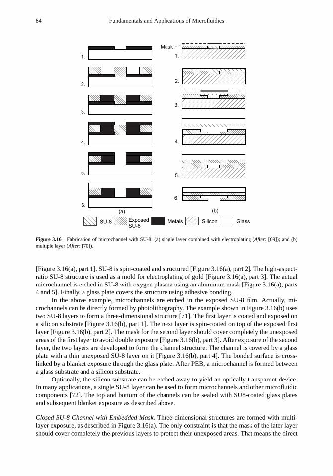
84 Fundamentals and Applications of Microfluidics
(a)
1.
2.
3.
4.
5.
6.
(b)
1.
2.
3.
4.
5.
6.
MetalsSU-8 Silicon GlassExposed
SU-8
Mask
Figure 3.16 Fabrication of microchannel with SU-8: (a) single layer combined with electroplating (After: [69]); and (b)multiple layer (After: [70]).
[Figure 3.16(a), part 1]. SU-8 is spin-coated and structured [Figure 3.16(a), part 2]. The high-aspect-ratio SU-8 structure is used as a mold for electroplating of gold [Figure 3.16(a), part 3]. The actualmicrochannel is etched in SU-8 with oxygen plasma using an aluminum mask [Figure 3.16(a), parts4 and 5]. Finally, a glass plate covers the structure using adhesive bonding.
In the above example, microchannels are etched in the exposed SU-8 film. Actually, mi-crochannels can be directly formed by photolithography. The example shown in Figure 3.16(b) usestwo SU-8 layers to form a three-dimensional structure [71]. The first layer is coated and exposed ona silicon substrate [Figure 3.16(b), part 1]. The next layer is spin-coated on top of the exposed firstlayer [Figure 3.16(b), part 2]. The mask for the second layer should cover completely the unexposedareas of the first layer to avoid double exposure [Figure 3.16(b), part 3]. After exposure of the secondlayer, the two layers are developed to form the channel structure. The channel is covered by a glassplate with a thin unexposed SU-8 layer on it [Figure 3.16(b), part 4]. The bonded surface is cross-linked by a blanket exposure through the glass plate. After PEB, a microchannel is formed betweena glass substrate and a silicon substrate.
Optionally, the silicon substrate can be etched away to yield an optically transparent device.In many applications, a single SU-8 layer can be used to form microchannels and other microfluidiccomponents [72]. The top and bottom of the channels can be sealed with SU8-coated glass platesand subsequent blanket exposure as described above.
Closed SU-8 Channel with Embedded Mask.Three-dimensional structures are formed with multi-layer exposure, as described in Figure 3.16(a). The only constraint is that the mask of the later layershould cover completely the previous layers to protect their unexposed areas. That means the direct

Fabrication Techniques for Microfluidics 85
SU-8 Exposed
SU-8
Substrate
(silicon or glass)
Sacrificial
material
(a) (b) (c)
1.
2.
3.
4.
1.
2.
3.
4.
1.
2.
3.
4.
Metal
Mask
Figure 3.17 Fabrication of covered channels with SU-8: (a) with embedded mask (After: [73]); (b) selective proton writing(After: [77]); and (c) with sacrificial layer (After: [74]).
fabrication of a closed structure, such as a covered channel, is not possible. One solution for thedouble-exposure problem is the use of an embedded mask [73, 74]. The process starts with exposureof the first SU-8 layer to form the bottom of the channel [Figure 3.17(a), part 1].
Subsequently, the second layer is coated. The next step is the fabrication of the embeddedmask. A thin metal layer such as gold [73] is sputtered on the second SU-8 layer. This metal layeris then patterned by common photolithography and etching. The patterned metal layer is used as anembedded mask for the subsequent exposure of the second SU-8 layer [Figure 3.17(a), part 2]. Athird SU-8 layer is spin-coated and exposed to fabricate the top wall of the channel [Figure 3.17(a),part 3]. In the final step, all three layers are developed in a single process, resulting in a coveredmicrochannel. The embedded mask is washed away after the developing process [Figure 3.17(a),part 4]. Instead of the embedded metal mask, a antireflection film, such as CK-6020L resist (FujiFilmOlin Inc., Japan), can be used for making covered SU-8 microchannel [75]. The use of antireflectioncoating ensures that this coating and the structural SU-8 can be developed at the same time.
Covered SU-8 Channel with Selective Proton Writing.A covered channel can be fabricated withselective proton writing or proton beam micromachining [77]. Similar to near-UV exposure, a protonbeam also causes polymerization in SU-8. The depth of the polymerized area depends on the protonbeam energy. This feature is used to form a three-dimensional structure in SU-8. Figure 3.17(b)illustrates the relatively simple steps of this technique. To start with, the SU-8 layer is spin-coated onthe substrate [Figure 3.17(b), part 1]. Writing with low energy forms the top of the channel. With lowenergy, a proton beam can only penetrate shallowly into the SU-8 layer. A thin polymerized layer isformed [Figure 3.17(b), part 2]. In the next step, the proton beam with higher energy polymerizes thesidewalls of the channel. The high energy allows the beam to penetrate through the SU-8 layer downto the substrate surface [Figure 3.17(b), part 3]. In the final step, the exposed SU-8 is developed,resulting in a covered microchannel [Figure 3.17(b), part 4].
Whole SU-8 Channel with a Sacrificial Layer.A further method of fabricating a closed SU-8 channelis using a sacrificial layer [74, 76]. The first SU-8 layer is coated, exposed, and developed to formthe bottom of the channel [Figure 3.17(c), part 1]. Subsequently, a sacrificial structure is deposited

86 Fundamentals and Applications of Microfluidics
Table 3.12
Comparison of Different Thick Film Resists
Resist PMMA SU-8 AZ4562
Exposure type X-ray (0.2–2 nm) UV (365, 405, 435 nm) UV (365, 405, 435 nm)Light source Synchrotron facility Mercury lamp Mercury lampMask substrate Beryllium (100µm) Quartz (1.5–3 mm) Glass (1.5-3 mm)
Titanium (2 mm) Glass (1.5–3 mm) Quartz (1.5–3 mm)Mask absorber Gold (10–15µm) Chromium (0.5µm) Chromium (0.5µm)Maximum height 1,000µm 250µm 100µmAspect-ratio ∼ 500 20–25 ∼ 10Young’s modulus (GPa) 2–3 4–5 —Poisson’s ratio — 0.22 —Glass temperature (◦C) 100 > 200 —
and patterned [Figure 3.17(c), part 2]. The sacrificial material can be thermoplastics, waxes, epoxies[74], or positive photoresist [77]. The sidewalls and the channel ceiling are formed with a secondSU-8 layer [Figure 3.17(c), part 3]. After developing the second layer, the sacrificial material insidethe channel is removed, leaving a closed SU-8 microchannel [Figure 3.17(c), part 4].
3.4.1.3 AZ4562 (Clariant)
AZ4562 (Clariant, Charlotte, North Carolina) is a positive photoresist that is commercially available.This resist belongs to the Novolak resist system, in common with most commercially availablepositive resists. Using multilayer spin-coating, thick resist layers up to 100µm can be achieved.This photoresist has no oxygen sensitivity, but a high resistance to plasma etching, good adhesionproperties, and high-resolution capability [78]. This photoresist is typically used as a mold forsubsequent metal electroplating [79, 81] or as master templates for micromolding. There areno reports of using AZ4562 directly as structural material. Table 3.12 gives a summary of theparameters of PMMA, SU-8, and AZ4562.
3.4.1.4 Other Thick Film Resists
AZ9260 is the other Novolak photoresist from Clariant. AZ9260 exhibits a better transparencycompared to AZ4562, and therefore promises a better aspect ratio. Aspect ratios up to 15 areachieved with a film thickness of 100µm [81]. A theoretical thickness of 150µm is expected fromthis photoresist.
Ma-P 100 (Microresist Technology, Berlin, Germany) is the other photoresist that can givestructure heights up to 100µm. This photoresist has aspect ratios on the order of 5, poorer than thatof the AZ-family [82].
3.4.2 Polymeric Bulk Micromachining
Similar to its silicon-based counterpart, polymeric bulk micromachining uses etching to transfer apattern directly into the bulk substrate. Polymers and almost all organic material can be etched withan oxygen plasma. Since photoresists are organic, they cannot be used for the the etching process inoxygen plasma. Metals such as titanium [83] or aluminum [84] work well as the masking materialfor this purpose.
Polymeric bulk micromachining can form simple microchannels in a polymeric substrate.Moveable structures in a polymeric substrate can be fabricated using two basic methods: multiple

Fabrication Techniques for Microfluidics 87
Oxygen plasma
Oxygen plasma
Oxygen plasma
Metal Polymer
(a)
(b)
1.
2.
3.
4.
1.
2.
3.
Figure 3.18 Fabrication of movable structures using polymeric bulk micromachining: (a) multistep etching in oxygenplasma; and (b) backside blanket-etching in oxygen plasma.
etching steps with different masks and backside blanket-etching. In the first method, the first etchingstep defines the thickness of the moveable structure. In the second step, the masking layer isremoved. The exposed area is etched, until the moveable structure is released [Figure 3.18(a)]. Inthe second method, the moveable structure is formed in the front side of the substrate using anypolymeric technique, such as etching, molding, or hot embossing [85]. The substrate is then turnedupside-down. Blanket-etching of the backside in oxygen plasma releases the moveable structure[Figure 3.18(b)].
Since most polymers have glass transition temperatures between 100◦C and 200◦C, movablestructures fabricated by polymeric bulk micromachining can be assembled by thermal direct bondingat a relatively low temperature. Combining both micromachining technique and bonding techniquewould allow a great flexibility in making polymeric microfluidic components. Almost all existingdesign concepts for micropumps, microvalves, and microflow sensors can be transferred fromsilicon-based technology to polymeric technology.
3.4.3 Polymeric Surface Micromachining
Polymeric surface micromachining is similar to silicon surface micromachining. Polymers are usedeither as structural material or as sacrificial material. The following common polymers can bedeposited and patterned in batch processes.
3.4.3.1 SU-8
SU-8 is a thick film resist, which can be structured using UV-lithography (Section 3.4.1.2). Witha Young’s modulus of 4 to 5 GPa and a Poisson’s ratio of 0.22, hardbacked SU-8 poses excellentmechanical properties and can be used for moveable parts. The sacrificial material for the release ofthe SU-8 part can be the silicon substrate, a metal layer, or a polymer layer. Figure 3.19 demonstratesthis technology for the fabrication of a microcheck valve [86]. The valve was first structured onsilicon substrate with a two-layer process. Developing both layers results in a three-dimensionalvalve structure with spring beams, a valve disc, and a sealing ring. Underetching silicon with KOH

88 Fundamentals and Applications of Microfluidics
(a)
(b)
(c)
(d)
(e)
(f)
SU-8 Si
Figure 3.19 Fabrication of a SU-8 micro check valve using polymeric surface micromachining: (a) coating the first SU-8layer; (b) structuring the spring structure and the valve disc; (c) coating the second SU-8 layer and structuring the sealingring; (d) developing SU-8; (e) underetching silicon to release the SU-8 structure; and (f) the fabricated check valve.
releases the valve. Circular access holes were placed on the structure for faster release. The smoothcontours of the design help to arrest surface stress and avoid cracks in the structure.
For many applications, a metal layer on the structural polymeric material is needed. The metallayer can be structured to form electrodes and heaters. Figure 3.20 shows the fabrication steps of aSU-8 microgripper, which has a thin metal layer on top acting as a heater [87]. Instead of silicon,a thin layer of polystyrene can be used as sacrificial layer. The polymeric sacrificial material canbe dissolved by organic solvents such as toluene. In contrast to KOH for sacrificial silicon etching,solvent does not attack the thin metal layer.
3.4.3.2 Polyimide
Polyimide is commercially available as photoresists such as Proimide 348 or 349 (Ciba Geigy) orPI-2732 (DuPont). A single spin can result in a film thickness up to 40µm. Photosensitive polyimidecan be used for the same purpose as other thick resists described in the previous sections [88].
Fluorinated polyimide is an interesting material because of its optical transparency and simplemachining. In RIE processes of this material, fluorine radicals are released from the fluorinatedpolyimide and act as etchants [89].
Polyimide is a good substrate material. Metals such as aluminum, titanium, and platinum canbe sputtered on it using the lift-off technique [90]. Similar to other polymers, polyimide can beetched with RIE in oxygen plasma. Combining photolithography, RIE, and lamination, complexchannel structures with metal electrodes can be fabricated in polyimide [91].
3.4.3.3 Parylene
Parylene is a polymer that can be deposited with CVD at room temperature. The CVD process allowscoating a conformal film with a thickness ranging from several microns to several millimeters.
The basic type is parylene N, which is poly-paraxylylene. Parylene N is a good dielectric,exhibiting a very low dissipation factor, high dielectric strength, and a frequency-independentdielectric constant.

Fabrication Techniques for Microfluidics 89
(a)
(b)
(c)
(d)
(e)
(f)
Stencil
Opening for bond pads
Opening for gripper areaSU-8 Si Pt/Ti
(g)
Figure 3.20 Fabrication of an SU-8 microgripper using polymeric surface micromachining: (a) blank silicon substrate orcoated with a polymeric sacrificial layer; (b) coating the SU-8 layer; (c) UV exposure; (d) developing the gripper structure;(e) coating the metal layer through a silicon stencil; (f) releasing the gripper; and (g) the fabricated microgripper.
CH
2
CH
2
Parylene
N
n
CH
2
CH
2
Parylene
C
n
Cl
CH
2
CH
2
Parylene
D
n
Cl
Cl
Figure 3.21 Chemical structures of parylene.
Parylene C is produced from the same monomer, modified only by the substitution of achlorine atom for one of the aromatic hydrogens. Parylene C has a useful combination of electricaland physical properties as well as a very low permeability to moisture and other corrosive gases.Parylene C is also able to provide a conformal insulation.
Parylene D is modified from the same monomer by the substitution of the chlorine atom fortwo of the aromatic hydrogens. Parylene D is similar in properties to parylene C with the addedability to withstand higher temperatures. Figure 3.21 shows the chemical structures of these threeparylene types. Deposition rates are fast, especially for parylene C, which is normally deposited ata rate of about 10µm/min. The deposition rates of parylene N and parylene D are slower. Parylenecan be used in microfluidic devices as a structural material, which offers low Young’s modulus.Such a soft material is needed in microvalves and micropumps (see Chapters 6 and 7). Furthermore,parylene coating can improve the biocompatibility of a microfluidic device.
3.4.3.4 Electrodepositable Photoresist
Eagle ED2100 and PEPR 2400 (Shipley Europe Ltd., England) are electrodepositable photoresists.These photoresists were originally developed for printed circuit boards. The photoresist is anaqueous emulsion consisting of polymer micelles. The resist is deposited on wafers by a cataphoreticelectrodeposition process [78]. In an electric field, positively charged micelles move to the wafer,

90 Fundamentals and Applications of Microfluidics
which works as a cathode. The polymer micelles coat the wafer until the film is so thick thatdeposition current approaches zero. The nominal resist thickness is about 3 to 10µm.
The thickness and aspect ratios of electrodepositable photoresists are not relevant for thick filmapplication. Electrodepositable photoresist is suited for applications where it is difficult to spin on aresist after patterning the substrate surface. Due to the relatively conformal nature of the depositionprocess, electrodepositable photoresists are interesting sacrificial materials for polymeric surfacemicromachining.
3.4.3.5 Conductive Polymers
Conductive polymers or conjugated polymers are polymeric materials, which have received thegrowing attention of the MEMS community. Conjugated polymers have alternating single anddouble bonds between a carbon atom along the polymer backbone. The conjugation results in abandgap and makes the polymers behave as semiconductors.
Conjugated polymers can be doped electrochemically, electrically, chemically, or physicallywith ion implantation. In the doped state, conjugated polymers are electrically conducting. Thesecharacteristics allow conductive polymers to be used as the material for electronic devices such asdiodes, light emitting diodes, and transistors.
Furthermore, the doping level of polymers is reversible and controllable. In some conductingpolymers, the change of doping level leads to volume change, which can be used as an actuator. Themost common and well-researched conjugated polymer is polypyrrole (PPy).
The major deposition techniques for conjugated polymers are the following.
• Spin-coating of polymers.The polymer is dispersed or dissolved in a solvent. The resin can bespin-coated on a substrate. Melted polymers can also be applied directly on the substrate.
• Spin-coating of precursor and subsequent polymerization.Precursor polymers are dissolved ina solvent. The polymerization occurs at an elevated temperature. Polymerization can also beachieved by a UV-crosslink of the precursor with a photoinitiator, similar to the developingprocess of SU-8.
• Chemical vapor depositionis similar to the technique used for parylene.
• Electrochemical depositionis similar to electroplating of a metal layer [92].
3.4.3.6 Fabrication of Microchannels with Polymeric Surface Micromachining
Polymeric surface micromachining is perfectly suitable for closed microchannels. Both the structurallayer and the sacrificial layer can be made of polymers. The typical fabrication process is shown inFigure 3.22(a). To start with, the sacrificial polymer is spin-coated on the substrate, which can besilicon or glass. The thickness of this layer determines the channel height. Similar to thick filmresists, the thickness of this polymer layer is controlled by the viscosity of the solution and thespin speed. Next, a metal layer is sputtered over the sacrificial layer as a mask [Figure 3.22(a), part1]. Using photolithography, channel patterns are transferred to the mask [Figure 3.22(a), part 2].The sacrificial layer is then structured by RIE with oxygen plasma [Figure 3.22(a), part 3]. Afterremoving the resist and mask layers, the structural layer is deposited over the sacrificial structures[Figure 3.22(a), part 4]. At elevated temperatures, the sacrificial polymer decomposes into volatileproducts and leaves behind the desired microchannel [93].
Polynorbornene (PNB) is a good sacrificial polymer [94]. The decomposition temperaturesof PNB are between 370◦C and 425◦C. Generally, silicon dioxide and silicon nitride are idealencapsulation materials at these relatively high temperatures. If polymers as structural materials arerequired, they should have high glass transition temperatures and high thermal stability. Polyimides

Fabrication Techniques for Microfluidics 91
(a)
1.
2.
3.
4.
5.
1.
2.
3.
4.
5.
(b)
1.
2.
3.
4.
5.
(c)
SiliconSacrificial
polymer
Coating
polymer
Structural
polymer Resist Oxide/nitride
Figure 3.22 Fabrication of microchannel with polymeric surface micromachining: (a) a simple channel (After: [93]); (b)and (c) microchannel with functional coating of inner wall (After: [114]).
(Amoco Ultradel 7501, Dupont PI-2611, and Dupont PI-2734) are ideal for this purpose because oftheir glass transition temperature of over 400◦C [94].
Polycarbonates, such as polyethylene carbonate (PEC) and polypropylene carbonate (PPC),offer relatively low decomposition temperature on the order of 200◦C to 300◦C [93]. The lowdecomposition temperature is needed for structural materials with less thermal stability. Inorganicglass, silicon dioxide, thermoplastic polymers, and thermoset polymers can be used as structuralmaterials [93].
Because of the increasing number of applications in life sciences, polymeric microchannelsmay need a biocompatible coating for their inner walls. Figures 3.22(b,c) illustrate the fabricationprocesses of such microchannels [114]. The two channel types differ in the type of fluidic access.The biocompatible material used in this example is parylene C. First, parylene is vapor-depositedon a silicon substrate, which is covered by a nitride/oxide barrier layer [Figures 3.22(b), part 1; and3.22(c), part 1]. Thick film resist AZ4620 is used as the sacrificial material. After photolithography,developing, and hard bake of the resist structures, a second parylene layer is deposited [Figures3.22(b), part 2; and 3.22(c), part 2]. After roughening the parylene surface with oxygen plasma,photosensitive polyimide is spin-coated as a structural layer on top of the second parylene layer.Next, polyimide is exposed and developed. In the case of fluidic access from the backside, via-holes to the sacrificial layer are opened by a combination of O2/CF4 and O2 plasma etch [Figure3.22(b), part 4]. In the case of fluidic access from the front side, the top parylene layer is etched inoxygen plasma with an aluminum mask [Figure 3.22(c), part 4]. In the last step, the sacrificial layeris removed with acetone. The resulting microchannels are optically transparent and hermetic.
3.4.4 Microstereo Lithography
In many polymeric micromachining techniques discussed above, resins are cured by UV exposure.The polymerization reactions are generated by the absorption of photons. The most common

92 Fundamentals and Applications of Microfluidics
Polymer Liquidprepolymer
Glass
(a) (b)
(c) (d)
Focused UV-beam
Figure 3.23 Standard configurations of microstereo lithography: (a) and (b) free surface configuration; and (c) and (d)constrained surface configuration. (After: [97].)
absorption process used in photolithography is single-photon absorption [95]. Concurrently, if thecombined energy of two photons matches the transition energy between the ground state of theexcited state of a material, a nonlinear phenomenon called two-photon absorption occurs [96].
The rate of two-photon absorption is a square function of incident light intensity, while the rateof single-photon absorption is a linear function of intensity. For a two-photon absorption, the laserbeam power should be high, which in turn requires a short pulse width on the order of femtoseconds.
3.4.4.1 Polymerization with Single-Photon Absorption
Using a directed UV beam, two-dimensional “slides” can be formed on the focusing plane in a liquidresin. Stacking many such slides allows shaping a three-dimensional structure. Stereo lithography isused for rapid prototyping in macroscale. Based on the state of the surface of the liquid resin, thereare two major conventional stereo configurations: constrained surface and free surface [97]. If thebeam is focused at a point in the liquid, the entire liquid volume from the surface to the focusingpoint is polymerized because of the relatively high absorbance of most resin in the UV range. Theonly solution for this problem is to keep the polymerization at the liquid surface.
Configurations with constrained surfacekeep the UV beam focused on the liquid surface. Theadvantage of this configuration is that moving the transparent glass plate can precisely control thethickness of each structural “slide” [Figure 3.23(a)].
Similar to SU-8, prepolymers for stereo lithography are epoxy-based materials, which workas an adhesive at the contact surface. This feature can be used for moving the prototype, as shownin Figure 3.23(b), but causes problems in separating the prototype from the glass plate in Figure3.23(a).
Figure 3.24 describes the typical setup of microstereo lithography with constrained surface.The most important part is the three-dimensional precision position control. The layout of the deviceis transferred from computer aided design (CAD) data to the control unit, and is scanned directly bythe x-y stage and the z-stage. The optical lens and the constraining glass are kept at a fixed distance,so that the UV beam is always focused at the surface [97].
Configurations with free surfacecan be realized by moving the prototype holder from thesurface into the liquid, while keeping the UV beam focused on the free surface [Figure 3.23(c)].

Fabrication Techniques for Microfluidics 93
UV Source
Shutter
X-Y-stage
Z-stage Control unit
Figure 3.24 System setup for microstereo lithography. (After [97].)
With this technique, the free surface of the liquid is not stable and leads to difficulties in controllingthe slide’s thickness.
The configuration shown in Figure 3.23(d) is feasible with transparent liquid and a nonlinearresponse of polymerization to incident light intensity. First, the light itself should have higherwavelengths than the UV range to keep the resin transparent to the incident light. He-Cd bluelaser (λ = 422 nm) is optimal for this purpose [103]. Second, keeping the laser intensity lowavoids polymerization propagating. Under an optimum exposure, the resin only polymerizes ina spot around the focus and not in the out-of-focus region, due to thermal nonlinearity of aphotopolymerization reaction [95]. This configuration has the advantage of true stereo lithography.Structures can be formed without the supporting base layer. By avoiding moving parts in the liquidand consequently the influence of viscosity and surface tension, this configuration can achieve aresolution better than 1µm [103].
3.4.4.2 Polymerization with Two-Photon Absorption
Polymerization with two-photon absorption is the second microstereo lithography technique that canuse the setup depicted in Figure 3.25. This technique has several requirements for the liquid resinand the laser.
First, the liquid resin should be transparent to the laser, so that the focus point can move freelyinside the liquid resin. The resin used in [96] is a mixture of urethane acrylate oligomers/monomersand photoinitiators. This resin has high absorbance in the UV range. The absorbance almost dropsto zero after the spectrum of green wavelengths. Thus, the resin is transparent to near infraredwavelengths. Titanium-sapphire laser has a wavelength of 770 nm, which is optimal for this purpose.Optical transparency means that there is almost no single-photon absorption.
Second, the condition for two-photon absorption requires a high-energy laser with an ex-tremely short pulse width. The titanium-sapphire laser used in [96] has a peak power of 3 kW atpulse width of 130 fs. With frequency doubling, a wavelength of 398 nm is used to form acrylic-ester-based Nopcocure 800 resin (San Nopco, Tokyo, Japan) [99].

94 Fundamentals and Applications of Microfluidics
Computer
He-Cd Laser
ND filter
Shutter
Galvano
scanner
XYZ stage
Lens
Figure 3.25 System setup for microstereo lithography with free surface configuration and blue laser. (After: [103].)
Liquid
resin
Optical
fiber
UV-
light
Figure 3.26 Setup for mass production with microstereo lithography. (After [104].)
Third, the refractive index between polymerized resin and liquid resin should be small enoughso that it does not affect the spatial accuracy of the scanning laser beam. At a wavelength of 770 nm,the resin described above has a refractive index of 0.02 [96].
The disadvantage of a prototyping approach can be solved with the setup shown in Figure3.26. Instead of a single light beam, the source beam splits into several beams that are guided byoptical fibers [100]. The number of optical fibers determines the number of devices, which can befabricated in parallel.
3.4.4.3 Polymerization with Layer-by-Layer Photolithography
The third approach of microstereo lithography combines the advantages of photolithography andstereo lithography [101]. Instead of scanning a two-dimensional pattern in each layer, the structuresare exposed at once with a pattern generator. The pattern generator works as a mask and shapes thelaser beam, so that it contains the image of the layer to be formed.
This process is similar to conventional photolithography. Selective polymerization of the liquidresin occurs in the exposed areas. This technique allows a much faster processing time than thescanning technique. By using multiple structures on the same mask, this technique may allow batchfabrication without any modification of the setup.

Fabrication Techniques for Microfluidics 95
3.4.4.4 Fabrication of Microfluidic Devices with Microstereo Lithography
Because of its flexibility in making any three-dimensional structure, microstereo lithography can beused for the fabrication of complex microfluidic devices. The technique allows the fabrication ofmicrovalves [97] and integrated fluid systems [102], which have a microchannel network embeddedin the transparent polymeric device. Microreactors with embedded photodiodes for biochemicalanalysis were reported in [103, 104]. Active devices such as SMA-actuated micropumps andmicrovalves can be integrated in the above systems for controlling fluid flow [105]. The techniqueof layer-by-layer photolithography is used for fabricating static Y-mixers [106]. The flexibility ofthe technique allows scaling down of the complex geometry of a macroscopic mixer.
The advantage of microstereo lithography is the self-packaged approach. While fluidic inter-connects are serious problems for microfluidic devices made with other microtechniques, intercon-nects are easily fabricated in the same process. Problems of leakage and expensive packaging canbe solved with microstereo lithography.
3.4.5 Micromolding
Micromolding enables large-scale production of polymeric devices with high accuracy. Besidespolymers, micromolding can also be used for ceramics. In the following, two common micromoldingtechniques are discussed: injection molding and compression molding.
3.4.5.1 Injection Molding
Injection molding is the last technique used in a conventional LIGA process (see Section 3.4.1.1).The metal mold inserts are used as replica master for the molding process [107]. Injection moldingis carried out at temperatures above the glass transition temperatures of amorphous thermoplas-tics such as polymethylmethacrylate (PMMA), polycarbonate (PC), and polysulfone (PSU). Forsemicrystalline thermoplastics such as polyoxymethylene (POM) and polyamide (PA), the moldingtemperature should be higher than the crystallite melting point. Table 3.13 compares the character-istics of different polymers commonly used for micromolding.
Mold inserts for injection molding can be fabricated with common microtechnologies such asbulk micromachining and LIGA. Alternatively, bulk-micromachined parts can be used as masters forelectroplating [108]. After separation from the silicon part, the metal parts can be used as negativemold inserts to fabricate replicas of the silicon parts [108].
Most of the structures have high-aspect ratios and microscopic filling channels. Therefore,high pressures are required for the injection of melted plastics. An alternative for high-pressureinjection molding is reaction injection molding (RIM), which involves the high-speed mixing of twoor more reactive chemicals, such as prepolymers, as an integral part of injecting them into a mold.In Figure 3.27(a), the two cylinders press the prepolymers into a mix head. The mixture flows intothe mold at relatively low temperature, pressure, and viscosity. Curing occurs in the mold, again atrelatively low temperature and pressure. The excess prepolymers are fed back in a recirculation loopby pumps. The entire process, from mixing to demolding, typically takes less than a minute. Thelow processing viscosity allows good filling and high molding accuracy.
Figure 3.27(b) shows the schematics of a typical injection molding system. The machineconsists of a hopper, a screw, a sprue, and a mold insert [109]. To start with, polymer pelletsare loaded into the hopper. Appendix C lists abbreviations of the most common plastics. Thereciprocating screw shears, melts, and pumps the polymer into the accumulation zone. If the desiredpolymer amount is reached, the screw moves forward and pushes the polymeric melt into the moldcavity through the sprue. The required pressure is typically on the order of 500 to 2,000 bars[110, 111]. After cooling, the melt solidifies, and can be taken out from the mold.

96 Fundamentals and Applications of Microfluidics
Table 3.13
Typical Characteristics of Different Polymers for Micromolding (After: [110, 111].)
Polymers PMMA PC PS COC PP
Heat resistance (◦C) 105 140 100 130 110Density (kg/m3) 1,190 1,200 1,050 1,020 900Refractive index 1.42 1.58 1.59 1.53 opaqueResistant to:Aqueous solutions yes limited yes yes yesConcentrated acids no no yes yes yesPolar hydrocarbons no limited limited yes yesHydrocarbons yes yes no no noSuitable for micromolding moderate good good good moderatePermeability coefficients(×10−17 m2/s-Pa):He 5.2 7.5 — — —O2 0.12 1.1 — — —H2O 480–1,900 720–1,050 — — —Hot-embossing parameters:Embossing temperature (◦C) 120–130 160–175 — — —Deembossing temperature (◦C) 95 135 — — —Embossing pressure (bars) 25–37 25–37 — — —Hold time (s) 30–60 30–60 — — —
3.4.5.2 Compression Molding
Compared to injection molding, compression molding or hot embossing is a simple technique. Thestructure is pressed under vacuum to a semifinished polymer material at elevated temperatures aboveits glass temperature, which is on the order of 50◦C to 150◦C [112, 113]. The vacuum is needed dueto the formation of gas bubbles in the small structures. The vacuum also prevents corrosion of themaster. The drawback of this technique is the relatively long cycle time (on the order of severalminutes), while injection molding has fast cycle times (on the order of several seconds).
The most important parameters of compression molding are embossing temperature, deem-bossing temperature, embossing pressures, and hold time. Table 3.13 lists the typical values of theseparameters for hot embossing of PMMA and PC. Hot embossing can only make open channel struc-tures. Fabricating covered channels and fluidic interconnects need additional packaging techniques,such as bonding to a sheet of the same material at temperatures above the glass temperature.
Injection compression molding combines the advantages of both injection and compressionmolding. The polymer melt is first injected into the mold. The mold melt is then compressed toshape the final part. The low viscosity of the melt results in good filling in the molded part.
3.4.5.3 Microcasting
Microcasting is also called soft lithography, which is a direct transfer technique. The term “soft”refers to an elastomeric stamp with patterned relief structures on its surface. Polydimethylsiloxane(PDMS) has been used successfully as the elastomeric material. There are different techniques totransfer the pattern on this elastomeric stamp: microcontact printing and replica micromolding [115].In many applications, the elastomeric PDMS part can be used directly as a microfluidic device withmicrochannels on it.
PDMS.Although all kinds of polymers can be used for the fabrication of an elastomeric stamp,PDMS exhibits unique properties suitable for this purpose. PDMS has an inorganic siloxane

Fabrication Techniques for Microfluidics 97
Screw Accumulation
Hopper Barrel Sprue Mold cavity
y
Mold insert
(b)
(a)
Mold insert
Prepolymer B
PumpPump
Heat exchangerCylinders
Prepolymer A
Heat exchanger
Figure 3.27 Schematics of injection molding systems: (a) reaction injection molding (prepolymers are circulated in twoloops); and (b) reciprocating screw unit.(After: [109].)
CH3
n
Si
CH3
CH3
O Si
CH3
CH3
O Si
CH3
CH3
CH3
Figure 3.28 Chemical structures of PDMS.
backbone with organic methyl groups attached to silicon (see Figure 3.28). Both prepolymers andcuring agents are commercially available. PDMS has high optical transparency above a wavelengthof 230 nm and low self-fluorescence. PDMS has a low interfacial free energy, which avoidsmolecules of most polymers sticking on or reacting with its surface. The interfacial free energyof PDMS can be manipulated with plasma treatment. The modified surface properties of PDMS areneeded for certain applications. PDMS is stable against humidity and temperature. This material isoptically transparent and can be cured by UV light. PDMS is an elastomer and can therefore attachon nonplanar surfaces. PDMS is mechanically durable. These characteristics make PDMS an idealmaterial for soft lithography [115].
However, PDMS also presents a number of drawbacks, such as volume change and elasticdeformation. The design of a PDMS part should consider the shrinking effect upon curing. A numberof organic solvents can swell PDMS as well. Furthermore, elastic deformation can limit the aspectratio of the designed structure. A too-high aspect ratio leads to a pairing effect, in which two parallelstructures attach to each other. An aspect ratio that is too low leads to a sagging of noncontact

98 Fundamentals and Applications of Microfluidics
Silicon
PDMS
(a) (b) (c)
Figure 3.29 Fabrication of PDMS stamps: (a) DRIE of silicon master; (b) coating; and (c) release.
Silicon PDMS
(a) (b)
Structural material
(c)
SAM
Figure 3.30 Microcontact printing with PDMS stamps: (a) immersion; (b) stamping; and (c) etching.
regions, which makes further steps of soft lithography impossible. The recommended aspect ratiosfor PDMS structures are between 0.2 and 2 [115].
Fabrication of the PDMS Device.The master for a PDMS device can be fabricated with con-ventional micromachining technologies, as described in Section 3.2. Figure 3.29 describes thefabrication process of a PDMS part. The silicon master is silanized by exposure to the vapor ofCF3(CF2)6(CH2)2SiCl3 for about 30 minutes [114]. The prepolymer is coated on the silicon or glassmaster. After curing in an elevated temperature, the embossed PDMS layer can be peeled off and isready for use in the subsequent steps.
The master can also be fabricated with SU-8 [116]. The PDMS part is used directly asstructural material. The PDMS device is bonded to a glass plate after oxidizing their surfaces withoxygen plasma. In a similar approach, three-dimensional structures are fabricated by the laminationof different structured PDMS layers [117]. Fluidic interconnects are embedded directly in the PDMSdevice.
Microcontact Printing with a PDMS Stamp.Microcontact printing uses the relief structures on thesurface of a PDMS part as a stamp to transfer a pattern of SAMs to the substrate surface by contact.SAMs can be created by immersion of the substrate in a solution containing a ligand Y(CH2)nX,where X is the head group and Y is the anchoring group. The head group determines the surfaceproperty of the monolayer. In microcontact printing, the stamp is wetted with the above solution andpressed on the substrate surface [Figures 3.30(a, b)].
The patterned SAM can be used as a resist layer to transfer its structure to an underlyingstructural layer. Because of its small thickness, SAM can be quickly destroyed by ion bombardment.Therefore, SAM resist is not suitable for reactive ion etching. However, SAM resist can be used forwet etching of the underlying structural layer [Figure 3.30(c)]. This thicker layer, in turn, can beused as a mask for the more aggressive RIE. The resolution of microcontact printing depends on theproperties of stamp material, and can reach several tens of nanometers.
Surface properties of patterned SAM can be used as templates for selective deposition of othermaterials. For example, a patterned hydrophilic SAM traps liquid prepolymer on its surface. Aftercuring, a polymer structure is formed on top of the patterned SAM. Furthermore, patterned SAMcan be used for controlled deposition of metals and ceramics by selective CVD.

Fabrication Techniques for Microfluidics 99
Prepolymer PDMS
1. 2. 3.
1. 2. 3.
(a)
(b)
1. 2. 3.
(c)
1. 2. 3.
(d)
Substrate Structural polymer
Figure 3.31 Micromolding with PDMS replica master: (a) replica molding; (b) microtransfer molding; (c) micromoldingin capillaries; and (d) solvent-assisted micromolding.
Micromolding with a PDMS Replica Master.Micromolding with a PDMS replica master can becategorized as: replica molding, microtransfer molding, micromolding in capillaries, and solvent-assisted micromolding [115].
In replica molding, the PDMS part is used as replica master for a prepolymer. The finalstructure is obtained by curing with a UV exposure or elevated temperature [Figure 3.31(a)]. Thistechnique can achieve resolutions of less than 10 nm.
In microtransfer molding, liquid prepolymer is applied on the PDMS master [Figure 3.31(b),part 1]. The prepolymer layer is then planarized by removing excess prepolymer. Only prepolymertrapped between the relief structures remains on the surface of the PDMS master [Figure 3.31(b),part 2]. The master is then placed on a planar substrate. UV exposure or heating solidifies theprepolymer. Peeling off the elastic PDMS master results in polymer structures on the substratesurface [Figure 3.31(b), part 3]. This method does not remove completely the excess prepolymeron top of the PDMS stamp. A thin polymer layer on the order of 100 nm remains on the substratesurface. If the pattered polymer is to be used as a mask for subsequent etching, this thin polymerlayer should be removed by oxygen plasma [115].
Micromolding in capillariesuses capillary forces to fill the gaps between the substrate andthe PDMS master. First, the PDMS master is pressed tightly on a planar substrate [Figure 3.31(c),part 1]. Elastic PDMS seals off walls and creates capillary channels. A drop of liquid prepolymeris placed at the ends of these channels and fills them automatically due to capillary forces [Figure3.31(c), part 2]. After curing and peeling of the PDMS master, polymer structures remain on thesubstrate surface [Figure 3.31(c), part 3]. This technique can be used to pattern silicon and glasswith different materials [115].
Solvent-assisted micromoldingis similar to the conventional embossing technique. Instead ofusing heat and compression, this technique uses a solvent to wet the PDMS stamp and soften thestructural polymer. The solvent only dissolves the structural polymer and not PDMS. The stamp ispressed on a polymer film, which dissolves in the solvent and fills the gaps between relief structures

100 Fundamentals and Applications of Microfluidics
(a) (b) (c)
Mask
SU8
Si
PDMS
Glass
Access
holes
Figure 3.32 Fabrication of microchannels with soft lithography: (a) spin coating a silicon wafer with SU-8, UV exposurewith a clear field mask, development of SU-8 master; (b) pouring PDMS on the mold, peeling off the PDMS part; and(c) surface treatment of PDMS in oxygen plasma and bonding to glass.
of the stamp. After dissipation and evaporation of the solvent, solid polymer remains on the substrate[Figure 3.31(d)] [115].
Fabrication of Microchannels with Soft Lithography.Soft lithography can be used for rapid proto-typing of microfluidic devices. Replica molding can be used for fabrication of microchannels [Figure3.31(a)] [115]. PDMS is a good device material because it has a number of useful properties: lowcost, low toxicity, transparency from the visible wavelengths into the near ultraviolet wavelengths,and chemical inertness.
First, PDMS is mixed from prepolymers. The weight ratio of the base and the curing agentcould be 10:1 or 5:1. The solid master is fabricated from SU-8 [Figure 3.32(a)]. Glass posts areplaced on the SU-8 master to define the inlets and reservoirs. The PDMS mixture is poured intothe master and stands for a few minutes to self-level. The whole set is then cured at relatively lowtemperature (from 60◦C to 80◦C) for several hours. After peeling off and having surface treatmentwith low-temperature oxygen plasma [Figure 3.32(b)], the structured PDMS membrane is broughtinto contact with clean glass, silica, or another piece of surface-activated PDMS [Figure 3.32(c)].The sealed channel can withstand pressures up to five bars. Without surface treatment, PDMS alsoforms a watertight seal when pressed against itself, glass, or most other smooth surfaces. Thesereversible seals are useful for detachable fluidic devices, which are often required in research andprototyping.
In a similar approach, the inlet and outlet tubes are embedded in the PDMS device [117].Three-dimensional structures are formed by lamination of many PDMS sheets. Methanol is usedas surfactant for both bonding and self-alignment. The surface tension at superimposed holes inthe PDMS sheets self-aligns them. Methanol prevents instant bonding between two PDMS sheetsafter plasma treatment. After evaporating methanol on a hot plate, the laminated stack is bonded.In [118], microchannels in PDMS are used for patterning surfaces. Micromolding in capillaries isutilized to fill the patterns. Colored UV-curable polymers with low viscosity (150 cps) are the fillingliquids. This technique of soft lithography has much potential in patterning colored dyes for displayapplications and in patterning molecules for biochemical analysis [118].
3.5 OTHER MICROMACHINING TECHNIQUES
Besides the above three major batch microtechniques, there are a number of serial microtechniquesfor fabrication of microfluidic devices. The advantage of these techniques is that they do notdepend on substrate materials. Microstereo lithography is actually a serial technique, but it isplaced in Section 3.4 to conform to the general term of polymeric micromachining. Here serial

Fabrication Techniques for Microfluidics 101
Table 3.14
Typical Ablation Depths Per Pulse of Different Material (Nanosecond Laser)
Material Depth Per Pulse (µm)
Polymers 0.3–0.7Ceramics and glass 0.1–0.2Diamond 0.05–0.1Metals 0.1–1.0
microtechniques are categorized as subtractive (removal) techniques and additive (deposition)techniques.
3.5.1 Subtractive Techniques
3.5.1.1 Laser Micromachining
Three types of lasers are commonly used for laser micromachining:
• Excimer lasers with ultraviolet wavelengths (351, 308, 248, 193 nm);
• Nd:YAG lasers with near infrared, visible, and UV wavelengths (1,067, 533, 355, 266 nm);
• CO2 lasers with deep infrared wavelength (10.6µm).
The two major parameters of laser micromachining are wavelength and laser power. The choiceof wavelength depends on the minimum structure size and the optical properties of the substratematerial, such as absorption and reflection characteristics. Theoretically, the minimum achievablefocal spot diameter and consequently the smallest size are about twice the laser wavelength.
The choice of power depends on the desired structure size and the ablation rate. When excimeror Nd:YAG lasers with a pulse duration of a few tens of nanoseconds are utilized, a single laser pulsewill typically vaporize the surface material to a depth of 0.1 to 1µm (see Table 3.14). Since eachpulse removes such a thin layer of material, the depth of the machined trench can be controlledaccurately by the number of laser pulses. Furthermore, laser pulses of very short duration eliminateheat flow to surrounding materials. Consequently, clean and accurate structures can be achieved withshortly pulsed lasers. There are two modes of laser micromachining: direct writing and using a mask[119]. In the direct writing mode, the laser beam is focused on the substrate surface. The pattern isscanned using a precision x-y stage or galvano scanning mirrors. The setup for this mode is similarto those of microstereo lithography depicted in Figures 3.24 and 3.25. In this mode, the smalleststructure depends on the accuracy of the scanning system, and is on the order of 25 to 50µm. In themask mode, a mask determines the shape of the structure. Therefore, the minimum structure sizecan be brought down to twice that of the laser wavelength.
Laser micromachining is suitable for fabrication of microchannels and fluidic access holes.A LIGA-like technique uses laser machining instead of X-ray lithography to machine PMMA[120]. Furthermore, the laser beam can be used for sealing polymeric devices fabricated with othertechniques or making shadow masks.
3.5.1.2 Focused Ion Beam Micromachining
In focused ion beam (FIB) micromachining, a highly focused ion beam scans and cuts the substratesurface. In a typical FIB system, the ion beam is ejected from a liquid metal ion source (usually

102 Fundamentals and Applications of Microfluidics
(a)
Dielectric
W orkpiece
Tool electrode
-
+
-
+
Wire electrode
Workpiece
Dielectric supply
(b)
Figure 3.33 Schematics of microelectro discharge machining: (a) die-sinking EDM; and (b) wire EDM.
gallium). With a spot size of less than 10 nm, the ion beam is scanned across the substrate materialin a manner similar to scanning electron microscopy (SEM).
3.5.1.3 Microelectro Discharge Machining
Microelectro discharge machining (EDM) or spark erosion is an electrothermal machining processthat applies sparks created between a tool electrode and a workpiece electrode to remove substratematerial. Each spark can create locally a temperature up to 10,000◦C. For this purpose, both thetool and the substrate material should be electrically conductive. Both electrodes are immersed ina dielectric fluid such as oil, which cools the electrodes and removes the debris out of the sparkinggap. The spark frequency can be up to 500 kHz.
The two major EDM techniques are die-sinking EDM and wire EDM. Die-sinking EDMis more relevant for fabrication of microfluidic devices. Microchannels and access holes can befabricated with this technique [Figure 3.33(a)]. Wire EDM cuts through the workpiece and is notrelevant for microfluidic applications [Figure 3.33(b)].
3.5.1.4 Powder Blasting
Powder blasting is another erosion technique that uses kinetic energy of powder particles to generatecracks on the substrate surface and consequently to remove material. The major process parametersof this technique are particle material, particle size, particle velocity, and incident angle [121].
The resolution of this technique depends on the particle size. As a rule of thumb, the smallestcut is about three times that of the particle size [122]. High resolutions are kept by the use of ahard metal mask, which is machined by another technique, such as laser micromachining. Otheralternative masks are thick resist foils and polyimide resist [122]. With particle velocities on theorder of 80 to 200 m/s, the erosion rate is on the order of 1 mm/min [121].
Using 30-µm alumina particles, microchannels of 100-µm width and 10-µm depth can befabricated in glass [121]. Changing the incident angle of the powder beam can lead to channels withslanted walls. Microchannels for capillary electrophoresis can be fabricated with powder blasting.Microchannels with 85-µm width and 22-µm depth are fabricated in glass using 9-µm aluminaparticles [123]. In microfluidics, powder blasting can be used for drilling fluidic access through asubstrate.
3.5.1.5 Ultrasonic Micromachining
Another practical technique for drilling fluidic access holes is ultrasonic drilling, which usesultrasonically induced vibrations delivered to a tool to machine the substrate. When combined withabrasive slurry, ultrasonic drilling can handle hard, brittle materials such as glass and silicon. Figure3.34 illustrates a typical setup.

Fabrication Techniques for Microfluidics 103
(a)
Electric signal
Piezoelectric
actuator
Tool holder
Vibration
Tool
Abrasive
slurry
Workpiece
(b)
Vibration
Tool
Abrasive
slurry
Slurry
Figure 3.34 Ultrasonic machining: (a) setup schematics; and (b) close-up of the tool and the workpiece.
(a) (b)
Plating solution
LCVD
structure
LECD-
structure
Figure 3.35 Additive techniques: (a) LCVD; and (b) LECD.
The drilling process starts with converting a high-frequency electrical signal into a mechanicaloscillation, which is acoustically transmitted to the tool. A piezoelectric stack actuator can be usedfor this purpose. The linear oscillation is typically at a rate of 20 kHz. With the use of abrasive slurryflowing around the cutting tool, microscopic grinding occurs between the surfaces of the tool andthe workpiece. The machined area becomes an exact counterpart of the tool.
In microfluidics, ultrasonic machining is often used for drilling via holes in glass and silicon.Hole diameters on the order of 100 to 200µm can be drilled. The tool for ultrasonic machining canbe fabricated with wire EDM, as described above.
3.5.2 Additive Techniques
3.5.2.1 Laser-Assisted Chemical Vapor Deposition
Laser-assisted chemical vapor deposition (LCVD) uses a focused laser beam to control the chemicaldeposition from the vapor phase. The common laser types used for this purpose are the Nd:YAGlaser and argon laser. Scanning the laser in space results in three-dimensional structures [Figure3.35(a)].

104 Fundamentals and Applications of Microfluidics
Glass
Silicon
+
-
Cathode
Anode
Chuck
Figure 3.36 Setup for anodic bonding.
3.5.2.2 Localized Electrochemical Deposition
Localized electrochemical deposition (LECD) has the opposite effect of EDM. Localized growth ofthe metal structure is determined by a sharp microelectrode. Scanning the electrode tip in spaceallows fabricating three-dimensional structures [Figure 3.35(b)]. A microneedle with a 125-µmdiameter and 500-µm length was fabricated with LECD [124].
3.6 ASSEMBLY AND PACKAGING OF MICROFLUIDIC DEVICES
Although batch fabrication and microtechnologies minimize the use of assembly processes, as-sembling and packaging techniques are still needed for the final microfluidic product. In fact, thecommercialization of microfluidic devices is difficult due to the bottleneck effect between microfab-rication and packaging. Because of additional fluidic interconnects, packaging may cause a muchhigher cost than the microdevice itself.
From the product perspective, the assembly and packaging hierarchy of a microfluidic devicecan be structured in the wafer level and the device level. In the wafer level, assembly and packagingstill can be carried out in batch, concurrently with other device components. In the device level, eachdevice should be packaged and readied to be shipped. The problem of fluidic interconnects and highcost arises in this level.
3.6.1 Wafer Level Assembly and Packaging
3.6.1.1 Anodic Bonding
Anodic bonding is the oldest bonding technique in MEMS. A glass wafer and a silicon wafer arebonded together at elevated temperatures on the order of 400◦C and high electrical field with bondingvoltage about 1 kV. Figure 3.36 describes the typical setup of anodic bonding. Silicon is connectedto the positive electrode and works as an anode, which gives the name to this bonding technique.
Because the bonding process occurs at a relatively high temperature, the thermal expansioncoefficients of glass and silicon should match, to avoid cracks after cooling the bonded stack to roomtemperature. Glasses suitable for this purpose are Corning 7740 (Pyrex), Corning 7750, Schott 8329,and Schott 8330. Thin metal layers on glass or silicon do not affect the bonding quality.
Anodic bonding can be used for sealing silicon to silicon. For this purpose, an intermediateglass layer between the two silicon wafers makes the seal possible. The glass layer can be depositedby different techniques, such as PVD and spin-on glass. Glass material with a matching thermalexpansion coefficient is used as a source or target for the evaporation or sputtering process. Thebonding processes work as usual with the glass-covered silicon wafer replacing the glass wafer inFigure 3.36. Because of the much thinner glass layer on the order of 0.5 to 4µm, much lower
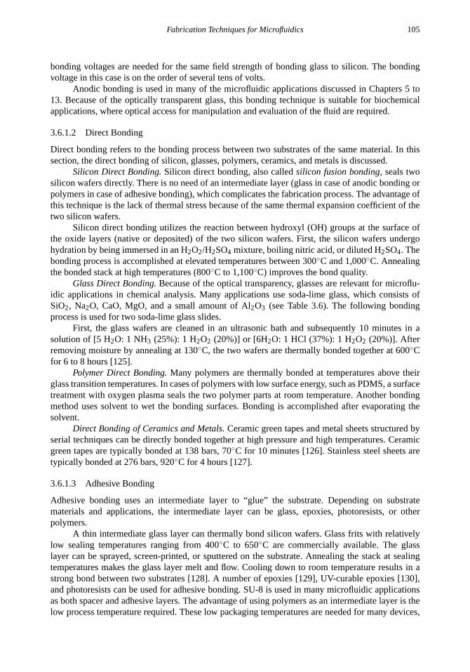
Fabrication Techniques for Microfluidics 105
bonding voltages are needed for the same field strength of bonding glass to silicon. The bondingvoltage in this case is on the order of several tens of volts.
Anodic bonding is used in many of the microfluidic applications discussed in Chapters 5 to13. Because of the optically transparent glass, this bonding technique is suitable for biochemicalapplications, where optical access for manipulation and evaluation of the fluid are required.
3.6.1.2 Direct Bonding
Direct bonding refers to the bonding process between two substrates of the same material. In thissection, the direct bonding of silicon, glasses, polymers, ceramics, and metals is discussed.
Silicon Direct Bonding.Silicon direct bonding, also calledsilicon fusion bonding, seals twosilicon wafers directly. There is no need of an intermediate layer (glass in case of anodic bonding orpolymers in case of adhesive bonding), which complicates the fabrication process. The advantage ofthis technique is the lack of thermal stress because of the same thermal expansion coefficient of thetwo silicon wafers.
Silicon direct bonding utilizes the reaction between hydroxyl (OH) groups at the surface ofthe oxide layers (native or deposited) of the two silicon wafers. First, the silicon wafers undergohydration by being immersed in an H2O2/H2SO4 mixture, boiling nitric acid, or diluted H2SO4. Thebonding process is accomplished at elevated temperatures between 300◦C and 1,000◦C. Annealingthe bonded stack at high temperatures (800◦C to 1,100◦C) improves the bond quality.
Glass Direct Bonding.Because of the optical transparency, glasses are relevant for microflu-idic applications in chemical analysis. Many applications use soda-lime glass, which consists ofSiO2, Na2O, CaO, MgO, and a small amount of Al2O3 (see Table 3.6). The following bondingprocess is used for two soda-lime glass slides.
First, the glass wafers are cleaned in an ultrasonic bath and subsequently 10 minutes in asolution of [5 H2O: 1 NH3 (25%): 1 H2O2 (20%)] or [6H2O: 1 HCl (37%): 1 H2O2 (20%)]. Afterremoving moisture by annealing at 130◦C, the two wafers are thermally bonded together at 600◦Cfor 6 to 8 hours [125].
Polymer Direct Bonding.Many polymers are thermally bonded at temperatures above theirglass transition temperatures. In cases of polymers with low surface energy, such as PDMS, a surfacetreatment with oxygen plasma seals the two polymer parts at room temperature. Another bondingmethod uses solvent to wet the bonding surfaces. Bonding is accomplished after evaporating thesolvent.
Direct Bonding of Ceramics and Metals.Ceramic green tapes and metal sheets structured byserial techniques can be directly bonded together at high pressure and high temperatures. Ceramicgreen tapes are typically bonded at 138 bars, 70◦C for 10 minutes [126]. Stainless steel sheets aretypically bonded at 276 bars, 920◦C for 4 hours [127].
3.6.1.3 Adhesive Bonding
Adhesive bonding uses an intermediate layer to “glue” the substrate. Depending on substratematerials and applications, the intermediate layer can be glass, epoxies, photoresists, or otherpolymers.
A thin intermediate glass layer can thermally bond silicon wafers. Glass frits with relativelylow sealing temperatures ranging from 400◦C to 650◦C are commercially available. The glasslayer can be sprayed, screen-printed, or sputtered on the substrate. Annealing the stack at sealingtemperatures makes the glass layer melt and flow. Cooling down to room temperature results in astrong bond between two substrates [128]. A number of epoxies [129], UV-curable epoxies [130],and photoresists can be used for adhesive bonding. SU-8 is used in many microfluidic applicationsas both spacer and adhesive layers. The advantage of using polymers as an intermediate layer is thelow process temperature required. These low packaging temperatures are needed for many devices,

106 Fundamentals and Applications of Microfluidics
which have, for instance, aluminum structures in them. The other advantage is that adhesive bondingis not limited to silicon and can be used for all kinds of substrate material.
3.6.1.4 Eutectic Bonding
Eutectic bonding is a common packaging technique in electronics. Gold-silicon eutectic bonding isachieved at a relatively low temperature of 363◦C. A thin gold film can be sputtered on the siliconsurface for this purpose. Furthermore, a gold-silicon preform with composition close to eutecticpoint can also be used as the intermediate layer.
3.6.2 Device Level Packaging
3.6.2.1 Fluidic Interconnects
Generally, a microsystem needs interconnects for power flow, information flow, and material flowto communicate with its environment. Interconnects for power flow supply the device with energy.Interconnects for information flow are actually signal ports, which allow information coming inand out of the device. Unlike other MEMS devices, microfluidic devices have interconnects formaterial flow. The material flow is the fluid flow, which is processed in microfluidic devices. Whilemany solutions for the first two types of interconnects exist in traditional microelectronics, fluidicinterconnections pose a big challenge. In this section, fluidic interconnects are categorized by thecoupling nature as press-fit interconnects and glued interconnects.
Press-Fit Interconnects.Press-fit interconnects utilize elastic forces of coupling parts to sealthe fluidic access. Figure 3.37 shows several examples of press-fit interconnects. Due to the relativelysmall sealing forces, this type of interconnect is only suitable for low-pressure applications.
Figure 3.37(a) illustrates the concept of interlocking finger joints [131]. The fingers arefabricated in bulk silicon. A structured polysiloxane film works as an O-ring at the interconnectinterface. This type of interconnect is suitable for coupling channel systems in different wafers.
For fluidic coupling out of the device, tubing interconnects are needed. Figure 3.37(b) showsa horizontal tubing interconnect fabricated by wet etching of silicon. The external polymeric tubingis press-fitted to the silicon tubing [131]. Vertical tubing interconnects can be etched in silicon usingDRIE [Figure 3.37(c)]. These vertical tubes can hold fused silica capillaries, which are perpendicularto the device surface [132].
If external capillaries are to be inserted directly into etched openings, plastic couplers can beused to keep them in place [Figure 3.37(d)] [131]. The plastic couplers in [132] are injection-moldedfrom POM. A PDMS gasket between the plastic coupler and the substrate surface can improve theseal [133].
The molded coupler shown in Figure 3.37(e) is fabricated from two bonded silicon wafers.The fused silica capillary is embedded in the plastic coupler. The capillary with the coupler is theninserted into the fluidic opening. Annealing the device at elevated temperatures allows the plastic toreflow. After cooling down to room temperature, the remolded plastic coupler hermetically seals thecapillary and the opening [134]. Plastic couplers can also be compression-molded. In Figure 3.37(f),the thermoplastic tube is inserted into the opening. Under pressure and temperatures above the glasstransition temperature, the plastic melts and fills the gaps between the coupler and silicon. Similarflanged tubes can be fabricated with the technique shown in Figure 3.37(g) [135].
In many cases, the elastic force of the couplers cannot withstand high pressures. One solutionfor high-pressure interconnects is the use of a mesoscale casing, which has conventional O-rings forsealing fluidic interconnects [136]. If a microfluidic system has multiple fluidic ports, many smallO-rings are required. In this case, it is more convenient to have integrated O-rings in the device.Figure 3.38 presents the fabrication steps of such integrated O-rings [137]. First, the cavities for theO-rings are etched in silicon with DRIE. After depositing an oxide/nitride layer [Figure 3.38(a)],
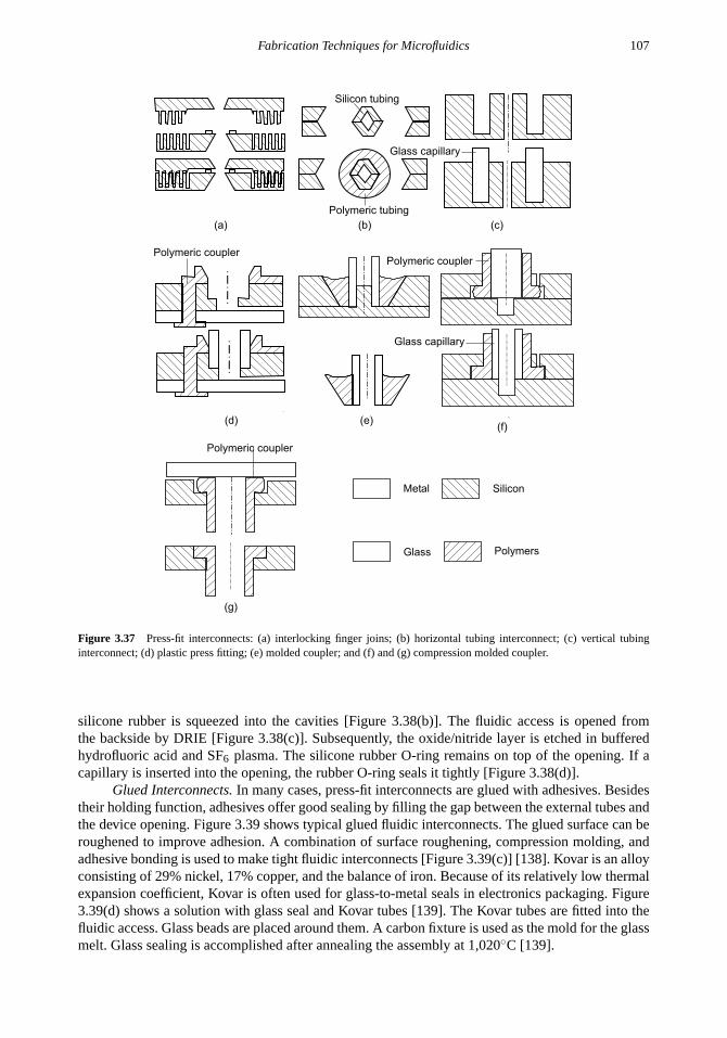
Fabrication Techniques for Microfluidics 107
(a) (b) (c)
(d)
Metal Silicon
Glass Polymers
(e)
(g)
(f)
Polymeric tubing
Silicon tubing
Glass capillary
Polymeric couplerPolymeric coupler
Glass capillary
Polymeric coupler
Figure 3.37 Press-fit interconnects: (a) interlocking finger joins; (b) horizontal tubing interconnect; (c) vertical tubinginterconnect; (d) plastic press fitting; (e) molded coupler; and (f) and (g) compression molded coupler.
silicone rubber is squeezed into the cavities [Figure 3.38(b)]. The fluidic access is opened fromthe backside by DRIE [Figure 3.38(c)]. Subsequently, the oxide/nitride layer is etched in bufferedhydrofluoric acid and SF6 plasma. The silicone rubber O-ring remains on top of the opening. If acapillary is inserted into the opening, the rubber O-ring seals it tightly [Figure 3.38(d)].
Glued Interconnects.In many cases, press-fit interconnects are glued with adhesives. Besidestheir holding function, adhesives offer good sealing by filling the gap between the external tubes andthe device opening. Figure 3.39 shows typical glued fluidic interconnects. The glued surface can beroughened to improve adhesion. A combination of surface roughening, compression molding, andadhesive bonding is used to make tight fluidic interconnects [Figure 3.39(c)] [138]. Kovar is an alloyconsisting of 29% nickel, 17% copper, and the balance of iron. Because of its relatively low thermalexpansion coefficient, Kovar is often used for glass-to-metal seals in electronics packaging. Figure3.39(d) shows a solution with glass seal and Kovar tubes [139]. The Kovar tubes are fitted into thefluidic access. Glass beads are placed around them. A carbon fixture is used as the mold for the glassmelt. Glass sealing is accomplished after annealing the assembly at 1,020◦C [139].
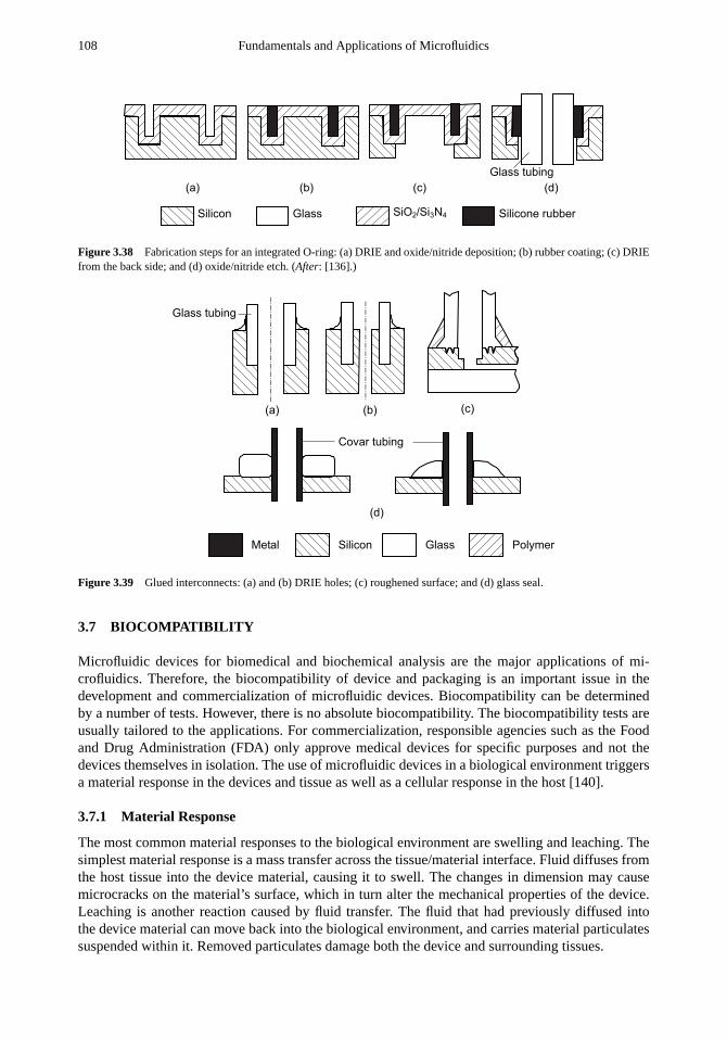
108 Fundamentals and Applications of Microfluidics
(a) (b) (c) (d)
Silicon SiO2/Si3N4 Silicone rubberGlass
Glass tubing
Figure 3.38 Fabrication steps for an integrated O-ring: (a) DRIE and oxide/nitride deposition; (b) rubber coating; (c) DRIEfrom the back side; and (d) oxide/nitride etch. (After: [136].)
(a) (b) (c)
(d)
Metal Silicon Glass Polymer
Covar tubing
Glass tubing
Figure 3.39 Glued interconnects: (a) and (b) DRIE holes; (c) roughened surface; and (d) glass seal.
3.7 BIOCOMPATIBILITY
Microfluidic devices for biomedical and biochemical analysis are the major applications of mi-crofluidics. Therefore, the biocompatibility of device and packaging is an important issue in thedevelopment and commercialization of microfluidic devices. Biocompatibility can be determinedby a number of tests. However, there is no absolute biocompatibility. The biocompatibility tests areusually tailored to the applications. For commercialization, responsible agencies such as the Foodand Drug Administration (FDA) only approve medical devices for specific purposes and not thedevices themselves in isolation. The use of microfluidic devices in a biological environment triggersa material response in the devices and tissue as well as a cellular response in the host [140].
3.7.1 Material Response
The most common material responses to the biological environment are swelling and leaching. Thesimplest material response is a mass transfer across the tissue/material interface. Fluid diffuses fromthe host tissue into the device material, causing it to swell. The changes in dimension may causemicrocracks on the material’s surface, which in turn alter the mechanical properties of the device.Leaching is another reaction caused by fluid transfer. The fluid that had previously diffused intothe device material can move back into the biological environment, and carries material particulatessuspended within it. Removed particulates damage both the device and surrounding tissues.

Fabrication Techniques for Microfluidics 109
3.7.2 Tissue and Cellular Response
Reactionary tissue response begins with inflammation at the device/tissue interface. The classicsymptoms of inflammation are reddening, swelling, heating, and pain. Chemical signals releasedby the damaged tissue trigger the inflammation and attract white blood cells as body response. Thedevice is covered with macrophages and foreign body giant cells leading to a fibrous encapsulation.The encapsulation can affect the functionality of the device. If the healing process occurs asdescribed above, the device can be called biocompatible.
Alternatively, a long-lasting inflammation can be caused by chemical or physical propertiesof the device material or by motion of the device itself. Constant local cell damages make aninflammation reaction continue to be released. If the device material causes cells to die, it is calledcytotoxic. If the device material is inert, its particulates cannot be digested by macrophages. Thematerial response to the biological environment can cause chemical changes in the device material,which can be cytotoxic and damage cells.
3.7.3 Biocompatibility Tests
There are two general test methods for biocompatibility:
• In vitro (in laboratory glassware);
• In vivo (in a live animal or human).
The usual procedure starts with in vitro tests, which can weed out the clearly dangerous, but may notexpose all problems that may occur in the complex living system. In vitro tests should also be carriedout to evaluate the adhesion behavior of cells, DNA, and other polymers. Furthermore, cytotoxicityof the device material should be tested for applications such as tissue engineering. Some animaltests may be required before the device moves to a human test stage. There are standardized tests tofollow for the in vitro assessment.
Problems
3.1 If the mask for KOH-etching of a{100}-wafer is a 200-nm thick silicon dioxide layer, what isthe maximum etched depth in silicon? Use averaged etch rates from Table 3.8.
3.2 An optical measurement in microchannels needs an optical path between two surfaces that havea 45◦ angle to each other. Develop a process for the mirror surfaces with anisotropy etching inbulk silicon.
3.3 Design the mask opening for fabricating a nozzle in silicon with KOH etching. The nozzleopening on the other side of the wafer has a dimension of 20µm × 20 µm. The wafer is 500µm thick.
3.4 We consider the channel depicted in Figure 3.10. The access gap for isotropic etching in Figure3.11(b) is 1µm. After sealing with thermal oxide, we need to inspect the channel and to openthe access gap. If the sealing thermal oxide layer is etched with a buffered HF solution, howlarge is the gap of the opening after etching away all silicon dioxide?
3.5 A deep trench is etched in a silicon wafer using DRIE. The trench measures 20µm × 100µm.After removing all protecting layers on the trench wall, the trench is further etched in KOH.Describe the final shape of the trench after KOH etching if the wafer orientation is (a){100},(b) {110}, or (c){111}.
3.6 Explain why it is difficult to reflow negative resists such as SU-8, but easy for positive resistssuch as the AZ4000 series.
110 Fundamentals and Applications of Microfluidics
3.7 In Figure 3.15(b), what is the final form of the channel if the channel in the second SU-8 layeris wider than that in the first SU-8 layer?
3.8 In Figure 3.16(a), why can lift-off technique not be used for structuring the embedded metalmask?
References
[1] Madou, M. J.,Fundamentals of Microfabrication: The Science of Miniaturization, 2nd ed., Boca Raton, FL: CRCPress, 2002.
[2] Thompson, L. F., Willson, C. G., and Bowden, M. J.,Introduction to Microlithography, Washington, D.C.: AmericanChemical Society, 1994.
[3] Friedrich, H., Widmann, D., and Mader, H.,Technologie hochintegrierter Schaltungen, Berlin: Springer-Verlag, 1996.
[4] Pearce, C. W., “Epitaxy,” inVLSI Technology, S. M. Sze (ed.), New York: McGraw-Hill, 1988, pp. 55–97.
[5] Adams, A. C., “Dielectric and Polysilicon Film Deposition,” inVLSI Technology, S. M. Sze (ed.), New York: McGraw-Hill, 1988, pp. 233–271.
[6] Becker, H., and Gartner, C., “Polymer Microfabrication Methods for Microfluidic Analytical Applications,”Elec-trophoresis, Vol. 21, 2000, pp. 12–26.
[7] Monreal, G., and Mari, C. M., “The Use of Polymer Materials as Sensitive Elements in Physical and ChemicalSensors,”Journal of Micromechanics and Microengineering, Vol. 7, No. 3, 1997, pp. 121–124.
[8] Soane, D. (ed.),Polymer Applications for Biotechnology: Macromolecular Separation and Identification, UpperSaddle River, NJ: Prentice-Hall, 1992.
[9] Kovacs, G. T. A., Maluf, N. I., and Petersen, K. E., “Bulk Micromachining of Silicon,”Proceedings of the IEEE,Vol. 86, No. 8, 1998, pp. 1536–1551.
[10] Williams, K. R., and Muller, R. S., “Etch Rates for Micromachining Processing,”Journal of MicroelectromechanicalSystems, Vol. 5, No. 4, 1996, pp. 256–269.
[11] Bean, K. E., “Anisotropic Etching of Silicon,”IEEE Transactions Electron Devices, Vol. ED-25, 1978, pp. 1185–1193.
[12] Seidel, H., et al., “Anisotropic Etching of Crystalline Silicon in Alkaline Solutions II: Influence of Dopants,”Journalof Electrochemical Society, Vol. 137, No. 11, 1990, pp. 3626–3632.
[13] Kaminsky, G., “Micromachining of Silicon Mechanical Structures,”Journal of Vacuum Science and Technology,Vol. B3, No. 4, 1985, pp. 1015–1024.
[14] Kern, W., “Chemical Etching of Silicon, Germanium, Gallium Arsenide and Gallium Phosphide,”RCA Review,Vol. 39, 1978, pp. 278–308.
[15] Schnakenberg, U., et al., “NH4OH Based Etchants for Silicon Micromachining: Influence of Additives and Stabilityof Passivation Layers,”Sensors and Actuators A, Vol. 25, No. 1-3, 1990, pp. 1–7.
[16] Tabata, O., et al., “Anisotropic Etching of Silicon in TMAH Solutions,”Sensors and Actuators A, Vol. 34, No. 1, 1992,pp. 51–57.
[17] Schnakenberg, U., Beneke, W., and Lange, P., “TMAHW Etchants for Silicon Micromachining,”Proceedings ofTransducers ’91, 6th International Conference on Solid-State Sensors and Actuators, San Francisco, June 23–27,1991, pp. 815–818.
[18] Petersen, K. E., “Silicon as a Mechanical Material,”Proceedings of IEEE, Vol. 70, 1982, pp. 420–457.
[19] Mehregany M., and Senturia, S. D., “Anisotropic Etching of Silicon in Hydrazine,”Sensors and Actuators, Vol. 13,No. 4, 1988, pp. 375–390.
[20] Linde, H., and Austin, L., “Wet Silicon Etching with Aqueous Amine Gallates,”Journal of Electrochemical Society,Vol. 139, No. 4, 1992, pp. 1170–1174.
[21] Fleming, J. G., “Combining the Best of Bulk and Surface Micromachining Using Si{111} Substrates,”ProceedingsSPIE Micromach. Microfab. IV Tech. Conf., Vol. 3511, 1998, pp. 162–168.
[22] Lehmann, V., “Porous Silicon — A New Material for MEMS,”Proceedings of MEMS’96, 9th IEEE InternationalWorkshop Micro Electromechanical System, San Diego, CA, Feb. 11–15, 1996, pp. 1–6.
[23] Larmer, P.,Method of Anisotropically Etching Silicon, German Patent DE 4 241 045, 1994.
[24] Sobek, D., Senturia, S. D., and Gray, M. L., “Microfabricated Fused Silica Flow Chambers for Flow Cytometry,”Technical Digest of the IEEE Solid State Sensor and Actuator Workshop, Hilton Head Island, SC, June 13–16, 1994,pp. 260–263.
Fabrication Techniques for Microfluidics 111
[25] Harrison, D. J., et al., “Miniaturized Chemical Analysis Systems Based on Electrophoretic Separations and Electroos-motic Pumping,”Proceedings of Transducers ’93, 7th International Conference on Solid-State Sensors and Actuators,Yokohama, Japan, June 7–10, 1993, pp. 403–406.
[26] Jacobson, S. C., et al., “Electrically Driven Separations on a Microchip,”Technical Digest of the IEEE Solid StateSensor and Actuator Workshop, Hilton Head Island, SC, June 13–16, 1994, pp. 65–68.
[27] Mobius, H., et al., “Sensors Controlled Processes in Chemical Reactors,”Proceedings of Transducers ’95, 8thInternational Conference on Solid-State Sensors and Actuators, Stockholm, Sweden, June 16–19, 1995, pp. 775–778.
[28] Jiang, L., Wong, M., and Zohar, Y., “A Micro-Channel Heat Sink with Integrated Temperature Sensors for PhaseTransition Study,”Proceedings of MEMS’99, 12th IEEE International Workshop Micro Electromechanical System,Orlando, FL, Jan. 17–21, 1999, pp. 159–164.
[29] Chen, J., and Wise, K. D., “A High Resolution Silicon Monolithic Nozzle Array for Inkjet Printing,”IEEE Transactionon Electron Devices, Vol. 44, No. 9, 1997, pp. 1401–1409.
[30] Chen, J., et al., “A Multichannel Neural Probe for Selective Chemical Delivery at the Cellular Level,”IEEETransaction on Biomedical Engineering, Vol. 44., No. 8, 1997, pp. 760–769.
[31] Tjerkstra, R. W., et al., “Etching Technology for Microchannels,”Proceedings of MEMS’97, 10th IEEE InternationalWorkshop Micro Electromechanical System, Nagoya, Japan, Jan. 26-30, 1997, pp. 147–151.
[32] De Boer, M. J., et al., “Micromachining of Buried Micro Channels in Silicon,”Journal of MicroelectromechanicalSystems, Vol. 9, No. 1, 2000, pp. 94–103.
[33] Osterbroek, R. E., et al., “Etching Methodologies in< 111>-Oriented Silicon Wafers,”Journal of Microelectromech-nical Systems, Vol. 9, No. 3, 2000, pp. 390–397.
[34] Chou, S. Y., Krauss, P. R., and Renstrom, P. J., “Imprint of Sub-25 nm Vias and Trenches in Polymers,”AppliedPhysics Letter, Vol. 67, No. 21, 1995, pp. 2114–3116.
[35] Cao, H., et al. “Fabrication of 10 nm Enclosed Nanofluidic Channels,”Applied Physics Letter, Vol. 81, No. 1, 2002,pp. 174–176.
[36] Bustillo, J. M., Howe, R. T., and Muller, R. S., “Surface Micromachining for Microelectromechanical Systems,”Proceedings of the IEEE, Vol. 86, No. 8, 1998, pp. 1552–1574.
[37] Tang, W. C., Nguyen, T. C. H., and Howe, R. T., “Laterally Driven Polysilicon Resonant Microstructures,”Sensorsand Actuators, Vol. 20, 1989, pp. 25–32.
[38] Keller, C., and Ferrari, M., “Milli-Scale Polysilicon Structures,”Technical Digest of the IEEE Solid State Sensor andActuator Workshop, Hilton Head Island, SC, June 13–16, 1994, pp. 132–137.
[39] Keller, C. G., and Howe, R. T., “Hexsil Bimorphs for Vertical Actuation,”Proceedings of Transducers ’95, 8thInternational Conference on Solid-State Sensors and Actuators, Stockholm, Sweden, June 16–19, 1995, pp. 99–102.
[40] Flannery, A. F., “PECVD Silicon Carbide for Micromachined Transducers,”Proceedings of Transducers ’97, 9thInternational Conference on Solid-State Sensors and Actuators, Chicago, IL, June 16–19, 1997, pp. 217–220.
[41] Rajan, N., et al., “Fabrication and Testing of Micromachined Silicon Carbide and Nickel Fuel Atomizers for GasTurbine Engines,”Journal of Microelectromechanical Systems, Vol. 8, No. 3, 1999, pp. 251–257.
[42] Shaw, K. A., Zhang, Z. L., and MacDonald, N. C., “SCREAM-I: A Single Mask, Single-Crystal Silicon, Reactive IonEtching Process for Microelectromechanical Structures,”Sensors and Actuators A, Vol. 40, No. 1, 1994, pp. 63–70.
[43] Li, Y. X., et al., “Fabrication of a Single Crystalline Silicon Capacitive Lateral Accelerometer Using MicromachiningBased on Single Step Plasma Etching,”Proceedings of MEMS’95, 8th IEEE International Workshop Micro Electrome-chanical System, Amsterdam, the Netherlands, Jan. 29-Feb. 2, 1995, pp. 398–403.
[44] Diem, B., et al., “SOI (SIMOX) as a Substrate for Surface Micromachining of Single Crystalline Silicon Sensorsand Actuators,”Proceedings of Transducers ’93, 7th International Conference on Solid-State Sensors and Actuators,Yokohama, Japan, June 7–10, 1993, pp. 233–236.
[45] Jansen, H., et al., “The Black Silicon Method IV: The Fabrication of Three-Dimensional Structures in Silicon withHigh Aspect Ratios For Scanning Probe Microscopy and Other Applications,”Proceedings of MEMS’95, 8th IEEEInternational Workshop Micro Electromechanical System, Amsterdam, the Netherlands, Jan. 29-Feb. 2, 1995, pp. 88–93.
[46] De Boer, M., Jansen, H., and Elwenspoek, M., “The Black Silicon Method V: A Study of the Fabricating of MoveableStructures for Micro Electromechanical Systems,”Proceedings of Transducers ’95, 8th International Conference onSolid-State Sensors and Actuators, Stockholm, Sweden, June 16–19, 1995, pp. 565–568.
[47] Jansen, H., de Boer, M., and Elwenspoek, M., “The Black Silicon Method VI: High Aspect Ratio Trench Etching forMEMS Applications,”Proceedings of MEMS’96, 9th IEEE International Workshop Micro Electromechanical System,San Diego, CA, Feb. 11–15, 1996, pp. 250–257.
[48] Bell, T. E., et al., “Porous Silicon as a Sacrificial Material,”Journal of Micromechanics and Microengineering, Vol. 6,1996, pp. 361–369.

112 Fundamentals and Applications of Microfluidics
[49] Lee, S., Park, S., and Cho, D., “The Surface/Bulk Micromachining (SBM) Process: A New Method for FabricatingReleased MEMS in Single Crystal Silicon,”Journal of Microelectromechanical Systems, Vol. 8, No. 4, 1999, pp. 409–416.
[50] Lin, L., Pisano, A. P., and Muller, R. S., “Silicon Processed Microneedles,”Proceedings of Transducers ’93, 7thInternational Conference on Solid-State Sensors and Actuators, Yokohama, Japan, June 7–10, 1993, pp. 237–240.
[51] Wu, S., et al., “A Suspended Microchannel with Integrated Temperature for High-Pressure Flow Studies,”Proceedingsof MEMS’98, 11th IEEE International Workshop Micro Electromechanical System, Heidelberg, Germany, Jan. 25–29,1998, pp. 87–92.
[52] Talbot, N. H., and Pisano, A. P., “Polymolding: Two Wafer Polysilicon Micromolding of Closed-Flow Passages forMicroneedles and Microfluidic Devices,”Technical Digest of the IEEE Solid State Sensor and Actuator Workshop,Hilton Head Island, SC, June 4–8, 1998, pp. 265–268.
[53] Spiering, V. L., et al., “Novel Microstructures and Technologies Applied in Chemical Analysis Techniques,”Proceed-ings of Transducers ’97, 9th International Conference on Solid-State Sensors and Actuators, Chicago, IL, June 16–19,1997, pp. 511–514.
[54] Papautsky, I., et al., “Micromachined Pipette Arrays,”IEEE Transaction on Biomedical Engineering, Vol. 47, No. 6,2000, pp. 812-819.
[55] Carlen, E. T., and Mastrangelo, C. H., “Parafin Actuated Surface Micromachined Valves,”Proceedings of MEMS’00,13th IEEE International Workshop Micro Electromechanical System, Miyazaci, Japan, Jan. 23–27, 2000, pp. 381–385.
[56] Becker, E. W., et al., “Fabrication of Microstructures with High Aspect Ratios and Great Structural Heights by Syn-chrotron Radiation Lithography, Glavanoforming, and Plastic Moulding (LIGA Process),Microelectronic Engineer-ing, Vol. 4, pp. 35–56.
[57] Guckel, H., Christensen T. R., and Skrobis, K. J.,Formation of Microstructures Using a Preformed Photoresist Sheet,U.S. Patent #5378583, January 1995.
[58] Chaudhuri, B., et al., “Photoresist Application for the LIGA Process,”Microsystem Technologies, Vol. 4, 1998,pp. 159–162.
[59] Mohr, J., et al., “Requirements on Resist Layers in Deep-Etch Synchrotron Radiation Lithography,”Journal of VacuumScience and Technology, Vol. B6, 1988, pp. 2264–2267.
[60] Guckel, H., et al., “Plasma Polymerization of Methyl Methacrylate: A Photoresist for 3D Applications,”TechnicalDigest of the IEEE Solid State Sensor and Actuator Workshop, Hilton Head Island, SC, June 4–7, 1988, pp. 43–46.
[61] Ghica, V., and Glashauser, W.,Verfahren fr die Spannungsfreie Entwicklung von Bestrahlten Polymethylmethacrylate-Schichten, German patent, #3039110, 1982.
[62] Lee, K., et al., “Micromachining Applications for a High Resolution Ultra-Thick Photoresist,”J. Vac. Scien. Technol.B, Vol. 13, 1995, pp. 3012–3016.
[63] Shaw, J. M., et al., “Negative Photoresists for Optical Lithography,”IBM Journal of Research and Development,Vol. 41, 1997, pp. 81–94.
[64] Lorenz, H., et al., “SU-8: A Low-Cost Negative Resist for MEMS,”Journal of Micromechanics and Microengineering,Vol. 7, 1997, pp. 121–124.
[65] Lorenz, H., et al., “Fabrication of Photoplastic High-Aspect Ratio Microparts and Micromolds Using SU-8 UV Resist,”Microsystem Technologies, Vol. 4, 1998, pp. 143–146.
[66] MicroChem Corp, NANOTM SU-8 Negative Tone Photoresists Formulations 2-25, Data sheets, 2001.
[67] MicroChem Corp, NANOTM SU-8 Negative Tone Photoresists Formulations 50-100, Data sheets, 2001.
[68] Chang, H. K., and Kim, Y. K., “UV-LIGA Process for High Aspect Ratio Structure Using Stress Barrier and C-ShapedEtch Hole,”Sensors and Actuators A, Vol. 84, 2000, pp. 342–350.
[69] Ghantasala, M. K., et al., “Patterning, Electroplating and Removal of SU-8 Moulds by Excimer Laser Micromachin-ing,” Journal of Micromechanics and Microengineering, Vol. 11, 2001, pp. 133–139.
[70] Ayliffe, H. E., Frazier, A.B., and Rabbitt, R.D., “Electric Impedence Spectroscopy Using Microchannels withIntegrated Metal Electrodes,”IEEE Journal of Microelectromechanical Systems, Vol. 8, No. 1, 1999, pp. 50–57.
[71] Jackman, R. J., et al., “Microfluidic Systems with On-Line UV Detection Fabricated in Photodefinable Epoxy,”Journalof Micromechanics and Microengineering, Vol. 11, 2001, pp. 263–269.
[72] Hostis, E. L., et al., “Microreactor and Electrochemical Detectors Fabricated Using Si and EPSON SU-8,”Sensorsand Actuators B, Vol. 64, 2000, pp. 156–162.
[73] Alderman, B. E. J., et al., “Microfabrication of Channels Using an Embedded Mask in Negative Resist,”Journal ofMicromechanics and Microengineering, Vol. 11, 2001, pp. 703–705.
[74] Guerin, L. J., et al., “Simple and Low Cost Fabrication of Embedded Micro Channels By Using a New Thick-FilmPhotoplastic,”Proceedings of Transducers ’97, 9th International Conference on Solid-State Sensors and Actuators,Chicago, IL, June 16–19, 1997, pp. 1419–1421.

Fabrication Techniques for Microfluidics 113
[75] Chuang, Y. J., et al., “A Novel Fabrication Method of Embedded Micro-Channels by Using SU-8 Thick-FilmPhotoresists,”Sensors and Actuators A, Vol. 103, 2003, pp. 64–69.
[76] Zhang, J., et al., “Polymerization Optimization Of SU-8 Photoresist and Its Applications in Microfluidic Systems andMEMS,” Journal of Micromechanics and Microengineering, Vol. 11, 2001, pp. 20–26.
[77] Tay, F. E. H., et al., “A Novel Micro-Machining Method for the Fabrication of Thick-Film SU-8 Embedded Micro-Channels,”Journal of Micromechanics and Microengineering, Vol. 11, 2001, pp. 27–32.
[78] O’Brien, J., et al., “Advanced Photoresist Technologies for Microsystems,”Journal of Micromechanics and Micro-engineering, Vol. 11, 2001, pp. 353–358.
[79] Qu, W., Wenzel, C., and Jahn, A., “One-Mask Procedure for The Fabrication of Movable High-Aspect-Ratio 3DMicrostructures,”Journal of Micromechanics and Microengineering, Vol. 8, 1998, pp. 279–283.
[80] Roth, S., et al., “High Aspect Ratio UV Photolithography for Electroplated Structures,”Journal of Micromechanicsand Microengineering, Vol. 9, 1999, pp. 105–108.
[81] Conedera, V., Le Goff, B., and Fabre, N., “Potentialities of a New Positive Photoresist for the Realization of ThickMoulds,” Journal of Micromechanics and Microengineering, Vol. 9, 1999, pp. 173–175.
[82] Loechel, B., “Thick-Layer Resists for Surface Micromachining,”Journal of Micromechanics and Microengineering,Vol. 10, 2000, pp. 108–115.
[83] Weston, D. F., et al., “Fabrication of Microfluidic Devices in Silicon and Plastic Using Plasma Etching,”Journal ofVacuum Science and Technology B, Vol. 19, 2001, pp. 2846–2851.
[84] Wang, X., Engel, J., and Liu, C., “Liquid Crystal Polymer (LCP) for MEMS: Processes and Applications,”Journal ofMicromechanics and Microengineering, Vol. 13, 2003, pp. 628–633.
[85] Zhao, Y., and Cui, “Fabrication of High-Aspect-Ratio Polymer-Based Electrostatic Comb Drives Using the HotEmbossing Technique,”Journal of Micromechanics and Microengineering, Vol. 13, 2003, pp. 430–435.
[86] Truong, T. Q., and Nguyen, N. T., “A Polymeric Piezoelectric Micropump Based on Lamination Technology,”Journalof Micromechanics and Microengineering, Vol. 14, 2004, pp. 632–638.
[87] Nguyen, N. T., Ho, S. S., and Low, L. N., “A Polymeric Microgripper with Integrated Thermal Actuators,”Journal ofMicromechanics and Microengineering, Vol. 14, 2004, pp. 969–974.
[88] Frazier, A. B., and Allen, M.G., “Metallic Microstructures Fabricated Using Photosensitive Polyimide ElectroplatingMolds,” Journal of Microelectromechanical Systems, Vol. 2, No. 2, 1993, pp. 87–94.
[89] Ito, T., et al., “Fabrication of Microstructure Using Fluorinated Polyimide and Silicon-Based Positive Photoresist,”Microsystem Technologies, Vol. 6, 2000, pp. 165–168.
[90] Stieglitz, T., “Flexible Biomedical Microdevices with Double-Sided Electrode Arrangements For Neural Applica-tions,” Sensors and Actuators A, Vol. 90, 2001, pp. 203–211.
[91] Metz, S., Holzer, R., and Renaud, P., “Polyimide-Based Microfluidic Devices,”Lab on a Chip, Vol. 1, No. 1, 2001,pp. 29–34.
[92] Smela, E., “Microfabrication of Ppy Microactuators and Other Conjugated Polymer Devices,”Journal of Microme-chanics and Microengineering, Vol. 9, 1999, pp. 1–18.
[93] Reed, H. A., et al., “Fabrication of Microchannels Using Polycarbonates as Sacrificial Materials,”Journal ofMicromechanics and Microengineering, Vol. 11, 2001, pp. 733–737.
[94] Bhusari, D., et al., “Fabrication of Air-Channel Structures for Microfluidic, Microelectromechanical, and Microelec-tronic Applications,”Journal of Micromechanics and Microengineering, Vol. 10, 2001, pp. 400–408.
[95] Maruo, S., and Ikuta, K., “Three-Dimensional Microfabrication by Use of Single-Photon-Absorbed Polymerization,”Applied Physics Letters, Vol. 76, No. 19, 2000, pp. 2656–2658.
[96] Maruo, S., and Kawata, S., “Two-Photon-Absorbed Near-Infrared Photopolymerization for Three-Dimensional Mi-crofabrication,”Journal of Microelectromechanical Systems, Vol. 7, No. 4, 1998, pp. 411–415.
[97] Ikuta, K., and Hirowatari, K., “Real Three Dimensional Micro Fabrication Using Stereo Lithography and MetalMolding,” Proceedings of MEMS’93, 6th IEEE International Workshop Micro Electromechanical System, San Diego,CA, Jan. 25–28, 1993, pp. 42–47.
[98] Ikuta, K., Maruo, S., and Kojima, S., “New Micro Stereo Lithography for Freely Moveable 3D Micro Structure—Super IH Process with Submicron Resolution,”Proceedings of MEMS’98, 11th IEEE International Workshop MicroElectromechanical System, Heidelberg, Germany, Jan. 25–29, 1998, pp. 290–295.
[99] Miwa, M., et al., “Femtosecond Two-Photon Stereo-Lithography,”Applied Physics A, Vol. 73, 2001, pp. 561–566.
[100] Ikuta, K., et al., “Development of Mass Productive Micro Stereo Lithography (Mass-IH Process),”Proceedings ofMEMS’96, 9th IEEE International Workshop Micro Electromechanical System, San Diego, CA, Feb. 11–15, 1996,pp. 301–306.

114 Fundamentals and Applications of Microfluidics
[101] Bertsch, A., Lorenz, H., and Renaud, H., “Combining Microstereolithography and Thick Resist UV Lithography for3D Microfabrication,”Sensors and Actuators A, Vol. 73, 1999, pp. 14–23.
[102] Ikuta, K., Hirowatari, K., and Ogata, T., “Three Dimensional Micro Integrated Fluid Systems (MIFS) Fabricated byStereo Lithography,”Proceedings of MEMS’94, 7th IEEE International Workshop Micro Electromechanical System,Oiso, Japan, Jan. 25–28, 1994, pp. 1–6.
[103] Ikuta, K., et al., “Biochemical IC Chip Toward Cell Free DNA Protein Synthesis,”Proceedings of MEMS’98, 11thIEEE International Workshop Micro Electromechanical System, Heidelberg, Germany, Jan. 25–29, 1998, pp. 131–136.
[104] Ikuta, K., et al., “Micro Concentrator with Opto-Sense Micro Reactor for Biochemical IC Chip Family—3D Com-posite Structure and Experimental Verification,”Proceedings of MEMS’99, 12th IEEE International Workshop MicroElectromechanical System, Orlando, FL, Jan. 17–21, 1999, pp. 376–381.
[105] Ikuta, K., et al., “Fluid Drive Chips Containing Multiple Pumps and Switching Valves for Biochemical IC Family—Development of SMA 3D Micro Pumps and Valves in Leak-Free Polymer Package,”Proceedings of MEMS’00, 13thIEEE International Workshop Micro Electromechanical System, Miyazaci, Japan, Jan. 23–27, 2000, pp. 739–744.
[106] Bertsch, A., et al., “Static Micromixers Based on Large-Scale Industrial Mixer Geometry,”Lab on a Chip, Vol. 1,2001, pp. 56–20.
[107] Piotter, V., et al., “Injection Molding and Related Techniques for Fabrication of Microstructures,”MicrosystemTechnologies, Vol. 4, 1997, pp. 129–133.
[108] Larsson, O., et al., “Silicon Based Replication Technology of 3D-Microstructures by Conventional CD-InjectionMolding Techniques,”Proceedings of Transducers ’97, 9th International Conference on Solid-State Sensors andActuators, Chicago, IL, June 16–19, 1997, pp. 1415–1418.
[109] Despa, M. S., Kelly, K. W., and Collier, J. R., “Injection Molding of Polymeric LIGA HARMS,”MicrosystemTechnologies, Vol. 6, 1999, pp. 60–66.
[110] Niggemann, M., et al., “Miniaturized Plastic Micro Plates for Applications in HTS,”Microsystem Technologies, Vol. 6,1999, pp. 48–53.
[111] Gerlach, A., et al., “Gas Permeability of Adhesives and Their Application for Hermetic Packaging of Microcompo-nents,”Microsystem Technologies, Vol. 7, 2001, pp. 17–22.
[112] Becker, H., and Heim, U., “Hot Embossing as a Method for the Fabrication of Polymer High Aspect Ratio Structures,”Sensors and Actuators A, Vol. 83, 2000, pp. 130–135.
[113] Heckele, M., Bacher, W., and Muller, K. D., “Hot Embossing—The Molding Technique for Plastic Microstructures,”Microsystem Technologies, Vol. 4, 1998, pp. 122–124.
[114] Man, P. F., Jones, D. K., and Mastrangelo, C. H., “Microfluidic Plastic Capillaries on Silicon Substrates: A NewInexpensive Technology for Bioanalysis Chips,”Proceedings of MEMS’97, 10th IEEE International Workshop MicroElectromechanical System, Nagoya, Japan, Jan. 26–30, 1997, pp. 311–316.
[115] Xia, Y., and Whitesides, G. M., “Soft Lithography,”Annual Review of Material Sciences, Vol. 28, 1998, pp. 153–194.
[116] Duffy, D. C., et al., “Rapid Prototyping of Microfluidic Switches in Poly (Dimethyl Siloxane) and Their Actuation byElectro-Osmotic Flow,Journal of Micromechanics and Microengineering, Vol. 9, 1999, pp. 211–217.
[117] Jo, B. H., et al., “Three-Dimensional Micro-Channel Fabrication in Polydimethylsiloxane (PDMS) Elastomer,”Journal of Microelectromechanical Systems, Vol. 9, No. 1, 2000, pp. 76–81.
[118] Juncker, D., et al., “Soft and Rigid Two-Level Microfluidic Networks for Patterning Surfaces,”Journal of Microme-chanics and Microengineering, Vol. 11, 2001, pp. 532–541.
[119] Chichkov, B., et al., “Femtosecond, Picosecond and Nanosecond Laser Ablation of Solids,”Applied Physics A, Vol. 63,1996, pp. 109–115.
[120] Laws, R. A., Holmes, A. S., and Goodall, F. N., “The Formation of Moulds for 3D Microstructures Using ExcimerLaser Ablation,”Microsystem Technologies, Vol. 3, 1996, pp. 17–19.
[121] Belloy, E., et al., “The Introduction of Powder Blasting for Sensor and Microsystem Applications,”Sensors andActuators A, Vol. 84, 2000, pp. 330–337.
[122] Wensink, H., et al., “Mask Materials for Powder Blasting,”Journal of Micromechanics and Microengineering, Vol. 10,2000, pp. 175–180.
[123] Shlautmann, S., et al., “Powder-Blasting Technology as an Alternative Tool for Microfabrication of CapillaryElectrophoresis Chips with Integrated Conductivity Sensors,”Journal of Micromechanics and Microengineering,Vol. 11, 2001, pp. 386–389.
[124] Yeo, S. H., and Choo, J. H., “Effects of Rotor Electrode In the Fabrication of High Aspect Ratio Microstructures byLocalized Electrochemical Deposition,”Journal of Micromechanics and Microengineering, Vol. 11, 2001, pp. 435–442.

Fabrication Techniques for Microfluidics 115
[125] Stjernstrom, M., and Roeraade J., “Method for Fabrication of Microfluidic System in Glass,”Journal of Microme-chanics and Microengineering, Vol. 8, 1998, pp. 33–38.
[126] Matson, D. W., et al., ”Laminated Ceramic Components for Micro Fluidic Applications,”SPIE Conference ProceedingVol 3877: Microfluidic Devices and Systems II, Santa Clara, CA, Sept. 20-22, 1999, pp. 95–100.
[127] Martin, P. M., et al., “Laser Micromachined and Laminated Microfluidic Components for Miniaturized Thermal,Chemical and Biological Systems,”SPIE Conference Proceedings, Vol. 3680: Design, Test, and Microfabrication ofMEMS and MOEMS, Paris, France, Mar. 30-Apr. 1, 1999, pp. 826–833.
[128] Ko, W. H., et al., “Bonding Techniques for Microsensors,” inMicromachining and Micropackaging of Transducers,Fung, C. D., et al. (eds.), Amsterdam: Elsevier, 1985, pp. 41–61.
[129] Weckwerth, M. V., et al., “Epoxy Bond and Stop-Etch (EBASE) Technique Enabling Backside Processing of (Al)GaAsHeterostructures,”Superlattices Microstructures, Vol. 20, No. 4, 1996, pp. 561–567.
[130] Nguyen H., et al., “A Substrate-Independent Wafer Transfer Technique for Surface-Micromachined Devices,”Pro-ceedings of MEMS’00, 13th IEEE International Workshop Micro Electromechanical System, Miyazaci, Japan, Jan.23-27, 2000, pp. 628–632.
[131] Gonzalez, C., Collins, S. D., and Smith, R. L., “Fluidic Interconnects for Modular Assembly of Chemical Microsys-tems,”Sensors and Actuators B, Vol. 49, 1998, pp. 40–45.
[132] Gray, B. L., et. al., “Novel Interconnection Technologies for Integrated Microfluidic Systems,”Sensors and ActuatorsA, Vol. 77, 1999, pp. 57–65.
[133] Mourlas, N. J., et al., “Reuseable Microfluidic Coupler with PDMS Gasket,”Proceedings of Transducers ’99, 10thInternational Conference on Solid-State Sensors and Actuators, Sendai, Japan, June 7–10, 1999, pp. 1888–1889.
[134] Meng, E., Wu, S., and Tai, Y.-C., “Micromachined Fluidic Couplers,” inMicro Total Analysis Systems 2000, A. vanden Berg et al. (eds.), Netherlands: Kluwer Academic Publishers, 2000, pp. 41–44.
[135] Puntambekar, A., and Ahn, C. H., “Self-Aligning Microfluidic Interconnects for Glass- and Plastic-Based MicrofluidicSystems,”Journal of Micromechanics and Microengineering, Vol. 12, No. 1, 2002, pp. 35–40.
[136] Trah, H. P., et al., “Micromachined Valve with Hydraulically Actuated Membrane Subsequent to a ThermoelectricallyControlled Bimorph Cantilever,”Sensors and Actuators A, Vol. 39, 1993, pp. 169–176.
[137] Yao, T. J., et al., “Micromachined Rubber O-Ring Micro-Fluidic Couplers,”Proceedings of MEMS’00, 13th IEEEInternational Workshop Micro Electromechanical System, Miyazaci, Japan, Jan. 23–27, 2000, pp. 745–750.
[138] Wijngarrt W., et al., “The First Self-Priming and Bi-Directional Valve-Less Diffuser Micropump for Both Liquidand Gas,”Proceedings of MEMS’00, 13th IEEE International Workshop Micro Electromechanical System, Miyazaci,Japan, Jan. 23–27, 2000, pp. 674–679.
[139] London, A. P., “Development and Test of a Microfabricated Bipropellant Rocket Engine,” Ph.D. thesis, MassachusettsInstitute of Technology, 2000.
[140] Black, J.,Biological Performance of Materials, New York: Marcel Dekker, 1992.

116 Fundamentals and Applications of Microfluidics

Chapter 4
Experimental Flow Characterization
4.1 INTRODUCTION
There are many areas in science and engineering where it is important to determine the flow fieldat the micron scale. These will be discussed in Chapters 5 through 13. Industrial applications ofmicrofabricated fluidic devices are present in the aerospace, computer, automotive, and biomedicalindustries. In the aerospace industry, for instance, micron-scale supersonic nozzles measuringapproximately 35µm are being designed for JPL/NASA to be used as microthrusters on micro-satellites, and for AFOSR/DARPA as flow control devices for palm-size microaircraft [1]. In thecomputer industry, inkjet printers, which consist of an array of nozzles with exit orifices on the orderof tens of microns in diameter, account for 65% of the computer printer market [2]. The biomedicalindustry is currently developing and using microfabricated fluidic devices for patient diagnosis,patient monitoring, and drug delivery. The i-STAT device (i-STAT, Inc.) is the first microfabricatedfluidic device that has seen routine use in the medical community for blood analysis. Other examplesof microfluidic devices for biomedical research include microscale flow cytometers for cancer celldetection, micromachined electrophoretic channels for DNA fractionation, and polymerase chainreaction (PCR) chambers for DNA amplification [3]. The details of the fluid motion through thesesmall channels, coupled with nonlinear interactions between macromolecules, cells, and the surface-dominated physics of the channels, create very complicated phenomena, which can be difficult tosimulate numerically.
A wide range of diagnostic techniques have been developed for experimental microfluidicresearch. Some of these techniques have been designed to obtain the highest spatial resolution andvelocity resolution possible, while other techniques have been designed for application in nonidealsituations where optical access is limited [4], or in the presence of highly scattering media [5].
4.1.1 Pointwise Methods
Laser Doppler velocimetry(LDV) has been a standard optical measurement technique in fluidmechanics since the 1970s. In the case of a dual-beam LDV system, two coherent laser beamsare aligned so that they intersect at some region. The volume of the intersection of the two laserbeams defines the measurement volume. In the measurement volume, the two coherent laser beamsinterfere with each other, producing a pattern of light and dark fringes. When a seed particle passesthrough these fringes, a pulsing reflection is created that is collected by a photomultiplier, processed,and turned into a velocity measurement. Traditionally, the measurement volumes of standard LDVsystems have characteristic dimensions on the order of a few millimeters. Compton and Eaton [6]used short focal length optics to obtain a measurement volume of 35µm × 66µm. Using very shortfocal length lenses, Tieu et al. [7] built a dual-beam solid-state LDA system with a measurementvolume of approximately 5µm × 10 µm. Their micro-LDV system was used to measure the flow
117
118 Fundamentals and Applications of Microfluidics
through a 175-µm-thick channel, producing time-averaged measurements that compare well to theexpected parabolic velocity profile, except within 18µm of the wall. Advances in microfabricationtechnology are expected to facilitate the development of new generations of self-contained solid-state LDV systems with micron-scale probe volumes. These systems will likely serve an importantrole in the diagnosis and monitoring of microfluidic systems [8]. However, the size of the probevolume significantly limits the number of fringes that it can contain, which subsequently limits theaccuracy of the velocity measurements.
Optical Doppler tomography(ODT) has been developed to measure micron-scale flowsembedded in a highly scattering medium. In the medical community, the ability to measure invivo blood flow under the skin allows clinicians to determine the location and depth of burns [5].ODT combines single-beam Doppler velocimetry, with heterodyne mixing from a low-coherenceMichelson interferometer. The lateral spatial resolution of the probe volume is determined by thediffraction spot size. The Michelson interferometer is used to limit the effective longitudinal lengthof the measurement volume to that of the coherence length of the laser. The ODT system developedby Chen et al. [5] has a lateral and longitudinal spatial resolution of 5µm and 15µm, respectively.The system was applied to measure flow through a 580-µm-diameter conduit.
4.1.2 Full-Field Methods
Full-field experimental velocity measurement techniques are those that generate velocities thatare minimally two-component velocity measurements distributed within a two-dimensional plane.These types of velocity measurements are essential in the microfluidics field for several reasons.First, global measurements, such as the pressure drop along a length of channel, can reveal thedependence of flow physics upon length scale by showing that the pressure drop for flow through asmall channel is smaller or larger than a flow through a large channel. However, global measurementsare not very useful for pointing to the precise cause of why the physics might change, such as losingthe no-slip boundary for high Knudsen number gas flows. A detailed view of the flow, such as thatprovided by full-field measurement techniques, is indispensable for establishing the reasons whyflow behavior changes at small scales. Full-field velocity measurement techniques are also usefulfor optimizing complicated processes like mixing, pumping, or filtering, on which some MEMSdepend. Several of the common macroscopic full-field measurement techniques have been extendedto microscopic length scales. These are scalar image velocimetry, molecular tagging velocimetry,and particle image velocimetry. These techniques will be introduced briefly in this section, and thendiscussed in detail in the following sections.
Scalar image velocimetry(SIV) refers to the determination of velocity fields by recordingimages of a passive scalar quantity and inverting the transport equation for a passive scalar. Dahmet al. [9] originally developed SIV for measuring turbulent jets at macroscopic length scales.Successful velocity measurements depend on having sufficient spatial variations in the passive-scalarfield and relatively high Schmidt numbers. Since SIV uses molecular tracers to follow the flow, ithas several advantages at the microscale over measurement techniques such as PIV or LDV, whichuse discrete flow-tracing particles. For instance, the molecular tracers will not become trapped ineven the smallest passages within a MEMS or NEMS device. In addition, the discrete flow tracingparticles used in PIV can acquire a charge and move in response to not only hydrodynamic forces butalso electrical forces, in a process calledelectrophoresis(see Chapter 2). However, molecular tracerstypically have much higher diffusion coefficients than do discrete particles, which can significantlylower the spatial resolution and velocity resolution of the measurements.
Paul et al. [10] analyzed fluid motion using a novel dye that, while not normally fluorescent,can be made fluorescent by exposure to the appropriate wavelength of light. Dyes of this class aretypically calledcaged dyes, because the fluorescent nature of the dye is defeated by a photoreactivebond that can be easily broken. This caged dye was used in microscopic SIV procedures to estimate

Experimental Flow Characterization 119
velocity fields for pressure- and electrokinetically driven flows in 75-µm-diameter capillary tubes.A 20-µm×500-µm sheet of light from aλ = 355-nm frequency-tripled Nd:YAG laser was used touncage a 20-mm-thick cross-sectional plane of dye in the capillary tube. In this technique, only theuncaged dye is excited when the test section is illuminated with a shuttered beam from a continuouswave Nd:YVO4 laser. The excited fluorescent dye is imaged using a 10×, NA = 0.3 objective lensonto a charge-coupled device (CCD) camera at two known time exposures. The velocity field isthen inferred from the motion of the passive scalar. We approximate the spatial resolution of thisexperiment to be on the order of 100× 20 × 20 µm, based on the displacement of the fluorescentdye between exposures, and the thickness of the light sheet used to uncage the fluorescent dye.
Molecular tagging velocimetry(MTV) is another technique that has shown promise in mi-crofluidics research. In this technique, flow-tracing molecules fluoresce or phosphoresce after beingexcited by a light source. The excitement is typically in the form of a pattern such as a line orgrid written into the flow. The glowing gridlines are imaged twice, with a short time delay betweenthe two images. Local velocity vectors are estimated by correlating the gridlines between the twoimages [11]. MTV has the same advantages and disadvantages, at least with respect to the flowtracing molecules, as SIV. In contrast to SIV, MTV infers velocity in much the same way as particleimage velocimetry—a pattern is written into the flow and the evolution of that pattern allows forinferring the velocity field. MTV was demonstrated at microscopic length scales by Maynes andWebb [12] in their investigation of liquid flow through capillary tubes, as well as by Lempert et al.[13] in an investigation of supersonic micronozzles. Maynes and Webb [12] investigated aqueousglycerin solutions flowing at Reynolds numbers ranging from 600 to 5,000 through a 705-mm-diameter fused-silica tube of circular cross section. They state that the spatial resolution of theirtechnique is 10 mm across the diameter of the tube and 40 mm along the axis of the tube. Themain conclusion of this work is that the velocity measured in their submillimeter tube agreed quitewell with laminar flow theory, and that the flow showed a transition to turbulence beginning at aReynolds number of 2,100. Lempert et al. [13] flowed a mixture of gaseous nitrogen and acetonethrough a 1-mm straight-walled “nozzle” at pressure ratios ranging from highly underexpanded toperfectly matched. Because the nozzle was not transparent, the measurement area was limited topositions outside the nozzle. A single line was written in the gas, normal to the axis of the nozzle,by a frequency quadrupled Nd:YAG (266 nm) laser. The time evolution of the line was observed byan intensified CCD camera. They report measurements at greater than Mach 1 with an accuracy of±8 m/s(±3%) and a spatial resolution of 10µm perpendicular to the nozzle axis.
The machine vision community developed a class of velocimetry algorithms, calledoptical-flow algorithms, to determine the motion of rigid objects. The technique can be extended to fluidflows by assuming the effect of molecular diffusion is negligible, and by requiring that the velocityfield is sufficiently smooth. Since the velocity field is computed from temporal and spatial derivativesof the image field, the accuracy and reliability of the velocity measurements are strongly influencedby noise in the image field. This technique imposes a smoothness criterion on the velocity field,which effectively lowpass filters the data, and can lower the spatial resolution of the velocitymeasurements [14]. Lanzillotto et al. [4] applied the optical-flow algorithms to infer velocity fieldsfrom 500 to 1,000-µm diameter microtubes by indirectly imaging 1 to 20-µm diameter X-ray-scattering emulsion droplets in a liquid flow. High-speed X-ray microimaging techniques werepresented by Leu et al. [15]. A synchrotron is used to generate high-intensity X-rays that scatteroff the emulsion droplets onto a phosphorous screen. A CCD camera imaging the phosphorousscreen detects variations in the scattered X-ray field. The primary advantage of the X-ray imagingtechnique is that one can obtain structural information about the flow field, without having opticalaccess. Hitt et al. [16] applied the optical flow algorithm to in vivo blood flow in microvascularnetworks, with diameters≈ 100µm. The algorithm spectrally decomposes subimages into discretespatial frequencies by correlating the different spatial frequencies to obtain flow field information.

120 Fundamentals and Applications of Microfluidics
Figure 4.1 The same interrogation region at two different times. Notice the displacement of the particle image pattern.
Figure 4.2 PIV cross-correlation peak.
The advantage of this technique is that it does not require discrete particle images to obtain reliablevelocity information. Hitt et al. [17] obtained in vivo images of blood cells flowing through amicrovascular network using a 20× water-immersion lens with a spatial resolution on the orderof 20µm in all directions.
Particle image velocimetry(PIV) has been used since the mid-1980s to obtain high spatialresolution two-dimensional velocity fields in macroscopic flows. The experimental procedure is,at its heart, conceptually simple to understand. A flow is made visible by seeding it with parti-cles. The particles are photographed at two different times. The images are sectioned into manysmaller regions calledinterrogation regions, as shown in Figure 4.1. The motion of the group ofparticles within each interrogation region is determined using a statistical technique called across-correlation. If the array of gray values comprising the first image is calledf (i, j ) and the secondimageg(i, j ), the cross-correlation is given by
8(m,n) =
q∑j =1
p∑i =1
f (i, j ) · g(i + m, j + n) (4.1)
The cross-correlation for a high-quality set of PIV measurements should look like Figure 4.2.The location of the peak indicates how far the particles have moved between the two images. Curvefitting with an appropriate model is used to obtain displacement results accurate to 0.1 pixels.

Experimental Flow Characterization 121
1996 1997 1998 1999 2000 2001 2002 2003 2004
0
10
20
30
40
50
60
70
80
90
100
Year
Num
ber
ofP
apers
Figure 4.3 Number ofµPIV journal papers per year since its invention.
A PIV bibliography by Adrian [18] lists more than 1,200 references describing various PIVmethods, and the problems investigated by them. For a good reference describing many of thetechnical issues pertinent at macroscopic length scales see [19]. This section will provide a briefexplanation of how PIV works in principle, and then concentrate on how PIV is different at smalllength scales.
In 1998, Santiago et al. [20] demonstrated the firstµPIV system—a PIV system with a spatialresolution sufficiently small enough to be able to make measurements in microscopic systems. Sincethen, the technique has grown in importance at a tremendous rate. Figure 4.3 shows the number ofjournal papers usingµPIV over the last seven years. As of 2005, there are well over 250µPIVjournal articles. Because of this large amount of activity, well over an order of magnitude more thanthe previously described techniques combined, the remainder of this chapter will concentrate onapplications and extensions ofµPIV.
The first µPIV system was capable of measuring slow flows—velocities on the order ofhundreds of microns per second—with a spatial resolution of 6.9× 6.9× 1.5µm [20]. The systemused an epifluorescent microscope and an intensified CCD camera to record 300-nm-diameterpolystyrene flow-tracing particles. The particles are illuminated using a continuous Hg-arc lamp.The continuous Hg-arc lamp is chosen for situations that require low levels of illumination light(e.g., flows containing living biological specimens), and where the velocity is sufficiently smallenough so that the particle motion can be frozen by the CCD camera’s electronic shutter (Figure4.4).
Koutsiaris et al. [21] demonstrated a system suitable for slow flows that used 10-µm glassspheres for tracer particles and a low spatial resolution, high-speed video system to record theparticle images, yielding a spatial resolution of 26.2µm. They measured the flow of water inside236-µm round glass capillaries and found agreement between the measurements and the analyticalsolution within the measurement uncertainty.

122 Fundamentals and Applications of Microfluidics
Microscope lens
lens
(Intensified)
CCD camera
Nd:YAG Laser
Beam
e xpander
Epifluorescent
prism/filter cube
l = 532 nm
l = 560 nm
Microfluidic
deviceImmersion fluid
Figure 4.4 Schematic of aµPIV system. A pulsed Nd:YAG laser is used to illuminate fluorescent 200-nm flow-tracingparticles, and a cooled CCD camera is used to record the particle images.
Later applications of theµPIV technique moved steadily toward faster flows more typical ofaerospace applications. The Hg-arc lamp was replaced with a New Wave two-headed Nd:YAG laserthat allowed cross-correlation analysis of singly exposed image pairs acquired with submicrosecondtime steps between images. At macroscopic length scales, this short time step would allow analysisof supersonic flows. However, because of the high magnification, the maximum velocity measurablewith this time step is on the order of meters per second. Meinhart et al. [22] appliedµPIV tomeasure the flow field in a 30µm high × 300 µm wide rectangular channel, with a flow rate of50µl/hr, equivalent to a centerline velocity of 10 mm/s or three orders of magnitude greater than theinitial effort a year before. The experimental apparatus, shown in Figure 4.4, images the flow witha 60×, NA = 1.4, oil-immersion lens. The 200-nm-diameter polystyrene flow-tracing particleswere chosen small enough so that they faithfully followed the flow and were 150 times smallerthan the smallest channel dimension. A subsequent investigation by Meinhart and Zhang [23] ofthe flow inside a microfabricated inkjet printer head yielded the highest speed measurements madewith µPIV. Using a slightly lower magnification (40×) and consequently lower spatial resolution,measurements of velocities as high as 8 m/s were made. Considering the clear advantages thatµPIVhas over other techniques enumerated in Table 4.1, the rest of the chapter will concentrate onµPIV.However, some of the algorithms that will be presented are equally applicable to other microflowdiagnostic techniques. In the following sections, we will give an overview ofµPIV techniques andprovide several application examples.
4.2 OVERVIEW OF µPIV
4.2.1 Fundamental Physics Considerations ofµPIV
Three fundamental problems differentiateµPIV from conventional macroscopic PIV: the particlesare small compared to the wavelength of the illuminating light; the illumination source is typicallynot a light sheet but rather an illuminated volume of the flow; and the particles are small enough thatthe effects of Brownian motion must be considered.
4.2.1.1 Particles Small Compared toλ
Flow-tracing particles must also be large enough to scatter sufficient light so that their images canbe recorded. In the Rayleigh scattering regime, where the particle diameterd is much smaller than

Exp
erim
en
talF
low
Ch
ara
cteriza
tion
123
Table 4.1 Comparison of High-Resolution Velocimetry Techniques [24].
Technique Author Flow Tracer Spatial Resolution (µm) Observation
LDA Tieu et al. (1995) - 5×5×10 4-8 fringes limits velocity resolutionOptical Doppler tomography (ODT) Chen et al. (1997) 1.7-µm polystyrene beads 5×15 Can image through highly scattering mediaOptical flow using video microscopy Hitt et al. (1996) 5-µm blood cells 20×20×20 In vivo study of blood flowOptical flow using X-ray imaging Lanzillotto et al. (1996) 1 - 20-µm emulsion droplets ∼ 20 - 40 Can image without optical accessUncaged fluorescent dyes Paul et al. (1997) Molecular Dye 100×20×20 Resolution limited by molecular diffusionParticle streak velocimetry Brody et al. (1996) 0.9-µm polystyrene beads ∼ 10 Particle streak velocimetryPIV Urushihara et al. (1993) 1-µm oil droplets 280×280×200 Turbulent flowsSuper-resolution PIV Keane et al. (1995) 1-µm oil droplets 50×50×200 Particle tracking velocimetryµPIV Santiago et al. (1998) 300-nm polystyrene particles 6.9×6.9×1.5 Hele-Shaw FlowµPIV Meinhart et al. (1999) 200-nm polystyrene particles 5.0×1.3×2.8 Microchannel flowµPIV Westerweel et al. (2004) 500-nm polystyrene particles 0.5×0.5×2.0 Silicon microchannel flow

124 Fundamentals and Applications of Microfluidics
the wavelength of light,d � λ, the amount of light scattered by a particle varies asd−6 [25]. Sincethe diameter of the flow-tracing particles must be small enough that the particles not disturb the flowbeing measured, they can frequently be on the order from 50 to 100 nm. Their diameters are thenone-tenth to one-fifth the wavelength of green light,λgreen= 532 nm, and are therefore approachingthe Rayleigh scattering criteria. This places significant constraints on the image recording optics,making it extremely difficult to record particle images.
One solution to this imaging problem is to use epifluorescence imaging to record lightemitted from fluorescently-labeled particles in which an optical wavelength-specific long-pass filteris used to remove the background light, leaving only the light fluoresced by the particles. Thistechnique has been used successfully in liquid flows many times to record images of 200 to 300-nm-diameter fluorescent particles [18, 22]. While fluorescently-labeled particles are well suited forµPIV studies in liquid flows, they are not readily applicable to gaseous flows for several reasons.First, commercially available fluorescently-labeled particles are generally available as aqueoussuspensions. A few manufacturers (e.g., Duke Scientific) do have dry fluorescent particles available,but only in larger sizes, greater than 7µm. In principle, the particle-laden aqueous suspensions canbe dried, and the particles subsequently suspended in a gas flow, but this often proves problematicbecause the electrical surface charge that the particles easily acquire allows them to stick to the flowboundaries and to each other. Successful results have been reported using theatrical fog and smoke—both non-fluorescent [26]. Furthermore, the emission decay time of many fluorescent molecules is onthe order of several nanoseconds, which may cause streaking of the particle images for high-speedflows.
In-Plane Spatial Resolution. The in-plane spatial resolution can be analyzed by consideringhow the tracer particles are imaged. The particles should be imaged with high numerical aperturediffraction-limited optics, and with sufficiently high magnification so that they are resolved with atleast three to four pixels across their diameter. Following Adrian [27], the diffraction-limited spotsize of a point source of lightds imaged through a circular aperture is given by
ds = 2.44(M + 1) f #λ (4.2)
whereM is the magnification,f # is the f-number of the lens, andλ is the wavelength of the lightscattered or emitted by the particle. For infinity-corrected microscope objective lenses, Meinhart andWereley [28] showed that
f #=
1
2
[( n
NA
)2− 1
] 12
. (4.3)
The numerical aperture NA is defined as NA≡ n sinθ , wheren is the index of refraction of therecording medium andθ is the half-angle subtended by the aperture of the recording lens. Numericalaperture is a more convenient expression to use in microscopy because of the different immersionmedia used. In photography, air is the only immersion medium generally used and hencef # issufficient. To avoid confusion when reading theµPIV literature, it must be noted here that (4.3)reduces to
f #≈
1
2NA(4.4)
for the immersion medium being air(nair ≈ 1.0) and small numerical apertures. This is a smallangle approximation that is accurate to within 10% for NA≤ 0.25 but approaches 100% error forNA ≥ 1.2 [28]. This approximation is used, for example, by [20, 29]. Combining (4.2) and (4.3)yields the expression
ds = 1.22Mλ
[( n
NA
)2− 1
] 12
(4.5)

Experimental Flow Characterization 125
Table 4.2
Effective Particle Image Diameters When Projected Back Into the Flow,de/M (µm) [30]
M 60 40 40 20 10NA 1.40 0.75 0.60 0.50 0.25
n 1.515 1.00 1.00 1.00 1.00
dp (µm) Effective particle image diameters de/M (µm)
0.01 0.29 0.62 0.93 1.24 2.910.10 0.30 0.63 0.94 1.25 2.910.20 0.35 0.65 0.95 1.26 2.920.30 0.42 0.69 0.98 1.28 2.930.50 0.58 0.79 1.06 1.34 2.950.70 0.76 0.93 1.17 1.43 2.991.00 1.04 1.18 1.37 1.59 3.083.00 3.01 3.06 3.14 3.25 4.18
for the diffraction-limited spot size in terms of the numerical aperture directly. The actual recordedimage can be estimated as the convolution of the point-spread function with the geometric image.Approximating both these images as Gaussian functions, the effective image diameterde can bewritten as [31]
de =
[d2
s + M2d2p
] 12
(4.6)
This expression is dominated by diffraction effects and reaches a constant value ofds when thesize of the particle’s geometric imageMdp is considerably smaller thands. It is dominated by thegeometric image size for geometric image sizes considerably larger thands wherede ≈ Mdp.
The most common microscope objective lenses range from diffraction-limited oil-immersionlenses withM = 60, NA = 1.4 to low magnification air-immersion lenses withM = 10, NA = 0.1.Table 4.2 gives effective particle diameters recorded through a circular aperture and then projectedback into the flow,de/M . Using conventional microscope optics, particle image resolutions ofde/M ≈ 0.3µm can be obtained using oil-immersion lenses with numerical apertures of NA= 1.4and particle diametersdp < 0.2 µm. For particle diametersdp > 0.3µm, the geometric componentof the image decreases the resolution of the particle image. The low magnification air-immersionlens withM = 10, NA = 0.25 is diffraction-limited for particle diametersdp < 1.0 µm.
Effective Numerical Aperture. In experiments where the highest possible spatial resolution isdesired, researchers often choose high numerical aperture oil-immersion lenses. These lenses arequite complicated and designed to conduct as much light as possible out of a sample (see Figure4.5) by not allowing the light to pass into a medium with a refractive index as low as that of air(nair ≈ 1.0). When the index of refraction of the working fluid is lower than that of the immersionmedium, the effective numerical aperture that an objective lens can deliver is decreased from thatspecified by the manufacturer because of total internal reflection. Meinhart and Wereley [28] haveanalyzed this numerical aperture reduction through a ray-tracing procedure.
As a specific example, assume that a 60× magnification, numerical aperture NAD=1.4 oil-immersion lens optimized for use with a 170-µm coverslip, and a maximum working distancewd of200µm is used with immersion oil having an index of refractionno matching that of the coverslipand a working fluid (water) with a lower refractive index (nw). This is a common situation inµPIVand is described in [22], among many others. The following analysis is not restricted to these specificparameters and is easily generalizable to any arbitrary immersion medium and working fluid as longas the immersion medium refractive index exceeds that of the working fluid.

126 Fundamentals and Applications of Microfluidics
Figure 4.5 Geometry of a high numerical aperture oil-immersion lens, immersion oil, coverslip, and water as the workingfluid. A point source of light emanating from a depth in the water,lw , appears to be at a distancewd from the lens entrance.(After: [28].)
Table 4.3
Estimates of the Diffraction-Limited Spot Sizeds for Various Imaging Media as a Function of Imaging Depthlw [28]
Imaging Depthlw Imaging Medium NAeff ds (µm)
All Depths Oil 1.40 18.80 µm (min) Water 1.33 24.8
200µm (max) Water 1.21 34.2
Using a complicated ray-tracing procedure, Meinhart and Wereley [28] derived an implicitexpression, relating the depth into the flow at which the focal plane is located, called the imagingdepthlw, to the effective numerical aperture NAeff. The expression is
wd[(no
N AD
)− 1
] 12
=lw[(
nwNAeff
)− 1
] 12
+wd −
nonw
lw[(no
NAeff
)− 1
] 12
(4.7)
whereno andnw are the refractive indices of the oil and water andwd is the lens’s working distance.Since no closed-form analytical solution is possible for (4.7), it is solved numerically for the imagingdepthlw in terms of NAeff. Figure 4.6 shows the numerical solution of (4.7) usingno=1.515 andnw=1.33. When imaging at the coverslip boundary (i.e., only slightly into the water), the effectivenumerical aperture is approximately equal to the refractive index of the water, 1.33. The effectivenumerical aperture decreases with increasing imaging depth. At the maximum imaging depth theeffective numerical aperture is reduced to approximately 1.21. The effective numerical aperture andthe diffraction-limited spot size are given as a function of the imaging medium and imaging depth inTable 4.3. The refractive index change at the water/glass interface significantly reduces the effectivenumerical aperture of lens, even when the focal plane is right at the surface of the glass. This inturn increases the diffraction-limited spot size, which reduces the spatial resolution of theµPIVtechnique.
In experiments where the working fluid is water, a similar diffraction-limited spot size can beachieved using a NA= 1.0 water-immersion lens,ds = 39.8 µm, compared to an oil-immersion

Experimental Flow Characterization 127
Nondimensional imaging depth
Figure 4.6 Effective numerical aperture of an oil-immersion lens imaging into water as a function of the dimensionlessimaging depth. (After: [28].)
lens, which may only achieve an effective numerical aperture, NAeff ≈ 1.21 whereds = 34.2 µm.A water-immersion lens with NAD = 1.2 will exhibit better performance than the oil-immersionlens, havingds = 21.7 µm. Further, water-immersion lenses are designed to image into water andwill produce superior images to the oil-immersion lens when being used to image a water flow.
Relationship Between Spot Size and Spatial Resolution. The effective particle image diameterplaces a bound on the spatial resolution that can be obtained by PIV. Assuming that the particleimages are sufficiently resolved by the CCD array, such that a particle diameter is resolved by threeto four pixels, the location of the correlation peak can be sufficiently resolved to within one-tenththe particle image diameter [32]. Therefore, the uncertainty of the correlation peak location fora dp = 0.2 µm diameter particle recorded with a NA= 1.4 lens isδx ≈ de/10M = 35 nm.The measurement error due to detectabilityεd can be written as the ratio of the uncertainty in thecorrelation peak locationδx to the particle displacement1x according to
εd =δx
1x(4.8)
For an uncertainty ofεd = 2%, the required particle displacement is1x = 1.8 µm, for the highestresolved case. For a low resolution case with adp = 3.0µm diameter particle, image with aM = 10,NA = 0.25 objective lens, the required particle displacement would be1x = 21µm. From (4.8), thetradeoff between spatial resolution and accuracy of the velocity measurements is clear. The spatialresolution of the measurements will be higher if the particles are allowed to displace only slightly(i.e., small1x), but the accuracy of the measurements will be higher if the particles are allowed todisplace significantly (i.e., large1x) presumingδx to remain constant.
4.2.1.2 Volume Illumination of the Flow
Another significant difference betweenµPIV and macroscopic PIV is that, due to a lack of opticalaccess along with significant diffraction in light sheet forming optics, light sheets are typically not apractical source of illumination for microflows. Consequently, the flow must be volume illuminated,leaving two choices for how to visualize the seed particles—with an optical system whose depthof field exceeds the depth of the flow being measured, or with an optical system whose depth of

128 Fundamentals and Applications of Microfluidics
L
G
a�
Cone of illuminating light
Test section
Object plane
Objective lens
Figure 4.7 Schematic showing the geometry for volume illumination particle image velocimetry. The particles carried bythe flow are illuminated by light coming out of the objective lens (i.e., upward).
field is small compared to that of the flow. Both of these techniques have been used in variousimplementations ofµPIV. Cummings [33] uses a large depth of field imaging system to exploreelectrokinetic and pressure-driven flows. The advantage of the large depth of field optical systemis that all particles in the field of view of the optical system are well-focused and contribute to thecorrelation function comparably. The disadvantage of this scheme is that all knowledge of the depthof each particle is lost, resulting in velocity fields that are completely depth-averaged. For example,in a pressure-driven flow where the velocity profile is expected to be parabolic with depth, the fastmoving particles near the center of the channel will be focused at the same time as the slow-movingparticles near the wall. The measured velocity will be a weighted-average of the velocities of all theparticles imaged. Cummings [33] addresses this problem with advanced processing techniques thatwill not be covered here.
The second choice of imaging systems is one whose depth of field is smaller than that of theflow domain, as shown in Figure 4.7. The optical system will then sharply focus those particlesthat are within the depth of fieldδ of the imaging system, while the remaining particles will beunfocused—to greater or lesser degrees—and contribute to the background noise level. Since theoptical system is being used to define thickness of the measurement domain, it is important tocharacterize exactly how thick the depth of field, or more appropriately, thedepth of correlationzcorr, is. The distinction between depth of field and depth of correlation is an important althoughsubtle one. The depth of field refers to the distance a point source of light may be displaced from thefocal plane and still produce an acceptably focused image, whereas the depth of correlation refers tohow far from the focal plane a particle will contribute significantly to the correlation function. Thedepth of correlation can be calculated starting from the basic principles of how small particles areimaged [34, 30].
Three-Dimensional Diffraction Pattern.Following Born and Wolf [25], the intensity distribu-tion of the three-dimensional diffraction pattern of a point source imaged through a circular apertureof radius a can be written in terms of the dimensionless diffraction variables (u, v):
I (u, v) =
(2
u
)2 [U2
1 (u, v)+ U22 (u, v)
]I0 (4.9a)
I (u, v) =
(2
n
)2{
1 + V20 (u, v)+ V2
1 (u, v)− 2V0(u, v) cos
[1
2
(u +
v2
u
)]

Experimental Flow Characterization 129
Geometric
shadow
dp
r
z
f
2a
�
Figure 4.8 Geometry of a particle with a diameter,dp, being imaged through a circular aperture of radius,a, by a lens offocal length, f . (After: [34].)
− 2V1(u, v) sin
[1
2
(u +
v2
u
)]}I0 (4.9b)
whereUn(u, v) andVn(u, v) are calledLommelfunctions, which may be expressed as an infiniteseries of Bessel functions of the first kind:
Un(u, v) =∑
∞
s=0(−1)s(uv
)n+2sJn+2s(v)
Vn(u, v) =∑
∞
s=0(−1)s(vu
)n+2sJn+2s(v)
(4.10)
The dimensionless diffraction variables are defined as:
u = 2π zλ
(af
)2
v = 2π rλ
(af
)2(4.11)
where f is the radius of the spherical wave as it approaches the aperture (which can be approximatedas the focal length of the lens),λ is the wavelength of light, andr andz are the in-plane radius andthe out-of-plane coordinate, respectively, with the origin located at the point source (Figure 4.8).
Although both (4.9a) and (4.9b) are valid in the region near the point of focus, it is computa-tionally convenient to use (4.9a) within the geometric shadow, where|u/v| < 1, and to use (4.9b)outside the geometric shadow, where|u/v| > 1 [25].
Within the focal plane, the intensity distribution reduces to the expected result
I (0, v) =
[2J1(v)
v
]2
I0 (4.12)
which is the Airy function for Fraunhofer diffraction through a circular aperture. Along the opticalaxis, the intensity distribution reduces to
I (u,0) =
[sinu/4
u/4
]2
I0 (4.13)
The three-dimensional intensity distribution calculated from (4.9a) and (4.9b) is shown in Figure4.9. The focal point is located at the origin, the optical axis is located atv = 0, and the focal plane

130 Fundamentals and Applications of Microfluidics
u
v
Figure 4.9 Three-dimensional intensity distribution pattern expressed in diffraction units (u, v), following Born and Wolf[25]. The focal point is located at the origin, the optical axis is located alongv = 0, and the focal plane is located alongu = 0. (After: [25].)
is located atu = 0. The maximum intensity,I0, occurs at the focal point. Along the optical axis, theintensity distribution reduces to 0 atu = ±4π , ±8π , while a local maximum occurs atu = ±6π .
Depth of Field.The depth of field of a standard microscope objective lens is given by Inoueand Spring [35] as:
δz =nλ0
NA2+
ne
NA · M(4.14)
wheren is the refractive index of the fluid between the microfluidic device and the objective lens,λ0 is the wavelength of light in a vacuum being imaged by the optical system, NA is the numericalaperture of the objective lens,M is the total magnification of the system, ande is the smallestdistance that can be resolved by a detector located in the image plane of the microscope (for the caseof a CCD sensor,e is the spacing between pixels). Equation (4.14) is the summation of the depthsof field resulting from diffraction (first term on the right-hand side), and geometric effects (secondterm on the right-hand side).
The cutoff for the depth of field due to diffraction [first term on the right-hand side of (4.14)]is chosen by convention to be one-quarter of the out-of-plane distance between the first two minimain the three-dimensional point spread function; that is,u = ±π in Figure 4.9 and (4.9a) and (4.9b).Substituting NA= n sinθ = n · a/ f , andλ0 = nλ yields the first term on the right-hand side of(4.14).
If a CCD sensor is used to record particle images, the geometric term in (4.14) can be derivedby projecting the CCD array into the flow field, and then, considering the out-of-plane distance, theCCD sensor can be moved before the geometric shadow of the point source occupies more than asingle pixel. This derivation is valid for small light collection angles, where tanθ ≈ sinθ = NA/n.
Depth of Correlation.The depth of correlation is defined as twice the distance that a particlecan be positioned from the object plane so that the intensity along the optical axis is an arbitrarilyspecified fraction of its focused intensity, denoted byε. Beyond this distance, the particle’s intensityis sufficiently low that it will not influence the velocity measurement.
While the depth of correlation is related to the depth of field of the optical system, it isimportant to distinguish between them. The depth of field is defined as twice the distance fromthe object plane in which the object is considered unfocused in terms of image quality. In thecase of volume-illuminatedµPIV, the depth of field does not define precisely the thickness of the

Experimental Flow Characterization 131
measurement plane. The theoretical contribution of an unfocused particle to the correlation functionis estimated by considering: (1) the effect due to diffraction, (2) the effect due to geometric optics,and (3) the finite size of the particle. For the current discussion, we shall choose the cutoff for theon-axis image intensity,ε, to be arbitrarily one-tenth of the in-focus intensity. The reason for thischoice is that the correlation function varies like the intensity squared, so a particle image with one-tenth the intensity of a focused image can be expected to contribute less than 1% to the correlationfunction.
The effect of diffraction can be evaluated by considering the intensity of the point spreadfunction along the optical axis in (4.13). Ifφ = 0.1, then the intensity cutoff will occur atu ≈ ±3π . Using (4.11), substitutingδz = 2z, and using the definition of numerical aperture,NA ≡ n sinθ = n · a/ f , one can estimate the depth of correlation due to diffraction as:
δcg =3nλ0
NA2(4.15)
The effect of geometric optics upon the depth of correlation can be estimated by consideringthe distance from the object plane in which the intensity along the optical axis of a particle witha diameter,dp, decreases an amount,ε = 0.1, due to the spread in the geometric shadow, thatis, the lens’s collection cone. If the light flux within the geometric shadow remains constant, theintensity along the optical axis will vary as≈ z−2. From Figure 4.9, if the geometric particle imageis sufficiently resolved by the CCD array, the depth of correlation due to geometric optics can bewritten for an arbitrary value ofφ as:
δzcd =(1 −
√φ)dp
√φ tanθ
for dp >e
M(4.16)
Following the analysis of Olsen and Adrian [29, 66] and using (4.3), the effective imagediameter of a particle displaced a distancez from the objective plane can be approximated bycombining (4.6) with a geometric approximation to account for the particle image spreading dueto displacement from the focal plane to yield
de =
{M2d2
p + 1.49(M + 1)2 λ2[( n
NA
)2− 1
]+
[M Daz
so + z
]2} 1
2
(4.17)
whereso is the object distance andDa is the diameter of the recording lens aperture.The relative contributionε of a particle displaced a distancez from the focal plane, compared
to a similar particle located at the focal plane can be expressed in terms of the ratio of the effectiveparticle image diameters raised to the fourth power
ε =
[de(0)
de (zcorr)
]4
(4.18)
Approximating D2a
(so+z)2≈
D2a
s2o
= 4[( n
NA
)2− 1
]−1, combining (4.17) and (4.18), and solving for
zcorr yields an expression for the depth of correlation
zcorr =
{(1 −
√ε
√ε
) [d2
p
[(n/NA)2 − 1
]4
+1.49(M + 1)2 λ2
[(n/NA)2 − 1
]2
4M2
]} 12
(4.19)

132 Fundamentals and Applications of Microfluidics
Table 4.4
Thickness of the Measurement Plane for Typical Experimental Parameters, 2zcorr (µm) [30]
M 60 40 40 20 10NA 1.40 0.75 0.60 0.50 0.25
n 1.515 1.00 1.00 1.00 1.00
dp (µm) Measurement plane thickness2zcorr (µm)
0.01 0.36 1.6 3.7 6.5 340.10 0.38 1.6 3.8 6.5 340.20 0.43 1.7 3.8 6.5 340.30 0.52 1.8 3.9 6.6 340.50 0.72 2.1 4.2 7.0 340.70 0.94 2.5 4.7 7.4 351.00 1.3 3.1 5.5 8.3 363.00 3.7 8.1 13 17 49
From (4.19), it is evident that the depth of correlationzcorr is strongly dependent on numericalaperture NA and particle sizedp and is weakly dependent upon magnificationM . Table 4.4 givesthe thickness of the measurement plane, 2zcorr, for various microscope objective lenses and particlesizes. The highest out of plane resolution for these parameters is 2zcorr=0.36µm for a NA = 1.4,M = 60 oil-immersion lens and particle sizesdp < 0.1 µm. For these calculations, it is importantto note that the effective numerical aperture of an oil-immersion lens is reduced according to (4.7)when imaging particles suspended in fluids such as water, where the refractive index is less than thatof the immersion oil.
One important implication of volume illumination that affects both large and small depth offocus imaging systems is that all particles in the illuminated volume will contribute to the recordedimage. This implies that the particle concentrations will have to be minimized for deep flows, andlead to the use of low image density images as described below.
Olsen and Adrian [29] used a small angle approximation to derive the depth of correlation as
zcorr =
{(1 −
√ε
√ε
) [f #2d2
p +5.95(M + 1)2 λ2 f #4
M2
]} 12
(4.20)
where all the variables are as given above. Because it is given in terms off # instead of NA, it is onlyapplicable for air-immersion lenses and not oil- or water-immersion lenses. This model for the depthof correlation has been indirectly experimentally confirmed for low magnification(M ≤ 20×) andlow numerical aperture (NA≤ 0.4) air-immersion lenses. The depth of correlation was not evaluatedexplicitly, but rather a weighting function used in the model for how the particle intensity varies withdistance from the object plane was confirmed with experimental measurements [36].
Particle Visibility. The quality ofµPIV velocity measurements strongly depends upon thequality of the recorded particle images from which those measurements are calculated. In macro-scopic PIV experiments, it is customary to use a sheet of light to illuminate only those particlesthat are within the depth of field of the recording lens. The light sheet has two important effects—itminimizes the background noise from out of focus particles and ensures that every particle visibleto the camera is well-focused. However, inµPIV, the microscopic length scales and limited opticalaccess necessitate using volume illumination.
Experiments using theµPIV technique must be designed so that focused particle images can beobserved even in the presence of background light from unfocused particles and test section surfaces.

Experimental Flow Characterization 133
The background light scattered from test section surfaces can be removed by using fluorescencetechniques to filter out elastically scattered light (at the same wavelength as the illumination) whileleaving the fluoresced light (at a longer wavelength) virtually unattenuated [20].
Background light fluoresced from unfocused tracer particles is not so easily removed becauseit occurs at the same wavelength as the signal, the focused particle images, but it can be loweredto acceptable levels by choosing proper experimental parameters. Olsen and Adrian [29] present atheory to estimate particle visibility, defined as the ratio of the intensity of a focused particle imageto the average intensity of the background light produced by the unfocused particles. The analysisin this section refers to the dimensions labelled on Figures 4.5 and 4.7.
Assuming light is emitted uniformly from the particle, the light from a single particle reachingthe image plane can be written as
J(z) =JpD2
a
16(so + z)2(4.21)
where Jp is total light flux emitted by a single particle. Approximating the intensity of a focusedparticle image as Gaussian,
I (r ) = I0 exp(−4β2r 2
d2e
)(4.22)
where the unspecified parameterβ is chosen to determine the cutoff level that defines the edge of theparticle image. Approximating the Airy distribution by a Gaussian distribution, with the area of thetwo axisymmetric functions being equal, the first zero in the Airy distribution corresponds to [31]
I
I0= exp
(−β2
≈ −3.67)
(4.23)
Integrating (4.22) over an entire particle image and equating that result to (4.21) allowsI0 to beevaluated and (4.22) to be written as
I (r, z) =JpD2
aβ2
4πd2e (so + z)2
exp−4β2r 2
d2e
(4.24)
Making the simplifying assumption that particles located outside a distance|z| > δ/2 fromthe object plane as being completely unfocused and contributing uniformly to background intensity,while particles located within a distance|z| < δ/2 as being completely focused, the total flux ofbackground lightJB can be approximated by
JB = AvC
{∫−δ2
−aJ(z)dz+
∫ L−a
δ2
J(z)dz
}(4.25)
whereC is the number of particles per unit volume of fluid,L is the depth of the device, andAvis the average cross-sectional area contained within the field of view. Combining (4.21) and (4.25),correcting for the effect of magnification, and assumingso � δ/2, the intensity of the backgroundglow can be expressed as [29]
I B =C JP L D2
a
16M2 (so − a) (so − a + L). (4.26)
Following Olsen and Adrian [29], thevisibility V of a focused particle can be obtained by combining(4.17) and (4.24), dividing by (4.26), and settingr = 0 andz = 0,
V =I (0,0)
I B=
4M2β2 (so − a) (so − a + L)
πC Ls2o
{M2d2
p + 1.49(M + 1)2 λ2[( n
NA
)2− 1
]} (4.27)

134 Fundamentals and Applications of Microfluidics
Table 4.5
Maximum Volume Fraction of ParticlesVfr , Expressed in Percent,
Necessary to Maintain a VisibilityV Greater than 1.5 When Imaging the Center of anL = 100µm-Deep Device [30].
M 60 40 40 20 10NA 1.40 0.75 0.60 0.50 0.25
n 1.515 1.00 1.00 1.00 1.00so(mm) 0.38 0.89 3 7 10.5
dp (µm) Volume Fraction (%)
0.01 2.0E-5 4.3E−6 1.9E−6 1.1E−6 1.9E−70.10 1.7E−2 4.2E−3 1.9E−3 1.1E−3 1.9E−40.20 1.1E−1 3.1E−2 1.4E−2 8.2E−3 1.5E−30.30 2.5E−1 9.3E−2 4.6E−2 2.7E−2 5.1E−30.50 6.0E−1 3.2E−1 1.8E−1 1.1E−1 2.3E−20.70 9.6E−1 6.4E−1 4.1E−1 2.8E−1 6.2E−21.00 1.5E+0 1.2E+0 8.7E−1 6.4E−1 1.7E−13.00 4.8E+0 4.7E+0 4.5E+0 4.2E+0 2.5E+0
From this expression, it is clear that for a given recording optics configuration, particle visibilityVcan be increased by decreasing particle concentrationC or by decreasing test section thicknessL.For a fixed particle concentration, the visibility can be increased by decreasing the particle diameterdp or by increasing the numerical aperture NA of the recording lens. Visibility depends only weaklyon magnification and object distanceso.
An expression for the volume fractionVfr of particles in solution that produce a specificparticle visibility can be obtained by rearranging (4.27) and multiplying by the volume occupiedby a spherical particle to get
Vfr =2d3
p M2β2 (so − a) (so − a + L)
3V Ls2o
{M2d2
p + 1.49(M + 1)2 λ2[( n
NA
)2− 1
]} (4.28)
Reasonably high quality velocity measurements require visibilities in excess of 1.5. Although thisis an arbitrary threshold, it works well in practice. To see this formula in practice, assume thatwe are interested in measuring the flow at the centerline(a = L/2) of a microfluidic device witha characteristic depth ofL = 100 µm. Table 4.5 shows for various experimental parameters themaximum volume fraction of particles that can be seeded into the fluid while maintaining a focusedparticle visibility greater than 1.5. Here, the object distanceso is estimated by adding the workingdistance of the lens to the designed coverslip thickness.
Meinhart et al. [34] verified these trends with a series of imaging experiments using knownparticle concentrations and flow depths. The particle visibilityV was estimated from a series ofparticle images taken of four different particle concentrations and four different device depths. Aparticle solution was prepared by dilutingdp = 200 nm diameter polystyrene particles in de-ionizedwater. Test sections were formed using two feeler gauges of known thickness sandwiched between aglass microscope slide and a coverslip. The images were recorded with an oil-immersionM = 60×,NA = 1.4 objective lens. The remainder of theµPIV system was as described above.
The measured visibility is shown in Table 4.6. As expected, the results indicate that, fora given particle concentration, a higher visibility is obtained by imaging a flow in a thinnerdevice. This occurs because decreasing the thickness of the test section decreases the number ofunfocused particles, while the number of focused particles remains constant. Increasing the particle

Experimental Flow Characterization 135
Table 4.6
Experimental Assessment of Particle Visibility [22]
Particle Concentration (by Volume)
Depth (µm) 0.01% 0.02% 0.04% 0.08%
25 2.2 2.1 2.0 1.950 1.9 1.7 1.4 1.2125 1.5 1.4 1.2 1.1170 1.3 1.2 1.1 1.0
concentration also decreases the visibility, as expected. In general, thinner test sections allow higherparticle concentrations to be used, which can be analyzed using smaller interrogation regions.Consequently, the seed particle concentration must be chosen judiciously so that the desired spatialresolution can be obtained, while maintaining adequate image quality (i.e., particle visibility).
4.2.1.3 Effects of Brownian Motion
When the seed particle size becomes small, the collective effect of collisions between the particlesand a moderate number of fluid molecules is unbalanced, preventing the particle from followingthe flow to some degree. This phenomenon, commonly calledBrownian motion, has two potentialimplications forµPIV: one is to cause an error in the measurement of the flowvelocity; the otheris to cause an uncertainty in thelocationof the flow-tracing particles. In order to fully consider theeffect of Brownian motion, it is first necessary to establish how particles suspended in flows behave.These three issues will be considered.
Flow/Particle Dynamics.In stark contrast to many macroscale fluid mechanics experiments,the hydrodynamic size of a particle (a measure of its ability to follow the flow based on the ratioof inertial to drag forces) is usually not a concern in microfluidic applications because of the largesurface-to-volume ratios at small length scales. A simple model for the response time of a particlesubjected to a step change in local fluid velocity can be used to gauge particle behavior. Based ona simple first-order inertial response to a constant flow acceleration (assuming Stokes flow for theparticle drag), the response timeτp of a particle is:
τp =d2
pρp
18η(4.29)
wheredp andρp are the diameter and density of the particle, respectively, andη is the dynamicviscosity of the fluid. Considering typicalµPIV experimental parameters of 300-nm-diameterpolystyrene latex spheres immersed in water, the particle response time would be 10−9 seconds.This response time is much smaller than the time scales of any realistic liquid or low-speed gas flowfield.
In the case of high-speed gas flows, the particle response time may be an important considera-tion when designing a system for microflow measurements. For example, a 400-nm particle seededinto an air micronozzle that expands from the sonic at the throat to Mach 2 over a 1-mm distance mayexperience a particle-to-gas relative flow velocity of more than 5% (assuming a constant accelerationand a stagnation temperature of 300K). Particle response to flow through a normal shock would besignificantly worse. Another consideration in gas microchannels is the breakdown of the no-slip andcontinuum assumption as the particle Knudsen number Knp (see Chapter 2), defined as the ratio ofthe mean free path of the gas to the particle diameter, approaches (and exceeds) one. For the case of

136 Fundamentals and Applications of Microfluidics
the slip-flow regime (10−3 < Knp < 0.1), it is possible to use corrections to the Stokes drag relationto quantify particle dynamics [37]. For example, a correction offered by Melling [38] suggests thefollowing relation for the particle response time:
τp = (1 + 2.76Knp)d2
pρp
18η(4.30)
Velocity Errors.Santiago et al. [18] briefly considered the effect of the Brownian motionon the accuracy ofµPIV measurements. A more in-depth consideration of the phenomenon ofBrownian motion is necessary to completely explain its effects inµPIV. Brownian motion is therandom thermal motion of a particle suspended in a fluid [39]. The motion results from collisionsbetween fluid molecules and suspended microparticles. The velocity spectrum of a particle dueto the Brownian motion consists of frequencies too high to be resolved fully and is commonlymodeled as Gaussian white noise [40]. A quantity more readily characterized is the particle’saverage displacement after many velocity fluctuations. For time intervals1t much larger thanthe particle inertial response time, the dynamics of Brownian displacement are independent ofinertial parameters such as particle and fluid density, and the mean square distance of diffusionis proportional toD1t , whereD is the diffusion coefficient of the particle. For a spherical particlesubject to Stokes drag law, the diffusion coefficientD was first given by Einstein [41] as:
D =K T
3πηdp(4.31)
wheredp is the particle diameter,K is Boltzmann’s constant,T is the absolute temperature of thefluid, andη is the dynamic viscosity of the fluid. The random particle displacements measuredwith respect to the moving fluid can be described by the following three-dimensional (Gaussian)probability density function:
p(x, y, z) =exp [−(x2
+ y2+ z2)/4D1t ]
(2π)3/2(2D1t)3/2(4.32)
where the displacements in thex, y, andz directions can be considered statistically independentrandom variables.
In all of theµPIV techniques developed to date and discussed here, particle displacements aredetermined by tracking the two-dimensional projections of particles located within some measure-ment depth. Therefore, the probability density function of the imaged particle displacements withrespect to the moving fluid can be described by integrating (4.32) along the optical axis (z) to get:
p(x, y) =
∫∞
−∞
p(x, y, z)dz =exp [−(x2
+ y2)/4D1t ]
4πD1t(4.33)
where the coordinatesx, y, and z are taken to be displacements with respect to the movingfluid, assumed constant throughout the region over which the Brownian particle diffuses; thatis, the diffusing particles are assumed to sample a region of low velocity gradient. In practice,(4.33) is an approximation to the imaged particle displacement distribution since particles mayleave the measurement volume altogether during the interval1t due to diffusion or convectionin the z-direction. Therefore, the two-point probability density function described by (4.33) canbe interpreted as being valid for cases where1z = w1t < δzm, wherew is the z-componentof velocity. This limitation is not especially restrictive in microflows because of the absence ofturbulence and the relatively large depth of correlation.

Experimental Flow Characterization 137
The random Brownian displacements cause particle trajectories to fluctuate about the deter-ministic pathlines of the fluid flow field. Assuming the flow field is steady over the time of mea-surement and the local velocity gradient is small, the imaged Brownian particle motion can beconsidered a fluctuation about a streamline that passes through the particle’s initial location. Anideal, non-Brownian (i.e., deterministic) particle following a particular streamline for a time period1t hasx- andy-displacements of:
1x = u1t
1y = v1t(4.34)
whereu andv are thex- andy- components of the time-averaged, local fluid velocity, respectively.The relative errors,εx andεy, incurred as a result of imaging the Brownian particle displacementsin a two-dimensional measurement of thex- andy-components of particle velocity, are given as:
lεx =σx
1x=
1
u
√2D
1t(4.35a)
εy =σy
1y=
1
u
√2D
1t(4.35b)
This Brownian error establishes a lower limit on the measurement time interval1t since, forshorter times, the measurements are dominated by uncorrelated Brownian motion. These quantities(ratios of the rms fluctuation-to-average velocity) describe the relative magnitudes of the Brownianmotion and will be referred to here as Brownian intensities. The errors estimated by (4.35a) and(4.35b) show that the relative Brownian intensity error decreases as the time of measurementincreases. Larger time intervals produce flow displacements proportional to1t while the rms ofthe Brownian particle displacements grows as1t1/2. In practice, Brownian motion is an importantconsideration when tracing 50 to 500,-nm particles in flow field experiments with flow velocities ofless than about 1 mm/s. For a velocity on the order of 0.5 mm/s and a 500-nm seed particle, the lowerlimit for the time spacing is approximately 100µs for a 20% error due to Brownian motion. Thiserror can be reduced by both averaging over several particles in a single interrogation spot and byensemble averaging over several realizations. The diffusive uncertainty decreases as 1/
√N, where
N is the total number of particles in the average [42].Equation (4.35) demonstrates that the effect of the Brownian motion is relatively less important
for faster flows. However, for a given measurement, whenu increases,1t will generally decrease.Equations (4.35a) and (4.35b) also demonstrate, that when all conditions but Dt are fixed, goingto a larger1t will decrease the relative error introduced by the Brownian motion. Unfortunately, alonger1t will decrease the accuracy of the results because the PIV measurements are based on afirst order accurate approximation to the velocity. Using a second-order accurate technique [calledcentral difference interrogation (CDI) and presented in Section 4.2.3.1] allows for a longer1t to beused without increasing this error.
Particle Position Error.In addition to the flow velocity measurement error associated withparticle displacement measurements, the Brownian motion incurred during the exposure timetexpmay also be important in determining the particle location, especially for slow flows with longexposures and small tracer particles. For example, a 50-nm particle in water at room temperaturewill have an rms displacement of 300 nm if imaged with a 10-ms exposure time. For this particleimage, the Brownian displacements projected into the image plane during the time of exposureare on the order of the image size estimated by (4.30) (given the best available far-field, visualoptics with a numerical aperture of 1.4). This random displacement during image exposure canincrease the uncertainty associated with estimating the particle location. For low velocity gradients,the centroid of this particle image trace is an estimate of the average location of the particle during

138 Fundamentals and Applications of Microfluidics
the exposure. This particle location uncertainty is typically negligible for exposure times where thetypical Brownian displacement in the image plane is small compared to the particle image diameteror a value of the diffusion timed2
e/(4DM2)much less than the exposure time. For the experimentalparameters mentioned above,d2
e/(4DM2) is 300 ms and the exposure time is 5 ns for a typicalNd:YAG laser.
4.2.2 Special Processing Methods forµPIV Recordings
When evaluating digital PIV recordings with conventional correlation-based algorithms or image-pattern tracking algorithms, a sufficient number of particle images are required in the interrogationwindow or the tracked image pattern to ensure reliable and accurate measurement results. However,in many cases, especially inµPIV measurements, the particle image density in the PIV recordings isusually not high enough [Figure 4.10(a)]. These PIV recordings are called low-image density (LID)recordings and are usually evaluated with particle-tracking algorithms. When using particle-trackingalgorithms, the velocity vector is determined with only one particle, and hence the reliability andaccuracy of the technique are limited. In addition, interpolation procedures are usually necessaryto obtain velocity vectors on the desired regular gridpoints from the random distributed particle-tracking results [Figure 4.11(a)], and therefore, additional uncertainties are added to the final results.Fortunately, some special processing methods can be used to evaluate theµPIV recordings, so thatthe errors resulting from the low-image density can be avoided [43]. In this section, two methodsare introduced to improve measurement accuracy ofµPIV: by using a digital image processingtechnique and by improving the evaluation algorithm.
4.2.2.1 Overlapping of LID-PIV Recordings
In early days of PIV, multiple exposure imaging techniques were used to increase the particle imagenumbers in PIV recordings. Similar to multiply exposing a single frame, high-image density (HID)PIV recordings can be generated by computationally overlapping a number of LID-PIV recordingswith:
g0(x, y) = max[gk(x, y), k = 1,2,3, ..., N] (4.36)
whereingk(x, y) is the gray value distribution of the LID-PIV recordings with a total numberN, andg0(x, y) is the overlapped recording. Note that in (4.36) the particle images are positive (i.e., withbright particles and dark background); otherwise, the images should be inverted or the minimumfunction used. An example of the image overlapping can be seen in Figure 4.7(b) for overlapping
Figure 4.10 Example of image overlapping: (a) one of the LID-PIV recordings; and (b) result of overlapping 9 LID-PIVrecordings. Image size: 256× 256 pixels. ([43]. c©2002, AIAA. Reprinted with permission.)

Experimental Flow Characterization 139
( a ) ( b )
Figure 4.11 Effect of image overlapping: (a) results for a single LID-PIV recording pair with a particle-tracking algorithm;and (b) results for the overlapped PIV recording pair with a correlation-based algorithm. ([43].c©2002, AIAA. Reprintedwith permission.)
nine LID-PIV recordings. The size of the PIV recordings in Figure 4.11 is 256× 256 pixels, and thecorresponding measurement area is 2.5× 2.5 mm2. The effect of the image overlapping is shown inFigure 4.11. Figure 4.12(a) has the evaluation results for one of the LID-PIV recording pairs witha particle-tracking algorithm [44]. Figure 4.11(b) has the results for the overlapped PIV recordingpair (out of nine LID-PIV recording pairs) with a correlation-based algorithm. The results in Figure4.11(b) are more reliable, more dense, and more regularly spaced than those in Figure 4.11(a).
The image overlapping method is based on the fact that flows in microdomains typicallyhave very low Reynolds numbers, so that the flow can be considered as laminar and steady in thedata acquisition period. Note that this method cannot be extended to measurements of turbulent orunsteady flows, and it may not work very well with overlapping HID-PIV recordings or too manyLID-PIV recordings, because with large numbers of particle images, interference between particleimages will occur [45]. Further study of this technique will be necessary to quantify these limitationsbut the promise of the technique is obvious.
4.2.2.2 Ensemble Correlation Method
For correlation-based PIV evaluation algorithms, the correlation function at a certain interrogationspot is usually represented as:
8k(m,n) =
q∑j =1
p∑i =1
fk(i, j ) · gk(i + m, j + n) (4.37)
where fk(i, j ) and gk(i, j ) are the gray value distributions of the first and second exposures,respectively, in thekth PIV recording pair at a certain interrogation spot of a size ofp × q pixels.The correlation function for a singly exposed PIV image pair has a peak at the position of theparticle image displacement in the interrogation spot (or window), which should be the highestamong all the peaks of8k. The subpeaks, which result from noise or mismatch of particle images,are obviously lower than the main peak (i.e., the peak of the particle image displacement). However,when the interrogation window does not contain enough particle images or the noise level is toohigh, the main peak will become weak and may be lower than some of the subpeaks, and as such,an erroneous velocity vector is generated. In the laminar and steady flows measured by theµPIVsystem, the velocity field is independent of the measurement time. That means the main peak of8k(m,n) is always at the same position for PIV recording pairs taken at different times, while the

140 Fundamentals and Applications of Microfluidics
n
m
�ens
(m,n)
( b )n
m
�k(m,n)
( a )
Figure 4.12 Effect of ensemble correlation: (a) results with conventional correlation for one of the PIV recording pairs; and(b) results with ensemble correlation for 101 PIV recording pairs. ([43].c©2002, AIAA. Reprinted with permission.)
subpeaks appear with random intensities and positions in different recording pairs. Therefore, whenaveraging8k(m,n) over a large number of PIV recording pairs (N), the main peak will remainat the same position in each correlation function, but the noise peaks, which occur randomly, willaverage to zero. The averaged (or ensemble) correlation function is given as:
8ens(m,n) =1
N
N∑k=1
8k(m,n) (4.38)
Just as with the image overlapping method detailed above, the ensemble correlation requires a steadyflow. However, in contrast with the image overlapping method, the technique is not limited to LIDrecordings or to a small number of recordings. The concept of averaging correlation functions canalso be applied to other evaluation algorithms such as correlation tracking and the MQD method.This method was first proposed and demonstrated by Meinhart et al. [45].
The ensemble correlation function technique is demonstrated for 101 LID-PIV recording pairs(8ens) in Figure 4.12 in comparison to the correlation function for one of the single recording pair(8k). These PIV recording pairs are chosen from the flow measurement in a microfluidic biochipfor impedance spectroscopy of biological species [46]. With the conventional evaluation function inFigure 4.12(a), the main peak cannot easily be identified among the subpeaks, so the evaluation resultis neither reliable nor accurate. However, the ensemble correlation function in Figure 4.12(b) showsa very clear peak at the particle image displacement, and the subpeaks can hardly be recognized.
The effect of the ensemble correlation technique on the resulting velocity field is demonstratedin Figure 4.9 with the PIV measurement of flow in the microfluidic biochip. All the obviousevaluation errors resulting from the low-image density and strong background noise [Figure 4.13(a)]are avoided by using the ensemble correlation method based on 101 PIV recording pairs [Figure4.13(b)]. One important note here is that since the bad vectors in Figure 4.13(a) all occur at thelower left corner of the flow domain, the removal of these bad vectors and subsequent replacementby interpolated vectors will only coincidentally generate results that bear any resemblance to thetrue velocity field in the device. In addition, if the problem leading to low signal levels in the lowerleft-hand corner of the images is systematic (i.e., larger background noise), even a large collection ofimages will not generate better results, because they will all have bad vectors at the same location.
4.2.2.3 Removing Background Noise
For using the recording overlapping or ensemble correlation techniques, a great number ofµPIVrecording pairs are usually obtained, enabling the removal of the background noise from theµPIVrecording pairs. One of the possibilities for obtaining an image of the background from plenty of PIVrecordings is averaging these recordings [44]. Because the particles are randomly distributed and

Experimental Flow Characterization 141
( a ) ( b )
Figure 4.13 Comparison of the evaluation function of (a) a single PIV recording pair with (b) the average of 101 evaluationfunctions. ([43]. c©2002, AIAA. Reprinted with permission.)
n
mn
�ens
(a)m
n
�ens
w/o removing background with removing background
(b)
Figure 4.14 Ensemble correlation function for 100 image sample pairs (a) without and (b) with background removal ([43].c©2002, AIAA. Reprinted with permission.)
quickly move through the camera view area, their images will disappear in the averaged recording.However, the image of the background (including the boundary, contaminants on the glass cover, andparticles adhered to the wall) maintains the same brightness distribution in the averaged recording,because it does not move or change. Another method is building at each pixel location a minimumof the ensemble of PIV recordings, because the minimal gray value at each pixel may reflect thebackground brightness in the successively recorded images [47]. The background noise may besuccessfully removed by subtracting the background image from the PIV recordings.
A dataset from a flow in a microchannel is used to demonstrate this point. The size of theinterrogation regions are 64× 64 pixels and the total sample number is 100 pairs. The mean particleimage displacement is about 12.5 pixels from left to right. In one particular interrogation region inthe images, the particle images in a region at the left side of the interrogation region look darker thanthose outside this region. This may result from an asperity on the glass cover of the microchannel.
The ensemble correlation function for the 100 image sample pairs without backgroundremoval is given in Figure 4.14(a), which shows a dominant peak near zero displacement becausethe fleck does not move. When the background image is built with the minimum gray value methodand subtracted from the image sample pairs, the influence of the asperity is reduced, so that the peakof the particle image displacement appears clearly in the evaluation function in Figure 4.14(b).
4.2.3 Advanced Processing Methods Suitable for Both Micro/Macro-PIV Recordings
For further improving the reliability and accuracy ofµPIV measurements, a number of evaluationtechniques, which also work well for standard PIV systems, are applied. It is known that the

142 Fundamentals and Applications of Microfluidics
( a ) 30 pixels ( b ) 1 pixel
Figure 4.15 Simulation of the four-roll-mill test: (a) desired flow pattern; and (b) evaluation errors with FDI. ([43].c©2002,AIAA. Reprinted with permission.)
measurement uncertainty of PIV data includes both bias error and precision error. One of the mosteffective methods for reducing the bias error of PIV measurements in complex flows is the CDImethod. For reducing the precision (or random) error, image correction methods are suggested. TheCDI method and one of the image correction methods are introduced below.
4.2.3.1 CDI
Currently, adaptive window offsetting is widely used with the FFT-based correlation algorithm forreducing the evaluation error and with the image pattern tracking algorithms for increasing thespatial resolution. The adaptive window offset method, as typically implemented, can be referredto as forward difference interrogation (FDI), because the second interrogation window is shifted inthe forward direction of the flow an amount equal to the mean displacement of the particle imagesinitially in the first window. Although the FDI method leads to significant improvements in theevaluation quality of PIV recordings in many cases, there are still some potentially detrimental biaserrors that cannot be avoided when using an FDI method. The CDI method was initially introducedby Wereley et al. [48], and further developed and explored by Wereley and Meinhart [49], to avoidthe shortcoming of FDI and increase the accuracy of the PIV measurement. The comparison betweenthe CDI and FDI methods is analogous to the comparison between central difference and forwarddifference discretizations of derivatives, wherein the central difference method is accurate to theorder of1t2 while the forward difference method is only accurate to the order of1t . When usingCDI, the first and second interrogation windows are shifted backwards and forwards, respectively,each by one-half of the expected particle image displacement (see Figure 3 in [49]). As with manyadaptive window shifting techniques, this technique requires iteration to achieve optimum results.
In order to demonstrate the advantage of CDI over the FDI, a typical curvature flow (i.e.,the flow in a four-roll-mill) is used here as an example. Based on actual experimental parameters,such as particle image size, concentration, and intensity, PIV recording pairs are simulated withthe desired flow field shown in Figure 4.15(a). The maximal particle image displacement in the PIVrecording pair of size of 1,024×1,024 pixels is about 30 pixels. The corresponding measurement areaand the maximal velocity are 10×10 mm2 and 0.04 mm/s, respectively. When combining the FFT-based correlation algorithm with FDI, the evaluation errors of a pair of the simulated recordings aredetermined by subtracting the desired flow field from the evaluation results, and are given in Figure4.15(b). The evaluation errors in Figure 4.15(b) are obviously dominated by bias errors that dependon the radial position (i.e., the distance between the vector location and the flow field center).
In this test, the bias errors are determined by averaging 500 individual error maps. As shown inFigure 4.16(b) distribution of rms values of the random errors is further computed. The dependence

Experimental Flow Characterization 143
FDI CDI
Evalu
ation
err
or
(pix
el)
Radius (pixel)(a)
Bias error
Precision error
Total error
(w/o image correction)
Evalu
ation
err
or
(pix
el)
Radius (pixel)(b)
Bias error
Precision error
Total error
(w/o image correction)
Figure 4.16 Dependence of evaluation errors on the location (radius) of the evaluation with (a) FDI and (b) CDI for thefour-roll-mill test. ([43]. c©2002, AIAA. Reprinted with permission.)
of the bias and random errors on the radial position are determined and shown in Figures 4.16(a andb) for the FDI and CDI, respectively. The total error is defined as the root-sum-square (RSS) of thebias and random error. It is shown in Figure 4.16 that the evaluation error of FDI is dominated bythe bias error, at radial positions greater than 200 pixels. When CDI is used, the bias error is so smallthat it can be neglected in comparison to the random error that does not depend on the location.
4.2.3.2 Image Correction Technique
In the above example, the bias error of the four-roll-mill test is minimized by using the CDI method.In order to further reduce the measurement uncertainty (i.e., the total error), the random errorsmust also be reduced. In the four-roll-mill test case, even when the flow is ideally seeded andthe PIV recordings are made without any noise, evaluation errors may result from the deformationof the measured flow. To account for the deformation of the PIV image pattern, image correctiontechniques have been developed. The idea of image correction was presented by Wereley et al. [50],and similar ideas were also applied by others. However, since the image correction was a complexand time-consuming procedure, it has not been widely used. In order to accelerate the evaluation, theauthors modified the image correction method as follows. Based on previous iterations, the particleimage displacements at the four corners of each interrogation window are calculated and used todeform the image patterns in the interrogation area for both exposures of the PIV recording pairusing a simple bilinear interpolation, so that the image patterns have a good match despite spatialvelocity gradients at the particle image displacement (see Figure 1 in [51]). Combining the modifiedimage correction technique with the FFT-based correlation algorithm, the evaluation can be run at avery high speed. The effect of the image correction is presented in Figure 4.13. By comparing Figure4.16 with Figure 4.17, the effect of the image correction can be seen to reduce the total error of themeasurement scheme by about one-half.

144 Fundamentals and Applications of Microfluidics
rms
err
or
(pix
el)
rms
err
or
(pix
el)
Radius (pixel) Radius (pixel)(a) (b)
Bias error
Precision error
Total error
(with image correction) (with image correction)
Bias error
Precision error
Total error
Figure 4.17 Dependence of evaluation errors on the location of the evaluation with FDI (a) and CDI (b) by using imagecorrection. ([43]. c©2002, AIAA. Reprinted with permission.)
4.3 µPIV EXAMPLES
4.3.1 Flow in a Microchannel
No flow is more fundamental than the pressure driven flow in a straight channel of constant crosssection. Since analytical solutions are known for most such flows, they prove invaluable for gaugingthe accuracy ofµPIV.
4.3.1.1 Analytical Solution to Channel Flow
Although the solution to flow through a round capillary is the well-known parabolic profile, theanalytical solution to flow through a capillary of a rectangular cross section is less well-known.Since one of the goals of this section is to illustrate the accuracy ofµPIV by comparing to a knownsolution, it is useful here to briefly discuss the analytical solution. The velocity field of flow through arectangular duct can be calculated by solving the Stokes equation (the low Reynolds number versionof the Navier-Stokes equation discussed in Chapter 2), with no-slip velocity boundary conditionsat the wall [52] using a Fourier Series approach. Figure 4.18 shows a rectangular channel in whichthe width W is much greater than the heightH . Sufficiently far from the wall (i.e.,Z � H ),the analytical solution in theY direction (for constantZ), converges to the well-known parabolicprofile for flow between infinite parallel plates. In theZ direction (for constantY), however, theflow profile is unusual in that it has a very steep velocity gradient near the wall (Z < H ), whichreaches a constant value away from the wall (Z � H ).
4.3.1.2 Experimental Measurements
A 30× 300× 25µm glass rectangular microchannel, fabricated by Wilmad Industries, was mountedflush to a 170-µm-thick glass coverslip and a microscope slide. By carefully rotating the glasscoverslip and the CCD camera, the channel was oriented to the optical plane of the microscopewithin 0.2◦ in all three angles. The orientation was confirmed optically by focusing the CCD cameraon the microchannel walls. The microchannel was horizontally positioned using a high-precisionx − y stage, and verified optically to within≈ 400 nm using epifluorescent imaging and imageenhancement. The experimental arrangement is sketched in Figure 4.18.

Experimental Flow Characterization 145
2W
Flow direction 2H
x
z
y
x
Measurement plane
Figure 4.18 Geometry of the microchannel. The microchannel is 2H high and 2W wide, and is assumed infinitely long inthe axial direction. The measurement plane of interest is orientated in thex − z plane and includes the microchannel wall atz = 0. The centerline of the channel is aty = 0. The microscope objective images the test section from below, in the lowerpart of the figure.
The flow in the glass microchannel was imaged through an inverted epifluorescent microscopeand a Nikon Plan Apochromat oil-immersion objective lens with a magnificationM = 60 and anumerical aperture NA= 1.4. The object plane was placed at approximately 7.5 ± 1 mm from thebottom of the 30-µm-thick microchannel. The Plan Apochromat lens was chosen for the experimentbecause it is a high-quality microscope objective designed with low curvature of field, low distortion,and is corrected for spherical and chromatic aberrations.
Since deionized water (refractive indexnw = 1.33) was used as the working fluid but thelens immersion fluid was oil (refractive indexni = 1.515), the effective numerical aperture of theobjective lens was limited to NA≈ nw/ni = 1.23 [35].
A filtered continuous white light source was used to align the test section with the CCD cameraand to test for proper particle concentration. During the experiment, the continuous light source wasreplaced by the pulsed Nd:YAG laser. A Harvard Apparatus syringe pump was used to produce a200 ml hr−1 flow through the microchannel.
The particle-image fields were analyzed using a custom-written PIV interrogation programdeveloped specifically for microfluidic applications. The program uses an ensemble-averagingcorrelation technique to estimate velocity vectors at a single measurement point by: (1) cross-correlating particle-image fields from 20 instantaneous realizations, (2) ensemble averaging thecross-correlation functions, and (3) determining the peak of the ensemble-averaged correlationfunction. The signal-to-noise ratio is significantly increased by ensemble-averaging the correlationfunction before peak detection, as opposed to either ensemble-averaging the velocity vectors afterpeak detection, or ensemble-averaging the particle-image field before correlation. The ensemble-averaging correlation technique is strictly limited to steady, quasi-steady, or periodic flows, which iscertainly the situation in these experiments. This process is described in detail in Section 4.2.2.2. Forthe current experiment, 20 realizations were chosen because that was more than a sufficient numberof realizations to give an excellent signal, even with a first interrogation window of only 120× 8pixels.
The signal-to-noise ratio resulting from the ensemble-average correlation technique was highenough that there were no erroneous velocity measurements. Consequently, no vector validationpostprocessing was performed on the data after interrogation. The velocity field was smoothed usinga 3× 3 Gaussian kernel with a standard deviation of one grid spacing in both directions.
Figure 4.19(a) shows an ensemble-averaged velocity-vector field of the microchannel. Theimages were analyzed using a low spatial resolution away from the wall, where the velocity gradientis low, and using a high spatial resolution near the wall, where the wall-normal velocity gradientis largest. The interrogation spots were chosen to be longer in the streamwise direction than in thewall-normal direction. This allowed for a sufficient number of particle images to be captured inan interrogation spot, while providing the maximum possible spatial resolution in the wall-normal

146 Fundamentals and Applications of Microfluidics
direction. The spatial resolution, defined by the size of the first interrogation window, was 120× 40pixels in the region far from the wall, and 120× 8 pixels near the wall. This corresponds to aspatial resolution of 13.6× 4.4 µm and 13.6× 0.9 µm, respectively. The interrogation spotswere overlapped by 50% to extract the maximum possible amount of information for the choseninterrogation region size according to the Nyquist sampling criterion. Consequently, the velocityvector spacing in the wall-normal direction was 450 nm near the wall. The streamwise velocityprofile was estimated by line-averaging the measured velocity data in the streamwise direction.Figure 4.20 compares the streamwise velocity profile estimated from the PIV measurements (shownas symbols) to the analytical solution for laminar flow of a Newtonian fluid in a rectangular channel(shown as a solid curve). The agreement is within 2% of full-scale resolution. Hence, the accuracyof µPIV is at worst 2% of full-scale for these experimental conditions. The bulk flow rate of theanalytical curve was determined by matching the free-stream velocity data away from the wall. Thewall position of the analytical curve was determined by extrapolating the velocity profile to zeronear the wall.
Since the microchannel flow was fully developed, the wall-normal component of the velocityvectors is expected to be close to zero. The average angle of inclination of the velocity field wasfound to be small, 0.0046 radians, suggesting that the test section was slightly rotated in the planeof the CCD array relative to a row of pixels on the array. This rotation was corrected mathematicallyby rotating the coordinate system of the velocity field by 0.0046 radians. The position of the wallcan be determined to within about 400 nm by direct observation of the image because of diffraction,as well as the blurring of the out-of-focus parts of the wall. The precise location of the wall wasmore accurately determined by applying the no-slip boundary condition, which is expected to holdat these length scales for the combination of water flowing through glass, and extrapolating thevelocity profile to zero at 16 different streamwise positions [Figure 4.19(a)]. The location of thewall at every streamwise position agreed to within 8 nm of each other, suggesting that the wall isextremely flat, the optical system has little distortion, and the PIV measurements are very accurate.This technique is the precursor for the nanoscope technique, which will be explored in greater detailin Section 4.4.1.
Most PIV experiments have difficulty measuring velocity vectors very close to the wall. Inmany situations, hydrodynamic interactions between the particles and the wall prevent the particlesfrom traveling close to the wall, or background reflections from the wall overshadow particle images.By using 200-nm-diameter particles and epifluorescence to remove background reflections, we havebeen able to make accurate velocity measurements to within about 450 nm of the wall; see Figure4.19.
4.3.2 Flow in a Micronozzle
The utility of these new imaging and processing algorithms along with theµPIV technique itself canbe demonstrated by measuring the flow through a micronozzle. The micronozzles were designedto be operated with supersonic gas flows. In the initial stages of this investigation, however,they were operated with a liquid in order to assess the spatial resolution capabilities of theµPIV technique without having to push the temporal envelope simultaneously. Consequently, theconverging-diverging geometry of the micronozzle served as a very small venturi. The micronozzleswere fabricated by Robert Bayt and Kenny Breuer (now at Brown University) at MIT in 1998.The two-dimensional nozzle contours were etched using DRIE in 300-µm-thick silicon wafers. Thenozzles used in these experiments were etched 50µm deep into the silicon wafer. A single 500-µm-thick glass wafer was anodically bonded to the top of the wafer to provide an end wall. The waferswere mounted to a macroscopic aluminum manifold, pressure sealed using #0 O-rings and vacuumgrease, and connected with plastic tubing to a Harvard Apparatus syringe pump.

Experimental Flow Characterization 147
(a)
(b)
Figure 4.19 (a) Large area view of ensemble-averaged velocity-vector field measured in a 30-µm deep× 300-µm wide×
25-µm channel. The spatial resolution, defined by the interrogation spot size of the first interrogation window, is 13.6µm ×
4.4µm away from the wall, and 13.6µm × 0.9µm near the wall. (b) Near wall view of boxed region from (a). ([22]c©1999,Springer. Reprinted by permission.)

148 Fundamentals and Applications of Microfluidics
Figure 4.20 Velocity profile measured in a nominally 30-µm × 300-µm channel. The symbols represent the experimentalPIV data while the solid curve represents the analytical solution. ([22].c©1999, Springer. Reprinted by permission.)
The liquid (de-ionized water) flow was seeded with relatively large 700-nm diameterfluorescently-labeled polystyrene particles (available from Duke Scientific). The particles were im-aged using an air-immersion NA= 0.6, 40× objective lens, and the epifluorescent imaging systemdescribed in Section 4.2. A flow rate of 4 ml hr−1 was delivered to the nozzle by the syringe pump.
Figure 4.21 is the velocity field inside a nozzle with a 15◦ half-angle and a 28-µm throat.The velocity field was calculated using the CDI technique with image overlapping (10 image pairs)and image correction, as explained above. The interrogation windows measured 64× 32 pixels inthe x and y directions, respectively. When projecting into the fluid, the correlation windows were10.9 × 5.4µm in thex andy directions, respectively. The interrogation spots were overlapped by50% in accordance with the Nyquist criterion, yielding a velocity-vector spacing of 5.4µm in thestreamwise direction and 2.7µm in the spanwise direction. The Reynolds number, based upon bulkvelocity and throat width, is Re = 22.
Turning now from a converging geometry to a diverging geometry, we can explore whetherinstabilities well-predicted by the Reynolds number at macroscopic length scales are indeed as well-predicted by the Reynolds number at small length scales. The diffuser has a throat width of 28µmand a thickness of 50µm. The divergence half angle is quite large—40◦. The expected behavior forthis geometry would be that at low Reynolds numbers the flow would be entirely Stokes flow (i.e.,no separation), but at larger Reynolds numbers, where inertial effects become important, separationshould appear. Indeed, this is just what happens. At a Reynolds number of 22, the flow in thediverging section of the nozzle remains attached to the wall (not shown), while at a Reynolds numberof 83, the flow separates as shown in Figure 4.22. This figure is based on a single pair of images, andas such represents an instantaneous snapshot of the flow. The interrogation region size measured32 × 32 pixels2 or 5.4× 5.4 µm2. A close inspection of Figure 4.22 reveals that the separationcreates a stable, steady vortex standing at the point of separation. After the flow has dissipated someof its energy in the vortex, it no longer has sufficient momentum to exist as a jet, and it reattaches tothe wall immediately downstream of the vortex. This is arguably the smallest vortex ever measured.Considering that the Kolmogorov length scale is frequently on the order of 0.1 to 1.0 mm,µPIV hasmore than enough spatial resolution to measure turbulent flows at, and even significantly below, the

Experimental Flow Characterization 149
Figure 4.21 Velocity field produced from 10 overlapped image pairs. The spatial resolution is 10.9µm in the horizontaldirection and 5.4µm in the vertical direction. For clarity only every fifth column of measurement is shown. ([43].c©2002,AIAA. Reprinted with permission.)
Kolmogorov length scale. The example shown has 25 vectors measured across the 60-µm extent ofthe vortex.
4.3.3 Flow Around a Blood Cell
A surface tension driven Hele-Shaw flow with a Reynolds number of 3×10⁻⁴ was developed byplacing deionized water seeded with 300-nm diameter polystyrene particles between a 500-µm-thick microscope slide and a 170-µm coverslip. Human red blood cells, obtained by autophlebotomy,were smeared onto a glass slide. The height of the liquid layer between the microscope slide andthe coverslip was measured as approximately 4µm by translating the microscope objective to focuson the glass surfaces immediately above and below the liquid layer. The translation stage of themicroscope was adjusted until a single red blood cell was visible (using white light) in the centerof the field of view. This type of flow was chosen because of its excellent optical access, ease ofsetup, and its 4-µm thickness, which minimized the contribution of out-of-focus seed particles tothe background noise. Since red blood cells have a maximal tolerable shear stress, above whichhemolysis occurs, this flow also is potentially interesting to the biomedical community.
The images were recorded in a serial manner by opening the shutter of the camera for 2 ms toimage the flow, and then waiting 68.5 ms before acquiring the next image. Twenty-one images werecollected in this manner. Since the camera is exposed to the particle reflections at the beginning ofevery video frame, each image can be correlated with the image following it. Consequently, the 21images recorded can produce 20 pairs of images, each with the same time between exposures,1t .Interrogation regions, sized 28× 28 pixels, were spaced every 7 pixels in both the horizontal andvertical directions for a 75% overlap. Although technically, overlaps greater than 50% oversamplethe images, they effectively provide more velocity vectors to provide a better understanding of thevelocity field.
Two velocity fields are shown in Figure 4.23. Part (a) is the result of a forward differenceinterrogation and part (b) is the result of a CDI. The differences between these two figures will bediscussed below while the commonalities will be considered now. The flow exhibits the features thatwe expect from a Hele-Shaw flow. Because of the disparate length scales in a Hele-Shaw flow, withthe thickness much smaller than the characteristic length and width of the flow, an ideal Hele-Shawflow will closely resemble a two-dimensional potential flow [53]. However, because a typical redblood cell is about 2µm, while the total height of the liquid layer between the slides is 4µm, there

150 Fundamentals and Applications of Microfluidics
y [�m]
x [�m]
Figure 4.22 Recirculation regions in a microdiffuser with spatial resolution of 5.4×5.4 mm2: (a) only every fourth columnand every second row are shown for clarity; and (b) close up view of vortex region with all rows and columns of data shown.([43]. c©2002, AIAA. Reprinted with permission.)
is a possibility that some of the flow will go over the top of the cell instead of around it in a Hele-Shaw configuration. Since the velocity field in Figure 4.23 closely resembles that of a potential flowaround a right circular cylinder, we can conclude that the flow is primarily a Hele-Shaw flow. Farfrom the cylinder, the velocity field is uniformly directed upward and to the right at about a 75◦
angle from the horizontal. On either side of the red blood cell, there are stagnation points where thevelocity goes to zero. The velocity field is symmetric with respect to reflection in a plane normal tothe page and passing through the stagnation points. The velocity field differs from potential flow inthat near the red blood cell there is evidence of the no-slip velocity condition. These observationsagree well with the theory of Hele-Shaw.
For both algorithms, measurement regions that resulted in more than 20% of the combined areaof the first and second interrogation windows inside of the blood cell are eliminated and replacedwith a ‘×’ symbol, because they will tend to produce velocity measurements with serious errors.The CDI scheme is able to accurately measure velocities closer to the surface of the cell than theFDI scheme. The CDI scheme has a total of 55 invalid measurement points, equivalent to 59.4µm2 of image area that cannot be interrogated, while the FDI has 57 invalid measurement pointsor 61.6 µm2. Although this difference of two measurement points may not seem significant, itamounts to the area that the FDI algorithm cannot interrogate being 3.7% larger than the area theCDI algorithm cannot interrogate. Furthermore, the distribution of the invalid points is significant.By carefully comparing Figure 4.23(a) with Figure 4.23(b), it is apparent that the FDI has threemore invalid measurement points upstream of the blood cell than does the CDI scheme, while theCDI scheme has one more invalid point downstream of the blood cell. This difference in distributionof invalid points translates into the centroid of the invalid area being nearly twice as far from thecenter of the blood cell in the FDI case (0.66µm, or 7.85%, of the cell diameter) versus the CDIcase (0.34µm, or 4.05%, of the cell diameter). This difference means that the FDI measurementsare less symmetrically distributed around the blood cell than the CDI measurements are. In fact,they are biased toward the time the first image was recorded. Computing the average distance

Experimental Flow Characterization 151
(a) (b)
Figure 4.23 Flow around a single human red blood cell: (a) forward difference adaptive window offset analysis; and (b)central difference adaptive window offset analysis. Cross symbols (×) indicate points that cannot be interrogated becausethey are too close to the cell. ([49].c©2001, Springer. Reprinted with permission.)
between the invalid measurement points and the surface of the blood cell indicates how closely to theblood cell surface each algorithm will allow the images to be accurately interrogated. On average,the invalid measurement points bordering the red blood cell generated using the FDI scheme are12% farther from the cell than the invalid measurement points generated with the CDI scheme.Consequently, the adaptive CDI algorithm is more symmetric than the adaptive FDI algorithm, andallows measurement of the velocity field nearer the cell surface.
4.3.4 Flow in Microfluidic Biochip
Microfluidic biochips are microfabricated devices that are used for delivery, processing, and analysisof biological species (molecules and cells). Gomez et al. [46] successfully usedµPIV to measurethe flow in a microfluidic biochip designed for impedance spectroscopy of biological species. Thisdevice was studied further in [54]. The biochip is fabricated in a silicon wafer with a thickness of450 µm. It has a series of rectangular test cavities ranging from tens to hundreds of microns ona side, connected by narrow channels measuring 10µm across. The whole pattern is defined by asingle anisotropic etch of single crystal silicon to a depth of 12µm. Each of the test cavities hasa pair or series of electrodes patterned on its bottom. The array of test cavities is sealed with apiece of glass of about 0.2 mm thick, allowing optical access to the flow. During the experiment,water-based suspensions of fluorescein-labeled latex beads with a mean diameter of 1.88µm wereinjected into the biochip and the flow was illuminated with a constant intensity mercury lamp.Images are captured with a CCD camera through an epifluorescence microscope and recorded ata video rate (30 Hz). One of the PIV images covering an area of 542× 406µm2 on the chip witha digital resolution of 360× 270 pixels is shown in Figure 4.24. The flow in a rectangular cavityof the biochip is determined by evaluating more than 100µPIV recording pairs with the ensemble-correlation method, CDI, and the image correction technique, and the results are given in Figure4.25. An interrogation window of 88 pixels is chosen for the PIV image evaluation, so that thecorresponding spatial resolution is about 12×12 µm2. The measured velocities in the cavity rangefrom about 100 mm/s to 1,600µm/s.
This biochip can function in several different modes, one of which is by immobilizing on theelectrodes antibodies specific to an antigen being sought. The rate at which the antibodies capture theantigens will be a function of the concentration of the antigens in the solution as well as the solutionflux past the electrodes. Consequently, knowledge of the velocity field is critical to characterizingthe performance of the biochip. Since this is an example of theµPIV technique, the reader is directedto [46] for more details about the biochip performance characterization.

152 Fundamentals and Applications of Microfluidics
Figure 4.24 Digital image of the seeded flow in the cavities and channels of the biochip (360× 270 pixels, 542× 406µm2). ([54]. c©2001, AIAA. Reprinted with permission.)
X [�m]
Y [�m]
0 50 100 150 200 2500
50
100
150
200
250
15 mm/s
Figure 4.25 PIV measurement results in a rectangular cavity of the biochip with a spatial resolution of 12×12µm2. ([54].c©2001, AIAA. Reprinted with permission.)

Experimental Flow Characterization 153
4.3.5 Conclusions
Currently, applying all the advanced techniques outlined here, the maximum spatial resolution ofthe µPIV technique stands at approximately 1µm. By using smaller seed particles that fluoresceat shorter wavelengths, this limit could be reduced by a factor of two to four. Still higher spatialresolutions could be obtained by adding a particle tracking step after the correlation-based PIV.Spatial resolutions of an order of magnitude smaller could then reasonably be reached.
The variousµPIV apparatus and algorithms described above have been demonstrated to allowmeasurements at length scales on the order of 1µm, significantly below the typical Kolmogorovlength scale. These spatial resolutions are indispensable when analyzing flows in microdomains orthe smallest scales of turbulence. The most significant problem standing in the way of extendingµPIV to gas phase flows is seeding. With adequate seeding, the results presented here can beextended to gas flows. The significant issues associated with extending the results presented hereto gas phase flows are further explored by Meinhart et al. [34].
4.4 EXTENSIONS OF THE µPIV TECHNIQUE
TheµPIV technique is very versatile and can be extended in several meaningful ways to make dif-ferent but related measurements of use in characterizing microflows. One extension involves turningtheµPIV system into a high-resolution microscope, called amicrofluidic nanoscope, for probing thelocation of flow boundaries. Another extension, calledmicroparticle image thermometry, involvesusing theµPIV to measure fluid temperature in the same high spatial resolution sense as the ve-locity is measured. A third extension involves using a similar measurement technique but havingwavelengths longer than visual, called thenear infrared, to measure flows completely encased insilicon—a real benefit in the MEMS field. These extensions will be discussed next.
4.4.1 Microfluidic Nanoscope
Since the invention of the microscope, it has been possible to visualize objects with length scales onthe order of microns. Modern optical microscope objectives have magnifications as high as 100×
and can be used where there is sufficient optical access. With some care, optical microscopes canhave diffraction-limited resolutions approaching 0.5µm in the lateral directions [55], nearly thewavelength of the illuminating light. Unfortunately, this resolution is not sufficient when featuresizes are submicron, as is the case in many MEMS and biological systems. Traditional opticalmicroscopes have even lower resolutions in the out-of-plane direction.
The scanning electron microscope (SEM) and the scanning probe microscope (SPM) providemuch higher spatial resolution than traditional optical microscopes. An SEM uses a focused electronbeam instead of light to displace electrons from the surface of an object to create an image. Featureswithin the plane of view of the microscope are resolvable to length scales of about±5 nm with theSEM [55]. The SEM has several disadvantages that make it undesirable for microfluidic applications.First, the imaging sample must be placed in a vacuum. In addition, the surface of the object must behighly conductive to prevent an accumulation of charge. Due to the nature of SEMs, it is difficultto make out-of-plane measurements with high resolution, and it is not possible to image an internalcavity within a device.
The SPM, of which there are many varieties, including the atomic force microscope (AFM),measures the deflection of an atomically sharp probe tip mounted on the end of a cantilever as thetip is scanned over the surface being imaged. It has the greatest resolution of the three microscopesdescribed and the slowest speed. Its resolution is typically±0.1 to 1.0 nm in thex, y (in-plane)directions, and±0.01 nm in thez (out-of-plane) direction [55, 56]. The SPM is the only microscopytechnique able to measure with nanometer accuracy in thez direction. The SPM and its derivatives

154 Fundamentals and Applications of Microfluidics
suffer from two primary drawbacks: they have a small depth of focus and the surface must beexposed and accessible to the probe in order to be imaged [56].
The microfluidic nanoscope is a recent development [57] for measuring the shape of internalcavities and flow channels with a spatial resolution of tens of nanometers. This new technique usesµPIV to measure the motion of fluid near a cavity wall. This information, combined with a model forthe fluid’s boundary condition, typically the no-slip boundary condition, can be used to determinethe wall’s location and topology. The microfluidic nanoscope has been demonstrated on flat walls,but can, in principle, detect other boundary shapes. The only limitations on possible shapes that canbe detected are that the wall position should change slowly relative to the size of the interrogationregions used in the nanoscope technique.
The excellent spatial resolution of the microfluidic nanoscope technique can be demonstratedby considering again the microchannel flow discussed in Section 4.3.1.1. By overlapping interroga-tion regions by 50%, the vector spacing in the spanwise and streamwise directions was 450 nm and6.8µm, respectively. In this manner, more than 5,000 time-averaged velocity measurements were ob-tained simultaneously, each representing a volume of fluid with dimensions of 0.9× 13.6×1.8µm.Figure 4.26(b) shows the velocity data nearest the wall for a 35-mm streamwise section of themicrochannel. Careful inspection of the velocity vectors within two to five particle diameters (i.e.,from 400 to 1,000 nm) of the wall reveals that they seem to be inclined away from the wall. Thesepoints must be treated as suspect because of the potential hydrodynamic interactions between theflow-tracing particles and the wall. These points are ignored in the following analysis.
4.4.1.1 Estimation of the Wall Position
The goal of this technique is to estimate the wall location as accurately as possible using thefluid velocity field. Since at these length scales we expect the fluid to behave as a continuum, itis reasonable to assume that the velocity field will vary continuously. As a further refinement onthat assumption, it is also reasonable to assume that the fluid will behave according to the Stokesequation because of the low Reynolds number of this flow. Consequently, we will try to estimatethe wall location using two different curve fits, one derived from the analytical solution for laminarflow in a rectangular cross section capillary (see Section 4.3.1.1), and one that is based on a simplepolynomial.
Analytical Fit.A velocity profile from the analytical solution of the channel flow was overlaidwith streamwise-averagedµPIV velocity measurements (see Figure 4.27). The measured velocityvectors agree with the analytical solution to within 2%. Initial wall positions were estimated as theedge of the particle-image field. By visual inspection of the recorded images, these positions werewell inside the channel wall, but were still used as a starting point for the following calculations.A discrete velocity profile was created from the analytical solution with velocity vectors spacedevery nanometer in the spanwise direction. The experimentally measured velocity vectors weregrouped into 16 spanwise profiles for the purpose of the fitting process. Each analytical profile wasnormalized by the average of the far-field velocity of the measured profile. Since the wall estimationalgorithm essentially matches variations in the measured data versus the variations in the analyticalsolution, only the region where the velocity profile varies rapidly (close to the wall) is examined. As aresult, the mean square error between the analytical and the measured velocity vectors was estimatedby averaging over each measurement location only within the nearest 16µm of the wall for eachvelocity profile. The zero velocity position of the analytical solution was incremented relative tothe experimental data by the resolution of the analytical data (in this case, 1 nm), and a new meansquare error was estimated. This process was repeated to determine the zero position that minimizesthe mean square error, corresponding to the best agreement between the analytical solution andthe measured velocity profile. Extrapolating to the location where the analytical solution goes tozero (assuming the no-slip condition) is an estimation of the location of the wall, averaged over

Experimental Flow Characterization 155
(a)
(b)
Figure 4.26 Velocity measurements averaged in the streamwise direction (symbols) compared to (a) the analytical solution(solid curve); and (b) a second-order polynomial fit to the velocity measurements (solid curve). (After: [57]. Courtesy ofMeinhart and Stone.)
the streamwise and out-of-plane resolution of the velocity measurements (13.6× 1.8 µm, in ourcase). In essence, the wall imparts information into the fluid velocity field in varying locations andwavenumbers via the momentum deficit near the wall. The location and dynamics of the momentumdeficit are directly related to the location of the no-slip boundary. Using this method, the location ofthe microchannel wall was determined with an rms error of 62 nm.
Second-Order Polynomial Fit.Even though an analytical solution matches the streamwise-averaged data profile within a 2% error, qualitatively the analytical solution fails to capture thetrends of the measured profile very near the wall [Figure 4.26(a)]. In order to fit a more representativecurve, a second-order polynomial was fit to the experimental data at each location in the streamwisedirection. The polynomial had the following form:
x = C1U2+ C2U + C3 (4.39)
wherex is the distance in the streamwise direction andC1, C2, andC3 are constants. The velocityvectors ranging from 5 to 15 mm from the wall were used to fit the data at each streamwise location.

156 Fundamentals and Applications of Microfluidics
Figure 4.27 Best-fit curve of the velocity profile (solid line) overlaying measured velocity data (black diamonds). Thebest-fit curve is a second order polynomial fit to the measured data. Extrapolating the best-fit curve to zero velocity givesan estimate of the location of the channel wall. Zero velocity occurs where the best-fit curve intersects the horizontal axis.(After: [57]. Courtesy of Meinhart and Stone.)
The root of the second-order polynomial (where velocity is zero) was assumed to be the locationof the wall. Qualitatively, the shape of the second-order polynomial corresponded more closely tothe shape of the measured profile [Figure 4.26(b)] than did the shape of the analytical solution[Figure 4.26(a)]. Figure 4.27 shows the 16 velocity profiles of measured data (symbols) overlayingthe second-order polynomial fit (solid line). The difference between the second-order polynomialand the fitted portion of the measured velocity profile was less than 0.1%. Assuming the wall to beflat, the wall position was measured to be flat with an rms uncertainty of 62 nm. Figure 4.28 showsthe results of the wall estimation algorithm versus position in the streamwise direction. Nearly allof the measurements agree to within 100 nm. Higher-order polynomials, beyond second-order,were also explored. The higher-order polynomials required more datapoints to be included in the fit,to obtain the same rms uncertainty, and they often failed to agree qualitatively with the measureddata. Near the wall, the higher-order polynomials matched the measured velocity profiles quite well.However, in the flatter region away from the wall, the two curves did not agree.
4.4.1.2 Effect of Noise in Velocity Measurements
Numerical simulations were conducted to determine the effect that noise in the velocity measure-ments has upon the uncertainty of measuring wall position. A test dataset was created by addingunbiased white noise to the analytical channel flow. The magnitude of the random component wasa percentage of the magnitude of each velocity vector. The vector spacing was every 450 nm, cor-responding to the resolution of the velocity measurements. A randomly prescribed offset was alsoadded to the spanwise position of the test profile. The uncertainty in the wall position was definedas the difference between the actual specified wall position and the wall position determined by thesecond-order polynomial fit. The uncertainty in the wall position scales approximately linearly withthe noise in the velocity data. An rms uncertainty of 62 nm for the wall position of the microchannelcorresponds to a noise level of 2.5% in the velocity measurements.

Experimental Flow Characterization 157
150
100
50
0
-50
-100
-150
0 20 40 60 80 100 120
Estim
ate
dlo
ca
tio
n(n
m)
Streamwise position ( m)�
Figure 4.28 Measurements of wall position by extrapolating the second order polynomial fit to the velocity field to zero.Assuming the wall is approximately flat, the rms uncertainty of the measurements is 62 nm. (After: [57]. Courtesy of Meinhartand Stone.)
The surface roughness of the test section was assessed by scanning a line on the outside of oneof the glass microchannels using a Sloan Dektak IIa profilometer. Since the glass microchannel wasmanufactured by an extrusion process, it was assumed that the inside wall roughness matches theoutside wall roughness. The rms uncertainty of the outside of the glass microchannel was 2.5 nm,which is well below the noise of the nanoscope. Therefore, for all practical purposes, the walls areconsidered to be flat.
4.4.1.3 Discussion
The nanoscope is capable of resolving lateral features of±62 nm rms. The close velocity-vectorspacing of 450 nm in the spanwise direction (which allows 62 nm resolution) comes at the costof averaging over a large streamwise distance of 13.6µm. Streamwise resolution can be improvedby either choosing shorter interrogation regions, or by ensemble-averaging the correlation functionof more image pairs. While the nanoscope presented in this section is one-dimensional, two-dimensional information can be obtained by varying they-location of the measurement plane.
4.4.1.4 Hydrogels
There are several scientific and engineering problems that may be examined using the microfluidic-based nanoscope. In principle, the combination of hydrogels and the nanoscope may lead to a newtype of chemical sensor. Hydrogels are cross-linked polymers that can undergo volume changesin response to physical and chemical changes in their environment [58, 59]. The deformation ofthe hydrogel can be detected to within tens of nanometers using theµPIV technique. Hydrogelperformance is a diffusion-limited process that is rate-limited by surface area. Consequently,macroscale applications of hydrogels have response times of hours to days [60]. However, thehigh surface-to-volume ratios found in microscale applications promote a dramatic decrease inthe response time. Lui et al. [60] reported a hydrogel-based microvalve with a closure time of 39seconds, while Madou et al. [61] found that by using micropores, the swelling time of poly (HEMA)hydrogel was approximately 3 minutes.
Olsen et al. [62] have reported development of a technique for measuring hydrogel deforma-tion rate related to the microfluidic nanoscope. Since hydrogels are typically made from a liquid

158 Fundamentals and Applications of Microfluidics
Figure 4.29 Configuration for measuring hydrogel deformation withµPIV. (After: [62].)
prepolymer mixture, fluorescent seed particles can easily be incorporated into this mixture in vol-ume fractions from 0.1% to 1.0%. The prepolymer mixture is then formed into functional structuresinside microfluidic channels, as described by Beebe et al. [63]. Since the hydrogel is relativelytransparent at visual wavelengths, all the principles of theµPIV technique developed thus far shouldbe applicable to these seed particles, despite the fact that they are held fixed with respect to thehydrogel. Figure 4.29 demonstrates how the deformation rate can be measured usingµPIV. Thehydrogel structure is represented by the cylinder in the center of the figure. It is anchored to thetop and bottom planes of the figure, which represent the top and bottom walls of a microchannel.The sides of the microchannel are not shown. The seed particles are represented as the small blackcircles distributed randomly throughout the hydrogel. As in the otherµPIV apparatus describedhere, the entire flow is volume-illuminated by a microscope system (not shown) and imaged by thesame system. The working distance of the microscope objective lens defines the focal plane of themeasurement system, which is shown as the gray plane in the vertical center of the microchannel.Deformations of the hydrogel in the focal plane are measured the same way movement of fluid ismeasured—by acquiring two images and cross-correlating them.
In the experiments described in [62], 1-µm seed particles are used in a volume concentrationof 1%. The seed particles are illuminated by a Nd:YAG laser and recorded by a CCD camera.The magnification is chosen such that the interrogation regions represent 30× 30 × 38 µm. Thehydrogel, initially at its smallest size of about 400µm in a solution of pH= 3.0, was immersedin a solution of pH = 12.0 and allowed to expand over the course of 10 minutes. Using arelatively long time separation between the images of1t = 1 second, maximum deformation ratesof approximately 10µm/s were measured. This technique has the potential to provide importantquantitative information about the response of hydrogels to their environment which could be usedto optimize hydrogel shape or other properties. The same technique could be used to visualize thedeformation of other flexible materials commonly used in microfabrication, such as PDMS andPMMA.
4.4.1.5 Conclusions
A novel microfluidic-based nanoscope is presented. With this instrument, surface shapes can bemeasured inside microscale fluidic devices, where the surface is immersed in a fluid and notexposed to a free surface. Such configurations cannot be measured with traditional scanning electronmicroscopes or scanning probe microscopes. The instrument has a demonstrated accuracy of±62 nm rms over a measurement length of 120µm. The surface position is determined by assumingthe no-slip velocity boundary condition, and then by extrapolatingµPIV measured velocity profilesto zero.
4.4.2 Microparticle Image Thermometry
Regardless of the length scale of the experimental work, fluid dynamics and heat transfer intertwineto govern the physics of mechanical processes. Therefore, the ability of aµPIV system to producehigh-resolution velocity data naturally begins the search for methods that provide temperature

Experimental Flow Characterization 159
measurements with the same high spatial resolution. The small scales of such MEMS devices oftenmake physically probing a flow impractical, as even the smallest probe would likely be on the orderof the size of the device itself. This condition puts minimally invasive measurement techniques,such as PIV, at a premium. Several other noninvasive temperature measurement techniques havebeen developed but have serious restrictions. Liquid crystal thermometry [64] has been developed,but has a limited temperature range and the liquid crystal particles are too large to be practical ina microdevice. Ratiometric techniques [65], which depend on two dyes of different fluorescencetemperature dependence, are not directly compatible with velocimetry and have relatively largeuncertainties.
Early literature onµPIV noted that for small seed-particles (< 1 µm) and low speed flows(< 10 µm/s), the Brownian particle motion was measurable and could be significant enoughto introduce considerable error into velocity measurements [20]. Because it was viewed as anundesirable effect on velocity data, the effect of the Brownian motion on the PIV correlationfunction—namely, a width-wise spreading of the correlation peak that added to the uncertaintyof locating the peak center—was often intentionally and substantially reduced through ensemble-averaging over multiple images for a given flow field. However, Olsen and Adrian [66] postulatedthat such spreading of the correlation peak could be used to deduce fluid temperature since Brownianmotion has a direct, explicit temperature dependence. Furthermore, since peak location (which yieldsvelocity information) and peak width are independent parameters, it is conceivable that PIV may beused to simultaneously measure both temperature and velocity [67].
The following section experimentally applies the latter approach to the creation and analysis ofµPIV data. Instead of imaging a moving flow, measuring its velocity field, and ensemble-averagingaway the effects of Brownian particle motions (which take the form of correlation peak broadening),this work—in implementing PIV-based thermometry—images stagnant flows and measures thevariations in correlation peak broadening with variations in temperature. The end goal, whichis theoretically possible but not experimentally treated in this work, is aµPIV algorithm thatinterprets both peak-location and peak-width data from the same image set to yield both velocityand temperature information for the flow field.
4.4.2.1 Theory of PIV-Based Thermometry
The theoretical basis for the hypothesis of the current work—that temperature measurements can bededuced from the images of individual particles in a flow—rests on the theory of particle diffusiondue to the Brownian motion. Constant random bombardment by fluid molecules results in a randomdisplacement in the seed particles. This random particle displacement will be superimposed on anyparticle displacement due to the fluid velocity. This phenomenon, previously discussed in Section4.2.1.2, is described by (4.31):
D =K T
3πηdp
where the diffusivityD of particles of diameterdp is immersed in a liquid of temperatureT anddynamic viscosityη. K is Boltzmann’s constant. Noting the dimension ofD is [length2/time], thesquare of the expected distance traveled by a particle with diffusivityD in some time window1t isgiven by:
〈s2〉 = 2D1t (4.40)
Combining (4.31) and (4.40), it can be observed that an increase in fluid temperature, with allother factors held constant, will result in a greater expected particle displacement,
√〈s2〉. However,
the dynamic viscosity,ηf , is a strong function of temperature and〈s2〉 ∝ T/ηf . The effect of
this relationship depends on the phase of the fluid. For a liquid, increasing temperature decreases

160 Fundamentals and Applications of Microfluidics
absolute viscosity—so the overall effect on the ratioT/ηf follows the change inT . For a gas,however, increasing temperature increases absolute viscosity, meaning that the effect onT/ηf , andhence
√〈s2〉, would need to be determined from fluid-specific properties.
Relating changes in fluid temperature to changes in the magnitude of a random seed-particlemotion due to the Brownian motion is the key to measuring temperature using PIV. To demonstratethe feasibility of using PIV for temperature measurement, an analytical model of how the peak widthof the spatial cross-correlation varies with relative Brownian motion levels must be developed.
In a typical PIV experiment, two images are taken of the flow field at timest1 andt2 = t1+1t .If these two images are denoted byI1(X) and I2(X), then the spatial cross-correlation can beestimated by the convolution integral (following Keane and Adrian [68]):
R(s) =
∫I1(X)I2(X + s)dX (4.41)
R(s) can be decomposed into three components, such that:
R(s) = RC(s)+ RF(s)+ RD(s) (4.42)
whereRC(s) is the convolution of the mean intensities of the two images and is a broad functionof s with a diameter of the order of the interrogation spot diameter,RF(s) is the fluctuating noisecomponent, andRD(s) is the displacement component of the correlation function, and as such givesthe particle displacement from timet1 to t2. Thus, RD(s) contains the information necessary tocalculate the velocity vector; that is, it is the PIV signal peak.
The displacement and width of the signal peak are dependent on the probability functionf (x′, t2; x, t1|u(x), T) where f is the probability that a particle initially at(x, t1) moves into thevolumex′, x′
+ dx at t2 for a given velocity fieldu(x) and temperatureT . Letting1x = u(x, t)1tbe the displacement undergone by a particle that was initially at(x, t), in the absence of Brownianmotion f is simply described by a delta function, that is:
f (x′, t2; x, t1|u(x), T) = δ(x′− x −1x) (4.43)
because for a given velocity field, there is only one possible end location for the particle.When Brownian motion is present, however,anydisplacement1x is possible, andf will no
longer be a delta function. Instead,f will have a probability distribution centered atx′= x+1x with
a shape defined by the space-time correlation for the Brownian motion derived by Chandrasekhar[69] (see also [70]):
f (x′, t2; x, t1|u(x), T) = (4πD1t)−3/2× exp
(−(x′
− x −1x)2
4D1t
)(4.44)
This change inf due to the Brownian motion has two effects on the signal peak: It broadensit and reduces its height. It is the broadening of the signal peak in the cross-correlation function thatis the key to measuring temperature using PIV. This effect is demonstrated in Figure 4.30 for a pairof experimental PIV images.
Olsen and Adrian [66] derived analytical equations describing the shape and height of thecross-correlation function in the presence of the Brownian motion for both light-sheet illuminationand volume illumination (as is used inµPIV). In both cases, the signal peak in the cross-correlationhas a Gaussian shape with the peak located at the mean particle displacement. One of the keydifferences between light-sheet PIV andµPIV (volume illumination PIV) lies in the images formedby the seed particles. In light-sheet PIV, if the depth of focus of the camera is set to be greater

Experimental Flow Characterization 161
Figure 4.30 A pair of correlation functions demonstrates possible variations in peak width due to Brownian motion. Theautocorrelation (no Brownian motion) is on the left, while the cross-correlation (contains Brownian motion) is shown on theright. Both figures are shown in the same scale.
than the thickness of the laser sheet, then all of the particle images will (theoretically) have thesame diameter and intensity. The relationship between a particle’s actual cross-sectional area andthat of its image will be governed by the characteristics of the imaging optics [27]. The image ofa particle will be the convolution of two quantities: the geometric image of the particle, and, givena diffraction-limited lens, the point response function of the imaging system. The point responsefunction is an Airy function with diameter given by:
ds = 2.44(1 + M) f #λ (4.45)
whereM is the magnification of the lens,f # is the f-number of the lens, andλ is the wavelengthof light reflected, scattered, or fluoresced by the particle. Adrian and Yao [31] found that the Airyfunction can accurately be approximated by a Gaussian function. If both the geometric image andthe point response function are approximated by Gaussian functions, the following approximateformula for particle image diameter is obtained:
de = (M2d2p + d2
s )1/2 (4.46)
wheredp is the actual particle diameter andM is the magnification of the lens.In µPIV, the particle images are a bit more complex. Because the entire volume of fluid is
illuminated inµPIV, all of the particles throughout the depth of the flow field will contribute to theresulting PIV image. Those particles close to the focal plane will form sharp, bright images, whileparticles farther from the focal plane will form blurry, dim images. Olsen and Adrian [29] found thatthe image formed by a particle inµPIV can be approximated by:
de = (M2d2p + d + s2)1/2 (4.47)
where
dz =MzDa
x0 + z(4.48)
and z is the distance of the particle from the object plane,Da is the aperture diameter of themicroscope objective, andx0 is the object distance (typically,x0 � z, and the image diameteras a function of distance from the focal plane is a hyperbola).
From their analysis of cross-correlation PIV, Olsen and Adrian [29] found that one effect ofthe Brownian motion on cross-correlation PIV is to increase the correlation peak width1so—taken

162 Fundamentals and Applications of Microfluidics
as thee−1 diameter of the Gaussian peak. For the case of light-sheet PIV, they found that:
1so,a =√
2de
β(4.49)
when the Brownian motion is negligible, to:
1so,c =√
2(d2
e + 8M2β2D1t)1/2
β(4.50)
when the Brownian motion is significant. Note that in any experiment, even one with a significantBrownian motion,1so,a, can be determined by computing the autocorrelation of one of the PIVimage pairs. It can be seen that (4.49) reduces to (4.50) in cases where the Brownian motion is anegligible contributor to the measurement (i.e., whenD · 1t → 0). The constantβ is a parameterarising from the approximation of the Airy point-response function as a Gaussian function [see(4.32)]. Adrian and Yao [31] found a best fit to occur forβ2
= 3.67.For the case of volume illumination PIV, the equations for1s0 are a bit more complex. The
equations have the same form, but because of the variation ofde with distance from the focal plane,instead of being constants, thede terms in (4.49) and (4.50) are replaced with integrals over thedepth of the device.
The difficulty in calculating the integral term forde for volume illumination PIV can beavoided by strategic manipulation of (4.49) and (4.50). Squaring both equations respectively, takingtheir difference, and multiplying by the quantityπ/4, converts the individual peak width (peakdiameter for a three-dimensional peak) expressions to the difference of two correlation peak areas—namely, the difference in area between the auto- and cross-correlation peaks. Performing thisoperation and substituting (4.31) forD yields:
1A =π
4
(1s2
o,c − δs2o,a
)= C0
T
η1t (4.51)
whereC0 is the parameter 2M2K/3dp. The expected particle displacement,√
〈s2〉, of the classicaldiffusion theory can now be tied to the peak width of the correlation function,1s0, or the change inpeak area,1A, through the diffusivity,D. These relationships are established in (4.50) and (4.51)and qualify the current experimental work.
4.4.2.2 Modeling
Before any measurements were made using theµPIV system, an experimental model and feasibilityanalysis were designed using simulated particle images and the cross-correlation PIV algorithm. Theinitial analysis allowed for the characterization of the algorithm’s sensitivity to particle displacementand anticipated the likelihood that good experimental images would result in measurable trends.
The particle image simulation code starts with ann × n pixel black image (n indicating auser-prescribed image size) and creates a number of white particles analogous in size and numberdensity (particles/pixel area) to an expected experimental particle image. Particle placement withinthe image frame is set by uniformly distributed random numbers assigned tox and y coordinates.This is done to simulate the actual random distribution of particle locations within an experimentalimage. The light intensity of the simulated particles is given a Gaussian distribution because aspherical particle image is a convolution of an Airy point-spread function and a geometric particleimage—both of which are well-modeled as Gaussian functions.
After an initial particle image was generated, a random number generator (mean-zero, normaldistribution) was used to impart a random shift to thex andy position of each particle. The particle

Experimental Flow Characterization 163
Power
supply
Thermocouple
Microscope
objective
Metal plate
Heater
Insulation
Microchannel
Figure 4.31 Microchannel, heater, and thermocouple arrangement used for experimentation. (After: [67].)
shift routine was repeated several times, each time imparting a random shift from the previousparticle positions, in order to produce an image set. These successive shifts approximated the spatialshifts that the experimental particles undergo between successive frames of video.
The simulated particle images were then cross-correlated and the trends in peak broadeningand peak location observed. Assuming truly random shifts, it was expected that the averagecorrelation would indicate a net-zero velocity. Furthermore, because the shifts were done in anadditive fashion, a simulated sequence of images, 1-2-3, should yield an increase in peak-widthfrom a correlation of 1-2 to a correlation of 1-3, and so on.
The major difference between the simulated images and experimentalµPIV images is thatthe effects of out-of-focus particles are not present—out-of-focus particles negatively contribute tothe image by effectively varying the particle image size and luminous intensity, raising the signal-to-noise ratio, and ultimately affecting the correlation [29, 29]. However, (4.51) demonstrates thatthese effects, which are present in both the autocorrelation and cross-correlation peak morphology,are removed from consideration by using the difference of the cross-correlation and autocorrelationpeak widths to infer temperature. Therefore, even though the simulated images more closelyapproximate PIV images under light-sheet illumination than volume illumination, they shouldprovide considerable insight into the volume-illumination case.
4.4.2.3 Experimental Technique
An Olympus BX50 system microscope with BX-FLA fluorescence light attachment (housing thedichroic mirror/prism and optical filter cube) was used to image the particle-laden solution. Allexperiments were carried out with a 50× objective (NA=0.8). A Cohu (model 4915-3000) 8-bit CCDvideo camera was used—the CCD array consisted of 768 (horizontal)× 494 (vertical) pixels anda total image area of 6.4×4.8 mm. The particles-700-nm-diameter polystyrene latex microspheres(Duke Scientific, Palo Alto, California)—had a peak excitation wavelength at 542 nm and peakemission at 612 nm. A variable intensity halogen lamp was used for illumination-optical filters wereused to isolate the wavelength bands most applicable to the particles—from 520 to 550 nm for theincident illumination, and greater than 580 nm for the particle fluorescence.
In the experiments, the power supplied to a patch heater (Figure 4.31) was adjusted incremen-tally, and several successive images of the random particle motion were captured at each of severaltemperature steps. At each temperature, the system was allowed five minutes to come to a steadytemperature as recorded by a thermocouple.
The gating between frames was fixed by the camera frame rate of 30 frames per second. Inorder to get numerical data, the individual frames were cross-correlated using a custom-written PIVinterrogation code capable of outputting the correlation function. The first frame in each sequencewas correlated with itself (i.e., autocorrelated) to provide a reference value of correlation peak width.Then the first frame was cross-correlated with the second frame, and then with the third, and the

164 Fundamentals and Applications of Microfluidics
0.0
0.2
0.4
0.6
0.8
0 1 2 3 4 5
Image Number
Fra
ctio
na
lP
ea
kA
rea
Incre
ase
0
1
2
3
4
0 1 2 3 4 5
Image Number
Fra
ctio
na
lP
ea
kA
rea
Incre
ase
(a) (b)
Figure 4.32 Measured versus theoretical peak broadening trend for particle diffusion in (a) simulated images; and (b) actualexperimental images. (After [67].)
fourth, and so on, and time between cross-correlated frames linearly increased. Each individualcross-correlation of such successive pairs of images produced one correlation peak (the average overeach interrogation region peak). The width of each peak was recorded, and trends, both temporal andthermal dependence, in the measurements of peak widths were observed. Temperatures from 20◦Cto 50◦C were measured in this way.
4.4.2.4 Results
The results of the simulated particle images are shown in Figure 4.32(a), while the experimentalresults are shown in Figure 4.32(b) for a certain fixed temperature. In both figures, the PIV-determined peak area data is plotted as the rhomboid symbols, while the line is a best-fit linearprofile. The salient feature of these two plots is that the area increase is very nearly proportionalto time, as predicted by (4.51). The quality of the linear fit gives an estimate of the uncertaintyof the technique. The rms difference between experimental and theoretical values of peak areaincrease (at each datapoint) was taken for many such curves. This rms difference in square-pixelswas converted to an equivalent temperature difference, which is the nominal value of temperatureresolution given above. The average error over all the test cases is about±3◦C. By combiningmany such datasets, the temperature at many different values can be assessed and compared to thethermocouple measurements, as in Figure 4.33.
4.4.2.5 Experimental Uncertainty
To examine the uncertainty of the temperature measurement technique, rms difference betweenexperimental and theoretical values of peak area increase (at each datapoint) was computed fora wide range of operating conditions. This rms difference in square-pixels was converted to anequivalent temperature difference, which is the nominal value of temperature resolution given above.The average error over all the test cases is about±3◦C.
To further explore the uncertainty of the measurements, (4.51) can be used in a standarduncertainty analysis to find:
δT = ±T
(1 −
T
η
dη
dT
)−1
·
√(δ(1A)
1A
)2
+
(2δM
M
)2
+
(δ(1t)
1t
)2 (δdp
dp
)2
(4.52)

Experimental Flow Characterization 165
20
25
30
35
40
45
50
20 25 30 35 40 45 50
Thermocouple Temp. [C]
PIV
Te
mp
.[C
]
Figure 4.33 Temperature inferred from PIV measurements plotted versus thermocouple-measured temperature. Error barsindicate the range of average experimental uncertainty,±3◦C. (After: [67].)
The one unusual result in this uncertainty calculation is the term raised to the negative onepower that comes from the temperature dependence of the viscosity, combined with the assumptionthat the viscosity is a known property of the fluid dependent only on the temperature. Uponsubstituting the values of the parameters present in (4.52) used in the current work, the expectedaccuracy of the technique can be assessed. At this stage, we will assume that the particles aremonodisperse (δdp = 0), that the laser pulse separation is exactly known [δ(1t) = 0], and thatthe magnification of the microscope is exactly known (δM = 0). These assumptions are reasonablebecause the uncertainty in the area differenceδ(1A) dominates the right-hand side of (4.53). Asan estimate of the uncertainty in area differenceδ(1A), we can use the standard error betweenthe datapoints and the curve fits in Figure 4.32. For the simulations,δ(1A) = 0.95 pixels2 andδ(1A) = 42 pixels2, while for the experiments,δ(1A) = 5.0 pixels2 andδ(δA) = 126 pixels2.Using these values, we can plot in Figure 4.34 the expected uncertainty of the measurements andsimulations over the range for which water is normally a liquid. The measurement uncertainty ofthe simulations is about one-half as large as that of the experiments. There are several possibleexplanations for this. One is that the experiments were performed using volume-illuminatedµPIVwhile the simulations were done more in keeping with light sheet PIV, wherein the particles haveuniform brightness and size within the light sheet and no particles are visible in front of or behind thelight sheet. Both of these factors tend to lower the signal-to-noise ratio and raise the uncertainty ofthe measurements. The second reason is that the statistics may not have been stationary for theexperimental results. Further experiments and simulation using more particle images and bettersimulation approximations will shed further light on the best possible results achievable.
4.4.2.6 Simultaneous Velocity and Temperature Measurement
In Section 4.1, the potential for the simultaneous measurement of both velocity and temperature wasnoted. While it is true that all experimental measurements reported in the current work were madeusing fluids with a net-zero velocity, it is also true that the correlation peak location (from whichthe velocity measurement is derived) and the correlation peak width (which yields the temperature

166 Fundamentals and Applications of Microfluidics
0.0
0.5
1.0
1.5
2.0
2.5
3.0
3.5
0 20 40 60 80 100
Temperature (oC)
�T (K)
Figure 4.34 Measurement uncertainty over the range of temperatures for which water is a liquid. (After [67]).
measurement) are independent measurements whose convolution results in the correlation function.Therefore, it is not mere speculation to say that the two may be simultaneously measured. The keyis finding the range of flow parameters over which both may be measured. The following analysis,based on the results of this work, establishes a range over which both velocity and temperature maybe measured using PIV.
For a control surface, take a standardn × n pixel interrogation region (IR) in a larger imageof a particle-seeded fluid at some temperatureT and some steady, bulk velocityV . A set of imagesis recorded—with some time delay between each image—for the purposes of measuringT andV .The time delay,1t , must satisfy two criteria: (1) it needs to be sufficiently long to allow measurableparticle motion to take place, yet (2) short enough that a significant fraction of the particles in thefirst image also be present in the second. The former criterion is imposed by Brownian particlemotion, the latter by bulk fluid motion.
The first criterion establishes a minimum1t and requires that particles move beyond ameasurable threshold—a property of the optical system—in order to be accurately resolved. With aprecision of microns and stationary fluorescing particles (dried onto a microscope slide) under theexperimental (50×) microscope objective, the threshold of the current system was found to be about100 nm.
The second criterion establishes a maximum1t and requires that particles not leave theinterrogation region between frames. While there are two possible ways a particle can leave anIR—either by convection, following a streamline of the flow or by diffusion, following a Brownianpath—for bulk flows with velocities greater than 10 mm/s (using particles on the order of 100 nm),bulk motion will dominate diffusion in violating the second criterion [20]. Furthermore, judiciouswindow shifting can allow particles to move a distance bounded only by the size of the CCD array—much farther than the size of an interrogation region, which is the bound that exists without a

Experimental Flow Characterization 167
window-shifting scheme. Combining (4.30) and (4.40) yields:
√〈s2〉 =
(K T1t
3πηd
) 12
(4.53)
which gives the average particle displacement due to the Brownian motion in terms of experimentalparameters. This value is bounded below by the measurement threshold of the system, about 100 nm,and above by the size of the CCD. Constraining the analysis to the current experimental parameters,the minimum1t required to get a
√〈s2〉100 nm, for 700-nm-diameter particles in liquid water,
ranges from 0.016 seconds for 20◦C to 0.008 seconds for 50◦C. Furthermore, using the size ofthe CCD array (6.4 mm) as the limiting factor for bulk flow, a1t of 0.016 seconds under 50×
magnification limits velocities to 8 mm/s. A1t of 0.008 seconds allows for velocities up to 16mm/sec. Extending the calculation to the limit of liquid water, a 100◦C pool would allow velocitymeasurements to approach 3.5 cm/s.
4.4.2.7 Conclusions
The random component of the Brownian particle motion is directly related to the temperature of afluid through the self-diffusion mechanism. Changes in fluid temperature result in changes in themagnitude of Brownian particle motions. Such fluctuations can be detected by analyzing a spatialcross-correlation of successive particle images.
A cross-correlation-based PIV algorithm provides a reliable spatial cross-correlation. Whereasstandard PIV looks at correlation peak location to measure velocity, PIV thermometry focuses onchanges in correlation peak area—the cross-sectional peak area being a measure of the averagemagnitude of Brownian motion. Experimentally, temperatures were measured for zero-velocitypools of particle-seeded water over the range from 20◦C to 50◦C using a standard PIV system.Results for experimentally measured temperatures, when compared with thermocouple-measuredtemperatures, agreed within a range of±3◦C.
The experimental error for PIV thermometry is tied closely to the optical resolution of thePIV system being used—the higher the optical resolution, the more accurately fluid temperaturescan be measured using this technique. The effects of thermal gradients on the accuracy of thetemperature measurement have not yet been assessed. Increasing optical resolution also has effectson the potential for PIV to simultaneously measure both velocity and temperature. The results of thecurrent work indicate that, using water as the fluid, measurements of fluid velocity less than or equalto 8 mm/s can be made while simultaneously measuring temperatures greater than 20◦C.
4.4.3 Infrared µPIV
Another recent extension ofµPIV that has potential to benefit microfluidics research in general andsilicon MEMS research in particular is that of infrared PIV (IR-PIV) [71]. The main differencebetween the established technique ofµPIV and IR-PIV is the wavelength of the illumination, whichis increased from visible to infrared wavelengths to take advantage of silicon’s relative transparencyat IR wavelengths. While this difference may seem trivial, it requires several important changes tothe technique while enabling several important new types of measurements to be made.
4.4.3.1 Differences BetweenµPIV and IR-PIV
The fluorescent particles that allow the use of epifluorescent microscopes forµPIV are not availablewith both absorption and emission bands at IR wavelengths [71]. Consequently, elastic scatteringmust be used in which the illuminating light is scattered directly by the seed particles with no changein wavelength. Using this mode of imaging, it is not possible to separate the images of the particles

168 Fundamentals and Applications of Microfluidics
from that of the background using colored barrier filters as in theµPIV case. The intensity of elasticscattering intensityI of a small particle of diameterd varies according to:
I ∝d6
λ4(4.54)
whereλ is the wavelength of the illuminating light [25]. Thus, a great price is exacted for imagingsmall particles with long wavelengths. The main implication of (4.54) is that there is a trade-offbetween using longer wavelengths where silicon is more transparent and using shorter wavelengthswhere the elastic scattering is more efficient. Typically, infrared cameras are also more efficient atlonger wavelengths. Breuer et al. [71] found a good compromise among these competing factors byusing 1-µm polystyrene particles and an illumination wavelength ofλ = 1,200 nm. An experimentalapparatus suitable for making IR-PIV measurements is described by Breuer et al. [71] and is shownin Figure 4.35. As withµPIV, a dual-headed Nd:YAG laser is used to illuminate the particles.However in this case, the 532-nm laser light is used to drive an optoparametric oscillator (OPO)—a nonlinear crystal system that transforms the 532-nm light into any wavelength between 300 and2,000 nm. The laser light retains its short pulse duration when passing through the OPO. The outputof the OPO is delivered via fiber optics to the microfluidic system being investigated. Breuer et al.[71] use an off-axis beam delivery, as shown in Figure 4.35, with an angle of 65◦ between thenormal surface of the device and the axis of the beam. Alternatively, dark field illumination could beused. The light scattered by the particles is collected by a Mititoyo near infrared (NIR) microscopeobjective (50×, NA = 0.42) mounted on a 200-mm microscope tube and delivered to an IndigoSystems indium gallium arsenide (InGaAs) NIR camera.
The camera has a 320× 256 pixel array with 30-µm pixels—a relatively small number ofrelatively large pixels compared to the high resolution cameras typically used forµPIV applications.The NIR is a video rate camera that cannot be triggered, meaning that the PIV technique needs to bemodified slightly. Instead of using the computer as the master for the PIV system, the camera is themaster, running at its fixed frequency of 60 Hz. The laser pulses are synchronized to the video syncpulses generated by the camera and can be programmed to occur at any point within a video frame.For high-speed measurements, a process calledframe straddlingis used, in which the first laser pulseis timed to occur at the very end of one frame and the second laser pulse is timed to occur at the verybeginning of the next video frame. Using the frame-straddling technique, the time between imagescan be reduced to as little as 0.12 ms—suitable for measuring velocities on the order of centimetersper second. Higher-speed flows can be measured by recording the images from both laser pulses ona single video frame. The signal-to-noise ratio of the double-exposed images is decreased somewhatwhen compared to the single exposed images, but flows on the order of hundreds of meters persecond can be measured with the double-exposed technique.
Breuer et al. [71] demonstrated their system on a flow through a silicon micronozzle. Thenozzle was constructed using DRIE. The nozzle was 300µm deep into a 500-µm-thick silicon wafer.The nozzle was sealed by fusion-bonding a second, planar silicon wafer to the wafer with the nozzlegeometry. The nozzle, shown in Figure 4.36, had a 40-µm throat width. The measurements weremade downstream of the throat in an area where the nozzle had expanded to 1,000µm wide. For theinitial experiments, Breuer et al. [71] measured a water flow through the nozzle. The flow-tracingparticles were 1-mm polystyrene particles with a refractive index of 1.56 at 589 nm. These particles,combined with the imaging system, produce images on the CCD array of 181µm in diameter. Thisvalue would be prohibitively large for a visual wavelength CCD imager, which typically has pixelsof 6 to 8µm. Fortunately, pixels in IR imagers tend to be larger—on the order of 30 mm—and so theparticle images are only 6 pixels across instead of 30 pixels across. Breuer et al. [71] successfullymade measurements in two regions of the nozzle—a high-speed region with flow on the order of3 cm/s and a low-speed region with flow on the order of 50µm/s. These regions are labeled “Hi”

Experimental Flow Characterization 169
NIR Objective
IR Camera
Extension Tube
Tube Lens
Test Section
Delay
Generator
Fiber Optic
Adapter
Spacer Ring
Computer
OPO Laser
System
Figure 4.35 Schematic of the experimental apparatus for IR-PIV. (After: [67].)
Hi
Lo
Flow
Figure 4.36 Schematic view of Breuer et al. [71] nozzle with the two interrogation regions used—one for high-speedmeasurements and one for low-speed measurements.
and “Lo” in Figure 4.36. Although this technique is still being developed, it shows great promise formaking measurements inside devices that would otherwise be inaccessible.
4.4.4 Particle Tracking Velocimetry
A typical method for increasing the resolution of PIV measurements at macroscopic length scales iscalledsuper-resolution PIV[68]. In this technique, a typical PIV analysis is first used to determinethe average velocity of the particles within each interrogation region. This spatially averaged velocityinformation is then used by a particle tracking velocimetry (PTV) algorithm as an initial estimateof the velocity of each particle in the interrogation region. This estimate is progressively refined byone of several methods [72, 73] to eventually determine the displacement of as many individual seedparticles as possible. Recently this super-resolution technique has been applied at microscopic lengthscales by Devasenathipathy et al. [74] to produce very high spatial resolution velocity measurementsof flow through microfabricated devices. The super-resolution PIV algorithm presented in their workis based on Kalman filtering for prediction of the particle trajectory and testing for validation ofparticle identification [75]. An estimate of the velocity field is obtained fromµPIV, and individualparticle images are identified and located in both images by a particle mask correlation method.The approximate velocity of each particle in the first image is then found by interpolating theµPIV

170 Fundamentals and Applications of Microfluidics
0 50 100 150 200 2500
50
100
150
105 110 115 120 12585
90
95
100
85
y (�m)
x (�m)
(a)
(b)
Figure 4.37 (a) Velocity field at the intersection of a cross-channel system obtained by applying a combined PIV and PTVanalysis. More than 5,200 velocity measurements were recorded using 10 image pairs, 10 times the number produced byµPIV analysis; and (b) close-up view of the velocity field at the intersection of the cross-channel system from part (a). Thespatial coordinates correspond to those in the previous figure. (After: [74]. Courtesy of Devasenathipathy and Santiago).
data. This velocity is used as a predictor for the particle pairing search in the second image byKalman filtering. An iterative procedure is implemented until the number of particle pairs matchedis maximized.
Devasenathipathy et al. [74] measured the flow in prototypical microfluidic devices made ofboth silicon and acrylic in several shapes. The acrylic microfluidic devices used were fabricated byACLARA BioSciences. These microchannels were embossed on an acrylic substrate and have theD-shaped crosssection typical of an isotropic etch (depth at centerline: 50µm; top width: 120µm).A 115-µm-thick acrylic sheet thermally laminated to the top of the channels acted as an opticalcoverslip and the top wall of the channels. The flow in these microchannels was driven using thehydrostatic pressure head of liquid columns established in reservoirs mounted at the ends of themicrochannels.
Figure 4.37(a) shows the raw experimental measurements obtained using a combinedµPIV/PTVanalysis. Because of the high concentration of measurements, it is not possible to see individualvectors. Figure 4.37(b) zooms in on a smaller region of the flow. In this figure, it is possible to get
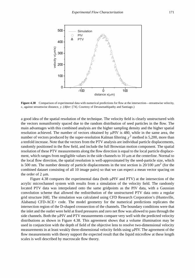
Experimental Flow Characterization 171
Figure 4.38 Comparison of experimental data with numerical predictions for flow at the intersection—streamwise velocity,v, against streamwise distance,y. (After: [74]. Courtesy of Devasenathipathy and Santiago.)
a good idea of the spatial resolution of the technique. The velocity field is clearly unstructured withthe vectors nonuniformly spaced due to the random distribution of seed particles in the flow. Themain advantages with this combined analysis are the higher sampling density and the higher spatialresolution achieved. The number of vectors obtained byµPIV is 480, while in the same area, thenumber of vectors produced by the super-resolution Kalman filteringχ2 method is 5,200, more thana tenfold increase. Note that the vectors from the PTV analysis are individual particle displacements,randomly positioned in the flow field, and include the full Brownian motion component. The spatialresolution of these PTV measurements along the flow direction is equal to the local particle displace-ment, which ranges from negligible values in the side channels to 10µm at the centerline. Normal tothe local flow direction, the spatial resolution is well-approximated by the seed-particle size, whichis 500 nm. The number density of particle displacements in the test section is 20/100µm2 (for thecombined dataset consisting of all 10 image pairs) so that we can expect a mean vector spacing onthe order of 2µm.
Figure 4.38 compares the experimental data (bothµPIV and PTV) at the intersection of theacrylic microchannel system with results from a simulation of the velocity field. The randomlylocated PTV data was interpolated onto the same gridpoints as the PIV data, with a Gaussianconvolution scheme that allowed the redistribution of the unstructured PTV data onto a regulargrid structure [68]. The simulation was calculated using CFD Research Corporation’s (Huntsville,Alabama) CFD-ACE+ code. The model geometry for the numerical predictions replicates theintersection region of the D-shaped crosssection of the channels. The boundary conditions were thatthe inlet and the outlet were held at fixed pressures and zero net flow was allowed to pass through theside channels. Both theµPIV and PTV measurements compare very well with the predicted velocitydistributions as shown in Figure 4.38. This agreement shows that a volume illumination may beused in conjunction with the depth of field of the objective lens to resolve two-dimensional velocitymeasurements in at least weakly three-dimensional velocity fields usingµPIV. The agreement of theflow measurements with theory support the expected result that the liquid microflow at these lengthscales is well described by macroscale flow theory.

172 Fundamentals and Applications of Microfluidics
Problems
4.1 Compute the particle response times for polystyrene latex seed particles (ρp = 1,050 kg/m3)suspended in water (η = 10−3 kg/ms). Consider particle diameters of 1µm, 300 nm, and 100nm.
4.2 Compute the diffusion coefficientD for a 300-nm polystyrene latex seed particle in water atroom temperature. Given a flow speed of 10 mm/s and 10 particles in an interrogation region,what1t is required to achieve 10% relative error? 1% relative error?
4.3 Given aµPIV imaging system consisting of a 40× magnification, air-immersion lens, 0.7 NAmicroscope objective, and 600-nm illumination, what is the depth of correlation for particles ofdiameters 1µm, 300 nm, and 100 nm?
4.4 What particle concentration will give a signal-to-noise ratio of 1.5 in a 50-µm-deep microchan-nel (Table 4.6)? What are the characteristics of the imaging system necessary to achieve thissignal-to-noise ratio? What happens to the signal-to-noise ratio if this particle concentration isused in a channel that is 150µm deep?
4.5 What are several methods that can be used to compensate for having too few particles in aµPIVvelocity measurement? What are their respective advantages and disadvantages?
4.6 A flow of water carries 500-nm seed particles that are imaged using a 50× magnification lensand a1t of 100 ms. TheµPIV autocorrelation peak is found to measure 5 pixels in diameterand the cross-correlation peak is found to measure 7 pixels in diameter. What is temperature-to-viscosity ratio (T/η) for this flow? How would you determine the temperature from thisinformation?
4.7 Given a 500-nm particle being imaged with 500-nm light, by what fraction is the elasticscattering intensityI increased or decreased when the wavelength of the illumination isdoubled? How isI changed when the particle diameter is reduced to 100 nm?
References
[1] Bayt, R. L., and Breuer, K. S., “Fabrication and Testing of Micron-Sized Cold-Gas Thrusters In Micropropulsion ofSmall Spacecraft,”Advances in Aeronautics and Astronautics, Vol. 187, pp. 381–398. Eds. Micci, M & Ketsdever, A.AIAA Press. Washington, D.C., 2001.
[2] Kamisuki S., et al., “A Low Power, Small, Electrostatically-Driven Commercial Inkjet Head,”Proceedings ofMEMS’98, 11th IEEE International Workshop Micro Electromechanical System, Heidelberg, Germany, Jan. 25-29,1998, pp. 63–68.
[3] Northrup, M. A., et al., “A MEMS-Based DNA Analysis System,”Proceedings of Transducers ’95, 8th InternationalConference on Solid-State Sensors and Actuators, Stockholm, Sweden, June 16-19, 1995, pp. 764–767.
[4] Lanzillotto, A. M., et al., “Applications of X-Ray Micro-Imaging, Visualization and Motion Analysis Techniques toFluidic Microsystems,”Technical Digest of the IEEE Solid State Sensor and Actuator Workshop, Hilton Head Island,SC, June 3–6, 1996, pp. 123–126.
[5] Chen, Z., et al., “Optical Doppler Tomographic Imaging of Fluid Flow Velocity in Highly Scattering Media,”OpticsLetters, Vol. 22, 1997, pp. 64–66.
[6] Compton, D. A., and Eaton, J. K., “A High-Resolution Laser Doppler Anemometer for Three-Dimensional TurbulentBoundary Layers,”Exp. Fluids, Vol. 22, 1996, pp. 111–117.

Experimental Flow Characterization 173
[7] Tieu, A. K., Mackenzie, M. R., and Li, E. B., “Measurements in Microscopic Flow with a Solid-State LDA,”Exp.Fluids, Vol. 19, 1995, pp. 293–294.
[8] Gharib M, et al., “Optical Microsensors for Fluid Flow Diagnostics,”AIAA, Aerospace Sciences Meeting and Exhibit,40th, Reno, NV, Jan. 14–17, AIAA Paper 2002–0252, 2002.
[9] Dahm, W. J. A., Su, and L. K., Southerland, K. B., “A Scalar Imaging Velocimetry Technique for Fully ResolvedFour-Dimensional Vector Velocity Field Measurements in Turbulent Flows,”Physics of Fluids A (Fluid Dynamics),Vol. 4, No. 10, 1992, pp. 2191–2206.
[10] Paul, P. H., Garguilo, M. G., and Rakestraw, D. J., “Imaging of Pressure- and Electrokinetically Driven Flows ThroughOpen Capillaries,”Anal. Chem., Vol. 70, 1998, pp. 2459–2467.
[11] Koochesfahani, M. M., et al., “Molecular Tagging Diagnostics for the Study of Kinematics and Mixing in Liquid PhaseFlows,” Developments in Laser Techniques in Fluid Mechanics, R. J. Adrian et al. (eds.), New York: Springer-Verlag,1997, pp. 125–134.
[12] Maynes, D., and Webb, A. R., “Velocity Profile Characterization in Sub-Millimeter Diameter Tubes Using MolecularTagging Velocimetry,”Exp. Fluids, Vol. 32, 2002, pp. 3–15.
[13] Lempert, W. R., et al., “Molecular Tagging Velocimetry Measurements in Supersonic Micro Nozzles,”Proceedings of39th AIAA Aerospace Sciences Meeting and Exhibit, Reno, NV, Jan. 8–11, 2001, pp. 2001–2044.
[14] Wildes, R. P., et al., “Physically Based Fluid Flow Recovery from Image Sequences,”Proceedings of IEEE ComputerSociety Conference on Computer Vision and Pattern Recognition, Los Alamitos, CA, June 17–19, 1997, pp. 969–975.
[15] Leu, T. S., et al., “Analysis of Fluidic and Mechanical Motions in MEMS by Using High Speed X-Ray Micro-ImagingTechniques,”Proceedings of Transducers ’97, 9th International Conference on Solid-State Sensors and Actuators,Chicago, IL, June 16–19, 1997, pp. 149–150.
[16] Hitt, D. L., et al., “A New Method for Blood Velocimetry in the Microcirculation,”Microcirculation, Vol. 3, No. 3,1996, pp. 259–263.
[17] Hitt, D. L., Lowe M. L., and Newcomer, R., “Application of Optical Flow Techniques to Flow Velocimetry,”Phys.Fluids, Vol. 7, No. 1, 1995, pp. 6–8.
[18] Adrian, R. J.,Bibliography of Particle Image Velocimetry Using Imaging Methods: 1917-1995, Urbana, IL: Universityof Illinois at Urbana-Champaign, 1996.
[19] Raffel, M., Willert, C., and Kompenhans, J.,Particle Image Velocimetry: A Practical Guide, New York: Springer,1998.
[20] Santiago, J. G., et al., “A Particle Image Velocimetry System for Microfluidics,”Exp. Fluids, Vol. 25, 1998, pp. 316–319.
[21] Koutsiaris, A. G., Mathioulakis, D. S., and Tsangaris, S., “Microscope PIV for Velocity-Field Measurement of ParticleSuspensions Flowing Inside Glass Capillaries,”Meas. Sci. Technol., Vol. 10, 1999, pp. 1037–1046.
[22] Meinhart, C. D., Wereley, S. T., and Santiago, J. G., “PIV Measurements of a Microchannel Flow,”Exp. Fluids, Vol.27, 1999, pp. 414–419.
[23] Meinhart, C. D., and Zhang, H., “The Flow Structure Inside a Microfabricated Inkjet Printer Head,”J. Microelec-tromechanical Systems, Vol. 9, 2000, pp. 67–75.
[24] Meinhart, C. D., Wereley, S. T., and Santiago, J. G., “Micron-Resolution Velocimetry Techniques,”Laser TechniquesApplied to Fluid Mechanics, R. J. Adrian et al. (eds.), New York: Springer-Verlag, 2000, pp. 57–70.
[25] Born, M., and Wolf, E.,Principles of Optics, New York: Pergamon Press, 1997.
[26] Kim, Y. H., Wereley, S.T. and Chun, C.H., “Phase-resolved flow field produced by a vibrating cantilever plate betweentwo endplates,”Phys. Fluids, Vol. 16, 2004, pp. 145–162.
[27] Adrian, R. J., “Particle-Imaging Techniques for Experimental Fluid Mechanics,”Annual Review of Fluid Mechanics,Vol. 23, 1991, pp. 261–304.

174 Fundamentals and Applications of Microfluidics
[28] Meinhart, C. D. and Wereley, S. T., “Theory of Diffraction-Limited Resolution in Micro Particle Image Velocimetry,”Meas. Sci. Technol., Vol. 14, 2003, pp. 1047–1053.
[29] Olsen, M. G., and Adrian, R. J., “Out-of-Focus Effects on Particle Image Visibility and Correlation in Particle ImageVelocimetry,”Exp. Fluids [Suppl.], 2000, pp. 166–174.
[30] Wereley, S. T. and Meinhart, C. D., “Micron-Resolution Particle Image Velocimetry” inMicro- and Nano-ScaleDiagnostic Techniques, K. S. Breuer (ed.), Springer-Verlag, New York, 2005.
[31] Adrian, R. J., and Yao, C. S., “Pulsed Laser Technique Application to Liquid and Gaseous Flows and the ScatteringPower of Seed Materials,”Applied Optics, Vol. 24, 1985, pp. 44–52.
[32] Prasad, A. K., Adrian, R. J., Landreth, C. C., and Offutt, P. W., “Effect of resolution on the speed and accuracy ofparticle image velocimetry interrogation,”Exp. Fluids, Vol. 13, 1992, pp. 105–116.
[33] Cummings, E. B., “An Image Processing and Optimal Nonlinear Filtering Technique for PIV of Microflows,”Exp.Fluids, Vol. 29 [Suppl.], 2001, pp. 42–50.
[34] Meinhart, C. D., Wereley S. T., and Gray, M. H. B., “Depth Effects in Volume Illuminated Particle Image Velocimetry,”Meas. Sci. Technol., Vol. 11, 2000, pp. 809–814.
[35] Inoue, S., and Spring, K. R.,Video Microscopy, 2nd ed., New York: Plenum Press, 1997.
[36] Bourdon, C. J., Olsen, M. G. and Gorby, A. D., “Validation of an analytical solution for depth of correlation inmicroscopic particle image velocimetry,”Meas. Sci. Technol., Vol. 15, 2004, pp. 318-327.
[37] Beskok, A., Karniadakis, G., E., and Trimmer, W., “Rarefaction and Compressibility,”Journal of Fluids Engineering,Vol. 118, 1996, pp. 448–456.
[38] Melling, A., Seeding Gas Flows for Laser Anemometry, 1986.
[39] Probstein, R. F.,Physicochemical Hydrodynamics: An Introduction, New York: Wiley, 1994.
[40] Van Kampen, N. G.,Stochastic Processes in Physics and Chemistry, Amsterdam: Elsevier, 1997.
[41] Einstein, A., “On the Movement of Small Particles Suspended in a Stationary Liquid Demanded by the Molecular-Kinetic Theory of Heat,”Theory of Brownian Movement, New York: Dover, 1905, pp. 1–18.
[42] Bendat, J. S., and Piersol, J. G.,Random Data: Analysis and Measurement Procedures, New York: Wiley, 1986.
[43] Wereley, S. T., Gui, L., and Meinhart, C. D., “Advanced Algorithms for Microscale Particle Image Velocimetry,”AIAAJ., Vol. 40, 2002, pp. 1047–1055.
[44] Gui L., Merzkirch, W., and Shu, J. Z., “Evaluation of Low Image Density PIV Recordings with the MQD Method andApplication to the Flow in a Liquid Bridge,”J. Flow Vis. And Image Proc., Vol. 4, No. 4, 1997, pp. 333–343.
[45] Meinhart, C. D., Wereley, S. T., and Santiago, J. G., “A PIV Algorithm for Estimating Time-Averaged Velocity Fields,”Journal of Fluids Engineering, Vol. 122, 2000, pp. 285–289.
[46] Gomez, R., et al., “Microfluidic Biochip for Impedance Spectroscopy of Biological Species,”Biomedical Microde-vices, Vol. 3, No. 3, 2001, pp. 201–209.
[47] Cowen, E. A., and Monismith, S. G., “A Hybrid Digital Particle Tracking Velocimetry Technique,”Exp. Fluids, Vol.22, 1997, pp. 199–211.
[48] Wereley, S. T., et al., “Velocimetry for MEMS Applications,”Proc. of ASME/DSC Vol. 66, Micro-fluidics Symposium,Anaheim, CA, Nov. 1998, pp. 453–459.
[49] Wereley S. T., and Meinhart, C. D., “Adaptive Second-Order Accurate Particle Image Velocimetry,”Exp. Fluids, Vol.31, 2001, pp. 258–268.
[50] Wereley, S.T., and Gui, L.C., “PIV Measurement in a Four-Roll-Mill Flow with a Central Difference Image Correction(CDIC) Method,”Proceedings of 4th International Symposium on Particle Image Velocimetry, Gttingen, Germany,Sept. 2001, paper number 1027.

Experimental Flow Characterization 175
[51] Meinhart C. D., Gray, M. H. B., and Wereley, S. T., “PIV Measurements of High-Speed Flows in Silicon-Micromachined Nozzles,” AIAA-99-3756,Proceedings of 35th AIAA/ASME/SAE/ASEE Joint Propulsion Conferenceand Exhibit, Los Angeles, CA, June 20–24, 1999.
[52] Deen, W.,Analysis of Transport Phenomena, New York: Oxford University Press, 1998.
[53] Batchelor, G. K.,An Introduction to Fluid Dynamics, Cambridge, England: Cambridge University Press, 1987.
[54] Wereley S. T., Gui, L., and Meinhart, C. D., “Flow Measurement Techniques for the Microfrontier,” AIAA,AerospaceSciences Meeting and Exhibit, 39th, Reno, NV, Jan. 8–11, 2001, AIAA Paper 2001-0243.
[55] Wiesendanger, R.,Scanning Probe Microscopy and Spectroscopy: Methods and Applications, Cambridge, England:Cambridge University Press, 1994.
[56] Revenco, I., and Proksch, R., “Magnetic and Acoustic Tapping Mode Microscopy of Liquid Phase PhospholipidBilayers and DNA Molecules,”J. App. Phys., Vol. 87, 2000, pp. 526–533.
[57] Stone, S. W., Meinhart, C.D., and Wereley, S.T., “A Microfluidic-Based Nanoscope,”Exp. Fluids, Vol. 33, No. 5, 2002,613–619.
[58] Kataoka, K., et al., “Totally Synthetic Polymer Gels Responding to External Glucose Concentration: Their Preparationand Application to On-Off Regulation of Insulin Release,”J. Am. Chem. Soc., Vol. 120, 1998, pp. 12694–12695.
[59] Osada, Y., and Ross-Murphy, S., “Intelligent Gels,”Scientific American, Vol. 268, 1993, pp. 82–87.
[60] Liu, R., et al., “In-Channel Processing to Create Autonomous Hydrogel Microvalves,”Micro Total Analysis Systems2000, A. van den Berg et. al. (eds.), Boston, MA: Kluwer Academic Publishers, 2000, pp. 45–48.
[61] Madou, M., He, K., and Shenderova, A. “Fabrication of Artificial Muscle Based Valves for Controlled Drug Delivery,”Micro Total Analysis Systems 2000, A. van den Berg et. al. (eds.), Boston, MA: Kluwer Academic Publishers, 2000,pp. 147–150.
[62] Olsen, M. G., Bauer, J. M., and Beebe, D. J., “Particle Imaging Technique for Measuring the Deformation Rate ofHydrogel Microstructures,”Applied Physics Letters, Vol. 76, 2000, pp. 3310–3312.
[63] Beebe, D. J., et al., “Functional Hydrogel Structures for Autonomous Flow Control Inside Microfluidic Channels,”Nature, Vol. 404, 2000, pp. 588–590.
[64] Fujisawa, N., and Adrian, R. J., “Three-Dimensional Temperature Measurement in Turbulent Thermal Convection byExtended Range Scanning Liquid Crystal Thermometry,”Journal of Visualization, Vol. 1, No. 4, 1999, pp. 355–364.
[65] Sakakibara, J., and Adrian, R. J., “Whole Field Measurement of Temperature in Water Using Two-Color Laser InducedFluorescence,”Experiments in Fluids, Vol. 26, No.1–2, 1999, pp. 7–15.
[66] Olsen, M. G., and Adrian, R. J., “Brownian Motion and Correlation in Particle Image Velocimetry,”Optics and LaserTech., Vol. 32, 2000, pp. 621–627.
[67] Keane, R. D., and Adrian, R. J., “Theory of Cross-Correlation Analysis of PIV Images,”Applied Scientific Research,Vol. 49, 1992, pp. 1–27.
[68] Keane, R. D., Adrian, R. J., and Zhang. Y., “Super-Resolution Particle Imaging Velocimetry,”Measurement ScienceTechnology, Vol. 6, 1995, pp. 754–768.
[69] Chandrasekhar, S., “Stochastic Problems in Physics and Astronomy,”Review of Modern Physics, Vol. 15, 1941, pp.1–89.
[70] Edwards, R., et al., “Spectral Analysis from the Laser Doppler Flowmeter: Time-Independent Systems,”Journal ofApplied Physics, Vol. 42, 1971, pp. 837–850.
[71] Han, G. and Breuer, K. S., “Infrared PIV for Measurement of Fluid and Solid Motion Inside Opaque SiliconMicrodevices,”Proceedings of 4th International Symposium on Particle Image Velocimetry, Gttingen, Germany, Sept.2001, paper number 1146.

176 Fundamentals and Applications of Microfluidics
[72] Guezennec, Y. G., et al., “Algorithms for Fully Automated 3-Dimensional Particle Tracking Velocimetry,”Exp. Fluids,Vol. 17, 1994, pp. 209–219.
[73] Ohmi, K., and Li, H. Y., “Particle-Tracking Velocimetry with New Algorithm,”Measurement Science Technology,Vol. 11, 2000, pp. 603–616.
[74] Devasenathipathy, S., et al., “Particle Tracking Techniques for Microfabricated Fluidic Systems,”Exp. Fluids, 2002,in press.
[75] Takehara, K., et al., “A Kalman Tracker for Super-Resolution PIV,”Exp. Fluids, Vol. 29, 2000, pp. 34–41.

Chapter 5
Microfluidics for External Flow Control
5.1 VELOCITY AND TURBULENCE MEASUREMENT
In a turbulent regime, tiny flow structures are responsible for viscous drag increase of aerodynamicsurfaces, such as wings and engine inlet ducts in an aircraft. These structures are called eddies.Eddies are typically several hundred microns in width and several millimeters in length. The lengthscale of eddies is broad, ranging from the same size as the width of the flow field to the microscale,where viscous effects become dominant and energy is transferred from kinetic into internal [1].
Beside the small sizes, the short lifetime of eddies also pose a challenge for measurement andcontrol. The lifetime of eddies is on the order of milliseconds [2]. Conventional instruments withlow response time are not able to detect such a fast dynamic.
Because of their small size, micromachined devices are suitable for measuring and manipu-lating eddies in a turbulent flow. In addition to the spatial and temporal advantages, micromachinedsensors and actuators can be integrated with microelectronics, which make them “smart.” The smallsize and the batch machining process allow fabricating arrays of such devices, which can give moredetailed information about the flow field.
The following sections discuss the design of microsensors for velocity and turbulence mea-surement. In contrast to the flow sensors in Chapter 8, velocity measurement in this section is re-ferred to as point velocity measurement. The other type of turbulence measurement is shear stresssensing on walls. Although flow sensors, velocity sensors, and shear stress sensors serve differentpurposes, they can share the same operation concept and design. For example, hot-film and hot-wiresensors can be used for measuring both flow velocity and shear stress. In order to avoid redundancy,Section 5.1.1 focuses on design considerations with illustrating calculation examples, while Section5.1.2 and Chapter 8 deal with design examples of thermal shear stress sensors and thermal flowsensors, respectively.
5.1.1 Velocity Sensors
5.1.1.1 Design Considerations
The two common sensor types of classical point velocity measurement are Pitot-probe anemometerand thermal anemometer. The Pitot probe utilizes the dependence of the static pressure on thevelocity:
1p =ρu2
2(5.1)
whereρ is the fluid density,u is the flow velocity, and1p is the pressure drop across the Pitottube as shown in Figure 5.1(a). In microscale, the design of a Pitot probe becomes the design ofmicropressure sensors. Examples for designing pressure sensors are discussed in Section 8.1.
177

178 Fundamentals and Applications of Microfluidics
u
�p Pitot tube
Pressure sensor
Impact hole
Static hole(a)
u
(b)
Hot wire
Figure 5.1 Velocity sensors: (a) Pitot-probe anemometer; and (b) thermal anemometer (hot wire).
The thermal anemometer measures flow velocities based on the correlation between velocityand heat transfer. Figure 5.1(b) depicts a conventional hot-wire anemometer. The sensor consistsof a heater, which is a thin wire made of platinum or tungsten. The typical diameter of the wireranges from 5 to 25µm. The wire is 1 to 3 mm long. The resistance of the wire is typically onthe order of several tens of ohms. Using a temperature sensor as the reference, the wire can becontrolled at a constant wire temperature or at a constant heating power. The corresponding electricpowers (in the case of constant temperature) or the wire temperatures (in the case of constant heatingpower) are related directly to the flow velocities. In terms of spatial and temporal resolutions, thermalanemometry has more advantages. A micro hot wire fabricated in silicon can resolve few micronsin space and few microseconds in time. Electrothermal behavior of a hot wire is analyzed in thefollowing examples.
Example 5.1: Characteristics of a Hot-Wire Sensor
A polycrystalline silicon wire with a length ofL = 50 µm and a cross section ofA = 2× 5 µmis used as a hot-wire sensor. The temperature coefficient and thermal conductivity of polysiliconare 8× 10⁻⁴ K−1 and 32 Wm−1K−1, respectively. The bulk substrate temperature is 25◦C. Theresistivity of polysilicon at 25◦C is 4× 10⁻⁵ Wm. Determine the maximum temperature of thewire and its resistance at a current of 10 mA.
Solution. With the temperatureT as a function ofx, κ the thermal conductivity of the wire, andρits resistivity, the energy balance between the flux and heat generated by the current is describedas:
−κA[T ′(x +1x)− T ′(x)] = I 2R = I 2 ρ1xA
−κA [T ′(x+1x)−T ′(x)]1x = I 2 ρ
A
−κAT′′= I 2 ρ
A
−κAT′′=
I 2
A2ρ
−κAT′′= J2ρ
whereJ = I /A is the current density in the wire. We assume that resistivity is a linear functionof temperature with a temperature coefficient ofα:
ρ = ρ0[1 + α(T − T0)]
Thus, the final differential equation describing the heat balance has the form:
κT ′′= J2ρ0[1 + α(T − T0)]

Microfluidics for External Flow Control 179
Solving the above equation with boundary condition ofT(0) = T(L) = Tb, one gets [3]:
T(x) =
(T0 −
1
α
)+
(Tb − T0 +
1
α
) cos[β
(2xL − 1
)]cosβ
with:
β =J L
2
√αρ0
κ=
10−2× 5 × 10−5
2 × 2 × 5 × 10−12
√8 × 10−4 × 4 × 10−5
31= 0.79 rad
The maximum temperature at the wire center is:
Tmax = T(L/2) =
(T0 −
1
α
)+
(Tb − T0 +
1α
)cosβ
Tmax =
(25−
1
8 × 10⁻⁴
)+
(25− 25+
18×10−4
)cos 0.79
The resistance of the wire is:
R =
∫ L
0
ρ(x)
Adx =
ρ0L
A[1 + α(Tb − T0)]
tanβ
β+ R0
Assuming thatR0 is zero, the resistance of the wire at 10 mA is:
R =4 × 10−5
× 5 × 10−5
2 × 5 × 10−12[1 + 8 × 10−4
× (552− 25)]tan 0.79
0.79
Example 5.2: Characteristics of a Hot-Wire Sensor, Simplified Approach
For the hot wire of Example 5.1, determine the maximum temperature, and its resistance, byassuming constant resistivity. Compare the results with Example 5.1 and estimate the thermaltime constant of the wire. The thermal diffusivity of polysilicon is 1.85×10⁻⁵ m2/s.
Solution. We start with the governing differential equation:
−κT ′′= J2ρ
Solving the above equation by assuming a quadratic trial function and constant resistivity, we get[4]:
T(x) = Tb + Tmax
[1 −
(2x
L− 1
)2]
where the maximum temperature at the center of the wire is:
Tmax =I 2ρ0L2
8A2κ=(10−2)2 × 4 × 10−5
× (5 × 10−5)2
8 × (2 × 5 × 10−12)2 × 32= 391◦C

180 Fundamentals and Applications of Microfluidics
Using the quadratic temperature profile above, the resistance at the given condition (Tb = T0 =
25◦C) can be estimated as:
R =1
A
∫ L
0ρ0[1 + α(T(x)− T0)] =
ρ0L
A
[1 +
2
3α(Tmax − Tb)
]
R =4 × 10−5
× 5 × 10−5
2 × 5 × 10−12
[1 +
2
3× 8 × 10−4(391− 25)
]= 239�
Compared to the exact solution in Example 5.1, the simplified model results in an error of 29%for the maximum temperature and an error of 34% for the resistance. For further simplification,the above parabolic profile can be developed to a Fourier series. Using the first eigenmode and anexponential cooling function, we have a transient trial function for the temperature profile:
T(x, t) = Tb + (Tmax − Tb) cos
(π(x − L/2)
L
)exp
(−t
τth
)whereτth is the thermal time constant of the wire. The partial differential equation describing thecooling (heating) process is [4]:
∂2T
∂x2=
cρ
κ
∂T
∂t
wherec is the specific heat of polysilicon. Using the above two equations, we get the estimatedtime constant of the wire as a function of the lengthL and thermal diffusivitya = κ/cρ :
τth =cρL2
π2κ=
L2
π2a=
(5 × 10⁻⁵)2
π2 × 1.85× 10−5s = 13.7 µs
Example 5.3: Characteristics of a Hot-Film Sensor
A hot-film sensor is made of a platinum heater on a thin silicon nitride membrane. Determine thetime function of the temperature distribution.
Solution. The partial differential equation describing the cooling (heating) process is (see Section2.2.2.2):
∂2T
∂x2+∂2T
∂y2=
cρ
κ
∂T
∂t
Solving the above equation, we get the simplified form of a temperature distribution of the hot-film plate:
T(x, t) = Tmaxcos(πx
w
)cos
(πy
L
)exp
(−t
τ
)whereTmax is the maximum temperature at the center of the membrane and−w/2 < x < w/2;−L/2< y < L/2.
5.1.1.2 Design Examples
The micromachined hot-wire anemometer reported in [5] has a free-standing polysilicon heater. Theheater wire is 0.5µm thick, 1µm wide, and 10 to 160µm long. Heating time and cooling time ofthe sensors are a few microseconds. With a 10-µm wire, the wire reaches its fastest time constantof 0.5µs, which corresponds to a temporal bandwidth of 1.4 MHz. More examples are discussed inSection 5.1.2.2 and in Chapter 8.

Microfluidics for External Flow Control 181
Flow U
(a)
Flow U
(b)
Preston tube
to pressure sensor
Flow U
(c)
Stanton tube
to pressure sensor
Razor blade
Magnet
Flow U
(d)
Hot film
Hot wire
Figure 5.2 Operation principles of shear stress sensor: (a) direct type with flush-mounted floating plate; (b) indirect typewith Preston tube for measuring the stagnation pressure; (c) indirect type with Stanton tube; and (d) indirect type based onheat and mass transfer.
5.1.2 Shear Stress Sensors
One of the most important requirements for external flow control is the measurement of wall shearstress. Phenomena such as viscous drag, transition from laminar to turbulence, flow separation, andturbulent eddies can be detected with a shear stress sensor. Micromachined shear stress sensors offerthe advantages of miniaturization for higher resolution and improved dynamics. Shear stress sensorscan be divided into two categories: direct and indirect types [6]. Figure 5.2 illustrates basic principlesof shear stress sensors.
The direct types measure local shear stress using a floating plate, which is flush-mountedon the wall bounding the flow [Figure 5.2(a)]. The shear force displaces the floating plate. Thedisplacement can then be measured capacitively, piezoresistively, or optically. The indirect typesmeasure shear stress by means of its subsequent effects, such as stagnation pressure, heat transfer,or near-wall velocity. The stagnation pressure type utilizes an obstacle embedded in the boundarylayer. The stagnation pressure caused by the obstacle increases with higher shear stress and can bemeasured with a pressure sensor. Figures 5.2(b, c) show two typical setups for this type: the Prestontube and the Stanton tube.
The heat-transfer type uses heat and mass transfer analogies to measure the correlationbetween measured properties and the actual shear stress [7]. The velocity type measures the near-wall velocity profile. The measurement requires multiple velocity sensors or optical techniques suchas PIV (see Chapter 4). Because of the external instruments, the third indirect type is not suitable foran integrated solution.
5.1.2.1 Design Considerations
Hot-film and hot-wire sensors are the simplest indirect shear-stress sensors, which can be imple-mented easily with micromachining technology. However, there are two drawbacks related to thisconcept.
The first drawback of thermal shear stress sensors is the dependence on empirical correlation,which requires extensive calibration measurements. The correlation function for the heating powerP of a hot-film sensor and the wall shear stressτw is given as [8]:
P = 1T(C0 + C1τ1/3w ) (5.2)

182 Fundamentals and Applications of Microfluidics
where1T is the temperature difference between the heater and the fluid, andC0 and C1 arecalibration constants.
Since sensor signals depend strongly on the thermal behavior of the sensor, the seconddrawback of hot-film sensors is the error caused by heat conduction into the sensor substrate. Carefulthermal insulation should be considered in the design of this sensor type.
Example 5.4: Influence of Thermal Insulation on Thermal Shear Stress Sensor
A thin-film heater with an overall dimension of 100× 100µm is deposited on a silicon substrateover an oxide layer. The sensor characteristics follow (5.2) withC0 = 10 mW/K andC1 = 1mW/K-Pa1/3. Estimate the thickness of silicon oxide. If the oxide layer is used as a sacrificiallayer and is etched away, how much would the heat ratio improve? The thermal conductivity ofsilicon oxide and air is 1.1 W/m−1K−1 and 0.0257 W/m−1K−1, respectively.
Solution. Following (5.2), we estimate that the offset1T × C0 is caused by heat conduction.In this analysis, we only consider the heat conduction to silicon substrate and assume that thesubstrate has the same temperature of the fluid.C0 represents the thermal conductance of thesilicon oxide layer:
C0 =κA
d→ d =
κA
C0=
1.1 × (10−4)2
10−2= 1.1 × 10⁻⁶m = 1.1 µm
If the gap is replaced by air, this factor would be:
C0,air =κairA
d=
0.0257× (10−4)2
1.1 × 10−6= 0.234× 10⁻³ W = 0.234 mW
Thus, the ratioC1/C0 improves:
C1/C0,air
C1/C0=
C0
C0,air≈ 43 times
Designing other indirect sensors, which are based on the measurement of stagnation pressure,leads to the development of pressure sensors. However, the realization of an obstacle and the pressuresensors make the design complex and impractical.
The most suitable technique for micromachining is direct sensing with a floating elementflush-mounted in the wall. Refer to [6] for detailed considerations of floating element sensors. Thedesign problems associated with this sensor type are discussed here.
The presence of a gap around the floating element can disturb the flow field and cause errorsin the measurement. The error can be neglected if the gap is smaller than the characteristic lengthl :
l =ν
uτ(5.3)
whereν is kinematic viscosity of the fluid, anduτ is the friction velocity:
uτ =
√τw
ρ(5.4)
whereρ is fluid density and the wall shear stressτw:
τw ≈ 0.03ρu2
Re(x)0.2(5.5)

Microfluidics for External Flow Control 183
Flow U zh
t
g
l
Figure 5.3 Geometry parameters of a floating-element shear stress sensor.
The Reynolds number Re(x) based on streamwise distancex is defined as:
Re(x) =ux
ν(5.6)
whereu is the free-stream velocity. If the floating element is not perfectly flush-mounted on the wall,the resulting drag force can lead to the error1τw [6]:
1w
τw=
ρz3
3(η2L2e)
(5.7)
wherez is the misalignment of the floating element,Le is the streamwise length of the floatingelement, andη is the dynamic viscosity.
The pressure gradient along the floating element can cause further error1τw, which isdetermined by the geometry of the sensor [6]:
1w
τw=
g
h+
2t
h(5.8)
The geometry parameters are defined in Figure 5.3. Further error sources are the acceleration of thefloating element, fluctuation of the normal pressure, and temperature dependence [6].
Example 5.5: Typical Parameters of a Floating-Element Shear Stress Sensor
A floating-element shear stress sensor is flush-mounted on a flat plate at a distance of 1m fromthe plate front. The free stream velocity is 10 m/s. Determine the Reynolds number at themeasurement position and the shear stress expected at this position. What is the largest gapallowable around the floating element? Kinematic viscosity and density of air are assumed tobe 1.6×10⁻⁵ m2/s and 1.164 kg/m3, respectively.
Solution. According to (5.6), the Reynolds number at the measurement position is:
Re(x) =ux
ν=
10× 1
1.6 × 10−5= 6.25× 10⁵
According to (5.5), the shear stress expected for this position is:
τw ≈ 0.03ρu2
Re(x)0.2= 0.03×
1.164× 102
(6.25× 10⁵)0.2≈ 0.24 Pa

184 Fundamentals and Applications of Microfluidics
For this shear stress and Reynolds number, the largest gap allowed for the floating element is:
l =ν
uτ=
ν√τw/ρ
= 35× 10−6 m = 35µm
Example 5.6: Errors Related to Geometrical Parameters
If the floating element of the above sensor is 5 mm long and the plate is mounted 20µm too highinto the flow, determine the measurement error caused by the drag force.
Solution. The dynamic viscosity of the air is:
η = νρ = 1.6 × 10−5× 1.164= 1.8624× 10⁻⁵ Ns/m2
According to (5.7), the error due to drag force is:
1τw = τwρz3
3η2L2e
= 0.241.164× (20× 10−6)3
3 × (1.8624× 10−5)2 × (5 × 10−3)2= 8.66× 10⁻² Pa
The drag error is about 36%, and it cannot be neglected.
Example 5.7: Designing an Optical Floating-Element Shear Stress Sensor
The above sensor is made of a silicon plate with a dimension of 1× 1 mm. The plate is suspendedon four flexures as shown in the figure below. The exposed width of each of the photodiodes is10µm. Design the flexures so that the velocity in Example 5.5 results in a change of 100% in thephotocurrent.
u = 10m/s
L
w =5�m
1 mm
x
y
�x
D1 D2
Light
�x
Photodiodes
Solution. The shear force acted on the floating plate at 10 m/s is:
Fp = τw A = 0.24× (10−3)2 = 0.24× 10⁻⁶ N
Assuming that the force is distributed equally among four flexures, each of them has a load of:
Ff =Fp
4=
0.24× 10⁻⁶
4= 0.06× 10⁻⁶ N
In order to use the small deflection theory of beams, we choose a flexure width oft = 5 µm anda thickness ofw = 10µm. The displacement of a beam with a tip guide is (see Appendix D):
1x =Ff L3
Ewt3

Microfluidics for External Flow Control 185
The change of light-induced current is proportional to the displaced area:
1I
I=
21x
wdiode= 100%→ 1x =
wdiode
2= 5 µm
Thus, the required length of the flexure is:
L =3
√E1xwt3
Ff=
3
√170× 109 × 5 × 10× 53 × (10−6)5
0.06× 10−6= 26× 10−4 m = 2.6 mm
Example 5.8: Designing a Piezoresistive Floating-Element Shear Stress Sensor
If piezoresistors are integrated on the sides of the four flexures in the above sensor, is the resistancechange measurable?
Solution. The deflection of a beam with a guided tip can be described as (see Appendix D):
F
u = 10 m/s
LW
y
x
Piezoresistive sensor
y
x
x(y) =F
2E I
(−y3
3+
Ly2
2
)The function of the radius of curvature can be described as:
1
r (y)=
d2x
dy2=
F
2E I(−2y + L)
Thus, the strain along the beam is:
ϕ(y) =t
2r (y)=
Ft
4E I(−2y + L)
The maximum strain at the beam endx = 0 is:
ϕmax = ε(0) =Ft L
4E I=
3Ft L
Ewt3=
3F L
Ewt2
Assuming a piezoresistive coefficient of 100, we get the change of a resistor integrated on thebeam end:
1R
R= 100ϕmax = 100×
3F L
Ewt2= 100×
3 × 0.06× 10−6× 2.6 × 10−3
170× 109 × 10−5 × (5 × 10−6)2= 0.0011= 0.11%
The change of 0.11% is small but measurable.

186 Fundamentals and Applications of Microfluidics
Example 5.9: Designing a Capacitive Floating-Element Shear Stress Sensor
If the floating plate is used as an electrode of a capacitor, what is the change of the capacitance?
Solution. The capacitance of a parallel plate capacitor of a dimensionW × L and a gapd is:
d
u = 10 m/s
LWL
�x
Thus, the capacitance is proportional to the plate length. The capacitance change is proportionalto the displacement:
1C
C=1x
L=
5 × 10⁻⁶
10−3= 5 × 10−3
= 0.5%
5.1.2.2 Design Examples
Thermal Shear Stress Sensors.A hot-film flow sensor can be used as a thermal shear-stress sensor[8]. The sensor has thermopiles as temperature sensors. Due to the large heat capacity of thesubstrate, the sensor has a very low bandwidth (see Example 5.2) [Figure 5.4(a)]. Using a hotwire with smaller geometry and better thermal isolation, higher bandwidth up to 500 Hz can beachieved [9] [Figure 5.4(b)]. Smaller polysilicon wires with widths on the order of 1µm can increasebandwidth up to 500 kHz [3].
An array of micromachined hot wires can measure the distribution of wall stress over thesensor surface. Such a sensor array can resolve a spatial distribution of 300µm and a temporalbandwidth of 30 kHz [10]. Several design variations are shown in Figures 5.4(c–f).
The design illustrated in Figure 5.4(c) has a 2-µm deep vacuum cavity and a 0.25-µm-thickpolysilicon wire embedded in the nitride membrane. The design of Figure 5.4(d) is similar tothat shown in Figure 5.4(c)—the polysilicon wire stands up 4µm above the nitride membrane.Consequently, better thermal isolation can be achieved. The design shown in Figure 5.4(e) is similarto that of Figure 5.4(d), but there is no vacuum cavity. The design shown in Figure 5.4(f) is aconventional hot-wire design with a freestanding polysilicon bridge.
The sensor presented in [11] uses diodes as temperature sensors and is able to measure up to40 kHz. The sensor is fabricated with SOI technology. The bottom wafer is etched to the siliconoxide layer to form an isolation membrane. An isolation trench is etched into the top wafer, and thetrench is then filled with polyimide. The heater is a polysilicon resistor located inside the isolationtrench. An integrated diode detects the temperature [Figure 5.4(g)].
Since most of the airfoil objects have a curved form, there is a need of a flexible sensoror sensor arrays, which can attach smoothly to curved surfaces. Developments at University ofCalifornia at Los Angeles and California Institute of Technology led to a new technology calledflexible skin. These flexible sensor arrays are silicon islands, which are connected by a flexiblepolyimide membrane [Figure 5.4(h)]. The array consists of 32 thermal shear stress sensors, whichare able to wrap around a 0.5-inch edge radius. This array can detect the separation line on therounded leading edge of a delta wing. The information is crucial for employing microactuators tocontrol a delta-wing aircraft [12].

Microfluidics for External Flow Control 187
(a)(b)
(c) (d)
(e) (f)
(g)
Silicon
Nitride
Oxide
Aluminum
PolySi
DopedSilicon
aaaaaaaaaaaaaaaaaaaaaaaaaaaaaaaaaaaaaaaaaaaaaaaaaaaaaaaaaaaaaaaaaaaaaaaaaaaaa
Polyimide
aaaaaaaaaaaaaaaaaaaaaaaaaaaaaaaaaaaaaaaaaaaaaaaaaaaaaaaaaaaaaaaaaaaaaaaaaaaaaaaaaaaaaaaaaaaaaaaaaaaaaaaaaaaaaaaaaaaaaaaaaaaaaaaaaaaaaaaaaaaaaaaaaaaaaaaaaaaaaaaaaaaaaaaaaaaaaaaaaaaaaaaaaaaaaaaaaaaaaaaaaaaaaaaaaaaaaaaaaaaaaaaaaaaaaaaaaaaaaaaaaaaaaaaaaaaa
aaaaaaaaaaaaaaaaaaaaaaaaaaaaaaaaaaaaaaaaaaaaaaaaaaaaaaaaaaaaaaaaaaaaaaaaaaaaaaaaaaaaaaaaaaaaaaaaaaaaaaaaaaaaaaaaaaaaaaaaaaaaaaaaaaaaaaaaaaaaaaaaaaaaaaaaaaaaaaaaaaaaaaaaaaaaaaaaaaaaaaaaaaaaaaaaaaaaaaaaaaaaaaaaaaaaaaaaaaaaaaaaaaaaaaaaaaaaaaaaaaaaaaaaaaaaaaaaaaaaaaaaaaaaaaaaaaaaaaaaaaaaaaaaaaaaaaaaaaaaaaaaaaaaaaaaaaaaaaaaaaaaaaaaaaaaaaaaaaaaaaaaaaaaaaaaaaaaaaaaaaaaaaaaaaaaaaaaaaaaaaaaaaaaaaaaaaaaaaaaaaaaaaaaaaaaaaaaaaaaaaaaaaaaaaaaaaaaaaaaaaaaaaaaaaaaaaaaaaaaaaaaaaaaaaaaaaaaaaaaaaaaaaaaaaaaaaaaaaaaaaaaaaaaaaaaaaaaaaaaaaaaaaaaaaaaaaaaaaaaaaaaaaaaaaaaaaaaaaaaaaaaaaaaaaaaaaaaaaaaaaaaaaaaaaaaaaaaaaaaaaaaaaaaaaaaaaaaaaaaaaaaaaaaaaaaaaaaaaaaaaaaaaaaaaaaaaaaaaaaaaaaaaaaaaaaaaaaaaaaaaaaaaaaaaaaaaaaaaaaaaaaaaaaaaaaaaaaaaaaaaaaaaaaaaaaaaaaaaaaaaaaaaaaaaaaaaaaaaaaaaaaaaaaaaaaaaaaaaaaaaaaaaaaaaaaaaaaaaaaaaaaaaaaaaaaaaaaaaaaaaaaaaaaaaaaaaaaaaaaaaaaaaaaaaaaaaaaaaaaaaaaaaaaaaaaaaaaaaaaaaaaaaaaaaaaaaaaaaaaaaaaaaaaaaaaaaaaaaaaaaaaaaaaaaaaaaaaaaaaaaaaaaaaaaaaaaaaaaaaaaaaaaaaaaaaaaaaaaaaaaaaaaaaaaaaaaaaaaaaaaaaaaaaaaaaaaaaaaaaaaaaaaaaaaaaaaaaaaaaaaaaaaaaaaaaaaaaaaaaaaaaaaaaaaaaaaaaaaaaaaaaaaaaaaaaaaaaaaaaaaaaaaaaaaaaaaaaaaaaaaaaaaaaaaaaaaaaaaaaaaaaaaaaaaaaaaaaaaaaaaaaaaaaaaaaaaaaaaaaaaaaaaaaaaaaaaaaaaaaaaaaaaaaaaaaaaaaaaaaaaaaaaaaaaaaaaaaaaaaaaaaaaaaaaaaaaaaaaaaaaaaaaaaaaaaaaaaaaaaaaaaaaaaaaaaaaaaaaaaaaaaaaaaaaaaaaaaaaaaaaaaaaaaaaaaaaaaaaaaaaaaaaaaaaaaaaaaaaaaaaaaaaaaaaaaaaaaaaaaaaaaaaaaaaaaaaaaaaaaaaaaaaaaaaaaaaaaaaaaaaaaaaaaaaaaaaaaaaaaaaaaaaaaaaaaaaaaaaaaaaaaaaaaaaaaaaaaaaaaaaaaaaaaaaaaaaaaaaaaaaaaaaaaaaaaaaaaaaaaaaaaaaaaaaaaaaaaaaaaaaaaaaaaaaaaaaaaaaaaaaaaaaaaaaaaaaaaaaaaaaaaaaaaaaaaaaaaaaaaaaaaaaaaaaaaaaaaaaaaaaaaaaaaaaaaaaaaaaaaaaaaaaaaaaaaaaaaaaaaaaaaaaaaaaaaaaaaaaaaaaaaaaaaaaaaaaaaaaaaaaaaaaaaaaaaaaaaaaaaaaaaaaaaaaaaaaaaaaaaaaaaaaaaaaaaaaaaaaaaaaaaaaaaaaaaaaaaaaaaaaaaaaaaaaaaaaaaaaaaaaaaaaaaaaaaaaaaaaaaaaaaaaaaaaaaaaaaaaaaaaaaaaaaaaaaaaaaaaaaaaaaaaaaaaaaaaaaaaaaaaaaaaaaaaaaaaaaaaaaaaaaaaaaaaaaaaaaaaaaaaaaaaaaaaaaaaaaaaaaaaaaaaaaaaaaaaaaaaaaaaaaaaaaaaaaaaaaaaaaaaaaaaaaaaaaaaaaaaaaaaaaaaaaaaaaaaaaaaaaaaaaaaaaaaaaaaaaaaaaaaaaaaaaaaaaaaaaaaaaaaaaaaaaaaaaaaaaaaaaaaaaaaaaaaaaaaaaaaaaaaaaaaaaaaaaaaaaaaaaaaaaaaaaaaaaaaaaaaaaaaaaaaaaaaaaaaaaaaaaaaaaaaaaaaaaaaaaaaaaaaaaaaaaaaaaaaaaaaaaaaaaaaaaaaaaaaaaaaaaaaaaaaaaaaaaaaaaaaaaaaaaaaaaaaaaaaaaaaaaaaaaaaaaaaaaaaaaaaaaaaaaaaaaaaaaaaaaaaaaaaaaaaaaaaaaaaaaaaaaaaaaaaaaaaaaaaaaaaaaaaaaaaaaaaaaaaaaaaaaaaaaaaaaaaaaaaaaaaaaaaaaaaaaaaaaaaaaaaaaaaaaaaaaaaaaaaaaaaaaaaaaaaaaaaaaaaaaaaaaaaaaaaaaaaaaaaaaaaaaaaaaaaaaaaaaaaaaaaaaaaaaaaaaaaaaaaaaaaaaaaaaaaaaaaaaaaaaaaaaaaaaaaaaaaaaaaaaaaaaaaaaaaaaaaaaaaaaaaaaaaaaaaaaaaaaaaaaaaaaaaaaaaaaaaaaaaaaaaaaaaaaaaaaaaaaaaaaaaaaaaaaaaaaaaaaaaaaaaaaaaaaaaaaaaaaaaaaaaaaaaaaaaaaaaaaaaaaaaaaaaaaaaaaaaaaaaaaaaaaaaaaaaaaaaaaaaaaaaaaaaaaaaaaaaaaaaaaaaaaaaaaaaaaaaaaaaaaaaaaaaaaaaaaaaaaaaaaaaaaaaaaaaaaaaaaaaaaaaaaaaaaaaaaaaaaaaaaaaaaaaaaaaaaaaaaaaaaaaaaaaaaaaaaaaaaaaaaaaaaaaaaaaaaaaaaaaaaaaaaaaaaaaaaaaaaaaaaaaaaaaaaaaaaaaaaaaaaaaaaaaaaaaaaaaaaaaaaaaaaaaaaaaaaaaaaaaaaaaaaaaaaaaaaaaaaaaaaaaaaaaaaaaaaaaaaaaaaaaaaaaaaaaaaaaaaaaaaaaaaaaaaaaaaaaaaaaaaaaaaaaaaaaaaaaaaaaaaaaaaaaaaaaaaaaaaaaaaaaaaaaaaaaaaaaaaaaaaaaaaaaaaaaaaaaaaaaaaaaaaaaaaaaaaaaaaaaaaaaaaaaaaaaaaaaaaaaaaaaaaaaaaaaaaaaaaaaaaaaaaaaaaaaaaaaaaaaaaaaaaaaaaaaaaaaaaaaaaaaaaaaaaaaaaaaaaaaaaaaaaaaaaaaaaaaaaaaaaaaaaaaaaaaaaaaaaaaaaaaaaaaaaaaaaaaaaaaaaaaaaaaaaaaaaaaaaaaaaaaaaaaaaaaaaaaaaaaaaaaaaaaaaaaaaaaaaaaaaaaaaaaaaaaaaaaaaaaaaaaaaa
(h)
Figure 5.4 Typical thermal shear stress sensors: (a) hot film with thermopiles; (b)-(f) hot wires; (g) hot film with diodes;and (h) hot wire with flexible skin.
Direct Shear Stress Sensor.The direct shear stress sensor in [13] has a plate suspended by four beamsas the floating element. The displacement of the floating element is detected by means of differentialcapacitive principle. The sensor can measure shear stress in low-speed turbulent boundary layerswith a bandwidth of 10 kHz. The sensor is fabricated with surface micromachining technology,which utilizes aluminum as a sacrificial layer. The floating element is made of polyimide. A 30-nm-thick evaporated chrome layer is used as the embedded electrode in the floating element. The counterelectrode is made of polysilicon in a standard CMOS process. The low spring constant allows thesensor to measure small shear stress on the order of 1 Pa.
The sensors presented in [14, 15] have piezoresistors in the suspending flexures. The sensorin [14] is designed for a polymer extrusion flow, which has very high shear stress. The sensor isfabricated with the SOI techniques. Since the suspending flexures are parallel to the flow direction orparallel to the shear force, high shear stress on the order of 10 kPa can be measured. The arrangementcauses tensile stress on the two upstream beams and compressive stress on the two downstreambeams [Figure 5.5(b)]. The change in strain of each beam pair leads to change in resistance, whichcan be detected using a Wheatstone bridge.

188 Fundamentals and Applications of Microfluidics
Silicon
Oxide
PolySi
Metal
(a)
A-A
Polyimide
(b)
A-A
A
A
Flow
A
A
Flow
Flow
(c)
(d)
A
A
Flow
Dopedsilicon
A-A
Incident light
Photodiodes
Figure 5.5 Typical floating-element shear stress sensors: (a) capacitive; (b) piezoresistive; (c) capacitive; and (d) optical.
The sensor presented in [16] is fabricated with surface micromachining. The floating plateis made of polysilicon. The arrangement in the measured flow is similar to the design of [14]. Thedisplacement is detected with the comb-finger structure depicted in Figure 5.5(c). This design allowsthe sensor to work in the force-balanced mode, where the electrostatic force keeps the plate at itsinitial position by a closed loop control circuitry.
The sensor reported in [17] has the same floating element structure as the design of [14],and the displacement is detected by photodiodes, which are connected in the differential mode.The floating element is made of single-crystalline silicon, which is bonded to a handle wafer. Thehandle wafer carries the detecting photodiodes [Figure 5.5(d)]. In the absence of the shear stress,the exposed area of the two photodiodes are equal and their differential photoelectric current is zero.In the presence of the shear stress, the displacement of the floating element causes an increase inthe exposed area on the leading-edge diode and a decrease in area in the trailing-edge diode. The

Microfluidics for External Flow Control 189
Table 5.1
Typical Parameters of Micromachined Shear Stress Sensors
Refs. Type Size (mm×mm) τmax (Pa) fmax (kHz) Technology
[5] Hot film (thermoelectric) 4× 3 2 0.001 Bulk[6] Hot wire (thermoresistive) 0.2 × 0.2 1.4 0.5 Surface[3] Hot wire(thermoresistive) 0.01× 0.001 — 500 Surface[7] Hot wire (thermoresistive) 0.15× 0.003 — 30 Surface[8] Hot film (thermoelectronic) 0.3 × 0.06 4 40 Bulk[10] Floating element (capacitive) 0.5 × 0.5 1 10 Surface[11] Floating element (piezoresistive) 0.12× 0.14 105 — Bulk[11] Floating element (piezoresistive) 0.5 × 0.5 105 — Bulk[13] Floating element (capacitive) 0.1 × 0.1 10 — Bulk[14] Floating element (optical) 0.12× 0.12 140 52 Bulk
resulting differential photoelectric current is proportional to the wall shear stress [17]. Table 5.1summarizes the most important parameters of the above shear stress sensors.
5.2 TURBULENCE CONTROL
Conventional air vehicles use large flaps at their wings to generate enough torque for aerodynamiccontrol. This control mechanism requires large and powerful actuators. Taking advantage of thesensitivity of flow separation to perturbation at its origin, microactuators can control vortices atthe leading edge separation line. Small forces and displacements at the separation line can lead tolarge global vortex pair asymmetry. Using shear stress sensors described in the previous part, theseparation line on a wing can be detected. The global field can then be controlled by an array ofmicroactuators, which deliver disturbance deflections on the order of the boundary layer thickness[18].
Since the boundary layer thickness of common air vehicles is on the order of one to severalmillimeters, the microactuators must be able to deliver the same out-of-plane displacement, andwithstand a load on the order of several hundred micronewtons. Although the displacements forthis purpose are in the range of mesoscopic actuators, micromachined actuators are still attractivebecause of the possibility of integration of both shear stress sensor and actuator in a single device.
Figure 5.6 explains the use of microactuators for controlling a macroscopic flying object. Theobject in this example is a delta-wing airfoil. In a laminar flow and at a certain angle of attack, twocounterrotating vortices separate from the laminar flow. The vortices start at the leading edge andpropagate over the wing’s top. The vortices cause underpressure over the wing, and consequently,lifting forces. The sum of these forces can contribute up to 40% of the total lifting force of thedelta wing. By disturbing the boundary layer at the leading edges, the microactuators can make thevortices asymmetrical. This causes an imbalance of lifting forces on the two sides of the wing and arolling moment, which can be used to maneuver the flying object [19].
In the following section, different actuating schemes for turbulence control are discussed. Allmicroactuators can be fabricated with microtechnology, but have a typical size on the order of 1 mmto match the required boundary layer thickness. Typical devices are microflaps, microballoons, andmicrosynthetic jets.

190 Fundamentals and Applications of Microfluidics
(a) (b)
�
Leading edges
A
A
p1
p2<p1
F F
p1
p2<p1
FF
(c) (d) Actuator
Figure 5.6 Controlling a delta-wing with microactuators: (a) side view of the delta-wing at an angle of attackα; (b) topview of the delta-wing; (c) Section A-A with symmetrical vortices (actuator off); and (d) Section A-A with asymmetricalvortices (actuator on).
5.2.1 Microflaps
Microflaps are used to induce a disturbance on the order of 1 mm. For microdevices, this lengthscale is relatively large. The mechanical load on the flap is several hundred micronewtons, which isa large force for microactuators. Therefore, microflaps require an actuator with a large force and alarge displacement. The most suitable actuating scheme is the electromagnetic principle. Using anexternal magnetic field, the magnetic microactuator can be realized in two ways:
• Active actuator with microcoil;
• Passive actuator with magnetic material.
5.2.1.1 Design Considerations
The required large displacement should compromise the high dynamics in designing the spring ofthe microflap. Large displacement requires a soft design or a low spring constant. High dynamics inturn needs stiff design with a large spring constant. For the force balance, the intrinsic stress in theflap should be taken in account. Because high currents are expected for actuators with microcoils, theself-heating effect and, consequently, the thermomechanical bending of the structure can stronglyinfluence the actuator’s operation.
For actuators with microcoil, the magnetic force can be calculated as [20]:
F = (−→m ·−→∇ )
−→B (5.9)
where−→B (in tesla) is magnetic flux density of the external field and−→m (in Am2) is magnetic moment
of the coil [Figure 5.7(a)]: as [20]:−→m = N Iπr 2−→n (5.10)
whereN is the number of coil turns,I is the current,r is the average coil radius, and−→n is the normalvector of the current loop. In a permanent magnet, the magnetizationMm represents the density ofmicroscopic magnetic moments in the magnet and has the unit of A/m [Figure 5.7(b)]. The force inthez direction of a magnetic flux densityB on a permanent magnet with a magnetizationMm is [21](see Section 6.7.1):
F = Mm
∫(dBz/dz)dV (5.11)

Microfluidics for External Flow Control 191
(a)
r
I B B
z
(b)
Figure 5.7 Magnetic actuation principle: (a) microcoil; and (b) permanent magnet.
(a) (b)
Silicon
Nitride
SiO2Metal
PolySi
Figure 5.8 Magnetic microactuators with (a) microcoil and (b) micromagnet.
5.2.1.2 Design Examples
Figure 5.8(a) shows a magnetic microactuator fabricated with surface micromachining [22]. The flapis made of polysilicon and silicon nitride. A metal layer (Al or Cr/Au) forms the coil. The flap sizesvary from 250 to 900µm. A 420× 420-µm flap can achieve 100-µm vertical deflection. Because ofthe undesirable thermomechanical deflection, this type of magnetic actuator is not robust and breakseasily.
The improved version shown in Figure 5.8(b) [19] has a more robust design. The actuator isbased on the concept of a permanent magnet. The magnet is made of Permalloy (80% nickel and20% iron), which is electroplated on the polysilicon flap. At a magnetic field intensity of 60,000A/m, a 1 mm× 1 mm× 5 µm can reach 65◦ angular displacement and exert 87µN force in thedirection perpendicular to the substrate. The actuator is able to control a delta wing [19].
5.2.2 Microballoon
The microflaps described in Section 5.2.1 are not robust enough for real aircraft with speeds higherthan 50 m/s. With magnetic actuators, the deflection could not exceed 1 mm, which is required forefficient control of the boundary layer [23]. A simple design of silicone rubber microballoons wouldsolve the above-mentioned problem [23]. However, microballoons are pneumatic actuators, whichrequire external pressure supply. The relatively low response of a thermopneumatic actuator maynot meet the requirement on dynamics of turbulence control.
The actuator consists of a silicon wafer, which is etched from the backside. Silicone rubber isspin-coated (Figure 5.9). Each balloon membrane is 23× 8.6 mm large and 120µm thick. With 48kPa supply pressure, a deflection of 1.8 mm can be achieved. The device survived real flights withvelocities close to the speed of sound and temperatures ranging from−23 ◦C to 43◦C.

192 Fundamentals and Applications of Microfluidics
Silicon
Nitride
Silicone Rubber
Parylene
Figure 5.9 Microballoon for turbulence control.
Flexible membrane
Vortex ring
Time-averagedvelocity profile
Figure 5.10 Principle of synthetic jets.
5.2.3 Microsynthetic Jet
A microsynthetic jet is a further control concept that does not expose moving parts to the mean flow.A synthetic jet device has a cavity, which has a flexible actuating membrane on one side and anorifice on the other side (Figure 5.10). If the membrane is actuated, the fluid is pumped in and out ofthe cavity through the same orifice. This fluid movement forms a series of vortices, which propagateaway from the orifice. This principle allows the actuator to transfer momentum into the surroundingfluid without a net mass injection. Therefore, this device is called zero mass-flux actuator.
The addressable microjet array described in [24] consists of an array of small orificespositioned on top of an array of actuator cavities as shown in Figure 5.11.
Both the orifices and the cavities are batch fabricated with silicon bulk micromachining. Thelength of an orifice is defined by the wafer thickness, typically 250µm. The orifice width ranges
Silicon AluminumPolyimide
Figure 5.11 Addressable microjet array.
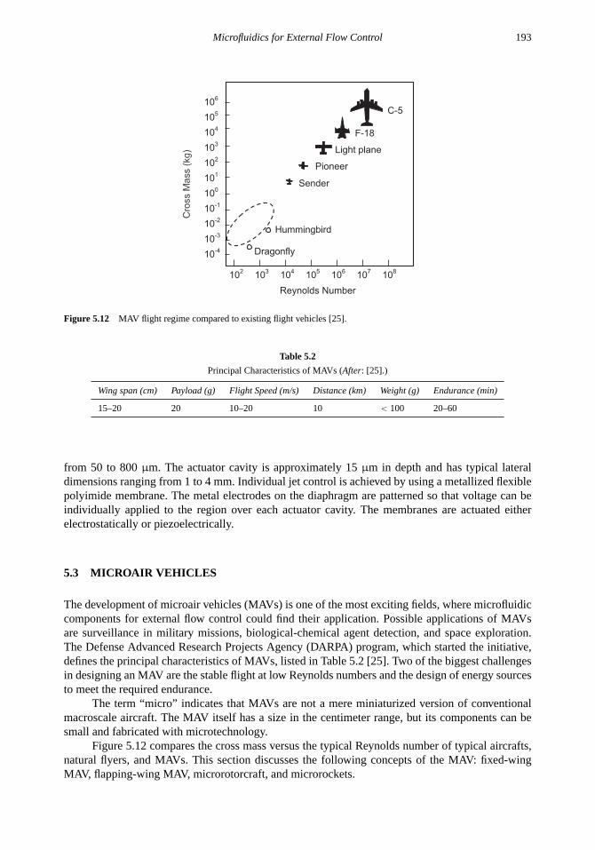
Microfluidics for External Flow Control 193
Reynolds Number
102
103
108
104
105
106
107
10-4
10-3
10-2
10-1
100
101
102
103
104
105
106
C-5
F-18
Light plane
Pioneer
Sender
Hummingbird
Dragonfly
Figure 5.12 MAV flight regime compared to existing flight vehicles [25].
Table 5.2
Principal Characteristics of MAVs (After: [25].)
Wing span (cm) Payload (g) Flight Speed (m/s) Distance (km) Weight (g) Endurance (min)
15–20 20 10–20 10 < 100 20–60
from 50 to 800µm. The actuator cavity is approximately 15µm in depth and has typical lateraldimensions ranging from 1 to 4 mm. Individual jet control is achieved by using a metallized flexiblepolyimide membrane. The metal electrodes on the diaphragm are patterned so that voltage can beindividually applied to the region over each actuator cavity. The membranes are actuated eitherelectrostatically or piezoelectrically.
5.3 MICROAIR VEHICLES
The development of microair vehicles (MAVs) is one of the most exciting fields, where microfluidiccomponents for external flow control could find their application. Possible applications of MAVsare surveillance in military missions, biological-chemical agent detection, and space exploration.The Defense Advanced Research Projects Agency (DARPA) program, which started the initiative,defines the principal characteristics of MAVs, listed in Table 5.2 [25]. Two of the biggest challengesin designing an MAV are the stable flight at low Reynolds numbers and the design of energy sourcesto meet the required endurance.
The term “micro” indicates that MAVs are not a mere miniaturized version of conventionalmacroscale aircraft. The MAV itself has a size in the centimeter range, but its components can besmall and fabricated with microtechnology.
Figure 5.12 compares the cross mass versus the typical Reynolds number of typical aircrafts,natural flyers, and MAVs. This section discusses the following concepts of the MAV: fixed-wingMAV, flapping-wing MAV, microrotorcraft, and microrockets.

194 Fundamentals and Applications of Microfluidics
Example 5.10: Characteristics of an MAV
An MAV flies with a speed of 5 m/s. The device is 15 cm long. Determine the correspondingReynolds number. The kinematic viscosity of air is 1.6 × 10⁻⁵ m2/s.
Solution. The typical Reynolds number is:
Re=uL
ν=
5 × 15× 10−2
1.6 × 19−5= 46,875
The Reynolds number is on the order of those of small birds.
5.3.1 Fixed-Wing MAV
5.3.1.1 Design Considerations
The first approach of designing MAVs is the miniaturization of conventional fixed-wing vehicles.The major concern of this approach is the power source. Assuming a constant energy density inpower sources (i.e., batteries, charged capacitors, and fuels), the available power decreases withthe third power of miniaturization. The power requirementP for a propeller driven aircraft can beestimated as [25]:
P =
W CD
C3/2L
√W
Awing
√2ρair
η(5.12)
whereW is the aircraft weight,Awing is the wing surface area,ρair is the air density, andη is thepropeller efficiency. The lift coefficientCL is defined as:
CL =2FL
ρairAwingu2(5.13)
whereu is the flight speed andFL is the lift force. The drag (or thrust) coefficient can be expressedas:
CD =2FD
ρairAwingu2(5.14)
whereFD is the drag (or thrust) force.Equation (5.12) reveals that for a long endurance one should increase the total stored energy,
minimize the weight, and minimize the weight-to-wing surface ratio. For the maximum energyrequired, high-density power sources are needed. Beside batteries, fuel cells are possible candidates.The small weight-to-wing surface ratio leads to a low aspect ratio design, which looks more like aflying wing [25].
Example 5.11: Power Requirement and Endurance of a Fixed-Wing MAV
An MAV is designed as a delta wing, which is driven by a propeller. The delta wing is anequilateral triangle with side dimension of 15 cm. The design velocity is 10 m/s. The propeller isdriven by an electric motor and has an efficiency of 80%. The lift and drag coefficients of the wingare 0.5 and 0.1, respectively. The device uses energy from a NiCd battery, which supplies 1.5 Ahat 1.5 V. The total mass of the device is 100g. Determine the flight endurance and the maximummission distance. Air density is assumed to be 1.118 kg/m3.
Solution. The total weight of the MAV is:
W = mg= 100× 10−3× 9.8 = 0.98 N

Microfluidics for External Flow Control 195
The total wing area of the device is:
Awing =√
3a2/4 =√
3 × (15× 10−2)2/4 = 97.4 × 10⁻⁴ m2
The expected power consumption for the given characteristics and speed is (5.12):
P =
W CD
C3/2L
√W
Awing
√2ρair
η=
0.98×0.1
0.53/2
√0.98
97.4×10⁻⁴
√2
1.118
0.8= 4.65W
The energy stored in the battery is:
E = 1.5 × 1.5 × 3,600= 8,100 J
Thus, the flight endurance is:
t =E
P=
8,100
4.65= 1,742 sec≈ 29 min
The MAV is able to maintain autonomy for 29 minutes. The maximum mission distance is thedistance the device can reach and then return to its initial location:
D =1
2ut =
1
2× 10× 1,742= 8,710 m
5.3.1.2 Design Examples
The fixed-wing MAV developed by AeroVironment Inc. (Simi Valley, California) has a total massof 80g [26]. The device, called Black Widow, has a 15-cm wing span and has the form of a disk.A propeller drives the MAV. A lithium battery delivers energy for the entire device. The propellermeasures 9.5 cm and has a best efficiency of 83%. The device is able to carry a video camerasystem with downlink transmitter, which has a maximum communication range of 2 km. The entireelectronic subsystem includes a 2g video camera, 2g video transmitter, 5g radio control systems, and0.5g actuators. The device is able to fly with a speed of 13.4 m/s in 30 minutes. Parts of the deviceare fabricated with conventional precision technology as well as manually. The propeller is moldedfrom unidirectional and woven carbon-fiber composites. The motor and the electronic subsystem arecommercially available.
5.3.2 Flapping-Wing MAV
5.3.2.1 Design Considerations
The second approach of flapping wings mimics natural flyers such as birds and insects. Observingnatural flyers leads to a statistical relation between mass and speed [27]:
u = 4.77m16 (5.15)
whereu is the flight speed in m/s andm is the mass in grams. For a flapping-wing MAV, the designspeed and mass can be estimated from the above relation.
The other useful statistical relations taken from nature are wingtip speed and mass [28, 29]:
11.7m−0.065< uwingtip < 9.6m−0.0434 (5.16)

196 Fundamentals and Applications of Microfluidics
10-1 1 10 10
2 103
1
10
102
105
Body mass (g)
Wingtip speed
Flight speed
Unsteady Quasi-steady
Steady (fixed-wing)
Flapping-wingMAV regime
Fixed-wingMAV regime
Figure 5.13 The flying regimes of natural flyers and MAVs. (After: [25].)
whereuwingtip is the wingtip speed in meters per second andm is the mass in grams.The relation reveals that larger flyers have lower wingtip speeds and lower flapping frequen-
cies. Figure 5.13 shows the typical flying regimes of natural flyers and MAVs. Flapping-wing MAVswork in an unsteady regime, where the airflow over the wing is not constant in time. Most insectsand small birds fly in this regime.
The characteristic Reynolds number for flapping-wing flyers is defined as [30]:
Re=Luwingtip
ν=
48 f R2
ν�(5.17)
whereL is the mean chord length,R is the length of one wing,� = 2R/L4 is the aspect ratio,f isthe wing beat frequency, and8 is the peak-to-peak wing beat amplitude in radians. The maximummass that can be supported by flapping wings during hovering with a horizontal stroke plane isestimated as [30]:
m = 0.38782 f 2R4CL
�(5.18)
whereCL is the lift coefficient defined in (5.13). The total power in watts, which is needed forovercoming lift and drag, can then be estimated with the massm as:
P = Plift + Pdrag = m f R
[14.0
(8CL
�
)1/2
+ 18.28CD
CL
](5.19)
The drag coefficientCD of typical insect wings can be estimated with [27]:
CD = 7√
Re (5.20)
where the Reynolds number is defined in (5.6).

Microfluidics for External Flow Control 197
Example 5.12: Power Requirement and Endurance of a Flapping-Wing MAV
A flapping-wing MAV is designed with 15-cm mean chord length and a wing length of 5 cm. Theflapping frequency is optimized for 50 Hz. The stroke amplitude is 120◦. The lift coefficient ofthe wing is 1.5. The drag coefficient is 0.15. The device uses energy from a NiCd battery, whichsupplies 1.5 Ah at 1.5V. Determine the maximum mass of the MAV and the flight endurance inthis case.
Solution. The aspect ratio of the device is:
� =2R
L=
2 × 5
15= 0.67
With a stroke amplitude of 120◦ or 0.67π , the maximum mass of the MAV is:
m = 0.38782 f 2R4CL�
m = 0.3870.672π2502(5×10⁻²)4×1.50.67 = 0.0597 kg= 59.7 g
The power requirement for the device during flight is:
P = m f R
[14.0
(8CL�
)1/2+ 18.28CD
CL
]
P = 0.155× 50× 5 × 10−2[14×
(0.67π×1.5
0.67
)1/2+ 18.2 × 0.67π 1.5
0.15
]= 5.1W
The energy stored in the battery is:
Eenergy= 1.5 × 1.5 × 3,600= 8,100 J
Thus, the flight endurance is:
t =Eenergy
P=
8,100
5.1= 1,588 sec= 26.5 min
The results of the flapping-wing MAV are comparable to those of the fixed-wing MAV in Example5.11.
5.3.2.2 Design Examples
Figure 5.14 shows the process for fabricating wing structures [28]. The structures made of siliconare too fragile for the relatively large size required for the wing, which is on the order of severalcentimeters. A similar process utilizing titanium alloy as the substrate and carbon fiber rod is shownin Figure 5.15. The titanium alloy structure is formed in an enchant solution (HF, HNO3, H2O) [29].The most critical points in the development of such a flapping-wing MAV are the power source andenergy-saving actuating schemes. The device reported in [28, 29] can only fly for 5 to 18 seconds,while the required minimum flight duration is about 20 minutes.
5.3.3 Microrotorcraft
Considering the definitions of lift and drag coefficients in (5.13) and (5.14), the ratio between liftand thrust or the ratio between weight and drag is derived as:
W
FD=
CL
CD(5.21)

198 Fundamentals and Applications of Microfluidics
Silicon
Nitride Parylene
Figure 5.14 Fabrication process of silicon MEMS-wings.
Ti-alloy
Film resist
Parylene
Carbon fiber
1)
2)
3)
4)
5)
6)
Figure 5.15 Fabrication process of Ti-alloy MEMS-wings.
The ratio for typical aircrafts and mesoscale MAVs ranges from 10 to 20. Since the weight isproportional to volume and the drag force is proportional to surface area, the ratio in [21] obeys thecubic square relation of scaling law. In other words, the ratioW/FD decreases with miniaturization.In microscale, the drag force can be many orders larger than the weight of the device. The aboveflight concepts with wings, which utilize smaller thrust to balance drag force, will not work well inthe microscale.
If drag force is much larger than weight, the thrust alone can be used to balance drag forceand weight. The advantage of scaling law can be used in designing a microrotorcraft, which is moreefficient than helicopters in the macroscale.
The work at Stanford University dealt with a centimeter-size electric helicopter [31]. This sizescale fills the gap between the true microscale (millimeters or less) and the conventional scale (tensof centimeters or more). The air vehicle is therefore called Mesicopter. There is no report indicatingthat this device can fly.
Table 5.3 compares the most important parameters of the design examples of the fixed-wingMAV, flapping-wing MAV, and the microrotorcraft discussed above and illustrated in Figure 5.16.
5.3.4 Microrockets
5.3.4.1 Design Considerations
The mean application of microrockets will be providing precise thrust for controlling satelliteposition. The basic idea behind microrockets is the gain of the thrust-to-weight ratioF/W withminiaturization. The thrustF is proportional to square of length scalel :
F ∝ pcAt ∝ l 2 (5.22)

Microfluidics for External Flow Control 199
Table 5.3
Typical Parameters of MAVs
Refs. Type Size (mm×mm) Speed (m/s) Endurance (min) Mass (g) Maximum Altitude (m)
[26] Fixed-wing 150×150 13.4 30 80 234[29] Flapping-wing 150×150 4.4 ≈ 0.3 10.5 ≈ 10
15 cm
(a) (b) (c)
5 cm
Propeller
Motor, gear box
Flapping wing
Actuator and battery
Propeller
Motor
Space for batteryand load
Figure 5.16 Design examples of MAV: (a) fixed-wing MAV Black Widow (After: [26]); (b) flapping-wing MAV Ornithopter(After: [29]); and (c) microrotorcraft Mesicopter (After: [31]).
where pc is the combustion chamber pressure andAt is the throat area. Since the weight isproportional to the volumel 3, the thrust-to-weight ratio is inversely proportional to the length scale:
F
W∝
l 2
l 3=
1
l(5.23)
Conventional rockets with a typical dimension of 1m have thrust-to-weight ratios on the order of 50.Microrockets with a typical dimension of 1 mm will result in a thrust-to-weight ratio of 50,000. Thebetter performance promises the use of many microrockets in parallel to achieve the desired thrustin macroscale applications.
In a rocket engine, thermal energy is converted into the kinetic energy of a working gas.Kinetic energy of the exhaust gas through a nozzle provides thrust needed for the application. Basedon the source of thermal energy, rockets are categorized as [32]:
• Cold-gas rockets;
• Chemical rockets;
• Electric rockets;
• Nuclear rockets;
• Solar thermal rockets.
The first three types are relevant for miniaturization. Cold-gas rockets only need a high-pressure gas supply. Chemical rockets use a combustion reaction to provide heat. Electric rocketsutilize the high temperature of an electric arc to generate heat for the engine. This section focuseson the design of cold-gas microrockets and chemical microrockets.
Based on the type of fuels, chemical rockets can be further categorized as cold-gas rockets, liq-uid propellant rockets, and solid propellant rockets. Liquid propellants have two forms: bipropellantand monopropellant. A bipropellant consists of a liquid fuel and a liquid oxidizer. A monopropellantis a single liquid containing both fuel and oxidizer.
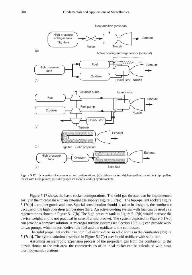
200 Fundamentals and Applications of Microfluidics
Figure 5.17 Schematics of common rocket configurations: (a) cold-gas rocket; (b) bipropellant rocket; (c) bipropellantrocket with turbo pumps; (d) solid propellant rockets; and (e) hybrid rockets.
Figure 5.17 shows the basic rocket configurations. The cold-gas thruster can be implementedeasily in the microscale with an external gas supply [Figure 5.17(a)]. The bipropellant rocket [Figure5.17(b)] is another good candidate. Special consideration should be taken in designing the combustorbecause of the high operation temperature there. An active cooling system with fuel can be used as aregenerator as shown in Figure 5.17(b). The high-pressure tank in Figure 5.17(b) would increase thedevice weight, and is not practical in case of a microrocket. The system depicted in Figure 5.17(c)can provide a compact solution. A microgas turbine system (see Section 13.2.1.1) can provide workto two pumps, which in turn deliver the fuel and the oxidizer to the combustor.
The solid propellant rocket has both fuel and oxidizer in solid forms in the combustor [Figure5.17(d)]. The hybrid solution described in Figure 5.17(e) uses liquid oxidizer with solid fuel.
Assuming an isentropic expansion process of the propellant gas from the combustor, to thenozzle throat, to the exit area, the characteristics of an ideal rocket can be calculated with basicthermodynamic relations.

Microfluidics for External Flow Control 201
Combustion Chamber Characteristics.The most important properties of a combustor are pressurepc and temperatureTc. The chamber temperature can be estimated with the maximum adiabatictemperature of a combustion reaction. However, because of massive cooling, the actual temperaturesin a combustor are much lower than the estimated adiabatic combustion temperature. The chamberpressure can be estimated with the mass flow rate of propellant and chamber temperature using theideal gas equation.
Throat Characteristics.If the throat velocity reaches the speed of sound (Mach number Ma = 1),the following relations at the nozzle throat can be derived for pressurept, specific volumevt,temperatureTt, and velocityut [32]:
pt
pc=
[2
k + 1
] kk−1
(5.24)
vt
vc=
[k + 1
2
] 1k−1
(5.25)
Tt
Tc=
2
k + 1(5.26)
ut =
√2k
k + 1RTc (5.27)
where k is the specific heat ratio, and subscripts t and c represent the throat and combustor,respectively.
Exit Area Characteristics.Using the energy balance equation for the process across the rocket throatand assuming that the velocity in the combustion chamber is zero, the exit velocity can be estimatedas [32]:
uexit =
√√√√ 2k
k − 1RTc
[1 −
(pe
pc
) k−1k
](5.28)
whereR is the gas constant of the propellant. The gas temperatureTexit and the specific volume atthe exitvexit can be estimated from the isentropic relations:
Texit
Tc=
[pexit
pc
] k−1k
(5.29)
vexit
vc=
[pc
pexit
] 1k
(5.30)
Performance of a Microrocket.The first important parameter for a microrocket is its specific impulse:
Ysp =F
mg(5.31)
whereF is the thrust,m is the mass flow rate, andg is the acceleration of gravity. The ratioF/m iseffective exhaust velocityuexit. Thus, the specific impulse can be defined as:
Ysp =uexit
g(5.32)

202 Fundamentals and Applications of Microfluidics
The specific impulse has the unit of time, and represents the time during which a certain amountof fuel can deliver the same thrust as its own weight. Thus, the specific impulse is the primaryperformance indicator for microrockets. For evaluating the effectiveness of the nozzle, the thrustcoefficientCF can be used:
CF =F
pcAt(5.33)
whereAt is the throat area. The thrust coefficient is given for an ideal isentropic rocket flow by [29]:
CF =
√√√√ 2k2
k − 1
[1 −
(pe
pc
) k−1k
] (2
k + 1
) k+12(k−1)
+pe − patm
pc
Ae
At(5.34)
wherepe and Ae are the exit pressure and exit area of the nozzle, respectively, andk is the specificheat ratio of the gas. If the characteristic exhaust velocityc∗ is defined as:
c∗=
pcAt
m(5.35)
the characteristic exhaust velocity for an ideal rocket is [32]:
c∗=
√RTc
(k + 1
2k
) k+12(k−1)
(5.36)
Combining the above relations, the exit velocity can be described as:
uexit = Ispg = CFc∗ (5.37)
Example 5.13: Characteristics of a Microrocket
A microrocket is made of silicon. The height of the combustion chamber, throat, and exit area is1 mm. The exit width is 5 mm. The rocket is designed to work with 10 bars chamber pressure and1,000K chamber temperature. Determine the theoretical thrust coefficient, the exit velocity, andthe specific impulse. For the propellant gas, usek = 1.3 andR = 355.4 J/kg-K.
Solution. Assuming that the rocket operates at atmospheric conditions (pexit = patm = 1 bar),the theoretical thrust coefficient is (5.34):
CF =
√√√√ 2k2
k − 1
[1 −
(pe
pc
) k−1k
] (2
k + 1
) k+12(k−1)
+pe − patm
pc
Ae
At
CF =
√√√√2 × 1.32
1.3 − 1
[1 −
(1
10
) 1.3−11.3
] (2
1.3 + 1
) 1.3+12(1.3−1)
= 1.26
The exit velocity of the microrocket is (5.28):
uexit =
√√√√ 2k
k − 1RTc
[1 −
(pe
pc
) k−1k
]
uexit =
√√√√2 × 1.3
1.3 − 1355.4 × 1000
[1 −
(1
10
) 1.3−11.3
]= 1,127 m/sec
(5.38)

Microfluidics for External Flow Control 203
Assuming an acceleration of gravity of 9.8 m/s2, the specific impulse is:
Isp =uexit
g=
1,127
9.8= 115 sec
Example 5.14: Thrust and Thrust-to-Weight Ratio
We consider the microrocket described above. If the total device weight is 1.5g, determine themass flow rate, the thrust, and the thrust-to-weight ratio.
Solution. The cross-sectional exit area of the microrocket is:
Aexit = 5 × 1 × 10−6= 5 × 10⁻⁶ m2
Thus, the volumetric flow rate at exit is:
(Au)exit = 5 × 10−6× 1,127= 5,635× 10−6 m2/s
We assume an isentropic expansion across the rocket nozzle. Using the relation of (5.29), the exittemperature can be estimated as:
Texit = Tc
[pexit
pc
] k−1k
= 1,000
[1
10
] 1.3−11.3
= 588 K
For this temperature, the specific volume of propellant gas is:
uexit =RTexit
pexit= 2.09 m3/kg
Thus, the mass flow rate of exhaust gas is:
mexit =(Au)exit
uexit=
5,635× 10−6
2.09= 2.7 × 10⁻³ kg/s
With the exit velocity of the previous example, the thrust of the microrocket is:
F = mexituexit = 2.7 × 10−3× 1,127≈ 3.04 N
Considering only the weight of the combustion chamber and nozzle, the thrust-to-weight ratio ofthe microrocket is:
F
W=
2.48
1.5 × 10−3 × 9.8= 207
Example 5.15: Designing an Ideal Microrocket
An ideal microrocket, which operates at a pressure of 1 bar, should have a thrust of 1N at apressure of 10 bars and a temperature of 1,000K in the combustion chamber. The chamber andnozzle heights are 1 mm. Assuming thatk = 1.3, andR = 355.4 J/kg-K, determine the exitvelocity, throat width, and exit width.

204 Fundamentals and Applications of Microfluidics
Solution. The microrocket is designed for the critical case of the speed of sound at the nozzlethroat. The throat velocity is determined by (5.27):
ut =
√2k
k + 1RTc =
√2 × 1.3
1.3 + 1355.4 × 1,000= 634 m/s
The exit velocity is estimated with (5.28):
uexit =
√√√√ 2k
k − 1RTc
[1 −
(pe
pc
) k−1k
]=
√√√√2 × 1.3
1.3 − 1× 355.4 × 1,000×
[1 −
(1
10
) 1.3−11.3
]= 407 m/s
The mass flow rate of propellant gas can be estimated from the relations in (5.31) and (5.32) as:
m = mexit =F
uexit=
1
407= 2.457× 10⁻³ kg/s
The specific volume of propellant gas in combustion chamber is:
vc =RTc
pc=
355.4 × 1,000
10× 105= 355.4 × 10⁻³m3/kg
The specific volume at throat can be estimated with (5.25):
vt = vc
[k + 1
2
] 1k−1
= 355.4 × 10⁻³[
1.3 + 1
2
] 11.3−1
= 566.3 × 10³ m3/kg
The specific volume at exit can be estimated with (5.30):
vexit = vc
(pc
pexit
) 1k
= 355.4 × 10⁻³(10)1
1.3 m3/kg
The width of throat is:
wt =At
h=
mvt
uth=
0.8878× 10−3× 566.3 × 10−3
634× 10−3= 2.195× 10⁻³ m = 2.195 mm
The width of exit is:
wexit =Aexit
h=
mvexit
uexith=
0.8878× 10−3× 2089× 10−3
1,127× 10−3= 12.61× 10⁻³ m = 12.61 mm
The major drawbacks of silicon technology in fabricating microrockets are its high thermalconductivity and its relatively low melting point. Consequently, the combustion chamber needs tobe cooled actively. Furthermore, the high thermal conductivity causes difficulties for ignition of thecombustion process.
The other drawback is the limit of planar structures in silicon technology. For places with highpressure such as the combustion chamber of a microrocket, the planar silicon/glass structure cannotresist the pressure emerging after ignition. Silicon/silicon structures fabricated with fusion bondingare better for microrockets.
However, the special characteristics of high thrust-to-weight ratio and relatively low exhaustvelocity are interesting and give microrockets functions complementary to conventional rockets(Figure 5.18).
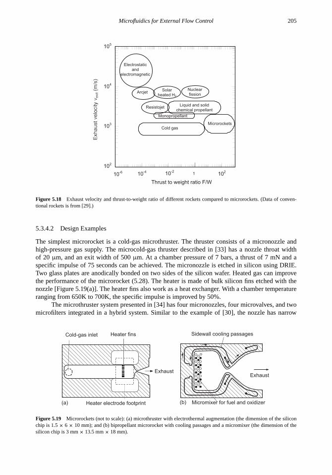
Microfluidics for External Flow Control 205
10-6
10-4
10-2
1 102
102
103
104
105
Thrust to weight ratio F/W
Electrostatic
and
electromagnetic
ArcjetSolar
heated H2
Nuclear
fission
ResistojetLiquid and solid
chemical propellant
Monopropellant
Cold gas
Microrockets
Figure 5.18 Exhaust velocity and thrust-to-weight ratio of different rockets compared to microrockets. (Data of conven-tional rockets is from [29].)
5.3.4.2 Design Examples
The simplest microrocket is a cold-gas microthruster. The thruster consists of a micronozzle andhigh-pressure gas supply. The microcold-gas thruster described in [33] has a nozzle throat widthof 20 µm, and an exit width of 500µm. At a chamber pressure of 7 bars, a thrust of 7 mN and aspecific impulse of 75 seconds can be achieved. The micronozzle is etched in silicon using DRIE.Two glass plates are anodically bonded on two sides of the silicon wafer. Heated gas can improvethe performance of the microrocket (5.28). The heater is made of bulk silicon fins etched with thenozzle [Figure 5.19(a)]. The heater fins also work as a heat exchanger. With a chamber temperatureranging from 650K to 700K, the specific impulse is improved by 50%.
The microthruster system presented in [34] has four micronozzles, four microvalves, and twomicrofilters integrated in a hybrid system. Similar to the example of [30], the nozzle has narrow
Cold-gas inlet
Exhaust
Heater fins
Heater electrode footprint(a) Micromixer for fuel and oxidizer(b)
Exhaust
Sidewall cooling passages
Figure 5.19 Microrockets (not to scale): (a) microthruster with electrothermal augmentation (the dimension of the siliconchip is 1.5× 6 × 10 mm); and (b) bipropellant microrocket with cooling passages and a micromixer (the dimension of thesilicon chip is 3 mm× 13.5 mm× 18 mm).

206 Fundamentals and Applications of Microfluidics
Table 5.4
Typical Parameters of Microrockets
Refs. Type Size (mm×mm) F (mN) Is(sec) Technology/Material
[33] Gas microthruster 1.5 × 6 × 10 7 75 DRIE/ Silicon[34] Gas microthruster — 0.1–10 ≈ 100 DRIE/ Silicon[35] Bipropellant microrocket 3× 13.5 × 18 1,000 30 DRIE/ Silicon[36] Solid fuel microrocket 3.2 × 12.7(25.4) 15 10–20 Hybrid/ ceramic, silicon[37] Vaporizing microthruster — — — Bulk/ Silicon[38] Vaporizing microthruster — — — Bulk/ Silicon
curved fins as a heat exchanger. With a throat width ranging from 10 to 40µm and an exit angle of13◦, thrusts ranging from 0.1 to 10 mN are achieved.
The micronozzle developed for cold-gas microthrusters can be used in a bipropellant micro-rocket [35]. The microrocket uses liquid oxygen and methane as a propellant. Ethanol is fed througha channel system, which actively cools the combustion chamber. The active cooling system keepsthe chamber wall temperature at 900K. In further development, ethanol could serve as fuel. Fuel andan oxidizer are mixed with a parallel micromixer (see Chapter 10). The mixer has 484 injectors, 242each for fuel and oxidizer. At a chamber pressure of 12.16 bars, a thrust of 1N can be achieved. Thecorresponding thrust power is 750W.
A ceramic microrocket with solid fuel was reported in [36]. The microrocket is made ofalumina ceramic, the thermal conductivity of which is five times lower than that of silicon. Thecombustion chambers have inner diameters of 3.2 mm and lengths of either 12.7 or 25.4 mm. Thepropellant is a solid composite fuel containing 74% oxidizer ammonium perchlorate (AP) and 14%binder hydroxyl-terminated polybutadiene (HTPB). The nozzles have throat diameters of 1.57 mmand lengths of either 6.35 or 12.7 mm. This rocket is able to deliver a maximum thrust of from 4 to10 mN and specific impulses ranging from 10 to 20 seconds.
Microthrusters can be propelled with vaporizing liquid as well [37, 38]. Thermal bubblesgenerate the thrust. The concept is similar to that of an inkjet printer head. The energy is supplied byresistive heating. Thus, the efficiency of such a microthruster is relatively low. Table 5.4 comparesthe most important parameters of the above microrockets.
An array of microrockets can improve the performance with their redundancy. Furthermore,digital propulsion is possible with an array of microrockets [39]. The corresponding number of fired“microrocket bits” can deliver precisely the desired thrust.

Microfluidics for External Flow Control 207
Problems
5.1 The pressure drop across a Pitot probe is 30 mbar. Determine the flow velocity if the fluid is (a)water and (b) air.
5.2 For a polysilicon wire with a length ofL = 60 µm, a cross section ofA = 2 × 4 µm isused as a hot-wire sensor. The temperature coefficient and thermal conductivity of polysiliconare 8× 10⁻⁴K−1 and 32W m−1K−1, respectively. The bulk substrate temperature is 25◦C. Theresistivity of polysilicon at 25◦C is 4×10⁻⁵ �m. Determine the current required for a maximumtemperature of 200◦C at the center of the wire.
5.3 The polysilicon wire described in Example 5.1 is used as a hot wire for measuring turbulentvelocities. Determine the highest turbulence frequency the sensor can detect.
5.4 Determine the Reynolds number and the shear stress expected at 2m from the front of a flat plate.The free stream velocity is 5 m/s. If a shear stress sensor is flush-mounted at this position andthe gap around the floating plate is 50µm, can the error caused by flow field disturbance beignored? Kinematic viscosity and density of air are assumed to be 1.6 × 10⁻⁵ m2/s and 1.164kg/m3, respectively.
5.5 The sensor mentioned in Problem 5.4 is made of a silicon plate with a dimension of 2× 2 mm.The plate is suspended on four flexures. Each flexure has a dimension of 1 mm× 10µm× 10µm.Displacement of the floating element is detected with an interdigitated comb electrode structure.Each side of the floating plate has 20 electrodes. The gap between two counterelectrodes is 2 mm.Design the capacitive sensor so that the capacitance change at 10 m/s is 10%.
v=10 m/s2 �m
Direction of displacement
5.6 Repeat the design process if sensing comb structures are perpendicular to flow direction.
v=10 m/s
Direction of
displacement
5.7 An MAV is designed as a disk wing, which is driven by a propeller. The circular disk wing has adiameter of 10 cm. The design velocity is 15 m/s. The propeller is driven by an electric motor andhas an efficiency of 60%. The lift and drag coefficients of the wing are 1.5 and 0.1, respectively.The device is designed for a total mass of 100g. Determine the capacity in mAh of a battery for aflight endurance of 20 minutes. The battery supplies a voltage of 3.3V. Air density is assumed tobe 1.118 kg/m3.
5.8 A flapping-wing MAV is designed with 15-cm mean chord length and a wing length of 10 cm.The flapping frequency is optimized for 30 Hz. The stroke amplitude is 80◦. The lift coefficient

208 Fundamentals and Applications of Microfluidics
of the wing is 1.5. The drag coefficient is 0.15. Determine the maximum mass of the device, theflight speed, and the energy capacity needed for a flight endurance of 20 minutes.
5.9 Design an ideal microrocket, which operates at a pressure of 0.01 bar and has a thrust of 2N.The pressure and temperature in combustion chamber are 10 bar and 1,000 K, respectively. Thechamber and nozzle heights are 1 mm. Assuming thatk = 1.3, andR = 355.4 J/kg-K, determinethe exit velocity, throat width, and exit width of the microrocket.
References
[1] Gad-el-Hak, M., “The Fluid Mechanics of Microdevices - The Freeman Scholar Lecture,”Journal of Fluids Engineer-ing, Vol. 121, 1999, pp. 5–32.
[2] Ho, C. M., and Tai, Y. C, “Review: MEMS and Its Applications for Flow Control,”Journal of Fluids Engineering,Vol. 118, 1996, pp. 437–447.
[3] Fedder, G. K., “Simulation of Microelectromechanical Systems,” Ph.D. thesis, University of California at Berkeley,1994.
[4] Senturia, S. D.,Microsystem Design, Boston: Kluwer Academic Publishers, 2001, pp. 632–634.
[5] Jiang, F., et al., “A Micromachined Polysilicon Hot-Wire Anemometer,”Technical Digest of the IEEE Solid StateSensor and Actuator Workshop, Hilton Head Island, SC, June 13–16, 1994, pp. 264–267.
[6] Padmanabhan, A., “Silicon Micromachined Sensors and Sensor Arrays for Shear Stress Measurement in AerodynamicFlow,” Ph.D. thesis, Massachusetts Institute of Technology, 1997.
[7] Haritonidis, J. H., “The Measurement of Wall Shear Stress,”Advances in Fluid Mechanics Measurements, M. Gad-el-Hak (ed.), New York: Springer Verlag, 1989, pp. 229–261.
[8] Oudheusden B., and J.Huijsing, “Integrated Flow Friction Sensor,”Sensors and Actuators A, Vol. 15, 1988, pp. 135–144.
[9] Liu, C., et al., “Surface-Micromachined Thermal Shear Stress Sensor,”Journal of Microelectromechanical Systems,Vol. 8, No. 1, 1999, pp. 90–99.
[10] Jang, F, et al., “A Surface Micromachined Shear Stress Imager,”Proceedings of MEMS’96, the 9th IEEE InternationalWorkshop Micro Electromechanical System, San Diego, CA, Feb. 11-15, 1996, pp. 110–115.
[11] Kalvesten, E., “Pressure and Wall Shear Stress Sensors for Turbulence Measurements,” Ph.D. thesis, Royal Instituteof Technology, Stockholm, Sweden, 1996.
[12] Jang, F., et al., “ A Flexible Micromachine-Based Shear-Stress Sensor Array and Its Application to Separation-PointDetection,”Sensors and Actuators A, Vol. 79, No. 3, 2000, pp. 194–203.
[13] Schmidt, M. A., et al., “Design and Calibration of a Microfabricated Floating-Element Shear-Stress Sensor,”IEEETransactions on Electron Devices, Vol. ED-35, 1988, pp. 750–757.
[14] Ng, K-Y., “A Liquid Shear-Stress Sensor Using Wafer-Bonding Technology,” M.S. thesis, Massachusetts Institute ofTechnology, 1990.
[15] Goldberg, H. D., Breuer, K. S., and Schmidt, M. A., “A Silicon Wafer-Bonding Technology for Microfabricated Shear-Stress Sensors with Backside Contacts,”Technical Digest of the IEEE Solid State Sensor and Actuator Workshop,Hilton Head Island, SC, June 13–16, 1994, pp. 111–115.
[16] Pan, T., et al., “Calibration of Microfabricated Shear Stress Sensors,”Proceedings of Transducers ’95, 8th Interna-tional Conference on Solid-State Sensors and Actuators, Stockholm, Sweden, June 16–19, 1995, pp. 443–446.
[17] Padmanabhan, A., et al., “A Wafer-Bonded Floating-Element Shear Stress Microsensor with Optical Position Sensingby Photodiodes,”Journal of Microelectromechanical Systems, Vol. 5, No. 4, 1996, pp. 307–315.

Microfluidics for External Flow Control 209
[18] Lee, G. B., et al., “Sensing and Control of Aerodynamic Separation by MEMS,”The Chinese Journal of Mechanics,Vol. 16, No. 1, 2000, pp. 45–52.
[19] Liu, C., et al., “Out-of-Plane Magnetic Actuators with Electroplated Permalloy for Fluid Dynamics Control,”Sensorsand Actuators A, Vol. 78, No. 2–3, 1999, pp. 190–197.
[20] Dwight, H. B.,Electrical Coils and Conductors, New York: McGraw-Hill, 1945.
[21] Benecke, W., “Silicon Microactuators: Activation Mechanisms and Scaling Problems,”Proceedings of Transducers’91, 6th International Conference on Solid-State Sensors and Actuators, San Francisco, CA, June 23–27, 1991, pp.46–50.
[22] Liu, C., et al., “Surface Micro-Machined Magnetic Actuators,”Proceedings of MEMS’94, 7th IEEE InternationalWorkshop Micro Electromechanical System, Oiso, Japan, Jan. 25–28, 1994, pp. 57–62.
[23] Grosjean, C., et al., “Micro Balloon Actuators for Aerodynamic Control,”Proceedings of MEMS’98, 11th IEEEInternational Workshop Micro Electromechanical System, Heidelberg, Germany, Jan. 25–29, 1998, pp. 166–171.
[24] Coe, D. J., et al., “Addressable Micromachined Jet Arrays,”Proceedings of Transducers ’95, 8th InternationalConference on Solid-State Sensors and Actuators, Stockholm, Sweden, June 16–19, 1995, pp. 329–332.
[25] Marischal, J. M., and Francis, M. S., “Micro Air Vehicles—Toward a New Dimension in Flight,”http://www.darpa.mil/tto/mav/mavauvsi.html, 1997.
[26] Grasmeyer, J. M., and Keennon, M. T., “Development of the Black Widow Micro Air Vehicle,”http://www.aerovironment.com/area-aircraft/prod-serv/bwidpap.pdf, 2001.
[27] Dickinson, M. H., Lehmann, F. O., and Sane, S. P., “Wing Rotation and the Aerodynamic Basis of Insect Flight,”Science, Vol. 284, 1999, pp. 1954–1960.
[28] Pornsin-Sirirak, T. N., et al., “Titanium-Alloy MEMS Wing Technology for a Micro Aerial Vehicle Application,”Sensors and Actuators A, Vol. 89, No 1–2, 2001, pp. 95–103.
[29] Pornsin-Sirirak, T. N., et al., “MEMS Wing Technology for a Battery-Powered Ornithopter,”Proceedings ofMEMS’00, 13th IEEE International Workshop Micro Electromechanical System, Miyazaci, Japan, Jan. 23–27, 2000,pp. 799–804.
[30] Ellington, C. P., “The Novel Aerodynamics of Insect Flight: Applications to Micro-Air Vehicles,”The Journal ofExperimental Biology, Vol. 202, 1999, pp. 3439–3448.
[31] Kroo, I., Mesicopter project, http://aero.stanford.edu/mesicopter/, Stanford University.
[32] Sutton, G. P., and Biblarz, O.,Rocket Propulsion Elements, 7th ed., New York: Wiley, 2001.
[33] Bayt, R., “Analysis, Fabrication, and Testing of a MEMS-Based Micropropulsion System,” Ph.D. thesis, Mas-sachusetts Institute of Technology, 1999.
[34] Kohler, J., et al., “A Hybrid Cold Gas Microthruster System for Spacecraft,”Proceedings of Transducers ’01, 11thInternational Conference on Solid-State Sensors and Actuators, Munich, Germany, June 6–7, 2001, pp. 886–889.
[35] London, A. P., “Development and Test of a Microfabricated Bipropellant Rocket Engine,” Ph.D. thesis, MassachusettsInstitute of Technology, 2000.
[36] Teasdale, D., “Solid Propellant Microrockets,” M.Sc. thesis, University of California at Berkeley, 2000.
[37] Wallace, A. P., et al., “Design, Fabrication, and Demonstration of a Vaporizing Liquid Attitude Control Microthruster,”Proceedings of Transducers ’99, 10th International Conference on Solid-State Sensors and Actuators, Sendai, Japan,June 7–10, 1999, pp. 1800–1803.
[38] Kim, S., Kang, T., Cho, Y., “High-Impulse Low-Power Microthruster Using Liquid Propellant with High-ViscousFluid-Plug,” Proceedings of Transducers ’01,11th International Conference on Solid-State Sensors and Actuators,Munich, Germany, June 6–7, 2001, pp. 898–901.
[39] Lewis, D. H., “Digital Micropropulsion,”Proceedings of MEMS’99, 12th IEEE International Workshop MicroElectromechanical System, Orlando, FL, Jan.17–21, 1999, pp. 517–522.

210 Fundamentals and Applications of Microfluidics

Chapter 6
Microfluidics for Internal Flow Control:Microvalves
Microvalves are one of the most important microfluidic components. Besides pumps and flow sen-sors, active valves are critical components for controlling fluid flows in microfluidic systems. Today,the industry requirements for microfluidic systems continue to force an evolution and a revolutionin valve design because of the new effects in microscale. Smaller device size, higher pressures,biocompatibility, response, and, most importantly, the microtechnology, are all contributing to thevalve design in microscale. Sincepassive valvesor check-valves are a part of micropumps, thischapter only deals with active microvalves for flow control.
With the conventional design, anactive valveis a pressure-containing mechanical device usedto shut off or otherwise modify the flow of a fluid that passes through it. The working state ofthe valve is determined by a closure element—the valve seat, which is driven by an actuator. Thisdefinition reveals that a valve is a very simple device. It has a body to contain the fluid and itspressure, a valve seat to manipulate the fluid, and an actuator to control the position of the valveseat.
There are many ways to categorize active microvalves. Based on their initial working state,there are three microvalve types: normally open, normally closed, and bistable. Bistable microvalvescan actively open and close the valve seat; an off-state is not defined.
Similar to an electronic transistor, valves can control flow in two ways: analog and digital.In the analog, or proportional, mode, at a constant inlet pressure, the valve actuator varies the gapbetween the valve seat and valve opening to change the fluidic resistance and, consequently, the flowrate. In the digital mode, there are only two valve states: fully open and fully closed. However, adigital active valve can be driven in pulse-width-modulation (PWM) mode or as a digitally weightedvalve array for proportional flow control. In the PWM mode, the open time is controlled, and as aresult, the net flow rate can be varied proportionally with the opening time. In an array, many digitalvalves are used to control the flow. If the flow rates of each valve are equal, the net flow rate isproportional to the number of opened valves. A more elegant solution is to weight the flow rate ofeach valve with the binary system. Thus, the array can represent a fluidic digital/analog converter.With, for example, 8 binary valves, 256 different flow rate values can be controlled (Figure 6.1). Inthis chapter, active microvalves are categorized by their actuation principles as:
• Pneumatic microvalves;
• Thermopneumatic microvalves;
• Thermomechanical microvalves;
• Piezoelectric microvalves;
211

212 Fundamentals and Applications of Microfluidics
(d) (e)
(a) (b) (c)t t t
Q Q Q
Q Q
Figure 6.1 Functional classification of microvalves: (a) analog (proportional) valve; (b) digital normally closed (NC) valve;(c) digital normally open (NO) valve; (d) PWM proportional valve; and (e) fluidic digital-analog converter.
• Electrostatic microvalves;
• Electromagnetic microvalves;
• Electrochemical and chemical microvalves;
• Capillary force microvalves.
The major specification bases for microvalves are leakage, valve capacity, power consumption,closing force (pressure range), temperature range, response time, reliability, biocompatibility, andchemical compatibility.
The ideal active valve should have zero leakage in the closed position. Theleakage ratio Lvalveis defined as the ratio between the flow rate of the closed stateQclosedand of the fully open stateQopenat a constant inlet pressure:
Lvalve =Qclosed
Qopen(6.1)
Sometimes, the leakage is defined as the on/off ratio. In order to avoid the confusion betweennormally closed valves and normally open valves, the above definition of leakage (6.1) is keptthroughout this chapter.
The valve capacitycharacterizes the maximum flow rate the valve can handle. The valvecapacityCvalve is defined as:
Cvalve =Qmax
√1pmax/(Lρg)
(6.2)
whereQmax and1pmax are the flow rate and the pressure drop across the valve at the fully openposition, respectively;L is the characteristic length of the valve;ρ is the fluid density; andg is theacceleration of gravity. The power consumption is the total input power of the valve in its active,power-consuming state. Depending on the actuating principle, the power consumption may varyseveral orders of magnitude from very small (electrochemical) to very large (thermopneumatic).
The closing forcedepends on the pressure generated by the actuator. Figure 6.2 gives anoverview of the pressure range of different actuators used in microvalves [1].
Thetemperature rangeof the valve depends strongly on the material and its actuation concept.Pneumatic valves are often used for high-temperature applications because the temperature rangedepends only on their material. The valve response time is actually the response time of the actuatorin use. Figure 6.3 compares the response time of different actuators.

Microfluidics for Internal Flow Control: Microvalves 213
kPa102
101
Stack type
piezoelectric
Pneumatic
Thermopneumatic
Shape-memory alloy
Thermomechanic
Electromagnetic
Disk type piezoelectric
Electrostatic
Electrochemical
103
104
Chemical
Figure 6.2 Pressure range of different actuators used in microvalves.
second110-1
10-2
10-3
10-4
Pneumatic
Shape-memory alloy
Electrochemical
Thermopneumatic
Thermomechanic
Piezoelectric
Electromagnetic
ElectrostaticChemical
Figure 6.3 Time response range of different actuators used in microvalves.
The actuators and the operating conditions determine the reliability of a microvalve. Inthe microscale, the operation failure is often caused by particulate contamination and not bythe reliability of its actuator. Therefore, it is important to use filters to keep particulates out ofmicrovalves.
6.1 DESIGN CONSIDERATIONS
At the start of a microvalve design project, some important questions should be answered.
• What specifications should the valve meet for the intended application?
• What material should be used for valve fabrication?
• How much will it cost?
• What type of actuator best suits the specifications and constraints?
• What is the optimal form of valve spring and valve seat for the maximum closure pressure andminimum leakage?
All the specifications and constraints of the application should be analyzed carefully before startingto design the valve. Since a large number of microvalves are used for biomedical and chemicalanalysis, the choice of valve material and its biocompatibility as well as chemical compatibility arecrucial for the final product. The overall cost of the valve is also a very important factor. Constrainedby high safety requirements, biomedical analysis often needs disposable devices, which should bemass fabricated at a low cost. In this section, design considerations of functional elements, such asactuators, valve springs, and valve seats, are discussed in detail.
6.1.1 Actuators
Figure 6.4 illustrates the basic actuation concepts for an active microvalve. The actuators haveseveral purposes in valve operation.
• Moving function:The actuator should be able to move the valve seat to the desired position. Forthis function, the actuator should provide enough force, displacement, and controllability.

214 Fundamentals and Applications of Microfluidics
(a)
Pressure
supply
(b)
Heater Working medium
(gas, liquid, or solid)
(c)
Metal
Heater
(d)
Piezodisc
(e)
Piezostack
(g)
Magnet core
Solenoid
(h)
Electrodes
Electrolyte
Gas bubble
(i)
Hydrogel
Porous membraneDiffusion
of species
fromexternal solution
(f)
Electrodes
Figure 6.4 Basic actuation concepts for an active microvalve: (a) pneumatic; (b) thermopneumatic; (c) thermomechanic;(d) piezoelectric; (e) piezoelectric; (f) electrostatic; (g) electromagnetic; (h) electrochemical; and (i) chemical.
• Holding function:The actuator should be able to keep the valve seat in the desired position,especially in the case of proportional valves. The actuator and the valve spring should be able toovercome the inlet pressure.
• Dynamic function:Since the response time of the valve is determined mainly by the actuator, theactuator should meet the dynamic requirement of the application.
The parameter that characterizes actuator performance is the work produced:
Wa = Fasa (6.3)
whereFa is the actuator force andsa is the maximum displacement. Because the size of the actuatoris crucial for miniaturization, the energy densityE′
a stored in each actuator can be used for ratingtheir performance:
E′a =
Wa
Va=
Fasa
Va(6.4)
whereVa is the total actuator volume. Figure 6.5 represents the range of energy density for differenttypes of microactuator [1].

Microfluidics for Internal Flow Control: Microvalves 215
J/m3
107
106
105
104
103
Piezoelectric
Shape-memory alloy
Thermopneumatic
102
BimetallicMagneticElectrostatic
Figure 6.5 Energy density range of different actuators used in microvalves.
The energy density of thermomechanical actuators can be estimated from Young’s modulusE, the thermal expansion coefficientγ , and the temperature difference1T :
E′a =
1
2E(γ1T)2 (6.5)
The energy density of piezoelectric actuators can be calculated with the electric field strengthEel, from Young’s modulusE, and the piezoelectric coefficientd33:
E′a =
1
2
Eel
(d33E)2(6.6)
The energy density stored in electrostatic actuators can be calculated based on the energystored in the capacitance between their two electrodes:
E′a =
1
2εE2
el (6.7)
where ε = εrε0 is the dielectric constant of the material between two electrodes (i.e., air forelectrostatic actuators and piezoelectric material for piezoelectric actuators),ε0 = 8.85418× 10⁻¹²
F/m is the permittivity of vacuum, andεr is the relative dielectric constant of the material.The energy density stored in an electromagnetic actuator is:
E′a =
1
2
B2
µ(6.8)
where B is the magnetic flux density (in tesla),µ = µrµ0 is the permeability of the operatingmedium,µ0 = 4π × 10−7
= 1.26× 10⁻⁶ H/m is the permeability of vacuum, andµr is the relativepermeability of the material.
6.1.1.1 Pneumatic Actuators
Pneumatic actuation is the simplest actuation concept. Pneumatic actuation can be used for simplevalve tests in the characterization stage. Because a pneumatic valve needs an external pressuresource, it is not suitable for compact applications. In terms of temperature ranges, pneumatic valvesoffer the widest range of operation, since an applied external pneumatic pressure always deflects thevalve membrane, regardless of the thermal state of the system that may influence other actuationprinciples. Pneumatic valves have a membrane structure as the valve seat. The valve should beoptimized for the following specifications:
• Low actuating pressure, high differential pressure across the valve;
• Low leakage or high on/off ratio of the flow rate;
• Low spring constant of the membrane.

216 Fundamentals and Applications of Microfluidics
The response time of pneumatic microvalves depends on external switching devices, which aremuch slower than the microvalve itself. Due to the relatively large external pneumatic supply system,pneumatic microvalves expect a response time on the order from several hundred milliseconds toseveral seconds.
Example 6.1: Designing a Pneumatic Microvalve
A pneumatic microvalve has a circular silicon membrane as the valve seat. The membrane is20 µm thick and has a diameter of 4 mm. The valve is normally open with a gap of 20µmbetween the membrane and the valve inlet. Determine the pressure required for closing the valveat an inlet pressure ofpin = 1 bar. The opening diameter is 200µm.
Solution. Assume a distributed load on the valve membrane, a Poisson’s ratio of 0.25, and a bulkYoung’s modulus of silicon of 170 GPa. For a small deflection, the spring constant of the valvemembrane is estimated as (see Appendix D):
k =16πEt3
3r 2(1 − ν2)=
16π × 170× 109× (2 − ×10−6)3
3 × (2 × 10−3)2(1 − 0.252)= 6.08× 10³ N/m
If the microvalve is closed atpact, the force balance on the membrane is:
pactAm = pin Am + Fspring
Thus:
pact = pin +Fspring
Am= pin +
kgπr 2
m
pact = 105+
6.08×103×20×10−6
π×(2×10−3)2= 100,000+ 9,677= 109,677 Pa
The reader can calculate the pressure required for keeping the valve closed and compare it withthe above result.
6.1.1.2 Thermopneumatic Actuators
Thermopneumatic actuation relies on the change in volume of sealed liquid or solid under thermalloading. The principle also uses the phase change from liquid to gas or from solid to liquid to gain alarger volume expansion. The mechanical work generated in such a thermodynamic process exceedsthe energy stored in an electrostatic or electromagnetic field.
Although the nucleation and boiling process in the microscale behaves differently than in themacroscale, an explosion-like phase transition was widely used for droplet generation (see Chapter11). This section considers the simple phase transition model because most of the thermopneumaticactuators are on the scale of millimeters.

Microfluidics for Internal Flow Control: Microvalves 217
Figure 6.6 Working principle of thermopneumatic valves.
The actuation material of the thermopneumatic valve can be gas, liquid, or solid. Due to thelarge change in specific volume of the phase transition, thermopneumatic actuators can utilize thesolid/liquid and liquid/gas phase change to obtain the maximum performance. Figure 6.6 representsthe typical thermodynamic states of a thermopneumatic valve with a liquid as the initial actuatingmaterial. The volumeV and massm determine the specific volumev and the densityρ of theworking material in the actuation chamber:
v =V
m=
1
ρ(6.9)
Because the actuating material is sealed hermetically, the mass remains constant. The specificvolume is proportional to the volume. Assuming a linear spring load, the states and closing processesare depicted in Figure 6.6.
Expansion in the Liquid Region (Process 1-1’).In the initial state, the fluid in the actuator chamberis in the liquid phase. With the increasing temperature caused by the heater, the volume expandswith an amount of1V :
1V = V0γf(T2 − T1) (6.10)
whereV0 is the initial fill volume at temperatureT1, γf is the thermal expansion coefficient of theliquid, andT2 is the operating temperature of the actuator.
If in this state the valve membrane already closes the valve inlet, and the specific volumeremains constant, the pressure and the temperature increase as a result. Based on the specific volumev defined in (6.9) and the known operating temperature, the pressure inside the actuator chamber canbe determined from the properties of compressed liquids.
Expansion in the Liquid-Vapor Mixture Region (Process 1-2-2’).If there is enough space insidethe chamber, the fluid transforms into the liquid-vapor phase. If the valve is closed in this state,temperature and pressure increase as a result of the heat transfer. Because the pressure increaseswith temperature in state 2’, keeping the temperature constant can close the valve with a constantpressure. In this state, the dryness fractionx or the mass percentage of the vapor phase can bedetermined from its specific volumev and the specific volumes of saturated liquidvf and saturated

218 Fundamentals and Applications of Microfluidics
vaporvg:
x =v − vf
vg − vf(6.11)
Expansion in the Superheated Vapor Region (Process 1-2-3-3’).If the heat transfer continues, thefluid can jump from the liquid-vapor mixture region into the superheated vapor region. In this state,the generated pressurep in the actuator chamber is given by:
p = p0 exp
(−L0
RT
)(6.12)
whereR = 8.314 kJ/kmol-K is the universal gas constant,L0 is the molar latent heat of evaporationof the actuating fluid, andT is the absolute temperature in Kelvin. Equation (6.12) assumes thatthe vapor behaves as an ideal gas. For a practical design, we can use the thermodynamic approachillustrated in the following examples.
Example 6.2: Designing a Thermopneumatic Microvalve with Air as Working Fluid
The valve described in Example 6.1 is designed with a thermopneumatic actuator on top of themembrane. The actuator chamber is a cylinder with a height of 500µm. If the chamber is filledwith air and hermetically sealed, determine the temperature required for closing the valve at aninlet pressure of 1 bar. The initial pressure and temperature in the chamber are 1 bar and 27◦C.
Solution. Assuming that the volume of the actuating chamber is constant, the relation betweentemperature and pressure is:
T1
T2=
p1
p2→ T2 = T1
p2
p1= 300×
109,677
100,000= 329 K = 56◦C
In order to close the valve at an inlet pressure of 1 bar, the temperature in the actuating chambershould be at least 56◦C.
Example 6.3: Thermopneumatic Valve with a Liquid-Vapor Mixture as Working Fluid
The valve described in Example 6.2 is now redesigned with a small actuation chamber and alarge gap for minimum pressure drop in the opening state. The membrane is made of siliconerubber and the spring force is negligible. The initial actuating chamber height is 20µm. The gapat the opening position is 500µm. The water is filled and hermetically sealed at 1 bar, 25◦C. Inoperation, the chamber is heated up to 120◦C. Determine the actuating pressure. (Thermodynamicdata of water at 120◦C: specific volume of saturated liquidv f = 1.985× 10⁻³ m3/kg, specificvolume of saturated vapor:vg = 0.8919 m3/kg, saturation pressurep = 1.986 bar.)

Microfluidics for Internal Flow Control: Microvalves 219
Solution. The mass of water in the chamber is:
m =V
v1=(20× 10−6)× π × (2 × 10⁻³)2
1.0029× 10−3=
251.33× 10⁻¹²
1.0029× 10−3= 250× 10−9 kg
At the actuating position, we assume that the entire pressure chamber is filled with water; thus,the specific volume at this final state is:
v2 =V2
m=
[520× 10−6× π × (2 × 10⁻³)]2
250.6 × 10−9= 0.0261 m3/kg
Since the specific volume of saturated liquid and saturated vapor at 120◦C are 1.985×10⁻³ m3/kgand 0.8919 m3/kg, respectively, the final state is in the mixture region and the actuating pressureis equal to the saturation pressure of 1.986 bar.
Example 6.4: Thermopneumatic Valve with Water Vapor as Working Fluid
What are the temperature and pressure at which the working fluid of the valve described inExample 6.3 totally evaporates? Thermodynamic properties are given in the following table.
Boiling Point (◦C) Specific Volume v (m3/kg) Pressure (bars)
280 0.03017 64.12290 0.02557 74.36
Solution. The operation state will be point 2’ in theT − v diagram of Example 6.3. Interpolatingin the table for the specific volume, we get the operation temperature and actuating pressure:
T2 ≈ 289◦C, p2 = 73.18 bar
With this high temperature and pressure, it is unlikely that microvalves can be actuated using thevapor phase of a working liquid.
6.1.1.3 Solid-Expansion Actuators
Thermal-expansion actuators use the volume change of a solid body to induce stress in it. Thegenerated force is proportional to the temperature difference1T between the heater and the ambienttemperature:
F ∝ γs1T (6.13)
whereγs is the thermal expansion coefficient of the solid material (Table 6.1).Careful design of heaters, their location, and thermal isolation are needed for the optimal
operation of microvalves based on solid-expansion actuation. The valve depicted in Figure 6.7 usesa polysilicon heater on a membrane, which is suspended on four flexures [4]. The hot membraneexpands while the colder frame remains fixed. The high compressive stress within the membrane isaccumulated up to a critical value and buckles instantaneously. The buckling stress opens the valve.Due to the relatively high heat conductivity of silicon, the valve consumes several watts of heatingpower.
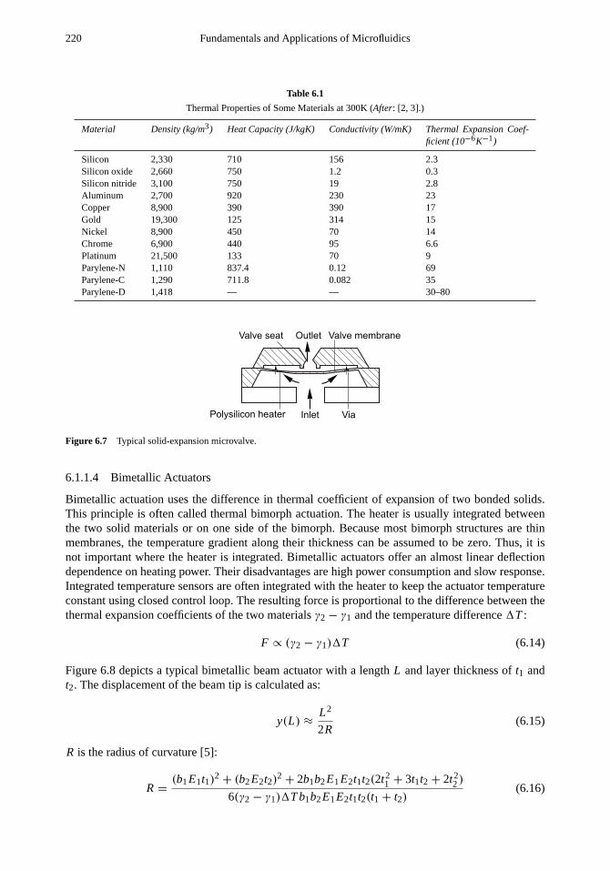
220 Fundamentals and Applications of Microfluidics
Table 6.1
Thermal Properties of Some Materials at 300K (After: [2, 3].)
Material Density (kg/m3) Heat Capacity (J/kgK) Conductivity (W/mK) Thermal Expansion Coef-ficient (10−6K−1)
Silicon 2,330 710 156 2.3Silicon oxide 2,660 750 1.2 0.3Silicon nitride 3,100 750 19 2.8Aluminum 2,700 920 230 23Copper 8,900 390 390 17Gold 19,300 125 314 15Nickel 8,900 450 70 14Chrome 6,900 440 95 6.6Platinum 21,500 133 70 9Parylene-N 1,110 837.4 0.12 69Parylene-C 1,290 711.8 0.082 35Parylene-D 1,418 — — 30–80
Outlet
Inlet
Valve membrane
Via
Valve seat
Polysilicon heater
Figure 6.7 Typical solid-expansion microvalve.
6.1.1.4 Bimetallic Actuators
Bimetallic actuation uses the difference in thermal coefficient of expansion of two bonded solids.This principle is often called thermal bimorph actuation. The heater is usually integrated betweenthe two solid materials or on one side of the bimorph. Because most bimorph structures are thinmembranes, the temperature gradient along their thickness can be assumed to be zero. Thus, it isnot important where the heater is integrated. Bimetallic actuators offer an almost linear deflectiondependence on heating power. Their disadvantages are high power consumption and slow response.Integrated temperature sensors are often integrated with the heater to keep the actuator temperatureconstant using closed control loop. The resulting force is proportional to the difference between thethermal expansion coefficients of the two materialsγ2 − γ1 and the temperature difference1T :
F ∝ (γ2 − γ1)1T (6.14)
Figure 6.8 depicts a typical bimetallic beam actuator with a lengthL and layer thickness oft1 andt2. The displacement of the beam tip is calculated as:
y(L) ≈L2
2R(6.15)
R is the radius of curvature [5]:
R =(b1E1t1)2 + (b2E2t2)2 + 2b1b2E1E2t1t2(2t2
1 + 3t1t2 + 2t22)
6(γ2 − γ1)1T b1b2E1E2t1t2(t1 + t2)(6.16)

Microfluidics for Internal Flow Control: Microvalves 221
Heat
L
t1
t2E2, � 2
E1, � 1
r
y
� 1<� 2
F
Figure 6.8 Bimetallic beam actuator.
whereb1 and b2 are the widths of the two material layers.E1 and E2 are Young’s moduli. Theequivalent force on the tip of the beam is:
F =3(E I )beamy(L)
L3(6.17)
The flexural rigidity of the beam(E I )beamis:
(E I )beam=(b1E1t2
1)2+ (b2E2t2)2 + 2b1b2E1E2t1t2(2t2
1 + 3t1t2 + 2t22)
12(t1b1E1 + t2b2E2)(6.18)
Assuming that the two layers have the same widthb, the radius of curvature and the equivalent tipforce can be simplified to:
r =t1 + t2
6
3(1 +
t1t2
)2+
(1 +
t1E1t2E2
) [(t1t2
)2+
t2E2t1E1
](γ2 − γ1)1T
(1 +
t1t2
)2(6.19)
F =3b
4L
t1 + t21
t1E1+
1t2E2
(γ2 − γ1)1T (6.20)
Example 6.5: Design of a Thermomechanical Valve with Bimetallic Actuator
A thermomechanical microvalve has a rigid square seat of 500× 500 µm. The valve seat issuspended on four flexures. Each flexure is 500µm long and 200µm wide. The flexure is made of10-µm silicon and 2-µm aluminum. The silicon heater is integrated in the flexure. The aluminumlayer is evaporated at 400◦C. If a normally closed microvalve is to be designed at 25◦C, whatis the maximum gap between valve opening and the surface of the valve seat wafer? Materialproperties are given in the figure below.
Si: t1=10 �m, �1=2.3�10-6
K-1
, E1=170 GPa
�m
F(�T)x
ymax
500 �m
500 �m
200 �m
A
A
A-A
Al: t2=2 �m, �2=23�10-6
K-1
, E2=70 GPa

222 Fundamentals and Applications of Microfluidics
Solution.From (6.20), we get the equivalent force at the tip of each actuating flexure as a functionof the temperature difference:
F =3b
4L
t1 + t21
t1E1+
1t2E2
(γ2 − γ1)1T = 9.639× 10−61T N
Assuming that the two layers are stress-free under evaporation conditions, the force acting at eachflexure tip at room temperature is:
F = 9.639× 10−61T = 9.639× 10⁻⁶(400− 25) = 3.615× 10⁻³ N
Using (6.18), the flexural rigidity of the composite beam is:
(E I )beam =(b1E1t2
1)2+(b2E2t2)2+2b1b2E1E2t1t2(2t2
1+3t1t2+2t22)
12(t1b1E1+t2b2E2)
= 3.774× 10⁻⁹ Pa.m4
Since the rectangular valve seat is rigid, we need to assume that the slope at the tip is zero. Ify isthe function of the deflection along the beam, the differential equation fory is:
(E I )beamy′′′= −F
Solving the above equation with boundary conditions at (x = 0) and (x = L):
y′(0) = 0; y′(L) = 0; y(0) = 0
we get the beam deflection as a function ofx (see Appendix D):
y(x) =F
2(E I )beam
(−x3
3+
Lx2
2
)Thus, the maximum deflection at the beam tip is:
ymax =F L3
12(E I )beam=
3.615× 10−3× (5 × 10−4)−3
12× 3.774× 10−9= 10× 10−6 m = 10µm
The gap between the valve opening and the surface of the valve seat wafer should be less than10µm to have a normally closed valve.
Example 6.6: Minimum Opening Pressure and Temperature
If the gap between valve opening and surface of the valve seat wafer is 5µm, how large shouldthe inlet pressure be to open the valve? What is the minimum temperature difference for openingthe valve at zero inlet pressure? The valve opening is 200× 200µm.
Solution. The force for keeping the flexure deflection at 5µm is:
F = y12(E I )beam
L3= 5 × 10⁻⁶ 12× 3.774× 10−9
(5 × 10⁻⁴)3= 1.812× 10⁻³ N = 1.812 mN
Thus, the closing force of the valve seat is:
Fclosing = 4 × (3.615− 1.812)× 10−3= 7.212× 10⁻³ N

Microfluidics for Internal Flow Control: Microvalves 223
Table 6.2
Typical SMAs (After: [6].)
Alloy Composition Transformation Tempera-ture Range (◦C)
Transformation Hysteresis(◦C)
Ag-Cd 44/49 at.% Cd −190 to−50 15Au-Cd 46.5/50 at.% Cd 30 to 100 15Cu-Al-Ni 14/14.5 wt.% Al 3/4.5 wt.% Ni −140 to 100 35Cu-Sn approx. 15 at.% Sn −120 to 30 —Cu-Zn 38.5/41.5 wt.% Zn −180 to−10 10In-Ti 18/23 at.% Ti 60 to 100 4Ni-Al 36/38 at.% Al −180 to 100 10Ni-Ti 49/51 at.% Ni −50 to 110 30Fe-Pt approx. 25 at.% Pt approx.−130 4Mn-Cu 5/35 at.% Cu −250 to 180 25Fe-Mn-Si 32 wt.% Mn, 6 wt.% Si −200 to 150 100
The corresponding minimum opening pressure required is:
1popening=Fclosing
A=
7.212× 10⁻³
(200× 10−6)2= 1.803× 10⁵ Pa= 1.803 bar
From the solution of Example 6.5, the thermomechanical force as a function of temperaturedifference is given as:
F = 9.639× 10−61T N
The temperature difference needed for opening the valve is:
1T = 400−1.812× 10⁻³
9.639× 10−6= 188◦C
6.1.1.5 Shape-Memory Alloy Actuators
Shape-memory alloys (SMA) are materials such as titanium/nickel alloy, which, once mechanicallydeformed, return to their original undeformed shape upon a change of temperature. SMAs undergophase transformations from a “soft” state (martensite) at low temperatures to a “hard” state (austen-ite) at higher temperatures. Since the alloy structure represents an electrical resistor, passing a currentthrough it can generate heat. Table 6.2 lists the most important parameters of some common SMAs[6].
Of all these alloys, the Ni/Ti alloys have received the most development effort and commercialexploitation. Figure 6.9 shows the typical stress-strain curves of an SMA at different phases. At alow temperatureT1, the martensite is soft with a low Young’s modulus. At a high temperatureT3,the austenite has a much higher Young’s modulus. The dashed line on the martensite curve indicatesthat upon heating and after removing the stress, the alloy remembers and takes its unstrained shapeas the SMA transforms back to austenite. The shape recovery is not found in the austenite phase.
6.1.1.6 Piezoelectric Actuators
Piezoelectricity is a reversible effect in which a mechanical stress on a material generates electricalcharge, and an applied electric field generates a mechanical strain in the material. Piezoelectric actua-tors generally generate small strain (usually less than 0.1%) and high stresses (several megapascals).

224 Fundamentals and Applications of Microfluidics
Strain
Stress (I)
(III)
(II)
T1, cold (martensite)
Open
Closed
A B
CD
Spring load
T2, phase transition
(pseudoelastic)
T3, hot (austenite)
Figure 6.9 Typical stress-strain curves at different temperatures relative to the transformation, showing (I) austenite,(II) pseudoelastic, and (III) martensite behavior.
�
�
�(2) tra
nsversal
(1) longitudinal(3
)vert
ical
Figure 6.10 Piezoelectric actuator.
Therefore, they are suitable for applications which require large forces but small displacements. Therelation between the strain and electric field strength is described with the piezoelectric coefficientsd31 andd32. The indices indicate the directions of polarization. In the case of an electric fieldEel asdepicted in Figure 6.10, the strains in three directions are given by:
ϕl = ϕt = d31Eelϕv = d33Eel
(6.21)
whereϕl , ϕt, andϕv are the longitudinal, transversal, and vertical strains, respectively. Table 6.3 liststhe properties of some common piezoelectric materials. Common piezoelectric materials, whichcan be integrated with microtechnology, are polyvinylidene fluoride (PVDF), lead zirconate titanate(PZT), and zinc oxide (ZnO). PZT offers high piezoelectric coefficients but is very difficult to depositas a thin film. PVDF and ZnO are often used in microfabrication.
Because of the large force and commercial availability, piezoelectric actuators were amongthe first to be used in microvalves. Thin-film piezoelectric actuators do not deliver enough forcefor valve applications. All reported piezoelectric microvalves used external actuators, such aspiezostacks, bimorph piezocantilevers, or bimorph piezodiscs. Compared to a piezostack, bimorphpiezocantilevers have the advantage of large displacements. The relatively small forces are notcritical due to the small opening in microvalves. Example 6.7 illustrates the use of a bimorphpiezocantilever.
Example 6.7: Designing a Piezoelectric Valve with a Piezobimorph Actuator
The specification of a piezobimorph is given in the following table:

Microfluidics for Internal Flow Control: Microvalves 225
Table 6.3
Properties of Common Piezoelectric Materials (After: [3, 7])
Material d31 (10−12 C/N) d33 (10−12 C/N) Relative Permittivityεr
PZT −60–−270 380 to 590 1,700ZnO −5 12.4 1,400PVDF 6–10 13–22 12BaTiO3 78 190 1,700LiNbO3 −0.85 6 —
Dimension (mm) Voltage (V) C (nF) Ymax (µm) Fmax (N) Frequency (Hz)
25× 7.5 × 0.4 ±70 20 ±200 0.15 300
The actuator is used for closing a silicon microvalve, which has a 300× 300 µm valve seatsuspended on four flexures as described in the following figure. The initial gap between the valveseat and the valve inlet is 20µm. The dimensions of the flexures are 500× 100× 20 µm. Thevalve inlet is drilled in a glass substrate with a diameter of 200µm. Determine the maximum inletpressure.
Solution. The spring constant of the valve seat can be modeled as that of four beams:
k =4Ewt3
l 3=
4 × 170× 109× 10−4
× (2 × 10−5)3
(5 × 10⁻⁴)3= 4,352 N/m
The characteristics of the actuator and the valve spring are described in the figure above. Themaximum achievable force at displacementd0 is:
Fmax@d0 = Fmax
(1 −
d0
ymax
)= 0.15× (1 − 20/200) = 0.135 N
The maximum closing force is:
Fmax@d0 = Fmax@d0 − kd0 = 0.135− 4,352× 20× 10−6= 0.048 N
The maximum inlet pressure the valve can withstand is:
1pmax = Fclosing,max/A = 0.048/π(10−4)2 = 15.28× 10⁵ Pa= 15.28 bar

226 Fundamentals and Applications of Microfluidics
Radius (µm)
0
5
10
15
20
25
0 400 800 1,200 1,400 1,600 2,000
Curved electrode
V
Moving electrode
Moving electrode
Curved electrode
Valve seat
Valve membrane
Insulator
InletOutlet
(a) (b)
Deflection
(µm
)Figure 6.11 Concept of a curved electrode for a large electrostatic displacement: (a) valve concept, and (b) simulatedmembrane deflection of the membrane; the arrow indicates the increase of drive voltage.
6.1.1.7 Electrostatic Actuators
Electrostatic actuation is based on the attractive force between two oppositely charged plates. Thesimplest approximation for electrostatic forces is the force between two plates with the overlappingplate areaA, distanced, applied voltageV , relative dielectric coefficientεr (Table 6.4), and thepermittivity of vacuumε0 = 8.85418× 10⁻¹² F/m :
F =1
2εrε0A
(V
d
)2
(6.22)
If an insulator layer of thicknessdi and a relative dielectric coefficientεi separate the twoplates, the electrostatic force becomes:
F =1
2εrε0A
(V
d
)2 (εid
εrdi + εid
)2
(6.23)
The biggest advantage of an electrostatic actuator is its fast response. However, the highdrive voltage and small displacement make it difficult to integrate electrostatic microvalves intoa microfluidic system. One solution for this problem is the use of curved electrodes. Figure 6.11(a)shows an example of an electrostatic actuator with a curved electrode. The gap between the twoelectrodes is small at the clamped edge of the moving electrode and increases along its length.When a voltage is applied, the moving electrode deforms and attaches to the curved electrode [Figure6.11(b)]. An insulator layer on the fixed electrode is required to prevent a short circuit between thetwo electrodes.
Example 6.8: Designing an Electrostatic Valve
A normally open electrostatic valve for air flow is designed with a silicon nitride/aluminum valveseat. The aluminum layer and the silicon substrate represent the actuator electrodes. The valveopening is 100× 100µm. The valve seat is a 500-× 500-µm square plate, which is suspendedon four flexures. Each flexure is 100µm long and 20µm wide. The aluminum layer is 5µm thick,and the silicon nitride layer is 2µm thick. The gap between the valve seat and the valve opening is5 µm. Assume that there is no residual stress at room temperature. Determine the pull-in voltage

Microfluidics for Internal Flow Control: Microvalves 227
Table 6.4
Permittivity of Common Materials (After: [7, 3].)
Material Relative Permittivity
Silicon oxide 3.8Silicon nitride 4Polyimide 3.4 (at 1 MHz)Parylene-N (C, D) 2.65 (3.15, 2.84)Silicone rubber 2.8 (at 1 MHz)Al2O3 10 (at 1 MHz)Quartz 3.8 (at 1 MHz)Silicon 11.8Silicon carbide 9.7
of the actuator and the maximum inlet pressure that the valve can withstand at this drive voltage(Enitride = 270 GPa,εnitride = 4, EAl = 704 GPa). If the voltage decreases, what is the pull-upvoltage?
Solution. Neglecting the areas of the flexures, the active area of the electrostatic actuator is:
1A = Aseat− Aorifice = (500× 10−6)2 − (100× 10−6)2 = 24× 10−8 m2
Based on the model of a composite beam described in Example 6.5, the spring constant of eachflexure is:
k0 =12(E I )beam
L3
=(b1E1t2
1)2+(b2E2t2)2+2b1b2E1E2t1t2(2t2
1+3t1t2+2t22)
L3(t1b1E1+t2b2E2)
= 468.78 N/m
The spring constant of the valve seat is:
k = 4k0 = 4 × 468.78 = 1,875 N/m
Assuming that the relative dielectric coefficient of air is 1, and rearranging (6.23), the electrostaticforce acting on the valve seat at a gapd is:
F =ε0AV2
2(d +
diεi
)2
With the initial gapd0 = 5 mm, the net force acting on the valve seat is the sum of electrostaticforce and spring force:
F =−ε0AV2
2(d +
diεi
)2+ k(d0 − d)
Since the net force is a function of the gapd, the change of this force is calculated as:
1Fnet(d) = F ′net(d)1d =
[ε0AV2
4×
1
(d + di/εi)3
− k
]1d

228 Fundamentals and Applications of Microfluidics
At the pull-in voltage, the actuator reaches an unstable equilibrium, where the following condi-tions are fulfilled: { Fnet = 0
1Fnet = 0
or k =ε0AV2
4 ×1
(d+di/εi)3 (a)
ε0AV2
2(d+di/εi)2= k(d0 − d) (b)
Substituting (a) in (b), we get a quadratic equation ind. Solving this equation and taking thepositive solution, we get the critical gapdcr:
dcr =d03 −
2di3εi
dcr =5×10⁻⁶
3 −2×2×2×10−6
3×4 = 1.33× 10⁻⁶ m
Substituting the critical gapdcr into (a) and rearranging it for the critical pull-in voltage, which isthe voltage required to close the valve, we get:
Vcr = 2
√k (dcr + di/εi)
3
ε0A
With the given data, we get the critical pull-in voltage of the valve seat:
Vcr = 2
√1,875×
(1.33× 10−6 + 2 × 10⁻⁶/4
)3
8.85418× 10−12 × 24× 10−8
At this voltage, the closing force of the valve is:
Fclosing =εiε0AV2
2d2i
− kd0
=4×8.85418×10−12
×24×10−8×1472
2(2×10⁻⁶)2− 1,875× 5 × 10−6
= 13.6 × 10⁻³ N
Thus, the maximum inlet pressure in this case is:
1p =Fclosing
Aopening=
13.6 × 10⁻³
(10−4)2= 13.6 × 10⁵ Pa= 13.6 bars
The pull-up voltage, which is required to open the valve, is reached if the electrostatic force isequal to the spring force:
εiε0AV2
2d2i
− kd0 → V =
√2kd0d2
i
εiε0A=
√2 × 1875× 5 × 10−6 × (2 × 10−6)2
4 × 8.8541× 10−12 × 24× 10−8
This example describes the general behavior of a normally open, electrostatic valve. Increasingthe drive voltage up to pull-in voltage causes the valve seat to snap down. The closing force withthis voltage is large enough to keep the valve closed against an inlet pressure. If this voltagedecreases, the valve remains closed until the pull-up voltage is reached. The spring force pushesthe valve seat back to its opening position.

Microfluidics for Internal Flow Control: Microvalves 229
Table 6.5
Magnetization of Common Materials atB = 0 T (After: [7].)
Material Magnetization Mm (A/m) Note
Nickel 3,000 Electroplated, annealedIron 320 —Fe-Ni78 < 80 Electroplated, annealedFe-Ta-Ni 46 SputteredFe-Al-Si 40 Sputtered
6.1.1.8 Electromagnetic Actuators
Electromagnetic actuators offer a large deflection. The vertical force of a magnetic fluxB in directionz acting on a magnet with its magnetizationMm (Table 6.5) and volumeV is given by:
F = Mm
∫dB
dzdV (6.24)
The relation between the magnetic fluxB and the magnetic field strength is:
B = µH = µ0µr H = µ(1 + χm)H (6.25)
whereµ, µ0, µr, andχm are the permeability, permeability of free space (4π × 10−7 H/m), relativepermeability, and the magnetic susceptibility of the medium, respectively.
Electromagnetic microvalves often use a solenoid actuator with a magnetic core and a coil forgenerating the magnetic field. One or both components can be integrated in silicon for a compactdesign. The drawback of electromagnetic actuators is the low efficiency due to heat loss in the coil.The magnetic field strength inside a solenoid withN turns, a lengthL and a driving currentI canbe estimated as:
H =N I
L(6.26)
6.1.1.9 Electrochemical Actuators
The pressure drop1p across a liquid-gas interface in a capillary can be used as the active valvepressure:
1p =2σlg cosθ
r0(6.27)
whereσlg is the gas-liquid surface tension,θ is the contact angle, andr0 is the channel radius.Electrochemical valves are actuated using gas microbubbles generated by the electrolysis of
water:2H2O → 2H2 ↑ +O2 ↑ (6.28)
The generated gases have a volume that is about 600 times that of the water volume neededfor it. This ratio exceeds that of thermopneumatic actuators. The pressure inside the bubble isproportional to the surface tensionσ and the radius of curvatureR of the meniscus. Equation (6.27)becomes:
1p =2σ
R(6.29)

230 Fundamentals and Applications of Microfluidics
The reversed reaction converts the two gases back to water. The reaction needs a catalyst suchas platinum. Platinum is able to absorb hydrogen. The hydrogen-platinum bond is weaker than thehydrogen-hydrogen bond. Therefore, the energy barrier required for freeing hydrogen atoms fromH2 and bonding with oxygen is lower than in the gas phase:
2H2 + O2Pt,heat−→ 2H2O (6.30)
Example 6.9: Designing an Electrochemical Valve
Determine the energy required for generating an electrolysis bubble with an approximateddimension of 200× 100 × 28 µm. Compare it to a thermal bubble of the same size. Thespecific density of hydrogen and oxygen at 1 bar and 25◦C are 0.08988 kg/m3 and 1.429 kg/m3,respectively. The surface tension of water is assumed to be constant at 72×10−3 N/m. Enthalpy offormation of water is 285.83 kJ/kmol. The thermodynamic properties of liquid water at 1 bar are:v(25◦C) = 1.0029×10⁻³ m3/kg, u(25◦C) = 104.88 kJ/kg; and of vapor: v(100◦C) = 1.673 m3/kg,u(25◦C) = 2506.5 kJ/kg.
Solution. Assuming a contact angle of zero, the pressure inside the bubble can be estimated as:
1p =2σ
r=
4σ
h=
4 × 72× 10−3
28× 10−6≈ 105 Pa= 1 bar
Thus, all properties at 1 bar can be taken for the analysis. The specific density of the electrolysisgas mixture is:
ρmixture =ρoxygen+ 2ρhydrogen
3=
1.429+ 2 × 0.08988
3= 0.5363 kg/m3
Thus, the amount of water required for generating the electrolysis bubble is:
m = Vρmixture = 2 × 10−4× 10−4
× 28× 10−6× 0.5363= 30.03× 10⁻¹⁴ kg
The mole number is:
n =m
MH2O=
30.03× 10⁻¹⁴
18= 1.67× 10⁻¹⁴ kmol
The energy required for making an electrolysis bubble is:
1Uelectrolysis= nh0f = 1.67× 10⁻¹⁴(2506.5 − 104.88)× 103
= 0.804× 10⁻⁶ J
The specific volume of water vapor at 100◦C is 1.673 m3/kg, and the mass of water is:
m =V
v=
2 × 10−4× 10−4
× 28× 10−6
1.673= 33.47× 10⁻¹⁴ kg
Ignoring the heat losses, the energy required for making a thermal bubble is:
1Uthermal= m(u2 − u1) = 33.47× 10⁻¹⁴(2506.5 − 104.88)× 103= 0.804× 10⁻⁶
In both cases, the expansion work done by the bubble is:
W = p1V = 105× (2 × 10−4
× 10−4× 28× 10−6) = 56× 10−9 J

Microfluidics for Internal Flow Control: Microvalves 231
The efficiency of an electrolysis bubble is:
ηelectrolysis=W
W +1Uelectrolysis=
56× 10−9
56× 10−9 + 477× 10−11≈ 100%
The maximum efficiency of a thermal bubble is:
ηthermal=W
W +1Uthermal=
56× 10−9
56× 10−9 + 0.804× 10−6= 6.51%
6.1.1.10 Chemical Actuators
In all the above actuating concepts, electrical energy is converted into mechanical energy using anumber of physical effects. In contrast, chemical actuators convert chemical energy into mechanicalenergy. Furthermore, the increasing use of polymers in the fabrication of microfluidic systems (seeChapter 3) is compatible with the integration of polymer-based chemical actuators.
One of the major drawbacks of polymeric material in microfluidic systems is their swellingbehavior. However, this behavior is attractive for actuator applications. Hydrogels are polymerswith high water content. Hydrogels can change their volume if changes in temperature, solventconcentration, and ionic strength are induced. The swelling behavior is controlled by diffusionand thus is very slow in macroscale. In microscale, the response time to stimuli is drasticallyreduced due to the shorter diffusion path. Another advantage of this actuation scheme is thatthese polymers can be designed to suit conventional microtechnologies such as photolithography.For instance, a hydrogel called PNIPAAm [poly-(N-isopropylacrylamide)] [8] can be designed tohave a compromise between film coating, UV polymerization, and working conditions at roomtemperatures. Hoffmann et al. reported a hydrogel system, which can be coated with a thicknessof several tens of microns and cross-linked with conventional UV exposure units [8]. This polymerhas a phase transition temperature of approximately 33◦C. At room temperature below this value,the polymer is swollen. The polymer shrinks if the temperature increases above the transitiontemperature. Thus, together with a microheater, the hydrogel can be used as a thermomechanicalactuator [9].
The swelling effect can also be achieved with the diffusion of a solvent such as water. Sincethe temperature diffusivity is on the order of 10−3 cm2/s, the diffusion coefficient of a solvent is onthe order of 10−5 cm2/s, the cooperative diffusion coefficient of polymer chains is on the order of10−7 cm2/s, and the swelling dynamics are determined by the later coefficient. The characteristictime constant of swelling response can be estimated as [10]:
τ =d2
Dcoop(6.31)
whered is the characteristic dimension of the hydrogel, andDcoop is the cooperative diffusioncoefficient of the polymer chains. From (6.31), the dynamics of chemical actuators depends onlyon the size and the bulk polymer. Using packed small particles instead of a bulk material wouldimprove the response of the actuator.
Other types of hydrogels such as polymethacrylic acid tri-ethyleneglycol (pMAA-g-EG)[11], polyacrylic acid-2-hydroxymethylmethacrylate (pAA-2-HEMA) [12], and polyacrylamide-3-methaacrylamidophenylboronic acid (pAAm-3-MPBA) [13] swell and shrink in response to changesin concentrations of pH (potenz of hydrogen). The pH of distilled water is 7, which is neutral. Anysolution with a pH below 7 is an acid and any solution with a pH above 7 is an alkali. The hydrogelswells in alkali solution and shrinks in acidic solution. The transition region of pAA-2-HEMA and

232 Fundamentals and Applications of Microfluidics
pMAA-g-EG is approximately 4< pH< 7 [11, 12], while AAm-3-MPBA [13] switches its volumeat approximately 7< pH < 9. The swelling effect results from the tendency of the polymer chainsto mix with the solution. Swelling stops when the elastic restoring force is in equilibrium with theosmotic force.
6.1.1.11 Capillary-Force Actuators
When considering miniaturization, surface tension becomes an important force in microscale. Whilecapillary forces and surface tension cause sticking problems in other MEMS applications, theyare useful for microfluidic applications. Surface tension and capillary forces can be controlledactively or passively using different effects: electrocapillary, thermocapillary, and passive capillary.Applications of surface tension driven flow for pumping are discussed in Chapter 7.
Electrocapillary Effect.Theelectrocapillary effect[14], also known aselectrowetting, changes thesurface tension between two immiscible, conductive liquids, or between a solid surface and a liquid,by varying their potential difference. The effect is based on the adsorption characteristics of ions inthe wetting interface. This interface is an electric double layer. This layer, typically 10A to 100Athick, works as an electrical insulator between the two conductive liquids. By changing the electricalpotential across this double layer, the surface tensionσ between the two liquids becomes [14]:
σ = σ0 −C
2(V − V0)
2 (6.32)
whereσ0 is the maximum value of surface tension atV = V0, C is the capacitance per unit areaof the double layer, andV is the voltage applied across the liquid interface. Readers can refer toChapter 7 for more configurations and applications of electrocapillary effect.
Example 6.10: Characteristics of an Electrocapillary Actuator
The contact angle of the nonwetted side of a capillary is 140◦ and the angle on the wettingelectrode is 30◦. The gap between the bottom electrode and the nonwetted side is 10µm.Determine the pressure gain from the electrocapillary effect if the liquid is a water-basedelectrolyte.
Wetting electrode
�dry
�wet
dLiquid Air
Solution. The pressure gain can be calculated from the contact angles and the surface tension ofwater-airσ = 72× 10−3 N/m [15]:
1p = σ[2 cos
(θdry+θwet
2
)cos
(θdry−θwet
2
)/d
]1p = 72× 10−3
[2 cos(85◦) cos(55◦)/10× 10−6
]= 144× 102 Pa= 144 mbar
Thermocapillary Effect.The thermocapillary effect is caused by the temperature dependence ofthe surface tension. The surface tension reflects the surface energy. At a higher temperature, themolecules of the liquid move faster and their attractive force becomes smaller. The smaller attractive

Microfluidics for Internal Flow Control: Microvalves 233
L
x
(a) (b)
Ta
Tr
�a �r
�a�
r
Tr T
a
Heat Heat
Figure 6.12 Thermocapillary effect (Marangoni effect): (a) a gas bubble is attracted to the heat source; and (b) a liquid plugis driven away from a heat source.
Figure 6.13 Passive capillary effect: (a) bubble in small channel; (b) bubble in the intersection; and (c) bubble in the largechannel.
force causes lower viscosity and lower surface tension. Figure 6.12 demonstrates the principleof the thermocapillary effect, or the so-called Marangoni effect. Imagine a vapor bubble in acapillary [Figure 6.12(a)]. Across the bubble exists a temperature gradient. At the left-hand side,the temperature is higher, so the surface tension is lower. That causes a pressure gradient acrossthe bubble, which leads to bubble movement from right to left. Since the rate of change of surfacetension with temperature is not large, the effect requires considerable heating power to get the desiredforce. The same effect causes a liquid droplet to move away from the heat source. This effect can beutilized for designing droplet micropumps described in Chapter 7.
Passive Capillary Effect.The passive capillary effect utilizes dependence on the geometry. Thesurface tension increases with the smaller radius of curvature, which can be controlled by channelwidth or the solid/liquid contact angle [16]. Figure 6.13 explains the principle of the passive capillaryeffect. If a bubble is confined in a channel with a hydrophilic wall, the bubble is forced to adopt theshape of the channel [Figure 6.13(a)]. The surface tension or surface energy usually tends to haveits minimum values. That explains the spherical surface of a bubble. In the case of Figure 6.13(b),the bubble is forced to have different surface tensions on the left-hand and right-hand sides becauseof the different radii of curvature. The surface tension gradient moves the bubble toward the largersection of the channel. In the large section, the bubble forms a sphere to minimize its surface energy[Figure 6.13(c)]. Refer to Chapter 7 for more applications of this effect.
Example 6.11: Characteristics of a Passive Capillary Valve
A bubble valve is designed with a vapor bubble between channel sections with different widths of50 and 200µm (Figure 6.12). Determine the pressure difference the valve can withstand.
Solution. Assuming that the radii of curvature of the bubble are equal to channel widths, and thesurface tension of the water-air interfacesσ = 72× 10−3 N/m, and using (6.29) for each side ofthe bubble, we get the pressure difference across it:
1p = 2σ(
1r1
−1r2
)= 2 × 72× 10−3
(1
50×10−6 −1
200×10−6
)= 2,160 Pa= 21.6 mbar

234 Fundamentals and Applications of Microfluidics
(a) Normally open valve
(b) Normally closed valve
Fflow
Fspring
Factuator
Fspring
Factuator
Fflow
Factuator
Fflow
Fspring
Factuator
Fspring
Fflow
Figure 6.14 Functions of valve springs and force balance in (a) NO valves and (b) NC valves;Finlet, Fspring, andFactuatorare forces of fluid, spring, and actuator, respectively.
More than one-fiftieth of atmospheric pressure can be achieved with this passive capillary valve.
6.1.2 Valve Spring
In most microvalve designs, the valve seat structure can be thought of as a spring. The spring forcecloses the valve in normally closed valves. In the case of normally open valves, the spring worksagainst the actuator and decreases the closing force. Figure 6.14 illustrates different arrangementsof forces acting on the valve seat.
Figure 6.15 depicts common forms of the valve spring and their corresponding spring con-stants. In normally closed valves, the spring constant should be large to resist the inlet pressure. Innormally open valves, the spring constant is to be optimized for a minimum value, which allows alarger closing force of the actuator. A small spring constant can be realized with a soft material suchas rubber. The solution with soft materials offers a further advantage of excellent fitting character-istics. The leakage ratio can be improved from three to four orders of magnitude compared to thosemade of hard material such as silicon, glass, or silicon nitride.
If the valve is designed for bistable operation, there is no need for a valve spring because thetwo valve states are controlled actively. Since the nonpowered state is undefined, a valve spring canstill be considered for the initial, nonpowered state to assure safe operation.
A bistable valve spring allows the valve seat to snap into its working position. In this case,the actuator just needs to be powered in a short period to have enough force to trigger the positionchange. The force generated by the spring is then high enough to seal the valve inlet. Thus, theactuator does not need to be powered over the entire operation. A spring in the form of a prestressedbeam [Figure 6.15(a)] or prestressed circular membrane [Figure 6.15(d, e)] has for instance, thisbistable characteristic. For the buckling behavior of a beam, readers may refer to Timoshenko’sclassic “Theory of Elastic Stability” [17].

Microfluidics for Internal Flow Control: Microvalves 235
F L
Wt
FL
t
W
(a) (b) (c)
(d) (e)
F2R
t
Fa
t
p2R
t
t t t
t t
a
Figure 6.15 Typical valve springs and their spring constants (linear theory for small deflection, which is smaller than thestructure thickness;k: spring constant,E: Young’s modulus,t : structure thickness,W: structure width,L: structure length,ν: Poisson’s ratio,R: radius, anda: membrane width; see Appendix D): (a) cantilever; (b) suspended plate; (c) rectangularmembrane,ν = 0.3; (d) circular membrane, point load; and (e) circular membrane, distributed load.
For a prestressed circular valve membrane with a radius ofR and a thickness oft , the twostable deflection positions of the membrane center are [18]:
ysnap= ±1
24
√−105
(3R2σ0
1 − ν2
E+ 4t2
)(6.33)
whereσ0, E, andν are the prestress of the membrane at nondeflected position [y(r ) = 0], theYoung’s modulus, and the Poisson ratio, respectively. The deflection of the membrane under adistributed load can be estimated as:
y(r ) = y0
(1 −
r 2
R2
)2(6.34)
At a given center deflectiony0, the pressure and the force exerted by the valve membrane are:
p =4ty0
R2
(4
3
t2
R2
E
1 − ν2+ σ0 +
64
105
y20
R2
E
1 − ν2
)(6.35)
F = −2π
3
(8
3t3 E
1 − ν2
y0
R2+ 2y0tσ0 +
128
105
E
1 − ν2
ty30
R2−
1
2pR2
)(6.36)
wherep is the pressure acting on the membrane. Thus, with a gapd between valve membrane, andan inlet and a inlet radius ofRinlet, the inlet pressure can be estimated as:
pinlet =4
3
dt
R2inlet
(4
3
t2
R2
E
1 − ν2+ σ0 +
64
105
E
1 − ν2
d2
R2
)(6.37)
Example 6.12: Operation Conditions of a Bistable Microvalve

236 Fundamentals and Applications of Microfluidics
A microvalve is designed with a circular membrane [Figure 6.15(e)] working as both valve springand valve seat. The membrane is made of hardbacked SU-8, and has a radius ofR = 2 mm and athickness oft = 20µm. The gap between the membrane and the valve inlet is 100µm, while theradius of the valve inlet is 100µm. The center deflection of the membrane at nonloading conditionis y0,ini = 150µm. Determine critical switching pressure and the maximum inlet pressure thatthe valve can withstand in its closing state.
Solution. The Young’s modulus and Poisson ratio of hardbacked SU-8 are assumed to beE = 4GPa andν = 0.22, respectively. The membrane is deflected at nonloading condition. Thus, itis prestressed with an initial stress ofσ0. Setting the loading pressurep in (6.35) to zero andrearranging for the initial stress results in:
σ0 = −4
105E
1−ν2
16y20,ini+35t2
R2
= −4
1054×109
1−0.22216×(100×10−6)2+35(20×10−6)2
(2×10⁻³)2= −1.50× 10⁷Pa= −15.0 MPa
From (6.33), the critical switching positions are:
ysnap = ±124
√−105
(3R2σ0
1−ν2
E + 4t2)
= ±124
√−105
[3(2 × 10⁻³)2(−1.5 × 10⁷)1−0.222
4×10⁹ + 4(20× 10−6)2]
= ±8.66× 10⁻⁵ m = ±86.6 µm
Inserting the critical positionysnapin (6.35) results in the critical switching pressure for the valvemembrane:
psnap =4ty0R2
(43
t2
R2E
1−ν2 + σ0 +64105
y20
R2E
1−ν2
)
=4×20×10−6
×86.6×10−6
(2×10⁻³)2
[43(20×10−6)2
(2×10⁻³)24×109
1−0.222 − 15× 106+
64105
(86.6×10⁻⁶)2
(2×10⁻³)24×109
1−0.222
]= −1.66× 10⁴ Pa= −16.6 kPa
From (6.37), the maximum inlet pressure the valve can withstand is:
pinlet =43
dtR2
inlet
[43
t2
R2E
1−ν2 + σ0 +64105
E1−ν2
d2
R2
]=
43
−100×10−6×20×10−6
(100×10−6)2
[43(20×10−6)2
(2×10⁻³)24×109
1−0.222 − 15× 106+
64105
4×10⁹
1−0.222(100×10−6)2
(2×10⁻³)2
]= 2.13× 10⁶ Pa= 21.3 bars
Example 6.13: Optimization of a Bistable Microvalve [18]
Determine for the bistable valve of Example 6.12 the optimal membrane thicknesst and theoptimal gapd between the valve membrane and the inlet. If both parameters are to be optimal,what is the maximum achievable inlet pressure?

Microfluidics for Internal Flow Control: Microvalves 237
Solution. If the gap is fixed, the optimal membrane thickness results from setting the differentia-tion of (6.37) fort to be zero:
toptimal =
√−
16105d2 −
14σ0
1−ν2
E R2
=
√−
16105(−100× 10−6)2 −
14 × (−15× 106)1−0.222
4×10⁶ (2 × 10⁻³)2
= 4.51× 10⁻⁵ m = 45.1 µm.
If the membrane thickness is fixed, the optimal gap results from setting the differentiation of(6.37) ford to be zero:
doptimal =
√10524
√−3σ0
1−ν2
E R2 − 4t2
=
√10524
√−3 × −15× 106 1−0.222
4×10⁹ (2 × 10⁻³)2 − 4 × (20× 10−6)2
= 8.66× 10⁻⁵ m = 86.6 µm
If both thicknesst and the gapd are to be optimized, the above two equations result in:
tideal =14 R
√−3σ0
1−ν2
E
=14(2 × 10⁻²)
√−3(−15× 106)1−0.222
4×109
= 5.17× 10⁻⁵ m = 51.7 µm
and
dideal =R16
√−105σ0
1−ν2
E
=2×10⁻³
16
√−105× (−15× 106)1−0.222
4×109
= 7.64× 10⁻⁵ m = 76.4 µm
The maximum achievable inlet pressure is then:
pmax =
√35
32 σ20
1−ν2
ER2
R2inlet
=
√35
32 (−5 × 10⁶)2 1−0.222
4×10⁹(2×10⁻³)2
(100×10−6)2
= 3.94× 10⁶ Pa= 39.4 bars
6.1.3 Valve Seat
Valve seats represent a large challenge to microvalve design and fabrication. The valve seat shouldsatisfy two requirements: zero leakage and resistance against particles trapped in the sealing area.

238 Fundamentals and Applications of Microfluidics
(a) (b) (c)
(d) (e)
Figure 6.16 Methods for leakage-free valve seat: (a) large force, hard surface; (b) particle traps; (c) soft valve seat;(d) combination of (a) and (b); and (e) combination of (c) and (b).
(a)
pin
pact
(b)
pin
pact
pin
(c)
Spiral channel
Figure 6.17 Pressure compensation in microvalves: (a) behavior at the valve seat; and (b) passive flow controller.
For a minimum leakage rate, the valve should be designed with a large sealing area, which has to beextremely flat. Softer materials such as rubber or other elastomers are recommended for the valveseat.
Resistance against particles can be realized in many ways. First, a hard valve seat can simplycrush the particles. For this purpose, the valve needs actuators with large force such as piezostacksand hard coating layer for the valve seat. Second, the particles can be surrounded and sealed by asoft coating on the valve seat. Third, small particle traps such as holes or trenches can be fabricatedon the valve seat or on the opposite valve base [Figure 6.16(c)]. A combination of the third measurewith the first and the second measures is recommended, so that tiny particles can be trapped andburied after being crushed by the large actuation force [Figures 6.16(d, e)]. For the first and thirdmeasures, the valve seat needs to be coated with hard, wear-resistant material such as silicon nitride,silicon carbide, or diamond-like carbon.
6.1.4 Pressure Compensation Design
The closing pressure generated by the actuator should be greater than the inlet pressure to keep thevalve functioning. If the inlet pressure varies, there is a need for closed loop control for the actuatorto maintain the closing force [Figure 6.17(a)]. If the inlet pressure exceeds the maximum closingpressure of the actuator, the compensation approach described in Figure 6.17(b) can be used. Withthis method, the closing pressure is the sum of the inlet pressurepin and the actuator pressurepact.
This concept assures that the closing pressure is always larger than the inlet pressure. Theclosing pressure only depends on the actuator, which can be controlled by a simple open loop. Thedifferential pressure concept is very useful for normally closed valves, where the closing force reliesentirely on the relatively small spring force.

Microfluidics for Internal Flow Control: Microvalves 239
Table 6.6
Typical Parameters of Pneumatic Valves (Lvalve: Leakage ratio)
Refs. Type Size (mm×mm) Qmax (mL/min) pmax/pactuator(kPa)
Lvalve Material Technology
[20] NC 15× 15 120 air 241/69 > 300 Glass, silicon Bulk[21] NC 2× 5 4 air 50/80 − − − Glass, silicon Bulk[22] NO 0.225× 0.225 0.26 water 100/50 10,000 Rubber, silicon Bulk[23] NC 1× 1 0.01 water 70/20 — PDMS Polymeric[24] NC 20× 20 35 N2 65/12 35 Glass, silicon Bulk[25] NO 8.5 × 4.2 0.5 water 60/10 10,000 Rubber, silicon Bulk[26] NO 10× 10 5 N2 107/275 100,000 Glass, silicon Bulk
Another pressure compensation approach is the passive regulation of flow rates. This passivecomponent can also be categorized as a pneumatic proportional valve. Figure 6.17(c) shows a designexample [19]. If the pressure difference across the device increases, the deformation of the siliconmembrane increases as well. The deformed membrane covers more of the channel beneath themembrane. Thus, the channel length increases, and the higher fluidic impedance compensates theincrease of the pressure. The principle results in a constant flow rate. The device is relevant fordisposable drug delivery systems.
6.2 DESIGN EXAMPLES
6.2.1 Pneumatic Valves
A low leakage rate can be achieved by designing the valve seat carefully. Soft materials such asrubber improve the leakage ratio significantly, as shown in Table 6.6, which compares the leakageratio of rubber/silicon and glass/silicon valves.
The valve shown in Figure 6.18(a) has a bossed membrane [20]. The circular membrane has adiameter of 3.6 mm and a thickness of 25µm. The stack of three silicon wafers is directly bonded at1,000◦C (see Section 3.6.1). The inlets and the outlet are drilled in a glass plate, which is mountedon the silicon stack using anodic bonding (see see Section 3.6.1). A chromium layer on the glasssubstrate avoids bonding the valve seat. A similar design, reported in [21], shows that the behaviorof a pneumatically driven valve is analogous to that of field effect transistor (FET) in electronics.
The 225× 125-µm valve membrane shown in Figure 6.18(b) is made of a 25-µm siliconerubber layer, which is spin-coated on the silicon substrate [22]. The pneumatic access in the topwafer is drilled with laser. The valve can also be fabricated entirely from silicone rubber forimproving sealing properties as reported in [23].
The two membranes in Figure 6.18(c) are fabricated with polymeric surface micromachining(see Section 3.4). A 30-µm-thick silicone rubber layer works as the structural material, while thickpositive photoresists work as sacrificial layers. The heights of the pressure chamber in the lowerpart, and of the channel in the upper part, are defined by a photoresist thickness of 5 and 30µm,respectively.
Besides soft materials such as silicon rubber [22, 25], thinner membranes or corrugatedmembranes [22, 26] also provide low spring constants. In the valve of Figure 6.18(d), the membranethickness is defined by deep-boron diffusion in silicon (see Section 3.3.1).
For parallel displacement of the valve seat, the membrane can be designed with a bossed regionat its center. In the case of a corrugated membrane, the corrugation is structured in silicon by dry

240 Fundamentals and Applications of Microfluidics
(a) (b)
(c) (d)
Si Glass Rubber
Pressure chamber
Pressure chambers
Pressure chambers
Pressure chamber
Figure 6.18 Typical pneumatic valve: (a) bossed silicon membrane; (b) rubber membrane; (c) rubber membrane, two ways;and (d) corrugated silicon membrane.
(a)
(b)
(c)
(d)
Photoresist
Figure 6.19 Fabrication of corrugated membrane: (a) photoresist patterning; (b) dry etching of silicon substrate; (c) ionimplantation of boron; and (d) anisotropic etching from backside.
etching or isotropic etching (HF, HNO3) prior to the deep-boron diffusion. The wet-etching processin KOH from the backside forms the corrugated membrane (Figure 6.19). Additional coating withparylene improves the leakage ratio [26].
6.2.2 Thermopneumatic Valves
Figure 6.20 shows design examples of thermopneumatic valves. The metal membrane and the siliconmembrane of the valves depicted in Figures 6.20(a, b) have large spring constants. Their deflectionand the closing force are small. Soft materials such as rubber offer a higher displacement, lowerspring force, and, consequently, higher closing force [Figure 6.20(c)]. Since silicon is a thermalconductive material, the heat loss, and consequently the required operating power of a valve witha silicon membrane, are high. Table 6.7 shows that power consumption is one or two orders ofmagnitude larger for a silicon membrane compared to those with rubber membrane.
The heater in the valve depicted in Figure 6.20(b) is made of platinum, which is sputtered onthe Pyrex glass wafer. The filling ports are drilled in the glass wafer. Fluorocarbon (FC) works asactuation fluid. The valve membrane and valve seat are fabricated with bulk silicon micromachining(see Section 3.3.1). The valve is assembled with silicon direct bonding and anodic bonding (seeSection 3.6.1) [28, 29].
The valve membrane in Figure 6.20(c) is made of a 50-µm-thick silicone rubber and measures1.5× 2.5µm [30]. For better thermal insulation, the Cr/Au heater is placed on a low-stress siliconnitride membrane [31]. FC is also used as actuation fluid. Kim et al. reported a microvalve made

Microfluidics for Internal Flow Control: Microvalves 241
Figure 6.20 Typical thermopneumatic valves: (a) aluminum membrane; (b) silicon membrane; (c) rubber membrane;(d) gate valve; and (e) parylene-C membrane, paraffin as actuation material.
entirely in PDMS [32]. The indium-tin-oxide (ITO) heater is deposited on a glass substrate. Despitethe heat loss in the bulk glass substrate, the operation power can be kept at a reasonable level due tothe soft valve material.
The valve shown in Figure 6.20(d) utilizes as actuation fluid the same fluid, which is to becontrolled [33]. The pressurep generated by the microbubble can be described as a function ofsurface tensionσ and the radius of curvature of the bubbleR:
p =2σ
R(6.38)
The bubble works as a piston to move the gate valve. The force generated by this type ofactuator is on the order of 100µN [33]. The valve is fabricated with DRIE of a SOI wafer (seeSection 3.3.1). The piston head measures 100× 75 µm. The whole structure is covered with aglass plate using adhesive bonding with a two-component epoxy (see Section 3.6.1). Subsequenttreatment in oxygen plasma removes the epoxy from open areas such as microchannels, and releasesthe moving structures. The lateral valve arrangement allows the integration of the valve in a planarmicrofluidic system. However, the poor leakage ratio of 1.15 makes this type of valve unsuitable formost applications.
One disadvantage of a thermopneumatic valve using liquid as actuation fluid is the complexityof the technology. Each valve must be primed, filled, and sealed individually. This process increasesthe cost and lowers the repeatability of the valve. The valve shown in Figure 6.20(e) has solid paraffinas an actuating medium [34]. The thin film solid paraffin can be integrated in a batch fabricationprocess. The valve membrane is made of a 3-µm-thick parylene-C layer (see Chapter 3). The circularmembrane has a diameter of 400µm. A 9-µm-thick paraffin layer works as actuation material. The

242 Fundamentals and Applications of Microfluidics
Table 6.7
Typical Parameters of Thermopneumatic Valves
Refs. Type Size(mm×mm)
Qmax(mL/min)
Pmax(kPa)
Lvalve P (mW) MembraneMaterial
Actuation Fluid
[27] NO 5×5 1,500 air 700 – 200 Aluminum Methyl chloride[28–29] NO 8×6 10 N2 1.3 33,000 3,500 Silicon FC[30, 31] NO 8×8 1,800 N2 227 – 100 Rubber FC[32] NO 2.4×2.4 0.3 water 3 – 100 PDMS Air[33] NO 0.1×0.8 0.24 water 1.4 1.15 100 – Water[34, 35] NO 8.5×4.2 2 N2 100 14 50 Rubber Paraffin
heater is made of sputtered Cr/Au. This actuator allows 2-µm deflection at a 50-mW heating power.The valve seat and channel structures are fabricated with surface micromachining. Thick-film resistAZ9260 (see Chapter 3) works as sacrificial material. The 20-µm-thick electroplated titanium layerworks as structural material.
6.2.3 Thermomechanical Valves
Thermomechanical microvalves utilize actuators, which convert thermal energy directly into me-chanical stress. There are three types of thermomechanical actuators: solid-expansion, bimetallic,and shape-memory alloy.
The valve depicted in Figure 6.21(a) has an actuator in the form of a bossed membrane. Dopedsilicon resistors integrated in the membrane act as heaters. An aluminum layer is the second part ofthe bimetallic actuator [36, 37]. The deflection of the membrane in Figure 6.21(b) at zero force isgiven by [37]:
y =Ky
1 + ν2a2 (6.39)
wherea is the radius of the membrane,Ky is a constant that is a function of the ratio (b/a), and2is the temperature term:
2 =6(γ2 − γ1)1T(t1 + t2)(1 + νe)
t22 Kl
(6.40)
whereγ1 andγ2 are the thermal expansion coefficients of aluminum and silicon,t1 and t2 are thecorresponding thickness values,νe is the effective Poisson ratio of the composite membrane, andKl
is a factor that depends on the relative stiffness of the two components.The valve shown in Figure 6.21(b) [38] has a bimetallic actuator membrane. The heaters
are integrated in the silicon substrate by boron diffusion. The 4× 4-mm silicon membrane is20 µm thick. The bossed area measures 500× 500µm for closing outlets 1 and 2, which measure200× 200µm and 400× 400µm, respectively. The 10-µm aluminum layer is sputtered and wet-etched over the bossed area of the membrane. The four 400× 400-µm orifices are etched into themembrane, allowing a three-way operation. The flow coming in can be switched between outlet 1and outlet 2, alternatively. This valve also consumes several watts heating power for its operation.
The above bimetallic actuators have one drawback, in that the membrane also deflects at ahigher ambient temperature. The valve described in [39] has an improved bimetallic actuator, whichallows the buckling effect to be controlled only by a heater. With the symmetric arrangement ofbimetallic layers, the membrane only buckles at thin membrane areas. The bossed region remainsunaffected by higher ambient temperature. Only if the bimetallic layer close to the boss is heatedcan the valve seat be moved upward, as shown in Figure 6.21(c). The actuator membrane is defined

Microfluidics for Internal Flow Control: Microvalves 243
Inlet Outlet 1
Outlet 2
Si Glass
Metal
Material 1Material 2
(a) (b)
(c)
(d)
Inlet
Outlet Valve seat Valve seat 1
Valve seat 2
InletOutlet Valve seat
Bimetallic actuator
Bimetallic actuator
Bimetallic actuator
Inlet
Outlet 1Valve seat
Outlet 2 Valve membrane
Figure 6.21 Typical bimetallic microvalves: (a) and (b) bossed membrane; (c) bossed membrane, temperature compensa-tion; and (d) beam actuator.
by an n-type epitaxial layer grown on a p-type silicon substrate. The heaters are integrated in themembrane by diffusion.
An unconventional approach of designing a three-way valve is the fluidic switch [Figure6.21(d)] [40]. The inlet fluid flow is switched between two outlets by a bimetallic cantilever. Thefluid jet is passing along the bimetallic cantilever. By actuating the cantilever, the jet can be aimedabove or under the valve membrane. In the first case, the jet drags on the valve membrane and closesoutlet 1. The fluid flow can only exit the valve through outlet 2. In the latter case, the kinetic energyof the jet is partially transformed into static pressure energy, which opens the valve.
The advantages of SMA actuators are high force and large stroke. Disadvantages include thelow efficiency and the low operation bandwidth (1 to 5 Hz). Figure 6.22(a) describes the workingprinciple of a normally closed SMA microvalve. The valve is kept closed with an external beryllium-copper spring [41]. Heating the SMA lifts off the bossed valve membrane against the spring andopens the valve. Because the temperature profile across the membrane and the SMA structure isnonuniform, some portions of the SMA reach the transition temperature while other portions arebelow this temperature. Thus, the exerted force by the SMA can be proportionally controlled by theheating power. These characteristics make the proportional operation possible. The response time ofthis valve ranges from 0.5 to 5 Hz. The example depicted in Figure 6.22(b) also uses Ni/Ti as theSMA system [42], but the spring is made of silicon and bonded to the valve body.
The normally open valve shown in 6.22(b) [2] uses a polyimide film as the valve membrane.The valve membrane has a diameter of 2 mm and a thickness of 2µm. The polyimide membrane istransferred from a silicon wafer to the valve body, which is fabricated with conventional cuttingtechniques. The SMA is the material system Ti/Ni/Pd. Varying the composition of this systemcan adjust the transition temperatures in a range below 222◦C. This relatively low temperature isneeded for this valve because PMMA works as structural material. After patterning, the SMA film istransferred from a ceramic substrate onto the valve membrane. A spacer prestrains the SMA film andis used for adjusting the maximum back pressure at the inlet. Via holes are opened in the polyimidemembrane to compensate the pressures above and below the SMA film.

244 Fundamentals and Applications of Microfluidics
closed Heated, openSpring SMA
(a)
(b)
(c)
Si SMAPlastic
SMASpring
Inlet
Outlet Valve seat
SMA
Outlet Inlet
Outlet Inlet
closed Heated, open
PolyimideSpaceropen Heated, closed
Valve seat
Figure 6.22 Typical SMA microvalves: (a) external metal spring; (b) silicon spring; and (c) polymer spring.
The device is then sealed with adhesive bonding. In the cooled state, due to the low springconstants of both valve membrane and SMA film, the inlet pressure deflects the membrane andopens the valve. Thus, the valve is normally open. In the heated state, the force exerted by the SMAfilm closes the valve seat. Table 6.8 compares typical parameters of different thermomechanicalvalves.
6.2.4 Piezoelectric Valves
The valve depicted in Figure 6.23(a) has two piezostacks as its actuator [43]. The 50-µm valvemembrane and the valve seat are fabricated in silicon with bulk micromachining (see Section 3.2.1).The external actuators are mounted on the valve membrane with epoxy. The improved versions withrubber valve seats are shown in Figures 6.23(b, c) [44]. The valves are designed as normally open[Figure 6.23(b)] or normally closed [Figure 6.23(c)]. In the upper silicon part, two 50-µm-thickbeams work as valve springs, which suspend a mesa structure. Piezostacks are glued on the upperpart. In the lower part, polymeric surface micromachining (see Chapter 3) is used to fabricate theflexible valve seat. A 5-µm-thick positive photoresist (AZ4562, see Chapter 3) works as a sacrificiallayer. A 7-µm-thick photoresist works as the structural material. After coating and patterning thetwo polymeric layers, the inlet and outlet are anisotropically etched from the back of the siliconwafer. The sacrificial positive resist is removed with acetone through the etched openings.
The two parts of the valve are press-fitted readily for operation. The normally closed versionof this valve needs three piezostacks [Figure 6.23(c)]. The two piezostacks on both sides are usedto pull up the mesa and to open the valve. The piezostack in the middle exerts a bias force to closethe valve if it is leaky in the closed state. The large external piezostack’s manual assembly and high

Microfluidics for Internal Flow Control: Microvalves 245
Table 6.8
Typical Parameters of Thermomechanical Valves
(W: Width, l : Length,Qmax: Maximum flow rate,pmax: Maximum pressure,L: Leakage ratio,P: Input power)
Refs. Type W× l(mm2)
Qmax(mL/min)
pmax(kPa)
L P (mW) ThermomechanicalMaterial
Material Technology
[4] NC 5×5 700 N2 100 70 4,000 12µm Si Silicon Bulk[36, 37] NC — 80 air 207 3,000 400 5µm Al/8 µmSi Silicon Bulk[38] NC 6×6 800 air 1,000 35
N2
1,500 10µm Al/20 µmSi
Silicon Bulk
[39] NC 10×6 5 water 100 — 1,000 Al, Si Silicon Bulk[40] NC 14.5×8.5 75 water 6000 — 10,000 Al, Si Silicon Bulk[41] NC — 6,000 air 550 — 290 Ti/Ni Silicon Bulk[42] NC 5 water 1.3 1,000 — Ti/Ni Silicon Bulk[2] NO 3×3 360 gas 250 — 40; 250 Ti/Ni, Ti/Ni/Pd Plastic Precision
drive voltage make this type of valve unattractive for integrated microfluidic systems. However,external actuators are attractive for disposable devices because they can be integrated in the reusableplatform. This concept would make the design of the disposable part simpler and lower the totalcost.
The valve shown in Figure 6.23(d) has a corrugated membrane as a valve spring. The valveseat is designed with particle traps in the form of trenches to improve the resistance to contamination[45]. The three silicon parts of the valve are fabricated with DRIE (see Section 3.3.1). The partsare assembled using eutectic bonding of a 0.26-mm Ti/Pt/Au system (see Section 3.6.2) at hightemperature (350circC) and high pressure (10 to 200 bars).
In Figures 6.23(d, e), piezobimorph actuators are used. This type of actuator consists of twobonded piezoelectric layers with antiparallel polarization [46] or of a piezoelectric layer bondedto a nonpiezoelectric layer [47]. The valve membranes and valve seats are fabricated with bulkmicromachining of silicon and glass. In the design of Figure 6.23(d), the glass part is used directlyas the valve membrane. The actuator is a piezobimorph cantilever. The valve membrane in Figure6.23(e) is etched in silicon. The actuator is a piezobimorph disc. Table 6.9 compares the typicalparameters of piezoelectric microvalves.
6.2.5 Electrostatic Valves
The microvalve shown in Figure 6.24(a) has a valve seat in the form of a cantilever. The cantileverstructure and the embedded metal electrodes are fabricated by surface micromachining. The valveinlet is opened with the common KOH wet etching process. The small gap between the electrode andthe valve inlet allows the valve to close at a relatively low voltage of 30 V [48]. The same principlewith a flexible electrode is used in the valve described in [49, 50]. The valve seat has the form ofa flexible metal bridge, which can be bent in an S-shape [Figure 6.24(b)]. Because of the relativelylarge gap of 2 mm caused by the silicone resin spacer, the valve requires large actuating voltages, onthe order of several hundreds of volts.
The valve depicted in Figure 6.24(c) has a silicon valve seat in the form of a bossed plate. Theupper silicon plate acts as one fixed electrode. A Ti/Pt/Au layer works as the other fixed electrode onthe lower glass substrate. The two electrodes above and under the valve seat allow the active controlof both open and closed states. Thus, the design presents a bistable microvalve. With a gap of 2µm,the pull-in and pull-up (see Example 6.8) voltages are 82V and 73V, respectively.

246 Fundamentals and Applications of Microfluidics
Figure 6.23 Typical piezoelectric microvalves: (a) bossed membrane; (b) rubber membrane, NO; (c) rubber membrane,NC; (d) corrugated membrane, particle trap; (e) piezobimorph cantilever, glass membrane; and (f) piezobimorph disc.
Combining the electrostatic force, the buckling effect, and pneumatic force, large deflectioncan be achieved with relatively small drive voltages [52]. The two air chambers with underlyingelectrodes shown in Figure 6.24(d) are hermetically sealed but pneumatically connected. Thus, ifone of the chambers is closed by attaching the membrane to the curved counterelectrode, the air iscompressed in the other chamber and causes large deflections. The moving electrode is a membrane,which has a diameter of 2 or 3 mm. The membrane is made of an SOI wafer with a 7-µm silicon layerand a 1-µm-thick silicon dioxide layer. After etching back, the 7-µm silicon layer remains as themoving electrode. The fixed electrode is curved. The curvature is made with grayscale lithography ofa 13-µm-thick photoresist. Subsequent dry etching of photoresist and silicon transfers the curvatureto the silicon substrate. The pull-in voltages for the 2 and 3-mm membranes are 50V and 15V,respectively.
The valve shown in Figure 6.24(e) utilizes the same concept of curved electrodes for largevalve seat deflection. The pressure is compensated at both sides of the actuating membrane. Thus,there is no need for a large force to keep the valve closed [47]. The curvature in the silicon substrate isfabricated with a silicon shadow mask and dry etching. The curved electrode is formed by depositionof polysilicon on the curved surface. An oxide/nitride insulating layer covers the polysilicon layer.The fixed electrode is made of n-type silicon. At a back pressure of 100 mbar, the pull-in and pull-upvoltages are 162V and 145V, respectively.

Microfluidics for Internal Flow Control: Microvalves 247
Table 6.9
Typical Parameters of Piezoelectric Valves
(W: Width, l : Length,Qmax: Maximum flow rate,pmax: Maximum pressure,L: Leakage ratio,V : Actuating voltage)
Refs. Type W× l(mm2)
Qmax(mL/min)
pmax(kPa)
L V(V)
Actuator Material Tech-nology
[43] NC 20×20 85 N2 74 > 850 100 Ext. piezostack Silicon, glass Bulk[44] NO
NC10×10 0.03 water 25 100 100 Ext. piezostack Silicon, polymer Bulk
[45] NC 10×10 0.025 water 10 10 100 Ext. piezostack Silicon, polymer Bulk[46] NC 5.3×5.3 1.5 water 10 > 200 150 Ext. piezo-
bimorphcantilever
Silicon, Perspex Bulk
[47] NC 5×5 — 50 — 100 Ext. piezobi-morph disc
Silicon, glass Bulk
Table 6.10
Typical Parameters of Electrostatic Valves
Refs. Type Size(mm×mm)
Qmax(mL/min)
Pmax(kPa)
L V (V) Valve Form Material Technology
[48] NO 3.6×3.6 130 air 12 24 30 Cantilever Silicon Surface, bulk[49, 50] 3-way 76×45 1 air 100 — 250 Bridge Silicon Bulk[51] Bistable 10×10 1 air 13 167 60 Beam Silicon, glass Bulk[53] NO 10×10 150 air 10 15 250 Membrane Silicon Surface
The valve depicted in Figure 6.24(f) is made with surface micromachining. The polysiliconlayer represents the valve membrane and the moving electrode. The fixed electrode is the bulksilicon. A 0.5-µm silicon nitride layer works as the insulator between the two electrodes. The valve isdesigned with rectangular membranes whose edge ranges from 300 to 500µm. The air gap betweenthe moving electrode and the nitride surface is 5µm. For a 300× 300-µm valve, the pull-in voltagesare about 150V and 250V for back pressures of 0 and 135 mbar, respectively. These valves arearranged in a 5×5 array, which can control the flow rate digitally, as discussed at the beginning ofthis chapter. Table 6.10 compares the above valves.
6.2.6 Electromagnetic Valves
Figure 6.25(a) shows a typical microvalve with an external solenoid actuator. The valve nozzle andvalve seat are fabricated in silicon using bulk micromachining [54]. The valve seat has the formof a plate suspended on four folded beams [Figure 6.25(b)]. The valve works proportionally bychanging the gap between the seat and the nozzle [42]. In the example of Figure 6.25(b), the valveseat represents the magnetic core itself. The valve seat is made of sputtered NiFe. The magnetic coilis placed outside a pipe, which carries the fluid flow and the valve inside [55]. This design allowselectrically isolated operation. The valve shown in Figure 6.25(c) also has an external actuator. Theactuator allows bistable operation, which keeps the valve open or closed. The rubber membraneimproves the tightness and resistance against particles [Figure 6.25(c)] [56].
The design shown in Figure 6.25(d) uses an integrated microcoil and an external magneticcore. The coil is made of electroplated gold and is placed on the valve seat. The valve seat is a plate

248 Fundamentals and Applications of Microfluidics
Figure 6.24 Typical electrostatic valves: (a) surface micromachined; (b) flexible electrode; (c) bistable; (d) curvedelectrode, pneumatic; (e) curved electrode; and (f) surface micromachined.
suspended on four folded beams. With a field gradient of 310 T/m and a current of 25 mA, a closingforce of 800µN can be achieved [57].
The valve shown in Figure 6.25(e) has a flapper valve seat, which rotates under magneticforce. The NiFe alloy coil is integrated in the valve body. Magnetic foil is used for fabricating themagnetic core. The complete package is then magnetized [58].
The needle valve depicted in Figure 6.25(f) has only the microcoil as a micromachined part.With a PWM drive signal, the valve is able to generate proportional flow rates at a constant inletpressure [59]. Table 6.11 compares the above electromagnetic valves.
6.2.7 Electrochemical and Chemical Valves
The valve shown in Figure 6.26(a) [60] has the same form as its thermopneumatic predecessor shownin Figure 6.20(d) [33]. The valve structure lies in the horizontal plane. The gas bubble generated in
Table 6.11
Typical Parameters of Electromagnetic Valves
Refs. Type Size(mm×mm)
Qmax(mL/min)
Pmax(kPa)
L P(mW)
Valve Type Material Technology
[54] NO 4× 4 500 air — — 1,000 Flapper Silicon Bulk[56] NO 7× 7 0.7 10 100 — Membrane Silicon/rubber Bulk[58] NC 8× 8 0.03 2 — 0.4 Flapper Silicon/Fe-Ni alloy Bulk[59] NC 5× 5 0.9 water 980 90/2 — Needle Silicon/Fe-Ni alloy Bulk

Microfluidics for Internal Flow Control: Microvalves 249
(a)
(c)
(f)
(e)
(b)
(d)
Si Glass MetalPolyimideRubber
Solenoid Magnet core
Inlet
Outlet
Inlet
Outlet
Solenoid
Valve seat
Solenoid
Valve seat
Permanent magnet Armature
Inlet Outlet
Valve membrane
InletOutlet
Microcoil
Solenoid
MicrocoilInlet
Outlet Permanent magnet
Microcoil
Permanent magnet
Needle
Inlet
Outlet
Figure 6.25 Typical electromagnetic valves: (a) external solenoid; (b) external coil, integrated core; (c) external solenoid,rubber membrane; (d) external solenoid, integrated coil; (e) integrated coil and magnet; and (f) microcoil, permanent magnet.
each chamber pushes the valve into open and closed positions. Therefore, the valve is bistable and novalve spring is needed for this design. The valve consumes 4.3µW electrical power, which is 10,000times smaller than the same type with its thermopneumatic actuator. The low operation voltage of2.5V is a further advantage. Electrochemical actuators are suitable for power-saving applications,which do not require a fast response time.
In the example shown in Figure 6.26(b), the electrochemically generated gas bubble is used forovercoming the pressure difference caused by surface tension differences between wide and smallchannels. The structure can be used as a normally closed valve (without gas bubble). The gas bubbletriggers the valve to open [16].
A number of microvalves with chemical actuators have been reported. All designs are based onthe volume change of a hydrogel due to a stimulus such as temperature and pH value. Richter et al.[9] reported a microvalve with PNIPAAm as hydrogel. The hydrogel shrinks at higher temperature.The switching region is between 25◦C and 35◦C. Temperature change is induced by integratedmicroheaters. The valve consumes several hundreds of milliwatts power and has a response timeof several tens of seconds. The microvalves reported by Liu et al. use purely chemical stimuli tooperate. The solution with controlling pH is fed directly into the actuator chamber filled with pAA-HEMA copolymer to control the PDMS valve membrane. The response time of this valve is severalminutes. The hydrogel can also be placed directly in a microchannel to block the flow if the pH
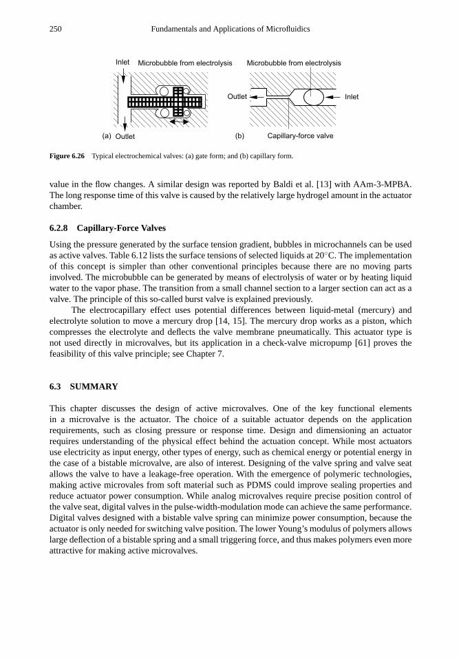
250 Fundamentals and Applications of Microfluidics
(a) (b)Outlet
Inlet Microbubble from electrolysis Microbubble from electrolysis
Capillary-force valve
InletOutlet
Figure 6.26 Typical electrochemical valves: (a) gate form; and (b) capillary form.
value in the flow changes. A similar design was reported by Baldi et al. [13] with AAm-3-MPBA.The long response time of this valve is caused by the relatively large hydrogel amount in the actuatorchamber.
6.2.8 Capillary-Force Valves
Using the pressure generated by the surface tension gradient, bubbles in microchannels can be usedas active valves. Table 6.12 lists the surface tensions of selected liquids at 20◦C. The implementationof this concept is simpler than other conventional principles because there are no moving partsinvolved. The microbubble can be generated by means of electrolysis of water or by heating liquidwater to the vapor phase. The transition from a small channel section to a larger section can act as avalve. The principle of this so-called burst valve is explained previously.
The electrocapillary effect uses potential differences between liquid-metal (mercury) andelectrolyte solution to move a mercury drop [14, 15]. The mercury drop works as a piston, whichcompresses the electrolyte and deflects the valve membrane pneumatically. This actuator type isnot used directly in microvalves, but its application in a check-valve micropump [61] proves thefeasibility of this valve principle; see Chapter 7.
6.3 SUMMARY
This chapter discusses the design of active microvalves. One of the key functional elementsin a microvalve is the actuator. The choice of a suitable actuator depends on the applicationrequirements, such as closing pressure or response time. Design and dimensioning an actuatorrequires understanding of the physical effect behind the actuation concept. While most actuatorsuse electricity as input energy, other types of energy, such as chemical energy or potential energy inthe case of a bistable microvalve, are also of interest. Designing of the valve spring and valve seatallows the valve to have a leakage-free operation. With the emergence of polymeric technologies,making active microvales from soft material such as PDMS could improve sealing properties andreduce actuator power consumption. While analog microvalves require precise position control ofthe valve seat, digital valves in the pulse-width-modulation mode can achieve the same performance.Digital valves designed with a bistable valve spring can minimize power consumption, because theactuator is only needed for switching valve position. The lower Young’s modulus of polymers allowslarge deflection of a bistable spring and a small triggering force, and thus makes polymers even moreattractive for making active microvalves.

Microfluidics for Internal Flow Control: Microvalves 251
Table 6.12
Surface Tensions of Selected Liquids (at 20◦C if not otherwise indicated)
Liquid σ (10−3 N/m) Liquid σ (10−3 N/m)
Trifluoroacetic Acid 13.63 (24◦C) Methyl Ethyl Ketone 24.0 (25◦C)Pentane 15.48 (25◦C) n-Butyl Alcohol 24.57Ethyl Ether 17.06 Cyclohexane 24.98Hexane 17.91 (25◦C) n-Butyl Acetate 25.09Iso-Octane 18.77 Methyl n-Propyl Ketone 25.09Acetonitrile 19.10 Tetrahydrofuran 26.4 (25◦C)Methyl t-Butyl Ether 19.4 (24◦C) o-Dichlorobenzene 26.84Heptane 20.30 Chloroform 27.16Triethylamine 20.66 Dichloromethane 28.12Isopropyl Alcohol 21.79 (15◦C) Toluene 28.53Ethyl Alcohol 22.32 o-Xylene 30.03Cyclopentane 22.42 2-Methoxyethanol 31.8 (15◦C)Methanol 22.55 Ethylene Dichloride 32.23Isobutyl Alcohol 22.98 Dimethyl Acetamide 32.43 (30◦C)Acetone 23.32 Chlorobenzene 33.28Methyl Isobutyl Ketone 23.64 1,4-Dioxane 34.45 (15◦C)n-Propyl Alcohol 23.70 N,N-Dimethylformamide 36.76n-Butyl Chloride 23.75 Pyridine 36.88Ethyl Acetate 23.75 Propylene Carbonate 41.93
Water 72.8
Problems
6.1 For the microvalve depicted in Figure 6.20(d), determine the actuating force on the gate. The areaof the piston-like structure on each side is 100× 73µm. The gap, which determines the minimumradius of curvature, is 8µm wide.
6.2 The thermodynamic properties of liquid water are:v(25◦C) = 1.0029× 10⁻³ m3/kg, u(25◦C) =
104.88 kJ/kg, and of vapor arev(100◦C) = 1.673 m3/kg, u(25◦C) = 2,506.5 kJ/kg. Determinethe maximum efficiency of a thermal bubble with an actuating pressure of 1 bar.
6.3 Regarding the situation described in Figure 6.13, calculate the work done by an air bubbleescaping a narrow channel of 10µm in diameter into a larger section of 40µm. The diffusersection is 10µm long.
References
[1] Shoji, S., and Esashi, M., “Microflow Devices and Systems,”Journal of Micromechanics and Microengineering,Vol. 4, No. 4, 1994, pp. 157-171.
[2] Kohl, M., et al., “Thin Film Shape Memory Microvalves with Adjustable Operation Temperature,”Sensors andActuators A, Vol. 83, 2000, pp. 214–219.
[3] Maluf, N., An Introduction to Microelectromechanical Systems Engineering, Norwood, MA: Artech House 2000.
[4] Lisec, T., et al., “Thermally Driven Microvalve with Buckling Behaviour for Pneumatic Applications,”Proceedingsof MEMS’94, 7th IEEE International Workshop Micro Electromechanical System, Oiso, Japan, Jan. 25–28, 1994,pp. 13–17.
252 Fundamentals and Applications of Microfluidics
[5] Chu, W. H., Mehregany, M., and Mullen, R. L., “Analysis of Tip Deflection and Force of a Bimetallic CantileverMicroactuator,”Journal of Micromechanics and Microengineering, Vol. 3, 1993, pp. 4–7.
[6] Shimizu, K., and Tadaki, T.,Shape Memory Alloys, H. Funakubo, (ed.), Gordon and Breach Science Publishers, 1987.
[7] Gerlach, G., and Dotzel, W.,Grundlagen der Mikrosystemtechnik, Hanser Verlag, 1997.
[8] Hoffmann, J., et al., “Photopatterning of Thermally Senstive Hydrogels Useful for Microactuators,”Sensors andActuators A, Vol. 77, 1999, pp. 139–144.
[9] Richter, A., et al., “Electronically Controllable Microvalves Based on Smart Hydrogels: Magnitudes and PotentialApplications,”Journal of Microelectromechanical Systems, Vol. 12, 2003, pp. 748–753.
[10] Richter, A., et al., “Influence of Volume Phase Transition Phenomena on the Behavior of Hydrogel-Based Valves,”Sensors and Actuators B, Vol. 99, 2004, pp. 451–458.
[11] Cao, X., Lai, S., Lee, L. J., “Design of a Self-Regulated Drug Delivery Device,”Biomedical Microdevices, Vol. 3,2001, pp. 109–118.
[12] Liu, R. H., Yu, Q., Beebe, D. J., “Fabrication and Characterization of Hydrogel-Based Microvalves,”Journal ofMicroelectromechanical Systems, Vol. 11, 2002, pp. 45–53.
[13] Baldi, A., et al., “A Hydrogel-Actuated Environmentally Sensitive Microvalve for Active Flow Control,”Journal ofMicroelectromechanical Systems, Vol. 12, 2003, pp. 613–621.
[14] Lee, J., and Kim, C. J., “Surface-Tension-Driven Microactuation Based on Continuous Electrowetting,”Journal ofMicroelectromechanical Systems, Vol. 9, No. 2, 2000, pp. 171–180.
[15] Lee, J., et al., “Addressable Micro Liquid Handling by Electric Control of Surface Tension,”Proceedings of MEMS’01,14th IEEE International Workshop Micro Electromechanical System, Interlaken, Switzerland, Jan. 21–25, 2001,pp. 499–502.
[16] Man, P. F., et al., “Microfabricated Capillary-Driven Stop Valve and Sample Injector,”Proceedings of MEMS’98, 11thIEEE International Workshop Micro Electromechanical System, Heidelberg, Germany, Jan. 25–29, 1998, pp. 45–50.
[17] Timoshenko, S. P., and Gere, J. M.,Theory of Elastic Stability, 2nd ed., New York: McGraw-Hill, 1963.
[18] Schomburg, W. K., and Goll, C., “Design Optimization of Bistable Microdiaphragm Valves,”Sensors and ActuatorsA, Vol. 64, 1998, pp. 259–264.
[19] Cousseau, P., et al., “Improved MicroFlow Regulator for Drug Delivery Systems,”Proceedings of MEMS’01, 14thIEEE International Workshop Micro Electromechanical System, Interlaken, Switzerland, Jan. 21–25, 2001, pp. 527–530.
[20] Huff, M. A., and Schmidt, M. A., “Fabrication, Packaging, and Testing of a Wafer-Bonded Microvalve,”TechnicalDigest of the IEEE Solid State Sensor and Actuator Workshop, Hilton Head Island, SC, June 22–25, 1992, pp. 194–197.
[21] Takao, H., and Ishida, M. “Microfluidic Integrated Circuits for Signal Processing Using Analogous RelationshipBetween Pneumatic Microvalve and MOSFET”Journal of Microelectromechanical Systems, Vol. 12, 2003, pp. 497–505.
[22] Vieider, C., Oehman, O., and Elderstig, H., “A Pneumatic Actuated Micro Valve with a Silicon Rubber Membrane forIntegration with Fluid-Handling Systems,”Proceedings of Transducers ’95, 8th International Conference on Solid-State Sensors and Actuators, Stockholm, Sweden, June 16–19, 1995, pp. 284–286.
[23] Hosokawa, K., and Maeda, R., “A Pneumatically-Actuated Three-Way Microvalve Fabricated with Polydimethyl-siloxane Using the Membrane Transfer Technique,”Journal of Micromechanics and Microengineering, Vol. 10, 2000,pp. 415–420.
[24] Sim, D. Y., Kurabayashi, T., and Esashi, M., “Bakable Silicon Pneumatic Microvalve,”Proceedings of Transducers’95, 8th International Conference on Solid-State Sensors and Actuators, Stockholm, Sweden, June 16–19, 1995,pp. 280–283.
Microfluidics for Internal Flow Control: Microvalves 253
[25] Ohori, T., et al., “Three-Way Microvalve for Blood Flow Control in Medical Micro Total Analysis Systems (mTAS),”Proceedings of MEMS’97, 10th IEEE International Workshop Micro Electromechanical System, Nagoya, Japan, Jan.26–30, 1997, pp. 333–337.
[26] Rich, C. A., and Wise, K. D., “A High-Flow Thermopneumatic Microvalve With Improved Efficiency and IntegratedState Sensing,”Journal of Microelectromechanical Systems, Vol. 12, 2003, pp. 201–208.
[27] Zdeblic, M. J., et. al, “Thermopneumatically Actuated Microvalves and Integrated Electro-Fluidic Circuits,”TechnicalDigest of the IEEE Solid State Sensor and Actuator Workshop, Hilton Head Island, SC, June 13–16, 1994, pp. 251–255.
[28] Henning, A. K., “Microfluidic MEMS,” Proceedings of the IEEE Aerospace Conference, Snowmass at Aspen, CO,March 1998, pp. 471–486.
[29] Henning, A. K., et al., “Microfluidic MEMS for Semiconductor Processing,”IEEE Transactions on Components,Hybrids, and Manufacturing Technology, Part B: Advanced Packaging, Vol. 21, No. 4, 1998, pp. 329–337.
[30] Yang, X., et al., “A MEMS Thermopneumatic Silicone Membrane Valve,”Proceedings of MEMS’97, 10th IEEEInternational Workshop Micro Electromechanical System, Nagoya, Japan, Jan. 26-30, 1997, pp. 114–118.
[31] Grosjean, C., Yang, X., Tai, Y. C., “A Practical Thermopneumatic Valve,”Proceedings of MEMS’99, 12th IEEEInternational Workshop Micro Electromechanical System, Orlando, FL, Jan. 17–21, 1999, pp. 147–152.
[32] Kim, J. H., et al., “A Disposable Thermopneumatic-Actuated Microvalve Stacked with PDMS Layers and ITO-CoatedGlass,”Microelectronic Engineering, Vol. 73–74, 2004, pp. 864–869.
[33] Papavasiliou, A. P., Liepmann, D., and Pisano, A. P., “Fabrication of a Free Floating Gate Valve,”Proceedings ofIMECE, International Mechanical Engineering Congress and Exposition, Vol. 1, Nashville, TN, Nov. 14–19, 1999,pp. 435–440.
[34] Carlen, E. T., and Mastrangelo, C. H., “Surface Micromachined Paraffin-Actuated Microvalve,”Journal of Microelec-tromechanical Systems, Vol. 11, 2002, pp. 408–420.
[35] Carlen, E. T., and Mastrangelo, C. H., “Simple, High Actuation Power, Thermally Activated Parafin Microactuator,”Proceedings of Transducers ’99, 10th International Conference on Solid-State Sensors and Actuators, Sendai, Japan,June 7–10, 1999, pp. 1364–1367.
[36] Jerman, H., “Electrically-Activated Micromachined Diaphragm Valves,”Technical Digest of the IEEE Solid StateSensor and Actuator Workshop, Hilton Head Island, SC, June 4–7, 1990, pp. 65–69.
[37] Jerman, H., “Electrically-Activated Normally-Closed Diagphragm Valves,”Proceedings of Transducers ’91, 6thInternational Conference on Solid-State Sensors and Actuators, San Francisco, CA, June 23–27, 1991, pp. 1045–1048.
[38] Messner, S., et al., “A Normally-Closed, Bimetallically Actuated 3-Way Microvalve for Pneumatic Application,”Proceedings of MEMS’98, 11th IEEE International Workshop Micro Electromechanical System, Heidelberg, Germany,Jan. 25–29, 1998, pp. 40–44.
[39] Franz, J., Baumann, H., and Trah, H.-P., “A Silicon Microvalve with Integrated Flow Sensor,”Proceedings ofTransducers ’95, 8th International Conference on Solid-State Sensors and Actuators, Stockholm, Sweden, June 16–19,1995, pp. 313–316.
[40] Trah, H. P., et al., “Micromachined Valve with Hydraulically Actuated Membrane Subsequent to a ThermoelectricallyControlled Bimorph Cantilever,”Sensors and Actuators A, Vol. 39, 1993, pp. 169–176.
[41] Barth, P. W., “Silicon Microvalves for Gas Flow Control,”Proceedings of Transducers ’95, 8th InternationalConference on Solid-State Sensors and Actuators, Stockholm, Sweden, June 16–19, 1995, pp. 276–279.
[42] Kahn, H., Huff, M. A., and Heuer, A. H., “The Ti Ni Shape-Memory Alloy and Its Applications for MEMS,”Journalof Micromechanics and Microengineering, Vol. 8, 1998, pp. 213–221.
[43] Esashi, M., Shoji, S., and Nakano, A., “Normally Closed Microvalve and Micropump Fabricated on a Silicon Wafer,”Proceedings of MEMS’89, 1st IEEE International Workshop Micro Electromechanical System, Salt Lake City, UT,Feb. 1989, pp. 29–34.

254 Fundamentals and Applications of Microfluidics
[44] Shoji, S., et al., “Smallest Dead Volume Microvalves for Integrated Chemical Analyzing Systems,”Proceedings ofTransducers ’91, 6th International Conference on Solid-State Sensors and Actuators, San Francisco, CA, June 23–27,1991, pp. 1052–1055.
[45] Chakraborty, I., et al., “MEMS Micro-Valve for Space Applications,”Sensors and Actuators A, Vol. 83, 2000, pp. 188–193.
[46] Stehr, M., et al., “The VAMP—A New Device for Handling Liquids or Gases,”Sensors and Actuators A, Vol. 57,1996, pp. 153–157.
[47] Nguyen, N. T., et al., “Hybrid-Assembled Micro Dosing System Using Silicon-Based Micropump/Valve and MassFlow Sensor,”Sensors and Actuators A, Vol. 69, 1998, pp. 85–91.
[48] Ohnstein, T. R. et al., “Micromachined Silicon Microvalve,”Proceedings of MEMS’90, 2th IEEE InternationalWorkshop Micro Electromechanical System, Napa Valley, CA, Feb. 11–14, 1990, pp. 95–98.
[49] Shikida, M., et al., “Electrostatically Driven Gas Valve with High Conductance,”Journal of Micro ElectromechanicalSystems, Vol. 3, No. 2, June 1994, pp. 76–80.
[50] Shikida, M., and Sato, K., “Characteristics of an Electrostatically-Driven Gas Valve Under High-Pressure Conditions,”Proceedings of MEMS’94, 7th IEEE International Workshop Micro Electromechanical System, Oiso, Japan, Jan. 25–28, 1994, pp. 235–240.
[51] Robertson, J. K., and Wise, K. D., “A Nested Electrostatically-Actuated Microvalve for an Integrated MicroflowController,” Proceedings of MEMS’94, 7th IEEE International Workshop Micro Electromechanical System, Oiso,Japan, Jan. 25–28, 1994, pp. 7–12.
[52] Wagner, B., et al., “Bistable Microvalve With Pneumatically Coupled Membranes,”Proceedings of MEMS’96, 9thIEEE International Workshop Micro Electromechanical System, San Diego, CA, Feb. 11–15, 1996, pp. 384–388.
[53] Vandelli, N., et al., “Development of a MEMS Microvalve Array for Fluid Flow Control,”Journal of MicroElectromechanical Systems, Vol. 7, No. 4, Dec. 1998, pp. 395–403.
[54] Pourahmadi, F., et al., “Variable-Flow Micro-Valve Structure Fabricated with Silicon Fusion Bonding,”TechnicalDigest of the IEEE Solid State Sensor and Actuator Workshop, Hilton Head Island, SC, June 4–7, 1990, pp. 78–81.
[55] Yanagisawa, K., Kuwano, H., Tago, A., “An Electromagnetically Driven Microvalve,”Proceedings of Transducers ’93,7th International Conference on Solid-State Sensors and Actuators, Yokohama, Japan, June 7–10, 1993, pp. 102–105.
[56] Bohm, S., et al., “A Micromachined Silicon Valve Driven by a Miniature Bistable Electromagnetic Actuator,”Sensorsand Actuators A, Vol. 80, 2000, pp. 77–83.
[57] Meckes, A., et al., “Microfluidic System for the Integration on Cyclic Operation of Gas Sensors,”Sensors andActuators A, Vol. 76, 1999, pp. 478–483.
[58] Capanu, M., et al., “Design, Fabrication, and Testing of a Bistable Electromagnetically Actuated Microvalve,”Journalof Microelectromechanical Systems, Vol. 9, No. 2, 2000, pp. 181–189.
[59] Shinozawa, Y., Abe, T., and Kondo, T., “A Proportional Microvalve Using a Bi-Stable Magnetic Actuator,”Proceed-ings of MEMS’97, 10th IEEE International Workshop Micro Electromechanical System, Nagoya, Japan, Jan. 26–30,1997, pp. 233–237.
[60] Papavasiliou, A. P., Liepmann, D., and Pisano, A. P., “Electrolysis-Bubble Actuated Gate Valve,”Technical Digest ofthe IEEE Solid State Sensor and Actuator Workshop, Hilton Head Island, SC, June 4–8, 2000, pp. 48–51.
[61] Yun, K. S., et al., “A Micropump Driven by Continuous Electrowetting Actuation for Low Voltage and LowPower Operations,”Proceedings of MEMS’01, 14th IEEE International Workshop Micro Electromechanical System,Interlaken, Switzerland, Jan. 21–25, 2001, pp. 487–490.

Chapter 7
Microfluidics for Internal Flow Control:Micropumps
The next active components of a microfluidic system are micropumps. With the growing importanceof genomics, proteomics, and the discovery of new drugs, controlled transport of fluids in microscalebecomes an important and crucial task. New transport effects, such as electrokinetic effects,interfacial effects, acoustic streaming, magnetohydrodynamic effects, and electrochemical effects,which previously were neglected in macroscopic applications, now gain in importance on themicroscale. Overviews on micropumps were reported in several excellent review papers. Gravesenet al. gave a general overview on fluidic problems in the microscale [1]. Shoji and Esashi discussedmicrofluidics from the device point of view, and considered micropumps, microvalves, and flowsensors [2]. This chapter only deals with micropumps, and discusses their design considerations aswell as the published design examples.
In contrast to other MEMS devices, micropumps are one of the components with the largestvariety of operating principles. The most important actuation principles are discussed in Chapter 6.Thus, in this chapter micropumps are categorized according to their pumping principles.
Similar to other MEMS applications, the first approach in designing a micropump is theminiaturization of well-known mechanical principles from the macroscale. The next approacheswere to apply new pumping effects, which are more effective on the microscale than the macroscale.Most of the micropumps developed with the latter approach are nonmechanical pumps. Therefore,micropumps are categorized in this chapter as either mechanical pumps or nonmechanical pumps.
Mechanical pumpscan be further categorized according to the principles by which mechanicalenergy is applied to the fluid. Under this system, mechanical pumps are divided into two major cate-gories: displacement pumps and dynamic pumps [3]. Indisplacement pumps, energy is periodicallyadded by the application of force to one or more moveable boundaries of any desired number of en-closed, fluid-containing volumes, resulting in a direct increase in pressure, up to the value required tomove the fluid through check valves or ports into the discharge line. Check-valve pumps, peristalticpumps, valveless rectification pumps, and rotary pumps belong to the displacement category (Table7.1). In dynamic pumps, mechanical energy is continuously added to increase the fluid velocitieswithin the machine. The higher velocity at the pump outlet increases the pressure. Centrifugal pumpsand ultrasonic pumps belong to the dynamic category.
Nonmechanical pumpsadd momentum to the fluid by converting another nonmechanicalenergy form into kinetic energy. While mechanical pumping is mostly used in macroscale pumpsand micropumps with a relatively large size and high flow rates, this second category discovers itsadvantages in the microscale. Since the viscous force in microchannels increases in the second orderwith miniaturization, the first pump category cannot deliver enough power to overcome the high
255

256 Fundamentals and Applications of Microfluidics
Table 7.1
Mechanical Pumping Principles
Displacement Pumps Dynamic Pumps
Check-valve pumps Ultrasonic pumpsPeristaltic pumps Centrifugal pumpsValveless rectification pumpsRotary pumps
Table 7.2
Nonmechanical Pumping Principles
Pressure Gradient ConcentrationGradient
Electrical PotentialGradient
Magnetic Potential
Fluidflow
Surface tension drivenflow (electrowetting,Marangoni-effect, surfacemodification)
Osmosis (semiperme-able membrane, sur-factants)
Electro-osmosis (elec-trolyte), Electrohydrody-namic (dielectric fluid)
Ferrofluidic
Soluteflux
Ultrafiltration Diffusion Electrophoresis, Dielec-trophoresis
Magneto-hydrodynamic flow
fluidic impedance in the microscale. Table 7.2 lists the common nonmechanical pumping principles.Figure 7.1 illustrates the typical flow rate range of micropumps.
For flow rates more than 10 mL/min, miniature pumps or macroscale pumps are the mostcommon solutions. The typical operation range of displacement micropumps lies between oneand ten milliliters per minute. For flow rates less than 10µL/min, alternative dynamic pumps ornonmechanical pumps are needed for an accurate control of these small fluid amounts.
7.1 DESIGN CONSIDERATIONS
7.1.1 Mechanical Pumps
7.1.1.1 Actuators
All mechanical pumps require an electromechanical actuator, which generally converts electricalenergy into mechanical work. Actuators can be categorized by their physical principles as seen inChapter 6. Alternatively, regarding their integration ability, actuators can be categorized as external
Figure 7.1 Flow rate range of different pump principles.
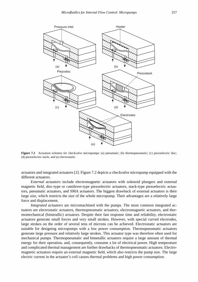
Microfluidics for Internal Flow Control: Micropumps 257
Pressure inlet
(a) (b)
Heater
(c)
Piezodisc
(d)
Piezostack
(e)
Electrodes
Figure 7.2 Actuation schemes for checkvalve micropumps: (a) pneumatic; (b) thermopneumatic; (c) piezoelectric disc;(d) piezoelectric stack; and (e) electrostatic.
actuators and integrated actuators [2]. Figure 7.2 depicts a checkvalve micropump equipped with thedifferent actuators.
External actuatorsinclude electromagnetic actuators with solenoid plungers and externalmagnetic field, disc-type or cantilever-type piezoelectric actuators, stack-type piezoelectric actua-tors, pneumatic actuators, and SMA actuators. The biggest drawback of external actuators is theirlarge size, which restricts the size of the whole micropump. Their advantages are a relatively largeforce and displacement.
Integrated actuatorsare micromachined with the pumps. The most common integrated ac-tuators are electrostatic actuators, thermopneumatic actuators, electromagnetic actuators, and ther-momechanical (bimetallic) actuators. Despite their fast response time and reliability, electrostaticactuators generate small forces and very small strokes. However, with special curved electrodes,large strokes on the order of several tens of microns can be achieved. Electrostatic actuators aresuitable for designing micropumps with a low power consumption. Thermopneumatic actuatorsgenerate large pressure and relatively large strokes. This actuator type was therefore often used formechanical pumps. Thermopneumatic and bimetallic actuators require a large amount of thermalenergy for their operation, and, consequently, consume a lot of electrical power. High temperatureand complicated thermal management are further drawbacks of thermopneumatic actuators. Electro-magnetic actuators require an external magnetic field, which also restricts the pump size. The largeelectric current in the actuator’s coil causes thermal problems and high power consumption.

258 Fundamentals and Applications of Microfluidics
Dimensionless pressure
p*
Dimensionless membrane thickness t*
Dim
en
sio
nle
ss
ce
nte
rd
efle
ctio
ny
*0
Figure 7.3 Dimensionless center deflection of a circular membrane as a function of dimensionless thickness and dimen-sionless pressure.
7.1.1.2 Pump Membrane
Many mechanical micropumps are based on the reciprocating concept. This pumping conceptrequires a flexible reciprocating membrane to displace a defined volume called theStroke volume.The displaced volume is transported forward using rectifying elements such as check valves. Thestroke volume can be estimated for a circular membrane, clamped at its perimeter and subjected toa pressure load from the deflection curve (6.34):
y(r ) = y0
(1 −
r 2
R2
)2(7.1)
wherey0 is the center deflection of the membrane, andR is the membrane radius. Also from themodel discussed in Section 6.1.2 (6.35), the relation between the applied pressurep and the centerdeflectiony0 of a circular membrane without prestress also can be estimated as:
p =16ty0
3R4
E
1 − ν2
(t2
+16
35y2
0
)(7.2)
whereE, ν, andt are the Young’s modulus, the Poisson ratio, and the thickness of the membrane,respectively. Withp∗
= p/E, y∗
0 = y0/R, andt∗ = t/R, the relation between the dimensionlesspressurep∗, the dimensionless thicknesst∗, and the dimensionless center deflectiony∗
0 can beformulated as (Figure 7.3):
p∗=
16t∗y∗
0
3(1 − ν2)
(t∗2
+16
35y∗2
0
)(7.3)
For the dynamic behavior, the resonant frequency of the membrane without prestress can beestimated as [4]:
fkn = 2πβ2kn
√D/m (7.4)

Microfluidics for Internal Flow Control: Micropumps 259
whereD is the flexural rigidity:
D =Et3
12(1 − ν2)(7.5)
andm is the mass of the membrane. The integersk = 0,1, ... andn = 1,2, ... denote the vibrationmodes of the pump membrane. The eigenvaluesβkn for the first three vibration modes are:
β01 = 1.015π/Rβ11 = 1.468π/Rβ02 = 2.007π/R
(7.6)
7.1.1.3 Parameters of Micropumps
The most important specification bases for micropumps are the maximum flow rate, the maximumbackpressure, the pump power, and the efficiency.The maximum flow rate, or pump capacityQmax,is the volume of liquid per unit time delivered by the pump at zero backpressure.The maximumbackpressureis the maximum pressure the pump can work against. At this pressure, the flow rateof the pump becomes zero. The term “pump head” is also often used as a parameter for pumpperformance. The pump headh represents the net work done on a unit weight of liquid in passingfrom the inlet or suction tube to the discharge tube. It is given as [3]:
h =
( p
ρ+
u2
2g+ z
)out
−
( p
ρ+
u2
2g+ z
)in
(7.7)
whereρ is the fluid density. The termp/ρ is called thepressure heador flow work, and represents thework required to move a unit weight of fluid across an arbitrary plane perpendicular to the velocityvectoru against a pressurep. The termu2/2g is the velocity head, which represents the kineticenergy of the fluid. The termz is the elevation head or potential head. The first parenthetical termin (7.7) represents the outlet or discharge head, and the second, the inlet or suction head. Assumingthat the static pressure at the inlet and outlet are equal,u becomes zero, and the maximum pumphead can be derived from (7.7) as:
hmax = zout − zin (7.8)
Based on the maximum flow rateQmax, the maximum back-pressurepmax, or the maximum pumpheadhmax, the power of the pumpPpump can be calculated as:
Ppump =pmaxQmax
2=ρgQmaxhmax
2(7.9)
Thepump efficiencyη is defined as:
η =Ppump
Pactuator(7.10)
wherePactuatoris the input power of the actuator.
Example 7.1: Pump Efficiency
A thermopneumatic checkvalve pump delivers a maximum flow rate of 34 mL/min and amaximum backpressure of 5 kPa. The heater resistance is 15�. The pump works with a symmetricsquare signal with a maximum voltage of 6V at 0.5 Hz. Determine the pump efficiency (data from[5]).
Solution. The power of the pump is:
Ppump =pmaxQmax
2=
5 × 103× 34× 10−9/60
2= 1.42× 10⁻⁶ W

260 Fundamentals and Applications of Microfluidics
pactuator
Inlet valve
Outlet valve
Stroke volume �V
Dead volume V0
Membrane
pin
pout
Q
Figure 7.4 General structure of a checkvalve pump.
Considering only the active half of the drive signal, the electrical power input is:
Pactuator=1
2
V2
R=
62
2 × 15= 1.2W
Thus, the pump efficiency is:
η =Ppump
Pactuator=
1.42× 10⁻⁶
1.2= 1.18× 10−6
= 1.18× 10⁻⁴ %
7.1.1.4 Check-Valve Pumps
Check-valve pumps are the most common pump type in the macroscale. Therefore, the firstattempts in designing a mechanical micropump were the realization of checkvalve pumps. Figure7.4 illustrates the general concept of a checkvalve pump. A checkvalve pump consists of an actuatorunit, a pump membrane that creates the stroke volume1V , a pump chamber with the dead volumeV0, and two checkvalves, which start to be opened by the critical pressure difference1pcrit.
Check-valve pumps function under conditions of a small compression ratio and of a high pumppressure [6]. The compression ratioψ is the ratio between the stroke volume and the dead volume:
ψ =1V
V0(7.11)
A high pump pressurep fulfills the conditions:{|p − pout| > 1pcrit|p − pin| > 1pcrit
(7.12)
where1pcrit is the critical pressure required for opening the check valves. Reference [7] lists anumber of methods for measuring the critical pressure. The critical pressures of a cantilever valve(1,700× 1,000× 15µm) and an orifice (400× 400µm) are in the range from 10 to 100 mbar [6].
The criterion for the minimum compression ratioψgasof a gas pump is given as [6]:
ψgas>
(p0
p0 − |1pcrit|
) 1k
− 1 (7.13)
wherep0 is the atmospheric pressure, andk is the specific heat ratio of the gas (k = 1.4 for air). Atlow pump frequency and small critical pressure1pcrit, the above relation can be simplified as [6]:
ψgas>1
k
|1pcrit|
p0(7.14)

Microfluidics for Internal Flow Control: Micropumps 261
For liquids, the criterion for the minimum compression ratioψliquid is:
ψliquid > 2|1pcrit| (7.15)
where2 is the compressibility of the liquid (for water,2 = 0.5×10⁻⁸ m2/N). Since the value of2is very small compared to the pressure generated by different actuators, this criterion is easily met.However, this situation is only true if the pump chamber is filled entirely with water. In practice, thereare always gas bubbles in the pump chamber due to outgassing, or to bubbles that are transported bythe liquid. Therefore, the condition in (7.14) should be kept for designing a self-priming micropump.
The above conditions lead to the following design rules for checkvalve micropumps.
• Minimize the critical pressure1pcrit by using more flexural valve design or valve material with asmall Young’s modulus.
• Maximize the stroke volume1V by using actuators with a large stroke or more flexible pumpmembrane.
• Minimize the dead volumeV0 by using a thinner spacer or wafer.
• Maximize the pump pressurep by using actuators with large forces.
Example 7.2: Designing a Micropump for Gases
A checkvalve pump has circular orifices as inlet and outlet. The orifices have diameters of 400µm.Determine the minimum compression ratio for self-priming.
Solution. The critical opening pressure is important for the compression ratio. There are manysources for the initial closing force of a checkvalve, such as preloaded spring force, van der Walforces, and capillary forces. For pumps working in moist conditions, the capillary force can havethe biggest impact. Richter et al. [6] gave the following theory.
The surface energy of a wetted inlet orifice is:
Usurface= σπdz
whered is the orifice diameter andz is the small gap between the checkvalve and the orifice,which is filled with a liquid. The external force applied on the check valve causes a mechanicalwork over the gap lengthz:
W = 1pcritπd2
4z
This work should overcome the surface energy; thus:
W = Usurface→ 1pcritπd2
4z = σπdz → 1pcrit =
4σ
d
Using the surface tension of water (72× 10−3 N/m), the critical pressure for the pump is:
1pcrit =4σ
d=
4 × 72× 10−3
400× 10−6= 720 Pa
Using (7.14) and the specific heat ratio of air (k = 1.4) and ambient pressure of 1 bar, we get theminimum compression ratio:
ψmin =1
k
|1pcrit|
p0=
1
1.4
720
105= 5.14× 10⁻³
That means that the total stroke volume should be at least 0.5% of the dead volume.

262 Fundamentals and Applications of Microfluidics
Tim
e
Figure 7.5 Working principle of a peristaltic pump with three pump chambers.
7.1.1.5 Peristaltic Pumps
In contrast to checkvalve pumps, peristaltic pumps do not require passive valves for flow rectifica-tion. The pumping concept is based on the peristaltic motion of the pump chambers, which squeezesthe fluid in the desired direction (Figure 7.5). Theoretically, peristaltic pumps need three or morepump chambers with actuating membranes. Most of the realized pumps have three chambers.
Peristaltic pumps are easily implemented because of the lack of the more complicated checkvalves. From an operational point of view, peristaltic pumps are active valves connected in series, asdescribed in Chapter 6. The design rules and different actuation schemes can therefore be adoptedfrom the design of microvalves described in Chapter 6. The most serious problem of peristalticmicropumps is leakage. A small pressure difference between the outlet and the inlet will cause abackflow in the nonactuated state. A one-way check valve should be connected in series with aperistaltic pump for applications such as drug delivery systems and chemical analysis, which do notallow a backflow. The one-way check valve can be implemented in the pump design.
The general optimization strategies for peristaltic pumps are maximizing the compressionratio and increasing the number of pump chambers. Since a peristaltic pump does not require a highchamber pressure, the most important optimization factors are the large stroke volume and the largecompression ratio.
Example 7.3: Designing a Peristaltic Micropump
A peristaltic pump has three pump chambers and three circular unimorph piezodiscs as actuators.The pump membrane has a diameter of 4 mm. The pump works with a frequency of 100 Hz.Determine the volume flow rate at zero backpressure if the maximum membrane deflection is40µm.
Solution. We assume that the membrane deflection follows the deflection function of a thincircular plate (7.1):
y(r ) = y0
[1 −
( r
R
)2]2

Microfluidics for Internal Flow Control: Micropumps 263
According to the definition in Figure 7.4, the maximum liquid volume that a pump chamber cantake in is:
1V = 2 ×∫ 2π
0
∫ R0 y0
[1 −
( rR
)2]2
r dr drφ =2π3 y0R2
=2π3 4 × 10−5
× (2 × 10−3)2 = 3.35× 10⁻¹⁰ m3
At the relatively low frequency of 100 Hz, we assume a linear relation between flow rate andpump frequency. The estimated volume flow rate is:
Q = 1V f = 3.35× 10−10× 100= 3.35× 10⁻⁸ m3/sec= 2 mL/min
7.1.1.6 Valveless Rectification Pumps
The structure of valveless rectification pumps is similar to those of checkvalve pumps. The onlydifference is the use of diffusers/nozzles or valvular conduits instead of check valves for flowrectification. The pressure loss1p at a rectification structure is given by:
1p = ξρu2
2(7.16)
whereξ is the pressure loss coefficient,ρ is the fluid density, andu is the average velocity atthe rectification structure. The ratio between the pressure loss coefficients between the inlet andoutlet of the pump is the so-called fluidic diodicityηF, which characterizes the performance of therectification structure:
ηF =ξ−
ξ+(7.17)
whereξ− and ξ+ are the pressure loss coefficients of the rectification structure in negative andpositive flow directions, respectively. For common diffuser/nozzle structures,η ranges from 1 to 5.With the known fluidic diodicityηF, the pump frequencyf , and the stroke volume1V , the flowrate of the pump can be estimated as [8]:
Q = 21V f√ηF − 1
√ηF + 1
(7.18)
The last term in (7.18) can be defined as the static rectification efficiencyχ [10]:
χ =
√ηF − 1
√ηF + 1
(7.19)
Figure 7.6 shows the net flow in a diffuser/nozzle pump in the supply and pump mode. Forsmall diffuser angles, the nozzle works as pump inlet, while the diffuser works as pump outlet.Figure 7.7 depicts the theoretical function of static rectification efficiency versus the diffuser angleθ . The datapoints are collected from the design examples presented later in this section. Dependingon the fabrication constraints, the two operation ranges for a diffuser/nozzle are 5◦ < θ < 10◦ andθ ≈ 70◦.
Valveless rectification pumps are more sensitive to backflow than peristaltic pumps becauseof the low fluidic impedance in both directions. Similar to peristaltic pumps, a one-way valve isrecommended for this type of micropump. Maximizing the stroke volume and minimizing the deadvolume are the major optimization measures for valveless rectification micropumps.

264 Fundamentals and Applications of Microfluidics
(a)(b)
Figure 7.6 Working principle of a diffuser/nozzle pump: (a) supply phase; and (b) pump phase. (After: [9].)
[8]
[8]
[11]
[10]
�
�
Figure 7.7 Theoretical function of rectification efficiency and experimental data. (From: [8, 10, 11].) (Schematic, adaptedfrom [11]).

Microfluidics for Internal Flow Control: Micropumps 265
Example 7.4: Designing a Diffuser/Nozzle Micropump
A diffuser/nozzle pump has a pump membrane diameter of 10 mm and a maximum deflection of10µm. Determine the volume flow rate if the pump frequency is 100 Hz and the fluidic diodicityof the diffuser/nozzle structure is 1.58.
Solution. With the assumption made in Example 7.3, the volume per stroke of the pump iscalculated as:
1V =2π
3dmaxR
2=
2π
310−5
× (5 × 10−3)2 = 5.24× 10⁻¹⁰ m3
Thus, after (7.18), the volume flow rate can be estimated as:
Q = 21V f√ηF−1
√ηF+1 = 5.25× 10−10
× 100×
√1.58−1
√1.58+1
= 1.19× 10⁻⁸ m3/s = 715µL/min
7.1.1.7 Rotary Pumps
In macroscale, rotary pumps are suitable for pumping highly viscous fluids. However, the hightorque caused by the viscous forces requires strong external actuators. A fully integrated actuator isimpractical in this case because of this high load. A rotary pump is designed as a pair of spur gears(Figure 7.8). The flow rate of gear pumps is given by [12]:
Q = hπn( D2
2−
C2
2−
m2gearπ
2
6cosφ2
)(7.20)
whereh is the channel height,n is the number of revolutions per minute,D is the gear diameter(pitch diameter),C is the center distance,φ is the pressure angle, andmgear is the module, which isdetermined by the gear diameter and the teeth numberN:
mgear=D
N(7.21)
Example 7.5: Designing a Rotary Gear Pump
A rotary gear pump has the following parameters: 596-µm gear diameter, 12 teeth, 20◦ pressureangle, 515-µm center distance, and 500-µm thickness (data from [12]). Determine the volumeflow rate at a speed of 300 rpm.
Solution. The volume flow rate is calculated from (7.20) and (7.21):
Q = hπn
(D2
2 −C2
2 −m2
gearπ2
6 cosφ2)
= 500π300(
5962
2 −5152
2 −(596/12)2π2
6 cosφ2)
= 19.5 × 109 µm3/min

266 Fundamentals and Applications of Microfluidics
D
C
�
Figure 7.8 Rotary pump with spur gears.
R1
R2
Rr
�
Fc
Fs
Disc center
�R
a
Lwetted
Figure 7.9 Concept of a centrifugal pump on CD platform.
Because of the high viscosity and the small radius of the rotor, centrifugal pumps with internalactuators are not powerful enough to drive liquids in microchannel. A simple but more practicalsolution is the use of an external spinning motor. The pump only has channel structures in a compactdisc (CD) platform. The flow velocity is controlled by the angular velocity of the disc. The changeof the pumping force dFc, which is the change of the centrifugal force, is calculated as [13]:
dFc
dr= ρω2r (7.22)
wherer is the radial coordinate andω is the angular velocity of the CD platform. The capillary forceFs at a channel outlet due to the surface tension is given by:
Fs =σ cosθ · Lwetted
A(7.23)
whereσ is the surface tension,θ is the contact angle,A is the cross-section area of the channel, andLwetted is the wetted perimeter of the channel (Figure 7.9).

Microfluidics for Internal Flow Control: Micropumps 267
At the channel exit, the liquid will burst out if the centrifugal forceFc is larger than thecapillary forceFs. The required burst frequency of the rotating disc is [13]:
fb =
√σ cosθ
π2ρRa1RDh(7.24)
whereDh is the hydraulic diameter of the channel, andRa = (R1 + R2)/2 is the average radialdistance of the liquid drop. Other geometrical parameters are given in Figure 7.9. Based on the burstfrequency or the angular velocity, liquid flows in the channel systems can be controlled precisely.
Example 7.6: Designing a Centrifugal Pump
Determine the burst frequency of a water column, which is 2 mm long and an average distance todisc center of 4 mm. The channel cross section is 100×50µm. The contact angle of water surfaceis 30◦. Surface tension and density of water are 72× 10−3 N/m and 1,000 kg/m3, respectively.What is the frequency to burst of the same water column at an average distance of 16 mm?
Solution. The hydraulic diameter of the channel is:
dh = 4A/U = 4 × 100× 50/(2 × 150) = 66.67µm
From (7.24), the burst frequency is:
fb =
√σ cosθ
π2ρRa1RDh
=
√72×10−3×cos 30◦
π2×1,000×4×10−3×2×10−3×66.67×10−6 = 108.8 Hz
According to (7.24), the ratio of burst frequencies is:
f2/ f1 =√
R1/R2
Thus, the burst frequency atR2 = 16µm is:
f2 = f1√
R1/R2 = 108.8 ×√
4/16 = 54.4 Hz
7.1.1.8 Ultrasonic Pumps
The ultrasonic concept is a gentle pumping principle with no moving parts, heat, or strong electricfield involved. The pumping effect is caused by acoustic streaming, which is induced by a mechani-cal traveling wave (Figure 7.10). The mechanical wave can be a flexural plate wave (FPW) [14, 15]or a surface acoustic wave [16]. This mechanical wave is excited by interdigitated transducers (IDT)placed on a thin membrane coated with a piezoelectric film [14], or on a piezoelectric bulk material[16].
The effect of acoustic streaming is based on the time-independent second-order component ofthe velocity field. Figure 7.10 shows the typical velocity field of acoustic streaming. The fast movinglayer close to the actuating membrane is typical for flexural plate wave (FPW) acoustic streaming.The velocity profile of acoustic streaming is characterized by the acoustic evanescent decay lengthand the viscous evanescent decay length. The acoustic evanescent decay length can be estimated as:
δa =λ
2π√
1 − up/us(7.25)

268 Fundamentals and Applications of Microfluidics
�v
�a
t
�u
p
A
Figure 7.10 Acoustic streaming and its key parameters.
x 10x 10-4
x 10-4
x 10x 10-4
x 10-4
Bidirectional Unidirectional
Position x Position x
E 1
E 2
E1
E2
Wave
�/2�
�/4�
(a) (b)
E1
E2
Wave
E 1
E 2
Figure 7.11 Pumping modes with acoustic streaming: (a) bidirectional; and (b) unidirectional.
whereλ, up, andus are the wavelength, the phase velocity of the wave, and the sound speed in thefluid, respectively. The viscous evanescent decay length depends on the properties of the fluid andthe excitation frequency
δv =
√ν
π f(7.26)
whereν is the kinematic viscosity of the fluid. The acoustic streaming velocity can then be estimatedas [14]:
ua =5
4
(2π f A)2
up(kδa)
3(
1
kδa+ kδv
) (1 −
t
2δa
)2
(7.27)
whereA is the wave amplitude,k = 2π/λ is the wave number, andt is the thickness of the flexuralmembrane. It is apparent that acoustic streaming velocity is a square function of the wave amplitude.
Conventional FPW systems have interdigitated electrodes with finger distance equal to thewavelengthλ. The fingers of the counter electrode are placed at a distanceλ/2 apart from the otherelectrode’s fingers [Figure 7.11(a)]. The phase shift of the wave generated by the two electrodes is180◦. The resulting wave can be described as:
A(x, t) =A0
2
{sin(2π f t − k|x|)+ sin
[2π f
(t −
1
2 f
)− k
∣∣∣∣x −λ
2
∣∣∣∣]}(7.28)

Microfluidics for Internal Flow Control: Micropumps 269
Figure 7.12 Electrical pumping principles. (After: [17].)
As depicted in Figure 7.11(a), the wave propagates in both directions. Thus, acoustic streaming isbidirectional.
If the finger of the counter electrode is placed at a distanceλ/4 apart from the other electrode’sfingers, the phase shift of the waves is 90◦. The superposition of the two waves results in wavepropagation in one direction only:
A(x, t) =A0
2
{sin(2π f t − k|x|)+ sin
[2π f
(t −
1
4 f
)− k
∣∣∣∣x −λ
4
∣∣∣∣]}. (7.29)
Acoustic streaming in this mode is unidirectional.
7.1.2 Nonmechanical Pumps
7.1.2.1 Electrohydrodynamic Pumps
Electrical micropumps utilize both static and dynamic electrical fields for pumping. Both typesof electrical fields can be used for generating a pumping force. Based on the actual implemen-tation and the type of fluid, different electrical pumping schemes can be achieved (Figure 7.12).Electrohydrodynamic (EHD) pumps are based on electrostatic forces acting on nonconductive fluids.The force densityF acting on a dielectric fluid with free space-charge densityqf in an inhomoge-neous electric fieldEel is given as [17, 18]:
F = qf Eel︸ ︷︷ ︸Coulomb force
+ EP∇Eel︸ ︷︷ ︸Kelvin polarization force
−1
2E2
el∇ε︸ ︷︷ ︸Dielectric force
+ ∇
(1
2ρ∂ε
∂ρE2
el
)︸ ︷︷ ︸
Electrostrictive force
(7.30)
whereε = εrε0 is the fluid permittivity, EP is the polarization vector, andρ is the fluid density.For pumping applications, Coulomb force and dielectric force play the most significant roles. EHDpumps can be categorized as EHD induction pumps and EHD injection pumps.

270 Fundamentals and Applications of Microfluidics
Fluid 2
(b) (c)
Particles
(a)
T Electrode array
�1 , �1
Fluid
�2 > �1,
T2>T1
T1
Temperature andconductivity gradient
(d)
Emitter Collector
E
u
(e)
Fluid 1
Figure 7.13 Principles of electrohydrodynamic pumps: (a) general concept of EHD induction pump; (b) EHD inductionpump with layered fluids; (c) EHD induction pump with suspended particles; (d) EHD induction pump with anisotropy offluid properties; and (e) EHD injection pump.
EHD Induction Pumps.The EHD induction pump is based on the induced charge at the materialinterface. A traveling wave of electric field drags and pulls the induced charges along the wavedirection [Figure 7.13(a)]. EHD induction pumps can be categorized as:
• Pumps with layered fluids;
• Pumps with suspended particles;
• Pumps with anisotropy of fluid properties.
Pumps with Layered Fluids.This pump type requires a fluid-fluid interface [Figure 7.13(b)]. If thereis a second liquid phase with low permittivity and low electrical conductance close to the isolatingchannel wall, a double charge layer exists at the interface between the two fluids. The travelingcharge wave on the interface moves the fluid along the channel.
Pumps with Suspended Particles.This pumping concept utilizes the dielectrophoretic effect of smalldielectric particles suspended in the fluid [Figure 7.13(c)]. If a traveling charge wave exists on thechannel wall, the particles are polarized. Depending on the delay of the particle reaction to theinduced field and the wave period, the particle moves in the same direction or in the oppositedirection of the wave propagation. Due to viscosity forces, the movement of the particles causesthe pumping effect in the bulk fluid.
Pumps with Anisotropy of Fluid Properties.The pump utilizes the temperature dependence ofelectric properties of a fluid [Figure 7.13(d)]. A temperature gradient from the top to the bottomof the channel causes a gradient in electric conductivity and permittivity [Figure 7.13(d)].
A higher temperature leads to higher electric conductivitykel, lower permittivity ε, and,consequently, to a lower charge relaxation timeτ [17]:
τ =ε
kel(7.31)
As a result, a temperature gradient and a traveling charge wave on the channel wall lead to agradient of charge relaxation time in the fluid, which in turn causes the pumping effect.

Microfluidics for Internal Flow Control: Micropumps 271
The pumping direction depends on the propagation velocity of the traveling charge wave.A temperature rise can be reached at the wall-fluid interface with an intense electric field in theelectrically conducting fluid. The local anisotropy of the fluid properties can also lead to the pumpingeffect described above. In contrast to the EHD induction pumps, electrokinetic pumps utilize a staticelectrical field for pumping conductive fluid. The electrokinetic phenomenon can be divided intoelectrophoresis and electro-osmosis [19].
7.1.2.2 Electrokinetic Pumps
Electrical Double Layer.An electric double layer (EDL) develops between an electrolyte liquid anda charged solid surface. Counter-ions from the liquid are attracted to the solid surface and form athin charge layer called the Stern layer. The Stern layer is immobile, and holds tightly to the solidsurface due to electrostatic force. The Stern layer attracts a thicker charge layer in the liquid calledthe Gouy-Chapman layer. The Gouy-Chapman layer is mobile and can be moved by an electricalfield. Both charge layers form the so-called EDL. The potential at the shear surface between thesetwo layers is called the Zeta potentialζ . The potential distribution in the liquid is determined by thePoisson-Boltzmann equation:
d28
dy2=
2zen∞ε
sinh
(ze8
K T
)(7.32)
where z and n∞ are the valence number and the number density of the ionic species,e is theelementary charge,K is the Boltzmann constant, andT is the absolute temperature. Assuming asmall EDL compared to the channel dimension, the hyperbolic function can be approximated by alinear functionx = sinh(x). Thus, the Poisson-Boltzmann equation reduces to:
d28
dy2=8
λD(7.33)
where the so-called Debye lengthλD is the characteristic thickness of the EDL:
λD =
√εK T
2z2e2n∞
(7.34)
Solving (7.33) results in the potential distribution:
8 = 8wall exp(−y/λD) (7.35)
Electrophoresis.Electrophoresis is the effect by which charged species in a fluid are moved byan electrical field relative to the fluid molecules. The electric field accelerates charged speciesuntil the electric force is equal to the frictional force. The acceleration process after applying theelectrical field is on the order of a few picoseconds [19]. Thus, the velocity of the charged species isproportional to the field strengthEel:
u = µepEel (7.36)
whereµep is the electrophoretic mobility of the species, which is determined by the charge of thespeciesqs, the radius of the speciesr0, and the fluid viscosityη [19]:
µep =qs
6πr0η(7.37)

272 Fundamentals and Applications of Microfluidics
Wall(a)
Fluid
E
(b)
Mobile cation
Immobilized anionDouble layer
Figure 7.14 Electro-osmotic flow: (a) surface charge on the channel wall; and (b) electro-osmotic flow field.
The most common application of electrophoresis is the separation of large molecules like DNAor proteins in gel matrices, in which these biomolecules are separated by their sizes. The separationin microchannels is called capillary electrophoresis. Webster et al. [20] used gel electrophoresis forseparating DNA molecules in microchannels, with relatively low field strength (5 to 10 V/cm). Sinceelectrophoresis and electro-osmosis occur at the same time, electro-osmosis usually determines theoverall direction of the fluid.
Electro-osmosis.Electro-osmosis is the pumping effect generated in a fluid in a channel under theapplication of an electrical field. If pH> 2, a negative surface charge characterized by the zetapotentialζ exists at the plane of shear between the stationary and mobile layers of the electricdouble layer (see Section 2.4). The zeta potential is typically on the order of−20 to−150 mV. Thesurface charge comes either from the wall property or the absorption of charged species in the fluid.In the presence of an electrolyte solution, the surface charge induces the formation of a double layeron the wall by attracting oppositely charged ions from the solution [Figure 7.14(a)]. This layer hasa typical thickness on the order of nanometers. An external electrical field forces the double layer tomove. Due to the viscous force of the fluid, the whole fluid in the channel moves until the velocitygradient approaches zero across the microchannel. This effect results in a flat velocity profile (plugflow) [Figure 7.14(b)]. The momentum transfer process after applying the electrical field is on a timescale between 100µm and 1 ms. The electro-osmotic flow velocity is calculated as (see Chapter 2):
ueof = µeoEel (7.38)
whereµeo is the electro-osmotic mobility of the fluid, andµeo is a function of the dielectric constantof the solventε, its viscosityη, and the zeta potentialζ [19]:
µeo =εζ
η(7.39)
Due to its nature, the electro-osmosis effect is used for pumping fluid into small channelswithout a high external pressure. In microanalysis systems, electro-osmosis is used for delivering abuffer solution, and, in combination with the electrophoretic effect, for separating molecules.
Because the linear flow velocity is independent of channel geometry, a large channel crosssection will result in high flow rate and low backpressure. A low flow rate and a high backpressurerequire a small channel cross section. The high backpressure can be achieved by making small andlong channels.
Example 7.7: Designing an Electrokinetic Pumping Network
The figure below describes an electrokinetic pumping network for capillary electrophoresis.The circular microchannels are etched in glass and have a diameter of 100 mm. The channellengths are depicted in the figure. Measuring the electrical impedance across ports 1 and 2 results

Microfluidics for Internal Flow Control: Micropumps 273
in 400 M�. The potentials at ports 1, 2, 3, and 4 are 1,000 V, 1,000 V, 1,500 V, and 0 V,respectively. The zeta potential is assumed to be−100 mV. Determine the direction and flowrate of the electrokinetic flow in the longest channel. The viscosity and the relative dielectricconstant of the fluid are 10−3 kg/m-sec and 50, respectively. The dielectric constant of vacuum isε0 = 8.85418× 10⁻¹⁴ F/cm.
1
2
3 4
20 mm
20 mm
10 mm
0100 mm
�1
�2
�3 �4
�0
I1
I2
I3 I4
R1
R2
R3 R4
Solution. We assume that the fluid in the microchannel system is homogeneous; thus, theelectrical impedance of each filled channel is proportional to its length. The system can beanalyzed as a resistor network shown in the above picture, with:
R1 = 200 M�, R2 = 200 M�, R3 = 100 M�, R4 = 1,000 M� (7.40)
Using the potentials and current directions assigned in the above figure, the relationship betweenthe four currents can be described using Kirchhoff’s law:
I1 + I2 + I3 + I4 = 0
81 −82 = I1R1 − I2R2
83 −84 = I3R3 − I4R4
81 −83 = I1R1 − I3R3
Solving the above linear equation system, we get the current in the longest channel:
I4 =(84−81)R2R3+(84−82)R1R2+(84−83)R1R2
R1R2R3+R2R3R4+R3R4R1+R4R1R2
= −1.2 × 10⁻⁶ A = −1.2 µA
The current is negative. Thus, the current and consequently the fluid flows toward port 4. Theelectric field strength in the longest channel (R4) can be calculated as:
Eel,4 =80 −84
L=
I4R4
L=
1.2 × 10−6× 1,000× 106
100× 10−3= 11.9 × 10³ V/m
According to (7.39), the electro-osmotic mobility of the system is:
µeo =εε0ζη
µeo =50×8.85418×10−12
×100×10−3
10−3 = 4.43× 10⁻⁸ m2/V-s
According to (7.38), the velocity of the electro-osmotic flow in the longest channel is:
u4 = µeoEel,4 = 4.43× 10−8× 11.9 × 103
= 5.27× 10⁻⁴ m/sec= 527µm/s

274 Fundamentals and Applications of Microfluidics
Thus, the flow rate in the longest channel is:
Q4 = u4A = u4πR2
= 5.27× 10−4× 3.14× (50× 10−6)2 = 4.14× 10⁻¹² m3/s ≈ 248 nL/min
Example 7.8: Application of an Electrokinetic Pumping Network for CapillaryElectrophoresis
The system described above is used for capillary electrophoresis (see Section 12.2.2). Ports 1 and2 are the inlet and the outlet for the sample, respectively. Port 3 is the inlet of the carrier buffer.The longest channel is the separation line. Port 4 is the waste port. In the situation described inExample 7.7, the sample is supposed to be separated in the longest channel. Do the fluids fromports 1 and 2 contaminate the separation process? Assume that the sample solution and buffersolution have identical electrokinetic properties.
Solution. The condition for a clean separation is that the sample solutions should flow away fromthe junction “0.” Since flow direction corresponds to the current direction, we just need to checkthe direction of currentsI1 and I2. Because of the symmetry of the potentials81 and82, only I1needs to be investigated. Solving the linear equation system in Example 7.7 forI1, we get:
I4 =(81−84)R2R3+(81−82)R4R3+(81−83)R4R2
R1R2R3+R2R3R4+R3R4R1+R4R1R2
= −9.5 × 10⁻⁷ A = −0.95µA
The negative sign indicates the current and the fluid flow away from the junction to ports 1 and 2.Thus, the separation is not contaminated.
For calculating the volumetric flow rates of an electro-osmotic pump, there is a need to get thevelocity distribution across the channel cross section. Assuming the simplified Poisson-Boltzmannequation (7.33), the velocity distribution between two parallel plates is:
u(y) = ueof
cosh(
H2λD
y)
cosh(H/λD)− 1 (7.41)
where H is the gap between the two parallel plates. With the same assumption for the potentialdistribution, the velocity distribution in a cylindrical capillary with a radiusR is:
u(r ) = 2ueof
(R
λD
)2 I1(R/λD)
I0(R/λD)
∞∑n=1
1
λn
J0(λnr/R)
J1(λn)
[1
λ2n + (R/λD)2
](7.42)
where In is then-order modified Bessel functions of the first kind, andJn is then-order Besselfunction of the first kind.λn is thenth positive root of the zero-order Bessel function of the first kind[ J0(λn) = 0].
7.1.2.3 Surface Tension Driven Pumps
According to the scaling laws, forces that are functions of the surface decrease more slowly thanforces that depend on the volume. Thus, surface tension effects are dominant over inertial effects inmicroscale. Surface tension can be used as a driving force at these scales. Surface tension drivenpumping is based on capillary effects. Liquids are pumped passively by capillary effect or by

Microfluidics for Internal Flow Control: Micropumps 275
Table 7.3
Surface Tensions of Common Liquids at 20◦C
Liquid σ(10−3) N/m Liquid σ(10−3) N/m
Acetone 23.32 Acetonitrile 19.10Chloroform 27.16 Cyclohexane 24.98Cyclopentane 22.42 Dichloromethane 28.12Ethyl ether 17.06 Ethyl alcohol 22.32Ethylene dichloride 32.23 Ethyl acetate 23.75Glycerin 63 Isobutyl alcohol 22.98Mercury 484 Water 72.8
transpiration concept borrowed from nature. Active control of surface tension also allows pumpingliquid. There are a number of effects for controlling surface tension actively.Thermocapillary effectutilizes the temperature dependence of surface tension, whileelectrocapillary effectsor electrowet-ting controls the surface energy by electrostatic forces.Electrochemicalor photochemical capillaryeffectsuse the dependence of surface tension on the concentration of surfactants. Electrochemicalor photochemical reactions can be used to control the surfactant concentration.Photomechanicalcapillary effectcontrols the hydrophobicity of the solid surface by means of photochemical reaction.Following, the different capillary effects and their applications for pumping liquids are discussed indetail.
Passive Capillary Effect.Passive capillary effect occurs if the movement of a fluid system is causedby the difference in surface tension. The fluid system should have a liquid, which is in contact withanother liquid, gas, or solid. The driven pressure in passive capillary effect depends on three factors:
• Surface tensions;
• Geometry of the interface between the different phases;
• Geometry of the solid phase at the border line between the three phases (liquid, gas, solid).
The force balance at the interface is represented by the contact angleθ . This balance equationis called the Young’s equation:
σsg − σsl = σlg cosθ (7.43)
whereσsg, σsl, andσlg are the tensions at the solid/gas, solid/liquid, and liquid/gas interface. Thesolid surface is hydrophobic if 90◦ < θ < 180◦. If the solid surface is hydrophilic (0◦ < θ < 90◦),cosθ is positive and the solid-liquid interface has a lower surface energy than the solid-gas interface.Table 7.3 lists the tension values at the air/liquid interface of some common liquids.
The surface tension can be determined by the so-called “capillary rise” experiment shown inFigure 7.15(a). The force balance of the liquid column in a vertical circular microchannel is:
2πRL(σsg − σsl) = 1pπR2L = ρghπR2L (7.44)
Substituting (7.43) in (7.44) results in the liquid/gas surface tension:
σlg =ρgL R
2 cosθ(7.45)
where ρ is the density of the liquid,g is the acceleration of gravity,R is the radius of themicrochannel, andL is the column length [Figure 7.15(a)].

276 Fundamentals and Applications of Microfluidics
L
(a) (b)
2R
x0
x
�
2R
x
�
Figure 7.15 Passive capillary flow (a) in a vertical microchannel and (b) in a horizontal microchannel.
In the following two examples, the dynamics of passive capillary flow in a circular microchan-nel are considered. The two basic configurations of vertical and horizontal microchannels are de-picted in Figure 7.15(a). Vertical configuration can be used for sample collection, while horizontalconfiguration can be used for self-filling of sample liquids in lab-on-chip applications.
Example 7.9: Dynamics of Passive Capillary Flow in Vertical Configuration
Determine the time function of the position and velocity of the meniscus shown in Figure 7.15(a).
Solution.The dynamic behavior of the meniscus can be described by the one-dimensional Navier-Stokes equation, which is a balance equation between the gravitational force, the viscous force,the interfacial force, and the inertial force:
ddt
(mdx
dt
)= −m,g − 2τπR(x + x0)+ 2πRσlg cosθ
ddt
{[ρπR2(x + x0)
] dxdt
}= −
(ρπR2x
)g − πR2 dp
dx (x + x0)+ 2πRσlg cosθ
wherex is the position variable,x0 is the immersed length,m is the mass of the liquid column,m,
is the mass of the liquid column part above the reservoir surface,τ is the shear force, and dp/dxis the pressure gradient in the flow direction. The viscous force can assume the Hagen-Poiseuille-model:
dp
dx=
8µ
R2
dx
dt
The above equations result in the inhomogeneous second-order differential equation:
d2x
dt2+
1
x + x0
(dx
dt
)2
+8µ
R2ρ
dx
dt+ g
x
x + x0−
2σlg cosθ
ρR
1
x + x0= 0
The initial conditions of the above equation are:
x∣∣∣t=0
= 0,dx
dt
∣∣∣t=0
= 0
The above inhomogeneous second-order differential equation can be solved numerically with theRunge-Kutta method. Figure 7.16 shows the typical results of the position and the velocity of themeniscus.
As mentioned above, the governing equation of the meniscus position is inhomogeneous andcannot be solved analytically. However, further simplification of this equation can deliver an

Microfluidics for Internal Flow Control: Micropumps 277
0 0.2 0.4 0.6 0.8 1 1.2
x(m
m)
u(m
/s)
t (s)
5
10
20
40
60
80
0
0
15
Figure 7.16 Dynamics of passive capillary filling in a vertical microchannel (water, 400-µm channel radius).
analytical solution. First, a small initial positionx0 is assumed (x0 � x∞). The final columnlength x∞ = L is depicted in Figure 7.15(a). Analytical solutions can be found for the twoasymptotic cases (t → 0) and (t → ∞).
At the beginning of the filling process (t → 0), the inertial term and the gravitational term can beneglected with a small initial positionx0. Thus, the governing equation can be simplified as:
8µ
R2ρ
dx
dt−
2σlg cosθ
ρR
1
x + x0= 0
replacingx + x0 by a variableX results in:
XdX
dt=σlg cosθ
4µR
The solution of this asymptotic case is:
X =
√σlg cosθR
2µt → x(t) =
√σlg cosθR
2µt + x0
At the end of the filling process (t → ∞), the solution ofX∞ = x0 + x∞ = x0 + L is known.With X = x + x0 andν = µ/ρ, the governing equation is reduced to:
4ν
gR2
d(X2)
dt+ X − X∞ = 0
Taking the distance between the final position and the transient positionχ = X∞ − X as thevariable, the differential term of the above equation can be simplified as:
d(X2)
dt
∣∣∣χ→0
= 2XdX∣∣∣χ→0
= −2X∞χ
Substituting the above term back into the differential equation results in the equation:
8ν
gR2χ + χ = 0

278 Fundamentals and Applications of Microfluidics
0 0.05 0.1 0.15 0.2 0.25 0.3 0.35 0.4 0.45
0
5
10
15
20
x(m
m)
t (s)
Numerical solutionAsymptote 1 (t 0)�
Asymptote 2 (t )��
Figure 7.17 Asymptotic solutions of the meniscus position in a vertical microchannel (water, 400µm channel radius).
and its solution:
χ(t) = χ∞ exp(
−R2g
8νχ∞
t)
Bringing this solution back to the original variablex leads to the solution at the second asymptote(t → ∞):
X(t) = X∞
[1 − exp
(−
R2g8νX∞
t)]
x(t) = L − (L + x0)exp[−
R2g8ν(L+x0)
t].
Figure 7.17 compares the numerical solution obtained by the Runge-Kutta method and the abovetwo asymptotic solutions. The solutions show that the time constant:
τrising =8(L + x0)ν
R2g(7.46)
is characteristic for the filling process based on passive capillary in a vertical microchannel.
Example 7.10: Dynamics of Passive Capillary Flow in Horizontal Configuration
Determine the time function of the position and velocity of the meniscus shown in Figure 7.15(b).
Solution.Using the kinematic viscosityν = µ/ρ, settingx0 = 0, and neglecting the gravitationalterm in the governing equation of Example 7.9 leads to the governing equation for the meniscuspositionx in a horizontal microchannel:
d2x
dt2= −
1
x
(dx
dt
)2
−8ν
R2
dx
dt+
1
x
2σlg cosθ
ρR
In the above equation, the term1x
(dxdt
)2is small and can be neglected. The initial conditions are:
x∣∣∣t=0
= x0,dx
dt
∣∣∣t=0
= 0
SubstitutingX = x2 in the above equation leads to the ordinary differential equation:
X + α X = β

Microfluidics for Internal Flow Control: Micropumps 279
Air
u0
L
q’
Hydrophobic patch
pv0
pv
Liquid reservoir
u
A Aevap
x
Figure 7.18 Concept of transpiration pump.
with
A =8ν
R2, B =
4σlg cosθ
ρR
The solutions for the meniscus position and meniscus velocity are:
x =√
X =
√BA2 exp(−At)+
BtA + x2
0 −BA2
u = B[1 − exp(−At)
]/(2Ax)
Transpiration Effect.Passive capillary effect, as described above, needs a liquid/gas surface tofunction. If the microchannel is filled, the liquid stops flowing. In nature, water supply to tree leavesstill continues, due to the phenomenon calledtranspiration. Water lost by vaporizing through poreson the leaf surface is compensated by a fresh supply. Figure 7.18 shows the concept of pumpingbased on transpiration reported by Namasivayam et al. [21]. Liquid from a reservoir fills a horizontalmicrochannel due to passive capillary effect (see Example 7.10). The liquid meniscus is stopped bya hydrophobic patch at one end of the channel. If the liquid is heated at the meniscus, the vaporpressure at the interface increases. Air supplied from an external source carries away the liquidvapor, and generates a gradient in vapor concentration as well as vapor pressure from the meniscusto the air flow channel. The gradient allows vapor to diffuse out and fresh liquid supply to flow intothe channel. The velocity of the liquid can be controlled by the evaporation rate, which in turn iscontrolled by the vapor pressure or temperature at the meniscus. The temperature at the meniscuscan be controlled by an integrated heater.
With a flow channel cross sectionA, and the cross section at the evaporation sideAevap, thebalance between supply liquid and evaporation is:
ρu A = M Aevapnevap (7.47)
whereρ, M are the density and molecular weight of the liquid,A is the channel cross section, andnis molar evaporation flux at the meniscus. Rearranging (7.47) results in the average supply velocity:
u = M Aevapnevap/(ρA) (7.48)
The relation between the vapor concentration and the vapor pressure is determined by the ideal gasequation:
pvV = nRT → c =n
V=
pv
RT(7.49)

280 Fundamentals and Applications of Microfluidics
Figure 7.19 Performance of transpiration pump: (a) saturation pressure of water as a function of temperature; and (b)average velocity as a function of temperature at the mensicus.
where R = 8.314 J/mol-K is the universal gas constant. Solving the mass transport equation (seeChapter 10) results in the relation between the vapor pressure gradient and the vapor pressure at themeniscuspv:
dp
dx=
( pv − pv0
L
)(1 +
√u0Dh
D
)(7.50)
where pv0 is the vapor pressure at the air flow side,u0 is the air velocity, andD is the diffusioncoefficient of the vapor. Thus, the molar evaporation flux can be calculated as:
nevap= Ddc
dx=
D
RT
dpv
dx(7.51)
Substituting (7.50) and (7.51) in (7.48) results in the average velocity of transpiration pumping [21]:
u =M D
ρ RT
Aevap
A
( Pv − Pv0
L
)(1 +
√u0Dh
D
)(7.52)
whereDh is the hydraulic diameter of the channel.
Example 7.11: Design of a Transpiration Pump
A transpiration pump for water is designed based on the concept shown in Figure 7.18. Themicrochannel is a circular capillary with a diameter of 100µm and cross-section ratio ofAevap/A = 1. The length of the hydrophobic patch is 1 cm. The diffusion coefficient of watervapor in air is 0.229×10⁻⁴ m2/s. Assume that the relative humidities at the meniscus and at theair flow side are both 100%. The air temperature is 25◦. Plot the average water velocity in themicrochannel as a function of temperature at the meniscus and of the air flow velocity.
Solution. At a relative humidity ofφ = 100%, the vapor pressure at the meniscus is equal to thesaturation pressure at the given temperatureT :
pv@T = φpsat@T = 100%psat@T = psat@T

Microfluidics for Internal Flow Control: Micropumps 281
Table 7.4
Surface Tension of Water as Function of Temperature
T(◦C) 0 10 20 30 40 50 60 70 80 100
σlg(10−3) 75.6 74.22 72.75 71.18 69.56 67.91 66.18 64.4 62.6 58.9
L
x
�a
�r
Tr T
a
Lc
R Rc
q’
Figure 7.20 Model of a liquid plug in a transient temperature field.
The relation between saturation pressure and temperature is depicted in Figure 7.19(a) [22]. Forinstance, the vapor pressure at the air flow side is:
pv@25◦ = φpsat@25◦ = 100%psat@25◦ = 3.169 kPa
Substituting the values for vapor pressure at different temperatures and different air flow velocitiesin (7.52) results in the flow velocity depicted in Figure 7.19(b). The results show clearly that thetemperature is the key parameter for controlling the flow velocity as well as the flow rate. The lowvelocity on the order of 1µm/s can be improved by using a higher cross-section ratioAevap/Aand a high air velocityu.
Thermocapillary Effect.Thermal pumping principles are based on the temperature dependence offluid properties such as density, viscosity, or surface tension. Temperature gradients in a fluid causedensity gradients, which in turn generate buoyancy force on the hotter and lighter fluid. However,in the microscale, the inertial effect such as a buoyancy force becomes insignificant. Thus, freeconvection is not suitable as a pumping effect. The temperature dependence of viscosity can be usedfor designing valveless rectification pumps. In the previous section, the temperature dependence ofvapor pressure was used as the pumping concept. Temperature dependence of surface tension can bedirectly used for driving a liquid droplet. The temperature dependence of surface energy or surfacetension (Table 7.4) causes the thermal-capillary effect (Marangoni effect), as mentioned in Section6.1.1.11.
Example 7.12: Dynamics of a Liquid Droplet in a Microchannel Under ThermocapillaryEffect [23]
A horizontal cylindrical capillary with a lengthLc, an inner radiusR, and an outer diameter ofRo, is heated on one end with a heat flux ofq, as shown in Figure 7.20. A liquid droplet of thelengthL is placed at the same end of the capillary. Applying the heat flux drives the droplet awayfrom the heater due to thermocapillary effect. Determine the dynamic behavior of the droplet.
Solution. Thermocapillary effect is caused by the temperature gradient along the capillary. First,the transient temperature field needs to be determined. For relatively low heater temperature,heat radiation can be neglected. Thus, the energy equation for heat transport in the capillary is

282 Fundamentals and Applications of Microfluidics
formulated as:
∂T
∂t= a
∂2T
∂x2−
2hRo
ρc(R2o − R2)
T
whereT is the temperature difference compared to the ambient temperature, anda, ρ, andc arethe thermal diffusivity, density, and specific heat capacity of the capillary material, respectively.The outer and inner radii of the capillary areRo and Ri , respectively. The first term of the rightside of the above equation describes heat conduction, while the second term describes free heatconvection at the capillary outer wall. The initial and boundary conditions of temperature fieldare:
t = 0 : T(x) = 0
t > 0 :
{x = 0 dT/dx = −q,/kx = Lc T = 0
wherek is heat conductivity of capillary material. By introducing the dimensionless variablesT∗
= T/(q′Lc/k), x∗= X/Lc t∗ = t/(L2
ca), and
β =
√2hL2
c R2o
k(R2o − R2)
whereh = 0.631ka/(2Ro) is the heat transfer coefficient on the outer capillary surface [24],ka,the heat conductivity of air, the dimensionless equation for the temperature field is:
∂T∗
∂t∗=∂2T∗
∂x∗2− β2T∗
The dimensionless boundary conditions are:
t∗ = 0 : T∗(x∗) = 0
t∗ > 0 :
{x∗
= 0 dT∗/dx∗= −1
x∗= 1 T∗
= 0
Using separation of variables results in the dimensionless temperature and temperature gradient:
T∗(x∗, t∗) =1β
[sinh(β) cosh(βx∗)/ cosh(β)− sinh(βx∗)
]+
+∑
∞
n=1 Dn exp{−
[(n − 1/2)2π2
+ β2]
t∗}
cos[(n − 1/2) πx∗
]dT∗(x∗,t∗)
dx∗=
[sinh(β) sinh(βx∗)/ cosh(β)− cosh(βx∗)
]−
−∑
∞
n=1 (n − 1/2) Dn exp{−
[(n − 1/2)2π2
+ β2]
t∗}
sin[(n − 1/2) πx∗
]with
Dn = 2∫ 1
0
{−
1
β
[sinh(β) cosh(βx∗)/ cosh(β)− sinh(βx∗)
]}cos
[(n − 1/2) πx∗
]dx∗

Microfluidics for Internal Flow Control: Micropumps 283
If a weak thermal interaction between the plug and the capillary can be assumed, surface tensionsat the two droplet ends are functions of temperature, which in turn is a function of positionx asdetermined above:
σlg(T) = f [T(x)] = g(x) = σlg(x)
The simplest model for the friction between the liquid plug and the capillary wall is the Hagen-Poiseuille model:
dp
dx=
8µ
R2
dx
dt,
whereR is the radius of the plug andµ is the dynamic viscosity of the liquid. The force balanceequation for the liquid droplet is:
ρπR2Ld2x
dt2= −8πµL
dx
dt− 2πR[σlg(x + L) cosθa − σlg(x) cosθr]
whereθr und θa are the contact angles at the receding and advancing ends of the liquid plug,respectively. Introducing the velocityu = dx/dt , the kinetic viscosityν = µ/ρ, and rearrangingthe governing equation results in:
du
dt+
(8ν
R2
)u +
2
ρRL[σlg(x + L) cosθa − σlg(x) cosθr] = 0
The three terms on the left-hand side of the above equation represent the acceleration, the frictionand the surface tension, respectively. For a small temperature range, the surface tension can beassumed as a linear function of temperature:
σlg(T) = σlg0 − γ (T − T0)
whereσlg0 is the surface tension at the reference temperatureT0. The temperature coefficientγcan be determined from the temperature function of the surface tension values. Solving the aboveordinary differential equation results in the velocityu:
u =B
A[1 − exp(−At)]
with
A =8ν
R2, B =
2
ρRL[σlg(x + L) cosθa − σlg(x) cosθr]
The time, position, and velocity can be nondimensionalized ast∗ = t/(L2c/a), x∗
= x/Lc andu∗
= u/(Lc/a). The reference velocityu0 = Lc/a can be considered as the diffusion speed ofthe temperature. Assuming the same contact angle at the receding and advancing endsθ and ashort dropletL � Lc, the dimensionless form of the governing equation is:
du∗
dt∗2+
8
R∗2
ν
au∗
+2
R∗
L3q′
ρka2γ cos(θ)
dT∗
dx∗= 0

284 Fundamentals and Applications of Microfluidics
0 0.005 0.010
0.01
0.02
0.03
0.04
0.05
0.06
0.07
x*
t*
10cSt 100cSt
0 0.02 0.04 0.06
0
10
20
30
40
50
60
u*
10cSt
100cSt
x*
Figure 7.21 Thermocapillary effect of a liquid plug: (a) position as a function of time; and (b) velocity as a function ofposition.
The temperature gradient dT∗/dx∗ was obtained in the first part of this analysis. The solution forthe dimensionless velocityu∗ is then:
u∗=
B∗
A∗[1 − exp(−A∗t∗)]
with
A∗=
8
R∗2
ν
a, B∗
=2
R∗
L3q′
ρka2γ cos(θ)
dT∗
dx∗
whereR∗= R/Lc is the dimensionless capillary radius. Figure 7.21 shows the typical results
of position and velocity for liquid plugs with different viscosities. The dynamic behavior of theliquid plug can be divided into two periods: the acceleration period and the stabilizing period.The acceleration period is determined byA∗, while the stabilizing period is determined byB∗. Aless viscous plug will accelerate faster and reach a higher velocity initially. Since the liquid pluginitially moves faster than the thermal diffusion, which is represented byLc/a, the velocity thendecreases due to the lower temperature gradient.
Electrocapillary Effect.Electrocapillary effect, also called electrowetting, is based on the electro-static force at the interface of different phases. For microfluidics, the three relevant electrocapillaryeffects are:
• Continuous electrowetting;
• Direct electrowetting;
• Electrowetting on dielectric.
Continuous electrowettingis the electrocapillary effect at the interface between two electri-cally conducting liquids. If a liquid metal droplet such as a mercury droplet comes in contact withan electrolyte, an EDL exists at the interface between these two liquids. With this EDL, the droplet

Microfluidics for Internal Flow Control: Micropumps 285
can be considered as a charged particle. Similar to the electrophoresis effect, an electric field causesthe droplet to move. For a droplet with a lengthL in a flat channel with a heightH (Figure 7.22),the force balance of the droplet can be described as:
qsEel = 6µu/H (7.53)
whereqs is the surface charge of the droplet,Eel is the electric field strength,µ is the dropletviscosity, andu is the velocity. The left-hand side of (7.53) describes the friction force and assumesthe simple Hagen-Poiseuille model. If the voltage difference across the droplet is18, the dropletvelocity can be estimated based on the electric fieldEel = 18/L as:
u =qsH
6µL18 (7.54)
Direct electrowettingis the electrocapillary effect at the interface between an electricallyconducting liquid and a solid electrode. Similar to the case of electro-osmosis, a thin EDL existsbetween the electrolyte and the electrode [Figure 7.23(a)]. The EDL of a thicknessλD acts as acapacitor with the capacitance per unit surface:
cEDL =ε0εr
λD(7.55)
whereε0 and εr are the dielectric constant of vacuum and the relative dielectric constant of theelectrolyte, respectively. The surface energy is reduced by the amount of energy stored in thecapacitor. The relation between surface tension and the applied voltage across the interface isdescribed by the Lippmann equation [25]:
σsl = σsl0 −cEDL18
2
2(7.56)
where18 is the voltage across the interface, andσsl0 is the initial surface tension at18 = 0.Combining the Lippmann equation (7.56) with the Young equation (7.43) results in the relationbetween the contact angleθ and the applied voltage18 [Figure 7.23(b)]:
θ = arccos(
cosθ0 +1
σlg
c182
2
)(7.57)
From (7.57), the condition for the applied voltage to make an originally hydrophobic surfaceθ0 > 90◦ hydrophilic (θ < 90◦) is:
18 >√
−2σlg cosθ0/c (7.58)
(a) (b)
H
L
1
2
1
2 E
Figure 7.22 Continous electrowetting: (a) formation of an electric double layer at the interface; (b) the droplet moves in anelectric field.

286 Fundamentals and Applications of Microfluidics
(a) (b)
Electrode
Electrolyte
EDL
�D
��
�����
����
Figure 7.23 Direct electrowetting: (a) formation of an electric double layer at the interface; and (b) an applied voltagechanges the contact angle.
In practice, increasing the voltage decreases the contact angle until a critical voltage is reached.At voltages higher than the critical value, the contact angle does not follow the Lippmann relation(7.56).
Example 7.13: Direct Electrowetting on an Electrode
An electrolyte droplet is placed on a hydrophobic electrode. The initial contact angle isθ0 = 120◦.The electrolyte is a NaCl solution with a concentration of 10−6 M and a relative dielectric constantof 80. The surface tension of the electrolyte is 72 mN/m. Determine the minimum voltage neededto make the surface hydrophilic.
Solution. The Debye length of the EDL is:
λD =
√εK T
2z2e2n∞
=
√80×8.854×10−12×1.38×10−23×298
2×12×(1.602×10−19)2(NA×10−6×10⁻³)= 3.07× 10⁻⁷ m.
The capacitance per surface unit is:
c =ε0εr
λD=
8.854× 10−12× 80
0.307−6= 2.3 × 10⁻³ F/m2
The minimum voltage needed to make the surface hydrophilic is:
18min =
√−
2σlg
ccosθ0 =
√−
2 × 0.072
2.3 × 10⁻³ cos 120◦= 5.6V
Electrowetting on dielectric.The major drawback of direct electrowetting is the fixed capaci-tance per unit surface and electrolysis at the electrodes. If the electrode is coated with a hydrophobicdielectric material such as Teflon (εr = 2), the capacitance per unit surface can be controlled by thethicknessd of the dielectric coating (Figure 7.24):
c =εrε0
d(7.59)
The relation between the contact angle and the applied voltage in the case of electrowetting ondielectric can then be described with the Lippmann equation (7.56) and (7.57).
Electrochemical and Photochemical Capillary Effect.Besides temperature and electrostatic force,surface tension can be controlled by surface-active molecules, also called surfactants. A surfactant

Microfluidics for Internal Flow Control: Micropumps 287
(a) (b)
Electrode
Electrolyte
Insulator
d
��
�����
�����
Figure 7.24 Electrowetting on dielectric: (a) the hydrophobic dielectric layer acts as a capacitor; and (b) an applied voltagechanges the contact angle.
is a linear molecule with a hydrophilic head and a hydrophobic end. Surfactant molecules tend toform a surface between the liquid and the gas phase. The hydrophobic tails are in the gas phase,while hydrophilic heads are in the liquid phase. Increasing the surfactant concentration decreasesthe surface tension, until the critical concentration called Critical Micelle Concentration (CMC) isreached. Beyond CMC, the surface tension does not change significantly.
The surfactant concentration can be controlled by electrochemical reactions. Gallardo et al.[26] demonstrated that oxidation and reduction reactions at electrodes can transform a surfactantsuch as Fc(CH2)11-N+(CH3)3Br− between the surface-active state and the surface-inactive state.This concept only needs electrical potentials less than 1V. Compared to thermocapillary effect,electrochemical capillary effect is more efficient, due to the minimum energy lost.
The contact angle to a solid surface can also be controlled by the surface property. The solidsurface is coated with an insoluble monolayer, which is light sensitive. Irradiating the monolayerwith light transforms the layer between states that are rich in eithercisor trans isomer. Correspond-ingly, the monolayer expands or contracts. The nanoscale change of morphology affects the contactangle at the liquid/gas/solid interface [27].
Photochemical reactions can control the water-soluble azobenzene-based surfactants. Underlight irradiation, the change in the aggregation state of the surfactant in the bulk solution leads to adecrease in surface tension [27].
7.1.2.4 Electrochemical and Chemical Pumps
Electrochemical actuating concepts were explained in Chapter 6. The generation of gas bubblesis used for displacing liquids. Chemical pumping is referred to as osmosis or osmotic pumping.Osmosis is the movement of a solvent through a membrane, which is permeable only to the solvent,from an area of low solute concentration to an area of high solute concentration. Osmosis is afundamental effect in biological systems. This effect is applied to water purification and desalination,waste material treatment, and many other chemical and biochemical processes. The pressure thatstops the osmotic flow is called the osmotic pressure. The osmotic pressureposmotic is given by thevan’t Hoff formula [28]:
posmotic= cRT (7.60)
wherec is the molar solute concentration,R is the universal gas constant, andT is the absolutetemperature. This formula is similar to that of the pressure of an ideal gas derived previously fortranspiration effect (7.49).

288 Fundamentals and Applications of Microfluidics
F
B
L
W
(b)
F
B
I F
B
I
(a)
Electrodes
Figure 7.25 Magnetohydrodynamic pump: (a) right-hand rule; (b) concept.
7.1.2.5 Magnetohydrodynamic Pumps
The pumping effect of a magnetohydrodynamic (MHD) pump is based on the Lorentz force actedon a conducting solution:
EF = EI × EBw (7.61)
whereEI is the electric current across the pump channel,EB is the magnetic flux density, andw isthe distance between the electrodes. The flow direction depends on the direction of the magneticfield and the direction of the applied electrical field. Assuming that the flow direction is equal tothe direction of the Lorentz force acted on a positively charged particle, the flow direction can bedetermined with the right-hand rule. First, the thumb of the right hand points in the direction of thecurrentEI . Second, the index finger points in the direction of the magnetic fieldEB. Then the palmor the middle finger points in the direction of the Lorentz force [Figure 7.25(a)]. In the rectangularchannel shown in Figure 7.25(b), the maximum pressure and maximum flow rate can be estimatedas:
pmax = J BL (7.62)
Qmax = J BπD4
h
128µ(7.63)
whereL is the channel length,J is the current density, andB is the magnetic flux density.Because the Lorentz force acts on the bulk fluid and creates a pressure gradient, MHD pumps
generate a parabolic velocity profile, similar to pressure-driven flows.
7.2 DESIGN EXAMPLES
7.2.1 Mechanical Pumps
7.2.1.1 Check-Valve Pumps
The terms for passive microvalves used here are adopted from Shoji in [2]. Figure 7.26 depicts sometypical microcheck valves realized in silicon. One of the first micropumps made in silicon is shownin Figure 7.27(a) [5]. The pump has check valves in the form of a ring diaphragm, which is relativelystiff and consumes a large lateral area almost equivalent to that of a pump chamber. The same valveswere also used in the pumps reported in [29], which have thermopneumatic actuators instead ofpiezodiscs.
Check-Valves with Low Spring Constant.The next design improvement is shown in Figure 7.27(e)[9]. The pump has check valves made of polysilicon by using surface micromachining. The valveis a disc supported by four thin polysilicon beams. This design allows small valves to be integrated

Microfluidics for Internal Flow Control: Micropumps 289
Table 7.5
Young’s Modulus of Different Materials
Material Young’s Modulus (GPa) Material Young’s Modulus (GPa)
Stainless steel ≈240 Silicon oxide ≈70Aluminum ≈70 Polyimide ≈10Silicon ≈200 Parylene ≈3Silicon nitride ≈300 Silicone rubber ≈0.0005
under the pump chamber. The pump uses an external piezoelectric actuator, which can deliver a largepump pressure.
References [30, 31] presented other small and more flexible designs. The valve has a form of acantilever [Figure 7.27(f)]. The pump utilizes an integrated electrostatic actuator, which has a 5-µmgap between the electrodes and requires a peak actuation voltage of 200V. If the pump frequencyis higher than the resonance frequency of the flap valves, the pump is able to pump backward. Thesame valve type was used in micropumps reported in [32, 33], which have bimorph piezoelectricdiscs as actuators.
Check Valves Made of Soft Material.Another way to make check valves flexible is to use a materialwith a lower Young’s modulus. Table 7.5 compares the common materials used for check valvesin micropumps. Polymers such as polyimide, polyester, and parylene are one order of magnitudemore flexible than silicon. Pumps presented in [34, 35] used polyimide as material for the discvalve [Figure 7.4(b)]. While the pumps reported in [34, 35] used gold and titanium as devicematerial, the pump reported in [36, 37] was made of plastic (PSU; see Appendix C) using LIGA andinjection molding. The latter has polyimide ring diaphragm valves [Figure 7.4(c)] able to deliver amaximum flow rate of 44 mL/min and a maximum pressure head of 38 mbar with an average powerconsumption of 0.45W.
A similar design with polyester valves was reported in [38]. The pump was fabricated byplastic injection molding. Conventional cutting techniques were used for fabricating the aluminummold. The pump utilizes external actuators such as an electromagnetic actuator and piezoelectricbimorph disc. In the pump presented in [39], the disc valve was realized in parylene, which canbe deposited with a CVD process [Figure 7.27(d)]. This pump takes the advantage of a soft pumpmembrane made of silicone rubber.
(a)
(b)
(c) (d)
(e) (f)
Figure 7.26 Microcheck valves: (a) ring mesa; (b) cantilever; (c) disc; (d) V-shape; (e) membrane; and (f) float. (After: [2].)

290 Fundamentals and Applications of Microfluidics
(h)(i)
(f)
(g)
(a)
(b)
Polyimide disc valve
Gold
Titanium
(c)
(j)
Silicon
Glass
Piezoelectric material
Plastic Metal
(d) (e)
Rubber membrane
Piezodisc
Ring-mesa check valve
Pump chamber
Pump chamber
Polyimide disc valve
Pump chamber
Parylene disc valve Pump chamber
Piezostack
Poly-Si disc valve Pump chamber
Moving electrode Fixed electrode
Cantilever check valve Pump chamber
Piezodisc
Cantilever check valve
Pump chamber
Piezodisc
Ring-mesa check valve Pump chamber
Piezodisc
Ring-mesa check valve Pump chamber
Piezostack
Ring-mesa check valvePump chamber
Figure 7.27 Check-valve micropumps: (a) ring-mesa check valve; (b) and (c) polyimide disc valve; (d) parylene disc valve;(e) polysilicon disc valve; (f) and (g) silicon cantilever check valve; and (h), (i), and (j) ring-mesa check valve.

Microfluidics for Internal Flow Control: Micropumps 291
(a)
(b)
(c)
Piezodisc
Electrodes
Heater
Figure 7.28 Design examples of peristaltic micropumps: (a) piezoelectric; (b) electrostatic; and (c) thermopneumatic.
Pump Membranes Made of Soft Material.The next optimization measure is the fabrication ofthe pump membrane with flexible material such as polyimide [36] [Figure 7.27(c)] or siliconerubber [39] [Figure 7.27(d)]. These membranes require small actuating pressures, and have largedeflection as well as large stroke volume. This type of membrane is suitable for pneumatic andthermopneumatic actuators.
Pumps with Smaller Dead Volume.Using thinner spacer or thinner wafers for the pump chamber,one can minimize the dead volume and consequently maximize the compression ratio. The pumpshown in Figure 7.27(f) [40] is improved in the newer version depicted in Figure 7.27(g) [41].The middle wafer is polished and thinned to 70µm. As a result, the compression ratio increasesfrom 0.002 to 0.085 [7]. The improved pump design is able to pump gas and is self-priming. Thedesign shown in Figure 7.27(a) [5] was improved in the later version [42] [Figure 7.27(h)] and hasa compression ratio of 1.16. This pump is self-priming and insensitive to ambient pressure becauseof the implementation of a special pump membrane limiter, which protects the membrane againstoverloading. Other good designs combine the valves with the pump chamber [43] [Figure 7.27(i)],or make a small pump chamber with DRIE [43] [Figure 7.27(j)].
Table 7.6 lists the most important parameters of the above micropumps. The pump designsdepicted in Figure 7.4 also illustrate the “evolution” in designing checkvalve micropumps. Thedevelopment shows clearly how the dead volume of the pump chamber has become smaller overtime, and how the check valves and the pump membrane have become more flexible. Most of thedeveloped micropumps tend to have a piezoelectric disc as an actuator, which is reasonable for theperformance and size needed for this pump type.

292 Fundamentals and Applications of Microfluidics
Table 7.6
Typical Parameters of Check-Valve Micropumps
(Values for water, except [35] for air) (S: Chamber size;h: Chamber height;D: Maximum deflection;Qmax: Maximum
flow rate; pmax: Maximum backpressure;f : Typical frequency; ICPF: Ionic conducting polymer gel film)
Refs. S (µm) h (µm) D(µm)
Qmax(µL/min)
pmax(Pa)
f (Hz) Technology Actuator
[5] 12,500 130 8 9,800 1 Bulk, anodic bonding Piezoelectric[29] 7,500 273 23 30 4,000 0.5 Bulk, anodic bonding Thermopneumatic[44] 7,500 261 23 58 2,940 5 Bulk, anodic bonding Thermopneumatic[40] 5,000 — 20 14,700 40 Bulk, surface Piezoelectric[30] 4,000 425 4 70 2,500 25 Bulk, adhesive bonding Electrostatic[31] 4,000 425 5 850 31,000 1,000 Bulk, adhesive bonding Electrostatic[32] 4,000 380 1.7 150 2,000 200 Bulk, adhesive bonding Piezoelectric[33] 5,000 370 — 365 2,380 25 Bulk, adhesive bonding Piezoelectric[35] 5,000 100 100 44 3,800 5 LIGA Pneumatic[37] 10,000 — 30 400 210,000 50 LIGA Piezoelectric[38] 10,000 200 — 2,100 11,000 100 Plastic molding Piezoelectric,
Electromagnetic[39] 7,000 400 — 13,000 5,900 12 Bulk, silicone Pneumatic, Elec-
tromagnetic[41] 5,700 15 15 1,300 90,000 200 Bulk, direct bonding Piezoelectric[42] 4,000 — — 4 35,000 2 Bulk, anodic bonding Piezoelectric[43] 14,000 200 100 9,000 40 Bulk, anodic bonding Piezoelectric[45] 3,600 18 18 1,400 300,000 3,500 Bulk, direct bonding Piezoelectric[46] 10,000 1,500 — 780 5,500 264 Plastic molding Electromagnetic[47,48]
6,000 — 100 40 2 Precision machining ICPF
[49] 10,000 — — 600 9,800 2 Precision machining Piezoelectric[50] 8,400 450 — 50 519 1 Bulk, adhesive bonding SMA
7.2.1.2 Peristaltic Pumps
The peristaltic micropump shown in Figure 7.28(a) [51] has piezoelectric actuators and pumpchambers that are etched in silicon. The pump represents three connected piezoelectric microvalves.The piezoelectric discs are glued to the pump membrane and work like piezobimorph discs. Inbatch fabrication, piezoelectric material can be deposited on the membrane. However, the requiredthickness of the piezoelectric layer makes this process impractical. An alternative is screen-printinga thick piezoelectric film [32].
The peristaltic pump shown in Figure 7.28(b) utilizes surface micromachining and electro-static actuators [52]. The polysilicon electrodes are embedded in silicon nitride. The pump chamberis defined by the thickness of the sacrificial layer. Consequently, the dead volume can be kept verysmall. No results for maximum flow rate and backpressure were reported for this pump. The pumpshown in Figure 7.28(c) has thermopneumatic actuators. Air was used as the actuation fluid [53]. Theachieved deflection and the pump chamber height are about 10 mm. However, the heat loss causedby the good thermal conductivity of silicon minimizes the thermopneumatic effect and increases thepower consumption. The pump depicted in Figure 7.28(c) also uses thermopneumatic actuators todrive four chambers [54]. The only difference to the conventional thermopneumatic actuators is thatthis pump has external laser light as its heat source.
Similar to the methods discussed in the previous section on checkvalve micropumps, siliconerubber can be used to form a more flexible pump membrane [55]. With external pneumatic sources,

Microfluidics for Internal Flow Control: Micropumps 293
Polymer
Fixed electrodes
Upper moving electrode
Lower moving electrode
outlet
inlet
1) 2) 3)
4) 5) 6)
Figure 7.29 Concept of dual-diaphragm pump: 1) to 3) pump phase; and 4) to 6): supply phase. (After: [57].)
Table 7.7
Typical Parameters of Peristaltic Micropumps
(Values for water,S: Chamber size;h: Chamber height;D: Maximum deflection;Qmax: Maximum flow rate)
Refs. S(µm)
h(µm)
D(µm)
Qmax (µL/min) pmax(Pa) f (Hz) Technology Actuator
[51] 5,000 — 100 5,880 15 Bulk micromach. Piezoelectric[52] 400 4 4 — — Surface micromach. Electrostatic[53] 1,000 10 10 7 — 20 Thermopneumatic[54] 800 18 35 3 4,822 3 Bulk micromach. Thermopneumatic[55] 500 60 60 4.2 3,447 2 Bulk, precision mach. Thermopneumatic[56] 800 500 500 8,000 — 100 Plastic molding Electrostatic[57] 800 500 500 30,000 air — 100 Plastic molding Electrostatic[58] 10,000 400 40 2,450 1 Bulk, anodic bonding Piezoelectric
the pump can generate a flow rate up to 120µL/min. In thermopneumatic mode, it only delivers afew microliters per minute like similar designs in [54], because of the insufficient pressure generatedby heated air in the pressure chamber.
The pump reported by Cabuz et al. increases the compression ratio to 10 by using curvedpump chambers and flexible plastic pump membrane for electrostatic actuation [56]. The numerouspump chambers are designed by using a three-dimensional array structure. With these optimizationmeasures, the pump is able to deliver 8 mL/min with only 75 V drive voltage and 4-mW electricalpower. Electrostatic actuators allow a fast operation frequency of 100 Hz, which is almost two ordersof magnitude faster than its thermopneumatic counterparts. The improved version of this pump hastwo actuating membranes in the pump chamber. These membranes have orifices and act alternativelyas check valves (Figure 7.29). This new pumping principle was called the dual-diaphragm pump(DDP) [57].
The pump body is made of a polymer by injection molding (see Section 3.4.5). The fixedelectrodes are deposited by evaporation. A thin insulator layer is deposited on top of the metalelectrodes by ion beam sputtering. The moving electrodes are made of metalized Kapton films,which are coated with thin insulator layers as well. The fixed electrodes are connected to the ground,and the two moving electrodes are connected to two different drive signals. The operation phasesof the pump are depicted in Figure 7.29. This pump is able to deliver 28-mL/min air flow at a drivevoltage of 200V and drive frequency of 95 Hz. The pump reported in [58] utilized active valves in itsdesign, similar to that of [51]. Table 7.7 lists the most important parameters of the above examples.

294 Fundamentals and Applications of Microfluidics
(a)
Piezodisc Pump chamber
Diffuser
Nozzle
Brass
Pump chamberPiezodisc
Nozzle
Diffuser
(c)
Silicon
Pump chamberThermopneumatic
actuator
Silicon
Pump chamberPiezodisc
Nozzle
Diffuser
(b)
Glass
Silicon
Nozzle
Diffuser
Glass
(d)
Figure 7.30 Design examples of valveless rectification micropumps: (a) and (b) small diffuser angle; and (c) and (d) largediffuser angle.
7.2.1.3 Valveless Rectification Pumps
The first pump with diffuser/nozzle structures is reported in [8]. The pump is fabricated in brassusing precision machining [Figure 7.30(a)]. The same design can be realized by printed circuit boardtechnology [9]. Further development of this pump led to the flat design in silicon [Figure 7.30(b)][11]. Using small opening angles (7◦ to 15◦), the fluid is pumped out of the diffuser side [Figure7.30(a)]. Deep reactive ion etching can achieve small chamber height, and, consequently, small deadvolume and large compression ratio. Two such pumps connected in parallel, operating in oppositemodes (supply mode and pump mode), allow relatively smooth flow rates. Piezobimorph discs arepump actuators, which allow the pumps to operate at resonant frequencies on the order of kilohertz.This pump design can also be realized with a thermopneumatic actuator. The actuator has the formof an expanding and collapsing bubble. The heater is integrated in the pump chamber, and there isno need for a pump membrane or other moving parts [59].
The pump effect occurs in the opposite direction if the opening angle is large. The pumppresented in [60] has an opening of 70.5◦, which is determined by the{111} surface freed withanisotropic wet etching of a{100}-wafer [Figure 7.30(c)]. The optimized version of this design hasa thermopneumatic actuator and a corrugated pump membrane, which increase the stroke volume[61]. However, the thermopneumatic actuator results in pump frequencies that are two orders ofmagnitude lower than piezoelectric actuators.
The next feasible actuation scheme for this pump type is magnetostrictive actuation [62].Magnetostrictive effect is the process by which a ferromagnetic material transforms from one shapeto another in the presence of a magnetic field. This effect is a result of the rotation of small magneticdomains, causing internal strains in the material. These strains cause the material to expand in the

Microfluidics for Internal Flow Control: Micropumps 295
Z
X
Y
Z
(a)
Inlet
Outlet
Flow in positive direction
Flow in negative direction
(b)
Figure 7.31 Tesla pump: (a) design example; and (b) rectification effect.
direction of the magnetic field. As the field is increased, more domains rotate and become aligneduntil magnetic saturation is achieved. Since the magnetostrictive forces are molecular in origin,this type of actuator has a fast response, on the order of microseconds. Thick TbFe/FeCo film issputtered on the membrane, which is used as an actuating layer. The rectification efficiency of theabove mentioned pumps is depicted in Figure 7.7.
The pump shown in Figure 7.31 [63, 64] applies the valvular conduit structure in microscale.This principle was first invented by Tesla [65]. Similar to diffuser/nozzle structures, the valvularconduits shown in Figure 7.31 cause rectification effects without check valves. This pump typecan be realized easily in silicon with DRIE technology. A maximum fluidic diodicityη = 1.2 anda maximum rectification efficiencyχ = 0.045 can be reached with the Tesla structure [Figure7.31(b)].
The next valveless concept takes advantage of the temperature dependency of viscosity [66].The fluidic impedance at the outlet and inlet are modulated by means of heat. The heating cyclesare synchronized with the pump cycle [Figure 7.32(a)]. This pump is optimized by thin-walledstructures for lower heat capacity at the inlet and outlet. A similar design is used in [67]. Theinlet and outlet are heated until they generate microbubbles. The bubbles work as active valves.The pressure difference between the gas phase and liquid phase generated by surface tension canrestrict the flow. The pump uses the same bubble actuator as described in [59]. No pump membraneis required. By synchronizing the bubbles of the actuator and of the valves, pump effects can beachieved. This design is suitable for the general concept of planar microfluidics.
Another approach of valveless pumping is shown in Figures 7.32(b–d) [68]. Their authorscalled the pump concepts the elastic buffer mechanism [Figure 7.32(b)] and the variable gapmechanism [Figure 7.32(c)]. The pumps are actual microvalves, as described in Chapter 6. Thedynamic interaction between the valve membrane and the fluid system causes the pumping effect.This pump type is able to pump liquids in two directions depending on its drive frequency. Thepump effect is also achieved with a piezobimorph disc in a similar structure [Figure 7.32(d)] [69].Table 7.8 gives an overview of typical parameters of the above-mentioned valveless rectificationmicropumps.
7.2.1.4 Rotary Pumps and Centrifugal Pumps
The micropump based on the concept shown in Figure 7.8 has two gears made of iron-nickel alloyusing LIGA technique [12]. An external motor drives the gears. The gears forced the fluid along bysqueezing it into an outlet. The gears have a diameter of 600µ and run at a speed of 2,250 rpm. For a

296 Fundamentals and Applications of Microfluidics
Pump chamberPiezodisc
Heaters
(a)
Silicon
Pump chamber Piezocantilever
Buffer
(b)
Silicon
Glass
Pump chamber Piezocantilever
(c)
Silicon
Glass
Glass
Silicon
Piezodisc
(d)
Figure 7.32 Other valveless pumps: (a) based on temperature dependency of viscosity; (b) elastic buffer mechanism; and(c) and (d) variable gap mechanism.
glycerol-water solution, the pump can deliver a maximum flow rate of 180µL/min and a maximumbackpressure of 100 kPa. The pump works best for moderately highviscosity liquids.
The gears reported by Terray et al. [70] are made of several 3-µm silica microspheres arrangedin a pump chamber. The gears are controlled by a laser beam. This pumping system was able togenerate a flow rate on the order of 1 nL/h.
Actuating by means of an external magnetic field is possible. Magnetic force can be applieddirectly on a ferrofluid, which in turn is a plug for moving fluid in a microchannel. Figure 7.33explains the concept of ferrofluidic pumping. A hydrocarbon-based ferrofluid is suspended inthe channel. An external permanent magnet fixes the position of the ferrofluid plug. Moving thepermanent magnet pushes the ferrofluid plug in the desired direction. The ferrofluid plug pushes thefluid on the one side, and pulls it on the other side. The effect causes a pumping effect with a pumphead1h. If the magnet stops, the magnetic field holds the plug at its current location and preventsthe pumped fluid from going back. In this way, the ferrofluid plug also works as an active valve. Thepumping power depends on the gradient of the external magnetic field and the magnetization of theferrofluid. The field strength can be adjusted by the external permanent magnet, so the pump designbecomes independent of the type of pumped fluid.
Magnetic pumping using a ferrofluid can be implemented in microscale [71]. The pump isrealized in a planar concept. The channel structure is etched in silicon and covered by a borosilicateglass plate. The glass wafer and the silicon wafer are bonded anodically. Two permanent magnetsare used as valve actuator and plug actuator.
The working principle of this rotary concept is explained in Figure 7.34. A fixed permanentmagnet creates a stationary ferrofluid plug between the inlet and the outlet (1). First, a movingpermanent magnet merges a second plug with the stationary plug (2). After merging completely, thelarge plug blocks both inlet and outlet (3). By separating the large plug into one stationary and onemoving plug, the fluid is primed into the inlet and pushed out of the outlet (4).
The pump design is similar to the concept of a rotary pump and a checkvalve pump. However,this design is a pure magnetic micropump because no mechanical moving part is involved. The

Microfluidics for Internal Flow Control: Micropumps 297
Table 7.8
Typical Parameters of Valveless Rectification Micropumps
(S: Chamber size;h: Chamber height;D: Maximum deflection;Qmax: Maximum flow rate)
Refs. S (µm) h (µm) D (µm) Qmax (µL/min) pmax(Pa) f (Hz) Technology Actuator
[8] 19,000 — 13 16,000 7,840 110 Precision eng Piezoelectric[9] 14,000 40 40 200 5,000 3,900 PCB Piezoelectric[11] 5,000 80 13 1,200 16,000 1,400 Plastic Molding Piezoelectric[59] 1,000 50 — 5 350 400 Bulk, deep RIE Thermopneumatic[60] 5,000 430 45 400 3,200 3,500 Bulk Piezoelectric[61] 4,000 115 100 14 — 4 Bulk Thermopneumatic[62] 10,000 400 16 290 4,900 10,000 Bulk Magnetostrictive[64] 6,000 156 — 900 14,700 3,700 Bulk, deep RIE Piezoelectric[66] 5,000 250 — 5.5 — 5 Bulk Piezoelectric[68] 5,300 425 40 900 6,000 50 Bulk Piezoelectric
�h
N S N S
Ferrofluid plug
Permanent magnet
Figure 7.33 Ferrofluidic magnetic pumping. (After: [71].)
micropump is able to deliver a maximum flow rate of 70 mL/min and a maximum pump head of1.3 kPa.
Ahn and Allen reported a centrifugal pump design with microturbine as a rotor in an integratedelectromagnetic motor [72]. The pump simply adds momentum to the fluid by means of fastmoving blades. The rotor, stator, and coils are fabricated by electroplating of iron-nickel alloy. Thehigh aspect ratio structures were fabricated at a low cost by using conventional photolithographyof polyimide. Table 7.9 compares the performance of the above mentioned rotary pumps andcentrifugal pumps.
1 2 3 4 5
Figure 7.34 Ferrofluidic magnetic pump. (After: [71].)

298 Fundamentals and Applications of Microfluidics
Table 7.9
Typical Parameters of Rotary Micropumps
(typical size is the size of the turbine or the gear;S: Typical size;h: Chamber height;Qmax: Maximum flow rate;pmax:
Maximum backpressure;n: Rotation speed)
Refs. S (µm) h (µm) Qmax (µL/min) pmax(Pa) n (rpm) Technology Actuator
[12] 596 500 55 12,500 2,250 LIGA External motor[72] 500 160 24 10,000 5,000 Bulk Integrated motor[13] 50 200 — — 524–1,126 Plastic External motor
IDT Silicon
Aluminum
Silicon nitride
t=1...3 m�
Zincoxide
Figure 7.35 Ultrasonic micropump based on acoustic streaming.
7.2.1.5 Ultrasonic Pumps
A micropump based on acoustic streaming needs a thin flexible actuating membrane. Figure 7.35depicts the conventional design of a flexural actuating membrane. The thin membrane consists of sil-icon nitride, zinc oxide, and aluminum. While aluminum is the electrode material, zinc oxide worksas the piezoelectric material. The membrane is typically 1 to 3µm thick. With a wave frequencyof around 3 MHz, the typical wavelength is 100µm. The interdigitated electrodes are placed onewavelength apart. Depending on the type of the pump (bidirectional or unidirectional), the fingersof the counter electrode are placed one-half of the wavelength or one-fourth of the wavelength apartfrom the first electrode fingers. The electrodes are sputtered directly on piezoelectric zinc oxideand allowing electric excitation and wave generation. Nguyen et al. reported a FPW pump withan integrated flow sensor for feedback control [15]. The membrane has an additional polysiliconlayer acting as the ground electrode. Aluminum and polysilicon form a thermocouple for detectingtemperature change in the integrated thermal flow sensor (see Chapter 8).
Acoustic streaming can be used in an active micromixer [73] or for handling cells andlarge molecules [74]. Chapters 10 and 12 give more examples of acoustic streaming in designingmicrofilters and micromixers.
7.2.2 Nonmechanical Pumps
7.2.2.1 Electrohydrodynamic Pumps
The first micromachined EHD induction pump was reported by Bart et al. [18]. Fuhr et al.[17, 76, 75] and Ahn et al. [78] have reported similar designs. Fluid velocities of several hundredmicrons per second can be achieved with this pump type. For a better pumping effect, external heat

Microfluidics for Internal Flow Control: Micropumps 299
Table 7.10
Typical Parameters of EDH Micropumps
(S: Chamber size;h: Chamber height;Qmax: Maximum flow rate;pmax: Maximum backpressure)
Refs. S (µm) h (µm) Qmax (µL/min) pmax(Pa) Principle Technology
[18] 500 — — — EHD induction Bulk[77]—[17] 600 50 0.45 — EHD induction Bulk[78] 3,000 200 50 220 EHD injection Bulk[79] 3,000 — 15,000 500 EHD injection Bulk[80] 400 100 0.12 — EHD injection Bulk
sources and heat sinks generate a temperature gradient and consequently a conductivity gradientacross the channel height. The heat sink is actively cooled by a Peltier element [17].
In EHD injection pumps, the Coulomb’s force is responsible for moving ions injected from oneor both electrodes by means of electrochemical reaction. Richter et al. demonstrated this pumpingconcept with micromachined silicon electrodes [79]. The electrodes are grids made of silicon.Electrode structures allow a high electric field between them, and concurrently let the fluid passthrough the grids. The pressure gradient built up in the electric field causes the pumping effect.
Furuya et al. used electrode grids standing perpendicular to a device surface to increase thepressure gradient [80]. The pump can deliver 0.12 mL/min with a drive voltage of 200V. Table 7.10lists the most important parameters of the EHD-pumps discussed above. All micropumps discussedabove are realized with silicon bulk micromachining.
7.2.2.2 Electrophoresis Pumps
Gunji et al. [81] presented an electrophoresis pump with parallel finger electrodes, which are ableto generate and transport liquid droplets on the order of 60 nL at a frequency of 100 kHz. Smallerdroplet volumes are possible with higher frequencies. The drawback of this pumping concept isthe high field strength, caused by a drive voltage on the order of 500V to 700V over a relativelysmall gap of 100µm. Dielectrophoresis can be extended to manipulation of small bioparticles suchas cells, DNA strands, or viruses. Direct manipulation can be realized by combining microfluidicpumping and dielectrophoresis trapping. Chapter 12 will discuss more about these applications ofelectrophoresis.
7.2.2.3 Electrokinetic Pumps
Because of the high voltages required for electrokinetic pumping, silicon is not a suitable devicematerial. Silicon itself is electrically conductive. Even in the case of coating an insulator layersuch as silicon dioxide, the high electrical field strength needed for pumping and separation mayreach the breakdown limit. Furthermore, the condition for an electro-osmotic flow is the presence ofimmobilized surface charges at the interface between the channel wall and an electrolyte solution.Glasses offer the best conditions for these surface charges. Because of these reasons, most ofthe devices for electrokinetic pumping are made of glass. With emerging polymeric technology,polymeric devices are promising.
The device with a long capillary proposed by Harrison et al. [82] could generate a fluid velocityof 100µm/s in a field strength of 150 V/cm. Figure 7.36(a) illustrates an electrokinetic micropumpwith a short, wide, and extremely shallow channel [83]. The micropump with a 40-mm length, 1-mmwidth, and 1-µm depth is fabricated on soda-lime glass substrates using standard micromachiningtechniques. Deionized water (10−3 S/m) is used as the working fluid. The pump is able to deliver

300 Fundamentals and Applications of Microfluidics
Inlet Outlet
+ - +
+
+
-
+
+
+
(a) (b)
Figure 7.36 Electrokinetic micropumps: (a) short and wide channel; and (b) parallel pumping.
Table 7.11
Typical Parameters of Electrokinetic Pumps
(W: Channel width;H : Channel height;L: Channel length;N: Number of channels;Qmax: Maximum flow rate;pmax:
Maximum backpressure;Vmax: Maximum voltage)
Refs. W (µm) H (µm) L (µm) N Qmax (µL/min) pmax(Pa) Vmax (kV) Technology
[83] 40,000 1 1 1 2.5 150 3 Bulk, glass[84, 85] 300 50 83 6 1.8 0.441 1.5 Bulk, glass
a maximum flow rate of 2.5µL/min and a maximum backpressure of 150 kPa. The pump requireshigh operating voltages on the order of several kilovolts.
Figure 7.36(b) illustrates the other pump with six small and long channels. The pump ismicromachined in Pyrex glass [84, 85]. Borax solution (Na2B4O7) is the working liquid. Becauseof the weaker field strength, the backpressure of this pump is two orders of magnitude smaller thanthe pump shown in Figure 7.36(a).
Electro-osmotic micropumps can reach higher flow rates with porous structures or packedbeads in the microchannel. The pores work as tortuous capillaries for electro-osmotic flows. Table7.11 compares the most important parameters of the above-mentioned electrokinetic micropumps.
7.2.2.4 Capillary Pumps
Passive Capillary Micropumps.Passive capillary is the simplest solution for liquid filling in mi-crofludic systems. Tseng et al. used microchannels made in PDMS and SU-8 to transport bloodsamples and enzyme solution for glucose detection [86]. The SU-8 surface was treated with oxygenplasma to make it more hydrophilic.
Thermocapillary Micropumps.Takagi et al. [87] presented the first phase transfer pump. Thealternate phase change was generated by an array of 10 integrated heaters [Figure 7.37(a)]. Thesame pump principle was realized with stainless steel and three heaters in [88]. Jun and Kim [89]fabricated a much smaller pump based on surface micromachining. The pump has six integratedpolysilicon heaters in a channel that is 2µm in height and 30µm in width [Figure 7.37(b)]. Thepump is capable of delivering a flow velocity of 160µm/s or flow rates less than 1 nL/min. Song andZhao reported an analytical model for pumping with a vapor bubble [90]. The concept was testedwith a mesoscale capillary system (1 mm in diameter) and external heating wires. This pumpingsystem can deliver a maximum flowrate of 5µL/s and a maximum backpressure of 60 mm water.
Geng et al. [91] reported a self-heating pump. Ohmic heating of electrically conductingliquids generates the actuating bubble. The growth and collapse of a bubble at a conical sectionbetween a large channel and a smaller channel induces the pumping effect. With channel diameters

Microfluidics for Internal Flow Control: Micropumps 301
Figure 7.37 Phase transfer pumps: (a) external heater; and (b) integrated heater.
Table 7.12
Typical Parameters of Phase Transfer Micropumps
(S: Chamber size;H : Chamber height;Qmax: Maximum flow rate;pmax: Maximum backpressure;f : Typical frequency)
Refs. S (µm) h (µm) Qmax (µL/min) pmax(Pa) f (Hz) Technology
[87, 88] 180 180 210 — 4 Bulk micromachining[89] 30 2 5.05× 10⁻⁴ 800 1–4 Surface micromachining[91] 1,600 150 265 4–10 Precision machining
of 1.6 and 0.8 mm, the pump is able to deliver a maximum flow rate of 150µL/min and amaximum backpressure of 265 Pa. The pumped liquid is a saturated sodium chloride (NaCl)solution. Yokoyama et al. reported a thermocapillary pump made of copper [92]. The microchannelsare fabricated by electroplating using a SU-8 mold. The microheaters were made of indium tin oxide(ITO) and sputtered on a glass substrate.
Darhuber et al. [93] manipulated liquid droplets using microheater arrays. The metal heaterswere sputtered on a glass substrate and protected by a silicon oxide layer. The droplets areguided by hydrophilic stripes, which are defined by hydrophobic coating of PFOTS (1H,1H,2H,2H-perfluorooctyltrichlorosilane). Tseng et al. [94] reported a similar system with titanium/platinumheaters and silicon nitride protecting layer. A maximum velocity of about 1 mm/s was reported forsilicone oil droplets. Table 7.12 compares the parameters of the above phase transfer micropumps.
Electrocapillary Micropumps.An electrocapillary pump, also called the electrowetting pump, wasproposed by Matsumoto et al. [95]. The pump concept exploits the dependence of the surface tensionat the solid/liquid interface on the charge of the surface. Lee and Kim [96] reported a microactuatorbased on the electrowetting of a mercury drop, which can be used for driving a mechanical pumpwith check valves, as proposed in [95] (Figure 7.38). The pump can deliver a maximum flow rate of63 µL/min and a maximum backpressure of 600 Pa. The actuator only requires a power supply of2.3V at 10 Hz.
Direct electrowetting and electrowetting on dielectric are well suited for droplet-based mi-crofluidics. Electrowetting can be used for dispensing and transporting a liquid droplet. Figure7.39(a) depicts the device concept reported by Ren et al. [97]. The aqueous droplet is surrounded byimmiscible oil. The droplet is aligned with the control electrode at the bottom. The 1× 1 mm con-trol electrode changes the hydrophobicity of the solid/liquid interface. A 800-nm Parylene C layerworks as the insulator. The ground electrode is made of transparent ITO for optical investigation.A 60-nm Teflon layer was coated over the surface to make it hydrophobic. Electrowetting allowsdifferent droplet handling operations, such as droplet dispensing [Figure 7.39(b)], droplet merging[Figure 7.39(c)], droplet cutting [Figure 7.39(d)], and droplet transport [Figure 7.39(e)]. These basicoperations allow merging and fast mixing of liquid droplets. Chapter 10 will discuss more aboutmixing with droplet-based microfluidics. Lee et al. [98] reported a similar device utilizing both

302 Fundamentals and Applications of Microfluidics
Silicon SU8 Hg Metal
Check valve Pump chamber Silicone tube
Inlet Outlet
Hg-plugElectrode Electrolyte Silicone rubber membrane
Figure 7.38 Electrowetting pumps. (After: [96].)
Glass Metal
ITO
Insulator Hydrophobic
coating
Droplet
Ground electrode
Control electrode
(a)
(b)
(c)
(d)
(e)
Figure 7.39 Droplet-based microfluidics using electrowetting on dielectric: (a) device concept; (b) droplet dispensing;(c) droplet merging; (d) droplet cutting; and (e) droplet transport.
direct electrowetting and electrowetting on dielectric. The device is able to transport liquid dropletssurrounded by air. The liquid/air system may have a disadvantage of evaporation. However, theevaporation rate is slow due to the encapsulated small space around the droplet.
7.2.2.5 Electrochemical and Magnetohydrodynamic Pumps
Bohm et al. reported on electrochemical pumps that use the pressure of gas bubbles generated byelectrolysis water. Bidirectional pumping can be achieved by reversing the actuating current, whichmakes the hydrogen and oxygen bubbles react to water. The pumped fluid volume can be measuredby estimating the gas volume from the measurement of the conductivity between electrodes 2 and 3(Figure 7.40) [99]. Furdui et al. reported a similar system for isolating rare cells in blood [100]. Ateyaet al. [101] reported a micropump based on the phase transfer concept described in the previoussection. Instead of using heat, the bubbles were generated electrochemically. The pump is a straightmicrochannel with 25×25µm cross section and five electrode pairs. The generated bubbles arekept in five corresponding pockets. Applying synchronized voltages ranging from 3.3V to 4.5V candeliver liquids with a maximum flow rate of 24 nL/min and a maximum backpressure of 110 kPa.
Lemoff et al. [102] realized the magnetohydrodynamic concept in silicon. The pump is ableto generate a nonpulsatile flow like that of EHD pumps and electrokinetic pumps. The pump can

Microfluidics for Internal Flow Control: Micropumps 303
H2-Reservoir O2-Reservoir
1 - 2
+
3
Figure 7.40 Electrochemical pump. (After: [99].)
achieve a maximum flow velocity of 1.5 mm/s (1M NaCl solution, 6.6V). Jang and Lee [103]reported a MHD pump with a channel width on the order of 1 mm. The pump operates with amagnetic flux density of 0.44T provided by a permanent magnet. The pump delivered a maximumflow rate of 63µL/min and a maximum backpressure of 170 Pa. Eijkel et al. [104] reported a MHDmicropump made of a glass/gold/glass system. The channel has a cross section of 200× 30µm. Ata magnetic flux density of 0.1T the pump can deliver a maximum flow velocity of 40µm/s.
7.3 SUMMARY
Mechanical pumps are the most widely reported micropump types. Most of the mechanical pumpshave sizes between 5 mm and 1 cm, due to their relatively large piezoelectric actuator unit. Withthe use of alternatives such as thermopneumatic actuators [59, 67], electrowetting actuators [96], orelectrochemical actuators [99], the pump size can be reduced to less than 100µm. No mechanicalmicropump was able to generate a flow rate less than 1µL/min accurately, due to the large viscousforces and their relatively “large” size. The lower flow rate range belongs to nonmechanical pumps,such as electrohydrodynamic, magnetohydrodynamic, electrokinetic, and electrochemical pumps.The other challenge for micropumps is the relation between pump power and the pump size.Power of mechanical pumps also decreases with miniaturization. Reported data show clearly thatthe pumped energy varies between 1 nW and 0.1 mW, while the pump size is restricted between0.6 mm and 10 mm. Smaller thermopneumatic actuators (almost 10 times smaller than piezoelectricactuators) can be integrated in the micromachining process, but the pump power is also 10 times lessthan that of piezoelectric actuators.
Nonmechanical pumps have a good potential for lab-on-a-chip applications due to their sim-plicity and robustness, which is achieved by the lack of moving parts. Electro-osmotic micropumpsand mechanical micropumps can deliver comparable performance for the same size. Surface ten-sion effects are promising but still not fully explored. The concept of droplet-based microfluidicspromises interesting applications. Despite electrowetting, droplet-based systems can also be real-ized by effects such as thermocapillary, electrochemical capillary, or photochemical capillary, asdiscussed in the first section of this chapter.
Problems
7.1 Two diffuser/nozzle pumps A and B have the same piezoelectric actuator and pump chambersize. The rectification efficiency of the pumps are 0.19 and 0.25, respectively. Pump A deliversa maximum flow rate of 11.5 mL/min and a maximum pressure head of 0.5 mH2O. Assumingboth pumps are working with the same frequency, what is the maximum flow rate and maximumpressure head of pump B?
7.2 Design an ultrasonic micropump using FPW to achieve a pumped fluid layer of 300 microns.

304 Fundamentals and Applications of Microfluidics
7.3 The stroke volume of a piezoelectric checkvalve pump is estimated by:
V0 = CV d4
t2
whered is the diameter of the pump chamber,V is the drive voltage,t is the thickness of thepump membrane, andC is a dimensionless constant depending on the geometry and material ofthe piezoelectric bimorph. The pump has a pick drive voltage of 200V, the membrane thicknessis 200 mm, and the pump chamber diameter is 15 mm. AssumingC = 3 × 10⁻⁶ and the criticalpressure for opening the check valve is 10 mbar, determine the largest dead volume allowable forpumping air.
7.4 For the pump described in Problem 7.3, design a cantilever check valve as depicted in Figure7.6(b). Assume the valve is made of parylene and has a thickness of 10 mm. The inlet and outletorifices are 100× 100µm in size.
7.5 In a CD-lab platform, the pressure across the liquid/gas interface in a channel (50µm wide, 100µm deep) is 25 mbar. Assuming a surface tension of the liquid/air interface of 71.97×10⁻⁷ J/cm2,determine the number of revolutions per minute needed for bursting a liquid drop of a length of 1mm at an average radial distance of 2 cm.
7.6 Determine the pump efficiency of a checkvalve pump with an electrostatic actuator. The actuatorhas a maximum stroke of 10µm at a peak voltage of 100V, and the gap between the electrodes isfilled with air. The pump is able to deliver a maximum flow rate of 850µL/min and a maximumbackpressure of 300 mbar at a pump frequency of 1 kHz. Assume a parallel plate actuator for thesolution.
7.7 For the situation in Example 7.9, determine the flow velocity at a height of 5 mm. How much timedoes the water column need to reach this height?
References
[1] Gravesen, P., Brandebjerg, J., and Jensen, O. S., “Microfluidics—A Review,”Journal of Micromechanics andMicroengineering, Vol. 3, 1993, pp. 168–182.
[2] Shoji, S., and Esashi, M., “Microflow Devices and Systems,”Journal of Micromechanics and Microengineering,Vol. 4, 1994, pp. 157–171.
[3] Karassik, I. J. et al.,Pump Handbook, 2nd ed., New York: McGraw-Hill, 1986.
[4] Geradin, M., and Rixen, D.,Mechanical Vibrations: Theory and Applications to Structural Dynamics, 2nd ed., NewYork: Wiley, 1997.
[5] van Lintel, H. T. G., van den Pol, F. C. M., and Bouwstra, S., “A Piezoelectric Micropump Based on Micromachiningin Silicon,” Sensors and Actuators A, Vol. 15, 1988, pp. 153–167.
[6] Richter, M., Linnemann, R., and Woias, P., “Robust Design of Gas and Liquid Micropumps,”Sensors and ActuatorsA, Vol. 68, 1998, pp. 480–486.
[7] Linneman, R., et al., “A Self-Priming and Bubble Tolerant Piezoelectric Silicon Micropump for Liquids and Gases,”Proceedings of MEMS’98,11th IEEE International Workshop Micro Electromechanical System, Heidelberg, Germany,Jan. 25–29, 1998, pp. 532–537.
[8] Stemme, E., and Stemme, G., “A Valveless Diffuser/Nozzle-Based Fluid Pump,”Sensors and Actuators A, Vol. 39,1993, pp. 159–167.

Microfluidics for Internal Flow Control: Micropumps 305
[9] Nguyen, N. T., and Huang, X. Y., “Miniature Valveless Pumps Based on Printed Circuit Board Technique,”Sensorsand Actuators A, Vol. 88, No. 2, 2001, pp. 104–111.
[10] Gerlach, T., “Microdiffusers as Dynamic Passive Valves for Micropump Applications,”Sensors and Actuators A,Vol. 69, 1998, pp. 181–191.
[11] Olsson, A., et al., “Micromachined Flat-Walled Valve-Less Diffuser Pumps,”Journal of Micro ElectromechanicalSystems, Vol. 6, No. 2, 1997, pp. 161–166.
[12] Doepper, J., et al., “Micro Gear Pumps for Dosing of Viscous Fluids,”Journal of Micromechanics and Microengineer-ing, Vol. 7, 1997, pp. 230–232.
[13] Madou, M. J., et al., “Design and Fabrication of CD-Like Microfluidic Platforms for Diagnostics: MicrofluidicFunctions,”Journal of Biomedical Microdevices, Vol. 3, No. 3, 2001, pp. 245–254.
[14] Moroney, R. M.,Ultrasonic Microtransport, Ph.D. Thesis, University of California Berkeley, 1995.
[15] Nguyen, N. T., et al., “Integrated Flow Sensor for In-Situ Measurement and Control of Acoustic Streaming in FlexuralPlate Wave Micro Pumps,”Sensors and Actuators A, Vol. 79, 2000, pp. 115–121.
[16] Miyazaki, S., Kawai, T., and Araragi, M., “A Piezoelectric Pump Driven by a Flexural Progressive Wave,”Proceedingsof MEMS’91, 4th IEEE International Workshop Micro Electromechanical System, Nara, Japan, Jan. 30-Feb. 4, 1991,pp. 283–288.
[17] Fuhr, G., Schnelle, T. and Wagner, B., “Travelling Wave-Driven Microfabricated Electrohydrodynamic Pumps forLiquids,” Journal Micromechanics Microengineering, Vol. 4, 1994, pp. 217–226.
[18] Bart, S. F., et al., “Microfabricated Electrohydrodynamic Pumps,”Sensors and Actuators A, Vol. 21–23, 1990, pp. 193–198.
[19] Manz, A., et al., “Electroosmotic Pumping and Electrophoretic Separations for Miniaturized Chemical AnalysisSystems,”Journal of Micromachanics Microengineering, Vol. 4, 1994, pp. 257–265.
[20] Webster, J. R., et al., “Electrophoresis System with Integrated On-Chip Fluorescence Detection,”Proceedings ofMEMS’00, 13rd IEEE International Workshop Micro Electromechanical System, Miyazaci, Japan, Jan. 23–27, 2000,pp. 306–310.
[21] Namasivayam, V., “Transpiration-Based Micropump for Delivering Continous Ultra-Low Flow Rates,”Journal ofMicromechanics and Microengineering, Vol. 13, 2003, pp. 261–271.
[22] Cengel, Y. A., and Boles, M. A.,Thermodynamics, 4th ed., Boston: Mc Graw Hill, 2002.
[23] Nguyen, N. T., and Huang, X. Y., “Thermocapillary Effect of a Liquid Plug in Transient Temperature Fields,”JapaneseJournal of Applied Physics, Vol. 44, 2005, pp. 1139–1142.
[24] Yarin, A. L., Liu, W., Reneker, D. H., “Motion of Droplets Along Thin Fibers with Temperature Gradient,”Journal ofApplied Physics, Vol. 91, 2002, pp. 4751–4760.
[25] Lippmann, M. G., “Relations Entre LesenomenElectriques et Capillares,”Ann. Chim. Phys., Vol. 5, 1875, pp. 494–549.
[26] Gallardo, B. S., et al., “Electrochemical Principles for Active Control of Liquids on Submillimeter Scale,”Science,Vol. 283, 1999, pp. 57–60.
[27] Rosslee, C., and Abbott, N. L. “Active Control of Interfacial Properties,”Current Opinion in Colloid & InterfaceScience, Vol. 5, 2000, pp. 81–87.
[28] van’t Hoff, J. H., “The Role of Osmotic Pressure in the Analogy Between Solutions and Gases,”Zeitschrift frphysikalische Chemie, Vol. 1, 1887, pp. 481–508.
[29] van den Pol, F. C. M., et al., “A Thermopneumatic Micropump Based on Micro-Engineering Techniques,”Sensorsand Actuators A, Vol. 21-23, 1990, pp. 198–202.

306 Fundamentals and Applications of Microfluidics
[30] Zengerle, R., Richter, A., and Sandmaier, H., “A Micromembrane Pump with Electrostatic Actuation,”Proceedingsof MEMS’92, 5th IEEE International Workshop Micro Electromechanical System, Travemuende, Germany, Jan. 25–28,1992, pp. 31–36.
[31] Zengerle, R., et al., “A Bi-Directional Silicon Micropump,”Proceedings of MEMS’95, 8th IEEE InternationalWorkshop Micro Electromechanical System, Amsterdam, The Netherlands, Jan. 29–Feb. 2, 1995, pp. 19–24.
[32] Koch, M., et al., “A Novel Micromachined Pump Based on Thick-Film Piezoelectric Actuation,”Sensors andActuators A, Vol. 70, 1998, pp. 98-103.
[33] Wang, X., et al., “A PZT-Driven Micropump,”Proc. of Micro Mechatronics and Human Science 98, 1998, pp. 269–272.
[34] Rapp, R., et al., “LIGA Micropump for Gases and Liquids,”Sensors and Actuators A, Vol. 40, 1994, pp. 57–61.
[35] Schomburg, W. K., et al., “Active Valves and Pumps for Microfluidics,”Journal of Micromechanics and Microengi-neering, Vol. 3, 1993, pp. 216–218.
[36] Schomburg, W. K., et al., “Microfluidic Components in LIGA Technique,”Journal of Micromechanics and Micro-engineering, Vol. 4, 1994, pp. 186–191.
[37] Kamper, K. P., et al., “A Self Filling Low Cost Membrane Micropump,”Proceedings of MEMS’98, 11th IEEEInternational Workshop Micro Electromechanical System, Heidelberg, Germany, Jan. 25-29, 1998, pp. 432–437.
[38] Bohm, S., Olthuis, W., and Bergveld, P., “A Plastic Micropump Constructed with Conventional Techniques andMaterials,”Sensors and Actuators A, Vol. 77, 1999, pp. 223–228.
[39] Meng, E., et al., “A Check-Valved Silicone Diaphragm Pump,”Proceedings of MEMS’00, 13th IEEE InternationalWorkshop Micro Electromechanical System, Miyazaci, Japan, Jan. 23–27, 2000, pp. 23–27.
[40] Shoji, S., Nakafawa, S., and Esashi, M., “Micropump and Sample-Injector for Integrated Chemical AnalyzingSystems,”Sensors and Actuators A, Vol. 21–23, 1990, pp. 189–192.
[41] Linnemann, R., Richter, M., and Woias, P., “A Self Priming and Bubble Tolerant Silicon Micropump for Space Re-search,”Proceedings 2nd Round Table on Micro/Nano Technologies for Space (ESTEC), Noordwijk, The Netherlands,Oct. 15–17, 1997, pp. 83–90.
[42] Maillefer, D., et al., “A High-Performance Silicon Micropump for an Implantable Drug Delivery System,”Proceedingsof MEMS’99, 12th IEEE International Workshop Micro Electromechanical System, Orlando, FL, Jan. 17-21, 1999,pp. 541–546.
[43] Gass, V., et al., “Integrated Flow-Regulated Silicon Micropump,”Sensors and Actuators A, Vol. 43, 1994, pp. 335–338.
[44] Lammerink, T. S. J., Elwenspoek, M., and Fluitman, J. H. J., “Integrated Micro-Liquid Dosing System,”Proceedingsof MEMS’93, 6th IEEE International Workshop Micro Electromechanical System, San Diego, CA, Jan. 25-28,1993,pp. 254–259.
[45] Li, H. Q., et al., “A High Frequency High Flow Rate Piezoelectrically Driven MEMS Micropump,”Tech. Dig. Solid-State Sensor and Actuator Workshop, Hilton Head, SC, 2000, pp. 69–72.
[46] Dario, P., et al., “A Fluid Handling System for a Chemical Microanalyzer,”Journal of Micromechanics and Micro-engineering, Vol. 6, 1996, pp. 95–98.
[47] Guo, S., et al., “Design and Experiments of Micro Pump Using ICPF Actuator,”Proc. of Micro Mechatronics andHuman Science 96, 1996, pp. 235–240.
[48] Guo, S., et al., “A New Type of Capsule Micropump Using ICPF Actuator,”Proc. of Micro Mechatronics and HumanScience 98, 1998, pp. 255–260.
[49] Accoto, D., et al., “Theoretical Analysis and Experimental Testing of Miniature Piezoelectric Pump,”Proc. of MicroMechatronics and Human Science 98, 1998, pp. 261–268.
[50] Benard, W. L., et al., “Thin Film Shape-Memory Alloy Actuated Micropumps,”Journal of Micro ElectromechanicalSystems, Vol. 7, No. 2, 1998, pp. 245–251.

Microfluidics for Internal Flow Control: Micropumps 307
[51] Smits, J. G., “Piezoelectric Micropump with Three Valves Working Peristaltically,”Sensors and Actuators, Vol. 15,1988, pp. 153–167.
[52] Judy, J. W., Tamagawa, T., and Polla, D. L., “Surface-Machined Micromechanical Membrane Pump,”Proceedings ofMEMS’91, 3rd IEEE International Workshop Micro Electromechanical System, Nara, Japan, Jan. 30–Feb. 4, 1991,pp. 182–186.
[53] Folta, J. A., Raley, N. F., and Hee, E. W., “Design Fabrication and Testing of a Miniature Peristaltic Membrane Pump,”Technical Digest of the IEEE Solid State Sensor and Actuator Workshop, Hilton Head Island, SC, June 22–25, 1992,pp. 186–189.
[54] Mizoguchi, H., et al., “Design and Fabrication of Light Driven Micropump,”Proceedings of MEMS’92, 5th IEEEInternational Workshop Micro Electromechanical System, Travemuende, Germany, Jan. 25–28, 1992, pp. 31–36.
[55] Grosjean, C., Tai, Y. C., “A Thermopneumatic Peristaltic Micropump,”Proceedings of Transducers ’99, 10thInternational Conference on Solid-State Sensors and Actuators, Sendai, Japan, June 7–10, 1999, pp. 1776–1779.
[56] Cabuz, C., et al., “Mesoscopic Sampler Based on 3D Array of Electrostatically Activated Diaphragms,”Proceedingsof Transducers ’99, 10th International Conference on Solid-State Sensors and Actuators, Sendai, Japan, June 7–10,1999, pp. 1890–1891.
[57] Cabuz, C., et al., “The Dual Diaphragm Pump,”Proceedings of MEMS’01, 14th IEEE International Workshop MicroElectromechanical System, Interlaken, Switzerland, Jan. 21–25, 2001, pp. 519–522.
[58] Shinohara, J., et al., “A High Pressure Resistance Micropump Using Active and Normally Closed Valves,”Proceedingsof MEMS’00, 13th IEEE International Workshop Micro Electromechanical System, Miyazaci, Japan, Jan. 23–27, 2000,pp. 86–91.
[59] Tsai J. H., and Lin, L., “A Thermal Bubble Actuated Micro Nozzle-Diffuser Pump,”Proceedings of MEMS’01, 14thIEEE International Workshop Micro Electromechanical System, Interlaken, Switzerland, Jan. 21–25, 2001, pp. 409–412.
[60] Gerlach, T., and Wurmus, H., “Working Principle and Performance of the Dynamic Micropump,”Sensors andActuators A, Vol. 50, 1995, pp. 135–140.
[61] Jeong, O. C., and Yang, S. S., “Fabrication and Test of a Thermopneumatic Micropump with a Corrugated p+Diaphragm,”Sensors and Actuators A, Vol. 83, 2000, pp. 249–255.
[62] Quandt, E., and Ludwig, A., “Magnetostrictive Actuation in Microsystems,”Sensors and Actuators A, Vol. 81, 2000,pp. 275–280.
[63] Forster, F. K., et al., “Design, Fabrication and Testing of Fixed-Valve Micro-Pumps,”Proc. of ASME Fluids Engineer-ing Division, IMECE’95, Vol. 234, 1995, pp. 39–44.
[64] Bardell, R. L., et al., “Designing High-Performance Micro-Pumps Based on No-Moving-Parts Valves,”Proc. ofMicroelectromechanical Systems (MEMS) ASME, DSC-Vol. 62/ HTD-Vol. 354, 1997, pp. 47–53.
[65] Tesla, N.,Valvular Conduit, U.S. patent 1 329 559, 1920.
[66] Matsumoto, S., Klein, A., and Maeda, R., “Development of Bi-Directional Valve-Less Micropump for Liquid,”Proceedings of MEMS’99, 12th IEEE International Workshop Micro Electromechanical System, Orlando, FL, Jan.17–21, 1999, pp. 141–146.
[67] Evans, J., Liepmann, D., and Pisano, A., “Planar Laminar Mixer,”Proceedings of MEMS’97, 10th IEEE InternationalWorkshop Micro Electromechanical System, Nagoya, Japan, Jan. 26–30, 1997, pp. 96–101.
[68] Stehr, M., et al., “A New Micropump with Bidirectional Fluid Transport and Selfblocking Effect,”Proceedings ofMEMS’96, 9th IEEE International Workshop Micro Electromechanical System, San Diego, CA, Feb. 11-15, 1996,pp. 485-490.
[69] Nguyen, N. T., et al., “Hybrid-Assembled Micro Dosing System Using Silicon-Based Micropump/Valve and MassFlow Sensor,”Sensors and Actuators A, Vol. 69, 1998, pp. 85–91.

308 Fundamentals and Applications of Microfluidics
[70] Terray, A., Oakey, J., and Marr, D. W. M., “Microfluidic Control Using Colloidal Devices,”Science, Vol. 296, 2002,pp. 1841–1844.
[71] Jatch, A., et al., “A Ferrofluidic Magnetic Micropump,”Journal of Microelectromechanical Systems, Vol. 10, No. 2,2001, pp. 215–221.
[72] Ahn, C. H., and Allen, M. G., “Fluid Micropumps Based on Rotary Magnetic Actuators,”Proceedings of MEMS’95,8th IEEE International Workshop Micro Electromechanical System, Amsterdam, The Netherlands, Jan. 29-Feb. 2,1995, pp. 408–412.
[73] Caton, P. F., and White, R. M., “MEMS Microfilter with Acoustic Cleaning,”Proceedings of MEMS’01, 14th IEEEInternational Workshop Micro Electromechanical System, Interlaken, Switzerland, Jan. 21–25, 2001, pp. 479–482.
[74] Meng, A. H., Nguyen, N. T., and White R. M.. “Focused Flow Micropump Using Ultrasonic Flexural Plate Waves,”Biomedical Microdevices Journal, Vol. 2, No. 3, 2000, pp. 169–174.
[75] Fuhr, G., et al., “Pumping of Water Solutions in Microfabricated Electrohydrodynamic Systems,”Proceedings ofMEMS’92, 5th IEEE International Workshop Micro Electromechanical System, Travemuende, Germany, Feb. 4–7,1992, pp. 25–30.
[76] Fuhr, G., “From Micro Field Cages for Living Cells to Brownian Pumps for Submicron Particles,”Proc. of IEEEMicro Mechatronics and Human Science 97, 1997, pp. 1–4.
[77] Fuhr, G., et al., “Microfabricated Electrohydrodynamic (EHD) Pumps for Liquids of Higher Conductivity,”Journal ofMicro Electromechanical Systems, Vol. 1, No. 3, 1992, pp. 141–145.
[78] Ahn, S. H., and Kim, Y. K., “Fabrication and Experiment of a Planar Micro Ion Drag Pump,”Sensors and ActuatorsA, Vol. 70, 1998, pp. 1–5.
[79] Richter, A., et al., “A Micromachined Electrohydrodynamic (EHD) Pump,”Sensors and Actuators A, Vol. 29, 1991,pp. 159–168.
[80] Furuya, A., et al., “Fabrication of Fluorinated Polyimide Microgrids Using Magnetically Controlled Reactive IonEtching (MC-RIE) and Their Applications to an Ion Drag Integrated Micropump,”Journal Micromechanics Micro-engineering, Vol. 6, 1996, pp. 310–319.
[81] Gunji, M., Jones, T. B. , and Washizu, M., “DEP Microactuators of Liquids,”Proceedings of MEMS’01, 14th IEEEInternational Workshop Micro Electromechanical System, Interlaken, Switzerland, Jan. 21–25, 2001, pp. 385–388.
[82] Harrison, D. J., et al., “Chemical Analysis and Electrophoresis Systems Integrated on Glass and Silicon Chips,”Technical Digest of the IEEE Solid State Sensor and Actuator Workshop, Hilton Head Island, SC, June 22–25, 1992,pp. 110–113.
[83] Chen, C. H., et al., “Development of a Planar Electrokinetic Micropump,”2000 ASME International MechanicalEngineering Congress and Exposition, Orlando, FL, 2000, pp. 523–528.
[84] Morf, W. E., Guenat, O. T., and de Rooij, N. F., “Partial Electroosmotic Pumping in Complex Capillary Systems. Part1: Principles and General Theoretical Approach,”Sensors and Actuators B, Vol. 72, 2001, pp. 266–272.
[85] Guenat, O. T., et al., “Partial Electroosmotic Pumping in Complex Capillary Systems. Part 2: Fabrication andApplication of a Micro Total Analysis System (mTAS) Suited for Continuous Volumetric Nanotitrations,”Sensorsand Actuators B, Vol. 72, 2001, pp. 273–282.
[86] Tseng F. G., et al., “A Surface-Tension-Driven Fluidic Network for Precise Enzyme Batch-Dispensing and GlucoseDetection ,”Sensors and Actuators A, Vol. 111, 2004, pp. 107–117.
[87] Takagi, H., et al., “Phase Transformation Type Micropump,”Proc. of Micro Mechatronics and Human Sciences 94,1994, pp. 199–202.
[88] Ozaki, K., “Pumping Mechanism Using Periodic Phase Changes of a Fluid,”Proceedings of MEMS’95, 8th IEEEInternational Workshop Micro Electromechanical System, Amsterdam, The Netherlands, Jan. 29-Feb. 2,1995, pp. 31–36.

Microfluidics for Internal Flow Control: Micropumps 309
[89] Jun, T. K., and Kim, C.-J., “Valveless Pumping Using Traversing Vapor Bubbles in Microchannels,”J. Applied Physics,Vol. 83, No. 11, 1998, pp. 5658–5664.
[90] Song, Y. J. and Zhao, T. S., “Modelling and Test of a Thermally-Driven Phase-Change Nonmechanical Micropump,”Journal of Micromechanics and Microengineering, Vol. 11, 2001, pp. 713–719.
[91] Geng X., et al., ”Bubble-Based Micropump for Electrically Conducting Liquids,”Journal of Micromechanics andMicroengineering, Vol. 11, 2001, pp. 270–276.
[92] Yokoyama, Y., et al., “Thermal Micro Pumps for a Loop-Type Micro Channel,”Sensors and Actuators A, Vol. 111,2004, pp. 123–128.
[93] Darhuber, A. A. et al., “Thermocapillary Actuation of Droplets on Chemically Patterned Surfaces by ProgrammableMicroheater Arrays,”Journal of Microelectromechanical Systems, Vol. 12, 2003, pp. 873–879.
[94] Tseng, Y. T., et al., “Fundamental Studies on Micro-Droplet Movement by Marangoni and Capillary Effects,”Sensorsand Actuators A, Vol. 114, 2004, pp. 292–301.
[95] Matsumoto, H., and Colgate, J. E., “Preliminary Investigation of Micropumping Based on Electrical Control ofInterfacial Tension,”Proceedings of MEMS’90, 2nd IEEE International Workshop Micro Electromechanical System,Napa Valley, CA, Feb. 11–14, 1990, pp. 105–110.
[96] Lee, J., and Kim, C. J., “Liquid Micromotor Driven by Continuous Electrowetting,”Proceedings of MEMS’98, 11thIEEE International Workshop Micro Electromechanical System, Heidelberg, Germany, Jan. 25–29, 1998, pp. 538–543.
[97] Ren, H., Fair, R. B., and Pollack, M. G., “Automated On-Chip Droplet Dispensing with Volume Control by Electro-Wetting Actuation and Capacitance Metering,”Sensors and Actuators A, Vol. 98, 2004, pp. 319–327.
[98] Lee, J., et al., “Electrowetting and Electrowetting-on-Dieclectric for Microscale Liquid Handling,”Sensors andActuators A, Vol. 95, 2002, pp. 259–268.
[99] Bohm, S., et al., “A Closed-Loop Controlled Electrochemically Actuated Micro-Dosing System,”Journal of Microme-chanics and Microengineering, Vol. 10, 2000, pp. 498–504.
[100] Furdui, V. I., Kariuki, J. K., and Harrison, D. J., “Microfabricated Electrolysis Pump System for Isolating Rare Cellsin Blood,” Journal of Micromechanics and Microengineering, Vol. 13, 2003, pp. S164–S170.
[101] Ateya, D. A., Shah, A. A., and Hua S. Z., “An Electrolytically Actuated Micropump,”Review of Scientific Instruments,Vol. 75, 2004, pp. 915–920.
[102] Lemoff, A. V., and Lee, A. P., “An AC Magnetohydrodynamic Micropump,”Sensors and Actuators B, Vol. 63, 2000,pp. 178–185.
[103] Jang, J. S., and Lee, S. S., “Theoretical and Experimental Study of MHD (Magnetohydrodynamic) Micropump,”Sensors and Actuators A, Vol. 80, 2000, pp. 84–89.
[104] Eijkel, J. C. T., “A Circular AC Magnetohydrodyanmic Micropump for Chromatographic Applications,”Sensors andActuators B, Vol. 92, 2003, pp. 215–222.

310 Fundamentals and Applications of Microfluidics

Chapter 8
Microfluidics for Internal Flow Control: MicroflowSensors
8.1 DESIGN CONSIDERATIONS
8.1.1 Design Parameters
Microflow sensors are another important component for controlling fluid flow in a microfluidicsystem. Microflow sensors could complement microvalves and micropumps in a control loop. Sinceflow measurement is a classical field of measurement technology, the sensing principles includealmost all fields of physics (Figure 8.1). Similar to other microfluidic components, the first approachof designing microflow sensors follows conventional concepts, which readily exist in large scales.Governed by their small geometry, the biggest advantages of microflow sensors are the low energyconsumption and the ability to measure very small flow rates, on the order of microliters per minuteto nanoliters per minute.
Different parameters determine the performance of a microflow sensor: the dynamic range ofoperation, sensitivity, response time, power consumption, biocompatibility, and chemical compati-bility. The range of operationis limited by the maximum flow velocity or flow rate that the sensorcan measure. The flow range can be adjusted by geometrical parameters, sensor materials, and thesensing principle. Thesensitivityis defined as the derivative of the sensor signalV with respect tothe flow rateQ or flow velocityu:
S =dV
dQor S =
dV
du(8.1)
For nonlinear characteristics, one can use the zero-sensitivityS0 at zero flow rate:
S0 =dV
dQ
∣∣∣Q→0
ordV
du
∣∣∣u→0
(8.2)
The response timeis defined as the time that the sensor signal requires to stabilize after a changein flow rate. Thepower consumptiondepends on the sensor principle. Because of their tiny size,micromachined thermal flow sensors often consume an electrical power on the order of severalmilliwatts.
Almost all physical effects are temperature-dependent. Since thermal transfer accompaniesthe mass transfer of a fluid flow, flow sensors based on thermal principles are most common.Thermal transducers have a wide range of detecting effects. They are simple to implement insilicon technology, and represent the majority of developed microflow sensors. Microflow sensorsare categorized in this chapter as nonthermal and thermal flow sensors. Micromachined nonthermalor mechanical flow sensors are mainly based on the following principles: differential pressure
311

312 Fundamentals and Applications of Microfluidics
Flow
Measurement
Hydro-
dynamics
Electro-
dynamics
Optics
Nuclear
physics
Mechanics
Acoustics
Stochastics
Thermo-
dynamics
ThrustPressure
differenceEddy Buoyancy Pressure
Conductivity
Induction
Schlieren
Laser-
anemo-
metry
Isotrope
injection
Nuclear
resonanceMomentumMomentForceVolume
Doppler-
effect
Time of flight
Correlation
Heat
conduction
Heat
convection
Figure 8.1 Physical principles of flow measurement.
in microchannels or orifices, drag force, lift force, Coriolis force, and electrohydrodynamics.Thermal flow sensors are categorized as hot film, hot wire, calorimetric sensor, and time-of-flightsensor. Each type can be further categorized by their thermal sensing principles, as thermoresistive,thermocapacitive, thermoelectric, thermoelectronic, and pyroelectric.
8.1.2 Nonthermal Flow Sensors
8.1.2.1 Differential Pressure Flow Sensors
Because of the small channel size, and, consequently, the small hydraulic diameter as well as a smallReynolds number, flows in microchannels are in most cases laminar. The pressure loss1p along amicrochannel is therefore a linear function of the linear flow velocityu (see Section 2.2.4.1):
1p = RefηL
2D2h
u (8.3)
where Re is the Reynolds number,f is the friction coefficient (Ref = 64 for circular cross section,Ref = 50...60 for rectangular microchannels),L is the channel length,η is the dynamic viscosityof the fluid, andDh is the hydraulic diameter (see Chapter 2).
According to (8.3), the pressure loss is also a linear function of the flow rate, which is theproduct of the flow velocity and the channel cross section. In (8.3), the dynamic viscosity is the onlyparameter that is strongly temperature-dependent. Thus, a microflow sensor based on the pressureloss should have integrated sensors for temperature compensation.
Designing a differential pressure flow sensor actually involves designing pressure sensors. Thepressure differences are evaluated by the deformation of a sensing element such as a thin membrane.The deformation produces displacements, stresses, and strains, which are evaluated capacitively orpiezoresistively to give a calibrated measurement of the pressure.

Microfluidics for Internal Flow Control: Microflow Sensors 313
Capacitive Sensors.A capacitive pressure sensor consists of a membrane and a counterelectrode.Pressure load causes the membrane to deform. The deformation leads to a change of the distancebetween the membrane and its counterelectrode. If the membrane serves as an electrode of acapacitor, the initial value of the capacitor is:
C =ε0εr A
d(8.4)
whereε0 andεr are the permittivity of vacuum and the relative permittivity of the material betweentwo electrodes, respectively,A is the overlapping electrode surface, andd is the gap between them.The counterelectrode is stationary and is typically formed by a deposited metal layer. The change ofcapacitance1C in terms of change in the gap width1d is:
1C =dC
dd1d =
−ε0εr A1d
d2(8.5)
Example 8.1: Designing a Capacitive Differential Pressure Flow Sensor
A differential pressure flow sensor is to be developed after the concept shown below. Each of thepressure sensors is made of a circular silicon membrane with a radius of 2 mm. The membraneis 20 µm thick. The initial gap between the sensor electrode is 20µm. The flow channel hasa cross-section area of 100× 100 µm. The sensor should measure air flow rate up to 100mL/min. Dynamic viscosity and density of air are 1.82×10⁻⁵ N·sec/m2 and 1 kg/m3, respectively.Determine: (a) the maximum capacitance change of the pressure sensor, and (b) the length of theflow channel.
R = 2 mm t = 20 �m d = 20 �m Cross section: 100 �m � 100 �m
Air flow
Solution. If the deflection of the membrane is smaller than its thickness, the deflection followsthe function (see Appendix D):
y(r ) =2(1−ν2)16Et3
(R2− r 2)2p (a)
Thus, the maximum deflection at membrane center is:
y0 = y(0) =2(1−ν2)16Et3
R4 p (b)
The maximum pressure that the sensor can work with is:
pmax =y016Et3
3(1 − nu2)R4=
20× 10−6× 16× 170× 109
× (20× 10−6)3
3(1 − 0.252)(2 × 10⁻³)4= 9,671 Pa
Combining (8.5) with function (a) and integrating the capacitance function across the radial axisx as well as over 360◦, the capacitance change can be derived as a function of pressure:
1CC =
(1−ν2)R4
16Edt3p (c)

314 Fundamentals and Applications of Microfluidics
Thus, the maximum capacitance change is:
1CmaxC0
=(1−ν2)R4
16Edt3pmax
=(1−0.252)(2×10⁻³)4
16×170×109×20×10−6×(20×10−6)3× 9,671= 0.33 = 33%
The maximum mean velocity in the channel is:
umax =Qmax
A=
100× 10−6/60
(100× 10−6)2= 16.7 m/s
The Reynolds number at this velocity is (hydraulic diameterDh = 100µm):
Remax =umaxDhρ
η=
16.7 × 10−4× 1
1.82× 10−5= 918
Therefore, it is expected that the flow in the sensor channel is laminar. The required channel lengthis derived as (Ref = 55 for rectangular microchannels):
1p = Ref ηuL2D2
h→ L =
1Ref
21pmaxD2h
ηumax
=2×9.671×(10−4)2
55×1.82×10−5×167= 1.16× 10⁻³ m = 1.16 mm
Piezoresistive Sensors.Piezoresistive sensors are the most common types of pressure sensors. Thepiezoresistive effect is a change in the electric resistance1R/R of a material when stresses or strainsϕ are applied:
1R
R= αϕ (8.6)
whereα is the piezoresistive coefficient or the gauge factor. If the strain is parallel to the direction ofthe current flow,α is the longitudinal gauge factor. If the strain is perpendicular to the direction ofthe current flow,α is the transverse gauge factor. Typical longitudinal gauge factors are on the orderof 2 for metals, 10 to 40 for polycrystalline silicon, and 50 to 150 for single-crystalline silicon.
Example 8.2: Designing a Piezoresistive Differential Pressure Flow Sensor
If the piezoresistive concept is used for the same geometry of Example 8.1, is the signaldetectable?
Solution. The stress along the radial axis of the circular can be estimated for small deflection as:
σ r =3R2
8t2
[(3 + ν)
x2
r 2− (1 + ν)
]p
Thus, the maximum stress on the membrane edge at the pressure of 9,671 Pa is:
σmax =3R2
4t2p =
3 × 2,0002
4 × 202× 9,671= 7,253.25× 104 Pa

Microfluidics for Internal Flow Control: Microflow Sensors 315
The strain at the membrane edge is estimated as:
ϕmax =σmax
E/(1 − ν)=
7,253.25× 104
170× 109/(1 − 0.25)= 32× 10−5
With a piezoresistive coefficient on the order of 100, the maximum change of resistance wouldbe:
1Rmax
R= α × ϕmax = 100× 32× 10−5
= 3.2 × 10−2= 3.2%
The change is not comparable to the capacitive concept in Example 8.1, but is still good fordetection. Attention should be paid to the temperature dependence of the resistors. The designshould include measures for temperature compensation such as the integration of temperaturesensors.
8.1.2.2 Drag Force Flow Sensors
The flow can be measured indirectly by the drag force using an obstacle such as a rectangular platein the flow. In laminar flow conditions, with a small Reynolds number, the drag force parallel to theflow direction is given by:
F1 = C1Luη (8.7)
where F1 is the drag force,C1 is a constant depending on the form of the cantilever,L is thedimension of the cantilever,u is the flow velocity, andη is the dynamic viscosity of the fluid. Theflow rate Q and the gap area around the obstacleAg determine the average velocityu. Thus, thedrag force is a linear function of the flow rateQ, and (8.7) becomes:
F1 =C1LηQ
Ag(8.8)
The pressure loss in the gap causes an additional force on the obstacle:
F2 =C2ρ Q2
A0A2g
(8.9)
where A0 is the surface of the obstacle. The total force, which can be evaluated for detecting theflow, is the sum of the two forcesF1 andF2:
F = F1 + F2 =C1LηQ
Ag+
C2ρ
A0A2g
Q2 (8.10)
For very low flow rates, the linear term dominates and the sensor has linear characteristics. Forhigher flow rates, the quadratic term dominates, and the sensor has quadratic characteristics.
Example 8.3: Designing a Piezoresistive Drag Force Flow Sensor
A drag force flow sensor consists of a 1-mm× 2-mm× 10-µm rectangular beam and integratedpiezoresistive sensors. Water flow passes through a gap on the tip of the beam. The gap has ahydraulic diameter of 100µm. Water is fed into the sensor by a circular tube with diameter of400µm. Determine the resistive change of the sensor at a volume flow rate of 1µL/min. Is thechange detectable? If the noise-signal ratio is on the order of 0.1%, what is the resolution of thesensor (ηwater = 10−3 kg/m-s)?

316 Fundamentals and Applications of Microfluidics
Solution. The average velocity at the beam tip is:
u =4Q
πD2h
=4 × 10⁻⁹/60
π(10−4)2= 2.1 × 10⁻³ m/s
At this low velocity and low dimension, the Reynolds number is small. Thus, the quadratic termof (8.10) is negligible. Using (8.8) and assuming an obstacle dimension of 400µm, for a circularobstacle (C1 = 16) the force at the tip of the beam is:
F = C1Lηu = 16× 400× 10−6× 10−3
× 2.1 × 10−3= 13.44× 10⁻⁹ N
The stress on the beam surface is estimated as:
σ =6F Lbeam
wbeamt2beam
=6 × 13.44× 10−9
× 2 × 10−3
10−3(10−5)2= 1,612.8 Pa
With a piezoresistive coefficient on the order of 100, the change of resistance would be:
1R
R= αϕ =
ασ
E=
100× 1,612.8
170× 109= 0.95× 10⁻⁶
≈ 10−5
The change on the order of 10−5 is too small and is under the noise level. With the noise-signalratio of 10−3, the resolution of the sensor is:
Qmax =1 × 10⁻³
10−5= 100µL/min = 0.1 mL/min
8.1.2.3 Lift Force Flow Sensors
In contrast to the drag force, the lift force acts perpendicularly to the flow direction. The generalexpression of the lift force is (see Section 5.3.1):
FL =CL Aρu2
2(8.11)
whereC is the lift force coefficient,A is the surface area of the airfoil structure,ρ is the fluid density,andu is the free stream velocity. It is obvious that this sensor type has quadratic characteristics.
8.1.2.4 Coriolis Flow Sensors
A true mass flow sensor can be achieved with the Coriolis concept. The basic concept is shown inFigure 8.2. The fluid flows through a U-shaped tube. The tube is fixed at the two ends and oscillatesup and down. The twisting Coriolis-force that acts on the tube can be written as:
FC = 2m × ω (8.12)
whereFC is the force per unit tube length,m is the mass flow rate in the tube, andω is the angularvelocity of the oscillating tube (Figure 8.2).

Microfluidics for Internal Flow Control: Microflow Sensors 317
�
m
m
Figure 8.2 Concept of a Coriolis flow sensor.
Example 8.4: Designing a Coriolis Flow Sensor
A Coriolis flow sensor is designed based on the concept shown in Figure 8.2. The channeldimension is 1× 1 mm. The oscillating frequency is 100 Hz. Determine the force on each side ofthe U-shaped tube at a water flow rate of 10 mL/min.
Solution. Assuming a density of 1,000 kg/m3, the mass flow rate in the sensor is:
m = Qρ =10× 10−6
60× 1,000= 1.67× 10⁻⁴ kg/s
The bending force on each side of the U-shaped tube is (the mass flow rate and the vibration axisare perpendicular):
FC = 2mω = 4πm fosc. = 4π × 1.67× 10−4× 100= 0.21N
8.1.3 Thermal Flow Sensors
In Section 8.1.2, a mechanical sensor converts the flow energy directly to mechanical variablessuch as forces and pressures. Transducers such as piezoresistors convert the mechanical variablesinto electrical signals. In contrast, thermal flow sensors convert the flow energy indirectly over heattransfer into electrical signals. Because of their structural and electronic simplicity, thermal sensorscan be easily integrated into the micromachining fabrication process.
A thermal flow sensor generally consists of a heater and one or more temperature sensors. Theeffects caused by heat transfer are evaluated in different ways, which correspond to the operatingmodes of a thermal flow sensor. Measuring the heating power or heater temperature and feedingback to heating current allow the heater to be controlled in two modes: constant heating powerand constant heater temperature. The flow velocity is evaluated by measuring heating power, heatertemperature, fluid temperature, and time of flight of a heat pulse. Two heater control modes and threeevaluation modes result in six operating modes shown in Table 8.1 and three types of thermal flowsensors: hot-wire (hot-film) type, calorimetric type, and time-of-flight type. The following analyticalmodels explain the concept of these operation modes in detail.
8.1.3.1 Sensor Models
A two-dimensional model of the temperature distribution allows the evaluation of both flow velocityand flow direction. Figure 8.3 shows the two-dimensional model of a thermal flow sensor. Thesensor consists of a circular heater. The heater can be modeled as a linear source with a heat rate ofq′ (W/m) [Figure 8.3(a)] or as a constant temperatureTh at the heater circumference [Figure 8.3(b)].For simplification, the flow direction is assumed to beθ = 0. The fluid flow is assumed to havea uniform velocity ofu. The inlet temperature is the reference ambient temperatureT0. Boundarylayer effects and hydrodynamic effects behind the heater are neglected in this model.

318 Fundamentals and Applications of Microfluidics
Table 8.1
Operational Modes of Thermal Mass Flow Sensors
Heater Controls Constant Heating Power Constant Heater Temperature
EvaluationHeater temperature Temperature
differenceHeating power Temperature
difference
Operationalmodes
Hot-wire and hot-film type
Calorimetric type Hot-wire and hot-film type
Calorimetric type
Time-of-flight type Time-of-flight type
x
y
u, To
Rh
Rs
q’q
(a)
x
y
Rh
Rs
q
(b)
Th
u, To
1 2 1 2
Figure 8.3 A two-dimensional model of temperature distribution around a heater: (a) constant heat rate; and (b) constantheater temperature.
Ignoring the source term for a homogenous form, the two-dimensional governing equation forthe temperature field of the model in Figure 8.3 is:
∂2T
∂x2+∂2T
∂y2=v
a
∂T
∂x(8.13)
wherea is the thermal diffusivity of the fluid. The temperature difference1T is a product of avelocity-dependent part and a symmetrical part9:
1T = T − T0 = exp(vx
2α
)9(x, y) (8.14)
Substitution of:T = T0 +1T = T0 + exp
(vx
2α
)9(x, y) (8.15)
in (8.13) results to:∂29
∂x2+∂29
∂y2=
( v2α
)9 (8.16)
with the boundary condition:
∂9
∂x
∣∣∣x=±∞
= 0 ,∂9
∂y
∣∣∣y=±∞
= 0
Considering the radiusr =
√x2 + y2 around the center of the system, the boundary condition for a
linear heat source is:
∂T
∂r
∣∣∣r =Rh
= −q′
2πRhk.

Microfluidics for Internal Flow Control: Microflow Sensors 319
In the case of a constant heater temperature, the boundary condition is:
T∣∣∣r =Rh
= Th
Since the boundary conditions and9 are symmetric with respect tor , (8.16) can be formulated inthe cylindrical coordinate system as:
d29
dr2+
1
r
d9
dr−
( v2α
)29 = 0 (8.17)
The solution of (8.17) is the modified Bessel function of the second kind and zero order:
9 = K0[vr/(2α)] (8.18)
In the following analysis, the results are nondimentionalized by introducing the Peclet numberPe= 2vRh/α with the diameter of the heater 2Rh as the characteristic length. The radial variable isnondimentionalized byRh: r ∗
= r/Rh.
Temperature Field with a Constant Heating Power.Considering the constant linear heat sourceq′
(in W/m), the solution for the temperature difference is:
1T(r, θ) =q′α
πk Rhv−1 K0[vr/(2α)]
K1[vRh/(2α)] − K0[vRh/(2α)] cosθ
exp[vr cosθ/(2α)]
exp[vRh cosθ/(2α)](8.19)
If the dimensionless temperature difference is defined as
1T∗=
1T
2q′/(πk)
the dimensionless solution of the temperature field at a constant heating power is:
1T∗(r ∗, θ) =K0(Per ∗/4)/Pe
K1(Pe/4)− K0(Pe/4) cosθ{exp[Pe(r ∗
− 1)/4]}cosθ (8.20)
where K1 is the Bessel function of the second kind and first order. The heater temperature is afunction ofθ and can be expressed in the dimensionless form as:
1T∗
h (1, θ) =K0(Pe/4)/Pe
K1(Pe/4)− K0(Pe/4) cosθ(8.21)
The temperature difference1T∗s between the two positions 1 and 2 on the evaluation ring across the
heater in flow direction is calculated as:
1T∗s = 1T∗
2 −1T∗
1 = 1T∗(R∗s ,0)−1T∗(R∗
s , π)
=K0(PeR∗
s/4)Pe
{exp[Pe(R∗
s−1)/4]K1(Pe/4)−K0(Pe/4) −
exp[−Pe(R∗s−1)/4]
K1(Pe/4)+K0(Pe/4)
} (8.22)
Since1T∗
h and1T∗s are functions of Peclet numbers or the velocities of a given fluid, they are used
for measuring the one-dimensional flow. The corresponding methods are called the hot-wire conceptand calorimetric concept, respectively.

320 Fundamentals and Applications of Microfluidics
Temperature Field with a Constant Heater Temperature.Considering the constant temperatureboundary condition, the solution for the temperature difference is:
1T(r, θ) = 1ThK0[vr/(2α)]
K0[vRh/(2α)]
exp [vr cosθ/(2α)]
exp [vRh cosθ/(2α)](8.23)
By introducing the dimensionless temperature difference:
1T∗= 1T/1Th
the dimensionless temperature field at a constant heater temperature has the form:
1T∗(r ∗, θ) =K0(Per ∗/4)
K0(Pe/4){exp[Pe(r ∗
− 1)/4]}cosθ (8.24)
For the case of the flow sensor presented in this section, the heat rate can be represented by thedimensionless Nusselt number (Nu). Assuming a linear heat sourceq′ and a characteristic length of2Rh, the Nusselt number can be defined as:
Nu =q′
πk1Th(8.25)
Using the condition at the heater circumference:
q′(θ)
2πRhk= −
dT(r, θ)
dr
∣∣∣r =Rh
(8.26)
the heat rate at the heater circumference is:
q′(θ) =πk1Th
2
[cosθ −
K1(Pe/4)
K0(Pe/4)
](8.27)
From (8.25), the average Nusselt number of the heater is:
Nu =1
πk1Th
1
2π
∫ π
−πq′(θ)dθ =
1
2Pe
K1(Pe/4)
K0(Pe/4)(8.28)
The temperature difference between two positions upstream and downstream at a constantheater temperature is:
1T∗s =
K0(PeR∗s/4)
K0(Pe/4){exp[Pe(R∗
s − 1)/4] − exp[−Pe(R∗s − 1)/4]} (8.29)
Both (8.28) and (8.29) are used in conventional hot-wire sensors and calorimetric sensors todetermine the flow velocity, which is represented by the Peclet number.
8.1.3.2 Hot-Wire and Hot-Film Sensors
The effects observed by the analytical model leads to the operation concept of hot-wire and hot-filmsensors. Forced convection causes an increase of the heating power at a constant heater temperatureand a decrease of the heater temperature at a constant heating power. Figure 8.4 presents typicalcharacteristics of a hot-film sensor. The heating powerP for a heated plate with a surfaceAh is

Microfluidics for Internal Flow Control: Microflow Sensors 321
Pe
�T
*h
Pe
�T
*s
(a) (b)
2 4 6 8 10
0.1
0.2
0.3
0.4
0.5
0.6
0.7
0.8
0.9
1
0 2 4 6 8
0.2
0.25
0.3
0.35
0.4
0.45
R* =2s
R* =3s
R* =4s
R* =5s
R* =10s
���
�����
�����
�����
���
100
R* =1s
Figure 8.4 Hot-film and hot-wire sensors: (a) heating power as a function of the flow rate with a constant heater temperature;and (b) heater temperature as a function of the flow rate with a constant heating power.
given as [1]:
P =NuκAh1T
L(8.30)
whereκ is the thermal conductivity of the fluid,Ah is the heated area,1T is the temperaturedifference between the heated body and the ambient, andL is the characteristic length of the body.For a laminar flow, the dimensionless Nusselt number is estimated for flat plates and wires as:
Nu = 0.664√
Re 3√
Pr (8.31)
where Re and Pr are the dimensionless Reynolds number and Prandtl number of the fluid, respec-tively.
8.1.3.3 Calorimetric Sensors
Calorimetric sensors are thermal flow sensors that measure the asymmetry of temperature profilesaround the heater, which is modulated by the fluid flow. Figure 8.5(a) shows the theoretical distri-bution of the temperature field around a heater. Figure 8.5(a) shows the measured temperature fieldon a silicon membrane with a heater in the center. In the case of zero flow, the temperature profileis symmetric. When a flow from right to left exists, the temperature field becomes asymmetric. Twotemperature sensors upstream and downstream can measure this asymmetry, and, consequently, theflow rate.
Example 8.5: Characteristics of a Calorimetric Flow Sensor
The flow sensor described in Figure 8.6 has a distance of 1 mm between the temperature sensorand the heater. The channel height is 0.5 mm. The heater is 0.5 mm wide. If the heater temperatureis kept at a constant value of 80K over the fluid temperature, what is the temperature differencebetween the two temperature sensors at a flow velocity of 100 mm/s? The fluid is assumed to bewater with a thermal diffusivity of 0.6 × 10⁻³.

322 Fundamentals and Applications of Microfluidics
-10 -5 0 5 10
-10
-5
0
5
10
0.3
0.3
0.4
0.4
0.4
0.4
0.5
0.5
0.5
0.5
0.5
0.5
0.6
0.6
0.6
0.6
0.7
0.70
.7
0.8
0.8 0.9
y/R
h
10
x/Rh
Pe=0.1
-10 -5 0 5 10-10
-5
0
5
10
0.1
0.1
0.1
0.1
0.2
0.2
0.2
0.2
0.30.3
0.30.3
0.4
0.4
0.4
0.4
0.5
0.5
0.5
0.6
0.6
0.7
0.7
0.8
0.9
x/Rh
y/R
h
Pe=1
(a)
(b)
Figure 8.5 Calorimetric sensors are based on the change of temperature profile around a heater: (a) analytical model;(b) temperature distribution measured with thermometry around a heater on a silicon membrane (left: zero flow, right: withflow).
Solution. For the model depicted in Figure 8.6, the temperature difference between two positionsupstream and downstream is calculated as [2]:
1T(u) = T0
{exp
[γ2
(ls −
lH2
)]− exp
[γ1
(−ls +
lH2
)]}(a)
with:
γ1,2 =u±
√u2+8a2/ l 2
z2a (b)
and
T0 =PH
8κlylH/ lz+Aκ(γ1−γ2)(c) (8.32)
Flow
Heater Downstream sensorUpstream sensor
lH
lsls
lz
z
x
(a) (b)
zy
lz
ly
Figure 8.6 Analytical model for calorimetric sensors: (a) length cut; and (b) cross section.

Microfluidics for Internal Flow Control: Microflow Sensors 323
a = κ/ρ is the thermal diffusivity of the fluid.PH is the heating power.A = lylz is the channelcross section. All other geometrical parameters are defined in Figure 8.6. According to (a), thevalues forγ1 andγ2 are:
γ1 =10−1
+
√(10−1)2 + 8(0.6 × 10⁻³)2/(0.5 × 10−3)2
2 × 0.6 × 10−3= 2,913
(8.33)
γ2 =10−1
−
√(10−1)2 + 8(0.6 × 10⁻³)2/(0.5 × 10−3)2
2 × 0.6 × 10−3= −2,746
The temperature difference between the downstream and the upstream sensors is:
1T(u) = T0
{exp
[γ2
(ls −
lH2
)]− exp
[γ1
(−ls +
lH2
)]}= 80{exp[−2,746(10−3
− 5 × 10⁻⁴/2)] − exp[2,913(−10−3+ 5 × 10⁻⁴/2)]}
= 1.2K
8.1.3.4 Time-of-Flight Sensors.
Time-of-flight sensors are thermal flow sensors that measure the time for passage of a heat pulse overa known distance. The transport of the heat generated in a line source through a fluid is governedby the energy equation. The transport of the heat generated in a point source through the fluid isgoverned by the energy equation:
a∂21T
∂x2= u
∂1T
∂x+∂1T
∂t(8.34)
With a pulse signalq′ (W/m), the solution for (8.34) is [3]:
1T(x, t) =q′
4πktexp
[−(x − vt)2
4at
](8.35)
wherea is the thermal diffusivity of the fluid (Figure 8.7). Measuring the top timeτ at which thesignal passes the detection element at (x = L) leads to the basic equation of the “time of flight” ofthe heat pulse:
u = L/t (8.36)
For (8.36) to be valid, the term 4at in (8.35) must be much smaller than the heater-sensor distanceL.It assumes that forced convection by the flow is dominating over the diffusive component. In otherwords, (8.36) is true only at a high Peclet number. When diffusive effect is taken into account, thetop time is given by (u 6= 0):
τ =−2a +
√4a2 + u2L2
u2(8.37)
or for u = 0:
τ =x2
4a(8.38)
Figure 8.7 illustrates the time-of-flight concept. The temperature distribution over time alongx-axisis depicted in Figure 8.7(a), while the sensor characteristics (8.37) and (8.38) are shown in Figure8.7(b).

324 Fundamentals and Applications of Microfluidics
0 0.002 0.004 0.006 0.008 0.010
5
10
15
20
X-axis (m)
v=2mm/st1=1s
t2=2s
t3=3s
(a)0 2 4 6 8 10
0
0.5
1
1.5
2
Velocity (mm/s)
t=L/v
(b)
Figure 8.7 Time-of-flight sensors: (a) temperature profile at different moments; and (b) sensor characteristics (dashed lineis the theoretical characteristics; solid line takes the diffusion effect into account).
Example 8.6: Characteristics of a Time-of-Flight Flow Sensor
The sensor described in Example 8.5 is used as a time-of-flight sensor. Determine the time a pulsesignal arrives on the downstream sensor. What is the minimum measurable velocity of this sensor?
Solution. Using (8.35), the time needed atu = 100 mm/s is:
τ =−2a+
√4a2+u2L2
u2
=−2×0.6×10−3
+
√4×0.36×10−6+0.12×0.0012
0.12 = 0.416× 10⁻³ sec= 0.416 ms
Comparing with the time of thermal diffusion at zero velocity:
τ0 =L2
4a=
0.12
4 × 0.6 × 10−3≈ 0.417× 10⁻³ sec= 0.417 ms
we get the approximated minimum measurable velocity of 100 mm/s.
8.2 DESIGN EXAMPLES
8.2.1 Nonthermal Flow Sensors
8.2.1.1 Differential Pressure Sensors
Figure 8.8(a) shows a flow sensor with two piezoresistive pressure sensors at the two ends ofthe channel [4]. The sensor used thermoresistive sensors integrated with the same process fortemperature compensation. Because the fluid is sucked into the sensor, the flow sensor depicted inFigure 8.8(b) uses only one capacitive pressure sensor to evaluate the pressure loss, because the inletpressure is equal to the ambient pressure [5]. The sensor shown in Figure 8.8(c) utilizes the sameprinciple as that shown in Figure 8.8(a) [6]. The flow sensor has two capacitive pressure sensors atthe channel ends. Table 8.2 compares the different differential pressure flow sensors.
8.2.1.2 Drag Force Sensors
The obstacle can be designed in the form of a cantilever or a membrane with an orifice in its center.Figure 8.9(a) depicts a flow sensor with a silicon cantilever as the sensing component. Piezoresistors

Microfluidics for Internal Flow Control: Microflow Sensors 325
(a) (b)
(c)
Figure 8.8 Typical differential pressure flow sensors: (a) piezoresistive; and (b, c) capacitive.
Table 8.2
Differential Pressure Flow Sensors
(Dh: Hydraulic diameter;L: Channel length;Qmax: Maximum flow rate;S0: Zero-sensitivity;τ : Response time)
Refs. Dh (mm) L (mm) Qmax (mL/min) τ (ms) Technology
[4] 33–70 1.2–25 83 water < 2 Bulk[5] 21 2.9 270 water < 0.5 Bulk
were integrated into the substrate at the end of the cantilever. The stress caused by the deflection ofthe cantilever induces a change in the resistors, which can be evaluated with a Wheatstone bridge[7]. The sensor operates in a low flow range and has linear characteristics because the quadratic termin (8.10) can be neglected.
A similar design is reported in [8]. The sensing component has the form of a paddle. Theobstacle structure is designed as a square plate. The sensing element is a small cantilever [Figure8.9(b)]. The design utilizes both drag pressure and differential pressure. The flow range of this sensoris large and the sensor has quadratic characteristics. The sensor depicted in Figure 8.9(c) is actuallya piezoresistive pressure sensor with a flow orifice in the middle of the membrane. The mean forcein this sensor is caused by the pressure loss at the orifice. Thus, its characteristics are quadratic [9].
Figure 8.9(d) shows a design that only evaluates the drag force. The sensing element is analuminum wire bonded to the center of a crossed beam structure. The beam has piezoresistive sensorsat its four ends. The drag force on the aluminum wire bends the beam structure, which converts thestress into an electrical signal. This sensor mimics the wind receptor hairs of insects. Since thesensor is only based on the drag force, its characteristics are linear [10]. Table 8.3 compares theperformance of different drag force flow sensors.
8.2.1.3 Lift Force Sensors
Figure 8.10 illustrates a design example of lift force sensors. The airfoil structure is a rectangularplate suspended on two beams. The lift force causes a rotational bending of the beams, which have
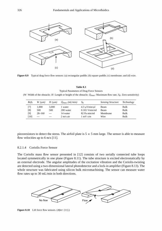
326 Fundamentals and Applications of Microfluidics
(a)(b)
(c) (d)
Figure 8.9 Typical drag force flow sensors: (a) rectangular paddle; (b) square paddle; (c) membrane; and (d) wire.
Table 8.3
Typical Parameters of Drag Force Sensors
(W: Width of the obstacle;H : Length or height of the obstacle;Qmax: Maximum flow rate;S0: Zero-sensitivity)
Refs. W (µm) H (µm) Qmax (mL/min) S0 Sensing Structure Technology
[7] 1,000 3,000 1 water 4.3µVmin/µl Beam Bulk[8] 500 500 200 water 0.165 Vmin/ml Beam Bulk[9] 28–160 — 14 water 82 Pa min/ml Membrane Bulk[10] — — 2 m/s air 1 mV s/m Wire Bulk
piezoresistors to detect the stress. The airfoil plate is 5× 5 mm large. The sensor is able to measureflow velocities up to 6 m/s [11].
8.2.1.4 Coriolis Force Sensor
The Coriolis mass flow sensor presented in [12] consists of two serially connected tube loopslocated symmetrically in one plane (Figure 8.11). The tube structure is excited electrostatically byan external electrode. The angular amplitudes of the excitation vibration and the Coriolis-twistingare detected using a two-dimensional lateral photodetector and a lock-in amplifier (Figure 8.13). Thewhole structure was fabricated using silicon bulk micromachining. The sensor can measure waterflow rates up to 30 mL/min in both directions.
No flow Flow
Figure 8.10 Lift force flow sensors. (After: [11].)

Microfluidics for Internal Flow Control: Microflow Sensors 327
(b)(a)�
�
Figure 8.11 Coriolis flow sensor: (a) flows inside the sensor tube; and (b) design example
Table 8.4
Transducer Principles and Realization of Thermal Transducers Using Micromachining Technology
Principle Examples Measurement of
Thermoresistive Platinum, polysilicon, silicon, metal alloys (NiCr,NiFe)
Temperature, temperaturedifference, heating power
ThermocapacitiveThermoelectrical pSi-Al (bipolar-technology), PolySi- Al (CMOS-
technology), pPolySi-nPolySiTemperature, temperaturedifference
Thermoelectronical Transistors, diodes Temperature, temperaturedifference
Pyroelectrical LiTaO3 Heating powerFrequency analog SAW-oscillator, Lamb-wave-oscillator Temperature
The major disadvantage of this sensor type is that the Coriolis force depends on the fluiddensity. The density in turn depends on the temperature. Temperature compensation is necessary forthis sensing principle.
8.2.1.5 Electrohydrodynamic Flow Sensors
A nonmechanical, nonthermal sensing concept is the electrohydrodynamic method, which can beimplemented in microtechnology. The working principle is similar to the thermal time-of-flightsensors described in Section 8.1.3.4. This method is based on the charge transport caused by masstransport. First, a charge is injected into the flow by an electrode in the form of a charge pulse.A second electrode downstream detects the charge in the flow. The time of flight of the charge orthe time shift between the injected signal and the detected signal is evaluated. The flow velocity isthen derived by the known distance between the two electrodes and the time of flight. The sensorpresented in [13] can detect flow rates up to 1.6 mL/min with a resolution of 8µL/min.
8.2.2 Thermal Flow Sensors
In the following sections, thermal flow sensors are categorized by their transducers. The most im-portant transducer principles are thermoresistive, thermocapacitive, thermoelectrical, thermoelec-tronical, pyroelectrical, and frequency analog. Table 8.4 shows an overview of these principles. Theindirect transformation over an oscillating mechanical element is referred to here as the frequencyanalog principle.

328 Fundamentals and Applications of Microfluidics
Table 8.5
Typical Parameters of Thermoresistive Hot-Wire Sensors
(W × L × H : Dimension of the heater;vmax: Maximum flow velocity;Qmax: Maximum volume flow rate;Pmax:
Maximum heating power;Tmax: Maximum heater temperature;S0: Zero-sensitivity;τ : Response time )
Refs. W× L × H (µm) vmax, or Qmax Pmax (mW) 1Tmax(K)
S0 τ
(ms)Material
[14] 270× 3 × 1 100 mL/min air 8 230 0.3 mV min/ml 0.5 Polysilicon[15] 20× 2,000× 2 600 nL/min water 0.14 33 0.0263 K nL/min 0.14 Polysilicon[16] 2 × 40× 0.45 — 15 280 — 0.35 Polysilicon[17] 290× 290× 0.5 200 mL/min wa-
ter2,400 50 ≈0.2 V min/ml 1 Polysilicon
[18] 200× 200× 11.8 4 m/s air 1,600 180 ≈1.7Vs/m — Silicon[19] — 60 m/s air 2,400 160 ≈0.5 V s/m — Nickel
8.2.2.1 Thermoresistive Flow Sensors
The approximated linear relation between the resistanceR and temperatureT is:
R = R0[1 + α(T − T0)] (8.39)
whereR0 is the resistance at the temperatureT0, andα is the temperature coefficient of resistance(TCR). Since the absolute values of integrated resistors vary widely (±20%), they should beevaluated relatively in a bridge circuitry such as the Wheatstone bridge. The ratio of two resistancesfabricated in the same batch is usually accurate with a tolerance less than 1%.
Hot-Wire and Hot-Film Type.Hot-wire and hot-film sensors generally need one resistor as a heater,and in some cases a second thermoresistor as temperature sensor for the ambient. Microtechnologyallows the fabrication of thermoresistive sensors from different materials: polycrystalline silicon,single-crystalline silicon, metals, metal alloys, and temperature resistant materials. Table 8.5 givesan overview of the characteristics of this sensor type reported in the literature [14, 19].
Polysilicon.Polysilicon has a relatively high TCR compared to single-crystalline silicon. Theonly disadvantage is that the TCR of polysilicon strongly depends on technology parameters suchas deposition temperature and annealing temperature. It is also difficult to reproduce the exact TCRin different process batches. The flow sensor reported in [14] has a hot wire in the form of a heavilydoped polycrystalline bridge [Figure 8.12(a)]. The bridge is supported on a silicon oxide mesa. Theflow channel is etched in silicon. The sensor is able to measure air flow rate up to 100 mL/min.The same hot wire shown in Figure 8.12(b) is integrated in a silicon nitride microchannel [15]. Thissensor can resolve water flow rates as low as 10 nL/min. The hot-film sensor is fabricated on a siliconnitride membrane [16] [Figure 8.12(c)] or on a silicon membrane [17] [Figure 8.12(d)].
Single-Crystalline Silicon.Single-crystalline silicon can also be used as a heater. However,the resistor is integrated directly in the bulk material, which is thermally conductive. It is thereforedifficult to assure thermal isolation. Furthermore, the presence of a p-n junction limits the operatingrange of the sensor at higher temperatures. The sensor described in [18] has spreading resistors asheaters and temperature sensors.
Metals and Alloys.Metals and metal alloys are stable materials for designing heaters andtemperature sensors. They have advantages over single-crystalline silicon due to the absence of p-njunctions, and over polysilicon due to the low pressure dependence. However, the good electricalconductivity requires a long structure or a large meander form, which represents a hurdle for

Microfluidics for Internal Flow Control: Microflow Sensors 329
(a) (b) (c)
(d) (e)
Si Glass MetalSi3N4PolySi SiO2
Figure 8.12 Hot-wire and hot-film sensor based on thermoresistive polysilion and metal: (a) bridge inside a microchannel;(b) embedded in a silicon-nitride microchannel; (c) on a silicon nitride membrane; (d) on a silicon membrane; and (e) metalresistors on a silicon beam.
(c)
(a) (b)
(d)
HeaterTemperature sensors
Heater
Temperature sensors
Heater
Temperature sensors
Heater
Temperature sensors
Si
Glass
Metal
Si3N
4
PolySi
Doped Si
Figure 8.13 Thermoresistive flow sensors of calorimetric type: (a) silicon; and (b, c, d) metals.
miniaturization. The sensor presented in [19] has a nickel heater embedded in silicon nitride andsilicon oxide. The heater is suspended on a silicon beam and works as a hot wire [Figure 8.12(e)].Materials such as silicon carbide are interesting for high-temperature applications. Thin film siliconcarbide exhibits thermal conductivity on the same order of single-crystalline silicon and has a fastthermal response.
Calorimetric Type.Thermoresistive sensors are best suited for the calorimetric principle. Thetemperature sensors upstream and downstream of the heater can be connected to a Wheatstonebridge, which provides directly the differential signal and does not depend on fabrication tolerance.Similar to hot-wire and hot-film types, a variety of materials can be used.
Single-crystalline silicon is used in [20] to form a full Wheatstone bridge. A second bridgecompensates the offset and improves the stability of the sensor. Three operational amplifiers aremonolithically integrated on the chip. The sensor reported in [21] has single-crystalline siliconresistors as temperature sensors. The heaters and sensors are located on a membrane out of theflow, which makes measurement of corrosive fluid possible [Figure 8.13(a)]. The drawback of thisdesign is the heat loss through conduction in the silicon membrane.

330 Fundamentals and Applications of Microfluidics
Table 8.6
Typical Parameters of Thermoresistive Calorimetric Sensors
(W × L: Dimension of the heater;vmax: Maximum flow velocity;Qmax: Maximum volume flow rate;Pmax: Maximum
heating power;Tmax: Maximum heater temperature;S0: Zero-sensitivity;τ : Response time)
Refs. W× L (µm) vmax, or Qmax Pmax(mW)
1Tmax(K)
S0 τ (ms) Material
[20] 4,000× 4,000 0.33 m/s air 250 168 780 mV s/m 0.5 Single crystalline[21] — — — — — — Single crystalline[22] 400× 500 100 mL/min air — 160 0.03V min/ml — Permalloy[23] 4,000× 6,000 2 m/s 7.7 55 — < 150 Gold[2] 500× 1,000 2 m/s air, 0.002
m/s water10 — 30K s/m air,
2,000K s/m water— Au/Cr
[25] 3,000× 3,000 3.5 m/s air 240 — 400 mV s/m 2.5 SiC
Nickel-iron alloy (Permalloy) is used for temperature sensors in [22]. The heater and sensorsare laminated within a 1-µm-thin thermal isolating silicon nitride layer that are suspended in theform of two bridges over an etched pit in the silicon [Figure 8.13(b)]. The development reported in[23] is similar. A heat sink and flow guide integrated on the backside of the flow sensor are used toachieve an extended measurement range [Figure 8.13(c)].
The flow sensor presented in [2] has suspended CrAu-resistors as heater and temperaturesensors. The resistors are carried by a silicon nitride grid. The flow channel is fabricated by usingsilicon etching and anodic bonding [Figure 8.13(d)]. The newer version of this sensor has highdynamics, which allows the sensor to measure acoustic flow and can be used as a microphone [24].
In the sensor reported in [25], doped silicon carbide film was used as heater and temperaturesensors. The silicon carbide resistors form several bridges above a flow channel etched in silicon.Due to the high melting point of silicon carbide (about 2,800◦C), high heater temperature is possible.Thermal cleaning can be achieved by elevating the heater temperature to above 1,000◦C, at whichcontaminants are completely burnt. Table 8.6 compares the performance of the above calorimetricsensors.
8.2.2.2 Thermocapacitive Flow Sensors
The temperature dependence of the dielectric constant allows the realization of temperature sensorsbased on the thermocapacitive principle. The sensor described in [26] has tantalum oxide Ta2O5as dielectric material in the sensing capacitor. The sensor works in the hot-film mode. The heaterand the sensing capacitor are integrated on a cantilever suspended above a trench etched in silicon[Figure 8.14(a)]. The circuit schematic of the sensor is shown in Figure 8.14(b). The sensorconsumes a maximum power of 57 mW. The maximum range of operation is 20 m/s air flow, andthe sensitivity is 4.25 mVs/m.
8.2.2.3 Thermoelectric Flow Sensors
The thermoelectric effect, or the Seebeck effect, can be used for measuring temperature differences.The effect yields a voltage between two ends of a semiconductor or metal with a temperaturedifference of1T :
1V = αS1T (8.40)
whereαS is the thermoelectric coefficient, or Seebeck coefficient, of the material. When taking twomaterials with different Seebeck coefficients at the hot junction, the voltages are subtracted. An

Microfluidics for Internal Flow Control: Microflow Sensors 331
(a) (b)
Si heater
PolySi Ta 2O5
Al
5V
8.2KCantilever area
Figure 8.14 Hot-film sensor based on thermocapacitive principle: (a) design; and (b) evaluation circuit.
Table 8.7
Seebeck Coefficients of Different Materials
Material αs (300 K)µV/K Material αs (300 K)µV/K
p-Si 300 to 1,000 Gold (Au) 1.94n-PolySi −200 to−500 Copper (Cu) 1.83Antimony (Sb) 43 Aluminum (Al) −1.7Chromium (Cr) 17.3 Platinum (Pt) −5.28
effective coefficient remains for the thermocouple. Many thermocouples connected serially form athermopile, which multiplies the thermoelectric coefficient by the number of thermocouples. Table8.7 lists the Seebeck coefficient of some common materials [27].
Hot-Film Type.Thermopiles are used for measuring the heater temperature in hot-film mode. Thecooling of the heater for a constant heating power can be evaluated directly with the thermopileoutput. The sensor presented in [28] has aluminum/polysilicon thermopiles whose hot junctions areplaced next to the heater. The whole structure is suspended on a cantilever [Figure 8.15(a)]. Thethermopile output is used in the example of [29] to control the heating current, which is connectedto a sigma-delta converter. The sensor delivers a direct digital output. The thermopile in this sensorwas made of p-Si and aluminum. The example of [30] has two thermopiles to measure the heatertemperature [Figure 8.15(b)]. The thermopile was made of GaAs and AlGaAs, which is compatiblewith GaAs technology and suitable for high temperature applications.
Calorimetric Type.For sensing the temperature difference between downstream and upstreampositions, two thermopiles are used. The thermopiles can be fabricated with standard bipolar process[31]. Thermopiles made of aluminum and single crystalline silicon show a larger Seebeck coefficientthan those with aluminum and polysilicon (Table 8.7). For better thermal isolation, the sensorstructures are suspended on a thin silicon membrane or silicon plate.
The other possibility is the use of doped polysilicon. Thermopiles made of n-doped/p-dopedpolysilicon [32] or aluminum/polysilicon [33] are compatibile with standard CMOS technology[Figure 8.15(c)]. The technology allows integration of the sensor with digital electronics, whichprovides an A/D converter with direct digital bitstream output. The sensor presented in [34]was designed for detecting small flow rates generated by acoustic streaming—a gentle pumpingprinciple. The sensor in [35] has thermopiles made of gold and doped polysilicon. The arrangementof thermopiles allows the downstream sensor to work in the time-of-flight mode. Alternativematerials such as BiSb and Sb can improve the Seebeck coefficient [36]. Table 8.8 lists theparameters of the above thermoelectric sensors.

332 Fundamentals and Applications of Microfluidics
(a) (b)
(c)
Si MetalSiO2PolySi GaAs GaAsAl
Temperature sensor
Heater
Temperature sensors
Heater
Temperature sensors
Heater
Temperature sensors
Heater
(d)
Figure 8.15 Thermoelectric sensors: (a) aluminum/polysilicon; (b) aluminium/single crystalline silicon; (c) and (d) alu-minum/polysilicon.
8.2.2.4 Thermoelectronic Flow Sensors
The thermoelectronic effect is based on the temperature dependence of the pn-junction in diodes orbipolar transistors. The voltage drop over a forward biased base-emitter junction follows the relation:
VBE = VG +K T
eln
(IC
IR
)(8.41)
whereVG is the material bandgap,K is the Boltzmann’s constant,e is the elementary charge,ICthe collector current, andIR is the reference current [37]. Figure 8.16 shows the typical evaluationcircuits for thermoelectronic flow sensors.
Hot-Film Type.The diode as a temperature sensor can be fabricated by standard microtechniques,described in Chapter 3. For good thermal isolation, the thin single crystalline silicon membraneof an SOI wafer can be used as a substrate for the heater and diode structures [38]. The thermalisolation is achieved with deep trenches, which are filled with thermal oxide. A second identicaldiode measures the ambient temperature [Figure 8.17(a)]. The analog circuitry for evaluation isshown in Figure 8.16(c).
Using a comparator circuit, the analog output of the diodes can be fed back to the heater[39]. The principle allows the design of a semidigital sensor with pulse width modulated output[39, 40] [Figure 8.16(d)]. The sensor shown in Figure 8.17(b) is thermally isolated by a free-standingcantilever. A trench filled with polyimide separates the two sensing diodes. Furthermore, MOS-FETscan work as both sensor and heater [Figure 8.16(e)] [41].
Calorimetric Type.In [42], both heating and sensing elements are diodes that are positioned beneathdiamond-shaped silicon pyramids. The pyramids are placed in the flow channel to obtain goodthermal contact between fluid flow and the heater as well as sensing elements [Figure 8.17(c)]. Thesensing diodes downstream can also work in the time-of-flight mode. Table 8.9 lists the parametersof the above thermoelectronic sensors.

Microfluidics for Internal Flow Control: Microflow Sensors 333
(a) (b)
IC
A
Sensor
VBE Vout
A
A
IC1 IC2
Sensor1
T=T1
Sensor2
T=T2
D1 D2Vout
(c)
D1 D2
(d)
Heater Vout
(e)
SensorSensor
Heater
Sensor
Figure 8.16 Configuration for evaluation of thermoelectronic flow sensors: (a) hot-film type with transistors; (b) calorimet-ric type with transistors; (c) hot-film type with diodes; (d) hot-film type with diodes, semidigital output; and (e) hot-film typewith field effect transistors.
(a)
D1 D2D1
D2
(b)
D1 D2
(c)
Si MetalSiO2Doped Si Polyimide
Temperature sensorsHeater Heater Temperature sensors
Heater
Temperature sensors
Figure 8.17 Typical thermoelectronic flow sensors: (a) diodes on a membrane; (b) diodes on a cantilever; and (c) diodeswith diamond-shaped silicon pyramids.

334 Fundamentals and Applications of Microfluidics
Table 8.8
Typical Parameters of Thermoelectric Sensors
(W × L × H : Dimension of the heater;vmax: Maximum flow velocity;Qmax: Maximum volume flow rate;Pmax:
Maximum heating power;Tmax: Maximum heater temperature;N: Number of thermocouples;αs: Seebeck-coefficient)
Refs. W× L (µm) vmax, or Qmax Pmax (mW) 1Tmax (K) N αs (ms) Material
Hot-film type
[28] 250× 130 25 m/s N2 10 250 20 58 n-PolySi/Al[29]] 5,000× 5,000 50 m/s air 20 — 6 833 p-Si/Al[30] 1,280× 2,000 30 m/s air 33 300 16 175 GaAs/AlGaAs
Calorimetric type
[31] 6,000× 6,000 20 m/s air 595 17 25 600 n-Si/Al[32] 4,000× 5,000 40 m/s air 3 — 20 415 n-PolySi/p-PolySi[33] 1,000× 1,000 2 m/s air 3 40 20 108 n-PolySi/Al[34] 1,000× 1,000 — 3.5 — 10 ≈100 n-Poly/Al[35] 600× 600 10 mm/s water 50 — 20 — PolyS/Au[36] 3,600× 1,150 2.3 m/s air 1 5 100 135 BiSb/Sb
LiTaO -substrate3
Heater
Electrodes
Gold contact
Figure 8.18 Pyroelectric hot-film flow sensor.
8.2.2.5 Pyroelectric Flow Sensors
The pyroelectric effect is based on the dependence of surface charge of a pyroelectric material onthe change of the supplied heat. The pyroelectric current is given by [43]:
I = CpAdT
dt(8.42)
where Cp, A, and T are the pyroelectric coefficient, the area of the detecting electrode, andtemperature of the pyroelectric material, respectively. Therefore, a sinusoidal electric current issupplied to the heater at a frequencyf that both heats the pyroelectric substrate to a stationarydc temperature and produces an ac sinusoidal temperature variation at a frequency 2f .
The heat from the thin-film heater flows through the substrate and is dissipated to the flow(Figure 8.18). The ac temperature variation under the two electrodes includes pyroelectric currentsin each of the symmetrically disposed measuring electrodes. The ac pyroelectric currents generatedat the two symmetric electrodes produce the sensor signal.
Because lithium tantalate (LiTaO3) has a fairly high pyroelectric coefficient,Cp = 2.3 ×
10−4 [Asm−2K−1] which is not affected by ambient temperatures up to about 200◦C [43]. Thepyroelectric material was used as the substrate material. The electrodes and heater are made fromNiCr-alloy or gold thin film [43, 44].

Microfluidics for Internal Flow Control: Microflow Sensors 335
Table 8.9
Typical Parameters of Thermoelectronic Flow Sensors
(W × L: Dimension of the heater;vmax: Maximum flow velocity;Qmax: Maximum volume flow rate;Pmax: Maximum
heating power;Tmax: Maximum heater temperature;τ : Response time)
Refs. W× L (µm) vmax, or Qmax Pmax(mW)
1Tmax(K)
τ (ms) τ (ms) Material
Hot-film type
[38] 4,000× 5,000 1m/s oil 66 55 — 50 p-n Si[39] 2,000× 1,400 30 m/s air 110 130 3% /m/s — p-nSi[40] 1,000× 1,000 0.7m/s N2 — 25 16 mVs/m 30,000 Si
Calorimetric type, time-of-flight sensor
[41] 9,000× 5,000 0.1mL/min oil 60 — 3.5 Vmin/ml 30 Al/Si/Glass
(a) (b)
Figure 8.19 Typical frequency analog flow sensors: (a) resonating bridge; and (b) SAW.
8.2.2.6 Frequency Analog Sensors
Frequency analog sensors are realized by using thermal excitation and evaluation of oscillatingfrequency [45, 46]. The sensing principle is based on the temperature dependence of the oscillatingbehavior of mechanical elements such as cantilevers and membranes. The change of temperaturecauses a change of mechanical stress in the element, which leads to a change of its resonantfrequency [Figure 8.19(a)]. Further frequency analog sensors are based on the dependence of surfacewave frequency on the temperature [47]:
1 f
f0=αf Ah1T
Geff(8.43)
where1 f is the frequency shift,f0 is initial oscillator frequency under no gas flow,αf is thetemperature coefficient of frequency for the surface acoustic wave (SAW) substrate,A is the heatedsurface,h is the heat transfer coefficient, andGeff is the effective thermal conductance between thesubstrate and the ambient [Figure 8.19(b)]. A frequency shift of 140 kHz can be reached with amaximum flow rate of 1,000 mL/min. Similar devices can be designed with a Lamb-wave [48].
8.3 SUMMARY
This chapter discusses the design and fabrication of microflow sensors. Microflow sensors togetherwith microvalves and micropumps form a feedback controlled system for fluid delivery. Because themajority of flow sensors realized by microtechnology are based on thermal concepts, microflowsensors are categorized in this chapter as nonthermal and thermal types. Most nonthermal flowsensors are based on pressure changes or forces induced by a fluid flow. The design of these

336 Fundamentals and Applications of Microfluidics
flow sensors reduces to designing pressure sensors or force sensors. Thermal flow sensors arefurther categorized as hot-film/hot-wire sensors, calorimetric sensors, and time-of-flight sensors.All these types are based on heat transfer between a heated body and the fluid flow. The design ofthermal sensors typically leads back to designing temperature sensors. Physical phenomena, such asthermoresistive effect, thermocapacitive effect, thermoelectric effect, thermoelectronic effect, andpyroelectric effect, are available for converting temperatures or temperature differences into anelectric signal. Thermal-induced stress changes the resonance frequency of a mechanical structure,and thus can also be used for detecting temperature.
Problems
8.1 For the sensor of Example 8.4, determine the strain at the ends of the tube. The tube is made ofsilicon and is 50µm thick. If piezoresistive effect is used, is the signal detectable at a signal-to-noise ratio of 0.1%?
8.2 Determine the maximum electric power required for a thermal flow sensor. The sensor consistsof a microchannel with a cross section of 500× 500µm and a heater with a heated surface of500 × 200 µm. The sensor is designed for a maximum water flow rate of 10µL/min, and thetemperature difference between the heater and the fluid is kept constant at 40K.
8.3 Determine the measured flow range of the sensor in Problem 8.2, working in the electrocaloricmode with a distance of 500 mm between the heater and the temperature sensor. The heater andtemperature sensors are suspended in the flow channel; neglect heat loss by conduction to thesubstrate.
8.4 The temperature sensor in Problem 8.3 is to be designed as a thermopile with p-type silicon andaluminum (αs = 833 mV/K). Determine the number of thermocouples required for achieving aresolution of 1:50 of the full measurement range. The signal-to-noise ratio of the sensor is 1:1,000,and the maximum output voltage is 5V.
References
[1] Nguyen, N. T., et al., “Investigation of Forced Convection in Micro-Fluid Systems,”Sensors and Actuators A, Vol. 55,1996, pp. 49–55.
[2] Lammerink, T. S. J., et al., “Micro-Liquid Flow Sensor,”Sensors and Actuators A, Vol. 37–38, 1993, pp. 45–50.
[3] van Kuijk, J., et al., “Multiparameter Detection in Fluid Flows,”Sensor and Actuators A, Vol. 46/47, 1995, pp. 380–384.
[4] Boillant, M. A., et al., “A Differential Pressure Liquid Flow Sensor for Flow Regulation and Dosing Systems,”Proceedings of MEMS’95, 8th IEEE International Workshop Micro Electromechanical System, Amsterdam, TheNetherlands, Jan. 29–Feb. 2., 1995, pp. 350–352.
[5] Cho, S. T., and Wise, K. D., “A High-Performance Microflowmeter with Built-In Self Test,”Sensors and Actuators A,Vol. 36, 1993, pp. 47–56.
[6] Oosterbroek, R. E., et al., “A Micromachined Pressure/Flow-Sensor,”Sensors and Actuators A, Vol. 77, 1999, pp. 167–177.
[7] Gass, V., van der Shoot, B. H., and de Rooij, N. F., “Nanofluid Handling by Micro-Flow-Sensor Based on Drag ForceMeasurements,”Proceedings of MEMS’93, 6th IEEE International Workshop Micro Electromechanical System, SanDiego, CA, Jan. 25–28, 1993, pp. 167–172

Microfluidics for Internal Flow Control: Microflow Sensors 337
[8] Zhang, L., et al., “A Micromachined Single Crystal Silicon Flow Sensor with a Cantilever Paddle,”InternationalSymposium on Micromechatronics and Human Science, Nagoya, Japan, Oct. 1997, pp. 225–229.
[9] Richter, M., et al., “A Novel Flow Sensor with High Time Resolution Based on Differential Pressure Principle,”Proceedings of MEMS’99, 12th IEEE International Workshop Micro Electromechanical System, Orlando, FL, Jan.17–21, 1999, pp. 118–123.
[10] Ozaki, Y., et al., “An Air Flow Sensor Modeled on Wind Receptor Hairs of Insects,”Proceedings of MEMS’00, 13thIEEE International Workshop Micro Electromechanical System, Miyazaci, Japan, Jan. 23–27, 2000, pp. 531–536.
[11] Svedin, N., et al., “A New Silicon Gas-Flow Sensor Based on Lift Force,”Journal of Microelectromechanical Systems,Vol. 7, No. 3, 1998, pp. 303–308.
[12] Enoksson, P., Stemme, G., and Stemme, E., “A Coriolis Mass Flow Sensor Structure in Silicon,”Proceedings ofMEMS’96, 9th IEEE International Workshop Micro Electromechanical System, Feb. 11–15, 1996, San Diego, CA,pp. 156–161.
[13] Richter, A., et al., “The Electrohydrodynamic Micro Flow Meter,”Proceedings of MEMS’91, 3rd IEEE InternationalWorkshop Micro Electromechanical System, Nara, Japan, Jan. 30-Feb. 4, 1991, pp. 935–938.
[14] Mastrangelo, C. H., and Muller, R. S., “A Constant-Temperature Gas Flowmeter with a Silicon MicromachinedPackage,”Technical Digest of the IEEE Solid State Sensor and Actuator Workshop, Hilton Head Island, SC, June4–7, 1988, pp. 43–46.
[15] Wu, S., et. al., “MEMS Flow Sensors for Nano-Fluidic Applications,”Proceedings of MEMS’00, 13th IEEE Interna-tional Workshop Micro Electromechanical System, Miyazaci, Japan, Jan. 23–27, 2000, pp. 745–750.
[16] Liu, C., et al., “A Micromachined Flow Shear-Stress Sensor Based on Thermal Transfer Principles,”Journal ofMicroelectromechanical Systems, Vol. 8, No. 1, 1999, pp. 90–99.
[17] Nguyen, N. T, and Kiehnscherf R., “Low-Cost Silicon Sensors for Mass Flow Measurement of Liquids and Gases,”Sensors and Actuators A, Vol. 49, 1995, pp. 17–20.
[18] Lai, P. T., et al., “Monolithic Integrated Spreading-Resistance Silicon Flow Sensor,”Sensors and Actuators A, Vol. 58,1997, pp. 85–88.
[19] Stephan, C. H., and Zanini, M., “A Micromachined, Silicon Mass Air Flow Sensor for Automotive Application,”Proceedings of MEMS’91, 3rd IEEE International Workshop Micro Electromechanical System, Nara, Japan, Jan. 30–Feb. 4, 1991, pp. 30–33.
[20] van Putten, A. F. P., “An Integrated Silicon Double Bridge Anemometer,”Sensors and Actuators A, Vol. 4, 1983,pp. 387–396
[21] Kuttner, H., et al., “Microminiaturized Thermistors Arrays for Temperature Gradient, Flow and Perfusion Measure-ments,”Sensors and Actuators A, Vol. 25–27, 1991, pp. 641–645.
[22] Johnson, R. G., and Egashi, R. E., “A Highly Sensitive Silicon Chip Microtransducer for Air Flow and DifferentialPressure Sensing Applications,”Sensors and Actuators A, Vol. 11, 1987, pp. 63–67.
[23] Qiu, L., Obermeier, E., and Schubert, A., “A Microsensor with Integrated Heat Sink and Flow Guide for Gas FlowSensing Applications,”Proceedings of Transducers ’95, 8th International Conference on Solid-State Sensors andActuators, Stockholm, Sweden, June 16–19, 1995, pp. 520–523.
[24] de Bree, H. E., et al., “The -FLOWN, A Novel Device Measuring Acoustical Flows,”Proceedings of Transducers ’95,8th International Conference on Solid-State Sensors and Actuators, Stockholm, Sweden, June 16–19, 1995, pp. 356–359.
[25] Lyons, C., et al., “A High-Speed Mass Flow Sensor with Heated Silicon Carbide Bridges,”Proceedings of MEMS’98,11th IEEE International Workshop Micro Electromechanical System, Heidelberg, Germany, Jan. 25–29, 1998,pp. 356–360.
[26] Lin, K. M., Kwok, C. Y., and Huang, R. S., “An Integrated Thermo-Capacitive Type MOS Flow Sensor,”IEEEElectron. Device Letters, Vol. 17, No. 5, 1996, pp. 247–249.

338 Fundamentals and Applications of Microfluidics
[27] van Herwaarden A. W., and Sarro, P. M., “Thermal Sensor Based on The Seebeck Effect,”Sensors and Actuators A,Vol. 10, 1986, pp. 321–346.
[28] Wachutka, G., et al., “Analytical 2D-Model of CMOS Micromachined Gas Flow Sensors,”Proceedings of MEMS’91,3rd IEEE International Workshop Micro Electromechanical System, Nara, Japan, Jan. 30–Feb. 4, 1991, pp. 22–25.
[29] Verhoeven, H. J., and Huijsing, J. H., “An Integrated Gas Flow Sensor with High Sensitivity, Low Response Time andPulse-Rate Output,”Sensors and Actuators A, Vol. 41–42, 1994, pp. 217–220.
[30] Fricke, K., “Mass-Flow Sensor with Integrated Electronics,”Sensors and Actuators A, Vol. 45, 1994, pp. 91–94.
[31] van Oudheusden, B. W., “Silicon Thermal Flow Sensors,”Sensors and Actuators A, Vol. 30, 1992, pp. 5–26.
[32] Moser, D., and Baltes, H., “A High Sensitivity CMOS Gas Flow Sensors on a Thin Dielectric Membrane,”Sensorsand Actuators A, Vol. 37–38, 1993, pp. 33–37.
[33] Robaday, J., Paul, O., and Baltes, H., “Two-Dimensional Integrated Gas Flow Sensors by CMOS IC Technology,”Journal of Micromechanics and Microengineering, Vol. 5, 1995, pp. 243–250.
[34] Nguyen, N. T., et al., “Integrated Thermal Flow Sensor for In-Situ Measurement and Control of Acoustic Streamingin Flexural-Plate-Wave Pumps,”Sensors and Actuators A, Vol. 79, No. 2, 2000, pp. 115–121.
[35] Ashauer, M., et al., “Thermal Flow Sensor for Liquids and Gases,”Proceedings of MEMS’98, 11th IEEE InternationalWorkshop Micro Electromechanical System, Heidelberg, Germany, Jan. 25–29, 1998, pp. 351–355.
[36] Dillner, U., et al., “Low Power Consumption Thermal Gas-Flow Sensor Based on Thermopiles of Highly EffectiveThermoelectric Materials,”Sensors and Actuators A, Vol. 60, 1997, pp. 1–4.
[37] Meijer, G. C. M., “Thermal Sensors Based on Transistors,”Sensors and Actuators A, Vol. 10, pp. 103–125.
[38] Kersjes, R., et al., “An Integrated Sensor for Invasive Blood-Velocity Measurement,”Sensors and Actuators A, Vol. 37-38, 1993, pp. 674–678.
[39] Stemme, G., “A CMOS Integrated Silicon Gas-Flow Sensor with Pulse-Modulated Output,”Sensors and Actuators A,Vol. 14, 1988, pp. 293–303.
[40] Pan, Y., and Huijsing, J. H., “New Integrated Gas-Flow Sensor with Duty Cycle Output,”Electronics Letters, Vol. 24,No. 9, 1988, pp. 542–543.
[41] Tong, Q. Y., and Huang, J. B., “A Novel CMOS Flow Sensor with Constant Chip Temperature (CCT) Operation,”Sensors and Actuators A, Vol. 12, 1987, pp. 9–12.
[42] Yang, C. Q., and Soeberg, H., “Monolithic Flow Sensor for Measuring Millilitre per Minute Liquid Flow,”Sensorsand Actuators A, Vol. 33, 1992, pp. 143–153.
[43] Yu, D., Hsieh, H. Y., and Zemel, J. N., “Microchannel Pyroelectric Anemometer,”Sensors and Actuators A, Vol. 39,1993, pp. 29–35.
[44] Hsieh, H. Y., Bau, H. H., and Zemel, J. N., “Pyroelectric Anemometry,”Sensor and Actuators A, Vol. 49, 1995,pp. 125–147.
[45] Legtenberg, R., Bouwstra, S., and Fluitman, J. H. J., “Resonating Microbridge Mass Flow Sensor with Low-Temperature Class-Bonded Cap Wafer,”Sensors and Actuators A, Vol. 25–27, 1991, pp. 723-727.
[46] Geijselaers, H. J. M., and Tijdeman, H., “The Dynamic Mechanical Characteristics of a Resonating MicrobridgeMass-Flow Sensor,”Sensors and Actuators A, Vol. 29, 1991, pp. 37–41.
[47] Joshi, S. G., “Flowsensors Based on Surface Acoustic Waves,”Sensor and Actuators A, Vol. 44, 1994, pp. 63–72.
[48] Vellekoop, M. J., “A Smart Lamb-Wave Sensor System for the Determination of Fluids Properties,” Ph.D. thesis, DelftUniversity of Technology, Delft, Netherlands, 1994.

Chapter 9
Microfluidics for Life Sciences and Chemistry:Microneedles
Micromachining technology offers great opportunities for biomedical instrumentation. One of themost common and simplest biomedical instruments is the needle. Traditionally, hypodermic needlesare used for delivering drugs and aspirating body fluid through the human skin. The smallest needlesfabricated by conventional machining methods have a minimum diameter on the order of 300µm.These relatively large needles cause pain and are less accurate for targeted delivery in microscale.Furthermore, the advances in biotechnology requires delivery of molecules in nanometer scale withmicron precision. Conventional hypodermic needles can not fulfill these requirements.
Micromachining technology is able to fabricate needles smaller than the previous limit of300µm. The small size opens new application fields for this simple device. The main applicationsof microneedles are:
• Painless drug delivery through skin (transdermal or intradermal);
• Closed-loop chemical stimulation of tissues;
• Cell manipulation;
• Sample collection and delivery in chemical and biochemical analysis;
• Interconnection between microscopic and macroscopic fluidic systems.
Figure 9.1 shows the structure of human skin. The outer layer is the stratum corneum (SC),which is 10 to 15µm thick and is a dead tissue. On the one hand, the SC layer offers protectionfor the body. On the other hand, this layer poses a barrier and limits the transport rate across theskin in transdermal delivery of drugs. The next layer is viable epidermis (VE) with a thickness ofabout 50 to 100µm. This tissue layer consists of living cells, which have blood vessels capable oftransporting drugs, but contains very few nerves.
A number of methods, such as injection with needles, chemical/lipid enhancers, iontophoresis,electroporation, acoustic, and photoacoustic effect, have been used for increasing the transport rateacross the skin [1]. While direct injection delivers drugs intradermally, the other methods createsmall pores in the SC layer for improving the transport rate of drug molecules. Most of these methodscreate pores in the submicron scale. A microneedle is the another alternative for a transport pathwaywith pore size on the order of microns, large enough for a high transport rate but still too small tocause damage of clinical significance. Hypodermic needles need medical expertise and are not wellsuited for controlled delivery of a small amount of drug over a long period of time. Furthermore,microneedles make highly localized, even intracellular delivery possible.
339

340 Fundamentals and Applications of Microfluidics
10-15 m stratum corneum�
50-100 m viable epidermis�
dermis
subcutaneous fatty tissue
oil gland
hair erector musclesweat gland
parcinian corpuscle
blood vessel
sweat pore
melanocytes
Hair follicle
hairmicroneedles
Figure 9.1 Human skin and microneedle for painless drug delivery.
If a microneedle can reach the region of VE, it would be able to deliver drugs without pain.The microneedle should penetrate into the skin from 15 to 100µm in order to fulfill this function.In transdermal drug delivery, microneedles are needed to puncture the skin. The tiny pores createdby the microneedles allow faster drug diffusion [2]. The microneedles can also remain on the skinafter insertion. An array of solid microneedles sandwiched with a gel containing drugs improves thetransport rate through the gap between the needle and the punctured skin. Besides the puncturingfunction, microneedles may also have a delivering function. Higher transport rates can be reachedwith microneedles coated with drugs. Hollow microneedles allow direct intradermal delivery to theVE region. Drugs are delivered through the bore inside the microneedle by diffusion or pressure-driven flow.
Since micromachining technology is compatible with microelectronics, it is possible tointegrate more functions into the needle. The monolithic integration of sensors in microneedlesallows measurement of the reaction of tissues and cells. The chemical stimulation function of thedrug and the response signal from the sensors make closed-loop controlled cell stimulation possible[3]. Microneedles can manipulate a single cell as well as measure its response. A further applicationof microneedles is precise fluid sampling for chemical and biochemical analysis. The small size ofmicroneedles can improve the resolution of the dispensed amount.
The following sections first consider the mechanical design of microneedles. Importantparameters such as insertion force, buckling force, and fracture force are analyzed. The designshould ensure trouble-free insertion into the skin and prevent needle fracture. Mass transportmechanisms such as pressure-driven flow and diffusion with microneedles are discussed. Based onthe orientation of insertion direction relative to substrate surface, microneedles can be categorized asin-plane needles and out-of-plane needles. In the following, microneedles are categorized by theirfunction as solid needles and hollow needles. Each type can be further classified by its substratematerial, such as silicon, metal, polymer, or glass.

Microfluidics for Life Sciences and Chemistry: Microneedles 341
9.1 DESIGN CONSIDERATIONS
The requirements for a microneedle depend on its applications. The general requirements of amicroneedle are:
• Sharpness for penetrating tissues;
• Strength against fracture, bending, and buckling;
• Biocompatibility of needle material;
• Sufficient flow rate in the needle’s bore.
The first two requirements are characterized by the insertion forceFi,max, the buckling forceFb, andthe fracture forceFf . For safety, the insertion force should be less than the buckling force, which inturn should be less then the fracture force (Fi,max< Fb � Ff). The ratio between the insertion forceand the fracture forceFi,max/Ff is called the margin of safety [4].
9.1.1 Mechanical Design
9.1.1.1 Insertion Force
In contrast to conventional technologies, micromachining allows fabrication of needle tips witharbitrary shape and sharpness defined by photolithography. Needle tips with a submicron tip radiusare possible. The areaA of contact surface at the needle tip is considered as the determining factorfor the insertion forceFi .
The theory of skin insertion is based on the puncture toughnessGp, which is the work per areaneeded to initiate a crack:
Gp =W
A(9.1)
whereW is the total work input andA is the surface of the affected skin area. In case of a hollowneedle, the total area determined by the outer perimeter is considered equal the affected skin area.The relation between the work and the insertion force is described as:
W =
∫ x=xi
x=0Fidx = GpA (9.2)
wherexi is the the puncture position. The insertion force is assumed to be an exponential functionof insertion axisx [4]:
Fi(x) = F0 exp(x/χ) (9.3)
where F0 and χ are to be determined experimentally by curve fitting. The variableχ can beconsidered as the characteristic insertion length. Substituting (9.3) in (9.2) results in:
W =∫ x=xi
x=0 F0 exp(x/χ)dx = GpA
F0χ exp(xi /χ)− F0χ = GpA
Fi,max = Fi(xi) = F0 +1χ GpA
(9.4)
The insertion force in (9.4) is for the static case, where the insertion speed is slow and the kineticenergy of the needle is negligible. Adding kinetic energy into the insertion work in (9.1) will reducethe required insertion force significantly. Yang and Zahn [5] used vibratory actuation and reducedthe insertion force to 30% of the value in the static case. The typical vibration frequency is in thekilohertz range.

342 Fundamentals and Applications of Microfluidics
Example 9.1: Insertion Force of a Microneedle
The tip radius of a microneedle is 50µm. Assume a puncture toughness of the skin of 30 kJ/m2, acharacteristic insertion length of 150µm, and an initial force ofF0 = 0.1N. Determine the forcerequired for puncturing the skin.
Solution. The affected skin area is:
A = πr 2= π × (50× 10−6)2 = 7.85× 10⁻¹⁹ m2
According to (9.4), the insertion force is:
Fi,max = F0 +1
χGpA = 0.1 +
1
150× 10−6× 30× 103
× 7.85× 10−9= 1.67N
9.1.1.2 Buckling Force
Euler’s Model of Microneedle with Constant Cross Section.If the needle’s length is relatively longcompared to its width, the first failure mode is buckling. The critical force can be determined basedon the simple model of Euler’s column [6]. The column is assumed to have the same cross sectionalong its length (Figure 9.2). The deflection curve of the column is governed by the differentialequation:
E Id2y
dx2+ M(x) = 0 (9.5)
whereE is the Young’s modulus andI is the moment of inertia of the beam cross section. With aslightly defected positionδ at x = L, the bending moment isM(z) = −F(δ − y). Equation (9.5)has then the form:
E Id2y
dx2= F(δ − y) (9.6)
Solving (9.6) with the boundary conditions of the fixed end of the needle (x = 0):
y = 0 anddy
dx= 0 (9.7)
results in:y = δ(1 − coskx) (9.8)
wherek2= F/E I . Applying the condition (y = δ) at the insertion point (x = L) results in the
different buckling modes:
kL = (2n − 1)π/2 wheren = 1,2,3, ... (9.9)
The critical buckling force is considered as the buckling force of the first mode (n = 1):
Fb =π2E I
4L2(9.10)
The moments of inertia of different needle cross section are listed in Table 9.1.
Example 9.2: Bending of a Microneedle
A microneedle is made of parylene C and has channel dimensions of 200µm × 200µm × 2 mm.The parylene layer is chemically deposited in 4 hours at a rate of 5µm/h. Assume that the Young’s

Microfluidics for Life Sciences and Chemistry: Microneedles 343
x
y
x=Lx=0
�
Fb
Insertion point
Figure 9.2 Buckling model of a microneedle.
modulus of parylene C is 3.2 GPa. Determine the tip deflection of the microneedle under a forceof 15 mN at the tip.
Solution.For a rough estimation, the bending stiffness of the needle can be modeled by the springconstantk:
k =3E I
L3=
E
4L3(W H3
− wh3)
whereE is the Young’s modulus of the needle material, andI is the needle moment of inertia.The geometry parameters are defined in Table 9.1. The wall thickness of the needle is:
5 µm/h× 4 hr = 20µm
Thus, the outer dimensions of the needle are:
W = 200+ 40 = 240µm
The bending spring constant of the microneedle is:
k =3E
12L3(W4
− w4) =3 × 3.2 × 109
12(2 × 10⁻³)3[(240× 10−6)4 − (200× 10−6)4] ≈ 172 N/m
The tip deflection is:
x = F/k = 0.015/172= 87× 10−6= 87µm
Example 9.3: Buckling of a Microneedle
Determine the critical buckling force for the above microneedle.
Solution. The critical buckling force is given by (9.10):
Fb =π2E
4×12L2 (W4− w4)
=2.25×π2
×3.2×109
12×(2×10−3)2[(240× 10−6)4 − (200× 10−6)4] = 2.83× 10⁻¹ N = 283 mN
Example 9.4: Needle Characteristics of Different Materials
If the above needle is made of polysilicon, what are the tip deflection and the critical bucklingforce? Assume that all other parameters are the same, and Young’s modulus of polysilicon is150 GPa.

344 Fundamentals and Applications of Microfluidics
Table 9.1
Moments of Inertia for Different Microneedles’ Cross Sections. (After: [7].)
Geometry Moment of Inertia Geometry Moment of Inertia
W
W
y
z
Solid squareI =
112W4
W
H
y
z
Solid rectangleI =
112W H3
y
z
W
w
W w
Hollow squareI =
112(W
4− w4)
y
z
W
w
W w
Hollow rectangleI =
112(W H3
− wh3)
R
Solid circleI =
π4 R4
R
r
Hollow circleI =
π4 (R
4− r 4)
R
t
Thin annulusI = πR3t
Solution. The tip deflection of a needle is inversely proportional to its Young’s modulus. Thus,the tip deflection of a polysilicon needle is:
xpoly = xparyleneEparylene
Epoly= 87×
3.2
150= 1.9 µm
The critical buckling force is proportional to the Young’s modulus:
Fpoly = FparyleneEpoly
Eparylene= 0.283×
150
3.2= 13.3N
Microneedle with Continuously Varying Cross Section.In many practical cases, microneedles aredesigned with a tapered shape. The sharp tip improves insertion, while the broad base offersmechanical stability. A varying cross section results in a varying moment of inertia. The governingequation of buckling curve has then the form:
E I (x)d2y
dx2+ M(x) = 0 (9.11)
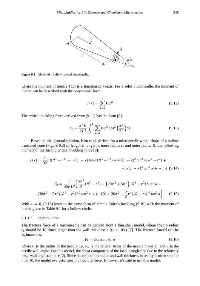
Microfluidics for Life Sciences and Chemistry: Microneedles 345
L
R
r
x
�
Figure 9.3 Model of a hollow tapered microneedle.
where the moment of inertiaI (x) is a function ofx-axis. For a solid microneedle, the moment ofinertia can be described with the polynomial form:
I (x) =
n∑i =0
ki xn (9.12)
The critical buckling force derived from (9.11) has the form [8]:
Fb =π2E
2L3
∫ L
0
n∑i =0
ki xn cos2
(πx
2L
)dx (9.13)
Based on this general solution, Kim et al. derived for a microneedle with a shape of a hollowtruncated cone (Figure 9.3) of lengthL, angleα, inner radiusr , and outer radiusR, the followingmoment of inertia and critical buckling force [9]:
I (x) =π
32[8(R4
− r 4)+ 32(L − x) tanα(R3− r 3)+ 48(L − x)2 tan2 α(R2
− r 2)+
+32(L − x)3 tan3 α(R − r )] (9.14)
Fb =E
40πL2
[5π4
2(R4
− r 4)+
(20π2
+ 5π4)(R3
− r 3)L tanα +
+(30π2+ 5π4)(R2
− r 2)L2 tan2 α + (−120+ 30π2+
5
2π4)(R − r )L3 tan3 α
](9.15)
With α = 0, (9.15) leads to the same form of simple Euler’s buckling (9.10) with the moment ofinertia given in Table 9.1 for a hollow circle.
9.1.1.3 Fracture Force
The fracture force of a microneedle can be derived from a thin shell model, where the tip radiusr t should be 10 times larger than the wall thicknesst (r t > 10t) [7]. The fracture forced can beestimated as:
Ff = 2πr ttσcr sinα (9.16)
wherer t is the radius of the needle tip,σcr is the critical stress of the needle material, andα is theneedle wall angle. For this model, the shear component of the load is neglected due to the relativelylarge wall angle (α → π/2). Since the ratio of tip radius and wall thickness in reality is often smallerthan 10, the model overestimates the fracture force. However, it’s safe to use this model.

346 Fundamentals and Applications of Microfluidics
Example 9.5: Buckling and Fracturing of a Tapered Microneedle
A microneedle made of electroplated nickel has a wall angle of 3◦ and a wall thickness of 20µm.The tip inner diameter isr = 40µm. The needle is 500µm long. Determine the critical bucklingforce and the fracture force of the microneedle, if the Young’s modulus and yield strength ofelectroplated nickel are 23 GPa and 830 MPa, respectively.
Solutions.Using (9.15) withr = 40µm, R = r + t = 40+ 20 = 60µm, L = 500µm,α = 3◦,andE = 23 GPa, the critical buckling force of the needle is:
Fb = 4.77N
The critical fracture force at the needle tip is:
Ff = 2πr ttσcr sinα = 2.18× 10⁻¹ N
Thus, the needle will fracture before bending occurs.
9.1.2 Delivery Modes
9.1.2.1 Delivery with Hollow Microneedles
The channel inside the needle should be designed as large as possible to minimize the pressure lossalong the microneedle and to allow a maximum flow rate at a given pressure. The pressure loss1palong a microneedle can be calculated as (see Section 2.2.4.1):
1p = RefηL
2D2h
u (9.17)
whereη is the viscosity of the fluid,u is the average velocity,L is the channel length in the needle,andDh is the hydraulic diameter of the channel (see Section 2.2.4.2):
Dh =4 × Cross Section Area
Wetted Perimeter=
4A
Pwet(9.18)
The product of the Reynolds number and the factor (Ref ) is about 64 (circular pipe) and60 (trapezoidal duct) in conventional, macroscopic fluid dynamics [10]. The friction factor ofmicrochannels is different from that of conventional theories, and lies between 50 and 60 [11].
Example 9.6: Pressure Loss in a Microneedle
Determine the pressure drop along the needle bore of Example 9.2 if it is used for delivering waterat a flow rate of 100µL/min.
Solution. The hydraulic diameter of the needle’s bore is:
Dh =4 × 200× 200
4 × 200= 200µm
The average velocity of water flow in the needle is (viscosity of water isη = 10−3 Pa.s):
u =100× 10−9/60
(200× 10−6)2= 41.7 × 10⁻³ m/s= 41.7 mm/s
Assuming a factor of Ref = 55, the pressure drop becomes:
1p = RefηuL
2D2h
= 55×10−3
× 41.7 × 10−3× 2 × 10−3
2 × (200× 10−6)2= 57 Pa
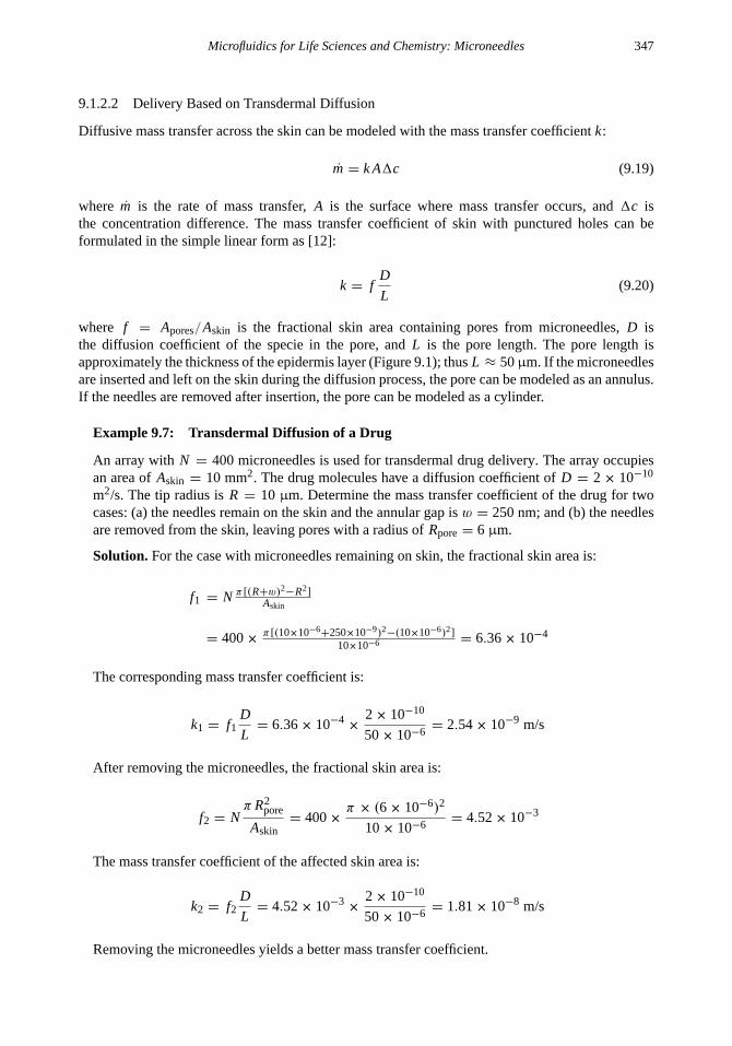
Microfluidics for Life Sciences and Chemistry: Microneedles 347
9.1.2.2 Delivery Based on Transdermal Diffusion
Diffusive mass transfer across the skin can be modeled with the mass transfer coefficientk:
m = k A1c (9.19)
where m is the rate of mass transfer,A is the surface where mass transfer occurs, and1c isthe concentration difference. The mass transfer coefficient of skin with punctured holes can beformulated in the simple linear form as [12]:
k = fD
L(9.20)
where f = Apores/Askin is the fractional skin area containing pores from microneedles,D isthe diffusion coefficient of the specie in the pore, andL is the pore length. The pore length isapproximately the thickness of the epidermis layer (Figure 9.1); thusL ≈ 50µm. If the microneedlesare inserted and left on the skin during the diffusion process, the pore can be modeled as an annulus.If the needles are removed after insertion, the pore can be modeled as a cylinder.
Example 9.7: Transdermal Diffusion of a Drug
An array withN = 400 microneedles is used for transdermal drug delivery. The array occupiesan area ofAskin = 10 mm2. The drug molecules have a diffusion coefficient ofD = 2 × 10⁻¹⁰
m2/s. The tip radius isR = 10 µm. Determine the mass transfer coefficient of the drug for twocases: (a) the needles remain on the skin and the annular gap isw = 250 nm; and (b) the needlesare removed from the skin, leaving pores with a radius ofRpore = 6 µm.
Solution. For the case with microneedles remaining on skin, the fractional skin area is:
f1 = N π [(R+w)2−R2]Askin
= 400×π [(10×10−6
+250×10−9)2−(10×10−6)2]10×10−6 = 6.36× 10⁻⁴
The corresponding mass transfer coefficient is:
k1 = f1D
L= 6.36× 10−4
×2 × 10−10
50× 10−6= 2.54× 10⁻⁹ m/s
After removing the microneedles, the fractional skin area is:
f2 = NπR2
pore
Askin= 400×
π × (6 × 10⁻⁶)2
10× 10−6= 4.52× 10⁻³
The mass transfer coefficient of the affected skin area is:
k2 = f2D
L= 4.52× 10−3
×2 × 10−10
50× 10−6= 1.81× 10⁻⁸ m/s
Removing the microneedles yields a better mass transfer coefficient.

348 Fundamentals and Applications of Microfluidics
(a) (b) (c) (d) (e) (f)
Figure 9.4 Typical shapes of solid microneedle: (a) silicon, etched in SF6 and O2 plasma [2]; (b) silicon, etched withseparated DRIE and RIE [13]; (c) silicon, dicing and wet etching in KOH [14]; (d) stainless steel, laser machined and bent[15]; (e) titanium, wet etched and bent [16]; and (f) SU-8, photo lithography, filled with a sacrificial polymer, and etched witha metal mask.
9.2 DESIGN EXAMPLES
9.2.1 Solid Microneedles
Solid microneedles only have the puncturing function. The design of this needle type is relativelysimple. According to (9.4), the needles only need to have a sharp tip to reduce the insertion force andkeep this force under the critical buckling force and the fracture force. Solid microneedles can befabricated by direct micromachining or molding from a micromachined template. Different designexamples of solid microneedles are categorized in this section by their materials.
9.2.1.1 Silicon Needles
Single-crystalline silicon is readily available at low cost. Micromachining technologies are wellestablished for silicon (Chapter 3). Thus, the fabrication of silicon microneedles is with a singlemask relatively simple. The fabrication process of silicon microneedles consists of two basic steps:forming and sharpening.
Henry et al. [2] combined the two etch gases SF6 and O2 in a reactive ion etcher to shapethe needle. While SF6 etches anisotropically and forms the needle body, O2 etches isotropically andsharpens the needle tip [Figure 9.4(a)].
Besides the puncturing function, solid microneedles made of silicon can be used as intracellu-lar sensing probes. Hanein et al. [13] separated the fabrication process into two steps: forming of theneedle body and sharpening. First, the needle body and its length are defined by the DRIE process(Chapter 3). Subsequently, the needles are sharpened with RIE in SF6. Protecting pillars that havesmaller diameters than the needle were used for forming a strong base for the needle [Figure 9.4(b)].
Shikida et al. [14] proposed a maskless approach, where the needle body was first formedby dicing. Subsequent anisotropic wet etching in KOH sharpens the needles [Figure 9.4(c)]. Thistechnique involves dicing and is not suitable for batch fabrication. Furthermore, the needle size isdetermined by the geometry of the dicing saw and cannot be adjusted.
9.2.1.2 Needles Made of Metals and Other Materials
Solid microneedles made of metals can be fabricated based on molding techniques. The solidmicroneedles made of silicon are used as a positive master for casting a polymeric negative mold.The polymeric mold forms the metal replica of the original silicon needles by electroplating.

Microfluidics for Life Sciences and Chemistry: Microneedles 349
Table 9.2
Typical Parameters of Solid Microneedles
Refs. Tip (µm) Base (µm) Length (µm) Material
[2] 1 80 200 Silicon[13] 0.01 70 230 Silicon[14] 0.01 150 300 Silicon[15] 0.01 75× 200 1,000 Stainless steel[17] — 50 250–600 SU-8
Laser machining can form microneedles directly from a metal sheet and bend 90◦ out of theplane of the sheet [15] [Figure 9.4(d)]. A similar approach was reported by Matriano et al. [16]. Theneedles are etched in-plane on a titanium sheet. They are subsequently bent out of plane [Figure9.4(e)].
The relation between the critical buckling force and the needle’s length (9.10) shows thateven a soft material such as a polymer can withstand high axial load if the length is reduced.Thus, a sharp polymer microneedle is able to puncture the skin without buckling. Similar toelectroplated metal microneedles, polymer microneedles can be fabricated from a micromachinedmold. Polymer replicas of silicon microneedles are fabricated using the negative mold describedabove. Furthermore, molds for polymeric microneedles can be micromachined directly in silicon,SU-8, or electroplated metal.
Polymer microneedles can directly be formed by photolithography of a thick film resist, suchas SU-8 [17]. The sharpening process starts with filling of the gap between the SU-8 cylinderswith a sacrificial polymer polyactic-co-glycolic acid (PLGA). The polymer layers (SU8 and PLGA)was subsequently dry etched with a metal mask. The mask is positioned asymmetrically to theSU-8 cylinders. Thus, underetching results in a beveled shape of the SU-8 cylinder. Removing thesacrificial polymer with a solvent releases the SU-8 microneedles [Figure 9.4(f)]. Table 9.2 comparestypical parameters of the solid microneedles.
9.2.2 Hollow Microneedles
In contrast to solid microneedles, the fabrication of hollow microneedles is more complex due to theadditional hollow bore. Generally, hollow microneedles can be fabricated either in the bulk substrate,or using surface micromachining with a sacrificial material. In the first approach, the completehollow microneedles are fabricated directly from a substrate material using bulk micromachining.In the latter approach, a variety of materials can be used as functional layer. First, a functional layersuch as polysilicon or electroplated metal is deposited on a sacrificial solid microneedle. Removingthe sacrificial material results in a hollow microneedle. Hollow microneedles are categorizedaccording to their substrate materials.
9.2.2.1 Silicon Needles
One of the first approaches to make microneedles with micromachining technology is to fabricatethem in silicon. Figure 9.5(a) depicts a solution in single-crystalline silicon reported by Chen andWise [3]. The microchannel is wet-etched by ethylene-diamine pyrocatechol (EDP) (see Section3.3.1). The highly boron-doped silicon layer is structured as a grid, which allows etch access tothe underlying silicon. EDP etching forms the buried channel, because it does not attack the gridcovering the channel. The channel is then sealed by thermal oxidation. Deep boron diffusion definesthe shape of the needle shank. Wet etching in EDP subsequently releases the needle. Since this

350 Fundamentals and Applications of Microfluidics
(a)
1. wafer
2. wafer
opening
A
A
A-A
aaaaaaaaaaaaaaaaaaaaaaaaaaaaaaaaaaaaaaaaaaaaaaaaaaaaaaaaaaaaaaaaaaaaaaaaaaaaaaaaaaaaaaaaaaaaaaaaaaaaaaaaaaaaaaaaaaaaaaaaaaaaaaaaaaaaaaaaaaaaaaaaaaaaaaaaaaaaaaaaaaaaaaaaaaaaaaaaaaaaaaaaaaaaaaaaaaaaaaaaaaaaaaaaaaaaaaaa
A
A
opening
(b)
A-A
filled trench
A
A
(c)
A-A
opening
A
A
(d)
A-A
(e) (f)
Si{111}
protected
wall
opening
opening
(g)
Si PolySiSi3N4SiO2
opening
opening
Figure 9.5 Hollow silicon microneedle: (a) buried channel, wet etched in EDP [3]; (b) buried channel, DRIE [18]; (c) directbonding, DRIE [19]; (d) surface micromachined channel [20]; (e) out-of-plane, sharpened by dry etching [22]; (f) out-of-plane, sharpened by wet etching [23]; and (g) out-of-plane, sharpened by dry etching with a cross-shaped mask [24].
process is compatible to microelectronics, electrodes can be integrated into the needle for measuringthe tissue reaction after injecting drugs. Paik et al. [18] used a similar approach to make a planararray of hollow microneedles. The needles are shaped by DRIE [Figure 9.5(b)]. The advantage overthe technology of Chen and Wise is the well-defined needle shape and the opening at the needle’stip.
Since the diffusion profile of boron is not uniform, it is difficult to control the vertical geometryof this needle. The other way of making microneedles in single-crystalline silicon is by using atwo-wafer process with DRIE and an SOI wafer (see Section 3.1.2.7). A DRIE process defines therectangular channel in the first wafer. The channel is covered with an SOI wafer (second wafer). Thefirst wafer is then etched from the back until the trench meets the oxide layer of the SOI wafer. Thissecond DRIE process defines the outer shape of the needle. Etching away the oxide layer releasesthe microneedle [Figure 9.5(c)] [19].
The example depicted in Figure 9.5(d) is made of highly boron-doped silicon, similar to theexample shown in Figure 9.5(a). The channel is made of silicon nitride with surface micromachining.The drawback of this solution is the limited channel height, which is defined by the thickness of thesacrificial layer (on the order of several microns). The access holes for the sacrificial layer are thensealed with a second nitride deposition [20].
For out-of-plane needles that are perpendicular to the wafer surface, the tube structure canbe fabricated in single-crystalline silicon using DRIE. The drawback of this solution is that theneedle tip is not sharp [21]. Mukerjee et al. [22] used DRIE to etch the bore of the microneedle

Microfluidics for Life Sciences and Chemistry: Microneedles 351
first. Subsequently, the needle body was defined by dicing. The needles were sharpened by isotropicetching of silicon in a wet etchant composed of hydrofluoric, nitric, and acetic acids [Figure 9.5(e)].Gardeniers et al. [23] sharpened the out-of-plane hollow microneedles using isentropic etchingin KOH. While the needle wall is protected by a nitride layer, one side of the needle is etchedisentropically and results in a slanted{111} surface [Figure 9.5(f)]. Griss et al. [24] used a cross-shaped mask for the isotropic dry etching process to open the bore on the needle’s side wall [Figure9.5(g)].
The second approach is to make microneedles of polysilicon. The needle is formed by a siliconmold, which has phosphosilicate glass (PSG) as a sacrificial layer [25, 26]. Polysilicon is depositedand annealed in the inner wall of the mold repeatedly, until the desired thickness of 15 to 20 micronsis reached. This process results in high yields, but is time-consuming because of the relatively thickdeposition layer. The needle shape is similar to that depicted in Figure 9.5(c). The outlet orifice isopened on the side of the needle.
Coating silicon needles with metals, such as titanium, platinum, chromium, gold, or nickel,improves their strength. A 10-µm platinum coating increases the median bending moment of theabove polysilicon needle from 0.25 to 0.43 mNm [25]. The fabrication process is compatible withother surface micromachining techniques. Thus, polysilicon needles can be integrated on the samechip with other microfluidic devices, such as micropumps or microvalves [26].
9.2.2.2 Needles Made of Metals and Other Materials
Hollow metal needles can be fabricated by coating a metal layer on sacrificial materials. Thesacrificial material works as a mold and defines the shape of the microneedle. The thickness ofthe metal layer determines the strength of the needle. Because of the required thickness, the metallayer is often electroplated on a thin seed layer, which may be deposited by sputtering.
Figures 9.6(a,b) show the two fabrication methods of hollow microtubes and microneedlesusing negative mold and positive mold [21]. The negative mold is formed by lithography of a SU-8layer. Afterward, a seed layer is sputtered on the photoresist wall. Electroplating with the desiredmetal forms the actual needle. At the end, the sacrificial mold is etched with O2/CHF3 plasma.Negative molds can only be used for fabrication of microcylinders because of their parallel walls[Figure 9.6(a)].
A needle with a sharp tip needs a positive mold. The positive mold is a solid microneedle,as described in [2]. The negative mold is made of SU-8, which is coated on the positive siliconmold. After etching away silicon, the negative SU-8 mold remains and the process continues asdescribed above. Using this method, needles with 150-µm height, 80-µm base diameter, and 10-µm tip diameter were fabricated [Figure 9.6(b)]. A similar mold can be created by laser machiningof a polyethylene terephthalate sheet. After electroplating of nickel, the sacrificial polymer can beremoved in boiling NaOH [4].
Figure 9.6(c) shows a solution for in-plane metal microneedles [27–29]. The needles arefabricated by electroplating on a sacrificial silicon membrane. A thick photoresist sacrificial layer(AZ4620 or AZ9260 [28]) forms the channel. The channel height can be adjusted from 5 to 50µm bythe thickness of the photoresist layer. A second electroplating process with a gold seed layer on thephotoresist surface forms the hollow metal needle. After removing the photoresist with acetone, thesacrificial silicon membrane is wet-etched to free the needle structure. With this method, differentmetals can be used for fabricating the needle.
One of the most important requirements for microneedles is biocompatibility. Silicon or metalneedles can be coated with biocompatible materials. While sputtering or evaporation can depositmetal, CVD can deposit other materials, such as parylene or silicon carbide.
Microneedles made of silicon oxide are depicted in Figure 9.6(d) [30]. First, the channel isetched through the entire wafer. Second, the wafer is wet-oxidized. Wet oxidation creates a thick

352 Fundamentals and Applications of Microfluidics
(a) (b)
(c) (d)
Si Glass MetalSiO2
SU-8
metal metal
metal
SiO2
Figure 9.6 Hollow microneedle made of metals and other materials: (a) microcylinder [21]; (b) tapered microneedle [4];(c) hollow rectangular needle [27–29]; and (d) microneedles made of silicon oxide [20].
silicon oxide layer. Etching the silicon wafer from the back side frees the needle. Ohigashi et al.reported a similar process [31]. In this process, a thin fluorocarbon (CFx) layer is deposited byPECVD and works as a protecting layer for the needle. Similar to the process for polysiliconneedles in [25], CVD-coated materials such as parylene can be used for fabricating microneedles.Electroplated photoresist works as the sacrificial layer for this process. Parylene needles canalso be made with a positive mold. The mold is fabricated from silicon using conventional bulkmicromachining. After the conformal deposition and structuring of the parylene layer, etching awaysilicon releases the needles. Table 9.3 compares the hollow microneedles.
9.3 SUMMARY
A microneedle is a simple but important component, which directly benefits from the microtechnol-ogy. While microneedles can be used for extraction of body fluids and accurate dispensing of liquids,drug delivery remains the most significant application of microneedles [1]. While solid needlesimprove transdermal diffusion across the punctured skin area, hollow needles allow well-defineddiffusion pores or high delivery rate by pressure-driven flow. Solid microneedles were successfullyused in combination with an iontophoretic electrode to deliver oligonucleotide [32]. Two orders ofimprovement were observed with the use of microneedles. Microneedles embedded in the skin allowinsulin delivery and significant decreases of blood glucose level [15]. Solid microneedles coated withvaccine show clear antibody response [16].
The mechanical design of microneedles should consider the different critical forces: theinsertion force, the buckling force, and the fracture force. The basic criteria is an insertion force

Microfluidics for Life Sciences and Chemistry: Microneedles 353
Table 9.3
Typical Parameters of Hollow Microneedles
Refs. Tip (µm) Base (µm) Length (µm) Wall Thickness (µm) Material Technology
[3] — 80 × 9 1,000–6,000 1 Silicon nitride, silicon Bulk, surface[20] — 192× 110 7,000 15–20 Polysilicon, metals Bulk[22] ≈ 10 130 200 3–5 at tip Silicon Bulk[24] — 100 210 — Silicon Bulk[25] — 192× 110 192× 110 15–20 Polysilicon Surface[21] 30× 5 30× 5 500–10,000 20–40 Metals Electroplating[4] 43 400 500 12 Metals Electroplating[30] 5 × 5 5× 5 10–500 1–2 Silicon oxide Bulk
much smaller than the buckling force or the fracture force. Depending on the geometry and materialof the needle, fracture or buckling may occur first if the axial load is increased. A thick needlewall can improve the mechanical stability, while the tip radius is the only parameter for a minimuminsertion force. Thus, a sharp needle tip is always desirable.
Problems
9.1 A microneedle is made of single-crystalline silicon. The channel is 1.5 mm long and has a widthof 100µm and a height of 200µm. The needle wall is 20 mm thick. Determine: (a) the maximumbending force at the tip of the needle; (b) the critical buckling force; and (c) the water flow rate inthe needle if a pressure difference of 100 Pa is applied across the needle.
9.2 A microneedle is made of single-crystalline silicon. The needle has the form of a cylinder with aradius of 40µm. The needle wall is 50µm. Determine the needle length, so that buckling occursbefore fracture.
9.3 If the above needle needs to be 200µm long, what is the critical needle wall for the case thatbuckling first occurs?
9.4 A silicon microneedle has a hollow rectangular cross section. The outer dimension measures10 × 50 µm. Assume a puncture toughness of the skin of 30 kJ/m2, a characteristic insertionlength of 150µm, and an initial force ofF0 = 0.1N. Determine the insertion force needed for theneedle. If the needle is 150µm long, what is the safety margin?
9.5 If the above needle is inserted and remains on the skin for transdermal drug delivery, determinethe rate of mass transfer coefficient of a drug with a diffusion coefficient of 1.5×10⁻¹⁰ m2/s. Thegap between the solid needle’s wall and the tissue is assumed to be 200 nm.
References
[1] Prausnitz, M. R., “Microneedles for Transdermal Drug Delivery,”Advanced Drug Delivery Reviews, Vol. 56, 2004,pp. 581–587.
[2] Henry S., et al., “Microfabricated Microneedles: a Novel Method to Increase Transdermal Drug Delivery,”J. Pharm.Sci., Vol. 87, 1998, pp. 922–925.
[3] Chen, J., et al., “A Multichannel Neural Probe for Selective Chemical Delivery at the Cellular Level,”IEEETransactions on Biomedical Engineering, Vol. 44, No. 8, 1997, pp. 760–769.

354 Fundamentals and Applications of Microfluidics
[4] Davis, S. P., et al., “Insertion of Microneedles into Skin: Measurement and Prediction of Insertion Force and NeedleFracture Force,”Journal of Biomechanics, Vol. 37, 2004, pp. 1155–1163.
[5] Yang, M., and Zahn, J. D. “Microneedle Insertion Force Reduction Using Vibratory Actuation,”Biomedical Microde-vices, Vol. 6, No. 3, 2004, pp. 177–182.
[6] Timoshenko, S. P., and Gere, J. M.,Theory of Elastic Stability, Auckland: McGraw-Hill, 1963.
[7] Young, W. C.,Roark’s Formulas for Stress & Strain, New York, NY: McGraw-Hill, 1989.
[8] Smith, W. G., “Analytic Solution for Tapered Column Buckling,”Computers & Structures, Vol. 28, 1988, pp. 677–681.
[9] Kim, K., et al., “A Tapered Hollow Metallic Microneedle Array Using Backside Exposure of SU-8,”Journal ofMicromechanics and Microengineering, Vol. 14, 2004, pp. 597–603.
[10] Shah, R. K., and London, A. L.,Laminar Flow Forced Convection in Ducts, New York: Academic, 1978.
[11] Pfahler, J., Harley, J., and Bau, H., “Liquid Transport in Micron and Submicron Channels,”Sensors and Actuators A,Vol. 21–23, 1990, pp. 431–434.
[12] McAllister D. V., et al. “Microfabricated Needles for Transdermal Delivery of Macromolecules and Nanoparticles:Fabrication Methods and Transport Studies,”PNAS, Vol. 100, No. 24, pp. 13755–13760.
[13] Hanein, Y., et al., “High-Aspect Ratio Submicron Needles for Intrecellular Applications”,Journal of Micromechanicsand Microengineering, Vol. 13, 2003, pp. 91–95.
[14] Shikida, M., et al., “Non-Photolithographic Pattern Transfer for Fabricating Pen-Shaped Microneedle Structures”,Journal of Micromechanics and Microengineering, Vol. 14, 2004, pp. 1462–1467.
[15] Martanto, J. A., et al., “Transdermal Delivery of Insulin Using Microneedles in Vivo,”Proceedings of InternationalSymposium on Controlled Release Bioactive Material, Glasgow, Scotland, 2003, p. 666.
[16] Matriano, J. A., et al., “Macroflux Microprojection Array Patch Technology: a New and Efficient Approach forIntracutaneous Immunization”,Pharmaceutical Research, Vol. 19, 2002, 63–70.
[17] Park, J. H., et al., “Continuous On-Chip Micropumping Through a Microneedle,”Proceedings of MEMS’03, 16thIEEE International Workshop Micro Electromechanical System, Kyoto, Japan, Jan. 19–23, 2003, pp. 371–374.
[18] Paik, S. J., et al., “In-Plane Single-Crystal-Silicon Microneedles for Minimally Invasive Microfluid Systems,”Sensorsand Actuators A, Vol. 114, 2004, pp. 276-284.
[19] Sparks, D., and Hubbard, T., “Micromachined Needles and Lancets with Design Adjustable Bevel Angles,”Journalof Micromechanics and Microengineering, Vol. 14, 2004, 1230–1233.
[20] Lin, L., and Pisano, A. P., “Silicon-Processed Microneedles,”Journal of Microelectromechanical Systems, Vol. 8,No. 1, 1999, pp. 78–84.
[21] Mc Allister, D. V., et al., “Three-Dimensional Hollow Microneedle and Microtube Arrays,”Proceedings of Trans-ducers ’99, 10th International Conference on Solid-State Sensors and Actuators, Sendai, Japan, June 7–10, 1999,pp. 1098–1107.
[22] Mukerjee, E. V., et al., “Microneedle Array for Transdermal Biological Fluid Extraction and In Situ Analysis,”Sensorsand Actuators A, Vol. 114, 2004, pp. 267-275.
[23] Gardeniers, H. J. G. E., et al., “Silicon Micromachined Hollow Microneedles for Transdermal Liquid Transport,”Journal of Microelectromechanical Systems, Vol. 12, No. 6, 2003, pp. 855–862.
[24] Griss, P. and Stemme, G., “Side-Opened Out-of-Plane Microneedles for Microfluidic Transdermal Liquid Transfer,”Journal of Microelectromechanical Systems, Vol. 12, No. 3, 2003, pp. 296–301.
[25] Zahn, J. D., et al., “Microfabricated Polysilicon Microneedles for Minimally Invasive Biomedical Devices,”Journalof Biomedical Microdevices, Vol. 2, No. 4, 2000, pp. 295–303.
[26] Zahn, J. D. et al., “Continuous On-Chip Micropumping for Microneedle Enhanced Drug Delivery,”Journal ofBiomedical Microdevices, Vol. 6, No. 3, 2004, pp. 183–190.

Microfluidics for Life Sciences and Chemistry: Microneedles 355
[27] Papautsky, I., et al., “A Low-Temperature IC-Compatible Process for Fabricating Surface-Micromachined MetallicMicrochannels,”IEEE Journal of Microelectromechanical Systems, Vol. 7, No. 2, 1998, pp. 267–273.
[28] Brazzle, J. D., Papautsky, I., and Frazier, A. B., “Hollow Metallic Micromachined Needle Arrays,”BiomedicalMicrodevices, Vol. 2, No. 3, 2000, pp. 197–205.
[29] Papautsky, I., et al., “Micromachined Pipette Arrays,”IEEE Transactions on Biomedical Engineering, Vol. 47, No. 6,2000, pp. 812–819.
[30] Chun, K., et al., “An Array of Hollow Microcapillaries for the Controlled Injection of Genetic Materials intoAnimal/Plant Cells,”Proceedings of MEMS’99, 12th IEEE International Workshop Micro Electromechanical System,Orlando, FL, Jan. 17–21, 1999, pp. 406–411.
[31] Ohigashi, R., et al., “Micro Capillaries Array Head for Direct Drawing of Fine Patterns,”Proceedings of MEMS’01,14th IEEE International Workshop Micro Electromechanical Systems, Interlaken, Switzerland, Jan. 21–25, 2001,pp. 389–392.
[32] Lin, W., et al., “Transdermal Delivery of Antisense Oligonucleotides with Microprojection path (Macroflux) Technol-ogy,” Pharmaceutical Research, Vol. 18, 2001, pp. 1789–1793.

356 Fundamentals and Applications of Microfluidics

Chapter 10
Microfluidics for Life Sciences and Chemistry:Micromixers
In biomedical and chemical analysis, a sample solution is often to be tested with a reagent. Thetwo solutions should be well mixed to make the reaction possible. While in macroscale, mixingis achieved with turbulence, mixing in microscale relies mainly on diffusion due to the laminarbehavior at low Reynolds numbers. The mixing rate is determined by the flux of diffusionj :
j = −Ddc
dx(10.1)
whereD is the diffusion coefficient in meters squared per second andc is the species concentrationin kilograms per cubic meter. The relationship in (10.1) is called the Fick’s law. The diffusioncoefficient is a fluid property, which was derived by Einstein as [1]:
D =RT
f NA(10.2)
where R is the gas constant,T is the absolute temperature,NA = 6.02 × 10²³ is the Avogadronumber, andf is the friction factor that is proportional to the viscosityη. At a constant temperature,D is inversely proportional toη:
D = CD/η (10.3)
whereCD is the constant incorporating all other factors. Figure 10.1 depicts the range of diffusioncoefficients of different materials. Tables 10.1 and 10.2 list some typical values for gases and liquids.
Diffusion coefficients of solutions containing large molecules, such as hemoglobin, myosin,or even viruses, are two orders of magnitude lower than those of most liquids [2]. With a constantflux, the diffusive transport is proportional to the contact surface of the species [3]. The average
cm2/sec10
-210
-410
-6
GasesLiquidSolid
10-10
10-8
100
Polymers
Glasses
Figure 10.1 Diffusion coefficient range.
357
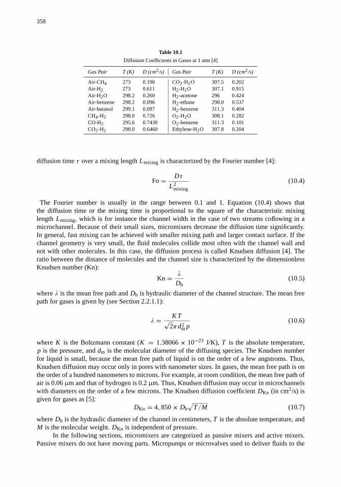
358
Table 10.1
Diffusion Coefficients in Gases at 1 atm [4]
Gas Pair T (K) D (cm2/s) Gas Pair T (K) D (cm2/s)
Air-CH4 273 0.196 CO2-H2O 307.5 0.202Air-H2 273 0.611 H2-H2O 307.1 0.915Air-H2O 298.2 0.260 H2-acetone 296 0.424Air-benzene 298.2 0.096 H2-ethane 298.0 0.537Air-butanol 299.1 0.087 H2-benzene 311.3 0.404CH4-H2 298.0 0.726 O2-H2O 308.1 0.282CO-H2 295.6 0.7430 O2-benzene 311.3 0.101CO2-H2 298.0 0.6460 Ethylene-H2O 307.8 0.204
diffusion timeτ over a mixing lengthLmixing is characterized by the Fourier number [4]:
Fo =Dτ
L2mixing
(10.4)
The Fourier number is usually in the range between 0.1 and 1. Equation (10.4) shows thatthe diffusion time or the mixing time is proportional to the square of the characteristic mixinglength Lmixing, which is for instance the channel width in the case of two streams coflowing in amicrochannel. Because of their small sizes, micromixers decrease the diffusion time significantly.In general, fast mixing can be achieved with smaller mixing path and larger contact surface. If thechannel geometry is very small, the fluid molecules collide most often with the channel wall andnot with other molecules. In this case, the diffusion process is called Knudsen diffusion [4]. Theratio between the distance of molecules and the channel size is characterized by the dimensionlessKnudsen number (Kn):
Kn =λ
Dh(10.5)
whereλ is the mean free path andDh is hydraulic diameter of the channel structure. The mean freepath for gases is given by (see Section 2.2.1.1):
λ =K T
√2πd2
m p(10.6)
whereK is the Boltzmann constant (K = 1.38066× 10⁻²³ J/K), T is the absolute temperature,p is the pressure, anddm is the molecular diameter of the diffusing species. The Knudsen numberfor liquid is small, because the mean free path of liquid is on the order of a few angstroms. Thus,Knudsen diffusion may occur only in pores with nanometer sizes. In gases, the mean free path is onthe order of a hundred nanometers to microns. For example, at room condition, the mean free path ofair is 0.06µm and that of hydrogen is 0.2µm. Thus, Knudsen diffusion may occur in microchannelswith diameters on the order of a few microns. The Knudsen diffusion coefficientDKn (in cm2/s) isgiven for gases as [5]:
DKn = 4,850× Dh√
T/M (10.7)
whereDh is the hydraulic diameter of the channel in centimeters,T is the absolute temperature, andM is the molecular weight.DKn is independent of pressure.
In the following sections, micromixers are categorized as passive mixers and active mixers.Passive mixers do not have moving parts. Micropumps or microvalves used to deliver fluids to the

Microfluidics for Life Sciences and Chemistry: Micromixers 359
Table 10.2
Diffusion Coefficients in Water at 25◦C [4]
Solute D (×10−5cm2/s) Solute D (×10−5cm2/s)
Air 2.00 Ammonia 1.64Carbon dioxide 1.92 Benzene 1.02Chlorine 1.25 Sulfuric acid 1.73Ethane 1.20 Nitric acid 2.60Ethylene 1.87 Acetylene 0.88Hydrogen 4.50 Methanol 0.84Methane 1.49 Ethanol 0.84Nitrogen 1.88 Formic acid 1.50Oxygen 2.10 Acetic acid 1.21Propane 0.97 Propionic acid 1.06Glycine 1.06 Benzoic acid 1.00Valine 0.83 Acetone 1.16Ovalbumin 0.078 Urease 0.035Hemoglobin 0.069 Fibrinogen 0.020
mixing area are not considered part of the mixer. In active mixers, moving parts are involved. Movingparts are used to manipulate or control the pressure gradients in the mixing area. Because of thenature of the mixing phenomena, the two mixer types are also called static and dynamic mixers.
Because of their simple implementation, passive mixers are a favorable solution for microflu-idic systems. The next section presents analytical models describing and discussing the basic passivemixing concepts.
10.1 DESIGN CONSIDERATIONS
Conventionally, turbulent flows and mechanical agitation make rapid mixing possible by segregatingthe fluid in small domains, which increase the contact surface and decrease the mixing path. Sincethe Reynolds numbers in microfluidic devices are on the order of 1 or less, far below the criticalReynolds number, turbulence is not achievable in microscale. All micromixers work in laminarregime and rely entirely on diffusion. General design requirements for micromixers are:
• Fast mixing time;
• Small device area;
• Integration ability in a more complex system.
Fast mixing time can be achieved by decreasing the mixing path and increasing the interfacialarea. The basic concepts for decreasing the mixing path used in passive micromixers are parallellamination, sequential lamination, sequential segmentation, segmentation based on injection, andfocusing. The diffusive/convective transport of the solute in these concepts is governed by thetransport equation:
∂c
∂t+ u
∂c
∂x+ v
∂c
∂y+ w
∂c
∂z= D
( ∂2c
∂x2+∂2c
∂y2+∂2c
∂z2
)+ q (10.8)
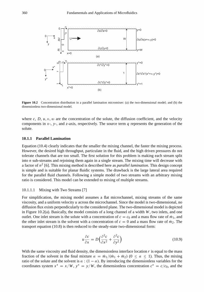
360 Fundamentals and Applications of Microfluidics
x
y
W
cc
0
0
0U
� �/ xc =0
� �c/ x(x= ,y)=0�
� �c/ y=0
x*
y*
1
c*1
0
0
� �c*/ y*=0
� �c*/ x*(x*= ,y*)=0�
� �c*/ y*=01
y=0
y=W
x*=0
x=0(a)
(b)
y*=0
y*=1
0
y
y*
0r
rWW
Figure 10.2 Concentration distribution in a parallel lamination micromixer: (a) the two-dimensional model; and (b) thedimensionless two-dimensional model.
wherec, D, u, v, w are the concentration of the solute, the diffusion coefficient, and the velocitycomponents inx-, y-, andz-axis, respectively. The source termq represents the generation of thesolute.
10.1.1 Parallel Lamination
Equation (10.4) clearly indicates that the smaller the mixing channel, the faster the mixing process.However, the desired high throughput, particulate in the fluid, and the high driven pressures do nottolerate channels that are too small. The first solution for this problem is making each stream splitinto n sub-streams and rejoining them again in a single stream. The mixing time will decrease witha factor ofn2 [6]. This mixing method is described here asparallel lamination. This design conceptis simple and is suitable for planar fluidic systems. The drawback is the large lateral area requiredfor the parallel fluid channels. Following a simple model of two streams with an arbitrary mixingratio is considered. This model can be extended to mixing of multiple streams.
10.1.1.1 Mixing with Two Streams [7]
For simplification, the mixing model assumes a flat microchannel, mixing streams of the sameviscosity, and a uniform velocityu across the microchannel. Since the model is two-dimensional, nodiffusion flux exists perpendicularly to the considered plane. The two-dimensional model is depictedin Figure 10.2(a). Basically, the model consists of a long channel of a widthW, two inlets, and oneoutlet. One inlet stream is the solute with a concentration ofc = c0 and a mass flow rate ofm1, andthe other inlet stream is the solvent with a concentration ofc = 0 and a mass flow rate ofm2. Thetransport equation (10.8) is then reduced to the steady-state two-dimensional form:
u∂c
∂x= D
( ∂2c
∂x2+∂2c
∂y2
)(10.9)
With the same viscosity and fluid density, the dimensionless interface locationr is equal to the massfraction of the solvent in the final mixtureα = m1/(m1 + m2) (0 ≤ α ≤ 1). Thus, the mixingratio of the solute and the solvent isα : (1 − α). By introducing the dimensionless variables for thecoordinates systemx∗
= x/W, y∗= y/W, the dimensionless concentrationc∗
= c/c0, and the

Microfluidics for Life Sciences and Chemistry: Micromixers 361
Peclet number Pe= uW/D, (10.9) has the dimensionless form:
Pe∂c∗
∂x∗=∂2c∗
∂x∗2+∂2c∗
∂y∗2(10.10)
The corresponding boundary conditions for the inlets are:
f (y∗) =
c∗
∣∣∣(x∗=0,0≤y∗<r )
= 1
c∗
∣∣∣(x∗=0,r ≤y∗≤1)
= 0
(10.11)
Full mixing is assumed for the mixer outlet. Thus, the boundary condition for (x∗= ∞) is:
∂c∗
∂x∗
∣∣∣(x∗=∞,0≤y∗≤1)
= 0 (10.12)
The channel wall is impermeable and the corresponding boundary condition is:
∂c∗
∂y∗
∣∣∣y∗=0,1
= 0 (10.13)
Equation (10.13) is also the symmetry condition for mixing with multiple streams, which isdiscussed later in the next section.
Separating the variables in (10.10) and applying the corresponding boundary conditions(10.11), (10.12), and (10.13), results in the dimensionless concentration distribution in the mixingchannel:
c∗(x∗, y∗) = α +2
π
∞∑n=1
sinαπn
ncos(nπy∗)exp
(−
2n2π2
Pe+
√Pe2 + 4n2π2
x∗
)(10.14)
n = 1,2,3 . . .
Equation (10.14) consists of three parts: the modulating coefficients, the cosine function, and theexponential function. The decay of concentration profile along flow direction is determined by theexponential function with the Peclet number as a variable. A small Peclet number leads to fastmixing. At a constant diffusion coefficientD and a constant flow velocityu, a small Peclet numbercan be achieved by decreasing the mixing pathW. Figure 10.3(a) depicts the typical dimensionlessconcentration distribution for two streams with a mixing ratio of 1 : 1.
10.1.1.2 Mixing with Multiple Streams
The solution of (10.14) for mixing with two streams can be extended to the case of multiple mixingstreams. The wall boundary condition is identical to the symmetry condition in the middle of eachstream. Thus, (10.14) can be extended periodically along the channel width direction. Consideringthe distance between two neighboring concentration extremaWmin,max, (10.14) also represents thecase with multiple streams. In this case, the mixing ratio can also be arbitrary, and the Peclet numberis evaluated as Pe= U Wmin,max/D. The typical concentration distribution of mixing with multiplestream is shown in Figure 10.3(b).

362 Fundamentals and Applications of Microfluidics
y*
(a)
y*
c*
0
1
0.5
0.5
0
1
x*0
1020
30
c*
0
1
0.5
0.5
0
1
x*0
1020
30
(b)
Figure 10.3 Dimensionless concentration distribution in a microchannel with parallel lamination (Pe= 100, mixing ratio1:1 orα = r = 0.5): (a) two streams; and (b) multiple streams.
Example 10.1: Designing a Y-Mixer
Mix ethanol completely with water in a parallel micromixer with two inlets (Y-mixer) at roomtemperature. The flow rates of both ethanol and water are 10µL/min. The Fourier number forthis case is assumed to be 0.5. Determine the required length of the mixing channel if the channelcross section has a dimension of 100µm × 100µm.
Solution. According to Table 10.2, the diffusion coefficient of ethanol in water at room tem-perature (25◦C) is 0.84 × 10⁻⁵ cm2/s. The characteristic mixing length is the channel widthLmixing = W = 100µm. The required mixing time is:
Fo =Dτ
L2mixing
→ τ = FoL2
mixingD = FoW2
D
τ = 0.5W2
D =(100×10−6)2
2×0.84×10−5×10−4 = 5.95 sec
The average velocity of the mixed liquid is:
u =Qwater+ Qethanol
A=
2 × 10× 10−9/60
(100× 10−6)2= 33.33× 10⁻³ m/s
Thus, the required length of the mixing channel is:
L = uτ = 33.33× 10−3× 5.95 = 0.198 m= 198 mm
Example 10.2: Designing a Long Mixing Channel
The above mixing channel is to be designed with a meander shape to save lateral device surface.If the channel structure is to be placed inside a square area, determine the dimension of this area.Determine the number of turns.
W
W

Microfluidics for Life Sciences and Chemistry: Micromixers 363
Solution. We assume that the channel walls consume the same amount of area as the channelitself. The total surface area required for the mixing channel is:
A = 2W L = 2 × 100× 198× 103= 3.96× 107 µm2
The dimension of the square area is:
a =√
A =√
39.6 × 103 µm ≈ 6,293µm
Each turn consumes 2× 100µm for walls and 2× 100µm for channel width. The total numberof turns is:
N =6,293
4 × 100≈ 16
Example 10.3: Designing a Parallel Lamination Mixer
The above mixer has to be redesigned with more lamination layers. In the new design, the channellength should be 1 mm. In how many layers should each stream be separated?
Solution. Since the average velocity remains the same as in the mixer of Example 10.2, the newmixing time is proportional to the new length:
τnew = τoldLnew
Lold= 5.95×
1
198= 3 × 10⁻² sec
Assuming that each stream is separated inton layers, the characteristic mixing length is thenW/n. The new mixing time is:
τnew = 0.5W2
n2D
Rearranging the above equation forn, we get:
n =
√0.5
W2
τnewD=
W√
2τnewD=
100× 10−6
√2 × 3 × 10−2 × 0.84× 10−9
≈ 14
By splitting each stream into 14 layers we can design a mixing channel, which is 200 timesshorter than the original Y-mixer. Even if the original channel is coiled in a meander shape, thetotal dimension is still 4.5 times larger than the new design.
10.1.2 Sequential Lamination
Sequential lamination segregates the joined stream into two channels, and rejoins them in the nextstage. Usingn such splitting stages in serial, one is able to laminate 2n layers, which causes 4(n−1)
times faster mixing [8]. Figure 10.4 illustrates this mixing concept, with three stages [Figure 10.4(a)]and two stages [Figure 10.4(b)].
The arrangement described in Figure 10.4 is referred to as sequential lamination with verticallamination and horizontal splitting. Alternatively, sequential lamination can have horizontal lami-nation and vertical splitting. This mixing concept requires relatively complicated three-dimensionalfluidic structures that can only be made in a bulk system. For the same device area consumed by achannel (parallel concept) or by a stage (sequential concept), the sequential concept results in muchfaster mixing [Figure 10.4(c)].

364 Fundamentals and Applications of Microfluidics
1. stage
2. stage
3. stage
(a) (c)
0
50
100
150
200
250
300
1 2 3 4 5
Number of stages/ channels n
Yie
ldin
mix
ing
tim
e
Parallel lamination n2
Sequential lamination 4(n-1)
1. stage
2. stage(b)
Figure 10.4 Concept of sequential lamination (vertical lamination and horizontal splitting): (a)n = 3; (b) n = 2; and(c) comparison between parallel and sequential lamination.
Example 10.4: Designing a Sequential Lamination Mixer
For the same mixing time of the design in Example 10.3, determine the number of stages requiredif we decide to make a sequential lamination mixer.
Solution. The improvement of mixing time in a parallel lamination mixer withn layers is:
τnew/τ = 1/n2
The improvement of mixing time in a sequential lamination mixer withm stages is:
τnew/τ = 1/4(m−1)
For the same improvement, we get:
1/4(m−1)= 1/n2
Rearranging the above equation, the required stage number for the sequential lamination mixer is:
m = 1 + 2 lnn/ ln 4 = 1 + 2 ln 10/ ln 4 ≈ 5
That means that if the entire mixing channel is constrained by 1 mm, each mixing stage of thenew design only occupies 200µm.
10.1.3 Sequential Segmentation
Sequential segmentation divides the solvent and solute into segments, that occupy the whole channelwidth. Mixing occurs through diffusion in flow direction. Sequential segmentation can be achieved

Microfluidics for Life Sciences and Chemistry: Micromixers 365
off
(a)
off
on
on
on
on
time
solute
solvent
off
off
t
cc
0
�T/2 T(1- /2)�
T0
�T
T/2
(b)
Figure 10.5 Sequential segmentation: (a) concept of sequential switching; and (b) time signal of the concentration at theinlet for a mixing ration ofα
.
by alternate switching of the inlet flows, using controlled valves for instance [Figure 10.5(a)]. Themixing ratio, can be adjusted by the switching ratio as depicted for the concentration at the inlet inFigure 10.5(b).
A simple one-dimensional model is assumed for sequential segmentation. Pressure-driven flowin microchannels with low aspect ratio (W � H ) can be reduced to the model of two parallel plates.The model assumes a flat velocity profile in the channel width direction (z-axis) and a Poiseuillevelocity profile in the channel height (y-axis):
u(y) = 6U(1 −
y
H
) y
H(10.15)
whereU is the mean velocity in the flow direction along thex-axis. The parabolic velocity profilecauses axial dispersion, which can be described by an effective diffusion coefficientD∗. Usingthe Taylor-Aris approach and the velocity profile (10.15), the effective diffusion coefficient can bedetermined as [9]:
D∗= D +
H2U2
210D(10.16)
where D is the molecular diffusion coefficient of the solute in the solvent, andH is the channelheight. In the case of a circular channel of radiusR, the effective diffusion coefficient is [9]:
D∗= D +
R2U2
48D(10.17)
The concentration distribution across the channel width and height is assumed to be uniform;thus, only the concentration profile along the flow directionx is considered. At a flow velocityu anda switching periodT , the characteristic segment length is defined asL = uT. The general transportequation (10.8) can be then reduced to the transient one-dimensional form:
∂c
∂t+ u
∂c
∂x= D∗
∂2c
∂x2(10.18)
Figure 10.6 depicts this one-dimensional model with the boundary condition at the inlet. Figure10.5(b) already depicts the periodic boundary condition at the inlet (x = 0):
c(t,0) =
c0 0 ≤ t ≤ αT/2
0 αT/2< t ≤ T − αT/2
c0 T − αT/2< t ≤ T
(10.19)

366 Fundamentals and Applications of Microfluidics
Figure 10.6 Transient one-dimensional model for a micromixer with sequential segmentation.
wherec0, T , andα are the initial concentration of the solute, the period of the segmentation, and themixing ratio, respectively.
Introducing the dimensionless variablesc∗= c/c0, x∗
= x/L, andt∗ = t/T , (10.18) has thedimensionless form:
∂c∗
∂t∗=
1
Pe
∂2c∗
∂x∗2−∂c∗
∂x∗(10.20)
where the Peclet number is defined as Pe= uL/D∗. The dimensionless boundary condition of(10.20) is then:
c∗(t∗,0) =
1 0 ≤ t∗ ≤ α/2
0 α < t∗ ≤ 1/2(10.21)
Solving (10.20) with (10.21) andc∗(∞) = α results in the transient behavior of the concentrationprofile along the mixing channel as:
c∗(x∗, t∗) = <
⟨α +
∞∑1
2 sin(απn)
πn
{exp
[1
2
(Pe−
√Pe2 + 8πnPei
)x∗
]× exp
(2π t∗i
)}⟩(10.22)
where i is the imaginary unit and< indicates the real component of a complex number. Theconcentration distributions along the mixing channel are depicted in Figure 10.7. Figure 10.7(a)shows clearly that only a short mixing channel is required if the Peclet number is small; that is,either a low flow velocityu, a short characteristic segment lengthL, or a short switching timeT .Sequential segmentation can achieve different final concentrations simply by adjusting the switchingratioα [Figure 10.7(b)].
10.1.4 Segmentation Based on Injection
Segmentation based on injection is another passive method for reducing the mixing path andincreasing the contact surface between the solvent and the solute. The concept divides the soluteflow into many streams, and injects them through a nozzle array into the solute flow. Figure 10.8(a)illustrates this concept with four circular injection nozzles.
For simplification, the analytical model of this mixing concept only considers a single nozzle.The model assumes a circular nozzle with a radius ofR. The solute enters the solvent flow with amass flow rate ofm2 (kilograms per second) and an inlet concentration ofc0. The solvent flow is

Microfluidics for Life Sciences and Chemistry: Micromixers 367
Figure 10.7 Concentration profile along the flow direction: (a) with different Peclet numbers (α = 0.5); (b) with differentmixing ratios (Pe = 100).
assumed to have a uniform velocity ofu. The solvent flow has a mass flow rate ofm1 and an inletconcentration ofc = 0.
Considering a steady-state, two-dimensional problem and neglecting the source term, thetransport equation (10.8) reduces to the form:
u
D
∂c
∂x=∂2c
∂x2+∂2c
∂y2(10.23)
The solution of (10.23) could be described as a product of a velocity-dependent term and asymmetric term9:
c = exp( ux
2D
)9(x, y) (10.24)
Substituting (10.24) in (10.23) results in the partial differential equation for the symmetric term9:
( u
2D
)9 =
∂29
∂x2+∂29
∂y2(10.25)
Defining the variabler =
√x2 + y2 in the polar coordinate system shown in Figure 10.8(b), the
boundary condition of the solute flow is after the Fick’s law (10.1):
dc
dr
∣∣∣r =R
= −j
D= −
m2
2πRH D(10.26)

368 Fundamentals and Applications of Microfluidics
y
R
2
, u, c=0
0.1
0.1
0.1
0.2
0.2
0.2
0.2
0.3
0.30.3
0.4
0.4
0.5
0.6
0.1
0.1
0.1
0.2
0.2
0.2
0.2
0.3
0.30.3
0.4
0.4
0.5
0.6
0.1
0.1
0.1
0.2
0.2
0.2
0.2
0.3
0.30.3
0.4
0.4
0.5
0.6
0.1
0.1
0.1
0.2
0.2
0.2
0.2
0.3
0.30.3
0.4
0.4
0.5
0.6
(b)(a)
�
,um1
.m1
.
m.
Figure 10.8 Injection mixer: (a) typical dimensionless concentration distribution of a microplume (Pe = 1); and (b) two-dimensional model.
whereH is the height of the mixing chamber above the injection nozzle. Assuming a small mixingratio (m2 � m1), the following boundary condition is acceptable for (10.25):
d9
dr∣∣∣r =±∞
= 0 (10.27)
Equation (10.25) can be rewritten for the polar coordinate system as:
d29
dr 2+
1
r
d9
dr−
( u
2D
)29 = 0 (10.28)
The solution of (10.28) is the modified Bessel function of the second kind and zero order:
9 = K0[ur/(2D)] (10.29)
The solution of (10.23) with the above-mentioned boundary conditions is:
c(r, θ) =Q2D
πRHu−1 K0[ur/(2D)]
K1[uR/(2D)] − K0[uR/(2D)] cosθ
exp[ur cosθ/(2D)]
exp[uRcosθ/(2D)](10.30)
whereθ is the angular variable of the polar coordinate system.Introducing the Peclet number Pe= 2uR/D, the dimensionless radial variabler ∗
= r/R, andthe dimensionless concentration:
c∗=
c
2m2/(πH)(10.31)
the dimensionless form of (10.30) is:
c∗(r ∗, θ) =K0(Per ∗/4)/Pe
K1(Pe/4)− K0(Pe/4) cosθ{exp[Pe(r ∗
− 1)/4]}cosθ (10.32)
whereK1 is the modified Bessel function of the second kind and first order. Figure 10.9 shows thetypical dimensionless concentration distribution around a single injection nozzle at different Pecletnumbers.

Microfluidics for Life Sciences and Chemistry: Micromixers 369
-10-5
05
-10
0
100
0.5
1
y/Rh
c*
x/Rh
(a) Pe=1
-10-5
05
-10
0
100
0.5
1
y/Rh
c*
x/Rh
(b) Pe=10
Figure 10.9 Dimensionless concentration distribution around the injection nozzle: (a) Pe = 1; (b) Pe = 10.
10.1.5 Focusing of Mixing Streams
Another solution for fast mixing is the focusing of the mixing streams to achieve a smaller streamand thinner lamination width. This concept can be realized by means of geometric focusing [Figure10.10(a)], or by hydrodynamic focusing [Figure 10.10(b)]. The velocity is inversely proportionalto the stream width, while the mixing time according to (10.4) is proportional to the square of thestream width. As a result, the mixing time or the residence time in the mixing channel is proportionalto the stream width. Decreasing the stream width causes faster mixing. The following analyticalmodel analyzes the effect of hydrodynamic focusing for reducing the width of the mixing streams[10].
The model of two-phase focusing consists of three streams: the sample stream sandwichedbetween two identical sheath streams (Figure 10.11). The sample stream and the sheath stream areassumed to be immiscible. In many cases of microfluidics, the flow channel has a rectangular crosssection. Figure 10.11(a) shows the actual geometry of the channel cross section with the two phases.The width and height of the channel are 2W and H , respectively. The position of the interfaceis rW. Since the model is symmetrical regardingy-axis andz-axis, only one-fourth of the crosssection needs to be considered.
(b)Sheath flow
(a)
Sheath flow
Sample flow
Focused sample flow
Figure 10.10 Focusing concepts: (a) geometric focusing; and (b) hydrodynamic focusing.

370 Fundamentals and Applications of Microfluidics
y*
z*
1-1
h/2
- r r
-h/2
y
z
W-W
H/2
rW-rW
0
-H/2(a)
(b)
2 1 2
2 1 2
Figure 10.11 Analytical model for two phases focusing: (a) actual geometry; and (b) the dimensionless model.
The velocity distributionu1 and u2 in the channel can be described by the Navier-Stokesequations:
∂2u1
∂y2+∂2u1
∂z2=
1
η1
∂p
∂x
∂2u2
∂y2+∂2u2
∂z2=
1
η2
∂p
∂x
(10.33)
where indices 1 and 2 describe the sample flow and the sheath flow, respectively. In (10.23)η1 andη2are the viscosities of the sample fluid and of the sheath fluid. Nondimensionalizing the velocity by areference velocityu0, and the coordinates byW leads to the dimensionless model [Figure 10.11(b)]:
∂2u∗
1
∂y∗2+∂2u∗
1
∂z∗2= P′
∂2u∗
2
∂y∗2+∂2u∗
2
∂z∗2= P′
(10.34)
With P′=
W
η1u0
∂p
∂x∗, β = η2/η1, andθ = (2n − 1)π/h, the solutions of (10.34) have the forms
(0< y∗ < 1, 0< z∗ < h/2):
u∗
1(y∗, z∗) = P′
[z∗2
− h2/4
2+
∞∑n=1
cosθz∗(A1 coshθy∗+ B1 sinhθy∗)
]
u∗
2(y∗, z∗) =
P′
β
[z∗2
− h2/4
2+
∞∑n=1
cosθz∗(A2 coshθy∗+ B2 sinhθy∗)
] (10.35)
The nonslip conditions at the wall are
u∗
2(1, z∗) = 0. (10.36)

Microfluidics for Life Sciences and Chemistry: Micromixers 371
Figure 10.12 The dimensionless velocity profile (h = 0.14,κ = 1): (a)β = 0.5; (b)β = 1; and (c)β = 2.
The symmetry condition at thez∗-axis is:
∂u∗
1
∂y∗
∣∣∣y∗=0
= 0 (10.37)
At the interface between the sample flow and the sheath flow, the velocity and the shear rate arecontinuous:
u∗
2(r, z∗) = u∗
1(r, z∗)
∂u∗
1
∂y∗
∣∣∣y∗=r
= β∂u∗
2
∂y∗
∣∣∣y∗=r
(10.38)
For a flat channel (h � 1), the position of the interface can be estimated as:
r =1
1 + 2βκ(10.39)
whereκ = m2/m1 is the flow rate ratio between the sheath streams and the mixing streams.

372 Fundamentals and Applications of Microfluidics
carrier
solute
solvent
mixed droplet
(a) mixing
solute
solvent
carrier
solute droplet
solvent droplet
(b) separated droplets
solute
solvent
carrier
solute droplet
solvent droplet
(c) separated small droplets
solute
solvent
carrier
(d) laminar flow
Figure 10.13 Formation of droplets: (a) merging and mixing of solvent and solute; (b) formation of separated droplets;(c) formation of small separated droplets; and (d) laminar flow. (After: [11])
A Fourier analysis with the above boundary conditions results in the coefficients of (10.35):
A1 = D[β sinhθr cosh2 θr coshθ − sinh3 θr coshθ − (β − 1) sinh2 θr sinhθ coshθ−
(β − 1) sinh2 θr (coshθ − coshθr )+ (β − 1) sinhθr coshθr coshθ(coshθ − coshθr )]/[
β cosh2 θr sinhθr cosh2 θ − sinh3 θr cosh2 θ − (β − 1) sinh2 θr coshθr sinhθ coshθ]
A2 = D[β cosh2 θr coshθ − sinh2 θr coshθ − (β − 1) sinhθr coshθr sinhθ−
(β − 1) sinhθr (coshθ − coshθr )]/[β cosh2 θr sinh2 θ − sinh2 θr cosh2 θ−
(β − 1) sinhθr coshθr sinhθ coshθ]
B1 = 0B2 = D
[(β − 1) sinhθr (coshθ − coshθr )
]/[β cosh2 θr coshθ − sinh2 θr coshθ−
(β − 1) sinhθr coshθr sinhθ]
(10.40)
whereD = (−1)n+1 4h2
(2n − 1)3π3. Figure 10.12 shows the typical velocity distribution inside the
flow channel for the same flow rate in all streams (κ = 1). The velocity of the sample flow is lower,if the sample flow is more viscous than the sheath flow (β < 1) [Figure 10.12(a)]. If the viscositiesare equal (β = 1), the flows behave as a single phase [Figure 10.12(b)]. If the sheath flows are moreviscous (β > 1), the sample flow is faster [Figure 10.12(c)].
10.1.6 Formation of Droplets and Chaotic Advection
Smaller mixing path and possible chaotic advection can be achieved by forming droplets of solventand solute. The basic configuration is similar to that of hydrodynamic focusing shown in Figure10.10(b). For the formation of droplets, the middle inlet is used for the carrier fluid, which isimmiscible to both solvent and solute. The flows of solvent and solute enter from the two sides.The formation behavior of droplets depend on the capillary number Ca= uν/σ and the samplefractionr = (Qsolvent+ Qsolute)/(Qsolvent+ Qsolute+ Qcarrier), whereu is the average velocity,ν isthe viscosity, andQsolvent, Qsolute, andQcarrier are the flow rates of solvent, solute, and carrier fluid.Section 11.1.2.1 will discuss more about droplet formation in a multiphase system.

Microfluidics for Life Sciences and Chemistry: Micromixers 373
1
0
0.5
0 0.20.1
sam
ple
fraction
r
capillary number Ca
laminar flow
mix
ing
separa
ted
dro
ple
tsseparated small droplets
Figure 10.14 Typical phase diagram of droplet formation in a multiphase system. (After: [11].)
At a low capillary number, the solvent and solute can merge into a sample droplet andmix rapidly due to chaotic advection inside the droplet [Figure 10.13(a)]. Increasing the capillarynumber at the same fractionr , the droplets form separately and are not able to merge and mix[Figure 10.13(b)]. Increasing further the capillary number, the alternate droplets become smallerand unstable [Figure 10.13(c)]. At a high capillary number, the three streams flow side-by-side asin the case of missile fluids [Figure 10.13(d)]. Figure 10.14 depicts the typical phase diagram ofdroplet formation based on the results reported by Zheng et al. [11].
The droplet train formed in the configuration described above can be stored over a long time,because the carrier fluid, such as an oil, can protect the aqueous sample from evaporation. The long-term stability of the sample allows protein crystallization in the microscale [12].
The flow patterns measured withµPIV inside a droplet moving in a rectangular microchannelare depicted in Figures 10.15(a,b). If both solute and solvent merge and mix, these flow patternsinside the mixed droplet could make chaotic advection possible. However, if the microchannel isstraight, as depicted in Figure 10.15(c), the flow pattern inside the droplet is steady. The two vorticescontaining the solvent and solute exist in each half of the droplet and mixing is not improvedsignificantly. If the microchannel has turns as depicted in Figure 10.15(d), the flow pattern isperiodical. Each side of the droplet takes a turn to have a faster vortex. Thus, chaotic advectionand consequently faster mixing are possible in this case [13]. Furthermore, the larger vortex maydominate the smaller vortex at each turn, which resembles the concept of reorientation, stretching,and folding in serial lamination discussed previously. Since the number of cycles depends on thenumber of turnsn, the improvement of mixing time compared to the case of a straight channel is4(n−1). Compared to diffusive mixing with parallel lamination, the improvement of mixing time canbe described as [13]:
tchaotic
tdiffusive=
Pe
L∗ log(Pe)(10.41)
where Pe= uW/D is the Peclet number, andL∗= L/W is the dimensionless droplet length
normalized by the channel widthW.

374 Fundamentals and Applications of Microfluidics
(c) (d)
y(
�m
)
-220
-200
-180
-160
-140
-120
-100
-80
-60
-40
-20
0
x ( � m)
0 20 40 60 80 100 120 140 160 180 200 220 240 260 280 30050 100 150 200 250 300
-220
-200
-180
-160
-140
-120
-100
-80
-60
-40
x ( m)�
y(
m)
�
Carrier flow directionCarrier flow direction
(a) (b)
Figure 10.15 Flow pattern in a microdroplet: (a) measured flow pattern during formation process; (b) measured flow patternduring passage in a straight rectangular channel; (c) schematic flow patterns inside a droplet in a straight channel; and (d) ina channel with turns.
10.2 DESIGN EXAMPLES
As mentioned in the introduction of this chapter, micromixers can be categorized as passive mi-cromixers and active micromixers. Passive micromixers do not require external disturbance to im-prove mixing. The passive mixing process relies entirely on diffusion and chaotic advection. Basedon the arrangement of the mixed phases, passive mixing concepts can be further categorized as paral-lel lamination, serial lamination, injection, chaotic advection, and droplet mixing. Active micromix-ers use external disturbance for accelerating the mixing process. Based on the types of disturbance,active mixing can be categorized in pressure-driven, temperature-induced, electrohydrodynamic,dielectrophoretic, electrokinetic, magnetohydrodynamic, and acoustic concepts. Because of the in-tegrated components and external power supply for the generation of disturbance fields, the design ofactive micromixers is often complicated and requires a complex fabrication process. The integrationof active mixers in a microfluidic system is therefore both challenging and expensive. The majoradvantage of passive micromixers is the lack of actuators. The simple passive structures are robust,stable in operation, and easy to be integrated. Figure 10.16 illustrates the systematic overview ofdifferent micromixer types.
10.2.1 Passive Micromixers
The theoretical background of passive mixing was already discussed in Section 10.1. The theoriesare based on the diffusive/convective transport equation, and show that mixing in passive micromix-ers relies mainly on molecular diffusion and advection. Increasing the contact surface between thedifferent fluids and decreasing the diffusion path between them could improve molecular diffusion.Chaotic advection can be induced by manipulating the laminar flow in microchannels. The resultingflow pattern shortens the diffusion path and thus improves mixing. The following sections discussthe different designs of passive micromixers as categorized in Figure 10.16.

Microfluidics for Life Sciences and Chemistry: Micromixers 375
Micromixers
Passive
micromixers
Active
micromixers
Injection
LaminationChaotic
advection
Droplets
Parallel
lamination
Serial
lamination
Dielectro-
phoreticElectrokinetic
Magneto
hydrodynamic
Electro-
hydrodynamic
Pressure
driven
Acoustic
Thermal
Figure 10.16 Overview of different micromixer types.
10.2.1.1 Parallel Lamination Micromixers
As discussed in Section 10.1.1, fast mixing can be achieved by decreasing the mixing path andincreasing the contact surface between the solvent and the solute. The basic design of a parallellamination micromixer is a long microchannel with two inlets. According to their shapes, thesedesigns are often called the T-mixer or the Y-mixer [14–16] [Figures 10.17(a,b)]. The inlet streamsof a T-mixer can be twisted and laminated as two thin liquid sheets to reduce the mixing path [17]. Asa basic design, a T-mixer is suitable for investigations of basic transport phenomena in microscale,such as scaling law, Taylor’s dispersion [14, 16], and other nonlinear effects [18].
According to the analytical model (10.14), a long mixing channel is needed for a high Pecletnumber, if the channel width and the diffusion coefficient are fixed. A shorter mixing channel canachieve full mixing at extremely high Reynolds numbers [19, 20]. At these high Reynolds numbers,chaotic advection and even turbulent flows can be expected. Wong et al. [20] reported a T-mixerfabricated in glass and silicon. This mixer utilizes Reynolds numbers up to 500, where flow velocitycan be as high as 7.6 m/s at a driven pressure up to 7 bars. High shear rate at fluid interfaces underextremely high Reynolds numbers can generate fast vortices, which in turn can be used for mixing.Lim et al. reported fast vortices and fast mixing of fluorescent dyes inside a diamond-shaped cavityclose to a straight microchannel [21]. At a flow velocity of 45 m/s, the Reynolds number reaches avalue of Re= 245. Bohm et al. [22] reported a micromixer with multiple inlet streams focused in acircular chamber to generate fast vortices. In the above-mentioned micromixers, the high velocitieson the order of 1 m/s, 10 m/s [22], or even higher (e.g., 45 m/s [21]), cause problems in designing thefluidic interconnects. Such high flow rates require pressures on the order of bars. The high pressures(1.0 to 5.5 bars in [20], 15 bars in [22]) are serious challenges for bonding and interconnectiontechnologies.
Instead of a straight design, mixing channels with turns and geometrical obstacles could causeinstability in the flow at moderate Reynolds numbers. A Y-mixer made of cofired ceramic tapes

376 Fundamentals and Applications of Microfluidics
(b)
(c) (d)
Sheath flow
Sheath flow
(a)
solute
solvent
solute
solv
ent
solute
solvent
solute
solvent
Figure 10.17 Parallel lamination micromixer: (a) T-mixer; (b) Y-mixer; (c) parallel lamination with multiple streams; and(d) hydraulic focusing.
with a 90◦ bend in the mixing channel can generate vortices at Reynolds numbers above 10 [19]. AtReynolds numbers higher than 30, mixing is achieved right after the bend. Geometrical obstacles inthe basic T-design can be implemented by roughening the channel wall [23] or throttling the channelentrance [24]. Other types of obstacles for generating vortices and chaotic advection are discussedin Section 10.2.1.4.
According to Section 10.1.1, a simple method to reduce the mixing path is narrowing mixingstreams. Narrow mixing streams are realized with the use of microchannels [25]. Furthermore,smaller streams can be achieved by splitting the solvent and the solute in multiple streams andrejoining them [26–28] [Figure 10.17(c)] or by interdigitating them three-dimensionally [29].Bessoth et al. reported a parallel lamination mixer with 32 streams that can achieve full mixingafter a few milliseconds [30, 31]. The flow in micromixers based on parallel lamination are usuallydriven by pressure. However, electro-osmosis can also be used as an alternative for fluid delivery[32-34].
As analyzed in Section 10.1.5, another concept of reducing the mixing path for parallellamination micromixers is hydrodynamic focusing [35]. The basic configuration for hydrodynamicfocusing is a long microchannel with three inlets. The middle inlet is used for the focused sampleflow, while the the sheath flows join though the other two inlets [Figure 10.17(d)]. Knight et al.[35] reported a prototype with a mixing channel of 10× 10 µm cross section. The width of thesample stream was focused by adjusting the pressure ratio between the sample flow and the sheathflow. In the reported experiments, the mixing time can be reduced to a few microseconds [36]. Thesame configuration of hydrodynamic focusing and mixing were used for cell infection [37]. Wu andNguyen reported a configuration with two sample streams. The sample streams are focused by twosheath streams. The narrow width improves mixing between the two streams significantly [10]. Table10.3 summarizes the typical parameters of the above-mentioned parallel lamination micromixers.
10.2.1.2 Serial Lamination Micromixers
Similar to parallel lamination micromixers, serial lamination micromixers also enhance mixingthrough splitting and later joining the streams [Figure 10.18(a)] [8, 38–40]. The inlet streams arefirst joined horizontally and then in the next stage vertically. Aftern splitting and joining stages, 2n

Microfluidics for Life Sciences and Chemistry: Micromixers 377
Table 10.3
Typical Parameters of Parallel Lamination Micromixers (n/a: not applicable)
Ref. Type ChannelWidth(µm)
ChannelHeight(µm)
TypicalVelocity(mm/s)
Re Pe Materials
[14, 15] T-mixer 550 25 6 0.3 725 Silicon-glass[16] Y-mixer 90 90 7 0.4 240 PDMS-glass[17] Y-mixer 1,000 20 83 1.7 830 CaF2-SU8-metal-glass[18] Y-mixer 900 50 0.27 0.02 150 PMMA[19] Y-mixer 200 200 50–200 80 80,000 Ceramic[20] T-mixer 100 50 7,000 500 700,000 Silicon-glass[22] Vortex 20 200 10,000 200 200,000 Silicon-glass[23] Cross-
shaped30 40 5,000-10,000 170–
340150,000 Ceramic
[24] T-mixer 500 300 0.3 0.1 150 n/a[25] T-mixer 100 200 0.17 0.023 170 Silicon-glass[28] Parallel
lamination85 5 0.7 0.0035 60 Silicon-glass
[30] Parallellamination
20 50 1.5 0.07 60 Glass
[33] T-mixer 35 9 1 0.014 35 Glass[35] Focusing 10 10 50 0.5 500 Silicon-PDMS-glass[37] Focusing 200–1,000 150 1 0.15 200 PDMS-glass[10] Focusing 900 50 1 0.05 100 PMMA
liquid layers can be laminated. The process leads to 4n−1 times improvement in mixing time. Dueto their complex geometry, most of the reported serial lamination mixers [Figure 10.18(b)] werefabricated in silicon, using bulk micromachining technologies such as wet etching in KOH [8, 38] orDRIE technique [39]. Polymeric micromachining is another alternative for making serial laminationmicromixers. Lamination of multiple polymer layers also allows making complex three-dimensionalchannel structures [40] [Figure 10.18(c)].
The concept of serial lamination can be extended to electrokinetic flows as reported by Heet al. [41] [Figure 10.18(d)]. Serial lamination was realized through electro-osmosis flows betweenthe multiple intersecting microchannels. A similar design for a pressure-driven flow was reported byMelin et al. [42]. However, this design only works for a plug of the two mixed liquids. Table 10.4lists the most important parameters of serial lamination micromixers.
10.2.1.3 Injection Micromixers
As explained in Section 10.1.4, the concept of injection mixer [43–47] is based on the generalconcept of decreasing mixing path and increasing contact surface between the solute and the solvent.Instead of splitting both inlet flows, these injection micromixers only split the solute flow into manystreams and inject them through a nozzle array into the solvent flow. The nozzle array creates anumber of microplumes of the solute [Figure 10.8(a)]. These plumes increase the contact surfaceand decrease the mixing path. Mixing efficiency can be improved significantly.
The micromixers reported by Miyake et al. [43, 44] have 400 nozzles arranged in a squarearray. The nozzle array is located in a mixing chamber, which is fabricated in silicon using DRIE.Larsen et al. [45] reported a similar concept with a different nozzle shape and array arrangement.Seidel et al. [46] and Voldman et al. [47] utilized capillary forces for generating microplumes. These
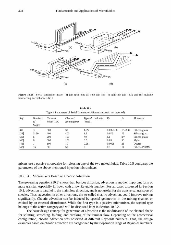
378 Fundamentals and Applications of Microfluidics
(b)
(c)
(a)
(d)
solute
solvent
solute
solvent
solute
solvent
solute
solvent
Figure 10.18 Serial lamination mixer: (a) join-split-join; (b) split-join [8]; (c) split-split-join [40]; and (d) multipleintersecting microchannels [41].
Table 10.4
Typical Parameters of Serial Lamination Micromixers (n/r: not reported)
Ref. NumberofStages
ChannelWidth (µm)
ChannelHeight (µm)
Typical Velocity(mm/s)
Re Pe Materials
[8] 3 300 30 1–22 0.03-0.66 15–330 Silicon-glass[38] 5–20 400 400 1.8 0.072 72 Silicon-glass[39] 6 200 100 n/r n/r n/r Silicon-glass[40] 6 600 100 0.5 0.05 50 Mylar[41] 1 100 10 0.25 0.0025 25 Quartz[42] 16 50 50 2 0.1 14 Silicon-PDMS
mixers use a passive microvalve for releasing one of the two mixed fluids. Table 10.5 compares theparameters of the above-mentioned injection micromixers.
10.2.1.4 Micromixers Based on Chaotic Advection
The governing equation (10.8) shows that, besides diffusion, advection is another important form ofmass transfer, especially in flows with a low Reynolds number. For all cases discussed in Section10.1, advection is parallel to the main flow direction, and is not useful for the transversal transport ofspecies. Thus, advection in other directions, the so-called chaotic advection, could improve mixingsignificantly. Chaotic advection can be induced by special geometries in the mixing channel orexcited by an external disturbance. While the first type is a passive micromixer, the second typebelongs to the active category and will be discussed later in Section 10.2.2.
The basic design concept for generation of advection is the modification of the channel shapefor splitting, stretching, folding, and breaking of the laminar flow. Depending on the geometricalconfiguration, chaotic advection was observed at different Reynolds numbers. Thus, the designexamples based on chaotic advection are categorized by their operation range of Reynolds numbers.

Microfluidics for Life Sciences and Chemistry: Micromixers 379
Table 10.5
Typical Parameters of Injection Micromixers (n/r: not reported)
Ref. Number ofNozzles
ChannelWidth (µm)
NozzleSize (µm)
ChannelHeight (µm)
Typical Velocity(mm/s)
Re Pe Materials
[43, 44] 400 2,000 330 15×15 1.2 0.018 18 Silicon-glass[45] 10–20 n/r 100 50 1 0.1 100 Silicon-glass[46] 1 280–600 135–175 20–43 n/r n/r n/r Silicon-glass[47] 1 820 7 70 15 0.1 105 Silicon-glass
(a) (b) (c)
solute
solvent
solute
solvent
solute
solvent
Figure 10.19 Planar designs for mixing with chaotic advection at high Reynolds numbers: (a) obstacles on walls [23];(b) obstacles in the channel [48, 50]; and (c) zigzagging channel [51].
Although there is no fixed range for a particular design, a range of Re> 100 is considered in thissection as high, while the ranges of 10< Re< 100 and of Re< 10 are regarded as intermediateand low, respectively.
Chaotic Advection at High Reynolds Numbers.The simplest way to induce chaotic advection is toinsert obstacles in the mixing channel. The obstacles can be placed on the wall [Figure 10.19(a)].Wang et al. numerically investigated the role of obstacles in a mixing channel at high Reynoldsnumbers [49]. The simulated mixing channel is 300µm in width, 100µm in depth, and 1.2 to2 mm in length; the diameter of the obstacle is 60µm [Figure 10.19(b)]. The simulation resultsshow that obstacles in a microchannel at low Reynolds numbers cannot generate instabilities orrecirculations. However, the obstacles can improve mixing at high Reynolds numbers. Under high-Reynolds-number conditions, the asymmetric arrangement of obstacles alters the flow directionsand creates transversal mass transport. Lin et al. [50] used cylinders placed in a narrow channelto enhance mixing [Figure 10.19(b)]. The 50× 100× 100µm mixing chamber was fabricated insilicon. Seven cylinders of 10-µm diameter were arranged in the mixing chamber. The micromixerworked with Reynolds numbers ranging from 200 to 2,000 and achieved a mixing time of 50µs.
Another method to generate chaotic advection at high Reynolds numbers is generatingrecirculation around the turns of a zigzagging mixing channel [Figure 10.19(c)]. Based on anumerical investigation, Mengeaud et al. [51] used the zigzagging period as the optimizationparameter. The micromixers were fabricated using excimer laser on polyethylene terephthalate(PET) substrate. The microchannel has a width of 100µm, a depth of 48µm, and a length of2 mm. A critical Reynolds number of 80 was observed. Below this number, the mixing processrelied entirely on molecular diffusion. Above this number, fast mixing through recirculations at theturns was observed.

380 Fundamentals and Applications of Microfluidics
(a) (b) (c)
(d) (e)
solutesolute
solventsolvent
solute
solvent
solute
solvent
solute
solvent
Figure 10.20 Micromixer designs for mixing with chaotic advection at intermediate Reynolds numbers: (a) modified Tesla-structure; (b) C-shape [53]; (c) L-shape [54]; (d) connected out-of-plane L-shapes [55]; and (e) twisted microchannel [56].
Chaotic Advection at Intermediate Reynolds Numbers.At intermediate Reynolds numbers, chaoticadvection can be induced by special channel designs. Hong et al. [52] demonstrated an in-planemicromixer with modified Tesla structures [Figure 10.20(a)]. One branch of the Tesla structure hasthe form of a nozzle. The flows in the two branches cause the Coanda effect, which leads to chaoticadvection and improves mixing significantly. The mixer was made of cyclic olefin copolymer (COC)by hot embossing and thermal direct bonding. The mixer works well at higher Reynolds numbers(Re> 5).
Three-dimensionally twisted channels also induce chaotic advection. Liu et al. [53] reporteda three-dimensional serpentine mixing channel fabricated in silicon and glass. The channel wasconstructed as a series of C-shaped segments positioned in perpendicular planes [Figure 10.20(b)].The micromixer consists of two inlets joined in a T-junction, a 7.5-mm-long straight channel, and asequence of six mixing segments. The total mixing length was about 20 mm. Fast mixing caused bychaotic advection was observed at relatively high Reynolds numbers from 25 to 70.
A similar micromixer with a three-dimensional serpentine mixing channel fabricated in PDMSwas reported by Vijayendran et al. [54] . The channel was designed as a series of L-shaped segmentsin perpendicular planes [Figure 10.20(c)]. The channel has a width of 1 mm and a depth of 300µm.The total length of the mixing channel is about 30 mm. The mixer was tested at the Reynoldsnumbers of 1, 5, and 20. The reported experimental results also indicated that better mixing wasachieved at higher Reynolds numbers. Another complex design on PDMS was reported by Chen andMeiners [55]. The mixing unit, called by the authors “flow-folding topological structure,” is formedby two connected out-of-plane L-shapes and measures about 400×300µm [Figure 10.20(d)]. Themicrochannel has a width of 100µm and a depth of 70µm. With this design, effective mixing canbe achieved with a purely laminar flow at Reynolds numbers ranging from 0.1 to 2.
Park et al. reported a more complex three-dimensional micromixer [56]. The channel rotatesand separates the two fluids by partitioned walls [Figure 10.20(e)]. The channel structure was fabri-cated in PDMS and then bonded to glass. Jen et al. proposed other designs of twisted microchannelsfor mixing of gases [57]. These designs were only tested numerically. The channel has a width

Microfluidics for Life Sciences and Chemistry: Micromixers 381
(a) (b) (c)
(d) (e) (f)
solute
solvent
solute
solvent
solute
solvent
solute
solvent
solute
solvent
solute
solvent
Figure 10.21 Modification of mixing channel for chaotic advection at low Reynolds numbers: (a) slanted ribs; (b) slantedgrooves [61, 62]; (c) staggered-herringbone grooves [61, 62]; and (d–f) Patterns for surface modification in a micromixerwith electrokinetic flows [64].
and height of 500 and 300µm, respectively. Mixing of methanol and oxygen at different velocitiesranging from 0.5 to 2.5 m/s was considered in the simulation.
Chaotic advection in a mixing chamber was generated actively by a planar pulsed source-sinksystem [58] as reported by Evans et al. [59]. The mixer was fabricated in silicon on a 1-cm2 area.The mixing chamber measures 1,500× 600µm with a height of 100µm.
Chaotic Advection at Low Reynolds Numbers.Similar to their macroscale counterparts, rips [Figure10.21(a)] or grooves [Figures 10.21(b,c)] on the channel wall can twist the flow and generate chaoticadvection. Jonson et al. [60] ablated slanted grooves on the bottom wall of the mixing channel usinglaser machining. This structure twists an electrokinetic flow into helical stream lines and allowsmixing at a relatively low velocity of 300µm/s. The micromixers were fabricated by excimer laserablation on a polycarbonate sheet (PC). The substrate is bonded to a cover made of polyethyleneterephthalate glycol (PETG). The mixing channel was 72µm wide at the top, 28µm wide at thebottom, and 31µm in depth. The width of an ablated groove was 14µm, the center-to-center spacingbetween the grooves was 35µm. The length of the region occupied by the wells from the T-junctionwas 178µm.
The same configuration was investigated later by Strook et al. [61]. Two different groovepatterns were considered [Figure 10.21(b,c)]. The so-called staggered herringbone mixer [Figure10.21(c)] can work well at Reynolds numbers ranging from 1 to 100. This concept can be appliedto electrokinetic flow by modifying the surface charge [62]. The effect of chaotic advection with theripped channel was numerically investigated by Wang et al. [48]. The length, width, and depth ofthe channels were 5 mm, 200µm, and 100µm, respectively. The mean velocity ranges from 100µm/s to 50 mm/s. The grooves were also ablated on the PDMS substrate by laser [63]. Electrokineticmixing [64] with only patterned surface modification [65] can also enhance mixing [Figure 10.21(d–f)]. Compared to the conventional T-configuration, Biddiss et al. reported an improvement ofmixing efficiencies from 22 to 68% at Peclet numbers ranging from 190 to 1500.
Kim et al. [66] improved the design of Stroock et al. [61] with embedded barriers parallelto the flow direction. This embedded barrier forces the flow to change the original elliptic mixingpattern [61] to a hyperbolic pattern [66]. The mixing channel of this design is 240µm in width,60µm in depth, and 21 mm in length. The barriers have a cross section of 40µm × 30µm.

382 Fundamentals and Applications of Microfluidics
Table 10.6
Typical Parameters of Chaotic Advection Micromixers (n/r: not reported; n/a: not applicable)
Ref. Type ChannelWidth(µm)
ChannelHeight(µm)
TypicalVelocity(mm/s)
Re Pe Materials
[49] Cyl. obstacles 300 100 0.17 0.25 51 n/a[50] Cyl. obstacles 10 100 20 0.2 200 Silicon-glass[51] Zigzag shaped 100 48 1.3–40 0.26-267 130–4,000 Mylar[52] 2D Tesla 200 90 5 6.2 104 COC[53] 3D serpentine 300 150 30–350 6–70 9,000–104 Silicon-glass[54] 3D serpentine 1,000 300 2–40 1–20 2,000–4×10⁴ PDMS[55] 3D serpentine 100 70 1–20 0.1–2 10-200 PDMS[56] 3D serpentine 100 50 n/r 1–50 0.015–0.7 PDMS[57] 3D serpentine 500 300 2,000 48 0.36 n/a[59] Source-sink 1,500×600 100 n/r n/r n/r Silicon-glass[60] Patterned wall 72 31 0.6 0.024 15 PC-PETG[61, 62] Patterned wall 200 70 15 0.01 3,000 PDMS[48] Patterned wall 200 100 0.1–50 0.0013–6.65 20–104 PDMS[64] Patterned wall 200 8 0.01–0.09 0.08-0.7 190–1,500 PDMS[66] Patterned wall 240 60 11.6 0.5 2,784 PDMS
Bertsch et al. reported a miniaturized version of a conventional mixer with helical flow-twisting elements [67]. The design concept is to modify the three-dimensional inner wall of acylindrical mixing channel. Two designs were tested for this concept. The first design was formedby four mixing elements, which was made of 24 rectangular bars placed at 45◦. The four mixingelements were arranged at 45◦ in the channel. The second design consists of right-handed and left-handed helical elements containing six small-helix structures. Because of the complex geometry,the micromixer was fabricated by stereo microphotography (Section 3.4.4), which builds up thecomplex structure layer by layer. Table 10.6 summarizes the most important parameters of the abovemicromixers based on chaotic advection.
10.2.1.5 Droplet Micromixers
A tiny droplet containing both solvent and solute will reduce the total amount of samples signifi-cantly. The small size of the droplet also fulfills the requirement for a short mixing path. If the dropletis set in motion, the flow field inside the droplet further improves the mixing effect. The internalflow field depends on the droplet motion; thus the mixing pattern can be controlled externally by themotion pattern of the droplet.
In general, droplets can be generated and transported individually using pressure [68] orcapillary effects such as thermocapillary [69] and electrowetting [70]. Furthermore, droplets areformed in microchannels with immiscible phases, such as oil/water or water/gas, due to the largedifference of surface forces [71]. Hosokawa et al. [68] reported the earliest droplet micromixer,which was fabricated in PDMS and covered by a PMMA sheet. The concept utilized a hydrophobicmicrocapillary vent, which join the solute with the solvent droplet. By simplifying the mass transportequation and introducing an effective dispersion coefficient for a rectangular channel, Handique andBurns reported an analytical model for droplet mixing actuated by thermocapillary [69]. The mixingdroplet can also be generated and transported by electrowetting (Section 7.2.2). Paik et al. [70]reported different mixing schemes with the electrowetting concept. Droplets can be merged and

Microfluidics for Life Sciences and Chemistry: Micromixers 383
split repeatedly to generate the mixing pattern. The merged droplet can then be transported withdifferent motion patterns to induce mixing.
Flow instability between two immiscible liquids can form droplets, which can be used formixing [71], [72]. Using a carrier liquid such as oil, droplets of the aqueous samples are formed in amicrochannel. While moving along the microchannel, the shear force between the carrier liquid andthe sample induces an internal flow field and accelerates the mixing process in the droplet. Table10.7 lists the typical parameters of the above droplet micromixers.
10.2.2 Active Micromixers
10.2.2.1 Pressure-Driven Disturbance
Disturbance caused by pressure was used in one of the earliest active micromixers. Deshmukhet al. [73] reported a T-mixer with pressure disturbance [Figure 10.22(a)]. The mixing concept usedin this mixer was categorized previously in Section 10.1.3 as a passive concept with sequentialsegmentation. However, considering the integrated pumps, the segmentation can be referred to asa pressure-driven disturbance. The mixer is integrated in a microfluidic system, which is fabricatedin silicon using DRIE. An integrated planar micropump drives and stops the flow in the mixingchannel causing sequential segmentation, as discussed in Section 10.1.3 [Figure 10.22(a)] [74]. Thissegmentation concept can also be realized by an external micropump [75].
An alternative method to pressure disturbance is the generation of pulsing velocity [76, 77][Figure 10.22(b)]. Glasgow et al. [76] demonstrated a simple T-mixer and its simulation with apulsed side flow at a small Reynolds number of 0.3. Niu and Lee [77] generated pressure disturbanceusing a computer controlled source-sink system. This concept is partly similar to that of Evans et al.[59]. The performance of the mixing process is determined by the pulse frequency and the numberof mixing units. Okkels et al. [78] reported a numerical analysis of the mixing pattern in a chamberdisturbed by transient pressure field.
Disturbance can be caused directly by moving parts in the mixing channel. Suzuki and Ho[79] reported a micromixer with integrated conductors. The concept is similar to a commercialmacroscale magnetic stirrer. The electrical conductors generate a magnetic field, which in turnmoves magnetic beads of 1 to 10µm in diameter. The chaotic movement induced by the magneticbeads improves mixing significantly. An integrated magnetic microstirrer was reported by Lu et al.[80] [Figure 10.22(c)]. The micromachined stirrer is placed at the interface between two liquids in aT-mixer. An external magnetic field drives the stirrer at speeds ranging between 100 and 600 rpm.
10.2.2.2 Electrohydrodynamic Disturbance
Electrohydrodynamic effect (Section 7.1.2) can be used to disturb the laminar streams. The structureof the micromixer with eletrohydrodynamic disturbance reported by El Moctar et al. [81] is similar tothe concept reported by Niu et al. [77] for pressure-driven disturbance. Instead of pressure sources,electrodes are placed along the mixing channel [Figure 10.22(d)]. The mixing channel is 30 mm
Table 10.7
Typical Parameters of Droplet Micromixers (n/r: not reported)
Ref. Transport Type Droplet Size (nL) Channel Width (µm) Channel Height (µm) Materials
[68] Pressure driven 10 100 150 PDMS/PMMA[70] Electrowetting 1,600 2,480 600–1000 Glass[71] Multiple phases 75–150 20–100 n/r PDMS

384 Fundamentals and Applications of Microfluidics
Figure 10.22 Active micromixers: (a) serial segmentation; (b) pressure disturbance along mixing channel; (c) integratedmicrostirrer in the mixing channel; (d) electrohydrodynamic disturbance; (e) dielectrophoretic disturbance; (f) electrokineticdisturbance in a mixing chamber; (g) electrokinetic disturbance in a mixing channel; and (h) disturbance caused bythermocapillary convection induced by a tranverse temperature gradient.
long, 250µm wide and 250µm deep. A number of titanium electrodes are placed in the directionperpendicular to the mixing channel. By changing the voltage and frequency on the electrodes, goodmixing was achieved after less than 0.1 second at a Reynolds number as low as 0.02.
10.2.2.3 Dielectrophoretic Disturbance
Dielectrophoresis (DEP) is the polarization of a particle relative to its surrounding medium in anon-uniform electrical field (Section 7.1.2). This effect causes the particle to move to and from anelectrode. Micromixers based on this active concept were reported by Deval et al. [82] and Lee et al.[83]. Chaotic advection was generated by the motion of embedded particles, due to a combinationof electrical actuation and local geometry channel variation [Figure 10.22(e)].

Microfluidics for Life Sciences and Chemistry: Micromixers 385
10.2.2.4 Electrokinetic Disturbance
In passive micromixers, electro-osmosis can be used to transport liquid as an alternative to pressure-driven flow. Jacobson et al. [34] reported electrokinectically driven mixing in a conventional T-mixer.Lettieri et al. used electro-osmosis to disturb the pressure-driven flow in the mixing channel [84]. Inanother case [85], oscillating electro-osmotic flow in a mixing chamber is induced by an ac-voltage.The pressure-driven flow becomes unstable in a mixing chamber [Figure 10.22(f)] or in a mixingchannel [Figure 10.22(g)] and improves mixing through advection.
Similar to the pressure-driven sequential segmentation [73], Tang et al. [86] also utilizedswitching of electrokinetic flow to generate short segments of solvent and solute in the mixingchannel. This flow modulation scheme was capable of injecting reproducible and stable fluidsegments into microchannels at a frequency between 0.01 and 1 Hz.
10.2.2.5 Magnetohydrodynamic Disturbance
Transversal transport of species in microchannels can be improved with magnetohydrodynamiceffect [87]. In the presence of an external magnetic field, an applied dc-voltage on the electrodesgenerates Lorentz forces, which in turn induce transversal movement in the mixing channel.Depending on the control modes, the Lorentz force can roll and fold the liquids in the mixingchannel. However, active mixing based on magnetohydrodynamics only works with an electrolytesolution. The mixer of Bau et al. [87] was fabricated from cofired ceramic tapes. The electrodes areprinted with a gold paste.
10.2.2.6 Acoustic Disturbance
Similar to their macroscale counterparts, micromixers can utilize acoustic waves to stir fluids andinduce mixing. The proof of concept for acoustic mixing was reported by Moroney et al. [88] withan FPW device. Zhu and Kim [89] reported active mixing with focused acoustic waves in a mixingchamber. The mixing chamber was fabricated in silicon and measures 1mm× 1mm× 10 µm. Azinc oxide membrane is located at the bottom of the mixing chamber. Changing the frequency andthe voltage of the input signal determines the induced acoustic field inside the mixing chamber.The concept of acoustically induced flow, or acoustic streaming, was also used as an active mixingscheme [90]. Focused acoustic streaming with different electrode patterns was used for mixing [91].Besides the integrated design, stirring at high frequency can also be realized by an external pump[92].
Ultrasonic mixing may have complications for biological analysis. Temperature rise causedby acoustic energy is the first concern, because many biological fluids are highly sensitive totemperature. Secondly, ultrasonic waves around 50 kHz are harmful to biological samples becauseof the possible cavitations. The acoustic micromixer reported by Yasuda [93] uses loosely focusedacoustic waves to generate stirring movements. The wave is generated by a thin zinc oxide film.The actuator was driven by sinusoidal waves with frequencies corresponding to the thickness-mode resonance (e.g., 240 and 480 MHz) of the piezoelectric film. The mixer operated withoutany significant temperature increase and could be used for temperature-sensitive fluid. Yang et al.[94, 95] reported further acoustic devices for mixing water and ethanol, as well as water and uranine.
Liu et al. [96, 97] utilized acoustic streaming induced around an air bubble for mixing. In thismixer, air pockets with 500-µm diameter and 500-µm depth were used for trapping the air bubbles.Acoustic streaming was induced by the field, generated by an integrated PZT actuator. Yaraliogluet al. [98] also utilized acoustic streaming to disturb the flow in a conventional Y-mixer. While thechannel is made of PDMS, the acoustic actuator is integrated into the cover quartz wafer. An 8-µmthick zinc oxide layer with gold electrodes works as the actuator.

386 Fundamentals and Applications of Microfluidics
Table 10.8
Typical Parameters of Active Micromixers (n/r: not reported; n/a: not applicable)
Ref. Disturbance ChannelWidth(µm)
ChannelHeight(µm)
TypicalVelocity(mm/s)
Frequency(Hz)
Re Pe St Materials
[74] Pressure 400 78 0.09 1 0.01 36 4.4 Silicon-glass[75] Pressure 150 150 0.9 100 0.13 133 17 PDMS[76] Pressure 200 120 2 0.3 0.3 400 0.03 n/a[78] Pressure 200 26 1.6 0.85 0.04 321 0.11 PDMS[79] Pressure 160 35 0.3 0.02 0.05 48 4 Silicon-glass[80] Pressure 750 70 0.14 5 0.01 105 n/a PDMS-glass[81] Electro
hydrodynamic250 250 4.2 0.5 0.02 1,050 0.03 n/a
[82] Dielectrophoretic 50 25 0.5 1 0.02 25 0.1 Si-SU8-glass[83] Electrokinetic 200 25 0.5 1 0.01 100 0.4 n/a[85] Electrokinetic 1,000 300 0.5 10 0.15 1,050 20 PDMS-glass[86] Electrokinetic 500 35 1 0.17 0.04 509 0.09 PDMS-glass[87] Magneto
hydrodynamic4,700 1,000 n/r n/r n/r n/r n/r Ceramic
[88] Acoustic 1,000 400 0.5 10 0.15 1,050 20 Si-glass[90] Acoustic 1,600 1,600 1 n/r 1.6 1,600 n/r n/r[93] Acoustic 2,000 2,000 6.4 n/r 12.8 12,800 n/r Si-glass[95] Acoustic 6,000 60 0.5 n/r 0.03 30 n/r Si-glass[96] Acoustic 15,000 300 5 n/r 1.5 1,500 n/r Si-glass[98] Acoustic 300 50 1 n/r 0.86 300 n/r PDMS-Quartz
10.2.2.7 Thermal Disturbance
Since the diffusion coefficient depends highly on temperature, thermal energy also can be used to en-hance mixing [99, 100]. Darhuber et al. [99] proposed and numerically analyzed the thermocapillaryconvection induced by tranverse temperature gradient [Figure 10.22(h)]. The temperature gradientinduces helical streamlines, which significantly increases the interfacial area between the solventand the solute. The concept of Tsai et al. [100] utilized a thermal bubble to generate disturbance ina mixing channel. Table 10.8 summarizes typical parameters of the above active micromixers.
10.3 SUMMARY
The operation conditions of micromixers can be determined by the characteristic dimensionlessnumbers, such as Reynolds number (Re) and Peclet number (Pe). From the definitions, the relationbetween Pe and Re can be derived as:
Pe
Re=
uL/D
uDh/ν=
L
Dh
ν
D(10.42)
whereu, D, and ν are the bulk velocity, the diffusion coefficient, and the kinematic viscosity,respectively. The hydraulic diameterDh and the mixing pathL are usually on the same order;therefore, we can assumeL/Dh ≈ 1. The kinematic viscosity and the diffusion coefficient of liquidsare on the order ofν = 10−6 m2/s andD = 10−9 m2/s, respectively. Thus, (10.42) leads to anestimated relation between Peclet number and Reynolds number of (Pe≈ 1000Re) for liquids. On a

Microfluidics for Life Sciences and Chemistry: Micromixers 387
103
102
101
100
10-1
10-2
10-3
10-1
100
101
102
103
104
105
106
Passive mixing at low Re
Passive mixing at high Re
Figure 10.23 The Pe-Re diagram of micromixers.
Pr-Re diagram, the relation Pe= 1000Re represents a straight line (Figure 10.23). Operation pointsof micromixers for liquids are expected to be around this line.
The typical kinematic viscosity and a diffusion coefficient of gases are on the ordersν = 10−5
m2/s andD = 10−5 m2/s. The operation points of gases can be expected around the line of Pe = Re(Figure 10.23).
Accurate quantification of the extent of mixing is important for evaluation of performanceas well as design optimization of micromixers. While the measurement of concentration can becarried out with full-field methods as described in Chapter 4, the valuation of the two-dimensionalfluorescent images is still a big challenge.
As mentioned in Chapter 4, the common quantification technique is using intensity of fluores-cent dye to determine the extent of mixing. The intensity image can then be recorded and evaluatedusing a fluorescent microscope with a corresponding filter set. Since the concentration of the dyeis proportional to the intensity of the recorded image, the uniformity of the concentration imagecan be quantified by determining the standard deviation of the pixel intensity values [53, 61]. Ifthe standard deviation of intensity values cannot resolve the differences between regions in theimage, spatial probability density functions (PDF) of intensities integrated over a finite region canbe used to quantify mixing [85]. Furthermore, a two-dimensional power spectrum of the intensityimage can also be considered as another quantification method [85, 77]. Because these techniquesare statistical, they rely on the orientation of the mixed fluids relative to the imaging direction. Ifthe imaging direction is perpendicular to the fluid layers, as in the case of the mixer reported byHinsmann et al. [17], the two layers appear to be completely mixed even at the entrance of themixing channel. For such cases, a three-dimensional imaging system with a confocal microscope isnecessary for the spacial distribution of the concentration field [16, 35].
While the measurements with fluorescent dyes assume no chemical reaction during the mixingprocess, measuring the fluorescent product of a chemical reaction [14] can be used to quantify the

388 Fundamentals and Applications of Microfluidics
extent of mixing. Typically, this process is an acid-base reaction, with a dye having a fluorescencequantum yield that is pH-dependent.
Munson and Yager [40] reported a pH-dependent concept for the quantification of mixing.The method relies on the increase of intensity of fluorescein at basic pH. In this method, both liquidsare diluted with fluorescein. They only have different buffers with different pH values. The increasein fluorescence in the initially acidic solution overwhelms the small decrease in fluorescence of theother solution. The total fluorescence increases by a factor of two and can work as a measure for theextent of mixing [40].
As mentioned in the introduction of this chapter, micromixers are widely used in chemicaland biomedical analysis. Almost every chemical assay requires mixing of reagents with a sample.The basic T-mixer was used by Kamholz et al. [14] for measurement of analyte concentrations of acontinuous flow. The concentration of a target analyte is measured with the fluorescence intensityof the region where the analyte and a fluorescent indicator have diffused [14, 16]. The micromixerreported by Hinsmann et al. [17] was used for the study of rapid chemical reactions in solution withstopped-flow, time-resolved Fourier transform infrared (TR-FTIR) spectroscopy. Wu et al. [18] useda Y-mixer for investigating nonlinear diffusive behavior of a fluorescein. Micromixers can be usedas sensors in environmental monitoring, such as detection of ammonia in aqueous solutions [25].The fast mixing time in a micromixer benefits time-resolved measurement of reaction kinetics usingnuclear magnetic resonance (NMR) [31]. Fluri et al. [32] combines CE separation with a T-mixeras a postcolumn reactor. Hadd et al. [33] used an electrokinetically driven T-mixer for performingenzyme assays. Walker et al. utilized the short mixing length of hydrodynamic focusing to infect acell with virus [37]. Fast mixing with a micromixer was used for the freeze-quenching technique,which is useful for trapping metastable intermediates populated during fast chemical or biochemicalreactions [50]. Vijayendran used micromixers for sample preparation of a surface-based biosensor[54].
Besides the sensing and analysis applications discussed above, micomixers were used as toolsfor dispersing immiscible liquids and forming microdroplets [29]. Adjusting the inlet conditions ofthe two immiscible phases makes different droplet sizes possible. Generation of droplets combinedwith polymerization has a big potential in making nanoparticles, which have a wide range ofapplications. Furthermore, micromixers work as a separator for particles based on their differentdiffusion coefficients [101, 102], or as a generator of concentration gradients [103–107].
Problems
10.1 Water is to mix with nitric acid at room temperature in a micro-Y-mixer. Design the mixingchannel if the flow rate of water and nitric acid are both 5 mL/min. The channel is 50µm in widthand 150µm in depth. The channel should be fitted into a rectangular area with edge ratio of 3:2.
10.2 With the same conditions in Problem 10.1, design a parallel lamination mixer so that the lengthof the mixing channel cannot exceed 2 mm.
10.3 How many mixing stages does a sequential mixer require for the same time performance of themixer designed in Problem 10.2?
10.4 If the inlet condition of the concentration in the model of sequential segmentation (Section 10.1.3)is c = c0 sin 2π t/T , determine the transient concentration profile along the mixing channel.

Microfluidics for Life Sciences and Chemistry: Micromixers 389
References
[1] Einstein, A.,Investigations on the Theory of the Brownian Movements, New York: Dover Publications, 1956.
[2] Brody, J. B., and Yager, P., “Low Reynolds Number Microfluidic Devices,”Technical Digest of the IEEE Solid StateSensor and Actuator Workshop, Hilton Head Island, SC, June 3–6, 1996, pp. 105–108.
[3] Brodky, R. S.,Turbulence in Mixing Operations, New York: Academic Press Inc., 1975.
[4] Cussler, E. L.,Diffusion Mass Transfer in Fluid Systems, 2nd ed., New York: Cambridge University Press, 1996.
[5] Cunningham, R. E., and William, R. J. J.,Diffusion in Gases and Porous Media, New York: Plenum Press, 1980.
[6] Erbacher, C., et al., “Towards Integrated Continuous-Flow Chemical Reactors,”Mikrochimica Acta, Vol. 131, 1999,pp. 19–24.
[7] Wu, Z., Nguyen N. T. “Convective-Diffusive Transport in Parallel Lamination Micromixers,”Microfluidics Nanoflu-idics, Vol. 1, 2005, pp. 208–217
[8] Branebjerg, J., et al., “Fast Mixing by Lamination,”Proceedings of MEMS’96, 9th IEEE International WorkshopMicro Electromechanical System, San Diego, CA, Feb. 11–15, 1996, pp. 441–446.
[9] Brenner, H., and Edwards, D. A.:Macrotransport Processes, Boston: Butterworth-Heinemann, 1993.
[10] Wu, Z., and Nguyen N. T. “Rapid Mixing Using Two-Phase Hydraulic Focusing in Microchannels,”BiomedicalMicrodevices, Vol. 1, 2005, pp.
[11] Zheng, B., Tice J. D., and Ismagilov, R. F., “Formation of Droplets of Alternating Composition in MicrofluidicChannels and Applications to Indexing of Concentrations in Droplet-Based Assays,”Analytical Chemistry, Vol. 76,2004, pp. 4977–4982.
[12] Zheng, B., et al., “A Droplet-Based, Composite PDMS/Glass Capillary Microfluidic System for Evaluating ProteinCrystallization Conditions by Microbatch and Vapor-Diffusion Methods with On-Chip X-Ray Diffraction,”Ange-wandte Chemie-International Edition, Vol. 43, 2004, pp. 2508–2511.
[13] Bringer, M., et al., “Microfluidic Systems for Chemical Kinetics That Rely on Chaotic Mixing in Droplets,”Phil.Trans. R. Soc. Lond. A, Vol. 362, 2004, pp. 1087–1104.
[14] Kamholz, A. E. et al., “Quantitative Analysis of Molecular Interaction in Microfluidic Channel: the T-Sensor,”Analytical Chemistry, Vol. 71, 1999, pp. 5340–5347.
[15] Kamholz, A. E. and Yager, P., “Molecular Diffusive Scaling Laws in Pressure-Driven Microfluidic Channels:Deviation from One-Dimensional Einstein Approximations,”Sensor and Actuators B, Vol. 82, 2002, pp. 117–121.
[16] Ismagilov, R. F., et al., “Experimental and Theoretical Scaling Laws for Transverse Diffusive Broadening in Two-Phase Laminar Flows in Microchannels,”Applied Physics Letters, Vol. 76, pp. 2376–2378.
[17] Hinsmann, P., et al., “Design, Simulation and Application of a New Micromixing Device for Time Resolved InfraredSpectroscopy of Chemical Reactions in Solutions,”Lab on a Chip, Vol. 1, 2001, pp. 16–21.
[18] Wu, Z., Nguyen, N. T., and Huang, X. Y., “Non-Linear Diffusive Mixing in Microchannels: Theory and Experiments,”Journal of Micromechanics and Microengineering, Vol. 14, 2004, pp. 604–611.
[19] Yi, M., and Bau, H. H., “The Kinematics of Bend-Induced Mixing in Micro-Conduits,”International Journal of Heatand Fluid Flow, Vol. 24, 2003, pp. 645-656.
[20] Wong, S. H., Ward, M. C. L., and Wharton, C. W., “Micro T-Mixer as a Rapid Mixing Micromixer,”Sensors andActuators B, Vol. 100, 2004, pp. 365–385.
[21] Lim, D. S. W., et al., “Dynamic Formation of Ring-shaped Patterns of Colloidal Particles in Microfluidic Systems,”Applied Physics Letters, Vol. 83, 2003, pp. 1145–1147.
[22] Bohm, S., et al., “A Rapid Vortex Micromixer for Studying High-Speed Chemical Reactions,”Technical Proceedingsof Micro Total Analysis Systems MicroTAS 2001, Monterey, CA, 2001, Oct. 21-25, 2001, pp. 25–27.

390 Fundamentals and Applications of Microfluidics
[23] Wong, S. H., et al., “Investigation of Mixing in a Cross-Shaped Micromixer with Static Mixing Elements for ReactionKinetics Studies,”Sensors and Actuators B, Vol. 95, 2003, pp. 414–424.
[24] Gobby, D., Angeli, P., and Gavriilidis, A., “Mixing Characteristics of T-Type Microfluidic Mixers,”Journal ofMicromechanics and Microengineering, Vol. 11, 2001, pp. 126–132.
[25] Veenstra, T. T., “Characterization Method for a New Diffusion Mixer Applicable in Micro Flow Injection AnalysisSystems,”Journal of Micromechanics and Microengineering, Vol. 9, 1999, pp. 199–202.
[26] Jackman, R. J., et al., “Microfluidic Systems with On-Line UV Detection Fabricated in Photodefineable Epoxy,”Journal of Micromechanics and Microengineering, Vol. 11, 2001, pp. 263–269.
[27] Mobius et al., “A Sensor Controlled Processes in Chemical Microreactors,”Proceedings of Transducers ’95, 8thInternational Conference on Solid-State Sensors and Actuators, Stockholm, Sweden, June 16-19, 1995, pp. 775–778.
[28] Koch, M., et al., “Improved Characterization Technique for Micromixers,”Journal of Micromechanics and Microengi-neering, Vol. 9, 1999, pp. 156–158.
[29] Haverkamp, V., et al., “The Potential of Micromixers for Contacting of Disperse Liquid Phases,”Fresenius Journal ofAnalytical Chemistry, Vol. 364, 1999, pp. 617–624.
[30] Bessoth, F. G., de Mello, A. J., and Manz, A., “Microstructure for Efficient Continuous Flow Mixing,”Anal. Comm.,Vol. 36, 1999, pp. 213–215.
[31] Kakuta, M., et al., “Micromixer-Based Time-Resolved NMR: Applications to Ubiquitin Protein Conformation,”Analytical Chemistry, Vol. 75, 2003, pp. 956–960.
[32] Fluri, K., et al., “Integrated Capillary Electrophoresis Devices with an Efficient Postcolumn Reactor in Planar Quartzand Glass Chips,”Analytical Chemistry, Vol. 68, 1996, pp. 4285–4290.
[33] Hadd, A. G., et al., “Microchip Device for Performing Enzyme Assays,”Analytical Chemistry, Vol. 69, pp. 3407–3412.
[34] Jacobson, S. C., McKnight, T. E., and Ramsey, J. M., “Microfluidic Devices for Electrokinematically Driven Paralleland Serial Mixing,”Analytical Chemistry, Vol. 71, 1999, pp. 4455–4459.
[35] Knight, J. B., Vishwanath, A., Brody J. P., and Austin, R. H., “Hydrodynamic Focusing on a Silicon Chip: MixingNanoliters in Microseconds,”Physical Review Letters, Vol. 80, 1998, pp. 3863–3866.
[36] Jensen, K., “Chemical Kinetics: Smaller, Faster Chemistry,”Nature, Vol. 393, 1998, pp. 735–736.
[37] Walker, G. M., Ozers, M. S., and Beebe, D. J., “Cell Infection Within a Microfluidic Device Using Virus Gradients,”Sensors and Actuators B, Vol. 98, 2004, pp. 347–355.
[38] Schwesinger, N., et al., “A Modular Microfluid System with an Integrated Micromixer,”Journal of Micromechanicsand Microengineering, Vol. 6, 1996, pp. 99–102.
[39] Gray, B. L., et al., “Novel Interconnection Technologies for Integrated Microfluidic Systems,”Sensors and ActuatorsA, Vol. 77, 1999, pp. 57–65.
[40] Munson, M. S., Yager, P., “Simple Quantitative Optical Method for Monitoring the Extent of Mixing Applied to aNovel Microfluidic Mixer,” Analytica Chimica Acta, Vol. 507, 2004, pp. 63–71.
[41] He, B., et al., “A Picoliter-Volume Mixer for Microfluidic Analytical Systems,”Analytical Chemistry, Vol. 73, 2001,pp. 1942–1947
[42] Melin, J., et al., “A Fast Passive and Planar Liquid Sample Micromixer,”Lab on a Chip, Vol. 3, 2004, pp. 214–219.
[43] Miyake, R., et al., “Micro Mixer with Fast Diffusion,”Proceedings of MEMS’93, 6th IEEE International WorkshopMicro Electromechanical System, San Diego, CA, Jan. 25-28, 1993, pp. 248–253.
[44] Miyake, R., et al., “A Highly Sensitive and Small Flow-Type Chemical Analysis System with Integrated Absorb-tionmetric Micro-Flowcell,”Proceedings of MEMS’97, 10th IEEE International Workshop Micro ElectromechanicalSystem, Nagoya, Japan, Jan. 26-30, 1997, pp. 102–107.

Microfluidics for Life Sciences and Chemistry: Micromixers 391
[45] Larsen, U. D., Rong, W., and Telleman, P., “Design of Rapid Micromixers Using CFD,”Proceedings of Transducers’99, 10th International Conference on Solid-State Sensors and Actuators, Sendai, Japan, June 7-10, 1999, pp. 200–203
[46] Seidel, R. U., et al., “Capilary Force Mixing Device as Sampling Module for Chemical Analysis,”Proceedings ofTransducers ’99, 10th International Conference on Solid-State Sensors and Actuators, Sendai, Japan, June 7-10, 1999,pp. 438–441.
[47] Voldman, J., Gray, M. L., and Schmidt, M. A., “An Integrated Liquid Mixer/Valve,”Journal of MicroelectromechanicalSystems, Vol. 9, 2000, pp. 295–302.
[48] Wang, H., et al., “Numerical Investigation of Mixing in Microchannels with Patterned Grooves,”Journal of Microme-chanics and Microengineering, Vol. 13, 2003, pp. 801–808.
[49] Wang, H., et al., “Optimizing Layout of Obstacles for Enhanced Mixing in Microchannels,”Smart Materials andStructuresVol. 11, 2002, Vol. 662–667.
[50] Lin, Y., et al., “Ultrafast Microfluidic Mixer and Freeze-Quenching Device,”Analytical Chemistry, Vol. 75, 2003,pp. 5381–5386.
[51] Mengeaud, V., Josserand, J., and Girault, H. H., “Mixing Processes in a Zigzag Microchannel: Finite ElementSimulation and Optical Study,”Analytical Chemistry, Vol. 74, 2002, pp. 4279–4286.
[52] Hong, C. C., Choi, J. W., and Ahn, C. H., “A Novel In-Plane Microfluidic Mixer with Modified Tesla Structures,”Labon a Chip, Vol. 4, 2004, pp. 109–113.
[53] Liu, R. H., et al., “Passive Mixing in a Three-Dimensional Serpentine Microchannel,”Journal of Microelectromechan-ical Systems, Vol. 9, 2000, pp. 190–197.
[54] Vijiayendran, R. A. et al., “Evaluation of a Three-Dimensional Micromixer in a Surface-Based Biosensor,”Langmuir,Vol. 19, 2003, pp. 1824–1828.
[55] Chen, H., and Meiners, J. C., “Topologic Mixing on a Microfluidic Chip,”Applied Physics Letters, Vol. 84, 2004,pp. 2193–2195.
[56] Park, S. J., et al., “Rapid Three-Dimensional Passive Rotation Micromixer Using the Brackup Process,”Journal ofMicromechanics and Microengineering, Vol. 14, 2004, pp. 6–14.
[57] Jen, C. P., et al., “Design and Simulation of the Micromixer with Chaotic Advection in Twisted Microchannels,”Labon a ChipVol. 3, 2003, pp. 77–81.
[58] Johnes, S., and Aref, H., “Chaotic Advection in Pulsed Source-Sink Systems,”Physics of Fluids, Vol. 31, 1988,pp. 469–485
[59] Evans, J., Liepmann, D., and Pisano, A. P., “Planar Laminar Mixer,”Proceedings of MEMS’97, 10th IEEE Interna-tional Workshop Micro Electromechanical System, Nagoya, Japan, Jan. 26–30, 1997, pp. 96–101.
[60] Johnson, T. J., Ross, D., and Locascio, L. E., “Rapid Microfluidic Mixing,”Analytical Chemistry, Vol. 74, 2002,pp. 45–51.
[61] Stroock, A. D., et al., “Chaotic Mixer for Microchannels,”Science, Vol. 295, 2002, pp. 647–451.
[62] Stroock, A. D., and Whitesides, G. M., “Controlling Flows in Microchannels with Parterned Surface Charge andTopography,”Accounts of Chemical Research, Vol. 36, 2003, pp. 597–604.
[63] Lim, D., et al., “Fabrication of Microfluidic Mixers and Artificial Vasculatures Using a High-Brightness Diode-Pumped Nd:YAG Laser Direct Write Method,”Lab on a Chip, Vol. 3, 2003, pp. 318–323.
[64] Biddiss, E., Erickson, D., and Li, D., “Heterogeneous Surface Charge Enhanced Micromixing for ElectrokineticFlows,” Analytical Chemistry, Vol. 76, 2004, pp. 3208–3213.
[65] Hau, W. I., et al., “Surface-Chemistry Technology for Microfluidics,”Journal Micromechanics and Microengineering,Vol. 13, 2003, pp. 272–278.

392 Fundamentals and Applications of Microfluidics
[66] Kim, D. S., et al., “A Barrier Embedded Chaotic Micromixer,”Journal of Micromechanics and Microengineering,Vol. 14, 2004, pp. 798–805.
[67] Bertsch, A., et al., “Static Micromixers Based on Large-Scale Industrial Mixer Geometry,”Lab on a Chip, Vol. 1,2001, pp. 56–60.
[68] Hosokawa, K., Fujii, T., and Endo, I., “Droplet-Based Nano/Picoliter Mixer Using Hydrophobic Microcapillary Vent,”Proceedings of the IEEE International Workshop Micro Electromechanical System, Piscataway, NJ, USA, 1999,pp. 388–393.
[69] Handique, K., and Burns, M. A., “Mathematical Modeling of Drop Mixing in a Slit-Type Microchannel,”Journal ofMicromechanics and Microengineering, Vol. 11, 2001, pp. 548–554.
[70] Paik, P., Pamula, V. K., and Fair, R. B., “Rapid Droplet Mixers for Digital Microfluidic Systems,”Lab on a Chip,Vol. 3, 2003, pp. 253–259.
[71] Song, H. et al., “Experimental Test of Scaling of Mixing by Chaotic Advection in Droplets Moving ThroughMicrofluidic Channels,”Applied Physics Letters, Vol. 83, 2003, pp. 4664–4666.
[72] Tice, J. D., Lyon, A. D., and Ismagilov R. F., “Effects of Viscosity on Droplet Formation and Mixing in MicrofluidicChannels,”Analytica Chimica Acta, Vol. 507, 2003, pp. 73–77.
[73] Deshmukh, A. A., Liepmann, D., and Pisano, A. P., “Continuous Micromixer with Pulsatile Micropumps,”TechnicalDigest of the IEEE Solid State Sensor and Actuator Workshop, Hilton Head Island, SC, June 4-8, 2000, pp. 73–76.
[74] Deshmukh, A. A., Liepmann, D., and Pisano, A. P., “Characterization of a Micro-Mixing, Pumping, and ValvingSystem,” Proceedings of Transducers ’01, 11th International Conference on Solid-State Sensors and Actuators,Munich, Germany, June 6-7, 2001, pp. 779–782.
[75] Fujii, T., et al., “A Plug and Play Microfluidic Device,”Lab on a Chip, Vol. 3, 2003, pp. 193–197.
[76] Glasgow, I., and Aubry, N., “Enhancement of Microfluidic Mixing Using Time Pulsing,”Lab on a Chip, Vol. 3, 2003,pp. 114–120.
[77] Niu, X. Z., and Lee, Y. K., “Efficient Spatial-Temporal Chaotic Mixing in Microchannels,”Journal of Micromechanicsand Microengineering, Vol. 13, 2003, pp. 454–462.
[78] Okkels, F., and Tabeling, P., “Spatiotemporal Resonances in Mixing of Open Viscous Fluidis,”Physical ReviewLetters, Vol. 92, 2004, pp. 228–301.
[79] Suzuki, H., and Ho, C. M., “A Magnetic Force Driven Chaotic Micro-Mixer,”Proceedings of MEMS’02, 15th IEEEInternational Workshop Micro Electromechanical System, Las Vegas, NV, Jan. 20–24, 2002, pp. 40–43.
[80] Lu, L. H., Ryu, K. S., and Liu, C., “A Magnetic Microstirrer and Array for Microfluidic Mixing,”Journal ofMicroelectromechanical Systems, Vol. 11, 2002, pp. 462–469.
[81] El Moctar, A. O., Aubry, N., and Batton, J., “Electro-Hydrodynamic Micro-fluidic Mixer,”Lab on a Chip, Vol. 3,2003, pp. 273–280.
[82] Deval, J., Tabeling, P., and Ho, C. M., “A Dielectrophoretic Chaotic Mixer,”Proceedings of MEMS’02, 15th IEEEInternational Workshop Micro Electromechanical System, Las Vegas, NV, Jan. 20–24, 2002, pp. 36–39.
[83] Lee, Y. K., et al., “Chaotic Mixing in Electrokinetically and Pressure Driven Micro Flows,”Proceedings of MEMS’01,14th IEEE International Workshop Micro Electromechanical System, Interlaken, Switzerland, Jan. 21–25, 2001,pp. 483–486.
[84] Letteri, G. L., et al., “Consequences of Opposing Electrokinetically and Pressure-Induced Flows in Microchannels ofVarying Geometries,”Proc. Micro Total Analysis Systems,Enschede, Netherlands, May 14–18, 2000, pp. 351–354.
[85] Oddy, M. H., Santiago, J. G., and Mikkelsen, J. C., “Electrokinetic Instability Micromixing,”Analytical Chemistry,Vol. 73, 2001, pp. 5822–5832.
[86] Tang, Z., et al., “Electrokinetic Flow Control for Composition Modulation in a Microchannel,”Journal of Microme-chanics and Microengineering, Vol. 12, 2002, pp. 870–877.

Microfluidics for Life Sciences and Chemistry: Micromixers 393
[87] Bau, H. H., Zhong, J., and Yi, M., “A Minute Magneto Hydro Dynamic (MHD) Mixer,”Sensors and Actuators B,Vol. 79, 2001, pp. 207–215.
[88] Moroney, R. M., White, R. M., and Howe, R. T., “Ultrasonically Induced Microtransport,”Proceedings of MEMS’91,3th IEEE International Workshop Micro Electromechanical System, Nara, Japan, Jan. 30–Feb. 4., 1991, pp. 277–282.
[89] Zhu, X., and Kim, E. S., “Acoustic-Wave Liquid Mixer,”Microelectromechanical Systems (MEMS) American Societyof Mechanical Engineers, Dynamic Systems and Control Division (Publication) DSC.ASME, Fairfield, NJ, Vol. 62,1997, pp. 35–38.
[90] Rife, J. C., et al., “Miniature Valveless Ultrasonic Pumps and Mixers,”Sensors and Actuators A, Vol. 86, 2000,pp. 135–140.
[91] Vivek, V., Zeng, Y., and Kim, E. S., “Novel Acoustic-Wave Micromixer,”Proceedings of MEMS’00, 13th IEEEInternational Workshop Micro Electromechanical System, Miyazaci, Japan, Jan. 23–27, 2000, pp. 668–673.
[92] Woias, P., Hauser, K., and Yacoub-George, E., “An Active Silicon Micromixer for mTAS Applications,”Micro TotalAnalysis Systems 2000, A. van den Berg et al. (eds.), Boston: Kluwer Academic Publishers, 2000, pp. 277–282.
[93] Yasuda, K., “Non-Destructive, Non-Contact Handling Method for Biomaterials in Micro-Chamber by Ultrasound,”Sensors and Actuators B, Vol. 64, 2000, pp. 128–135.
[94] Yang, Z., et al., “Active Micromixer for Microfluidic Systems Using Lead-Zirconate-Titanate (PZT)-GeneratedUltrasonic Vibration,”Electrophoresis, Vol. 21, 2000, pp. 116–119.
[95] Yang, Z., et al., “Ultrasonic Micromixer for Microfluidic Systems,”Sensors and Actuators A, Vol. 93, 2001, pp. 266–272.
[96] Liu, R. H., et al., “Bubble-Induced Acoustic Micromixing,”Lab on a Chip, Vol. 2, 2002, pp. 151–157.
[97] Liu, R. H., et al., “Hybridization Enhancement Using Cavication Microstreaming,”Analytical Chemistry, Vol. 75,2003, pp. 1911–1917.
[98] Yaralioglu, G. G., et al., “Ultrasonic Mixing in Microfluidic Channels Using Integrated Transducers,”AnalyticalChemistry, Vol. 76, 2004, pp. 3694–3698.
[99] Darhuber, A., A., “Microfluidic Actuation by Modulation of Surface Stresses,”Applied Physics Letters, Vol. 82, 2003,pp. 657–659.
[100] Tsai. J, H, and Lin, L., “Active Microfluidic Mixer and Gas Bubble Filter Drivern by Thermal Bubble Pump,”Sensorsand Actuators A, Vol. 97–98, 2002, pp. 665–671.
[101] Brody, J. P., and Yager, P., “Diffusion-Based Extraction in a Microfabricated Device,”Sensors and Actuators A,Vol. 58, 1997, pp. 13–18.
[102] Weigl, B., and Yager, P., “Microfluidic Diffusion-Based Separation and Detection,”Science, Vol. 283, 1999, pp. 346–347.
[103] Burke, B. J., and Regnier, F. E., “Stopped-Flow Enzyme Assays on a Chip Using a Microfabricated Mixer,”AnalyticalChemistry, Vol. 75, 2003, pp. 1786–1791.
[104] Dertinger, S. K. W., et al., “Generation of Gradients Having Complex Shapes Using Microfluidic Networks,”Analytical Chemistry, Vol. 73, 2001, pp. 1240–1246.
[105] Holden, M. A., et al., “Generating Fixed Concentration Array in a Microfluidic Device,”Sensors and Actuators B,Vol. 92, 2003, pp. 199–207.
[106] Holden, M. A., et al., “Microfluidic Diffusion Diluter: Bulging of PDMS Microchannels Under Pressure-Driven Flow,”Journal of Micromechanics and Microengineering, Vol. 13, 2003, pp. 412–418.
[107] Yang, M., et al., “Generation of Concentration Gradient by Controlled Flow Distribution and Diffusive Mixing in aMicrofluidic Chip,” Lab on a Chip, Vol. 2, 2002, pp. 158–163.

394 Fundamentals and Applications of Microfluidics

Chapter 11
Microfluidics for Life Sciences and Chemistry:Microdispensers
Microdispensers are important devices for chemical and biomedical analysis. The precise amountof liquid is often required for dosing and analysis applications. Microdispensers can be seen asmicrodosing systems, microinjectors, or micropipettes. In general, microdispensers are categorizedas closed-loop controlled dispensers or open-loop controlled dispensers.
Closed-loop controlled dispensersare complex systems with a fluidic actuator and a flow sen-sor. The fluidic actuator is a micropump or microvalve. Chapters 6 and 7 discuss these componentsin detail. In a closed-loop controlled dispenser, the flow rate signal is fed back to a controller whereit is compared with the setpoint. The control signal from the controller is connected to the actuatorof the pump or the valve to adjust the set-flow rate [1–4]. This type of dispenser is suitable forcontinuous flow systems. For a fixed amount of fluid, errors can occur in the starting and stoppingphases of the system.
Open-loop controlled dispensersare single devices which can be divided into droplet dis-pensers and in-channel dispensers. The first type generates external droplets with a constant volume,while the second type prepares the fixed volume in the channel for further analysis on the same chip.Each can be categorized by the actuating principle. Common actuating schemes for microdispensersare thermopneumatic (thermal bubble) [5–8], thermomechanic [9], electrostatic [10, 11], piezoelec-tric [12, 13], pneumatic [14, 15], electrochemical [15, 16], and electrokinetic. Droplet dispensershave the advantage of massive parallel dosing, which is common in biochemical application. In-channel dispensers are simple and have the advantage of monolithic integration [17]. Figure 11.1depicts this classification scheme of microdispensers. This chapter only discusses open-loop con-trolled dispensers.
11.1 DESIGN CONSIDERATIONS
11.1.1 Droplet Dispensers
11.1.1.1 Kinetics of a Droplet
Microdroplets have the advantage of small stored energy. The small energy leads to a clean dropletformation. The total energyEd of a droplet can be described as the sum of surface energyEs andkinetic energyEk:
Ed = Es + Ek (11.1)
The surface energyEs is calculated as:
Es = πd20σ (11.2)
395

396 Fundamentals and Applications of Microfluidics
Microdispenser
Close-loop controlled dispenser Open-loop controlled dispenser
� Pump and flow sensor
� Valve and flow sensor
Droplet dispenser In-channel dispenser
� Thermopneumatic
� Electrochemical
� Thermomechanic
� Electrostatic
� Piezoelectric
� Pneumatic
� Thermopneumatic
� Electrokinetic
Figure 11.1 Microdispensers.
whered0 is the droplet diameter andσ is the surface tension. The kinetic energy is given by:
Ek =1
2mu2
=1
12πρd3
0u2 (11.3)
whereρ is the density of the liquid andu is the droplet velocity. While the surface energy isproportional to the surface area of the droplet, the kinetic energy is proportional to its volume.According to scaling laws, the surface-volume ratio, or the ratio between surface energy and kineticenergy, increases with miniaturization. As a result, the surface energy dominates in the microscale.The droplet is clean because there is not enough kinetic energy for forming new surfaces, avoidingsplashing and formation of satellite droplets after an impact. Comparing the kinetic energy (11.3) tothe surface energy (11.2) results in the ratio:
Ek
Es=
1/12× πρd30u2
πd20σ
=1
12
ρu2d0
σ(11.4)
The second term on the right-hand side of (11.4) is known as the Weber number (We):
We =ρu2Lch
σ(11.5)
whereLch is the characteristic length. With the droplet diameter as the characteristic length, the ratiobetween kinetic energy and surface energy can be described as:
Ek
Es=
1
12We (11.6)
Equations (11.5) and (11.6) make clear that the Weber number is proportional to the dropletsize. Thus, the kinetic energy is much smaller than the surface energy. The Weber number istherefore a key parameter determining the droplet behavior.
Example 11.1: Energy Relation in a Microdroplet
Determine the Weber number and the ratio between the kinetic energy and the surface energy of awater droplet of 50µm diameter moving with a velocity of 1 m/s. The surface tension and densityof water are assumed to be 72×10−3 N/m, and 1,000 kg/m3, respectively.
Microfluidics for Life Sciences and Chemistry: Microdispensers 397
Solution. According to (11.5) andLch = d0, the Weber number for this case is:
We =ρu2Lch
σ=
1,000× 12× 50× 10−6
72× 10−3= 0.694
From (11.6), the ratio between kinetic energy and surface energy is:
Ek
Es=
1
12We =
0.694
12= 5.79× 10⁻²
Example 11.2: Critical Injection Velocity for Breaking Up a Droplet
Determine the required minimum velocity of the droplet if the water droplet in Example 11.1breaks up in two identical droplets. The energy loss due to friction is to be neglected.
Solution. If the droplet breaks up in two identical droplets, the new droplet should have one-halfof the initial volumes. Thus, the new droplet diameter is:
d′= d0/
3√
2
In order to make the break-up possible, the initial kinetic energy should be greater than the surfaceenergies of the new droplets:
112πρd3
0u2≥ 2πd′2σ →
112πρd3
0u2≥ 2πd2
03√
4σ →
u ≥
√243√4
σρd0
→ u ≥ 3.89√
σρd0
→
u ≥ 3.89√
7×10⁻³
1,000×50×10−3 → u ≥ 4.67 m/s
The required minimum velocity for the break-up is 4.67 m/s.
Example 11.3: Critical Droplet Size for Breaking-Up
If the droplet velocity is fixed at 1m/s, determine the smallest droplet size for breaking up in twoidentical smaller droplets. The energy loss due to friction is to be neglected.
Solution. Rearranging the inequality in Example 11.2 for the initial diameter results in:
d0 ≥243√4
σρu2 → d0 ≥ 15.1 σ
ρu2 →
d0 ≥ 15.1 7×10⁻³
1000×12 = 1.09× 10⁻³ m → d0 ≥ 1.09 mm
At a velocity of 1 m/s, the water droplet should be approximately larger than 1 mm to break up intwo identical smaller droplets.
Examples 11.2 and 11.3 show that the impact behavior of a microdroplet on a solid surface canbe controlled by the injection velocity and the droplet size. The kinetic energy should be kept smallerthan the surface energy to avoid splashing. Thus, the impact of a droplet of a Newtonian fluid can bewell characterized by the Reynolds number and the Weber number. However, the impact behavior ofthe droplet on a solid surface also depends on surface properties, such as roughness and temperature.Furthermore, the kinetic energy can be absorbed by the potential energy of large polymer moleculesin a droplet of a non-Newtonian fluid, which has a viscoelastic behavior [18].

398 Fundamentals and Applications of Microfluidics
Since the Reynolds number characterizes the ratio between the kinetic energy and the frictionforce between the liquid droplet and surrounding air, the Reynolds number for the droplet isdetermined as:
Re=ud0
νa(11.7)
whereνa is the kinematic viscosity of air. The drag coefficient of the droplet depends on the rangesof Reynolds numbers: Stokes regime (Re≤ 2), Allen regime (2< Re ≤ 500), and Newtonregime (500< Re ≤ 105) [19]. Because of the small size and the relatively slow velocity, dropletmicrodispensers mainly work in the Stokes regime and the Allen regime.
Example 11.4: Reynolds Number of a Microdroplet
Determine the Reynolds number for the droplet in Example 11.1. Kinematic viscosity of air isassumed to be 1.55× 10⁻⁵ m2/s.
Solution. The Reynolds number for a 50-µm droplet at 1 m/s is:
Re=ud0
νa=
1 × 50× 10−6
1.55× 10−5= 3.23
The droplet is in the Allen regime.
11.1.1.2 Dynamics of a Droplet
The dynamics of a microdroplet is important for designing the dispensing system. Applying thescaling law for kinetic energy and friction force of a microdroplet, the friction force will dominate thedynamics of the droplet in microscale. Even if the droplet is injected with a high initial velocity, thekinetic energy will be quickly dissipated due to the friction loss. At the end, the droplet only moveswith its potential energy stored in the gravitational field. The terminal velocity is determined by theequilibrium between the friction force and the gravitation force. The terminal motion is vertical orin gravitation direction.
Following, the kinetics of a microdroplet is considered for two cases: vertical injection andhorizontal injection. The corresponding models are depicted in Figure 11.2. In the first injectionmode, the droplet is assumed to be injected into the gravitation direction. The dynamics of thedroplet is governed by the acceleration force, the gravitation force, and the friction force. Due todissipation through friction, the droplet reaches a constant terminal velocity. In the second injectionmode, the droplet first moves horizontally due to the initial kinetic energy, then ends up movingvertically with the same terminal velocity as in the first mode. Both the terminal velocity and thetrajectory are important parameters for designing the dispensing system.
Vertical Injection.In many cases, microdispensers are designed for vertical injection. The dynamicsof the droplet can be described by the force balance equation. Figure 11.2(a) shows the three forcecomponents acting on the droplet: gravitational forceFg, vertical inertial forceFi,v, and drag forceFd. Assuming the Stokes regime for the drag force (Fd = 3πηad0v), the governing equation of thespherical droplet is:
Fg + Fd + Fi,v = 0
mdvdt − 3πηad0v + mg= 0
(11.8)
whereηa is the dynamic viscosity of air,m is the mass of the droplet, andg is the accelerationof gravitation. The initial velocity at the nozzle exit isv(0) = −v0, and the terminal velocity isv(∞) = −v∞ = −mg/(3πηd0) = −ρgd2
0/18ηa. When acceleration force is in equilibrium with

Microfluidics for Life Sciences and Chemistry: Microdispensers 399
y
x
0
F =mgg
F =mdv/dti,v
Fd
y
x0
v
F =mgg
F =mdv/dti,v
Fd,y
u
v F =mdu/dti,uF
d,x
(a) Vertical injection (b) Horizontal injection
Figure 11.2 Injection models of a droplet microdispenser: (a) vertical injection, and (b) horizontal injection.
friction force, the solution for the spherical droplet velocity with the mass ofm = πρd30/6 is:
v(t) = −v∞ − (v0 − v∞)exp(
−t
ρd20/18ηa
)(11.9)
whereρ is the density of the droplet’s liquid. From (11.9), the time constantτi = ρd20/18ηa can be
considered as the characteristic time for the acceleration or deceleration of the droplet.
Example 11.5: Vertical Injection of a Droplet
If the droplet in Example 11.1 is rejected vertically in the gravitation direction, determine theterminal velocity and the characteristic time constant. The dynamic viscosity of air is assumedto be 1.83 × 10⁻⁵ Ns/m2. (a) Discuss the characteristics of velocities and traveling distanceswith different droplet diameters. (b) Discuss the characteristics with different initial injectionvelocities.
Solution. From the above analysis, the terminal velocity of the droplet is:
v∞ =ρgd2
0
18ηa=
1,000× (50× 10−6)2
18× 1.83× 10−5= 74.4 × 10⁻³ m/s= 74.4 mm/s
The characteristic time constant is:
τi =ρd2
0
18ηa=
1,000× (50× 10−6)2
18× 1.83× 10−5= 7.59× 10⁻³ sec= 7.59 ms
Both terminal velocity and characteristic time constant do not depend on the initial velocity.
From (11.9), the flying distance can be derived as:
y =
∫ t
0v(τ)dτ = −v∞t + (v0 − v∞)τi [exp(−t/τi − 1)]
Figure 11.3 plots the characteristics of microdroplets with different diameters 10, 30, and 50µm. All droplets have an initial velocity of 1 m/s. Since the terminal velocity is proportionalto the square of the droplet’s diameter, the smaller the droplet, the slower is the terminal velocity[Figure 11.3(a)]. Thus, small droplets may have problems with interference of ambient air flow. Ina dispensing system, the receiving part should therefore be placed at a distance where the kineticenergy is still dominant. For instance, with a droplet of 50µm in diameter, the receiving part

400 Fundamentals and Applications of Microfluidics
velo
city
v(m
/sec)
0
-0.1
-0.2
-0.3
-0.4
-0.5
-0.6
-0.7
-0.8
-0.9
-1.0
0.10 0.05
d =50 m0 �
d =30 m
d =10 m0
0
�
�
time t(sec)
0
-2
-4
-6
-8
-10
-12
-14
dis
tance
y(m
m)
0.10 0.05
time t(sec)
0
-2
-4
-6
-8
-10
-12
-14
dis
tance
y(m
m)
0-1 -0.5
velocity v(m/sec)
(a) (b) (c)
Figure 11.3 Characteristics of vertically injected microdroplets with different diameters: (a) velocity versus time; (b) dis-tance versus time; and (c) distance versus velocity.
should be placed at a distance less than 10 mm from the injection nozzle. For a 10-µm droplet,the allowed distance is only 400µm [Figure 11.3(b, c)].
As analyzed above, increasing initial velocities has no effect on the terminal velocity and thecharacteristic time constant. Thus, droplets with different initial velocities reach the terminalvelocity at the same time [Figure 11.4(a)]. The initial velocity only affects the flying distanceof the droplet. With a higher initial velocity, droplets can travel further away from the nozzlebefore reaching the terminal velocity. Thus, the distance between the dispensing nozzle and thereceiving part can be adjusted by the initial injection velocity [Figure 11.4(b, c)].
Horizontal Injection.If the droplet is injected horizontally [Figure 11.2(b)], the dynamics of thedroplet is governed by the force balances in thex andy axes. In thex axis, the drag forceFd,x is inbalance with the inertial forceFi,u. In the y axis, the drag forceFd,y is in balance with the sum ofthe inertial forceFi,v and the gravitational forceFg. The force balances result in:
Fi,u + Fd,x = 0
Fi,v + Fd,y + Fg = 0→
m
du
dt− 3πηd0u = 0
mdv
dt− 3πηd0v + mg = 0
(11.10)
Applying the conditions of the injection velocityu(0) = u0 and the terminal velocityv(∞) = −v∞,the results of the velocity components are:
u(t) = u0 exp(
−tτi
)v(t) = −v∞
[1 − exp
(−tτi
)] (11.11)

Microfluidics for Life Sciences and Chemistry: Microdispensers 401
velo
city
v(m
/sec)
time t(sec)
0.10 0.05
0
-0.5
-1.0
-1.5
-2.0
-2.5
-3.0
v =1 m/sec
v0
0
0
=2 m/sec
v =3 m/sec
0
-5
-10
-15
-20
-25
-30
dis
tance
y(m
m)
time t(sec)
0.10 0.05
0
-5
-10
-15
-20
-25
-30
dis
tance
y(m
m)
0-3 -2
velocity v(m/sec)
-1
(a) (b) (c)
Figure 11.4 Characteristics of a vertically injected microdroplet with different initial injection velocities: (a) velocity versustime; (b) distance versus time; and (c) distance versus velocity.
wherev∞ andτi are the terminal velocity and the characteristic time constant, as defined in the casefor vertical injection. Integrating (11.11) over times results in the trajectory of the microdroplet:
x(t) = u0τi
[1 − exp
(−tτi
)]y(t) = −v∞
{t − τi
[1 − exp
(−tτi
)]} (11.12)
Equation 11.12 shows that the horizontal flying distancex is proportional to the initial velocityu0.
Example 11.6: Horizontal Injection of a Droplet
The droplet in Example 11.1 is rejected horizontally. Discuss the effect of size on the kineticenergy and the trajectory of the droplets. Discuss the effect of initial velocity on the trajectory.The dynamic viscosity of air is assumed to be 1.83× 10⁻⁵ Ns/m2.
Solution. From (11.11), the droplet velocity can be calculated as:
ud(t) =
√u2
0 exp2
(−t
τi
)+ v2
∞
[1 − exp
(−t
τi
)]2
Thus, the total kinetic energy of the droplet is:
Ek(t) =mu2
d
2=
1
12πρd3
0
{u2
0 exp2(
−t
τi
)+ v2
∞
[1 − exp
(−t
τi
)]2}
Figure 11.5(a) plots the time functions of kinetic energy of droplets with the same initial velocitybut different sizes. For all cases, the final kinetic energy is determined by the size of the droplet.Due to the dominant surface effect, the kinetic energy of smaller droplets decay faster than the

402 Fundamentals and Applications of Microfluidics
Figure 11.5 (a) Kinetic energy and (b) Trajectory of horizontally injected microdroplets with different diameters.
Figure 11.6 Trajectory of horizontally injected microdroplet with different initial injection velocities.
terminal kinetic energy. Figure 11.5(b) compares the trajectories of the different droplets basedon (11.12). Smaller droplets cannot keep a long horizontal trajectory because of the small kineticenergy and the fast dissipation.
Figure 11.6 compares the trajectory of the same droplet at different initial velocities. Thetrajectory shows clearly that the horizontal flying distance is proportional to the initial velocity.
11.1.1.3 Injection Nozzle
The injection nozzle is an important part of a droplet microdispenser, because the nozzle size isone of the parameters determining the size of the droplet. In addition, the properties of the nozzlefront surface strongly affect the direction of dispensed droplets. There are two ways to minimize thiseffect: making a ring-shaped nozzle with minimum front surface area, or coating the outer surfacewith a hydrophilic layer.
Fabrication methods for microneedles described in Section 9.1 can be used for making nozzleswith small front surface. Figure 11.7 shows some typical methods for making ring-shaped nozzleswith a small front surface. The method used in Figure 11.7(a) [13] utilizes a highly boron-dopedlayer as an etch stop for making the nozzle ring. The wet-etching process is selective to the highlydoped layer. This layer forms the nozzle structure [Figure 11.7(a), part 4]. The depth of the dopedsilicon layer determines the ring surface area.
The method depicted in Figure 11.7(b) makes a ring-shaped nozzle of silicon oxide. The ringstructure is fabricated using a selective dry-etching process. Silicon oxide remains intact and formsthe nozzle [21]. The internal nozzle diameter can be adjusted in both cases by additional depositionof silicon oxide. For better and straight droplet trajectory, the outer surface of the nozzle can becoated with a hydrophobic layer such as silane [13].

Microfluidics for Life Sciences and Chemistry: Microdispensers 403
(a) (b)
1.
2.
3.
4.
1.
2.
3.
4.
Si Doped Si SiO2
Figure 11.7 Methods for making a ring-shaped nozzle: (a) 1: wet etching of the pyramid-shaped nozzle, 2: boron-dopingthe inverted pyramid surface, 3: blanket etching from the front to expose the nozzle orifice, and 4: selective wet etching fromthe front to shape the nozzle ring (After: [11]); and (b) 1: wet etching of the silicon recess, 2: DRIE from the front to form thenozzle structure, 3: selective oxidation to form the nozzle shape, and 4: selective dry etching to free the SiO2-nozzle. (After:[20].)
11.1.1.4 Actuation Concepts
At ultrasonic driving frequencies, the droplet diameterd0 is a function of the frequencyf [22]:
d0 = 0.34
(8πσ
ρ f 2
) 13
(11.13)
whereσ is the surface tension andρ is the density of the fluid. At a low frequency or at a singledroplet generation, the droplet diameter is assumed to be the same as the nozzle diameter. However,the droplet size also depends on other parameters, such as actuation stroke and viscosity. The dropletspeed can be estimated from (11.1), (11.2), and (11.3). The total energy of a dropletUd, or the workdone by the actuator per strokeWa, can be estimated by knowing the displaced fluid volumeVd andthe energy densityE′
a of the actuator, as discussed in Section 6.1.1.1:
d0 = 0.34
(8πσ
ρ f 2
) 13
(11.14)
Example 11.7: Thermal Efficiency of a Thermopneumatic Droplet Dispenser
A thermopneumatic droplet dispenser has a heater resistance of 57�. The ejection of a dropletfollows a voltage pulse of 15V and 0.8µs. The droplet has a volume of 3.2 pL and an initialvelocity of 9.6 m/s. Determine the thermal efficiency of this dispenser (data from [7]).
Solution. The total electrical energy of the heater is:
qin =V2
R1t =
152
57× 0.8 × 10−6
= 3.16× 10⁻⁶ J
According to (11.1), the diameter of a spherical droplet is:
Vd =πd3
6→ d0 =
√3
6Vd
π=
√3
6 × 3.2 × 10−15
π= 18.3 × 10⁻⁶ m ≈ 18µm

404 Fundamentals and Applications of Microfluidics
The energy of the droplet is:
Ud = πd2σ + πρd3v2/12
= π(18.28× 10⁻⁶)2 × 72× 10−3+ π×
1,000× (18.28× 10−6)3 × 9.62/12= 2.23× 10⁻¹⁰ J
Thus, the thermal efficiency of the device is:
η =Ed
qin=
2.23× 10⁻¹⁰
3.16× 10−6= 0.7 × 10−4
= 0.007%
11.1.2 In-Channel Dispensers
11.1.2.1 Droplet Formation in a Multiphase System
A new trend in microfluidics is the use of droplets in analytical systems. Chapter 10 alreadydiscussed the concept of droplet formation for mixing in microchannel. This concept can be appliedfor controlled dispensing of droplets. Droplets of sample fluids can be dispensed in microchannelsusing the instability between two immiscible phases. Thus, the basic condition for droplet formationis that the sample fluid and the carrier fluid are immiscible. The behavior of droplet formation andthe size of the dispensed droplet are determined by two parameters: the capillary number (Ca) andthe fraction of the sample flow.
The capillary number is defined as:
Ca=uη
σ(11.15)
whereu is the average flow velocity,η is the dynamic viscosity, andσ is the surface tension betweenthe two phases. The capillary number represents the ratio between the friction force and the surfacetension in a two-phase system. In microscale, the capillary number is small and surface effects aredominant. Thus, stable and reproducible droplet formation can be achieved. The fraction of thesample flow is defined as the ratio between the volumetric flow rate of the aqueous sample fluid andthe total volumetric flow rate of both phases:
r =Qsample
Qsample+ Qcarrier(11.16)
Figure 11.8 shows the typical regimes of droplet formation in a two-phase system with thesame viscosity [23]. At low capillary numbers, the droplets of the sample flow are formed at thejunction. The size of droplets and the distance between them are reproducible. For the same fractionr , increasing the capillary number decreases the droplet size. Increasing the capillary number further,a laminar side-by-side flow occurs beyond the junction before separating in droplets. Figure 11.8represents quantitatively the phase diagram for a system with the same viscosity [23].
Example 11.8: Droplet Formation and Breakup in Microchannels
Figure 11.9 depicts a simple model of the formation process of a liquid droplet in anotherimmiscible carrier fluid. The following model only serves the purpose of understanding therelations between key parameters, such as droplet size, formation frequency, flow rates, and mostimportantly, the interfacial tension between the two liquid phases. The model assumes a fixed

Microfluidics for Life Sciences and Chemistry: Microdispensers 405
Qsample
Qcarrier
dispensed liquid
plug regime
dispensed liquid
transition regime
dispensed liquid
laminar regime
0 0.1
0
1
plug regime
laminar regime
transitio
nre
gim
e
(a) (b)
Ca
r
Qsample
Qcarrier
Qsample
Qcarrier
Figure 11.8 Concept of droplet dispenser in a microchannel (a) different formation regimes; and (b) phase diagram of thedroplet formation for liquids with a same viscosity. (After: [23].)
Qd
Qc
Liquid dropletDi
Dc
Dd
Figure 11.9 Concept of formation and detection of liquid droplets in a microchannel.
flow rate ratio between the aqueous liquid and carrier liquid (α = Qd/Qc). We further assumethat the droplet size is small (α � 1). Since the droplets are formed in microscale and the flowsare in steady state, mass-related forces such as inertial force, momentum force, and buoyancyforce are neglected in this model. If the aqueous liquid contains a surfactant, the surfactantconcentration at the droplet surface is not uniformly distributed during the process of dropletgrowth. The distributed surfactant concentration leads to a gradient of interfacial tension on thedroplet surface. This interfacial tension gradient in turn induces a Marangoni force on the droplet.If the surfactant solution is diluted, the Marangoni force is assumed to be small and negligible.The injection channel and the carrier channel are both assumed to be cylindrical. Determine thedroplet sizes and the formation frequency of the droplets.
Solution. Considering all the above assumptions, the force balance includes only the drag forceof the carrier flow and the interfacial tension at the injection port:
Fdrag = Finterfacial tension
12CDρU2
c AD = CSπDiσ
whereρc, Uc, AD, Di , andσ are the density of the carrier fluid, the average velocity of the carrierflow, the effective drag surface, the diameter of the injection port, and the interfacial tension,respectively. In addition,CD andCS are the drag coefficient and the coefficient for the interfacialtension. The coefficientCS depends on the contact angle and the shape of the injection port. Inthis model,CS is assumed to be constant. We assume forCD the drag coefficient of a hard sphere

406 Fundamentals and Applications of Microfluidics
at a low Reynolds number Re:
CD =24
Re
The effective drag interfacialAD grows with the droplet. Assuming that the droplet is a sphere,the effective drag surface at the detachment moment is:
AD =πD2
d
2
whereDd is the diameter of the generated droplet. Initially, the interfacial tension is large enoughto keep the small droplet at the injection port. At the detachment moment, the continuous dropletgrowth makes the drag force large enough to release the droplet. Combining the above equationsresults in the droplet diameter:
Dd = 2
√CS
CDDi
σ
ρcU2c
The formation frequency can be estimated from the flow rate of the aqueous liquidQd and thedroplet volumeVd as:
f =Qd
Vd
Using the droplet diameterDd and the relationQd = αQc, the formation frequency in can beexpressed as:
f =3αD2
c
16(
CSCD
Di
) 32
ρ32c U4
c
σ32
whereDc is the diameter of the carrier channel. We can observe a nonlinear relation between theformation frequency and the average carrier’s velocity (f ∝ U4
c ) or flow rate (f ∝ Q4c).
11.1.2.2 Metering Dispenser
In-channel dispensers utilize common actuators used in micropumps for displacing fluids. In closed-loop control, fluid amounts on the order of 1 nL can be dispensed. Such closed-loop system consistsof a valve or a pump and a flow sensor (Figure 11.10). One of the earlier systems with integratedvalve and sensor was reported by Gass et al. [2]. The system consists of a piezoelectric microcheck-valve pump and a flow sensor based on drag force. The concepts of the pump and the flow sensor arediscussed in Chapters 7 and 8. The device was able to control a flow rate on the order of 100µL/min.The same flow rate was achieved with a similar closed-loop concept reported by Waibel et al. [24].Instead of a flow rate sensor, a liquid level sensor was used for metering the liquid amount. The signalfrom the sensor is used for controlling a piezoelectric valve. Cabuz et al. [25] used a system with ahybrid-assembled microvalve and a thermal flow sensor to control the sheath flows and the sampleflow for hydrodynamic focusing. A flow rate on the order of 50µL/min can be controlled with thissystem. An integrated solution for microvalves and microflow sensors was reported by Xie et al. [26].The electrostatic valve and the thermal flow sensor were placed in a 100-µm wide microchannel.
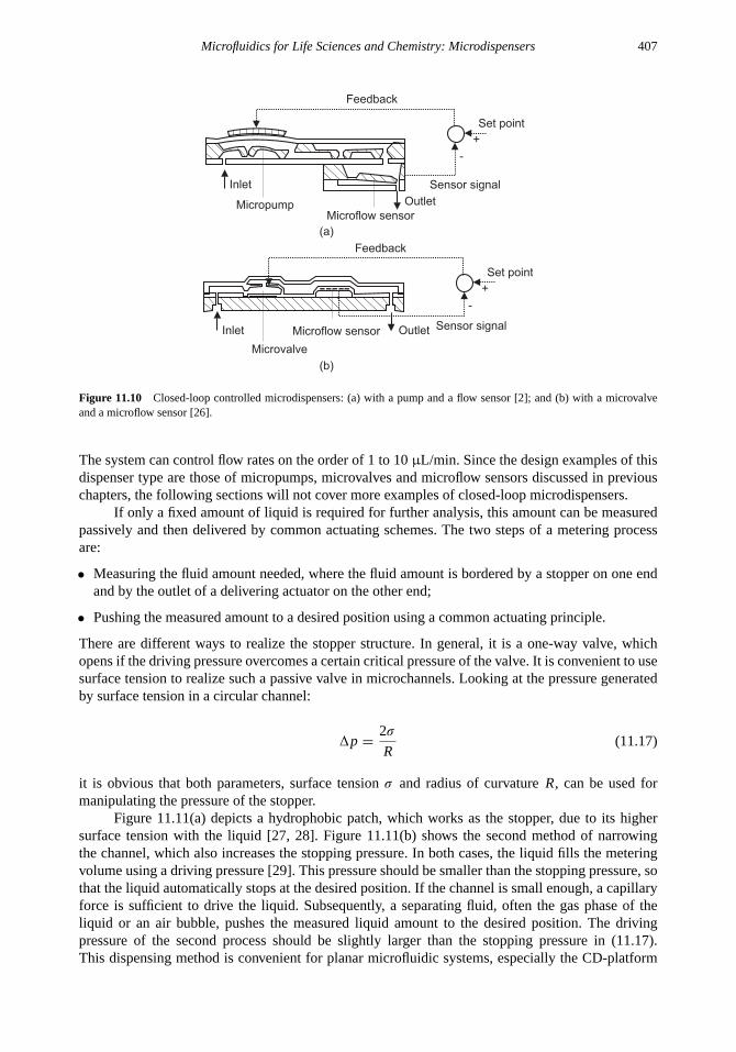
Microfluidics for Life Sciences and Chemistry: Microdispensers 407
Sensor signal
Sensor signal
Figure 11.10 Closed-loop controlled microdispensers: (a) with a pump and a flow sensor [2]; and (b) with a microvalveand a microflow sensor [26].
The system can control flow rates on the order of 1 to 10µL/min. Since the design examples of thisdispenser type are those of micropumps, microvalves and microflow sensors discussed in previouschapters, the following sections will not cover more examples of closed-loop microdispensers.
If only a fixed amount of liquid is required for further analysis, this amount can be measuredpassively and then delivered by common actuating schemes. The two steps of a metering processare:
• Measuring the fluid amount needed, where the fluid amount is bordered by a stopper on one endand by the outlet of a delivering actuator on the other end;
• Pushing the measured amount to a desired position using a common actuating principle.
There are different ways to realize the stopper structure. In general, it is a one-way valve, whichopens if the driving pressure overcomes a certain critical pressure of the valve. It is convenient to usesurface tension to realize such a passive valve in microchannels. Looking at the pressure generatedby surface tension in a circular channel:
1p =2σ
R(11.17)
it is obvious that both parameters, surface tensionσ and radius of curvatureR, can be used formanipulating the pressure of the stopper.
Figure 11.11(a) depicts a hydrophobic patch, which works as the stopper, due to its highersurface tension with the liquid [27, 28]. Figure 11.11(b) shows the second method of narrowingthe channel, which also increases the stopping pressure. In both cases, the liquid fills the meteringvolume using a driving pressure [29]. This pressure should be smaller than the stopping pressure, sothat the liquid automatically stops at the desired position. If the channel is small enough, a capillaryforce is sufficient to drive the liquid. Subsequently, a separating fluid, often the gas phase of theliquid or an air bubble, pushes the measured liquid amount to the desired position. The drivingpressure of the second process should be slightly larger than the stopping pressure in (11.17).This dispensing method is convenient for planar microfluidic systems, especially the CD-platform

408 Fundamentals and Applications of Microfluidics
Figure 11.11 Process steps of in-channel microdispenser: (a) with hydrophobic valve; (b) with capillary valve; and (c) withelectro-osmotic flow.
described in Section 7.1.1.7, where different driving pressures are available by changing the rotationspeed.
Figure 11.11(c) describes another concept of in-channel dispensing [17]. Electrokinetic flowinjects the liquid into the measured volume. By switching the injection potential to the dispensingflow, the measured liquid amount is pushed to the desired position. In most cases, the componentsin the measured liquid undergo a subsequent electrophoretic separation. This method is suitablefor conducting liquids, and requires glass as a device material or special treatment for the channelsurface because of the double layer needed for electrokinetic pumping.
11.2 DESIGN EXAMPLES
11.2.1 Droplet Dispensers
11.2.1.1 Thermopneumatic
Droplet dispensers were originally designed for printing applications. With an increasing need formassively parallel analysis, the same device can be used for printing the assay matrix of reagents.Figure 11.12(a) describes the simplified structure of the dispenser reported in [5]. The device is aninkjet print head, which has integrated CMOS control circuits. Therefore, its fabrication should becompatible to the CMOS technology.
The fabrication of the nozzles starts after completing the CMOS process. The droplet isinjected thermopneumatically by a thermal bubble. The heater is made of hafiniumdiboride. Anelectroplated Ni/Au layer on top of the device avoids overheating and ensures quick heat spreadingafter each injection. This top layer is used as the mask for the final dry etching process of the nozzle.

Microfluidics for Life Sciences and Chemistry: Microdispensers 409
Figure 11.12 Microdispensers: (a–d) thermopneumatic; (e) thermomechanical; and (f) and (g) electrostatic.
The dispenser depicted in Figure 11.12(b) is fabricated using a combination of bulk machiningand surface machining [6]. The heater is made of platinum. In contrast to other designs, thisdispenser utilizes two thermopneumatic actuators to control the droplet injection. Beside a largeheater structure for droplet injection, a second smaller heater works as a bubble valve, which usesthe surface tension to control the refill process. As a result, clean droplets without satellites can begenerated.
The dispenser shown in Figure 11.12(c) [21] has a nozzle made of silicon oxide. The fabri-cation process combines both bulk machining and surface machining. The ring-shaped polysiliconheater creates a doughnut-shaped bubble, which pushes the droplet out of the nozzle. The devicechamber is filled automatically by capillary force.
All three dispensers described above have bubbles, which grow in the opposite direction ofthe droplet. This principle is calledbackshooter. The other principle, calledsideshooter, ejects thedroplet vertically [8] [Figure 11.12(d)]. The sideshooter dispenser utilizes the same technologydescribed in [8] for making microneedles. The heater is made of polysilicon. The nozzles arearranged horizontally and are exposed by sawing through the flow channel.
11.2.1.2 Thermomechanical
In contrast to the thermopneumatically driven dispensers, the microdispenser depicted in Figure11.12(e) utilizes the buckling energy of a thermomechanic actuator to dispense a droplet [9]. The

410 Fundamentals and Applications of Microfluidics
actuator is a circular nickel membrane. The nickel heater is embedded in the electrically insulatedsilicon oxide layer. If the stress induced by the high temperature of the heater is greater than thecritical stress of the membrane, the membrane buckles rapidly. The rapid acceleration adds energyinto the droplet and ejects it out of the nozzle. The dispenser is fabricated by bulk micromachiningand surface micromachining using aluminum as a sacrificial layer.
11.2.1.3 Electrostatic
All dispensers described above operate at high temperatures. The high temperatures are not criticalfor the conventional ink-printing application, but can be fatal for printing biochemical reagents. Forapplications in life sciences, low-temperature actuators, such as the electrostatic actuator and thepiezoelectric actuator, should be considered. An electrostatic actuator [10] generates the dispensingpressure in the device depicted in Figure 11.12(f). The silicon membrane opposite the nozzle actsas an electrode of the actuator. The other electrode is made of transparent indium tin oxide (ITO),which is deposited on a glass substrate. Because of the extremely small gap of 0.2 mm, the actuatoronly needs 26.5V for its operation.
11.2.1.4 Piezoelectric
The microdispenser reported in [11] is fabricated entirely with surface micromachining [Figure11.12(g)]. The nozzle plate and a moveable piston plate are the two electrodes of an electrostaticactuator. The gap between the electrode is about 5µm. In contrast to the example shown in Figure11.12(f), the actuating field is applied directly through the dispensed liquid. That means the dispensercan only be used for a dielectric liquid, and the field strength should be below the breakdown strengthof the liquid. The other drawback is the possibility of electrolysis, which generates unwanted bubblesand leads to malfunction of the dispenser.
The other type of low-temperature driving mechanism suitable for biochemical applicationis the piezoelectric actuator. Piezoelectric actuators have the advantage of high drive pressureand fast dynamics. An external stack-type piezoelectric actuator is able to drive several nozzlesconcurrently. Therefore, passive parallel dispensing is possible with a single actuator. The drivepressure is programmable with the drive voltages. Fast dispensing process and slow reversing avoidair aspiration and allow refilling. This feature, and the high dynamics of piezoelectric actuators,make fast and clean dispensing possible.
The dispenser depicted in Figure 11.13(a) has a piezobimorph cantilever as an actuator [12].The driving scheme of this dispenser is similar to that of all other piezoelectric dispensers. Thecantilever retracts slowly, allowing the liquid to be filled in the device chamber, while air aspirationis avoided, due to the surface tension of the meniscus at the nozzle outlet. In the dispensing process,the tension is released quickly. The energy released in this fast process allows a droplet to be formedand ejected out of the nozzle. According to (13.25) and (13.26), the large energy is required to formthe surface of the droplet and to convert into kinetic energy. In this dispenser, only the nozzle plateis made of silicon using micromachining. The piezobimorph beam is mounted on a membrane inthe dispenser shown in Figure 11.13(b) [13]. The beam is glued on three cylindrical PMMA standsto generate a large displacement. The ring-shaped nozzle is fabricated with the process describedpreviously in Figure 11.7(a). This design has a fill chamber of 8.8µL and a droplet volume on theorder of 300 nL to 500 nL. Before assembly, the fill chamber and channel surfaces are oxidized toget a thick and stable silicon oxide layer. The hydrophobic characteristics of silicon oxide improvethe priming process of the dispenser. The ring-shaped nozzle and the treatment of its outer surfacewith a hydrophobic layer allow clean droplet generation and accurate trajectory.
The device depicted in Figure 11.13(c) integrates a nozzle on the outlet of a check-valvemicropump [30]. A piezodisc drives the pump. This design is more complex than the others and hasslow dynamics because of the large amount of liquid to be filled into the pump chamber. The outer

Microfluidics for Life Sciences and Chemistry: Microdispensers 411
(a) (b)
(c)
(d)
(e) (f)
Si
Metal
Piezo
material
Glass
SiO2
Brass
PiezocantileverFilling port Piezodisc
Piezodisc Filling port
Piezostack
Pressure sensor
Piezodisc
Piezodisc
Figure 11.13 Piezoelectric microdispensers: (a, b) with piezobimorph cantilever; (c) with piezodisc; (d) with piezostack;(e) with piezodisc on a glass membrane; and (f) piezodisc on a brass membrane.
surface of the nozzle is treated with a hydrophobic layer. The ring-shaped nozzle is formed by wetetching with a timed stop.
The design described in Figure 11.13(d) has a nozzle in the form of a needle [31]. Twocapacitive sensors are integrated into the device for the measurement of displacement and pressurein the fluid chamber. The device works as a pipette. In the aspiration mode, the needle is dipped intothe liquid reservoir and the actuator sucks the liquid into the needle.
In the dispensing mode, the actuator pushes the liquid amount out of the needle. The dispenserreported in [21] has a piezodisc as actuator [Figure 11.13(e)]. The extremely small nozzle, on theorder of 1µm, is made of silicon oxide with the process described in Figure 11.7(b). The deviceworks in burst mode with ultrasonic frequency (0.5 MHz). The extremely small nozzle and the highfrequency eject droplets on the order of several femtoliters (10−15 L).
The device described in [32] has 24 nozzles arranged in a 4×6 array. The nozzles areconnected to 24 reservoirs, which contain different liquids. Between the piezoelectric actuator andthe nozzles is an air gap. The system allows dispensing of 24 different liquids at once and is usedfor printing of reagents on a DNA chip.

412 Fundamentals and Applications of Microfluidics
Figure 11.14 The concept of metering and dispensing: (a) filling the reservoir; (b) filling the metering chamber withcapillary force; (c) ready for dispensing; (d) dispensing with a pressure pulse; (e) complete depletion of metering chamber;and (f) refilling of metering chamber. (After: [36].)
A simple piezoelectric dispenser is described in Figure 11.13(f) [33]. The acceleration of thepiezoelectric bimorph disc transmits the required energy to the droplet. However, the device cannotmeet the accuracy and controllability of micromachined devices.
According to the analysis in Section 11.1.1, the two important parameters for the dispensingprocess are the droplet size and the initial droplet velocity. While the initial droplet velocity isdirectly proportional to the actuation velocity and can be controlled precisely [32], it is not easyto have a controlled reproducible droplet size. All the above droplet dispensers have a large liquidreservoir. The size of the droplet depends on the actuation stroke and the viscosity of the liquid. Forthe same liquid, the droplet size is proportional to the actuation stroke [32] and the nozzle diameter[34]. For the same actuation condition and nozzle size, the droplet is also proportional to viscosity[35]. In order to achieve a controllable droplet size, Koltay et al. utilized the concept of metering inan in-channel dispenser to accurately dispense the required liquid amount. The metering chamber ispositioned directly above the nozzle. A microchannel connects this chamber with the larger reservoir[Figure 11.14(a)]. The microchannel works as the supply channel to fill the metering chamber byusing capillary force [Figure 11.14(b, c)]. During injection, both reservoir and metering chamberhave the same pressure. Thus, no additional flow crosses the microchannel [Figure 11.14(d)]. Thedroplet size can be determined precisely by the predesigned volume of the metering chamber[36] [Figure 11.14(e)]. After dispensing, the metering chamber is refilled by capillary force at themicrochannel [Figure 11.14(f)]. Table 11.1 gives an overview of the typical parameters of dropletmicrodispensers.
11.2.2 In-Channel Dispensers
Because of their simplicity, in-channel microdispensers are implemented in complex systems, suchas a DNA chip [27, 28], and commercial products [29]. Figure 11.15 shows a number of designexamples of in-channel dispensers. Both droplet formation and metering in microchannels are basedon a multiphase system. While the formation of droplets requires a liquid/liquid system, meteringand dispensing a liquid plug requires a gas/liquid system.
The basic configuration of an in-channel droplet dispenser shown in Figure 11.8 can bemodified to combine mixing with dispensing. In this case, the sample inlet is designed as a simpleY-mixer, which first merges the solute and solvent before dispensing them with the carrier fluid.If mixing should be avoided before entering the carrying stream, a third stream between the twosample streams can be used to separate them [37].

Microfluidics for Life Sciences and Chemistry: Microdispensers 413
Table 11.1
Typical Parameters of Droplet Microdispensers
Refs. Nozzle Size (µm) Array Size Droplet Volume (pL) Droplet Speed (m/s) Actuator
[5] 30×40 50×1 310 10–15 Thermopneumatic[6] 40 150×1 113–382 10 Thermopneumatic[7] 20–28 28×2 3.2–9.4 10 Thermopneumatic[8] 21 16×1 34 — Thermopneumatic[9] 35 1 1,150 8 Thermomechanic[10] 28 64×2 22.5 6 Electrostatic[11] 20 13×1 2 10 Electrostatic[12] 50 67×1 268–4,200 — Piezoelectric[13] 60 1 268–524 3.5 Piezoelectric[20] 400 1 140,000 0.8 Piezoelectric[31] 1.4 1 0.0034 — Piezoelectric[32] 100 4×6 4,200 — Piezoelectric[33] 60 1 125 1.64 Piezoelectric[36] 50-200 8×12 50 — Piezoelectric
The example depicted in Figure 11.15(a) uses hydrophobic valves made of SAM films [27].The hydrophobic patches are patterned on silicon and glass substrates using a lift-off technique.The dispensed volume is determined by the volume of the channel between the outlet of thethermopneumatic actuator and the hydrophobic valve. An overflow channel prevents the drivenpressure from exceeding the surface tension at the hydrophobic valve. The hydrophobic venton the right is used to keep the dispensed liquid at the desired position. Air coming from thethermopneumatic actuator exits the dispensing channel at the vent and lets the driven pressure dropdown to the initial value. This design is successfully implemented in a DNA-analysis system [28].
The dispenser in Figure 11.15(b) is a part of the analysis cartridge, commercially availablefrom i-STAT (i-STAT Inc., Ontario, Canada) [29]. The device is made of plastic. A capillary valve isused to stop the liquid. The measured amount is then pushed to the desired position by a pneumaticactuator. The use of a capillary valve keeps the fabrication of the device simple and cost-effective.
The same concept of a capillary valve is shown in Figure 11.15(c) [38]. The device is madeof PDMS using soft-lithography technology; see Section 3.4.5. The volume of the measurementchamber determines the amount of dispensed liquid. Different volumes of 50, 100, and 150 nL wererealized. Two capillary valves keep the liquid in the chamber until the external pneumatic actuatorpushes out the measured liquid.
The examples shown in Figure 11.15(d) look different, but work with the same concept ofin-channel metering and dispensing [39]. The tapered shape of the measurement chamber makesself-filling possible, when the liquid flows into the large inlet channel. The liquid stops at thenarrow end of the chamber. The liquid remains in the chamber after withdrawing or pushing awayexcessive liquid. A quick pressure pulse ejects the measured amount into the smaller channel. Thedevice is made of PDMS and is able to dispense 10 nL. The example reported in [17] uses theconventional method of capillary separation. The measured liquid amount is delivered and separatedby electrokinetic pumping. The concept shown in Figure 11.15(d) was used by Yamada and Seki[40] for accurate dosing and mixing. The device was fabricated based on molding of PDMS. Thedevice combines two in-channel dispensers to dispense and mix 3.5-pL droplets. The solvent andsolute are first introduced into the metering channels [Figure 11.16(a)]. Both liquids stop at thecapillary valves. Subsequently, the rest of the liquids are flushed away by air flow [Figure 11.16(b)].Applying a higher pressure than the capillary pressure of the valves dispenses the liquids into the

414 Fundamentals and Applications of Microfluidics
Figure 11.15 In-channel microdispensers: (a) with hydrophobic valve; and (b–d) with capillary valve.
mixing channel [Figure 11.16(c)]. The distance between the two capillary valves is to be carefullydetermined, so that each dispensed droplet does not block the other.
11.3 SUMMARY
This chapter discusses the design consideration and design examples of different microdispenserconcepts. In most cases, the dispensed liquid amount is confined by the interface between two ormore phases. Injected droplets in air are defined by the liquid/air interface. Droplets or plugs inmicrochannel are defined by the solid/liquid/liquid or solid/liquid/gas interfaces.
The existence of the interfaces leads to dimensionless numbers that can describe the behaviorof the dispensed liquid amount. For the liquid/air system in droplet dispensers, the Weber number(We) describes the ratio between kinetic energy and the surface tension. The Reynolds number basedon the air viscosity represents the ratio between the inertia force and the friction force. Thus, a We-Re diagram can be used to describe the behavior of the dispensed droplet.
For the liquid/liquid system in the case of in-channel droplet dispenser, the capillary number(Ca) represents the ratio between the friction force and the surface tension of the droplet. Thecapillary number is proportional to the Reynolds number. Thus, the other parameter for describingthis system is the volumetric fractionr of the droplet liquid. Anr -Ca diagram can describe well thebehavior of the dispensed droplet.

Microfluidics for Life Sciences and Chemistry: Microdispensers 415
Solvent
Solute
Mixing channel
Stop valves Metering channels
(a) (b) (c)
Mixed droplet
Figure 11.16 Application of in-channel microdispensers for micromixing: (a) Solute and solvent are introduced intometering channel. (b) The rest of the liquids are flushed away. (c) Metered solute and solvent are dispensed to form themixed droplet. (After: [40].)
The metering concept uses the volume determined by the geometry to dispense the requiredliquid amount. Combining this concept with a droplet dispenser can generate droplet sizes, whichare independent from other parameters, such as actuation stroke and viscosity.
Problems
11.1 A water droplet is rejected from a nozzle with a speed of 2 m/s. Determine the critical diameter ofthe droplet so that no satellite droplet can occur. The droplet is assumed to be stable if the kineticenergy is smaller than the surface energy. Surface tension and density of water are assumed to be72×10−3 N/m and 1,000 kg/m3, respectively.
11.2 Determine the minimum gap between the electrodes of an electrostatic actuator, which is used fordispensing a droplet. The actuating voltage is 200 V. The droplet has a size of 2 pL and moveswith an initial velocity of 10 m/s. [Hint: The electrostatic force isF = 1/2(εε0)A(V2/x2), whichgives the energy to overcome the squeezing forceFsf = (3w2ηA/2)x3dx/dt , and to form andto eject the droplet.A andw are the area and the lateral dimension of the moving plate,x is thegap,V is the applied voltage,η andε are the viscosity and relative permittivity of the liquid, andε0 = 8.854× 10⁻¹² F/m is the permittivity of free space].
11.3 A piezoelectric stack actuator is used for parallel dispensing of 96 water droplets. The dispensingprocess occurs during 5 ms. The actuating stroke is 10 mm. Determine the required force if alldroplets have a size of 20 pL and an initial velocity of 15 m/s.
11.4 Is the force in the above parallel dispenser large enough to aspirate air into the nozzles? Assumethat the nozzle diameter is equal to the droplet diameter.
11.5 A droplet of 100 nL is ejected on a glass plate. The droplet meets the plate at 10 m/s. Is it possiblethat this droplet is split into two satellite droplets after the impact?
11.6 Design an in-channel microdispenser with capillary valves and thermopneumatic actuators. Theamount to be dispensed is 200 nL, and the air temperature of the actuator cannot exceed 50◦C.

416 Fundamentals and Applications of Microfluidics
References
[1] Lammerink, T. S. J., Elwenspoek, and M., Fluitman, H. J., ”Integrated Micro-Liquid Dosing System,“Proceedingsof MEMS’93, 6th IEEE International Workshop Micro Electromechanical System, San Diego, CA, Jan. 25–28, 1993,pp. 254–259.
[2] Gass, V., et al., “Integrated Flow-Regulated Silicon Micropump,”Sensors and Actuators A, Vol. 43, 1994, pp. 335–338.
[3] Boillat, M. A., et al., “A Differential Pressure Liquid Flow Sensor for Flow Regulation and Dosing Systems,”Proceedings of MEMS’95, 8th IEEE International Workshop Micro Electromechanical System, Amsterdam, TheNetherlands, Jan. 29-Feb. 2,1995, pp. 350–352.
[4] Roßberg, R., and Sandmaier, H., “Portable Micro Liquid Dosing System,”Proceedings of MEMS’98, 11th IEEEInternational Workshop Micro Electromechanical System, Heidelberg, Germany, Jan. 25–29, 1998, pp. 526–531.
[5] Krause, P., Obermeier, E., and Wehl W., “Backshooter—A New Smart Micromachined Single-Chip Inkjet Printhead,”Proceedings of Transducers ’95, 8th International Conference on Solid-State Sensors and Actuators, Stockholm,Sweden, June 16–19, 1995, pp. 520–523.
[6] Tseng, F. G., Kim, C. J., and Ho, C. M., “A Novel Microinjector With Virtual Chamber Neck,”Proceedings ofMEMS’98, 11th IEEE International Workshop Micro Electromechanical System, Heidelberg, Germany, Jan. 25–29,1998, pp. 57–62.
[7] Lee, C. S., et al., “A Micromachined Monolithic Inkjet Print Head with Dome Shape Chamber,”Proceedings ofTransducers ’01, 11th International Conference on Solid-State Sensors and Actuators, Munich, Germany, June 10–14, 2001, pp. 902–905.
[8] Chen, J., and Wise, K. D., “A High-Resolution Silicon Monolithic Nozzle Array for Inkjet Printing,”IEEE Transac-tions on Electron Devices, Vol. 44, No. 9, 1997, pp. 1401–1409.
[9] Hirata, S., “An Inkjet Head Using Diaphragm Microactuator,”Proceedings of MEMS’96, 9th IEEE InternationalWorkshop Micro Electromechanical System, San Diego, CA, Feb. 11–15, 1996, pp. 418–423.
[10] Kamisuki, S., et al., “A High Resolution, Electrostatically Driven Commercial Inkjet Head,”Proceedings of MEMS’00,13th IEEE International Workshop Micro Electromechanical System, Miyazaci, Japan, Jan. 23–27, 2000, pp. 793–798.
[11] Galambos, P., et al., “A Surface Micromachined Electrostatic Drop Ejector,”Proceedings of Transducers ’01, 11thInternational Conference on Solid-State Sensors and Actuators, Munich, Germany, June 10–14, 2001, pp. 906–909.
[12] Ederer, I., Grasegger, J., and Tille, C., “Droplet Generator with Extraordinary High Flow Rate and Wide OperatingRange,”Proceedings of Transducers ’97, 9th International Conference on Solid-State Sensors and Actuators, Chicago,June 16–19, 1997, pp. 809–812.
[13] Laurell, T., Wallman, L., and Nilsson, J., “Design and Development of a Silicon Microfabricated Flow-ThroughDispenser for On-Line Picolitre Sample Handling,”Journal of Micromechanics and Microengineering, Vol. 9, 1999,pp. 369–376.
[14] Lee, S. W., Jeong, O. C., and Yang, S. S., “The Fabrication of a Micro Injector Actuated by Boiling and/or Electrol-ysis,” Proceedings of MEMS’98, 11th IEEE International Workshop Micro Electromechanical System, Heidelberg,Germany, Jan. 25–29, 1998, pp. 526–531.
[15] Lee, S. W., Sim, W. Y., and Yang, S. S., “Fabrication and In Vitro Test of a Microsyringe,”Sensors and Actuators A,Vol. 83, 2000, pp. 17–23.
[16] Bohm, S., Olthuis, W., and Bergveld, P., “An Integrated Micromachined Electrochemical Pump and Dosing System,”Journal of Biomedical Microdevices, Vol. 1, No. 2, 1999, pp. 121–130.
[17] Effenhauser, C. S., Manz, A., and Widmer, H. M., “Glass Chips for High-Speed Capillary Electrophoresis Separationswith Submicron Plate Heights,”Analytical Chemistry, Vol. 65, No. 19, 1993, pp. 2637–2642.
[18] Vance, B., Bonn, D., Martin, J. Y., et al., “Controlling Droplet Deposition with Polymer Additives,”Nature, Vol. 405,No. 6788, 2000, pp. 772–775.
[19] Douglas, J. F., Gasiorek, J. M., and Swaffield, J. A.,Fluid Mechanics, 4th ed., London: Longman, 1995.
[20] Koide, A., et al., “Micromachined Dispenser with High Flow Rate and High Resolution,”Proceedings of MEMS’00,13th IEEE International Workshop Micro Electromechanical System, Miyazaci, Japan, Jan. 23–27, 2000, pp. 424–428.
[21] Luginbuhl, Ph., et al., “Micromachined Injector for DNA Mass Spectrometry,”Proceedings of Transducers ’99, 10thInternational Conference on Solid-State Sensors and Actuators, Sendai, Japan, June 7–10, 1999, pp. 1130–1133.
[22] Lang, R. J., “Ultrasonic Atomization of Liquids,”Journal of the Acoustical Society of America, Vol. 34, No. 1, 1962,pp. 6–8.

Microfluidics for Life Sciences and Chemistry: Microdispensers 417
[23] Tice, J. D., Lyon, A. D., and Ismagilov R. F., “Effects of Viscosity on Droplet Formation and Mixing in MicrofluidicChannels,”Analytica Chimica Acta, Vol. 507, 2004, pp. 73–77.
[24] Waibel, G., et al., “Highly Integrated Autonomous Microdosage System,”Sensors and Actuators A, Vol. 103, 2003,pp. 225–230.
[25] Cabuz, E., et al., “MEMS-Based Flow Controller for Flow Cytometry,”Solid-State Sensor and Actuator Workshop.Hilton Head Island, SC, June. 2–6, 2002, pp. 110–111.
[26] Xie, J., Shih, J., and Tai, Y. C., “Integrated Surface-Micromachined Mass Flow Controller,”Proceedings of MEMS’03,16th IEEE International Workshop Micro Electromechanical System, Kyoto, Japan, Jan. 19–23, 2003, pp. 20–23.
[27] Handique, K., et al., “Microfluidic Flow Control Using Selective Hydrophobic Patterning,”Proceedings of SPIEConference on Micromachined Devices, Austin, TX, Sep. 29, 1997, pp. 185–195.
[28] Handique, K., et al., “Nanoliter-Volume Discrete Drop Injection and Pumping in Microfabricated Analysis Systems,”Technical Digest of the IEEE Solid State Sensor and Actuator Workshop, Hilton Head Island, SC, June 8-11, 1998,pp. 346–349.
[29] Glavina, P. G., “The I-STAT System: Biomedical Application of Microsensor Technology,”Proceedings of theInternational MEMS Workshop 2001 iMEMS, Singapore, July 4–6, 2001, pp. 15–20.
[30] Hey, N., et al., “A New Device for Multifunctional Dosage of Liquids by a Free Jet,”Proceedings of MEMS’98, 11thIEEE International Workshop Micro Electromechanical System, Heidelberg, Germany, Jan. 25–29, 1998, pp. 429–431.
[31] Szita, N., et al., “A Fast And Low-Volume Pipetor with Integrated Sensors for High Precision,”Proceedings ofMEMS’00, 13th IEEE International Workshop Micro Electromechanical System, Miyazaci, Japan, Jan. 23–27, 2000,pp. 409–413.
[32] de Heij, B., et al., “A Tuneable and Highly-Parallel Picolitre-Dispenser Based on Direct Liquid Displacement,”Sensorsand Actuators A, Vol. 103, 2003, pp. 88–92.
[33] Percin, G., et al., “Controlled Ink-Jet Printing and Deposition of Organic Polymers and Solid Particles,”AppliedPhysics Letters, Vol. 73, No. 16, 1998, pp. 2375-2377.
[34] Steinert, C. P., et al., “A Highly Parallel Picoliter Dispenser with an Integrated Novel Capillary Channel Structure,”Sensors and Actuators A, Vol. 116, 2004, pp. 171–177.
[35] Gutmann, O., et al., “Impact of Medium Properties on Droplet Release in a Highly Parallel Nanoliter Dispenser,”Sensors and Actuators A, Vol. 116, 2004, pp. 187–194.
[36] Koltay, P., et al., “The Dispensing Well Plate: A Novel Nanodispenser for the Multiparallel Delivery of Liquids (DWPPart I),” Sensors and Actuators A, Vol. 116, 2004, pp. 483–491.
[37] Shestopalov, I., Tice, J. D., and Ismagilov, R. F., “Multi-Step Synthesis of Nanoparticles Performed on MillisecondTime Scale in a Microfluidic Droplet-Based System,”Lab on a Chip, Vol. 4, 2004, pp. 316–321.
[38] Puntambekar, A., et al., “A New Fixed-Volume Metering Microdispenser Module Based on sPROMs Technology,”Proceedings of Transducers ’01, 11th International Conference on Solid-State Sensors and Actuators, Munich,Germany, June 10–14, 2001, pp. 1240–1243.
[39] Aoyama, R., et al., “Novel Liquid Injection Method with Wedge-Shaped Microchannel on a PDMS Microchip Systemfor Diagnostic Analysis,”Proceedings of Transducers ’01, 11th International Conference on Solid-State Sensors andActuators, Munich, Germany, June 10–14, 2001, pp. 1232–1235.
[40] Yamada, M., and Seki, M., “Nanoliter-Sized Liquid Dispenser Array for Multiple Biochemical Analysis in Microflu-idic Devices,”Analytical Chemistry, Vol. 76, 2004, pp. 895–899.

418 Fundamentals and Applications of Microfluidics

Chapter 12
Microfluidics for Life Sciences and Chemistry:Microfilters and Microseparators
Microfluidics has emerged as a new approach for improving performance and functionality of bio-chemical and medical analysis. Miniaturization and new effects in microscale promise completelynew system solutions in these fields. Dimension reduction results in faster processes and less reagentconsumption. The small size also allows parallel processing, in which more compounds can be pro-duced and analyzed. In addition, recent developments in biotechnology, such as mapping the humangenome, require new supporting tools and products. This chapter discusses devices for separationapplication. The main applications of separation are filteration/collection and analysis. Devices ofthe first application are considered here as microfilters, while the second types are called micro-separators. In contrast to microfilters as passive devices, microseparators are active components thatrequire external actuation. This chapter discusses these two device types in separated sections.
12.1 MICROFILTERS
Microfilters have two unique functions: filtration and collection. Microfilters separate particles forapplications that require a clean fluid for further processes. Microfilters are used for washing outwaste products of the precedent process. In packed-bed microreactors, filters are used for keepingbeads in reaction chambers. In other applications, the filtered particles are of interest. Microfiltersseparate particles from the mean flow and send them to further processing stages.
Based on the size range of filtered particles, filtration can be categorized as conventionalfiltration, ultrafiltration, and reverse osmosis. Figure 12.1 depicts the typical sizes of filteredparticles. Conventional filtration covers particle sizes above 10 microns. Ultrafiltration can handlemacromolecules with molecular size ranging from 10 nanometers to 10 microns. Filtration type formolecules or ions smaller than 10 nanometers is called reverse osmosis.
Based on their fabrication technology, and, consequently, their typical pore size, microfiltersare categorized as membrane filters and gap filters. The basic structure of the first type is athin membrane that contains filtering pores. Generally, such membranes are called semipermeablemembranes, which allow only one component to pass or to move through with faster velocity,resulting in selective transport across the membrane. The pores can be etched through the membranewith a mask defined by photolithography. Because of the limited resolution of the lithographyprocess, membrane filters have relatively large pores, on the order of microns.
The flux across a filter membrane can be driven by pressure, concentration gradient, orelectrical potential. The transport through the membrane depends on the size of the pores. In general,the transport rate is proportional to the pore size, while the selectivity of filtration is inversely
419

420 Fundamentals and Applications of Microfluidics
Figure 12.1 Ranges of typical particle sizes and the corresponding filtration types.
(a) bulk flow (b) diffusion
(c) restricted diffusion (d) solution diffusion
Figure 12.2 Different transport mechanisms through membranes: (a) bulk flow through pores; (b) diffusion through pores;(c) restricted diffusion or molecular sieving; and (d) solution diffusion.
proportional to the pore size. Micromachined pores are relatively large, larger than the mean freepart of the species. The transport through such large pores is governed by the bulk flow, wheremolecules can pass straight through the pores [Figure 12.2(a)]. Because of the small pore size, theflow can be assumed to be laminar. For circular pores with a diameter ofDpore and a pore length ofLpore, the bulk velocityU across the pore is according to Hagen-Poiseuille flow:
U =D2
pore
32ηLpore1p, (12.1)
whereη is the dynamic viscosity of the fluid, and1p is the pressure difference across the filtermembrane. The void fractionε, also called the porosity, is defined as the ratio between the pore areato the total membrane areaA:
ε =Aopening
A(12.2)
The rate of mass transfer can then be derived as:
m = uερ (12.3)
whereρ is the density of the species.If the pores are small compared to the mean free path but large enough for diffusion, the
transport mechanism through pores is diffusion. Molecules are passing through the pore in a randommanner [Figure 12.2(b)]. This random movement or Brownian motion is actually a diffusion process.Diffusion through pores was briefly discussed in Chapter 9 on microneedles. The rate of mass

Microfluidics for Life Sciences and Chemistry: Microfilters and Microseparators 421
transport can be derived from Fick’s law:
m =Deff
Lpore1c, (12.4)
whereDeff is the effective diffusion coefficient of the species, and1c is the concentration differenceacross the membrane. The effective diffusion coefficient is a function of the ordinary diffusioncoefficientD, the porosityε, and the tortuosityτ :
Deff = εD
τ(12.5)
The tortuosity takes into account the longer distance traversed in the pores. Typical tortuosity rangesfrom 2 to 6.
Restricted diffusion occurs if the pores are large enough only for some species, so that onlythey can diffuse across the membrane. This transport mechanism is also called molecular sieving[Figure 12.2(c)]. With pore sizes on the order 0.1 to 1µm, larger particles are restricted from enteringthe pores. This transport mechanism is common in ultrafiltration. If the pore size is on the order ofmolecular sizes, for instance in most polymers, species diffuse through the bulk membrane [Figure12.2(d)]. The transport mechanism is called solution diffusion or diffusion-solubility. The transportrate is determined by:
m = DH1c
Lmembrane(12.6)
where H is the partition coefficient or solubility.D and L are the diffusion coefficient and themembrane thickness, respectively. The productDH is called the permeability. Separation foranalytical applications often utilizes solution diffusion to distinguish different macromolecules. Thenext section on microseparators will discuss more about these applications.
Gap filters use the gap between two structural layers as the filtering pore. The gap can befabricated with surface micromachining or bulk micromachining. In surface micromachining, forexample, the gap height or the pore size is determined by the thickness of silicon oxide as a sacrificiallayer, which can be controlled precisely by thermal oxidation. In bulk micromachining, controlledetching processes determine the gap. A combination of both micromachining techniques can be usedfor greater design flexibility.
12.1.1 Design Considerations
Microfilters have different requirements:
• Small variation of pore size distribution;
• Low pressure loss;
• Mechanical strength.
In contrast to industry applications, many biomedical applications require an extremely high se-lectivity ratio of filtration. While a ratio of 1:102 is sufficient for industry applications, biomedicalapplications may need a ratio of 1:104 or higher. This high selectivity only allows a small variationof pore size. With precise micromachining technology, such as lithography and controlled growth ofsacrificial layers, microfilters could meet these requirements.
Since a microfilter represents an obstacle in the flow and causes pressure loss, a minimumpressure drop over the filter is required. The most important parameter of a microfilter, which hasa big impact on pressure loss, is its porosityε (12.2). For a maximum porosity, the pores in themembrane should be made as large and as numerous as possible. Another solution for low pressure

422 Fundamentals and Applications of Microfluidics
losses is replacing the membrane design by a lateral design. The lateral design is a gap filter, whichrepresents a short and wide channel with low fluidic resistance.
The requirement for large porosity conflicts with the desired robustness. Larger holes willdecrease the mechanical strength of the filter. The influence of pore geometry on the pressure lossshould therefore be considered. Robust filters are realized by a gap design, which is made in bulksilicon and can withstand high inlet pressure. Gap filters can therefore meet both requirements oflow pressure loss and high mechanical strength.
The following examples analyze the effect of pressure drop on the mechanical strength of amembrane filter, as well as the design of gap filters.
Example 12.1: Stress on Membrane Filter
Determine the maximum stress on a silicon nitride membrane filter. The membrane has adimension of 1× 1 × 1 mm. The Young’s modulus for silicon nitride is 3× 10¹¹ Pa, and itsPoisson’s ratio is 0.25. The porosity is 0.25. The working fluid is air at a flow rate of 100 mL/min.The density and the viscosity of air at room temperature are 1 kg/m3 and 1.82 × 10⁻⁵ Pa-sec,respectively. Would the filter work if the fluid were water?
Solution. The total opening area of the filter is:
Aopening= εA = 0.25× (10−3)2 = 0.25× 10⁻⁶ m2
The drag pressure can be estimated as (assuming a flow numberµflow = 0.75) [1]:
1p =1
2µ2flow
ρ Q2
A2opening
1p =1
2×0.7521(100/60×10−6)2
(0.25×10⁻⁶)2= 39.5 Pa
The maximum stress at the edge of the filter membrane is estimated as (with a Poisson’s ratio of0.25) [1]:
σtotal = 1.44√
31p2l 2Eh2
σtotal = 1.44√
339.52×(10−3)2×3×1011
(10−6)2= 11.2 MPa
The maximum stress is much smaller than the fracture limit of silicon nitride, which is on theorder of 104 MPa. If the fluid is water, the viscosity is 50 times larger, and the density is 1,000times larger. The drag pressure is more significant, and the total stress will increase with a factorof about 100, which is still under the fracture limit. The filter will work for water at the same flowrate.
Example 12.2: Adjusting Gap Size in the Gap Filter
Thermal oxidation is used for adjusting the gap size of a gap filter. Gaps of 2µm are etched insilicon using DRIE. After thermal oxidation, the oxide thickness is 500 nm. Determine the finalgap size of the filter.
Solution. Since the thermal oxidation consumes some of the silicon thickness, only 54% of thefinal oxide thickness is the net increase of the gap surface (see Section 3.1). The thickness gain ineach side of the gap is:
Tnet = 0.54× 0.5 = 0.27µm

Microfluidics for Life Sciences and Chemistry: Microfilters and Microseparators 423
Si
Parylene C
Nitride
(a)
(b)(c)
(d) (e)
Figure 12.3 Design examples of microfilters: (a) deposition of low-stress silicon nitride; (b) RIE of the silicon nitride layer;(c) wet etching of the back of the wafer; (d) releasing etch of the membrane; and (e) coating with parylene.
Thus, the final gap size is:
Dfinal = Dinit − 2Tnet = 2 − 2 × 0.27 = 1.46µm
12.1.2 Design Examples
12.1.2.1 Membrane Filters
Figure 12.3 illustrates the most common process steps for fabricating membrane microfilters. Thematerial is low-stress silicon nitride. Because of the strength requirement, relatively thick nitridelayers (about 1µm) [2, 3] should be deposited. The low stress is achieved with LPCVD of SiH2Cl2and NH3 at 850◦C [Figure 12.3(a)]. To have a silicon-rich nitride, the gas flow ratios betweenSiH2Cl2 and NH3 are 70:18 [2] or 4:1 [4]. In the next step, silicon nitride is etched by CHF3/O2RIE [Figure 12.3(b)]. The membrane is freed by KOH wet-etching from the backside. A thin siliconmembrane can be left before the dicing process to avoid damaging the nitride membrane [Figure12.3(c)] [4]. After dicing, the nitride layer is released with a final etch [Figure 12.3(d)]. A conformaldeposition of parylene C can improve the strength of the filter membrane [Figure 12.3(e)] [4]. Inaddition, varying the thickness of the parylene layer can adjust the pore size.
The relatively thick nitride layer allows membrane sizes from 1× 1 mm [2, 3] to 8× 8 mm[4]. The pore sizes range from 4 to 10µm. In order to go beyond the resolution of lithography, whichis limited by the exposure wavelength, a maskless method with interference pattern of laser light canbe used for making pore sizes ranging from 65 to 500 nm [5]. However, this method makes the poredistribution and the gaps between them depend on the wavelength of the laser. Figure 12.4 showstypical pore designs that can be formed by photolithography [5]. Circular pores are more robustbecause of the low stress concentration around them. Hexagonal and rectangular pores can result inhigher stress concentrations at the sharp corners.
The membrane filter described in [6] has an integrated acoustic micropump (FPW-pump; seeSection 7.2.1.5). The device can actively transport particles to the separation area (Figure 12.5).
12.1.2.2 Gap Filters
Gap filters have the advantage of small and precise pore size. Depending on the fabrication method,a gap filter can be categorized as a subtractive gap filter or an additive gap filter.
Subtractive Gap Filters.In subtractive gap filters, the etched depth in the substrate defines thefiltering gap. The depth depends on etch rates and etching time. The drawback of this filter typeis the low reproducibility and the high pressure loss caused by the filtering channel. Figure 12.6(a)shows the typical subtractive gap filter [7].

424 Fundamentals and Applications of Microfluidics
(a) (b)
(c) (d)
Figure 12.4 Design of filter pores: (a) circular; (b) rectangular; and (c) and (d) hexagonal. (After [5])
Si OxideNitride
Interdigitated
electrodes
ZnO SU-8 Glass
Large particles
Small particles
Figure 12.5 Active microfilter with acoustic cleaning (not to scale). (After [6])
Additive Gap Filters.Additive gap filters have a defining spacer layer. Theoretically, this layer canbe any material which can be deposited on the substrate with a controllable growth rate. Thermaloxide is often used as spacer material because of its slow growth rate, which is controlled preciselyby time (see Section 3.1). Based on their arrangement between the gap and the substrate surface,additive gap filters are divided into vertical and horizontal types.
Vertical Filters.Figure 12.6(b) illustrates the fabrication steps of a vertical gap filter. The verticalgap filter has the same form as the membrane filter described above. The membrane is made of6-µm highly boron-doped silicon, which is not attacked during wet etching. After a diffusion ofboron, large pores are etched into silicon by DRIE [Figure 12.6(b), part 1]. The oxide layer, whichdefines the actual pore size, is grown by dry thermal oxidation [Figure 12.6(b), part 2]. A layerthickness from 20 to 100 nm corresponds to the pore size on the membrane after sacrificial etching[Figure 12.6(b), part 2]. The large pore is then filled with polysilicon [Figure 12.6(b), part 3]. Afteropening an etch access on top of the polysilicon layer, the gap previously filled with silicon oxide isfreed and works as filtering pores [Figure 12.6(b), part 4] [8].

Microfluidics for Life Sciences and Chemistry: Microfilters and Microseparators 425
Si
Oxide
p+Si
PolySi
(c)
(d)
(a)
(b)
Glass
1.
2.
3.
4.
Figure 12.6 Gap filters: (a) subtractive type; (b) and (c) additive type (vertical); and (d) additive type (horizontal).
Table 12.1
Typical Parameters of Microfilters
Refs. Pore Size (mm) Maximum Flow Rate (mL/min/cm2) Maximum Pressure (Pa) Technology
[2, 3] 4 1,000 water 3×10⁵ Bulk[5] 3–20 90,000 air 3×10³ Bulk[9] 0.01–0.05 — — Bulk, surface[10] 0.04 1,800 nitrogen 3.105 Bulk, surface
Horizontal Filters.Figure 12.6(c) shows another membrane gap filter. The gap is arranged parallelto the substrate surface [9]. A highly boron-doped silicon layer defines the filter membrane. Thefabrication process of this filter is similar to the process depicted in Figure 12.6(b).
A robust design is depicted in Figure 12.6(d) [10]. The filtering gaps are placed parallel tothe wafer surface. Using bulk micromachining and direct wafer bonding, the filter can withstandseveral hundred kilopascals of pressure. The filtering gap is designed as a meander structure tominimize the pressure loss across the filter. The meander shape offers a maximum channel widthat a constant channel length while occupying a minimum surface area. Table 12.1 lists the mostimportant parameters of the above-mentioned microfilters.
12.2 MICROSEPARATOR
Microfilters discussed in Section 12.1 can be considered as the passive type of microseparators.For instance, passing whole blood through a microfilter can separate white blood cells from redblood cells. While red blood cells easily pass through the filter pores, the white blood cells tend to
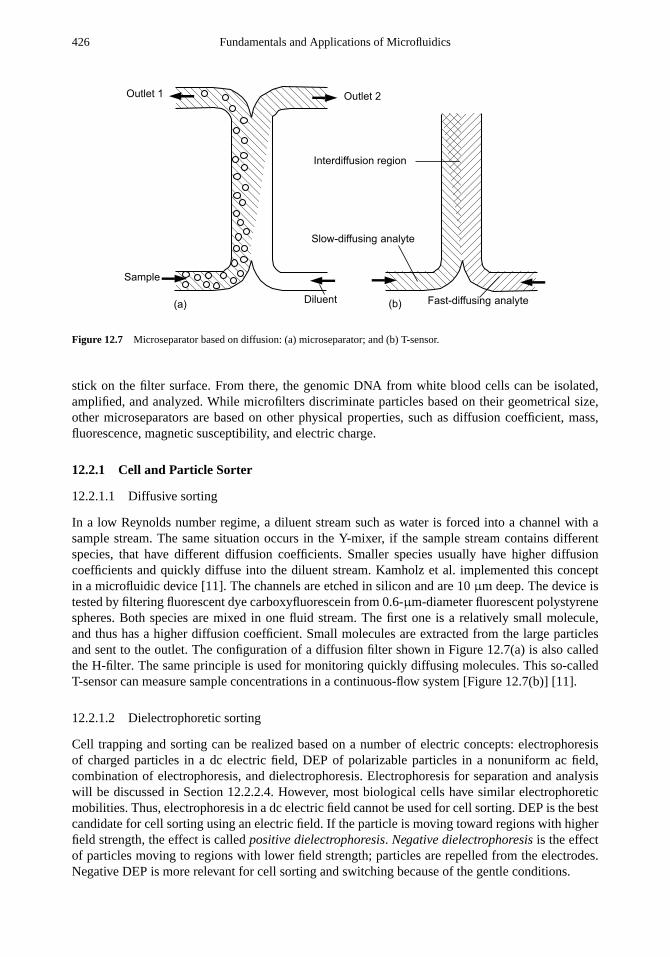
426 Fundamentals and Applications of Microfluidics
(a) (b)
Slow-diffusing analyte
Fast-diffusing analyte
Interdiffusion region
Outlet 2Outlet 1
Diluent
Sample
Figure 12.7 Microseparator based on diffusion: (a) microseparator; and (b) T-sensor.
stick on the filter surface. From there, the genomic DNA from white blood cells can be isolated,amplified, and analyzed. While microfilters discriminate particles based on their geometrical size,other microseparators are based on other physical properties, such as diffusion coefficient, mass,fluorescence, magnetic susceptibility, and electric charge.
12.2.1 Cell and Particle Sorter
12.2.1.1 Diffusive sorting
In a low Reynolds number regime, a diluent stream such as water is forced into a channel with asample stream. The same situation occurs in the Y-mixer, if the sample stream contains differentspecies, that have different diffusion coefficients. Smaller species usually have higher diffusioncoefficients and quickly diffuse into the diluent stream. Kamholz et al. implemented this conceptin a microfluidic device [11]. The channels are etched in silicon and are 10µm deep. The device istested by filtering fluorescent dye carboxyfluorescein from 0.6-µm-diameter fluorescent polystyrenespheres. Both species are mixed in one fluid stream. The first one is a relatively small molecule,and thus has a higher diffusion coefficient. Small molecules are extracted from the large particlesand sent to the outlet. The configuration of a diffusion filter shown in Figure 12.7(a) is also calledthe H-filter. The same principle is used for monitoring quickly diffusing molecules. This so-calledT-sensor can measure sample concentrations in a continuous-flow system [Figure 12.7(b)] [11].
12.2.1.2 Dielectrophoretic sorting
Cell trapping and sorting can be realized based on a number of electric concepts: electrophoresisof charged particles in a dc electric field, DEP of polarizable particles in a nonuniform ac field,combination of electrophoresis, and dielectrophoresis. Electrophoresis for separation and analysiswill be discussed in Section 12.2.2.4. However, most biological cells have similar electrophoreticmobilities. Thus, electrophoresis in a dc electric field cannot be used for cell sorting. DEP is the bestcandidate for cell sorting using an electric field. If the particle is moving toward regions with higherfield strength, the effect is calledpositive dielectrophoresis. Negative dielectrophoresisis the effectof particles moving to regions with lower field strength; particles are repelled from the electrodes.Negative DEP is more relevant for cell sorting and switching because of the gentle conditions.

Microfluidics for Life Sciences and Chemistry: Microfilters and Microseparators 427
The complex electric field around an electrode can be described as [12]:
E(r , t) = <
[Ere(r)+ ıEim(r)exp(ıωt)
](12.7)
where ı and < represent the imaginary unit and the real component of the complex number,respectively.E, r , andω are the field vector, the space vector, and the radial frequency, respectively.The time-averaged dielectrophoretic force acting on a particle of radiusR is:
〈F〉 = 2πεlε0R3×
<( fCM)∇
∑i
[(Ere
i )2+ (Eim
i )2]+
=( fCM)∑
i, j
[(Ere
i∂Eim
i∂ j − Eim
j∂Ere
i∂ j
)ej
] (12.8)
where i, j = x, y, z are indices for the Cartesian coordinates.< and = indicate the real andimaginary parts of a complex number. The Clausius-Mosotti factorfCM is determined as:
fCM =εp − εl
εp + 2εl(12.9)
whereε = σ + ıωε0ε is the complex permittivity,σ is the electric conductivity, indices p and ldenote the particle and the liquid. In (12.8), the first term is proportional to the rms value of the fieldstrength, while the second term is proportional to the gradient of the field phase. For an ac-field withno gradient in the phase, the condition for negative dielectrophoresis is:
<( fCM) < 0 (12.10)
Thus, the value of the complex permittivity of the particle is lower than that of the liquid. Becauseof the high permittivity of water, most living cells show negative DEP.
For an idealized electrode, the maximum repelling force perpendicular to the boundary of acapacitor is calculated as [12]:
FDEP =27π2V2
rms
32
(R
a
)3
εlε0<( fCM) (12.11)
where R, a, and Vrms are the particle radius, the distance to the electrode, and the rms voltage,respectively. In a continuous-flow system, the DEP force is on the order of the Stokes’s drag force.Thus, DEP can be used for trapping and manipulating particles suspended in a hydrodynamic flow.
Fiedler et al. used electrodes made of platinum/titanium and ITO on glass to trap and switchparticles and cells. Square-wave signals with a frequency of 1 MHz were applied on the electrodes.The device was able to trap and switch particles suspended in a water flow up to 10 mm/s. Huanget al. reported a 5×5 array of circular platinum electrodes. The electrodes are 80µm in diameter andplaced at a 200-µm distance. The device successfully concentratedEscherichia colifrom a dilutedsolution, as well as white blood cells from whole blood.
12.2.1.3 Ultrasonic Sorting
Nonlinear effects in an ultrasonic field cause the so-called acoustic streaming. The effect of acousticstreaming was discussed in Section 7.1.1.8. The interesting characteristics caused by an FPW is thehigh-flow velocity near the actuating membrane. Since this fast-moving layer is only 5µm [13, 14],which is in the same size order of cells, acoustic streaming on a FPW device can be used for sorting

428 Fundamentals and Applications of Microfluidics
(a)W
Wave
am
plitu
de
(nm
)
x y
0 0.5 1 1.5
x(mm)
-1
-
0
1y
(mm
)
(b)
Electrodes
Focal point
Focal point
Figure 12.8 Focused flexural plate wave device for particle concentration: (a) electrode arrangement and the typicalacoustic streaming field; and (b) the measured wave amplitudes.
particles. Different particles suspended on the FPW membrane experience different drag forcesdepending on their size. A typical FPW membrane consists of a nitride membrane, interdigitatedaluminum electrodes, piezoelectric zinc oxide, and an aluminium layer as ground electrode [15].Using curved electrodes, the acoustic energy and logically acoustic streaming can be focused. Afocused FPW device can be used for particle concentration. Figure 12.8(a) shows the arrangementof the curved electrodes and the generated acoustic streaming field. The measurement of the waveamplitudes indicates clearly a focal point [Figure 12.8(b)].
Acoustic streaming can also be focused using the cavity effect. Marmottant and Hilgenfeldt[16] used a 15-µm microbubble to attract cells. The microbubble is driven near its own resonancewith a frequency of 180 kHz. Acoustic streaming attracts cells to the microbubble and drives themin a defined trajectory.
Acoustic standing waves can separate particles with different acoustic impedance [17]. Harriset al. [18] used a cavity fabricated in silicon and glass to generate a standing wave. The acoustic waveis generated by a PZT layer deposited on silicon. The opposite glass plate works as the reflector. Thestanding wave generates a low-pressure node in the middle of the gap between silicon surface andreflector surface. Particles can be trapped in this low-pressure region.
12.2.1.4 Magnetic Sorting
Magnetic force can also be used for sorting particles. In a continuous flow, particles can be deflectedfrom their hydrodynamic trajectory by a magnetic field perpendicular to the flow. The magnitude ofthe magnetic force depends on the size and the magnetic property of the particles. Thus, magneticparticles can be separated from each other or from nonmagnetic materials. In a magnetic field, themagnetic force acting on a particle with a volumeVp is [19]:
F =χVp
µ0(∇ · B)B (12.12)
whereχ is the difference in susceptibility between the particle and the fluid,Vp is the volume of theparticle,µ0 = 4π×10−7 Wb/A-m is the permeability of vacuum, andB (T) is the flux density field.

Microfluidics for Life Sciences and Chemistry: Microfilters and Microseparators 429
optical lattice
sam
ple
solve
nt
Figure 12.9 Operation concept of an optical sorter.
The susceptibility is the ratio between the magnetizationM (A/m) and the field strengthH (A/m):
χ =MH
(12.13)
The magnetization of the particle is calculated as:
M =mVp
(12.14)
wherem is the magnetic moment. The general balance equation of a magnetic system is:
B = µ0(H + M) (12.15)
From (12.12), the magnetic field should be inhomogeneous (∇ ·B 6= 0), so that the magnetic particlecan experience a force.
Pamme and Manz [20] demonstrated a simple microfluidic device made of glass. Separationof magnetic particles suspended in the continuous flow was achieved with a permanent magnet.The magnetic sorting concept can be applied for analysis based on magnetic beads or separation ofmagnetically labeled cells [21].
12.2.1.5 Optical Sorting
A dielectric particle can be trapped in a tightly focused beam. This concept is well-known andcalled optical tweezers[22]. MacDonald et al. demonstrated an optical sorter for microparticleswith a three-dimensional optical lattice. The optical lattices are created by interferometric patternsof light. Dielectric particles follow defined paths through an optical lattice and can be sorted from acontinuous flow. The device has the form of the H-filter depicted in Figure 12.7(a). The basicH-configuration can only separate small molecules, because of the required high-diffusion coeffi-cient. Large subjects such as cells cannot be separated. In the optical sorter, an optical lattice isgenerated by a five-beam interference pattern and positioned at the separation microchannel (Figure12.9). When the sample flow with different cells passes through the optical lattice, selected cellsare deflected to the solvent side, while the others can pass straight. Since the optical force causedby the effect is smaller than the dielectrophoretic force described above, the hydrodynamic Stokes’sdrag force should be kept small. For instance, 2-µm protein microcapsules were sorted by a totallaser power of 530 mW (λ = 1,070 nm) at a flow speed of only 20µm/s [23]. Based on thisconcept, integrating a number of optically assembled, driven, and controlled components on a singlemicrofluidic chip can make an all-opticallab-on-a-microscopepossible [24].

430 Fundamentals and Applications of Microfluidics
Figure 12.10 Operation concept of a particle sorter: (a) hydrodynamic focusing; (b) detecting the particle; and (c) switchingthe focused sample flow to collection reservoir.
12.2.1.6 Hydrodynamic Sorting
Active microseparators use feedback control with external components such as valves and pumps toselectively sort particles in a continuous-flow system. The separation concept consists of the threebasic steps: focusing, detecting, and switching (Figure 12.10). First, the sample with particles suchas cells is focused into a narrow stream, so that each cell can be individually detected. The concept ofhydrodynamic focusing was already discussed analytically in Section 10.1.5. Two sheath streams areused to narrow the sample stream [Figure 12.10(a)]. After being focused, the particles are detectedwith an optical system, which gives the feedback signal to trigger the flow switch [Figure 12.10(b)].The switching steps can be followed hydrodynamically by changing the flow rates of the sheath flowand diverting the sample flow into the collecting reservoir [Figure 12.10(c)]. The sample flow canalso be switched using a valve, which just blocks or opens the gate to the collecting reservoir.
Kruger et al. developed a microfluidic device for activated cell sorting [25]. The microchannelsare formed by SU-8 on a silicon substrate. The channel structure is covered by a glass plate. Theswitching step was realized by both changing the sheath fluid ratio and external valves. Wolf et al.[26] developed a cell-sorting device in silicon. The microchannels are etched with DRIE and covered

Microfluidics for Life Sciences and Chemistry: Microfilters and Microseparators 431
Figure 12.11 Sorting with electrokinetic forces: (a) electro-osmotic switching; and (b) electrophoretic switching.
by anodic bonding to a glass wafer. Switching was realized by an external valve. This device hasintegrated waveguides for excitation and detection of the cells. Lin et al. [27] presented a similardevice in glass. The waveguides are glass fibers embedded in the device. Detection and countingwere demonstrated, but no switching was reported. Switching by adjusting the sheath flow ratiowas demonstrated by Lee et al. [28]. The microchannel was formed by hot embossing of a PMMAsubstrate.
Switching can also be achieved by manipulating the exit condition. Dittrich and Schwille [29]used electro-osmotic flow at the exit of a pressure-driven hydrodynamic focusing device to collectthe sorted particles [Figure 12.11(a)]. Lu et al. utilized electrophoretic forces to separate particles anddivert them into different exit channels [30]. After cell lysing, subcellular organelles were introducedinto a flow channel by pressure. Electrodes are positioned on both sides of the channel. The appliedelectric field separates the particles due to their different charges [Figure 12.11(b)]. This so-calledfree-flow separationconcept is discussed later in Section 12.2.2.4.
The following sections focus on microseparators for analytical applications. The basic con-cept of these microseparators is based on the different flow velocities of sample molecules in amicrochannel.
12.2.2 Chromatography
12.2.2.1 Design Considerations
In microfluidic systems, microseparators are extremely useful tools for injection analysis. This sec-tion focuses on microseparators for analysis applications. Based on the different separation concepts,the devices are categorized as gas chromatography, liquid chromatography, and electrophoresis.Electrophoresis is further divided into capillary electrophoresis, gel electrophoresis, and free-flowelectrophoresis.
Chromatography is a separation technique, which is based on the affinity differences betweena stationary phase and the components of a mobile phase [31]. The stationary phase, which can besolid or liquid, interacts with the components in the mobile phase and causes their different flow

432 Fundamentals and Applications of Microfluidics
velocities. The mobile phase consists of the sample to be investigated and a carrier medium. If thecarrier medium is a gas, the technique is called gas chromatography. If it is a buffer solution, theseparation method is called liquid chromatography. The results of chromatography are presented ina chromatogram, which is the time diagram of the concentration of different species in the sample.Each peak in the chromatograph represents a component. The surface area under the peak representsthe amount of this component.
Analysis Time.The analysis time or the separation time is defined as the time that the slowestcomponent needs to reach the sensor at the end of the separation channel:
t = Lchannel/Umin (12.16)
whereLchannelis the channel length andUmin is the speed of the slowest component.
Separation Speed.The number of theoretical platesN characterizes the separation efficiency:
N = L2channel/σ
2 (12.17)
whereσ 2 is the variance contribution of longitudinal diffusion. This definition indicates that thesmaller the signal peak is compared to channel length, the higher is the number of plates andthe better the separation. The variance contribution of longitudinal diffusionσ 2 represents thebroadening of the peaks. The variance contributionσ 2 should be kept as small as possible. Sincethe broadening caused by the separation channel is fixed, the broadening caused by dead volumesshould be minimized. The design of the channel systems should avoid dead volumes.
The separation efficiency can also be characterized by the plate heightH :
H = Lchannel/N = σ 2/Lchannel (12.18)
In contrast to micromixers, microseparators should avoid diffusion to gain a better separation. Con-sidering the Taylor-Aris dispersion with the initial pulse conditionc(0) = c0δ(x), the concentrationdistribution of a component along the flow axisx after a timet is:
c(x, t) =c0
√4πD∗τ
exp
[−(x − Ut)2
4D∗t
](12.19)
where D∗ is the effective diffusion coefficient (see Section 10.1.4). The separation speed or thenumber of theoretical plates per unit time is inversely proportional to the lateral diffusion time. Therelation between the separation timet and the dimension of separation channelsDchannelis [32]:
N/t ∝ 1/τ ∝ D∗/D2channel (12.20)
Baseline Resolution.The resolution between two close peaks is defined as:
R = 21x/(w1 + w2) (12.21)
where1x is the distance between the peaks, andw1, andw2 are their widths. The baseline resolutionis reached ifR is equal to 1.5.
Flow Velocity.Considering the longitudinal diffusion, which causes the dispersion in the separationresults, the optimum flow velocityU in separation channels is proportional to the ratio of effective

Microfluidics for Life Sciences and Chemistry: Microfilters and Microseparators 433
Flow controller Injection valve
Sensor
Carrier gas
Sample
PeaksSignal level of the carrier gas
Separation channel
Figure 12.12 Concept of a gas chromatograph.
diffusion coefficient and the channel dimension [32]:
U ∝ D∗/Dchannel (12.22)
Thus, miniaturization of separation channels requires a faster flow velocity, which in turn needshigher drive pressure. The problem is apparent in pressure-driven liquid chromatography.
Self-Heating Effect.In electrokinetic separation, the channel with the electrolyte represents a re-sistor, which causes self-heating with an electric current. Since the diffusion coefficient dependsstrongly on temperature, self-heating causes large dispersion in the separation results. Miniaturiza-tion increases the surface-to-volume ratio, which allows better heat conduction and minimizes theself-heating effect.
12.2.2.2 Gas Chromatography
A gas chromatograph consists of a flow controller, a sample injection port, a channel with solidphase, and a detector. The flow controller keeps the flow rate of the carrier gas constant. Thus, asteady-state condition for the analysis is warranted. The injection occurs at a valve, which allowsthe injection of a defined amount of the sample to be examined. Therefore, the injection port also hasthe function of a dispenser, as discussed in the previous section. The separation channel is actuallya gas-phase microreactor with a catalyst support. In this case, the catalyst is the stationary phase,which can be coated on the channel wall or on packed beads. The reactor chamber remains at hightemperatures, which keeps the sample in the gas phase. A detector is placed at the end of this systemfor measuring the time signal of passing components. The concept is depicted in Figure 12.12.
The first microfluidic gas chromatograph is reported in [31]. The device consists of a 1.5-m-long capillary channel, an electromagnetic valve, and a thermal conductivity sensor. The flowchannel is 200µm in width and 40µm in depth. The channel structure is etched in silicon andcovered by a glass plate. The microvalve uses an external solenoid actuator.
The chromatography process works as follows. First, the stationary phase is primed into thechannel system. Second, the system is supplied with an inert carrier gas such as nitrogen or helium.The carrier gas flow rate is kept constant. Third, a small sample gas is injected into the channel byquick opening of the valve. After closing the valve, the sample amount is pushed through the longchannel. Different molecules have different speeds and are separated at the channel end. A sensorat the channel end detects the change in thermal conductivity of the passing gas. Since differentcomponents in the sample have different conductivity values, the sensor signal represents each ofthe components in its peaks.

434 Fundamentals and Applications of Microfluidics
Example 12.3: Characteristics of a Gas Chromatograph
The channel of a gas chromatograph is 1.5m long and has a cross section of 200× 40 µm.Nitrogen is used as a carrier gas. The pressure drop across the channel is 200 kPa. How long willit take to get the first peak in the sensor signal after a sample injection? The viscosity of nitrogenat room temperature is 1.78× 10⁻⁶ Pa-sec.
Solution. The pressure drop across the channel is estimated as:
1p = ηLRef U/(2D2)
The hydraulic diameter of the channel is calculated as:
D = 4200× 40
2(200+ 40)× 10−6
= 66.67× 10⁻⁶ m
Assuming the product Ref is 55 for rectangular microchannels, the average velocity of the carriergas is:
U =21pD2
µLRef=
2 × 200× 103× (66.67× 10−6)2
1.78× 10−6 × 1.5 × 55= 12.1 m/s
The fastest component of the sample will reach the sensor after a time of:
t = L/U = 1.5/0.121= 0.124 sec
12.2.2.3 Liquid Chromatography
Liquid chromatography is similar to gas chromatography. The mobile phase in this case is aliquid. This separation method is categorized as liquid-liquid chromatography and liquid-solidchromatography. The first type is used for separation of organic compounds with silica gel holdingwater as stationary phase. The second type is in fact similar to a packed-bead reactor. The stationaryphase is the surface of spheres, packed in the separation channel.
Manz et al. presented a micromachined liquid chromatograph [33]. The silicon chip is5× 5 mm in size and has a separation channel that is 15 cm long and has a cross section of 6× 2µm.The sensor at the end of the channel measures the electrical conductivity of the passing liquid usingplatinum electrodes. This work did not demonstrate the separation function.
The first separation experiments in a micromachined liquid chromatograph were reported byOcvirk et al. [34]. The separation channel is a packed-bead chamber. The exit of the separationchamber is equipped with a 2-µm gap filter, which keeps the 5-µm beads in the chamber. Fluorescentdetection is used for the evaluation of the separation results. Because of the higher viscosity of theliquid phase and the pressure drag at the beads, extremely high pressure up to 1 to 15 bars is neededfor this liquid chromatograph. This high pressure can only be achieved with a powerful externalpump and with special design considerations for the fluidic interconnects. The device can reach amaximum number of 200 theoretical plates.
Example 12.4: Characteristics of a Liquid Chromatograph
The channel of a liquid chromatograph is 20 mm long and has a cross section of 200× 100µm.Water is used as a carrier liquid. The flow rate of the carrier liquid is 800 nL/min. The separationchamber is packed with 5-µm particles, which take about 70% of the total volume of the chamber.Determine the pressure difference required for driving the liquid. How long will it take to get the
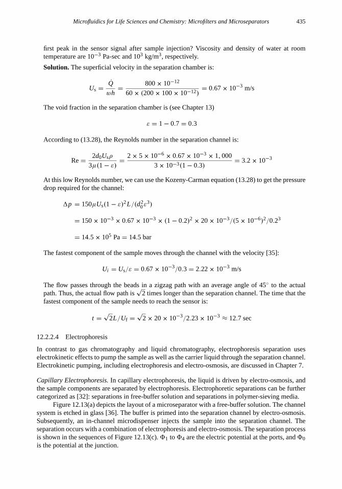
Microfluidics for Life Sciences and Chemistry: Microfilters and Microseparators 435
first peak in the sensor signal after sample injection? Viscosity and density of water at roomtemperature are 10−3 Pa-sec and 103 kg/m3, respectively.
Solution. The superficial velocity in the separation chamber is:
Us =Q
wh=
800× 10−12
60× (200× 100× 10−12)= 0.67× 10⁻³ m/s
The void fraction in the separation chamber is (see Chapter 13)
ε = 1 − 0.7 = 0.3
According to (13.28), the Reynolds number in the separation channel is:
Re=2d0Usρ
3µ(1 − ε)=
2 × 5 × 10−6× 0.67× 10−3
× 1,000
3 × 10⁻³(1 − 0.3)= 3.2 × 10⁻³
At this low Reynolds number, we can use the Kozeny-Carman equation (13.28) to get the pressuredrop required for the channel:
1p = 150µUs(1 − ε)2L/(d20ε
3)
= 150× 10−3× 0.67× 10−3
× (1 − 0.2)2 × 20× 10−3/(5 × 10−6)2/0.23
= 14.5 × 10⁵ Pa= 14.5 bar
The fastest component of the sample moves through the channel with the velocity [35]:
Ui = Us/ε = 0.67× 10⁻³/0.3 = 2.22× 10⁻³ m/s
The flow passes through the beads in a zigzag path with an average angle of 45◦ to the actualpath. Thus, the actual flow path is
√2 times longer than the separation channel. The time that the
fastest component of the sample needs to reach the sensor is:
t =√
2L/Uf =√
2 × 20× 10−3/2.23× 10−3≈ 12.7 sec
12.2.2.4 Electrophoresis
In contrast to gas chromatography and liquid chromatography, electrophoresis separation useselectrokinetic effects to pump the sample as well as the carrier liquid through the separation channel.Electrokinetic pumping, including electrophoresis and electro-osmosis, are discussed in Chapter 7.
Capillary Electrophoresis.In capillary electrophoresis, the liquid is driven by electro-osmosis, andthe sample components are separated by electrophoresis. Electrophoretic separations can be furthercategorized as [32]: separations in free-buffer solution and separations in polymer-sieving media.
Figure 12.13(a) depicts the layout of a microseparator with a free-buffer solution. The channelsystem is etched in glass [36]. The buffer is primed into the separation channel by electro-osmosis.Subsequently, an in-channel microdispenser injects the sample into the separation channel. Theseparation occurs with a combination of electrophoresis and electro-osmosis. The separation processis shown in the sequences of Figure 12.13(c).81 to84 are the electric potential at the ports, and80is the potential at the junction.

436 Fundamentals and Applications of Microfluidics
Sample inlet
Sample outlet
In-channel dispenser
Separation channel(a) (b)
(c) Sample injection Sample dispensing Separation
�1>0
�2=0
�0�3>�0
�4>�0
�1<�0
�2<�0
�3>0 �4=0
�1<�0
�2<�0
�3>0 �4=0
Figure 12.13 Concept of capillary electrophoresis with free buffer solution: (a, b) separation devices; and (c) separationconcept.
The dispensed sample volume in the device shown in Figure 12.13(b) has the minimumvolume defined by the cross area of the sample channel and the separation channel [37, 38]. Thedevice is fabricated in silicon by wet etching. A cover plate is anodically bonded to the siliconchip. Since silicon is a good conductor, the channel surface should be covered with a silicon oxideinsulator. However, the breakdown field strength of silicon oxide limits the range of applied voltage.Due to this problem, glass is a better material for capillary electrophoresis chips [39]. Shallowchannels of 12-µm depth and 50-µm width can be etched in glass. The shallow design allows abetter heat dissipation. The channels are covered by a second glass plate by direct bonding at 620◦C.
Polymer solutions are divided into three types based on their concentration: dilute, semidilute,and entangled. In a dilute solution, the molecules are isolated. With the high concentration of anentangled solution, the polymer molecules are close and interact with each other [40]. In a sievingmedia, the mobility of a molecule is inversely proportional to its length. Therefore, larger moleculeswill move more slowly if an electrical field is applied across the sieving media.
The device described in [41] uses polyacrylamide gel as a sieving media. Phosphorothioateoligonucleotides with 10 to 25 bases are successfully separated. A relatively high field strength of2,300 V/cm is used.
The separation of long double-stranded DNAs was first demonstrated in [42]. An entangledsolution of hydroxyethylcellulose is the sieving media. The separation channel is 3.5 cm long. Sepa-ration is achieved after 120 seconds. Nowadays, polymer solutions virtually replace polyacrylamideas sieving media.
Free-Flow Electrophoresis.Free-flow electrophoresis is a two-dimensional separation method,which combines hydrodynamic flow with electrophoresis. Figure 12.14 describes this concept. Thesample is continuously injected into a carrier flow. The carrier flow and the separation electricalfield are perpendicular to each other. Because of different mobility, the components follow differenttrajectories in the flow channel.
The free-flow electrophoresis device reported by Reymond et al. [43] is made of silicon. Aseparation channel of 50µm in depth is etched in silicon. The 100-nm silicon oxide and 600-nm sil-icon nitride are deposited on the channel surface. The breakdown voltage of this layer is about 200Vto 300V. A syringe pump drives the carrier flow, and the electrophoresis separation occurs under

Microfluidics for Life Sciences and Chemistry: Microfilters and Microseparators 437
Electrophoresis flow
Sample inlet
Pressure-driven carrier flow
Trajectory of
the separated component
Figure 12.14 Concept of free flow electrophoresis with pressure-driven carrier flow.
the applied voltage between the channel sides. This device is able to separate different biochemicalobjects such as DNAs, proteins, viruses, bacteria, and cells. Zhang and Manz [44] fabricated theseparation channel in PDMS. The separation area consists of an array of interconnecting channels.The small channels increase the electric resistance of the system, and thus allow the use of highvoltages.
12.2.2.5 Other Separation Concepts
A sieving structure with pore size or gap size on the order of nanometers can replace the gel matrixneeded in electrophoretic separation. Such a structure can be categorized asnanofilter. Turner et al.[45] reported a nanofiler consisting of 100-nm pillars, which are arranged at distances from 150 nmto 200 nm. These nanopillars were fabricated with electron beam lithography. Although the sievingstructures are in the nanoscale, the gap is still too large compared to molecular size, and thus onlysuitable for coarse separation. The separation of relatively large DNA molecules of 7.2 and 43 kbphave been reported.
Nanostructures similar to the gap filters described in Section 12.1.2.2 can be used for sep-aration purposes. The gaps work as the so-called entropic traps. The separation channel consistsof sections with different gap sizes [Figure 12.15(a)] [46]. If an electric field is applied across theseparation channel, DNA molecules move toward the anode under the electrophoretic force. If thegap is much smaller than the radius of gyration of the DNA molecule, the DNA is trapped. Themobility differences of the DNA molecules are determined by their size and the gap size. Han et al.[46] reported a separation channel with a width of 30µm, a length of 15 mm, and alternating depthsof from 1.5 to 3µm and from 75 to 100 nm. The device was able to separate DNA molecules withlengths ranging from 5 to 160 kbp. Nanopores such as ion channels formed byα-hemolysin havea size of 5 nm [47]. This size allows the passage of only one DNA fragment at a time. The lengthof the DNA fragment corresponds to the passage time, which can be measured by monitoring thecurrent through the ion channel. Filters with nanopores can be fabricated with ion beam machining.Li et al. reported the fabrication of nanopores with sizes ranging from 1.8 to 5 nm [48]. In a 1 M KClsolution, with a voltage of 120 mV across a 5-nm pore, an ion current of 1.66 pA was measured. A500-bp DNA fragment moving through the pore causes a drop of current by 88%.
Brownian ratchets are structures that selectively block the diffusion of particles in one direc-tion. Huang et al. placed a rachet array inside a microchannel. The different diffusion coefficientsseparate the particles across the channel width. Separation based on Brownian ratchets is similar

438 Fundamentals and Applications of Microfluidics
DNA
DNA
DNA
(a)
(b)
Flo
w
Rachet structure
start
Molecule with higher
diffusion coefficient
Molecule with lower
diffusion coefficient
Diffusion
Figure 12.15 Other separation concepts: (a) separation with entropic traps; and (b) separation with Brownian rachets.
to free-flow electrophoresis depicted in Figure 12.14. The only difference is that, instead of elec-trophoresis, Brownian motion causes the separation [Figure 12.15(b)]. Due to the long residencetime, the flow should be driven at a very slow speed (e.g., on the order of 1µ/sec [49]). The drawbackof separation based on Brownian ratchets is the relatively long residence time, which may limit thepotential use of this concept.
The so-called asymmetric Brownian ratchet is another trapping concept that can be used forseparation. This concept utilizes anisotropic potential fields to trap DNA molecules. The device forthis concept consists of asymmetrically interdigitated electrodes [Figure 12.16]. If an electric field isapplied between the two electrodes, the molecules are trapped in the potential well near the positiveelectrode. When the potentials are removed, the molecules are allowed to diffuse away [50, 51].According to Section 10.1, smaller molecules have higher diffusion coefficients. Thus, smaller DNAmolecules move further by diffusion and are trapped in the next potential well when the electric fieldis applied again. Repeating this process separates the DNA molecules based on the combination ofdiffusion and potential traps. Hammond et al. [50] reported a device with electrodes separated by0.1 µm. The electrode pair repeats along the transport axis every 1µm. Separation of small 24-bpDNA fragments from 25-bp fragments was achieved with 12,000 cycles in only 5.4 seconds.
12.3 SUMMARY
This chapter discusses two types of separation devices: microfilters and microseparators. Membranefilters fabricated by conventional microtechnologies (Chapter 3) are limited by the resolution ofthe lithography process or by the wavelength of the exposure light. Submicron filter pores can beachieved by using interference pattern of lasers [5]. However, the resulting pore size is still on theorder of hundreds of nanometers. As polymeric micromachining emerges as a versatile technologyfor microfluidics, polymers can be designed to work as the filtering matrix. Pore sizes in themolecular range can be achieved. One of the most significant applications of a polymer membranefilter is the microfuel cell, which will be discussed in the next chapter. Gap filters are an alternative
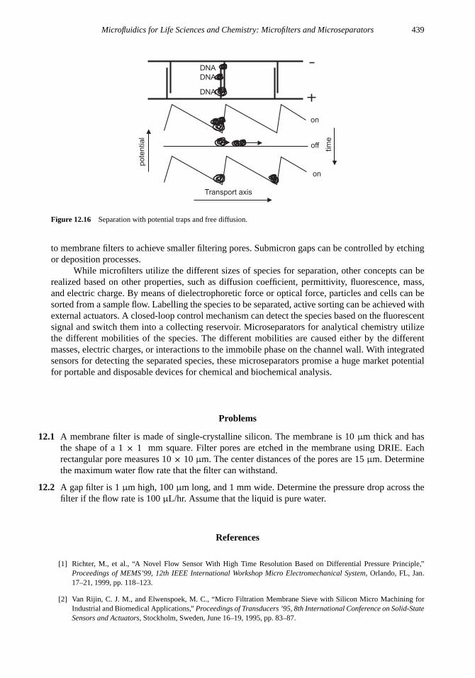
Microfluidics for Life Sciences and Chemistry: Microfilters and Microseparators 439
DNA
DNA
DNA
on
on
off
tim
e
Transport axis
pote
ntial
Figure 12.16 Separation with potential traps and free diffusion.
to membrane filters to achieve smaller filtering pores. Submicron gaps can be controlled by etchingor deposition processes.
While microfilters utilize the different sizes of species for separation, other concepts can berealized based on other properties, such as diffusion coefficient, permittivity, fluorescence, mass,and electric charge. By means of dielectrophoretic force or optical force, particles and cells can besorted from a sample flow. Labelling the species to be separated, active sorting can be achieved withexternal actuators. A closed-loop control mechanism can detect the species based on the fluorescentsignal and switch them into a collecting reservoir. Microseparators for analytical chemistry utilizethe different mobilities of the species. The different mobilities are caused either by the differentmasses, electric charges, or interactions to the immobile phase on the channel wall. With integratedsensors for detecting the separated species, these microseparators promise a huge market potentialfor portable and disposable devices for chemical and biochemical analysis.
Problems
12.1 A membrane filter is made of single-crystalline silicon. The membrane is 10µm thick and hasthe shape of a 1× 1 mm square. Filter pores are etched in the membrane using DRIE. Eachrectangular pore measures 10× 10 µm. The center distances of the pores are 15µm. Determinethe maximum water flow rate that the filter can withstand.
12.2 A gap filter is 1µm high, 100µm long, and 1 mm wide. Determine the pressure drop across thefilter if the flow rate is 100µL/hr. Assume that the liquid is pure water.
References
[1] Richter, M., et al., “A Novel Flow Sensor With High Time Resolution Based on Differential Pressure Principle,”Proceedings of MEMS’99, 12th IEEE International Workshop Micro Electromechanical System, Orlando, FL, Jan.17–21, 1999, pp. 118–123.
[2] Van Rijin, C. J. M., and Elwenspoek, M. C., “Micro Filtration Membrane Sieve with Silicon Micro Machining forIndustrial and Biomedical Applications,”Proceedings of Transducers ’95, 8th International Conference on Solid-StateSensors and Actuators, Stockholm, Sweden, June 16–19, 1995, pp. 83–87.

440 Fundamentals and Applications of Microfluidics
[3] Farooqui, M. M., and Evans, A. G. R., “Microfabrication of Sub Micron Nozzles in Silicon Nitride,”Proceedings ofMEMS’92, 5th IEEE International Workshop Micro Electromechanical System, Travemuende, Germany, Jan. 25–28,1992, pp. 150–153.
[4] Yang, X., et al., “Micromachined Membrane Particle Filters,”Sensors and Actuators A, Vol. 73, 1999, pp. 184–191.
[5] Kuiper, S., “Fabrication of Microsieves with Sub-Micron Pore Size by Laser Interference Lithography,”Journal ofMicromechanics and Microengineering, Vol. 11, No. 1, 2001, pp. 33–37.
[6] Caton, P. F., and White, R. M., “MEMS Microfilter with Acoustic Cleaning,”Proceedings of MEMS’01, 14th IEEEInternational Workshop Micro Electromechanical System, Interlaken, Switzerland, Jan. 21–25, 2001, pp. 479–482.
[7] Brody, J. P., et al., “A Planar Microfabricated Fluid Filter,”Proceedings of Transducers ’95, 8th InternationalConference on Solid-State Sensors and Actuators, Stockholm, Sweden, June 16–19, 1995, pp. 779–782.
[8] Desai, T. A., et al., “Nanopore Technology for Biomedical Applications,”Journal of Biomedical Microdevices, Vol. 2,No. 1, 1999, pp. 11–40.
[9] Kittilsland, G., et al., “A Sub-Micron Particle Filter in Silicon,”Sensors and Actuators A, Vol. 23, No. 1–3, 1990,pp. 904–907.
[10] Tu, J. K., et al., “Filtration of Sub-100nm Particles Using a Bulk-Micromachined, Direct-Bonded Silicon Filter,”Journal of Biomedical Microdevices, Vol. 1, No. 2, 1999, pp. 113–119.
[11] Kamholz, A. E., et al., “Quantitative Analysis of Molecular Interaction in a Microfluidic Channel: The T-Sensors,”Analytical Chemistry, Vol. 71, No. 23, 1999, pp. 5340–5347.
[12] Fiedler, S., et al., “Dielectrophoretic Sorting of Particles and Cells in a Microsystem,”Analytical Chemistry, Vol. 70,1998, pp. 1909–1915.
[13] Nguyen, N. T., and White, R. M., “Design and Optimization of an Ultrasonic Flexural Plate Wave Micropump UsingNumerical Simulation,”Sensors and Actuators A, Vol. 77, 1999, pp. 229–236.
[14] Nguyen, N. T., et al., “Integrated flow sensor for in situ measurement and control of acoustic streaming in flexuralplate wave micropumps,”Sensors and Actuators A, Vol. 79, 2000, pp. 115–121.
[15] Meng, A. H., Nguyen, N. T., and White, R. M., “Focused Flow Micropump Using Ultrasonic Flexural Plate Waves,”Biomedical Microdevices, Vol. 2, 2000, pp. 169–174.
[16] Marmottant, P., and Hilgenfeldt, S., “Controlled Vesicle Deformation and Lysis by Single Oscillating Bubbles,”Nature, Vol. 423, 2003, pp. 153–155.
[17] Groschl, M., “Ultrasonic Separation of Suspended Particles. Part I. Fundamentals,”Acustica, Vol. 3, 1998, pp. 432–447.
[18] Harris, N. R., et al. “A Silicon Microfluidic Ultrasonic Separator,”Sensors and Actuators B, Vol. 95, 2003, pp. 425–434.
[19] Hatch, G. P., and Stelter, R. E., “Magnetic Design Considerations for Devices and Particles Used for Biological High-Gradient Magnetic Separation (HGMS) Systems,”Journal of Magnetism and Magnetic Materials, Vol. 225, 2001,pp. 262–276.
[20] Pamme, N., and Manz, A., “On-Chip Free-Flow Magnetophoresis: Continous Flow Separation of Magnetic Particlesand Agglomerates,”Analytical Chemistry, Vol. 76, 2004, pp. 7250–7256.
[21] Furdui, V. I., Kariuki, and J. K., Harrison, D. J., “Microfabricated Electrolysis Pump System for Isolating Rare Cellsin Blood,” Journal of Micromechanics and Microengineering, Vol. 76, 2004, pp. 7250–7256.
[22] Ashkin, A., et al., “Observation of a Single-Beam Gradient Force Optical Trap for Dielectric Particles,”Optical Letters,Vol. 11, 1986, pp. 288–290.
[23] MacDonald, M. P., Spalding, G. C., and Dholakia, K., “Microfluidic Sorting in an Optical Lattice,”Nature, Vol. 426,2003, pp. 421–424.

Microfluidics for Life Sciences and Chemistry: Microfilters and Microseparators 441
[24] Gluckstad, J., “Sorting Particles with Light,”Nature Materials, Vol. 3, 2003, pp. 9–10.
[25] Kruger, J. et al. “Development of a Microfluidic Device for Fluorescence Activated Cell Sorting,”Journal ofMicromechanics and Microengineering, Vol. 12, 2002, pp. 486–494.
[26] Wolff, A., et al., “Integrating Advanced Functionality in a Microfabricated High-Throughput Fluorescent-ActivatedCell Sorter,”Lab Chip, Vol. 3, 2003, pp. 22–27.
[27] Lin, C. H., and Lee, G. B., “Micromachined Flow Cytometers with Embedded Etched Optic Fibers for OpticalDetection,”Journal of Micromechanics and Microengineering, Vol. 13, 2003, pp. 447–453.
[28] Lee, G. B., et al., “Micromachined Pre-Focused 1xN Flow Switches for Continous Sample Injection,”Journal ofMicromechanics and Microengineering, Vol. 11, 2001, pp. 567–573.
[29] Dittrich, P. S. and Schwille, P., “An Integrated Microfluidic System for Reaction, High-Sensitivity Detection, andSorting of Fluorescent Cells and Particles,”Analytical Chemistry, Vol. 75, 2003, pp. 5767–5774.
[30] Lu, H., et al., “A Microfabricated Device for Subcellular Organelle Sorting,”Analytical Chemistry, Vol. 76, 2004,pp. 5705–5712.
[31] Terry, S. C., Jerman, J. H., and Angell, J. B., “A Gas Chromatographic Air Analyzer Fabricated on a Silicon Wafer,”IEEE Transactions on Electron Devices, Vol. 26, 1979, pp. 1880–1886.
[32] Giddings, J. C.,Unified Separation Science, New York: Wiley, 1991.
[33] Manz, A., et al., “Design of an Open-Tubular Column Liquid Chromatograph Using Silicon Chip Technology,”Sensors and Actuators B, Vol. 1, 1990, pp. 249–255.
[34] Ocvirk, G., et al., “Integration of a Micro Liquid Chromatograph onto a Silicon Chip,”Proceedings of Transducers ’95,8th International Conference on Solid-State Sensors and Actuators, Stockholm, Sweden, June 16-19, 1995, pp. 756–759.
[35] Wilkes, J. O., and Bike, S. G.Fluid Mechanics for Chemical Engineers, Upper Saddle River, NJ: Prentice Hall, 1998.
[36] Effenhauser, C. S., “Integrated Chip-Based Microcolumn Separation Systems,” inMicrosystem Technology in Chem-istry and Life Sciences, A. Manz and H. Becker (eds.), New York: Springer, 1999, pp. 51–82.
[37] Harrison, D. J., Manz, A., and Glavina, P. G., “Electroosmotic Pumping Within a Chemical Sensor System Integratedon Silicon,”Proceedings of Transducers ’91, 6th International Conference on Solid-State Sensors and Actuators, SanFrancisco, CA, June 23–27, 1991, pp. 792–795.
[38] Manz, A., et al., “Integrated Electroosmotic Pumps and Flow Manifolds for Total Chemical Analysis Systems,”Proceedings of Transducers ’91, 6th International Conference on Solid-State Sensors and Actuators, San Francisco,CA, June 23–27, 1991, pp. 939–941.
[39] Harrison, D. J., et al., “Micromachining a Miniaturized Capillary Electrophoresis-Based Chemical Analysis Systemon a Chip,”Science, Vol. 261, 1993, pp. 895–897.
[40] Grossman, P. D., and Soane, D. S., “Experimental and Theoretical Studies of DNA Separations by CapillaryElectrophoresis in Entangled Polymer Solutions,”Biopolymers, Vol. 31, 1991, pp. 1221–1228.
[41] Effenhauser, C. S., et al., “High-Speed Separation of Antisense Oligonucleotides on a Micromachined CapillaryElectrophoresis Device,”Analytical Chemistry, Vol. 66, 1994, pp. 2949–2953.
[42] Wooly, A. T., and Mathies, R. A., “Ultra-High-Speed DNA Sequencing Using Capillary Electrophoresis Chips,”Analytical Chemistry, Vol. 67, 1995, pp. 3676–3680.
[43] Raymond, D. E., Manz, A., and Widmer, H. M., “Continuous Separation of High Molecular Weight Compounds Usinga Microliter Volume Free-Flow Electrophoresis Microstructure,”Analytical Chemistry, Vol. 68, 1996, pp. 2515–2522.
[44] Zhang, C. X. and Manz, A., “High-Speed Free-Flow Electrophoresis on Chip,”Analytical Chemistry, Vol. 75, 2003,pp. 5759–5766.

442 Fundamentals and Applications of Microfluidics
[45] Turner, S. W., et al., “Monolithic Nanofluid Sieving Structures for DNA Manipulations,”Journal of Vacuum Scienceand Technology, Vol. 16, 1998, pp. 3821–3824.
[46] Han, J., and Craighead, H. G., “Separation of Long DNA Molecules in a Microfabricated Entropic Trap Array,”Science, Vol. 288, 2000, pp. 1026–1029.
[47] Song, L. Z., et al., “Structure of Staphylococcal Alpha-Hemalysisn, a Hepatametric Transmembrane Pore,”Science,Vol. 274, 1996, pp. 1859–1866.
[48] Li, J., et al., “Ion Beam Sculpting at Nanometer Length Scales,”Nature, Vol. 412, 2001, pp. 166–169.
[49] Huang, L. R., et al., “Tilted Brownian Rachet for DNA Analysis,”Analytical Chemistry, Vol. 75, 2003, pp. 6963–6967.
[50] Hammond, R. W., et al., “Differential Transport of DNA by a Rectified Brownian Motion Device,”Electrophoresis,Vol. 21, 2000, pp. 74–80.
[51] Bader, J. S., et al., “A Brownian-Ratched DNA Pump with Applications to a Single-Nucleotide PolymorhismGenotyping,”Applied Physics A, Vol. 75, 2002, pp. 275–278.

Chapter 13
Microfluidics for Life Sciences and Chemistry:Microreactors
Micromachining technology offers unique opportunities for chemical analysis as well as chemicalproduction. The miniaturization of reactors and the integration of different components providenew capabilities and functionality, which exceed conventional counterparts. Microreactors offerpotentially high throughput and low-cost mass production. Since the requirements and workingconditions of microreactors for applications in life sciences are different than those in industrialapplications, this chapter considers each type of application accordingly. For industrial applications,the advantages of microreactors can be seen in four main aspects: functionality, safety, cost, andscientific merit.
Functionality.The functionality gains of microreactors are small thermal inertia, high gra-dients of physical properties, uniform temperature, short residence time, and high surface-volumeratio. The small size of the system leads to small thermal inertia of reactors. Since temperature isone of the most important reaction parameters, direct and precise temperature control in microreac-tors is easier and faster than in conventional reactors. The small size also leads to higher heat andmass transfer rates, which allow reactions carried out under more aggressive conditions than canbe achieved in conventional reactors. Furthermore, the high heat transfer rates allow reactions tobe performed under more uniform temperature conditions [1]. The small size also results in shorterresidence time in reactors. Unstable intermediate products can be transferred quickly to the next pro-cess. These characteristics open up new reaction pathways inaccessible for conventional reactions.According to scaling laws, microreactors offer a large surface-to-volume ratio, which leads to theeffective suppression of homogeneous side reactions in heterogeneously catalyzed gas phase reac-tions. Large free surfaces are strong sinks for radical species, which are required for homogeneousreactions. In addition, the reactions become safe because of the suppression of flames and explosions[2], due to the large ratio between surface heat losses and heat generation.
Safety.Besides the above-mentioned possibility of carrying out reactions without flames andexplosions, the small reactor size also leads to a potentially small quantity of chemicals releasedaccidentally, which does not lead to large-scale hazards and can be contained easily. The possibilityof sensor integration increases the safety of microreactors. Failed reactors can be detected, isolated,and replaced. The whole replacement process can be carried out automatically with an array ofreactors that are connected redundantly [1].
Cost. Rapid screening and high throughput make microreactors more efficient than theircounterparts, and that, in turn, makes microreactors cost-effective. The small volume of requiredreagents also minimizes the amount of expensive reagents. Because microreactors can be fabricatedin batch cheaply, numbering-up production can be carried out by replication of reactor units.Numbering-up makes the construction of technical plants less time-consuming because lab-scale
443

444 Fundamentals and Applications of Microfluidics
results can be transferred directly in commercial production. This aspect is particularly advantageousfor fine chemical and pharmaceutical industries with small production amounts per year [1]. Theflexibility of the microreactor concept is enormous, because only the number of production unitsneeds to be changed to fit the required production capacity.
Scientific Merit.Fluid flows in microreactors are of laminar regime, which is well studied andcan be handled by most CFD tools. For submicron structures, the flow can enter the molecular regimeand require new computational models. In most practical cases, the laminar model is sufficient fordesigning microreactors.
13.1 DESIGN CONSIDERATIONS
13.1.1 Specification Bases for Microreactors
Many microreactors are working on a continuous-flow basis. On the one hand, the reagents shouldhave enough time to react. On the other hand, the mean residence time should not be too long toaffect the throughput rate of the reactors. The meanresidence timein a reactor is defined by thetypical channel lengthL and the average velocityU :
τresidence=L
U(13.1)
Thereaction timeis determined by characteristic time of the reaction. For heterogeneous reactions,the characteristic reaction time is:
τreaction=D2
h
4DSh(13.2)
if the reaction is determined by diffusion, and:
τreaction=Dh
4ks(13.3)
if the reaction is determined by the reaction rate. For homogenous reaction, the characteristicreaction time is:
τreaction=1
kv. (13.4)
In the above equations,Dh, D, Sh,ks, andkv are the hydraulic diameter, the diffusion coefficient,the Sherwood number, and the reaction rates for surface and volume, respectively [3]. Thereactionrate is the flux of the product generated from the reaction. Microreactors can achieve reaction rateson the order of 10−6 mol/s-m2 [4].
The Sherwood number represents the ratio between overall mass transfer and diffusion:
Sh=kT Dh
D(13.5)
whereKT is the mass transfer coefficient, andD is the diffusion coefficient. Decreasing the channelsize may reduce the characteristic reaction time (13.2 and 13.3), or not at all (13.4). However,for a fixed throughput decreasing the channel size also means an increase of two orders in themean velocityU or a decrease of two orders in the mean residence timeτresidence∝ D2
h. Thus, inorder to match the required throughput with the reaction time, parallel reaction channels should beconsidered in the design. The parallel channels also help to keep the total pressure drop across thereactor constant.

Microfluidics for Life Sciences and Chemistry: Microreactors 445
As mentioned above, one of the advantages of microreactors is safety. Due to the highersurface-to-volume ratio, heat transfer rate is improved and sudden temperature rise can be avoided.Thus, chain reactions and thermal explosions can be avoided. The characteristictime of heat transferis estimated as [3]:
τthermal=ρcph2
4κNu, (13.6)
whereρ, cp, andκ are the density, heat capacity, and thermal conductivity of the fluid in the reactor,respectively. The Nusselt number (Nu) characterizes the heat transfer to the reactor walls:
Nu =hDh
κ(13.7)
whereh is the heat transfer coefficient. In order to prevent thermal explosion, the reaction timeshould be shorter than the characteristic time of heat transferτreaction� τthermal. Reaction tempera-ture determines the activation energy of a reaction. In microreactors, some reactions can be carriedout at ambient temperature rather than formerly at cryogenic conditions [5].
It is ideal for a reactor to yield a maximum amount of product in the smallest space and in theshortest time. The performance indication for a microreactor is therefore thespace-time yield:
STY =n
Vreactorτresidence(13.8)
wheren (mol) is the amount of the product, andVreactor is the volume of the reactor. Compared tothe macroscopic counterparts, high space-time yield can be expected from microreactors due to theirsmall volume and a shorter residence time. Space-time yields, on the order of 104 to 105 mol/h-m3
are typical for microreactors. This space-time yield is about three orders of magnitude higher thanconventional reactors [5].
13.1.2 Miniaturization of Chemical Processes
Reducing the size of chemical processes leads to a larger surface-to-volume ratio or the so-called“cube-square” law. The dominant surface effects are of advantage in reactions with catalysts ormultiple phases. Miniaturization also reduces the process path, and increases concentration as well astemperature gradients. Depending on the reaction, microreactors can be divided intoheterogeneousandhomogeneoustypes. Heterogeneous reactors involve two different reagent phases. The chemicalreactions occur at the interface of these two phases. In homogeneous reactors, the reactionstake place in a single phase, and good mixing of reagents is required. In microreactors, somehomogeneous reactions may turn into heterogeneous reactions because of the extremely largesurface-to-volume ratio.
Reducing the size further to microns and submicrons scale may not be advantageous forindustrial applications. For applications in life sciences and chemical analysis, the microreactorsare often disposable; thus, long-term behavior is not a concern while designing these reactors.In contrast, fouling and blocking of small channels could be a serious problem for industrialapplications. Furthermore, the small size leads to a shorter residence time, which should bematched with the required reaction time [6]. Heat removal and supply is another important issuefor microreactors. Elements such as heaters and heat exchangers may need to be integrated with themicroreactor.
For applications in life sciences, miniaturization allows fast heat supply and removal fromthe reactor. The fast temperature change allows a short thermal cycling period in reactions suchas polymerase chain reaction (PCR). Furthermore, the small size allows a more homogeneoustemperature distribution in the reactor, and thus increases the efficiency of the reaction. However,

446 Fundamentals and Applications of Microfluidics
miniaturization and the consequent high surface-to-volume ratio makes the surface of the reactionchamber one of the key parameters in the design. In contrast to industrial applications with acontinuous-flow system, microreactors for life sciences are often a closed system. The volume of theliquid in the reaction chamber could be on the order of picoliters. As already discussed in Section1.1.1, the total number of molecules available for the reaction also decreases with the small volume.While in macroscale, the reagent molecules in the chamber are numerous enough for the reaction,they could bind to the surface in microscale and inhibit the reaction. Native silicon and siliconnitride, for instance inhibit PCR in the microscale.
The small volume confined in the reaction chamber also poses further problems in fluidhandling. In practical applications, the sample liquids need to be prepared, and the reaction resultsneed to be analyzed. Thus, transferring a liquid amount on the order of picoliters between equipmentand devices is an almost impossible task. Therefore, designing a microreactor for application in lifesciences is often linked to designing integrated sample preconditioning devices and analysis devices.Such a system is complex and requires a more careful design consideration.
13.1.3 Functional Elements of a Microreactor
Depending on the type of reaction, microreactors consist of the following elements:
• Microchannels;
• Functional elements for thermal management: heaters, temperature sensors, heat sinks, and heatexchanger;
• Catalyst structures: porous surfaces, catalyst membranes, and catalyst layers;
• Sensing elements: chemical sensors;
• Mixing elements: micromixers.
The designs and operation concepts of different micromixer types were discussed in Chapter 10.The following sections only discuss the remaining four types: microchannels, functional elementsfor thermal management, catalyst structures, and sensing elements.
13.1.3.1 Microchannels
The most basic elements of a microreactor are microchannels and microreservoirs. Microchannelsare used for transport of reagents, or work directly as reactors. The fabrication of microchannelsbased on different technologies and materials was discussed in Chapter 3. From the analysis of thecharacteristic times in the previous section, the basic steps for designing reactor microchannels are:
• Determining the channel size according to the characteristic reaction time and the characteristictime of heat transfer;
• Determining the required residence time based on the other characteristic times;
• Determining the channel length based on the residence time and the required flow velocity;
• Determining the number of the channels based on the required throughput.
When microchannels are used directly as the reactor and fast heat transfer is needed for thereaction, the size of channel cross section should allow a smaller characteristic time for heat transferthan for the reaction (τthermal < τreaction). In contrast, reactions with an explosion hazard shouldhave channel size, which prevents the chain reaction caused by the sudden rise of the temperature(τreaction� τthermal).

Microfluidics for Life Sciences and Chemistry: Microreactors 447
(a) (b) (c) (d) (e)
Figure 13.1 Reaction steps in a microreactor with catalyst support: (a) diffusion to catalyst surface; (b) diffusion in catalystpores; (c) catalyst reaction; (d) diffusion out of the pores; and (e) transport of reaction products into bulk solution.
With the known size of the channel cross section, the length of the channel is to be determinednext. According to (13.1), the length of the channel is calculated from the required residence timeand the mean velocityL = τresidenceU . While the residence time can be optimized from either thecharacteristic times for heat transferτthermal or reactionτreaction, the optimal mean velocityU maybe determined by the Peclet number to minimize the effect of axial dispersion (Section 10.1.3). Withthe known channel cross sectionA, and mean velocityU , both flow rate and pressure drop acrossa channel can be determined. Based on the required throughput or the required total pressure drop,the number of microchannels connected in parallel can be finally calculated.
13.1.3.2 Functional Elements for Thermal Management
Heaters and temperature sensors can be integrated directly in reactors for temperature control. Thisunique feature allows precise control of temperatures, which is crucial in applications such as PCRfor DNA amplification [7]. The design of temperature sensors is well researched, and solutions forintegrated thermal sensors are established [8]. Common temperature sensing concepts for microreac-tors are thermoresistive [7] and thermoelectric [9]. The relatively high thermal conductivity of silicon(157 Wm−1K−1) makes it a good heat conductor. However, cooling is a more difficult task thanheating. For fast thermal control, we cannot rely entirely on heat conduction and free convection.Controllable active cooling is necessary. Common solutions are thermoelectric heat pumps, such asPeltier elements or forced convection. Heat exchangers such as microchannels are fabricated in thesame process of reactors.
Integrated heat exchangers can both supply and remove heat to and from the reactor. Heattransfer coefficients on the order of 104 to 105 W/m2-K, and heating rates on the order of 106 K/s,can be achieved with microheat exchangers [10].
13.1.3.3 Catalyst Structures
Many reactions are carried out with catalyst support. The reaction rates in a reactor with catalystsupport are proportional to the total reacting surface available. A porous catalyst can increase thereacting surface area. Figure 13.1 describes the main five steps of these reactions [11].
In the first step, reagents diffuse from the bulk solution to the catalyst surface. The masstransfer between the bulk solution and the catalyst controls this step [Figure 13.1(a)]. In the secondstep, reagents diffuse into the catalyst pores. Diffusion controls this step [Figure 13.1(b)]. For smallpores and gaseous reagents, the interactions with the pore wall should be considered. In this case,the Knudsen diffusion coefficient can be used. In the third step, reagents undergo a heterogeneousreaction with the pore walls. The catalyst reaction happens here [Figure 13.1(c)]. In the fourth step,the reaction products diffuse back out of the pore. The process is again controlled by diffusion[Figure 13.1(d)]. In the final step, the products move out of the pore, back into the solution,and can be washed away by the continuous flow. Bulk mass transfer controls this step [Figure13.1(e)]. Assuming small pores compared to the characteristic size of the catalyst structure, transport

448 Fundamentals and Applications of Microfluidics
equations formulated for a porous catalyst layer can use effective transport coefficients (thermal,diffusion), which are determined by the coefficients of the solid phase and fluid phase.
Most reactors require a catalyst to accelerate the chemical reactions. The catalyst can beimplemented in microreactors in the form of packed beads, wires, thin film, or high surface areaporous support. While beads [12] and wires [2] are not compatible with batch fabrication, thin filmand porous surface catalysts can be integrated in the fabrication processes of microreactors. Thinfilm catalysts are deposited by CVD or PVD. Using these techniques, the thin film material is oftenlimited to metals and oxides. In order to increase the surface area, the thin film can be roughened bythermal activation. In contrast to CVD and PVD, wet preparation allows a wider range of catalysts.Using inkjet printing or microplotter [13], a catalyst can be placed precisely in the reactor chamber.
Splinter et al. [14] gave an example of a microreactor with porous silicon. The reactionchamber is comprised of 32 channels. Each channel has a cross section of 50× 250 µm. Thechannel wall is anodized in a solution of hydrofluoric acid and ethanol. The pore size and themorphology are determined by the current densities. The enzyme is immobilized onto the porouswall. In micromachined reactors, the porous surface can be made of silicon. The silicon surfaceundergoes an anodization in an electrolyte. The typical composition given in [15] is (50% weightconcentration; HF : ethanol = 1:1). A porous layer of 70µm needs 8 minutes and a current densityof 0.25 A/cm2. The pore sizes range from 4 to 8µm. The resulting surface-to-volume ratio isapproximately 108 m−1. The advantage of this method is the possibility of making semipermeablemembranes, which are often needed in microanalysis systems. Since silicon is not a catalyst formany reactions, the surface of the pores should be covered with an active layer, such as a palladiumthin film. In a microreactor, the mixed fluid should be placed next to the catalytic site. Efficientmixing and access to the catalytic site can lead to orders of magnitude enhancement in performance[1].
13.1.3.4 Sensing Elements
Integrated Sensors.In-situ sensing elements such as temperature sensors and chemical sensors canbe implemented in the same fabrication process. These chemical sensors are often based on electro-chemical methods. Different methods, such as amperometry, conductimetry, and potentiometry, canbe easily implemented with simple integrated microelectrodes [16].
Amperometry is based on the measurement of currents resulting from the oxidation as well asthe reduction reactions of analytes at electrodes. The current density at a microelectrode is [17]:
i = nF Dc∞
δ(13.9)
wheren is the number of electrons,F is the Faraday constant,D is the diffusion coefficient ofreacting species, andc∞ is the concentration in the bulk of solution. The diffusion layer thicknessδis time dependent:
δ =√πDt (13.10)
From (13.9) and (13.10), the current through an electrode areaA is:
I = nF Ac∞
√D
π t(13.11)
Equation (13.11) describes the time behavior of the electrode current after switching on the potential.Nonlinear effects at the edges of the microelectrodes with an radius ofr at a longer time can bedescribed as:
I = nF Ac∞(√
D
π t+
D
r
)(13.12)

Microfluidics for Life Sciences and Chemistry: Microreactors 449
In order to increase the sensing current and improve signal-to-noise ratio, an array of electrodes canbe used for the measurement.
Conductimetry detects the change in conductivity. This technique is suitable for small ions,which are difficult to be detected by other methods. Potentiometry measures voltages using inte-grated devices such as ion selective electrodes (ISE) or ion-sensitive field effect transistors (ISFET).These devices are independent from miniaturization and do not benefit the scaling laws.
Optical Methods.Compared to electrical elements, a transparent window for optical sensing issimpler and cheaper to implement. Designing a microreactor with glass or plastic automaticallyprovides optical access to the measurement location. Fluorescent detection has been widely used inbiochemical applications due to its high selectivity. Amino acids and some biochemically relevantspecies can be derivatized with a fluorescent tag. The evaluation is achieved with the method oflaserinduced fluorescence(LIF). The species emit fluoresced light if they are excited by a laser beam of ahigher wavelength. The source could be a blue argon-ion laser (λ = 488 nm) [18], a red laser diode(λ = 635 nm) [19], or a violet laser [20].
Detection based onoptical absorptiondetects the change in light intensity. The opticalabsorbanceAop can be determined based on the so-called Beer’s law:
Aop = εopcL (13.13)
whereεop is the molar absorptivity,c is the molar concentration, andL is the optical path. Themolar absorptivity depends on the wavelength; thus, a type of molecule can be detected basedon the absorption of its characteristic wavelength. Absorption measurements with wavelengthsranging from UV to visible (vis) spectrum is called UV-vis absorption spectroscopy. According to(13.13), miniaturization results in a short optical path and limits the sensitivity of this method. Thesensitivity-of-absorbance method can be improved with multireflection cells to increase the opticalpath [21].
Chemiluminescenceis another method that can be detected optically. Some chemical reactionsform fluorescent molecules in their excited state. The implementation of chemiluminescence isrelatively simple because no light source is required [22].
13.2 DESIGN EXAMPLES
13.2.1 Gas-Phase Reactors
13.2.1.1 Oxidation Reactors
Common oxidation reactions realized in microscale are oxidation of ammonia, oxidation of ethyleneto ethylene oxide, oxidation of 1-butene to maleic anhydride, oxidation of methanol to formalde-hyde, oxidation of propene to acrolein, oxidation of isoprene to citraconic anhydride, and oxidationof carbon monoxide to carbon dioxide. For a review of these different oxidation reactions and theirrealization in microreactors, readers may refer to [5].
Combustion.One of the most common gas reactions is oxidation reaction or combustion. Because ofthe high energy density, the combustion of hydrocarbon or hydrogen has a huge potential in energygeneration. An efficient microengine can be realized with a microcombustor, which is capable ofproducing 10W to 50W of electrical power by consuming only about 7g of jet fuel per hour [23].The main challenges for a microcombustor are [24]:
• Shorter residence time for mixing and combustion: While keeping the same mass flow rate perunit area, miniaturization leads to faster flow velocity and a shorter residence time. With the

450 Fundamentals and Applications of Microfluidics
Figure 13.2 Gas reactors (not to scale): (a) microcombustor; and (b) microengine concept. (After: [26])
geometry depicted in Figure 13.2 the residence time will approach the limit of characteristicchemical kinetic time scale for hydrocarbon-air reactions from 0.01 to 0.1 ms.
• Large heat losses: The large surface-to-volume ratio and the high temperature gradient lead toheat losses, which is a safety advantage for chemical reactions, as discussed above, but may posea problem for the flammability of the air/fuel mixture in a microcombustor. The ratio between thesurface heat loss rate and the heat generation rate of the combustion should not exceed an upperlimit. These ratio scales with the hydraulic diameter of the combustion chamberDh as [24]:
qloss
qin∝
1
D1.2h
(13.14)
Therefore, there is a critical hydraulic diameter. Below this value, the air/fuel mixture will not beignited.
• High temperature: Combustion temperatures between 1,200K and 1,700K require heat-resistantmaterials such as ceramics.
Based on the problems discussed above, the design considerations for a microcombustor are [24]:
• Increasing the size of the combustion chamber relative to the size of the device, to increaseresidence time;
• Premixing of air and fuel before joining the combustion chamber;
• Using special combustion concepts, such as lean burning of hydrogen [25] and catalytic hydro-carbon burning, using platinum or palladium as surface catalysts;
• Using a recirculation jacket, which recovers the heat losses to heat the incoming fuel mixture andallows the compressor discharging air to lower the wall temperatures.
The microcombustor depicted in Figure 13.2(a) is fabricated with deep reactive ion etching in siliconand fusion bonding of a six-wafer stack [26, 27]. Hydrogen combustion is successfully carried out in

Microfluidics for Life Sciences and Chemistry: Microreactors 451
O2 + 2H2
Si Glass
Figure 13.3 Microburner as a gas-phase reactor.
this microcombustor. A heating wire ignites the combustion reaction. An exit temperature of 1,600Kand an efficiency as high as 95% can be reached. Further development uses this microcombustor fora microengine [Figure 13.2(b)]. A rotating shaft connects the compressor and turbine. The electricgenerator is integrated with the compressor/shaft/turbine system.
The microburner in [28] is able to generate a 1× 3 mm flame. The burner uses a hydro-gen/oxygen mixture provided by an electrolysis cell. The microburner is a part of a microatomicemission flame spectrometer. The device is fabricated in glass and silicon using bulk micromachin-ing [Figure 13.3]. The same reaction for the nonflammable regime with a platinum wire as a catalystis reported in [29].
Example 13.1: Air-Fuel Ratio in a Microcombustor
A microcombustor uses hydrogen as fuel. The combustor consumes hydrogen with a mass flowrate of 8 mg/s. Assuming that hydrogen burns completely with 100% theoretical air, determinethe air-fuel ratio in the combustor.
Solution. For air, we assume a molar ratio of oxygen and nitrogen of 1:3.76. The stoichiometriccombustion reaction of hydrogen in air is:
H2 + 0.5(O2 + 3.76N2) → H2O + 1.88N2
That means we need:
0.5(1 + 3.76) = 2.38 mol
air for burning 1-mol hydrogen. The mole rate of hydrogen in the combustor is:
nH2= mH2
/MH2= 8 × 10⁻⁶/2 = 4 × 10⁻⁶ kmol/s
The mole rate of air is:
nair = 2.38nH2= 2.38× 4 × 10−6
= 9.52× 10⁻⁶ kmol/s
The mass flow rate of air is:
mair = nair × Mair = 9.52× 10−6× 28.97 = 275.8 × 10⁻⁶ kg/s
The air-fuel ratio for the microcombustor is:
mair/mH2 = 275.8 × 10⁻⁶/8 × 10−6= 34.5

452 Fundamentals and Applications of Microfluidics
Example 13.2: Residence Time in a Microcombustor
A combustor is designed as shown in Figure 13.2(a). The outer diameter is 10 mm, the innerdiameter is 5 mm, and the height is 1 mm. The operating pressure is 4 atm. Estimate the residencetime of the air-fuel mixture in the combustor.
Solution. Since the volume flow rate is proportional to the molar rate and the volume is inverselyproportional to the pressure (for ideal gas), the total volume flow rate of the mixture at the inlet ofthe combustor chamber is:
Qin = Qair ×1 + 0.5 × 4.76
0.5 × 4.78×
1
4= 97.92× 10⁻⁶ m3/s
Thus, the inlet velocity at the outer diameter is:
Uin =Qin
2πrouth=
97.92× 10⁻⁶
2π × 5 × 10−3 × 10−3= 3.12 m/s
The exhaust gas contains water vapor and remaining nitrogen; thus, the volume flow rate of theexit gas is:
Qexit = Qair ×1 + 1.88
0.5 × 4.76×
1
4= 83.44× 10⁻⁶ m3/s
The exit velocity at the inner diameter is:
Uexit =Qexit
2πr inh=
83.44× 10⁻⁶
2π × 2.5 × 10−3 × 10−3= 5.31 m/s
We assume a linear acceleration from inlet to exit, thus the relation between the pathway and theresidence time is:
Rout − Rin = aτ2/2 = (Uexit − Uin)/2
Rearrange the above equation. We get the estimated residence time of:
τ =2(Rout − Rin)
Uexit − Uin=
2 × (5 − 2.5)× 10−3
5.31− 3.12= 2.28× 10⁻³ sec= 2.28 ms
Example 13.3: Total Energy Released from a Microcombustor
If air and hydrogen enter the combustor at 25◦C and 1 atm, the exhaust gas has an exit temperatureof 1,227◦C. Determine the heat rate released from the combustion. The related thermodynamicparameters are given in the following table. For further reading on the fundamentals of thermo-dynamics, see [30].
Enthalpy of formation of H2, N2, O2
(h0
f
)H2
,(h0
f
)N2
,(h0
f
)O2
0
Enthalpy of formation of H2O(h0
f
)H2O
−241,820 kJ/kmol
Enthalpy of water vapor at 1,227◦C hH2O(1,227◦C) 57,999 kJ/kmolEnthalpy of water vapor at 25◦C hH2O(25◦C) 9,904 kJ/kmolEnthalpy of nitrogen at 1,227◦C hN2(1,227◦C) 57,999 kJ/kmol

Microfluidics for Life Sciences and Chemistry: Microreactors 453
Solution. The heat rate released per mole flow rate is determined by the enthalpy differencebetween the combustion product and combustion reactants:
q/nH2 = hp − hr
Since the enthalpy of formation of the reactants (H2, N2, O2) is zero, and they enter the combustorat reference state (25◦C, 1 atm), the enthalpy of the reactants is zero. Thus, the above equationbecomes:
q/nH2 = hp =
(h0
f +1h)
H2O+ 1.88
(h0
f +1h)
N2
= −241,820+ (57,999− 9,904)+ 1.88(0 + 47,073− 8,669)
= −121,525.48 kJ/mol
The negative sign means that the system rejects heat. With the mole flow rate from Example 13.1,the total heat rate released from the microcombustor is:
Q = 4 × 10−6× 121,525.48 = 0.486 kW= 486W
Example 13.4: Designing a Microengine
The above microcombustor is used in a microengine. The microengine is a gas turbine enginethat follows an air-standard Brayton cycle. Determine the work developed by the turbine, the heatloss of the combustor, and the efficiency of the engine. The related thermodynamic parametersare given in the following table.
Temperature (K) Enthalpy h (kJ/kg) Relative Pressure pr
295 295.17 1.2311300 300.19 1.3860440 441.61 5.332450 451.80 5.7751,060 1,114.86 143.91,080 1,137.89 155.21,500 1,635.97 601.9
Solution. The following figure summarizes the schematic and the temperature-entropy (T-s)diagram of the cycle. We use the air-standard analysis for the microengine.

454 Fundamentals and Applications of Microfluidics
The state points of the cycle are:
• State 1: T1 = 298K→ h1 = 298.182 kJ/kg,pr1 = 1.35432
• State 2:The compression process is isentropic; thus, the relative pressure is:
pr2 = (p2/p1)pr1 = (4/1)× 1.35432= 5.4173
Interpolating from the property table, we get:T2 = 442K,h2 = 443.572 kJ/kg
• State 3: T3 = 1,500K→ h3 = 1,635.97 kJ/kg,pr3 = 601.9
• State 4:The process across the turbine is isentropic; thus, the relative pressure is:
pr4 = (p4/p3)pr3 = (1/4)× 601.9 = 150.475
Interpolating from the property table, we get:T4 = 1,066K,h2 = 1,128.26 kJ/kg
The calculation is based on the mass flow rate of air from Example 13.2. The work developed bythe turbine is:
Wt = mair(h3 − h4) = 275.8 × 10−6× (1,635.97− 1,128.26) = 0.140 kW= 140W
The work consumed by the compressor is:
Wc = mair(h2 − h1) = 275.8 × 10−6× (443.571− 298.182) = 0.040 kW= 40W
The heat absorbed from the combustor is:
qin = mair(h3 − h2) = 275.8 × 10−6× (1,635.97− 443.572) = 0.329 kW= 329W
Since the total heat released from the combustion is 486W (Example 13.3), the heat loss of thecombustor is:
qloss = qtotal − qin = 486− 329= 157W
The efficiency of the engine is calculated as the ratio of the work left for the electric generator tothe total heat released from the combustion:
η = (Wt − Wc)/Qtotal = (140− 40)/486= 20.58%
Compare this efficiency with the theoretically maximum efficiency of a power cycle operatingbetween 298K and 1,500K:
ηmax = (TH − TC)/TH = (1,500− 298)/1,500= 80%
Microfuel Cells.In a microengine, energy losses are caused by the combustion reactions. Further-more, microengines require another step to convert mechanical energy to electrical energy. Thehigh temperature involved in a microengine is a big challenge for material selection and fabricationtechnology. In contrast to a microengine, the oxidation reaction in fuel cells converts the chemicalenergy directly into electrical energy at a relatively low temperature, even at room temperature.

Microfluidics for Life Sciences and Chemistry: Microreactors 455
A typical fuel cell consists of an electrolyte layer in contact with a porous anode and cathodeon either side. Fuel, such as hydrogen, is fed continuously to the anode, and an oxidant, such asoxygen from air, is supplied continuously to the cathode. The electrochemical reactions are activatedat the electrodes by catalysts:
Anode : 2H2Pt
−→ 4H++ 4e−
Cathode : O2 + 4H++ 4e− Pt
−→ 2H2O(13.15)
Protons can pass through the electrolyte. The remaining electrons generate a current that can be usedby a load. The fuel cell is therefore a true energy converter. Electricity can be continuously producedas long as fuel and oxidant are supplied to the electrodes. The overall reaction of (13.15) is:
2H2 + O2 → 2H2O (13.16)
Some microfuel cells also use the oxidation reaction of methanol to generate electricity:
Anode : CH3OH + H2OPt
−→ CO2 + 6H++ 6e−
Cathode : 1.5O2 + 6H++ 6e− Pt
−→ 3H2O(13.17)
The overall reaction of methanol is:
CH3OH + 1.5O2 → CO2 + 2H2O (13.18)
Fuel cells based on methanol are actually liquid/gas reactors. However, this fuel cell type is discussedhere for a direct comparison with hydrogen-based fuel cells.
A microfuel cell can be realized by combining thin film materials with the microfluidictechnology. Microfuel cells with a power less than 5W can be developed by silicon micromachiningor polymeric micromachining (Chapter 3). Electrode structures for collecting the current can bedeposited directly on the wall of fuel-delivering microchannels. The key element of a microfuelcell is the membrane electrode assembly (MEA). Nafion membrane (DuPont) is usually used forthis purpose. The electrodes are made of a porous material such as carbon paper. The catalystlayer is coated on the electrode. The catalyst can be made of Nafion-bonded platinum on carbon,which extends the three-phase boundary for electrochemical reaction. This type of fuel cell iscalled polymer electrolyte membrane fuel cell (PEMFC). Figure 13.4 shows a typical microfuelcell with its characteristics. In all reported works, the membrane electrode assembly needs to beprepared separately. Only the fuel distribution system and current collector can be realized withmicromachining technology. Furthermore, fuel storage is still an unsolved problem for a hydrogen-based microfuel cell. The relatively large volume of a high-pressure container for hydrogen is amajor concern for safety and suitability in portable applications.
Lee et al. [31] developed a PEMC array with flip-flop interconnection. Hydrogen works asthe fuel. Both fuel and air are not delivered by microchannels but distributed by micropillars etchedin the substrate. Both glass and silicon were used as substrates. A thin gold layer was sputteredon the structured substrate and acts as current collector. The glass-based microfuel cell had a peakpower density of 20 mW/cm2, while the silicon-based device delivered a peak power density of42 mW/cm2. This microfuel cell works at room temperature. Yu et al. [32] reported a similar devicemade of silicon with a thicker current collector. The metal system consists of a titanium/tungstenadhesion layer, a thick copper layer, and a gold layer. This microfuel cell achieved a maximumpower density of 194.3 mW/cm2 (450 mA/cm2) at room temperature. The good performance iscaused by high flow rates of hydrogen and oxygen (50 mL/min). Furthermore, pure oxygen wasused as oxidizer.
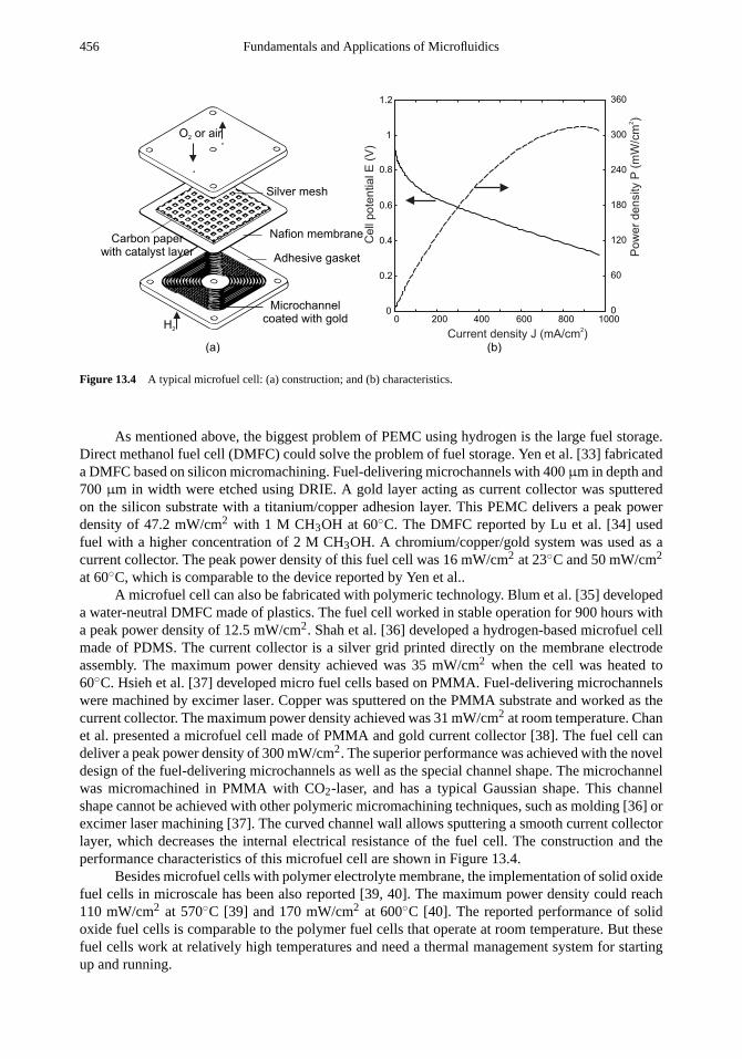
456 Fundamentals and Applications of Microfluidics
O or air2
H2
Adhesive gasket
Microchannel
coated with gold
Nafion membraneCarbon paper
with catalyst layer
Silver mesh
0 200 400 600 800 10000
0.2
0.4
0.6
0.8
1
1.2
0
60
120
180
240
300
360
Ce
llp
ote
ntia
lE
(V)
Current density J (mA/cm )2
Po
we
rd
en
sity
P(m
W/c
m)
2
(a) (b)
Figure 13.4 A typical microfuel cell: (a) construction; and (b) characteristics.
As mentioned above, the biggest problem of PEMC using hydrogen is the large fuel storage.Direct methanol fuel cell (DMFC) could solve the problem of fuel storage. Yen et al. [33] fabricateda DMFC based on silicon micromachining. Fuel-delivering microchannels with 400µm in depth and700 µm in width were etched using DRIE. A gold layer acting as current collector was sputteredon the silicon substrate with a titanium/copper adhesion layer. This PEMC delivers a peak powerdensity of 47.2 mW/cm2 with 1 M CH3OH at 60◦C. The DMFC reported by Lu et al. [34] usedfuel with a higher concentration of 2 M CH3OH. A chromium/copper/gold system was used as acurrent collector. The peak power density of this fuel cell was 16 mW/cm2 at 23◦C and 50 mW/cm2
at 60◦C, which is comparable to the device reported by Yen et al..A microfuel cell can also be fabricated with polymeric technology. Blum et al. [35] developed
a water-neutral DMFC made of plastics. The fuel cell worked in stable operation for 900 hours witha peak power density of 12.5 mW/cm2. Shah et al. [36] developed a hydrogen-based microfuel cellmade of PDMS. The current collector is a silver grid printed directly on the membrane electrodeassembly. The maximum power density achieved was 35 mW/cm2 when the cell was heated to60◦C. Hsieh et al. [37] developed micro fuel cells based on PMMA. Fuel-delivering microchannelswere machined by excimer laser. Copper was sputtered on the PMMA substrate and worked as thecurrent collector. The maximum power density achieved was 31 mW/cm2 at room temperature. Chanet al. presented a microfuel cell made of PMMA and gold current collector [38]. The fuel cell candeliver a peak power density of 300 mW/cm2. The superior performance was achieved with the noveldesign of the fuel-delivering microchannels as well as the special channel shape. The microchannelwas micromachined in PMMA with CO2-laser, and has a typical Gaussian shape. This channelshape cannot be achieved with other polymeric micromachining techniques, such as molding [36] orexcimer laser machining [37]. The curved channel wall allows sputtering a smooth current collectorlayer, which decreases the internal electrical resistance of the fuel cell. The construction and theperformance characteristics of this microfuel cell are shown in Figure 13.4.
Besides microfuel cells with polymer electrolyte membrane, the implementation of solid oxidefuel cells in microscale has been also reported [39, 40]. The maximum power density could reach110 mW/cm2 at 570◦C [39] and 170 mW/cm2 at 600◦C [40]. The reported performance of solidoxide fuel cells is comparable to the polymer fuel cells that operate at room temperature. But thesefuel cells work at relatively high temperatures and need a thermal management system for startingup and running.

Microfluidics for Life Sciences and Chemistry: Microreactors 457
Si Glass
Ptaaaaaaaaaaaaaaaaaaaaaaaaaaaaaaaaaaa
PDMS
Si3N4
Pd
SiO2
Al
aaaaaaaaaaaaaaaaaaaaaaaaaaaaaaaaaaaaaaaaaa
aaaaaaaaaaaaaaaaaaaaaaaaaaaaaaaaaaaa
aaaaaaaaaaaaaaaaaaaaaaaaaaaaaaaaaaaaaaaaaaaaa
aaaaaaaaaaaaaaaaaaaaaaaaaaaaaaaaaaaaaaaaaaaaa
C6H12C6H6H2
(b)
H2
N2 + H2
(a)
Figure 13.5 Gas-phase microreactors for (a) hydrogen separation; and (b) dehydrogenation.
13.2.1.2 Dehydrogenation Reactors
Thin palladium films have hydrogen-selective characteristics. A palladium membrane is permeablefor hydrogen. The reactor depicted in Figure 13.5(a) has a palladium membrane under a siliconoxide/silicon nitride membrane filter. The flow channels are fabricated in PDMS and silicon. Analuminum plate covers the bottom channel. A platinum heater integrated on the membrane filtercontrols the reactor temperature. The device can separate hydrogen from a nitrogen/hydrogenmixture. The hydrogen flux through the membrane increases with increasing temperature andincreasing hydrogen pressure gradient [41]. The palladium membrane can also be used as a catalystto remove hydrogen in the dehydrogenation reaction of hydrocarbon, such as cyclohexane [42]:
3C6H12Pt,Pd−→ C6H6 + 3H2 (13.19)
13.2.1.3 Hydrogenation Reactors
The conversion of carbon dioxide to methane is an example of a hydrogenation reaction [43]:
CO2 + 4H2 → CH4 + 2H2O (13.20)
This reaction is interesting for future manned Mars missions. The Martian carbon dioxide can beconverted with terrene hydrogen into fuel and water for astronaut life support systems. On Earth,microreactors for the hydrogenation of carbon dioxide are useful in distributed systems for globalcarbon dioxide management, which is crucial for reducing global warming [43].
13.2.2 Liquid-Phase Reactors
Liquid-phase reactors involve reagents in liquid phases. Most of the reactions are homogeneous;therefore, the reacting species need to be premixed. Unlike gases, liquids have a much smallerdiffusion coefficient (see Chapter 10). Designing a fully integrated liquid-phase microreactor isactually designing a micromixer, which was discussed in depth in Chapter 10.
One of the most famous liquid-phase reactors is the device for PCR. The reaction allowsamplifying DNA, which stores the genetic information of living species. The technique is necessaryfor the required concentration of DNA in an analysis (see Section 1.1). This section focuses on theprinciple and design of PCR reactors.

458 Fundamentals and Applications of Microfluidics
Denaturing
Hybridization
Extension
95
�C
60
�C
75
�C
PCR cycle
Time
Temperature
(a)
Number of DNA molecules
(b) Number
of cycles
10 20 30 40
E
=
1
E
<
1
E
=
0
Figure 13.6 (a) Temperature cycles in the reaction chamber of a PCR reactor; and (b) number of DNA molecules versusnumber of cycles.
Genetic information of living species is stored in the structure of a family of molecules callednucleic acids. DNA is a chainlike polymer made of four bases called nucleotides: adenine (A),guanine (G), cytosine (C), and thymine (T). These four bases are complementary in pairs. Thatmeans a nucleotide creates a chemical bond with only its complementary partner: adenine withthymine, and guanine with cytosine. In nature, DNA is often present in a double-stranded form. Twocomplementary strands are chemically bonded together and take up a double helix structure. PCRconsists of three different phases: denaturing, hybridization, and extension.
Denaturingis a process by which DNA loses its secondary structure. A heating temperatureabove 90◦C breaks a double-stranded DNA molecule into two complementary single-stranded DNAmolecules.
Hybridization, or annealing, cools the single-stranded DNA molecules at a lower temperatureunder 60◦C. Single DNA strands seek their complementary strands to create double-stranded DNAmolecules.
Extensionis a process by which the incomplete double-stranded DNA molecules are extendedwith the help of an enzyme called DNA polymerase. The enzyme attaches to the incomplete DNAmolecule and replicates the missing complementary bases using available nucleotides called primers.The extension process occurs at a temperature of 70◦C. The minimum time of the extension processis limited by the length of the segment to be amplified, the speed of the enzyme itself [30–100 basepairs per second (bp/s)] [44], and the diffusion of primers.
Figure 13.6(a) illustrates the temperature cycles required for the reaction chamber in a PCRprocess. Miniaturization improves the dynamics of the temperature control, and a faster cycle andfaster DNA amplification are possible.
The above three processes complete a cycle called the PCR cycle. Theoretically, repeating thePCR cyclen times amplifies a single double-stranded DNA molecule to 2n folds. In practice, theamplification factor0 is determined by [45]:
0 = [1 + EPCR(n)]n (13.21)
where EPCR is the efficiency factor, which is a function of the cycle numbern. For n < 20,EPCR ≈ 1. For higher cycle numbers (n > 20), the efficiency drops [Figure 13.6(b)].

Microfluidics for Life Sciences and Chemistry: Microreactors 459
Example 13.5: Extension Time in PCR
Determine the extension time for PCR, if the DNA segment to be amplified is 1,000 bp. Theenzyme in use is Tag Polymerase, which has an extension speed of 50 bp/s.
Solution. The required extension time is the time the enzyme needs for completing the entiresegment:
τ = L/U = 1,000/50 = 20 sec (13.22)
13.2.2.1 Design Considerations for PCR Reactors
Although PCR reactors are simple devices, the reaction is sensitive to contamination, especiallymetal ions. In addition, the chamber surface could adsorb enzyme and DNA, and may lead tononfunctional devices. Tests have been shown that native silicon and silicon nitride can inhibit PCRin microscale. Furthermore, the PCR device should be disposable, because a single DNA strand cancontaminate the next sample. Therefore, the substrate material and the machining technology are tobe considered carefully.
Silicon is used as a device material because silicon technology is established. The highthermal conductivity of silicon allows designing devices with fast thermal response. However, for afully integrated DNA-analysis system, silicon has many disadvantages. First, silicon is electricallyconductive and is difficult to incorporate into capillary electrophoresis due to the current required inthe fluidic channel. Second, silicon is optically opaque and transparent only to infrared light. Third,DNA tends to stick on native silicon. This sticking effect decreases the number of DNAs availablefor PCR. It is therefore difficult to use optical detection on silicon devices.
Glassis the traditional material in chemical analysis. The low electrical conductivity makesglass the perfect material for capillary electrophoresis. Glass is transparent and has a low nativefluorescence, and it is optimal for optical detection. The simple machining technique using wetetching in buffered HF makes glass an attractive material for DNA amplification reactors andanalysis devices. However, treatment of substrate surface should be considered.
Polymersare the other materials that allow on-chip capillary electrophoresis and optical char-acterization. However, background fluorescence is an important factor in material choice becausemany plastics are autofluorescent. Micromachining technology for plastics is still not well estab-lished, but it is promising (see Chapter 3).
Temperature controlis the next important factor in designing PCR reactors. For heating,a heater structure can be integrated into the reaction chamber. Precise temperature measurementis required because the success of the reaction also relies on the accuracy of a thermal cycle.Alternatively, noncontact methods, such as inductive heating [46] or use of an infrared source [47]can simplify the reactor design. For inductive heating, a secondary coil for induced current shouldbe either integrated or placed in close contact with the reactor. For cooling, passive cooling byconduction and natural convection does not require additional design consideration. Fast coolingis desired for a quick cycle. Active cooling using a forced convection or a Peltier element can beincorporated into the device. Kopf-Sill et al. used the Joule-heating effect of an electrolyte solutionto realize the temperature cycles for the PCR. An ac voltage was used for heating the liquid, to avoidelectrolysis and electrophoretic separation of the molecules [48].
Thermal management in a PCR reactor can be categorized as the temporal concept and thespatial concept. With the temporal concept, the temperature changes in time and the fluid remainsin the same location. The spatial concept uses continuous flow. The temperature is kept constant intime and the fluid changes its location. The PCR cycle is realized by feeding the solution throughthree temperature regions, which is repeated in a meander-shaped channel.

460 Fundamentals and Applications of Microfluidics
Example 13.6: DNA-Assay Preparation
If the concentration required for a perfect detection in a DNA assay is 105 copies per mL, howmany PCR cycles are needed for an initial sample with a concentration of 100 copies per mL?
Solution. The amplification factor required for the reaction is:
0 = 105/100= 1,000
In (13.4), we assume an efficiency factor of 1, thus:
0 = 2n→ n = ln0/ ln 2 = ln 1,000/ ln 2 ≈ 10
Example 13.7: Designing a Reaction Chamber for PCR
The chamber of a PCR reactor is made of silicon using DRIE. The chamber is a square with anedge length ofa = 2 mm and a depth ofd = 200µm. Determine the minimum ramping timeachievable with this reactor. Assume that the sample liquid is water with a density ofρ = 1,000kg/m3, a specific heat per unit mass ofc = 4,182 J/kgK, and a thermal conductivity ofκ = 0.6W/K-m (details on thermal simulation with SIMULINK are given in [49]).
Solution. The thermal capacitance or heat capacity of the fluid is estimated as:
Cthermal= mc= a2dρc
The thermal resistance from the heating membrane to the top of the chamber is estimated as:
Rthermal= d/(κa2)
Thus, the time constant of the liquid in the reaction chamber is:
τthermal= RthermalCthermal= d2ρc/κ = (200× 10−6)2 × 103× 4,182/0.6 = 0.28 sec
Taking the reactor frame and heat losses to the surroundings, the time constant may be higher thanthe value above. The ramping time is estimated as:
t = 3τthermal= 3 × 0.28 sec= 0.84 sec
Example 13.8: Total Preparation Time for DNA Assay
What is the time required for the preparation of the DNA assay described in Example 13.6 if weuse the reactor characterized in Example 13.7 to prepare the sample? The DNA sample and theenzyme for the assay are taken from Example 13.5. The time needed for denaturing and annealingis 5 seconds each.
Solution. We assume that the cooling time slope is the same as the ramping time slope. Thus,for one cycle we have three heating and cooling stages. From Example 13.5, the time needed forextension is 20 seconds. The estimated time of a cycle is:
T = tcooling + 2theating+ tdenaturing+ tannealing+ textension= 3 × 0.84+ 2 × 5 + 20 = 32.52 sec
Ten cycles (Example 13.6) are needed for the required concentration; that means the totalpreparation time is:
ttotal = 10× T = 10× 32.52 sec= 325.2 sec= 5 min 25 sec

Microfluidics for Life Sciences and Chemistry: Microreactors 461
Figure 13.7 Temporal PCR reactor: (a) silicon/glass; (b) and (c) silicon only; and (d) and (e) glass only.
13.2.2.2 Temporal PCR Reactors
Northrup et al. presented for the first time a PCR reactor in silicon [50, 51]. The reactor chamber(10× 10 mm) is etched in silicon and can contain 50µL [Figure 13.7(a)]. The temperature controlis achieved with a polysilicon heater on the back side of the reactor chip. The reactor chamber iscovered with a glass plate using silicone rubber. The small reactor allows a heating rate of 15 K/sand a cycle time of about 1 minute, which is four times faster than conventional PCR cyclers.
The reactor reported by Daniel et al. [52] also uses silicon as the substrate material. Heaterand temperature sensors are made of platinum. The reaction chamber is coated with silicon oxide[Figure 13.7(b)]. The chamber is covered with an oil drop to avoid the evaporation of the sampleliquid. Surrounding air chambers thermally insulate the chamber. Nitride grids over these chambersavoid thermally conducting liquid getting into the insulating chambers when filling the sample. Witha chamber size of 1.5µL, a thermal time constant of 0.4 seconds can be achieved.
The reactor array reported by Chaudhari et al. [53] is made of silicon and glass, which areanodically bonded. Temperature control is carried out with an external Peltier element. The Peltiereffect is the inverse effect of the thermoelectric effect or Seebeck effect; see Section 8.2. A currentpassing through metal-metal junctions can control their temperatures. For effective cooling, specialthermoelectric junctions such as (Bi2Te3-CuBr) are required for the Peltier element. These metalsare not compatible to standard silicon processes and are difficult to integrate on the microreactor.Similar reactor arrays are presented in [54]. The chambers are 2× 2 mm in size and have a volumeof 1.4 µL. The device is made in an SOI wafer with integrated titanium heaters [Figure 13.7(c)].Cheng et al. [55, 56] offered a solution in a silicon-glass chip. The PCR products can be separateddirectly in a capillary electrophoresis chip.
The PCR reactor presented in [57] is made in 0.55-mm-thick Corning 0211 glass sheets. Thereactor chamber is etched with hydrogen fluoride. The glass chip is 15× 15 mm. The heatingand cooling processes of the PCR cycles are carried out by an external Peltier element. Usingin situ fluorescence, the PCR efficiency can be detected. The fluorescence density-cycle numbercharacteristics are similar to the typical behavior shown in Figure 13.6(b). A similar solution is

462 Fundamentals and Applications of Microfluidics
95�C
60�C
75�C
Inlet Outlet
Figure 13.8 Spatial PCR reactor.
presented in [58] using two glass wafers bonded together. The 280-nL reactor chamber is connectedto the capillary system for subsequent separation processes [Figure 13.7(d)]. Bulk heating and bulkcooling in this device make parallel analyses with different cycling profiles impossible.
Plastics are used to make sample containers in conventional PCR systems. Polymeric devicescould be formed by a sacrificial process with CVD-deposited parylene [59, 45] or hot embossed inbulk PMMA substrate [60].
13.2.2.3 Spatial PCR Reactor
In the spatial concept, the sample is forced through three temperature zones with a constant velocity(Figure 13.8). At a constant velocity, the cycle time is proportional to the capillary length. Thelengths of the capillary at each temperature zone determine the cycle times. The device can becalled a chemical amplifier because the sample concentration at the inlet is amplified at the outlet[61]. The process only depends on the speed of the fluid flow and not on the thermal constant of thesystem. Therefore, the spatial concept allows a relatively fast cycling.
The channel is fabricated in glass and has a size of 40µm × 90 µm × 2.2 m. The channelsurface is treated with dichlorodimethylsilane to reduce the adsorption of enzyme and DNA. Theextremely long and small channel requires high pressure, on the order of bars. This concept ofspatial PCR reactor is implemented in a silicon/glass device [62]. The flow channel has a size of250µm × 100µm × 1.512 m. The heaters and temperature sensors are made of thin platinum filmson silicon. The heating zones are separated by thermal gaps etched in silicon. The glass wafer andthe silicon wafer are bonded anodically. Obeid et al. reported a device based on the same concept[63]. The microchannel was etched in glass and has a cross section of 100× 55 µm. Outlets arepositioned after 20, 25, 30, 35, and 50 cycles. Thus, the number of the total amplification cycles canbe selected.
Example 13.9: Designing a Spatial PCR Reactor
A spatial PCR reactor has a flow channel etched in glass. The channel height isH = 40µm, andthe width isW = 90 µm. The flow rates range from 6 to 72 nL/s. What are the dimensions ofthe reactor depicted in Figure 13.8 if we assume that the three temperature zones have the samewidth? The time ratio of denaturing, annealing, and extension is 0.5:5:0.5 seconds.
Solution. We assume that the sample has properties of water (density 1,000 kg/m3, specific heatper unit mass of 4,182 J/kgK, and a thermal conductivity of 0.6 W/Km).

Microfluidics for Life Sciences and Chemistry: Microreactors 463
The thermal capacitance of a channel segmentL is given as:
Cthermal= mc= LW Dρc
The thermal resistance from the bottom to the top of the channel is estimated as:
Rthermal= H/(κa2)ρc
The time constant for the isothermal condition of the liquid in the channel is:
τthermal= RthermalCthermal= H2ρc/κ = (40× 10−6)2 × 103× 4,182/0.6 = 0.011 sec
The smallest design considers the worst case of maximum flow rate or maximum velocity:
U = Q/(W H) = 72× 10−12/(90× 10−6× 40× 10−6) = 0.02 m/s
The time required for passing through the denaturing is:
t = 3τthermal+ tdenaturing= 3 × 0.011+ 0.5 = 0.533 sec
Thus, the channel length in the denaturing zone is:
L = Ut = 0.02× 0.533= 10.66× 10⁻³ m ≈ 11 mm
Since the channel makes one turn in this zone, the zone width will be:
Wzone= L/2 = 11/2 = 5.5 mm
If the extension zone has the same width, the required length is:
Lextension= Utextension= 0.02× (3 × 0.011+ 5) = 100× 10−3 m = 100 mm
The ramping time is insignificant in the above equation. The number of turns in the extensionzone is:
N = Lextension/(2W) = 100/(2 × 5.5) ≈ 9
Although buoyancy force is small in microscale, free convection can be used for realizingcontinuous flow in a closed channel system. The temperature gradients can be used for both drivingand realizing the thermal cycles. Krishnan et al. [64] reported a simple configuration with a 35-µLcylindrical cavity [Figure 13.9(a)]. The DNA sample was allowed to circulate vertically between97◦C and 61◦C. The parameters determining the behavior of the flow are the aspect ratio (H/D) ofthe chamber and the Rayleigh number:
Ra=gα1T
H
3
νκ (13.23)
where H and D are the height and diameter of the reaction chamber,g is the gravitationalacceleration, andα is the thermal expansion coefficient of the fluid,1T is the temperaturedifference,ν is the kinematic viscosity of the fluid, andκ is the thermal conductivity of the fluid.This basic concept can be extended to an array of reaction chambers, a rectangular flow loop [65][Figure 13.9(b)], a triangular flow loop [66] [Figure 13.9(b, c)], or a semicircular loop [67].

464 Fundamentals and Applications of Microfluidics
T =61 C2
o
T =97 C1
o
D
H
(a)
T =58 C2
o
T =90 C1
o
g
g
T =55 C2
o
T=72
C
1
o
T=90-9
6C
1
og
(b) (c)
T =94 C1
oT
=55
C
2
o
T =72 C1
o
(d)
Figure 13.9 Spatial PCR reactor based on free convection: (a) the basic configuration; (b) rectangular loop; (c) and (d)triangular loops.
13.2.3 Multiphase Reactors
Multiphase reactors discussed in this chapter are reactors for liquid-solid reactions. These reactionsare heterogeneous, meaning the reactions occur on the surface of the phases. The reacting surfacecan be realized with mobile solid phase in form of microbubbles or microspheres, or with a poroussubstrate material.
Gas-Liquid Reactors.In order to increase the reacting surface, gas-liquid reactors can berealized in the form of “trickle-bed” reactors, or reactors with bubble columns.
In the first type, the liquid phase is used to wet the surface of microspheres. The design ofsuch a reactor is similar to reactors with packed beads described below. The wetting efficiency ofthe beads and the flow distribution of the liquid phase characterize the reaction efficiency.
In the second type, the gas phase is dispersed in the liquid phase in the form of a bubblecolumn. Bubble size and dispersion characterize the reaction efficiency. The dispersion process canbe realized with parallel lamination mixers as described in [68]. In [68], the mixing effect is furtherimproved with a staggered array of 50-µm-diameter cylinders (Figure 13.10).
Reactors with Packed Beads.Reactors with packed beads use the enlarged interfacial area ofthe beads to improve the mass transfer from reagents coated on the beads to the sample solution,and thus, improve the reaction rates. The amount of reagent transferred is proportional to theconcentration difference and the interfacial surface area:
m = kT A(ci − cs) (13.24)
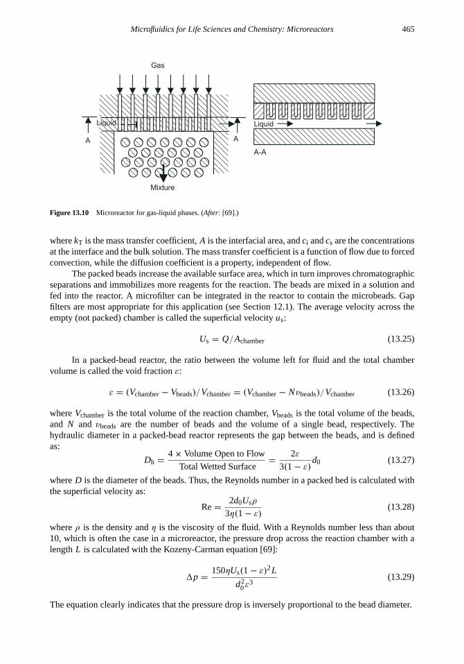
Microfluidics for Life Sciences and Chemistry: Microreactors 465
A A
A-A
Liquid Liquid
Gas
Mixture
Figure 13.10 Microreactor for gas-liquid phases. (After: [69].)
wherekT is the mass transfer coefficient,A is the interfacial area, andci andcs are the concentrationsat the interface and the bulk solution. The mass transfer coefficient is a function of flow due to forcedconvection, while the diffusion coefficient is a property, independent of flow.
The packed beads increase the available surface area, which in turn improves chromatographicseparations and immobilizes more reagents for the reaction. The beads are mixed in a solution andfed into the reactor. A microfilter can be integrated in the reactor to contain the microbeads. Gapfilters are most appropriate for this application (see Section 12.1). The average velocity across theempty (not packed) chamber is called the superficial velocityus:
Us = Q/Achamber (13.25)
In a packed-bead reactor, the ratio between the volume left for fluid and the total chambervolume is called the void fractionε:
ε = (Vchamber− Vbeads)/Vchamber= (Vchamber− Nvbeads)/Vchamber (13.26)
whereVchamberis the total volume of the reaction chamber,Vbeadsis the total volume of the beads,and N and vbeads are the number of beads and the volume of a single bead, respectively. Thehydraulic diameter in a packed-bead reactor represents the gap between the beads, and is definedas:
Dh =4 × Volume Open to Flow
Total Wetted Surface=
2ε
3(1 − ε)d0 (13.27)
whereD is the diameter of the beads. Thus, the Reynolds number in a packed bed is calculated withthe superficial velocity as:
Re=2d0Usρ
3η(1 − ε)(13.28)
whereρ is the density andη is the viscosity of the fluid. With a Reynolds number less than about10, which is often the case in a microreactor, the pressure drop across the reaction chamber with alengthL is calculated with the Kozeny-Carman equation [69]:
1p =150ηUs(1 − ε)2L
d20ε
3(13.29)
The equation clearly indicates that the pressure drop is inversely proportional to the bead diameter.

466 Fundamentals and Applications of Microfluidics
(a) (b)
Detection chamber
Reaction chamber
Figure 13.11 Microreactor with packed beads: (a) made of SU-8; and (b) made of silicon.
Figure 13.11(a) shows an example of an enzymatic microreactor [70]. The reactor is integratedmonolithically with an electrochemiluminescence (ECL) detector for the evaluation of the reactionresults. The reaction chamber is packed with glass beads modified with an immobilized enzyme(glucose oxidase). The active components of the detector are fabricated on the silicon substrate. Thereaction and detection chambers are formed with SU-8, and have volumes of 1.5µL and 2.7µL,respectively. The gap filter is designed as a group of microcolumns separating the two chambers.The entire device is covered by a PMMA plate with inlet and outlet ports machined in it.
The gap filter of the reactor depicted in Figure 13.11(b) is micromachined in silicon by DRIE.A glass plate is anodically bonded to the silicon structure and seals the device. The volumes ofreaction chambers can range from 0.5 to 50 nL [70].
Active filtering of beads is realized with magnetic beads. Magnetic beads are made ofmagnetite (Fe3O4) and are coated with the desired enzyme. Magnetic beads can be used for markingcells and DNA molecules. Reference [71] gives an example of integrated electromagnets for trappingmagnetic beads. The magnets are integrated as a planar inductive device. Because of the complexityof the integrated magnet, this method is impractical and not attractive for reactors with packed beads.
While the above reactors use a pressure-driven flow to pack microparticles, the packedchamber reported in [72] uses electrokinetic pumping to introduce the beads. The reactor isfabricated in glass by wet etching. The beads are kept in the chamber by two gap filters. Figure13.12 illustrates the packed chamber. The chamber is a three-way junction, with one inlet, one outletfor sample solution, and one inlet for bead introduction. The total volume of the chamber is 330 pL.The bead introduction channel is designed with a small width to increase its fluidic impedance, andconsequently to avoid unpacking the beads. The inlet and the outlet of sample flow are designedwith a 1-µm gap filter to retain the beads in the chamber. The bead introduction inlet is designedwith a hook structure, which makes the bead flow reverse its direction after filling the chamber [12].
Example 13.10: Interfacial Surface
The reaction chamber of a packed-bead microreactor is etched 200µm deep in silicon and has alateral dimension of 500× 500µm. The chamber is packed loosely with microspheres, that havea diameter of 10µm. The microspheres occupy 40% of the chamber volume, and the void fractionis 0.6. Determine the reacting surface and the reacting surface-to-volume ratio.
Solution. If the number of packed spheres isN, the volume ratio between the spheres and reactionchamber is:
NπD3/6
W L H= 40%

Microfluidics for Life Sciences and Chemistry: Microreactors 467
A
Beads introduction
A
A-A
Gap filters
Figure 13.12 Microreactor with electrokinetic bead introduction. (After: [12].)
Thus, the estimated particle number is:
N = 0.4 ×6W L HπD3
N = 0.4 ×6×(500×10−6)2×200×10−6
π×(10×10−6)3= 38,197
.
The total surface area of the spheres or the reaction surface is:
Atotal = NπD2
= 38,197× π × (10× 10−6)2 = 12× 10−6 m2= 12 mm2
The ratio between reacting surface and chamber volume is:
Atotal/Vtotal = 12× 10−6/(500× 500× 200× 10−24) = 2.4 × 10¹¹ m−1
Example 13.11: Mass Transfer in a Packed-Bead Reactor
The spheres described in Example 13.10 are made of benzoic acid. The mass transfer coefficientat the sphere surface is 10−3 cm/s. Determine the flow rate of pure water coming into the reactionchamber if the solution at the chamber’s exit is 60% saturated with benzoic acid. Assume thatwater is fed into the chamber laterally. What is the superficial velocity in the reaction chamber?
Solution. The flux of the solute at the exit is:
m = Q × 0.6 × csat
where csat is the saturation concentration of the solid sphere. From (13.5), we get:
Q × 0.6 × csat = k Atotal(csat− 0) →
Q = k Atotal/0.6Q = 10−3
× 10−2× 12× 10−6/0.6 = 2 × 10⁻¹⁰ m3/s = 12µL/min
The superficial velocity is the fluid velocity in the reaction chamber if there are no spheres:
U = Q/(W H) = 2 × 10⁻¹⁰/(500× 200× 10−12) = 2 × 10⁻³ m/s= 2 mm/s

468 Fundamentals and Applications of Microfluidics
13.2.4 Microreactors for Cell Treatment
In many applications for biochemical analysis, cells and biological agents often need to be analyzed.The cell itself can be considered here as a confined biological microreactor. Since micromachinedstructures and cells have the same order of sizes, biochemical and biophysical analysis of a singlecell is possible. A biochemical analysis process consists of many steps: sorting and collecting ofcells, cell lysis, polymerase chain reaction, and electrophoresis separation. In a biophysical analysis,mechanical [73] or electrical [74] properties of cells can be precisely tested and evaluated. Chapter12 already discussed the different methods for collecting cells and electrophoresis separation. Thedesign of a PCR microreactor is covered in Section 13.2.2. This chapter focuses on the differenttechniques for cell treatment, such as cell lysis, electroporation, and cell fusion.
13.2.4.1 Cell Lysis
Cell lysis breaks the protecting membrane to release DNA. In conventional sample preparationprotocols, cell membranes are broken by means of enzymes, chemical lytic agents, heat, mechanicalforces, or electric fields.
Cell lysis with enzymes and chemical lytic agents can be carried out in a micromixer asdescribed in Chapter 10. Schilling et al. used a simple T-mixer to dilute lytic agent into thesample flow with cells [75] [Figure 13.13(a)]. After cell lysing, intercellular components with higherdiffusion coefficients are separated, as explained earlier in Section 12.2.1. Thermal cell lysis is thesimplest technique, that can be realized in microscale. Waters et al. used thermal lysis at 90◦C forseveral minutes to extract DNA fromEscherichia coli. The DNA was subsequently amplified andanalyzed on the same glass chip. For integrated systems, thermal lysis can be achieved with anintegrated thermal management system.
In some applications, thermal and chemical treatments are not harsh enough to disrupt thecell membrane. The technique utilizing ultrasonic waves to destroy cell membranes is calledsonoporation. Mechanical forces caused by a combination of glass beads and ultrasonic wavesdeliver a harsher treatment. Belgrader et al. [76] used 106-µm glass beads and ultrasonic wavesof 47 kHz to breakBacillus subtilisspores. The sonication process used an external sonicator probeand took only 30 seconds. A flexible membrane between the sonicator probe and the sample liquidcan avoid cavitation effects [77]. However, cavitation effects in a controlled manner can be usedfor focusing and lysing cells. Marmottant and Hilgenfeldt [78] used a 15-µm microbubble to attractand disrupt cells. The microbubble is driven with a frequency of 180 kHz, which is near its ownresonance. Acoustic streaming attracts the cell to the microbubble and subsequently disrupts the celldue to the focused acoustic energy.
Due to the concentration differences of potassium ions across a cell membrane, an electricfield exists across the membrane to keep the potentials on both sides of the membrane in equilibrium.Increasing the field across the cell membrane can make it permeable. If the field strength is higherthan a critical value, the effect is irreversible and bursts the membrane. The other effect causingmembrane damage is osmosis. The difference in ion concentration caused by a permeable membraneleads further to unbalance in osmotic pressure across the membrane. The osmotic pressure differencecauses cell swelling and eventually disrupts the membrane. Lee and Tai [79] used dielecrophoreticforces to trap the cells and position them between two sharp electrodes [Figure 13.13(b)]. Thetrapping voltage is 6V ac at 2 MHz. After trapping, a short pulse of a higher voltage (20V, 100µs)bursts the cells open. Yeast cells (Sacharomyces cerevisiae) andEscherichia coliwere successfullylysed with this concept.

Microfluidics for Life Sciences and Chemistry: Microreactors 469
Cells
Lyticagents
Intracellular molecules
Detection molecules
Fluorescent product
Electrode
Parylene spacerCell
(a)
(b)
Figure 13.13 On-chip cell lysis techniques: (a) with chemical lytic agent; and (b) trapping and lysing with electrical fields.
13.2.4.2 Electroporation and Cell Fusion
In applications such as gene therapy, effective delivery of genes into living cells is an importanttask. Conventional gene delivery techniques are virus transfection [80], calcium phosphate-mediatedtransfection [81], liposome mediated transfection [82], particle bombardment [83], direct injectionwith microneedle [84], and electroporation [85]. As mentioned above, an impulse of high electricfield makes cell membrane permeable. The reversibility of permeabilization of the cell membranedepends on the amplitude, length, shape, repetition rate of the voltage pulse, the cell itself, and itsdevelopment stage. Thus, an electric field can be used for delivering of drug or DNA moleculesinto a cell. This technique was widely used with commercially available electroporators for proteintransfection, drug delivery, and cell fusion.
Commercial electroporators can only treat cells in batch and do not allow the detailed studyof electroporation. Microtechnology makes electroporation of a single cell possible. Huang andRubinsky [86] used a silicon device to trap and to probe a cell. The device immobilizes the cellwith hydrodynamic pressure. The cell is positioned on a pore etched in a silicon nitride membrane.With a pair of electrodes made of translucent polysilicon, the electric current across the fluidicchamber filled with an ionic solution and the cell can be measured. The electroporation process canbe therefore precisely controlled by monitoring the current across the cell.
The concept of electroporation can be applied to two cells to fuse them together. This processis calledcell fusion, and is one of the key techniques in biotechnology. Cloning is a typical exampleof cell fusion, where an adult cell from the mammary gland is fused with an egg cell. In a cell

470 Fundamentals and Applications of Microfluidics
A B
Electrofusion
A+B C
Figure 13.14 Concept of nanoreactors with liposomes. A liposome containing reactant A is fused with another liposomecontaining reactant B. Inside the hybrid liposome, A and B react to form C. The circles and squares represent differentphospholipods and proteins. (After: [87].)
fusion process, the cells are first brought into contact. Techniques such as dielectrophoretic trappingdescribed in Figure 13.13(b) can be used for this purpose. Subsequently, a short voltage pulse causesa high electric field across both cells. This pulse of high electric field fuses together the membraneareas, which are in close contact.
The concept of cell fusion can be well applied to liposomes, which makesnanoreactorsareality. Liposomesare synthetic lipid-bilayer containers, which are similar to the membranes ofnatural biological cells. The size of these containers ranges from tens of nanometers to tens ofmicrons [87]. Reagents and molecules in liposomes can mix and react after fusing. Mimickingnature, real biochemical nanoreactors can be realized in this way (Figure 13.14).
13.2.5 Hybridization Arrays
Hybridization arrays are biochemical microreactors for detection of genetic pathogens, antigens,or antibodies. The massively parallel screening process can be realized on a chip using microtech-nology. The concept of these arrays is based on the hybridization binding reaction. Loose hydro-gen bonds of complimentary bases on two single-stranded DNA chains attract and form a double-stranded DNA molecule. This concept can detect a small amount of DNA in a solution with a numberof unknown molecules. Figure 13.15 shows a typical gene expression process [88].Gene expressionindicates a gene’s activities in normal cells and in those treated with a drug. In the process of makinga protein, the corresponding gene (DNA) is translated into ribonucleic acid (RNA). For gene expres-sion, the RNA is extracted from the cell [Figure 13.15(b)]. The extracted RNA is used to make DNA,which is tagged with a fluorescent dye [Figure 13.15(c)]. The tagged DNA is brought to the arraysurface, where hybridization reaction occurs [ Figure 13.15(d, e)]. The signals of the known DNAon the array are collected with an epifluorescent microscope and a CCD camera [Figure 13.15(f)].Microarrays forsequence analysishave shorter oligos corresponding to the different disease andgene markers. The mutations of a single base in these DNA strands indicate the disease genes. Asequence analysis array can be used for personalized drug design as well as genetic risk assessments.
A microarray can be fabricated on different substrate materials such as silicon [89], glass [90],or polymer [91]. Microarrays with short DNA strands can be fabricated by the stepwise additionof bases [92]. The array is fabricated layer by layer using conventional lithography techniques.

Microfluidics for Life Sciences and Chemistry: Microreactors 471
(a) (b) (c)
Cell RNAs Marked DNAs
(d)
DN
Am
icroarray(e)
DN
Am
icroarray(f)
DN
Am
icroarray
Laser
Figure 13.15 Gene expression using a DNA microarray: (a) Genes of with drug-treated cells are to be compared with thoseof untreated cells. (b) The genes (DNA) are translated into ribonucleic acid (RNA). (c) The DNA copies of the RNA aretagged with fluorescent dyes. (d) The tagged DNAs are washed over the DNA array. (e) Hybridization reaction occurs withknown single-stranded DNA on the array. (f) The DNAs are identified by fluorescent detection.
A density of 106 probes/cm2 and a probe size of 8µm can be achieved [93, 94] (Figure 13.16).Microlithography requires masks for four nucleotides in a single layer. Making long oligos wouldneed a large number of masks. A flexible solution for this problem is the use of a pattern generator.Gao et al. [95] reported the use of a 480×640 digital micromirror device (DMD) as pattern generatorfor the microarray. The resolution of this microarray is determined by the digital mirror, which is30× 30µm2 in size.
Inkjet concepts can be utilized for printing the bases of a DNA fragment. This so-called in-situ printing technique replaces the four colors of the ink (cyan, magenta, yellow, and black) by thefour nucleotides (adenine, guanine, cytosine, and thymine). Layer by layer, this technique can buildfragments with up to 60 bases [Figure 13.16(b)] [88].
Inkjet printing can also print presynthesized oligos and gene fragments directly on thesubstrate, [Figure 13.16(c)] [96]. Inkjet printing has a resolution on the order of 70 to 120µmand allows making an microarray with about 25,000 spots. Contact printing is another methodfor bringing DNA fragments to the array surface [97]. A pin is first dipped into the solution withpresynthesized DNAs. The pin is subsequently pressed to the array surface and leaves behind adroplet of the solution. In order to avoid repeated dipping, a split tip or a hollow tip can act as asmall reservoir for multiple spotting steps. Section 11.1.1 discusses more about droplet dispensers.
A small DNA spot on a flat surface has a limited number of molecules, which in turn causesa weak signal for evaluation. A weak signal also means a higher signal-to-noise ratio. The signalcan be improved by increasing the number of immobilized molecules. For a given planar spot size,the number of molecules can only be increased if they are immobilized on all three dimensions.Timofeev et al. [98] immobilized the molecules on a gel matrix, which is coated on the glasssubstrate. Thus, immobilization occurs in volume, rather than on a surface. However, diffusivetransport inside the gel matrix causes different spot sizes and affects hybridization kinetics [99]. Inorder to avoid this effect, the porous structure can be micromachined into the substrate. Benoit et al.[100] etched tiny pores through the substrate. Each spot occupies a few hundred pores. Moleculesare allowed to immobilize on the pore wall. The immobilization rate can be further improved if thesample is allowed to flow through the pores.

472 Fundamentals and Applications of Microfluidics
A A A
A A AG G G
G G G
T
A A TT
(a) (b)
A A AG G GT
G
A
(c)
A A AG
G G GA
A A AG G G
G G GA TT
A A AG G G
G G G
T
A A TT
A A AG G G
G G G
T
A A TT
Figure 13.16 Fabrication techniques for DNA arrays (A: adenine, G: guanine, C: cytosine, T: thymine): (a) microlithogra-phy (the hatched area is photoresist); (b) in-situ printing with inkjet; and (c) direct printing.
13.3 SUMMARY
Microreactors find applications in both chemical industry and chemical/biochemical analysis. Thesmall scale and the high surface-to-volume ratio in microreactors offer a number of advantages forchemical production. The design of a microreactor starts with the requirements from the reaction.Key parameters are the residence time, the reaction time, and the thermal response time. Basedon these parameters, microchannels and microchambers for the reaction can be dimensioned. Highthroughput can be achieved by increasing the number of reactors units. Microreactors are in favorof the space-time yield, a performance indicator for reactors, because of the small size and shortresidence time. Microtechnology also allows the integration of other functional elements, such ascatalysts, sensors, and heat exchangers in the same device.
For chemical and biochemical analysis, scaling down the analysis brings tremendous advan-tage. Integrating all process steps on a single chip allows handling minute amounts of samples andchemicals. For DNA analysis, for instance, the entire analysis process can be integrated in a singledevice. While the previous chapters already started with methods and devices for cell sampling,this chapter discussed typical devices for cell lysis, DNA amplification, DNA separation, DNAhybridization, and detection. The same concepts can apply to the analysis of proteins and othermolecules.
Problems
13.1 A microcombustor uses methane as fuel. The combustor consumes methane (CH4) with a massflow rate of 50 mg/s. Assuming that methane burns completely with 100% theoretical air,determine the air-fuel ratio and the volume flow rate of air.
13.2 If the combustor is designed as a diffuser/nozzle structure with an inlet diameter of 2 mm and anoutlet diameter of 0.5 mm over a length of 10 mm, the operating pressure is 4 atm. Estimate theresidence time of the air/fuel mixture in the combustor.
13.3 The extension time in a PCR cycle is 50 seconds. The enzyme in use is Tag Polymerase, whichhas an extension speed of 50 base pairs per second (bp/s). Determine the length of the amplifiedDNA segment if heating and cooling delays are neglected.

Microfluidics for Life Sciences and Chemistry: Microreactors 473
13.4 Design a reaction chamber in silicon so that the minimum ramping time is 1 second. The siliconwafer is 500 mm thick.
13.5 Design a spatial PCR reactor. The channel depth isd = 100 mm and the width isw = 200 mm.The flow rates range from 100 to 500 nL/s. The temperature zones for denaturing and annealinghave the same width. The width of the temperature zone for extension is one-half of that of theother two. The time ratio of denaturing, annealing, and extension is 0.5:5:0.5 seconds.
13.6 Benzoic acid spheres of 5 microns in diameter are packed loosely in a 100× 500 × 500-µmreaction chamber. The interfacial area-to-volume ratio is about 1011 m−1. The mass transfercoefficient at the sphere surface is 10−3 cm/s. Determine the flow rate of pure water cominginto the reaction chamber if the solution at the chamber exit is 80% saturated with benzoic acid.Assume that water is fed into the chamber laterally. What is the superficial velocity in the reactionchamber?
References
[1] Jensen, K. F., “The Impact of MEMS on the Chemical and Pharmaceutical Industries,”Technical Digest of the IEEESolid State Sensor and Actuator Workshop, Hilton Head Island, SC, June 4–8, 2000, pp. 105-110.
[2] Veser, G., et al., “A Micro Reaction Tool for Heterogeneous Catalytic Gas Phase Reactions,”Proceedings of MEMS’99,12th IEEE International Workshop Micro Electromechanical System, Orlando, FL, Jan. 17–21, 1999, pp. 394–399.
[3] Commenge, J. M.,Reacteurs microstructures: hydrodynamique, thermique, transfert de matie et application auxprocedees, Ph.D/ Thesis, Institut National Polytechnique de Lorraine, Nancy, 2001.
[4] Kestenbaum, H., et al. “Silver-Catalyzed Oxidation of Ethylene to Ethylene Oxide in a Microreaction System,”Ind.Eng. Chem. Res., Vol. 41, 2002, pp. 710–719.
[5] Hessel, V., Hardt, S., and Lowe, H.,Chemical Micro Process Engineering,Weinheim: Wiley-VCH, 2004.
[6] Worz, O., et al., “Microreactors—a New Efficient Tool for Reactor Development,”Chemical Engineering Technology,Vol. 24, 2000, pp. 24–29.
[7] Lao, A. I. K., et al., “Precise Temperature Control of Microfluidic Chamber for Gas and Liquid Phase Reactions,”Sensors and Actuators A, Vol. 84, 2000, pp. 11–17.
[8] Meijer, G. C. M., and Herwaarden, A. W. (eds),Thermal Sensors, Bristol, U.K.: Institute of Physics Publication, 1994.
[9] Poser, S., et al., “Chip Elements for Fast Thermocycling,”Sensors and Actuators A, Vol. 62, 1997, pp. 672–675.
[10] Schubert, K., et al., “Microstructure Devices for Thermal and Chemical Process Engineering,”Microscale Thermo-physical Engineering, Vol. 5, 2001, pp. 17–39.
[11] Cussler, E. L.,Diffusion Mass Transfer in Fluid Systems,New York: Cambridge University Press, 1984.
[12] Oleschuk, R. D., et al., “Utilization of Bead Based Reagents in Microfluidic Systems,”Micro Total Analysis Systems2000, A. van den Berg, et al., (eds.), Boston: Kluwer Academic Publishers, 2000, pp. 11–14.
[13] Madou, M. J., et al., “A Centrifucal Microfluidic Platform—A Comparison,”Micro Total Analysis Systems 2000, A.van den Berg, et al. (eds), Boston: Kluwer Academic Publishers, 2000, pp. 565–570.
[14] Drott, J., et al., “Porous Silicon as the Carrier Matrix in Microstructured Enzyme Reactors Yielding High EnzymeActivities,” Journal of Micromechanics and Microengineering, Vol. 7, 1997, pp. 14-23.
[15] Splinter, A., et al., “Micro Membrane Reactor: A Flow-Through Membrane for Gas Pre-Combustion,”Proceedings ofTransducers ’01, 11th International Conference on Solid-State Sensors and Actuators, Munich, Germany, June 10–14,2001, pp. 1778–1781.

474 Fundamentals and Applications of Microfluidics
[16] Schwarz, M. A., and Hauser, P. C., “Recent Developments in Detection Methods for Microfabricated AnalyticalDevices,”Lab on a Chip, Vol. 1, 2001, pp. 1–6.
[17] Madou, M. J., and Cubicciotti, R., “Scaling Issues in Chemical and Biological Sensors,”Proceedings of the IEEE,Vol. 91, 2003, pp. 830–838.
[18] Ocvirk, G., Tang, T., and Harrison, D. J.,“Optimization of Confocal Epifluorescence Microscopy for Microchip-BasedMiniaturized Total Analysis Systems,”Analyst, Vol. 123, 1998, pp. 1429–1434.
[19] Jiang G., et al.,“Red Diode Laser Induced Fluorescence Detection with a Confocal Microscope on a Microchip forCapillary Electrophoresis.,”Biosensors and Bioelectronics, Vol. 14, 2000, pp. 861–869.
[20] Melanson, J. E., et al.,“Violet (405 nm) Diode Laser for Laser Induced Fluorescence Detection in Capillary Elec-trophoresis,”Analyst, Vol. 125, 2000, pp. 1049–1052.
[21] Verpoorte, E., et al.,“A Silicon Flow Cell for Optical Detection in Miniaturized Total Chemical Analysis Systems,”Sensors and Actuators B, Vol. 6, 1992, pp. 66–70.
[22] Greenway, G. M., et al., “The Use of a Novel Microreactor for High Throughput Continuous Flow Organic Synthesis,”Sensors and Actuators B, Vol. 63, 2000, pp. 153–158.
[23] Epstein, A. H., et al., “Power MEMS and Microengines,”Proceedings of Transducers ’97, 9th International Confer-ence on Solid-State Sensors and Actuators, Chicago, June 16-19, 1997, pp. 753–756.
[24] Waitz, I. A., et al., “Combustors for Micro-Gas Turbine Engines,”ASME Journal of Fluid Engineering, Vol. 120,1998, pp. 109–117.
[25] Mehra, A., and Waitz, I. A., “Development of a Hydrogen Combustor for a Microfabricated Gas Turbine Engine,”Technical Digest of the IEEE Solid State Sensor and Actuator Workshop, Hilton Head Island, SC, June 2–4, 1998,pp. 144–147.
[26] Mehra, A., et al., “Microfabrication of High Temperature Silicon Devices Using Wafer Bonding and Deep ReactiveIon Etching,”Journal of Microelectromechanical Systems, Vol. 8, No. 2, 1999, pp. 152-160.
[27] Mehra, A., et al., “A Six-Wafer Cobustion System for a Silicon Micro Gas Turbine Engine,”Journal of Microelec-tromechanical Systems, Vol. 9, No. 4, 2000, pp. 517–527.
[28] Zimmermann, S., Wischhusen, S., and Mller, A., “A mTAS—Atomic Emission Flame Spectrometer (AES),”MicroTotal Analysis Systems 2000, A. van den Berg, et al. (eds.), Boston: Kluwer Academic Publishers, 2000, pp. 135–138.
[29] Veser, G., et al., “A Micro Reaction Tool for Heterogeneous Catalytic Gas Phase Reactions,”Micro Total AnalysisSystems 2000, A. van den Berg, et al. (eds.), Boston: Kluwer Academic Publishers, 2000, pp. 394–399.
[30] Moran, M. J., and Shapiro, H. N.,Fundamentals of Engineering Thermodynamics, 4th ed., New York: Wiley, 2000.
[31] Lee, S. J., et al., “Design and Fabrication of a Micro Fuel Cell Array with Flip-Flop Interconnection,”Journal PowerSources, Vol. 112, 2002, pp. 410–418.
[32] Yu, J., et al., “Fabrication of Miniature Silicon Wafer Fuel Cells with Improved Performance,”Journal of PowerSources, Vol. 124, 2003 40–46.
[33] Yen, T. J., et al., “A Micro Methanol Fuel Cell Operating at Near Room Temperature,”Applied Physics Letter, Vol. 83,2003, pp. 4056–4058.
[34] Lu, G. Q., et al., “Development and Characterization of a Silicon-Based Micro Direct Methanol Fuel Cell,”Elec-trochim. Acta, Vol. 49, 2003, pp. 821–823.
[35] Blum, A., et al., “Water-Neutral Micro Direct-Methanol Fuel Cell (DMFC) for Portable Applications,”Journal ofPower Sources, Vol. 117, 2003, pp. 22–25.
[36] Shah, K., et al., “A PDMS Micro Proton Exchange Membrane Fuel Cell by Conventional and Non-ConventionalMicrofabrication Techniques,”Sensors and Actuators B, Vol. 97, 2004, pp. 157–167.
Microfluidics for Life Sciences and Chemistry: Microreactors 475
[37] Hsieh, S. S., “A Novel Design and Microfabrication for a Micro PEMFC,”Microsystem Technologies, Vol. 10, 2004,pp. 121–126.
[38] Chan, S. H., et al., “Development of a Polymeric Micro Fuel Cell Containing Laser-Micromachined Flow Channels,”Journal of Micromechanics and Micro Engineerings, Vol. 15, 2005, pp. 231–236.
[39] Chen, X., et al., “Thin-Film Heterostructure Solid Oxide Fuel Cells,”Applied Physics Letters, Vol. 84, 2004, pp. 2700–2702.
[40] Srikar, V. T., et al., “Structural Design Considerations for Micromachined Solid-Oxide Fuel Cells,”Journal PowerSources, Vol. 125, 2004, pp. 62–69.
[41] Franz, A. J., Jensen, K. F., and Schmidt, M. A., “Palladium Based Micromembranes for Hydrogen Separation andHydrogenation/Dehydrogenation Reactions,”Proceedings of MEMS’99, 12th IEEE International Workshop MicroElectromechanical System, Orlando, FL, Jan. 17–21, 1999, pp. 382–387.
[42] Cui, T., et al., “Fabrication of Microreactors for Dehydrogenation of Cyclohexane to Benzene,”Sensors and ActuatorsB, Vol. 71, 2000, pp. 228–231.
[43] Van der Wiel, D. P., et al., “Carbon Dioxide Conversions in Microreactors,”Proceedings of AlChe 2000 SpringNational Meeting, Atlanta, GA, March 6–9, 2000.
[44] Ehrlich, G. D., and Greenberg, S. J.,PCR-Based Diagnostics in Infectious Disease, Boston: Blackwell, 1994.
[45] Mastrangelo, C. H., Burns, M. A., and Burke, D. T., “Microfabricated Devices for Genetic Diagnostics,”IEEEProceedings, Vol. 86, 1998, pp. 1769–1787.
[46] Debjani, P., and Venkataranman V., “A Portable Battery-Operated Chip Thermocycler Based on Induction Heating,”Sensors and Actuators A, Vol. 102, 2002, pp. 151–156.
[47] Huhmer, A. F. R., and Landers, J. P., “Noncontact Infrared-Mediated Thermocycling for Effective Polymerase ChainReaction Amplification of DNA in Nanoliter Volumes,”Analytical Chemistry, Vol. 72, 2000, pp. 5507–5512.
[48] Kopf-Sill, A. R., “Microfabricated Devices for Genetic Diagnostics,”Abstracts of Papers of the American ChemicalSociety, Vol. 219, 2000, p. 389.
[49] Senturia, S. D.,Microsystem Design, Boston, MA: Kluwer Academic Publishers, 2001, pp. 617–621.
[50] Northrup, M. A., et al., “DNA Amplification with a Microfabricated Reaction Chamber,”Proceedings of Transducers’93, 7th International Conference on Solid-State Sensors and Actuators, Yokohama, Japan, June 7–10, 1993, pp. 924–926.
[51] Northrup, M. A., et al., “A MEMS-Based Miniature DNA Analysis System,”Proceedings of Transducers ’95, 8thInternational Conference on Solid-State Sensors and Actuators, Stockholm, Sweden, June 16–19, 1995, pp. 764–767.
[52] Daniel, J. H., et al., “Silicon Microchambers for DNA Amplification,”Sensors and Actuators A, Vol. 71, 1998, pp. 81–88.
[53] Chaudhari, A. M., et al., “Transient Liquid Crystal Thermometry of Microfabricated PCR Vessel Arrays,”Journal ofMicroelectromechanical Systems, Vol. 7, No. 4, 1998, pp. 345–355.
[54] Akahori, K., et al., “Multi Micro Reactors Consist of Individually Temperature Controlled Silicon Well ArraysRealizing Efficient Biochemical Reactions,”Micro Total Analysis Systems 2000, A. van den Berg, et al. (eds.), Boston:Kluwer Academic Publishers, 2000, pp. 493–496.
[55] Cheng, J., et al., “Chip PCR: Surface Passivation of Microfabricated Silicon-Glass Chips,”Nucleic Acids Research,Vol. 24, No. 2, 1996, pp. 375–379.
[56] Wilding, P., et al., “Integrated Cell Isolation and Polymerase Chain Reaction Analysis Using Silicon MicrofilterChambers,”Anal. Biochem., Vol. 257, 1998, pp. 95–100.
[57] Lagally, E. T., et al., “Monolithic Integrated Microfluidic DNA Amplification and Capillary Electrophoresis AnalysisSystem,”Sensors and Actuators B, Vol. 63, 2000, pp. 138–146.

476 Fundamentals and Applications of Microfluidics
[58] Waters, L. C., et al., “Microchip Device for Cell Lysis, Multiplex PCR Amplification, and Electrophoretic Sizing,”Analytical Chemistry, Vol. 70, 1998, pp. 158–162.
[59] Burns, M. A., et al., “An Integrated Nanoliter DNA Analysis Device,”Science, Vol. 282, 1998, pp. 484–487.
[60] Yu, H., et al., “A Poly-Methylmethacrylate Electrophoresis Microchip with Sample Preconcentrator,”Journal ofMicromechanics and Microengineering, Vol. 11, 2001, pp. 189–194.
[61] Kopp, M. U., de Mello, A. J., and Manz, A., “Chemical Amplification: Continuous-Flow PCR on Chip,Science,Vol. 280, 1998, pp. 1046–1048.
[62] Schneegaß, I., Brautigam, R., and Kohler, J. M., “Miniaturized Flow-Through PCR with Different Template Types ina Silicon Chip Thermocycler,”Lab on a Chip, Vol. 1, No. 1, 2001, pp. 42–49.
[63] Obeid, P. J., et al., “Microfabricated Device for DNA and RNA Amplification by Continous-Flow Polymerase ChainReaction and Reserve Transcription-Polymease Chain Reaction with Cycle Number Selection,”Analytical Chemistry,Vol. 75, 2003, pp. 288–295.
[64] Krishnan, M., Victor, M. U., and Burns, M. A., “PCR in a Rayleigh-Benard Convection Cell,”Science, Vol. 298, 2002,pp. 793.
[65] Krishnan, M., et al., “Reactions and Fluidics in Miniaturized Natural Convection Systems,”Analytical Chemistry,Vol. 76, 2004, pp. 6254–6265.
[66] Chen, Z., et al., “Thermosiphon-Based PCR Reactor: Experiment and Modeling,”Analytical Chemistry, Vol. 76, 2004,pp. 3707–3715.
[67] Wheeler, E. K., et al., “Convectively Driven Polymerase Chain Reaction Thermal Cycler,”Analytical Chemistry,Vol. 76, 2004, pp. 4011–4016.
[68] Losey, M. W., Schmidt, M. A., and Jensen K. F., “A Micro Packed-Bead Reactor for Chemical Synthesis,”Ind. Eng.Chem. Res., Vol. 40, 2001, pp. 2555–2558.
[69] Wilkes, J. O., and Bike, S. G.,Fluid Mechanics for Chemical Engineers, Upper Saddle River, NJ: Prentice Hall, 1998.
[70] Andersson, H., et al., “Micromachined Flow-Through Filter-Chamber for Chemical Reactions on Beads,”Sensors andActuators B, Vol. 67, 2000, pp. 203–208.
[71] Ahn, C. H., et al., “A Fully Integrated Micromachined Magnetic Particle Separator,”Journal of Microelectromechan-ical Systems, Vol. 5, No. 3, 1996, pp. 151–158.
[72] Oleschuk, R. D., et al., “Trapping of Bead-Based Reagents within Microfluidic Systems: On-Chip Solid-PhaseExtraction and Electrochromatography,”Analytical Chemistry, Vol. 72, 2000, pp. 585–590.
[73] Tracy, M., et al., “A Microfluidics-Based Instrument for Cytomechanical Studies of Blood,”Proc. IEEEEMBS Conf.Microtech. Med. Bio., Vol. 1, pp. 62–67.
[74] Huang, Y., and Rubinsky, B., “Micro-Electroporation: Improving the Efficiency and Understanding of ElectricalPermeabilization of Cells,”Biomedical Microdevices, Vol. 2, 1999, pp. 145–150.
[75] Schilling, E. A., et al., “Cell Lysis and Protein Extraction in a Microfluidic Device with Detection by a FluorogenicEnzyme Assay,”Analytical Chemistry, Vol. 74, 2002, pp. 1798–1804.
[76] Belgrader, P., et al., “A Minisonicator To Rapidly Disrupt Bacterial Spores for DNA Analysis,”Analytical Chemistry,Vol. 71, 1999, pp. 4232–4236.
[77] Taylor, M. T., et al., “Lysing Bacterial Spores by Sonication through a Flexible Interface in a Microfluidic System,”Analytical Chemistry, Vol. 73, 2001, pp. 492–496.
[78] Marmottant, P., and Hilgenfeldt, S., “Controlled Vesicle Deformation and Lysis by Single Oscillating Bubbles,”Nature, Vol. 423, 2003, pp. 153–155.
[79] Lee, S. W., and Tai, Y. C., “A micro cell lysis devices,”Sensors and Actuators A, Vol. 73, 1999, pp. 74–79.

Microfluidics for Life Sciences and Chemistry: Microreactors 477
[80] Yin, L. H., et al., “Results of Retroviral and Adenoviral Approaches to Cancer Gene Therapy,”Stem Cells, Vol. 16S1,1998, pp. 247–250.
[81] Lee, J. H., and Welsh, M. J., “Enhancement of Calcium Phosphate-Mediated Transfection by Inclusion of Adenovirusin Coprecipitates,”Gene Tharapy, Vol. 6, 1999, pp. 676–682.
[82] Schmid, R. M., et al., “Liposome Mediated Gene Transfer into Rat Oesophagus,”Gut, Vol. 41, 1997, pp. 549–556.
[83] Han, R., et al., “Immunization of Rabbits with Cottontail Rabbit Papillomavirus E1 and E2 Genes: Protective ImmunityInduced by Gene Gun-Mediated Intracutaneous Delivery But Not by Intramuscular Injection,”Vaccine, Vol. 18, 2000,pp. 2937–2944.
[84] Zhang, G., Budker, V., and Wolff, J. A., “High Levels of Foreign Gene Expresion in Hepatocytes After Tail VeinInjection of Naked Plasmid DNA,”Human Gene Therapy, Vol. 10, 1999, pp. 1735–1737.
[85] Rols, M. P., and Teissie, J., “Electropermeabilization of Mammalian Cells Quantitative Analysis of the Phenomenon,”Biophysics Journal, Vol. 58, 1990, pp. 1089–1098.
[86] Huang Y., and Rubinsky, B., “Microfabricated Electroporation Chip for Single Cell Membrane Permeabilization,”Sensors and Actuators A, Vol. 89, 2001, pp. 242–249.
[87] Stromberg, A. et al., “Microfluidic Device for Combinatoral Fusion of Liposomes and Cells,”Analytical Chemistry,Vol. 73, 2001, pp. 126–130.
[88] Moore, S. K., “Making Chips to Probe Genes,”IEEE Spectrum, Vol. 38, No. 3, 2001, pp.54–60.
[89] Sosnowski, R. G., et al., “Rapid Determination of Single Base Pair Mutations in DNA Hybrids by Direct Electric FieldControl,” Proceeddings of National Academy of Science, Vol. 94, 1997, pp. 1119–1123.
[90] Lipshutz, R., et al., “Using Oligonucleotide Probe Arrays to Access Genetic Diversity,”Biotechniques, Vol. 19, 1995,pp. 442–447.
[91] Lipshutz, R. S., et al., “Biopolymer Synthesis on Polypropylene Supports: Oligonucleotide Arrays,”AnalyticalBiochemistry, Vol. 224, 1995, pp. 110–116.
[92] Fodor, S. P. A., et al., “Multiplexed Biochemical Assays with Biological Chips,”Nature, Vol. 364, 1993, pp. 555–556.
[93] McGall, G. H., et al., “Light Directed Synthesis of High Density Oligonucleotide Arrays Using SemiconductorPhotoresists,”Proceedings of National Academy of Science, Vol. 93, 1996, pp. 13555–13560.
[94] Beecher, J. E., McGall, G. H., and Goldberg, M. J., “Chemically Amplified Photolithography for the Fabrication ofHigh Density Oligonucleotide Arrays,”Polymer Material Science and Engineering, Vol. 76, 1997, pp. 597–598.
[95] Gao, X., et al., “A Flexible Light-Directed DNA Chip Synthesis Gated by Deprotection Using Solution PhotogeneratedAcids,” Nucleic Acid Research, Vol. 29, 2001, pp. 4744–4750.
[96] Schena, R. A., et al., “Microarrays: Biotechnology,”Trends in Biotechnology, Vol. 16, 1998, pp. 301–306.
[97] Shalon, D., Smith, S. J., and Brown, P. O., “A DNA Microarray System for Analysing Complex DNA Samples UsingTwo Color Fluorescent Probe Hybridization,”Genome Reseacrh, Vol. 6, 1996, pp. 639–645.
[98] Timofeev, E., et al., “Regionselective Immobilization of Short Oligonucleotides to Acrylic Copolymergels,”NucleicAcid Reseacrh, Vol. 24, 1996, pp. 3142–3148.
[99] Lockhart, D., et al., “Expression Monitoring by Hybridization to High Density Oligonucleotides Aarrays,”NatureBiotechnology, Vol. 14, 1996, pp. 167–168.
[100] Benoit, V., et al., “Evaluation of Three-Dimensional Microchannel Glass Biochip for Multiplexed Nucleic AcidFluorescence Hybridization Assays,”Analytical Chemistry, Vol. 73, 2001, pp. 2412–2420.

478 Fundamentals and Applications of Microfluidics

Appendix A
LIST OF SYMBOLS
Symbol Description UnitA Thermal diffusivity m2/sA Surface m2
B Resolution mB Width mB Magnetic flux density TeslaC Solute concentration kg/m3
c∗ Exhaust velocity m/scp Specific heat at constant pressure J/kg-Kcph Phase velocity m/scs Speed of sound m/scv Specific heat at constant volume J/kg-KCvalve Valve capacity m2
C Capacitance FCD Drag coefficient —CF Thrust coefficient —CL Lift coefficient —Cp Pyroelectric coefficient A.sec/K-m2
D Piezoelectric coefficient N/Cd, D Diameter mD Diffusion coefficient m2/sDh Hydraulic diameter me Internal energy J/kge Spacing between pixels mE Young’s modulus PaEel Electric field strength V/mE′ Energy density J/m3
Ec Eckert number —f Frequency Hzf Friction factor —F Force Ng Acceleration of gravity m2/sGeff Effective thermal conductance W/Kh Height, pump head mh Heat transfer coefficient —I Current AIsp Specific impulse sI Moment of inertia m4
k Specific heat ratio —k Spring constant N/m
479

480 Fundamentals and Applications of Microfluidics
Symbol Description UnitKT Mass transfer coefficient m/secK Boltzmann’s constant J/KKn Knudsen number —l Characteristic length mL Length mLe Entrance length mLvalve Leakage ratio —L0 Latent heat kJ/kmolm Magnetic moment —m Mass kgmgear Gear module —m Mass flow rate kg/secMm Magnetization A/mM Molecular weight kg/kmolM Magnification of lens —Ma Mach number —n Rotation speed rpmNA Avogadro number —NA Numerical aperture —Nu Nusselt number —p Pressure PaP Power WPwet Perimeter mP Polarization vector C/m2
Pr Prandtl number —qf Free space charge density C/m3
Q Volumetric flow rate m3/sR Radius mR Wing length mR Gas constant J/kg-KR Electric resistance ohmR Separation resolution —Re Reynolds number —s Distance mS Sensitivity Vsec/m3
t Time secT Geometry parameter of a shear stress sensor mt Thickness mT Absolute temperature Ku Velocity m/suτ Friction velocity m/sU Energy Jv Specific volume m3/kgV Voltage VV Volume m3
Vi j Lennard-Jones potential Jw Width, distance mW Weight NW Work Jx Mass fraction —α Temperature coefficient of resistance ohm/Kαf Temperature coefficient of frequency Hz/KαS Thermoelectric (Seebeck) coefficient V/Kβ Opening factor —0 Amplification factor —γ Thermal expansion coefficient m/K

Appendix A 481
Symbol Description Unitδa Acoustic evanescent length m1p Pressure difference Pac Rectification efficiency —1T Temperature difference Kε Characteristic energy scale Jε Dielectric constant F/mε Strain —ε Void fraction —ζ Zeta potential Vη Dynamic viscosity kg/m-secηS Sensor efficiency —ηF Diodicity —θ Angle rad2 Compressibility of liquid m2/Nκ Thermal conductivity W/K-mλ Wavelength mλ Mean free path mλD Debye length mµ Permeability H/mµep Electrophoretic mobility m2/s-Vµeo Electro-osmotic mobility m2/s-Vν Kinematic viscosity m2/sν Poisson’s ratio —ξ Pressure loss coefficient —ρ Density kg/m3
σ Surface tension Paσ Characteristic length scale mt Time sectw Wall shear stress Paφ Gear pressure angle radψ Compression ratio —0 Efficiency factor —φ Dissipation J/m3
8 Wing beat amplitude rad8 Mass flux kg/m2
8 Electrical potential V� Aspect ratio -ω Angular velocity rad/s

482 Fundamentals and Applications of Microfluidics

Appendix B
RESOURCES FOR MICROFLUIDICS RESEARCH
Journals
• Sensors and Actuators A: A peer-reviewed journal for sensors and actuators with a lot of paperson silicon microfluidic devices. The journal is published by Elsevier Science, Amsterdam, TheNetherlands.
• Sensors and Actuators B: A traditional journal for chemical sensors published by Elsevier Science.With the recent issue on micrototal analysis system (mTAS), the journal is also a considerablesource for microfluidic devices and applications.
• Journal of Microelectromechanical Systems: A peer-reviewed journal for MEMS, publishedjointly by IEEE and ASME.
• Journal of Micromechanics and Microengineering: A peer-reviewed journal published by theInstitute of Physics, Bristol, United Kingdom.
• Journal of Biomedical Microdevices: A peer-reviewed journal published by Springer. The journalfocuses on microdevices for biomedical applications.
• Lab on a Chip: A peer-reviewed journal of Royal Society of Chemistry, London, England. Thejournal is dedicated to applications of microfluidics in life sciences and chemistry. The first issueappeared in September 2001.
• Microfluidics and Nanofluidics: A peer-reviewed journal published by Springer. The journal isdedicated to all aspects of microfluidics and nanofluidics. The first issue appeared in November2004.
Conferences
• International Conference on Solid-State Sensors and Actuators (Transducers): The conference isheld in odd years, rotating between North America, Europe, and Asia.
• Microelectromechanical Systems Workshop (MEMS): The international workshop is held annu-ally, and is sponsored by IEEE.
• Solid-State Sensor and Actuator Workshop (Hilton Head): The workshop is held in even years,focusing on North America, and is sponsored by the Transducers Research Foundation.
• Micro Total Analysis System (mTAS): Since 2000, the conference has been held annually. Theconference focuses entirely on mTAS.
483

484 Fundamentals and Applications of Microfluidics
• ASME International Mechanical Engineering Congress & Exposition: The conference is annualand has technical sessions on microfluidics.
• AIChe Annual National Spring Meeting, Annual Meeting: The conferences have technical sessionson microreactors, biochemical applications, and nanosciences.
• SPIE Micromachining and Microfabrication: The regular conference is sponsored by SPIE andhas a technical session on microfluidics.

Appendix C
ABBREVIATIONS OF DIFFERENT PLASTICS
Abbreviation PlasticsABS Acrylonitrile butadiene styreneCA, CAB, CAP Cellulosics (acetate, butyrates, propionate)ETFE Ethylene tetrafluoroethyleneFEP Florinated ethylene propyleneHDPE High-density polyethyleneHTN High-temperature nylon (Aromatic)LCP Liquid crystal polymerLDPE Low-density polyethylenePA Polyamide (nylon)PAEK PolyaryletherketonePBT Polybutylene terephthalatePC PolycarbonatePEEK PolyetheretherketonePEI PolyetherimidePEKK PolyetherketoneketonePES PolyethersulfonePET Polyethylene terephthalatePETG Polyethylene terephthalate glycol modifiedPFA PerfluoroalkoxyPMMA Poly methyl methacrylate (acrylic)PMP PolymethylpentenePP PolypropylenePPA Polyphthalamide (hot water moldable)PPE Modified polyphenylene etherPPS Polyphenylene sulfidePOM PolyoxymethylenePS PolystyrenePSU PolysulfonePTT Polytrimethylene terephthalatePVDF Polyvinylidene fluorideRTPU Rigid thermoplastic polyurethaneSAN Styrene acrylonitrileSPS Syndiotactic polystyreneTEO Olefinic thermoplastic elastomerTES Styrenic thermoplastic elastomerTPI Thermoplastic polyimideTPU Polyurethane thermoplastic elastomerTPE Polyester thermoplastic elastomer
485

486 Fundamentals and Applications of Microfluidics

Appendix D
LINEAR ELASTIC DEFLECTION MODELS
Models Formulas
Cantilever beam with a force at thefree end:
y
x
F
L�
y =Fx2
6E I(3L − x), ymax =
F L3
3E Iat x = L
θ =Fx
2E I(2L − x), θmax =
F L2
2E Iat x = L
Mmax = F L at x = 0
Cantilever beam with a force at aguided end:
y
x
F
L�
y =F
2E I
x3
3−
Lx2
2
, ymax =F L3
12E Iat x = L
θ =F
2E I(x2
− Lx), θmax =F L2
4E Iat x =
L
2
Mmax =F L
2at x = 0, L
Cantilever beam with fixed endsand center load:
y
xF
L
L/2
y =Fx2
48E I(3L − 4x), ymax =
F L3
192E Iat x =
L
2
θ =Fx
8E I(L − 2x) at x ≤
L
2, θmax =
F L2
64E Iat x =
L
4
Mmax =F L
8at x = 0,
L
2
For the above cantilever models: Function of radius of curvaturer (x): 1/r (x) = d2x/dy2
Strain along the beamϕ(x): ϕ(x) = t/2r (x) = t/2d2x/dy2
487

488 Fundamentals and Applications of Microfluidics
Models Formulas
Circular membrane with point load:
y
rFR
y =3F(1 − nu2)
4πEt3
[R2
− r 2(
1 + 2 lnR
r
)]ymax =
3F(1 − ν2)R2
4πEt3at r = 0
Circular membrane with distributedload (pressurep):
y
r
Rp
y =3p(1 − ν2)
16Et3(R2
− r 2)2
ymax =3(1 − ν2)
16Et3R4 p at r = 0
σ =3R2
8t2
[(3 + ν)
x2
r 2− (1 + ν)
]p
σmax =3R2
4t2p
ϕmax =3R2(1 − ν)
4Et2at r = R
θ : angle of free end,I : moment of inertia (I = bt3/12 for rectangular beamwith width b, and thicknesst); σ : stress;ϕ: strain;ν: Poisson’s ratio;E: Young’smodulus.
The above formulas are extracted from the following sources:
• Howell, L. L., Compliant Mechanisms, New York: Wiley, 2001.
• Timoshenko, S. P., and Gere, J. M.,Theory of Elastic Stability, 2nd ed., Auckland, New Zealand:McGraw-Hill, 1961.
• Timoshenko, S. P., and Goodier, J. N.,Theory of Elasticity, 3rd ed., Auckland, New Zealand:McGraw-Hill, 1970.
• Young, W. C.,Roark’s Formulas for Stress & Strain, 6th ed., New York: McGraw-Hill, 1989.

About the Authors
Nam-Trung Nguyen received a Diplom-Ingenieur (M.S.) in 1993, a Doktor-Ingenieur (Ph.D.) in1997, and a Doktor-Ingenieur Habilitatus (a German postdoctoral degree) in 2004 from ChemnitzUniversity of Technology in Germany, all in electrical engineering. From 1992 to 1993, he workedon microfluidics at Robert Bosch GmbH (Reutlingen) as a research student. Dr. Nguyen wasalso a postdoctoral research engineer at the University of California, Berkeley, in the BerkeleySensors and Actuators Center (BSAC). He is currently an Associate Professor with the Schoolof Mechanical and Aerospace Engineering at Nanyang Technological University, Singapore. Dr.Nguyen’s past and present research interests are the development of microtechnology and devicesfor microfluidic applications, especially in biomedical instrumentation. Dr. Nguyen is a memberof the American Society of Mechanical Engineers (ASME) and the Institute of Electrical andElectronics Engineers (IEEE).
Steven T. Wereley received a B.S. in physics from Lawrence University in Appleton, Wisconsin,and a B.S. in mechanical engineering from Washington University in St. Louis, Missouri, bothin 1990. He received an M.S. in 1992 and a Ph.D. in 1997 from Northwestern University, bothin mechanical engineering. Dr. Wereley joined the School of Mechanical Engineering at PurdueUniversity in 1999 after a two-year postdoctoral appointment at the University of California atSanta Barbara, in the Department of Mechanical and Environmental Engineering. His currentresearch interests include designing and testing microfluidic MEMS devices, investigating bio-logical flows at the cellular level, improving microscale laminar mixing, sensing and detectingbiological parameters, and developing new microfluidic diagnostic techniques. Dr. Wereley isa member of the American Physical Society (APS), the American Institute of Aeronautics andAstronautics (AIAA), and the American Society of Mechanical Engineers (ASME).
489

490 Fundamentals and Applications of Microfluidics

Index
absorptionsingle-photon, 92two-photon, 92, 93
accommodation coefficient, 12, 27, 51acoustic streaming, 267, 468Acrylic, 82actuator, 256
bimetallic, 220capillary-force, 232chemical, 231electrocapillary, 232electrochemical, 229, 249electromagnetic, 215, 229, 257electrostatic, 215, 226, 257, 293external, 257integrated, 257piezoelectric, 215, 223
piezocantilever, 224piezodisc, 224piezostack, 224
pneumatic, 215, 413shape-memory alloys, 223solid-expansion, 219thermocapillary, 232thermomechanical, 215, 257thermopneumatic, 216, 229, 249, 257, 292
AFM, 153AIChe, 6algorith
super-resolution, 169algorithm
CDI, 151correlation-based, 138cross-correlation-based, 167estimation, 156FDI, 150FFT-based correlation, 142image-pattern tracking, 138optical-flow, 119particle-tracking, 138PTV, 169
ammonia, 66amperometry, 448anemometer, 177
anisotropic, 30, 31anisotropy, 70anodic bonding, 104antistiction technique, 77APCVD, 57APE, 60ASME, 6aspect ratio, 60atomic force microscope (AFM), 153Avogadro number, 357AZ4562, 86, 244AZ9260, 86, 242
background light, 133background noise, 140BCT, 75BESOI, 59biochip, 151biocompatibility, 69, 108, 211
test, 109biomedical microdevice, 33, 35, 37biotechnology, 4Boltzmann constant, 13, 19, 358bonding
adhesive, 105direct
ceramics and metals, 105glass, 105polymer, 105silicon, 105
eutectic, 106fusion, 105
Bosch process, 74boundary condition, 25
Navier, 21, 22, 28, 29, 41no-slip, 11, 21, 22, 30temperature, 25, 26
Brownian motion, 135, 159, 160, 171Brownian ratchet, 437BSM, 79
capillary effectelectro-, 275, 284electrochemical, 275, 286passive, 275photochemical, 275thermo-, 275, 281
capillary number, 404catalyst, 446, 447
491

492 Fundamentals and Applications of Microfluidics
CCD array, 127, 130, 146, 168cell, 468cell lysis, 468chemical vapor deposition, 57chemiluminescence, 449chromatography, 431
gas, 433liquid, 434
Clausius-Mossotti factor, 49CMP, 59combustion, 449combustion chamber, 201compact disc platform, 266, 407computational fluid dynamics, 18concentration, 360, 365, 421, 464conductimetry, 449contact line, 29, 38, 39continuity, 15continuum assumption, 12, 15–18, 22, 24, 39, 40, 42cross-correlation, 120cube-square scaling, 18CVD, 57, 65, 66, 90, 98, 448Czocharalski method, 62
Debye length, 45–49Debye-Huckel, 45, 47depth of correlation, 128, 130depth of field, 130depth of focus, 56developing, 83development, 55dichlorosilane, 66dielectrophoresis, 49, 50
negative, 426positive, 426
diffraction, 125Fraunhofer, 129
diffraction pattern, 128diffuse layer, 45diffusion, 357
Knudsen, 358restricted, 421
diffusion coefficient, 136, 347, 357, 426, 444effective, 365, 421, 432
diffusivity, 159thermal, 323
dimensionless, 13, 20–22, 28, 34, 35, 41direct bonding, 105direct methanol fuel cell (DMFC), 456Direct simulation Monte Carlo (DSMC), 18, 39, 42DNA, 458, 466, 470DNA analysis, 69DNA chip, 411doping, 58DRIE, 60, 73, 78–80drive-in diffusion, 59drug delivery, 69
transdermal, 347
EBE, 58
Eckert number, 28ED2100, 89EDL, 271EDM, 102
die-sinking, 102wire, 102
efficiencypump, 259reaction, 445rectification, 263, 295thermal, 403
elastomer, 68electric double layer (EDL), 44–46, 52, 271electro-osmosis, 44, 46–49, 272electro-osmotic pumping, 68electrokinetic, 44electrolyte, 455electrophoresis, 271, 435
capillary, 431, 435free flow, 436free-flow, 431gel, 431
electroplating, 81electroporation, 339, 469electrowetting, 232, 275, 301
continuous, 284direct, 285on dielectric, 286
ensemble correlation method, 139entrance effect, 36, 37epifluorescence, 146epifluorescent imaging, 144etch rate, 59, 73etching
anisotropic, 69, 73chemical dry, 60dry, 59, 73isotropic, 59, 60physical dry, 59physical-chemical, 60wet, 59, 245
Euler’s column, 342evaporation, 58exposure, 55, 83
Faraday constant, 45FIB, 101field
electrical, 427magnetic, 428
film thickness, 82flexural plate wave (FPW), 267floating element, 188floating zone method, 62flow
continuous, 446electrokinetic, 408Hele-Shaw, 149, 150micro-, 135

Index 493
pressure-driven, 128flow cytometer, 117fluid
definition, 11Newtonian, 11, 23, 24, 29, 30, 34, 51, 52
fluorescence, 449focused ion beam (FIB), 101focusing, 369
geometric, 369hydrodynamic, 369, 372
forcebuckling, 342, 352
critical, 342buoyancy, 463centrifugal, 266closing, 212Coriolis, 316dielecrophoretic, 468drag, 429fracture, 345, 352insertion, 341, 352magnetic, 428optical, 429
forward difference interrogation (FDI), 142Foturan glass, 74Fourier analysis, 372Fourier heat conduction, 23, 24Fourier number, 358FPW, 267, 298, 423, 427free molecular flow, 21, 22, 51friction factor, 31, 346full-field methods, 118
gas, 14compressible, 20, 23definition, 14
gene expression, 470glass, 459
H-filter, 426hard bake, 83heat exchanger, 445
integrated, 447Helmholtz-Smoluchowski, 46, 49HexSil, 78, 81hot embossing, 96hot-film, 177, 320hot-wire, 177, 179, 320HTO-CVD, 65hybridization, 470hydraulic diameter, 31–33, 36, 37hydrogel, 157, 231hydrophilic, 29, 38, 39hydrophobic, 39
ideal gas law, 18, 19, 23IDT, 267IEEE, 6illumination, 121
light-sheet, 160, 163volume, 132, 162
image overlapping, 139interconnect, 106
glued, 107press-fit, 106
interdigitated transducers (IDT), 267interrogation region, 120interrogation window, 139ion implantation, 58iontophoresis, 339IR-PIV, 167isotropic, 23, 24, 30, 34, 49
Kalman filtering, 171kinetic gas theory, 19, 26Knudsen
number, 20–23, 26, 28, 39, 42, 44, 51, 118, 358pump, 27
KOH, 71
labs-on-a-chip, 5laminar flow, 21, 30, 31, 33lamination
parallel, 359, 360sequential, 359, 363
laserargon-ion, 449CO2, 456excimer, 101, 456Nd:YAG, 101, 119, 122, 145, 158
laser doppler velocimetry (LDV), 117laser micromachining, 101LCVD
laser-assisted, 103lead zirconate titanate (PZT), 224leakage ratio, 212Lennard-Jones, 12–14, 17, 29, 37, 38, 40–42lens, 161
oil-immersion, 125, 132, 134water-immersion, 127
lift-off, 61LIGA, 55, 61, 81, 83, 95lithography, 55
electron, 55ion, 55X-ray, 55, 82
low-image density (LID), 138LPCVD, 57, 64, 76LTO, 65LTO-CVD, 65Lucite, 82
Ma-P 100, 86Mach number, 20Marangoni effect, 233, 281MAV, 193
fixed-wing, 194, 195flapping-wing, 195, 197

494 Fundamentals and Applications of Microfluidics
microrotorcraft, 197MBE, 58, 64membrane, 423
semipermable, 419membrane electrode assembly (MEA), 455MEMS, 1, 59, 62, 153, 255MERIE, 60Michelson interferometer, 118micro-PIV, 122
infrared, 167microactuator, 189microair vehicle (MAV), 193microaircraft, 117microarray, 470microballoon, 191microbubble, 250, 468microburner, 451microcasting, 96microchannel, 61, 84, 91, 100, 141, 157, 404, 446, 455microcombustor, 450microdispenser, 395
closed-loop controlled, 395electrostatic, 410in-channel, 395, 404, 412metering, 406open-loop controlled, 395piezoelectric, 410thermomechanical, 409thermopneumatic, 408
microdroplet, 372, 395breakup, 404dynamics of, 398formation, 404horizontal injection, 400vertical injection, 398
microengine, 451, 453microfabrication, 8, 118microfilter, 419
gap, 419, 421, 423, 466additive, 424horizontal, 425substractive, 423vertical, 424
membrane, 419, 423microflap, 190microfluidics, 2microfuel cell, 454microgripper, 88microjet, 192micromachining
bulk, 421surface, 421
micromixer, 206, 357, 446active, 374passive, 359, 374
acoustic, 374, 385chaotic advection, 378dielectrophoretic, 374, 384droplet, 382
electrohydrodynamic, 374, 383electrokinetic, 374, 385injection lamination, 377magnetohydrodynamic, 374, 385parallel lamination, 375pressure-driven, 374, 383serial lamination, 376temperature induced, 374, 386
micromolding, 95, 99microneedle, 80, 339
hollow, 349solid, 348
micronozzle, 135, 146, 205injection, 402
micropillar, 455micropump, 61, 89, 95, 255
capillary, 300centrifucal, 297check-valve, 260checkvalve, 288diffuser/nozzle, 263electrocapillary, 301electrochemical, 287, 302electrohydrodynamic, 269, 298
induction, 270with anisotropy, 270with layered fluidcs, 270with suspended particles, 270
electrokinetic, 271, 299electrophoresis, 299magnetohydrodynamic, 288, 302mechanical, 255, 256
displacement, 255dynamic, 255
membrane, 258, 291nonmechanical, 255, 269, 298peristaltic, 262, 292rotary, 265, 295self-priming, 261surface tension driven, 274thermocapillary, 300ultrasonic, 267, 298valveless rectification, 263, 294
microreactor, 433, 443dehydrogenation, 457gas-liquid, 464gas-phase, 449homogeneous, 445inhomogeneous, 445liquid-phase, 457multiphase, 464packed beads, 464PCR, 461spatial, 462temporal, 461
microrocket, 198, 201microscale, 7microseparator, 419, 425microstereo lithography, 92

Index 495
microtechnology, 2microthruster, 117, 205microvalve, 61, 81, 89, 95, 211
active, 211capillary-force, 250chemical, 249electrochemical, 248electromagnetic, 247electrostatic, 245passive, 211, 260piezoelectric, 244pneumatic, 239seat, 237, 247spring, 234
bistable, 234thermomechanical, 242thermopneumatic, 240
Miller indices, 62mobility
electro-osmotic, 47electrophoretic, 49
mold insert, 95molding
compression, 95, 96in capillaries, 99injection, 95microtransfer, 99reaction injection, 95replica, 99solvent-assisted, 99
molecular dynamics, 14, 18, 28, 41molecular reflection
diffuse, 27specular, 27
moments of inertia, 344MST, 1MTV, 119
nanochannel, 76nanofilter, 437nanoimprint, 76nanoreactor, 470nanoscope
microfluidic, 153, 154nanostructure, 76, 437nanotechnology, 4, 7NaOH, 351Navier-Stokes, 17, 21, 22, 28, 42, 46Nd:YAG, 103nonwetting, 38numbering-up, 443numerical aperture, 124, 134
effective, 125Nusselt number, 321, 445
OCP, 73ODT, 118optical doppler tomography (ODT), 118optical tweezer, 429
Oroglas, 82osmosis, 287
electro-, 272reverse, 419
PA, 95parallel flow, 30, 46particle tracking velocimetry (PTV), 169parylene, 88, 91, 240, 289, 352
C, 89, 423D, 89N, 88
passive capillary effect, 233pattern transfer, 61
additive, 61subtractive, 61
PC, 95PCR, 457
cycle, 458denaturing, 458extension, 458hybridization, 458
PDMS, 96, 100, 158, 250, 456PEB, 83PEC, 91Peclet number, 361, 368, 373, 447PECVD, 57, 79, 80PEPR 2400, 89Perspex, 82photolithography, 55, 58, 61, 90, 94physical vapor deposition, 57PI-2611, 91PIV, 120planarization, 58plastics, 67plate height, 432Plexiglas, 82PMMA, 82, 95, 158, 456Poisson’s ratio, 67, 422Poisson-Boltzmann equation, 45, 46polyester, 289polyimide, 88, 243, 289
fluorinated, 88photosensitive, 88
polymer, 67, 459co-, 67conjugated, 90homo-, 67
polymer electrolyte membrane fuel cell (PEMFC), 455polymerase chain reaction, 445polymeric micromachining, 91
bulk, 86surface, 87, 90
polypyrrole, 90polysilicon, 64, 77, 81, 207, 349polyvinylidene fluoride (PVDF), 224POM, 95positioning, 55powder blasting, 102

496 Fundamentals and Applications of Microfluidics
PP, 73PPC, 91Prandtl number, 27pressure compensation, 238pressure drop, 31, 33pressure head, 259printing
contact, 55projection, 55proximity, 55
proton writing, 85PSG, 65, 77, 81PSM, 80PSU, 95PTV, 169pulse-width-modulation (PWM), 211PVD, 57, 104, 448PVDF, 224PZT, 58, 224
range of operation, 311RE, 58reaction
electrochemical, 299homogeneous, 443inflammation, 109oxidation, 455polymerase chain, 117polymerization, 67, 93
reaction chamber, 466reactor
hydrogenation, 457remove, 83repeatability, 59residence time, 444, 449resist, 56, 58, 61, 82, 89, 105
thick, 56resolution, 56
spatial, 153response, 311
material, 108tissue and cellular, 109
Reynolds number, 20, 21, 28, 33–36, 47, 346, 359, 378,398, 406, 426
RIE, 60, 74, 77, 79, 88, 90RNA, 470
sacrificial layer, 77, 81, 85SAM, 98SBM, 80scaling law, 7scanning electron microscope (SEM), 153scanning probe microscope (SPM), 153SCREAM, 79segmentation
focusing, 359injection, 359sequential, 359, 364
selectivity, 59, 72
SEM, 153sensitivity, 2, 311sensor
chemical, 446integrated, 448microflow, 311
calorimetric, 321, 331Coriolis force, 316, 326differential pressure, 312, 324drag force, 315, 324electrohydrodynamic, 327frequency analog, 335lift force, 316, 325nonthermal, 311, 312pyroelectric, 334thermal, 311, 317, 327thermocapacitive, 330thermoelectric, 330thermoelectronic, 332thermoresistive, 328time-of-flight, 323
optical, 449pressure
capacitive, 313piezoresistive, 314
shear stress, 181direct, 187hot-film, 181hot-wire, 181piezoresistive, 185thermal, 186
T-, 426temperature, 446
shape-memory alloys (SMA), 223Sherwood number, 444signal-to-noise ratio, 145silane, 66silane oxide, 65silicide, 66silicon, 242, 349, 459
epitaxial, 63polycrystalline, 62, 64single crystalline, 62, 78, 314, 348wafer, 63
silicon bulk micromachining, 69silicon dioxide, 57, 64
phosphorous, 65silicon etchant, 69silicon micromachining, 6silicon nitride, 66, 247, 423silicon surface micromachining, 76SIMOX, 59, 79SIMPLE, 79SIV, 118slip length, 25, 26, 28, 29, 52SMA, 223, 243soft bake, 83soft lithography, 96, 100SOI, 59, 79

Index 497
sol-gel, 58sonoporation, 468sorting
dielectrophoretic, 426diffusive, 426hydrodynamic, 430magnetic, 428optical, 429ultrasonic, 427
SPIE, 6spin coating, 58, 83, 90SPM, 153sputtering, 58standard conditions, 14, 16, 19Stern layer, 44, 45Stokes drag, 47, 136stratum corneum (SC), 339SU-8, 56, 82, 87, 100, 236, 430surface tension, 12, 37–39, 275
Taylor-Aris dispersion, 365TCPE, 60temperature
combustion, 450field, 319, 320melting, 67range, 212reaction, 445
temperature control, 459TEOS-CVD, 65thermal oxidation, 57
dry, 57wet, 57
thermometry, 322microparticle image, 153, 158
thermopile, 331TMAH, 71tortuosity, 421transpiration effect, 279TRIE, 60turbulence, 189, 359turbulent flow, 21, 31, 33–35
ultrafiltration, 421ultrasonic drilling, 102underetching, 59, 81, 87universal gas constant, 19
valve capacity, 212van der Waals, 12, 37velocimetry
molecular tagging, 119particle image, 120scalar image, 118
velocity error, 136Brownian, 137particle position, 137
viable epidermis (VE), 339
viscositydynamic, 404
visibility, 133volume
dead, 261, 263, 291stroke, 258, 261, 263
volume flow rate, 31, 33volume fraction, 134
maximum, 134volume illumination, 127VTA, 58
Weber number, 396
Young’s modulus, 67, 215, 342, 422
zeta potential, 45–48