Fundamental Algorithms Chapter 1:...
57
Sevag Gharibian WS 2019 (based on notes of Christian Scheideler) Fundamental Algorithms Chapter 1: Introduction 25.10.2019 1 Fundamental Algorithms - Ch. 1
Transcript of Fundamental Algorithms Chapter 1:...
Sevag GharibianWS 2019
(based on notes of Christian Scheideler)
Fundamental Algorithms
Chapter 1: Introduction
25.10.2019 1Fundamental Algorithms - Ch. 1
Basic Information
• Lectures: Fri 11:00-14:00, F1.110
• Tutorials: Fri 9:00-11:00 (F1.110)
• Assistant: Jannes Stubbemann
• Tutorials start in third week
• Course webpage:http://groups.uni-paderborn.de/fg-qi/courses/UPB_FUNDAMENTAL_ALGS/W2019/UPB_FUNDAMENTAL_ALGS.html
• Written exam at the end of the course
• Prerequisite: Data Structures and Algorithms (DuA)
25.10.2019 2Fundamental Algorithms - Ch. 1

Basic Information
Homework assignments and bonus points:• New homework assignment: every Friday on the
course webpage, starting with today.• Submission of homework: one week later, before
start of class. Homework can be submitted by a team of 1-4 people.
• Discussion of homework: one week later, in the tutorials (with exception of homework 1).
• Bonus: 1 step if >= 60% of points on homeworks2 steps if >= 80% of points on homeworksBonus applies only if final exam is passed.
25.10.2019 3Fundamental Algorithms - Ch. 1
Contents
• Advanced HeapsBinomial HeapsFibonacci HeapsRadix HeapsApplications
• Advanced Search StructuresSplay Trees(a,b)-Trees
• Graph AlgorithmsConnected ComponentsShortest PathsMatchings
25.10.2019 4Fundamental Algorithms - Ch. 1
• Network FlowsFord-Fulkerson AlgorithmPreflow-Push AlgorithmApplications
• Matrices and Scientific ComputingMatrix multiplication algsRandom walks Polynomial multiplication
Literature
• T.H. Corman, C.E.Leiserson, R.L. Rivest, C. Stein. Introduction to Algorithms. MIT Press, 2002.
• J. Kleinberg, E. Tardos. Algorithm Design. Pearson, 2006.
25.10.2019 5Fundamental Algorithms - Ch. 1
25.10.2019 Fundamental Algorithms - Ch. 1 6
Goal of this course
To study advanced algorithms making efficient use of resources (e.g. time, space, etc).
Why efficient?• Large amounts of data (bio informatics, WWW)• Real-time applications (games)• To classify complexity of problems (theory of CS)
To complete the picture (beyond this course):• Hardness results (e.g. NP-hard, QMA-hard, #P-hard)• Fine-grained complexity (what is the exact complexity of
problems in P?)
25.10.2019 Fundamental Algorithms - Ch. 1 7
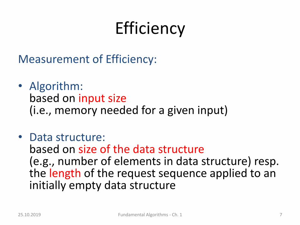
Efficiency
Measurement of Efficiency:
• Algorithm: based on input size(i.e., memory needed for a given input)
• Data structure: based on size of the data structure(e.g., number of elements in data structure) resp. the length of the request sequence applied to an initially empty data structure
25.10.2019 Fundamental Algorithms - Ch. 1 8
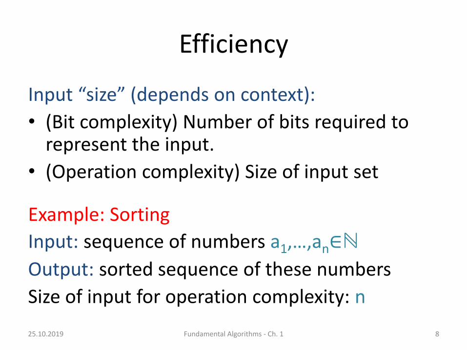
Efficiency
Input “size” (depends on context):
• (Bit complexity) Number of bits required to represent the input.
• (Operation complexity) Size of input set
Example: Sorting
Input: sequence of numbers a1,…,an∈ℕ
Output: sorted sequence of these numbers
Size of input for operation complexity: n

Notation for this course
• ℕ={1,2,3,...}: set of natural numbers
• ℕ0 = ℕ∪{0}: set of non-negative integers
• ℤ: set of integers
• ℝ: set of real numbers
• For all n∈ℕ0: [n]={1,...,n} and [n]0 = {0,...,n}
• Given a set L let ℘k(L) the set of subsets of L of
cardinality/size k
25.10.2019 Fundamental Algorithms - Ch. 1 9
25.10.2019 Fundamental Algorithms - Ch. 1 10
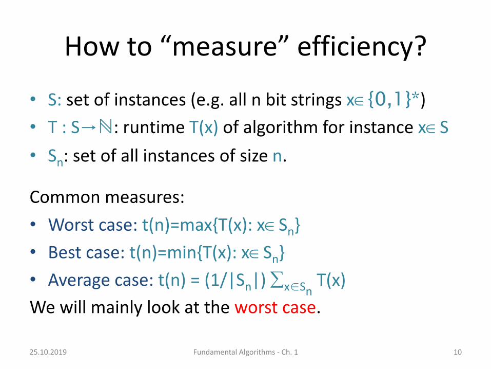
How to “measure” efficiency?
• S: set of instances (e.g. all n bit strings x{0,1}*)
• T : S→ℕ: runtime T(x) of algorithm for instance xS
• Sn: set of all instances of size n.
Common measures:
• Worst case: t(n)=max{T(x): xSn}
• Best case: t(n)=min{T(x): xSn}
• Average case: t(n) = (1/|Sn|) x∈SnT(x)
We will mainly look at the worst case.

25.10.2019 Fundamental Algorithms - Ch. 1 11
Measurement of Efficiency
Why worst case?
• “typical case” hard to grasp, average case is not necessarily a good measure for that
• gives guarantees for the efficiency of an algorithm (important for robustness)
How to classify efficiency: Asymptotic growth
• Big-Oh notation…
25.10.2019 Fundamental Algorithms - Ch. 1 12
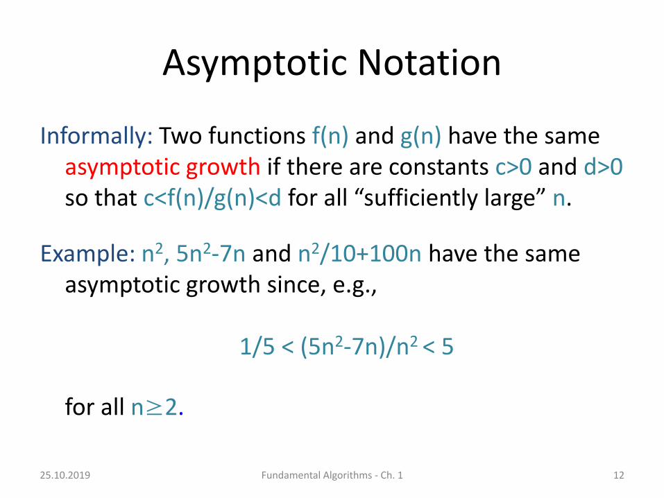
Asymptotic Notation
Informally: Two functions f(n) and g(n) have the same asymptotic growth if there are constants c>0 and d>0so that c<f(n)/g(n)<d for all “sufficiently large” n.
Example: n2, 5n2-7n and n2/10+100n have the same asymptotic growth since, e.g.,
1/5 < (5n2-7n)/n2 < 5
for all n≥2.
25.10.2019 Fundamental Algorithms - Ch. 1 13
Asymptotic Notation
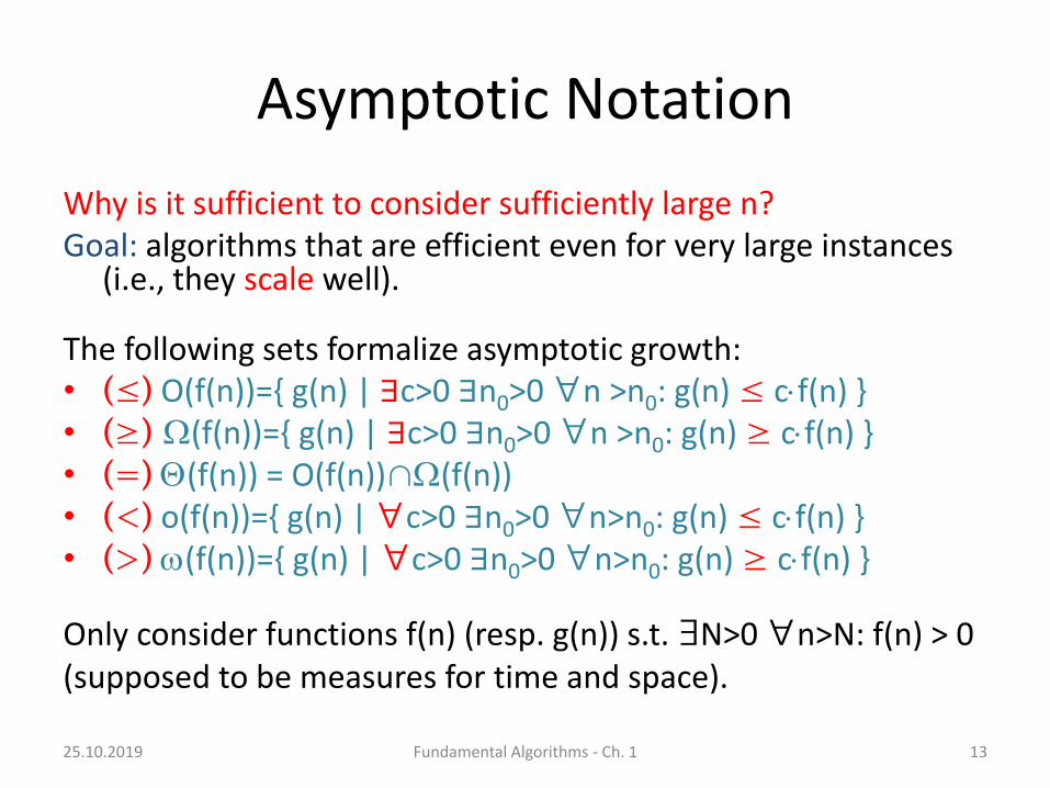
Why is it sufficient to consider sufficiently large n?Goal: algorithms that are efficient even for very large instances
(i.e., they scale well).
The following sets formalize asymptotic growth:• (≤) O(f(n))={ g(n) | ∃c>0 ∃n0>0 ∀n >n0: g(n) ≤ cf(n) } • (≥) W(f(n))={ g(n) | ∃c>0 ∃n0>0 ∀n >n0: g(n) ≥ cf(n) }• (=) Q(f(n)) = O(f(n))∩W(f(n))• (<) o(f(n))={ g(n) | ∀c>0 ∃n0>0 ∀n>n0: g(n) ≤ cf(n) }• (>) w(f(n))={ g(n) | ∀c>0 ∃n0>0 ∀n>n0: g(n) ≥ cf(n) }
Only consider functions f(n) (resp. g(n)) s.t. ∃N>0 ∀n>N: f(n) > 0 (supposed to be measures for time and space).

25.10.2019 Fundamental Algorithms - Ch. 1 14
Asymptotic Notation
f(n) = an + b
∈Q(f(n))
∈w(f(n))
∈o(f(n))

Asymptotic Notation
25.10.2019 Fundamental Algorithms - Ch. 1 15
• xn: limn (supm≥n xm)
sup: supremum (example: sup{ xℝ | x<2 } = 2 )
• xn: limn (infm≥n xm)
inf: infimum (example: inf { xℝ | x>3 } = 3 )
Alternative way of defining O-notation:
• O(g(n))={ f(n) | ∃ c>0 f(n)/g(n) ≤ c }• W(g(n))={ f(n) | ∃ c>0 f(n)/g(n) ≥ c }
• Q(g(n)) = O(g(n)) ∩ W(g(n))
• o(g(n))={ f(n) | f(n)/g(n) = 0 }• w(g(n))={ f(n) | g(n)/f(n) = 0 }
lim supn
lim supn
lim infn
lim infn
lim supn
lim infn
Crash Course on Limits
25.10.2019 Fundamental Algorithms - Ch. 1 16
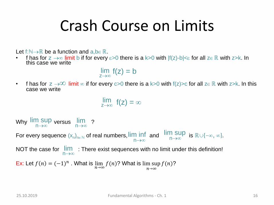
Let f:ℕℝ be a function and a,bℝ.• f has for z limit b if for every e>0 there is a k>0 with |f(z)-b|<e for all zℝ with z>k. In
this case we write
• f has for z limit if for every c>0 there is a k>0 with f(z)>c for all zℝ with z>k. In this case we write
Why versus ?
For every sequence (xn)nℕ of real numbers, and is ℝ∪{-, }.
NOT the case for : There exist sequences with no limit under this definition!
Ex: Let 𝑓 𝑛 = (−1)𝑛 . What is lim𝑛→∞
𝑓(𝑛)? What is lim sup𝑛→∞
𝑓(𝑛)?
limz
lim infn
lim supn
f(z) = b
limz f(z) =
limn
lim supn
limn
25.10.2019 Fundamental Algorithms - Ch. 1 17
Asymptotic Notation
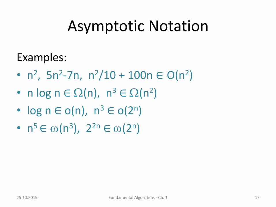
Examples:
• n2, 5n2-7n, n2/10 + 100n ∈ O(n2)
• n log n ∈ W(n), n3 ∈ W(n2)
• log n ∈ o(n), n3 ∈ o(2n)
• n5 ∈ w(n3), 22n ∈ w(2n)
Asymptotic Notation
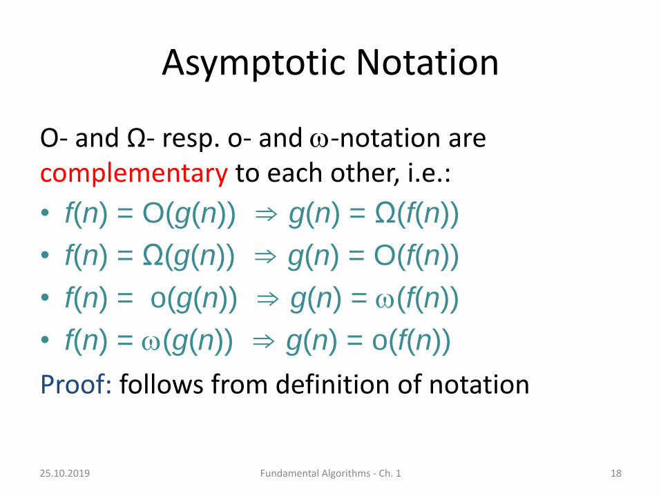
O- and Ω- resp. o- and w-notation are complementary to each other, i.e.:
• f(n) = O(g(n)) ⇒ g(n) = Ω(f(n))
• f(n) = Ω(g(n)) ⇒ g(n) = O(f(n))
• f(n) = o(g(n)) ⇒ g(n) = w(f(n))
• f(n) = w(g(n)) ⇒ g(n) = o(f(n))
Proof: follows from definition of notation
25.10.2019 Fundamental Algorithms - Ch. 1 18
Asymptotic Notation
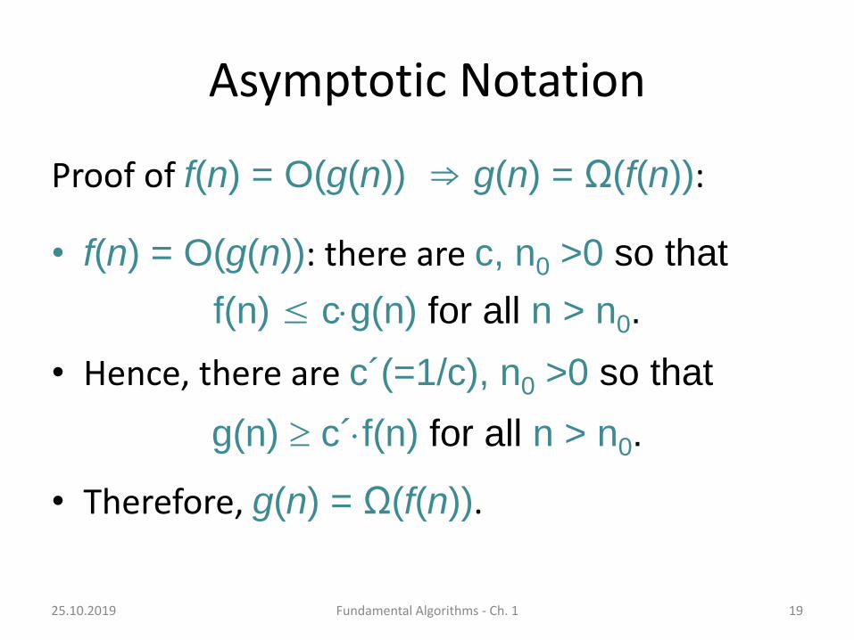
Proof of f(n) = O(g(n)) ⇒ g(n) = Ω(f(n)):
• f(n) = O(g(n)): there are c, n0 >0 so that
f(n) ≤ cg(n) for all n > n0.
• Hence, there are c´(=1/c), n0 >0 so that
g(n) c´f(n) for all n > n0.
• Therefore, g(n) = Ω(f(n)).
25.10.2019 Fundamental Algorithms - Ch. 1 19
Asymptotic Notation
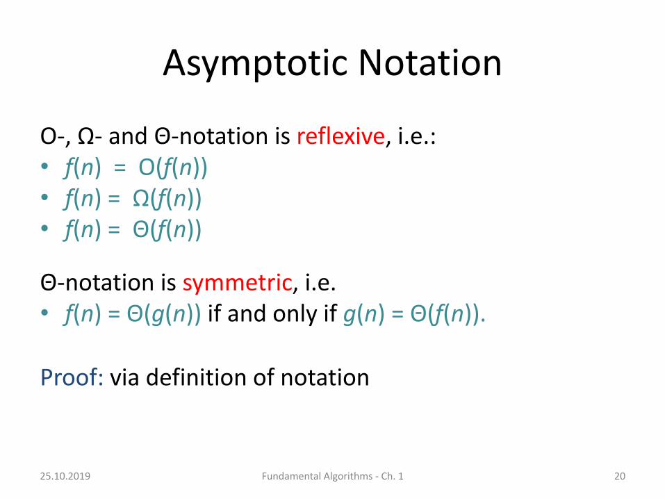
O-, Ω- and Θ-notation is reflexive, i.e.:• f(n) = O(f(n))• f(n) = Ω(f(n))• f(n) = Θ(f(n))
Θ-notation is symmetric, i.e.• f(n) = Θ(g(n)) if and only if g(n) = Θ(f(n)).
Proof: via definition of notation
25.10.2019 Fundamental Algorithms - Ch. 1 20
Asymptotic Notation
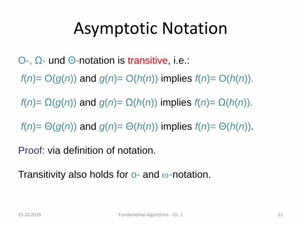
O-, Ω- und Θ-notation is transitive, i.e.:
f(n)= O(g(n)) and g(n)= O(h(n)) implies f(n)= O(h(n)).
f(n)= Ω(g(n)) and g(n)= Ω(h(n)) implies f(n)= Ω(h(n)).
f(n)= Θ(g(n)) and g(n)= Θ(h(n)) implies f(n)= Θ(h(n)).
Proof: via definition of notation.
Transitivity also holds for o- and w-notation.
25.10.2019 Fundamental Algorithms - Ch. 1 21

Asymptotic Notation
Proof for transitivity of O-notation:
• f(n) = O(g(n)) ⇔ there are c´, n´0 >0 so that
f (n) ≤ c´g(n) for all n > n´0.
• g(n) = O(h(n)) ⇔ there are c´´, n´´0 >0 so that
g(n) ≤ c´´h(n) for all n > n´´0.
Let n0 = max{n´0, n´´0} and c = c´·c´´. Then for all n > n0:
f (n) ≤ c´ · g(n) ≤ c´ · c´´· h(n) = c · h(n).
25.10.2019 Fundamental Algorithms - Ch. 1 22
Asymptotic Notation
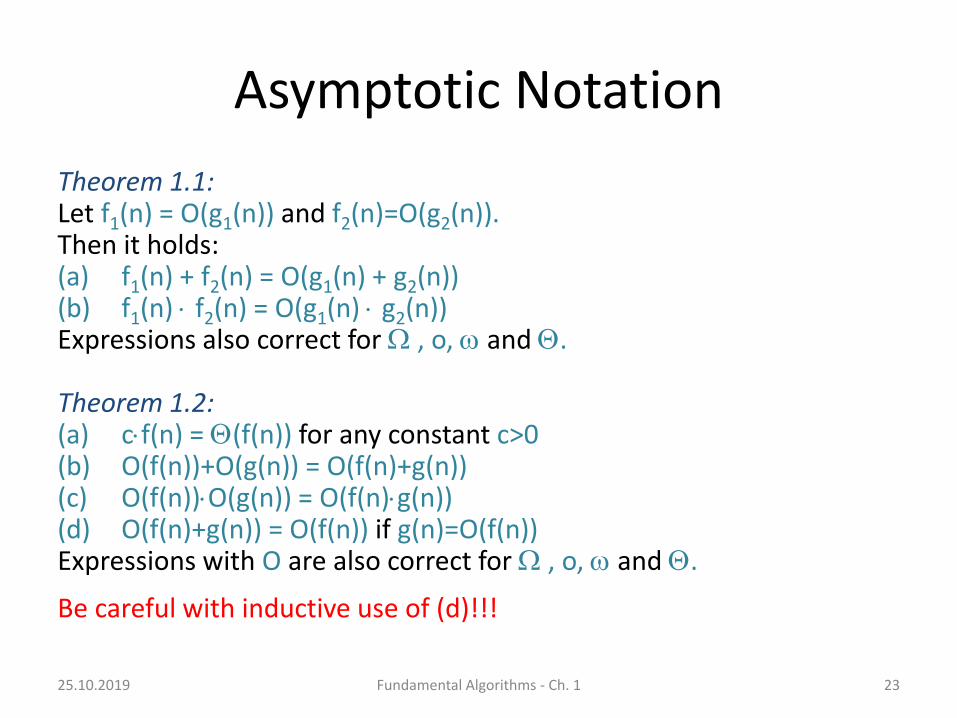
Theorem 1.1:Let f1(n) = O(g1(n)) and f2(n)=O(g2(n)). Then it holds:(a) f1(n) + f2(n) = O(g1(n) + g2(n))(b) f1(n) f2(n) = O(g1(n) g2(n))Expressions also correct for W , o, w and Q.
Theorem 1.2:(a) cf(n) = Q(f(n)) for any constant c>0(b) O(f(n))+O(g(n)) = O(f(n)+g(n))(c) O(f(n))O(g(n)) = O(f(n)g(n))(d) O(f(n)+g(n)) = O(f(n)) if g(n)=O(f(n))Expressions with O are also correct for W , o, w and Q.
Be careful with inductive use of (d)!!!
25.10.2019 23Fundamental Algorithms - Ch. 1

Asymptotic Notation
Proof of Theorem 1.1 (a):• Let f1(n) = O(g1(n)) and f2(n)=O(g2(n)).• Then it holds:∃ c1>0 ∃ n1>0 n≥n1: f1(n) ≤ c1g1(n)∃ c2>0 ∃ n2>0 n≥n2: f2(n) ≤ c2g2(n)
• Hence, with c0=max{c1,c2} and n0=max{n1,n2} we get:∃ c0>0 ∃ n0>0 n≥n0:
f1(n)+f2(n) ≤ c0(g1(n)+g2(n))• Therefore, f1(n)+f2(n) = O(g1(n)+g2(n)).
Proof of (b): exercise
25.10.2019 Fundamental Algorithms - Ch. 1 24
Asymptotic Notation
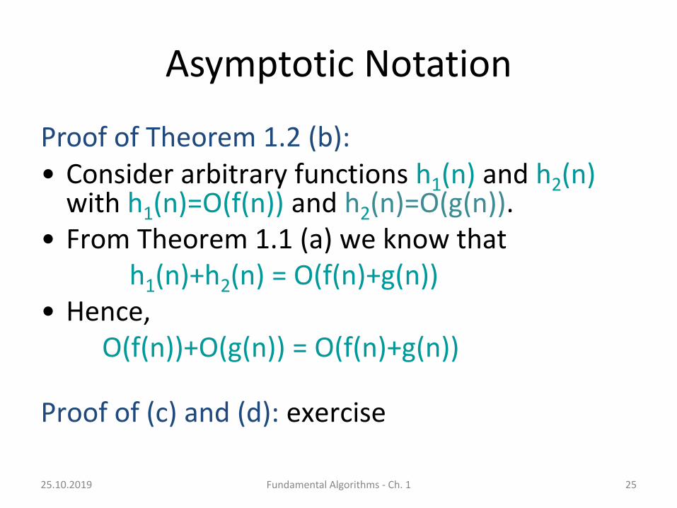
Proof of Theorem 1.2 (b):• Consider arbitrary functions h1(n) and h2(n)
with h1(n)=O(f(n)) and h2(n)=O(g(n)).• From Theorem 1.1 (a) we know that
h1(n)+h2(n) = O(f(n)+g(n))• Hence,
O(f(n))+O(g(n)) = O(f(n)+g(n))
Proof of (c) and (d): exercise
25.10.2019 Fundamental Algorithms - Ch. 1 25
Asymptotic Notation
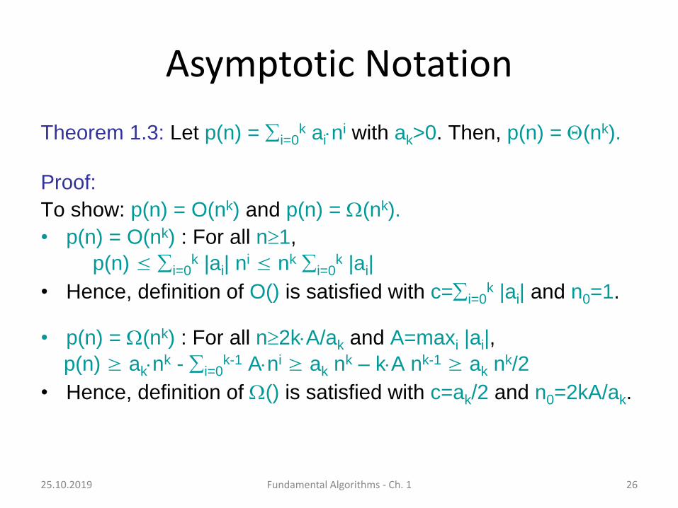
Theorem 1.3: Let p(n) = i=0k ain
i with ak>0. Then, p(n) = Q(nk).
Proof:
To show: p(n) = O(nk) and p(n) = W(nk).
• p(n) = O(nk) : For all n1,
p(n) ≤ i=0k |ai| n
i ≤ nk i=0k |ai|
• Hence, definition of O() is satisfied with c=i=0k |ai| and n0=1.
• p(n) = W(nk) : For all n2kA/ak and A=maxi |ai|,
p(n) ≥ aknk - i=0
k-1 Ani ≥ ak nk – kA nk-1 ≥ ak nk/2
• Hence, definition of W() is satisfied with c=ak/2 and n0=2kA/ak.
25.10.2019 Fundamental Algorithms - Ch. 1 26
25.10.2019 Fundamental Algorithms - Ch. 1 27
Pseudo Code
We will use pseudo code in order to formally specify an algorithm.
Declaration of variables:
v: T : Variable v of type T
v=x: T : is initialized with the value x
Types of variables:
• integer, boolean, char
• Pointer to T: pointer to an element of type T
• Array[i..j] of T: array of elements with index i to j of type T
25.10.2019 Fundamental Algorithms - Ch. 1 28
Pseudo-Code
Allocation and de-allocation of space:
• v:= allocate Array[1..n] of T
• dispose v
Important commands: (C: condition, I,J: commands)
• v:=A // v receives the result of expression A
• if C then I else J
• repeat I until C, while C do I
• for v:=a to e do I
• foreach e∈S do I
• return v
25.10.2019 Fundamental Algorithms - Ch. 1 29
Runtime Analysis
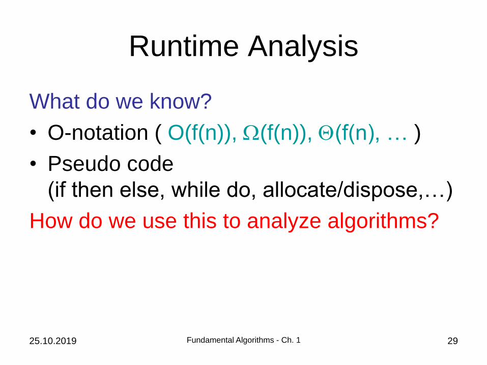
What do we know?
• O-notation ( O(f(n)), W(f(n)), Q(f(n), … )
• Pseudo code
(if then else, while do, allocate/dispose,…)
How do we use this to analyze algorithms?
Runtime Analysis
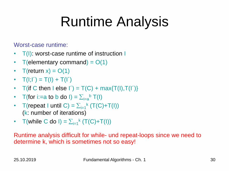
Worst-case runtime:
• T(I): worst-case runtime of instruction I
• T(elementary command) = O(1)
• T(return x) = O(1)
• T(I;I´) = T(I) + T(I´)
• T(if C then I else I´) = T(C) + max{T(I),T(I´)}
• T(for i:=a to b do I) = i=ab T(I)
• T(repeat I until C) = i=1k (T(C)+T(I))
(k: number of iterations)
• T(while C do I) = i=1k (T(C)+T(I))
Runtime analysis difficult for while- und repeat-loops since we need todetermine k, which is sometimes not so easy!
25.10.2019 Fundamental Algorithms - Ch. 1 30
25.10.2019 Fundamental Algorithms - Ch. 1 31
Example: Computation of Sign
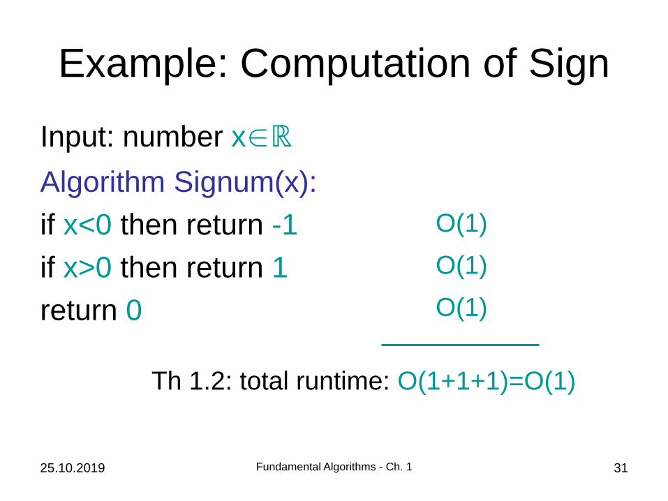
Input: number x∈ℝ
Algorithm Signum(x):
if x<0 then return -1
if x>0 then return 1
return 0
O(1)
O(1)
O(1)
Th 1.2: total runtime: O(1+1+1)=O(1)

25.10.2019 Fundamental Algorithms - Ch. 1 32
Example: Minimum
Input: array of numbers A[1],…,A[n]
Minimum Algorithm:
min := 1
for i:=1 to n do
if A[i]<min then min:=A[i]
return min
O(1)
O(i=1n T(I))
O(1)
O(1)
runtime: O(1 +(i=1n 1) + 1) = O(n)

25.10.2019 33
Example: Sorting
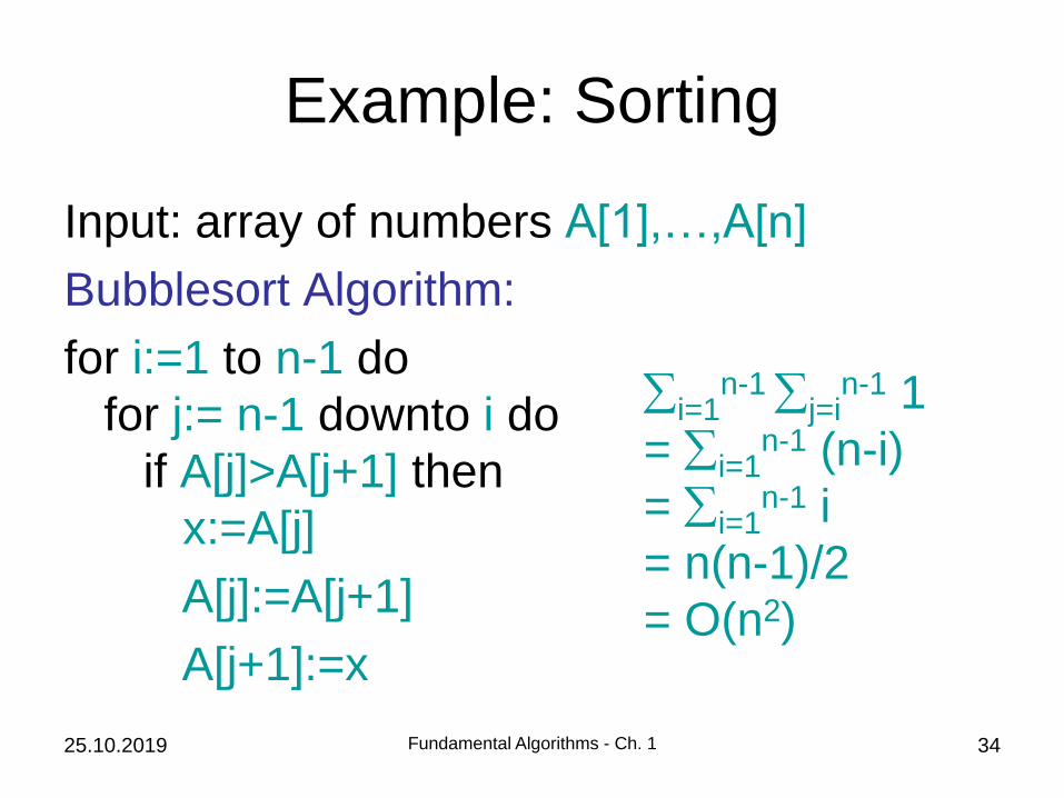
Input: array of numbers A[1],…,A[n]
Bubblesort Algorithm:
for i:=1 to n-1 do
for j:= n-1 downto i do
if A[j]>A[j+1] then
x:=A[j]
A[j]:=A[j+1]
A[j+1]:=x
O(i=1n-1 T(I))
O(j=in-1 T(I))
O(1)
O(1)
O(1)
O(1 + T(I))
runtime: O(i=1n-1 j=i
n-1 1)Fundamental Algorithms - Ch. 1
25.10.2019 Fundamental Algorithms - Ch. 1 34
Example: Sorting
Input: array of numbers A[1],…,A[n]
Bubblesort Algorithm:
for i:=1 to n-1 do
for j:= n-1 downto i do
if A[j]>A[j+1] then
x:=A[j]
A[j]:=A[j+1]
A[j+1]:=x
i=1n-1 j=i
n-1 1
= i=1n-1 (n-i)
= i=1n-1 i
= n(n-1)/2
= O(n2)
25.10.2019 Fundamental Algorithms - Ch. 1 35
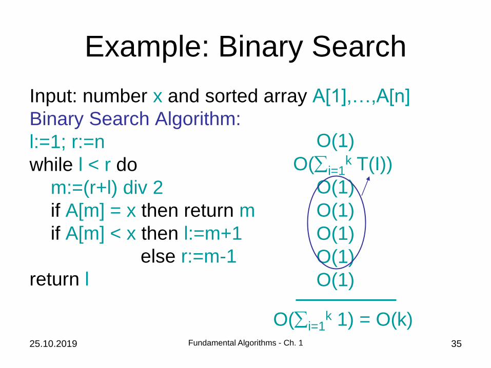
Example: Binary Search
Input: number x and sorted array A[1],…,A[n]
Binary Search Algorithm:
l:=1; r:=n
while l < r do
m:=(r+l) div 2
if A[m] = x then return m
if A[m] < x then l:=m+1
else r:=m-1
return l
O(1)
O(i=1k T(I))
O(1)
O(1)
O(1)
O(1)
O(1)
O(i=1k 1) = O(k)
25.10.2019 Fundamental Algorithms - Ch. 1 36
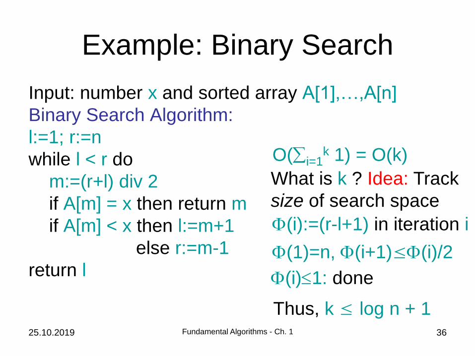
Example: Binary Search
Input: number x and sorted array A[1],…,A[n]
Binary Search Algorithm:
l:=1; r:=n
while l < r do
m:=(r+l) div 2
if A[m] = x then return m
if A[m] < x then l:=m+1
else r:=m-1
return l
O(i=1k 1) = O(k)
F(i):=(r-l+1) in iteration i
What is k ? Idea: Track
size of search space
F(1)=n, F(i+1)≤F(i)/2
F(i)1: done
Thus, k ≤ log n + 1

Runtime via Potential Function
Find a potential function F and d,D>0 so that
• F decreases (resp. increases) by at least d in
each iteration of the while-/repeat-loop and
• F is bounded from below (resp. above) by D.
Then the while-/repeat-loop is executed at most
1+|F0-D|/d times, where F0 is the initial value of F.
25.10.2019 Fundamental Algorithms - Ch. 1 37
F0 D
1 step
d
25.10.2019 Fundamental Algorithms - Ch. 1 38
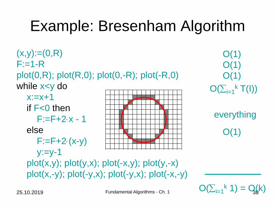
Example: Bresenham Algorithm
(x,y):=(0,R)
F:=1-R
plot(0,R); plot(R,0); plot(0,-R); plot(-R,0)
while x<y do
x:=x+1
if F<0 then
F:=F+2x - 1
else
F:=F+2(x-y)
y:=y-1
plot(x,y); plot(y,x); plot(-x,y); plot(y,-x)
plot(x,-y); plot(-y,x); plot(-y,x); plot(-x,-y)
O(1)
O(1)
O(1)
O(i=1k T(I))
O(1)
O(i=1k 1) = O(k)
everything
25.10.2019 Fundamental Algorithms - Ch. 1 39
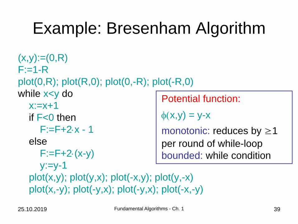
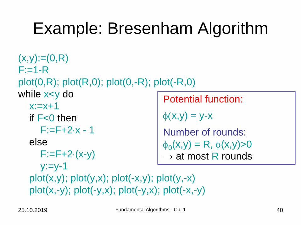
Example: Bresenham Algorithm
(x,y):=(0,R)
F:=1-R
plot(0,R); plot(R,0); plot(0,-R); plot(-R,0)
while x<y do
x:=x+1
if F<0 then
F:=F+2x - 1
else
F:=F+2(x-y)
y:=y-1
plot(x,y); plot(y,x); plot(-x,y); plot(y,-x)
plot(x,-y); plot(-y,x); plot(-y,x); plot(-x,-y)
Potential function:
(x,y) = y-x
monotonic: reduces by ≥1
per round of while-loop
bounded: while condition
25.10.2019 Fundamental Algorithms - Ch. 1 40
Example: Bresenham Algorithm
(x,y):=(0,R)
F:=1-R
plot(0,R); plot(R,0); plot(0,-R); plot(-R,0)
while x<y do
x:=x+1
if F<0 then
F:=F+2x - 1
else
F:=F+2(x-y)
y:=y-1
plot(x,y); plot(y,x); plot(-x,y); plot(y,-x)
plot(x,-y); plot(-y,x); plot(-y,x); plot(-x,-y)
Potential function:
(x,y) = y-x
Number of rounds:
0(x,y) = R, (x,y)>0
→ at most R rounds

25.10.2019 Fundamental Algorithms - Ch. 1 41
Example: Factorial
Input: natural number n
Algorithm Factorial(n):
if n=1 then return 1
else return n Factorial(n-1)
Runtime:
• T(n): runtime of Factorial(n)
• T(n) = T(n-1) + O(1), T(1) = O(1)
O(1)
O(1 + ??)
25.10.2019 Fundamental Algorithms - Ch. 1 42
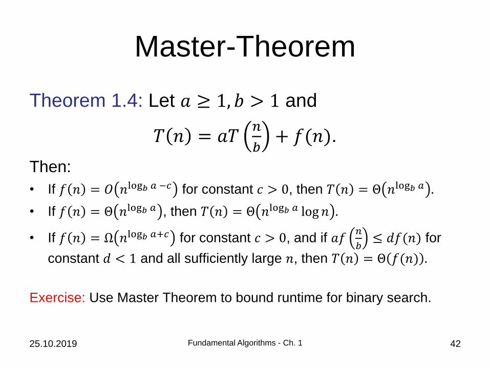
Master-Theorem
Theorem 1.4: Let 𝑎 ≥ 1, 𝑏 > 1 and
𝑇 𝑛 = 𝑎𝑇𝑛
𝑏+ 𝑓(𝑛).
Then:
• If 𝑓 𝑛 = 𝑂 𝑛log𝑏 𝑎 −𝑐 for constant 𝑐 > 0, then 𝑇 𝑛 = Θ 𝑛log𝑏 𝑎 .
• If 𝑓 𝑛 = Θ 𝑛log𝑏 𝑎 , then 𝑇 𝑛 = Θ 𝑛log𝑏 𝑎 log 𝑛 .
• If 𝑓 𝑛 = Ω 𝑛log𝑏 𝑎+𝑐 for constant 𝑐 > 0, and if 𝑎𝑓𝑛
𝑏≤ 𝑑𝑓(𝑛) for
constant 𝑑 < 1 and all sufficiently large 𝑛, then 𝑇 𝑛 = Θ 𝑓(𝑛) .
Exercise: Use Master Theorem to bound runtime for binary search.
r (n) =
½a falls n = 1
c ¢n + d ¢r (n=b) falls n > 1a = b

Amortized Analysis
25.10.2019 Fundamental Algorithms - Ch. 1 43
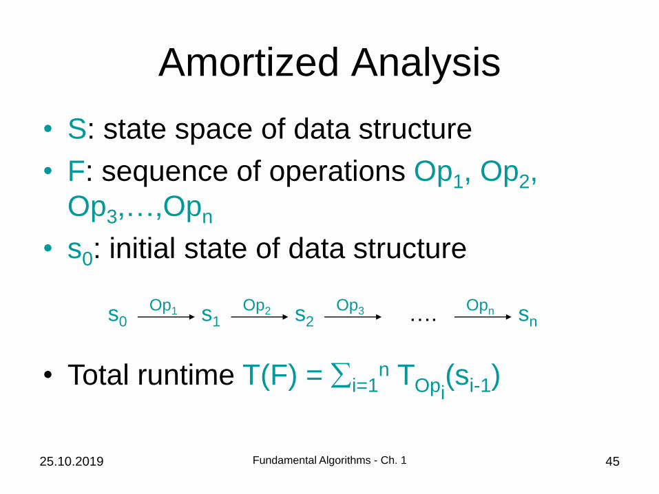
• S: state space of data structure
• F: sequence of operations Op1, Op2,
Op3,…,Opn
• s0: initial state of data structure
• Total runtime T(F) = i=1n TOpi
(si-1)
s0Op1 s1
Op2 s2Op3 sn
Opn….

Amortized Analysis: Intuition
25.10.2019 Fundamental Algorithms - Ch. 1 44
Question: What is daily cost of owning a car?
Day Activity Cost
1 Buy car 20,000
2 Buy gas 60
3-10 Drive 0
11 Buy gas 60
12 Drive 0 ... and so forth ....
So what is daily cost of owning a car?
• Worst case analysis: cost of worst operation over all days, O(20,000)!
... grossly overestimates the „typical“ daily cost
• Amortized analysis: add all costs, divide by # days, i.e. „average“ cost
per day.
Amortized Analysis
25.10.2019 Fundamental Algorithms - Ch. 1 45
• S: state space of data structure
• F: sequence of operations Op1, Op2,
Op3,…,Opn
• s0: initial state of data structure
• Total runtime T(F) = i=1n TOpi
(si-1)
s0Op1 s1
Op2 s2Op3 sn
Opn….
Amortized Analysis
25.10.2019 Fundamental Algorithms - Ch. 1 46
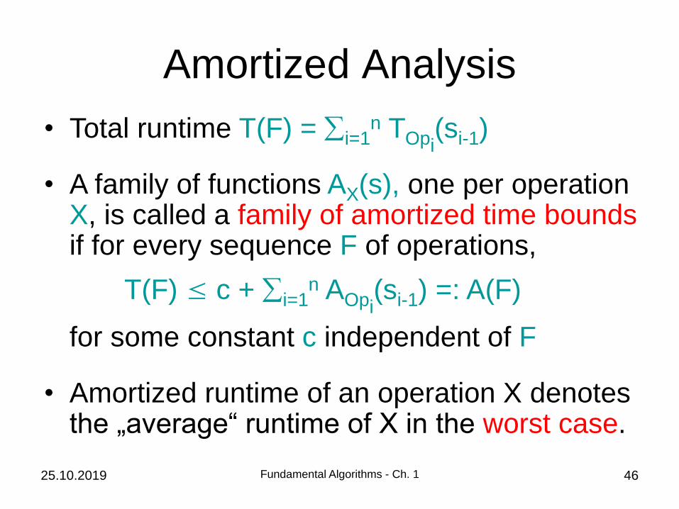
• Total runtime T(F) = i=1n TOpi
(si-1)
• A family of functions AX(s), one per operation X, is called a family of amortized time boundsif for every sequence F of operations,
T(F) ≤ c + i=1n AOpi
(si-1) =: A(F)
for some constant c independent of F
• Amortized runtime of an operation X denotes the „average“ runtime of X in the worst case.

How to choose AX(s)?
25.10.2019 Fundamental Algorithms - Ch. 1 47
• Trivial choice --- AX(s) := TX(s)
• More clever choice of AX(s) via potential function :Sℝ≥0 can simplify proofs
Amortized Analysis
25.10.2019 Fundamental Algorithms - Ch. 1 48
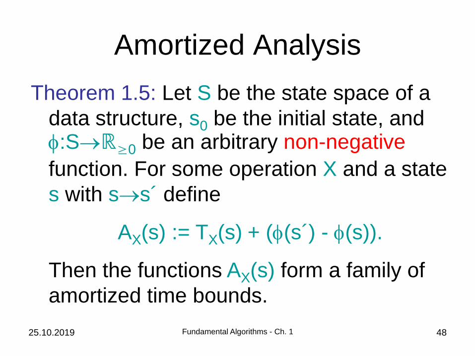
Theorem 1.5: Let S be the state space of a
data structure, s0 be the initial state, and:Sℝ≥0 be an arbitrary non-negative
function. For some operation X and a state
s with ss´ define
AX(s) := TX(s) + ((s´) - (s)).
Then the functions AX(s) form a family of
amortized time bounds.

Amortized Analysis
25.10.2019 Fundamental Algorithms - Ch. 1 49
To show: T(F) ≤ c + i=1n AOpi
(si-1)
Proof:
i=1n AOpi
(si-1) = i=1n [TOpi
(si-1) + (si) - (si-1)]
= T(F) + i=1n [(si) - (si-1)]
= T(F) + (sn) - (s0)
⇒ T(F) = i=1n AOpi
(si-1) + (s0) - (sn)
≤ i=1n AOpi
(si-1) + (s0) constant
Amortized Analysis
25.10.2019 Fundamental Algorithms - Ch. 1 50
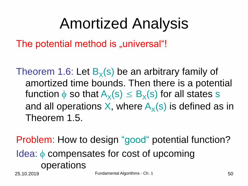
The potential method is „universal“!
Theorem 1.6: Let BX(s) be an arbitrary family of
amortized time bounds. Then there is a potential function so that AX(s) ≤ BX(s) for all states s
and all operations X, where AX(s) is defined as in
Theorem 1.5.
Problem: How to design “good“ potential function?
Idea: compensates for cost of upcoming
operations
Example: Dynamic Array
25.10.2019 Fundamental Algorithms - Ch. 1 51
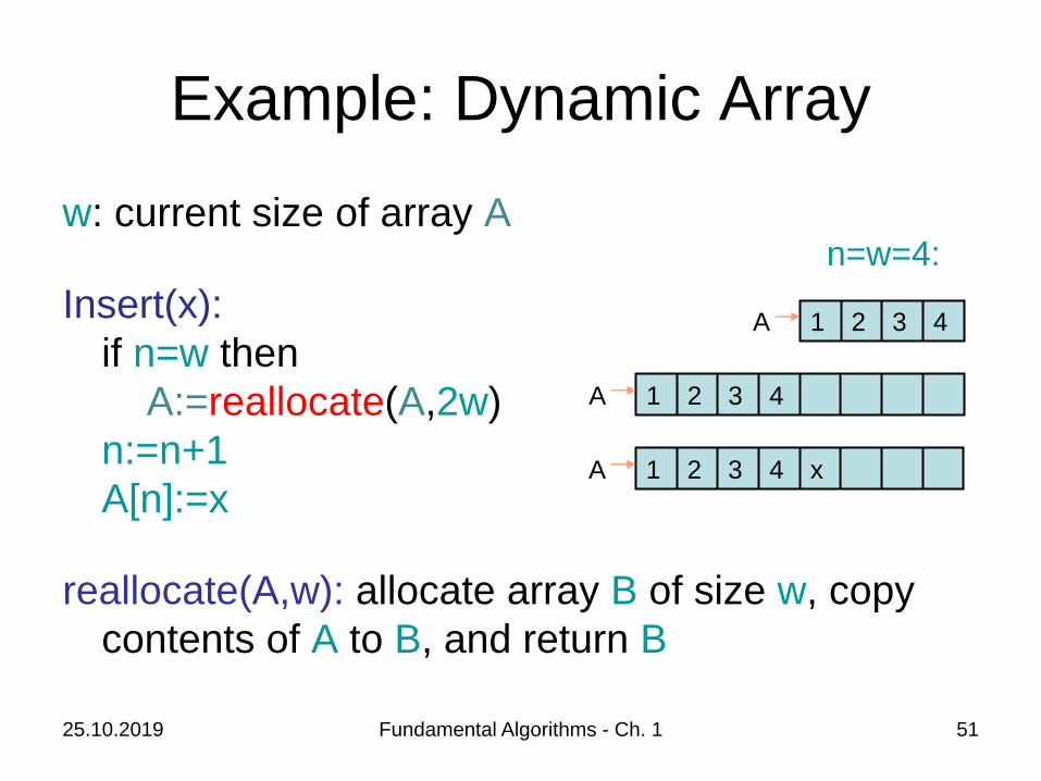
w: current size of array A
Insert(x):
if n=w then
A:=reallocate(A,2w)
n:=n+1
A[n]:=x
reallocate(A,w): allocate array B of size w, copy
contents of A to B, and return B
1 2 3 4A
1 2 3 4A
1 2 3 xA 4
n=w=4:
Example: Dynamic Array
25.10.2019 Fundamental Algorithms - Ch. 1 52
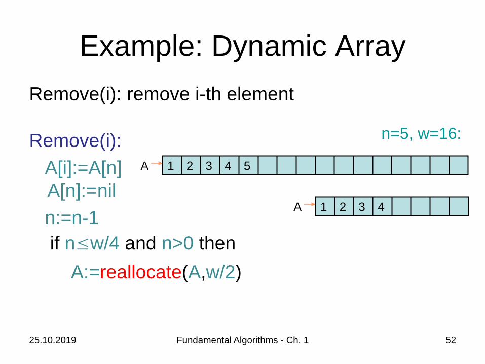
Remove(i): remove i-th element
Remove(i):
A[i]:=A[n]
A[n]:=nil
n:=n-1
if n≤w/4 and n>0 then
A:=reallocate(A,w/2)
1 2 3 5A
1 2 3A 4
4
n=5, w=16:
Example: Dynamic Array
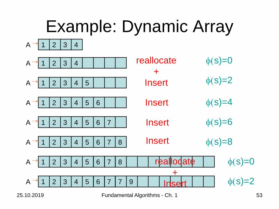
25.10.2019 Fundamental Algorithms - Ch. 1 53
1 2 3 4A
1 2 3 4A
1 2 3 4A
5
5 6
1 2 3 4A 5 6 7
1 2 3 4A 5 6 7 8
1 2 3 5A 4 6 7 8
(s)=0
(s)=2
(s)=4
(s)=6
(s)=8
(s)=0
reallocate
+
Insert
1 2 3 5A 4 6 7 7 9 (s)=2
reallocate
+
Insert
1 2 3 4A
Insert
Insert
Insert

Example: Dynamic Array
25.10.2019 Fundamental Algorithms - Ch. 1 54
1 2 3 4A (s)=0
1 2 3A (s)=2
1 2A (s)=4
1 2A
Remove
+
reallocate (s)=0
Remove
General formula for (s):
(ws: size of A, ns: number of entries)
(s) = 2|ws/2 – ns|
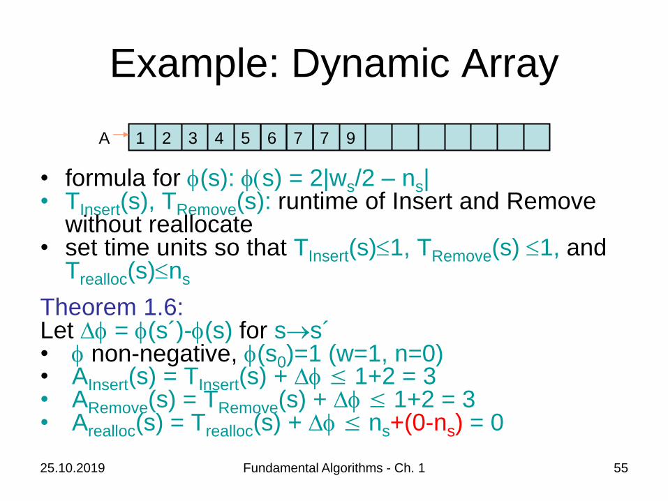
Example: Dynamic Array
• formula for (s): (s) = 2|ws/2 – ns|• TInsert(s), TRemove(s): runtime of Insert and Remove
without reallocate• set time units so that TInsert(s)1, TRemove(s) 1, and
Trealloc(s)ns
Theorem 1.6:Let D = (s´)-(s) for ss´• non-negative, (s0)=1 (w=1, n=0)• AInsert(s) = TInsert(s) + D ≤ 1+2 = 3• ARemove(s) = TRemove(s) + D ≤ 1+2 = 3 • Arealloc(s) = Trealloc(s) + D ≤ ns+(0-ns) = 0
25.10.2019 Fundamental Algorithms - Ch. 1 55
1 2 3 5A 4 6 7 7 9
Example: Dynamic Array
25.10.2019 Fundamental Algorithms - Ch. 1 56
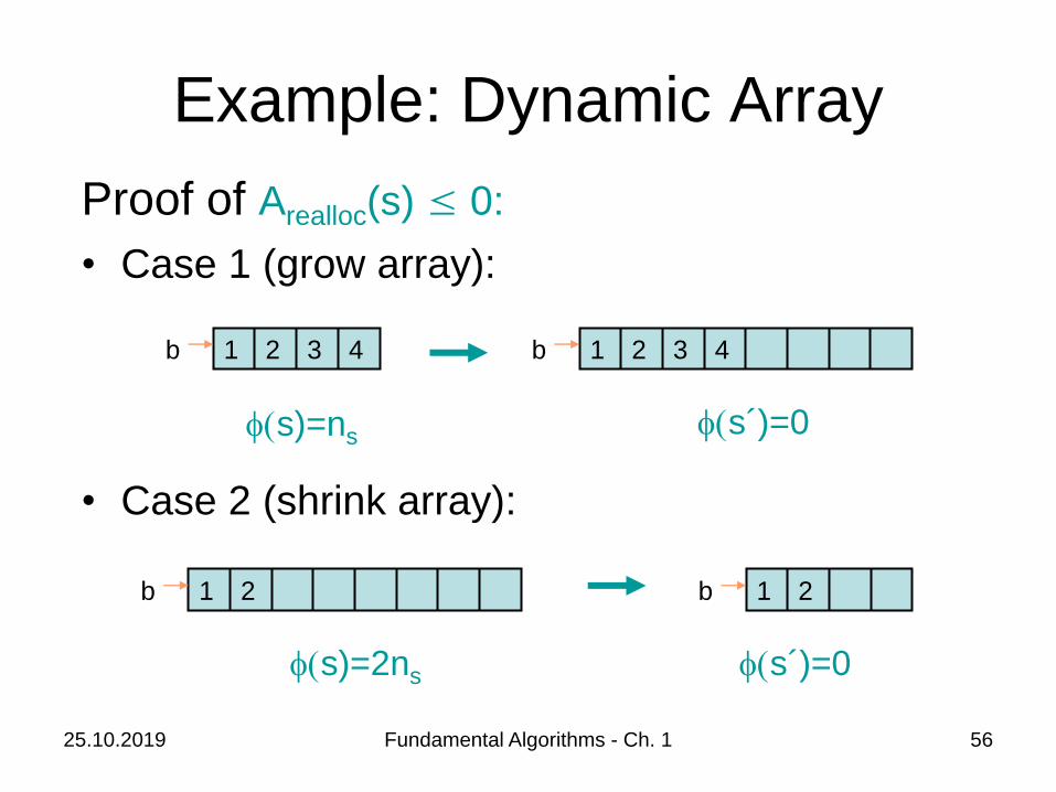
Proof of Arealloc(s) ≤ 0:
• Case 1 (grow array):
• Case 2 (shrink array):
1 2b 1 2 3 4b3 4
(s)=ns (s´)=0
1 2b 1 2b
(s)=2ns (s´)=0
Example: Dynamic Array
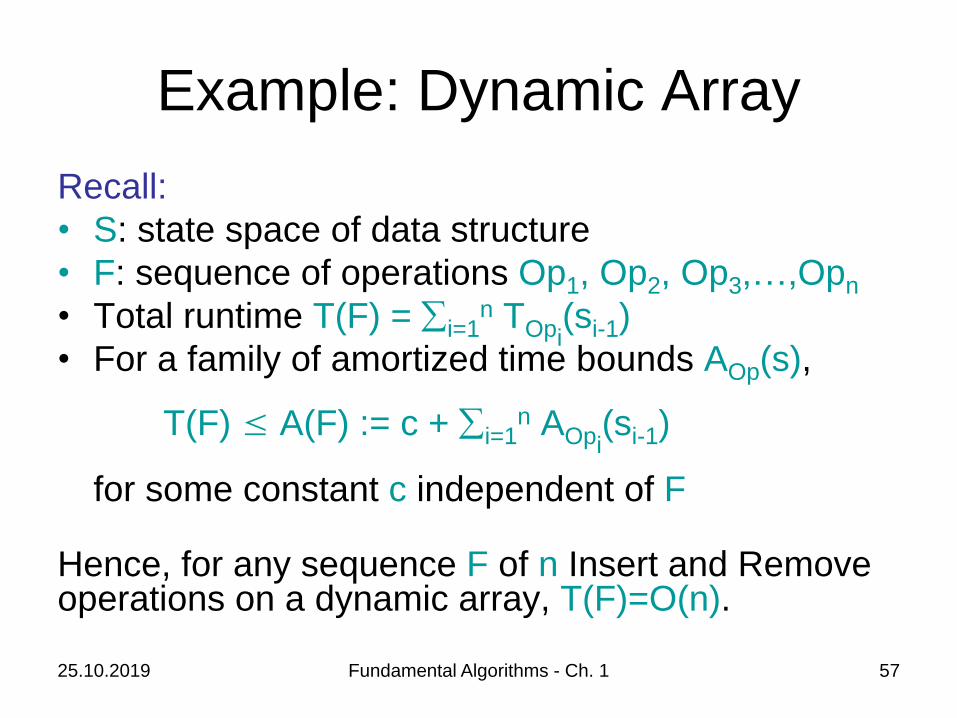
Recall:
• S: state space of data structure
• F: sequence of operations Op1, Op2, Op3,…,Opn
• Total runtime T(F) = i=1n TOpi
(si-1)
• For a family of amortized time bounds AOp(s),
T(F) ≤ A(F) := c + i=1n AOpi
(si-1)
for some constant c independent of F
Hence, for any sequence F of n Insert and Remove operations on a dynamic array, T(F)=O(n).
25.10.2019 Fundamental Algorithms - Ch. 1 57