Fundamental Algorithms Chapter 8: Matrices and Scientific...
339
Fundamental Algorithms Chapter 8: Matrices and Scientific Computing Sevag Gharibian Universität Paderborn WS 2019 Sevag Gharibian (Universität Paderborn) Ch. 8: Matrices and Scientific Computing Fundamental Algs WS 2019 1 / 115
Transcript of Fundamental Algorithms Chapter 8: Matrices and Scientific...
Fundamental AlgorithmsChapter 8: Matrices and Scientific Computing
Sevag Gharibian
Universität PaderbornWS 2019
Sevag Gharibian (Universität Paderborn) Ch. 8: Matrices and Scientific Computing Fundamental Algs WS 2019 1 / 115
Outline
1 Introduction to matrices (review)
2 Matrix multiplication algorithmsStrassen’s algorithm (1967)Drineas-Kannan-Mahoney randomized algorithm (2006)
3 Random walksGambler’s ruinGoogle’s PageRank algorithm (1999)
4 Polynomial multiplicationComplex numbersPolynomialsO(N log N)-time polynomial multiplication via Fourier Transform
Sevag Gharibian (Universität Paderborn) Ch. 8: Matrices and Scientific Computing Fundamental Algs WS 2019 2 / 115
References
CLRS Chapters 28.1, 28.2, 30.1, 30.2M. Mahoney lecture notes:https://www.stat.berkeley.edu/~mmahoney/f13-stat260-cs294/Lectures/lecture02.pdf
T. Leighton and T. Rubinfeld lecture notes: http://web.mit.edu/neboat/Public/6.042/randomwalks.pdf
O. Levin: http://discrete.openmathbooks.org/dmoi2/sec_recurrence.html
M. Nielsen lectures on Google technology:http://michaelnielsen.org/blog/lectures-on-the-google-technology-stack-1-introduction-to-pagerank/History of complex numbers https://www.cut-the-knot.org/arithmetic/algebra/HistoricalRemarks.shtml
Sevag Gharibian (Universität Paderborn) Ch. 8: Matrices and Scientific Computing Fundamental Algs WS 2019 3 / 115
Outline
1 Introduction to matrices (review)
2 Matrix multiplication algorithmsStrassen’s algorithm (1967)Drineas-Kannan-Mahoney randomized algorithm (2006)
3 Random walksGambler’s ruinGoogle’s PageRank algorithm (1999)
4 Polynomial multiplicationComplex numbersPolynomialsO(N log N)-time polynomial multiplication via Fourier Transform
Sevag Gharibian (Universität Paderborn) Ch. 8: Matrices and Scientific Computing Fundamental Algs WS 2019 4 / 115
MatricesMotivation - why matrices?
Applications in most technical fields
Physics: Classical mechanics, optics, electromagnetism, quantummechanics
Computer Science: Graphics, randomized algorithms, big data (e.g.Google’s PageRank algorithm), quantum computing
Mathematics: Graph theory, geometry, linear systems of equations,optimization
Economics, game theory
Note:
Throughout these notes, we assume all operations are done over thefield of real numbers, R.
We ignore issues of precision (which is an important topic).
Sevag Gharibian (Universität Paderborn) Ch. 8: Matrices and Scientific Computing Fundamental Algs WS 2019 5 / 115
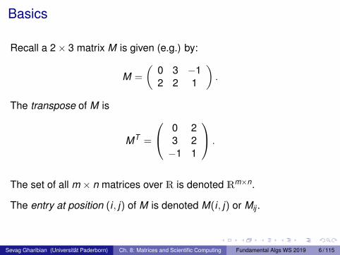
Basics
Recall a 2× 3 matrix M is given (e.g.) by:
M =
(0 3 −12 2 1
).
The transpose of M is
MT =
0 23 2−1 1
.
The set of all m × n matrices over R is denoted Rm×n.
The entry at position (i , j) of M is denoted M(i , j) or Mij .
Sevag Gharibian (Universität Paderborn) Ch. 8: Matrices and Scientific Computing Fundamental Algs WS 2019 6 / 115
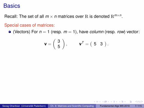
Basics
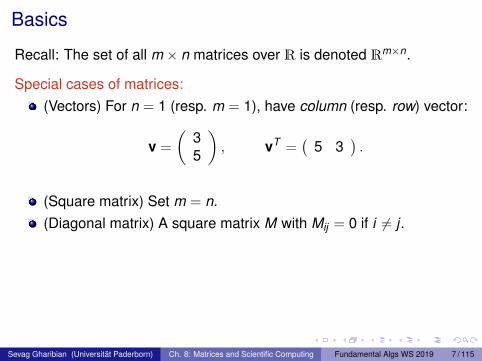
Recall: The set of all m × n matrices over R is denoted Rm×n.
Special cases of matrices:(Vectors) For n = 1 (resp. m = 1), have column (resp. row) vector:
v =
(35
), vT =
(5 3
).
(Square matrix) Set m = n.(Diagonal matrix) A square matrix M with Mij = 0 if i 6= j .(Identity matrix) The n × n (diagonal) matrix (n = 2 below)
I2 =
(1 00 1
).
Sevag Gharibian (Universität Paderborn) Ch. 8: Matrices and Scientific Computing Fundamental Algs WS 2019 7 / 115
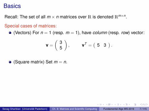
Basics
Recall: The set of all m × n matrices over R is denoted Rm×n.
Special cases of matrices:(Vectors) For n = 1 (resp. m = 1), have column (resp. row) vector:
v =
(35
), vT =
(5 3
).
(Square matrix) Set m = n.
(Diagonal matrix) A square matrix M with Mij = 0 if i 6= j .(Identity matrix) The n × n (diagonal) matrix (n = 2 below)
I2 =
(1 00 1
).
Sevag Gharibian (Universität Paderborn) Ch. 8: Matrices and Scientific Computing Fundamental Algs WS 2019 7 / 115
Basics
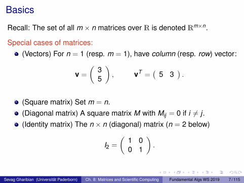
Recall: The set of all m × n matrices over R is denoted Rm×n.
Special cases of matrices:(Vectors) For n = 1 (resp. m = 1), have column (resp. row) vector:
v =
(35
), vT =
(5 3
).
(Square matrix) Set m = n.(Diagonal matrix) A square matrix M with Mij = 0 if i 6= j .
(Identity matrix) The n × n (diagonal) matrix (n = 2 below)
I2 =
(1 00 1
).
Sevag Gharibian (Universität Paderborn) Ch. 8: Matrices and Scientific Computing Fundamental Algs WS 2019 7 / 115
Basics
Recall: The set of all m × n matrices over R is denoted Rm×n.
Special cases of matrices:(Vectors) For n = 1 (resp. m = 1), have column (resp. row) vector:
v =
(35
), vT =
(5 3
).
(Square matrix) Set m = n.(Diagonal matrix) A square matrix M with Mij = 0 if i 6= j .(Identity matrix) The n × n (diagonal) matrix (n = 2 below)
I2 =
(1 00 1
).
Sevag Gharibian (Universität Paderborn) Ch. 8: Matrices and Scientific Computing Fundamental Algs WS 2019 7 / 115
Matrix operations
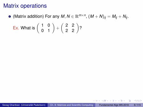
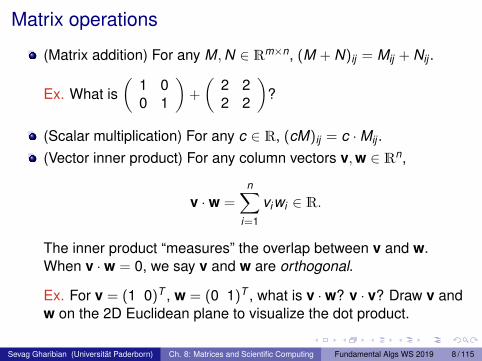
(Matrix addition) For any M,N ∈ Rm×n, (M + N)ij = Mij + Nij .
Ex. What is(
1 00 1
)+
(2 22 2
)?
(Scalar multiplication) For any c ∈ R, (cM)ij = c ·Mij .(Vector inner product) For any column vectors v,w ∈ Rn,
v ·w =n∑
i=1
viwi ∈ R.
The inner product “measures” the overlap between v and w.When v ·w = 0, we say v and w are orthogonal.
Ex. For v = (1 0)T , w = (0 1)T , what is v ·w? v · v? Draw v andw on the 2D Euclidean plane to visualize the dot product.
Sevag Gharibian (Universität Paderborn) Ch. 8: Matrices and Scientific Computing Fundamental Algs WS 2019 8 / 115
Matrix operations
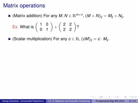
(Matrix addition) For any M,N ∈ Rm×n, (M + N)ij = Mij + Nij .
Ex. What is(
1 00 1
)+
(2 22 2
)?
(Scalar multiplication) For any c ∈ R, (cM)ij = c ·Mij .
(Vector inner product) For any column vectors v,w ∈ Rn,
v ·w =n∑
i=1
viwi ∈ R.
The inner product “measures” the overlap between v and w.When v ·w = 0, we say v and w are orthogonal.
Ex. For v = (1 0)T , w = (0 1)T , what is v ·w? v · v? Draw v andw on the 2D Euclidean plane to visualize the dot product.
Sevag Gharibian (Universität Paderborn) Ch. 8: Matrices and Scientific Computing Fundamental Algs WS 2019 8 / 115
Matrix operations
(Matrix addition) For any M,N ∈ Rm×n, (M + N)ij = Mij + Nij .
Ex. What is(
1 00 1
)+
(2 22 2
)?
(Scalar multiplication) For any c ∈ R, (cM)ij = c ·Mij .(Vector inner product) For any column vectors v,w ∈ Rn,
v ·w =n∑
i=1
viwi ∈ R.
The inner product “measures” the overlap between v and w.When v ·w = 0, we say v and w are orthogonal.
Ex. For v = (1 0)T , w = (0 1)T , what is v ·w? v · v? Draw v andw on the 2D Euclidean plane to visualize the dot product.
Sevag Gharibian (Universität Paderborn) Ch. 8: Matrices and Scientific Computing Fundamental Algs WS 2019 8 / 115
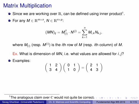
Matrix MultiplicationSince we are working over R, can be defined using inner product1.
For any M ∈ Rm×n, N ∈ Rn×p:
(MN)ij = MT(i) · N
(j) =n∑
k=1
Mi,k Nk,j ,
where M(i) (resp. M(i)) is the i th row of M (resp. i th column) of M.
Ex. What is dimension of MN, i.e. what values are allowed for i , j?
Examples: (1 23 4
)(0 11 0
)=
(2 14 3
)
(0 11 0
)(ab
)=
(ba
).
Q: In 2D plane, what operation does last equation encode?
1The analogous claim over C would not quite be correct.Sevag Gharibian (Universität Paderborn) Ch. 8: Matrices and Scientific Computing Fundamental Algs WS 2019 9 / 115

Matrix MultiplicationSince we are working over R, can be defined using inner product1.
For any M ∈ Rm×n, N ∈ Rn×p:
(MN)ij = MT(i) · N
(j) =n∑
k=1
Mi,k Nk,j ,
where M(i) (resp. M(i)) is the i th row of M (resp. i th column) of M.
Ex. What is dimension of MN, i.e. what values are allowed for i , j?
Examples: (1 23 4
)(0 11 0
)=
(2 14 3
)(
0 11 0
)(ab
)=
(ba
).
Q: In 2D plane, what operation does last equation encode?1The analogous claim over C would not quite be correct.
Sevag Gharibian (Universität Paderborn) Ch. 8: Matrices and Scientific Computing Fundamental Algs WS 2019 9 / 115
Matrix MultiplicationMore properties:
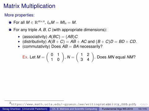
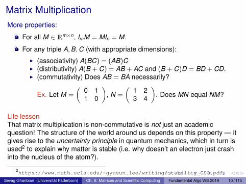
For all M ∈ Rm×n, ImM = MIn = M.
For any triple A,B,C (with appropriate dimensions):
I (associativity) A(BC) = (AB)CI (distributivity) A(B + C) = AB + AC and (B + C)D = BD + CD.I (commutativity) Does AB = BA necessarily?
Ex. Let M =
(0 11 0
), N =
(1 23 4
). Does MN equal NM?
Life lessonThat matrix multiplication is non-commutative is not just an academicquestion! The structure of the world around us depends on this property — itgives rise to the uncertainty principle in quantum mechanics, which in turn isused2 to explain why matter is stable (i.e. why doesn’t an electron just crashinto the nucleus of the atom?).
2https://www.math.ucla.edu/~gyueun.lee/writing/stability_GSO.pdf.Sevag Gharibian (Universität Paderborn) Ch. 8: Matrices and Scientific Computing Fundamental Algs WS 2019 10 / 115
Matrix MultiplicationMore properties:
For all M ∈ Rm×n, ImM = MIn = M.
For any triple A,B,C (with appropriate dimensions):
I (associativity) A(BC) = (AB)CI (distributivity) A(B + C) = AB + AC and (B + C)D = BD + CD.I (commutativity) Does AB = BA necessarily?
Ex. Let M =
(0 11 0
), N =
(1 23 4
). Does MN equal NM?
Life lessonThat matrix multiplication is non-commutative is not just an academicquestion! The structure of the world around us depends on this property — itgives rise to the uncertainty principle in quantum mechanics, which in turn isused2 to explain why matter is stable (i.e. why doesn’t an electron just crashinto the nucleus of the atom?).
2https://www.math.ucla.edu/~gyueun.lee/writing/stability_GSO.pdf.Sevag Gharibian (Universität Paderborn) Ch. 8: Matrices and Scientific Computing Fundamental Algs WS 2019 10 / 115

Bit versus operation complexity
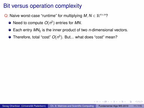
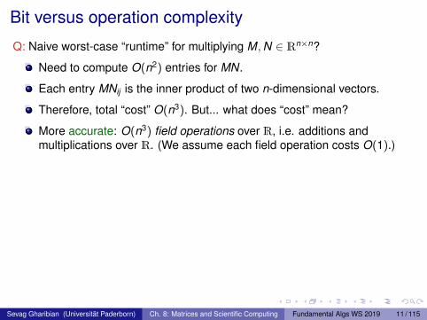
Q: Naive worst-case “runtime” for multiplying M,N ∈ Rn×n?
Need to compute O(n2) entries for MN.
Each entry MNij is the inner product of two n-dimensional vectors.
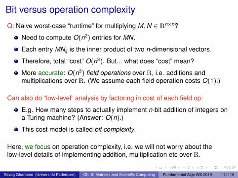
Therefore, total “cost” O(n3). But... what does “cost” mean?
More accurate: O(n3) field operations over R, i.e. additions andmultiplications over R. (We assume each field operation costs O(1).)
Can also do “low-level” analysis by factoring in cost of each field op:
E.g. How many steps to actually implement n-bit addition of integers ona Turing machine? (Answer: O(n).)
This cost model is called bit complexity.
Here, we focus on operation complexity, i.e. we will not worry about thelow-level details of implementing addition, multiplication etc over R.
Sevag Gharibian (Universität Paderborn) Ch. 8: Matrices and Scientific Computing Fundamental Algs WS 2019 11 / 115
Bit versus operation complexity
Q: Naive worst-case “runtime” for multiplying M,N ∈ Rn×n?
Need to compute O(n2) entries for MN.
Each entry MNij is the inner product of two n-dimensional vectors.
Therefore, total “cost” O(n3). But... what does “cost” mean?
More accurate: O(n3) field operations over R, i.e. additions andmultiplications over R. (We assume each field operation costs O(1).)
Can also do “low-level” analysis by factoring in cost of each field op:
E.g. How many steps to actually implement n-bit addition of integers ona Turing machine? (Answer: O(n).)
This cost model is called bit complexity.
Here, we focus on operation complexity, i.e. we will not worry about thelow-level details of implementing addition, multiplication etc over R.
Sevag Gharibian (Universität Paderborn) Ch. 8: Matrices and Scientific Computing Fundamental Algs WS 2019 11 / 115
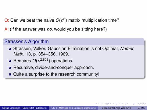
Q: Can we beat the naive O(n3) matrix multiplication time?
A: (If the answer was no, would you be sitting here?)
Strassen’s AlgorithmStrassen, Volker. Gaussian Elimination is not Optimal, Numer.Math. 13, p. 354–356, 1969.Requires O(n2.808) operations.Recursive, divide-and-conquer approach.Quite a surprise to the research community!
Sevag Gharibian (Universität Paderborn) Ch. 8: Matrices and Scientific Computing Fundamental Algs WS 2019 12 / 115
Outline
1 Introduction to matrices (review)
2 Matrix multiplication algorithmsStrassen’s algorithm (1967)Drineas-Kannan-Mahoney randomized algorithm (2006)
3 Random walksGambler’s ruinGoogle’s PageRank algorithm (1999)
4 Polynomial multiplicationComplex numbersPolynomialsO(N log N)-time polynomial multiplication via Fourier Transform
Sevag Gharibian (Universität Paderborn) Ch. 8: Matrices and Scientific Computing Fundamental Algs WS 2019 13 / 115
Goals of section
Practice working with matricesPractice working with randomizationStudy a mix of classic and modern algorithms
Sevag Gharibian (Universität Paderborn) Ch. 8: Matrices and Scientific Computing Fundamental Algs WS 2019 14 / 115
Outline
1 Introduction to matrices (review)
2 Matrix multiplication algorithmsStrassen’s algorithm (1967)Drineas-Kannan-Mahoney randomized algorithm (2006)
3 Random walksGambler’s ruinGoogle’s PageRank algorithm (1999)
4 Polynomial multiplicationComplex numbersPolynomialsO(N log N)-time polynomial multiplication via Fourier Transform
Sevag Gharibian (Universität Paderborn) Ch. 8: Matrices and Scientific Computing Fundamental Algs WS 2019 15 / 115
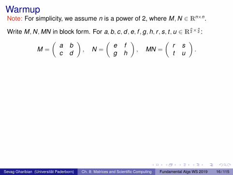
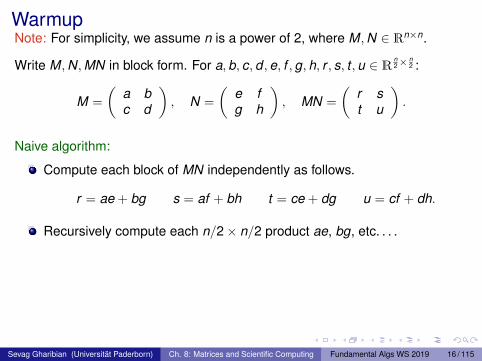
WarmupNote: For simplicity, we assume n is a power of 2, where M,N ∈ Rn×n.
Write M,N,MN in block form. For a,b, c,d ,e, f ,g,h, r , s, t ,u ∈ R n2×
n2 :
M =
(a bc d
), N =
(e fg h
), MN =
(r st u
).
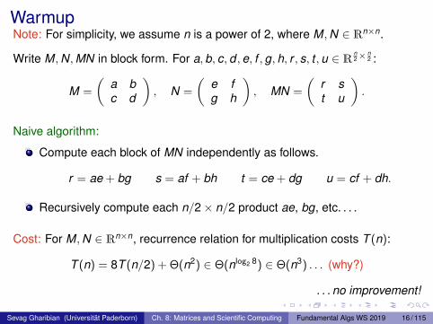
Naive algorithm:
Compute each block of MN independently as follows.
r = ae + bg s = af + bh t = ce + dg u = cf + dh.
Recursively compute each n/2× n/2 product ae, bg, etc. . . .
Cost: For M,N ∈ Rn×n, recurrence relation for multiplication costs T (n):
T (n) = 8T (n/2) + Θ(n2) ∈ Θ(nlog2 8) ∈ Θ(n3) . . . (why?)
. . . no improvement!
Sevag Gharibian (Universität Paderborn) Ch. 8: Matrices and Scientific Computing Fundamental Algs WS 2019 16 / 115
WarmupNote: For simplicity, we assume n is a power of 2, where M,N ∈ Rn×n.
Write M,N,MN in block form. For a,b, c,d ,e, f ,g,h, r , s, t ,u ∈ R n2×
n2 :
M =
(a bc d
), N =
(e fg h
), MN =
(r st u
).
Naive algorithm:
Compute each block of MN independently as follows.
r = ae + bg s = af + bh t = ce + dg u = cf + dh.
Recursively compute each n/2× n/2 product ae, bg, etc. . . .
Cost: For M,N ∈ Rn×n, recurrence relation for multiplication costs T (n):
T (n) = 8T (n/2) + Θ(n2) ∈ Θ(nlog2 8) ∈ Θ(n3) . . . (why?)
. . . no improvement!
Sevag Gharibian (Universität Paderborn) Ch. 8: Matrices and Scientific Computing Fundamental Algs WS 2019 16 / 115
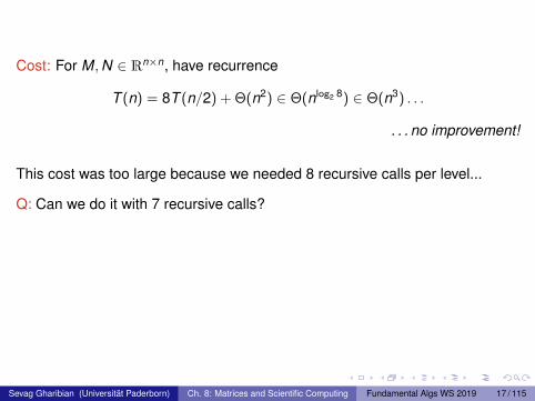
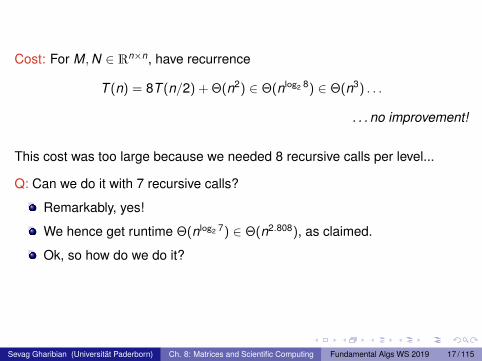
Cost: For M,N ∈ Rn×n, have recurrence
T (n) = 8T (n/2) + Θ(n2) ∈ Θ(nlog2 8) ∈ Θ(n3) . . .
. . . no improvement!
This cost was too large because we needed 8 recursive calls per level...
Q: Can we do it with 7 recursive calls?
Remarkably, yes!
We hence get runtime Θ(nlog2 7) ∈ Θ(n2.808), as claimed.
Ok, so how do we do it?
Sevag Gharibian (Universität Paderborn) Ch. 8: Matrices and Scientific Computing Fundamental Algs WS 2019 17 / 115
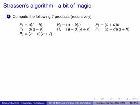
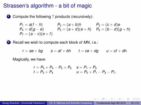
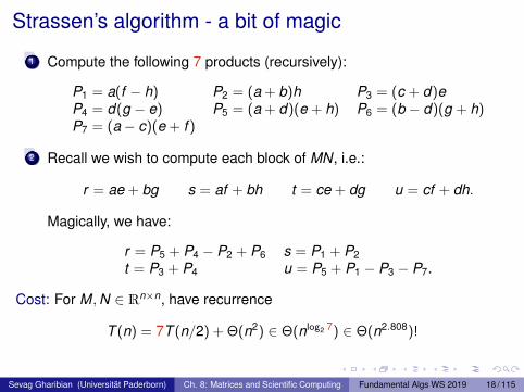
Strassen’s algorithm - a bit of magic
1 Compute the following 7 products (recursively):
P1 = a(f − h) P2 = (a + b)h P3 = (c + d)eP4 = d(g − e) P5 = (a + d)(e + h) P6 = (b − d)(g + h)P7 = (a− c)(e + f )
2 Recall we wish to compute each block of MN, i.e.:
r = ae + bg s = af + bh t = ce + dg u = cf + dh.
Magically, we have:
r = P5 + P4 − P2 + P6 s = P1 + P2t = P3 + P4 u = P5 + P1 − P3 − P7.
Cost: For M,N ∈ Rn×n, have recurrence
T (n) = 7T (n/2) + Θ(n2) ∈ Θ(nlog2 7) ∈ Θ(n2.808)!
Sevag Gharibian (Universität Paderborn) Ch. 8: Matrices and Scientific Computing Fundamental Algs WS 2019 18 / 115

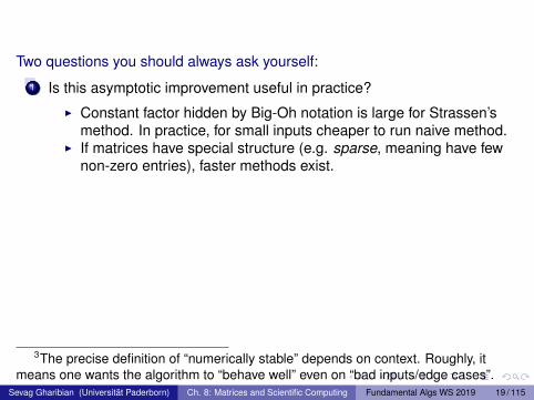
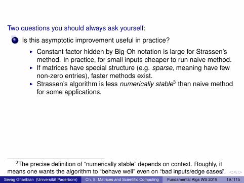
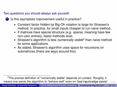
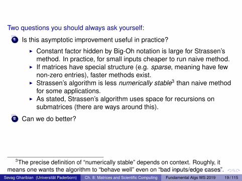
Two questions you should always ask yourself:
1 Is this asymptotic improvement useful in practice?
I Constant factor hidden by Big-Oh notation is large for Strassen’smethod. In practice, for small inputs cheaper to run naive method.
I If matrices have special structure (e.g. sparse, meaning have fewnon-zero entries), faster methods exist.
I Strassen’s algorithm is less numerically stable3 than naive methodfor some applications.
I As stated, Strassen’s algorithm uses space for recursions onsubmatrices (there are ways around this).
2 Can we do better?
3The precise definition of “numerically stable” depends on context. Roughly, itmeans one wants the algorithm to “behave well” even on “bad inputs/edge cases”.
Sevag Gharibian (Universität Paderborn) Ch. 8: Matrices and Scientific Computing Fundamental Algs WS 2019 19 / 115

Can we do better?
Lower boundsNaive lower bound of Ω(n2). (Why?)
Embarrassingly, unknown whether optimal is ω(n2) (after 50years!)If we restrict the type of circuit computing the matrix product, thena lower bound of Ω(n2 log n) can be shown [Raz, 2003]
Sevag Gharibian (Universität Paderborn) Ch. 8: Matrices and Scientific Computing Fundamental Algs WS 2019 20 / 115
Can we do better?
Lower boundsNaive lower bound of Ω(n2). (Why?)Embarrassingly, unknown whether optimal is ω(n2) (after 50years!)
If we restrict the type of circuit computing the matrix product, thena lower bound of Ω(n2 log n) can be shown [Raz, 2003]
Sevag Gharibian (Universität Paderborn) Ch. 8: Matrices and Scientific Computing Fundamental Algs WS 2019 20 / 115
Can we do better?
Lower boundsNaive lower bound of Ω(n2). (Why?)Embarrassingly, unknown whether optimal is ω(n2) (after 50years!)If we restrict the type of circuit computing the matrix product, thena lower bound of Ω(n2 log n) can be shown [Raz, 2003]
Sevag Gharibian (Universität Paderborn) Ch. 8: Matrices and Scientific Computing Fundamental Algs WS 2019 20 / 115

Can we do better?
Upper boundsStrassen (1969): O(n2.808).Pan (1978): o(n2.796)
Bini, Capovani, Romani, Lotti using border rank (1979): o(n2.78)
Schönhage via τ -theorem (1981): o(n2.548)
Romani (1982): o(n2.517)
Coppersmith, Winograd (1981): o(n2.496)
Strassen via laser method (1986): o(n2.479)
Coppersmith, Winograd (1989): o(n2.376)
V. V. Williams (2013): O(n2.3729)
Le Gall (2014): O(n2.3728639)
Sevag Gharibian (Universität Paderborn) Ch. 8: Matrices and Scientific Computing Fundamental Algs WS 2019 21 / 115
The more advanced these algorithms get, the less useful they tend tobe in practice. . .
What if we want something more useful in practice? Say for machinelearning or big data?
Common tool: Randomization
Tradeoff: Time/space versus accuracy
Sevag Gharibian (Universität Paderborn) Ch. 8: Matrices and Scientific Computing Fundamental Algs WS 2019 22 / 115
Sevag Gharibian (Universität Paderborn) Ch. 8: Matrices and Scientific Computing Fundamental Algs WS 2019 23 / 115
Outline
1 Introduction to matrices (review)
2 Matrix multiplication algorithmsStrassen’s algorithm (1967)Drineas-Kannan-Mahoney randomized algorithm (2006)
3 Random walksGambler’s ruinGoogle’s PageRank algorithm (1999)
4 Polynomial multiplicationComplex numbersPolynomialsO(N log N)-time polynomial multiplication via Fourier Transform
Sevag Gharibian (Universität Paderborn) Ch. 8: Matrices and Scientific Computing Fundamental Algs WS 2019 24 / 115

Basic probability theory
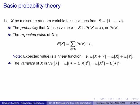
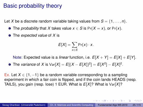
Let X be a discrete random variable taking values from S = 1, . . . ,n.
The probability that X takes value x ∈ S is Pr(X = x), or Pr(x).
The expected value of X is
E [X ] =∑x∈S
Pr(x) · x .
Note: Expected value is a linear function, i.e. E [X + Y ] = E [X ] + E [Y ].
The variance of X is Var[X ] = E [(X − E [X ])2] = E [X 2]− E [X ]2.
Ex. Let X ∈ 1,−1 be a random variable corresponding to a samplingexperiment in which a fair coin is flipped, and if the coin lands HEADS (resp.TAILS), you gain (resp. lose) 1 EUR. What is E [X ]? What is Var[X ]?
Sevag Gharibian (Universität Paderborn) Ch. 8: Matrices and Scientific Computing Fundamental Algs WS 2019 25 / 115
Basic probability theory
Let X be a discrete random variable taking values from S = 1, . . . ,n.
The probability that X takes value x ∈ S is Pr(X = x), or Pr(x).
The expected value of X is
E [X ] =∑x∈S
Pr(x) · x .
Note: Expected value is a linear function, i.e. E [X + Y ] = E [X ] + E [Y ].
The variance of X is Var[X ] = E [(X − E [X ])2] = E [X 2]− E [X ]2.
Ex. Let X ∈ 1,−1 be a random variable corresponding to a samplingexperiment in which a fair coin is flipped, and if the coin lands HEADS (resp.TAILS), you gain (resp. lose) 1 EUR. What is E [X ]? What is Var[X ]?
Sevag Gharibian (Universität Paderborn) Ch. 8: Matrices and Scientific Computing Fundamental Algs WS 2019 25 / 115
Back to matrix multiplication
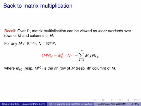
Recall: Over R, matrix multiplication can be viewed as inner products overrows of M and columns of N.
For any M ∈ Rm×n, N ∈ Rn×p:
(MN)ij = MT(i) · N
(j) =n∑
k=1
Mi,k Nk,j ,
where M(i) (resp. M(i)) is the i th row of M (resp. i th column) of M.
Sevag Gharibian (Universität Paderborn) Ch. 8: Matrices and Scientific Computing Fundamental Algs WS 2019 26 / 115
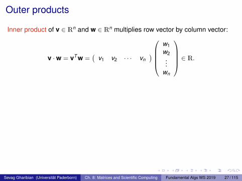
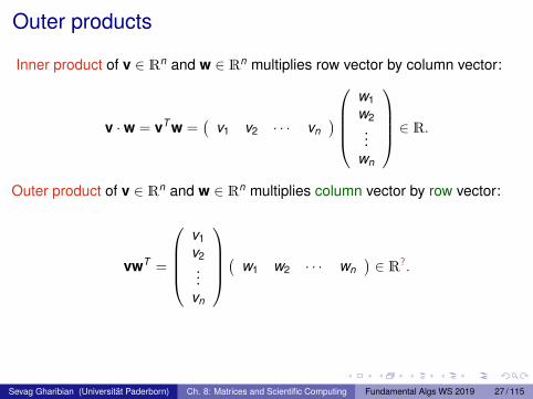
Outer products
Inner product of v ∈ Rn and w ∈ Rn multiplies row vector by column vector:
v ·w = vT w =(
v1 v2 · · · vn)
w1w2...
wn
∈ R.
Sevag Gharibian (Universität Paderborn) Ch. 8: Matrices and Scientific Computing Fundamental Algs WS 2019 27 / 115
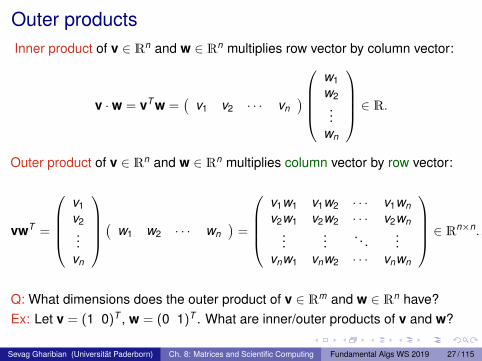
Outer products
Inner product of v ∈ Rn and w ∈ Rn multiplies row vector by column vector:
v ·w = vT w =(
v1 v2 · · · vn)
w1w2...
wn
∈ R.Outer product of v ∈ Rn and w ∈ Rn multiplies column vector by row vector:
vwT =
v1v2...
vn
( w1 w2 · · · wn)∈ R?.
Sevag Gharibian (Universität Paderborn) Ch. 8: Matrices and Scientific Computing Fundamental Algs WS 2019 27 / 115
Outer productsInner product of v ∈ Rn and w ∈ Rn multiplies row vector by column vector:
v ·w = vT w =(
v1 v2 · · · vn)
w1w2...
wn
∈ R.Outer product of v ∈ Rn and w ∈ Rn multiplies column vector by row vector:
vwT =
v1v2...
vn
( w1 w2 · · · wn)
=
v1w1 v1w2 · · · v1wnv2w1 v2w2 · · · v2wn
......
. . ....
vnw1 vnw2 · · · vnwn
∈ Rn×n.
Q: What dimensions does the outer product of v ∈ Rm and w ∈ Rn have?Ex: Let v = (1 0)T , w = (0 1)T . What are inner/outer products of v and w?
Sevag Gharibian (Universität Paderborn) Ch. 8: Matrices and Scientific Computing Fundamental Algs WS 2019 27 / 115
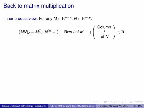
Back to matrix multiplication
Inner product view: For any M ∈ Rm×n, N ∈ Rn×p:
(MN)ij = MT(i) · N
(j) =(
Row i of M) Column
jof N
∈ R.
Outer product view: For any M ∈ Rm×n, N ∈ Rn×p:
MN =n∑
k=1
M(k)N(k) =n∑
k=1
Columnk
of M
( Row k of M)∈ Rm×p.
Q: What differences can you spot between the inner and outer product views?
Ex: Prove that the outer product view is correct.
Sevag Gharibian (Universität Paderborn) Ch. 8: Matrices and Scientific Computing Fundamental Algs WS 2019 28 / 115
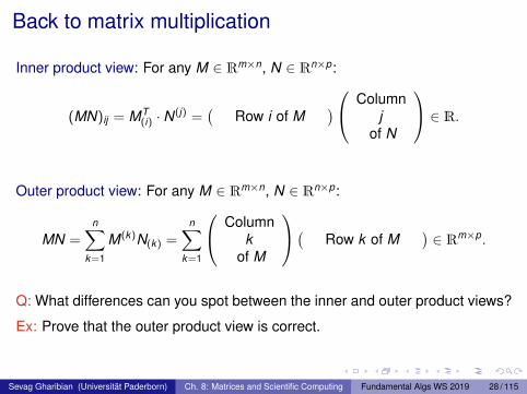
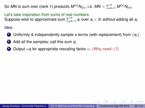
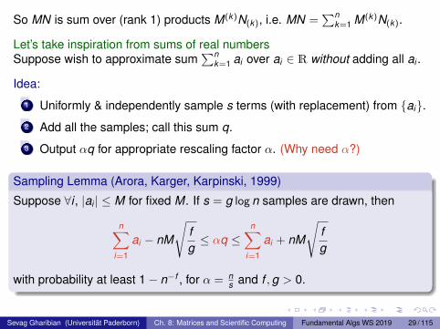
So MN is sum over (rank 1) products M(k)N(k), i.e. MN =∑n
k=1 M(k)N(k).
Let’s take inspiration from sums of real numbersSuppose wish to approximate sum
∑nk=1 ai over ai ∈ R without adding all ai .
Idea:
1 Uniformly & independently sample s terms (with replacement) from ai.2 Add all the samples; call this sum q.
3 Output αq for appropriate rescaling factor α. (Why need α?)
Sampling Lemma (Arora, Karger, Karpinski, 1999)
Suppose ∀i , |ai | ≤ M for fixed M. If s = g log n samples are drawn, then
n∑i=1
ai − nM
√fg≤ αq ≤
n∑i=1
ai + nM
√fg
with probability at least 1− n−f , for α = ns and f ,g > 0.
Sevag Gharibian (Universität Paderborn) Ch. 8: Matrices and Scientific Computing Fundamental Algs WS 2019 29 / 115
So MN is sum over (rank 1) products M(k)N(k), i.e. MN =∑n
k=1 M(k)N(k).
Let’s take inspiration from sums of real numbersSuppose wish to approximate sum
∑nk=1 ai over ai ∈ R without adding all ai .
Idea:
1 Uniformly & independently sample s terms (with replacement) from ai.
2 Add all the samples; call this sum q.
3 Output αq for appropriate rescaling factor α. (Why need α?)
Sampling Lemma (Arora, Karger, Karpinski, 1999)
Suppose ∀i , |ai | ≤ M for fixed M. If s = g log n samples are drawn, then
n∑i=1
ai − nM
√fg≤ αq ≤
n∑i=1
ai + nM
√fg
with probability at least 1− n−f , for α = ns and f ,g > 0.
Sevag Gharibian (Universität Paderborn) Ch. 8: Matrices and Scientific Computing Fundamental Algs WS 2019 29 / 115
So MN is sum over (rank 1) products M(k)N(k), i.e. MN =∑n
k=1 M(k)N(k).
Let’s take inspiration from sums of real numbersSuppose wish to approximate sum
∑nk=1 ai over ai ∈ R without adding all ai .
Idea:
1 Uniformly & independently sample s terms (with replacement) from ai.2 Add all the samples; call this sum q.
3 Output αq for appropriate rescaling factor α. (Why need α?)
Sampling Lemma (Arora, Karger, Karpinski, 1999)
Suppose ∀i , |ai | ≤ M for fixed M. If s = g log n samples are drawn, then
n∑i=1
ai − nM
√fg≤ αq ≤
n∑i=1
ai + nM
√fg
with probability at least 1− n−f , for α = ns and f ,g > 0.
Sevag Gharibian (Universität Paderborn) Ch. 8: Matrices and Scientific Computing Fundamental Algs WS 2019 29 / 115
So MN is sum over (rank 1) products M(k)N(k), i.e. MN =∑n
k=1 M(k)N(k).
Let’s take inspiration from sums of real numbersSuppose wish to approximate sum
∑nk=1 ai over ai ∈ R without adding all ai .
Idea:
1 Uniformly & independently sample s terms (with replacement) from ai.2 Add all the samples; call this sum q.
3 Output αq for appropriate rescaling factor α. (Why need α?)
Sampling Lemma (Arora, Karger, Karpinski, 1999)
Suppose ∀i , |ai | ≤ M for fixed M. If s = g log n samples are drawn, then
n∑i=1
ai − nM
√fg≤ αq ≤
n∑i=1
ai + nM
√fg
with probability at least 1− n−f , for α = ns and f ,g > 0.
Sevag Gharibian (Universität Paderborn) Ch. 8: Matrices and Scientific Computing Fundamental Algs WS 2019 29 / 115
Digesting the Sampling Lemma
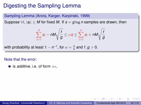
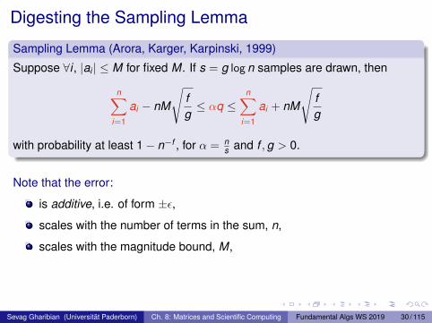
Sampling Lemma (Arora, Karger, Karpinski, 1999)
Suppose ∀i , |ai | ≤ M for fixed M. If s = g log n samples are drawn, then
n∑i=1
ai − nM
√fg≤ αq ≤
n∑i=1
ai + nM
√fg
with probability at least 1− n−f , for α = ns and f ,g > 0.
Note that the error:
is additive, i.e. of form ±ε,
scales with the number of terms in the sum, n,
scales with the magnitude bound, M,
scales inversely with coefficient in the number of samples, g.
Obvious question: Can we do something similar for matrix multiplication?
Sevag Gharibian (Universität Paderborn) Ch. 8: Matrices and Scientific Computing Fundamental Algs WS 2019 30 / 115
Digesting the Sampling Lemma
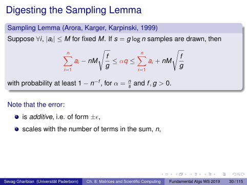
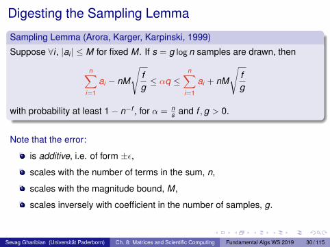
Sampling Lemma (Arora, Karger, Karpinski, 1999)
Suppose ∀i , |ai | ≤ M for fixed M. If s = g log n samples are drawn, then
n∑i=1
ai − nM
√fg≤ αq ≤
n∑i=1
ai + nM
√fg
with probability at least 1− n−f , for α = ns and f ,g > 0.
Note that the error:
is additive, i.e. of form ±ε,
scales with the number of terms in the sum, n,
scales with the magnitude bound, M,
scales inversely with coefficient in the number of samples, g.
Obvious question: Can we do something similar for matrix multiplication?
Sevag Gharibian (Universität Paderborn) Ch. 8: Matrices and Scientific Computing Fundamental Algs WS 2019 30 / 115
Digesting the Sampling Lemma
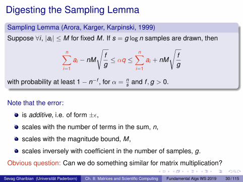
Sampling Lemma (Arora, Karger, Karpinski, 1999)
Suppose ∀i , |ai | ≤ M for fixed M. If s = g log n samples are drawn, then
n∑i=1
ai − nM
√fg≤ αq ≤
n∑i=1
ai + nM
√fg
with probability at least 1− n−f , for α = ns and f ,g > 0.
Note that the error:
is additive, i.e. of form ±ε,
scales with the number of terms in the sum, n,
scales with the magnitude bound, M,
scales inversely with coefficient in the number of samples, g.
Obvious question: Can we do something similar for matrix multiplication?
Sevag Gharibian (Universität Paderborn) Ch. 8: Matrices and Scientific Computing Fundamental Algs WS 2019 30 / 115
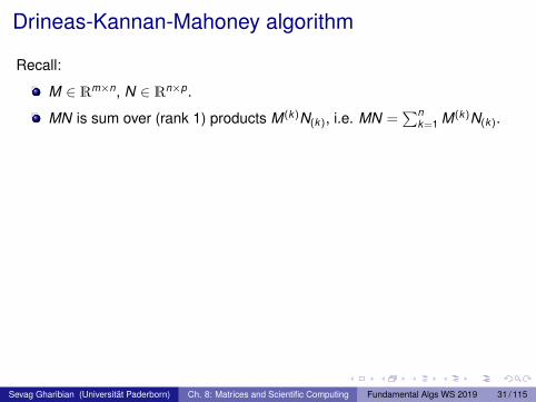
Drineas-Kannan-Mahoney algorithm
Recall:
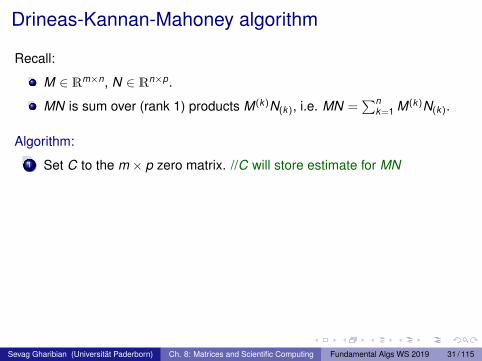
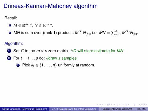
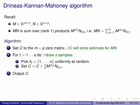
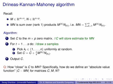
M ∈ Rm×n, N ∈ Rn×p.
MN is sum over (rank 1) products M(k)N(k), i.e. MN =∑n
k=1 M(k)N(k).
Algorithm:
1 Set C to the m × p zero matrix. //C will store estimate for MN
2 For t = 1 . . . s do: //draw s samples
1 Pick kt ∈ 1, . . . ,n uniformly at random.2 Set C = C + n
s M(kt )N(kt ).
3 Output C.
Q: How “close” is C to MN? Specifically, how do we define an “absolute valuefunction” |C −MN| for matrices C,M,N?
Sevag Gharibian (Universität Paderborn) Ch. 8: Matrices and Scientific Computing Fundamental Algs WS 2019 31 / 115
Drineas-Kannan-Mahoney algorithm
Recall:
M ∈ Rm×n, N ∈ Rn×p.
MN is sum over (rank 1) products M(k)N(k), i.e. MN =∑n
k=1 M(k)N(k).
Algorithm:
1 Set C to the m × p zero matrix. //C will store estimate for MN
2 For t = 1 . . . s do: //draw s samples
1 Pick kt ∈ 1, . . . ,n uniformly at random.
2 Set C = C + ns M(kt )N(kt ).
3 Output C.
Q: How “close” is C to MN? Specifically, how do we define an “absolute valuefunction” |C −MN| for matrices C,M,N?
Sevag Gharibian (Universität Paderborn) Ch. 8: Matrices and Scientific Computing Fundamental Algs WS 2019 31 / 115
Drineas-Kannan-Mahoney algorithm
Recall:
M ∈ Rm×n, N ∈ Rn×p.
MN is sum over (rank 1) products M(k)N(k), i.e. MN =∑n
k=1 M(k)N(k).
Algorithm:
1 Set C to the m × p zero matrix. //C will store estimate for MN
2 For t = 1 . . . s do: //draw s samples
1 Pick kt ∈ 1, . . . ,n uniformly at random.2 Set C = C + n
s M(kt )N(kt ).
3 Output C.
Q: How “close” is C to MN? Specifically, how do we define an “absolute valuefunction” |C −MN| for matrices C,M,N?
Sevag Gharibian (Universität Paderborn) Ch. 8: Matrices and Scientific Computing Fundamental Algs WS 2019 31 / 115
Drineas-Kannan-Mahoney algorithm
Recall:
M ∈ Rm×n, N ∈ Rn×p.
MN is sum over (rank 1) products M(k)N(k), i.e. MN =∑n
k=1 M(k)N(k).
Algorithm:
1 Set C to the m × p zero matrix. //C will store estimate for MN
2 For t = 1 . . . s do: //draw s samples
1 Pick kt ∈ 1, . . . ,n uniformly at random.2 Set C = C + n
s M(kt )N(kt ).
3 Output C.
Q: How “close” is C to MN? Specifically, how do we define an “absolute valuefunction” |C −MN| for matrices C,M,N?
Sevag Gharibian (Universität Paderborn) Ch. 8: Matrices and Scientific Computing Fundamental Algs WS 2019 31 / 115
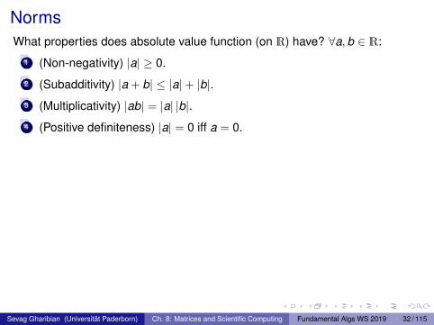
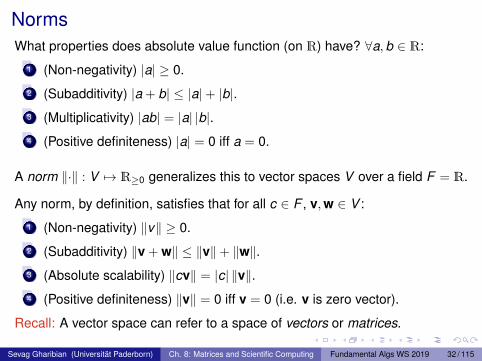
NormsWhat properties does absolute value function (on R) have? ∀a,b ∈ R:
1 (Non-negativity) |a| ≥ 0.
2 (Subadditivity) |a + b| ≤ |a|+ |b|.3 (Multiplicativity) |ab| = |a| |b|.4 (Positive definiteness) |a| = 0 iff a = 0.
A norm ‖·‖ : V 7→ R≥0 generalizes this to vector spaces V over a field F = R.
Any norm, by definition, satisfies that for all c ∈ F , v,w ∈ V :
1 (Non-negativity) ‖v‖ ≥ 0.
2 (Subadditivity) ‖v + w‖ ≤ ‖v‖+ ‖w‖.3 (Absolute scalability) ‖cv‖ = |c| ‖v‖.4 (Positive definiteness) ‖v‖ = 0 iff v = 0 (i.e. v is zero vector).
Recall: A vector space can refer to a space of vectors or matrices.
Sevag Gharibian (Universität Paderborn) Ch. 8: Matrices and Scientific Computing Fundamental Algs WS 2019 32 / 115
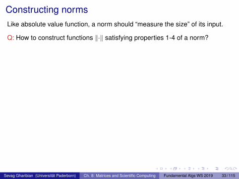
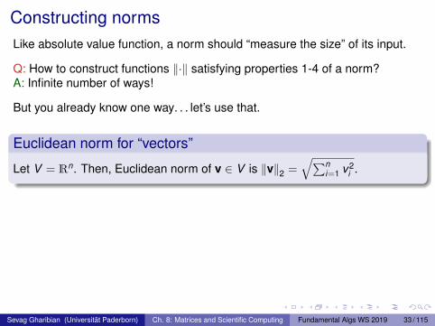
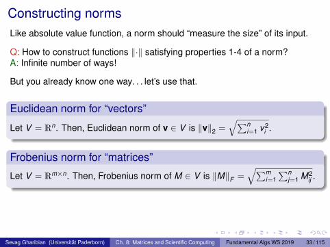
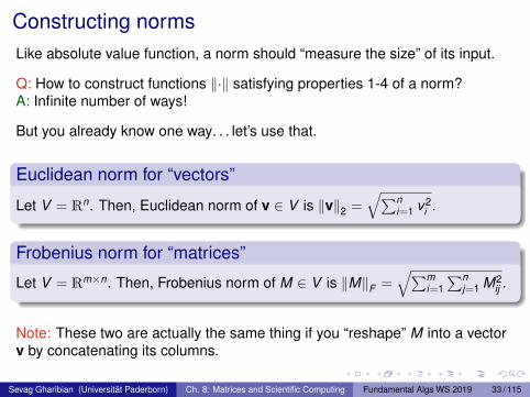
Constructing normsLike absolute value function, a norm should “measure the size” of its input.
Q: How to construct functions ‖·‖ satisfying properties 1-4 of a norm?
A: Infinite number of ways!
But you already know one way. . . let’s use that.
Euclidean norm for “vectors”
Let V = Rn. Then, Euclidean norm of v ∈ V is ‖v‖2 =√∑n
i=1 v2i .
Frobenius norm for “matrices”
Let V = Rm×n. Then, Frobenius norm of M ∈ V is ‖M‖F =√∑m
i=1∑n
j=1 M2ij .
Note: These two are actually the same thing if you “reshape” M into a vectorv by concatenating its columns.
Sevag Gharibian (Universität Paderborn) Ch. 8: Matrices and Scientific Computing Fundamental Algs WS 2019 33 / 115
Constructing normsLike absolute value function, a norm should “measure the size” of its input.
Q: How to construct functions ‖·‖ satisfying properties 1-4 of a norm?A: Infinite number of ways!
But you already know one way. . . let’s use that.
Euclidean norm for “vectors”
Let V = Rn. Then, Euclidean norm of v ∈ V is ‖v‖2 =√∑n
i=1 v2i .
Frobenius norm for “matrices”
Let V = Rm×n. Then, Frobenius norm of M ∈ V is ‖M‖F =√∑m
i=1∑n
j=1 M2ij .
Note: These two are actually the same thing if you “reshape” M into a vectorv by concatenating its columns.
Sevag Gharibian (Universität Paderborn) Ch. 8: Matrices and Scientific Computing Fundamental Algs WS 2019 33 / 115
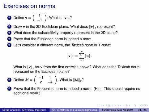
Exercises on norms
1 Define v =
(1−1
). What is ‖v‖2?
2 Draw v in the 2D Euclidean plane. What does ‖v‖2 represent?3 What does the subadditivity property represent in the 2D plane?4 Prove that the Euclidean norm is indeed a norm.5 Let’s consider a different norm, the Taxicab norm or 1-norm:
‖v‖1 =n∑
i=1
|vi | .
What is ‖v‖1 for v from the first exercise above? What does the Taxicab normrepresent on the Euclidean plane?
6 Define M =
(−1 12 −4
). What is ‖M‖F?
7 Prove that the Frobenius norm is indeed a norm. (Hint: This should require noadditional work.)
Note: There is more than one way to generalize the 1-norm to matrices.
Sevag Gharibian (Universität Paderborn) Ch. 8: Matrices and Scientific Computing Fundamental Algs WS 2019 34 / 115
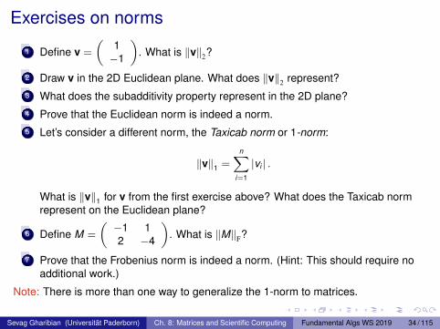
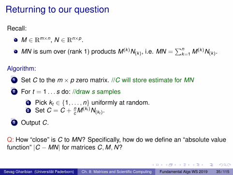
Returning to our question
Recall:
M ∈ Rm×n, N ∈ Rn×p.
MN is sum over (rank 1) products M(k)N(k), i.e. MN =∑n
k=1 M(k)N(k).
Algorithm:
1 Set C to the m × p zero matrix. //C will store estimate for MN
2 For t = 1 . . . s do: //draw s samples
1 Pick kt ∈ 1, . . . ,n uniformly at random.2 Set C = C + n
c M(kt )N(kt ).
3 Output C.
Q: How “close” is C to MN? Specifically, how do we define an “absolute valuefunction” |C −MN| for matrices C,M,N?
Sevag Gharibian (Universität Paderborn) Ch. 8: Matrices and Scientific Computing Fundamental Algs WS 2019 35 / 115
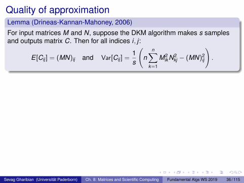
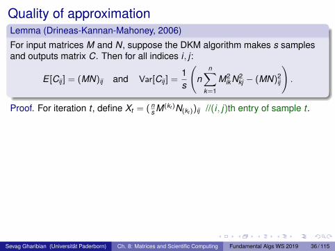
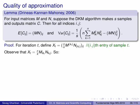
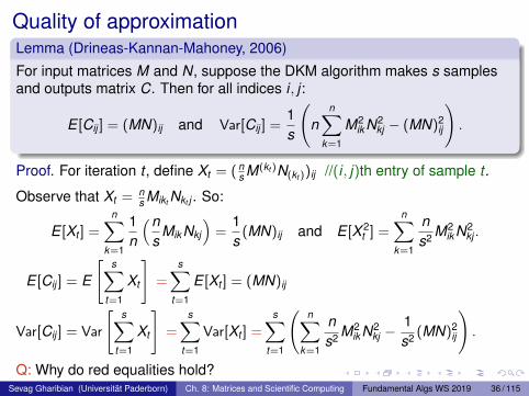
Quality of approximationLemma (Drineas-Kannan-Mahoney, 2006)
For input matrices M and N, suppose the DKM algorithm makes s samplesand outputs matrix C. Then for all indices i , j :
E [Cij ] = (MN)ij and Var[Cij ] =1s
(n
n∑k=1
M2ik N2
kj − (MN)2ij
).
Proof. For iteration t , define Xt = ( ns M(kt )N(kt ))ij //(i , j)th entry of sample t .
Observe that Xt = ns Mikt Nkt j . So:
E [Xt ] =n∑
k=1
1n
(ns
Mik Nkj
)=
1s
(MN)ij and E [X 2t ] =
n∑k=1
ns2 M2
ik N2kj .
E [Cij ] = E
[s∑
t=1
Xt
]=
s∑t=1
E [Xt ] = (MN)ij
Var[Cij ] = Var
[s∑
t=1
Xt
]=
s∑t=1
Var[Xt ] =s∑
t=1
(n∑
k=1
ns2 M2
ik N2kj −
1s2 (MN)2
ij
).
Q: Why do red equalities hold?
Sevag Gharibian (Universität Paderborn) Ch. 8: Matrices and Scientific Computing Fundamental Algs WS 2019 36 / 115
Quality of approximationLemma (Drineas-Kannan-Mahoney, 2006)
For input matrices M and N, suppose the DKM algorithm makes s samplesand outputs matrix C. Then for all indices i , j :
E [Cij ] = (MN)ij and Var[Cij ] =1s
(n
n∑k=1
M2ik N2
kj − (MN)2ij
).
Proof. For iteration t , define Xt = ( ns M(kt )N(kt ))ij //(i , j)th entry of sample t .
Observe that Xt = ns Mikt Nkt j . So:
E [Xt ] =n∑
k=1
1n
(ns
Mik Nkj
)=
1s
(MN)ij and E [X 2t ] =
n∑k=1
ns2 M2
ik N2kj .
E [Cij ] = E
[s∑
t=1
Xt
]=
s∑t=1
E [Xt ] = (MN)ij
Var[Cij ] = Var
[s∑
t=1
Xt
]=
s∑t=1
Var[Xt ] =s∑
t=1
(n∑
k=1
ns2 M2
ik N2kj −
1s2 (MN)2
ij
).
Q: Why do red equalities hold?Sevag Gharibian (Universität Paderborn) Ch. 8: Matrices and Scientific Computing Fundamental Algs WS 2019 36 / 115
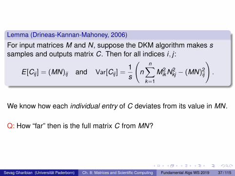
Lemma (Drineas-Kannan-Mahoney, 2006)
For input matrices M and N, suppose the DKM algorithm makes ssamples and outputs matrix C. Then for all indices i , j :
E [Cij ] = (MN)ij and Var[Cij ] =1s
(n
n∑k=1
M2ikN2
kj − (MN)2ij
).
We know how each individual entry of C deviates from its value in MN.
Q: How “far” then is the full matrix C from MN?
Sevag Gharibian (Universität Paderborn) Ch. 8: Matrices and Scientific Computing Fundamental Algs WS 2019 37 / 115
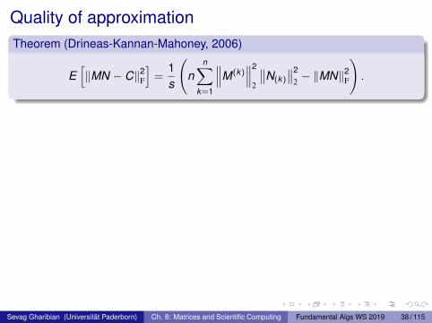
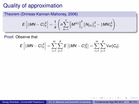
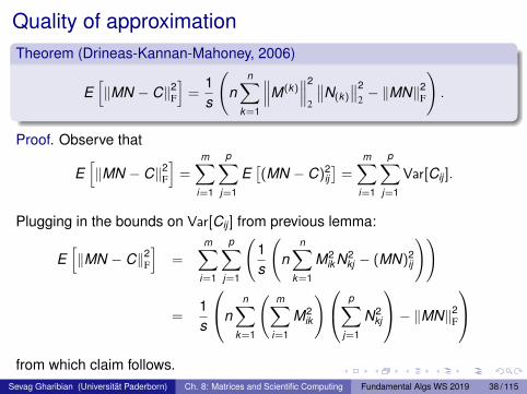
Quality of approximationTheorem (Drineas-Kannan-Mahoney, 2006)
E[‖MN − C‖2
F
]=
1s
(n
n∑k=1
∥∥∥M(k)∥∥∥2
2
∥∥N(k)∥∥2
2 − ‖MN‖2F
).
Proof. Observe that
E[‖MN − C‖2
F
]=
m∑i=1
p∑j=1
E[(MN − C)2
ij]
=m∑
i=1
p∑j=1
Var[Cij ].
Plugging in the bounds on Var[Cij ] from previous lemma:
E[‖MN − C‖2
F
]=
m∑i=1
p∑j=1
(1s
(n
n∑k=1
M2ik N2
kj − (MN)2ij
))
=1s
nn∑
k=1
(m∑
i=1
M2ik
) p∑j=1
N2kj
− ‖MN‖2F
from which claim follows.
Sevag Gharibian (Universität Paderborn) Ch. 8: Matrices and Scientific Computing Fundamental Algs WS 2019 38 / 115
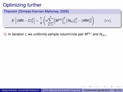
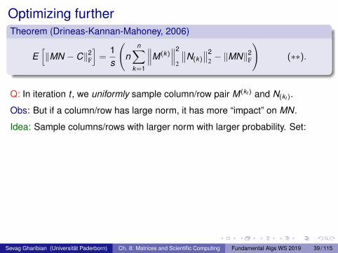
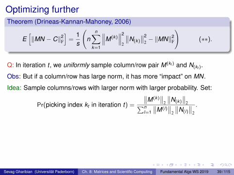
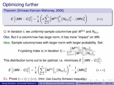
Optimizing furtherTheorem (Drineas-Kannan-Mahoney, 2006)
E[‖MN − C‖2
F
]=
1s
(n
n∑k=1
∥∥∥M(k)∥∥∥2
2
∥∥N(k)∥∥2
2 − ‖MN‖2F
)(∗∗).
Q: In iteration t , we uniformly sample column/row pair M(kt ) and N(kt ).
Obs: But if a column/row has large norm, it has more “impact” on MN.
Idea: Sample columns/rows with larger norm with larger probability. Set:
Pr(picking index kt in iteration t) =
∥∥M(k)∥∥
2
∥∥N(k)∥∥
2∑nl=1
∥∥M(l)∥∥
2
∥∥N(l)∥∥
2
.
This distribution turns out to be optimal, i.e. minimizes E[‖MN − C‖2
F
]:
E[‖MN − C‖2
F
]=
1s
(n∑
k=1
∥∥∥M(k)∥∥∥
2
∥∥N(k)∥∥
2
)2
− 1s‖MN‖2
F (∗ ∗ ∗).
Ex. Prove (∗ ∗ ∗) ≤ (∗∗). (Hint: Use Cauchy-Schwarz inequality.)
Sevag Gharibian (Universität Paderborn) Ch. 8: Matrices and Scientific Computing Fundamental Algs WS 2019 39 / 115
Optimizing furtherTheorem (Drineas-Kannan-Mahoney, 2006)
E[‖MN − C‖2
F
]=
1s
(n
n∑k=1
∥∥∥M(k)∥∥∥2
2
∥∥N(k)∥∥2
2 − ‖MN‖2F
)(∗∗).
Q: In iteration t , we uniformly sample column/row pair M(kt ) and N(kt ).
Obs: But if a column/row has large norm, it has more “impact” on MN.
Idea: Sample columns/rows with larger norm with larger probability. Set:
Pr(picking index kt in iteration t) =
∥∥M(k)∥∥
2
∥∥N(k)∥∥
2∑nl=1
∥∥M(l)∥∥
2
∥∥N(l)∥∥
2
.
This distribution turns out to be optimal, i.e. minimizes E[‖MN − C‖2
F
]:
E[‖MN − C‖2
F
]=
1s
(n∑
k=1
∥∥∥M(k)∥∥∥
2
∥∥N(k)∥∥
2
)2
− 1s‖MN‖2
F (∗ ∗ ∗).
Ex. Prove (∗ ∗ ∗) ≤ (∗∗). (Hint: Use Cauchy-Schwarz inequality.)Sevag Gharibian (Universität Paderborn) Ch. 8: Matrices and Scientific Computing Fundamental Algs WS 2019 39 / 115
Outline
1 Introduction to matrices (review)
2 Matrix multiplication algorithmsStrassen’s algorithm (1967)Drineas-Kannan-Mahoney randomized algorithm (2006)
3 Random walksGambler’s ruinGoogle’s PageRank algorithm (1999)
4 Polynomial multiplicationComplex numbersPolynomialsO(N log N)-time polynomial multiplication via Fourier Transform
Sevag Gharibian (Universität Paderborn) Ch. 8: Matrices and Scientific Computing Fundamental Algs WS 2019 40 / 115
Goals of section
More practice with randomization (life lesson: don’t gamble)Practice solving recurrence relationsReal world applications of matrices (life lesson: get rich)
Sevag Gharibian (Universität Paderborn) Ch. 8: Matrices and Scientific Computing Fundamental Algs WS 2019 41 / 115
Outline
1 Introduction to matrices (review)
2 Matrix multiplication algorithmsStrassen’s algorithm (1967)Drineas-Kannan-Mahoney randomized algorithm (2006)
3 Random walksGambler’s ruinGoogle’s PageRank algorithm (1999)
4 Polynomial multiplicationComplex numbersPolynomialsO(N log N)-time polynomial multiplication via Fourier Transform
Sevag Gharibian (Universität Paderborn) Ch. 8: Matrices and Scientific Computing Fundamental Algs WS 2019 42 / 115
Roulette
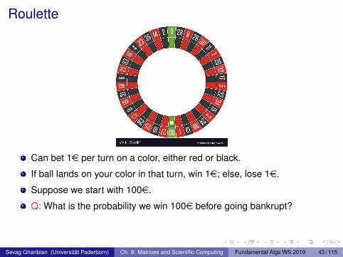
Can bet 1e per turn on a color, either red or black.
If ball lands on your color in that turn, win 1e; else, lose 1e.
Suppose we start with 100e.
Q: What is the probability we win 100e before going bankrupt?
Intuition: Since prob. winning in a turn is 18/38 ≈ 0.473 (why?), odds ofwinning 100e shouldn’t be too far from 1/2? (Ha ha.)
Sevag Gharibian (Universität Paderborn) Ch. 8: Matrices and Scientific Computing Fundamental Algs WS 2019 43 / 115
Roulette
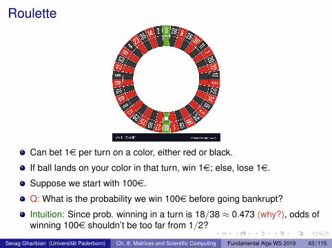
Can bet 1e per turn on a color, either red or black.
If ball lands on your color in that turn, win 1e; else, lose 1e.
Suppose we start with 100e.
Q: What is the probability we win 100e before going bankrupt?
Intuition: Since prob. winning in a turn is 18/38 ≈ 0.473 (why?), odds ofwinning 100e shouldn’t be too far from 1/2?
(Ha ha.)
Sevag Gharibian (Universität Paderborn) Ch. 8: Matrices and Scientific Computing Fundamental Algs WS 2019 43 / 115
Roulette
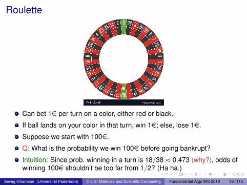
Can bet 1e per turn on a color, either red or black.
If ball lands on your color in that turn, win 1e; else, lose 1e.
Suppose we start with 100e.
Q: What is the probability we win 100e before going bankrupt?
Intuition: Since prob. winning in a turn is 18/38 ≈ 0.473 (why?), odds ofwinning 100e shouldn’t be too far from 1/2? (Ha ha.)
Sevag Gharibian (Universität Paderborn) Ch. 8: Matrices and Scientific Computing Fundamental Algs WS 2019 43 / 115
Let’s formalize this
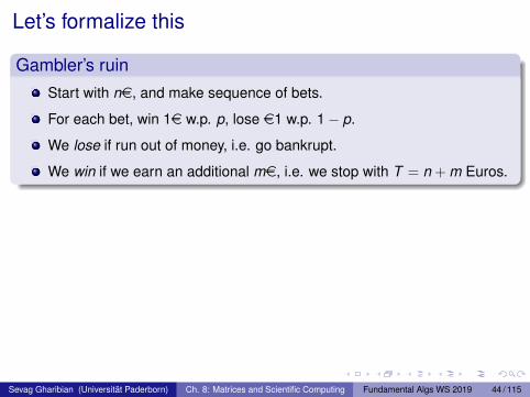
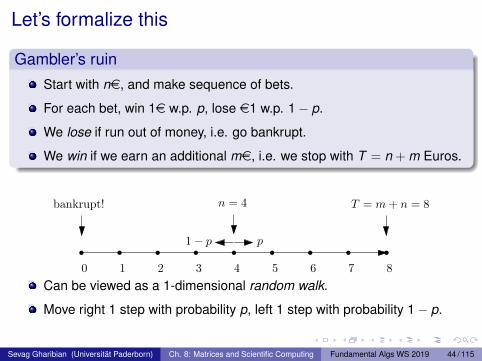
Gambler’s ruinStart with ne, and make sequence of bets.
For each bet, win 1e w.p. p, lose e1 w.p. 1− p.
We lose if run out of money, i.e. go bankrupt.
We win if we earn an additional me, i.e. we stop with T = n + m Euros.
0 1 2 3 4 5 6 7 8
n = 4 T = m+ n = 8bankrupt!
p1− p
Can be viewed as a 1-dimensional random walk.
Move right 1 step with probability p, left 1 step with probability 1− p.
Sevag Gharibian (Universität Paderborn) Ch. 8: Matrices and Scientific Computing Fundamental Algs WS 2019 44 / 115
Let’s formalize this
Gambler’s ruinStart with ne, and make sequence of bets.
For each bet, win 1e w.p. p, lose e1 w.p. 1− p.
We lose if run out of money, i.e. go bankrupt.
We win if we earn an additional me, i.e. we stop with T = n + m Euros.
0 1 2 3 4 5 6 7 8
n = 4 T = m+ n = 8bankrupt!
p1− p
Can be viewed as a 1-dimensional random walk.
Move right 1 step with probability p, left 1 step with probability 1− p.
Sevag Gharibian (Universität Paderborn) Ch. 8: Matrices and Scientific Computing Fundamental Algs WS 2019 44 / 115
Let’s formalize thisGambler’s ruin
Start with ne, and make sequence of bets.
For each bet, win 1e w.p. p, lose 1e w.p. 1− p.
We lose if run out of money, i.e. go bankrupt.
We win if we earn an additional me, i.e. have T = n + m Euros total.
Let W be event that we win before we lose.
Let Dt be random variable denoting # of Euros we have at time t .
ClaimLet Pn = Pr(W | D0 = n) be probability of W , given that start with ne. Then:
Pn =
0 if n = 01 if n = TpPn+1 + (1− p)Pn−1 if 0 < n < T .
Sevag Gharibian (Universität Paderborn) Ch. 8: Matrices and Scientific Computing Fundamental Algs WS 2019 45 / 115
Let’s formalize thisGambler’s ruin
Start with ne, and make sequence of bets.
For each bet, win 1e w.p. p, lose 1e w.p. 1− p.
We lose if run out of money, i.e. go bankrupt.
We win if we earn an additional me, i.e. have T = n + m Euros total.
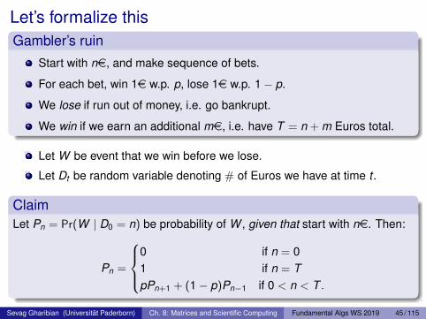
Let W be event that we win before we lose.
Let Dt be random variable denoting # of Euros we have at time t .
ClaimLet Pn = Pr(W | D0 = n) be probability of W , given that start with ne. Then:
Pn =
0 if n = 01 if n = TpPn+1 + (1− p)Pn−1 if 0 < n < T .
Sevag Gharibian (Universität Paderborn) Ch. 8: Matrices and Scientific Computing Fundamental Algs WS 2019 45 / 115
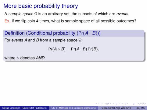
More basic probability theoryA sample space Ω is an arbitrary set, the subsets of which are events.
Ex. If we flip coin 4 times, what is sample space of all possible outcomes?
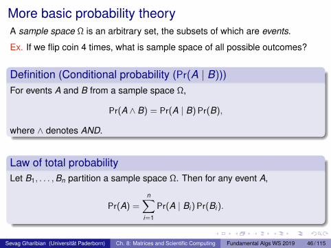
Definition (Conditional probability (Pr(A | B)))For events A and B from a sample space Ω,
Pr(A ∧ B) = Pr(A | B) Pr(B),
where ∧ denotes AND.
Law of total probabilityLet B1, . . . ,Bn partition a sample space Ω. Then for any event A,
Pr(A) =n∑
i=1
Pr(A | Bi ) Pr(Bi ).
Sevag Gharibian (Universität Paderborn) Ch. 8: Matrices and Scientific Computing Fundamental Algs WS 2019 46 / 115
More basic probability theoryA sample space Ω is an arbitrary set, the subsets of which are events.
Ex. If we flip coin 4 times, what is sample space of all possible outcomes?
Definition (Conditional probability (Pr(A | B)))For events A and B from a sample space Ω,
Pr(A ∧ B) = Pr(A | B) Pr(B),
where ∧ denotes AND.
Law of total probabilityLet B1, . . . ,Bn partition a sample space Ω. Then for any event A,
Pr(A) =n∑
i=1
Pr(A | Bi ) Pr(Bi ).
Sevag Gharibian (Universität Paderborn) Ch. 8: Matrices and Scientific Computing Fundamental Algs WS 2019 46 / 115
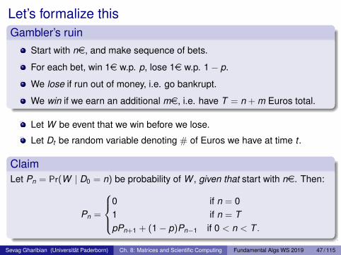
Let’s formalize thisGambler’s ruin
Start with ne, and make sequence of bets.
For each bet, win 1e w.p. p, lose 1e w.p. 1− p.
We lose if run out of money, i.e. go bankrupt.
We win if we earn an additional me, i.e. have T = n + m Euros total.
Let W be event that we win before we lose.
Let Dt be random variable denoting # of Euros we have at time t .
ClaimLet Pn = Pr(W | D0 = n) be probability of W , given that start with ne. Then:
Pn =
0 if n = 01 if n = TpPn+1 + (1− p)Pn−1 if 0 < n < T .
Sevag Gharibian (Universität Paderborn) Ch. 8: Matrices and Scientific Computing Fundamental Algs WS 2019 47 / 115
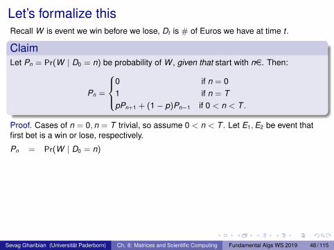
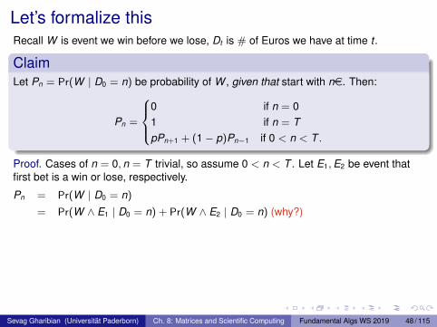
Let’s formalize thisRecall W is event we win before we lose, Dt is # of Euros we have at time t .
ClaimLet Pn = Pr(W | D0 = n) be probability of W , given that start with ne. Then:
Pn =
0 if n = 01 if n = TpPn+1 + (1− p)Pn−1 if 0 < n < T .
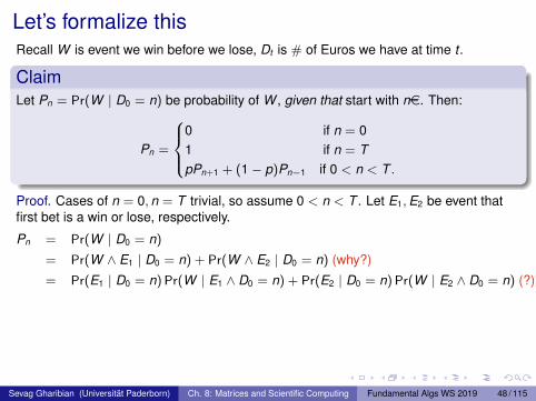
Proof. Cases of n = 0, n = T trivial, so assume 0 < n < T . Let E1,E2 be event thatfirst bet is a win or lose, respectively.
Pn = Pr(W | D0 = n)
= Pr(W ∧ E1 | D0 = n) + Pr(W ∧ E2 | D0 = n) (why?)
= Pr(E1 | D0 = n) Pr(W | E1 ∧ D0 = n) + Pr(E2 | D0 = n) Pr(W | E2 ∧ D0 = n) (?)
= p Pr(W | E1 ∧ D0 = n) + (1− p) Pr(W | E2 ∧ D0 = n) (why?)
= p Pr(W | D1 = n + 1) + (1− p) Pr(W | D1 = n − 1) (why?)
= p Pr(W | D0 = n + 1) + (1− p) Pr(W | D0 = n − 1) (why?)
= pPn+1 + (1− p)Pn−1.
Sevag Gharibian (Universität Paderborn) Ch. 8: Matrices and Scientific Computing Fundamental Algs WS 2019 48 / 115
Let’s formalize thisRecall W is event we win before we lose, Dt is # of Euros we have at time t .
ClaimLet Pn = Pr(W | D0 = n) be probability of W , given that start with ne. Then:
Pn =
0 if n = 01 if n = TpPn+1 + (1− p)Pn−1 if 0 < n < T .
Proof. Cases of n = 0, n = T trivial, so assume 0 < n < T . Let E1,E2 be event thatfirst bet is a win or lose, respectively.
Pn = Pr(W | D0 = n)
= Pr(W ∧ E1 | D0 = n) + Pr(W ∧ E2 | D0 = n) (why?)
= Pr(E1 | D0 = n) Pr(W | E1 ∧ D0 = n) + Pr(E2 | D0 = n) Pr(W | E2 ∧ D0 = n) (?)
= p Pr(W | E1 ∧ D0 = n) + (1− p) Pr(W | E2 ∧ D0 = n) (why?)
= p Pr(W | D1 = n + 1) + (1− p) Pr(W | D1 = n − 1) (why?)
= p Pr(W | D0 = n + 1) + (1− p) Pr(W | D0 = n − 1) (why?)
= pPn+1 + (1− p)Pn−1.
Sevag Gharibian (Universität Paderborn) Ch. 8: Matrices and Scientific Computing Fundamental Algs WS 2019 48 / 115
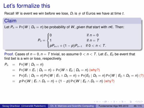
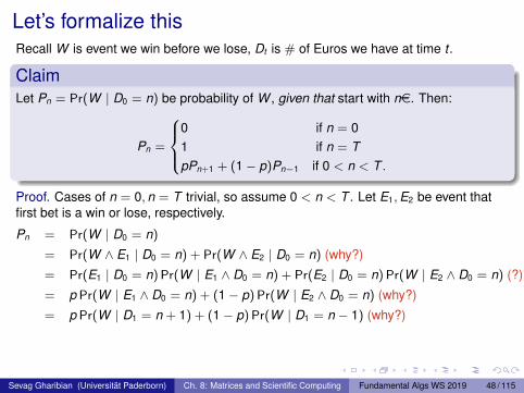
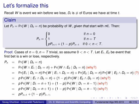
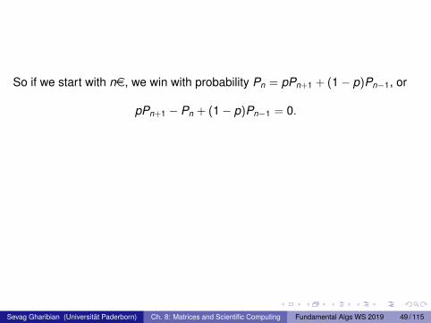
So if we start with ne, we win with probability Pn = pPn+1 + (1− p)Pn−1, or
pPn+1 − Pn + (1− p)Pn−1 = 0.
This is a linear homogeneous recurrence with P0 = 0 and PT = 1.
Let’s solve to get closed form for Pn, and determine odds of winning Roulette.
Idea: Use characteristic root technique.
Sevag Gharibian (Universität Paderborn) Ch. 8: Matrices and Scientific Computing Fundamental Algs WS 2019 49 / 115
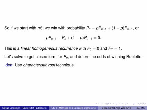
Characteristic root technique
Consider recurrence relation an + αan−1 + βan−2 = 0.
Its characteristic polynomial is x2 + αx + β.
Fact 1Suppose the characteristic polynomial has roots r1, r2 (i.e. solutions tocharacteristic equation x2 + αx + β = 0). Then:
If r1 6= r2, there exists constants a,b such that an = arn1 + brn
2 .
If r1 = r2, there exists constants a,b such that an = arn1 + bnrn
2 .
Ex. Let an = an−1 + an−2, with a0 = 0 and a1 = 1. Which famous recurrenceis this? Solve this recurrence.
In our setting, we have pPn+1 − Pn + (1− p)Pn−1 = 0.
Need to solve for roots of characteristic equation px2 − x + (1− p) = 0.
Sevag Gharibian (Universität Paderborn) Ch. 8: Matrices and Scientific Computing Fundamental Algs WS 2019 50 / 115
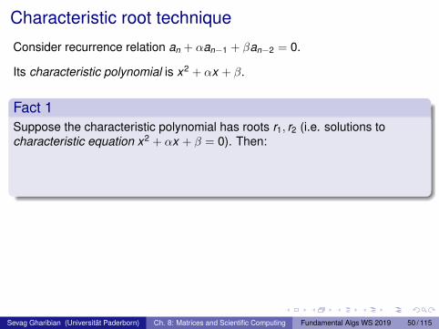
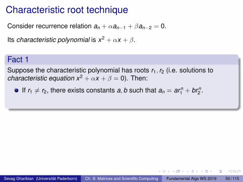
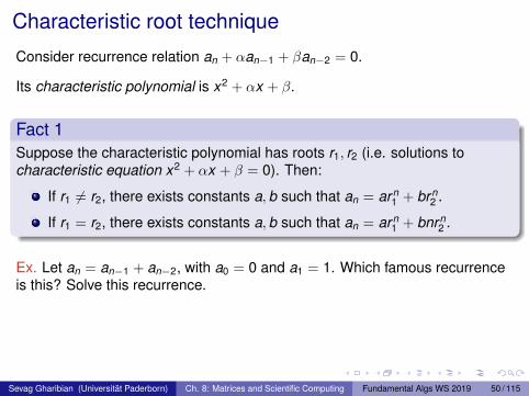
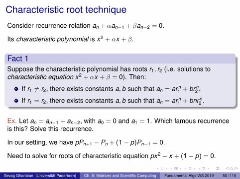
Solving the recurrenceIn our setting, we have pPn+1 − Pn + (1− p)Pn−1 = 0.
Need to solve for roots of characteristic equation px2 − x + (1− p) = 0.
By quadratic formula, x =1±√
1−4p(1−p)2p , i.e. have roots x = 1−p
p and x = 1.
Case 1: p 6= 1/2, i.e. distinct roots. By Fact 1, ∃ constants a,b s.t.
Pn = a(
1− pp
)n
+ b ≤(
p1− p
)m
.
Ex. Use initial conditions P0 = 0,PT = 1 to figure out a and b. Then,prove red inequality.
Conclusion: For Roulette, p = 1838 6=
12 . Thus, Pn ≤
(p
1−p
)m≤ 9
10m
.
I Probability of winning just 100e (i.e. m = 100) is less than 137648 !
I Note: Pn is independent of how much money, n, start with.
Ex. For what range of p is limm→∞ Pn = 0?
Sevag Gharibian (Universität Paderborn) Ch. 8: Matrices and Scientific Computing Fundamental Algs WS 2019 51 / 115
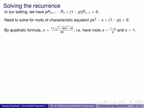
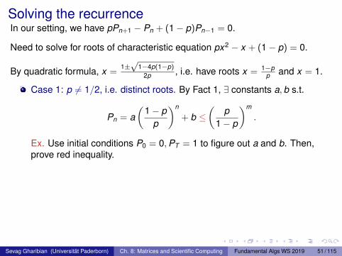
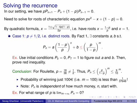

(Google’s disappointed face emoji)
Sevag Gharibian (Universität Paderborn) Ch. 8: Matrices and Scientific Computing Fundamental Algs WS 2019 52 / 115
Solving the recurrence
In our setting, we have pPn+1 − Pn + (1− p)Pn−1 = 0.
Need to solve for roots of characteristic equation px2 − x + (1− p) = 0.
By quadratic formula, x =1±√
1−4p(1−p)2p , i.e. have roots x = 1−p
p and x = 1.
Case 2: p = 1/2, i.e. same root. By Fact 1,
Pn = an + b =nT
=n
n + m.
Ex. Use initial conditions P0 = 0,PT = 1 to figure out a and b. Then,prove red equality.
Conclusion: When the game is fair (p = 1/2), odds of winning are whatyou expect — the closer you start (n) to your goal (T = n + m), the morelikely you are to win an additional me!
Sevag Gharibian (Universität Paderborn) Ch. 8: Matrices and Scientific Computing Fundamental Algs WS 2019 53 / 115
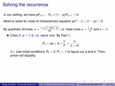
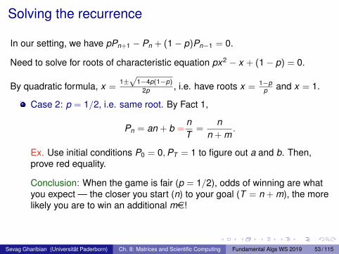

(Google’s thinking face emoji)
Sevag Gharibian (Universität Paderborn) Ch. 8: Matrices and Scientific Computing Fundamental Algs WS 2019 54 / 115
Outline
1 Introduction to matrices (review)
2 Matrix multiplication algorithmsStrassen’s algorithm (1967)Drineas-Kannan-Mahoney randomized algorithm (2006)
3 Random walksGambler’s ruinGoogle’s PageRank algorithm (1999)
4 Polynomial multiplicationComplex numbersPolynomialsO(N log N)-time polynomial multiplication via Fourier Transform
Sevag Gharibian (Universität Paderborn) Ch. 8: Matrices and Scientific Computing Fundamental Algs WS 2019 55 / 115
Now let’s take random walks beyond 1D and throw in matrices.
Sevag Gharibian (Universität Paderborn) Ch. 8: Matrices and Scientific Computing Fundamental Algs WS 2019 56 / 115
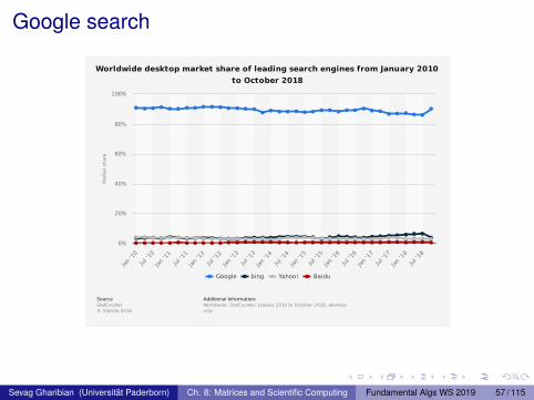
Google search
Marketsha
re
WorldwidedesktopmarketshareofleadingsearchenginesfromJanuary2010toOctober2018
AdditionalInformation:Worldwide;StatCounter;January2010toOctober2018;desktoponly
Google bing Yahoo! BaiduJan
'10
Jul'10
Jan'11
Jul'11
Jan'12
Jul'12
Jan'13
Jul'13
Jan'14
Jul'14
Jan'15
Jul'15
Jan'16
Jul'16
Jan'17
Jul'17
Jan'18
Jul'18
SourceStatCounter©Statista2018
0%
20%
40%
60%
80%
100%
Conclusion: Google has strong impact on which information is accessed.
Sevag Gharibian (Universität Paderborn) Ch. 8: Matrices and Scientific Computing Fundamental Algs WS 2019 57 / 115
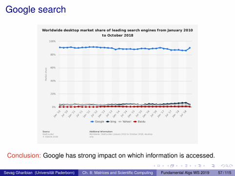

With great power comes great responsibility. . .
Q: How does Google decide which websites are more important than others?
Sevag Gharibian (Universität Paderborn) Ch. 8: Matrices and Scientific Computing Fundamental Algs WS 2019 58 / 115

With great power comes great responsibility. . .
Q: How does Google decide which websites are more important than others?
Sevag Gharibian (Universität Paderborn) Ch. 8: Matrices and Scientific Computing Fundamental Algs WS 2019 58 / 115

PageRank algorithm
Named after Larry Page (together with Sergey Brin, founded Google)
Ranks webpages by importance
Assumption: Pages with more links to them are “more important”
L. Page, S. Brin, R. Motwani, T. Winograd. “The PageRank citationranking: Bringing order to the Web”, 1999.
Sevag Gharibian (Universität Paderborn) Ch. 8: Matrices and Scientific Computing Fundamental Algs WS 2019 59 / 115
Idea sketch (simplified)Suppose internet consists of N webpages.
Imagine a random websurfer, who repeatedly does the following:
1 Pick a uniformly random link from current page.
2 Follow the link.
Intuition: Pages with “many” incoming links get visited “often” by websurfer.
Punchline: After “sufficiently long time”, the probability Pr(w) that surfer is onany particular webpage w approaches a steady state, denoted q(w).
The probability q(w) is the PageRank for w .
Observation: Websurfer is doing a random walk on the world wide web!
Sevag Gharibian (Universität Paderborn) Ch. 8: Matrices and Scientific Computing Fundamental Algs WS 2019 60 / 115
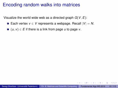
Encoding random walks into matrices
Visualize the world wide web as a directed graph G(V ,E):
Each vertex v ∈ V represents a webpage. Recall |V | = N.
(u, v) ∈ E if there is a link from page u to page v .
Ex. Consider directed graph G = (V ,E) with V = A,B,C,D:
P1 P2
P3 P4
The adjacency matrix A for G is
A =
0 1 1 01 0 0 01 0 0 11 1 1 0
.
Sevag Gharibian (Universität Paderborn) Ch. 8: Matrices and Scientific Computing Fundamental Algs WS 2019 61 / 115
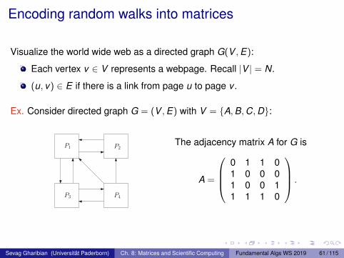
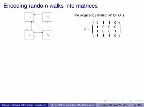
Encoding random walks into matrices
P1 P2
P3 P4
The adjacency matrix W for G is
A =
0 1 1 01 0 0 01 0 0 11 1 1 0
.
If websurfer starts at page P1, its state encoded by vector p0 =
1000
.
After 1 step, moves to P2 or P3, with prob. 1/2 each. New state p1 =
0
0.50.50
.
ObservationView pi as a distribution encoding probability that surfer at particular page after step i .
Q: Can we encode change in probabilities in each step by matrix multiplication?
Sevag Gharibian (Universität Paderborn) Ch. 8: Matrices and Scientific Computing Fundamental Algs WS 2019 62 / 115
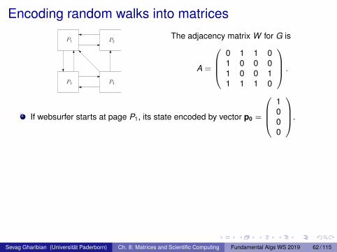
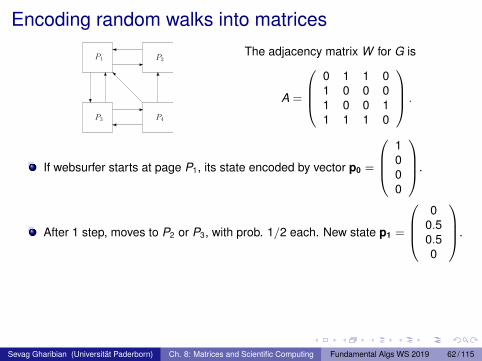
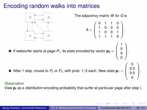
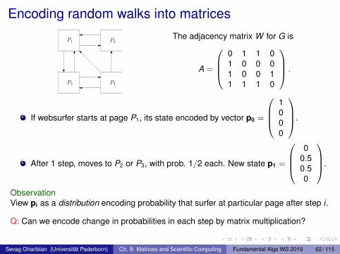
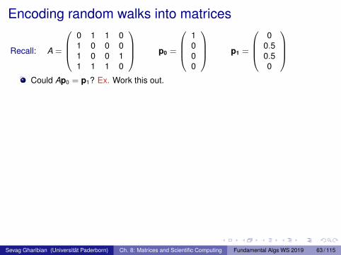
Encoding random walks into matrices
Recall: A =
0 1 1 01 0 0 01 0 0 11 1 1 0
p0 =
1000
p1 =
0
0.50.50
Could Ap0 = p1? Ex. Work this out.
Try taking transpose: AT p0 =(
0 1 1 0)T . Missing normalization. . .
Normalize each row of A by its out-degree (i.e. number of neighbors):
A =
0 1/2 1/2 01 0 0 0
1/2 0 0 1/21/3 1/3 1/3 0
, M := AT =
0 1 1/2 1/3
1/2 0 0 1/31/2 0 0 1/30 0 1/2 0
Now AT p0 = Mp0 = p1!
Multiplying by M updates surfer’s current distribution via 1 step of random walk!
Thus, after k steps, surfer’s distribution is pk = Mk p0.
Sevag Gharibian (Universität Paderborn) Ch. 8: Matrices and Scientific Computing Fundamental Algs WS 2019 63 / 115
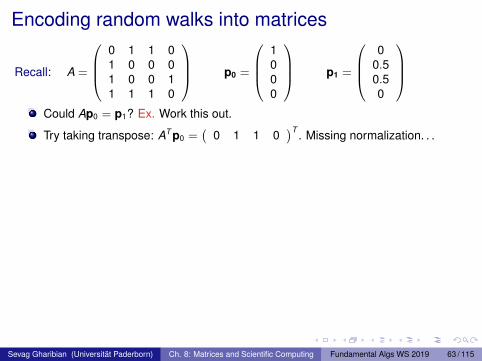
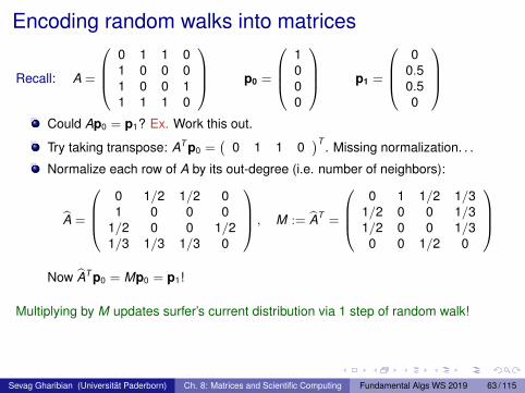
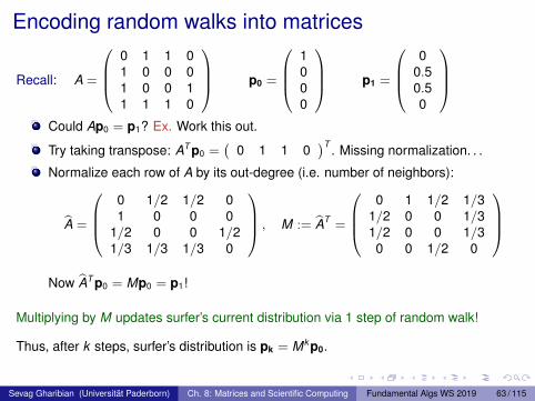

Idea sketch (simplified)Suppose internet consists of N webpages.
Imagine a random websurfer, who repeatedly does the following:
1 Pick a uniformly random link from current page.
2 Follow the link.
Intuition: Pages with “many” incoming links get visited “often” by websurfer.
Punchline: After “sufficiently long time”, the probability Pr(w) that surfer is onany particular webpage w approaches a steady state, denoted q(w).
The probability q(w) is the PageRank for w .
Observation: Websurfer is doing a random walk on the world wide web!
Sevag Gharibian (Universität Paderborn) Ch. 8: Matrices and Scientific Computing Fundamental Algs WS 2019 64 / 115

Defining PageRank more formally
Punchline: After “sufficiently long time”, the probability Pr(w) that surfer is onany particular webpage w approaches a steady state, denoted q(w).
The probability q(w) is the PageRank for w .
PageRank:
Recall if starting distribution is p0, after k steps have distributionpk = Mk p0.
A steady state would be a pi such that pi+1 = Mpi = pi , i.e. probabilityto be in any particular webpage no longer changes.
The w th entry of pi , corresponding to webpage w , is PageRank of w .
Observation: Note that Mpi = pi is just an eigenvalue equation!
Sevag Gharibian (Universität Paderborn) Ch. 8: Matrices and Scientific Computing Fundamental Algs WS 2019 65 / 115
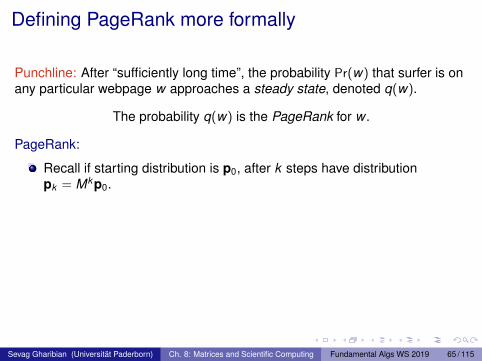
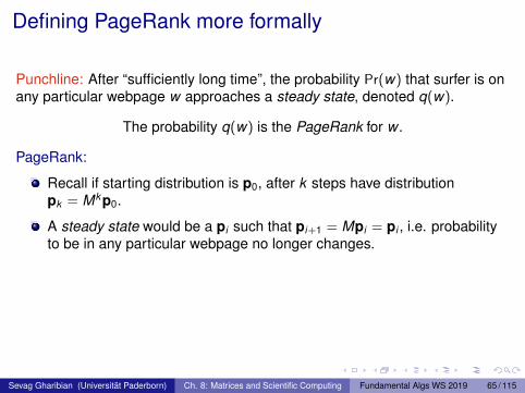
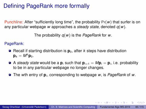
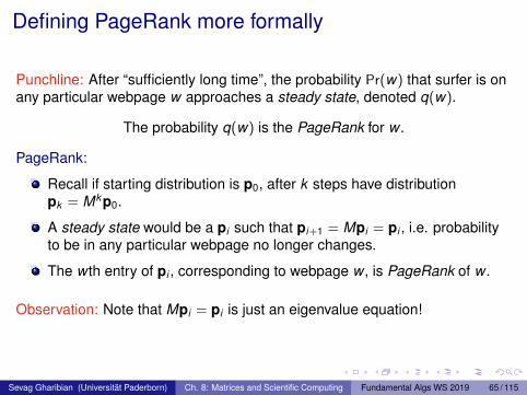
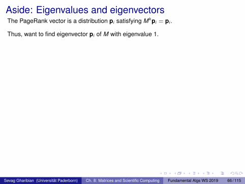
Aside: Eigenvalues and eigenvectorsThe PageRank vector is a distribution pi satisfying Mk pi = pi .
Thus, want to find eigenvector pi of M with eigenvalue 1.
Eigenvalues and eigenvectors
For A ∈ Rn×n and v ∈ Rn, say v is an eigenvector of A with eigenvalue λ ∈ R if
Av = λv. (1)
How to find eigenvectors and eigenvalues?
“Traditional” method:I Solve for roots of characteristic equation det(A− λI) = 0 to obtain
eigenvalues λ.I Substitute λ into Equation (1) to obtain a linear system of equations.I Solve the linear system to obtain v.
Power method (Von Mises, 1929):I Start with some vector v0.I In iteration k , set vk+1 = Avk
‖Avk‖.
PageRank implements Power method (with ‖·‖ the 1-norm/Taxicab norm (why?)).
Sevag Gharibian (Universität Paderborn) Ch. 8: Matrices and Scientific Computing Fundamental Algs WS 2019 66 / 115
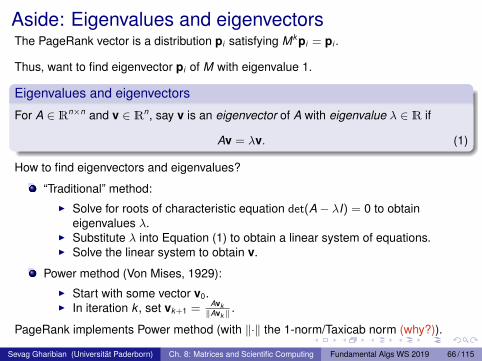
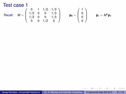
Test case 1
Recall: M =
0 1 1/2 1/3
1/2 0 0 1/31/2 0 0 1/30 0 1/2 0
p0 =
1000
pk = Mk p0.
Results (via Mathematica):
p0 (1., 0., 0., 0.)p1 (0., 0.5, 0.5, 0.)p2 (0.75, 0., 0., 0.25)p3 (0.0833333, 0.458333, 0.458333, 0.)p4 (0.6875, 0.0416667, 0.0416667, 0.229167)p5 (0.138889, 0.420139, 0.420139, 0.0208333)p6 (0.637153, 0.0763889, 0.0763889, 0.210069)p7 (0.184606, 0.3886, 0.3886, 0.0381944)p8 (0.595631, 0.105035, 0.105035, 0.1943)p9 (0.222319, 0.362582, 0.362582, 0.0525174)p10 (0.561379, 0.128665, 0.128665, 0.181291)p11 (0.253428, 0.34112, 0.34112, 0.0643326)p12 (0.533124, 0.148158, 0.148158, 0.17056)
Seems to be converging, but slowly. . . No unique most important page yet. . .
Sevag Gharibian (Universität Paderborn) Ch. 8: Matrices and Scientific Computing Fundamental Algs WS 2019 67 / 115
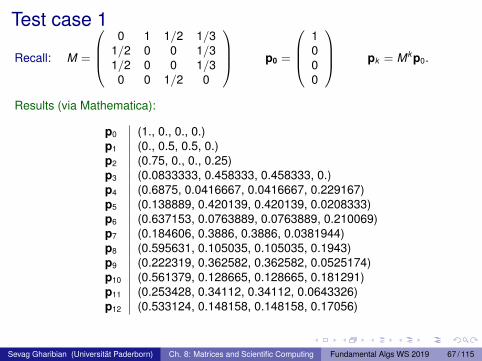
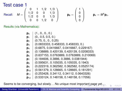
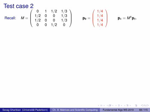
Test case 2
Recall: M =
0 1 1/2 1/3
1/2 0 0 1/31/2 0 0 1/30 0 1/2 0
p0 =
1/41/41/41/4
pk = Mk p0.
Results (via Mathematica):
p0 (0.25, 0.25, 0.25, 0.25)p1 (0.458333, 0.208333, 0.208333, 0.125)p2 (0.354167, 0.270833, 0.270833, 0.104167)p3 (0.440972, 0.211806, 0.211806, 0.135417)p4 (0.362847, 0.265625, 0.265625, 0.105903)p5 (0.433738, 0.216725, 0.216725, 0.132813)p6 (0.369358, 0.26114, 0.26114, 0.108362)p7 (0.427831, 0.2208, 0.2208, 0.13057)p8 (0.374723, 0.257439, 0.257439, 0.1104)p9 (0.422958, 0.224161, 0.224161, 0.128719)p10 (0.379148, 0.254385, 0.254385, 0.112081)p11 (0.418938, 0.226934, 0.226934, 0.127193)p12 (0.382799, 0.251867, 0.251867, 0.113467)
Much better! Singled out P1 as having largest PageRank.
Sevag Gharibian (Universität Paderborn) Ch. 8: Matrices and Scientific Computing Fundamental Algs WS 2019 68 / 115
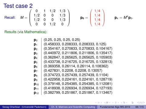
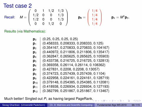
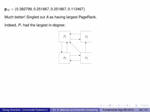
p12 = (0.382799, 0.251867, 0.251867, 0.113467)
Much better! Singled out A as having largest PageRank.
Indeed, P1 had the largest in-degree:
P1 P2
P3 P4
Rate of convergence:
Seems to depend on starting vector, which is not really surprising.
Can we hope to prove rigorous upper bound on number of required iterations toget “close” to PageRank vector?
Yes, but I’ve sort of been lying to you so far. . .
Sevag Gharibian (Universität Paderborn) Ch. 8: Matrices and Scientific Computing Fundamental Algs WS 2019 69 / 115
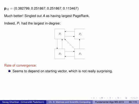
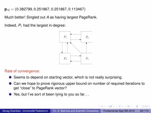

Q: Does a “real” websurfer just follow links all day?
A: No! Can enter address in browser’s address bar and jump straightthere.
Let’s try and include this “more realistic” behavior in our model. It willhelp us prove a convergence bound.
Steps:
1 Define more “realistic” model.
2 Define what we mean by being “close” to the target distribution.
3 “Show” that random walk algorithm converges exponentially quickly toPageRank vector.
Sevag Gharibian (Universität Paderborn) Ch. 8: Matrices and Scientific Computing Fundamental Algs WS 2019 70 / 115
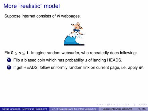
More “realistic” model
Suppose internet consists of N webpages.
Fix 0 ≤ s ≤ 1. Imagine random websurfer, who repeatedly does following:
1 Flip a biased coin which has probability s of landing HEADS.
2 If get HEADS, follow uniformly random link on current page, i.e. apply M.
3 If get TAILS, go to uniformly random page on internet, i.e. apply 1N J for J
the all-ones matrix.
Q: Why is the right transition matrix for TAILS 1N J?
So our new transition matrix is M(s) = sM + 1−sN J (why?).
Sevag Gharibian (Universität Paderborn) Ch. 8: Matrices and Scientific Computing Fundamental Algs WS 2019 71 / 115
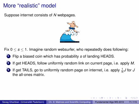
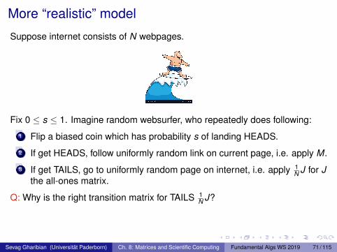
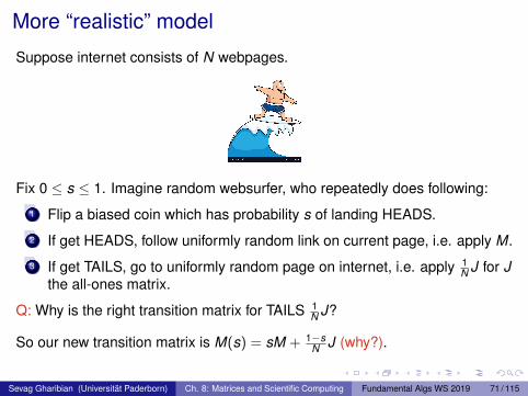
Quantifying “closeness” of distributions
Given p,q ∈ Rn whose entries form probability distributions, how to quantifyhow “close” these distributions are?
Total variation distanceThe total variation distance between distributions p,q ∈ Rn is
‖p− q‖1 =N∑
i=1
|pi − qi | .
Note this is just the Taxicab norm or 1-norm from earlier in slides.
Ex. What is the total variation distance between p = (1,0,0,0)T andq = (1/4,1/4,1/4,1/4)?
Sevag Gharibian (Universität Paderborn) Ch. 8: Matrices and Scientific Computing Fundamental Algs WS 2019 72 / 115
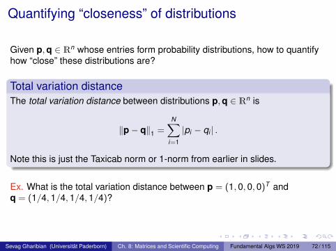
What does variational distance mean?
Suppose we play the following game on some sample space Ω.
1 I flip a fair coin.
2 If I get HEADS, I sample an element t ∈ Ω according to p.
3 Else, if I get TAILS, I sample an element t ∈ Ω according to q.
4 I send you t .
5 You try to guess whether I sampled from p or q.
It turns out that your optimal probability of guessing correctly is
12
+14‖p− q‖1 .
Ex. What is optimal probability of you winning the game for p = (1,0,0,0)T
and q = (1/4,1/4,1/4,1/4)? Can you think of an optimal guessing strategyfor achieving this?
Sevag Gharibian (Universität Paderborn) Ch. 8: Matrices and Scientific Computing Fundamental Algs WS 2019 73 / 115
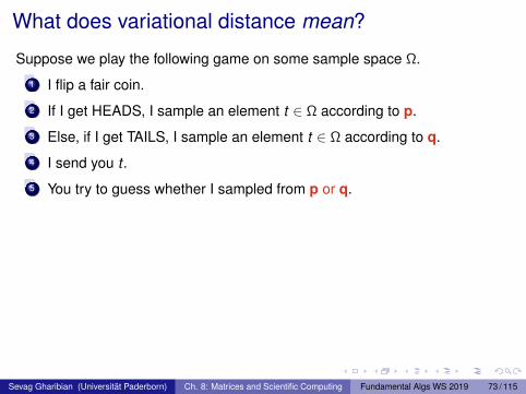
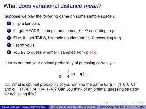

Convergence bounds
Can now bound how quickly we converge to PageRank vector.
Suppose start with arbitrary distribution p ∈ RN over webpages.
Fact 1. M(s) = sM + 1−sN J has unique PageRank vector, denoted q.
Claim 2. For all j ≥ 1,∥∥M(s)jp− q
∥∥1 ≤ s
∥∥M(s)j−1p− q∥∥
1.
Corollary. After k ≥ 1 iterations,∥∥M(s)k p− q
∥∥1 ≤ sk ‖p− q‖1 .(why?)
Notes:
In original PageRank paper, s = 0.85 was used.
Since ‖p− q‖1 ≤ 2 for any unit vectors p,q (why?), conclude that weconverge exponentially quickly (in k ) to PageRank vector q.
Magically, this bound is independent of size of internet, N.
Ok, so remains to prove Claim 2.
Sevag Gharibian (Universität Paderborn) Ch. 8: Matrices and Scientific Computing Fundamental Algs WS 2019 74 / 115
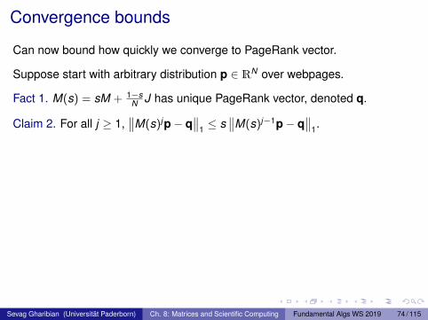
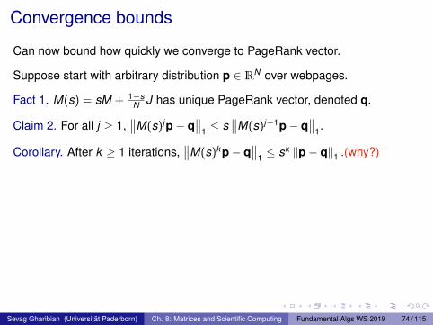
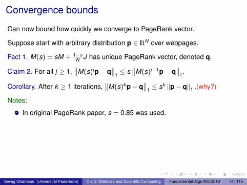
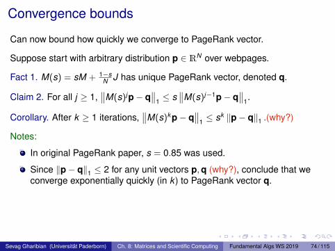
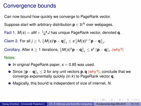
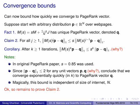
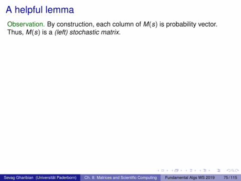
A helpful lemmaObservation. By construction, each column of M(s) is probability vector.Thus, M(s) is a (left) stochastic matrix.
Lemma (Contractivity of l1 norm)
For stochastic A ∈ Rn×n and v ∈ Rn, ‖Av‖1 ≤ ‖v‖1.
Proof.
‖Av‖1 =n∑
j=1
∣∣∣∣∣n∑
k=1
Ajk vk
∣∣∣∣∣ (def. of l1 norm)
≤n∑
k=1
n∑j=1
Ajk |vk | (triangle inequality, multiplicativity, |Ajk | = Ajk )
=n∑
k=1
|vk | (sum of column entries of A is 1)
= ‖v‖1 .
Sevag Gharibian (Universität Paderborn) Ch. 8: Matrices and Scientific Computing Fundamental Algs WS 2019 75 / 115
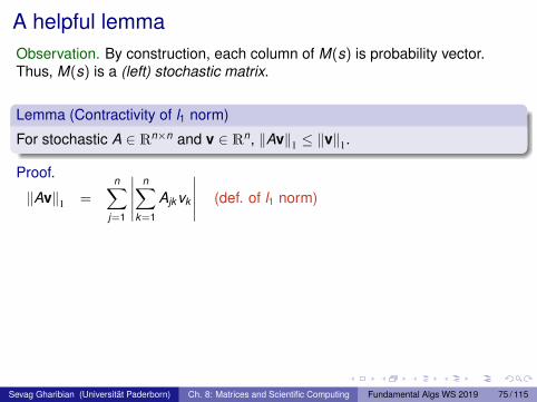
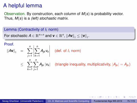
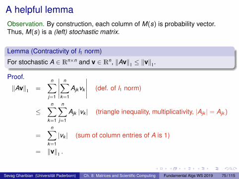
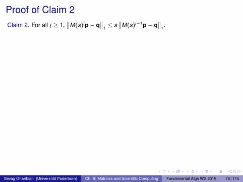
Proof of Claim 2Claim 2. For all j ≥ 1,
∥∥M(s)jp− q∥∥
1 ≤ s∥∥M(s)j−1p− q
∥∥1.
Proof.∥∥∥M(s)jp− q∥∥∥
1=
∥∥∥M(s)(M(s)j−1p− q)∥∥∥
1(M(s)q = q)
=
∥∥∥∥sM(M(s)j−1p− q) +1− s
NJ(M(s)j−1p− q)
∥∥∥∥1(
M(s) = sM +1− s
NJ)
=∥∥∥sM(M(s)j−1p− q)
∥∥∥1
(J(M(s)j−1p) = Jq
)(why?)
= s∥∥∥M(M(s)j−1p− q)
∥∥∥1
(absolute homogeneity, |s| = s)
≤ s∥∥∥M(s)j−1p− q
∥∥∥1
(contractivity of l1 norm, M stochastic).
Done! We conclude PageRank converges exponentially quickly (in number ofiterations, k ), to its stationary distribution (q), irrespective of size of the internet (N).
Sevag Gharibian (Universität Paderborn) Ch. 8: Matrices and Scientific Computing Fundamental Algs WS 2019 76 / 115
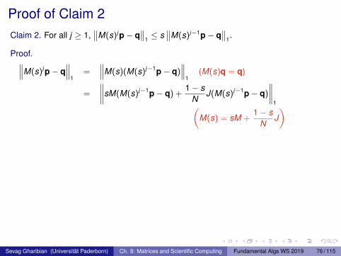
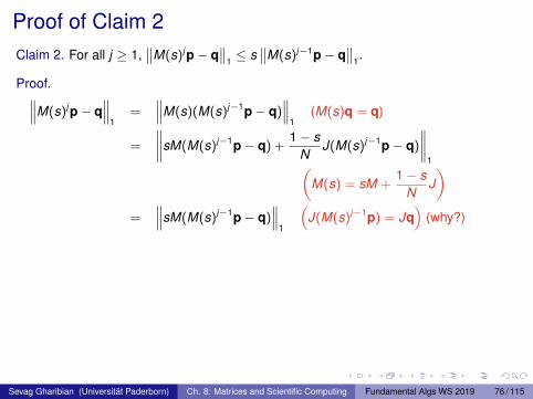
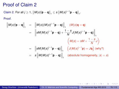
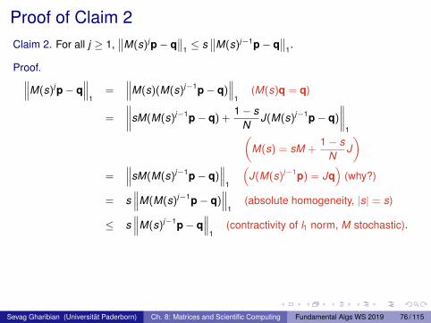
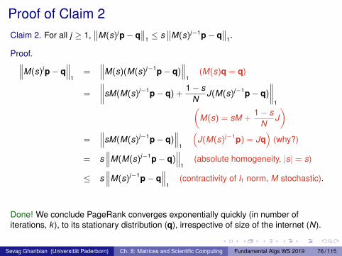

(Google’s happy face emoji)
Sevag Gharibian (Universität Paderborn) Ch. 8: Matrices and Scientific Computing Fundamental Algs WS 2019 77 / 115
Outline
1 Introduction to matrices (review)
2 Matrix multiplication algorithmsStrassen’s algorithm (1967)Drineas-Kannan-Mahoney randomized algorithm (2006)
3 Random walksGambler’s ruinGoogle’s PageRank algorithm (1999)
4 Polynomial multiplicationComplex numbersPolynomialsO(N log N)-time polynomial multiplication via Fourier Transform
Sevag Gharibian (Universität Paderborn) Ch. 8: Matrices and Scientific Computing Fundamental Algs WS 2019 78 / 115
Goals of section
Practice working with complex numbersPractice working with polynomialsIntroduce Fourier transform and its applications
Sevag Gharibian (Universität Paderborn) Ch. 8: Matrices and Scientific Computing Fundamental Algs WS 2019 79 / 115
Outline
1 Introduction to matrices (review)
2 Matrix multiplication algorithmsStrassen’s algorithm (1967)Drineas-Kannan-Mahoney randomized algorithm (2006)
3 Random walksGambler’s ruinGoogle’s PageRank algorithm (1999)
4 Polynomial multiplicationComplex numbersPolynomialsO(N log N)-time polynomial multiplication via Fourier Transform
Sevag Gharibian (Universität Paderborn) Ch. 8: Matrices and Scientific Computing Fundamental Algs WS 2019 80 / 115
Complex numbers
Question: What are the roots of x2 + 1 = 0?
i :=√−1 and −i
Selected history
(Cardano 1545) Considers square roots of negative numbers in solving for rootsof cubic polynomials. Calls them “as subtle as [they] are useless”.
(Bombelli 1572) Derives rules for basic arithmetic operations with roots ofnegative numbers
(Euler 1707-1783) Introduces symbol i , proves eit = cos(t) + i sin(t)
(Wessel 1745-1818, also Gauss 1777-1855) Introduces 2D complex plane
(Hamilton 1805-1865) Representation of complex numbers as 2-tuples fromR×R.
“The shortest path between two truths in the real domain passesthrough the complex domain.” – Hadamard
Sevag Gharibian (Universität Paderborn) Ch. 8: Matrices and Scientific Computing Fundamental Algs WS 2019 81 / 115
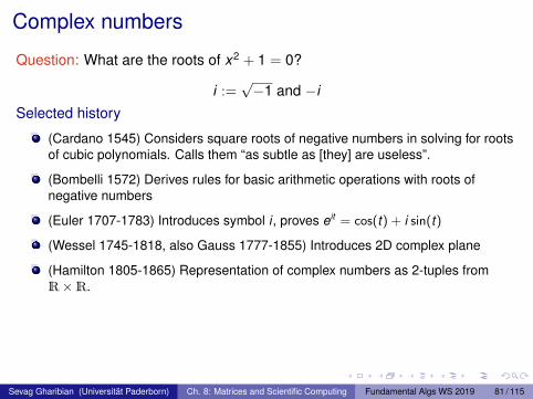
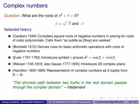
Why complex numbers?
Many, many applications, ranging from control theory to geometry toquantum mechanics.
Fundamental theorem of algebra (Argand 1806):
Every non-constant, univariate polynomial with complex coefficients hasat least one root in C.
or, equivalently,
Every non-zero, degree n univariate polynomial with complexcoefficients has precisely n complex roots.
e.g. x2 + 1 is degree 2, and has two complex roots: i , and −i .
Moral: You should care about complex numbers!
Sevag Gharibian (Universität Paderborn) Ch. 8: Matrices and Scientific Computing Fundamental Algs WS 2019 82 / 115
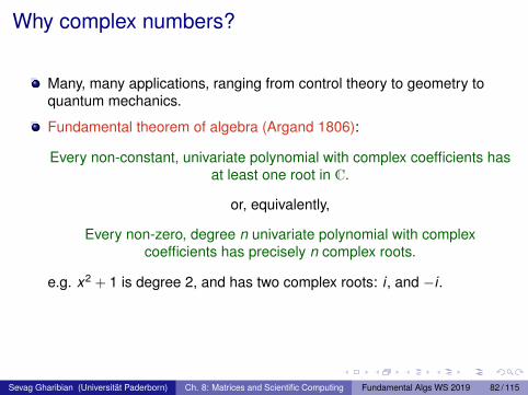
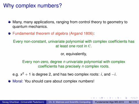
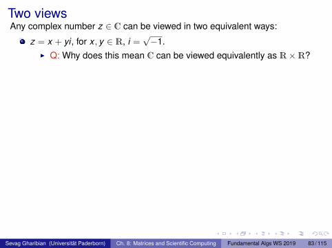
Two viewsAny complex number z ∈ C can be viewed in two equivalent ways:
z = x + yi , for x , y ∈ R, i =√−1.
I Q: Why does this mean C can be viewed equivalently as R×R?
I z = x − iy is complex conjugate of z. (Sometimes denoted z∗.)
(Polar form) z = reiφ for r , φ ∈ R. Here,I r is the “magnitude” of z, i.e. r = |z| =
√x2 + y2.
Q: What norm does the formula for magnitude remind you of?
I φ ∈ [π,−π) is the angle of z (in radians):
Sevag Gharibian (Universität Paderborn) Ch. 8: Matrices and Scientific Computing Fundamental Algs WS 2019 83 / 115
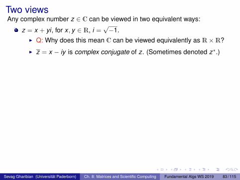
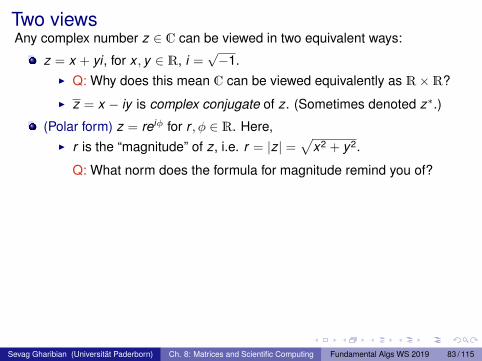
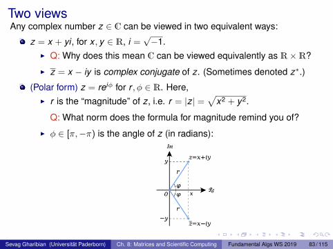
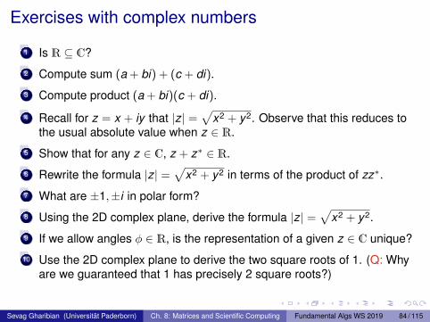
Exercises with complex numbers
1 Is R ⊆ C?
2 Compute sum (a + bi) + (c + di).
3 Compute product (a + bi)(c + di).
4 Recall for z = x + iy that |z| =√
x2 + y2. Observe that this reduces tothe usual absolute value when z ∈ R.
5 Show that for any z ∈ C, z + z∗ ∈ R.
6 Rewrite the formula |z| =√
x2 + y2 in terms of the product of zz∗.
7 What are ±1,±i in polar form?
8 Using the 2D complex plane, derive the formula |z| =√
x2 + y2.
9 If we allow angles φ ∈ R, is the representation of a given z ∈ C unique?
10 Use the 2D complex plane to derive the two square roots of 1. (Q: Whyare we guaranteed that 1 has precisely 2 square roots?)
Sevag Gharibian (Universität Paderborn) Ch. 8: Matrices and Scientific Computing Fundamental Algs WS 2019 84 / 115
With C in hand, can now define polynomials with coefficients from C.
Later, we will use C for the Fourier transform as well.
Sevag Gharibian (Universität Paderborn) Ch. 8: Matrices and Scientific Computing Fundamental Algs WS 2019 85 / 115
Outline
1 Introduction to matrices (review)
2 Matrix multiplication algorithmsStrassen’s algorithm (1967)Drineas-Kannan-Mahoney randomized algorithm (2006)
3 Random walksGambler’s ruinGoogle’s PageRank algorithm (1999)
4 Polynomial multiplicationComplex numbersPolynomialsO(N log N)-time polynomial multiplication via Fourier Transform
Sevag Gharibian (Universität Paderborn) Ch. 8: Matrices and Scientific Computing Fundamental Algs WS 2019 86 / 115
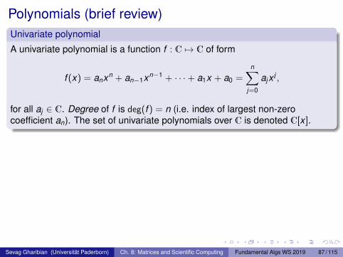
Polynomials (brief review)Univariate polynomial
A univariate polynomial is a function f : C 7→ C of form
f (x) = anxn + an−1xn−1 + · · ·+ a1x + a0 =n∑
j=0
ajx j ,
for all aj ∈ C. Degree of f is deg(f ) = n (i.e. index of largest non-zerocoefficient an). The set of univariate polynomials over C is denoted C[x ].
Sum and product of polynomials
For f ,g ∈ C[x ] with f (x) =∑n
j=0 ajx j and g(x) =∑n
j=0 bjx j ,
f (x) + g(x) =n∑
j=0
(aj + bj )x j , and f (x)g(x) =2n∑
j=0
( j∑k=0
ak bj−k
)x j .
Ex. Prove the multiplication formula for f (x)g(x) holds.
Sevag Gharibian (Universität Paderborn) Ch. 8: Matrices and Scientific Computing Fundamental Algs WS 2019 87 / 115
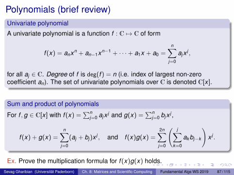
Polynomials (brief review)Univariate polynomial
A univariate polynomial is a function f : C 7→ C of form
f (x) = anxn + an−1xn−1 + · · ·+ a1x + a0 =n∑
j=0
ajx j ,
for all aj ∈ C. Degree of f is deg(f ) = n (i.e. index of largest non-zerocoefficient an). The set of univariate polynomials over C is denoted C[x ].
Sum and product of polynomials
For f ,g ∈ C[x ] with f (x) =∑n
j=0 ajx j and g(x) =∑n
j=0 bjx j ,
f (x) + g(x) =n∑
j=0
(aj + bj )x j , and f (x)g(x) =2n∑
j=0
( j∑k=0
ak bj−k
)x j .
Ex. Prove the multiplication formula for f (x)g(x) holds.Sevag Gharibian (Universität Paderborn) Ch. 8: Matrices and Scientific Computing Fundamental Algs WS 2019 87 / 115
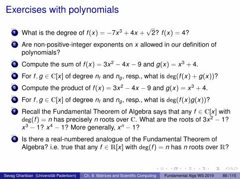
Exercises with polynomials
1 What is the degree of f (x) = −7x3 + 4x +√
2? f (x) = 4?
2 Are non-positive-integer exponents on x allowed in our definition ofpolynomials?
3 Compute the sum of f (x) = 3x2 − 4x − 9 and g(x) = x3 + 4.
4 For f ,g ∈ C[x ] of degree nf and ng , resp., what is deg(f (x) + g(x))?
5 Compute the product of f (x) = 3x2 − 4x − 9 and g(x) = x3 + 4.
6 For f ,g ∈ C[x ] of degree nf and ng , resp., what is deg(f (x)g(x))?
7 Recall the Fundamental Theorem of Algebra says that any f ∈ C[x ] withdeg(f ) = n has precisely n roots over C. What are the roots of 3x2 − 1?x3 − 1? x4 − 1? More generally, xn − 1?
8 Is there a real-numbered analogue of the Fundamental Theorem ofAlgebra? i.e. true that any f ∈ R[x ] with deg(f ) = n has n roots over R?
Sevag Gharibian (Universität Paderborn) Ch. 8: Matrices and Scientific Computing Fundamental Algs WS 2019 88 / 115
Cost of polynomial multiplication
How many field operations over C does the naive algorithm take to multiplytwo degree-n polynomials f ,g ∈ C[x ]?
A: Θ(n2) time.
Q: Can we do it in subquadratic time?
A: Surprisingly, yes! Can do it in Θ(n log n) time.
Battle plan:
1 Convert f ,g ∈ C[x ] from coefficient representation to point-valuerepresentation by evaluating f ,g at cleverly chosen points.
2 Multiplication in point-value representation takes only Θ(n) time.
3 Convert back from point-value representation to coefficientrepresentation (i.e. interpolate) to recover final answer.
Sevag Gharibian (Universität Paderborn) Ch. 8: Matrices and Scientific Computing Fundamental Algs WS 2019 89 / 115
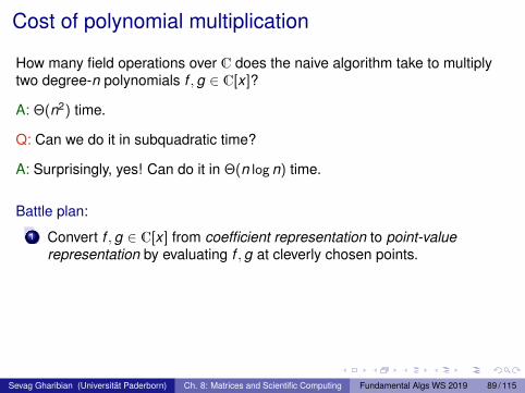
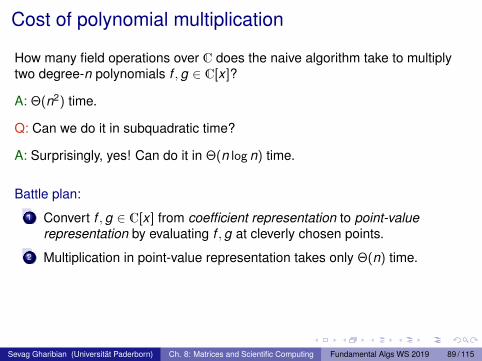
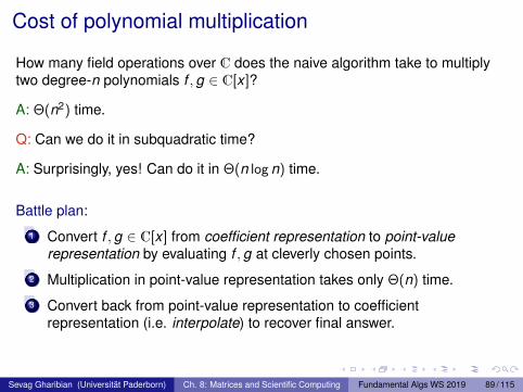
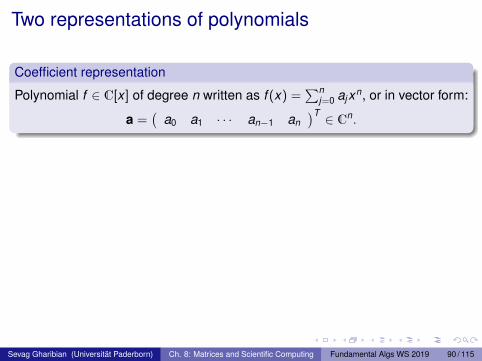
Two representations of polynomials
Coefficient representation
Polynomial f ∈ C[x ] of degree n written as f (x) =∑n
j=0 ajxn, or in vector form:
a =(
a0 a1 · · · an−1 an)T ∈ Cn.
Observation: Given f ∈ C[x ] in coefficient form, can evaluate f at any pointx ∈ C in Θ(n) time using Horner’s rule:
f (x) = a0 + x(a1 + x(a2 + · · ·+ x(an−1 + x(an)) · · · )).
Ex. Use Horner’s rule to evaluate f (x) = 5x3 − 2x2 − x + 1 at x = eiπ.
(Aside: What is eiπ?)
Sevag Gharibian (Universität Paderborn) Ch. 8: Matrices and Scientific Computing Fundamental Algs WS 2019 90 / 115
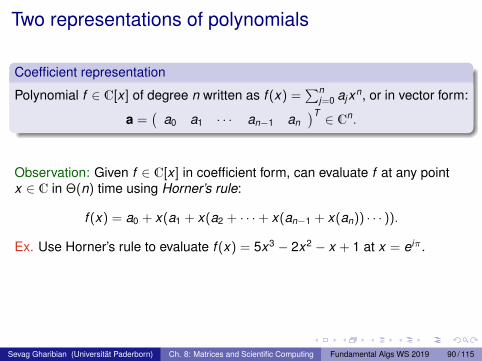
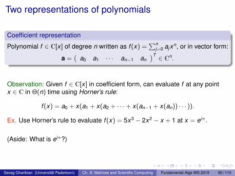
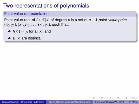
Two representations of polynomialsPoint-value representation
Point-value rep. of f ∈ C[x ] of degree n is a set of n + 1 point-value pairs(x0, y0), (x1, y1), . . . , (xn, yn), such that:
f (xi ) = yi for all xi , and
all xi are distinct.
Ex. Give two distinct point-value representations for f (x) = 3x2 + 1.
Obs: Not clear a priori that point-value representation captures f . . .
Interpolation Theorem
Any set of n + 1 point-value pairs (x0, y0), (x1, y1), . . . , (xn, yn) with distinctxi defines a unique polynomial f such that:
deg(f ) ≤ n,
f (xj ) = yj for j ∈ 0, . . . ,n.
Sevag Gharibian (Universität Paderborn) Ch. 8: Matrices and Scientific Computing Fundamental Algs WS 2019 91 / 115
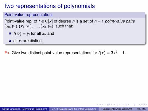
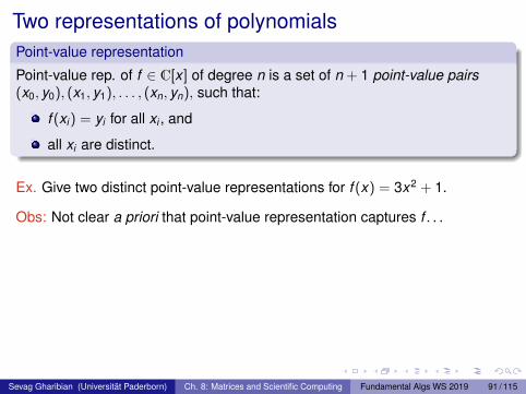
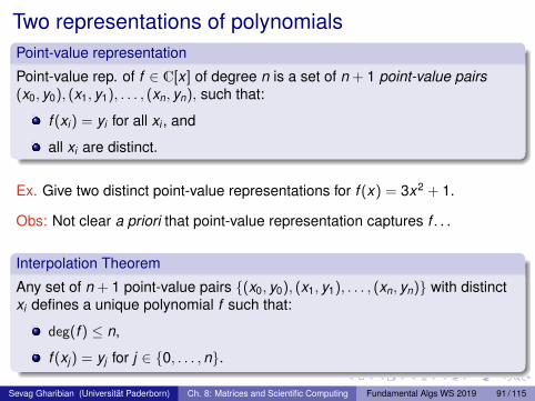
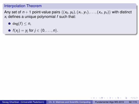
Interpolation Theorem
Any set of n + 1 point-value pairs (x0, y0), (x1, y1), . . . , (xn, yn) with distinctxi defines a unique polynomial f such that:
deg(f ) ≤ n,
f (xj ) = yj for j ∈ 0, . . . ,n.
Proof. Looking for f (x) =∑n
j=0 ajxn s.t. f (xi ) = yi . Encode as matrix mult.:1 x0 x2
0 · · · xn0
1 x1 x21 · · · xn
1...
......
. . ....
1 xn x2n · · · xn
n
a0a1...
an
=
y0y1...
yn
Write as V (x0, . . . , xn)a = y, for V ∈ Cn+1×n+1 a Vandermonde matrix.
Fact: Any Vandermonde matrix has an inverse if all xj are distinct.
Conclusion: Unique solution for a given by a = V (x0, . . . , xn)−1y.
Sevag Gharibian (Universität Paderborn) Ch. 8: Matrices and Scientific Computing Fundamental Algs WS 2019 92 / 115
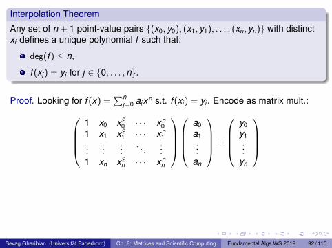
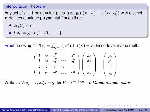
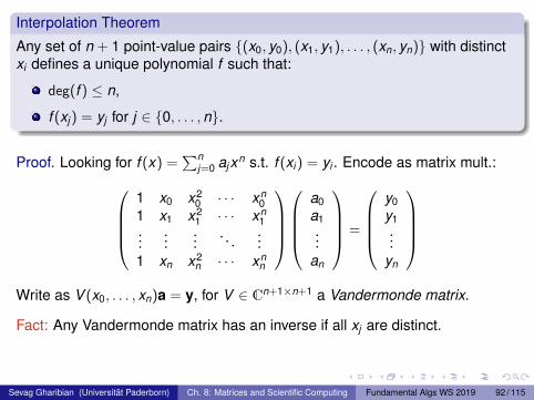
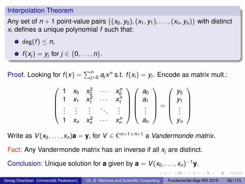

The big fuss about the point-value representation
Q: Given degree-n polynomials in point-value form,
f (x) “ = ” (x0, y0), (x1, y1), . . . , (xn, yn),g(x) “ = ”
(x0, y ′0), (x1, y ′1), . . . , (xn, y ′n)
,
what is cost of multiplying f (x) and g(x)? (Note: Shared xj values above!)
A: Θ(n) time! The point-value representation for f (x)g(x) is(x0, y0y ′0), (x1, y1y ′1), . . . , (xn, yny ′n)
, (2)
i.e. suffices to point-wise multiply. (Ex. Convince yourself of this claim.)
Q: Do you see a problem with the statement above?
A: Eq. (2) has n + 1 datapoints, but f (x)g(x) is degree ≤ 2n (i.e. not enough data touniquely identify f (x)g(x) via Interpolation Theorem).
Solution: Start with point-value representations for f and g which have 2n + 1 points(i.e. before multiplying).
Sevag Gharibian (Universität Paderborn) Ch. 8: Matrices and Scientific Computing Fundamental Algs WS 2019 93 / 115
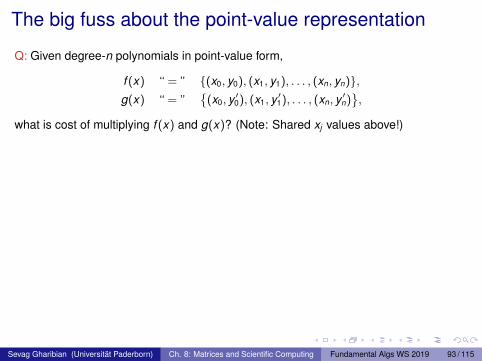
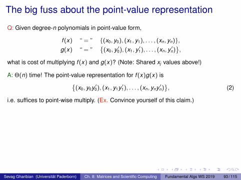
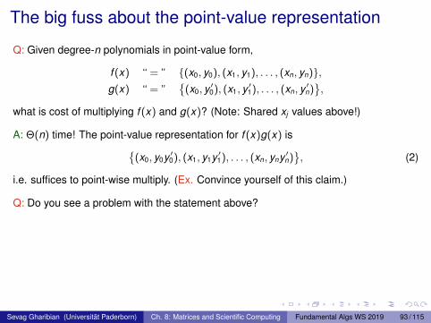
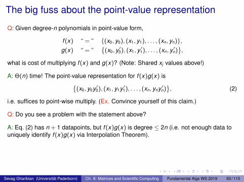
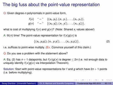
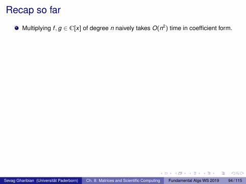
Recap so far
Multiplying f , g ∈ C[x ] of degree n naively takes O(n2) time in coefficient form.
Hope: If could convert to and from point-value form “quickly”, could instead dopoint-wise multiplication, which takes O(n) time.
Cost of going from coefficient to point-value form with 2n + 1 point-value pairs?I Via Horner’s rule, O(n)-time per evaluation of f at a point (x , y).I Repeating for 2n + 1 points xj yields O(n2) time total.
Fact: Can also convert back from point-value to coefficient form in O(n2) timeusing Lagrange’s formula.
But this is stupid. . . Just converting between representations takes as much timeas naive multiplication algorithm. . .
(Facebook worried emoji)
Sevag Gharibian (Universität Paderborn) Ch. 8: Matrices and Scientific Computing Fundamental Algs WS 2019 94 / 115
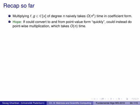
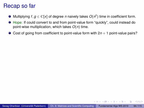
Recap so far
Multiplying f , g ∈ C[x ] of degree n naively takes O(n2) time in coefficient form.
Hope: If could convert to and from point-value form “quickly”, could instead dopoint-wise multiplication, which takes O(n) time.
Cost of going from coefficient to point-value form with 2n + 1 point-value pairs?
I Via Horner’s rule, O(n)-time per evaluation of f at a point (x , y).I Repeating for 2n + 1 points xj yields O(n2) time total.
Fact: Can also convert back from point-value to coefficient form in O(n2) timeusing Lagrange’s formula.
But this is stupid. . . Just converting between representations takes as much timeas naive multiplication algorithm. . .
(Facebook worried emoji)
Sevag Gharibian (Universität Paderborn) Ch. 8: Matrices and Scientific Computing Fundamental Algs WS 2019 94 / 115
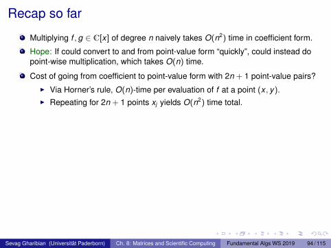
Recap so far
Multiplying f , g ∈ C[x ] of degree n naively takes O(n2) time in coefficient form.
Hope: If could convert to and from point-value form “quickly”, could instead dopoint-wise multiplication, which takes O(n) time.
Cost of going from coefficient to point-value form with 2n + 1 point-value pairs?I Via Horner’s rule, O(n)-time per evaluation of f at a point (x , y).I Repeating for 2n + 1 points xj yields O(n2) time total.
Fact: Can also convert back from point-value to coefficient form in O(n2) timeusing Lagrange’s formula.
But this is stupid. . . Just converting between representations takes as much timeas naive multiplication algorithm. . .
(Facebook worried emoji)
Sevag Gharibian (Universität Paderborn) Ch. 8: Matrices and Scientific Computing Fundamental Algs WS 2019 94 / 115
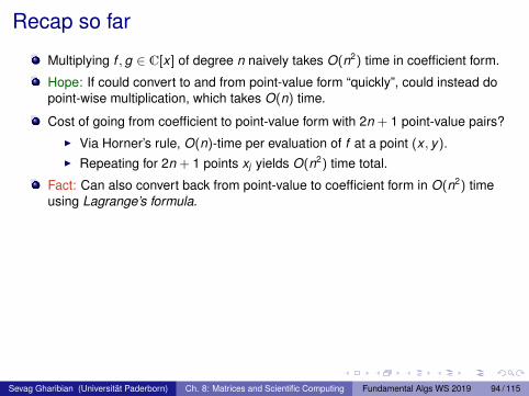
Recap so far
Multiplying f , g ∈ C[x ] of degree n naively takes O(n2) time in coefficient form.
Hope: If could convert to and from point-value form “quickly”, could instead dopoint-wise multiplication, which takes O(n) time.
Cost of going from coefficient to point-value form with 2n + 1 point-value pairs?I Via Horner’s rule, O(n)-time per evaluation of f at a point (x , y).I Repeating for 2n + 1 points xj yields O(n2) time total.
Fact: Can also convert back from point-value to coefficient form in O(n2) timeusing Lagrange’s formula.
But this is stupid. . . Just converting between representations takes as much timeas naive multiplication algorithm. . .
(Facebook worried emoji)
Sevag Gharibian (Universität Paderborn) Ch. 8: Matrices and Scientific Computing Fundamental Algs WS 2019 94 / 115
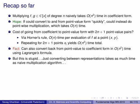
Recap so far
Multiplying f , g ∈ C[x ] of degree n naively takes O(n2) time in coefficient form.
Hope: If could convert to and from point-value form “quickly”, could instead dopoint-wise multiplication, which takes O(n) time.
Cost of going from coefficient to point-value form with 2n + 1 point-value pairs?I Via Horner’s rule, O(n)-time per evaluation of f at a point (x , y).I Repeating for 2n + 1 points xj yields O(n2) time total.
Fact: Can also convert back from point-value to coefficient form in O(n2) timeusing Lagrange’s formula.
But this is stupid. . . Just converting between representations takes as much timeas naive multiplication algorithm. . .
(Facebook worried emoji)
Sevag Gharibian (Universität Paderborn) Ch. 8: Matrices and Scientific Computing Fundamental Algs WS 2019 94 / 115

Recap so far
Hope: If could convert to and from point-value form “quickly”, could instead dopoint-wise multiplication, which takes O(n) time.
Key observation: Evaluating f at arbitrary points x0, . . . , x2n takes O(n2), but if wechoose the xj "carefully", can do it in O(n log n) time!
Then, our total cost for multiplying polynomials would be (why?)
O(n log n) + O(n) + O(n log n) ∈ O(n log n),
improving on O(n2) of naive algorithm.
Trick: Use Fourier transform.
(Facebook relieved emoji)
Sevag Gharibian (Universität Paderborn) Ch. 8: Matrices and Scientific Computing Fundamental Algs WS 2019 95 / 115
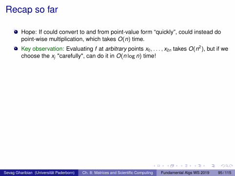
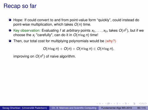
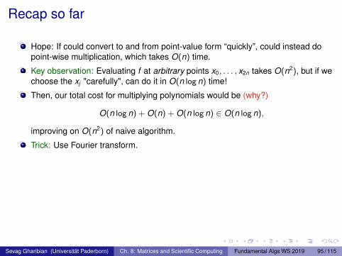
Outline
1 Introduction to matrices (review)
2 Matrix multiplication algorithmsStrassen’s algorithm (1967)Drineas-Kannan-Mahoney randomized algorithm (2006)
3 Random walksGambler’s ruinGoogle’s PageRank algorithm (1999)
4 Polynomial multiplicationComplex numbersPolynomialsO(N log N)-time polynomial multiplication via Fourier Transform
Sevag Gharibian (Universität Paderborn) Ch. 8: Matrices and Scientific Computing Fundamental Algs WS 2019 96 / 115
Roots of unity
The Discrete Fourier Transform (DFT) is a matrix, whose definition requiresspecial complex numbers known as roots of unity.
Recall: What are the roots of f (x) = xn − 1?
Nth roots of unity
The nth roots of unity are the roots of f (x) = xn − 1, namely
1,e2πi/n,e2·2πi/n,e3·2πi/n, . . . ,e(n−1)·2πi/n. (Why?)
More concisely, define principal nth root of unity as ωn = e2πi/n.
Then, nth roots of unity are: ω0n , ω1
n , ω2n ,. . . , ωn−1
n .
Ex. What is the magnitude of any root of unity, i.e.∣∣e2jπi/n
∣∣ for j ∈ Z?Ex. What are the 4th roots of unity?
Sevag Gharibian (Universität Paderborn) Ch. 8: Matrices and Scientific Computing Fundamental Algs WS 2019 97 / 115
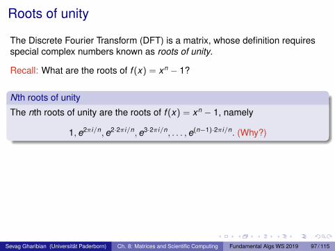
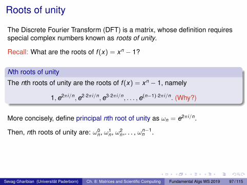
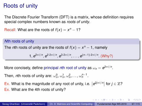
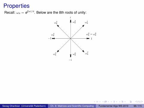
PropertiesRecall: ωn = e2πi/n. Below are the 8th roots of unity:
i
−i
1−1
ω18
ω28ω3
8
ω48
ω58 ω6
8ω78
ω08 = ω8
8
Cancellation Lemma: For any integers n, k ≥ 0, and d > 0, ωdkdn = ωk
n .
Summation Lemma: For any integer n ≥ 1 and integer k 6= 0 not divisible by n,
n−1∑j=0
(ωkn )j = 0. Q: What if k = 0?
Ex. Prove both lemmas above (Hint: Use closed form for geometric series). Can youvisualize proofs on 2D plane?
Sevag Gharibian (Universität Paderborn) Ch. 8: Matrices and Scientific Computing Fundamental Algs WS 2019 98 / 115
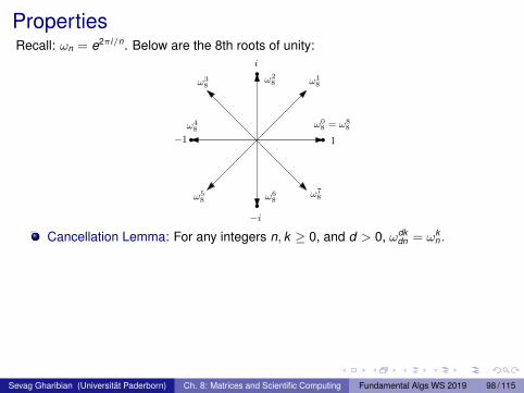
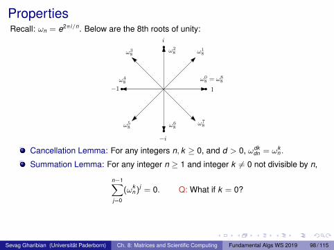
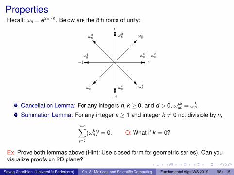
Let f =∑n
j=0 ajx j ∈ C[x ], and recall ωn = e2πi/n.
Recall:
Hope: If could convert f to and from point-value form “quickly”, could instead dopoint-wise multiplication, which takes O(n) time.
Key observation: Evaluating f at arbitrary points x0, . . . , x2n takes O(n2), but if wechoose the xj "carefully", can do it in O(n log n) time!
Moving forward:
The Discrete Fourier Transform (DFT) evaluates f at n "carefully" chosen pointsxj . Can you guess which ones?
A: The nth roots of unity, ωkn !
For succinctness, let N := n + 1. Then, DFT maps coefficient vector a to:
a =
a0
a1...
an
7→ y =
f (ω0
N)
f (ω1N)
...f (ωN−1
N )
,
i.e. yk = f (ωkN) =
∑j=0 aj
(ωk
N)j
.
Sevag Gharibian (Universität Paderborn) Ch. 8: Matrices and Scientific Computing Fundamental Algs WS 2019 99 / 115
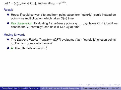
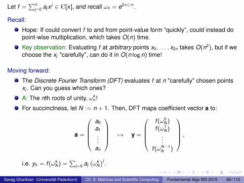
Discrete Fourier Transform (DFT)
Recall: The Discrete Fourier Transform (DFT) is a matrix, whose definitionrequires special complex numbers known as roots of unity.
Q: Can you guess the matrix now? (Hint: Vandermonde matrix.)
Sevag Gharibian (Universität Paderborn) Ch. 8: Matrices and Scientific Computing Fundamental Algs WS 2019 100 / 115
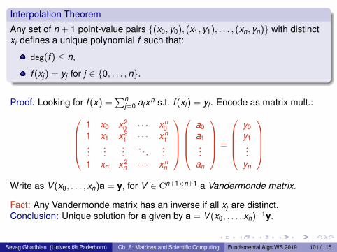
Interpolation Theorem
Any set of n + 1 point-value pairs (x0, y0), (x1, y1), . . . , (xn, yn) with distinctxi defines a unique polynomial f such that:
deg(f ) ≤ n,
f (xj ) = yj for j ∈ 0, . . . ,n.
Proof. Looking for f (x) =∑n
j=0 ajxn s.t. f (xi ) = yi . Encode as matrix mult.:1 x0 x2
0 · · · xn0
1 x1 x21 · · · xn
1...
......
. . ....
1 xn x2n · · · xn
n
a0a1...
an
=
y0y1...
yn
Write as V (x0, . . . , xn)a = y, for V ∈ Cn+1×n+1 a Vandermonde matrix.
Fact: Any Vandermonde matrix has an inverse if all xj are distinct.Conclusion: Unique solution for a given by a = V (x0, . . . , xn)−1y.
Sevag Gharibian (Universität Paderborn) Ch. 8: Matrices and Scientific Computing Fundamental Algs WS 2019 101 / 115
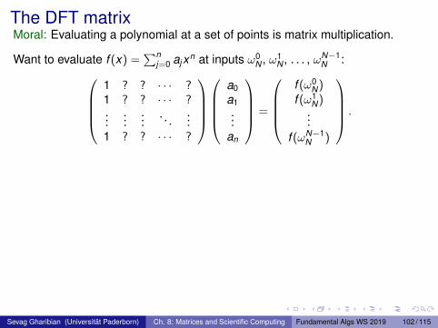
The DFT matrixMoral: Evaluating a polynomial at a set of points is matrix multiplication.
Want to evaluate f (x) =∑n
j=0 ajxn at inputs ω0N , ω1
N , . . . , ωN−1N :
1 ? ? · · · ?1 ? ? · · · ?...
......
. . ....
1 ? ? · · · ?
a0a1...
an
=
f (ω0
N)f (ω1
N)...
f (ωN−1N )
.
1(ω0
N
)1 (ω0
N
)2 · · ·(ω0
N
)(N−1)
1 ? ? · · · ?...
......
. . ....
1 ? ? · · · ?
a0a1...
an
=
f (ω0
N)f (ω1
N)...
f (ωN−1N )
.
1(ω0
N
)1 (ω0
N
)2 · · ·(ω0
N
)(N−1)
1(ω1
N
)1 (ω1
N
)2 · · ·(ω1
N
)(N−1)
......
.... . .
...1 ? ? · · · ?
a0a1...
an
=
f (ω0
N)f (ω1
N)...
f (ωN−1N )
.
Sevag Gharibian (Universität Paderborn) Ch. 8: Matrices and Scientific Computing Fundamental Algs WS 2019 102 / 115
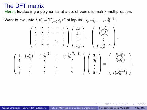
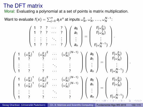
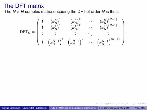
The DFT matrixThe N × N complex matrix encoding the DFT of order N is thus:
DFTN =
1
(ω0
N
)1 (ω0
N
)2 · · ·(ω0
N
)(N−1)
1(ω1
N
)1 (ω1
N
)2 · · ·(ω1
N
)(N−1)
......
.... . .
...
1(ωN−1
N
)1 (ωN−1
N
)2· · ·
(ωN−1
N
)(N−1)
.
Recap:
Wanted to beat O(n2) time polynomial multiplication.
To do so, wanted to map f from coefficient to point-value representation,and then do linear-time point-wise multiplication.
To do this conversion, decided to evaluate f at Nth roots of unity, ωkN .
This evaluation can be encoded as multiplication by the matrix DFTN .
Q: How long to naively compute DFTN v for arbitrary v ∈ CN?
A: O(N2) ∈ O(n2). . . (Recall N = n + 1.) #$&%&$%!
Sevag Gharibian (Universität Paderborn) Ch. 8: Matrices and Scientific Computing Fundamental Algs WS 2019 103 / 115
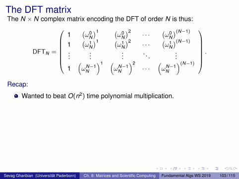
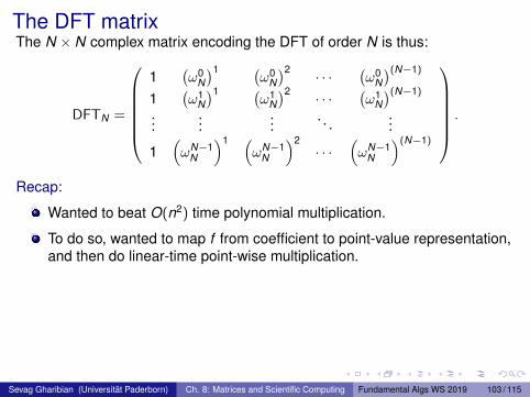
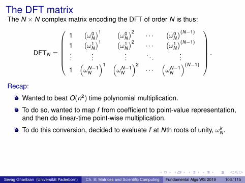
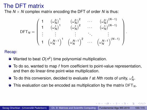
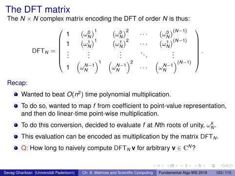
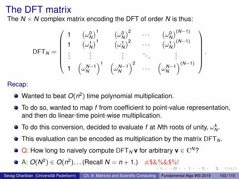

This makes me feel. . .
?
?
?
Sevag Gharibian (Universität Paderborn) Ch. 8: Matrices and Scientific Computing Fundamental Algs WS 2019 104 / 115

This makes me feel. . .
?
?
?
Sevag Gharibian (Universität Paderborn) Ch. 8: Matrices and Scientific Computing Fundamental Algs WS 2019 104 / 115

This makes me feel. . .
?
?
?
Sevag Gharibian (Universität Paderborn) Ch. 8: Matrices and Scientific Computing Fundamental Algs WS 2019 104 / 115

Breathe in, breathe out
We can’t stop now. . . Let’s remind ourselves why it really is importantto find a clever implementation of the DFT.
http://nautil.us/blog/the-math-trick-behind-mp3s-jpegs-and-homer-simpsons-faceTheMath Trick Behind MP3s, JPEGs, and Homer Simpson’s Face
(Click on link in pdf to follow link)
Warning: Must read. I will test you on this on exam.
Sevag Gharibian (Universität Paderborn) Ch. 8: Matrices and Scientific Computing Fundamental Algs WS 2019 105 / 115
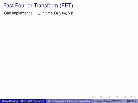
Fast Fourier Transform (FFT)Can implement DFTN in time O(N log N):
Via divide-and-conquer
Note: Only allows us to evaluate f at Nth roots of unity
Q: Why can we evaluate f at Nth roots of unity quickly, whereasevaluating f at N arbitrary points would take O(N2)?
Halving Lemma
Suppose N is even. Then, for any k ∈ Z+, (ωkN)2 = ωk
N/2.
Proof. Use Cancellation Lemma, which said:
For any integers n, k ≥ 0, and d > 0, ωdkdn = ωk
n .
Q: What value of d to choose to prove Halving Lemma?
Idea: Halving Lemma allows us to recurse by simulating order-N DFT by apair of order-(N/2) DFTs.
Sevag Gharibian (Universität Paderborn) Ch. 8: Matrices and Scientific Computing Fundamental Algs WS 2019 106 / 115
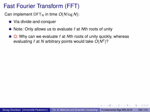
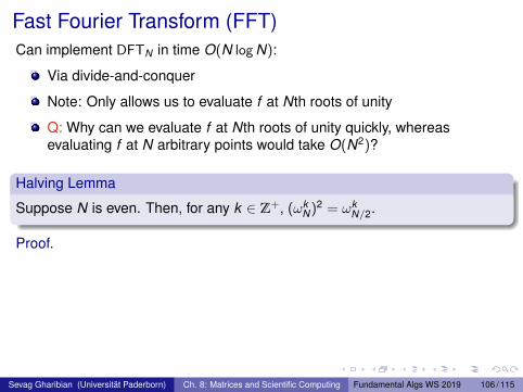
Fast Fourier Transform (FFT)Can implement DFTN in time O(N log N):
Via divide-and-conquer
Note: Only allows us to evaluate f at Nth roots of unity
Q: Why can we evaluate f at Nth roots of unity quickly, whereasevaluating f at N arbitrary points would take O(N2)?
Halving Lemma
Suppose N is even. Then, for any k ∈ Z+, (ωkN)2 = ωk
N/2.
Proof.
Use Cancellation Lemma, which said:
For any integers n, k ≥ 0, and d > 0, ωdkdn = ωk
n .
Q: What value of d to choose to prove Halving Lemma?
Idea: Halving Lemma allows us to recurse by simulating order-N DFT by apair of order-(N/2) DFTs.
Sevag Gharibian (Universität Paderborn) Ch. 8: Matrices and Scientific Computing Fundamental Algs WS 2019 106 / 115
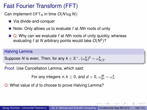
Fast Fourier Transform (FFT)Can implement DFTN in time O(N log N):
Via divide-and-conquer
Note: Only allows us to evaluate f at Nth roots of unity
Q: Why can we evaluate f at Nth roots of unity quickly, whereasevaluating f at N arbitrary points would take O(N2)?
Halving Lemma
Suppose N is even. Then, for any k ∈ Z+, (ωkN)2 = ωk
N/2.
Proof. Use Cancellation Lemma, which said:
For any integers n, k ≥ 0, and d > 0, ωdkdn = ωk
n .
Q: What value of d to choose to prove Halving Lemma?
Idea: Halving Lemma allows us to recurse by simulating order-N DFT by apair of order-(N/2) DFTs.
Sevag Gharibian (Universität Paderborn) Ch. 8: Matrices and Scientific Computing Fundamental Algs WS 2019 106 / 115
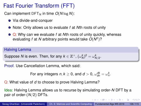
Fast Fourier Transform (FFT)Can implement DFTN in time O(N log N):
Via divide-and-conquer
Note: Only allows us to evaluate f at Nth roots of unity
Q: Why can we evaluate f at Nth roots of unity quickly, whereasevaluating f at N arbitrary points would take O(N2)?
Halving Lemma
Suppose N is even. Then, for any k ∈ Z+, (ωkN)2 = ωk
N/2.
Proof. Use Cancellation Lemma, which said:
For any integers n, k ≥ 0, and d > 0, ωdkdn = ωk
n .
Q: What value of d to choose to prove Halving Lemma?
Idea: Halving Lemma allows us to recurse by simulating order-N DFT by apair of order-(N/2) DFTs.
Sevag Gharibian (Universität Paderborn) Ch. 8: Matrices and Scientific Computing Fundamental Algs WS 2019 106 / 115
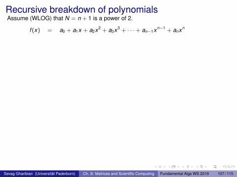
Recursive breakdown of polynomialsAssume (WLOG) that N = n + 1 is a power of 2.
f (x) = a0 + a1x + a2x2 + a3x3 + · · ·+ an−1xn−1 + anxn
=(
a0 + a2x2 + a4x4 + · · ·+ an−1xn−1)
+ (even)(a1x + a3x3 + a5x5 + · · ·+ anxn
)(odd)
=(
a0 + a2x2 + a4x4 + · · ·+ an−1xn−1)
+ (even)
x(
a1 + a3x2 + a5x4 + · · ·+ anxn−1)
(odd)
=(
a0 + a2(x2)1 + a4(x2)2 + · · ·+ an−1(x2)n−1
2
)+ (even)
x(
a1 + a3(x2)1 + a5(x2)2 + · · ·+ an(x2)n−1
2
)(odd)
=: f0(x2) + xf1(x2),
for f0(x) := a0 + a2x + · · · an−1x (n−1)/2 and f1(x) := a1 + a3x + · · · anx (n−1)/2.
Observe:
f0 and f1 have degree (n − 1)/2!
“Feels like” we’ve cut our problem into a pair of smaller problems of half the size.
Sevag Gharibian (Universität Paderborn) Ch. 8: Matrices and Scientific Computing Fundamental Algs WS 2019 107 / 115
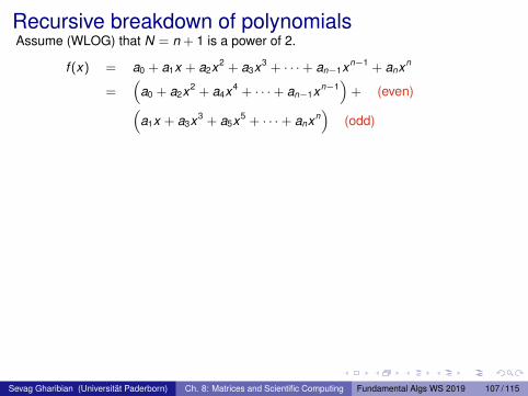
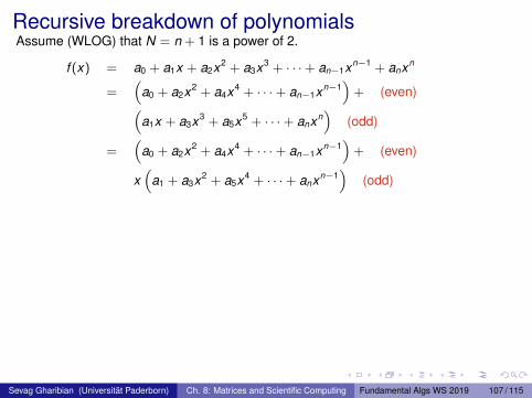
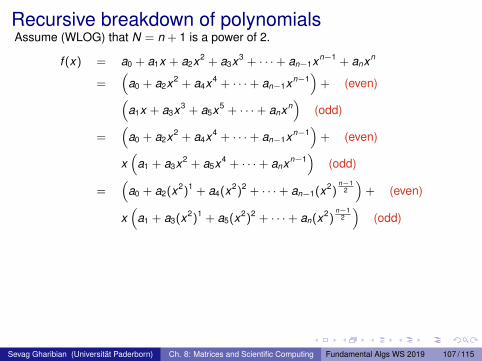
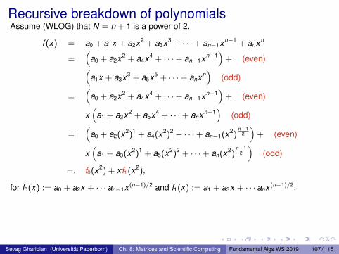
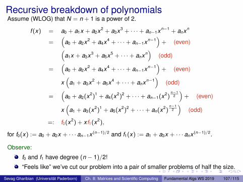
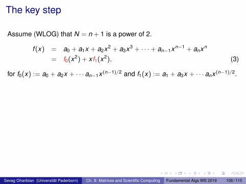
The key step
Assume (WLOG) that N = n + 1 is a power of 2.
f (x) = a0 + a1x + a2x2 + a3x3 + · · ·+ an−1xn−1 + anxn
= f0(x2) + xf1(x2), (3)
for f0(x) := a0 + a2x + · · · an−1x (n−1)/2 and f1(x) := a1 + a3x + · · · anx (n−1)/2.
DFTN evaluates degree-(N − 1) polynomial at Nth roots of unity.
By Halving Lemma: Letting x = ωkN in Eqn. (3),
f0(x2) = f0((ωkN)2) = f0(ωk
N/2).
Thus, roots of unity are very special — allow us to recursively simulateorder-N DFT via order-(N/2) DFTs.
Sevag Gharibian (Universität Paderborn) Ch. 8: Matrices and Scientific Computing Fundamental Algs WS 2019 108 / 115
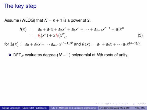
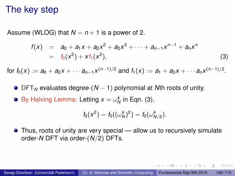
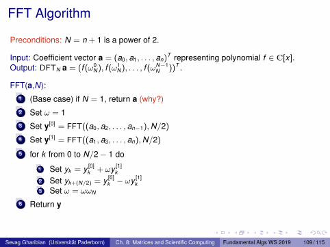
FFT Algorithm
Preconditions: N = n + 1 is a power of 2.
Input: Coefficient vector a = (a0, a1, . . . , an)T representing polynomial f ∈ C[x ].Output: DFTN a = (f (ω0
N), f (ω1N), . . . , f (ωN−1
N ))T .
FFT(a,N):1 (Base case) if N = 1, return a (why?)2 Set ω = 13 Set y[0] = FFT((a0, a2, . . . , an−1),N/2)
4 Set y[1] = FFT((a1, a3, . . . , an),N/2)
5 for k from 0 to N/2− 1 do
1 Set yk = y [0]k + ωy [1]
k
2 Set yk+(N/2) = y [0]k − ωy [1]
k3 Set ω = ωωN
6 Return y
Sevag Gharibian (Universität Paderborn) Ch. 8: Matrices and Scientific Computing Fundamental Algs WS 2019 109 / 115
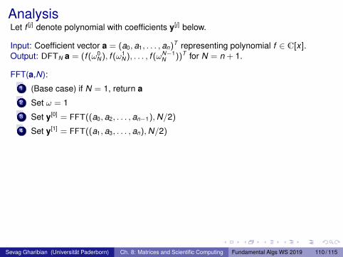
AnalysisLet f [j] denote polynomial with coefficients y[j] below.
Input: Coefficient vector a = (a0, a1, . . . , an)T representing polynomial f ∈ C[x ].Output: DFTN a = (f (ω0
N), f (ω1N), . . . , f (ωN−1
N ))T for N = n + 1.
FFT(a,N):1 (Base case) if N = 1, return a2 Set ω = 13 Set y[0] = FFT((a0, a2, . . . , an−1),N/2)
4 Set y[1] = FFT((a1, a3, . . . , an),N/2)
y [0]k = f [0](ωk
N/2) = f [0](ω2kN ) and y [1]
k = f [1](ωkN/2) = f [1](ω2k
N ) (why?)
5 for k from 0 to N/2− 1 do
1 Set yk = y [0]k + ωy [1]
k
yk = f [0](ω2kN ) + ωk
N f [1](ω2kN ) = f (ωk
N) by recursive decomposition
2 Set yk+(N/2) = y [0]k − ωy [1]
k3 Set ω = ωωN
6 Return y
Sevag Gharibian (Universität Paderborn) Ch. 8: Matrices and Scientific Computing Fundamental Algs WS 2019 110 / 115
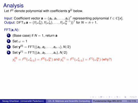
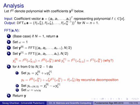
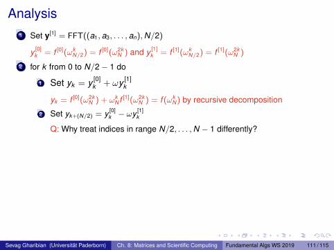
Analysis1 Set y[1] = FFT((a1, a3, . . . , an),N/2)
y [0]k = f [0](ωk
N/2) = f [0](ω2kN ) and y [1]
k = f [1](ωkN/2) = f [1](ω2k
N )
2 for k from 0 to N/2− 1 do
1 Set yk = y [0]k + ωy [1]
k
yk = f [0](ω2kN ) + ωk
N f [1](ω2kN ) = f (ωk
N) by recursive decomposition
2 Set yk+(N/2) = y [0]k − ωy [1]
k
Q: Why treat indices in range N/2, . . . ,N − 1 differently?
yk+(N/2) = y [0]k − ω
kNy [1]
k = y [0]k + ω
k+(N/2)N y [1]
k (ωN/2N = −1 for even N)
= f [0](ω2kN ) + ω
k+(N/2)N f [1](ω2k
N )
= f [0](ω2k+NN ) + ω
k+(N/2)N f [1](ω2k+N
N ) (ωNN = 1 by definition)
= f (ωk+(N/2)N ) (by recursive decomposition)
3 Set ω = ωωN
3 Return y
Sevag Gharibian (Universität Paderborn) Ch. 8: Matrices and Scientific Computing Fundamental Algs WS 2019 111 / 115
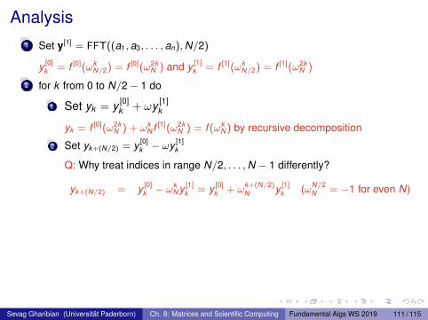
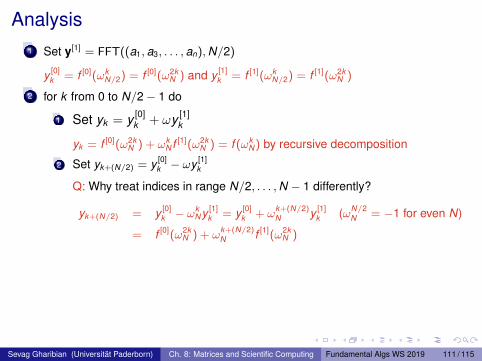
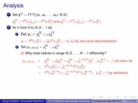
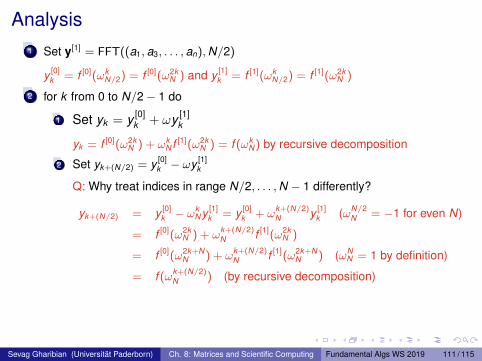
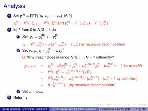
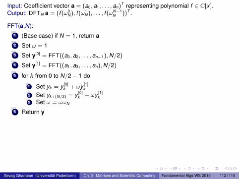
Input: Coefficient vector a = (a0, a1, . . . , an)T representing polynomial f ∈ C[x ].Output: DFTN a = (f (ω0
N), f (ω1N), . . . , f (ωN−1
N ))T .
FFT(a,N):1 (Base case) if N = 1, return a2 Set ω = 13 Set y[0] = FFT((a0, a2, . . . , an−1),N/2)
4 Set y[1] = FFT((a1, a3, . . . , an),N/2)
5 for k from 0 to N/2− 1 do
1 Set yk = y [0]k + ωy [1]
k
2 Set yk+(N/2) = y [0]k − ωy [1]
k3 Set ω = ωωN
6 Return y
Runtime
Each call to FFT takes O(N) time, and makes two recursive calls of size N/2.
Thus, runtime T (N) = 2T (N/2) + Θ(N) ∈ Θ(N log N).
Conclusion: Evaluate degree-(N − 1) polynomial at Nth roots of unity insubquadratic time.
Sevag Gharibian (Universität Paderborn) Ch. 8: Matrices and Scientific Computing Fundamental Algs WS 2019 112 / 115
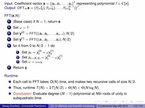
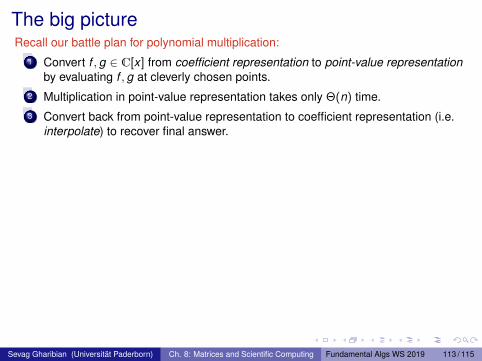
The big pictureRecall our battle plan for polynomial multiplication:
1 Convert f , g ∈ C[x ] from coefficient representation to point-value representationby evaluating f , g at cleverly chosen points.
2 Multiplication in point-value representation takes only Θ(n) time.3 Convert back from point-value representation to coefficient representation (i.e.
interpolate) to recover final answer.
Can now fill in details:
1 Convert f , g ∈ C[x ] from coefficient representation to point-value representationby evaluating f , g at Nth roots of unity.
I Takes O(N log N) time via FFT.2 Multiplication in point-value representation takes only Θ(n) time.
3 Convert back from point-value representation to coefficient representation (i.e.interpolate) to recover final answer.
I Claim. Interpolation corresponds to inverse DFT. Takes O(N log N) time.
Conclusion: Polynomial multiplication takes O(N log N) time.
Sevag Gharibian (Universität Paderborn) Ch. 8: Matrices and Scientific Computing Fundamental Algs WS 2019 113 / 115
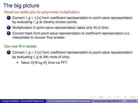
The big pictureRecall our battle plan for polynomial multiplication:
1 Convert f , g ∈ C[x ] from coefficient representation to point-value representationby evaluating f , g at cleverly chosen points.
2 Multiplication in point-value representation takes only Θ(n) time.3 Convert back from point-value representation to coefficient representation (i.e.
interpolate) to recover final answer.
Can now fill in details:
1 Convert f , g ∈ C[x ] from coefficient representation to point-value representationby evaluating f , g at Nth roots of unity.
I Takes O(N log N) time via FFT.
2 Multiplication in point-value representation takes only Θ(n) time.
3 Convert back from point-value representation to coefficient representation (i.e.interpolate) to recover final answer.
I Claim. Interpolation corresponds to inverse DFT. Takes O(N log N) time.
Conclusion: Polynomial multiplication takes O(N log N) time.
Sevag Gharibian (Universität Paderborn) Ch. 8: Matrices and Scientific Computing Fundamental Algs WS 2019 113 / 115
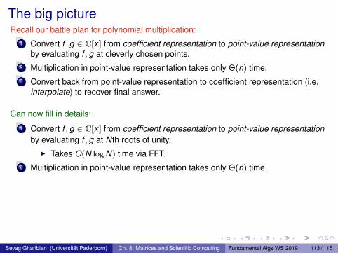
The big pictureRecall our battle plan for polynomial multiplication:
1 Convert f , g ∈ C[x ] from coefficient representation to point-value representationby evaluating f , g at cleverly chosen points.
2 Multiplication in point-value representation takes only Θ(n) time.3 Convert back from point-value representation to coefficient representation (i.e.
interpolate) to recover final answer.
Can now fill in details:
1 Convert f , g ∈ C[x ] from coefficient representation to point-value representationby evaluating f , g at Nth roots of unity.
I Takes O(N log N) time via FFT.2 Multiplication in point-value representation takes only Θ(n) time.
3 Convert back from point-value representation to coefficient representation (i.e.interpolate) to recover final answer.
I Claim. Interpolation corresponds to inverse DFT. Takes O(N log N) time.
Conclusion: Polynomial multiplication takes O(N log N) time.
Sevag Gharibian (Universität Paderborn) Ch. 8: Matrices and Scientific Computing Fundamental Algs WS 2019 113 / 115
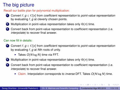
The big pictureRecall our battle plan for polynomial multiplication:
1 Convert f , g ∈ C[x ] from coefficient representation to point-value representationby evaluating f , g at cleverly chosen points.
2 Multiplication in point-value representation takes only Θ(n) time.3 Convert back from point-value representation to coefficient representation (i.e.
interpolate) to recover final answer.
Can now fill in details:
1 Convert f , g ∈ C[x ] from coefficient representation to point-value representationby evaluating f , g at Nth roots of unity.
I Takes O(N log N) time via FFT.2 Multiplication in point-value representation takes only Θ(n) time.
3 Convert back from point-value representation to coefficient representation (i.e.interpolate) to recover final answer.
I Claim. Interpolation corresponds to inverse DFT. Takes O(N log N) time.
Conclusion: Polynomial multiplication takes O(N log N) time.
Sevag Gharibian (Universität Paderborn) Ch. 8: Matrices and Scientific Computing Fundamental Algs WS 2019 113 / 115
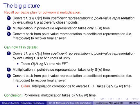
The big pictureRecall our battle plan for polynomial multiplication:
1 Convert f , g ∈ C[x ] from coefficient representation to point-value representationby evaluating f , g at cleverly chosen points.
2 Multiplication in point-value representation takes only Θ(n) time.3 Convert back from point-value representation to coefficient representation (i.e.
interpolate) to recover final answer.
Can now fill in details:
1 Convert f , g ∈ C[x ] from coefficient representation to point-value representationby evaluating f , g at Nth roots of unity.
I Takes O(N log N) time via FFT.2 Multiplication in point-value representation takes only Θ(n) time.
3 Convert back from point-value representation to coefficient representation (i.e.interpolate) to recover final answer.
I Claim. Interpolation corresponds to inverse DFT. Takes O(N log N) time.
Conclusion: Polynomial multiplication takes O(N log N) time.
Sevag Gharibian (Universität Paderborn) Ch. 8: Matrices and Scientific Computing Fundamental Algs WS 2019 113 / 115
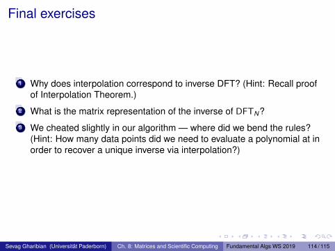
Final exercises
1 Why does interpolation correspond to inverse DFT? (Hint: Recall proofof Interpolation Theorem.)
2 What is the matrix representation of the inverse of DFTN?
3 We cheated slightly in our algorithm — where did we bend the rules?(Hint: How many data points did we need to evaluate a polynomial at inorder to recover a unique inverse via interpolation?)
Sevag Gharibian (Universität Paderborn) Ch. 8: Matrices and Scientific Computing Fundamental Algs WS 2019 114 / 115
Looking to the future
You didn’t think applications of Fourier transform end with today’stechnology?
Using a quantum implementation of DFTN , one can exponentiallyoutperform4 classical computers at a crucial problem: The IntegerFactorization Problem:
I Given an integer M, what are the prime factors of M?I The assumption that this problem is classically hard underlies
security of common cryptosystems like RSA.I Thus, a large-scale quantum computer would break today’s
cryptosystems completely. . .
Shameless advertisements:
I See upcoming Masters lecture on Introduction to QuantumComputation (SS2020)
I Interested in undergraduate research in quantum computation?Come talk to me! Required background is Linear Algebra.
4The best known classical factoring algorithms take superpolynomial time.Sevag Gharibian (Universität Paderborn) Ch. 8: Matrices and Scientific Computing Fundamental Algs WS 2019 115 / 115
Looking to the future
You didn’t think applications of Fourier transform end with today’stechnology?
Using a quantum implementation of DFTN , one can exponentiallyoutperform4 classical computers at a crucial problem: The IntegerFactorization Problem:
I Given an integer M, what are the prime factors of M?
I The assumption that this problem is classically hard underliessecurity of common cryptosystems like RSA.
I Thus, a large-scale quantum computer would break today’scryptosystems completely. . .
Shameless advertisements:
I See upcoming Masters lecture on Introduction to QuantumComputation (SS2020)
I Interested in undergraduate research in quantum computation?Come talk to me! Required background is Linear Algebra.
4The best known classical factoring algorithms take superpolynomial time.Sevag Gharibian (Universität Paderborn) Ch. 8: Matrices and Scientific Computing Fundamental Algs WS 2019 115 / 115
Looking to the future
You didn’t think applications of Fourier transform end with today’stechnology?
Using a quantum implementation of DFTN , one can exponentiallyoutperform4 classical computers at a crucial problem: The IntegerFactorization Problem:
I Given an integer M, what are the prime factors of M?I The assumption that this problem is classically hard underlies
security of common cryptosystems like RSA.
I Thus, a large-scale quantum computer would break today’scryptosystems completely. . .
Shameless advertisements:
I See upcoming Masters lecture on Introduction to QuantumComputation (SS2020)
I Interested in undergraduate research in quantum computation?Come talk to me! Required background is Linear Algebra.
4The best known classical factoring algorithms take superpolynomial time.Sevag Gharibian (Universität Paderborn) Ch. 8: Matrices and Scientific Computing Fundamental Algs WS 2019 115 / 115
Looking to the future
You didn’t think applications of Fourier transform end with today’stechnology?
Using a quantum implementation of DFTN , one can exponentiallyoutperform4 classical computers at a crucial problem: The IntegerFactorization Problem:
I Given an integer M, what are the prime factors of M?I The assumption that this problem is classically hard underlies
security of common cryptosystems like RSA.I Thus, a large-scale quantum computer would break today’s
cryptosystems completely. . .
Shameless advertisements:
I See upcoming Masters lecture on Introduction to QuantumComputation (SS2020)
I Interested in undergraduate research in quantum computation?Come talk to me! Required background is Linear Algebra.
4The best known classical factoring algorithms take superpolynomial time.Sevag Gharibian (Universität Paderborn) Ch. 8: Matrices and Scientific Computing Fundamental Algs WS 2019 115 / 115
Looking to the future
You didn’t think applications of Fourier transform end with today’stechnology?
Using a quantum implementation of DFTN , one can exponentiallyoutperform4 classical computers at a crucial problem: The IntegerFactorization Problem:
I Given an integer M, what are the prime factors of M?I The assumption that this problem is classically hard underlies
security of common cryptosystems like RSA.I Thus, a large-scale quantum computer would break today’s
cryptosystems completely. . .
Shameless advertisements:
I See upcoming Masters lecture on Introduction to QuantumComputation (SS2020)
I Interested in undergraduate research in quantum computation?Come talk to me! Required background is Linear Algebra.
4The best known classical factoring algorithms take superpolynomial time.Sevag Gharibian (Universität Paderborn) Ch. 8: Matrices and Scientific Computing Fundamental Algs WS 2019 115 / 115