Fully Convolutional Pixel Adaptive Image Denoiser

Sungmin Cha1 and Taesup Moon1,2

1Department of Electrical and Computer Engineering, 2 Department of Artificial Intelligence

Sungkyunkwan University, Suwon, Korea 16419

{csm9493,tsmoon}@skku.edu

Abstract

We propose a new image denoising algorithm, dubbed as

Fully Convolutional Adaptive Image DEnoiser (FC-AIDE),

that can learn from an offline supervised training set with

a fully convolutional neural network as well as adaptively

fine-tune the supervised model for each given noisy image.

We significantly extend the framework of the recently pro-

posed Neural AIDE, which formulates the denoiser to be

context-based pixelwise mappings and utilizes the unbiased

estimator of MSE for such denoisers. The two main contri-

butions we make are; 1) implementing a novel fully convo-

lutional architecture that boosts the base supervised model,

and 2) introducing regularization methods for the adaptive

fine-tuning such that a stronger and more robust adaptiv-

ity can be attained. As a result, FC-AIDE is shown to

possess many desirable features; it outperforms the recent

CNN-based state-of-the-art denoisers on all of the bench-

mark datasets we tested, and gets particularly strong for

various challenging scenarios, e.g., with mismatched im-

age/noise characteristics or with scarce supervised train-

ing data. The source code our algorithm is available at

https://github.com/csm9493/FC-AIDE-Keras.

1. Introduction

Image denoising, which tries to recover a clean image

from its noisy observation, is one of the oldest and most

prevalent problems in image processing and low-level com-

puter vision. While numerous algorithms have been pro-

posed over the past few decades, e.g., [8, 2, 7, 11, 9, 21],

the current throne-holders in terms of the average denois-

ing performance are convolutional neural network (CNN)-

based methods [38, 22, 31].

The main idea behind the CNN-based method is to treat

denoising as a supervised regression problem; namely, first

collect numerous clean-noisy image pairs as a supervised

training set, then learn a regression function that maps the

noisy image to the clean image. Such approach is rela-

tively simple since it does not require any complex priors

on the underlying clean images and let CNN figure out to

learn the correct mapping from the vast training data. De-

spite the conceptual simplicity, several recent variations of

the CNN-based denoisers using residual learning [38], skip-

connections [22], and densely connected structure [31] have

achieved impressive state-of-the-art performances.

However, we stress that one apparent drawback exists

in above methods; namely, they are solely based on of-

fline batch training of CNN, hence, lack adaptivity to the

given noisy image subject to denoising. Such absence of

adaptivity, which is typically possessed in other prior or

optimization-based methods, e.g., [8, 2, 7, 11, 9, 21], can se-

riously deteriorate the denoising performance of the CNN-

based methods in multiple practical scenarios in which var-

ious mismatches exist between the training data and the

given noisy image. One category of such mismatch is the

image mismatch, in which the image characteristics of the

given noisy image are not well represented in the offline

training set. The other category is noise mismatch, in which

the noise level or the distribution for the given noisy im-

age is different from what the CNN has been trained for.

Above drawbacks can be partially addressed by building a

composite training set with multiple noise and image char-

acteristics, e.g., the so-called blind training [16, 38], but the

limitation of such approach is evident since building large-

scale supervised training set that sufficiently contains all the

variations is not always possible in many applications.

To that end, we propose a new CNN-based denoising

algorithm that can learn from an offline supervised train-

ing set, like other recent state-of-the-arts, as well as adap-

tively fine-tune the denoiser for each given noisy image, like

other prior or optimization based methods. The main vehi-

cle for devising our algorithm, dubbed as FC-AIDE (Fully

Convolutional Adaptive Image DEnoiser), is the framework

recently proposed in [4]. Namely, we formulate the de-

noiser to be context-based pixelwise mappings and obtain

the SURE (Stein’s Unbiased Risk Estimator)[30]-like es-

timated losses of the mean-squared errors (MSE) for the

mappings. Then, the specific mapping for each pixel is

learned with a neural network first by supervised training

4160

using the MSE, then by adaptively fine-tuning the network

with the given noisy image using the devised estimated

loss. While following this framework, we significantly im-

prove the original Neural AIDE (N-AIDE) [4] by making

the following two main contributions. Firstly, we devise a

novel fully convolutional architecture instead of the sim-

ple fully-connected structure of N-AIDE so that the per-

formance of the base supervised model can be boosted.

Moreover, unlike [4], which only employed the pixelwise

affine mappings, we also consider quadratic mappings as

well. Secondly, we introduce two regularization methods

for the adaptive fine-tuning step: data augmentation and ℓ2-

SP (Starting Point) regularization [18]. While these tech-

niques are well-known for general supervised learning set-

ting, we utilize them such that the fine-tuned model does not

overfit to the estimated loss and generalize well to the MSE,

leading to larger and more robust improvements of the fine-

tuning step. With above two contributions, we show that

FC-AIDE significantly surpasses the performance of the

original N-AIDE as well as the CNN-based state-of-the-arts

in several widely used benchmark datasets. Moreover, we

highlight the effectiveness of the adaptivity of our algorithm

in multiple challenging scenarios, e.g., with image/noise

mismatches or with scarce supervised training data.

2. Related Work

There are vast number of literature on image denoising,

among which the most relevant ones are elaborated here.

Deep learning based denoisers Following the pioneer-

ing work [14, 3, 36], recent deep learning based methods

[38, 22, 31] apply variations of CNN within the supervised

regression framework and significantly surpassed the previ-

ous state-of-the-arts in terms of the denoising PSNR. More

recently, [6, 19] explicitly designed a non-local filtering

process within the CNN framework and showed some more

improvements with the cost of increased running time. For

the cases with lack of clean data in the training data, [17]

proposed a method that trains the CNN-based denoiser only

with the noisy data, provided that two independent noise re-

alizations for an image are available.

Adaptive denoisers In contrast to above CNN-based state-

of-the-arts, which freeze the model parameters once the

training is done, there are many approaches that can learn

a denoising function adaptively from the given noisy im-

age, despite some PSNR shortcomings. Some of the classi-

cal methods are the filtering approach [2, 7], optimization-

based methods with sparsity or low-rank assumptions [9,

21, 11], Wavelet transform-based [8], and effective prior-

based methods [39]. More recently, several work proposed

to implement deep learning-based priors or regularizers,

such as [32, 37, 20], but their PSNR results still could not

compete with the supervised trained CNN-based denoisers.

Another branch of adaptive denoising is the universal de-

noising framework [35], in which no prior or probabilis-

tic assumptions on the clean image are made, and only the

noise is treated as random variables. The original discrete

denoising setting of [35] was extended to grayscale image

denoising in [26, 28], but the performance was not very sat-

isfactory. A related approach is the SURE-based estimators

that minimize the unbiased estimates of MSE, e.g., [8, 10],

but they typically select only a few tunable hyperparameters

for the minimization. In contrast, using the unbiased esti-

mate as an empirical risk in the empirical risk minimization

(ERM) framework to learn an entire parametric model was

first proposed in [25, 4] for denoising. To the best of the

authors’ knowledge, [4] was the first deep learning-based

method that has both the supervised learning capability and

the adaptivity. [29] also proposed to use SURE and Monte-

Carlo approximation for training a CNN-based denoiser, but

the performance fell short of the supervised trained CNNs.

Blind denoisers Most of above methods assume that the

noise model and variance are known a priori. To allevi-

ate such strong assumption, the supervised, blindly trained

CNN models [16, 38] were proposed, and they show quite

strong performance due to CNN’s inherent robustness. But,

those models also lack adaptivity, i.e., they cannot adapt to

the specific noise realizations of the given noisy image.

3. Problem Setting and Preliminaries

3.1. Notations and assumptions

We generally follow [4], but introduce more compact no-

tations. First, we denote x ∈ Rn as the clean image and

Z ∈ Rn as its additive noise-corrupted version, namely,

Z = x+N. We make the following assumptions on N;

• E(N) = 0 and Cov(N) = σ2In×n.

• Each noise component, Ni, is independent and has a

symmetric distribution.re

Note we do not necessarily assume the noise is identically

distributed or Gaussian. Moreover, as in universal denois-

ing, we treat the clean x as an individual image without any

prior or probabilistic model and only treat Z as random,

which is reflected in the upper case notation.

A denoiser is generally denoted by X(Z) ∈ Rn, of

which the i-th reconstruction, Xi(Z), is a function of the

entire noisy image Z. The standard loss function to mea-

sure the denoising quality is MSE, denoted by

Λn(x, X(Z)) ,1

n‖x− X(Z)‖22. (1)

3.2. N­AIDE and the unbiased estimator

While Xi(Z) can be any general function, we can con-

sider a d-th order polynomial function form for the denoiser,

Xi(Z) =

d∑

m=0

am(Z−i)Zmi , i = 1, . . . , n, (2)

4161

in which Z−i stands for the entire noisy image except for

Zi, the i-th pixel, and am(Z−i) stands for the coefficient

for the m-th order term of Zi. Note [4] focused on the case

d = 1, and in this paper, we consider the case d = 2 as well.

Note Xi(Z) can be a highly nonlinear function of Z since

am(·)’s can be any nonlinear functions of Z.

For (2) with d ∈ {1, 2}, by denoting am(Z−i) as am,i

for brevity, we can define an unbiased estimator of (1) as

Ln(Z, X(Z);σ2) (3)

,1

n‖Z− X(Z)‖22 +

σ2

n

n∑

i=1

[

d∑

m=1

2mam,iZm−1i − 1

]

.

Note (3) does not depend on x, and the following lemma

states the unbiasedness of (3).

Lemma 1 For any N with above assumptions and X(Z)that has the form (2) with d ∈ {1, 2},

ELn(Z, X(Z);σ2) = EΛn(x, X(Z)). (4)

Moreover, when N is white Gaussian, (3) coincides with the

SURE [30].

Remark: The proof of the lemma is given in the Supple-

mentary Material, and it critically relies on the specific

polynomial form of the denoiser in (2). Namely, it exploits

the fact that x is an individual image and {am,i}’s are

conditionally independent of Zi given Z−i. Note (4)

holds for any additive white noise with symmetric distri-

bution, not necessarily only for Gaussian. (The symmetry

condition is needed only for d = 2 case.) Such property en-

ables the strong adaptivity of our algorithm as shown below.

N-AIDE in [4] can be denoted by XN-AIDE(w,Z) ∈ Rn,

of which Xi(w,Z) has the form (2) with d = 1 and

am,i = am(Z−i) , am(w,C−ik×k) (5)

for m = 0, 1. In (5), C−ik×k stands for the two-dimensional

noisy k × k patch surrounding Zi, but without Zi, and

{am(w,C−ik×k)}m=0,1 are the outputs of a fully-connected

neural network with parameter w that takes C−ik×k as input.

Note w does not depend on location i, hence, the denoising

by N-AIDE is done in a sliding-window fashion; that is, the

neural network subsequently takes C−ik×k as an input and

generates the affine mapping coefficients for Zi to obtain

the reconstruction for each pixel i.

As mentioned in the Introduction, the training of the net-

work parameter w for N-AIDE was done in two stages.

Firstly, for supervised training, a separate training set

D = {(xi, Ci,k×k)}Ni=1 based on many clean-noisy im-

age pairs, (x, Z), is collected. Here, Ci,k×k denote the

full k × k patch including the center pixel Zi. Then, a

supervised model, wsup, the network parameters for a de-

noiser X(w, Z) that has the form of (5), is learned by min-

imizing the MSE on D, i.e., ΛN (x, X(w, Z)). Secondly,

for a given noisy image Z subject to denoising, the adap-

tive fine-tuning is carried out by further minimizing the es-

timated loss Ln(Z, X(w,Z);σ2) starting from wsup. The

fine-tuned model parameters, denoted by wN-AIDE, are then

used to obtain the mapping for each pixel i as in (2) using

(5), and Z is pixelwise denoised with those affine mappings.

Note maintaining the denoiser form (2), and not the ordi-

nary form of the direct mapping from the full noisy patch to

the clean patch, is a key for enabling the fine-tuning.

4. FC-AIDE

4.1. Fully convolutional QED architecture

Limitation of N-AIDE While the performance of N-AIDE

[4] was encouraging, the final denoising performance was

slightly worse (about ∼ 0.15dB) than that of DnCNN-S

[38], which applies the ordinary supervised learning with

CNN and residual learning. We believe such performance

difference is primarily due to the simple fully-connected ar-

chitecture used in [4, Figure 1] as opposed to the fully con-

volutional architectures in recent work, e.g., [38, 22, 31].

In order to utilize the convolutional architecture for the

N-AIDE framework, we first make an observation that the

sliding-window nature of N-AIDE is indeed a convolution

operation. Namely, once we use the masked k × k con-

volution filters with a hole (i.e., the center set to 0) in the

first layer and use the ordinary 1 × 1 filters for the higher

layers, the resulting fully convolutional network operating

on a noisy image becomes equivalent to the fully-connected

network of N-AIDE working in a sliding-window fashion.

Note with the standard zero-padding, the output of the net-

work has the same size as the input image and consists of

two channels, one for each of {am,i}1m=0 for all location i.

From this observation, we identify a critical constraint

for implementing a fully convolutional architecture for the

denoisers that have the form (2); that is, the i-th pixel of any

feature maps at any layer should not depend on Zi, and the

filters at the output layer must keep the 1×1 structure. Such

property is necessary for maintaining the conditional inde-

pendence between {am,i}dm=0 and Zi given Z

−i, which is

critical for the unbiasedness of Ln(Z, X(Z);σ2) shown in

Lemma 1. Due to this constraint, we can see that simply ap-

plying the vanilla convolutional architecture as in [38] is not

feasible for extending N-AIDE beyond the 1× 1 structure.

Overall architecture of FC-AIDE To address above lim-

itation of N-AIDE, we now propose FC-AIDE, denoted

as XFC-AIDE (w,Z), that has the fully convolutional ar-

chitecture and gradually increases the receptive fields as

the layer increases, while satisfying above mentioned con-

straint. Moreover, we also extend to employ the quadratic

4162

𝑨𝟎

𝑿$(𝒁)

𝑎)

𝑎*

𝑎+

1x1

Conv

ResNet

Module

ResNet

Module

ResNet

Module

𝑨𝟏

𝑨𝟗

……

ResNet

Modul

AVG

(.))𝒒+

𝒆+

𝒅+ 𝒅ℓ

𝑨+

ℓ = 𝟏 ∶ 𝟗

𝐙

𝑄+

𝐸+

𝐷+

𝐸*ℓ

𝐷*ℓ

𝑄*ℓ

𝒆ℓ

𝒒ℓ

𝑨ℓ

PR

PR

PR

𝒅ℓ9*

𝒆ℓ9*

𝒒ℓ9*

Block1 Block2 Block3

AVG

PR

PR

PR

AVG = Average

PR = PReLU

AVG

1x1

Conv

PR

(a) Overall architecture of FC-AIDE

1x1

Conv

PR

1x1

Conv

AVG

PR

ResNetModule

(b) ResNet Module

0

0 0

0 0 0

0

0 0

0 0

0 0 0 0 0

0 0 0

0 0 0 0 0

0 0 0 0

!" !## !#

$

%&

(c) Q-filters and the receptive field at layer 3

0

0 0

0 0 0

0

0 0

0 0

0 0 0 0 0

0 0 0

0 0 0 0 0

0 0 0 0

!" !##

!#$

%&

(d) E-filters and the receptive field at layer 3

0 0 0

0 0 0

0 0 00 0 0 0 0

0 0 0 0 0

0 0

0 0 0 0 0

0 0

!" !##

!#$

%&

(e) D-filters and the receptive field at layer 3

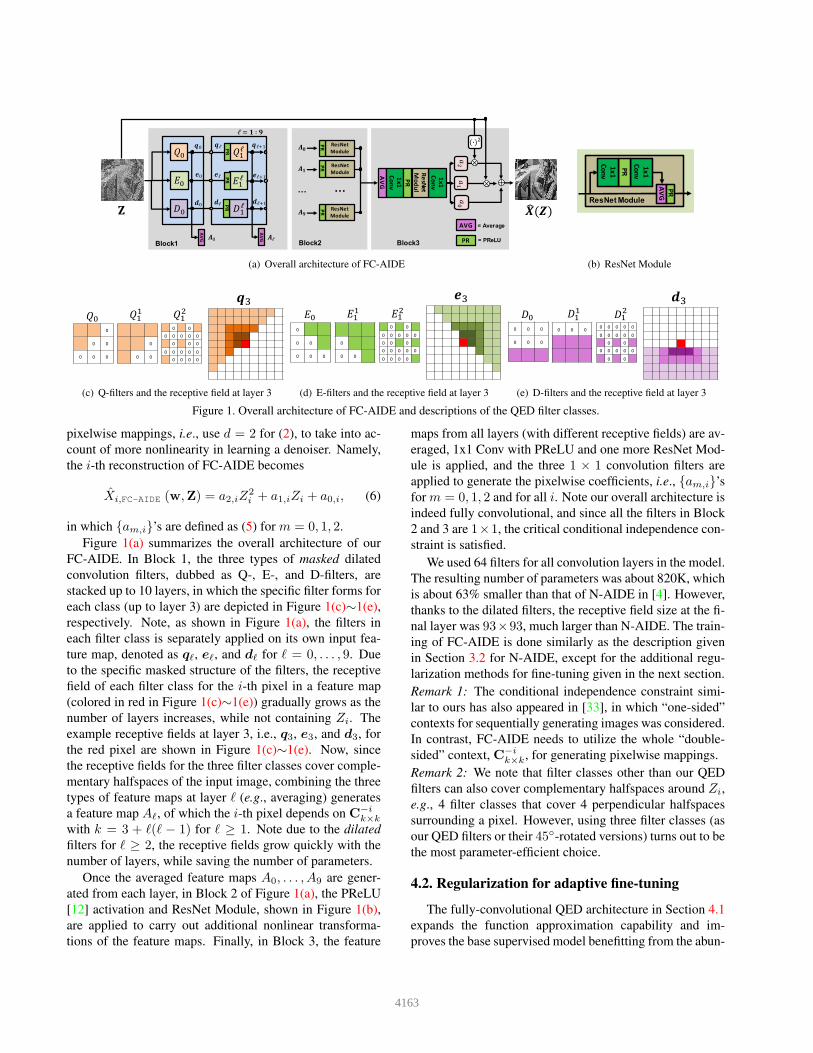
Figure 1. Overall architecture of FC-AIDE and descriptions of the QED filter classes.

pixelwise mappings, i.e., use d = 2 for (2), to take into ac-

count of more nonlinearity in learning a denoiser. Namely,

the i-th reconstruction of FC-AIDE becomes

Xi,FC-AIDE (w,Z) = a2,iZ2i + a1,iZi + a0,i, (6)

in which {am,i}’s are defined as (5) for m = 0, 1, 2.

Figure 1(a) summarizes the overall architecture of our

FC-AIDE. In Block 1, the three types of masked dilated

convolution filters, dubbed as Q-, E-, and D-filters, are

stacked up to 10 layers, in which the specific filter forms for

each class (up to layer 3) are depicted in Figure 1(c)∼1(e),

respectively. Note, as shown in Figure 1(a), the filters in

each filter class is separately applied on its own input fea-

ture map, denoted as qℓ, eℓ, and dℓ for ℓ = 0, . . . , 9. Due

to the specific masked structure of the filters, the receptive

field of each filter class for the i-th pixel in a feature map

(colored in red in Figure 1(c)∼1(e)) gradually grows as the

number of layers increases, while not containing Zi. The

example receptive fields at layer 3, i.e., q3, e3, and d3, for

the red pixel are shown in Figure 1(c)∼1(e). Now, since

the receptive fields for the three filter classes cover comple-

mentary halfspaces of the input image, combining the three

types of feature maps at layer ℓ (e.g., averaging) generates

a feature map Aℓ, of which the i-th pixel depends on C−ik×k

with k = 3 + ℓ(ℓ − 1) for ℓ ≥ 1. Note due to the dilated

filters for ℓ ≥ 2, the receptive fields grow quickly with the

number of layers, while saving the number of parameters.

Once the averaged feature maps A0, . . . , A9 are gener-

ated from each layer, in Block 2 of Figure 1(a), the PReLU

[12] activation and ResNet Module, shown in Figure 1(b),

are applied to carry out additional nonlinear transforma-

tions of the feature maps. Finally, in Block 3, the feature

maps from all layers (with different receptive fields) are av-

eraged, 1x1 Conv with PReLU and one more ResNet Mod-

ule is applied, and the three 1 × 1 convolution filters are

applied to generate the pixelwise coefficients, i.e., {am,i}’s

for m = 0, 1, 2 and for all i. Note our overall architecture is

indeed fully convolutional, and since all the filters in Block

2 and 3 are 1×1, the critical conditional independence con-

straint is satisfied.

We used 64 filters for all convolution layers in the model.

The resulting number of parameters was about 820K, which

is about 63% smaller than that of N-AIDE in [4]. However,

thanks to the dilated filters, the receptive field size at the fi-

nal layer was 93×93, much larger than N-AIDE. The train-

ing of FC-AIDE is done similarly as the description given

in Section 3.2 for N-AIDE, except for the additional regu-

larization methods for fine-tuning given in the next section.

Remark 1: The conditional independence constraint simi-

lar to ours has also appeared in [33], in which “one-sided”

contexts for sequentially generating images was considered.

In contrast, FC-AIDE needs to utilize the whole “double-

sided” context, C−ik×k, for generating pixelwise mappings.

Remark 2: We note that filter classes other than our QED

filters can also cover complementary halfspaces around Zi,

e.g., 4 filter classes that cover 4 perpendicular halfspaces

surrounding a pixel. However, using three filter classes (as

our QED filters or their 45◦-rotated versions) turns out to be

the most parameter-efficient choice.

4.2. Regularization for adaptive fine­tuning

The fully-convolutional QED architecture in Section 4.1

expands the function approximation capability and im-

proves the base supervised model benefitting from the abun-

4163

dant supervised training data. For the adaptive fine-tuning,

however, the only “training data” is the given noisy im-

age Z, i.e., the test data, hence, is prone to overfitting as

the complexity of model increases. Namely, while the esti-

mated loss (3), based on Z, is minimized during fine-tuning,

the true MSE (1), based on both x and Z, may not be min-

imized as much. Note the notion of overfitting and gener-

alization for the fine-tuning is different from the ordinary

one; i.e., while the ordinary supervised learning cares about

the performance with respect to the unseen test data, our

fine-tuning cares about the performance with respect to the

unseen clean data. In order to address this overfitting issue,

we implement two regularization schemes for adaptive fine-

tuning: data augmentation and ℓ2-SP regularization [18].

First, for data augmentation, we consider A(Z), which

is the augmented dataset that consists of Z and its horizo-

tally, vertically, and both horizontally and vertically flipped

versions. Then, we define Laugn (·) as the average of the esti-

mated losses on A(Z), i.e.,

Laugn (Z,w;σ2) ,

1

4

∑

Z(j)∈A(Z)

Ln

(

Z(j), X(w,Z(j));σ2

)

.

Then, the ℓ2-SP regularization adds the squared ℓ2-norm

penalty on the deviation from the supervised trained FC-

AIDE model, wsup, and modify the objective function for

fine-tuning as

Laugn (Z,w;σ2) + λ‖w − wsup‖

22, (7)

in which λ is a trade-off hyperparameter. This simple ad-

ditional penalty, also considered in [18] in the context of

transfer learning, can be interpreted as imposing a prior,

which is learned from the supervised training set, on the

network parameters; note the similarity of (7) to the formu-

lation of other prior-based denoising methods.

With above two regularization methods, we fine-tune the

supervised model wsup by minimizing (7) and obtain the

final weight parameters wFC-AIDE . The denoising is then

carried out by averaging the results obtained from applying

wFC-AIDE in (6) to the 4 images in A(Z) separately. Note

our data augmentation is different from the ordinary one in

supervised learning, since we are training with the test data

before testing. In Section 5.4, we analyze the effects of both

regularization techniques on fine-tuning more in details.

5. Experimental results

5.1. Data and experimental setup

Training details For the supervised training, we exactly

followed [38] and used 400 publicly available natural im-

ages of size 180 × 180 for building training dataset. We

randomly sampled total 20,500 patches of size 120 × 120from the images. Note the amount of information in our

training data, in terms of the number of pixels, is roughly

the same as that of DnCNN-S in [38] (204,800 patches of

size 40 × 40), which uses 10 times more patches that are 9

times smaller than ours. Moreover, we used standard Gaus-

sian noise augmentation for generating every mini-batch of

clean-noisy patch pair for training of both σ-specific and the

blindly trained models. Learning rates of 0.001 and 0.0003

were used for supervised training and fine-tuning, respec-

tively, and Adam [15] optimizer was used. Learning rate de-

cay was used only for the supervised training, and dropout

or BatchNorm were not used. All experiments used Keras

2.2.0 with Tensorflow 1.8.0 and NVIDIA GTX1080TI.

Evaluation data We first used five benchmark

datasets, Set5, Set12[38], BSD68[27] Urban100[13],

and Manga109[24], to objectively compare the per-

formance of FC-AIDE with other state-of-the-arts for

Gaussian denoising. Among the benchmarks, Set12 and

BSD68 contain general natural grayscale images of which

characteristics are similar to that of the training set. In

contrast, Set5 (visualized in the Supplementary Material),

Urban100 (images with many self-similar patterns), and

Manga109 (cartoon images) contain images that are quite

different from the training data. We tested with five

different noise levels, σ = {15, 25, 30, 50, 75}. Overall,

we used the standard metrics, PSNR(dB) and SSIM, for

evaluation.

In addition, we generated two additional datasets to eval-

uate and compare the adaptivities of the algorithms. Firstly,

Medical/Gaussian is a set of 50 medical images (collected

from the CT, MRI, and X-ray modalities) of size 400×400,

corrupted by Gaussian noise with σ = {30, 50}. The im-

ages were obtained from the open repositories [34, 1, 5].

Clearly, their characteristics are radically different from nat-

ural images. Secondly, BSD68/Laplacian is generated by

corrupting BSD68 by Laplacian noise with σ = {30, 50}.

These datasets are built to test the adaptivity for the image

and noise mismatches, respectively, since all the comparing

CNN-based methods, including FC-AIDE, are supervised

trained only on natural images with Gaussian noise.

Comparing methods The baselines we used were: BM3D

[7], RED [22], Memnet [31], DnCNN-S and DnCNN-B

[38], and N-AIDE [4]. For DnCNN and N-AIDE, we used

the available source codes to reproduce both training (on the

same supervised training data as FC-AIDE) and denoising,

and for BM3D/RED/MemNet, we downloaded the models

from the authors’ website and carried out the denoising in

our evaluation datasets. Thus, all the numbers in our tables

are fairly comparable.

We denote FC-AIDES+FT as our final model obtained

after the supervised training and adaptive fine-tuning. For

comparison purpose, we also report the results of the

FC-AIDE with subscripts S, B, and B+FT, which stand for

the supervised-only model, the blindly trained supervised

4164

Table 1. PSNR(dB)/SSIM on benchmarks with Gaussian noise. The best and the second best are denoted in red and blue, respectively.

Data Noise BM3D RED DnCNNS DnCNNB Memnet N-AIDES+FT FC-AIDES FC-AIDES+FT FC-AIDEB FC-AIDEB+FT

Set5

σ=15

σ=25

σ=30

σ=50

σ=75

29.64/0.8983

26.47/0.8983

25.32/0.8764

23.20/0.8139

21.21/0.7409

-

-

25.14/0.8953

23.02/0.8161

-

30.22/0.9479

27.01/0.9072

25.95/0.8882

22.67/0.7969

20.47/0.6899

28.76/0.9364

26.14/0.8948

25.15/0.8735

22.58/0.7949

17.30/0.5437

-

-

25.97/0.8909

23.17/0.8205

-

30.23/0.9480

27.05/0.9083

26.01/0.8896

23.08/0.8160

20.95/0.7323

29.96/0.9461

26.91/0.9083

25.85/0.8890

22.37/0.7992

20.38/0.7091

30.78/0.9518

27.88/0.9191

26.86/0.9038

24.20/0.8482

22.20/0.7889

29.67/0.9453

26.75/0.9070

25.72/0.8882

22.93/0.8117

20.62/0.7176

30.69/0.9514

27.83/0.9182

26.80/0.9030

24.23/0.8475

22.22/0.7857

Set12

σ=15

σ=25

σ=30

σ=50

σ=75

32.15/0.8856

29.67/0.8327

28.74/0.8085

26.55/0.7423

24.68/0.6670

-

-

29.68/0.8378

27.32/0.7748

-

32.83/0.8964

30.40/0.8513

29.53/0.8321

27.16/0.7667

25.27/0.7001

32.50/0.8899

30.15/0.8435

29.30/0.8233

26.94/0.7528

17.64/0.2802

-

-

29.62/0.8374

27.36/0.7791

-

32.58/0.8918

30.12/0.8420

29.24/0.8214

26.84/0.7492

24.90/0.6749

32.71/0.8962

30.32/0.8521

29.47/0.8334

27.16/0.7698

25.37/0.7094

32.99/0.9006

30.57/0.8557

29.74/0.8373

27.42/0.7768

25.61/0.7170

32.48/0.8929

30.16/0.8490

29.33/0.8303

27.04/0.7636

24.93/0.6703

32.91/0.8995

30.51/0.8545

29.63/0.8353

27.29/0.7693

25.39/0.6980

BSD68

σ=15

σ=25

σ=30

σ=50

σ=75

31.07/0.8717

28.56/0.8013

27.74/0.7727

25.60/0.6866

24.19/0.6216

-

-

28.45/0.7987

26.29/0.7124

-

31.69/0.8869

29.19/0.8202

28.36/0.7925

26.19/0.7027

24.64/0.6240

31.40/0.8804

28.99/0.8132

28.17/0.7847

26.05/0.6934

17.91/0.2856

-

-

28.42/0.7915

26.34/ 0.7190

-

31.49/0.8825

28.99/0.8137

28.15/0.7842

25.98/0.6911

24.40/0.6101

31.67/0.8885

29.20/0.8246

28.38/0.7974

26.27/0.7127

24.77/0.6402

31.78/0.8907

29.31/0.8281

28.49/0.8014

26.38/0.7181

24.89/0.6477

31.53/0.8859

29.11/0.8213

28.30/0.7937

26.18/0.7063

24.41/0.6151

31.71/0.8897

29.26/0.8267

28.44/0.7995

26.32/0.7132

24.75/0.6340

Urban100

σ=15

σ=25

σ=30

σ=50

σ=75

31.61/0.9301

28.76/0.8773

27.71/0.8520

25.22/0.7686

23.20/0.6804

-

-

28.58/0.8743

25.83/0.7946

-

32.32/0.9375

29.41/0.8884

28.38/0.8659

25.66/0.7843

23.57/0.6973

31.75/0.9257

29.04/0.8787

28.07/0.8556

25.42/0.7732

18.35/0.4254

-

-

28.57/0.8720

26.00/0.8021

-

31.96/0.9340

29.11/0.8861

28.10/0.8622

25.40/0.7767

23.31/0.6843

31.98/0.9311

29.15/0.8871

28.16/0.8646

25.55/0.7885

23.61/0.7099

32.85/0.9448

30.05/0.9053

29.06/0.8867

26.42/0.8178

24.42/0.7469

31.54/0.9299

28.91/0.8850

27.99/0.8635

25.46/0.7845

23.28/0.6902

32.65/0.9433

29.91/0.9033

28.91/0.8837

26.23/0.8087

24.11/0.7248

Manga109

σ=15

σ=25

σ=30

σ=50

σ=75

32.02/0.9362

29.00/0.8917

27.91/0.8691

25.24/0.7943

23.20/0.7143

-

-

29.52/0.9011

26.50/0.8358

-

33.52/0.9489

30.40/0.9121

29.33/0.8945

26.38/0.8237

24.04/0.7394

33.01/0.9406

30.15/0.9041

29.09/0.8851

26.17/0.8146

18.82/0.4308

-

-

29.55/0.9003

26.64/0.8403

-

33.07/0.9450

30.04/0.9071

28.96/0.8880

26.02/0.8160

23.75/0.7355

33.24/0.9457

30.24/0.9112

29.18/0.8935

26.28/0.8281

24.06/0.7577

33.86/0.9524

30.80/0.9193

29.75/0.9041

26.79/0.8428

24.54/0.7789

32.83/0.9433

30.02/0.9086

29.02/0.8913

26.19/0.8246

23.76/0.7281

33.70/0.9521

30.72/0.9191

29.65/0.9030

26.66/0.8361

24.33/0.7588

Training data ratio - x4.23 x1 x1 x4.23 x1 x1 x1 x1 x1

model, and the blindly trained model fine-tuned with true σ,

respectively. For N-AIDE, we also report the S+FT scheme,

but the fine-tuning was done without any regularization

methods. For the blind supervised models, DnCNN-B and

FC-AIDEB were all trained with Gaussian noise with σ ∈[0, 55]. The stopping epochs for all our FC-AIDE models

(both supervised and fine-tuned) as well as λ in (7) were

selected from a separate validation set that is composed of

32 images from BSD [23]. All details regarding the experi-

mental settings are given in the Supplementary Material.

5.2. Denoising results on the benchmark datasets

Table 1 shows the results on the 5 benchmark datasets,

supervised training data size ratios, and the average de-

noising time per image for all comparing models. For

RED and Memnet, we only have results for σ = 30, 50,

since the models for other σ were not available. There are

several observations that we can make. Firstly, we note

FC-AIDES+FT outperforms all the comparing state-of-the-

arts on most datasets in terms of PSNR/SSIM. Moreover,

the gains of FC-AIDES+FT against the strongest baselines

get significantly larger for the datasets that have the image

mismatches, i.e., Set5, Urban100, and Manga109. This is

primarily due to the effectiveness of the adaptive fine-tuning

step that significantly improves FC-AIDES . The additional

results that highlight such adaptivity are also given in Sec-

tion 5.3 and 5.4. Secondly, we note that FC-AIDES+FT uses

much less supervised training data than RED and Memnet

in terms of the number of pixels. Again, a more detailed

analysis on the data efficiency of FC-AIDES+FT is given in

Section 5.3. Thirdly, it is clear that FC-AIDES+FT is much

better than N-AIDES+FT , which has the fully-connected

structure and no regularizations for fine-tuning, confirming

our contributions given in Section 4.1 and 4.2.

Figure 2. Denoising results (σ = 30) for Barbara, F.print, and

Image60 in Urban100.

Fourthly, we note FC-AIDEB+FT also is quite strong, i.e.,

gets very close to FC-AIDES+FT and mostly outperforms

the other baselines with matched noise for supervised mod-

els. This result is interesting since it suggests maintaining

just a single blindly trained supervised model, FC-AIDEB ,

is sufficient as long as the true σ is available for the fine-

tuning. Note also DnCNN-B fails dramatically for σ = 75,

which is outside the noise levels that DnCNN-B is trained

for, but FC-AIDEB+FT corrects most of such noise mis-

match. Finally, the denoising time of FC-AIDES+FT is

larger than that of FC-AIDES, which is a cost to pay for

4165

the adaptivity.

Figure 2 visualizes the denoising results for σ = 30, par-

ticularly for images with many self-similar patterns. A no-

table example is Barbara, in which other CNN baselines are

worse than BM3D, but FC-AIDES+FT significantly outper-

forms all others. Overall, we see that FC-AIDES+FT per-

forms very well on the images with self-similarities without

any explicit non-local operations as in [19, 6].

5.3. Effects of adaptive fine­tuning

Here, we give additional results that highlight

the three main scenarios in which the adaptivity of

FC-AIDES+FT gets particularly effective.

Data scarcity Figure 3 compares the PSNR of

FC-AIDES+FT with DnCNN-S on BSD68 (σ = 25) with

varying training data size; i.e., the horizontal axis repre-

sents the relative training data size compared to that used for

training DnCNN-S in [38], in terms of the number of pixels.

The performance of N-AIDES and N-AIDES+FT are also

shown for comparison purpose. From the figure, we observe

that FC-AIDES+FT surpasses DnCNN-S (100%) with using

only 30% of the training data due to the two facts; the base

supervised model FC-AIDES is more data-efficient (i.e.,

FC-AIDES with 30% data outperforms DnCNN-S (30%)),

and the fine-tuning gives another 0.1dB PSNR boost.

10% 30% 50% 70% 90% 100%Training data ratio

28.6

28.7

28.8

28.9

29.0

29.1

29.2

29.3

PSNR

FC-AIDES+ FT

FC-AIDES

NAIDES+ FT (d=1, No Reg.)NAIDES (d=1)DnCNNS (100%)DnCNNS (30%)

Figure 3. Data efficiency over DnCNN[38] for BSD68 (σ = 25).

Image mismatch Table 2 gives denoising results on Med-

ical/Gaussian, which consists of 50 medical images with

radically different characteristics compared to the natu-

ral images in the supervised training set of RED, Mem-

net, and FC-AIDES . From the table, we again see

that FC-AIDES+FT outperforms RED and Memnet despite

FC-AIDES being slightly worse than them, thanks to the

adaptivity of fine-tuning. Moreover, we consider a scenario

in which there is only a small number of matched super-

vised training data available; i.e., FC-AIDES(M) in Table

2 is a supervised model trained with only 10 medical im-

ages. In this case, we observe that FC-AIDES(M) is even

worse than above three mismatched supervised models, due

to the small training data size. However, via fine-tuning, we

observe FC-AIDES(M)+FT surpasses all other models and

achieves the best PSNR, which shows the effectiveness of

the adaptivity for fixing the image mismatches.

Table 2. PSNR(dB)/SSIM on Medical/Gaussian. Color as before.Noise RED Memnet N-AIDES+FT FC-AIDES FC-AIDES+FT FC-AIDES(M) FC-AIDES(M)+FT

σ = 30σ = 50

35.12/0.9005

32.78/0.8660

35.02/0.8986

32.87/0.8691

34.70/0.8920

32.23/0.8499

35.01/0.8980

32.74/0.8641

35.26/0.9030

32.99/0.8703

34.96/0.8993

32.56/0.8628

35.37/0.9050

33.06/0.8727

From Table 1 and Figure 3, one may think the gain

of FC-AIDES+FT over FC-AIDES is relatively small for

BSD68 (e.g., 0.1dB on average for σ = 25). We stress,

however, that this is due to the similarity between the train-

ing data and BSD68. That is, Figure 4 shows the top 4

images in BSD68 (σ = 25) that FC-AIDES+FT had the

most improvement over FC-AIDES; the improvement for

each image was 0.53dB, 0.49dB, 0.38dB, and 0.29dB, re-

spectively, which are much higher than the average. The

pixels that had the most MSE improvements are shown as

yellow pixels in the second row. We clearly observe that

these images are with many self-similar patterns and see

that FC-AIDES+FT gets particularly strong primarily at pix-

els with those patterns. Images with specific self-similar

patterns can be considered as another form of image mis-

match, and we confirm the effectiveness of our fine-tuning.

Figure 4. Row 1: Top 4 images in BSD68 (σ = 25)

that had the most PSNR improvements by FC-AIDES+FT over

FC-AIDES Row 2: The pixels that had most improvements.

Noise mismatch Table 3 shows the denoising results

on BSD68/Laplacian. Since all the supervised models

in the table are trained with Gaussian noise, the setting

corresponds to the noise mismatch case. As ideal upper

bounds, we also report the performance of FC-AIDES(L)and FC-AIDES(L)+FT, which stand for the supervised

model trained with Laplacian noise-corrupted data and

its fine-tuned model, respectively. We can see that

among models using the mismatched supervised models,

FC-AIDES+FT again achieves the best denoising perfor-

mance followed by FC-AIDEB+FT, without any information

on the noise distribution other that σ. Moreover, we observe

the PSNR gap between FC-AIDES and FC-AIDES(L)

are much reduced after fine-tuning, and the gaps between

FC-AIDES+FT and the other baselines widened compared

to those in Table 1.

5.4. Ablation study and analyses

Here, we give more detailed analyses justifying our mod-

eling choices given in Section 4.1 and 4.2.

Ablation study on model architecture Figure 5 shows

several ablation studies on BSD68 (σ = 25) with varying

4166

Table 3. PSNR(dB)/SSIM on BSD68 with Laplacian noise. The best and the second best are denoted in red and blue, respectively.

Noise BM3D RED DnCNN-S DnCNN-B Memnet N-AIDES+FT FC-AIDES FC-AIDES+FT FC-AIDEB FC-AIDEB+FT FC-AIDES(L) FC-AIDES(L)+FT

σ=30

σ=50

27.48/0.7564

25.52/0.6669

28.18/0.7887

26.10/0.7030

28.01/0.7783

25.90/0.6878

27.69/0.7650

25.68/0.6769

28.26/0.7916

26.13/0.7098

28.08/0.7797

25.91/0.6858

28.28/0.7917

26.17/0.7067

28.42/0.7983

26.31/0.7123

28.12/0.7886

25.92/0.6954

28.41/0.7979

26.27/0.7077

28.63/0.8076

26.64/0.7293

28.70/0.8090

26.70/0.7317

model architectures. Firstly, Figure 5(a) shows the PSNR

1 5 10 15 20 25 30 35 40Epoch

28.7

28.8

28.9

29.0

29.1

29.2

29.3

PSNR

FC-AIDEs FullFC-AIDEs Model1FC-AIDEs Model2FC-AIDEs Model3

(a) Model architecture variations

1 5 10 15 20 25 30 35 40 45 50Epoch

28.7

28.8

28.9

29.0

29.1

29.2

29.3

PSNR FC-AIDES+ FT

FC-AIDES

FC-AIDES+ FT (d=1)FC-AIDES (d=1)NAIDES+ FT (d=1, No Reg.)NAIDES (d=1)

(b) Improvements over N-AIDE [4].

Figure 5. Ablation studies for FC-AIDE on BSD68 (σ = 25).

of FC-AIDES with several varying architectures with re-

spect to the training epochs. “Full” stands for the model ar-

chitecture in Figure 1(a), “Model 1” is without the ResNet

Modules in Block 2, “Model 2” is without the ResNet Mod-

ule in Block 3, and “Model 3” is without both ResNet Mod-

ules. The figure shows the ResNet Modules in Figure 1(a)

are all critical in our model. Secondly, Figure 5(b) com-

pares FC-AIDES+FT to its d = 1 version as well as to N-

AIDE [4]. We clearly observe the benefit of our QED ar-

chitecture over the fully-connected architecture, since the

supervised-only FC-AIDES (d = 1) significantly outper-

forms both N-AIDES and N-AIDES+FT . Moreover, we

observe the quadratic mappings for FC-AIDES+FT also are

beneficial in further improving the PSNR.

Table 4. PSNR(dB) on BSD68 (σ = 25).

Data\Alg. FC-AIDES FC-AIDES+FT No-QEDS No-QEDS+FT FC-AIDEFT

BSD68 29.20 29.31 29.16 21.93 23.76

In Table 4, we justify our QED architecture, which sat-

isfies the conditional independence constraint mentioned

in Section 4.1, by comparing with a CNN that learns the

same polynomial mapping (2) with vanilla convolution fil-

ters, which violates the constraint. Such model, dubbed as

No-QED, had the same number of layers and receptive field

as those of FC-AIDE. We observe that while the super-

vised model, NO-QEDS gets quite close to FC-AIDES, the

fine-tuned model NO-QEDS+FT dramatically deteriorates.

This shows the conditional independence constraint is in-

dispensable for the fine-tuning and justifies our QED archi-

tecture. Moreover, Table 4 also shows the performance of

FC-AIDEFT, which only carries out fine-tuning with ran-

domly initialized parameters. The result clearly shows the

importance of supervised training for FC-AIDE.

Effect of regularization Figure 6 shows the effect of

each regularization method in Section 4.2 on BSD68

(σ = 25). Firstly, Figure 6(a) compares the PSNR of

FC-AIDES+FT with and without the data augmentation. We

clearly observe that the data augmentation gives a further

boost of PSNR compared to just using single Z. Secondly,

Figure 6(b) shows MSE (orange) and estimated loss (blue)

during fine-tuning with and without ℓ2-SP. We can clearly

observe that when there is no ℓ2-SP, the trends of MSE

and the estimated loss diverges (i.e., overfitting occurs), but

with ℓ2-SP, minimizing the estimated loss generalizes well

to minimizing the MSE with robustness.

0 2 4 6 8 10 12 14 16 18 20Epoch

29.20

29.22

29.24

29.26

29.28

29.30

PSNR

FC-AIDES+ FT

FC-AIDES+ FT (No Aug.)FC-AIDES

(a) Data augmentation

1 3 5 7 9 11 13 15 17 19Epoch

1.165

1.170

1.175

1.180

1.185

MSE

1e 3

FC-AIDES+ FT

FC-AIDES+ FT (No 2-SP Reg.)1.2

1.3

1.4

1.5

1.6

Estim

ated

Los

s

1e 3FC-AIDES+ FT

FC-AIDES+ FT (No 2-SP Reg.)

(b) ℓ2-SP

Figure 6. Effects of regularization methods for BSD68 (σ = 25).

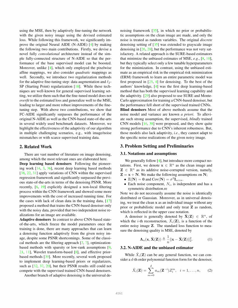
Visualization of polynomial mapping Figure 7 visualizes

the pixelwise polynomial coefficients {am,i}2m=0 learned

for Image13 of BSD68 (σ = 25). We note the coefficient

values for the higher order terms are relatively small com-

pared to {a0,i}’s. But, we observe they become more salient

particularly for the high frequency parts of the image, i.e.,

the edges. The effects of the polynomial coefficients on de-

noising is given in the Supplementary Material.

Figure 7. Visualization of a0, a1 and a2 for Image13 in BSD68.

6. Conclusion

We proposed FC-AIDE that can both supervised-train

and adaptively fine-tune the CNN-based pixelwise denois-

ing mappings. While surpassing the strong recent baselines,

we showed that the adaptivity of our method can resolve

various mismatch as well as data scarce scenarios com-

monly encountered in practice. Possible future research di-

rections include extending our method to other general im-

age restoration problems, e.g., image super-resolution, be-

yond denoising and devise a full blind denoising method

that can also estimate the noise σ.

Acknowledgement

This work is supported in part by the ICT R&D Pro-

gram [2016-0-00563], AI Graduate School Support Pro-

gram [2019-0-00421], and ITRC Support Program [2019-

2018-0-01798] of MSIT / IITP of the Korean government.

4167

References

[1] National cancer institute clinical pro-

teomic tumor analysis consortium (cptac).

https://doi.org/10.7937/k9/tcia.2018.oblamn27.

[2] A. Buades, B. Coll, and J. M. Morel. A review of im-

age denoising algorithms, with a new one. SIAM Jour-

nal on Multiscale Modeling and Simulation: A SIAM

Interdisciplinary Journal, 2005.

[3] H. Burger, C. Schuler, and S. Harmeling. Image

denoising: Can plain neural networks compete with

BM3D? In Computer Vision and Pattern Recognition

(CVPR), 2012.

[4] Sungmin Cha and Taesup Moon. Neural adaptive im-

age denoiser. In IEEE ICASSP, 2018.

[5] Jun Cheng. Brain tumor dataset, 2017.

[6] Cristovao Cruz, Alessandro Foi, Vladimir Katkovnik,

and Karen Egiazarian. Nonlocality-reinforced con-

volutional neural networks for image denoising.

https://arxiv.org/pdf/1803.02112.pdf, 2018.

[7] K. Dabov, A. Foi, V. Katkovnik, and K. Egiazarian.

Image denoising by sparse 3-d transform-domain col-

laborative filtering. IEEE Trans. Image Processing,

16(8):2080–2095, 2007.

[8] D. Donoho and I. Johnstone. Adapting to un-

known smoothness via wavelet shrinkage. Journal

of American Statistical Association, 90(432):1200–

1224, 1995.

[9] M. Elad and M. Aharon. Image denoising via sparse

and redundant representations over learned dictionar-

ies. IEEE Trans. Image Processing, 54(12):3736–

3745, 2006.

[10] Y. Eldar. Rethinking biased estimation: Im-

proving maximum likelihood and the Cramer-Rao

bound. Foundations and Trends in Signal Processing,

1(4):305–449, 2008.

[11] S. Gu, L. Zhang, W. Zuo, and X. Feng. Weighted nu-

clear norm minimization with applicaitons to image

denoising. In Computer Vision and Pattern Recogni-

tion (CVPR), 2014.

[12] Kaiming He, Xiangyu Zhang, Shaoqing Ren, and

Jian Sun. Delving deep into rectifiers: Surpassing

human-level performance on imagenet classification.

In CVPR, 2015.

[13] J-B Huang, A. Singh, and N. Ahuja. Single image

super-resolution from transformed self-exemplars. In

CVPR, 2015.

[14] V. Jain and H.S. Seung. Natural image denoising with

convolutional networks. In NIPS, 2008.

[15] D. Kingma and J. Ba. Adam: A method for stochastic

optimization. In International Conference on Learn-

ing Representations (ICLR), 2015.

[16] Stamatios Lefkimmiatis. Universal denoising net-

works: A novel CNN architecture for image denois-

ing. In CVPR, 2018.

[17] Jaakko Lehtinen, Jacob Munkberg, Jon Hasselgren,

Samuli Laine, Tero Karras, Miika Aittala, and Timo

Aila. Noise2Noise: Learning image restoration with-

out clean data. In ICML, 2018.

[18] X. Li, Y. Grandvalet, and F. Davoine. Explicit induc-

tive bias for transfer learning with convolutional net-

works. In ICML, 2018.

[19] Ding Liu, Bihan Wen, Yuchen Fan, Chen C. Loy, and

Thomas S. Huang. Non-local recurrent network for

image restoration. In NIPS, 2018.

[20] S. Lunz, O. Oktem, and C.-B. Schonlieb. Adversarial

regularizers in inverse problems. In NIPS, 2018.

[21] J. Mairal, F. Bach, J. Ponce, G. Sapiro, and A. Zis-

serman. Non-local sparse models for image restora-

tion. In International Conference on Computer Vision

(ICCV), 2009.

[22] X. Mao, C. Shen, and Y-B. Yang. Image restoration

using very deep convolutional encoder-decoder net-

works with symmetric skip connections. Neural In-

formation Processing Systems (NIPS), 2016.

[23] D. Martin, C. Fowlkes, D. Tal, and J. Malik. A

database of human segmented natural images and its

application to evaluating segmentation algorithms and

measuring ecological statistics. In International Con-

ference on Computer Vision (ICCV), 2001.

[24] Y. Matsui, K. Ito, Y. Aramaki, A. Fujimoto, T. Ogawa,

T. Yamasaki, and K. Aizawa. Sketch-based manga

retrieval using Manga109 dataset. Multimed. Tools

Appl., 76(21811), 2017.

[25] T. Moon, S. Min, B. Lee, and S. Yoon. Neural univer-

sal discrete denosier. In Neural Information Process-

ing Systems (NIPS), 2016.

[26] Giovanni Motta, Erik Ordentlich, Ignacio Ramirez,

Gadiel Seroussi, and Marcelo J. Weinberger. The

iDUDE framework for grayscale image denoising.

IEEE Trans. Image Processing, 20:1–21, 2011.

[27] S. Roth and M.J Black. Field of experts. International

Journal of Computer Vision, 82(2):205–229, 2009.

[28] K. Sivaramakrishnan and T. Weissman. Universal

denoising of discrete-time continuous-amplitude sig-

nals. IEEE Trans. Inform. Theory, 54(12):5632–5660,

2008.

[29] Shakarim Soltanayev and Se Young Chun. Training

deep learning based denoisers without ground truth

data. In NIPS, 2018.

4168

[30] C. Stein. Estimation of the mean of a multivariate nor-

mal distribution. The Annals of Statistics, 9(6):1135–

1151, 1981.

[31] Ying Tai, Jian Yang, Xiaoming Liu, and Chunyan

Xu. Memnet: A persistent memory network for im-

age restoration. In ICCV, 2017.

[32] Dmitry Ulyanov, Andrea Vedaldi, and Victor Lempit-

sky. Deep image prior. In CVPR, 2018.

[33] Aaron van den Oord, Nal Kalchbrenner, Oriol Vinyals,

Lasse Esleholt, Alex Graves, and Koray Kavukcuoglu.

Conditional image generation with PixelCNN de-

coders. In NIPS, 2016.

[34] Xiaosong Wang, Yifan Peng, Le Lu, Zhiyong Lu,

MohammadhadiBagheri, and Ronald M. Summers.

Chestx-ray8: Hospital-scale chest x-ray database and

benchmarks on weakly-supervised classification and

localization of common thorax diseases. In CVPR,

2017.

[35] T. Weissman, E. Ordentlich, G. Seroussi, S. Verdu,

and M. Weinberger. Universal discrete denois-

ing: Known channel. IEEE Trans. Inform. Theory,

51(1):5–28, 2005.

[36] J. Xie, L. Xu, and E. Chen. Image denoising and in-

painting with deep neural networks. In Neural Infor-

mation Processing Systems (NIPS), 2012.

[37] R.A. Yeh, T. Y. Lim, C. Chen, A. G. Schwing, M.

Hasegawa-Johnson, and M. N. Do. Image restoration

with deep generative models. In ICASSP, 2018.

[38] K. Zhang, W. Zuo, Y. Chen, D. Meng, and L. Zhang.

Beyond a gaussian denoiser: Residual learning of

deep cnn for image denoising. IEEE Trans. Image

Processing, 26(7):3142 – 3155, 2017.

[39] D. Zoran and Y. Weiss. From learning models of natu-

ral image patches to whole image restoration. Interna-

tional Conference on Computer Vision (ICCV), 2011.

4169