Pixel-Adaptive Convolutional Neural Networks

Hang Su1, Varun Jampani2, Deqing Sun2, Orazio Gallo2, Erik Learned-Miller1, and Jan Kautz2

1UMass Amherst 2NVIDIA

Abstract

Convolutions are the fundamental building blocks ofCNNs. The fact that their weights are spatially shared isone of the main reasons for their widespread use, but it isalso a major limitation, as it makes convolutions content-agnostic. We propose a pixel-adaptive convolution (PAC)operation, a simple yet effective modification of standardconvolutions, in which the filter weights are multiplied witha spatially varying kernel that depends on learnable, lo-cal pixel features. PAC is a generalization of several pop-ular filtering techniques and thus can be used for a widerange of use cases. Specifically, we demonstrate state-of-the-art performance when PAC is used for deep joint im-age upsampling. PAC also offers an effective alternative tofully-connected CRF (Full-CRF), called PAC-CRF, whichperforms competitively compared to Full-CRF, while beingconsiderably faster. In addition, we also demonstrate thatPAC can be used as a drop-in replacement for convolutionlayers in pre-trained networks, resulting in consistent per-formance improvements.

1. IntroductionConvolution is a basic operation in many image process-

ing and computer vision applications and the major build-ing block of Convolutional Neural Network (CNN) archi-tectures. It forms one of the most prominent ways of prop-agating and integrating features across image pixels due toits simplicity and highly optimized CPU/GPU implementa-tions. In this work, we concentrate on two important charac-teristics of standard spatial convolution and aim to alleviatesome of its drawbacks: Spatial Sharing and its Content-Agnostic nature.

Spatial Sharing: A typical CNN shares filters’ parame-ters across the whole input. In addition to affording trans-lation invariance to the CNN, spatially invariant convolu-tions significantly reduce the number of parameters com-pared with fully connected layers. However, spatial sharingis not without drawbacks. For dense pixel prediction tasks,such as semantic segmentation, the loss is spatially varyingbecause of varying scene elements on a pixel grid. Thus

𝐾

𝑊

f-1,-1 f-1,0 f-1,1

f0,-1 f0,0 f0,1

f1,-1 f1,0 f1,1

𝐾(f-1,-1,f0,0) 𝐾(f-1,0,f0,0) 𝐾(f-1,1,f0,0)

𝐾(f0,-1,f0,0) 𝐾(f0,0,f0,0) 𝐾(f0,1,f0,0)

𝐾(f1,-1,f0,0) 𝐾(f1,0,f0,0) 𝐾(f1,1,f0,0)

𝐾

Figure 1: Pixel-Adaptive Convolution. PAC modifies a standardconvolution on an input v by modifying the spatially invariant fil-ter W with an adapting kernel K. The adapting kernel is con-structed using either pre-defined or learned features f . ⊗ denoteselement-wise multiplication of matrices followed by a summation.Only one output channel is shown for the illustration.

the optimal gradient direction for parameters differs at eachpixel. However, due to the spatial sharing nature of convo-lution, the loss gradients from all image locations are glob-ally pooled to train each filter. This forces the CNN to learnfilters that minimize the error across all pixel locations atonce, but may be sub-optimal at any specific location.

Content-Agnostic: Once a CNN is trained, the same con-volutional filter banks are applied to all the images and allthe pixels irrespective of their content. The image contentvaries substantially across images and pixels. Thus a sin-gle trained CNN may not be optimal for all image types(e.g., images taken in daylight and at night) as well as dif-ferent pixels in an image (e.g., sky vs. pedestrian pixels).Ideally, we would like CNN filters to be adaptive to thetype of image content, which is not the case with standardCNNs. These drawbacks can be tackled by learning a largenumber of filters in an attempt to capture both image andpixel variations. This, however, increases the number ofparameters, requiring a larger memory footprint and an ex-tensive amount of labeled data. A different approach is touse content-adaptive filters inside the networks.

Existing content-adaptive convolutional networks can be

1

broadly categorized into two types. One class of techniquesmake traditional image-adaptive filters, such as bilateral fil-ters [2, 41] and guided image filters [18] differentiable, anduse them as layers inside a CNN [24, 28, 51, 11, 9, 21, 29,8, 13, 30, 43, 45]. These content-adaptive layers are usuallydesigned for enhancing CNN results but not as a replace-ment for standard convolutions. Another class of content-adaptive networks involve learning position-specific kernelsusing a separate sub-network that predicts convolutional fil-ter weights at each pixel. These are called “Dynamic Fil-ter Networks” (DFN) [47, 22, 12, 46] (also referred to ascross-convolution [47] or kernel prediction networks [4])and have been shown to be useful in several computer vi-sion tasks. Although DFNs are generic and can be used asa replacement to standard convolution layers, such a kernelprediction strategy is difficult to scale to an entire networkwith a large number of filter banks.

In this work, we propose a new content-adaptive convo-lution layer that addresses some of the limitations of the ex-isting content-adaptive layers while retaining several favor-able properties of spatially invariant convolution. Fig. 1 il-lustrates our content-adaptive convolution operation, whichwe call “Pixel-Adaptive Convolution” (PAC). Unlike a typ-ical DFN, where different kernels are predicted at differ-ent pixel locations, we adapt a standard spatially invariantconvolution filter W at each pixel by multiplying it with aspatially varying filter K, which we refer to as an “adapt-ing kernel”. This adapting kernel has a pre-defined form(e.g., Gaussian or Laplacian) and depends on the pixel fea-tures. For instance, the adapting kernel that we mainly usein this work is Gaussian: e−

12 ||fi−fj ||

2

, where fi ∈ Rd isa d-dimensional feature at the ith pixel. We refer to thesepixel features f as “adapting features”, and they can be ei-ther pre-defined, such as pixel position and color features,or can be learned using a CNN.

We observe that PAC, despite being a simple modifi-cation to standard convolution, is highly flexible and canbe seen as a generalization of several widely-used filters.Specifically, we show that PAC is a generalization of spatialconvolution, bilateral filtering [2, 41], and pooling opera-tions such as average pooling and detail-preserving pool-ing [35]. We also implement a variant of PAC that doespixel-adaptive transposed convolution (also called deconvo-lution) which can be used for learnable guided upsamplingof intermediate CNN representations. We discuss moreabout these generalizations and variants in Sec. 3.

As a result of its simplicity and being a generalization ofseveral widely used filtering techniques, PAC can be usefulin a wide range of computer vision problems. In this work,we demonstrate its applicability in three different visionproblems. In Sec. 4, we use PAC in joint image upsamplingnetworks and obtain state-of-the-art results on both depthand optical flow upsampling tasks. In Sec. 5, we use PAC in

a learnable conditional random field (CRF) framework andobserve consistent improvements with respect to the widelyused fully-connected CRF [24]. In Sec. 6, we demonstratehow to use PAC as a drop-in replacement of trained con-volution layers in a CNN and obtain performance improve-ments after fine-tuning. In summary, we observe that PACis highly versatile and has wide applicability in a range ofcomputer vision tasks.

2. Related WorkImage-adaptive filtering. Some important image-adaptivefiltering techniques include bilateral filtering [2, 41], guidedimage filtering [18], non-local means [6, 3], and propa-gated image filtering [34], to name a few. A common lineof research is to make these filters differentiable and usethem as content-adaptive CNN layers. Early work [51, 11]in this direction back-propagates through bilateral filteringand can thus leverage fully-connected CRF inference [24]on the output of CNNs. The work of [21] and [13] pro-poses to use bilateral filtering layers inside CNN archi-tectures. Chandra et al. [8] propose a layer that performsclosed-form Gaussian CRF inference in a CNN. Chen etal. [9] and Liu et al. [30] propose differentiable local prop-agation modules that have roots in domain transform fil-tering [14]. Wu et al. [45] and Wang et al. [43] proposeneural network layers to perform guided filtering [18] andnon-local means [43] respectively inside CNNs. Since thesetechniques are tailored towards a particular CRF or adap-tive filtering technique, they are used for specific tasks andcannot be directly used as a replacement of general convo-lution. Closest to our work are the sparse, high-dimensionalneural networks [21] which generalize standard 2D convo-lutions to high-dimensional convolutions, enabling them tobe content-adaptive. Although conceptually more genericthan PAC, such high-dimensional networks can not learnthe adapting features and have a larger computational over-head due to the use of specialized lattices and hash tables.

Dynamic filter networks. Introduced by Jia et al. [22], dy-namic filter networks (DFN) are an example of another classof content-adaptive filtering techniques. Filter weights arethemselves directly predicted by a separate network branch,and provide custom filters specific to different input data.The work is later extended by Wu et al. [46] with an addi-tional attention mechanism and a dynamic sampling strat-egy to allow the position-specific kernels to also learn frommultiple neighboring regions. Similar ideas have been ap-plied to several task-specific use cases, e.g., motion pre-diction [47], semantic segmentation [17], and Monte Carlorendering denoising [4]. Explicitly predicting all position-specific filter weights requires a large number of parame-ters, so DFNs typically require a sensible architecture de-sign and are difficult to scale to multiple dynamic-filter lay-ers. Our approach differs in that PAC reuses spatial filters

just as standard convolution, and only modifies the filters ina position-specific fashion. Dai et al. propose deformableconvolution [12], which can also produce position-specificmodifications to the filters. Different from PAC, the modifi-cations there are represented as offsets with an emphasis onlearning geometric-invariant features.Self-attention mechanism. Our work is also related to theself-attention mechanism originally proposed by Vaswaniet al. for machine translation [42]. Self-attention modulescompute the responses at each position while attending tothe global context. Thanks to the use of global information,self-attention has been successfully used in several appli-cations, including image generation [50, 33] and video ac-tivity recognition [43]. Attending to the whole image canbe computationally expensive, and, as a result, can only beafforded on low-dimensional feature maps, e.g., as in [43].Our layer produces responses that are sensitive to a more lo-cal context (which can be alleviated through dilation), andis therefore much more efficient.

3. Pixel-Adaptive ConvolutionIn this section, we start with a formal definition of

standard spatial convolution and then explain our gener-alization of it to arrive at our pixel-adaptive convolution(PAC). Later, we will discuss several variants of PAC andhow they are connected to different image filtering tech-niques. Formally, a spatial convolution of image featuresv = (v1, . . . ,vn),vi ∈ Rc over n pixels and c channelswith filter weights W ∈ Rc′×c×s×s can be written as

v′i =∑j∈Ω(i)

W [pi − pj ]vj + b (1)

where pi = (xi, yi)ᵀ are pixel coordinates, Ω(·) defines an

s×s convolution window, and b ∈ Rc′ denotes biases. Witha slight abuse of notation, we use [pi−pj ] to denote index-ing of the spatial dimensions of an array with 2D spatialoffsets. This convolution operation results in a c′-channeloutput, v′i ∈ Rc′ , at each pixel i. Eq. 1 highlights how theweights only depend on pixel position and thus are agnos-tic to image content. In other words, the weights are spa-tially shared and, therefore, image-agnostic. As outlined inSec. 1, these properties of spatial convolutions are limiting:we would like the filter weights W to be content-adaptive.

One approach to make the convolution operationcontent-adaptive, rather than only based on pixel locations,is to generalize W to depend on the pixel features, f ∈ Rd:

v′i =∑j∈Ω(i)

W (fi − fj)vj + b (2)

where W can be seen as a high-dimensional filter oper-ating in a d-dimensional feature space. In other words,we can apply Eq. 2 by first projecting the input signal

v into a d-dimensional space, and then performing d-dimensional convolution with W. Traditionally, such high-dimensional filtering is limited to hand-specified filters suchas Gaussian filters [1]. Recent work [21] lifts this re-striction and proposes a technique to freely parameterizeand learn W in high-dimensional space. Although genericand used successfully in several computer vision applica-tions [21, 20, 38], high-dimensional convolutions have sev-eral shortcomings. First, since data projected on a higher-dimensional space is sparse, special lattice structures andhash tables are needed to perform the convolution [1] re-sulting in considerable computational overhead. Second, itis difficult to learn features f resulting in the use of hand-specified feature spaces such as position and color features,f = (x, y, r, g, b). Third, we have to restrict the dimension-ality d of features (say, < 10) as the projected input imagecan become too sparse in high-dimensional spaces. In addi-tion, the advantages that come with spatial sharing of stan-dard convolution are lost with high-dimensional filtering.Pixel-adaptive convolution. Instead of bringing convolu-tion to higher dimensions, which has the above-mentioneddrawbacks, we choose to modify the spatially invariant con-volution in Eq. 1 with a spatially varying kernel K ∈Rc′×c×s×s that depends on pixel features f :

v′i =∑j∈Ω(i)

K (fi, fj)W [pi − pj ]vj + b (3)

where K is a kernel function that has a fixed parametricform such as Gaussian: K(fi, fj) = exp(− 1

2 (fi− fj)ᵀ(fi−

fj)). Since K has a pre-defined form and is not param-eterized as a high-dimensional filter, we can perform thisfiltering on the 2D grid itself without moving onto higherdimensions. We call the above filtering operation (Eq. 3) as“Pixel-Adaptive Convolution” (PAC) because the standardspatial convolution W is adapted at each pixel using pixelfeatures f via kernel K. We call these pixel features f as“adapting features” and the kernel K as “adapting kernel”.The adapting features f can be either hand-specified such asposition and color features f = (x, y, r, g, b) or can be deepfeatures that are learned end-to-end.Generalizations. PAC, despite being a simple modificationto standard convolution, generalizes several widely used fil-tering operations, including• Spatial Convolution can be seen as a special case of

PAC with adapting kernel being constant K(fi, fj) =1. This can be achieved by using constant adaptingfeatures, fi = fj ,∀i, j. In brief, standard convolution(Eq. 1) uses fixed, spatially shared filters, while PACallows the filters to be modified by the adapting kernelK differently across pixel locations.• Bilateral Filtering [41] is a basic image processing op-

eration that has found wide-ranging uses [32] in im-age processing, computer vision and also computer

graphics. Standard bilateral filtering operation can beseen as a special case of PAC, where W also has afixed parametric form, such as a 2D Gaussian filter,W [pi − pj ] = exp(− 1

2 (pi − pj)ᵀΣ−1(pi − pj)).

• Pooling operations can also be modeled by PAC. Stan-dard average pooling corresponds to the special caseof PAC where K(fi, fj) = 1, W = 1

s2 · 1. De-tail Preserving Pooling [35, 44] is a recently proposedpooling layer that is useful to preserve high-frequencydetails when performing pooling in CNNs. PAC canmodel the detail-preserving pooling operations by in-corporating an adapting kernel that emphasizes moredistinct pixels in the neighborhood, e.g., K(fi, fj) =

α+(|fi − fj |2 + ε2

)λ.

The above generalizations show the generality and thewide applicability of PAC in different settings and applica-tions. We experiment using PAC in three different problemscenarios, which will be discussed in later sections.

Some filtering operations are even more general than theproposed PAC. Examples include high-dimensional filter-ing shown in Eq. 2 and others such as dynamic filter net-works (DFN) [22] discussed in Sec. 2. Unlike most of thosegeneral filters, PAC allows efficient learning and reuse ofspatially invariant filters because it is a direct modificationof standard convolution filters. PAC offers a good trade-offbetween standard convolution and DFNs. In DFNs, filtersare solely generated by an auxiliary network and differentauxiliary networks or layers are required to predict kernelsfor different dynamic-filter layers. PAC, on the other hand,uses learned pixel embeddings f as adapting features, whichcan be reused across several different PAC layers in a net-work. When related to sparse high-dimensional filtering inEq. 2, PAC can be seen as factoring the high-dimensionalfilter into a product of standard spatial filter W and theadapting kernel K. This allows efficient implementationof PAC in 2D space alleviating the need for using hash ta-bles and special lattice structures in high dimensions. PACcan also use learned pixel embeddings f instead of hand-specified ones in existing learnable high-dimensional filter-ing techniques such as [21].

Implementation and variants. We implemented PAC as anetwork layer in PyTorch with GPU acceleration1. Our im-plementation enables back-propagation through the featuresf , permitting the use of learnable deep features as adapt-ing features. We also implement a PAC variant that doespixel-adaptive transposed convolution (also called “decon-volution”). We refer to pixel-adaptive convolution shownin Eq. 3 as PAC and the transposed counterpart as PACᵀ.Similar to standard transposed convolution, PACᵀ uses frac-tional striding and results in an upsampled output. Our PACand PACᵀ implementations allow easy and flexible specifi-

1Code can be found at https://suhangpro.github.io/pac/

Encoder

Guidance

CONV

PACT

PACT

PACT

CONV

CONV

CONV

CONV

Decoder

CONV

CONV

CONV

Figure 2: Joint upsampling with PAC. Network architectureshowing encoder, guidance and decoder components. Featuresfrom the guidance branch are used to adapt PACᵀ kernels that areapplied on the encoder output resulting in upsampled signal.

cation of different options that are commonly used in stan-dard convolution: filter size, number of input and outputchannels, striding, padding and dilation factor.

4. Deep Joint Upsampling NetworksJoint upsampling is the task of upsampling a low-

resolution signal with the help of a corresponding high-resolution guidance image. An example is upsamplinga low-resolution depth map given a corresponding high-resolution RGB image as guidance. Joint upsampling isuseful when some sensors output at a lower resolution thancameras, or can be used to speed up computer vision appli-cations where full-resolution results are expensive to pro-duce. PAC allows filtering operations to be guided by theadapting features, which can be obtained from a separateguidance image, making it an ideal choice for joint imageprocessing. We investigate the use of PAC for joint upsam-pling applications. In this section, we introduce a networkarchitecture that relies on PAC for deep joint upsampling,and show experimental results on two applications: jointdepth upsampling and joint optical flow upsampling.

4.1. Deep joint upsampling with PACA deep joint upsampling network takes two inputs,

a low-resolution signal x ∈ Rc×h/m×w/m and a high-resolution guidance g ∈ Rcg×h×w, and outputs upsampledsignal x↑ ∈ Rc×h×w. Here m is the required upsamplingfactor. Similar to [26], our upsampling network has threecomponents (as illustrated in Fig. 2):• Encoder branch operates directly on the low-resolution

signal with convolution (CONV) layers.• Guidance branch operates solely on the guidance im-

age, and generates adapting features that will be usedin all PACᵀ layers later in the network.• Decoder branch starts with a sequence of PACᵀ, which

perform transposed pixel-adaptive convolution, eachof which upsamples the feature maps by a factor of2. PACᵀ layers are followed by two CONV layers togenerate the final upsampled output.

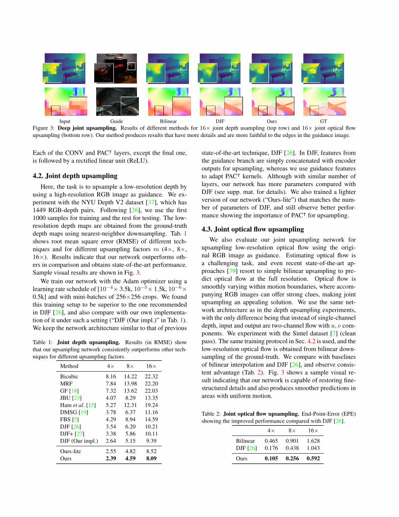
Input Guide Bilinear DJF Ours GTFigure 3: Deep joint upsampling. Results of different methods for 16× joint depth usampling (top row) and 16× joint optical flowupsampling (bottom row). Our method produces results that have more details and are more faithful to the edges in the guidance image.

Each of the CONV and PACᵀ layers, except the final one,is followed by a rectified linear unit (ReLU).

4.2. Joint depth upsamplingHere, the task is to upsample a low-resolution depth by

using a high-resolution RGB image as guidance. We ex-periment with the NYU Depth V2 dataset [37], which has1449 RGB-depth pairs. Following [26], we use the first1000 samples for training and the rest for testing. The low-resolution depth maps are obtained from the ground-truthdepth maps using nearest-neighbor downsampling. Tab. 1shows root mean square error (RMSE) of different tech-niques and for different upsampling factors m (4×, 8×,16×). Results indicate that our network outperforms oth-ers in comparison and obtains state-of-the-art performance.Sample visual results are shown in Fig. 3.

We train our network with the Adam optimizer using alearning rate schedule of [10−4× 3.5k, 10−5× 1.5k, 10−6×0.5k] and with mini-batches of 256×256 crops. We foundthis training setup to be superior to the one recommendedin DJF [26], and also compare with our own implementa-tion of it under such a setting (“DJF (Our impl.)” in Tab. 1).We keep the network architecture similar to that of previous

Table 1: Joint depth upsampling. Results (in RMSE) showthat our upsampling network consistently outperforms other tech-niques for different upsampling factors.

Method 4× 8× 16×

Bicubic 8.16 14.22 22.32MRF 7.84 13.98 22.20GF [18] 7.32 13.62 22.03JBU [23] 4.07 8.29 13.35Ham et al. [15] 5.27 12.31 19.24DMSG [19] 3.78 6.37 11.16FBS [5] 4.29 8.94 14.59DJF [26] 3.54 6.20 10.21DJF+ [27] 3.38 5.86 10.11DJF (Our impl.) 2.64 5.15 9.39

Ours-lite 2.55 4.82 8.52Ours 2.39 4.59 8.09

state-of-the-art technique, DJF [26]. In DJF, features fromthe guidance branch are simply concatenated with encoderoutputs for upsampling, whereas we use guidance featuresto adapt PACᵀ kernels. Although with similar number oflayers, our network has more parameters compared withDJF (see supp. mat. for details). We also trained a lighterversion of our network (“Ours-lite”) that matches the num-ber of parameters of DJF, and still observe better perfor-mance showing the importance of PACᵀ for upsampling.

4.3. Joint optical flow upsamplingWe also evaluate our joint upsampling network for

upsampling low-resolution optical flow using the origi-nal RGB image as guidance. Estimating optical flow isa challenging task, and even recent state-of-the-art ap-proaches [39] resort to simple bilinear upsampling to pre-dict optical flow at the full resolution. Optical flow issmoothly varying within motion boundaries, where accom-panying RGB images can offer strong clues, making jointupsampling an appealing solution. We use the same net-work architecture as in the depth upsampling experiments,with the only difference being that instead of single-channeldepth, input and output are two-channel flow with u, v com-ponents. We experiment with the Sintel dataset [7] (cleanpass). The same training protocol in Sec. 4.2 is used, and thelow-resolution optical flow is obtained from bilinear down-sampling of the ground-truth. We compare with baselinesof bilinear interpolation and DJF [26], and observe consis-tent advantage (Tab. 2). Fig. 3 shows a sample visual re-sult indicating that our network is capable of restoring fine-structured details and also produces smoother predictions inareas with uniform motion.

Table 2: Joint optical flow upsampling. End-Point-Error (EPE)showing the improved performance compared with DJF [26].

4× 8× 16×

Bilinear 0.465 0.901 1.628DJF [26] 0.176 0.438 1.043

Ours 0.105 0.256 0.592

5. Conditional Random FieldsEarly adoptions of CRFs in computer vision tasks were

limited to region-based approaches and short-range struc-tures [36] for efficiency reasons. Fully-Connected CRF(Full-CRF) [24] was proposed to offer the benefits of densepairwise connections among pixels, which resorts to ap-proximate high-dimensional filtering [1] for efficient infer-ence. Consider a semantic labeling problem, where eachpixel i in an image I can take one of the semantic labelsli ∈ 1, ...,L. Full-CRF has unary potentials usually de-fined by a classifier such as CNN: ψu(li) ∈ RL. And, thepairwise potentials are defined for every pair of pixel loca-tions (i, j): ψp(li, lj |I) = µ(li, lj)K(fi, fj), where K is akernel function and µ is a compatibility function. A com-mon choice for µ is the Potts model: µ(li, lj) = [li 6= lj ].[24] utilizes two Gaussian kernels with hand-crafted fea-tures as the kernel function:

K(fi, fj) =w1 exp

−‖pi − pj‖2

2θ2α

− ‖Ii − Ij‖2

2θ2β

+ w2 exp

−‖pi − pj‖2

2θ2γ

(4)

wherew1, w2, θα, θβ , θγ are model parameters, and are typ-ically found by a grid-search. Then, inference in Full-CRF amounts to maximizing the following Gibbs distribu-tion: P (l|I) = exp(−

∑i ψu(li)−

∑i<j ψp(li, lj)), l =

(l1, l2, ..., ln). Exact inference of Full-CRF is hard, and [24]relies on mean-field approximation which is optimizing foran approximate distribution Q(l) =

∏iQi(li) by minimiz-

ing the KL-divergence between P (l|I) and the mean-fieldapproximation Q(l). This leads to the following mean-field(MF) inference step that updates marginal distributions Qiiteratively for t = 0, 1, ... :

Q(t+1)i (l)← 1

Ziexp

− ψu(l)

−∑l′∈L

µ(l, l′)∑j 6=i

K(fi, fj)Q(t)j (l′)

(5)

The main computation in each MF iteration,∑j 6=iK(fi, fj)Q

(t)j , can be viewed as high-dimensional

Gaussian filtering. Previous work [24, 25] relies onpermutohedral lattice convolution [1] to achieve efficientimplementation.

5.1. Efficient, learnable CRF with PACExisting work [51, 21] back-propagates through the

above MF steps to combine CRF inference with CNNs re-sulting in end-to-end training of CNN-CRF models. Whilethere exists optimized CPU implementations, permutohe-dral lattice convolution cannot easily utilize GPUs becauseit “does not follow the SIMD paradigm of efficient GPU

dilation=16

dilation=64

PAC-CRF

PACdilation=16

PACdilation=64

So

ftm

ax

𝑀𝐹

So

ftm

ax

Una

ries

Pre

dict

ion

Inp

ut …

𝑡 steps

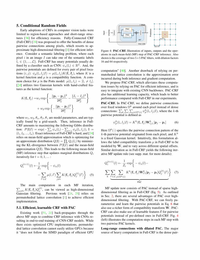
Figure 4: PAC-CRF. Illustration of inputs, outputs and the oper-ations in each mean-field (MF) step of PAC-CRF inference. Alsoshown is the coverage of two 5×5 PAC filters, with dilation factors16 and 64 respectively.

computation” [40]. Another drawback of relying on per-mutohedral lattice convolution is the approximation errorincurred during both inference and gradient computation.

We propose PAC-CRF, which alleviates these computa-tion issues by relying on PAC for efficient inference, and iseasy to integrate with existing CNN backbones. PAC-CRFalso has additional learning capacity, which leads to betterperformance compared with Full-CRF in our experiments.

PAC-CRF. In PAC-CRF, we define pairwise connectionsover fixed windows Ωk around each pixel instead of denseconnections:

∑k

∑i

∑j∈Ωk(i) ψ

kp(li, lj |I), where the k-th

pairwise potential is defined as

ψkp(li, lj |I) = Kk(fi, fj)Wklj li [pj − pi] (6)

Here Ωk(·) specifies the pairwise connection pattern of thek-th pairwise potential originated from each pixel, and Kk

is a fixed Gaussian kernel. Intuitively, this formulation al-lows the label compatibility transform µ in Full-CRF to bemodeled by W, and to vary across different spatial offsets.Similar derivation as in Full-CRF yields the following iter-ative MF update rule (see supp. mat. for more details):

Q(t+1)i (l)← 1

Ziexp

− ψu(l)−∑

k

∑l′∈L

∑j∈Ωk(i)

Kk(fi, fj)Wkl′l[pj − pi]Q

(t)j (l′)

︸ ︷︷ ︸PAC

(7)

MF update now consists of PAC instead of sparse high-dimensional filtering as in Full-CRF (Eq. 5). As outlinedin Sec. 2, there are several advantages of PAC over high-dimensional filtering. With PAC-CRF, we can freely pa-rameterize and learn the pairwise potentials in Eq. 6 thatalso use a richer form of compatibility transform W. PAC-CRF can also make use of learnable features f for pairwisepotentials instead of pre-defined ones in Full-CRF. Fig. 4(left) illustrates the computation steps in each MF step withtwo pairwise PAC kernels.

Long-range connections with dilated PAC. The majorsource of heavy computation in Full-CRF is the dense pair-

wise pixel connections. In PAC-CRF, the pairwise con-nections are defined by the local convolution windows Ωk.To have long-range pairwise connections while keeping thenumber of PAC parameters managable, we make use ofdilated filters [10, 48]. Even with a relatively small ker-nel size (5 × 5), with a large dilation, e.g., 64, the CRFcan effectively reach a neighborhood of 257 × 257. Aconcurrent work [40] also propose a convolutional versionof CRF (Conv-CRF) to reduce the number of connectionsin Full-CRF. However, [40] uses connections only withinsmall local windows. We argue that long-range connectionscan provide valuable information, and our CRF formulationuses a wider range of connections while still being efficient.Our formulation allows using multiple PAC filters in par-allel, each with different dilation factors. In Fig. 4 (right),we show an illustration of the coverage of two 5 × 5 PACfilters, with dilation factors 16 and 64 respectively. Thisallows PAC-CRF to achieve a good trade-off between com-putational efficiency and long-range pairwise connectivity.

5.2. Semantic segmentation with PAC-CRFThe task of semantic segmentation is to assign a seman-

tic label to each pixel in an image. Full-CRF is proven tobe a valuable post-processing tool that can considerably im-prove CNN segmentation performance [10, 51, 21]. Here,we experiment with PAC-CRF on top of the FCN semanticsegmentation network [31]. We choose FCN for simplicityand ease of comparisons, as FCN only uses standard convo-lution layers and does not have many bells and whistles.

In the experiments, we use scaled RGB color,[ RσR

, GσG, BσB

]ᵀ, as the guiding features for the PAC layersin PAC-CRF . The scaling vector [σR, σG, σB ]ᵀ is learnedjointly with the PAC weights W. We try two internal con-figurations of PAC-CRF: a single 5×5 PAC kernel with di-lation of 32, and two parallel 5×5 PAC kernels with dilationfactors of 16 and 64. 5 MF steps are used for a good balancebetween speed and accuracy (more details in supp. mat.).We first freeze the backbone FCN network and train onlythe PAC-CRF part for 40 epochs, and then train the wholenetwork for another 40 epochs with reduced learning rates.

Dataset. We follow the training and validation settings ofFCN [31] which is trained on PascalVOC images and vali-dated on a reduced validation set of 736 images. We alsosubmit our final trained models to the official evaluationserver to get test scores on 1456 test images.

Baselines. We compare PAC-CRF with three baselines:Full-CRF [24], BCL-CRF [21], and Conv-CRF [40]. ForFull-CRF, we use the publicly available C++ code, and findthe optimal CRF parameters through grid search. For BCL-CRF, we use 1-neighborhood filters to keep the runtimemanageable and use other settings as suggested by the au-thors. For Conv-CRF, the same training procedure is usedas in PAC-CRF. We use the more powerful variant of Conv-

Table 3: Semantic segmentation with PAC-CRF. Validation andtest mIoU scores along with the runtimes of different techniques.PAC-CRF results in better improvements than Full-CRF [24]while being faster. PAC-CRF also outperforms Conv-CRF [40]and BCL [21]. Runtimes are averaged over all validation images.

Method mIoU (val / test) CRF Runtime

Unaries only (FCN) 65.51 / 67.20 -

Full-CRF [24] +2.11 / +2.45 629 msBCL-CRF [21] +2.28 / +2.33 2.6 sConv-CRF [40] +2.13 / +1.57 38 ms

PAC-CRF, 32 +3.01 / +2.21 39 msPAC-CRF, 16-64 +3.39 / +2.62 78 ms

CRF with learnable compatibility transform (referred to as“Conv+C” in [40]), and we learn the RGB scales for Conv-CRF in the same way as for PAC-CRF. We follow the sug-gested default settings for Conv-CRF and use a filter size of11×11 and a blurring factor of 4. Note that like Full-CRF(Eq. 4), the other baselines also use two pairwise kernels.Results. Tab. 3 reports validation and test mean Intersectionover Union (mIoU) scores along with average runtimes ofdifferent techniques. Our two-filter variant (“PAC-CRF, 16-64”) achieves better mIoU compared with all baselines, andalso compares favorably in terms of runtime. The one-filtervariant (“PAC-CRF, 32”) performs slightly worse than Full-CRF and BCL-CRF, but has even larger speed advantage,offering a strong option where efficiency is needed. Sam-ple visual results are shown in Fig. 5. While being quan-titatively better and retaining more visual details overall,PAC-CRF produces some amount of noise around bound-aries. This is likely due to a known “gridding” effect ofdilation [49], which we hope to mitigate in future work.

6. Layer hot-swapping with PACSo far, we design specific architectures around PAC for

different use cases. In this section, we offer a strategy touse PAC for simply upgrading existing CNNs with minimalmodifications through what we call layer hot-swapping.Layer hot-swapping. Network fine-tuning has becomea common practice when training networks on new dataor with additional layers. Typically, in fine-tuning, newlyadded layers are initialized randomly. Since PAC general-izes standard convolution layers, it can directly replace con-volution layers in existing networks while retaining the pre-trained weights. We refer to this modification of existingpre-trained networks as layer hot-swapping.

We continue to use semantic segmentation as an exam-ple, and demonstrate how layer hot-swapping can be a sim-ple yet effective modification to existing CNNs. Fig. 6 illus-trates a FCN [31] before and after the hot-swapping modi-fications. We swap out the last CONV layer of the last threeconvolution groups, CONV3 3, CONV4 3, CONV5 3,

Input GT Unary Full-CRF BCL-CRF Conv-CRF PAC-CRF,32 PAC-CRF,16-64 PAC-FCN PAC-FCN-CRFFigure 5: Semantic segmentation with PAC-CRF and PAC-FCN. We show three examples from the validation set. Compared to Full-CRF [24], BCL-CRF [21], and Conv-CRF [40], PAC-CRF can recover finer details faithful to the boundaries in the RGB inputs.

with PAC layers with the same configuration (filter size,input and output channels, etc.), and use the output ofCONV2 2 as the guiding feature for the PAC layers. Bythis example, we also demonstrate that one could use ear-lier layer features (CONV2 2 here) as adapting features forPAC. Using this strategy, the network parameters do notincrease when replacing CONV layers with PAC layers.All the layer weights are initialized with trained FCN pa-rameters. To ensure a better starting condition for furthertraining, we scale the guiding features by a small constant(0.0001) so that the PAC layers initially behave very closelyto their original CONV counterparts. We use 8825 imagesfor training, including the Pascal VOC 2011 training imagesand the additional training samples from [16]. Validationand testing are performed in the same fashion as in Sec. 5.

Results are reported in Tab. 4. We show that our simplemodification (PAC-FCN) provides about 2 mIoU improve-ment on test (67.20 → 69.18) for the semantic segmenta-tion task, while incurring virtually no runtime penalty at in-ference time. Note that PAC-FCN has the same number of

Inp

ut

CO

NV

2_2

CO

NV

3_3

CO

NV

4_3

CO

NV

5_3

………

Pre

dic

tion

… …

Inp

ut

CO

NV

2_2

PA

C3

_3

PA

C4

_3

PA

C5

_3

………

Pre

dic

tion

… …

hot swapping

Figure 6: Layer hot-swapping with PAC. A few layers of a net-work before (top) and after (bottom) hot-swapping. Three CONVlayers are replaced with PAC layers, with adapting features com-ing from an earlier convolution layer. All the original networkweights are retained after the modification.

parameters as the original FCN model. The improvementbrought by PAC-FCN is also complementary to any addi-tional CRF post-processing that can still be applied. Aftercombined with a PAC-CRF (the 16-64 variant) and trainedjointly, we observe another 2 mIoU improvement. Samplevisual results are shown in Fig. 5.

Table 4: FCN hot-swapping CONV with PAC. Validation andtest mIoU scores along with runtimes of different techniques. Oursimple hot-swapping strategy provides 2 IoU gain on test. Com-bining with PAC-CRF offers additional improvements.

Method PAC-CRF mIoU (val / test) Runtime

FCN-8s - 65.51 / 67.20 39 msFCN-8s 16-64 68.90 / 69.82 117 ms

PAC-FCN - 67.44 / 69.18 41 msPAC-FCN 16-64 69.87 / 71.34 118 ms

7. ConclusionIn this work we propose PAC, a new type of filtering op-

eration that can effectively learn to leverage guidance infor-mation. We show that PAC generalizes several popular fil-tering operations and demonstrate its applicability on differ-ent uses ranging from joint upsampling, semantic segmenta-tion networks, to efficient CRF inference. PAC generalizesstandard spatial convolution, and can be used to directly re-place standard convolution layers in pre-trained networksfor performance gain with minimal computation overhead.

Acknowledgements H. Su and E. Learned-Miller ac-knowledge support from AFRL and DARPA (#FA8750-18-2-0126)2 and the MassTech Collaborative grant for fundingthe UMass GPU cluster.2The U.S. Gov. is authorized to reproduce and distribute reprints for Gov.purposes notwithstanding any copyright notation thereon. The views andconclusions contained herein are those of the authors and should not be in-terpreted as necessarily representing the official policies or endorsements,either expressed or implied, of the AFRL and DARPA or the U.S. Gov.

References[1] A. Adams, J. Baek, and M. A. Davis. Fast high-dimensional

filtering using the permutohedral lattice. Computer GraphicsForum, 29(2):753–762, 2010. 3, 6

[2] V. Aurich and J. Weule. Non-linear Gaussian filters perform-ing edge preserving diffusion. In DAGM, pages 538–545.Springer, 1995. 2

[3] S. P. Awate and R. T. Whitaker. Higher-order image statisticsfor unsupervised, information-theoretic, adaptive, image fil-tering. In Proc. CVPR, volume 2, pages 44–51. IEEE, 2005.2

[4] S. Bako, T. Vogels, B. McWilliams, M. Meyer, J. Novak,A. Harvill, P. Sen, T. Derose, and F. Rousselle. Kernel-predicting convolutional networks for denoising monte carlorenderings. ACM Trans. Graph., 36(4):97, 2017. 2

[5] J. T. Barron and B. Poole. The fast bilateral solver. In Proc.ECCV, pages 617–632. Springer, 2016. 5

[6] A. Buades, B. Coll, and J.-M. Morel. A non-local algorithmfor image denoising. In Proc. CVPR, volume 2, pages 60–65.IEEE, 2005. 2

[7] D. J. Butler, J. Wulff, G. B. Stanley, and M. J. Black. Anaturalistic open source movie for optical flow evaluation.In A. Fitzgibbon et al. (Eds.), editor, Proc. ECCV, Part IV,LNCS 7577, pages 611–625. Springer-Verlag, Oct. 2012. 5

[8] S. Chandra and I. Kokkinos. Fast, exact and multi-scale in-ference for semantic image segmentation with deep GaussianCRFs. In Proc. ECCV, pages 402–418. Springer, 2016. 2

[9] L.-C. Chen, J. T. Barron, G. Papandreou, K. Murphy, andA. L. Yuille. Semantic image segmentation with task-specificedge detection using CNNs and a discriminatively traineddomain transform. In Proc. CVPR, pages 4545–4554, 2016.2

[10] L.-C. Chen, G. Papandreou, I. Kokkinos, K. Murphy, andA. L. Yuille. Deeplab: Semantic image segmentation withdeep convolutional nets, atrous convolution, and fully con-nected CRFs. PAMI, 40(4):834–848, 2018. 7

[11] L.-C. Chen, A. Schwing, A. Yuille, and R. Urtasun. Learningdeep structured models. In Proc. ICML, pages 1785–1794,2015. 2

[12] J. Dai, H. Qi, Y. Xiong, Y. Li, G. Zhang, H. Hu, and Y. Wei.Deformable convolutional networks. arXiv:1703.06211,1(2):3, 2017. 2, 3

[13] R. Gadde, V. Jampani, M. Kiefel, D. Kappler, and P. V.Gehler. Superpixel convolutional networks using bilateralinceptions. In Proc. ECCV, pages 597–613. Springer, 2016.2

[14] E. S. Gastal and M. M. Oliveira. Domain transform for edge-aware image and video processing. ACM Trans. Graph.,30(4):69, 2011. 2

[15] B. Ham, M. Cho, and J. Ponce. Robust image filtering usingjoint static and dynamic guidance. In Proc. CVPR, pages4823–4831, 2015. 5

[16] B. Hariharan, P. Arbelaez, L. Bourdev, S. Maji, and J. Malik.Semantic contours from inverse detectors. In Proc. ICCV,2011. 8

[17] A. W. Harley, K. G. Derpanis, and I. Kokkinos.Segmentation-aware convolutional networks using local at-tention masks. In Proc. ICCV, volume 2, page 7, 2017. 2

[18] K. He, J. Sun, and X. Tang. Guided image filtering. PAMI,35(6):1397–1409, 2013. 2, 5

[19] T.-W. Hui, C. C. Loy, and X. Tang. Depth map super-resolution by deep multi-scale guidance. In Proc. ECCV,pages 353–369. Springer, 2016. 5

[20] V. Jampani, R. Gadde, and P. V. Gehler. Video propagationnetworks. In Proc. CVPR, 2017. 3

[21] V. Jampani, M. Kiefel, and P. V. Gehler. Learning sparse highdimensional filters: Image filtering, dense CRFs and bilateralneural networks. In Proc. CVPR, pages 4452–4461, 2016. 2,3, 4, 6, 7, 8

[22] X. Jia, B. De Brabandere, T. Tuytelaars, and L. V. Gool. Dy-namic filter networks. In Proc. NIPS, pages 667–675, 2016.2, 4

[23] J. Kopf, M. F. Cohen, D. Lischinski, and M. Uyttendaele.Joint bilateral upsampling. ACM Trans. Graph., 26(3):96,2007. 5

[24] P. Krahenbuhl and V. Koltun. Efficient inference in fully con-nected CRFs with Gaussian edge potentials. In Proc. NIPS,pages 109–117, 2011. 2, 6, 7, 8

[25] P. Krahenbuhl and V. Koltun. Parameter learning and con-vergent inference for dense random fields. In Proc. ICML,pages 513–521, 2013. 6

[26] Y. Li, J.-B. Huang, N. Ahuja, and M.-H. Yang. Deep jointimage filtering. In Proc. ECCV, pages 154–169. Springer,2016. 4, 5

[27] Y. Li, J.-B. Huang, N. Ahuja, and M.-H. Yang. Joint imagefiltering with deep convolutional networks. PAMI, 2018. 5

[28] Y. Li and R. Zemel. Mean field networks. arXiv:1410.5884,2014. 2

[29] G. Lin, C. Shen, A. Van Den Hengel, and I. Reid. Efficientpiecewise training of deep structured models for semanticsegmentation. In Proc. CVPR, pages 3194–3203, 2016. 2

[30] S. Liu, S. D. Mello, J. Gu, G. Zhong, M.-H. Yang, andJ. Kautz. Learning affinity via spatial propagation networks.In Proc. NIPS, 2017. 2

[31] J. Long, E. Shelhamer, and T. Darrell. Fully convolutionalnetworks for semantic segmentation. In Proc. CVPR, pages3431–3440, 2015. 7

[32] S. Paris, P. Kornprobst, J. Tumblin, F. Durand, et al. Bi-lateral filtering: Theory and applications. Foundationsand Trends R© in Computer Graphics and Vision, 4(1):1–73,2009. 3

[33] N. Parmar, A. Vaswani, J. Uszkoreit, Ł. Kaiser, N. Shazeer,and A. Ku. Image transformer. arXiv:1802.05751, 2018. 3

[34] J.-H. Rick Chang and Y.-C. Frank Wang. Propagated imagefiltering. In Proc. CVPR, pages 10–18, 2015. 2

[35] F. Saeedan, N. Weber, M. Goesele, and S. Roth. Detail-preserving pooling in deep networks. In cvpr, pages 9108–9116, 2018. 2, 4

[36] J. Shotton, J. Winn, C. Rother, and A. Criminisi. Texton-boost: Joint appearance, shape and context modeling formulti-class object recognition and segmentation. In Proc.ECCV, 2006. 6

[37] N. Silberman, D. Hoiem, P. Kohli, and R. Fergus. Indoorsegmentation and support inference from rgbd images. InProc. ECCV, pages 746–760. Springer, 2012. 5

[38] H. Su, V. Jampani, D. Sun, S. Maji, E. Kalogerakis, M.-H.Yang, and J. Kautz. Splatnet: Sparse lattice networks forpoint cloud processing. In Proc. CVPR, 2018. 3

[39] D. Sun, X. Yang, M.-Y. Liu, and J. Kautz. PWC-Net: CNNsfor optical flow using pyramid, warping, and cost volume. InProc. CVPR, pages 8934–8943, 2018. 5

[40] M. T. T. Teichmann and R. Cipolla. Convolutional CRFs forsemantic segmentation. arXiv:1805.04777, 2018. 6, 7, 8

[41] C. Tomasi and R. Manduchi. Bilateral filtering for gray andcolor images. In Proc. ICCV, 1998. 2, 3

[42] A. Vaswani, N. Shazeer, N. Parmar, J. Uszkoreit, L. Jones,A. N. Gomez, Ł. Kaiser, and I. Polosukhin. Attention is allyou need. In Proc. NIPS, pages 5998–6008, 2017. 3

[43] X. Wang, R. Girshick, A. Gupta, and K. He. Non-local neuralnetworks. In Proc. CVPR, 2018. 2, 3

[44] N. Weber, M. Waechter, S. C. Amend, S. Guthe, and M. Goe-sele. Rapid, detail-preserving image downscaling. ACMTrans. Graph., 35(6):205, 2016. 4

[45] H. Wu, S. Zheng, J. Zhang, and K. Huang. Fast end-to-endtrainable guided filter. In Proc. CVPR, pages 1838–1847,2018. 2

[46] J. Wu, D. Li, Y. Yang, C. Bajaj, and X. Ji. Dynamic samplingconvolutional neural networks. arXiv:1803.07624, 2018. 2

[47] T. Xue, J. Wu, K. Bouman, and B. Freeman. Visual dynam-ics: Probabilistic future frame synthesis via cross convolu-tional networks. In Proc. NIPS, pages 91–99, 2016. 2

[48] F. Yu and V. Koltun. Multi-scale context aggregation by di-lated convolutions. arXiv:1511.07122, 2015. 7

[49] F. Yu, V. Koltun, and T. Funkhouser. Dilated residual net-works. In Proc. CVPR, pages 472–480, 2017. 7

[50] H. Zhang, I. Goodfellow, D. Metaxas, and A. Odena.Self-attention generative adversarial networks.arXiv:1805.08318, 2018. 3

[51] S. Zheng, S. Jayasumana, B. Romera-Paredes, V. Vineet,Z. Su, D. Du, C. Huang, and P. H. Torr. Conditional randomfields as recurrent neural networks. In Proc. ICCV, pages1529–1537, 2015. 2, 6, 7