FRQWURO - ntnuopen.ntnu.no
122
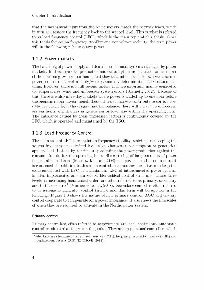
Doctoral theses at NTNU, 2017:48 Doctoral theses at NTNU, 2017:48 Anne Mai Ersdal Anne Mai Ersdal Model predictive load-frequency control ISBN 978-82-326-2168-2 (printed version) ISBN 978-82-326-2169-9 (electronic version) ISSN 1503-8181 NTNU Norwegian University of Science and Technology Faculty of Information Technology, Mathematics and Electrical Engineering Department of Engineering Cybernetics
Transcript of FRQWURO - ntnuopen.ntnu.no
Doctoral theses at NTNU, 2017:48
Doctoral theses at NTN
U, 2017:48
Anne Mai Ersdal
Anne Mai Ersdal
Model predictive load-frequencycontrol
ISBN 978-82-326-2168-2 (printed version)ISBN 978-82-326-2169-9 (electronic version)
ISSN 1503-8181
NTNU
Nor
weg
ian
Univ
ersi
ty o
fSc
ienc
e an
d Te
chno
logy
Facu
lty o
f Inf
orm
atio
n Te
chno
logy
,M
athe
mat
ics
and
Elec
tric
al E
ngin
eerin
gDe
part
men
t of E
ngin
eerin
g Cy
bern
etic
s

Norwegian University of Science and Technology
Thesis for the degree of Philosophiae Doctor
Anne Mai Ersdal
Model predictive load-frequencycontrol
Trondheim, February 2017
Faculty of Information Technology,Mathematics and Electrical EngineeringDepartment of Engineering Cybernetics

NTNUNorwegian University of Science and Technology
Thesis for the degree of Philosophiae Doctor
Faculty of Information Technology, Mathematics and Electrical Engineering Department of Engineering Cybernetics
© Anne Mai Ersdal
ISBN 978-82-326-2168-2 (printed version)ISBN 978-82-326-2169-9 (electronic version) ISSN 1503-8181ITK-report: 2017-6-W
Doctoral theses at NTNU, 2017:48
Printed by Skipnes Kommunikasjon as
Summary
The decrease in frequency quality seen in the Nordic power system over the pasttwo decades is a clear token of the major changes that power systems all around theworld are facing. These changes are to a large extent connected to the green shift inenergy production, which results in less controllable power production. Addition-ally, there are bottlenecks in the Nordic transmission grid, which at times excludesome of the resources from participating in frequency control, and the power trad-ing between the Nordic and the Continental European system is increasing, whichmeans that the Nordic system is being subjected to higher and more unpredictableconsumption.
One important mean for improving the frequency quality is to improve the loadfrequency control (LFC), which is the continuous operation of keeping producedand consumed power equal all times. With the Nordic power system in mind,an important task will be to implement a fully operable automatic generator con-trol (AGC), which automatically controls the power-production set point of eachgenerator. AGC was first implemented in the Nordic system in 2013, and due tounexpectedly high expenses, it is still not fully up and running. This thesis aims atinvestigating model predictive control (MPC) as a control design method for AGC,with application to the Nordic power system. It is believed that the natural han-dling of multiple inputs and system constraints, as well as the optimizing nature ofMPC makes it a promising candidate for AGC.
The main contribution of this thesis is an MPC-based solution to the LFC/AGCproblem, where state feedback is achieved through a state estimator and a simplifiedsystem model is used both in the MPC predictions and the state estimator. Systemconstraints include production limits and limits on generation rate of change, as wellas constraints on tie-line power transfer capacity. In order to include constraintson the individual generating units, and not only on the aggregated generating unitsof the simplified model, the participation factors of each generator are included asoptimization variables. Simulations on a proxy model show that the MPC-basedsolution outperforms a traditional PI-based solution. In order to make the controllermore robust against fluctuations in produced wind power, a multi-stage nonlinearMPC (MNMPC) is also presented. Based on estimates of the worst-case deviationin produced wind-power, the MNMPC makes sure there is enough available transfercapacity on tie lines to make use of all resources in case of large deviations in wind-power production. The approach of stochastic NMPC (SNMPC) is also tested as analternative to the MNMPC. The SNMPC has the theoretical advantage of stochasticguarantees for constraint fulfillment in the presence of disturbances (deviations in
i

produced wind power), while the MNMPC shows better tractability and is lesslikely to encounter feasibility issues.
Using the power transfer in high voltage direct current (HVDC) lines as con-trollable inputs to the system is also investigated as a method for improving anglestability, which is a different part of power system stability. The method of back-stepping was applied in this part of the thesis, which is a control-design method thatis not based on online optimization, contrary to the MPC. The work shows thatHVDC-lines can contribute in stabilizing the overall stability of a power system.
ii

Preface
This thesis is submitted in partial fulfillment of the requirements for the degree ofPhilosophiae Doctor (PhD) at the Norwegian University of Science and Technology(NTNU). The research has been conducted at the Department of Engineering Cy-bernetics (ITK) from August 2011 to October 2016. Funding for the research hasbeen provided by the Research Council of Norway Project 207690 Optimal PowerNetwork Design and Operation, for which I am very grateful.
First of all, I would like to show my gratitude to my supervisor Professor LarsImsland for all his encouragement, guidance and valuable inputs throughout thisperiod. I am very grateful for his support, and would like to thank him for alwaystaking the time to answer all my questions and offering his advise. It has been veryinspiring to have a supervisor who is so committed, and takes a genuine interest inmy work. I would also like to thank my co-supervisor Professor Kjetil Uhlen for allhis guidance, comments and suggestions. His eminent knowledge and experiencewithin power systems has been a very important contribution to this thesis, and Ihave learned a great deal from cooperating with him.
During the spring of 2013 I had the privilege of visiting Professor Nina F. Thorn-hill at Imperial College London. This was a very inspiring time, and I would liketo thank both Professor Thornill and Dr. Davide Fabozzi for close collaborationand very valuable inputs to my work. In many ways it defined the path I took inmy research, and this thesis would not have been the same without it.
I would also like to thank the members of my thesis committee, Professor BikashPal, Associate Professor Sebastien Gros, and Professor Marta Molinas, for theefforts and time you have spent on reviewing this thesis.
During my time at the department, I have enjoyed close friendship and goodcolleagueship with Anders Willersrud, Tor Aksel Heirung, Joakim Haugen, BrageRugstad Knudsen, Bjarne Grimstad, Parsa Rahmanpour, Hodjat Rahmati, EleniKelasidi, Mansoureh Jesmani, and several others. I have had a great time, sharingdiscussions, laughs and fellowship. I was also fortunate to make many new friendsduring my time in London, and would like to take the opportunity to express mygratitude to Ines M Cecılio, Sara Budinis, Adele Slotsvik, Pedro Rivotti, YuanyuanMa, Dionysios Xenos, Denis Schulze, and Alexandra Krieger for the warm andwelcoming atmosphere.
I would also like to thank my parents and my sister. Firts of all for being sur-vivors, and secondly for their unconditional support and encouragement, especiallyafter Edith’s arrival. Finishing this thesis would not have been easy without you,and without all your help with babysitting and daily dinner invitations. A special
iii

thank you to my father for introducing me to Engineering Cybernetics, and foralways helping me with my math homework. I am also deeply grateful to Ørjanfor always being there to support, encourage and comfort me, and for always beingso helpful and understanding. And last, but not least, I want to thank Edith; forsleepless nights, new priorities, and for being an endless source of love and motiva-tion.
Anne Mai ErsdalTromsø, February 2017
iv

Contents
1 Introduction 11.1 Introduction to Power Systems 11.2 Introduction to model predictive control 101.3 Software 201.4 Research objective 211.5 Outline and Contributions 21
2 Model predictive load-frequency control 252.1 Introduction 252.2 Modelling 282.3 Controller 322.4 Case Study 372.5 Discussion 432.6 Conclusion 45
3 Model predictive load-frequency control taking into account imbalanceuncertainty 473.1 Introduction 473.2 Modeling 513.3 Controller 573.4 Robustified NMPC 603.5 Case Study 633.6 Discussion 673.7 Conclusion 68
4 Scenario-based approaches for handling uncertainty in MPC for power systemfrequency control 714.1 Introduction 714.2 Model description 734.3 Controller 744.4 Case Study 784.5 Conclusion 84
5 Coordinated control of multiple HVDC links using backstepping 855.1 Introduction 855.2 System description 86
v

Contents
5.3 Controller Design 885.4 Network example 905.5 Discussion 965.6 Conclusion 98
6 Concluding remarks 99
vi

Abbreviations
AC Alternating currentACE Area control errorAGC Automatic generator controlAVR Automatic voltage regulatorCMPC Centralized model predictive controlCPM Control performance measureDAE Differential algebraic equationDC Direct currentDMPC Distributed model predictive controlEKF Extended Kalman filterFACTS Flexible alternating current transmission systemFCR Frequency containment reservesFRR Frequency restoration reservesHVDC High voltage direct currentIP Interior pointKF Kalman filterLFC Load frequency controlLP Linear programmingMNMPC Multi-stage nonlinear model predcitive controlMPC Model predictive controlNERC North American electric reliability corporationNLP Nonlinear programmingNMPC Nonlinear model predictive controlNNMPC Nominal nonlinear model predictive controlOCP Optimal control problemPI Proportional integralPID Proportional integral derivativePM Prediction modelPMU Phasor measurement unitPRM Plant replacement modelPSS Power system stabilizerRMPC Robust model predictive controlRNMPC Robustified nonlinear model predictive controlRR Replacement reservesSMPC Stochastic model predictive controlSNMPC Stochastic nonlinear model predictive control
vii

Contents
SQP Sequential quadratic programmingTSO Transmission system operatorQP Quadratic programming
viii
Chapter 1
Introduction
This chapter presents some background information on power systems in general,and the Nordic power system in particular. Power systems all around the worldare currently facing large changes, much because of the green shift seen in powerproduction, and the challenges related to this will be discussed. This aim of thisthesis is to investigate model predictive control (MPC) as a mean to solve some ofthese challenges, and the basics of MPC and nonlinear MPC (NMPC) will thereforebe presented as well.
1.1 Introduction to Power Systems
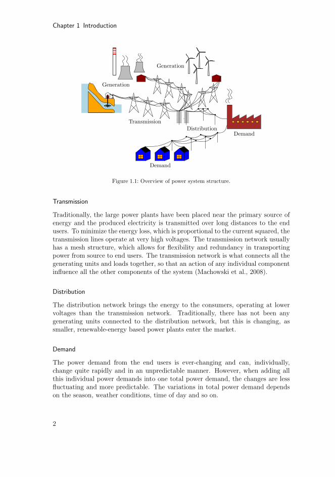
Modern power systems are large, complex, dynamical systems whose main task isto provide electric energy to the end user, i.e. the industry, households, agricultureand so on. The structure of these power systems can be divided into four mainparts: Generation, transmission, distribution and demand, see Figure 1.1.
Since the 1990s the energy markets have been liberalized. In a typical liberalizedmodel, there are several private companies who generate power using their ownindividual power stations, and who compete against each other in selling it. Thetransmission of the power is usually operated by one transmission system operator(TSO), which has monopoly and is independent of the generation companies. Thedistribution of power to the end users is also handled by several private companies,which own and manage the distribution network in their area. Finally there arethe companies who are responsible for retail, by buying power from the generationcompanies and selling it to the end users.
Generation
The main sources of electrical energy to the power system is the kinetic energy ofwater and the thermal energy derived from fossil fuels and nuclear fission (Kundur,1994). The task of the prime movers (often turbines) is to convert this kineticenergy into mechanical energy, which in turn is converted into electrical energyby the synchronous generators. A synchronous generator is a generator where, atsteady state, the frequency of the delivered output current is synchronized with therotation of the generator rotor. When many such generators work together in anetwork, they will all synchronize with the same network frequency at steady state.
1
Chapter 1 Introduction
Generation
TransmissionDistribution
Demand
Demand
Generation
Figure 1.1: Overview of power system structure.
Transmission
Traditionally, the large power plants have been placed near the primary source ofenergy and the produced electricity is transmitted over long distances to the endusers. To minimize the energy loss, which is proportional to the current squared, thetransmission lines operate at very high voltages. The transmission network usuallyhas a mesh structure, which allows for flexibility and redundancy in transportingpower from source to end users. The transmission network is what connects all thegenerating units and loads together, so that an action of any individual componentinfluence all the other components of the system (Machowski et al., 2008).
Distribution
The distribution network brings the energy to the consumers, operating at lowervoltages than the transmission network. Traditionally, there has not been anygenerating units connected to the distribution network, but this is changing, assmaller, renewable-energy based power plants enter the market.
Demand
The power demand from the end users is ever-changing and can, individually,change quite rapidly and in an unpredictable manner. However, when adding allthis individual power demands into one total power demand, the changes are lessfluctuating and more predictable. The variations in total power demand dependson the season, weather conditions, time of day and so on.
2

1.1 Introduction to Power Systems
Power system stability
Rotor angle stability Voltage stability
Small
angle stability
Transientstability
Large
voltage stability
Small
voltage stabilitydisturbance disturbancedisturbance
Frequency stability
Figure 1.2: Classification of power system stability (Machowski et al., 2008).
1.1.1 Power System Stability
In Kundur et al. (2004), the definition of power system stability is given as:
The ability of an electric power system, for a given initial operatingcondition, to regain a state of operating equilibrium after being sub-jected to a physical disturbance, with most system variables boundedso that practically the entire system remains intact.
When discussing power system stability, it is normal to divide the concept into threeparts: rotor angle stability, frequency stability and voltage stability, see Figure 1.2.
The rotor angle stability is the system’s ability to maintain synchronization ofthe generators after a severe (transient angle stability) or smaller (small distur-bance angle stability) momentary disturbance. These faults are often caused byshort circuits in the transmission network, and are often cleared without having tointerfere with the amount of mechanical power provided by the prime movers. Therotor angle stability is fairly well preserved using power system stabilizers (PSS),thyristor exciters, fast fault clearing and so on (Bevrani et al., 2011).
Voltage stability is the system’s ability to maintain the voltages of the systemat acceptable levels after being subjected to a disturbance. The voltage stabilityis strongly coupled with the reactive power balance in the power system, and itis stabilized by the automatic voltage regulator (AVR) which controls the internalvoltage of the generators.
Contrary to rotor angle stability, the frequency stability of a system is relatedto long-term imbalance between generation and consumption of active power. Thisactive power imbalance will initially be covered by the kinetic energy of the rotat-ing masses in the system (turbines, generators, motors), causing the frequency tochange in a similar manner to the level in a water tank: as the water level rises/fallswhen there is a surplus/shortage of supplied water, so does the frequency of a powersystem when there is a surplus/shortage of produced power. However, this is nopermanent solution, and such a power imbalance requires actions to be made so
3
Chapter 1 Introduction
that the mechanical input from the prime movers match the network loads, whichin turn will restore the frequency back to the wanted level. This is what is referredto as load frequency control (LFC), which is the main topic of this thesis. Sincethis thesis focuses on frequency stability and not voltage stability, the term powerwill in the following refer to active power.
1.1.2 Power markets
The balancing of power supply and demand are in most systems managed by powermarkets. In these markets, production and consumption are balanced for each hourof the upcoming twenty-four hours, and they take into account known variations inpower production as well as daily/weekly/annually deterministic load variation pat-terns. However, there are still several factors that are uncertain, mainly connectedto temperatures, wind and unforeseen system errors (Statnett, 2012). Because ofthis, there are also intra-day markets where power is traded up to one hour beforethe operating hour. Even though these intra-day markets contribute to correct pos-sible deviations from the original market balance, there will always be unforeseensystem faults and changes in generation or load also within the operating hour.The imbalance caused by these unforeseen factors is continuously covered by theLFC, which is operated and maintained by the TSO.
1.1.3 Load Frequency Control
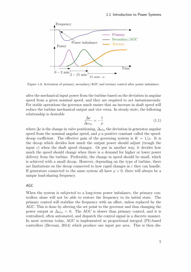
The main task of LFC is to maintain frequency stability, which means keeping thesystem frequency at a desired level when changes in consumption or generationappear. This is done by continuously adapting the power production against theconsumption during the operating hour. Since storing of large amounts of powerin general is inefficient (Machowski et al., 2008), the power must be produced as itis consumed. In addition to this main control task, another incentive is to keep thecosts associated with LFC at a minimum. LFC of interconnected power systemsis often implemented as a three-level hierarchical control structure. These threelevels, in increasing hierarchical order, are often referred to as primary, secondaryand tertiary control1 (Machowski et al., 2008). Secondary control is often referredto as automatic generator control (AGC), and this term will be applied in thefollowing. Figure 1.3 shows the nature of how primary control, AGC and tertiarycontrol cooperate to compensate for a power imbalance. It also shows the timescalesof when they are required to activate in the Nordic power system.
Primary control
Primary controllers, often referred to as governors, are local, continuous, automaticcontrollers situated at the generating units. They are proportional controllers which
1Also known as frequency containment reserve (FCR), frequency restoration reserve (FRR) andreplacement reserve (RR) (ENTSO-E, 2012).
4
1.1 Introduction to Power Systems
0− 2 min2− 15 min
15 min →
Time
Power
Frequency
Power imbalance
Primary
Secondary/AGC
Tertiary
Figure 1.3: Activation of primary, secondary/AGC and tertiary control after power imbalance.
alter the mechanical input power from the turbine based on the deviation in angularspeed from a given nominal speed, and they are required to act instantaneously.For stable operations the governor much ensure that an increase in shaft speed willreduce the turbine mechanical output and vice versa. In steady state, the followingrelationship is desirable
∆c
∆ωm= −1
ρ(1.1)
where ∆c is the change in valve positioning, ∆ωm the deviation in generator angularspeed from the nominal angular speed, and ρ a positive constant called the speed-droop coefficient. The effective gain of the governing system is K = 1/ρ. It isthe droop which decides how much the output power should adjust (trough theinput c) when the shaft speed changes. Or put in another way, it decides howmuch the speed should change when there is a demand for higher or lower powerdelivery from the turbine. Preferably, the change in speed should be small, whichis achieved with a small droop. However, depending on the type of turbine, thereare limitations on the droop connected to how rapid changes in c they can handle.If generators connected to the same system all have ρ > 0, there will always be aunique load-sharing frequency.
AGC
When the system is subjected to a long-term power imbalance, the primary con-trollers alone will not be able to restore the frequency to its initial state. Theprimary control will stabilize the frequency with an offset, unless replaced by theAGC. This is done by altering the set point to the governor and thus changing thepower output at ∆ωm = 0. The AGC is slower than primary control, and it iscentralized, often automated, and dispatch the control signal in a discrete manner.In most systems today, AGC is implemented as proportional integral (PI)-basedcontrollers (Bevrani, 2014) which produce one input per area. This is then dis-
5
Chapter 1 Introduction
tributed to the generating units of each area using participation factors, α, whichdefine the contribution of the individual generating units to the total generation(Machowski et al., 2008).
When there are multiple areas connected by tie lines with given power-flow setpoints, the AGC also tries to restore the power flow on the tie lines to these setpoints. The control input is then a combination of the frequency offset and the tie-line offset called the area control error (ACE). Because the Nordic power systemis operated as a unity with common markets, there is no need to minimize tie-lineoffsets, as long as the power flow is kept within the tie-line boundaries. Hence, suchtie-line set points will not be included in this work.
Tertiary control
Tertiary control is additional to, and slower than, AGC and primary control. It ismainly executed manually by the TSO, and its purpose is to ensure (Machowskiet al., 2008)
• Adequate AGC spinning reserves2.
• Optimal dispatch of units participating in AGC.
• Restoration of bandwidth of AGC.
Tertiary control is executed either via changing the AGC set point or by connectingor disconnecting generating units that participate in tertiary control.
1.1.4 The Nordic power system and challenges within LFC
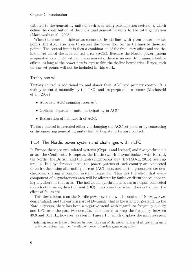
In Europe there are two isolated systems (Cyprus and Iceland) and five synchronousareas: the Continental European, the Baltic (which is synchronized with Russia),the Nordic, the British, and the Irish synchronous area (ENTSO-E, 2015), see Fig-ure 1.4. In a synchronous area, the power systems of each country are connectedto each other using alternating current (AC) lines, and all the generators are syn-chronous; sharing a common system frequency. This has the effect that everycomponent of a synchronous area will be affected by faults or disturbances appear-ing anywhere in that area. The individual synchronous areas are again connectedto each other using direct current (DC) interconnection which does not spread theeffect of faults etc.
This thesis focuses on the Nordic power system, which consists of Norway, Swe-den, Finland, and the eastern part of Denmark, that is the island of Zealand. In theNordic system, there has been a negative trend with regards to frequency qualityand LFC over the past two decades. The aim is to keep the frequency between49.9 and 50.1 Hz, however, as seen in Figure 1.5, which displays the minutes spent
2Spinning reserves is the difference between the sum of the power ratings of all operating unitsand their actual load, i.e. “available” power of on-line generating units.
6
1.1 Introduction to Power Systems
Figure 1.4: Synchronous and isolated areas in Europe (ENTSO-E, 2015).
7
Chapter 1 Introduction
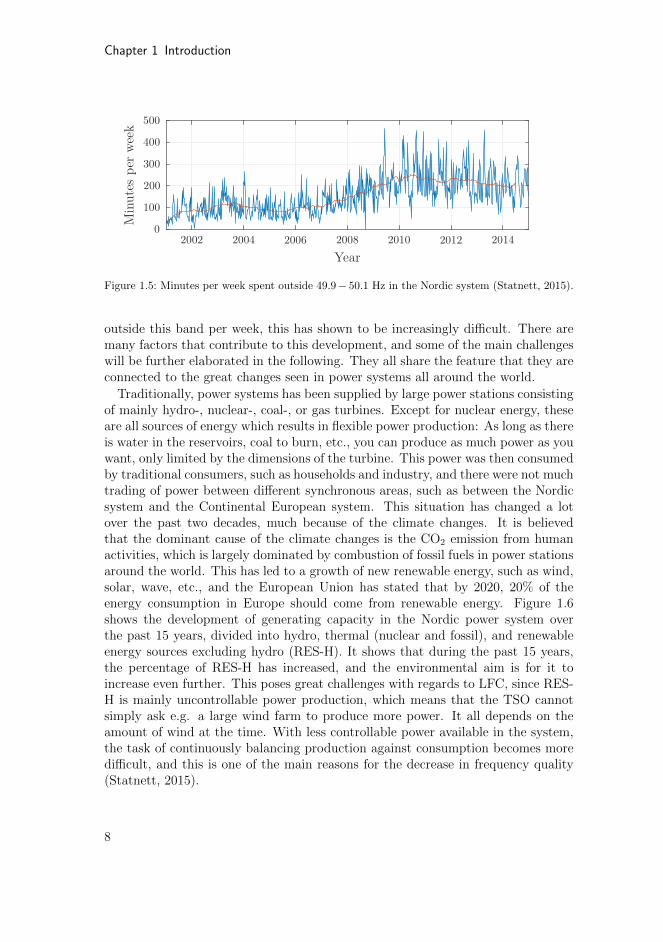
Figure 1.5: Minutes per week spent outside 49.9− 50.1 Hz in the Nordic system (Statnett, 2015).
outside this band per week, this has shown to be increasingly difficult. There aremany factors that contribute to this development, and some of the main challengeswill be further elaborated in the following. They all share the feature that they areconnected to the great changes seen in power systems all around the world.
Traditionally, power systems has been supplied by large power stations consistingof mainly hydro-, nuclear-, coal-, or gas turbines. Except for nuclear energy, theseare all sources of energy which results in flexible power production: As long as thereis water in the reservoirs, coal to burn, etc., you can produce as much power as youwant, only limited by the dimensions of the turbine. This power was then consumedby traditional consumers, such as households and industry, and there were not muchtrading of power between different synchronous areas, such as between the Nordicsystem and the Continental European system. This situation has changed a lotover the past two decades, much because of the climate changes. It is believedthat the dominant cause of the climate changes is the CO2 emission from humanactivities, which is largely dominated by combustion of fossil fuels in power stationsaround the world. This has led to a growth of new renewable energy, such as wind,solar, wave, etc., and the European Union has stated that by 2020, 20% of theenergy consumption in Europe should come from renewable energy. Figure 1.6shows the development of generating capacity in the Nordic power system overthe past 15 years, divided into hydro, thermal (nuclear and fossil), and renewableenergy sources excluding hydro (RES-H). It shows that during the past 15 years,the percentage of RES-H has increased, and the environmental aim is for it toincrease even further. This poses great challenges with regards to LFC, since RES-H is mainly uncontrollable power production, which means that the TSO cannotsimply ask e.g. a large wind farm to produce more power. It all depends on theamount of wind at the time. With less controllable power available in the system,the task of continuously balancing production against consumption becomes moredifficult, and this is one of the main reasons for the decrease in frequency quality(Statnett, 2015).
8

1.1 Introduction to Power Systems
Figure 1.6: Installed generation capacity in the Nordic power system (Nordel, 2008; ENTSO-E,2014).
This increase in uncontrollable power production is present all across Europe,and one way of making all the synchronous areas of Europe less affected is byincreasing the DC-connections between them, allowing them to cooperate in thetask of fading out non-renewable energy. One idea is to use the hydro-dominantNordic system as a battery for the increasingly wind- and sun influenced ContinentalEuropean system. This means more power transfer in and out of the Nordic system,resulting in higher and more unpredictable consumption, which also contributes tothe decrease in frequency quality (Statnett, 2015).
In addition to the challenges related to the green shift in energy production, theNordic system has not been expanded concurrent with the increasing energy needand the tighter connection to Continental Europe, leaving it under-dimensionedand operating close to its maximum transfer capacity (Statnett, 2015). This hasled to an increasing amount of of bottlenecks, which at times excludes some ofthe resources from participating in LFC, and according to Statnett (2015) thereis a tendency to a strong correlation between frequency incidents (i.e. minutesspent outside 49.9− 50.1 Hz) per week and the number and duration of bottleneckcongestions that week.
The last challenge mentioned here is the challenge of the hourly production set-point shifts. The change in power-production set points happens on the hour inthe Nordic system, while the change in consumption naturally happens during thehour. This leads to a large deviation between production and consumption at everyhour shift, resulting in large frequency deviations. In addition, the change in powerflow on the connecting DC lines also happens on the hour, which amplifies theproblem as the connection and trading with Continental Europe increase.
Figure 1.5 also shows that the number of frequency incidents has stabilized anddecreased some since 2011. This is mainly because of actions taken by the NordicTSOs since 2008, some of which temporary, resulting in better market solutions,more flexible power exchange with Continental Europe, and also an improved LFC.
9
Chapter 1 Introduction
In fact, the Nordic system did not practice AGC until 2013, and it is still not fullyup and running, much because of unexpectedly high expenses due to incompleteAGC market solutions (Statnett, 2015). This is however an ongoing project, andthe frequency quality is still far from the wanted levels. It is expected that thetemporary solutions will be replaced by among others a fully operable AGC inthe years to come, which is considered to be an important part of improving thefrequency quality. It is therefore of interest to find methods of conducting AGCwhich aid the power system in resolving some of the issues related to bottlenecksand the increasing amount of uncontrollable power production, and it is believedthat MPC could be an efficient solution.
1.2 Introduction to model predictive control
Model predictive control (MPC) is an advanced control method which has its rootsin optimal control, and it is one of the few advanced control methods that has madea significant impact on industrial control engineering (Maciejowski, 2002). MPCcomes in many shapes and sizes, however, they all share the same basic concept:a model of the system to be controlled is used to predict and optimize the futuresystem behavior. This is done by solving an optimal control problem (OCP), whichforms the heart of an MPC. A general discrete-time OCP is as follows
minxk,uk∀k=1,...,M
J (xk, uk) (1.2a)
subjected to
x0 − xinit = 0 (1.2b)
xk+1 − f (xk, uk, wk) = 0 ∀ k = 1, . . . ,M (1.2c)
g (xk, uk) ≤ 0 ∀ k = 1, . . . ,M (1.2d)
r (xM) ≤ 0 (1.2e)
where xk are the dynamic system states, uk the controllable system inputs, andwk the system disturbance. Equation (1.2b) is the fixed initial state, (1.2c) thesystem model, (1.2d) the path constraints, and (1.2e) the terminal constraints.The objective function
J (xk, uk) =M−1∑
k=0
L (xk, uk) + E (xM) (1.3)
is a central part of the OCP, and it consists of a stage cost L (xk, uk) and a ter-minal cost E (xM) (often referred to as the Lagrange term and the Mayer term,respectively). When solving the OCP, one finds the inputs uk which minimize theobjective function J(·) over the control horizon M , while fulfilling all system con-straints (1.2b)-(1.2e). The objective function J(·) and the control horizon M are
10
1.2 Introduction to model predictive control
x∗k
t
t+ 1
t+M
Past Future
t+M + 1
x∗k
xku∗k
xk
u∗k
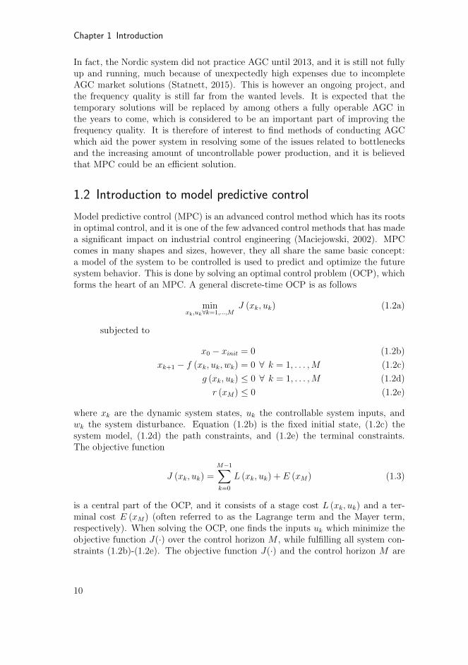
Figure 1.7: The receeding-horizon principle, k = 1, . . . ,M .
the main tuning variables of the OCP. The objective function states what is actu-ally regarded as optimal and what should be prioritized, while the control horizondictates how much of the future system behavior that should be included. In theobjective function it is common to punish deviations from a wanted steady stateor state trajectory x∗k, so that the optimal input u∗k steers the state to this value.
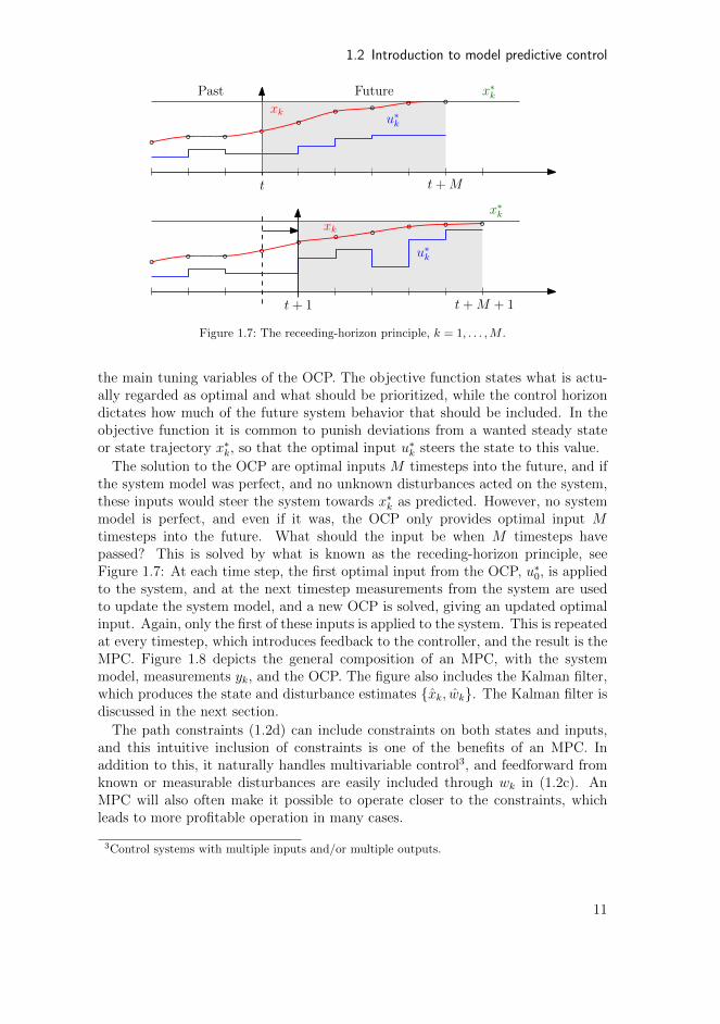
The solution to the OCP are optimal inputs M timesteps into the future, and ifthe system model was perfect, and no unknown disturbances acted on the system,these inputs would steer the system towards x∗k as predicted. However, no systemmodel is perfect, and even if it was, the OCP only provides optimal input Mtimesteps into the future. What should the input be when M timesteps havepassed? This is solved by what is known as the receding-horizon principle, seeFigure 1.7: At each time step, the first optimal input from the OCP, u∗0, is appliedto the system, and at the next timestep measurements from the system are usedto update the system model, and a new OCP is solved, giving an updated optimalinput. Again, only the first of these inputs is applied to the system. This is repeatedat every timestep, which introduces feedback to the controller, and the result is theMPC. Figure 1.8 depicts the general composition of an MPC, with the systemmodel, measurements yk, and the OCP. The figure also includes the Kalman filter,which produces the state and disturbance estimates {xk, wk}. The Kalman filter isdiscussed in the next section.
The path constraints (1.2d) can include constraints on both states and inputs,and this intuitive inclusion of constraints is one of the benefits of an MPC. Inaddition to this, it naturally handles multivariable control3, and feedforward fromknown or measurable disturbances are easily included through wk in (1.2c). AnMPC will also often make it possible to operate closer to the constraints, whichleads to more profitable operation in many cases.
3Control systems with multiple inputs and/or multiple outputs.
11
Chapter 1 Introduction
OCP
u∗0
System
yk
Kalman filterxk, wk
MPC
x∗k
wk
xk+1 = f(xk, uk, wk)yk = h(xk, uk)
u∗kConstraints
Figure 1.8: General composition of an MPC.
1.2.1 Feedback and updating the system model
The MPC predicts and optimizes the behavior of the system model, not the actualsystem itself. And in order for the MPC to function properly it is important thatthe model accurately (enough) reflects the most interesting properties of the actualsystem. However, it is also important that the model is not too detailed andcomplicated, as the OCP must be solved in time for the next timestep. One musttherefore expect model errors and unknown/unmodelled disturbances in an MPC,and updating the system model in order to maintain good quality predictions isalways necessary. One way of achieving this is through Kalman filtering.
The original Kalman filter (KF) was published by Rudolf E. Kalman in 1960,and it is a method for estimating the states of a linear system. A KF is a recursivealgorithm which exploits knowledge of both the system as well as the disturbancesit is subjected to, in order to estimate the state vector so that the mean squaredestimated error is minimized. The KF is run at each time step, and it involvesfour main steps: the incrementation of time, the integration, the computation ofthe Kalman gain, and the measurement update. After the time is incremented,the estimate is integrated forward in time using a system model. This estimateis then refined during the measurement update, using the current measurementand the Kalman gain. The Kalman gain is the solution to the Riccati equation(Simon, 2006), and it will in general decide how much to trust the model and howmuch to trust the measurements (through provided information of their respectedaccuracy). The Kalman filter (KF) has become popular within many areas of ap-plication, especially since the extended Kalman filter (EKF) for non-linear systemswas introduced in the late 1960s (Simon, 2006). The KF adapts the state estimateto fit the measurements from the true system response, and thereby updating thesystem model. The KF can also be modified to include estimation of unmeasurable,time varying disturbances, so that they can be included in the feed-forward part ofthe MPC.
12
1.2 Introduction to model predictive control
1.2.2 Solving the OCP
Solving an OCP is the same as solving a general optimization problem where (1.2b)-(1.2e) are all seen as equality and inequality constraints. A general optimizationproblem can be defined as
minυ
Γ(υ) (1.4a)
subject to
Θ(υ) = 0 (1.4b)
Σ(υ) ≤ 0 (1.4c)
where υ are the optimization variables, Γ(υ) the objective function, Θ(υ) the equal-ity constraints, and Σ(υ) the inequality constraints. Comparing to the OCP (1.2),(1.2b) and (1.2c) are equality constraints, while (1.2d) and (1.2e) are inequalityconstraints.
General optimization problems are solved through numerical optimization us-ing iteration-based algorithms, and there are many different types of optimizationproblems, which can be solved by many different algorithms. There are howeversome common classifications, and optimization problems sharing the same classifi-cation can in general be solved by the same algorithms. It is common to classifyoptimization problems using two different axes: convex vs. non-convex and linearvs. non-linear. An optimization problem such as (1.4) is said to be convex if theobjective function and the inequality constraint function are convex and the equal-ity constraint function is linear, otherwise it is non-convex (Nocedal and Wright,2006). A convex optimization problem is in general much easier to solve than anon-convex optimization problem, and all local optima are global optima, hencea global solution is always found (if a solution exists). Non-convex optimizationproblems can be more challenging, as they tend to have several stationary pointsand local optima. In a non-convex optimization problem one can find either a lo-cal or a global solution, the former can however be a quite challenging task, andmany algorithms return a local optima. The axis of linear vs. non-linear is basedon whether the system constraints (including the system model of an OCP) andthe objective function are linear or nonlinear, which results in the following threeclassifications
• Linear programming (LP). In an LP formulation, the objective function islinear, and so are all system constraints. Optimization problems of this typeare always convex, and they are probably the most widely solved optimizationproblems, especially within financial and economic applications (Nocedal andWright, 2006). They are easily solved with well known algorithms, and willalways produce a global optimum.
• Nonlinear programming (NLP). In an NLP formulation, either the sys-tem constraints or the objective function are nonlinear. These problems tends
13

Chapter 1 Introduction
to arise naturally in physical systems, however, they are more difficult, andhence more time consuming, to solve. An NLP can be either convex or non-convex, and this is what decides the difficulty of the NLP and which al-gorithms that can be used to solve it. A convex NLP can often be solvedefficiently using the same type of algorithms that are efficient for LP formu-lations.
• Quadratic Programming (QP). The QP formulation is a special case ofNLP, where the system constraints are linear, while the objective functionis quadratic. The characteristics of a QP can be exploited to find efficientalgorithms, and if a QP is convex it is often similar in difficulty to an LP(Nocedal and Wright, 2006). Convexity of a QP is rather simple to identify,as it is given by positive semi-definiteness of the Hessian H of the objectivefunction Γ(υ) = cTυ + υTHυ. A QP can always be solved or shown to beinfeasible in a finite amount of computations (Nocedal and Wright, 2006).
An OCP with a linear system model is often either an LP or a QP (unless thereare other nonlinear constraints), while an OCP with a nonlinear system model asequality constraint always will be a non-convex NLP. The distinction between linearand nonlinear system model is therefore important when it comes to the solvabilityand efficiency of an OCP, and it is the most important classification for an MPC:linear MPC and nonlinear MPC (NMPC). In this thesis, NMPC is applied, andhence a non-convex NLP is solved at each time step. The two most commonclasses of algorithms used to solve NLPs are sequential quadratic programming(SQP) methods, and interior-point (IP) methods. See Nocedal and Wright (2006)for more information on numerical optimization.
Continuous-time OCP
It is from now on assumed that the system model of (1.2) is nonlinear, and hencethat the discrete-time OCP is an NLP. As seen from (1.2a), the OCP has 2Moptimization variables consisting of both the states xk and the inputs uk, k =1, . . . ,M , and the NLP solver actually solves both the simulation problem andthe optimization problem at the same time. When dealing with system modelsand objective functions that are continuous, forming a continuous-time OCP, therewill be infinitely many optimization variables: x(t), u(t), ∀t ∈ [0, T ], where Tis the continuous-time control horizon. There are in general two approaches forsolving continuous-time OCPs: indirect or direct approaches (Biegler, 2010). Theindirect approach is often described as “first optimize, then discretize”. This leadsto a boundary value problem, which is often quite difficult to solve. The directapproach can be described as “first discretize, then optimize”. Here, the controltrajectory is parameterized in finite dimension, leaving a discrete-time OCP, whichcan be solved as an NLP. The most common methods for parameterization is singleshooting, multiple shooting, and collocation (Biegler, 2010).
14

1.2 Introduction to model predictive control
Collocation has been the method of choice in this thesis, and the details for thecollocation setup is therefore presented here. Given a general continuous-time OCP
minx(t),u(t)∀t=0,...,T
J (x(t), u(t)) (1.5a)
subjected to
x(0)− xinit = 0 (1.5b)
x(t)− f (x(t), u(t), w(t)) = 0 ∀ t = 0, . . . , T (1.5c)
g (x(t), u(t)) ≤ 0 ∀ t = 0, . . . , T (1.5d)
r (x(T )) ≤ 0 (1.5e)
With collocation this OCP is discretized in both control and states on a fixed grid.The optimization horizon T is first divided into N elements of length h, and withineach element the state profile is approximated using polynomial representationof order K + 1. A common choice of polynomial representation is the Lagrangeinterpolation polynomial, and with K + 1 interpolations points in element i, thestate in element i is approximated as (Biegler, 2010)
t = ti + hiτ (1.6)
xK(t) =K∑
j=0
lj(τ)xij (1.7)
where
lj(τ) =K∏
k=0,6=j
τ − τkτj − τk
(1.8)
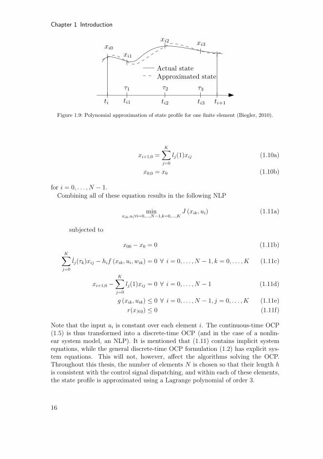
and t ∈ [ti, ti+1], τ ∈ [0, 1], τ0 = 0, τj < τj+1 and j = 0, . . . , K − 1. This approxi-mation has the property that the approximated states xK and the actual states xare equal at each interpolation point τj, see Figure 1.9.
The same can be done for the state time derivative, and by using these ap-proximations one can get equations which ensures that the equation for the timederivative is fulfilled at the collocation points. These are called the colloctaionequations, and for the Lagrange polynomial they are as follows
K∑
j=0
xijdlj(τk)
dτ= hif(xik, uik) (1.9)
for k = 1, . . . , K and i = 0, . . . , N − 1.In order to ensure continuity of the state profile in the element junctions, conti-
nuity equations are needed. For Lagrange interpolation profiles they are as follows
15
Chapter 1 Introduction
ti ti+1
τ1 τ2 τ3
xi0xi1
xi2 xi3
ti1 ti2 ti3
Actual stateApproximated state
Figure 1.9: Polynomial approximation of state profile for one finite element (Biegler, 2010).
xi+1,0 =K∑
j=0
lj(1)xij (1.10a)
x0,0 = x0 (1.10b)
for i = 0, . . . , N − 1.
Combining all of these equation results in the following NLP
minxik,ui∀i=0,...,N−1,k=0,...,K
J (xik, ui) (1.11a)
subjected to
x00 − x0 = 0 (1.11b)
K∑
j=0
lj(τk)xij − hif (xik, ui, wik) = 0 ∀ i = 0, . . . , N − 1, k = 0, . . . , K (1.11c)
xi+1,0 −K∑
j=0
lj(1)xij = 0 ∀ i = 0, . . . , N − 1 (1.11d)
g (xik, uik) ≤ 0 ∀ i = 0, . . . , N − 1, j = 0, . . . , K (1.11e)
r(xN0) ≤ 0 (1.11f)
Note that the input ui is constant over each element i. The continuous-time OCP(1.5) is thus transformed into a discrete-time OCP (and in the case of a nonlin-ear system model, an NLP). It is mentioned that (1.11) contains implicit systemequations, while the general discrete-time OCP formulation (1.2) has explicit sys-tem equations. This will not, however, affect the algorithms solving the OCP.Throughout this thesis, the number of elements N is chosen so that their length his consistent with the control signal dispatching, and within each of these elements,the state profile is approximated using a Lagrange polynomial of order 3.
16

1.2 Introduction to model predictive control
Feasibility
An important concept for all constrained optimization problems is that of the fea-sible region. The feasible region for the optimization problem (1.4) are those valuesof υ where the constraints (1.4b) and (1.4c) are fulfilled. If this region is non-empty,the optimization problem is feasible, and if there exists no values of υ where allconstraints are fulfilled, the optimization problem is infeasible, i.e. it cannot besolved. Translated to OCP and MPC: If no system input can be found that fulfillsall input constraints, and at the same time results in a system trajectory whichfulfills all state constraints, the OCP is infeasible. This is a severe situation, as noupdated optimal input can be produced, and it is important to have a strategy fordealing with infeasibility. One possible solution is to reuse the input calculated atthe previous timestep. Either by keeping the input unchanged, or by using the con-trol signal u∗1 from the previous timestep. This provides no guarantees for neitherfeasibility nor optimality, but it will work just fine in many situations.
Another possibility is to add slack variables to the soft constraints. Soft con-straints are often state constraints connected to control quality, i.e. violating themwill not cause any immediate danger. On the contrary, there are hard constraints,which are often related to input constraints that cannot be physically violated. Oneexample being a valve, which cannot open more than 100%. The slack variables ε,which must be positive, are added to the soft constraints, and they are also addedto the optimization variables
gs (xk, uk) ≤ εk (1.12a)
εk ≥ 0 (1.12b)
where k = 1, . . . ,M . In order not to use the slack variables unless absolutelynecessary, use of ε is penalized in the objective function
J (xk, uk, εk) =M−1∑
k=0
L (xk, uk) + E (xM) + γεk (1.13)
where γ is a constant of appropriate dimension. In this way, the soft constraintsgs (xk, uk) are allowed to exceed zero in severe situations. In (1.13), ε is linearlyincluded in the objective function, resulting in what is known as an exact penalty,which means that as long as γ is large enough, the constraint will not be violatedunless there is no feasible solution to the original problem (Maciejowski, 2002).
Other possible solutions for dealing with infeasiblity is to actively manage thehorizon or the constraints definition at each timestep, and through this avoid in-feasiblity.
1.2.3 Nominal stability of nonlinear MPC
It is common to consider nominal stability of an NMPC, which is stability of theNMPC with no model uncertainty or unmeasurable disturbance. If one could have
17
Chapter 1 Introduction
an infinite optimization horizon in the NMPC, one could prove nominal asymptoticstability using Lyapunov theory (Grune and Pannek, 2011). But solving an infinitehorizon optimization problem is difficult in general, and the closed-loop NMPCwith finite horizon (as described in Section 1.2) is not necessarily stable. First ofall, it does not make sense to look at the stability of the solution to the OCP, as thisis not what is actually implemented. What is actually implemented is only the firstof the optimized inputs, before a new OCP is solved. In addition it only considersthe system behavior M timesteps into the future, and does not care what happensafter that. Because of this, methods for ensuring nominal asymptotic stability ofan NMPC with finite optimization horizon has developed.
One way is to add stabilizing constraints to the NMPC. Either as equilibriumterminal constraints, demanding that the final state of the optimization horizon isequal to the systems steady state xM = x∗, or as regional terminal constraints andterminal cost (Grune and Pannek, 2011). In the latter, the terminal cost (Mayerterm) E(xM) which is added to the objective function, is defined so that thereexists a controller uk = κ (xk)∀k ≥M such that: (a) E(xM) works as a Lyapunovfunction for the closed loop system on a region X0 around x∗, (b) ensures that X0
is a forward invariant set for the closed loop system. In order to guarantee that thecontroller uk = κ (xk) is feasible for all k ≥ M , one must add a regional terminalconstraint, ensuring that the predicted state at timestep M is inside X0. This is alsoknown as recursive feasibility; ensuring that a feasible solution exists at the nexttimestep. Recursive feasibility is an important part of nominal stability analysis, asno stability can be proven without feasibility guarantees. With recursive feasibilityit is guaranteed that as long as the OCP is feasible at the first timestep, it will alsobe feasible for all future timesteps. By applying either of these methods, asymptoticstability can be proven using Lyapunov theory (Grune and Pannek, 2011).
The methods described above are often good for theoretical purposes, but thereare some practical issues related to implementing them, and they are seldom appliedin industry. For terminal equilibrium constraints the system needs to be controllableto x∗ in finite time, and for regional constraint set and terminal cost a Mayer termwhich can be used to prove stability might be difficult to find. Unison for both themethods is that the optimization horizon often becomes relatively large.
Grune and Pannek (2011) provides another method to prove asymptotic stabilitythrough the choice of objective function J and optimization horizon T . By designingthe Lagrange term of the objective function so that it fulfills certain bounds, alower bound for the optimization horizon which guarantees stability can be found.Finding both these lower bounds as well as the Lagrange term which fulfills them,can be a difficult task. The method can however be used to design a good objectivefunction, even though it may not necessarily prove stability (Grune and Pannek,2011).
18
1.2 Introduction to model predictive control
1.2.4 Robust MPC
The previous section treated the question of stability when no model uncertaintyor unmeasurable disturbances are present. A system model is an approximationof a real life system, and it is often desirable that the model is rather simple andlow dimensional. This is often achieved by designing the model to reflect certainimportant system properties, rather than modeling every detail of the system. Thisapproach results in a model-plant mismatch that naturally introduces uncertainty.In addition, there are also other external disturbances which influence the realsystem, and in order to perform a meaningful control analysis and design, theseuncertainties need to be described by an uncertainty model (Levine, 2010). Suchuncertainty models often define an admissible set of plant models F , and an ad-missible set of uncertain external input signalsW , which allows for system analysissuch as: Is closed-loop stability guaranteed for every system model in F? Will allsystem constraints be fulfilled for every external disturbance in W? It is also com-mon to divide between stochastic and deterministic disturbance models, where theelements of F and W are assigned different probabilities with a stochastic model,and seen as equally likely to occur in a deterministic model (Levine, 2010).
Within MPC, the issue of uncertainty is often addressed through robust MPC(RMPC), which considers uncertainties that are deterministic and lie in a boundedset (Mesbah, 2016; Bemporad and Morari, 1999). The work on RMPC has beendominated by min-max OCP formulations:
minxw,fk ,uk∀k=1,...,M
[max
w∈W,f∈FJ(xw,fk , uk
)](1.14a)
xw,f0 − xinit = 0 ∀ w ∈ W , f ∈ F (1.14b)
xw,fk+1 − f(xw,fk , uk, wk) = 0 ∀ k = 1, . . . ,M,w ∈ W , f ∈ F (1.14c)
g(xw,fk , uk) ≤ 0 ∀ k = 1, . . . ,M,w ∈ W , f ∈ F (1.14d)
r(xw,fM ) ≤ 0 ∀ w ∈ W , f ∈ F (1.14e)
In these OCP formulations, the optimization seeks to find minimizing inputs forthe disturbances in F and W that maximize the objective function, while fulfill-ing system constraints for all possible disturbances, see for example Rawlings andMayne (2009); Mayne et al. (2000); Lofberg (2003). Under certain assumptionsand modifications, open loop min-max MPC (one common input sequence for allpossible uncertainties) can be proven to be robust asymptotically stable (Mayneet al., 2000). This approach does however often results in large and complex opti-mization problems, often leading to conservative results or infeasible optimizationproblems (Scokaert and Mayne, 1998). To improve feasibility and ease compu-tational load, various approaches has been proposed, e.g. using closed-loop (orfeedback) min-max where the concept of feedback is implemented in the controlhorizon (Mayne, 2001), or tube-based MPC which is based on the precomputationof invariant sets (Langson et al., 2004). However, as problem dimensions grow,
19
Chapter 1 Introduction
closed-loop min-max and tube-based MPC still gives prohibitive complexity andconservative results. Another approach which shows better tractability results,is multi-stage MPC, which includes feedback, and where the disturbance is rep-resented by a scenario tree where the scenarios are combinations of the extremevalues of the disturbance (Lucia et al., 2013).
An alternative approach considers the uncertainty to be of probabilistic nature,i.e. it is stochastic and possibly unbounded. For many systems the stochasticsystem uncertainties can be adequately characterized, and it is natural to explic-itly account for the probabilistic occurrence of uncertainties (Mesbah, 2016). Thisapproach is commonly known as stochastic MPC (SMPC), and the stochastic de-scription of the uncertainties are used to define chance constrains (Li et al., 2002;Primbs and Sung, 2009):
minxk,uk∀k=1,...,M
E [J (xk, uk)] (1.15a)
P [x0 − xinit = 0] ≥ 1− σ (1.15b)
P [xk+1 − f(xk, uk, wk) = 0] ≥ 1− σ ∀ k = 1, . . . ,M (1.15c)
P [g(xk, uk) ≤ 0] ≥ 1− σ ∀ k = 1, . . . ,M (1.15d)
P [r(xM) ≤ 0] ≥ 1− σ (1.15e)
where w ∈ W and f ∈ F are assigned probability distributions, and P [·] denotesthe dependencies on the stochastic variables w and f . These chance constraints en-able systematic use of the stochastic description of uncertainties to define stochasticlevels of acceptable closed-loop constraint violation through σ (Mesbah, 2016), i.e.a small constraint violation probability is allowed. Chance-constrained optimiza-tion problems are hard to solve in general, and establishing theoretical propertiessuch as recursive feasibility and stability, poses a major challenge (Mesbah, 2016).To obtain tractable solutions, sample-based approximations such as the scenarioapproach (Campi et al., 2009) has been presented as an alternative. In the scenarioapproach only a finite number of uncertainty realizations are considered, and thechance-constrained optimization problem is approximated by replacing the chanceconstraint with hard constraints associated with the extracted disturbance realiza-tions only.
1.3 Software
All models and controllers in this thesis are implemented in Python using Casadi.Casadi is a framework for solving dynamic OCPs, and it has been developed withfocus on allowing users to implement their method of choice with any complexity,rather than being a black-box OCP-solver (Andersson, 2013). The name Casadioriginates from its form as a minimalistic computer algebra system (Cas) with ageneral implementation of automatic differentiation (ad). It is interfaced to variousNLP solvers, and in using these solvers from Casadi there is no need to implement
20
1.4 Research objective
functions for the derivatives, as they are automatically generated and interfaced byCasadi using automatic differentiation (Andersson, 2013).
1.4 Research objective
The main contribution of this thesis is the development of MPC-based controlstrategies to improve the frequency control of power systems, with the Nordic powersystem as a case study. As discussed in Section 1.1.4, the Nordic system is facingchallenges related to an increasing amount of energy from intermittent energy re-sources, a heavier loaded network with many bottlenecks, and an increase in powertrade with Continental Europe. These are all factors which has contributed to adecrease in frequency quality over the past two decades, and the aim of this thesisis to examine how use of MPC for AGC can help solve some of these challengesand improve frequency quality.
1.5 Outline and Contributions
This thesis is divided into four main parts. The first two parts consider differentways of improving LFC through the use of NMPC, the third part compares twodifferent approaches for achieving robustness of the NMPC, and the fourth partconsiders the use of a backstepping controller to control power flow in high voltagedirect current (HVDC) lines to improve angle stability. In the three first parts, asimulation model is used as a proxy for the physical system, as the transmissiongrid is a critical infrastructure which cannot be used as a test-bed. The powersystem model used as a proxy in this thesis was developed at SINTEF EnergyResearch (Norheim et al., 2005), and it reflects the real production and most in-teresting bottlenecks in the Nordic power system. All of the presented NMPCs arebased on continuous-time nonlinear system models which are simplifications of theproxy model, and the method of collocation is applied to form an NLP which issolved using the IPOPT algorithm (Wachter and Biegler, 2006). Since the func-tions for the derivatives are automatically generated by Casadi (using automaticdifferentiation), the IPOPT is based on the exact Hessian. Each chapter contains apeer-reviewed conference or journal paper, and is therefore self-contained and canbe read independently. As such, there will be some repetition in some of the chap-ters, especially the introduction, the modeling and the basic MPC-introduction inChapter 2 and 3. As an explanatory comment, it is mentioned that the robustifiedNMPC (RNMPC) of Chapter 3, and the multi-stage NMPC (MNMPC) of Chapter4 is the same controller.
• In Chapter 2 a nominal NMPC, which does not take into account distur-bances or uncertainties, is presented. The main contribution of this part is anMPC-based solution to the LFC problem, where state feedback is achieved
21

Chapter 1 Introduction
through a state estimator, and a simplified power system model is used bothin the NMPC predictions and the state estimator. The participation factorof each generating unit is included as optimization variables, and suggestionsare made as to how one can ensure tie-line power transfer margins throughslack variables. An approach for including pricing information in the objec-tive function is also presented.
This part consists of Ersdal et al. (2016a), which is based on preliminaryresults in Ersdal et al. (2013) and Ersdal et al. (2014).
• In Chapter 3 the NMPC from Chapter 2 is made more robust against vari-ations in produced wind power. The main contribution of this part is usingknowledge of estimated worst-case variations in wind-power production toensure available power-transfer capacity between different areas, where thewind-power capacity is concentrated in one area, leaving that area vulnerableto deviations in wind-power production.
This part consists of Ersdal et al. (2016b), which is based on preliminaryresults in Ersdal et al. (2014).
• In Chapter 4 a stochastic NMPC is implemented, which is an alternative ap-proach for achieving robust NMPC. This approach is compared to the multi-stage NMPC of Chapter 3. The main contribution is the comparison of thesetwo scenario-based approached, the discussion of their pros and cons, andhow they are connected to solving the issue of robust LFC.
This part consists of Ersdal and Imsland (2017).
• Chapter 5 concerns a different subject than the previous chapters. It is pos-sible to directly control the power flow in an HVDC line, and this is exploitedto use HVDC lines that connect different power systems as a mean to increasethe angle stability of the power systems. The controller is also designed usinga different approach than in the previous chapters, namely the method ofbackstepping. Even though this is a different subject than LFC, angle stabil-ity is still an important aspect within power system stability, and it is vitalfor safe operation of a power system that they both are attended to. It is alsoworth mentioning that controlling the power flow through HVDC-lines, alsocan be used within LFC, even though this is not the subject of this chapter.
This part consists of Ersdal et al. (2012).
• Chapter 6 concludes the thesis.
22

1.5 Outline and Contributions
1.5.1 Publications
The following list of publications form the basis of this thesis.
• Ersdal, A.M. and Imsland, L. (2017). Scenario-based approaches for handlinguncertainty in MPC for power system frequency control. In IFAC WorldCongress (submitted).
• Ersdal, A.M., Imsland, L., Uhlen, K., Fabozzi, D., and Thornhill, N.F.(2016b). Model predictive load-frequency control taking into account im-balance uncertainty. Control Engineering Practice, 53:139-150.
• Ersdal, A.M., Imsland, L., and Uhlen, K. (2016a). Model predictive load-frequency control. Power Systems, IEEE Transactions on, 31(1):777-785.
• Ersdal, A.M., Imsland, L., and Uhlen, K. (2012) Coordinated control of mul-tiple HVDC links using backstepping. In Control Applications (CCA), 2012IEEE International conferences on, pages 118-1123.
The following additional papers are not directly included in the thesis, but acts aspreliminary and background work.
• Ersdal, A.M., Fabozzi, D., Imsland, L., and Thornhill, N.F. (2014). Modelpredictive control for power system frequency control taking into accountimbalance uncertainty. In IFAC World Congress, volume 19, pages 981-986.
• Ersdal, A.M., Cecılio, I.M., Fabozzi, D., Imsland, L., and Thornhill, N.F.(2013). Applying model predictive control to power system frequency control.In Innovative Smart Grid Technologies Europe (ISGT EUROPE), 2013 4thIEEE/PES. IEEE.
The following publication was written in the period of the PhD study, but is notincluded in the thesis.
• Cecılio, I.M., Ersdal, A.M., Fabozzi, D., and Thornhill, N.F. (2013). Anopen-source educational toolbox for power system frequency control tuningand optimization. In Innovative Smart Grid Technologies Europe (ISGT EU-ROPE), 2013 4th IEEE/PES. IEEE.
23

Chapter 2
Model predictive load-frequency control
The work in this chapter was published in Ersdal et al. (2016a), which is an exten-sion of the work in Ersdal et al. (2013) and Ersdal et al. (2014).
Summary
A nonlinear model predictive controller (NMPC) for load frequencycontrol (LFC) of an interconnected power system is investigated. TheNMPC is based on a simplified system model of the Nordic power system,and it takes into account limitations on tie-line power flow, generationcapacity, and generation rate of change. The participation factors foreach generator are optimization variables, and suggestions are made asto how one can ensure tie-line power transfer margins through slack-variables, and pricing information through the objective function. Thesolution of NMPC for LFC is completed by including a Kalman filterfor state estimation. The presented NMPC is compared against a con-ventional LFC/AGC scheme with proportional integral (PI) controllers.Simulations show that the NMPC gives better frequency response whileusing cheaper resources. This chapter illustrates that NMPC could be arealistic solution to some of the LFC problems power systems are facingtoday.
2.1 Introduction
During the last two decades, power systems around the world has seen great de-velopment and change. First with the liberalizations of the power markets duringthe 1990’s, and in the later years as an increasing amount of renewable energyresources and distributed generation enters the systems. In addition, the energyneed around the world is steadily increasing, and all of these factors are causingchallenges, especially with regards to load frequency control (LFC).
Traditionally, LFC has had a hierarchical structure with primary, secondary, andtertiary control1. The primary and secondary control is automatic, often PI-based,and tuned based on operator practice (Bevrani, 2014), while tertiary control is
1Also known as frequency containment reserves (FCR), frequency restoration reserves (FRR)and replacement reserves (RR).
25
Chapter 2 Model predictive load-frequency control
1995 2000 2005 20100
200
400
600
800
1000
1200
Frequen
cyinciden
ts[m
in]
Time [Year]
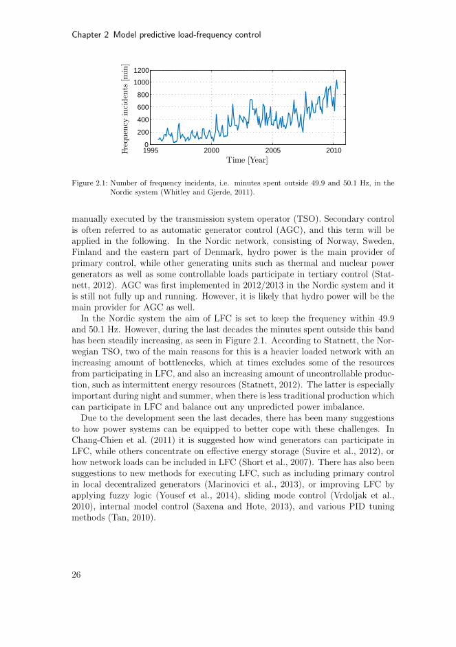
Figure 2.1: Number of frequency incidents, i.e. minutes spent outside 49.9 and 50.1 Hz, in theNordic system (Whitley and Gjerde, 2011).
manually executed by the transmission system operator (TSO). Secondary controlis often referred to as automatic generator control (AGC), and this term will beapplied in the following. In the Nordic network, consisting of Norway, Sweden,Finland and the eastern part of Denmark, hydro power is the main provider ofprimary control, while other generating units such as thermal and nuclear powergenerators as well as some controllable loads participate in tertiary control (Stat-nett, 2012). AGC was first implemented in 2012/2013 in the Nordic system and itis still not fully up and running. However, it is likely that hydro power will be themain provider for AGC as well.
In the Nordic system the aim of LFC is set to keep the frequency within 49.9and 50.1 Hz. However, during the last decades the minutes spent outside this bandhas been steadily increasing, as seen in Figure 2.1. According to Statnett, the Nor-wegian TSO, two of the main reasons for this is a heavier loaded network with anincreasing amount of bottlenecks, which at times excludes some of the resourcesfrom participating in LFC, and also an increasing amount of uncontrollable produc-tion, such as intermittent energy resources (Statnett, 2012). The latter is especiallyimportant during night and summer, when there is less traditional production whichcan participate in LFC and balance out any unpredicted power imbalance.
Due to the development seen the last decades, there has been many suggestionsto how power systems can be equipped to better cope with these challenges. InChang-Chien et al. (2011) it is suggested how wind generators can participate inLFC, while others concentrate on effective energy storage (Suvire et al., 2012), orhow network loads can be included in LFC (Short et al., 2007). There has also beensuggestions to new methods for executing LFC, such as including primary controlin local decentralized generators (Marinovici et al., 2013), or improving LFC byapplying fuzzy logic (Yousef et al., 2014), sliding mode control (Vrdoljak et al.,2010), internal model control (Saxena and Hote, 2013), and various PID tuningmethods (Tan, 2010).
26
2.1 Introduction
Model predictive control (MPC) is another possibility for LFC which has re-ceived attention. In McNamara et al. (2013) MPC is used for controlling powerflows in high voltage direct current (HVDC) links to improve LFC, and in Halv-gaard et al. (2012) MPC is applied for building climate control to benefit LFC.MPC has also been used for preventing severe line-overloads in power systems. InOtomega et al. (2007); Carneiro and Ferrarini (2010) MPC is proposed as a specialprotection scheme aimed at preventing thermal overloads on network lines duringemergencies. In Otomega et al. (2007) the MPC relies on a direct current (DC)approximation of the actual power flows, whereas Carneiro and Ferrarini (2010)has added a thermodynamical model of the conductors and weather information todetermine possible thermal overloads. In Almassalkhi and Hiskens (2015) a hierar-chical MPC control scheme is suggested, where the upper-level controller finds theoptimal energy schedule and the lower control level serves as a cascade mitigationcorrective scheme in case of large disturbances. Also here the MPC relies on a DCapproximation of the network power flow.
In this work MPC will be applied for AGC in a larger power system, which is alsothe topic in Shiroei et al. (2013); Mohamed et al. (2012), but there the MPC is basedon a model equal to the one used for simulation. In this work the MPC is based ona simplified equivalent of the full power system, and constraints on the generationcapacity and generation rate of change are included, as well as constraints on tie-linepower transfer capacities. A solution to how one can guarantee available transfercapacity on the tie-lines is also presented, and a proposal to how economy can beconsidered in the MPC and AGC decision making is included. Any participationfrom loads in LFC is omitted in this work, and hydro generators are the sole providerof primary control and AGC.
This chapter is an extension of the work presented in Ersdal et al. (2013, 2014).In Ersdal et al. (2013) a single-area model is considered and there is no model-plantmismatch, and in Ersdal et al. (2014) this is extended to a two-area model withtie-line limitations. In Ersdal et al. (2014) the MPC is also extended to take intoaccount uncertainty in wind power production. This topic is not further addressedhere, in part due to considerations related to computational complexity, but suchuncertainty-aware intelligence can also, in principle, be included when the hourlyset-points to the AGC are calculated (unit commitment), see for example Dvorkinet al. (2015) and the references therein. Such an approach would be compatible withthe MPC-based AGC controller presented here. In this work, the implementationof slack variables are relevant in this context, as they enable the MPC to exploitback-off margins to important constraints to handle uncertainties.
The main contribution of this chapter is the presentation of a solution to theLFC problem, where
• The participation factor of each generator is included in the optimizationproblem.
• State feedback to the MPC is achieved through a state estimator.
27

Chapter 2 Model predictive load-frequency control
G
GG
G
G
G
G
G
G
GG
G
G
G
GGG
GG
Figure 2.2: An overview of the generators in the SINTEF model (Norheim et al., 2005).
• A simplified power system model is used both in the MPC predictions andstate estimation.
The MPC will not function as an emergency protective scheme, but as an everydayLFC controller which corrects production set-points both during normal and moresevere operating conditions. In other words, this is a scheme for frequency restora-tion. The technical solution is analyzed without discussion of the market aspect ofit. However, we believe that this could be implemented as an auction-based schemesimilar to the present LFC implemented in the Nordic system.
The remainder of the chapter is organized as follows. In Section 2.2 the proxymodel used to represent the Nordic power system is presented, followed by a simplermodel to be used in the MPC. The details of the controller is given in Section 2.3,before the case study of the Nordic system is presented in Section 2.4 along withsome simulation results. Section 2.5 gives a short discussion about the results,before the conclusion in Section 2.6.
2.2 Modelling
The Nordic power system is represented by a proxy model, which is a reducedversion of a model developed by SINTEF Energy Research, where the placementof the generators and transmission lines reflects the real production and the mostinteresting bottlenecks in the Nordic power system (Norheim et al., 2005). Theversion implemented here consists of 15 hydro generators, 5 non-hydro generators,21 composite loads, and 36 nodes. The placement of the generators can be seen inFigure 2.2.
28
2.2 Modelling
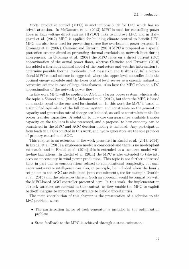
Governor Turbinecr
∆fc Pm
ξ1, ξ2, ξ3 q
Figure 2.3: Overview of governor and turbine states, inputs and output.
2.2.1 Proxy Model
The proxy model is described by a differential algebraic equation (DAE)
x = f(x, z, u, w) (2.1a)
0 = g(x, z, u, w) (2.1b)
where x are the dynamic system states, z the algebraic system states, u the con-trolled inputs to the system, and w the system disturbance.
The Swing Equation
For each generator k, the generator dynamics are given by the swing equation
δk = ωn∆ωk (2.2a)
∆ωk =1
Hk
(P km − P k
e −Dk(∆ωk −∆ωs
))(2.2b)
where δ is the rotor angle, ∆ω the rotor angular velocity relative a reference frame,∆ωs the inertial rotor angular velocity relative a reference frame, ωn the angularvelocity of this reference frame, Pm the mechanical power produced by the rotor,Pe = Re
(EgI
?g
)the electrical power acting on the rotor, H the inertia constant and
D the damping coefficient. The internal voltage of the generator is Eg = |Eg| ejδ,and I?g is the complex conjugate of the current delivered from the generator intothe network. In this work, voltage control is assumed to be much faster than thedynamics of interest, and is therefore not considered. Hence the internal generatorvoltages |Eg| are assumed constant.
The Turbine and Governor Dynamics
Because hydro turbines are the main provider for primary control in the Nordicnetwork, and most likely will be the main provider for AGC as well, only the hydroturbine and governor dynamics are modeled in this work. The remaining generatingunits will produce a constant amount of power.
A simplified diagram of the hydro turbine and governor dynamics are given inFigure 2.3. They are modeled as the nonlinear model of Machowski et al. (2008),usually denoted HYGOV, and has the states q, ξ1, ξ2, and ξ3. The valve openingis c, and cr is the valve opening set point provided to the generating unit by theTSO. Given a large power system consisting of m generators, where mh of these
29
Chapter 2 Model predictive load-frequency control
are hydro turbines, the total system dynamics can be written as (2.1a) with
x =[δk ∆ωk qi ξi1 ξi2 ξi3
]T(2.3)
u = cir (2.4)
where k = 1, . . . ,m and i = 1, . . . ,mh. In total 2m+ 4mh dynamic states, and mh
controllable inputs.
Network Current Equation
The current flow in the network is found using the internal node representation.Defining all currents as positive into node k, Kirchoff’s current law for each nodegives
Ikg + IkL +n∑
i=1
YkiUi = 0 (2.5)
where Ikg is the current delivered from generator k, IkL the load current from loadk, Yki the systems admittance matrix at position (k, i), Ui the voltage at node i,and n the number of nodes in the network. The current injected from generator kinto node k is
Ikg =Ekg − Uk
jx′dk
(2.6)
where x′dk is the generator transient reactance. The active power load at node
k is modeled as a constant current Ikl and the reactive power load as a constantadmittance Y k
l , such that the total current from load k is
IkL = −Ikl − UkY kl (2.7)
This means that the power flow is dependent on the nodal voltage, but not de-pendent on the system frequency. System loads are in general often both voltageand frequency dependent, however it could be argued that some of the frequency-dependency of the loads are modeled through the damping term of the swing equa-tion (2.2). In addition, the frequency-dependency of the loads in the Nordic powersystem is relatively low compared to the total power consumption.
Combining (2.5) - (2.7) gives an equation with two unknown: |U | and θ, the mag-nitude and angle of the nodal voltages, respectively. This makes up the algebraicsystem equation (2.1b), with a total of 2n algebraic states z. The disturbances wacting on the system are the absolute values of the active load currents as well asthe produced power from non-hydro generators, resulting in a total of n+m−mh
disturbances.
z =[∣∣Uk
∣∣ θk]T
(2.8)
w =[∣∣Ikl
∣∣ P pm
]T(2.9)
where k = 1, . . . , n and p = mh + 1, . . . ,m.
30

2.2 Modelling
2.2.2 Prediction Model
The model presented in the previous section is a large and complex model, and inmany cases it can be both sufficient and beneficial to consider a smaller, simplifiedpower system model. One example is the prediction model (PM) used in an MPC.To find this PM, the larger model of the previous section is first divided into Nareas connected to each other by tie lines. The states, inputs and disturbances ofthe PM are defined as x, u, and w. These are all given relative an initial steady statewhere the power supply and demand in the system are balanced, both with regardsto active and reactive power. This initial steady state is also used for linearizationpoints when this is needed.
The dynamics affecting the frequency response of a power system are rela-tively slow, and neglecting the fast dynamics reduces the complexity of the model(Bevrani, 2014). The nodal voltages and the electromechanical dynamics of theswing equation are considered to be fast dynamics, and can therefore be neglected.The dynamics of area i, including the generators, can in this case be representedby one single differential equation (Bevrani, 2014)
∆ ˙f i =1
2H i
(∆P i
m −∆P iD −∆P i
tie
)(2.10)
where ∆f is the deviation from the nominal frequency fs, ∆Pm the total change inmechanical power from primary control and AGC combined, ∆PD the total changein load power, ∆Ptie the change in total power flow from the area on all its tie lines,and H the inertia of the rotating masses of the area. The change in total tie-linepower flow from area i is (Bevrani, 2014)
∆ ˙P itie = 2π
(∆f i
N∑
j=1,j 6=iTij −
N∑
j=1,j 6=iTij∆f
j
)(2.11)
where ∆f i/j is the local frequency in area i/j, and Tij the synchronizing torquecoefficient between area i and j. The frequency deviation of the entire system isdefined as
∆f =
∑Ni=0 H
i∆f i∑Ni=0 H
i(2.12)
The equations for the hydraulic turbines and governors can be simplified bymodeling all the hydraulic power stations of an area as one aggregated hydraulicturbine and governor. The dynamics of the turbine can in turn be represented bya linearized version of the nonlinear model used in the proxy model. This gives thefollowing dynamic equation for the aggregated turbine of area i
∆ ˙qi = − 2
T iwc2ss/qss
(∆qi − qi2ss
ci2ss∆ci)
(2.13a)
∆P im = Aith
iss
(3∆qi − 2
qi2ssci2ss
∆ci)
(2.13b)
31
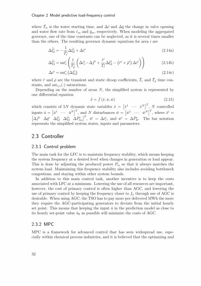
Chapter 2 Model predictive load-frequency control
where Tw is the water starting time, and ∆c and ∆q the change in valve openingand water flow rate from css and qss, respectively. When modeling the aggregatedgovernor, one of the time constants can be neglected, as it is several times smallerthan the others. The resulting governor dynamic equations for area i are
∆ ˙ξi2 = − 1
T ir∆ξi2 + ∆ci (2.14a)
∆ ˙ξi3 = satic
(1
T ig
(∆cir−∆f i +
ri
T ir∆ξi2 −
(ri + ρi
)∆ci))
(2.14b)
∆ci = satic(∆ξi3
)(2.14c)
where r and ρ are the transient and static droop coefficients, Tr and Tg time con-stants, and satc/c(·) saturations.
Depending on the number of areas N , the simplified system is represented byone differential equation
˙x = f (x, u, w) (2.15)
which consists of 5N dynamic state variables x =[x1 · · · xN
]T, N controlled
inputs u =[u1 · · · uN
]T, and N disturbances w =
[w1 · · · wN
]T, where xi =[
∆f i ∆qi ∆ξi2 ∆ξi3 ∆P itie
]T, ui = ∆cir, and wi = ∆P i
D. The bar notationrepresents the simplified system states, inputs and parameters.
2.3 Controller
2.3.1 Control problem
The main task for the LFC is to maintain frequency stability, which means keepingthe system frequency at a desired level when changes in generation or load appear.This is done by adjusting the produced power Pm so that it always matches thesystem load. Maintaining this frequency stability also includes avoiding bottleneckcongestions, and staying within other system bounds.
In addition to this main control task, another incentive is to keep the costsassociated with LFC at a minimum. Lowering the use of all resources are important,however, the cost of primary control is often higher than AGC, and lowering theuse of primary control by keeping the frequency closer to fn through use of AGC isdesirable. When using AGC, the TSO has to pay more per delivered MWh the morethey require the AGC-participating generators to deviate from the initial hourlyset point. This means that keeping the input u in the prediction model as close toits hourly set-point value u0 as possible will minimize the costs of AGC.
2.3.2 MPC
MPC is a framework for advanced control that has seen widespread use, espe-cially within chemical process industries, and it is believed that the optimizing and
32
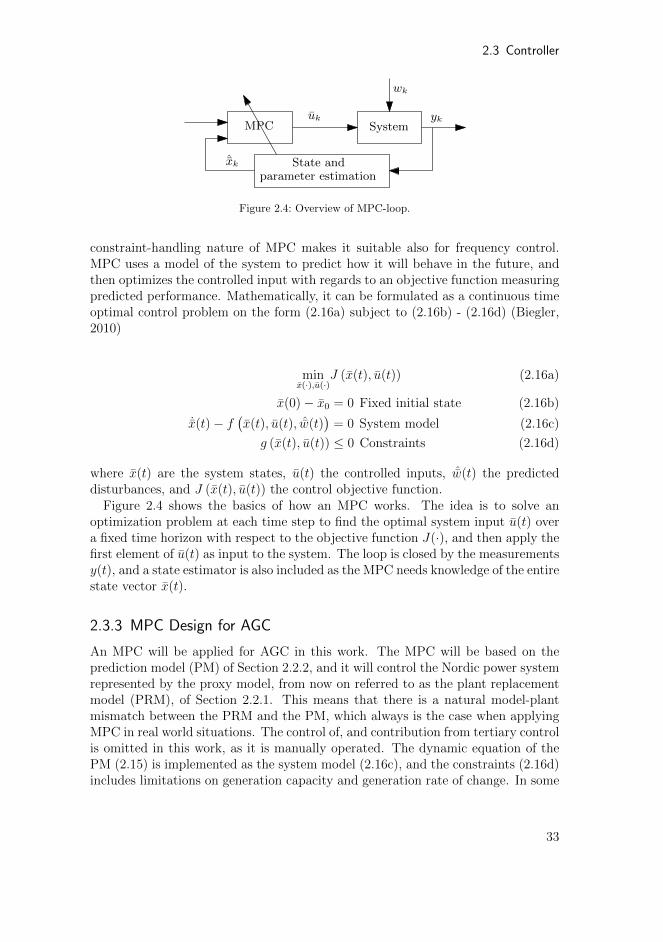
2.3 Controller
MPC Systemuk yk
wk
State andˆxk
parameter estimation
Figure 2.4: Overview of MPC-loop.
constraint-handling nature of MPC makes it suitable also for frequency control.MPC uses a model of the system to predict how it will behave in the future, andthen optimizes the controlled input with regards to an objective function measuringpredicted performance. Mathematically, it can be formulated as a continuous timeoptimal control problem on the form (2.16a) subject to (2.16b) - (2.16d) (Biegler,2010)
minx(·),u(·)
J (x(t), u(t)) (2.16a)
x(0)− x0 = 0 Fixed initial state (2.16b)
˙x(t)− f(x(t), u(t), ˆw(t)
)= 0 System model (2.16c)
g (x(t), u(t)) ≤ 0 Constraints (2.16d)
where x(t) are the system states, u(t) the controlled inputs, ˆw(t) the predicteddisturbances, and J (x(t), u(t)) the control objective function.
Figure 2.4 shows the basics of how an MPC works. The idea is to solve anoptimization problem at each time step to find the optimal system input u(t) overa fixed time horizon with respect to the objective function J(·), and then apply thefirst element of u(t) as input to the system. The loop is closed by the measurementsy(t), and a state estimator is also included as the MPC needs knowledge of the entirestate vector x(t).
2.3.3 MPC Design for AGC
An MPC will be applied for AGC in this work. The MPC will be based on theprediction model (PM) of Section 2.2.2, and it will control the Nordic power systemrepresented by the proxy model, from now on referred to as the plant replacementmodel (PRM), of Section 2.2.1. This means that there is a natural model-plantmismatch between the PRM and the PM, which always is the case when applyingMPC in real world situations. The control of, and contribution from tertiary controlis omitted in this work, as it is manually operated. The dynamic equation of thePM (2.15) is implemented as the system model (2.16c), and the constraints (2.16d)includes limitations on generation capacity and generation rate of change. In some
33
Chapter 2 Model predictive load-frequency control
of the examples of Section 2.4 limitations on the tie-line power transfer are alsoincluded.
The saturations in (2.14) are nonlinear, implying that we have nonlinear equalityconstraints (2.16c), and nonlinear MPC (NMPC) must be used. For the samereason, the optimization problem in (2.16) is non-convex. The continuous timeoptimization problem (2.16) in the NMPC is solved with direct methods, that is, itis discretized and transformed into a nonlinear program (NLP) using collocation.The NLP is then solved using the interior point optimizer IPOPT (Wachter andBiegler, 2006) with exact Hessian, all implemented in Casadi (Andersson, 2013).
The saturations will not only introduce nonlinearity to the PM, they are also non-smooth functions which can cause numerical problems when solving the NLP usingIPOPT. The problem is that the second-order derivative of the Lagrange function(known as the Hessian) is not necessarily Lipschitz continuous2, which can preventthe convergence of IPOPT. This problem can be dealt with by introducing smoothapproximations of the saturation functions. Given the saturation of a variable σ,which is limited by the upper and lower limits σmax and σmin:
sat(σ) = min(σmax,max(σmin, σ)). (2.17)
In this thesis, the following approximation of Equation (2.17) is applied to approx-imate the saturations in (2.14), where κ > 0 is an approximation factor.
sat(σ) ≈ min (σmax, σ) ≈ 1
2
(σmax + σ −
√(σmin − σ)2 + κ2
)(2.18a)
where
σ =1
2
(σmin + σ +
√(σmin − σ)2 + κ2
)≈ max(σmin, σ) (2.18b)
This leads to a smooth saturation function which will have a second-order derivativethat is Lipschitz continuous.
The MPC implemented here is a centralized MPC (CMPC), i.e. it is basedon a model of the full system and it controls all the controllable inputs to thesystem. An alternative approach would be a distributed MPC (DMPC) whereseparate MPCs, based on single-area models, would be responsible for controllingeach area. A natural choice of areas could then be by country or by control area.There are several examples where DMPC has been applied for LFC, such as Venkatet al. (2008); Mohamed et al. (2011), and the main benefits of distributed controlare smaller optimization problems for each MPC, hence shorter optimization time,and less demands for communication. This is very beneficial when consideringlarge power systems, such as in continental Europe or North America. The maindrawback of DMPC is that it may result in poor systemwide control performance
2A function is said to be Lipschitz continuous if it is limited how fast the function can change.See e.g. Khalil (2002) for details.
34

2.3 Controller
∆c1r
MPC...
∆cNr
α11
αN1
...
...
α1m1
h
αNmN
h
∆c1r1
∆c1rm1h
∆cNr1
∆cNrmN
h
...
...
Figure 2.5: Illustration of generator participation factors, where mih is the number of hydro gen-
erators in area i.
if the subsystems interact significantly (Venkat et al., 2008), which is the case inmost power systems. When considering the Nordic power system it is important tokeep in mind that it is quite small compared to the Central European system or theEastern Interconnection in North America, and it is mainly Norway and Swedenwhich supply primary control and AGC through hydro power. This means that inthis case there is not that much to gain by distributing the control when it comesto optimization time, especially when considering that the CMPC presented here isbased on a simplified model with a rather small amount of optimization variables. Inaddition to this, using a DMPC would complicate the tie-line constraint handling,which is an important feature of the presented controller.
Including Participation Factors in the NMPC
In the PM, there is one input for each area of the system. This leads to N optimalinputs from the NMPC: ∆cir, where i = 1, . . . , N . These N inputs will then bedistributed to the hydro generators of each area by individual participation factorsαij. As described in Figure 2.5
cirj = cir0j + αij∆cir (2.19)
where j = 1, . . . ,mih and mi
h is the number of hydro generators in area i. Bear inmind that
∑Ni=0m
ih = mh.
However, each of the inputs cr have individual constraints, and in order to beable to account for each of them in the NMPC, the participation factors α are in-cluded as optimization variables in the NMPC. In this way, individual constrains ongeneration and generation rate of change for each hydro generator can be includedin, and accounted for by the NMPC. It also allows for greater flexibility and betteruse of the NMPC’s strengths on coordination of multiple inputs. This is howeverat the expense of a larger optimization problem. With this modification, the PMnow has 5N dynamic states, mh optimization variables (controllable inputs), andN disturbances.
35
Chapter 2 Model predictive load-frequency control
Including Economics in the NMPC
One of the obvious opportunities of an NMPC is to include the pricing of AGCin the objective function. Economic MPC refers to an MPC where the objectivefunction is an economic profit function, often linearly dependent on state and input(Rawlings and Amrit, 2009), as opposed to the more widespread quadratic objectivefunction:
J (x, u) =
∫ T
t=0
xTQx+ uTRu dt (2.20)
Some previous work has focused on the use of economic MPC for LFC, such asHovgaard et al. (2010). In this work however, (2.20) is used, and pricing is includedin a quadratic manner through the matrix R by multiplying the price of activating
AGC in each generator, P =[p1 · · · pmh
]T, with the diagonal terms of R. This
will not give a direct link between money spent and objective function, as in aneconomic MPC, but it will provide good knowledge to the NMPC about whichgenerators that are more economic to use.
Using Slack Variables to Avoid Bottlenecks
Giving the NMPC constraints on the tie-line power transfer will result in a fulfill-ment of the transfer limit, but the NMPC won’t care if it reaches the limit andstays there. During normal operating conditions it can however be beneficial tokeep a certain amount of power transfer available, if a more severe situation wereto happen. This is something that might be solved by using slack variables in theNMPC. Slack variables are often used to avoid infeasible solutions in an NMPC by“softening” some of the state constraints (Maciejowski, 2002). The slack variableε, which must be positive, is added to the constraint which is to be softened, andit is also added to the optimization variables.
g (x(t), u(t)) ≤ ε (2.21a)
ε ≥ 0 (2.21b)
In order not to use the slack variable unless absolutely necessary, use of ε is penalizedin the objective function
minx,u,ε
J (x, u, ε) = minx,u,ε
∫ T
t=0
xTQx+ uTRu+ γε dt (2.22)
In this way, the constraints g (x(t), u(t)) are allowed to exceed zero in severe sit-uations. In (2.22), ε is linearly included in the objective function, and we havewhat is called exact penalty, which means that as long as γ is large enough, theconstraint will not be violated unless there is no feasible solution to the originalproblem (Maciejowski, 2002).
Such slack variables can also be used to achieve two levels of severity on thetie-line limitations. One for normal operation, and one for severe cases. The orig-inal constraints ∆Ptie,max on the tie-line power transfer is set so that there still is
36

2.4 Case Study
available transmission capacity for emergencies. These are then implemented assoft constraints through the use of slack variables ε. The choice of γ compared to Qand R in the objective function will then determine when the NMPC finds it bestto use the emergency transfer capacity. In order to achieve an absolute maximumlimit on ∆Ptie, ε can be limited accordingly
ε ≤ ∆Ptie,MAX −∆Ptie,max (2.23)
where ∆Ptie,MAX is the absolute maximum limit.
2.3.4 State and Parameter Estimator
The NMPC needs knowledge of the entire PM state vector x. In this work, wehave assumed the PRM measurements to be y =
[∆ωk ξi2 ξi3 |U |s θs
], where
k = 1, . . . ,m, i = 1, . . . ,mh, and s = 1, . . . , n. From this, an extended Kalman filter(EKF) (Simon, 2006) based on the PM is used to estimate the PM state vector x anddisturbance w = ∆PD. An EKF is chosen because Casadi automatically generatesthe system’s derivatives using automatic differentiation (Andersson, 2013), makingthe EKF a simple and effective choice.
2.4 Case Study
Based on the information given in the first paragraph of Section 2.2, the PRM (2.1)has a total of 100 dynamic states, 72 algebraic states, 15 controllable inputs, and 21disturbances. This system is then divided into two areas in the PM (2.15), henceN = 2. Area A covers South Sweden and Eastern Denmark, and Area B coversNorway, North Sweden and Finland. Between the two areas there is a tie line whichrepresents the total power flow between the areas. In total the PM has 10 dynamicstates, 15 controllable inputs, and 2 disturbances, which is a considerable reductionfrom the PRM. In both the PRM and the PM the AGC control signal is dispatchedevery 10 s.
2.4.1 Tuning the NMPC
The main tuning variables of the NMPC are the prediction horizon T , and theobjective function J(·). The objective function is set to
J (x, u, ε) =
∫ T
t=0
xTQx+ (u− u0)T R (u− u0) + γε dt (2.24)
The matrices Q and R are tuning matrices, where Q is real, symmetric and positivesemidefinite, and R is real, symmetric and positive definite, while γ is a tuningvector containing elements greater than or equal to zero. The non-zero elements
of Q are chosen as q11 = β(H1)
2
(H1+H2)2, q66 = β
(H2)2
(H1+H2)2, q16 = q61 = β H1H2
(H1+H2), where
37
Chapter 2 Model predictive load-frequency control
β = 105. This choice of Q originates from punishing deviation in overall systemfrequency (2.12). The matrix R is given as R = diag (mbase · P ), where mbase is avector containing the hydro generators’ base rating and P is a vector containing theprice of activating AGC. By including mbase in R the actual produced power fromeach power plant is included in the objective function, and not only the per unit-based u, and there is also the possibility of including pricing information throughP . The use of primary control is driven by ∆f , so lowering the frequency deviationwill also lower the use of primary reserves.
As mentioned in Section 2.3.3, the choice of γ compared to Q and R decideswhen the NMPC will find it beneficial to break the constraints. In this work, slackvariables are included for the tie-line between Area A and B, which means that γis a vector of dimension 2. The tuning of γ differs in the examples given in Section2.4.3, depending on whether we want to achieve exact penalty or a two-level tie-linelimit. The exact value of γ will therefore be stated for each case.
In order to match the control signal dispatching in the system, the NMPC wasset to have a time step of 10 s, and the optimization horizon T was chosen to be3 minutes, a decision based on a compromise between system time constants andcomplexity.
2.4.2 PI Controller
The presented NMPC will be tested against conventional PI controllers, where oneis situated in each of the two areas. These two are given by
uA = KAp ∆fA +KA
i
∫∆fAdt (2.25)
uB = KBp ∆fB +KB
i
∫∆fBdt (2.26)
where Kp is the proportional constant and Ki the integral constant. The controlsignals from the PI controllers, uA and uB, are distributed to the hydro generatorsthrough the participation factors α, which are constant. The PI controllers aretuned based on the SIMC method presented in Skogestad (2003). In order tocompare the two controllers, a control performance measure (CPM) is applied.It basically measures the average frequency deviation, and it is calculated in thefollowing manner: First, ∆f is averaged over windows of 30 s to filter out fastfluctuations. Then, the CPM is found by again averaging ∆f over all these windows.This CPM is inspired by the CPS1 and CPS2 performance criteria used by theNorth American electric reliability corporation (NERC) (Gross and Lee, 2001).
2.4.3 Simulation Results
In Case A-C, the AGC pricing P is equal for all generators, and γ1 = γ2 = 105 sothat exact penalty for the slack variables are achieved. Hence there is no two-levellimit for the tie-line in these cases.
38

2.4 Case Study
Time of day [HH:MM]
Pow
er[M
W]
06:30 06:40 06:50 07:00 07:10 07:20
×104
4.8
4.85
4.9
4.95
5
5.05
(a) Total PD and the set point to Pm.
Time of day [HH:MM]
∆Pm
[MW
]
06:30 06:40 06:50 07:00 07:10 07:20
−500
0
500
(b) Total ∆Pm = Pm − Pm,sp.
Time of day [HH:MM]
Frequency
[Hz]
06:55 07:00 07:05 07:1049.95
50
50.05
(c) Frequency response at set point changes.
Figure 2.6: Case A: Frequency response during hourly set-point changes. The change is spreadover 15 minutes, and 9 smaller intervals.
Case A
The change in production set point Pm,sp takes place on the hour in the Nordic powersystem, while the changes in power demand happens during the hour (Statnett,2012). This leads to large frequency deviations at these hourly set-point changes.In Case A, such a situation is recreated, and Figure 2.6(a) shows how PD changescontinuously over the hour from 06 : 30 to 07 : 30, while Pm,sp changes in smallersteps over 15 minutes at 07 : 00. Figure 2.6(c) and 2.6(b) shows the resultingfrequency response and the deviation in Pm from Pm,sp, and Table 2.1 displays theCPM and reserve usage. From Figure 2.6(c) it is seen that the NMPC manages tokeep the frequency closer to 50 Hz than the PI controller, and this is also supportedby the CPM in Table 2.1. The reason the NMPC performs better than the PIcontroller is that the NMPC is able to take the actions of the primary controller(governor) into account when planing the optimal input. This results in a better
39
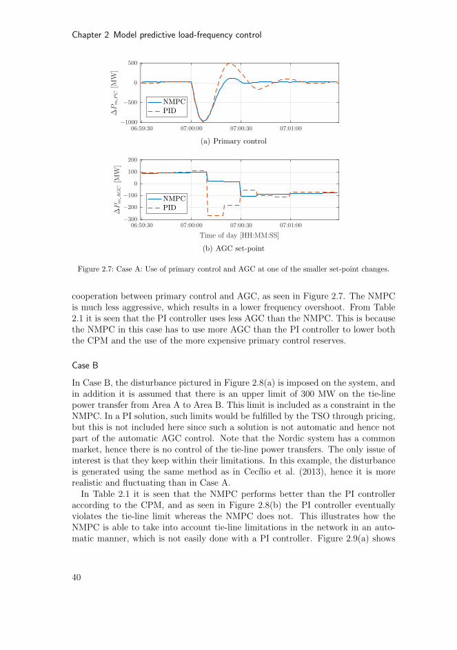
Chapter 2 Model predictive load-frequency control
Time of day [HH:MM:SS]
∆Pm,P
C[M
W]
06:59:30 07:00:00 07:00:30 07:01:00−1000
−500
0
500
(a) Primary control
Time of day [HH:MM:SS]
∆Pm,A
GC[M
W]
06:59:30 07:00:00 07:00:30 07:01:00−300
−200
−100
0
100
200
(b) AGC set-point
Figure 2.7: Case A: Use of primary control and AGC at one of the smaller set-point changes.
cooperation between primary control and AGC, as seen in Figure 2.7. The NMPCis much less aggressive, which results in a lower frequency overshoot. From Table2.1 it is seen that the PI controller uses less AGC than the NMPC. This is becausethe NMPC in this case has to use more AGC than the PI controller to lower boththe CPM and the use of the more expensive primary control reserves.
Case B
In Case B, the disturbance pictured in Figure 2.8(a) is imposed on the system, andin addition it is assumed that there is an upper limit of 300 MW on the tie-linepower transfer from Area A to Area B. This limit is included as a constraint in theNMPC. In a PI solution, such limits would be fulfilled by the TSO through pricing,but this is not included here since such a solution is not automatic and hence notpart of the automatic AGC control. Note that the Nordic system has a commonmarket, hence there is no control of the tie-line power transfers. The only issue ofinterest is that they keep within their limitations. In this example, the disturbanceis generated using the same method as in Cecılio et al. (2013), hence it is morerealistic and fluctuating than in Case A.
In Table 2.1 it is seen that the NMPC performs better than the PI controlleraccording to the CPM, and as seen in Figure 2.8(b) the PI controller eventuallyviolates the tie-line limit whereas the NMPC does not. This illustrates how theNMPC is able to take into account tie-line limitations in the network in an auto-matic manner, which is not easily done with a PI controller. Figure 2.9(a) shows
40
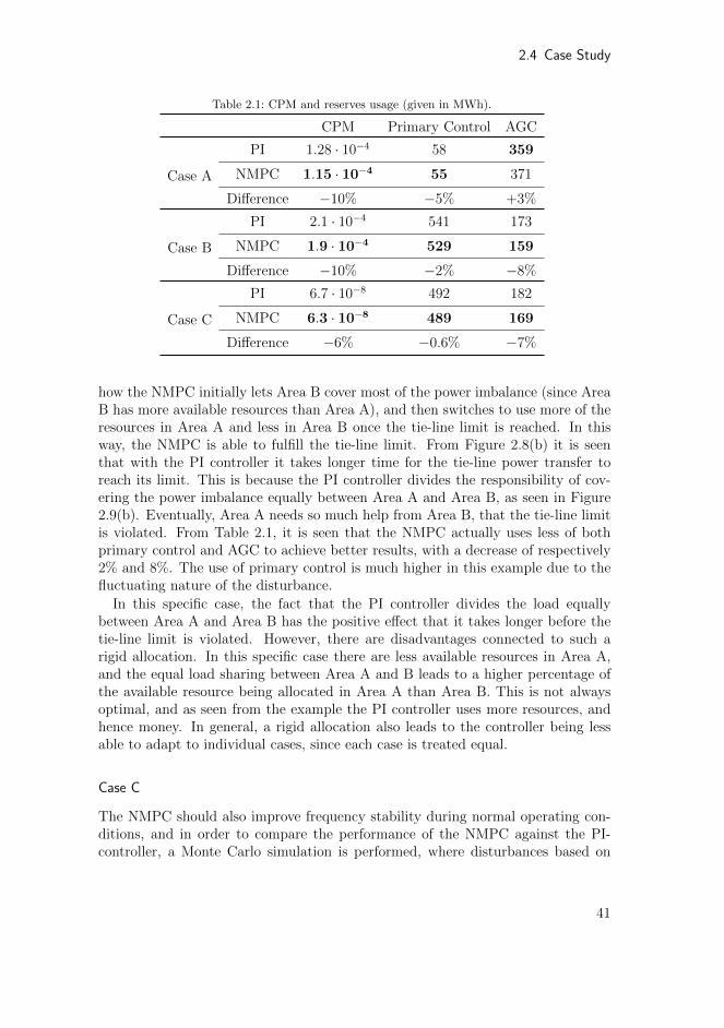
2.4 Case Study
Table 2.1: CPM and reserves usage (given in MWh).
CPM Primary Control AGC
Case A
PI 1.28 · 10−4 58 359
NMPC 1.15 · 10−4 55 371
Difference −10% −5% +3%
Case B
PI 2.1 · 10−4 541 173
NMPC 1.9 · 10−4 529 159
Difference −10% −2% −8%
Case C
PI 6.7 · 10−8 492 182
NMPC 6.3 · 10−8 489 169
Difference −6% −0.6% −7%
how the NMPC initially lets Area B cover most of the power imbalance (since AreaB has more available resources than Area A), and then switches to use more of theresources in Area A and less in Area B once the tie-line limit is reached. In thisway, the NMPC is able to fulfill the tie-line limit. From Figure 2.8(b) it is seenthat with the PI controller it takes longer time for the tie-line power transfer toreach its limit. This is because the PI controller divides the responsibility of cov-ering the power imbalance equally between Area A and Area B, as seen in Figure2.9(b). Eventually, Area A needs so much help from Area B, that the tie-line limitis violated. From Table 2.1, it is seen that the NMPC actually uses less of bothprimary control and AGC to achieve better results, with a decrease of respectively2% and 8%. The use of primary control is much higher in this example due to thefluctuating nature of the disturbance.
In this specific case, the fact that the PI controller divides the load equallybetween Area A and Area B has the positive effect that it takes longer before thetie-line limit is violated. However, there are disadvantages connected to such arigid allocation. In this specific case there are less available resources in Area A,and the equal load sharing between Area A and B leads to a higher percentage ofthe available resource being allocated in Area A than Area B. This is not alwaysoptimal, and as seen from the example the PI controller uses more resources, andhence money. In general, a rigid allocation also leads to the controller being lessable to adapt to individual cases, since each case is treated equal.
Case C
The NMPC should also improve frequency stability during normal operating con-ditions, and in order to compare the performance of the NMPC against the PI-controller, a Monte Carlo simulation is performed, where disturbances based on
41
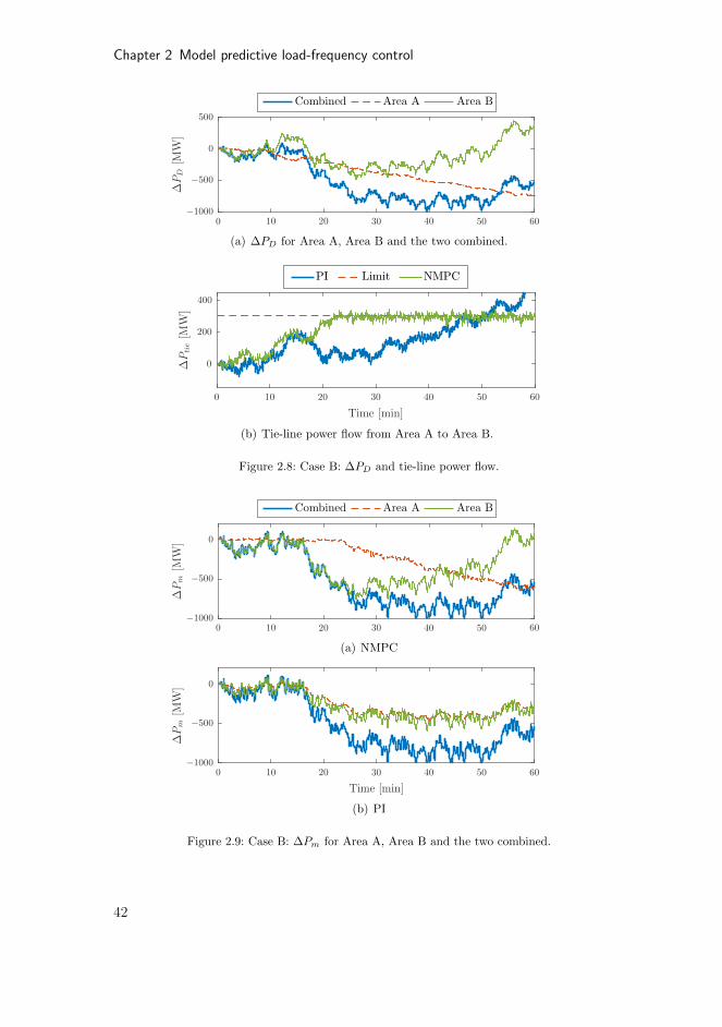
Chapter 2 Model predictive load-frequency control
(a) ∆PD for Area A, Area B and the two combined.
Time [min]
∆Ptie[M
W]
0 10 20 30 40 50 60
0
200
400
(b) Tie-line power flow from Area A to Area B.
Figure 2.8: Case B: ∆PD and tie-line power flow.
(a) NMPC
(b) PI
Figure 2.9: Case B: ∆Pm for Area A, Area B and the two combined.
42
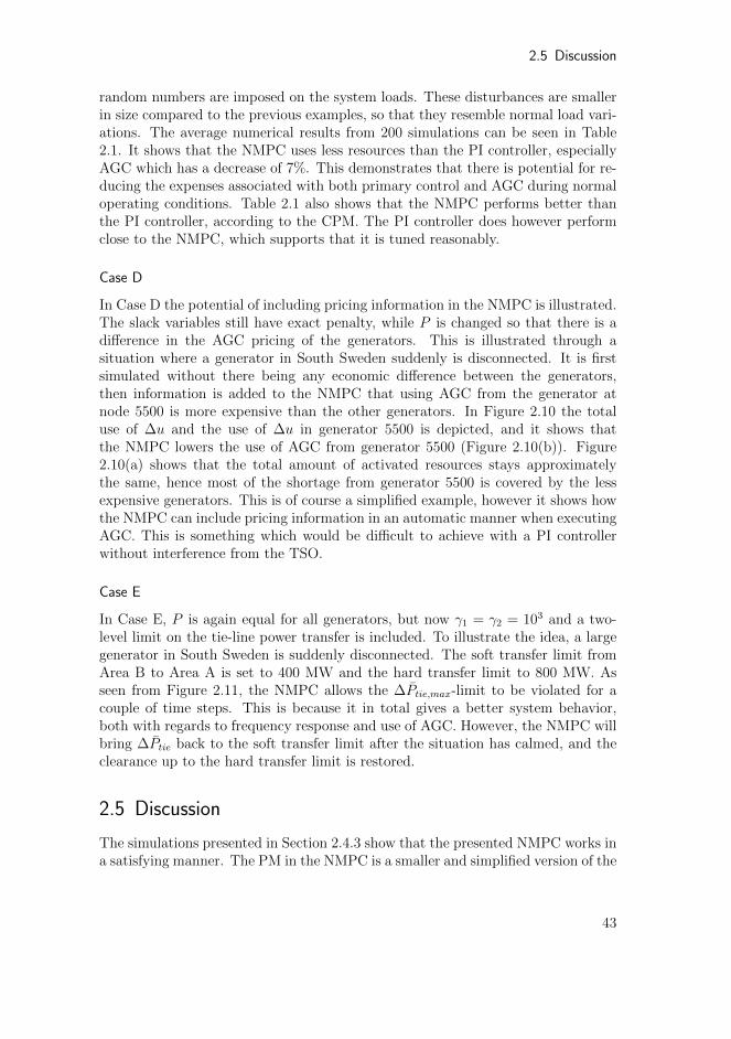
2.5 Discussion
random numbers are imposed on the system loads. These disturbances are smallerin size compared to the previous examples, so that they resemble normal load vari-ations. The average numerical results from 200 simulations can be seen in Table2.1. It shows that the NMPC uses less resources than the PI controller, especiallyAGC which has a decrease of 7%. This demonstrates that there is potential for re-ducing the expenses associated with both primary control and AGC during normaloperating conditions. Table 2.1 also shows that the NMPC performs better thanthe PI controller, according to the CPM. The PI controller does however performclose to the NMPC, which supports that it is tuned reasonably.
Case D
In Case D the potential of including pricing information in the NMPC is illustrated.The slack variables still have exact penalty, while P is changed so that there is adifference in the AGC pricing of the generators. This is illustrated through asituation where a generator in South Sweden suddenly is disconnected. It is firstsimulated without there being any economic difference between the generators,then information is added to the NMPC that using AGC from the generator atnode 5500 is more expensive than the other generators. In Figure 2.10 the totaluse of ∆u and the use of ∆u in generator 5500 is depicted, and it shows thatthe NMPC lowers the use of AGC from generator 5500 (Figure 2.10(b)). Figure2.10(a) shows that the total amount of activated resources stays approximatelythe same, hence most of the shortage from generator 5500 is covered by the lessexpensive generators. This is of course a simplified example, however it shows howthe NMPC can include pricing information in an automatic manner when executingAGC. This is something which would be difficult to achieve with a PI controllerwithout interference from the TSO.
Case E
In Case E, P is again equal for all generators, but now γ1 = γ2 = 103 and a two-level limit on the tie-line power transfer is included. To illustrate the idea, a largegenerator in South Sweden is suddenly disconnected. The soft transfer limit fromArea B to Area A is set to 400 MW and the hard transfer limit to 800 MW. Asseen from Figure 2.11, the NMPC allows the ∆Ptie,max-limit to be violated for acouple of time steps. This is because it in total gives a better system behavior,both with regards to frequency response and use of AGC. However, the NMPC willbring ∆Ptie back to the soft transfer limit after the situation has calmed, and theclearance up to the hard transfer limit is restored.
2.5 Discussion
The simulations presented in Section 2.4.3 show that the presented NMPC works ina satisfying manner. The PM in the NMPC is a smaller and simplified version of the
43
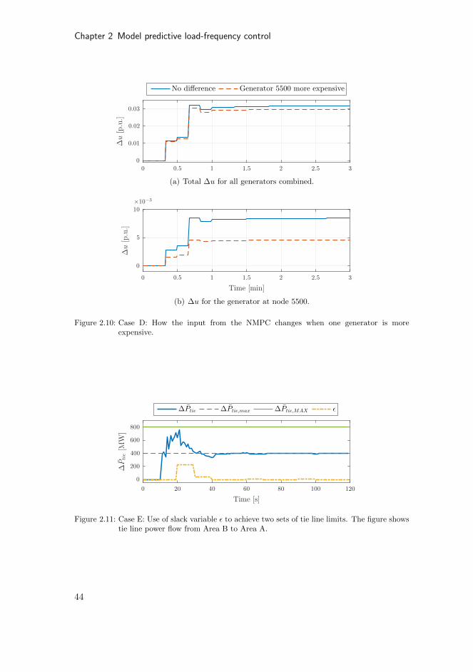
Chapter 2 Model predictive load-frequency control
(a) Total ∆u for all generators combined.
(b) ∆u for the generator at node 5500.
Figure 2.10: Case D: How the input from the NMPC changes when one generator is moreexpensive.
Figure 2.11: Case E: Use of slack variable ε to achieve two sets of tie line limits. The figure showstie line power flow from Area B to Area A.
44

2.6 Conclusion
PRM used for simulation. This causes a model-plant mismatch, which the NMPCis robust against. An EKF is used to estimate the PM states and disturbance,hence it adapts the PM to the PRM and through this it helps the NMPC deal withthe model-plant mismatch. There is not given a measurement or direct informationto the NMPC about the PM system disturbance ∆PD, it is only estimated usingthe EKF, which is applied as the future ∆PD when predicting the system behavior.
The simulations still show that the NMPC is able to both perform better thanthe PI controller, and to do so using less resources. In addition the NMPC is ableto take into account system limitations such as limitations on generator capacity,generator rate of change, and tie-line power transfer.
One of the reasons that the NMPC is performing well is that it is able to takeinto account the actions of the governor, and coordinate the inputs with regards tothis. In addition it can coordinate the inputs with respect to each other in a moreflexible manner than the PI controller. It is also able to use the information fromthe disturbance estimate to plan ahead.
With the computer and software used here, the NMPC based on a two-areaPM keeps well within the range of the real time requirements, with an averageoptimization time of less than 10 s. As an example the maximum and averageoptimization time for Case B in Section 2.4.3 is 0.73 s and 0.66 s, respectively.It is therefore believed that it will stay within these requirements if the PM isaugmented to more than two areas.
2.6 Conclusion
An NMPC based on a simplified system model is used for AGC in the Nordicpower system, represented by a larger, more complex proxy model. Both descriptiveexamples and extensive simulation has shown that applying NMPC to AGC canlead to both better control performance as well as a reduction in use of reserves,which again will reduce the costs associated with LFC. Ideas to how NMPC can beapplied to include economics in the AGC as well as methods for ensuring tie linecapacity, are also presented.
The work presented here shows some of the benefits an NMPC can provide withregards to LFC, such as flexibility and coordination between multiple inputs, takinginto account system limitations, and exploiting knowledge about the disturbanceacting on the system. All of these are qualities which could help in bringing abouta more flexible AGC which is able to deal with the challenges that power systemsare facing. It is also the authors’ opinion that since the prediction model in theNMPC is a significant reduction of the plant replacement model, it is reasonableto believe that an NMPC-based solution for AGC could work in a real situation.
45

Chapter 3
Model predictive load-frequency control taking intoaccount imbalance uncertainty
The work in this chapter was published in Ersdal et al. (2016b), which is an exten-sion of the work in Ersdal et al. (2014).
Summary
Nonlinear model predictive control (NMPC) is investigated for loadfrequency control (LFC) of an interconnected power system which isexposed to increasing wind power penetration. The robustified NMPC(RNMPC) proposed here uses knowledge of the estimated worst-casedeviation in wind-power production to make the NMPC more robust.The NMPC is based on a simplified system model that is updated usingstate- and parameter estimation by Kalman filters, and takes into ac-count limitations on among others tie-line power flow. Tests on a proxyof the Nordic power system, shows that the RNMPC is able to fulfill sys-tem constraints under worst-case deviations in wind-power productionin cases where the nominal NMPC is not.
3.1 Introduction
Power systems around the world have been through great development during thelast two decades. First with the liberalization of the power markets in the 1990’s,and second with the increasing amount of renewable energy resources, distributedgeneration, and increasing energy need seen around the world. These are all ele-ments which cause challenges for the operation of power systems, and especiallywith regards to load frequency control (LFC).
LFC is a term applied to describe the continuous operation of keeping the fre-quency of a power system stable. The frequency of a power system is connectedto the balancing of produced and consumed power in the way that if there is asurplus of produced power the frequency will rise, and if there is a lack of producedpower the frequency will fall. It is very important that this power balance is main-tained, if not the generators could lose synchronism, and the power system wouldcollapse. Traditionally, LFC has a hierarchical structure with primary, secondary,
47

Chapter 3 Model predictive LFC taking into account imbalance uncertainty
0− 2 min2− 15 min
15 min →
Time
Power
Frequency
Power imbalance
Primary
Secondary/AGC
Tertiary
Figure 3.1: Activation of primary, secondary (AGC) and tertiary control after a power imbalance.
and tertiary control1, see Figure 3.1. Primary control is continuous, automatic con-trol placed locally at the generators. It is often based on proportional control, andit instantaneously covers the power imbalance between produced and consumedpower. It does not, however, ensure that the frequency is restored to its set point.For this, secondary control is needed. Secondary control is a slower, centralized,and automatic controller which releases primary control. It is often referred to asautomatic generator control (AGC), and this term will be applied in the following.Tertiary control is an even slower, centralized controller, which again releases theAGC. This is manually operated by the transmission system operator (TSO). Inthe Nordic network, consisting of Norway, Sweden, Finland, and the eastern partsof Denmark, hydro generators are the main provider for primary control, whileother generating units such as thermal and nuclear power generators as well assome controllable loads participate in tertiary control (Statnett, 2012). AGC wasfirst implemented here in 2012/2013, and it is assumed that hydro generators willbe the main provider for this as well.
In the Nordic Network, the TSOs aim at keeping the frequency between 49.9 and50.1 Hz. This has proven to be increasingly difficult, and as seen from Figure 3.2,the number of frequency incidents (minutes spent outside 49.9 and 50.1 Hz) hasincreased concurrently with installed wind power capacity over the last decade. It isconfirmed by Statnett, the Norwegian TSO, that the increasing amount of intermit-tent energy resources is part of the reason for the decreasing control performance,along with a heavier loaded network and an increasing amount of bottlenecks, whichat times excludes some of the resources from participating in LFC (Statnett, 2012).
There have been many suggestions to how LFC can be improved to better copewith these challenges. In Short et al. (2007) and Fabozzi et al. (2013) loads areincluded in LFC, while Suvire et al. (2012) concentrate on effective energy storage,and Chang-Chien et al. (2011) suggests how wind generators can participate in LFC.
1Also known as frequency containment reserves (FCR), frequency restoration reserves (FRR),and replacement reserves (RR).
48

3.1 Introduction
1995 2000 2005 20100
2
4
6
Windpower
installed
capacity
[GW
]
Time [Year]
1995 2000 2005 20100
500
1000
Number
offreq
uen
cyinciden
ts[m
in]
Wind powerIncidents
Figure 3.2: Number of frequency incidents per month (Whitley and Gjerde, 2011) and installedwind power capacity (Nordel, 2008) in the Nordic system.
Others concentrate on new control methods for LFC, such as including primarycontrol in local decentralized generators (Marinovici et al., 2013), or improving LFCthrough fuzzy logic (Yousef et al., 2014), sliding mode control (Vrdoljak et al., 2010),internal model control (Saxena and Hote, 2013), and various PID tuning methods(Tan, 2010). Many have also investigated model predictive control (MPC) as a wayof improving LFC, e.g. through building climate control (Halvgaard et al., 2012),or control of power flows in high voltage direct current (HVDC) lines (McNamaraet al., 2013). In Otomega et al. (2007); Carneiro and Ferrarini (2010) MPC is usedas a special protection scheme to prevent severe line-overloads.
Some have also investigated MPC for AGC, for example Venkat et al. (2008);Shiroei et al. (2013); Mohamed et al. (2012). However, none of these considermodel-plant mismatch. Others discuss robust MPC (Shiroei et al., 2013), but thisis mainly against system parameter uncertainties, and the fulfillment of systemconstraints is not considered. Other control methods have also been suggested forrobust LFC, such as H∞ control (Singh et al., 2013; Bevrani et al., 2011), fuzzy logic(Cam and Kocaarslan, 2005), and robust PD tuning methods (Khodabakhshian andEdrisi, 2008).
Rather generally, robust MPC is formulated in a min-max framework, wherethe optimization seek to find minimizing inputs for the disturbances that maxi-mize the objective function. See for example Rawlings and Mayne (2009), Mayneet al. (2000) (nonlinear systems), Lofberg (2003) for linear systems, and variousapproaches to ease the computational load, e.g. based on precomputation of invari-ant sets (e.g. tube-based MPC (Langson et al., 2004)). Despite recent progress,min-max MPC still gives prohibitive complexity as problem dimensions grow. Inthis chapter, a simple approximation is chosen as the maximizing disturbances that
49
Chapter 3 Model predictive LFC taking into account imbalance uncertainty
gives reasonable computational performance, but will not give recursive feasibilityand guaranteed stability in general. The work presented in this chapter showsthat this approach will still be able to handle many, or most, disturbances in theproposed setup.
In Ersdal et al. (2016a) a nonlinear MPC (NMPC) based on a simplified sys-tem model was designed for AGC of the Nordic power system and tested againstconventional PI controllers. Through both descriptive examples and Monte Carlosimulations, it was shown that an NMPC can be beneficial in AGC, both with re-gards to control performance and reserve usage. It was also shown how the NMPCcan take system constraints into account, such as limitations on tie-line powertransfers. This is something which is not easily done with a PI controller. Ersdalet al. (2014) presented an NMPC for AGC which is robustified against variations inproduced wind power. This robustified NMPC (RNMPC) was tested without anymodel-plant mismatch, and it showed how the RNMPC was able to plan produc-tion so that it could handle a worst-case wind-power production scenario withoutbreaking any system constraints.
This chapter is an extension of the work presented in Ersdal et al. (2014, 2016a).The RNMPC from Ersdal et al. (2014) is implemented and tested with the proxysystem and prediction model from Ersdal et al. (2016a), hence there is a more real-istic test of the controller on a large, realistic simulator. Ersdal et al. (2016a) pre-sented a complete solution to the LFC problem by including generator participation-factors in the optimization problem as well as state estimation for full state feed-back. This chapter will be an extension of this by including knowledge of worst-casepredictions of future wind power production to robustify the NMPC. If the RNMPCcan plan so that there always is enough transfer capacity on important tie-lines tohandle some worst-case scenario, all generators are able to participate in LFC atall times, which will improve the system frequency.
In this work a centralized MPC (CMPC) is implemented, i.e. it is based on amodel of the full system and it controls all the controllable system inputs. Thereare several examples where distributed MPC (DMPC) has been applied for LFC,such as Venkat et al. (2008); Mohamed et al. (2011). In DMPC separate MPCs,based on single-area models, controls the inputs to each area, and the main benefitsare less demands for communication and smaller optimization problems for eachMPC, hence shorter optimization time. The main drawback of DMPC is thatit may result in poor systemwide control performance if the subsystems interactsignificantly (Venkat et al., 2008). For large power systems, such as the CentralEuropean system or the Eastern Interconnection in North America, the benefits ofDMPC are very relevant. With a considerable smaller network, such as the Nordicnetwork, on the other hand, there is not that much to gain by applying DMPCcompared to CMPC, especially when considering that the CMPC presented here isbased on a simplified model with a rather small amount of optimization variables. Inaddition to this, using a DMPC would complicate the tie-line constraint handling,which is an important feature of the presented controller.
The remainder of this chapter is organized as follows. In Section 3.2 the proxy
50

3.2 Modeling
G
GG
G
G
G
G
G
G
GG
G
G
G
GGG
GG
Figure 3.3: An overview of the generators in the SINTEF model (Norheim et al., 2005).
system used to represent the Nordic power system and the prediction model usedin the NMPC are presented. The nominal NMPC (NNMPC) is then discussed inSection 3.3, before the details of the RNMPC are given in Section 3.4. In Section3.5 the case study is presented along with the results from the tests on the proxysystem, which then are discussed in Section 3.6. Final conclusions on the presentedwork are given in Section 3.7.
3.2 Modeling
The proxy system and the prediction model used in this work are the same as theones used in Ersdal et al. (2016a). This section is therefore a condensed version ofSection 2.2. All variables, in both the proxy system and the prediction model, aregiven in per unit [p.u.], see Appendix A in Machowski et al. (2008) for details.
The transmission grid is a critical infrastructure which cannot be used as a test-bed. For research in grid transmission control, it is therefore always necessary touse a simulation as a proxy for the physical system. The power system model usedhere is a model of the Nordic power system developed by SINTEF Energy Research(Norheim et al., 2005). It includes 15 hydro generators, 5 non-hydro generators,21 composite loads, and 36 nodes. The placement of the generators can be seen inFigure 3.3, and they are chosen so that the model reflects the real production andmost interesting bottlenecks in the Nordic power system (Norheim et al., 2005).
3.2.1 SINTEF Proxy System
In general a power system can be modeled by a differential algebraic equation
x = f (x, z, u, w) (3.1a)
0 = g (x, z, u, w) (3.1b)
51
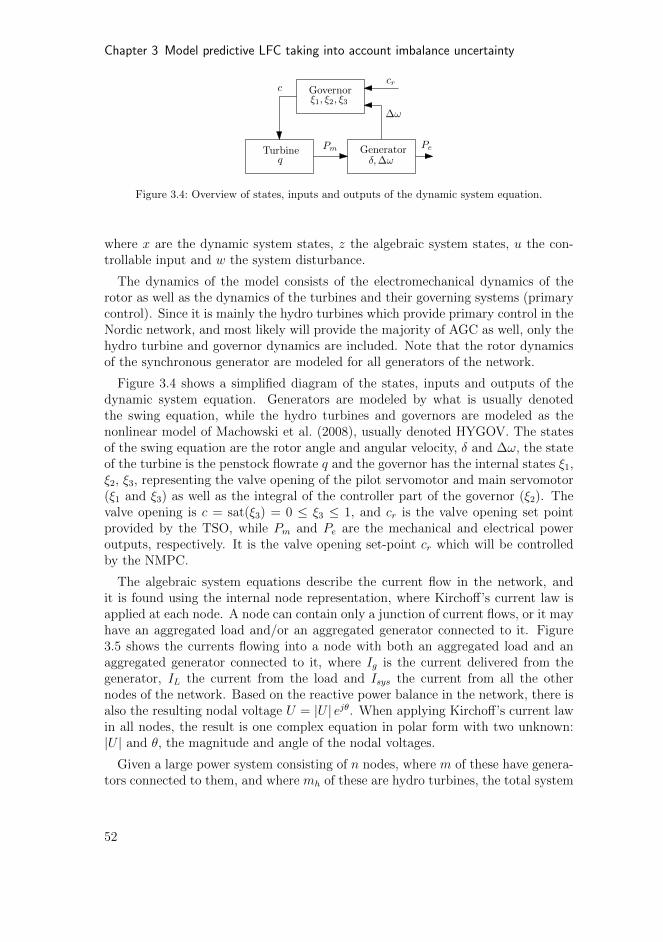
Chapter 3 Model predictive LFC taking into account imbalance uncertainty
Governor
Turbine
crc
Pm
ξ1, ξ2, ξ3
qGeneratorδ,∆ω
Pe
∆ω
Figure 3.4: Overview of states, inputs and outputs of the dynamic system equation.
where x are the dynamic system states, z the algebraic system states, u the con-trollable input and w the system disturbance.
The dynamics of the model consists of the electromechanical dynamics of therotor as well as the dynamics of the turbines and their governing systems (primarycontrol). Since it is mainly the hydro turbines which provide primary control in theNordic network, and most likely will provide the majority of AGC as well, only thehydro turbine and governor dynamics are included. Note that the rotor dynamicsof the synchronous generator are modeled for all generators of the network.
Figure 3.4 shows a simplified diagram of the states, inputs and outputs of thedynamic system equation. Generators are modeled by what is usually denotedthe swing equation, while the hydro turbines and governors are modeled as thenonlinear model of Machowski et al. (2008), usually denoted HYGOV. The statesof the swing equation are the rotor angle and angular velocity, δ and ∆ω, the stateof the turbine is the penstock flowrate q and the governor has the internal states ξ1,ξ2, ξ3, representing the valve opening of the pilot servomotor and main servomotor(ξ1 and ξ3) as well as the integral of the controller part of the governor (ξ2). Thevalve opening is c = sat(ξ3) = 0 ≤ ξ3 ≤ 1, and cr is the valve opening set pointprovided by the TSO, while Pm and Pe are the mechanical and electrical poweroutputs, respectively. It is the valve opening set-point cr which will be controlledby the NMPC.
The algebraic system equations describe the current flow in the network, andit is found using the internal node representation, where Kirchoff’s current law isapplied at each node. A node can contain only a junction of current flows, or it mayhave an aggregated load and/or an aggregated generator connected to it. Figure3.5 shows the currents flowing into a node with both an aggregated load and anaggregated generator connected to it, where Ig is the current delivered from thegenerator, IL the current from the load and Isys the current from all the othernodes of the network. Based on the reactive power balance in the network, there isalso the resulting nodal voltage U = |U | ejθ. When applying Kirchoff’s current lawin all nodes, the result is one complex equation in polar form with two unknown:|U | and θ, the magnitude and angle of the nodal voltages.
Given a large power system consisting of n nodes, where m of these have genera-tors connected to them, and where mh of these are hydro turbines, the total system
52
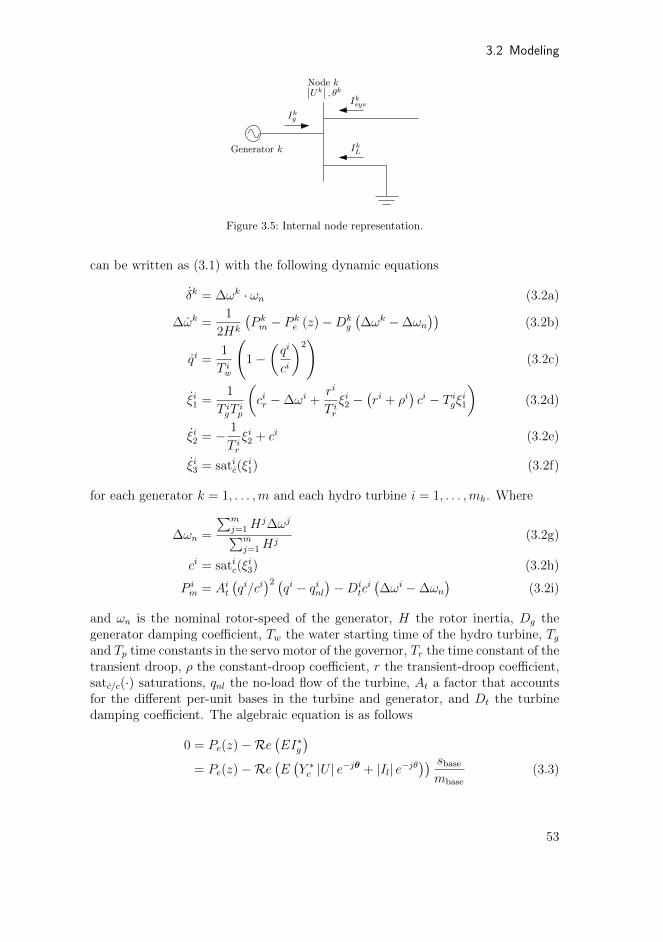
3.2 Modeling
Node k
Ikg
Iksys
IkLGenerator k
∣∣Uk∣∣ , θk
Figure 3.5: Internal node representation.
can be written as (3.1) with the following dynamic equations
δk = ∆ωk · ωn (3.2a)
∆ωk =1
2Hk
(P km − P k
e (z)−Dkg
(∆ωk −∆ωn
))(3.2b)
qi =1
T iw
(1−
(qi
ci
)2)
(3.2c)
ξi1 =1
T igTip
(cir −∆ωi +
ri
T irξi2 −
(ri + ρi
)ci − T igξi1
)(3.2d)
ξi2 = − 1
T irξi2 + ci (3.2e)
ξi3 = satic(ξi1) (3.2f)
for each generator k = 1, . . . ,m and each hydro turbine i = 1, . . . ,mh. Where
∆ωn =
∑mj=1 H
j∆ωj∑mj=1H
j(3.2g)
ci = satic(ξi3) (3.2h)
P im = Ait
(qi/ci
)2 (qi − qinl
)−Di
tci(∆ωi −∆ωn
)(3.2i)
and ωn is the nominal rotor-speed of the generator, H the rotor inertia, Dg thegenerator damping coefficient, Tw the water starting time of the hydro turbine, Tgand Tp time constants in the servo motor of the governor, Tr the time constant of thetransient droop, ρ the constant-droop coefficient, r the transient-droop coefficient,satc/c(·) saturations, qnl the no-load flow of the turbine, At a factor that accountsfor the different per-unit bases in the turbine and generator, and Dt the turbinedamping coefficient. The algebraic equation is as follows
0 = Pe(z)−Re(EI∗g
)
= Pe(z)−Re(E(Y ∗c |U | e−jθ + |Il| e−jθ
)) sbase
mbase
(3.3)
53
Chapter 3 Model predictive LFC taking into account imbalance uncertainty
where E is the internal voltage of the generators, I∗g the complex conjugate of thecurrent delivered from the generators, Y ∗c the complex conjugate of the network ad-mittance matrix, Il the absolute value of the active load currents, sbase the networkbase rating, and mbase the base rating of the generators.
This gives the following state, input and disturbance vectors
x =[δk ∆ωk qi ξi1 ξi2 ξi3
]T(3.4a)
z =[|U s| θs
]T(3.4b)
u = cir (3.4c)
w =[|Isl | P p
m
]T(3.4d)
where k = 1, . . . ,m, i = 1, . . . ,mh, s = 1, . . . , n, and p = mh + 1, . . . ,m. Thismeans that for each generator k (regardless of type), there are two dynamic states,for each hydro generator i there are in addition four extra dynamic states, and foreach node s there are two algebraic states. In total 2m + 4mh dynamic states, 2nalgebraic states, mh controllable inputs, and n+m−mh disturbances.
3.2.2 Prediction Model for Model Predictive Control
The prediction model (PM) is the model used by the NMPC to predict how thesystem will behave in the future, based on the inputs to-be-optimized and a dis-turbance model. In real-life situations, these models are always simplifications andapproximations to the actual processes which are being controlled. In this work,the NMPC is based on a reduced and simplified version of the system presented inthe previous section. This is done to ease the computational load of the NMPCand the state estimator, but it also incurs a natural model-plant mismatch in thetesting of the controller. To find the PM, the larger model of the previous sectionis first divided into N areas connected to each other by tie lines. All states, inputsand disturbances are given relative an initial steady state where both active andreactive power supply and consumption are balanced.
The dynamics affecting the frequency response of a power system are rela-tively slow, and neglecting the fast dynamics reduces the complexity of the model(Bevrani, 2014). The nodal voltages and the electromechanical dynamics of theswing equation are considered to be fast dynamics, and can therefore be neglected.The dynamics of area i, including the generators, can in this case be representedby one single differential equation (Bevrani, 2014)
∆ ˙f i =1
2H i
(∆P i
m −∆P iD −∆P i
tie
)(3.5)
where ∆f is the deviation from the nominal frequency fn, ∆Pm the total changein power from primary control and AGC combined, ∆PD the total change in loadpower and uncontrollable production, ∆Ptie the change in total power flow from
54

3.2 Modeling
the area on all its tie lines, and H the inertia of the rotating masses of the area.The change in total tie-line power flow from area i is (Bevrani, 2014)
∆ ˙P itie = 2π
(∆f i
N∑
j=1,j 6=iTij −
N∑
j=1,j 6=iTij∆f
j
)(3.6)
where ∆f i/j is the local frequency in area i/j, and Tij the synchronizing torquecoefficient between area i and j. The frequency deviation of the entire system isdefined as
∆f =
∑Ni=0 H
i∆f i∑Ni=0 H
i(3.7)
The hydraulic turbines and governor equations are simplified by modeling allthe hydraulic power stations of an area as one aggregated hydraulic turbine andgovernor. The dynamics of the turbine can in turn be represented by a linearizedversion of the nonlinear model used in the proxy system, where the reference pointsfor the PM system states are used for linearization. This gives the following dynamicequation for the aggregated turbine of area i
∆ ˙qi = − 2
T iwci2ss/q
iss
(∆qi − qi2ss
ci2ss∆ci)
(3.8a)
∆P im = Ait
qi2ssci2ss
(3∆qi − 2
qi2ssci2ss
∆ci)
(3.8b)
where ∆c and ∆q are the change in valve opening and water flow rate from css andqss, respectively. In the governor equations, one of the time constants is severaltimes smaller than the others, and it can therefore be neglected. This results in thefollowing governor dynamic equations for area i
∆ ˙ξi2 = − 1
T ir∆ξi2 + ∆ci (3.9a)
∆ ˙ξi3 = satic
(1
T ig
(∆cir−∆f i +
ri
T ir∆ξi2 −
(ri + ρi
)∆ci))
(3.9b)
∆ci = satic(∆ξi3
)(3.9c)
The manipulated input is still the valve opening set point ∆cr.
Disturbance Model
The balancing of power is managed by market transactions in most systems, andthrough these markets the predicted power demand and supply are balanced onslots of normally one hour. The markets take into account variations in productionfrom traditional power stations as well as the daily/weekly/annually deterministicload variation patterns. Because
55
Chapter 3 Model predictive LFC taking into account imbalance uncertainty
1. load variation patterns as well as production from some generators are difficultto predict in detail, and
2. changes in production set-point Pm,sp takes place on the hour, while changesin power demand happens during the hour (Statnett, 2012)
there will always be deviations from the hourly market balance. In order to keep thepower system safe and stable, it is important that this unpredicted power imbalanceis covered by the primary control and the AGC.
By choosing the initial steady state of the PM as the marked balance, the dis-turbance of the PM ∆P i
D represents the total unpredicted power imbalance of eacharea. This unpredicted power imbalance can roughly be divided into two differentdynamic components. One is a continuously, slowly varying imbalance due to in-termittent energy resources and loads. The other is an imbalance caused by suddendisconnections of loads or generators, which results in steep and sudden changes inthe power imbalance. Both of these components are important to consider whendealing with robust LFC. However, here we focus on the effects of an increasingwind-power penetration, and we will therefore concentrate on the former.
When dealing with power systems including a certain amount of wind power, suchas the Nordic grid, one can for simplicity assume that this intermittent unpredictedpower imbalance is dominated by the fluctuations in produced wind power. If, inaddition, it is assumed that the majority of wind power is situated in area p, ∆PDof all the other areas can be neglected, and the model is affected by one singledisturbance ∆PD = ∆P p
D. With the Nordic network in mind, Denmark and SouthSweden contribute with about 80% of the total wind power production (Statnett,2012). In Ersdal et al. (2016a) the disturbance ∆PD was kept constant over theprediction horizon. In this work however, the idea from Ersdal et al. (2014) tomake the NMPC more robust against fluctuations in produced wind power by usingdifferent disturbance scenarios in the predicted system behavior, is implemented.
Depending on the number of areas N , the simplified system is represented byone differential equation
˙x = f (x, u, w) (3.10a)
where
x =[∆f i ∆qi ∆ξi2 ∆ξi3 ∆P i
tie
]T(3.10b)
u = ∆cir (3.10c)
w = ∆P iD (3.10d)
and i = 1, . . . , N . In total 5N dynamic state variables, N controllable inputs, andone disturbance. The bar notation represents the simplified system states, inputsand parameters.
56
3.3 Controller
3.3 Controller
3.3.1 Control Problem
The main control task of the MPC is to balance the power production in the net-work against the consumption at all times, and to do so while avoiding bottleneckcongestions and staying within other system bounds. When large, unexpected dis-turbances appear, it is a problem in the Nordic network that some of the resourcesparticipating in primary control and AGC are prevented from participating due tobottlenecks in the network. For instance, the generators in the west may not beable to participate in covering a disturbance in the east if the east-west transmissionlines are already transferring close to maximum.
In addition to this primary control task, the MPC should also keep the costsassociated with LFC at a minimum. The cost of primary control is often higher thanAGC, and lowering the use of primary control by keeping the frequency closer to fnthrough use of AGC is desirable. When it comes to use of AGC, it is advantageousto keep the input in the PM u as close to its hourly set-point value u0 as possible.This is because the TSO has to pay more per delivered MWh the more they requirethe generators to deviate from the initial hourly set point. In Ersdal et al. (2016a)it was shown how a NMPC can lower the costs associated with LFC compared totradition PI-control. In this work the aim is not to further improve the reserveusage, but rather expand the NMPC while maintaining the results from Ersdalet al. (2016a).
3.3.2 MPC
MPC is a framework for advanced control that has seen widespread use, espe-cially within chemical process industries, and it is believed that the optimizing andconstraint-handling nature of MPC makes it suitable also for LFC. MPC uses amodel of the system to predict how it will behave in the future, and then optimizesthe controlled input with regards to an objective function measuring predictedperformance. Mathematically, it can be formulated as a continuous time optimalcontrol problem on the form (3.11a) subject to (3.11b) - (3.11d) (Biegler, 2010)
minx(·),u(·)
J (x(t), u(t)) (3.11a)
x(0)− x0 = 0 Fixed initial state (3.11b)
˙x(t)− f (x(t), u(t), w(t)) = 0 System model (3.11c)
g (x(t), u(t)) ≤ 0 Constraints (3.11d)
where x(t) are the system states, u(t) the controlled inputs, w(t) the predicteddisturbances, and J (x(t), u(t)) the control objective function.
Figure 3.6 shows the basics of how an MPC works. The idea is to solve anoptimization problem at each time step to find the optimal system input u(t) over
57
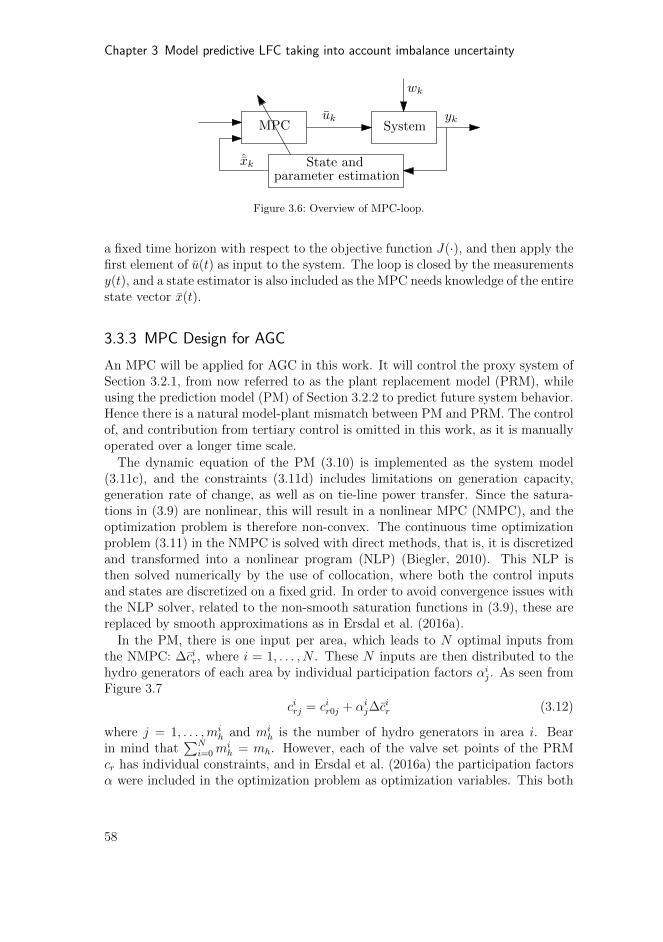
Chapter 3 Model predictive LFC taking into account imbalance uncertainty
MPC Systemuk yk
wk
State andˆxk
parameter estimation
Figure 3.6: Overview of MPC-loop.
a fixed time horizon with respect to the objective function J(·), and then apply thefirst element of u(t) as input to the system. The loop is closed by the measurementsy(t), and a state estimator is also included as the MPC needs knowledge of the entirestate vector x(t).
3.3.3 MPC Design for AGC
An MPC will be applied for AGC in this work. It will control the proxy system ofSection 3.2.1, from now referred to as the plant replacement model (PRM), whileusing the prediction model (PM) of Section 3.2.2 to predict future system behavior.Hence there is a natural model-plant mismatch between PM and PRM. The controlof, and contribution from tertiary control is omitted in this work, as it is manuallyoperated over a longer time scale.
The dynamic equation of the PM (3.10) is implemented as the system model(3.11c), and the constraints (3.11d) includes limitations on generation capacity,generation rate of change, as well as on tie-line power transfer. Since the satura-tions in (3.9) are nonlinear, this will result in a nonlinear MPC (NMPC), and theoptimization problem is therefore non-convex. The continuous time optimizationproblem (3.11) in the NMPC is solved with direct methods, that is, it is discretizedand transformed into a nonlinear program (NLP) (Biegler, 2010). This NLP isthen solved numerically by the use of collocation, where both the control inputsand states are discretized on a fixed grid. In order to avoid convergence issues withthe NLP solver, related to the non-smooth saturation functions in (3.9), these arereplaced by smooth approximations as in Ersdal et al. (2016a).
In the PM, there is one input per area, which leads to N optimal inputs fromthe NMPC: ∆cir, where i = 1, . . . , N . These N inputs are then distributed to thehydro generators of each area by individual participation factors αij. As seen fromFigure 3.7
cirj = cir0j + αij∆cir (3.12)
where j = 1, . . . ,mih and mi
h is the number of hydro generators in area i. Bearin mind that
∑Ni=0 m
ih = mh. However, each of the valve set points of the PRM
cr has individual constraints, and in Ersdal et al. (2016a) the participation factorsα were included in the optimization problem as optimization variables. This both
58

3.3 Controller
∆c1r
MPC...
∆cNr
α11
αN1
...
...
α1m1
h
αNmN
h
∆c1r1
∆c1rm1h
∆cNr1
∆cNrmN
h
...
...
Figure 3.7: Participation factors αij , where mi
h is the number of hydro generators in area i.
allows for individual input constraints and greater flexibility and better use of theNMPC’s strength on coordination of multiple inputs, however at the expense ofa larger optimization problem. This extension of the PM is also included in thiswork, and the PM now has 5N dynamic states, mh optimization variables and onedisturbance.
3.3.4 State and Parameter Estimation
The MPC relies on knowledge of the entire PM state vector x =[∆f i,∆qi,∆ξi2,∆ξ
i3,
∆P itie
]Tas well the current PM disturbances w = ∆P i
D. In order to find an estimateof these, it is assumed that the following PRM states are measured
y =[∆ωk ξi2 ξi3 |U |s θs
](3.13)
where k = 1, . . . ,m, i = 1, . . .mh, and s = 1, . . . n. In practice |U | and θ aremeasured using phasor measurement units (PMU), while ∆ω, ξ2, and ξ3 are mea-surable at the generators and governors. From these, the equivalent PM states∆f i = 2π∆ωi, ∆ξi2, and ∆ξi3 can be calculated, and the power flow between allnetwork nodes, including ∆P i
tie, can be found using |U | and θ. Hence the PMmeasurements are
y =[∆f i ∆ξi2 ∆ξi3 ∆P i
tie
]T(3.14)
where i = 1, . . . , N .An extended Kalman filter (EKF) (Simon, 2006) based on the PM is then applied
to estimate the full PM state vector as well as the PM disturbances, ∆P iD. In order
to estimate the change in load power and uncontrollable production of each area(∆P i
D), the PM is augmented to include ∆P iD as states with zero derivatives. To
illustrate the EKF, a simulation is performed using the proxy system. The PMis set to have one area, hence N = 1. The resulting estimate of ∆q and ∆PD,
∆ˆq and ∆ ˆPD, can be seen in Figure 3.8, and it illustrates that the implementedEKF manages to estimate the unmeasured state and disturbance in a satisfyingmanner. The EKF is chosen because the software used for implementation, Casadi(Andersson, 2013), automatically generates the system’s derivatives, making theEKF a simple and effective choice.
59

Chapter 3 Model predictive LFC taking into account imbalance uncertainty
Figure 3.8: Results from EKF: The estimate of ∆q and ∆PD, ∆ˆq and ∆ ˆPD.∆PD,m
ax
t
Figure 3.9: An example of how a worst-case estimate for ∆PD could look.
3.4 Robustified NMPC
3.4.1 Worst-Case Estimate of ∆PD
For a given wind farm, a worst-case estimate of the variation from the predictedpower output can be estimated, and Holttinen (2004) provides such data one second,one minute and one hour into the future t. If this information is combined for severalwind farms, one can create a total worst-case estimate for the future variation inwind-power production of one area, see Figure 3.9.
If the wind farms are distributed more evenly in the system, so that the as-sumption in Section 3.2.2 no longer applies, the disturbance would enter at severalpoints and a worst case combination of the disturbances, where system dynamicsare considered, has to be calculated.
3.4.2 Robustified NMPC
In the RNMPC a new state vector is constructed by combining the original statevector x (3.10b) and input u (3.10c) exposed to three different future disturbances:The zero, negative, and positive worst-case estimate for ∆PD added to the currentestimated disturbance w (3.10d), see Figure 3.10. The system equation for the
60
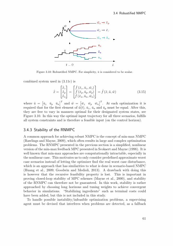
3.4 Robustified NMPC
Figure 3.10: Robustified NMPC. For simplicity, u is considered to be scalar.
combined system used in (3.11c) is
˙x =
˙xz˙xp˙xn
=
f (xz, uz, wz)f (xp, up, wp)f (xn, un, wn)
= f (x, u, w) (3.15)
where u =[uz up un
]Tand w =
[wz wp wn
]T. At each optimization it is
required that for the first element of u(t), uz, un and up must be equal. After this,they are free to vary in manners optimal for their designated system states, seeFigure 3.10. In this way the optimal input trajectory for all three scenarios, fulfillsall system constraints and is therefore a feasible input (on the control horizon).
3.4.3 Stability of the RNMPC
A common approach for achieving robust NMPC is the concept of min-max NMPC(Rawlings and Mayne, 2009), which often results in large and complex optimizationproblems. The RNMPC presented in the previous section is a simplified, nonlinearversion of the min-max feedback MPC presented in Scokaert and Mayne (1998). It iswell known that min-max approaches are computationally intractable, especially inthe nonlinear case. This motivates us to only consider predefined approximate worstcase scenarios instead of letting the optimizer find the real worst case disturbance,which is an approach that has similarities to what is done in scenario-based NMPC(Huang et al., 2009; Goodwin and Medioli, 2013). A drawback with doing thisis however that the recursive feasibility property is lost. This is important inproving closed-loop stability of MPC schemes (Mayne et al., 2000), and stabilityof the RNMPC can therefore not be guaranteed. In this work, stability is ratherapproached by choosing long horizons and tuning weights to achieve convergentbehavior in simulations. “Stabilizing ingredients” such as terminal costs couldhave been added, but this is not included in this study.
To handle possible instability/infeasible optimization problems, a supervisingagent must be devised that interferes when problems are detected, as a fallback
61

Chapter 3 Model predictive LFC taking into account imbalance uncertainty
mechanism. This could involve automatic fail-to-safe transitions, possible restart ofthe NMPC, or switching to manual control. It can be argued that such a mechanismwill have to be installed in any case, since it is very hard (and conservative) toinclude all thinkable disturbance scenarios in the prediction model. The role of therobustified NMPC is then to handle the disturbances most likely to happen.
An exact solution to such a supervising agent is not implemented in this work.However, some possible solutions are discussed in the following. The return codesand warning signals from the numerical optimization solver can be applied to detectconvergence problems and other computational issues. Moreover, one may monitorthe performance of the NMPC alongside the fallback controller. Motivated by thediscussions in Johansen (2015) on dependable embedded MPC, an idea is a controlselection scheme where the value of the NMPC objective function evaluated insimulations on a system model (in this case, the PRM would be natural, if available,if not the PM should be used) is used as a measure to select either the NMPC orthe fallback controller. The idea is that unstable/infeasible and poor solutions fromthe NMPC will be discarded in favor of the fallback controller. With regards tothe actual fallback controller, it could for example be conventional PI-based AGC,or in some cases manual control. In any case, such an event must generate analarm to the TSO, so that the situation can be supervised in a proper manner. Amechanism must also be devised for re-connecting the NMPC, this can for instancebe running the NMPC in open-loop for some time-steps to verify feasibility beforeit is manually re-connected by the TSO.
while true do1. Gather measurements, y;2. Calculate PM measurements, y;3. Use EKF to find estimate of PM state vector and disturbance, ˆx andˆPD, for use in the NMPC;4. Find optimal inputs u using NMPC based on PM;5. Check the computed input for problems (numerical/performance),e.g. as discussed above;if Problems then
A. Calculate system input using fallback controller, ufb;B. Apply ufb to system;
elseApply input u from NMPC to system;
end
endAlgorithm 1: Implementation of NMPC.
The main parts of the controller are summarized in Algorithm 1. The reconnec-tion of the NMPC is not included, as this would be a manual operation conductedby the TSO.
62
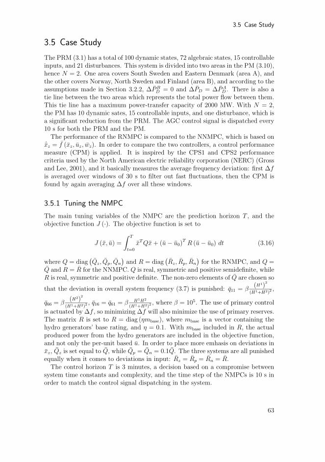
3.5 Case Study
3.5 Case Study
The PRM (3.1) has a total of 100 dynamic states, 72 algebraic states, 15 controllableinputs, and 21 disturbances. This system is divided into two areas in the PM (3.10),hence N = 2. One area covers South Sweden and Eastern Denmark (area A), andthe other covers Norway, North Sweden and Finland (area B), and according to theassumptions made in Section 3.2.2, ∆PB
D = 0 and ∆PD = ∆PAD . There is also a
tie line between the two areas which represents the total power flow between them.This tie line has a maximum power-transfer capacity of 2000 MW. With N = 2,the PM has 10 dynamic sates, 15 controllable inputs, and one disturbance, which isa significant reduction from the PRM. The AGC control signal is dispatched every10 s for both the PRM and the PM.
The performance of the RNMPC is compared to the NNMPC, which is based on˙xz = f (xz, uz, wz). In order to compare the two controllers, a control performancemeasure (CPM) is applied. It is inspired by the CPS1 and CPS2 performancecriteria used by the North American electric reliability corporation (NERC) (Grossand Lee, 2001), and it basically measures the average frequency deviation: first ∆fis averaged over windows of 30 s to filter out fast fluctuations, then the CPM isfound by again averaging ∆f over all these windows.
3.5.1 Tuning the NMPC
The main tuning variables of the NMPC are the prediction horizon T , and theobjective function J (·). The objective function is set to
J (x, u) =
∫ T
t=0
xTQx+ (u− u0)T R (u− u0) dt (3.16)
where Q = diag(Qz, Qp, Qn
)and R = diag
(Rz, Rp, Rn
)for the RNMPC, and Q =
Q and R = R for the NNMPC. Q is real, symmetric and positive semidefinite, whileR is real, symmetric and positive definite. The non-zero elements of Q are chosen so
that the deviation in overall system frequency (3.7) is punished: q11 = β(H1)
2
(H1+H2)2,
q66 = β(H2)
2
(H1+H2)2, q16 = q61 = β H1H2
(H1+H2)2, where β = 105. The use of primary control
is actuated by ∆f , so minimizing ∆f will also minimize the use of primary reserves.The matrix R is set to R = diag (ηmbase), where mbase is a vector containing thehydro generators’ base rating, and η = 0.1. With mbase included in R, the actualproduced power from the hydro generators are included in the objective function,and not only the per-unit based u. In order to place more emhasis on deviations inxz, Qz is set equal to Q, while Qp = Qn = 0.1Q. The three systems are all punishedequally when it comes to deviations in input: Rz = Rp = Rn = R.
The control horizon T is 3 minutes, a decision based on a compromise betweensystem time constants and complexity, and the time step of the NMPCs is 10 s inorder to match the control signal dispatching in the system.
63
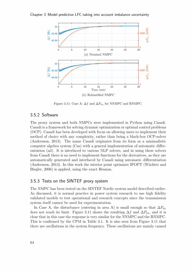
Chapter 3 Model predictive LFC taking into account imbalance uncertainty
Time [min]0 5 10 15 20 25 30
"f
[Hz]
49.96
49.98
50
"P
tie[M
W]
0
1000
(a) Nominal NMPC
Time [min]0 5 10 15 20 25 30
"f
[Hz]
49.96
49.98
50
"P
tie[M
W]
0
1000
(b) Robustified NMPC
Figure 3.11: Case A: ∆f and ∆Ptie for NNMPC and RNMPC.
3.5.2 Software
The proxy system and both NMPCs were implemented in Python using Casadi.Casadi is a framework for solving dynamic optimization or optimal control problems(OCP). Casadi has been developed with focus on allowing users to implement theirmethod of choice with any complexity, rather than being a black-box OCP-solver(Andersson, 2013). The name Casadi originates from its form as a minimalisticcomputer algebra system (Cas) with a general implementation of automatic differ-entiation (ad). It is interfaced to various NLP solvers, and in using these solversfrom Casadi there is no need to implement functions for the derivatives, as they areautomatically generated and interfaced by Casadi using automatic differentiation(Andersson, 2013). In this work the interior point optimizer IPOPT (Wachter andBiegler, 2006) is applied, using the exact Hessian.
3.5.3 Tests on the SINTEF proxy system
The NMPC has been tested on the SINTEF Nordic system model described earlier.As discussed, it is normal practice in power system research to use high fidelityvalidated models to test operational and research concepts since the transmissionsystem itself cannot be used for experimentation.
In Case A, the disturbance (entering in area A) is small enough so that ∆Ptiedoes not reach its limit. Figure 3.11 shows the resulting ∆f and ∆Ptie, and it isclear that in this case the response is very similar for the NNMPC and the RNMPC.This is confirmed by the CPM in Table 3.1. It is also seen from Figure 3.11 thatthere are oscillations in the system frequency. These oscillations are mainly caused
64
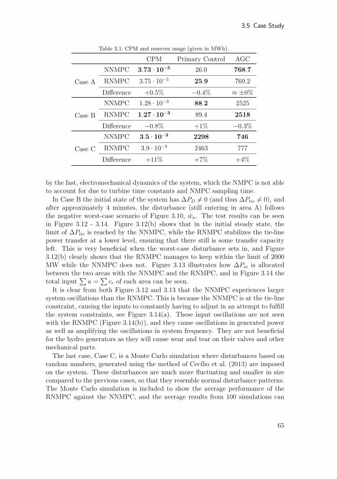
3.5 Case Study
Table 3.1: CPM and reserves usage (given in MWh).
CPM Primary Control AGC
Case A
NNMPC 3.73 · 10−5 26.0 768.7
RNMPC 3.75 · 10−5 25.9 769.2
Difference +0.5% −0.4% ≈ ±0%
Case B
NNMPC 1.28 · 10−3 88.2 2525
RNMPC 1.27 · 10−3 89.4 2518
Difference −0.8% +1% −0.3%
Case C
NNMPC 3.5 · 10−3 2298 746
RNMPC 3.9 · 10−3 2463 777
Difference +11% +7% +4%
by the fast, electromechanical dynamics of the system, which the NMPC is not ableto account for due to turbine time constants and NMPC sampling time.
In Case B the initial state of the system has ∆PD 6= 0 (and thus ∆Ptie 6= 0), andafter approximately 4 minutes, the disturbance (still entering in area A) followsthe negative worst-case scenario of Figure 3.10, wn. The test results can be seenin Figure 3.12 - 3.14. Figure 3.12(b) shows that in the initial steady state, thelimit of ∆Ptie is reached by the NNMPC, while the RNMPC stabilizes the tie-linepower transfer at a lower level, ensuring that there still is some transfer capacityleft. This is very beneficial when the worst-case disturbance sets in, and Figure3.12(b) clearly shows that the RNMPC manages to keep within the limit of 2000MW while the NNMPC does not. Figure 3.13 illustrates how ∆Pm is allocatedbetween the two areas with the NNMPC and the RNMPC, and in Figure 3.14 thetotal input
∑u =
∑cr of each area can be seen.
It is clear from both Figure 3.12 and 3.13 that the NNMPC experiences largersystem oscillations than the RNMPC. This is because the NNMPC is at the tie-lineconstraint, causing the inputs to constantly having to adjust in an attempt to fulfillthe system constraints, see Figure 3.14(a). These input oscillations are not seenwith the RNMPC (Figure 3.14(b)), and they cause oscillations in generated poweras well as amplifying the oscillations in system frequency. They are not beneficialfor the hydro generators as they will cause wear and tear on their valves and othermechanical parts.
The last case, Case C, is a Monte Carlo simulation where disturbances based onrandom numbers, generated using the method of Cecılio et al. (2013) are imposedon the system. These disturbances are much more fluctuating and smaller in sizecompared to the previous cases, so that they resemble normal disturbance patterns.The Monte Carlo simulation is included to show the average performance of theRNMPC against the NNMPC, and the average results from 100 simulations can
65
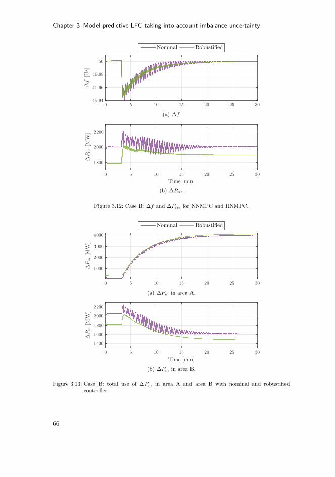
Chapter 3 Model predictive LFC taking into account imbalance uncertainty
(a) ∆f
(b) ∆Ptie
Figure 3.12: Case B: ∆f and ∆Ptie for NNMPC and RNMPC.
(a) ∆Pm in area A.
(b) ∆Pm in area B.
Figure 3.13: Case B: total use of ∆Pm in area A and area B with nominal and robustifiedcontroller.
66
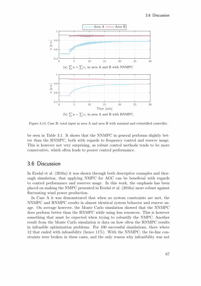
3.6 Discussion
(a)∑u =
∑cr in area A and B with NNMPC.
(b)∑u =
∑cr in area A and B with RNMPC.
Figure 3.14: Case B: total input in area A and area B with nominal and robustified controller.
be seen in Table 3.1. It shows that the NNMPC in general performs slightly bet-ter than the RNMPC, both with regards to frequency control and reserve usage.This is however not very surprising, as robust control methods tends to be moreconservative, which often leads to poorer control performance.
3.6 Discussion
In Ersdal et al. (2016a) it was shown through both descriptive examples and thor-ough simulation, that applying NMPC for AGC can be beneficial with regardsto control performance and reserves usage. In this work, the emphasis has beenplaced on making the NMPC presented in Ersdal et al. (2016a) more robust againstfluctuating wind power production.
In Case A it was demonstrated that when no system constraints are met, theNNMPC and RNMPC results in almost identical system behavior and reserve us-age. On average however, the Monte Carlo simulation showed that the NNMPCdoes perform better than the RNMPC while using less resources. This is howeversomething that must be expected when trying to robustify the NMPC. Anotherresult from the Monte Carlo simulation is data on how often the RNMPC resultsin infeasible optimization problems. For 100 successful simulations, there where12 that ended with infeasibility (hence 11%). With the NNMPC, the tie-line con-straints were broken in these cases, and the only reason why infeasibility was not
67

Chapter 3 Model predictive LFC taking into account imbalance uncertainty
encountered is that the NNMPC has slack variables to handle this. Adding slackvariables to system constraints is a common way of avoiding infeasibility in opti-mization problems (Maciejowski, 2002), as they allow the solution to break certainconstraints if absolutely necessary. Slack variables were not included in the RNMPCbecause they would deteriorate the aim of keeping clearances to system constraints.
Even though the RNMPC showed to be more conservative when more realistic,fluctuating disturances were imposed on the system, it is still less conservative thanthe RNMPC in Ersdal et al. (2014). The main reason for this difference is thatin Ersdal et al. (2014) there was only one input per area, whereas here there areseveral. Several inputs per area makes it easier for the RNMPC to fulfill the systemconstraints, also in case of worst-case disturbance scenarios, and it does not needto be as conservative.
In case B the difference between the NNMPC and RNMPC is displayed. Whenthe disturbance is at a level so that ∆Ptie approaches its limit, the NNMPC willstabilize ∆Ptie at the limit, while the RNMPC will keep some clearance to it in caseof a new worst-case disturbance. And as seen from Figure 3.12(b), the RNMPCmanages to keep within the tie-line limit when the worst-case disturbance setsin, while the NNMPC does not. In Figure 3.13 it is seen how the NNMPC andRNMPC allocates ∆Pm in area A and area B differently. It shows that the twocontrollers gives similar results, only that the RNMPC in general allocates moreof ∆Pm to area A where the disturbance enters, resulting in a lower ∆Ptie. BothFigure 3.12(a) and Table 3.1 shows that the control performance of the NNMPCand RNMPC in case B are very similar, and there is some increase in the use ofprimary control while the use of AGC is lowered. However, these are very smallnumbers, and for all practical purposes the two controllers performs equally withregards to frequency restoration and reserves usage.
3.7 Conclusion
The negative trend seen in the quality of LFC in the Nordic power system overthe last decades indicates that something must be done to better cope with thechallenges of intermittent energy resources and network bottlenecks. In Ersdalet al. (2016a) it was shown how applying NMPC for AGC can improve the LFC bybetter coordination of AGC and primary control, as well as including power-transferlimits as constraints in the NMPC. In this work, this has been extended to includethe robustified NMPC (RNMPC) from Ersdal et al. (2014), and simulations showthat also with a more realistic simulation setup (including model-plant mismatchand state estimation), the RNMPC manages to keep transfer capacity available forsevere situations of unpredicted fluctuations in produced wind power from the areaof South Sweden and East Denmark. The behavior of the RNMPC was comparedto that of the nominal NMPC (NNMPC) from Ersdal et al. (2016a), and MonteCarlo simulations show that the NNMPC is not able to avoid bottlenecks in thesame way as the RNMPC. The NNMPC does perform better than the RNMPC on
68

3.7 Conclusion
average, but there will almost always be a trade off between system performanceand robustness of a controller. The difference in performance and reserve usage ishowever not deterrent, and this work shows that the scheme presented here could bea realistic way of dealing with bottlenecks in the Nordic network, ensuring availabletransfer capacity so that all available resources are able to participate in the LFC.
69


Chapter 4
Scenario-based approaches for handling uncertaintyin MPC for power system frequency control
The work in this chapter is submitted to IFAC World Congress 2017.
Summary
A stochastic nonlinear model predictive controller (SNMPC) is de-signed for automatic generator control of a proxy of the Nordic powersystem, and it is compared with a multi-stage nonlinear model predictivecontroller (MNMPC). Both controllers are scenario based, but originatein two different disturbance modeling paradigms; stochastic and deter-ministic. A simulation study indicates that the two controllers behavesimilarly. The MNMPC is however less exposed to infeasibility issues,and it also has better tractability than the SNMPC. On the other hand,the SNMPC gives probabilistic guarantees for constraint fulfillment; afeature whose practical implications are debatable.
4.1 Introduction
Model predictive control (MPC) is a framework for advanced control that has itsroots in optimal control, and is one of the few advanced control methods that hasmade a significant impact on industrial control engineering (Maciejowski, 2002). Inshort, the MPC solves an optimal control problem (OCP) at each time step andthen implements the first instant of the solution in a receding horizon manner.
The MPC relies on good knowledge of the system it is controlling, and the systemmodel is very important. Full knowledge and 100% accurate models are howeverextremely rare, and in practise the MPC must be able to account for uncertaintiesand/or unmeasurable disturbances acting on the system. One way to systematicallyaddress this issue is through robust MPC (RMPC), which consideres uncertaintiesthat are assumed to be deterministic and lie in a bounded set (Mesbah, 2016; Be-mporad and Morari, 1999). The work on RMPC has been dominated by min-maxOCP formulations (Bemporad et al., 2003; Scokaert and Mayne, 1998), and relax-ations such as tube-based MPC (Langson et al., 2004). The RMPC is designed sothat system constraints are fulfilled for all possible disturbances within the predic-tion horizon, which often can lead to conservative results. A practical approach to
71
Chapter 4 Scenario-based approaches for handling uncertainty in MPC for FC
achieve robust MPC which is not as conservative, is multi-stage MPC. The multi-stage MPC is based on a representation of the evolution of the uncertainty as ascenario tree (Lucia et al., 2013), where the uncertainty is assumed to be discrete.The concept of future feedback is also included by allowing different inputs for dif-ferent disturbance scenarios, reducing the conservativeness of the robust approach(Lucia et al., 2013). Allowing feedback in the MPC results in what is known asfeedback MPC, and in the presence of uncertainty, feedback MPC is known to besuperior to nominal MPC, though resulting in a more complex OCP (Rawlings andMayne, 2009). An alternative approach to implementing feedback MPC is optimiz-ing over control laws u = µ(x), rather than control actions (Rawlings and Mayne,2009). This is used in e.g. tube-base MPC. For the general nonlinear case, there areno guarantees that the multi-stage MPC results in robust constraints satisfactionfor scenarios that are not included in the scenario tree, but it has been shown togive good results in practice (Lucia et al., 2013, 2014a).
An alternative to RMPC is stochastic MPC (SMPC), where the uncertainties areconsidered to be of probabilistic nature. The probabilistic description of uncertain-ties are used to define chance constraints (Li et al., 2002; Primbs and Sung, 2009)which enable systematic use of the stochastic description of uncertainties to definestochastic levels of acceptable closed-loop constraint violation (Mesbah, 2016), i.e.a small constraint violation probability is allowed. Chance-constrained optimiza-tion problems are hard to solve in general, and sample-based approximations suchas the scenario approach (Campi et al., 2009) has been presented as tractable alter-natives. In the scenario approach only a finite number of uncertainty realizationsare considered, and the chance-constraint optimization problem is approximated byreplacing the chance constraint with hard constraints associated with the extracteddisturbance realizations only.
This work compares the performance of a stochastic nonlinear MPC (SNMPC)inspired by Campi et al. (2009) and a multi-stage nonlinear MPC (MNMPC) similarto the robustified NMPC in Ersdal et al. (2016b), for automatic generator control(AGC) of the Nordic power system. AGC is currently facing challenges related tostability and reliability due to more intermittent energy resources in the system aswell as an increasing power demand, and during the last decade there has been anincreasing interest in applying MPC for AGC, see for example Venkat et al. (2008);Shiroei et al. (2013); Ersdal et al. (2016a,b). SMPC has also been investigatedas a method for reserve scheduling for power systems with wind power generation(Rostampour et al., 2013). In this work, the uncertainty of the model is dominatedby the fluctuations in produced wind power, and the aim is to design an NMPCfor AGC which is robust against these fluctuations.
The remainder of this chapter is organized as follows. In Section 4.2 the systemmodel is presented, before the SNMPC and the MNMPC are discussed in Sec-tion 4.3. In Section 4.4, the details of the case study are given, and the resultsfrom simulations on the proxy model are presented. The concluding remarks aresummarized in Section 4.5.
72
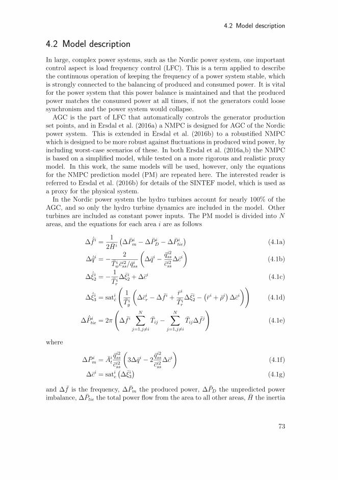
4.2 Model description
4.2 Model description
In large, complex power systems, such as the Nordic power system, one importantcontrol aspect is load frequency control (LFC). This is a term applied to describethe continuous operation of keeping the frequency of a power system stable, whichis strongly connected to the balancing of produced and consumed power. It is vitalfor the power system that this power balance is maintained and that the producedpower matches the consumed power at all times, if not the generators could loosesynchronism and the power system would collapse.
AGC is the part of LFC that automatically controls the generator productionset points, and in Ersdal et al. (2016a) a NMPC is designed for AGC of the Nordicpower system. This is extended in Ersdal et al. (2016b) to a robustified NMPCwhich is designed to be more robust against fluctuations in produced wind power, byincluding worst-case scenarios of these. In both Ersdal et al. (2016a,b) the NMPCis based on a simplified model, while tested on a more rigorous and realistic proxymodel. In this work, the same models will be used, however, only the equationsfor the NMPC prediction model (PM) are repeated here. The interested reader isreferred to Ersdal et al. (2016b) for details of the SINTEF model, which is used asa proxy for the physical system.
In the Nordic power system the hydro turbines account for nearly 100% of theAGC, and so only the hydro turbine dynamics are included in the model. Otherturbines are included as constant power inputs. The PM model is divided into Nareas, and the equations for each area i are as follows
∆ ˙f i =1
2H i
(∆P i
m −∆P iD −∆P i
tie
)(4.1a)
∆ ˙qi = − 2
T iwci2ss/q
iss
(∆qi − qi2ss
ci2ss∆ci)
(4.1b)
∆ ˙ξi2 = − 1
T ir∆ξi2 + ∆ci (4.1c)
∆ ˙ξi3 = satic
(1
T ig
(∆cir −∆f i +
ri
T ir∆ξi2 −
(ri + ρi
)∆ci))
(4.1d)
∆ ˙P itie = 2π
(∆f i
N∑
j=1,j 6=iTij −
N∑
j=1,j 6=iTij∆f
j
)(4.1e)
where
∆P im = Ait
qi2ssci2ss
(3∆qi − 2
qi2ssci2ss
∆ci)
(4.1f)
∆ci = satic(∆ξi3
)(4.1g)
and ∆f is the frequency, ∆Pm the produced power, ∆PD the unpredicted powerimbalance, ∆Ptie the total power flow from the area to all other areas, H the inertia
73

Chapter 4 Scenario-based approaches for handling uncertainty in MPC for FC
of the rotating masses of the area, Tij the synchronizing torque coefficient betweenarea i and j, ∆c and ∆q the changes in valve opening and water flow rate fromcss and qss, respectively, Tw the water starting time of the hydro turbine, At afactor that accounts for the different per-unit bases in the turbine and generator,∆ξ2 the integral of the governor, ∆ξ3 the valve opening of the main servo motor ofthe governor, Tg the time constant of the servo motor, Tr the time constant of thetransient droop, r the transient-droop coefficient, ρ the constant-droop coefficient,∆c the saturated valve opening, ∆cr the reference point for the valve opening, andi = 1, . . . , N . All defined relative an initial steady state. The controllable inputto the system is the valve-opening setpoint for each area ∆cir and the participationfactor for each generator j in area i, αij, and the disturbance acting on the systemis the unpredicted power imbalance for each area ∆P i
D.
4.2.1 System disturbance
The only disturbance we consider is that of the unpredicted power imbalance ∆P iD.
The main components of the unpredicted power imbalance with regards to LFCis the imbalance in production and consumption from intermittent generators andloads, respectively. When dealing with power systems including a certain amountof wind power, such as the Nordic system, one can for simplicity assume that ∆P i
D
is dominated by the fluctuations in produced wind power. If, in addition, it isassumed that the majority of wind power is situated in area p, ∆PD of all theother areas can be neglected, and the model is affected by one single disturbance∆PD = ∆P p
D. With the Nordic network in mind, Denmark and South Swedencontribute with about 80% of the total wind power production (Statnett, 2012).
The complete model is thus given by the nonlinear model
˙x = f (x, u, w) (4.2)
where x =[∆f i ∆qi ∆ξi2 ∆ξi3 ∆P i
tie
], u =
[∆cir αij
], w = ∆PD, i = 1, . . . , N ,
j = 1, . . . ,mih, and mi
h is the number of hydro generators in area i. The system isalso subjected to both input and state constraints
g (x, u) ≤ 0 (4.3)
including generation constraints, generator rate constraints, and constraints on thetie-line power transfer.
4.3 Controller
4.3.1 Disturbance modeling, deterministic vs stochastic.
When modeling a disturbance’s influence on a system, it is common to differentiatebetween deterministic and stochastic modeling. A system disturbance w is in gen-eral defined by an admissible set of disturbance signals w ∈ W , and the difference
74

4.3 Controller
between deterministic and stochastic modeling is whether or not one attempts toassign probabilities to the elements of the set W (Levine, 2010). With a determin-istic disturbance model all realizations in W are bounded and considered equallylikely to occur, while they are appointed different probabilities P [w] and are notnecessarily bounded when applying a stochastic disturbance model.
The disturbance acting on the system presented in Section 4.2 is the unpredictedpower imbalance w = ∆PD, which is assumed to be dominated by fluctuations inproduced wind power in area p. For each wind farm in area p, the probabilityspace of the future variation from the predicted power output can be estimated(Holttinen, 2004), and from this one can find the probability space of the futurevariation from the predicted power output for all wind farms in area p combined,i.e. w ∈ W , see Figure 4.2. The estimate of W is primarily based on weatherprognoses, which are stochastic by nature through the use of ensemble forecastingand model output statistics (Barry and Chorley, 2003). Hence, it would in manyways be natural to assign probabilities to the elements of W . However, it is notnecessarily the best choice when taking other aspects into account, and in thischapter two scenario-based approaches are compared, the SNMPC that is based ona stochastic disturbance model, and the MNMPC that is based on a deterministicdisturbance model. The aim of this chapter is to compare the two approaches,and discuss their strengths and weaknesses in view of their performance in the casestudy.
4.3.2 Stochastic NMPC
Given a system such as (4.2). If the disturbance signal w is modeled as a stochasticdisturbance with probability space W and probability distribution P [w] over W ,then it makes sense to replace hard constraints with chance constraints
Pw [g (x, u) ≤ 0 ∀ t] ≥ 1− σ (4.4)
where σ ∈ (0, 1) is the admissible constraint violation parameter, t = 1, . . . , T ,T is the optimization horizon, and Pw denotes the dependency of g (x, u) on thestochastic signal w. It basically states that the constraints are allowed to be violatedwith a probability no higher than 1− σ.
In scenario-based approaches to stochastic NMPC (Campi et al., 2009), S inde-pendent identically distributed samples of w (w1, . . . , wS) are used to approximatethe chance constraint, where only the constraints corresponding to the extracteddisturbance realizations are considered. The result is the SNMPC which includesa standard OCP with a finite number of constraints
minu,xj
S∑
j=1
J(xj, u
)(4.5a)
˙xj − f(xj, u, wj
)= 0 System model (4.5b)
g(xj, u
)≤ 0 Constraints (4.5c)
75

Chapter 4 Scenario-based approaches for handling uncertainty in MPC for FC
where j = 1, . . . , S, xj and wj are the state and disturbance associated with scenarioj, u the input, and J(xj, u) the following objective function.
J(xj, u
)=
∫ T
t=0
xjTQjxj + uTRu dt (4.6)
For convex OCPs, the scenario approach can be used to find the number ofscenarios needed to guarantee that the optimal solution to (4.5), u∗, satisfies allconstraints except a user-chosen fraction that tends rapidly to zero as S increases(Campi et al., 2009). The OCP (4.5) in the SNMPC has a quadratic objectivefunction and linear state and input constraints. The constraints imposed by thesystem model (4.5b) are however nonlinear because of the saturations in (4.1),hence the OCP is non-convex. It can however be argued that this is a modestnonlinearity, and we will apply the theory in Campi et al. (2009) as if we have alinear model and hence a convex OCP.
Generating scenarios
The scenarios used in the SNMPC are found by applying random numbers to gen-erate S independent and identically distributed disturbance realizations wj(t) =∆P j
D(t), j = 1, . . . , S, t = 0, . . . , T using the method in Cecılio et al. (2013) withthe probability space W as input. This method results in an unknown probabilitydistribution P , however, using the method of Campi et al. (2009) there is no needto knowW or P explicitly, only S realizations fulfilling this probability distributionis needed. When selecting the number of scenarios S, Theorem 1 in Campi et al.(2009) states that given the number of optimization variables nu, if S fulfills
S ≥ 2
κ
(ln
1
β+ nu
)(4.7)
the resulting solution to (4.5), u∗, will satisfy the chance constraints (4.4) with aprobability no smaller than 1− β, except for at most an κ-fraction. Theorem 1 inCampi et al. (2009) is developed with one common input u for all scenarios, and sou is equal for all j in the SNMPC (4.5).
4.3.3 Multi-stage NMPC
In Ersdal et al. (2016b) an NMPC for AGC of the Nordic power system whichis robustified against fluctuations in produced wind power is presented. It is aspecial case of the multi-stage NMPC (MNMPC) presented in Lucia et al. (2013),and it is also inspired by the min-max feedback MPC presented in Scokaert andMayne (1998). In both Lucia et al. (2013) and Scokaert and Mayne (1998) theconcept of future feedback is included in the NMPC. The idea is that the futurecontrol inputs can be adapted to the future disturbance measurements/estimates,and that only decisions based on the same information must be equal (Lucia et al.,
76
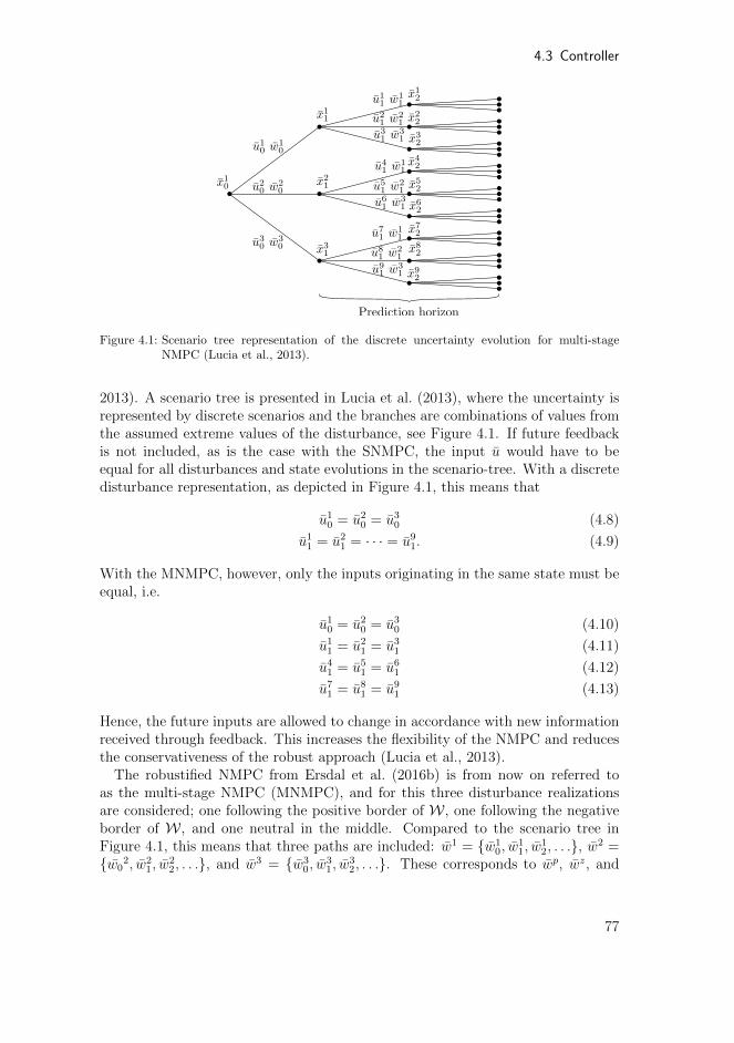
4.3 Controller
x10
x12
x22
x32
x42
x52
x62
x72
x82
x92
u21 w2
1
u11 w1
1
u31 w3
1
u41 w1
1
u51 w2
1
u61 w3
1
u71 w1
1
u81 w2
1
u91 w3
1
x11
x21
x31
u10 w1
0
u20 w2
0
u30 w3
0
Prediction horizon
Figure 4.1: Scenario tree representation of the discrete uncertainty evolution for multi-stageNMPC (Lucia et al., 2013).
2013). A scenario tree is presented in Lucia et al. (2013), where the uncertainty isrepresented by discrete scenarios and the branches are combinations of values fromthe assumed extreme values of the disturbance, see Figure 4.1. If future feedbackis not included, as is the case with the SNMPC, the input u would have to beequal for all disturbances and state evolutions in the scenario-tree. With a discretedisturbance representation, as depicted in Figure 4.1, this means that
u10 = u2
0 = u30 (4.8)
u11 = u2
1 = · · · = u91. (4.9)
With the MNMPC, however, only the inputs originating in the same state must beequal, i.e.
u10 = u2
0 = u30 (4.10)
u11 = u2
1 = u31 (4.11)
u41 = u5
1 = u61 (4.12)
u71 = u8
1 = u91 (4.13)
Hence, the future inputs are allowed to change in accordance with new informationreceived through feedback. This increases the flexibility of the NMPC and reducesthe conservativeness of the robust approach (Lucia et al., 2013).
The robustified NMPC from Ersdal et al. (2016b) is from now on referred toas the multi-stage NMPC (MNMPC), and for this three disturbance realizationsare considered; one following the positive border of W , one following the negativeborder of W , and one neutral in the middle. Compared to the scenario tree inFigure 4.1, this means that three paths are included: w1 = {w1
0, w11, w
12, . . .}, w2 =
{w02, w2
1, w22, . . .}, and w3 = {w3
0, w31, w
32, . . .}. These corresponds to wp, wz, and
77

Chapter 4 Scenario-based approaches for handling uncertainty in MPC for FC
Figure 4.2: Sketch of how the MNMPC works. For simplicity of illustration, u is considered to bescalar.
wn in Figure 4.2. In accordance to Lucia et al. (2013), the first element of u mustbe equal for all three scenarios (up0 = uz0 = un0 ), after this, they are free to vary inmanners optimal for their designated system states, see Figure 4.2.
The OCP solved at each time instant in the MNMPC is then
minuj ,xj
∑
j={p,z,n}J(xj, uj
)(4.14a)
˙xj − f(xj, uj, wj
)= 0 System model (4.14b)
g (xj, uj) ≤ 0uz0 = up0 = un0
}Constraints (4.14c)
where j = {p, z, n}, xj, wj, uj the state, disturbance and input associated withscenario j, and J(xj, uj) the following objective function.
J(xj, uj
)=
∫ T
t=0
xjTQjxj + ujTRjuj dt (4.15)
4.4 Case Study
The SNMPC is tested on the SINTEF Nordic power system test bed from Ersdalet al. (2016b) and compared against the MNMPC. The PM is chosen to have 2 areas,hence N = 2. One area covers South Sweden and Eastern Denmark (area A), andthe other covers Norway, North Sweden and Finland (area B), and according to theassumptions made in Section 4.2, ∆PB
D = 0 and ∆PD = ∆PAD . There is also a tie
line between the two areas which represents the total power flow between them, andhas a positive direction from area B to area A. The extended Kalman filter (EKF)presented in Ersdal et al. (2016b) is also applied here to close the control loop. Theproxy system and both NMPCs were implemented in Python using Casadi, wherethe continuous time OCPs (4.5) and (4.14) are discretized and transformed into
78
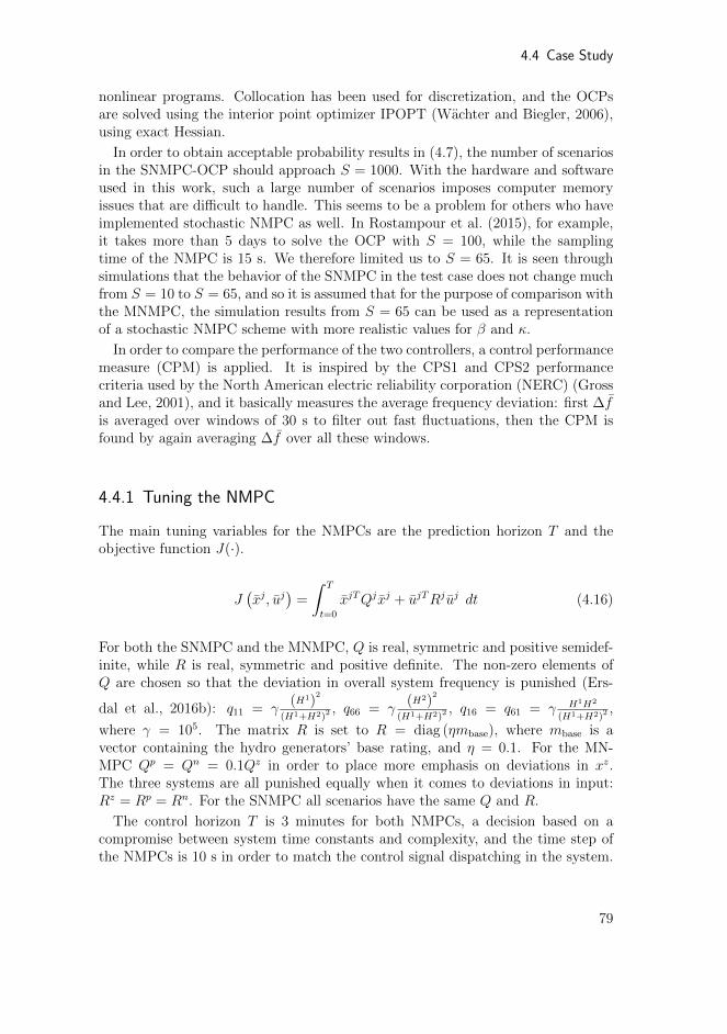
4.4 Case Study
nonlinear programs. Collocation has been used for discretization, and the OCPsare solved using the interior point optimizer IPOPT (Wachter and Biegler, 2006),using exact Hessian.
In order to obtain acceptable probability results in (4.7), the number of scenariosin the SNMPC-OCP should approach S = 1000. With the hardware and softwareused in this work, such a large number of scenarios imposes computer memoryissues that are difficult to handle. This seems to be a problem for others who haveimplemented stochastic NMPC as well. In Rostampour et al. (2015), for example,it takes more than 5 days to solve the OCP with S = 100, while the samplingtime of the NMPC is 15 s. We therefore limited us to S = 65. It is seen throughsimulations that the behavior of the SNMPC in the test case does not change muchfrom S = 10 to S = 65, and so it is assumed that for the purpose of comparison withthe MNMPC, the simulation results from S = 65 can be used as a representationof a stochastic NMPC scheme with more realistic values for β and κ.
In order to compare the performance of the two controllers, a control performancemeasure (CPM) is applied. It is inspired by the CPS1 and CPS2 performancecriteria used by the North American electric reliability corporation (NERC) (Grossand Lee, 2001), and it basically measures the average frequency deviation: first ∆fis averaged over windows of 30 s to filter out fast fluctuations, then the CPM isfound by again averaging ∆f over all these windows.
4.4.1 Tuning the NMPC
The main tuning variables for the NMPCs are the prediction horizon T and theobjective function J(·).
J(xj, uj
)=
∫ T
t=0
xjTQjxj + ujTRjuj dt (4.16)
For both the SNMPC and the MNMPC, Q is real, symmetric and positive semidef-inite, while R is real, symmetric and positive definite. The non-zero elements ofQ are chosen so that the deviation in overall system frequency is punished (Ers-
dal et al., 2016b): q11 = γ(H1)
2
(H1+H2)2, q66 = γ
(H2)2
(H1+H2)2, q16 = q61 = γ H1H2
(H1+H2)2,
where γ = 105. The matrix R is set to R = diag (ηmbase), where mbase is avector containing the hydro generators’ base rating, and η = 0.1. For the MN-MPC Qp = Qn = 0.1Qz in order to place more emphasis on deviations in xz.The three systems are all punished equally when it comes to deviations in input:Rz = Rp = Rn. For the SNMPC all scenarios have the same Q and R.
The control horizon T is 3 minutes for both NMPCs, a decision based on acompromise between system time constants and complexity, and the time step ofthe NMPCs is 10 s in order to match the control signal dispatching in the system.
79
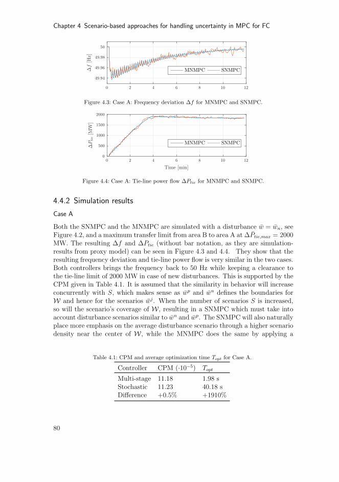
Chapter 4 Scenario-based approaches for handling uncertainty in MPC for FC
Figure 4.3: Case A: Frequency deviation ∆f for MNMPC and SNMPC.
Figure 4.4: Case A: Tie-line power flow ∆Ptie for MNMPC and SNMPC.
4.4.2 Simulation results
Case A
Both the SNMPC and the MNMPC are simulated with a disturbance w = wn, seeFigure 4.2, and a maximum transfer limit from area B to area A at ∆Ptie,max = 2000MW. The resulting ∆f and ∆Ptie (without bar notation, as they are simulation-results from proxy model) can be seen in Figure 4.3 and 4.4. They show that theresulting frequency deviation and tie-line power flow is very similar in the two cases.Both controllers brings the frequency back to 50 Hz while keeping a clearance tothe tie-line limit of 2000 MW in case of new disturbances. This is supported by theCPM given in Table 4.1. It is assumed that the similarity in behavior will increaseconcurrently with S, which makes sense as wp and wn defines the boundaries forW and hence for the scenarios wj. When the number of scenarios S is increased,so will the scenario’s coverage of W , resulting in a SNMPC which must take intoaccount disturbance scenarios similar to wn and wp. The SNMPC will also naturallyplace more emphasis on the average disturbance scenario through a higher scenariodensity near the center of W , while the MNMPC does the same by applying a
Table 4.1: CPM and average optimization time Topt for Case A.
Controller CPM (·10−5) Topt
Multi-stage 11.18 1.98 sStochastic 11.23 40.18 sDifference +0.5% +1910%
80

4.4 Case Study
higher weight to Qn in the objective function.However, as seen in Figure 4.3 and 4.4, the SNMPC results in a more “noisy”
system behavior than the MNMPC. There are two main reasons for this. First ofall, the scenarios used in the SNMPC fluctuate more than the smooth disturbancescenarios used in the MNMPC. These high frequency fluctuations will excite the fastsystem dynamics in the predictions, resulting in a more fluctuating and conservativecontroller. Secondly, the fact that the SNMPC has one common optimized inputfor all scenarios forces the input to fluctuate in order to fulfill system constraintsfor all scenarios, which again excites the dynamics of the actual system.
Case B
In Case B the transfer capacity on the tie line is changed so that the transfer windowis more narrow than in Case A. The limits are now set to ∆Ptie,min = −100 MWand ∆Ptie,max = 1000 MW, resulting in a transfer window of 1100 MW. Figure 4.5shows the predictions associated with wp and wn from the MNMPC-optimization att = 0, and Figure 4.6 shows the predictions associated with two of the disturbancerealizations from the last attempt at solving the SNMPC-optimization at t = 0.
In this case, the SNMPC was not able to find a feasible solution, and the reasonfor this is illustrated in Figure 4.6. It shows that the SNMPC is simply not ableto find a common input which fulfills the system constrains for all disturbancescenarios over the entire prediction horizon. Up until approximately 2.5 minutesinto the prediction horizon, the tie-line power transfer associated with w31 and w40
are kept at, or within, the transfer limits by keeping the total input relatively low.After this, however, it seems that some adjustments has to made, and the input isincreased, likely as an effort to keep ∆P 31
tie within the lower transfer limit. This inturn causes ∆P 40
tie to increase, and violate the upper transfer limit, as seen in thezoomed square of Figure 4.6(a).
The MNMPC is on the other hand able to find a feasible solution, and eventhough both ∆P p
tie and ∆P ntie stay at the limits, they never violate them. Figure
4.5(b) shows how the inputs associated with wp and wn are free to vary after thefirst two time steps (this is increased from one because of delays connected to theEKF), and this is the reason why the MNMPC is able to find a feasible solutionwhile the SNMPC is not.
4.4.3 Discussion
The benefit of the SNMPC is clearly the stochastic guarantees for constraint ful-fillment given by Theorem 1 in Campi et al. (2009). With S ≈ 1000, it would beguaranteed that with no probability smaller than 0.99, u∗ would satisfy all systemconstraints for all w ∈ W except for a small fraction of them whose probability issmaller than or equal to 0.07. These are theoretical guarantees which cannot bemade for the MNMPC. They are however made under unrealistic assumptions suchas perfect prediction model, and the practical implications are therefore arguable.
81

Chapter 4 Scenario-based approaches for handling uncertainty in MPC for FC
(a) Predicted tie-line power flow associated with wp and wn.
(b) Sum of predicted input associated with wp and wn.
Figure 4.5: Case B MNMPC: Predicted input and tie-line power flow.
(a) Predicted tie-line power flow associated with w31 and w40.
(b) Sum of predicted input for both w31 and w40.
Figure 4.6: Case B SNMPC: Predicted input and tie-line power flow.
82
4.4 Case Study
It is the authors’ opinion that the constraints of the control problem presentedin this chapter are of such a nature that the practical difference with respect toconstraint fulfillment is not prominent. However, it should be mentioned that theSNMPC does have the advantage of freedom to tune the conservativeness throughthe choice of η and β (and hence S), which is not as easy for the MNMPC.
There are also some issues with the tractability of the SNMPC as S increases.The MNMPC considers much fewer scenarios than the SNMPC, and therefore solvesa much smaller OCP. This is reflected in the maximum optimization time in CaseA, which was 2.1 s and 59.8 s for the MNMPC and the SNMPC, respectively, withan average optimization time of 2.0 s and 40.2 s. If a successful simulation ofSNMPC with S = 1000 could be conducted, the optimization time would increaseeven further, and with a time step of 10 s, this means that the MNMPC is able torun in real time, whereas the SNMPC is not. It can be argued that some of thesetractability issues can be resolved using more memory etc., however, the MNMPCwill still solve the OCP in less time.
Another issue is the feasibility and recursive feasibility of the OCP. For boththe MNMPC and the SNMPC there are no guarantees for neither feasibility norrecursive feasibility. However, in the MNMPC the optimization variable u foreach disturbance realization {wz, wp, wn} only needs to be equal for the first in-stant, before they are free to do what is optimal for their associated system states{xz, xp, xn}, whereas for the SNMPC u is equal for all disturbance realizations andtheir associated system states. This complicates matters for the SNMPC with re-gards to feasibility, as seen in Case B. When the scenarios included in the SNMPCresults in diverging system behavior and thereby diverging inputs needs, it becomesincreasingly difficult as S increases to find one common input to satisfy them all. Itcould be argued that feedback could be included in the SNMPC as well, this wouldhowever increase the already prominent tractability issues. If each of the scenariosof the SNMPC were to have their own input, the size of the OCP would increasesubstantially. In addition, since Theorem 1 from Campi et al. (2009) is developedwith one common input for all scenarios, it may not hold if feedback was included.When it comes to recursive feasibility, the MNMPC results in a standard, nominalNMPC, and recursive feasibility can be guaranteed using classical methods suchas terminal constraint regions which are control invariant (Maiworm et al., 2015),provided that such terminal ingredients can be calculated a priori. In the generalnonlinear case it is however very challenging to find the necessary terminal ingredi-ents, and if they can be found, they often lead to overly conservative control laws(Lucia et al., 2014b).
The MNMPC and the SNMPC are based upon two different disturbance modelingparadigms; deterministic and stochastic. And even though it could be argued thatit is intuitive to view the future variation from the predicted wind-power productionas stochastic, the robust control issue in this work is mainly handling the worst casedisturbance, since handling of the worst-case disturbance implies that less severedisturbances can be handled as well. The case study presented in this chapterillustrates that the SNMPC and the MNMPC have some similarities in practice,
83

Chapter 4 Scenario-based approaches for handling uncertainty in MPC for FC
however, the MNMPC is less conservative and less likely to encounter feasibilityissues because it takes into account feedback in its predictions.
4.5 Conclusion
This chapter presents a stochastic NMPC (SNMPC) for frequency control of theNordic power system, and compares it with the multi-stage NMPC (MNMPC)presented in Ersdal et al. (2016b). The nonlinearities of the SNMPC are verymodest, and the theory on stochastic assurance of constraint fulfillment from Campiet al. (2009) is used as if the optimal control problem of the SNMPC was convex.
Simulations on a proxy of the Nordic power system show that the SNMPC andthe MNMPC behaves similarly, and it argued that the SNMPC and the MNMPCshare some properties in practice. However, the MNMPC does not give stochasticguarantees for constraint fulfillment, such as the SNMPC. The practical conse-quences of this are unclear, especially given that these guarantees does not takeinto account other unknown disturbances and model errors. On the other hand,the MNMPC is less likely to encounter infeasibility, and there are also tractabilityand real-time issues with the SNMPC which are not seen in the MNMPC.
84

Chapter 5
Coordinated control of multiple HVDC links usingbackstepping
The work in this chapter was published in Ersdal et al. (2012).
Summary
This chapter regards a power system containing multiple High VoltageDirect Current (HVDC) links. The topic is to exploit the HVDC lines’ability to control the power supplied by them to increase the stabilityof the system. The nonlinear controller-design method backstepping isapplied to design a controller for the direct current (DC) through eachHVDC link. The simulation results show that the controller increasesboth transient stability and damping when some non-permanent errorsare imposed on the system.
5.1 Introduction
The electric power systems in Europe today are complex dynamical systems ofhigh dimension consisting of interconnected generators, transmission lines, loadsetc. In order to keep the power supply safe and stable, it is important that allthe generating units of an alternating current (AC) power system operate at thesame frequency. The recent and ongoing liberalization of the energy market aswell as increasing demand has in some cases reduced the stability margin of thepower systems (Morison et al., 2004), and it has become important to augmenttheir stability. Some of the possibilities for improving the power system stabilityare:
1. building new transmission lines,
2. installing new generation capacity,
3. better utilize the existing equipment in the power system.
High Voltage Direct Current (HVDC) links are in general used to transmit largeamounts of energy over long distances. Norway is for example connected to theNetherlands and Denmark with underwater HVDC cables. But HVDC lines also
85
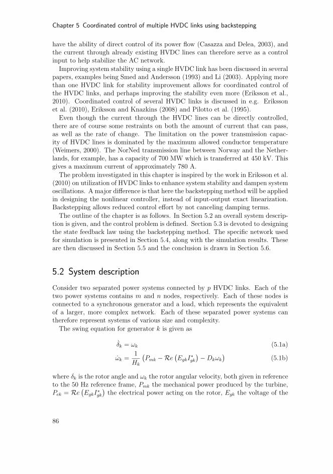
Chapter 5 Coordinated control of multiple HVDC links using backstepping
have the ability of direct control of its power flow (Casazza and Delea, 2003), andthe current through already existing HVDC lines can therefore serve as a controlinput to help stabilize the AC network.
Improving system stability using a single HVDC link has been discussed in severalpapers, examples being Smed and Andersson (1993) and Li (2003). Applying morethan one HVDC link for stability improvement allows for coordinated control ofthe HVDC links, and perhaps improving the stability even more (Eriksson et al.,2010). Coordinated control of several HVDC links is discussed in e.g. Erikssonet al. (2010), Eriksson and Knazkins (2008) and Pilotto et al. (1995).
Even though the current through the HVDC lines can be directly controlled,there are of course some restraints on both the amount of current that can pass,as well as the rate of change. The limitation on the power transmission capac-ity of HVDC lines is dominated by the maximum allowed conductor temperature(Weimers, 2000). The NorNed transmission line between Norway and the Nether-lands, for example, has a capacity of 700 MW which is transferred at 450 kV. Thisgives a maximum current of approximately 780 A.
The problem investigated in this chapter is inspired by the work in Eriksson et al.(2010) on utilization of HVDC links to enhance system stability and dampen systemoscillations. A major difference is that here the backstepping method will be appliedin designing the nonlinear controller, instead of input-output exact linearization.Backstepping allows reduced control effort by not canceling damping terms.
The outline of the chapter is as follows. In Section 5.2 an overall system descrip-tion is given, and the control problem is defined. Section 5.3 is devoted to designingthe state feedback law using the backstepping method. The specific network usedfor simulation is presented in Section 5.4, along with the simulation results. Theseare then discussed in Section 5.5 and the conclusion is drawn in Section 5.6.
5.2 System description
Consider two separated power systems connected by p HVDC links. Each of thetwo power systems contains m and n nodes, respectively. Each of these nodes isconnected to a synchronous generator and a load, which represents the equivalentof a larger, more complex network. Each of these separated power systems cantherefore represent systems of various size and complexity.
The swing equation for generator k is given as
δk = ωk (5.1a)
ωk =1
Hk
(Pmk −Re
(EgkI
∗gk
)−Dkωk
)(5.1b)
where δk is the rotor angle and ωk the rotor angular velocity, both given in referenceto the 50 Hz reference frame, Pmk the mechanical power produced by the turbine,Pek = Re
(EgkI
∗gk
)the electrical power acting on the rotor, Egk the voltage of the
86
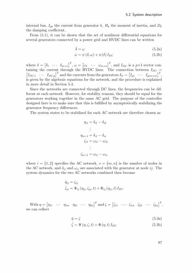
5.2 System description
internal bus, Igk the current from generator k, Hk the moment of inertia, and Dk
the damping coefficient.
From (5.1), it can be shown that the set of nonlinear differential equations forseveral generators connected by a power grid and HVDC lines can be written
δ = ω (5.2a)
ω = ψ (δ, ω) + φ (δ) IDC (5.2b)
where δ =[δ1 · · · δm+n
]T, ω =
[ω1 · · · ωm+n
]T, and IDC is a p×1-vector con-
taining the current through the HVDC lines. The connection between IDC =[IDC,1 · · · IDC,p
]Tand the currents from the generators IG =
[Ig1 · · · Ig(m+n)
]T,
is given by the algebraic equations for the network, and the procedure is explainedin more detail in Section 5.4.
Since the networks are connected through DC lines, the frequencies can be dif-ferent at each network. However, for stability reasons, they should be equal for thegenerators working together in the same AC grid. The purpose of the controllerdesigned here is to make sure that this is fulfilled by asymptotically stabilizing thegenerator frequency differences.
The system states to be stabilized for each AC network are therefore chosen as
ηi1 = δi1 − δi2...
ηis−1 = δi1 − δisζi1 = ωi1 − ωi2
...
ζis−1 = ωi1 − ωis
where i = {1, 2} specifies the AC network, s = {m,n} is the number of nodes inthe AC network, and δij and ωij are associated with the generator at node ij. Thesystem dynamics for the two AC networks combined then become
ηij = ζij
ζij = Ψij (ηij, ζij, t) + Φij (ηij, t) IDC
With η =[η11 · · · η1m η21 · · · η2n
]Tand ζ =
[ζ11 · · · ζ1m ζ21 · · · ζ2n
]T,
we can collect
η = ζ (5.3a)
ζ = Ψ (η, ζ, t) + Φ (η, t) IDC (5.3b)
87

Chapter 5 Coordinated control of multiple HVDC links using backstepping
where
Ψ (η, ζ, t) =
Ψ11 (η, ζ, t)...
Ψ1m (η, ζ, t)Ψ21 (η, ζ, t)
...Ψ2n (η, ζ, t)
, Φ (η, t) =
Φ11 (η, t)...
Φ1m (η, t)Φ21 (η, t)
...Φ2n (η, t)
.
It is not possible to write ζ merely as a function of η, ζ and IDC , there will also bedependencies on the original system variables ω and δ. This is solved by regardingδ and ω as time varying signals, hence the time-dependence in the system.
Since η does not necessarily have an equilibrium at the origin, a change of vari-ables is made so that η = η − η0:
˙η = ζ (5.4a)
ζ = Ψ (η + η0, ζ, t) + Φ (η + η0, t) IDC (5.4b)
where η0 is the equilibrium of (5.3a) and
Ψ (η + η0, ζ, t) = ΨR (η + η0, ζ, t)−Dζ (5.5)
whereDζ contains the “good” damping terms of Ψ (η + η0, ζ, t), and ΨR (η + η0, ζ, t)contains the remaining elements. The good damping terms consists of terms thatprovides desirable damping to the system states. The matrix D is a r×r diagonalmatrix containing combinations of Dk
Mk, where r = m + n. The equilibrium of ζ is
ζ = 0, and the system (5.4) therefore has its equilibrium at the origin.
Assumption 1. It is in the following assumed that Φ (η + η0, t) is quadratic, thatis, ζ and IDC have the same dimension, and invertible.
This assumption is restrictive with regards to the configuration of the powersystem, and future work should include relaxing this assumption and considering amore general network configuration.
5.3 Controller Design
Backstepping is a recursive procedure for designing nonlinear controllers. It requiresfull state feedback, and it is therefore assumed that all system states are eithermeasured by phasor measurement units (PMU) or that they are estimated by astate estimator.
Consider systems on the form
η = f (η) + g (η) ζ (5.6a)
ζ = u (5.6b)
88
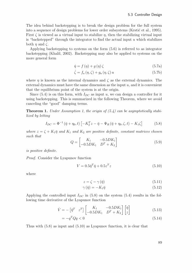
5.3 Controller Design
The idea behind backstepping is to break the design problem for the full systeminto a sequence of design problems for lower order subsystems (Krstic et al., 1995).First ζ is viewed as a virtual input to stabilize η, then the stabilizing virtual inputis “backstepped” through the integrator to find the actual input u which stabilizesboth η and ζ.
Applying backstepping to systems on the form (5.6) is referred to as integratorbackstepping (Khalil, 2002). Backstepping may also be applied to systems on themore general form
η = f (η) + g (η) ζ (5.7a)
ζ = fa (η, ζ) + ga (η, ζ)u (5.7b)
where η is known as the internal dynamics and ζ as the external dynamics. Theexternal dynamics must have the same dimension as the input u, and it is convenientthat the equilibrium point of the system is at the origin.
Since (5.4) is on this form, with IDC as input u, we can design a controller for itusing backstepping. This is summarized in the following Theorem, where we avoidcanceling the “good” damping terms.
Theorem 1. Under Assumption 1, the origin of (5.4) can be asymptotically stabi-lized by letting
IDC = Φ−1 (η + η0, t)[−KT
2 z − η −ΨR (η + η0, ζ, t)−K1ζ]
(5.8)
where z = ζ + K1η and K1 and K2 are positive definite, constant matrices chosensuch that
Q =
[K1 −0.5DK1
−0.5DK1 DT +K2
](5.9)
is positive definite.
Proof. Consider the Lyapunov function
V = 0.5ηT η + 0.5zT z (5.10)
where
z = ζ − γ (η) (5.11)
γ (η) = −K1η (5.12)
Applying the controlled input IDC in (5.8) on the system (5.4) results in the fol-lowing time derivative of the Lyapunov function
V = −[ηT zT
] [ K1 −0.5DK1
−0.5DK1 DT +K2
] [ηz
](5.13)
= −qTQq < 0 (5.14)
Thus with (5.8) as input and (5.10) as Lyapunov function, it is clear that
89
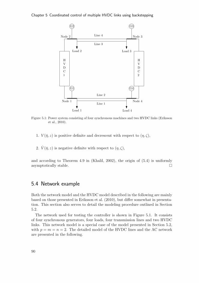
Chapter 5 Coordinated control of multiple HVDC links using backstepping
Node 2
Node 1
HVDC1
G2
G1
Node 3
Node 4
HVDC2
G3
G4
Line 4
Line 3
Line 2
Line 1
Load 2 Load 3
Load 4Load 1
Figure 5.1: Power system consisting of four synchronous machines and two HVDC links (Erikssonet al., 2010).
1. V (η, z) is positive definite and decrescent with respect to (η, ζ),
2. V (η, z) is negative definite with respect to (η, ζ),
and according to Theorem 4.9 in (Khalil, 2002), the origin of (5.4) is uniformlyasymptotically stable.
5.4 Network example
Both the network model and the HVDC model described in the following are mainlybased on those presented in Eriksson et al. (2010), but differ somewhat in presenta-tion. This section also serves to detail the modeling procedure outlined in Section5.2.
The network used for testing the controller is shown in Figure 5.1. It consistsof four synchronous generators, four loads, four transmission lines and two HVDClinks. This network model is a special case of the model presented in Section 5.2,with p = m = n = 2. The detailed model of the HVDC lines and the AC networkare presented in the following.
90
5.4 Network example
5.4.1 HVDC model
As in Eriksson et al. (2010), the HVDC lines are of conventional type, meaning thatreactive power is consumed by them and that the active power through them canbe controlled via the DC current. It is assumed that the HVDC lines are losslessand have ideal control capabilities. It is also assumed that the power factors onboth the inverter and rectifier side are equal. Positive direction for the currentthrough HVDC link 1 and 2 are from node 1 to node 2 and from node 4 to node3, respectively. This means that the current injected from the HVDC links havepositive sign at node 2 and 3 and negative sign at node 1 and 4 of Figure 5.1.
Assuming that the absolute value of the node voltages at each side of the HVDClinks are approximately equal, the injected current at node k by HVDC link l isgiven as
IHVDC,kl = IDC,kl · ejθk (5.15)
where θk is the voltage angle at node k, and IDC,l is the controlled DC currentthrough HVDC link l. Assuming that node k is directly connected to HVDC linkl, then IDC,kl = −IDC,l if node k is at the rectifier side, and IDC,kl = IDC,l if nodek is at the inverter side. If node k and HVDC link l are not directly connected,IDC,kl = 0.
Defining IHVDC,k as the total current injected at node k by both HVDC-links,leads to the following
IHVDC =
IHVDC,1IHVDC,2IHVDC,3IHVDC,4
=
−eiθ1 0eiθ2 00 eiθ3
0 −eiθ4
IDC (5.16)
where IDC =[IDC,1 IDC,2
]T.
5.4.2 Network model
The algebraic equation for the current flow in the network is found using the internalnode representation, where it is assumed that the loads in the network are constantresistances. Defining all currents as positive into node k, Kirchoff’s current lawgives
Igk + ILk + IHVDC,k +n+m∑
l=1
YklUl = 0 (5.17)
where Igk is the current injected by generator k, ILk the current from load k, IHVDC,kthe current injected by the HVDC-links, Ykl the systems admittance matrix atposition (k, l), Ul the voltage at node l, and n + m the number of nodes in thenetwork.
The current injected from generator k into node k is given by
Igk =Egk − Ukjx′dk
, ∀ k = 1, . . . , 4 (5.18)
91
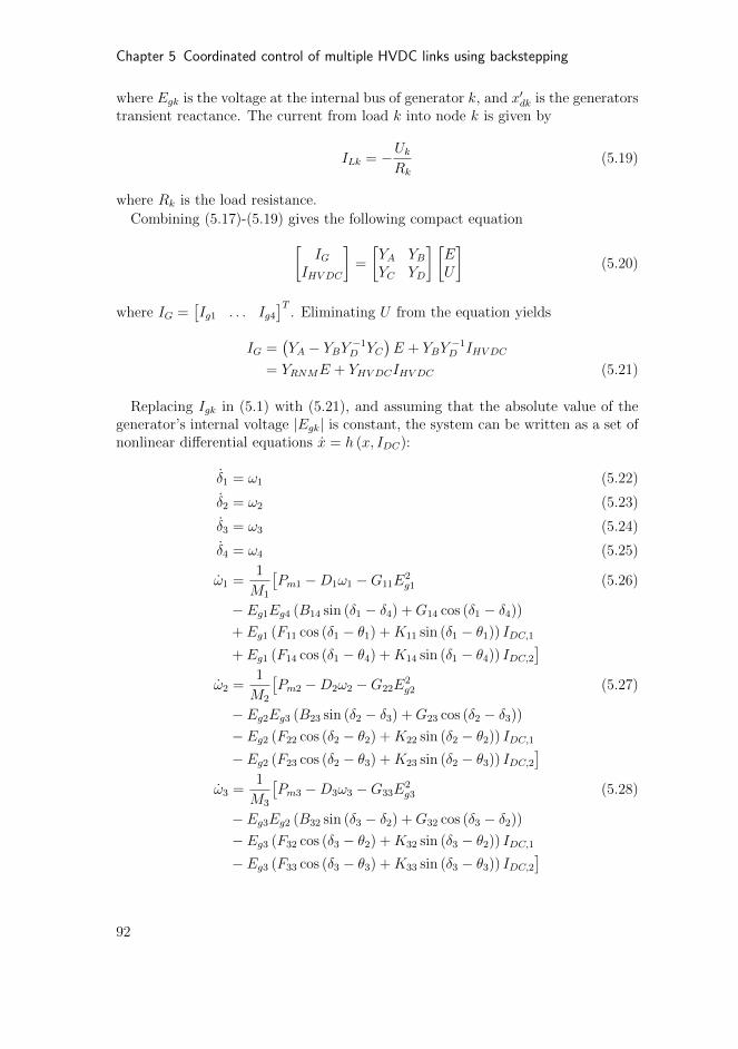
Chapter 5 Coordinated control of multiple HVDC links using backstepping
where Egk is the voltage at the internal bus of generator k, and x′dk is the generatorstransient reactance. The current from load k into node k is given by
ILk = −UkRk
(5.19)
where Rk is the load resistance.
Combining (5.17)-(5.19) gives the following compact equation
[IG
IHVDC
]=
[YA YBYC YD
] [EU
](5.20)
where IG =[Ig1 . . . Ig4
]T. Eliminating U from the equation yields
IG =(YA − YBY −1
D YC)E + YBY
−1D IHVDC
= YRNME + YHVDCIHVDC (5.21)
Replacing Igk in (5.1) with (5.21), and assuming that the absolute value of thegenerator’s internal voltage |Egk| is constant, the system can be written as a set ofnonlinear differential equations x = h (x, IDC):
δ1 = ω1 (5.22)
δ2 = ω2 (5.23)
δ3 = ω3 (5.24)
δ4 = ω4 (5.25)
ω1 =1
M1
[Pm1 −D1ω1 −G11E
2g1 (5.26)
− Eg1Eg4 (B14 sin (δ1 − δ4) +G14 cos (δ1 − δ4))
+ Eg1 (F11 cos (δ1 − θ1) +K11 sin (δ1 − θ1)) IDC,1
+ Eg1 (F14 cos (δ1 − θ4) +K14 sin (δ1 − θ4)) IDC,2]
ω2 =1
M2
[Pm2 −D2ω2 −G22E
2g2 (5.27)
− Eg2Eg3 (B23 sin (δ2 − δ3) +G23 cos (δ2 − δ3))
− Eg2 (F22 cos (δ2 − θ2) +K22 sin (δ2 − θ2)) IDC,1
− Eg2 (F23 cos (δ2 − θ3) +K23 sin (δ2 − θ3)) IDC,2]
ω3 =1
M3
[Pm3 −D3ω3 −G33E
2g3 (5.28)
− Eg3Eg2 (B32 sin (δ3 − δ2) +G32 cos (δ3 − δ2))
− Eg3 (F32 cos (δ3 − θ2) +K32 sin (δ3 − θ2)) IDC,1
− Eg3 (F33 cos (δ3 − θ3) +K33 sin (δ3 − θ3)) IDC,2]
92
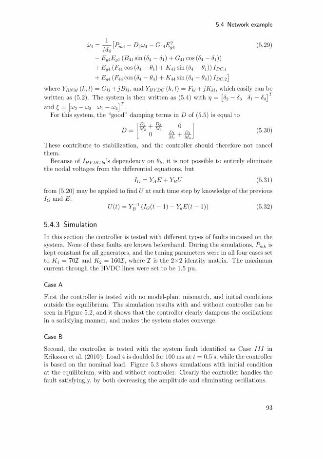
5.4 Network example
ω4 =1
M4
[Pm4 −D4ω4 −G44E
2g4 (5.29)
− Eg4Eg1 (B41 sin (δ4 − δ1) +G41 cos (δ4 − δ1))
+ Eg4 (F41 cos (δ4 − θ1) +K41 sin (δ4 − θ1)) IDC,1
+ Eg4 (F44 cos (δ4 − θ4) +K44 sin (δ4 − θ4)) IDC,2]
where YRNM (k, l) = Gkl + jBkl, and YHVDC (k, l) = Fkl + jKkl, which easily can be
written as (5.2). The system is then written as (5.4) with η =[δ2 − δ3 δ1 − δ4
]T
and ξ =[ω2 − ω3 ω1 − ω4
]T.
For this system, the “good” damping terms in D of (5.5) is equal to
D =
[D2
M2+ D3
M30
0 D1
M1+ D4
M4
](5.30)
These contribute to stabilization, and the controller should therefore not cancelthem.
Because of IHVDC,kl’s dependency on θk, it is not possible to entirely eliminatethe nodal voltages from the differential equations, but
IG = YAE + YBU (5.31)
from (5.20) may be applied to find U at each time step by knowledge of the previousIG and E:
U(t) = Y −1B (IG(t− 1)− YaE(t− 1)) (5.32)
5.4.3 Simulation
In this section the controller is tested with different types of faults imposed on thesystem. None of these faults are known beforehand. During the simulations, Pmk iskept constant for all generators, and the tuning parameters were in all four cases setto K1 = 70I and K2 = 160I, where I is the 2×2 identity matrix. The maximumcurrent through the HVDC lines were set to be 1.5 pu.
Case A
First the controller is tested with no model-plant mismatch, and initial conditionsoutside the equilibrium. The simulation results with and without controller can beseen in Figure 5.2, and it shows that the controller clearly dampens the oscillationsin a satisfying manner, and makes the system states converge.
Case B
Second, the controller is tested with the system fault identified as Case III inEriksson et al. (2010): Load 4 is doubled for 100 ms at t = 0.5 s, while the controlleris based on the nominal load. Figure 5.3 shows simulations with initial conditionat the equilibrium, with and without controller. Clearly the controller handles thefault satisfyingly, by both decreasing the amplitude and eliminating oscillations.
93
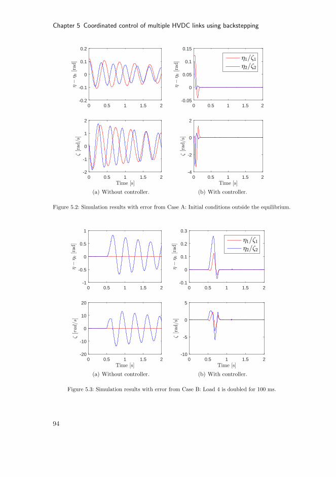
Chapter 5 Coordinated control of multiple HVDC links using backstepping
0 0.5 1 1.5 2-0.2
-0.1
0
0.1
0.2
2!20[rad
]
0 0.5 1 1.5 2Time [s]
-2
-1
0
1
2
1[rad
/s]
(a) Without controller.
0 0.5 1 1.5 2-0.05
0
0.05
0.1
0.15
2!20[rad
]
21=1122=12
0 0.5 1 1.5 2Time [s]
-4
-2
0
2
1[rad
/s]
(b) With controller.
Figure 5.2: Simulation results with error from Case A: Initial conditions outside the equilibrium.
0 0.5 1 1.5 2-1
-0.5
0
0.5
1
2!20[rad
]
0 0.5 1 1.5 2Time [s]
-20
-10
0
10
20
1[r
ad=s
]
(a) Without controller.
0 0.5 1 1.5 2-0.1
0
0.1
0.2
0.3
2!20[rad
]
21=1122=12
0 0.5 1 1.5 2Time [s]
-10
-5
0
5
1[rad
/s]
(b) With controller.
Figure 5.3: Simulation results with error from Case B: Load 4 is doubled for 100 ms.
94
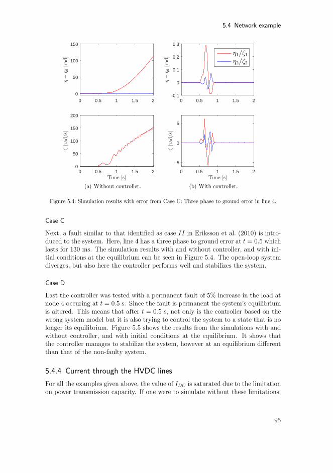
5.4 Network example
0 0.5 1 1.5 20
50
100
150
2!20[rad
]
0 0.5 1 1.5 2Time [s]
0
50
100
150
200
1[rad
/s]
(a) Without controller.
0 0.5 1 1.5 2-0.1
0
0.1
0.2
0.3
2!20[rad
]
21=1122=12
0 0.5 1 1.5 2Time [s]
-5
0
5
1[rad
/s]
(b) With controller.
Figure 5.4: Simulation results with error from Case C: Three phase to ground error in line 4.
Case C
Next, a fault similar to that identified as case II in Eriksson et al. (2010) is intro-duced to the system. Here, line 4 has a three phase to ground error at t = 0.5 whichlasts for 130 ms. The simulation results with and without controller, and with ini-tial conditions at the equilibrium can be seen in Figure 5.4. The open-loop systemdiverges, but also here the controller performs well and stabilizes the system.
Case D
Last the controller was tested with a permanent fault of 5% increase in the load atnode 4 occuring at t = 0.5 s. Since the fault is permanent the system’s equilibriumis altered. This means that after t = 0.5 s, not only is the controller based on thewrong system model but it is also trying to control the system to a state that is nolonger its equilibrium. Figure 5.5 shows the results from the simulations with andwithout controller, and with initial conditions at the equilibrium. It shows thatthe controller manages to stabilize the system, however at an equilibrium differentthan that of the non-faulty system.
5.4.4 Current through the HVDC lines
For all the examples given above, the value of IDC is saturated due to the limitationon power transmission capacity. If one were to simulate without these limitations,
95
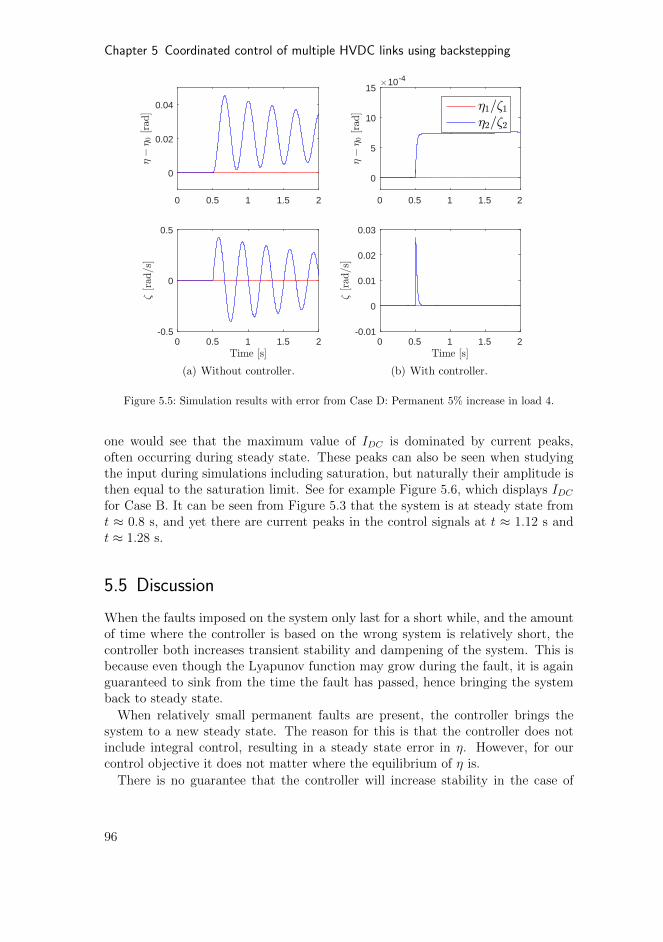
Chapter 5 Coordinated control of multiple HVDC links using backstepping
0 0.5 1 1.5 2
0
0.02
0.04
2!20[rad
]
0 0.5 1 1.5 2Time [s]
-0.5
0
0.5
1[rad
/s]
(a) Without controller.
0 0.5 1 1.5 2
0
5
10
15
2!20[rad
]
#10-4
21=1122=12
0 0.5 1 1.5 2Time [s]
-0.01
0
0.01
0.02
0.03
1[rad
/s]
(b) With controller.
Figure 5.5: Simulation results with error from Case D: Permanent 5% increase in load 4.
one would see that the maximum value of IDC is dominated by current peaks,often occurring during steady state. These peaks can also be seen when studyingthe input during simulations including saturation, but naturally their amplitude isthen equal to the saturation limit. See for example Figure 5.6, which displays IDCfor Case B. It can be seen from Figure 5.3 that the system is at steady state fromt ≈ 0.8 s, and yet there are current peaks in the control signals at t ≈ 1.12 s andt ≈ 1.28 s.
5.5 Discussion
When the faults imposed on the system only last for a short while, and the amountof time where the controller is based on the wrong system is relatively short, thecontroller both increases transient stability and dampening of the system. This isbecause even though the Lyapunov function may grow during the fault, it is againguaranteed to sink from the time the fault has passed, hence bringing the systemback to steady state.
When relatively small permanent faults are present, the controller brings thesystem to a new steady state. The reason for this is that the controller does notinclude integral control, resulting in a steady state error in η. However, for ourcontrol objective it does not matter where the equilibrium of η is.
There is no guarantee that the controller will increase stability in the case of
96
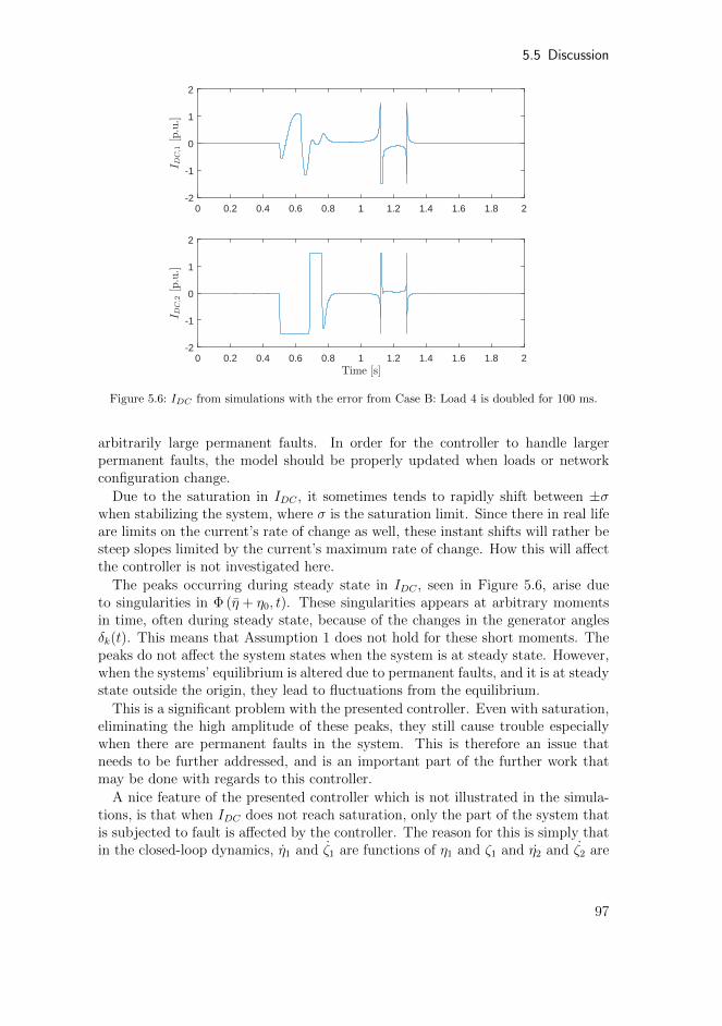
5.5 Discussion
0 0.2 0.4 0.6 0.8 1 1.2 1.4 1.6 1.8 2-2
-1
0
1
2
I DC
;1[p
.u.]
0 0.2 0.4 0.6 0.8 1 1.2 1.4 1.6 1.8 2Time [s]
-2
-1
0
1
2
I DC
;2[p
.u.]
Figure 5.6: IDC from simulations with the error from Case B: Load 4 is doubled for 100 ms.
arbitrarily large permanent faults. In order for the controller to handle largerpermanent faults, the model should be properly updated when loads or networkconfiguration change.
Due to the saturation in IDC , it sometimes tends to rapidly shift between ±σwhen stabilizing the system, where σ is the saturation limit. Since there in real lifeare limits on the current’s rate of change as well, these instant shifts will rather besteep slopes limited by the current’s maximum rate of change. How this will affectthe controller is not investigated here.
The peaks occurring during steady state in IDC , seen in Figure 5.6, arise dueto singularities in Φ (η + η0, t). These singularities appears at arbitrary momentsin time, often during steady state, because of the changes in the generator anglesδk(t). This means that Assumption 1 does not hold for these short moments. Thepeaks do not affect the system states when the system is at steady state. However,when the systems’ equilibrium is altered due to permanent faults, and it is at steadystate outside the origin, they lead to fluctuations from the equilibrium.
This is a significant problem with the presented controller. Even with saturation,eliminating the high amplitude of these peaks, they still cause trouble especiallywhen there are permanent faults in the system. This is therefore an issue thatneeds to be further addressed, and is an important part of the further work thatmay be done with regards to this controller.
A nice feature of the presented controller which is not illustrated in the simula-tions, is that when IDC does not reach saturation, only the part of the system thatis subjected to fault is affected by the controller. The reason for this is simply thatin the closed-loop dynamics, η1 and ζ1 are functions of η1 and ζ1 and η2 and ζ2 are
97

Chapter 5 Coordinated control of multiple HVDC links using backstepping
functions of η2 and ζ2. This means that the rest of the systems stays at steadystate during a fault, while the “subsystem” where the fault occurred deals with thestabilization.
5.6 Conclusion
The controller presented in this chapter is proven to asymptotically stabilize thesystem in theory, as long as the controller is based on the correct system. Simula-tions confirm that as long as the time the controller is based on an incorrect systemis limited, it increases the stability of the system and brings it back to steady state.
It is also shown that during small permanent faults, the controller increasesstability, but brings the system to a new equilibrium. However, it cannot necessarilyhandle arbitrary large permanent changes in the system. To address this issue thecontroller must work together with a good model updater, so that the model isupdated when larger changes in loads or network configuration appears.
The main challenge of the presented controller is however the restrictive natureof Assumption 1, and the fact that the controller becomes singular for some combi-nations of generator angles. These singularities in the controller is an issue whichmust be resolved in order for the controller to function in practice. Another prob-lem with Assumption 1 is of course that it confines the configuration of the networkit may be applied on, demanding that the number of external variables ζ and thenumber of HVDC lines are equal.
98
Chapter 6
Concluding remarks
In this thesis, the advanced control method known as model predictive control(MPC) is used for automatic generator control (AGC) of the Nordic power system.In Chapter 1 the composition of the Nordic power system was presented, and thefactors identified by the Norwegian transmission system operator (TSO) as themain challenges with regards to load frequency control (LFC) were presented. TheNordic power system has seen a decrease in frequency quality over the past twodecades, and the aim of this thesis has been to improve the frequency qualityand solve other issues related to this, such as avoiding bottleneck congestions andminimizing the effect of hourly production and trading set-point changes.
In Chapter 2 a nonlinear MPC (NMPC) was presented, including an extendedKalman filter (EKF) for state and disturbance estimation. The NMPC is based ona simplified model of the proxy system, and the constraints include limitations ontie-line power flow, generation capacity, and generation rate of change. Even thoughthe NMPC is based on a simplified system model (based on aggregated generators),it is able to account for individual generator constraints by including the generatorparticipation factors as optimization variables. This is an important feature, asthe limitations on both total production and production rate-of-change vary a lotbetween the individual generating units. Simulations showed that the NMPC isable to coordinate the AGC with the primary control, resulting in reduced costsand improved frequency quality both at hour-shifts and during normal operationthroughout the hour.
Performing LFC is a considerable expense for the TSO, and it is in many waysintuitive to include pricing in the NMPC in order to minimize costs. A suggestionto how this could be done is included in Chapter 2, where the cost of using the dif-ferent generating units for AGC is included in the objective function in a quadraticmanner. In an economic MPC, the objective function is often an economic profitfunction, which is linearly dependent on the state and input. The suggestion madehere is therefore not an economic MPC, but rather a suggestion to how it could beincluded in the given framework. This was illustrated through simulations, showingthat the MPC will favor the cheaper generating units.
The Nordic power system has not been sufficiently expanded since the liberal-ization of the power markets during the 1990s, which has led to a heavier loadednetwork with an increasing amount of bottlenecks. At times, these bottlenecksprevent some of the generating units in participating in LFC, which can lead to
99
Chapter 6 Concluding remarks
both poorer frequency quality and higher expenses connected to LFC. In Chapter2 another suggestion concerns how slack variables can be used to ensure availabletie-line power-transfer capacity, and hence avoid tie-line bottlenecks. The presentedsolution requires an a-priori calculation of the need for available transfer capacityon the tie-lines. This is a somewhat rigid solution, and in Chapter 3 a more flexiblesolution to this problem is presented in the form of robustified NMPC. Instead ofstating, for each tie-line, how much available transfer capacity is needed in case ofany unforeseen event, the focus is now on unforeseen changes in wind power produc-tion, and the aim is to improve frequency quality in the presence of uncontrollablepower production, such as wind power. A choice was made to focus on the slowlyvarying unpredicted power imbalance, and not on sudden changes caused by largeloads or generators disconnecting or connecting to the system. The choice to focusonly on the disturbance caused by unpredicted changes in wind power production isbased on the assumption that the general slowly varying unpredicted power imbal-ance in the Nordic power system is dominated by unpredicted deviations in windpower production in South-Sweden and Zealand. This is a realistic assumptionsince (a) the overall consumption follows, to a large extent, a predictable consump-tion pattern, and (b) South-Sweden and Zealand contribute with approximately80% of the total wind power production in the Nordic system (Statnett, 2012). Itis assumed that a worst-case deviation from the predicted wind-power productionin South Sweden and Zealand can be estimated, and the NMPC from Chapter2 is then made more robust against such deviations using a simplified version ofthe multi-stage NMPC in Lucia et al. (2013) and the feedback min-max NMPC inScokaert and Mayne (1998). This NMPC is referred to as the robustified NMPC(RNMPC) in Chapter 3 and as the multi-stage NMPC (MNMPC) in Chapter 4and in the following. Simulations showed that the MNMPC keeps enough trans-fer capacity available so that it is able to use all generating units in covering asudden drop or increase in wind-power production, resulting in better LFC. TheMNMPC from Chapter 3 is based on a deterministic disturbance model, and inChapter 4 it is compared to a stochastic NMPC (SNMPC) which is based on astochastic disturbance model. Even though it intuitively might make more sense toview predictions of deviation in wind power production as stochastic, the results inChapter 4 shows that in this case, the MNMPC results in a similar control resultwhile showing better tractability and less chance of encountering infeasibility.
The prediction model (PM) used in the NMPCs divides the proxy system intotwo areas, which are chosen so that one area contains the majority of wind-powerproduction. The tie-line constraints which are handled by the NMPCs are thereforeconstraints on the total sum of power transfer on all tie-lines connecting the twoareas. If a more detailed control of power flow is wanted, the prediction model hasto be expanded into more areas, which will affect the size of the OCP, and hence thetime it takes to solve it. However, for the purpose of ensuring sufficient availabletie-line capacity into an area with high wind-power density, it is the authors opinionthat the PM used in this thesis sufficiently reflects the real power flow in the system.For the results in Chapter 3 and 4, it is also an important assumption that the
100

Number of optimization variables
Controller u x ε Total
Nominal NMPC 270 730 72 1072RNMPC/MNMPC 810 2409 0 3219SNMPC, s = 65 270 52195 0 52465SNMPC, s = 1000 270 803000 0 803270
Table 6.1: Number of optimization variables of each NMPC. Specified for inputs u, states x andslack variables ε.
majority of wind power is gathered in one area, so that the disturbance in theother area can be neglected. If this is not the case, and the wind power is spreadmore evenly in the system, the estimate of the worst-case deviation in producedwind-power has to be adapted accordingly.
With regards to numerical issues encountered in the NMPCs of this thesis, it canbe mentioned that with the smooth approximation of the saturation function, thePM is generally well behaved. With N = 2 areas, it is a fairly small model, andthere were not any significant numerical issues. The only exception is the SNMPCfrom Chapter 4. With the number of scenarios included in the SNMPC approaching100, it became very difficult to find a solution with the software and hardware usedin this thesis. The OCP simply became too complex. Table 6.1 shows the size ofthe OCP for the different NMPCs.
With regards to nominal stability properties, none of the above NMPCs areproven to be stable. Stabilizing ingredients such as terminal constraints and termi-nal cost function could be added to ensure nominal asymptotic stability, this couldhowever deteriorate the control performance by making the NMPC more conser-vative. In addition, terminal constraints and terminal cost functions that can beused to prove stability can be difficult to find. Nominal stability is therefore ratherapproach by choosing long horizons and tuning weights to achieve convergent be-havior in simulations, and the Monte Carlo simulations presented in Chapter 2and 3 supports this. However, since no stability proofs are given, it is importantthat the presented NMPC-based control regimes are supported by appropriate fall-back controllers which ensures safe operations in case of unstable/infeasible or poorsolutions from the NMPC.
The last contribution to the thesis, presented in Chapter 5, focuses on anglestability. This chapter investigates the possibility of using HVDC lines to increaseangle stability in a power system, using a backstepping controller. The presentedbackstepping controller is tested on an arbitrary system where two synchronouspower systems are connected by HVDC-lines, and simulations show that by con-trolling the power flow through the HVDC-lines, the electromechanical oscillationsfollowing a fault can be dampened. The same approach can also be used to stabilizethe frequency of the power systems, however operating at a higher time scale. In
101

Chapter 6 Concluding remarks
fact, if the controller for the power flow is properly designed, the power flow inHVDC lines can be used as a resource for both angle and frequency stability. TheNMPCs presented in this thesis would however be to slow to handle the controlof angle stability. In to the Nordic power system, the HVDC lines connecting theNordic system to the Continental European system are appropriate candidates, andthe NMPC schemes presented in Chapter 2 and 3 could make use of them for LFC.There are however some complicating issues that must be dealt with, one of whichis scheduled power flow. The power trading between synchronous areas decides howmuch power that flow in the HVDC lines, which restricts how much they can beused for power-system stability purposes. However, they can be utilized when pos-sible, and perhaps especially during hour shifts when set points for both productionand power flow in HVDC lines change.
With regards to the control-design method used in Chapter 5, backstepping isvery different from NMPC. They share the features that they are advanced, model-based control methods that are suitable for multivariable and nonlinear systems.However, backstepping is a theoretical approach resulting in an explicit control lawwhich results in an asymptotically stable (nominal) system, whereas the NMPC isa practical approach which often suffers from the lack of theoretical stability proof.On the other hand, including and handling constraints and known/measurabledisturbances is much easier with an NMPC than with a backtepping controller. Thetheoretical stability guarantees provided by the backstepping controller will also bejeopardized in the presence of model-plant mismatch and unknown disturbances,and as seen in Chapter 5, singularities in the controller is also a common issue(Khalil, 2002). Another issue for the backstepping controller from Chapter 5, whichin general would not be a problem for an NMPC, is that of unequal number of inputsand outputs. The backstepping controller from Chapter 5 is not able to deal withsuch systems, which is a significant drawback.
Unresolved issues and possible future research directions
In this thesis, all of the NMPCs are tested under fairly realistic conditions, includ-ing model-plant mismatch as well as state and disturbance estimation. There arehowever some practical issues that are not yet resolved. One of these is communi-cation. All of the NMPCs are centralized controllers which rely on measurementsmade in different parts of the power system. It has however not been the scope ofthis thesis to investigate proper solutions for safe, reliable and precise communi-cation, this is never the less an important part of implementing the NMPCs on areal power system. The NMPCs also rely on different TSOs being willing to sharemeasurements and information across borders.
When it comes to further development of the NMPCs, it is an evident possibilityto include the costs related to AGC in order to minimize the expenses for the TSO.This was barely touched upon in Chapter 2, and it could be interesting to see if thiscould be included in a more holistic manner, either by including it in the presentedNMPCs, or by approaching it in a hierarchic manner.
102

Another possibility that has not been addressed in this thesis is the use of flexiblealternating current transmission systems (FACTS). FACTS are power electronics-based devices that are able to enhance power system controllability and stabilityand increase power transfer capability. They do so by facilitating power flow control,power oscillation damping and transient stability improvement. Including these inthe NMPC would increase controllability and flexibility, at the expense of a largerand more complex OCP.
103

Bibliography
Almassalkhi, M. and Hiskens, I. (2015). Model-predictive cascade mitigation in electricpower systems with storage and renewables; Part I: Theory and implementation. PowerSystems, IEEE Transactions on, 30(1):67–77.
Andersson, J. (2013). A General-Purpose Software Framework for Dynamic Optimization.PhD thesis, Arenberg Doctoral School, KU Leuven.
Barry, R. and Chorley, R. (2003). Atmosphere, Weather, and Climate. Routledge.
Bemporad, A., Borrelli, F., and Morari, M. (2003). Min-max control of constraineduncertain discrete-time linear systems. Automatic Control, IEEE Transactions on,48(9):1600–1606.
Bemporad, A. and Morari, M. (1999). Robust model predictive control: A survey. Ro-bustness in identification and control, pages 207–226.
Bevrani, H. (2014). Robust Power System Frequency Control. Springer.
Bevrani, H., Hiyama, T., and Bevrani, H. (2011). Robust PID based power systemstabilizer: Design and real-time implementation. International Journal of ElectricalPower & Energy Systems, 33:179–188.
Biegler, L. T. (2010). Nonlinear Programming: Concepts, Algorithms, and Applicationsto Chemical Processes. SIAM.
Campi, M. C., Garatti, S., and Prandini, M. (2009). The scenario approach for systemsand control design. Annual Reviews in Control, 33(2):149–157.
Carneiro, J. and Ferrarini, L. (2010). Preventing thermal overloads in transmission cir-cuits via model predictive control. Control Systems Technology, IEEE Transactionson, 18(6):1406–1412.
Casazza, J. and Delea, F. (2003). Understanding Electric Power Systems. IEEE Press.
Cam, E. and Kocaarslan, I. (2005). Load frequency control in two area power systemusing fuzzy logic controller. Energy Conversion Management, 46:233–243.
Cecılio, I. M., Ersdal, A. M., Fabozzi, D., and Thornhill, N. F. (2013). An open-sourceeducational toolbox for power system frequency control tuning and optimization. InInnovative Smart Grid Technologies Europe (ISGT EUROPE), 2013 4th IEEE/PES.IEEE.
105

Bibliography
Chang-Chien, L.-R., Lin, W.-T., and Yin, Y.-C. (2011). Enhancing frequency responsecontrol by DFIGs in the high wind penetrated power systems. Power Systems, IEEETransactions on, 26(2):710–718.
Dvorkin, Y., Pandic, H., Ortega-Vazquez, M. A., and Kirschen, D. S. (2015). A hy-brid stochastic/interval approach to transmission-constrained unit commitment. IEEETransactions on Power Systems, 30(2):621–631.
ENTSO-E (2012). Operational reserve ad hoc team report. Technical re-port. Available at https://www.entsoe.eu/fileadmin/user_upload/_library/
resources/LCFR/2012-06-14_SOC-AhT-OR_Report_final_V9-3.pdf.
ENTSO-E (2014). Yearly statistics & adequacy retrospect 2012-2014. Tech-nical report. Available at https://www.entsoe.eu/publications/statistics/
yearly-statistics-and-adequacy-retrospect/Pages/default.aspx.
ENTSO-E (2015). ENTSO-E at a glance. Technical report. Avail-able at https://www.entsoe.eu/Documents/Publications/ENTSO-E%20general%
20publications/entsoe_at_a_glance_2015_web.pdf.
Eriksson, R. and Knazkins, V. (2008). On the Coordinated Control of Multiple HVDCLinks: Modal Analysis Approach. GMSARN International Journal, 2:15–20.
Eriksson, R., Knazkins, V., and Soder, L. (2010). Coordinated control of multipleHVDC links using input-output exact linearization. Electric Power Systems Research,80(12):1406–1412.
Ersdal, A., Imsland, L., and Uhlen, K. (2016a). Model predictive load-frequency control.Power Systems, IEEE Transactions on, 31(1):777–785.
Ersdal, A. M., Cecılio, I. M., Fabozzi, D., Imsland, L., and Thornhill, N. F. (2013).Applying model predictive control to power system frequency control. In InnovativeSmart Grid Technologies Europe (ISGT EUROPE), 2013 4th IEEE/PES. IEEE.
Ersdal, A. M., Fabozzi, D., Imsland, L., and Thornhill, N. F. (2014). Model predictivecontrol for power system frequency control taking into account imbalance uncertainty.In IFAC World Congress, volume 19, pages 981–986.
Ersdal, A. M. and Imsland, L. (2017). Scenario-based approaches for handling uncertaintyin MPC for power system frequency control. In IFAC World Congress (submitted).
Ersdal, A. M., Imsland, L., and Uhlen, K. (2012). Coordinated control of multiple HVDClinks using backstepping. In Control Applications (CCA), 2012 IEEE InternationalConference on, pages 1118–1123.
Ersdal, A. M., Imsland, L., Uhlen, K., Fabozzi, D., and Thornhill, N. F. (2016b). Modelpredictive load-frequency control taking into account imbalance uncertainty. ControlEngineering Practice, 53:139 – 150.
106
Bibliography
Fabozzi, D., Thornhill, N. F., and Pal, B. C. (2013). Frequency restoration reserve controlscheme with participation of industrial loads. In Proc. 2013 IEEE Grenoble PowerTechconf.
Goodwin, G. C. and Medioli, A. M. (2013). Scenario-based, closed-loop model predictivecontrol with application to emergency vehicle scheduling. International Journal ofControl, 86(8):1338–1348.
Gross, G. and Lee, J. W. (2001). Analysis of load frequency control performance assess-ment criteria. Power Systems, IEEE Transactions on, 16:520–525.
Grune, L. and Pannek, J. (2011). Nonlinear Model Predictive Control. Theory and Algo-rithms. Springer.
Halvgaard, R., Poulsen, N. K., Madsen, H., and Jørgensen, J. B. (2012). Economic modelpredictive control for building climate control in a smart grid. In Innovative SmartGrid Technologies (ISGT), 2012 IEEE PES, pages 1–6. IEEE.
Holttinen, H. (2004). The impact of large scale wind power production on the Nordicelectricity system. PhD thesis, Helsinki University of Technology.
Hovgaard, T. G., Edlund, K., and Bagterp Jorgensen, J. (2010). The potential of eco-nomic MPC for power management. In Decision and Control (CDC), 2010 49th IEEEConference on, pages 7533–7538. IEEE.
Huang, R., Patwardhan, S. C., and Biegler, L. T. (2009). Multi-scenario-based robustnonlinear model predictive control with first principle models. Computer Aided Chem-ical Engineering, 27:1293–1298.
Johansen, T. (2015). Toward dependable embedded model predictive control. SystemsJournal, IEEE. (to appear).
Khalil, H. K. (2002). Nonlinear Systems. Prentice Hall, 3rd edition.
Khodabakhshian, A. and Edrisi, M. (2008). A new robust PID load frequency controller.Control Engineering Practice, 16:1069–1080.
Krstic, M., Kanellakopoulos, I., and Kokotovic, P. (1995). Nonlinear and Adaptive ControlDesign. John Wiley & Sons, Inc.
Kundur, P. (1994). Power system stability and control. The EPRI power system engi-neering series. McGraw-Hill.
Kundur, P., Paserba, J., Ajjarapu, V., Andersson, G., Bose, A., Canizares, C., Hatziar-gyriou, N., Hill, D., Stankovic, A., Taylor, C., Van Custem, T., and Vittal, V. (2004).Definition and Classification of Power System Stability. IEEE Transactions on PowerSystsems, 19(2):1387–1401.
Langson, W., Chryssochoos, I., Rakovic, S., and Mayne, D. Q. (2004). Robust modelpredictive control using tubes. Automatica, 40(1):125–133.
107
Bibliography
Levine, W. (2010). The Control Handbook, Second Edition: Control System Fundamen-tals, Second Edition. Electrical Engineering Handbook. CRC Press.
Li, P., Wendt, M., and Wozny, G. (2002). A probabilistically constrained model predictivecontroller. Automatica, 38(7):1171–1176.
Li, X. (2003). A nonlinear emergency control strategy for HVDC transmission systems.Electric Power System Research, 67(3):153 – 159.
Lofberg, J. (2003). Minimax approaches to robust model predictive control. PhD thesis,Linkoping University.
Lucia, S., Andersson, J. A., Brandt, H., Diehl, M., and Engell, S. (2014a). Handlinguncertainty in economic nonlinear model predictive control: A comparative case study.Journal of Process Control, 24(8):1247–1259.
Lucia, S., Finkler, T., and Engell, S. (2013). Multi-stage nonlinear model predictivecontrol applied to a semi-batch polymerization reactor under uncertainty. Journal ofProcess Control, 23(9):1306 – 1319.
Lucia, S., Limon, D., and Engell, S. (2014b). Stability properties of multi-stage robustnonlinear model predictive control. Automatica (Submitted).
Machowski, J., Bialek, J. W., and Bumby, J. R. (2008). Power System Dynamics. Stabilityand Control. Wiley.
Maciejowski, J. M. (2002). Predictive Control with Constraints. Pearson Education.
Maiworm, M., Bathge, T., and Findeisen, R. (2015). Scenario-based model predictivecontrol: Recursive feasibility and stability. The 9th IFAC Symposium on AdvancedControl of Chemical Processes ADCHEM 2015, 48(8):50 – 56.
Marinovici, L., Lian, J., Kalsi, K., Du, P., and Elizondo, M. (2013). Distributed hier-archical control architecture for transient dynamics improvement in power systems.Power Systems, IEEE Transactions on, 28(3):3065–3074.
Mayne, D. (2001). Control of constrained dynamic systems. European Journal of Control,7(2):87 – 99.
Mayne, D., Rawlings, J., Rao, C., and Scokaert, P. (2000). Constrained model predictivecontrol: Stability and optimality. Automatica, 36(6):789 – 814.
McNamara, P., Negenborn, R. R., De Schutter, B., and Lightbody, G. (2013). Optimalcoordination of a multiple HVDC link system using centralized and distributed control.Control Systems Technology, IEEE Transactions on, 21(2):302–314.
Mesbah, A. (2016). Stochastic model predictive control: An overview and perspectivesfor future research. Control Systems Magazine, IEEE. (to appear).
108
Bibliography
Mohamed, T., Bevrani, H., Hassan, A., and Hiyama, T. (2011). Decentralized modelpredictive based load frequency control in an interconnected power system. EnergyConversion and Management, 52(2):1208 – 1214.
Mohamed, T. H., Morel, J., Bevrani, H., and Hiyama, T. (2012). Model predictivebased load frequency control design concerning wind turbines. International Journalof Electrical Power & Energy Systems, 43(1).
Morison, K., Wang, L., and Kundur, P. (2004). Power System Security Assessment.Power & Energy magazine, IEEE, 2(5):30–39.
Nocedal, J. and Wright, S. J. (2006). Numerical Optimization. Springer, second edition.
Nordel (2008). Nordel annual statistics 1997-2008. Technical report. https://www.
entsoe.eu/news-events/former-associations/nordel/annual-statistics/
Pages/default.aspx.
Norheim, I., Lindgren, E., Uski, S., Srensen, P., and Jauch, C. (2005). WILMAR WP5- Deliverable D5.1. System Stability Analysis. Technical report, SITNEF Energy Re-search.
Otomega, B., Marinakis, A., Glavic, M., and Van Cutsem, T. (2007). Emergency allevi-ation of thermal overloads using model predictive control. In Proc. 2007 IEEE PESPowerTech Conference.
Pilotto, L., Szechtman, M., Wey, A., Long, W., and Nilsson, S. (1995). Synchronizingand damping torque modulation controllers for multi-infeed HVDC systems. IEEETransactions on Power Delivery, 10(3):1505–1513.
Primbs, J. A. and Sung, C. H. (2009). Stochastic receding horizon control of constrainedlinear systems with state and control multiplicative noise. Automatic Control, IEEETransactions on, 54(2):221–230.
Rawlings, J. B. and Amrit, R. (2009). Optimizing process economic performance us-ing model predictive control. In Nonlinear model predictive control, pages 119–138.Springer.
Rawlings, J. B. and Mayne, D. Q. (2009). Model Predictive Control: Theory and Design.Nob Hill Publishing.
Rostampour, V., Esfahani, P. M., and Keviczky, T. (2015). Stochastic nonlinear modelpredictive control of an uncertain batch polymerization reactor. In IFAC Conferenceon Nonlinear Model Predictive Control.
Rostampour, V., Margellos, K., Vrakopoulou, M., Prandini, M., Andersson, G., andLygeros, J. (2013). Reserve requirements in AC power systems with uncertain gener-ation. In IEEE PES ISGT Europe 2013, pages 1–5.
Saxena, S. and Hote, Y. (2013). Load frequency control in power systems via internalmodel control scheme and model-order reduction. Power Systems, IEEE Transactionson, 28(3):2749–2757.
109
Bibliography
Scokaert, P. and Mayne, D. (1998). Min-max feedback model predictive control forconstrained linear systems. IEEE Transactions on Automatic Control, 43(8):1136–1142.
Shiroei, M., Toulabi, M. R., and Ranjbar, A. M. (2013). Robust multivariable predic-tive based load frequency control considering generation rate constraint. InternationalJournal of Electrical Power & Energy Systems, 46:405–413.
Short, J., Infield, D., and Freris, L. (2007). Stabilization of grid frequency throughdynamic demand control. Power Systems, IEEE Transactions on, 22(3):1284–1293.
Simon, D. (2006). Optimal State Estimation. Wiley.
Singh, V. P., Mohanty, S. R., Kishor, N., and Ray, P. K. (2013). Robust H-infinity loadfrequency control in hybrid distributed generation systems. International Journal ofElectric Power & Energy Systems, 46:294–305.
Skogestad, S. (2003). Simple analytic rules for modeling reduction and PID controllertuning. Journal of Process Control, 13:291–309.
Smed, T. and Andersson, G. (1993). Utilizing HVDC to damp power oscillations. IEEETransactions on Power Delivery, 8(2):620 – 627.
Statnett (2012). Systemdrifts- og markedsutviklingsplan 2012. Technical report. availableat issuu.com/statnett/docs/statnett_smup.
Statnett (2015). Arsrapprt fra systemansvarlig 2015. Technical report.
Suvire, G., Molina, M., and Mercado, P. (2012). Improving the integration of windpower generation into AC microgrids using flywheel energy storage. Smart Grid, IEEETransactions on, 3(4):1945–1954.
Tan, W. (2010). Unified tuning of PID load frequency controller for power systems viaIMC. Power Systems, IEEE Transactions on, 25(1):341–350.
Venkat, A., Hiskens, I., Rawlings, J., and Wright, S. (2008). Distributed MPC strate-gies with application to power system automatic generation control. Control SystemsTechnology, IEEE Transactions on, 16(6):1192–1206.
Vrdoljak, K., Peric, N., and Petrovic, I. (2010). Sliding mode based load-frequency controlin power systems. Electric Power Systems Research, 80(5):514–527.
Wachter, A. and Biegler, L. T. (2006). On the implementation of an interior-point filterline-search algorithm for large-scale nonlinear programming. Mathematical Program-ming, 106(1):25–57.
Weimers, L. (2000). Bulk power transmission at extra high voltages, a comparison be-tween transmission lines for HVDC at voltages above 600 kV DC and 800 kV AC.
110

Bibliography
Whitley, D. and Gjerde, O. (2011). LFC/AGC-Nordic and European per-spective. Presentation at workshop: Exchange of balancing services be-tween the Nordic and the Central European synchronous systems. Avail-able at http://www.sintef.no/globalassets/project/balance-management/
gardermoen/8---gjerde-statnett---lfc-and-agc---nordic-perspective.pdf.
Yousef, H., AL-Kharusi, K., Albadi, M., and Hosseinzadeh, N. (2014). Load frequencycontrol of a multi-area power system: An adaptive fuzzy logic approach. Power Sys-tems, IEEE Transactions on, 29(4):1822–1830.
111
![V FRQWURO RYHUWKH7+]HQKDQFHGWUDQVPLVVLRQ](https://static.fdocuments.in/doc/165x107/6169bb2e11a7b741a34abb50/v-frqwuro-ryhuwkh7hqkdqfhgwudqvplvvlrq.jpg)