Control of Marine Propellers - ntnuopen.ntnu.no
335
Thesis for the degree of philosophiae doctor Trondheim, September 2006 Norwegian University of Science and Technology Faculty of Engineering Science & Technology Department of Marine Technology Øyvind Notland Smogeli Control of Marine Propellers From Normal to Extreme Conditions
Transcript of Control of Marine Propellers - ntnuopen.ntnu.no

Thesis for the degree of philosophiae doctor
Trondheim, September 2006
Norwegian University ofScience and TechnologyFaculty of Engineering Science & TechnologyDepartment of Marine Technology
Øyvind Notland Smogeli
Control of Marine PropellersFrom Normal to Extreme Conditions

NTNUNorwegian University of Science and Technology
Thesis for the degree of philosophiae doctor
Faculty of Engineering Science & TechnologyDepartment of Marine Technology
©Øyvind Notland Smogeli
ISBN 82-471-8148-7 (printed ver.)ISBN 82-471-8147-9 (electronic ver.)ISSN 1503-8181
Doctoral Theses at NTNU, 2006:187
Printed by Tapir Uttrykk

Abstract
This is a thesis about control of marine propellers. All ships and underwatervehicles, as well as an increasing number of offshore exploration and exploitationvessels, are controlled by proper action of their propulsion systems. For safe andcost effective operations, high performance vessel control systems are needed.To achieve this, all parts of the vessel control system, including both plantlevel and low-level control, must be addressed. However, limited attention hasearlier been given to the effects of the propulsion system dynamics. The possibleconsequences of improper thruster control are:
• Decreased closed-loop vessel performance due to inaccurate thrust pro-duction
• Increased vessel down-time and maintenance cost due to unnecessary me-chanical wear and tear.
• Increased fuel consumption and risk of blackouts due to unpredictablepower consumption.
By focusing explicitly on the propeller operating conditions and the available op-tions for low-level thruster control, this thesis presents several results to remedythese problems.Two operational regimes are defined: normal, and extreme conditions. In
normal operating conditions, the dynamic loading of the propellers is consideredto be moderate, and primarily caused by oscillations in the inflow. In extremeconditions, the additional dynamic loads due to ventilation and in-and-out-of-water effects can be severe. In order to improve the understanding of these loadsand develop a simulation model suitable for control system design and testing,systematic model tests with a ventilating propeller in a cavitation tunnel and atowing tank have been undertaken.In conventional propulsion systems with fixed-pitch propellers, the low-level
thruster controllers are usually aimed at controlling the shaft speed. Othercontrol options are torque control and power control, as well as combinations ofthe three. The main scientific contributions of this thesis are:
• A combined torque/power controller and a combined speed/torque/powercontroller are designed. When compared to conventional shaft speed con-
iv ABSTRACT
trol, the proposed controllers give improved thrust production, decreasedwear and tear, and reduced power oscillations.
• A propeller load torque observer and a torque loss estimation scheme isdeveloped, enabling on-line monitoring of the propeller performance.
• An anti-spin thruster controller that enables use of torque and power con-trol also in extreme operating conditions is motivated and designed. Byapplying the load torque observer to detect ventilation incidents, the anti-spin controller takes control of the shaft speed and lowers it until theventilation incident is terminated.
• A propeller performance measure that can be used to improve thrust al-location in extreme operating conditions is introduced.
The proposed controllers and estimation schemes are validated through theoreti-cal analyses, numerical simulations, and experiments on a model-scale propeller.

Acknowledgments
This thesis is the main result of my doctoral studies, undertaken in the periodAugust 2002 through September 2006 at the Norwegian University of Technol-ogy and Science (NTNU). My funding has been provided by a scholarship fromthe Research Council of Norway (NFR), and in part also by contributions fromthe Centre for Ships and Ocean Structures (CeSOS) and the project on EnergyEfficient All-Electric Ship (EEAES), both sponsored by the NFR.Most of all I would like to thank my supervisor, Professor Asgeir J. Sørensen
at the Department of Marine Technology: first of all for taking me in as a MScstudent, then for convincing me to do a PhD, and finally for being a great advisorand friend. Special thanks also to my co-advisor, Professor Knut J. Minsaas,for sharing from his immense knowledge of propellers. Additional thanks toProfessor Thor I. Fossen for his help on the theoretical parts of this thesis, toProfessor Tor Arne Johansen for valuable discussions, and to Dr. Tristan Perezfor his support and advice. I would also like to thank my fellow PhD students fora great working environment, and especially Eivind Ruth, Luca Pivano, JosteinBakkeheim, Damir Radan, and Roger Skjetne for their collaboration on jointpublications. Another thanks to the MSc students who have suffered under mysupervision, and especially to Leif Aarseth and Eivind Ruth, who have madesignificant contributions to the results presented in this thesis. Thanks also toKnut Arne Hegstad at the lab for his help with the experimental setups.I’ve had many fruitful discussions with industrial partners in the various
projects I’ve been involved in, helping to point my research in the right direction;in particular I will mention Kongsberg Maritime, Rolls-Royce Marine, ABB,Brunvoll Thrusters, Wärtsila Propulsion, and Siemens Energy and Automation.I have also received valuable help from Dr. Alf Kåre Ådnanes and Professor RoyNilsen on practical issues regarding power systems and motor drives.Finally, I would like to express my gratitude to all my family and friends
for their support and patience, and especially to my parents for their continuedsupport in all my choices.All the work put into this thesis would not have been possible without some-
one at home to lean upon. Thank you, Anette, for your love and support, andfor putting everything into perspective.
Trondheim, September 29th 2006 Øyvind Notland Smogeli

vi ACKNOWLEDGMENTS

Contents
Abstract iii
Acknowledgments v
Nomenclature xiii
1 Introduction 11.1 Background . . . . . . . . . . . . . . . . . . . . . . . . . . . . . . 11.2 Problem statement . . . . . . . . . . . . . . . . . . . . . . . . . . 61.3 Main contributions . . . . . . . . . . . . . . . . . . . . . . . . . . 61.4 List of publications . . . . . . . . . . . . . . . . . . . . . . . . . . 71.5 Organization of the thesis . . . . . . . . . . . . . . . . . . . . . . 9
2 Propeller modelling 112.1 Propeller characteristics . . . . . . . . . . . . . . . . . . . . . . . 11
2.1.1 Open-water characteristics . . . . . . . . . . . . . . . . . . 132.1.2 4-quadrant model . . . . . . . . . . . . . . . . . . . . . . . 162.1.3 Simplified 4-quadrant model . . . . . . . . . . . . . . . . . 182.1.4 General momentum theory with propeller lift and drag . . 182.1.5 Controllable pitch propellers . . . . . . . . . . . . . . . . 192.1.6 Characteristics of various propeller types . . . . . . . . . 202.1.7 Propeller efficiency . . . . . . . . . . . . . . . . . . . . . . 202.1.8 Thrust and torque relationships . . . . . . . . . . . . . . . 22
2.2 Dynamic effects . . . . . . . . . . . . . . . . . . . . . . . . . . . . 242.2.1 Shaft dynamics . . . . . . . . . . . . . . . . . . . . . . . . 242.2.2 Motor dynamics . . . . . . . . . . . . . . . . . . . . . . . 252.2.3 Accounting for gears . . . . . . . . . . . . . . . . . . . . . 262.2.4 Bollard pull relationships . . . . . . . . . . . . . . . . . . 272.2.5 Propeller flow dynamics . . . . . . . . . . . . . . . . . . . 28
2.3 Loss effects . . . . . . . . . . . . . . . . . . . . . . . . . . . . . . 292.3.1 In-line water inflow . . . . . . . . . . . . . . . . . . . . . . 302.3.2 Ventilation and propeller emergence . . . . . . . . . . . . 32
2.4 Ventilation experiments and simulation model . . . . . . . . . . . 362.4.1 Cavitation tunnel test results . . . . . . . . . . . . . . . . 37
viii CONTENTS
2.4.2 Open-water test results . . . . . . . . . . . . . . . . . . . 392.4.3 Scaling of test results . . . . . . . . . . . . . . . . . . . . 412.4.4 Ventilation simulation model . . . . . . . . . . . . . . . . 422.4.5 Ventilation simulation model verification . . . . . . . . . . 452.4.6 Blade-frequency loading . . . . . . . . . . . . . . . . . . . 48
2.5 Propeller simulation model . . . . . . . . . . . . . . . . . . . . . 49
3 Propulsion control in normal conditions 513.1 Constraints . . . . . . . . . . . . . . . . . . . . . . . . . . . . . . 513.2 Control objectives . . . . . . . . . . . . . . . . . . . . . . . . . . 52
3.2.1 Thrust production . . . . . . . . . . . . . . . . . . . . . . 523.2.2 Mechanical wear and tear . . . . . . . . . . . . . . . . . . 533.2.3 Power consumption . . . . . . . . . . . . . . . . . . . . . . 543.2.4 Robustness . . . . . . . . . . . . . . . . . . . . . . . . . . 553.2.5 Surface vessels vs. underwater vehicles . . . . . . . . . . . 55
3.3 Thruster controller structure . . . . . . . . . . . . . . . . . . . . 553.4 State of the art . . . . . . . . . . . . . . . . . . . . . . . . . . . . 563.5 Control coefficients . . . . . . . . . . . . . . . . . . . . . . . . . . 59
3.5.1 Shaft speed, torque, and power reference . . . . . . . . . . 593.5.2 Choosing KTC and KQC . . . . . . . . . . . . . . . . . . 603.5.3 Reverse thrust . . . . . . . . . . . . . . . . . . . . . . . . 60
3.6 Reference generator . . . . . . . . . . . . . . . . . . . . . . . . . 613.6.1 Rate limiting function . . . . . . . . . . . . . . . . . . . . 623.6.2 Shaft speed reference with rate limit . . . . . . . . . . . . 633.6.3 Shaft speed reference with low-pass filter and rate limit . 633.6.4 Power reference generator . . . . . . . . . . . . . . . . . . 643.6.5 Reference generator comparison . . . . . . . . . . . . . . . 65
3.7 Friction and inertia compensation . . . . . . . . . . . . . . . . . . 653.7.1 Friction compensation . . . . . . . . . . . . . . . . . . . . 673.7.2 Inertia compensation . . . . . . . . . . . . . . . . . . . . . 683.7.3 Feedforward compensation properties . . . . . . . . . . . 69
3.8 Torque and power limiting . . . . . . . . . . . . . . . . . . . . . . 693.9 Feedback signal filtering . . . . . . . . . . . . . . . . . . . . . . . 703.10 Shaft speed feedback control . . . . . . . . . . . . . . . . . . . . . 713.11 Torque feedforward control . . . . . . . . . . . . . . . . . . . . . 713.12 Power feedback control . . . . . . . . . . . . . . . . . . . . . . . . 723.13 Combined torque/power control . . . . . . . . . . . . . . . . . . . 73
3.13.1 Weighting function . . . . . . . . . . . . . . . . . . . . . . 743.13.2 Controller formulation . . . . . . . . . . . . . . . . . . . . 74
3.14 Modified combined torque/power control . . . . . . . . . . . . . . 753.14.1 Additive integral action . . . . . . . . . . . . . . . . . . . 763.14.2 Vanishing integral action . . . . . . . . . . . . . . . . . . 77
3.15 Combined speed/torque/power control . . . . . . . . . . . . . . . 783.16 Thrust control and additional instrumentation . . . . . . . . . . 793.17 Controller summary . . . . . . . . . . . . . . . . . . . . . . . . . 80
CONTENTS ix
3.18 Simulation results . . . . . . . . . . . . . . . . . . . . . . . . . . 803.18.1 Controller response . . . . . . . . . . . . . . . . . . . . . . 813.18.2 Fundamental controllers in waves and current . . . . . . . 833.18.3 Fundamental controllers with time-varying thrust reference 843.18.4 Combined controllers with time-varying thrust reference . 84
3.19 Discussion . . . . . . . . . . . . . . . . . . . . . . . . . . . . . . . 92
4 Sensitivity to thrust losses 954.1 Thrust, torque, power, and shaft speed relations . . . . . . . . . 964.2 Thrust sensitivity . . . . . . . . . . . . . . . . . . . . . . . . . . . 97
4.2.1 Shaft speed control thrust sensitivity . . . . . . . . . . . . 974.2.2 Torque control thrust sensitivity . . . . . . . . . . . . . . 974.2.3 Power control thrust sensitivity . . . . . . . . . . . . . . . 984.2.4 Thrust control thrust sensitivity . . . . . . . . . . . . . . 984.2.5 Combined torque/power control thrust sensitivity . . . . . 98
4.3 Shaft speed sensitivity . . . . . . . . . . . . . . . . . . . . . . . . 994.4 Torque sensitivity . . . . . . . . . . . . . . . . . . . . . . . . . . . 1004.5 Power sensitivity . . . . . . . . . . . . . . . . . . . . . . . . . . . 1004.6 Sensitivity function summary . . . . . . . . . . . . . . . . . . . . 1014.7 Steady-state performance . . . . . . . . . . . . . . . . . . . . . . 1024.8 Sensitivity to changes in advance velocity . . . . . . . . . . . . . 103
4.8.1 Non-dimensional parametrization for Va and Tr . . . . . . 1044.8.2 Friction compensation errors . . . . . . . . . . . . . . . . 109
4.9 Sensitivity to large thrust losses . . . . . . . . . . . . . . . . . . . 1094.10 Stability properties . . . . . . . . . . . . . . . . . . . . . . . . . . 115
4.10.1 System definition . . . . . . . . . . . . . . . . . . . . . . . 1154.10.2 Nominal system stability . . . . . . . . . . . . . . . . . . 1194.10.3 Perturbed system stability . . . . . . . . . . . . . . . . . . 1204.10.4 Implications for shaft speed, torque, and power control . . 122
5 Propeller observers 1255.1 Propeller load torque observer . . . . . . . . . . . . . . . . . . . . 126
5.1.1 Observer tuning . . . . . . . . . . . . . . . . . . . . . . . 1285.1.2 Torque loss estimation . . . . . . . . . . . . . . . . . . . . 128
5.2 KQ estimation . . . . . . . . . . . . . . . . . . . . . . . . . . . . 1295.3 Thrust estimation . . . . . . . . . . . . . . . . . . . . . . . . . . 1325.4 Performance monitoring . . . . . . . . . . . . . . . . . . . . . . . 1325.5 Simulation results . . . . . . . . . . . . . . . . . . . . . . . . . . 133
5.5.1 Simulations in waves . . . . . . . . . . . . . . . . . . . . . 1335.5.2 Simulations with ventilation . . . . . . . . . . . . . . . . . 134
6 Propulsion control in extreme conditions 1376.1 Anti-spin control objectives . . . . . . . . . . . . . . . . . . . . . 1386.2 The anti-spin control concept . . . . . . . . . . . . . . . . . . . . 1396.3 Ventilation detection . . . . . . . . . . . . . . . . . . . . . . . . . 140
x CONTENTS
6.4 Anti-spin control actions . . . . . . . . . . . . . . . . . . . . . . . 1416.5 Main anti-spin control result: torque scaling . . . . . . . . . . . . 142
6.5.1 Primary anti-spin action . . . . . . . . . . . . . . . . . . . 1436.5.2 Secondary anti-spin action . . . . . . . . . . . . . . . . . . 1456.5.3 Resulting anti-spin controller . . . . . . . . . . . . . . . . 1476.5.4 Steady-state analysis . . . . . . . . . . . . . . . . . . . . . 147
6.6 Alternative anti-spin controllers . . . . . . . . . . . . . . . . . . . 1496.6.1 Speed bound anti-spin control . . . . . . . . . . . . . . . . 1496.6.2 Additive PI anti-spin control . . . . . . . . . . . . . . . . 1506.6.3 Shaft speed anti-spin control . . . . . . . . . . . . . . . . 150
6.7 Controller summary . . . . . . . . . . . . . . . . . . . . . . . . . 1526.8 Simulation results . . . . . . . . . . . . . . . . . . . . . . . . . . 153
6.8.1 Controller tuning . . . . . . . . . . . . . . . . . . . . . . . 1536.8.2 TS AS control vs. API AS control . . . . . . . . . . . . . 1556.8.3 Single ventilation incidents . . . . . . . . . . . . . . . . . 1566.8.4 Time-varying Tr . . . . . . . . . . . . . . . . . . . . . . . 158
6.9 Discussion . . . . . . . . . . . . . . . . . . . . . . . . . . . . . . . 158
7 Experimental results 1657.1 Experimental setup . . . . . . . . . . . . . . . . . . . . . . . . . . 165
7.1.1 Measurements, data logging, and filtering . . . . . . . . . 1677.1.2 Propeller characteristics and control coefficients . . . . . . 1687.1.3 Friction and inertia compensation . . . . . . . . . . . . . 172
7.2 Experiments in normal conditions . . . . . . . . . . . . . . . . . . 1727.2.1 Controller parameters . . . . . . . . . . . . . . . . . . . . 1747.2.2 Quasi-static tests . . . . . . . . . . . . . . . . . . . . . . . 1757.2.3 Dynamic tests in waves . . . . . . . . . . . . . . . . . . . 1757.2.4 Tracking tests . . . . . . . . . . . . . . . . . . . . . . . . . 1787.2.5 Test of the combined SQP controller . . . . . . . . . . . . 180
7.3 Experiments in extreme conditions . . . . . . . . . . . . . . . . . 1887.3.1 Controller parameters . . . . . . . . . . . . . . . . . . . . 1887.3.2 Controller tuning . . . . . . . . . . . . . . . . . . . . . . . 1897.3.3 Single ventilation incidents with the ducted propeller . . . 1907.3.4 Single ventilation incidents with the open propeller . . . . 1927.3.5 Additional tests . . . . . . . . . . . . . . . . . . . . . . . . 196
7.4 Discussion . . . . . . . . . . . . . . . . . . . . . . . . . . . . . . . 202
8 Extensions to CPP and transit 2078.1 Extensions to CPP . . . . . . . . . . . . . . . . . . . . . . . . . . 207
8.1.1 Controller modifications for CCP . . . . . . . . . . . . . . 2088.1.2 Consolidated controller example . . . . . . . . . . . . . . 2098.1.3 Observer and estimation extensions to CCP . . . . . . . . 2128.1.4 Anti-spin controller extensions to CCP . . . . . . . . . . . 2128.1.5 A near optimal controller . . . . . . . . . . . . . . . . . . 214
8.2 Extensions to transit . . . . . . . . . . . . . . . . . . . . . . . . . 214
CONTENTS xi
8.2.1 DP vs. transit . . . . . . . . . . . . . . . . . . . . . . . . 2158.2.2 Controller modifications for transit . . . . . . . . . . . . . 2168.2.3 Performance evaluation for transit . . . . . . . . . . . . . 2178.2.4 Observer and estimation extensions to transit . . . . . . . 2178.2.5 Anti-spin controller extensions to transit . . . . . . . . . . 217
9 Thrust allocation in extreme conditions 2199.1 Basic principles . . . . . . . . . . . . . . . . . . . . . . . . . . . . 219
9.1.1 Actuator configuration . . . . . . . . . . . . . . . . . . . . 2209.1.2 Unconstrained allocation for non-rotatable thrusters . . . 220
9.2 Current thrust allocation solutions . . . . . . . . . . . . . . . . . 2219.3 Motivation . . . . . . . . . . . . . . . . . . . . . . . . . . . . . . 2219.4 Performance monitoring . . . . . . . . . . . . . . . . . . . . . . . 222
9.4.1 Sensitivity estimation . . . . . . . . . . . . . . . . . . . . 2229.4.2 Ventilation monitoring . . . . . . . . . . . . . . . . . . . . 2239.4.3 A thruster performance measure . . . . . . . . . . . . . . 223
9.5 Implications for thrust allocation . . . . . . . . . . . . . . . . . . 224
10 Conclusions and recommendations 22510.1 Conclusions . . . . . . . . . . . . . . . . . . . . . . . . . . . . . . 22510.2 Recommendations for future work . . . . . . . . . . . . . . . . . 227
Bibliography 228
A Propeller simulation data a-1A.1 Main propeller parameters . . . . . . . . . . . . . . . . . . . . . . a-1A.2 4-quadrant model parameters . . . . . . . . . . . . . . . . . . . . a-1
B Thruster controller tuning issues a-5B.1 Shaft speed controller PI tuning . . . . . . . . . . . . . . . . . . . a-5B.2 Torque and power control tuning . . . . . . . . . . . . . . . . . . a-7B.3 Inertia and friction compensation tuning . . . . . . . . . . . . . . a-7B.4 Choice of parameters for the combined controllers . . . . . . . . . a-8
C Simulation of relative propeller motion a-9C.1 Vessel motion . . . . . . . . . . . . . . . . . . . . . . . . . . . . . a-9C.2 Transformation tools . . . . . . . . . . . . . . . . . . . . . . . . . a-11C.3 Wave- and current-induced velocities . . . . . . . . . . . . . . . . a-12C.4 Calculation of relative motion . . . . . . . . . . . . . . . . . . . . a-13C.5 Simplified calculations . . . . . . . . . . . . . . . . . . . . . . . . a-14
D Additional ventilation results a-15D.1 Experimental set-up . . . . . . . . . . . . . . . . . . . . . . . . . a-15D.2 Scaling laws . . . . . . . . . . . . . . . . . . . . . . . . . . . . . . a-18
D.2.1 The non-ventilated regime . . . . . . . . . . . . . . . . . . a-19D.2.2 The fully ventilated regime . . . . . . . . . . . . . . . . . a-20
xii CONTENTS
D.2.3 The partially ventilated regime . . . . . . . . . . . . . . . a-20D.2.4 Effect of Weber’s number . . . . . . . . . . . . . . . . . . a-20
D.3 Additional experimental results . . . . . . . . . . . . . . . . . . . a-21D.3.1 Ducted propeller . . . . . . . . . . . . . . . . . . . . . . . a-21D.3.2 Open propeller . . . . . . . . . . . . . . . . . . . . . . . . a-24
E Additional thruster control results a-27E.1 Fault-tolerant control . . . . . . . . . . . . . . . . . . . . . . . . . a-27E.2 Additional instrumentation . . . . . . . . . . . . . . . . . . . . . a-29
E.2.1 Thrust feedback control . . . . . . . . . . . . . . . . . . . a-29E.2.2 Thrust control from torque feedback . . . . . . . . . . . . a-30E.2.3 Propeller torque feedback control . . . . . . . . . . . . . . a-30E.2.4 Propeller power feedback control . . . . . . . . . . . . . . a-31E.2.5 Dynamic control coefficients . . . . . . . . . . . . . . . . . a-31
E.3 Thrust, torque, and power output feedback control . . . . . . . . a-33E.3.1 Thrust output feedback . . . . . . . . . . . . . . . . . . . a-34E.3.2 Torque output feedback . . . . . . . . . . . . . . . . . . . a-34E.3.3 Power output feedback . . . . . . . . . . . . . . . . . . . . a-35
E.4 Shaft speed control with implicit Va compensation . . . . . . . . a-35E.4.1 Controller formulation . . . . . . . . . . . . . . . . . . . . a-36E.4.2 Experimental results . . . . . . . . . . . . . . . . . . . . . a-38
F Additional sensitivity function results a-41F.1 Combined controller thrust sensitivity . . . . . . . . . . . . . . . a-41F.2 Friction compensation sensitivity function errors . . . . . . . . . a-43
F.2.1 Linear friction compensation . . . . . . . . . . . . . . . . a-43F.2.2 Static friction compensation error . . . . . . . . . . . . . a-45F.2.3 Result of errors . . . . . . . . . . . . . . . . . . . . . . . . a-46
F.3 Robustness analysis using Lyapunov theory . . . . . . . . . . . . a-46F.3.1 Using the comparison method . . . . . . . . . . . . . . . . a-46F.3.2 Determining the damping . . . . . . . . . . . . . . . . . . a-50F.3.3 Quantifying the trajectory bound . . . . . . . . . . . . . . a-51
G Additional observer results a-53G.1 Adaptive load torque observer . . . . . . . . . . . . . . . . . . . . a-53
G.1.1 Observability . . . . . . . . . . . . . . . . . . . . . . . . . a-53G.1.2 Kω estimation . . . . . . . . . . . . . . . . . . . . . . . . a-54G.1.3 Adaptive observer design . . . . . . . . . . . . . . . . . . a-56G.1.4 Experimental results . . . . . . . . . . . . . . . . . . . . . a-59G.1.5 Extensions . . . . . . . . . . . . . . . . . . . . . . . . . . a-60
G.2 Online control parameter estimation . . . . . . . . . . . . . . . . a-60G.2.1 Implementation for normal conditions . . . . . . . . . . . a-62G.2.2 Extension to extreme conditions . . . . . . . . . . . . . . a-62
Nomenclature
Abbreviations
API Additive PI anti-spin (control)AS Anti-spin (control)AUV Autonomous underwater vehicleCCP Consolidated controlled CPPCPP Controllable pitch propellerDOF Degree of freedomDP Dynamic positioningEMS Energy management systemFPP Fixed pitch propellerGES Globally exponentially stableGNC Guidance, navigation, and controlGPS Global positioning systemISS Input-to-state stableLP Low-passMQP1 Modified combined torque/power (control) type 1MQP2 Modified combined torque/power (control) type 2MTC Manual thruster controlp Primary anti-spin actionP Power (control)PE Persistently excitingPM Pierson-Moskowitz (wave spectrum) or Position MooringPMS Power management systemQ Torque (control)Qff Friction feedforward (control)Qif Inertia feedforward (control)QP Combined torque/power (control)ROV Remotely operated vehiclerps revolutions-per-seconds secondary anti-spin actionS Speed (control)SB Speed bound anti-spin (control)
xiv NOMENCLATURE
SQP Combined speed/torque/power (control)TS Torque scaling anti-spin (control)UGES Uniformly globally exponentially stableUGS Uniformly globally stableUUB Uniformly ultimately boundedUUV Untethered underwater vehicle
Lowercase
a [-] Symmetrical optimum tuning constantat [-] Propeller constant for a linear KT −KQ relationshipbt [-] Propeller constant for a linear KT −KQ relationshipdf [kg/m] Flow dynamics quadratic damping coefficiente [rps] Shaft speed erroreb [rps] Shaft speed bound error for SB anti-spin controllerfQ [Nm] Propeller torque modelfT [N] Propeller thrust modelh [m] Propeller shaft submergenceh0 [m] Mean propeller shaft submergencek [-] Parameter for weighting function α(z)ka [-] Load torque observer gainkb [-] Load torque observer gainkg [-] Gear ratio motor:propellerkj [m−1] Wave number for harmonic wave component jkm [-] Maximum motor torque/power constantkp [-] Per unit gain for shaft speed controlkt [-] PID integral time constant tuning factork0 [-] KQ estimation scheme gainm [-] Thrust/torque loss relation exponentmf [kg] Flow dynamics equivalent massmV [-] Count of ventilation incidents the last TV secondsmV,max [-] Maximum count of ventilation incidents the last TV secondsn [rps] Propeller shaft speednas [rps] Desired shaft speed during ventilationnb [rps] Shaft speed bound for SB anti-spin controlnbp [rps] Propeller bollard pull shaft speednc [rps] Control coefficient switch half widthnd [rps] Desired shaft speed, related to Tdnf [rps] Friction compensation switch half widthnm [rps] Motor speednmin [rps] Minimum shaft speed for ventilation detectionnN [rps] Rated motor speednr [rps] Propeller shaft speed referencenras [rps] Shaft speed reference for anti-spin control

NOMENCLATURE xv
ns [rps] MQP controller threshold shaft speedns1 [rps] SQP controller threshold shaft speed (speed/torque)ns3 [rps] SQP controller threshold shaft speed (torque/power)n+slew [s−2] Reference generator increasing speed rate limitn−slew [s−2] Reference generator decreasing speed rate limitn+vent [s−2] Rate limit for increasing nrasn−vent [s−2] Rate limit for decreasing nrasp [-] Parameter for weighting function α(z)r [-] Parameter for weighting function α(z)rb [-] Speed bound factor for SB anti-spin controls [-] The Laplace operatorsni [-] Shaft speed sensitivity function for controller ispi [-] Power sensitivity function for controller isqi [-] Torque sensitivity function for controller isti [-] Thrust sensitivity function for controller it [s] Timetd [-] Thrust deduction coefficientwh [-] Hull wake factorxp [-] Vector of time-varying propeller states
Uppercase
Ap [m2] Propeller disc areaCQ [-] 4-quadrant propeller torque coefficientCT [-] 4-quadrant propeller thrust coefficientD [m] Propeller diameterHs [m] Sea state significant wave heightIc [kgm2] Inertia compensation rotational inertiaIm [kgm2] Rotational inertia seen from the motorIs [kgm2] Rotational inertia seen from the propellerJa [-] Advance ratio/advance numberJr [-] Reference advance ratioJrn [-] Reference advance ratio for speed controlJrp [-] Reference advance ratio for power controlJrq [-] Reference advance ratio for torque controlJrt [-] Reference advance ratio for thrust controlKd [-] PID controller derivative gainKi [-] PID controller integral gainKp [-] PID controller proportional gainKQ [-] Actual torque coefficientKQC [-] Control torque coefficientKQJ [-] Open-water torque coefficientKQ0 [-] Nominal torque coefficientKQ0r [-] Reverse nominal torque coefficient
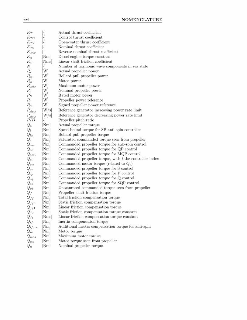
xvi NOMENCLATURE
KT [-] Actual thrust coefficientKTC [-] Control thrust coefficientKTJ [-] Open-water thrust coefficientKT0 [-] Nominal thrust coefficientKT0r [-] Reverse nominal thrust coefficientKy [Nm] Diesel engine torque constantKω [Nms] Linear shaft friction coefficientN [-] Number of harmonic wave components in sea statePa [W] Actual propeller powerPbp [W] Bollard pull propeller powerPm [W] Motor powerPmax [W] Maximum motor powerPn [W] Nominal propeller powerPN [W] Rated motor powerPr [W] Propeller power referencePrs [W] Signed propeller power referenceP+slew [W/s] Reference generator increasing power rate limitP−slew [W/s] Reference generator decreasing power rate limitP/D [-] Propeller pitch ratioQa [Nm] Actual propeller torqueQb [Nm] Speed bound torque for SB anti-spin controllerQbp [Nm] Bollard pull propeller torqueQc [Nm] Saturated commanded torque seen from propellerQcas [Nm] Commanded propeller torque for anti-spin controlQcc [Nm] Commanded propeller torque for QP controlQccm [Nm] Commanded propeller torque for MQP controlQci [Nm] Commanded propeller torque, with i the controller indexQcm [Nm] Commanded motor torque (related to Qc)Qcn [Nm] Commanded propeller torque for S controlQcp [Nm] Commanded propeller torque for P controlQcq [Nm] Commanded propeller torque for Q controlQcs [Nm] Commanded propeller torque for SQP controlQc0 [Nm] Unsaturated commanded torque seen from propellerQf [Nm] Propeller shaft friction torqueQff [Nm] Total friction compensation torqueQff0 [Nm] Static friction compensation torqueQff1 [Nm] Linear friction compensation torqueQf0 [Nm] Static friction compensation torque constantQf1 [Nms] Linear friction compensation torque constantQif [Nm] Inertia compensation torqueQif,as [Nm] Additional inertia compensation torque for anti-spinQm [Nm] Motor torqueQmax [Nm] Maximum motor torqueQmp [Nm] Motor torque seen from propellerQn [Nm] Nominal propeller torque

NOMENCLATURE xvii
QN [Nm] Rated motor torqueQPI [Nm] Additive commanded torque for API anti-spin controlQr [Nm] Propeller torque referenceQs [Nm] Static shaft friction torque constantR [m] Propeller radiusTa [N] Actual total thrustTad [N] Actual duct thrustTap [N] Actual propeller thrustTbp [N] Bollard pull propeller thrustTd [N] Desired thrust from the thrust allocation systemTf [s] Shaft speed filter time constantTi [s] PID controller integral time constantTIs [s] Mechanical time constantTm [s] Motor time constantTn [N] Nominal propeller thrustTp [s] Sea state peak wave periodTr [N] Thrust reference, input to the low-level controllerTras [N] Anti-spin thrust referenceTvent [s] Dwell-time for ventilation detectionTV [s] Time interval for thruster performance evaluationU [m/s] Vessel surge velocityUa [m/s] Induced velocity in the propeller wakeV0.7 [m/s] Undisturbed incident velocity to the prop. blade at 0.7RVa [m/s] Propeller advance (inflow) velocityVp [m/s] Flow velocity through the propeller discY [-] Diesel engine fuel index
Greek
αb [-] Torque loss calculation weighting functionαc [-] QP controller weighting functionαs [-] SQP controller weighting functionαχ [-] Performance factor weighting functionβ [rad] Propeller blade angle of attack at radius 0.7Rβv,off [-] Threshold torque loss for ventilation terminationβv,on [-] Threshold torque loss for ventilation detectionβQ [-] Total torque loss factorβQJ [-] Torque loss factor for inline flowβQV [-] Torque loss factor for ventilation, hysteresis, and disc areaβT [-] Total thrust loss factorβTA [-] Thrust loss factor for loss of propeller disc areaβTH [-] Thrust loss factor for lift hysteresisβTJ [-] Thrust loss factor for inline flowβTV [-] Thrust loss factor for ventilation, hysteresis, and disc area

xviii NOMENCLATURE
βTV 0 [-] Thrust loss factor for ventilationγQ [-] Anti-spin commanded torque scaling factorγT [-] Anti-spin thrust reference scaling factorγfall [s−1] Rate limit for decreasing γQγrise [s−1] Rate limit for increasing γQc [-] Control coefficient switch constantf [-] Friction compensation switch constantφ [-] Constant for CCP pitch mappingζ [-] Ventilation detection flagζj [m] Amplitude of harmonic wave component jζr [-] Reference generator damping ratioζw [m] Surface elevation due to wavesηa [-] Propeller efficiency parameterηh [-] Hull efficiencyηm [-] Mechanical efficiencyηp [-] Overall propulsion efficiencyηr [-] Relative rotative efficiencyη0 [-] Open-water propeller efficiencyθp [-] Vector of fixed propeller parametersλc [-] Control coefficient switching functionρ [kg/m3] Density of waterτ [N,Nm] 3DOF total thrust vector acting on the vesselτd [N,Nm] 3DOF desired thrust vector from thrust allocationτn [s] Time constant for nras filterτm [s] Diesel engine time delayτ r [s] Reference generator time constantτγ [s] Time constant for γQ filterφ [rad] Pitch angleφDP [rad] Maximum pitch angle for DPφj [rad] Phase of harmonic wave component jφr [rad] Reference pitch angle for CPPχj [-] Performance measure for thruster jχQ [-] Torque performance factorχT [-] Thrust performance factorχV [-] Ventilation performance factorχV,min [-] Minimum ventilation performance factorω [rad/s] Propeller angular velocity (ω = 2πn)ωj [rad/s] Circular frequency of harmonic wave component jωr0 [rad/s] Reference generator natural frequency

Chapter 1
Introduction
Most marine vessels are fitted with propellers and thrusters, and rely on theseto conduct station-keeping, manoeuvring, and transit operations. The mainfocus of this thesis will be on modelling, simulation, and control of propellerson surface vessels with electric propulsion systems. Examples of such vesselsare offshore service vessels, shuttle tankers, drilling vessels, pipe-laying vessels,and diving support vessels. The operation of the propellers and thrusters hasseveral important implications:
• The thrust production affects the positioning capability of the vessel.
• The power consumption affects the vessel’s fuel consumption, generatorwear and tear, and risk of power system blackouts.
• Mechanical wear and tear leads to repairs and vessel down-time.
The operational philosophy of the propulsion system hence affects three impor-tant aspects of the operation of a marine vessel: safety, economy, and perfor-mance.
1.1 BackgroundThe real-time control hierarchy of a marine guidance, navigation, and control(GNC) system may be divided into three levels (Balchen et al., 1976, 1980a,b;Sørensen et al., 1996; Strand, 1999; Strand and Fossen, 1999; Fossen and Strand,1999, 2001; Strand and Sørensen, 2000; Lindegaard and Fossen, 2001; Fossen,2002; Lindegaard, 2003; Bray, 2003; Sørensen, 2005) :
• The guidance and navigation system, including local set-point and pathgeneration.
• The high-level plant control, including thrust allocation and power man-agement.
2 Introduction
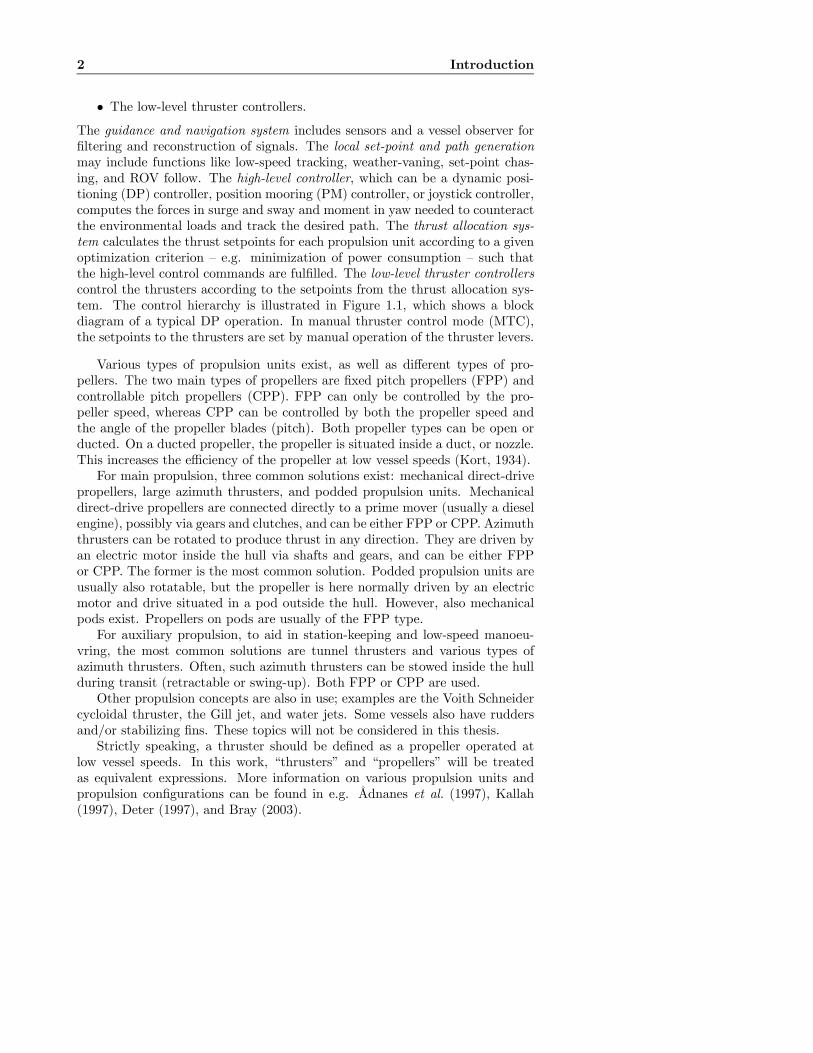
• The low-level thruster controllers.The guidance and navigation system includes sensors and a vessel observer forfiltering and reconstruction of signals. The local set-point and path generationmay include functions like low-speed tracking, weather-vaning, set-point chas-ing, and ROV follow. The high-level controller, which can be a dynamic posi-tioning (DP) controller, position mooring (PM) controller, or joystick controller,computes the forces in surge and sway and moment in yaw needed to counteractthe environmental loads and track the desired path. The thrust allocation sys-tem calculates the thrust setpoints for each propulsion unit according to a givenoptimization criterion — e.g. minimization of power consumption — such thatthe high-level control commands are fulfilled. The low-level thruster controllerscontrol the thrusters according to the setpoints from the thrust allocation sys-tem. The control hierarchy is illustrated in Figure 1.1, which shows a blockdiagram of a typical DP operation. In manual thruster control mode (MTC),the setpoints to the thrusters are set by manual operation of the thruster levers.
Various types of propulsion units exist, as well as different types of pro-pellers. The two main types of propellers are fixed pitch propellers (FPP) andcontrollable pitch propellers (CPP). FPP can only be controlled by the pro-peller speed, whereas CPP can be controlled by both the propeller speed andthe angle of the propeller blades (pitch). Both propeller types can be open orducted. On a ducted propeller, the propeller is situated inside a duct, or nozzle.This increases the efficiency of the propeller at low vessel speeds (Kort, 1934).For main propulsion, three common solutions exist: mechanical direct-drive
propellers, large azimuth thrusters, and podded propulsion units. Mechanicaldirect-drive propellers are connected directly to a prime mover (usually a dieselengine), possibly via gears and clutches, and can be either FPP or CPP. Azimuththrusters can be rotated to produce thrust in any direction. They are driven byan electric motor inside the hull via shafts and gears, and can be either FPPor CPP. The former is the most common solution. Podded propulsion units areusually also rotatable, but the propeller is here normally driven by an electricmotor and drive situated in a pod outside the hull. However, also mechanicalpods exist. Propellers on pods are usually of the FPP type.For auxiliary propulsion, to aid in station-keeping and low-speed manoeu-
vring, the most common solutions are tunnel thrusters and various types ofazimuth thrusters. Often, such azimuth thrusters can be stowed inside the hullduring transit (retractable or swing-up). Both FPP or CPP are used.Other propulsion concepts are also in use; examples are the Voith Schneider
cycloidal thruster, the Gill jet, and water jets. Some vessels also have ruddersand/or stabilizing fins. These topics will not be considered in this thesis.Strictly speaking, a thruster should be defined as a propeller operated at
low vessel speeds. In this work, “thrusters” and “propellers” will be treatedas equivalent expressions. More information on various propulsion units andpropulsion configurations can be found in e.g. Ådnanes et al. (1997), Kallah(1997), Deter (1997), and Bray (2003).

1.1 Background 3
Propulsionsystem
Vessel
Environment
Sensors
Thrustallocation
DPcontroller
WavesWind
Current
WavesCurrent
Motion
Measure-ments
Desiredthrustvector
Thrustsetpoints
Vesselobserver
Filtered &reconstructed
signals
MotionThrustforces
Low-levelthruster
controller Thrustsetpoint
Vesselmotion
Thrustforce
WavesCurrent
rMotordynamics
n Q
Q
Ta
a
m QcPropeller
hydro-dynamics
Load torque
Shaft speed
T
Propulsion unit
Motor torque
Shaftdynamics
Setpoint
High-level controller
Guidance and navigation system
Setpoint/pathgenerator
Figure 1.1: Block diagram of a typcial DP operation, including environment,vessel, guidance and navigation system, high-level control, and thruster dynam-ics including low-level thruster control.
Measurements of the actual propeller thrust is normally not available. Hence,the mapping from desired to actual thrust must be considered as an open-loopsystem, and there is no guarantee of fulfilling the high-level control commands.Therefore, if the low-level controllers have bad performance, the stability andbandwidth of the whole positioning system will be affected. Still, the topicof propulsion control has received relatively little attention in literature, eventhough the use of electrical thrusters have opened up new possibilities for im-proved low-level control. It appears that the same has been true for industry;with notable exceptions, most propeller manufacturers have focused on the pro-peller design, and the control system vendors have focused on the high-levelcontrollers.More recently, also the issues of low-level thruster dynamics and controller
design have received increased attention, and their impact on the overall vesselperformance have become more apparent. However, this work has mostly beenfocused on underwater applications like remotely operated vehicles (ROVs) andautonomous underwater vehicles (AUVs), see Yoerger et al. (1991), Healey et al.
4 Introduction
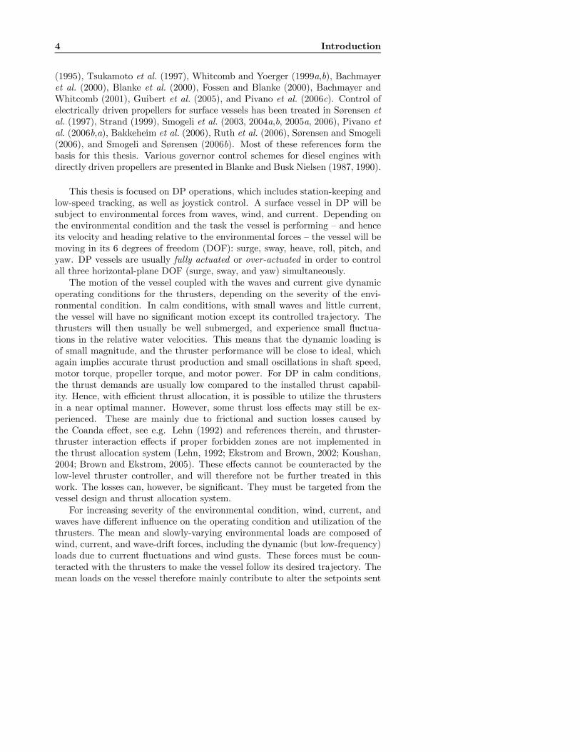
(1995), Tsukamoto et al. (1997), Whitcomb and Yoerger (1999a,b), Bachmayeret al. (2000), Blanke et al. (2000), Fossen and Blanke (2000), Bachmayer andWhitcomb (2001), Guibert et al. (2005), and Pivano et al. (2006c). Control ofelectrically driven propellers for surface vessels has been treated in Sørensen etal. (1997), Strand (1999), Smogeli et al. (2003, 2004a,b, 2005a, 2006), Pivano etal. (2006b,a), Bakkeheim et al. (2006), Ruth et al. (2006), Sørensen and Smogeli(2006), and Smogeli and Sørensen (2006b). Most of these references form thebasis for this thesis. Various governor control schemes for diesel engines withdirectly driven propellers are presented in Blanke and Busk Nielsen (1987, 1990).
This thesis is focused on DP operations, which includes station-keeping andlow-speed tracking, as well as joystick control. A surface vessel in DP will besubject to environmental forces from waves, wind, and current. Depending onthe environmental condition and the task the vessel is performing — and henceits velocity and heading relative to the environmental forces — the vessel will bemoving in its 6 degrees of freedom (DOF): surge, sway, heave, roll, pitch, andyaw. DP vessels are usually fully actuated or over-actuated in order to controlall three horizontal-plane DOF (surge, sway, and yaw) simultaneously.The motion of the vessel coupled with the waves and current give dynamic
operating conditions for the thrusters, depending on the severity of the envi-ronmental condition. In calm conditions, with small waves and little current,the vessel will have no significant motion except its controlled trajectory. Thethrusters will then usually be well submerged, and experience small fluctua-tions in the relative water velocities. This means that the dynamic loading isof small magnitude, and the thruster performance will be close to ideal, whichagain implies accurate thrust production and small oscillations in shaft speed,motor torque, propeller torque, and motor power. For DP in calm conditions,the thrust demands are usually low compared to the installed thrust capabil-ity. Hence, with efficient thrust allocation, it is possible to utilize the thrustersin a near optimal manner. However, some thrust loss effects may still be ex-perienced. These are mainly due to frictional and suction losses caused bythe Coanda effect, see e.g. Lehn (1992) and references therein, and thruster-thruster interaction effects if proper forbidden zones are not implemented inthe thrust allocation system (Lehn, 1992; Ekstrom and Brown, 2002; Koushan,2004; Brown and Ekstrom, 2005). These effects cannot be counteracted by thelow-level thruster controller, and will therefore not be further treated in thiswork. The losses can, however, be significant. They must be targeted from thevessel design and thrust allocation system.For increasing severity of the environmental condition, wind, current, and
waves have different influence on the operating condition and utilization of thethrusters. The mean and slowly-varying environmental loads are composed ofwind, current, and wave-drift forces, including the dynamic (but low-frequency)loads due to current fluctuations and wind gusts. These forces must be coun-teracted with the thrusters to make the vessel follow its desired trajectory. Themean loads on the vessel therefore mainly contribute to alter the setpoints sent

1.1 Background 5
to the thrusters from the high-level control system. The first order oscillatorywave forces (Froude-Krylov and diffraction forces) give rise to an oscillatoryvessel motion in all six DOF. These wave-frequency motions should not becounteracted in normal to moderate seas, since this would lead to unnecessarywear and tear of the thrusters, as well as increased fuel consumption. Thisis solved by proper wave-filtering in the DP system (Strand and Fossen, 1999;Lindegaard and Fossen, 2001; Lindegaard, 2003; Fossen, 2002). Dong (2005)and the references therein showed that in high to extreme seas, wave-filteringshould not be used, and that hybrid control could be used to switch between abank of controllers suitable for varying environmental conditions. Even thoughthe thrusters have slowly-varying setpoints, the oscillatory vessel motion com-bined with the sea elevation and the current- and wave-induced water velocitiesmean that the thrusters are operating in a dynamic environment. This leadsto dynamic loading of the propeller which, depending on the chosen controlstrategy, leads to oscillations in propeller thrust and torque, shaft speed, motortorque, and motor power. In addition, the mean relative velocity due to cur-rent and low-frequency vessel motion alter the operating point of the thrusters.Depending on the performance of the low-level thruster controllers, the resultis a deviation of the average produced thrust from the thrust setpoints. This iscompensated for by the integral action of the DP system, but at the expense ofreduced positioning bandwidth.In severe to extreme conditions, the large environmental loads often lead
to high utilization of the installed thrust capacity. At the same time, the seaelevation and vessel motion means that the thrusters will experience large mo-tions relative to the water. If the thrusters are well submerged, the inflow willbe highly disturbed, and the propeller loading affected accordingly. If the sub-mergence becomes too low, the thrusters may suffer severe thrust losses due toventilation and in-and-out-of-water effects, leading to reduced thrust capabilityand large power transients. Appropriate operation of the propulsion system isthen of high importance for the stability and performance of the power gen-eration and distribution system, since the thrusters often are the main powerconsumers. This is a critical issue with respect to safe operation of the ves-sel, which in addition affects the fuel consumption and wear and tear of thegenerator sets. Recent results also indicate that the unsteady loading duringventilation can give rise to significant mechanical wear and tear of the propulsionunit (Koushan, 2004, 2006). This is believed to be the cause of the widespreadmechanical failures of tunnel thrusters and azimuth thrusters, with costly re-pairs and increased vessel down-time as consequences.
6 Introduction
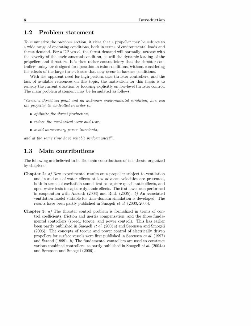
1.2 Problem statementTo summarize the previous section, it clear that a propeller may be subject toa wide range of operating conditions, both in terms of environmental loads andthrust demand. For a DP vessel, the thrust demand will normally increase withthe severity of the environmental condition, as will the dynamic loading of thepropellers and thrusters. It is then rather contradictory that the thruster con-trollers today are designed for operation in calm conditions, without consideringthe effects of the large thrust losses that may occur in harsher conditions.With the apparent need for high-performance thruster controllers, and the
lack of available references on this topic, the motivation for this thesis is toremedy the current situation by focusing explicitly on low-level thruster control.The main problem statement may be formulated as follows:
“Given a thrust set-point and an unknown environmental condition, how canthe propeller be controlled in order to:
• optimize the thrust production,
• reduce the mechanical wear and tear,
• avoid unnecessary power transients,
and at the same time have reliable performance?”.
1.3 Main contributionsThe following are believed to be the main contributions of this thesis, organizedby chapters:
Chapter 2: a) New experimental results on a propeller subject to ventilationand in-and-out-of-water effects at low advance velocities are presented,both in terms of cavitation tunnel test to capture quasi-static effects, andopen-water tests to capture dynamic effects. The test have been performedin cooperation with Aarseth (2003) and Ruth (2005). b) An associatedventilation model suitable for time-domain simulation is developed. Theresults have been partly published in Smogeli et al. (2003, 2006).
Chapter 3: a) The thruster control problem is formalized in terms of con-trol coefficients, friction and inertia compensation, and the three funda-mental controllers (speed, torque, and power control). This has earlierbeen partly published in Smogeli et al. (2005a) and Sørensen and Smogeli(2006). The concepts of torque and power control of electrically drivenpropellers for surface vessels were first published in Sørensen et al. (1997)and Strand (1999). b) The fundamental controllers are used to constructvarious combined controllers, as partly published in Smogeli et al. (2004a)and Sørensen and Smogeli (2006).

1.4 List of publications 7
Chapter 4: Shaft speed, torque, and power sensitivity functions are intro-duced, and thrust sensitivity functions, as presented in Sørensen et al.(1997) and Strand (1999), are put into an improved framework. An im-proved steady-state analysis of the controller performance in presence ofthrust losses is also presented. The results have been partly published inSørensen and Smogeli (2006).
Chapter 5: The complete chapter on propeller observers, loss estimation, andperformance monitoring is believed to be a new contribution. The resultshave been partly published in Smogeli et al. (2004a,b, 2006) and Smogeliand Sørensen (2006b).
Chapter 6: The complete chapter on anti-spin thruster control is believed tobe a new contribution. The results have been partly published in Smogeliet al. (2004b, 2006) and Smogeli and Sørensen (2006b).
Chapter 7: a) An experimental comparison of the fundamental controllers andthe combined controllers, as partly published in Smogeli et al. (2005a) andSørensen and Smogeli (2006), is presented. b) An experimental validationof the various anti-spin controllers, and a comparison with the fundamentalcontrollers in extreme conditions, are also presented. The results have beenpartly published in Smogeli and Sørensen (2006b).
Chapter 8: Extensions of the new control concepts to CPP and transit arepresented.
Chapter 9: a) The concept of anti-spin thrust allocation is introduced. b)A thruster performance measure that can be utilized to improve thrustallocation is developed.
1.4 List of publications
The following authored and coauthored publications are directly connected withthe work presented in this thesis, presented in chronological order:
1. Ø. N. Smogeli and A. J. Sørensen (2006b). Anti-Spin Thruster Controlfor Ships. Submitted to Automatica.
2. A. J. Sørensen and Ø. N. Smogeli (2006). Torque and Power Control ofElectrically Driven Propellers on Ships. Accepted for publication in IEEEJournal of Oceanic Engineering.
3. E. Ruth and Ø. N. Smogeli (2006). Ventilation of Controllable PitchThrusters. SNAME Marine Technology, 43(4):170-179.
4. Ø. N. Smogeli, A. J. Sørensen and K. J. Minsaas (2006). The Concept ofAnti-Spin Thruster Control. To appear in Control Engineering Practice.
8 Introduction
5. L. Pivano, Ø. N. Smogeli, T. A. Johansen and T. I. Fossen (2006a). Ex-perimental Validation of a Marine Propeller Thrust Estimation Schemefor a Wide Range of Operations. Proceedings of the 7th IFAC Confer-ence on Manoeuvring and Control of Marine Craft (MCMC’06). Lisbon,Portugal, September 20-22.
6. E. Ruth, Ø. N. Smogeli and A. J. Sørensen (2006). Overview of PropulsionControl for Surface Vessels. Proceedings of the 7th IFAC Conference onManoeuvring and Control of Marine Craft (MCMC’06). Lisbon, Portugal,September 20-22.
7. D. Radan, Ø. N. Smogeli, A. J. Sørensen and A. K. Ådnanes (2006).Operating Criteria for Design of Power Management Systems on Ships.Proceedings of the 7th IFAC Conference on Manoeuvring and Control ofMarine Craft (MCMC’06). Lisbon, Portugal, September 20-22.
8. J. Bakkeheim, Ø. N. Smogeli, T. A. Johansen and A. J. Sørensen (2006).Improved Transient Performance by Lyapunov-based Integrator Reset ofPI Thruster Control in Extreme Seas. Proceedings of the 45th IEEE Con-ference on Decision and Control (CDC’06). San Diego, California, De-cember 13-15.
9. L. Pivano, Ø. N. Smogeli, T. A. Johansen and T. I. Fossen (2006b). MarinePropeller Thrust Estimation in Four-Quadrant Operations. Proceedingsof the 45th IEEE Conference on Decision and Control (CDC’06). SanDiego, California, December 13-15.
10. Ø. N. Smogeli and A. J. Sørensen (2006a). Adaptive Observer Design fora Marine Propeller. Proceedings of the 14th IFAC Symposium on SystemIdentification (SYSID’06). Newcastle, Australia, March 29-31.
11. Ø. N. Smogeli, E. Ruth and A. J. Sørensen (2005a). Experimental Val-idation of Power and Torque Thruster Control. Proceedings of the 13thMediterranean Conference on Control and Automation (MED’05). Limas-sol, Cyprus, June 27-29.
12. Ø. N. Smogeli, J. Hansen, A. J. Sørensen and T. A. Johansen (2004b).Anti-spin control for marine propulsion systems. Proceedings of the 43rdIEEE Conference on Decision and Control (SYSID’04), Paradise Island,Bahamas, December 14-17.
13. Ø. N. Smogeli, A. J. Sørensen and T. I. Fossen (2004a). Design of a hybridpower/torque thruster controller with thrust loss estimation. Proceed-ings of the IFAC Conference on Control Applications in Marine Systems(CAMS’04). Ancona, Italy, July 7-9.
14. Ø. N. Smogeli, L. Aarseth, E. S. Overå, A. J. Sørensen and K. J. Min-saas (2003). Anti-spin thruster control in extreme seas. Proceedings of
1.5 Organization of the thesis 9
the 6th IFAC Conference on Manoeuvring and Control of Marine Craft(MCMC’03). Girona, Spain, September 17-19.
Other authored and coauthored publications that have been of supporting im-portance for this thesis are, in chronological order:
15. T. Perez, Ø. N. Smogeli, T. I. Fossen, and A. J. Sørensen (2005). AnOverview of Marine Systems Simulator (MSS): A Simulink Toolbox forMarine Control Systems. Proceedings of the Scandinavian Conference onSimulation and Modeling (SIMS’05). Trondheim, Norway, October 13-14.
16. Ø. N. Smogeli, T. Perez, T. I. Fossen and A. J. Sørensen (2005b). TheMarine Systems Simulator State-Space Model Representation for Dynam-ically Positioned Surface Vessels. Proceedings of the 11th Congress ofthe International Maritime Association of the Mediterranean (IMAM’05).Lisbon, Portugal, September 26-30.
17. T. I. Fossen and Ø. N. Smogeli (2004). Nonlinear Time-Domain Strip The-ory Formulation for Low-Speed Maneuvering and Station-Keeping. Mod-eling, Identification and Control (MIC), 25(4):201-221.
18. R. Skjetne, Ø. N. Smogeli and T. I. Fossen (2004a). Modeling, Identifica-tion, and Adaptive Maneuvering of CyberShip II: A complete design withexperiments. Proceedings of the IFAC Conference on Control Applicationsin Marine Systems (CAMS’04). Ancona, Italy, July 7-9.
19. R. Skjetne, Ø. N. Smogeli and T. I. Fossen (2004b). A non-linear shipmaneuvering model: Identification and adaptive control with experimentsfor a model ship. Modeling, Identification and Control (MIC), 25(1):3-27.
20. A. J. Sørensen, E. Pedersen and Ø. N. Smogeli (2003). Simulation-BasedDesign and Testing of Dynamically Positioned Marine Vessels. Proceedingsof the International Conference on Marine Simulation And Ship Maneu-verability, MARSIM’03. Kanazawa, Japan, August 25-28.
1.5 Organization of the thesis
In order to investigate the importance of proper low-level thruster control, onemust start with studying the loads that the propeller is subjected to. This is thetopic of Chapter 2, which deals with propeller modelling and simulation. Focusis put on the thrust loss effects that can be counteracted by the low-level thrustercontrollers, both in normal and extreme conditions. The characteristics of apropeller subject to ventilation and in-and-out-of water effects is investigated,and systematic tests from a cavitation tunnel and a towing tank at NTNU arepresented. Based on this, a simplified simulation model that captures the main

10 Introduction
characteristics of the losses is proposed. Finally, a complete propeller simulationmodel suitable for thruster controller design and testing is presented.Chapter 3 considers thruster control in normal operating conditions. The
main control objectives are defined, and the general structure of the proposedthruster controller is shown. Some important aspects regarding choice of controlparameters, use of reference generators, and the need for friction and inertiacompensation are discussed, before the three fundamental control concepts arepresented: shaft speed, torque, and power control. It is then shown how thefundamental controllers can be combined in various ways to exploit their bestindividual properties, followed by a controller comparison by simulations.The fundamental control concepts are further analyzed in Chapter 4, where
sensitivity functions are established to investigate the steady-state thrust, torque,shaft speed, and power in the presence of thrust losses. These analysis tools areapplied to two cases: losses due to changes in inflow to the propeller, and lossesdue to ventilation. Further, the transient response of the controllers is discussedwith the aid of a Lyapunov analysis of the shaft speed equilibrium.In Chapter 5 a propeller load torque observer is designed, and a loss esti-
mation scheme developed. In addition, a scheme for monitoring of the thrusterperformance is proposed. Simulations are provided to demonstrate the perfor-mance of the presented concepts.Chapter 6 is dedicated to controller design for extreme operating conditions.
Motivated by the similar problem of a car wheel losing friction on a slipperysurface during braking or acceleration, the concept of anti-spin thruster controlis introduced. In order to detect the high thrust loss incidents, a ventilationdetection scheme is designed. An anti-spin thruster controller that is applicableto all the controllers designed for normal operating conditions is then proposed.Finally, some alternative anti-spin control concepts are presented, and the pro-posed anti-spin controller tested by simulations.To further validate the proposed control concepts and estimation schemes,
extensive model tests in the Marine Cybernetics Laboratory (MCLab) at NTNUhave been undertaken. The results from these tests — both in normal and ex-treme conditions — are presented in Chapter 7, showing that the controllers andobservers perform as intended.Chapter 8 shows how the presented concepts can be extended to CPP and
transit. This applies to the controllers for normal conditions, the observers andloss estimation schemes, and the anti-spin thruster controllers.Finally, anti-spin thrust allocation in extreme conditions is discussed in
Chapter 9. The main concept is to monitor the performance of all the propulsionunits on a vessel, and attempt to utilize the propellers with the best operatingconditions. This may both improve the vessel’s positioning performance andreduce the mechanical wear and tear of the propulsion units.The appendices provide additional background material, extensions of the
presented concepts, and additional results.
Chapter 2
Propeller modelling
The actual propeller thrust Ta and torque Qa are influenced by many parame-ters. Ta and Qa can in general be formulated as functions of the shaft speedn in revolutions-per-second (rps), time-varying states xp (e.g. pitch ratio, ad-vance velocity, submergence), and fixed thruster parameters θp (e.g. propellerdiameter, geometry, position):
Ta = fT (n,xp,θp), (2.1)
Qa = fQ(n,xp,θp). (2.2)
In this work, speed controlled FPP are of main concern. The pitch ratio is then afixed parameter. The functions fT (·) and fQ(·) may include thrust and torquelosses due to e.g. in-line and transverse velocity fluctuations, ventilation, in-and-out-of water effects, thruster-thruster interaction, and dynamic flow effects.In addition, the dynamics of the motor and shaft must be considered. In thefollowing sections, propeller characteristics, some quasi-static loss effects, anddynamic effects due to the water inflow, motor, and shaft are considered.
Remark 2.1 Modelling of propellers will in this thesis be treated from a controlpoint of view. This means that the models are required to be accurate enough tocapture the main physical effects, and such facilitate control system design andtesting. However, details on propeller design and hydrodynamic performancewill not be considered.
2.1 Propeller characteristics
Propellers are, with the exception of tunnel thrusters, usually asymmetric andoptimized for producing thrust in one direction. The propeller characteristicswill therefore depend on both the rotational direction of the propeller and theinflow direction. The four quadrants of operation of a propeller are defined inTable 2.1. The quasi-static relationships between Ta, Qa, n, the diameter D,

12 Propeller modelling
1st 2nd 3rd 4th
n ≥ 0 < 0 < 0 ≥ 0Va ≥ 0 ≥ 0 < 0 < 0
Table 2.1: The 4 quadrants of operation of a propeller, parameterized by theadvance velocity Va and the shaft speed n.
and the density of water ρ are commonly given by:
Ta = fT (·) = sign(n)KTρD4n2, (2.3)
Qa = fQ(·) = sign(n)KQρD5n2. (2.4)
KT and KQ are the thrust and torque coefficients, where the effects of thrustand torque losses have been accounted for. For normal operation, KT > 0 andKQ > 0. The propeller power consumption Pa is written as:
Pa = 2πnQa = sign(n)2πKQρD5n3. (2.5)
In general, the thrust and torque coefficients can be expressed in a similarmanner as Ta and Qa in (2.1, 2.2):
KT = KT (n,xp,θp) =Ta
sign(n)ρD4n2, (2.6)
KQ = KQ(n,xp,θp) =Qa
sign(n)ρD5n2. (2.7)
For ease of notation, the arguments of KT and KQ will mostly be omitted inthe remainder of this work. The nominal thrust Tn, torque Qn, and power Pnare the ideal values when no thrust losses are present. They are expressed bythe nominal thrust and torque coefficients KT0 and KQ0:
Tn = sign(n)KT0ρD4n2, (2.8)
Qn = sign(n)KQ0ρD5n2, (2.9)
Pn = 2πnQn = sign(n)2πKQ0ρD5n3. (2.10)
The nominal thrust, torque, and power of a reversed propeller are expressed as in(2.8, 2.9, 2.10), but with KT0 and KQ0 replaced with their reverse counterparts,KT0r > 0 and KQ0r > 0. The nominal coefficients are assumed to be constantfor a given propeller geometry.The difference between the nominal and actual thrust and torque may be
expressed by the thrust and torque reduction coefficients — or thrust and torqueloss factors — βT and βQ (Faltinsen et al., 1980; Minsaas et al., 1983, 1987):
βT = βT (n,xp,θp) =TaTn
=KT
KT0, (2.11)
βQ = βQ(n,xp,θp) =Qa
Qn=
KQ
KQ0. (2.12)

2.1 Propeller characteristics 13
If the difference between KT0 and KT0r is included in βT , and the differencebetween KQ0 and KQ0r is included in βQ, the actual thrust, torque, and powermay be written as:
Ta = sign(n)KT0ρD4n2βT (n,xp,θp), (2.13)
Qa = sign(n)KQ0ρD5n2βQ(n,xp,θp), (2.14)
Pa = sign(n)2πKQ0ρD5n3βQ(n,xp,θp). (2.15)
Hence, all disturbances and external states are introduced through βT and βQ.The arguments of βT and βQ will for notational simplicity mostly be omitted.
2.1.1 Open-water characteristics
The thrust and torque coefficients for deeply submerged propellers subject toan in-line inflow will here be termed KTJ and KQJ . These coefficients areexperimentally determined by so-called open water tests, usually performed ina cavitation tunnel or a towing tank. For a specific propeller geometry, KTJ
and KQJ are often given as functions of the advance number Ja:
Ja =VanD
, (2.16)
where Va is the propeller advance (inflow) velocity. This relationship is com-monly referred to as an open-water propeller characteristics. In general, thecoefficients are written as KTJ = KTJ(Va, n) and KQJ = KQJ(Va, n). In thefollowing, the arguments Va and n will mostly be omitted. The correspondingopen-water efficiency η0 is defined as the ratio of produced to consumed powerfor the propeller:
η0 =VaTa2πnQa
=VaKTJ
2πnKQJD=
JaKTJ
2πKQJ. (2.17)
Systematic tests with similar propellers are typically compiled in a propellerseries. The perhaps most well-known series is the Wageningen B-series fromMARIN in the Netherlands, see van Lammeren et al. (1969), Oosterveld andvan Oossanen (1975), and the references therein. In the latter reference, KTJ
and KQJ are given from:
KTJ = f1
µJa,
P
D,Ae
A0, Z
¶, (2.18)
KQJ = f2
µJa,
P
D,Ae
A0, Z,Rn,
t
c
¶, (2.19)
where P/D is the pitch ratio, Ae/A0 is the expanded blade-area ratio, Z is thenumber of blades, Rn is the Reynolds number, t is the maximum thickness ofthe blade section, and c is the chord length of the blade section. Figure 2.1
14 Propeller modelling
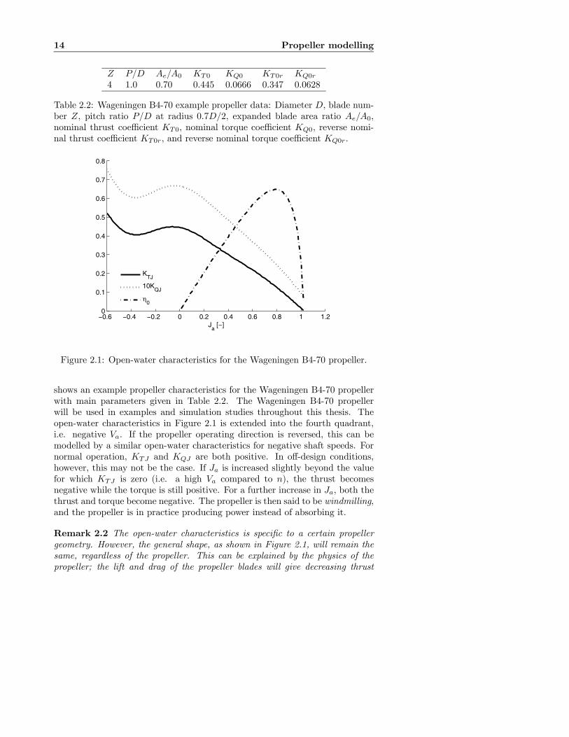
Z P/D Ae/A0 KT0 KQ0 KT0r KQ0r
4 1.0 0.70 0.445 0.0666 0.347 0.0628
Table 2.2: Wageningen B4-70 example propeller data: Diameter D, blade num-ber Z, pitch ratio P/D at radius 0.7D/2, expanded blade area ratio Ae/A0,nominal thrust coefficient KT0, nominal torque coefficient KQ0, reverse nomi-nal thrust coefficient KT0r, and reverse nominal torque coefficient KQ0r.
−0.6 −0.4 −0.2 0 0.2 0.4 0.6 0.8 1 1.20
0.1
0.2
0.3
0.4
0.5
0.6
0.7
0.8
Ja [−]
KTJ
10KQJ
η0
Figure 2.1: Open-water characteristics for the Wageningen B4-70 propeller.
shows an example propeller characteristics for the Wageningen B4-70 propellerwith main parameters given in Table 2.2. The Wageningen B4-70 propellerwill be used in examples and simulation studies throughout this thesis. Theopen-water characteristics in Figure 2.1 is extended into the fourth quadrant,i.e. negative Va. If the propeller operating direction is reversed, this can bemodelled by a similar open-water characteristics for negative shaft speeds. Fornormal operation, KTJ and KQJ are both positive. In off-design conditions,however, this may not be the case. If Ja is increased slightly beyond the valuefor which KTJ is zero (i.e. a high Va compared to n), the thrust becomesnegative while the torque is still positive. For a further increase in Ja, both thethrust and torque become negative. The propeller is then said to be windmilling,and the propeller is in practice producing power instead of absorbing it.
Remark 2.2 The open-water characteristics is specific to a certain propellergeometry. However, the general shape, as shown in Figure 2.1, will remain thesame, regardless of the propeller. This can be explained by the physics of thepropeller; the lift and drag of the propeller blades will give decreasing thrust

2.1 Propeller characteristics 15
and torque for increasing Ja, and the unsteady operating conditions for smallnegative Ja will lead to a drop in the thrust and torque.
Model representations
For simulation purposes, various representations of the open-water characteris-tics may be used. By expressing KTJ and KQJ as second order polynomials inJa, Ta and Qa can be written explicitly as functions of Va and n:
KTJ = KT0 + αT1Ja + αT2Ja |Ja| , (2.20)
KQJ = KQ0 + αQ1Ja + αQ2Ja |Ja| , (2.21)
⇓Ta = Tnnn |n|+ Tnv |n|Va + TvvVa |Va| , (2.22)
Qa = Qnnn |n|+Qnv |n|Va +QvvVa |Va| , (2.23)
where αT1, αT2, aQ1, and αQ2 are constants, and:
Tnn = ρD4KT0, Qnn = ρD5KQ0,Tnv = ρD3αT1, Qnv = ρD4αQ1,Tvv = ρD2αT2, Qvv = ρD3αQ2.
(2.24)
With αT2 = αQ2 = 0, this reduces to the linear approximation commonly usedin the control literature (Blanke, 1981; Fossen, 2002):
KTJ = KT0 + αT1Ja, (2.25)
KQJ = KQ0 + αQ1Ja, (2.26)
⇓Ta = Tnnn |n|+ Tnv |n|Va, (2.27)
Qa = Qnnn |n|+Qnv |n|Va. (2.28)
It can be argued that the quadratic polynomial is a physically more reasonablerepresentation that the linear one (Kim and Chung, 2006). (2.22) and (2.23)clearly show the dependence of the thrust and torque on the advance velocity.Figure 2.1 indicates that the linear and quadratic polynomial representations inreality only are applicable in the first quadrant: they clearly cannot capture thedrop in KTJ and KQJ for small negative Ja. In addition, as will be discussedin Section 2.1.6, the open-water characteristics of a ducted propeller is usuallysignificantly different, and less linear, than for an open propeller. Hence, theseapproximations must be used with care both for simulations and controller-observer design, and verified against the open-water characteristics of the actualpropeller.Is it then possible to formulate a better simulation model in terms of KTJ
and KQJ? If a higher-order polynomial in Ja is chosen for KTJ and KQJ , theresulting representation is singular for n = 0. Another option is to tabulateKTJ and KQJ as functions of Ja, and use interpolation and equations (2.3,
16 Propeller modelling
2.4) to calculate Ta and Qa. However, since n → 0 from (2.16) implies thatJa → ±∞, a zero-crossing of n is not covered by the open-water characteristicsunless special precautions are taken. In addition, since Ta and Qa are givenas quadratic functions of n, Ta = Qa = 0 for n = 0, regardless of Va (andhence Ja). For simulation purposes, the singularity for n = 0 is therefore aninherent weakness in this model representation. The reason is probably thatthe open-water characteristics originally was developed for propellers on vesselsin transit, i.e. for the first quadrant of operation, where only nonzero n wereconsidered.In order to capture the correct quasi-static behavior for all 4 quadrants,
and also give physically reasonable results for time-varying inflow and shaftspeed, it appears necessary to use another parametrization than the open-watercharacteristics.
2.1.2 4-quadrant model
A more accurate propeller characteristics model was apparently first definedby Miniovich (1960), and later used by amongst others van Lammeren et al.(1969) for some of the Wageningen B-series propellers. It is based on the angleof attack β of the propeller blade at radius 0.7R:
β = arctan(Va
0.7πnD) = arctan(
Va0.7ωR
), (2.29)
where R = D/2 is the propeller radius, and ω = 2πn is the propeller angularvelocity. The four quadrants of operation are now defined as:
1st : 0◦ ≤ β ≤ 90◦, Va ≥ 0, n ≥ 0,2nd : 90◦ < β ≤ 180◦, Va ≥ 0, n < 0,3rd : −180◦ < β ≤ −90◦, Va < 0, n < 0,4th : −90◦ < β ≤ 0◦, Va < 0, n ≥ 0.
(2.30)
This model hence covers also the windmilling regime. The non-dimensionalthrust and torque coefficients CT and CQ are defined as:
CT =Ta
12ρ(Va
2 + (0.7ωR)2)π4D2=
Ta12πR
2ρV0.72, (2.31)
CQ =Qa
12ρ(Va
2 + (0.7ωR)2)π4D3=
Qa
πR3ρV0.72, (2.32)
where the undisturbed incident velocity to the propeller blade at radius 0.7R isdefined as:
V0.7 =
qVa
2 + (0.7ωR)2. (2.33)
For a specific propeller, CT is in van Lammeren et al. (1969) modelled by a 20th
order Fourier series in β with coefficients AT (k) and BT (k), and CQ similarly
2.1 Propeller characteristics 17
−3 −2 −1 0 1 2 3
−1
−0.5
0
0.5
1
1.5
β [rad]
CT
10CQ
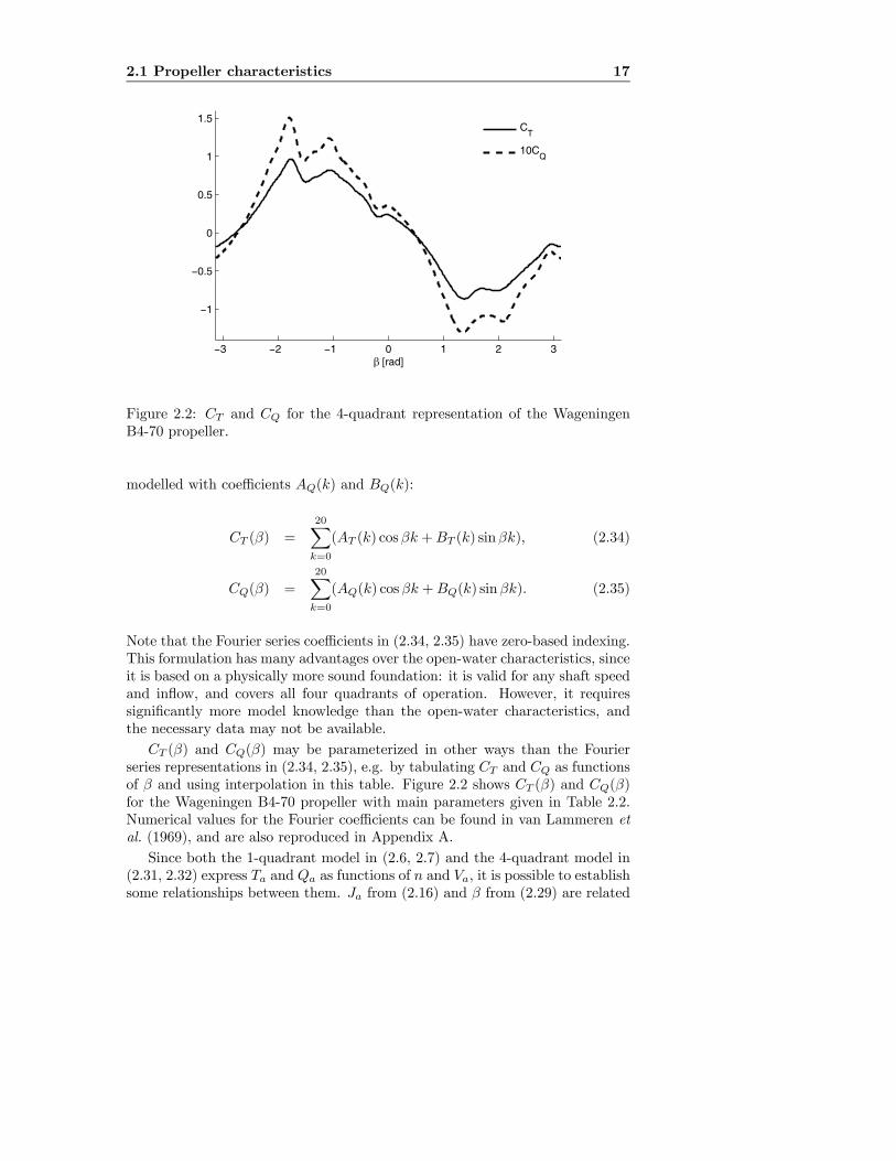
Figure 2.2: CT and CQ for the 4-quadrant representation of the WageningenB4-70 propeller.
modelled with coefficients AQ(k) and BQ(k):
CT (β) =20Xk=0
(AT (k) cosβk +BT (k) sinβk), (2.34)
CQ(β) =20Xk=0
(AQ(k) cosβk +BQ(k) sinβk). (2.35)
Note that the Fourier series coefficients in (2.34, 2.35) have zero-based indexing.This formulation has many advantages over the open-water characteristics, sinceit is based on a physically more sound foundation: it is valid for any shaft speedand inflow, and covers all four quadrants of operation. However, it requiressignificantly more model knowledge than the open-water characteristics, andthe necessary data may not be available.
CT (β) and CQ(β) may be parameterized in other ways than the Fourierseries representations in (2.34, 2.35), e.g. by tabulating CT and CQ as functionsof β and using interpolation in this table. Figure 2.2 shows CT (β) and CQ(β)for the Wageningen B4-70 propeller with main parameters given in Table 2.2.Numerical values for the Fourier coefficients can be found in van Lammeren etal. (1969), and are also reproduced in Appendix A.Since both the 1-quadrant model in (2.6, 2.7) and the 4-quadrant model in
(2.31, 2.32) express Ta and Qa as functions of n and Va, it is possible to establishsome relationships between them. Ja from (2.16) and β from (2.29) are related

18 Propeller modelling
by:
β = arctan(Va
0.7πnD) = arctan(
Ja0.7π
). (2.36)
By equating (2.6) and (2.31), the relationship between KT and CT is found tobe:
KT = CTπ
8(J2a + 0.7
2π2), (2.37)
and similarly betwenn KQ and CQ from (2.7) and (2.32):
KQ = CQπ
8(J2a + 0.7
2π2). (2.38)
2.1.3 Simplified 4-quadrant model
A simplified 4-quadrant model may be derived by using only the first terms inthe Fourier series for CT and CQ:
CTS(β) = AT (0) +AT (1) cosβ +BT (1) sinβ
= AT0 +AT1 cosβ +BT1 sinβ, (2.39)
CQS(β) = AQ(0) +AQ(1) cosβ +BQ(1) sinβ
= AQ0 +AQ1 cosβ +BQ1 sinβ, (2.40)
where CTS and CQS are the simplified 4-quadrant coefficients. This modelpreserves the good properties of the 4-quadrant representation, but gives verycoarse approximations of the true propeller characteristics.
2.1.4 General momentum theory with propeller lift anddrag
An alternative representation of the propeller thrust and torque can be obtainedby treating the lift and drag of the individual propeller blades as the source ofpropeller thrust and torque. This approach is based on the generalized Rankine-Froude momentum theory, and is called the blade element theory (Drzewiecki,1920). It is described in detail in Durand (1963), and can also be found in e.g.Lewis (1989) or Carlton (1994).While useful for understanding the physics of the propeller, this formulation
is less convenient for quasi-static simulation purposes than the representationspresented above. The lift and drag based model requires calculation of theaxially and rotationally induced velocities in the propeller disc in order to cal-culate the effective angle of attack of and incident velocity to the propellerblades. Since these velocities depend on the propeller thrust, the representationbecomes implicit. However, if the dynamics of the inflow to the propeller isto be accounted for, as done in Healey et al. (1995), Whitcomb and Yoerger(1999a), and Bachmayer et al. (2000), such a formulation may be necessary. Intheir model, however, the advance velocity is set to zero, and rotational flow isneglected. Flow dynamics is further treated in Section 2.2.5.
2.1 Propeller characteristics 19
0 0.2 0.4 0.6 0.8 1 1.2 1.4−0.1
0
0.1
0.2
0.3
0.4
0.5
0.6
0.7
0.8
0.9
P/D=1.2P/D=1.0P/D=0.8P/D=0.6
Ja [−]
KTJ
10KQJ
η0
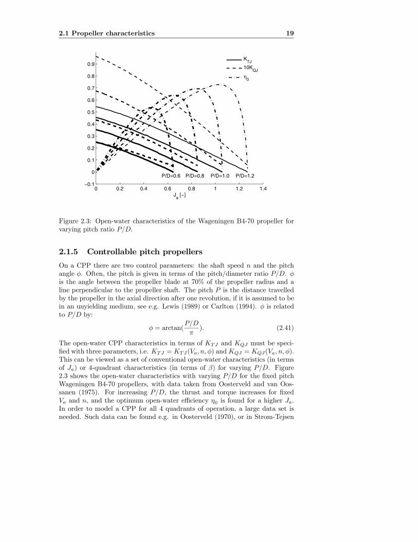
Figure 2.3: Open-water characteristics of the Wageningen B4-70 propeller forvarying pitch ratio P/D.
2.1.5 Controllable pitch propellers
On a CPP there are two control parameters: the shaft speed n and the pitchangle φ. Often, the pitch is given in terms of the pitch/diameter ratio P/D. φis the angle between the propeller blade at 70% of the propeller radius and aline perpendicular to the propeller shaft. The pitch P is the distance travelledby the propeller in the axial direction after one revolution, if it is assumed to bein an unyielding medium, see e.g. Lewis (1989) or Carlton (1994). φ is relatedto P/D by:
φ = arctan(P/D
π). (2.41)
The open-water CPP characteristics in terms of KTJ and KQJ must be speci-fied with three parameters, i.e. KTJ = KTJ(Va, n, φ) andKQJ = KQJ(Va, n, φ).This can be viewed as a set of conventional open-water characteristics (in termsof Ja) or 4-quadrant characteristics (in terms of β) for varying P/D. Figure2.3 shows the open-water characteristics with varying P/D for the fixed pitchWageningen B4-70 propellers, with data taken from Oosterveld and van Oos-sanen (1975). For increasing P/D, the thrust and torque increases for fixedVa and n, and the optimum open-water efficiency η0 is found for a higher Ja.In order to model a CPP for all 4 quadrants of operation, a large data set isneeded. Such data can be found e.g. in Oosterveld (1970), or in Strom-Tejsen
20 Propeller modelling
and Porter (1972) based on the work by Gutsche and Schroeder (1963). A 1-quadrant model can be found in Chu et al. (1979). Some of these data sets arealso reproduced in Carlton (1994).
Remark 2.3 It is important to distinguish between a series of FPP with varyingP/D, as given in e.g. van Lammeren et al. (1969) and Oosterveld and vanOossanen (1975), and a single CPP with varying P/D, as given in e.g. Chu etal. (1979) and Strom-Tejsen and Porter (1972).
2.1.6 Characteristics of various propeller types
The propeller characteristics presented here are applicable to open and ductedpropellers. Tunnel thrusters are a special case where the propeller is not sig-nificantly affected by Va. This can be explained by the sheltered position ofthe propeller inside the tunnel, as well as limited sway velocity of the vessel.Tunnel thrusters are therefore usually modelled without any influence from Va.For a FPP, this means that KTJ(Va, n) = KT0 and KQJ(Va, n) = KQ0. Notethat the effective thrust of a tunnel thruster is strongly affected by the surgevelocity of the vessel (Chislett and Björheden, 1966; Brix, 1978; Karlsen et al.,1986). This is regarded as a thrust loss effect, and not included in the propellercharacteristics.From a modelling point of view, the main difference between open and ducted
propellers lies in the shape of the thrust and torque coefficients. If the open-water diagrams of an open propeller and a ducted propeller are compared, thetotal thrust coefficient of the ducted propeller (i.e. including the duct thrust)typically has the steeper slope. The torque coefficient, on the other hand, hasa smaller slope. This means that the efficiency of the ducted propeller is higherat low Ja and lower at high Ja. Equivalently, the duct increases the efficiency ofa heavily loaded propeller, whereas it decreases the efficiency of a lightly loadedpropeller. These relationships are strongly affected by the length of the ductrelative to the propeller diameter. More on this can be found in e.g. Lewis(1989), Carlton (1994), and the references therein. A comparison of the open-water characteristics of the Wageningen B4-70 propeller and the WageningenKa4-70 propeller in a 19A nozzle (Oosterveld, 1970) is given in Figure 2.4. Thedifference in characteristics is the reason for ducted propellers being used one.g. anchor-handling vessels and tugs, where the bollard pull thrust is of mainimportance, whereas open propellers are preferred for vessels where the focus ison efficiency in transit.
2.1.7 Propeller efficiency
The presence of a hull close to a main propeller affects the propeller efficiencyin several ways, see e.g. Lewis (1989). The average advance velocity of thepropeller differs from the ship speed U by the hull wake fraction number wh:
Va = U(1− wh). (2.42)
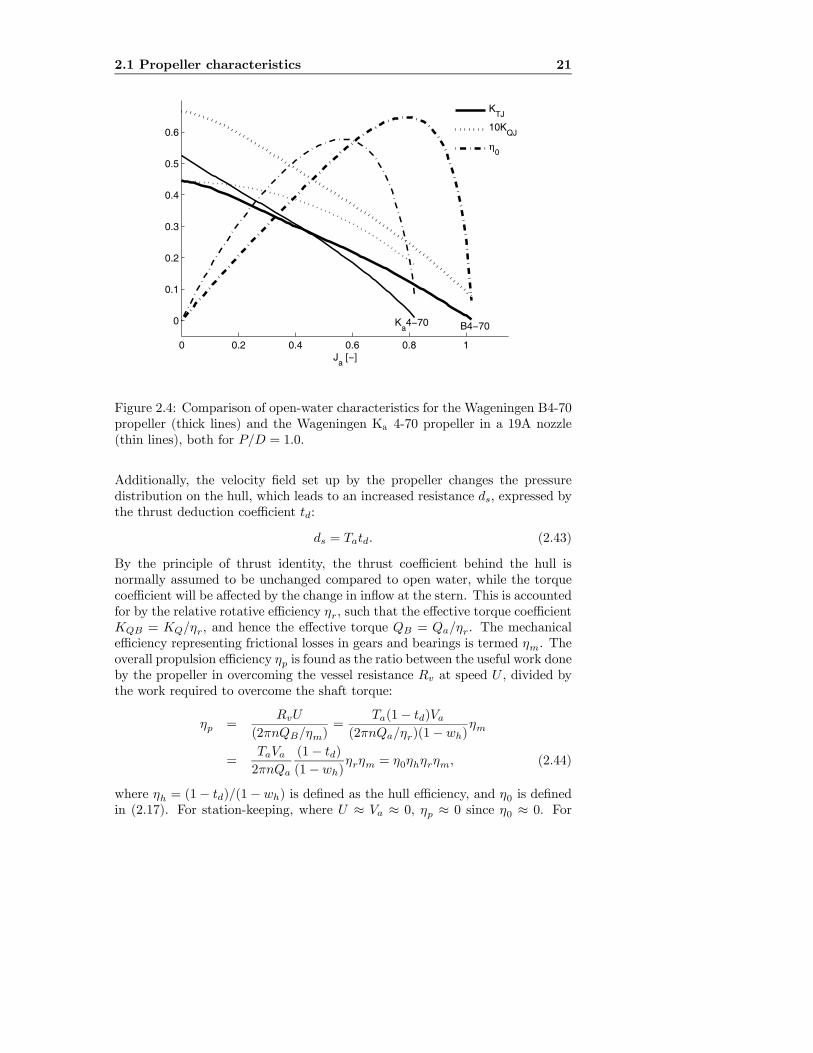
2.1 Propeller characteristics 21
0 0.2 0.4 0.6 0.8 1
0
0.1
0.2
0.3
0.4
0.5
0.6
Ja [−]
KTJ
10KQJ
η0
Ka4−70 B4−70
Figure 2.4: Comparison of open-water characteristics for the Wageningen B4-70propeller (thick lines) and the Wageningen Ka 4-70 propeller in a 19A nozzle(thin lines), both for P/D = 1.0.
Additionally, the velocity field set up by the propeller changes the pressuredistribution on the hull, which leads to an increased resistance ds, expressed bythe thrust deduction coefficient td:
ds = Tatd. (2.43)
By the principle of thrust identity, the thrust coefficient behind the hull isnormally assumed to be unchanged compared to open water, while the torquecoefficient will be affected by the change in inflow at the stern. This is accountedfor by the relative rotative efficiency ηr, such that the effective torque coefficientKQB = KQ/ηr, and hence the effective torque QB = Qa/ηr. The mechanicalefficiency representing frictional losses in gears and bearings is termed ηm. Theoverall propulsion efficiency ηp is found as the ratio between the useful work doneby the propeller in overcoming the vessel resistance Rv at speed U , divided bythe work required to overcome the shaft torque:
ηp =RvU
(2πnQB/ηm)=
Ta(1− td)Va(2πnQa/ηr)(1− wh)
ηm
=TaVa2πnQa
(1− td)
(1− wh)ηrηm = η0ηhηrηm, (2.44)
where ηh = (1− td)/(1− wh) is defined as the hull efficiency, and η0 is definedin (2.17). For station-keeping, where U ≈ Va ≈ 0, ηp ≈ 0 since η0 ≈ 0. For
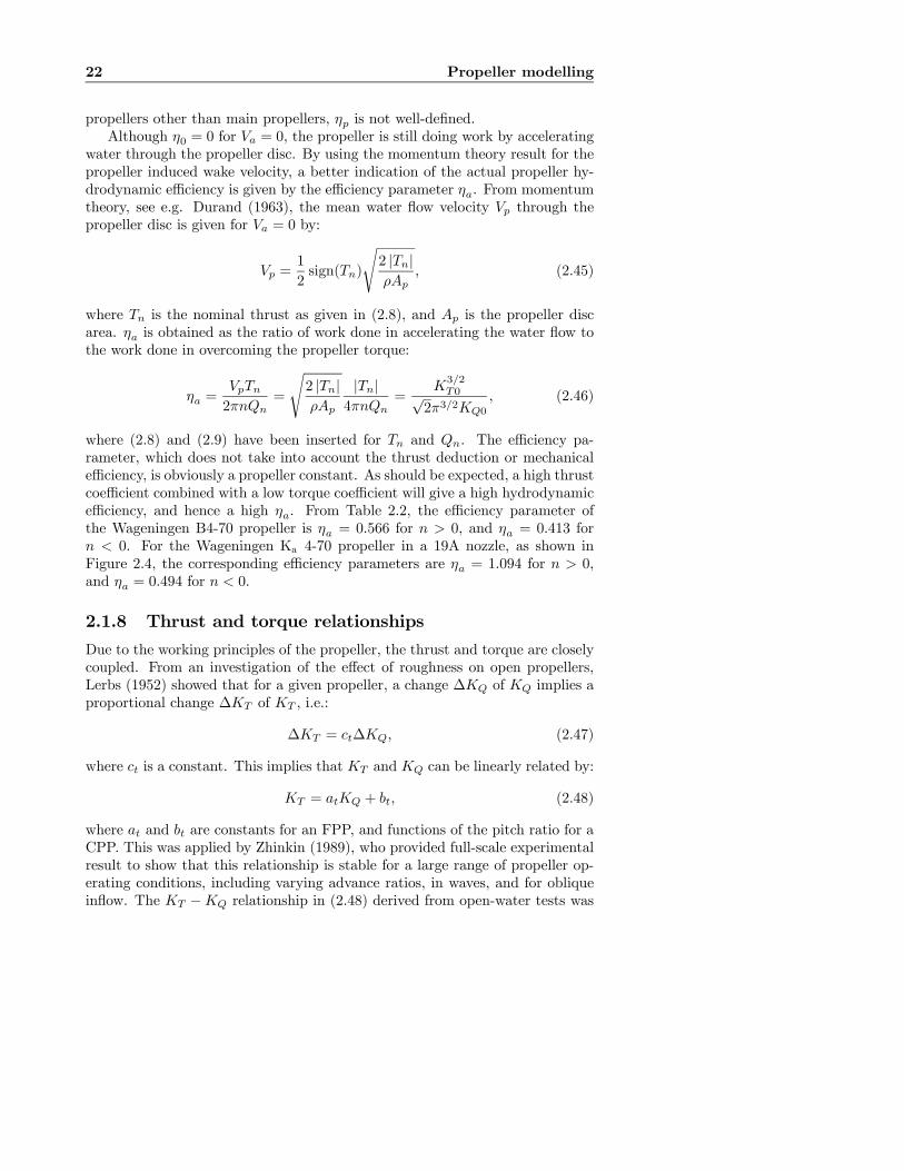
22 Propeller modelling
propellers other than main propellers, ηp is not well-defined.Although η0 = 0 for Va = 0, the propeller is still doing work by accelerating
water through the propeller disc. By using the momentum theory result for thepropeller induced wake velocity, a better indication of the actual propeller hy-drodynamic efficiency is given by the efficiency parameter ηa. From momentumtheory, see e.g. Durand (1963), the mean water flow velocity Vp through thepropeller disc is given for Va = 0 by:
Vp =1
2sign(Tn)
s2 |Tn|ρAp
, (2.45)
where Tn is the nominal thrust as given in (2.8), and Ap is the propeller discarea. ηa is obtained as the ratio of work done in accelerating the water flow tothe work done in overcoming the propeller torque:
ηa =VpTn2πnQn
=
s2 |Tn|ρAp
|Tn|4πnQn
=K3/2T0√
2π3/2KQ0
, (2.46)
where (2.8) and (2.9) have been inserted for Tn and Qn. The efficiency pa-rameter, which does not take into account the thrust deduction or mechanicalefficiency, is obviously a propeller constant. As should be expected, a high thrustcoefficient combined with a low torque coefficient will give a high hydrodynamicefficiency, and hence a high ηa. From Table 2.2, the efficiency parameter ofthe Wageningen B4-70 propeller is ηa = 0.566 for n > 0, and ηa = 0.413 forn < 0. For the Wageningen Ka 4-70 propeller in a 19A nozzle, as shown inFigure 2.4, the corresponding efficiency parameters are ηa = 1.094 for n > 0,and ηa = 0.494 for n < 0.
2.1.8 Thrust and torque relationships
Due to the working principles of the propeller, the thrust and torque are closelycoupled. From an investigation of the effect of roughness on open propellers,Lerbs (1952) showed that for a given propeller, a change ∆KQ of KQ implies aproportional change ∆KT of KT , i.e.:
∆KT = ct∆KQ, (2.47)
where ct is a constant. This implies that KT and KQ can be linearly related by:
KT = atKQ + bt, (2.48)
where at and bt are constants for an FPP, and functions of the pitch ratio for aCPP. This was applied by Zhinkin (1989), who provided full-scale experimentalresult to show that this relationship is stable for a large range of propeller op-erating conditions, including varying advance ratios, in waves, and for obliqueinflow. The KT −KQ relationship in (2.48) derived from open-water tests was

2.1 Propeller characteristics 23
−0.04 −0.02 0 0.02 0.04 0.06 0.08 0.1 0.12 0.14−0.4
−0.2
0
0.2
0.4
0.6
0.8
1
Ja = 1.2
Ja = 0.8
Ja = 0.1
Ja = −0.7
Ja = −0.9
Ja = 1.2
Ja = 0.9
Ja = 0.5
Ja = −0.7
Ja = −0.9
KQ
KT
n > 0n < 0
Figure 2.5: Relationship between KT and KQ for the Wageningen B4-70 pro-peller in the range −0.9 < Ja < 1.2.
shown to hold also when the propeller is installed behind a hull. It appears,however, that Zhinkin (1989) only considered the first quadrant of operation.In order to use a relation like (2.48) for all four quadrants, it is hence necessaryto investigate its validity in the remaining three quadrants. Figure 2.5 showsthe relationship between KT and KQ for the Wageningen B4-70 propeller inthe range −0.9 < Ja < 1.2, both for positive n (first and fourth quadrant) andnegative n (second and third quadrant). For n > 0, the KT −KQ relationship isalmost exactly linear. For n < 0, there are some discrepancies, especially in thesecond quadrant (negative Ja), corresponding to KQ < 0.06. The agreement isstill found to be acceptable. Although one should not generalize, this indicatesthat the relationship in (2.48) derived from the first quadrant data is applicablein all four quadrants. For other propellers, it may be that two KT −KQ rela-tionships should be used: one for n > 0 and one for n < 0. For the WageningenB4-70 propeller, the KT −KQ relationship is given by the coefficients:
at = 7.52, bt = −0.054. (2.49)
From the discussion in Section 2.1.6, it can be anticipated that (2.48) will nothold equally well for ducted propellers, since the shapes of the KT and KQ
curves then are inherently different. Figure 2.6 shows the KT −KQ relationshipfor a Wageningen Ka4-70 propeller in a 19A nozzle, with data from the first andthird quadrant taken from Oosterveld (1970). This indicates that the linearrelationship is less applicable to ducted propellers.
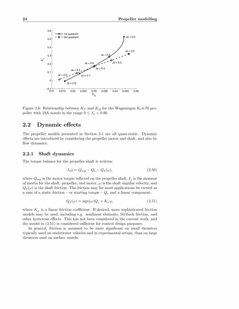
24 Propeller modelling
0.01 0.015 0.02 0.025 0.03 0.035 0.04 0.045 0.05−0.1
0
0.1
0.2
0.3
0.4
0.5
0.6
Ja = 0.8
Ja = 0.7
Ja = 0.6
Ja = 0.4
Ja = 0.0
Ja = 0.6
Ja = 0.5Ja = 0.4
Ja = 0.2
Ja = 0.0
KQ
KT
1st quadrant3rd quadrant
Figure 2.6: Relationship between KT and KQ for the Wageningen Ka4-70 pro-peller with 19A nozzle in the range 0 ≤ Ja < 0.86.
2.2 Dynamic effectsThe propeller models presented in Section 2.1 are all quasi-static. Dynamiceffects are introduced by considering the propeller motor and shaft, and also byflow dynamics.
2.2.1 Shaft dynamics
The torque balance for the propeller shaft is written:
Isω = Qmp −Qa −Qf (ω), (2.50)
where Qmp is the motor torque inflicted on the propeller shaft, Is is the momentof inertia for the shaft, propeller, and motor, ω is the shaft angular velocity, andQf (ω) is the shaft friction. The friction may for most applications be viewed asa sum of a static friction — or starting torque — Qs and a linear component:
Qf (ω) = sign(ω)Qs +Kωω, (2.51)
where Kω is a linear friction coefficient. If desired, more sophisticated frictionmodels may be used, including e.g. nonlinear elements, Stribeck friction, andother hysteresis effects. This has not been considered in the current work, andthe model in (2.51) is considered sufficient for control design purposes.In general, friction is assumed to be more significant on small thrusters
typically used on underwater vehicles and in experimental setups, than on largethrusters used on surface vessels.

2.2 Dynamic effects 25
Remark 2.4 The propeller torque Qa in (2.50) should in general also includean added mass term due to hydrodynamic forces in phase with ω. This is dis-cussed in the context of propeller vibrations in e.g. Wereldsma (1965) and Par-sons and Vorus (1981). However, the added mass will depend on propeller shaftspeed, advance velocity, and propeller submergence, and extensive model knowl-edge is required in order to include such terms. Neglecting the added mass willgive a reduced rotational inertia, and hence faster dynamics. If the necessarymodel knowledge is available, the added mass could be included in Is.
2.2.2 Motor dynamics
Electric motor
The inner torque control loop — or inner current loop — is inherent in the designof most applied control schemes for variable speed drive systems. The torque iscontrolled by means of motor currents and motor fluxes with high accuracy andbandwidth. By the cascaded control principle, an outer control loop — e.g. aspeed controller — sets the commanded torque setpoint of the inner loop. For thisprinciple to work, the inner current loop must have a much higher bandwidththan the outer loop. In the design of the outer control loop, the closed loop ofan electric motor and its current controller may be assumed to be equivalentwith a first order system (Leonhard, 1996):
Qm =1
Tm(Qcm −Qm), (2.52)
where Qm is the motor torque, Tm is the time constant, and Qcm is the com-manded motor torque from the thruster controller. This model is applicable toboth AC and DC motors; once the current loop is closed, there is little differencebetween the two types of machines. From a practical point of view, the currentloop is usually embedded in the motor drive, and is not at the disposition of theuser. The main importance is therefore to account for its dynamics in the designof the higher-level controllers (Leonhard, 1996). According to Nilsen (2001), thedynamics of the current loop are, in the context of shaft speed controller design,dominated by the filter on the shaft speed measurement. The motor power Pmis given by:
Pm = Qm2πnm, (2.53)
where nm is the motor speed. The rated (nominal) torque and power for con-tinuous operation of the motor are denoted QN and PN . The correspondingrated motor shaft speed nN is given from:
PN = QN2πnN . (2.54)
The maximum torque Qmax and power Pmax for the motor are usually set to:
Qmax = kmQN , Pmax = kmPN , (2.55)
where km typically is in the range of 1.1− 1.2 (Sørensen et al., 1997).

26 Propeller modelling
Diesel engine
A diesel engine is modelled in a similar way as the electric motor. According toBlanke (1981), the diesel engine dynamics may for control design and propulsionperformance evaluation be approximated by a time constant Tm and a time delayτm. The diesel engine transfer function becomes:
Qm(s) = e−sτmKy
1 + sTmY (s), (2.56)
where s is the Laplace operator, Ky is the motor torque constant, and Y isthe fuel index (governor setting). This means that Qcm in (2.52) is given byQcm = KyY , where Y is the control signal from the diesel controller. The dieselengine power is proportional to the fuel flow (Blanke, 1994). From Blanke(1981), the time constant is empirically found to be:
Tm ≈0.9
2πnm, (2.57)
and the time delay can be approximated by half the period between consecutivecylinder firings. A diesel engine with N cylinders rotating at speed nm rps thenhas the time delay:
τm ≈1
2nmN. (2.58)
2.2.3 Accounting for gears
Many electrically driven propulsion units are equipped with a gearbox betweenthe motor and the propeller shaft. In this work, Qm is the motor torque asseen from the motor, and n is the shaft speed as seen from the propeller. Therelations between the motor torque Qm, the motor shaft speed nm, the motortorque Qmp seen from the propeller, and the propeller shaft speed n, are givenby the gear ratio kg:
Qmp = kgQm, (2.59)
n = nm/kg. (2.60)
For thruster controller design and analysis, all torques and shaft speeds are asseen from the propeller, with the exception of Qm and Qcm. For example, thecommanded torque Qc from the controller is referred to the propeller, and Qcm
calculated from Qcm = Qc/kg. The various terms are illustrated in Figure 2.7.By the principle of conservation of energy, the rotational inertia Is seen by thepropeller can be transformed to the rotational inertia Im seen by the motor by:
Isωω = Imkgωkgω,
⇓Im = Is/k
2g . (2.61)
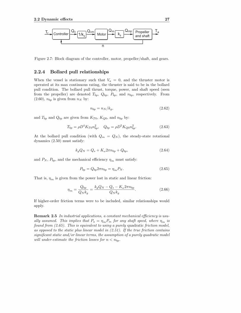
2.2 Dynamic effects 27
Q TamQcTr
n
Controller kg1/kg
Propellerand shaftMotor
Qcm Qmp
Figure 2.7: Block diagram of the controller, motor, propeller/shaft, and gears.
2.2.4 Bollard pull relationships
When the vessel is stationary such that Va = 0, and the thruster motor isoperated at its max continuous rating, the thruster is said to be in the bollardpull condition. The bollard pull thrust, torque, power, and shaft speed (seenfrom the propeller) are denoted Tbp, Qbp, Pbp, and nbp, respectively. From(2.60), nbp is given from nN by:
nbp = nN/kg, (2.62)
and Tbp and Qbp are given from KT0, KQ0, and nbp by:
Tbp = ρD4KT0n2bp, Qbp = ρD5KQ0n
2bp. (2.63)
At the bollard pull condition (with Qm = QN ), the steady-state rotationaldynamics (2.50) must satisfy:
kgQN = Qs +Kω2πnbp +Qbp, (2.64)
and PN , Pbp, and the mechanical efficiency ηm must satisfy:
Pbp = Qbp2πnbp = ηmPN . (2.65)
That is, ηm is given from the power lost in static and linear friction:
ηm =Qbp
QNkg=
kgQN −Qs −Kω2πnbpQNkg
. (2.66)
If higher-order friction terms were to be included, similar relationships wouldapply.
Remark 2.5 In industrial applications, a constant mechanical efficiency is usu-ally assumed. This implies that Pa = ηmPm for any shaft speed, where ηm isfound from (2.65). This is equivalent to using a purely quadratic friction model,as opposed to the static plus linear model in (2.51). If the true friction containssignificant static and/or linear terms, the assumption of a purely quadratic modelwill under-estimate the friction losses for n < nbp.

28 Propeller modelling
2.2.5 Propeller flow dynamics
Experimental results have shown that overshoots in thrust and torque duringtransient operation cannot be explained by steady state theory. An investiga-tion into the effects of flow dynamics on the performance of low-level thrustercontrollers and underwater vehicle positioning was initiated by Yoerger et al.(1991). In this work, a lumped parameter one-state model for the shaft dynam-ics and flow dynamics was proposed:
Isω = Qmp −K1ω |ω| ,Ta = K2ω |ω| , (2.67)
where an instantaneous relationship between the propeller shaft speed and theflow rate is included in the parameters K1 and K2. The shaft friction is ne-glected.To describe overshoots in thrust found in experimental data, Healey et al.
(1995) extended (2.67) to include the flow velocity Vp through the propeller asa state. From momentum theory, see e.g. Durand (1963), Vp is connected withthe advance velocity Va and the induced velocity in the wake UA through:
Vp = Va +1
2UA. (2.68)
In the work of Healey et al. (1995), a control volume of water around the pro-peller was modelled as a mass-damper system, leading to the following two-statemodel:
Isω = Qmp −Kωω −Qa,
mf Vp = Ta − dfVp |Vp| ,Ta = Ta(ω, Vp),
Qa = Qa(ω, Vp), (2.69)
where mf can be viewed as the mass of water in the control volume, and df isa quadratic damping coefficient. The mappings T (ω, Vp) and Qa(ω, Vp) employfoil theory with sinusoidal lift and drag curves and the local angle of attack atradius 0.7R to model the propeller blade lift and drag. Healey et al. (1995) alsoproposed using a time constant on the thrust and torque for open propellers tomodel lift and drag build-up. A summary of the theory and assumptions behindthese models, as well as experimental verification, can be found in Whitcomband Yoerger (1999a).Discrepancies between (2.69) and experimental results were attempted ex-
plained by Bachmayer et al. (2000). Here it was concluded that the inclusionof rotational flow dynamics did not improve model performance, whereas theuse of non-sinusoidal lift and drag curves specific to the tested propeller gavesignificant performance improvements. Note that these models all assume thatVa = 0, and hence only are applicable for station-keeping operations with smallcurrent.
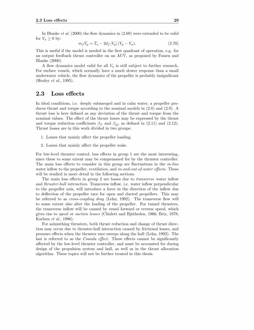
2.3 Loss effects 29
In Blanke et al. (2000) the flow dynamics in (2.69) were extended to be validfor Va ≥ 0 by:
mf Vp = Ta − 2df |Vp| (Vp − Va). (2.70)
This is useful if the model is needed in the first quadrant of operation, e.g. foran output feedback thrust controller on an AUV, as proposed by Fossen andBlanke (2000).A flow dynamics model valid for all Va is still subject to further research.
For surface vessels, which normally have a much slower response than a smallunderwater vehicle, the flow dynamics of the propeller is probably insignificant(Healey et al., 1995).
2.3 Loss effectsIn ideal conditions, i.e. deeply submerged and in calm water, a propeller pro-duces thrust and torque according to the nominal models in (2.8) and (2.9). Athrust loss is here defined as any deviation of the thrust and torque from thenominal values. The effect of the thrust losses may be expressed by the thrustand torque reduction coefficients βT and βQ, as defined in (2.11) and (2.12).Thrust losses are in this work divided in two groups:
1. Losses that mainly affect the propeller loading,
2. Losses that mainly affect the propeller wake.
For low-level thruster control, loss effects in group 1 are the most interesting,since these to some extent may be compensated for by the thruster controller.The main loss effects to consider in this group are fluctuations in the in-linewater inflow to the propeller, ventilation, and in-and-out-of-water effects. Thesewill be studied in more detail in the following sections.The main loss effects in group 2 are losses due to transverse water inflow
and thruster-hull interaction. Transverse inflow, i.e. water inflow perpendicularto the propeller axis, will introduce a force in the direction of the inflow dueto deflection of the propeller race for open and ducted propellers. This maybe referred to as cross-coupling drag (Lehn, 1992). The transverse flow willto some extent also alter the loading of the propeller. For tunnel thrusters,the transverse inflow will be caused by vessel forward or reverse speed, whichgives rise to speed or suction losses (Chislett and Björheden, 1966; Brix, 1978;Karlsen et al., 1986).For azimuthing thrusters, both thrust reduction and change of thrust direc-
tion may occur due to thruster-hull interaction caused by frictional losses, andpressure effects when the thruster race sweeps along the hull (Lehn, 1992). Thelast is referred to as the Coanda effect. These effects cannot be significantlyaffected by the low-level thruster controller, and must be accounted for duringdesign of the propulsion system and hull, as well as in the thrust allocationalgorithm. These topics will not be further treated in this thesis.
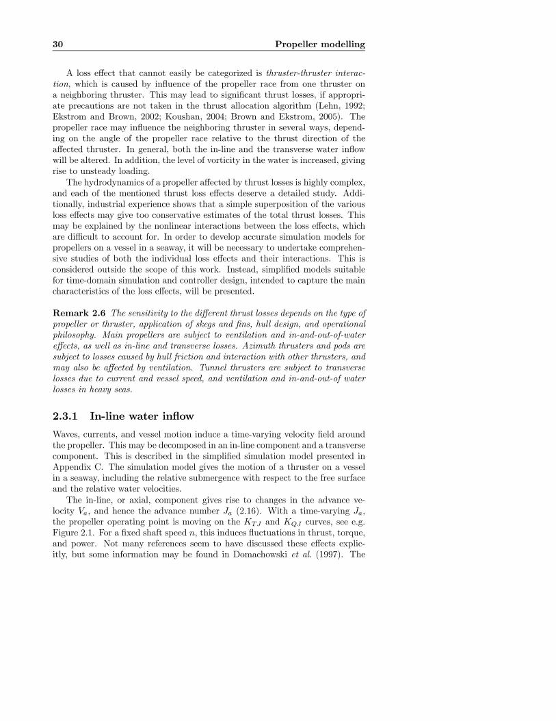
30 Propeller modelling
A loss effect that cannot easily be categorized is thruster-thruster interac-tion, which is caused by influence of the propeller race from one thruster ona neighboring thruster. This may lead to significant thrust losses, if appropri-ate precautions are not taken in the thrust allocation algorithm (Lehn, 1992;Ekstrom and Brown, 2002; Koushan, 2004; Brown and Ekstrom, 2005). Thepropeller race may influence the neighboring thruster in several ways, depend-ing on the angle of the propeller race relative to the thrust direction of theaffected thruster. In general, both the in-line and the transverse water inflowwill be altered. In addition, the level of vorticity in the water is increased, givingrise to unsteady loading.The hydrodynamics of a propeller affected by thrust losses is highly complex,
and each of the mentioned thrust loss effects deserve a detailed study. Addi-tionally, industrial experience shows that a simple superposition of the variousloss effects may give too conservative estimates of the total thrust losses. Thismay be explained by the nonlinear interactions between the loss effects, whichare difficult to account for. In order to develop accurate simulation models forpropellers on a vessel in a seaway, it will be necessary to undertake comprehen-sive studies of both the individual loss effects and their interactions. This isconsidered outside the scope of this work. Instead, simplified models suitablefor time-domain simulation and controller design, intended to capture the maincharacteristics of the loss effects, will be presented.
Remark 2.6 The sensitivity to the different thrust losses depends on the type ofpropeller or thruster, application of skegs and fins, hull design, and operationalphilosophy. Main propellers are subject to ventilation and in-and-out-of-watereffects, as well as in-line and transverse losses. Azimuth thrusters and pods aresubject to losses caused by hull friction and interaction with other thrusters, andmay also be affected by ventilation. Tunnel thrusters are subject to transverselosses due to current and vessel speed, and ventilation and in-and-out-of waterlosses in heavy seas.
2.3.1 In-line water inflow
Waves, currents, and vessel motion induce a time-varying velocity field aroundthe propeller. This may be decomposed in an in-line component and a transversecomponent. This is described in the simplified simulation model presented inAppendix C. The simulation model gives the motion of a thruster on a vesselin a seaway, including the relative submergence with respect to the free surfaceand the relative water velocities.The in-line, or axial, component gives rise to changes in the advance ve-
locity Va, and hence the advance number Ja (2.16). With a time-varying Ja,the propeller operating point is moving on the KTJ and KQJ curves, see e.g.Figure 2.1. For a fixed shaft speed n, this induces fluctuations in thrust, torque,and power. Not many references seem to have discussed these effects explic-itly, but some information may be found in Domachowski et al. (1997). The
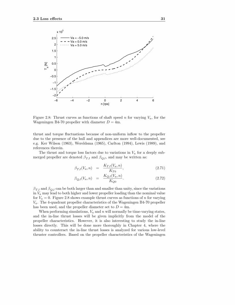
2.3 Loss effects 31
−6 −4 −2 0 2 4 6
−2
−1.5
−1
−0.5
0
0.5
1
1.5
2
2.5
x 105
n [rps]
Ta [N
]
Va = −5.0 m/sVa = 0.0 m/sVa = 5.0 m/s
Figure 2.8: Thrust curves as functions of shaft speed n for varying Va, for theWageningen B4-70 propeller with diameter D = 4m.
thrust and torque fluctuations because of non-uniform inflow to the propellerdue to the presence of the hull and appendices are more well-documented, seee.g. Ker Wilson (1963), Wereldsma (1965), Carlton (1994), Lewis (1989), andreferences therein.The thrust and torque loss factors due to variations in Va for a deeply sub-
merged propeller are denoted βTJ and βQJ , and may be written as:
βTJ(Va, n) =KTJ(Va, n)
KT0, (2.71)
βQJ(Va, n) =KQJ(Va, n)
KQ0. (2.72)
βTJ and βQJ can be both larger than and smaller than unity, since the variationsin Va may lead to both higher and lower propeller loading than the nominal valuefor Va = 0. Figure 2.8 shows example thrust curves as functions of n for varyingVa. The 4-quadrant propeller characteristics of the Wageningen B4-70 propellerhas been used, and the propeller diameter set to D = 4m.When performing simulations, Va and n will normally be time-varying states,
and the in-line thrust losses will be given implicitly from the model of thepropeller characteristics. However, it is also interesting to study the in-linelosses directly. This will be done more thoroughly in Chapter 4, where theability to counteract the in-line thrust losses is analyzed for various low-levelthruster controllers. Based on the propeller characteristics of the Wageningen
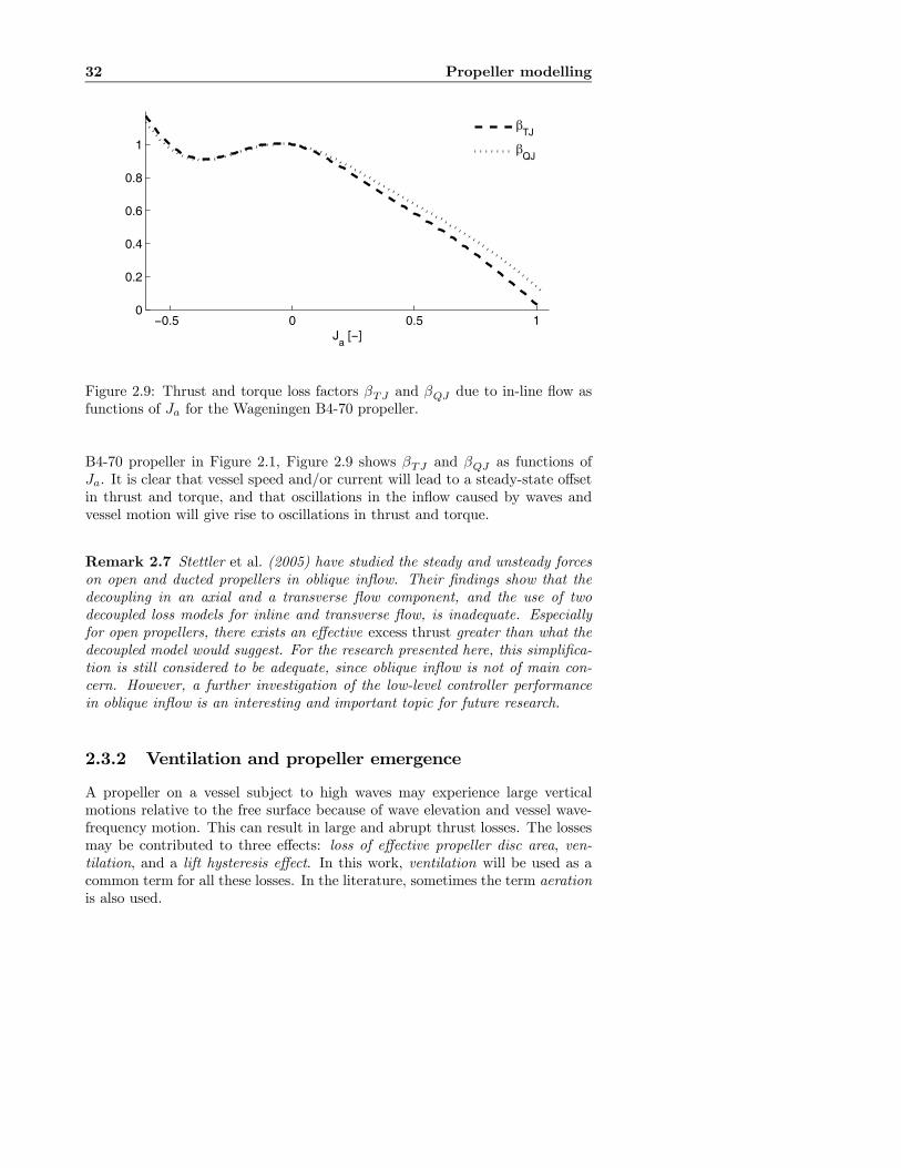
32 Propeller modelling
−0.5 0 0.5 10
0.2
0.4
0.6
0.8
1
Ja [−]
βTJ
βQJ
Figure 2.9: Thrust and torque loss factors βTJ and βQJ due to in-line flow asfunctions of Ja for the Wageningen B4-70 propeller.
B4-70 propeller in Figure 2.1, Figure 2.9 shows βTJ and βQJ as functions ofJa. It is clear that vessel speed and/or current will lead to a steady-state offsetin thrust and torque, and that oscillations in the inflow caused by waves andvessel motion will give rise to oscillations in thrust and torque.
Remark 2.7 Stettler et al. (2005) have studied the steady and unsteady forceson open and ducted propellers in oblique inflow. Their findings show that thedecoupling in an axial and a transverse flow component, and the use of twodecoupled loss models for inline and transverse flow, is inadequate. Especiallyfor open propellers, there exists an effective excess thrust greater than what thedecoupled model would suggest. For the research presented here, this simplifica-tion is still considered to be adequate, since oblique inflow is not of main con-cern. However, a further investigation of the low-level controller performancein oblique inflow is an interesting and important topic for future research.
2.3.2 Ventilation and propeller emergence
A propeller on a vessel subject to high waves may experience large verticalmotions relative to the free surface because of wave elevation and vessel wave-frequency motion. This can result in large and abrupt thrust losses. The lossesmay be contributed to three effects: loss of effective propeller disc area, ven-tilation, and a lift hysteresis effect. In this work, ventilation will be used as acommon term for all these losses. In the literature, sometimes the term aerationis also used.

2.3 Loss effects 33
Loss of effective disc area
If the propeller emerges from the water, a thrust loss due to loss of effectivepropeller disc area is experienced (Gutsche, 1967; Fleischer, 1973). The corre-sponding thrust loss factor βTA can be found from a simple geometrical consid-eration, by assuming that the resulting thrust is proportional to the submergedpropeller disc area:
βTA = real
µ1− arccos(h/R)
π+
h/R
π
p1− (h/R)2
¶. (2.73)
Here, h/R is the relative submergence, with h the propeller shaft submergenceand R the propeller radius. An alternative representation, where also the pro-peller hub diameter is accounted for, is given in Koushan (2004). This lossmodel is assumed to be valid for any propeller loading. A simplified, piecewiselinear representation is given by:
βTA ≈ 0.5 + 0.5(min(max(h/R,−1), 1)). (2.74)
An alternative representation is given in Minsaas et al. (1983) based on theresults from Faltinsen et al. (1980):
βTA =
⎧⎨⎩ 0, h/R < −0.48,1− 0.675(1− 0.769h/R)1.258, −0.48 ≤ h/R ≤ 1.3,
1, h > 1.3.(2.75)
(2.75) includes contributions from the so-called Wagner effect. This is conve-nient if the dynamic effects of ventilation can be neglected, and only the averagethrust values are needed. In the following, the alternative representation (2.75)will not be used, since the Wagner effect is included as a part of the lift hysteresiseffect. The three representations are compared in Figure 2.10.
Ventilation
Ventilation may occur when a propeller is operating in the proximity of thefree surface. If the propeller loading is sufficiently high, the low pressure onthe propeller blades may create a funnel through which air is drawn from thefree surface. This phenomenon is connected with co-orientation of the energyin the surrounding water. The propeller sets up a rotating flow which causesthe free surface to deform, and a vortex starts to develop. Unless the rotatingflow is disturbed, this is a self-amplifying process, and the vortex develops intoa funnel. Air cavities then spread on the propeller blades, reducing their liftand drag. A fully ventilated propeller may lose as much as 70-80% of its thrustand torque. Several thorough studies of ventilated and partially submergedpropellers have been performed, see e.g. Shiba (1953), Gutsche (1967), Kruppa(1972), Brandt (1973), Fleischer (1973), Scherer (1977), Hashimoto et al. (1984),Guoqiang et al. (1989), and Olofsson (1996). Additional results and further

34 Propeller modelling
−2 −1.5 −1 −0.5 0 0.5 1 1.5 2
0
0.2
0.4
0.6
0.8
1
h/R
β TAExact
Linear
Alternative
Figure 2.10: Comparison of three different representations for the thrust lossdue to loss of effective disc area: exact (2.73), linear (2.74), and alternative(2.75).
studies with respect to vessel operational performance can be found in Faltinsenet al. (1980), Minsaas et al. (1983, 1986, 1987), Karlsen et al. (1986), and Lehn(1992). Ventilation is in the above references typically divided in three regimes:non-ventilated, partially ventilated, and fully ventilated.Non-ventilated regime: The propeller is deeply submerged, or fully sub-
merged and with low propeller loading. No ventilation occurs.Partially ventilated regime: The propeller is partly, but not stationary ven-
tilated. That is, the level of ventilation and the location of the air cavities onthe propeller are time-varying. For high Ja, this regime is persistent. For lowJa, it is an unstable regime that mainly exists as a transition between the twoother regimes.Fully ventilated regime: A single ventilated cavity covers each of the propeller
blades, meaning that the pressure on the suction side of the propeller blades isalmost atmospheric. This is a relatively stable condition.The three regimes are sketched as a function of Ja and h/R in Figure 2.11,
based on a similar figure in Olofsson (1996). The partially ventilated, unstableregime for low Ja is marked as unstable. The regimes that are relevant for DPare indicated on the Ja-axis.The thrust loss factor due to ventilation is termed βTV 0, and is in general
expected to be a function of shaft speed, advance velocity, and submergence.
Lift hysteresis
For ventilation to terminate, the supply of air to the cavities on the propellerblades must be stopped. The three most apparent causes for the funnel from

2.3 Loss effects 35
J
h/R
a
Non-ventilated regime
Partiallyventilated
regimeFully-ventilated
regime
Unstable regime1
Fu
llysu
bm
erg
ed
Pa
rtia
llysu
bm
erg
ed
DP regime
Figure 2.11: Ventilation flow regimes, with the regimes relevant for DP indicatedon the Ja axis. Adopted from Olofsson (1996).
the surface to collapse are increased submergence of the propeller, disturbancesin the water, and decreased loading of the propeller. For a propeller in dy-namic operating conditions, a combination of the two first causes will lead totermination of the ventilation incident relatively soon after the propeller is fullysubmerged. When the air supply to the cavities is stopped, two events musttake place before the full thrust is restored:
1. The cavities on the propeller blades must vanish in order to restore thesuction-side pressure.
2. The produced lift of the propeller blades must build up.
It appears that the first of these two effects has not been explicitly discussed inthe literature. However, a lot can be learned by studying the behavior of the aircavities on the propeller blades, as done in Koushan (2006). It seems apparentthat the result is a time delay before the lift starts building up.When the ventilated cavities disappear, there will be a sudden increase in
lift on the propeller blades. Wagner (1925) studied a similar problem for a two-dimensional foil, and found that the sudden increase was 50% of the steady-statelift, see also Newman (1977) or Durand (1963). The Wagner function gives theratio between the instantaneous lift and the steady-state lift, and shows that thefoil must travel about 20 chord lengths to recover its full lift. A similar behavioris seen for a propeller that is moving in and out of ventilated condition, as first
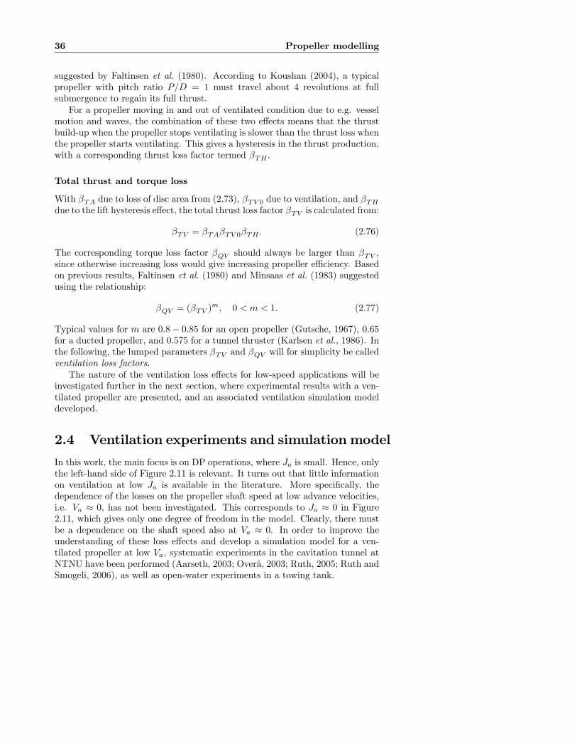
36 Propeller modelling
suggested by Faltinsen et al. (1980). According to Koushan (2004), a typicalpropeller with pitch ratio P/D = 1 must travel about 4 revolutions at fullsubmergence to regain its full thrust.For a propeller moving in and out of ventilated condition due to e.g. vessel
motion and waves, the combination of these two effects means that the thrustbuild-up when the propeller stops ventilating is slower than the thrust loss whenthe propeller starts ventilating. This gives a hysteresis in the thrust production,with a corresponding thrust loss factor termed βTH .
Total thrust and torque loss
With βTA due to loss of disc area from (2.73), βTV 0 due to ventilation, and βTHdue to the lift hysteresis effect, the total thrust loss factor βTV is calculated from:
βTV = βTAβTV 0βTH . (2.76)
The corresponding torque loss factor βQV should always be larger than βTV ,since otherwise increasing loss would give increasing propeller efficiency. Basedon previous results, Faltinsen et al. (1980) and Minsaas et al. (1983) suggestedusing the relationship:
βQV = (βTV )m, 0 < m < 1. (2.77)
Typical values for m are 0.8− 0.85 for an open propeller (Gutsche, 1967), 0.65for a ducted propeller, and 0.575 for a tunnel thruster (Karlsen et al., 1986). Inthe following, the lumped parameters βTV and βQV will for simplicity be calledventilation loss factors.The nature of the ventilation loss effects for low-speed applications will be
investigated further in the next section, where experimental results with a ven-tilated propeller are presented, and an associated ventilation simulation modeldeveloped.
2.4 Ventilation experiments and simulation model
In this work, the main focus is on DP operations, where Ja is small. Hence, onlythe left-hand side of Figure 2.11 is relevant. It turns out that little informationon ventilation at low Ja is available in the literature. More specifically, thedependence of the losses on the propeller shaft speed at low advance velocities,i.e. Va ≈ 0, has not been investigated. This corresponds to Ja ≈ 0 in Figure2.11, which gives only one degree of freedom in the model. Clearly, there mustbe a dependence on the shaft speed also at Va ≈ 0. In order to improve theunderstanding of these loss effects and develop a simulation model for a ven-tilated propeller at low Va, systematic experiments in the cavitation tunnel atNTNU have been performed (Aarseth, 2003; Overå, 2003; Ruth, 2005; Ruth andSmogeli, 2006), as well as open-water experiments in a towing tank.

2.4 Ventilation experiments and simulation model 37
2.4.1 Cavitation tunnel test results
A description of the experimental setup is given in Appendix D. In order to testthe propeller performance for normal free surface conditions, the pressure in thecavitation tunnel was kept at atmospheric level. The advance velocity was keptlow, and the shaft speed and submergence were systematically varied. Timeseries of the propeller thrust and torque were recorded, and the mean values foreach test run were calculated. Most of the experiments were conducted witha ducted propeller with diameter D = 0.25m and pitch ratio P/D = 1. Someresults with an open propeller have also been obtained. Technical specificationsof the propeller are given in Section 7.1.As an example of the obtained results, Figure 2.12 shows the ventilation
thrust loss factor βTV as a function of the relative submergence h/R and pro-peller shaft speed n for a ducted propeller at advance ratio Ja ≈ 0.2. Figure2.13 shows the corresponding relative thrust Ta/Tmax, where Tmax is the maxi-mum thrust obtained in the experiments. The torque loss factor and propellertorque are presented in Appendix D. The results obtained here agree well withprevious research, see. e.g. Shiba (1953) or Fleischer (1973), but contain addi-tional information for the case of low Va. When deeply submerged, the thrusterperforms as expected, with thrust proportional to n2. For low shaft speeds, andhence low propeller loading, the thrust is constant for h/R = 1.5 to h/R = 1,and then decreases almost linearly from h/R = 1 to h/R = 0. This is due to lossof effective propeller disc area. For higher propeller loads, the thrust and torquedrop rapidly with decreasing submergence, indicating onset of ventilation. It isevident that for a heavily loaded propeller, proximity to the surface may leadto an abrupt loss of thrust and torque. The results indicate that a reduction ofthe shaft speed in such a case may increase the thrust, since there is a “ridge” ifhigher thrust for n ≈ 9rps. However, further experience with open-water testsin a towing tank shows that once the propeller is ventilated, such an increase inthrust is difficult to obtain. This will be further discussed below. The figure alsoindicates that it is not possible to increase the thrust significantly by increasingthe shaft speed.For an open propeller, the “ridge” of higher thrust seems to be less apparent,
and the thrust during ventilation is slightly increasing for increasing shaft speed.This seems to be the major difference between the two propeller types whenconsidering ventilation; the structure of the losses is otherwise similar. Thisis further explained in Appendix D, where additional experimental results foran open propeller are presented. More experimental results, where also thepropeller pitch ratio is varied, can be found in Ruth and Smogeli (2006).
Remark 2.8 It has been assumed that the results obtained at Ja ≈ 0.2 arerepresentative for low Va in general, and hence also for Ja ≈ 0. From thecharacteristics of the flow regimes sketched in Figure 2.11, this appears to be avalid assumption.

38 Propeller modelling
68
1012
1416
0
0.5
1
1.5
0
0.2
0.4
0.6
0.8
1
n [rps]h/R
β TV
Figure 2.12: Ventilation thrust loss factor βTV vs. relative submergence h/Rand propeller shaft speed n at Ja ≈ 0.2 for a ducted propeller. From experi-ments.
68
1012
1416
0
0.5
1
1.5
0
0.2
0.4
0.6
0.8
1
n [rps]h/R
Ta/T
max
Figure 2.13: Relative thrust Ta/Tmax vs. relative submergence h/R and pro-peller shaft speed n at Ja ≈ 0.2 for a ducted propeller. From experiments.
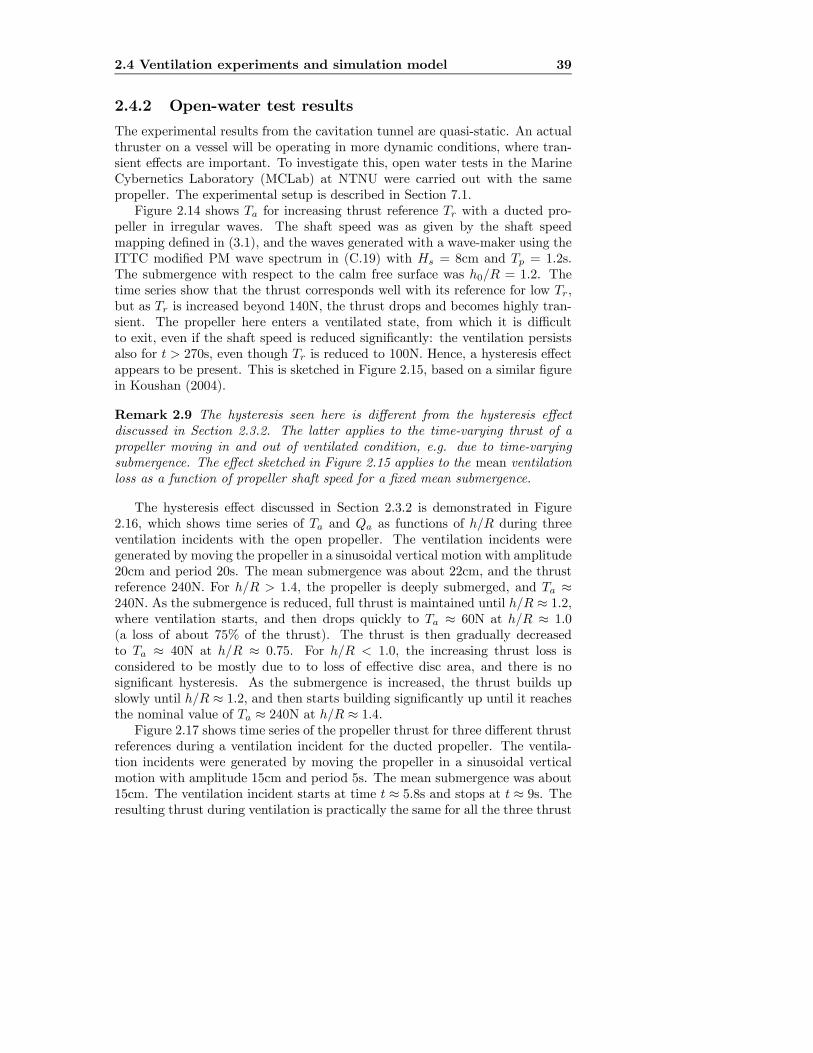
2.4 Ventilation experiments and simulation model 39
2.4.2 Open-water test results
The experimental results from the cavitation tunnel are quasi-static. An actualthruster on a vessel will be operating in more dynamic conditions, where tran-sient effects are important. To investigate this, open water tests in the MarineCybernetics Laboratory (MCLab) at NTNU were carried out with the samepropeller. The experimental setup is described in Section 7.1.Figure 2.14 shows Ta for increasing thrust reference Tr with a ducted pro-
peller in irregular waves. The shaft speed was as given by the shaft speedmapping defined in (3.1), and the waves generated with a wave-maker using theITTC modified PM wave spectrum in (C.19) with Hs = 8cm and Tp = 1.2s.The submergence with respect to the calm free surface was h0/R = 1.2. Thetime series show that the thrust corresponds well with its reference for low Tr,but as Tr is increased beyond 140N, the thrust drops and becomes highly tran-sient. The propeller here enters a ventilated state, from which it is difficultto exit, even if the shaft speed is reduced significantly: the ventilation persistsalso for t > 270s, even though Tr is reduced to 100N. Hence, a hysteresis effectappears to be present. This is sketched in Figure 2.15, based on a similar figurein Koushan (2004).
Remark 2.9 The hysteresis seen here is different from the hysteresis effectdiscussed in Section 2.3.2. The latter applies to the time-varying thrust of apropeller moving in and out of ventilated condition, e.g. due to time-varyingsubmergence. The effect sketched in Figure 2.15 applies to the mean ventilationloss as a function of propeller shaft speed for a fixed mean submergence.
The hysteresis effect discussed in Section 2.3.2 is demonstrated in Figure2.16, which shows time series of Ta and Qa as functions of h/R during threeventilation incidents with the open propeller. The ventilation incidents weregenerated by moving the propeller in a sinusoidal vertical motion with amplitude20cm and period 20s. The mean submergence was about 22cm, and the thrustreference 240N. For h/R > 1.4, the propeller is deeply submerged, and Ta ≈240N. As the submergence is reduced, full thrust is maintained until h/R ≈ 1.2,where ventilation starts, and then drops quickly to Ta ≈ 60N at h/R ≈ 1.0(a loss of about 75% of the thrust). The thrust is then gradually decreasedto Ta ≈ 40N at h/R ≈ 0.75. For h/R < 1.0, the increasing thrust loss isconsidered to be mostly due to to loss of effective disc area, and there is nosignificant hysteresis. As the submergence is increased, the thrust builds upslowly until h/R ≈ 1.2, and then starts building significantly up until it reachesthe nominal value of Ta ≈ 240N at h/R ≈ 1.4.Figure 2.17 shows time series of the propeller thrust for three different thrust
references during a ventilation incident for the ducted propeller. The ventila-tion incidents were generated by moving the propeller in a sinusoidal verticalmotion with amplitude 15cm and period 5s. The mean submergence was about15cm. The ventilation incident starts at time t ≈ 5.8s and stops at t ≈ 9s. Theresulting thrust during ventilation is practically the same for all the three thrust
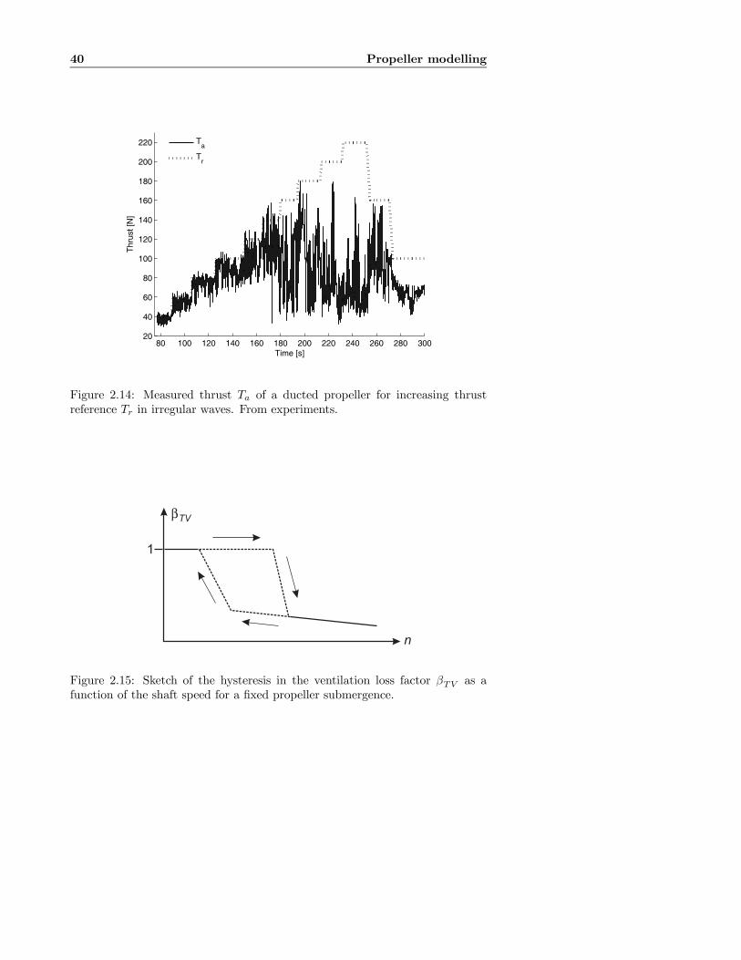
40 Propeller modelling
80 100 120 140 160 180 200 220 240 260 280 30020
40
60
80
100
120
140
160
180
200
220
Thr
ust [
N]
Time [s]
Ta
Tr
Figure 2.14: Measured thrust Ta of a ducted propeller for increasing thrustreference Tr in irregular waves. From experiments.
n
bTV
1
Figure 2.15: Sketch of the hysteresis in the ventilation loss factor βTV as afunction of the shaft speed for a fixed propeller submergence.

2.4 Ventilation experiments and simulation model 41
0.6 0.8 1 1.2 1.4 1.6 1.8 2 2.2 2.4 2.6
50
100
150
200
250
h/R
Ta [N
]
0.6 0.8 1 1.2 1.4 1.6 1.8 2 2.2 2.4 2.62
4
6
8
10
12
h/R
Qa [N
m]
Figure 2.16: Measured thrust Ta and torque Qa vs. relative submergence h/Rduring three ventilation incidents with a ducted propeller, illustrating the thrustand torque hysteresis effect. From experiments.
references. For Tr = 300N, the loss of thrust is approximately 85%. The devia-tion of the measured submergence from the imposed motion may be explainedby local surface elevation due to disturbances in the water, and possibly also bydeviation in the actual from the commanded vertical motion.
2.4.3 Scaling of test results
Care must be taken in order to scale the model tests results to be valid for alarge propeller. However, the general behavior of a full-scale propeller subjectto ventilation and in-and-out-of water effects is expected to be similar to theresults from model scale. A discussion on the scaling laws that must be satisfiedin order to transfer the results to full scale is undertaken in Appendix D.In Section 7, experimental results for a model scale propeller subject to
ventilation with various thruster controllers will be presented. These time seriescannot easily be transformed to full scale, and must be interpreted as they are— in model scale. Investigation of the performance of various controllers in fullscale will instead be done by simulations, where realistic full-scale propeller datacan be used. This is believed to be a more appropriate approach, since thereare several important structural differences between model scale and full scale:in addition to the problems with scaling of the propeller load, the friction andinertia properties of the propeller and drive system may change significantly.

42 Propeller modelling
0
0.5
1
1.5
2h/
R
5 6 7 8 9 100
100
200
300
Ta [N
]
Time [s]
Tr = 100N
Tr = 200N
Tr = 300N
Figure 2.17: Time series of measured thrust during ventilation at three differentthrust references for a ducted propeller. From experiments.
2.4.4 Ventilation simulation model
Based on the experimental results presented in the previous sections, simplifiedventilation models suitable for time-domain simulation may be developed. Theventilation thrust loss factor βTV can be expressed as a function of the relativeimmersion h/R and the relative shaft speed n/nbp, where nbp is the bollard pullshaft speed of the propeller, see (2.62). Because of the different characteristicsof the thrust during ventilation for open and ducted propellers, two simulationmodels are proposed.
Open propeller
For an open propeller, there is no pronounced “ridge” of higher thrust, andthe thrust is slightly increasing for increasing shaft speed during ventilation.The proposed ventilation loss model is shown in Figure 2.18. The loss modelis parameterized by two relative shaft speeds, two submergence ratios, and twoloss factors, marked as n1, n2, h1, h2, b1, and b2 in the figure. Additionally,the main coordinates defining the loss surface are drawn as circles — the lossfactor surface is found by linear interpolation between these points. In theregime with h/R > h2, the propeller is deeply submerged, and no losses areexperienced (βTV = 1). For h/R < −1 the propeller exits the water completely,and no thrust is produced (βTV = 0). The remaining regime is −1 < h/R < h2.For n/nbp < n1 the propeller is lightly loaded, and only losses due to loss of

2.4 Ventilation experiments and simulation model 43
0
0.2
0.4
0.6
0.8
1 −2−1
01
23
0
0.5
1
1.5
n2
b2
n1
h/R
b1
h2h
1
n/nbp
β TV
Figure 2.18: Ventilation thrust loss model for an open propeller, as functionof relative shaft speed n/nbp and relative submergence h/R, with n1 = 0.2,n2 = 0.5, h1 = 1.1, h2 = 1.3, b1 = 0.3, and b2 = 0.25.
effective disc area are experienced. This is seen as the gradually decreasingβTV for −1 < h/R < h1, modelled as in (2.74). For n/nbp > n2, the propelleris heavily loaded, and decreasing submergence will lead to an abrupt loss ofthrust due to ventilation. The transition to-and-from the ventilated regimehappens for n1 < n/nbp < n2 and h1 < h/R < h2. For h/R < h1, additionalthrust losses are experienced due to loss of effective disc area (meaning that h1should be close to 1). The thrust loss for a fully submerged and fully ventilatedpropeller is defined by the two loss factors b1 and b2. b1 is the loss factor wherefull ventilation starts (h/R = h1 and n/nbp = n2), and b2 is the loss factor atmaximum shaft speed (h/R = h1 and n/nbp = 1), with b2 equal to or slightlylower than b1. For n > nbp, the loss function should be extrapolated. Theparameters in Figure 2.18 are chosen as n1 = 0.2, n2 = 0.5, h1 = 1.1, h2 = 1.3,b1 = 0.3, and b2 = 0.25.
Ducted propeller
For a ducted propeller, there is a “ridge” of higher thrust, and the thrust isnearly constant for increasing shaft speed during ventilation. The ventilationloss model therefore becomes slightly more complicated, but is still simple toparameterize. The difference from the simulation model for the open propeller isthat the loss factor during ventilation, i.e. for n/nbp > n2 and −1 < h/R < h2,is modified to give constant thrust independently of n. This is done by the
44 Propeller modelling
0
0.2
0.4
0.6
0.8
1 −2−1
01
23
0
0.5
1
1.5n
2
n1
h/R
b1
h2h
1
n/nbp
β TV
Figure 2.19: Ventilation thrust loss model for a ducted propeller, as functionof relative shaft speed n/nbp and relative submergence h/R, with n1 = 0.4,n2 = 0.45, h1 = 1.1, h2 = 1.3, and b1 = 0.3.
following curve for h/R = h1:
βTV |h/R=h1 = b1(n2
n/nbp)2, (2.78)
and with a linear decrease of βTV as function of h/R, with βTV = 0 for h/R =−1. Hence, the parameter b2 is not needed for this model, since the loss factor forhigh n/nbp is implicitly given by b1. In addition, the change from non-ventilatedto ventilated condition is more rapid, which is implemented by a smaller intervalbetween n1 and n2. Figure 2.19 shows an example of the loss model for ductedpropellers, with n1 = 0.4, n2 = 0.45, h1 = 1.1, h2 = 1.3, and b1 = 0.3. The twoloss models are further compared with the experimental results in Appendix D.
Hysteresis effect
The hysteresis in the propeller loading may be modelled by introducing a posi-tive rate limit βVH on βTV , such that the load is allowed to drop more quicklythan it is allowed to build up, i.e. −∞ < βTV ≤ βVH . This approach gives rea-sonable correspondence with experimental time series. It is of course possible todevelop more sophisticated models of the hysteresis effect, but this has not beenconsidered necessary for the present applications. Using as a rule-of-thumb that4 complete revolutions of the propeller is needed to develop full lift (Koushan,
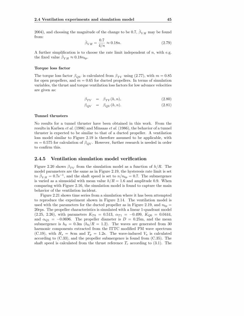
2.4 Ventilation experiments and simulation model 45
2004), and choosing the magnitude of the change to be 0.7, βVH may be foundfrom:
βVH =0.7
4/n≈ 0.18n. (2.79)
A further simplification is to choose the rate limit independent of n, with e.g.the fixed value βVH ≈ 0.18nbp.
Torque loss factor
The torque loss factor βQV is calculated from βTV using (2.77), with m = 0.85for open propellers, and m = 0.65 for ducted propellers. In terms of simulationvariables, the thrust and torque ventilation loss factors for low advance velocitiesare given as:
βTV = βTV (h, n), (2.80)
βQV = βQV (h, n). (2.81)
Tunnel thrusters
No results for a tunnel thruster have been obtained in this work. From theresults in Karlsen et al. (1986) and Minsaas et al. (1986), the behavior of a tunnelthruster is expected to be similar to that of a ducted propeller. A ventilationloss model similar to Figure 2.19 is therefore assumed to be applicable, withm = 0.575 for calculation of βQV . However, further research is needed in orderto confirm this.
2.4.5 Ventilation simulation model verification
Figure 2.20 shows βTV from the simulation model as a function of h/R. Themodel parameters are the same as in Figure 2.19, the hysteresis rate limit is setto βVH = 0.7s−1, and the shaft speed is set to n/nbp = 0.7. The submergenceis varied as a sinusoidal with mean value h/R = 1.6 and amplitude 0.9. Whencomparing with Figure 2.16, the simulation model is found to capture the mainbehavior of the ventilation incident.Figure 2.21 shows time series from a simulation where it has been attempted
to reproduce the experiment shown in Figure 2.14. The ventilation model isused with the parameters for the ducted propeller as in Figure 2.19, and nbp =20rps. The propeller characteristics is simulated with a linear 1-quadrant model(2.25, 2.26), with parameters KT0 = 0.513, αT1 = −0.499, KQ0 = 0.0444,and αQ1 = −0.0696. The propeller diameter is D = 0.25m, and the meansubmergence is h0 = 0.3m (h0/R = 1.2). The waves are generated from 30harmonic components extracted from the ITTC modified PM wave spectrum(C.19), with Hs = 8cm and Tp = 1.2s. The wave-induced Va is calculatedaccording to (C.33), and the propeller submergence is found from (C.35). Theshaft speed is calculated from the thrust reference Tr according to (3.1). The
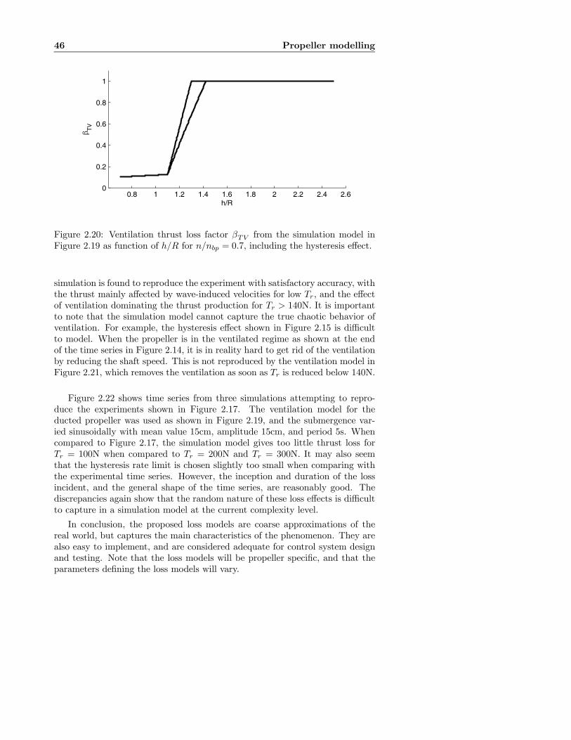
46 Propeller modelling
0.8 1 1.2 1.4 1.6 1.8 2 2.2 2.4 2.60
0.2
0.4
0.6
0.8
1
h/R
β TV
Figure 2.20: Ventilation thrust loss factor βTV from the simulation model inFigure 2.19 as function of h/R for n/nbp = 0.7, including the hysteresis effect.
simulation is found to reproduce the experiment with satisfactory accuracy, withthe thrust mainly affected by wave-induced velocities for low Tr, and the effectof ventilation dominating the thrust production for Tr > 140N. It is importantto note that the simulation model cannot capture the true chaotic behavior ofventilation. For example, the hysteresis effect shown in Figure 2.15 is difficultto model. When the propeller is in the ventilated regime as shown at the endof the time series in Figure 2.14, it is in reality hard to get rid of the ventilationby reducing the shaft speed. This is not reproduced by the ventilation model inFigure 2.21, which removes the ventilation as soon as Tr is reduced below 140N.
Figure 2.22 shows time series from three simulations attempting to repro-duce the experiments shown in Figure 2.17. The ventilation model for theducted propeller was used as shown in Figure 2.19, and the submergence var-ied sinusoidally with mean value 15cm, amplitude 15cm, and period 5s. Whencompared to Figure 2.17, the simulation model gives too little thrust loss forTr = 100N when compared to Tr = 200N and Tr = 300N. It may also seemthat the hysteresis rate limit is chosen slightly too small when comparing withthe experimental time series. However, the inception and duration of the lossincident, and the general shape of the time series, are reasonably good. Thediscrepancies again show that the random nature of these loss effects is difficultto capture in a simulation model at the current complexity level.
In conclusion, the proposed loss models are coarse approximations of thereal world, but captures the main characteristics of the phenomenon. They arealso easy to implement, and are considered adequate for control system designand testing. Note that the loss models will be propeller specific, and that theparameters defining the loss models will vary.
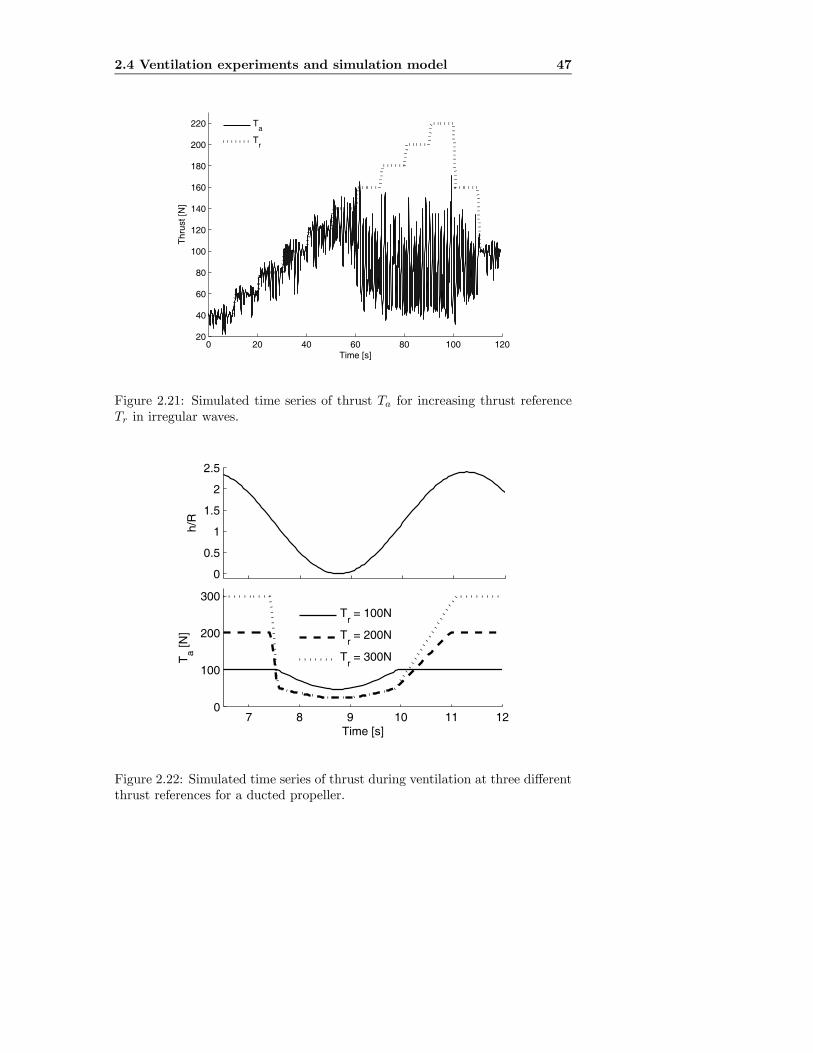
2.4 Ventilation experiments and simulation model 47
0 20 40 60 80 100 12020
40
60
80
100
120
140
160
180
200
220
Time [s]
Thr
ust [
N]
Ta
Tr
Figure 2.21: Simulated time series of thrust Ta for increasing thrust referenceTr in irregular waves.
7 8 9 10 11 120
100
200
300
Time [s]
Ta [N
]
0
0.5
1
1.5
2
2.5
h/R
Tr = 100N
Tr = 200N
Tr = 300N
Figure 2.22: Simulated time series of thrust during ventilation at three differentthrust references for a ducted propeller.
48 Propeller modelling
Remark 2.10 Although the proposed ventilation simulation models show rea-sonably good performance when compared to the experiments, it is difficult togeneralize the model, e.g. to other propeller types or to full scale propellers.This is due to the many scaling laws that must be satisfied in order to makesuch a generalization. However, the general structure of the ventilation lossfunctions, as shown in Figures 2.18 and 2.19, are expected to be applicable alsoto other propellers and in full scale. The models are therefore used for full-scalesimulations in Chapter 6. Scaling is further discussed in Appendix D. A moresophisticated ventilation loss model, which is valid also for varying pitch ratios,is presented in Ruth and Smogeli (2006).
2.4.6 Blade-frequency loading
The cavitation tunnel results and the ventilation simulation model only considerthe mean load of the propeller during ventilation. The dynamic loading of thepropeller at higher frequencies during ventilation is also an important topic,especially when considering mechanical wear and tear. There are few availablereferences considering such high-frequency dynamic loads, but a summary ofprevious findings and a thorough investigation can be found in Olofsson (1996).The following summarizes the facts that are most relevant for this work:
• During ventilation, the loads on each propeller blade fluctuate in timeas the blade goes through four phases: in-air, blade-entry, in-water, andblade-exit. These fluctuating forces introduce structural loads on the pro-peller blades.
• The sum of the blade loads for the whole propeller gives an oscillatingpropeller thrust and torque, as well as oscillating vertical and transverseforces. The main loads are found at the blade frequency, i.e. the shaftspeed in rps times the number of propeller blades. The loads are highlydependent on the operating condition.
• It is especially in the transition to-and-from ventilation, i.e. the unstable,partially ventilated regime, that large high-frequency dynamic loads occur.
• In addition to the above mentioned loads, resonant blade vibration maycause large transient loads. This is especially evident at low advance veloc-ities, since there is little hydrodynamic damping when the propeller is fullyventilated. This problem increases with increasing propeller speed, whenthe magnitude and frequency content of the encountered load increasesdanger of resonance. During resonance, the vibrations are amplified, andthe resulting dynamic load is a combination of hydrodynamic and inertialloads due to fluid-structure interaction. Resonance typically occurs closeto the blade’s natural frequency in air and water. These loads can causeserious problems, since large stress transients may develop, resulting inpeak stresses exceeding the yield strength of the blade material and hencecausing structural fatigue.

2.5 Propeller simulation model 49
In Hashimoto et al. (1984), it was also found that significant transverse andvertical force oscillations at the propeller frequency and twice the propeller fre-quency could be observed during ventilation. It should be noted that Olofsson(1996) and Hashimoto et al. (1984) mainly considered propellers at higher ad-vance velocities. However, the effect of dynamic loading on the propeller shouldfrom a mechanical point of view be independent of the advance velocity. Theresults in Olofsson (1996) actually indicated that the loads on the propellerincreased for decreasing Va, due to decreased damping and resonance problems.Recent results for the blade loading of a ventilated thruster at low advance
velocity can be found in Koushan (2004, 2006). These results confirm that thehigh-frequency dynamic loading can be significant. The standard deviation ofthe shaft frequency propeller blade force fluctuations was found to be almost100% of the average force when the propeller was partially submerged. Largefluctuations were found also for the fully submerged, ventilated condition. Thedynamic loads on a propeller in high sea states can hence be divided in two:
• Wave frequency (or encounter frequency) fluctuations due to the meanpropeller load during ventilation, caused by relative motion of the thrusterwith respect to the free surface. This corresponds to the loss of thrust e.g.shown in Figure 2.17.
• High frequency fluctuations due to individual propeller blade loads duringventilation.
In the experimental setup used in this work, the measurements of propellerthrust and torque were not of sufficient quality for studying the blade-frequencyloading. For such a detailed analysis, more sophisticated equipment like theexperimental setup used in Olofsson (1996) or Koushan (2004, 2006) must beused. Hence, no specific results on the high-frequency loading are presented inthis thesis.
2.5 Propeller simulation model
From (2.50), (2.52), (2.13, 2.14), (2.71, 2.72), and (2.80, 2.81), the resultingsimulation model of a propeller subject to time-varying inflow and submergence,including shaft and motor dynamics, becomes:
Isω = kgQm −Qa −Qf (ω), (2.82)
Qm =1
Tm(Qc −Qm), (2.83)
Ta = fT (·) = TnβTJ(Va, n)βTV (h, n)
= ρD4n2KTJ(Va, n)βTV (h, n), (2.84)
Qa = fQ(·) = QnβQJ(Va, n)βQV (h, n)
= ρD5n2KQJ(Va, n)βQV (h, n). (2.85)
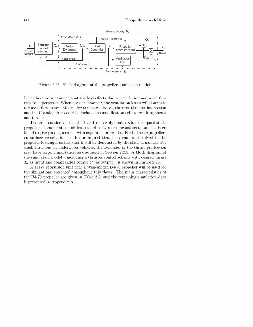
50 Propeller modelling
Thrustsetpoint
Ventilationloss
bTV
Shaft speed
Motor torque
Propellercharacteristics
nQ
Q
Ta
a
mMotorDynamics
QcTd ShaftDynamics
Thrustercontrolscheme
X
X
bQV
Propeller load torque
h
Va
Propulsion unit
Thrust
Advance velocity
Submergence
Figure 2.23: Block diagram of the propeller simulation model.
It has here been assumed that the loss effects due to ventilation and axial flowmay be superposed. When present, however, the ventilation losses will dominatethe axial flow losses. Models for transverse losses, thruster-thruster interactionand the Coanda effect could be included as modifications of the resulting thrustand torque.The combination of the shaft and motor dynamics with the quasi-static
propeller characteristics and loss models may seem inconsistent, but has beenfound to give good agreement with experimental results. For full-scale propellerson surface vessels, it can also be argued that the dynamics involved in thepropeller loading is so fast that it will be dominated by the shaft dynamics. Forsmall thrusters on underwater vehicles, the dynamics in the thrust productionmay have larger importance, as discussed in Section 2.2.5. A block diagram ofthe simulation model — including a thruster control scheme with desired thrustTd as input and commanded torque Qc as output — is shown in Figure 2.23.A 4MW propulsion unit with a Wageningen B4-70 propeller will be used for
the simulations presented throughout this thesis. The main characteristics ofthe B4-70 propeller are given in Table 2.2, and the remaining simulation datais presented in Appendix A.
Chapter 3
Propulsion control innormal conditions
The purpose of the low-level thruster controller is to relate the desired thrustTd to the commanded torque Qc. As discussed in Section 1.1, Td may be givenby the thrust allocation in DP or joystick mode, or manually in MTC mode.The thruster controllers may be divided in two control regimes, depending onthe operating conditions:
a) Thruster control in normal conditions, when experiencing low to moderatethrust losses.
b) Thruster control in extreme conditions, when experiencing large and abruptthrust losses due to ventilation and in-and-out-of-water effects.
This chapter first considers control aspects common to both control regimes,and then focuses on control regime a). Control regime b) is treated in Chapter6.
3.1 ConstraintsIn most of this work, it is assumed that only the shaft speed n and the motortorque Qm are available as measurements. Additional instrumentation on thepropulsion unit is not common in industrial installations. For electric motors,Qm is easily inferred from the motor current, and for diesel engines it is related tothe fuel index. Some of the control options that become available with additionalinstrumentation are discussed in Appendix E.2. The presented controllers aremainly aimed at low-speed applications with FPP driven by electric motors, butmay also be applicable to mechanical direct-drive FPP. The current conceptsare also extendable to CPP with consolidated control (i.e. control of both pitchand speed) and transit operations. This will be shortly treated in Chapter 8.
52 Propulsion control in normal conditions
The parameters needed for the various control schemes will be introducedconsecutively. The basic control parameters are the propeller diameter D, thenominal thrust coefficient KT0 from (2.8), and the nominal torque coefficientKQ0 from (2.9). These three parameters are usually well known — KT0 and KQ0
can be found e.g. from the bollard pull thrust (2.63) and power (2.65), or fromthe open-water characteristics of the propeller. For asymmetric propellers, thereverse nominal thrust and torque coefficients KT0r and KQ0r are also neededfor good performance.Depending on the application and the chosen low-level thruster controller,
knowledge of the friction parameters Qs and Kω in (2.51), and the rotationalinertia Is in (2.50) may be desirable. Qs and Kω may be found from systemidentification of the drive system. Is is an important parameter for choice ofelectric motor, and should in most cases therefore be known. In Appendix B.3,it is discussed how estimates of these parameters can be identified during manualtuning of the controllers.
3.2 Control objectivesThe ultimate goal of any thruster controller is to make the actual thrust Tatrack the thrust reference Tr. In dynamic operating conditions, however, othergoals may be as important as tracking Tr, e.g. reducing mechanical wear andtear and limiting power oscillations and peak values. This is especially true inthruster control regime b), where severe dynamic loads may persist over longperiods of time. In this work, the following performance criteria are considered:
1. Thrust production in the presence of disturbances, i.e. ability to locallycounteract thrust losses.
2. Mechanical wear and tear caused by transients and oscillations in motorand propeller torque.
3. Predictable power consumption.
4. Robust performance.
3.2.1 Thrust production
The structure of a DP system — including high-level controller, thrust allocation,and low-level thruster control — was introduced in Section 1.1. In order for thepropulsion system to produce the desired thrust forces, the low-level thrustercontrollers must have reasonable accuracy with respect to thrust production. Ifthis is not the case, the thrust allocation will have a difficult task in distributingthrust to the various propulsion units, since there is no feedback available fromthe actually produced thrust. An offset between the desired thrust and theactually produced thrust will eventually be captured by the integral action inthe DP control system, and the setpoints to the thrusters increased or decreased
3.2 Control objectives 53
accordingly. However, this is a slow process, and inaccurate low-level thrustercontrol will therefore lead to reduced bandwidth of the positioning system asa whole. Hence, significantly better positioning and tracking performance isexpected with improved low-level thruster controllers (Sørensen et al., 1997;Strand, 1999). Note that for the DP control system, it is the mean and slowly-varying values of thrust that are important: the oscillations in thrust inducedby waves and wave-frequency vessel motion do not normally affect the vesselmotion significantly.
3.2.2 Mechanical wear and tear
Normal conditions
There are few references discussing mechanical wear and tear of propulsion unitsin normal operating conditions. In older references, the torque loads on thepropeller shaft from the firing of individual diesel engine cylinders have been animportant topic. Apparently, the frequent failures of propeller shaft-lines werea main driving force for research on vibrations, vibration induced loads, andstructural fatigue in general. This is extensively dealt with in e.g. Ker Wilson(1963). Another topic that has been researched is the dynamic shaft loadingdue to the non-uniform inflow to a propeller installed behind a hull, and itsimplications for structural fatigue, see e.g. Wereldsma (1965), Lewis (1989),and Carlton (1994).From Section 2.3.1, it is clear that a time-varying inflow to the propeller,
as induced by waves, will result in a time-varying propeller loading. Dependingon the chosen low-level thruster control strategy, this will lead to oscillationsin propeller torque and thrust, shaft speed, and motor torque and power. Es-pecially in heavy seas, the time-varying loads can be significant, even if thepropeller is deeply submerged. The oscillations in propeller and motor torqueare transmitted through the shafts and gears, resulting in increased dynamicloads. This was investigated by Domachowski et al. (1997), who concluded thatthe dynamic loading because of waves gave rise to significant oscillations of tor-sional torques in shaft elements and flexible couplings, and that this over timewould cause reduced fatigue strength and increased wear and tear.To reduce mechanical wear and tear, it is assumed to be advantageous to
reduce the torque oscillations to a minimum.
Extreme conditions
As discussed in Section 2.4.6, a propeller on a vessel in high to extreme seasmay be subject to severe dynamic loading, both at the wave frequency due tothe large changes in mean load during ventilation, and at the blade frequencyand above due to the individual blade loads. As well as posing danger forstructural damage to the propeller, dynamic loading of the propeller may leadto mechanical wear and tear of the propulsion system. In all propulsion units,the propulsive power is transmitted from the motor to the propeller through a

54 Propulsion control in normal conditions
shaft held by bearings, and with a seal to protect against water ingress. Manythruster units in addition contain a transmission system consisting of gears,shafts, and bearings. Hence, the gears will be subject to the dynamic propellerand motor torque, the thrust gear or thrust block will be subject to the dynamicpropeller thrust, and the bearings holding the propeller shaft and the shaft sealwill be subject to transverse and vertical loads. The whole thruster unit will alsobe subject to any high-frequency vibration of the propeller. Although not welldocumented in the literature, mechanical wear and tear of thrusters is a well-known industrial problem that has received increased attention in recent years,especially for azimuthing thrusters and tunnel thrusters (Koushan, 2004, 2006).It is believed that the widespread mechanical failures in gears and bearings ofsuch thrusters are mainly due to the combination of low-frequency ventilationloads and blade frequency load oscillations.Various failure modes of propellers are extensively treated in IMCA M-129
(1995) and IMCA M-162 (2001). Although the topic of dynamic propeller load-ing is only briefly mentioned in these references, it seems apparent that thefailures of shafts, gears, bearings, and seals may be partly contributed to dy-namic loads and vibrations. This is also reflected in the recent efforts made toimprove the understanding of these loads and their effects on the mechanicalparts of the propulsion unit. As an example, Rolls-Royce in 2005 appointedNTNU in cooperation with MARINTEK as one of 25 world-wide UniversityTechnology Centres (UTC). The programme, which is to run for 10 years withextensive financing, is entitled “Performance in a Seaway”, and has specific fo-cus on propulsion issues like dynamic propeller loading and improved controllers(Rolls-Royce Press Release, 2005; NTNU Press Release, 2005).
3.2.3 Power consumption
For DP vessels, the propulsion system is usually one of the main power con-sumers. It is also regarded as a critical system with respect to safety. Forsafe operation and minimization of fuel consumption, optimal control of thepower generation and distribution system is essential. This task is usually per-formed by a Power Management System (PMS), or a more sophisticated EnergyManagement System (EMS). The PMS stops, starts, and synchronizes the maingenerator sets in response to the system loading, with the objective of preventingblackouts while minimizing the number of on-line generator sets. If the powerload is increased too fast for the generators to respond, or the load is higher thanthe available power, the result is under-frequency on the power network. If thenetwork frequency becomes too low, the generators will be disconnected, witha blackout as result. This is one of the worst scenarios onboard a DP vessel. Insevere weather conditions, the dynamic loading of the thrusters may result inunpredictable power variations. In order to meet the power peaks, the operatormay then be forced to have more power available than necessary. This increasesfuel consumption, as well as wear, tear, and maintenance of the generator sets,since they get more running hours at lower loads. Hence, predictable power

3.3 Thruster controller structure 55
consumption is of major concern to the power management system in order toavoid blackouts, improve the performance and stability of the power generationand distribution network, and minimize fuel consumption and wear and tear(Lauvdal and Ådnanes, 2000; May, 2003; Sørensen and Ådnanes, 2005; Radanet al., 2005).
3.2.4 Robustness
As with all control systems, robustness is an important issue. The thrustercontroller should be robust with respect to modelling uncertainties, since onecannot assume perfect knowledge of the necessary parameters. In addition, someof the physical properties of the system, like the shaft friction, may change overthe life-time of the propeller. The controller must also be able to handle awide range of operating conditions, from calm seas with low thrust demands, toextreme seas with high thrust demands.
3.2.5 Surface vessels vs. underwater vehicles
For low-level thruster control, the main difference between surface vessels andsmall underwater vehicles like ROVs and AUVs is the dynamic response ofthe vessel. Because the time constants of the underwater vehicles are small,their closed-loop behavior may be strongly affected by the thruster dynamics(Yoerger et al., 1991; Healey et al., 1995). For a surface vessel, the dynamicresponse of the thruster will be of less importance for e.g. the station-keepingability, since the time constant of the vessel itself is dominating. However, thethrust production is still of high importance.There are also differences in the expected operating conditions for the pro-
pellers. The operating condition of a propeller on a surface vessel is influencedby the vessel load condition, vessel motions, waves, and current. An underwa-ter vehicle is usually operated below the wave zone, and hence only affectedby vehicle motions and current. Furthermore, the vessel motions due to thewaves are much more violent for a surface vessel than for an underwater vehicle.This means that the requirements to the thruster controllers on a surface vesselmay differ significantly from the corresponding requirements for an underwatervehicle. In this thesis, the main focus is on surface vessels.
3.3 Thruster controller structureA block diagram of a propulsion unit with a reference generator, a thrustercontroller, and a torque limiting function is shown in Figure 3.1. The desiredthrust Td from the thrust allocation or manual thruster control is passed througha reference generator to avoid entering transients into the thruster controller.The output of the reference generator is the thrust reference Tr. The thrustercontroller calculates the commanded torqueQc0, which in turn is passed througha torque limiting function in order to avoid commanding excessive torque or

56 Propulsion control in normal conditions
nf
Q
Q
Ta
a
T
m( )
fQ ( ).
.Motordynamics
QcTorquelimit
.
p xp
Shaftdynamics
xpPmaxQmax
Propulsionunit
n
q
qp
Qc0Thrustercontroller
Td Referencegenerator
Tr
Control scheme
Figure 3.1: Block diagram of a propulsion unit with control scheme, including areference generator, a thruster controller, and a torque/power limiting function.
power from the thruster motor. The torque and power limited commandedtorque, Qc, is used to control the motor. The output of the system is the thrustTa. In the block diagram, the propeller thrust and torque are represented bythe functions fT (·) and fQ(·) from (2.1) and (2.2).
Remark 3.1 In this work, the interface to the low-level thruster controller ischosen to be the desired thrust Td. In industrial applications with shaft speedcontrol, is is common that the interface is the desired shaft speed, which is cal-culated from Td using the static mapping given in (3.1). This is only applicableif shaft speed control is used.
3.4 State of the art
Three types of propellers are common: speed controlled FPP, pitch controlledCPP, and consolidated controlled CPP (CCP). For CCP, both the shaft speedand pitch can be controlled. Since the desired thrust can be produced by anumber of combinations of shaft speed and pitch, this can be formulated as anoptimal control problem. Optimal control of CCP is mainly relevant for transitoperation. This is treated in e.g. Schanz (1967), Winterbone (1980), Beek andMulder (1983), Parsons and Wu (1985), Bakountouzis (1992), Chachulski et al.(1995), Fukuba et al. (1996), Morvillo (1996), Young-Bok et al. (1998), andWhalley and Ebrahimi (2002), and an overview given in Ruth et al. (2006). ACCP may also be controlled by fixed mappings from desired thrust to pitch andshaft speed. This will be further discussed in Section 8.1, where the controlconcepts developed for FPP are extended to CCP.For surface vessels with FPP, shaft speed control is the industry standard,
both for electrically driven and mechanical direct-drive propellers (often, how-ever, mechanical direct-drive propellers are CPP). The origin of PID type con-trollers for propeller shaft speed control is uncertain, but they have probablybeen utilized for as long as propellers have been used. The early mechanical
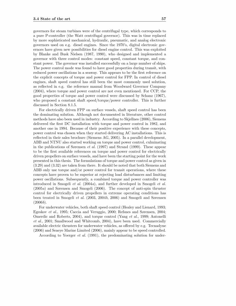
3.4 State of the art 57
governors for steam turbines were of the centrifugal type, which corresponds toa pure P-controller (the Watt centrifugal governor). This was in time replacedby more sophisticated mechanical, hydraulic, pneumatic, and analog electronicgovernors used on e.g. diesel engines. Since the 1970’s, digital electronic gov-ernors have given new possibilities for diesel engine control. This was exploitedby Blanke and Busk Nielsen (1987, 1990), who designed and implemented agovernor with three control modes: constant speed, constant torque, and con-stant power. The governor was installed successfully on a large number of ships.The power control mode was found to have good properties during transit, withreduced power oscillations in a seaway. This appears to be the first reference onthe explicit concepts of torque and power control for FPP. In control of dieselengines, shaft speed control has still been the most commonly used solution,as reflected in e.g. the reference manual from Woodward Governor Company(2004), where torque and power control are not even mentioned. For CCP, thegood properties of torque and power control were discussed by Schanz (1967),who proposed a constant shaft speed/torque/power controller. This is furtherdiscussed in Section 8.1.5.For electrically driven FPP on surface vessels, shaft speed control has been
the dominating solution. Although not documented in literature, other controlmethods have also been used in industry. According to Skjellnes (2006), Siemensdelivered the first DC installation with torque and power control in 1982, andanother one in 1994. Because of their positive experience with these concepts,power control was chosen when they started delivering AC installations. This isreflected in their sales brochure (Siemens AG, 2005). In a parallel development,ABB and NTNU also started working on torque and power control, culminatingin the publications of Sørensen et al. (1997) and Strand (1999). These appearto be the first available references on torque and power control for electricallydriven propellers on surface vessels, and have been the starting point for the workpresented in this thesis. The formulations of torque and power control as given in(3.29) and (3.32) are taken from there. It should be noted that both Siemens andABB only use torque and/or power control for transit operations, where theseconcepts have proven to be superior at rejecting load disturbances and limitingpower oscillations. Subsequently, a combined torque and power controller wasintroduced in Smogeli et al. (2004a), and further developed in Smogeli et al.(2005a) and Sørensen and Smogeli (2006). The concept of anti-spin thrustercontrol for electrically driven propellers in extreme operating conditions hasbeen treated in Smogeli et al. (2003, 2004b, 2006) and Smogeli and Sørensen(2006b).For underwater vehicles, both shaft speed control (Healey and Lienard, 1993;
Egeskov et al., 1995; Caccia and Veruggio, 2000; Refsnes and Sørensen, 2004;Omerdic and Roberts, 2004), and torque control (Yang et al., 1999; Antonelliet al., 2001; Smallwood and Whitcomb, 2004), have been used. Commerciallyavailable electric thrusters for underwater vehicles, as offered by e.g. Tecnadyne(2006) and Seaeye Marine Limited (2006), mainly appear to be speed controlled.According to Yoerger et al. (1991), the predominating solution for under-

58 Propulsion control in normal conditions
water vehicles at that time was torque control. They found that the thrusterdynamics had a strong influence on the closed-loop underwater vehicle behavior.To compensate for this, they proposed several controllers, all based on torquecontrol of the thruster motor. An adaptive sliding mode controller containinga compensation for propeller-induced flow effects was shown to improve theclosed-loop vehicle performance significantly.The investigation of model-based thruster control for underwater vehicles
was continued by Whitcomb and Yoerger (1999b). They compared a puretorque controller with a high-gain proportional shaft speed controller, and acorresponding shaft speed controller with axial flow compensation. The latterwas implemented with an ad hoc stable open-loop estimator for the axial flowvelocity. They concluded that the torque controller was unsatisfactory for lowthrust commands, probably due to unmodelled friction effects, but with im-proved performance for higher thrust commands. The high-gain shaft speedcontroller was shown to have poor performance, but gave good results withthe addition of the axial flow compensation. It should be noted that all theseexperiments were performed at zero advance velocity.Continuing the concept of axial flow compensation, Fossen and Blanke (2000)
proposed a nonlinear output feedback shaft speed controller for propellers onunderwater vehicles, with feedback from an estimate of the advance velocity.The advance velocity observer was designed based on the vehicle surge dynam-ics and a model of the flow dynamics. The closed-loop controller was shownto be globally asymptotically stable. The results were mainly applicable to aan underwater vehicle with one propeller operating in the first quadrant (i.e.positive shaft speed and positive advance velocity).Tsukamoto et al. (1997) presented an experimental comparison study of five
thruster control systems for underwater robots: on-line neural network control,off-line neural network control, fuzzy control, adaptive-learning control, andPID control. However, the controllers were based on direct control of the vehiclesurge position using one thruster, evading the decoupling in thrust allocationand low-level thruster control that is considered here. Neural networks, fuzzycontrol, and adaptive-learning control will not be treated any further in thisthesis.Bachmayer and Whitcomb (2001) presented two model based thrust tracking
controllers. The controllers were based on detailed knowledge of the propellerlift and drag curves for all 4 quadrants of operation, in addition to the shaft fric-tion coefficients (2.51), the rotational inertia (2.50), and the parameters neededto describe an axial flow model, see Section 2.2.5. They were also based on theassumption that the advance velocity Va ≈ 0. Under these assumptions, experi-mental evidence of an asymptotically stable open-loop thrust tracking controllerwas presented, although no theoretical proof was given. A shaft speed feedbackthrust tracking controller was shown to influence the rate of convergence of thetracking error. The proposed controllers appear to be mainly suited for under-water applications with high bandwidth positioning requirements, and strongcoupling between the vessel and thruster dynamics. For industrial applications

3.5 Control coefficients 59
on surface ships, the detailed model knowledge needed for such a controller can-not be expected to be available. Particularly, the complete hydrodynamic modelof the propeller is practically never obtainable. The assumption of Va ≈ 0 isalso difficult to justify in practice.Guibert et al. (2005) presented an output feedback thrust controller. The
controller was based on a stationary extended Kalman filter for estimation ofthe hydrodynamic load torque Qa, estimation of the thrust Ta from a numericalinversion of the propeller lift and drag curves and the flow dynamics model(2.70), and a PI controller operating on the thrust error. The controller requiredextensive model knowledge — both the lift and drag curves of the propeller andthe parameters for the flow dynamics. The controller was tested by simulations,and found to be highly sensitive to modelling errors, both in the mechanicaland the hydrodynamic model. Moreover, the flow dynamics model (2.70) isonly valid in the first quadrant of operation, and requires knowledge of Va. Thisapproach is therefore not considered applicable to surface vessels. A differentoutput feedback thrust controller, which circumvents most of these problems, ispresented in Appendix E.3.
3.5 Control coefficients
The thruster control schemes are based on the thrust/torque/speed/power re-lationships given in (2.8), (2.9), and (2.10). Since the propeller diameter D anddensity of water ρ are known and constant, the only remaining parameters arethe thrust and torque coefficients KT and KQ. The thrust and torque coeffi-cients used in the controllers are termed KTC and KQC , and denoted controlcoefficients.
3.5.1 Shaft speed, torque, and power reference
The shaft speed reference nr, torque reference Qr, and power reference Pr willbe needed in the following sections. nr is calculated from the thrust referenceTr by the static mapping gn(Tr):
nr = gn(Tr) = sign(Tr)
s|Tr|
ρD4KTC, (3.1)
which is the inverse function of the nominal characteristics given in (2.8), withKT0 replaced by KTC . The mapping gq(Tr) from Tr to Qr can be found from(2.8) and (2.9) with KT0 and KQ0 replaced by KTC and KQC :
Qr = gq(Tr) =KQC
KTCDTr. (3.2)
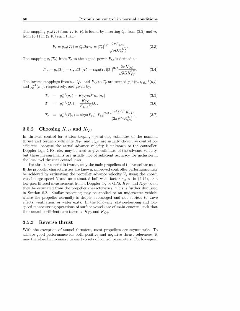
60 Propulsion control in normal conditions
The mapping gp0(Tr) from Tr to Pr is found by inserting Qr from (3.2) and nrfrom (3.1) in (2.10) such that:
Pr = gp0(Tr) = Qr2πnr = |Tr|3/22πKQC√ρDK
3/2TC
. (3.3)
The mapping gp(Tr) from Tr to the signed power Prs is defined as:
Prs = gp(Tr) = sign(Tr)Pr = sign(Tr)|Tr|3/22πKQC√ρDK
3/2TC
. (3.4)
The inverse mappings from nr, Qr, and Prs to Tr are termed g−1n (nr), g−1q (nr),and g−1p (nr), respectively, and given by:
Tr = g−1n (nr) = KTCρD4nr |nr| , (3.5)
Tr = g−1q (Qr) =KTC
KQCDQr, (3.6)
Tr = g−1p (Prs) = sign(Prs) |Prs|2/3ρ1/3D2/3KTC
(2π)2/3K2/3QC
. (3.7)
3.5.2 Choosing KTC and KQC
In thruster control for station-keeping operations, estimates of the nominalthrust and torque coefficients KT0 and KQ0 are usually chosen as control co-efficients, because the actual advance velocity is unknown to the controller.Doppler logs, GPS, etc. may be used to give estimates of the advance velocity,but these measurements are usually not of sufficient accuracy for inclusion inthe low-level thruster control laws.For thruster control in transit, only the main propellers of the vessel are used.
If the propeller characteristics are known, improved controller performance maybe achieved by estimating the propeller advance velocity Va using the knownvessel surge speed U and an estimated hull wake factor wh as in (2.42), or alow-pass filtered measurement from a Doppler log or GPS. KTC and KQC couldthen be estimated from the propeller characteristics. This is further discussedin Section 8.2. Similar reasoning may be applied to an underwater vehicle,where the propeller normally is deeply submerged and not subject to waveeffects, ventilation, or water exits. In the following, station-keeping and low-speed manoeuvring operations of surface vessels are of main concern, such thatthe control coefficients are taken as KT0 and KQ0.
3.5.3 Reverse thrust
With the exception of tunnel thrusters, most propellers are asymmetric. Toachieve good performance for both positive and negative thrust references, itmay therefore be necessary to use two sets of control parameters. For low-speed

3.6 Reference generator 61
operations, this means that KT0 and KQ0 should be used for positive Tr, andthe reverse thrust and torque coefficients KT0r and KQ0r for negative Tr, seeSection 2.1. The following control coefficients are therefore proposed:
KTC = KT0λc + (1− λc)KT0r, (3.8)
KQC = KQ0λc + (1− λc)KQ0r, (3.9)
where λc is a smooth switching function given by:
λc = λc(nr) =1
2+1
2tanh(εc
nrnc). (3.10)
The shaft speed reference nr is given from Tr by (3.1), and nc > 0 and εc > 0are constants. With a properly chosen εc, the switching between the coefficientsoccurs smoothly in the interval nr ∈ [−nc, nc], such that λc ≈ 0 for nr < −ncand λc ≈ 1 for nr > nc. The switch “width” nc may be chosen freely. (3.8,3.9) does not affect the stability properties of the controllers when comparedto using constant control coefficients, since KT0, KQ0, KT0r, and KQ0r all arestrictly positive, and the values of KTC and KQC only affect the mappings fromTr to nr, Qr, and Prs. Using nr as the switching variable instead of e.g. themeasured shaft speed n means that no measurement noise is entered into thecontrol law through (3.8, 3.9).As an example, Figure 3.2 shows λc from (3.10) and KTC from (3.8) for the
4MWWageningen B4-70 example propeller with parameters given in Table 2.2,and the parameters for λc chosen as εc = 3 and nc = 0.2rps.
3.6 Reference generator
The desired thrust from the high-level controller should be filtered through areference generator. There are several important reasons for doing this:
• It is in general undesirable to enter transients into a control loop. Es-pecially in the case of a shaft speed thruster controller, the transients inmotor torque may be large if no rate limits on the reference are imposed:if e.g. a large step in thrust is commanded, and the speed controller istightly tuned, the motor will inevitably reach its maximum rating in a splitsecond. Such torque transients may damage the mechanical componentsin the thruster unit, as discussed in Section 3.2.2.
• The power distribution network should be protected from large distur-bances. If the loading of the network suddenly increases, the result maybe a large frequency drop. If the frequency drop is too large, the gener-ators may trip and a blackout occur, see Section 3.2.3. In order to avoidthis, rapid increases of the power load of the thrusters should be avoided.
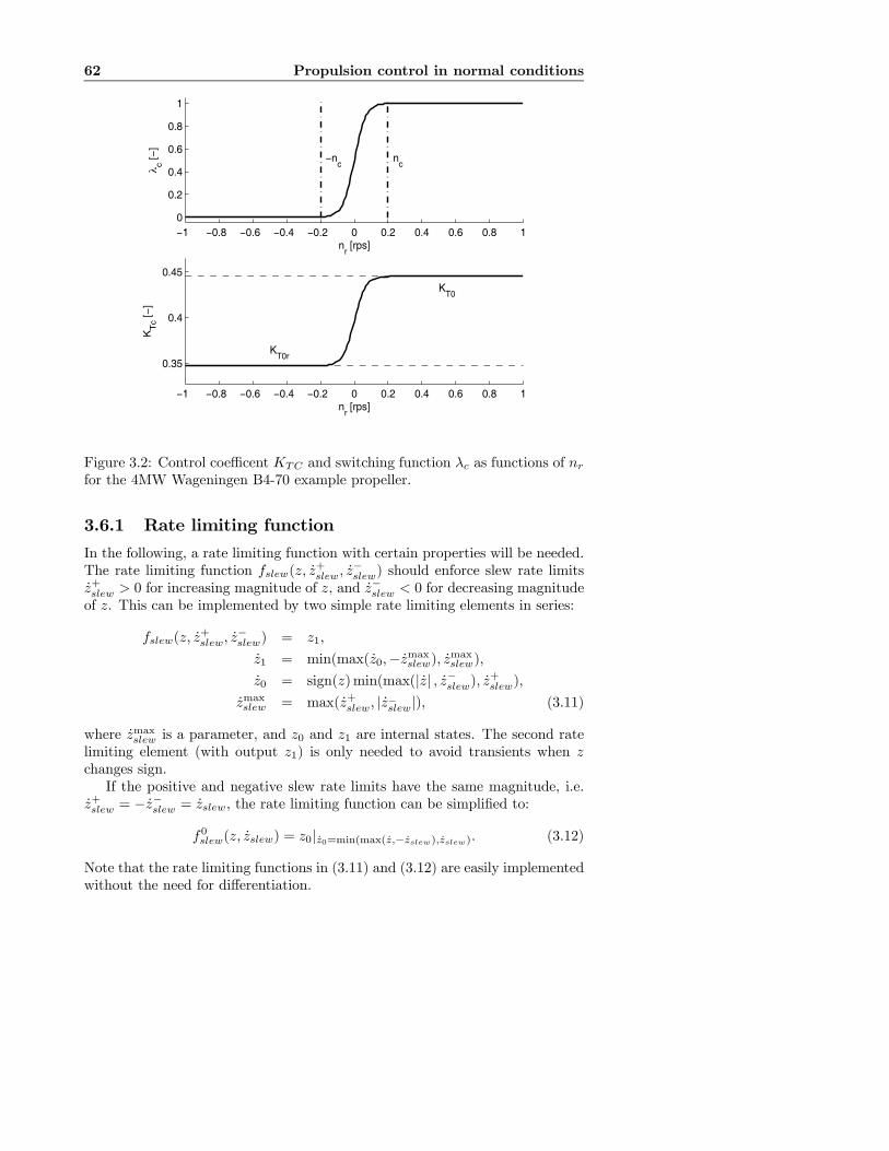
62 Propulsion control in normal conditions
−1 −0.8 −0.6 −0.4 −0.2 0 0.2 0.4 0.6 0.8 10
0.2
0.4
0.6
0.8
1
nr [rps]
λ c [−
]−n
cn
c
−1 −0.8 −0.6 −0.4 −0.2 0 0.2 0.4 0.6 0.8 1
0.35
0.4
0.45
nr [rps]
KT
c [−
]
KT0r
KT0
Figure 3.2: Control coefficent KTC and switching function λc as functions of nrfor the 4MW Wageningen B4-70 example propeller.
3.6.1 Rate limiting function
In the following, a rate limiting function with certain properties will be needed.The rate limiting function fslew(z, z
+slew, z
−slew) should enforce slew rate limits
z+slew > 0 for increasing magnitude of z, and z−slew < 0 for decreasing magnitudeof z. This can be implemented by two simple rate limiting elements in series:
fslew(z, z+slew, z
−slew) = z1,
z1 = min(max(z0,−zmaxslew), zmaxslew),
z0 = sign(z)min(max(|z| , z−slew), z+slew),
zmaxslew = max(z+slew, |z_slew|), (3.11)
where zmaxslew is a parameter, and z0 and z1 are internal states. The second ratelimiting element (with output z1) is only needed to avoid transients when zchanges sign.If the positive and negative slew rate limits have the same magnitude, i.e.
z+slew = −z−slew = zslew, the rate limiting function can be simplified to:
f0slew(z, zslew) = z0|z0=min(max(z,−zslew),zslew). (3.12)
Note that the rate limiting functions in (3.11) and (3.12) are easily implementedwithout the need for differentiation.

3.6 Reference generator 63
3.6.2 Shaft speed reference with rate limit
In the marine industry, the commonly used reference generator appears to bea rate limiting function on the shaft speed reference nr (Ådnanes, 2006). Therecommended magnitude of the slew rate will depend on the size and type ofthe propulsion unit. A typical 1-2 MW unit with shaft speed control would havea slew rate equivalent to ramping nr from zero to max in about 7-8 seconds,and a typical 3-4 MW unit a slew rate equivalent to 10-15 seconds. The slewrate must be chosen in connection with the tuning of the speed controller, suchthat the total closed loop — including reference generator, speed control loop,and inner torque control loop — has the desired performance. It is also possibleto implement a speed dependent reference generator. As a trade-off betweenthruster response and undesired disturbances on the power network, a solutionsometimes seen in the industry is to use a fast reference generator for low shaftspeeds, and a slower reference generator for high shaft speeds.Since the chosen interface to the thruster unit is Td, the reference generator
for Tr can be implemented by using the shaft speed mapping gn(Tr) in (3.1), itsinverse g−1n (nr) in (3.5), and the rate limiting function in (3.11) with slew ratelimits n+slew and n−slew:
nd = gn(Td),
nr = fslew(nd, n+slew, n
−slew),
Tr = g−1n (nr). (3.13)
3.6.3 Shaft speed reference with low-pass filter and ratelimit
In order to reduce the transients in the commanded torque, it may be ben-eficial to add a low-pass filter to the reference generator in (3.13). For thissystem, a second-order filter with damping ratio ζr and natural frequency ωr0is appropriate. The reference generator then becomes:
nd = gn(Td),
nd2 = fslew(nd, n+slew, n
−slew),
nr(s) = nd2(s)ω2r0
s2 + 2ζrωr0s+ ω2r0,
Tr = g−1n (nr). (3.14)
The resulting reference generator is shown in Figure 3.3. Notice that the refer-ence generator gives a continuous acceleration reference nr. This will be utilizedin Section 3.7.2, where an inertia compensation scheme based on nr is designed.An alternative formulation, where the speed rate limit is implemented by anacceleration saturation element inside the filter, is proposed in Fossen (2002).A simple tuning rule for the filter parameters is to choose ζr = 1 (criticallydamped) and ωr0 = 1.5/τ r, where τ r is the approximate “time constant” of thefilter.
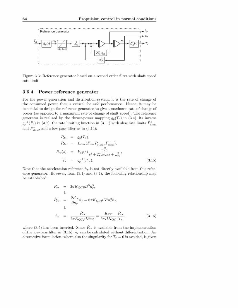
64 Propulsion control in normal conditions
Tdg
n( ).
-Tr
nd nr�
r02 g
n( ).-1
�r02
�r0�
r2
-
nr.
nr
Reference generator
rate limit
Figure 3.3: Reference generator based on a second order filter with shaft speedrate limit.
3.6.4 Power reference generator
For the power generation and distribution system, it is the rate of change ofthe consumed power that is critical for safe performance. Hence, it may bebeneficial to design the reference generator to give a maximum rate of change ofpower (as opposed to a maximum rate of change of shaft speed). The referencegenerator is realized by the thrust-power mapping gp(Tr) in (3.4), its inverseg−1p (Pr) in (3.7), the rate limiting function in (3.11) with slew rate limits P
+slew
and P−slew, and a low-pass filter as in (3.14):
Pds = gp(Td),
Pd2 = fslew(Pds, P+slew, P
−slew),
Prs(s) = Pd2(s)ω2r0
s2 + 2ζrωr0s+ ω2r0,
Tr = g−1p (Prs). (3.15)
Note that the acceleration reference nr is not directly available from this refer-ence generator. However, from (3.1) and (3.4), the following relationship maybe established:
Prs = 2πKQCρD5n3r,
⇓
Prs =∂Prs∂nr
nr = 6πKQCρD5n2rnr,
⇓
nr =Prs
6πKQCρD5n2r=
KTC
6πDKQC
Prs|Tr|
. (3.16)
where (3.5) has been inserted. Since Prs is available from the implementationof the low-pass filter in (3.15), nr can be calculated without differentiation. Analternative formulation, where also the singularity for Tr = 0 is avoided, is given
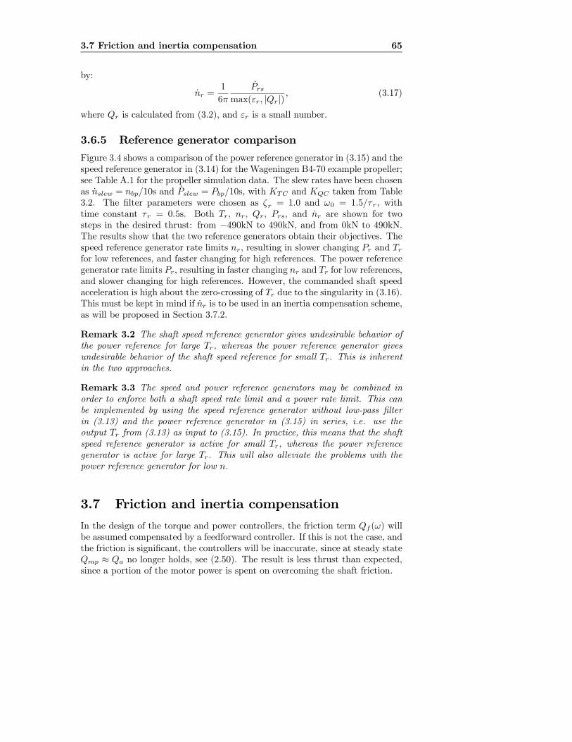
3.7 Friction and inertia compensation 65
by:
nr =1
6π
Prsmax(εr, |Qr|)
, (3.17)
where Qr is calculated from (3.2), and εr is a small number.
3.6.5 Reference generator comparison
Figure 3.4 shows a comparison of the power reference generator in (3.15) and thespeed reference generator in (3.14) for the Wageningen B4-70 example propeller;see Table A.1 for the propeller simulation data. The slew rates have been chosenas nslew = nbp/10s and Pslew = Pbp/10s, with KTC and KQC taken from Table3.2. The filter parameters were chosen as ζr = 1.0 and ω0 = 1.5/τr, withtime constant τr = 0.5s. Both Tr, nr, Qr, Prs, and nr are shown for twosteps in the desired thrust: from −490kN to 490kN, and from 0kN to 490kN.The results show that the two reference generators obtain their objectives. Thespeed reference generator rate limits nr, resulting in slower changing Pr and Trfor low references, and faster changing for high references. The power referencegenerator rate limits Pr, resulting in faster changing nr and Tr for low references,and slower changing for high references. However, the commanded shaft speedacceleration is high about the zero-crossing of Tr due to the singularity in (3.16).This must be kept in mind if nr is to be used in an inertia compensation scheme,as will be proposed in Section 3.7.2.
Remark 3.2 The shaft speed reference generator gives undesirable behavior ofthe power reference for large Tr, whereas the power reference generator givesundesirable behavior of the shaft speed reference for small Tr. This is inherentin the two approaches.
Remark 3.3 The speed and power reference generators may be combined inorder to enforce both a shaft speed rate limit and a power rate limit. This canbe implemented by using the speed reference generator without low-pass filterin (3.13) and the power reference generator in (3.15) in series, i.e. use theoutput Tr from (3.13) as input to (3.15). In practice, this means that the shaftspeed reference generator is active for small Tr, whereas the power referencegenerator is active for large Tr. This will also alleviate the problems with thepower reference generator for low n.
3.7 Friction and inertia compensationIn the design of the torque and power controllers, the friction term Qf (ω) willbe assumed compensated by a feedforward controller. If this is not the case, andthe friction is significant, the controllers will be inaccurate, since at steady stateQmp ≈ Qa no longer holds, see (2.50). The result is less thrust than expected,since a portion of the motor power is spent on overcoming the shaft friction.

66 Propulsion control in normal conditions
−500
0
500
Tr [k
N]
−2
−1
0
1
2
n r [rps
]
−200
0
200
Qr [k
Nm
]
−4000
−2000
0
2000
4000
Prs
[kW
]
0 5 10 15 20 250
1
2
n r [rps
/s]
Time [s]
Power reference generator Speed reference generator
.
Figure 3.4: Comparison of the power and speed reference generators for twosteps in desired thrust.

3.7 Friction and inertia compensation 67
For a large thruster, the rotational inertia may be a dominating dynamicterm. In order to achieve the desired closed loop properties with respect toresponse and tracking, it may therefore be beneficial to include an inertia com-pensation term.In general, feedforward terms to account for friction and inertia should there-
fore be included in the control law, such that the total controller output Qc0 isgiven by:
Qc0 = Qci +Qff +Qif , (3.18)
where Qif is the inertia compensation, Qff is the friction compensation, andthe i in Qci is an index specific to the controller in use. For example, i = n forshaft speed control, i = q for torque control, and i = p for power control.
3.7.1 Friction compensation
For a full-scale thruster on a surface vessel, the shaft friction will in most casesbe relatively small compared to the propeller torque. For smaller vehicles likeROV’s and AUV’s, the friction may be significant and lead to severely degradedperformance if not accounted for in the controllers. This has been investigatedin e.g. Whitcomb and Yoerger (1999b) and Bachmayer et al. (2000), where afriction model similar to (2.51) was proposed. In the experimental setup utilizedin the current work, the friction was also found to be significant.
Qff should be designed to compensate for the friction term Qf (ω), i.e.Qff ≈ Qf (ω), without destabilizing the system. Therefore, a feedforward com-pensation based on the reference shaft speed nr from (3.1) is chosen insteadof a destabilizing feedback compensation based on n. Motivated by (2.51) thefriction is assumed to consist of a static and a linear term, and the frictioncompensation scheme is proposed as:
Qff (nr) = Qff0(nr) +Qff1(nr), (3.19)
where the static term Qff0(nr) and the linear term Qff1(nr) are defined be-low. If considered necessary, higher-order friction compensation terms may beincluded in a similar manner.
Static friction
The contribution from the static termQs in (2.51) is discontinuous for ω = 0. Toavoid discontinuities in the control law, the signum function is replaced with asmooth switching function, such that the static friction compensation Qff0(nr)is proposed as:
Qff0(nr) = Qf0 tanh(εfnrnf), (3.20)
where Qf0, εf , and nf are constants. With a properly chosen εf , the switchingbetween −Qf0 and Qf0 occurs smoothly in the interval nr ∈ [−nf , nf ], suchthat |nr| > nf ⇒ Qff0(nr) = sign(nr)Qf0, and nr = 0 ⇒ Qff0(nr) = 0. Note
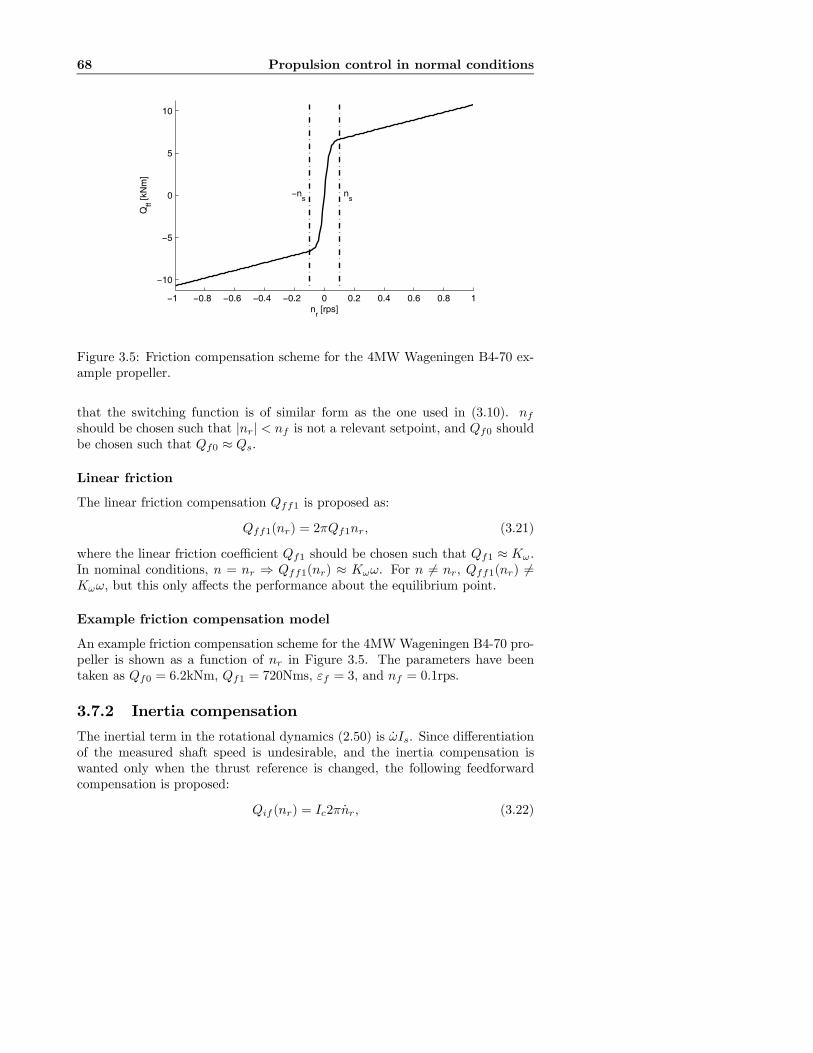
68 Propulsion control in normal conditions
−1 −0.8 −0.6 −0.4 −0.2 0 0.2 0.4 0.6 0.8 1
−10
−5
0
5
10
nr [rps]
Qff [k
Nm
]
−ns
ns
Figure 3.5: Friction compensation scheme for the 4MW Wageningen B4-70 ex-ample propeller.
that the switching function is of similar form as the one used in (3.10). nfshould be chosen such that |nr| < nf is not a relevant setpoint, and Qf0 shouldbe chosen such that Qf0 ≈ Qs.
Linear friction
The linear friction compensation Qff1 is proposed as:
Qff1(nr) = 2πQf1nr, (3.21)
where the linear friction coefficient Qf1 should be chosen such that Qf1 ≈ Kω.In nominal conditions, n = nr ⇒ Qff1(nr) ≈ Kωω. For n 6= nr, Qff1(nr) 6=Kωω, but this only affects the performance about the equilibrium point.
Example friction compensation model
An example friction compensation scheme for the 4MWWageningen B4-70 pro-peller is shown as a function of nr in Figure 3.5. The parameters have beentaken as Qf0 = 6.2kNm, Qf1 = 720Nms, εf = 3, and nf = 0.1rps.
3.7.2 Inertia compensation
The inertial term in the rotational dynamics (2.50) is ωIs. Since differentiationof the measured shaft speed is undesirable, and the inertia compensation iswanted only when the thrust reference is changed, the following feedforwardcompensation is proposed:
Qif (nr) = Ic2πnr, (3.22)

3.8 Torque and power limiting 69
where Ic is an estimate of the rotational inertia Is, and nr is given by thereference generator, as shown e.g. in Figure 3.3. The inertia compensationscheme is expected to be important mainly for large propellers. In an industrialinstallation, the rotational inertia should be relatively accurately known, sinceit is an important parameter for the choice of electric motor and tuning of themotor drive, see Appendix B.1.
Remark 3.4 Qif is written as a function of nr instead of nr in order to haveconsistent notation with other parts of the control schemes. In block diagramsetc. Qif may take nr or Tr as input, even though nr from the reference generatoris used in practice.
3.7.3 Feedforward compensation properties
The friction and inertia feedforward compensation schemes in (3.19) and (3.22)may be related to the concept of feedback linearization, where the basic idea isto transform a nonlinear system to a linear one. This is treated in detail in e.g.Slotine and Li (1991), Isidori (1995), and Khalil (2002). In robotics, a similarconcept is called computed torque control, see e.g. Sciavicco and Siciliano (2000).This is also utilized to develop control laws for marine systems in Fossen (2002).For the propeller, the effect of the feedforward compensation schemes can
be seen from the rotational dynamics (2.50). By neglecting the motor torquedynamics in (2.52), such that Qmp = Qc0, and inserting (3.18), the rotationaldynamics become:
Isω = Qci +Qff (nr) +Qif (nr)−Qa −Qf (ω). (3.23)
By assuming perfect model knowledge such that Qf0 = Qs, Qf1 = Kω, andIc = Is, that |nr| > nf ⇒ Qff0(nr) = sign(nr)Qf0, that sign(ω) = sign(nr),and inserting (2.51), (3.19), and (3.22), (3.23) reduces to:
2πIs(n− nr) = Qci −Qa − 2πKω(n− nr). (3.24)
Hence, it remains to design Qci to compensate for the propeller torque Qa. Thisis done by the various control laws presented in Sections 3.10 to 3.15.
3.8 Torque and power limitingIn order to avoid commanding excessive torque or power from the thrustermotor, a torque limiting function — as shown in Figure 3.1 — should be included inthe control scheme. The maximum admissible torque Qmax and power Pmax forthe motor are related to the rated torque and power (for continuous operation)by (2.55). The controller output should therefore be limited by a torque limitingfunction given by:
Qc = max{Qc0, kgQmax,Pmax2πn
}, (3.25)

70 Propulsion control in normal conditions
Q
Q P
P
P
Q
n
n
max
max
max
c
N
N
N
2�
Reduced
n
Figure 3.6: Torque limiting function parameterized by the maximum torqueQmax and maximum power Pmax, adopted from Sørensen et al. (1997).
where Qc0 is the commanded torque from the controller, friction compensation,and inertia compensation (3.18), and kg is the gear ratio, see Section 2.2.3. Thecommanded motor torque Qcm to the motor is finally given as
Qcm = Qc/kg. (3.26)
The maximum power limit yields hyperbolic limit curves for the torque as afunction of motor speed. This is shown in Figure 3.6, where nN is the ratedmotor shaft speed. Since the maximum power is not limited by the converterand motor ratings only, but also by the available power on the network, thislimit should be varied accordingly. By this method the power limitation willbecome fast and accurate, allowing to utilize the power system power capabilitywith a built-in blackout prevention (Sørensen et al., 1997).
3.9 Feedback signal filtering
The feedback signals n and Qm should be filtered before they are entered intothe control loop. This is proposed done by first order filters with appropriatelychosen time constants Tf and Tfq, respectively. In a discrete-time implemen-tation, the usual requirements to the filter bandwidth with respect to samplingperiod applies, see e.g. Åström and Wittenmark (1997).

3.10 Shaft speed feedback control 71
QcTorquelimit
QcnTr gn( ).
PmaxQmax
n
+
+
Td Referencegenerator +
Qc0
n
Shaft speed control
PIDnr
n
e
Qff
Qif
+
Figure 3.7: Shaft speed control scheme.
3.10 Shaft speed feedback controlThe shaft speed controller is designed to keep the shaft speed n equal to thereference speed nr (3.1). The typical solution is to use a PID controller operatingon the shaft speed error e = nr − n, which sets the commanded torque Qcn
according to
Qcn = Kpe+Ki
Z t
0
e(τ)dτ +Kde, (3.27)
where Kp > 0, Ki > 0, and Kd ≥ 0 are the PID gains. The motor torque iscontrolled by its inner torque control loop, as discussed in Section 2.2.2. Ki isoften given as Ki = Kp/Ti, where Ti is the integral time constant. The integralterm in the PID controller should be limited according to some maximumQi,max
to avoid integral windup, i.e.¯Ki
Z t
0
e(τ)dτ
¯≤ Qi,max,
Qi,max = κskgQmax, (3.28)
where 0 < κs ≤ 1 is a constant, usually chosen as κs ≈ 0.8 − 0.9. In controlof electric motors, a PI controller is considered to be the most appropriatesolution (Leonhard, 1996). In this thesis, only PI controllers have been applied,such that Kd = 0. In the shaft speed control scheme, the friction compensationQff and the inertial compensation Qif may be omitted, since the controllerautomatically compensates for these terms when the shaft speed is kept at itsreference. Hence, Qc0 = Qcn in this case. Figure 3.7 shows a block diagramof the shaft speed control scheme, including a reference generator and a torquelimiting block. It is also indicated how Qff and Qif could be included if wanted.Tuning of the PI parameters is discussed in Appendix B.1.
3.11 Torque feedforward controlIn the torque control strategy the outer speed control loop is removed, and thethruster is controlled by its inner torque control loop with a commanded torque
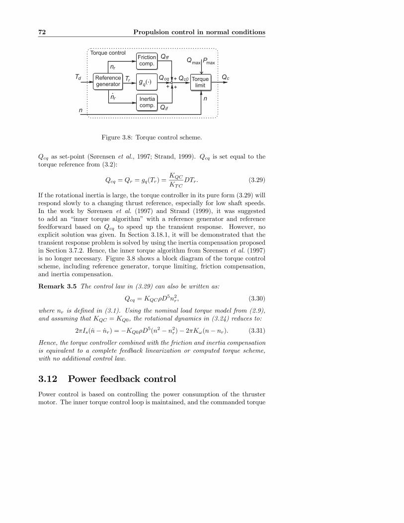
72 Propulsion control in normal conditions
QcTorquelimit
QcqTr gq( ).
PmaxQmax
n
Frictioncomp.
+
+
Qff
Td Referencegenerator
Inertiacomp. Qif
+
Qc0
n
Torque control
nr
nr
.
Figure 3.8: Torque control scheme.
Qcq as set-point (Sørensen et al., 1997; Strand, 1999). Qcq is set equal to thetorque reference from (3.2):
Qcq = Qr = gq(Tr) =KQC
KTCDTr. (3.29)
If the rotational inertia is large, the torque controller in its pure form (3.29) willrespond slowly to a changing thrust reference, especially for low shaft speeds.In the work by Sørensen et al. (1997) and Strand (1999), it was suggestedto add an “inner torque algorithm” with a reference generator and referencefeedforward based on Qcq to speed up the transient response. However, noexplicit solution was given. In Section 3.18.1, it will be demonstrated that thetransient response problem is solved by using the inertia compensation proposedin Section 3.7.2. Hence, the inner torque algorithm from Sørensen et al. (1997)is no longer necessary. Figure 3.8 shows a block diagram of the torque controlscheme, including reference generator, torque limiting, friction compensation,and inertia compensation.
Remark 3.5 The control law in (3.29) can also be written as:
Qcq = KQCρD5n2r, (3.30)
where nr is defined in (3.1). Using the nominal load torque model from (2.9),and assuming that KQC = KQ0, the rotational dynamics in (3.24) reduces to:
2πIs(n− nr) = −KQ0ρD5(n2 − n2r)− 2πKω(n− nr). (3.31)
Hence, the torque controller combined with the friction and inertia compensationis equivalent to a complete feedback linearization or computed torque scheme,with no additional control law.
3.12 Power feedback controlPower control is based on controlling the power consumption of the thrustermotor. The inner torque control loop is maintained, and the commanded torque
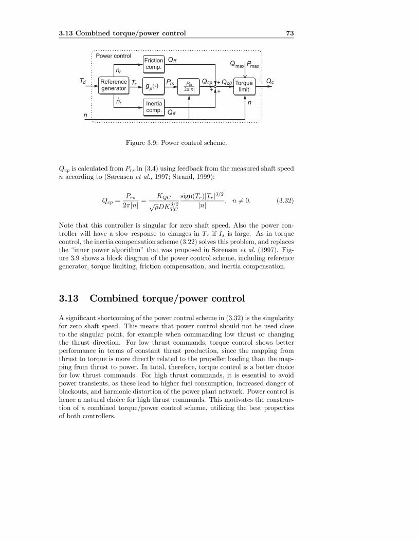
3.13 Combined torque/power control 73
QcTorquelimit
QcpTr gp( ).
PmaxQmax
n
Frictioncomp.
+
+
Qff
Td Referencegenerator
Inertiacomp. Qif
+
Qc0
n
Power control
nr
nr
.
Prs Prs
|n|2p
Figure 3.9: Power control scheme.
Qcp is calculated from Prs in (3.4) using feedback from the measured shaft speedn according to (Sørensen et al., 1997; Strand, 1999):
Qcp =Prs2π|n| =
KQC√ρDK
3/2TC
sign(Tr)|Tr|3/2|n| , n 6= 0. (3.32)
Note that this controller is singular for zero shaft speed. Also the power con-troller will have a slow response to changes in Tr if Is is large. As in torquecontrol, the inertia compensation scheme (3.22) solves this problem, and replacesthe “inner power algorithm” that was proposed in Sørensen et al. (1997). Fig-ure 3.9 shows a block diagram of the power control scheme, including referencegenerator, torque limiting, friction compensation, and inertia compensation.
3.13 Combined torque/power control
A significant shortcoming of the power control scheme in (3.32) is the singularityfor zero shaft speed. This means that power control should not be used closeto the singular point, for example when commanding low thrust or changingthe thrust direction. For low thrust commands, torque control shows betterperformance in terms of constant thrust production, since the mapping fromthrust to torque is more directly related to the propeller loading than the map-ping from thrust to power. In total, therefore, torque control is a better choicefor low thrust commands. For high thrust commands, it is essential to avoidpower transients, as these lead to higher fuel consumption, increased danger ofblackouts, and harmonic distortion of the power plant network. Power control ishence a natural choice for high thrust commands. This motivates the construc-tion of a combined torque/power control scheme, utilizing the best propertiesof both controllers.
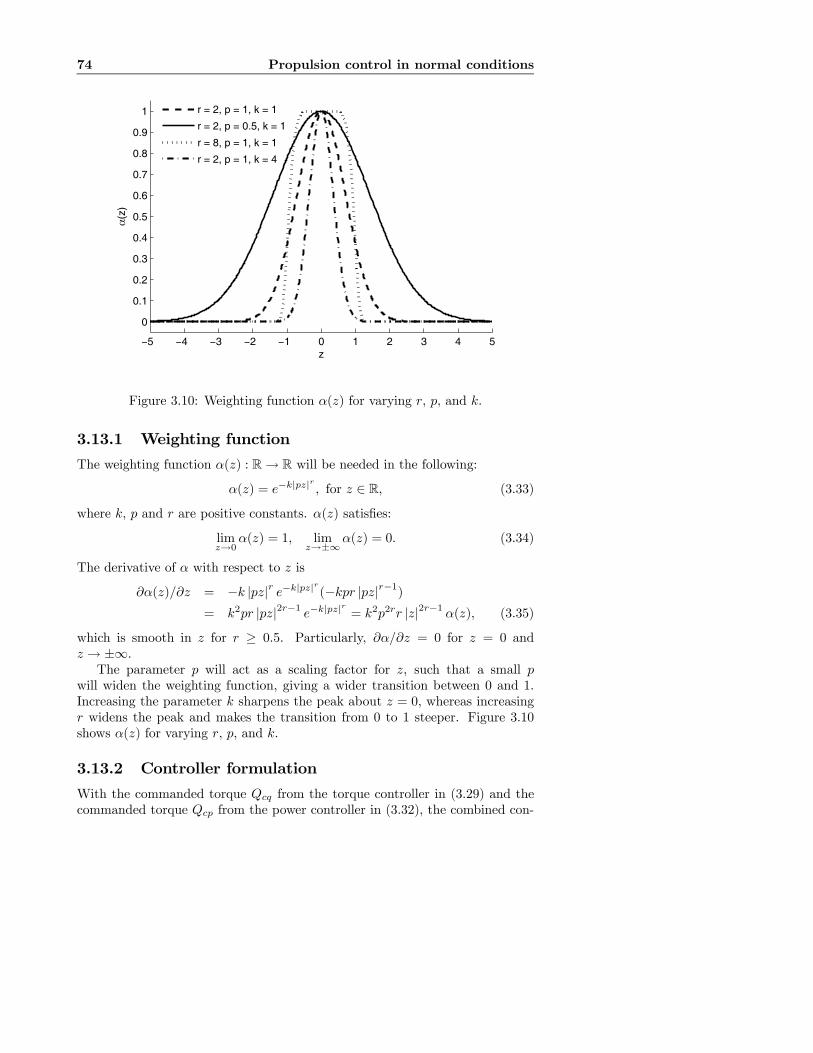
74 Propulsion control in normal conditions
−5 −4 −3 −2 −1 0 1 2 3 4 5
0
0.1
0.2
0.3
0.4
0.5
0.6
0.7
0.8
0.9
1
z
α(z)
r = 2, p = 1, k = 1
r = 2, p = 0.5, k = 1
r = 8, p = 1, k = 1
r = 2, p = 1, k = 4
Figure 3.10: Weighting function α(z) for varying r, p, and k.
3.13.1 Weighting function
The weighting function α(z) : R→ R will be needed in the following:
α(z) = e−k|pz|r
, for z ∈ R, (3.33)
where k, p and r are positive constants. α(z) satisfies:
limz→0
α(z) = 1, limz→±∞
α(z) = 0. (3.34)
The derivative of α with respect to z is
∂α(z)/∂z = −k |pz|r e−k|pz|r(−kpr |pz|r−1)= k2pr |pz|2r−1 e−k|pz|r = k2p2rr |z|2r−1 α(z), (3.35)
which is smooth in z for r ≥ 0.5. Particularly, ∂α/∂z = 0 for z = 0 andz → ±∞.The parameter p will act as a scaling factor for z, such that a small p
will widen the weighting function, giving a wider transition between 0 and 1.Increasing the parameter k sharpens the peak about z = 0, whereas increasingr widens the peak and makes the transition from 0 to 1 steeper. Figure 3.10shows α(z) for varying r, p, and k.
3.13.2 Controller formulation
With the commanded torque Qcq from the torque controller in (3.29) and thecommanded torque Qcp from the power controller in (3.32), the combined con-
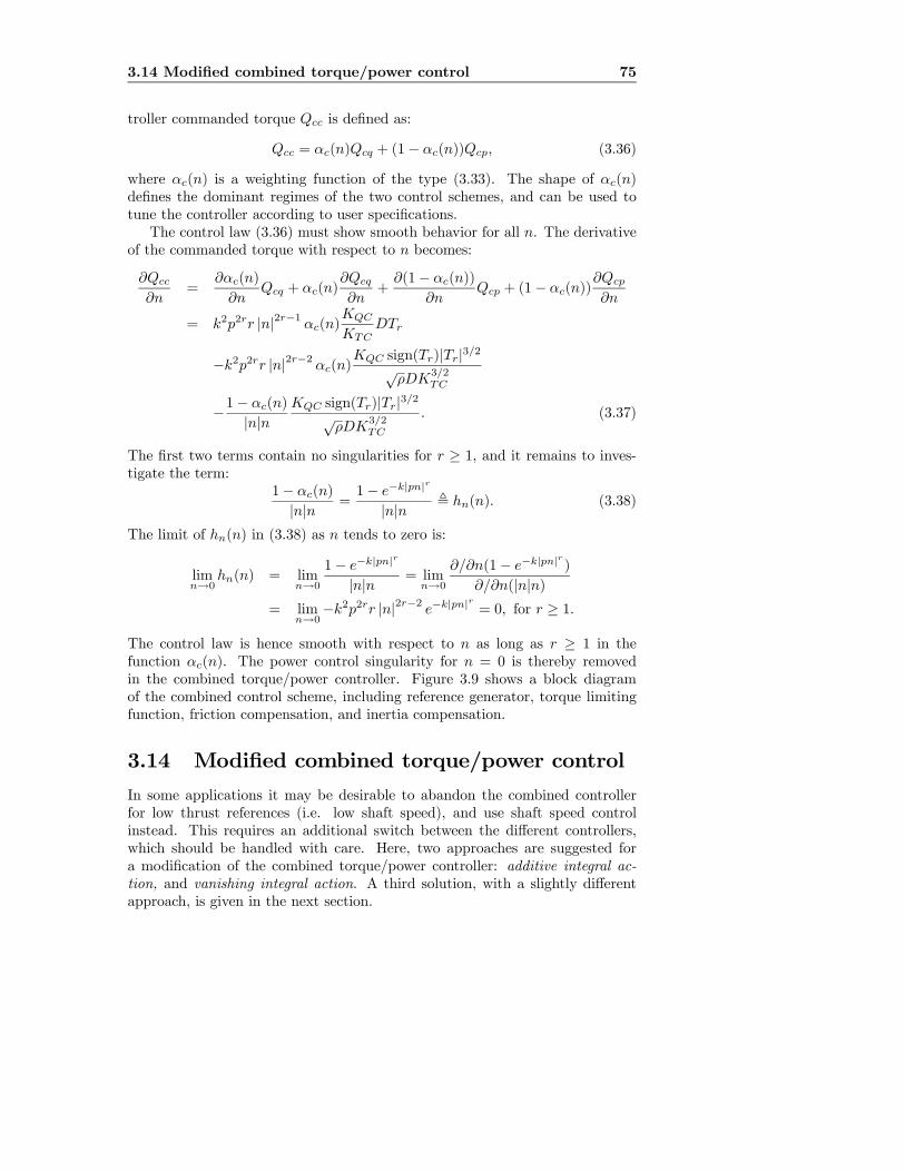
3.14 Modified combined torque/power control 75
troller commanded torque Qcc is defined as:
Qcc = αc(n)Qcq + (1− αc(n))Qcp, (3.36)
where αc(n) is a weighting function of the type (3.33). The shape of αc(n)defines the dominant regimes of the two control schemes, and can be used totune the controller according to user specifications.The control law (3.36) must show smooth behavior for all n. The derivative
of the commanded torque with respect to n becomes:
∂Qcc
∂n=
∂αc(n)
∂nQcq + αc(n)
∂Qcq
∂n+
∂(1− αc(n))
∂nQcp + (1− αc(n))
∂Qcp
∂n
= k2p2rr |n|2r−1 αc(n)KQC
KTCDTr
−k2p2rr |n|2r−2 αc(n)KQC sign(Tr)|Tr|3/2
√ρDK
3/2TC
−1− αc(n)
|n|nKQC sign(Tr)|Tr|3/2
√ρDK
3/2TC
. (3.37)
The first two terms contain no singularities for r ≥ 1, and it remains to inves-tigate the term:
1− αc(n)
|n|n =1− e−k|pn|
r
|n|n , hn(n). (3.38)
The limit of hn(n) in (3.38) as n tends to zero is:
limn→0
hn(n) = limn→0
1− e−k|pn|r
|n|n = limn→0
∂/∂n(1− e−k|pn|r
)
∂/∂n(|n|n)= lim
n→0−k2p2rr |n|2r−2 e−k|pn|r = 0, for r ≥ 1.
The control law is hence smooth with respect to n as long as r ≥ 1 in thefunction αc(n). The power control singularity for n = 0 is thereby removedin the combined torque/power controller. Figure 3.9 shows a block diagramof the combined control scheme, including reference generator, torque limitingfunction, friction compensation, and inertia compensation.
3.14 Modified combined torque/power controlIn some applications it may be desirable to abandon the combined controllerfor low thrust references (i.e. low shaft speed), and use shaft speed controlinstead. This requires an additional switch between the different controllers,which should be handled with care. Here, two approaches are suggested fora modification of the combined torque/power controller: additive integral ac-tion, and vanishing integral action. A third solution, with a slightly differentapproach, is given in the next section.
76 Propulsion control in normal conditions
QcTorquelimit
Qcp
Tr
gp( ).
PmaxQmax
n
Frictioncomp.
++
Qff
Td Referencegenerator
Inertiacomp. Qif
+
Qc0
n
Combined torque/power control
nr
nr
.Prs Prs
|n|2p
a ( )nc
1-
gq( ).
a ( )nc
Qcq
Qcc
+
+
Figure 3.11: Combined torque/power control scheme.
3.14.1 Additive integral action
If the starting torque Qs is significant but unknown, the static term Qff0 inthe friction compensation scheme (3.19) cannot be implemented. This meansthat the combined torque/power controller will give poor performance for lowthrust references, since Qs then will be of significant magnitude compared to thecommanded torque Qci from the controller. For higher thrust references, Qs willbe small compared to Qci, and the performance will probably be satisfactory.A solution to this is to add an integral term operating on the shaft speed erroras in (3.27) to the combined controller in (3.36) for low thrust references, anddisable the integral update for high thrust references.As in the friction compensation scheme, the shaft speed reference nr from
(3.1) is used as the switching variable. The threshold shaft speed for the switchis termed ns > 0, such that |nr| ≤ ns ⇒ shaft speed control, and |nr| > ns ⇒combined control. The reason for using nr instead of the measured shaft speedn to define the operating regimes is to avoid switching due to measurement noiseand shaft speed oscillations. The controller output Qccm is formulated as thesum of the commanded torque Qcc from the combined controller in (3.36) andan integral term Qi:
Qccm = Qcc +Qi. (3.39)
Qi is defined as:
Qi =
½ R t0Ki(nr(τ)− n(τ))dτ for |nr| ≤ ns,
Qi for |nr| > ns,(3.40)
where Ki is the integral gain, and Qi is the value of Qi when |nr| = ns. This iseasily implemented by freezing or disabling the integrator update when |nr| >ns. This can also be written as
Qi =
Z t
0
Kiei(τ)dτ, ei =
½nr − n for |nr| ≤ ns,0 for |nr| > ns.
(3.41)

3.14 Modified combined torque/power control 77
Assuming perfect shaft speed control (i.e. n = nr) for |nr| ≤ ns, the torquebalance when n = nr = ns from (2.50) becomes:
Qcc + Qi +Qf12πnr = sign(n)Qs +Kω2πn+Qa. (3.42)
The combined controller has been designed to cancel the propeller torque, suchthat Qcc ≈ Qa. If the linear friction compensation is accurate, such thatQf12πnr ≈ Kω2πn, it is clear that the frozen integral term is given by:
Qi ≈ sign(n)Qs. (3.43)
Hence, by keeping Qi as a term in the controller also for |nr| > ns, the staticfriction is cancelled for the entire range of controller operation. For this towork properly, the limit ns should be chosen relatively low, such that it canbe assumed that the static friction is a significant term for |nr| ≤ ns. If nsis chosen too high, the static friction may be dominated by dynamics in thepropeller loading, such that the assumption Qcc ≈ Qa, and hence also (3.43),no longer holds. If no linear friction compensation is included, the frozen integralterm will be given by Qi ≈ sign(n)Qs +Kω2πns.
Remark 3.6 Perfect matching of Qi with the static friction can only be ob-tained in the ideal case, when Kω is known, the control coefficients KTC andKQC in the combined controller match the true thrust and torque coefficients,and there is no dynamic loading of the propeller (nominal conditions). If theconditions deviate from the nominal, perfect compensation can no longer beachieved, and the frozen integral term Qi 6= sign(n)Qs. However, if Qf0 is un-known, the total controller performance will still probably be superior to the onewithout the added integral action.
3.14.2 Vanishing integral action
If Qs is known and can be included in the friction compensation (by Qf0 = Qs),but it still is desirable to use the shaft speed controller for low Tr, the approachdescribed in the previous section is not appropriate. In this case it is possible touse a similar formulation, where the integral term used for shaft speed controlwhen |nr| ≤ ns is removed for high nr. This is facilitated by adding a weightingfunction αi(nr) of the type (3.33) to the integral term Qi in (3.39):
Qccm = Qcc +Qiαi(nrel), (3.44)
nrel = max(0, |nr|− ns). (3.45)
Hence, αi(nrel) = 1 for |nr| ≤ ns, such that the controller here is identical to(3.39). For |nr| > ns, Qi is scaled with αi(nrel) such that Qiαi(nrel) tends tozero for increasing nr. The shaft speed reference for which Qiαi(nrel) ≈ 0 isimplicitly given by the parameters r, p, and k in αi(nrel).
78 Propulsion control in normal conditions
3.15 Combined speed/torque/power controlAs an alternative to the modified combined torque/power controller formula-tions presented in Section 3.14, it is possible to specify three control regimesexplicitly: speed control for low shaft speed, torque control for medium shaftspeed, and power control for high shaft speed. The regimes are defined as fol-lows:
|nr| ≤ ns1 ⇒ shaft speed control,ns1 < |nr| ≤ ns2 ⇒ transition speed↔ torque,ns2 < |nr| ≤ ns3 ⇒ torque control,ns3 < |nr| ≤ ns4 ⇒ transition torque↔ power,|nr| > ns4 ⇒ power control,
with switching shaft speeds ns1 < ns2 < ns3 < ns4. The two transitions aredone by the weighting functions α1(nr) and α2(nr):
α1(nr) = αs(max(0, |nr|− ns1)), (3.46)
α2(nr) = αs(max(0, |nr|− ns3)), (3.47)
where αs is a weighting function of the type (3.33). ns1 and ns3 are chosenexplicitly by the designer, whereas ns2 and ns4 are given implicitly by the func-tions α1 and α2. Figure 3.12 shows the three control regimes with transitionareas and weighting functions. With a modification of the shaft speed controllerfrom (3.27), the torque controller from (3.29), a modification of the power con-troller from (3.32), and the two weighting functions α1 and α2, the controlleroutput Qcs of the combined speed/torque/power controller is given from:
nr = sgn(Tr)
s|Tr|
ρD4KTC, e = nr − n,
Qcn = Kpe+
Z t
0
Kiei(τ)dτ, ei =
½e for |nr| ≤ ns1,0 for |nr| > ns1,
Qcq =KQC
KTCDTr,
Qcp =KQC
√ρDK
3/2TC
sgn(Tr)|Tr|3/2max(|n| , εp)
,
α1(nr) = exp(−k(pmax(0, |nr|− ns1))r),
α2(nr) = exp(−k(pmax(0, |nr|− ns3))r),
Qcs = α1α2Qcn + (1− α1)α2Qcq + (1− α1)(1− α2)Qcp. (3.48)
Remark 3.7 In the combined power/torque controller it was necessary to usethe shaft speed n in the weighting function in order to avoid the singularity forzero shaft speed. In (3.48), the singularity is easily avoided by using max(|n| , εp)instead of |n| in the power equation, where εp is a small positive number. Sinceα2(nr) ≡ 1 for |nr| < ns3 (and hence the contribution from the power controlleris zero), this does not affect the controller output.

3.16 Thrust control and additional instrumentation 79
0
0
0.2
0.4
0.6
0.8
1
nr
−ns1
ns1
ns2
ns3
ns4
Speedcontrol
Torquecontrol
Powercontrol
α1(n
r) α
2(n
r)
Figure 3.12: Example weighting functions α1(nr) and α2(nr) used in the com-bined speed/torque/power controller, with controller regimes and transition ar-eas. The weighting functions are symmetric about nr = 0.
Remark 3.8 The modification of the shaft speed controller term Qcn is similarto the vanishing integral term in Section 3.14.2, with a disabled integrator for|nr| > ns.
Remark 3.9 The control scheme in (3.48) is easily combined with the frictionand inertia compensation schemes as in (3.18) if desired. However, by usingshaft speed control for the lowest thrust references, the most important reason forusing the friction compensation scheme, i.e. tracking properties for low thrustreferences, will in most cases be diminished. In some applications, like e.g. theexperimental setup presented in Section 7.1, the friction is of significance alsofor the higher thrust references.
3.16 Thrust control and additional instrumen-tation
If the propulsion unit could be equipped with additional instrumentation, newcontrol options would appear. With a measurement of the actual thrust, thrustcontrol becomes an option. This could be implemented e.g. by a PI controlleroperating on the thrust error. Without additional instrumentation, it is insome cases possible to construct an output feedback thrust controller, as pro-

80 Propulsion control in normal conditions
Controller Abbreviation SectionShaft speed control S control 3.10Torque control Q control 3.11Power control P control 3.12Combined torque/power control QP control 3.13Modified QP control w/ additive integral MQP1 control 3.14.1Modified QP control w/ vanishing integral MQP2 control 3.14.2Combined speed/torque/power control SQP control 3.15Friction compensation scheme w/Qff 3.7.1Inertia compensation scheme w/Qif 3.7.2
Table 3.1: Controllers for normal conditions.
posed in Guibert et al. (2005). These topics, as well as other control optionsthat become available with additional instrumentation, are further treated inAppendices E.2 and E.3. Due to the increased complexity and necessary modelknowledge, thrust control is not considered to be a desirable solution for indus-trial implementation on surface vessels.
3.17 Controller summary
For ease of notation, the controllers presented above will be given abbreviationsas defined in Table 3.1. Shaft speed, torque, and power control are consideredto be the fundamental controllers, since the other controllers are combinationsof these. The abbreviations will be used as e.g. “QP w/Qff”, meaning combinedtorque/power control with friction compensation.
3.18 Simulation results
This section presents simulations with the 4MW Wageningen B4-70 examplepropeller, with specifications given in Appendix A.The control coefficients are taken according to (3.8, 3.9), with parameters
given in Table 3.2. The resulting control coefficient KTC is shown as a functionof nr in Figure 3.2. Note that the thrust and torque coefficients in Table 3.2are identical to the true nominal model parameters as given in Table A.1. Withthe chosen εc, λc(nc) = 0.9975, and λc(−nc) = 0.0025. Hence, the controlcoefficients are accurate for |nr| > 0.2rps.The shaft speed reference generator in (3.14) is utilized, with parameters
given in Table 3.3. Unless otherwise specified, the friction and inertia compen-sation schemes are taken according to (3.19) and (3.22), with the parametersgiven in Table 3.4. The resulting friction compensation scheme is shown as afunction of nr in Figure 3.5. Perfect model knowledge has been assumed, suchthat the parameters Ic, Qf0, and Qf1 in Table 3.4 are identical to the true model
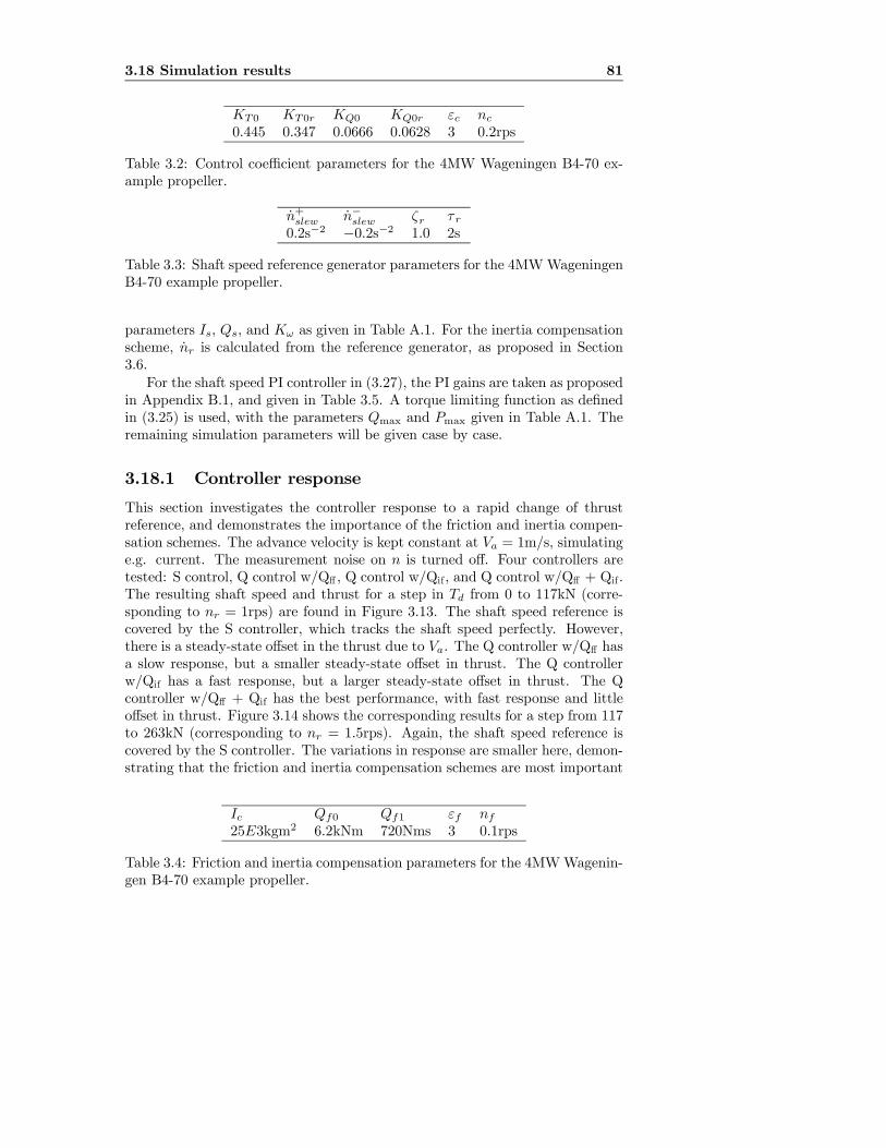
3.18 Simulation results 81
KT0 KT0r KQ0 KQ0r εc nc0.445 0.347 0.0666 0.0628 3 0.2rps
Table 3.2: Control coefficient parameters for the 4MW Wageningen B4-70 ex-ample propeller.
n+slew n−slew ζr τ r0.2s−2 −0.2s−2 1.0 2s
Table 3.3: Shaft speed reference generator parameters for the 4MWWageningenB4-70 example propeller.
parameters Is, Qs, and Kω as given in Table A.1. For the inertia compensationscheme, nr is calculated from the reference generator, as proposed in Section3.6.For the shaft speed PI controller in (3.27), the PI gains are taken as proposed
in Appendix B.1, and given in Table 3.5. A torque limiting function as definedin (3.25) is used, with the parameters Qmax and Pmax given in Table A.1. Theremaining simulation parameters will be given case by case.
3.18.1 Controller response
This section investigates the controller response to a rapid change of thrustreference, and demonstrates the importance of the friction and inertia compen-sation schemes. The advance velocity is kept constant at Va = 1m/s, simulatinge.g. current. The measurement noise on n is turned off. Four controllers aretested: S control, Q control w/Qff , Q control w/Qif, and Q control w/Qff + Qif.The resulting shaft speed and thrust for a step in Td from 0 to 117kN (corre-sponding to nr = 1rps) are found in Figure 3.13. The shaft speed reference iscovered by the S controller, which tracks the shaft speed perfectly. However,there is a steady-state offset in the thrust due to Va. The Q controller w/Qff hasa slow response, but a smaller steady-state offset in thrust. The Q controllerw/Qif has a fast response, but a larger steady-state offset in thrust. The Qcontroller w/Qff + Qif has the best performance, with fast response and littleoffset in thrust. Figure 3.14 shows the corresponding results for a step from 117to 263kN (corresponding to nr = 1.5rps). Again, the shaft speed reference iscovered by the S controller. The variations in response are smaller here, demon-strating that the friction and inertia compensation schemes are most important
Ic Qf0 Qf1 εf nf25E3kgm2 6.2kNm 720Nms 3 0.1rps
Table 3.4: Friction and inertia compensation parameters for the 4MWWagenin-gen B4-70 example propeller.

82 Propulsion control in normal conditions
Kp Ti Qi,max Tf7.6E5 0.10s 0.9kgQN 0.01s
Table 3.5: Shaft speed PI controller parameters for the 4MWWageningen B4-70example propeller.
0
0.2
0.4
0.6
0.8
1
n [r
ps]
0 2 4 6 8 10 12 14 16 18 20
0
20
40
60
80
100
120
Time [s]
Ta [k
N]
ReferenceS controlQ control w/Q
ff
Q control w/Qif
Q control w/Qff + Q
if
Figure 3.13: Comparison of the shaft speed and thrust response to a step in Tdfrom 0 to 117kN at Va = 1.0m/s for four controllers.
for small Tr. Still, however, the inertia compensation speeds up the response,and the friction compensation reduces the steady-state thrust offset. In total,the Q controller w/Qff + Qif has the best performance also here.For Va = 0, which is not shown here, the S controller and Q controller w/Qff
+ Qif both track nr and Tr perfectly, and only the Q controller w/Qif has asteady-state offset. The response of the Q controller w/Qff is still slow. Inconclusion, the friction compensation scheme is needed to avoid steady-stateoffset, and the inertia compensation needed get satisfactory response of theQ controller. However, as was seen in Figures 3.13 and 3.14, the resultingthrust without friction compensation may still be better than for the shaftspeed controller when operating away from the nominal design point Va = 0.Without the inertia compensation scheme, the response of the P controller
is slightly better than for the Q controller. Without the friction compensationscheme, the steady-state thrust offset of the P controller is slightly larger thanfor the Q controller.
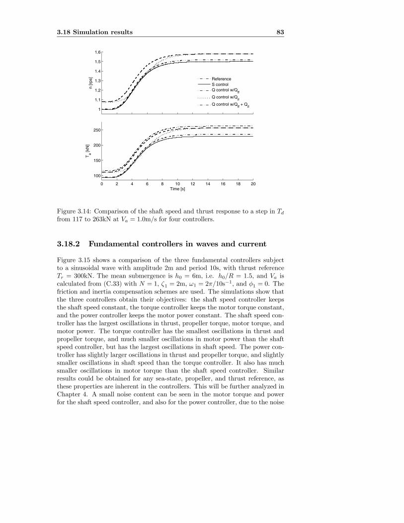
3.18 Simulation results 83
1
1.1
1.2
1.3
1.4
1.5
1.6
n [r
ps]
0 2 4 6 8 10 12 14 16 18 20
100
150
200
250
Time [s]
Ta [k
N]
ReferenceS controlQ control w/Q
ff
Q control w/Qif
Q control w/Qff + Q
if
Figure 3.14: Comparison of the shaft speed and thrust response to a step in Tdfrom 117 to 263kN at Va = 1.0m/s for four controllers.
3.18.2 Fundamental controllers in waves and current
Figure 3.15 shows a comparison of the three fundamental controllers subjectto a sinusoidal wave with amplitude 2m and period 10s, with thrust referenceTr = 300kN. The mean submergence is h0 = 6m, i.e. h0/R = 1.5, and Va iscalculated from (C.33) with N = 1, ζ1 = 2m, ω1 = 2π/10s
−1, and φ1 = 0. Thefriction and inertia compensation schemes are used. The simulations show thatthe three controllers obtain their objectives: the shaft speed controller keepsthe shaft speed constant, the torque controller keeps the motor torque constant,and the power controller keeps the motor power constant. The shaft speed con-troller has the largest oscillations in thrust, propeller torque, motor torque, andmotor power. The torque controller has the smallest oscillations in thrust andpropeller torque, and much smaller oscillations in motor power than the shaftspeed controller, but has the largest oscillations in shaft speed. The power con-troller has slightly larger oscillations in thrust and propeller torque, and slightlysmaller oscillations in shaft speed than the torque controller. It also has muchsmaller oscillations in motor torque than the shaft speed controller. Similarresults could be obtained for any sea-state, propeller, and thrust reference, asthese properties are inherent in the controllers. This will be further analyzed inChapter 4. A small noise content can be seen in the motor torque and powerfor the shaft speed controller, and also for the power controller, due to the noise

84 Propulsion control in normal conditions
on the shaft speed feedback signal.Figure 3.16 shows the same three controllers, sea state, and thrust reference,
but with the addition of a current that linearly increases the mean value of Vafrom 0m/s at t = 5s to 3m/s at t = 105s. The results further demonstrate thegood properties of the torque and power controllers. When the loading decreasesdue to the increased advance velocity, the controllers increase the shaft speedto keep the torque or power constant. The result is superior thrust production,in addition to reduced oscillations in torque and power.
3.18.3 Fundamental controllers with time-varying thrustreference
Figure 3.17 shows a comparison of the three fundamental controllers with asinusoidal Td of amplitude 50kN and period 50s. The mean submergence ish0 = 6m. The propeller is subject to a current velocity of 0.5m/s (givinga positive Va) and irregular waves with Hs = 1m, Tp = 7.6s, defined by 30harmonic components extracted from the modified PM spectrum in (C.19).The wave-induced velocities are calculated from (C.33). The friction and inertiacompensation schemes are used, but with a 20% error in both Qf0, Qf1, andIc when compared to the true parameters, i.e. Qf0 = 0.8Qs, Qf1 = 0.8Kω,and Ic = 0.8Is. In addition, the torque controller is simulated without frictionand inertia compensation. Figure 3.18 shows corresponding results with Td ofamplitude 200kN and period 70s. All the controllers track the thrust referencessatisfactory, except the pure torque controller. This shows the importance of thecompensation schemes, and also that the compensation schemes work well in thepresence of modelling errors. The singularity of the power controller for n = 0is clearly seen in the Qm plots. The shaft speed controller has an overshootin Qm about the zero-crossing of n. This is mainly due to the static friction.However, inclusion of the friction compensation scheme does not remedy thisproblem. A small transient exists also for the torque controller, although muchless apparent.
Remark 3.10 The reference generator gives a slight loss of amplitude in Tr,and also enforces a smoother zero-crossing of n when compared to the sinusoidalTd.
3.18.4 Combined controllers with time-varying thrust ref-erence
As stated in Sections 3.13 and 3.15, the idea behind the combined QP and SQPcontrollers is to utilize the best properties of the various fundamental controllers.Figure 3.19 shows time series where the QP controller w/Qff + Qif is tested
in regular waves with amplitude 2m and period 5s for a time-varying Td, in-cluding two zero-crossings of n. The chosen weighting function parameters for

3.18 Simulation results 85
1.6
1.62
1.64
n [r
ps]
S controlQ control w/Q
ff + Q
if
P control w/Qff + Q
if
280
290
300
Ta [k
N]
170
175
180
Qa [k
Nm
]
45
46
47
48
Qm
[kN
m]
10 15 20 25 30 35 401800
1900
2000
Pm
[kW
]
Time [s]
Figure 3.15: Comparison of shaft speed, torque, and power control for Tr =300kN in harmonic waves.

86 Propulsion control in normal conditions
1.6
1.7
1.8
1.9
n [r
ps]
S controlQ control w/Q
ff + Q
if
P control w/Qff + Q
if
150
200
250
300
Ta [k
N]
100
120
140
160
180
Qa [k
Nm
]
30
35
40
45
Qm
[kN
m]
10 20 30 40 50 60 70 80 90 100
1200140016001800200022002400
Pm
[kW
]
Time [s]
Figure 3.16: Comparison of shaft speed, torque, and power control for Tr =300kN in harmonic waves and linearly increasing current.
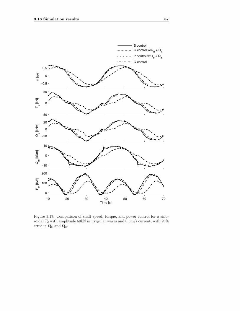
3.18 Simulation results 87
−0.5
0
0.5
n [r
ps]
S controlQ control w/Q
ff + Q
if
P control w/Qff + Q
if
Q control
−50
0
50
Ta [k
N]
−20
0
20
Qa [k
Nm
]
−10
0
10
Qm
[kN
m]
10 20 30 40 50 60 70
0
100
200
Pm
[kW
]
Time [s]
Figure 3.17: Comparison of shaft speed, torque, and power control for a sinu-soidal Td with amplitude 50kN in irregular waves and 0.5m/s current, with 20%error in Qff and Qif.
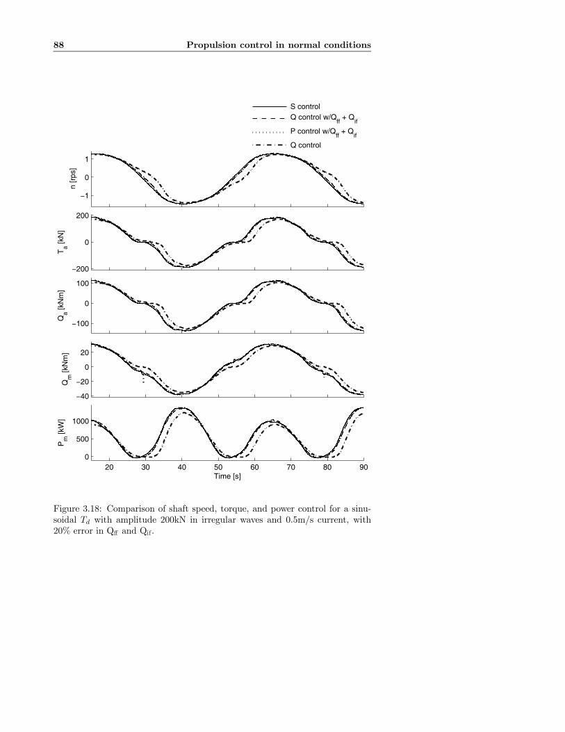
88 Propulsion control in normal conditions
−1
0
1
n [r
ps]
S controlQ control w/Q
ff + Q
if
P control w/Qff + Q
if
Q control
−200
0
200
Ta [k
N]
−100
0
100
Qa [k
Nm
]
−40
−20
0
20
Qm
[kN
m]
20 30 40 50 60 70 80 900
500
1000
Pm
[kW
]
Time [s]
Figure 3.18: Comparison of shaft speed, torque, and power control for a sinu-soidal Td with amplitude 200kN in irregular waves and 0.5m/s current, with20% error in Qff and Qif .
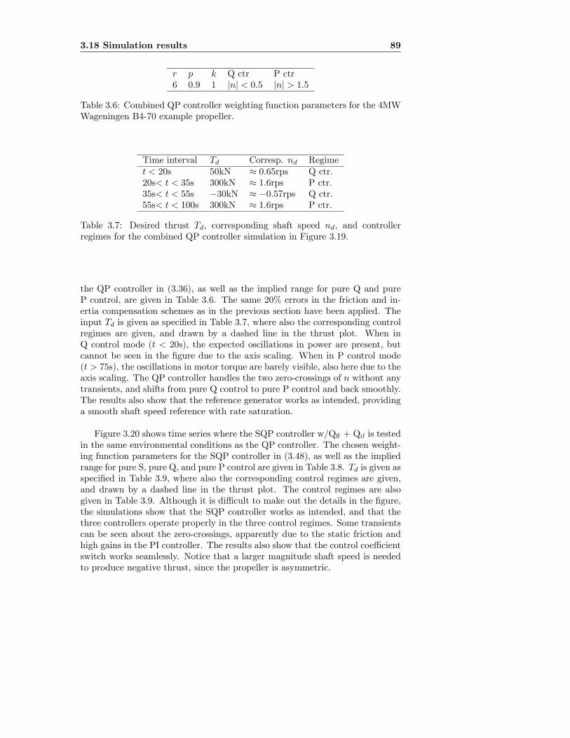
3.18 Simulation results 89
r p k Q ctr P ctr6 0.9 1 |n| < 0.5 |n| > 1.5
Table 3.6: Combined QP controller weighting function parameters for the 4MWWageningen B4-70 example propeller.
Time interval Td Corresp. nd Regimet < 20s 50kN ≈ 0.65rps Q ctr.20s< t < 35s 300kN ≈ 1.6rps P ctr.35s< t < 55s −30kN ≈ −0.57rps Q ctr.55s< t < 100s 300kN ≈ 1.6rps P ctr.
Table 3.7: Desired thrust Td, corresponding shaft speed nd, and controllerregimes for the combined QP controller simulation in Figure 3.19.
the QP controller in (3.36), as well as the implied range for pure Q and pureP control, are given in Table 3.6. The same 20% errors in the friction and in-ertia compensation schemes as in the previous section have been applied. Theinput Td is given as specified in Table 3.7, where also the corresponding controlregimes are given, and drawn by a dashed line in the thrust plot. When inQ control mode (t < 20s), the expected oscillations in power are present, butcannot be seen in the figure due to the axis scaling. When in P control mode(t > 75s), the oscillations in motor torque are barely visible, also here due to theaxis scaling. The QP controller handles the two zero-crossings of n without anytransients, and shifts from pure Q control to pure P control and back smoothly.The results also show that the reference generator works as intended, providinga smooth shaft speed reference with rate saturation.
Figure 3.20 shows time series where the SQP controller w/Qff + Qif is testedin the same environmental conditions as the QP controller. The chosen weight-ing function parameters for the SQP controller in (3.48), as well as the impliedrange for pure S, pure Q, and pure P control are given in Table 3.8. Td is given asspecified in Table 3.9, where also the corresponding control regimes are given,and drawn by a dashed line in the thrust plot. The control regimes are alsogiven in Table 3.9. Although it is difficult to make out the details in the figure,the simulations show that the SQP controller works as intended, and that thethree controllers operate properly in the three control regimes. Some transientscan be seen about the zero-crossings, apparently due to the static friction andhigh gains in the PI controller. The results also show that the control coefficientswitch works seamlessly. Notice that a larger magnitude shaft speed is neededto produce negative thrust, since the propeller is asymmetric.

90 Propulsion control in normal conditions
−0.5
0
0.5
1
1.5
n [r
ps]
QP control w/Qff + Q
if
0
100
200
300
Ta [k
N]
Td
0
50
100
150
Qa [k
Nm
]
0
20
40
Qm
[kN
m]
10 20 30 40 50 60 70 80 90 1000
1000
2000
Pm
[kW
]
Time [s]
Figure 3.19: Time series of the combined QP controller in regular waves for atime-varying Td.
r p k ns1 ns3 S ctr Q ctr P ctr4 4 2 0.3 1.1 |n| < 0.3 0.64 < |n| < 1.1 |n| > 1.44
Table 3.8: Combined SQP controller weighting function parameters for the4MW Wageningen B4-70 example propeller.
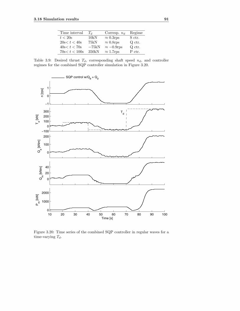
3.18 Simulation results 91
Time interval Td Corresp. nd Regimet < 20s 10kN ≈ 0.3rps S ctr.20s< t < 40s 75kN ≈ 0.8rps Q ctr.40s< t < 70s −75kN ≈ −0.9rps Q ctr.70s< t < 100s 350kN ≈ 1.7rps P ctr.
Table 3.9: Desired thrust Td, corresponding shaft speed nd, and controllerregimes for the combined SQP controller simulation in Figure 3.20.
−1
0
1
n [r
ps]
SQP control w/Qff + Q
if
−100
0
100
200
300
Ta [k
N]
Td
0
100
200
Qa [k
Nm
]
0
20
40
Qm
[kN
m]
10 20 30 40 50 60 70 80 90 1000
1000
2000
Pm
[kW
]
Time [s]
Figure 3.20: Time series of the combined SQP controller in regular waves for atime-varying Td.

92 Propulsion control in normal conditions
Speed ctr. Torque ctr. Power ctr.Thrust fluctuations Large Small MediumTorque fluctuations Large Small MediumPower fluctuations Large Medium SmallOther issues Tuning Power peaks Singularity
Friction FrictionInertia Inertia
Table 3.10: Comparison of the main properties of the fundamental thrustercontrollers.
Light load Medium load Heavy loadThrust production High High HighMech. wear & tear Low Medium HighPower fluctuations Low Medium HighFriction/Inertia High Low/Medium LowPreferred ctr. Speed or Torque Torque Power
Table 3.11: Summary of the relevance (low, medium, high) of the main perfor-mance criteria for light, medium, and heavy propeller loading.
3.19 Discussion
This chapter has presented several thruster controllers for normal operatingconditions, including various additions like friction and inertia compensation,reference generators, and torque/power limiting. The controllers are summa-rized in Table 3.1. A summary of the main properties of the three fundamentalcontrollers — shaft speed, torque, and power control — is given in Table 3.10.A summary of the relevance (low, medium, or high) of the main performancecriteria for varying propeller loading is given in Table 3.11.From these two tables, it is easy to motivate the construction of the combined
controllers, i.e. QP, MQP1, MQP2, and SQP control:
• For medium propeller loading, the torque controller is preferable, and forhigh propeller loading the power controller is preferable. In these oper-ating regimes, the knowledge of the friction and inertia parameters is ofreduced importance. However, improved transient response and trackingproperties is expected if the friction and inertia compensation schemes areused.
• For low propeller loading, torque or shaft speed control is preferable. Ifsufficient system knowledge to implement the friction and inertia compen-sation schemes is at hand, torque control will probably be sufficient. Then,the QP controller is a good choice. If the friction and inertia compensationschemes are implemented, but expected to be less accurate due to limited

3.19 Discussion 93
Small propellers Large propellersFriction Important Less importantInertia Less important Important
Table 3.12: Importance of the friction and inertia compensation schemes forvarying propeller sizes.
system knowledge, some kind of shaft speed control for low shaft speedswill be preferable. Then, the MQP1 or MQP2 controller is a good choice.
• If no inertia or friction compensation scheme is implemented, it is probablynecessary to use shaft speed control for low to medium propeller loading,depending on the significance of the friction and inertia terms. In thiscase, the SQP controller may be the best option.
For small propellers, like thrusters on small underwater vehicles and pro-pellers used in experimental setups, it is expected that the friction is of largersignificance than the inertia. For large thrusters, the opposite is expected.Hence, it may not be necessary with both compensation schemes in all appli-cations. The importance of the friction and inertia compensation schemes issummarized in Table 3.12.The recommendations above should only serve as guidelines for the choice
of controller. For some applications, other controllers than the ones presentedhere may be preferable. It is e.g. simple to construct a combined speed/powercontroller based on the SQP controller. In other applications, one of the fun-damental controllers, i.e. S, Q, or P control, may be the better choice. In theliterature, also other controllers — that may be more appropriate for the appli-cations studied there — have been proposed, see the references listed in Section3.4. Some additional control options, based on output feedback, are presentedin Appendices E.3 and E.4.

94 Propulsion control in normal conditions

Chapter 4
Sensitivity to thrust losses
The steady-state performance of the various control schemes introduced inChapter 3 can be theoretically analyzed by establishing their sensitivity to thrustlosses. Depending on the control scheme, a loss of propeller loading may, in ad-dition to changes in propeller thrust and torque, lead to changes in shaft speedand power. The relationship between the actual and reference thrust, torque,shaft speed, and power are termed sensitivity functions :
Thrust sensitivity: sti(n,xp,θp, Tr) ,TaTr
. (4.1)
Speed sensitivity: sni(n,xp,θp, Tr) ,n
nr. (4.2)
Torque sensitivity: sqi(n,xp,θp, Tr) ,Qa
Qr. (4.3)
Power sensitivity: spi(n,xp,θp, Tr) ,PaPr
. (4.4)
The index i indicates the type of controller: i = n for shaft speed control (Section3.10), i = q for torque control (Section 3.11), i = p for power control (Section3.12), and i = t for thrust control (Section 3.16). For notational simplicity, thearguments of the sensitivity functions will be omitted. nr, Qr, and Pr are givenfrom Tr by (3.1), (3.2), and (3.3), respectively.When developing the sensitivity functions, it is assumed that all controllers
obtain their objectives perfectly, i.e. n = nr for shaft speed control, Qa = Qr fortorque control, Pa = Pr for power control, and Ta = Tr for thrust control. It hashence been assumed that the friction is perfectly compensated for in torque andpower control, i.e. Qff = Qf . In Appendix F it is shown how this assumptionmay be relaxed. The sensitivity function concept was introduced in Sørensenet al. (1997) and Strand (1999), where the thrust sensitivity function sti(·)was used to analyze the properties of shaft speed, torque, and power control.The current presentation of the thrust sensitivity functions differs slightly fromthe original formulations. The sensitivity analysis is mainly of interest for the
96 Sensitivity to thrust losses
fundamental thruster controllers, i.e. shaft speed, torque, and power control,as well as thrust control. The sensitivities of the other controllers in Table 3.1may be directly inferred from the sensitivity of the fundamental controllers,depending on the chosen weighting functions.The sensitivity analysis can only be used to evaluate the quasi-static per-
formance of the various control schemes. To gain insight into the transientperformance of the controllers, Section 4.10 presents a stability analysis basedon Lyapunov theory.
Remark 4.1 As mentioned in Section 3.16, the thrust controller requires addi-tional instrumentation or a complex output feedback formulation, and is henceof limited industrial relevance. This is further discussed in Appendix E.2.1 andAppendix E.3.1. The sensitivity functions for thrust control are still derived,since it is interesting to analyze its properties alongside the fundamental con-trollers.
4.1 Thrust, torque, power, and shaft speed re-lations
In the following, the relationships between thrust, torque, power, and shaftspeed will be needed. The shaft speed n can be expressed in terms of the thrustTa or the torque Qa by inverting (2.3) and (2.4):
n = sign(Ta)
s|Ta|
ρD4KT, (4.5)
n = sign(Qa)
s|Qa|
ρD5KQ. (4.6)
From (2.5), the magnitude of the shaft speed is expressed in terms of Pa by:
|n| = P1/3a
(2πKQρ)1/3D5/3. (4.7)
The thrust Ta can be expressed in terms of the torque Qa by eliminatingsign(n)ρn2D4 between (2.3) and (2.4):
Ta =KT
KQDQa. (4.8)
Similarly, Ta can be expressed in terms of Pa by eliminating sign(n)ρn2D4
between (2.3) and (2.5) and inserting (4.5):
|Ta| =ρ1/3D2/3KT
(2π)2/3K2/3Q
P 2/3a . (4.9)
4.2 Thrust sensitivity 97
Finally, Qa can be expressed in terms of Pa by inserting (4.6) in (2.5):
|Qa| =ρ1/3D5/3K
1/3Q
(2π)2/3P 2/3a . (4.10)
The shaft speed, torque, and power mappings in (3.1), (3.2), and (3.3) can beused to establish the following relationships between the references Tr, Pr, Qr,and nr:
Tr = KTCρD4nr |nr| , (4.11)
Qr = KQCρD5nr |nr| , (4.12)
Pr = 2πKQCρD5 |nr|3 . (4.13)
4.2 Thrust sensitivity
4.2.1 Shaft speed control thrust sensitivity
Assuming perfect control at steady state, i.e. n = nr, the shaft speed is givenin terms of Tr from (3.27):
n = nr = sign(Tr)
s|Tr|
ρD4KTC. (4.14)
The actual thrust for shaft speed control is then given from (2.3) and (4.14):
Ta = sign(Tr)KT ρD4 |Tr|ρD4KTC
=KT
KTCTr, (4.15)
and the sensitivity function for shaft speed control stn(·) is:
stn(·) =TaTr=
KT
KTC. (4.16)
4.2.2 Torque control thrust sensitivity
Assuming perfect control at steady state, i.e. Qa = Qr, the propeller torque isgiven in terms of Tr from (3.2):
Qa = Qr =KQC
KTCDTr. (4.17)
The actual thrust for torque control is expressed in terms of Tr by inserting(4.17) in (4.8):
Ta =KT
KQDQa =
KQC
KQ
KT
KTCTr, (4.18)
and the sensitivity function for torque control stq(·) is:
stq(·) =TaTr=
KT
KTC
KQC
KQ. (4.19)
98 Sensitivity to thrust losses
4.2.3 Power control thrust sensitivity
Assuming perfect control at steady state, i.e. Pa = Pr, the propeller power isgiven in terms of Tr from (3.32):
Pa = Pr = Qr2πnr = |Tr|3/22πKQC√ρDK
3/2TC
. (4.20)
The actual thrust for power control is expressed in terms of Tr by inserting(4.20) in (4.9):
|Ta| = (√ρDK
3/2T
KQ2πPa)
2/3 =KT
KTC
K2/3QC
K2/3Q
|Tr|. (4.21)
Assuming that the signs of the reference and produced thrust are equal, i.e.sign(Ta) = sign(Tr), the sensitivity function for power control stp(·) is:
stp(·) =TaTr=
KT
KTC(KQC
KQ)2/3. (4.22)
4.2.4 Thrust control thrust sensitivity
If a thrust feedback or thrust output feedback controller is used, the thrustsensitivity function stt(·) by definition becomes unity:
stt(·) = 1, (4.23)
since Ta ≡ Tr when perfect control is assumed.
4.2.5 Combined torque/power control thrust sensitivity
The analysis of the sensitivity of the combined torque/power controller is notas straightforward as in the preceding cases. However, since the combined con-troller is a linear combination of the torque and power controllers, it is a rea-sonable assumption that its sensitivity function stc(·) may be expressed as:
stc(·) =KT
KTC(KQC
KQ)κ, for κ ∈ [ 2
3, 1], (4.24)
such that for high n, stc(·) ≈ stp(·) and for low n, stc(·) ≈ stq(·). In AppendixF.1, it is shown that a good approximation of κ is given by
κ ≈ 2/3 + 1/3αc(n), (4.25)
where αc(n) is the combined controller weighting function, as used in (3.36).For analysis purposes, the following approximation to the combined controllerthrust sensitivity function can therefore be used:
stc(·) ≈βTC
β2/3+1/3αc(n)QC
. (4.26)
4.3 Shaft speed sensitivity 99
Through αc(n), stc(·) depends on the shaft speed n, which makes it less conve-nient for analysis. However, it is clear that stc(·) will lie in-between stq(·) andstp(·) for all n.
4.3 Shaft speed sensitivityThe shaft speed sensitivity function for shaft speed control snn(·) is:
snn(·) =n
nr=
nrnr= 1, (4.27)
since in this case n = nr. Using (4.6) and (3.2), the shaft speed for torquecontrol is expressed in terms of Tr by:
n = sign(Qa)
s|Qa|
ρD5KQ= sign(Tr)
K1/2QC |Tr|
1/2
ρ1/2D2K1/2Q K
1/2TC
, (4.28)
and the shaft speed sensitivity function for torque control snq(·) is:
snq(·) =n
nr=sign(Tr)
qKQC |Tr|
KTCρD4KQ
sign(Tr)q
|Tr|ρD4KTC
=
sKQC
KQ. (4.29)
Using (4.7) and (3.4) the shaft speed for power control is expressed in terms ofTr by:
|n| = P1/3a
(2πKQρ)1/3D5/3=
K1/3QC
ρ1/2D2K1/2TCK
1/3Q
|Tr|1/2. (4.30)
Assuming sign(n) = sign(nr), the shaft speed sensitivity function for powercontrol snp(·) is:
snp(·) =|n||nr|
=
K1/3QC
ρ1/2D2K1/2TCK
1/3Q
|Tr|1/2¯sign(Tr)
q|Tr|
ρD4KTC
¯ = K1/3QC
K1/3Q
. (4.31)
From (4.5), the shaft speed for thrust control is:
n = sign(Ta)
s|Ta|
ρD4KT= sign(Tr)
s|Tr|
ρD4KT, (4.32)
and the shaft speed sensitivity function for thrust control snt(·) becomes:
snt(·) =n
n r=sign(Tr)
q|Tr|
ρD4KT
sign(Tr)q
|Tr|ρD4KTC
=
rKTC
KT. (4.33)

100 Sensitivity to thrust losses
4.4 Torque sensitivity
Using (2.4) and (3.1), the torque for shaft speed control is expressed in termsof Tr by:
Qa = sign(n)KQρD5n2 =
KQρD5Tr
ρD4KTC=
KQD
KTCTr, (4.34)
and the torque sensitivity function for shaft speed control sqn(·) is:
sqn(·) =Qa
Qr=
KQDKTC
TrKQCDKTC
Tr=
KQ
KQC. (4.35)
In torque control, Qa = Qr, and hence the torque sensitivity function for torquecontrol sqq(·) is:
sqq(·) =Qa
Qr=
Qr
Qr= 1. (4.36)
Using (4.10) and (3.4), the torque for power control is expressed in terms of Trby:
|Qa| =ρ1/3D5/3K
1/3Q
(2π)2/3P 2/3a =
DK1/3Q K
2/3QC
KTC|Tr|. (4.37)
Assuming sign(Qa) = sign(Qr), the torque sensitivity function for power controlsqp(·) is:
sqp(·) =|Qa||Qr|
=
DK1/3Q K
2/3QC
KTC|Tr|¯
KQCDKTC
Tr
¯ =K1/3Q
K1/3QC
. (4.38)
From (4.8) and (3.2), the torque sensitivity for thrust control sqt(·) becomes:
sqt(·) =Qa
Qr=
KQDKT
TaKQCDKTC
Tr=
KQDKT
TrKQCDKTC
Tr=
KQ
KQC
KTC
KT. (4.39)
4.5 Power sensitivity
Using (2.5) and (3.1), the power for shaft speed control is expressed in terms ofTr by:
Pa = sign(n)2πKQρD5n3 =
2πKQ
ρ1/2DK3/2TC
|Tr|3/2 , (4.40)
and the power sensitivity function for shaft speed control spn(·) is:
spn(·) =PaPr=
KQ
KQC. (4.41)
4.6 Sensitivity function summary 101
Using (4.10) and (3.2), the power for torque control is expressed in terms of Trby:
Pa =2π
ρ1/2D5/2K1/2Q
|Qa|3/2 =2πK
3/2QC
ρ1/2DK1/2Q K
3/2TC
|Tr|3/2 , (4.42)
and the power sensitivity function for torque control spq(·) is:
spq(·) =PaPr=
K1/2QC
K1/2Q
. (4.43)
In power control Pa = Pr, and hence the power sensitivity function for powercontrol spp(·) is:
spp(·) =PaPr=
PrPr= 1. (4.44)
From (4.9) and (3.4), the power sensitivity function for thrust control spt(·)becomes:
spt(·) =PaPr=
2πKQ
ρ1/2DK3/2T
|Ta|3/2
2πKQC
ρ1/2DK3/2TC
|Tr|3/2=
KQ
K3/2T
|Tr|3/2
KQC
K3/2TC
|Tr|3/2=
KQ
KQC
K3/2TC
K3/2T
. (4.45)
4.6 Sensitivity function summaryThe various sensitivity functions are summarized in Table 4.1. If the controlparameters KTC and KQC are replaced with the nominal parameters KT0 andKQ0, as is proposed for thruster control in low-speed applications, the sensitivityfunctions may be expressed in terms of the thrust and torque loss factors βTand βQ from (2.11) and (2.12). This is summarized in Table 4.2.
Remark 4.2 It is interesting to note that if the controllers have knowledge ofthe instantaneous values of KT and KQ, such that KTC = KT and KQC = KQ
at all times, all the sensitivity functions in Table 4.1 reduce to unity. Thismeans that all controllers perform identically.
Intuitively, the various sensitivity functions should be interrelated, regardlessof the chosen controller. This is also the case, as can be found by inserting (2.3),(2.4), (2.5), (4.11), (4.12), and (4.13) in (4.1), (4.3), and (4.4), and inserting for(4.2):
sti(·) =ρD4KTn
2
ρD4KTCn2r= βT sni(·)2, (4.46)
sqi(·) =ρD5KQn
2
ρD5KQCn2r= βQsni(·)2, (4.47)
spi(·) =2πρD5KQn
3
2πρD5KQCn3r= βQsni(·)3. (4.48)

102 Sensitivity to thrust losses
Sensitivity Speed control Torque controlThrust stn(·) = KT
KTCstq(·) = KT
KTC
KQC
KQ
Speed snn(·) = 1 snq(·) = (KQC
KQ)1/2
Torque sqn(·) = KQ
KQCsqq(·) = 1
Power spn(·) = KQ
KQCspq(·) = (KQC
KQ)1/2
Sensitivity Power control Thrust controlThrust stp(·) = KT
KTC(KQC
KQ)2/3 stt(·) = 1
Speed snp(·) = (KQC
KQ)1/3 snt(·) = (KTC
KT)1/2
Torque sqp(·) = ( KQ
KQC)1/3 sqt(·) = KQ
KQC
KTC
KT
Power spp(·) = 1 spt(·) = KQ
KQC(KTC
KT)3/2
Table 4.1: Thrust, torque, power, and shaft speed sensitivity functions definedin terms of KTC , KQC , KT , and KQ.
Sensitivity Speed ctr. Torque ctr. Power ctr. Thrust ctr.Thrust stn(·) = βT stq(·) = βT
βQstp(·) = βT
β2/3Q
stt(·) = 1Speed snn(·) = 1 snq(·) = 1
β1/2Q
snp(·) = 1
β1/3Q
snt(·) = 1
β1/2T
Torque sqn(·) = βQ sqq(·) = 1 sqp(·) = β1/3Q sqt(·) =
βQβT
Power spn(·) = βQ spq(·) = 1
β1/2Q
spp(·) = 1 spt(·) =βQ
β3/2T
Table 4.2: Sensitivity functions defined in terms of the thrust and torque lossfactors βT and βQ, under the assumption that KTC = KT0 and KQC = KQ0.
From (4.47) and (4.48), it is also clear that:
spi(·) = sqi(·)sni(·), (4.49)
as could have been expected. These relationships can also be verified for theindividual controllers in Tables 4.1 and 4.2.
4.7 Steady-state performanceThe steady-state performance of the various control schemes during a loss in-cident is conveniently analyzed with the sensitivity functions. However, thevalidity of the sensitivity functions rely on the steady-state values of βT and βQbeing correct. This is not necessarily trivial, since βT and βQ in general dependon n, and for the same operating conditions therefore will change between thedifferent controllers.For the shaft speed controller (assuming that n = nr), βT and βQ are
given directly. For the torque controller (assuming that Qa = Qr), the analysis
4.8 Sensitivity to changes in advance velocity 103
becomes more complicated, because the resulting shaft speed is unknown. Theloss factor βQ = βQ(·, n) and the shaft speed must satisfy:
Qr = Qa = KQρn2D5 = KQ0ρn
2D5βQ(·, n), (4.50)
where n is unknown. If βQ(·, n) can be expressed in terms of n, an analyticalsolution might be found. In the general case however, this is not possible, andn must be found by iteration. For the power controller (assuming Pa = Pr), theanalysis becomes similar as for torque control, but now the equation that mustbe satisfied is:
Pr = Pa = KQρn2D52πn = 2πKQ0ρn
3D5βQ(·, n). (4.51)
If an iterative analysis is performed for the combined controller, the equationthat has to be satisfied is (assuming Qcc = Qa):
αc(n)Qr + (1− αc(n))Prs2π|n| = KQ0ρn
2D5βQ(·, n).
In thrust control, the equation to be satisfied is (assuming Tr = Ta):
Tr = KT0ρn2D4βT (·, n). (4.52)
Remark 4.3 The iterative solution procedure used to arrive at the correct steady-state sensitivity values can be viewed as an extension of the original presentationin Sørensen et al. (1997) and Strand (1999), where the influence of n on βTand βQ was not considered.
4.8 Sensitivity to changes in advance velocityUsing the iterative solution procedure described above, the sensitivity to changesin advance velocity may be analyzed by expressing the various sensitivity func-tions as functions of Va for given Tr. This is done in Figures 4.1 to 4.4 for theWageningen B4-70 example propeller (see Figure 2.1 and Appendix A). Thethrust references Tr = 50, 200, and 400kN have been chosen. The curves forTr = 50kN stop at Va ≈ 2.7m/s, since the propeller here starts windmillingfor shaft speed control, i.e. the thrust becomes negative. Figure 4.1 shows thethrust sensitivity functions stn(·) for shaft speed control, stq(·) for torque con-trol, and stp(·) for power control. Clearly, the torque controller is the leastsensitive to changes in Va, the shaft speed controller the most sensitive, and thepower controller in-between. This shows that the torque and power controllerswill give significantly better thrust production than the shaft speed controllerwhen subject to disturbances in Va. Figure 4.2 shows the shaft speed sensitivityfunctions snn(·) for shaft speed control, snq(·) for torque control, and snp(·) forpower control. From this, it is clear that the torque and power controller achievethe increased thrust by increasing the shaft speed as Va increases. Figure 4.3

104 Sensitivity to thrust losses
shows the torque sensitivity functions sqn(·) for shaft speed control, sqq(·) fortorque control, and sqp(·) for power control. This confirms that the loadingof the propeller decreases with Va for shaft speed and power control, whereasit is kept constant in torque control — explaining why the thrust production issuperior. Figure 4.4 shows the power sensitivity functions spn(·) for shaft speedcontrol, spq(·) for torque control, and spp(·) for power control. This shows thatthe power controller keeps the power consumption constant regardless of Va,whereas the torque controller power consumption increases and the shaft speedcontroller power consumption decreases with Va. If control of the power con-sumption is of major concern, the power controller will therefore be superior tothe torque controller.
Remark 4.4 Figure 4.1 is conveniently used to illustrate how the integral actionin the DP controller must be used to counteract the thrust losses with a givenlow-level controller. If e.g. Tr = 200kN and Va = 2m/s, and shaft speed controlis used, the thrust sensitivity becomes stn ≈ 0.7. Hence, there is a lack of30% of the thrust. Since the shaft speed controller is unable to counteract thisloss, the DP controller must increase the setpoint until Ta = Trstn(·) = 200kN.From iteration, the resulting thrust setpoint can be found to be Tr ≈ 270kN. Intorque control, the thrust sensitivity is stq ≈ 0.94, and there is hence only a 6%lack of thrust. From iteration, the resulting thrust setpoint needed to achieveTa = Trstq(·) = 200kN is Tr ≈ 212kN. In power control, stp ≈ 0.86, and theresulting thrust setpoint needed to achieve Ta = Trstp(·) = 200kN is Tr ≈ 230kN.
Remark 4.5 The figures show that higher thrust references give less sensitivityto Va. This is natural, since the loading of the propeller is less affected by agiven Va when the shaft speed increases.
Remark 4.6 The power sensitivity function slope is for most Va larger for shaftspeed control than for torque control. This means that in a time-varying inflow,the oscillations in power will be larger for the shaft speed controller than for thetorque controller.
Figure 4.5 shows the thrust sensitivity function stc(·) for the combined con-troller as a function of Tr, together with stn(·), stq(·), and stp(·). The parame-ters for the weighting function αc(nr) in the combined controller were chosenas r = 10, p = 0.8, and k = 0.3, which gives pure torque control for n < 0.8 rpsand pure power control for n > 1.6 rps. This is mirrored in stc(·), which equalsstq(·) for low Tr and stp(·) for high Tr.
4.8.1 Non-dimensional parametrization for Va and Tr
In order to plot unique sensitivity functions for any combination of Tr and Va,valid for any propeller diameter, an alternative approach using the referenceadvance number Jr exists. This approach will also remove the necessity of an

4.8 Sensitivity to changes in advance velocity 105
−2 −1 0 1 2 3 4 5 60
0.2
0.4
0.6
0.8
1
Va [m/s]
Thrust sensitivity
Tr=50kN
Tr=50kN
Tr=50kN
Tr=200kN
Tr=200kN
Tr=200kN
Tr=400kN
Tr=400kN
Tr=400kN
stn(⋅)
stq(⋅)
stp(⋅)
Figure 4.1: Thrust sensitivity stn(·) for shaft speed control, stq(·) for torquecontrol, and stp(·) for power control as functions of advance velocity Va.
−2 −1 0 1 2 3 4 5 60.8
0.9
1
1.1
1.2
1.3
1.4
Va [m/s]
Shaft speed sensitivity
Tr=50kN
Tr=50kN
Tr=50kN
Tr=200kN
Tr=200kN
Tr=200kN
Tr=400kN
Tr=400kN
Tr=400kN
snn(⋅)
snq(⋅)
snp(⋅)
Figure 4.2: Shaft speed sensitivity snn(·) for shaft speed control, snq(·) fortorque control, and snp(·) for power control as functions of advance velocity Va.

106 Sensitivity to thrust losses
−2 −1 0 1 2 3 4 5 60.1
0.2
0.3
0.4
0.5
0.6
0.7
0.8
0.9
1
1.1
Torque sensitivity
Va [m/s]
Tr=50kN
Tr=50kN
Tr=50kN
Tr=200kN
Tr=200kN
Tr=200kN
Tr=400kN
Tr=400kN
Tr=400kN
sqn(⋅)
sqq(⋅)
sqp(⋅)
Figure 4.3: Torque sensitivity sqn(·) for shaft speed control, sqq(·) for torquecontrol, and sqp(·) for power control as functions of advance velocity Va.
−2 −1 0 1 2 3 4 5 6
0.2
0.4
0.6
0.8
1
1.2
1.4
Power sensitivity
Va [m/s]
Tr=50kN
Tr=50kN
Tr=50kN
Tr=200kN
Tr=200kN
Tr=200kN
Tr=400kN
Tr=400kN
Tr=400kN
spn(⋅)
spq(⋅)
spp(⋅)
Figure 4.4: Power sensitivity spn(·) for shaft speed control, spq(·) for torquecontrol, and spp(·) for power control as functions of advance velocity Va.
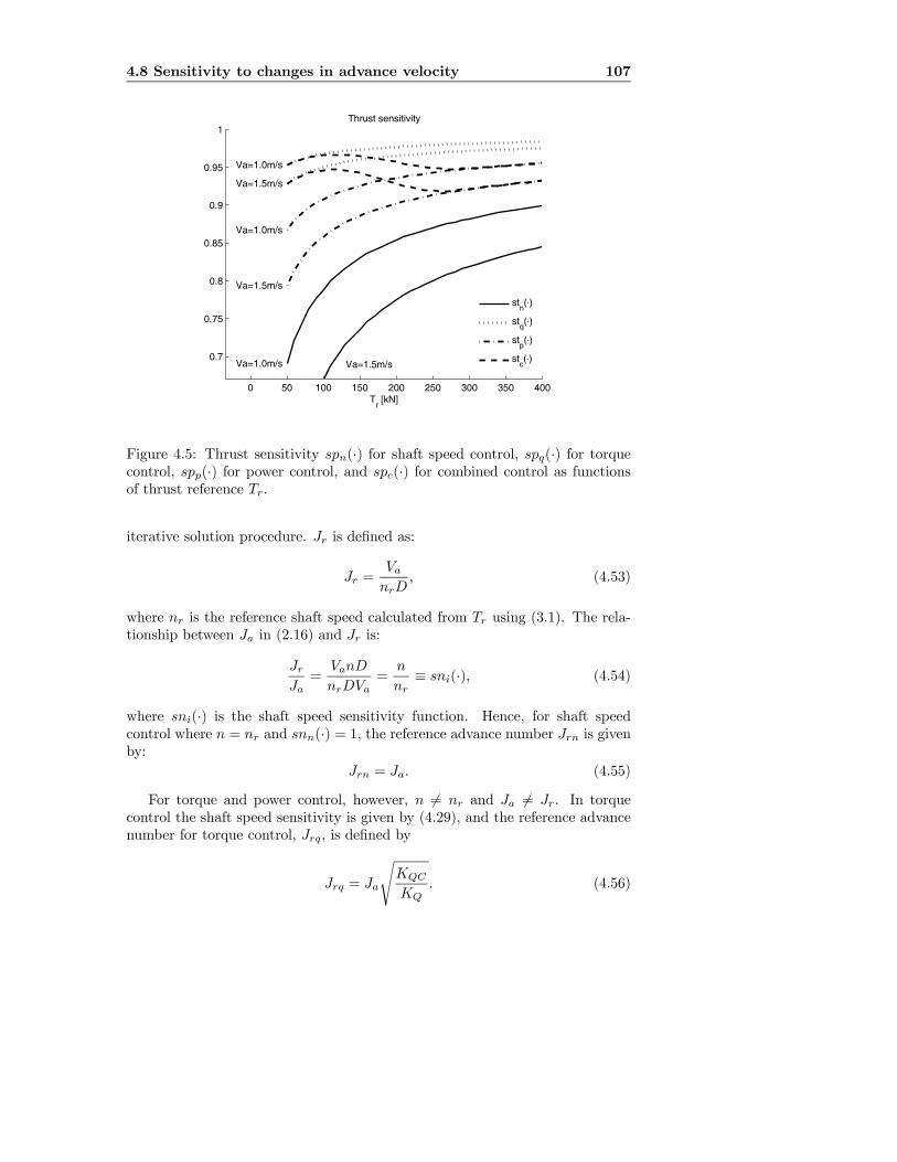
4.8 Sensitivity to changes in advance velocity 107
0 50 100 150 200 250 300 350 400
0.7
0.75
0.8
0.85
0.9
0.95
1Thrust sensitivity
Tr [kN]
Va=1.0m/s
Va=1.0m/s
Va=1.0m/s
Va=1.5m/s
Va=1.5m/s
Va=1.5m/s
stn(⋅)
stq(⋅)
stp(⋅)
stc(⋅)
Figure 4.5: Thrust sensitivity spn(·) for shaft speed control, spq(·) for torquecontrol, spp(·) for power control, and spc(·) for combined control as functionsof thrust reference Tr.
iterative solution procedure. Jr is defined as:
Jr =VanrD
, (4.53)
where nr is the reference shaft speed calculated from Tr using (3.1). The rela-tionship between Ja in (2.16) and Jr is:
JrJa=
VanD
nrDVa=
n
nr≡ sni(·), (4.54)
where sni(·) is the shaft speed sensitivity function. Hence, for shaft speedcontrol where n = nr and snn(·) = 1, the reference advance number Jrn is givenby:
Jrn = Ja. (4.55)
For torque and power control, however, n 6= nr and Ja 6= Jr. In torquecontrol the shaft speed sensitivity is given by (4.29), and the reference advancenumber for torque control, Jrq, is defined by
Jrq = Ja
sKQC
KQ. (4.56)

108 Sensitivity to thrust losses
For a deeply submerged propeller, there is a particular value of KQ for a givenJa, which again implies that there is a particular Jrq(Ja):
Jrq(Ja) = Ja
sKQC
KQ(Ja). (4.57)
Hence, it is possible to re-parameterizeKT andKQ as functions of Jrq instead ofJa (i.e. given Jrq, there exists particular values of KT and KQ). Furthermore,since Jrq is determined uniquely by Va and Tr, the sensitivity functions fortorque control are parameterized by Jrq using (4.57).Using the shaft speed sensitivity function for power control in (4.31) and the
same reasoning as for torque control, KT and KQ can be re-parameterized inthe power control reference advance ratio Jrp(Ja):
Jrp(Ja) = JaK1/3QC
KQ(Ja)1/3. (4.58)
For thrust control, KT and KQ can be re-parameterized in the thrust controlreference advance ratio Jrt(Ja) by using (4.33):
Jrt(Ja) = Ja
sKTC
KT (Ja). (4.59)
In order to establish the sensitivity functions without resorting to iteration, thefollowing procedure can now be followed:
1. Choose the range of Ja for which to calculate the sensitivity functionvalues.
2. For the chosen range of Ja, calculate the corresponding Jrn (speed con-trol), Jrq (torque control), Jrp (power control), and Jrt (thrust control)from Ja, KT , KQ, KTC , andKQC using the relationships defined in (4.55),(4.57), (4.58), and (4.59).
3. For each Jri, calculate the sensitivity functions from KT and KQ.
What actually happens is that the advance ratio axis is scaled individuallyfor each controller. Notice that neither Tr, Va, nor D appear explicitly inthe calculations. Figures 4.6 to 4.9 show the thrust, shaft speed, torque, andpower sensitivity functions for shaft speed, torque, power, and thrust controlas functions of Jr for the Wageningen B4-70 propeller. These curves are hencegeneralizations of the curves shown in Figures 4.1 to 4.4, with the additionof the sensitivity functions for thrust control. If thrust control is a feasiblesolution, these curves show that the increased performance in thrust productionis achieved by increasing the shaft speed, torque, and power additionally withrespect to the torque controller.

4.9 Sensitivity to large thrust losses 109
Remark 4.7 Since stt(·) = 1 by definition, the sensitivity curves for thrustcontrol are conveniently used to investigate how much the thrust setpoint mustbe increased to achieve a certain thrust for the various controllers, as discussedin Remark 4.4. Applying the same example, with Tr = 200kN and Va = 2m/s,the shaft speed reference nr ≈ 1.31rps from (3.1), and the reference advance ratiofrom (4.53) becomes Jr ≈ 0.38. For shaft speed control, Figure 4.7 shows thatJr ≈ 0.38⇒ snt ≈ 1.16. This means that in order to get Ta = 200kN, n must beincreased to n = nrsnt ≈ 1.52. Mapping n back to Tr using (3.5), the resultingthrust reference is Tr ≈ 270kN. Similarly, for torque control, Qr ≈ 120kNmfrom (3.2), and Figure 4.8 shows that Jr ≈ 0.38 ⇒ sqt ≈ 1.06. This meansthat in order to get Ta = 200kN, Qa must be increased to Qa = Qrsqt ≈ 127kN.Mapping Qa back to Tr using (3.6), the resulting thrust reference is Tr ≈ 212kN.Finally, for power control, Prs ≈ 985kW from (3.4), and Figure 4.9 shows thatJr ≈ 0.38⇒ spt ≈ 1.23. This means that in order to get Ta = 200kN, Pa mustbe increased to Pa = Prsspt ≈ 1212kW. Mapping Pa back to Tr using (3.7), theresulting thrust reference is Tr ≈ 230kN.
Remark 4.8 If some external integral action on Tr exists (e.g. a DP con-troller), such that Tr is increased until the desired Ta is produced, the meanvalues of Ta, Qa, Pa, and n will be the same for all the controllers. Hence, alsothe sensitivity functions will have the same values. The differences between thecontrollers then lie in the responses to dynamic load changes due to e.g. wavesand wave-frequency vessel motion, as well as the speed of convergence to thedesired Ta.
4.8.2 Friction compensation errors
In the derivation of the sensitivity functions, perfect friction compensation wasassumed. However, since Qff is a function of nr only, the linear compensationterm is not adjusted when the shaft speed differs from nr, as is the case in torque,power, and thrust control. This will give a small offset from the ideal sensitivityfunctions defined above, even with perfect model knowledge. In addition, ifthe static friction compensation term is wrong, such that Qf0 ≈ Qs, additionaloffsets from the ideal solutions are introduced. In either case, the sensitivityfunctions in terms of Jr will no longer be uniform for any Va, Tr, and D. Hence,the non-dimensional representation presented in Section 4.8.1 cannot be used.Appendix F.2 shows how the iterative solution procedure from Section 4.7 canbe modified to account for the friction compensation errors, and how the errorsaffect the resulting sensitivity functions.
4.9 Sensitivity to large thrust lossesThe sensitivity to the large thrust losses experienced during ventilation andwater exits may also be analyzed with the sensitivity functions. This can be
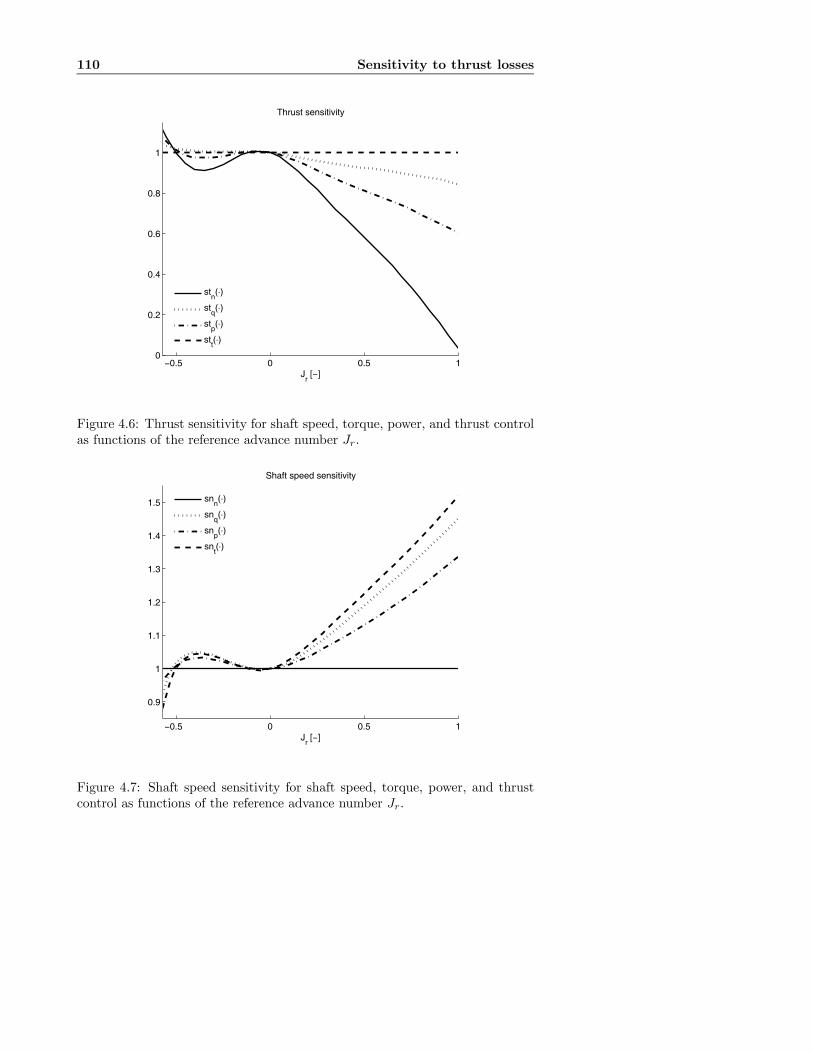
110 Sensitivity to thrust losses
−0.5 0 0.5 10
0.2
0.4
0.6
0.8
1
Thrust sensitivity
Jr [−]
stn(⋅)
stq(⋅)
stp(⋅)
stt(⋅)
Figure 4.6: Thrust sensitivity for shaft speed, torque, power, and thrust controlas functions of the reference advance number Jr.
−0.5 0 0.5 1
0.9
1
1.1
1.2
1.3
1.4
1.5
Shaft speed sensitivity
Jr [−]
snn(⋅)
snq(⋅)
snp(⋅)
snt(⋅)
Figure 4.7: Shaft speed sensitivity for shaft speed, torque, power, and thrustcontrol as functions of the reference advance number Jr.

4.9 Sensitivity to large thrust losses 111
−0.5 0 0.5 10.1
0.2
0.3
0.4
0.5
0.6
0.7
0.8
0.9
1
1.1
Torque sensitivity
Jr [−]
sqn(⋅)
sqq(⋅)
sqp(⋅)
sqt(⋅)
Figure 4.8: Torque sensitivity for shaft speed, torque, power, and thrust controlas functions of the reference advance number Jr.
−0.5 0 0.5 1
0.2
0.4
0.6
0.8
1
1.2
1.4
1.6
1.8Power sensitivity
Jr [−]
spn(⋅)
spq(⋅)
spp(⋅)
spt(⋅)
Figure 4.9: Power sensitivity for shaft speed, torque, power, and thrust controlas functions of the reference advance number Jr.
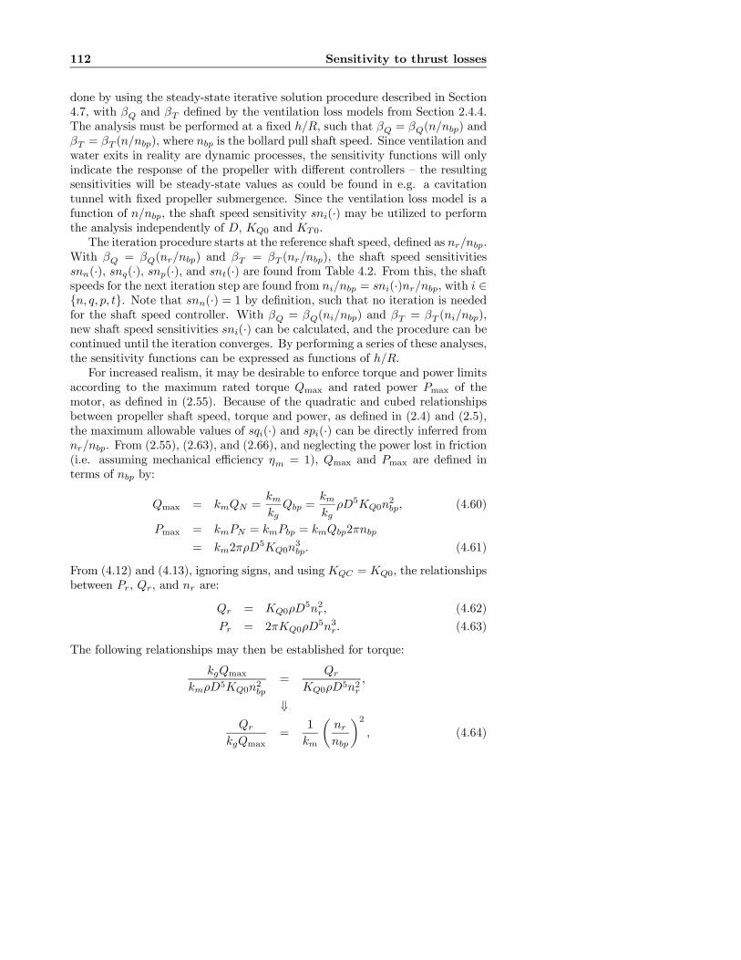
112 Sensitivity to thrust losses
done by using the steady-state iterative solution procedure described in Section4.7, with βQ and βT defined by the ventilation loss models from Section 2.4.4.The analysis must be performed at a fixed h/R, such that βQ = βQ(n/nbp) andβT = βT (n/nbp), where nbp is the bollard pull shaft speed. Since ventilation andwater exits in reality are dynamic processes, the sensitivity functions will onlyindicate the response of the propeller with different controllers — the resultingsensitivities will be steady-state values as could be found in e.g. a cavitationtunnel with fixed propeller submergence. Since the ventilation loss model is afunction of n/nbp, the shaft speed sensitivity sni(·) may be utilized to performthe analysis independently of D, KQ0 and KT0.The iteration procedure starts at the reference shaft speed, defined as nr/nbp.
With βQ = βQ(nr/nbp) and βT = βT (nr/nbp), the shaft speed sensitivitiessnn(·), snq(·), snp(·), and snt(·) are found from Table 4.2. From this, the shaftspeeds for the next iteration step are found from ni/nbp = sni(·)nr/nbp, with i ∈{n, q, p, t}. Note that snn(·) = 1 by definition, such that no iteration is neededfor the shaft speed controller. With βQ = βQ(ni/nbp) and βT = βT (ni/nbp),new shaft speed sensitivities sni(·) can be calculated, and the procedure can becontinued until the iteration converges. By performing a series of these analyses,the sensitivity functions can be expressed as functions of h/R.For increased realism, it may be desirable to enforce torque and power limits
according to the maximum rated torque Qmax and rated power Pmax of themotor, as defined in (2.55). Because of the quadratic and cubed relationshipsbetween propeller shaft speed, torque and power, as defined in (2.4) and (2.5),the maximum allowable values of sqi(·) and spi(·) can be directly inferred fromnr/nbp. From (2.55), (2.63), and (2.66), and neglecting the power lost in friction(i.e. assuming mechanical efficiency ηm = 1), Qmax and Pmax are defined interms of nbp by:
Qmax = kmQN =kmkg
Qbp =kmkg
ρD5KQ0n2bp, (4.60)
Pmax = kmPN = kmPbp = kmQbp2πnbp
= km2πρD5KQ0n
3bp. (4.61)
From (4.12) and (4.13), ignoring signs, and using KQC = KQ0, the relationshipsbetween Pr, Qr, and nr are:
Qr = KQ0ρD5n2r, (4.62)
Pr = 2πKQ0ρD5n3r. (4.63)
The following relationships may then be established for torque:
kgQmaxkmρD5KQ0n2bp
=Qr
KQ0ρD5n2r,
⇓Qr
kgQmax=
1
km
µnrnbp
¶2, (4.64)
4.9 Sensitivity to large thrust losses 113
and power:
Pmaxkm2πρD5KQ0n3bp
=Pr
2πKQ0ρD5n3r,
⇓PrPmax
=1
km
µnrnbp
¶3. (4.65)
The saturation limits sqmax for sqi(·) and spmax for spi(·) should correspond toQa = kgQmax and Pa = Pmax respectively, such that:
sqmax =kgQmaxQr
= km
µnrnbp
¶−2, (4.66)
spmax =PmaxPr
= km
µnrnbp
¶−3, (4.67)
where (4.64) and (4.65) have been inserted. This shows that if e.g. nr/nbp = 0.5is chosen as a starting point for the sensitivity analysis, the saturation limits fortorque and power become sqmax = 4km and spmax = 8km, where km = 1.1−1.2.Implementation of the torque and power limits requires an additional iterationprocedure to satisfy (4.66) or (4.67), which is activated if either limit is reached.Figure 4.10 shows the ventilation thrust loss sensitivity analysis for an open
propeller, i.e. with the ventilation loss function defined in Figure 2.18. Thethrust reference Tr corresponds to nr/nbp = 0.5. Curves for the shaft speed,torque, power, and thrust controllers are shown. Notice that the shaft speedsensitivity for some controllers exceeds 2, which corresponds to n/nbp = 1, sincethe shaft speed during ventilation can be higher than nbp without exceedingsqmax or spmax. In this analysis, the torque and power saturation limits werenot reached. With respect to the performance criteria defined in Section 3.2,these results show that the thrust production is least sensitive to the ventilationloss incident using the thrust controller, followed by the torque controller, powercontroller, and shaft speed controller. However, the increased thrust productionfrom the thrust and torque controllers will lead to excessive power consumptionand propeller racing. This will probably lead to severe dynamic loading of thepropeller, and hence increased mechanical wear and tear. The power controllerwill also lead to propeller racing, but keeps the power consumption constant.Figure 4.11 shows the same analysis for a ducted propeller, i.e. with the
ventilation loss function defined in Figure 2.19, with nr/nbp = 0.5 and km = 1.2such that sqmax = 4.8 and spmax = 9.6. In this analysis the power limit isreached both for the torque and the thrust controller. The other main differ-ence that can be noticed, is that all controllers give the same thrust when thepropeller is fully ventilated, as is inherent in the ventilation loss function forducted propellers. Hence, when compared to the shaft speed controller, theperformance of the thrust, torque, and power controllers is in this case evenworse than for the open propeller. In the extreme case of a water exit, when
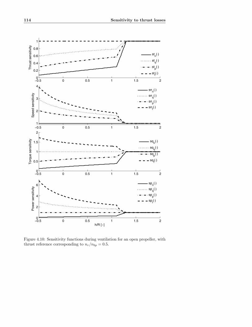
114 Sensitivity to thrust losses
−0.5 0 0.5 1 1.5 20
0.2
0.4
0.6
0.8
1
Thr
ust s
ensi
tivity
stn(⋅)
stq(⋅)
stp(⋅)
stt(⋅)
−0.5 0 0.5 1 1.5 21
2
3
4
Spe
ed s
ensi
tivity
snn(⋅)
snq(⋅)
snp(⋅)
snt(⋅)
−0.5 0 0.5 1 1.5 20
0.5
1
1.5
2
Tor
que
sens
itivi
ty sqn(⋅)
sqq(⋅)
sqp(⋅)
sqt(⋅)
−0.5 0 0.5 1 1.5 20
2
4
6
Pow
er s
ensi
tivity
h/R [−]
spn(⋅)
spq(⋅)
spp(⋅)
spt(⋅)
Figure 4.10: Sensitivity functions during ventilation for an open propeller, withthrust reference corresponding to nr/nbp = 0.5.
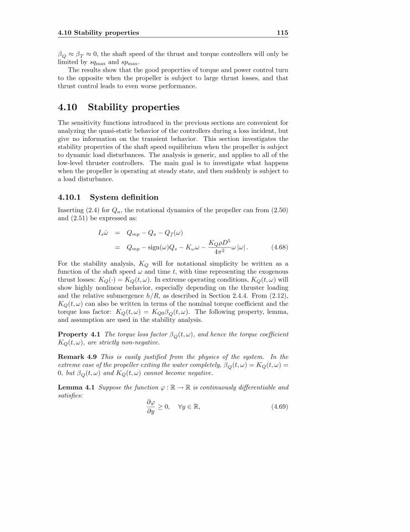
4.10 Stability properties 115
βQ ≈ βT ≈ 0, the shaft speed of the thrust and torque controllers will only belimited by sqmax and spmax.The results show that the good properties of torque and power control turn
to the opposite when the propeller is subject to large thrust losses, and thatthrust control leads to even worse performance.
4.10 Stability propertiesThe sensitivity functions introduced in the previous sections are convenient foranalyzing the quasi-static behavior of the controllers during a loss incident, butgive no information on the transient behavior. This section investigates thestability properties of the shaft speed equilibrium when the propeller is subjectto dynamic load disturbances. The analysis is generic, and applies to all of thelow-level thruster controllers. The main goal is to investigate what happenswhen the propeller is operating at steady state, and then suddenly is subject toa load disturbance.
4.10.1 System definition
Inserting (2.4) for Qa, the rotational dynamics of the propeller can from (2.50)and (2.51) be expressed as:
Isω = Qmp −Qa −Qf (ω)
= Qmp − sign(ω)Qs −Kωω −KQρD
5
4π2ω |ω| . (4.68)
For the stability analysis, KQ will for notational simplicity be written as afunction of the shaft speed ω and time t, with time representing the exogenousthrust losses: KQ(·) = KQ(t, ω). In extreme operating conditions, KQ(t, ω) willshow highly nonlinear behavior, especially depending on the thruster loadingand the relative submergence h/R, as described in Section 2.4.4. From (2.12),KQ(t, ω) can also be written in terms of the nominal torque coefficient and thetorque loss factor: KQ(t, ω) = KQ0βQ(t, ω). The following property, lemma,and assumption are used in the stability analysis.
Property 4.1 The torque loss factor βQ(t, ω), and hence the torque coefficientKQ(t, ω), are strictly non-negative.
Remark 4.9 This is easily justified from the physics of the system. In theextreme case of the propeller exiting the water completely, βQ(t, ω) = KQ(t, ω) =0, but βQ(t, ω) and KQ(t, ω) cannot become negative.
Lemma 4.1 Suppose the function ϕ : R→ R is continuously differentiable andsatisfies:
∂ϕ
∂y≥ 0, ∀y ∈ R, (4.69)
116 Sensitivity to thrust losses
−0.5 0 0.5 1 1.5 20
0.2
0.4
0.6
0.8
1
Thr
ust s
ensi
tivity
stn(⋅)
stq(⋅)
stp(⋅)
stt(⋅)
−0.5 0 0.5 1 1.5 20
2
4
6
8
10
Spe
ed s
ensi
tivity
snn(⋅)
snq(⋅)
snp(⋅)
snt(⋅)
−0.5 0 0.5 1 1.5 20
0.5
1
1.5
2
2.5
Tor
que
sens
itivi
ty
sqn(⋅)
sqq(⋅)
sqp(⋅)
sqt(⋅)
−0.5 0 0.5 1 1.5 20
5
10
Pow
er s
ensi
tivity
h/R [−]
spn(⋅)
spq(⋅)
spp(⋅)
spt(⋅)
Figure 4.11: Sensitivity functions during ventilation for a ducted propeller, withthrust reference corresponding to nr/nbp = 0.5.
4.10 Stability properties 117
then it follows that:
(y − y0)(ϕ(y)− ϕ(y0)) ≥ 0, ∀{y, y0} ∈ R. (4.70)
Proof. From the mean value theorem, see e.g. Khalil (2002), the followingrelationship holds:
ϕ(y)− ϕ(y0) =∂ϕ
∂y
¯y=z
(y − y0),
where z is a point on the line segment connecting y and y0. It follows that:
(y − y0)(ϕ(y)− ϕ(y0)) =∂ϕ
∂y
¯y=z
(y − y0)2 ≥ 0, ∀{y, y0} ∈ R. (4.71)
Assumption 4.1 The motor time constant Tm in (2.52) is negligible comparedto the mechanical time constant, such that Qm ≈ Qcm and Qmp ≈ Qc.
Remark 4.10 This is a common assumption — the motor dynamics are usuallydominated by the rotational dynamics, and may in practice be neglected, at leastfor full-scale thrusters.
The analysis proceeds by writing out the commanded torque, which from(3.18), (3.19), (3.20), (3.21), and (3.22) is expressed by:
Qc0 = Qci +Qif +Qff = Qci + Icωr + tanh(ωr/ε)Qf0 +Qf1ωr. (4.72)
Here, ωr = 2πnr, nr is defined in (3.1), and ε is given from (3.20) as:
ε = 2πnf/εf . (4.73)
Using Assumption 4.1, assuming that the torque limiting function is inactivesuch that Qc = Qc0, and inserting (4.72), the rotational dynamics in (4.68)becomes:
Isω = Qci + Icωr + tanh(ωr/ε)Qf0 +Qf1ωr
− sign(ω)Qs −Kωω −KQ(t, ω)ρD
5
4π2ω |ω|
= Qci + Isωr −Qs(tanh(ω/ε)− tanh(ωr/ε))−Kω(ω − ωr)
−KQ(t, ω)ρD5
4π2ω |ω|+ ωr(Ic − Is) + δQf1(ωr) + δQf2(ω),(4.74)
where the friction modelling error terms δQf1(ωr) and δQf2(ω) are:
δQf1(ωr) = tanh(ωr/ε)(Qf0 −Qs) + ωr(Qf1 −Kω), (4.75)
δQf2(ω) = (tanh(ω/ε)− sign(ω))Qs. (4.76)
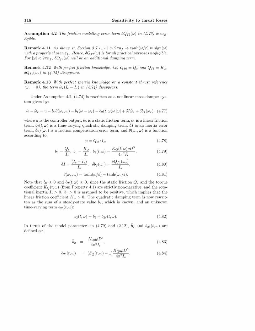
118 Sensitivity to thrust losses
Assumption 4.2 The friction modelling error term δQf2(ω) in (4.76) is neg-ligible.
Remark 4.11 As shown in Section 3.7.1, |ω| > 2πnf ⇒ tanh(ω/ε) ≈ sign(ω)with a properly chosen εf . Hence, δQf2(ω) is for all practical purposes negligible.For |ω| < 2πnf , δQf2(ω) will be an additional damping term.
Remark 4.12 With perfect friction knowledge, i.e. Qf0 = Qs and Qf1 = Kω,δQf1(ωr) in (4.75) disappears.
Remark 4.13 With perfect inertia knowledge or a constant thrust reference(ωr = 0), the term ωr(Ic − Is) in (4.74) disappears.
Under Assumption 4.2, (4.74) is rewritten as a nonlinear mass-damper sys-tem given by:
ω − ωr = u− b0θ(ωr, ω)− b1(ω − ωr)− b2(t, ω)ω |ω|+ δIωr + δbf (ωr), (4.77)
where u is the controller output, b0 is a static friction term, b1 is a linear frictionterm, b2(t, ω) is a time-varying quadratic damping term, δI is an inertia errorterm, δbf (ωr) is a friction compensation error term, and θ(ωr, ω) is a functionaccording to:
u = Qci/Is, (4.78)
b0 =Qs
Is, b1 =
Kω
Is, b2(t, ω) =
KQ(t, ω)ρD5
4π2Is, (4.79)
δI =(Ic − Is)
Is, δbf (ωr) =
δQf1(ωr)
Is, (4.80)
θ(ωr, ω) = tanh(ω/ε)− tanh(ωr/ε). (4.81)
Note that b0 ≥ 0 and b2(t, ω) ≥ 0, since the static friction Qs and the torquecoefficient KQ(t, ω) (from Property 4.1) are strictly non-negative, and the rota-tional inertia Is > 0. b1 > 0 is assumed to be positive, which implies that thelinear friction coefficient Kw > 0. The quadratic damping term is now rewrit-ten as the sum of a steady-state value b2, which is known, and an unknowntime-varying term b2δ(t, ω):
b2(t, ω) = b2 + b2δ(t, ω). (4.82)
In terms of the model parameters in (4.79) and (2.12), b2 and b2δ(t, ω) aredefined as:
b2 =KQ0ρD
5
4π2Is, (4.83)
b2δ(t, ω) = (βQ(t, ω)− 1)KQ0ρD
5
4π2Is. (4.84)
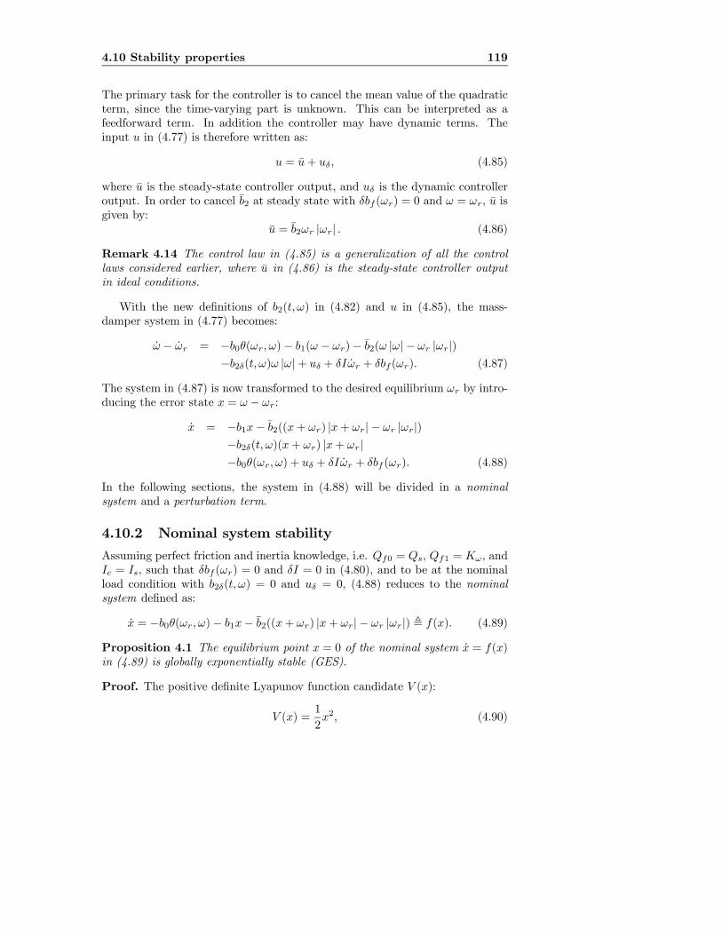
4.10 Stability properties 119
The primary task for the controller is to cancel the mean value of the quadraticterm, since the time-varying part is unknown. This can be interpreted as afeedforward term. In addition the controller may have dynamic terms. Theinput u in (4.77) is therefore written as:
u = u+ uδ, (4.85)
where u is the steady-state controller output, and uδ is the dynamic controlleroutput. In order to cancel b2 at steady state with δbf (ωr) = 0 and ω = ωr, u isgiven by:
u = b2ωr |ωr| . (4.86)
Remark 4.14 The control law in (4.85) is a generalization of all the controllaws considered earlier, where u in (4.86) is the steady-state controller outputin ideal conditions.
With the new definitions of b2(t, ω) in (4.82) and u in (4.85), the mass-damper system in (4.77) becomes:
ω − ωr = −b0θ(ωr, ω)− b1(ω − ωr)− b2(ω |ω|− ωr |ωr|)−b2δ(t, ω)ω |ω|+ uδ + δIωr + δbf (ωr). (4.87)
The system in (4.87) is now transformed to the desired equilibrium ωr by intro-ducing the error state x = ω − ωr:
x = −b1x− b2((x+ ωr) |x+ ωr|− ωr |ωr|)−b2δ(t, ω)(x+ ωr) |x+ ωr|−b0θ(ωr, ω) + uδ + δIωr + δbf (ωr). (4.88)
In the following sections, the system in (4.88) will be divided in a nominalsystem and a perturbation term.
4.10.2 Nominal system stability
Assuming perfect friction and inertia knowledge, i.e. Qf0 = Qs, Qf1 = Kω, andIc = Is, such that δbf (ωr) = 0 and δI = 0 in (4.80), and to be at the nominalload condition with b2δ(t, ω) = 0 and uδ = 0, (4.88) reduces to the nominalsystem defined as:
x = −b0θ(ωr, ω)− b1x− b2((x+ ωr) |x+ ωr|− ωr |ωr|) , f(x). (4.89)
Proposition 4.1 The equilibrium point x = 0 of the nominal system x = f(x)in (4.89) is globally exponentially stable (GES).
Proof. The positive definite Lyapunov function candidate V (x):
V (x) =1
2x2, (4.90)

120 Sensitivity to thrust losses
satisfies:k1 kxka ≤ V (x) ≤ k2 kxka , (4.91)
with a = 2 (Euclidian norm), k1 ≤ 1/2, and k2 ≥ 1/2 for all x ∈ R. Thederivative of V (x) along the trajectories of f(x) in (4.89) is:
V (x) = −b0θ(ωr, ω)x− b1x2
−b2((x+ ωr)− ωr)((x+ ωr) |x+ ωr|− ωr |ωr|). (4.92)
From Lemma 4.1, with ϕ(y) = y |y|, y = x+ ωr, and y0 = ωr, it is clear that:
((x+ ωr)− ωr)((x+ ωr) |x+ ωr|− ωr |ωr|) ≥ 0. (4.93)
Also from Lemma 4.1, with ϕ(y) = tanh(y/ε), y = ω, and y0 = ωr:
θ(ωr, ω)x = (tanh(ω/ε)− tanh(ωr/ε))(ω − ωr) ≥ 0. (4.94)
With b2 > 0 and b0 ≥ 0 it follows that:
V (x) ≤ −b1x2 ≤ −k3 kxka , (4.95)
with a = 2 and 0 < k3 ≤ b1 for all x ∈ R. The equilibrium point x = 0 istherefore GES.
Remark 4.15 In practice, the linear damping term b1x in (4.89) will be domi-nated by the quadratic damping term proportional to b2. This is further discussedin Appendix F.3, where it is shown that for |x| < |ωr|, V (x) complies to:
V (x) ≤ −(b1 + b2 |ωr|)x2. (4.96)
Hence, the result in (4.95) is conservative.
4.10.3 Perturbed system stability
In dynamic operating conditions, b2δ(t, ω) = 0 and uδ = 0 no longer holds.In general, also the friction error term δbf (ωr) 6= 0 and δI 6= 0. The system(4.88) can then be viewed as the sum of the nominal system in (4.89) and aperturbation term g(t, x):
x = f(x) + g(t, x), (4.97)
where f(x) is given in (4.89) and g(t, x) is defined as:
g(t, x) , uδ − b2δ(t, ω)(x+ ωr) |x+ ωr|+ δIωr + δbf (ωr). (4.98)
The perturbation term does not necessarily vanish at the origin x = 0, sinceg(t, 0) = b2δ(t, ω)ωr |ωr|+δIωr+δbf (ωr) 6= 0. g(t, x) is, therefore, a nonvanish-ing perturbation, which means that the origin will not be an equilibrium pointof the perturbed system.

4.10 Stability properties 121
Proposition 4.2 For any uniformly bounded disturbance g(t, x), the solutionsx(t) of the perturbed system in (4.97) are uniformly ultimately bounded (UUB).
Proof. V (x) given in (4.90) satisfies:°°°°∂V∂x°°°° ≤ k4 kxk , (4.99)
for all x ∈ R and k4 ≥ 1, since k∂V/∂xk = kxk. With the origin of the nominalsystem (4.89) exponentially stable, Lemma 9.2 in Khalil (2002) can be applied.Since (4.91), (4.95), and (4.99) are satisfied for all x ∈ R, they also hold forx ∈ Dr, where Dr is a ball of radius r:
Dr = {x ∈ R | kxk < r} . (4.100)
Assume that the perturbation term g(t, x) in (4.98) satisfies:
kg(t, x)k ≤ δ <k3k4
rk1k2
θr, (4.101)
∀t ≥ 0, ∀x ∈ Dr, and some positive constant θ < 1. The solution of theperturbed system then satisfies the bound:
kx(t)k ≤ ke−ξ(t−t0) kx(t0)k , ∀t0 ≤ t < t0 + T, (4.102)
for all kx(t0)k <pk1/k2r, and the ultimate bound:
kx(t)k ≤ b, ∀t ≥ t0 + T, (4.103)
for some finite T , where
k =
rk2k1
, ξ =(1− θ)k32k2
, b =k4k3
rk2k1
δ
θ. (4.104)
Hence, the solutions x(t) of (4.97) are UUB, and the ultimate bound b is pro-portional to the upper bound δ on the perturbation. Since the origin of thenominal system (4.89) is GES and δ → ∞ as r → ∞ in (4.101), x(t) will beUUB for all uniformly bounded perturbations.
Remark 4.16 The friction model error δbf (ωr) in (4.80) is expected to besmall. The effect of δbf (ωr) 6= 0 is from Proposition 4.2 that the equilibrium of(4.97) will be shifted.
Remark 4.17 For |ω| > 2πnf , Assumption 4.2 can be relaxed without implica-tions. For |ω| < 2πnf , relaxation of Assumption 4.2 will give a slightly shiftedequilibrium.

122 Sensitivity to thrust losses
4.10.4 Implications for shaft speed, torque, and powercontrol
The analysis in the previous sections considers a generic control law given in(4.85). This section investigates the implications of the stability analysis forshaft speed, torque, and power control. For the sake of simplicity, it is hereassumed that δIωr + δbf (ωr) = 0 in (4.98).In terms of the original system parameters, (4.85) translates to:
Qci = Qci + δQci =KQCρD
5
4π2ωr |ωr|+ δQci, (4.105)
where (4.83) and (4.78) have been inserted, Qci is the steady-state controlleroutput, and δQci is the dynamic controller output. KQC has been used insteadof KQ0 in (4.83) since KQC is the torque coefficient used in the controller. Thismeans that Qci ≡ Qr from (4.12).The shaft speed controller in (3.27) attempts to keep the shaft speed constant
regardless of the disturbance. In an ideal speed controller, this means that theperturbation term g(t, x) = 0 in (4.98), and hence that uδ = b2δ(t, ω)ω |ω|. Inthe system parameters, this translates to:
δQci = (βQ(t, ω)− 1)KQ0ρD
5
4π2ω |ω| , (4.106)
where (4.84) and (4.78) have been used. This essentially means that the changein propeller loading (parameterized by βQ(t, ω)) is instantly compensated forby the controller.The torque controller in (3.29) is a pure feedforward controller. Hence,
uδ = δQci = 0, such that u = u in (4.85) and Qci = Qci = Qr in (4.105).This means that g(t, x) in (4.98) consists only of the load perturbation. Thedisturbance bound δ in (4.101), and hence also the ultimate bound b in (4.104),will then depend only on the size of the perturbation, since the torque controllertakes no action to reduce the perturbation (and thereby control the shaft speed).The dynamic controller term of the power controller in (3.32) can be found
by equating Pr from (4.13) with the power implied by (4.105):
2πKQCρD5 |nr|3 = 2πn(KQCρD
5nr |nr|+ δQci)
⇓
δQci = KQCρD5nr |nr|
nr − n
n= Qr
nr − n
n, (4.107)
where Qr from (4.12) has been inserted. Hence, n = nr ⇒ δQci = 0. This showsthat the feedback from n will reduce the controller output when the shaft speedincreases, and increase the controller output when the shaft speed decreases withrespect to nr. Hence, the power controller will reduce g(t, x) when compared tothe torque controller, and hence also δ and b.

4.10 Stability properties 123
Remark 4.18 During ventilation the load may drop suddenly by 70-80%, asshown in Section 2.4. For the torque and power controllers, this means thatthe bound b will be large, such that the shaft speed will increase significantly.These considerations are consistent with the sensitivity analysis for high thrustlosses presented in Section 4.9: if no action is taken during ventilation, theperformance of the torque and power controllers will be unsatisfactory. Thismotivates the need for an anti-spin controller that can detect the ventilationincidents and take control of the shaft speed to reduce the propeller racing.

124 Sensitivity to thrust losses
Chapter 5
Propeller observers
Most of the work presented in this thesis is based on the assumption that theonly available measurements are the shaft speed n and the motor torque Qm.However, in some applications it will be convenient to have estimates of othersystem states. Based on the available measurements, this chapter introducesestimation schemes that can be used for e.g. performance monitoring, thrust lossestimation, ventilation detection, anti-spin thruster control, thrust allocation,and output feedback thrust control.
A physical limitation is that only thrust loss effects that are observable fromthe propeller can be estimated. In Section 2.3, the loss effects were divided intwo groups: losses that affect the propeller loading, and losses that affect thepropeller race. It is only the first group, which consists of variations in thein-line inflow to the propeller, ventilation, and in-and-out-of-water effects, thatcan be estimated in the low-level thruster control scheme.
Section 5.1 presents a propeller load torque observer. This is a modificationof the observer first introduced in Smogeli et al. (2004a). Section 5.2 presents analternative load torque estimation scheme based on nonlinear parameter estima-tion. Both schemes yield estimates of the load torque Qa, the torque coefficientKQ, and the torque loss factor βQ. Section 5.3 shows how estimates of the pro-peller thrust Ta and thrust loss factor βT in some cases may be deduced fromthe torque coefficient estimate. Performance monitoring for use in e.g. thrustallocation is treated in Section 5.4. Section 5.5 demonstrates the performanceof the various schemes by simulations. Extensions of the estimation schemes totransit and CPP is treated in Chapter 8. An adaptive load torque observer forthe case of an unknown linear friction coefficient can be found in Appendix G.

126 Propeller observers
5.1 Propeller load torque observer
From (2.50), the following control plant model of the propeller rotational dy-namics is proposed:
Isω = Qmp −Qa −Qff0(nr)−Qf1ω + δf ,
Qa = wQa. (5.1)
Since fQ(n,xp,θp) in (2.2) is unknown and may exhibit highly nonlinear behav-ior, Qa is modelled as a bias term driven by an exogenous, bounded disturbancewQa . The static friction compensation term Qff0(nr) from (3.20) is used in-stead of a static friction model based on ω, in order to avoid oscillations in thisterm about ω = 0. Errors in the friction model when compared to Qf (ω) in(2.51) are accounted for by δf :
δf = Qff0(nr)−Qf1ω −Qs sign(ω)−Kωω. (5.2)
With the measurement y = ω + v contaminated with a bounded disturbance vand the input u given by:
u = Qmp −Qff0(nr) = kgQm −Qff0(nr), (5.3)
the shaft dynamics (5.1) can be written on matrix form as:
x = Ax+Bu+ w,
y = Cx+ v, (5.4)
where:
x =
∙ωQa
¸, A =
∙−Qf1/Is −1/Is
0 0
¸,
B =
∙1/Is0
¸, w =
∙δf/IswQa
¸, C =
£1 0
¤. (5.5)
The system is observable from y, since the observability matrix:
O =
∙CCA
¸=
∙1 0
−Qf1/Is −1/Is
¸, (5.6)
has full rank. Copying the control plant model (5.1), the proposed propellerload torque observer is:
˙ω =1
Is
³u− Qa −Qf1ω
´+ ka(y − y),
˙Qa = kb(y − y), (5.7)
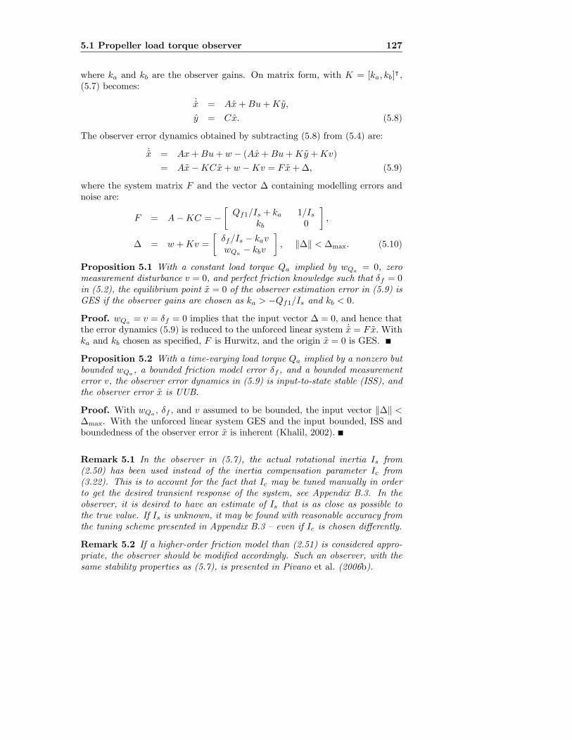
5.1 Propeller load torque observer 127
where ka and kb are the observer gains. On matrix form, with K = [ka, kb]| ,
(5.7) becomes:
˙x = Ax+Bu+Ky,
y = Cx. (5.8)
The observer error dynamics obtained by subtracting (5.8) from (5.4) are:
˙x = Ax+Bu+ w − (Ax+Bu+Ky +Kv)
= Ax−KCx+ w −Kv = Fx+∆, (5.9)
where the system matrix F and the vector ∆ containing modelling errors andnoise are:
F = A−KC = −∙Qf1/Is + ka 1/Is
kb 0
¸,
∆ = w +Kv =
∙δf/Is − kavwQa − kbv
¸, k∆k < ∆max. (5.10)
Proposition 5.1 With a constant load torque Qa implied by wQa= 0, zero
measurement disturbance v = 0, and perfect friction knowledge such that δf = 0in (5.2), the equilibrium point x = 0 of the observer estimation error in (5.9) isGES if the observer gains are chosen as ka > −Qf1/Is and kb < 0.
Proof. wQa = v = δf = 0 implies that the input vector ∆ = 0, and hence thatthe error dynamics (5.9) is reduced to the unforced linear system ˙x = Fx.Withka and kb chosen as specified, F is Hurwitz, and the origin x = 0 is GES.
Proposition 5.2 With a time-varying load torque Qa implied by a nonzero butbounded wQa , a bounded friction model error δf , and a bounded measurementerror v, the observer error dynamics in (5.9) is input-to-state stable (ISS), andthe observer error x is UUB.
Proof. With wQa , δf , and v assumed to be bounded, the input vector k∆k <∆max. With the unforced linear system GES and the input bounded, ISS andboundedness of the observer error x is inherent (Khalil, 2002).
Remark 5.1 In the observer in (5.7), the actual rotational inertia Is from(2.50) has been used instead of the inertia compensation parameter Ic from(3.22). This is to account for the fact that Ic may be tuned manually in orderto get the desired transient response of the system, see Appendix B.3. In theobserver, it is desired to have an estimate of Is that is as close as possible tothe true value. If Is is unknown, it may be found with reasonable accuracy fromthe tuning scheme presented in Appendix B.3 — even if Ic is chosen differently.
Remark 5.2 If a higher-order friction model than (2.51) is considered appro-priate, the observer should be modified accordingly. Such an observer, with thesame stability properties as (5.7), is presented in Pivano et al. (2006b).

128 Propeller observers
5.1.1 Observer tuning
The observer gains ka and kb can be tuned based on the error dynamics (5.9)using e.g. pole placement. The poles si are found from:
si =−(Qf1/Is + ka)±
p(Qf1/Is + ka)2 + 4kb/Is2
,
and the undamped natural frequency ωn and damping ratio ζ are:
ωn =
r−kbIs
, ζ =Qf1 + kaIs
2√−kbIs
. (5.11)
The gains may hence be chosen by specifying desired values for ωn and ζ:
ka = 2ζωn −Qf1/Is, kb = −Isω2n. (5.12)
Typically, the damping ratio could be chosen in the range 0.7 < ζ < 1.1.The natural frequency should be chosen according to the specific thruster. Asuggestion is choose it to be as fast as the bollard pull shaft speed nbp of thepropeller, i.e. ωn = 2πnbp. Using these rules for the 4MW Wageningen B4-70example propeller (see Appendix A), with ζ = 0.7 and ωn = 2π · 2 ≈ 12.6, thegains become:
ka ≈ 17.6, kb ≈ −4E6. (5.13)
5.1.2 Torque loss estimation
The estimated load torque Qa can be used to calculate an estimate βQ of thetorque loss factor βQ. For DP operation the expected nominal propeller loadtorque Qn may be calculated from (2.9) by feedback from the propeller shaftspeed n as:
Qn = KQCρD5n |n| , (5.14)
where the control coefficient KQC (usually equal to KQ0) is used. Based on(2.12), βQ is calculated from Qa in (5.7) and Qn in (5.14) as:
βQ =Qa
Qn
=Qa
KQCρD5n |n| , n 6= 0. (5.15)
βQ should be saturated by an upper limit βQ,max and a lower limit βQ,min inorder to avoid out-of-bounds values for low n, and the singularity for n = 0should be avoided. Since there are no thrust losses for n = 0, the singularitycan be avoided by redefining (5.15) as:
βQ = max(min([αb(n) + (1− αb(n))Qa/Qn], βQ,max), βQ,min), (5.16)
where αb(n) is a weighting function of the type (3.33), and the saturation limitsβQ,max and βQ,min have been implemented. Applying similar reasoning as in

5.2 KQ estimation 129
Section 3.13, it can be shown that the singularity is removed by choosing r ≥ 1.5in αb(n). In this work, the limits will be taken as βQ,max = 2 and βQ,min = 0.If desired, an estimate KQ of the torque coefficient is easily inferred from βQ in(5.16) by:
KQ = KQC βQ. (5.17)
5.2 KQ estimation
As an alternative to the load torque observer presented in Section 5.1, it is pos-sible to use a nonlinear online parameter estimation scheme to find an estimateKQ of the propeller torque coefficient. Estimates of the load torque Qa andtorque loss factor βQ can then be calculated directly from KQ, motivated by(2.4) and (2.12) respectively:
Qa = KQρD5n |n| , (5.18)
βQ = KQ/KQC . (5.19)
An advantage of this approach is that the singularity in the calculation of βQis removed.As in (5.1), the parameter estimation scheme is based on the shaft dynamics
in (2.50) and the friction model from (3.19), with the addition of the torquemodel from (2.4). The control plant model then becomes:
Isω = Qmp −KQρD
5
4π2ω |ω|−Qff0(nr)−Qf1ω. (5.20)
It is here assumed that the friction parameters are known, such that δf ≈ 0 in(5.2). Defining the input u as in (5.3) and the unknown parameter θ as:
θ =KQρD
5
4π2, (5.21)
the system in (5.20), which is affine in θ, can be rewritten as:
ω = f(ω, u, θ) = F (ω)θ + g(ω, u), (5.22)
where:
f(ω, u, θ) =1
Is(u− θω |ω|−Qf1ω), (5.23)
F (ω) =∂f(ω, u, θ)
∂θ= −ω |ω|
Is, (5.24)
g(ω, u) =1
Is(u−Qf1ω). (5.25)

130 Propeller observers
Proposition 5.3 The nonlinear parameter estimation scheme:
KQ =4π2
ρD5θ, (5.26)
θ = −k0|ω|3
3Is+ z, (5.27)
z = k0ω |ω|I2s
(u− θω |ω|−Qf1ω), (5.28)
will yield the error dynamics ˙θ = θ − ˙θ uniformly globally stable (UGS) for allω, and uniformly globally exponentially stable (UGES) for ω 6= 0.
Proof. From Friedland (1997), an estimate θ of θ can be obtained from thefollowing parameter update law:
θ = φ(ω) + z, (5.29)
z = −Φ(ω)f(ω, u, θ), (5.30)
where φ(ω) is a nonlinear function to be defined, and Φ(ω) its Jacobian:
Φ(ω) = ∂φ(ω)/∂ω. (5.31)
Assuming θ to be slowly-changing, the estimation error θ and its dynamics are:
θ = θ − θ,
˙θ = − ˙θ = −φ(ω)− z = −∂φ(ω)/∂ωω − z
= −Φ(ω)ω +Φ(ω)f(ω, u, θ)= −Φ(ω)[f(ω, u, θ)− f(ω, u, θ)]
= −Φ(ω)F (ω)(θ − θ) = −L(t)θ, (5.32)
where L(t) = Φ(ω(t))F (ω(t)) is time-varying. Stability properties are investi-gated by the positive definite Lyapunov function V (θ):
V (θ) =1
2θ2. (5.33)
The derivative of V along the trajectories of (5.32) is given by:
V = θ ˙θ = −L(t)θ2. (5.34)
It remains to choose φ(ω) to yield L(t) positive semidefinite. One option is tochoose φ(ω) to satisfy (Friedland, 1997):
Φ(ω) = k0F (ω) = −k0ω |ω|Is
, (5.35)
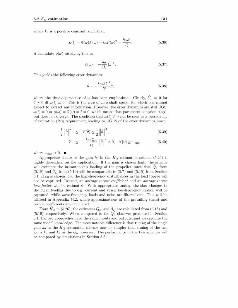
5.2 KQ estimation 131
where k0 is a positive constant, such that:
L(t) = Φ(ω)F (ω) = k0F (ω)2 =
k0ω4
I2s. (5.36)
A candidate φ(ω) satisfying this is:
φ(ω) = − k03Is
|ω|3 . (5.37)
This yields the following error dynamics:
˙θ = −k0ω(t)
4
I2sθ, (5.38)
where the time-dependence of ω has been emphasized. Clearly, V1 = 0 forθ 6= 0 iff ω(t) ≡ 0. This is the case of zero shaft speed, for which one cannotexpect to extract any information. However, the error dynamics are still UGS:ω(t) = 0⇒ φ(ω) = Φ(ω) = z = 0, which means that parameter adaption stops,but does not diverge. The condition that ω(t) 6= 0 can be seen as a persistencyof excitation (PE) requirement, leading to UGES of the error dynamics, since:
1
2
°°°θ°°°2 ≤ V (θ) ≤ 12
°°°θ°°°2 , (5.39)
V ≤ −k0ω4min
I2s
°°°θ°°°2 < 0, ∀ |ω| ≥ ωmin. (5.40)
where ωmin > 0.Appropriate choice of the gain k0 in the KQ estimation scheme (5.26) is
highly dependent on the application. If the gain is chosen high, the schemewill estimate the instantaneous loading of the propeller, such that Qa from(5.18) and βQ from (5.19) will be comparable to (5.7) and (5.15) from Section5.1. If k0 is chosen low, the high-frequency disturbances in the load torque willnot be captured. Instead, an average torque coefficient and an average torqueloss factor will be estimated. With appropriate tuning, the slow changes inthe mean loading due to e.g. current and vessel low-frequency motion will becaptured, while wave-frequency loads and noise are filtered out. This will beutilized in Appendix G.2, where approximations of the prevailing thrust andtorque coefficients are calculated.From KQ in (5.26), the estimates Qa, and βQ are calculated from (5.18) and
(5.19), respectively. When compared to the Qa observer presented in Section5.1, the two approaches have the same inputs and outputs, and also require thesame model knowledge. The most notable difference is that tuning of the singlegain k0 in the KQ estimation scheme may be simpler than tuning of the twogains ka and kb in the Qa observer. The performance of the two schemes willbe compared by simulations in Section 5.5.

132 Propeller observers
5.3 Thrust estimationIn some applications it is feasible to use the estimated propeller torque to es-timate also the propeller thrust. For open propellers, it was in Section 2.1.8shown that a linear relationship between KT and KQ holds across a wide rangeof operating conditions. Motivated by (2.48), an estimate KT can be calculatedfrom KQ in (5.17) or (5.26) by:
KT = atKQ + bt, (5.41)
where at and bt are propeller constants inferred from the open-water character-istics. From (2.3) and (2.11), estimates Ta of the propeller thrust and βT of thethrust loss factor are then found from:
Ta = KT ρD4n |n| , (5.42)
βT = KT /KTC . (5.43)
A similar thrust estimation scheme is presented in more detail in Pivano etal. (2006b), and experimentally validated in Pivano et al. (2006a). The thrustestimate will be utilized in Appendix E.3.1, where an output feedback thrustcontroller is proposed.
5.4 Performance monitoring
Whereas βQ gives important information on the local operating conditions of thepropeller, no information of its performance with respect to the thrust setpointTd can be directly inferred. This is due to the fact that βQ is calculated fromthe measured shaft speed. Depending on the low-level thruster controller andthe instantaneous propeller operating conditions, the shaft speed, thrust, andtorque may deviate significantly from the reference values. This was furtheranalyzed in Chapter 4. For performance monitoring of the thruster, the mainidea is to compare the actual thrust production with the thrust reference. Sincethe estimated thrust Ta only can be estimated with reasonable accuracy for anopen propeller, it is in general necessary to use Qa from (5.7) or (5.18) for theperformance monitoring. The proposed torque performance factor estimate χQis defined as the ratio of Qa to the reference load torque Qr from (3.2):
χQ =Qa
Qr=
Qa
KQC
KTCDTr
, Tr 6= 0. (5.44)
χQ is singular for Tr = 0, so a similar precaution as for βQ in (5.16) should betaken for the zero-crossing of Tr:
χQ = αχ(Tr) + (1− αχ(Tr))Qa
Qr, (5.45)
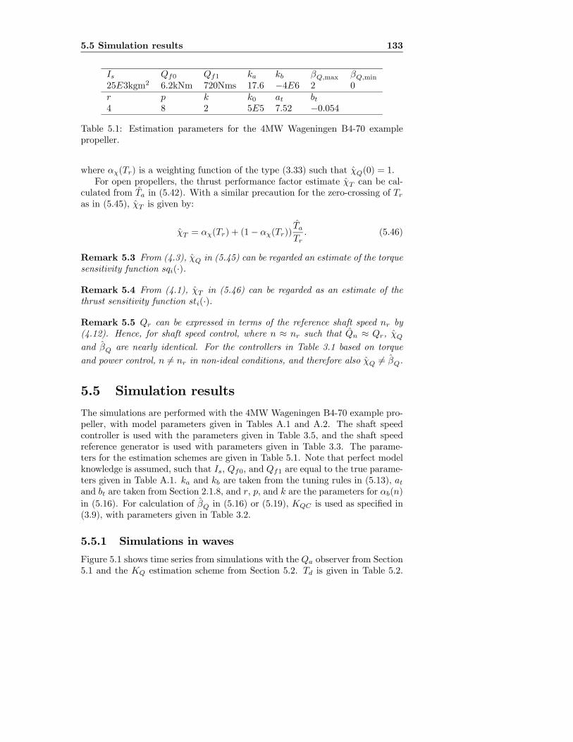
5.5 Simulation results 133
Is Qf0 Qf1 ka kb βQ,max βQ,min25E3kgm2 6.2kNm 720Nms 17.6 −4E6 2 0r p k k0 at bt4 8 2 5E5 7.52 −0.054
Table 5.1: Estimation parameters for the 4MW Wageningen B4-70 examplepropeller.
where αχ(Tr) is a weighting function of the type (3.33) such that χQ(0) = 1.For open propellers, the thrust performance factor estimate χT can be cal-
culated from Ta in (5.42). With a similar precaution for the zero-crossing of Tras in (5.45), χT is given by:
χT = αχ(Tr) + (1− αχ(Tr))TaTr
. (5.46)
Remark 5.3 From (4.3), χQ in (5.45) can be regarded an estimate of the torquesensitivity function sqi(·).
Remark 5.4 From (4.1), χT in (5.46) can be regarded as an estimate of thethrust sensitivity function sti(·).
Remark 5.5 Qr can be expressed in terms of the reference shaft speed nr by(4.12). Hence, for shaft speed control, where n ≈ nr such that Qn ≈ Qr, χQand βQ are nearly identical. For the controllers in Table 3.1 based on torqueand power control, n 6= nr in non-ideal conditions, and therefore also χQ 6= βQ.
5.5 Simulation results
The simulations are performed with the 4MW Wageningen B4-70 example pro-peller, with model parameters given in Tables A.1 and A.2. The shaft speedcontroller is used with the parameters given in Table 3.5, and the shaft speedreference generator is used with parameters given in Table 3.3. The parame-ters for the estimation schemes are given in Table 5.1. Note that perfect modelknowledge is assumed, such that Is, Qf0, and Qf1 are equal to the true parame-ters given in Table A.1. ka and kb are taken from the tuning rules in (5.13), atand bt are taken from Section 2.1.8, and r, p, and k are the parameters for αb(n)in (5.16). For calculation of βQ in (5.16) or (5.19), KQC is used as specified in(3.9), with parameters given in Table 3.2.
5.5.1 Simulations in waves
Figure 5.1 shows time series from simulations with the Qa observer from Section5.1 and the KQ estimation scheme from Section 5.2. Td is given in Table 5.2.
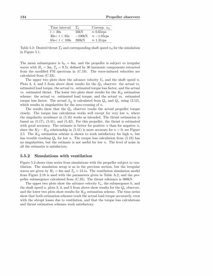
134 Propeller observers
Time interval Td Corresp. ndt < 30s 50kN ≈ 0.65rps30s< t < 65s −100kN ≈ −1.05rps65s< t < 100s 200kN ≈ 1.31rps
Table 5.2: Desired thrust Td and corresponding shaft speed nd for the simulationin Figure 5.1.
The mean submergence is h0 = 6m, and the propeller is subject to irregularwaves with Hs = 3m, Tp = 9.7s, defined by 30 harmonic components extractedfrom the modified PM spectrum in (C.19). The wave-induced velocities arecalculated from (C.33).The upper two plots show the advance velocity Va and the shaft speed n.
Plots 3, 4, and 5 from above show results for the Qa observer: the actual vs.estimated load torque, the actual vs. estimated torque loss factor, and the actualvs. estimated thrust. The lower two plots show results for the KQ estimationscheme: the actual vs. estimated load torque, and the actual vs. estimatedtorque loss factor. The actual βQ is calculated from Qa and Qn using (2.12),which results in singularities for the zero-crossing of n.The results show that the Qa observer tracks the actual propeller torque
closely. The torque loss calculation works well except for very low n, wherethe singularity avoidance in (5.16) works as intended. The thrust estimation isbased on (5.17), (5.41), and (5.42). For this propeller, the thrust is estimatedwith good accuracy. The estimate is better for positive n than for negative n,since the KT −KQ relationship in (5.41) is more accurate for n > 0; see Figure2.5. The KQ estimation scheme is shown to work satisfactory for high n, buthas trouble tracking Qa for low n. The torque loss calculation from (5.19) hasno singularities, but the estimate is not useful for low n. The level of noise inall the estimates is satisfactory.
5.5.2 Simulations with ventilation
Figure 5.2 shows time series from simulations with the propeller subject to ven-tilation. The simulation setup is as in the previous section, but the irregularwaves are given by Hs = 8m and Tp = 13.1s. The ventilation simulation modelfrom Figure 2.18 is used with the parameters given in Table A.2, and the pro-peller submergence calculated from (C.35). The thrust reference is 300kN.The upper two plots show the advance velocity Va, the submergence h, and
the shaft speed n, plots 3, 4, and 5 from above show results for the Qa observer,and the lower two plots show results for KQ estimation scheme. The time seriesshow that both estimation schemes track the actual load torque accurately, evenwith the abrupt losses due to ventilation, and that the torque loss calculationsand thrust estimation schemes work satisfactory.
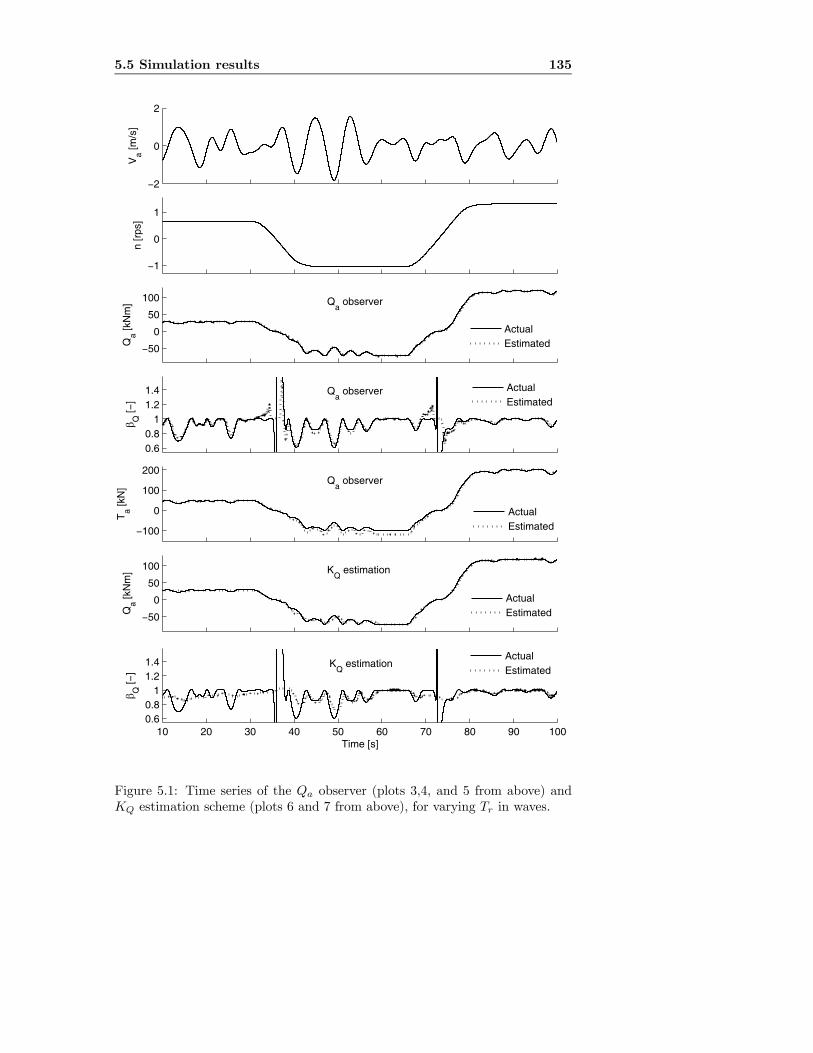
5.5 Simulation results 135
−2
0
2
Va [m
/s]
−1
0
1
n [r
ps]
−50
0
50
100
Qa [k
Nm
] Qa observer
ActualEstimated
0.60.8
11.21.4
β Q [−
]
Qa observer Actual
Estimated
−100
0
100
200
Ta [k
N]
Qa observer
ActualEstimated
−50
0
50
100
Qa [k
Nm
] KQ
estimation
ActualEstimated
10 20 30 40 50 60 70 80 90 1000.60.8
11.21.4
Time [s]
β Q [−
]
KQ
estimationActualEstimated
Figure 5.1: Time series of the Qa observer (plots 3,4, and 5 from above) andKQ estimation scheme (plots 6 and 7 from above), for varying Tr in waves.

136 Propeller observers
−5
0
5
10
15 Va [m/s]
h [m]
1.561.58
1.61.621.641.661.68
n [r
ps]
−500
50100150
Qa [k
Nm
]
Qa observer
ActualEstimated
0
0.5
1
β Q [−
]
Qa observer
ActualEstimated
−100
0
100
200
300
Ta [k
N]
Qa observer
ActualEstimated
−500
50100150
Qa [k
Nm
]
KQ
estimation
ActualEstimated
10 20 30 40 50 60 70 80 90 100
0
0.5
1
Time [s]
β Q [−
]
KQ
estimation
ActualEstimated
Figure 5.2: Time series of the Qa observer (plots 3,4, and 5 from above) and KQ
estimation scheme (plots 6 and 7 from above), for Tr = 300kN in large waves,with the propeller subject to ventilation.
Chapter 6
Propulsion control inextreme conditions
The various controllers designed in Chapter 3 have so far mainly been evaluatedfor normal operating conditions, i.e. subject to moderate thrust losses. Fromthe simulations in Section 3.18 and the sensitivity analysis in Section 4.8, it wasfound that controllers based on torque and power control have many desirableproperties. However, as shown in Section 2.4, a propeller subject to extremeconditions may experience large load transients due to ventilation and in-and-out-of water effects. The controllers designed for normal conditions may thenno longer give satisfactory performance. This was briefly treated in Section 4.9,where the controller performance when subject to large thrust losses was inves-tigated with the quasi-static sensitivity functions, and in Section 4.10, where thestability properties of the shaft speed equilibrium was investigated. The resultsshowed that the torque and power controllers have very poor performance insuch conditions: since the objectives of torque and power control are to keepthe motor torque or power constant, a loss of propeller load torque will leadto severe motor racing. As discussed in Sections 2.4.6 and 3.2.2, this leads tomechanical wear and tear because of the unsteady loading of the propeller. Thetorque controller will also give excessive power consumption. The shaft speedcontroller is partly able to handle the high thrust losses, since the objective ofthe controller is to keep the shaft speed constant. However, problems couldarise because a well-tuned PID controller for normal conditions may give badperformance when subject to the rapid variations in load torque experiencedduring ventilation.
To assure satisfactory performance for all conditions, it is therefore necessaryto introduce a new control strategy for use also in extreme conditions. Thisstrategy has been denoted anti-spin thruster control. The nature of the controltask is in many ways similar to that of controlling a car wheel with loss oftraction on a slippery surface during acceleration or braking. The work on anti-

138 Propulsion control in extreme conditions
spin thruster control has therefore been motivated by similar control strategies incar anti-spin and ABS braking systems, see for example Haskara et al. (2000) orJohansen et al. (2001) and the references therein. This is also further discussedin Smogeli et al. (2006).The concept of anti-spin thruster control was first introduced in Smogeli et
al. (2003), followed by the introduction of combined torque/power control and aload torque observer with loss estimation in Smogeli et al. (2004a). Based on thetwo previous publications, the first complete anti-spin thruster control solutionwas presented in Smogeli et al. (2004b). The concept was further analyzed inSmogeli et al. (2006), where also two new, simplified anti-spin solutions werepresented. Experimental results and a stability analysis of the proposed conceptis presented in Smogeli and Sørensen (2006b).
6.1 Anti-spin control objectivesThe general objectives of a thruster controller, as discussed in Section 3.2, areindependent of the operating condition. However, because of the special natureof the ventilation losses, some additional considerations on the control objectivesin extreme conditions are appropriate. The main objectives of anti-spin thrustercontrol are to:
• Reduce the mechanical wear and tear of the propulsion unit.
• Limit power peaks.
• Assure robust and predictable performance.
From the experimental results with ventilated propellers, as presented in Sec-tions 2.4.1 and 2.4.2 and Appendix D — and also from the discussions on me-chanical wear and tear in Sections 2.4.6 and 3.2.2 — the following observationsrelevant to low-level thruster control can be made:
• Ventilation may occur abruptly when the propeller is operated at highloading and close to the free surface. It is a stochastic process that cannoteasily be predicted.
• A ventilated propeller experiences large high-frequency loads and vibra-tions due to blade-frequency loading. The severity of these dynamic loadsincrease with the shaft speed.
• For a highly loaded propeller, the thrust during ventilation is almost in-dependent of the shaft speed, especially for ducted propellers. For openpropellers, a small increase in thrust is achievable by increasing the shaftspeed.
• From a quasi-static point of view, there appears to be an optimal shaftspeed that gives the highest thrust (“optimal thrust”) during ventilation,
6.2 The anti-spin control concept 139
especially for ducted propellers. Once ventilation has occurred, however,even a significant reduction of shaft speed may be insufficient for terminat-ing the air suction (see Figure 2.15 and Remark 2.9). Hence, the optimalthrust can only be achieved by avoiding ventilation inception. This is notconsidered a realistic option, since it is assumed that ventilation cannotbe predicted.
To summarize, the shaft speed of a highly loaded propeller during ventilationshould be lowered in order to reduce the mechanical wear and tear. This canbe done without significantly affecting the thrust production. From a totalevaluation of the control objectives and the known behavior of a ventilatingpropeller, it is hence found that the following actions are the most appropriateduring ventilation:
1. Primary anti-spin action: take control of the shaft speed.
2. Secondary anti-spin action: reduce the shaft speed.
The first action mainly applies to the torque and power controllers, which suf-fer from severe propeller racing during ventilation. The second action appliesequally to all controllers. Its main objective is to reduce mechanical wear andtear, and ease the transition back to the fully loaded condition.
6.2 The anti-spin control concept
The proposed anti-spin concept is a hybrid control scheme, where the conditionof the thruster is monitored, and anti-spin control actions are invoked whena ventilation incident is detected. The complete thruster control scheme iscomposed of four main functions:
1. The core thruster controller, which normally is left to work undisturbed.This could be any of the controllers in Table 3.1.
2. A performance monitoring scheme. This would typically be one of theobservers presented in Chapter 5.
3. A ventilation detection scheme, based on the output of the performancemonitoring scheme.
4. An anti-spin controller, which is invoked by the ventilation detectionscheme.
A block diagram of the proposed anti-spin control concept is shown in Figure6.1, where the performance monitoring and ventilation detection schemes havebeen assembled in one block. When comparing this figure with the structure ofthe control scheme for normal conditions in Figure 3.1, the proposed concept can

140 Propulsion control in extreme conditions
nf
Q
Q
Ta
a
T
m( )
fQ ( ).
.Motordynamics
Qc
.
Tr
Shaftdynamics
Propulsion unit
Monitoringand
detection
Anti-spincontroller
Torquelimit
PmaxQmax
n
Qm
Control scheme
p xpq
p xpq
Qc0Core thrustercontroller
Td Referencegenerator
Tr
Figure 6.1: Block diagram of the proposed anti-spin control concept, includingthe core thruster controller, detection scheme, and anti-spin controller.
be seen as an add-on of the two functional blocks “Monitoring and detection”and “Anti-spin controller”.In this work, anti-spin thruster control is primarily treated as a necessary
addition to the controllers based on torque and/or power control, since thesehave been found preferable in normal operating conditions. However, it mayalso be possible to improve the performance of a shaft speed controller duringventilation by introducing anti-spin control: a primary anti-spin action can beadded in order to improve the transient performance at ventilation inceptionand termination, and a secondary anti-spin action can be used to reduce theshaft speed during ventilation. This is shortly treated in Section 6.6.3.
6.3 Ventilation detection
The detection of high thrust losses may be done in several ways. A simplisticapproach is to set the detection criteria by rate of change of shaft speed and/ormotor torque — if the shaft speed increases quickly or the torque drops quickly,this indicates a high loss situation. A similar approach for car wheel anti-spinwas presented in Haskara et al. (2000). A more sophisticated detection algorithmcan be designed based on the performance monitoring tools presented in Chapter5. Since the anti-spin control scheme is highly dependent on fast and accuratedetection of the ventilation incidents, the latter approach has been preferred.Estimates of the propeller load torque, torque coefficient, and torque loss
factor can be found from the propeller load torque observer in (5.7), or the KQ
estimation scheme in (5.26). From experience with the various formulations, theload torque torque observer in (5.7) has been found to give the best over-all per-formance. The torque loss estimate βQ is then calculated from (5.16), and theventilation detection is done by monitoring βQ and the motor torque Qm. Thedetection algorithm is implemented by defining limits for the onset and termi-

6.4 Anti-spin control actions 141
nation of ventilation, βv,on and βv,off . An additional criterion for detection isthat the magnitude of the motor torque is non-increasing, i.e. sign(Qm)Qm ≤ 0.Finally, the detection scheme should only be active for |nr| > nmin, where nminis a chosen threshold, and nr given from (3.1). This is to avoid false detectionand chattering for low propeller loading, where anti-spin control is not needed— the simulation results in Section 5.5 clearly showed that the loss estimationwas unreliable for low n.The detection signal is termed ζ. It is set to 1 when ventilation is detected,
and 0 otherwise. A typical ventilation incident will then give the followingevolution of ζ, with time instants t1 < t2 < t3:
t1 : βQ > βv,on ⇒ ζ = 0,
t2 : βQ ≤ βv,on ∩ sign(Qm)Qm ≤ 0 ∩ |nr| > nmin ⇒ ζ = 1,
t3 : βQ ≥ βv,off ⇒ ζ = 0.
(6.1)
To avoid switching and chattering of ζ due to measurement noise and transients,an algorithm implementing a detection delay is added, such that once ζ haschanged value, it cannot be reset until after a given time interval Tvent. Thedetection delay can be seen as an implementation of the switching dwell-timeproposed in Hespanha and Morse (2002) and Hespanha et al. (2003). Themotor torque should be low-pass filtered before numerical differentiation. Thisventilation detection scheme has shown good performance in both simulationsand experiments.
Remark 6.1 To allow natural oscillations about the nominal propeller loadingdue to time-varying inflow to the propeller, and noise in the estimate βQ, βv,onmust be chosen significantly lower than 1.
6.4 Anti-spin control actions
During operation in normal conditions, one of the core thruster controllers pro-posed in Table 3.1 is used. When extreme conditions are encountered, theanti-spin control actions are triggered by the ventilation detection algorithm.Different approaches to the anti-spin actions are possible, with the two mostgeneral being:
1. Switch to a completely new control strategy.
2. Modify the existing control strategy.
If an approach with switching is chosen, two options exist:
1a. Switch anti-spin on and off every time ventilation is detected and termi-nated.

142 Propulsion control in extreme conditions
1b. Switch to an anti-spin control mode when ventilation is first detected, andstay in this mode until no ventilation incidents have been detected for agiven time interval.
Alternative 1a may introduce problems with ensuring performance and stabilityduring switching, although new results have improved the ability to analyze sta-bility of such switching control schemes (Hespanha and Morse, 2002; Hespanhaet al., 2003). Bumpless transfer and switching problems are also discussed infor example Åström and Wittenmark (1997). This approach will not be furthertreated here. Alternative 1b is a more practical approach for this problem —one could e.g. use a controller based on torque and power control for normalconditions, and once a ventilation incident is detected switch to shaft speedcontrol. This scheme is of course based on the presumption that the shaft speedcontroller has acceptable performance during ventilation. An implementationlike this was apparently used for the diesel engine governor presented in Blankeand Busk Nielsen (1987, 1990); when the governor was run in power mode, andan excessive shaft speed was detected, the governor was automatically switchedto shaft speed control.The switching problem of strategy 1a is alleviated by choosing the second
anti-spin approach. In this case, the existing control strategy must be compati-ble with the desired anti-spin control actions. Two natural modifications of thecore thruster control strategies when ventilation is detected are:
2a. Reduce the controller output Qci (3.18) in order to reduce the motor torqueand lower the shaft speed.
2b. Lower the thrust reference Tr in order to reduce the motor torque indirectly.
The torque and thrust modification factors are termed γQ and γT , respectively,and used such that the anti-spin commanded torque Qcas and anti-spin thrustreference Tras are defined as:
Qcas = γQQci, (6.2)
Tras = γTTr. (6.3)
In the next section, it will be shown that alternative 2a, i.e. (6.2), is convenientfor implementing the primary anti-spin action, which is to take control of theshaft speed, while alternative 2b, i.e. (6.3), is convenient for implementing thesecondary anti-spin action, which is to reduce the shaft speed to an appropriatevalue.
6.5 Main anti-spin control result: torque scalingThe proposed anti-spin controller is based on the ventilation detection schemefrom Section 6.3, which gives a detection signal ζ ∈ {0, 1}, and the estimatedtorque loss factor βQ from Section 5.1.
6.5 Main anti-spin control result: torque scaling 143
6.5.1 Primary anti-spin action
The primary anti-spin control action will be motivated from a Lyapunov stabilityanalysis, with the analysis from Section 4.10 as a starting point. The followingassumption is made for the anti-spin analysis:
Assumption 6.1 The friction and inertia coefficients are known, such thatδbf (ωr) = 0 and δI = 0 in (4.80).
Under Assumption 6.1, the rotational dynamics in (4.88) is written as:
x = −b1x− b2((x+ ωr) |x+ ωr|− ωr |ωr|)−b2δ(t, ω)(x+ ωr) |x+ ωr|− b0θ(ωr, ω) + uδ
= f(x) + g(t, x), (6.4)
where f(x) is defined in (4.89). g(t, x) from (4.98) (under Assumption 6.1) isrewritten as:
g(t, x) = uδ + (1− βQ(t, x+ ωr))b2(x+ ωr) |x+ ωr| . (6.5)
Note that (4.84) has been used to insert b2δ(t, ω) = −(1− βQ(t, ω))b2.Assume that the propeller is initially operating at steady state with input u
and quadratic damping coefficient b2. The loading of the propeller then changesdue to a ventilation incident, described by the torque loss factor βQ(t, ω). Mo-tivated by (6.2), the primary anti-spin action is to modify the controller outputQci with a torque scaling factor γQ:
Qcas = γQQci ⇔ u = γQu, (6.6)
where Qcas is the anti-spin commanded torque. During ventilation, γQ is pro-posed to be given by γQ = βQ. In normal operation, γQ = 1 such thatQcas = Qci. In order to reduce transients, the transitions of γQ between 1and βQ at ventilation detection and termination should not be done abruptly.It is therefore proposed to add a rate limiting function as given in (3.11) withslew rate limits γrise > 0 and γfall < 0, and a first order low-pass filter withtime constant τγ . The filter will also remove noise in the estimate βQ thatotherwise would have been inserted into the control law. The implementationof γQ becomes:
γ1 =
½1 for ζ = 0 (not ventilated),βQ for ζ = 1 (ventilated),
γ2 = fslew(γ1, γrise, γfall),
γQ(s) = γ2(s)1
τγs+ 1, (6.7)
where γ1 and γ2 are internal states. Tuning of γrise, γfall, and τγ is discussedin Section 6.8.1.

144 Propulsion control in extreme conditions
Theorem 6.1 In the presence of an unknown disturbance βQ(t, ω), the primaryanti-spin control law from (6.6) and (6.7):
u = γQu, (6.8)
will yield the solutions x(t) of (6.4) UUB.
Proof. With u given by (6.8), uδ = (γQ − 1)u. Inserting u from (4.86), theperturbation term g(t, x) in (6.5) becomes:
g(t, x) = (γQ − 1)b2ωr |ωr|+ (1− βQ(t, ω))b2(x+ ωr) |x+ ωr|= h(t, x) + g2(t, x), (6.9)
where h(t, x) and g2(t, x) are given by:
h(t, x) = b2(1− βQ(t, ω))((x+ ωr) |x+ ωr|− ωr |ωr|), (6.10)
g2(t, x) = (γQ − βQ(t, ω))b2ωr |ωr| = (γQ − βQ(t, ω))u. (6.11)
The perturbed system (6.4) can now be rewritten in terms of a new nominalsystem f2(t, x) and a new perturbation term g2(t, x):
x = f2(t, x) + g2(t, x), (6.12)
where f2(t, x) from (4.89) and (6.10) is:
f2(t, x) = f(t, x) + h(t, x) (6.13)
= −b0θ(ωr, ω)− b1x− b2βQ(t, ω)((x+ ωr) |x+ ωr|− ωr |ωr|).
The stability of the unperturbed system (6.12) with g2(t, x) = 0 is analyzed withV (x) given by (4.90). The derivative of V (x) along the trajectories of f2(t, x)in (6.12) becomes:
V (x) = −b0θ(ωr, ω)x− b1x2 − b2βQ(t, ω)x((x+ ωr) |x+ ωr|− ωr |ωr|). (6.14)
Using Lemma 4.1, (4.93), and (4.94) as in the proof of Proposition 4.1, andProperty 4.1, it follows that:
b0θ(ωr, ω)x+ b2βQ(·)x((x+ ωr) |x+ ωr|− ωr |ωr|) ≥ 0, (6.15)
for all x ∈ R. Hence, (4.95) holds also in this case:
V (x) ≤ −b1x2 ≤ −k3 kxk2 . (6.16)
The equilibrium point x = 0 of the unperturbed system (6.12) and hence (6.4)is therefore GES.The perturbed system (6.12) with g2(t, x) 6= 0 is subject to a non-vanishing
perturbation. By using Lemma 9.2 in Khalil (2002) as in Proposition 4.2, thesolutions x(t) of (6.12) and hence (6.4) are shown to be UUB.

6.5 Main anti-spin control result: torque scaling 145
Corollary 6.1 In the presence of a known disturbance βQ(t, ω), the anti-spincontrol law:
u = βQ(t, ω)u, (6.17)
will yield the equilibrium x = 0 of (6.4) GES.
Proof. With u given by (6.17), this is equivalent to using γQ = βQ(t, ω) in(6.8). Hence, the perturbation term g2(t, x) = 0 in (6.11), and (6.12) reducesto the unperturbed system x = f2(t, x), which was shown to be GES.
For a further investigation of the transient behavior of the perturbed systemin (6.4), the Lyapunov analysis can be extended to give estimates of the trajec-tory bounds by using the comparison method, as shown in Lemma 9.4 and 9.6in Khalil (2002). This is further treated in Appendix F.3.
Remark 6.2 The proposed primary anti-spin action in (6.6) is independentof the chosen core thruster controller, and is hence compatible with any of thecontrollers in Table 3.1. However, a well-tuned shaft speed PI controller will notbenefit from the primary anti-spin action, since there is no need for additionalmeasures to control the shaft speed in this case. For the controllers based ontorque and/or power control (i.e. the Q, P, QP, MQP1, MQP2, and SQPcontrollers), the primary anti-spin action will alleviate the problem of propellerracing during ventilation.
Remark 6.3 Corollary 6.1 states that perfect shaft speed control during ventila-tion would be possible if the ventilation incident could be foreseen, and βQ(t, ω)was known. However, since the propeller torque is not available as a mea-surement, and the ventilation incidents are random processes caused by waveelevation and vessel motion, this is not possible. An implementable solution istherefore to use the torque loss estimation and ventilation detection schemes asproposed in Theorem 6.1. The deviation of the shaft speed from the steady-statesolution will depend on the time series of the deviation of the torque modifica-tion factor γQ from the actual torque loss factor βQ(t, ω), as shown in (6.11).The deviation will be affected by the ventilation detection scheme, the accuracyof the estimated torque loss factor βQ, and the chosen rate limits and low-passfilter for γQ.
6.5.2 Secondary anti-spin action
For reduction of wear and tear due to dynamic propeller loading during venti-lation, it may be desirable to lower the propeller shaft speed, as discussed inSection 6.1. As indicated in (6.3), this can be done by modifying the thrustreference during ventilation, since the primary anti-spin control action assuresthat the shaft speed is kept close to its reference. The desired shaft speed duringventilation, nas, will be a thruster specific parameter, and must be chosen asa trade-off between thrust production, wear and tear, and response time. nr

146 Propulsion control in extreme conditions
should not be changed to nas instantaneously, as this will lead to undesired tran-sients. It is therefore proposed to add a low-pass filter with time constant τn anda rate limiting algorithm with rate limits n+vent > 0 and n−vent < 0 to the switchbetween nr and nas at ventilation detection and termination. The filtered andrate limited shaft speed reference is termed nras, and the corresponding thrustreference termed Tras.The implementation is similar to the shaft speed reference generator in
(3.14), with the mappings gn(Tr) and g−1n (nr) defined in (3.1) and (3.5), arate limiting function fslew(·) as defined in (3.11), and a first order filter:
nr = gn(Tr),
nr2 =
½nr for ζ = 0 (not ventilated),
sign(nr)nas for ζ = 1 (ventilated),
nr3 = fslew(nr2, n+vent, n
−vent),
nras(s) = nr3(s)1
τns+ 1,
Tras = g−1n (nras), (6.18)
where nr2 and nr3 are internal states. The mapping from Tr to Tras in (6.18)will also be referred to as a setpoint mapping.
Including inertia compensation
If the rotational inertia is significant, it was shown in Section 3.18.1 that theresponse of the thruster to a change of torque setpoint may be slow, and thatan inertia compensation scheme was needed to speed up the response of thecontrollers based on torque and power control. Hence, if a fast response tothe secondary anti-spin action is wanted, it may be necessary to include anadditional inertia compensation term. This can be done by extracting nras fromthe low-pass filter in (6.18) and nr from the reference generator, and use thedifference between nr and nras in an additional inertia compensation scheme:
Qif,as = sign(Tr)min(0, sign(Tr)Ic2π(nras − nr)). (6.19)
Here, Ic is the rotational inertia as in (3.22), and Qif,as is the additional inertiacompensation torque. With a time-varying Tr and no ventilation, nras = nr,and Qif,as = 0. During ventilation, with nras 6= nr, (6.19) will speed up theconvergence to nras at ventilation detection.
Remark 6.4 With the formulation of Qif,as in (3.22), no additional inertiacompensation is used to speed up the transition to nr at ventilation termination.This is to avoid a too rapid increase in motor torque and shaft speed.
To reduce mechanical wear and tear, the additional inertia compensationfrom (6.19), should not be allowed to change the commanded torque direction.
6.5 Main anti-spin control result: torque scaling 147
A saturation of the total commanded torque can be implemented by redefiningQcas in (6.6) as:
Qcas = sign(γQQci)max(0, [sign(γQQci)(γQQci +Qif,as)]). (6.20)
6.5.3 Resulting anti-spin controller
Figure 6.2 shows a block diagram of the resulting thruster controller with anti-spin. The additional inertia compensation for the secondary anti-spin actionhas been omitted in the figure.
6.5.4 Steady-state analysis
A similar result as the one given in Corollary 6.1 may be obtained by analyzingthe steady-state properties of the proposed ideal anti-spin control law (6.17)during a ventilation incident with a constant torque loss factor βQ. At a steadystate ventilation condition with perfect friction compensation, i.e. Qff (nr) =Qf (ω), the propeller load torque Qa and the commanded torque Qc are equal.With Qa = Qc, Qc = βQQci from (6.17), and βQ from (2.12) and (2.9), thefollowing relationship can be established:
Qa = Qc = βQQci =Qa
sign(n)KQ0ρD5n2Qci, n 6= 0. (6.21)
Under the assumption that sign(n) = sign(Qci) and KQ0 = KQC , the resultingshaft speed is:
n = sign(Qci)
s|Qci|
KQCρD5. (6.22)
Inserting for the torque controller in (3.29), the steady-state shaft speed be-comes:
n = sign(Qcq)
s|Qcq|
KQCρD5= sign(Tr)
sKQC
KTCD |Tr|
KQCρD5
= sign(Tr)
s|Tr|
ρD4KTC= nr, (6.23)
where nr is the shaft speed reference given by (3.1). Inserting for the powercontroller (3.32) in (6.22) and solving with respect to n, the same result isobtained. This is also true for the combined controller, since it is a linearcombination of the torque and power controllers. Actually, from Corollary 6.1,n = nr regardless of the choice of core thruster controller, as long as (6.17) isapplied.It is interesting to note that this also could be inferred from the shaft speed
sensitivity functions presented in Chapter 4. Using (6.17) with the torque or
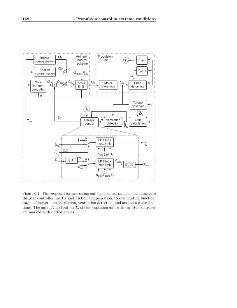
148 Propulsion control in extreme conditions
n
f
Q
Q
Ta
a
T
m
( )
f Q ( ).
.
Motordynamics
Qc
Frictioncompensation
.
Tr
XQci
g
Corethruster
controller
Shaftdynamics
Losscalculation
Torqueobserver
Ventilationdetection
bQ
Anti-spincontrol
Qa
Tras
Qcas
zT
Propulsionunit
as
Tr
n
z
LP filter +rate limit
nslew nslew tn
nras
1
bQ
LP filter +rate limit g
Tras
rise fall tg g g
nr
1
0
1
0
{0,1}
++
. .
. .
Qff
n
Torquelimit
PQmax max
gn( ).
gn
( ).-1
Qc0
QifInertiacompensation
++
+
Q
Q
Anti-spincontrolscheme
Figure 6.2: The proposed torque scaling anti-spin control scheme, including corethruster controller, inertia and friction compensation, torque limiting function,torque observer, loss calculation, ventilation detection, and anti-spin control ac-tions. The input Tr and output Ta of the propulsion unit with thruster controllerare marked with dotted circles.

6.6 Alternative anti-spin controllers 149
power controller involves multiplying the controller formulations in (3.29) and(3.32) with βQ = KQ/KQC , see (2.12). This is the same as using the twocontrollers with KQC ≡ KQ. From the definitions of the shaft speed sensitivityfunctions snq(·) and snp(·) in Table 4.1, this implies that snq(·) ≡ 1 and snp(·) ≡1, which means that n ≡ nr.
6.6 Alternative anti-spin controllersThe anti-spin controller presented in Section 6.5 was shown to be compatiblewith all the core thruster controllers in Table 3.1, and has been chosen as thepreferred solution. This section presents some alternative anti-spin solutions,with varying degrees of complexity.
6.6.1 Speed bound anti-spin control
This is the simplest of the anti-spin control formulations presented in this work.A dynamic shaft speed bound is added to the core thruster controller, whichcan be any of the controllers in Table 3.1 based on torque and/or power control.This limits the propeller racing, since the shaft speed is kept within the desiredbounds. Using the shaft speed reference nr from (3.1), the dynamic speed boundnb is defined as:
nb = (1 + rb)nr, (6.24)
where rb is the speed bound factor, typically in the range rb ∈ [0.2, 0.3]. Thismeans that the shaft speed is allowed to deviate by 20− 30% from its nominalvalue. The shaft speed can then vary freely as long as |n| < |nb|, such that thecore thruster controller mostly is allowed to work undisturbed. In a high losssituation, when torque or power control normally would lead to severe propellerracing, the shaft speed is bounded by n ≈ nb.The shaft speed bound is implemented by an additive shaft speed PI con-
troller, which is only activated when |n| ≥ |nb|:
Qcas = Qci +Qb, (6.25)
where Qci is the core thruster controller output, and the additive PI term Qb isdefined as:
Qb = sign(Tr)min
µ0, Kpeb +Ki
Z t
0
eb(τ)dτ
¶,
eb = |nb|− |n| . (6.26)
As in (3.27), Kp > 0 and Ki > 0 are the proportional and integral gains, whichshould be tuned to give rapid response, and eb is the bound error. The minimumoperator in (6.26) means that Qb is only allowed to reduce the magnitude of thecommanded torque. To avoid integral windup, the integral term in (6.26) mayonly assume negative values (upper windup limit at zero). With respect to the
150 Propulsion control in extreme conditions
anti-spin control actions defined in Section 6.4, only the torque modification γQis used, with γQ in this case implicitly given by:
γQ =Qcas
Qci=
Qci +Qb
Qci. (6.27)
This formulation does not utilize a dedicated ventilation detection scheme asproposed in Section 6.3, but “detects” ventilation simply by an excessive shaftspeed. The number of control parameters is therefore kept low, such that thecontroller is relatively easy to tune.
Remark 6.5 When the propeller is subject to increasing advance velocities, thetorque and power controllers will increase the shaft speed in order to compensatefor the reduced loading. This increase should not be detected as a ventilationincident. A weakness of the speed bound anti-spin controller is therefore thatin order to allow the core thruster controller to work undisturbed, rb should bechosen relatively high. This means that the propeller is allowed to spin more outduring ventilation.
6.6.2 Additive PI anti-spin control
This anti-spin control scheme is similar to the solution presented in Section 6.5,but applies an additive shaft speed PI controller as primary anti-spin actioninstead of the torque scaling used in (6.6). Using the detection scheme fromSection 6.3, the primary anti-spin control action is formulated as follows:
Qcas =
½Qci for ζ = 0,
sign(Tr)max(0, sign(Tr)(Qci +QPI)) for ζ = 1,(6.28)
where Qci is the core thruster controller output, and the additive PI term QPI
is defined similarly as in (3.27):
QPI = Kpe+Ki
Z t
0
e(τ)dτ ,
e = nr − n. (6.29)
As before, Kp > 0 and Ki > 0 are the proportional and integral tuning gains,and e is the shaft speed error. The integral term in (6.29) is continuously resetfor ζ = 0 to avoid integral windup. To reduce mechanical wear and tear, thetotal commanded torque Qcas in (6.28) is saturated as in (6.20), such that thetorque direction cannot be reversed by the additive PI controller.As a secondary antispin action, the thrust reference Tr may be lowered when
ζ = 1 as in (6.18).
6.6.3 Shaft speed anti-spin control
If a well-tuned shaft speed controller is chosen for operation in normal condition,the need for anti-spin control is reduced. Since the shaft speed controller aims at
6.6 Alternative anti-spin controllers 151
keeping the shaft speed constant regardless of the propeller loading, no primaryanti-spin action to regain control of the shaft speed during ventilation may benecessary. Actually, the primary anti-spin control action presented in (6.6) iscompatible with the shaft speed PI controller. Simulations show, however, thatthe performance of the shaft speed controller is not improved by adding (6.6).This could be expected, since (6.6) does not modify the PI controller directly,but only scales its output; in order to improve the performance, it is necessaryto address the PI terms directly.
PI controller with setpoint mapping
If the secondary anti-spin action is deemed appropriate, the setpoint mappingin (6.18) may be applied directly to a conventional shaft speed PI controller.This requires a ventilation detection scheme, as proposed in Section 6.3. Inaddition to the torque observer and the ventilation detection scheme, the equa-tions for implementation are taken directly from (3.1), (3.27), and (6.18). Witha well-tuned PI controller, the performance of this scheme during ventilation isexpected to be similar to the scheme presented in Section 6.5.
Remark 6.6 This scheme relies on the PI gains to be tuned to give good per-formance during ventilation. As will be shown in Section 6.8, a PI controllerthat is tightly tuned for good performance in normal conditions, may give un-satisfactory results when subject to the large load transients experienced duringventilation. If such a scheme is chosen, the PI gains should therefore be tunedwith care.
PI controller with integrator reset and setpoint mapping
One of the potential problems with a shaft speed PI controller during ventilationis integrator discharge. When most of the propeller load suddenly disappears,the integral term must wind down quickly. If the PI gains are not tuned to copewith this situation, the consequence may be large oscillations in the controlleroutput. This is certainly not desirable, and may inflict damage to the mechanicalcomponents of the thruster.A possible solution to this problem is to use an integrator reset mechanism,
see e.g. Zheng et al. (2000) and the references therein. The idea is to monitorthe control system performance, and reset the integral term when large processdiscrepancies are detected. A simple approach is to use the ventilation detectionscheme from Section 6.3, and reset the integral term to zero when ventilation isdetected. Combined with the secondary anti-spin action in (6.18), this approachgives a very rapid reduction in shaft speed. However, it gives no performanceimprovements when ventilation terminates. From simulations and experiments,this approach seems to be too coarse to get good results. The rapid changein controller output may also add to the mechanical wear and tear instead ofreducing it.

152 Propulsion control in extreme conditions
Controller Abbreviation SectionTorque scaling anti-spin control TS AS control 6.5Speed bound anti-spin SB AS control 6.6.1Additive PI anti-spin control API AS control 6.6.2Primary anti-spin action p 6.5.1Secondary anti-spin action s 6.5.2
Table 6.1: Anti-spin controllers for extreme conditions.
A more sophisticated Lyapunov-based integrator reset approach is presentedin Bakkeheim et al. (2006). In this work, a load torque observer as presentedin Section 5.1 is utilized for online calculation of a Lyapunov function origin(equilibrium point). The Lyapunov function value will jump to a higher valuewhen the propeller starts or stops ventilating. A multiple model Lyapunovalgorithm then decides when to take integrator reset actions, and selects theintegrator value that gives the greatest drop in the Lyapunov function value.This enables tuning of the PI gains to be done with focus on normal operatingconditions, since the reset mechanism handles the transients during extremeconditions. The setpoint mapping in (6.18) may also be applied. The conceptwas tested experimentally with the setup described in Section 7.1, and provensuccessful.
Remark 6.7 The complexity of the shaft speed PI controller with Lyapunov-based integrator reset is comparable to that of the proposed anti-spin schemein Section 6.5. The two approaches share the load torque observer, ventilationdetection scheme, and secondary anti-spin action. The properties of the PIcontroller, including the integrator reset mechanism, can therefore be directlycompared with the torque/power controller, including the primary anti-spin ac-tion. Since the controllers based on torque and power control have been shownto be superior in normal operating conditions, and their performance duringventilation rendered acceptable by the anti-spin controller in Section 6.5, thishas been chosen as the preferred solution. The shaft speed anti-spin controllersintroduced in this section will therefore not be further treated here.
6.7 Controller summary
For ease of notation, the anti-spin controllers presented above will be givenabbreviations as defined in Table 6.1. The abbreviations will be used as e.g.“QP TS AS p+s”, meaning “combined torque/power control with torque scalinganti-spin, using both primary and secondary anti-spin action”.

6.8 Simulation results 153
βv,on βv,off nmin Tvent0.6 0.9 0.5rps 2s
Table 6.2: Ventilation detection scheme parameters for the 4MW WageningenB4-70 example propeller.
τγ γrise γfall τn n+vent n−vent nas0.1s 0.5s−1 −1s−1 0.5s 1s−2 −1s−2 1.1rps
Table 6.3: TS anti-spin controller parameters for the 4MW Wageningen B4-70example propeller.
6.8 Simulation results
The simulations are performed with the 4MW Wageningen B4-70 example pro-peller, with model parameters given in Tables A.1 and A.2. For the ventilationdetection scheme, the Qa observer from Section 5.1 is used with the parametersgiven in Table 5.1. The motor torque is filtered by a second order Butterworthfilter with cutoff at 10Hz before numerical differentiation. The remaining de-tection scheme parameters are given in Table 6.2. The basic control parametersare given in Table 3.2, the parameters for the friction and inertia compensationschemes in Table 3.4, the parameters for the S controller in Table 3.5, and theparameters for the combined QP controller in Table 3.6. The Q, P, and QP con-trollers are in this section always used with the friction and inertia compensationschemes, which are not explicitly mentioned in the controller abbreviations. Thecombined SQP controller from Section 3.15 is not tested here, since it is assumedthat the speed control regime will be chosen such that ns2 ≤ nmin. That is, theanti-spin controller is de-activated in the speed control regime. For higher shaftspeeds, the SQP controller becomes a QP controller. Hence, the anti-spin sim-ulations with the QP controller are valid also for the SQP controller. The samereasoning applies to the MQP1 and MQP2 controllers.The chosen parameters for the TS anti-spin controller from Section 6.5 are
given in Table 6.3. However, Section 6.8.1 will discuss tuning of the variousparameters, as well as the shaft speed PI control parameters. The additionalinertia compensation scheme for the secondary anti-spin action is implementedas proposed in (6.19) and (6.20). The parameters for the SB and API anti-spinschemes are given in Table 6.4. Notice that the same PI parameters as for the Scontroller in Table 3.5 have been chosen. For the API anti-spin controller, thesecondary anti-spin parameters from Table 6.3 are used.
6.8.1 Controller tuning
Figure 6.3 shows the shaft speed and motor torque for four different shaft speedPI controllers during a ventilation incident. The ventilation incident is generatedby a sinusoidal heave (vertical) motion of the propeller with mean submergence
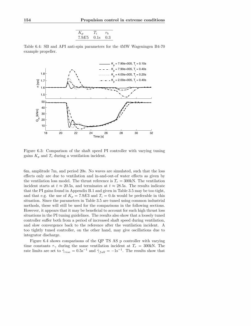
154 Propulsion control in extreme conditions
Kp Ti rb7.9E5 0.1s 0.3
Table 6.4: SB and API anti-spin parameters for the 4MW Wageningen B4-70example propeller.
1.5
1.6
1.7
1.8
n [r
ps]
Kp = 7.90e+005, T
i = 0.10s
Kp = 7.90e+005, T
i = 0.40s
Kp = 4.00e+005, T
i = 0.20s
Kp = 2.00e+005, T
i = 0.40s
18 20 22 24 26 28 30 32
10
20
30
40
50
Qm
[kN
m]
Time [s]
Figure 6.3: Comparison of the shaft speed PI controller with varying tuninggains Kp and Ti during a ventilation incident.
6m, amplitude 7m, and period 20s. No waves are simulated, such that the losseffects only are due to ventilation and in-and-out-of water effects as given bythe ventilation loss model. The thrust reference is Tr = 300kN. The ventilationincident starts at t ≈ 20.5s, and terminates at t ≈ 28.5s. The results indicatethat the PI gains found in Appendix B.1 and given in Table 3.5 may be too tight,and that e.g. the use of Kp = 7.9E3 and Ti = 0.4s would be preferable in thissituation. Since the parameters in Table 3.5 are tuned using common industrialmethods, these will still be used for the comparisons in the following sections.However, it appears that it may be beneficial to account for such high thrust losssituations in the PI tuning guidelines. The results also show that a loosely tunedcontroller suffer both from a period of increased shaft speed during ventilation,and slow convergence back to the reference after the ventilation incident. Atoo tightly tuned controller, on the other hand, may give oscillations due tointegrator discharge.Figure 6.4 shows comparisons of the QP TS AS p controller with varying
time constants τγ during the same ventilation incident at Tr = 300kN. Therate limits are set to γrise = 0.5s
−1 and γfall = −1s−1. The results show that

6.8 Simulation results 155
1.4
1.6
1.8
2
n [r
ps]
No γQ
filter
τγ = 0.2s
τγ = 0.5s
τγ =1.0s
18 20 22 24 26 28 30 32
10
20
30
40
50
Qm
[kN
m]
Time [s]
Figure 6.4: Comparison of the QP TS AS p controller with varying filter timeconstants τγ during a ventilation incident.
increasing τγ gives a smoother motor torque, but also increased shaft speedduring ventilation. With the current noise content in βQ, there is limited needfor the filter, and τγ = 0.1s will be used in the remainder of the simulations.Figure 6.5 shows comparisons of the QP TS AS p controller with varying
torque scaling slew rates γrise and γfall during the same ventilation incident atTr = 300kN. The filter time constant is set to τγ = 0.1s. The results show thatthe main importance for avoiding shaft speed racing is not to choose the slewrates too small. In the remainder of the simulations, the parameters are chosenas γrise = 0.5s
−1 and γfall = −1s−1.Tuning of the secondary anti-spin parameters is less critical for the controller
performance; the three parameters n+vent, n−vent, and nas must be chosen as a
trade-off between desired speed reduction during ventilation, and possible wearand tear as a result of the setpoint mapping.
6.8.2 TS AS control vs. API AS control
The TS AS and API AS controllers are relatively similar in principle; the dif-ference is the manner in which the anti-spin controller takes control of the shaftspeed during ventilation. The two primary anti-spin schemes are therefore com-pared in Figures 6.6 and 6.7, with the QP and the Q controller as core thrustercontrollers, respectively. All the controllers are tested both with primary andprimary + secondary anti-spin action. The simulation scenario from the previ-ous section is used, with Tr = 300kN in Figure 6.6, and Tr = 200kN in Figure6.7. With |n| > 1.5 for the QP controller, it acts as a pure P controller. The re-
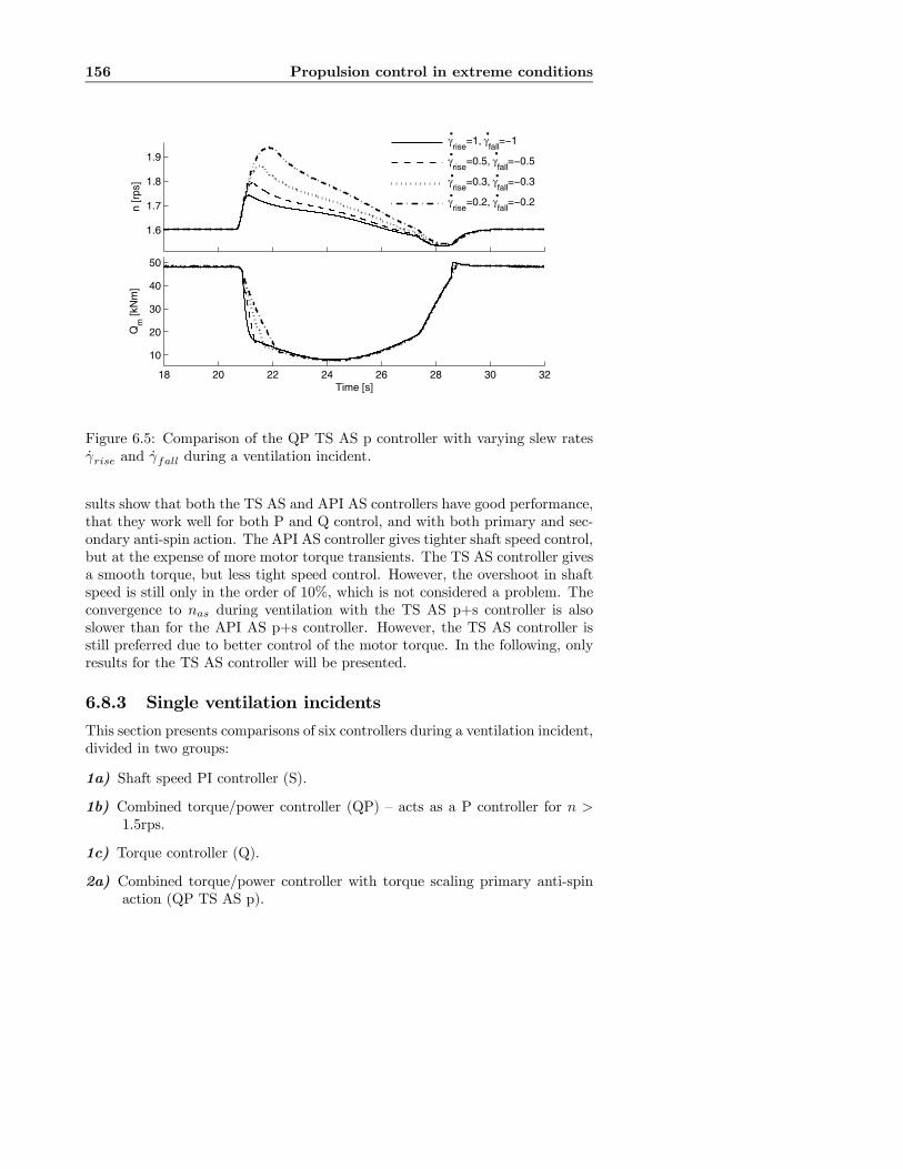
156 Propulsion control in extreme conditions
1.6
1.7
1.8
1.9
n [r
ps]
γrise
=1, γfall
=−1
γrise
=0.5, γfall
=−0.5
γrise
=0.3, γfall
=−0.3
γrise
=0.2, γfall
=−0.2
18 20 22 24 26 28 30 32
10
20
30
40
50
Qm
[kN
m]
Time [s]
. .
. .
. .
. .
Figure 6.5: Comparison of the QP TS AS p controller with varying slew ratesγrise and γfall during a ventilation incident.
sults show that both the TS AS and API AS controllers have good performance,that they work well for both P and Q control, and with both primary and sec-ondary anti-spin action. The API AS controller gives tighter shaft speed control,but at the expense of more motor torque transients. The TS AS controller givesa smooth torque, but less tight speed control. However, the overshoot in shaftspeed is still only in the order of 10%, which is not considered a problem. Theconvergence to nas during ventilation with the TS AS p+s controller is alsoslower than for the API AS p+s controller. However, the TS AS controller isstill preferred due to better control of the motor torque. In the following, onlyresults for the TS AS controller will be presented.
6.8.3 Single ventilation incidents
This section presents comparisons of six controllers during a ventilation incident,divided in two groups:
1a) Shaft speed PI controller (S).
1b) Combined torque/power controller (QP) — acts as a P controller for n >1.5rps.
1c) Torque controller (Q).
2a) Combined torque/power controller with torque scaling primary anti-spinaction (QP TS AS p).

6.8 Simulation results 157
0
100
200
300
Ta [k
N]
QP TS AS p controlQP TS AS p+s controlQP API AS p controlQP API AS p+s control
1.2
1.4
1.6
n [r
ps]
18 20 22 24 26 28 30 32
10
20
30
40
50
Qm
[kN
m]
Time [s]
Figure 6.6: Comparison of TS and API anti-spin control during a ventilationincident at Tr = 300kN, using the QP core thruster controller.
50
100
150
200
Ta [k
N]
Q TS AS p controlQ TS AS p+s controlQ API AS p controlQ API AS p+s control
1.1
1.2
1.3
1.4
n [r
ps]
18 20 22 24 26 28 30 32
10
20
30
Qm
[kN
m]
Time [s]
Figure 6.7: Comparison of TS and API anti-spin control during a ventilationincident at Tr = 200kN, using the Q core thruster controller.
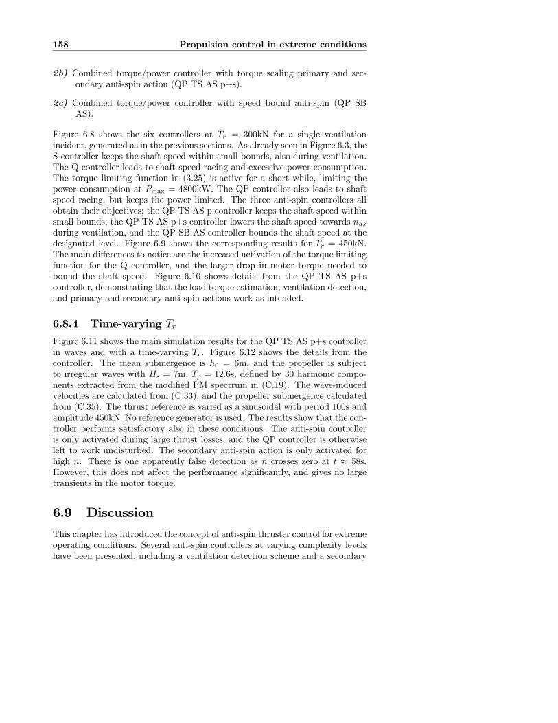
158 Propulsion control in extreme conditions
2b) Combined torque/power controller with torque scaling primary and sec-ondary anti-spin action (QP TS AS p+s).
2c) Combined torque/power controller with speed bound anti-spin (QP SBAS).
Figure 6.8 shows the six controllers at Tr = 300kN for a single ventilationincident, generated as in the previous sections. As already seen in Figure 6.3, theS controller keeps the shaft speed within small bounds, also during ventilation.The Q controller leads to shaft speed racing and excessive power consumption.The torque limiting function in (3.25) is active for a short while, limiting thepower consumption at Pmax = 4800kW. The QP controller also leads to shaftspeed racing, but keeps the power limited. The three anti-spin controllers allobtain their objectives; the QP TS AS p controller keeps the shaft speed withinsmall bounds, the QP TS AS p+s controller lowers the shaft speed towards nasduring ventilation, and the QP SB AS controller bounds the shaft speed at thedesignated level. Figure 6.9 shows the corresponding results for Tr = 450kN.The main differences to notice are the increased activation of the torque limitingfunction for the Q controller, and the larger drop in motor torque needed tobound the shaft speed. Figure 6.10 shows details from the QP TS AS p+scontroller, demonstrating that the load torque estimation, ventilation detection,and primary and secondary anti-spin actions work as intended.
6.8.4 Time-varying Tr
Figure 6.11 shows the main simulation results for the QP TS AS p+s controllerin waves and with a time-varying Tr. Figure 6.12 shows the details from thecontroller. The mean submergence is h0 = 6m, and the propeller is subjectto irregular waves with Hs = 7m, Tp = 12.6s, defined by 30 harmonic compo-nents extracted from the modified PM spectrum in (C.19). The wave-inducedvelocities are calculated from (C.33), and the propeller submergence calculatedfrom (C.35). The thrust reference is varied as a sinusoidal with period 100s andamplitude 450kN. No reference generator is used. The results show that the con-troller performs satisfactory also in these conditions. The anti-spin controlleris only activated during large thrust losses, and the QP controller is otherwiseleft to work undisturbed. The secondary anti-spin action is only activated forhigh n. There is one apparently false detection as n crosses zero at t ≈ 58s.However, this does not affect the performance significantly, and gives no largetransients in the motor torque.
6.9 Discussion
This chapter has introduced the concept of anti-spin thruster control for extremeoperating conditions. Several anti-spin controllers at varying complexity levelshave been presented, including a ventilation detection scheme and a secondary

6.9 Discussion 159
1
2
3
4
n [r
ps]
0
200
400
600
Ta [k
N]
0
200
400
Qa [k
Nm
]
10
20
30
40
50
Qm
[kN
m]
20 25 300
2000
4000
Pm
[kW
]
Time [s]
1
2
3
4
0
200
400
600
0
200
400
10
20
30
40
50
20 25 300
2000
4000
Time [s]
S controlQ controlQP control
QP TS AS p controlQP TS AS p+s controlQP SB AS control
Figure 6.8: Comparison of six controllers during a ventilation incident at Tr =300kN.
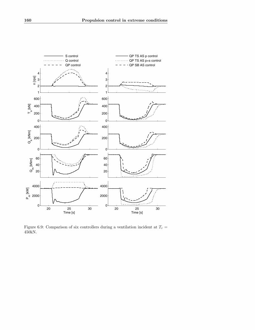
160 Propulsion control in extreme conditions
1
2
3
4
n [r
ps]
0
200
400
600
Ta [k
N]
0
200
400
Qa [k
Nm
]
20
40
60
Qm
[kN
m]
20 25 300
2000
4000
Pm
[kW
]
Time [s]
1
2
3
4
0
200
400
600
0
200
400
20
40
60
20 25 300
2000
4000
Time [s]
S controlQ controlQP control
QP TS AS p controlQP TS AS p+s controlQP SB AS control
Figure 6.9: Comparison of six controllers during a ventilation incident at Tr =450kN.

6.9 Discussion 161
50
100
150
200
250
Qa k
[Nm
]
0
0.5
1
β Q, ζ
[−]
20 25 30
0.2
0.4
0.6
0.8
1
γ [−
]
Time [s]
0
0.2
0.4
0.6
γ −
βQ
[−]
1.2
1.4
1.6
1.8
2
n ras [r
ps]
20 25 30
0
2
4
6
h/R
[−]
Time [s]
EstimatedActual
βQ
ζ
^
<
Figure 6.10: Details from the QP TS AS p+s controller during a ventilationincident at Tr = 450kN.
anti-spin action that reduces the shaft speed during ventilation. The resultsindicate that:
• If a shaft speed controller is found acceptable for normal operating con-ditions, the anti-spin controllers are of limited applicability. However, theperformance during ventilation may be improved by accounting for suchsituations during tuning of the PI control parameters, and possibly alsoby modifications of the integral term. The secondary anti-spin action maybe applied to reduce the dynamic loading during ventilation.
• If a controller based on torque and/or power control is chosen for normaloperating conditions, ventilation will lead to excessive power consump-tion (mainly for the torque controller) and increased mechanical wear andtear due to unsteady propeller loading. Both analyses and simulationsshow that the unacceptable performance of torque and power control whensubject to large thrust losses can be rendered acceptable by an anti-spincontroller.
• The main purpose of the anti-spin controller is to limit the shaft speed dur-ing ventilation. All the proposed anti-spin schemes in Table 6.1 containssuch functionality.
162 Propulsion control in extreme conditions
−2
0
2
n [r
ps]
−400
−200
0
200
400
Ta [k
N]
ActualReference
−200
0
200
Qa [k
Nm
]
−50
0
50
Qm
[kN
m]
10 20 30 40 50 60 70 80 90 100 110
0
2000
4000
Pm
[kW
]
Time [s]
Figure 6.11: Simulation results for the QP TS AS p+s controller in waves for atime-varying Tr.

6.9 Discussion 163
−200
0
200
Qa k
[Nm
]
EstimatedActual
0
0.5
1
1.5
β Q, ζ
[−]
βQ
ζ
0
0.5
1
γ [−
]
−2
0
2
n ras [r
ps]
10 20 30 40 50 60 70 80 90 100 110
0
2
4
6
h/R
[−]
Time [s]
^
<
Figure 6.12: Details from the QP TS AS p+s controller in waves for a time-varying Tr.

164 Propulsion control in extreme conditions
• The SB anti-spin controller, which is the simplest formulation presentedhere, gives the least control over the shaft speed, and is not compatiblewith the secondary anti-spin action. Its simplicity may, however, be anadvantage for industrial applications.
• The TS and API anti-spin controllers give increased control over the shaftspeed during ventilation, and can be combined with the secondary anti-spin action. These controllers give the best over-all performance, but atthe expense of increased complexity.

Chapter 7
Experimental results
In order to test and validate the proposed control concepts, experiments witha model scale propeller have been carried out in the Marine Cybernetics Labo-ratory (MCLab) at NTNU. The experimental setup is described in Section 7.1,followed by experiments in normal conditions in Section 7.2, and experimentsin extreme conditions in Section 7.3.
7.1 Experimental setup
The MCLab basin is 40m long, 6.45m wide, and 1.5m deep, and is equippedwith a towing carriage and a wave-maker system. The tested propeller was ofconventional design, and used both with and without duct. The main dimen-sions of the propeller and duct are given in Tables 7.1 and 7.2. The propellerwas attached to a shaft equipped with thrust and torque sensors inside an un-derwater housing, and driven by an electric motor via shafts and gears with gearratio 1:1. The rig with motor, gears, underwater housing, shaft and propellerwas fixed to the towing carriage on a vertical slide, which was used to controlthe submergence of the propeller relative to the free surface. The submergencewas measured with a wave probe. The advance velocity of the propeller wasequal to the towing velocity of the carriage, in addition to components fromcurrent and/or waves. The motor torque was controlled from a PC onboard thecarriage, using feedback from the propeller shaft speed and the motor torque.The control code was generated by rapid control prototyping using Opal RT-Laband source code in Matlab/Simulink. This enabled use of the same Simulinkcode that was used for simulations. A sketch of the experimental setup is givenin Figure 7.1, and a picture shown in Figure 7.2.
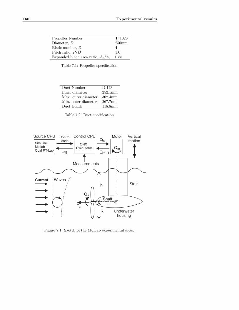
166 Experimental results
Propeller Number P 1020Diameter, D 250mmBlade number, Z 4Pitch ratio, P/D 1.0Expanded blade area ratio, Ae/A0 0.55
Table 7.1: Propeller specification.
Duct Number D 143Inner diameter 252.1mmMax. outer diameter 302.4mmMin. outer diameter 267.7mmDuct length 118.8mm
Table 7.2: Duct specification.
Motor
WavesStrut
Underwaterhousing
Shaft
Qa
Ta
Qm
Current
Control CPUSource CPU
SimulinkMatlabOpal RT-Lab
QNXExecutable
Qc
Qm,n
h
R
Controlcode
Log
Measurements
Verticalmotion
Figure 7.1: Sketch of the MCLab experimental setup.
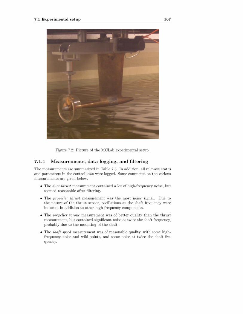
7.1 Experimental setup 167
Figure 7.2: Picture of the MCLab experimental setup.
7.1.1 Measurements, data logging, and filtering
The measurements are summarized in Table 7.3. In addition, all relevant statesand parameters in the control laws were logged. Some comments on the variousmeasurements are given below.
• The duct thrust measurement contained a lot of high-frequency noise, butseemed reasonable after filtering.
• The propeller thrust measurement was the most noisy signal. Due tothe nature of the thrust sensor, oscillations at the shaft frequency wereinduced, in addition to other high-frequency components.
• The propeller torque measurement was of better quality than the thrustmeasurement, but contained significant noise at twice the shaft frequency,probably due to the mounting of the shaft.
• The shaft speed measurement was of reasonable quality, with some high-frequency noise and wild-points, and some noise at twice the shaft fre-quency.
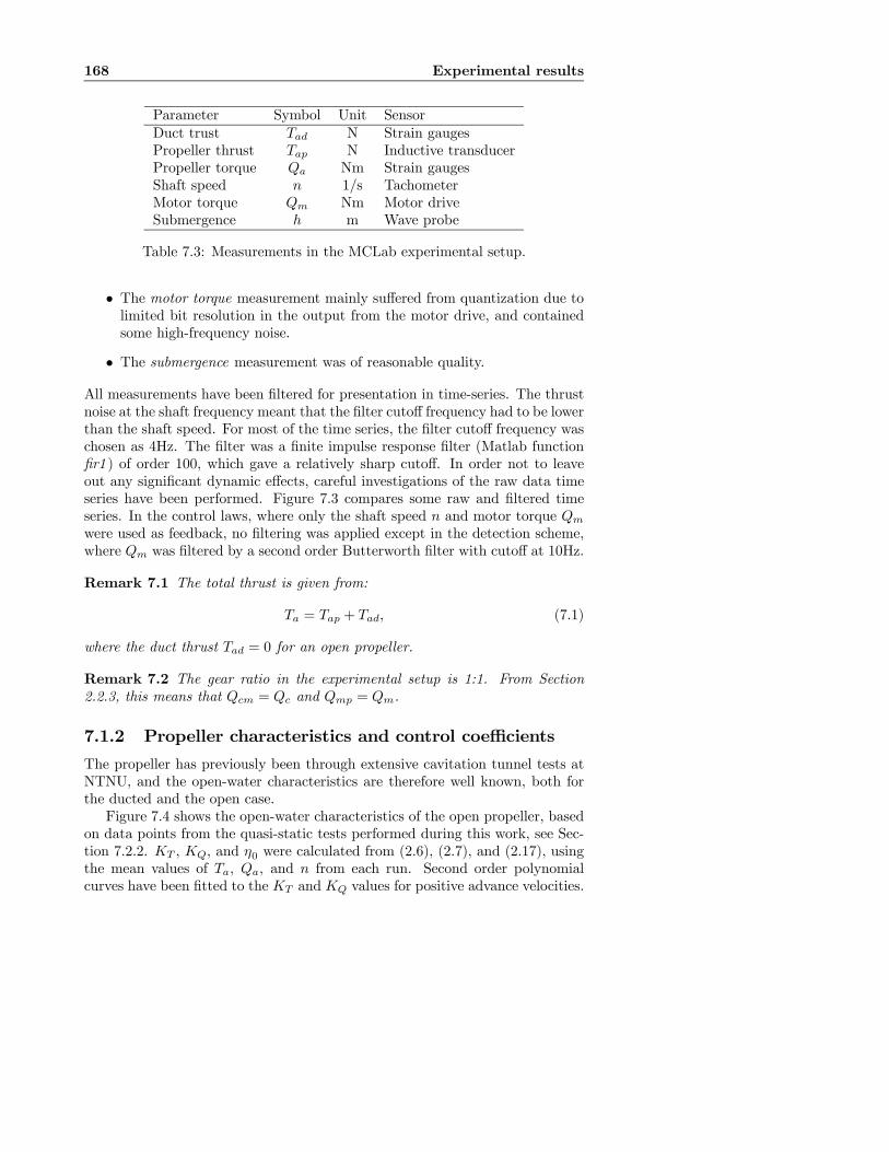
168 Experimental results
Parameter Symbol Unit SensorDuct trust Tad N Strain gaugesPropeller thrust Tap N Inductive transducerPropeller torque Qa Nm Strain gaugesShaft speed n 1/s TachometerMotor torque Qm Nm Motor driveSubmergence h m Wave probe
Table 7.3: Measurements in the MCLab experimental setup.
• The motor torque measurement mainly suffered from quantization due tolimited bit resolution in the output from the motor drive, and containedsome high-frequency noise.
• The submergence measurement was of reasonable quality.
All measurements have been filtered for presentation in time-series. The thrustnoise at the shaft frequency meant that the filter cutoff frequency had to be lowerthan the shaft speed. For most of the time series, the filter cutoff frequency waschosen as 4Hz. The filter was a finite impulse response filter (Matlab functionfir1 ) of order 100, which gave a relatively sharp cutoff. In order not to leaveout any significant dynamic effects, careful investigations of the raw data timeseries have been performed. Figure 7.3 compares some raw and filtered timeseries. In the control laws, where only the shaft speed n and motor torque Qm
were used as feedback, no filtering was applied except in the detection scheme,where Qm was filtered by a second order Butterworth filter with cutoff at 10Hz.
Remark 7.1 The total thrust is given from:
Ta = Tap + Tad, (7.1)
where the duct thrust Tad = 0 for an open propeller.
Remark 7.2 The gear ratio in the experimental setup is 1:1. From Section2.2.3, this means that Qcm = Qc and Qmp = Qm.
7.1.2 Propeller characteristics and control coefficients
The propeller has previously been through extensive cavitation tunnel tests atNTNU, and the open-water characteristics are therefore well known, both forthe ducted and the open case.Figure 7.4 shows the open-water characteristics of the open propeller, based
on data points from the quasi-static tests performed during this work, see Sec-tion 7.2.2. KT , KQ, and η0 were calculated from (2.6), (2.7), and (2.17), usingthe mean values of Ta, Qa, and n from each run. Second order polynomialcurves have been fitted to the KT and KQ values for positive advance velocities.

7.1 Experimental setup 169
10
10.5
11
11.5n
[rps
]RawFiltered
100
150
200
Tap
[N]
RawFiltered
100
150
200
Tad
[N]
RawFiltered
4
5
6
7
Qa [N
m]
RawFiltered
6
7
8
Qm
[Nm
]
RawFiltered
0 5 10 15 20 25 30 35 40 45
0.38
0.382
0.384
0.386
0.388
h [m
]
Time [s]
RawFiltered
Figure 7.3: Examples of the raw and filtered measurements in the MCLabexperimental setup.

170 Experimental results
−0.6 −0.4 −0.2 0 0.2 0.4 0.6 0.8 1
0
0.1
0.2
0.3
0.4
0.5
0.6
0.7
0.8
Ja
KT
10KQ
η0
Figure 7.4: Open-water characteristics for the open propeller.
The curves correspond well with previously reported open-water characteris-tics. Note that the uncertainty of the tests increase with decreasing negativeadvance numbers, which give unsteady inflow to the propeller. The nominalthrust and torque coefficients were found to be KT0 = 0.570 and KQ0 = 0.0750.The nominal thrust and torque coefficients for reverse thrust were found to beKT0r = 0.393 and KQ0r = 0.0655. Figure 7.5 shows the KT −KQ relationship,and a linear fit as proposed in Section 2.1.8. The same data points that areshown in Figure 7.4 are used (i.e. −0.6 ≤ Ja ≤ 0.9), and the parameters for thelinear fit are at = 8.4 and bt = −0.068. Clearly, the linear relationship fits well.The ducted propeller has mainly been used for testing of the anti-spin control
schemes, i.e. at Va ≈ 0. The open-water characteristics were therefore notexperimentally determined during the experiments. Figure 7.6 shows the open-water characteristics from previous tests (Ruth, 2005). The nominal thrust andtorque coefficients were found to be KT0 = 0.513 and KQ0 = 0.0444. Thereverse coefficients were not determined.
Remark 7.3 Comparing coefficients for the open and ducted propeller, it isclear that the addition of the duct gives a better bollard pull efficiency, as dis-cussed in Section 2.1.6.
For the open propeller, the control coefficients KTC and KQC were chosenas in (3.8, 3.9) with εc = 4.5, nc = 3, and using the nominal thrust and torque

7.1 Experimental setup 171
0.02 0.03 0.04 0.05 0.06 0.07 0.080
0.1
0.2
0.3
0.4
0.5
0.6
KQ
KT
Ja = −0.6
Ja = −0.5
Ja = −0.3
Ja = 0.0
Ja = 0.3
Ja = 0.5
Ja = 0.6
Ja = 0.7
Ja = 0.9
Measured, Va > 0
Measured, Va < 0
Linear fit
Figure 7.5: Relationship between KT and KQ for the open propeller, in therange −0.6 ≤ Ja ≤ 0.9.
0 0.1 0.2 0.3 0.4 0.5 0.6 0.7 0.8
0
0.1
0.2
0.3
0.4
0.5
Ja
KT
10KQ
η0
Figure 7.6: Open-water characteristics for the ducted propeller, with data takenfrom Ruth (2005).

172 Experimental results
coefficients specified above. The ducted propeller was not tested with n < 0,such that the coefficients could be set as constants, i.e. KTC = KT0 and KQC =KQ0.
Remark 7.4 The smooth switch of the control coefficients for the open propellerwas not implemented as in (3.10), but instead as:
λc = λc(nr) =1
2+1
πarctan(7
nrnc+ 125
n3rn3c). (7.2)
This is almost equivalent to using (3.10) with εc = 4.5.
7.1.3 Friction and inertia compensation
In the experiments presented here, the shaft friction turned out to affect theperformance of the torque and power controllers significantly. A feedforwardfriction compensation scheme as proposed in Section 3.7.1 was therefore imple-mented. The friction was found to be rather nonlinear. It was clearly affected bythe temperature in the gears, bearings, and oil, with decreasing friction as thetemperature increased. Additionally, the friction exhibited a hysteresis, withless friction for reducing shaft speed than for increasing shaft speed. This isdescribed in more detail in Pivano et al. (2006c). However, for control purposesthe static plus linear friction compensation in (3.19) was found to be satisfac-tory. Over the course of the experiments, the friction coefficients were foundto be in the range Qs ∈ [0.8, 1.0] and Kω ∈ [0.009, 0.011]. The switch “width”of the smooth switching function in (3.20) was chosen as nf = 0.5, and theconstant εf = 4.5. Figure 7.7 shows an example friction model where Qf0 = 1.0and Qf1 = 0.01, together with a time series for a sinusoidal thrust reference.This clearly illustrates the nonlinearities in the experienced friction.The rotational inertia was approximated to Is ≈ 0.05kgm2, and did not ap-
pear to affect the response of the system significantly. An inertia compensationscheme as proposed in (3.22) was therefore not implemented.
Remark 7.5 The smooth switch in the static friction compensation was notimplemented as in (3.20), but instead as:
Qff0(nr) = Qf02
πarctan(7
nrnf+ 125
n3rn3f). (7.3)
This is almost equivalent to using (3.20) with εf = 4.5.
7.2 Experiments in normal conditions
This section presents experimental results with the controllers from Chapter3, i.e. designed for normal operating conditions, including validation of the

7.2 Experiments in normal conditions 173
0 2 4 6 8 10 12 141
1.1
1.2
1.3
1.4
1.5
1.6
1.7
1.8
1.9
n [rps]
Qf [N
m]
Time seriesModel
Figure 7.7: Linar friction compensation used in the experiments, together withexperimental time series for a sinusoidal thrust reference.
sensitivity functions from Chapter 4. The importance of the friction compensa-tion scheme is investigated, and the dynamic performance of the controllers invarious operating conditions tested.The majority of the experiments were conducted for shaft speed control,
torque control, and power control, in order to test the properties of the funda-mental thruster control schemes. Three main sets of tests are presented in thefollowing:
1. Quasi-static tests with the open propeller: steady-state tests with con-stant Va and Tr, used to validate the steady-state performance of thefundamental controllers and verify the sensitivity functions.
2. Test in waves with the open propeller: dynamic tests in waves with con-stant Tr, used to investigate the disturbance rejection properties of thefundamental controllers.
3. Tracking tests with the open propeller: dynamic tests in calm water withtime-varying Tr, used to investigate the tracking properties of the fun-damental controllers, as well as some of the other controllers from Table3.1.
Finally, an additional test of the combined SQP controller is presented. Thesubmergence ratio was kept constant at h/R = 4 for the quasi-static and track-ing tests, and at h/R = 3 for the tests in waves. For all the tests, time seriesare shown for the shaft speed n, total thrust Ta, propeller torque Qa, motor

174 Experimental results
D KT0 KQ0 KT0r KQ0r nc0.25m 0.570 0.0750 0.393 0.0655 3rpsQf0 Qf1 nf Ic1.0Nm 0.01Nms 0.5rps 0kgm2
Table 7.4: Basic control parameters used in the experiments with the openpropeller.
Ctr. Kp Ti[s] r p k ns[rps] ns1[rps] ns3[rps]S 0.2 0.05 - - - - - -QP - - 4 0.5 1 - - -SQP 0.3 0.03 3 1 1 - 5 8MQP1 0.3 0.03 4 0.5 1 5 - -
Table 7.5: Parameters for the various controllers used in the experiments withthe open propeller.
torque Qm, and motor power Pm. The motor torque differs from the com-manded torque only by a small time constant, and illustrates the output of thecontrollers.
7.2.1 Controller parameters
Due to the relatively noisy shaft speed measurement, the shaft speed PI con-troller in (3.27) could not be tuned too tightly. The parameters were chosen asKp = 0.2 and Ti = 0.05s, which gave adequate tracking properties in normalconditions. The choice of PI parameters will be further motivated in Section7.3.2. For the combined QP controller in (3.36), the parameters for the weight-ing function αc(n) in (3.33) were chosen as [r, p, k] = [4, 0.5, 1]. This gave a puretorque controller for n < 0.5rps and a pure power controller for n > 3rps.For the combined SQP controller in (3.48), the PI parameters were chosen as
Kp = 0.3 and Ti = 0.03, the parameters for the weighting function αs(nr) werechosen as [r, p, k] = [3, 1, 1], and the switching shaft speeds chosen as ns1 = 5rpsand ns3 = 8rps. This gives pure shaft speed control for nr < 5rps, pure torquecontrol for 6.8rps< nr < 8rps, and pure power control for nr > 9.8rps.For the combined MQP1 controller, the weighting function parameters were
chosen as for the QP controller, i.e. [r, p, k] = [4, 0.5, 1], the integral gain waschosen as Ki = 10, and the integral threshold shaft speed was chosen as ns =5rps. This means that the torque controller in practice was used only to facilitatethe zero-crossings of n, since the additive integral action overlaps the torquecontrol regime.A summary of all the control parameters is given in Tables 7.4 and 7.5. Note
that the MQP1 controller only has integral action, with parameter Ki = Kp/Ti.

7.2 Experiments in normal conditions 175
7.2.2 Quasi-static tests
In the quasi-static tests the thrust reference was kept constant at Tr = 100N,the advance velocities were Va = {−1,−0.5, 0, 0.5, 1, 1.5}m/s, and the speed,torque, and power controllers were used. Each combination was run three times,showing good repeatability. The length of the test series were limited by thelength of the basin, but gave adequate statistical values.The performance of the three controllers is summed up in Figure 7.8, where
the mean values of Ta, Qa, n, Qm, and Pm are shown for varying advancespeeds. The friction compensation is not included in the plots of motor torqueand power. The three controllers obtain their objectives: the shaft speed con-troller keeps the shaft speed most constant, the torque controller keeps themotor torque most constant, and the power controller keeps the motor powermost constant. As the advance speed increases, the effective angle of attackof the propeller blades is decreased, and the propeller loading decreases for aconstant shaft speed. This can be seen in terms of reduced propeller thrustand torque at increasing advance velocities for the shaft speed controller: atVa = 1.5m/s, the propeller thrust is reduced from 100N to 18N. The torque andpower controllers have much better performance, since they increase the shaftspeed as the propeller loading decreases: at Va = 1.5m/s, the propeller thrustis reduced from 100N to 65N and 50N, respectively.The performance of the various controllers may also be studied in terms of
the sensitivity functions described in Section 4. The thrust, shaft speed, torque,and power sensitivity functions for the quasi-static tests can be found in Figure7.9. They compare well with the theoretically derived sensitivity functions inTable 4.1.
7.2.3 Dynamic tests in waves
To validate the dynamic performance of the fundamental controllers when thepropeller is subject to a rapidly changing inflow, tests in regular and irregularwaves were performed. The thrust reference was Tr = 90N and the carriage waskept stationary. A comparison of the controller performance in regular waveswith wave height 8cm and period 1s is shown in Figure 7.10. The results aresummarized in the following:
• The shaft speed controller keeps the shaft speed constant, and has tovary the motor torque and power in order to achieve this. The resultingpropeller thrust and torque have the largest variance.
• The torque controller keeps the motor torque constant, and as a result theshaft speed varies with the loading. The resulting propeller thrust andtorque have the smallest variance.
• The power controller keeps the motor power constant, and as a resultboth the shaft speed and motor torque varies with the loading. The re-
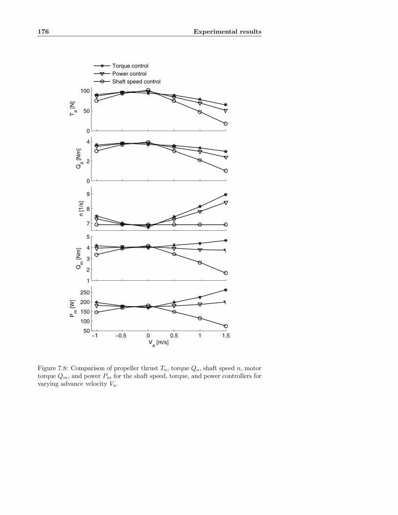
176 Experimental results
0
50
100
Ta [N
]
0
2
4
Qa [N
m]
7
8
9
n [1
/s]
1
2
3
4
5
Qm
[Nm
]
−1 −0.5 0 0.5 1 1.550
100
150
200
250
Pm
[W]
Va [m/s]
Torque controlPower controlShaft speed control
Figure 7.8: Comparison of propeller thrust Ta, torque Qa, shaft speed n, motortorque Qm, and power Pm for the shaft speed, torque, and power controllers forvarying advance velocity Va.

7.2 Experiments in normal conditions 177
0
0.2
0.4
0.6
0.8
1
Thr
ust
stq(⋅)
stp(⋅)
stn(⋅)
1
1.2
1.4
Sha
ft sp
eed
snq(⋅)
snp(⋅)
snn(⋅)
0.2
0.4
0.6
0.8
1
Tor
que
sqq(⋅)
sqp(⋅)
sqn(⋅)
−1 −0.5 0 0.5 1 1.50
0.5
1
1.5
Va [m/s]
Pow
er
spq(⋅)
spp(⋅)
spn(⋅)
Figure 7.9: Experimental thrust, shaft speed, torque, and power sensitivityfunctions for torque control (star), power control (triangle), and speed control(circle).

178 Experimental results
sulting propeller thrust and torque lie between the shaft speed and torquecontroller values.
Similar results were obtained for other thrust references and waves. Resultsfor the three fundamental controllers with a slowly-varying advance velocity areshown in Appendix E.4.
7.2.4 Tracking tests
The tests presented in this section were performed in calm water with zeroadvance velocity and time-varying thrust reference Tr, in order to investigatethe tracking properties of the various controllers. Results for seven controllersare presented, divided in two groups:
1a) Shaft speed PI controller (S).
1b) Torque controller with friction compensation (Q w/Qff).
1c) Combined torque/power controller with friction compensation (QP w/Qff).
2a) Torque controller without friction compensation (Q).
2b) Combined torque/power controller without friction compensation (QP).
2c) Combined speed/torque/power controller with friction compensation (SQPw/Qff).
2d) Combined torque/power controller with additive integral action and nofriction compensation (MQP1).
The controllers were tested for three different cases, using sinusoidal thrustreferences with amplitude TrA:
1. TrA = 50N, period 3s.
2. TrA = 100N, period 5s.
3. TrA = 200N, period 7s.
The power controller could not be tested due to the zero-crossing of Tr (andhence n), but with the chosen weighting function parameters, the QP controllerwas a pure power controller for n > 3.Figures 7.11 and 7.12 show the controllers in group 1 and 2 for TrA = 50N.
The thrust measurements suffer from the noise problems discussed in Section7.1.1, since the shaft speed is too low to allow proper filtering. However, thetrend is still clear. Figures 7.13 and 7.14 show the corresponding results forTrA = 100N, and Figures 7.15 and 7.16 for TrA = 200N.From Figures 7.11, 7.13, and 7.15, the controllers in group 1 have accept-
able performance for all the test cases. The S controller has a small overshoot

7.2 Experiments in normal conditions 179
6.7
6.8
6.9
7
n [r
ps]
85
90
95
Ta [N
]
3.4
3.6
3.8
Qa [N
m]
4.6
4.8
5
Qm
[Nm
]
0 1 2 3 4 5 6 7
205
210
215
Pm
[W]
Time [s]
Torque controlPower controlShaft speed control
Figure 7.10: Comparison of shaft speed, torque, and power control in regularwaves.

180 Experimental results
in the shaft speed after the zero-crossings. This is believed to be connectedwith the static friction. Apart from this, the three controllers have comparableperformance in terms of all the measured parameters. For increasing TrA, theQ w/Qff and QP w/Qff controllers track the thrust reference better than the Scontroller, which gives an overshoot in thrust for positive shaft speed and a lossof thrust for negative shaft speed. Such thrust overshoots during rapid com-mand changes has earlier been described in Healey et al. (1995) and Whitcomband Yoerger (1999a), and was explained by the dynamics of the inflow to thepropeller. It is interesting to note that the Q w/Qff and QP w/Qff controllersavoid this overshoot, and therefore give better tracking properties without anyexplicit compensation for the advance velocity.The importance of the friction compensation in the Q and QP controllers
can be seen in Figures 7.12, 7.14, and 7.16. Without the friction compensation,the performance is not acceptable for TrA = 50N, but improves with increasingTrA, and is acceptable at TrA = 200N. This is consistent with the results fromWhitcomb and Yoerger (1999b), where a feedforward torque control scheme wascompared with two shaft speed controllers. The poor performance of the torquecontroller was explained by unmodelled friction. It was found that the problemswere most evident at low thrust references, where friction is more dominating.Figures 7.12, 7.14, and 7.16 also show results for the SQP w/Qff and MQP1
controllers. For TrA = 50N, nr < 5rps, and both controllers become shaft speedcontrollers. This is seen in the time series, which are similar to the S controller.The difference in performance is probably due to the lack of a proportional termin the MQP1 controller. For TrA = 100N and 200N, the SQP w/Qff controllergives acceptable performance, although the tracking properties (with respectto Tr) are not as good as for the Q w/Qff and QP w/Qff controllers, with asmall overshoot after the zero-crossings. This appears to be due to the shaftspeed controller being engaged and disengaged for low Tr. A similar behavior isseen for the MQP1 controller. In addition, the MQP1 controller gives too highthrust for TrA = 100N and 200N, especially in reverse. This is due to the frozenintegral term, which gives a too big contribution after the rapid transition pastns (at 5rps). For a slower-changing thrust reference, this would probably nothave been a problem.
7.2.5 Test of the combined SQP controller
To further test the properties of the SQP w/Qff controller, the carriage wasmoved in the propeller axial direction, with motion amplitude 0.5m and veloc-ity amplitude 0.25m/s. The thrust reference was increased in steps from 50N to120N and 220N. The three levels correspond to pure speed, torque, and powercontrol. The results are shown in Figure 7.17, and corresponds well with the re-sults with the fundamental controllers shown in Figure 7.10. This demonstratesthat the three controllers work as intended, with seamless transitions betweenthe control regimes. There were some problems with the thrust measurements,which can be seen as noise for Tr = 220N.
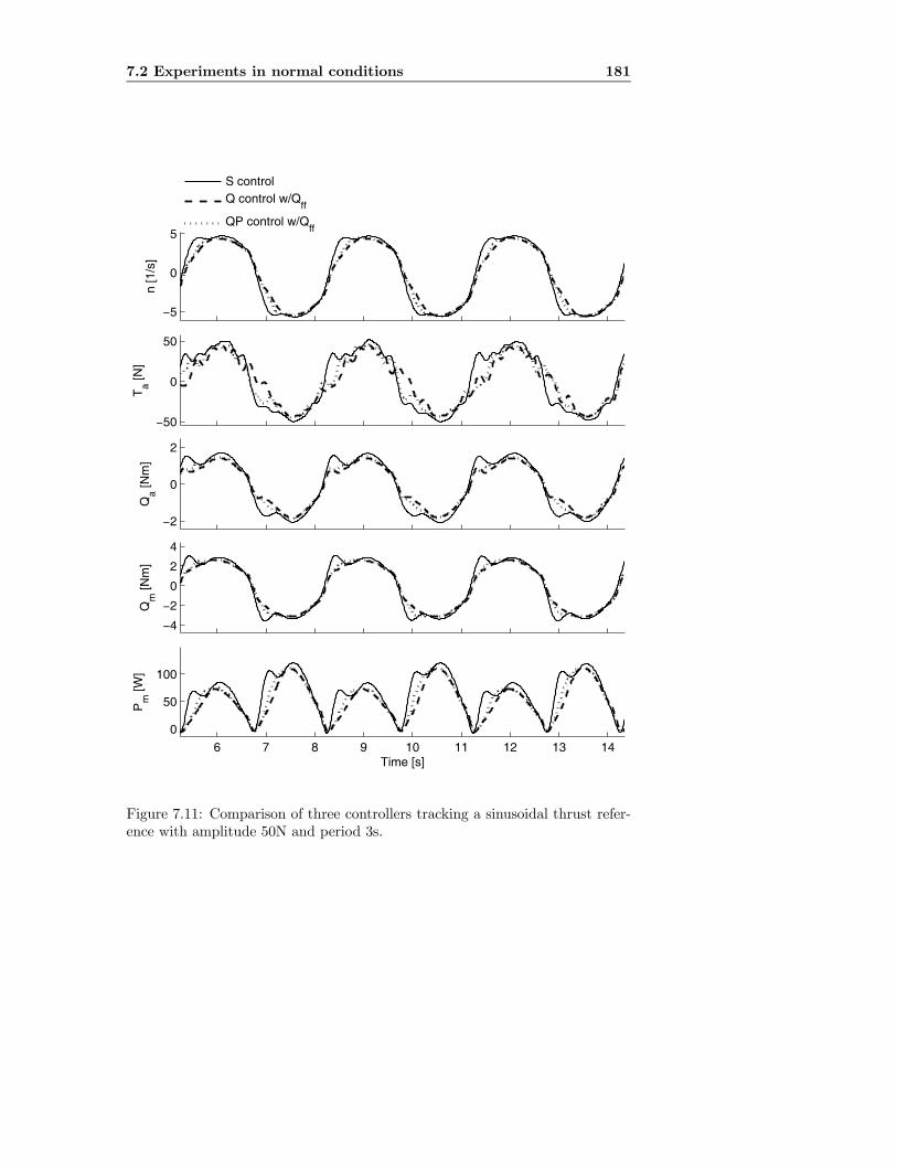
7.2 Experiments in normal conditions 181
−5
0
5
n [1
/s]
−50
0
50
Ta [N
]
−2
0
2
Qa [N
m]
−4
−2
0
2
4
Qm
[Nm
]
6 7 8 9 10 11 12 13 14
0
50
100
Pm
[W]
Time [s]
S controlQ control w/Q
ff
QP control w/Qff
Figure 7.11: Comparison of three controllers tracking a sinusoidal thrust refer-ence with amplitude 50N and period 3s.
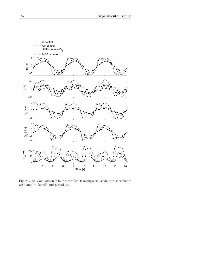
182 Experimental results
−5
0
5
n [1
/s]
−50
0
50
Ta [N
]
−2
0
2
Qa [N
m]
−4
−2
0
2
4
Qm
[Nm
]
6 7 8 9 10 11 12 13 14
0
50
100
Pm
[W]
Time [s]
Q controlQP controlSQP control w/Q
ff
MQP1 control
Figure 7.12: Comparison of four controllers tracking a sinusoidal thrust referencewith amplitude 50N and period 3s.
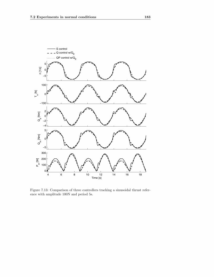
7.2 Experiments in normal conditions 183
−5
0
5
n [1
/s]
−100
0
100
Ta [N
]
−4
−2
0
2
Qa [N
m]
−5
0
5
Qm
[Nm
]
4 6 8 10 12 14 16 180
100
200
300
Pm
[W]
Time [s]
S controlQ control w/Q
ff
QP control w/Qff
Figure 7.13: Comparison of three controllers tracking a sinusoidal thrust refer-ence with amplitude 100N and period 5s.
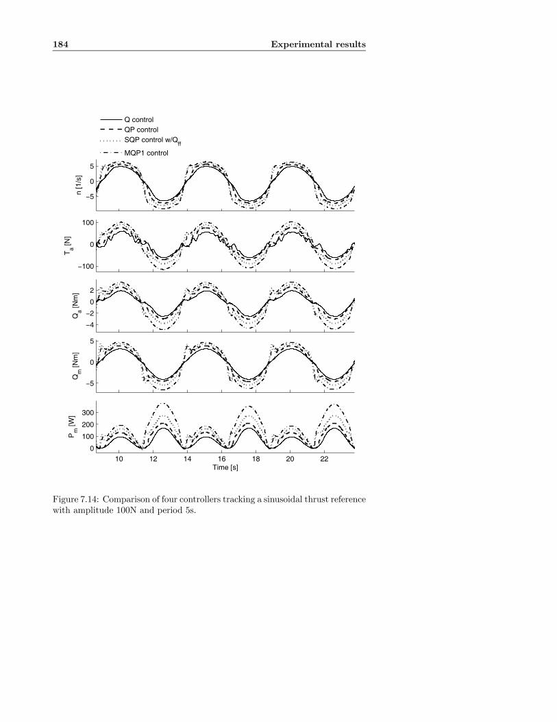
184 Experimental results
−5
0
5
n [1
/s]
−100
0
100
Ta [N
]
−4
−2
0
2
Qa [N
m]
−5
0
5
Qm
[Nm
]
10 12 14 16 18 20 22
0
100
200
300
Pm
[W]
Time [s]
Q controlQP controlSQP control w/Q
ff
MQP1 control
Figure 7.14: Comparison of four controllers tracking a sinusoidal thrust referencewith amplitude 100N and period 5s.

7.2 Experiments in normal conditions 185
−10
0
10
n [1
/s]
−200
0
200
Ta [N
]
−5
0
5
Qa [N
m]
−10
−5
0
5
Qm
[Nm
]
6 8 10 12 14 16 18 20 22 24 260
200
400
600
Pm
[W]
Time [s]
S controlQ control w/Q
ff
QP control w/Qff
Figure 7.15: Comparison of three controllers tracking a sinusoidal thrust refer-ence with amplitude 200N and period 7s.
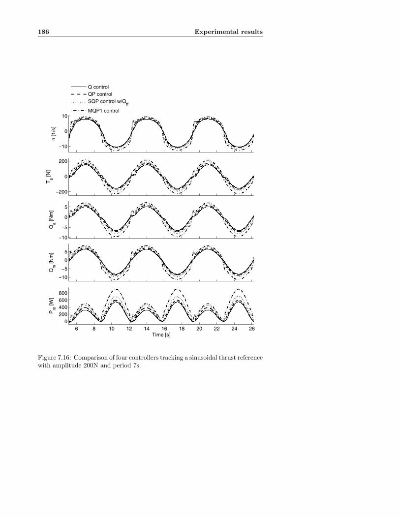
186 Experimental results
−10
0
10
n [1
/s]
−200
0
200
Ta [N
]
−10
−5
0
5
Qa [N
m]
−10
−5
0
5
Qm
[Nm
]
6 8 10 12 14 16 18 20 22 24 260
200400600800
Pm
[W]
Time [s]
Q controlQP controlSQP control w/Q
ff
MQP1 control
Figure 7.16: Comparison of four controllers tracking a sinusoidal thrust referencewith amplitude 200N and period 7s.
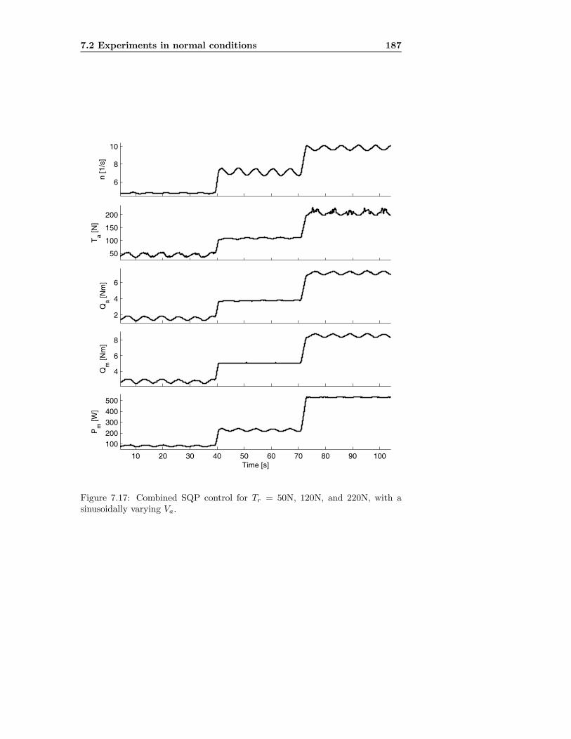
7.2 Experiments in normal conditions 187
6
8
10
n [1
/s]
50
100
150
200
Ta [N
]
2
4
6
Qa [N
m]
4
6
8
Qm
[Nm
]
10 20 30 40 50 60 70 80 90 100
100200
300
400500
Pm
[W]
Time [s]
Figure 7.17: Combined SQP control for Tr = 50N, 120N, and 220N, with asinusoidally varying Va.
188 Experimental results
7.3 Experiments in extreme conditions
This section presents experiments with the propeller subject to extreme con-ditions. Results are given for some of the controllers for normal conditionspresented in Chapter 3, as well as for the controllers designed for extreme con-ditions presented in Chapter 6. The observer and loss estimation scheme fromSection 5.1 are tested as parts of the anti-spin controllers. Results are givenboth for the ducted and open propeller.The propellers have been tested in a variety of operating conditions: for
constant and time-varying thrust references, in waves, with a calm free surfaceand forced vertical motion, and in combinations of waves and vertical motion.In the majority of the results presented here, the thrust reference was keptconstant during forced vertical motion with a calm free surface. This improvedthe repeatability and enabled comparison of various controllers, since the timeseries could be synchronized by comparing the relative vertical motion of thepropeller. Because of the chaotic nature of ventilation, the actual operatingconditions for the propeller vary from one test run to another. The time seriesmust therefore only be considered as examples of the performance of the variouscontrollers. However, the repeatability is in general good. The forced verticalmotion is parameterized in terms of the sinusoidal amplitude Av and period Tv,as well as the mean submergence h0. Two cases will mainly be used:
1. h0 = 25 cm, Av = 15 cm, and Tv = 10 s. This means that the propellerblades just exit the surface at the highest point of the trajectory.
2. h0 = 15 cm, Av = 15 cm, and Tv = 5 s. This means that the submergenceratio h/R = 0 at the highest point of the trajectory, i.e. the propellershaft is level with the free surface.
As for the tests in normal conditions, the results are shown in terms of n, Ta,Qa, Qm, and Pm.
7.3.1 Controller parameters
For the open propeller, the basic control parameters were chosen as in Table7.4. For the ducted propeller, KTC and KQC were taken as 0.513 and 0.0444,respectively. That is, (3.8) and (3.9) were implemented with KT0 = KT0r =0.513 and KQ0 = KQ0r = 0.0444. A summary of the ducted propeller controlparameters is given in Table 7.6. Notice that all the basic control parametersexcept the thrust and torque coefficients are equal for both propellers. Theparameters for the S and QP controller were chosen as in Table 7.5. However,the next section will discuss tuning of the S controller PI parameters.For the load torque observer and loss calculation from Section 5.1, Qf0 and
Qf1 were chosen as in Table 7.4, Is was set to 0.05kgm2, the observer gainswere chosen as ka = 15 and kb = −25, and the parameters for the weightingfunction αb(n) were chosen as [r, p, k] = [8, 0.5, 1]. In the ventilation detection

7.3 Experiments in extreme conditions 189
D KT0 KQ0 KT0r KQ0r nc0.25m 0.513 0.0444 0.513 0.0444 3rpsQf0 Qf1 nf Ic1.0Nm 0.01Nms 0.5rps 0kgm2
Table 7.6: Basic control parameters used in the experiments with the ductedpropeller.
Qf0 Qf1 Is ka kb1.0Nm 0.01Nms 0.05kgm2 15 −25r p k βv,on βv,off Tvent8 0.5 1 0.6 0.9 1.0s
Table 7.7: Parameters for the load torque observer, loss estimation, and venti-lation detection, used for both propellers.
scheme from Section 6.3, the threshold parameters were chosen as βv,on = 0.6and βv,off = 0.9, and the detection delay was set to Tvent = 1s. A summary ofthe observer and loss calculation parameters is given in Table 7.7.For the TS AS controller from Section 6.5, the settings for the primary
anti-spin action were γrise = 1s−1, γfall = −1s−1, and unless otherwise stated
τγ = 0.3s. Tuning of τγ is discussed in the next section. For the secondaryanti-spin action, the filter time constant was chosen as τn = 0.05s, and the ratelimits were chosen as n+vent = 3s
−2 and n−vent = −3s−2. The desired shaft speedduring ventilation was set to nas = 9rps. This choice was motivated from obser-vations during the tests, where it seemed that the most violent dynamic loadingdisappeared below 10rps. A summary of the TS AS controller parameters isgiven in Table 7.8.For the SB AS controller from Section 6.6.1, the PI parameters were chosen
as Kp = 0.5 and Ti = 0.05s, and the speed bound factor was chosen as rb = 0.2.The parameters are summed up in Table 7.9.A maximum shaft speed of nmax = 25rps was enforced in all the experiments,
in order to avoid damaging the setup by uncontrolled propeller racing.
7.3.2 Controller tuning
Figure 7.18 shows the shaft speed and the motor torque during a ventilationincident for the open propeller with three different shaft speed controllers. The
γrise γfall τγ n+vent n−vent τn nas1s−1 −1s−1 0.3s 3s−2 −3s−2 0.05s 9rps
Table 7.8: Parameters for the torque scaling anti-spin (TS AS) controller, usedfor both propellers.

190 Experimental results
Kp Ti rb0.5 0.05s 0.2
Table 7.9: Parameters for the speed bound anti-spin (SB AS) controller, usedfor both propellers.
ventilation incidents were generated by vertical motion of the propeller, withparameters h0 = 15cm, Av = 15cm, and Tv = 5s. The thrust reference wasTr = 200N. The figure demonstrates the importance of the tuning of the PI pa-rameters. Too low gains lead to significant propeller racing during ventilation,as well as long recovery time after the incident has terminated. On the otherhand, too high gains may lead to oscillations in the controller output due tointegrator discharge, or high sensitivity to measurement noise if a high propor-tional gain is chosen. Kp = 0.2 and Ti = 0.05s were found to be good trade-offs,and are used in the following. Figure 7.19 shows similar time series for the QPTS AS p controller, with varying filter time constants τγ . With primary actiononly, the goal of the anti-spin controller was to keep the shaft speed constant.The choice of τγ can be seen to have a similar effect as the choice of PI para-meters for the shaft speed controller. If no filter is used, the response of thecontroller is fast, but at the expense of a more noisy control signal. If the filtertime constant is too high, the anti-spin controller becomes slow and allows thepropeller to race out significantly before the ventilation incident is “caught”.This could have been expected from the analysis in Section 6.5.1, where it wasshown that the bound on the shaft speed was determined by the deviation ofγ from βQ during the ventilation incident. τγ = 0.3s was found to be a goodtrade-off between response time and noise in the control law, and used in theremainder of the tests. By comparing the shaft speeds in Figures 7.18 and 7.19it is apparent that the QP TS AS p controller has similar performance as areasonably well-tuned PI shaft speed controller during ventilation.
7.3.3 Single ventilation incidents with the ducted propeller
This section presents comparisons of six controllers during a ventilation incidentwith the ducted propeller, divided in two groups:
1a) Torque controller (Q).
1b) Combined torque/power controller (QP) — acts as a P controller for n >3rps.
1c) Shaft speed PI controller (S).
2a) Combined torque/power controller with torque scaling primary anti-spinaction (QP TS AS p).
2b) Combined torque/power controller with torque scaling primary and sec-ondary anti-spin action (QP TS AS p+s).

7.3 Experiments in extreme conditions 191
8
10
12
14
16
n [1
/s]
8 9 10 11 12 13 14 15
4
5
6
7
8
Qm
[Nm
]
Time [s]
Kp=0.2, T
i=0.05
Kp=0.1, T
i=0.1
Kp=0.3, T
i=0.03
Figure 7.18: Comparison of shaft speed and motor torque during a ventilationincident for the shaft speed controller with varying PI parameters at Tr = 200N.
8
9
10
11
12
13
14
n [1
/s]
8 9 10 11 12 13 14
4
5
6
7
8
Qm
[Nm
]
Time [s]
No filterτγ = 0.3 s
τγ = 0.5 s
τγ = 1.0 s
Figure 7.19: Comparison of shaft speed and motor torque during a ventilationincident for the QP TS AS p controller, using varying filter time constants atTr = 200N.
192 Experimental results
2c) Combined torque/power controller with speed bound anti-spin (QP SBAS).
The friction compensation scheme was used for all the controllers.The ventilation incidents were generated by vertical motion of the propeller,
with parameters h0 = 15cm, Av = 15cm, and Tv = 5s. Figures 7.20, 7.21, and7.22 show results for Tr = 100N, 200N, and 300N, respectively. The time seriesshow that the Q controller and the QP controller both lead to propeller racing.The S controller and the anti-spin controllers limit the shaft speed as intended,with the secondary anti-spin action of the QP TS AS p+s controller giving areduced shaft speed during ventilation. The Q controller could not be testedfor Tr = 300N, since the propeller racing was too severe to give sensible results.At Tr = 100N, nr < nas, such that the secondary action of the QP TS ASp+s controller never is activated. The time series is therefore nearly identicalto the QP TS AS p controller. Note also that there is a transient in the motortorque at the end of the ventilation incident for these controllers. This is dueto a “false” detection — the antispin controller is first switched off, and thenon and off again. This is unfortunate with respect to mechanical wear andtear. For all thrust references, the resulting thrust during ventilation is aboutthe same for all controllers — in Figure 7.21 the QP TS AS p+s controller,which reduces the shaft speed to 9rps during ventilation, produces the samethrust as the Q controller, which races to 25rps. The power consumption of theQ controller is unacceptably high, whereas the QP controller keeps the powerconsumption limited. The reason for the power not being constant is that thecontrol coefficients KTC and KQC no longer match the true coefficients duringventilation. The S and anti-spin controllers give a significantly reduced powerconsumption during ventilation. This is inevitable, and may be a problem ifthe power system and PMS are not designed to cope with the sudden excess ofpower. It can be noted that the QP TS AS p controller has a similar performanceas the S controller during ventilation, which also is the intention. Figure 7.23shows details from the QP TS AS p+s controller during a ventilation incidentat Tr = 300N, showing that the proposed anti-spin controller — including theload torque observer and ventilation detection scheme — performs as intended.
7.3.4 Single ventilation incidents with the open propeller
Figures 7.24, 7.25, and 7.26 present similar results as in the previous section,but for the open propeller. The same six controllers are tested, with the verticalmotion given by h0 = 25cm, Av = 15cm, and Tv = 10s. Since the averagesubmergence is higher in these tests, the ventilation is less severe than in theprevious section. The QP TS AS p+s controller was not tested for Tr = 100Nin Figure 7.24, since it is identical to the QP TS AS p controller in this case.For Tr = 300N in Figure 7.26, the Q controller was not tested, since the pro-peller racing was considered too severe. The main difference to notice fromthe previous section, is that increased shaft speed gives increased thrust dur-ing ventilation. This is consistent with the findings in Section 2.4. The result
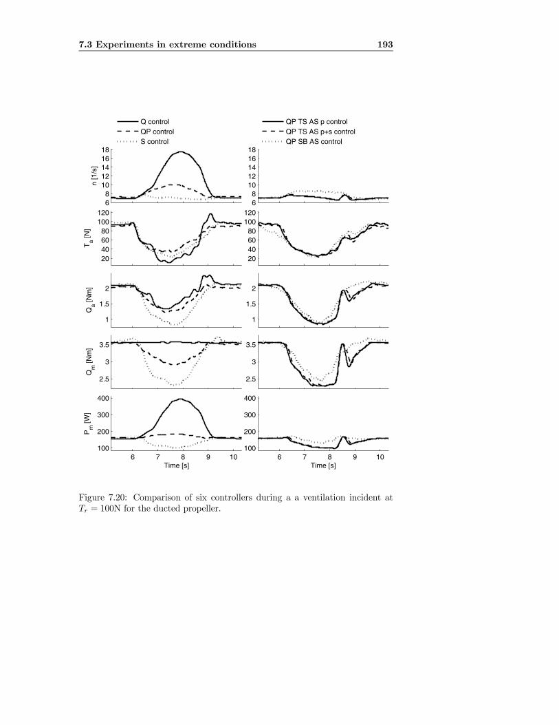
7.3 Experiments in extreme conditions 193
68
1012141618
n [1
/s]
20406080
100120
Ta [N
]
1
1.5
2
Qa [N
m]
2.5
3
3.5
Qm
[Nm
]
6 7 8 9 10100
200
300
400
Pm
[W]
Time [s]
68
1012141618
20406080
100120
1
1.5
2
2.5
3
3.5
6 7 8 9 10100
200
300
400
Time [s]
Q controlQP controlS control
QP TS AS p controlQP TS AS p+s controlQP SB AS control
Figure 7.20: Comparison of six controllers during a a ventilation incident atTr = 100N for the ducted propeller.

194 Experimental results
10
15
20
25
n [1
/s]
0
100
200
Ta [N
]
1
2
3
4
5
Qa [N
m]
2
4
6
Qm
[Nm
]
16 17 18 19 20
200
400
600
800
Pm
[W]
Time [s]
10
15
20
25
0
100
200
1
2
3
4
5
2
4
6
16 17 18 19 20
200
400
600
800
Time [s]
Q controlQP controlS control
QP TS AS p controlQP TS AS p+s controlQP SB AS control
Figure 7.21: Comparison of six controllers during a a ventilation incident atTr = 200N for the ducted propeller.

7.3 Experiments in extreme conditions 195
10
15
20
25
n [1
/s]
0
100
200
300
Ta [N
]
2
4
6
Qa [N
m]
2
4
6
8
Qm
[Nm
]
26 27 28 29 30
200
400
600
800
Pm
[W]
Time [s]
10
15
20
25
0
100
200
300
2
4
6
2
4
6
8
26 27 28 29 30
200
400
600
800
Time [s]
QP controlS control
QP TS AS p controlQP TS AS p+s controlQP SB AS control
Figure 7.22: Comparison of five controllers during a a ventilation incident atTr = 300N for the ducted propeller.
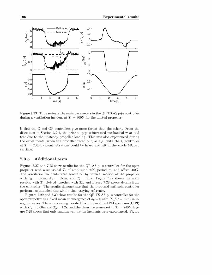
196 Experimental results
0
2
4
6
Qa [N
m]
0
0.5
1
β Q, ζ
[−]
0 1 2 3 4 5
0.2
0.4
0.6
0.8
1
γ [−
]
Time [s]
−0.2
0
0.2
0.4
γ −
βQ
[−]
9
10
11
12
n ras [1
/s]
0 1 2 3 4 5
0.1
0.2
0.3
h [m
]
Time [s]
βQ
ζ
EstimatedMeasured
^
<
Figure 7.23: Time series of the main parameters in the QP TS AS p+s controllerduring a ventilation incident at Tr = 300N for the ducted propeller.
is that the Q and QP controllers give more thrust than the others. From thediscussion in Section 3.2.2, the price to pay is increased mechanical wear andtear due to the unsteady propeller loading. This was also experienced duringthe experiments; when the propeller raced out, as e.g. with the Q controllerat Tr = 200N, violent vibrations could be heard and felt in the whole MCLabcarriage.
7.3.5 Additional tests
Figures 7.27 and 7.28 show results for the QP AS p+s controller for the openpropeller with a sinusoidal Tr of amplitude 50N, period 7s, and offset 200N.The ventilation incidents were generated by vertical motion of the propellerwith h0 = 15cm, Av = 15cm, and Tv = 10s. Figure 7.27 shows the mainresults, with Tr plotted together with Ta, and Figure 7.28 shows details fromthe controller. The results demonstrate that the proposed anti-spin controllerperforms as intended also with a time-varying reference.Figures 7.29 and 7.30 show results for the QP TS AS p+s controller for the
open propeller at a fixed mean submergence of h0 = 0.44m (h0/R = 1.75) in ir-regular waves. The waves were generated from the modified PM spectrum (C.19)with Hs = 0.06m and Tp = 1.2s, and the thrust reference set to Tr = 240N. Fig-ure 7.29 shows that only random ventilation incidents were experienced. Figure
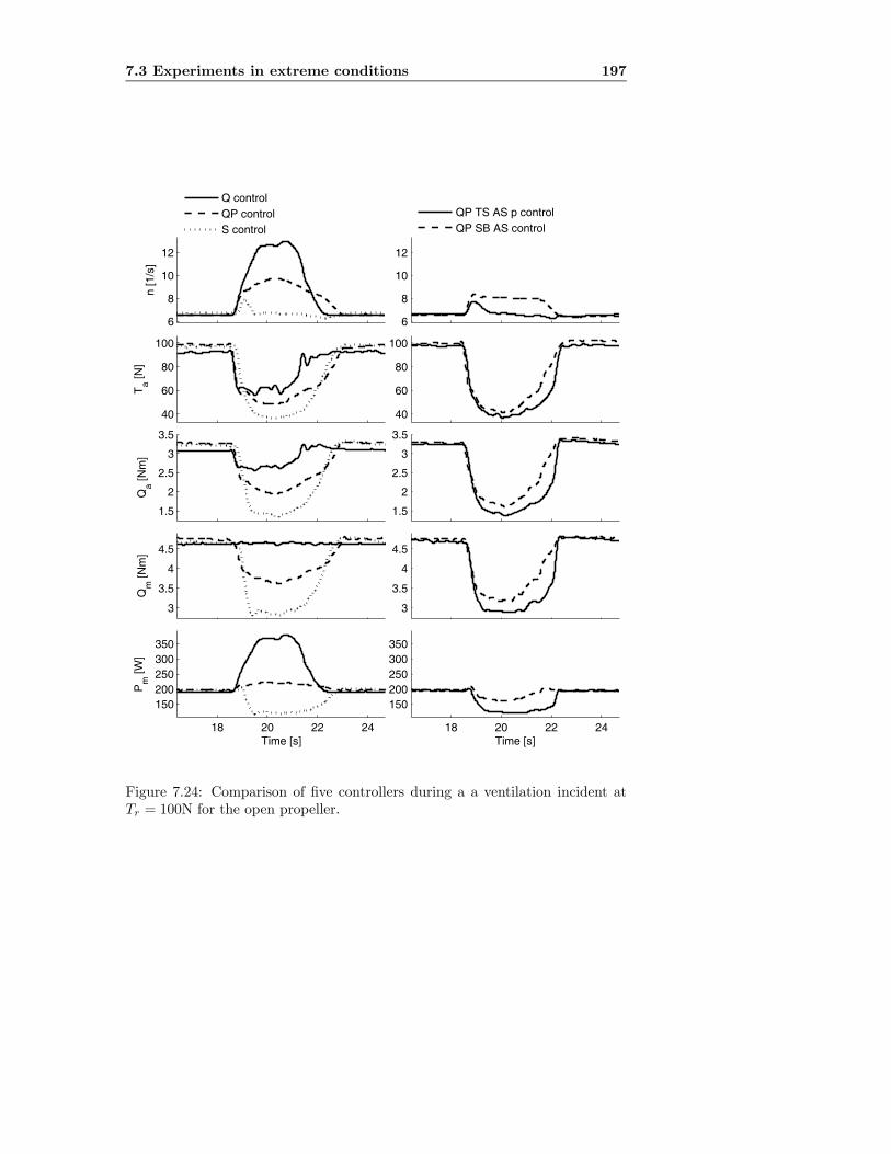
7.3 Experiments in extreme conditions 197
6
8
10
12
n [1
/s]
40
60
80
100
Ta [N
]
1.5
2
2.5
3
3.5
Qa [N
m]
3
3.5
4
4.5
Qm
[Nm
]
18 20 22 24
150200250300350
Pm
[W]
Time [s]
6
8
10
12
40
60
80
100
1.5
2
2.5
3
3.5
3
3.5
4
4.5
18 20 22 24
150200250300350
Time [s]
Q controlQP controlS control
QP TS AS p controlQP SB AS control
Figure 7.24: Comparison of five controllers during a a ventilation incident atTr = 100N for the open propeller.

198 Experimental results
10
15
20
25
n [1
/s]
50
100
150
200
Ta [N
]
2
4
6
Qa [N
m]
4
6
8
Qm
[Nm
]
18 20 22 24200400600800
10001200
Pm
[W]
Time [s]
10
15
20
25
50
100
150
200
2
4
6
4
6
8
18 20 22 24200400600800
10001200
Time [s]
Q controlQP controlS control
QP TS AS p controlQP TS AS p+s controlQP SB AS control
Figure 7.25: Comparison of six controllers during a a ventilation incident atTr = 200N for the open propeller.

7.3 Experiments in extreme conditions 199
10
15
20
n [1
/s]
100
200
300
Ta [N
]
2
4
6
8
10
Qa [N
m]
4
6
8
10
12
Qm
[Nm
]
12 14 16 18200
400
600
800
1000
Pm
[W]
Time [s]
10
15
20
100
200
300
2
4
6
8
10
4
6
8
10
12
12 14 16 18200
400
600
800
1000
Time [s]
QP controlS control
QP TS AS p controlQP TS AS p+s controlQP SB AS control
Figure 7.26: Comparison of five controllers during a a ventilation incident atTr = 300N for the open propeller.
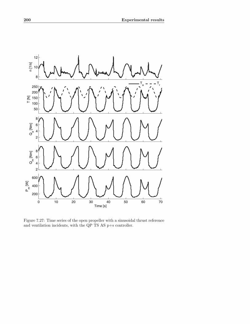
200 Experimental results
50
100
150
200
250
T [N
]
2
4
6
8
Qa [N
m]
8
10
12
n [1
/s]
2
4
6
8
Qm
[Nm
]
0 10 20 30 40 50 60 70
200
400
600
Pm
[W]
Time [s]
Ta
Tr
Figure 7.27: Time series of the open propeller with a sinusoidal thrust referenceand ventilation incidents, with the QP TS AS p+s controller.
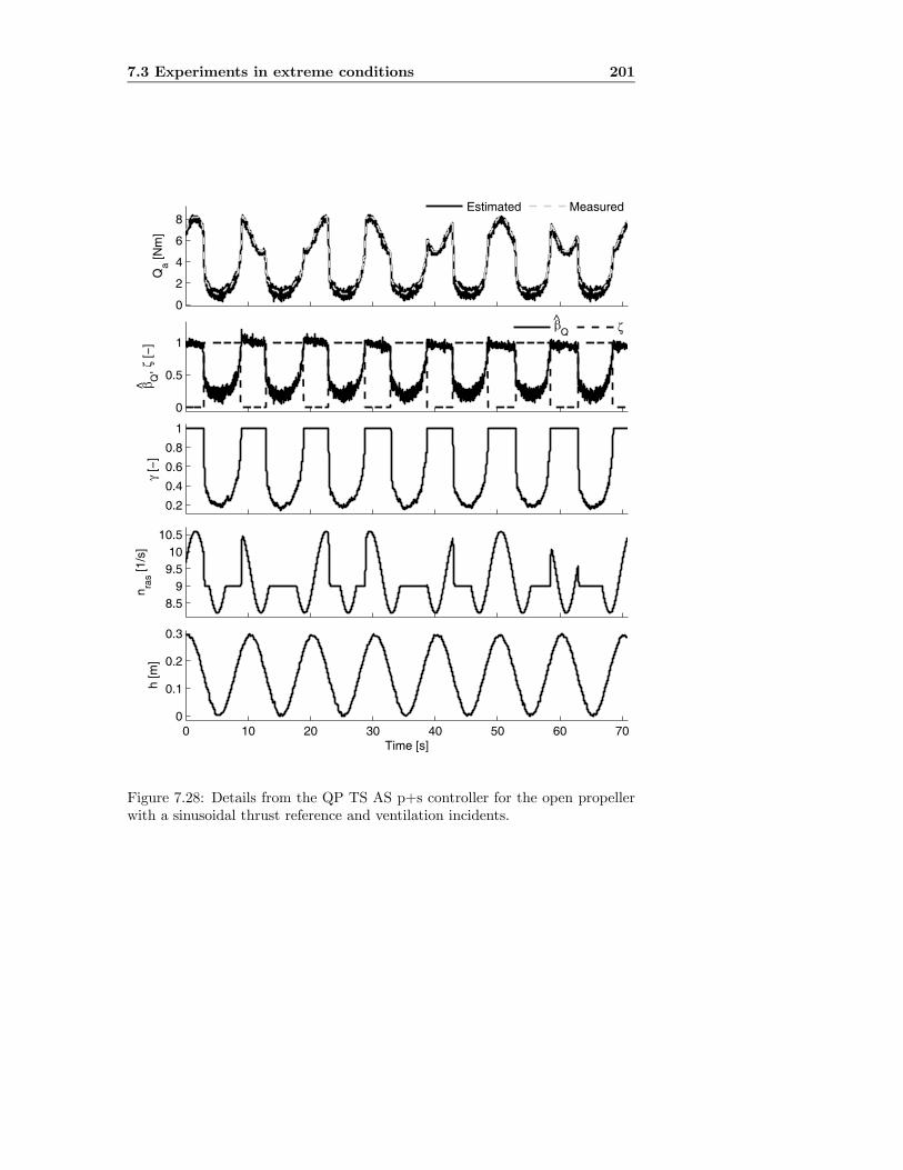
7.3 Experiments in extreme conditions 201
0
2
4
6
8
Qa [N
m]
0
0.5
1
β Q, ζ
[−]
0.2
0.4
0.6
0.8
1
γ [−
]
8.59
9.510
10.5
n ras [1
/s]
0 10 20 30 40 50 60 700
0.1
0.2
0.3
h [m
]
Time [s]
Estimated Measured
βQ ζ
^
<
Figure 7.28: Details from the QP TS AS p+s controller for the open propellerwith a sinusoidal thrust reference and ventilation incidents.

202 Experimental results
7.30 shows that the anti-spin controller works as intended: when there is noor little ventilation, the QP controller is left to work undisturbed, and whena ventilation incident suddenly appears, the anti-spin actions are activated totake control of and reduce the shaft speed.
7.4 Discussion
The experiments presented in this chapter have provided a fairly extensive val-idation of the various proposed control concepts. The results also act as averification of the simulation results presented in Chapters 3, 5, and 6.The quasi-static properties of the fundamental controllers when subject to
varying advance velocity were theoretically analyzed in Chapter 4, and theirperformance in waves and current was tested by simulations in Chapter 3. Theexperimental results confirmed that the shaft speed controller is the most sensi-tive to changes in Va, followed by the power and torque controllers, as summedup in Table 3.10. The experimentally derived sensitivity functions in Figure 7.9also compared well with the theoretical functions derived in Chapter 4.The tracking tests with the fundamental controllers confirmed the simula-
tions in Chapter 3, and showed that the performance of the torque and powercontrollers with the appropriate friction and inertia compensation schemes wereas good as or better than that of the shaft speed controller. The experiments alsoconfirmed that, if the friction is significant, the lack of a friction compensationscheme in the torque and power controllers would lead to poor tracking perfor-mance for low thrust references. The combined QP controller — which with theweighting function parameters in Table 7.5 essentially was a power controllerwith torque control to facilitate zero-crossings — worked as intended, with aseamless transition between the two fundamental controllers. The combinedSQP and MQP1 controllers also worked satisfactory, with the MQP1 controllerfacilitating reasonable tracking properties even without a friction compensationscheme.In extreme conditions, the experiments confirmed the bad performance of
torque and power control. This verified the analysis in Chapter 4 and the simula-tions in Chapter 6, which also showed severe propeller racing during ventilationincidents. However, it is apparent that the propeller rotational inertia has asignificant influence on the amount of propeller racing; the simulations with afull-scale propeller from Chapter 6 gave less racing than the experiments withthe model-scale propeller presented in this chapter.The experiments further confirmed that the problems with propeller rac-
ing could be alleviated by introducing anti-spin control. The proposed torquescaling anti-spin scheme from Section 6.5 (TS AS p+s) was shown to work asintended, including the load torque observer, loss estimation, ventilation detec-tion, and primary and secondary anti-spin action. The observer gave reasonableestimates of the propeller load torque, even with relatively noisy feedback sig-nals, and the ventilation incidents were detected with acceptable accuracy. The
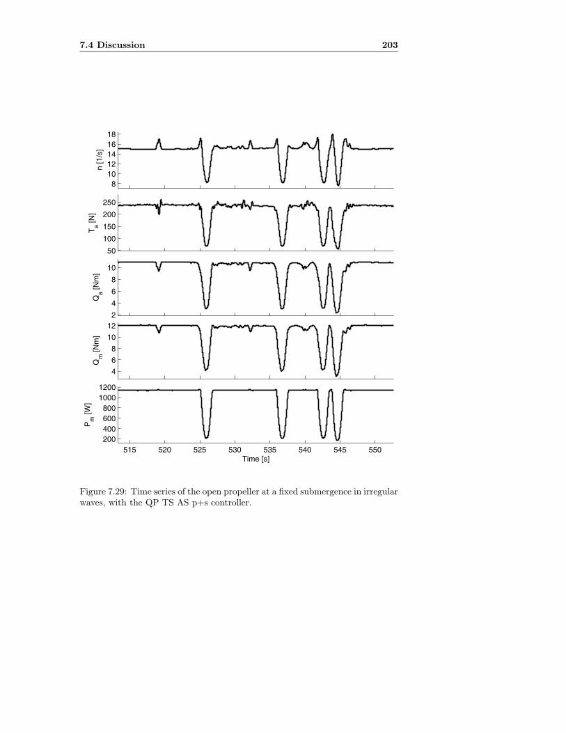
7.4 Discussion 203
50
100
150
200
250
Ta [N
]
2
4
6
8
10
Qa [N
m]
81012141618
n [1
/s]
4
6
8
10
12
Qm
[Nm
]
515 520 525 530 535 540 545 550200400600800
10001200
Pm
[W]
Time [s]
Figure 7.29: Time series of the open propeller at a fixed submergence in irregularwaves, with the QP TS AS p+s controller.
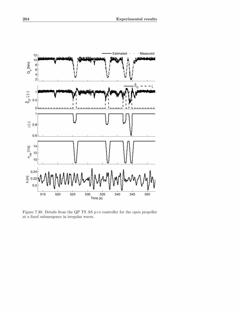
204 Experimental results
2
4
6
8
10
12
Qa [N
m]
0
0.5
1
β Q, ζ
[−]
0.6
0.8
1
γ [−
]
10
12
14
n ras [1
/s]
515 520 525 530 535 540 545 550
0.2
0.22
0.24
h [m
]
Time [s]
Estimated Measured
βQ ζ^
<
Figure 7.30: Details from the QP TS AS p+s controller for the open propellerat a fixed submergence in irregular waves.
7.4 Discussion 205
results were hence consistent with the simulations from Chapter 6. The stabil-ity analysis in Section 6.5 was performed for a constant thrust reference. Bothsimulations and experiments, however, showed that the anti-spin scheme workedwell also for a time-varying Tr.The speed bound anti-spin controller (SB AS) was also shown to work as
intended, with experimental results comparable to the simulations from Chapter6.The weighting function parameters for the QP controller were chosen to
give pure power control for n > 3rps. Hence, the anti-spin controllers were inpractice only presented as add-ons to P control. Anti-spin experiments witha Q controller have also been also performed (i.e. with anti-spin as an add-on to torque control, Q TS AS). The results were comparable to the QP TSAS controller, although with a slightly reduced performance during ventilation.This is consistent with the simulations presented in Figures 6.6 and 6.7.From the discussions in Sections 2.4.6 and 3.2.2, ventilation of a propeller
at low Va will give large unsteady loads, which are suspected to cause signif-icant mechanical wear and tear. The experimental setup was not capable ofmeasuring these high-frequency loads, and the benefits of limiting the propellerracing could hence not be verified directly. The unsteady loads were, however,physically experienced during the experiments through vibrations and noise asthe propeller raced out.
In conclusion, the introduction of anti-spin control meant that the perfor-mance of the torque and power controllers became acceptable also in extremeenvironmental conditions. From an over-all performance evaluation, the QP,SQP, or MQP controllers with anti-spin and the appropriate friction and inertiacompensation schemes appear to be the best solution, combining the advantagesof the QP controller in normal conditions with acceptable shaft speed controland limited transients in the motor torque during ventilation. However, thechoice of core thruster controller and eventually an anti-spin controller will de-pend on the type of propeller, the type of vessel, and the expected operatingconditions.If an anti-spin controller is deemed appropriate, additional tuning is re-
quired. This will complicate commissioning of the thruster controller. Themain challenge will probably be tuning of the load torque observer, since this isthe core element of the anti-spin controller. However, with the tuning guidelinesfrom Section 5.1.1, reasonable model knowledge, and increased experience, thisshould not be of major concern.

206 Experimental results
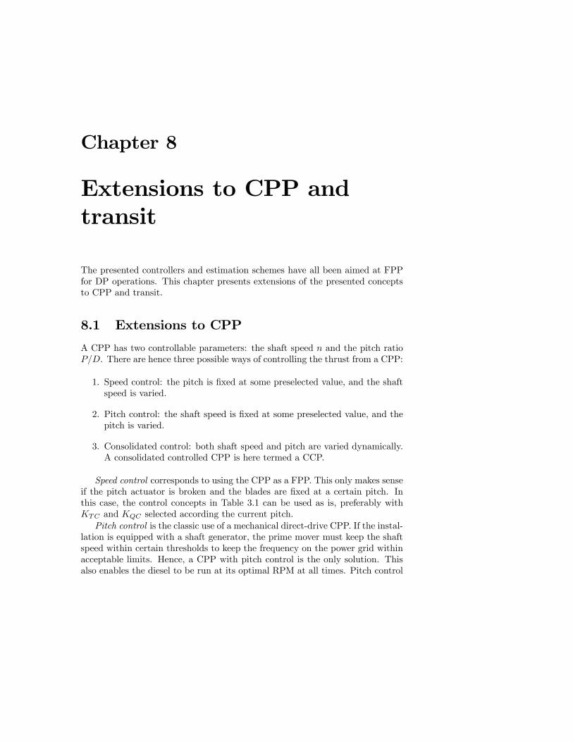
Chapter 8
Extensions to CPP andtransit
The presented controllers and estimation schemes have all been aimed at FPPfor DP operations. This chapter presents extensions of the presented conceptsto CPP and transit.
8.1 Extensions to CPP
A CPP has two controllable parameters: the shaft speed n and the pitch ratioP/D. There are hence three possible ways of controlling the thrust from a CPP:
1. Speed control: the pitch is fixed at some preselected value, and the shaftspeed is varied.
2. Pitch control: the shaft speed is fixed at some preselected value, and thepitch is varied.
3. Consolidated control: both shaft speed and pitch are varied dynamically.A consolidated controlled CPP is here termed a CCP.
Speed control corresponds to using the CPP as a FPP. This only makes senseif the pitch actuator is broken and the blades are fixed at a certain pitch. Inthis case, the control concepts in Table 3.1 can be used as is, preferably withKTC and KQC selected according the current pitch.Pitch control is the classic use of a mechanical direct-drive CPP. If the instal-
lation is equipped with a shaft generator, the prime mover must keep the shaftspeed within certain thresholds to keep the frequency on the power grid withinacceptable limits. Hence, a CPP with pitch control is the only solution. Thisalso enables the diesel to be run at its optimal RPM at all times. Pitch control

208 Extensions to CPP and transit
has also been widespread in diesel-electric installations, where fixed speed elec-tromotors have been used in tunnel thrusters and azimuthing thrusters due totheir low cost and simplicity.Consolidated control combines many of the good properties of both variable
speed FPP and fixed speed, variable pitch CPP, but also inherits some of thecons of the CPP propellers (Schanz, 1967; Morvillo, 1996; Andresen, 2000). Themain advantages of a CCP are reduced noise and the ability to operate at highefficiency for a wide range of Va and n. This is clearly seen in Figure 2.3, wherethe optimal open-water efficiency is found at higher Ja for increasing P/D. Withtwo controllable parameters, optimal control also becomes a feasible solution,since the desired thrust often can be met by a number of combinations of speedand pitch. The task is then to find the combination of shaft speed and pitch thate.g. gives the lowest power demand, and hence fuel consumption. For DP, thiscombination can be found from the pitch dependent propeller characteristics.In transit, however, the optimization becomes a dynamic task. This is furthertreated in Schanz (1967), Winterbone (1980), Beek and Mulder (1983), Parsonsand Wu (1985), Bakountouzis (1992), Chachulski et al. (1995), Fukuba et al.(1996), Morvillo (1996), Young-Bok et al. (1998), and Whalley and Ebrahimi(2002). More details on this can also be found in Ruth et al. (2006). In thefollowing, extensions of the presented control and estimation concepts for FPPto CCP will be treated. Consolidated control based on optimal control will notbe further treated.
8.1.1 Controller modifications for CCP
A consolidated control scheme must contain mappings from the thrust referenceTr to the pitch angle reference φr, and one other parameter. In a conventionalimplementation based on pitch and shaft speed control, the other parameterwould be the shaft speed reference nr. Not considering optimal control schemes,which are more complex, there is then a unique relationship between Tr and φr,expressed by the function gφ:
φr = gφ(Tr). (8.1)
The relationship between the pitch ratio P/D and the pitch angle φ is givenin (2.41). From Section 2.1.5, the open-water characteristics of a CPP can beparameterized by φ (in addition to Va and n). Hence, the nominal thrust andtorque coefficients may be expressed as functions of φ:
KT0 = KT0(φ), KQ0 = KQ0(φ). (8.2)
The relationships in (8.2) should be known from the propeller characteristics.It is therefore possible to parameterize the control coefficients from (3.8, 3.9) inthe same manner, based on φr:
KTC = KTC(nr, φr), KQC = KQC(nr, φr). (8.3)
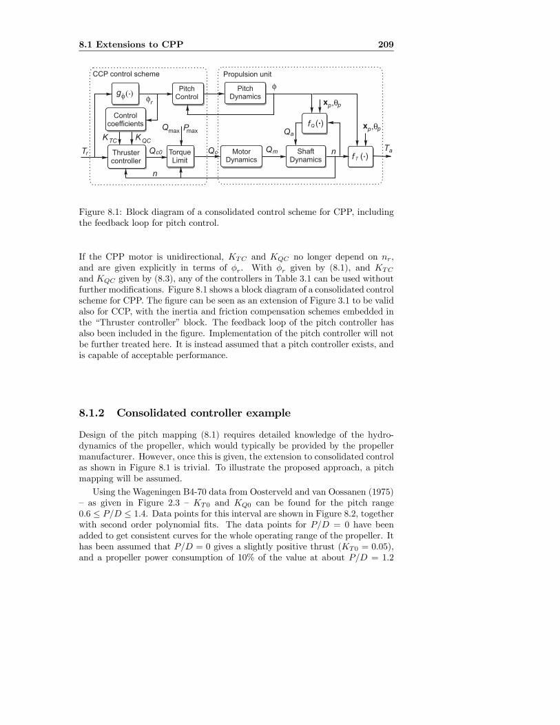
8.1 Extensions to CPP 209
nf
Q
Q
Ta
a
T
m( )
fQ ( ).
.MotorDynamics
QcTorqueLimit
.
pxp
ShaftDynamics
PmaxQmax
Propulsion unit
n
,q
Qc0Tr Thrustercontroller
PitchDynamics
r
pxp,q
f
f
KTC KQC
g�( ).
Controlcoefficients
PitchControl
CCP control scheme
Figure 8.1: Block diagram of a consolidated control scheme for CPP, includingthe feedback loop for pitch control.
If the CPP motor is unidirectional, KTC and KQC no longer depend on nr,and are given explicitly in terms of φr. With φr given by (8.1), and KTC
and KQC given by (8.3), any of the controllers in Table 3.1 can be used withoutfurther modifications. Figure 8.1 shows a block diagram of a consolidated controlscheme for CPP. The figure can be seen as an extension of Figure 3.1 to be validalso for CCP, with the inertia and friction compensation schemes embedded inthe “Thruster controller” block. The feedback loop of the pitch controller hasalso been included in the figure. Implementation of the pitch controller will notbe further treated here. It is instead assumed that a pitch controller exists, andis capable of acceptable performance.
8.1.2 Consolidated controller example
Design of the pitch mapping (8.1) requires detailed knowledge of the hydro-dynamics of the propeller, which would typically be provided by the propellermanufacturer. However, once this is given, the extension to consolidated controlas shown in Figure 8.1 is trivial. To illustrate the proposed approach, a pitchmapping will be assumed.
Using the Wageningen B4-70 data from Oosterveld and van Oossanen (1975)— as given in Figure 2.3 — KT0 and KQ0 can be found for the pitch range0.6 ≤ P/D ≤ 1.4. Data points for this interval are shown in Figure 8.2, togetherwith second order polynomial fits. The data points for P/D = 0 have beenadded to get consistent curves for the whole operating range of the propeller. Ithas been assumed that P/D = 0 gives a slightly positive thrust (KT0 = 0.05),and a propeller power consumption of 10% of the value at about P/D = 1.2
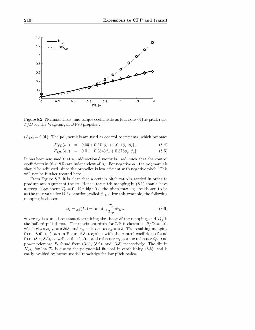
210 Extensions to CPP and transit
0 0.2 0.4 0.6 0.8 1 1.2 1.40
0.2
0.4
0.6
0.8
1
1.2
1.4
P/D [−]
KT0
10KQ0
Figure 8.2: Nominal thrust and torque coefficients as functions of the pitch ratioP/D for the Wageningen B4-70 propeller.
(KQ0 = 0.01). The polynomials are used as control coefficients, which become:
KTC(φr) = 0.05 + 0.974φr + 1.044φr |φr| , (8.4)
KQC(φr) = 0.01− 0.0843φr + 0.878φr |φr| . (8.5)
It has been assumed that a unidirectional motor is used, such that the controlcoefficients in (8.4, 8.5) are independent of nr. For negative φr, the polynomialsshould be adjusted, since the propeller is less efficient with negative pitch. Thiswill not be further treated here.From Figure 8.2, it is clear that a certain pitch ratio is needed in order to
produce any significant thrust. Hence, the pitch mapping in (8.1) should havea steep slope about Tr = 0. For high Tr, the pitch may e.g. be chosen to beat the max value for DP operation, called φDP . For this example, the followingmapping is chosen:
φr = gφ(Tr) = tanh(εφTrTbp
)φDP , (8.6)
where εφ is a small constant determining the shape of the mapping, and Tbp isthe bollard pull thrust. The maximum pitch for DP is chosen as P/D = 1.0,which gives φDP = 0.308, and εφ is chosen as εφ = 0.3. The resulting mappingfrom (8.6) is shown in Figure 8.3, together with the control coefficients foundfrom (8.4, 8.5), as well as the shaft speed reference nr, torque reference Qr, andpower reference Pr found from (3.1), (3.2), and (3.3) respectively. The dip inKQC for low Tr is due to the polynomial fit used in establishing (8.5), and iseasily avoided by better model knowledge for low pitch ratios.

8.1 Extensions to CPP 211
0
0.1
0.2
0.3
0.4
φ r [rad
]
0
0.2
0.4
0.6
0.8
KT
C, 1
0KQ
C
KTC
10KQC
0
1
2
3
n r [rps
]
0
50
100
150
Qr [k
N]
0 50 100 150 200 250 3000
1000
2000
3000
Pr [k
W]
Tr [kN]
Figure 8.3: Consolidated controller example, with a chosen mapping from Trto φr, the corresponding KTC and KQC from the propeller characteristics, andnr, Qr and Pr to be used in shaft speed, torque, or power control, respectively.
212 Extensions to CPP and transit
Remark 8.1 The whole pitch range is not necessarily used in DP, since it maybe advantageous with higher pitch ratios in transit than in DP. The chosenmaximum pitch for DP will depend on the rating and speed range of the thrustermotor.
8.1.3 Observer and estimation extensions to CCP
The estimated load torque Qa and torque coefficient KQ from (5.7) and (5.17), or(5.18) and (5.26), are completely independent of the propeller hydrodynamicsand the operating conditions — they are calculated solely from the rotationaldynamics of the propeller shaft. Hence, these schemes are valid also for CCPand transit without modifications. However, the estimated torque loss factorβQ from (5.16) or (5.19) is based on the control coefficient KQC , and the torqueperformance factor χQ from (5.45) is based on both KQC and KTC . This mustbe accounted for if the loss estimation and performance monitoring schemes areto be used for CCP or transit.Section 8.1.1 showed how the control schemes for FPP could be extended
to CCP by letting KTC and KQC be functions of the the pitch angle referenceφr. Since KTC and KQC are used to represent the nominal performance ofthe propeller, the same approach can be used for βQ and χQ. Hence, the lossestimation and performance monitoring schemes are valid also for CCP whenKTC(φr) and KQC(φr) are chosen as for the thruster controllers, i.e. as in (8.3).
8.1.4 Anti-spin controller extensions to CCP
The ventilation detection scheme in (6.1) and the primary anti-spin action in(6.6) are both based on βQ, and are hence valid as long as the calculation of βQis valid. The secondary anti-spin action in (6.18) is based on the shaft speedmapping in (3.1), which again is based on KTC , and therefore holds as long as(8.3) is applied.This means that the proposed anti-spin thruster control scheme in Section 6.5
is valid also for CCP simply by applying (8.3), since the four main componentsin the scheme:
• Core thruster controller,
• Load torque observer,
• Ventilation detection,
• Anti-spin control actions,
all have been shown to be valid.As for FPP, the main purpose of the proposed anti-spin control scheme for
CCP is to take control of the shaft speed during severe thrust loss incidents.This is performed by the primary anti-spin action, which does not affect the
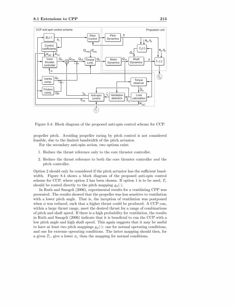
8.1 Extensions to CPP 213
nf
Q
Q
Ta
a
T
m( )
fQ ( ).
.MotorDynamics
QcTorqueLimit
.
pxp
ShaftDynamics
PmaxQmax
Propulsion unit
n
��
Corethruster
controller
PitchDynamics
r
pxp��
�
�
K TCKQC
g ( ).
Controlcoefficients
PitchControl
Qa
gLoss
calculation
Torqueobserver
Ventilationdetection
bQ
Anti-spincontrol
Tras
z
T
Tr
Frictioncomp. Qff
ifInertiacomp.
XQci Qcas Qc0
Q
�
Q
CCP anti-spin control scheme
++
++
KQC
Figure 8.4: Block diagram of the proposed anti-spin control scheme for CCP.
propeller pitch. Avoiding propeller racing by pitch control is not consideredfeasible, due to the limited bandwidth of the pitch actuator.For the secondary anti-spin action, two options exist:
1. Reduce the thrust reference only to the core thruster controller.
2. Reduce the thrust reference to both the core thruster controller and thepitch controller.
Option 2 should only be considered if the pitch actuator has the sufficient band-width. Figure 8.4 shows a block diagram of the proposed anti-spin controlscheme for CCP, where option 2 has been chosen. If option 1 is to be used, Trshould be routed directly to the pitch mapping gφ(·).In Ruth and Smogeli (2006), experimental results for a ventilating CPP was
presented. The results showed that the propeller was less sensitive to ventilationwith a lower pitch angle. That is, the inception of ventilation was postponedwhen φ was reduced, such that a higher thrust could be produced. A CCP can,within a large thrust range, meet the desired thrust for a range of combinationsof pitch and shaft speed. If there is a high probability for ventilation, the resultsin Ruth and Smogeli (2006) indicate that it is beneficial to run the CCP with alow pitch angle and high shaft speed. This again suggests that it may be usefulto have at least two pitch mappings gφ(·): one for normal operating conditions,and one for extreme operating conditions. The latter mapping should then, fora given Tr, give a lower φr than the mapping for normal conditions.

214 Extensions to CPP and transit
This result also indicates that, if the pitch actuator bandwidth is sufficientlyhigh, option 2 for the secondary anti-spin action should be chosen; a reducedpitch angle during ventilation would probably hasten termination of the ven-tilation incident and reduce the load transients. This must, however, only beconsidered as speculation, since the experimental setup did not allow for testingof a CPP with dynamic pitch control.
8.1.5 A near optimal controller
A basic problem with on-line optimal control of CCP is the need to know thepropeller advance speed. If the advance speed is not known, an off-line opti-mization scheme must be utilized. This is discussed in more detail in Ruth etal. (2006). A simple, yet smart, consolidated controller that avoids this problemwas presented by Schanz (1967). In this control scheme, the motor torque iskept constant, while the shaft speed is kept constant by adjusting the propellerpitch (called a “propeller governor”). The pitch can be controlled by e.g. a PIDcontroller operating on the shaft speed error, exactly as for the PID shaft speedcontroller in (3.27). With constant motor torque and shaft speed, also the poweris constant. Hence, the propeller governor gives a constant speed/torque/powercontroller, which can be shown to be very near optimal.The performance of the controller will depend on the PID tuning and band-
width of the pitch actuator. If a relatively low bandwidth is chosen, such thatwave-frequency disturbances are not counteracted, the controller will be verysimilar to the torque controller in (3.29) with control coefficient curves from(8.3). This will give wave-frequency oscillations in power. If the pitch actua-tor bandwidth is sufficiently high, and the PID is tuned tightly, the constantspeed/torque/power relationships will be maintained also in waves. This may,however, give unnecessary wear and tear of the pitch actuator.
8.2 Extensions to transit
During DP operation, the advance velocities of the propellers are assumed to beof moderate magnitude. The controllers in Table 3.1 are then expected to giveadequate performance with control coefficients based on the nominal thrust andtorque coefficients, as proposed in Section 3.5.During transit, the propellers are subject to higher advance velocities, and
the actual thrust and torque coefficients will deviate significantly from the nom-inal coefficients proposed as control coefficients in (3.8, 3.9). This is easily seenfrom e.g. (2.25, 2.26) or (2.20, 2.21). Depending on the chosen controller, themapping from reference to actual thrust will become inaccurate, and one mayask if the controllers in Table 3.1 then are appropriate. In order to investigatethis, the differences in control objectives for DP and transit operations must beclarified, before possible extensions of the controllers are introduced.

8.2 Extensions to transit 215
8.2.1 DP vs. transit
In DP mode, the vessel is usually fully actuated or over-actuated. As described inSection 3.2.1, accurate thrust production is then important for the bandwidthof the vessel control system as a whole. In transit, normally only the mainpropellers are used. This means that the vessel becomes underactuated, i.e. it isunable to command accelerations in all 3 horizontal-plane DOF simultaneously.The control task therefore inherently becomes a 2DOF problem, where the mainobjectives usually are to keep a certain vessel speed and heading. It is importantto note that vessels that are fully actuated for low-speed applications, from apractical point of view still may become underactuated at higher speeds. Suchvessels may e.g. be equipped with main propellers in the stern and a numberof tunnel thrusters in the bow and stern. At higher vessels speeds, the tunnelthrusters lose most of their efficiency due to the water speed at the tunneloutlets (Chislett and Björheden, 1966; Brix, 1978; Karlsen et al., 1986). It isalso becoming increasingly common to have one or two azimuthing thrusters inthe bow or mid-ship to assist in DP operations. These are often of the retractableor swing-up type, and are stowed inside the hull for transit operations.In classic autopilot schemes, see e.g. Fossen (2002) and references therein,
the control task is usually divided in two: a dedicated speed controller, anda course auto-pilot. Typically, the speed controller, which also could be man-ual speed control from the bridge, controls the setpoint of the main propellers,whereas the course autopilot controls the rudder or azimuth angles. The twocontrol objectives (speed and course) are hence decoupled. The control alloca-tion therefore becomes much simpler than in the DP case, especially for thepropeller setpoints, which are set by the speed controller. Control allocation forthe rudders or azimuth angles may become more involved, especially if includingother control objectives such as rudder-roll damping. This is treated in detail inPerez (2005). In this thesis, only control of the propellers is considered. Withthe speed/course decoupling, the mapping from the thrust reference to the ac-tually produced thrust is of less importance. Since the bandwidth requirementsfor the speed controller are less strict than for DP, the setpoints of the mainpropellers can simply be increased until the desired vessel speed is reached.Hence, the mean values of thrust, torque, shaft speed, and power will be thesame, regardless of the chosen low-level thruster controller. With respect to theperformance criteria defined in Section 3.2, the dynamic properties of the vari-ous controllers in Table 3.1 will remain the same, even if there is a steady-stateoffset between thrust reference and the actually produced thrust.A third vessel control regime that must be considered is trajectory tracking
and manoeuvring control (Fossen, 2002; Skjetne, 2004; Skjetne et al., 2004). Intrajectory tracking, the objective is to force the vessel to track a desired pathin time. In manoeuvring control the objective is to converge to and follow aparameterized path, and satisfy a desired dynamic behavior along the path.Such controllers are appropriate where high performance with respect to pathfollowing is required, e.g. for manoeuvring in restricted waters, replenishment
216 Extensions to CPP and transit
operations, and formation control. These concepts will therefore probably bene-fit from a higher system bandwidth than what is necessary for the speed/coursedecoupled autopilot; the latter is usually used for long distance journeys likeocean crossings, where accurate path following is of less importance. Hence,modifications of the low-level thruster controllers to meet these requirementsshould be considered.For a vessel that operates across a large speed regime, the traditional ap-
proach has been to design dedicated controllers for each regime, and switchbetween these controllers according to given criteria. However, recent resultshave demonstrated that a unified control concept valid for a larger speed enve-lope is feasible (Brevik and Fossen, 2005). Such a controller may also benefitfrom the increased system bandwidth provided by improved low-level thrustercontrol across all operating regimes.
8.2.2 Controller modifications for transit
Having clarified the requirements to the low-level thruster controllers for thevarious vessel control regimes, the following conclusions may be drawn:
• For a decoupled speed controller/course autopilot, the low-level thrustercontrollers in Table 3.1 based on the nominal thrust and torque coefficientswill probably be adequate.
• For a trajectory tracking/manoeuvring or unified controller, it may bedesirable to modify the controllers to increase the system bandwidth.
As for CCP, a modification of the thruster controllers for transit should berealized by changing the control coefficients KTC and KQC . In transit, thepropellers will be in the first quadrant of operation, for which the open-watercharacteristics normally is available. Using the measured ship speed U andan estimate of the hull wake factor wh, the advance velocity Va and advancenumber Ja of the propeller may be calculated from (2.42) and (2.16). Then,the estimated KTJ and KQJ from the open-water characteristics can be usedas control coefficients, i.e.
KTC = KTJ(Va, n), KQC = KQJ(Va, n). (8.7)
It may be preferable to use gain scheduling with discrete updates of KTC andKQC , in order to avoid dynamically changing control coefficients. Note that thisapproach requires that the ship speed measurement is made available to the low-level thruster controllers, which may be a practical limitation. If gain-scheduledcontrol coefficients are used, the properties of the various low-level thrustercontrollers from Table 3.1 will remain the same with respect to disturbancerejection, as well as oscillations in torque and power.
8.2 Extensions to transit 217
8.2.3 Performance evaluation for transit
The performance evaluations undertaken in Section 3.18 and Chapter 4 areapplicable also to transit. For example, it is a known problem that a vessel inheavy head seas will experience large load variations on the propellers. Thisis because of oscillations in inflow to the propeller, due to both waves andoscillations in the ship forward speed. If shaft speed control is used, the resultingmotor torque and power will have large oscillations. This increases the dangerof exceeding the motor torque or power limit, and increases the mechanicalwear and tear. In torque or power control, the propeller shaft speed will adaptitself to the propeller loading, giving lower oscillations in torque and power.Power control for transit has been successfully used in industrial installationsby Siemens (Siemens AG, 2005) and ABB (Ådnanes, 2006), and possibly alsoby other vendors.In Blanke (1994), various control schemes for diesel engines on vessels in
transit were evaluated based on an economical cost criterion. In particular, inwas investigated how the ship speed control loop should react to changes in localweather and actual ship resistance characteristics. It was concluded that torquecontrol of the diesel engine would reduce the economical loss when compared toshaft speed control if the ship experiences added resistance due to waves andwind. In Blanke and Busk Nielsen (1990), it is stated that power control of thediesel engine has a similar beneficial effect on fuel consumption.
8.2.4 Observer and estimation extensions to transit
As stated in Section 8.1.3, the load torque observer in (5.7) and KQ estimationscheme in (5.26) are valid for transit without modifications. However, exten-sions of the loss and performance estimation schemes to transit depends onthe application for which they are intended. For the performance monitoringscheme, KTC and KQC should be used without modifications, i.e. equal to thecoefficients used in the controllers. χQ will then resemble the torque sensitivityfunction sqi from (4.3). If the controllers are used with the nominal coefficients(KTC = KQ0 and KQC = KQ0), the performance of the shaft speed and powercontrollers will deteriorate with increasing advance velocity, as shown in Figure4.3. If KTC and KQC are updated according the the vessel speed, as suggestedin Section 8.2.2, the performance of the various controllers will be more similar.For the loss estimation scheme, things get more tricky. This is mainly a
problem for anti-spin control in transit, which is further discussed in the nextsection.
8.2.5 Anti-spin controller extensions to transit
Whether the core thruster controller should be modified for transit or not, wasdiscussed in Section 8.2.2. This choice can be made separately from the anti-spin controller, since both the primary and the secondary anti-spin actions arecompatible with any core thruster controller.
218 Extensions to CPP and transit
Section 8.2.4 clarified that the load torque estimation schemes in (5.7) and(5.26) were valid for transit without modifications. For the calculation of βQ,however, precautions must be taken. βQ is calculated from (5.16) or (5.19), andreflects the loss of torque when compared to the operating condition describedby KQC . If KQC is chosen as suggested in Section 3.5 , i.e. KQC = KQ0,βQ is an estimate of the total loss of torque when compared to the nominalsituation with Va = 0 and no other losses. When Va > 0, KQ decreases, and sodoes βQ, see e.g. Figure 2.1. This behavior of βQ means that it is difficult tochoose values for the ventilation detection parameters βv,on and βv,off in (6.1).The scheme should not detect a high Va as a ventilation incident, and henceβv,on and βv,off should be chosen small. On the other hand, for the detectionscheme to work at a low Va, βv,on and βv,off should not be chosen too low. Inconclusion, the detection scheme must modified for transit.The solution to this problem is to let KQC in (5.15) or (5.19) be updated
according to the vessel speed, i.e. KQC = KQJ(Va, n), such that it reflects theprevailing operating conditions, in a similar manner as proposed in (8.7). Then,βQ will stay close to unity when there is no ventilation, and the ventilationdetection scheme can be used with the same parameters as for DP. Note thatthe update of KQJ(Va, n) for calculation of βQ may be done independently ofan eventual update of control parameters for the core thruster controllers.If external updates of KQC according to the vessel speed are not available,
it may be possible to incorporate the update of KQC in the low-level thrustercontroller without the use of additional instrumentation. This is discussed inAppendix G.2.
Chapter 9
Thrust allocation inextreme conditions
The bulk of this thesis has been focused on low-level thruster control. In thiscontext, the thrust setpoint Td has been considered as en exogenous input. Asdiscussed in Section 1.1, Td is for DP and joystick operations calculated by thethrust allocation algorithm, which distributes the high-level thrust demandsto the various propulsion units. This chapter investigates how the thrusterperformance monitoring tools presented in Chapter 5 can be utilized also toimprove thrust allocation. The goals are closely related to the control objectivespresented in Section 3.2, and can be summarized as:
• Reduce mechanical wear and tear.
• Reduce power transients.
• Improve the overall propulsion efficiency.
The concept of anti-spin thrust allocation has been motivated by the workingprinciples of advanced four-wheel drive systems on cars. In essence, these sys-tems aim at transferring the maximum achievable torque to each wheel; if onewheel starts spinning, the torque is instead transferred to the other wheels. Ina similar manner, it should be possible to detect that a propeller has lost its“traction”, and transfer the desired thrust to other propellers with better work-ing conditions. This, of course, necessitates that the vessel is over-actuated,such that there exists propellers to which the desired thrust can be transferred.This will be a presumption in the remainder of the chapter.
9.1 Basic principlesAs a background for the following sections, the basic principles of thrust allo-cation will be shortly summarized.

220 Thrust allocation in extreme conditions
9.1.1 Actuator configuration
Considering only 3 degrees of freedom, a thruster located at the horizontal-planeposition [xpj , ypj ] producing a thrust Taj in the direction αj will give the thrustvector τ j :
τ j =
⎡⎣ τxjτyjτmj
⎤⎦ =⎡⎣ cosαj
sinαjxpj sinαj − ypj cosαj
⎤⎦Taj = tjTaj , (9.1)
where tj is the thrust configuration vector for thruster j. With N thrusters,the total thrust vector becomes:
τ = τ 1 + τ 2 + ...+ τN =£t1 t2 ... tN
¤⎡⎢⎢⎣Ta1Ta2...TaN
⎤⎥⎥⎦ = TF, (9.2)
where T is the thrust configuration matrix, and F is the vector of thrust forces.
9.1.2 Unconstrained allocation for non-rotatable thrusters
The simplest thrust allocation scheme considers only thrusters with fixed di-rections, and do not account for thruster saturation limits. While simple, themethod is illustrative for the general task of thrust allocation. The optimalthrust allocation for non-rotatable thrusters is given by the generalized inverseT†w of T, see e.g. Fossen (2002):
T†w =W−1T|(TW−1T|)−1, (9.3)
where W is a positive definite cost matrix (usually diagonal) weighting thecontributions from each thruster. A high cost factor means that a thruster is“expensive” to use, and gets less thrust allocated. The vector of generalizeddesired forces from the high-level control system is denoted τ d, and the thrustsetpoint vector u is calculated from τ d using T†w by:
u =
⎡⎢⎢⎣Td1Td2...TdN
⎤⎥⎥⎦ = T†w⎡⎣ Fx
FyMz
⎤⎦ = T†wτ d, (9.4)
where Tdj is the thrust setpoint of thruster j, and Fx, Fy, and Mz are thedesired forces in surge and sway and moment in yaw. For W = IN×N , T†wreduces to the Moore-Penrose pseudo-inverse T† = T|(TT|)−1. Note that themagnitude of the cost factors inW are irrelevant; only the ratio of the individualentries affects T†w. W can be used to cancel the allocation to one thruster bysetting its cost to a high value. This may, however, result in a close to singularmatrix. Instead, the allocation should be performed without that thruster, i.e.by removing the corresponding column from T.
9.2 Current thrust allocation solutions 221
9.2 Current thrust allocation solutions
Various thrust allocation schemes exist. For non-rotatable thrusters with con-straints, Johansen et al. (2004a) presented a solution using multi-parametricquadratic programming. For azimuthing thrusters with constraints, an explicitsolution using singular value decomposition and filtering techniques was pre-sented in Sørdalen (1997a) and Sørdalen (1997b), iterative solutions using linearprogramming were presented in Lindfors (1993) and Webster and Sousa (1999),and solutions using quadratic programming were presented in Johansen et al.(2004b) and Liang and Cheng (2004). Thrust allocation for surface vessels withrudders was treated in Lindegaard and Fossen (2003) and Johansen et al. (2003).A general Lyapunov-based nonlinear control allocation scheme was presented inJohansen (2004), and an adaptive extension presented in Tjønnås and Johansen(2005). The common point of all these solutions is that they attempt to ful-fill the high-level thrust command, i.e. τ = τ d, while meeting a given set ofconstraints and optimizing a certain criterion.
9.3 Motivation
What happens when the performance of the individual thrusters is not accountedfor in the thrust allocation algorithm? In calm to moderate seas this is no prob-lem, since the thrusters will have decent operating conditions, and the thrustlosses will be limited. In high to extreme seas, however, when the thrustersmay be subject to ventilation and water exits, and the thrust losses increase,problems may arise. Assume that thruster j is subject to heavy ventilation, andnot producing its demanded thrust, i.e. Taj 6= Tdj . The vessel will then eventu-ally start to drift off position, since Taj 6= Tdj from (9.2) and (9.4) implies thatτ 6= τ d. The response from the high-level control system is then to increase τ dto stay on position. Through T†w in (9.4), this is transformed to new setpoints uto the thrusters. Since the loss of thrust on thruster j is reflected in the motionof the vessel, and the new τ d is calculated to compensate for this motion, thesetpoint of thruster j will be increased (along with other co-allocated thrusters)in order to produce the “missing” thrust. Hence, the response of the completevessel control system to the loss of thrust on a given propulsion unit, is to in-crease its setpoint. As discussed in Sections 2.4.6 and 3.2.2, increasing the shaftspeed when a thruster is subject to ventilation may lead to increaseddynamicloading, and correspondingly increased mechanical wear and tear. At the sametime, the actual thrust is not increased significantly. Hence, this response israther unfortunate. Not only does it increase wear and tear, it also means thatthe overall closed-loop performance of the vessel deteriorates, since the thrustcommands from the high-level control system are not properly met. Instead, thethrust allocation system should have attempted to re-allocate thrust to otherpropulsion units that were less subject to thrust losses.
222 Thrust allocation in extreme conditions
9.4 Performance monitoringThe tools presented in Chapter 5 may be utilized to monitor the performanceof the individual propulsion units. There is, however, a multitude of possibleperformance criteria. In the following, a thruster performance measure that isbelieved to be appropriate for thrust allocation will be proposed.
9.4.1 Sensitivity estimation
For monitoring of the instantaneous working conditions of the propeller, thetorque loss factor βQ is the most relevant parameter. This was utilized e.g.in the anti-spin controllers presented in Chapter 6. For thrust allocation, themain interest is in the propeller thrust production with respect to its reference,i.e. Ta vs. Tr. As shown in Section 5.4, an estimate Ta of Ta is in general notavailable, since the KT −KQ relationship in (5.41) used to calculate Ta in (5.42)only holds for open propellers. The thrust performance factor estimate χT in(5.46) is therefore not always available. Instead, the performance monitoringwill be based on the torque performance factor defined in (5.44):
χQ =Qa
Qr, Qr 6= 0, (9.5)
and the non-singular representation in (5.45). Qa is calculated e.g. by theobserver in (5.7) or from the KQ estimation scheme in (5.26) using (5.18),and Qr is calculated from Tr using (3.2). As stated in Section 5.4, χQ canbe seen as an estimate of the torque sensitivity function sqi(·) in (4.3). χQtherefore contains specific information on the performance of the propulsionunit with respect to its torque reference. However, since the propeller thrustand torque are closely related, χQ is considered also to be a good measure ofthe performance with respect to the thrust reference.If χQ in (9.5) is based on the load torque observer in (5.7), or the KQ estima-
tion scheme in (5.26) with a high estimation gain k0, it will be an instantaneousestimate. For use in thrust allocation, an average performance factor may bemore appropriate. The average torque performance factor χQ is defined as:
χQ =1
T
Z t
t−TχQ(τ)dτ , (9.6)
where T is the averaging period. A larger T will give less fluctuation in χQ,but also a slower response to changes in the operating conditions. A similarestimate could be obtained with the KQ estimation scheme in (5.26) using alow estimation gain k0.
Remark 9.1 χQ will be affected by both current, wave- and vessel-induced in-flow velocities, and ventilation. For χQ, the wave-frequency disturbances will bemore or less filtered out, leaving only current, vessel low-frequency motion, andventilation.
9.4 Performance monitoring 223
Remark 9.2 From a statistical consideration, the minimum theoretical valueof χQ is approximately 0.5. This corresponds to the thruster being above waterhalf the time, and otherwise fully submerged. In practice, the minimum valuewill probably be larger.
9.4.2 Ventilation monitoring
Another criterion that may be used to evaluate the thruster performance, isthe count of the number of ventilation incidents over a given time interval.This gives explicit information about the level of mechanical wear and tearand power transients, and is easily implemented by monitoring the ventilationdetection signal ζ from (6.1). Since ventilation detection is a discrete event, somechoices must be made with respect to continuous-time performance evaluation.A suggestion is as follows, with the performance factor denoted χV :
• Select a time interval TV for performance evaluation.
• Select a lower limit χV,min for χV .
• Denote the count of ventilation incidents during the last TV seconds mV .
• Select the number of ventilation incidents mV,max during TV that shouldgive χV = χV,min.
Choosing χV to be linear in mV , it can then be calculated from:
χV = 1−min(mV ,mV,max)
mV,max(1− χV,min). (9.7)
A scheme for counting of mV based on ζ and TV is easily implemented.
9.4.3 A thruster performance measure
To arrive at a total thruster performance measure, it seems sensible to com-bine the two performance factors χQ in (9.6) and χV in (9.7). The proposedperformance measure χj is therefore chosen as:
χj = χQχV . (9.8)
In calm seas with no current and little vessel motion, χj ≈ 1 since χQ ≈ 1 andχV = 1. In normal operating conditions, with moderate waves and some current,χj = χQ ≈ sqi(·), since χV = 1 as long as there are no ventilation incidents.This means that χj will depend on the ability of the low-level thruster controllerto counteract disturbances from current and low-frequency vessel motion, as canbe seen e.g. in Figure 4.3. In extreme operating conditions, when the thruster issubject to ventilation, χj = χQχV , since both χQ and χV will decrease with thenumber of ventilation incidents. However, depending on the choice of χV,min,χj will probably be dominated by χV .

224 Thrust allocation in extreme conditions
Remark 9.3 In nominal conditions with ideal performance, χj = 1. With thetheoretical minimum value of χQ ≈ 0.5, and the chosen minium value χV,minfor χV , the minimum value of χj becomes χmin ≈ χV,min/2. The range of χjhence is:
χj ∈ [χV,min2
, 1]. (9.9)
9.5 Implications for thrust allocationHaving a arrived at the performance measure χj , the next challenge is to incor-porate this into the thrust allocation scheme. As summarized in Section 9.2, avariety of allocation schemes exist, with varying degree of complexity and appli-cation areas. To arrive at a general answer to how the performance measure canbe integrated into the allocation schemes is therefore considered neither feasiblenor practical, since the various schemes may benefit from different approaches.In the following, some considerations regarding use of χj will still be made.It is assumed that the performance monitoring scheme is implemented for
all the thrusters on the vessel, such that the performance measure vector χ canbe defined as:
χ = [χ1, χ2, ..., χN ]|, (9.10)
where χj is the performance measure for propulsion unit number j, and N isthe total number of thrusters.
Remark 9.4 If χj for some reason is not available for some of the propulsionunits, their values can simply be set to 1. These propulsion units will then betreated as if they were working perfectly at all times. This could be the case e.g.for a mechanical direct-drive main propeller with a shaft generator, for which aload torque observer may be difficult to implement.
As shown in Section 9.2, the various thrust allocation schemes all have anoptimization criterion and a set of constraints that must be met. How to inte-grate χ from (9.10) into the allocation scheme, if at all possible, largely dependson the implementation. At least two options seem apparent:
1. Use χ to adjust the entries in the cost matrixW. By increasing the costof an ill-performing thruster, it will be less utilized as long as there areother thrusters available that can take its load.
2. Include χ in the optimization criterion, e.g. as maximization of kχk.This criterion must then be weighted against the other criteria in theoptimization routine.
Venturing further into the details of implementation would require a thoroughanalysis of a given thrust allocation scheme. This is not further considered here.
Chapter 10
Conclusions andrecommendations
10.1 Conclusions
This thesis has focused on modelling, simulation, and control of marine pro-pellers. More specifically, the problem statement formulated in Section 1.2 hasbeen thoroughly explored, and various thruster controllers have been designed,analyzed, and tested.Chapter 2 gave an overview of propeller modelling for simulation and control
design. Based on systematic model tests from a cavitation tunnel and time-seriesfrom open water tests, the behavior of a propeller subject to ventilation andwater exits at low advance velocities was analyzed, and a simplified simulationmodel of the corresponding thrust loss effects was developed.Chapter 3 introduced the main control objectives considered in this work:
thrust production, mechanical wear and tear, predicable power consumption,and robust performance. The use of reference generators, friction compensa-tion, inertia compensation, and torque/power limiting was motivated, and theapplicability of these concepts to various control options was discussed. The fun-damental thruster controllers — shaft speed, torque, and power control — wereintroduced, followed by various combined controllers. The performance of thecontrollers was compared by simulations, and the importance of the referencegenerator and friction and inertia compensation schemes was demonstrated.Chapter 4 introduced thrust, torque, shaft speed, and power sensitivity func-
tions, which were used to analyze the steady-state performance of the funda-mental control concepts in the presence of thrust losses. For thrust losses dueto changes in advance velocity, the results showed that the torque and powercontrollers were much less sensitive than the shaft speed controller. This agreedwith the simulation results from Chapter 3, and confirmed that torque andpower control have superior properties in normal operating conditions. The
226 Conclusions and recommendations
sensitivity functions were also utilized to investigate the controller response tolarge thrust losses due to ventilation and water exits. The results showed thatthe performance of the torque and power controllers was highly unacceptable,since the loss of loading led to severe propeller racing for both controllers, andalso to excessive power consumption for the torque controller.Chapter 5 presented several tools for monitoring of the propeller perfor-
mance. The main result was a propeller load torque observer, which basedon the available measurements estimated the hydrodynamic load torque of thepropeller. The estimated load torque was utilized to estimate the torque lossfactor, which gave explicit information on the operating condition of the pro-peller. The proposed estimation scheme was validated by simulations in variousoperating conditions, and shown to be able to capture even the rapid changesin load torque during ventilation and water exits.Thruster control in extreme conditions was treated in detail in Chapter 6,
where the concept of anti-spin thruster control was introduced. The proposedanti-spin thruster controller was designed to let the core thruster controllerwork undisturbed in normal conditions, and take action only when a ventilationincident was detected. It then took control of and reduced the shaft speed untilthe ventilation incident was terminated. The purpose of this was to reducethe dynamic loads on the propeller, and ease the transition back to the non-ventilated condition. The stability of the proposed anti-spin control scheme wasinvestigated by a Lyapunov analysis, and its performance tested by simulations.In Chapter 7 results from open-water experiments with a model scale pro-
peller were presented. The results confirmed the performance characteristicspreviously inferred from simulations and sensitivity functions, and showed thatit is feasible to use torque and power control with anti-spin in all operatingregimes. The anti-spin controller was shown to work well also in the presenceof unmodelled dynamics, model uncertainty, and noisy measurements.Chapter 8 showed how the presented control concepts could be extended to
CPP and transit simply by letting the control coefficients be functions of thepropeller pitch and vessel speed, respectively.Chapter 9 introduced the concept of anti-spin thrust allocation. Based on
the performance monitoring tools presented in Chapter 5, the idea was to re-distribute the thrust setpoints in order to utilize the various propulsion unitsin the most sensible way. In this manner, the total thrust production could beimproved, and the need for anti-spin thruster control reduced, since the mostexposed propulsion units would be less utilized.
The main purpose of this thesis has been to demonstrate the importance oflow-level thruster control and the many aspects of the total vessel performancethat it affects. Based on a total evaluation of the performance across all operat-ing regimes, the results indicate that the combined torque/power controller fromSection 3.13 or the combined speed/torque/power controller from Section 3.15are the most favorable solutions. If the propeller may be subject to high thrustlosses, this solution requires the addition of an anti-spin controller, as proposed
10.2 Recommendations for future work 227
in Section 6.5. Also, if the rotational inertia and/or friction is significant, thecorresponding compensation schemes from Section 3.7 may be necessary. How-ever, the choice of control solution for a specific installation should probably bemade from an independent evaluation of the performance criteria on a case bycase basis.
10.2 Recommendations for future work• The theoretical work and testing of the proposed thruster control schemes— both for normal and extreme conditions — have reached a point wherepreliminary full-scale testing in DP is the natural next step. With theexperience gained from this, full-scale industrial implementation could beclose at hand.
• As discussed in Section 8.2.5, some modifications of the ventilation de-tection scheme and anti-spin control laws are necessary for use in transit.Although a solution is suggested, this problem requires further attention.
• The fundamental controllers should be tested for oblique inflow to thepropeller. Based on the results on “thrust vectoring” in Stettler et al.(2005), it would be interesting to see how the torque and power controllershandle this situation. If the performance differs significantly from that ofa shaft speed controller, this will also have an impact on thrust allocation,both in DP and transit.
• Some of the results presented in the appendices are incomplete, and requirefurther work on analysis and testing.
• This work has only briefly touched upon the topic of thrust allocation,and attempted to illustrate how the overall performance of the propulsionsystem on a vessel may be improved by accounting for the performanceof the individual thruster units. In this connection, a thruster perfor-mance criterion was proposed, based on available measurements and sys-tem knowledge. How to incorporate this information into existing thrustallocation schemes has not been further considered. This is a challengefor future research: with increasingly complex installations, the need forimproved thrust allocation schemes accounting for thruster performance,as well as e.g. power consumption on individual power buses, will be animportant contribution in the quest for increased performance.

228 Conclusions and recommendations
Bibliography
Aarseth, L. (2003). Anti-spin control system for marine thrusters. Master’s the-sis. Department of Marine Technology, Norwegian University of Science andTechnology — NTNU.
Ådnanes, A. K. (2006). Private conversations with Dr. A. K. Ådnanes, now IPPConsulting, previously ABB.
Ådnanes, A. K., A. J. Sørensen and T. Hackmann (1997). Essential Character-istics of Electrical Propulsion and Thruster Drives in DP Vessels. In: Proc.DP Conference. Houston, Texas.
Andresen, K. (2000). Thrusters for Auxiliary Propulsion and Manoeuvrability.In: Proc. Int. Conf. Ship Propulsion Systems - SPS 2000. Manchester, UK.Organized by Lloyds List.
Antonelli, G., S. Chiaverini, N. Sarkar and M. West (2001). Adaptive Control ofan Autonomous Underwater Vehicle: Experimental Results on ODIN. IEEETransactions on Control Systems Technology 9(5), 756—765.
Åström, K. J. and B. Wittenmark (1997). Computer-Controlled Systems. Pren-tice Hall, New Jersey.
ATTC (1974). Surface Ventilated Flows. In: 17th American Towing Tank Con-ference. Vol. 1. pp. 185—187.
Bachmayer, R. and L. L. Whitcomb (2001). A Nonlinear Model Based ThrustController for Marine Thrusters. In: Proc. 2001 IEEE/RSJ InternationalConference on Intelligent Robots and Systems. Hawaii. pp. 1817—1823.
Bachmayer, R., L. L. Whitcomb and M. A. Grosenbaugh (2000). An Ac-curate Four-Quadrant Nonlinear Dynamical Model for Marine Thrusters:Theory and Experimental Validation. IEEE Journal of Oceanic Engineering25(1), 146—159.
Bakkeheim, J., Ø. N. Smogeli, T. A. Johansen and A. J. Sørensen (2006).Improved Transient Performance by Lyapunov-based Integrator Reset of PIThruster Control in Extreme Seas. In: Proc. 45th IEEE Conference on Deci-sion and Control (CDC’2006). San Diego, California.

230 BIBLIOGRAPHY
Bakountouzis, L. (1992). CPP Systems Optimization Requirements of Auto-matic Control. In: Maritime Technology 21st Century Conference. Melbourne,Australia.
Balchen, J. G., N. A. Jenssen and S. Sælid (1976). Dynamic Positioning UsingKalman Filtering and Optimal Control Theory. In: Proc. of the IFAC/IFIPSymp. On Automation in Offshore Oil Field Operation. Bergen, Norway.pp. 183—186.
Balchen, J. G., N. A. Jenssen and S. Sælid (1980a). Dynamic Positioning ofFloating Vessels Based on Kalman Filtering and Optimal Control.. In: Pro-ceedings of the 19th IEEE Conference on Decision and Control. New York,NY. pp. 852—864.
Balchen, J. G., N. A. Jenssen, E. Mathisen and S. Sælid (1980b). Dynamic Po-sitioning System Based on Kalman Filtering and Optimal Control. Modeling,Identification and Control MIC-1(3), 135—163.
Beek, O. and E. Mulder (1983). A New Generation of Controllable Pitch Pro-pellers. International Shipbuilding Progress 30(351), 258—266.
Blanke, M. (1981). Ship Propulsion Losses Related to Automated Steering andPrime Mover Control. PhD thesis. The Technical University of Denmark.Lyngby, Denmark.
Blanke, M. (1994). Optimal Speed Control for Cruising. In: Proc. 3rd IFAC Con-ference on Manoeuvring and Control of Marine Craft (MCMC’94). Southamp-ton, UK. pp. 125—134.
Blanke, M. and P. Busk Nielsen (1987). Electronic Governor Control for twostroke Engines. In: Nordisk Sjöfartsteknisk Årsbok — Svensk Sjöfarts Tidning.Vol. 40. pp. 82—84.
Blanke, M. and P. Busk Nielsen (1990). The Marine Engine Governor. In:Proc. 2nd Int. Conf. on Maritime Communications and Control. London,UK. pp. 11—20.
Blanke, M., K. P. Lindegaard and T. I. Fossen (2000). Dynamic Model forThrust Generation of Marine Propellers. In: Proc. 5th IFAC Conference ofManoeuvring and Control of Marine Craft (MCMC’00). Aalborg, Denmark.
Blanke, M., M. Kinnaert, J. Lunze and M. Staroswiecki (2003). Diagnosis andFault-Tolerant Control. Springer-Verlag.
Blanke, M., R. Izadi-Zamanabadi and T. F. Lootsma (1998). Fault Monitoringand Re-configurable Control for a Ship Propulsion Plant. Journal of AdaptiveControl and Signal Processing 12, 671—688.

BIBLIOGRAPHY 231
Brandt, H. (1973). Modellversuche mit Schiffspropellern an der Wasserober-fläche. Schiff und Hafen 26(5,6), 243—256 + 493—504. In German. “ModelTests with Ship Propellers at the Water Surface”.
Bray, D. (2003). Dynamic Positioning. Vol. 9 of Oilfield Seamanship. OilfieldPublications Limited.
Brevik, M. and T. I. Fossen (2005). A Unified Concept for Controlling a MarineSurface Vessel Through the Entire Speed Envelope. In: Proc. MediterraneanConference on Control and Automation (MED’05). Limassol, Cyprus.
Brix, J. (1978). Querstrahlsteuer. Forschungzentrum des Deutschen Schiffbaus,Bericht Nr. 80. In German. “Steering with Lateral Thrusters”.
Brown, D. T. and L. Ekstrom (2005). Vessel Thruster-Thruster InteractionsDuring Azimuthing Operations. In: Proc. 24th Int. Conf. on Offshore Me-chanics and Arctic Engineering (OMAE’05). Halkidiki, Greece.
Caccia, M. and G. Veruggio (2000). Guidance and Control of a ReconfigurableUnmanned Underwater Vehicle. Control Engineering Practice 8, 21—37.
Carlton, J. S. (1994). Marine Propellers & Propulsion. Butterworth-HeinemannLtd.
Chachulski, K., W. Kozera and J. Szczesniak (1995). Optimal Control Systemfor Propulsion Unit with Controllable Pitch Propeller. In: Proc. 3rd IFACWorkshop on Control Applications in Marine Systems (CAMS’95). pp. 332—337.
Chislett, M. S. and O. Björheden (1966). Influence of Ship Speed on the Ef-fectiveness of a Lateral-Thrust Unit. Hydro- og Aerodynamisk LaboratoriumReport No Hy-8. Lyngby, Denmark.
Chu, C., Z. L. Chan, Y. S. She and V. Z. Yuan (1979). The 3-Bladed JD-CPPSeries. In: Proc. 4th LIPS Propeller Symposium. Drunen, Holland. pp. 53—79.
Deniellou, L., P. Gallou, P. Gourmelen and N. Seube (1998). Force Control ofUnderwater Thrusters with Application to AUV Motion Control. In: Proc.IEEE/OES OCEANS’98. Nice, France. pp. 1054—1058.
Deter, D. (1997). Principal Aspects of Thruster Selection. In: Proc. DP Con-ference. Houston, Texas.
Domachowski, Z., W. Próchnicki and Z. Puhaczewski (1997). The investiga-tion of the influence of the disturbances caused by the ship propeller on thedynamic processes of the ship propulsion system. In: Marine Technology II(T. Graczyk, T. Jastrzebski and C. A. Brebbia, Eds.). pp. 237—246. WITPress, Southampton, UK.
232 BIBLIOGRAPHY
Dong, Nguyen Trong (2005). Design of Hybrid Marine Control Systems forDynamic Positioning. PhD thesis. National University of Singapore.
Drzewiecki, S. (1920). Théorie Générale de l’Hélice Propulsive. Paris. In French.“General Theory of the Propulsive Helix”.
Durand, W. F. (Ed.) (1963). Aerodynamics Theory. Vol. IV. Dover Publications,Inc., New York.
Egeskov, P., A. Bjerrum, A. Pascoal, C. Silvestre, C. Aage and L. Wagner Smitt(1995). Design, Construction, and Hydrodynamic Testing of the MARIUSAUV. In: Proc. IEEE Symp. Autonomous Underwater Vehicle Technology.Cambrigde, Massachusetts. pp. 199—207.
Ekstrom, L. and D. T. Brown (2002). Interactions Between Thrusters Attachedto a Vessel Hull. In: Proc. 21st Int. Conf. on Offshore Mechanics and ArcticEngineering (OMAE’02). Oslo, Norway.
Faltinsen, O. M., K. J. Minsaas, N. Liapis and S. O. Skjørdal (1980). Predictionof Resistance and Propulsion of a Ship in a Seaway. In: Proceedings of theThirteenth Symposium on Naval Hydrodynamics, Tokyo.
Fleischer, K. P (1973). Untersuchungen über Das Zusammenwirken Von Schiffund Propeller Bei Teilgetauchten Propellern. Bericht Nr. 35 Forschungszen-trum des Deutschen Schiffbaus. In German. “Investigations of the InteractionBetween Ship and Propeller for Partly Submerged Propellers”.
Fossen, T. I. (2002). Marine Control Systems: Guidance, Navigation and Con-trol of Ships, Rigs and Underwater Vehicles. Marine Cybernetics. Trondheim,Norway.
Fossen, T. I. and J. P. Strand (1999). Passive Nonlinear Observer Design forShips Using Lyapunov Methods: Experimental Results with a Supply Vessel.Automatica 35(1), 3—16.
Fossen, T. I. and J. P. Strand (2001). Nonlinear Passive Weather Optimal Posi-tioning Control (WOPC) System for Ships and Rigs: Experimental Results.Automatica 37(5), 701—715.
Fossen, T. I. and M. Blanke (2000). Nonlinear Output Feedback Control ofUnderwater Vehicle Propellers Using Feedback From Estimated Axial FlowVelocity. IEEE Journal of Oceanic Engineering 25(2), 241—255.
Fossen, T. I. and Ø. N. Smogeli (2004). Nonlinear Time-Domain Strip The-ory Formulation for Low-Speed Maneuvering and Station-Keeping. ModellingIdentification and Control (MIC) 25(4), 201—221.
Friedland, B. (1997). A Nonlinear Observer for Estimating Parameters in Dy-namic Systems. Automatica 33(8), 1525—1530.

BIBLIOGRAPHY 233
Fukuba, H., S. Morita and T. Maeda (1996). Simulation of NOx Reduction byConsolidated Control of Main Engine and CPP. Bulletin of Marine Engineer-ing Society in Japan 24(1), 21—27.
Grøvlen, Å., A. J. Sørensen and M. F. Aarset (1998). Impacts of Signal Process-ing and Local Thrust Control in an Integrated Power, Automation and Posi-tioning System. In: Proc. IMCA 98- Station Keeping Seminar & Workshops.Rio de Janeiro, Brazil.
Guibert, C., E. Foulon, N. Aït-Ahmed and L. Loron (2005). Thrust controlof electric marine thrusters. In: Proc. 32nd Annual Conf. IEEE IndustrialElectronics Society (IECON2005). Raleigh, North Carolina, USA.
Guoqiang, W., J. Dashan, C. Meiliang and S. Zhenbang (1989). Propeller AirVentilation and Performance of Ventilated Propeller. In: Proc. 4th Int. Symp.Practical Design of Ships and Mobile Units (PRADS’89). Vol. 1. Varna, Bul-garia. pp. 6—1—6—8.
Gutsche, F. A. (1967). Einfluss der Tauchung auf Schub und Wirknungsgrad vonSchiffpropellern. Schiffbauforchung 6(5/6), 256—277. In German. “Influenceof Submergence on Thrust and Efficiency of Ship Propellers”.
Gutsche, F. A. and G. Schroeder (1963). Freifahruntersuche an Propellern mitFesten und Verstellbaren Flügeln ‘Voraus’ und ‘Zuruck’. Schiffbauforchung. InGerman. “Free-running Tests of Propellers with Fixed and Adjustable Blades‘Ahead’ and ‘Astern’ ”.
Haessig, D. and B. Friedland (1997). A Method for Simultaneous State andParameter Estimation in Nonlinear Systems. In: Proceedings of the AmericanControl Conference (ACC’97). Albuquerque, New Mexico, USA. pp. 947—951.
Hashimoto, J., E. Nishikawa and Z. Li (1984). An Experimental Study on Pro-peller Air Ventilation and Its Induced Vibratory Forces. Bulletin of MarineEngineering Society of Japan 11(1), 11—21.
Haskara, I., Ü. Özgüner and J. Winkelman (2000). Wheel Slip Control for Anti-spin Acceleration via Dynamic Spark Advance. Control Engineering Practice8, 1135—1148.
Healey, A. J. and D. Lienard (1993). Multivariable Sliding-Mode Control forAutonomous Diving and Steering of Unmanned Underwater Vehicles. IEEEJournal of Oceanic Engineering 18(3), 327—339.
Healey, A. J., S. M. Rock, S. Cody., D. Miles and J. P. Brown (1995). Toward animproved understanding of thruster dynamics for underwater vehicles. IEEEJournal of Oceanic Engineering 29(4), 354—361.
Hermann, R. and A. J. Krener (1977). Nonlinear controllability and observabil-ity. IEEE Trans. on Automatic Control 22(5), 728—740.

234 BIBLIOGRAPHY
Hespanha, J. P. and A. S. Morse (2002). Switching between stabilizing con-trollers. Automatica 38(11), 1905—1917.
Hespanha, J. P., D. Liberzon and A. S. Morse (2003). Hysteresis-based switch-ing algorithms for supervisory control of uncertain systems. Automatica39(2), 263—272.
IMCA M-129 (1995). Failure Modes of CPP Thrusters. Technical Report M 129.IMCA Marine Division.
IMCA M-162 (2001). Failure Modes of Variable Speed Thrusters. TechnicalReport M 162. IMCA Marine Division.
Ioannou, P. A. and J. Sun (1995). Robust Adaptive Control. 1st ed.. PrenticeHall PTR.
Isidori, A. (1995). Nonlinear Control Systems. 3rd ed.. Springer-Verlag.
ITTC (1999a). ITTC—Recommended Procedures, 7.5-02-03-01.4. Technical re-port. ITTC.
ITTC (1999b). The Special Committee on Unconventional Propulsors, SurfacePiercing Propellers. In: 22th International Towing Tank Conference. Vol. 2.pp. 316—317.
Johansen, T. A. (2004). Optimizing Nonlinear Control Allocation. In: Proc.43rd IEEE Conference on Decision and Control (CDC’04). Paradise Island,Bahamas. pp. 3435—3440.
Johansen, T. A., J. Kalkkuhl and I. Petersen (2001). Hybrid Control Strategiesin ABS. In: Proc. American Control Conference (ACC’01). Arlington, VA,USA. pp. 1704—1705.
Johansen, T. A., T. I. Fossen and P. Tøndel (2004a). Efficient Optimal Con-strained Control Allocation via Multi-Parametric Programming. AIAA Jour-nal of Guidance, Control and Dynamics 28, 506—515.
Johansen, T. A., T. I. Fossen and S. P. Berge (2004b). Constrained NonlinearControl Allocation with Singularity Avoidance using Sequential QuadraticProgramming. IEEE Transactions on Control Systems Technology 12(1), 211—216.
Johansen, T. A., T. P. Fugleseth, P. Tøndel and T. I. Fossen (2003). OptimalConstrained Control Allocation in Marine Surface Vessels with Rudders. In:Proc. 6th IFAC Conference on Manoeuvring and Control of Marine Craft(MCMC’03). Girona, Spain. pp. 215—220.
Kallah, A. (1997). A Comparison of Thruster Propellers and Variable SpeedDrives for DP Vessels. In: Proc. DP Conference. Houston, Texas.
BIBLIOGRAPHY 235
Karlsen, S., K. Martinussen and K. J. MinsaaS (1986). Towing Performance andEffectiveness of Bow Thrusters in Waves and Current. In: The InternationalTug Convention.
Ker Wilson, W. (1963). Practical Solution of Torsional Vibration Problems. Vol.2: Amplitude Calculations. 3rd ed.. Chapman & Hall, London.
Khalil, H. K. (2002). Nonlinear Systems. Prentice-Hall, New Jersey.
Kim, J. and W. K. Chung (2006). Accurate and Practical Thruster Modelingfor Underwater Vehicles. Ocean Engineering 33, 566—586.
Kort, L. (1934). Der neue Düsenschrauben-Antrieb. Werft, Reederei und Hafen15(4), 41—43. In German. “The New Ducted Thruster”.
Koushan, K. (2004). Environmental and Interaction Effects on PropulsionSystems used in Dynamic Positioning, an Overview. In: Proc. 9th Int.Symp. Practical Design of Ships and Other Floating Structures (PRADS’04).Lübeck-Travemünde, Germany. pp. 1013—1020.
Koushan, K. (2006). Dynamics of Ventilated Propeller Blade Loading onThrusters. In: World Maritime Technology Conference (WMTC’06). London,U.K.
Kruppa, C. (1972). Testing of Partially Submerged Propellers. In: 13th Interna-tional Towing Tank Conference (ITTC). pp. 761—775. Report of CavitationCommittee, Appendix V.
Lauvdal, T. and A. K. Ådnanes (2000). Power Management System with FastActing Load Reduction for DP Vessels. In: Proc. DP Conference. Houston,Texas.
Lehn, E. (1992). FPS-2000 Mooring and Positioning, Part 1.6 Dynamic Position-ing - Thruster Efficiency: Practical Methods for Estimation of Thrust Losses.Technical Report 513003.00.06. Marintek, SINTEF, Trondheim, Norway.
Lemarquand, V. (1997). Differential Inductive Torque Sensor for AutonomousUnderwater Vehicles. In: Proc. 10th International Symposium on UnmannedUntethered Submersible Technology (UUST’97). Durham, New Hampshire.pp. 170—176.
Leonhard, W. (1996). Control of Electrical Drives. 2nd ed.. Springer-Verlag,Berlin.
Lerbs, H. W. (1952). On the Effects of Scale and Roughness on Free RunningPropellers. Naval Engineers Journal.
Lewis, E. V. (Ed.) (1989). Principles of Naval Architecture. 2nd ed.. Society ofNaval Architects and Marine Engineers (SNAME).
236 BIBLIOGRAPHY
Liang, C. C. andW. H. Cheng (2004). The Optimum Control of Thruster Systemfor Dynamically Positioned Vessels. Control Engineering Practice 31, 97—110.
Lindegaard, K.-P. (2003). Acceleration Feedback in Dynamic Positioning Sys-tems. PhD thesis. Dept. of Engineering Cybernetics, Norwegian University ofScience and Technology. Trondheim.
Lindegaard, K.-P. and T. I. Fossen (2001). A Model Based Wave Filter forSurface Vessels using Position, Velocity and Partial Acceleration Feedback.In: Proc. of the IEEE Conf. on Decision and Control (CDC’2001). IEEE.Orlando, FL. pp. 946—951.
Lindegaard, K.-P. and T. I. Fossen (2003). Fuel Efficient Rudder and PropellerControl Allocation for Marine Craft: Experiments with a Model Ship. IEEETransactions on Control Systems Technology 11(6), 850—862.
Lindfors, I. (1993). Thrust Allocation Method for the Dynamic Positioning Sys-tem. In: 10th International Ship Control Systems Symposium (SCSS’93). Ot-tawa, Canada. pp. 3.93—3.106.
Lloyd, A. R. J. M. (1998). Seakeeping; Ship Behavior in Rough Weather. RPMReprographics, Sussex, UK.
May, J. J. (2003). Improving Engine Utilization on DP Drilling Vessels. In: Proc.DP Conference. Houston, Texas.
Miniovich, I. Y. (1960). Investigation of Hydrodynamic Characteristics of ScrewPropellers under Conditions of Reversing and Calculation Methods for Back-ing of Ships. Buships Translation 697.
Minsaas, K. J., H. J. Thon and W. Kauczynski (1986). Influence of OceanEnvironment on Thruster Performance. In: Proc. Int. Symp. Propeller andCavitation, supplementary volume. Shanghai, China. pp. 124—142.
Minsaas, K. J., H. J. Thon and W. Kauczynski (1987). Estimation of RequiredThruster Capacity for Operation of Offshore Vessels under Severe WeatherConditions. In: Proc. 3rd Int. Symp. Practical Design of Ship and MobileUnits (PRADS’87). Trondheim, Norway. pp. 411—427.
Minsaas, K. J., O. Faltinsen and B. Persson (1983). On the Importance ofAdded Resistance, Propeller Immersion and Propeller Ventilation for LargeShips in a Seaway. In: Proc. 2nd Int. Symp. Practical Design in Shipbuilding(PRADS’83). Tokyo & Seoul. pp. 149—159.
Morvillo, R. A. (1996). Application of Modern Digital Controls to Improve theOperational Efficiency of Controllable Pitch Propellers. In: SNAME AnnualMeeting Technical Sessions. pp. 6—1—6—15.
Newman, J. N. (1977). Marine Hydrodynamics. MIT Press. Cambridge, MA.

BIBLIOGRAPHY 237
Nilsen, R. (2001). SIE1025 Elektriske Motordrifter. NTNU. Trondheim, Norway.Lecture notes in Norwegian. “Electric Motor Drives”.
Nilsen, R. (2006). Private conversations with Prof. Roy Nilsen, Dept. of ElectricPower Engineering NTNU.
NTNU Press Release (2005). 09.05.05 Rolls-Royce establishes University Tech-nology Centre (UTC) at the Norwegian University of Science and Technology.<http://www.ntnu.no/pm>.
Ochi, M. K. (1998). Ocean Waves, The Stochastic Approach. Cambridge OceanTechnology Series, Vol. 6. Cambridge University Press.
Olofsson, N. (1996). Force and Flow Characteristics of a Partially SubmergedPropeller. PhD thesis. Chalmers University of Technology. Göteborg, Sweden.
Omerdic, E. and G. Roberts (2004). Thruster Fault Diagnosis and Accommo-dation for Open-frame Underwater Vehicles. Control Engineering Practice12, 1575—1598.
Oosterveld, M. W. C. (1970). Wake Adapted Ducted Propellers. Technical Re-port 345. NSMB Wageningen Publ.
Oosterveld, M. W. C. and P. van Oossanen (1975). Further Computer AnalyzedData of the Wageningen B-Screw Series. International Shipbuilding Progress22(251), 251—262.
Overå, E. S. (2003). A theoretical and experimental study of a ventilating ductedpropeller. Master’s thesis. Department of Marine Technology, Norwegian Uni-versity of Science and Technology — NTNU.
Panteley, E., A. Loria and A. Sokolov (1999). Global Uniform Asymptotic Sta-bility of Nonlinear Nonautonomous Systems: Application to a Turbo-DieselEngine. European Journal of Control 5, 107—115.
Parsons, M. G. and J. Y.-C. Wu (1985). Limit Cycles in Diesel/ControllablePitch Propeller Propulsion Systems using Load Control. International Ship-building Progress 32(375), 246—263.
Parsons, M. G. and W. S. Vorus (1981). Added Mass and Damping Estimates forVibrating Propellers. In: Proc. SNAME Propellers ’81 Symposium. VirginiaBeach, Virginia. pp. 273—301.
Perez, T. (2005). Ship Motion Control: Course Keeping and Roll Reductionusing Rudders and Fins. Advances in Industrial Control. Springer-Verlag,London.
Perez, T. and T. I. Fossen (2006). Time-domain Models of Marine Surface Ves-sels Based on Seakeeping Computations. In: Proc. 7th IFAC Conference onManoeuvring and Control of Marine Craft (MCMC’06). Lisbon, Portugal.

238 BIBLIOGRAPHY
Pivano, L., Ø. N. Smogeli, T. A. Johansen and T. I. Fossen (2006a). Experimen-tal Validation of a Marine Propeller Thrust Estimation Scheme for a WideRange of Operations. In: Proc. 7th IFAC Conference on Manoeuvring andControl of Marine Craft (MCMC’06). Lisbon, Portugal.
Pivano, L., Ø. N. Smogeli, T. A. Johansen and T. I. Fossen (2006b). Marine Pro-peller Thrust Estimation in Four-Quadrant Operations. In: Proc. 45th IEEEConference on Decision and Control (CDC’2006). San Diego, California.
Pivano, L., T. I. Fossen and T. A. Johansen (2006c). Nonlinear model identifica-tion of a marine propeller over four-quadrant operations. In: Proc. 14th IFACSymposium on System Identification (SYSID’06). Newcastle, Australia.
Radan, D., T. A. Johansen, A. J. Sørensen and A. K. Ådnanes (2005). Op-timization of Load Dependent Start Tables in Marine Power ManagementSystems with Blackout Prevention. WSEAS Transactions on Circuits andSystems 4(12), 1861—1866.
Refsnes, J. E. and A. J. Sørensen (2004). Design of Control System of TorpedoShaped ROV with Experimental Results. In: Proc. MTS/IEEE OCEANS’04.Kobe, Japan. pp. 262—270.
Rolls-Royce Press Release (2005). 09.05.05 Rolls-Royce opens first technol-ogy centre in Norway to conduct marine research. <http://www.rolls-royce.com/media>.
Ruth, E. (2005). Modelling and control of controllable pitch thrusters subjectto large losses. Master’s thesis. Department of Marine Technology, NorwegianUniversity of Science and Technology — NTNU.
Ruth, E. and Ø. N. Smogeli (2006). Ventilation of Controllable Pitch Thrusters.SNAME Marine Technology 43(4), 170—179.
Ruth, E., Ø. N. Smogeli and A. J. Sørensen (2006). Overview of PropulsionControl for Surface Vessels. In: Proc. 7th IFAC Conference on Manoeuvringand Control of Marine Craft (MCMC’06). Lisbon, Portugal.
Schanz, F. (1967). The Controllable Pitch Propeller as an Integral Part of theShip’s Propulsion System. In: Transactions of SNAME. Vol. 75. pp. 1—24.
Scherer, J. O. (1977). Partially Submerged and Supercavitating Propeller Sys-tems. In: 18th general meeting of the American Towing Tank Conference(ATTC). Vol. 1. pp. 161—166.
Sciavicco, L. and B. Siciliano (2000). Modeling and Control of Robot Manipula-tors. 2nd ed.. Sprenger-Verlag. London, UK.
Seaeye Marine Limited (2006). Seaeye Brushless DC Thrusters.<http://www.seaeye.com/thrusters.html>.
BIBLIOGRAPHY 239
Shiba, H. (1953). Air-Drawing of Marine Propellers. In: Report of Transporta-tion Technical Research Institute. The Unyu-Gijutsu Kenkyujo, Japan.
Siemens AG (2005). Improved Dynamic Behavior and Pro-tection for Propulsion Systems with SISHIPCIS Drive LV.<http://www.industry.siemens.com/broschueren/pdf/marine/siship/en/SISHIP_propulsion_drives.pdf>.
Skjellnes, A. (2006). Private e-mail correspondence with A. Skjellnes, TechnicalManager, Energy and Automation Division, Siemens AG.
Skjetne, R. (2004). The Maneuvering Problem. PhD thesis. Dept. of EngineeringCybernetics, Norwegian University of Science and Technology.
Skjetne, R., T. I. Fossen and P. V. Kokotovic (2004). Robust Output Maneu-vering for a Class of Nonlinear Systems. Automatica 40(3), 373—383.
Slotine, J. J. E. and W. Li (1991). Applied Nonlinear Control. Prentice-HallInc.. Englewood Cliffs, New Jersey.
Smallwood, D. A. and L. L. Whitcomb (2004). Model-based dynamic positioningof underwater robotic vehicles: Theory and experiment. IEEE Journal ofOceanic Engineering 29(1), 169—185.
Smogeli, Ø. N., A. J. Sørensen and K. J. Minsaas (2006). The Concept of Anti-Spin Thruster Control. Control Engineering Practice. To appear.
Smogeli, Ø. N., A. J. Sørensen and T. I. Fossen (2004a). Design of a HybridPower/Torque Thruster Controller with Thrust Loss Estimation. In: Proc.IFAC Conference on Control Applications in Marine Systems (CAMS’04).Ancona, Italy.
Smogeli, Ø. N. and A. J. Sørensen (2006a). Adaptive Observer Design for aMarine Propeller. In: Proc. 14th IFAC Symposium on System Identification(SYSID’06). Newcastle, Australia.
Smogeli, Ø. N. and A. J. Sørensen (2006b). Anti-Spin Thruster Control forShips. Automatica. Submitted.
Smogeli, Ø. N., E. Ruth and A. J. Sørensen (2005a). Experimental Validationof Power and Torque Thruster Control. In: Proc. Mediterranean Conferenceon Control and Automation (MED’05). Limassol, Cyprus.
Smogeli, Ø. N., J. Hansen, A. J. Sørensen and T. A. Johansen (2004b). Anti-Spin Control for Marine Propulsion Systems. In: Proc. 43rd IEEE Conferenceon Decision and Control (CDC’04). Paradise Island, Bahamas.
Smogeli, Ø. N., L. Aarseth, E. S. Overå, A. J. Sørensen and K. J. Minsaas (2003).Anti-spin Thruster Control in Extreme Seas. In: Proc. 6th IFAC Conferenceon Manoeuvring and Control of Marine Craft (MCMC’03). Girona, Spain.pp. 221—226.

240 BIBLIOGRAPHY
Smogeli, Ø. N., T. Perez, T. I. Fossen and A. J. Sørensen (2005b). The Ma-rine Systems Simulator State-Space Model Representation for DynamicallyPositioned Surface Vessels. In: Proc. 11th Cong. International Maritime As-sociation of the Mediterranean (IMAM’05). Lisbon, Portugal.
Sørdalen, O. J. (1997a). Full Scale Sea Trials with Optimal Thrust Allocation.In: Proceedings of the 4th IFAC Conference on Manoeuvring and Control ofMarine Craft (MCMC’97). Brijuni, Croatia. pp. 150—155.
Sørdalen, O. J. (1997b). Optimal Thrust Allocation for Marine Vessels. ControlEngineering Practice 5(9), 1223—1231.
Sørensen, A. J. (2005). Structural Issues in the Design and Operation of MarineControl Systems. IFAC Journal of Annual Reviews in Control 29(1), 125—149.
Sørensen, A. J., A. K. Ådnanes, T. I. Fossen and J. P. Strand (1997). A NewMethod of Thruster Control in Positioning of Ships based on Power Control.In: Proc. 4th IFAC Conference on Manoeuvring and Control of Marine Craft(MCMC’97). Brijuni, Croatia.
Sørensen, A. J. and A. K. Ådnanes (2005). Reconfigurable Marine Control Sys-tems and Electrical Propulsion Systems for Ships. In: Proc. ASNE Reconfig-uration and Survivability Symposium. Florida.
Sørensen, A. J. and Ø. N. Smogeli (2006). Torque and Power Control of Elec-trically Driven Propellers on Ships. IEEE Journal of Oceanic Engineering.Accepted for publication.
Sørensen, A. J., S. I. Sagatun and T. I. Fossen (1996). The Design of a DynamicPositioning System Using Model-Based Control. Control Engineering Practice4(3), 359—368.
Stettler, J. W., F. S. Hover and M. S. Triantafyllou (2005). Investigating thesteady and unsteady maneuvering dynamics of an azimuthing podded propul-sor. Transactions of SNAME.
Strand, J. P. (1999). Nonlinear Position Control Systems Design for MarineVessels. PhD thesis. Department of Engineering Cybernetics, Norwegian Uni-versity of Science and Technology. Trondheim, Norway.
Strand, J. P. and A. J. Sørensen (2000). Marine Positioning Systems. In: OceanEngineering Handbook (F. El-Hawary, Ed.). Chap. 3, pp. 163—176. CRC Press,USA.
Strand, J. P. and T. I. Fossen (1999). Nonlinear Passive Observer for Ships withAdaptive Wave Filtering. In: New Directions in Nonlinear Observer Design(H. Nijmeijer and T. I. Fossen, Eds.). Chap. I-7, pp. 113—134. Springer-Verlag.London.
BIBLIOGRAPHY 241
Strom-Tejsen, J. and R. R. Porter (1972). Prediction of Controllable-pitch Pro-peller Performance in Off-design Conditons. In: Third Ship Control SystemsSymposium, Paper VII B-1. Bath, UK.
Tecnadyne (2006). Tecnadyne DC Brushless Thrusters.<http://www.tecnadyne.com/thrusters.htm>.
Tjønnås, J. and T. A. Johansen (2005). Optimizing Nonlinear Adaptive ControlAllocation. In: Proc. IFAC World Congress. Prague, Czech Republic.
Tsukamoto, C. L., W. Lee, S. K. Choi and J. Lorentz (1997). Comparison Studyon Advanced Thruster Control of Underwater Robots. In: Proc. IEEE Int.Conf. on Robotics and Automation. Albuquerque, New Mexico. pp. 1845—1850.
van Lammeren, W. P. A., J. D. van Manen and M. W. C. Oosterveld (1969).The Wageningen B-Screw Series. Transactions of SNAME.
Wagner, H. (1925). Über die Entstehung des dynamischen Auftriebes vomTragflügeln. Zeitschrift für angew. Math. und Mech. 5(1), 17—35. In German.“On the Origin of dynamic Lift on a Lifting Surface”.
Webster, W. C. and J. Sousa (1999). Optimum Allocation for MultipleThrusters. In: Proc. of the Int. Society of Offshore and Polar Engineers Con-ference (ISOPE’99). Brest, France.
Wereldsma, R. (1965). Dynamic Behavior of Ship Propellers. Internationale Pe-riodieke Pers, Rotterdam.
Whalley, R. and M. Ebrahimi (2002). Gas Turbine Propulsion Plant Control.Naval Engineers Journal 114(4), 79—94.
Whitcomb, L. L. and D. R. Yoerger (1999a). Development, Comparison, andPreliminary Experimental Validation of Nonlinear Dynamic Thruster Models.IEEE Journal of Oceanic Engineering 24(4), 481—494.
Whitcomb, L. L. and D. R. Yoerger (1999b). Preliminary Experiments in Model-Based Thruster Control for Underwater Vehicle Positioning. IEEE Journal ofOceanic Engineering 24(4), 495—506.
Winterbone, D. E. (1980). Adaptive Multi-Variable Control of Ship PropulsionPlant. In: 3rd IFAC Symposium on Ship Operation Automation. pp. 305—312.
Woodward Governor Company (2004). Reference Manual26260: Governor Fundamentals and Power Management.<http://www.woodward.com/pubs/pubpage.cfm>.
Yang, K. C. H., J. Yuh and S. K. Choi (1999). Fault-tolerant System Designof an Autonomous Underwater Vehicle — ODIN: an Experimental Study. Int.Journ. Systems Science 30(9), 1011—1019.

242 BIBLIOGRAPHY
Yoerger, D. R., J. G. Cooke and J. J. E. Slotine (1991). The Influence of ThrusterDynamics on Underwater Vehicle Behavior and Their Incorporation Into Con-trol System Design. IEEE Journal of Oceanic Engineering 15(3), 167—179.
Young-Bok, K., J. Byun, B. Jung and J. Yang (1998). Optimalization Control forFuel Consumption of a Ship Propulsion System with CPP using Decouplingand LMI Approach. In: Proc. IFAC Conf. Control Applications in MarineSystems (CAMS’98). pp. 315—320.
Zheng, Y., Y. Chait, C. V. Hollot, M. Steinbuch and M. Norg (2000). Experi-mental Demonstration of Reset Control Design. Control Engineering Practice8(2), 113—120.
Zhinkin, V. B. (1989). Determination of the Screw Propeller Thrust when theTorque or Shaft Power is Known. In: Fourth Int. Symp. on Practical Designof Ships and Mobile Units (PRADS’89). pp. 121—1—121—4.

Appendix A
Propeller simulation data
This appendix presents simulation data for a 4MW propulsion unit equippedwith a Wageningen B4-70 propeller of diameter 4m. The simulation parametersare assumed to be representative for a typical azimuth or podded propeller usedfor main propulsion on e.g. an offshore service vessel1. Note that a modernpropeller will have better hydrodynamic properties than the Wageningen B-series propeller, which means that less power would be required to produce thesame thrust. However, for the simulation studies performed here, this is of nomajor importance.
A.1 Main propeller parameters
The main parameters of the B4-70 propeller are given in Table 2.2, and theopen-water characteristics in Figure 2.1. The remaining simulation parametersfor the propeller dynamics are given in Table A.1. The measurements n andQm are contaminated by white noise with power wn and wQm, respectively,and filtered with first order filters with time constants Tf and Tfq. Simulationparameters for the ventilation loss function are given in Table A.2. Many ofthe simulation parameters in Table A.1 are interrelated. The maximum motortorque and power, Qmax and Pmax, are related to the rated torque and powerfor continuous operation, QN and PN , by (2.55) with km = 1.2. In addition,the various parameter relationships from Section 2.2.3 are satisfied.
A.2 4-quadrant model parameters
Table A.3 shows the Fourier coefficients used in the 4-quadrant model of theWageningen B4-70 propeller, taken from van Lammeren et al. (1969). The
1Thanks to Leif Aarseth at Rolls-Royce Ulsteinvik, Norway, for providing realistic exampledata for various thruster types.
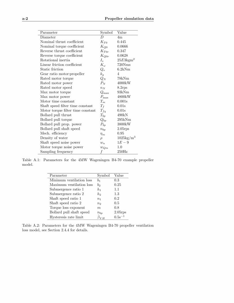
a-2 Propeller simulation data
Parameter Symbol ValueDiameter D 4mNominal thrust coefficient KT0 0.445Nominal torque coefficient KQ0 0.0666Reverse thrust coefficient KT0r 0.347Reverse torque coefficient KQ0r 0.0628Rotational inertia Is 25E3kgm2
Linear friction coefficient Kω 720NmsStatic friction Qs 6.2kNmGear ratio motor:propeller kg 4Rated motor torque QN 78kNmRated motor power PN 4000kWRated motor speed nN 8.2rpsMax motor torque Qmax 93kNmMax motor power Pmax 4800kWMotor time constant Tm 0.001sShaft speed filter time constant Tf 0.01sMotor torque filter time constant Tfq 0.01sBollard pull thrust Tbp 490kNBollard pull torque Qbp 295kNmBollard pull prop. power Pbp 3800kWBollard pull shaft speed nbp 2.05rpsMech. efficiency ηm 0.95Density of water ρ 1025kg/m3
Shaft speed noise power wn 1E − 9Motor torque noise power wQm 1.0Sampling frequency f 250Hz
Table A.1: Parameters for the 4MW Wageningen B4-70 example propellermodel.
Parameter Symbol ValueMinimum ventilation loss b1 0.3Maximum ventilation loss b2 0.25Submergence ratio 1 h1 1.1Submergence ratio 2 h2 1.3Shaft speed ratio 1 n1 0.2Shaft speed ratio 2 n2 0.5Torque loss exponent m 0.8Bollard pull shaft speed nbp 2.05rpsHysteresis rate limit βVH 0.5s−1
Table A.2: Parameters for the 4MW Wageningen B4-70 propeller ventilationloss model, see Section 2.4.4 for details.
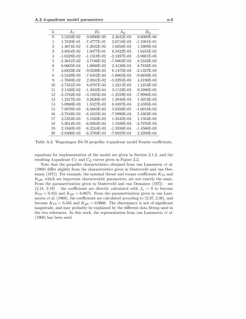
A.2 4-quadrant model parameters a-3
k AT BT AQ BQ
0 2.5350E-02 0.0000E-00 2.4645E-03 0.0000E-001 1.7820E-01 -7.4777E-01 2.6718E-02 -1.1081E-012 1.4674E-02 -1.3822E-02 1.6056E-03 1.5909E-043 2.8054E-02 1.0077E-01 6.5822E-03 1.6455E-024 -1.6328E-02 -1.1318E-02 -2.2497E-03 -2.0601E-035 -5.3041E-02 4.7186E-02 -7.8062E-03 8.5343E-036 6.0605E-04 1.0666E-02 2.4126E-04 8.7856E-047 3.6823E-02 -9.0239E-03 6.1475E-03 -3.1327E-038 -2.5429E-03 -7.8452E-03 -1.6065E-03 -9.6650E-049 -1.7680E-02 2.3941E-02 -3.3291E-03 4.3190E-0310 2.7331E-03 8.0787E-03 1.2311E-03 1.2453E-0311 2.1436E-02 -1.4942E-04 3.1123E-03 9.5986E-0512 -2.4782E-03 -3.1925E-03 -1.2559E-03 -7.9986E-0413 1.2317E-03 9.2620E-03 1.3948E-03 1.5073E-0314 5.0980E-03 1.5527E-03 8.8397E-04 2.4595E-0415 7.8076E-03 -6.5683E-03 5.0358E-05 -1.6918E-0316 -3.7816E-03 -6.1655E-04 -7.9990E-04 5.1603E-0417 3.5353E-03 5.1033E-03 1.3345E-03 1.1504E-0318 5.3014E-03 -6.0263E-04 1.1928E-03 -4.7976E-0419 2.1940E-03 -8.2244E-03 -1.3556E-04 -1.4566E-0320 -2.8306E-03 -6.3789E-04 -7.0825E-04 2.3280E-04
Table A.3: Wageningen B4-70 propeller 4-quadrant model Fourier coefficients.
equations for implementation of the model are given in Section 2.1.2, and theresulting 4-quadrant CT and CQ curves given in Figure 2.2.Note that the propeller characteristics obtained from van Lammeren et al.
(1969) differ slightly from the characteristics given in Oosterveld and van Oos-sanen (1975). For example, the nominal thrust and torque coefficients KT0 andKQ0, which are important characteristic parameters, are not exactly the same.From the parametrization given in Oosterveld and van Oossanen (1975) — see(2.18, 2.19) — the coefficients are directly calculated with Ja = 0 to becomeKT0 = 0.455 and KQ0 = 0.0675. From the parametrization given in van Lam-meren et al. (1969), the coefficients are calculated according to (2.37, 2.38), andbecome KT0 = 0.445 and KQ0 = 0.0666. The discrepancy is not of significantmagnitude, and may probably be explained by the different data fitting used inthe two references. In this work, the representation from van Lammeren et al.(1969) has been used.

a-4 Propeller simulation data

Appendix B
Thruster controller tuningissues
An inevitable challenge when attempting to make a fair comparison of variouscontrollers is tuning. This appendix presents some rules-of-thumb for tuning ofthe controllers presented in Chapter 3.
B.1 Shaft speed controller PI tuning
The PI controller tuning parameters Kp and Ti should be chosen according tothe rating of the motor, the motor time constant Tm, the shaft speed filter timeconstant Tf , the rotational inertia Is, and the desired closed loop properties.Various guides to the tuning of PI controllers exist.From Leonhard (1996), a commonly used model-based PI tuning rule for
variable speed drives is the so-called “symmetrical optimum”. Using the first-order representation of motor and inner current loop from (2.52), the transferfunction h0(s) of the open speed control loop is approximated by:
h0(s) = KpTis+ 1
Tis
1
Tms+ 1
1
Tfs+ 1
1
TIss, (B.1)
where Tm is the time constant of the motor and current loop, Tf is the shaftspeed filter time constant, and TIs is the mechanical time constant, which isequal to the rotational inertia, i.e. TIs = Is. Since Tm ¿ TIs and Tf ¿ TIs,(B.1) can be approximated by (Nilsen, 2001):
h0(s) ≈ KpTis+ 1
Tis
1
Tsums+ 1
1
TIss, (B.2)
Tsum = Tm + Tf . (B.3)

a-6 Thruster controller tuning issues
The symmetric optimum tuning guideline is:
Ti = a2Tsum,
Kp =1
a
TIsTsum
=1
a
IsTsum
, (B.4)
where a > 1 is a constant related to the damping ratio ζ by:
ζ =a− 12
. (B.5)
Nilsen (2001, 2006) recommends a = 2 − 3, which gives an underdamped tocritically damped system, i.e. ζ = 0.5−1.0. The resulting step response exhibitsa large overshoot. It is therefore recommended to use a reference generator forthe speed command (Leonhard, 1996). In this method, the hydrodynamic loadtorque — which effectively represents a large quadratic damping term — has notbeen accounted for. Hence, a submerged propeller will have a significantly moredamped response than what is indicated by ζ. For a propeller subject to largethrust losses, e.g. due to a water exit, the hydrodynamic damping is muchsmaller.A rule-of-thumb used for initial tuning, also in marine industrial installa-
tions, is to choose Kp such that 10 − 20% error in the shaft speed gives 100%torque, and Ti at least four times larger than Tsum (Ådnanes, 2006; Nilsen,2006). This corresponds to a proportional gain of 5− 10 in a “per unit” sense,as is commonly used in electrical engineering. With the parameter kp represent-ing the per unit gain, i.e. kp ∈ [5, 10], and kt the integral time constant ratio,i.e. kt ≥ 4, the tuning rule becomes:
Kp = kpkgQN
nbp, Ti = ktTsum, (B.6)
where nbp is the bollard pull shaft speed. After application of (B.6) for ini-tial tuning, the motor drives are usually tuned manually to give satisfactoryperformance (Ådnanes, 2006).Using the example propeller from Table A.1, the tuning rules in (B.6) with
kp = 5 and kt = 5 gives:
Kp = kpkgQN
nbp= 5
4 · 78E32.05
≈ 7.6E5,
Ti = 0.05. (B.7)
Using the tuning rules in (B.4) with a = 3, the result is:
Kp =1
a
IsTsum
=1
3
25E3
(0.01 + 0.001)≈ 7.6E5,
Ti = 9(0.01 + 0.001) ≈ 0.1. (B.8)
The values in (B.8) have been used in the simulation studies in this thesis.

B.2 Torque and power control tuning a-7
B.2 Torque and power control tuning
In their pure form, as given in (3.29) and (3.32), the only parameters neededin the torque and power controllers are the control coefficients KTC and KQC ,which leaves no tunable parameters. However, for good performance, thesecontrollers rely on the inertia and friction feedforward compensation schemes in(3.22) and (3.19), which require tuning.
B.3 Inertia and friction compensation tuning
Tuning of the friction compensation scheme Qff (nr) in (3.19) and inertia com-pensation scheme Qif (nr) in (3.22) is mainly done by choosing the frictionparameters Qf0 and Qf1, and the rotational inertia Ic. If Qs and Kω in (2.51),and Is in (2.50) are known, no further tuning should be necessary with thefollowing choices: Qf0 = Qs, Qf1 = Kω, and Ic = Is. Is is usually known withreasonable accuracy, since it is an important parameter for the choice of electricmotor and PI controller tuning, as shown in Section B.1. It is less likely to havedecent a priori knowledge of Qs andKω. The main purpose of the compensationschemes are:
• Qff (nr): Improve the steady-state performance of the system.
• Qif (nr): Improve the transient response of the system.
If Qs and/or Kω are unknown, Qf0 and Qf1 must be tuned manually. SinceQff (nr) only is intended to improve the steady-state performance, tuning shouldbe performed at steady state. One possible approach is as follows:
1. Run the motor until it oil, bearings, etc. reaches working temperature.
2. Initially, let Qf0 = 0 and Qf1 = 0.
3. Set Td to a low value, such that the friction at steady state is dominatedby the static term Qs. A suggestion is to choose Td such that nr = nffrom (3.20), i.e. Td = KTCρD
4n2f .
4. Increase Qf0 slowly until the motor turns with n = nf . This shouldcorrespond to Qf0 ≈ Qs, and Qf0 can be fixed at this value.
5. Set Td to a high value, preferably to the bollard pull thrust Tbp. Thecorresponding shaft speed nbp should be known from the propeller char-acteristics.
6. Increase Qf1 until n ≈ nbp. This should correspond to Qf1 ≈ Kω andQf1 can be fixed at this value.
a-8 Thruster controller tuning issues
If Is is unknown or uncertain, Ic may be tuned manually. Since the solepurpose of Qif (nr) is to improve the tracking properties of the controllers, Iccan be adjusted to give the desired step response of the system. With a referencegenerator as in (3.14), nr is available to Qif (nr). Tuning can then be done bycommanding a step in Td, and comparing nr with n. If Qff (nr) is alreadytuned, Ic should be adjusted until n ≈ nr. If Qff (nr) is not tuned, Ic should beadjusted such that n ≈ nr during the step. This implies that, if desired, Ic canbe chosen different from Is to get the desired transient response of the system.
B.4 Choice of parameters for the combined con-trollers
The QP, MQP1, MQP2, and SQP controllers — see Table 3.1 — all rely onthe weighting function α(z) in 3.33 for transitions between the fundamentalcontrollers. How k, p, and r affect the shape of α(z) is discussed in Section3.13.1. It will probably be beneficial to choose the parameters to give a limitedsteepness of the weighting function, in order to make the transition between thefundamental controllers smoother.
Appendix C
Simulation of relativepropeller motion
In order to perform realistic simulations of a propulsion system, including losseffects, it is necessary to have reasonable approximations of the motion of eachthruster unit relative to the surrounding water. This appendix provides thetransformation tools needed to couple the thruster and vessel motion and forces.
C.1 Vessel motion
Vessel motion is typically described by the motion of a body-fixed frame (b-frame) with respect to an earth-fixed frame (n-frame), see Fossen (2002) fordetails. The n-frame position pn = [n, e, d]> (north, east, down) and Eulerangles Θ = [φ, θ, ψ]> (roll, pitch, yaw) are defined in terms of the generalizedcoordinate vector η:
η = [(pn)>,Θ>]> =[n, e, d, φ, θ, ψ]>. (C.1)
The b-frame translational velocities vbo = [u, v, w]> (surge, sway, heave) andangular velocities ωb
nb = [p, q, r]> (roll, pitch, yaw) of the b-frame with respect
to the n-frame, expressed in the b-frame, are defined in terms of the generalizedvelocity vector ν:
ν = [(vbo)>, (ωb
nb)>]> = [u, v, w, p, q, r]>. (C.2)
O is the origin of the b-frame. The translational velocity transformation betweenthe b- and n-frame is:
vno = Rnb (Θ)v
bo, (C.3)
a-10 Simulation of relative propeller motion
where vno = pn, and the Euler angle rotation matrix (zyx-convention) from the
b-frame to the n-frame Rnb (Θ) ∈ R3×3 is defined as:
Rnb (Θ) =
⎡⎣ cψcθ −sψcφ+ cψsθsφ sψsφ+ cψcφsθsψcθ cψcφ+ sφsθsψ −cψsφ+ sθsψcφ−sθ cθsφ cθcφ
⎤⎦ . (C.4)
Here, s· = sin(·) and c· = cos(·). Note that the rotation matrix Rba between
any two frames a and b (from a to b) has the special properties that (Rba)−1 =
(Rba)> = Ra
b . The Euler angle rates satisfy:
Θ = TΘ(Θ)ωbbn, (C.5)
where TΘ(Θ) ∈ R3×3 is the Euler angle attitude transformation matrix:
TΘ(Θ) =
⎡⎣ 1 sφtθ cφtθ0 cφ −sφ0 sφ/cθ cφ/cθ
⎤⎦ , θ 6= ±π
2, (C.6)
and t· = tan(·). Consequently:
η = J(Θ)ν, (C.7)
where J(Θ) ∈ R6×6 is the generalized velocity transformation matrix:
J(Θ) =
∙Rnb (Θ) 03×303×3 TΘ(Θ)
¸, θ 6= ±π
2. (C.8)
To sum up, the rigid-body vessel motion is uniquely expressed by the two vectorsη in (C.1) and ν in (C.2), which are related through (C.7).There are two conventional ways of calculating the total vessel motion. In
the control literature, the vessel motion has usually been decoupled into a low-frequency part and a wave-frequency part. The low-frequency motion is thencalculated from the vessel rigid-body dynamics and the low-frequency loads fromcurrent, wind, wavedrift, and the propulsion system, and the wave-frequencymotion is calculated from motion transfer functions (or response amplitude op-erators — RAOs). The two contributions are then superposed to yield the totalvessel motion.In an alternative approach, force transfer functions are used to represent
the first-order wave excitation forces, and the fluid memory effects associatedwith the radiation forces are expressed in a state-space form. In this way, thewave-frequency model is integrated with the low-frequency model through forcesuperposition instead of motion superposition. Other effects like viscous forces,multi-body interactions, and ship motion control systems can then be incorpo-rated into the model by means of force superposition; see Fossen and Smogeli(2004), Smogeli et al. (2005b), Perez and Fossen (2006), and the referencestherein.
C.2 Transformation tools a-11
C.2 Transformation toolsCalculation of the motion of an arbitrary point P fixed to the vessel and inclusionof the forces acting on this point in the b-frame equations of motion requirestransformations of positions, velocities, accelerations, and forces between the b-frame origin O and P. The translational velocity vbp of the point P decomposedin the b-frame is given by:
vbp = vbo + ωb
nb × rbp, (C.9)
where rbp = [xp, yp, zp]| is the vector from O to P. The vector cross product ×
is defined in terms of the matrix S(rbp) ∈ R3×3 such that:
ωbnb × rbp , −S(rbp)ωb
nb = S(rbp)>ωb
nb, (C.10)
where:
S(rbp) = −S>(rbp) =
⎡⎣ 0 −zp ypzp 0 −xp−yp xp 0
⎤⎦ . (C.11)
Since the angular velocities in P and O are the same, the translational andangular velocity transformation from O to P can be expressed by the screwtransformation matrix H(rbp) ∈ R6×6:∙
vbpωbnb
¸= H(rbp)
∙vboωbnb
¸, (C.12)
H(rbp) ,∙I3×3 S(rbp)
>
03×3 I3×3
¸. (C.13)
From this, the position xnp , generalized velocity νp = [vbp,ω
bnb]
| , and generalizedacceleration νp of P are given by:
xnp = pn+Rnb (Θ)r
bp, (C.14)
νp = H(rbp)ν, (C.15)
νp = H(rbp)ν, (C.16)
where Rnb (Θ) and H(r
bp) are defined by (C.4) and (C.13), respectively. Corre-
spondingly, the generalized force vector τ p with point of attack P is transformedto the generalized force τ in the origin O by:
τ =
∙I3×3 03×3S(rbp) I3×3
¸τ p =H
>(rbp)τ p. (C.17)
Hence, given the vessel motion in terms of η and ν, the motion of a propellerlocated at P is given by (C.14)-(C.16). The thrust Ta is transformed to theb-frame equations of motion by (C.17) and:
τ p =
⎡⎣ cosαpsinαp04×1
⎤⎦Ta, (C.18)
a-12 Simulation of relative propeller motion
where αp is the propeller azimuth (i.e. angle between the propeller shaft andthe b-frame x-axis).
Remark C.1 The first, second, and sixth entry in τ given from (C.17) and(C.18) corresponds to the 3DOF thrust vector τ j in (9.1).
C.3 Wave- and current-induced velocities
Irregular waves are commonly described by a wave spectrum Sw(ωw, ψw) =S(ωw)D(ψw), where the frequency spectrum S(ωw) describes the distributionof wave energy in the sea state over different frequencies ωw, and the spreadingfunction D(ψw) describes the distribution of wave energy over directions ψw inthe n-frame. Common frequency spectra and spreading functions may be foundin e.g. Ochi (1998). In this work, the two-parameter ITTC/ISSC modifiedPierson-Moskowitz (PM) spectrum is used (Lloyd, 1998):
S(ωw) =A
ω5wexp(
−Bω4w
), A = 487H2s
T 4p, B =
1949
T 4p, (C.19)
where Hs is the significant wave height, and Tp is the peak (modal) wave period.For simulation, the sea state is realized as a superposition of harmonic com-
ponents extracted from the wave spectrum, where harmonic component j isdefined in terms of wave amplitude ζj , frequency ωj , direction ψj , and randomphase φj . The wave particle velocities in the n-frame due to harmonic compo-nent j at the point P are termed uwj , vwj , and wwj in the x-, y-, and z-direction,and are written as:
uwj(xp, yp, zp, t) = ζjωj exp(−kjzp) cosψj sin θj , (C.20)
vwj(xp, yp, zp, t) = ζjωj exp(−kjzp) sinψj sin θj , (C.21)
wwj(xp, yp, zp, t) = ζjωj exp(−kjzp) sin(θj −π
2), (C.22)
θj = ωjt+ φj − kj(xp cosψj + yp sinψj). (C.23)
Here, the wave number kj is given by the deep-water dispersion relation kj =ω2j/g, where g is the acceleration of gravity. Letting P move about with the shipin the n-frame, it can be shown that the frequency of encounter is captured in thechange of xp and yp in (C.23). Using linear theory, the harmonic components aresuperposed to give the total wave-induced velocity vector Vw = [uw, vw, ww]
| ,i.e.:
Vw(xp, yp, zp, t) =NXj=1
[uwj(·), vwj(·), wwj(·)]| , (C.24)
where N is the number of harmonic components. The corresponding surface
C.4 Calculation of relative motion a-13
elevation ζw(xp, yp, t) and shaft submergence h(xp, yp, t) are calculated from:
ζw(xp, yp, t) =NXj=1
ζj sin[ωjt+ φj − kj(xp cosψj + yp sinψj)], (C.25)
h(xp, yp, t) = h0 + ζw(xp, yp, t), (C.26)
where h0 is the submergence of the shaft with respect to the mean free surface.
For freely-floating surface vessels, only the surface current is of any impor-tance. If the current is given by magnitude Uc and direction βc in the n-frame,the current velocity vector Vc in the n-frame is written as:
Vc = Uc[cosβc, sinβc, 0]| . (C.27)
C.4 Calculation of relative motionThe propeller rigid-body velocity Vv in the n-frame is calculated from vbp in(C.12) by:
Vv = Rnb (Θ)v
bp. (C.28)
Accounting for the wave-induced velocitiesVw from (C.24), the current-inducedvelocityVc from (C.27), and the motion of the propeller due to the vessel motionVv from (C.28), the total relative velocity Vn
p of the water with respect to thepropeller in the n-frame is given by:
Vnp = Vw +Vc −Vv. (C.29)
The relative velocities are decomposed in an in-line component, which corre-sponds to Va, and a transverse component Vt by transforming Vn
p into theb-frame velocity vector Vb
p:
Vbp = R
nb (Θ)
>Vnp , (C.30)
where Rnb (Θ) is given in (C.4). Then, Va and Vt are found from:
Va = −[cosαp, sinαp, 0]Vbp, (C.31)
Vt =°°[− sinαp, cosαp, 0]Vb
p + [0, 0, 1]Vbp
°°2, (C.32)
where αp is the propeller azimuth.
Remark C.2 The sign of Va in (C.31) is needed since a positive Va is definedas water flow into the propeller, whereas the propeller frame of reference haspositive x-axis in the thrust direction.
Remark C.3 The approach described here should only serve as a rough esti-mate, since it is assumed that the waves are unaffected by the presence of thevessel hull, and the velocity contributions from waves, current, and vessel motionhave been superposed.
a-14 Simulation of relative propeller motion
C.5 Simplified calculationsIn the simulations presented in this thesis, only long-crested waves are con-sidered, and no vessel motion is included. It has therefore been chosen to setxp = yp = 0, zp = h0, ψj = 0, R
nb (Θ) = I3×3, αp = 0, βc = 0, and Vv = 01×3,
such that (C.31), (C.25), and (C.26) can be simplified to:
Va(t) = −NXj=1
ζjωj exp(−kjh0) sin[ωjt+ φj ], (C.33)
ζw(t) =NXj=1
ζj sin[ωjt+ φj ], (C.34)
h(t) = h0 + ζw(t). (C.35)

Appendix D
Additional ventilationresults
As an extension of Section 2.4, this appendix presents the experimental set-upused in the cavitation tunnel, gives a discussion on scaling laws for ventilatedpropellers, shows additional experimental results for ducted and open propellerssubject to ventilation and in-and-out-of water effects, and provides further com-parisons of the simulation model and the experimental results.
D.1 Experimental set-up
The tests in the cavitation tunnel at NTNU were conducted on two occasions:the first time by Aarseth (2003) and Overå (2003), and the second time by Ruth(2005). The description of the experimental setup has been adopted from Ruth(2005). The equipment was arranged according to Figures D.1 and D.2. Most ofthe test runs were performed with a ducted propeller, but some were performedwithout the duct present. The main dimensions of the duct and propeller aregiven in Section 7.1.A list of the measurements is given in Table D.1. The accuracy is high for
all the measurements, except for the advance speed Va when it is lower than1m/s. The measured duct thrust Tad includes the drag on the pole holding theduct. This error source is of little importance because of the low advance speedsduring the tests. The total thrust is given from Ta = Tad + Tap.The measurements were sampled at 1000Hz. The mean values were obtained
by averaging the time series over a period of approximately 5s. This correspondsto at least 10 propeller revolutions per averaging period for n > 2rps, which issufficient to obtain representative mean values. The averaged segments of thetime series were chosen manually.
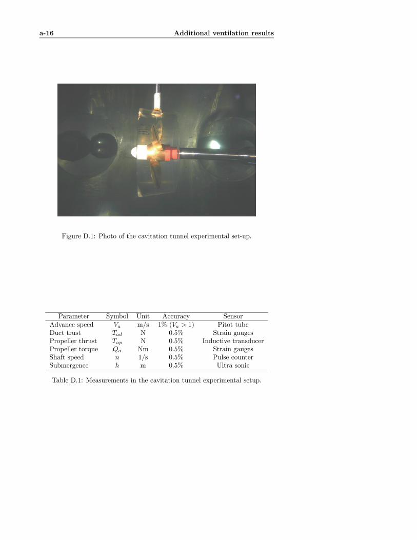
a-16 Additional ventilation results
Figure D.1: Photo of the cavitation tunnel experimental set-up.
Parameter Symbol Unit Accuracy SensorAdvance speed Va m/s 1% (Va > 1) Pitot tubeDuct trust Tad N 0.5% Strain gaugesPropeller thrust Tap N 0.5% Inductive transducerPropeller torque Qa Nm 0.5% Strain gaugesShaft speed n 1/s 0.5% Pulse counterSubmergence h m 0.5% Ultra sonic
Table D.1: Measurements in the cavitation tunnel experimental setup.

D.1 Experimental set-up a-17
Figure D.2: Sketch of the cavitation tunnel experimental set-up, taken fromRuth (2005).
a-18 Additional ventilation results
D.2 Scaling laws
This section is taken entirely from Ruth and Smogeli (2006). According to Shiba(1953) the two most important parameters when scaling propeller performancefrom model scale to full scale are:
1. Geometrical similarity:LsLm
= λ. (D.1)
2. Kinematic similarity:
Ja,m =Va,mnmDm
=Va,snsDs
= Ja,s. (D.2)
Here, λ is the scale, L is any characteristic length, Ja is the advance number,Va is the advance speed, n is the shaft speed, D the propeller diameter, suffixs means full scale, and suffix m means model scale. Further, depending on theoperational condition, the following dimensionless parameters have influence onthe propeller performance (Shiba, 1953; Gutsche, 1967; Kruppa, 1972; Brandt,1973; ATTC, 1974; Scherer, 1977; Guoqiang et al., 1989; Olofsson, 1996; ITTC,1999b):
3. Submergence ratio:h
R. (D.3)
4. Reynolds’ number:
Rn =V∞c
ν. (D.4)
Reynolds’ number similarity is not required if Rn > 5·105, or if correctionsfor Rn are done according to ITTC (1999a), which requires Rn > 2 · 105.
5. Froude number:
FnD = n
sD
g. (D.5)
Froude number similarity is not required if FnD > 3−4. In full scale, FnDwill typically be between 0 and 1.4 (Shiba, 1953).
6. Cavitation number:σc =
pstatic − pcav12ρV
2∞
. (D.6)
7. Weber’s number:
W = nD
rρ
sD. (D.7)
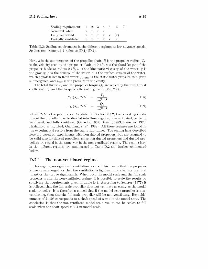
D.2 Scaling laws a-19
Scaling requirement: 1 2 3 4 5 6 7Non-ventilated x x x xFully ventilated x x x x x (x)Partially ventilated x x x x x x
Table D.2: Scaling requirements in the different regimes at low advance speeds.Scaling requirement 1-7 refers to (D.1)-(D.7).
Here, h is the submergence of the propeller shaft, R is the propeller radius, V∞is the velocity seen by the propeller blade at 0.7R, c is the chord length of thepropeller blade at radius 0.7R, ν is the kinematic viscosity of the water, g isthe gravity, ρ is the density of the water, s is the surface tension of the water,which equals 0.072 in fresh water, pstatic is the static water pressure at a givensubmergence, and pcav is the pressure in the cavity.The total thrust Ta and the propeller torque Qa are scaled by the total thrust
coefficient KT and the torque coefficient KQ, as in (2.6, 2.7):
KT (Ja, P/D) =Ta
ρD4n2, (D.8)
KQ (Ja, P/D) =Qa
ρD5n2, (D.9)
where P/D is the pitch ratio. As stated in Section 2.3.2, the operating condi-tion of the propeller may be divided into three regions; non-ventilated, partiallyventilated, and fully ventilated (Gutsche, 1967; Brandt, 1973; Fleischer, 1973;Hashimoto et al., 1984; Guoqiang et al., 1989). All these regimes are found inthe experimental results from the cavitation tunnel. The scaling laws describedhere are based on experiments with non-ducted propellers, but are assumed tobe valid also for ducted propellers, since non-ducted propellers and ducted pro-pellers are scaled in the same way in the non-ventilated regime. The scaling lawsin the different regimes are summarized in Table D.2 and further commentedbelow.
D.2.1 The non-ventilated regime
In this regime, no significant ventilation occurs. This means that the propelleris deeply submerged, or that the ventilation is light and not affecting the totalthrust or the torque significantly. When both the model scale and the full scalepropeller are in the non-ventilated regime, it is possible to scale the results bysatisfying the requirements given in Table D.2. According to Scherer (1977) itis believed that the full scale propeller does not ventilate as easily as the modelscale propeller. It is therefore assumed that if the model scale propeller is non-ventilating, then also the full-scale propeller will be non-ventilating. Reynolds’number of 2 · 105 corresponds to a shaft speed of n = 4 in the model tests. Theconclusion is that the non-ventilated model scale results can be scaled to fullscale when the shaft speed n > 4 in model scale.

a-20 Additional ventilation results
D.2.2 The fully ventilated regime
This is when a single ventilated cavity is covering the propeller blade, meaningthat the pressure on the suction side of the propeller blade is almost atmospheric.If the conditions given in Table D.2 are satisfied, and both the model scalepropeller and the full-scale propeller are fully ventilated, it is possible to scalethe results in this regime. It is, however, uncertain how to confirm whetheror not the full scale propeller is going to be fully ventilated. Requirement 6,cavitation number similarity, is actually obtained through kinematic similarity,submergence ratio similarity, and Froude number similarity. With pstatic =patm + ρgh, where patm is the atmospheric pressure, the cavitation numberbecomes:
σc =patm + ρgh− pcav
12ρV
2∞
. (D.10)
Since pcav ≈ patm when the propeller is fully ventilated, (D.10) can be simplifiedto:
σc =2gh
V 2∞=
1³(0.35π)2 + J2a
´ h
R
g
Dn2. (D.11)
If Ja,m = Ja,s, hm/Rm = hs/Rs and FnD,m = FnD,s, the result is thatσc,m = σc,s. The Reynolds’ number criterion restricts the scaling to shaftspeeds equal to 4 and larger in model scale. The realistic Froude numbers infull scale corresponds to shaft speeds from 0 to 9 in model scale.
D.2.3 The partially ventilated regime
This is when only part of the propeller is ventilated. The ventilation is said tobe unstable when the propeller’s degree of ventilation is not stationary, but isa function of time. The required scaling parameters are summarized in TableD.2. Although the pressure in the ventilated cavity is nearly atmospheric, theremay exist other non-ventilated cavities (Kruppa, 1972). These non-ventilatedcavities require cavitation number similarity. It would then require a free sur-face depressurized cavitation tunnel to do the experiments. The model testspresented here were all performed at atmospheric pressure.In conclusion, it is not possible to scale the results in the partially ventilated
regime to full scale for the experimental results presented here. There is, how-ever, no reason to believe that the qualitative behavior of a full scale propellerwill differ much from the results obtained for a model scale propeller.
D.2.4 Effect of Weber’s number
TheWeber’s numberW describes the relationship between surface tension forcesand inertial forces. Shiba (1953) and ITTC (1999b) state that W is importantwhen determining the critical advance number, which is the advance number atwhich ventilation occurs for a given submergence ratio and shaft speed. In this
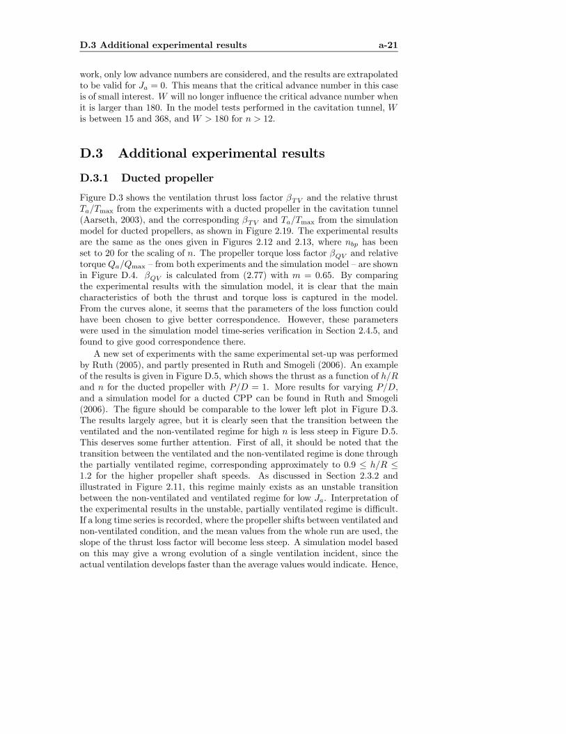
D.3 Additional experimental results a-21
work, only low advance numbers are considered, and the results are extrapolatedto be valid for Ja = 0. This means that the critical advance number in this caseis of small interest. W will no longer influence the critical advance number whenit is larger than 180. In the model tests performed in the cavitation tunnel, Wis between 15 and 368, and W > 180 for n > 12.
D.3 Additional experimental results
D.3.1 Ducted propeller
Figure D.3 shows the ventilation thrust loss factor βTV and the relative thrustTa/Tmax from the experiments with a ducted propeller in the cavitation tunnel(Aarseth, 2003), and the corresponding βTV and Ta/Tmax from the simulationmodel for ducted propellers, as shown in Figure 2.19. The experimental resultsare the same as the ones given in Figures 2.12 and 2.13, where nbp has beenset to 20 for the scaling of n. The propeller torque loss factor βQV and relativetorque Qa/Qmax — from both experiments and the simulation model — are shownin Figure D.4. βQV is calculated from (2.77) with m = 0.65. By comparingthe experimental results with the simulation model, it is clear that the maincharacteristics of both the thrust and torque loss is captured in the model.From the curves alone, it seems that the parameters of the loss function couldhave been chosen to give better correspondence. However, these parameterswere used in the simulation model time-series verification in Section 2.4.5, andfound to give good correspondence there.A new set of experiments with the same experimental set-up was performed
by Ruth (2005), and partly presented in Ruth and Smogeli (2006). An exampleof the results is given in Figure D.5, which shows the thrust as a function of h/Rand n for the ducted propeller with P/D = 1. More results for varying P/D,and a simulation model for a ducted CPP can be found in Ruth and Smogeli(2006). The figure should be comparable to the lower left plot in Figure D.3.The results largely agree, but it is clearly seen that the transition between theventilated and the non-ventilated regime for high n is less steep in Figure D.5.This deserves some further attention. First of all, it should be noted that thetransition between the ventilated and the non-ventilated regime is done throughthe partially ventilated regime, corresponding approximately to 0.9 ≤ h/R ≤1.2 for the higher propeller shaft speeds. As discussed in Section 2.3.2 andillustrated in Figure 2.11, this regime mainly exists as an unstable transitionbetween the non-ventilated and ventilated regime for low Ja. Interpretation ofthe experimental results in the unstable, partially ventilated regime is difficult.If a long time series is recorded, where the propeller shifts between ventilated andnon-ventilated condition, and the mean values from the whole run are used, theslope of the thrust loss factor will become less steep. A simulation model basedon this may give a wrong evolution of a single ventilation incident, since theactual ventilation develops faster than the average values would indicate. Hence,

a-22 Additional ventilation results
0.4
0.6
0.8
0
0.5
1
1.5
0
0.2
0.4
0.6
0.8
1
n/nbp
Experiments
h/R
β TV
0.4
0.6
0.8
0
0.5
1
1.5
0
0.2
0.4
0.6
0.8
1
n/nbp
Model
h/R
β TV
0.4
0.6
0.8
0
0.5
1
1.5
0
0.2
0.4
0.6
0.8
1
n/nbp
Experiments
h/R
Ta/T
max
0.4
0.6
0.8
0
0.5
1
1.5
0
0.2
0.4
0.6
0.8
1
n/nbp
Model
h/R
Ta/T
max
Figure D.3: Comparison of the thrust of a ducted propeller during ventilation,from experimental results (left) and the simulation model (right).
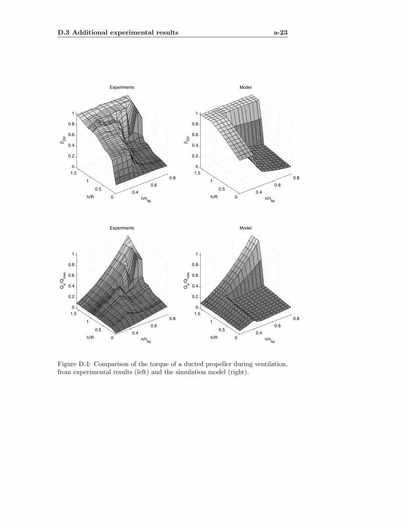
D.3 Additional experimental results a-23
0.4
0.6
0.8
0
0.5
1
1.5
0
0.2
0.4
0.6
0.8
1
n/nbp
Experiments
h/R
β QV
0.4
0.6
0.8
0
0.5
1
1.5
0
0.2
0.4
0.6
0.8
1
n/nbp
Model
h/R
β QV
0.4
0.6
0.8
0
0.5
1
1.5
0
0.2
0.4
0.6
0.8
1
n/nbp
Experiments
h/R
Qa/Q
max
0.4
0.6
0.8
0
0.5
1
1.5
0
0.2
0.4
0.6
0.8
1
n/nbp
Model
h/R
Qa/Q
max
Figure D.4: Comparison of the torque of a ducted propeller during ventilation,from experimental results (left) and the simulation model (right).
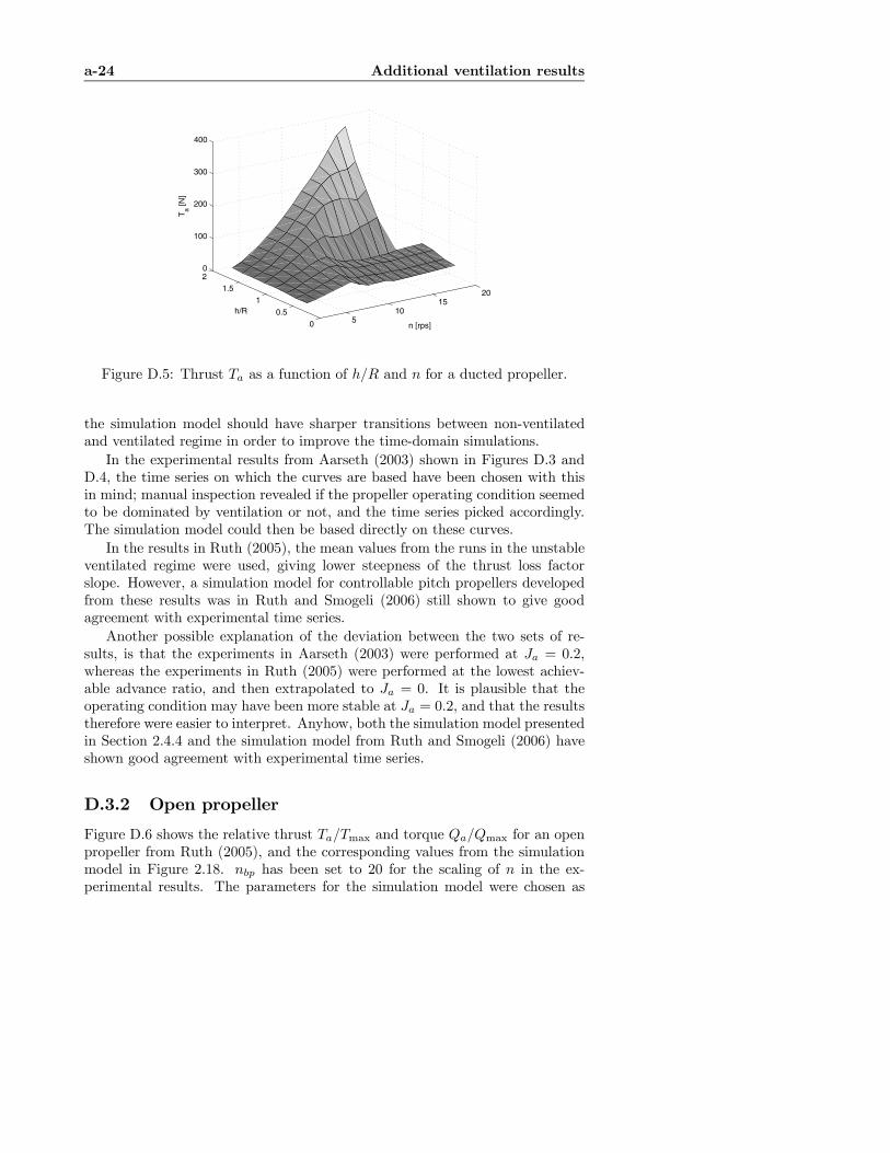
a-24 Additional ventilation results
510
1520
0
0.5
1
1.5
20
100
200
300
400
n [rps]
h/R
Ta [N
]
Figure D.5: Thrust Ta as a function of h/R and n for a ducted propeller.
the simulation model should have sharper transitions between non-ventilatedand ventilated regime in order to improve the time-domain simulations.In the experimental results from Aarseth (2003) shown in Figures D.3 and
D.4, the time series on which the curves are based have been chosen with thisin mind; manual inspection revealed if the propeller operating condition seemedto be dominated by ventilation or not, and the time series picked accordingly.The simulation model could then be based directly on these curves.In the results in Ruth (2005), the mean values from the runs in the unstable
ventilated regime were used, giving lower steepness of the thrust loss factorslope. However, a simulation model for controllable pitch propellers developedfrom these results was in Ruth and Smogeli (2006) still shown to give goodagreement with experimental time series.Another possible explanation of the deviation between the two sets of re-
sults, is that the experiments in Aarseth (2003) were performed at Ja = 0.2,whereas the experiments in Ruth (2005) were performed at the lowest achiev-able advance ratio, and then extrapolated to Ja = 0. It is plausible that theoperating condition may have been more stable at Ja = 0.2, and that the resultstherefore were easier to interpret. Anyhow, both the simulation model presentedin Section 2.4.4 and the simulation model from Ruth and Smogeli (2006) haveshown good agreement with experimental time series.
D.3.2 Open propeller
Figure D.6 shows the relative thrust Ta/Tmax and torque Qa/Qmax for an openpropeller from Ruth (2005), and the corresponding values from the simulationmodel in Figure 2.18. nbp has been set to 20 for the scaling of n in the ex-perimental results. The parameters for the simulation model were chosen as
D.3 Additional experimental results a-25
in Figure 2.18, and βQV calculated from (2.77) with m = 0.8. As discussedabove, it has been chosen to model a sharper transition between the ventilatedand non-ventilated condition than what is indicated by the experimental re-sults. Apart from this, the simulation model can be seen to capture the maincharacteristics of the ventilation loss effects. It is interesting to notice thedifference in behavior during ventilation for the ducted propeller in Figure D.5and the open propeller in Figure D.6. For low h/R, the ducted propeller has adistinct “ridge” of higher thrust for low shaft speed (n ≈ 9rps is Figure D.5, andn/nbp ≈ 0.35 in Figure D.3), and the thrust is not increasing for increasing shaftspeed during ventilation. For the open propeller, the “ridge” of higher thrustseems not to be present, and the thrust during ventilation is slightly increasingfor increasing shaft speeds. This difference in characteristics is also present inthe experimental results presented in Chapter 7.

a-26 Additional ventilation results
0.20.4
0.60.8
0.5
1
1.5
20
0.2
0.4
0.6
0.8
1
n/nbp
Experiments
h/R
Ta/T
max
0.20.4
0.60.8
0.5
1
1.5
20
0.2
0.4
0.6
0.8
1
n/nbp
Model
h/R
Ta/T
max
0.20.4
0.60.8
0.5
1
1.5
20
0.2
0.4
0.6
0.8
1
n/nbp
Experiments
h/R
Qa/Q
max
0.20.4
0.60.8
0.5
1
1.5
20
0.2
0.4
0.6
0.8
1
n/nbp
Model
h/R
Qa/Q
max
Figure D.6: Comparison of the thrust and torque of an open propeller duringventilation, from experimental results (left) and the simulation model (right).
Appendix E
Additional thruster controlresults
This appendix contains additional control laws and discussions. Section E.1shows how torque control can be used in fault-tolerant thruster control, SectionE.2 demonstrates some of the control options that become available with addi-tional instrumentation, and Section E.3 presents some related output feedbackcontrollers. Section E.4 presents an output feedback shaft speed controller withimplicit advance velocity compensation, including experimental results.
E.1 Fault-tolerant control
Fault-tolerant control is in general considered to be outside the scope of thisthesis. However, it is interesting to note that the torque controller as formulatedin (3.29) with the friction compensation scheme from (3.19) and the inertiacompensation scheme from (3.22) is a pure feedforward controller, and henceindependent of any feedback signal. If one of the controllers in Table 3.1 is inuse, and the shaft speed feedback fails, it is then possible to switch to the torquecontroller. It is assumed that the inner torque control loop of the motor still isworking; this is a prerequisite for any thruster controller to work. If a torquelimiting algorithm as in (3.25) is implemented in the controller, it will also benecessary to replace n with nr from (3.1) in (3.25). The operation can then becontinued without significant performance deterioration.This fault-tolerant control scheme requires that the shaft speed feedback
signal failure is detected. This may be done by common signal quality checking,considering e.g. signal range, wild-points, and signal variance (Grøvlen et al.,1998), or by statistical methods like the CUSUM algorithm (Blanke et al., 2003).Since the performance of the active controller already may be unacceptable
by the time the sensor failure is detected, it is desirable to carry out a rapidswitch to torque control. Additionally, it is not considered pertinent to have an
a-28 Additional thruster control results
automatic switch back to the old controller — when a sensor failure is detected,the failure should be corrected before a manual restart of the system is per-formed. Hence, concepts like dwell-time and hysteresis-based switching, whichcan be utilized to ensure stability when switching between a set of controllers(Hespanha and Morse, 2002; Hespanha et al., 2003), will probably not be nec-essary. It is instead considered sufficient to switch from the current controlleroutput Qci to the output Qcq of the torque controller immediately after thefailure has been detected. It may also be appropriate to include a rate limit onthe switched output in order to reduce transients in the motor input. Details ofimplementation will not be further considered here.The scenario outlined above is reminiscent of the case study of a ship propul-
sion system presented in Blanke et al. (1998, 2003), where fault-tolerant controlof a diesel engine with a mechanical direct-drive CPP is considered. The shippropulsion system is in these references treated in a much broader perspective,with various fault scenarios, diagnosis, and fault handling. However, one spe-cific case study, which also is the focus of Blanke et al. (1998), is a fault in theshaft speed feedback measurement. This is considered to be a high risk fault. Itis detected by a nonlinear adaptive observer, which also enables distinguishingbetween a fault in the shaft speed feedback and a fault in the engine governor.When a shaft speed feedback fault is detected, the proposed remedial action isto apply sensor fusion using the relationships between propeller torque, vesselspeed, and shaft speed. For a given pitch, the propeller torque characteristicsis taken to be linear as in (2.26), i.e.:
Qa ≈ Qnn(P/D)n |n|+Qnv(P/D) |n|Va, (E.1)
where Qnn and Qnv are functions of the pitch ratio P/D. The advance velocityVa is estimated from the vessel speed U and a hull wake factor wh using (2.42).The motor torque Qm is assumed measurable from the governor setting, i.e.Qm = KyY , where Y is the governor input from a shaft speed PI controlleras in (3.27), and Ky the motor torque constant, see (2.56). Neglecting frictionand using the steady-state torque balance from the rotational dynamics (2.50),an estimate n of the shaft speed, which is assumed to be positive for a CPP, isfound from:
Qm = Qa
KyY = Qnn(P/D)n |n|+Qnv(P/D) |n|U(1− wh)
⇓
n =−Qnv(P/D)U(1− wh)
2Qnn(P/D)
+
pQnv(P/D)2U2(1− wh)2 + 4Qnn(P/D)KyY
2Qnn(P/D). (E.2)
The faulty signal n is then replaced by n in the shaft speed controller, and theoperation can continue with reduced performance.
E.2 Additional instrumentation a-29
There are, however, a few limitations that should be addressed. The lin-ear torque characteristics is mainly applicable to open propellers in the firstquadrant of operation. It is also assumed that the ship speed U is available asa measurement to the low-level thruster controller. Additionally, for propellersother than the main propeller, there is normally no good estimate of the advancevelocity available. Hence, for DP operations with multiple propellers operatingin dynamic flow, this approach may be of limited applicability. The simpler ap-proach outlined in the beginning of this section may then be more appropriate.It is also expected that the thrust production will be superior with the torquecontroller when compared to the re-configured shaft speed controller based onn.
E.2 Additional instrumentationIn most of this work, it has been assumed that only the shaft speed and themotor torque are available as measurements, see Section 3.1. However, if thepropulsion unit could be equipped with additional instrumentation, new con-trol options would appear. The two most desirable measurements for low-levelthruster controller design would be the propeller thrust and torque, with thefeedback signals termed Tfb and Qfb, respectively. This section explores someof the new options that become available with propeller thrust and/or torquemeasurements.
E.2.1 Thrust feedback control
If a thrust feedback signal of high quality is available, it is possible to close theloop directly with the thrust measurement in e.g. a PID controller. With thethrust error et, the thrust controller output Qct becomes :
et = Tr − Tfb,
Qct = Ktpet +Kti
Z t
0
et(τ)dτ +Ktdet, (E.3)
where Ktp, Kti, and Ktd are the nonnegative PID gains. As before, the motortorque is controlled by its inner torque loop. In order to give good performance,such a formulation requires a relatively low level of noise on Tfb. Additionally,the thrust sensor must have a high level of reliability. As of today, thrust controlseems not to be a realistic solution in industrial implementations for surfacevessels. This may be explained by a lack of suitable sensors, and industrialreluctance to install such sensors even if available.In Beek and Mulder (1983) a system for fuel optimization of CCP is pre-
sented, based on measurements of propeller speed, pitch, and thrust. Theproposed thrust measurement was realized by sensitive semi-conductor straingauges attached to the propeller shaft, achieving repeatability better than 0.5%over several successful trials. A similar approach is taken in Bakountouzis
a-30 Additional thruster control results
(1992). However, long-term reliability of the feedback signal is not discussed.Deniellou et al. (1998) proposed a thrust control scheme as in (E.3) for AUV’s.The thrust was measured by a displacement gauge and a displacement sensor,with a measurement uncertainty of less than 0.1% of the effective measurementrange. Also the dynamic response was investigated, and found to be satisfac-tory. Experimental results with a PI controller were provided to show the stepresponse and tracking properties of the controller.With a controller such as (E.3), the torque feedback Qfb becomes superflu-
ous. However, if available, it could be used for diagnostics and fault-tolerantcontrol. This will not be further treated here. A thrust controller will be validfor any vessel speed, since the mapping from reference to actual thrust is ac-curate regardless of the inflow to the propeller. Hence, controller modificationsfor transit, as discussed in Section 8.2, are not needed.
E.2.2 Thrust control from torque feedback
In Section 2.1.8, it was shown that there for open propellers is a nearly linear re-lationship between the thrust and torque coefficients, and that this relationshipis valid across a large range of operating conditions. Hence, if a thrust feedbacksignal is unavailable, but a propeller torque feedback signal is available, theKT −KQ relationship in (2.48) can be used to calculate an estimate Tfb of Tafrom Qfb:
KT = atKQ + bt,
⇓Tfb =
atDQfb + btρn
2D4, (E.4)
where at and bt are propeller constants found from the open-watercharacteristics. Tfb from (E.4) can then replace Tfb in (E.3). This controlformulation requires a high quality torque feedback signal. The performanceof the thrust controller with torque feedback is then expected to be similar tothe one with thrust feedback. A torque sensor for this purpose was presented inLemarquand (1997), and reported to give satisfactory signal quality. The torquefeedback thrust controller is in principle only feasible for open propellers. Forducted propellers, no simple relationship between thrust and torque has beenshown, and (E.4) cannot be expected to hold.
E.2.3 Propeller torque feedback control
With a propeller torque feedback signal, it is possible to close the thrustercontrol loop directly with this, instead of using the torque-thrust relationshipas proposed in the previous section. This can be done in a similar manner as in
E.2 Additional instrumentation a-31
Section E.2.1, with a PID controller operating on the torque error eq:
eq = Qr −Qfb,
Qcqp = Kqpeq +Kqi
Z t
0
eq(τ)dτ +Kqdeq, (E.5)
where Qr is the torque reference calculated from (3.2), Qcqp is the propellertorque controller output, and Kqp, Kqi, and Kqd are the nonnegative PID gains.As before, the motor torque is controlled by its inner torque loop. The same re-quirements to signal quality and reliability as for the thrust controller presentedin Section E.2.1 apply. The friction and inertia compensation schemes fromSection 3.7 become unnecessary with the propeller torque feedback controller,since the propeller torque is controlled directly.
E.2.4 Propeller power feedback control
Another control option that becomes available with a propeller torque measure-ment, is propeller power control. With the measurements Qfb and n, the signedmeasured propeller power Pfb becomes:
Pfb = Qfb2π |n| , (E.6)
and the control loop may be closed with a PID controller operating on the powererror ep:
ep = Prs − Pfb,
Qcpp = Kppep +Kpi
Z t
0
ep(τ)dτ +Kpdep, (E.7)
where Prs is the signed power reference calculated from (3.4), Qcpp is the pro-peller power controller output, and Kpp, Kpi, and Kpd are the nonnegative PIDgains. The motor torque is controlled by its inner torque loop, and the samerequirements to signal quality and reliability as for the thrust controller pre-sented in Section E.2.1 apply. The friction and inertia compensation schemesfrom Section 3.7 become unnecessary with the propeller power controller, sincethe propeller power is controlled directly.
E.2.5 Dynamic control coefficients
If both propeller thrust and torque measurements are available, but the qualityof the signals is not of sufficient quality for closing the loop directly (due tonoise, update rate, reliability, etc.), an alternative approach exists. From (2.6,2.7), the feedback signals Tfb and Qfb may, together with the measured n, beused in an on-line parameter estimation scheme for the prevailing thrust andtorque coefficients, termed KT and KQ. The adaption should be slow enoughto avoid e.g. wave-induced disturbances and noise, but fast enough to capture

a-32 Additional thruster control results
the change in operating conditions due to steady-state current or vessel speed.The estimates can then be used as control coefficients, i.e. KTC = KT andKQC = KQ, with any one of the control schemes defined in Table 3.1. Thismeans that KT and KQ are used instead of the nominal coefficients KT0 andKQ0 in the controllers. Assuming that the estimates KT and KQ will be closeto the true mean values of KT and KQ, the main advantages of this approachare:
• The control schemes will give good performance for all vessel speeds, sinceestimates of the actual thrust and torque coefficients are used. This re-moves most of the difficulties discussed in Section 8.2, since less modelknowledge is needed.
• The quality of the feedback signals is less critical for performance, whichmeans that the control schemes are feasible with low-cost sensors.
• If a sensor fails, the parameter adaption can be switched off, and either 1)the current values of the estimates can be used in continued operation, or2) the control coefficients can be ramped back to the nominal values KT0
and KQ0. The control scheme is therefore robust with respect to sensorfailure.
• For e.g. the combined torque/power controller, the good properties withrespect to wear and tear and predictable power consumption may be uti-lized, with increased performance during transit.
The on-line parameter estimation schemes for KT and KQ can be foundfrom e.g. Ioannou and Sun (1995). Defining the output yT = Tfb and the inputuT = ρD4n |n|, (2.3) can be written as:
yT = KTuT . (E.8)
Using the estimate KT of KT , the predicted output yT and the prediction errorεT become:
yT = KTuT , (E.9)
εT = yT − yT = KTuT − KTuT = −KTuT , (E.10)
where the parameter estimation error KT = KT − KT . Using the gradientmethod, the recursive parameter estimation scheme becomes:
˙KT = −γT εTuT , KT (0) = KT , (E.11)
where γT > 0 is the adaptive gain and KT the initial value of KT . For anybounded u(t) and u(t), the prediction error converges to zero (Ioannou and Sun,1995). Additionally, it can be shown that a necessary and sufficient conditionfor KT (t) to converge to zero exponentially fast is that u(t) is PE. u(t) is PE

E.3 Thrust, torque, and power output feedback control a-33
if it is sufficiently rich of order 1, i.e. at least a nonzero constant signal. Thiscorresponds to nonzero shaft speed, which is an intuitively sensible requirement.Correspondingly, the estimate KQ of KQ can be calculated from:
˙KQ = −γQεQuQ, KQ(0) = KQ, (E.12)
with adaption gain γQ > 0, output yQ = Qfb, input uQ = ρD5n |n|, predictionerror εQ = yQ − KQuT , and initial value KQ. As stated above, the gains γTand γQ should be chosen such that noise and wave-frequency disturbances arerejected, while a change in operating condition due to vessel speed or currentis captured. From a practical point of view, it may also be desirable to disableadaption below a certain shaft speed threshold na, i.e.
εT =
½yT − yT , |n| ≥ na,0, |n| < na,
(E.13)
and similarly for εQ.In extreme operating conditions, with ventilation and water exits, the adap-
tion should be switched off, since the thrust and torque models (2.6, 2.7) thenwill lead to rapidly changing KT and KQ. With low adaption gains, KT andKQ will not converge to any sensible values, and probably exhibit a drifting be-havior. These uncertain parameters are not wanted in the control laws, and itwould hence be preferable to use the values found from steady-state operation.How to detect such high loss incidents was treated in Section 6.3.The torque measurement could, together with the motor torque Qm, also be
used to estimate the coefficients Qf0 and Qf1 used in the friction compensationscheme (3.19).
E.3 Thrust, torque, and power output feedbackcontrol
In Section E.2, several new control options that become available with addi-tional instrumentation were presented. All these controllers were of the PIDtype, closing the control loop with the error between desired and measured pro-peller thrust, torque, or power. Usually, however, additional instrumentation isnot available. As additional control options, the controllers from Section E.2may instead be implemented by output feedback, using one of the propellertorque estimation schemes presented in Chapter 5. These controllers then be-come significantly more complex than the other controllers for normal operatingconditions, which are summarized in Table 3.1. As briefly discussed in SectionE.2, the thrust, propeller torque, and propeller power feedback controllers cir-cumvent the need for friction and inertia compensation, and hence reduce thenecessary model knowledge. However, when implemented as output feedbackcontrollers, this model knowledge is needed in order to implement the load
a-34 Additional thruster control results
torque observer. For extreme conditions, the output feedback controllers arenot believed to be appropriate, due to the problems with assuring robust per-formance during ventilation. The stability properties of the output feedbackcontrollers will not be further considered.
E.3.1 Thrust output feedback
The thrust output feedback scheme is similar to the thrust control scheme fromSection E.2.2, except that the propeller load torque feedback Qfb in (E.4) isreplaced with the estimated load torque Qa from one of the observers. Thisscheme is therefore mainly applicable to open propellers, where the linear KT −KQ relationship in (2.48) holds. As discussed in Section 4.9, a thrust controlleris not suited for applications where the propeller may be subject to large thrustlosses — its performance during ventilation is significantly worse than that ofthe torque and power controllers. Hence, the thrust output feedback scheme ismostly relevant for underwater applications like AUV’s or ROV’s, or for deeplysubmerged propellers like azimuthing thrusters on a semi-submersibles. Thelatter are, however, usually of the ducted type, where (2.48) may not hold.Using the linear observer from (5.7), the thrust-torque mapping from (E.4),
and the controller from (E.3), the thrust output feedback scheme may be sum-marized as:
u = kgQm −Qff0(nr),
˙ω =1
Is
³u− Qa −Qf1ω
´+ ka(ω − ω),
˙Qa = kb(ω − ω),
Ta =atDQa + btρn
2D4,
et = Tr − Ta,
Qct = Ktpet +Kti
Z t
0
et(τ)dτ +Ktdet. (E.14)
Here, Qct is the controller output, nr is given from Tr by (3.1), ω = 2πn,Qff0(nr) is given by (3.20), Is, Qf1, D, at, and bt are propeller constants, kaand kb are the observer gains, and Ktp, Kti, and Ktd are the PID gains.
E.3.2 Torque output feedback
The torque output feedback controller is similar to (E.5), with Qfb replaced byQa. The Qa observer is formulated as in (E.14), and the remaining controllergiven from:
eq = Qr − Qa,
Qcqp = Kqpeq +Kqi
Z t
0
eq(τ)dτ +Kqdeq, (E.15)
E.4 Shaft speed control with implicit Va compensation a-35
with Qcqp the controller output, Qr given from Tr by (3.2), and Kqp, Kqi, andKqd the PID gains.
E.3.3 Power output feedback
The power output feedback controller is similar to (E.7), with Pfb replaced byPa, and Pa calculated from Qa. The Qa observer is formulated as in (E.14),and the remaining controller given from:
Pa = Qa |ω| ,ep = Prs − Pa,
Qcpp = Kppep +Kpi
Z t
0
ep(τ)dτ +Kpdep, (E.16)
with Qcpp the controller output, Prs given from Tr by (3.4), and Kpp, Kpi, andKpd the PID gains.
E.4 Shaft speed control with implicit Va com-pensation
In Fossen and Blanke (2000), a nonlinear output feedback propeller shaft speedcontroller for underwater vehicles, with feedback from estimated advance veloc-ity, was presented. The advance velocity observer was designed based on thevehicle surge dynamics and a model of the flow dynamics. The flow dynamicsmodel was as proposed in Blanke et al. (2000), based on the results by Yoergeret al. (1991), Healey et al. (1995), and Whitcomb and Yoerger (1999a). Asdiscussed in Section 2, increasing advance velocity leads to decreasing thrust ifthe shaft speed is kept constant. The idea behind the controller in Fossen andBlanke (2000) was to compensate for the advance velocity, in order to improvethe mapping from desired to actually produced thrust. The output feedbackcontroller was shown to be uniformly globally asymptotically and uniformly lo-cally exponentially stable. There are, however, three main limitations to theresult: the propeller model was based on a linear open-water characteristics asin (2.25, 2.26), the advance velocity observer was only valid for Va ≥ 0, andthe observer relied on the coupling between the propeller thrust and the vehi-cle surge dynamics. The two first limitations indicate that the result only isvalid for open propellers in the first quadrant of operation, where the linearopen-water characteristics approximation is relatively accurate, and Va ≥ 0.The third limitation indicates that the observer only will work for a vehicleequipped with a single propeller for each degree of freedom (or alternativelywith several coordinated propellers), since it otherwise may be difficult to sep-arate the contributions from several propellers to the surge dynamics. For anAUV or UUV, the limitations are not of major importance, since these vehiclesusually operate at cruising speed in the first quadrant of operation, and are

a-36 Additional thruster control results
equipped with a simple propulsion system for surge motion. For other vehicles,e.g. ROVs and surface vessels in DP, that may experience changing inflow dueto current, waves, and low-speed manoeuvring, these limitations may become aproblem.
E.4.1 Controller formulation
Instead of calculating an explicit estimate of Va and using this in a model of thepropeller characteristics, it is possible to formulate a shaft speed controller thatimplicitly compensates for changes in the advance velocity. The starting pointis the shaft speed thrust sensitivity function from (4.16):
stn(·) ,TaTr=
KT
KTC. (E.17)
In Figures 4.2 and 4.6, it is shown how stn(·) decreases with increasing Va. Thisis also easily seen from an open-water diagram, e.g. Figure 2.1, since KT for afixed n decreases with increasing Va. This is the behavior that the controllerfrom Fossen and Blanke (2000) attempts to compensate for by increasing theshaft speed when the advance velocity increases. From (E.17), this could alsobe achieved by adjusting the control coefficient KTC : with KTC = KT , thethrust sensitivity stn(·) = 1, and the desired thrust is produced. It is thereforeproposed to use one of the observers from Section 5 to calculate an estimateKQ of KQ, use the KT − KQ relationship in (2.48) to calculate an estimateKT of KT , and use KTC = KT in the normal shaft speed PI controller from(3.27). Using the KQ estimation scheme in (5.26), the shaft speed controllerwith implicit advance speed compensation becomes:
u = kgQm −Qff0(nr),
KQ =4π2
ρD5θ,
θ = −k0 |ω|3
3Is+ z,
z = k0ω |ω|I2s
(u− θω |ω|−Qf1ω),
KTC = atKQ + bt,
nr = sign(Tr)
s|Tr|
ρD4KTC,
Qcn = Kpe+Ki
Z t
0
e(τ)dτ , e = nr − n. (E.18)
Here, Qcn is the controller output, k0 is the estimation gain, and Kp and Ki arethe PI gains. A block diagram of the resulting control scheme is given in Figure

E.4 Shaft speed control with implicit Va compensation a-37
nf
Q
Q
Ta
a
T
m( )
fQ ( ).
.MotorDynamics
QcTorqueLimit
.
pxp
ShaftDynamics
PmaxQmax
Thrusterunit
,q
pxp,q
KTC
estimation
Tr Qcng
n( ). PID
nr
n
e
+
KQ KQKTKQ
Figure E.1: Block diagram of the shaft speed controller with implicit Va com-pensation.
E.1. Notice that the sole purpose of the observer is to aid in calculating theshaft speed setpoint nr. Hence, the PI controller and KQ estimation schemecan be tuned separately. The choice of k0 should be motivated from the desiredproperties of the closed-loop controller. If it is desired to compensate for allchanges in inflow, also due waves and wave-frequency vessel motion, k0 mustbe chosen sufficiently high to capture these effects. If the motivation is tocompensate only for the mean changes in inflow due to current and vessel low-frequency motion, k0 should be chosen lower, such that the wave-frequencydisturbances are filtered out. If desired, the load torque observer in (5.7) withKQ calculation from (5.17) and (5.16) may be used instead of theKQ estimationscheme from (5.26).Since no assumption about the advance velocity or shape of the open-water
characteristics has been made, except for the linear KT − KQ relationship in(2.48), this controller is valid for all 4 quadrants of operation — or as long as(2.48) holds. In addition, since no vessel dynamics are involved in the observer,the controller is valid for any open propeller on any vessel. The restrictionto open propellers is due to the limitation in applicability of (2.48) for ductedpropellers.
Remark E.1 If the main purpose of the controller is to counteract the loss ofthrust due to varying advance velocity, the pure torque controller in (3.29) shouldalso be considered. As can be seen in Figures 4.2 and 4.6, the torque controller issignificantly less sensitive to changes in Va than the other controllers. The levelof complexity of the torque controller with friction and inertia compensation isalso lower than that of the implicit Va compensation controller in (E.18).
Remark E.2 The stability of the proposed control scheme has not yet beenaddressed, and is considered a topic for further research.

a-38 Additional thruster control results
30 35 40 45 50 55 60 65 70 750.35
0.4
0.45
0.5
0.55
0.6
0.65
KT
C
Time [s]
Figure E.2: Control coefficient KTC used in the implict Va compensationscheme, calculated from the nonlinear observer. From experiments.
E.4.2 Experimental results
The implicit Va compensation scheme was tested with the experimental facil-ity described in Chapter 7.1, using the open propeller. As seen in Figure 7.5,the linear KT − KQ relationship in (2.48) holds well in this case. The pro-peller was kept deeply submerged, with no waves, and the carriage moved in asinusoidal motion in the axial direction of the propeller to create inflow oscilla-tions with velocity amplitude 1m/s and period 31.4s. The thrust reference wasTr = 200N. Four controllers were compared: shaft speed control, torque con-trol, power control, and shaft speed control with implicit Va compensation. Thethree fundamental controllers were used with the friction compensation schemeand other settings as described in Tables 7.4 and 7.5.For the implicit Va compensation scheme in (E.4), the PI gains were chosen
as for the pure shaft speed controller, i.e. Kp = 0.2 and Ti = 0.05. In theKQ estimation scheme, Qf0, Qf1, and Is were chosen as in Table 7.7, and theestimation gain was chosen as k0 = 1E− 10. In addition, it was chosen to filterKQ using a first order filter with time constant 0.1s.The estimated thrust coefficient used in the implicit Va compensation scheme
is shown in Figure E.2, and the resulting time series of n, Ta, Qa, Qm, and Pmare shown in Figure E.3. The propeller has positive inflow approximately for30s < t < 45s and 62s < t < 77s, and negative inflow approximately for 45s< t < 62s. Because of the uncontrollable nature of the flow in the basin, thetime series should not be compared directly, but only serve as an indicationof the performance of the various controllers. Especially for reverse flow, theloading is highly unstable. The three fundamental controllers can be seen toobtain their objectives: the shaft speed controller keeps the shaft speed nearlyconstant, the torque controller keeps the motor power constant, and the power

E.4 Shaft speed control with implicit Va compensation a-39
controller keeps the motor power nearly constant. It is interesting to note thatthe behavior of the implicit Va compensation scheme is quite similar to thetorque controller; the thrust and torque are kept nearly constant, even in thereverse flow regime, and the oscillations in shaft speed and power follow closely.

a-40 Additional thruster control results
9
10
11
n [1
/s]
100
150
200
Ta [N
]
4
5
6
7
Qa [N
m]
6
7
8
Qm
[Nm
]
30 35 40 45 50 55 60 65 70 75
350400450500550
Pm
[W]
Time [s]
Shaft speed control with Va compensation
Shaft speed controlTorque controlPower control
Figure E.3: Comparison of the implicit Va compensation scheme with shaftspeed, torque, and power control. From experiments.

Appendix F
Additional sensitivityfunction results
This appendix presents additional results for the sensitivity functions that wereintroduced in Chapter 4. Section F.1 presents the derivation of the combinedQP controller thrust sensitivity function presented in Section 4.2.5, Section F.2presents an extension of the sensitivity functions to account for friction com-pensation errors, and Section F.3 extends the Lyapunov analysis from Section6.5.1 to get explicit bounds on the trajectories of the perturbed system.
F.1 Combined controller thrust sensitivityIn Section 4.2.5, it was assumed that the combined controller thrust sensitivityfunction could be expressed as:
stc(·) =KT
KTC(KQC
KQ)κ, for κ ∈ [ 2
3, 1]. (F.1)
An approximation to κ will be derived in the following. Assume as before thatat steady state Qa = Qcc, with αc = αc(n) from (3.36):
Qa = Qcc = αcQcq + (1− αc)Qcp. (F.2)
Inserting (3.29) for Qcq, (3.32) for Qcp, and (4.5) for n in (F.2):
Qa = αcKQC
KTCDTr + (1− αc)
Prs2π|n|
= αcKQC
KTCDTr + (1− αc)
KQC√ρDK
3/2TC
sgn(Tr)|Tr|3/2
|sgn(Ta)q
|Ta|ρD4KT
|
=KQC
KTCD[αcTr + (1− αc)
K1/2T
K1/2TC
sgn(Tr)|Tr|3/2
|Ta|1/2]. (F.3)

a-42 Additional sensitivity function results
Using (4.8) and solving for Ta/Tr:
Ta =KT
KQDQa
=KT
KTC
KQC
KQ[αcTr + (1− αc)
K1/2T
K1/2TC
sgn(Tr)|Tr|3/2
|Ta|1/2], (F.4)
⇓TaTr
=KT
KTC
KQC
KQ[αc + (1− αc)
K1/2T
K1/2TC
|Tr|1/2
|Ta|1/2]
= αcKT
KTC
KQC
KQ+ (1− αc)
K3/2T
K3/2TC
KQC
KQ(TrTa)1/2. (F.5)
Inserting the definition of stc(·) from (4.1) in (F.5), and defining the ratios ofcontrol to actual thrust and torque parameters βTC =
KT
KTCand βQC =
KQ
KQC:
stc = αcβTCβ−1QC + (1− αc)β
3/2TCβ
−1QCst
−1/2c
= αcβTCβQC
+ (1− αc)β3/2TC
βQC
1
st1/2c
. (F.6)
Assuming the solution of (F.6) to be given by (F.1):
stc =βTCβκQC
,
⇓βTCβκQC
= αcβTCβQC
+ (1− αc)β3/2TC
βQC
1
( βTCβκQC)1/2
,
βTCβκQC
= αcβTCβQC
+ (1− αc)βTCβ
κ/2QC
βQC,
1
βκQC=
αcβQC
+ (1− αc)βκ/2QC
βQC
¯·βκQCβQC ,
0 = (1− αc)β3κ/2QC − βQC + αcβ
κQC , (F.7)
which implicitly gives κ under the assumption in (F.1). The limiting values areαc = 1 ⇒ κ = 1 (as in pure torque control), and αc = 0 ⇒ κ = 2/3 (as inpure power control). Clearly, for βQC = 1 and βQC = 0, any values for κ arevalid, independently of αc. It remains to find a solution for κ in the intervalβQC ∈ h0, 1i, αc ∈ h0, 1i. The result from solving (F.7) numerically (i.e. κ asfunction of αc and βQC) is shown in Figure F.1. A good approximation to thissurface is the following intuitive linear function in αc:
κ ≈ 2/3 + 1/3αc, (F.8)

F.2 Friction compensation sensitivity function errors a-43
00.2
0.40.6
0.81
0
0.5
1
0.65
0.7
0.75
0.8
0.85
0.9
0.95
αc
βQ
κ
Figure F.1: κ as function of αc and βQ.
which for βQC > 0.02 gives an error of less than 5%, and has the correct limitingvalues for αc = 0 and αc = 1. Hence, stc(·) can be approximated by:
stc(·) =KT
KTC(KQC
KQ)2/3+1/3αc(n). (F.9)
F.2 Friction compensation sensitivity functionerrors
In the derivation of the sensitivity functions, perfect friction compensation wasassumed. As discussed in Section 4.8.2 the linear friction compensation willgive a small deviation from the ideal sensitivity functions, even with perfectmodel knowledge, and an error in the static friction compensation will givean additional offset. In the following, modifications of the iterative solutionprocedure from Section 4.7 to account for the friction compensation errors willbe presented.
F.2.1 Linear friction compensation
Since Qff in (3.19) is a function of nr only, the linear compensation term isnot adjusted when the shaft speed differs from nr, as is the case in torque and
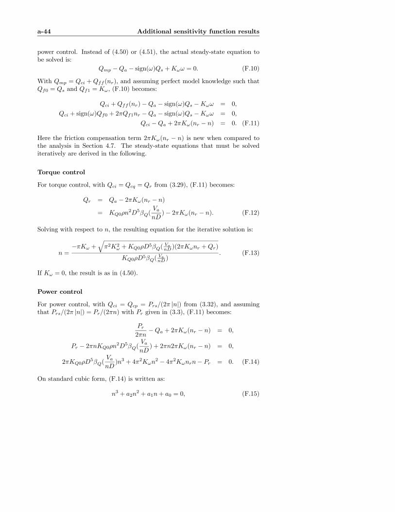
a-44 Additional sensitivity function results
power control. Instead of (4.50) or (4.51), the actual steady-state equation tobe solved is:
Qmp −Qa − sign(ω)Qs +Kωω = 0. (F.10)
With Qmp = Qci +Qff (nr), and assuming perfect model knowledge such thatQf0 = Qs and Qf1 = Kω, (F.10) becomes:
Qci +Qff (nr)−Qa − sign(ω)Qs −Kωω = 0,
Qci + sign(ω)Qf0 + 2πQf1nr −Qa − sign(ω)Qs −Kωω = 0,
Qci −Qa + 2πKω(nr − n) = 0. (F.11)
Here the friction compensation term 2πKω(nr − n) is new when compared tothe analysis in Section 4.7. The steady-state equations that must be solvediteratively are derived in the following.
Torque control
For torque control, with Qci = Qcq = Qr from (3.29), (F.11) becomes:
Qr = Qa − 2πKω(nr − n)
= KQ0ρn2D5βQ(
VanD
)− 2πKω(nr − n). (F.12)
Solving with respect to n, the resulting equation for the iterative solution is:
n =−πKω +
qπ2K2
ω +KQ0ρD5βQ(VanD )(2πKωnr +Qr)
KQ0ρD5βQ(VanD )
. (F.13)
If Kω = 0, the result is as in (4.50).
Power control
For power control, with Qci = Qcp = Prs/(2π |n|) from (3.32), and assumingthat Prs/(2π |n|) = Pr/(2πn) with Pr given in (3.3), (F.11) becomes:
Pr2πn
−Qa + 2πKω(nr − n) = 0,
Pr − 2πnKQ0ρn2D5βQ(
VanD
) + 2πn2πKω(nr − n) = 0,
2πKQ0ρD5βQ(
VanD
)n3 + 4π2Kωn2 − 4π2Kωnrn− Pr = 0. (F.14)
On standard cubic form, (F.14) is written as:
n3 + a2n2 + a1n+ a0 = 0, (F.15)

F.2 Friction compensation sensitivity function errors a-45
where the coefficients ai are defined as:
a2 =4π2Kω
2πKQ0ρD5βQ(VanD )
, (F.16)
a1 = − 4π2Kωnr
2πKQ0ρD5βQ(VanD )
, (F.17)
a0 = − Pr
2πKQ0ρD5βQ(VanD )
. (F.18)
The polynomial has the real solution:
n = −13a2 + (S + T ), (F.19)
where S and T are given by:
S =3
qR+√U, T =
3
qR−√U, (F.20)
U = Q3 +R2, Q =3a1 − a22
9, (F.21)
R =9a2a1 − 27a0 − 2a32
54. (F.22)
The solution for n, which constitutes the equation for the iterative solutionprocedure, can hence be found directly, but is not suited for being written outexplicitly. In the case where Kω = 0, (F.19) reduces to (4.51).
F.2.2 Static friction compensation error
If the static friction compensation term is wrong such that Qf0 6= Qs, thesensitivity analysis as presented in Chapter 4 also becomes wrong. Assumingω > 0, the steady-state equation to be solved by the iterative solution procedurebecomes:
Qci +Qff (nr)−Qa −Qs −Kωω = 0,
Qci +Qf0 + 2πQf1nr −Qa −Qs −Kωω = 0,
Qci +∆Qf −Qa + 2πKω(nr − n) = 0, (F.23)
which is identical to (F.11), except for the static friction compensation error∆Qf = Qf0 − Qs. The solution will then be the same, except that Qci mustbe adjusted with the term ∆Qf . In the solutions for torque and power controlgiven in (F.13) and (F.19), respectively, this is easily done by adding ∆Qf towhere 2πKωnr appears in the expressions for n. Hence, for torque control, theexpression for n from (F.13) becomes:
n =−πKω +
qπ2K2
ω +KQ0ρD5βQ(VanD )(2πKωnr +Qr +∆Qf )
KQ0ρD5βQ(VanD )
. (F.24)

a-46 Additional sensitivity function results
In the case where Kω = 0 the result is:
n =
sQr +∆Qf
KQ0ρD5βQ(VanD )
. (F.25)
Similarly, the result for power control in (F.19) is adjusted by redefining a1 in(F.17) as:
a1 = −4π2Kωnr + 2π∆Qf
2πKQ0ρD5βQ(VanD )
. (F.26)
F.2.3 Result of errors
The error due to the linear friction compensation will always be present, evenwith perfect model knowledge. The error due to the static friction compensa-tion, however, disappears with perfect model knowledge. As an example, theWageningen B4-70 simulation propeller is used. The linear friction term andfriction compensation are taken as Kω = Qf1 = 720 Nms, and the error in thestatic friction compensation is taken as ∆Qf = −2E3 kNm. In Figures F.2 toF.5 the thrust, shaft speed, torque, and power sensitivities are shown for twothrust references: Tr = 50 kN and Tr = 400 kN. The effect of accounting forthe linear friction compensation is best seen in slope of the torque sensitivitycurves for torque control, sqq(·) in Figure F.4, and the slope of the power sen-sitivity curves for power control, spp(·) in Figure F.5. If the friction had notbeen accounted for, these would have been flat. The effect of the static frictioncompensation error can be seen in all the figures, since the torque and powercontrollers no longer give unity sensitivity functions for Va = 0. Obviously, theerror has a larger impact for the lowest thrust reference.
F.3 Robustness analysis using Lyapunov theoryAccurate estimates of the resulting (steady-state) shaft speed during a thrustloss incident with a given controller is most conveniently found by using thesensitivity functions presented in Section 4 and summarized in Table 4.1, oreventually by the extensions provided in Section F.2. For analysis of the tran-sient behavior of the system, an analysis based on Lyapunov tools may proveuseful.
F.3.1 Using the comparison method
With the stability analysis in Section 6.5.1 as a starting point, the bound on thesolutions of the perturbed system in (6.4) may be estimated by the comparisonmethod for non-vanishing perturbations, as described in Lemma 9.4 and 9.6 inKhalil (2002). Assume that (4.91), (4.95), and (4.99) hold for x ∈ Dr, whereDr is a ball of radius r:
Dr = {x ∈ R | kxk2 < r} . (F.27)
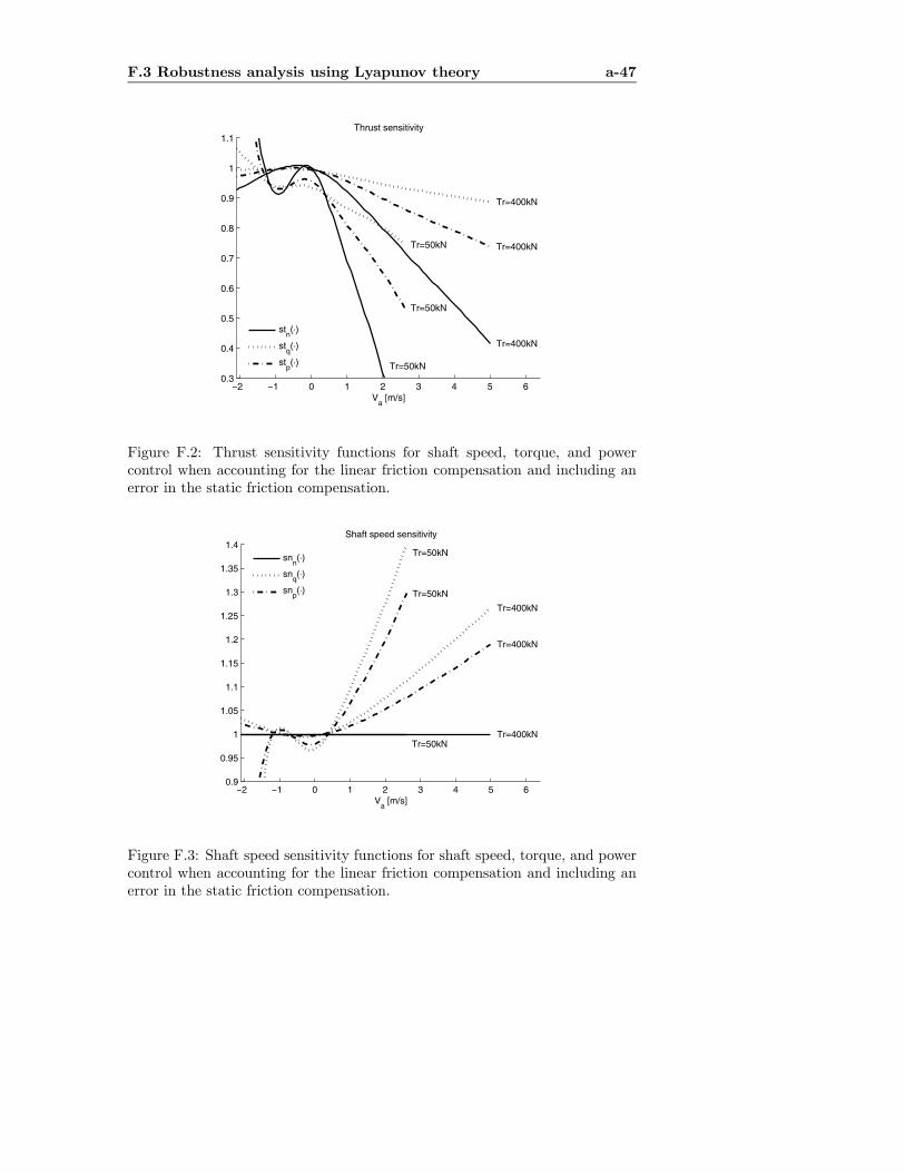
F.3 Robustness analysis using Lyapunov theory a-47
−2 −1 0 1 2 3 4 5 60.3
0.4
0.5
0.6
0.7
0.8
0.9
1
1.1
Va [m/s]
Thrust sensitivity
Tr=50kN
Tr=50kN
Tr=50kN
Tr=400kN
Tr=400kN
Tr=400kN
stn(⋅)
stq(⋅)
stp(⋅)
Figure F.2: Thrust sensitivity functions for shaft speed, torque, and powercontrol when accounting for the linear friction compensation and including anerror in the static friction compensation.
−2 −1 0 1 2 3 4 5 60.9
0.95
1
1.05
1.1
1.15
1.2
1.25
1.3
1.35
1.4
Va [m/s]
Shaft speed sensitivity
Tr=50kN
Tr=50kN
Tr=50kN
Tr=400kN
Tr=400kN
Tr=400kN
snn(⋅)
snq(⋅)
snp(⋅)
Figure F.3: Shaft speed sensitivity functions for shaft speed, torque, and powercontrol when accounting for the linear friction compensation and including anerror in the static friction compensation.

a-48 Additional sensitivity function results
−2 −1 0 1 2 3 4 5 60.1
0.2
0.3
0.4
0.5
0.6
0.7
0.8
0.9
1
1.1Torque sensitivity
Va [m/s]
Tr=50kN
Tr=50kN
Tr=50kN
Tr=400kN
Tr=400kN
Tr=400kN
sqn(⋅)
sqq(⋅)
sqp(⋅)
Figure F.4: Torque sensitivity functions for shaft speed, torque, and powercontrol when accounting for the linear friction compensation and including anerror in the static friction compensation.
−2 −1 0 1 2 3 4 5 6
0.2
0.4
0.6
0.8
1
1.2
Power sensitivity
Va [m/s]
Tr=50kN
Tr=50kN
Tr=50kN
Tr=400kN
Tr=400kN
Tr=400kN
spn(⋅)
spq(⋅)
spp(⋅)
Figure F.5: Power sensitivity functions for shaft speed, torque, and power con-trol when accounting for the linear friction compensation and including an errorin the static friction compensation.
F.3 Robustness analysis using Lyapunov theory a-49
The numerical values k1 = k2 = 1/2 and k4 = 1 can be chosen in (4.91) and(4.99). How to choose k3 in (4.95) is further discussed below. The perturbationterm g2(t, x) is defined in (6.11). Suppose that g2(t, x) satisfies:
kg2(t, x)k ≤ ξ(t) kxk+ δ(t), ∀t ≥ 0,∀x ∈ D, (F.28)
where ξ : R → R is nonnegative, continuous for all t ≥ 0, and satisfies thecondition: Z t
t0
ξ(t)dτ ≤ ε(t− t0) + η, (F.29)
for 0 ≤ ε < k3 and η ≥ 0, and that δ : R → R is nonnegative, continuous, andbounded for all t ≥ 0. For this system, ε and η can be chosen as ε = 0 andη = 0, such that g2(t, x) must satisfy:
kg2(t, x)k ≤ δ(t), ∀t ≥ 0,∀x ∈ D. (F.30)
From Lemma 9.4 in Khalil (2002), provided:
kx(t0)k <r
ρ
rk1k2= r, (F.31)
supt≥t0
δ(t) <2k1αr
k4ρ= k3r, (F.32)
where it has been inserted that:
ρ = exp(k4η
2k1) = exp(η) = 1,
α =1
2(k3k2− ε
k4k1) = k3 − ε = k3, (F.33)
the solution of the perturbed system then satisfies:
kx(t)k ≤ kx(t0)k e−k3(t−t0) +Z t
t0
e−k3(t−τ)δ(τ)dτ. (F.34)
Additionally, from Lemma 9.6 in Khalil (2002), if:R tt0e−k3(t−τ)δ(τ)dτ ≤ σ, ∀t ≥ t0, (F.35)
for some constant σ > 0, then x(t) is uniformly ultimately bounded with ulti-mate bound b:
b =σ
θ, (F.36)
where θ is an arbitrary constant 0 < θ < 1. This shows that the bound andultimate bound on x(t) depend only on its initial condition and the time historyof the bound δ(t) on the perturbation term g(t, x). The remaining difficulties inorder to achieve realistic numerical bounds on the solutions is to find a sensiblevalue for k3 in (4.95), and a reasonable model for the disturbance bound δ(t) in(F.30). The ultimate bound will not be further considered here — for steady-stateperformance, the sensitivity functions give a more correct analysis.

a-50 Additional sensitivity function results
F.3.2 Determining the damping
In the proofs of Proposition 4.1 and Theorem 6.1, Lemma 4.1 was used to re-move the nonlinear damping from the analysis, and hence it would seem naturalto choose k3 = b1. In reality, the nonlinear terms may give a much larger con-tribution to the stability of the system that the linear terms. For the nominalsystem (4.89), assume e.g. to be operating about a positive equilibrium ωr, andthat |x| < ωr such that x+ ωr > 0. V (x) in (4.92) then becomes:
V (x) = −b0θ(ωr, ω)x− b1x2 − b2x((x+ ωr)
2 − ω2r), (F.37)
and by applying (4.94):
V (x) ≤ −b1x2 − b2x((x+ ωr)2 − ω2r)
= −b1x2 − b2x(x2 + 2xωr + ω2r − ω2r)
= −b1x2 − b2x3 − 2b2x2ωr
= −(b1 + 2b2ωr)x2 − b2x3. (F.38)
The sign of the x3 term is indefinite, and must be dominated by the x2 term.Since it is assumed that |x| < ωr and ωr > 0, it follows that ωrx2 > x3. Hence:
V (x) ≤ −(b1 + b2ωr)x2 − b2ωrx
2 − b2x3
≤ −(b1 + b2ωr)x2. (F.39)
Similarly, if ωr < 0 and |x| < |ωr| such that x+ ωr < 0, V (x) becomes:
V (x) = −b0θ(ωr, ω)x− b1x2 − b2x(−(x+ ωr)
2 + ω2r)
≤ −b1x2 − b2x(−x2 − 2xωr − ω2r + ω2r)
= −b1x2 + b2x3 + 2b2x
2ωr
= −b1x2 + b2x3 − 2b2x2 |ωr|
= −(b1 + 2b2 |ωr|)x2 + b2x3. (F.40)
As above, it follows that ωrx2 > x3 such that:
V (x) ≤ −(b1 + b2 |ωr|)x2 − b2 |ωr|x2 + b2x3
≤ −(b1 + b2 |ωr|)x2. (F.41)
Combining the results for positive and negative ωr, i.e. (F.39) and (F.41), itfollows that for all |x| < |ωr|, V (x) complies to:
V (x) ≤ −(b1 + b2 |ωr|)x2. (F.42)
This demand on x is quite realistic, since it only excludes perturbations thatcause the rotational direction of the propeller to change, or increase to morethan the double of its nominal value ωr. For normal operation, the shaft speedwill not change direction. With some kind of anti-spin functionality in the
F.3 Robustness analysis using Lyapunov theory a-51
controller, the shaft speed should not be allowed to exceed 2ωr, even duringlarge thrust losses. Without an anti-spin controller, however, this may well bethe case with torque and power control. These considerations show, as shouldbe expected, that the damping introduced by the fluid also contributes to thestability properties of the system. Comparing realistic values of b1 and b2 |ωr|,it is apparent that the nonlinear damping by far is the dominating. Hence, forthe following Lyapunov analysis, k3 is chosen as:
k3 = b1 + b2 |ωr| . (F.43)
For the system during ventilation, as analyzed in Theorem 6.1, such a con-sideration becomes more difficult, since the nonlinear damping depends on thetorque loss factor βQ(t, ω). The Lyapunov analysis of the nominal system (6.4)during the loss incident resulted in (6.14):
V (x) = −b0θ(ωr, ω)x− b1x2 − b2βQ(t, ω)x((x+ωr) |x+ ωr|− ωr |ωr|). (F.44)
Similar reasoning as for the nominal system without losses may be applied, suchthat for all |x| < |ωr|, V (x) complies to:
V (x) ≤ −(b1 + βQ(t, ω)b2 |ωr|)x2. (F.45)
The presence of βQ(t, ω) means that a more conservative estimate of k3 isneeded. During pure ventilation, when the propeller still is submerged, theminimum value of βQ(t, ω) is approximately 0.2, see Section 2.4. In the case ofa complete water exit, the propeller loses all load torque, such that βQ(t, ω) ≈ 0.The bound on the shaft speed then only depends on the friction term. This isclearly seen in the analysis, since k3 then must be taken as k3 = b1. This demon-strates the importance of designing a fast anti-spin controller: if the ventilationincident is not caught quickly, the shaft speed may increase rapidly, since mostof the damping in the system is removed. For the ventilated propeller, k3 musthence be taken as:
k3 = b1 + βQb2 |ωr| , (F.46)
where βQ is the lowest expected value of βQ(t, ω) during the loss incident.
F.3.3 Quantifying the trajectory bound
In order to quantify the trajectory bound in (F.34) further, some simplificationsare needed. As an example, take a ventilation incident where the propellerinitially is at its equilibrium, such that x(t0) = 0, and βQ(t, ω) drops from 1to βQ instantaneously. The anti-spin controller needs some time to catch theventilation incident before γQ converges to βQ, and the error γQ − βQ(t, ω)is modelled as a square wave with amplitude γe and duration T seconds. Theperturbation bound δ(t) from (F.30) then becomes a square wave with amplitudeγeu and duration T , i.e.:
δ(t) =
½γeu for t ≤ t0 + T,0 for t > t0 + T.
(F.47)
a-52 Additional sensitivity function results
With βQ(t, ω) = βQ, k3 can be taken as in (F.46). According to (F.34), thetrajectories of the system then satisfy:
kx(t)k ≤ x(t0) +
Z t
t0
e−k3(t−τ)δ(τ)dτ
= 0 + γeu
Z t0+T
t0
e−k3(t−τ)dτ =γeu
k3(ek3T − 1)ek3(t0−t)
=γeu
b1 + βQb2 |ωr|(e(b1+βQb2|ωr|)T − 1)e(b1+βQb2|ωr|)(t0−t).(F.48)
In the conservative case of zero linear damping, i.e. b1 = 0, this reduces to:
kx(t)k ≤ γeu
βQb2 |ωr|(e(βQb2|ωr|)T − 1)e(βQb2|ωr|)(t0−t)
= ωrγeβQ(e(βQb2|ωr|)T − 1)e(βQb2|ωr|)(t0−t),
where u = b2ωr |ωr| from (4.86) has been inserted. Clearly, the bound onthe trajectories is proportional to the magnitude of the perturbation γe, andincreasing with the duration T .
Remark F.1 For zero duration T = 0, or zero magnitude γe = 0, kx(t)k ≡ 0as should be expected. This corresponds to the case of a known disturbance, asshown in Corollary 6.1.
Appendix G
Additional observer results
This appendix contains additional observer results. Section G.1 presents anadaptive extension of the load torque observer from Section 5.1, including ex-perimental results, and section G.2 shows how the prevailing control coefficientscan be estimated from the available measurements.
G.1 Adaptive load torque observer
The load torque observer presented in Section 5.1 is based on knowledge of theshaft friction parameters Qs and Kω. In the case were these are uncertain, orexpected to change significantly over the life-time of the thruster, the observermay be extended to include a parameter adaption scheme for Kω. It is stillassumed that the static friction term Qs is known with reasonable accuracy.The estimate Kω can then also be used to replace the parameter Qf1 in thelinear friction compensation (3.21). The adaptive observer was first publishedin Smogeli and Sørensen (2006a).
G.1.1 Observability
If Kω is modelled as a random process driven by a bounded disturbance wKω,
and augmented to the observer state vector x in (5.4), this will give the newstate vector xa:
xa = [ω, Qa, Kω]>, (G.1)
and process plant model:
xa = fa(xa) +Bau+Gawa, (G.2)
y = h(xa) = Caxa + v, (G.3)
a-54 Additional observer results
where the following matrices and vectors have been used:
fa(xa) =
⎡⎣ −ωKω/Is −Qa/Is00
⎤⎦ , Ga = I3×3,
Ba =
⎡⎣ 1/Is00
⎤⎦ wa =
⎡⎣ δf/IswQa
wKω
⎤⎦ , Ca =
⎡⎣ 100
⎤⎦| . (G.4)
The bounded disturbances wa and v are assumed uncorrelated. From Isidori(1995), the observability matrix of the nonlinear system becomes:
O =
⎡⎣ ∂∂xa
h(xa)∂∂xa
Lfah(xa)∂∂xa
L2fah(xa)
⎤⎦ =⎡⎢⎣ 1 0 0−Kω
Is− 1
Is− ω
IsK2ω
I2s
Kω
I2s
2ωKω+Qa
I2s
⎤⎥⎦ , (G.5)
which has rank 3 for all xa ∈ R3 − [0, 0, 0]| . The nonlinear system is henceweakly locally observable according to the definitions in Hermann and Krener(1977). Notice, however, that the linearization about the current estimate xaas used in e.g. an extended Kalman filter becomes:
Aa =∂fa(xa)
∂xa
¯xa=xa
=
∙−Kω/Is −1/Is −ω/Is
02x3
¸, (G.6)
and the Kalman observability matrix becomes:
O =
⎡⎣ Ca
CaAa,CaA
2a
⎤⎦ =⎡⎢⎣ 1 0 0
− Kω
Is− 1
Is− ω
IsK2ω
I2s
Kω
I2s
KωωI2s
⎤⎥⎦ , (G.7)
which has rank 2. This means that linear estimation methods like extendedKalman filtering, SDRE Filtering (Haessig and Friedland, 1997), etc. are non-applicable, whereas a nonlinear estimation scheme should be possible to con-struct.
G.1.2 Kω estimation
The nonlinear system dynamics used in the estimation scheme is based on theshaft dynamics (2.50), with the static friction Qs sign(ω) replaced by the staticfriction compensation (3.20), and Qa replaced by the nominal torque model Qn
from (5.14):Isω = kgQm −Qff0(nr)−Kωω − Qn. (G.8)
The error in the static friction compensation, i.e. the deviation of Qff0(nr)from Qs sign(ω), will partly be captured in the adaption of Kω.

G.1 Adaptive load torque observer a-55
Remark G.1 Using the nominal torque model Qn in the parameter estimationcan be justified, since the estimation of Kω is a slow process, and in DP thedeviation of KQ from KQ0 will be small. In waves, the deviation will averageto zero over time, whereas in current there will be a small steady-state offset.The offset will depend on the size and type of propeller, and the magnitude anddirection of the current. Note that an offset in KQ will lead to an offset in theestimate of Kω, but in DP this deviation is expected to be small.
With the motor torque adjusted for the static friction as input as in (5.3),i.e. u = kgQm − Qff0(nr), the shaft friction coefficient Kω as an unknownparameter, and inserting for Qn, the system in (G.8) becomes:
ω =1
Isu− Kω
Isω − KQCρD
5
4π2Isω |ω| , f(ω, u,Kω). (G.9)
The system is affine in Kω, and can be written as:
f(ω, u,Kω) = F (ω)Kω + g(ω, u), (G.10)
where:
F (ω) =∂f(ω, u,Kω)
∂Kω= − ω
Is, (G.11)
g(ω, u) =1
Isu− KQ0ρD
5
4π2Isω |ω| . (G.12)
Following a similar approach as in Section 5.2, an estimate Kω of Kω can beobtained from a parameter update law on the form (Friedland, 1997):
Kω = φ(ω) + z,
z = −Φ(ω)f(ω, u, Kω), (G.13)
where φ(ω) is a nonlinear function to be defined, and Φ(ω) is its Jacobian,Φ(ω) = ∂φ(ω)/∂ω. As in Section 5.2, the estimation error Kω and its dynamicsare:
Kω = Kω − Kω, (G.14)˙Kω = − ˙Kω = −φ(ω)− z
= −Φ(ω)F (ω)(Kω − Kω) = −L(t)Kω, (G.15)
where L(t) = Φ(ω(t))F (ω(t)) is time-varying. It remains to choose φ(ω) to yieldL(t) positive semidefinite. From Friedland (1997), one option is to choose φ(ω)to satisfy
Φ(ω) = kcF (ω) = −kcω
Is, (G.16)
where kc is a positive constant, such that
L(t) = kcF (ω)2 = kc
ω2
I2s. (G.17)
a-56 Additional observer results
A candidate φ(ω) satisfying this is:
φ(ω) = −kcω2
2Is. (G.18)
This yields the following error dynamics:
˙Kω = −kcω(t)2
I2sKω, (G.19)
where the time-dependence of ω has been emphasized. Stability properties areinvestigated by the positive definite Lyapunov function V1(Kω):
V1(Kω) =1
2K2ω, (G.20)
such that the derivative of V1 along the trajectories of (G.9) are given by:
V1 = Kω˙Kω = −kc
ω(t)2
I2sK2ω ≤ 0. (G.21)
Clearly, V1 = 0 for Kω 6= 0 iff ω(t) ≡ 0. This is the case of zero shaft speed,for which one cannot expect to extract any information. However, the errordynamics are still uniformly globally stable (UGS). Note that ω(t) = 0 ⇒φ(ω) = Φ(ω) = z = 0, which means that parameter adaption stops, but does notdiverge. The condition that ω(t) 6= 0 can be seen as a persistency of excitation(PE) requirement, leading to uniform global exponential stability (UGES) ofthe error dynamics, since:
r1
°°°Kω
°°°2 ≤ V1(Kω) ≤ r2
°°°Kω
°°°2 , (G.22)
V1 ≤ −r3°°°Kω
°°°2 , (G.23)
for r1 = r2 = 0.5 and r3 = kcω2min/I
2s , where ωmin is the lowest shaft speed
magnitude to be considered.
G.1.3 Adaptive observer design
With the chosen decoupling of parameter estimation and observer, the parame-ter estimation scheme in (G.13) may be combined with the observer in (5.7) togive an adaptive observer in the following form:
˙ω =1
Is(u− Qa − Kωω) + kaω,
˙Qa = kbω,
z = kcω
I2s(u− Kωω −
KQCρD5
4π2ω |ω|),
Kω = −kcω2
2Is+ z, (G.24)
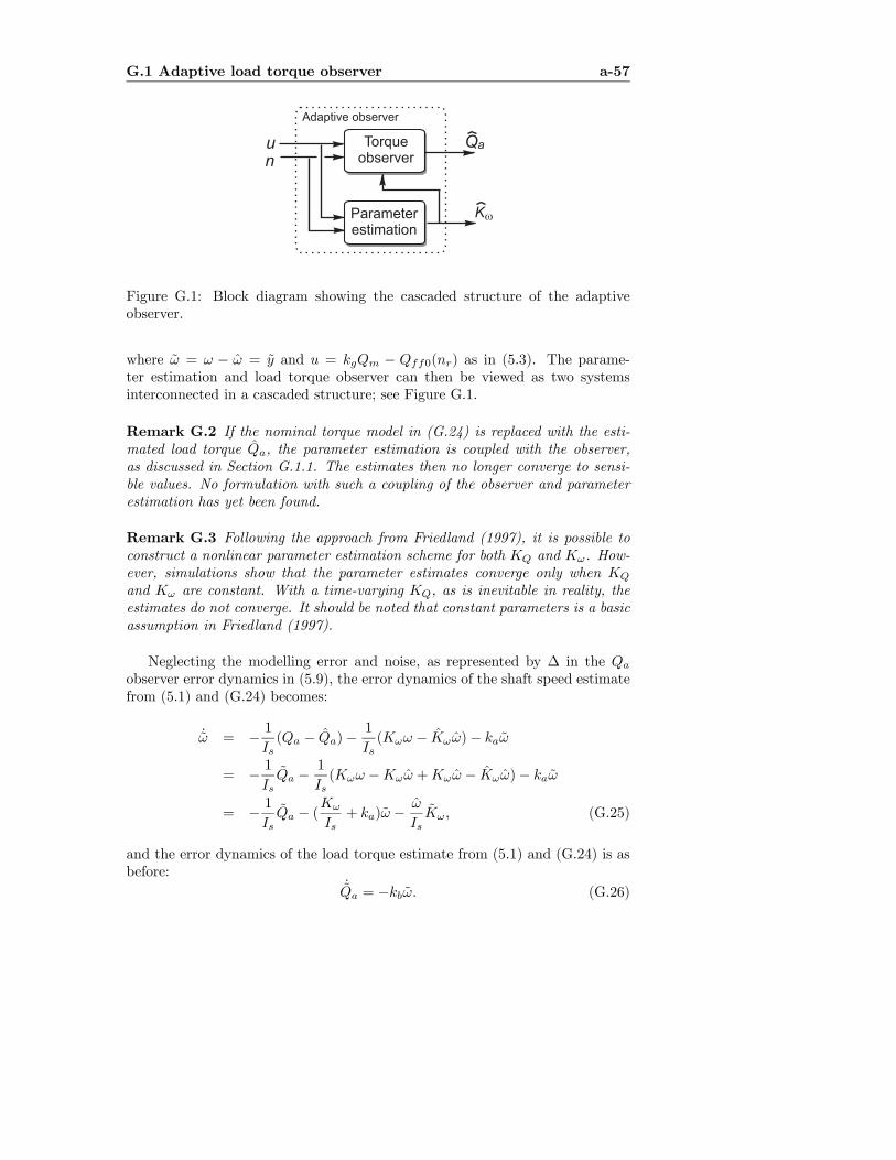
G.1 Adaptive load torque observer a-57
nu QaTorque
observer
Parameterestimation
Adaptive observer
Kw
Figure G.1: Block diagram showing the cascaded structure of the adaptiveobserver.
where ω = ω − ω = y and u = kgQm − Qff0(nr) as in (5.3). The parame-ter estimation and load torque observer can then be viewed as two systemsinterconnected in a cascaded structure; see Figure G.1.
Remark G.2 If the nominal torque model in (G.24) is replaced with the esti-mated load torque Qa, the parameter estimation is coupled with the observer,as discussed in Section G.1.1. The estimates then no longer converge to sensi-ble values. No formulation with such a coupling of the observer and parameterestimation has yet been found.
Remark G.3 Following the approach from Friedland (1997), it is possible toconstruct a nonlinear parameter estimation scheme for both KQ and Kω. How-ever, simulations show that the parameter estimates converge only when KQ
and Kω are constant. With a time-varying KQ, as is inevitable in reality, theestimates do not converge. It should be noted that constant parameters is a basicassumption in Friedland (1997).
Neglecting the modelling error and noise, as represented by ∆ in the Qa
observer error dynamics in (5.9), the error dynamics of the shaft speed estimatefrom (5.1) and (G.24) becomes:
˙ω = − 1Is(Qa − Qa)−
1
Is(Kωω − Kωω)− kaω
= − 1IsQa −
1
Is(Kωω −Kωω +Kωω − Kωω)− kaω
= − 1IsQa − (
Kω
Is+ ka)ω −
ω
IsKω, (G.25)
and the error dynamics of the load torque estimate from (5.1) and (G.24) is asbefore:
˙Qa = −kbω. (G.26)

a-58 Additional observer results
The parameter estimation error dynamics is given in (G.19). On state-spaceform, the adaptive observer error dynamics can be written as two cascadedsystems:
Σ1 : x1 = f1(x1) + g(t, x1)x2,
Σ2 : x2 = f2(t, x2), (G.27)
where:
x1 =
∙ω
Qa
¸, x2 = Kω, (G.28)
f1(x1) =
∙− 1
IsQa − (Kω
Is+ ka)ω
−kbω
¸= Fx1, (G.29)
g(t, x1) = − ω(t)Is
= −ω(t)− ω
Is, (G.30)
f2(t, x2) = −kcω(t)2
I2sKω. (G.31)
The parameter estimation error in Σ2 was in Section G.1.2 shown to be UGESunder PE conditions, and the observer error dynamics without the couplingterm g(t, x1) in Σ1 was in Section 5.1 shown to be GES. That is, the positivedefinite Lyapunov function V2(x1):
V2(x1) =1
2x|1Px1, P =
∙p11 00 p22
¸, (G.32)
has a derivative along the trajectories of f1(x1) given by:
V2 = x|1Px1 < 0 ∀ x1 ∈ {R2 − (0, 0)}, (G.33)
for any positive constants p11 and p22, given that the observer gain requirementsin Proposition 5.1 are met. To demonstrate stability of the cascaded system, itmust be shown that the interconnection term g(t, x1) satisfy certain growth raterequirements. With Σ2 UGES and the unperturbed Σ1 system GES, Theorem 2in Panteley et al. (1999) states that the cascaded system in (G.27) is uniformlyglobally asymptotically stable (UGAS) if the following additional requirementsare met:
1. V2(x1) must satisfy:°°°°∂V2∂x1
°°°° kx1k ≤ c1V2(x1) for all kx1k ≥ η. (G.34)
2. The function g(t, x) must satisfy:
kg(t, x1)k ≤ θ1(kx2k) + θ2(kx2k) kx1k , (G.35)
where θ1, θ2 : R≥0 → R≥0 are continuous.

G.1 Adaptive load torque observer a-59
Since: ¯∂V2∂x1
¯|x1| =
¯∂
∂x1(1
2p11x
21 +
1
2p22x
22)
¯|x1|
= |p11x1| |x1| = p11x21, (G.36)
and:c1V2(x1) = c1
1
2(p11x
21 + p22x
22) ≥
c12p11x
21, (G.37)
requirement 1 is met for c1 = 2 and η = 0. Furthermore, since g(t, x1) satisfies:
|g(t, x1)| =|ω(t)− ω|
Is≤ |ω(t)|+ |ω|
Is
≤ ωmax + |ω|Is
=ωmaxIs
+1
Is|ω|
≤ ωmaxIs
+1
Is|x1| = θ1 + θ2 |x1| , (G.38)
where ωmax is the maximum shaft speed of the propeller and:
θ1 =ωmaxIs
, θ2 =1
Is, (G.39)
also requirement 2 is met. The cascaded system (G.27) is thereby shown to beUGAS. Note that the PE condition on ω (i.e. ω(t) 6= 0) still applies.
G.1.4 Experimental results
The experiments were conducted at the Marine Cybernetics Laboratory(MCLab) at NTNU with the experimental setup described in Section 7.1.The open propeller was used. The true friction coefficient was found to beKω ≈ 0.01Nms.The adaptive observer (G.24) was implemented together with a torque con-
troller (3.29) and friction feedforward scheme (3.19) with Qf1 replaced withthe estimate Kω. The observer and parameter adaption gains were chosen aska = 15, kb = −25, and kc = 5E − 10. Experiments in calm water with theadaptive observer alone confirmed that the parameter estimate converged to itstrue value, and that the propeller torque was tracked by the observer. In the ex-periments presented here, the propeller shaft had a mean submergence of 30cm,and the propeller was subject to irregular waves from the modified PM spectrum(C.19), with Hs = 5cm and Tp = 1.2s. The initial friction coefficient estimatewas Kω0 = 0, and the thrust reference was kept constant at Tr = 200N. Theresulting time series are given in Figure G.1, which shows the raw and filteredshaft speed n, the raw and filtered motor torque Qm, the actual friction coef-ficient Kω versus the estimated friction coefficient Kω, the commanded torqueQc with and without friction compensation Qff , the thrust reference Tr versus

a-60 Additional observer results
the actual thrust Ta, and the actual torque Qa versus the estimated torque Qa.The raw shaft speed and motor torque signals — which are used by the adap-tive observer — are contaminated with some noise, and the motor torque is alsoclearly subject to quantization due to limited bit resolution. The parameteradaption scheme is enabled at approximately t = 12s, and clearly tracks theactual friction coefficient. This leads to an increased commanded torque (dueto Qff ), and hence also increased shaft speed and thrust. The adaption of Kω
also leads to a more correctly estimated load torque, which before the adaptionwas estimated too high. Experiments with varying thrust references and otheroperating conditions show similar performance.
G.1.5 Extensions
As discussed in Chapter 8 with respect to the thruster controllers and observers,the adaptive observer is extendable to CPP and transit by lettingKQC in (G.24)be a function of the propeller pitch and vessel speed respectively.The adaptive observer can also be used in extreme operating conditions, i.e.
when the propeller is subject to ventilation. In order to get convergence of Kω,however, it is necessary to disable estimation during ventilation. From Section6.3, a ventilation detection signal ζ is available from the loss calculation in (5.16)and the ventilation detection scheme in (6.1). The following modification canthen be made to the adaptive observer in (G.24):
kc =
½kcc, for ζ = 0 (no ventilation),0, for ζ = 1 (ventilation),
(G.40)
where kcc > 0 is the chosen estimation gain. Experiments show that the adaptiveobserver then gives convergence of Kω and a good estimate of Qa, even if thepropeller is subject to frequent ventilation.
G.2 Online control parameter estimation
In some applications, it will be useful to have estimates of the prevailing thrustand torque coefficients, in order to substitute these for the nominal values in thecontrol coefficients. The prevailing thrust and torque coefficients, KT and KQ,are here defined as the mean coefficients over a finite time horizon, includingthe effect of steady-state advance velocity changes (due to current and vessellow-frequency motion), but excluding the losses due to ventilation, water exits,wave-induced water velocities, and vessel wave-frequency motion. That is, theywould ideally be equal to low-pass filtered versions of KTJ and KQJ defined inSection 2.1.1. The desired properties of KT and KQ are the same as for thecoefficient estimates proposed in Section E.2.5.

G.2 Online control parameter estimation a-61
8.8
9
9.2
9.4
n [r
ps]
RawFiltered
6.6
6.8
7
Qm
[Nm
]
RawFiltered
0
5
10
Kω [k
g/s⋅
1E−
3]
TrueEstimate
6.6
6.8
7
7.2
Qc [N
m]
Qc
Qc + Q
ff
170
180
190
200
T [N
]
ReferenceMeasured
0 10 20 30 40 50
6
6.5
7
7.5
Q [N
m]
Time [s]
MeasuredEstimated
Figure G.2: Experimental results with the adaptive observer in irregular waves.

a-62 Additional observer results
G.2.1 Implementation for normal conditions
In normal operating conditions, KQ can be estimated directly from the KQ
estimation scheme in (5.26) using an appropriately low gain k0. Alternatively,the load torque observer in (5.7) and KQ calculation in (5.17) can be used, andKQ taken as an average value of KQ over a time interval T :
KQ(t) =1
T
Z t
t−TKQ(τ)dτ. (G.41)
KT can then be calculated from KQ using (2.48) by:
KT = atKQ + bt. (G.42)
Remark G.4 The prevailing thrust coefficient KT can only be calculated withreasonable accuracy for an open propeller, due to the limitations of the KT −KQ
relationship in (2.48).
G.2.2 Extension to extreme conditions
A possible useful application of KQ is ventilation detection during transit. Thisproblem was discussed in Section 8.2.5. If KQ is used to replace KQC in (5.16)and (5.19), βQ will stay close to unity regardless of the vessel forward speed andcurrent, and be affected only by wave-frequency disturbances and ventilation.For rejecting disturbances due to waves in KQ, it is sufficient to use a low
estimation gain, or equivalently average the estimate over a time period T , assuggested in (G.41). If the propeller is subject to ventilation, however, addi-tional measures are needed to remove the large thrust losses in the estimationof KQ. If not, KQ would be estimated too low. In Section 6.3, a ventilationdetection scheme based on βQ ,which outputs a detection signal ζ ∈ {0, 1}, wasdeveloped. This can be utilized to disable estimation during ventilation:
KQ = −k0c(ζ) + z,
z = kv(ζ)ω |ω|I2s
(u− KQω |ω|−Qf1ω),
kv(ζ) =
½k0, for ζ = 0 (no ventilation),0, for ζ = 1 (ventilation),
c(ζ) =
(|ω|33Is
, for ζ = 0 (no ventilation),c, for ζ = 1 (ventilation),
(G.43)
where the KQ estimation scheme from (5.26) has been used as a starting point,and c is the value of c(ζ) at the instant of the switch ζ : 0→ 1 (i.e. the “frozen”value of c(ζ)).
Remark G.5 The combination of KQ with KQ to calculate βQ depends ontime scale separation: for the scheme to be valid, the update of KQ must bemuch slower than the update of KQ.


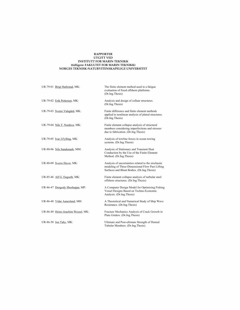
RAPPORTER UTGITT VED
INSTITUTT FOR MARIN TEKNIKK (tidligere: FAKULTET FOR MARIN TEKNIKK)
NORGES TEKNISK-NATURVITENSKAPELIGE UNIVERSITET
UR-79-01 Brigt Hatlestad, MK: The finite element method used in a fatigue
evaluation of fixed offshore platforms. (Dr.Ing.Thesis)
UR-79-02 Erik Pettersen, MK: Analysis and design of celluar structures.
(Dr.Ing.Thesis) UR-79-03 Sverre Valsgård, MK: Finite difference and finite element methods
applied to nonlinear analysis of plated structures. (Dr.Ing.Thesis)
UR-79-04 Nils T. Nordsve, MK: Finite element collapse analysis of structural
members considering imperfections and stresses due to fabrication. (Dr.Ing.Thesis)
UR-79-05 Ivar J.Fylling, MK: Analysis of towline forces in ocean towing
systems. (Dr.Ing.Thesis) UR-80-06 Nils Sandsmark, MM: Analysis of Stationary and Transient Heat
Conduction by the Use of the Finite Element Method. (Dr.Ing.Thesis)
UR-80-09 Sverre Haver, MK: Analysis of uncertainties related to the stochastic
modeling of Three-Dimensional Flow Past Lifting Surfaces and Blunt Bodies. (Dr.Ing.Thesis)
UR-85-46 Alf G. Engseth, MK: Finite element collapse analysis of turbular steel
offshore structures. (Dr.Ing.Thesis) UR-86-47 Dengody Sheshappa, MP: A Computer Design Model for Optimizing Fishing
Vessel Designs Based on Techno-Economic Analysis. (Dr.Ing.Thesis)
UR-86-48 Vidar Aanesland, MH: A Theoretical and Numerical Study of Ship Wave
Resistance. (Dr.Ing.Thesis) UR-86-49 Heinz-Joachim Wessel, MK: Fracture Mechanics Analysis of Crack Growth in
Plate Girders. (Dr.Ing.Thesis) UR-86-50 Jon Taby, MK: Ultimate and Post-ultimate Strength of Dented
Tubular Members. (Dr.Ing.Thesis)
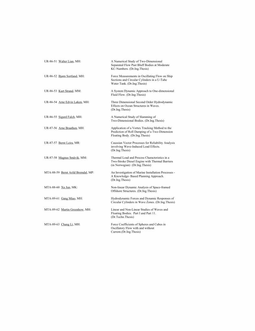
UR-86-51 Walter Lian, MH: A Numerical Study of Two-Dimensional
Separated Flow Past Bluff Bodies at Moderate KC-Numbers. (Dr.Ing.Thesis)
UR-86-52 Bjørn Sortland, MH: Force Measurements in Oscillating Flow on Ship
Sections and Circular Cylinders in a U-Tube Water Tank. (Dr.Ing.Thesis)
UR-86-53 Kurt Strand, MM: A System Dynamic Approach to One-dimensional
Fluid Flow. (Dr.Ing.Thesis) UR-86-54 Arne Edvin Løken, MH: Three Dimensional Second Order Hydrodynamic
Effects on Ocean Structures in Waves. (Dr.Ing.Thesis)
UR-86-55 Sigurd Falch, MH: A Numerical Study of Slamming of
Two-Dimensional Bodies. (Dr.Ing.Thesis) UR-87-56 Arne Braathen, MH: Application of a Vortex Tracking Method to the
Prediction of Roll Damping of a Two-Dimension Floating Body. (Dr.Ing.Thesis)
UR-87-57 Bernt Leira, MR: Caussian Vector Processes for Reliability Analysis
involving Wave-Induced Load Effects. (Dr.Ing.Thesis)
UR-87-58 Magnus Småvik, MM: Thermal Load and Process Characteristics in a
Two-Stroke Diesel Engine with Thermal Barriers (in Norwegian) (Dr.Ing.Thesis)
MTA-88-59 Bernt Arild Bremdal, MP: An Investigation of Marine Installation Processes -
A Knowledge- Based Planning Approach. (Dr.Ing.Thesis)
MTA-88-60 Xu Jun, MK: Non-linear Dynamic Analysis of Space-framed
Offshore Structures. (Dr.Ing.Thesis) MTA-89-61 Gang Miao, MH: Hydrodynamic Forces and Dynamic Responses of
Circular Cylinders in Wave Zones. (Dr.Ing.Thesis) MTA-89-62 Martin Greenhow, MH: Linear and Non-Linear Studies of Waves and
Floating Bodies. Part I and Part 11. (Dr.Techn.Thesis)
MTA-89-63 Chang Li, MH: Force Coefficients of Spheres and Cubes in
Oscillatory Flow with and without Current.(Dr.Ing.Thesis)
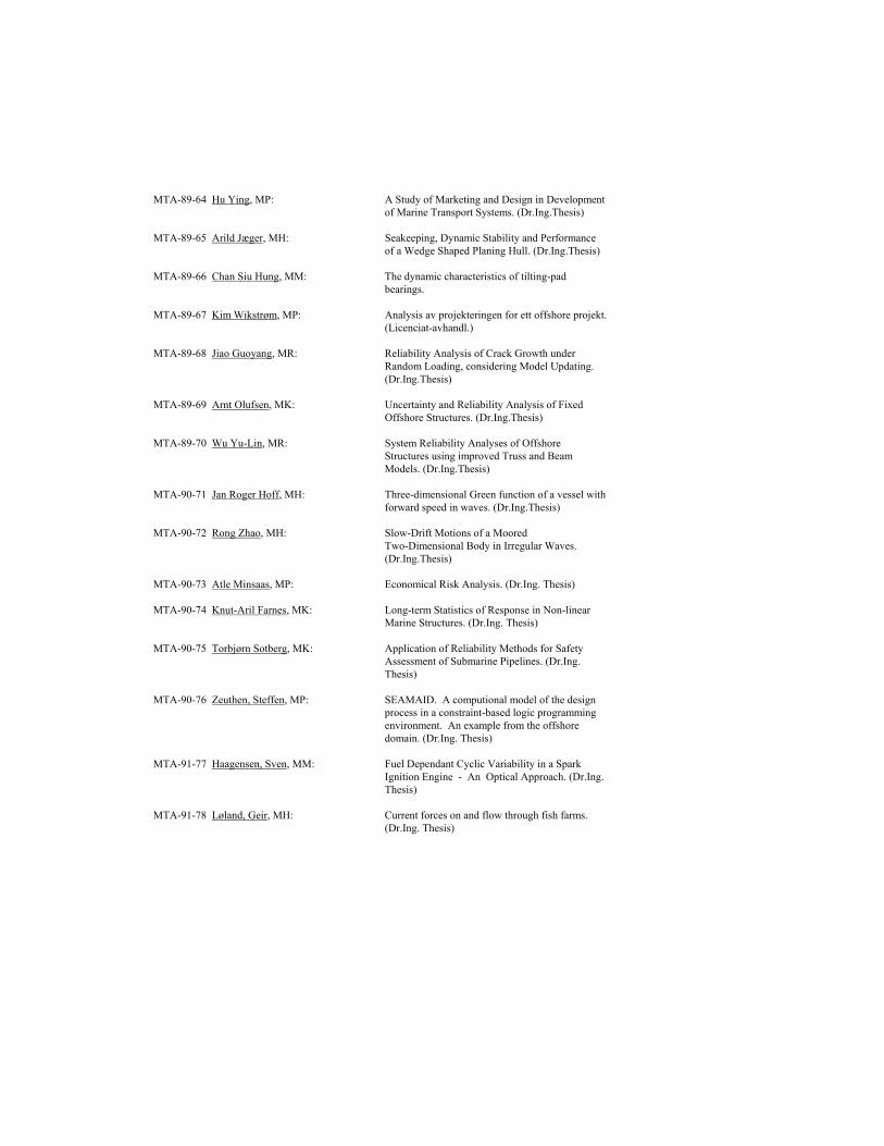
MTA-89-64 Hu Ying, MP: A Study of Marketing and Design in Development of Marine Transport Systems. (Dr.Ing.Thesis)
MTA-89-65 Arild Jæger, MH: Seakeeping, Dynamic Stability and Performance
of a Wedge Shaped Planing Hull. (Dr.Ing.Thesis) MTA-89-66 Chan Siu Hung, MM: The dynamic characteristics of tilting-pad
bearings. MTA-89-67 Kim Wikstrøm, MP: Analysis av projekteringen for ett offshore projekt.
(Licenciat-avhandl.) MTA-89-68 Jiao Guoyang, MR: Reliability Analysis of Crack Growth under
Random Loading, considering Model Updating. (Dr.Ing.Thesis)
MTA-89-69 Arnt Olufsen, MK: Uncertainty and Reliability Analysis of Fixed
Offshore Structures. (Dr.Ing.Thesis) MTA-89-70 Wu Yu-Lin, MR: System Reliability Analyses of Offshore
Structures using improved Truss and Beam Models. (Dr.Ing.Thesis)
MTA-90-71 Jan Roger Hoff, MH: Three-dimensional Green function of a vessel with
forward speed in waves. (Dr.Ing.Thesis) MTA-90-72 Rong Zhao, MH: Slow-Drift Motions of a Moored
Two-Dimensional Body in Irregular Waves. (Dr.Ing.Thesis)
MTA-90-73 Atle Minsaas, MP: Economical Risk Analysis. (Dr.Ing. Thesis) MTA-90-74 Knut-Aril Farnes, MK: Long-term Statistics of Response in Non-linear
Marine Structures. (Dr.Ing. Thesis) MTA-90-75 Torbjørn Sotberg, MK: Application of Reliability Methods for Safety
Assessment of Submarine Pipelines. (Dr.Ing. Thesis)
MTA-90-76 Zeuthen, Steffen, MP: SEAMAID. A computional model of the design
process in a constraint-based logic programming environment. An example from the offshore domain. (Dr.Ing. Thesis)
MTA-91-77 Haagensen, Sven, MM: Fuel Dependant Cyclic Variability in a Spark
Ignition Engine - An Optical Approach. (Dr.Ing. Thesis)
MTA-91-78 Løland, Geir, MH: Current forces on and flow through fish farms.
(Dr.Ing. Thesis)

MTA-91-79 Hoen, Christopher, MK: System Identification of Structures Excited by
Stochastic Load Processes. (Dr.Ing. Thesis) MTA-91-80 Haugen, Stein, MK: Probabilistic Evaluation of Frequency of Collision
between Ships and Offshore Platforms. (Dr.Ing. Thesis)
MTA-91-81 Sødahl, Nils, MK: Methods for Design and Analysis of Flexible
Risers. (Dr.Ing. Thesis) MTA-91-82 Ormberg, Harald, MK: Non-linear Response Analysis of Floating Fish
Farm Systems. (Dr.Ing. Thesis) MTA-91-83 Marley, Mark J., MK: Time Variant Reliability Under Fatigue MTA-91-79 Hoen, Christopher, MK: System Identification of Structures Excited by
Stochastic Load Processes. (Dr.Ing. Thesis) MTA-91-80 Haugen, Stein, MR: Probabilistic Evaluation of Frequency of Collision
between Ships and Offshore Platforms. (Dr.Ing. Thesis)
MTA-91-81 Sødahl, Nils, MK: Methods for Design and Analysis of Flexible
Risers. (Dr.Ing. Thesis) MTA-91-82 Ormberg, Harald, MK: Non-linear Response Analysis of Floating Fish
Farm Systems. (Dr.Ing. Thesis) MTA-91-83 Marley, Mark J., MK: Time Variant Reliability Under Fatigue
Degradation. (Dr.Ing. Thesis) MTA-91-84 Krokstad, Jørgen R., MH: Second-order Loads in Multidirectional Seas.
(Dr.Ing. Thesis) MTA-91-85 Molteberg, Gunnar A., MM: The application of system identification
techniques to Performance Monitoring of four stroke turbocharged Diesel Engines. (Dr.Ing. Thesis)
MTA-92-86 Mørch, Hans Jørgen Bjelke, MH: Aspects of Hydrofoil Design; with Emphasis on
Hydrofoil Interaction in Calm Water. (Dr.Ing. Thesis)
MTA-92-87 Chan Siu Hung, MM: Nonlinear Analysis of Rotordynamic Instabilities
in High-speed Turbomachinery. (Dr.Ing. Thesis) MTA-92-88 Bessason, Bjarni, MK: Assessment of Earthquake Loading and Response
of Seismically Isolated Bridges. (Dr.Ing. Thesis)

MTA-92-89 Langli, Geir, MP: Improving Operational Safety through exploitation
of Design Knowledge - an investigation of offshore platform safety. (Dr.Ing. Thesis)
MTA-92-90 Sævik, Svein, MK: On Stresses and Fatigue in Flexible Pipes. (Dr.Ing.
Thesis) MTA-92-91 Ask, Tor Ø., MM: Ignition and Flame Growth in Lean Gas-Air
Mixtures. An Experimental Study with a Schlieren System. (Dr.Ing. Thesis)
MTA-86-92 Hessen, Gunnar, MK: Fracture Mechanics Analysis of Stiffened Tubular
Members. (Dr.Ing. Thesis) MTA-93-93 Steinebach, Christian, MM: Knowledge Based Systems for Diagnosis of
Rotating Machinery. (Dr.Ing. Thesis) MTA-93-94 Dalane, Jan Inge, MK: System Reliability in Design and Maintenance of
Fixed Offshore Structures. (Dr.Ing. Thesis) MTA-93-95 Steen, Sverre, MH: Cobblestone Effect on SES. (Dr.Ing. Thesis) MTA-93-96 Karunakaran, Daniel, MK: Nonlinear Dynamic Response and Reliability
Analysis of Drag-dominated Offshore Platforms. (Dr.Ing. Thesis)
MTA-93-97 Hagen, Arnulf, MP: The Framework of a Design Process Language.
(Dr.Ing. Thesis) MTA-93-98 Nordrik, Rune, MM: Investigation of Spark Ignition and Autoignition
in Methane and Air Using Computational Fluid Dynamics and Chemical Reaction Kinetics. A Numerical Study of Ignition Processes in Internal Combustion Engines. (Dr.Ing.Thesis)
MTA-94-99 Passano, Elizabeth, MK: Efficient Analysis of Nonlinear Slender Marine
Structures. (Dr.Ing.Thesis) MTA-94-100 Kvålsvold, Jan, MH: Hydroelastic Modelling of Wetdeck Slamming on
Multihull Vessels. (Dr.Ing.Thesis) MTA-94-101 (Dr.Ing.Thesis) Ikke godkjent. MTA-94-102 Bech, Sidsel M., MK: Experimental and Numerical Determination of
Stiffness and Strength of GRP/PVC Sandwich Structures. (Dr.Ing.Thesis)
MTA-95-103 Paulsen, Hallvard, MM: A Study of Transient Jet and Spray using a
Schlieren Method and Digital Image Processing. (Dr.Ing.Thesis)

MTA-95-104 Hovde, Geir Olav, MK: Fatigue and Overload Reliability of Offshore
Structural Systems, Considering the Effect of Inspection and Repair. (Dr.Ing.Thesis)
MTA-95-105 Wang, Xiaozhi, MK: Reliability Analysis of Production Ships with
Emphasis on Load Combination and Ultimate Strength. (Dr.Ing.Thesis)
MTA-95-106 Ulstein, Tore, MH: Nonlinear Effects of a Flexible Stern Seal Bag on Cobblestone Oscillations of an SES. (Dr.Ing.Thesis)
MTA-95-107 Solaas, Frøydis, MH: Analytical and Numerical Studies of Sloshing in
Tanks. (Dr.Ing.Thesis) MTA-95-108 Hellan, øyvind, MK: Nonlinear Pushover and Cyclic Analyses in
Ultimate Limit State Design and Reassessment of Tubular Steel Offshore Structures. (Dr.Ing.Thesis)
MTA-95-109 Hermundstad, Ole A., MK: Theoretical and Experimental Hydroelastic
Analysis of High Speed Vessels. (Dr.Ing.Thesis) MTA-96-110 Bratland, Anne K., MH: Wave-Current Interaction Effects on Large-
Volume Bodies in Water of Finite Depth. (Dr.Ing.Thesis)
MTA-96-111 Herfjord, Kjell, MH: A Study of Two-dimensional Separated Flow by a
Combination of the Finite Element Method and Navier-Stokes Equations. (Dr.Ing.Thesis)
MTA-96-112 Æsøy, Vilmar, MM: Hot Surface Assisted Compression Ignition in a
Direct Injection Natural Gas Engine. (Dr.Ing.Thesis)
MTA-96-113 Eknes, Monika L., MK: Escalation Scenarios Initiated by Gas Explosions
on Offshore Installations. (Dr.Ing.Thesis) MTA-96-114 Erikstad, Stein O.,MP: A Decision Support Model for Preliminary Ship
Design. (Dr.Ing.Thesis) MTA-96-115 Pedersen, Egil, MH: A Nautical Study of Towed Marine Seismic
Streamer Cable Configurations. ( Dr.Ing.Thesis) MTA-97-116 Moksnes, Paul O., MM: Modeling Two-Phase Thermo-Fluid Systems
Using Bond Graphs. (Dr.Ing. Thesis) MTA-97-117 Halse, Karl H., MK: On Vortex Shedding and Prediction of Vortex-
Induced Vibrations of Circular Cylinders. (Dr.Ing. Thesis)
MTA-97-118 Igland, Ragnar T., MK: A Thesis Submitted in Partial Fulfilment of the
Requirements for the Degree of "Doktor Ingeniør". (Dr.Ing. Thesis)
MTA-97-119 Pedersen, Hans-P., MP: Levendefiskteknologi for fiskefartøy. ( Dr.Ing.
Thesis) MTA-98-120 Vikestad, Kyrre, MK: Multi-Frequency Response of a Cylinder
Subjected to Vortex Shedding and Support Motions. (Dr.Ing. Thesis)
MTA-98-121 Azadi, Mohammad R.E., MK: Analysis of Static and Dynamic Pile-Soil-Jacket
Behaviour. (Dr.Ing. Thesis) MTA-98-122 Ulltang, Terje, MP: A Communication Model for Product Information.
(Dr.Ing. Thesis) MTA-98-123 Torbergsen, Erik, MM: Impeller/Diffuser Interaction Forces in Centrifugal
Pumps. (Dr.Ing. Thesis) MTA-98-124 Hansen, Edmond, MH: A Descrete Element Model to Study Marginal Ice
Zone Dynamics and the Behaviour of Vessels Moored in Broken Ice. (Dr.Ing. Thesis)
MTA-98-125 Videiro, Paulo M., MK: Reliability Based Design of Marine Structures.
(Dr.Ing. Thesis) MTA-99-126 Mainçon, Philippe, MK: Fatigue Reliability of Long Welds Application to
Titanium Risers. (Dr.Ing. Thesis) MTA-99-127 Haugen, Elin M., MH: Hydroelastic Analysis of Slamming on Stiffened
Plates with Application to Catamaran Wetdecks. (Dr.Ing. Thesis)
MTA-99-128 Langhelle, Nina K., MK: Experimental Validation and Calibration of
Nonlinear Finite Element Models for Use in Design of Aluminium Structures Exposed to Fire. (Dr.Ing. Thesis)
MTA-99-129 Berstad, Are J., MK: Calculation of Fatigue Damage in Ship Structures.
(Dr.Ing. Thesis) MTA-99-130 Andersen, Trond M., MM: Short Term Maintenance Planning.
(Dr.Ing.Thesis) MTA-99-131 Tveiten, Bård Wathne, MK: Fatigue Assessment of Welded Aluminum Ship
Details. (Dr.Ing.Thesis)
MTA-99-132 Søreide, Fredrik, MP: Applications of underwater technology in deep water archaeology. Principles and practice. (Dr.Ing.Thesis)
MTA-99-133 Tønnessen, Rune, MH: A Finite Element Method Applied to Unsteady
Viscous Flow Around 2D Blunt Bodies With Sharp Corners. (Dr.Ing.Thesis)
MTA-99-134 Elvekrok, Dag R., MP: Engineering Integration in Field Development
Projects in the Norwegian Oil and Gas Industry. The Supplier Management of Norne. (Dr.Ing.Thesis)
MTA-99-135 Fagerholt, Kjetil, MP: Optimeringsbaserte Metoder for Ruteplanlegging
innen skipsfart. (Dr.Ing.Thesis) MTA-99-136 Bysveen, Marie, MM: Visualization in Two Directions on a Dynamic
Combustion Rig for Studies of Fuel Quality. (Dr.Ing.Thesis)
MTA-2000-137 Storteig, Eskild, MM: Dynamic characteristics and leakage performance
of liquid annular seals in centrifugal pumps. (Dr.Ing.Thesis)
MTA-2000-138 Sagli, Gro, MK: Model uncertainty and simplified estimates of
long term extremes of hull girder loads in ships. (Dr.Ing.Thesis)
MTA-2000-139 Tronstad, Harald, MK: Nonlinear analysis and design of cable net
structures like fishing gear based on the finite element method. (Dr.Ing.Thesis)
MTA-2000-140 Kroneberg, André, MP: Innovation in shipping by using scenarios.
(Dr.Ing.Thesis) MTA-2000-141 Haslum, Herbjørn Alf, MH: Simplified methods applied to nonlinear motion of
spar platforms. (Dr.Ing.Thesis) MTA-2001-142 Samdal, Ole Johan, MM: Modelling of Degradation Mechanisms and
Stressor Interaction on Static Mechanical Equipment Residual Lifetime. (Dr.Ing.Thesis)
MTA-2001-143 Baarholm, Rolf Jarle, MH: Theoretical and experimental studies of wave
impact underneath decks of offshore platforms. (Dr.Ing. Thesis)
MTA-2001-144 Wang, Lihua, MK: Probabilistic Analysis of Nonlinear Wave-induced
Loads on Ships. (Dr.Ing. Thesis)

MTA-2001-145 Kristensen, Odd H. Holt, MK: Ultimate Capacity of Aluminium Plates under Multiple Loads, Considering HAZ Properties. (Dr.Ing. Thesis)
MTA-2001-146 Greco, Marilena, MH: A Two-Dimensional Study of Green-Water
Loading. (Dr.Ing. Thesis) MTA-2001-147 Heggelund, Svein E., MK: Calculation of Global Design Loads and Load
Effects in Large High Speed Catamarans. (Dr.Ing. Thesis)
MTA-2001-148 Babalola, Olusegun T., MK: Fatigue Strength of Titanium Risers - Defect
Sensitivity. (Dr.Ing. Thesis) MTA-2001-149 Mohammed, Abuu K., MK: Nonlinear Shell Finite Elements for Ultimate
Strength and Collapse Analysis of Ship Structures. (Dr.Ing. Thesis)
MTA-2002-150 Holmedal, Lars E., MH: Wave-current interactions in the vicinity of the sea
bed. (Dr.Ing. Thesis) MTA20-02-151 Rognebakke, Olav F., MH: Sloshing in rectangular tanks and interaction with
ship motions (Dr.ing.thesis) MTA-2002-152 Lader, Pål Furset, MH: Geometry and Kinematics of Breaking Waves.
(Dr.Ing. Thesis) MTA-2002-153 Yang, Qinzheng, MH: Wash and wave resistance of ships in finite water
depth. (Dr.Ing. Thesis) MTA-2002-154 Melhus, Øyvin, MM: Utilization of VOC in Diesel Engines. Ignition
and combustion of VOC released by crude oil tankers. (Dr.Ing. Thesis)
MTA-2002-155 Ronæss, Marit, MH: Wave Induced Motions of Two Ships Advancing
on Parallel Course. (Dr.Ing. Thesis) MTA-2002-156 Økland, Ole D., MK: Numerical and experimental investigation of
whipping in twin hull vessels exposed to severe wet deck slamming. (Dr.Ing. Thesis)
MTA-2002-157 Ge, Chunhua, MK: Global Hydroelastic Response of Catamarans due
to Wet Deck Slamming. (Dr.Ing. Thesis) MTA-2002-158 Byklum, Eirik, MK: Nonlinear Shell Finite Elements for Ultimate
Strength and Collapse Analysis of Ship Structures. (Dr.Ing. Thesis).
IMT-2003-1 Chen, Haibo, MK: Probabilistic Evaluation of FPSO-Tanker Collision in Tandem Offloading Operation. (Dr.Ing.Thesis)
IMT-2003-2 Skaugset, Kjetil Bjørn, MK On the Suppression of Vortex Induced Vibrations
of Circular Cylinders by Radial Water Jets. (Dr.ing.Thesis)
IMT-2003-3 Chezhian, Muthu Three-Dimensional Analysis of Slamming (Dr.ing.
Thesis) IMT-2003-4 Buhaug, Øyvind Deposit Formation on cylinder Liner Surfaces in
Medium Speed Engines (Dr.ing.thesis) IMT-2003-5 Tregde, Vidar Aspects of Ship Design; Optimization of Aft Hull
with Inverse Geometry Design (Dr.ing.thesis) IMT-2003-6 Wist, Hanne Therese Statistical Properties of Successive Ocean Wave
Parameters (Dr.ing.thesis) IMT-2004-7, Ransau, Samuel Numerical Methods for Flows with Evolving
Interfaces (Dr.ing.thesis) IMT-2004-8, Soma, Torkel Blue-Chip or Sub-Standard. A data interrogation
approach of identity safety characteristics of shipping organization (Dr.ing.thesis)
IMT-2004-9 Ersdal, Svein An experimental study of hydrodynamic forces on
cylinders and cables in near axial flow (Dr.ing.thesis)
IMT-2005-10 Brodtkorb, Per Andreas The Probability of Occurrence of Dangerous
Wave Situations at Sea (Dr.ing.thesis) IMT-2005-11 Yttervik, Rune Ocean current variability in relation to offshore
engineering (Dr.ing.thesis) IMT-2005-12 Fredheim, Arne Current Forces on Net-Structures (Dr.ing.thesis) IMT-2005-13 Heggernes, Kjetil Flow around marine structures (Dr.ing. thesis) IMT-2005-14 Fouques, Sebastien Lagrangian Modelling of Ocean Surface Waves
and Synthetic Aperture Radar Wave Measurements (Dr.ing. thesis)
IMT-2006-15 Holm, Håvard Numerical calculation of viscous free surface flow
around Marine structures
IMT-2006-16 Bjørheim, Lars G. Failure Assessment of Long Through Thickness Fatigue Cracks in Ship Hulls (Dr.ing.thesis)
IMT-2006-17 Hansson, Lisbeth Safety Management for Prevention of
Occupational Accidents (Dr.ing.thesis) IMT-2006-18 Zhu, Xinying Application of the CIP Method to Strongly
Nonlinear Wave-Body Interaction Problems (Dr.ing.thesis)
IMT-2006-19 Reite, Karl Johan Modeling and Control of Trawl Systems