
From your textbook - TRIBGROUP TAMUrotorlab.tamu.edu/me617/HD14 Vibrations of bars and beams.pdf ·...
61
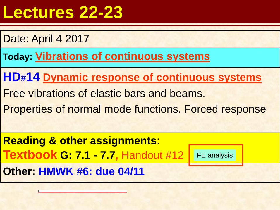
Lectures 22-23 Date: April 4 2017 Today: Vibrations of continuous systems HD#14 Dynamic response of continuous systems Free vibrations of elastic bars and beams. Properties of normal mode functions. Forced response Reading & other assignments: Textbook G: 7.1 - 7.7, Handout #12 Other: HMWK #6: due 04/11 FE analysis
Transcript of From your textbook - TRIBGROUP TAMUrotorlab.tamu.edu/me617/HD14 Vibrations of bars and beams.pdf ·...
Lectures 22-23Date: April 4 2017Today: Vibrations of continuous systems
HD#14 Dynamic response of continuous systemsFree vibrations of elastic bars and beams.Properties of normal mode functions. Forced response
Reading & other assignments: Textbook G: 7.1 - 7.7, Handout #12Other: HMWK #6: due 04/11
FE analysis
l-sanandres
Text Box
Handout 6 - Numerical integration (non linear systems)
2
Recommended problems –
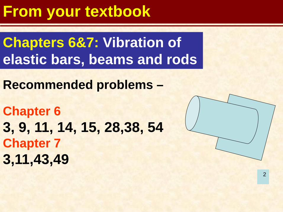
Chapter 63, 9, 11, 14, 15, 28,38, 54Chapter 73,11,43,49
Chapters 6&7: Vibration of elastic bars, beams and rods
From your textbook
l-sanandres
Rectangle
l-sanandres
Rectangle
l-sanandres
Text Box
important
MEEN 617 – HD#14 Vibrations of Continuous Systems. L. San Andrés © 2008 1
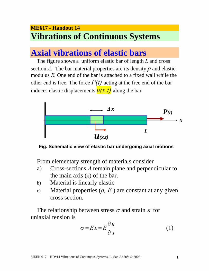
ME617 - Handout 14
Vibrations of Continuous Systems
Axial vibrations of elastic bars The figure shows a uniform elastic bar of length L and cross
section A. The bar material properties are its density ρ and elastic modulus E. One end of the bar is attached to a fixed wall while the other end is free. The force P(t) acting at the free end of the bar induces elastic displacements u(x,t) along the bar
xP(t)
u(x,t)
Δ x
L
Fig. Schematic view of elastic bar undergoing axial motions From elementary strength of materials consider a) Cross-sections A remain plane and perpendicular to
the main axis (x) of the bar. b) Material is linearly elastic c) Material properties (ρ, E ) are constant at any given
cross section. The relationship between stress σ and strain ε for
uniaxial tension is uE Ex
σ ε ∂= =
∂ (1)
l-sanandres
Rectangle
MEEN 617 – HD#14 Vibrations of Continuous Systems. L. San Andrés © 2008 2
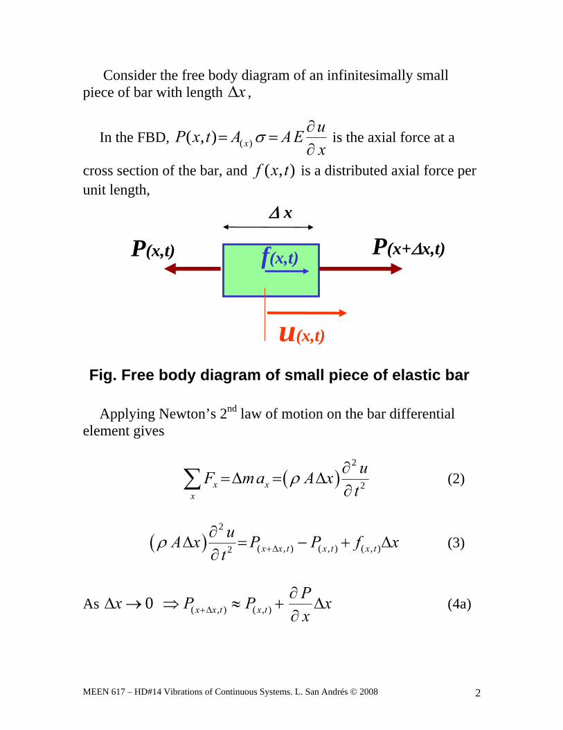
Consider the free body diagram of an infinitesimally small piece of bar with length xΔ ,
In the FBD, ( )( , ) xuP x t A AEx
σ ∂= =
∂ is the axial force at a
cross section of the bar, and ( , )f x t is a distributed axial force per unit length,
u(x,t)
Δ x
P(x+Δx,t)P(x,t) f(x,t)
Fig. Free body diagram of small piece of elastic bar Applying Newton’s 2nd law of motion on the bar differential
element gives
( )2
2x xx
uF ma A xt
ρ ∂=Δ = Δ
∂∑ (2)
( )2
( , ) ( , ) ( , )2 x x t x t x tuA x P P f x
tρ +Δ
∂Δ = − + Δ
∂ (3)
As ( , ) ( , )0 x x t x tPx P P xx+Δ
∂Δ → ⇒ ≈ + Δ
∂ (4a)
MEEN 617 – HD#14 Vibrations of Continuous Systems. L. San Andrés © 2008 3
( )2
( , )2 x tu PA x x f x
t xρ ∂ ∂
Δ = Δ + Δ∂ ∂
2
( , )2 x tu PA f
t xρ ∂ ∂
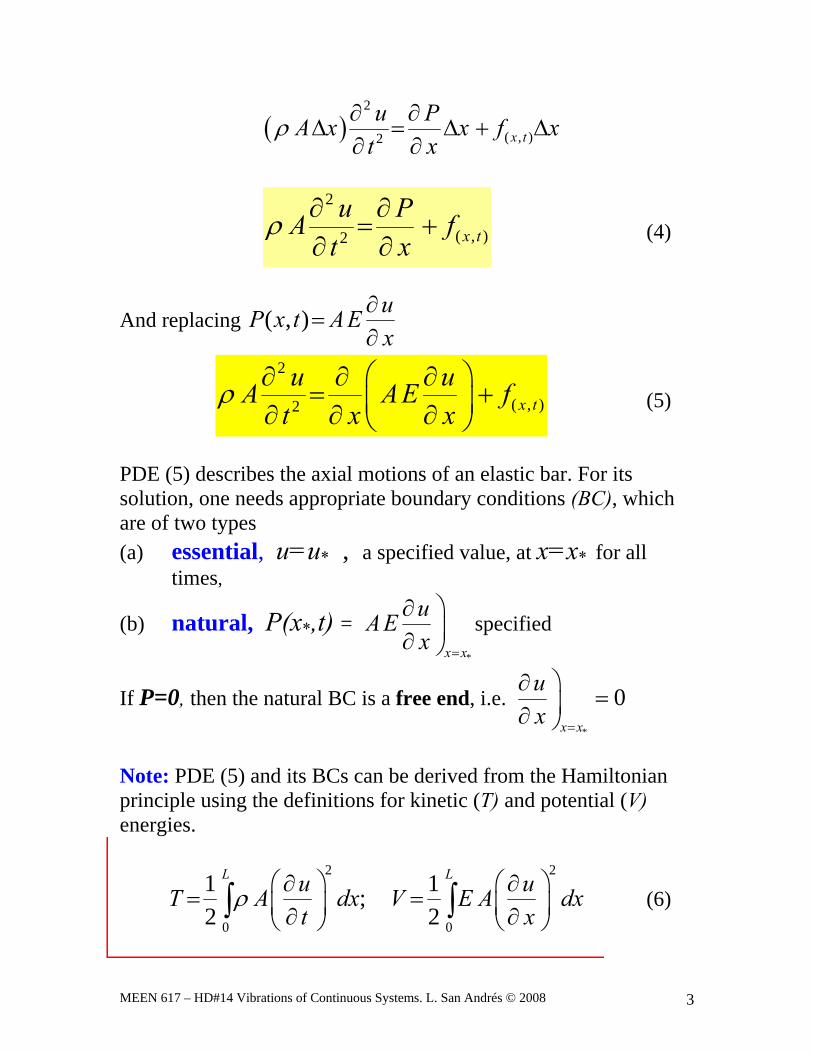
= +∂ ∂ (4)
And replacing ( , ) uP x t AEx
∂=
∂
2
( , )2 x tu uA AE f
t x xρ ⎛ ⎞∂ ∂ ∂
= +⎜ ⎟∂ ∂ ∂⎝ ⎠ (5)
PDE (5) describes the axial motions of an elastic bar. For its solution, one needs appropriate boundary conditions (BC), which are of two types (a) essential, u=u* , a specified value, at x=x* for all
times,
(b) natural, P(x*,t) = *x x
uAEx =
⎞∂⎟∂ ⎠
specified
If P=0, then the natural BC is a free end, i.e. *
0x x
ux =
⎞∂=⎟∂ ⎠
Note: PDE (5) and its BCs can be derived from the Hamiltonian principle using the definitions for kinetic (T) and potential (V) energies.
2 2
0 0
1 1;2 2
L Lu uT A dx V E A dxt x
ρ ⎛ ⎞ ⎛ ⎞∂ ∂= =⎜ ⎟ ⎜ ⎟∂ ∂⎝ ⎠ ⎝ ⎠
∫ ∫ (6)
l-sanandres
Rectangle
l-sanandres
Rectangle
l-sanandres
Callout
recommended exercise (bonus) +5 to exam 2
MEEN 617 – HD#14 Vibrations of Continuous Systems. L. San Andrés © 2008 4
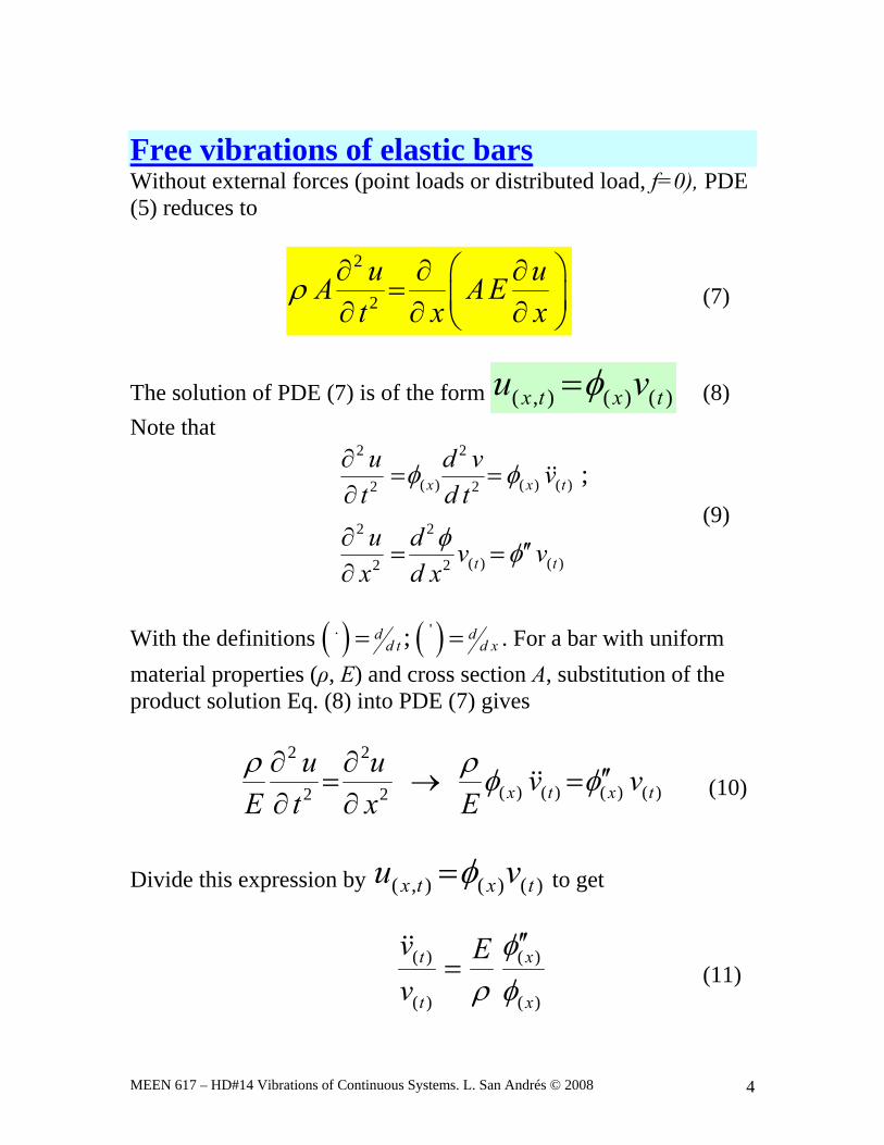
Free vibrations of elastic bars Without external forces (point loads or distributed load, f=0), PDE (5) reduces to
2
2u uA AE
t x xρ ⎛ ⎞∂ ∂ ∂
= ⎜ ⎟∂ ∂ ∂⎝ ⎠ (7)
The solution of PDE (7) is of the form ( , ) ( ) ( )x t x tu vφ= (8) Note that
2 2
( ) ( ) ( )2 2
2 2
( ) ( )2 2
;x x t
t t
u d v vt d tu d v v
x d x
φ φ
φ φ
∂= =
∂
∂ ′′= =∂
(9)
With the definitions ( ) ( ). ';d d
d t d x= = . For a bar with uniform material properties (ρ, E) and cross section A, substitution of the product solution Eq. (8) into PDE (7) gives
2 2
( ) ( ) ( ) ( )2 2 x t x tu u v v
E t x Eρ ρ φ φ∂ ∂ ′′= → =
∂ ∂ (10)
Divide this expression by ( , ) ( ) ( )x t x tu vφ= to get
( ) ( )
( ) ( )
t x
t x
v Ev
φρ φ
′′= (11)
lsanandres
Callout
METHOD: Separation of variables
MEEN 617 – HD#14 Vibrations of Continuous Systems. L. San Andrés © 2008 5
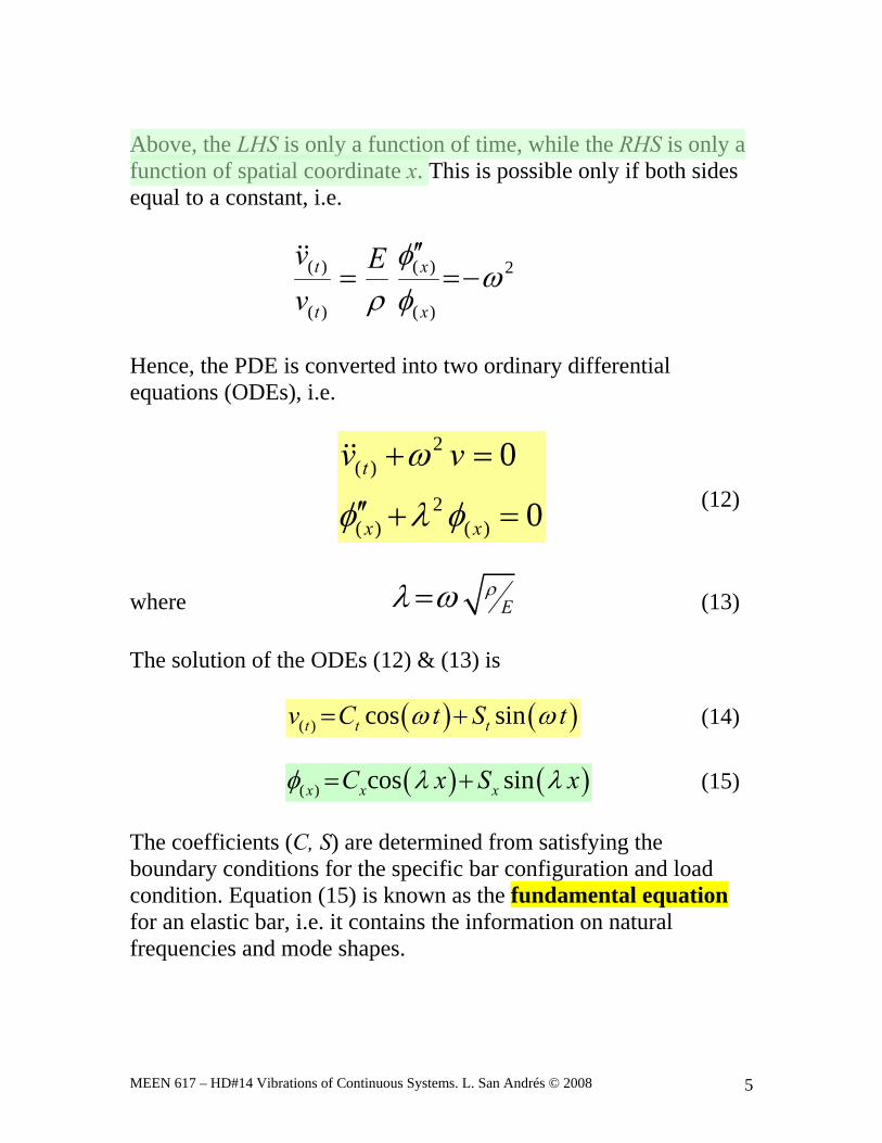
Above, the LHS is only a function of time, while the RHS is only a function of spatial coordinate x. This is possible only if both sides equal to a constant, i.e.
( ) ( ) 2
( ) ( )
t x
t x
v Ev
φω
ρ φ′′
= =−
Hence, the PDE is converted into two ordinary differential equations (ODEs), i.e.
2( )
2( ) ( )
0
0t
x x
v vω
φ λ φ
+ =
′′ + = (12)
where Eρλ ω= (13)
The solution of the ODEs (12) & (13) is
( ) ( )( ) cos sint t tv C t S tω ω= + (14)
( ) ( )( ) cos sinx x xC x S xφ λ λ= + (15) The coefficients (C, S) are determined from satisfying the boundary conditions for the specific bar configuration and load condition. Equation (15) is known as the fundamental equation for an elastic bar, i.e. it contains the information on natural frequencies and mode shapes.
lsanandres
Highlight
lsanandres
Rectangle
MEEN 617 – HD#14 Vibrations of Continuous Systems. L. San Andrés © 2008 6
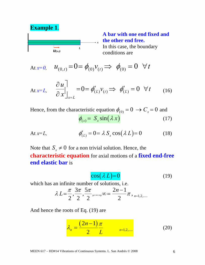
Example 1. A bar with one end fixed and the other end free. In this case, the boundary conditions are
At x=0, (0, ) (0) ( ) (0)0 0t tu v tφ φ= = ⇒ = ∀
At x=L, ( ) ( ) ( )0 0L t Lx L
u v tx
φ φ=
⎤∂ ′ ′= = ⇒ = ∀⎥∂ ⎦ (16)
Hence, from the characteristic equation (0) 0 0xCφ = → = and
( )( ) sinx xS xφ λ= (17) At x=L, ( )( ) 0 cos 0L xS Lφ λ λ′ = = = (18) Note that 0xS ≠ for a non trivial solution. Hence, the characteristic equation for axial motions of a fixed end-free end elastic bar is
( )cos 0Lλ = (19) which has an infinite number of solutions, i.e.
1,2,.....3 5 2 1, , ,...., ,
2 2 2 2 nnL π π πλ π =
−= ∞ =
And hence the roots of Eq. (19) are
( )1,2,.....
2 12n n
nLπλ =
−= (20)
x
u(x,t)L
lsanandres
Rectangle
lsanandres
Callout
for all times
lsanandres
Rectangle
l-sanandres
Rectangle
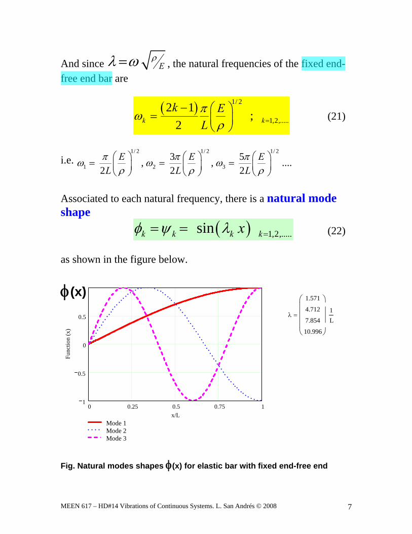
MEEN 617 – HD#14 Vibrations of Continuous Systems. L. San Andrés © 2008 7
And since Eρλ ω= , the natural frequencies of the fixed end-
free end bar are
( ) 1/ 2
1,2,.....2 1
;2k k
k ELπω
ρ =
− ⎛ ⎞= ⎜ ⎟⎝ ⎠
(21)
i.e. 1/ 2 1/ 2 1/ 2
1 2 33 5, , ....
2 2 2E E E
L L Lπ π πω ω ω
ρ ρ ρ⎛ ⎞ ⎛ ⎞ ⎛ ⎞= = =⎜ ⎟ ⎜ ⎟ ⎜ ⎟⎝ ⎠ ⎝ ⎠ ⎝ ⎠
Associated to each natural frequency, there is a natural mode shape
( ) 1,2,.....sink k k kxφ ψ λ == = (22) as shown in the figure below.
0 0.25 0.5 0.75 11
0.5
0
0.5
1
Mode 1Mode 2Mode 3
x/L
Func
tion
(x)
φ(x)λ
1.571
4.712
7.854
10.996
⎛⎜⎜⎜⎜⎝
⎞⎟⎟⎟⎟⎠
=1L
Fig. Natural modes shapes φ(x) for elastic bar with fixed end-free end
lsanandres
Line
lsanandres
Line
lsanandres
Line
l-sanandres
Highlight
l-sanandres
Line

MEEN 617 – HD#14 Vibrations of Continuous Systems. L. San Andrés © 2008 8
See more examples on page 13-ff.
The displacement function response ( , ) ( ) ( )x t x tu vφ= equals to the superposition of all the found responses, i.e.
( ) ( )
( )
( , )
( )1
cos( ) sink
x t k kk
x k k k kk
u x v t
C t S t
φ
φ ω ω∞
=
= =
+⎡ ⎤⎣ ⎦
∑
∑ (23a)
For example 1 (fixed end –free end bar)
( ) ( )( , )1sin cos( ) sinx t k k k k k
ku x C t S tλ ω ω
∞
=
= +⎡ ⎤⎣ ⎦∑ (23b)
and velocity:
( ) ( )( , )1sin sin( ) cosx t k k k k k k
ku x C t S tλ ω ω ω
∞
=
= − +⎡ ⎤⎣ ⎦∑ (24)
The set of coefficients (Ck, Sk) are determined by satisfying the
initial conditions. That is at time t=0,
( )
( )
( ,0) ( )1
( ,0) ( )1
sin
sin
x x k kk
x x k k kk
u U x C
u U x S
λ
ω λ
∞
=
∞
=
= =
= =
∑
∑ (25)
lsanandres
Rectangle
l-sanandres
Line
MEEN 617 – HD#14 Vibrations of Continuous Systems. L. San Andrés © 2008 9
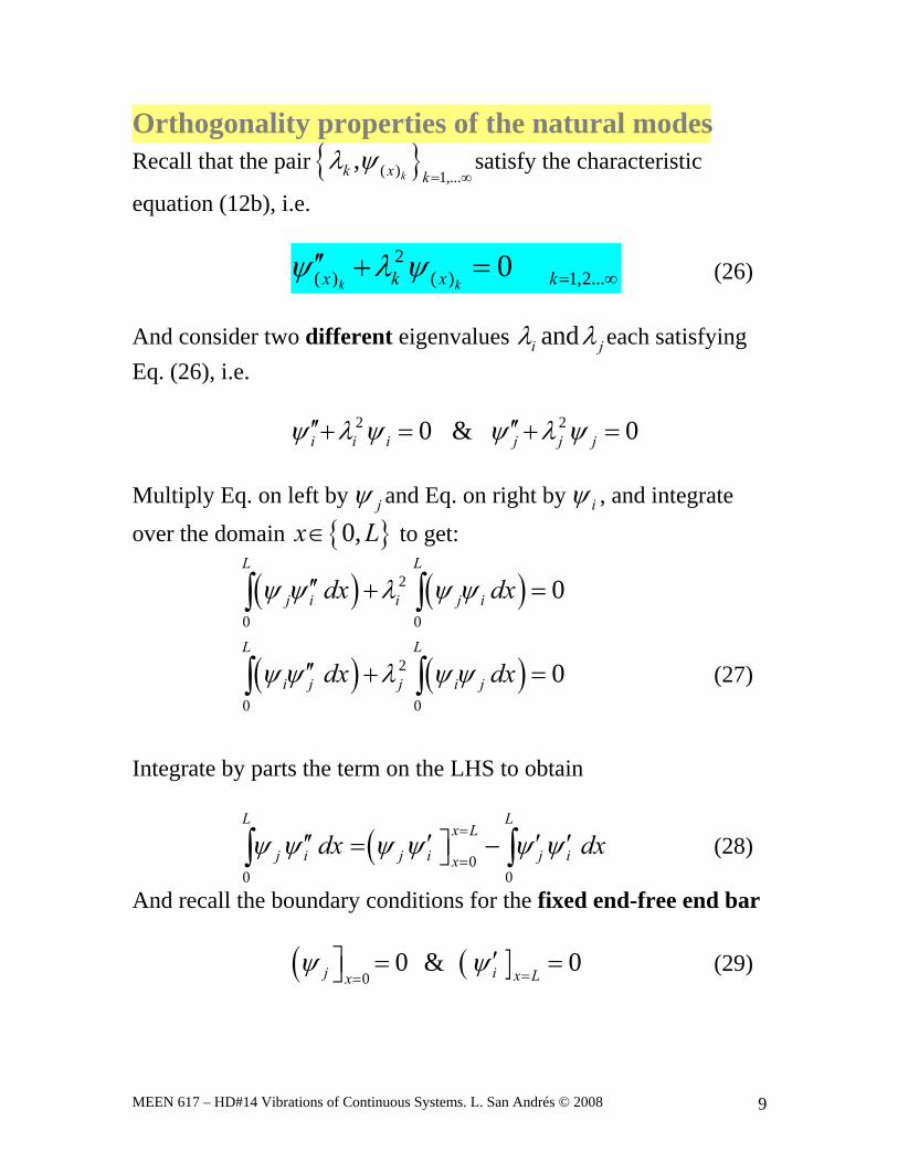
Orthogonality properties of the natural modes Recall that the pair { }( ) 1,...
,kk x k
λ ψ= ∞
satisfy the characteristic
equation (12b), i.e.
2( ) ( ) 1,2...0
k kx k x kψ λ ψ = ∞′′ + = (26) And consider two different eigenvalues andi jλ λ each satisfying Eq. (26), i.e.
2 20 & 0i i i j j jψ λ ψ ψ λ ψ′′ ′′+ = + = Multiply Eq. on left by jψ and Eq. on right by iψ , and integrate over the domain { }0,x L∈ to get:
( ) ( )
( ) ( )
2
0 0
2
0 0
0
0
L L
j i i j i
L L
i j j i j
dx dx
dx dx
ψ ψ λ ψ ψ
ψ ψ λ ψ ψ
′′ + =
′′ + =
∫ ∫
∫ ∫ (27)
Integrate by parts the term on the LHS to obtain
( 00 0
L Lx L
j i j i j ixdx dxψ ψ ψ ψ ψ ψ
=
=′′ ′ ′ ′⎤= −⎦∫ ∫ (28)
And recall the boundary conditions for the fixed end-free end bar
( ( ]0
0 & 0j i x Lxψ ψ
==′⎤ = =⎦ (29)
lsanandres
Rectangle
lsanandres
Highlight
lsanandres
Line
lsanandres
Callout
INT(u dv) = uv - INT (v du)
lsanandres
Line
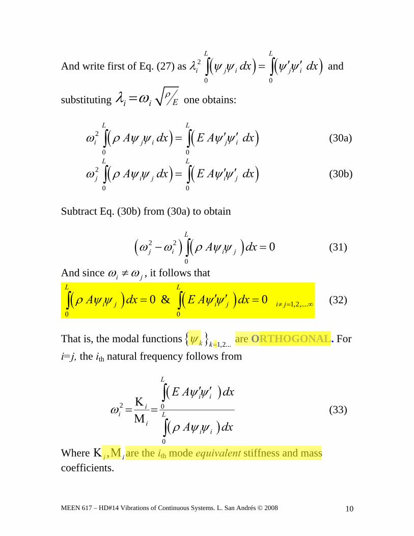
MEEN 617 – HD#14 Vibrations of Continuous Systems. L. San Andrés © 2008 10
And write first of Eq. (27) as ( ) ( )2
0 0
L L
i j i j idx dxλ ψ ψ ψ ψ′ ′=∫ ∫ and
substituting Ei iρλ ω= one obtains:
( ) ( )2
0 0
L L
i j i j iA dx E A dxω ρ ψ ψ ψ ψ′ ′=∫ ∫ (30a)
( ) ( )2
0 0
L L
j i j i jA dx E A dxω ρ ψ ψ ψ ψ′ ′=∫ ∫ (30b)
Subtract Eq. (30b) from (30a) to obtain
( ) ( )2 2
0
0L
j i i jA dxω ω ρ ψ ψ− =∫ (31)
And since i jω ω≠ , it follows that
( ) ( ) 1,2,....0 0
0 & 0L L
i j i j i jA dx E A dxρ ψ ψ ψ ψ ≠ = ∞′ ′= =∫ ∫ (32)
That is, the modal functions { } 1,2...k kψ
= are ORTHOGONAL. For
i=j, the ith natural frequency follows from
( )
( )
2 0
0
L
i ii
i Li
i i
E A dx
A dx
ψ ψω
ρ ψ ψ
′ ′Κ
= =Μ
∫
∫ (33)
Where ,i iΚ Μ are the ith mode equivalent stiffness and mass coefficients.
lsanandres
Highlight
lsanandres
Line
lsanandres
Highlight
lsanandres
Rectangle
lsanandres
Highlight
l-sanandres
Rectangle
MEEN 617 – HD#14 Vibrations of Continuous Systems. L. San Andrés © 2008 11
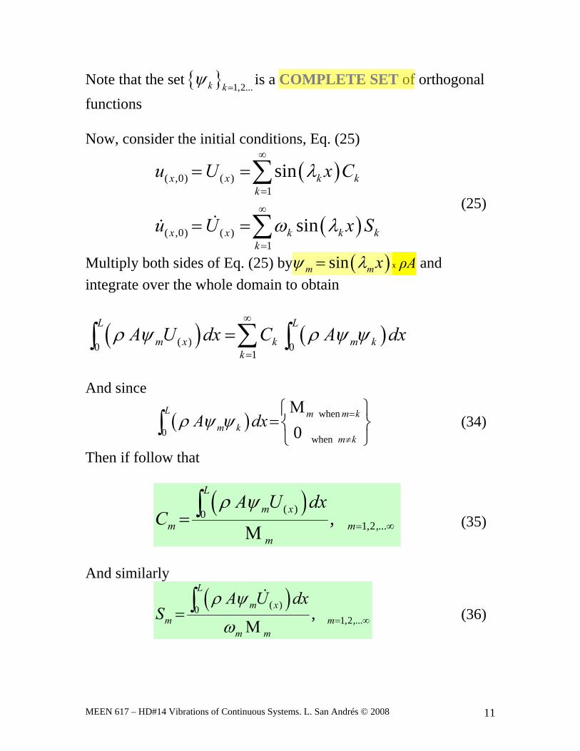
Note that the set { } 1,2...k kψ=
is a COMPLETE SET of orthogonal functions Now, consider the initial conditions, Eq. (25)
( )
( )
( ,0) ( )1
( ,0) ( )1
sin
sin
x x k kk
x x k k kk
u U x C
u U x S
λ
ω λ
∞
=
∞
=
= =
= =
∑
∑ (25)
Multiply both sides of Eq. (25) by ( )sinm mxψ λ= x ρA and integrate over the whole domain to obtain
( ) ( )( )0 01
L L
m x k m kk
A U dx C A dxρ ψ ρ ψ ψ∞
=
=∑∫ ∫
And since
( ) when
0when0
L m m km k
m kA dxρ ψ ψ =
≠
Μ⎧ ⎫=⎨ ⎬
⎩ ⎭∫ (34)
Then if follow that
( )( )01,2,...,
L
m xm m
m
A U dxC
ρ ψ= ∞=
Μ∫
(35)
And similarly
( )( )01,2,...,
L
m xm m
m m
A U dxS
ρ ψ
ω = ∞=Μ
∫ (36)
lsanandres
Highlight
lsanandres
Rectangle
lsanandres
Oval
lsanandres
Oval
l-sanandres
Line
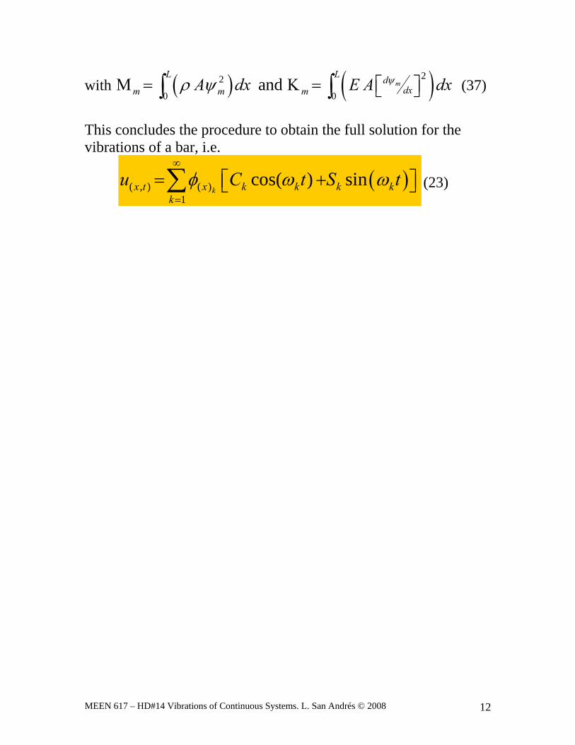
MEEN 617 – HD#14 Vibrations of Continuous Systems. L. San Andrés © 2008 12
with ( ) ( )22
0 0and m
L L ddxm m mA dx E A dxψρ ψΜ = Κ = ⎡ ⎤⎣ ⎦∫ ∫ (37)
This concludes the procedure to obtain the full solution for the vibrations of a bar, i.e.
( )( , ) ( )1
cos( ) sinkx t x k k k k
ku C t S tφ ω ω
∞
=
= +⎡ ⎤⎣ ⎦∑ (23)
MEEN 617 – HD#14 Vibrations of Continuous Systems. L. San Andrés © 2008 13
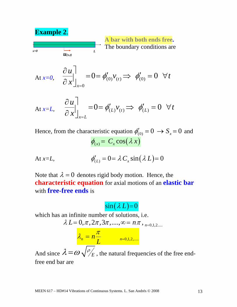
Example 2. A bar with both ends free. The boundary conditions are
At x=0, (0) ( ) (0)0
0 0t
x
uv t
x
At x=L, ( ) ( ) ( )0 0L t L
x L
uv t
x
Hence, from the characteristic equation (0) 0 0xS and
( ) cosx xC x At x=L, ( ) 0 sin 0L xC L Note that 0 denotes rigid body motion. Hence, the characteristic equation for axial motions of an elastic bar with free-free ends is
sin 0L which has an infinite number of solutions, i.e.
0,1,2.....0, ,2 ,3 ,...., , nL n
0,1,2,.....n nnL
And since E , the natural frequencies of the free end-
free end bar are
x=0 Lu(x,t)
lsanandres
Rectangle
lsanandres
Highlight
lsanandres
Highlight
lsanandres
Rectangle
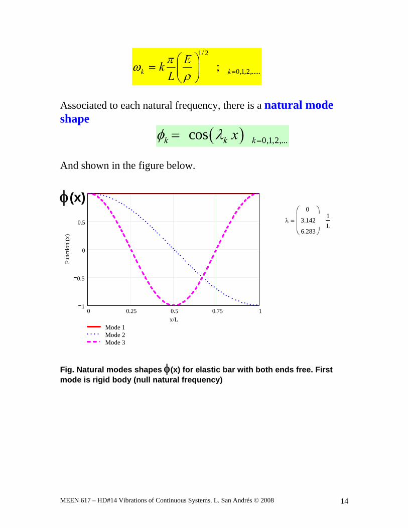
MEEN 617 – HD#14 Vibrations of Continuous Systems. L. San Andrés © 2008 14
1/ 2
0,1,2,.....;k kEk
Lπω
ρ =⎛ ⎞= ⎜ ⎟⎝ ⎠
Associated to each natural frequency, there is a natural mode shape
( ) 0,1,2,...cosk k kxφ λ == And shown in the figure below.
0 0.25 0.5 0.75 11
0.5
0
0.5
1
Mode 1Mode 2Mode 3
x/L
Func
tion
(x)
φ(x)λ
0
3.142
6.283
⎛⎜⎜⎝
⎞⎟⎟⎠
=1L
Fig. Natural modes shapes φ(x) for elastic bar with both ends free. First mode is rigid body (null natural frequency)
lsanandres
Line
lsanandres
Line
lsanandres
Line
l-sanandres
Line
MEEN 617 – HD#14 Vibrations of Continuous Systems. L. San Andrés © 2008 15
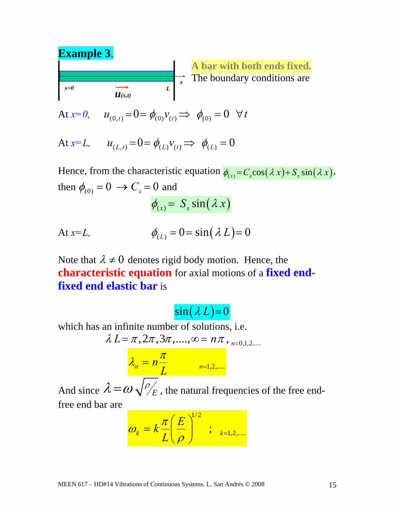
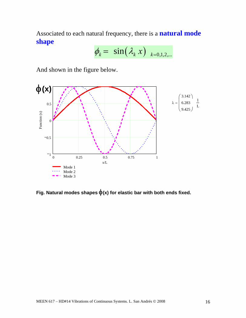
Example 3. A bar with both ends fixed. The boundary conditions are
At x=0, (0, ) (0) ( ) (0)0 0t tu v tφ φ= = ⇒ = ∀ At x=L, ( , ) ( ) ( ) ( )0 0L t L t Lu vφ φ= = ⇒ = Hence, from the characteristic equation ( ) ( )( ) cos sinx x xC x S xφ λ λ= + , then (0) 0 0xCφ = → = and
( )( ) sinx xS xφ λ= At x=L, ( )( ) 0 sin 0L Lφ λ= = = Note that 0λ ≠ denotes rigid body motion. Hence, the characteristic equation for axial motions of a fixed end-fixed end elastic bar is
( )sin 0Lλ = which has an infinite number of solutions, i.e.
0,1,2.....,2 ,3 ,...., , nL nλ π π π π == ∞=
1,2,.....n nnLπλ ==
And since Eρλ ω= , the natural frequencies of the free end-
free end bar are 1/ 2
1,2,.....;k kEk
Lπω
ρ =⎛ ⎞= ⎜ ⎟⎝ ⎠
x=0 Lu(x,t)
x
lsanandres
Highlight
lsanandres
Rectangle
MEEN 617 – HD#14 Vibrations of Continuous Systems. L. San Andrés © 2008 16
Associated to each natural frequency, there is a natural mode shape
( ) 0,1,2,...sink k kxφ λ == And shown in the figure below.
0 0.25 0.5 0.75 11
0.5
0
0.5
1
Mode 1Mode 2Mode 3
x/L
Func
tion
(x)
φ(x)λ
3.142
6.283
9.425
⎛⎜⎜⎝
⎞⎟⎟⎠
=1L
Fig. Natural modes shapes φ(x) for elastic bar with both ends fixed.
lsanandres
Line
lsanandres
Line
lsanandres
Line
l-sanandres
Line
MEEN 617 – HD#14 Vibrations of Continuous Systems. L. San Andrés © 2012 17
ME617 - Handout 14 (b)
Vibrations of Continuous Systems
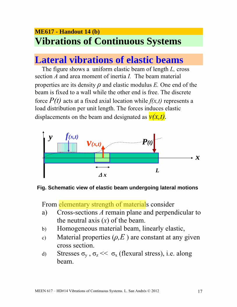
Lateral vibrations of elastic beams The figure shows a uniform elastic beam of length L, cross
section A and area moment of inertia I. The beam material properties are its density ρ and elastic modulus E. One end of the beam is fixed to a wall while the other end is free. The discrete
force P(t) acts at a fixed axial location while f(x,t) represents a load distribution per unit length. The forces induces elastic
displacements on the beam and designated as v(x,t).
x
P(t)v(x,t)
xL
Fig. Schematic view of elastic beam undergoing lateral motions
y f(x,t)
From elementary strength of materials consider a) Cross-sections A remain plane and perpendicular to
the neutral axis (x) of the beam. b) Homogeneous material beam, linearly elastic, c) Material properties (ρ,E ) are constant at any given
cross section. d) Stresses σy , σz << σx (flexural stress), i.e. along
beam.
lsanandres
Rectangle
lsanandres
Highlight
MEEN 617 – HD#14 Vibrations of Continuous Systems. L. San Andrés © 2012 18
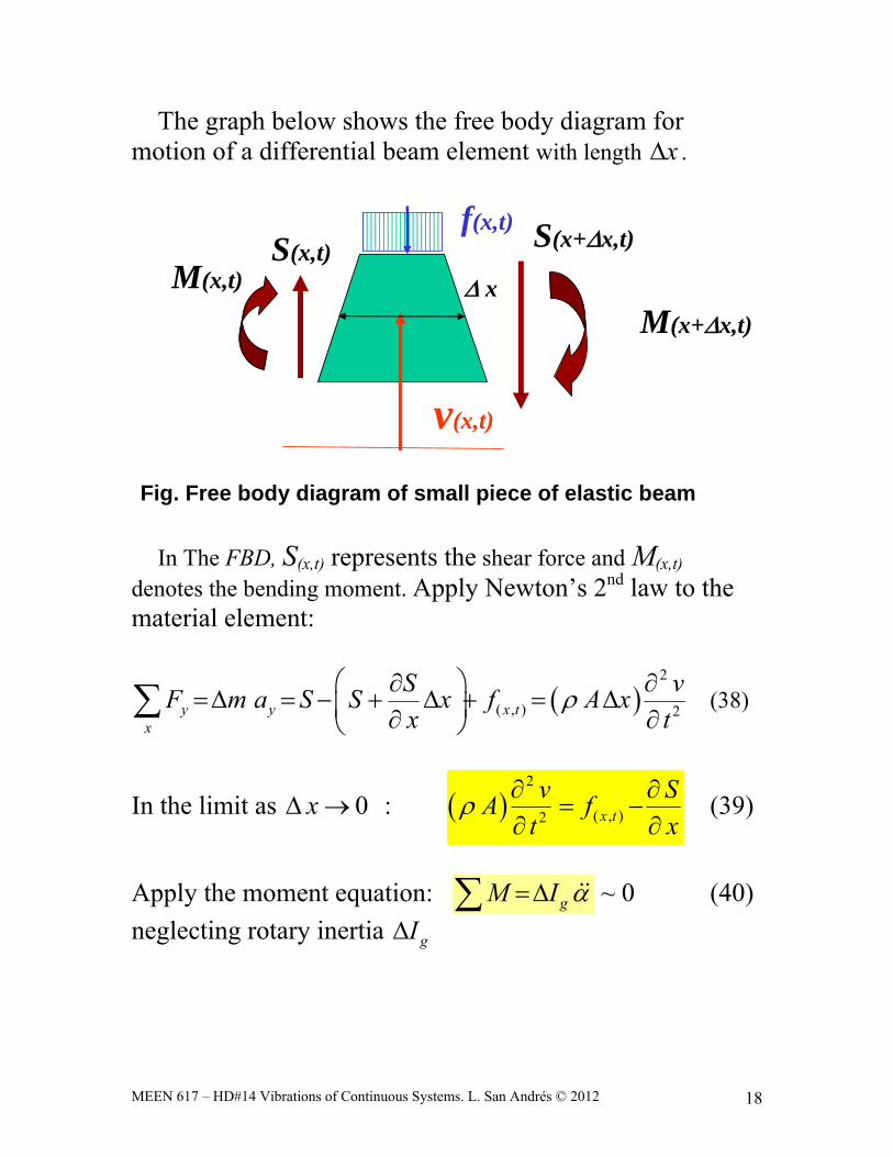
The graph below shows the free body diagram for motion of a differential beam element with length x .
v(x,t)
x
S(x+x,t)S(x,t)f(x,t)
Fig. Free body diagram of small piece of elastic beam
M(x,t)
M(x+x,t)
In The FBD, S(x,t) represents the shear force and M(x,t) denotes the bending moment. Apply Newton’s 2nd law to the material element:
2
( , ) 2y y x tx
S vF m a S S x f A xx t
(38)
In the limit as 0x : 2
( , )2 x tv SA f
t x
(39)
Apply the moment equation: gM I ~ 0 (40)
neglecting rotary inertia gI
lsanandres
Line
MEEN 617 – HD#14 Vibrations of Continuous Systems. L. San Andrés © 2012 19
Then
2
( , ) ( , )
2
02
2
x x t x txM M M f S x
M xM x M f S xx
In the limit as 0x : ( , )x tM Sx
(41)
Combining Eqs. (41) and (39) gives:
2 2
( , )2 2x tv MA f
t x
(42)
If the slope v
x
remains small, then the beam curvature
is 2
21 v
x
. From Euler’s beam theory:
2
2
E I vM E Ix
(43)
where 2I y dA is the beam area moment of inertia.
Substitute Eq. (43) into (42) to obtain the equation for lateral motions of an elastic beam:
2 2 2
( , )2 2 2x tv vA f E I
t x x
(44)
lsanandres
Rectangle
lsanandres
Highlight
lsanandres
Line
lsanandres
Line
l-sanandres
Text Box
second moment of area (m^4)
l-sanandres
Line
MEEN 617 – HD#14 Vibrations of Continuous Systems. L. San Andrés © 2012 20
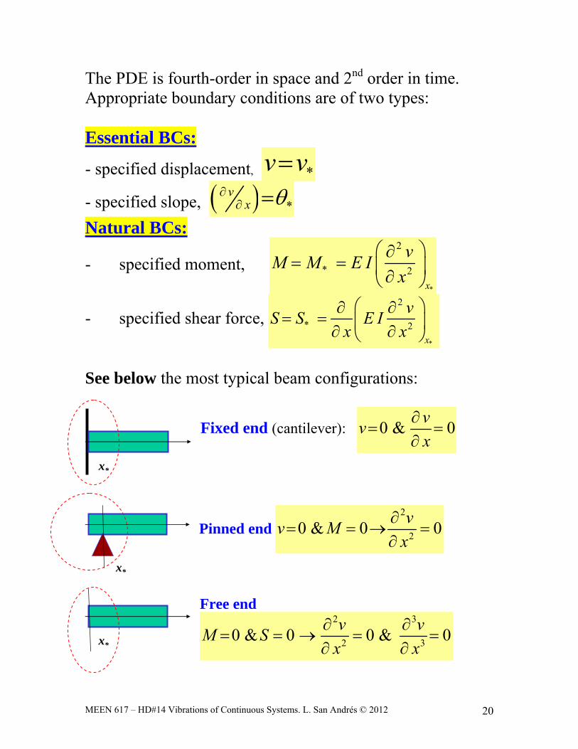
The PDE is fourth-order in space and 2nd order in time. Appropriate boundary conditions are of two types: Essential BCs:
- specified displacement, *v v
- specified slope, *v
x
Natural BCs:
- specified moment,
*
2
* 2
x
vM M E Ix
- specified shear force, *
2
* 2
x
vS S E Ix x
See below the most typical beam configurations:
Fixed end (cantilever): 0 & 0vvx
Pinned end 2
20 & 0 0
vv Mx
Free end
2 3
2 30 & 0 0 & 0
v vM Sx x
x*
x*
x*
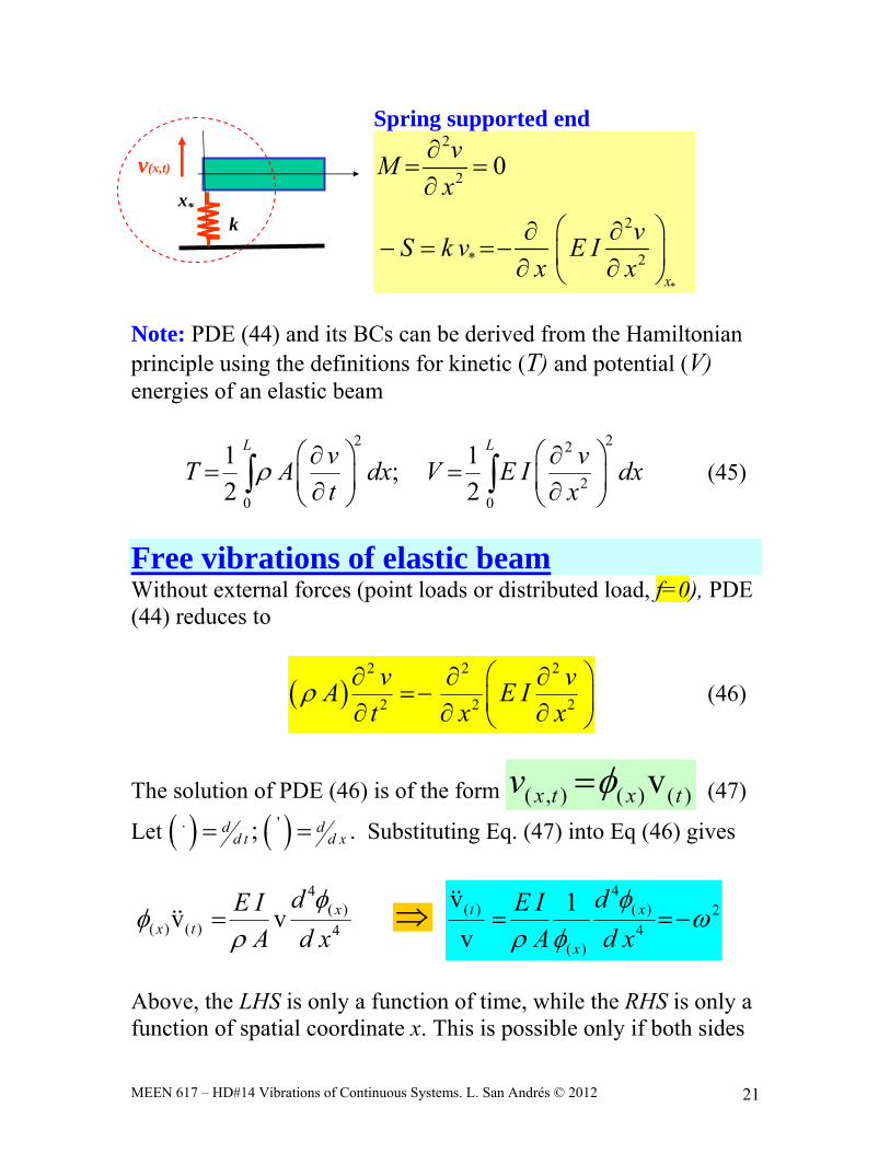
MEEN 617 – HD#14 Vibrations of Continuous Systems. L. San Andrés © 2012 21
Spring supported end
*
2
2
2
* 2
0
x
vMx
vS k v E Ix x
Note: PDE (44) and its BCs can be derived from the Hamiltonian principle using the definitions for kinetic (T) and potential (V) energies of an elastic beam
22 2
20 0
1 1;
2 2
L Lv vT A dx V E I dxt x
(45)
Free vibrations of elastic beam Without external forces (point loads or distributed load, f=0), PDE (44) reduces to
2 2 2
2 2 2
v vA E It x x
(46)
The solution of PDE (46) is of the form ( , ) ( ) ( )vx t x tv (47)
Let . ';d dd t d x . Substituting Eq. (47) into Eq (46) gives
4
( )( ) ( ) 4v v xx t
dE IA d x
4( ) ( ) 2
4( )
v 1
vt x
x
dE IA d x
Above, the LHS is only a function of time, while the RHS is only a function of spatial coordinate x. This is possible only if both sides
k
v(x,t)
x*
lsanandres
Rectangle
lsanandres
Callout
A rewarding intellectual pursuit, Bonus +5 to Exam 2 (by Tuesday 04/11)
lsanandres
Rectangle
MEEN 617 – HD#14 Vibrations of Continuous Systems. L. San Andrés © 2012 22
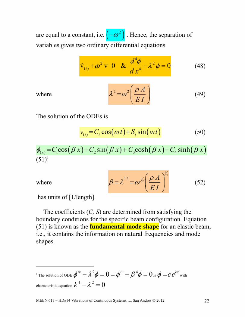
are equal to a constant, i.e. 2 . Hence, the separation of
variables gives two ordinary differential equations
42 2
( ) 4v v=0 & 0tdd x (48)
where 2 2 AE I
(49)
The solution of the ODEs is
( ) cos sint t tv C t S t (50)
( ) 1 2 3 4cos sin cosh sinhx C x C x C x C x
(51)1
where
14
1/2 12
AE I
(52)
has units of [1/length].
The coefficients (C, S) are determined from satisfying the boundary conditions for the specific beam configuration. Equation (51) is known as the fundamental mode shape for an elastic beam, i.e., it contains the information on natural frequencies and mode shapes.
1 The solution of ODE 2 40 0iv iv is
kxce with
characteristic equation 4 2 0k
lsanandres
Rectangle
lsanandres
Rectangle
lsanandres
Rectangle
MEEN 617 – HD#14 Vibrations of Continuous Systems. L. San Andrés © 2012 23
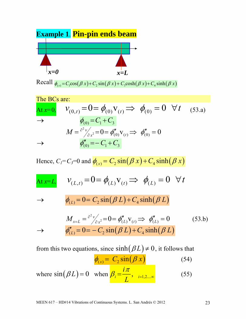
Example 1. Pin-pin ends beam
x=0 x=L
Recall ( ) 1 2 3 4cos sin cosh sinhx C x C x C x C x
The BCs are:
At x=0, (0, ) (0) ( ) (0)0 v 0t tv t (53.a)
(0) 1 3C C
2
2 (0) ( ) (0)0 v 0vtxM
(0) 1 3C C
Hence, C1=C3=0 and ( ) 2 4sin sinhx C x C x
At x=L, ( , ) ( ) ( ) ( )0 v 0L t L t Lv t
( ) 2 40 sin sinhL C L C L
2
2 ( ) ( ) ( )0 v 0vx L L t LxM
(53.b)
( ) 2 40 sin sinhL C L C L
from this two equations, since sinh 0L , it follows that
( ) 2 sinx C x (54)
where sin 0L when 1,2....,i iiL (55)
lsanandres
Callout
for all time
lsanandres
Rectangle
lsanandres
Rectangle
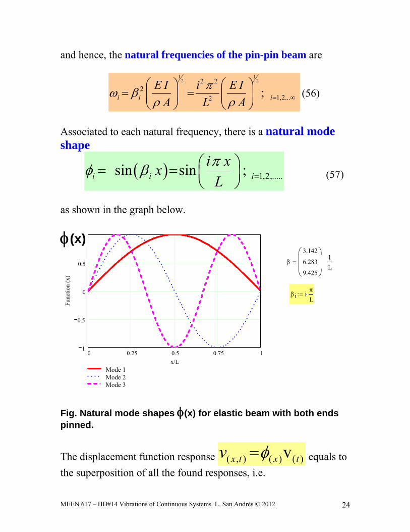
MEEN 617 – HD#14 Vibrations of Continuous Systems. L. San Andrés © 2012 24
and hence, the natural frequencies of the pin-pin beam are
1 12 22 2
21,2...2
;i i iE I i E I
A L A
(56)
Associated to each natural frequency, there is a natural mode shape
1,2,.....sin sin ;i i ii xx
L
(57)
as shown in the graph below.
0 0.25 0.5 0.75 11
0.5
0
0.5
1
Mode 1Mode 2Mode 3
x/L
Fun
ctio
n (x
)
(x)
3.142
6.283
9.425
1
L
i i
L
Fig. Natural mode shapes (x) for elastic beam with both ends pinned.
The displacement function response ( , ) ( ) ( )vx t x tv equals to
the superposition of all the found responses, i.e.
lsanandres
Line
lsanandres
Line
lsanandres
Line
l-sanandres
Line
l-sanandres
Line
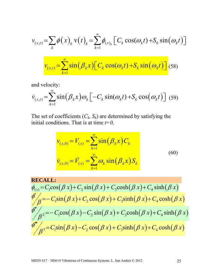
MEEN 617 – HD#14 Vibrations of Continuous Systems. L. San Andrés © 2012 25
( , ) ( )1
v cos( ) sinkx t x k k k kk k
k kv x t C t S t
( , )1
sin cos( ) sinx t k k k k kk
v x C t S t
(58)
and velocity:
( , )1
sin sin( ) cosx t k k k k k kk
v x C t S t
(59)
The set of coefficients (Ck, Sk) are determined by satisfying the initial conditions. That is at time t=0,
( ,0) ( )1
( ,0) ( )1
sin
sin
x x k kk
x x k k kk
v V x C
v V x S
(60)
RECALL:
( ) 1 2 3 4cos sin cosh sinhx C x C x C x C x
1 2 3 4sin cos sinh coshC x C x C x C x
2 1 2 3 4cos sin cosh sinhC x C x C x C x
3 1 2 3 4sin cos sinh coshC x C x C x C x
lsanandres
Rectangle
MEEN 617 – HD#14 Vibrations of Continuous Systems. L. San Andrés © 2012 26
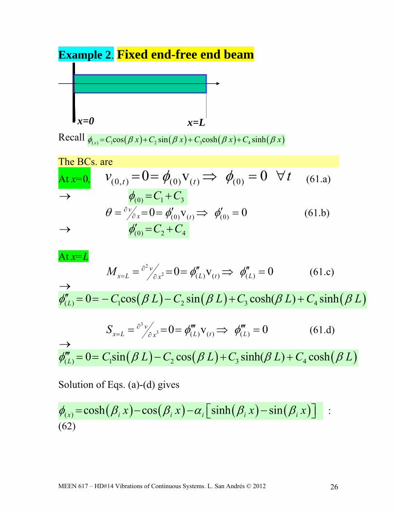
Example 2. Fixed end-free end beam
x=0 x=L
Recall ( ) 1 2 3 4cos sin cosh sinhx C x C x C x C x
The BCs. are
At x=0, (0, ) (0) ( ) (0)0 v 0t tv t (61.a)
(0) 1 3C C
(0) ( ) (0)0 v 0vx t
(61.b) (0) 2 4C C
At x=L
2
2 ( ) ( ) ( )0 v 0vx L L t LxM
(61.c)
( ) 1 2 3 40 cos sin cosh( ) sinhL C L C L C L C L
3
3 ( ) ( ) ( )0 v 0vx L L t LxS
(61.d)
( ) 1 2 3 40 sin cos sinh( ) coshL C L C L C L C L Solution of Eqs. (a)-(d) gives
( ) cosh cos sinh sinx i i i i ix x x x :
(62)
lsanandres
Rectangle
lsanandres
Rectangle
MEEN 617 – HD#14 Vibrations of Continuous Systems. L. San Andrés © 2012 27
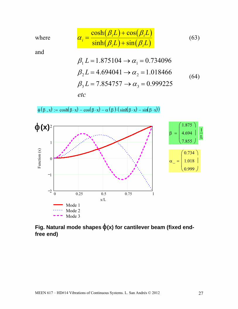
where
cosh cos
sinh sini i
ii i
L LL L
(63)
and
1 1
2 2
3 3
1.875104 0.734096
4.694041 1.018466
7.854757 0.999225
L
L
Letc
(64)
x cosh x cos x sinh x sin x
0 0.25 0.5 0.75 12
1
0
1
2
Mode 1Mode 2Mode 3
x/L
Fun
ctio
n (x
)
(x)
1.875
4.694
7.855
1
L
_
0.734
1.018
0.999
Fig. Natural mode shapes (x) for cantilever beam (fixed end-free end)
lsanandres
Line
lsanandres
Line
lsanandres
Line
l-sanandres
Line
MEEN 617 – HD#14 Vibrations of Continuous Systems. L. San Andrés © 2012 28
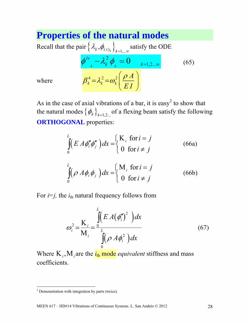
Properties of the natural modes Recall that the pair ( ) 1,...
,kk x k
satisfy the ODE
21,2...0
k k
ivk k (65)
where 4 2 2k k k
AE I
As in the case of axial vibrations of a bar, it is easy2 to show that the natural modes 1,2...k k
of a flexing beam satisfy the following
ORTHOGONAL properties:
0
for
0 for
Li
i j
i jE A dx
i j
(66a)
0
for
0 for
Li
i j
i jA dx
i j
(66b)
For i=j, the ith natural frequency follows from
2
2 0
2
0
L
ii
i Li
i
E A dx
A dx
(67)
Where ,i i are the ith mode equivalent stiffness and mass coefficients.
2 Demonstration with integration by parts (twice).
lsanandres
Rectangle
lsanandres
Line
lsanandres
Rectangle
MEEN 617 – HD#14 Vibrations of Continuous Systems. L. San Andrés © 2012 29
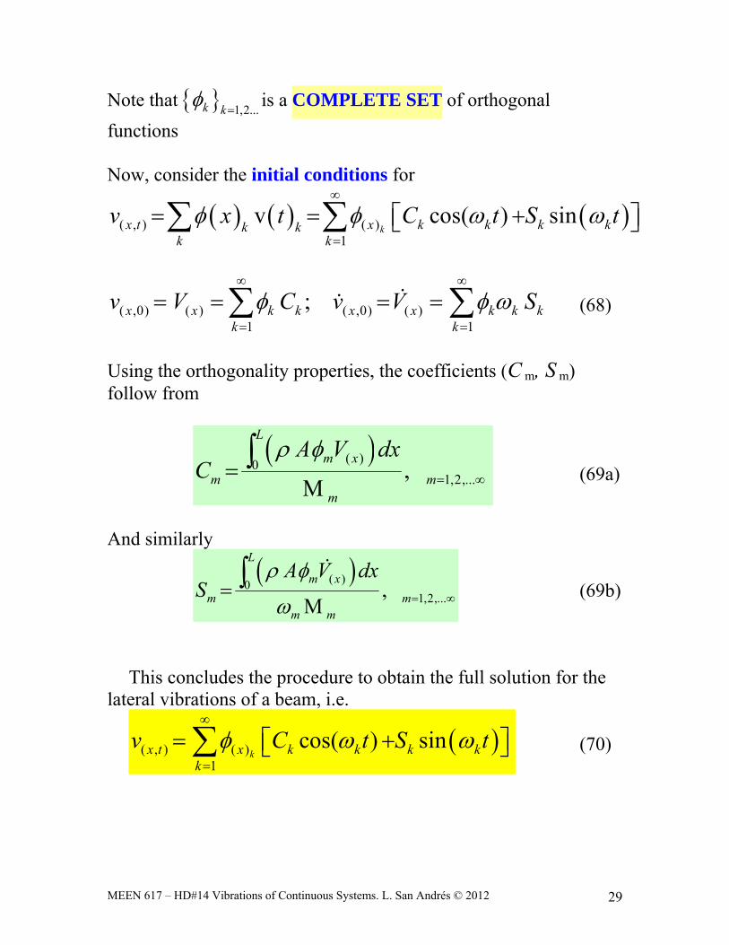
Note that 1,2...k k
is a COMPLETE SET of orthogonal
functions Now, consider the initial conditions for
( , ) ( )1
v cos( ) sinkx t x k k k kk k
k kv x t C t S t
( ,0) ( ) ( ,0) ( )1 1
;x x k k x x k k kk k
v V C v V S
(68)
Using the orthogonality properties, the coefficients (C m, S m)
follow from
( )01,2,...,
L
m xm m
m
A V dxC
(69a)
And similarly
( )01,2,...,
L
m xm m
m m
A V dxS
(69b)
This concludes the procedure to obtain the full solution for the lateral vibrations of a beam, i.e.
( , ) ( )1
cos( ) sinkx t x k k k k
kv C t S t
(70)
MEEN 617 – HD#14 Vibrations of Continuous Systems. L. San Andrés © 2012 30
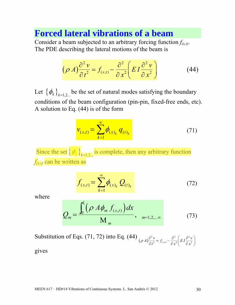
Forced lateral vibrations of a beam Consider a beam subjected to an arbitrary forcing function f(x,t). The PDE describing the lateral motions of the beam is
2 2 2
( , )2 2 2x tv vA f E I
t x x
(44)
Let 1,2...k k
be the set of natural modes satisfying the boundary
conditions of the beam configuration (pin-pin, fixed-free ends, etc). A solution to Eq. (44) is of the form
( , ) ( ) ( )1
k kx t x tk
v q
(71)
Since the set 1,2...k k
is complete, then any arbitrary function
f(x,t) can be written as
( , ) ( ) ( )1
k kx t x tk
f Q
(72)
where
( , )01,2,...,
L
m x tm m
m
A f dxQ
(73)
Substitution of Eqs. (71, 72) into Eq. (44)
2 2 2
( , )2 2 2x tv vA f E I
t x x
gives
lsanandres
Rectangle
lsanandres
Highlight
MEEN 617 – HD#14 Vibrations of Continuous Systems. L. San Andrés © 2012 31
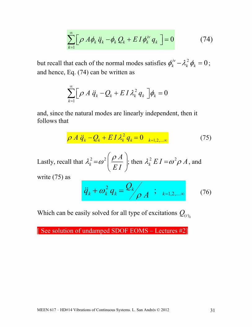
1
0ivk k k k k k
kA q Q E I q
(74)
but recall that each of the normal modes satisfies 2 0ivk k k ;
and hence, Eq. (74) can be written as
2
1
0k k k k kk
A q Q E I q
and, since the natural modes are linearly independent, then it follows that
21,2,....0k k k k kA q Q E I q (75)
Lastly, recall that 2 2k
AE I
; then 2 2
k E I A , and
write (75) as
21,2,....;k
k k k kQq q A (76)
Which can be easily solved for all type of excitations ( )ktQ
[ See solution of undamped SDOF EOMS – Lectures #2]
lsanandres
Rectangle
lsanandres
Rectangle
MEEN 617 – HD#14 Vibrations of Continuous Systems. L. San Andrés © 2012 32
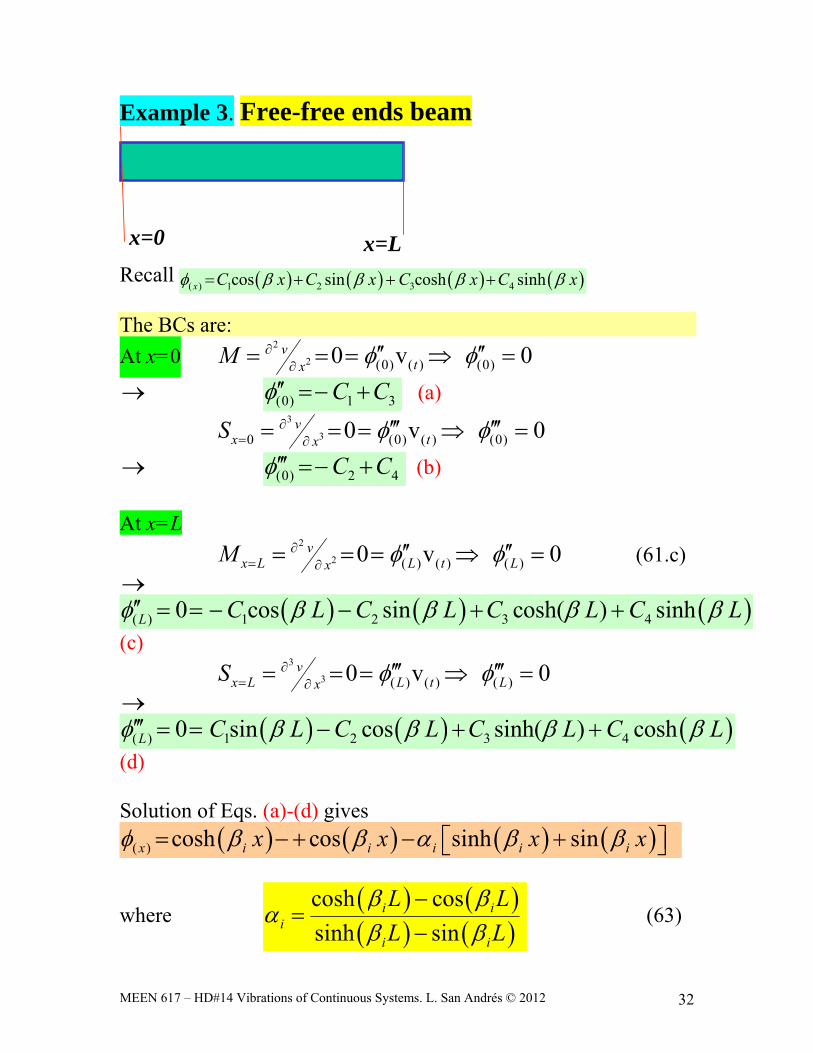
Example 3. Free-free ends beam
x=0 x=L
Recall ( ) 1 2 3 4cos sin cosh sinhx C x C x C x C x
The BCs are:
At x=0 2
2 (0) ( ) (0)0 v 0vtxM
(0) 1 3C C (a)
3
30 (0) ( ) (0)0 v 0vx txS
(0) 2 4C C (b)
At x=L
2
2 ( ) ( ) ( )0 v 0vx L L t LxM
(61.c)
( ) 1 2 3 40 cos sin cosh( ) sinhL C L C L C L C L (c)
3
3 ( ) ( ) ( )0 v 0vx L L t LxS
( ) 1 2 3 40 sin cos sinh( ) coshL C L C L C L C L (d) Solution of Eqs. (a)-(d) gives
( ) cosh cos sinh sinx i i i i ix x x x
where
cosh cos
sinh sini i
ii i
L LL L
(63)
lsanandres
Rectangle
l-sanandres
Line
l-sanandres
Text Box
+
l-sanandres
Line
l-sanandres
Text Box
correction
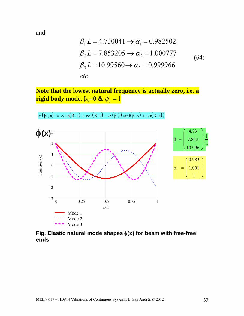
MEEN 617 – HD#14 Vibrations of Continuous Systems. L. San Andrés © 2012 33
and
1 1
2 2
3 3
4.730041 0.982502
7.853205 1.000777
10.99560 0.999966
L
L
Letc
(64)
Note that the lowest natural frequency is actually zero, i.e. a rigid body mode. 0=0 & 0 1 x cosh x cos x sinh x sin x
0 0.25 0.5 0.75 13
2
1
0
1
2
3
Mode 1Mode 2Mode 3
x/L
Fun
ctio
n (x
)
(x)
4.73
7.853
10.996
1
L
_
0.983
1.001
1
Fig. Elastic natural mode shapes (x) for beam with free-free ends
lsanandres
Line
lsanandres
Line
lsanandres
Line
l-sanandres
Line
MEEN 617 – HD#14 Vibrations of Continuous Systems. L. San Andrés © 2012 34
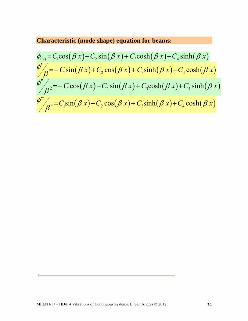
Characteristic (mode shape) equation for beams:
( ) 1 2 3 4cos sin cosh sinhx C x C x C x C x
1 2 3 4sin cos sinh coshC x C x C x C x
2 1 2 3 4cos sin cosh sinhC x C x C x C x
3 1 2 3 4sin cos sinh coshC x C x C x C x
lsanandres
Text Box
Students: The following pages contain five worked examples for prediction of the vibration response of bars, rods, strings, and beams.
lsanandres
Text Box
The solution to the ODEs is simple, i.e.:
v t( ) At cos Ω t⋅( )⋅ Bt sin Ω t⋅( )⋅+=(3)
φ x( ) Ax cos λ x⋅( )⋅ Bx sin λ x⋅( )⋅+=
Satisfy the boundary conditions. At x=0, u(0,t)=0 (fixed end). Thus
φ 0( ) Ax cos λ 0⋅( )⋅ Bx sin λ 0⋅( )⋅+=Then: Ax 0=φ 0( ) Ax 1⋅ Bx 0⋅+=
andφ x( ) sin λ x⋅( )= (4)
At the right end, x=L, the appropriate boundary condition is: axial force = M accel
E− A⋅x
udd⋅ M 2t
ud
d
2⋅= (5a)
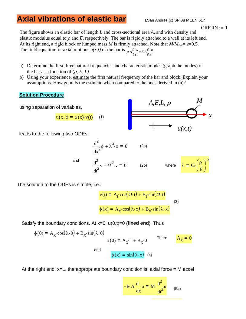
Axial vibrations of elastic bar LSan Andres (c) SP 08 MEEN 617
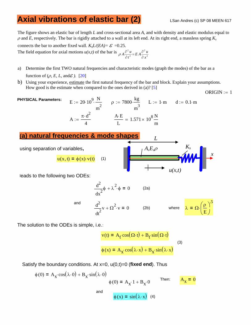
The figure shows an elastic bar of length L and cross-sectional area A, and with density and elastic modulus equal to ρ and E, respectively. The bar is rigidly attached to a wall at its left end. At its right end, a rigid block or lumped mass M is firmly attached. Note that M/Mbar= ε=0.5. The field equation for axial motions u(x,t) of the bar is
2
2
2
2
x
uAE
t
uA
∂∂
=∂∂ρ
a) Determine the first three natural frequencies and characteristic modes (graph the modes) of
the bar as a function of (ρ, E, L). b) Using your experience, estimate the first natural frequency of the bar and block. Explain your
assumptions. How good is the estimate when compared to the ones derived in (a)?
ORIGIN 1:=
M A,E,L, ρ
x
u(x,t)
Solution Procedure
using separation of variables,
u x t,( ) φ x( ) v t( )⋅= (1)
leads to the following two ODEs:
2xφd
d
2λ
2φ⋅+ 0= (2a)
and
2tvd
d
2Ω
2 v⋅+ 0= (2b) where λ ΩρE⎛⎜⎝
⎞⎟⎠
.5⋅=
lsanandres
Rectangle

tan λ⎯( ) 1
ε λ⎯⋅
= (6)
from experience or having worked other problems, using a calculator, ε 0.5:=
f y( ) tan y( )1
y ε⋅−:=n 3:=guess values
y
1
2
6
⎛⎜⎜⎜⎝
⎞⎟⎟⎟⎠
:= # of roots
λ_ root f y( ) y,( )→⎯⎯⎯⎯⎯
:=λ_
1.077
3.643
6.578
⎛⎜⎜⎜⎝
⎞⎟⎟⎟⎠
= where λ_ λ L⋅= & Ω λEρ⎛⎜⎝
⎞⎟⎠
.5⋅=
0 1 2 3 4 5 6 7 8 9 100.1
1
10
100
tan(y)1/(ye)
Graphical solution
tan Y( )
1Y ε⋅
Y
And thus, the first three natural frequencies are
Ω
1.077
3.643
6.578
⎛⎜⎜⎜⎝
⎞⎟⎟⎟⎠
1L⋅
Eρ⎛⎜⎝
⎞⎟⎠
.5⋅=
The shape functions areφ1 z( ) sin λ_1 z⋅( ):=
φ2 z( ) sin λ_2 z⋅( ):= where zxL
=
φ3 z( ) sin λ_3 z⋅( ):=
or: E− A⋅ v⋅xφd
d⋅ M φ⋅ 2t
vd
d
2⋅= . Noting that
2tvd
d
2Ω
2− v⋅= from (2a)
then, at x=LE− A⋅
xφd
d⋅ M− Ω
2⋅ φ L( )⋅= (5b)
recall λ2
Ω2 ρ
E⎛⎜⎝
⎞⎟⎠
⋅= E A⋅xφd
d⋅ M λ
2⋅
Eρ⋅ φ L( )⋅= (5b)--->
Replacing (4) φ x( ) sin λ x⋅( )= &
xφd
dλ cos λ x⋅( )⋅= into (5b) gives
ρ A⋅ L⋅M
cos λ⎯( )⋅ λ
⎯sin λ
⎯( )⋅− 0= where λ⎯
λ L⋅=
define
εM
ρ A⋅ L⋅( )= , and write the characteristic equation as:.
0 0.25 0.5 0.75 11
0
1
Mode 1Mode 2Mode 3
x/L
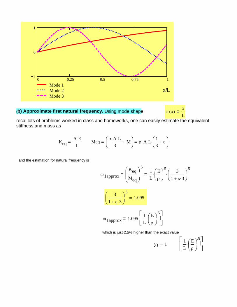
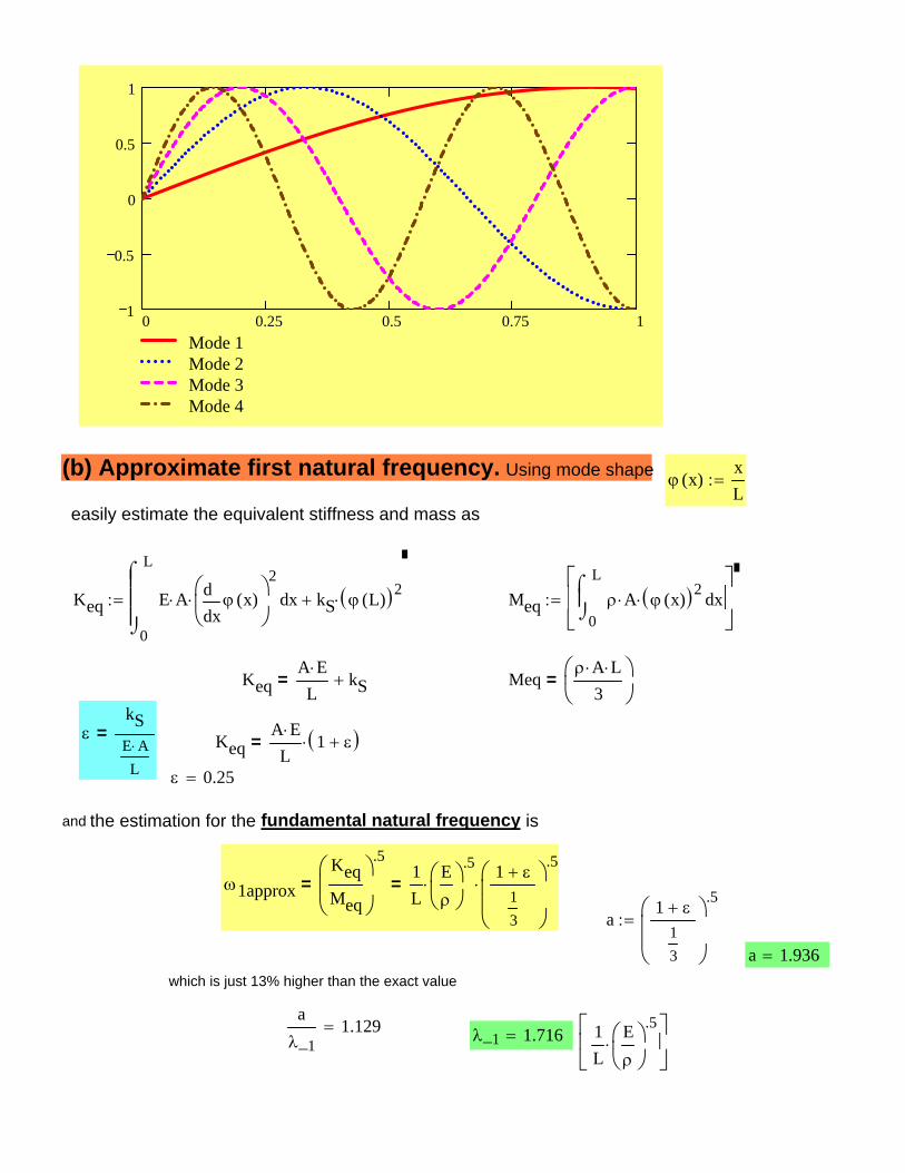
(b) Approximate first natural frequency. Using mode shape ϕ x( )xL
=
recal lots of problems worked in class and homeworks, one can easily estimate the equivalent stiffness and mass as
KeqA E⋅L
= Meqρ A⋅ L⋅
3M+⎛
⎜⎝
⎞⎟⎠
= ρ A⋅ L⋅13
ε+⎛⎜⎝
⎞⎟⎠
⋅=
and the estimation for natural frequency is
ω1approxKeqMeq
⎛⎜⎝
⎞⎟⎠
.5
= 1L
Eρ⎛⎜⎝
⎞⎟⎠
.5⋅
31 ε 3⋅+⎛⎜⎝
⎞⎟⎠
.5⋅=
31 ε 3⋅+⎛⎜⎝
⎞⎟⎠
.51.095=
ω1approx 1.0951L
Eρ⎛⎜⎝
⎞⎟⎠
.5⋅
⎡⎢⎣
⎤⎥⎦
⋅=
which is just 2.5% higher than the exact value
y1 1=1L
Eρ⎛⎜⎝
⎞⎟⎠
.5⋅
⎡⎢⎣
⎤⎥⎦
u x t,( )
1
n
i
sin λ_ixL⋅⎛⎜
⎝⎞⎟⎠
Ai cos Ωi t⋅( )⋅( )⋅∑=
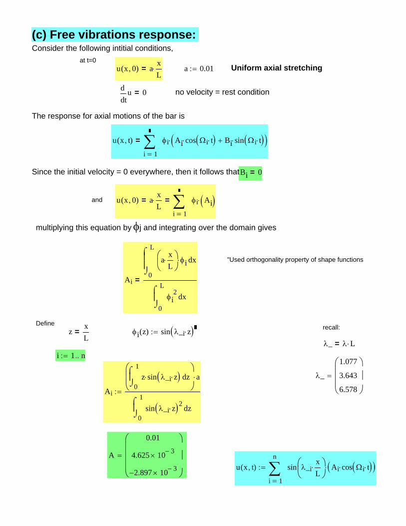
:=A
0.01
4.625 10 3−×
2.897− 10 3−×
⎛⎜⎜⎜⎝
⎞⎟⎟⎟⎠
=
Ai0
1zz sin λ_i z⋅( )⋅
⌠⎮⌡
d⎛⎜⎜⎝
⎞⎟⎟⎠
a⋅
0
1
zsin λ_i z⋅( )2⌠⎮⌡
d
:=
λ_
1.077
3.643
6.578
⎛⎜⎜⎜⎝
⎞⎟⎟⎟⎠
=
i 1 n..:=λ_ λ L⋅=
φi z( ) sin λ_i z⋅( ):=zxL
= recall:Define
Ai0
L
xaxL⋅⎛⎜
⎝⎞⎟⎠φi⋅
⌠⎮⎮⌡
d
0
L
xφi2⌠
⎮⌡
d
=
"Used orthogonality property of shape functions
multiplying this equation by φj and integrating over the domain gives
u x 0,( ) axL⋅=
1i
φi Ai( )⋅∑=
=and
Bi 0=Since the initial velocity = 0 everywhere, then it follows that
u x t,( )
1i
φi Ai cos Ωi t⋅( )⋅ Bi sin Ωi t⋅( )⋅+( )⋅∑=
=
The response for axial motions of the bar is
no velocity = rest conditiontud
d0=
Uniform axial stretchinga 0.01:=u x 0,( ) axL⋅=
at t=0
Consider the following intitial conditions, (c) Free vibrations response:
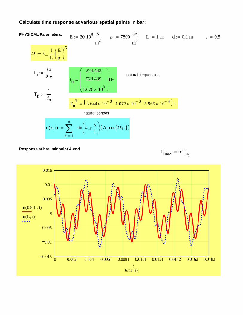
0 0.002 0.004 0.0061 0.0081 0.0101 0.0121 0.0142 0.0162 0.01820.015
0.01
0.005
0
0.005
0.01
0.015
time (s)
u 0.5 L⋅ t,( )
u L t,( )
t
Tmax 5 Tn1⋅:=Response at bar: midpoint & end
u x t,( )
1
n
i
sin λ_ixL⋅⎛⎜
⎝⎞⎟⎠
Ai cos Ωi t⋅( )⋅( )⋅∑=
:=
natural periods
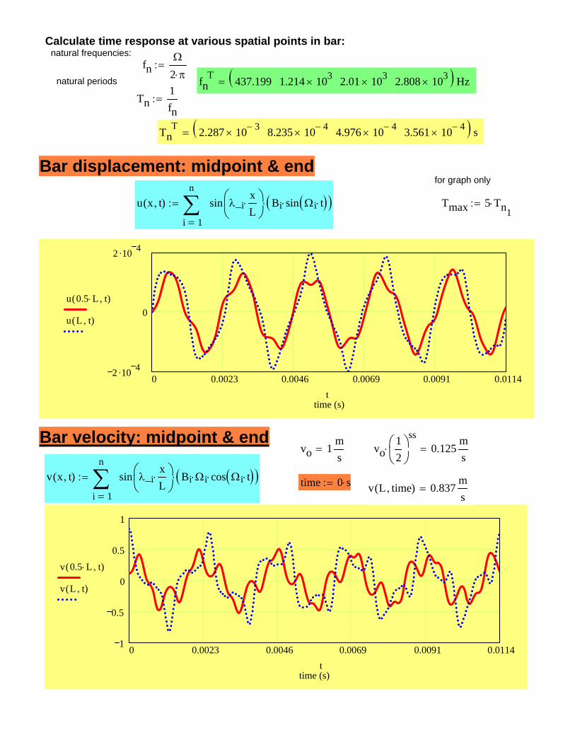
TnT 3.644 10 3−× 1.077 10 3−× 5.965 10 4−×( ) s=
Tn1fn
:=
fn
274.443
928.439
1.676 103×
⎛⎜⎜⎜⎝
⎞⎟⎟⎟⎠
Hz=natural frequenciesfn
Ω
2 π⋅:=
Ω λ_1L⋅
Eρ⎛⎜⎝
⎞⎟⎠
.5⋅:=
ε 0.5=d 0.1 m⋅:=L 1 m⋅:=ρ 7800kg
m3⋅:=E 20 109⋅
N
m2⋅:=PHYSICAL Parameters:
Calculate time response at various spatial points in bar:
(2a)
and
2tvd
d
2Ω
2 v⋅+ 0= (2b) where λ ΩρE⎛⎜⎝
⎞⎟⎠
.5⋅=
The solution to the ODEs is simple, i.e.:
v t( ) At cos Ω t⋅( )⋅ Bt sin Ω t⋅( )⋅+=(3)
φ x( ) Ax cos λ x⋅( )⋅ Bx sin λ x⋅( )⋅+=
Satisfy the boundary conditions. At x=0, u(0,t)=0 (fixed end). Thus
φ 0( ) Ax cos λ 0⋅( )⋅ Bx sin λ 0⋅( )⋅+=Then: Ax 0=φ 0( ) Ax 1⋅ Bx 0⋅+=
andφ x( ) sin λ x⋅( )= (4)
Axial vibrations of elastic bar (2) LSan Andres (c) SP 08 MEEN 617
The figure shows an elastic bar of length L and cross-sectional area A, and with density and elastic modulus equal to ρ and E, respectively. The bar is rigidly attached to a wall at its left end. At its right end, a massless spring Ks connects the bar to another fixed wall. KsL/(EA)= ε =0.25. The field equation for axial motions u(x,t) of the bar is
2
2
2
2
x
uAE
t
uA
∂∂
=∂∂ρ
a) Determine the first TWO natural frequencies and characteristic modes (graph the modes) of the bar as a
function of (ρ, E, L, andε ). [20] b) Using your experience, estimate the first natural frequency of the bar and block. Explain your assumptions.
How good is the estimate when compared to the ones derived in (a)? [5]ORIGIN 1:=
PHYSICAL Parameters: E 20 109⋅N
m2⋅:= ρ 7800
kg
m3⋅:= L 1 m⋅:= d 0.1 m⋅:=
Aπ d2⋅
4:=
A E⋅L
1.571 108×Nm
=
Ks A,E,ρx
u(x,t)
L(a) natural frequencies & mode shapes
using separation of variables,
u x t,( ) φ x( ) v t( )⋅= (1)
leads to the following two ODEs:
2xφd
d
2λ
2φ⋅+ 0=
l-sanandres
Rectangle
ε .25:=n 4:=guess values
from graphicalsoln
y 1.71 4.76 7.88 11( )T:= # of roots f y( ) tan y( )1ε
y⋅+:=
λ_ root f y( ) y,( )→⎯⎯⎯⎯⎯
:=where
λ_
1.716
4.765
7.886
11.018
⎛⎜⎜⎜⎜⎝
⎞⎟⎟⎟⎟⎠
= λ_ λ L⋅= & Ω λEρ⎛⎜⎝
⎞⎟⎠
.5⋅=
And thus, the first four natural frequencies are
0 1 2 3 4 5 6 7 8 910111240
20
0
tan(y)-(ye)
Graphical solution
tan Y( )
Y−
ε
Y
Ω λ_1L⋅
Eρ⎛⎜⎝
⎞⎟⎠
.5⋅:=
ΩT
2.747 103× 7.63 103× 1.263 104× 1.764 104×( ) rads
=
The shape functions are
φ1 z( ) sin λ_1 z⋅( ):=
φ2 z( ) sin λ_2 z⋅( ):= where zxL
=
φ3 z( ) sin λ_3 z⋅( ):=
φ4 z( ) sin λ_4 z⋅( ):=
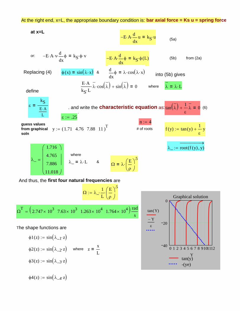
At the right end, x=L, the appropriate boundary condition is: bar axial force = Ks u = spring force
at x=LE− A⋅
xud
d⋅ kS u⋅= (5a)
or: E− A⋅ v⋅xφd
d⋅ kS φ⋅ v⋅= E− A⋅
xφd
d⋅ kS φ L( )⋅= (5b) from (2a)
Replacing (4) φ x( ) sin λ x⋅( )= &xφd
dλ cos λ x⋅( )⋅= into (5b) gives
E A⋅kS L⋅
λ⎯⋅ cos λ
⎯( )⋅ sin λ⎯( )+ 0= where λ
⎯λ L⋅=
define
εkSE A⋅
L
= , and write the characteristic equation as: tan λ⎯( ) 1
ελ⎯⋅+ 0= (6)
.
1L
Eρ⎛⎜⎝
⎞⎟⎠
.5⋅
⎡⎢⎣
⎤⎥⎦
λ_1 1.716=aλ_1
1.129=
which is just 13% higher than the exact value
a 1.936=
a1 ε+
13
⎛⎜⎜⎝
⎞⎟⎟⎠
.5:=
ω1approxKeqMeq
⎛⎜⎝
⎞⎟⎠
.5
= 1L
Eρ⎛⎜⎝
⎞⎟⎠
.5⋅
1 ε+13
⎛⎜⎜⎝
⎞⎟⎟⎠
.5⋅=
and the estimation for the fundamental natural frequency is
ε 0.25=
KeqA E⋅L
1 ε+( )⋅=εkSE A⋅
L
=
Meqρ A⋅ L⋅
3⎛⎜⎝
⎞⎟⎠
=KeqA E⋅L
kS+=
Meq0
L
xρ A⋅ ϕ x( )( )2⋅
⌠⎮⌡
d⎡⎢⎢⎣
⎤⎥⎥⎦
:=Keq0
L
xE A⋅xϕ x( )d
d⎛⎜⎝
⎞⎟⎠
2⋅
⌠⎮⎮⎮⌡
d kS ϕ L( )( )2⋅+:=
easily estimate the equivalent stiffness and mass as
ϕ x( )xL
:=(b) Approximate first natural frequency. Using mode shape
x/L0 0.25 0.5 0.75 11
0.5
0
0.5
1
Mode 1Mode 2Mode 3Mode 4
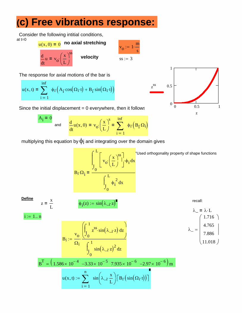
u x t,( )
1
n
i
sin λ_ixL⋅⎛⎜
⎝⎞⎟⎠
Bi sin Ωi t⋅( )( )⋅⎡⎣ ⎤⎦⋅∑=
:=
BT 1.586 10 4−× 3.33− 10 5−× 7.935 10 6−× 2.97− 10 6−×( ) m=
BivoΩi
0
1zzss sin λ_i z⋅( )⋅
⌠⎮⌡
d⎛⎜⎜⎝
⎞⎟⎟⎠
0
1
zsin λ_i z⋅( )2⌠⎮⌡
d
⋅:=
λ_
1.716
4.765
7.886
11.018
⎛⎜⎜⎜⎜⎝
⎞⎟⎟⎟⎟⎠
=
i 1 n..:=λ_ λ L⋅=
φi z( ) sin λ_i z⋅( ):=zxL
= recall:Define
Bi Ωi⋅0
L
xvoxL⎛⎜⎝
⎞⎟⎠
ss⋅
⎡⎢⎣
⎤⎥⎦φi⋅
⌠⎮⎮⌡
d
0
L
xφi2⌠
⎮⌡
d
=
"Used orthogonality property of shape functions
multiplying this equation by φj and integrating over the domain gives
tu x 0,( )d
dvo
xL⎛⎜⎝
⎞⎟⎠
s⋅=
1
inf
i
φi Bi Ωi⋅( )⋅∑=
=and
Ai 0=
Since the initial displacement = 0 everywhere, then it follows that
u x t,( )
1
inf
i
φi Ai cos Ωi t⋅( )⋅ Bi sin Ωi t⋅( )⋅+( )⋅∑=
=
The response for axial motions of the bar is
0 0.5 10
0.5
1
zss
z
ss 3:=tud
dvo
xL⎛⎜⎝
⎞⎟⎠
ss⋅= velocity
vo 1ms
⋅:=u x 0,( ) 0= no axial stretchingat t=0Consider the following intitial conditions,
(c) Free vibrations response:
[m/s]
0 0.0023 0.0046 0.0069 0.0091 0.01141
0.5
0
0.5
1
time (s)
v 0.5 L⋅ t,( )
v L t,( )
t
v L time,( ) 0.837ms
=time 0 s⋅:=v x t,( )
1
n
i
sin λ_ixL⋅⎛⎜
⎝⎞⎟⎠
Bi Ωi⋅ cos Ωi t⋅( )⋅( )⋅∑=
:=
vo12⎛⎜⎝⎞⎟⎠
ss⋅ 0.125
ms
=vo 1ms
=Bar velocity: midpoint & end
[m]
0 0.0023 0.0046 0.0069 0.0091 0.01142 .10 4
0
2 .10 4
time (s)
u 0.5 L⋅ t,( )
u L t,( )
t
Tmax 5 Tn1⋅:=u x t,( )
1
n
i
sin λ_ixL⋅⎛⎜
⎝⎞⎟⎠
Bi sin Ωi t⋅( )⋅( )⋅∑=
:=
for graph onlyBar displacement: midpoint & end
TnT 2.287 10 3−× 8.235 10 4−× 4.976 10 4−× 3.561 10 4−×( ) s=
Tn1fn
:=fn
T 437.199 1.214 103× 2.01 103× 2.808 103×( ) Hz=natural periods
fnΩ
2 π⋅:=
natural frequencies:Calculate time response at various spatial points in bar:
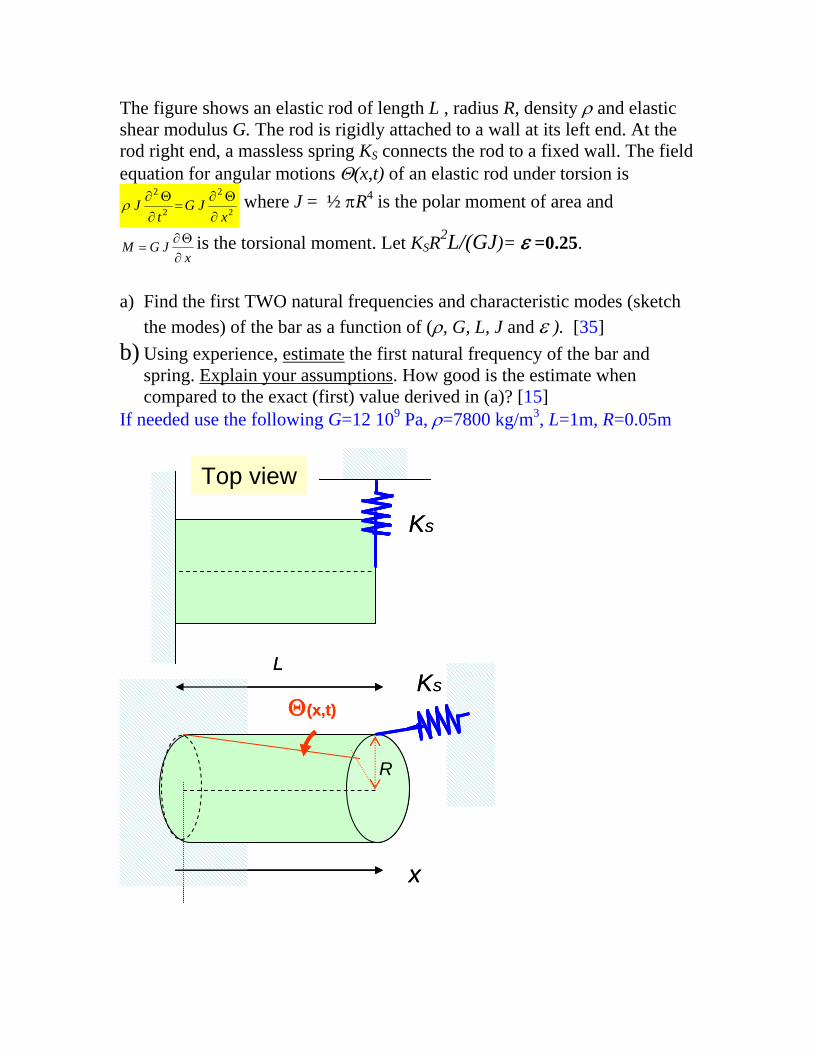
The figure shows an elastic rod of length L , radius R, density and elastic shear modulus G. The rod is rigidly attached to a wall at its left end. At the rod right end, a massless spring KS connects the rod to a fixed wall. The field equation for angular motions (x,t) of an elastic rod under torsion is
2 2
2 2J G Jt x
where J = ½ R4 is the polar moment of area and
M G Jx
is the torsional moment. Let KSR
2L/(GJ)= =0.25.
a) Find the first TWO natural frequencies and characteristic modes (sketch
the modes) of the bar as a function of (, G, L, J and ). [35] b) Using experience, estimate the first natural frequency of the bar and
spring. Explain your assumptions. How good is the estimate when compared to the exact (first) value derived in (a)? [15]
If needed use the following G=12 109 Pa, =7800 kg/m3, L=1m, R=0.05m
x
(x,t)
L
R
KS
Top view
KS
x
(x,t)
L
R
KS
Top view
KS
l-sanandres
Text Box
TORSIONAL VIBRATIONS OF AN ELASTIC ROD

Torsional vibrations of elastic rod L San Andres (c) SP 12 MEEN 617
The figure shows an elastic rod of length L , radius R, density and elastic shear modulus G. The rod is rigidly attached to a wall at its left end. At the rod right end, a massless spring KS connects the rod to a fixed wall. The field equation for angular motions (x,t) of an elastic rod under torsion is
2 2
2 2J G Jt x
where J = ½ R4 is the polar moment of area and M G Jx
is the torsional
moment. Let KSR2L/(GJ)= =0.25. a) Find the first TWO natural frequencies and characteristic modes (sketch the modes) of the bar as a
function of (, G, L, J and ). [35] b) Using experience, estimate the first natural frequency of the bar and spring. Explain your assumptions.
How good is the estimate when compared to the exact (first) value derived in (a)? [15] If needed use the following G=12 109 Pa, =7800 kg/m3, L=1m, R=0.05m
ORIGIN 1
PHYSICAL Parameters: G 12 109N
m2 7800
kg
m3 L 1 m d 0.1 m
A d2
4 J
0
rAr2
d= J d432
J 9.817 10 6 m4
x
(x,t)
L
R
KS
Top view
KS
x
(x,t)
L
R
KS
Top view
KS
2 2
2 2J G Jt x
(0)
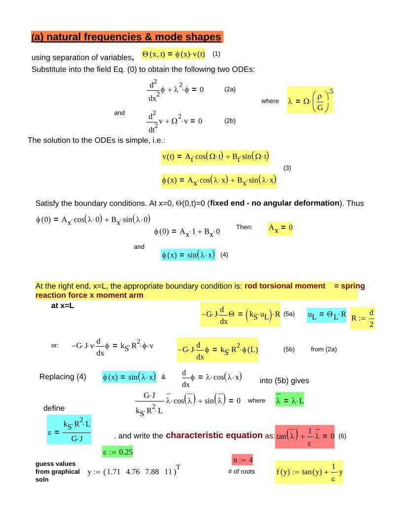
uL L R= Rd2
or: G J vxd
d kS R2 v= G J
xd
d kS R2 L( )= (5b) from (2a)
Replacing (4) x( ) sin x = &xd
d cos x = into (5b) gives
G J
kS R2 L cos
sin 0= where
L=
define
kS R2 L
G J= , and write the characteristic equation as: tan
1 0= (6)
. 0.25
n 4guess valuesfrom graphicalsoln
y 1.71 4.76 7.88 11( )T # of roots f y( ) tan y( )1
y
(a) natural frequencies & mode shapes x t( ) x( ) v t( )= (1)using separation of variables,
Substitute into the field Eq. (0) to obtain the following two ODEs:
2xd
d
2
2 0= (2a)
where G
.5=
and
2tvd
d
2
2 v 0= (2b)
The solution to the ODEs is simple, i.e.:
v t( ) At cos t Bt sin t =(3)
x( ) Ax cos x Bx sin x =
Satisfy the boundary conditions. At x=0, (0,t)=0 (fixed end - no angular deformation). Thus
0( ) Ax cos 0 Bx sin 0 =Then: Ax 0= 0( ) Ax 1 Bx 0=
and x( ) sin x = (4)
At the right end, x=L, the appropriate boundary condition is: rod torsional moment = spring reaction force x moment arm
at x=LG J
xd
d kS uL R= (5a)
x/L0 0.25 0.5 0.75 11
0.5
0
0.5
1
Mode 1Mode 2Mode 3Mode 4
4 z( ) sin _4 z
3 z( ) sin _3 z
zxL
=where2 z( ) sin _2 z
1 z( ) sin _1 z
The shape functions are
T
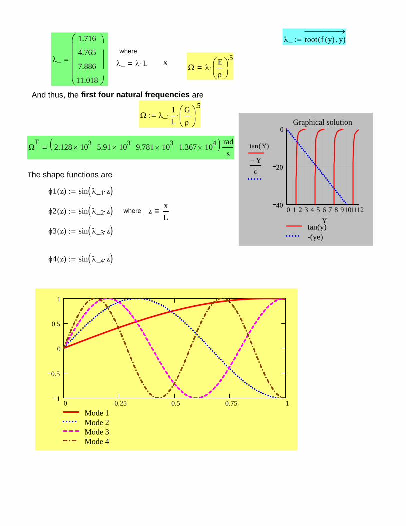
2.128 103 5.91 103 9.781 103 1.367 104 rads
_1L
G
.5
0 1 2 3 4 5 6 7 8 910111240
20
0
tan(y)-(ye)
Graphical solution
tan Y( )
Y
Y
And thus, the first four natural frequencies are
E
.5=&_ L=_
1.716
4.765
7.886
11.018
where
_ root f y( ) y( )
kS 1.178 107Nm
kS G J
R2 L
, i.e just 13 % higher than the exact valuea_1
1.129
1L
G
.5
_1 1.716compare to theexact value:
a 1.936
where1approxKeq
Ieq
.5
= 1L
G
.5 a= a
1 13
.5
and the estimation for the fundamental natural frequency is
0.25
kS R2 L
G J=with
Ieq J L
3
=KeqG JL
1 =KeqG JL
kS R2=
Ieq0
L
x J x( ) 2
d
Keq0
L
xG Jx x( )d
d
2
d kS R L( ) 2
easily estimate the equivalent torsional stiffness and mass moment of inertia from
x( )xL
(b) Approximate first natural frequency. Using mode shape
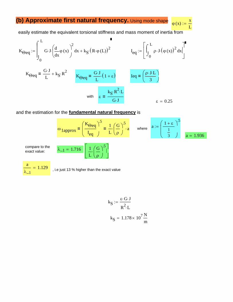
l-sanandres
Text Box
Note: do realize the torsional bar vibration problem is dimensionally and physically equivalent to the axial vibrations of an elastic bar
where λ Ωρ A⋅E IP⋅⎛⎜⎝
⎞⎟⎠
.5⋅=
and
2tvd
d
2Ω
2 v⋅+ 0= (2b)
The solution to the ODEs is simple, i.e.:
v t( ) At cos Ω t⋅( )⋅ Bt sin Ω t⋅( )⋅+=(3)
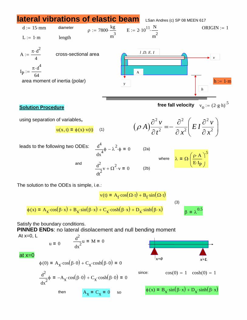
φ x( ) Ax cos β x⋅( )⋅ Bx sin β x⋅( )⋅+ Cx cosh β x⋅( )⋅+ Dx sinh β x⋅( )⋅+= β λ0.5=
Satisfy the boundary conditions. PINNED ENDs: no lateral displacement and null bending moment At x=0, L
x=0 x=L
2xud
d
2M= 0=u 0=
at x=0φ 0( ) Ax cos β 0⋅( )⋅ Cx cosh β 0⋅( )⋅+= 0=
since: cos 0( ) 1= cosh 0( ) 1=
2xφd
d
2Ax− cos β 0⋅( )⋅ Cx cosh β 0⋅( )⋅+= 0=
φ x( ) Bx sin β x⋅( )⋅ Dx sinh β x⋅( )⋅+=then Ax Cx= 0= so
lateral vibrations of elastic beam LSan Andres (c) SP 08 MEEN 617
d 15 mm⋅:= diameter ORIGIN 1:=ρ 7800kg
m3⋅:= E 2 1011⋅
N
m2⋅:=
L 1 m⋅:= length
A
h
l ,D, E, Ix
y
Aπ d2⋅
4:= cross-sectional area
IPπ d4⋅64
:=
area moment of inertia (polar) h 1 m⋅:=
free fall velocity vo 2 g⋅ h⋅( ).5:=Solution Procedure
( )2 2 2
2 2 2v v
A E It x x
ρ ⎛ ⎞∂ ∂ ∂=− ⎜ ⎟∂ ∂ ∂⎝ ⎠
using separation of variables,
u x t,( ) φ x( ) v t( )⋅= (1)
leads to the following two ODEs:4xφd
d
4λ
2φ⋅− 0= (2a)
lsanandres
Text Box
beam and frame are dropped from height h. find the response.
lsanandres
Rectangle
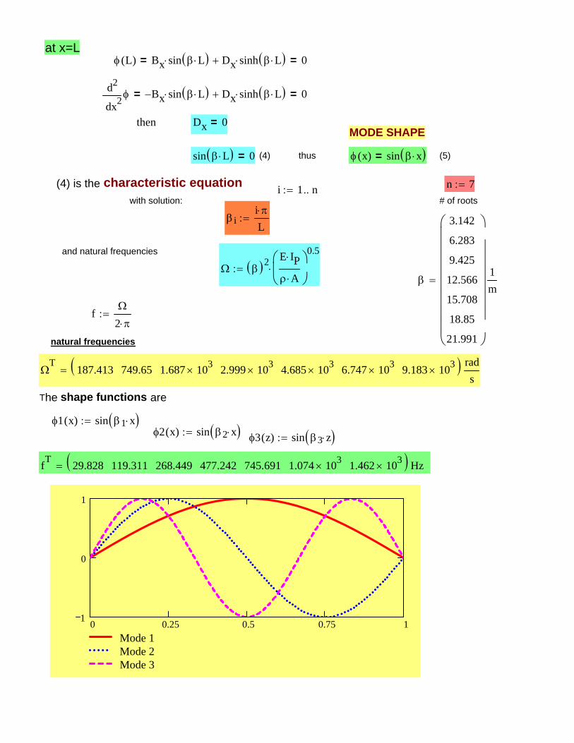
x/L
0 0.25 0.5 0.75 11
0
1
Mode 1Mode 2Mode 3
fT 29.828 119.311 268.449 477.242 745.691 1.074 103× 1.462 103×( ) Hz=
φ3 z( ) sin β3 z⋅( ):=φ2 x( ) sin β2 x⋅( ):=φ1 x( ) sin β1 x⋅( ):=
The shape functions are
ΩT
187.413 749.65 1.687 103× 2.999 103× 4.685 103× 6.747 103× 9.183 103×( ) rads
=
natural frequencies
fΩ
2 π⋅:=
β
3.142
6.283
9.425
12.566
15.708
18.85
21.991
⎛⎜⎜⎜⎜⎜⎜⎜⎜⎝
⎞⎟⎟⎟⎟⎟⎟⎟⎟⎠
1m
=Ω β( )2 E IP⋅
ρ A⋅
⎛⎜⎝
⎞⎟⎠
0.5
⋅:=
and natural frequencies
β ii π⋅L
:=
# of rootswith solution:i 1 n..:= n 7:=(4) is the characteristic equation
(5)φ x( ) sin β x⋅( )=thus(4)sin β L⋅( ) 0=
MODE SHAPEDx 0=then
2xφd
d
2Bx− sin β L⋅( )⋅ Dx sinh β L⋅( )⋅+= 0=
φ L( ) Bx sin β L⋅( )⋅ Dx sinh β L⋅( )⋅+= 0=at x=L
The response for lateral motions of a beam is
velocity = free fall velocitytud
dvo=
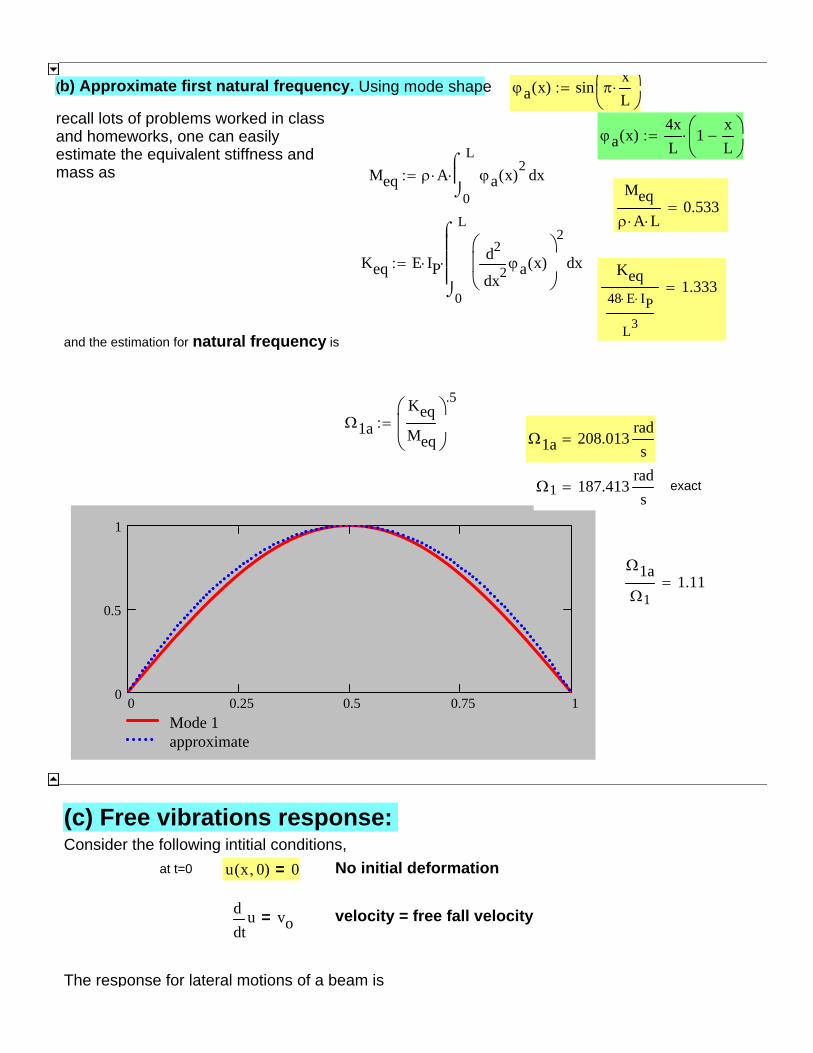
No initial deformationu x 0,( ) 0=at t=0
Consider the following intitial conditions, (c) Free vibrations response:
Ω1aΩ1
1.11=
0 0.25 0.5 0.75 10
0.5
1
Mode 1approximate
exactΩ1 187.413rads
=
Ω1a 208.013rads
=Ω1a
KeqMeq
⎛⎜⎝
⎞⎟⎠
.5
:=
and the estimation for natural frequency is
Keq48 E⋅ IP⋅
L3
1.333=Keq E IP⋅
0
L
x2xϕa x( )d
d
2⎛⎜⎜⎝
⎞⎟⎟⎠
2⌠⎮⎮⎮⌡
d⋅:=
Meqρ A⋅ L⋅
0.533=
Meq ρ A⋅0
L
xϕa x( )2⌠⎮⌡
d⋅:=
ϕa x( )4xL
1xL
−⎛⎜⎝
⎞⎟⎠
⋅:=recall lots of problems worked in class and homeworks, one can easily estimate the equivalent stiffness and mass as
ϕa x( ) sin πxL⋅⎛⎜
⎝⎞⎟⎠
:=(b) Approximate first natural frequency. Using mode shape
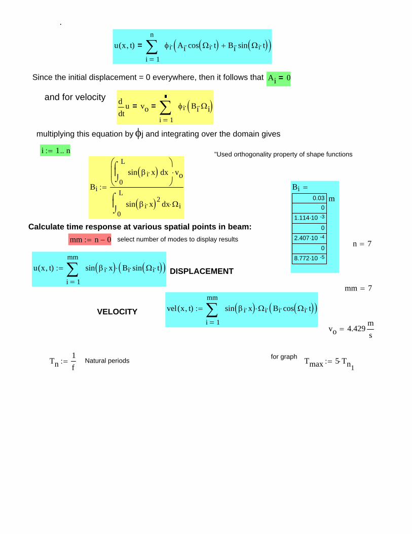
Tmax 5 Tn1⋅:=Natural periodsTn
1f
:= for graph
vo 4.429ms
=
VELOCITY vel x t,( )
1
mm
i
sin β i x⋅( ) Ωi⋅ Bi cos Ωi t⋅( )⋅( )⋅∑=
:=
mm 7=
DISPLACEMENTu x t,( )
1
mm
i
sin β i x⋅( ) Bi sin Ωi t⋅( )⋅( )⋅∑=
:=
n 7=select number of modes to display resultsmm n 0−:=
Calculate time response at various spatial points in beam:
Bi0.03
0
1.114·10 -3
0
2.407·10 -4
0
8.772·10 -5
m=Bi
0
Lxsin β i x⋅( )⌠
⎮⌡
d⎛⎜⎜⎝
⎞⎟⎟⎠
vo⋅
0
L
xsin β i x⋅( )2⌠⎮⌡
d Ωi⋅
:=
"Used orthogonality property of shape functionsi 1 n..:=
multiplying this equation by φj and integrating over the domain gives
tud
dvo=
1i
φi Bi Ωi⋅( )⋅∑=
=and for velocity
Ai 0=Since the initial displacement = 0 everywhere, then it follows that
u x t,( )
1
n
i
φi Ai cos Ωi t⋅( )⋅ Bi sin Ωi t⋅( )⋅+( )⋅∑=
=
p
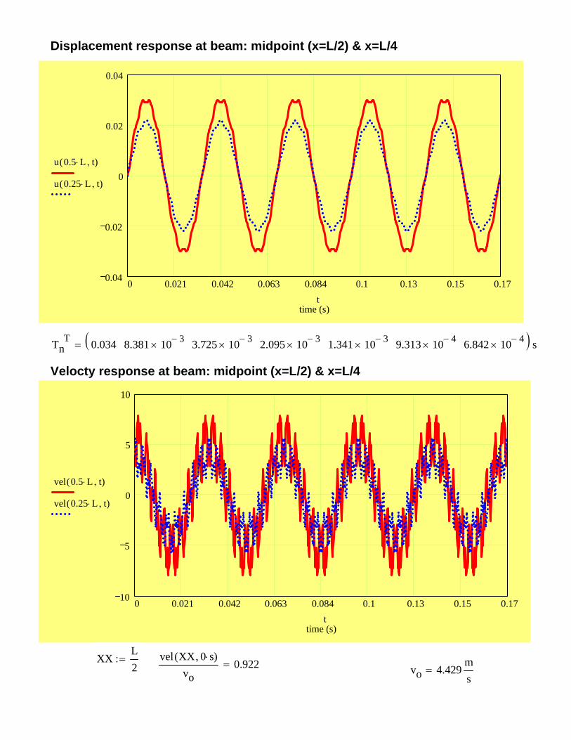
Displacement response at beam: midpoint (x=L/2) & x=L/4
0 0.021 0.042 0.063 0.084 0.1 0.13 0.15 0.170.04
0.02
0
0.02
0.04
time (s)
u 0.5 L⋅ t,( )
u 0.25 L⋅ t,( )
t
TnT 0.034 8.381 10 3−× 3.725 10 3−× 2.095 10 3−× 1.341 10 3−× 9.313 10 4−× 6.842 10 4−×( ) s=
Velocty response at beam: midpoint (x=L/2) & x=L/4
0 0.021 0.042 0.063 0.084 0.1 0.13 0.15 0.1710
5
0
5
10
time (s)
vel 0.5 L⋅ t,( )
vel 0.25 L⋅ t,( )
t
XXL2
:= vel XX 0 s⋅,( )vo
0.922= vo 4.429ms
=
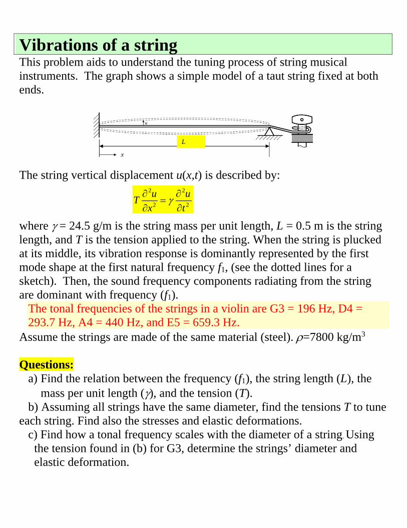
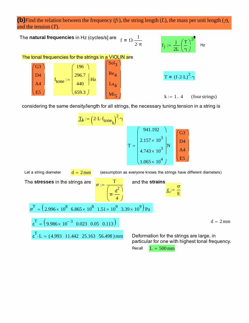
Vibrations of a string This problem aids to understand the tuning process of string musical instruments. The graph shows a simple model of a taut string fixed at both ends.
The string vertical displacement u(x,t) is described by:
2 2
2 2
u uT
x t
where = 24.5 g/m is the string mass per unit length, L = 0.5 m is the string length, and T is the tension applied to the string. When the string is plucked at its middle, its vibration response is dominantly represented by the first mode shape at the first natural frequency f1, (see the dotted lines for a sketch). Then, the sound frequency components radiating from the string are dominant with frequency (f1).
The tonal frequencies of the strings in a violin are G3 = 196 Hz, D4 = 293.7 Hz, A4 = 440 Hz, and E5 = 659.3 Hz.
Assume the strings are made of the same material (steel). =7800 kg/m3
Questions:
a) Find the relation between the frequency (f1), the string length (L), the mass per unit length (), and the tension (T).
b) Assuming all strings have the same diameter, find the tensions T to tune each string. Find also the stresses and elastic deformations.
c) Find how a tonal frequency scales with the diameter of a string. Using the tension found in (b) for G3, determine the strings’ diameter and elastic deformation.
L
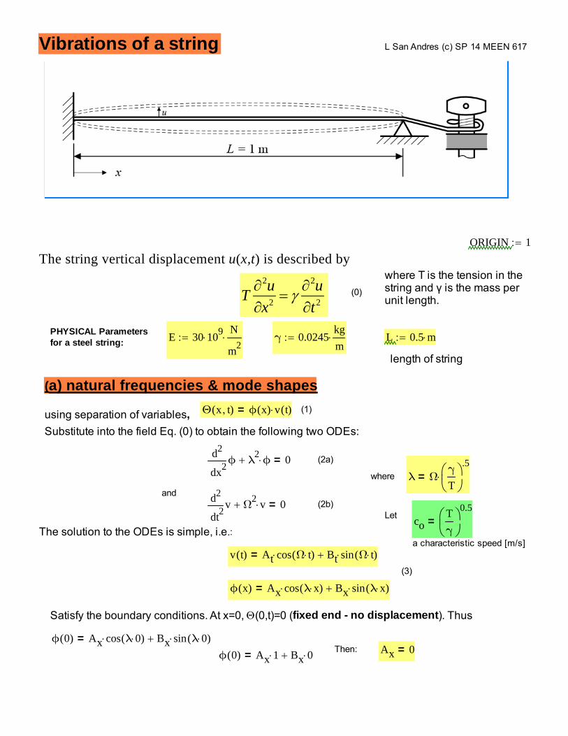
Vibrations of a string L San Andres (c) SP 14 MEEN 617
ORIGIN 1
The string vertical displacement u(x,t) is described by
2 2
2 2
u uT
x t
where T is the tension in thestring and γ is the mass perunit length.
(0)
PHYSICAL Parametersfor a steel string: E 30 109
N
m2 γ 0.0245
kgm
L 0.5 m
length of string
( a) natural frequencies & mode shapesΘ x t( ) ϕ x( ) v t( )= (1)using separation of variables,
Substitute into the field Eq. (0) to obtain the following two ODEs:
2xϕ
d
d
2λ
2ϕ 0= (2a)
where λ Ωγ
T
.5=
and
2tvd
d
2Ω
2 v 0= (2b)Let co
Tγ
0.5=
The solution to the ODEs is simple, i.e.:a characteristic speed [m/s]
v t( ) At cos Ω t( ) Bt sin Ω t( )=(3)
ϕ x( ) Ax cos λ x( ) Bx sin λ x( )=
Satisfy the boundary conditions. At x=0, (0,t)=0 (fixed end - no displacement). Thus
ϕ 0( ) Ax cos λ 0( ) Bx sin λ 0( )=Then: Ax 0=
ϕ 0( ) Ax 1 Bx 0=
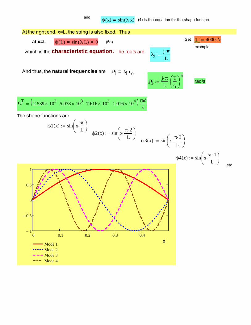
andϕ x( ) sin λ x( )= (4) is the equation for the shape funcion.
At the right end, x=L, the string is also fixed. Thus
Set T 4000 Nat x=L ϕ L( ) sin λ L( )= 0= (5a)example
which is the characteristic equation. The roots areλj
j πL
And thus, the natural frequencies are Ωj λj co=
Ωjj πL
Tγ
.5 rad/s
ΩT 2.539 103 5.078 103 7.616 103 1.016 104 rad
s
The shape functions are
ϕ1 x( ) sin xπ
L
ϕ2 x( ) sin x
π 2L
ϕ3 x( ) sin x
π 3L
ϕ4 x( ) sin xπ 4L
0 0.1 0.2 0.3 0.41
0.5
0
0.5
1
Mode 1Mode 2Mode 3Mode 4
etc
x
(b)Find the relation between the frequency (f1), the string length (L), the mass per unit length (),and the tension (T).
The natural frequencies in Hz (cycles/s] are f Ω1
2 π=
f jj
2LTγ
.5 Hz
The tonal frequencies for the strings in a VIOLIN are
T f 2 L( )2γ=
G3
D4
A4
E5
ftone
196
296.7
440
659.3
Hz
Sol3
Re4
La4
Mi5
k 1 4 four strings( )
considering the same density/length for all strings, the necessary tuning tension in a string is
Tk 2 L ftonek 2
γ
T
941.192
2.157 103
4.743 103
1.065 104
N
G3
D4
A4
E5
Let a string diameter d 2mm (assumption as everyone knows the strings have different diameters)
The stresses in the strings are and the strainsσ
T
πd2
4
ε
σ
E
σT 2.996 108 6.865 108 1.51 109 3.39 109 Pa
d 2mmε
T 9.986 10 3 0.023 0.05 0.113
εT L 4.993 11.442 25.163 56.498( ) mm Deformation for the strings are large, in
particular for one with highest tonal frequency. Recall L 500mm
l-sanandres
Text Box
Note: do realize the vibrations of a string is dimensionally and physically equivalent to the axial vibrations of an elastic bar and the torsional vibrations of a rod
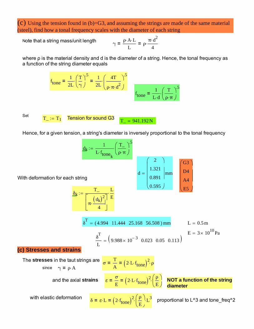
(c) Using the tension found in (b)=G3, and assuming the strings are made of the same material(steel), find how a tonal frequency scales with the diameter of each string
Note that a string mass/unit lengthγ
ρ A LL
= ρπ d2
4=
where ρ is the material density and d is the diameter of a string. Hence, the tonal frequency asa function of the string diameter equals
ftone1
2LTγ
.5= 1
2L4T
ρ π d2
.5=
ftone1
L dT
ρ π
.5=
Set T_ T1 Tension for sound G3 T_ 941.192N
Hence, for a given tension, a string's diameter is inversely proportional to the tonal frequency
dk1
L ftonek
T_ρ π
.5
d
2
1.321
0.891
0.595
mm
G3
D4
A4
E5
With deformation for each string
δkT_
πdk 2
4
LE
δT 4.994 11.444 25.168 56.508( ) mm L 0.5m
E 3 1010 Paδ
T
L9.988 10 3 0.023 0.05 0.113
(c) Stresses and strains
The stresses in the taut strings areσ
TA
= 2 L ftone 2ρ=
since γ ρ A=
and the axial strains εσ
E= 2 L ftone 2 ρ
E
= NOT a function of the stringdiameter
with elastic deformationδ ε L= 2 ftone 2 ρ
E
L3= proportional to L^3 and tone_freq^2


![MD5-HD14-2X/3X 홀드 오프 신호가 1ms 이상 [L]일 때 정상적인 여자 상태 ※반드시 모터를 정지시킨 상태에서 사용하십시오. ※ 입/출력 회로 및](https://static.fdocuments.in/doc/165x107/600087b71db0dd08834753c6/md5-hd14-2x3x-eoe-e-1ms-f-l-eoe-f-.jpg)


![NOTES 15 GAS FILM LUBRICATION - TRIBGROUP TAMUrotorlab.tamu.edu/me626/Notes_pdf/Notes15 Gas Film Lubrication.pdf · San Andrés et al. [7-16] report the results of a comprehensive](https://static.fdocuments.in/doc/165x107/5a9ff5d07f8b9a89178d5f2a/notes-15-gas-film-lubrication-tribgroup-gas-film-lubricationpdfsan-andrs-et-al.jpg)