ME617 - Handout 7 (Undamped) Modal Analysis of MDOF … 7 Modal Analysis Undamped MDOF.pdfThe...
45
MEEN 617 – HD#7 Undamped Modal Analysis of MDOF systems. L. San Andrés © 2008 1 ME617 - Handout 7 (Undamped) Modal Analysis of MDOF Systems The governing equations of motion for a n-DOF linear mechanical system with viscous damping are: () () t t MU+DU+KU =F (1) where and U, U, U are the vectors of generalized displacement, velocity and acceleration, respectively; and () t F is the vector of generalized (external forces) acting on the system. M,D,K represent the matrices of inertia, viscous damping and stiffness coefficients, respectively 1 . The solution of Eq. (1) is uniquely determined once initial conditions are specified. That is, (0) (0) at 0 , o o t = → = = U U U U (2) In most cases, i.e. conservative systems, the inertia and stiffness matrices are SYMMETRIC, i.e. , T T = = M M K K . The kinetic energy (T) and potential energy (V) in a conservative system are 1 1 , 2 2 T T T V = = U MU U KU (3) 1 The matrices are square with n-rows = n columns, while the vectors are n- rows.
Transcript of ME617 - Handout 7 (Undamped) Modal Analysis of MDOF … 7 Modal Analysis Undamped MDOF.pdfThe...

MEEN 617 – HD#7 Undamped Modal Analysis of MDOF systems. L. San Andrés © 2008 1
ME617 - Handout 7
(Undamped) Modal Analysis of MDOF Systems
The governing equations of motion for a n-DOF linear mechanical system with viscous damping are:
( ) ( )t tM U + DU +K U =F (1) where andU,U, U are the vectors of generalized displacement, velocity and acceleration, respectively; and ( )tF is the vector of generalized (external forces) acting on the system. M,D,K represent the matrices of inertia, viscous damping and stiffness coefficients, respectively1.
The solution of Eq. (1) is uniquely determined once initial conditions are specified. That is,
(0) (0)at 0 ,o ot = → = =U U U U (2)
In most cases, i.e. conservative systems, the inertia and stiffness matrices are SYMMETRIC, i.e. ,T T= =M M K K . The kinetic energy (T) and potential energy (V) in a conservative system are
1 1,2 2
T TT V= =U M U U K U (3)
1 The matrices are square with n-rows = n columns, while the vectors are n-rows.
MEEN 617 – HD#7 Undamped Modal Analysis of MDOF systems. L. San Andrés © 2008 2
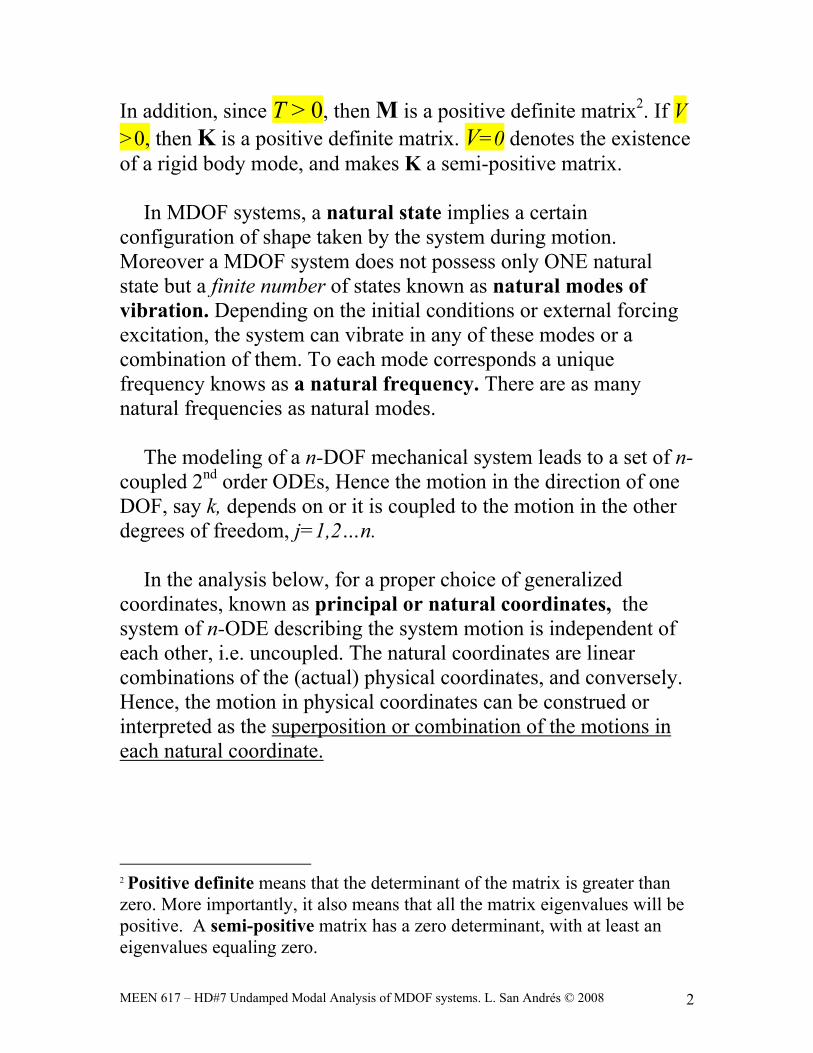
In addition, since T > 0, then M is a positive definite matrix2. If V >0, then K is a positive definite matrix. V=0 denotes the existence of a rigid body mode, and makes K a semi-positive matrix.
In MDOF systems, a natural state implies a certain configuration of shape taken by the system during motion. Moreover a MDOF system does not possess only ONE natural state but a finite number of states known as natural modes of vibration. Depending on the initial conditions or external forcing excitation, the system can vibrate in any of these modes or a combination of them. To each mode corresponds a unique frequency knows as a natural frequency. There are as many natural frequencies as natural modes.
The modeling of a n-DOF mechanical system leads to a set of n-
coupled 2nd order ODEs, Hence the motion in the direction of one DOF, say k, depends on or it is coupled to the motion in the other degrees of freedom, j=1,2…n.
In the analysis below, for a proper choice of generalized
coordinates, known as principal or natural coordinates, the system of n-ODE describing the system motion is independent of each other, i.e. uncoupled. The natural coordinates are linear combinations of the (actual) physical coordinates, and conversely. Hence, the motion in physical coordinates can be construed or interpreted as the superposition or combination of the motions in each natural coordinate.
2 Positive definite means that the determinant of the matrix is greater than zero. More importantly, it also means that all the matrix eigenvalues will be positive. A semi-positive matrix has a zero determinant, with at least an eigenvalues equaling zero.

MEEN 617 – HD#7 Undamped Modal Analysis of MDOF systems. L. San Andrés © 2008 3
For simplicity, begin the analysis of the system by neglecting damping, D=0. Hence, Eq.(1) reduces to
( ) ( )t tM U +K U =F (4)
and (0) (0)at 0 ,o ot = → = =U U U U Presently, set the external force F=0, and let’s find the free
vibrations response of the system.
M U +K U =0 (5)
The solution to the homogenous Eq. (5) is simply
cos( )tω θ−U = φ (6) which denotes a periodic response with a typical frequency ω . From Eq. (6),
2 cos( )tω ω θ− −U = φ (7) Note that Eq. (6) is a simplification of the more general solution
with and where 1s te s i iω= = −U = φ (8) Substitution of Eqs. (6) and (7) into the EOM (5) gives:
2
2
cos( ) cos( )
cos( )
t t
t
ω ω θ ω θ
ω ω θ
→
→ − − −
⎡ ⎤→ − −⎣ ⎦
M U +K U =0Mφ +Kφ =0
M +K φ =0
and since cos( ) 0tω θ− ≠ for most times, then
MEEN 617 – HD#7 Undamped Modal Analysis of MDOF systems. L. San Andrés © 2008 4
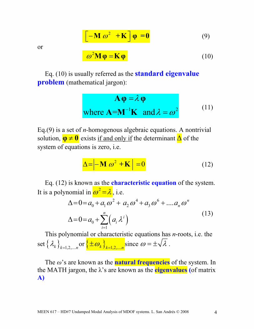
2ω⎡ ⎤−⎣ ⎦M +K φ =0 (9) or
2ω =Mφ Kφ (10)
Eq. (10) is usually referred as the standard eigenvalue problem (mathematical jargon):
1 2where = andλ
λ ω−
=
=
Aφ φΑ M K (11)
Eq.(9) is a set of n-homogenous algebraic equations. A nontrivial solution, ≠φ 0 exists if and only if the determinant Δ of the system of equations is zero, i.e.
2 0ωΔ= − =M +K (12)
Eq. (12) is known as the characteristic equation of the system. It is a polynomial in 2ω λ= , i.e.
( )
2 4 60 1 2 3
01
0 ....
0
nn
ni
ii
a a a a a
a a
ω ω ω ω
λ=
Δ= = + + + +
Δ= = +∑ (13)
This polynomial or characteristic equations has n-roots, i.e. the set 1,2,....k k n
λ=
or 1,2,....k k nω
=± since ω λ= ± .
The ω’s are known as the natural frequencies of the system. In
the MATH jargon, the λ’s are known as the eigenvalues (of matrix A)
MEEN 617 – HD#7 Undamped Modal Analysis of MDOF systems. L. San Andrés © 2008 5
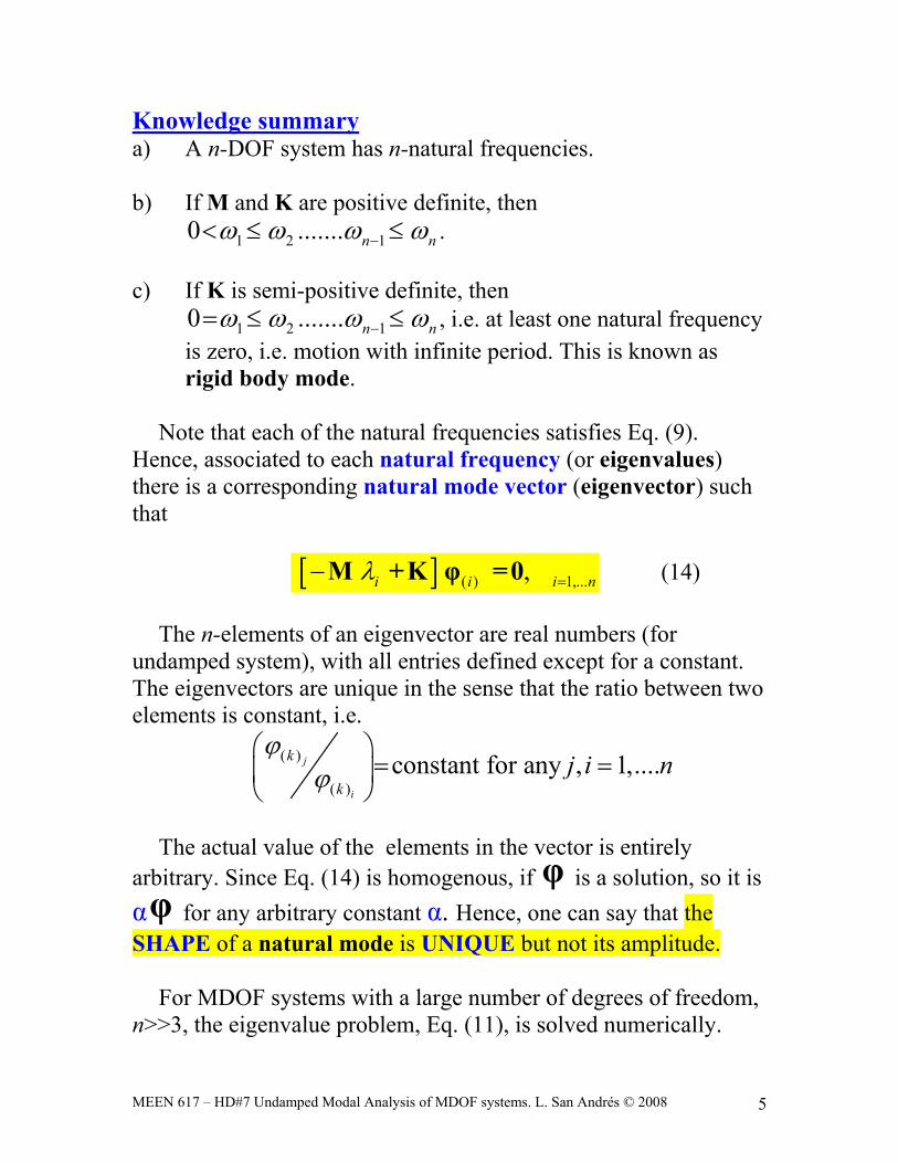
Knowledge summary a) A n-DOF system has n-natural frequencies. b) If M and K are positive definite, then
1 2 10 ....... n nω ω ω ω−< ≤ ≤ . c) If K is semi-positive definite, then
1 2 10 ....... n nω ω ω ω−= ≤ ≤ , i.e. at least one natural frequency is zero, i.e. motion with infinite period. This is known as rigid body mode.
Note that each of the natural frequencies satisfies Eq. (9).
Hence, associated to each natural frequency (or eigenvalues) there is a corresponding natural mode vector (eigenvector) such that
[ ] ( ) 1,...,i i i nλ =−M +K φ =0 (14)
The n-elements of an eigenvector are real numbers (for undamped system), with all entries defined except for a constant. The eigenvectors are unique in the sense that the ratio between two elements is constant, i.e.
( )
( )constant for any , 1,....j
i
k
kj i n
ϕϕ
⎛ ⎞= =⎜ ⎟
⎝ ⎠
The actual value of the elements in the vector is entirely
arbitrary. Since Eq. (14) is homogenous, if φ is a solution, so it is αφ for any arbitrary constant α. Hence, one can say that the SHAPE of a natural mode is UNIQUE but not its amplitude.
For MDOF systems with a large number of degrees of freedom,
n>>3, the eigenvalue problem, Eq. (11), is solved numerically.
MEEN 617 – HD#7 Undamped Modal Analysis of MDOF systems. L. San Andrés © 2008 6
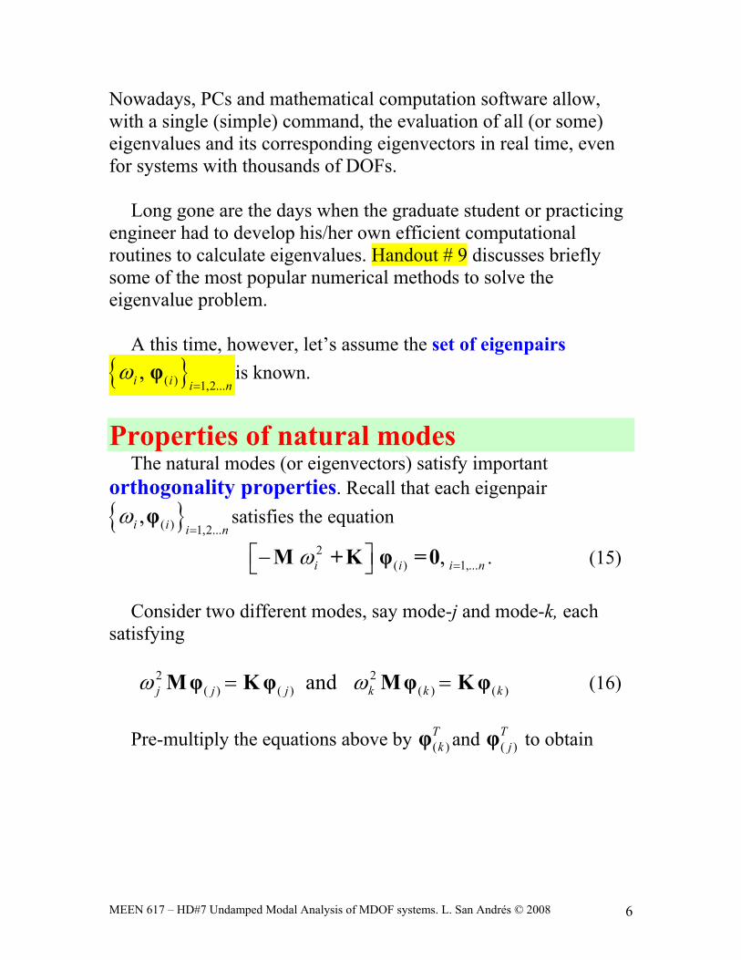
Nowadays, PCs and mathematical computation software allow, with a single (simple) command, the evaluation of all (or some) eigenvalues and its corresponding eigenvectors in real time, even for systems with thousands of DOFs.
Long gone are the days when the graduate student or practicing
engineer had to develop his/her own efficient computational routines to calculate eigenvalues. Handout # 9 discusses briefly some of the most popular numerical methods to solve the eigenvalue problem.
A this time, however, let’s assume the set of eigenpairs
( ) 1,2...,i i i n
ω=
φ is known.
Properties of natural modes
The natural modes (or eigenvectors) satisfy important orthogonality properties. Recall that each eigenpair ( ) 1,2...
,i i i nω
=φ satisfies the equation
2( ) 1,...,i i i nω =⎡ ⎤−⎣ ⎦M +K φ =0 . (15)
Consider two different modes, say mode-j and mode-k, each
satisfying
2 2( ) ( ) ( ) ( )andj j j k k kω ω= =Mφ Kφ Mφ Kφ (16)
Pre-multiply the equations above by ( )
Tkφ and ( )
Tjφ to obtain
MEEN 617 – HD#7 Undamped Modal Analysis of MDOF systems. L. San Andrés © 2008 7
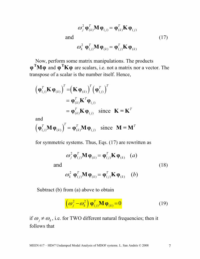
2( ) ( ) ( ) ( )
2( ) ( ) ( ) ( )
and
T Tj k j k j
T Tk j k j k
ω
ω
=
=
φ Mφ φ Kφ
φ Mφ φ Kφ
(17)
Now, perform some matrix manipulations. The products
φTMφ and φTKφ are scalars, i.e. not a matrix nor a vector. The transpose of a scalar is the number itself. Hence,
( ) ( ) ( )( ) ( ) ( ) ( )
( ) ( )
( ) ( ) since
T TTT Tj k k j
T Tk j
T Tk j
=
=
=
φ Kφ Kφ φ
φ K φ
φ Kφ K = K
and
( )( ) ( ) ( ) ( ) sinceTT T T
j k k j=φ Mφ φ Mφ M = M for symmetric systems. Thus, Eqs. (17) are rewritten as
2( ) ( ) ( ) ( )
2( ) ( ) ( ) ( )
( )
and( )
T Tj j k j k
T Tk j k j k
a
b
ω
ω
=
=
φ Mφ φ Kφ
φ Mφ φ Kφ
(18)
Subtract (b) from (a) above to obtain
( )2 2( ) ( ) 0T
j k j kω ω− =φ Mφ (19) if j kω ω≠ , i.e. for TWO different natural frequencies; then it follows that
MEEN 617 – HD#7 Undamped Modal Analysis of MDOF systems. L. San Andrés © 2008 8
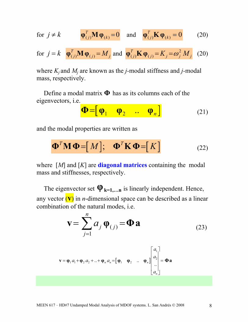
for j k≠ ( ) ( ) 0Tj k =φ Mφ and ( ) ( ) 0T
j k =φ Kφ (20) for j k= ( ) ( )
Tj j jM=φ Mφ and 2
( ) ( )T
j j j j jK Mω= =φ Kφ (20) where Kj and Mj are known as the j-modal stiffness and j-modal mass, respectively.
Define a modal matrix Φ has as its columns each of the eigenvectors, i.e.
[ ]1 2 .. n=Φ φ φ φ (21) and the modal properties are written as
[ ] [ ];T TM K= =Φ MΦ Φ KΦ (22) where [M] and [K] are diagonal matrices containing the modal mass and stiffnesses, respectively.
The eigenvector set φ k=1,…n is linearly independent. Hence, any vector (v) in n-dimensional space can be described as a linear combination of the natural modes, i.e.
( )1
n
j jj
a=
= =∑v φ Φa (23)
[ ]
1
21 1 2 2 1 2.. ..
..n n n
n
aa
a a a
a
⎡ ⎤⎢ ⎥⎢ ⎥= + + + = =⎢ ⎥⎢ ⎥⎣ ⎦
v φ φ φ φ φ φ Φa
MEEN 617 – HD#7 Undamped Modal Analysis of MDOF systems. L. San Andrés © 2008 9
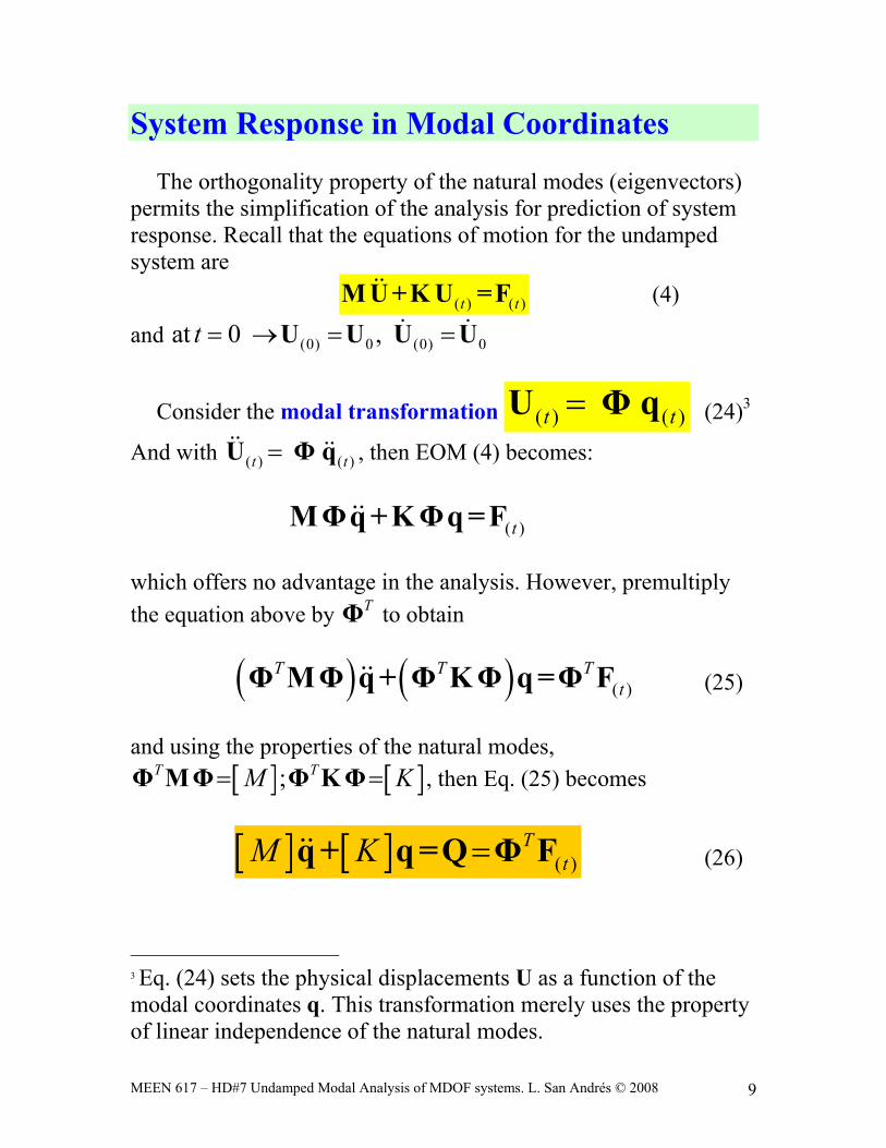
System Response in Modal Coordinates
The orthogonality property of the natural modes (eigenvectors) permits the simplification of the analysis for prediction of system response. Recall that the equations of motion for the undamped system are
( ) ( )t tM U +K U =F (4)
and (0) 0 (0) 0at 0 ,t = → = =U U U U
Consider the modal transformation ( ) ( )t t=U Φ q (24)3
And with ( ) ( )t t=U Φ q , then EOM (4) becomes:
( )tMΦq +KΦq =F which offers no advantage in the analysis. However, premultiply the equation above by TΦ to obtain
( ) ( ) ( )T T T
tΦ MΦ q + Φ KΦ q =Φ F (25) and using the properties of the natural modes,
[ ] [ ];T TM K= =Φ MΦ Φ KΦ , then Eq. (25) becomes
[ ] [ ] ( )T
tM K =q + q =Q Φ F (26)
3 Eq. (24) sets the physical displacements U as a function of the modal coordinates q. This transformation merely uses the property of linear independence of the natural modes.
MEEN 617 – HD#7 Undamped Modal Analysis of MDOF systems. L. San Andrés © 2008 10
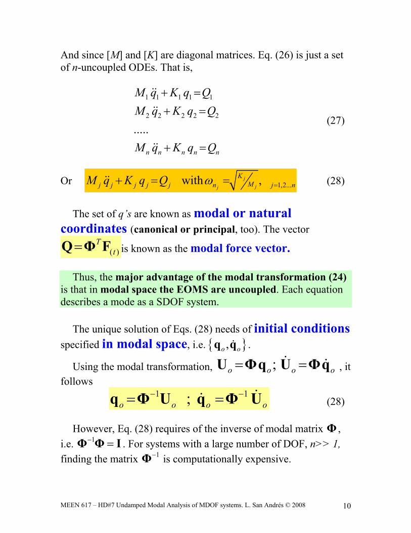
And since [M] and [K] are diagonal matrices. Eq. (26) is just a set of n-uncoupled ODEs. That is,
1 1 1 1 1
2 2 2 2 2
.....
n n n n n
M q K q QM q K q Q
M q K q Q
+ =+ =
+ =
(27)
Or 1,2...with ,jjj
KMj j j j j n j nM q K q Q ω =+ = = (28)
The set of q’s are known as modal or natural
coordinates (canonical or principal, too). The vector
( )T
t=Q Φ F is known as the modal force vector.
Thus, the major advantage of the modal transformation (24) is that in modal space the EOMS are uncoupled. Each equation describes a mode as a SDOF system.
The unique solution of Eqs. (28) needs of initial conditions specified in modal space, i.e. ,o oq q .
Using the modal transformation, ;o o o o= =U Φq U Φq , it follows
1 1;o o o o− −= =q Φ U q Φ U (28)
However, Eq. (28) requires of the inverse of modal matrix Φ ,
i.e. 1− =Φ Φ I . For systems with a large number of DOF, n>> 1, finding the matrix 1−Φ is computationally expensive.
MEEN 617 – HD#7 Undamped Modal Analysis of MDOF systems. L. San Andrés © 2008 11
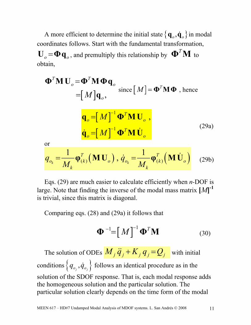
A more efficient to determine the initial state ,o oq q in modal coordinates follows. Start with the fundamental transformation,
o o=U Φq , and premultiply this relationship by TΦ M to obtain,
[ ] ,
T To o
oM=
=
Φ M U Φ MΦqq
since [ ] TM =Φ MΦ , hence
[ ][ ]
1
1
,To o
To o
M
M
−
−
=
=
q Φ M U
q Φ M U (29a)
or
( ) ( )( ) ( )1 1,
k k
T To k o o k o
k k
q qM M
= =φ M U φ M U (29b)
Eqs. (29) are much easier to calculate efficiently when n-DOF is
large. Note that finding the inverse of the modal mass matrix [M]-1 is trivial, since this matrix is diagonal.
Comparing eqs. (28) and (29a) it follows that
[ ] 11 TM −− =Φ Φ M (30) The solution of ODEs j j j j jM q K q Q+ = with initial
conditions ,j jo oq q follows an identical procedure as in the
solution of the SDOF response. That is, each modal response adds the homogeneous solution and the particular solution. The particular solution clearly depends on the time form of the modal

MEEN 617 – HD#7 Undamped Modal Analysis of MDOF systems. L. San Andrés © 2008 12
force Q(t), i.e step-load, ramp-load, pulse-load, periodic load, or arbitrary time form. Free response in modal coordinates
Without modal forces, Q=0, the modal equations are
0j H j j H j jM q K q Q+ = = (31a) with solutions, for an elastic mode
( ) ( )cos sinj
j j j
j
oH j o n n
n
qq q t tω ω
ω= + if 0
jnω ≠ (31b)
; and for a rigid body mode
j jH j o oq q q t= + if 0jnω = (31c)
j=1,2,….n Forced response in modal coordinates
For step-loads, S jQ , the modal equations are
j j j j S jM q K q Q+ = (32a) and; for an elastic mode, 0
jnω ≠ ,
( ) ( ) ( )cos sin 1 cosj j
j j j j
j
o Sj o n n n
n j
q Qq q t t t
Kω ω ω
ω⎡ ⎤= + + −⎣ ⎦ (32a)

MEEN 617 – HD#7 Undamped Modal Analysis of MDOF systems. L. San Andrés © 2008 13
; and for a rigid body mode, 0jnω = ,
212
j
j j
Sj o o
j
Qq q q t t
M= + + (32c)
j=1,2,….n For periodic loads,, the modal equations are
cos( )
jj j j j PM q K q Q t+ = Ω (33a) with solutions for an elastic mode, 0
jnω ≠ , and jnωΩ ≠
( ) ( )( )
( )21cos sin cos
1j
j j
j
Pj j n j n
j n
Qq C t S t t
Kω ω
ω
⎡ ⎤⎢ ⎥= + + Ω⎢ ⎥− Ω⎢ ⎥⎣ ⎦
(33b) Note that if
jnωΩ = , a resonance appears that will lead to system destruction.
For a rigid body mode, 0jnω = ,
2 cos( )j
j j
Pj o o
j
Qq q q t t
M= + − Ω
Ω (33c)
For arbitrary-loads jQ , the modal response is
( )0
1cos( ) sin( ) sin ( )o
o j j j
j j
tjj j n n j n
n j n
qq q t t Q t d
M τω ω ω τ τω ω
⎡ ⎤= + + −⎣ ⎦∫(34) for an elastic mode, 0
jnω ≠ .
MEEN 617 – HD#7 Undamped Modal Analysis of MDOF systems. L. San Andrés © 2008 14
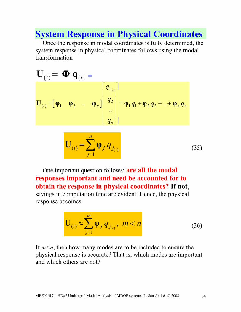
System Response in Physical Coordinates Once the response in modal coordinates is fully determined, the
system response in physical coordinates follows using the modal transformation
( ) ( )t t=U Φ q =
[ ]
( )1
2( ) 1 2 1 1 2 2.. ..
..
t
t n n n
n
q
q q q q
q
⎡ ⎤⎢ ⎥⎢ ⎥= = + + +⎢ ⎥⎢ ⎥⎢ ⎥⎣ ⎦
U φ φ φ φ φ φ
( )( )1
t
n
t j jj
q=
=∑U φ (35)
One important question follows: are all the modal
responses important and need be accounted for to obtain the response in physical coordinates? If not, savings in computation time are evident. Hence, the physical response becomes
( )( )1
,t
m
t j jj
q m n=
≈ <∑U φ (36)
If m<n, then how many modes are to be included to ensure the physical response is accurate? That is, which modes are important and which others are not?

MEEN 617 – HD#7 Undamped Modal Analysis of MDOF systems. L. San Andrés © 2008 15
Example: Consider the case of force excitation with frequency
jnωΩ ≠ and acting for very long times. The EOMs in physical space are
( )cos tΩPM U +K U =F Let’s assume there is a little damping; hence, the steady state periodic response in modal coordinates is (see eq. (33b)):
( )( )2
1 cos1
j
j
Pj
j n
Qq t
K ω
⎡ ⎤⎢ ⎥≈ Ω⎢ ⎥− Ω⎢ ⎥⎣ ⎦
(37a)
And thus,
( )( )2
1
1cos( ) cos1
j
j
nP
jj j n
Qt t
K ω=
⎛ ⎞⎡ ⎤⎜ ⎟⎢ ⎥= Ω = = Ω⎜ ⎟⎢ ⎥⎜ ⎟− Ω⎢ ⎥⎣ ⎦⎝ ⎠
∑PU U Φq φ
(38) The physical response is also periodic with same frequency as the force excitation. Recall that 2
( ) ( )j
Tj n j j jK Mω= = φ Kφ and ( )j
TP jQ = Pφ F
However, nowadays the engineer in a hurry prefers to dump the problem into a super computer; and for cos( )tΩPU = U , finds the solution
12P
−⎡ ⎤−Ω⎣ ⎦ PU = K M F (39)
at a fixed excitation frequency Ω. Brute force substitutes beauty and elegance, time savings in lieu of understanding!
The roots (eigenvalues) of the characteristic equation are
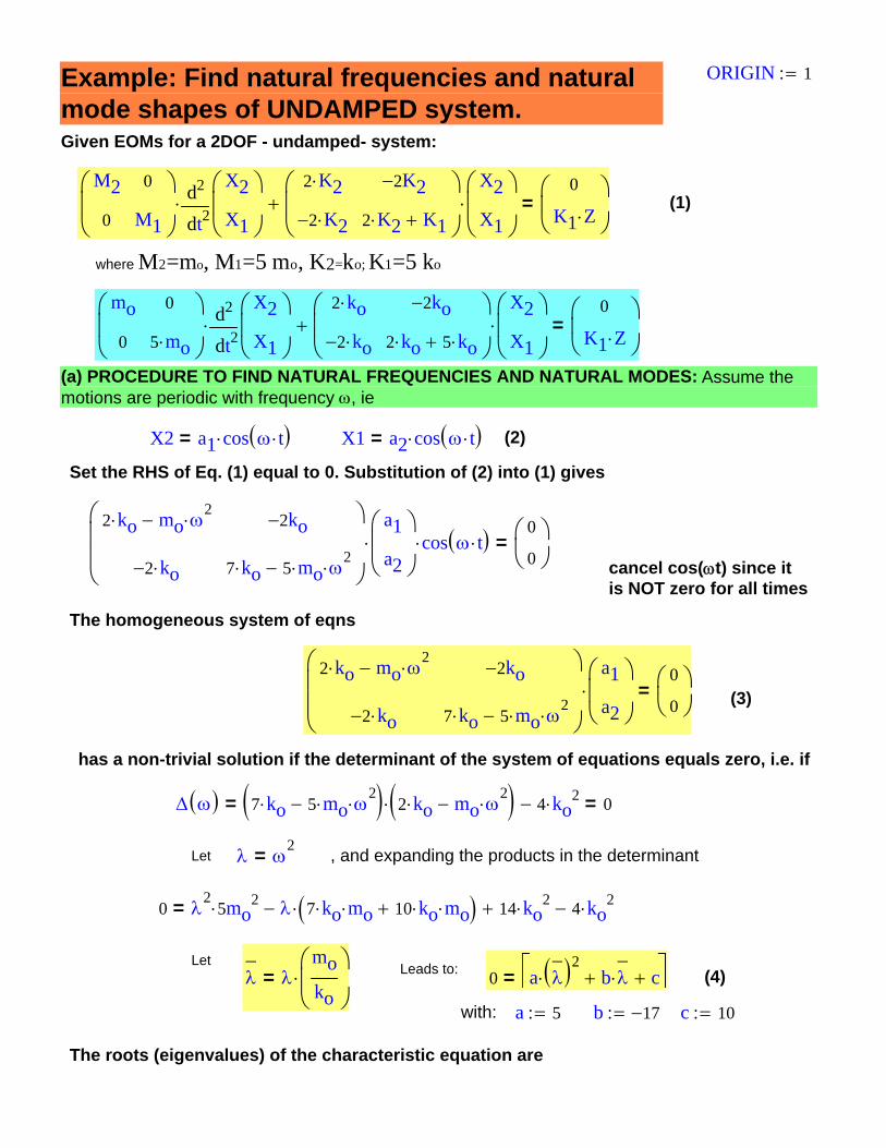
c 10:=b 17−:=a 5:=with:
(4)0 a λ⎯( )2
⋅ b λ⎯
⋅+ c+⎡⎣ ⎤⎦=λ⎯
λmoko
⎛⎜⎝
⎞⎟⎠
⋅= Leads to:Let
0 λ2
5⋅ mo2 λ 7 ko⋅ mo⋅ 10 ko⋅ mo⋅+( )⋅− 14 ko
2⋅+ 4 ko2⋅−=
, and expanding the products in the determinantλ ω2=Let
Δ ω( ) 7 ko⋅ 5 mo⋅ ω2
⋅−( ) 2 ko⋅ mo ω2
⋅−( )⋅ 4 ko2⋅−= 0=
has a non-trivial solution if the determinant of the system of equations equals zero, i.e. if
ORIGIN 1:=Example: Find natural frequencies and natural mode shapes of UNDAMPED system.Given EOMs for a 2DOF - undamped- system:
M2
0
0
M1
⎛⎜⎜⎝
⎞⎟⎟⎠
2t
X2
X1
⎛⎜⎜⎝
⎞⎟⎟⎠
dd
2⋅
2 K2⋅
2− K2⋅
2− K2
2 K2⋅ K1+
⎛⎜⎜⎝
⎞⎟⎟⎠
X2
X1
⎛⎜⎜⎝
⎞⎟⎟⎠
⋅+0
K1 Z⋅⎛⎜⎝
⎞⎟⎠
= (1)
where M2=mo, M1=5 mo, K2=ko; K1=5 ko
mo
0
0
5 mo⋅
⎛⎜⎜⎝
⎞⎟⎟⎠
2t
X2
X1
⎛⎜⎜⎝
⎞⎟⎟⎠
dd
2⋅
2 ko⋅
2− ko⋅
2− ko
2 ko⋅ 5 ko⋅+
⎛⎜⎜⎝
⎞⎟⎟⎠
X2
X1
⎛⎜⎜⎝
⎞⎟⎟⎠
⋅+0
K1 Z⋅⎛⎜⎝
⎞⎟⎠
=
(a) PROCEDURE TO FIND NATURAL FREQUENCIES AND NATURAL MODES: Assume the motions are periodic with frequency ω, ie
X2 a1 cos ω t⋅( )⋅= X1 a2 cos ω t⋅( )⋅= (2)
Set the RHS of Eq. (1) equal to 0. Substitution of (2) into (1) gives
2 ko⋅ mo ω2⋅−
2− ko⋅
2− ko
7 ko⋅ 5 mo⋅ ω2⋅−
⎛⎜⎜⎝
⎞⎟⎟⎠
a1
a2
⎛⎜⎜⎝
⎞⎟⎟⎠
⋅ cos ω t⋅( )⋅0
0⎛⎜⎝
⎞⎟⎠
=cancel cos(ωt) since it is NOT zero for all times
The homogeneous system of eqns
2 ko⋅ mo ω2⋅−
2− ko⋅
2− ko
7 ko⋅ 5 mo⋅ ω2⋅−
⎛⎜⎜⎝
⎞⎟⎟⎠
a1
a2
⎛⎜⎜⎝
⎞⎟⎟⎠
⋅0
0⎛⎜⎝
⎞⎟⎠
= (3)
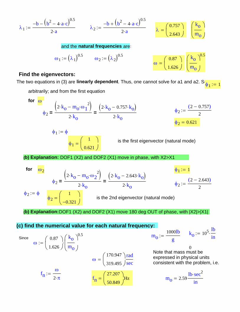
(b) Explanation: DOF1 (X2) and DOF2 (X1) move in phase, with X2>X1
for ω2 φ1 1:=
φ2
2 ko⋅ mo ω22
⋅−( )2 ko⋅
=2 ko⋅ 2.643 ko⋅−( )
2 ko⋅= φ2
2 2.643−( )2
:=
φ2 φ:=φ2
1
0.321−⎛⎜⎝
⎞⎟⎠
= is the 2nd eigenvector (natural mode)
(b) Explanation:DOF1 (X2) and DOF2 (X1) move 180 deg OUT of phase, with |X2|>|X1|
(c) find the numerical value for each natural frequency:ko 105 lb
in⋅:=mo
1000lbg
:=Sinceω
0.87
1.626⎛⎜⎝
⎞⎟⎠
komo
⎛⎜⎝
⎞⎟⎠
0.5
⋅:=0
Note that mass must be expressed in physical units consistent with the problem, i.e.
ω170.947
319.495⎛⎜⎝
⎞⎟⎠
radsec
=
fnω
2 π⋅:=
fn27.207
50.849⎛⎜⎝
⎞⎟⎠
Hz= mo 2.59lb sec2⋅
in=
λ1b− b2 4 a⋅ c⋅−( )0.5
−2 a⋅
:= λ2b− b2 4 a⋅ c⋅−( )0.5
+2 a⋅
:= λ0.757
2.643⎛⎜⎝
⎞⎟⎠
=komo
⎛⎜⎝
⎞⎟⎠
and the natural frequencies are:
ω1 λ1( )0.5:= ω2 λ2( )0.5
:=ω
0.87
1.626⎛⎜⎝
⎞⎟⎠
=komo
⎛⎜⎝
⎞⎟⎠
0.5
Find the eigenvectors:The two equations in (3) are linearly dependent. Thus, one cannot solve for a1 and a2. Setφ1 1:=
arbitrarily; and from the first equation
for ω1
φ22 0.757−( )
2:=φ2
2 ko⋅ mo ω12
⋅−( )2 ko⋅
=2 ko⋅ 0.757 ko⋅−( )
2 ko⋅=
φ2 0.621=
φ1 φ:=
is the first eigenvector (natural mode)φ11
0.621⎛⎜⎝
⎞⎟⎠
=
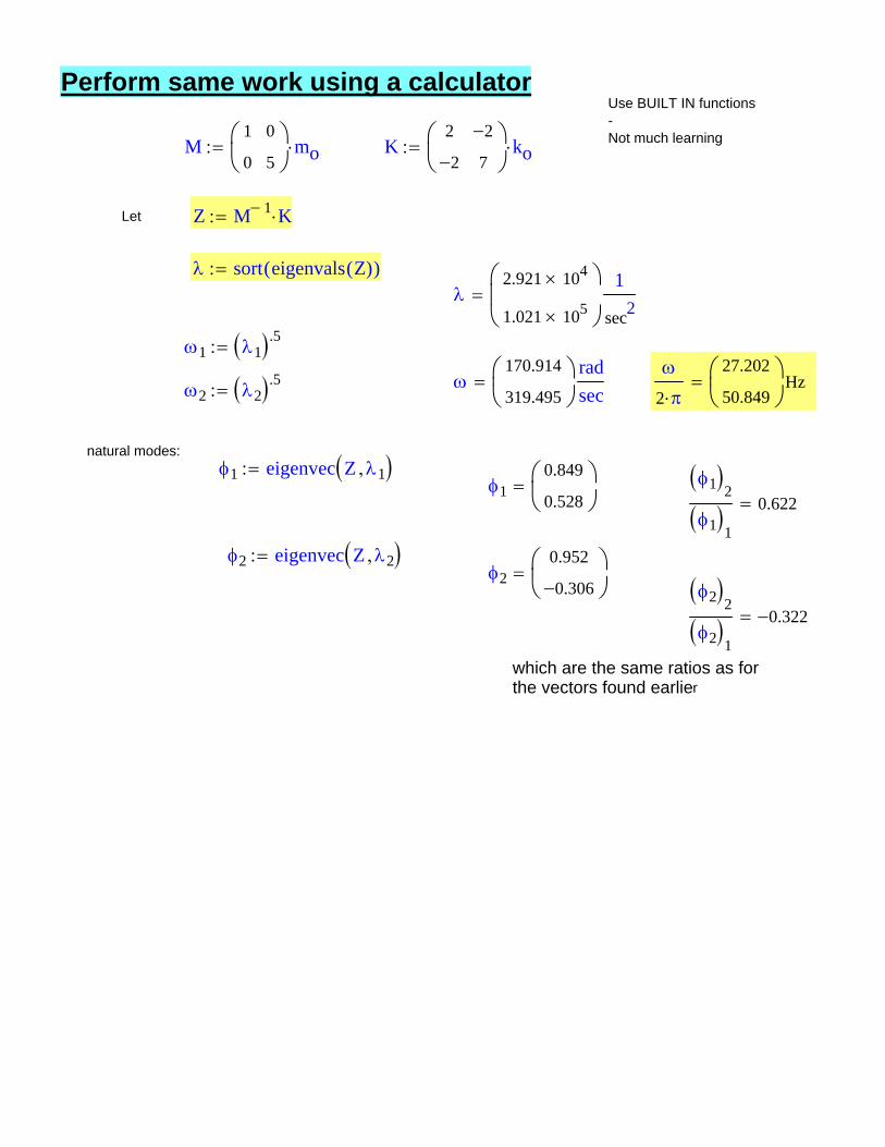
which are the same ratios as for the vectors found earlier
φ2( )2
φ2( )1
0.322−=
φ20.952
0.306−⎛⎜⎝
⎞⎟⎠
=φ2 eigenvec Z λ2,( ):=
φ1( )2
φ1( )1
0.622=φ1
0.849
0.528⎛⎜⎝
⎞⎟⎠
=φ1 eigenvec Z λ1,( ):=
natural modes:
ω2 λ2( ).5:=
ω
2 π⋅
27.202
50.849⎛⎜⎝
⎞⎟⎠
Hz=ω170.914
319.495⎛⎜⎝
⎞⎟⎠
radsec
=
ω1 λ1( ).5:=
λ2.921 104×
1.021 105×
⎛⎜⎝
⎞⎟⎠
1
sec2=
λ sort eigenvals Z( )( ):=
Z M 1− K⋅:=Let
K2
2−
2−
7⎛⎜⎝
⎞⎟⎠
ko⋅:=M1
0
0
5⎛⎜⎝
⎞⎟⎠
mo⋅:=
Use BUILT IN functions-Not much learning
Perform same work using a calculator
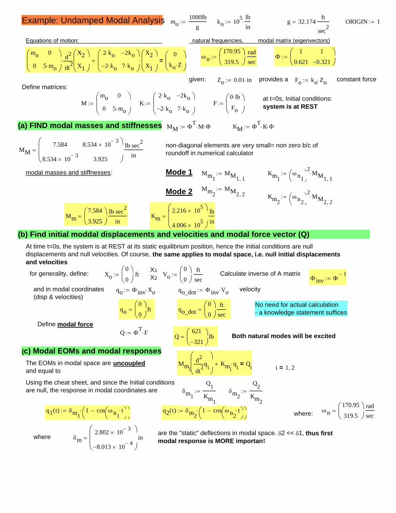
(b) Find initial moddal displacements and velocities and modal force vector (Q)At time t=0s, the system is at REST at its static equilibrium position, hence the initial conditions are null displacements and null velocities. Of course, the same applies to modal space, i.e. null initial displacements and velocities
X1X2
for generality, define: Xo0
0⎛⎜⎝
⎞⎟⎠
ft⋅:= Vo0
0⎛⎜⎝
⎞⎟⎠
ftsec
⋅:= Calculate inverse of A matrixΦinv Φ
1−:=
and in modal coordinates(disp & velocities)
qo Φ inv Xo⋅:= qo_dot Φinv Vo⋅:= velocity
No need for actual calculation- a knowledge statement sufficesqo
0
0⎛⎜⎝
⎞⎟⎠
ft= qo_dot0
0⎛⎜⎝
⎞⎟⎠
ftsec
=
Define modal force
δm2.802 10 3−
×
8.013− 10 4−×
⎛⎜⎜⎝
⎞⎟⎟⎠
in=where are the "static" deflections in modal space. δ2 << δ1, thus first modal response is MORE important
where: ωn170.95
319.5⎛⎜⎝
⎞⎟⎠
radsec
=q2 t( ) δm21 cos ωn2
t⋅⎛⎝
⎞⎠
−⎛⎝
⎞⎠
⋅:=q1 t( ) δm11 cos ωn1
t⋅⎛⎝
⎞⎠
−⎛⎝
⎞⎠
⋅:=
δm2
Q2
Km2
:=δm1
Q1
Km1
:=Using the cheat sheet, and since the Initial conditions are null, the response in modal coordinates are
i 1= 2,Mmi 2t
qid
d
2⎛⎜⎜⎝
⎞⎟⎟⎠
Kmiqi⋅+ Qi=The EOMs in modal space are uncoupled
and equal to
(c) Modal EOMs and modal responses
Both natural modes will be excitedQ621
321−⎛⎜⎝
⎞⎟⎠
lb=Q Φ
T F⋅:=
Example: Undamped Modal Analysis mo1000lb
g:= ko 105 lb
in⋅:= g 32.174
ft
sec2= ORIGIN 1:=
Equations of motion: natural frequencies, modal matrix (eigenvectors)
ωn170.95
319.5⎛⎜⎝
⎞⎟⎠
radsec
⋅:= Φ1
0.621
1
0.321−⎛⎜⎝
⎞⎟⎠
:=mo
0
0
5 mo⋅
⎛⎜⎜⎝
⎞⎟⎟⎠
2t
X2
X1
⎛⎜⎜⎝
⎞⎟⎟⎠
d
d
2⋅
2 ko⋅
2− ko⋅
2− ko
7 ko⋅
⎛⎜⎜⎝
⎞⎟⎟⎠
X2
X1
⎛⎜⎜⎝
⎞⎟⎟⎠
⋅+0
ko Z⋅⎛⎜⎝
⎞⎟⎠
=
given: Zo 0.01 in⋅:= provides a Fo ko Zo⋅:= constant forceDefine matrices:
at t=0s, Initial conditions:system is at REST
Km2.216 105
×
4.006 105×
⎛⎜⎜⎝
⎞⎟⎟⎠
lbin
=Mm7.584
3.925⎛⎜⎝
⎞⎟⎠
lb sec2⋅
in=
Km2ωn2
⎛⎝
⎞⎠
2MM2 2,
⋅:=Mode 2 Mm2
MM2 2,:=
Km1ωn1
⎛⎝
⎞⎠
2MM1 1,
⋅:=Mm1MM1 1,
:=Mode 1modal masses and stiffnesses:
MM7.584
8.534 10 3−×
8.534 10 3−×
3.925
⎛⎜⎜⎝
⎞⎟⎟⎠
lb sec2⋅
in=
non-diagonal elements are very small= non zero b/c of roundoff in numerical calculator
KM ΦT K⋅ Φ⋅:=MM Φ
T M⋅ Φ⋅:=(a) FIND modal masses and stiffnesses
F0 lb⋅
Fo
⎛⎜⎝
⎞⎟⎠
:=K2 ko⋅
2− ko⋅
2− ko
7 ko⋅
⎛⎜⎜⎝
⎞⎟⎟⎠
:=Mmo
0
0
5 mo⋅
⎛⎜⎜⎝
⎞⎟⎟⎠
:=
2t
X1
X2
⎛⎜⎜⎝
⎞⎟⎟⎠
d
d
2 0
0⎛⎜⎝
⎞⎟⎠
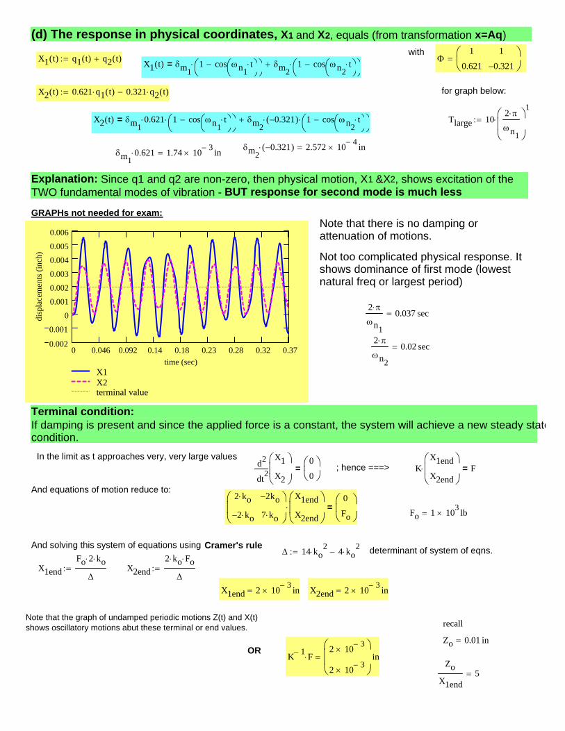
= ; hence ===> KX1end
X2end
⎛⎜⎜⎝
⎞⎟⎟⎠
⋅ F=
And equations of motion reduce to:2 ko⋅
2− ko⋅
2− ko
7 ko⋅
⎛⎜⎜⎝
⎞⎟⎟⎠
X1end
X2end
⎛⎜⎜⎝
⎞⎟⎟⎠
⋅0
Fo
⎛⎜⎝
⎞⎟⎠
= Fo 1 103× lb=
And solving this system of equations using Cramer's ruleΔ 14 ko
2⋅ 4 ko
2⋅−:= determinant of system of eqns.
X1endFo 2⋅ ko⋅
Δ:= X2end
2 ko⋅ Fo⋅
Δ:=
X1end 2 10 3−× in= X2end 2 10 3−
× in=
Note that the graph of undamped periodic motions Z(t) and X(t) shows oscillatory motions abut these terminal or end values. recall
Zo 0.01 in=OR
K 1− F⋅2 10 3−
×
2 10 3−×
⎛⎜⎜⎝
⎞⎟⎟⎠
in=Zo
X1end5=
(d) The response in physical coordinates, X1 and X2, equals (from transformation x=Aq)with
X1 t( ) q1 t( ) q2 t( )+:= Φ1
0.621
1
0.321−⎛⎜⎝
⎞⎟⎠
=X1 t( ) δm11 cos ωn1
t⋅⎛⎝
⎞⎠
−⎛⎝
⎞⎠
⋅ δm21 cos ωn2
t⋅⎛⎝
⎞⎠
−⎛⎝
⎞⎠
⋅+=
X2 t( ) 0.621 q1 t( )⋅ 0.321 q2 t( )⋅−:= for graph below:
X2 t( ) δm10.621⋅ 1 cos ωn1
t⋅⎛⎝
⎞⎠
−⎛⎝
⎞⎠
⋅ δm20.321−( )⋅ 1 cos ωn2
t⋅⎛⎝
⎞⎠
−⎛⎝
⎞⎠
⋅+= Tlarge 102 π⋅
ωn1
⎛⎜⎜⎝
⎞⎟⎟⎠
1⋅:=
δm20.321−( )⋅ 2.572 10 4−
× in=δm1
0.621⋅ 1.74 10 3−× in=
Explanation: Since q1 and q2 are non-zero, then physical motion, X1 &X2, shows excitation of the TWO fundamental modes of vibration - BUT response for second mode is much less
GRAPHs not needed for exam:
0 0.046 0.092 0.14 0.18 0.23 0.28 0.32 0.370.002
0.001
0
0.001
0.002
0.003
0.004
0.005
0.006
X1X2terminal value
time (sec)
disp
lace
men
ts (i
nch)
Note that there is no damping or attenuation of motions.
Not too complicated physical response. It shows dominance of first mode (lowest natural freq or largest period)
2 π⋅
ωn1
0.037 sec=
2 π⋅
ωn2
0.02 sec=
Terminal condition:If damping is present and since the applied force is a constant, the system will achieve a new steady statecondition.
In the limit as t approaches very, very large values
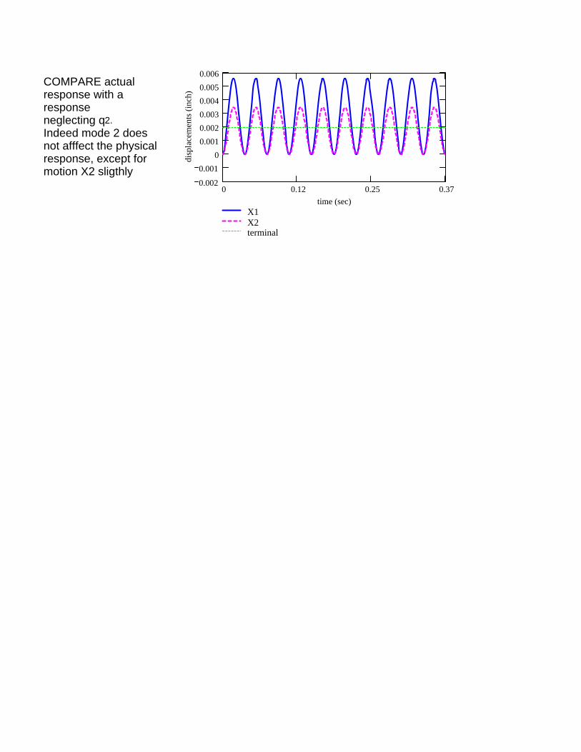
0 0.12 0.25 0.370.002
0.0010
0.0010.0020.0030.0040.0050.006
X1X2terminal
time (sec)di
spla
cem
ents
(inc
h)
COMPARE actual response with a responseneglecting q2.Indeed mode 2 does not afffect the physical response, except for motion X2 sligthly

MEEN 617 – HD#7 Undamped Modal Analysis of MDOF systems. L. San Andrés © 2008 16
Normalization of eigenvectors (natural modes)
Recall that the components of an eigenvector jφ are ARBITRARY but for a multiplicative constant. If one of the elements of the eigenvector is assigned a certain value, then this vector becomes unique, since then n-1 remaining elements are automatically adjusted to keep constant the ratio between any two elements in the vector.
In practice, the eigenvectors are normalized. The resulting vectors are called NORMAL MODES. Some typical NORMS are L1 norm: ( )( ) 1 max
kj jq= =q (39a) L2 norm:
1 2
2 2 2( ) 1 ....
nj j j jq q q= = + + +q (39b) Or making the mass modal matrix equal to the identity matrix, [M]=I, i.e. ( ) ( ) 1T
j j jM= =φ Mφ (39c) hence 2 2
( ) ( )T
j j j j j n jK Mω ω= = =φ Kφ (39d)
This normalization has obvious advantages since it will reduce the number of operations when conducting the modal analysis. However, the physical significance of the modal equations is lost. Note that the modal Eqs. (26) become:
MEEN 617 – HD#7 Undamped Modal Analysis of MDOF systems. L. San Andrés © 2008 17
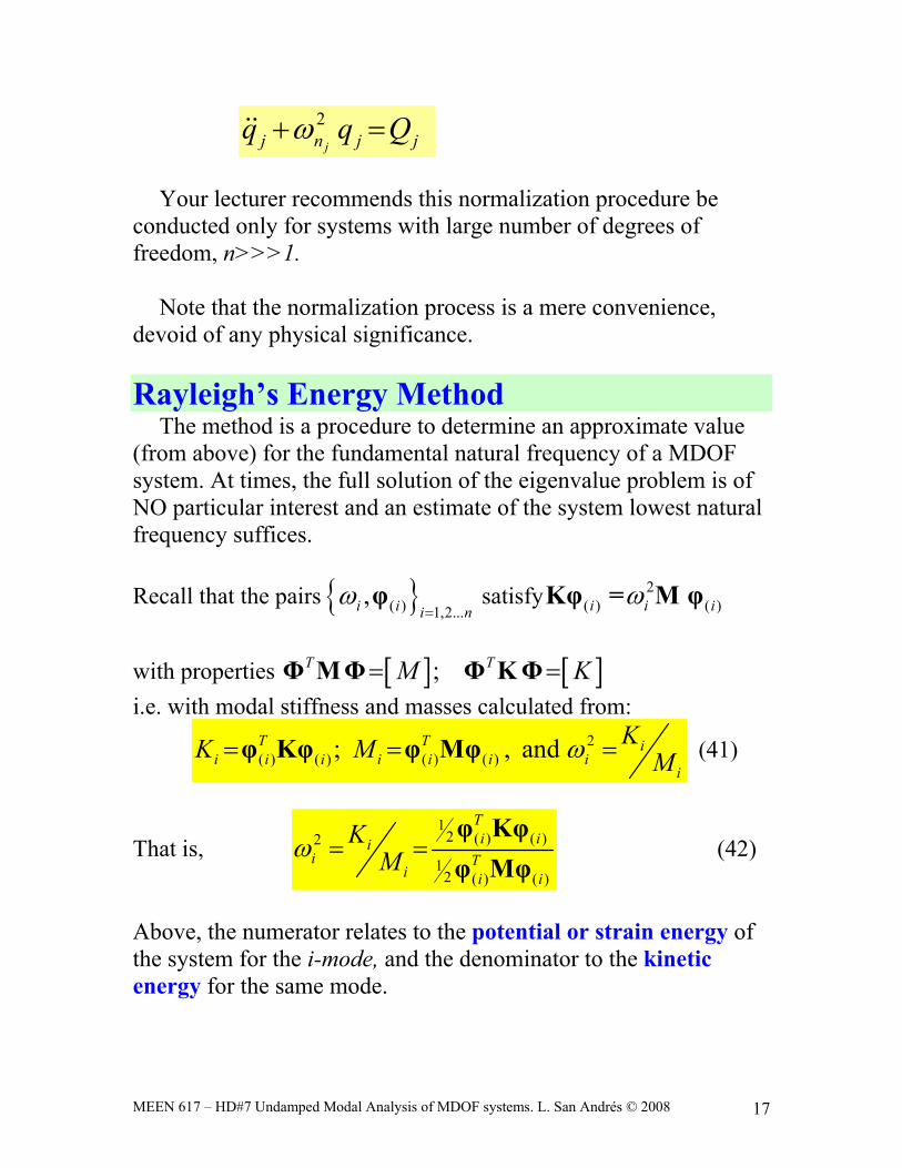
2jj n j jq q Qω+ =
Your lecturer recommends this normalization procedure be
conducted only for systems with large number of degrees of freedom, n>>>1.
Note that the normalization process is a mere convenience,
devoid of any physical significance.
Rayleigh’s Energy Method The method is a procedure to determine an approximate value
(from above) for the fundamental natural frequency of a MDOF system. At times, the full solution of the eigenvalue problem is of NO particular interest and an estimate of the system lowest natural frequency suffices. Recall that the pairs ( ) 1,2...
,i i i nω
=φ satisfy 2
( ) ( )i i iωKφ = M φ
with properties [ ] [ ];T TM K= =Φ MΦ Φ KΦ i.e. with modal stiffness and masses calculated from:
2( ) ( ) ( ) ( ); , andT T i
i i i i i i ii
KK M Mω= = =φ Kφ φ Mφ (41)
That is, 1
2 ( ) ( )2
12 ( ) ( )
Ti ii
i Ti i i
KMω = =
φ Kφφ Mφ
(42)
Above, the numerator relates to the potential or strain energy of the system for the i-mode, and the denominator to the kinetic energy for the same mode.
MEEN 617 – HD#7 Undamped Modal Analysis of MDOF systems. L. San Andrés © 2008 18
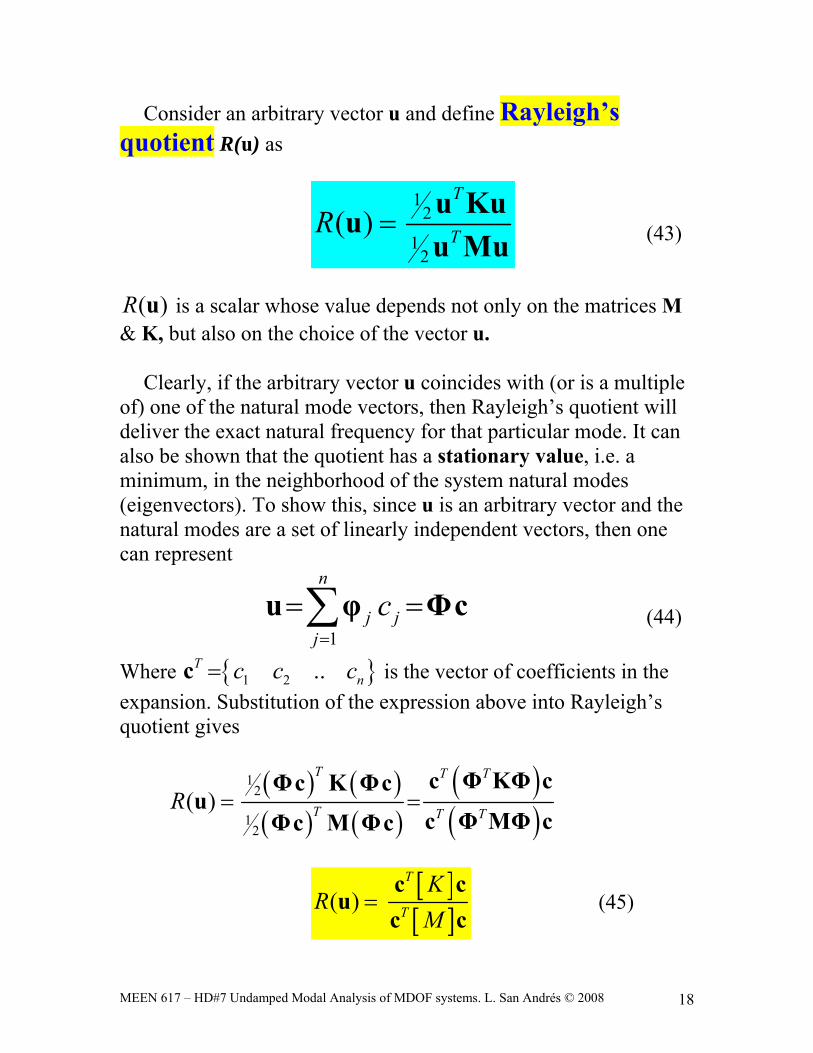
Consider an arbitrary vector u and define Rayleigh’s quotient R(u) as
12
12
( )T
TR =u Kuuu Mu (43)
( )R u is a scalar whose value depends not only on the matrices M
& K, but also on the choice of the vector u.
Clearly, if the arbitrary vector u coincides with (or is a multiple of) one of the natural mode vectors, then Rayleigh’s quotient will deliver the exact natural frequency for that particular mode. It can also be shown that the quotient has a stationary value, i.e. a minimum, in the neighborhood of the system natural modes (eigenvectors). To show this, since u is an arbitrary vector and the natural modes are a set of linearly independent vectors, then one can represent
1
n
j jj
c=
= =∑u φ Φc (44)
Where 1 2 ..Tnc c c=c is the vector of coefficients in the
expansion. Substitution of the expression above into Rayleigh’s quotient gives
( ) ( )( ) ( )
( )( )
12
12
( )T T T
T T TR = =
c Φ KΦ cΦc K Φcu
c Φ MΦ cΦc M Φc
[ ][ ]
( )T
T
KR
M=
c cu
c c (45)

MEEN 617 – HD#7 Undamped Modal Analysis of MDOF systems. L. San Andrés © 2008 19
Assume the modes have been normalized with respect to the
mass matrix, i.e. 2 2
21
2
1
( )i
n
T i nn i
nT
ii
cR
c
ωω=
=
⎡ ⎤⎣ ⎦= =∑
∑
c cu
c Ic (46a)
Next, consider that the arbitrary vector u (which at this time can be regarded as an assumed mode vector) differs very little from the natural mode (eigenvector) ( )rφ . This means that in the expansion of vector u, the coefficients ; for 1,2,... andi rc c i n i r<< = ≠ Or
; <<1 for 1,2,... andi i r ic c i n i rς ς= = ≠ Then, Rayleigh’s quotient is expressed as
2 2 2 2 2
1,
2 2 2
1,
( )r i
n
r n r i ni i r
n
r r ii i r
c cR
c c
ω ς ω
ς
= ≠
= ≠
+=
+
∑
∑u
( )22 2 2
1, 1,2
2 2
1, 1,
1( )
1 1
i nir i nr
r
n n
n i ni i r i i r
nn n
i ii i r i i r
R
ς ωωω ς ω
ως ς
= ≠ = ≠
= ≠ = ≠
+ += =
+ +
∑ ∑
∑ ∑u (46b)
The quantities 2iς are small, of second order, hence R(u) differs
from the natural frequency by a small quantity of second order.
MEEN 617 – HD#7 Undamped Modal Analysis of MDOF systems. L. San Andrés © 2008 20
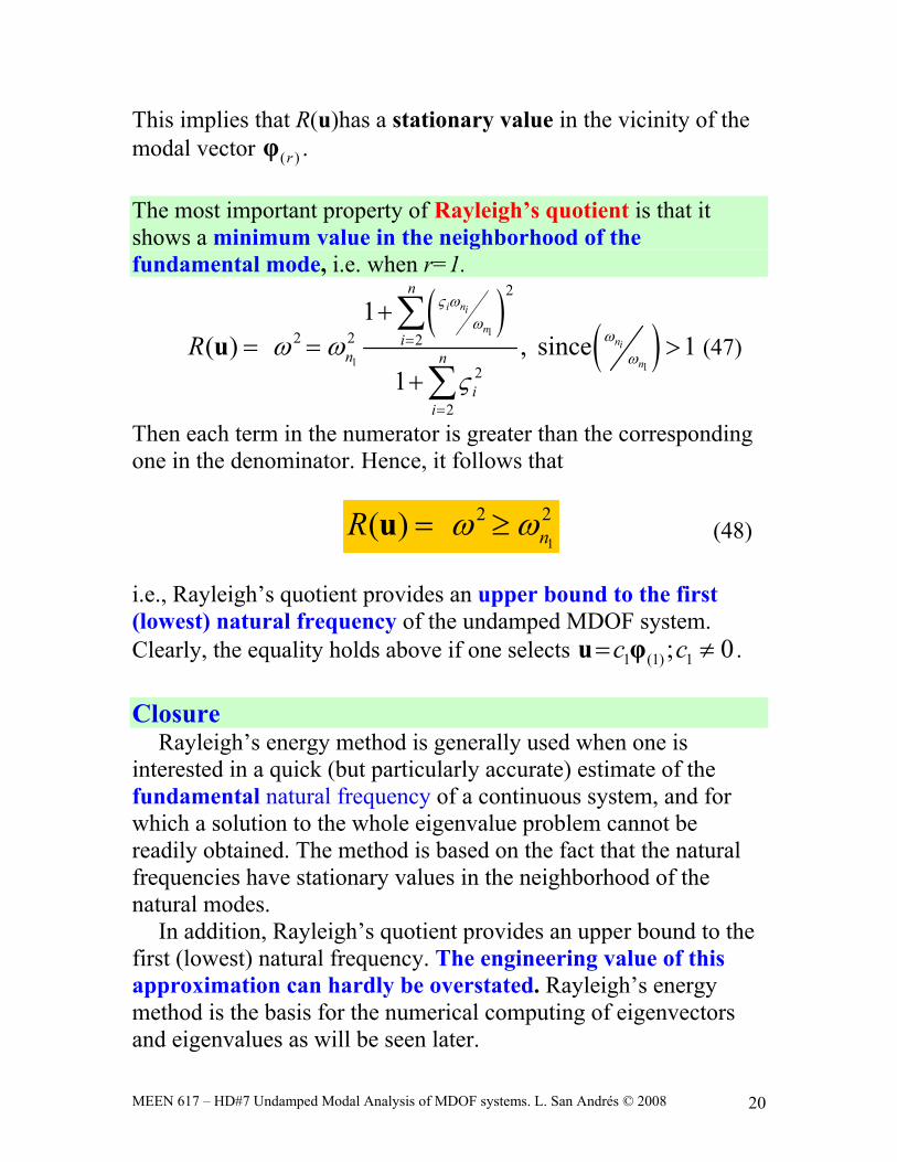
This implies that R(u)has a stationary value in the vicinity of the modal vector ( )rφ . The most important property of Rayleigh’s quotient is that it shows a minimum value in the neighborhood of the fundamental mode, i.e. when r=1.
( )( )1
1 1
2
2 2 2
2
2
1( ) , since 1
1
i ni
nni
n
n
in n
ii
R
ς ωω
ωωω ω
ς
=
=
+= = >
+
∑
∑u (47)
Then each term in the numerator is greater than the corresponding one in the denominator. Hence, it follows that
1
2 2( ) nR ω ω= ≥u (48) i.e., Rayleigh’s quotient provides an upper bound to the first (lowest) natural frequency of the undamped MDOF system. Clearly, the equality holds above if one selects 1 (1) 1; 0c c= ≠u φ . Closure
Rayleigh’s energy method is generally used when one is interested in a quick (but particularly accurate) estimate of the fundamental natural frequency of a continuous system, and for which a solution to the whole eigenvalue problem cannot be readily obtained. The method is based on the fact that the natural frequencies have stationary values in the neighborhood of the natural modes.
In addition, Rayleigh’s quotient provides an upper bound to the first (lowest) natural frequency. The engineering value of this approximation can hardly be overstated. Rayleigh’s energy method is the basis for the numerical computing of eigenvectors and eigenvalues as will be seen later.

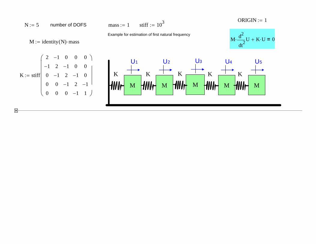
ORIGIN 1N 5 number of DOFS mass 1 stiff 103
Example for estimation of first natural frequencyM 2t
Ud
d
2 K U 0=M identity N( ) mass
K
M
U1
K
M
U2
K
M
U3
K
M
U4
K
M
U5
KK stiff
2
1
0
0
0
1
2
1
0
0
0
1
2
1
0
0
0
1
2
1
0
0
0
1
2
lsanandres
Callout
Prepared by Lecturer Luis San Andres for ME617 course
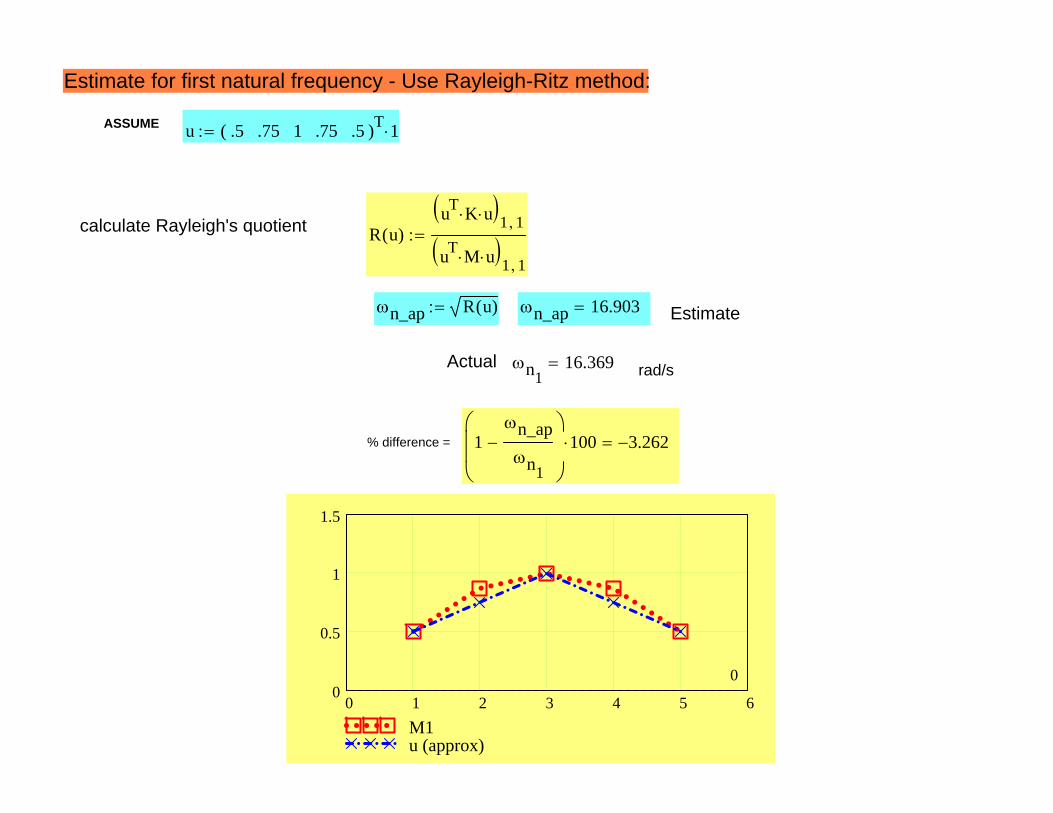
Estimate for first natural frequency - Use Rayleigh-Ritz method:
ASSUME u .5 .75 1 .75 .5( )T 1
calculate Rayleigh's quotient R u( )uT K u
1 1
uT M u 1 1
n_ap R u( ) n_ap 16.903 Estimate
Actual n116.369 rad/s
% difference = 1n_apn1
100 3.262
0 1 2 3 4 5 60
0.5
1
1.5
M1u (approx)
0
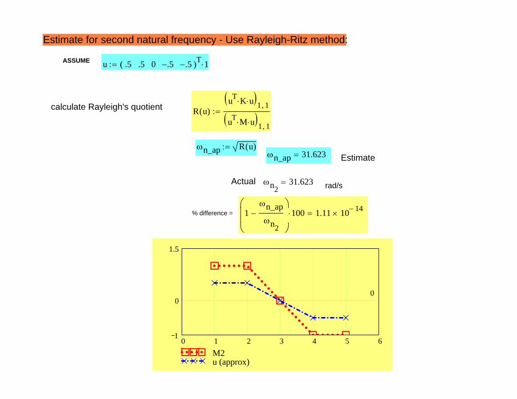
Estimate for second natural frequency - Use Rayleigh-Ritz method:
ASSUME u .5 .5 0 .5 .5( )T 1
calculate Rayleigh's quotient R u( )uT K u
1 1
uT M u 1 1
n_ap R u( )n_ap 31.623 Estimate
Actual n231.623 rad/s
% difference = 1n_apn2
100 1.11 10 14
0 1 2 3 4 5 61
0
1.5
M2u (approx)
0
ORIGIN 1N 5 number of DOFS mass 1 stiff 103
Example for estimation of first natural frequencyM 2t
Ud
d
2 K U 0=M identity N( ) mass
K
M
U1
K
M
U2
K
M
U3
K
M
U4
K
M
U5
K stiff
2
1
0
0
0
1
2
1
0
0
0
1
2
1
0
0
0
1
2
1
0
0
0
1
1
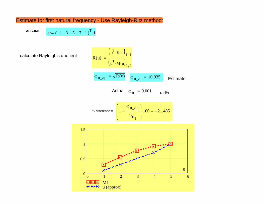
Estimate for first natural frequency - Use Rayleigh-Ritz method:
ASSUME u .1 .3 .5 .7 1( )T 1
calculate Rayleigh's quotient R u( )uT K u
1 1
uT M u 1 1
n_ap R u( ) n_ap 10.935 Estimate
Actual n19.001 rad/s
% difference = 1n_apn1
100 21.485
0 1 2 3 4 5 60
0.5
1
1.5
M1u (approx)
0
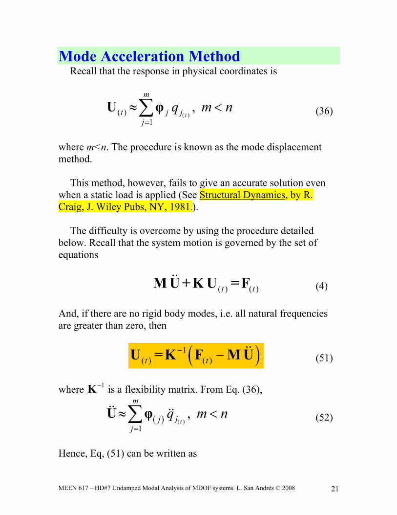
MEEN 617 – HD#7 Undamped Modal Analysis of MDOF systems. L. San Andrés © 2008 21
Mode Acceleration Method Recall that the response in physical coordinates is
( )( )1
,t
m
t j jj
q m n=
≈ <∑U φ (36)
where m<n. The procedure is known as the mode displacement method.
This method, however, fails to give an accurate solution even when a static load is applied (See Structural Dynamics, by R. Craig, J. Wiley Pubs, NY, 1981.).
The difficulty is overcome by using the procedure detailed below. Recall that the system motion is governed by the set of equations
( ) ( )t tM U +K U =F (4) And, if there are no rigid body modes, i.e. all natural frequencies are greater than zero, then
( )1( ) ( )t t
− −U =K F M U (51)
where 1−K is a flexibility matrix. From Eq. (36),
( ) ( )1
,t
m
jjj
q m n=
≈ <∑U φ (52)
Hence, Eq, (51) can be written as

MEEN 617 – HD#7 Undamped Modal Analysis of MDOF systems. L. San Andrés © 2008 22
( ) ( )
1 1( ) ( )
1t
m
t t jjj
q− −
=
≈ − ∑U K F K M φ (53)
Using the fundamental identity,
2 1( ) ( ) ( ) ( )2
1i i i i i
i
ωω
−= ⇒ =Kφ Mφ φ K Mφ
Write Eq. (53) as
( )( )
1( ) ( ) 2
1t
mj
t t jj j
qω
−
=
⎛ ⎞≈ − ⎜ ⎟⎜ ⎟
⎝ ⎠∑
φU K F (54)
Note that 1
( )S t−=U K F (55)
is the displacement response vector due to a “pseudo-static” force F(t), i.e. without the system inertia accounted for. Hence write Eq. (54), as
( )
( )( ) ( ) 21
t
mj
t s t jj j
qω=
⎛ ⎞≈ − ⎜ ⎟⎜ ⎟
⎝ ⎠∑
φU U ; m<n (56)
The second term above can be thought as the “inertia induced response.” Example: Consider the case of force excitation with frequency
jnωΩ ≠ and acting for very long times. The EOMs in physical space are:
MEEN 617 – HD#7 Undamped Modal Analysis of MDOF systems. L. San Andrés © 2008 23
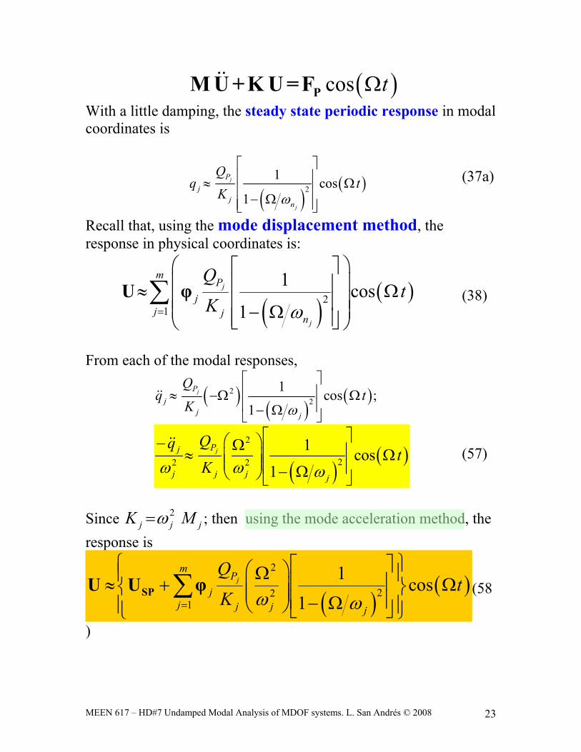
( )cos tΩPM U +K U =F With a little damping, the steady state periodic response in modal coordinates is
( )( )2
1 cos1
j
j
Pj
j n
Qq t
K ω
⎡ ⎤⎢ ⎥≈ Ω⎢ ⎥− Ω⎢ ⎥⎣ ⎦
(37a)
Recall that, using the mode displacement method, the response in physical coordinates is:
( )( )2
1
1 cos1
j
j
mP
jj j n
Qt
K ω=
⎛ ⎞⎡ ⎤⎜ ⎟⎢ ⎥≈ Ω⎜ ⎟⎢ ⎥⎜ ⎟− Ω⎢ ⎥⎣ ⎦⎝ ⎠
∑U φ (38)
From each of the modal responses,
( )( )
( )22
1 cos ;1
jPj
j j
Qq t
K ω
⎡ ⎤⎢ ⎥≈ −Ω Ω⎢ ⎥− Ω⎣ ⎦
( )( )
2
22 2
1 cos1
jPj
j j j j
Qqt
Kω ω ω
⎡ ⎤⎛ ⎞− Ω ⎢ ⎥≈ Ω⎜ ⎟⎜ ⎟ ⎢ ⎥− Ω⎝ ⎠ ⎣ ⎦
(57)
Since 2
j j jK Mω= ; then using the mode acceleration method, the response is
( )( )
2
221
1 cos1
jm
Pj
j j j j
Qt
K ω ω=
⎧ ⎫⎡ ⎤⎛ ⎞Ω⎪ ⎪⎢ ⎥≈ + Ω⎜ ⎟⎨ ⎬⎜ ⎟ ⎢ ⎥− Ω⎝ ⎠⎪ ⎪⎣ ⎦⎩ ⎭∑SPU U φ (58
)
lsanandres
Highlight
MEEN 617 – HD#7 Undamped Modal Analysis of MDOF systems. L. San Andrés © 2008 24
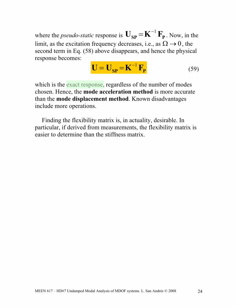
where the pseudo-static response is 1−=SP PU K F . Now, in the
limit, as the excitation frequency decreases, i.e., as 0Ω→ , the second term in Eq. (58) above disappears, and hence the physical response becomes:
1−= =SP PU U K F (59) which is the exact response, regardless of the number of modes chosen. Hence, the mode acceleration method is more accurate than the mode displacement method. Known disadvantages include more operations.
Finding the flexibility matrix is, in actuality, desirable. In particular, if derived from measurements, the flexibility matrix is easier to determine than the stiffness matrix.
lsanandres
Highlight
are symmetric matrices
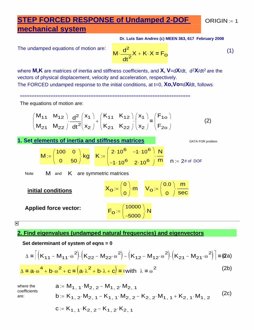
Xo0
0⎛⎜⎝
⎞⎟⎠
m⋅:= Vo0.0
0⎛⎜⎝
⎞⎟⎠
msec
⋅:=initial conditions
Applied force vector: Fo10000
5000−⎛⎜⎝
⎞⎟⎠
N⋅:=
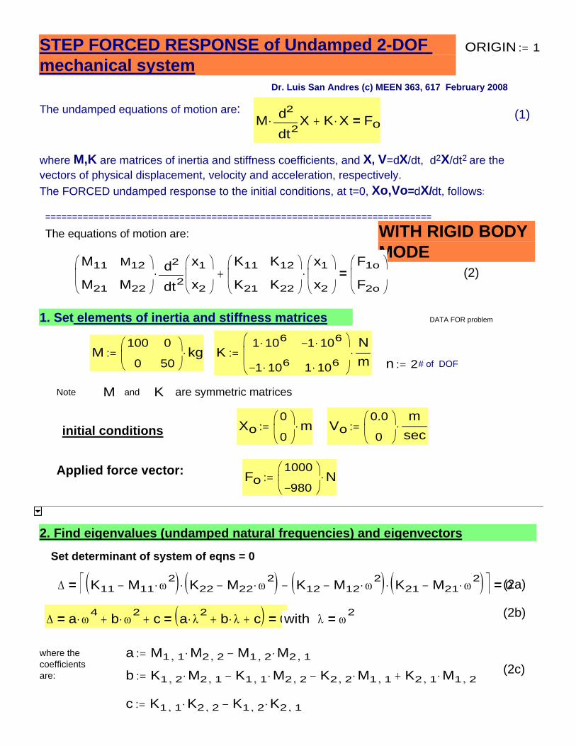
2. Find eigenvalues (undamped natural frequencies) and eigenvectors
Set determinant of system of eqns = 0
Δ K11 M11 ω2
⋅−( ) K22 M22 ω2
⋅−( )⋅ K12 M12 ω2
⋅−( ) K21 M21 ω2
⋅−( )⋅−⎡⎣ ⎤⎦= 0= (2a)
(2b)Δ a ω4
⋅ b ω2
⋅+ c+= a λ2
⋅ b λ⋅+ c+( )= 0= with λ ω2=
where thecoefficientsare:
a M1 1, M2 2,⋅ M1 2, M2 1,⋅−:=(2c)b K1 2, M2 1,⋅ K1 1, M2 2,⋅− K2 2, M1 1,⋅− K2 1, M1 2,⋅+:=
c K1 1, K2 2,⋅ K1 2, K2 1,⋅−:=
STEP FORCED RESPONSE of Undamped 2-DOF mechanical system
ORIGIN 1:=
Dr. Luis San Andres (c) MEEN 363, 617 February 2008
The undamped equations of motion are: (1)M2t
Xdd
2⋅ K X⋅+ Fo=
where M,K are matrices of inertia and stiffness coefficients, and X, V=dX/dt, d2X/dt2 are the vectors of physical displacement, velocity and acceleration, respectively. The FORCED undamped response to the initial conditions, at t=0, Xo,Vo=dX/dt, follows:
========================================================================
The equations of motion are:
M11
M21
M12
M22
⎛⎜⎝
⎞⎟⎠ 2t
x1
x2
⎛⎜⎝
⎞⎟⎠
dd
2⋅
K11
K21
K12
K22
⎛⎜⎝
⎞⎟⎠
x1
x2
⎛⎜⎝
⎞⎟⎠
⋅+F1o
F2o
⎛⎜⎝
⎞⎟⎠
= (2)
1. Set elements of inertia and stiffness matrices DATA FOR problem
M100
0
0
50⎛⎜⎝
⎞⎟⎠
kg⋅:= K2 106⋅
1− 106⋅
1− 106⋅
2 106⋅
⎛⎜⎝
⎞⎟⎠
Nm
⋅:=n 2:= # of DOF
Note M and K
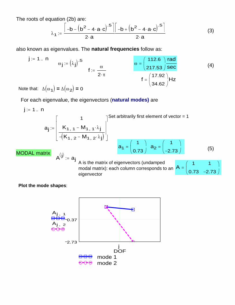
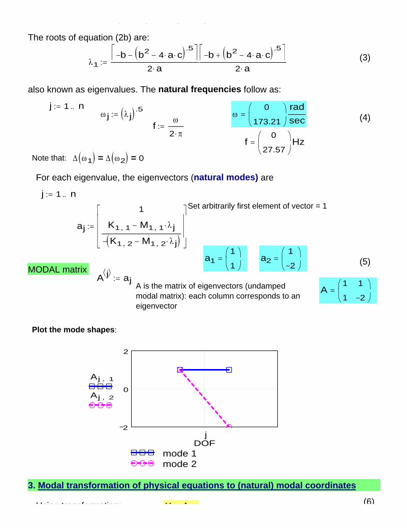
2.73
0.37
mode 1mode 2
DOF
Aj 1,
Aj 2,
j
Plot the mode shapes:
A1
0.73
1
2.73−⎛⎜⎝
⎞⎟⎠
=A is the matrix of eigenvectors (undampedmodal matrix): each column corresponds to an eigenvector
A j⟨ ⟩ aj:=MODAL matrix
(5)a21
2.73−⎛⎜⎝
⎞⎟⎠
=a11
0.73⎛⎜⎝
⎞⎟⎠
=
aj
1
K1 1, M1 1, λ j⋅−
K1 2, M1 2, λ j⋅−( )−
⎡⎢⎢⎢⎣
⎤⎥⎥⎥⎦
:=
Set arbitrarily first element of vector = 1j 1 n..:=
For each eigenvalue, the eigenvectors (natural modes) are
Δ ω1( ) Δ ω2( )= 0=Note that:
f17.92
34.62⎛⎜⎝
⎞⎟⎠Hz=
fω
2 π⋅:=
(4)ω112.6
217.53⎛⎜⎝
⎞⎟⎠
radsec
=ω j λ j( ) .5:=j 1 n..:=
also known as eigenvalues. The natural frequencies follow as:
λ2b− b2 4 a⋅ c⋅−( ) .5+⎡⎣ ⎤⎦
2 a⋅:=λ1
b− b2 4 a⋅ c⋅−( ) .5−⎡⎣ ⎤⎦2 a⋅
:= (3)
The roots of equation (2b) are:
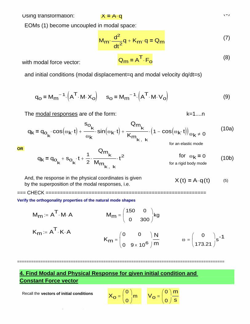
for an elastic modeOR
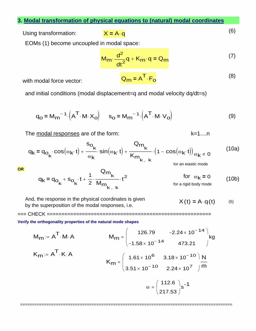
for ωk 0=qk qok
sok
t⋅+12
Qmk
Mmk k,
⋅ t2⋅+= (10b)for a rigid body mode
And, the response in the physical coordinates is givenby the superposition of the modal responses, i.e.
X t( ) A q t( )⋅= (5)
=== CHECK ========================================================Verify the orthogonality properties of the natural mode shapes
Mm AT M⋅ A⋅:= Mm126.79
1.58− 10 14−×
2.24− 10 14−×
473.21
⎛⎜⎝
⎞⎟⎠kg=
Km AT K⋅ A⋅:=Km
1.61 106×
3.51 10 10−×
3.18 10 10−×
2.24 107×
⎛⎜⎝
⎞⎟⎠
Nm
=
ω112.6
217.53⎛⎜⎝
⎞⎟⎠s-1=
=========================================================================================
3. Modal transformation of physical equations to (natural) modal coordinates
(6)Using transformation: X A q⋅=EOMs (1) become uncoupled in modal space:
(7) Mm 2tqd
d
2⋅ Km q⋅+ Qm=
(8)Qm AT Fo⋅=with modal force vector:
and initial conditions (modal displacement=q and modal velocity dq/dt=s)
qo Mm1− AT M⋅ Xo⋅( )⋅= so Mm
1− AT M⋅ Vo⋅( )⋅= (9)
The modal responses are of the form: k=1....n
(10a)qk qok
cos ωk t⋅( )⋅so
k
ωksin ωk t⋅( )⋅+
Qmk
Kmk k,
1 cos ωk t⋅( )−( )⋅+= ωk 0≠
lsanandres
Line
lsanandres
Line
lsanandres
Line
lsanandres
Line
0.01Response in modal coordinates
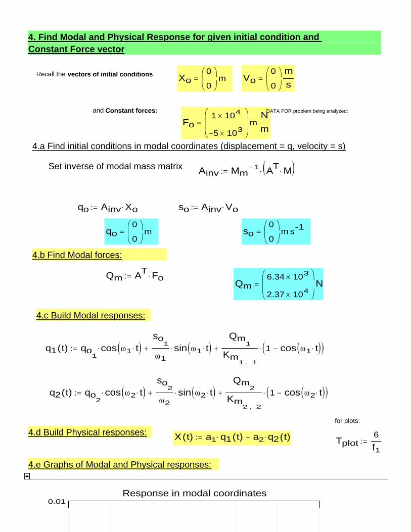
4.e Graphs of Modal and Physical responses:
Tplot6f1
:=X t( ) a1 q1 t( )⋅ a2 q2 t( )⋅+:=4.d Build Physical responses:for plots:
q2 t( ) qo2
cos ω2 t⋅( )⋅so
2
ω2sin ω2 t⋅( )⋅+
Qm2
Km2 2,
1 cos ω2 t⋅( )−( )⋅+:=
q1 t( ) qo1
cos ω1 t⋅( )⋅so
1
ω1sin ω1 t⋅( )⋅+
Qm1
Km1 1,
1 cos ω1 t⋅( )−( )⋅+:=
4.c Build Modal responses:
Qm6.34 103×
2.37 104×
⎛⎜⎝
⎞⎟⎠N=
Qm AT Fo⋅:=
4.b Find Modal forces:
so0
0⎛⎜⎝
⎞⎟⎠m s-1=qo
0
0⎛⎜⎝
⎞⎟⎠m=
so Ainv Vo⋅:=qo Ainv Xo⋅:=
Ainv Mm1− AT M⋅( )⋅:=Set inverse of modal mass matrix
4.a Find initial conditions in modal coordinates (displacement = q, velocity = s)
Fo1 104×
5− 103×
⎛⎜⎝
⎞⎟⎠m
Nm
=DATA FOR problem being analyzed:and Constant forces:
Vo0
0⎛⎜⎝
⎞⎟⎠
ms
=Xo0
0⎛⎜⎝
⎞⎟⎠m=Recall the vectors of initial conditions
4. Find Modal and Physical Response for given initial condition and Constant Force vector
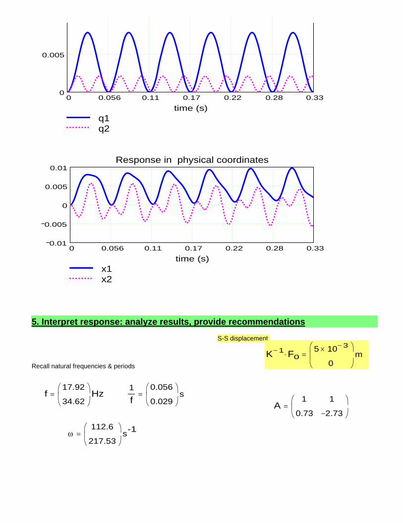
0 0.056 0.11 0.17 0.22 0.28 0.330
0.005
q1q2
time (s)
0 0.056 0.11 0.17 0.22 0.28 0.330.01
0.005
0
0.005
0.01
x1x2
Response in physical coordinates
time (s)
5. Interpret response: analyze results, provide recommendations
S-S displacement
K 1− Fo⋅5 10 3−×
0
⎛⎜⎝
⎞⎟⎠m=
Recall natural frequencies & periods
f17.92
34.62⎛⎜⎝
⎞⎟⎠Hz=
1f
0.056
0.029⎛⎜⎝
⎞⎟⎠s=
A1
0.73
1
2.73−⎛⎜⎝
⎞⎟⎠
=
ω112.6
217.53⎛⎜⎝
⎞⎟⎠s-1=
K are symmetric matrices
Xo0
0⎛⎜⎝
⎞⎟⎠
m⋅:= Vo0.0
0⎛⎜⎝
⎞⎟⎠
msec
⋅:=initial conditions
Applied force vector: Fo1000
980−⎛⎜⎝
⎞⎟⎠
N⋅:=
2. Find eigenvalues (undamped natural frequencies) and eigenvectors
Set determinant of system of eqns = 0
Δ K11 M11 ω2⋅−( ) K22 M22 ω2⋅−( )⋅ K12 M12 ω2⋅−( ) K21 M21 ω2⋅−( )⋅−⎡⎣ ⎤⎦= 0= (2a)
(2b)Δ a ω4⋅ b ω2⋅+ c+= a λ2⋅ b λ⋅+ c+( )= 0= with λ ω2=
where thecoefficientsare:
a M1 1, M2 2,⋅ M1 2, M2 1,⋅−:=(2c)b K1 2, M2 1,⋅ K1 1, M2 2,⋅− K2 2, M1 1,⋅− K2 1, M1 2,⋅+:=
c K1 1, K2 2,⋅ K1 2, K2 1,⋅−:=
STEP FORCED RESPONSE of Undamped 2-DOF mechanical system
ORIGIN 1:=
Dr. Luis San Andres (c) MEEN 363, 617 February 2008
The undamped equations of motion are: (1)M2t
Xdd
2⋅ K X⋅+ Fo=
where M,K are matrices of inertia and stiffness coefficients, and X, V=dX/dt, d2X/dt2 are the vectors of physical displacement, velocity and acceleration, respectively. The FORCED undamped response to the initial conditions, at t=0, Xo,Vo=dX/dt, follows:
========================================================================
The equations of motion are: WITH RIGID BODY MODEM11
M21
M12
M22
⎛⎜⎝
⎞⎟⎠ 2t
x1
x2
⎛⎜⎝
⎞⎟⎠
dd
2⋅
K11
K21
K12
K22
⎛⎜⎝
⎞⎟⎠
x1
x2
⎛⎜⎝
⎞⎟⎠
⋅+F1o
F2o
⎛⎜⎝
⎞⎟⎠
= (2)
1. Set elements of inertia and stiffness matrices DATA FOR problem
M100
0
0
50⎛⎜⎝
⎞⎟⎠
kg⋅:= K1 106⋅
1− 106⋅
1− 106⋅
1 106⋅
⎛⎜⎝
⎞⎟⎠
Nm
⋅:=n 2:= # of DOF
Note M and
lsanandres
Rectangle
lsanandres
Text Box
RIGID BODY MODE
X AUsing transformation: (6)
3. Modal transformation of physical equations to (natural) modal coordinates
2
0
2
mode 1mode 2
DOF
Aj 1,
Aj 2,
j
Plot the mode shapes:
A1
1
1
2−⎛⎜⎝
⎞⎟⎠
=A is the matrix of eigenvectors (undampedmodal matrix): each column corresponds to an eigenvector
A j⟨ ⟩ aj:=MODAL matrix
(5)a21
2−⎛⎜⎝
⎞⎟⎠
=a11
1⎛⎜⎝
⎞⎟⎠
=
aj
1
K1 1, M1 1, λ j⋅−
K1 2, M1 2, λ j⋅−( )−
⎡⎢⎢⎢⎣
⎤⎥⎥⎥⎦
:=
Set arbitrarily first element of vector = 1j 1 n..:=
For each eigenvalue, the eigenvectors (natural modes) are
Δ ω1( ) Δ ω2( )= 0=Note that:
f0
27.57⎛⎜⎝
⎞⎟⎠Hz=
fω
2 π⋅:=
(4)ω0
173.21⎛⎜⎝
⎞⎟⎠
radsec
=ω j λ j( ) .5:=j 1 n..:=
also known as eigenvalues. The natural frequencies follow as:
λ2b− b2 4 a⋅ c⋅−( ) .5+⎡⎣ ⎤⎦
2 a⋅:=λ1
b− b2 4 a⋅ c⋅−( ) .5−⎡⎣ ⎤⎦2 a⋅
:= (3)
The roots of equation (2b) are:
, , , ,
ωk 0=qk qok
sok
t⋅+12
Qmk
Mmk k,
⋅ t2⋅+= (10b)for a rigid body mode
And, the response in the physical coordinates is givenby the superposition of the modal responses, i.e.
X t( ) A q t( )⋅= (5)
=== CHECK ========================================================Verify the orthogonality properties of the natural mode shapes
Mm AT M⋅ A⋅:= Mm150
0
0
300⎛⎜⎝
⎞⎟⎠kg=
Km AT K⋅ A⋅:=Km
0
0
0
9 106×
⎛⎜⎝
⎞⎟⎠
Nm
= ω0
173.21⎛⎜⎝
⎞⎟⎠s-1=
=========================================================================================
4. Find Modal and Physical Response for given initial condition and Constant Force vector
Recall the vectors of initial conditions Xo0
0⎛⎜⎝
⎞⎟⎠m= Vo
0
0⎛⎜⎝
⎞⎟⎠
ms
=
d C t t f
(6)Using transformation: X A q⋅=
EOMs (1) become uncoupled in modal space:
(7) Mm 2tqd
d
2⋅ Km q⋅+ Qm=
(8)Qm AT Fo⋅=with modal force vector:
and initial conditions (modal displacement=q and modal velocity dq/dt=s)
qo Mm1− AT M⋅ Xo⋅( )⋅= so Mm
1− AT M⋅ Vo⋅( )⋅= (9)
The modal responses are of the form: k=1....n
(10a)qk qok
cos ωk t⋅( )⋅so
k
ωksin ωk t⋅( )⋅+
Qmk
Kmk k,
1 cos ωk t⋅( )−( )⋅+= ωk 0≠
for an elastic modeOR
for
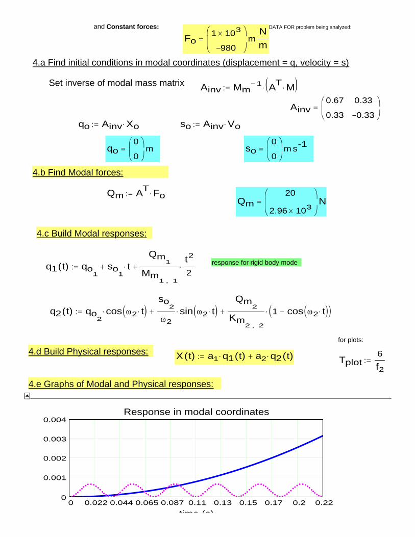
0 0.022 0.044 0.065 0.087 0.11 0.13 0.15 0.17 0.2 0.220
0.001
0.002
0.003
0.004Response in modal coordinates
time (s)
4.e Graphs of Modal and Physical responses:
Tplot6f2
:=X t( ) a1 q1 t( )⋅ a2 q2 t( )⋅+:=4.d Build Physical responses:for plots:
q2 t( ) qo2
cos ω2 t⋅( )⋅so
2
ω2sin ω2 t⋅( )⋅+
Qm2
Km2 2,
1 cos ω2 t⋅( )−( )⋅+:=
q1 t( ) qo1
so1
t⋅+Qm
1
Mm1 1,
t2
2⋅+:= response for rigid body mode
4.c Build Modal responses:
Qm20
2.96 103×
⎛⎜⎝
⎞⎟⎠N=
Qm AT Fo⋅:=
4.b Find Modal forces:
so0
0⎛⎜⎝
⎞⎟⎠m s-1=qo
0
0⎛⎜⎝
⎞⎟⎠m=
so Ainv Vo⋅:=qo Ainv Xo⋅:=
Ainv0.67
0.33
0.33
0.33−⎛⎜⎝
⎞⎟⎠
=
Ainv Mm1− AT M⋅( )⋅:=Set inverse of modal mass matrix
4.a Find initial conditions in modal coordinates (displacement = q, velocity = s)
Fo1 103×
980−
⎛⎜⎝
⎞⎟⎠m
Nm
=DATA FOR problem being analyzed:and Constant forces:
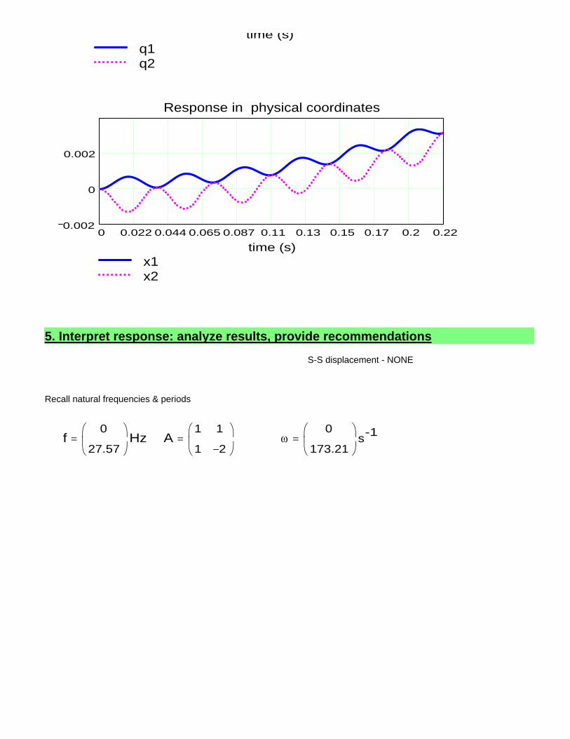
q1q2
time (s)
0 0.022 0.044 0.065 0.087 0.11 0.13 0.15 0.17 0.2 0.220.002
0
0.002
x1x2
Response in physical coordinates
time (s)
5. Interpret response: analyze results, provide recommendations
S-S displacement - NONE
Recall natural frequencies & periods
f0
27.57⎛⎜⎝
⎞⎟⎠Hz= A
1
1
1
2−⎛⎜⎝
⎞⎟⎠
= ω0
173.21⎛⎜⎝
⎞⎟⎠s-1=