FROM THE GROUND UP:

AN AGENT-BASED MODEL OF

REGIONAL STRUCTURAL CHANGE

A Thesis

Submitted to the College of Graduate Studies and Research

in Partial Fulfillment of the Requirements

for the Degree of

Master of Science

In the

Department of Agricultural Economics

University of Saskatchewan

by

Tyler R. Freeman

© Copyright Tyler R. Freeman, October 2005. All Rights Reserved

i

PERMISSION TO USE

In presenting this thesis in partial fulfillment of the requirements for a Postgraduate degree from the

University of Saskatchewan, I agree that the Libraries of this University may make it freely available for

inspection. I further agree that permission for copying of this thesis in any manner, in whole or in part, for

scholarly purposes may be granted by the professor or professors who supervised my thesis work or, in

their absence, by the Head of the Department of the Dean of the College in which my thesis work was

done. It is understood that any copying or publication or use of this thesis or parts thereof for financial gain

shall not be allowed without my written permission. It is also understood that due recognition will be given

to me and the University of Saskatchewan in any scholarly use that may be made of any material in this

thesis.

Requests for permission to copy or to make other use of the material in this thesis in whole or part should

be addressed to:

Head of the Department of Agricultural Economics University of Saskatchewan Saskatoon, Saskatchewan S7N 5A8

ii

ABSTRACT

Freeman, Tyler, M.Sc. University of Saskatchewan, Saskatoon, October 2005. From the Ground Up: An Agent-Based Model of Regional Structural Change. Supervisors: J. F. Nolan and R. A. Schoney. The Saskatchewan farm sector is a dynamic system that is faced with the reality of farm consolidation and

other structural adjustments. While structural adjustment may result in increased productivity at the farm-

level, the declining farm population has a direct impact on rural regions. Given the economic difficulties

now inherent in many rural regions, there has never been a more important time to improve our

understanding of the structural dynamics of the farm sector.

By utilizing agent-based methods, competition that exists between farm households in land markets is

modelled in a dynamic framework. By modeling land markets in this manner, structural adjustments that

occur due to the re-allocation of land among farm household becomes endogenous to the model. The

farming simulation was validated by evaluating its ability to replicate actual structural shifts that occurred

during the period of 1960-2000. The results obtained from the simulation were found to mirror historic

shifts, which gives the author confidence that the parsimonious assumptions made are robust, yet still

characteristic of farm level behaviour in the region. Other scenarios were simulated in order to estimate a

counterfactual structural evolution of the modelled region, in the absence of government stabilization and

support programs. Significant deviations are observed between the base and zero transfer scenarios with

regards to the consolidation of farm assets among a declining number of farm households. Most

significantly, the decline in farm numbers accelerated significantly in the late 1980’s in the zero transfer

scenario compared to the base simulations.

The application of an agent-based framework allowed for the study of regional structure with an emphasis

on the behaviour and actions of the primary decisions makers within the system. While structural change is

driven by a number of factors, the ability of a farm household to fully employ their labour resource was an

important factor in the simulations. This contrasts with the finding that productive efficiency, and

purchasing and market power at the farm level is not a necessary condition for the observed consolidation

of farm assets.

iii

ACKNOWLEDGEMENTS

As I look back on the occasionally random path that has lead me to this point, I realize the substantial

number of people that have played an important role in helping keep me on course. A great debt of

gratitude is owed to you all.

To my supervisors Dr. James Nolan and Dr. Richard Schoney, for giving me the freedom to seek my way

through an unfamiliar field of research while offering timely and professional guidance and

encouragement.

To committee member William Brown and external examiner Dr. Derek Brewin, for their enthusiasm and

professional insight that made for both a challenging and rewarding defence and an improved final product.

To my parents, who always offered their full support and love and taught me the value of an honest day’s

work. To my family, for their encouragement and willingness to offer research suggestions and alternative

views on economic theory. You always gave me something to think about (or laugh at).

And finally, to my fellow classmates who quickly realized that no matter what side they took on any issue I

would always argue the opposite. You made the past two years a memorable experience.

iv

TABLE OF CONTENTS

PERMISSION TO USE ……………………………………………………………………...................... i ABSTRACT ………………………………………………………………………………....................... ii ACKNOWLEDEMENTS …………………………………………………………………….................. iii TABLE OF CONTENTS ……………………………………………………………………................... iv LIST OF TABLES ..............................................................................................................................…... vi LIST OF FIGURES …………………………………………………………………............................... vii CHAPTER ONE ...………………………………………………………………………………………… 1 1.0 Introduction ………………………………………………………………………………………. 1 1.1 Objectives ………………………………………………………………………………………… 2 1.2 Motivation for Study ………………………………………………………………………..……. 3 1.3 Thesis Organization …………………………………………………………………………….… 4 CHAPTER TWO…………………………………………………………………………………………... 5 2.0 Introduction ………………………………………………………………….……………………. 5 2.1 What is Structural Change? ………………………………………………………………………. 5 2.2 Trends and Patterns of Structural Change in Saskatchewan Agriculture ………………………… 6 2.3 Forces Driving Structural Change …………………………………………………………….… 11 2.3.1 Technology and Relative Factor Prices ………………………………………………...... 11 2.3.2 Labour Mobility and Non-Farm Opportunities …………………………........................... 13 2.3.3 Capital Immobility ……………………………………………………….......................... 13 2.3.4 Demographics and the Life-Cycle Hypothesis ……………………………....................... 14 2.3.5 Productive Heterogeneity …………………………………………………........................ 15 2.4 Farm Management / Entrepreneurship ……………………………………….........................…. 16 2.5 Summary …………………………………………………………………….........................….. 17 CHAPTER THREE ………………………………………………………………...........................……. 19 3.0 Introduction ……………………………………………………………………........................... 19 3.1 An Alternative to the Neoclassical Economic “Toolkit” ……………………………................. 20 3.2 Current Farm-Level / Land-Use Modeling Methodologies …………………..........................… 22 3.2.1 Farm Budgeting / Planning Models ……………………………………........................… 22 3.2.2 Equation Driven Models ……………………………………………….........................… 23 3.3 Agent-Based Systems: A New Farm-Level Modeling Paradigm ……………............................. 25 3.3.1 Why Agent-Based Methods? …………………………………………..........................… 27 3.3.1.1 Flexibility and Complexity ………………………………………........................... 27 3.3.1.2 Emergent Characteristics ………………………………………..........................… 28 3.3.1.3 The Importance of Time and Space ……………………………..........................… 29 3.3.1.4 The Importance of Heterogeneous Producers …......................……......................... 29 3.3.2 Challenges and Limitations ……………………………………………............................ 30 3.4 Summary …………………………………………………………………….............................. 32 CHAPTER FOUR …………………………………………………………………..............................… 34 4.0 Introduction …………………………………………………………………............................... 34 4.1 Central Model Assumptions ......................................................................................................... 35 4.2 NetLogo© Platform …………………………………………………………............................... 36 4.3 Model Logic and Organization ..................................................................................................... 37 4.4 Production Factors …………………………………………………………................................. 38 4.4.1 Land …………………………………………………………………............................… 38 4.4.2 Farm Labour and Capital …………………………………………………….................... 40 4.5 Risk Preference / Entrepreneurial Classification / Farm Goals ……………................................ 40 4.6 The Farm Agent - Farm Actions …………………………………………................................... 42 4.6.1 Crop Production …………………………………………………….................................. 42 4.6.1.1 Gross Crop Revenue …………………………………………................................. 43 4.6.1.2 Variable Production Costs ……….……………………………............................... 45 4.6.1.3 Fixed Production Costs …………………………………………............................. 46 4.6.1.4 Family / Management Withdrawal ……………………………............................... 47 4.6.2 Farm Accounting ……………………………………………………................................ 48 4.6.3 Expectation Formation ………………………………………………............................... 49

v

4.6.4 Farm Management ………………………………………………….................................. 51 4.6.4.1 Farm Exits ……………………………………………………................................ 51 4.6.4.2 Crop Mix Adjustment ………………………………………….............................. 52 4.6.5 Farmland Market ………………………………………………………........................... 53 4.6.6 Non-Land Capital Investment …………………………………………………................ 59 4.7 Initializing the Model……………………………………………………................................... 60 4.7.1 Initial Farm Population Profile …………………………………….................................. 61 4.7.1.1 Operator Age and Farm Acreage ……………………………................................. 61 4.7.1.2 Land Tenure ……………………………………………….................................… 62 4.7.1.3 Assets and Debt …………………………………………………............................ 62 4.7.1.4 Risk Attitude / Entrepreneurial Classification / Farm Goals ………........................ 63 4.7.2 Production Data …………...……………………………………….................................... 64 4.7.2.1 Crop Yields and Price …………...……………………………................................ 64 4.7.2.2 Variable Costs ……………………...…………………………................................ 66 4.7.2.3 Fixed Costs and Debt Servicing ...……………………………................................. 68 4.7.2.4 Family / Management Withdrawal ….……………...…………............................... 69 4.7.3 Behavioural Data ……………..…………………………………….................................. 69 4.7.3.1 Crop Mix …………………...…………………………………................................ 70 4.7.3.2 Land Valuation …………………...…………………………................................... 70 4.7.3.3 Retirement and Intergenerational Transfers ………………….................................. 71 4.7.4 Using the Model: Assessing the impact of Farm Stabilization and Support Programs ...... 72 4.7.4.1 The Agricultural Stabilization Act ………………………….................................... 73 4.7.4.2 Western Grain Stabilization Act ……………………………................................... 73 4.7.4.3 Special Canadian Grains and Drought Assistance Programs ………....................... 76 4.7.4.4 Farm Income Protection Act …………….…………………................................... 77 4.7.4.5 Agricultural Income Disaster Assistance …………………..................................... 80 4.8 Summary ....................................................................................................................................... 81 CHAPTER FIVE ....................................................................................................................................... 82 5.0 Introduction .................................................................................................................................. 82 5.1 Simulation Results: Base Scenario ……………………………………….................................... 83 5.1.1 Number and Mean Size of Farms …………………………………................................ ... 83 5.1.2 Distribution of Farm Size …………………………………………................................ ... 85 5.1.3 The Land Market …………………………………………………................................. ... 87 5.1.4 Farm Debt …………………………………………………………................................ ... 90 5.1.5 Farm Exits …………………………………………………………................................... 91 5.2 Simulation Results: Zero Transfer Scenario ……………………………..................................... 93 5.2.1 Number and Mean Size of Farms ………………………………….................................. 93 5.2.2 Distribution of Farm Size ………………………………………….................................. 95 5.2.3 The Land Market ………………………………………………….................................... 96 5.2.4 Farm Debt ………………………………………………………….................................. 97 5.3 Model Drivers and Structural Change .......................................................…............................... 98 5.3.1 Entrepreneurial Behaviour and Farm Household Expectations ...…………...................... 98 5.3.2 Cost of Production and Productive Efficiency …………...……………............................ 100 5.3.3 Path Dependence and the Farm Life-Cycle ..……………………….................................. 101 5.3.4 Government Transfers and Regional Structure................................................................. 102 5.4 Summary ……………………………………………………………........................................ 103 CHAPTER SIX ....................................................................................................................................... 105 6.1 Summary …………………………………………………………….....................................… 105 6.2 Conclusions ………………………………………………………….....................................… 106 6.3 Limitations…………................................................................................................................... 107 6.4 Suggestions for Further Study .................................………………………............................... 108 REFERENCES …………………………………………….................................……………………… 110 APPENDIX A …………………………………………………………………….................................. 116 APPENDIX B ...............................................................................................................…........................ 118 APPENDIX C ........................................................................................................................................... 121

vi

LIST OF TABLES Table 4.1: Initial Distribution of Farm Agents by Age and Plots Managed ………………………......... 61 Table 4.2: Distribution of Farms by Tenure …………………………………………………….........… 62 Table 4.3: Value of Farm Assets 1960 ……………………………………………………………......... 63 Table 4.4: Farm Debt of Grain Farms by Age of Operator and Size in the Prairie Region...................... 63 Table 4.5: Managerial Classification and Risk Aversion Factor ……………………………..............… 64 Table 4.6: Simulated Managerial Distributions ………………………………………………............… 64 Table 4.7: Detrended Crop Yields and Price 1955-2002 …………………………………………......... 65 Table 4.8: Whole Farm Data, Dark Brown Soil Zone, Saskatchewan, 1961-1964 ……......................... 66 Table 4.9: Estimated Crop Production Variable Costs (excluding non-family labour)………………... 67 Table 4.10: Crop Acreages (percent of total), Saskatchewan, 1960-1964 ................................................ 70 Table 4.11: Land Valuation and Management Classification ………………………………...........…..... 71 Table 4.12: Net Exit of Farm Operators by Age Cohort (1961-1986) ………………………………....... 72 Table 5.1: Simulation Results (Base Scenario) - Farm Exits by Exit Type …………………………..... 91 Table 5.2: Simulation Results (Base Scenario) - Farm Exits by Managerial Class ………………......... 91 Table 5.3: Simulation Results (Base Scenario) - Farm Exits and Initial Farm Attributes ………........... 92 Table 5.4: Simulation Results (Base Scenario) - Farm Exits by Farm Size (acres) ……………….....… 92 Table B.1: Agricultural Stabilization Act Crop Subsidies ....................................................................... 120

vii

LIST OF FIGURES

Figure 2.1: Saskatchewan Farm Numbers and Mean Acreage 1960-2000 …………………………….... 6 Figure 2.2: Distribution of Farm Acreage (Saskatchewan) 1960 and 2000 ……………........................... 7 Figure 2.3: Saskatchewan Spring Wheat, Canola and Fallow Acreage 1970-2000 ……........................... 8 Figure 2.4: Farm Debt per Cultivated Acre (Saskatchewan) 1960-2000 ………………………………... 9 Figure 2.5: Proportion of Land under Lease Agreement (Saskatchewan) 1960-2000 …........................... 9 Figure 2.6: Land Values per Acre (Saskatchewan) 1960-2000 ………………………………………… 10 Figure 2.7: Dimensions of Structural Change: Industry Structure and Casual Factors ………………... 11 Figure 3.1: Bottom Up Modeling Logic ......……….……………………………………........................ 26 Figure 4.1: Conceptual Model of a Regional Agricultural System …………………………………….. 34 Figure 4.2: General Model Procedure Flowchart ………………….…………………………………… 38 Figure 4.3: Spatial Data and Characteristics of Modeled Agricultural Region ………………………… 39 Figure 4.4: Individual Farm Agent Flowchart of Activities ……………………………........................ 42 Figure 4.5: Relative Crop Yield, Soil Productivity, and Annual Growing Conditions…........................ 44 Figure 4.6: Representative Producer Balance Sheet ……………………………………........................ 48 Figure 4.7: Production Margin, Fixed Labour Allowance and Rent ....................................................... 50 Figure 4.8: 3-person, 2 Available Plots Land Auction …………………………………………………. 58 Figure 4.9: Agricultural Stabilization and Support Programs 1958-2000 …………………………....... 73 Figure 5.1: Simulation Results (base scenario) - Number of Farm Agents ……………………………. 83 Figure 5.2: Simulation Results (base scenario) - Mean Farm Size (cultivated acres) …………………. 84 Figure 5.3: Simulation Results (base scenario) - Distribution of Farm Size (year 10) …...……………. 85 Figure 5.4: Simulation Results (base scenario) - Distribution of Farm Size (year 20) …………..……. 86 Figure 5.5: Simulation Results (base scenario) - Distribution of Farm Size (year 30) ……..…………. 86 Figure 5.6: Simulation Results (base scenario) - Distribution of Farm Size (year 40) …..……………. 87 Figure 5.7: Simulation Results (base scenario) - Land Value per Cultivated Acre ……………………. 88 Figure 5.8: Simulation Results (base scenario) - Proportion of Land under Lease Agreement ...........… 89 Figure 5.9: Simulation Results (base scenario) - Farm Debt per Cultivated Acre ……………............... 90 Figure 5.10: Simulation Results (base scenario) - Net Aggregate Stabilization Transfers ……................ 93 Figure 5.11: Simulation Results (zero transfer scenario) - Number of Farm Agents …………..…........... 94 Figure 5.12: Simulation Results (zero transfer scenario) - Distribution of Farm Size (year 30) …........... 95 Figure 5.13: Simulation Results (zero transfer scenario) - Distribution of Farm Size (year 40) …........... 96 Figure 5.14: Simulation Results (zero transfer scenario) - Net Transfer Payments and Land Premiums .. 96 Figure 5.15: Simulation Results (zero transfer scenario) - Proportion of Land under Lease Agreement .. 97 Figure 5.16: Simulation Results (zero transfer scenario) - Farm Debt per Cultivated Acre …………….. 98 Figure 5.17: Farm Agent Family Labour Costs.......................................................................................... 99 Figure 5.18: Farm Agent Production Costs (excluding Family Labour).................................................... 100

1

CHAPTER ONE

INTRODUCTION

1.0 Introduction Significant structural change is occurring at the farm level in Saskatchewan. While not well understood,

these changes appear to be due to a number of factors that are both endogenous and exogenous to farming

and agriculture – including industrial decline and consolidation, demographics, entrepreneurial behaviour,

rural migration, implementation of the WTO and the removal of many farming subsidies. There has never

been a more important time to improve our understanding of regional issues and the farm sector.

Agriculture is a multi-layered economic system comprising numerous individual agents. These agents

compete for limited resources, including land, against a constantly changing backdrop of agricultural

policies, technologies, markets and natural events. Farm characteristics like operator age, land tenure, farm

type, farm size, debt level and motivation vary widely across Canada. Changes in these factors underlie

farm industry structure, and this issue is of perennial interest to agricultural policy makers. The desire to

understand farm structure has led to the development of a number of well documented farm-level models,

including FLIPSIM in the U.S. and CRAM (Canadian Regional Agricultural Model) in Canada (Klein and

Narayanan 1992).

I argue that adaptive farm models based on individual interactions are necessary to help unravel the

intricate interplay among natural and economic developments in the farming sector. Part of the motivation

in this research is the realization that farming behaviour possesses characteristics of a complex system in

the computational sense, and complex systems often generate large-scale behaviour that cannot readily be

predicted by simply examining components of the system. In the complexity literature, such large-scale

phenomena are referred to as “emergent” if they require new categories or methods of description,

2

categories that were not required to explain the actions of the underlying agents (Gilbert and Troitszch

2002). To their credit, the previous generation of farm-level models were not designed to capture

complexity or emergent behaviour, yet complexity is arguably one of the most crucial characteristics of any

economic system. It is the potential to reveal emergent farm level behaviour that will distinguish new

generation behavioural models from the older generation of atomistic farm level policy models.

At the micro level, there are many potential drivers for rural structural change. These include 1) the

presence of economies of size and scale, 2) technological change and 3) changing lifestyle expectations and

income. Another underlying driver that has not been fully explored in this context is the fundamental and

intrinsic difference in farming “management style”. Considerable anecdotal evidence exists among

agricultural professionals as to how differences in decision making lead to a management style (Jensen

1977). While there are many possible management attributes, management style should encompass: 1) a

willingness to accept/or reject the current situation or status quo, 2) a willingness/unwillingness to act or

respond under incomplete information and to accept risk (entrepreneurship), and 3) a view of farming as a

business/life style. These particular attributes are not necessarily independent and may be in turn

influenced by a number of demographic variables. I will explore each of these alternative explanations of

rural structural change in this thesis

1.1 Objectives The focus of this thesis is to better capture the inter-relational dynamics of individual farm

households/managerial units and to examine the resulting aggregate structure at the regional level. By

building on an assumption that an agrarian region can be modelled as a complex system, issues concerning

the limitations of farm-level modeling and policy analysis are re-examined using agent-based systems

theory. In turn the aggregate outcome of historic market conditions as well as policies directed at the farm-

level is analyzed by focusing on decisions made at the level of the individual farm household/managerial

unit. These decisions become the underlying driver of regional structure.

I also seek to improve upon the limited predictive ability of previous farm-level modeling methodologies.

Through the application of agent-based modeling techniques, and their inherent flexibility, the potential of

including structural change as an endogenous factor to farm-level models will be illustrated. First, the

3

structural evolution of a proto-typical rural municipality (RM) in the dark brown soil zone of Saskatchewan

for the period of 1960-2000 will be simulated in the agent framework. By comparing the simulated and

actual structural adjustments, the validity of the simulation can be evaluated. Subsequently, initializing the

simulation model with alternative distributions of managerial characteristics allows the sensitivity of the

model to variations in the initial farm population management profile to be evaluated. This also permits an

analysis of the role of individual farm household/managerial units’ management style as a driver of

structural change. The latter has never been done before in the farm-level modeling literature, and

represents a major contribution of this thesis.

Ultimately, a set of hypothetical or counterfactual scenarios will be simulated to assess the impact of

historic farm stabilization and support programs on the structural evolution of the region. I call these zero-

transfer scenarios. By directly comparing the results from both the validated base and hypothetical zero

transfer scenarios, I can directly assess the impact of government transfers to the farm household on the

structural evolution of the studied region.

1.2 Motivation for Study Agent-based modeling is a newly emerging tool for the study of agricultural and resource management

issues. Agent-based models serve as laboratories (or artificial societies) where competing hypotheses and

theories of individual and social behaviour and rules can be tested in an empirical manner (Gumerman et al

2002). The use of agent-based models for creating artificial societies ranges from the development of

abstract worlds1 to recreating historic societies (Rauch 2002). Within the field of natural resource

management there is a growing use of agent-based methods for the study of property rights, externalities

(Parker 2000) and the use of common pool resources (Deadman 1999; Rouchier et al 2001).

The use of agent-based methods to study agricultural issues is limited but expanding. Some agricultural

economists have begun to utilize these methods to study a number of important agricultural issues, ranging

from regional structural change (Balmann 1997), EU farm policy-reform (Happe 2004), technology

diffusion and resource use (Berger 2001) and land-use management (Polhill et al 2001). There is a need to

1 A good example is the Sugarscape model. The simplest version of the Sugarscape artificial world consists of a single population of agents gathering a renewable resource (sugar) from the environment (a two dimensional lattice), and is used to investigate the distribution of wealth that arises (Epstein and Axtell 1996).

4

further develop these models in order to gain insight into structural change associated with the unique

properties of Saskatchewan agriculture. And as there are still some concerns surrounding the use of agent-

based methodologies, especially among economists, these concerns need to be acknowledged before these

models are applied to study structural change in the farm sector.

1.3 Thesis Organization This thesis is composed of six chapters. A brief review of the literature pertaining to the relevant issues of

structural change in the agricultural sector and the role of farm management and entrepreneurial behaviour

is found in chapter two. Within chapter three, the strengths and limitations of a number of farm-level

modeling methodologies are outlined. As well, a substantial portion of chapter three discusses complexity

theory and how it relates and leads to the use of agent-based systems and modeling. The structural logic,

assumptions and initial characteristics of the simulated regional model of farming activity are laid out in

chapter four in significant detail. The fifth chapter includes a presentation and discussion of the model

results within the context of the issues and questions raised in chapters two and three. Finally, a summary

and conclusion is presented in the final chapter, along with a discussion of model limitations and

suggestions for further research.

5

CHAPTER TWO

TRENDS AND FACTORS OF STRUCTURAL CHANGE

2.0 Introduction Farming and farm policy is faced with the reality of structural change. The underlying characteristics of

the agricultural industry may change from the time a policy is introduced and the time its full impact is

realized. As a result, policy makers are faced with the unenviable task of formulating and enacting policy

that not only meets the short term objectives, but ultimately has a net positive impact on the long term

sustainability of the industry. In order to assist policy makers, farm-level models for forecasting have been

developed to help assess and predict the impact of policies, including its collateral or second order effects.

Assessment and prediction becomes a significant challenge when policies have long term impacts that are

difficult to capture in a model without explicitly endogenizing structural change. In order to improve the

assessment and predictive ability of farm-level models, structure change needs to be made endogenous to

these models. In order to achieve this, a thorough understanding of the factors contributing to rural

structural change is required.

2.1 What is Structural Change? Significant structural change occurs at all levels of the agriculture industry. A number of authors have

categorized structural shifts in the agricultural sector under the rubric of the “industrialization of

agriculture” and the consolidation and integration of production on larger operations (Sofranko et al 1999).

The majority of academic and mass media publications describing structural change within Canadian

agriculture have focused on the declining number of farms and the trend towards larger economic units

although other issues related to increased capital assets, reduced labour requirements and part-time farming

have also generated significant interest (Jones and Buckley 1980). Structural change in the sector is

defined by Goddard et al (1993) as “changes in the essential characteristics of productive activities”. As a

6

result, structural change encompasses not only characteristics describing the number and size of farm units,

but also the demographic and economic characteristics of the farm operators, the methods of production

and the mix of products produced by industry participants. Simply stated, structural change in agriculture

encompasses shifts in what is produced, how it is produced and where and by whom it is produced.

2.2 Trends and Patterns of Structural Change in Saskatchewan Agriculture The long term structural transformation of agriculture has been well documented within the Canadian

industry (Bollman, Whitener and Tung 1995). The focus of this brief discussion on structural change

trends will be on the region of interest for this study, the Canadian province of Saskatchewan. Foremost,

structural shifts in Saskatchewan agriculture center on a declining number of farms, shifts in the crop

portfolio and cultivation practices, and an increased integration between the farm and non-farm sectors of

the rural and urban regional economies.

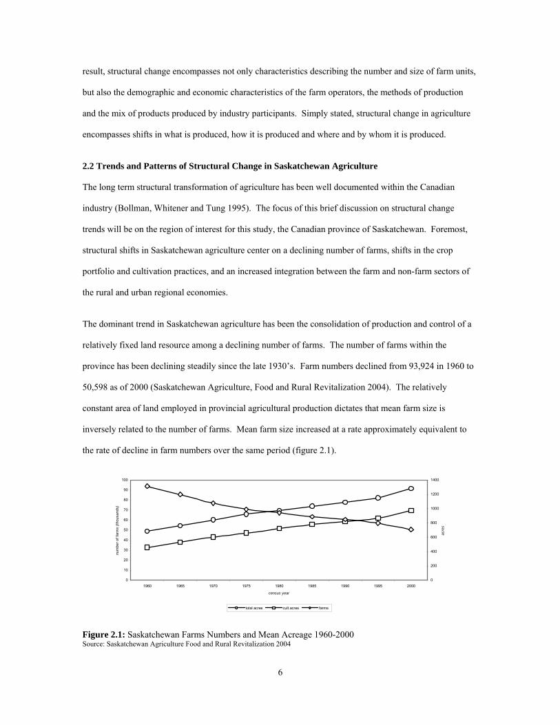
The dominant trend in Saskatchewan agriculture has been the consolidation of production and control of a

relatively fixed land resource among a declining number of farms. The number of farms within the

province has been declining steadily since the late 1930’s. Farm numbers declined from 93,924 in 1960 to

50,598 as of 2000 (Saskatchewan Agriculture, Food and Rural Revitalization 2004). The relatively

constant area of land employed in provincial agricultural production dictates that mean farm size is

inversely related to the number of farms. Mean farm size increased at a rate approximately equivalent to

the rate of decline in farm numbers over the same period (figure 2.1).

0

10

20

30

40

50

60

70

80

90

100

1960 1965 1970 1975 1980 1985 1990 1995 2000

census year

num

ber o

f far

ms

(thou

sand

s)

0

200

400

600

800

1000

1200

1400

acre

s

total acres cult.acres farms

Figure 2.1: Saskatchewan Farms Numbers and Mean Acreage 1960-2000 Source: Saskatchewan Agriculture Food and Rural Revitalization 2004

7

The number of farms, and mean farm size, which are generally well published figures in the popular press,

are only summary statistics and fail to portray key aspects of underlying change in the distribution of farm

size. For example, while mean farm size approximately doubled between 1960 and 2000 (figure 2.1) the

proportion of farms managing less than 400 acres remained relatively constant (figure 2.2).

0%

10%

20%

30%

40%

50%

60%

less than 400 400 - 559 560 - 759 760 - 1119 1120 - 1599 1600 - 2239 2240 - 2879 2880 and over

farm size (cultivated acres)

perc

enta

ge o

f all

farm

s

1960 2000

Figure 2.2: Distribution of Farm Acreage (Saskatchewan) 1960 and 2000 Source: Census of Canada: Agriculture: Saskatchewan In addition to the persistence of small farm operations, the contrast between the distributions of farm size

for the 1960 and 2000 periods highlights the growing heterogeneity between individual farms. In 1960

farms managing less than 1120 acres accounted for approximately 87% of all farms, whereas by 2000 this

had fallen to 60% of all farms (figure 2.2).

Methods of crop production and the portfolio of crops produced by Saskatchewan farmers have also shifted

over the past 30 years (figure 2.3). One of the most dramatic changes in production methods has been the

reduction in soil cultivation and in particular the practice of leaving crop land in fallow. Summer fallowing

farm land was a common practice for the majority of crop producers in the 1970’s. Throughout the 1970’s

close to 40% of Saskatchewan’s crop producing land was fallowed in a given year (figure 2.3), while over

the following decades the proportion of crop land in annual fallow declined steadily, accounting for less

than 20% of crop land in 2000 (figure 2.3).

8

0

20

40

60

80

100

120

140

160

180

200

1971 1973 1975 1977 1979 1981 1983 1985 1987 1989 1991 1993 1995 1997 1999

Acr

es (h

undr

ed th

ousa

nds)

Summerfallow Acreage Spring Wheat (Harvested) Acreage Canola (Harvested) Acreage

Figure 2.3: Saskatchewan Spring Wheat, Canola and Summer Fallow Acreage 1971-2000 Source: Saskatchewan Agriculture Food and Rural Revitalization 2004 The importance of spring wheat production also declined significantly over the same period. Spring wheat

production accounted for approximately one-half of the harvested crop acres as recently as the early 1990’s

(Saskatchewan Agriculture, Food and Rural Revitalization 2004). Spring wheat production has declined in

the past ten years to a level representing approximately 30% of the harvested crop acres annually

(Saskatchewan Agriculture, Food and Rural Revitalization 2004). Reductions in the relative proportion of

farm output represented by spring wheat have been offset by the increasing acreage of alternative crops,

including canola (figure 2.3) and pulse crops. In fact, the number of Saskatchewan farms classified as

wheat type2 has declined from 64% to less than 20% of all farms over the period 1971-2000 (Statistics

Canada).

At the production level, one of the most significant, but least understood, structural adjustments occurring

in the industry is the substitution of capital assets for labour input. An increased proportion of farm equity

tied up in capital assets and increasing levels of debt financing (figure 2.4) has had a significant impact on

the aggregate behaviour of the farm sector. This aspect of structural adjustment needs to be properly

analyzed.

The growth of part-time farming and off-farm income are closely related to the trend of farm capitalization

and the high cost of labour relative to capital. The structure of the farm household has shifted dramatically

2Defined as a farm on which potential wheat sales account for at least 51% of the total farm receipts (Statistics Canada).

9

from the ideals of independence and self-reliance (Raup 1972), to the current reality where most farm

households earn more money from off-farm sources than from agricultural production (Short 2004).

0

5

10

15

20

25

1960 1965 1970 1975 1980 1985 1990 1995 2000

year

debt

per

acr

e (1

960$

)

Figure 2.4: Saskatchewan Farm Debt per Cultivated Acre (in constant 1960s dollars) 1960-2000 Source: Saskatchewan Agriculture Food and Rural Revitalization 2004 In addition to the increasing capital intensity of crop production, and the related increase in farm debt, the

importance of capital associated with non-farming land owners has increased over the 1960-2000 period.

With the exception of the early 1960s, the percentage of farm land owned by non-farming individual and

organizations, and subsequently leased3 to farm operators, has increased (figure 2.5).

0%

10%

20%

30%

40%

50%

60%

70%

80%

90%

100%

1960 1965 1970 1975 1980 1985 1990 1995 2000

year

perc

enta

ge o

f far

m la

nd u

nder

a le

ase

agre

emen

t

Figure 2.5: Proportion of Land under Lease Agreement (Saskatchewan) 1960-2000 Source: Census of Canada: Agriculture: Saskatchewan The prevalence of land leases increased significantly in the first part of the 1980s, with an approximately

6% increase between 1980 and 1985 (figure 2.5). A significant adjustment in the proportion of farm land

3 Lease arrangements consist of two general types: cash leases and crop share leases.

10

operated under leases can be expected to have a number of potential consequences that may alter both

aggregate and individual behaviours.

The market value of farmland is determined by a number of factors, including regional supply and demand.

The demand for farm land in this model is a function of its productive capacity, and the number of potential

bidders. The latter is determined, at least in part, by the financial characteristics, cost structures and

geographic location of individual farm operations. The supply of farm land is also a function of the

characteristics of individual farm operations. If land is the residual earner of farm profits, all of the

characteristics of structural change discussed are indirectly captured in land values or cash leases. In

addition, it is through land markets that land control is obtained and transferred4. Accordingly a model that

attempts to capture the underlying farm structural dynamics must play close attention to the underlying

characteristics of the farmland market and land values.

0

20

40

60

80

100

120

140

1960 1965 1970 1975 1980 1985 1990 1995 2000

year

dolla

rs p

er c

ultiv

ated

acr

e (1

960$

)

Figure 2.6: Saskatchewan Land Values per Acre (in constant 1960s dollars) 1960-2000 Source: Saskatchewan Agriculture, Food and Rural Revitalization 2004 Saskatchewan land values grew rapidly during the 1970s period and reached a peak of approximately $120

(1960$) in 1981 (figure 2.6). This period of rapid inflation in land values was followed by an equally

dramatic downward adjustment in prices which resulted in land values returning to their pre-rally levels by

the early 1990s (figure 2.6).

4 This ignores the importance of inter-family land transfers.

11

2.3 Forces Driving Structural Change While effort has been exerted on understanding the dynamics of structural change, research conclusions

have not been consistent, and have lead to strikingly varied conclusions and policy recommendations

(Harrington and Reinsel 1995). Figure 2.7 highlights eight major causative factors of structural change

identified by Goddard et al (1993). The remainder of this section will be dedicated to a brief discussion

about those key drivers of structural change within the Saskatchewan and western Canadian crop

production sector.

Public Programs - Commodity support, credit, taxation, monetary and fiscal policy and research and extension

Related Market Structure - Institutional development

Demographics - Farm entrants, consumption patterns

Off-farm Employment - Income effects, time allocation

Economic Growth - Non-farm opportunities, product demand

Prices - Substitution effects (inputs and consumption), induced innovation

Human Capital - Managerial ability, consumption patterns

Factors Affecting Structural Change

Technology (economies of size, labour bias technical change adoption rates)

Industry Structure

Characteristics of Productive Activities(What, where and how is output produced)

Figure 2.7: Dimensions of Structural Change: Industry Structure and Casual Factors (Goddard et al 1993). 2.3.1 Technology and Relative Factor Prices Technological innovation is an important factor in the constantly evolving structure of Saskatchewan

agriculture. Cochrane’s (1958) “technological treadmill” is a well-known theory of structural change that

is based on the incentives of individual producer’s to adopt new technology. The typical producer, who is

unable to individually influence market prices but has the ability to control production costs, has a strong

incentive to search for cost reducing (output increasing) innovations (Cochrane 1958). Early adopters

benefit in the short run, but diffusion of the innovation increases the industry output and results in lower

commodity prices. Subsequently, a reduction in farm revenue forces other farmers to either adopt the new

technology to maintain farm revenue at the level realized prior to the introduction of the innovation, or to

12

exit the industry and transfer resources to the innovating producers (Harrington and Reinsel 1995). The

consolidation of resource ownership is further accelerated when technological innovations are embodied in

capital goods that require a minimum production size to be profitably adopted by producers. Technology

embodied in capital assets result in larger farmers being better positioned to innovate and capture the

benefits of early adoption (Harrington and Reinsel 1995). However, in contrast to these a priori supporting

arguments, Giannakas et al (2001) found no clear relationship between farm size and technical efficiency

among wheat producers in the province of Saskatchewan.

Technological innovation involving the mechanization of agriculture has resulted due to the price of capital

falling relative to the price of labour. Producers respond to changes in relative prices by seeking out

technology that saves the relatively more expensive factor of production (Karagiannis and Furtan 1990).

As a result of changes in the relative prices of capital and labour, producers have incentive to replace labour

inputs with capital inputs.

Others observe that technological change results in more than a simple alteration of the mix of inputs

employed to produce a given level of output. It can also give rise to increases in economies of scale,

requiring the producer to employ greater units of input (specifically land) in order to utilize labour inputs

efficiently (Helmberger 1972). The presence of increasing returns to scale at low or moderate output levels

suggests that farms within this size range will either exit the industry or expand to a size that is consistent

with minimum long run average cost. Consequently, growth in farm size is consistent with economies of

scale (Goddard et al 1993). Meanwhile, others have suggested that observed increases in farm scale are the

result of farms attempting to garner higher total returns to bridge the gap between farm and non-farm

returns to labour. This line of thinking postulates that it is not the presence of economies of scale, but

rather the non-existence of significant diseconomies of scale that is driving farm growth (Goddard et al

1993). Both hypotheses are consistent with empirical evidence suggesting that agricultural production is

characterized by either a steep L-shaped or a lazy U-shaped cost curve (Schoney 1997).

13

2.3.2 Labour Mobility and Non-Farm Opportunities Kislev and Peterson (1982) focus their explanation of farm size growth on the assumption of perfect labour

mobility between farm and non-farm sectors. A rise in non-farm incomes provides a strong incentive for

producers to leave the farm to obtain higher returns to their labour, thus freeing resources for the remaining

producers to decrease the urban-rural income gap. Kislev and Peterson (1982) hypothesize that the out-

migration of farm labour and the growth in farm size are two aspects of a single economic process. Goetz

and Debertin (2001) apply a similar idea to explain an individual’s decision to quit or to remain farming (or

start). Individual producers compare the utility they expect to derive from operating a farm to the utility

derived from off-farm opportunities. A farm family, earning an opportunity wage on their labour, must

increase in size as the real off-farm wage increases to maintain equilibrium between farm and non-farm

returns to labour (Huffman and Evenson 2001). Thus, as the non-farm wage rate declines relative to farm

returns to labour, this theory would suggest that the number of farms would increase.5

An increase in non-farm wages results in an increased opportunity cost for the farm family’s labour input.

The increasing cost of labour lowers the relative cost of capital and will result in an increase in the optimal

capital-labour ratio (Kislev and Peterson 1982). The farm family is forced to either expand the farming

operation to fully employ their labour input, or employ their excess labour in alternative markets. Both

scenarios have a profound effect on the structure of the agricultural sector. The decision made by the

individual farm family will be constrained by the opportunities that are available in both the farm and non-

farm sectors.

2.3.3 Capital Immobility The asset fixity or capital immobility argument also provides a rational basis for the observed diversity of

farm size and technology adoption (Harrington and Reinsel 1995). Johnson (1972) argued that capital

investments become fixed over a wide range of rates of returns between the acquisition cost of expanding

capacity and the salvage value of reducing capacity. A resource becomes fixed for a given farm if its

earning power is too low to justify the purchase of more of the resource at the market (acquisition) value,

5 The economy wide depression of the 1930’s was characterized by an increasing number of farm operators which may be at least partially explained by the lack of non-farm employment opportunities, and the resulting lower expected non-farm labour returns.

14

yet too high to justify selling the asset at its salvage value (Johnson 1972). The direct result is that in the

short run, farm structure can be characterized by significant diversity of farm size and technology.

2.3.4 Demographics and the Life-Cycle Hypothesis Demography is a powerful and often under-utilized factor in understanding economic activity. Foot (1996)

argues that it is not possible to do any accurate economic forecasting without knowledge of demographics.

Demographic characteristics of a population play an important role in both public policy and business

analysis in the long run. Demand for education and health care services are two prime examples where

public policy and demographics interact.

Extant demographic characteristics of a population are the best predictor of the future demographic

structure of an economy. As a simple example of the power of demographics for educational policy

analysis, consider that the number of births in a school district in 2004 constitutes a highly accurate forecast

of the number of children entering the first grade in 2010. By failing to understanding the obvious future

consequences of current demographic characteristics, the task of developing a forecast is needlessly

complicated (Foot 1996).

One of the most useful statistics for predicting general economic behaviour is the age composition of a

population (Foot 1996). While humans make decisions independently, individuals in the same age cohort

generally engage in similar activities as their peers. In fact, highly similar patterns of behaviour are

observed among age cohorts over time. Some observe that this behaviour can only be marginally altered

by economic conditions, government programs, or external shocks (Harrington and Reinsel 1995). In most

instances the participation rates of various age groups in different activities are relatively stable over the

medium run. For instance, it is highly likely that a 45 year old in 2014 will behave the same as a 45 year

old in 2004; chances are also good that an individual will move out of their parent’s home, buy their first

car, and get married about the same age as peers (Foot 1996). This basic life-cycle model of economic

activity can have important impacts on the aggregate economy as the population ages6 and the age

composition of the population shifts and alters the number of individuals in each stage of the life cycle.

6 “Population aging” refers to the basic fact that each year every individual is one year older, and should not be confused with an “aging population” which is generally characterized by an increase in the average age of the population.

15

A basic farm life cycle model will explicitly recognize the various life stages as well as management

objectives an operator experiences. The operational ladder typically followed by a farm operator in Canada

is to enter the industry by renting farm assets, add additional rented land for part of their lives while

progressively acquiring ownership of land and capital assets throughout a growth phase, and finally

relinquishing control of leased and owned assets as they exit from farming (Harrington and Reinsel 1995).

Ultimately, structural change is the result of micro-level dynamics of entry, growth and exit. Some offer

that government policies, economic conditions, and technological change may only marginally affect the

incentives and opportunities within the life cycle of the farm operator (Harrington and Reinsel 1995).

Demographics imply are that while operator ability and hard work are important factors in farming, the

timing of start up and initial capital stock may play a significant role in determining the success of a farm

operation. Operators who have inherited substantial farm assets, or who operate established farms with a

significant level of equity, are better positioned to withstand extended downturns in the farm economy that

may bankrupt equally able and efficient operations. As a result, it is important to incorporate family and

farm life cycles when analysing current and future farm survival and structural shifts (Barlett 1984)

In an industry where the bulk of the entry occurs from a relatively young age cohort (i.e. between 20-30;

Harrington and Reinsel 1995), a reduction in the number of farmers, as well as young people raised on

farms, has implications for the future of the food production sector (Goddard et al 1993). A declining

number of young people raised on farms, who historically have accounted for the majority of new farm

entrants, will lead to a further decline in farm entry. This in turn signals a shift away from the traditional

single owner-operator farm arrangement (Goddard et al 1993).

2.3.5 Productive Heterogeneity The changing structure of agricultural production is thought by some agricultural economists to be a

consequence of the heterogeneous nature of productive efficiency. The existence of varied levels of

productive efficiency among farm operations might also explain the consolidation of farm assets among

fewer operators (Harrington and Reinsel 1995). Deferring to a mechanism similar to Cochrane’s (1958)

“technology treadmill”, some have argued that efficient producers will earn economic profit, while the

inefficient farms will incur losses. Facing a downward sloping demand, this cumulative process will result

16

in the transfer of land and capital assets from the inefficient farms to the efficient farms. Increases in

production resulting from the efficient use of these resources will increase aggregate supply, further leading

to relatively low market prices and still more pressure on the net incomes of less efficient farms

(Harrington and Reinsel 1995).

2.4 Farm Management/Entrepreneurship At the farm level, there are many potential drivers for rural structural change. But one possible underlying

driver that has not been fully explored in the literature is the fundamental and intrinsic difference in

farming “management style.” Much anecdotal evidence exists among agricultural professionals as to how

differences in decision making lead to a management style (Jensen 1977). While there are many possible

management attributes, management style should encompass; 1) a willingness to accept/or reject the

current situation or status quo, 2) a willingness/unwillingness to act or respond under incomplete

information and to accept risk (entrepreneurship), and 3) a view of farming as a business/life style. Clearly,

these attributes are not necessarily independent and may be in turn influenced by a number of demographic

variables.

Agricultural and rural structure is related to the ownership and control of agricultural land. The past,

present and future ownership and/or control of the land resource are directly linked to the relative bidding

potential of land market participants (Harris and Nehring 1976). A number of economic factors, including

net income, income variability, wealth, marginal tax rate and interest rate, have a direct impact on the land

bidding behaviour of an individual (Harris and Nehring 1976). Which farms are best suited for future

growth and will gain the most from expanding their farm acreage? In turn, this leads to a second,

potentially more important, question of the growth willingness of the farm manager/entrepreneur (Welter

2002).

The growth aspirations/willingness of the individual farm agents may have a profound effect on the final

allocation of land. While theoretically growth is initially desirable to achieve a sustainable scale of

production, personal growth ambitions play a significant role in shaping a farm’s growth path (Welter

2002). A farm agent with a higher bidding potential and thus having more to gain from farm growth may

ultimately end up being outbid by another farm manager with a lower bidding potential due to the agent’s

17

lower growth aspiration. In fact, the individual farm entrepreneur’s growth ambition can be incorporated

into their land market bidding behaviour in a number of ways, including the incorporation of a degree of

risk aversion when forming a land bid (see Harris and Nehring 1976) as well as the simple choice of

entering the land market or remaining on the sidelines. A general pattern of land market participation

behaviour can be observed based on the age of the farm manager and the corresponding business phase.

Studies have shown that participation is typically limited to established farms still in the growth phase, as

farm managers nearing retirement typically refrain from participating in the land market as buyers. In

addition, young farmers still in the entry/establishment phase are typically blocked from entering due to

high debt-levels (Olson 2004).

The growth of a farm operation is directly linked with the underlying management style of the farm

household. Within the literature, a rather consistent categorization of farm management styles has emerged

(Taylor et al 1998). The business-oriented style of management encompasses the entrepreneur (Olsson

1988), dedicated producer (Fairweather and Keating 1994), and the efficient operator (Walker 1989). In

contrast the lifestyle approach to farm management is typically characterized by strategic caution (Olsson

1988) and sufficing behaviour (Fairweather and Keating 1994). A number of researchers (Bennett 1982;

Fairweather and Keating 1994) suggest that farm management styles are largely influenced by the life-

cycle of the enterprise and may vary as time progresses. Ultimately, different approaches to farm

management exist, and the distribution of management styles among a relevant farm population may have

an effect on the aggregate agricultural structure of a region.

2.5 Summary The literature on structural change in agriculture suggests a number of factors that may be driving the

transformation of agriculture and in general, the composition of the farming sector in Saskatchewan in

particular. The factors considered and highlighted here include technology, labour mobility, capital

immobility, demographics and productive heterogeneity. While a diverse literature, a consensus has

emerged that at the aggregate level, structural change results from transformations occurring at the

individual farm level. Thus, theories concerning the sources of structural change have in common the

importance of the individual farm household as the significant decision making unit in agriculture. This

18

buttresses the need to establish the individual farm operation or household as the primary unit of analysis in

a study of aggregate farming behaviour.

19

CHAPTER THREE

FARM LEVEL MODELING

3.0 Introduction General policy analysis in agriculture often uses computational farm-level models. Early versions of these

traditional models were designed by government and universities beginning in the 1960’s to better

understand the farming sector and the overall impact of policy change. Even today, the vast majority of

farming models are founded on one of either representative producer, input/output or computational general

equilibrium (CGE) methods. The first method is not statistically defensible when the population is highly

diverse. The latter two types of models offer macro predictions based on structural equation parameters

estimated from highly aggregated data. One of the inherent limitations of all of these traditional farm-level

models is that due to hysteresis, they are often unable to accurately forecast behaviour very far beyond

those years from which the model parameters were derived. This situation is a major impediment to

formulating sound agricultural policy in an ever-changing economic environment.

This inherent limitation of the traditional models for understanding and predictive purposes has led to

research into a new generation of farm-level models. General advancements in computer simulation

environments have sparked the development of detailed, microscopic computational approaches to simulate

the behaviour of human systems (Parker et al 2003). While these models are now widely used in some

fields of research, there has been limited application so far to agriculture. Great potential exists for this

kind of simulation modeling to better assess and forecast the major structural change now happening in

Saskatchewan agriculture. The appropriateness and application of these new computing and simulation

tools to the issues of farm-level modeling, agricultural production and land use will be the focus of this

thesis.

20

3.1 An Alternative to the Neoclassical Economic “Toolkit” Neoclassical economics has been the dominant paradigm in both economic research and teaching since the

1940’s (Happe and Balmann 2003). This has resulted in the widespread acceptance of modeling economic

problems and individual behaviour using the mathematical optimization ‘toolkit’. The widespread use of

optimization techniques to represent individual behaviour has resulted in some confusion regarding the

fundamental economic concept of individual rationality. Rationality is often confused as a technique, the

optimization technique, rather than a concept (Vriend 1996). Rationality, in economic terms, simply refers

to an individual selecting the option, from their perceived opportunity set, believed to be in their best

interest (Vriend 1996). Mathematical models are simply one way of representing an individual’s selection

process, but they should not be understood as an economic principle in spite of their widespread use.

Alternative models of individual behaviour may result in the selection of different ‘optimal’ choices under

assumptions using equivalent information, without violating economic rationality.

The concept of bounded-rationality in economics is defined as situations where limited resources constrain

fully rational decision-making and this can also be described as ignorance. Bounded information is the

direct result of economic search costs, and should not be confused with rationality, which is unaffected by

economic factors (Vriend 1996). Modeling bounded-rationality presents two problems - modeling

ignorance and modeling rationality. While agent-based modeling facilitates the development of a tractable

model of individual learning and ignorance, some authors argue it is the second issue that will ultimately

lead to its widespread acceptance as a new economic modeling ‘toolkit’ (Arthur 1994).

Agent-based systems are generally defined by a set of autonomous entities, or agents, which have limited

knowledge and computational abilities (Berger 2001). As the name suggests, individual agents are the

primary component of any agent-based model. Of primary interest to social scientists is the interaction and

information exchange between agents that occurs in a decentralized and “somewhat social” manner within

the simulation environment (Berger 2001). I will argue that the technique maps well onto farming and

farm behaviour, especially the paradigm of interacting yet autonomous decision-makers conducting their

business on a physical landscape.

21

The unit of analysis in an agent based system model is the individual actor or agent behaving as a result of

autonomous decisions. Many systems are not controlled by a central planner; rather, stability or

equilibrium in these models is generated via the decisions and actions of multiple individual agents,

coupled with their interactions with other agents and the environment (Schelling, 1978). One advantage of

the de-centralized decision making inherent in agent based modeling is that many well specified models

generate unpredicted (‘emergent’7) patterns of behaviour at the macro level (Bonfanti et al, 1998). Today,

the agent-based literature is firm about the simulation algorithm - once initial conditions are set, all future

events in these virtual worlds are initiated and driven by agent-agent and agent-environment interactions,

with no further intervention by the modeller required or permitted (Tesfatsion, 2000).

The path to widespread acceptance of agent-based modeling methodologies is expected to parallel the

development of the field of experimental economics from its pseudo-science status in the early 1960’s.

Experimental economics gained acceptance with the development of new equilibrium concepts (e.g. Nash

equilibrium, and the core) in the late 1960’s, and primarily as a methodology for choosing between

alternative theories of behaviour (Friedman and Sunder 1994). The development of alternative equilibrium

theories resulted in the focus of behavioural economics expanding from causal propositions in the form of

“If x then y” under the existence of a single rationality theory to actual testing of the suitability of

alternative theories based on experimental data (Friedman and Sunder 1994).

The development of alternative models of human behaviour to compete with the “economic man” paradigm

has resulted in a need for methodologies to accommodate appropriate individual behaviour. It has also

been argued that agent-based models have the ability to serve as a “social laboratory” for testing the

plausibility of various behavioural models (Casti 1999). Furthermore, agent-based modeling can provide

the researcher with a method that allows the modeling and testing of alternative models of individual

behaviour that have been previously neglected due to tractability and complexity issues.

7 Emergence is the property that a system is not simply equal to the sum of its individual parts. Phenomena at the macro level cannot always be explained by observing the properties of the system in isolation. Macro level structures are rather the result of interactions of the individual components of the system (Happe and Balmann 2003).

22

3.2 Current Farm-Level/Land-Use Modeling Methodologies Research within the multidisciplinary fields of agricultural production and land-use has resulted in the

application of a variety of model building methodologies. The appropriate modeling methodology must be

based on the structure of the underlying system and the objectives of the research project. As a result the

focus of this section will be to briefly examine the strengths and weaknesses of a number of broadly

categorized alternative methodologies.

Agarwal et al (2002) identified three general components that are important for the evaluation of land-use

models including space, time and human decision making. These three axioms form the basis for a

discussion on alternative modeling methodologies. These authors argue that in order to adequately capture

all relevant dynamics within a system characterized by a strong human-environment relationship, the

interactions between the temporal and spatial environments and human choice must be explicitly

incorporated into the model system.

3.2.1 Farm Budgeting/Planning Models Initial modeling efforts at the farm-level are best described as farm management tools that were developed

to study financial problems at the individual farm level. These early farm models consisted of simple

partial budgets to predict the outcomes of alternative production scenarios, along with case studies of

successful farms to determine common characteristics of successful producers (Klein and Narayanan,

1992).

While individual producers remain key factors in any agricultural system, the increasingly heterogeneous

profile of remaining producers and the farm specific nature of these types of models limit their use for

policy analysis as stand alone models. That is not to say that these simple partial budget and case studies

are useless to the development and analysis of future policy tools. In fact they may help lead to a solution

for the problem identified by Simon (1955), replacing the “economic man” model of human action based

on global rationality with a model consistent with the computational capacity and access to information

actually possessed by human actors in an economic system. The successful development of future farm

level policy models within an increasingly complex and heterogeneous industry will require a better

understanding of the characteristics that drive individual farm management decisions.

23

3.2.2 Equation Driven Models Equation driven (quantitative) models have traditionally played an important role in the development and

analysis of agricultural policy. The structure of these models has generally taken either a macro-

perspective or a micro-perspective of the system under analysis. Attempts were made at developing

classical spatial equilibrium models of agriculture, but they were inherently complex, difficult to solve and

led to poor forecasts (Takayama and Labys, 1986). In addition, by focusing on either the macro level

(country, province or region) or the individual farm (micro perspective), a number of significant issues that

are functionally situated in between these extreme perspectives, such as structural and distributional effects,

are effectively lost (Happe and Balmann 2003).

Micro-level models generally select a typical farm to represent a relatively homogenous group. The

representative farm incorporates detailed micro data and is most often used to simulate adjustment to a

policy change (Happe and Balmann 2003). The method of modeling each individual solution and then

aggregating the results to determine the macro effects of a policy is referred to in the literature as

microprogramming (Fisher and Kelley 1982). Modeling each individual farm is costly, and in many cases

the solutions are non-feasible (Kelley and Fisher 1982). This problem is usually solved by aggregating

similar producers and building so-called ‘representative’ farms. The development of the CRAM model

(Canadian Regional Agricultural Model) of the Canadian agricultural sector and the REPFARM model of

the U.S. sector are examples of behavioural farm-level models (Klein and Narayanan 1992) that focus on a

limited number of representative farms which in turn are assumed to exist in isolation with no allowance

for explicit inter-farm interactions.

In addition, analysis of the results generated through the aggregation of representative farms is subject to

aggregation bias and error due to the difficulty in developing artificial farms that are truly representative of

the entire group. As far back as the 1960s, Day (1963) argued that even though it is theoretically possible

to achieve exact aggregation in economic models under certain conditions, developing satisfactory criterion

remains a major problem.

Significant advancements in computational capacity allow researchers to avoid aggregation issues by

facilitating much more disaggregate micro-programming. While decreasing computer processing costs

24

may avoid the classic aggregation problem, current microprogramming methodologies are still hindered by

a second aggregation bias identified by Happe and Balmann (2003). The simple arithmetical aggregation

of individual farm models, solved independently to represent an industry or a region, completely omits any

interactions and dynamical effects that can occur between individual farms and the subsequent macro level

phenomena that emerge from these interactions (Happe and Balmann 2003). Berger (2001) compared the

inability to capture interactions between farm-households to the assumption that no transaction or

information costs exist. A second criticism of mathematical programming based on simulation models

identified by Berger (2001) is the inadequate representation of the important spatial dimensions of

agricultural activities. As a result, the role of internal transport costs and the immobility of land are often

ignored in traditional farm-level models – an effect that can be likened to the assumption of zero

transaction costs (Berger, 2001).

Through the 1970s, the growing importance of world markets and the cost of commodity based support

programs resulted in a shift in farm modeling towards aggregate supply response of the industry (Klein and

Narayanan 1992). However, a macro-level approach ignores the heterogeneity in behaviour and resource

endowment among individual producers that form the aggregate response (Happe and Balmann 2003). The

lack of understanding about the effects of policy at the individual producer level is the major point of

criticism directed at macro-level modeling. Predictions generated from macro-level models are based on

extrapolation from historic aggregate data patterns, with minimal attention paid to the behaviour of

individual economic agents (Stoker, 1993). The use of macro-level modeling techniques not only masks

the distributional effects of a policy change, it also fails to capture the important linkage between response

at the individual level and the aggregate response. A relatively small shift in individual producer incentives

or a change in the profile of producers in the region, resulting from a policy change, can potentially result

in a significant impact on the aggregate response. The latter is not something macro-level models based on

historical data can easily incorporate.

The inability of current farm-level models to readily adapt to shifts in individual responses also limits long-

run predictive ability. If policy issues, such as structural change, are in fact path dependent8 (Balmann

8 See page 28 for a definition of path dependency

25

1997), the current models lack the ability, due to their limitations for long-run prediction, to fully assess the

impacts of a policy option. Policy makers using these models must be careful to ensure that those policies

intended to have a positive impact in the short-run do not have an unwanted and damaging impact on the

long-run performance of the sector.

3.3 Agent-Based Systems: A New Farm-Level Modeling Paradigm The use of agent-based or multi-agent systems originated in computer science through the field of

distributive artificial intelligence. Today, the use of agent-based systems is a growing multidisciplinary

research tool. Unfortunately, a degree of uncertainty still exists concerning the precise definition of an

agent. The definition adopted by individual researchers varies depending on the area of study. However, a

minimal common definition, as proposed by Ferber (1999), is as follows:

An agent is a physical or virtual entity;

o which is capable of acting in an environment

o which can communicate directly with other agents

o which is driven by a set of tendencies (in the form of individual objectives)

o which possesses its own resources

o which is capable of perceiving its environment (to a limited extent)

Balmann (2000) offers a more succinct definition, which captures Ferber’s - agents are reactive,

autonomous and goal orientated entities with the ability to sense their environment and, in particular cases

the ability to communicate, learn and be mobile.

A number of concepts and issues associated with agent-based systems draw from the related field of

complexity theory. While a detailed description of complexity theory (Manson 2001) is outside the scope

of this thesis, it is worth briefly exploring the relationship between agent-based modeling and complexity.

Complexity theory covers a variety of analytical concepts and is inherently a multidisciplinary field of

research. It is important to note a fundamental difference between complexity theory, which is often

concerned with non-linear relationships, and the linear relationships defined by stocks and flows in general

systems theory (Manson 2001).

26

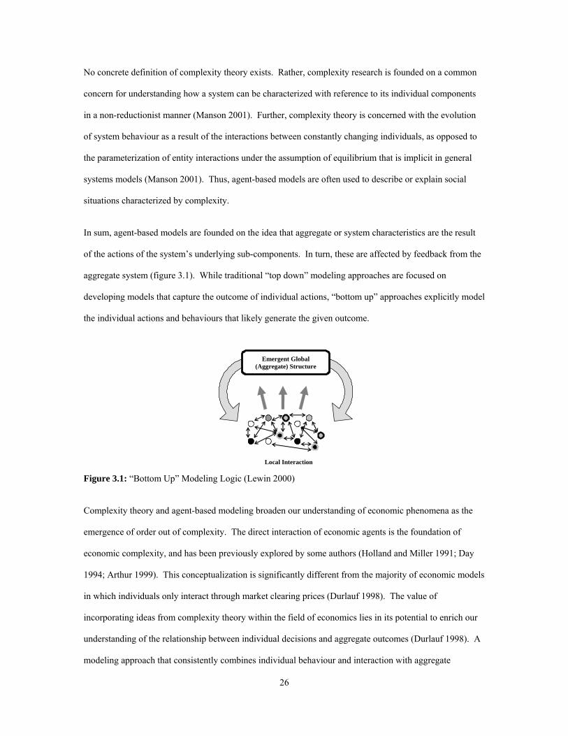
No concrete definition of complexity theory exists. Rather, complexity research is founded on a common

concern for understanding how a system can be characterized with reference to its individual components

in a non-reductionist manner (Manson 2001). Further, complexity theory is concerned with the evolution

of system behaviour as a result of the interactions between constantly changing individuals, as opposed to

the parameterization of entity interactions under the assumption of equilibrium that is implicit in general

systems models (Manson 2001). Thus, agent-based models are often used to describe or explain social

situations characterized by complexity.

In sum, agent-based models are founded on the idea that aggregate or system characteristics are the result

of the actions of the system’s underlying sub-components. In turn, these are affected by feedback from the

aggregate system (figure 3.1). While traditional “top down” modeling approaches are focused on

developing models that capture the outcome of individual actions, “bottom up” approaches explicitly model

the individual actions and behaviours that likely generate the given outcome.

Figure 3.1: “Bottom Up” Modeling Logic (Lewin 2000)

Complexity theory and agent-based modeling broaden our understanding of economic phenomena as the

emergence of order out of complexity. The direct interaction of economic agents is the foundation of

economic complexity, and has been previously explored by some authors (Holland and Miller 1991; Day

1994; Arthur 1999). This conceptualization is significantly different from the majority of economic models

in which individuals only interact through market clearing prices (Durlauf 1998). The value of

incorporating ideas from complexity theory within the field of economics lies in its potential to enrich our

understanding of the relationship between individual decisions and aggregate outcomes (Durlauf 1998). A

modeling approach that consistently combines individual behaviour and interaction with aggregate

Local Interaction

Emergent Global (Aggregate) Structure

27

phenomena is lacking within the mainstream economic literature. Agent-based systems offer the potential

to remedy this issue by explicitly acknowledging the contribution of each individual in the system under

analysis to outcomes at the aggregated level (Happe and Balmann 2003).

3.3.1 Why Agent-Based Methods? There are a number of well-developed techniques of farm-level modeling for the purpose of policy

analysis. However, each of these modeling methodologies has significant limitations. Equation-based

spatial and aspatial models are generally only able to capture a limited degree of realism due to analytical

and computational tractability issues (Takayama and Labys, 1986). And while analytical models can

provide some insight on the impact of heterogeneity and neighbour effects in spatial modeling, they are

generally limited to representing average and not extreme effects (Parker et al 2003). Due to the multitude

of potential spatial and social interactions that may occur within a complex system, these analytical

techniques can be inadequate for assessing issues that are guided by these interactions.

If formulated correctly, agent-based systems provide the researcher with the ability to overcome these and

other limitations. The capability of agent-based systems to evolve solutions to phenomena that are

regarded as systems of autonomous interacting components, like a farm economy, provide the motivation

for increasing interest in ABS research in the social sciences (Sycara, 1998).

3.3.1.1 Flexibility and Complexity Agent-based modeling is characterized as a “bottom up” approach, in that it is not driven by central

coordinating mechanisms. “Bottom up” modeling approaches do not rely on exogenously imposed

assumptions, including fixed decision rules, global rationality, representative agents or market equilibrium

constraints, all of which are generally required within “top down” approaches such as computational

general equilibrium models (Happe and Balmann 2003). In equilibrium models, the inclusion of these

assumptions is usually required in order to analytically determine a solution, while solutions quickly

become intractable as the level of system complexity increases. As a direct result of the comparatively less

restrictive assumptions required for iterating a solution within an agent-based model, the researcher can

endow individual agents with a more complete and realistic spectrum of properties and behavioural rules.

28

Ultimately, the attraction of traditional analytical economic models is their ability to yield stable,

equilibrium solutions. However, many solutions fail to provide the researcher with an adequate

understanding of the transition period between equilibrium states (Nelson 1995). Mathematicians and

economists now recognize that it may not be the case that an economic system will always reach a stable

equilibrium. For instance, frequent internal and external shocks may hinder identifying the equilibrium.

The existence of a fixed or moving economic equilibrium needs to be viewed as an attractor9, or desired

state, rather than a description of the system state (Nelson 1995). In contrast, agent-based models permit

quasi-equilibrium sinks or states to evolve from the interactions of individual actors without explicitly

incorporating restrictive equilibrium constraints. This not only provides improved understanding of the

transition period between equilibrium states, it also leaves open the opportunity for the equilibrium state to

be altered prior to the system fully adjusting.

3.3.1.2 Emergent Characteristics Emergent properties in systems analysis are those characteristics of a dynamic system (in equilibrium or

not) that could not readily have been predicted before the experiment or simulation (Parker et al., 2003).

Furthermore, emergent properties are the direct result of synergism between individual system components

and are not simply additive affects of the system components (Manson 2001). The notion of aggregate

system characteristics emerging from the interactions of individual actors is deeply embedded within

traditional economic theory. Economists have long regarded market processes as being the result of

unguided interactions between rational individuals, including most notability the Smithian “invisible hand”

paradigm used to describe self-coordination within a market economy (Happe and Balmann 2003).

Parker et al (2003) argue that emergent phenomenon can only be practically modeled with computational

tools such as agent-based models. This is due to the difficulty of constructing analytical spatial equilibrium

models that can incorporate all relevant microscopic interactions. To date, a number of researchers have

identified useful examples of emergent system properties in dynamic models in this context. These include

land use patterns (Parker and Meretsky 2004) and the overall distribution of farm sizes in Europe (Balmann

9 An equilibrium state can be thought of as an attractor in the sense that it is the state the system will reach if it is allowed to fully adjust, but full adjustment may not necessarily occur due to a number of internal and external factors.

29

1997) both of which are best described as emergent properties of systems of individuals interacting within a

spatial market.

3.3.1.3 The Importance of Time and Space The primary importance of time and space within any human driven system can be summarized by two

undeniable physical truths for all matter, save for sub-atomic particles - 1) it is impossible for matter to be

in two places at a single point in time and 2) time is irreversible. Past actions cannot be undone, and only

their long term outcome can be altered by current and future decisions (Happe and Balmann 2003).

Balmann (1999) among others calls this notion “path dependence”, and refers to the phenomena that in a

stochastic world, the current state depends upon previous actions and events. In such a case, agents

operating within the same system may differ in their actions, even if the same information set is available to

all agents, as past actions and observations affect their opportunity set and perceptions of the world. As an

example of this, two farmers may be aware of a new technology that will potentially improve profitability,

but a one may opt not to adopt the new technology due to financial constraints that were caused by an

earlier action.

In many ways human perception of the world is largely shaped by space and geography (Fellmann et al

1999). For geographers, the importance of location and the influence of neighbours parallel the

economist’s reliance on theories of constrained (by resource or budget) utility maximization (Nelson 2002).

The importance of modeling an agricultural system in a spatially explicit manner becomes increasingly

evident when one considers the importance of space and location in a number of agricultural decisions. For

example, an important factor in farm growth is the cost of internal transportation and the increased cost of

farming geographically scattered units of land. As a result, producers with a desire for farm growth are

generally limited to competing with their neighbours for additional units of land (Berger 2001).

3.3.1.4 The Importance of Heterogeneous Producers The individual producer is ultimately the driving force behind and the recipient of the eventual outcomes of

any agricultural policy. If agricultural policy makers do not understand the importance of individual

management and behavioural characteristics, it becomes difficult to design policies to achieve a desired

outcome. Furthermore, there are challenges solving any system involving dynamic, independent and

30

intelligent actors with free will. At present, with only 39% of Canadian farmers self-described as business

focused and 50% as lifestyle farmers (Short 2004), the development of effective agricultural policy must

depend in part on understanding the varied management strategies that exist between and within these two

drastically different groups. Thus, even under the assumption that all individuals are pursuing the same

goals (i.e. utility maximization), a large variance in individual behaviour will result unless all individuals

have identical information, computational abilities, and utility functions.

Within the framework of agent-based modeling, individual agents must be assumed to act according to

some model of cognition (Parker et al 2003). At the most basic level, individual agents must also have the

ability to react to their environment in a manner that is compatible with their individual perceptions of the

world and their goals. This somewhat extends the notion of traditional economic theory, based on the idea

of an “economic man” presumed to behave rationally under the assumption of perfect information (Simon

1955). While rational choice models developed under the assumptions of the “economic man” provide

significant explanatory power, they may fail to accurately predict behaviour under realistic assumptions of

imperfect information (Parker et al, 2003). Simon (1955) and others argue that even under assumptions of

imperfect information, the “economic man” paradigm overstates the computational capacities actually

possessed by many individuals.

The primary advantage agent-based models offer over traditional economic modeling approaches with

regard to modeling human behaviour is the ability to readily incorporate a significant degree of

individualism in the decision making process. The ability to design a multitude of individual agents also

allows the researcher to incorporate a number of varied decision making models. And while not followed

in this thesis, the researcher is not actually limited to assuming that all individuals follow the same decision

making process. In fact, agent models can de designed to endow each individual with a unique decision

making algorithm.

3.3.2 Challenges and Limitations Economic models are designed to understand issues as part of a more complex economic system. Agent-

based models have a unique characteristic in that their flexibility of specification and design is both a great

advantage and a potential problem (Parker et al 2003). As these models become increasingly more

31

realistic, they also increase rapidly in complexity, which can result in the loss of an ability to draw direct

cause and effect conclusions (Happe and Balmann 2003). The inability to assign a direct causal link may

pose a significant problem for theoretical research, but the point may be less important for policy analysis

based on simulation models that are developed using empirically grounded assumptions. In addition,

model verification and validation10 become increasingly more difficult as the level of complexity increases

(Kelton et al 2004). Kelton et al (2004) concede that it is “almost impossible to verify totally a model for a

complex system” and it seems the only option is to rigorously test the simulation model under multiple

scenarios to verify that it behaves correctly for a reasonable set of potential scenarios.

In addition, to move beyond replicative and predictive validity11 based on comparing simulated and

observed data is rather difficult. This is often accomplished in a qualitative context by agreement of

participating stakeholders that the modeled behaviour is an acceptable theory that cannot be rejected based

on current knowledge. Note that this is not a situation unique to agent-based modelling, as the scientific

method is based on rejecting false hypothesis and theories rather than directly accepting true ones.

The wider acceptance of agent-based models as a tool for economic and policy analysis is currently

hindered by a number of concerns that must be overcome. The greatest challenge facing researchers in this

emerging field is the communication of model constructs and results without a standardized toolkit or a

common base of knowledge. The lack of a standardized toolkit is further aggravated by the complex nature

of agent-based problems, which often require long and detailed documentation. In contrast, while possibly

misleading, agricultural models that have been widely accepted as tools for policy analysis seem to be

appealing due to their reliance on neoclassical economic theory (Happe and Balmann 2003). Researchers

must be aware that additional time and resources are currently required to outline underlying model

assumptions and theories compared to researchers engaged in traditional economic research.

A number of the challenges and limitations identified within this section are not inherent to agent-based

methods themselves, but rather result from a lack of understanding about underlying system dynamics.

10 Verification ensures that the encoded model accurately represents the researcher’s abstraction from the real world, while validation is concerned with comparing the model results to real world data and expectations (Parker et al 2003). 11 Troitzsch (2004) identifies three types of validity; 1) Replicative Validity: the model matches data already acquired from the real system; 2) Predictive Validity: the model matches data before data are acquired from the real system; 3) Structural Validity: the model represents the manner in which the real system operates to produce the behaviour.

32

This point becomes increasingly obvious when attempting to model the behaviour of individual agents,

while standard economic analysis has generally sidestepped issues related to the mechanisms used by

agents to make choices in a perpetually novel world (Holland and Miller 1991). Current models of

individual behaviour based on optimization techniques are often justified by postulating that adaptive,

market driven, mechanisms result in agents acting ‘as if’ they are optimizing (Holland and Miller 1991).

While this may in fact be a valid argument, it does little to address the structural behaviours driving the

broader economy. Applications of the agent-based ‘toolkit’ stretch the boundaries of existing economic

models and have the potential to dramatically alter the discipline of economics and the related field of

farm-level modeling.

3.4 Summary In any field of research, it is important to re-examine the methods of study from an alternative viewpoint or

theoretical base. Agent-based simulations, combined with spatially explicit behavioural models, provide

researchers interested in agricultural policy analysis the opportunity to view social and economic processes

from an alternative perspective (Balmann 2000). Researchers must be aware of the advantages, as well as

the limitations, of emerging research methods such as agent-based modeling when evaluating the available

strategies for assessing both new and old issues and problems.

The modeling paradigm selected by a researcher must be driven by the objectives of the study and

characteristics of the system under study. Systems that can be characterized as complex may be well suited

for the application of agent-based methodologies. The ability of agent-based models to explicitly capture

the complexity and emergent characteristics of economic systems in turn gives its application to farm-level

modeling the potential to overcome the limitations of the previous generation of farm-level analysis.

The importance of understanding the limitations of any modeling paradigm should not be overlooked,

particularly in the case of an emerging field. Without a standardized toolkit or knowledge base available,

researchers utilizing agent-based models and complexity theory must ensure that all model assumptions and

constructs are carefully documented and empirically and/or theoretically justified. While it is clear that the

use of agent-based models results in some validity and verification problems, these problems can usually be

distilled as problems associated with the specific research question rather than the methodology (Balmann

33

2000). The use of agent-based models also provides a significant degree of flexibility, particularly through

incorporating individual behaviour and decision making characteristics. Like any new methodology that

questions existing theories and ideas, agent-based modeling faces a number of challenges, but recent

developments within the field should encourage other researchers interested in this newly emerging field of

study.

34

CHAPTER FOUR

MODEL FRAMEWORK

4.0 Introduction

In the previous chapter, I argued that agent-based models are suitable for analyzing the structure of

complex economic systems. In this light, there are now several agent-based models in the economics

literature that have incorporated market-based agent interactions (Happe, Kellerman and Balmann 2004).

The economic landscape of an agrarian region can be modeled as a result of local interactions between

three primary components of agriculture: farms, land and markets (for products and land) (figure 4.1).

farm 1

farm 4 farm 2

farm 3

Farms Land / space

Markets

Figure 4.1: Conceptual Model of a Regional Agricultural System (Happe, Kellerman & Balmann 2004) This representation of a regional agricultural system as an agent based model is appealing for two

additional reasons. Rule based interpretation of farms as individually acting agents is a primary strength of

agent based modeling methodologies. And a spatial issue like the allocation of a scarce and immobile

resource, such as agricultural land, among a geographically dispersed set of farms can be dealt with in a

relatively tractable manner in the agent framework.

35

4.1 Central Model Assumptions

Independent farming operations evolve based on the opportunities and constraints presented by their

constantly changing environment. In this thesis, the farmer is considered to be engaged in two related but

separate activities - producing and marketing field crops, and investing in agricultural assets. In the former,

farms are essentially independent and annual production and marketing decisions are not directly

constrained by the actions of neighbouring farms. In contrast, a farm’s ability to increase asset investment,

specifically in land, is directly constrained by the actions of all farms within a limited geographical area.

The inability of a farm to produce output independently from the scarce land resource results in direct

competition between farms for agricultural land.

Competition for agricultural land is organized in this model through the assignment of property rights and

the continued functioning of well-defined agricultural land markets. An individual farm’s production is

constrained by the availability of additional crop land which is affected directly by the collective actions of

all farms in the local land market. It is assumed that the farm manager’s ability to acquire additional land

for a price that is not in excess of its true future return is the key to the long term profitability of the farm

operation.

A number of non-farming individuals, including retired farmers and speculators, are also assumed to be

active within the agricultural land market. In fact, it is the presence of non-farming land owners in the land

market that leads to the establishment of a lease market. It is assumed that the non-farming land owner will

sell land when the return from selling outweighs the expected return from owning land, and will purchase

land if the market price is less than the present value of the expected lease return.

In order to assess the impact of agricultural stabilization and support programs of the past few decades in

Canada, the spatial and producer profile is initialized to represent an agricultural region typical of one that

would be found in the dark brown soil zone of Saskatchewan in the year 1960. In addition all farms are

assumed to be limited by the crop production technology of the initial time period for the duration of the

model. In order to adjust for this assumption of constant technology, real commodity prices and production

costs are also de-trended. Non-land capital investment stocks are assumed to be constant over farm size

and between individual farms. Farms require a constant investment stock of machinery and equipment per

36

acre for crop production. By assuming that technology and non-land capital stocks are constant, the role of

managerial attributes on the evolution of regional agricultural structure can be studied in isolation from the

effects of non-land capital variability and technological advancement.

Finally, the effect of income and property taxation over time is ignored and is not explicitly modelled.

Income taxation is an important consideration for farm planning and cash flow, and can be assumed to be

implicitly modelled as part of the annual farm household living/managerial withdrawal. Property tax is

incorporated into the farm agents land bid value. The exclusion of property taxes results in a higher

expected land rent (return to land) which results in a higher bid value compared to scenarios including

property taxes.

4.2 Netlogo© Platform

NetLogo© is one of the several software packages that is currently available to facilitate the study of agent

based systems research and model development. The NetLogo© software package was developed and is

continually updated by the Center for Connected Learning and Computer-Based Modeling in the Dept. of

Computer Science at Northwestern University in Evanston, Illinois. Its flexibility means that NetLogo©

has a wide range of applications as both a research and a teaching tool. The program is useful to

researchers because it contains a modeling environment suitable for simulating complex natural and social

phenomena. The NetLogo© software readily permits the representation of thousands of independent agents

all acting and interacting contemporaneously in a spatial environment. It is flexible and powerful enough

to enable detailed study of the relationships that emerge from these individual actions and interactions, both

at the micro and macro level (Wilensky 1999).

The Netlogo© ‘world’ is composed of multiple agents, each with the ability to carry out individual

instructions and activity in a simultaneous manner. Within the software package, three general classes of

agents are used (Wilensky 1999):

o “Turtles” - are a class of agent that can move around the environment

o “Patches” - each patch represents a piece of ‘ground’ over which the turtle agents move

o “Observer” - the observer is a ‘god-like’ agent, controlling all other classes of agents

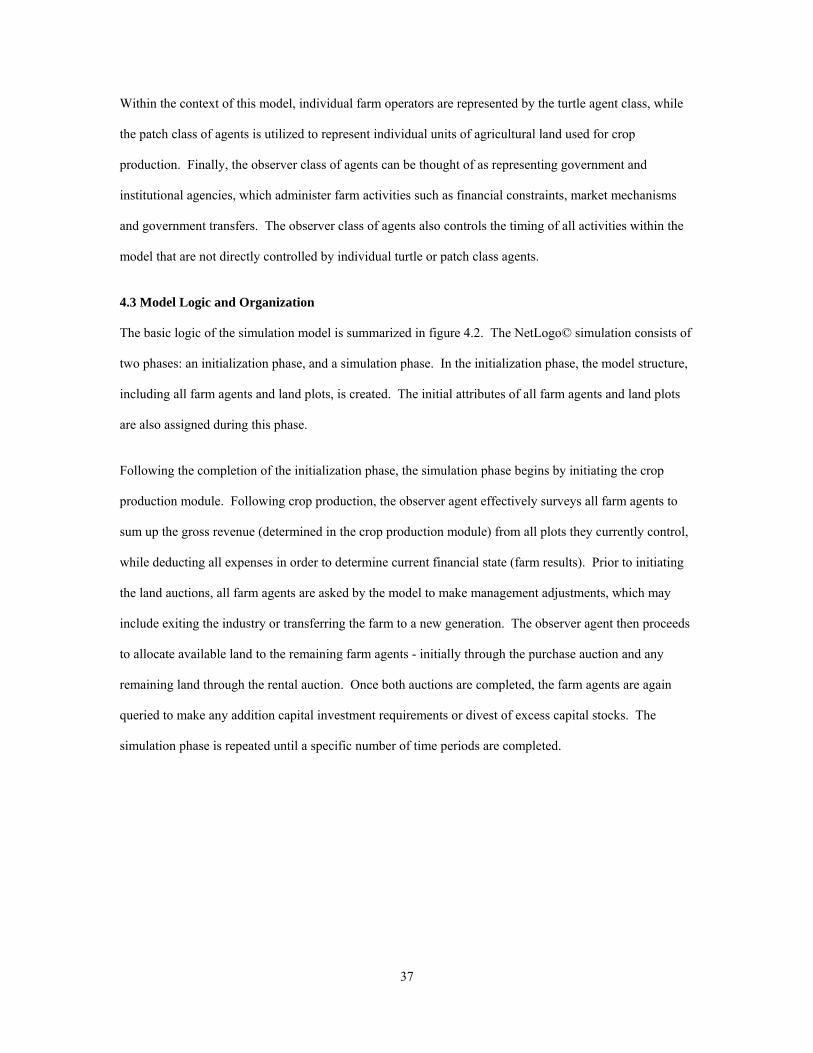
37

Within the context of this model, individual farm operators are represented by the turtle agent class, while

the patch class of agents is utilized to represent individual units of agricultural land used for crop

production. Finally, the observer class of agents can be thought of as representing government and

institutional agencies, which administer farm activities such as financial constraints, market mechanisms

and government transfers. The observer class of agents also controls the timing of all activities within the

model that are not directly controlled by individual turtle or patch class agents.

4.3 Model Logic and Organization

The basic logic of the simulation model is summarized in figure 4.2. The NetLogo© simulation consists of

two phases: an initialization phase, and a simulation phase. In the initialization phase, the model structure,

including all farm agents and land plots, is created. The initial attributes of all farm agents and land plots

are also assigned during this phase.

Following the completion of the initialization phase, the simulation phase begins by initiating the crop

production module. Following crop production, the observer agent effectively surveys all farm agents to

sum up the gross revenue (determined in the crop production module) from all plots they currently control,

while deducting all expenses in order to determine current financial state (farm results). Prior to initiating

the land auctions, all farm agents are asked by the model to make management adjustments, which may

include exiting the industry or transferring the farm to a new generation. The observer agent then proceeds

to allocate available land to the remaining farm agents - initially through the purchase auction and any

remaining land through the rental auction. Once both auctions are completed, the farm agents are again

queried to make any addition capital investment requirements or divest of excess capital stocks. The

simulation phase is repeated until a specific number of time periods are completed.

38

create patchesassign attributes to patches

create turtlesassign attributes to patches

assign parameters

repeat

management adjustments

land auctions

capital investment

Initialization Phase Simulation Phase

crop production

farm results

stop?Output Data

noyes

Figure 4.2: General Model Procedure Flow Chart (adapted from Happe, Kellermann and Balmann 2004) 4.4 Production Factors The individual farm agent requires land, labour and capital inputs for annual crop production. Like the

popular perspective of farming on the Canadian Prairies, it is assumed in this model that field crop

production dominates the farming landscape. The importance of land as an input cannot be understated in a

region characterised by field crop production as the sole form of agricultural activity.

4.4.1 Land The spatial representation of the model utilizes the patch class of agents. A single patch agent represents an

individual 160-acre plot of agricultural land. Note that just as in reality, total acres suitable for crop

production on a given plot may be less than the total plot acreage. The simulated region used here consists

of 1296 individual plots, and is equivalent to an idealized Rural Municipality in the province of

Saskatchewan. Plots differ in three respects: productivity, land-use, and ownership. While this ‘world’

appears as a single two-dimensional grid in the model, the underlying characteristics and data structure can

be simplified by separating the grid into multiple data and algorithmic layers (figure 4.3). The combination

of five critical layers and their underlying characteristics form the physical and institutional spatial

environment where the farm agents co-exist and alter their production decisions.

39

Layer 1: Farm Location

- location of individual farmer's home quarter

Layer 2: Land Tenure

- owned - unfarmed

- leased

Layer 3: Land Use / Cropping

- crop 1 - crop 3

- crop 2 - crop 4

Layer 4: Annual Growing Conditions

low high

Layer 5: Land Quality

low high

Figure 4.3: Spatial Data and Characteristics of the Simulation The top two layers control institutional characteristics with respect to land control and tenure. Layer 1

maps out the spatial location of all agricultural plots available to an individual farm agent for productive

activities. Note that the initial location of a given farm agent is determined randomly through each

replication of the model. The second layer is essentially a regional map that identifies the owner and/or

lessee (in the case of a non-farming land owner) of each individual plot of land, which is initially allocated

based on the location of the farm agents. With respect to the top two layers, a given plot of land may exist

in the following set of states:

o Plot is owned by farm agent k;

o Plot is leased by farm agent k;

o Plot is a farmstead;

o Plot is currently not managed (idle).

The land use/crop cover layer (layer 3) captures a producer’s annual production decisions, and is the model

equivalent of an aerial photograph of the region. Related research on the dynamics of land use and cover

change utilizing the ABS framework typically focuses on this layer (Parker et al 2001). Annual crop

production achieved from an individual unit of land is dependent on a number of exogenous factors,

including soil productivity and annual weather patterns. The model algorithm incorporates these factors in

40

a parsimonious way, yet the model consistently captures many of the subtleties of crop production. The

impact of annual weather patterns and soil productivity are captured within layers 4 and 5, respectively.

While overall weather conditions can differ dramatically between growing seasons, soil quality tends to be

relatively constant over the relatively short geologic time period considered in the simulations. Therefore,

soil quality is assumed to be stable within the simulation. Annual weather patterns and constant soil

productivity are captured by a simple index value, where a value of unity corresponds to the average. Thus,

a plot of land with average soil productivity and annual weather patterns (corresponding to index values of

unity) realizes an average level of production. The exact meaning of an “average level of production” will

be discussed again in section 4.6.1.1, which focuses directly on crop production.

4.4.2 Farm Labour and Capital

Farm agents are assumed to supply the majority, but not all, of the required labour for the farm operation.

In turn, labour costs consist of both a family/managerial withdrawal and a charge for hired labour/custom

work12. In addition, it is assumed that equipment and facilities inputs are fixed in constant proportions

relative to the land input13. As a result, a farm agent who desires to double their farm acreage would also

be required to double his/her equipment and facilities investment value.

4.5 Risk Preference/Entrepreneurial Classification/Farm Goals

A farm business deals with three primary types of risk – production/marketing, financial and asset risk. In

this model, the farm manager’s willingness to assume risk has a well defined impact on both annual crop

production and long-term growth decisions.

Willingness of a farm manager to assume risk is a function of a number of factors, including personal

goals/objectives, coupled with the entrepreneurial characteristics of the individual. I assume here that the

life cycle of a farm business means operating in one of three life phases, where each phase is characterized

by different levels of risk aversion: an entry and establishment phase, a development and growth phase, and

an exit and retirement phase (Keatings and Munro 1989). The objectives of the farm business evolve as the

12 The per acre cost of hiring additional non-family labour and/or custom work is assumed to be characterised as a logistic growth function and will be discussed further in chapter 5. 13 While it is noted that farm machinery investments are often characterized as ‘lumpy inputs’, the existence of well functioning markets for machinery rental and custom operators will result in relatively constant economies of scale with regard to equipment and facility investment.

41

farm progresses through the three phases, while a farms’ progression through the phases is strongly

correlated with the age of the farm manager (Bennet and Kohl 1982). Throughout the development and

growth stage, the farm manager will be primarily concerned with farm growth14 and thus will be less risk

averse than a farm manager in the exit and retirement phase, a time when equity protection and avoiding

risk become the primary objectives (Olson 2004).

While it is possible to predict general patterns of behaviour based on age and other demographic

characteristics (Foot 1996), the behaviour of individuals within a demographic group may still vary

significantly. It would be naive to assume that all farms in the same business phase would have the same

willingness to assume risk, and it can be expected that the risk profile will vary significantly among

producers. Yet on aggregate, there are observable consistencies in risk behaviour. Tractability and data

limitations mean that for my purposes, farm managers are segregated into four distinct managerial classes

with correspondingly different (but equal within each category) risk preferences:

o Exit and Retirement phase manager (most risk averse)

o Lifestyle farm manager

o Cautious expanding farm manager

o Expanding farm manager (least risk averse)

All farm agents are assumed to enter the Exit and Retirement phase at a pre-determined age, after which

they will no longer place bids on additional farm land15. During this phase, retirement planning and asset

protection replace farm growth as the farms primary objective. Prior to shifting into the Exit and

Retirement phase, farm agents belong to one of the three alternative classes for the entire farm development

and growth phase16.

Farm agents are assumed here to be concerned with farm expansion and will attempt to increase the number

of plots managed throughout the growth and development phase. The farm agent’s willingness to assume

risk corresponds directly with their risk aversion factor. In this model, a risk neutral farm agent would have

14 Farm growth includes both growth in the size of the farm through land acquisition and the growth of farm equity. 15 The farm agent will still attempt to renew previous lease agreements 16 The farm growth period occurs from the age the farm agent begins managing the farm to the age when the farm manager enters the exit and retirement phase.

42

a risk aversion factor set to unity and values land based on their undiscounted land rent expectations.

Alternately, risk averse farm agents discount their land rent expectations with a risk aversion factor less

than one, meaning the probability of purchasing land at a price that overestimates its true earning potential

is reduced. And an increase in the level of risk aversion will lead to a reduction in a farms’ land valuation

(Harris and Nehring 1976). The less risk averse a farm agent is, the greater their risk aversion factor is, and

the less their land rent expectations are discounted.

4.6 The Farm Agent - Farm Actions Over the course of a single simulation year cycle, a farm agent engages in a number of distinct activities as

shown in figure 4.4.

start stop

no

yes

Re-New Land Leases?

Rental Agreement

Land Purchase Auction

Purchase

Land Rental Auction

Rental Agreement

Crop Production Farm Accounting Managerial Adjustments

Expectation Formation

Financial Statements

Land Market

step influence

capital requirement per acre

Capital Investment

Calculate Offer

Calculate Bid

Calculate Offer

continue farming?

Figure 4.4: Individual Farm Agent Flowchart of Activities (based on Balmann 1997) The activities undertaken by a farm agent include producing and marketing field crops, farm accounting,

management decisions, renewing existing leases and acquiring control over additional land and capital

assets.

4.6.1 Crop Production

Sale of crops produced generates gross cash income and variable cash expenses which becomes part of

cash flows. Additional cash outflows include fixed production expenses and family living and managerial

withdrawals.

43

4.6.1.1 Gross Crop Revenue Annual crop production is characterised by gross revenue uncertainty, which can be separated into yield

and price risks. The stochastic nature of annual crop production and commodity prices results in a varying

short term profit and long term viability of each individual farm operation. Randomness within price and

crop yield is composed of both global and local effects. On a global scale, commodity price is affected by

world supply and demand dynamics - individual producers can have no impact on prices. However at the

local level, individual producers may choose to market their crops at different times or to different

locations, a strategy that may generate a price different from that of a neighbours’ identical crop. Crop

yields are determined by both global weather patterns applied to the region as well as local variations

within the region of study. As an example, a drought will reduce the crop yields for all producers in the

region, but localized weather patterns and other agronomic factors within the region determine the degree

of yield reduction for individual plots of land.

The variability inherent in average annual world prices is exogenous to the simulation and is captured by an

array of crop prices for all crops in a given year. Local variation among farmers is not permitted in this

model, meaning that all producers receive the annual average world price for their production17. The global

variability of crop yields is captured in the same manner as the global commodity prices. While the global

price refers to a world market price, the global yield refers to the general yield pattern of the region.

Within the simulation, varied weather patterns and soil productivity lead to variation in the individual plots’

actual crop yield. The relative production yield of an individual plot is determined by both fixed

productivity factors such as soil quality, and annual productivity factors including weather. This

combination of both fixed soil productivity and annual growing conditions determines the relative yield of

the plot (see figure 4.5).

17 This is probably not an onerous oversight. Local revenue effects will likely average out over the entire region, making this a rent-seeking issue, not a productivity issue.

44

Figure 4.5: Relative crop yield, soil productivity, and annual growing conditions A plot with soil productivity and annual growing condition index values both equal to 1 would produce a

crop yield equivalent to the mean yield value for the current production period. Plots with a higher soil

productivity index value have a higher probability of realizing a crop yield above the annual regional

average crop yield than a plot with a lower soil productivity index value. A plot of land possessing a less

than average soil productivity value (< 1) would require annual growing conditions exceeding the regional

average growing conditions in order to produce a crop above the regional yield average for the same

period.

The farm agent’s realized gross revenue from crop production is a function of the global variability of

commodity prices/yields and local yield variability. Global commodity prices and yields are input into the

simulation as an array of values for each crop year, remaining consistent over all model replications18.

Simply, the gross revenue of an individual farm agent is equal to the summation of the revenue generated

by all crops grown on land controlled by the farm agent (equation 4.1).

∑=

=I

iiGRGR

1

(4.1)

where GR = gross revenue of farm agent k GRi = gross revenue from crop i

18For example if the price of wheat is set at $2/bushel for crop year 1, and $3/bushel for crop year 2, these values would remain constant for all replications of the model.

45

Crop revenue is computed based on the global commodity price and yield, which are the same for all farm

agents, as well as the individual farm agent’s adjustment factor and the area of land allocated to production

of the crop in question (equation 4.2).

iiii APFYPGR ⋅⋅⋅= (4.2)

where Pi¯ = mean price of crop i Yi = mean yield of crop i PF = productivity factor of farm agent k Ai = area (acres) of crop i seeded/harvested by farm agent k The productivity factor for each farm agent is the mean value of the productivity index (soil productivity

index multiplied by annual growing conditions index) of all owned and leased plots weighted by the

number of cultivated acres (equation 4.3).

∑ ⎟⎟⎠

⎞⎜⎜⎝

⎛⋅=

KK

PIPF xyxy

(4.3)

where PIxy = productivity index of plotxy Kxy = crop acres of plotxy

K = crop acres managed by farm agent k By computing the gross revenue in this manner, it is further assumed that each farm agent produces the

same crop mix on all plots they manage.

4.6.1.2 Variable Production Costs

Variable crop production costs are dependent on both the area of cultivated land and the production level.

For example, the cost of seed and fuel for planting and tillage operations are independent of the production

level realized19, but the cost of harvesting is related to the volume of production. In order to capture these

cost relationships, the variable crop production costs are modelled as a function of both realized production

level and the area of land employed. The total variable crop production costs for the farm agent are the

sum of variable costs for all crops grown in the current period and the total non-family labour cost

(equation 4.4).

19 The possibilities that a farm agent may reduce input use when the production level is expected to be poor are ignored.

46

( )( )∑=

⋅++⋅=I

i

volii

acreii VCVWVCAVC

1

(4.4)

where VC = variable production costs of farm agent k VCi

acre = variable production costs per acre of crop i W = non-family labour cost per acre of farm agent k Vi = production volume of crop i VCi

vol = variable production costs per volume of crop i

Crop production costs are also dependent on distance, due to the cost of transporting farm products and

machinery. Thus, holding all other factors constant, the cost of producing a crop on a given plot of land

increases as the distance from the farm agent’s farmstead increases. The relationship between production

costs and distance can be expressed by the cost of transporting machinery20 and the cost of transporting

farm product by truck. Therefore, this model assumes that all crop production is marketed from the

farmstead, with no farmstead-to-deliver-point freight variability between farm agents. As a result, the cost

of transporting farm production is just the cost of moving product from the field to the managing farm

agent’s farmstead.

The total transportation cost of a farm agent is simply the sum of transportation costs of all plots currently

managed. In turn the annual transportation cost for an individual plot of land is dependent on the distance21

to the managing farm agent’s farmstead and the volume of production realized (equation 4.5).

( )TruckVTravelDTE xyxyxy ⋅+⋅= (4.5)

where TExy = transportation costs associated with plotxy Dxy = distance between plotxy and managing farm agent’s farmstead Travel = annual cost of transporting farm equipment per unit of distance Vxy = production volume (all crops) of plotxy

Truck = annual cost of transporting crop production per unit of distance 4.6.1.3 Fixed Production Costs

Fixed production costs include the two categories of fixed inputs used in the simulation –

machinery/equipment, and land. Total annual fixed costs are composed of machinery and equipment

replacement charges and land lease payments (equation 4.6).

20 The cost of transporting machinery consists of machinery operating expenses (fuel, depreciation), and the opportunity cost of travel time. 21Distance is measured as the summation of the east-west and north-south distances between the farmstead and the plot.

47

LPCFC replace += (4.6)

where FC = fixed production costs of farm agent k Creplace = machinery and building replacement charge of farm agent k LP = land lease payment cost of farm agent k

Machinery and equipment replacement charges are assumed to equal annual economic depreciation. This

implies each farm agent makes an annual cash investment in machinery and equipment equivalent to the

annual reduction in machinery and equipment value due to economic depreciation. The net result is a

constant machinery and equipment value per crop acre over time. Annual land lease expense is calculated

as the sum of the annual per acre lease payment multiplied by the number of crop acres of all farm plots

leased by the farm agent.

4.6.1.4 Family/Management Withdrawal

The farm agent requires a minimum level of “cash” that must be withdrawn annually for family living and

managerial expenses22. All farm agents are given the same minimum withdrawal requirement and marginal

propensity to consume from gross revenue. Annual withdrawals increase with farm size due to the

additional labour and managerial requirements of producing on additional plots. When the farm agent’s

annual cash flow is unable to meet the producer’s withdrawal value, the deficiency is made up by the equity

built up in previous periods (or initially endowed). The annual withdrawal is evaluated as:

KGRWDWD ⋅+⋅+= σβmin (4.7)

where WD = family/management withdrawal of farm agent k WDmin = minimum family/management withdrawal amount β = marginal propensity to consume from gross revenue σ = management cost adjustment factor for an additional acre of crop land managed

22 While it is noted that off-farm income currently may be used to meet a significant portion of the family living requirement of many farm households, this was historically not the case. In order to remain consistent with the assumptions of constant technology and purchasing power and a 1960’s base period in these simulations the farm household’s farm/non farm labour allocation decision is ignored.

48

4.6.2 Farm Accounting

Like their real world counterparts, many of the decisions made by producers within the simulation are

influenced by financial constraints. In order to fully capture reality, a set of basic accounting rules and data

structures are implemented. While some producers may be unaware of the true financial state of their

farming operation and may sometimes make decisions that are not conducive to financial success, large

capital and land purchases are ultimately constrained by credit availability. This in turn is based on the

financial solvency of the producer. As a result of the large investments required to expand a given farm,

and the general requirement of credit procurement by individual producers, producer decisions can be

influenced by financial constraints even in cases where producers are unaware of their true financial health.

Farm agents are concerned with both their short-run profitability and the long-run growth of equity in the

farm operation. In the short-run, a farm must be able to generate cash flow levels capable of covering all

production costs and family living withdrawals. This coverage ensures the long term sustainability and

growth of the farm. The long-term financial health of each agent in the simulation is tracked continuously

via a simplified balance sheet (figure 4.6).

$5,000Crop Inventories b $0 payments remaining 15

annual payment $463Principal balance $4,500

adjusted acres c 310 average market value $45 Debt # 2Land Value $13,950 payments remaining 18

annual payment $462$4,800 $5,000

$9,500

$14,250

$23,750 $23,750

a Cash includes all non-land and machinery/building assetsb crop production is assumed to be sold in the same period it is produced, resulting in zero inventories at year endc cultivated acres pro-rated by soil productivity (i.e. 1 acre with a soil productivity index value of 0.85 = 0.85 adjusted acres)

Total Assets

Principal balance

Total Liabilities

Liabilities + Equity

Equity

Smith FarmBalance Sheet

December 31, 1960

Machinery/Equipment

Debt # 1

Assets Liabilities

Cash a

Land

Figure 4.6: Representative producer balance sheet

The cash account can be thought of as a residual account that tracks the accumulated annual net cash flow

of the farm. The land assets are valued at market levels, which is equivalent in the simulations to the

49

average selling price (adjusted for soil productivity) from the most recent period in which at least one plot

of land was purchased through the land auction23. Machinery and equipment assets are also valued at their

market value. Due to the assumption that annual replacement expense is equivalent to annual economic

depreciation, this is calculated simply as the product of the total number of crop acres managed by the farm

agent and the required per acre capital investment value.

In addition to the farm agent’s long run financial indicators, annual net cash flow is also tracked within the

model. Net cash flow is determined as the farm agent’s net increment to their cash account after all farm

and family living expenses, including investment and financing flows, have been calculated (equation 4.8).

FINANCEINVEST NCFNCFWDFCTEVCGovGRNCF ++−−−−+= (4.8)

where NCF = net cash flow of farm agent k Gov = net government transfers received by farm agent k TE = annual transportation cost of farm agent k NCFINVEST = equipment and facilities sale proceeds less purchases of farm agent k NCFFINANCE= new borrowing less principal and interest payments

While an individual farm agent has the ability to cover negative annual cash flow with built up equity in the

operation, prolonged periods of negative cash flow will erode the equity of the farm and may result in the

farm agent eventually exiting the industry. At a minimum, in the simulation a prolonged period of negative

cash flow and an erosion of farm equity will limit the future credit availability and land purchasing ability

of a farm agent.

4.6.3 Expectation Formation

Individual farm agents make a number of important managerial decisions based on their expectations of

future production margins. Land and family labour/management are modelled as the residual claimants of

farm profit; as a result a farm manager’s willingness to pay for addition farm land (rent) is a direct function

of both future production margin expectations and family/managerial withdrawal requirements (figure 4.7).

23 Only land sold through the land market is used to evaluate the market value of land. This eliminates “non arms-length” sales between family members that result when farms are transferred to a new generation. In the scenario where no farm agents purchase farm land the minimum acceptable land bid is used; when no land is available for sale in a period, and thus no land bids are calculated, the value from the previous period is used.

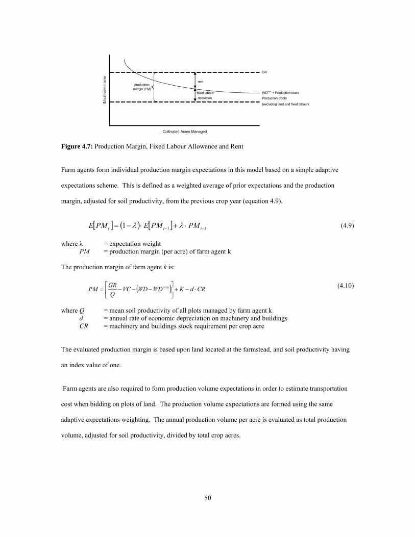
50

rent

fixed labour WDmin + Production costs deduction Production Costs

(excluding land and fixed labour)

Cultivated Acres Managed

$/cu

ltiva

ted

acre

GR

production margin (PM)

Figure 4.7: Production Margin, Fixed Labour Allowance and Rent

Farm agents form individual production margin expectations in this model based on a simple adaptive

expectations scheme. This is defined as a weighted average of prior expectations and the production

margin, adjusted for soil productivity, from the previous crop year (equation 4.9).

[ ] ( ) [ ] lttt PMPMEPME −− ⋅+⋅−= λλ 11 (4.9)

where λ = expectation weight PM = production margin (per acre) of farm agent k

The production margin of farm agent k is:

( ) CRdKWDWDVCQ

GRPM ⋅−÷⎥⎦

⎤⎢⎣

⎡−−−= min (4.10)

where Q = mean soil productivity of all plots managed by farm agent k d = annual rate of economic depreciation on machinery and buildings CR = machinery and buildings stock requirement per crop acre

The evaluated production margin is based upon land located at the farmstead, and soil productivity having

an index value of one.

Farm agents are also required to form production volume expectations in order to estimate transportation

cost when bidding on plots of land. The production volume expectations are formed using the same

adaptive expectations weighting. The annual production volume per acre is evaluated as total production

volume, adjusted for soil productivity, divided by total crop acres.

51

4.6.4 Farm Management Farm management in the context of this research refers to the farm agent’s decision to exit the industry or

to continue farming and select a crop mix for the next production period. The decision to quit farming is

the most drastic management adjustment any farm agent can make. In reality, it can be the result of a

number of factors, including financial and family pressures.

4.6.4.1 Farm Exits

Farm exits are triggered as either an early forced exit due to financial factors or a more orderly exit due to

old-age retirement/succession. In the case of forced exits, operations cease and all farm assets are released

when either of the early shutdown conditions is met:

o Insolvency (forced exit)

farm liabilities ≥ 0.9 · farm assets24 (4.11)

o Prolonged Equity Erosion (voluntary exit)

NCF < 0 for 5 continuous periods25 (4.12)

Farming is typically a lifetime commitment, and exits from farming are often less responsive to market

conditions than many non-farm industries (Gale 1996). As a result, a farm manager will likely continue to

operate, in the short-term, even if the full value of their labour input is not realised (see equation 4.12).

The farm agent’s probability of a voluntary exit due to old-age retirement increases as the farm agent ages26

and is based on probabilities common to all farm agents. When the decision to discontinue farming is made

as part of an old-age retirement/succession plan, the farm has the potential to be transferred to an heir of the

current farm agent as a transaction between family members. The possibility of a transfer of the complete

farm to a non- family member is ignored here since most farms in North America have historically been

transferred from parent to child (Bennet & Kohl 1982). The decision of the next generation to continue the

operation of the farm is captured as a likelihood occurring at the time of retirement of the original farm

24 A farm is deemed to be insolvent when total liabilities exceed total assets, but in general a farm is vulnerable when their debt to asset ratio exceeds 0.7:1 (Olson 2004). 25 While it is unrealistic to assume that all farmers will exit after exactly 5 continuous years of negative cash flow, on average the assumption of five years seems reasonable and tends to fit real data with reasonable accuracy. 26 The probability of retirement increases as the farm agent moves into a new 5 year age bracket and remains constant while in the same bracket.

52

agent. All farms operated by farm agents that are exiting due to old-age retirement and have a strong

current net worth, with a debt to asset ratio no greater than 0.4:1 (Olson 2004), have the same probability (a

parameter value between 0 and 1) of being taken over by the next generation. The new farm agent is

assumed to gain control over all existing farm assets, including all lease agreements. The new agent is also

assumed to “buyout” the original farm agent by assuming all existing liabilities and a cash buyout of a

proportion of the equity value of the farm (equation 4.13).

buyout value = farm liabilities + α · farm equity (4.13)

where α = proportion of farm equity debt financed when farm is transferred to new generation

The next generation farm agent is assumed to finance the purchase of farm equity by financing over a

twenty-year amortization period27. In a situation where the farm is not transferred to a new generation, all

land assets are released for other farm agents to acquire through the land market.

4.6.4.2 Crop Mix Adjustment Farm agents select their annual crop mix from a discrete set of available crop alternatives. Producers are

assumed to maximize their total expected utility ( E[U ] ) based on the simple summation of the expected

utility of the individual crops ( E[Ui] ) that are included in the selected crop mix, subject to land and

agronomic constraints (equation 4.14).

[ ] ( )[ ]∑=

⋅Π=I

iii aUEUEMax

1

(4.14)

s.t.

ii

I

ii

ba

a

≤

=∑=1

1

where ai = proportion of farm agent k’s crop acres allotted to production of crop i bi = maximum proportion of farm agent k’s crop acres allotted to production of crop i

27 A twenty year amortization period corresponds with Farm Credit Canada’s (FCC) general lending terms (Guide to Farm Practice in Saskatchewan 1960).

53

The expected utility of an individual crop is evaluated as a linear function of mean crop return28 and the

variance of crop return (Selley 1984), where each is computed based on the five previous production

periods. The individual crop options can then be ranked based on an expected utility value, evaluated as:

( ) ( ) 2121][

iiiUE ∏Φ−−Π=Π σ (4.15)

where ∏i = mean crop return (GR - VC) of crop i

Φ = risk aversion factor of farm agent k σ2

∏i = variance of crop return of crop i

As a net result of the computed individual crop utility values, crop options can be ranked in an ordinal

manner. The farm agent will then proceed to allocate his total crop acres in a manner that maximizes the

production of crops with the highest rankings, subject to agronomic constraints. Note that while the

functional form of the farmer’s expected utility function ignores the covariance between the returns of crop

alternatives, it significantly reduces the complexity of this part of the model. Due to the limited number of

crops commonly produced in the study region and the strong correlations of crop returns29, this is not likely

an onerous over-simplification.

A risk neutral agent (Φ = 1) would behave in a pure profit maximizing manner and would select a crop mix

that maximizes their expected total crop return. The risk averse (Φ < 1) farm agent will evaluate the

individual crops based on a trade off between expected returns and variances. The more risk averse an

individual farm agent is the lower the value of the risk parameter (Φ) will be. Intuitively this would mean

that a more risk averse farmer would require a greater expected crop return than a less risk averse farm to

take on the same level of risk (Hadar & Russell 1969).

4.6.5 Farmland Market

Farm agents can expand either by purchasing or leasing additional land, and they compete in two

segmented farmland markets. All farmland tracts are based on a fixed plot size, and this defines the

smallest unit by which farm acreage can change. In each period, land available for sale and leases are

28 Crop return (π) = P x Y - VC (fixed costs are equivalent across all crops and are ignored in the analysis). 29 The covariances of returns for the four crop alternatives modelled all exceed 0.7. This simplification may need to be revisited if the modelled crop alternatives are expanded in subsequent research.

54

allocated to farms through two separate iterative auctions,30 with the lease auction occurring subsequent to

the purchase auction. The order of the two land auctions attempts to capture the belief that farm agents

have a strict preference for purchasing relative to leasing additional land.

Land becomes available for sale/lease when a farm agent exits (forced or voluntary) from the industry or

continuing farm agents do not renew existing lease agreements. The manner in which land becomes

available for re-allocation directly determines the land market in which the plot becomes available for farm

agents to bid on. Available land is re-allocated based on the following rules:

o Forced Exit - Land owned by the exiting farm agent enters the ‘for sale’ market;

land leased by the exiting farm agent enters the ‘for lease’ market.

o Voluntary Exit - Land owned by the exiting farm agent enters the ‘for lease’ market; land leased by the exiting farm agent enters the ‘for lease’ market.

o Non-Renewed Lease - Land enters the ‘for sale’ market.

o No Buyer Found - Land failing to find a buyer in the ‘for sale’ market enters the ‘for lease’ market.

In order to participate in either of the land markets, an individual farm agent must meet certain eligibility

requirements. In this simulation, the requirements for purchasing land are more restrictive compared to the

land lease market. In order to purchase additional farm plots, a producer requires debt financing and must

be deemed credit worthy. Credit worthiness is tracked via a simplified credit scorecard. Credit can only be

obtained if the farm agent meets each of the following requirements:

o Liquidity Cash > ( Λ· K + Kxy · PL · Ω ) (4.16)

o Solvency Debt to Asset Ratio < 0.4: 1 (Olson 2004) (4.17)

o Repayment31 [ ] 1min

>+−⋅DPLP

WDKPME (4.18)

where Λ = minimum cash balance per acre PL = mean price of land per crop acre (adjusted to reflect unitary soil productivity) Ω = proportion of new investment equity financed (required down payment)

30 The iterative auction algorithm is based on the algorithm developed in Balmann (1997) 31 Equation 4.18 is approximately equivalent to the formula ((gross revenue – cash expenses + inventory change – family labour + interest)/annual debt payment) (Olson 2004).

55

Liquidity refers to the ability of the farm to meet short term liabilities using short term assets. The farm is

financially vulnerable when the value of current liabilities exceeds the value of short term assets (Olson

2004). In the simulation, a farm agent is in a liquid financial position provided that their short term assets

(cash value) are greater than their current liabilities, which include an allowance for covering the cash

production costs for a single production period (Λ · K) and the expected cash outlay required for the

purchase of an additional plot of land (Kxy · PL · Ω). Second, an upper limit is placed on the total amount of

debt. Finally, the last constraint restricts credit to farm agents whose current debt and lease payments can

be serviced based on current land rent expectations and minimum living deductions (see figure 4.7).

Repayment capacity is concerned with the ability of a farm to generate an annual cash flow capable of

covering the annual debt payment (principal + interest).

Farm agents are also screened before participating in the land lease auction based on the first restriction on

the credit scorecard, minus the cash down payment portion. A second requirement restricts bidding to

those farm agents whose expected land rent is positive.

The next stage in both land allocation procedures requires all eligible farm agents to determine which

available plot of land they have the greatest interest in managing. The mechanism for determining the

optimal plot of land available is identical for both land auctions, but the evaluated set of plots is different.

Farm agents select land to bid on by computing the highest expected annual land rent (equation 4.19).

[ ] [ ] [ ] [ ]xy

xyxyxyxy KKWDDTEEGovEQPMErentE+

−⋅−+⋅=min

(4.19)

where rentxy = rent value for of plotxy in subset A (available land) Qxy = soil productivity of plotxy

Due to uncertainty that is present surrounding government transfer payments to western Canadian grain

producers, the expected government transfer is assumed here to be zero32 (equation 4.20). Note that while

it is assumed that farm agents have no expectation of future government transfers, this does not rule out

actual payments occurring.

32 While it is unlikely that future government transfer expectations are in fact zero, this assumption is a reasonable starting point.

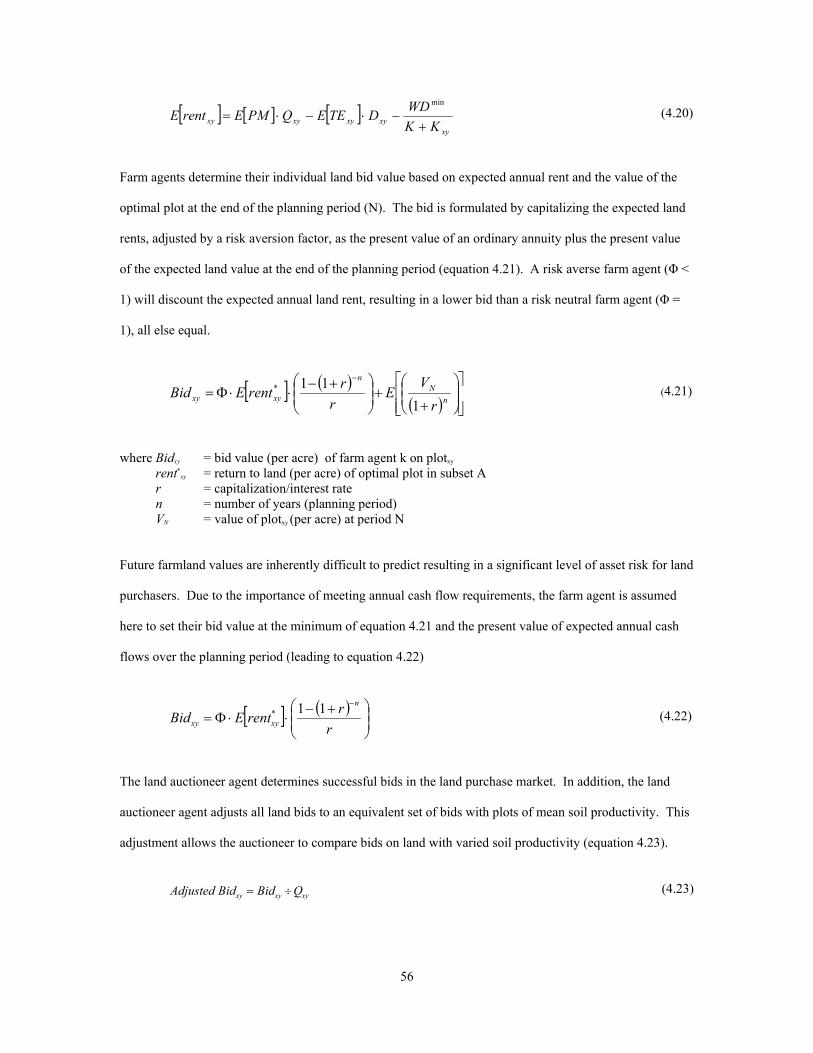
56

[ ] [ ] [ ]xy

xyxyxyxy KKWDDTEEQPMErentE+

−⋅−⋅=min

(4.20)

Farm agents determine their individual land bid value based on expected annual rent and the value of the

optimal plot at the end of the planning period (N). The bid is formulated by capitalizing the expected land

rents, adjusted by a risk aversion factor, as the present value of an ordinary annuity plus the present value

of the expected land value at the end of the planning period (equation 4.21). A risk averse farm agent (Φ <

1) will discount the expected annual land rent, resulting in a lower bid than a risk neutral farm agent (Φ =

1), all else equal.

[ ] ( )( ) ⎥

⎥⎦

⎤

⎢⎢⎣

⎡⎟⎟⎠

⎞⎜⎜⎝

⎛

++⎟⎟⎠

⎞⎜⎜⎝

⎛ +−⋅⋅Φ=

−

nN

n

xyxy rV

Er

rrentEBid1

11* (4.21)

where Bidxy = bid value (per acre) of farm agent k on plotxy

rent*xy = return to land (per acre) of optimal plot in subset A

r = capitalization/interest rate n = number of years (planning period) VN = value of plotxy (per acre) at period N Future farmland values are inherently difficult to predict resulting in a significant level of asset risk for land

purchasers. Due to the importance of meeting annual cash flow requirements, the farm agent is assumed

here to set their bid value at the minimum of equation 4.21 and the present value of expected annual cash

flows over the planning period (leading to equation 4.22)

[ ] ( )⎟⎟⎠

⎞⎜⎜⎝

⎛ +−⋅⋅Φ=

−

rrrentEBid

n

xyxy11* (4.22)

The land auctioneer agent determines successful bids in the land purchase market. In addition, the land

auctioneer agent adjusts all land bids to an equivalent set of bids with plots of mean soil productivity. This

adjustment allows the auctioneer to compare bids on land with varied soil productivity (equation 4.23).

xyxyxy QBidBidAdjusted ÷= (4.23)

57

The land auctioneer sorts all current adjusted bid values and allocates the unit of land selected by the farm

agent with the maximum adjusted bid value, provided the maximum bid is greater than a minimum value.

The minimum bid for a single representative landlord agent is set as the weighted value of leasing out the

land at the current mean lease rate and the mean value of current period purchase bids (equation 4.24). The

value to the landlord of leasing out farmland is evaluated using an income capitalization method (Olson

2004).

⎟⎟⎠

⎞⎜⎜⎝

⎛⋅⋅Ψ=

rleaseBidBidMinimum (4.24)

where Ψ = risk aversion factor of representative non-farming agent Bid¯¯¯ = mean bids in current land auction lease¯¯¯¯ = mean annual lease payment for all plots currently leased As constructed, a risk neutral landlord agent (with Ψ = 1) would accept a bid that is equivalent to the

expected return from leasing out the land at their current weighted land valuation. A risk averse landlord

agent (with Ψ < 1) would accept a land bid that was less than the expected return from leasing out the land.

The final price paid by the successful farm agent in the land purchase auction does not correspond directly

with their evaluated bid value. Farm agents are assumed to adjust their bids based on the best available

land market information available to them, namely the mean value of all current period land bids33. Bids

are adjusted to represent an equal weighting of the current periods mean land bid and the farm agent’s

individual land valuation34 (equation 4.25).

xyxyxy QBidBidprice ⋅⋅= (4.25)

where pricexy = final price paid for plotxy by purchasing/leasing farm agent

The down payment proportion of the land purchase is deducted directly from the farm agent’s cash

account, while the balance is debt financed based on the same amortization period and interest rate utilized

to calculate the bid.

33 The mean bid, is the same value for all participating farm agents and is only set during the first auction iteration and remains constant for the remainder of the current period. 34 The bid adjustment is similar to Happe, Balmann and Kellermann (2004). The mean bid is set separately for the purchase and lease auction, and is set only during the first iteration of the two auctions and remains constant, in the respective auctions, until the next model year.

58

The dynamics of the individual farm agents and the land auctioneer agent are illustrated below through a

simple example with 3 farms and 2 available plots, with average soil productivity (figure 4.8).

3-farm Land Auction Iteration # 1

Farmer Land Bid On E[RL*xy] Valuation Factor Bid a

Purchase Price c

1 B # 1 B $3.00/acre 0.90 $30.97 / acre $30.39/acre

3 # 2 A $2.90/acre 0.85 $28.27 / acre $29.03/acre

A # 3 B $3.10/acre 0.85 $30.22 / acre 30.02/acre

2 Minimum Bid: $29.49/acre b

High Bid: $30.97/acre (farmer # 1 on land B)Outcome: Farmer # 1 purchases land unit B for $30.39/acre

3-farm Land Auction Iteration # 2

Farmer Land Bid On E[RL*xy] Valuation Factor Bid a

Purchase Price c

1 # 1 A $2.75/acre 0.90 $28.38/acre $29.09/acre

3 # 2 A $2.90/acre 0.85 $28.27/acre $29.03/acre

A # 3 A $2.85/acre 0.85 $27.79/acre $28.79/acre

2 Minimum Bid: $29.47/acre b

High Bid: $28.38/acre (farmer # 1 on land A)Outcome: High bid rejected, Land A enters lease market

a bid values based on r = 6%, n = 20 yearsb Minimum bid base on mean lease rate = $1.75 / acre and Ψ = 1 (land seller is risk neutral)c purchase price if bid is successful; based on an mean land bid $29.82/acre

Figure 4.8: 3-person, 2 available plots land auction

In the example, note that in the second iteration of the land auction, farmer # 1 is the high bidder but is

unsuccessful in purchasing land unit A due to the bid being less than the reservation price. Due to

utilization of this iterative auction algorithm, individual bids compete against all land bidders and not only

against those bids on the same unit of land.

Rental auction bid formation follows the same structure as the purchase price bid. Farm agents are

assumed to be willing to pay an annual lease rate equivalent to 80% of annual debt payment they would

accept if they were bidding to purchase the same plot of land35. The successful farm agent will be entered

in a lease agreement at an annual lease rate equivalent to their bid value and for an upper-bound random

lease period. In the example, assuming that the three farmers represent all producers in the lease market,

35 Based on a 20 year planning horizon and a 6% discount (interest) rate the farm agent’s annual cash lease bid is equivalent to approximately 7% of their individual land valuation. A reasonable cash lease for farmland is estimated at 6-8% of the land’s value plus the cost of property taxes which are ignored in the simulation (Guide to Farm Practice in Saskatchewan 1960).

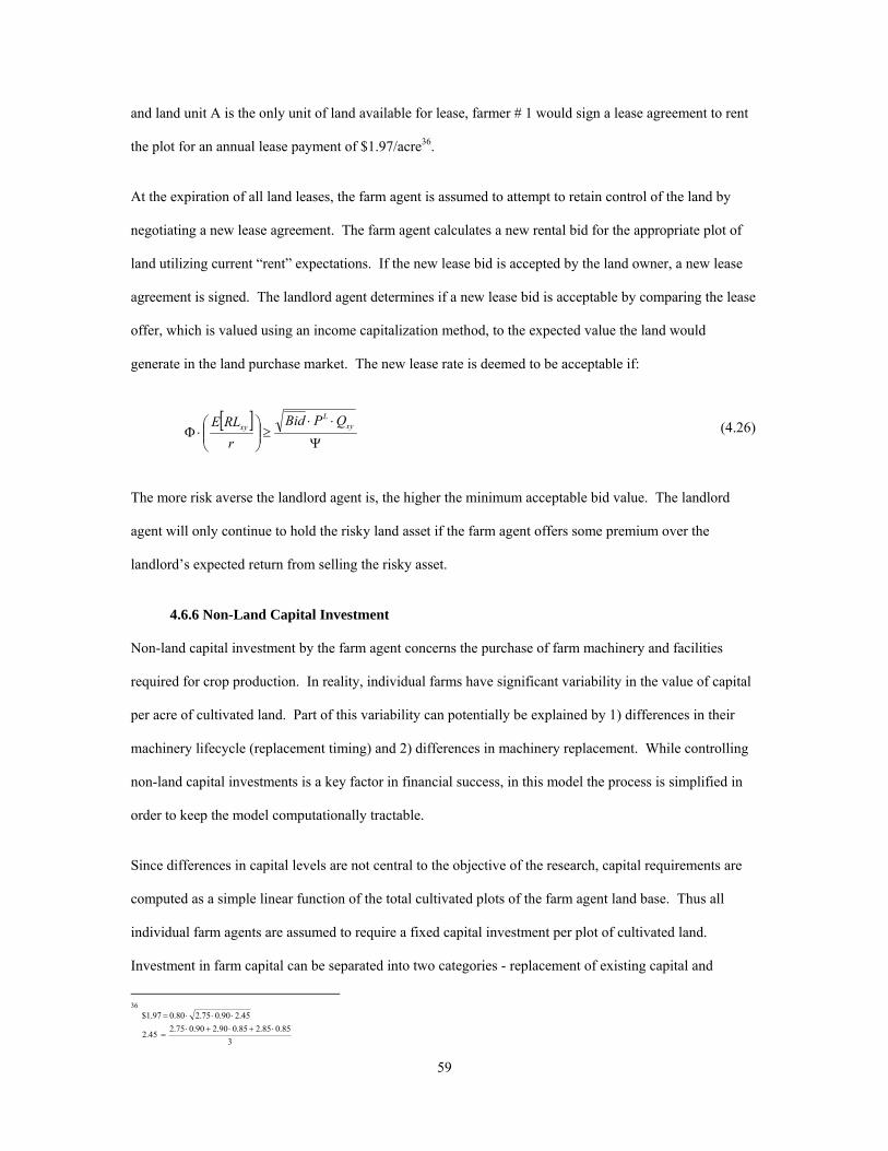
59

and land unit A is the only unit of land available for lease, farmer # 1 would sign a lease agreement to rent

the plot for an annual lease payment of $1.97/acre36.

At the expiration of all land leases, the farm agent is assumed to attempt to retain control of the land by

negotiating a new lease agreement. The farm agent calculates a new rental bid for the appropriate plot of

land utilizing current “rent” expectations. If the new lease bid is accepted by the land owner, a new lease

agreement is signed. The landlord agent determines if a new lease bid is acceptable by comparing the lease

offer, which is valued using an income capitalization method, to the expected value the land would

generate in the land purchase market. The new lease rate is deemed to be acceptable if:

[ ]Ψ

⋅⋅≥⎟⎟

⎠

⎞⎜⎜⎝

⎛⋅Φ xy

Lxy QPBid

rRLE (4.26)

The more risk averse the landlord agent is, the higher the minimum acceptable bid value. The landlord

agent will only continue to hold the risky land asset if the farm agent offers some premium over the

landlord’s expected return from selling the risky asset.

4.6.6 Non-Land Capital Investment

Non-land capital investment by the farm agent concerns the purchase of farm machinery and facilities

required for crop production. In reality, individual farms have significant variability in the value of capital

per acre of cultivated land. Part of this variability can potentially be explained by 1) differences in their

machinery lifecycle (replacement timing) and 2) differences in machinery replacement. While controlling

non-land capital investments is a key factor in financial success, in this model the process is simplified in

order to keep the model computationally tractable.

Since differences in capital levels are not central to the objective of the research, capital requirements are

computed as a simple linear function of the total cultivated plots of the farm agent land base. Thus all

individual farm agents are assumed to require a fixed capital investment per plot of cultivated land.

Investment in farm capital can be separated into two categories - replacement of existing capital and

36

385.085.285.090.290.075.2

45.2

45.290.075.280.097.1$⋅+⋅+⋅

=

⋅⋅⋅=

60

investment in additional capital. Replacement of existing capital stocks is discussed further in section

4.6.1.3 and is covered by the assumptions made in the depreciation model. New investment in non-land

capital only occurs when the farm agent has expanded their land base either by purchasing or leasing

additional land. New non-land capital investment is equal to the fixed per plot non-land capital

requirement multiplied by the total new cultivated plots acquired. In turn, all new non-land capital

expenditures are assumed to be financed with a 25% cash down payment and a 5 year amortization

period37. The net new non-land capital investment calculation of a farm agent is:

NCI = CR ·(C t - C t-1) (4.27)

where NCI = net investment in machinery and buildings of farm agent k C = stock of machinery and buildings of farm agent k

Non-land capital is assumed to be perfectly mobile, meaning that the full per plot non-land capital

investment is recovered when the farm agent’s total acreage is reduced. In the event of a net reduction in

the farm agent’s land base, the net non-land capital investment is negative and the producer will receive a

cash payment.

4.7 Initializing the Model Thus far, this chapter has outlined and described the encoded model algorithms and assumptions while

avoiding a discussion of the initial spatial and population profile and production data utilized in the

simulations. The following section contains a detailed summary of the initial profiles and production data.

In order to initialize the model with a population of farm agents consistent with a 1960’s profile, farm

agents are assigned a number of attributes based on available census and survey data. The attributes

include 1) age, 2) farm size, 3) tenure status, 4) finances, and 5) management. The success of individual

farms is partially dependent on the boom-bust cycle of gross crop returns. As a result, crop yield and

market price data are important considerations. Due to the small level of production in the studied region

relative to the world market, commodity prices are modelled as exogenous to the model and are equivalent

to real de-trended values for the 1955-2000 crop years. In addition, to remain consistent with the constant

technology assumption, variable and fixed production costs and family living/management withdrawals are

37 The assumed loan terms are consistent with the maximum lending terms (75% of asset value and 10 year repayment period) for chattel offered by Farm Credit Corporation for the 1960 period (Guide to Farm Practice in Saskatchewan 1960).

61

based on real 1960 values. In this manner, individual farm agent behaviour and actions play an important

role in the evolution of the region. Behavioural data is required in three primary areas, including 1) crop

mix selection, 2) land valuation and 3) retirement and farm transfer.

4.7.1 Initial Farm Population Profile Delineating the demographic characteristics of the relevant farm population is a critical step in the

simulation process because demographic characteristics are one of the key predictors of the future structure

of industry (Foot 1996). Further, the age composition of the initial farm population appears to be the best

predictor of the number and timing of voluntary farm exits and the resulting transfer of farm assets (Gale

2003). Ultimately, an initial population with low farm equity will most likely result in tight credit markets,

and this will have consequences for future land markets.

4.7.1.1 Operator Age and Farm Acreage The initial distribution of farm operators is classified by age and total acreage in table 4.1, and is based on

data from the 1961 census of agriculture for the province of Saskatchewan. The simulation is initialized

with a farm population of 310 primary farm operators with a median age of 46 and an average farm size of

approximately 4 plots (640 acres).

Table 4.1: Initial Distribution of Farm Agents by Age and Plots Managed

1 2 3 4 5-7 8-10 11-14 15-18 19 & over totalunder 25 years 2 3 2 2 1 0 0 0 0 1025-34 years 5 11 10 9 9 4 1 0 0 4935-44 years 7 16 15 15 16 8 3 1 1 8245-54 years 8 17 15 14 15 8 3 1 1 8255-59 years 4 8 6 5 5 2 1 0 0 3160-64 years 4 6 5 3 3 1 0 0 0 2265-69 years 3 5 3 3 2 1 0 0 0 1770 years and over 4 5 3 2 2 1 0 0 0 17

plots farmed (1 plot = 160 acres)

Source: Author based on Census of Canada: Agriculture: Saskatchewan (1961) While the distribution of age profile is approximately normal across the age groups, the age profile of the

initial farm population is assumed to be uniformly distributed within the census age classifications. A

minimum operator age of 20 and a maximum age of 80 years are also assumed.

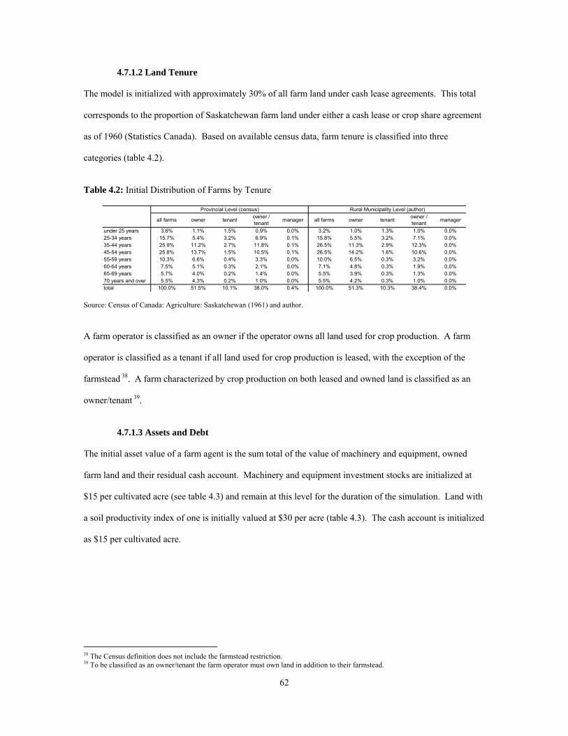
62

4.7.1.2 Land Tenure The model is initialized with approximately 30% of all farm land under cash lease agreements. This total

corresponds to the proportion of Saskatchewan farm land under either a cash lease or crop share agreement

as of 1960 (Statistics Canada). Based on available census data, farm tenure is classified into three

categories (table 4.2).

Table 4.2: Initial Distribution of Farms by Tenure

under 25 years 3.6% 1.1% 1.5% 0.9% 0.0% 3.2% 1.0% 1.3% 1.0% 0.0%25-34 years 15.7% 5.4% 3.2% 6.9% 0.1% 15.8% 5.5% 3.2% 7.1% 0.0%35-44 years 25.9% 11.2% 2.7% 11.8% 0.1% 26.5% 11.3% 2.9% 12.3% 0.0%45-54 years 25.8% 13.7% 1.5% 10.5% 0.1% 26.5% 14.2% 1.6% 10.6% 0.0%55-59 years 10.3% 6.6% 0.4% 3.3% 0.0% 10.0% 6.5% 0.3% 3.2% 0.0%60-64 years 7.5% 5.1% 0.3% 2.1% 0.0% 7.1% 4.8% 0.3% 1.9% 0.0%65-69 years 5.7% 4.0% 0.2% 1.4% 0.0% 5.5% 3.9% 0.3% 1.3% 0.0%70 years and over 5.5% 4.3% 0.2% 1.0% 0.0% 5.5% 4.2% 0.3% 1.0% 0.0%total 100.0% 51.5% 10.1% 38.0% 0.4% 100.0% 51.3% 10.3% 38.4% 0.0%

tenant owner / tenant

owner / tenant manager

Provincial Level (census) Rural Municipality Level (author)

manager all farms owner tenantall farms owner

Source: Census of Canada: Agriculture: Saskatchewan (1961) and author. A farm operator is classified as an owner if the operator owns all land used for crop production. A farm

operator is classified as a tenant if all land used for crop production is leased, with the exception of the

farmstead 38. A farm characterized by crop production on both leased and owned land is classified as an

owner/tenant 39.

4.7.1.3 Assets and Debt The initial asset value of a farm agent is the sum total of the value of machinery and equipment, owned

farm land and their residual cash account. Machinery and equipment investment stocks are initialized at

$15 per cultivated acre (see table 4.3) and remain at this level for the duration of the simulation. Land with

a soil productivity index of one is initially valued at $30 per acre (table 4.3). The cash account is initialized

as $15 per cultivated acre.

38 The Census definition does not include the farmstead restriction. 39 To be classified as an owner/tenant the farm operator must own land in addition to their farmstead.

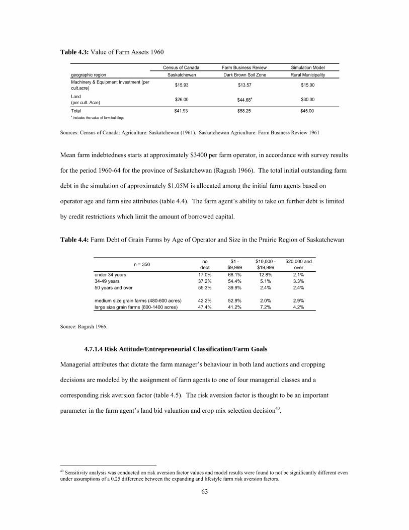
63

Table 4.3: Value of Farm Assets 1960

Census of Canada Farm Business Review Simulation Modelgeographic region Saskatchewan Dark Brown Soil Zone Rural Municipality

Total $41.93 $58.25 $45.00a includes the value of farm buildings

$30.00

$15.93 $13.57 $15.00 Machinery & Equipment Investment (per cult.acre)

Land (per cult. Acre) $26.00 $44.68a

Sources: Census of Canada: Agriculture: Saskatchewan (1961). Saskatchewan Agriculture: Farm Business Review 1961 Mean farm indebtedness starts at approximately $3400 per farm operator, in accordance with survey results

for the period 1960-64 for the province of Saskatchewan (Ragush 1966). The total initial outstanding farm

debt in the simulation of approximately $1.05M is allocated among the initial farm agents based on

operator age and farm size attributes (table 4.4). The farm agent’s ability to take on further debt is limited

by credit restrictions which limit the amount of borrowed capital.

Table 4.4: Farm Debt of Grain Farms by Age of Operator and Size in the Prairie Region of Saskatchewan

under 34 years 17.0% 68.1% 12.8% 2.1%34-49 years 37.2% 54.4% 5.1% 3.3%50 years and over 55.3% 39.9% 2.4% 2.4%

medium size grain farms (480-600 acres) 42.2% 52.9% 2.0% 2.9%large size grain farms (800-1400 acres) 47.4% 41.2% 7.2% 4.2%

n = 350 $20,000 and over

no debt

$1 - $9,999

$10,000 - $19,999

Source: Ragush 1966.

4.7.1.4 Risk Attitude/Entrepreneurial Classification/Farm Goals

Managerial attributes that dictate the farm manager’s behaviour in both land auctions and cropping

decisions are modeled by the assignment of farm agents to one of four managerial classes and a

corresponding risk aversion factor (table 4.5). The risk aversion factor is thought to be an important

parameter in the farm agent’s land bid valuation and crop mix selection decision40.

40 Sensitivity analysis was conducted on risk aversion factor values and model results were found to not be significantly different even under assumptions of a 0.25 difference between the expanding and lifestyle farm risk aversion factors.

64

Table 4.5: Managerial Classification and Risk Aversion Factor

expanding farm least risk averse 0.95cautious expanding farm intermediate risk aversion 0.90lifestyle farm most risk averse 0.85exit and retirement farm includes all farm agents with age ≥ 55 0.85 a

a risk aversion factor used only in crop mix selection

risk aversion factor (Φ)descriptionManagerial Classification

Source: Author In reality, the exit and retirement phase generally begins relatively early, when the farm manager is in

his/her early fifties (Keating & Munro 1989). All farm agents here are moved into the Exit and Retirement

phase when they reach the age of 55 and will remain in that managerial class for the rest of their farming

career. Due to uncertainty of the actual composition of managerial classes, a set of five alternative

distributions are implemented at various times in the simulation runs (see Table 4.6).

Table 4.6: Simulated Managerial Distributions

expanding cautious expanding lifestyle

uniform 33.2% 33.2% 33.6%normal 15.8% 68.4% 15.8%skew 10.0% 30.0% 60.0%all 1 100.0% 0.0% 0.0%all 3 0.0% 0.0% 100.0%

proportion of all farmsscenario

Source: Author 4.7.2 Production Data Production data is required to generate annual cash flow for individual farm agents. A separate yield and

price value is required for each individual crop option for each year of the simulation. Under the

assumptions of the base scenario, production costs are estimated for the initial period only and are held

constant throughout the duration of the simulation.

4.7.2.1 Crop Yields and Price Yield and price arrays for the crops included in the simulation are based on Saskatchewan Agriculture Food

and Rural Revitalization data for the period 1955-2002, which have been adjusted to represent 1960

65

technology41 and purchasing power42. As a direct result of these adjustments, the long term crop yield and

real price trends are flat. Crop prices are based on data at the provincial level, while yields are based on

data for a representative rural municipality (RM)43 in the dark brown soil zone. The yield and price data

utilized within the simulation are presented in table 4.7.

Table 4.7: Detrended Crop Yield and Price 1955-2002

year yield (bu/acre) price ($/acre) yield (bu/acre) price ($/acre) yield (bu/acre) price ($/acre) yield (bu/acre) price ($/acre)1955 23 1.42 37 0.64 30 0.90 12 2.801956 25 1.27 44 0.50 33 0.80 15 2.581957 18 1.28 36 0.49 24 0.76 6 2.521958 16 1.32 26 0.54 21 0.73 9 2.581959 12 1.30 30 0.62 25 0.74 6 3.061960 23 1.57 28 0.59 29 0.79 10 2.761961 8 1.66 13 0.64 12 1.05 5 3.371962 21 1.64 38 0.59 32 0.92 9 3.121963 27 1.76 56 0.55 40 0.95 14 2.981964 17 1.59 27 0.63 27 1.01 6 2.961965 23 1.67 45 0.68 37 1.02 13 2.751966 27 1.69 48 0.65 42 1.01 11 2.721967 16 1.54 26 0.62 23 0.81 7 2.971968 20 1.26 31 0.47 30 0.74 7 2.781969 26 1.21 52 0.49 37 0.64 10 2.461970 27 1.34 50 0.49 41 0.72 14 2.161971 27 1.25 54 0.48 46 0.19 12 2.171972 17 1.47 29 0.73 29 1.02 9 3.401973 21 3.15 55 1.09 43 1.82 11 6.661974 16 2.72 42 0.98 36 1.46 8 6.331975 17 2.18 37 0.86 27 1.42 6 4.261976 32 1.76 51 0.68 50 1.16 11 4.191977 27 1.46 50 0.51 40 0.86 14 2.961978 26 2.04 43 0.57 42 0.98 14 3.931979 18 2.28 27 0.69 27 1.18 8 3.891980 18 2.41 31 0.81 35 1.37 10 4.041981 27 2.06 42 0.69 42 1.15 11 3.621982 31 1.80 44 0.56 52 0.92 12 2.871983 29 1.79 46 0.61 39 1.00 12 3.311984 17 1.74 23 0.61 29 0.99 3 3.211985 24 1.44 35 0.54 38 0.88 9 2.831986 27 1.24 40 0.50 39 0.74 17 2.291987 27 1.29 51 0.59 46 0.73 16 2.471988 4 1.69 2 0.73 8 0.95 6 3.321989 13 1.48 15 0.51 14 0.89 3 3.211990 20 1.27 23 0.44 29 0.74 3 2.411991 25 1.24 52 0.49 22 0.77 9 2.221992 24 1.29 35 0.53 36 0.42 12 2.521993 20 1.30 62 0.52 48 0.73 20 2.611994 21 1.56 56 0.54 24 0.87 12 2.871995 18 1.79 50 0.67 36 1.08 9 3.011996 20 1.53 52 0.63 38 0.92 8 3.191997 19 1.49 18 0.63 29 0.91 10 3.251998 23 1.51 35 0.56 36 0.84 14 3.111999 27 1.60 47 0.54 35 0.87 12 2.752000 25 1.48 43 0.55 33 0.90 10 2.892001 9 1.60 24 0.74 15 0.98 5 3.232002 14 1.66 22 0.76 17 1.02 5 3.49mean 21.3 1.66 38.4 0.62 33.3 0.94 9.9 3.20

trend valuea 0.190 -0.022 0.560 -0.001 0.312 -0.001 0.239 -0.049

a annual rate of inflation/deflation in crop yield/price

wheat oats barley flaxseed

Source: Author’s calculations based on data from Saskatchewan Agriculture, Food and Rural Revitalization (2004). 41 Crop yields were adjusted to remove yield inflation due to technological advancements. Yield inflation was assumed to be constant over time, but varied between crops. The effects of technology on crop prices were handled in a similar manner. 42 Crop prices are evaluated in constant 1960 dollars based on Statistics Canada CPI data. 43 Rural Municipality of Wood Creek (#281)

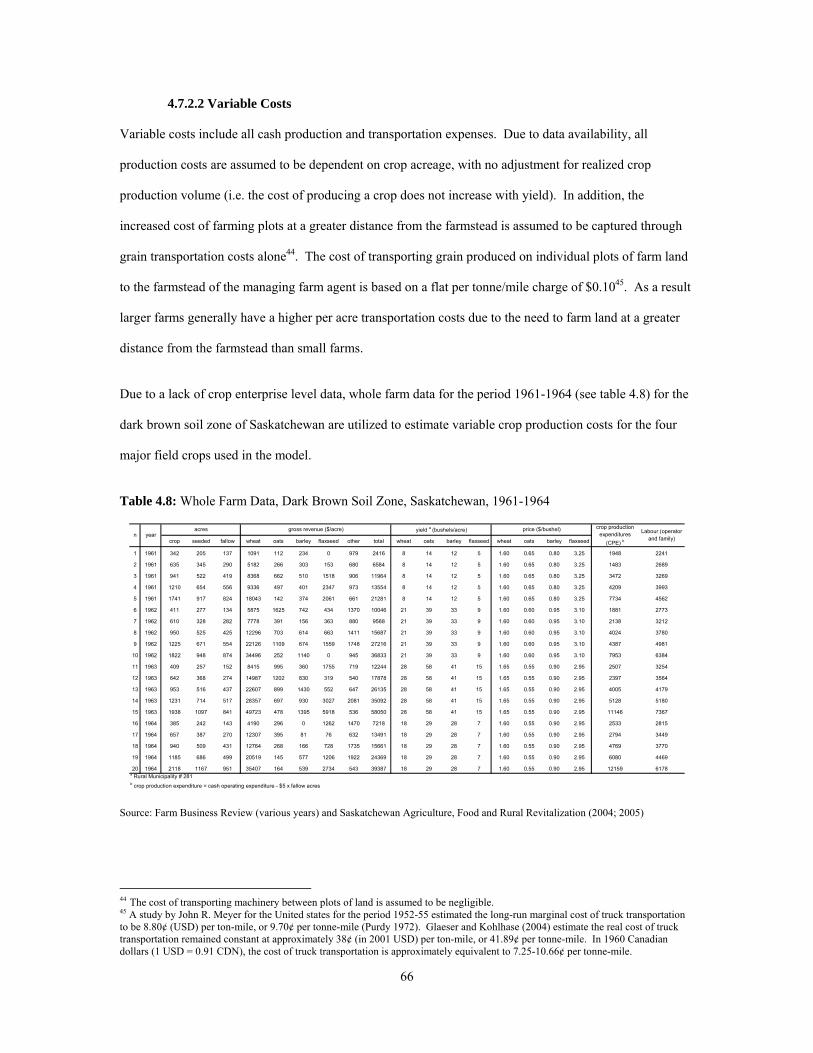
66

4.7.2.2 Variable Costs Variable costs include all cash production and transportation expenses. Due to data availability, all

production costs are assumed to be dependent on crop acreage, with no adjustment for realized crop

production volume (i.e. the cost of producing a crop does not increase with yield). In addition, the

increased cost of farming plots at a greater distance from the farmstead is assumed to be captured through

grain transportation costs alone44. The cost of transporting grain produced on individual plots of farm land

to the farmstead of the managing farm agent is based on a flat per tonne/mile charge of $0.1045. As a result

larger farms generally have a higher per acre transportation costs due to the need to farm land at a greater

distance from the farmstead than small farms.

Due to a lack of crop enterprise level data, whole farm data for the period 1961-1964 (see table 4.8) for the

dark brown soil zone of Saskatchewan are utilized to estimate variable crop production costs for the four

major field crops used in the model.

Table 4.8: Whole Farm Data, Dark Brown Soil Zone, Saskatchewan, 1961-1964

crop seeded fallow wheat oats barley flaxseed other total wheat oats barley flaxseed wheat oats barley flaxseed

1 1961 342 205 137 1091 112 234 0 979 2416 8 14 12 5 1.60 0.65 0.80 3.25 1948 2241

2 1961 635 345 290 5182 266 303 153 680 6584 8 14 12 5 1.60 0.65 0.80 3.25 1483 2689

3 1961 941 522 419 8368 662 510 1518 906 11964 8 14 12 5 1.60 0.65 0.80 3.25 3472 3269

4 1961 1210 654 556 9336 497 401 2347 973 13554 8 14 12 5 1.60 0.65 0.80 3.25 4209 3993

5 1961 1741 917 824 18043 142 374 2061 661 21281 8 14 12 5 1.60 0.65 0.80 3.25 7734 4562

6 1962 411 277 134 5875 1625 742 434 1370 10046 21 39 33 9 1.60 0.60 0.95 3.10 1881 2773

7 1962 610 328 282 7778 391 156 363 880 9568 21 39 33 9 1.60 0.60 0.95 3.10 2138 3212

8 1962 950 525 425 12296 703 614 663 1411 15687 21 39 33 9 1.60 0.60 0.95 3.10 4024 3780

9 1962 1225 671 554 22126 1109 674 1559 1748 27216 21 39 33 9 1.60 0.60 0.95 3.10 4387 4981

10 1962 1822 948 874 34496 252 1140 0 945 36833 21 39 33 9 1.60 0.60 0.95 3.10 7953 6384

11 1963 409 257 152 8415 995 360 1755 719 12244 28 58 41 15 1.65 0.55 0.90 2.95 2507 3254

12 1963 642 368 274 14987 1202 830 319 540 17878 28 58 41 15 1.65 0.55 0.90 2.95 2397 3564

13 1963 953 516 437 22607 899 1430 552 647 26135 28 58 41 15 1.65 0.55 0.90 2.95 4005 4179

14 1963 1231 714 517 28357 697 930 3027 2081 35092 28 58 41 15 1.65 0.55 0.90 2.95 5128 5180

15 1963 1938 1097 841 49723 478 1395 5918 536 58050 28 58 41 15 1.65 0.55 0.90 2.95 11146 7367

16 1964 385 242 143 4190 296 0 1262 1470 7218 18 29 28 7 1.60 0.55 0.90 2.95 2533 2815

17 1964 657 387 270 12307 395 81 76 632 13491 18 29 28 7 1.60 0.55 0.90 2.95 2794 3449

18 1964 940 509 431 12764 268 166 728 1735 15661 18 29 28 7 1.60 0.55 0.90 2.95 4769 3770

19 1964 1185 686 499 20519 145 577 1206 1922 24369 18 29 28 7 1.60 0.55 0.90 2.95 6080 4469

20 1964 2118 1167 951 35407 164 539 2734 543 39387 18 29 28 7 1.60 0.55 0.90 2.95 12159 6178a Rural Municipality # 281

Labour (operator and family)

b crop production expenditure = cash operating expenditure - $5 x fallow acres

ncrop production

expenditures (CPE) b

yearacres yield a (bushels/acre) price ($/bushel)gross revenue ($/acre)

Source: Farm Business Review (various years) and Saskatchewan Agriculture, Food and Rural Revitalization (2004; 2005)

44 The cost of transporting machinery between plots of land is assumed to be negligible. 45 A study by John R. Meyer for the United states for the period 1952-55 estimated the long-run marginal cost of truck transportation to be 8.80¢ (USD) per ton-mile, or 9.70¢ per tonne-mile (Purdy 1972). Glaeser and Kohlhase (2004) estimate the real cost of truck transportation remained constant at approximately 38¢ (in 2001 USD) per ton-mile, or 41.89¢ per tonne-mile. In 1960 Canadian dollars (1 USD = 0.91 CDN), the cost of truck transportation is approximately equivalent to 7.25-10.66¢ per tonne-mile.

67

The variable production costs for the four individual crops are proportional to the weighted mean variable

production cost per seeded acre, based on the values reported in table 4.9.

ii RVCVC ˆ⋅= (4.28)

where VC¯¯ = estimated weighted mean variable production costs per seeded acre 1961-1964 Ri

^ = estimated relative production cost of crop i

( )

( )∑ ∑

∑

=

=

⎥⎦

⎤⎢⎣

⎡⋅

=20

1

20

1

ˆn i

ii

n

Racres

CPEVC

(4.29)

where CPE = crop production expenditures, 1961-1964 acresi = estimated acreage of crop i, 1961-1964

( )seeded

YPGR

YPGRacres

iii

iii ⋅=

∑ ˆˆ/

ˆˆ/ (4.30)

where Pi^ = estimated price of crop i, 1961-1964

Yi^ = estimated yield of crop I, 1961-1964

seeded = total seeded acres of all crops, 1961-1964 Due to a lack of data, the relative variable production costs ( iR ) for the individual crops were estimated

based on crop enterprise data for the dark brown soil zone of Saskatchewan for the period 1994-200446

(Table 4.9).

Table 4.9: Estimated Crop Production Variable Costs (excluding non-family labour)

wheat $8.00 oats $6.80 barley $7.60 flaxseed $8.40 fallow $5.00

variable production cost (per acre)

a

a based on Saskatchewan Agriculture Food & Rural Revitalization crop planning guides dark brown soil zone (1994-2004).

1.000.850.951.05

iR

Source: Author

46 It is assumed that technological development has been crop neutral and has not altered relative crop production expenditures among the four modeled cropping options.

68

The estimated variable production costs are reasonably close to the reported mean variable production cost

of $7.50 per acre for fallow seeded crops (Guide to Farm Practice in Saskatchewan 1960). And the annual

cost of leaving a plot in fallow is estimated at $5.00/acre (Guide to Farm Practice in Saskatchewan 1960).

In addition to the variable production costs per acre outlined in table 4.9, farm agents are faced with cost of

hiring non-family labour and/or custom work. The cost of non-family labour is assumed here to be

characterized by a logistic growth function, with increasing per acre costs as farm acreage increases up to a

maximum cost per acre at a minimum acreage threshold. The logistic function was selected due to the

reality that small farms are able to supply the majority of the required labour, while the non-family labour

requirement increases drastically as the farm expands up to a size where the majority of labour is non-

family. The per acre cost of non-family labour for an individual farm agent was estimated utilizing

equation 4.31.

KeW

⋅−⋅++= 009.0145001

8.003.0 (4.31)

R2 = 0.95

The maximum cost of non-family labour is $0.83 per acre and is incurred by all farms that manage a total

land base in excess of approximately 1800-1900 cultivated acres. While it is recognized that non-family

labour requirements are likely correlated with operator age47, data restrictions make it difficult to estimate

such a relationship.

4.7.2.3 Fixed Costs and Debt Servicing Fixed costs include farm machinery and equipment replacement costs and land lease payments. Due to the

assumption that total machinery and equipment investment remain constant per cultivated acre, the annual

machinery and equipment replacement charge is computed as $15 multiplied by the rate of economic

depreciation. The base scenario of chapter five assumes a fixed annual rate of economic depreciation of

10%48. The annual machinery and equipment replacement charge of $1.50 per cultivated acre is in line

47 The supply of family labour will decline as the farm agent ages due to both 1) offspring leaving the household and 2) the physical abilities of the agent declining over time. 48 Based on a 10 year useful life, the salvage value is approximately 35% of the purchase price which is consistent with American Society of Agricultural Engineers estimates of 36% for farm tractors (ASEA 2003).

69

with actual depreciation expenditures estimates for the period (Saskatchewan Agriculture, various years).

Annual lease payments are determined within the model through the land lease auction, with the exception

of land under a lease agreement at the initial period. Land leases are initialized with an annual lease

payment of $2.25 per cultivated acre49 multiplied by the soil productivity index of the plot in question. The

initial cash lease payment is in line with a reasonable cash lease allowance of 6%-8% of the current land

value (Guide to Farm Practice in Saskatchewan 1960).

The annual debt servicing cost of individual farm agents is determined by their initial level of debt and any

new debt acquired over the duration of the study period. Farm agents are assumed to finance new land

purchases with a 25% cash down payment, with a 20 year amortization period. Interest is assumed to

accrue at a rate of 6.0%50, compounded annually, on all outstanding principal balances.

4.7.2.4 Family/Managerial Withdrawal The family living and managerial deduction from farm revenue is based on data in Table 4.8 and was

estimated as:

KGRWD ⋅+⋅+= 834.0068.01882 51 (4.32)

R2 = 0.98

The family living and managerial deductions are characterized by an L-shaped cost curve; indicative of

significant economies of scale.

4.7.3 Behavioural Data Setting agent behavioural parameters is one of the most important and challenging aspects of agent based

models. Within this framework, farm operator agents are assumed to make three primary types of

managerial decisions: they select a crop mix, determine a value for farm land, and decide when to exit the

industry.

49 $2.25 = $30.00 x 7.5%. 50 7.5% (mean Bank of Canada rate 1960-2000) - 3.0% (inflation adjustment) + 1.5% = 6.0% 51 T-statistics available upon request.

70

4.7.3.1 Crop Mix Farm agents here are restricted to the production of four field crops, wheat52, oats, barley and flaxseed.

These four field crops represent the major production options available to Saskatchewan grain producers

located within the dark brown soil zone in the 1960’s (Table 4.10). It should be noted that rapeseed

(canola), which is now an important crop, was not recommended for production in the dark brown soil

zone, due to its low drought tolerance (Guide to Farm Practice in Saskatchewan 1960).

Table 4.10: Crop Acreages (percent of total), Saskatchewan, 1960-1964

1960 40.6% 6.5% 6.3% 0.7% 3.1% 1.4% 41.4%1961 42.2% 3.9% 4.8% 0.6% 2.5% 1.0% 45.0%1962 43.8% 6.8% 4.1% 0.7% 1.0% 0.4% 43.1%1963 44.8% 5.5% 4.8% 0.8% 1.3% 0.5% 42.2%1964 48.0% 3.7% 3.5% 0.8% 1.3% 0.8% 42.0%

mean 43.9% 5.3% 4.7% 0.7% 1.8% 0.8% 42.7%max 48.0% 6.8% 6.3% 0.8% 3.1% 1.4% 45.0%min 40.6% 3.7% 3.5% 0.6% 1.0% 0.4% 41.4%

flaxseed rapeseed fallow

note: percentages are based on harvested acres of included field crops and fallow acres

all wheat oats barley rye

Source: Saskatchewan Agriculture Food and Rural Revitalization (2004) Based on relative production acreages of the four primary field crops (see table 4.10), all farms in the

simulation are assumed to determine their annual crop mix based on the following cropping constraints:

o Fallow acres = 0.40 x cultivated acreage

o Wheat acres ≤ 0.55 x cultivated acreage

o Oat acre ≤ 0.10 x cultivated acreage

o Barley acres ≤ 0.10 x cultivated acreage

o Flaxseed acres ≤ 0.05 x cultivated acreage 4.7.3.2 Land Valuation Interaction through the land auctions requires all farm agents to form individual valuations of available

plots of agricultural land. In turn a farm agent’s land valuation is dependent on two factors; the agent’s

expectations of rent generated from a given plot of land, and their level of risk aversion. A farm agent’s

expectations are based on both their prior expectations and the most recent realized rent from land. The

52 For simplicity all wheat (including spring, winter and durum) is classed as a single crop alternative.

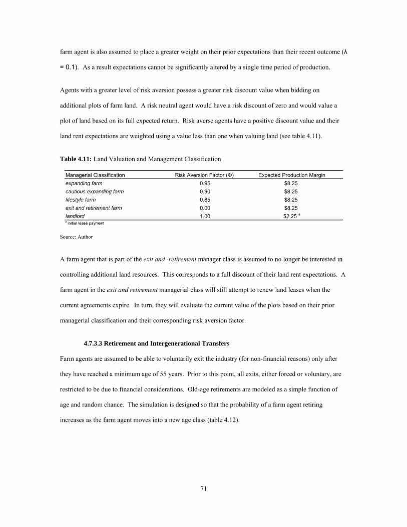
71

farm agent is also assumed to place a greater weight on their prior expectations than their recent outcome (λ

= 0.1). As a result expectations cannot be significantly altered by a single time period of production.

Agents with a greater level of risk aversion possess a greater risk discount value when bidding on

additional plots of farm land. A risk neutral agent would have a risk discount of zero and would value a

plot of land based on its full expected return. Risk averse agents have a positive discount value and their

land rent expectations are weighted using a value less than one when valuing land (see table 4.11).

Table 4.11: Land Valuation and Management Classification

Managerial Classification Risk Aversion Factor (Φ) expanding farm 0.95cautious expanding farm 0.90lifestyle farm 0.85exit and retirement farm 0.00landlord 1.00a initial lease payment

$8.25$2.25 a

Expected Production Margin$8.25$8.25$8.25

Source: Author A farm agent that is part of the exit and -retirement manager class is assumed to no longer be interested in

controlling additional land resources. This corresponds to a full discount of their land rent expectations. A

farm agent in the exit and retirement managerial class will still attempt to renew land leases when the

current agreements expire. In turn, they will evaluate the current value of the plots based on their prior

managerial classification and their corresponding risk aversion factor.

4.7.3.3 Retirement and Intergenerational Transfers Farm agents are assumed to be able to voluntarily exit the industry (for non-financial reasons) only after

they have reached a minimum age of 55 years. Prior to this point, all exits, either forced or voluntary, are

restricted to be due to financial considerations. Old-age retirements are modeled as a simple function of

age and random chance. The simulation is designed so that the probability of a farm agent retiring

increases as the farm agent moves into a new age class (table 4.12).

72

Table 4.12: Net Exit of Farm Operators by Age Cohort (1961-1986)

55-59 years 25% 6%60-64 years 40% 10%65-69 years 64% 18%70 years & over 30% a

80 years 100% a

a author's estimate

5-years period Annual Probability of Exit

Source: Author’s calculations. Census of Canada: Agriculture: Saskatchewan The net exit of farm operators within an age cohort is calculated as the net change in the number of farms in

an age cohort over a five year period53 relative to the initial age cohort size (equation 4.34).

⎥⎦

⎤⎢⎣

⎡

−−

−=− +

t

t

farmsnofarmsno

yearsexitnet5955.

6460.15955 5 (4.34)

When a farm agent voluntarily exits from the industry, it is assumed that the farm will continue to be

operated with the next generation54 taking over as the farm manager. The new generation is in turn

assumed to buyout the exiting generation by assuming all existing farm assets and debts and purchasing

40%55 of the existing farm equity with additional debt financing.

4.7.4 Using the Model: Assessing the Impact of Farm Stabilization and Support Programs Government intervention, with goals of stabilizing and supporting the farm sector, has played a significant

role in the evolution of farm structure in Canada. Fulton et al. (1989) argue that without these farm

programs the health of the prairie economy and farm sector would have been significantly worse since

1985. Beginning in the late 1950’s, and reaching its peak in the mid-1980s, significant transfer payments

have come from federal and provincial governments to agricultural producers. Over the duration of the

period of study selected for simulation, a number of significant programs and payments to Saskatchewan

53i.e. farms in the 55-59 age cohort in the current time period will make up the 60-64 age cohort in five years. 54 The model assumes a 30 year age gap between generations (i.e. if the retiring farm agent is 60 years old the new farm agent will have an initial age of 30 years. 55 Due to the private and often complex nature of intra-family farm transfers, a crude estimate of the buyout rate had to be used. Based on the survey data of Ragush (1966), the debt carried by the successor is on average approximately double that of the retiring farm agent. A transfer price based on new debt financing of 40% of the equity capital (all existing debt is also assumed), and the injection of new equity capital equal to 25% of the total transfer price by the successor, results in the farm assets being transferred for 53-85¢ on the dollar. After the transfer, the farms total debt is increased to a level that is 1.6–4.6 (0.4:1– 0.1:1 debt to asset ratio) times the pre-transfer debt level.

73

producers have occurred. While not all transfers occurring over the 1960-200 period are included within

this simulation, an effort was made to incorporate all the major programs and transfers in the base scenario

of chapter five (see figure 4.9).

1958 - Agricultural Stabilization Act introduced

2000

1991 - Farm Income Protection Act introduced

1998 - Agricultural Income Disaster Assistance

1986 - Special Canadian Grains Program I

1984 - Western Grain Stabilization Act amended

1976 - Western Grain Stabilization Act introduced

1958

1986 - Prairie Crop Drought Assistance

Program

1987 - Special Canadian Grains Program II

1988 - Canadian Crop Drought Assistance

Program

Figure 4.9: Agricultural Stabilization and Support Programs 1958-2000. 4.7.4.1 The Agricultural Stabilization Act

In 1958 the federal government implemented the Agricultural Stabilization Act, and introduced the first

significant program aimed at stabilizing the Canadian farm sector (Schmitz et al. 2002). The program was

designed with the primary objective of stabilizing the prices of specific farm commodities including those

grains typically grown on the prairies. Under the Agricultural Stabilization Act, farmers where guaranteed

90 percent of a three-year moving-average commodity price. In the event that the market price fell below

the guaranteed price, farmers received a per-unit subsidy payment equivalent to the price deficiency

(Schmitz at al. 2002). Western grains were removed from the Agricultural Stabilization Act in 1976 with

the introduction of the Western Grains Stabilization Act.

4.7.4.2 Western Grain Stabilization Act Unlike the Agricultural Stabilization Act, which focused on stabilizing commodity price, the Western

Grains Stabilization Act (WGSA) aimed to stabilize the net cash flow from the major grain and oilseed

crops on the Prairies (Fulton et al. 1989). Individual producers voluntarily entered into the program, which

was funded through both producer levies and government contributions. Participating farmers contributed

a percentage of their gross sales56 to the stabilization fund, an amount that was matched by the federal

government in addition to a further contribution equivalent to 2 percent of gross sales (Fulton et al. 1989).

56 The producer levy ranged between 1 an 4 percent of gross sale depending on the balance of the stabilization fund (Fulton et al 1989).

74

Payments to producers under the WGSA where triggered when net cash flow from the major grains grown

in the Prairie region fell below 90 percent of the previous five-year average net cash flow (Fulton et al.

1989). In response to criticism directed at the program, Bill C-33 was passed to amend the WGSA. The

amendment was intended to make the program more responsive to crop production volume changes

(Schmitz et al. 2002). Under this program, when a payment was triggered, individual producers received a

payout proportional to their contributions to the stabilization fund in the current and two previous program

periods (Fulton et al. 1989).

Within the simulation, all farm agents are assumed to be enrolled in the WGSA. A farm agent’s net annual

cash flow from the WGSA program is evaluated as the difference between program payments received and

levy contributions to the stabilization fund (equation 4.35).

WGSAk

WGSAk

WGSAk LevyPaymentNCF −= (4.35)

where NCFk

WGSA = net cash flow from WGSA to farm agent k Paymentk

WGSA = gross WGSA payment to farm agent k Levyk

WGSA = total WGSA levy paid by farm agent k

k

WGSAk GRLevy ⋅= 02.0 (4.36)

As a result of the program’s design, the payouts received by individual producers are based on the

aggregate net cash flow of the entire region. The total payout received within the region is based on the

aggregate net cash flow of all farms (equation 4.37).

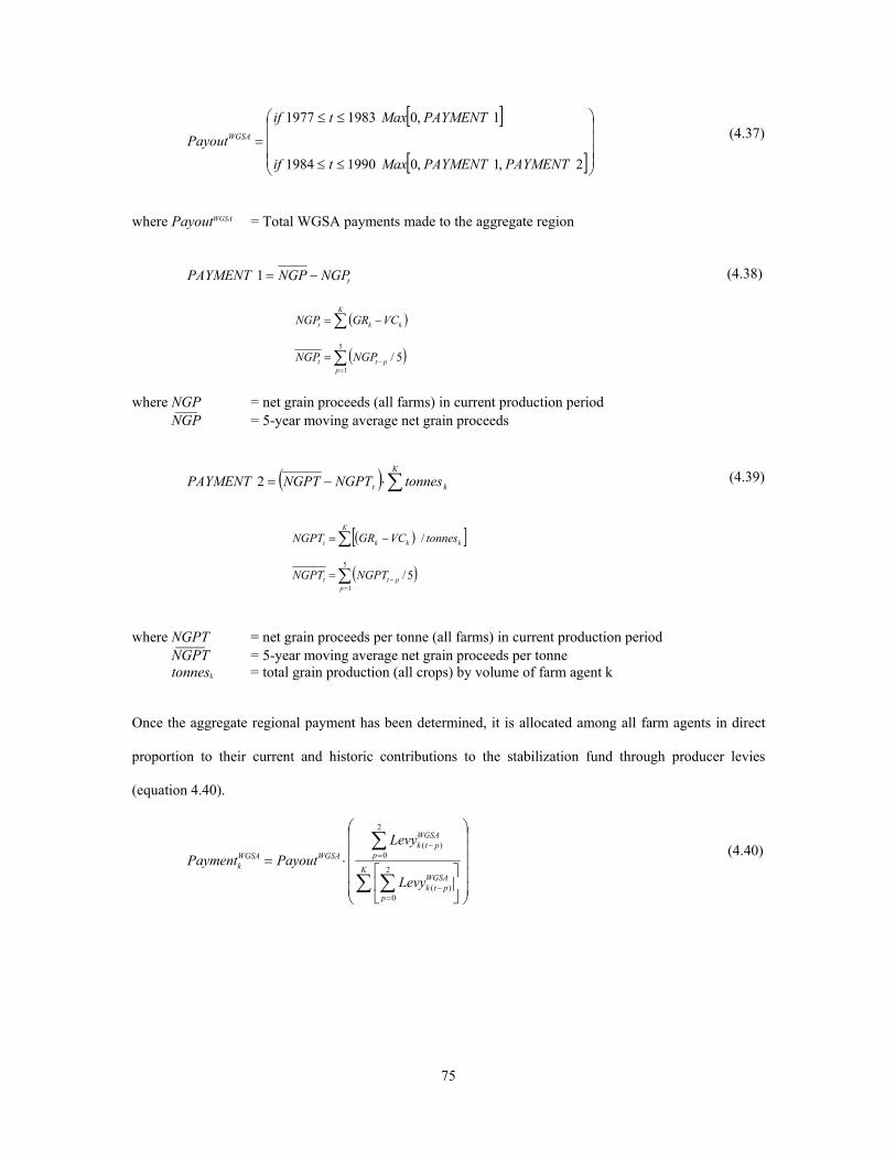
75

[ ]

[ ]⎟⎟⎟⎟

⎠

⎞

⎜⎜⎜⎜

⎝

⎛

≤≤

≤≤

=

2,1,019901984

1,019831977

PAYMENTPAYMENTMaxtif

PAYMENTMaxtif

PayoutWGSA (4.37)

where PayoutWGSA = Total WGSA payments made to the aggregate region

tNGPNGPPAYMENT −=1 (4.38)

( )

( )∑

∑

=−=

−=

5

1

5/p

ptt

K

kkt

NGPNGP

VCGRNGP

where NGP = net grain proceeds (all farms) in current production period NGP¯¯¯ = 5-year moving average net grain proceeds

( ) ∑⋅−=K

kt tonnesNGPTNGPTPAYMENT 2 (4.39)

( )[ ]

( )∑

∑

=−=

−=

5

1

5/

/

pptt

K

kkkt

NGPTNGPT

tonnesVCGRNGPT

where NGPT = net grain proceeds per tonne (all farms) in current production period NGPT¯¯¯¯ = 5-year moving average net grain proceeds per tonne tonnesk = total grain production (all crops) by volume of farm agent k Once the aggregate regional payment has been determined, it is allocated among all farm agents in direct

proportion to their current and historic contributions to the stabilization fund through producer levies

(equation 4.40).

⎟⎟⎟⎟⎟

⎠

⎞

⎜⎜⎜⎜⎜

⎝

⎛

⎥⎦

⎤⎢⎣

⎡⋅=

∑ ∑

∑

=−

=−

K

p

WGSAptk

p

WGSAptk

WGSAWGSAk

Levy

LevyPayoutPayment

2

0)(

2

0)( (4.40)

76

4.7.4.3 Special Canadian Grains and Drought Assistance Programs In 1986 the government of Canada paid out $1 billion to grain producers under the Special Canadian Grains

Program (SCGP) to cushion the impact of the subsidy war between the United States and the European

Economic Community (Agriculture Canada 1986a). Additional payments were made in the subsequent

crop year, bringing the total assistance to just over $2 billion (in nominal dollars). Payments to individual

producers were based on seeded acreages of eligible crops, regional yields, and assistance rates57. The

payment received by an individual farm agent in the model is the sum of acres seeded to eligible

commodities multiplied by the subsidy rate (equation 4.41). In addition, payments to individual producers

are capped at $25,000 ($5,500 in 1960$).

( )⎥⎦

⎤⎢⎣

⎡⋅= ∑

=

4

1

,5500mini

acreii

SCGPk SubsAPayment (4.41)

where PaymentkSCGP = SCGP payment to farm agent k

Subsiacre = SCGP assistance rate per acre of crop i

In the simulation, the assistance rates are set at: wheat $0.11, oats $0.04, barley $0.06 and flax $0.1158 for

both crop periods (1986, 1987) covered by the program.

In addition to the payments made under the Special Canadian Grains programs, prairie producers also

received significant direct payments from the federal government for drought assistance (DAP) in 1986 and

1988 (Agriculture Canada 1986b, 1988). The payment received by individual farmers under these

programs is evaluated as:

∑=

⋅=4

1ii

acreDAPk ASubsPayment (4.42)

where Paymentk

DAP = DAP to farm agent k Subsacre = DAP assistance rate per seeded acre

57Commodity specific assistance rates are proportional to the relative price decline attributed to the subsidy war (Agriculture Canada 1986a) 58 Payouts in 1960$ based on reported rates of: wheat $0.48, oats $0.18, barley $0.06 and flax $0.50 (Agriculture Canada 1986a).

77

Under the Prairie Crop Drought Assistance Program, farmers in areas worst hit by drought conditions

received $15 ($3.30 in 1960$) per seeded acre. In 1988, prairie farmers received an additional $40 ($8.80

in 1960$) under the Canadian Crop Drought Assistance Program.

4.7.4.4 Farm Income Protection Act As a result of a sharp decline in world grain prices in 1985 and the subsequent large payout, the WGSA

program was in a significant deficit position and only offered farmers limited income support by the

closing years of the 1980’s (Schmitz et al. 2002). As a result new federal legislation, entitled the Farm

Income Protection Act, was passed in 1991 to replace the WGSA. In addition to crop insurance59, the Farm

Income Protection Act encompassed two farm stabilization programs: the Gross Revenue Insurance Plan

(GRIP) and the Net Income Stabilization Account (NISA) programs (Schmitz et al. 2002).

The short lived GRIP provided farmers with revenue protection through guaranteed per-acre gross returns.

Within 18 months of its implementation, the government of Saskatchewan significantly altered the program

and by 1992 withdrew completely from GRIP (Schmitz et al. 2002). Under the GRIP a farm agent’s net

program annual cash flow is evaluated as:

GRIPk

GRIPk

GRIPk IndemPaymentNCF −= (4.43)

where NCFk

GRIP = net cash flow from GRIP to farm agent k Paymentk

GRIP = gross GRIP payment to farm agent k Indemk

GRIP = total GRIP indemnity paid by farm agent k GRIP payments and indemnity costs are calculated based on the long term average yields (LTAY) for the

individual crops reported in table 4.7. The guaranteed price under the GRIP was set as a 15-year indexed

moving average price (IMAP), lagged by two crop production periods60. Under the revised Saskatchewan

GRIP, introduced for the 1991-92 crop production period, the payouts received and premiums paid by an

individual producer were based on their risk area and its corresponding premium rate and per acre payment.

Under the revised program the payouts and premiums were based on total seeded acres with no individual

crop differentiation at the farm level. 59 While crop insurance programs may offer participating producer’s a significant source of income stabilization, due to the complexity of modelling the individual nature of coverage and premiums, it has been omitted from simulation. Due to the historic levels of relatively low participation rates in the program, its omission is likely trivial. 60 Under the GRIP program, individual IMAP were set for each of the eligible crops as an average from the previous fifteen years, lagged by two years, indexed by a farm input price index (Schmitz et al. 2002). Due to the fixed variable costs assumption of the simulation, the simulation does not index the historic crop prices and uses a simple arithmetic mean price.

78

([ )( ) ]

( )( )

⎟⎟⎟⎟⎟⎟⎟⎟⎟⎟⎟⎟

⎠

⎞

⎜⎜⎜⎜⎜⎜⎜⎜⎜⎜⎜⎜

⎝

⎛

⋅−⋅⋅⋅

=

⋅⋅⋅−⋅=

=

∑∑∑

∑∑

∑

=

=

=

=

4

44

1

4

1

4

1

,1992

0,max,1991

iiK

ii

K

iiiii

iiiiii

GRIPk

AA

PIMAPQLTAYAtif

QALTAYIMAPprodnPtif

Payment (4.44)

where prodni = total production (volume) of crop i on land managed by farm agent k IMAPi = indexed moving average price of crop i LTAYi = long term average yield of crop i The farmer was responsible for one-third of the total GRIP premium, with the balance paid by the

provincial and federal government (Schmitz et al. 2002). The total indemnity costs are based on indemnity

rates61 published by Agriculture Canada for the 1991-92 program year.

( )

( )

⎟⎟⎟⎟⎟⎟⎟⎟⎟⎟⎟⎟

⎠

⎞

⎜⎜⎜⎜⎜⎜⎜⎜⎜⎜⎜⎜

⎝

⎛

⋅⋅⋅⋅⋅

⋅=

⋅⋅⋅⋅⋅=

=

∑∑∑

∑∑

∑

=

=

=

=

4

14

1

4

1

4

1

%

31,1992

%31,1991

iiK

ii

K

iiiii

iiiii

GRIPk

AA

IndemAQLTAYIMAPtif

IndemAQLTAYIMAPtif

Indem (4.45)

where Indem%i = indemnity rate of crop i The Net Income Stabilization Account (NISA) program was introduced along with GRIP in 1991, and

unlike the latter, remained as the major stabilization program for many Canadian producers through the

year 2001 (Schmitz et al. 2002). The basic mechanism of the NISA program was the establishment of a

government matched savings account from which producers where able to withdraw funds during period of

decreased farm income. Individual producers voluntarily joined the NISA program by opening up a NISA

61 Wheat 18.55%, Oats 11.26%, Barley 16.51% and Flaxseed 18.42% (Agriculture Canada 1992)

79

account (Fund 1) into which they had the ability to deposit up to 3%62 of their annual eligible net sales

(Schmitz et al 2002). In addition to the producer’s deposit, a matching deposit, a cost shared by the

provincial and federal governments, was made into a separate account (Fund 2). The balance of the

combined NISA accounts was capped at three-times the three-year moving average eligible net sales.

Producers earned a rate of interest equal to the rate on a short-term deposit63 on the combined balance, as

well as an additional 3% on the balance of Fund 1. For the purpose of the simulation, all farm agents are

assumed to maximize their matching deposit by depositing a cash amount equivalent to 3% of their gross

revenue into Fund 1.

Under the program, producers were able to withdraw funds from their NISA account if farm income fell

below 70 percent of the previous three year average64 (Schmitz et al. 2002). When a withdrawal is

triggered, the producer was able to withdraw funds65 to bring farm income up to the 70 percent of the three

year average, provided their NISA account did not go into a deficit position. In this model, the maximum

annual withdrawal an individual farm agent can make from their NISA account is determined by their

annual and historic farm income and combined NISA balance (equation 4.46).

( ) ⎥⎦⎤

⎢⎣⎡ +⎟

⎠⎞⎜

⎝⎛ −= 21,min FundFundNINITWD NISANISANISA (4.46)

3/

3

1∑=

−=

−=

p

NISApt

NISA

NISA

NINI

VCGRNI

where TWDNISA = maximum triggered withdrawal from NISA account for farm agent k NI NISA = net income for NISA program of farm agent k NI¯¯ NISA = 3-year moving average net income for NISA program of farm agent k Fund 1 = balance of NISA fund 1 of farm agent k Fund 2 = balance of NISA fund 2 of farm agent k As in reality, farm agents are able to manage their NISA accounts individually, and may not always

withdrawal NISA funds up to the maximum allowable level. All farm agents are assumed to manage their

62 The Saskatchewan NISA program falls under the enhanced NISA guidelines which allows for government matching deposits of 3% of eligible net sales versus the standard NISA maximum of 2%. Individual producers were able to make addition deposits over and above the 3% level, but additional deposits were not matched by the government. 63 For the purpose of the simulation, the short term rate has been set as one-half the interest rate charged on debt capital. 64 In addition to this withdrawal trigger, a withdrawal is also triggered if farm net income falls below $10,000 (increased to $20,000 in 1999) (Schmitz et al. 2002). 65 Withdrawals must first be made from Fund 2 (government deposits), as withdrawals from this fund are taxable. Due to the assumption of a tax-free region this separation is not significant, but has been included to aid in future model extensions.

80

NISA accounts using a simple rule based on meeting annual cash flow requirements. Farm agents can only

withdraw NISA funds when two conditions are met: 1) a withdrawal has been triggered and 2) annual net

cash flow, prior to additional land investment, is negative. The farm agent will withdraw funds up to the

level where either net cash flow is zero, or the total triggered withdrawal is made (equation 4.47).

[ ]NCFTWDWD NISANISA −= ,max (4.47)

where WDNISA = actual withdrawal from NISA account of farm agent k 4.7.4.5 Agricultural Income Disaster Assistance In 1998 the federal government unveiled the Agricultural Income Disaster Assistance (AIDA) program, a

new support program structured according to WTO guidelines (Schmitz et al. 2002). AIDA remained in

place until 2001 when it was replaced by the Canadian Farm Income Program (CFIP). Producers became

eligible for a payout from AIDA when their net income (not including depreciation) fell below 70 percent

of their reference net income (Schmitz et al. 2002). The farm agent’s payout here is calculated as 70

percent of their three-year average net income less current net income (equation 4.48).

⎥⎦⎤

⎢⎣⎡ ⎟

⎠⎞⎜

⎝⎛ −⋅= AIDAAIDAAIDA

k NINIMaxPayment 7.0,0 (4.48)

where PaymentkAIDA = AIDA payment to farm agent k

NI¯¯ AIDA = 3-year moving average net income for AIDA program of farm agent k NI AIDA = net income for AIDA program of farm agent k A farm agent’s net income is calculated for AIDA as their gross revenue (GR) less variable production

costs (VC). The farm agent’s reference net income is equivalent to the arithmetic mean of the farm agent’s

net income from the previous three production periods.

81

4.8 Summary Regional structural change is dependent on not only the independent actions of individual farm households,

but also the interaction of the same through land and product markets. The application of agent based

methods to study such changes is intuitively attractive, as it allows for the development of models that

incorporate both the heterogeneity of the farm household, or decision making unit, and the inherent

interactions that exist between individual farms. In turn, the farm household is assumed to be engaged in

the two related, but separate, activities of producing and marketing field crops and investing in agricultural

assets. It is the second activity, namely investment in farmland, which incorporates the interactions

between individual farm households through the assignment of property rights and well-defined land

markets.

This regional model of farming activity is initialized with a base scenario representative of the 1960-2000

time period. Farm agents are endowed with a number of attributes including 1) age, 2) farm size, 3) tenure,

4) finance and 5) management, based on available census and survey data. Production costs correspond

with 1960 cost levels and are held constant throughout the model duration. In addition, real commodity

prices and yields are de-trended to a 1960 base period to adjust for constant production technology and

practices. Finally, transfer payments from the federal and provincial government beginning in the late

1950’s, and reaching a peak in the mid-1980’s have played a prominent role in the annual cash flow of

many farm households. In order to replicate and assess the impact of government intervention into the

farming sector, the most significant farm stabilization and support programs are modelled as part of the

base simulation framework.

82

CHAPTER FIVE

DISCUSSION OF RESULTS

5.0 Introduction A profile of 310 farms is initialized to represent a proto-typical RM in the dark brown soil zone of

Saskatchewan. The profile contains the following structural farm characteristics: 1) age, 2) farm size, 3)

tenure, 4) finance and 5) management. Farm costs and returns are set up to represent those of the 1960

time period. This agent based model simulates farm expansion and contraction in the region through

farmland ownership and leasing markets. The model starts in the year 1960 and runs to the year 2000; each

scenario is replicated 200 times to achieve statistically useful results. In addition to the base scenarios

described earlier, zero government transfer scenarios are also simulated. The first set of scenarios test the

sensitivity of the final structural predictions to initial assumptions as to the distribution of varied

managerial classes. The second set of counterfactual scenarios examines the impact of removing

government programs on structural change in the region. The simulation environment was implemented

using NetLogo © version 2.1 on a Windows XP platform66.

The model results reported illustrate a limited number of structural characteristics of the study region

including: 1) the number of farm units, 2) mean farm size, 3) the distribution of farm size, 4) land values, 5)

proportion of farm land leased from non farming owners, and 6) farm debt. The results presented in this

chapter provide evidence of the ability of agent-based models to generate patterns and trends that closely

mirror the historic structural evolution of a Saskatchewan region dominated by crop production agriculture.

Model validity has been tested through direct comparison to available census and survey data. While

model validation of results is important when dealing with “proof of concept” issues, it also allows the

researcher to draw conclusions from the model that can be used to improve understanding of the system of

66 A copy of the NetLogo © source code is included in Appendix C

83

study. To move beyond the scope of simply validating model results based on direct comparisons to actual

data, a number of the drivers of structural changed discussed in chapter two are revisited and discussed in

the context of the simulation results.

5.1 Simulation Results: Base Scenario

Under the base scenario, the model is executed as outlined in chapter 4. Two hundred replications are

simulated for each of the 5 managerial distributions outlined in table 4.6. The base scenario results are

evaluated based on their ability to mirror historic structural adjustments over the study period of 1960-

2000.

5.1.1 Number and Mean Size of Farms

The trend towards fewer and larger farm units has a number of important implications for agricultural

policy. As farm production becomes more consolidated, the aggregate response of the sector may also shift

in a significant manner. The simulated consolidation of farm land among a declining number of farm

agents are compared to actual farm numbers and mean farm size data (figures 5.1 and 5.2).

0

50

100

150

200

250

300

350

0 5 10 15 20 25 30 35 40

year

num

ber o

f far

ms

uniform normal 10% skew all 1 all 3 actual

Figure 5.1: Simulation Results (base scenario) - Number of Farm Agents

84

0

200

400

600

800

1000

1200

1400

0 5 10 15 20 25 30 35 40

year

acre

s

uniform normal 10% skew all 1 all 3 actual (total) actual(cult.)

Figure 5.2: Simulation Results (base scenario) - Mean Farm Size (cultivated acres) Over the simulated period, the number of farms decreased at an annualized rate between 1.59 - 1.72%, as

compared to an actual rate of 1.53%. The corresponding mean farm size increased at an annualized rate of

between 1.61 - 1.76%, as compared to an actual rate of 1.58%. While the model closely approximates

overall trends, a more interesting comparison occurs with respect to sub-periods. There are five distinct

periods of simulated farm numbers and mean size observations: 1960-1970, 1970-1972, 1972-1992, 1992-

1997 and 1997-2000. Prior to 1970, the model under-estimates the rate of consolidation with an annualized

decline in farm numbers ranging from 0.38 - 0.86% (1.97% actual) and the rate of growth in farm size

ranging from 0.38 - 0.88% (2.11% actual). During the 1970-72 period, the simulation makes an over

adjustment resulting in a two period annual rate of decline of farms of 9.64 - 11.26% (1.39% actual) and a

growth of 10.61 - 12.70% (1.78% actual) in mean farm size. For the combined 1960-1972 period, the

model results estimate a 2.25 - 2.39% (1.88% actual) annual decline in farm numbers and a 2.39 - 2.45%

(2.05% actual) increase in farm size. For the period of 1972-1992, the number of farms is relatively

constant with an estimated annual rate of decline between 0.06 - 0.09% (1.15% actual) and annual growth

in farm size of 0.06 - 0.16% (1.16% actual). The simulated period 1992-2000 is characterised by an annual

decline in farms of 4.12 - 4.88% (1.96% actual) and an annual increase in farm size of 4.31 - 5.14% (1.77%

actual). Like the previous time period, this latter period is characterized by rapid consolidation followed by

a period of relatively little restructuring. The number of farms declined rapidly during the period 1992-

1997 with an annual rate of decline between 5.89 - 7.20% (1.77% actual) and a corresponding increase in

mean farm size of 6.28 - 7.80% (1.53% actual). The rate of decline slows significantly for all managerial

85

classification distributions evaluated for the final period (1997-2000). The annual rate of farm decline is

estimated at 0.76 - 1.09% (2.34% actual) and growth in mean farm size is estimated at 0.77 - 1.09% (2.18%

actual). And all five distributions of managerial characteristics tested returned results that closely replicate

the actual decline in farm operators (figure 5.1) and increase in farm size (figure 5.2) over the study period.

5.1.2 Distribution of Farm Size

The changing distribution of farm size is of greater importance than summary characteristics such as mean

farm size. Over the course of the period under study, the relative amount of farms smaller than 400 acres

remained relatively constant, ranging from a high of 35% of all farms in 1960 (Census of Canada:

Agriculture: Saskatchewan 1961) to 29% in 2000 (Census of Canada: Agriculture: Saskatchewan 2001). In

direct contrast, the proportion of farms occupying the largest size class (≥ 2880 acres) has increased

significantly from 1% in 1960 to 9% of all farms in 2000. Over this same period, the distribution of farm

size has flattened compared to the situation in 1960, where 87% of all farms operated less than 1120 acres.

By 2000 this had fallen to only 60%.

After a simulation period of 10 years, the proportion of farms operating less than 400 acres is over

estimated by the model at 49 - 51% of all farms (27% actual) under all the assumed initial distributions of

the managerial types (see table 4.6). While not as well defined as in the actual distribution, a small bulge in

the distribution begins to emerge in the simulated 760-1119 acre size class (see figure 5.3).

0%

10%

20%

30%

40%

50%

60%

less than 400 400 - 559 560 - 759 760 - 1119 1120 - 1599 1600 - 2239 2240 - 2879 2880 and over

farm size (cultivated acres)

perc

enta

ge o

f all

farm

s

uniform normal 10% skew all 1 all 3 actual

Figure 5.3: Simulation Results (base scenario) - Distribution of Farm Size (year 10)

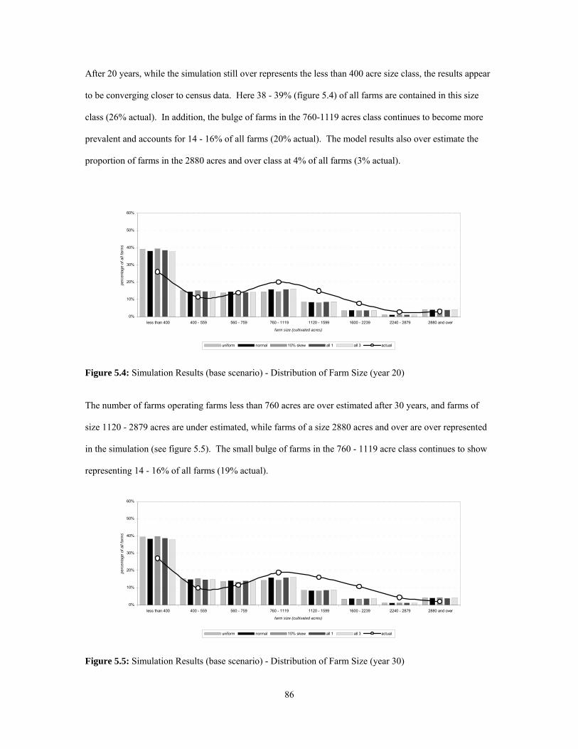
86

After 20 years, while the simulation still over represents the less than 400 acre size class, the results appear

to be converging closer to census data. Here 38 - 39% (figure 5.4) of all farms are contained in this size

class (26% actual). In addition, the bulge of farms in the 760-1119 acres class continues to become more

prevalent and accounts for 14 - 16% of all farms (20% actual). The model results also over estimate the

proportion of farms in the 2880 acres and over class at 4% of all farms (3% actual).

0%

10%

20%

30%

40%

50%

60%

less than 400 400 - 559 560 - 759 760 - 1119 1120 - 1599 1600 - 2239 2240 - 2879 2880 and over

farm size (cultivated acres)

perc

enta

ge o

f all

farm

s

uniform normal 10% skew all 1 all 3 actual

Figure 5.4: Simulation Results (base scenario) - Distribution of Farm Size (year 20) The number of farms operating farms less than 760 acres are over estimated after 30 years, and farms of

size 1120 - 2879 acres are under estimated, while farms of a size 2880 acres and over are over represented

in the simulation (see figure 5.5). The small bulge of farms in the 760 - 1119 acre class continues to show

representing 14 - 16% of all farms (19% actual).

0%

10%

20%

30%

40%

50%

60%

less than 400 400 - 559 560 - 759 760 - 1119 1120 - 1599 1600 - 2239 2240 - 2879 2880 and over

farm size (cultivated acres)

perc

enta

ge o

f all

farm

s

uniform normal 10% skew all 1 all 3 actual

Figure 5.5: Simulation Results (base scenario) - Distribution of Farm Size (year 30)

87

After 40 years (figure 5.6), corresponding to the end of the time period studied, the proportion of farms

occupying the less than 400 acre class has adjusted to a level (20 - 22% of all farms) that under estimates

the census data observation for the period (29%). The model results for all five managerial distributions

estimate the proportion of farms managing a land holding of 400-1119 cultivated acres at 53 - 55% (31%

actual) of all farms. The proportion of farms managing 1120-2879 acres is estimated to be 18-19% (31%

actual) of all farms.

0%

10%

20%

30%

40%

50%

60%

less than 400 400 - 559 560 - 759 760 - 1119 1120 - 1599 1600 - 2239 2240 - 2879 2880 and over

farm size (cultivated acres)

perc

enta

ge o

f all

farm

s

uniform normal 10% skew all 1 all 3 actual

Figure 5.6: Simulation Results (base scenario) - Distribution of Farm Size (year 40) The result shown here show that in spite of the inherent limitations within the simulation environment, the

model closely replicates the dynamic distribution of farm size actually observed during the relevant

timeframe67. This gives confidence that the assumptions made to conduct this simulation are a

parsimonious, yet robust, characterization of individual level behaviour in Saskatchewan agriculture

. 5.1.3 The Land Market

Farmers interact in this agent based environment and land is allocated among individual farm operators and

absentee land owners through direct competition in land market auctions. This interaction and the bidding

behaviour of agents results in varying value for farmland and the proportion of farmland owned by non-

farming individuals. All farmland values reported here are listed in constant 1960s dollars.

67 The simulated distributions were tested against the actual distribution using a non-parametric Kruskal-Wallis test statistic with K-1 degrees of freedom. The null hypothesis, that all of the all of the tested distributions are equivalent, could not be reject with a critical region of 0.05 for years 10 and 40 and a critical region of 0.01 for years 20 and 30.

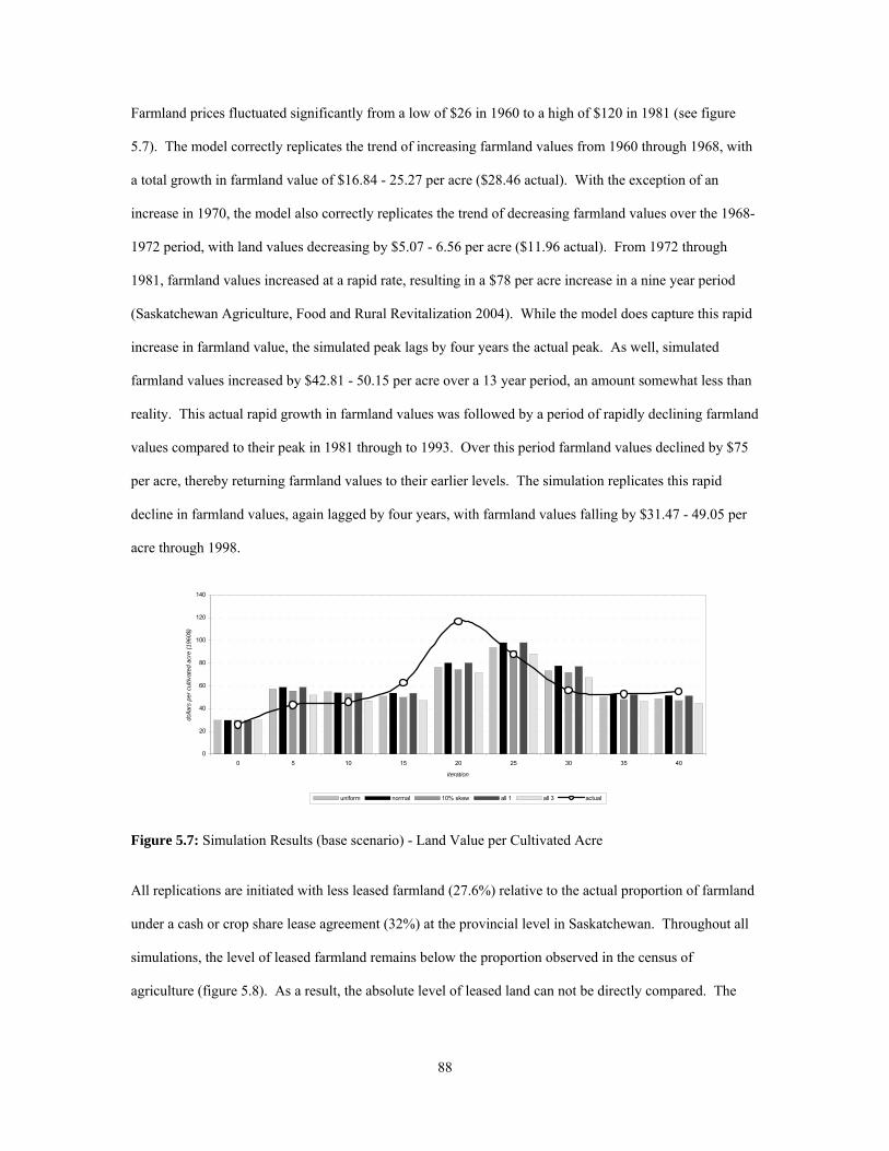
88

Farmland prices fluctuated significantly from a low of $26 in 1960 to a high of $120 in 1981 (see figure

5.7). The model correctly replicates the trend of increasing farmland values from 1960 through 1968, with

a total growth in farmland value of $16.84 - 25.27 per acre ($28.46 actual). With the exception of an

increase in 1970, the model also correctly replicates the trend of decreasing farmland values over the 1968-

1972 period, with land values decreasing by $5.07 - 6.56 per acre ($11.96 actual). From 1972 through

1981, farmland values increased at a rapid rate, resulting in a $78 per acre increase in a nine year period

(Saskatchewan Agriculture, Food and Rural Revitalization 2004). While the model does capture this rapid

increase in farmland value, the simulated peak lags by four years the actual peak. As well, simulated

farmland values increased by $42.81 - 50.15 per acre over a 13 year period, an amount somewhat less than

reality. This actual rapid growth in farmland values was followed by a period of rapidly declining farmland

values compared to their peak in 1981 through to 1993. Over this period farmland values declined by $75

per acre, thereby returning farmland values to their earlier levels. The simulation replicates this rapid

decline in farmland values, again lagged by four years, with farmland values falling by $31.47 - 49.05 per

acre through 1998.

0

20

40

60

80

100

120

140

0 5 10 15 20 25 30 35 40

iteration

dolla

rs p

er c

ultiv

ated

acr

e (1

960$

)

uniform normal 10% skew all 1 all 3 actual

Figure 5.7: Simulation Results (base scenario) - Land Value per Cultivated Acre All replications are initiated with less leased farmland (27.6%) relative to the actual proportion of farmland

under a cash or crop share lease agreement (32%) at the provincial level in Saskatchewan. Throughout all

simulations, the level of leased farmland remains below the proportion observed in the census of

agriculture (figure 5.8). As a result, the absolute level of leased land can not be directly compared. The

89

change from one census year to the next (5 year intervals) is of greater importance in evaluating the

model’s ability to capture historic shifts.

0%

10%

20%

30%

40%

50%

60%

70%

80%

90%

100%

0 5 10 15 20 25 30 35 40

iteration

perc

enta

ge o

f far

m la

nd u

nder

a le

ase

agre

emen

t

uniform normal 10% skew all 1 all 3 actual

Figure 5.8: Simulation Results (base scenario) - Proportion of Land under Lease Agreement Under all initial distributions of the managerial types, the model correctly replicates the trend in the

proportion of farmland leased from 1960 to 1965. However, it over estimates the actual reduction in leased

land -leased land is estimated to decline by 9.01 - 9.32% compared to an actual reduction of only 4.5%.

From 1965 to 1970, the actual level of leased farmland increased by 1.5% as compared to a simulated

change in leased land between -0.25 - 1.02%. Only the “all 3” distribution of managerial attributes

replicated the increase in leased land during the period. During the period 1970-1975, the simulated

proportion of leased land increased by 3.86 - 4.72% as compared to an actual increase of 2.0%. In the

subsequent 1975-1990 period, simulated land tenure is relatively stable (leased land increasing by only 0.01

- 0.03%), in sharp contrast to actual increases of 8.54%. The rapid growth in leased farmland (5.90%) that

occurred between 1980 and 1985 does not show up in any of the simulations until the period 1990-1995,

when the proportion of leased land increases by 6.12 - 7.48%. The trend of an increasing level of leased

farm land continues for the final 1995-2000 period with the proportion of leased farm land increasing by an

additional 4.50 - 5.83%.

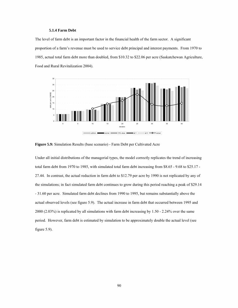
90

5.1.4 Farm Debt

The level of farm debt is an important factor in the financial health of the farm sector. A significant

proportion of a farm’s revenue must be used to service debt principal and interest payments. From 1970 to

1985, actual total farm debt more than doubled, from $10.32 to $22.06 per acre (Saskatchewan Agriculture,

Food and Rural Revitalization 2004).

0

5

10

15

20

25

30

35

0 5 10 15 20 25 30 35 40

iteration

debt

per

acr

e (1

960$

)

uniform normal 10% skew all 1 all 3 actual

Figure 5.9: Simulation Results (base scenario) - Farm Debt per Cultivated Acre Under all initial distributions of the managerial types, the model correctly replicates the trend of increasing

total farm debt from 1970 to 1985, with simulated total farm debt increasing from $8.65 - 9.68 to $25.17 -

27.44. In contrast, the actual reduction in farm debt to $12.79 per acre by 1990 is not replicated by any of

the simulations; in fact simulated farm debt continues to grow during this period reaching a peak of $29.14

- 31.60 per acre. Simulated farm debt declines from 1990 to 1995, but remains substantially above the

actual observed levels (see figure 5.9). The actual increase in farm debt that occurred between 1995 and

2000 (2.03%) is replicated by all simulations with farm debt increasing by 1.50 - 2.24% over the same

period. However, farm debt is estimated by simulation to be approximately double the actual level (see

figure 5.9).

91

5.1.5 Farm Exits

One of the outcomes from the consolidation of farm production on a declining number of farms is the

exodus of farm families. Policy makers need to concern themselves with the distribution effects of

structural adjustments and the varied impacts these shifts have on the farm population. The agent based

results generated shed light on a number of these distributional issues with regard to the characteristics of

farm closure over the duration of the period studied.

Policy makers concerned with the rate of decline in farm numbers need to understand the reasons

individual farm operations cease production. In the simulation, the significant majority (97.7%) of all

farms that ceased operating did so due to a prolonged period of equity erosion and cash flow short fall.

Only a small proportion of farms exited when the current manager retired (0.3%). While intuitively

correct, this result suggests that the intergenerational farm transfer algorithm incorporated into the model

needs to be developed and extended in further research.

Table 5.1: Simulation Results (Base Scenario) - Farm Exits by Exit Type

a farms transferred to a new generation are not counted as exits

exit type

mean percentage of all exits 97.7% 2.0% 0.3%

Equity Erosion (eq 4.12)

Insolvency (eq 4.11)

Old-Age Retirementa

One of the more interesting results that emerges from the simulations concerns the farm agent’s managerial

attribute and the probability of an individual farm discontinuing production over the course of the period

studied. A farm agent in the Lifestyle managerial class is 2.6% more likely to exit when compared to an

Expanding farm agent (table 5.2).

Table 5.2: Simulation Results (Base Scenario) - Farm Exits by Managerial Class

a probability of farm exit = exits / initial number of farms

managerial class

48.7%

Lifestyle Cautious Expanding Expanding All

probability of farm exita 49.0% 48.6% 46.4%

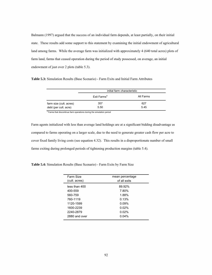
92

Balmann (1997) argued that the success of an individual farm depends, at least partially, on their initial

state. These results add some support to this statement by examining the initial endowment of agricultural

land among farms. While the average farm was initialized with approximately 4 (640 total acres) plots of

farm land, farms that ceased operation during the period of study possessed, on average, an initial

endowment of just over 2 plots (table 5.3).

Table 5.3: Simulation Results (Base Scenario) - Farm Exits and Initial Farm Attributes

farm size (cult. acres)debt (per cult. acre)a Farms that discontinue farm operations during the simulation period

Exit Farmsa All Farms

357 627

initial farm characteristic

5.50 5.45

Farm agents initialized with less than average land holdings are at a significant bidding disadvantage as

compared to farms operating on a larger scale, due to the need to generate greater cash flow per acre to

cover fixed family living costs (see equation 4.32). This results in a disproportionate number of small

farms exiting during prolonged periods of tightening production margins (table 5.4).

Table 5.4: Simulation Results (Base Scenario) - Farm Exits by Farm Size

less than 400400-559560-759760-11191120-15991600-22392240-28792880 and over 0.04%

0.13%0.09%0.02%0.02%

Farm Size (cult. acres)

1.88%

89.92%7.80%

mean percentage of all exits

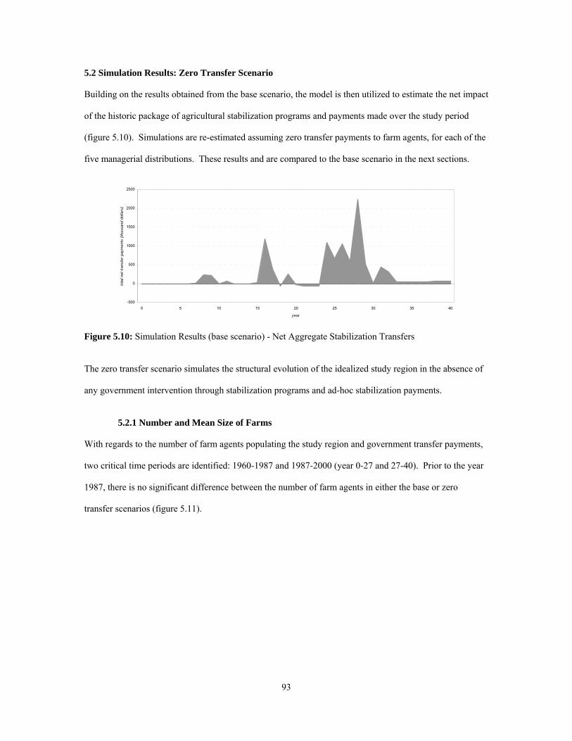
93

5.2 Simulation Results: Zero Transfer Scenario Building on the results obtained from the base scenario, the model is then utilized to estimate the net impact

of the historic package of agricultural stabilization programs and payments made over the study period

(figure 5.10). Simulations are re-estimated assuming zero transfer payments to farm agents, for each of the

five managerial distributions. These results and are compared to the base scenario in the next sections.

-500

0

500

1000

1500

2000

2500

0 5 10 15 20 25 30 35 40

year

tota

l net

tran

sfer

pay

men

ts (t

hous

and

dolla

rs)

Figure 5.10: Simulation Results (base scenario) - Net Aggregate Stabilization Transfers The zero transfer scenario simulates the structural evolution of the idealized study region in the absence of

any government intervention through stabilization programs and ad-hoc stabilization payments.

5.2.1 Number and Mean Size of Farms With regards to the number of farm agents populating the study region and government transfer payments,

two critical time periods are identified: 1960-1987 and 1987-2000 (year 0-27 and 27-40). Prior to the year

1987, there is no significant difference between the number of farm agents in either the base or zero

transfer scenarios (figure 5.11).

94

0

50

100

150

200

250

300

350

0 5 10 15 20 25 30 35 40

year

num

ber o

f far

ms

uniform normal skew all 1 all 3 base scenario (mean)

Figure 5.11: Simulation Results (zero transfer scenario) - Number of Farm Agents While the 1960-1987 period does not exhibit any significant difference in the rate of farm decline over the

base scenario, in contrast the 1987-2000 period is characterized by a significant increase in the rate of farm

consolidation. By the end of the simulated time period, the number of farms declined to a level of 64 - 68%

of the base scenario results (figure 5.11). Both the base and zero transfer scenarios exhibit a period of rapid

farm consolidation after 1987. Under the zero transfer assumption, the number of farm agents in the region

undergoes a period of rapid decline from 1987-1993, with an annualized rate of decline of 11.02 - 12.80%.

This period of decline is followed by a period of moderate decline (1.15 - 1.51% annual drop for the period

1987-2000). In contrast, the base scenario exhibits a period of rapid decline (mean annual rate of 6.78%)

from 1992-1997 which is preceded and followed by periods of relatively constant farm numbers.

The growth rate in farm size is inversely related to the fall in farm numbers. As a result the rate of change

in mean farm size in the simulations is observed to be approximately proportional to the rate of decline in

farm numbers. Like the observed trends obtained concerning farm numbers in the simulations, the rate of

growth in mean farm size is not observed to be significantly different from the base scenario prior to 1987.

In addition, the delayed period of farm decline found in the base scenario compared to the zero transfer

scenario is mirrored by the varied periods of rapid growth in farm size.

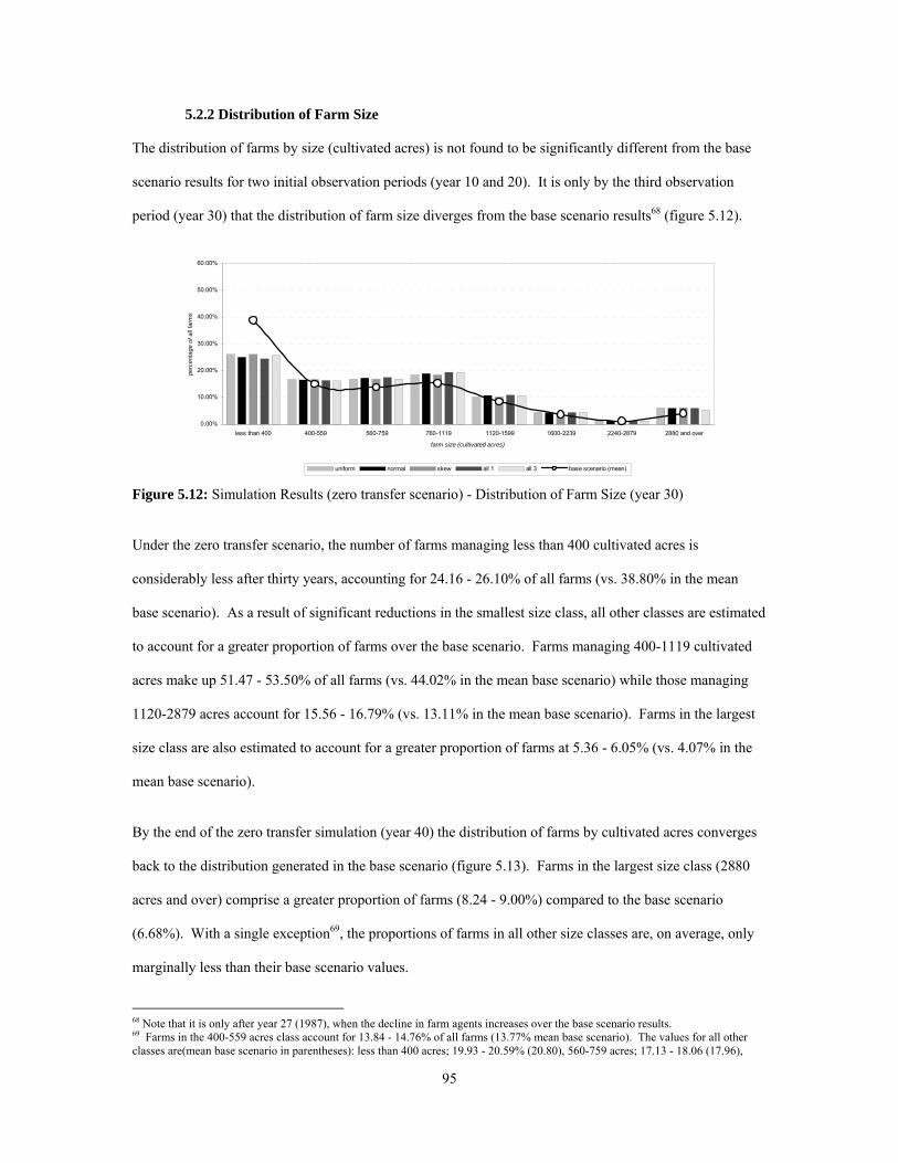
95

5.2.2 Distribution of Farm Size The distribution of farms by size (cultivated acres) is not found to be significantly different from the base

scenario results for two initial observation periods (year 10 and 20). It is only by the third observation

period (year 30) that the distribution of farm size diverges from the base scenario results68 (figure 5.12).

0.00%

10.00%

20.00%

30.00%

40.00%

50.00%

60.00%

less than 400 400-559 560-759 760-1119 1120-1599 1600-2239 2240-2879 2880 and over

farm size (cultivated acres)

perc

enta

ge o

f all

farm

s

uniform normal skew all 1 all 3 base scenario (mean)

Figure 5.12: Simulation Results (zero transfer scenario) - Distribution of Farm Size (year 30) Under the zero transfer scenario, the number of farms managing less than 400 cultivated acres is

considerably less after thirty years, accounting for 24.16 - 26.10% of all farms (vs. 38.80% in the mean

base scenario). As a result of significant reductions in the smallest size class, all other classes are estimated

to account for a greater proportion of farms over the base scenario. Farms managing 400-1119 cultivated

acres make up 51.47 - 53.50% of all farms (vs. 44.02% in the mean base scenario) while those managing

1120-2879 acres account for 15.56 - 16.79% (vs. 13.11% in the mean base scenario). Farms in the largest

size class are also estimated to account for a greater proportion of farms at 5.36 - 6.05% (vs. 4.07% in the

mean base scenario).

By the end of the zero transfer simulation (year 40) the distribution of farms by cultivated acres converges

back to the distribution generated in the base scenario (figure 5.13). Farms in the largest size class (2880

acres and over) comprise a greater proportion of farms (8.24 - 9.00%) compared to the base scenario

(6.68%). With a single exception69, the proportions of farms in all other size classes are, on average, only

marginally less than their base scenario values.

68 Note that it is only after year 27 (1987), when the decline in farm agents increases over the base scenario results. 69 Farms in the 400-559 acres class account for 13.84 - 14.76% of all farms (13.77% mean base scenario). The values for all other classes are(mean base scenario in parentheses): less than 400 acres; 19.93 - 20.59% (20.80), 560-759 acres; 17.13 - 18.06 (17.96),

96

0%

10%

20%

30%

40%

50%

60%

less than 400 400-559 560-759 760-1119 1120-1599 1600-2239 2240-2879 2880 and over

farm size (cultivated acres)

perc

enta

ge o

f all

farm

s

uniform normal skew all 1 all 3 base scenario (mean)

Figure 5.13: Simulation Results (zero transfer scenario) - Distribution of Farm Size (year 40) 5.2.3 The Land Market The effects on the land markets of the package of stabilization programs and ad-hoc payments are

measured by comparing farmland values and the proportion of land under a lease agreement for both the

base and zero transfer scenarios. The effect of government transfers on farmland values are reported as

either a premium or discount over the base scenario values based on mean values over five year periods

(figure 5.14). Prior to the 1986-1990 (year 26-30), government transfers do not result in either a significant

premium or discount in the farmland market.

-4.00

-2.00

0.00

2.00

4.00

6.00

8.00

10.00

1-5 6-10 11-15 16-20 21-25 26-30 31-35 36-40

year

dolla

rs p

er a

cre

(196

0$)

uniform normal skew all 1 all 3 transfers

Figure 5.14: Simulation Results (zero transfer scenario) - Net Transfer Payments and Land Premiums Over the 1986-1990 period, farmland values are estimated to be at a $0.27 - $0.65 per cultivated acre

premium over the base scenario values. Farmland continues to be valued at a premium ($1.70 - $3.30) over

760-1119 acres; 21.19-22.43% (22.06%), 1120-1599 acres; 11.10-12.29% (12.18%), 1600-2239 acres; 4.61-4.95% (5.15%), 2240-2879 acres; 0.97-1.35% (1.42%).

97

the base scenario during the 1991-1995 (year 31-35). During the final five year time period (year 36-40)

land values are on average discounted over the base scenario by between $1.62 - $1.66 per cultivated acre.

Like the other structural characteristics, land tenure under zero transfer does not show significant

divergence from the base scenario prior to year 27 (figure 5.15). Under zero transfer, the proportion of

farmland under a lease agreement increases both earlier and more rapidly than the base scenario.

0

10

20

30

40

50

60

70

80

90

100

0 5 10 15 20 25 30 35 40

year

perc

enta

ge o

f far

m la

nd u

nder

a le

ase

agre

emen

t

uniform normal skew all 1 all 3 base scenario (mean)

Figure 5.15: Simulation Results (zero transfers scenario) - Proportion of Land under Lease Agreement Over the 1987-1991 (year 27-31) period, the proportion of farm land under lease agreement increases at an

annualized rate of 7.26 - 10.55% (vs. 0.12% in the mean base scenario). Under the base scenario, the

number of lease agreements increases rapidly at a mean annual rate of 7.41%, but this is substantially less

than the 20.43 - 23.60% annual growth estimated within the zero transfer scenario. Unlike the base case

(3.79% mean) the prevalence of lease agreements increases only marginally (0.16 - 0.23%) for the duration

of the simulation.

5.2.4 Farm Debt As might be expected, the level of farm debt per acre does not show any significant variation from the base

scenario prior to 1987 (figure 5.16). Under the zero transfer scenario, farm debt per acre does not reach the

same peak level ($31.27 mean in 1991) as the base scenario and is estimated to $3.91 - $4.64 per acre less

in 1990 (iteration 30). Farm debt per acre remains less than the base scenario after year 35 ($4.54 - $5.47

98

per acre), but converges to the base scenario level after year 40, with debt levels only marginally less per

acre ($0.32 - $1.68).

0

5

10

15

20

25

30

35

0 5 10 15 20 25 30 35 40

year

debt

per

acr

e (1

960$

)

uniform normal skew all 1 all 3 base scenario (mean)

Figure 5.16: Simulation Results (zero transfers scenario) - Farm Debt per Cultivated Acre

5.3 Model Drivers and Structural Change The forces driving structural adjustment in the farm sector have generated significant debate and research

within the field of agricultural and regional economics. While a significant amount of time and effort has

been exerted on understanding the drivers of structural change, no general consensus has been achieved and

a strikingly varied number of explanations and policy recommendations exist. A number of the driving

forces of structural change outlined in chapter two are revisited next and briefly discussed within the

context of the simulation framework. The drivers on which I will focus include 1) entrepreneurial

behaviour and farm household expectations, 2) cost of production and productive efficiency, 3) path

dependency and the farm life-cycle and 4) government transfers.

5.3.1 Entrepreneurial Behaviour and Farm Household Expectations Underlying differences between farm household management strategies and styles has been suggested as a

potential driver of structural change. It seems that the fundamental and intrinsic difference between

management styles could have a measurable impact on the behaviour of individual farm households. While

it was implicitly assumed that all farm households held the same fundamental goal about farm growth, they

were classified into three management classes. This affected their behaviour in both land markets and crop

mix selection. It is interesting to note that even though the simulations were set up so that all farm

households had an inherent desire for farm growth, a significantly skewed distribution of farm size still

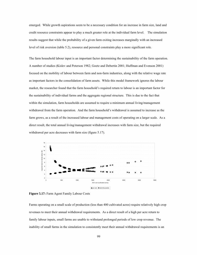
99

emerged. While growth aspirations seem to be a necessary condition for an increase in farm size, land and

credit resource constraints appear to play a much greater role at the individual farm level. The simulation

results suggest that while the probability of a given farm exiting increases marginally with an increased

level of risk aversion (table 5.2), resource and personal constraints play a more significant role.

The farm household labour input is an important factor determining the sustainability of the farm operation.

A number of studies (Kislev and Peterson 1982; Goetz and Debertin 2001; Huffman and Evenson 2001)

focused on the mobility of labour between farm and non-farm industries, along with the relative wage rate

as important factors in the consolidation of farm assets. While this model framework ignores the labour

market, the researcher found that the farm household’s required return to labour is an important factor for

the sustainability of individual farms and the aggregate regional structure. This is due to the fact that

within the simulation, farm households are assumed to require a minimum annual living/management

withdrawal from the farm operation. And the farm household’s withdrawal is assumed to increase as the

farm grows, as a result of the increased labour and management costs of operating on a larger scale. As a

direct result, the total annual living/management withdrawal increases with farm size, but the required

withdrawal per acre decreases with farm size (figure 5.17).

0

2

4

6

8

10

12

14

16

18

0 500 1000 1500 2000 2500 3000 3500

farm size (cultivated acres)

requ

ired

retu

rn to

fam

ily la

bour

($)

per acre total (thousands)

Figure 5.17: Farm Agent Family Labour Costs Farms operating on a small scale of production (less than 400 cultivated acres) require relatively high crop

revenues to meet their annual withdrawal requirements. As a direct result of a high per acre return to

family labour inputs, small farms are unable to withstand prolonged periods of low crop revenue. The

inability of small farms in the simulation to consistently meet their annual withdrawal requirements is an

100

important driver of structural change. Periods of low crop revenue result in the transfer of farm assets from

small farms to larger operators who are able to meet their withdrawal requirements more consistently.

5.3.2 Cost of Production and Productive Efficiency The changing structure of the farming sector is often thought to be the consequence of heterogeneous

production efficiency among farms. The argument is that the most efficient farms acquire the assets of the

less efficient producers, resulting in the consolidation of farm assets among the most efficient (Harrington

and Reinsel 1995). Economists often acknowledge the relationship between economies of scale in

purchasing inputs and marketing output and the consolidation of farm assets. It is often assumed that by

expanding the area of production, the farm can benefit from economies of scale. While economies of scale

in purchase inputs and marketing products may in fact be a sufficient condition to explain the structural

shifts that have occurred, this study finds they are not necessary. This series of simulations explicitly

assumes that farms operate with constant economies of scale with respect to non-labour costs of producing

a crop (before transportation costs). When non-family labour is included, small farms actually have a cost

advantage over large farms that are required to hire a greater level of non-family labour (figure 5.18).

8.00

8.25

8.50

8.75

9.00

9.25

9.50

9.75

10.00

0 500 1000 1500 2000 2500 3000 3500

farm size (cultivated acres)

prod

uctio

n co

sts

per a

cre

(exc

ludi

ng fa

mily

labo

ur)

Figure 5.18: Farm Agent Production Costs (excluding Family Labour) The observed variation in production costs in the simulation among farms of the same size (figure 5.18) is

the direct result of transportation costs. Farms with land spread out over a larger area have higher

production costs, attributable to the incremental cost of moving crop production to the farmstead to be

marketed. In general, larger farms are found to have a higher transportation cost per acre compared to

small farms. Larger farms must farm land at a greater distance from their farmstead than small farms.

101

Ultimately, it can be concluded that the distribution of farm size that emerged in the simulations under the

assumption of constant (decreasing) returns to scale for crop production undermines the traditional

argument that economies of scale and producer efficiency are the only significant drivers in the observed

consolidation of farm assets in this chapter.

5.3.3 Path Dependency and the Farm Life-Cycle Structural change at the individual farm level is affected not only by the economic situation faced by

individual farms, but also the interdependencies between farms (Balmann 1999). Farms wanting to expand

are faced with the reality of competing with neighbouring farms for the control of limited resources. As a

direct result, the spatial location of a farm may be a key factor in the long term sustainability of a given

farm. The ability of any farm to expand is directly related to the availability of land within a reasonable

distance from an existing land base. In addition, the ability of a given farm to acquire an available plot of

land is affected by the actions of other farms within the same general geographic region. This situation is

defined by Balmann (1999) in the farming context as path dependence, whereby, in a stochastic world, the

current state of a system is directly dependent on historic actions and events. Given the results obtained

here, in particular the consistency with regard to changes in distributions of management classes and the

marginal variation between exit rates among the three management classes considered, factors other than

varied risk preference must be important in determining the growth path of individual farms.

In this light, it is found that one of the most important factors in determining the sustainability of a given

farm appears to be its initial land base. The mean initial size (cultivated acres) of farms that discontinued

production during the simulation period was found to be approximately one-half that of the mean initial

size of all farms. Based on simulation results, the study found that farms which declined over a five year

period managed, on average, a total land base of only 76% (std dev = 28%) of the average for the region.

In direct contrast, those farms that expanded over a given 5 year interval operated on a scale that was

significantly greater, with a mean size advantage of approximately 450% (std dev =270%) over the regional

average. Thus while farms operating on a large scale have significant advantages in the land market, this is

not a guarantee of growth in a given time period. Farms that experienced zero growth over a given five

102

year interval had an average scale of production of 94% (std dev = 91%) of the regional average, with

approximately 7% of this group operating on a scale at least three times the regional average.

On average, a farm operation in the simulation with an initial land holding greater than the regional mean is

significantly more likely to realize their growth aspirations. In addition, due to the spreading of the

family/management withdrawal over a greater number of acres, the large farm is better able to withstand

periods of reduced crop revenues. Finally, while operating on a large scale effectively reduces the risk of

continued operation, it is not a guarantee of success. On average 4% of the total exits over the simulated

period were by farms operating within the largest size classification measured (see table 5.4).

5.3.4 Government Transfers and Regional Structure Government policies and support programs are commonly discussed concurrently with issues of structural

change and the resulting reallocation of resources (Fulton et al 1989). In fact it is prudent that policy

makers understand the relationship between stabilization/support programs and structural change. Goddard

et al (1993) identified public programs as one the eight factors affecting structural change in the agriculture

sector. In the simulations, it is found that prior to the rapid decline in farm land values throughout the late

1980’s, simulated government transfers aimed at stabilizing the income of farm agents played no

significant role in the evolution of regional farm structure. In fact, prior to the mid 1980’s, no significant

difference is found between the base and zero transfer scenarios.

The period that overlaps the late 1980’s and early 1990’s is characterized in the simulations by a rapid

downward trend in farmland values and an increased rate of consolidation. Fulton et al’s (1989)

supposition that without the significant transfers farmers received from stabilization and support programs,

the rate of decline in the farm population would have been significantly greater is supported by the results

obtained in this research. A significant level of divergence occurs for the observed farm number trends

between the base and zero transfer scenarios. It is also interesting to note that while the number of farms

declined at a significantly faster rate in the zero transfer scenario, the distribution of farms by cultivated

acres at the end of the simulation did not differ significantly from the base scenario. Thus, the ability of

governments to alter the rate of structural change must not be dismissed. But, whether the increased rate of

103

consolidation that would surely have occurred in the absence of direct government transfers in Canadian

agriculture would have led to a more productive agricultural sector in the long run is still open for debate.

5.4 Summary

The application of an agent-based framework to study structural change at the regional level allows the

issue to be analyzed with a focus on the decisions made at the individual or farm level. The drivers of

structural change discussed in chapter two all focus on the incentives and decisions of farms at this level.

As a result, a study of structural change at the regional level is well suited for the application of this new

modeling paradigm.

The simulation environment was designed to attempt to replicate the actual structural shifts that occurred in

Saskatchewan agriculture over the period from1960 to 2000, under the assumption that technology and

farming practices remained constant throughout the simulated period. To do this, five distributions of

farms among three primary managerial classes are simulated. Relatively consistent results are obtained

from all distributions. All five distributions closely replicate the trend of declining farm numbers and

increasing farm size. The distribution of farms by number of acres managed generated by all our

simulations closely replicate the actual distribution observed over the time period. In addition, the

simulations replicate the sharp increase in farmland values during the 1970’s as well as the subsequent

decline throughout the 1980’s, albeit with a time lag. The decline in the proportion of farmland managed

under a lease agreement that occurred between the 1961 and 1966 census periods, as well as the later trend

of increased farm land owned by non-farming individuals, is correctly replicated by all simulations.

A second simulation scenario was run to estimate the structural evolution of the region under the

assumption of zero government stabilization transfers. By comparing the results estimated for both the

base and zero transfer scenarios, the net results of the package of stabilization programs and ad-hoc

payments can be estimated. The package of stabilization programs and payments do not show a significant

impact on the regional structural characteristics in the simulation prior to 1987. However, significant

divergence begins to emerge between the base and zero transfer scenarios in the post 1987 time period. In

the absence of government transfers to grain operations, the simulated number of farms is significantly

reduced by the end of the simulation compared to the base scenario. This result is consistent with the

104

earlier findings of Fulton et al (1989) and the post 1985 impact of government farm programs. As a direct

result, the mean area cultivated by individual farm agents increased substantially without transfers, but

interestingly, we found that the distribution of farms does not vary significantly from the base scenario. I

conclude that while transfers have certainly had an effect on the agricultural sector, the consequences of

transfers have not necessarily transpired as originally intended by policymakers. The simulations show that

transfers tend to have minor impacts on the small farm, and instead have contributed to the growth of the

larger farms in the region.

In the sense described in Chapter 3, a number of key insights about agriculture in this region emerged from

this research. For example, while economies of scale in purchasing inputs and marketing production may

work in reality for larger producers, they are not necessary to replicate the structural shifts that occurred

over the period studied. Instead, the ability of the farm agent to fully employ their labour and management

input emerges as an important factor in the sustainability and growth of an individual farm. Those farm

agents that were unable to expand their farm to a sustainable scale are found to be incapable of consistently

meeting their annual living/management withdrawal requirements during periods of depressed crop returns.

Finally, it appears that opportunity and luck often play a more important role than individual ability. In

fact, it is possible that a less productive farm agent may succeed while a more productive farm agent may

fail, and this is due to the immobility of farmland.

105

CHAPTER SIX

SUMMARY AND CONCLUSIONS

6.1 Summary The Saskatchewan farm sector continues to be a dynamic industry, faced with the reality of significant

structural adjustment. While structural adjustment can result in more efficient production, the

consolidation of farm assets among a decreasing number of farm operations also has a significant impact on

the population base of rural regions. Structural change continues to one of the most important issues for

both the farm sector and rural regions, but the process and its underlying drivers continue to be weakly

understood. Farm characteristics like operator age, land tenure, farm type, farm size, debt level and

motivation vary widely across Canada (Statistics Canada), and it is clear that these factors are key drivers

of farm industry structure. Given the economic difficulties now inherent in rural Saskatchewan, there has

never been a more important time to improve our understanding of the structural dynamics of the farming

sector.

The desire to understand farming and farm structure has led to the development of a number of well

documented farm-level models, including FLIPSIM in the U.S. and CRAM (Canadian Regional

Agricultural Model) in Canada (Klein and Narayanan 1992). To their credit, the previous generation of

farm-level models were not designed to capture complexity or emergent behaviour, yet complexity is

arguably one of the most important characteristics of any dynamic economic system. It is argued that

adaptive farm models based on individual interactions are necessary to help unravel the intricate interplay

among natural and economic developments in the farming sector. Part of the motivation for this research is

the realization that farming behaviour possesses characteristics of a complex system in the computational

sense, and complex systems often generate large-scale behaviour that cannot readily be predicted by simply

examining components of the system. It is the potential to reveal emergent farm level behaviour that

106

distinguishes new generation behavioural farm models from the older generation of atomistic farm level

policy models.

The rigidity that generally characterizes previous farm-level modeling methodologies limited their ability

to incorporate and predict structural change. Through the application of an agent-based simulation

framework, the potential of incorporating structural change as an endogenous factor to the farm model can

be realized. The developed model of an idealized agricultural region in the Canadian province of

Saskatchewan was then evaluated on its ability to replicate historic structural shifts for the period 1960-

2000.

6.2 Conclusions Agent-based methods exhibit a strong potential to overcome one of the major limitations of current farm

level modeling frameworks. The highly heterogeneous nature of agricultural production is in sharp contrast

to the general assumption of a homogenous population required for traditional farm-level models. The

highly flexible nature of agent-based models, due to their focus on a building system from the ‘ground up’,

allows the researcher/policymaker an improved understanding of the interplay between aggregate level

behaviour and patterns and the underlying characteristics of the individuals that constitute the system of

study.

I offer that the demonstrated ability of this agent based model of a rural region, characterized by annual

crop production, to mirror the actual structural adjustments that played out over the study period can be at a

minimum regarded as a strong “proof of concept”. The research and model development discussed in this

thesis offers the potential to provide a fundamental framework for future research focused on structural

dynamics and policy analysis.

While significant discussion in agricultural and regional economics has been concerned with the

importance of producer efficiency and economies of scale, the results generated here suggest that this is not

a necessary condition for structural change. The ability of a farm household to fully employ their labour

resource is found to play a far greater role in determining the continued existence of a given farm than the

107

ability to produce a crop efficiently. As a result, I find that a less efficient producer70 operating on a large

scale is more likely to remain in the industry than a small, yet more efficient producer. While a non-farm

labour market for the farm household’s excess labour was not explicitly considered here, I offer that it is

highly unlikely that its inclusion would significantly alter the simulation results.

Varied management styles were also incorporated into the simulations, and they only marginally improved

the mean survival rate of the least risk averse relative to the most risk averse farm households. While, all

else constant, the least risk averse farm household has a greater probability of achieving their aspiration for

farm growth, simple opportunity and timing appear to play a more significant role in the long term

profitability and sustainability of a given farm.

6.3 Limitations Agent-based methodologies provide the agricultural researcher with a highly flexible and adaptable toolkit

for studying complex physical/social interactions and networks. One of the greatest challenges faced when

developing the simulation model utilized in this thesis, a challenge faced by all who undertake this type of

research, was trying to find an appropriate balance between model realism and tractability. It is a relatively

simple task to highlight a number of areas in which the model abstracts significantly from reality. But

given the multitude of layers of reality that could potentially be incorporated within the basic framework,

the selection of those key drivers and structures to incorporate was a time consuming and difficult process.

This study is not unique in making this assessment about agent based simulations (see Robinson 2003).

It is not the purpose of this section to outline all areas where the simulation model abstracts from the target

system modeled, but rather to highlight those key areas the reader needs to be aware of when interpreting

the results and conclusions presented. First, due to the nature of the methodology selected and the

individual and behavioural level data requirements, data availability proved to be a significant limitation.

While great care was taken to track down the required data/parameter values, in a number of situations an

approximation of the actual value was the only viable option. Significant care has been taken to ensure that

all approximations are clearly stated and explained. Second, due to the long standing tradition in economic

research to focus on the outcome of individual behaviour (i.e. individuals behave “as if” they are

70 Producer efficiency refers to cost of producing a crop excluding the family/management withdrawal.

108

profit/utility maximizing), rather than the underlying behavioural rules being utilized, the modeling of

sound behavioural rules is a rather daunting task.

Thus, while the level of realism incorporated into the model is an appropriate abstraction from the true

system, three key areas where the model differs significantly from reality should be noted. The first

significant variation deals with the assumption of constant 1960’s farm practices and technology, as well as

de-trended crop yields and market prices. Secondly, a lack of an explicit non-farm labour market and

potential the use of off-farm income to subsidize the farm operation likely resulted in an under-estimation

of the number of small farms in the final simulated distribution. The relatively small proportion of farm

agents who retire due to old age without a new generation continuing to operate the farm also suggests that

a more realistic algorithm is required to model the intergenerational transfer of farm assets.

6.4 Suggestions for Further Study One of the underlying objectives of this research was to develop a relatively simple framework on which to

base future farming model developments. Of primary importance in this framework is the

conceptualization of the farmland markets. While the farmland market mechanisms incorporated within

the model are justifiable and defendable, it would be interesting to test alternative specifications against the

results obtained in this study. Ultimately, due to the flexibility of the toolkit utilized, it is possible to

outline an almost unlimited number of potential model extensions and improvements. In an attempt to

sidestep listing multiple potential model extension, it should be noted that new developments will need to

be driven by the research problems tackled in the future. It is not the coding of model constructs that will

limit future research71, but rather the ability to understand what to code.

In order to improve future research utilizing the agent based model framework, regardless of the issue to be

studied, research needs to be focused on two inter-related aspects. There is a stark need to develop an

improved understanding of the behaviour of individuals and the varied behavioural patterns that exist

among the relevant agent populations. This is an area economists have traditionally ignored and would

benefit substantially form an interdisciplinary approach to future research. Economists interested in

71 While the author may be nearing the upper limits of his programming skills, it is assumed that more skilled programmers are available.

109

utilizing agent-based methodologies may need to seek out collaborators from other academic disciplines.

In particular for this research considerable efforts need to be made to collect and compile survey data

describing the managerial and behavioural characteristics of farm decision making units. By improving our

understanding of the underlying behavioural and managerial decisions of the farm household, a number of

the limitations outlined in the previous section can be overcome.

110

REFERENCES Agriculture Canada. (1986a) Special Canadian Grains Program. Communications Branch. Ottawa:

December 9. Agriculture Canada. (1986b) Applications for Crop Drought Assistance in Mail. Communications Branch.

Ottawa: January 17 Agriculture Canada (1988) Special Drought Assistance for Crop Producers. Communications Branch.

Ottawa: November 10. Agriculture Canada (1992) Backgrounder: Gross Revenue Insurance Program. Communications Branch.

Ottawa. Agarwal, C., G.Green, J. M. Grove, T.Evans and C. Schwelk.(2002) A Review and Assessment of Land-

Use Change Models: Dynamics of Space, Time, and Human Choice. General Technical Report NE-297. Newton Square, PA: U.S. Department of Agriculture, Forest Service, Northeastern Research Station. 61 p.

American Society of Agricultural Engineers (2003) “Agricultural Machinery Management Data” American

Society of Agricultural Engineers, St. Joseph, Michigan. D497.4 February 2003. Arthur, B.W. (1994) “Bounded Rationality and Inductive Behavior” American Economic Review 84: 406-

411. Arthur, B.W. (1999) “Complexity and the Economy” Science (April) 284: 107-109. Balmann, A (1997) “Farm-based Modelling of Regional Structural Change: A Cellular Automata

Approach”, European Review of Agricultural Economics, 24, 85-108. Balmann, A. (1999). “The Dynamics of Structural Change and Farmers’ Income in a Maturing Sector”

Working Paper, Humboldt University of Berlin. Balmann, A.(2000). “Modeling Land Use with Multi-Agent Systems: Perspectives for the Analysis of

Agricultural Policies” In IIFET 2000: Microbehavior and Macroresults, Proceedings, International Institute of Fisheries Economics and Trade, Oregon State University, Corvallis, Oregon, USA.

Barlett, P.F. (1984) “Microdynamics of Debt, Drought, and Default in South Georgia” American Journal of

Agricultural Economics December: 836-843. Bennett, J.W. (1982) Of Time and the Enterprise: North American Family Farm Management in a context

of Resource Marginality. Minneapolis, MN: University of Minnesota Press. Bennett, J.W. and S.B. Kohl (1982) “Farms and Family in North American Agriculture” in Of Time and the

Enterprise: North American Family Farm Management in a context of Resource Marginality. Minneapolis: University of Minnesota Press.

Berger, T. (2001) “Agent-based Spatial Models Applied to Agriculture: a Simulation Tool for Technology

Diffusion, Resource Use Changes and Policy Analysis”. Agricultural Economics 25: 245-260. Bollman, R.D., L.A. Whitener and F.L. Tung (1995) “Trends and Patterns of Agricultural Structural

Change: A Canada-U.S. Comparison” Canadian Journal of Agricultural Economics special issue: 15-28.

111

Bonfanti, P.L., Castelli, G., Lazzari, M., Mazzetto, F. and P. Sacco (1998) “Simulation of farmers’ decision-making processes based upon agri-environmental policy effects: the IMAGES Project”, available on-line at: http://www.uniud.it/cartesio/images/Articoli/rabat.html

Casti, J.L. (1997) Would-Be Worlds: How Simulation is Changing the Frontiers of Science. John Wiley

and Sons, New York. Cochrane, W. (1958) Farm Prices Myths and Reality. University of Minnesota Press, Minneapolis,

Minnesota. Day, R. H. (1963). Recursive Programming and Production Response. North-Holland, Amsterdam. Day, R. H. (1994) Complex Economic Dynamics, Volume 1: An Introduction to Dynamical Systems and

Market Mechanisms. MIT Press, Cambridge, MA. Deadman, P.J. (1999) “Modelling Individual Behavior and Group Performance in an intelligent Agent

Based Simulation of the tragedy of the Commons” Journal of Environmental Management 56(3): 159-172.

Durlauf, S. (1998) “What Should Policymakers Know About Economic Policy”, The Washington Quarterly

21(1): 159-165. Epstein, J. M. and R. L. Axtell. (1996) Growing Artificial Societies: Social Science from the Bottom Up.

Cambridge: MIT Press / Brookings Institute. Fairweather, J.R. and N.C. Keating (1994) “Goals and Management Styles of New Zealand Farmers”

Agricultural Systems 44: 181-200. Fellmann, J. D., A. Gettis and J. Gettis. (1999). Human Geography: Landscapes of Human Activity. WCB

McGraw-Hill, Boston. Ferber, J. (1999). Multi-Agent Systems: An Introduction to Distributed Artificial Intelligence. Addison-

Wesley, Harlow. Fisher, W. D. and P. L. Kelley (1982). Selecting Representative Firms in Linear Programming. in

Economic Analysis and Agricultural Policy. Iowa State University Press, Ames, Iowa. Friedman, D. and S. Sunder (1994) “The Emergence of Experimental Economics” in Experimental

Methods: A Primer for Economists. Cambridge University Press. New York, NY. Foot, D. K. (1996) Boom, Bust & Echo: How to Profit from the Coming Demographic Shift. Macfarlane

Walter & Ross. Toronto. Fulton, M., K. Rosaasen and A. Scmitz (1989) “Canadian Agricultural Policy and Prairie Agriculture” a

study prepared for the Economic Council of Canada. Gale, H.F. (2003) “Age-Specific Patterns of Exit and Entry in U.S. Farming, 1978-1997” Review of

Agricultural Economics 25(1): 168-186. Gale, H.F. (1996) “Age Cohort Analysis of the 20th Century Decline in U.S. Farm Numbers” Journal of

Rural Studies 12(1): 15-25. Giannakas, K., R. Schoney and V. Tzouvelekas (2001) “Technical Efficiency, Technological Change and

Output Growth of Wheat Farms in Saskatchewan. Canadian Journal of Agricultural Economics 49: 135-152.

112

Gilbert, N. and K. Troitzsch (2002) Simulation for the Social Scientist. Open University Press, Philadelphia.

Glaeser, E.L. and J.E. Kohlhase (2004) “Cities, Regions and the Decline of Transport Costs” Papers in

Regional Science 83: 197-228 Goddard, E., A. Weersink, K. Chen and C.G. Turvey (1993). “Economics of Structural Change in

Agriculture” Canadian Journal of Agricultural Economics 41: 475-489. Goetz, S.J. and D. Debertin (2001) “Why Farmers Quit: A Country-Level Analysis” American Journal of

Agricultural Economics 83(4): 1010-1023. Guide to Farm Practice in Saskatchewan (1960) Published under the authority of The Saskatchewan Co-

operative Agricultural Extension Program. Gumerman, G., A. Swedlund, J. Dean,and J. Epstein (2002) “The Evolution of Social Behavior in the

Prehistoric American Southwest” Santa Fe Institute working paper 02-12-067. Hadar, J. and W.R. Russell (1969) “Rules for Ordering Uncertain Prospects” The American Economic

Review 59(1): 25-34. Happe, K. (2004) Agricultural Policies and Farm Structure: Agent-Based Modelling and Application to

EU-policy Reform. Institute of Agricultural Development in Central and Eastern Europe (IAMO) Happe, K and A Balmann (2003) “Agent-based Modeling in Agricultural Economics –Perspectives and

Challenges”, Institute of Agricultural Development in Central and Eastern Europe (IAMO) Happe, K, A.Balmann and K. Kellerman (2004) “The Agricultural Policy Simulator (AgriPoliS) - An

Agent-Based Model to Study Structural Change in Agriculture (Version 1.0)” Discussion Paper No. 71. Institute of Agricultural Development in Central and Eastern Europe (IAMO).

Harrington, D.H. and R.D. Reinsel (1995) “A Synthesis of Forces Driving Structural Change” Canadian

Journal of Agricultural Economics special issue: 3-14. Harris, D.G. and R.F. Nehring (1976) “Impact of Farm Size on the Bidding Potential for Agricultural

Land” American Journal of Agricultural Economics 58(2): 161-169. Holland, J. and J. Miller (1991). “Artificial Adaptive Agents in Economic Theory” The American

Economic Review 81(2): 365-370, Papers and Proceedings of the Hundred and Third Annual Meeting of the American Economic Association.

Huffman, W.E. and R.E. Evenson (2001) “Structural and Productivity Change in U.S. Agriculture, 1950-

1982” Agricultural Economics 24: 127-147. Helmberger, P.G. (1972) “Markets, Farm Size, and Integration” in Size, Structure, and the Future of

Farms. The Iowa State University Press, Ames, Iowa. Jensen, H. (1977) “Farm Management and Production Economics, 1946-1970”, Part I in A Survey of

Agricultural Economics Literature, L. Martin, Ed. University of Minnesota Press, Minneapolis. Jones, W. and C. Buckley (1980) “Measuring Structural Change in the Canadian Farm Industry” Canadian

Farm Economics 15(6): 9-41. Johnson, G.L. (1972) “Theoretical Considerations” in The Overproduction Trap in U.S. Agriculture. The

Johns Hopkin University Press, Baltimore, Maryland.

113

Karagrannis, G. and W.H. Furtan (1990). “Induced Innovation in Canadian Agriculture: 1926-87” Canadian Journal of Agricultural Economics 38: 1-21.

Keating, N.C. and B. Munro (1989) “Transferring the Family Farm: Process and Implications” Family

Relations 38(2): 215-219. Kelton, W, Sadowski, R. and D. Sturrock. (2004) Simulation with Arena. Third Edition. McGraw Hill. New

York, NY. Kislev, Y. and W. Peterson (1982). “Prices, Technology and Farm Size” The Journal of Political Economy

90 (3): 578-595. Klein, K.K. and S.A. Narayanan. (1992) “Farm level models: A review of developments, concepts and

applications in Canada”, Can. J. Agric. Econ. 40(3):351-368. Lewin, R. (2000) Complexity: Life on the Edge of Chaos. Second Edition. University of Chicago Press. Manson, S. (2001). “Simplifying Complexity: A review of complexity theory”, GeoForum 32(3): 405-414. Nelson, G. C. (2002). “Introduction to the special issue on spatial analysis for agricultural economists”

Agricultural Economics 27:197-200. Nelson, R.R. (1995). “Recent Evolutionary Theorizing About Economic Change” Journal of Economic

Literature 33(1): 48-90. Olson, K.D. (2004) Farm Management: Principles and Strategies. Iowa State Press. Ames, Iowa. Olsson, R. (1988) “Management for Success in Modern Agriculture” European Review of Agricultural

Economics 15: 239-259. Parker, D.C. (2000). Edge-effect externalities: Theoretical and empirical implications of spatial

heterogeneity. Ph D.diss. University of California at Davis, Davis, CA Parker, D. C, S. Manson, M. Janssen, M. Hoffman and P. Deadman. (2003). Multi-Agent Systems for the

Simulation of Land-Use and Land-Cover Change: A Review. Annals of the Association of American Geographers, 93(2): 314-337.

Parker, D. C., and V. Meretsky (2004). “Measuring pattern outcomes in an agent-based model of edge-

effect externalities using spatial metrics” Agriculture, Ecosystems and Environment 101(2-3): 233-250.

Polhill, J. G., N. M. Gotts, and A. N. R. Law. (2001). “Imitative versus nonimitative strategies in a land-use

simulation”, Cybernetics and Systems 32 (1): 285-307. Purdy, H.L. (1972) Transport Competition and Public Policy in Canada. University of British Columbia

Press. Vancouver, British Columbia. Ragush, M. (1966) “Use of Farm Credit in Saskatchewan, 1960-64” Canadian Farm Economics 1: 18-22. Rauch, J. (2002) “Seeing Around Corners” The Atlantic Monthly, April 2002: 35-48. Raup, P.M. (1972) “Societal Goals in Farm Size” in Size, Structure, and the Future of Farms. The Iowa

State University Press, Ames, Iowa.

114

Robinson, D. T. (2003). Modelling Farmer Household Decision-making and Its Effects on Land use/cover Change in the Altamira Region, Párá, Brazil. Masters Thesis. University of Waterloo, Waterloo, Ontario, Canada.

Rouchier, J., F. Bousquet, M. Requier-Desjardins, and M. Antona (2001) “A Multi-Agent Model for

Describing Transhumance in North Cameroon: Comparison of Different Rationality to Develop a Routine” Journal of Economic Dynamics and Control 25: 527-559.

Saskatchewan Agriculture (various years) Farm Business Review for the Year 1960-1964. Statistics

Branch. Saskatchewan Agriculture, Food and Rural Revitalization (2005) Historic Crop Yields: Rural Municipality

# 281. www.agr.gov.sk.ca. Regina, SK. Saskatchewan Agriculture, Food and Rural Revitalization.

Saskatchewan Agriculture, Food and Rural Revitalization (2004) Agricultural Statistics Handbook 2003.

www.agr.gov.sk.ca. Regina, SK. Saskatchewan Agriculture, Food and Rural Revitalization. Saskatchewan Agriculture, Food and Rural Revitalization (various years) Crop Production Guide; Dark

Brown Soil Zone (1994-2004). Saskatchewan Agriculture, Food and Rural Revitalization. Schelling, T. C. (1978). Micromotives and Macrobehavior. W. W. Norton, New York. Schmitz, A, H. Furtan and K. Baylis (2002) Agricultural Policy, Agribusiness, and Rent-Seeking

Behaviour. University of Toronto Press, Toronto. Schoney, R.A (1997) An Economic Analysis of the 1987-95 Saskatchewan Wheat, Barley and Canola

Production Costs. Agriculture and Agri-Food Canada Selley, R. (1984) Decision Rules in Risk Analysis, in Risk Management in Agriculture. Edited by P.J.

Barry. Iowa State University Press, Ames, Iowa. Short, C (2004) A Proposal to Develop for A Microsmulation Model of Canadian Farm Households: Risk

Management, Households and Microsimulation. Agriculture Canada. Simon, H. A. (1955). “A Behavioral Model of Rational Choice” The Quarterly Journal of Economics 69:

99-118. Sofranko, A., R. Frerichs, M. Samy and B. Swanson (1999). “Will Farmers Organize: Structural Change

and Loss of Control over Production” paper presented at the 62nd Annual Meeting of the Rural Sociological Society, Chicago, Illinois. August 4-8, 1999.

Statistics Canada (various years) Census of Canada: Agriculture: Saskatchewan. 1961-2001. Stoker, T. M. (1993). “Empirical approaches to the problem of aggregation over individuals” Journal of

Economic Literature 31(4): 1827-1875. Sycara, K.P. (1998) “Multiagent Systems” AI Magazine Summer 1998, pp 79-92. Takayama, T. and W. Labys (1986) Spatial Equilibrium Analysis. Ch. 5 in Handbook of Regional and

Urban Economics, Volume 1: Regional Economics. Peter Nijkamp. Ed. North Holland, New York, NY.

Taylor, J.E., J.E. Norris and W.H. Howard (1998) “Succession Patterns of Farmer and Successor in

Canadian Farm Families” Rural Sociology 63(4): 553-573.

115

Tesfatsion, L. (2000) “Agent-Based Computational Economics: A Brief Guide to the Literature”, Working Paper, Iowa State University. Available on-line at: http://www.econ.iastate.edu/tesfatsi/ace.htm

Troitzsch, K.G. (2004) “Validating Simulation Models”, Proceedings 18th European Simulation

Multiconference. Graham Horton © SCS Europe. Vriend, N. (1996) “Rational Behavior and Economic Theory” Journal of Economic Behavior and

Organizations 29: 263-285. Walker, L.J.S. (1989) “Farm Management Strategies to Family Style” Canadian Journal of Agricultural

Economics 37: 747-754. Welter, F (2002) “Who Wants to Grow? Growth Intentions and Growth Profiles of (Nascent) Entrepreneurs

in Germany” Babson College http://www.babson.edu/entrep/fer/Babson2001/I/IH/I_H/i-h.htm. Wilensky, U. (1999) NetLogo. http://ccl.northwestern.edu/netlogo/. Center for Connected Learning and

Computer-Based Modeling, Northwestern University. Evanston, IL.

116

APPENDIX A List of Variable Names

Farm agent (k = 1,…,K)

GR Gross revenue of farm agent k PF Productivity factor of farm agent k K Crop acres managed (owned or leased) by farm agent k P Number of plots managed by farm agent k VC Variable production expenses of farm agent k TE Transportation expense of farm agent k Travel Unit cost of transporting farm equipment of farm agent k Truck Unit cost of transporting farm production of farm agent k FC Fixed production expenses of farm agent k Creplace Machinery and building replacement expense of farm agent k DS Principal and Interest expense of farm agent k LP Land leasing expense of farm agent k WD Family living and managerial withdrawal of farm agent k NCI Net investment in additional equipment and facilities of farm agent k NCFPRODN Net cash flow from crop production of farm agent k NCFINVEST Equipment and facilities sale proceeds less purchases of farm agent k NCFFINANCE New borrowing less principal and interest payments of farm agent k NCF Net cash flow of farm agent k Gov Net government transfers received by farm agent k PM Production Margin (per acre) of farm agent k rent Residual return to Land of farm agent k Q Mean soil productivity of all plots managed by farm agent k Bidxy Bid of farm agent k on plotxy Φ Land valuation / risk aversion parameter of farm agent k C Stock of machinery and buildings of farm agent k W Non-family labour costs per cultivated acre Λ Minimum cash balance per acre NCFk

WGSA Net cash flow from WGSA of farm agent k Paymentk

WGSA Gross payment from WGSA to farm agent k Levyk

WGSA Total levy paid under WGSA by farm agent k tonnesk Total grain production by volume of farm agent k Paymentk

SCGP Gross payment from SCGP to farm agent k Ai Total acreage of crop i for farm agent k Paymentk

DAP Gross payment from DAP to farm agent k NCFk

GRIP Net cash flow from GRIP of farm agent k Paymentk

GRIP Gross payment from GRIP to farm agent k Indemk

GRIP Total indemnity paid under GRIP by farm agent k prodni Total production by volume of crop i by farm agent k TWDNISA Maximum triggered withdrawal from NISA account for farm agent k NINISA Net income of farm agent k for NISA program NI¯¯ NISA 3- year moving average net income of farm agent k for NISA program Fund 1 Balance of NISA account, fund 1, of farm agent k Fund 2 Balance of NISA account, fund 2, of farm agent k WDNISA Actual withdrawal from NISA account of farm agent k Paymentk

AIDA Gross payment from AIDA to farm agent k NIAIDA Net income of farm agent k for AIDA program NI¯¯ AIDA 3-year moving average net income of farm agent k for AIDA program Plotxy (x = x co-ordinate, y = y co-ordinate)

Qxy Fixed soil productivity value of plotxy Rxy Annual growing conditions value of plotxy PIxy Productivity index of plotxy

Kxy Crop acres of plotxy TExy Transportation expense of plotxy Dxy Distance between plotxy and managing farm agent’s farmstead Vxy Volume of total crop production on plotxy

rentxy Rent value for plotxy VN Value of plotxy (per acre) at period N Pricexy Final price paid for plotxy by purchasing/leasing farm agent

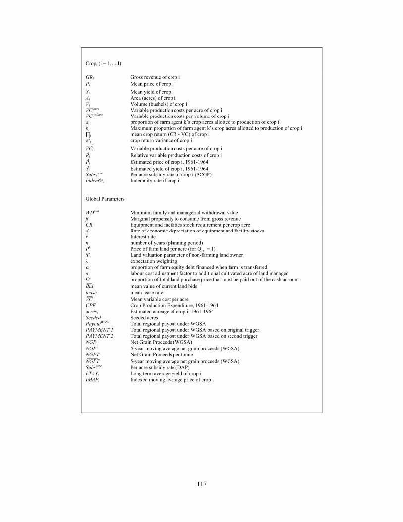
117

Cropi (i = 1,…,I)

GRi Gross revenue of crop i

Pi Mean price of crop i

Yi Mean yield of crop i Ai Area (acres) of crop i Vi Volume (bushels) of crop i

VCiacre Variable production costs per acre of crop i

VCivolume Variable production costs per volume of crop i

ai proportion of farm agent k’s crop acres allotted to production of crop i bi Maximum proportion of farm agent k’s crop acres allotted to production of crop i ∏i mean crop return (GR - VC) of crop i σ2

∏i crop return variance of crop i

VCi Variable production costs per acre of crop i

Riˆ Relative variable production costs of crop i Piˆ Estimated price of crop i, 1961-1964 Yiˆ Estimated yield of crop i, 1961-1964 Subsi

acre Per acre subsidy rate of crop i (SCGP) Indem%i Indemnity rate if crop i Global Parameters

WDmin Minimum family and managerial withdrawal value ß Marginal propensity to consume from gross revenue CR Equipment and facilities stock requirement per crop acre d Rate of economic depreciation of equipment and facility stocks r Interest rate n number of years (planning period) PL Price of farm land per acre (for Qxy = 1) Ψ Land valuation parameter of non-farming land owner λ expectation weighting α proportion of farm equity debt financed when farm is transferred σ labour cost adjustment factor to additional cultivated acre of land managed Ω proportion of total land purchase price that must be paid out of the cash account Bid¯¯ mean value of current land bids lease¯¯¯¯ mean lease rate VC ¯¯ Mean variable cost per acre CPE Crop Production Expenditure, 1961-1964 acresi Estimated acreage of crop i, 1961-1964 Seeded Seeded acres PayoutWGSA Total regional payout under WGSA PAYMENT 1 Total regional payout under WGSA based on original trigger PAYMENT 2 Total regional payout under WGSA based on second trigger NGP Net Grain Proceeds (WGSA) NGP¯¯¯ 5-year moving average net grain proceeds (WGSA) NGPT Net Grain Proceeds per tonne NGPT¯¯¯¯ 5-year moving average net grain proceeds (WGSA) Subsacre Per acre subsidy rate (DAP) LTAYi Long term average yield of crop i IMAPi Indexed moving average price of crop i

118

APPENDIX B

Model Initial Values/Distributions

Name in Model Name in Text Description Initial Value

0.834

na

0.068

na

$0.10

$1,882

(24.66, 23.75, 15.04, 13.12, 8.60)

(16.88, 15.20, 10.84, 7.24, 11.8)

$5.00

na

na

na

$8.00

$6.80

$7.60

$8.40

marginal propensity to consume from gross farm revenue

σ labour cost adjustment for an additional cultivated acre of land managed

β

trucking-rate cost of transporting grain ($/tonne-mile)

min-family-withdrawal mimimum level of cash withdrawn from farm for family and managerial expensesWDmin

per-bu-vc-4 variable production expenses per bushel (flaxseed)

travel-adjustment cost of transporting machinery between plots ($/mile)

crop-1-list historic production margin 1955-1959 (wheat)

crop-2-list historic production margins 1955-1959 (oats)

crop-3-list

VCivolume

per-bu-vc-2 variable production expenses per bushel (oats)

per-bu-vc-3 variable production expenses per bushel (barley)

VCivolume

VCivolume

per-acre-vc-5 variable production expenses per acre (summerfallow)

per-bu-vc-1 variable production expenses per bushel (wheat)

VCiacre

VCivolume

per-acre-vc-3 variable production expenses per acre (barley)

per-acre-vc-4 variable production expenses per acre (flaxseed)

VCiacre

VCiacre

per-acre-vc-1 variable production expenses per acre (wheat)

per-acre-vc-2 variable production expenses per acre (oats)

VCiacre

VCiacre

price-crop-3 mean barley price value

price-crop-4 mean flaxseed price value

Pi

Pi

price-crop-1 mean wheat price value

price-crop-2 mean oats price value

Pi

Pi

yield-crop-3 mean barley yield value

yield-crop-4 mean flaxseed yield value

Yi

Yi

yield-crop-1 mean wheat yield value

yield-crop-2 mean oats yield value

Yi

Yi

subsidy-ASA-crop-1 annual per bushel subsidy 1960-1975 (wheat)

subsidy-ASA-crop-3 annual per bushel subsidy 1960-1975 (barley)

subsidy-ASA-crop-2 annual per bushel subsidy 1960-1975 (oats)

subsidy-ASA-crop-4 annual per bushel subsidy 1960-1975 (flaxseed)

Travel

Truck

see Table B.1

value embedded in code

value embedded in code

see Table 4.7

historic production margins 1955-1959 (barley) (19.40, 18.80, 10.64, 7.73, 10.90)

crop-4-list historic production margins 1955-1959 (flaxseed) (25.20, 30.30, 6.72, 14.82, 9.96)

119

Name in Model Name in Text Description Initial Value

80

0.06

0.10

0.18

0.3

lease-term number of years a lease agreement is in effect

rain annual growing conditions index

depreciation-rate rate of economic depreciation of farm equipment and facilities

Rxy

Qxy

Kxy

d

interest-rate rate of interest for borrowing capital

expectation-weight weight of most recent observation in expectation formation

r

λ

preretirement-age age at which farm agents stop buying land

value embedded in code proportion of debt to assets at which a farm is deemed insolvent

retirement-tendency-55-59 probability of a farm agent retiring each year when age is between 55 and 59

retirement-tendency-60-64 probability of a farm agent retiring each year when age is between 60 and 64

retirement-tendency-65-69 probability of a farm agent retiring each year when age is between 65 and 69

retirement-tendency-70-over

probability of a farm agent retiring each year when age is 70 or above

maximum-age age at which farm agents are forced to retire

transfer-sell-rate proportion of equity that must be refinanced when farm transferred

α

D-A-ratio maximum ratio of debt to assets a farm agent can have in order to obtain credit

discount-value-1 land valuation factor of farm agents with attitude = 1

Φ

discount-value-2 land valuation factor of farm agents with attitude = 2

discount-value-3 land valuation factor of farm agents with attitude = 3

Φ

Φ

discount-value-NA land valuation factor of non-farming land owners

capital-per-acre value of machinery and buildings required per acre for crop production

Ψ

CR

downpayment land and equipment down payment requirement

equipment-amor-period amortization period for equipment purchases

land-amor-period amortization period for land purchases

average-rent intial mean lease payment value

plots-leased-percent proportion of plots leased

initila mean land value

farms number of farmagents

PL

age age of farm agents

debt initial value of farm agent debt

uniform distribution 1-5

~N(1,0.02)

~N(1,0.02)quality fixed growing conditions index

K-acres crop acres on a given plot

land-price

0.90

~N(150,5.5), max 160

10%

6%

0.10

55

0.40

0.40

0.95

0.90

0.85

1.00

$15

25%

see Table 4.4

see Table 4.1

5

20

$2.25/cultivated acre

$30/cultivated acre

27.62%

310

120

Name in Model Name in Text Description Initial Value

expanding (0.55, 0, 0, 0.05)cautious (0.55, 0, 0.05, 0)lifestyle (0.55, 0.05, 0, 0)

farms 55+ (0.55, 0.05, 0, 0)

$8.25/cultivated acre

0.58 tonnes/cultivate acre

see Table 4.6

$15/cultivated acre

1

see Table 4.1 and Table 4.2

attitude managerial group

proportion of total cultivated acres alloacted to each crop (wheat, oats, barley, flaxseed)

Rent

expected-production-volume initial expectation of crop production volume

expected-return-to-land initial expectation of residual return to land

generation current generation managing the farm

cash initial value of farm agent cash

plots-owned intial number of plots owned by a farm agent

plots-leased intitial number of plots leased by a farm agent

crop-mix

Table B.1: Agricultural Stabilization Act Crop Subsidies

year wheat oats barley flaxseed1960 0.00 0.00 0.00 0.001961 0.00 0.00 0.00 0.001962 0.00 0.00 0.00 0.001963 0.00 0.00 0.00 0.001964 0.00 0.00 0.00 0.001965 0.00 0.00 0.00 0.001966 0.00 0.00 0.10 0.001967 0.20 0.12 0.11 0.001968 0.14 0.03 0.13 0.081969 0.00 0.00 0.00 0.301970 0.00 0.00 0.44 0.051971 0.00 0.00 0.00 0.001972 0.00 0.00 0.00 0.001973 0.00 0.00 0.00 0.001974 0.02 0.00 0.00 0.661975 0.66 0.20 0.25 0.99

per bushel payment

Source: Author based on data from Saskatchewan Agriculture, Food and Rural Revitalization (2004)

121

APPENDIX C

NetLogo© Source Code

globals [ yield-crop-1 ;; Array of wheat yields yield-crop-2 ;; Array of oat yields yield-crop-3 ;; Array of barley yields yield-crop-4 ;; Array of flax yields price-crop-1 ;; Array of wheat prices price-crop-2 ;; Array of oat yields price-crop-3 ;; Array of barley yields price-crop-4 ;; Array of flax yields land-price ;; mean purchase price of land (adjusted for quality) sold in most recent auction bids ;; list of successful bids in current auction average-rent ;; mean lease rate of all plots currently leased land-unit-sold ;; tracking variable, holds ID value of the last plot sold land-unit-rented ;; tracking variable, holds ID value of the last plot leased year ;; tracks current simulation time period plots-leased-percent ;; number of plots leased divided by total number of plots plots-not-in-crop-prodn-percent ;; number of plots not currently managed divided by total number of plots farms ;; total number of farm agents currently managing a minimum of 1 plot crop-1-rank ;; used in crop mix selection algorithm to track relative rank of wheat production crop-2-rank ;; used in crop mix selection algorithm to track relative rank of oat production crop-3-rank ;; used in crop mix selection algorithm to track relative rank of barley production crop-4-rank ;; used in crop mix selection algorithm to track relative rank of flax production crop-1-value ;; used in crop mix selection algorithm to rank crops (value for wheat) crop-2-value ;; used in crop mix selection algorithm to rank crops (value for oat) crop-3-value ;; used in crop mix selection algorithm to rank crops (value for barley) crop-4-value ;; used in crop mix selection algorithm to rank crops (value for flax) crop-1-list ;; holds five years of data on gross return (wheat) crop-2-list ;; holds five years of data on gross return (oats) crop-3-list ;; holds five years of data on gross return (barley) crop-4-list ;; holds five years of data on gross return (flax) mix ;; variable use in crop mix selection algorithm sold ;; number of plots sold in the current auction period bankrupt ;; total number of farm agents exiting due to bankruptcy condition cashflow ;; total number of farm agents exiting due to cash-flow condition oldage ;; total number of farm agents exiting, without an intergenerational transfer transfers ;; total number of farm agents exiting, with an intergenerational transfer tracking-number ;; variable used in GRIP algorithms equip-purchase-adjustment ;; deduction from residual return to land and labour to cover the cost of equipment IMAP-1 ;; GRIP indexed moving average price (wheat) IMAP-2 ;; GRIP indexed moving average price (oats) IMAP-3 ;; GRIP indexed moving average price (barley) IMAP-4 ;; GRIP indexed moving average price (flax) mean-bid ;; mean bid value of all farm agents, active in the first iteration of the land auction WGSA-NCF-MA ;; WGSA program net cash flow moving average WGSA-NCFPT-MA ;; WGSA program net cash flow per tonne moving average WGSA-total-payout ;; WGSA program total payment to the region WGSA-total-levy ;; WGSA program total levy amount collected from the region susidy-ASA-crop-1 ;; ASA program subsidy value per bushel of wheat subsidy-ASA-crop-2 ;; ASA program subsidy value per bushel of oats subsidy-ASA-crop-3 ;; ASA program subsidy value per bushel of barley subsidy-ASA-crop-4 ;; ASA program subsidy value per bushel of flax ] patches-own [ quality ;; relative index value (0-1) of soil productivity rain ;; relative index value (0-1) of annual growing conditions annual-multiplier ;; quality * rain farmer ;; ID number of farm agent managing plot renter ;; ID number of farm agent leasing plot owner ;; ID number of farm agent who owns plot k-acres ;; total number of acres suitable for crop production distance-to-farmstead ;; distance between plot and farmstead of managing farm agent prodn-volume ;; total crop production of plot

122

lease-payment ;; annual lease payment per k-acre lease-term ;; number of years remaining on current lease agreement patch-id ;; unique ID number for each plot for-sale? ;; TRUE if land is available for sale, else FALSE for-rent? ;; TRUE if land is available for lease, else FALSE ] turtles-own [ age ;; age of farm agent generation ;; family generation of farm agent crop-revenue ;; gross crop revenue of farm agent average-multiplier ;; mean value of annual multiplier values of all plots managed by farm agent average-soil-quality ;; mean value of quality values of all plots managed by farm agent crop-mix ;; list of proportion of crops relative to total k-acres of farm agent acres-total-crop ;; summation of all crop acres from all managed plots acres-crop-1 ;; total acres of wheat production acres-crop-2 ;; total acres of oats production acres-crop-3 ;; total acres of barley production acres-crop-4 ;; total acres of flax production acres-crop-5 ;; total acres of fallow prodn-crop-total ;; summation of all crop production from all managed plots prodn-crop-1 ;; total production volume of wheat prodn-crop-2 ;; total production volume of oats prodn-crop-3 ;; total production volume of barley prodn-crop-4 ;; total production volume of flax variable-prodn-costs ;; total variable costs for farm agent in current production period hired-labour ;; total cost of hired labour for farm agent in current production period travel-cost ;; total cost of traveling, moving machinery between plots trucking-cost ;; total cost of transporting crop production from plots to farmstead capital-replacement-charge ;; total cost of equipment replacement (assumed to equal economic depreciation) debt-list ;; tracks each debt separately [payments remaining, annual payment, principal balance] debt ;; summation of individual principal balances of all outstanding debts debt-payment ;; summation of individual annual payments of all outstanding debts cash ;; residual asset account capital-value ;; value of farm equipment and facilities land-value ;; market value of all land owned by farm agent asset-value ;; summation of land-value, capital-value, cash and NISA account equity-value ;; asset-value less debt total-lease-payment ;; summation of annual lease-payment of all plots leased by farm agent family-withdrawal ;; managerial and operator annual withdrawal NCFBI ;; Net CashFlow Before Investment (cashflow prior to purchasing additional land) plots-owned ;; number of plots owned by farm agent plots-leased ;; number of plots leased by farm agent residual-to-land-labor ;; annual residual return to land and labour of farm agent residual-to-land-labor-exp ;; expected residual return to land and labour of farm agent expected-production-volume ;; expectation of crop production on an acre of crop land current-plot-bid-on ;; used in auctions to track plot interesting in purchasing, leasing attitude ;; managerial attitude of farm agent current-bid ;; used in auctions to track current bid value of farm agent years-neg-cash ;; tracks number of years since farm realized a net positive cashflow prodn-conv-factor ;; used to convert bushels to tonnes transfers-received ;; tracks value of annual transfer payments to farm agent WGSA-levy ;; annual levy paid to WGSA program by farm agent WGSA-levy-list ;; list of levies paid to WGSA program by farm agent in previous periods NISA-MA ;; NISA program list of historic farm returns over variable costs NISA-ENS ;; NISA program list of historic farm eligible net sales in previous periods NISA-fund-1 ;; NISA program balance in NISA account fund 1 NISA-fund-2 ;; NISA program balance in NISA account fund 2 NISA-deposit ;; NISA program cash deposit into NISA account by farm agent NISA-withdrawal ;; NISA program maximum triggered withdrawal SCGP-transfer ;; SCGP program transfers received by farm agent AIDA-MA ;; AIDA program list of historic farm returns over variable costs AIDA-payment ;; AIDA program payment received by farm agent ] breeds [farmers] ;; farm agents

123

-------------------------------------------------------------------------------------------------------------------------------------------------------------------------------------------------------------------------- INITIALIZATION PHASE CONTROL -------------------------------------------------------------------------------------------------------------------------------------------------------------------------------------------------------------------------- to initialization-phase-control if "yes" = (user-choice "Have Output Files Been Initialized?" ["no" "yes"]) [ setup ] end to setup ca clear-output create-plots initialize-farm-agents import-crop-arrays export-data show "initialization complete" end ---------------------------------------------------------------------------------------------------------------------------------------------------------------------------------------------------------------------------------------- CREATE PLOTS --------------------------------------------------------------------------------------------------------------------------------------------------------------------------------------------------------------------------------------- to create-plots assign-patch-id clear-land-tenure set-quality-and-cultivated-acres set land-price initial-land-price set average-rent initial-lease-rate end to assign-patch-id locals [counter] ask patches with [pxcor = screen-edge-x][set patch-id "border"] ask patches with [pycor = screen-edge-y][set patch-id "border"] set counter 1 ask patches with [patch-id != "border"][without-interruption [set patch-id counter set counter counter + 1]] ask patches with [patch-id = "border"][set pcolor 7] end to clear-land-tenure ask patches [set owner "NA" set farmer "NA" set renter "NA"] ask patches with [patch-id != "border"] [set for-sale? true set for-rent? true] end to set-quality-and-cultivated-acres ask patches [set quality random-normal 1 0.05]

124

diffuse quality 0.75 ask patches [set quality precision quality 2] ask patches with [patch-id = "border"][set quality 0] ask patches [set k-acres random-normal 150 15] diffuse k-acres .75 ask patches [set k-acres precision k-acres 0] ask patches with [patch-id = "border"][set k-acres 0] ask patches with [patch-id != "border"][if k-acres > 160 [set k-acres 160]] end ------------------------------------------------------------------------------------------------------------------------------------------------------------------------------------------------------------------------------------- CREATE FARM AGENTS ------------------------------------------------------------------------------------------------------------------------------------------------------------------------------------------------------------------------------ to initialize-farm-agents create-farm-agents assign-farm-agent-attributes end to create-farm-agents create-farmers 310 ask farmers [set color red] ask farmers [set heading random 360] ask farmers [fd random 1000] ask farmers [if any? other-turtles-here or patch-id-of patch-at 0 0 = "border" [ find-new-spot ]] ask farmers [set xcor pxcor-of patch-at 0 0] ask farmers [set ycor pycor-of patch-at 0 0] ask farmers [set owner-of (patch-at 0 0) who] ask farmers [set farmer-of(patch-at 0 0) who] ask patches with [patch-id != "border" and farmer != "NA"][set for-sale? false set for-rent? false] end to assign-farm-agent-attributes ask farmers [set generation 1] file-open "age profile.txt" ask farmers [set age file-read] file-close file-open "plots-owned.txt" ask farmers [set plots-owned file-read] file-close file-open "plots-leased.txt" ask farmers [set plots-leased file-read] file-close ask farmers [own rent] file-open "debt-list.txt" ask farmers [set debt-list file-read] file-close file-open "initial-cash-value.txt" ask farmers [set cash file-read] file-close ask farmers [set attitude 3] ask random-n-of attitude-2-initial farmers with [attitude = 3][set attitude 2] ask random-n-of attitude-1-initial farmers with [attitude = 3][set attitude 1] ask farmers with [attitude = 1][set crop-mix (list 0.55 0.0 0.0 0.05)]

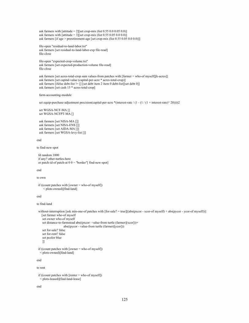
125

ask farmers with [attitude = 2][set crop-mix (list 0.55 0.0 0.05 0.0)] ask farmers with [attitude = 3][set crop-mix (list 0.55 0.05 0.0 0.0)] ask farmers [if age > preretirement-age [set crop-mix (list 0.55 0.05 0.0 0.0)]] file-open "residual-to-land-labor.txt" ask farmers [set residual-to-land-labor-exp file-read] file-close file-open "expected-crop-volume.txt" ask farmers [set expected-production-volume file-read] file-close ask farmers [set acres-total-crop sum values-from patches with [farmer = who-of myself][k-acres]] ask farmers [set capital-value (capital-per-acre * acres-total-crop)] ask farmers [ifelse debt-list != [] [set debt item 2 item 0 debt-list][set debt 0]] ask farmers [set cash 15 * acres-total-crop] farm-accounting-module set equip-purchase-adjustment precision(capital-per-acre *(interest-rate / (1 - (1 / (1 + interest-rate)^ 20))))2 set WGSA-NCF-MA [] set WGSA-NCFPT-MA [] ask farmers [set NISA-MA []] ask farmers [set NISA-ENS []] ask farmers [set AIDA-MA []] ask farmers [set WGSA-levy-list []] end to find-new-spot fd random 1000 if any? other-turtles-here or patch-id-of patch-at 0 0 = "border"[ find-new-spot] end to own if ((count patches with [owner = who-of myself]) < plots-owned)[find-land] end to find-land without-interruption [ask min-one-of patches with [for-sale? = true][(abs(pxcor - xcor-of myself) + abs(pycor - ycor-of myself))] [set farmer who-of myself set owner who-of myself set distance-to-farmstead abs((pxcor - value-from turtle (farmer)[xcor]))+ abs((pycor - value-from turtle (farmer)[ycor])) set for-sale? false set for-rent? false set pcolor blue ]] if ((count patches with [owner = who-of myself]) < plots-owned)[find-land] end to rent if ((count patches with [renter = who-of myself]) < plots-leased)[find-land-lease] end

126

to find-land-lease without-interruption [ask min-one-of patches with [for-rent? = true][(abs(pxcor - xcor-of myself) + abs(pycor - ycor-of myself))] [set farmer who-of myself set renter who-of myself set lease-term random 5 + 1 set lease-payment (initial-lease-rate * quality) set distance-to-farmstead abs((pxcor - value-from turtle (farmer)[xcor]))+ abs((pycor - value-from turtle (farmer)[ycor])) set for-sale? false set for-rent? false set pcolor green ]] if ((count patches with [renter = who-of myself]) < plots-leased)[find-land-lease] end ---------------------------------------------------------------------------------------------------------------------------------------------------------------------------------------------------------------------------------- ASSIGN PARAMETERS ----------------------------------------------------------------------------------------------------------------------------------------------------------------------------------------------------------------------------------- to import-crop-arrays file-open "yield crop 1.txt" set yield-crop-1 file-read file-close file-open "yield crop 2.txt" set yield-crop-2 file-read file-close file-open "yield crop 3.txt" set yield-crop-3 file-read file-close file-open "yield crop 4.txt" set yield-crop-4 file-read file-close import-price-arrays if ASA = true[import-price-support] file-open "crop-1-list.txt" set crop-1-list file-read file-close file-open "crop-2-list.txt" set crop-2-list file-read file-close file-open "crop-3-list.txt" set crop-3-list file-read file-close file-open "crop-4-list.txt" set crop-4-list file-read file-close end

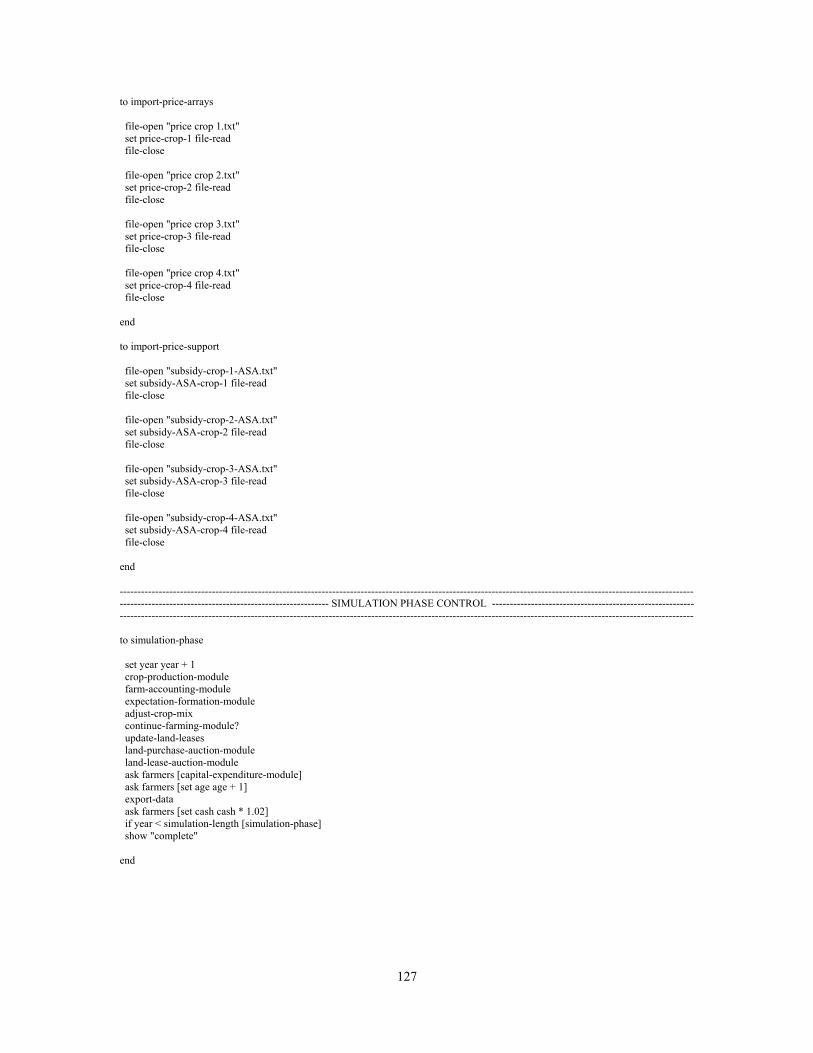
127

to import-price-arrays file-open "price crop 1.txt" set price-crop-1 file-read file-close file-open "price crop 2.txt" set price-crop-2 file-read file-close file-open "price crop 3.txt" set price-crop-3 file-read file-close file-open "price crop 4.txt" set price-crop-4 file-read file-close end to import-price-support file-open "subsidy-crop-1-ASA.txt" set subsidy-ASA-crop-1 file-read file-close file-open "subsidy-crop-2-ASA.txt" set subsidy-ASA-crop-2 file-read file-close file-open "subsidy-crop-3-ASA.txt" set subsidy-ASA-crop-3 file-read file-close file-open "subsidy-crop-4-ASA.txt" set subsidy-ASA-crop-4 file-read file-close end ----------------------------------------------------------------------------------------------------------------------------------------------------------------------------------------------------------------------------- SIMULATION PHASE CONTROL --------------------------------------------------------------------------------------------------------------------------------------------------------------------------------------------------------------------------- to simulation-phase set year year + 1 crop-production-module farm-accounting-module expectation-formation-module adjust-crop-mix continue-farming-module? update-land-leases land-purchase-auction-module land-lease-auction-module ask farmers [capital-expenditure-module] ask farmers [set age age + 1] export-data ask farmers [set cash cash * 1.02] if year < simulation-length [simulation-phase] show "complete" end

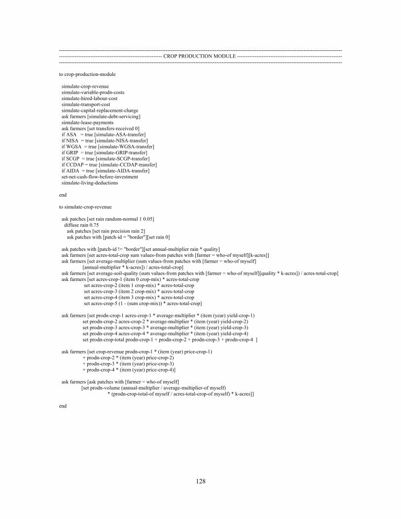
128

----------------------------------------------------------------------------------------------------------------------------------------------------------------------------------------------------------------------------- CROP PRODUCTION MODULE ------------------------------------------------------------------------------------------------------------------------------------------------------------------------------------------------------------------------------ to crop-production-module simulate-crop-revenue simulate-variable-prodn-costs simulate-hired-labour-cost simulate-transport-cost simulate-capital-replacement-charge ask farmers [simulate-debt-servicing] simulate-lease-payments ask farmers [set transfers-received 0] if ASA = true [simulate-ASA-transfer] if NISA = true [simulate-NISA-transfer] if WGSA = true [simulate-WGSA-transfer] if GRIP = true [simulate-GRIP-transfer] if SCGP = true [simulate-SCGP-transfer] if CCDAP = true [simulate-CCDAP-transfer] if AIDA = true [simulate-AIDA-transfer] set-net-cash-flow-before-investment simulate-living-deductions end to simulate-crop-revenue ask patches [set rain random-normal 1 0.05] diffuse rain 0.75 ask patches [set rain precision rain 2] ask patches with [patch-id = "border"][set rain 0] ask patches with [patch-id != "border"][set annual-multiplier rain * quality] ask farmers [set acres-total-crop sum values-from patches with [farmer = who-of myself][k-acres]] ask farmers [set average-multiplier (sum values-from patches with [farmer = who-of myself] [annual-multiplier * k-acres]) / acres-total-crop] ask farmers [set average-soil-quality (sum values-from patches with [farmer = who-of myself][quality * k-acres]) / acres-total-crop] ask farmers [set acres-crop-1 (item 0 crop-mix) * acres-total-crop set acres-crop-2 (item 1 crop-mix) * acres-total-crop set acres-crop-3 (item 2 crop-mix) * acres-total-crop set acres-crop-4 (item 3 crop-mix) * acres-total-crop set acres-crop-5 (1 - (sum crop-mix)) * acres-total-crop] ask farmers [set prodn-crop-1 acres-crop-1 * average-multiplier * (item (year) yield-crop-1) set prodn-crop-2 acres-crop-2 * average-multiplier * (item (year) yield-crop-2) set prodn-crop-3 acres-crop-3 * average-multiplier * (item (year) yield-crop-3) set prodn-crop-4 acres-crop-4 * average-multiplier * (item (year) yield-crop-4) set prodn-crop-total prodn-crop-1 + prodn-crop-2 + prodn-crop-3 + prodn-crop-4 ] ask farmers [set crop-revenue prodn-crop-1 * (item (year) price-crop-1) + prodn-crop-2 * (item (year) price-crop-2) + prodn-crop-3 * (item (year) price-crop-3) + prodn-crop-4 * (item (year) price-crop-4)] ask farmers [ask patches with [farmer = who-of myself] [set prodn-volume (annual-multiplier / average-multiplier-of myself) * (prodn-crop-total-of myself / acres-total-crop-of myself) * k-acres]] end

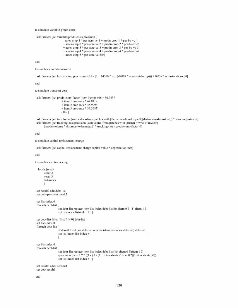
129

to simulate-variable-prodn-costs ask farmers [set variable-prodn-costs precision ( acres-crop-1 * per-acre-vc-1 + prodn-crop-1 * per-bu-vc-1 + acres-crop-2 * per-acre-vc-2 + prodn-crop-2 * per-bu-vc-2 + acres-crop-3 * per-acre-vc-3 + prodn-crop-3 * per-bu-vc-3 + acres-crop-4 * per-acre-vc-4 + prodn-crop-4 * per-bu-vc-4 + acres-crop-5 * per-acre-vc-5)0] end to simulate-hired-labour-cost ask farmers [set hired-labour precision (((0.8 / (1 + 14500 * exp (-0.009 * acres-total-crop))) + 0.03) * acres-total-crop)0] end to simulate-transport-cost ask farmers [set prodn-conv-factor (item 0 crop-mix * 36.7437 + item 1 crop-mix * 64.8418 + item 2 crop-mix * 45.9296 + item 3 crop-mix * 39.3683) / 0.6 ] ask farmers [set travel-cost (sum values-from patches with [farmer = who-of myself][distance-to-farmstead]) * travel-adjustment] ask farmers [set trucking-cost precision (sum values-from patches with [farmer = who-of myself] [prodn-volume * distance-to-farmstead] * trucking-rate / prodn-conv-factor)0] end to simulate-capital-replacement-charge ask farmers [set capital-replacement-charge capital-value * depreciation-rate] end to simulate-debt-servicing locals [result result2 result3 list-index ] set result2 add debt-list set debt-payment result2 set list-index 0 foreach debt-list [ set debt-list replace-item list-index debt-list list (item 0 ? - 1) (item 1 ?) set list-index list-index + 1] set debt-list filter [first ? != 0] debt-list set list-index 0 foreach debt-list [ if item 0 ? = 0 [set debt-list remove (item list-index debt-list) debt-list] set list-index list-index + 1 ] set list-index 0 foreach debt-list [ set debt-list replace-item list-index debt-list (list (item 0 ?)(item 1 ?) (precision (item 1 ? * ((1 - ( 1 / (1 + interest-rate)^ item 0 ?))/ interest-rate))0)) set list-index list-index + 1] set result3 add2 debt-list set debt result3 end

130

----------------------------------------------- ---------- CALCULATORS -------------- ----------------------------------------------- to-report product [lst] locals[result] set result 1 foreach lst [set result result * ?] report result end to-report add [lst] locals [result] set result 0 foreach lst [set result result + item 1 ?] report result end to-report add2 [lst] locals [result] set result 0 foreach lst [set result result + item 2 ?] report result end to simulate-lease-payments ask farmers [set total-lease-payment (sum values-from patches with [farmer = who-of myself][lease-payment * k-acres])] end to set-net-cash-flow-before-investment ask farmers [set NCFBI crop-revenue + transfers-received - NISA-deposit - variable-prodn-costs - hired-labour - travel-cost - trucking-cost - capital-replacement-charge - debt-payment - total-lease-payment] end to simulate-living-deductions ask farmers [set family-withdrawal min-family-withdrawal + 0.068 * crop-revenue + 125 * (plots-owned + plots-leased)] ask farmers [set NCFBI precision (NCFBI - family-withdrawal)0] ask farmers [if (NCFBI < 0 and NISA-withdrawal > 0) [make-NISA-withdrawal]] ask farmers [ifelse (NCFBI < 0) [set years-neg-cash years-neg-cash + 1][set years-neg-cash 0]] ask farmers [set NISA-fund-1 precision (NISA-fund-1 + NISA-deposit)0] ask farmers [set NISA-fund-2 precision (NISA-fund-2 + NISA-deposit)0] ask farmers [set cash precision(cash + NCFBI)0] end

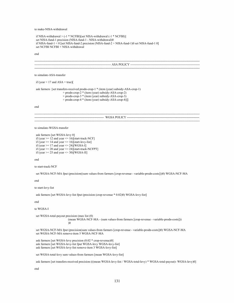
131

to make-NISA-withdrawal if NISA-withdrawal > (-1 * NCFBI)[set NISA-withdrawal (-1 * NCFBI)] set NISA-fund-1 precision (NISA-fund-1 - NISA-withdrawal)0 if NISA-fund-1 < 0 [set NISA-fund-2 precision (NISA-fund-2 + NISA-fund-1)0 set NISA-fund-1 0] set NCFBI NCFBI + NISA-withdrawal end --------------------------------------------------------------------------------------------------------------------------------------------------------------------------------------------------------------------------------------------- ASA POLICY -------------------------------------------------------------------------------------------------------------------------------------------------------------------------------------------------------------------------------------- to simulate-ASA-transfer if (year < 17 and ASA = true)[ ask farmers [set transfers-received prodn-crop-1 * (item (year) subsidy-ASA-crop-1) + prodn-crop-2 * (item (year) subsidy-ASA-crop-2) + prodn-crop-3 * (item (year) subsidy-ASA-crop-3) + prodn-crop-4 * (item (year) subsidy-ASA-crop-4)]] end -------------------------------------------------------------------------------------------------------------------------------------------------------------------------------------------------------------------------------------- WGSA POLICY ----------------------------------------------------------------------------------------------------------------------------------------------------------------------------------------------------------------------------------------- to simulate-WGSA-transfer ask farmers [set WGSA-levy 0] if (year >= 12 and year <= 16)[start-track-NCF] if (year >= 14 and year <= 16)[start-levy-list] if (year >= 17 and year <= 24)[WGSA-I] if (year >= 20 and year <= 24)[start-track-NCFPT] if (year >= 25 and year <= 30)[WGSA-II] end to start-track-NCF set WGSA-NCF-MA fput (precision((sum values-from farmers [crop-revenue - variable-prodn-costs]))0) WGSA-NCF-MA end to start-levy-list ask farmers [set WGSA-levy-list fput (precision (crop-revenue * 0.02)0) WGSA-levy-list] end to WGSA-I set WGSA-total-payout precision (max list (0) (mean WGSA-NCF-MA - (sum values-from farmers [crop-revenue - variable-prodn-costs])) )0 set WGSA-NCF-MA fput (precision(sum values-from farmers [crop-revenue - variable-prodn-costs])0) WGSA-NCF-MA set WGSA-NCF-MA remove-item 5 WGSA-NCF-MA ask farmers [set WGSA-levy precision (0.02 * crop-revenue)0] ask farmers [set WGSA-levy-list fput WGSA-levy WGSA-levy-list] ask farmers [set WGSA-levy-list remove-item 3 WGSA-levy-list] set WGSA-total-levy sum values-from farmers [mean WGSA-levy-list] ask farmers [set transfers-received precision (((mean WGSA-levy-list / WGSA-total-levy) * WGSA-total-payout)- WGSA-levy)0] end

132

to start-track-NCFPT set WGSA-NCFPT-MA fput (precision(sum values-from farmers [(crop-revenue - variable-prodn-costs)] /(sum values-from farmers [prodn-crop-total]))2) WGSA-NCFPT-MA end to WGSA-II set WGSA-total-payout precision (max (list (0) (mean WGSA-NCF-MA - (sum values-from farmers [crop-revenue - variable-prodn-costs])) ((mean WGSA-NCFPT-MA * (sum values-from farmers [prodn-crop-total])) - (sum values-from farmers [crop-revenue - variable-prodn-costs]))) )0 set WGSA-NCF-MA fput (precision(sum values-from farmers [crop-revenue - variable-prodn-costs])0) WGSA-NCF-MA set WGSA-NCF-MA remove-item 5 WGSA-NCF-MA set WGSA-NCFPT-MA fput (precision(sum values-from farmers [(crop-revenue - variable-prodn-costs)] /(sum values-from farmers [prodn-crop-total]))2) WGSA-NCFPT-MA set WGSA-NCFPT-MA remove-item 5 WGSA-NCFPT-MA ask farmers [set WGSA-levy precision (0.02 * crop-revenue)0] ask farmers [set WGSA-levy-list fput WGSA-levy WGSA-levy-list] ask farmers [set WGSA-levy-list remove-item 3 WGSA-levy-list] set WGSA-total-levy sum values-from farmers [mean WGSA-levy-list] ask farmers [set transfers-received precision (((mean WGSA-levy-list / WGSA-total-levy) * WGSA-total-payout)- WGSA-levy)0] end ------------------------------------------------------------------------------------------------------------------------------------------------------------------------------------------------------------------------------------------ GRIP POLICY --------------------------------------------------------------------------------------------------------------------------------------------------------------------------------------------------------------------------------------- to simulate-GRIP-transfer if (year >= 31 and year <= 32)[calculate-GRIP-transfer] end to calculate-GRIP-transfer set-IMAPs if year = 31 [GRIP-transfer-1] if year = 32 [GRIP-transfer-2] end to set-IMAPs set IMAP-1 0 set tracking-number 3 set-IMAP-1 set IMAP-2 0 set tracking-number 3 set-IMAP-2 set IMAP-3 0 set tracking-number 3 set-IMAP-3 set IMAP-4 0 set tracking-number 3 set-IMAP-4 end

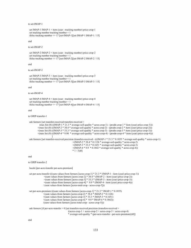
133

to set-IMAP-1 set IMAP-1 IMAP-1 + item (year - tracking-number) price-crop-1 set tracking-number tracking-number + 1 ifelse tracking-number <= 17 [set-IMAP-1][set IMAP-1 IMAP-1 / 15] end to set-IMAP-2 set IMAP-2 IMAP-2 + item (year - tracking-number) price-crop-2 set tracking-number tracking-number + 1 ifelse tracking-number <= 17 [set-IMAP-2][set IMAP-2 IMAP-2 / 15] end to set-IMAP-3 set IMAP-3 IMAP-3 + item (year - tracking-number) price-crop-3 set tracking-number tracking-number + 1 ifelse tracking-number <= 17 [set-IMAP-3][set IMAP-3 IMAP-3 / 15] end to set-IMAP-4 set IMAP-4 IMAP-4 + item (year - tracking-number) price-crop-4 set tracking-number tracking-number + 1 ifelse tracking-number <= 17 [set-IMAP-4][set IMAP-4 IMAP-4 / 15] end to GRIP-transfer-1 ask farmers [set transfers-received transfers-received + (max list (0) ((IMAP-1 * 21.3 * average-soil-quality * acres-crop-1) - (prodn-crop-1 * item (year) price-crop-1))) +(max list (0) ((IMAP-2 * 38.4 * average-soil-quality * acres-crop-2) - (prodn-crop-2 * item (year) price-crop-2))) +(max list (0) ((IMAP-3 * 33.3 * average-soil-quality * acres-crop-3) - (prodn-crop-3 * item (year) price-crop-3))) +(max list (0) ((IMAP-4 * 9.90 * average-soil-quality * acres-crop-4) - (prodn-crop-4 * item (year) price-crop-4))) ] ask farmers [set transfers-received precision (transfers-received - (((IMAP-1 * 21.3 * 0.1855 * average-soil-quality * acres-crop-1) +(IMAP-2 * 38.4 * 0.1126 * average-soil-quality * acres-crop-2) +(IMAP-3 * 33.3 * 0.1651 * average-soil-quality * acres-crop-3) +(IMAP-4 * 9.9 * 0.1842 * average-soil-quality * acres-crop-4)) * 1 / 3))0] end to GRIP-transfer-2 locals [per-acre-transfer per-acre-premium] set per-acre-transfer (((sum values-from farmers [acres-crop-1] * 21.3 * (IMAP-1 - item (year) price-crop-1)) +(sum values-from farmers [acres-crop-2] * 38.4 * (IMAP-2 - item (year) price-crop-2)) +(sum values-from farmers [acres-crop-3] * 33.3 * (IMAP-3 - item (year) price-crop-3)) +(sum values-from farmers [acres-crop-4] * 9.9 * (IMAP-4 - item (year) price-crop-4))) / (sum values-from farmers [acres-total-crop - acres-crop-5])) set per-acre-premium (((sum values-from farmers [acres-crop-1] * 21.3 * IMAP-1 * 0.1855) +(sum values-from farmers [acres-crop-2] * 38.4 * IMAP-2 * 0.1126) +(sum values-from farmers [acres-crop-3] * 33.3 * IMAP-3 * 0.1651) +(sum values-from farmers [acres-crop-4] * 9.9 * IMAP-4 * 0.1842)) /(sum values-from farmers [acres-total-crop - acres-crop-5])) ask farmers [if per-acre-transfer > 0 [set transfers-received precision (transfers-received + ((acres-crop-1 + acres-crop-2 + acres-crop-3 + acres-crop-4) * average-soil-quality * (per-acre-transfer - per-acre-premium)))0]] end

134

--------------------------------------------------------------------------------------------------------------------------------------------------------------------------------------------------------------------------------------- SCGP POLICY ----------------------------------------------------------------------------------------------------------------------------------------------------------------------------------------------------------------------------------------- to simulate-SCGP-transfer ask farmers [set SCGP-transfer 0] if (year = 26)[SCGP-I] if (year = 27)[SCGP-II] end to SCGP-I ask farmers [set SCGP-transfer precision ((acres-crop-1 * 21.3 * 0.11) + (acres-crop-2 * 38.4 * 0.04) + (acres-crop-3 * 33.3 * 0.06) + (acres-crop-4 * 9.90 * 0.11))0] ask farmers [if SCGP-transfer > 5500 [set SCGP-transfer 5500]] ask farmers [set cash precision (cash + SCGP-transfer)0] ask farmers [set transfers-received precision (transfers-received + SCGP-transfer)0] end to SCGP-II SCGP-I end --------------------------------------------------------------------------------------------------------------------------------------------------------------------------------------------------------------------------------------- CCDAP POLICY ---------------------------------------------------------------------------------------------------------------------------------------------------------------------------------------------------------------------------------------- to simulate-CCDAP-transfer if year = 26 [ask farmers [set transfers-received transfers-received + 3.3 * acres-total-crop * 0.6 set cash cash + 3.3 * acres-total-crop * 0.6]] if year = 28 [ask farmers [set transfers-received transfers-received + 8.8 * acres-total-crop * 0.6 set cash cash + 8.8 * acres-total-crop * 0.6]] end --------------------------------------------------------------------------------------------------------------------------------------------------------------------------------------------------------------------------------------- NISA POLICY ------------------------------------------------------------------------------------------------------------------------------------------------------------------------------------------------------------------------------------------- to simulate-NISA-transfer if (year >= 28 and year <= 30)[start-track-NISA] if (year >= 31 and year <= 41)[NISA-transfer] end to start-track-NISA ask farmers [set NISA-MA fput (precision (crop-revenue - variable-prodn-costs)0) NISA-MA] ask farmers [set NISA-ENS fput (precision (crop-revenue)0) NISA-ENS] end to NISA-transfer ask farmers [ifelse (NISA-fund-1 + NISA-fund-2) < ((mean NISA-ENS) * 1.5) [set NISA-deposit 0.03 * crop-revenue][set NISA-deposit 0]] ask farmers [set NISA-fund-1 precision (NISA-fund-1 * (1 + 0.5 * interest-rate + 0.03))0] ask farmers [set NISA-fund-2 precision (NISA-fund-2 * (1 + 0.5 * interest-rate))0] ask farmers [set NISA-withdrawal precision (min list (mean NISA-MA - (crop-revenue - variable-prodn-costs)) (NISA-fund-1 + NISA-fund-2))0]

135

ask farmers [if NISA-withdrawal < 0 [set NISA-withdrawal 0]] ask farmers [set NISA-MA fput (precision(crop-revenue - variable-prodn-costs)0)NISA-MA] ask farmers [set NISA-MA remove-item 3 NISA-MA] ask farmers [set NISA-ENS fput (precision(crop-revenue)0) NISA-ENS] ask farmers [set NISA-ENS remove-item 3 NISA-ENS] end ------------------------------------------------------------------------------------------------------------------------------------------------------------------------------------------------------------------------------------ AIDA POLICY -------------------------------------------------------------------------------------------------------------------------------------------------------------------------------------------------------------------------------------------- to simulate-AIDA-transfer if (year >= 35 and year <= 37)[start-track-AIDA] if (year >= 38 and year <= 40)[AIDA-transfer] end to start-track-AIDA ask farmers [set AIDA-MA fput (precision (crop-revenue - variable-prodn-costs)0) AIDA-MA] end to AIDA-transfer ask farmers [set AIDA-payment (( 0.7 * mean AIDA-MA) - (crop-revenue - variable-prodn-costs))] ask farmers [if AIDA-payment < 0 [set AIDA-payment 0]] ask farmers [set cash cash + AIDA-payment] ask farmers [set transfers-received transfers-received + AIDA-payment] ask farmers [set AIDA-MA fput (precision (crop-revenue - variable-prodn-costs)0) AIDA-MA] ask farmers [set AIDA-MA remove-item 3 AIDA-MA] end ------------------------------------------------------------------------------------------------------------------------------------------------------------------------------------------------------------------------- FARM ACCOUNTING MODULE -------------------------------------------------------------------------------------------------------------------------------------------------------------------------------------------------------------------------------- ;; NOTES i. net cash flow before investment calculated in crop production section ;; ii. debt values updated in crop production section ;; iii. total cultivated acres updated in crop production section ;; iv. capital value updates in capital investment section to farm-accounting-module ask farmers [determine-land-market-value] ask farmers [refinance-loans?] ask farmers [determine-asset-value] ask farmers [determine-equity-value] ask farmers [determine-land-tenure-state] end to determine-land-market-value set land-value precision((sum values-from patches with [owner = who-of myself ][k-acres * quality]) * land-price)0 end to refinance-loans? locals [payment] if debt > (0.75 * (land-value + capital-value)) [set cash cash - (debt - 0.75 * (land-value + capital-value)) set payment precision((0.75 * (land-value + capital-value)) * ((interest-rate) / ( 1 - ( 1 / ((1 + interest-rate)^ 20)))))2 set debt-list []

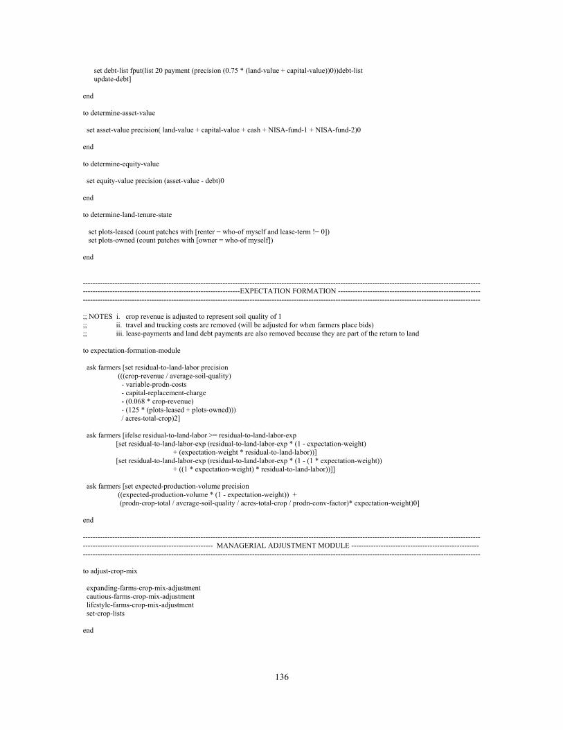
136

set debt-list fput(list 20 payment (precision (0.75 * (land-value + capital-value))0))debt-list update-debt] end to determine-asset-value set asset-value precision( land-value + capital-value + cash + NISA-fund-1 + NISA-fund-2)0 end to determine-equity-value set equity-value precision (asset-value - debt)0 end to determine-land-tenure-state set plots-leased (count patches with [renter = who-of myself and lease-term != 0]) set plots-owned (count patches with [owner = who-of myself]) end ----------------------------------------------------------------------------------------------------------------------------------------------------------------------------------------------------------------------------------EXPECTATION FORMATION ---------------------------------------------------------------------------------------------------------------------------------------------------------------------------------------------------------------------------- ;; NOTES i. crop revenue is adjusted to represent soil quality of 1 ;; ii. travel and trucking costs are removed (will be adjusted for when farmers place bids) ;; iii. lease-payments and land debt payments are also removed because they are part of the return to land to expectation-formation-module ask farmers [set residual-to-land-labor precision (((crop-revenue / average-soil-quality) - variable-prodn-costs - capital-replacement-charge - (0.068 * crop-revenue) - (125 * (plots-leased + plots-owned))) / acres-total-crop)2] ask farmers [ifelse residual-to-land-labor >= residual-to-land-labor-exp [set residual-to-land-labor-exp (residual-to-land-labor-exp * (1 - expectation-weight) + (expectation-weight * residual-to-land-labor))] [set residual-to-land-labor-exp (residual-to-land-labor-exp * (1 - (1 * expectation-weight)) + ((1 * expectation-weight) * residual-to-land-labor))]] ask farmers [set expected-production-volume precision ((expected-production-volume * (1 - expectation-weight)) + (prodn-crop-total / average-soil-quality / acres-total-crop / prodn-conv-factor)* expectation-weight)0] end ----------------------------------------------------------------------------------------------------------------------------------------------------------------------------------------------------------------------- MANAGERIAL ADJUSTMENT MODULE ---------------------------------------------------------------------------------------------------------------------------------------------------------------------------------------------------------------------- to adjust-crop-mix expanding-farms-crop-mix-adjustment cautious-farms-crop-mix-adjustment lifestyle-farms-crop-mix-adjustment set-crop-lists end

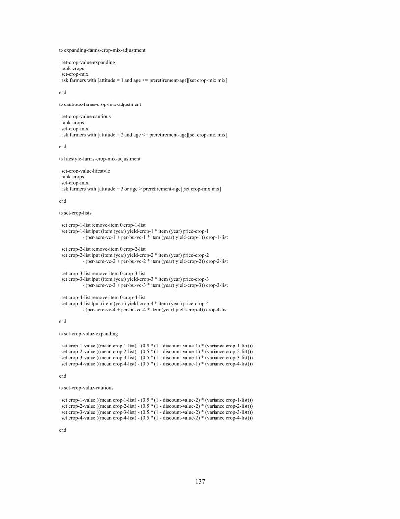
137

to expanding-farms-crop-mix-adjustment set-crop-value-expanding rank-crops set-crop-mix ask farmers with [attitude = 1 and age <= preretirement-age][set crop-mix mix] end to cautious-farms-crop-mix-adjustment set-crop-value-cautious rank-crops set-crop-mix ask farmers with [attitude = 2 and age <= preretirement-age][set crop-mix mix] end to lifestyle-farms-crop-mix-adjustment set-crop-value-lifestyle rank-crops set-crop-mix ask farmers with [attitude = 3 or age > preretirement-age][set crop-mix mix] end to set-crop-lists set crop-1-list remove-item 0 crop-1-list set crop-1-list lput (item (year) yield-crop-1 * item (year) price-crop-1 - (per-acre-vc-1 + per-bu-vc-1 * item (year) yield-crop-1)) crop-1-list set crop-2-list remove-item 0 crop-2-list set crop-2-list lput (item (year) yield-crop-2 * item (year) price-crop-2 - (per-acre-vc-2 + per-bu-vc-2 * item (year) yield-crop-2)) crop-2-list set crop-3-list remove-item 0 crop-3-list set crop-3-list lput (item (year) yield-crop-3 * item (year) price-crop-3 - (per-acre-vc-3 + per-bu-vc-3 * item (year) yield-crop-3)) crop-3-list set crop-4-list remove-item 0 crop-4-list set crop-4-list lput (item (year) yield-crop-4 * item (year) price-crop-4 - (per-acre-vc-4 + per-bu-vc-4 * item (year) yield-crop-4)) crop-4-list end to set-crop-value-expanding set crop-1-value ((mean crop-1-list) - (0.5 * (1 - discount-value-1) * (variance crop-1-list))) set crop-2-value ((mean crop-2-list) - (0.5 * (1 - discount-value-1) * (variance crop-2-list))) set crop-3-value ((mean crop-3-list) - (0.5 * (1 - discount-value-1) * (variance crop-3-list))) set crop-4-value ((mean crop-4-list) - (0.5 * (1 - discount-value-1) * (variance crop-4-list))) end to set-crop-value-cautious set crop-1-value ((mean crop-1-list) - (0.5 * (1 - discount-value-2) * (variance crop-1-list))) set crop-2-value ((mean crop-2-list) - (0.5 * (1 - discount-value-2) * (variance crop-2-list))) set crop-3-value ((mean crop-3-list) - (0.5 * (1 - discount-value-2) * (variance crop-3-list))) set crop-4-value ((mean crop-4-list) - (0.5 * (1 - discount-value-2) * (variance crop-4-list))) end

138

to set-crop-value-lifestyle set crop-1-value ((mean crop-1-list) - (0.5 * (1 - discount-value-3) * (variance crop-1-list))) set crop-2-value ((mean crop-2-list) - (0.5 * (1 - discount-value-3) * (variance crop-2-list))) set crop-3-value ((mean crop-3-list) - (0.5 * (1 - discount-value-3) * (variance crop-3-list))) set crop-4-value ((mean crop-4-list) - (0.5 * (1 - discount-value-3) * (variance crop-4-list))) end to rank-crops set crop-1-rank 4 set crop-2-rank 4 set crop-3-rank 4 set crop-4-rank 4 if crop-1-value > crop-2-value [set crop-1-rank crop-1-rank - 1] if crop-1-value > crop-3-value [set crop-1-rank crop-1-rank - 1] if crop-1-value > crop-4-value [set crop-1-rank crop-1-rank - 1] if crop-2-value > crop-1-value [set crop-2-rank crop-2-rank - 1] if crop-2-value > crop-3-value [set crop-2-rank crop-2-rank - 1] if crop-2-value > crop-4-value [set crop-2-rank crop-2-rank - 1] if crop-3-value > crop-1-value [set crop-3-rank crop-3-rank - 1] if crop-3-value > crop-2-value [set crop-3-rank crop-3-rank - 1] if crop-3-value > crop-4-value [set crop-3-rank crop-3-rank - 1] if crop-4-value > crop-1-value [set crop-4-rank crop-4-rank - 1] if crop-4-value > crop-2-value [set crop-4-rank crop-4-rank - 1] if crop-4-value > crop-3-value [set crop-4-rank crop-4-rank - 1] end to set-crop-mix locals [list-acres max-acres] set mix [0 0 0 0] if crop-1-rank = 1 [set mix replace-item 0 mix 0.55] if crop-2-rank = 1 [set mix replace-item 1 mix 0.10] if crop-3-rank = 1 [set mix replace-item 2 mix 0.10] if crop-4-rank = 1 [set mix replace-item 3 mix 0.05] if crop-1-rank = 2 [set list-acres [0.55 0] set list-acres replace-item 1 list-acres (precision (0.6 - (sum mix))2) set mix replace-item 0 mix (min list-acres)] if crop-2-rank = 2 [set list-acres [0.10 0] set list-acres replace-item 1 list-acres (precision(0.6 - (sum mix))2) set mix replace-item 1 mix (min list-acres)] if crop-3-rank = 2 [set list-acres [0.10 0] set list-acres replace-item 1 list-acres (precision(0.6 - (sum mix))2) set mix replace-item 2 mix (min list-acres)] if crop-4-rank = 2 [set list-acres [0.05 0] set list-acres replace-item 1 list-acres (precision(0.6 - (sum mix))2) set mix replace-item 3 mix (min list-acres)] if crop-1-rank = 3 [set list-acres [0.55 0] set list-acres replace-item 1 list-acres (precision (0.6 - (sum mix))2) set mix replace-item 0 mix (min list-acres)] if crop-2-rank = 3 [set list-acres [0.10 0] set list-acres replace-item 1 list-acres (precision(0.6 - (sum mix))2) set mix replace-item 1 mix (min list-acres)]

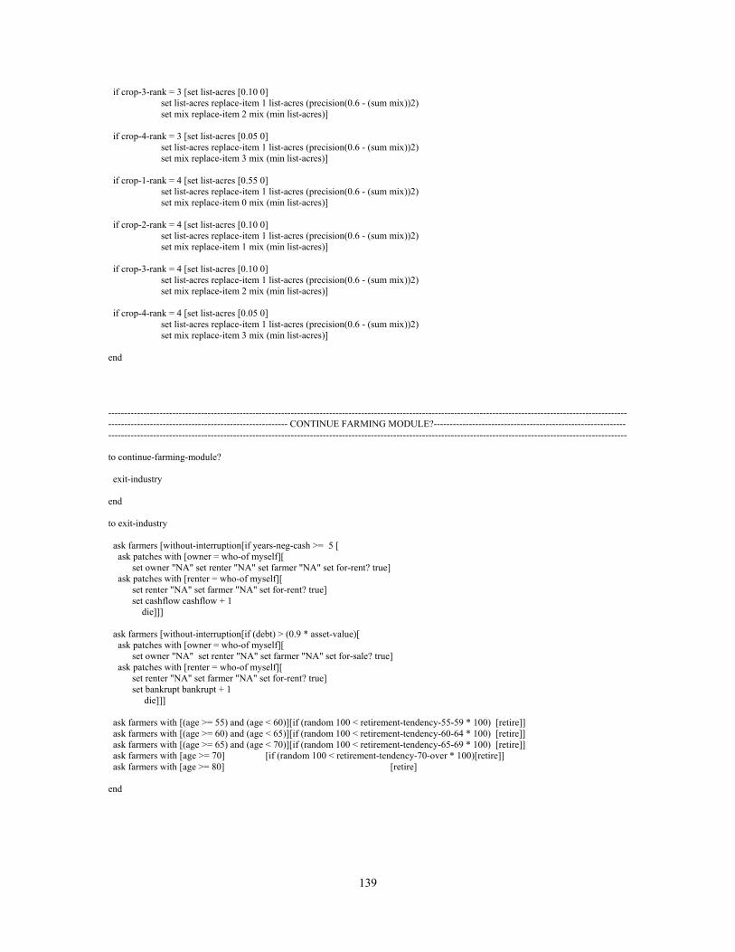
139

if crop-3-rank = 3 [set list-acres [0.10 0] set list-acres replace-item 1 list-acres (precision(0.6 - (sum mix))2) set mix replace-item 2 mix (min list-acres)] if crop-4-rank = 3 [set list-acres [0.05 0] set list-acres replace-item 1 list-acres (precision(0.6 - (sum mix))2) set mix replace-item 3 mix (min list-acres)] if crop-1-rank = 4 [set list-acres [0.55 0] set list-acres replace-item 1 list-acres (precision(0.6 - (sum mix))2) set mix replace-item 0 mix (min list-acres)] if crop-2-rank = 4 [set list-acres [0.10 0] set list-acres replace-item 1 list-acres (precision(0.6 - (sum mix))2) set mix replace-item 1 mix (min list-acres)] if crop-3-rank = 4 [set list-acres [0.10 0] set list-acres replace-item 1 list-acres (precision(0.6 - (sum mix))2) set mix replace-item 2 mix (min list-acres)] if crop-4-rank = 4 [set list-acres [0.05 0] set list-acres replace-item 1 list-acres (precision(0.6 - (sum mix))2) set mix replace-item 3 mix (min list-acres)] end -------------------------------------------------------------------------------------------------------------------------------------------------------------------------------------------------------------------------- CONTINUE FARMING MODULE?------------------------------------------------------------------------------------------------------------------------------------------------------------------------------------------------------------------------------ to continue-farming-module? exit-industry end to exit-industry ask farmers [without-interruption[if years-neg-cash >= 5 [ ask patches with [owner = who-of myself][ set owner "NA" set renter "NA" set farmer "NA" set for-rent? true] ask patches with [renter = who-of myself][ set renter "NA" set farmer "NA" set for-rent? true] set cashflow cashflow + 1 die]]] ask farmers [without-interruption[if (debt) > (0.9 * asset-value)[ ask patches with [owner = who-of myself][ set owner "NA" set renter "NA" set farmer "NA" set for-sale? true] ask patches with [renter = who-of myself][ set renter "NA" set farmer "NA" set for-rent? true] set bankrupt bankrupt + 1 die]]] ask farmers with [(age >= 55) and (age < 60)][if (random 100 < retirement-tendency-55-59 * 100) [retire]] ask farmers with [(age >= 60) and (age < 65)][if (random 100 < retirement-tendency-60-64 * 100) [retire]] ask farmers with [(age >= 65) and (age < 70)][if (random 100 < retirement-tendency-65-69 * 100) [retire]] ask farmers with [age >= 70] [if (random 100 < retirement-tendency-70-over * 100)[retire]] ask farmers with [age >= 80] [retire] end

140

to retire locals [payment] ifelse (equity-value / asset-value > 0.6) [set age age - 30 set transfers transfers + 1 set preretirement-age 55 set generation generation + 1 set payment precision((transfer-sell-rate * equity-value) * ((interest-rate) / ( 1 - ( 1 / ((1 + interest-rate)^ 20)))))2 set debt-list fput (list 20 payment (precision (transfer-sell-rate * equity-value)0)) debt-list update-debt determine-asset-value determine-equity-value] [ask patches with [owner = who-of myself] [set owner "NA" set renter "NA" set farmer "NA" set for-rent? true] ask patches with [renter = who-of myself] [set renter "NA" set farmer "NA" set for-rent? true] set oldage oldage + 1 die] end to update-debt locals [result result2 result3 list-index ] set result2 add debt-list set debt-payment result2 set list-index 0 foreach debt-list [ set debt-list replace-item list-index debt-list (list (item 0 ?)(item 1 ?) (precision (item 1 ? * ((1 - ( 1 / (1 + interest-rate)^ item 0 ?))/ interest-rate))0)) set list-index list-index + 1] set result3 add2 debt-list set debt result3 end -------------------------------------------------------------------------------------------------------------------------------------------------------------------------------------------------------------------------------- RE-NEW LAND LEASE MODULE ------------------------------------------------------------------------------------------------------------------------------------------------------------------------------------------------------------------------ to update-land-leases ask patches with [lease-term != 0 and patch-id != "border"][set lease-term lease-term - 1] ask patches with [lease-term = 0 and renter != "NA" and patch-id != "border"][set for-sale? true] ask farmers [set current-plot-bid-on "NA"] ask farmers [without-interruption [ ifelse (((cash > 10 * acres-total-crop + 150 * land-price * downpayment)) and ((debt / asset-value) < D-A-ratio) and ((lease-payment + debt-payment + min-family-withdrawal) < (residual-to-land-labor-exp * acres-total-crop)) and (age <= preretirement-age) ) [select-land] [set current-bid 0]]] set mean-bid (mean values-from farmers with [current-plot-bid-on != "NA"] [current-bid]) ask farmers with [current-plot-bid-on != "NA"] [set current-bid precision(((current-bid * mean-bid)^ 0.5) * (value-from (random-one-of patches with [patch-id = current-plot-bid-on-of myself])[quality]))2] ask farmers [set acres-total-crop acres-total-crop - 150]

141

ask patches with [lease-term = 0 and renter != "NA" and patch-id != "border"][without-interruption [ask turtle (farmer) [set current-plot-bid-on (patch-id-of myself) set-bid-rent set current-bid precision((current-bid * (mean-bid / (((1 - (1 / (1 + interest-rate))^ 20)) / interest-rate)))^ 0.5 * (value-from (random-one-of patches with [patch-id = current-plot-bid-on-of myself])[quality]))2 ifelse (current-bid / interest-rate) >= ((((mean-bid * land-price)^ 0.5) * quality) / landlord-discount) [set lease-term-of myself 5 set lease-payment-of myself current-bid set for-sale?-of myself false] [set renter-of myself "NA" set farmer-of myself "NA"]]]] ask farmers [set acres-total-crop sum values-from patches with [farmer = who-of myself][k-acres] set plots-leased count patches with [renter = who-of myself]] ask farmers [capital-expenditure-module] set average-rent mean values-from patches with [renter != "NA" and patch-id != "border"][lease-payment * quality] end -------------------------------------------------------------------------------------------------------------------------------------------------------------------------------------------------------------------------- LAND PURCHASE AUCTION MODULE ---------------------------------------------------------------------------------------------------------------------------------------------------------------------------------------------------------------------- to land-purchase-auction-module set bids [] check-if-land-available-for-sale ifelse (bids != []) [set land-price mean bids] [set land-price (average-rent * (((1 - (1 / (1 + interest-rate))^ 20)) / interest-rate))] end to check-if-land-available-for-sale ask farmers [set current-plot-bid-on "NA"] if (count patches with [for-sale? = true]) > 0 [screen-farmers] end to screen-farmers ask farmers [without-interruption [ ifelse ((cash > (10 * acres-total-crop + 150 * land-price * downpayment)) and ((debt / asset-value) < D-A-ratio) and ((lease-payment + debt-payment + min-family-withdrawal) < (residual-to-land-labor-exp * acres-total-crop)) and (age <= preretirement-age) ) [select-land] [set current-bid 0]]] set mean-bid (mean values-from farmers with [current-plot-bid-on != "NA"][current-bid]) ask farmers with [current-plot-bid-on != "NA"] [set current-bid precision((current-bid * (mean-bid)) ^ 0.5 * (value-from (random-one-of patches with [patch-id = current-plot-bid-on-of myself])[quality]))0] if (count farmers with [current-bid > 0] > 0)[auction-land] end

142

to select-land set current-plot-bid-on value-from (max-one-of patches with [for-sale? = true] [((abs(pxcor - xcor-of myself) + abs(pycor - ycor-of myself)) * -1 *((trucking-rate * expected-production-volume-of myself) + travel-adjustment / k-acres)) + residual-to-land-labor-exp-of myself * quality]) [patch-id] set-bid end to set-bid locals [expected-value-plot] set expected-value-plot ((abs((value-from random-one-of patches with [patch-id = current-plot-bid-on-of myself][pxcor]) - xcor)) + (abs((value-from random-one-of patches with [patch-id = current-plot-bid-on-of myself][pycor]) - ycor))) * ((trucking-rate * expected-production-volume) + (travel-adjustment / (value-from random-one-of patches with [patch-id = current-plot-bid-on-of myself][k-acres]))) * -1 + value-from (random-one-of patches with [patch-id = current-plot-bid-on-of myself])[quality] * residual-to-land-labor-exp if attitude = 1 [set current-bid precision (((expected-value-plot - equip-purchase-adjustment - (min-family-withdrawal / (acres-total-crop + 150)) - ((0.8 / (1 + 14500 * exp (-0.009 * (acres-total-crop + 150)))) + 0.03)) * (discount-value-1 )) * (((1 - (1 / (1 + interest-rate))^ 20)) / interest-rate)) 2] if attitude = 2 [set current-bid precision (((expected-value-plot - equip-purchase-adjustment - (min-family-withdrawal / (acres-total-crop + 150)) - ((0.8 / (1 + 14500 * exp (-0.009 * (acres-total-crop + 150)))) + 0.03)) * (discount-value-2 )) * (((1 - (1 / (1 + interest-rate))^ 20)) / interest-rate)) 2] if attitude = 3 [set current-bid precision (((expected-value-plot - equip-purchase-adjustment - (min-family-withdrawal / (acres-total-crop + 150)) - ((0.8 / (1 + 14500 * exp (-0.009 * (acres-total-crop + 150)))) + 0.03)) * (discount-value-3 )) * (((1 - (1 / (1 + interest-rate))^ 20)) / interest-rate)) 2] if current-bid < 0 [set current-bid 0] end to auction-land locals [payment total-bid adjusted-bid counter] ask max-one-of farmers [current-bid][ set adjusted-bid (current-bid / value-from (random-one-of patches with [patch-id = current-plot-bid-on-of myself])[quality]) if adjusted-bid >= ((landlord-discount) * (mean-bid * (average-rent / interest-rate))^ 0.5)[ set owner-of(random-one-of patches with [patch-id = current-plot-bid-on-of myself]) who set farmer-of(random-one-of patches with [patch-id = current-plot-bid-on-of myself]) who set renter-of(random-one-of patches with [patch-id = current-plot-bid-on-of myself]) "NA" set total-bid (current-bid * k-acres-of (random-one-of patches with [patch-id = current-plot-bid-on-of myself])) set land-unit-sold current-plot-bid-on set payment precision(((1 - downpayment) * total-bid)* (interest-rate / (1 - (1 / (1 + interest-rate)^ 20))))0 set cash precision(cash - (downpayment * total-bid))0 set debt-list fput (list 20 payment (precision (0.75 * total-bid)0)) debt-list set for-sale?-of (random-one-of patches with [patch-id = current-plot-bid-on-of myself])false set for-rent?-of (random-one-of patches with [patch-id = current-plot-bid-on-of myself])false set pcolor-of (random-one-of patches with [patch-id = current-plot-bid-on-of myself])blue set debt precision (debt + (0.75 * total-bid))0 set debt-payment precision(debt-payment + payment)0 set plots-owned plots-owned + 1 set acres-total-crop acres-total-crop + value-from random-one-of patches with [patch-id = current-plot-bid-on-of myself][k-acres] set distance-to-farmstead-of(random-one-of patches with [patch-id = current-plot-bid-on-of myself]) abs((xcor - value-from random-one-of patches with[patch-id = current-plot-bid-on-of myself][pxcor]))+

143

abs((ycor - value-from random-one-of patches with[patch-id = current-plot-bid-on-of myself][pycor])) set land-value land-value + total-bid set sold sold + 1 capital-expenditure-module determine-asset-value determine-equity-value set bids lput adjusted-bid bids ]] ifelse adjusted-bid >= ((landlord-discount) * (mean-bid * (average-rent / interest-rate))^ 0.5) [check-if-more-land-available-for-sale] [set bids lput ((landlord-discount) * (mean-bid * (average-rent / interest-rate))^ 0.5) bids] end to check-if-more-land-available-for-sale if (count patches with [for-sale? = true]) > 0 [screen-farmers-bidding-on-sold-land] end to screen-farmers-bidding-on-sold-land ask farmers with [current-plot-bid-on = land-unit-sold][without-interruption [ifelse ( ((cash > 10 * acres-total-crop + 150 * land-price * downpayment)) and ((debt / asset-value) < D-A-ratio) and ((lease-payment + debt-payment + min-family-withdrawal) < (residual-to-land-labor-exp * acres-total-crop)) and (age <= preretirement-age) ) [select-land] [set current-bid 0]]] ask farmers with [current-plot-bid-on = land-unit-sold] [set current-bid precision((current-bid * (mean-bid))^ 0.5 * (value-from (random-one-of patches with [patch-id = current-plot-bid-on-of myself])[quality]))0] if (count farmers with [current-bid > 0] > 0)[auction-land] end --------------------------------------------------------------------------------------------------------------------------------------------------------------------------------------------------------------------------- LAND LEASE AUCTION MODULE --------------------------------------------------------------------------------------------------------------------------------------------------------------------------------------------------------------------------- to land-lease-auction-module check-if-land-available-for-rent end to check-if-land-available-for-rent ask patches [if for-sale? = true [set for-rent? true]] ask farmers [set current-plot-bid-on "NA"] set units-for-sale (count patches with [for-rent? = true]) if (count patches with [for-rent? = true]) > 0 [screen-farmers-rent] end to screen-farmers-rent ask farmers [without-interruption [ifelse ((cash > 10 * acres-total-crop) and (residual-to-land-labor-exp > 0) and (age <= preretirement-age) ) [select-land-rent] [set current-bid 0]]] set mean-bid (mean values-from farmers with [current-plot-bid-on != "NA"] [current-bid])

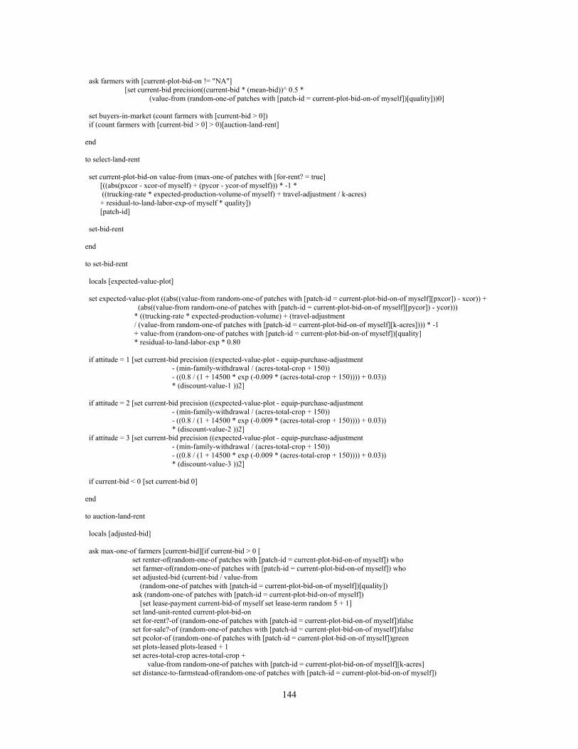
144

ask farmers with [current-plot-bid-on != "NA"] [set current-bid precision((current-bid * (mean-bid))^ 0.5 * (value-from (random-one-of patches with [patch-id = current-plot-bid-on-of myself])[quality]))0] set buyers-in-market (count farmers with [current-bid > 0]) if (count farmers with [current-bid > 0] > 0)[auction-land-rent] end to select-land-rent set current-plot-bid-on value-from (max-one-of patches with [for-rent? = true] [((abs(pxcor - xcor-of myself) + (pycor - ycor-of myself))) * -1 * ((trucking-rate * expected-production-volume-of myself) + travel-adjustment / k-acres) + residual-to-land-labor-exp-of myself * quality]) [patch-id] set-bid-rent end to set-bid-rent locals [expected-value-plot] set expected-value-plot ((abs((value-from random-one-of patches with [patch-id = current-plot-bid-on-of myself][pxcor]) - xcor)) + (abs((value-from random-one-of patches with [patch-id = current-plot-bid-on-of myself][pycor]) - ycor))) * ((trucking-rate * expected-production-volume) + (travel-adjustment / (value-from random-one-of patches with [patch-id = current-plot-bid-on-of myself][k-acres]))) * -1 + value-from (random-one-of patches with [patch-id = current-plot-bid-on-of myself])[quality] * residual-to-land-labor-exp * 0.80 if attitude = 1 [set current-bid precision ((expected-value-plot - equip-purchase-adjustment - (min-family-withdrawal / (acres-total-crop + 150)) - ((0.8 / (1 + 14500 * exp (-0.009 * (acres-total-crop + 150)))) + 0.03)) * (discount-value-1 ))2] if attitude = 2 [set current-bid precision ((expected-value-plot - equip-purchase-adjustment - (min-family-withdrawal / (acres-total-crop + 150)) - ((0.8 / (1 + 14500 * exp (-0.009 * (acres-total-crop + 150)))) + 0.03)) * (discount-value-2 ))2] if attitude = 3 [set current-bid precision ((expected-value-plot - equip-purchase-adjustment - (min-family-withdrawal / (acres-total-crop + 150)) - ((0.8 / (1 + 14500 * exp (-0.009 * (acres-total-crop + 150)))) + 0.03)) * (discount-value-3 ))2] if current-bid < 0 [set current-bid 0] end to auction-land-rent locals [adjusted-bid] ask max-one-of farmers [current-bid][if current-bid > 0 [ set renter-of(random-one-of patches with [patch-id = current-plot-bid-on-of myself]) who set farmer-of(random-one-of patches with [patch-id = current-plot-bid-on-of myself]) who set adjusted-bid (current-bid / value-from (random-one-of patches with [patch-id = current-plot-bid-on-of myself])[quality]) ask (random-one-of patches with [patch-id = current-plot-bid-on-of myself]) [set lease-payment current-bid-of myself set lease-term random 5 + 1] set land-unit-rented current-plot-bid-on set for-rent?-of (random-one-of patches with [patch-id = current-plot-bid-on-of myself])false set for-sale?-of (random-one-of patches with [patch-id = current-plot-bid-on-of myself])false set pcolor-of (random-one-of patches with [patch-id = current-plot-bid-on-of myself])green set plots-leased plots-leased + 1 set acres-total-crop acres-total-crop + value-from random-one-of patches with [patch-id = current-plot-bid-on-of myself][k-acres] set distance-to-farmstead-of(random-one-of patches with [patch-id = current-plot-bid-on-of myself])

145

abs((xcor - value-from random-one-of patches with[patch-id = current-plot-bid-on-of myself][pxcor]))+ abs((ycor - value-from random-one-of patches with[patch-id = current-plot-bid-on-of myself][pycor])) set total-lease-payment total-lease-payment + current-bid * k-acres-of (random-one-of patches with [patch-id = current-plot-bid-on-of myself]) capital-expenditure-module determine-asset-value determine-equity-value ]] if adjusted-bid > 0 [check-if-more-land-available-for-rent] end to check-if-more-land-available-for-rent if (count patches with [for-rent? = true]) > 0 [screen-farmers-bidding-on-rented-land] end to screen-farmers-bidding-on-rented-land ask farmers with [current-plot-bid-on = land-unit-rented][without-interruption [ifelse ( (cash > 10 * acres-total-crop) and (residual-to-land-labor-exp > 0) and (age <= preretirement-age) ) [select-land-rent] [set current-bid 0]]] ask farmers with [current-plot-bid-on = land-unit-rented] [set current-bid precision((current-bid * (mean-bid))^ 0.5 * (value-from (random-one-of patches with [patch-id = current-plot-bid-on-of myself])[quality]))0] if (count farmers with [current-bid > 0] > 0)[auction-land-rent] set average-rent mean values-from patches with [renter != "NA" and patch-id != "border"][lease-payment * quality] end ------------------------------------------------------------------------------------------------------------------------------------------------------------------------------------------------------------------------------ CAPITAL INVESTMENT MODULE ------------------------------------------------------------------------------------------------------------------------------------------------------------------------------------------------------------------------ to capital-expenditure-module locals [payment capital-purchase] set capital-purchase ((acres-total-crop * capital-per-acre) - capital-value) ifelse capital-purchase > 0 [set payment precision(((1 - downpayment) * capital-purchase) * (interest-rate / (1 - (1 / (1 + interest-rate) ^ 5))))0 set cash precision(cash - (downpayment * capital-purchase))0 set debt-list fput (list 5 payment (precision (0.75 * capital-purchase)0)) debt-list set debt precision (debt + (0.75 * capital-purchase))0 set debt-payment precision(debt-payment + payment)0 ] [set cash precision(cash - capital-purchase)0] set capital-value (acres-total-crop * capital-per-acre) end

146

------------------------------------------------------------------------------------------------------------------------------------------------------------------------------------------------------------------------------- UPDATE DATA AND PARAMETERS -------------------------------------------------------------------------------------------------------------------------------------------------------------------------------------------------------------------- to export-data let plots-total count patches with [patch-id != "border"] set plots-not-in-crop-prodn-percent ((count patches with [patch-id != "border" and farmer = "NA"]) / (plots-total) * 100) set plots-leased-percent ((count patches with [patch-id != "border" and renter != "NA"]) / (plots-total) * 100) set farms (count farmers) file-open "farms.txt" file-print farms file-close file-open "debt.txt" file-print (mean values-from farmers [debt]) file-close file-open "debt per acre.txt" file-print (mean values-from farmers [debt / acres-total-crop]) file-close file-open "mean size.txt" file-print (mean values-from farmers [acres-total-crop]) file-close file-open "leased.txt" file-print plots-leased-percent file-close file-open "unmanaged.txt" file-print plots-not-in-crop-prodn-percent file-close file-open "land price.txt" file-print land-price file-close file-open "lease rate.txt" file-print average-rent file-close file-open "returns.txt" file-print (mean values-from farmers [residual-to-land-labor]) file-close file-open "transfers.txt" file-print sum values-from farmers [transfers-received + NISA-deposit] file-close file-open "age.txt" file-print mean values-from farmers [age] file-close file-open "attitude-1.txt" file-print count farmers with [attitude = 1] file-close file-open "attitude-2.txt" file-print count farmers with [attitude = 2] file-close file-open "attitude-3.txt" file-print count farmers with [attitude = 3] file-close file-open "land-attitude-1.txt" file-print sum values-from farmers with [attitude = 1][acres-total-crop] file-close file-open "land-attitude-2.txt" file-print sum values-from farmers with [attitude = 2][acres-total-crop] file-close file-open "land-attitude-3.txt" file-print sum values-from farmers with [attitude = 3][acres-total-crop] file-close file-open "mean-size-attitude-1.txt" file-print mean values-from farmers with [attitude = 1][acres-total-crop] file-close file-open "mean-size-attitude-2.txt" file-print mean values-from farmers with [attitude = 2][acres-total-crop] file-close file-open "mean-size-attitude-3.txt" file-print mean values-from farmers with [attitude = 3][acres-total-crop]

147

file-close file-open "mean-equity-attitude-1.txt" file-print mean values-from farmers with [attitude = 1][equity-value] file-close file-open "mean-equity-attitude-2.txt" file-print mean values-from farmers with [attitude = 2][equity-value] file-close file-open "mean-equity-attitude-3.txt" file-print mean values-from farmers with [attitude = 3][equity-value] file-close file-open "mean-equity.txt" file-print mean values-from farmers [equity-value] file-close file-open "acres-wheat.txt" file-print sum values-from farmers [acres-crop-1] file-close file-open "acres-oats.txt" file-print sum values-from farmers [acres-crop-2] file-close file-open "acres-barley.txt" file-print sum values-from farmers [acres-crop-3] file-close file-open "acres-flaxseed.txt" file-print sum values-from farmers [acres-crop-4] file-close export-size-distn end to export-size-distn file-open "size-1.txt" file-print (count farmers with [acres-total-crop < 400 ]) file-close file-open "size-2.txt" file-print (count farmers with [acres-total-crop >= 400 and acres-total-crop < 560 ]) file-close file-open "size-3.txt" file-print (count farmers with [acres-total-crop >= 560 and acres-total-crop < 760 ]) file-close file-open "size-4.txt" file-print (count farmers with [acres-total-crop >= 760 and acres-total-crop < 1120]) file-close file-open "size-5.txt" file-print (count farmers with [acres-total-crop >= 1120 and acres-total-crop < 1600]) file-close file-open "size-6.txt" file-print (count farmers with [acres-total-crop >= 1600 and acres-total-crop < 2240]) file-close file-open "size-7.txt" file-print (count farmers with [acres-total-crop >= 2240 and acres-total-crop < 2880]) file-close file-open "size-8.txt" file-print (count farmers with [acres-total-crop >= 2880]) file-close end