FRIST - Flipping and Rotation Invariant Sparsifying...
24
FRIST - Flipping and Rotation Invariant Sparsifying Transform Learning and Applications of Inverse Problems Bihan Wen 1 , Saiprasad Ravishankar 2 , and Yoram Bresler 1 1 Department of Electrical and Computer Engineering and the Coordinated Science Laboratory, University of Illinois at Urbana-Champaign, Champaign, IL 61801, USA. 2 Department of Electrical Engineering and Computer Science University of Michigan, Ann Arbor, MI 48109, USA. E-mail: [email protected], [email protected], and [email protected] January 2016 Abstract. Features based on sparse representation, especially using synthesis dictionary model, have been heavily exploited in signal processing and computer vision. However, synthesis dictionary learning involves NP-hard sparse coding and expensive learning steps. Recently, sparsifying transform learning received interest for its cheap computation and closed-form solution. In this work, we develop a methodology for learning of Flipping and Rotation Invariant Sparsifying Transform, dubbed FRIST, to better represent natural images that contain textures with various geometrical directions. The proposed alternating learning algorithm involves simple closed- form solutions. We provide the convergence guarantee, and demonstrate empirical convergence behavior of the proposed FRIST learning algorithm. Preliminary experiments show the usefulness of adaptive sparse representation by FRIST for image sparse representation, segmentation, denoising, robust inpainting, and MRI reconstruction with promising performances. Keywords: Sparsifying transform learning, Dictionary learning, Convergence guarantee, Overcomplete representation, Machine learning, Clustering, Image representation, Inverse problem, Image denoising, Inpainting, Magnetic resonance imaging. 1. Introduction Sparse representation of natural signals in certain transform domain or dictionary has been widely exploited. Various sparse models, such as the synthesis model [1, 2] and the transform model [3], have been studied. The popular synthesis model suggests that a signal y ∈ R n can be sparsely represented as y = Dx + η, where D ∈ R n×m is synthesis dictionary, the x ∈ R m is sparse code, and η is small approximation error in the signal domain. Synthesis dictionary learning methods [4, 5] typically involve
Transcript of FRIST - Flipping and Rotation Invariant Sparsifying...

FRIST - Flipping and Rotation Invariant
Sparsifying Transform Learning and Applications of
Inverse Problems
Bihan Wen1, Saiprasad Ravishankar 2, and Yoram Bresler1
1 Department of Electrical and Computer Engineering and the Coordinated Science
Laboratory, University of Illinois at Urbana-Champaign, Champaign, IL 61801, USA.2 Department of Electrical Engineering and Computer Science
University of Michigan, Ann Arbor, MI 48109, USA.
E-mail: [email protected], [email protected], and [email protected]
January 2016
Abstract. Features based on sparse representation, especially using synthesis
dictionary model, have been heavily exploited in signal processing and computer vision.
However, synthesis dictionary learning involves NP-hard sparse coding and expensive
learning steps. Recently, sparsifying transform learning received interest for its cheap
computation and closed-form solution. In this work, we develop a methodology for
learning of Flipping and Rotation Invariant Sparsifying Transform, dubbed FRIST,
to better represent natural images that contain textures with various geometrical
directions. The proposed alternating learning algorithm involves simple closed-
form solutions. We provide the convergence guarantee, and demonstrate empirical
convergence behavior of the proposed FRIST learning algorithm. Preliminary
experiments show the usefulness of adaptive sparse representation by FRIST for
image sparse representation, segmentation, denoising, robust inpainting, and MRI
reconstruction with promising performances.
Keywords: Sparsifying transform learning, Dictionary learning, Convergence guarantee,
Overcomplete representation, Machine learning, Clustering, Image representation,
Inverse problem, Image denoising, Inpainting, Magnetic resonance imaging.
1. Introduction
Sparse representation of natural signals in certain transform domain or dictionary has
been widely exploited. Various sparse models, such as the synthesis model [1, 2] and
the transform model [3], have been studied. The popular synthesis model suggests that
a signal y ∈ Rn can be sparsely represented as y = Dx + η, where D ∈ Rn×m is
synthesis dictionary, the x ∈ Rm is sparse code, and η is small approximation error
in the signal domain. Synthesis dictionary learning methods [4, 5] typically involve

FRIST Learning and Applications of Inverse Problems 2
a synthesis sparse coding step which is, however, NP-hard [6], such that approximate
solution techniques [7, 8, 9] are widely used. Various dictionary learning algorithms
[4, 10, 11, 13], especially the well-known K-SVD method [5], have been proposed and
are popular in numerous applications such as denoising, inpainting, deblurring, and
demosaicing [12, 14, 15]. However, they are typically computationally expensive when
used for large-scale problems. Moreover, heuristic methods such as K-SVD can get
easily caught in local minima, or saddle points [16].
The alternative transform model suggests that the signal y is approximately
sparsifiable using a transform W ∈ Rm×n, i.e., Wy = x + e, with x ∈ Rm sparse,
and e a small approximation error in the transform domain (rather than in the signal
domain). It is well-known that natural images are sparsifiable by analytical transforms
such as discrete cosine transform (DCT), or wavelet transform [17]. Furthermore,
recent works proposed learning square sparsifying transforms (SST) [18], which turn
out to be advantageous in various applications such as image denoising, magnetic
resonance imaging (MRI), and computed tomography (CT) [18, 19, 20, 21]. Alternating
minimization algorithms for learning SST have been proposed with cheap and closed-
form solutions [22].
Since SST learning is restricted to one adaptive square transform for all data, the
diverse patches of natural images may not be sufficiently sparsified in the SST model.
A recent work focuses on learning a union of (unstructured) sparsifying transforms
[23, 24], dubbed OCTOBOS, to sparsify images with different contents and diverse
features. However, the unstructured OCTOBOS suffers from overfitting in various
applications. While previous works exploited transformation symmetries in synthesis
model sparse coding [25], and applied rotational operators with analytical transforms
[26], the usefulness of rotational invariance property in learning adaptive sparse model
has not been explored. Hence, in this work, we propose the Flipping and Rotation
Invariant Sparsifying Transform (FRIST) learning scheme, and show that it can provide
better sparse representation by capturing the “optimal” orientations of patches in
natural images.
2. FRIST Model and Its Learning Formulation
FRIST Model. The learning of the sparsifying transform model [18] has been proposed
recently. Here, we propose a FRIST model that first applies a flipping (corresponds to a
mirror image of the patch) and rotation (FR) operator Φ ∈ Rn×n to a signal y ∈ Rn, and
suggests that Φ y is approximately sparsifiable by some sparsifying transform W ∈ Rm×n
as WΦy = x+ e, with x ∈ Rm sparse, and e small. A finite set of flipping and rotation
operators ΦkKk=1 is considered, and the sparse coding problem for FRIST model is as
follows,
(P1) min1≤k≤K
minzk
∥∥W Φk y − zk∥∥2
2s.t.
∥∥zk∥∥0≤ s ∀ k

FRIST Learning and Applications of Inverse Problems 3
Here, zk denotes the sparse code of Φk y in the transform W domain, with maximum
sparsity s. Equivalently, the optimal zk is called the sparse code in the FRIST domain.
We further decompose the FR matrix as Φk , Gq F , where F can be either an identity
matrix, or a left-to-right flipping permutation matrix. Though there are various methods
of formulating the rotation operator G with arbitrary angles [27, 28]), rotating image
patches by an angle θ that is not a multiple of 90 requires interpolation, and may
result in misalignment with the pixel grid. Here, we adopt the matrix Gq , G(θq)
which permutes the patch pixels along a set of geometrical directions θq without
interpolation. The details of constructing such Gq and its implementations have been
proposed in existing works [29, 30, 26]. With such implementation, the total number
of generated rotations via Gq is Q, which is finite and grows linearly with the data
dimension n. The possible number of FR operators is K = 2Q.
In practice, one can select a subset ΦkKk=1, containing a constant number of FR
candidates K (K ≤ K), from which the optimal Φ = Φk is chosen. For each Φk, the
optimal sparse code zk can be solved exactly as zk = Hs(WΦky), where Hs(·) is the
projector onto the s-`0 ball [31], i.e., Hs(b) zeros out all but the s elements of largest
magnitude in b ∈ Rm. The optimal FR operator Φk is selected to provide the smallest
sparsification (modeling) error ‖W Φk y −Hs(WΦky)‖22.
The FRIST model can be interpreted as a structured union-of-transforms model,
or structured OCTOBOS model [23]. In parcular, we can construct structured sub-
transform Wk as Wk = WΦk, in which case the collection WkKk=1 represents a union-
of-transforms model. Thus, each signal y is best sparsified by one particular Wk from
the union of transforms Wk. The transforms in the collection all share a common
transform W . We name the shared common transform W as the parent transform in
FRIST, and each generated Wk is refered as a child transform. Problem (P1) is similar
to the OCTOBOS sparse coding problem [23], where each Wk corresponds to a block of
OCTOBOS. Similar to the clustering procedure in OCTOBOS, Problem (P1) matches
a signal y to a particular child transform Wk with its directional FR operator Φk. Thus,
FRIST is potentially capable of automatically clustering a collection of signals (i.e.,
image patches) according to their geometric orientations. When the parent transform
W is unitary, FRIST is also equivalent to an overcomplete synthesis dictionary model
with block sparsity [32], with W Tk denoting the kth block of the equivalent overcomplete
dictionary. Compared to an overcomplete dictionary or OCTOBOS, FRIST is much
more constrained, with fewer free parameters. This property turns out to be useful in
inverse problems such as denoising and inpainting, and represents the overfitting of the
model in the presence of limited or highly corrupted data or measurements.
FRIST Learning Formulation. Generally, the parent transform W can be
overcomplete [33, 23, 21]. In this work, we restrict ourselves to learning FRIST with
square parent transform W (i.e., m = n), which leads to highly efficient learning
algorithm with closed-form solution. Note that the FRIST model is still overcomplete,
even with a square parent W . Given the training data Y ∈ Rn×N , we formulate the

FRIST Learning and Applications of Inverse Problems 4
FRIST learning problem as follows
(P2) minW,Xi,Ck
K∑k=1
∑i∈Ck
‖WΦkYi −Xi‖22
+ λQ(W )
s.t. ‖Xi‖0 ≤ s ∀ i, Ck ∈ Γ
where Xi represent the FRIST-domain sparse codes of the corresponding columns
Yi of Y . The l0 “norm” counts the number of non-zeros in Xi, and the set Ckindicates a clustering of the signals Yi such that each signal is associated exactly with
one FR operator Φk. The set Γ is the set of all possible partitions of the set of integers
1, 2, ..., N, which enforces all of the Ck’s to be disjoint [23].
Problem (P2) is to minimize the FRIST learning objective that includes the
modeling error∑K
k=1
∑i∈Ck‖WΦkYi −Xi‖2
2
for Y , as well as the regularizer Q(W ) =
− log |detW | + ‖W‖2F to prevent trivial solutions [18]. Here, the log determinant
penalty − log |detW | enforces full rank on W , and the ‖W‖2F penalty helps remove
‘scale ambiguity’ in the solution. Regularizer Q(W ) fully controls the condition number
and scaling of the learned parent transform [18]. The regularizer weight λ is chosen
as λ = λ0 ‖Y ‖2F , in order to scale with the first term in (P2). Previous works [18]
showed that the condition number and spectral norm of the optimal parent transform
W approaches to 1 and 1/√
2 respectively, as λ0 →∞ in (P2).
3. FRIST Learning Algorithm and Convergence Analysis
3.1. Learning Algorithm
We propose an efficient algorithm for solving (P2) which alternates between a sparse
coding and clustering step, and a transform update step.
Sparse Coding and Clustering. Given the training matrix Y , and fixed parent
transform W , we solve the following Problem (P3) for the sparse codes and clusters,
(P3) minCk,Xi
K∑k=1
∑i∈Ck
‖WΦkYi −Xi‖22 s.t. ‖Xi‖0 ≤ s ∀ i, Ck ∈ Γ
The modeling error ‖WΦkYi −Xi‖22 serves as the clustering measure corresponding to
signal Yi, where the best sparse code with FR permutation Φk ‡ is Xi = Hs(WΦkYi).
Problem (P3) is to find the “optimal” FR permutation Φkifor each data vector that
minimizes such measure by clustering. Clustering of each signal Yi can thus be decoupled
into the following optimization problem,
min1≤k≤K
‖WΦkYi −Hs(WΦkYi)‖22 ∀ i (1)
‡ The FR operator Φk = GqF , where both Gq and F are permutation matrices. Therefore the
composite operator Φk is a permutation matrix.
FRIST Learning and Applications of Inverse Problems 5
where the minimization over k for each Yi determines the optimal Φki, or the cluster
Cki to which Yi belongs. The corresponding optimal sparse code for Yi in (P3) is thus
Xi = Hs(WΦkiYi). Given the sparse code §, one can also easily recover a least square
estimate of each signal as Yi = ΦTkiW−1Xi. Since the Φk’s are permutation matrices,
applying and computing ΦTk (which is also a permutation matrix) is cheap.
Transform Update Step. We solve for W in (P2) with fixed Ck and Xi,which leads to the following problem:
(P4) minW
∥∥∥WY −X∥∥∥2
F+ λQ(W )
where Y =[Φk1
Y1 | Φk2Y2 | ... | ΦkN
YN
]contains signals after applying their optimal
FR operations, and the columns of X are the corresponding sparse codes Xi’s. Problem
(P4) has a closed-form solution, which is similar to the transform update step in SST
[22]. We first decompose the positive-definite matrix Y Y T + λIn = UUT (e.g., using
Cholesky decomposition). Then, denoting the full singular value decomposition (SVD)
of the matrix U−1Y XT = SΣV T , where S,Σ, V ∈ Rn×n, an optimal transform W in
(P4) is
W = 0.5V(
Σ + (Σ2 + 2λIn)12
)STU−1 (2)
where (·) 12 above denotes the positive definite square root, and In is the n× n identity.
Initialization Insensitivity and Cluster Elimination. Unlike the previously
proposed OCTOBOS learning algorithm [23], which requires initialization of the clusters
using heuristic methods such as K-means, The FRIST learning algorithm only needs
initialization of the parent transform. In Section 5.1, numerical results demonstrate
the fast convergence of the proposed FRIST learning algorithm, which is insensitive
to parent transform initialization. In practice, we apply a heuristic cluster elimination
strategy in the FRIST learning algorithm, to select the desired K operators. In the first
iteration, all of the available FR operators Φk’s (i.e., all available child transforms Wk’s)
are considered for sparse coding and clustering. After each clustering step, the learning
algorithm eliminates half of the operators with smallest cluster sizes, until the number
of selected reduces to K.
Computational Cost Analysis. The sparse coding and clustering step computes
the optimal sparse codes and clusters, with O(Kn2N) cost. In the transform update
step, we compute the closed-form solution for the square parent transform. The cost
of the closed-form solution scales as O(n2N), assuming N n, which is cheaper
than the sparse coding step. Thus, the overall computational cost per iteration of
FRIST learning using the proposed alternating algorithm scales as O(Kn2N), which is
typically lower than the cost per iteration of overcomplete KSVD learning algorithm.
We observe that FRIST learning algorithm normally requires less number of iterations
§ The sparse code includes the value of Xi, as well as the membership index k which adds just log2K
bits to the code storage.
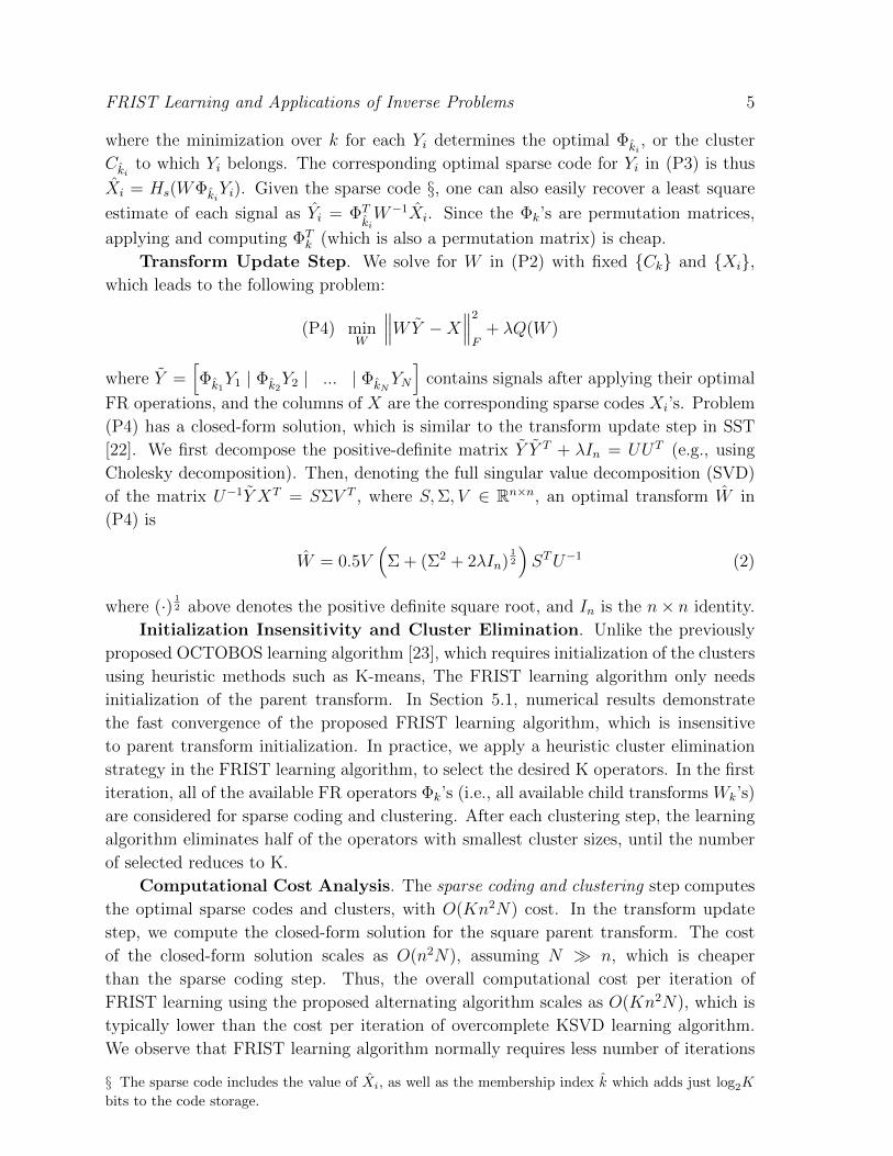
FRIST Learning and Applications of Inverse Problems 6
Table 1: Computational cost comparison among SST (W ∈ Rn×n), OCTOBOS (K
clusters, each Wk ∈ Rn×n), FRIST and KSVD (D ∈ Rn×m) learning. N is the amount
of training data.
SST. OCTOBOS FRIST KSVD
Cost O(n2N) O(Kn2N) O(Kn2N) O(mn2N)
to converge, compared to K-SVD method. The computational costs per-iteration of
SST, OCTOBOS, FRIST, and K-SVD learning are summarized in Table 1.
3.2. Convergence Analysis
We analyze the convergence behavior of the proposed FRSIT learning algorithm that
solves (P2), assuming that every steps in the algorithms (such as SVD) are computed
exactly.
Notations. The Problem (P2) is formulated with sparsity constraint, which is
equivalent to the unconstrained formulation with sparsity barrier penalty φ(X) (which
equals to +∞ when the constraint is violated, and zero otherwise). Thus, the objective
function of Problem (P2) can be rewritten as
f (W,X,Λ) =K∑k=1
∑i∈Ck
‖WΦkYi −Xi‖22 + φ(X) + λQ(Wk) (3)
where Λ ∈ R1×N is the row vector whose ith element Λi ∈ 1, .., K, which denotes the
cluster label k, corresponding to the signal Yi ∈ Ck. We use W t, X t,Λt to denote the
output in each iteration t, generated by the proposed FRIST learning algorithm. We
define the infinity norm of matrix as ‖A‖ , maxi,j |Ai,j|, the operator ψs(·) to return
the sth largest magnitude of a vector.
Main Results. As FRIST can be interpreted as structured OCTOBOS, the
convergence results of the FRIST learning algorithm take the similar form as those
obtained for the OCTOBOS learning algorithms [23] in recent works. The convergence
result for the FRIST learning algorithm, solving (P2), is summarized in the following
theorem and corollaries.
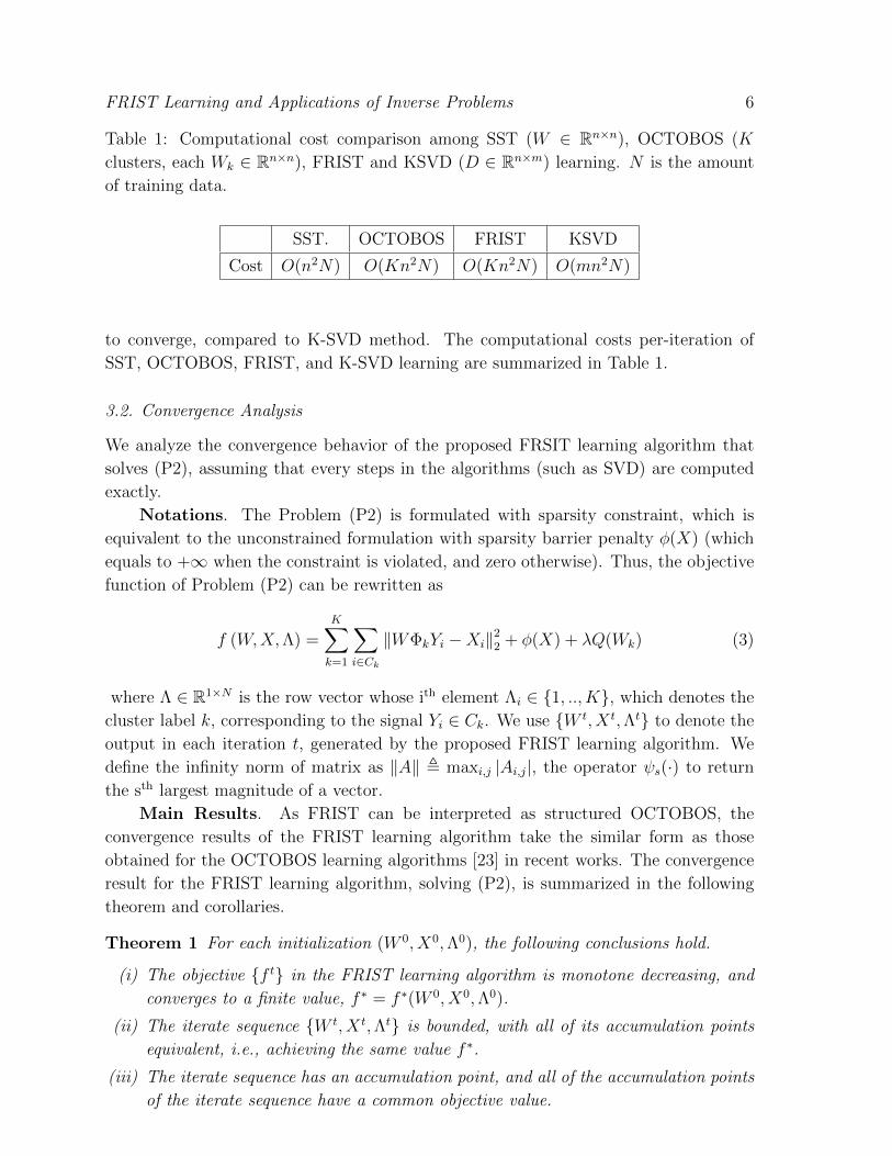
Theorem 1 For each initialization (W 0, X0,Λ0), the following conclusions hold.
(i) The objective f t in the FRIST learning algorithm is monotone decreasing, and
converges to a finite value, f ∗ = f ∗(W 0, X0,Λ0).
(ii) The iterate sequence W t, X t,Λt is bounded, with all of its accumulation points
equivalent, i.e., achieving the same value f ∗.
(iii) The iterate sequence has an accumulation point, and all of the accumulation points
of the iterate sequence have a common objective value.
FRIST Learning and Applications of Inverse Problems 7
(iv) Every accumulation point W,X,Λ of the iterate sequence satisfies the following
partial global optimality conditions
(X,Λ) ∈ arg minX,Λ
f(W, X, Λ
)(4)
W ∈ arg minW
g(W ,X,Λ
)(5)
(v) Each accumulation point W,X,Λ satisfies the local optimality condition
g (W + dW,X + ∆X,Γ) ≥ g (W,X,Γ) (6)
which holds for all dW ∈ Rn×n satisfying ‖dW‖F ≤ ε for some ε > 0, and all
∆X ∈ Rn×N satisfying ‖∆X‖∞ < mink mini∈Ckψs(WΦkYi) : ‖WΦkYi‖0 > s
Corollary 1 For a particular initial (W 0, X0,Λ0), the iterate sequence in FRIST
learning algorithm converges to an equivalence class of accumulation points, which are
also partial minimizers satisfying (4), (5), and (6).
Corollary 2 The iterate sequence W t, X t,Λt in FRIST learning algorithm is globally
convergent to the set of partial minimizers of the non-convex objective f (W,X,Λ).
Due to the space limit, we only provide the outline of proofs. The conclusion (i) in
Theorem 1 is obvious, as the proposed alternating algorithm solve problem in each step
exactly. The proof of conclusions (ii) and (iii) follow the same arguments of Lemma
3 and Lemma 5 in [23]. In the conclusion (iv), the condition (4) can be proved using
the arguments in Lemma 7 from [23], while the condition (5) can be proved with the
arguments in Lemma 6 from [22]. The last conclusion in Theorem 1 can be shown using
arguments from Lemma 9 in [22].
The Theorem 1, and the Corollary 1 and 2 establish that with any initialization
(W 0, X0,Λ0), the iterate sequence W t, X t,Λt, generated by the FRIST learning
algorithm, converges to an equivalent class of fixed points, or an equivalence class of
partial minimizers of the objective.
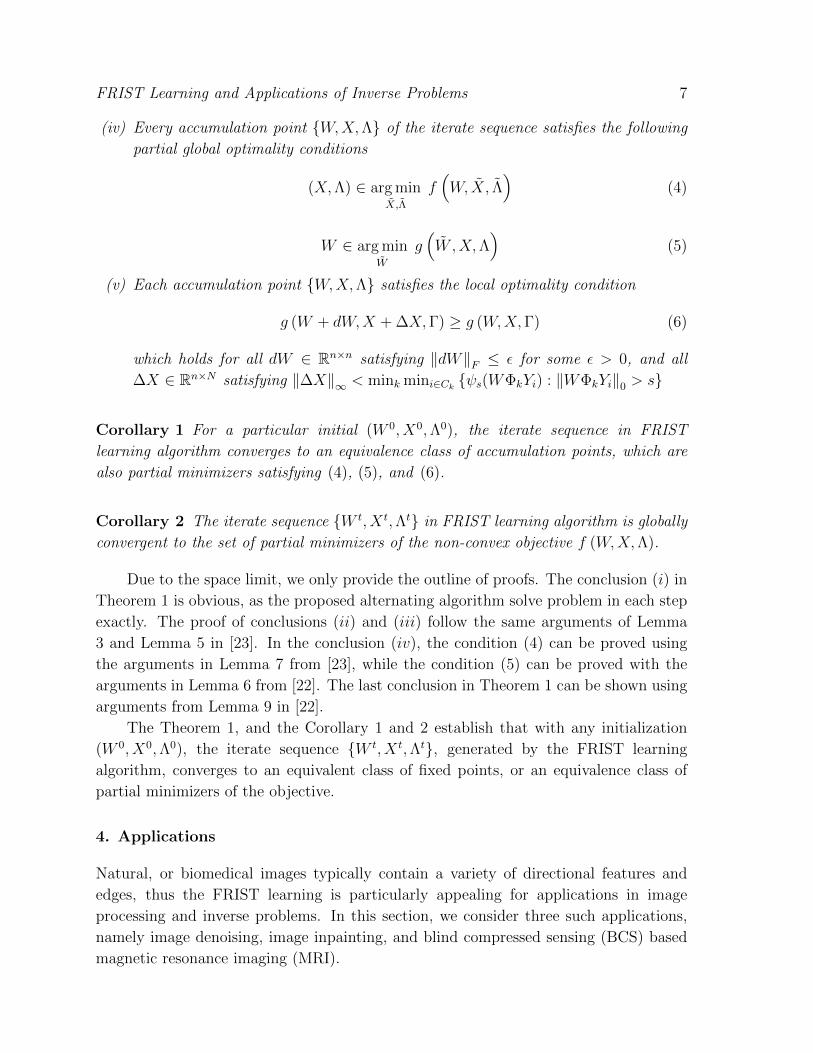
4. Applications
Natural, or biomedical images typically contain a variety of directional features and
edges, thus the FRIST learning is particularly appealing for applications in image
processing and inverse problems. In this section, we consider three such applications,
namely image denoising, image inpainting, and blind compressed sensing (BCS) based
magnetic resonance imaging (MRI).
FRIST Learning and Applications of Inverse Problems 8
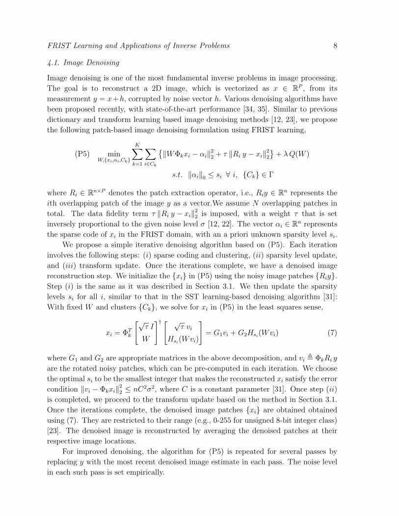
4.1. Image Denoising
Image denoising is one of the most fundamental inverse problems in image processing.
The goal is to reconstruct a 2D image, which is vectorized as x ∈ RP , from its
measurement y = x+h, corrupted by noise vector h. Various denoising algorithms have
been proposed recently, with state-of-the-art performance [34, 35]. Similar to previous
dictionary and transform learning based image denoising methods [12, 23], we propose
the following patch-based image denoising formulation using FRIST learning,
(P5) minW,xi,αi,Ck
K∑k=1
∑i∈Ck
‖WΦkxi − αi‖2
2 + τ ‖Ri y − xi‖22
+ λQ(W )
s.t. ‖αi‖0 ≤ si ∀ i, Ck ∈ Γ
where Ri ∈ Rn×P denotes the patch extraction operator, i.e., Riy ∈ Rn represents the
ith overlapping patch of the image y as a vector.We assume N overlapping patches in
total. The data fidelity term τ ‖Ri y − xi‖22 is imposed, with a weight τ that is set
inversely proportional to the given noise level σ [12, 22]. The vector αi ∈ Rn represents
the sparse code of xi in the FRIST domain, with an a priori unknown sparsity level si.
We propose a simple iterative denoising algorithm based on (P5). Each iteration
involves the following steps: (i) sparse coding and clustering, (ii) sparsity level update,
and (iii) transform update. Once the iterations complete, we have a denoised image
reconstruction step. We initialize the xi in (P5) using the noisy image patches Riy.Step (i) is the same as it was described in Section 3.1. We then update the sparsity
levels si for all i, similar to that in the SST learning-based denoising algorithm [31]:
With fixed W and clusters Ck, we solve for xi in (P5) in the least squares sense,
xi = ΦTk
[√τ I
W
]† [ √τ vi
Hsi(Wvi)
]= G1vi +G2Hsi(Wvi) (7)
where G1 and G2 are appropriate matrices in the above decomposition, and vi , ΦkRi y
are the rotated noisy patches, which can be pre-computed in each iteration. We choose
the optimal si to be the smallest integer that makes the reconstructed xi satisfy the error
condition ‖vi − Φkxi‖22 ≤ nC2σ2, where C is a constant parameter [31]. Once step (ii)
is completed, we proceed to the transform update based on the method in Section 3.1.
Once the iterations complete, the denoised image patches xi are obtained obtained
using (7). They are restricted to their range (e.g., 0-255 for unsigned 8-bit integer class)
[23]. The denoised image is reconstructed by averaging the denoised patches at their
respective image locations.
For improved denoising, the algorithm for (P5) is repeated for several passes by
replacing y with the most recent denoised image estimate in each pass. The noise level
in each such pass is set empirically.

FRIST Learning and Applications of Inverse Problems 9
4.2. Image Inpainting
The goal of image inpainting is to recover missing pixels in an image. The given image
measurement, with missing pixel intensities set to zero, is denoted as y = Ξx+ ε, where
ε is the additive noise on the available pixels, and Ξ ∈ RP×P is a diagonal binary matrix
with zeros only at locations corresponding to missing pixels. We propose the following
patch-based image inpainting formulation using FRIST learning,
(P6) minW,xi,αi,Ck
K∑k=1
∑i∈Ck
‖WΦkxi − αi‖2
2 + τ 2 ‖αi‖0 + γ ‖Pixi − yi‖22
+ λQ(W )
where yi = Riy and xi = Rix. The diagonal binary matrix Pi ∈ Rn×n captures the
available (non-missing) pixels in yi. The sparsity penalty τ ‖αi‖0 is imposed, and
γ ‖Pixi − yi‖22 is the fidelity term for the ith patch, with the coefficient γ that is inversely
proportional to the noise standard deviation σ. The threshold τ is proportional to the
noise level σ, and also increases as more pixels are removed in y.
Our proposed iterative algorithm for solving (P6) involves the following steps: (i)
sparse coding and clustering, and (ii) transform update. Once the iterations complete,
we have a (iii) patch reconstruction step. The sparse coding problem with sparse
penalty has closed-form solution [36], and thus Step (i) is equivalent to solving the
following problem,
min1≤k≤K
‖WΦkxi − Tτ (WΦkxi)‖22 ∀ i (8)
where the hard thresholding operator Tτ (·) is defined as
(Tτ (b))j =
0 , |bj| < τ
bj , |bj| ≥ τ(9)
where the vector b ∈ Rn, and the subscript j indexes its vector entries. Step (ii) is
similar to that in the denoising algorithm in Section 5.4.
Ideal image inpainting without noise. In the ideal case when the noise ε is
absent, i.e., σ = 0, the coefficient of the fidelity term γ → ∞. Thus the fidelity term
can be replaced with hard constraints Pi xi = yi ∀ i. In the noiseless reconstruction
step, with fixed αi, Ck and W , we first reconstruct each image patch xi by solving the
following problem:
minxi‖WΦkixi − αi‖
22 s.t. Pi xi = yi (10)
We define yi = Pixi , xi−ei, where ei = (In−Pi)xi. Because Φk only rearranges pixels,
Φkei has the support Ωi = supp(Φkei) = j| (Φkei)j 6= 0, which is complementary to
supp(Φkyi). Since the constraint leads to the relationship xi = yi + ei with yi given, we
solve the equivalent minimization problem over ei as follow,
minei‖WΦkei − (αi −WΦk yi)‖2
2 s.t. supp(Φkei) = Ωi (11)

FRIST Learning and Applications of Inverse Problems 10
Here, we define WΩito be the submatrix of W formed by columns indexed in Ωi, and
(Φkei)Ωito be the vector containing the non-zero entries of Φkei. Thus, WΦkei =
WΩi(Φkei)Ωi
, and we define ξi , Φkei. The reconstruction problem is then re-written as
the following unconstrained problem,
minξiΩi
∥∥WΩiξiΩi− (αi −WΦk yi)
∥∥2
2∀ i (12)
The above least squares problem has a simple solution given as ξiΩi= W †
Ωi(αi−WΦk yi).
Accordingly, we can calculate ei = ΦTk ξ
i, and thus the reconstructed patches xi = ei+yi.
Robust image inpainting. We now extend to noisy y, and propose the robust
inpainting algorithm. This is useful because real image measurements are inevitably
corrupted with noise [14]. The robust reconstruction step for each patch is to solve the
following problem,
minxi‖WΦkixi − αi‖
22 + γ ‖Pixi − yi‖2
2 (13)
We define yi , Φkiyi, ui , Φkixi, and Pi , ΦkiPiΦTki
, where Φki is permutation matrix
which preserves the norm. Thus the optimization problem (13) is equivalent to
minui‖Wui − αi‖2
2 + γ∥∥∥Piui − yi∥∥∥2
2(14)
which has a least square solution ui = (W TW + γP T P )−1(W Tαi + γP T yi). As the
matrix inversion (W TW + γP T P )−1 is expensive with a cost of O(n3) for each patch
reconstruction, we apply Woodbury Matrix Identity [37] and derive equivalent solution
to (14) as
ui = [B − (FiB)T (1
γIqi + FiBF
Ti )−1(FiB)](W Tαi + γP T
i yi) (15)
where Fi , (Pi)Υiand Υi , supp(yi). The scalar qi = |Υi| counts the number
of available pixels in yi (qi < n for inpainting problem), and B , (W TW )−1 can
be pre-computed. Since FiB can be easily calculated as BΥi, the matrix inversion
( 1γIqi + FiBF
Ti )−1 is less expensive, with a cost of O((qi)3). Once ui is computed, the
patch is recovered as xi = ΦTkiui.
The reconstructed patches are all restricted to their range (e.g., 0-255 for unsigned
8-bit integer class) [23]. Eventually, we output the inpainted image by averaging the
reconstructed patches at their respective image locations. We perform multiple passes
in the inpainting algorithm for (P6) for improved inpainting. In each pass, we initialize
xi using patches extracted from the most recent inpainted image. By doing so, we
indirectly reinforce the dependency between overlapping patches in each pass.
4.3. BCS-based MRI
Compressed Sensing (CS) enables accurate MRI reconstruction from far fewer
measurements than required by Nyquist sampling [43, 19, 44]. However, CS-based
FRIST Learning and Applications of Inverse Problems 11
MRI suffers from various artifacts at high undersampling rate, using non-adaptive
analytical transforms [43]. Recent works [19] proposed BCS-based MRI methods using
adaptively learned sparsifying transform, and generated superior reconstruction results.
Furthermore, MRI image patches normally contain various orientations [26], which have
recently been shown to be well sparsifiable by directional wavelets [30]. Compared to
directional analytical transforms, FRIST can adapt to the MRI data by supervised
learning, while clustering the image patches simultaneously based on their geometric
orientations, which leads to more accurate sparse modeling of MRI image.
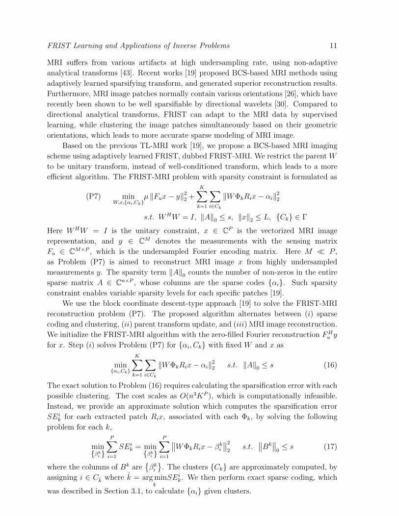
Based on the previous TL-MRI work [19], we propose a BCS-based MRI imaging
scheme using adaptively learned FRIST, dubbed FRIST-MRI. We restrict the parent W
to be unitary transform, instead of well-conditioned transform, which leads to a more
efficient algorithm. The FRIST-MRI problem with sparsity constraint is formulated as
(P7) minW,x,αi,Ck
µ ‖Fux− y‖22 +
K∑k=1
∑i∈Ck
‖WΦkRix− αi‖22
s.t. WHW = I, ‖A‖0 ≤ s, ‖x‖2 ≤ L, Ck ∈ Γ
Here WHW = I is the unitary constraint, x ∈ CP is the vectorized MRI image
representation, and y ∈ CM denotes the measurements with the sensing matrix
Fu ∈ CM×P , which is the undersampled Fourier encoding matrix. Here M P ,
as Problem (P7) is aimed to reconstruct MRI image x from highly undersampled
measurements y. The sparsity term ‖A‖0 counts the number of non-zeros in the entire
sparse matrix A ∈ Cn×P , whose columns are the sparse codes αi. Such sparsity
constraint enables variable sparsity levels for each specific patches [19].
We use the block coordinate descent-type approach [19] to solve the FRIST-MRI
reconstruction problem (P7). The proposed algorithm alternates between (i) sparse
coding and clustering, (ii) parent transform update, and (iii) MRI image reconstruction.
We initialize the FRIST-MRI algorithm with the zero-filled Fourier reconstruction FHu y
for x. Step (i) solves Problem (P7) for αi, Ck with fixed W and x as
minαi,Ck
K∑k=1
∑i∈Ck
‖WΦkRix− αi‖22 s.t. ‖A‖0 ≤ s (16)
The exact solution to Problem (16) requires calculating the sparsification error with each
possible clustering. The cost scales as O(n3KP ), which is computationally infeasible.
Instead, we provide an approximate solution which computes the sparsification error
SEik for each extracted patch Rix, associated with each Φk, by solving the following
problem for each k,
minβk
i
P∑i=1
SEik = minβk
i
P∑i=1
∥∥WΦkRix− βki∥∥2
2s.t.
∥∥Bk∥∥
0≤ s (17)
where the columns of Bk areβki
. The clusters Ck are approximately computed, by
assigning i ∈ Ck where k = arg mink
SEik. We then perform exact sparse coding, which
was described in Section 3.1, to calculate αi given clusters.

FRIST Learning and Applications of Inverse Problems 12
Cam. Pep. Man Couple House Finger. Lena
Figure 1: Testing images used in the image denoising and image inpainting the
experiments.
Step (ii) updates the parent transform W with unitary constraint. The solution,
which is similar to previous work [22], is exact with fixed αi, Ck and x. We first
calculate the full SVD ∆A = SΣV H , where the columns of ∆ are ΦkRix. The
optimal unitary parent transform is then W = V SH .
Step (iii) solves for x with fixed W and αi, Ck as
minx
K∑k=1
∑i∈Ck
‖WΦkRix− αi‖22 + µ ‖Fux− y‖2
2 s.t. ‖x‖2 ≤ L (18)
As Problem (18) is a least squares problem with `2 constraint, it can solved exactly
using the Lagrange multiplier method [45, 19], which is equivalently to solving
minx
K∑k=1
∑i∈Ck
‖WΦkRix− αi‖22 + µ ‖Fux− y‖2
2 + ρ(‖x‖22 − L) (19)
where ρ ≥ 0 is the Lagrange multiplier. Similar to the simplification that was proposed
in previous TL-MRI work [19], the normal equation of Problem 19 can be simplified as
(FEFH + µFFHu FuF
H + ρI)Fx = FK∑k=1
∑i∈Ck
RHi ΦH
k WHαi + µFFH
u y (20)
where E ,∑K
k=1
∑i∈Ck
RHi ΦH
k WHWΦkRi =
∑Pi=1R
Hi Ri. As FEFH , µFFH
u FuFH ,
and ρI are all diagonal matrices, the matrix which pre-multiplies Fx is diagonal and
invertible. Thus, x can be reconstructed efficiently using the method proposed by TL-
MRI work [19].
5. Experiments
We present numerical convergence result of the FRIST learning algorithm, image
segmentation, as well as some preliminary results demonstrating the promise of
FRIST learning in applications including image sparse representation, denoising, robust
inpainting, and MRI reconstruction. We work with 8 × 8 non-overlapping patches
for convergence and sparse representation, 8 × 8 overlapping patches for the image
segmentation, denoising, and robust inpainting, and 6×6 overlapping patches (including
wrap-around patches) for MRI experiments. Figure.1 lists the testing images which are
used in image denoising and inpainting experiments.

FRIST Learning and Applications of Inverse Problems 13
100
101
102
Iteration Number
6.3
6.4
6.5
6.6
6.7
6.8
6.9
7
Ob
jective
Fu
nctio
n
×108
KLT
DCT
Random
Identity
1 200 400 600 800
Iteration Number
1000
3000
5000
7000
9000
Clu
ste
r S
ize
Cluster 1
Cluster 2
1 200 400 600 800
Iteration Number
2000
4000
6000
8000
Clu
ste
r S
ize
Cluster 1
Cluster 2
(a) FRIST Objective (b) DCT initialization (c) KLT initialization
Figure 2: Convergence of FRIST objective and cluster size with various parent transform
initializations.
5.1. Empirical convergence results
We first illustrate the convergence behavior of FRIST learning. We randomly extract
104 non-overlapping patches from the 44 images in the USC-SIPI database [38] (the color
images are converted to gray-scale images), and learn a FRIST, with a 64 × 64 parent
transform W , from the randomly selected patches using fixed sparsity level s = 10. We
set K = 2, and λ0 = 3.1 × 10⁻³ for visualization simplicity. In the experiment, we
initialize the learning algorithm with different square 64 × 64 parent transform W ’s,
including (i) Karhunen-Loeve Transform (KLT), (ii) 2D DCT, (iii) random matrix
with i.i.d. Gaussian entries (zero mean and standard deviation 0.2), and (iv) identity
matrix. Figure 2(a) illustrates the convergence behavior of the objective functions over
iterations, with different parent W initializations. The final values of the objective are
identical for all the initializations. Figure 2(b) and Figure 2(c) show the cluster size
changes over iterations for 2D DCT and KLT initializations. The final values of the
cluster sizes are similar (although, not necessarily identical) for various initializations.
The numerical results demonstrate that our FRIST learning algorithm is reasonably
robust, or insensitive to initialization. Good initialization for the parent transform
W , such as DCT, leads to faster convergence of learning. Thus, we initialize parent
transform W using 2D DCT, in the rest of the experiments.
5.2. Image Segmentation and Clustering Behavior
FRIST learning algorithm is capable of clustering image patches according to their
orientations. In this subsection, we illustrate the FRIST clustering behavior by image
segmentation experiment. First, we consider natural images Wave (512 × 512) and
Field (512 × 512) as inputs, shown in Fig. 3(a) and Fig. 4(a). Both images contains
directional textures, and we aim to cluster the pixels of the images into one of the four
classes, which represent different orientations. For each input image, we convert it into
gray-scale, and extract the overlapping mean-subtracted patches, and learn a FRIST
while clustering the patches using algorithm in Section 3.1. As the overlapping patches
are used, each pixel in the image may belong to several classes. We cluster a pixel into
FRIST Learning and Applications of Inverse Problems 14
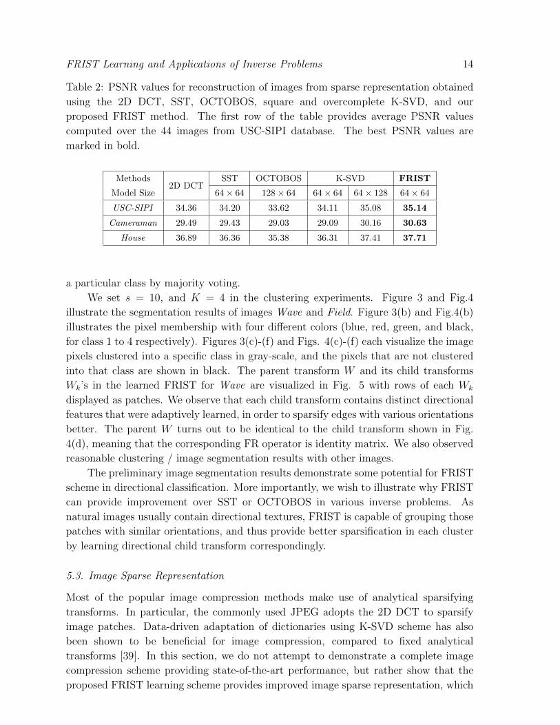
Table 2: PSNR values for reconstruction of images from sparse representation obtained
using the 2D DCT, SST, OCTOBOS, square and overcomplete K-SVD, and our
proposed FRIST method. The first row of the table provides average PSNR values
computed over the 44 images from USC-SIPI database. The best PSNR values are
marked in bold.
Methods2D DCT
SST OCTOBOS K-SVD FRIST
Model Size 64× 64 128× 64 64× 64 64× 128 64× 64
USC-SIPI 34.36 34.20 33.62 34.11 35.08 35.14
Cameraman 29.49 29.43 29.03 29.09 30.16 30.63
House 36.89 36.36 35.38 36.31 37.41 37.71
a particular class by majority voting.
We set s = 10, and K = 4 in the clustering experiments. Figure 3 and Fig.4
illustrate the segmentation results of images Wave and Field. Figure 3(b) and Fig.4(b)
illustrates the pixel membership with four different colors (blue, red, green, and black,
for class 1 to 4 respectively). Figures 3(c)-(f) and Figs. 4(c)-(f) each visualize the image
pixels clustered into a specific class in gray-scale, and the pixels that are not clustered
into that class are shown in black. The parent transform W and its child transforms
Wk’s in the learned FRIST for Wave are visualized in Fig. 5 with rows of each Wk
displayed as patches. We observe that each child transform contains distinct directional
features that were adaptively learned, in order to sparsify edges with various orientations
better. The parent W turns out to be identical to the child transform shown in Fig.
4(d), meaning that the corresponding FR operator is identity matrix. We also observed
reasonable clustering / image segmentation results with other images.
The preliminary image segmentation results demonstrate some potential for FRIST
scheme in directional classification. More importantly, we wish to illustrate why FRIST
can provide improvement over SST or OCTOBOS in various inverse problems. As
natural images usually contain directional textures, FRIST is capable of grouping those
patches with similar orientations, and thus provide better sparsification in each cluster
by learning directional child transform correspondingly.
5.3. Image Sparse Representation
Most of the popular image compression methods make use of analytical sparsifying
transforms. In particular, the commonly used JPEG adopts the 2D DCT to sparsify
image patches. Data-driven adaptation of dictionaries using K-SVD scheme has also
been shown to be beneficial for image compression, compared to fixed analytical
transforms [39]. In this section, we do not attempt to demonstrate a complete image
compression scheme providing state-of-the-art performance, but rather show that the
proposed FRIST learning scheme provides improved image sparse representation, which

FRIST Learning and Applications of Inverse Problems 15
(a) Wave (c) Class 1 (e) Class 3
(b) Pixel memberships (d) Class 2 (f) Class 4
Figure 3: Image segmentation result of Wave (512× 512) using FRIST learning on the
gray-scale version of the image. The Four different colors present pixels that are belong
to the four classes. Pixels which are clustered into a specific class are shown in the
gray-scale, while pixels which are not clustered into that class, are shown in black for
(c)-(f).
(a) Field (c) Class 1 (e) Class 3
(b) Pixel memberships (d) Class 2 (f) Class 4
Figure 4: Image segmentation result of Field (256× 512) using FRIST learning on the
gray-scale version of the image. The Four different colors present pixels that are belong
to the four classes. Pixels which are clustered into a specific class are shown in the
gray-scale, while pixels which are not clustered into that class, are shown in black for
(c)-(f).

FRIST Learning and Applications of Inverse Problems 16
(a) Parent transform
(b) (c) (d) (e)
Figure 5: Visualization of the learned (a) parent transform, and (b)-(e) child transforms
in FRIST for image Wave. The rows of each child transform is displayed as patches.
can be potentially applied in adaptive image compression framework.
We learn a FRIST, with 64× 64 parent transform, from the 104 randomly selected
patches (from USC-SIPI images) used in Section 5.1. We set K = 32, s = 10 and
λ0 = 3.1× 10⁻³. To compare with other popular adaptive sparse models, we also train
a 64 × 64 SST [22], 128 × 64 OCTOBOS [23], as well as a 64 × 64 square (synthesis)
dictionary and a 64 × 128 overcomplete dictionary using KSVD [12] using the same
training patches.
With the learned models, we represent each image from the USC-SIPI database
compactly, by storing its sparse representation, including (i) non-zeros in the sparse
codes of the 8 × 8 non-overlapping patches, (ii) locations of the non-zeros (plus the
cluster membership if necessary) which needs only small overhead cost, and (iii) the
adaptive sparse model. For each method, the patch sparsity (or equivalently, the number
of (i) non-zeros in each patch) is set to be consistently as s = 10. The adaptive SST,
square KSVD, and FRIST methods stores only 64 × 64 square matrix, whereas the
overcomplete KSVD and OCTOBOS methods stores 128× 64 matrix.
The images are then reconstructed from their sparse representations in a least
squares sense, and the reconstruction quality for each image is evaluated using Peak-
Signal-to-Noise Ratio (PSNR), expressed in decibels (dB). We use the average of the
PSNR values over all 44 images as the indicator of the quality of compression of the
USC-SIPI database. Additionally, we apply the learned sparse models to compress some
standard images that are not included in the USC-SIPI database.
FRIST Learning and Applications of Inverse Problems 17
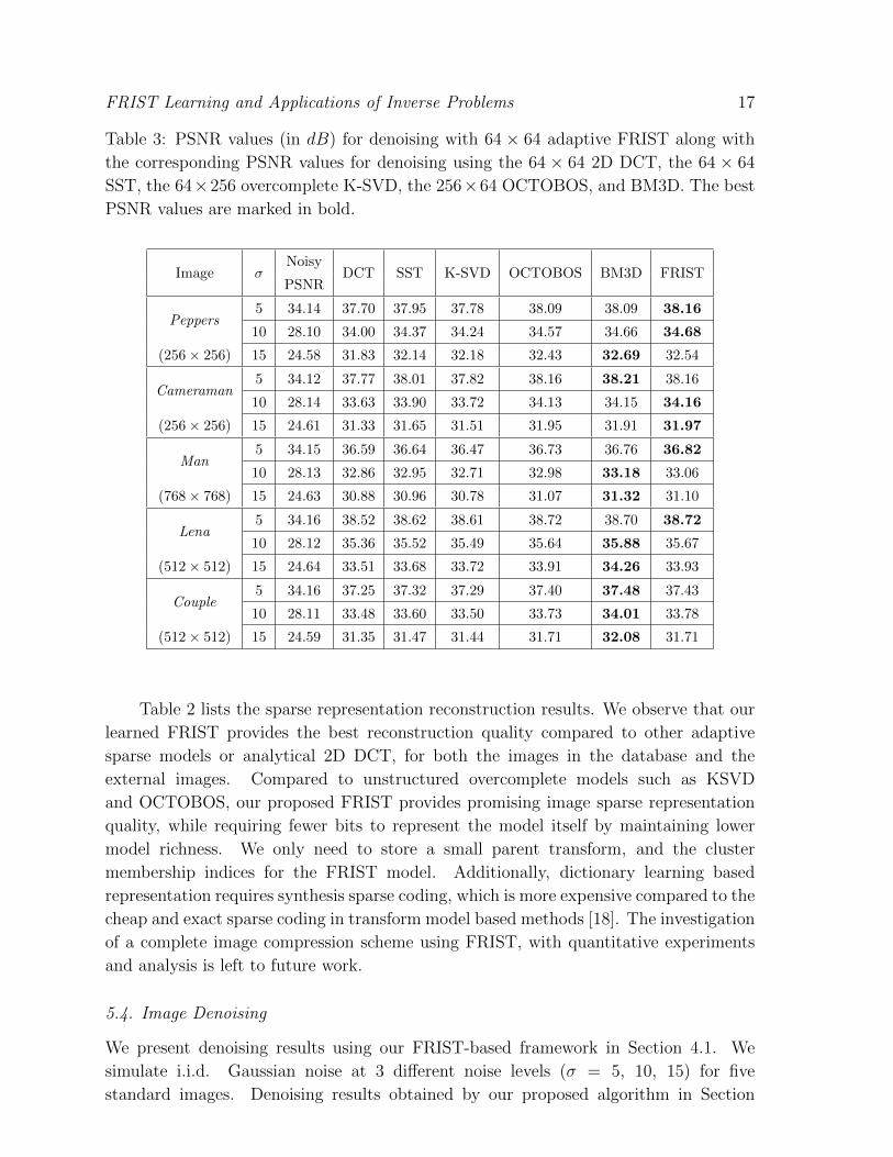
Table 3: PSNR values (in dB) for denoising with 64 × 64 adaptive FRIST along with
the corresponding PSNR values for denoising using the 64 × 64 2D DCT, the 64 × 64
SST, the 64×256 overcomplete K-SVD, the 256×64 OCTOBOS, and BM3D. The best
PSNR values are marked in bold.
Image σNoisy
DCT SST K-SVD OCTOBOS BM3D FRISTPSNR
Peppers5 34.14 37.70 37.95 37.78 38.09 38.09 38.16
10 28.10 34.00 34.37 34.24 34.57 34.66 34.68
(256× 256) 15 24.58 31.83 32.14 32.18 32.43 32.69 32.54
Cameraman5 34.12 37.77 38.01 37.82 38.16 38.21 38.16
10 28.14 33.63 33.90 33.72 34.13 34.15 34.16
(256× 256) 15 24.61 31.33 31.65 31.51 31.95 31.91 31.97
Man5 34.15 36.59 36.64 36.47 36.73 36.76 36.82
10 28.13 32.86 32.95 32.71 32.98 33.18 33.06
(768× 768) 15 24.63 30.88 30.96 30.78 31.07 31.32 31.10
Lena5 34.16 38.52 38.62 38.61 38.72 38.70 38.72
10 28.12 35.36 35.52 35.49 35.64 35.88 35.67
(512× 512) 15 24.64 33.51 33.68 33.72 33.91 34.26 33.93
Couple5 34.16 37.25 37.32 37.29 37.40 37.48 37.43
10 28.11 33.48 33.60 33.50 33.73 34.01 33.78
(512× 512) 15 24.59 31.35 31.47 31.44 31.71 32.08 31.71
Table 2 lists the sparse representation reconstruction results. We observe that our
learned FRIST provides the best reconstruction quality compared to other adaptive
sparse models or analytical 2D DCT, for both the images in the database and the
external images. Compared to unstructured overcomplete models such as KSVD
and OCTOBOS, our proposed FRIST provides promising image sparse representation
quality, while requiring fewer bits to represent the model itself by maintaining lower
model richness. We only need to store a small parent transform, and the cluster
membership indices for the FRIST model. Additionally, dictionary learning based
representation requires synthesis sparse coding, which is more expensive compared to the
cheap and exact sparse coding in transform model based methods [18]. The investigation
of a complete image compression scheme using FRIST, with quantitative experiments
and analysis is left to future work.
5.4. Image Denoising
We present denoising results using our FRIST-based framework in Section 4.1. We
simulate i.i.d. Gaussian noise at 3 different noise levels (σ = 5, 10, 15) for five
standard images. Denoising results obtained by our proposed algorithm in Section

FRIST Learning and Applications of Inverse Problems 18
1 2 4 8 16 32 64 128
Number of Clusters
37.8
37.9
38
38.1
38.2
De
no
ise
d P
SN
R
OCTOBOS
FRIST
1 2 4 8 16 32 64 128
Number of Clusters
31.8
32
32.2
32.4
32.6
De
no
ise
d P
SN
R
OCTOBOS
FRIST
(a) σ = 5 (b) σ = 15
Figure 6: Denoising PSNR for Peppers as a function of the number of cluster K.
4.1 are compared, with those obtained by the adaptive overcomplete K-SVD denoising
scheme [12], adaptive SST denoising scheme [22], adaptive OCTOBOS denoising scheme
[23], and BM3D [35], which is a state-of-the-art image denoising method. We also
compare to the denoising result using the SST method, but with fixed 2D DCT.
We set K = 64, n = 64, C = 1.04 for the FRIST denoising method. For
adaptive SST, and OCTOBOS denoising methods, we follow the same parameter
settings proposed in the previous works [22, 23]. The same parameter settings for SST
method is used for DCT based denoising algorithm. A corresponding 64×256 synthesis
dictionary is used in the synthesis K-SVD denoising method, to match with the same
model richness as the 256 × 64 OCTOBOS. For the K-SVD, and BM3D methods, we
use the publicly available implementations in this experiment.
Table 3 lists the denoised PSNR results. The proposed FRIST scheme constantly
provides better PSNRs compared to other fixed or adaptive sparse modeling methods
including DCT, SST, K-SVD, and OCTOBOS for all testing bases. Figure 6 plot the
denoising PSNRs for Peppers as a function of the number of child transforms (i.e., the
number of clusters) K for σ = 5 and σ = 15. In both cases, the denoising PSNRs of
OCTOBOS and FRIST schemes increase with K initially. Beyond an optimal value
of K, OCTOBOS denoising scheme suffers from overfitting which causes the denoising
PSNR decreases [23]. This effect is more pronounced the higher the noise level, by
comparing Fig. 6(a) and Fig. 6(b). Instead, FRIST based denoising scheme, which
has constant degree of freedom while K increases, provides monotonically increasing
denoising PSNR. Compared to BM3D, FRIST can also provide comparable denoising
PSNRs. We expect the denoising PSNRs for FRIST to improve further with optimal
parameter tuning.
5.5. Image Inpainting
We present preliminary results for our adaptive FRIST-based inpainting framework
(based on (P6)). We randomly remove 80% and 90% of the pixels of the entire image, and
simulate i.i.d. additive Gaussian noise with σ = 0, 5, 10, and 15. We set K = 64, n = 64,

FRIST Learning and Applications of Inverse Problems 19
Corrupted Cubic (30.25 dB) Smoothing (31.96 dB)
SST (32.22 dB) FRIST (32.35 dB) Original Lena
Figure 7: Illutration of image inpainting results for Lena, with regional zoom-in
comparisons.
and apply the proposed FRIST inpaiting algorithm to reconstruct the image from
the highly corrupted and noisy measurements. We additionally replace the adaptive
FRIST in the proposed inpainting algorithm with fixed 2D DCT, adaptive SST [22],
and OCTOBOS [23], and evaluate the inpainting performance using the corresponding
models for comparison. The image inpainting results obtained by the FRIST based
methods are also compared with those obtained by the cubic interpolation [40, 41], and
patch smoothing method [42]. We used the Matlab function “griddata” to implement
the cubic interpolation, and use the publicly available implementations of the patch
smoothing methods. For the DCT, SST, OCTOBOS and FRIST based methods, we
initialize the image patches using Cubic method in noiseless cases, and using Smooth
method in noisy cases.
Table 4 lists the image inpainting PSNR results, with various amount of missing
pixels and noise levels. The proposed FRIST inpainting scheme provides better PSNRs
compared to all other inpainting methods based on interpolation, transform-domain
sparsity, and spatial similarity. Figure 7 provides an illustration of the inpainting results,
with regional zoom-in for visual comparison. We observe that the cubic interpolation
produces blurry effects in various locations. Cubic interpolation method is extremely
sensitive to noise, whereas the FRIST based method is the most robust. Compared to
the competitors, FRIST method provides larger inpainting PSNR improvement as the
FRIST Learning and Applications of Inverse Problems 20
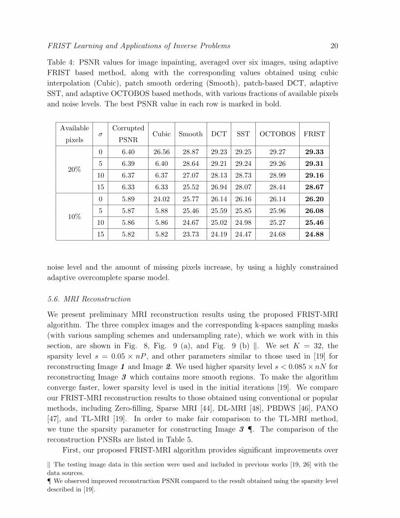
Table 4: PSNR values for image inpainting, averaged over six images, using adaptive
FRIST based method, along with the corresponding values obtained using cubic
interpolation (Cubic), patch smooth ordering (Smooth), patch-based DCT, adaptive
SST, and adaptive OCTOBOS based methods, with various fractions of available pixels
and noise levels. The best PSNR value in each row is marked in bold.
Availableσ
CorruptedCubic Smooth DCT SST OCTOBOS FRIST
pixels PSNR
20%
0 6.40 26.56 28.87 29.23 29.25 29.27 29.33
5 6.39 6.40 28.64 29.21 29.24 29.26 29.31
10 6.37 6.37 27.07 28.13 28.73 28.99 29.16
15 6.33 6.33 25.52 26.94 28.07 28.44 28.67
10%
0 5.89 24.02 25.77 26.14 26.16 26.14 26.20
5 5.87 5.88 25.46 25.59 25.85 25.96 26.08
10 5.86 5.86 24.67 25.02 24.98 25.27 25.46
15 5.82 5.82 23.73 24.19 24.47 24.68 24.88
noise level and the amount of missing pixels increase, by using a highly constrained
adaptive overcomplete sparse model.
5.6. MRI Reconstruction
We present preliminary MRI reconstruction results using the proposed FRIST-MRI
algorithm. The three complex images and the corresponding k-spaces sampling masks
(with various sampling schemes and undersampling rate), which we work with in this
section, are shown in Fig. 8, Fig. 9 (a), and Fig. 9 (b) ‖. We set K = 32, the
sparsity level s = 0.05 × nP , and other parameters similar to those used in [19] for
reconstructing Image 1 and Image 2. We used higher sparsity level s < 0.085× nN for
reconstructing Image 3 which contains more smooth regions. To make the algorithm
converge faster, lower sparsity level is used in the initial iterations [19]. We compare
our FRIST-MRI reconstruction results to those obtained using conventional or popular
methods, including Zero-filling, Sparse MRI [44], DL-MRI [48], PBDWS [46], PANO
[47], and TL-MRI [19]. In order to make fair comparison to the TL-MRI method,
we tune the sparsity parameter for constructing Image 3 ¶. The comparison of the
reconstruction PNSRs are listed in Table 5.
First, our proposed FRIST-MRI algorithm provides significant improvements over
‖ The testing image data in this section were used and included in previous works [19, 26] with the
data sources.¶ We observed improved reconstruction PSNR compared to the result obtained using the sparsity level
described in [19].

FRIST Learning and Applications of Inverse Problems 21
(a) (b) (c) (d)
Figure 8: Testing MRI images and their k-space sampling masks: (a) Image 1 ; (b)
k-space sampling mask (Cartesian with 7× undersampling) for Image 1 ; (c) Image 2 ;
(d) k-space sampling mask (2D random with 5× undersampling) for Image 2.
Table 5: Comparison of the PSNRs, corresponding to the Zero-filling, Sparse MRI [44],
DL-MRI [48], PBDWS [46], PANO [47], TL-MRI [19], and the proposed FRIST-MRI
reconstructions for various images, sampling schemes, and undersampling factors. The
best PSNR for each MRI image is marked in bold.
ImageSampling Under- Zero- Sparse DL-
PBDWS PANOTL- FRIST-
Scheme sampl. filling MRI MRI MRI MRI
1 Cartesian 7× 27.9 28.6 30.9 31.1 31.1 31.2 31.4
2 2D Random 5× 26.9 27.9 30.5 30.3 30.4 30.6 30.7
3 Cartesian 2.5× 24.9 29.9 36.6 35.8 34.8 36.3 36.7
the Zero-filling results (the initialization of the algorithm) with 6.4dB higher PSNR, as
well as the reconstruction results using Sparse MRI with 4.2dB higher PSNR, averaged
over all testing data. Comparing to recently proposed popular MRI reconstruction
methods, FRIST-MRI algorithm demonstrates reasonably better performance for each
testing case. We obtained an average PSNR improvement of 0.8dB, 0.5dB, and 0.3dB
for FRIST-MRI over the non-local patch similarity-based PANO method, the partially
adaptive PBDWS method, and the adaptive dictionary-based DL-MRI method. We
observed that the MRI methods with adaptively learned regularizer usually provide
much better reconstruction quality, compared to those using fixed models.
The proposed FRIST-MRI reconstruction quality is somewhat better than TL-MRI,
with an 0.2dB PSNR improvement in average. As we followed the similar reconstruction
framework and parameters used by the TL-MRI method, the quality improvement using
FRIST-MRI is solely because the learned FRIST can serve as a better regularizer for
MRI image reconstruction, compared to the single square transform. We also observed
that FRIST-MRI used lower average sparsity level than TL-MRI for each testing case,
and thus it provides better sparse representations for MRI images. Figure 9 visualizes the
FRIST Learning and Applications of Inverse Problems 22
(a) (c) (e)
0
0.02
0.04
0.06
0.08
0.1
0
0.02
0.04
0.06
0.08
0.1
(b) (d) (f)
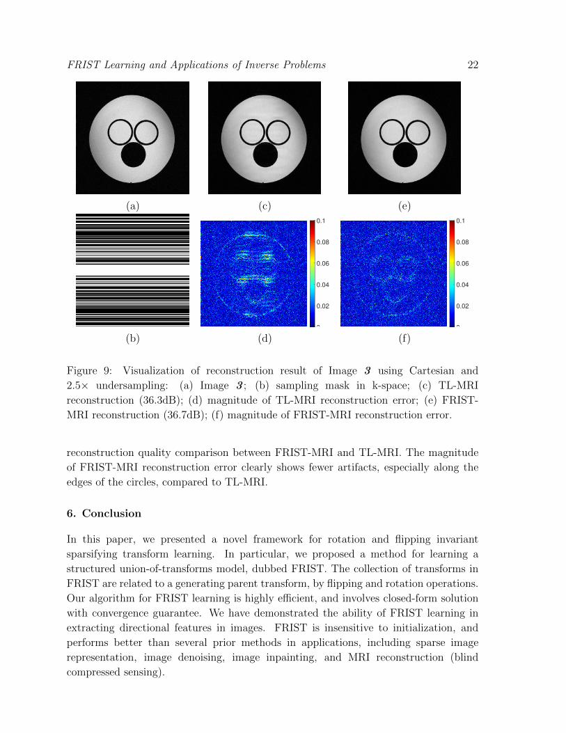
Figure 9: Visualization of reconstruction result of Image 3 using Cartesian and
2.5× undersampling: (a) Image 3 ; (b) sampling mask in k-space; (c) TL-MRI
reconstruction (36.3dB); (d) magnitude of TL-MRI reconstruction error; (e) FRIST-
MRI reconstruction (36.7dB); (f) magnitude of FRIST-MRI reconstruction error.
reconstruction quality comparison between FRIST-MRI and TL-MRI. The magnitude
of FRIST-MRI reconstruction error clearly shows fewer artifacts, especially along the
edges of the circles, compared to TL-MRI.
6. Conclusion
In this paper, we presented a novel framework for rotation and flipping invariant
sparsifying transform learning. In particular, we proposed a method for learning a
structured union-of-transforms model, dubbed FRIST. The collection of transforms in
FRIST are related to a generating parent transform, by flipping and rotation operations.
Our algorithm for FRIST learning is highly efficient, and involves closed-form solution
with convergence guarantee. We have demonstrated the ability of FRIST learning in
extracting directional features in images. FRIST is insensitive to initialization, and
performs better than several prior methods in applications, including sparse image
representation, image denoising, image inpainting, and MRI reconstruction (blind
compressed sensing).
FRIST Learning and Applications of Inverse Problems 23
References
[1] Bruckstein A M, Donoho D L and Elad M 2009 SIAM Review 51 34–81
[2] Elad M, Milanfar P and Rubinstein R 2007 Inverse Problems 23 947–968
[3] Pratt W K, Kane J and Andrews H C 1969 Proc. IEEE 57 58–68
[4] Engan K, Aase S and Hakon-Husoy J 1999 Method of optimal directions for frame design Proc.
IEEE International Conference on Acoustics, Speech, and Signal Processing pp 2443–2446
[5] Aharon M, Elad M and Bruckstein A 2006 IEEE Transactions on signal processing 54 4311–4322
[6] Davis G, Mallat S and Avellaneda M 1997 Journal of Constructive Approximation 13 57–98
[7] Pati Y, Rezaiifar R and Krishnaprasad P 1993 Orthogonal matching pursuit : recursive function
approximation with applications to wavelet decomposition Asilomar Conf. on Signals, Systems
and Comput. pp 40–44 vol.1
[8] Mallat S G and Zhang Z 1993 IEEE Transactions on Signal Processing 41 3397–3415
[9] Chen S S, Donoho D L and Saunders M A 1998 SIAM J. Sci. Comput. 20 33–61
[10] Yaghoobi M, Blumensath T and Davies M 2009 IEEE Transaction on Signal Processing 57 2178–
2191
[11] Skretting K and Engan K 2010 IEEE Transactions on Signal Processing 58 2121–2130
[12] Elad M and Aharon M 2006 IEEE Trans. Image Process. 15 3736–3745
[13] Mairal J, Bach F, Ponce J and Sapiro G 2010 J. Mach. Learn. Res. 11 19–60
[14] Mairal J, Elad M and Sapiro G 2008 IEEE Trans. on Image Processing 17 53–69
[15] Aharon M and Elad M 2008 SIAM Journal on Imaging Sciences 1 228–247
[16] Rubinstein R, Bruckstein A M and Elad M 2010 Proceedings of the IEEE 98 1045–1057
[17] Mallat S 1999 A Wavelet Tour of Signal Processing (Academic Press)
[18] Ravishankar S and Bresler Y 2013 IEEE Trans. Signal Process. 61 1072–1086
[19] Ravishankar S and Bresler Y 2015 Efficient blind compressed sensing using sparsifying transforms
with convergence guarantees and application to magnetic resonance imaging vol 8 pp 2519–2557
[20] Pfister L and Bresler Y 2014 Adaptive sparsifying transforms for iterative tomographic
reconstruction International Conference on Image Formation in X-Ray Computed Tomography
[21] Pfister L and Bresler Y 2015 Learning sparsifying filter banks Proc. SPIE Wavelets & Sparsity
XVI
[22] Ravishankar S and Bresler Y 2014 ell 0 sparsifying transform learning with efficient optimal
updates and convergence guarantees vol 63 pp 2389–2404
[23] Wen B, Ravishankar S and Bresler Y 2015 Int. J. Computer Vision 114 137–167
[24] Wen B, Ravishankar S and Bresler Y 2014 Learning overcomplete sparsifying transforms with
block cosparsity IEEE International Conference on Image Processing (ICIP)
[25] Wersing H, Eggert J and Korner E 2003 Sparse coding with invariance constraints Artificial Neural
Networks and Neural Information ProcessingICANN/ICONIP pp 385–392
[26] Zhan Z, Cai J, Guo D, Liu Y, Chen Z and Qu X 2015 arXiv preprint arXiv:1503.02945
[27] Lowe D G 1999 Object recognition from local scale-invariant features IEEE International
Conference on Computer vision (ICCV) vol 2 pp 1150–1157
[28] Ke Y and Sukthankar R 2004 Pca-sift: A more distinctive representation for local image descriptors
IEEE Computer Society Conference on Computer Vision and Pattern Recognition (CVPR) vol 2
pp II–506
[29] Pennec E L and Mallat S 2005 Multiscale Modeling & Simulation 4 992–1039
[30] Qu X, Guo D, Ning B, Hou Y, Lin Y, Cai S and Chen Z 2012 Magnetic resonance imaging 30
964–977
[31] Ravishankar S and Bresler Y 2013 IEEE Trans. Image Process. 22 4598–4612
[32] Zelnik-Manor L, Rosenblum K and Eldar Y 2012 IEEE Transactions on Signal Processing 60
2386–2395
[33] Ravishankar S and Bresler Y 2013 Learning overcomplete sparsifying transforms for signal
processing IEEE International Conference on Acoustics, Speech and Signal Processing (ICASSP)

FRIST Learning and Applications of Inverse Problems 24
pp 3088–3092
[34] Yu G and Sapiro G 2011 Image Processing On Line 1
[35] Dabov K, Foi A, Katkovnik V and Egiazarian K 2007 IEEE Trans. on Image Processing 16
2080–2095
[36] Ravishankar S, Wen B and Bresler Y 2015 IEEE Journal of Selected Topics in Signal Process. 9
625–636
[37] Woodbury M 1950 Memorandum report 42 106
[38] The USC-SIPI Image Database [Online: http://sipi.usc.edu/database/database.php?volume=misc;
accessed July-2014]
[39] Bryt O and Elad M 2008 Journal of Visual Communication and Image Representation 19 270–282
[40] Yang T 1986 Finite element structural analysis vol 2 (Prentice Hall)
[41] Watson D 2013 Contouring: a guide to the analysis and display of spatial data (Elsevier)
[42] Ram I, Elad M and Cohen I 2013 IEEE Transactions on Image Processing 22 2764–2774
[43] Trzasko J and Manduca A 2009 iEEE Transactions on Medical imaging 28 106–121
[44] Lustig M, Donoho D and Pauly J M 2007 Magnetic resonance in medicine 58 1182–1195
[45] Gleichman S and Eldar Y C 2011 IEEE Transactions on Information Theory 57 6958–6975
[46] Ning B, Qu X, Guo D, Hu C and Chen Z 2013 Magnetic resonance imaging 31 1611–1622
[47] Qu X, Hou Y, Lam F, Guo D, Zhong J and Chen Z 2014 Medical image analysis 18 843–856
[48] Ravishankar S and Bresler Y 2011 Medical Imaging, IEEE Transactions on 30 1028–1041