Freie Universitätftp.imp.fu-berlin.de › klima › NavierStokes › Temam-Navi... · CBMS-NSF...
160
Transcript of Freie Universitätftp.imp.fu-berlin.de › klima › NavierStokes › Temam-Navi... · CBMS-NSF...


CBMS-NSF REGIONAL CONFERENCE SERIESIN APPLIED MATHEMATICS
A series of lectures on topics of current research interest in applied mathematics under the direction ofthe Conference Board of the Mathematical Sciences, supported by the National Science Foundation andpublished by SIAM.
GARRETT BIRKHOFF, The Numerical Solution of Elliptic EquationsD. V. LINDLEY, Bayesian Statistics, A ReviewR. S. VARGA, Functional Analysis and Approximation Theory in Numerical AnalysisR. R. BAHADUR, Some Limit Theorems in StatisticsPATRJCK BILLINGSLEY, Weak Convergence of Measures: Applications in ProbabilityJ. L. LIONS, Some Aspects of the Optimal Control of Distributed Parameter SystemsROGER PENROSE, Techniques of Differential Topology in RelativityHERMAN CHERNOFF, Sequential Analysis and Optimal DesignJ. DURBIN, Distribution Theory for Tests Based on the Sample Distribution FunctionSOL I. RUBINOW, Mathematical Problems in the Biological SciencesP. D. LAX, Hyperbolic Systems of Conservation Laws and the Mathematical Theory of Shock
WavesI. J. SCHOEKBERG, Cardinal Spline InterpolationIVAN SINGER, The Theory of Best Approximation and Functional AnalysisWERNER C. RHEWBOLDT, Methods of Solving Systems of Nonlinear EquationsHANS F. WEINBERGER, Variational Methods for Eigenvalue ApproximationR. TYRRELL ROCKAFELLAR, Conjugate Duality and OptimizationSIR JAMES LIGHTHILL, Mathematical BiofluiddynamicsGERARD SALTON, Theory of IndexingCATHLEEN S. MORAWETZ, Notes on Time Decay and Scattering for Some Hyperbolic ProblemsF. HOPPENSTEADT, Mathematical Theories of Populations: Demographics, Genetics and EpidemicsRICHARD ASKEY, Orthogonal Polynomials and Special FunctionsL. E. PAYNE, Improperly Posed Problems in Partial Differential EquationsS. ROSEN, Lectures on the Measurement and Evaluation of the Performance of Computing SystemsHERBERT B. KELLER, Numerical Solution of Two Point Boundary Value ProblemsJ. P. LASALLE, The Stability of Dynamical Systems - Z. ARTSTEIN, Appendix A: Limiting Equations
and Stability of Nonautonomous Ordinary Differential EquationsD. GOTTLIEB AND S. A. ORSZAG, Numerical Analysis of Spectral Methods: Theory and ApplicationsPETER J. HUBER, Robust Statistical ProceduresHERBERT SOLOMON, Geometric ProbabilityFRED S. ROBERTS, Graph Theory and Its Applications to Problems of SocietyJURIS HARTMANIS, Feasible Computations and Provable Complexity PropertiesZOHAR MANNA, Lectures on the Logic of Computer ProgrammingELLIS L. JOHNSON, Integer Programming: Facets, Subadditivity, and Duality for Group and Semi-
Group ProblemsSHMUEL WINOGRAD, Arithmetic Complexity of ComputationsJ. F. C. KINGMAN, Mathematics of Genetic DiversityMORTON E. GURTIN, Topics in Finite ElasticityTHOMAS G. KURTZ, Approximation of Population Processes
(continued on inside back cover)

Navier-Stokes Equationsand Nonlinear FunctionalAnalysis

This page intentionally left blank

Roger TemamUniversité de Paris-Sud, Orsay, FranceIndiana University, Bloomington, Indiana
Navier-Stokes Equationsand Nonlinear FunctionalAnalysisSecond Edition
SOCIETY FOR INDUSTRIAL AND APPLIED MATHEMATICS
PHILADELPHIA

Copyright © 1983, 1995 by the Society for Industrial and Applied Mathematics.
1 0 9 8 7 6 5 4 3 2
All rights reserved. Printed in the United States of America. No part of this book maybe reproduced, stored, or transmitted in any manner without the written permission ofthe publisher. For information, write to the Society for Industrial and AppliedMathematics, 3600 University City Science Center, Philadelphia, PA 19104-2688.
Library of Congress Cataloging-in-Publication Data
Temam, Roger.Navier-stokes equations and nonlinear functional analysis / RogerTemam. — 2nd ed.
p. cm. — (CBMS-NSF regional conference series in appliedmathematics ; 66)
Includes bibliographical references.ISBN 0-89871-340-41. Fluid dynamics. 2. Navier-Stokes equations—Numerical
solutions. 3. Nonlinear functional analysis. I. Title.II. SeriesQA911.T39 1995532'.051'01515353—dc20 94-43733
is a registered trademark.

ContentsPreface to the Second Edition ix
Introduction xi
Part I. Questions Related to the Existence, Uniqueness and Regularityof Solutions
Orientation 1
1. REPRESENTATION OF A FLOW. THE NAVIER-STOKESEQUATIONS
2. FUNCTIONAL SETTING OF THE EQUATIONS2.1. Function spaces 72.2. The Stokes problem and the operator A 92.3. Sobolev inequalities. The trilinear form b 112.4. Variational formulation of the equations 132.5. Flow in a bounded domain 15
3. EXISTENCE AND UNIQUENESS THEOREMS (MOSTLYCLASSICAL RESULTS)3.1. A priori estimates 173.2. Existence and uniqueness results 213.3. Outlines of the proofs 233.4. Generic solvability of the Navier-Stokes equations 25
4. NEW A PRIORI ESTIMATES AND APPLICATIONS4.1. Energy inequalities and consequences 294.2. Structure of the singularity set of a weak solution 324.3. New a priori estimates 32
5. REGULARITY AND FRACTIONAL DIMENSION5.1. Hausdorff measure. Time singularities 355.2. Space and time singularities 36
6. SUCCESSIVE REGULARITY AND COMPATIBILITY CON-DITIONS AT t=0 (BOUNDED CASE)6.1. Further properties of the operators A and B 436.2. Regularity results 446.3. Other results 47
V

Vi CONTENTS
7. ANALYTICITY IN TIME7.1. The analyticity result 517.2. Remarks 56
8. LAGRANGIAN REPRESENTATION OF THE FLOW8.1. The main result 578.2. Proof of Theorem 8.1 588.3. Appendix 60
Part II. Questions Related to Stationary Solutions and FunctionalInvariant Sets (Attractors)
Orientation 61
9. THE COUETTE-TAYLOR EXPERIMENT
10. STATIONARY SOLUTIONS OF THE NAVIER-STOKESEQUATIONS10.1. Behavior for t—»oo. The trivial case 6710.2. An abstract theorem on stationary solutions 7110.3. Application to the Navier-Stokes equations 7210.4. Counterexamples 76
11. THE SQUEEZING PROPERTY11.1. An a priori estimate on strong solutions 7911.2. The squeezing property 79
12. HAUSDORFF DIMENSION OF AN ATTRACTOR12.1. Functional invariant sets and attractors 8512.2. Hausdorflf dimension of functional invariant sets 8612.3. Other properties of functional invariant sets 89
Part III. Questions Related to the Numerical Approximation
Orientation 91
13. FINITE TIME APPROXIMATION13.1. An example of space-time discretization 9313.2. The convergence theorem 95

CONTENTS Vii
13.3. A compactness theorem 9713.4. Proof of Theorem 13.1 (conclusion) 100
14. LONG TIME APPROXIMATION OF THE NAVIER-STOKESEQUATIONS14.1. Long time finite dimensional approximation 10514.2. Galerkin approximation 109
APPENDIX: INERTIAL MANIFOLDS AND NAVIER-STOKESEQUATIONS 113A. 1. Inertial manifolds and inertial systems 113A.2. Survey of the main results 114A.3. Inertial system for the Navier-Stokes equations 118A.4. Flow around a sphere 124
Comments and Bibliography 127
Comments and Bibliography: Update for the Second Edition . . . . 129
References 131

This page intentionally left blank
Preface to the Second Edition
Since publication of the first edition of this book in 1983, a very active area inthe theory of Navier-Stokes equations has been the study of these equations asa dynamical system in relation to the dynamical system approach to turbulence.A large number of results have been derived concerning the long-time behaviorof the solutions, the attractors for the Navier-Stokes equations and their approxi-mation, the problem of the existence of exact inertial manifolds and approximateinertial manifolds, and new numerical algorithms stemming from dynamical sys-tems theory, such as the nonlinear Galerkin method. Numerical simulations ofturbulence and other numerical methods based on different approaches have alsobeen studied intensively during this decade.
Most of the results presented in the first edition of this book are still relevant;they are not altered here. Recent results on the numerical approximation of theNavier-Stokes equation or the study of the dynamical system that they generateare addressed thoroughly in more specialized publications.
In addition to some minor alterations, the second edition of Navier-Stokes Equa-tions and Nonlinear Functional Analysis has been updated by the addition ofa new appendix devoted to inertial manifolds for Navier-Stokes equations. Inkeeping with the spirit of these notes, which was to arrive as rapidly and assimply as possible at some central problems in the Navier-Stokes equations, wechoose to add this section addressing one of the topics of extensive research inrecent years.
Although some related concepts and results had existed earlier, inertial mani-folds were first introduced under this name in 1985 and systematically studied forpartial differential equations of the Navier-Stokes type since that date. At thistime the theory of inertial manifolds for Navier-Stokes equations is not complete,but there is already available a set of results which deserves to be known, in thehope that this will stimulate further research in this area.
Inertial manifolds are a global version of central manifolds. When they existthey encompass the complete dynamics of a system, reducing the dynamics of aninfinite system to that of a smooth, finite-dimensional one called the inertial sys-tem. In the Appendix we describe the concepts and recall the definitions and sometypical results; we show the existence of inertial manifolds for the Navier-Stokesequations with an enhanced viscosity. We also describe a tentative route for prov-ing the existence of inertial systems for the actual two-dimensional Navier-Stokesequations and for the two-dimensional version of the Navier-Stokes equationscorresponding to the flow around a sphere (flow of a thin layer of fluid around asphere), a subject of obvious interest for geophysical flows and climate problems.
As indicated earlier, another aspect of inertial manifolds not presented here isthe use of approximation of inertial manifolds for the development of new multi-level algorithms adapted to the resolution of the many scales present in turbulentflows. These aspects are addressed (and will be addressed further) in publicationsmore numerically or computationally oriented; some bibliographic references aregiven in the Appendix.
ix

This page intentionally left blank

Introduction
The Navier-Stokes equations are the equations governing the motion ofusual fluids like water, air, oi l , . . . , under quite general conditions, and theyappear in the study of many important phenomena, either alone or coupledwith other equations. For instance, they are used in theoretical studies inaeronautical sciences, in meteorology, in thermo-hydraulics, in the petroleumindustry, in plasma physics, etc. From the point of view of continuummechanics the Navier-Stokes equations (N.S.E.) are essentially the simplestequations describing the motion of a fluid, and they are derived under a quitesimple physical assumption, namely, the existence of a linear local relationbetween stresses and strain rates. These equations, which are recalled in § 1,are nonlinear. The nonlinear term (u • V)u contained in the equations comesfrom kinematical considerations (i.e., it is the result of an elementarymathematical operation) and does not result from assumptions about thenature of the physical model; consequently this term cannot be avoided bychanging the physical model.
While the physical model leading to the Navier-Stokes equations is simple,the situation is quite different from the mathematical point of view. In particular,because of their nonlinearity, the mathematical study of these equations isdifficult and requires the full power of modern functional analysis. Even now,despite all the important work done on these equations, our understanding ofthem remains fundamentally incomplete.
Three types of problems appear in the mathematical treatment of theseequations. Although they are well known, we recall them briefly for thenonspecialist.
1) Existence, uniqueness and regularity. It has been known since the work ofJ. Leray [1] that, provided the data are sufficiently smooth (see § 3), the initialvalue problem for the time-dependent Navier-Stokes equations possesses aunique smooth solution on some interval of time (0, T^); according to J. Leray[3] and E. Hopf [1], this solution can be extended for subsequent time as a(possibly) less regular function. A major question as yet unanswered is whetherthe solution remains smooth all the time. In the case of an affirmative answerthe question of existence and uniqueness would be considerably clarified. Inthe case of a negative answer, then it would be important to have informationon the nature of the singularities, and to know whether the weak solutions areunique and, should they be not unique, how to characterize the "physical"ones.
All these and other related questions are interesting not only for mathemati-cal understanding of the equations but also for understanding the phenomenonof turbulence. Recall here that J. Leray's conjecture [l]-[3] on turbulence, andhis motivation for the introduction of the concept of weak solutions, was thatthe solutions in three space dimensions are not smooth, the velocity or the
Xi

Xii INTRODUCTION
vorticity (the curl of the velocity) becoming infinite at some points or on some"small" sets where the turbulence would be located.
All the mathematical problems that we have mentioned are as yet open. Letus mention, however, some recent studies on the Hausdorff dimension of theset of singularities of solutions (the set where the velocity is infinite), studiesinitiated by B. Mandelbrot [1] and V. Scheffer [l]-[4] and developed by L.Caffarelli-R. Kohn-L. Nirenberg [1] (see also C. Foias-R. Temam [5]). Thestudies are meant to be some hopeful steps towards the proof of regularity ifthe solutions are smooth, or else some steps in the study of the singular set ifsingularities do develop spontaneously.
2) Long time behavior. If the volume forces and the given boundary values ofthe velocity are independent of time, then time does not appear explicitly inthe Navier-Stokes equations and the equations become an autonomous infinitedimensional dynamical system. A question of interest is then the behavior fort —> oo of the solution of the time-dependent N.S.E. A more detailed descriptionof this problem is contained in § 9, but, essentially, the situation is as follows. Ifthe given forces and boundary values of the velocity are small then there existsa unique stable stationary solution and the time-dependent solution convergesto it as t —» oo. On the other hand, if the forces are large, then it is very likelyfrom physical evidence and from our present understanding of bifurcationphenomena that, as £—»°o, the solution tends to a time periodic one or to amore complicated attracting set. In the latter case, the long time behavior ofthe solution representing the "permanent" regime, could well appear chaotic.This is known to happen even for very simple dynamical systems in finitedimensional spaces, such as the Lorenz model (cf. also O. Lanford [1]) or theexamples of mappings of the unit interval of R into itself, discussed by M.Feigenbaum [1] and O. Lanford [2]. Such chaotic behavior is another way toexplain turbulence; it is based on the ideas of dynamical systems and strangeattractors, following D. Ruelle [1], [2], D. Ruelle-F. Takens [1] and S. Smale[2]. Actually, for the moment, these two ways for the description of turbulenceare not mutually exclusive, as singularities and long time chaotic behavior couldperhaps be both present in the Navier-Stokes equations. Let us mention alsothat, as observed by D. Ruelle [3], the strange attractor point of view is notsufficient to explain the chaotic structure in space of the physical flow1.
A great number of mathematical problems relating to the behavior for t —» oof the solutions of the N.S.E. are open. They include convergence to a stablestationary or time periodic solution in connection with bifurcation theory2 orconvergence to a more complicated attractor (cf. C. Foias-R. Temam [5], [8],[9] and also J. Mallet-Paret [1]). Of course in three space dimensions the
1 We specify "physical flow" since the word "flow" is also used in the dynamical system contextto describe the trajectory of u(t) in the function space.
2 From the abundant literature we refer, for instance, to C. Bardos-C. Bessis [1], P. Rabinowitz[1] and the references therein.

INTRODUCTION xiii
difficulties are considerable, and the problem is perhaps out of reach for themoment since we do not even know whether the initial value problem for theN.S.E. is well posed.
3) Numerical solution. We mentioned at the beginning that the N.S.E. playan important role in several scientific and engineering fields. The needs thereare usually not for a qualitative description of the solution but rather for aquantitative one, i.e., for the values of some quantities related to the solution.Since the exact resolution of the N.S.E. is totally out of reach (we actuallyknow only a very small number of exact solutions of these equations), the datanecessary for engineers can be provided only through numerical computations.Also, for practical reasons there is often a need for accurate solutions of theN.S.E. and reliance on simplified models is inadequate.
Here again the problem is difficult and the numerical resolution of the N.S.E.will require (as in the past) the simultaneous efforts of mathematicians,numerical analysts and specialists in computer science. Several significantproblems can already be solved numerically, but much time and effort will benecessary until we master the numerical solution of these equations for realisticvalues of the physical parameters. Besides the need for the development ofappropriate algorithms and codes and the improvement of computers inmemory size and computation speed, there is another difficulty of a moremathematical (as well as practical) nature. The solutions of the N.S.E. underrealistic conditions are so highly oscillatory (chaotic behavior) that even if wewere able to solve them with a great accuracy we would be faced with toomuch useless information. One has to find a way, with some kind of averaging,to compute mean values of the solutions and the corresponding desiredparameters.
As mentioned before, some analytical work is necessary for the numericalresolution of the N.S.E. But, conversely, one may hope that if improvednumerical methods are available, they may help the mathematician in theformulation of realistic conjectures about the N.S.E., as happened for theKorteweg-de Vries equations.
After these general remarks on fluid dynamics and the Navier-Stokesequations, we describe the content of this monograph, which constitutes a verymodest step towards the understanding of the outstanding problems mentionedabove. The monograph contains 14 sections grouped into three parts (§§ 1-8,9-12, 13-14), corresponding respectively to the three types of problems whichwe have just presented.
Part I (§§ 1-8) contains a set of results related to the existence, uniquenessand regularity of the weak and strong solutions. The material in Part I mayappear technical, but most of it is essential for a proper understanding of morequalitative or more concrete questions. In § 1 the N.S.E. are recalled and wegive a brief description of the boundary value problems usually associated withthem. Sections 2 and 3 contain a description of the classical existence anduniqueness results for weak and strong solutions. We have tried to simplify the

Xiv INTRODUCTION
presentation of these technical results. In particular, we have chosen to em-phasize the case of the flow in a cube in (Rn, n = 2 or 3, with space periodicboundary conditions. This case, which is not treated in the available books orsurvey articles, leads to many technical simplifications while retaining the maindifficulties of the problem (except for the boundary layer question, which is notconsidered here). Of course the necessary modifications for the case of the flowin a bounded region of Rn are given. The results in §§ 2 and 3 are essentiallyself-contained, except for some very technical points that can be foundelsewhere in the literature, (cf. in particular O. A. Ladyzhenskaya [1], J. L.Lions [1] and R. Temam [6] to which we will refer more briefly as [RT]).
New (or recent) developments, related either to weak solutions or to strongsolutions, are then presented in §§4 to 8. New a priori estimates for weaksolutions are proved in § 4 following C. Foias-C. Guillopé-R. Temam [1].They imply in particular, as noticed by L. Tartar, that the L°°-norm of a weaksolution is L1 in time, and this allows us in §8 to define the Lagrangianrepresentation of the flow associated with a weak solution. In § 5 we present theresult established in C. Foias-R. Temam [5] concerning the fractional dimen-sion of the singular set of a weak solution.
In § 6 we derive, after R. Temam [8], the necessary and sufficient conditionsfor regularity, at time t = 0 of the (strong) solutions to the N.S.E. The resultrelates to the question of compatibility conditions between the given initial andboundary values of the problem. This question, which is a well-known one forother initial and boundary value problems including linear ones, apparently hasnot been solved for the N.S.E.; of course the question of regularity at t = 0 hasnothing to do with the singularities which may develop at positive time.
Finally in § 7 we prove a result of analyticity in time of the solutions,following with several simplifications C. Foias-R. Temam [5]. The proof, whichcould be used for other nonlinear evolution problems, is simple and is closelyrelated to the methods used elsewhere in these notes.
Part II (§§ 9-12) deals with questions related to the behavior for t —> o° of thesolutions of the N.S.E. Section 9 explains the physical meaning of theseproblems through the example of the Couette-Taylor experiment. Section 10 isdevoted to stationary solutions of the N.S.E.; contains a brief proof ofexistence and uniqueness (for small Reynolds number), and the fact that thesolution to the N.S.E. tends, as t—*°°, to the unique stationary solution whenthe Reynolds number is small. This section contains also a proof of a finitenessproperty of the set of stationary solutions based on topological methods.
The results in §§ 11 and 12 (following C. Foias-R. Temam [5]) are related tothe behavior for r — > o o of the solutions to the N.S.E. at arbitrary (or large)Reynolds numbers. They indicate that a turbulent flow is somehow structured anddepends (for the cases considered, see below), on a finite number of parame-ters. These properties include a squeezing property of the trajectories in thefunction space (§ 11) and the seemingly important fact that, as t —> <», a solutionto the Navier-Stokes equations converges to a functional invariant set (anw-limit set, or an attractor), which has a finite Hausdorff dimension (§ 12).

INTRODUCTION XV
Intuitively, this means that under these circumstances all but a finite set ofmodes of the flow are damped.
Both results are proved for a space dimension n = 2 or 3, without anyrestriction for n = 2, but for n = 3 with the restriction that the solutionconsidered has a bounded H^-norm for all time. It is shown (cf. § 12.3 and C.Foias-R. Temam [13]) that if this boundedness assumption is not satisfied thenthere exists a weak solution to the N.S.E. which displays singularities. Alterna-tively, this means that the relevant results in §§11 and 12 (and some of theresults in Part III) fail to be true in dimension 3 only if Leray's conjecture onturbulence is verified (existence of singularities).
Although the problems studied in Part II are totally different from thosestudied in Part I, the techniques used are essentially the same as in the firstsections, and particularly in §§ 2 and 3.
Part III (§§ 13 and 14) presents some results related to the numericalapproximation of the Navier-Stokes equations. At moderate Reynolds num-bers, the major difficulties for the numerical solution of the equations are thenonlinearity and the constraint div u = 0. In §13 we present one of thealgorithms which have been derived in the past to overcome these difficulties,and which has been recently applied to large scale engineering computations.Section 14 contains some remarks related to the solution of the N.S.E. forlarge time: it is shown (and this is not totally independent of the result in PartII) that the behavior of the solution for large time depends on a finite numberof parameters and an estimate of the number of parameters is given. A moreprecise estimate of the number of parameters in terms of the Reynolds numberand further developments will appear elsewhere (C. Foias-R. Temam [9], C.Foias-O. Manley-R. Temam-Y. Trève [1], C. Foias-R. Temam [11], [12]).
At the level of methods and results, there is again a close relation betweenPart III and Part I (§§ 3 and 13 in particular), and there is a connection asalready mentioned with Part II (§§ 12 and 14).
It is not the purpose of these notes to make an exhaustive presentation ofrecent results on the Navier-Stokes equations. We have only tried to presentsome typical results, and the reader is referred to the bibliographical commentsin the text and at the end for further developments. In particular we haverefrained from developing the stochastic aspect of the Navier-Stokes equa-tions, which would have necessitated the introduction of too many differenttools. The interested reader can consult A. Bensoussan-R. Temam [1], C.Foias [1], C. Foias-R. Temam [6] [7], M. Viot [1], M. I. Vishik [1], M. I.Vishik-A. V. Fursikov [1], [2], [3].
Our aim while writing these notes was to try to arrive as rapidly and assimply as possible at some central problems in the Navier-Stokes equations.We hope that they can stimulate some interest in these equations. One canhope also that the demand of new technologies and the accelerated improve-ment of the opportunities offered by new (existing or projected) computers willhelp stimulate further interest in these problems in the future.
In conclusion I would like to thank all those who helped in the preparation
Xvi INTRODUCTION
of these notes: C. Foias for his collaboration which led to several articles onwhich these notes are partly based, C. Guillopé, Ch. Gupta, J. C. Saut, D.Serre and the referee for reading the manuscript and for the comments theymade. Finally I would like to thank the mathematical secretary at DekalbUniversity and Mrs. Le Meur at Orsay for kindly typing the manuscript.
PART I
Questions Related to the Existence,Uniqueness and Regularity of Solutions
Orientation. In this first Part, which contains §§ 1 to 8, we present theNavier-Stokes equations of viscous incompressible fluids, and the main bound-ary value problems which are usually associated with these equations. Then westudy the case of the flow in a bounded domain with periodic or zero boundaryconditions, and we give in this case the functional setting of the equation, andvarious results on existence, uniqueness and regularity of time-dependentsolutions. We emphasize the case of the flow with space periodic boundaryconditions, treating more briefly the zero boundary conditions which are muchmore often considered in the literature; see for instance O. A. Ladyzhenskaya[1], J. L. Lions [1], and R. Temam [6] to which we will refer more briefly as[RT].
In § 1 we recall the Navier-Stokes equations and the corresponding bound-ary value problems. In § 2 we present the appropriate functional setting. In§ 3 we recall the main existence and uniqueness results (which are essentiallyclassical), with the details of various a priori estimates used frequently in thesequel and we sketch the proof of existence and uniqueness. Section 4 containssome new a priori estimates, used in particular in § 8. Section 5 includes someresults on the Hausdorff dimension of the singular set of a weak solution.Section 6 presents the necessary and sufficient conditions of regularity of thesolution at time f = 0 (the compatibility conditions). Section 7 shows underappropriate assumptions that the solution is analytic in time with values inD(A). Finally, in § 8 we exhibit the Lagrangian representation of the flowassociated with a weak solution of the Navier-Stokes equations.

This page intentionally left blank

1Representation of a Flow.The Navier-Stokes Equations
Let us assume that a fluid fills a region fl of space. For the Eulerianrepresentation of the flow of this fluid, we consider three functions p = p(x, t),p = p(x, t), u = u(x, t), x = (x1; x2, x3)eft, teR, where p(x, t) (or p(x, 0) is thedensity (or the pressure) of the fluid at point x at time t and u(x, t) = (uj(x, f )»u2(x, r), u3(x, t)) is the velocity of the particle of fluid which is at point x at timet. One may also consider Lagrangian representation of the flow, in which casewe introduce functions p = p(a, r), p = p(a, t}, u = u(a,t); here u(a, t) is thevelocity of the particle of fluid which was at point a e H at some reference timef0, and the meanings of p(a, t}, p(a, t) are similar. The Lagrangian representa-tion of a flow is less often used, but we will make some comments on it in § 8.
If the fluid is Newtonian, then the functions p, p, u are governed by themomentum conservation equation (1.1) (Navier-Stokes equation), by the con-tinuity equation (1.2) (mass conservation equation) and by some constitutivelaw connecting p and p:
where JLL > 0 is the kinematic viscosity, A. another physical parameter andf = /(x, r) represents a density of force per unit volume. If the fluid ishomogeneous and incompressible, then p is a constant independent of x and t,and the equations reduce to
Usually we take p = 1, set v — /n and, using the differential operator V = (d/dXj,d/3x2, 6/3x3) arrive at
We can also consider (1.5) as the nondimensional form of the Navier-Stokesequation (1.3), which is obtained as follows. We set p = p*p', p = p#p', u-Wstcii ' , x = L^x', t = T*t', / = (p4cl/*/T*)f, where p#, L*, T* are respectively areference density, a reference length and a reference time for the flow, andt/* = L-jc/T^, p* = L^p*. By substitution into (1.3) we get (1.5) for the reduced
3

where e^,... ,en is the canonical basis of IR", and L is the period in the ithdirection; Q = (]0, L[)n is the cube of the period2. The advantage of theboundary condition (1.11) is that it leads to a simpler functional setting, whilemany of the mathematical difficulties remain unchanged (except of course thoserelated to the boundary layer difficulty, which vanish). In fact, in § 2 we willdescribe in detail the corresponding functional setting of the problem (i.e. for(1.4), (1.5), (1.8), (1.11)), and we will mention only briefly the case with a
1 For special unbounded sets H further conditions must be added to (1.9), (1.10); cf. J. G.Heywood [1], O. A. Ladyzhenskaya-V. A. Solonnikov [1], [2].
2 Of course one may consider different periods L(,..., Ln in the different directions, and in thiscase Q=W=iQO,Li[).
4 PART I. QUESTIONS RELATED TO SOLUTIONS
quantities u'(x', f'), P'(*', 0, /'(*', 0, but in this case the inverse of vrepresents the Reynolds number of the flow:
The equations (1.4), (1.5) are our basic equations. We note that they makesense mathematically (and in some way physically) if (1 is an open set in IR2,u = (u1, u2), /—(fi , /2)- Since it is useful to consider this situation too, and inorder to cover both cases simultaneouslv, we assume from now on that
(1 is an open set of IR", n = 2 or 3, with boundary P.
(1.7) We assume furthermore that H is located locally on one side of F and thatF is Lipschitzian or sometimes of class Cr for a specified r.
One of the first mathematical questions concerning the equations (1.4), (1.5)is the determination of a well-posed boundary value problem associated withthese equations. This is still an open problem, but it is believed (and has beenproved for n=2) that (1.4), (1.5) must be completed by the following initialand boundary conditions (for flow for f>0 , xeO).
Initial condition:
ty given1.Instead of (1.9) (and (1.10)) it is interesting to consider another boundary
condition which has no physical meaning:
If H is unbounded (and in particular for fl = IR"), we add to (1.9) a conditionat infinity:
Boundary condition:

REPRESENTATION OF A FLOW. THE NAVIER-STOKES EQUATIONS 5
boundary, which is presented in detail in the references already quoted(Ladyzhenskaya [1], Lions [1], [RT]).
Remark 1.1. In the periodic case (i.e. (1.11)), it is convenient to introducethe average of u on the cube of the period,
The average m is explicitly determined in terms of the data. By integration of(1.5) on Q, using (1.4), the Stokes formula and the fact that the integrals on theboundary 3Q of Q vanish because of (1.11), we get
so that
By substitution of (1.13) into (1.5) we find
The quantity mu being known, the study of (1.16) is very similar to that of(1.5). Therefore in the periodic case we will assume for simplicity that theaverage flow vanishes, mu = 0.
and to set

This page intentionally left blank

^7 Functional Setting of the Equations
In this section we describe the functional setting of the equations, insistingmore particularly on the space periodic case (boundary condition (1.11)).
2.1. Function spaces. We denote by L2(ft) the space of real valued func-tions on fl which are L2 for the Lebesgue measure dx = dxv • • • dxn; this spaceis endowed with the usual scalar product and norm
Ho(H) is the Hilbert subspace of H^O), made of functions vanishing on F. Thereader is referred to R. Adams [1] and J. L. Lions-E. Magenes [1] for thetheory of Sobolev spaces.
We denote by H^(Q), m e N , the space of functions which are in H^OR")(i.e., u \G<=Hm(G) for every open bounded set 0} and which are periodic withperiod Q:
The functions in H^(O) are easily characterized by their Fourier seriesexpansion
We denote by Hm(fl) the Sobolev space of functions which are in L2(ft),together with all their derivatives of order ^m. This is as usual a Hilbert spacefor the scalar product and the norm
For m = 0, H°(Q) coincides simply with L2(Q) (the restrictions of the functionsin H°(Q) to O are the whole space L2(Q)). For an arbitrary m eN, H^(Q) is aHilbert space for the scalar product and the norm
and the norm |u|m is equivalent to the norm &kez" (l + |k|2m) kk|2}1/2. We also
set
7

8 PART I. QUESTIONS RELATED TO SOLUTIONS
We observe that the right-hand side of (2.2) makes sense more generally form e R , and we actually define H™(Q), meIR, m^O, by (2.2); it is a Hilbertspace for the norm indicated above. For meIR , we define H™(Q) with (2.3);this is a Hilbert space for the norm {ZfceZ-> |fc|2m |ck|
2}1/2, and H™(Q) andH~m(Q) are in duality for all meIR .
Two spaces frequently used in the theory of Navier-Stokes equations are
1 Let 0 be an open bounded set of Rn of class (€2. Then if v eL2(C) and div v e L2(6], we candefine yvv e H~l/2(d6), which coincides with v • v M if v is smooth (v denotes the unit outwardnormal on d6). Furthermore, for every u in H l(G), we have the generalized Stokes formula(v, Vu) + (div v, u) = (yvv, yuu), where •y()
M = Mlac denotes the trace of u on d€, and (•, •) is thepairing between H'/2(dG) = y0H'(0) and its dual H~1/2(d0).
is dense in V, H and V.Remark 2.1. i) Using the trace theorem, one can show that u e V if and
only if its restriction «|Q to Q belongs to
where we have numbered the faces F l 5 . . . , F2n of Q as follows:
and u|r. is an improper notation for the trace of v on Fy. The characterizationof u|Q for ueH is more delicate and relies on a trace theorem given in [RT,Chap. I., Thm. 1.2]1: ueH if and only if u belongs to
This norm is equivalent to that induced by (Hp(Q))n, and V is a Hilbert spacefor this norm. It is easy to see that the dual V of V is
|| • ||v will denote the dual norm of || • || on V. We have
where the injections are continuous and each space is dense in the followingone. One can also show by mollification that the space of smooth functions,
where H™(Q) = {H™(Q)}n; more generally, for any function space X we denoteby X the space Xn endowed with the product structure. We equip V with thescalar product and the Hilbert norm

FUNCTIONAL SETTING OF THE EQUATIONS 9
ii) Let G be the orthogonal complement of H in H(p = (Lj(Q)/R)n. We have
2.2. The Stokes problem and the operator A. The Stokes problem as-sociated with the space periodicity condition (1.11) is the following one.
It is easy to solve this problem explicitly using Fourier series. Let us introducethe Fourier expansions of u, p and /;
Equations (2.9) reduce for every k ̂ 0 to
Taking the scalar product of (2.10) with k and using (2.11) we find the pk's:
then (2.10) provides the wk?s:
By the definition (2.2) of H^(O), if /eHj(Q) then u EHj(Q) and p e HP(Q);if / eHp 'CQ) then uelHlJ(Q) and peHj(Q). Now if / belongs to H, thenk • fk = 0 for every k so that p = 0 and
We define in this way a one-to-one mapping / —> u from H onto
Its inverse from D(A) onto H is denoted by A, and in fact
If D(A) is endowed with the norm induced by Hp(Q), then A becomes anisomorphism from D(A) onto H. If follows that the norm |Au on D(A) isequivalent to the norm induced by Hp(Q).
The operator A can be seen as an unbounded positive linear selfadjointoperator on H, and we can define the powers A", a elR, with domain D(A") in

2 The letters c, c', cf, c\ indicate various positive constants. The letters cf represent well-definedconstants while the constants represented by the letters c, c', c[ may be different in different placesin the text.
In fact the sequence of w,'s and A/'s is the sequence of functions wka andnumbers Aka,
and since this limsup is arbitrarily small, wm —»0 in Va_e.Eigenfunctions of A. The operator A"1 is linear continuous from H into
D(A), and since the injection of D(A) in H is compact, A"1 can be consideredas a compact operator in H. As an operator in H it is also selfadjoint. Hence itpossesses a sequence of eigenfunctions w,, j eN , which form an orthonormalbasis of H,
PART I. QUESTIONS RELATED TO SOLUTIONS10
H. We set
Va is a closed subspace of H£(Q), and in fact
In particular, V2 = D(A), Vl=V, V0 = H, V_! = V; A is an isomorphism fromVa+2 onto Va, D(A) onto H, V onto V, and so forth. The norm |Aa/2u| on Va
is equivalent to the norm induced by Hp(Q),
with2 c, c' depending on L and a.The operator A is an isomorphism from Va+2 onto Va for all aeR. We
recall also that the injection of Va into Va_e is compact for every a e!R, e >0.Indeed if u^ is a sequence converging weakly to 0 in Va, then
a constant independent of m,
For every KelR, K>0,
FUNCTIONAL SETTING OF THE EQUATIONS 11
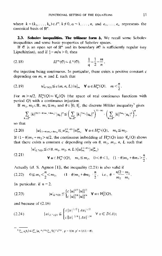
where k = (kl,. . ., kn)eZ", k^O, a = 1,. . . , n, and e\,...,en represents thecanonical basis of [R".
2.3. Sobolev inequalities. The trilinear fonn 6. We recall some Sobolevinequalities and some basic properties of Sobolev spaces.
If G is an open set of R" and its boundary d€ is sufficiently regular (sayLipschitzian), and if ^ — m / n > 0 , then
the injection being continuous. In particular, there exists a positive constant cdepending on m, n and L such that
For m>n/2, H™(Q)c: ̂ p(Q) (the space of real continuous functions withperiod Q) with a continuous injection.
If m l 5 m2e!R, ml^m2 and 0e]0,1[, the discrete Holder inequality3 gives
and because of (2.16)
If (1 —0)m 1 + m2>n/2, the continuous imbedding of H^(O) into C€P(Q) showsthat there exists a constant c depending only on 6, m l 5 m2, n, L such that
Actually (cf. S. Agmon [1]), the inequality (2.21) is also valid if
In particular, if n = 2,

If one or more of the m( 's is larger than n/2 we proceed as before, with thecorresponding q; replaced by +00 and the other q,'s equal to 2. If some of thera^'s are equal to n/2, we replace them by m|<mj, m; — m! sufficiently small sothat the corresponding inequality (2.29) still holds.
Remark 2.2. i) As a particular case of Lemma 2.1 and (2.29), ft is a tnlmearcontinuous form on VmixVm2+1x Vmi, mt as in (2.28) and
The form b. We now show how to apply these properties of Sobolev spacesto the study of the form b.
Let O be an open bounded set of Rn which will be either H or Q. Foru, v, w ELl(®\ we set
if n = 3
12 PART I. QUESTIONS RELATED TO SOLUTIONS
Proof. If m, < n/2 for i = 1, 2, 3, then by (2.18) Hm-(C] c Lq>(0) where 1/q, =^-mjn. Due to (2.28), (!Ah + l/q2+ 1/^3)= 1, the product u^DjU^Wj isintegra-ble and 6(u, u, w) makes sense. By application of Holder's inequality we get
whenever the integrals in (2.22) make sense. In particular, we have:LEMMA 2.1. Let 0 = fl or Q. The form b is defined and is trilinear continuous
on Hm'(0)xHm2+1(<9)xHm3(<!?) where m^O, and
In particular, b is a trilinear continuous form on V x V x V and even onVx Vx V1/2.
ii) We can supplement (2.29)-(2.30) by other inequalities which follow from(2.29)-(2.30) and (2.20)-(2.26). For instance the following inequalities combin-ing (2.30) and (2.20) will be useful.

iii) Less frequently, we will use the following inequalities. We observe thatUjlDjUjOw, is summable if (for instance) 14 e L00^), D ,̂, w, e L2(€], and
Since b is a trilinear continuous form on V, B is a bilinear continuous operatorfrom V x V into V. More generally, by application of Lemma 2.1 we see that
B is a bilinear continuous operator from VmixVm2+1 (or from(2.36) Hm '(C')xHm2+1(<5>)) into V^, where m1? m2, m3 satisfy the as-
sumptions in Lemma 2.1.
It is clear that various estimates for the norm of the bilinear operator B(% •)can be derived from the above estimates for b.
2.4. Variational formulation of the equations. As indicated before, we areinterested in the boundary value problem (1.4), (1.5), (1.8), (1.11), when theaverage of u on Q is 0; u0 and / are given, and we are looking for u and p.
Let T>0 be given, and let us assume that u and p are sufficiently smooth,say we^2(!R"x[0, T]), pe ^'(GT x[0, T]), and are classical solutions of thisproblem. Let u(t) and p(t) be respectively the functions {x elR" •->• w(x, f)},{x e(Rn f-> p(x, t}}. Obviously u e L2(0, T; V), and if v is an element of V thenby multiplying (1.5) by u, integrating over Q and using (1.4), (1.11) and the
FUNCTIONAL SETTING OF THE EQUATIONS 13
In this manner, and using also (2.24), we get in the case n = 2
and in the case n = 3, using (2.26)
Finally we recall a fundamental property of the form b:
This property is easily established for w, v, w e V (cf. [RT, p. 163]) and followsby continuity for u, u, w e V. With u = w, (2.33) implies
The operator B. For w, D, w e V we define B(u, v} e V and Bu e V by setting

Furthermore, (cf. [RT, Chap. Ill, § 1]) u is almost everywhere equal to acontinuous function from [0, T] into V, and (2.42) makes sense.
We refer to [RT] (and the sequel) for more details and in particular for threlation of Problem 2.1 to the initial problem (1.4), (1.5), (1.8), (1.11). One canshow that if u is a solution of Problem 2.1, then there exists p such that (1.4)(1.5), (1.8), (1.11) are satisfied in a weak sense (cf. [RT, p. 307]).
Of course a weak solution of the Navier-Stokes equations (Problem 2.1) mayor may not possess further regularity properties. For convenience we willintroduce a class of more regular solutions which we call strong solutions.
and
find u satisfying
By continuity, (2.37) holds also for each v e V.This suggests the following weak formulation of the problem, due to J. Leray
[1], [2], [3].Problem 2.1 (weak solutions). For f and u0 given,
Stokes formula we find (cf. [RT, Chap. Ill] for the details) that
14 PART I. QUESTIONS RELATED TO SOLUTIONS
and since f-vAu-Bu£Ll(Q, T; V), u' = du/dt belongs to La(0, T; V), and
If u merely belongs to L2(0, T; V), the condition (2.42) need not makesense. But if u belongs to L2(0, T; V) and satisfies (2.41), then (cf. below) u isalmost everywhere on [0, T] equal to a continuous function, so that (2.42) ismeaningful.
We can write (2.41) as a differential equation in V by using the operators Aand B. We recall that A is an isomorphism from V onto V and B is a bilinearcontinuous operator from V x V into V. If weL2(0, T; V), the functionBu: {t^Bu(t)} belongs (at least) to L\Q, T; V). Consequently (2.41) is equi-valent to

2.5. Flow in a bounded domain. Although up to now we have concentratedon the space periodic case, all of what follows applies as well to the case of flowin a bounded domain with a fixed boundary (1.4), (1.5), (1.8), (1.9) with $ = 0,ft bounded, provided we properly define the different spaces and operators.
In this case (cf. [RT],
find u satisfying
Problem 2.2 (strong solutions). For f and u0 given,
FUNCTIONAL SETTING OF THE EQUATIONS 15
and (2.41)-(2.43).Further regularity properties of strong solutions are investigated in § 4 (for
the space periodic case) and § 6 (for the bounded case). Let us observe herethat, by application of (2.32) and (2.41)-(2.42),
Hence if u is a strong solution, then for almost every t,
and the function Bu :{t >->Bu(0} belongs to L4(0, T; H). Since / and Aubelong to L2(0, T; H), u' = f- vAu~Bu belongs to this space too, and
The two conditions ueL2(0, T; D(A)), u'eL2(0, T; H) imply by interpolation(cf. J. L. Lions-E. Magenes [1] or [RT, Chap. Ill § 1.4), that u is almosteverywhere equal to a continuous function from [0, T] into V:
where P is the orthogonal projector in L2(ft) onto H.Most of the abstract results in § 2.2 remain valid in this case. We cannot use

16 PART I. QUESTIONS RELATED TO SOLUTIONS
Fourier series any more, so that neither can A'lf be explicitly written, nor canthe eigenfunctions of A be calculated. Still, A is an isomorphism from V ontoV and from D(A) onto H, but this last result is a nontrivial one relying on thetheory of regularity of solutions of elliptic systems (cf. S. Agmon-A. Douglis-L. Nirenberg [1]), L. Cattabriga [1], V. A. Solonnikov [1], I. I. Vorovitch-V. I.Yodovich [1]). The spaces Va = D(A°'/2), a >0, (which will not be used toooften) are still closed subspaces of Ha(n), but their characterization is moreinvolved than (2.15) and contains boundary conditions on F. All the in-equalities in § 2.3 apply to the bounded case, replacing just H™(Q) by Hm(H)(assuming that (1.7) is satisfied with an appropriate r). The proof of (2.20)4,which was elementary, relies in the bounded case on the theory of interpola-tion, as well as on the definition of Hm((l), m e [ R \ N (cf. J. L. Lions-E.Magenes [1]). Finally, with these definitions of A, V, H , . . . , § 2.4 applies tothe bounded case without any modification.
4 In the bounded case, (2.20) becomes

3 Existence and Uniqueness Theorems(Mostly Classical Results)
By integration in f from 0 to T, we obtain, after dropping unnecessary terms,
ii) Assuming again that u is smooth, in (3.1) we replace v by Au(t):
Then by integration in t of (3.3) from 0 to s, 0<s < T, we obtain
Hence
Replacing v by u(t) we get, with (2.34),
3.1. A priori estimates. We assume that u is a sufficiently regular solution ofProblems 2.1-2.2, and we establish a priori estimates on u, i.e., majori-zations of some norms of u in terms of the data u{), / , . . . .
i) By (2.41), for every re(0, T) and v e V,
In this section we derive basic a priori estimates for the solutions ofNavier-Stokes equations, and we recall the classical existence or uniquenesstheorems of weak or strong solutions. The only recent result is the theorem ofgeneric solvability of Navier-Stokes equations, given in §3.4 and due to A. V.Fursikov [1].
17

Now the computations are different, depending on the dimension,iii) Dimension n = 2. We use the relation (2.31); (3.9) implies
or
Momentarily dropping the term v \A.u(t)\ , we have a differential inequality,
from which we obtain by the technique of Gronwall's lemma:
using Young s inequality in the form
The right-hand side can be majorized by
this relation can be written
Since
18 PART I. QUESTIONS RELATED TO SOLUTIONS
with p = 5 and e = v/2. We obtain

iv) Before treating the case n = 3, let us mention an improvement of thepreceding estimates in the periodic case, for n = 2. This improvement, whichdoes not extend to the case of the flow in a bounded domain or if n - 3, is basedon:
LEMMA 3.1. In the periodic case and if n = 2,
and the second one because the sum £?/tk = i D^D^D^ vanishes identically(straightforward calculation).
1 c2 (and therefore c{) depends on the domain 0, i.e., on L if 0 = Q.
We come back to (3.11), which we integrate from 0 to T:
With (3.4)-(3.7),
EXISTENCE AND UNIQUENESS THEOREMS (MOSTLY CLASSICAL RESULTS) 19
Proof. In the periodic case A(f> = — Ac/>, and
Now both integrals vanish, the first one because
and, by integration by parts, using the Stokes formula,

We conclude that
20 PART I. QUESTIONS RELATED TO SOLUTIONS
This lemma allows us to transform (3.9) into the simpler energy equality
from which we derive, as for (3.4)-(3.7),
v) Dimension n = 3. In the case n = 3, we derive results which are similar tothat in part iii) (but weaker).
After (3.9) we use (2.32) instead of (2.31), and we obtain
(by Young's inequality),
But
This is similar to (3.11), but instead of (3.12), the comparison differentialinequality is now
21
for
EXISTENCE AND UNIQUENESS THEOREMS (MOSTLY CLASSICAL RESULTS)
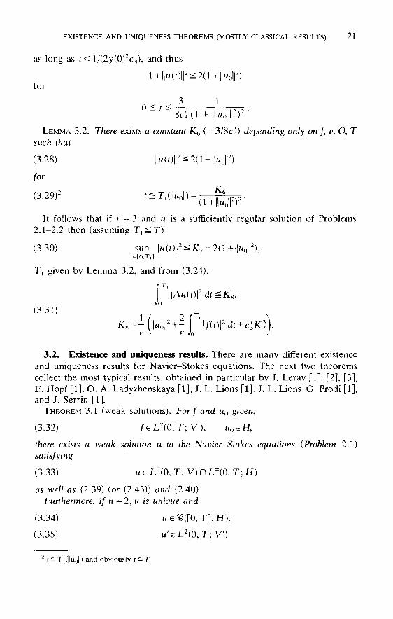
as long as t < l/(2y(0) c4), and thus
LEMMA 3.2. There exists a constant K6 (= 3/8c4) depending only on /, v, Q, Tsuch that
for
It follows that if n = 3 and u is a sufficiently regular solution of Problems2.1-2.2 then (assuming 7^ ̂ T)
Tj given by Lemma 3.2, and from (3.24),
3.2. Existence and uniqueness results. There are many different existenceand uniqueness results for Navier-Stokes equations. The next two theoremscollect the most typical results, obtained in particular by J. Leray [1], [2], [3],E. Hopf [1], O. A. Ladyzhenskaya [1], J. L. Lions [1], J. L. Lions-G. Prodi [1],and J. Serrin [1].
THEOREM 3.1 (weak solutions). For f and u0 given,
there exists a weak solution u to the Navier-Stokes equations (Problem 2.1)satisfying
as well as (2.39) (or (2.43)) and (2.40).Furthermore, if n = 2, u is unique and
2 t ̂ T,(||u0!|) and obviously t ̂ T.

ii) For n = 3, f and u0 given, satisfying (3.38), there exists TH.= T^e(u0) =min (T, T^UoH)), Ti(lluoll) given by (3.29), and, on [0, T%], there exists a uniquestrong solution u to the Navier-Stokes equations, satisfying (3.39), (3.40) with Treplaced by T*.
Remark 3.1. i) The theory of existence and uniqueness of solutions is notcomplete for n = 3: we do not know whether the weak solution is unique (orwhat further condition could perhaps make it unique); we do not knowwhether a strong solution exists for an arbitrary time T. See, however, § 3.4.
ii) We recall that as long as a strong solution exists (n = 3), it is unique in theclass of weak solutions (cf. J. Sather and J. Serrin in J. Serrin [1], or [RT, Thm.III.3.9]).
iii) Due to a regularizing effect of the Navier-Stokes equations for strongsolutions, those solutions can have further regularity properties than (3.39)-(3.40) if the data are sufficiently smooth: regularity properties will be investi-gated in § 4 for the space periodic case and in § 6 for the bounded case.
Let us also mention that if n = 2 and in (3.38) we assume only that u0eH,then the solution u is in L?oc ((0, T]; D(A)) and <g((0, T]; V).
Remark 3.2. The strong solutions (and the weak solution if n = 2) satisfy theenergy equality (3.2). For n - 3 we know only that there exists a weak solutionwhich verifies the energy inequality
;/eL2(0, T;H) is sufficient for n = 2.
It is not known whether all the weak solutions satisfy this inequality or whetherthis inequality is actually an equality.
Remark 3.3. Let us assume that the conditions (3.38) are verified. Then forn = 2, if u is a weak solution to the Navier-Stokes equations (Problem 2.1), uis automatically a strong solution by uniqueness and Theorem 3.2. For n =3,
there exists a unique strong solution to the Navier-Stokes equations (Problem2.2), satisfying3:
THEOREM 3.2 (strong solutions, n = 2, 3). i) For n = 2, / and u0 given,
If n - 3, u is weakly continuous from [0, T] into H:
22 PART I. QUESTIONS RELATED TO SOLUTIONS
and

Thus \\u(t)\\ is bounded for t —> T' - 0, contradicting the assumption that T' < T.
3.3. Outlines of the proofs. The proofs of Theorem 3.1 and 3.2 can befound in the original papers or in the books of O. A. Ladyzhenskaya [1], J. L.Lions [1], [RT]. We finish this section with some outlines of the proofs whichwe need for the sequel.
i) We implement a Galerkin method, using as a basis of H the eigenfunc-tions w,-,/eN, of the operator A (cf. (2.17)). For every integer m, we arelooking for an approximate solution um of Problems 2.1-2.2,
4 Due to the definition of the w,-'s, Pm is also the orthogonal projector on Wm, inV, V, D ( A ) , . . . .
The function um satisfies, instead of (2.39)-(2.40),
where
Pm is the orthogonal projector in H onto Wm.
The semiscalar equation (3.42) is equivalent to the ordinary differentialsystem
and by the technique of Gronwall's lemma,
On the other hand, the energy inequality (3.24), which is valid on (0, T'-e) forall e > 0, implies
the same is true on (0, T#(u0)), but u will be a strong solution on the wholeinterval [0, T] if u satisfies some further regularity property.
For instance, if a weak solution u belongs to L4(0, T; V), then u is a strongsolution: indeed u is a strong solution on some interval (0, T%), T*^= T, Let usassume that the largest possible value of T# is T' < T. Then we must have
EXISTENCE AND UNIQUENESS THEOREMS (MOSTLY CLASSICAL RESULTS) 23

The passage to the limit in (3.42), (3.43) allows us to conclude that u is asolution of Problem 2.1 and proves the existence in Theorem 3.1. However,this step necessitates a further a priori estimate and the utilization of acompactness theorem; we will come back to this point in a more generalsituation in § 13. Finally, we refer to [RT] for the proof of the other results inTheorem 3.1.
iii) For n = 2, the only new element in Theorem 3.2 is (3.39)-(3.40). Weobtain that ueL2(0, T; D(A))nL°°(0, T; V) by deriving further a priori esti-mates on um, in fact, a priori estimates similar to (3.14)-(3.17). We obtain themby taking the scalar product of (3.45) with Aum. Since Pm is selfadjoint in Hand PmAum - APmum = Aum, we obtain, using (3.8),
This relation is the same as (3.2), and we deduce from it the bounds on u^analogous to (3.4)-(3.7):
The existence and uniqueness of a solution wm to (3.42)-(3.45) defined onsome interval (0, Tm), Tm>0, is clear; in fact the following a priori estimateshows that Tm = T.
ii) The passage to the limit m —> °° (and the fact that Tm = T) is based onobtaining a priori estimates on um. The first estimate, needed for Theorem 3.1,is obtained by replacing v by um (= um(t)} in (3.42). Using (2.34) we get
24 PART I. QUESTIONS RELATED TO SOLUTIONS
Then, as usual in the Galerkin method, we extract a subsequence wm, weaklyconvergent in L2(0, T; V) and L°°(0, T; H),
Since |u0m| = |PmM0| = |MO|, we get for um exactly the same bounds as (3.4)-(3.7),from which we conclude that
This relation is similar to (3.9). Exactly as in §3.1, we obtain the bounds(3.14)-(3.17) for um, with u0 replaced by w0m. Since u0m = Pmu0 and Pm is anorthogonal projector in V,

Bu is still in L2(0, T; H), and u' is too.Remark 3.4. Except for Lemma 3.1 and (3.20)-(3.23), the a priori estimates
and the existence and uniqueness results are absolutely the same for both thespace periodic case and the flow in a bounded domain with u — 0 on theboundary (cf. §2.5). If u = < / > ^ 0 on the boundary and/or n is unbounded,similar results are valid. We refer to the literature for the necessary modifica-tions.
3.4. Generic solvability of the Navier-Stokes equations. We do not knowwhether Problem 2.2 is solvable for an arbitrary pair u(), /, but this is generi-cally true in the following sense (A. V. Fursikov [1]):
THEOREM 3.3. For n = 3, given v, 0 (= Q or fl) and u0 belonging to V, thereexists a set F, included in L2(0, T; H) and dense in
so that Bu belongs to L4(0, T; H) and u' belongs to L2(0, T; H).The proof of Theorem 3.2 in the case n = 3 is exactly the same, except that
we use the estimates (3.30), (3.31) valid on [0, T^WoU)] instead of the estimates(3.14)-(3.17) valid on the whole interval [0, T]. Also, instead of using (2.31)and obtaining (3.53), we use the relation (2.32) which gives us
and the properties of B;f and Au are obviously in L (0, T; H) and for B wenotice in the relation (2.31) that
By extraction of a subsequence as in (3.48), we find that u is inL2(0, T;D(A))nL~(0, T; V). The continuity property (3.40) results from(3.39) by interpolation (cf. J. L. Lions-E. Magenes [1] or [RT]). The fact thatu'eL2(0, T;H) follows from (2.43),
and we then find for um exactly the same bounds as for u in (3.14)-(3.17):
EXISTENCE AND UNIQUENESS THEOREMS (MOSTLY CLASSICAL RESULTS) 25
such that for every /eF, Problem 2.2 corresponding to u0,/, possesses a uniquesolution (strong solution}.
Proof, i) Since L2(0, T;H) is dense in Lq(0, T; V), l^q<|, it suffices toshow that every /eL2(0, T; H) can be approximated in the norm ofLq(0, T; V) by a sequence of /m's, fm e L2(0, T; H), such that Problem 2.2 foru0, fm possesses a unique solution.
For that purpose, given /, we consider the Galerkin approximation um
described in § 3.3 above (cf. (3.41)-(3.45)). It is clear that u^ is in L2(0, T; Wm)and hence in L2(0, T; D(A)) and that um is continuous from [0, T] into Wm
and hence into D(A). Now for every m we consider also the solution vm of the

PART I. QUESTIONS RELATED TO SOLUTIONS26
linearized problem
It is standard that the linear problem (3.56)-(3.57) possess a unique solutionsatisfying in particular
We then set wm = um + vm and observe that vvm satisfies
and by adding (3.56) to (3.45) and (3.57) to (3.43),
The proof will be complete if we show that, for m —> o°,
ii) Since |(/-Pm)/(0|->0 for m^<x> for almost every t, and \(I-Pm)f(t)\^\f(t)\, it is clear by the Lebesgue dominated convergence theorem that (I—Pm)/-» 0 in L2(0, T; H) for m -* «.
Multiplying (3.56) by Avm we get
from which it follows that, for m -* °°,
Using (3.64), the estimate (3.47) for um and Lemma 2.1 (with m^O, m2 =1, m3 = 1), we find
In a similar manner we prove that
for m —> oo, and the proof of (3.63) is reduced to that of

l/p = e(l-0) + 0/2. We conclude that um -> u in Lp(0, T; V3/4), and with(3.67), that Bi^-^Bu in Lp/2(0, T; V). Finally, since p<8/3, p-^ 8/3, ase —» 0, we choose e sufficiently small so that p/2 = q
Remark 3.5. As indicated in Remark 3.1, the theory of existence anduniqueness of solutions is not complete when n = 3, while it is totally satisfac-tory for n = 2.
It was Leray's conjecture on turbulence, which is not yet proved nordisproved, that the solutions of Navier-Stokes equations do develop sin-gularities (cf. also B. Mandelbrot [1], [2]). It seems useful to study the propertiesof weak solutions of Navier-Stokes equations with the hope of either provingthat they are regular, or studying the nature of their singularities if they arenot.
The results in §§ 4, 5 and 8 tend in this direction. Of course they (as wouldTheorem 3.3) would lose all of their interest if the existence of strong solutionswere demonstrated.
In (3.48) a subsequence um< of um converges to u, but this is sufficient.Cf. [RT]; this is how (3.37) is proved.
It follows from the proof of Theorem 3.1 (cf. the cited references) that um
converges to u strongly in L2(0, T; V^J and L1/e(0, T;H) for all e >0. By(2.20) with m j = 0 , m 2 =l -e , 0m2 + (l-0)m1 = 0(l-e) = i and the Holderinequality,
therefore B is a bilinear continuous operator from V3/4 x V3/4 into V (see also(2.36)) and
Due to (2.33) and Lemma 2.1,
iii) The proof of (3.65) is technical and we give only a sketch of it.The sequence um converges to some limit u (cf. (3.48))5. Since Bu e
L4/3(0, T; V')6, and since, by Lebesgue's theorem, (I~Pm) Bu -»0 inL4/3(0, T; V), it suffices to show that
EXISTENCE AND UNIQUENESS THEOREMS (MOSTLY CLASSICAL RESULTS) 27

This page intentionally left blank

A New A Priori Estimates and Applications
In this section we establish some properties of weak solutions of Navier-Stokes equations. The results are proved for the space periodic case, but theydo not all extend to the bounded case (cf. the comments, following § 14). Weassume throughout this section that n = 3 and the boundary condition is spaceperiodicity.
By the definition (2.42) of B and as Au = -Au in the space periodic case (cf.(2.14)), we can write
The first term in the right-hand side of (4.3) is majorized by
The second term is a sum of integrals of the type
We can integrate by parts using Stokes' formula; the boundary terms on dQcancel each other due to the periodicity of u, and the integrals take the form
29
where L'r depends also on v, Q and Nr_ t(/).Proof, i) We take the scalar product in H of (2.43) with Aru, and we obtain
where the constant Lr depends on the data, v, Q and Nr_ t(/) = |/|L«.(O,T;V,_,)•Moreover, for any r^3, we have
4.1. Energy inequalities and consequences. We derive formal energy in-equalities assuming that u0, /, u are sufficiently regular.
LEMMA 4.1. If u is a smooth solution of Problems 2.1-2.2 (space periodic case,n = 3), then for each t >0, for any r^l,
c { depending on k, r, Q.We then apply the interpolation inequality (2.20) with
to get
30 PART I. QUESTIONS RELATED TO SOLUTIONS
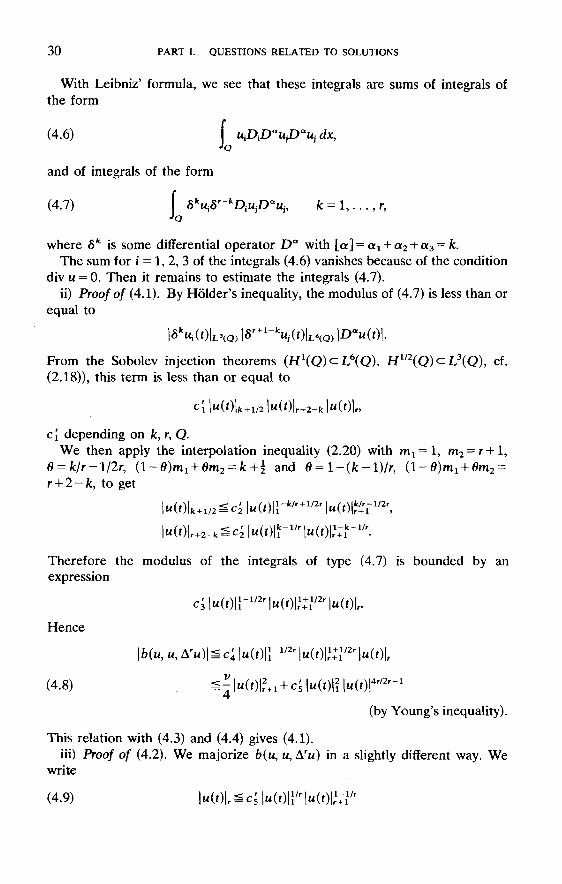
With Leibniz' formula, we see that these integrals are sums of integrals ofthe form
and of integrals of the form
From the Sobolev injection theorems(2.18)), this term is less than or equal to
where 5k is some differential operator Da withThe sum for i = 1, 2, 3 of the integrals (4.6) vanishes because of the condition
div u = 0. Then it remains to estimate the integrals (4.7).ii) Proof of (4.1). By Holder's inequality, the modulus of (4.7) is less than or
equal to
Therefore the modulus of the integrals of type (4.7) is bounded by anexpression
Hence
(by Young's inequality
This relation with (4.3) and (4.4) gives (4.1).iii) Proof of (4.2). We majorize b(u, u, Aru) in a slightly different way. We
write

We then check that Bu, and therefore u = f-vAu-Bu, belongs toL2(Q, T%; V r_j); the continuity of u from [0, T^] into Vr follows by interpolation(cf. J. L. Lions-E. Magenes [1] or [RT, §111.1]).
ii) For u0e V, we observe that the solution u of Problem 2.2 belongs toL2(0, T*; D(A)). Thus u(t}e D(A) = Vr almost everywhere on (0, T*), and wecan find ^ arbitrarily small such that u(t1)eV2 . The first part of the proofshows that ae^d^, T*]; V2]nL2(tl; T*; V3). Hence u(f2)e V3 for some r2e[*i, 7*], t2 arbitrarily close to ta, and ue^([t2, T*]; V3)nL2(f2, T*; V4). Byinduction we arrive at u < # ([*,_!, T*]; Vr)nL2(<,._!, T*; V^) and, since f r_1 isarbitrarily close to 0, the result is proved.
NEW A PRIORI ESTIMATES AND APPLICATIONS 31
by application of (2.20) with m^ = 1, m2 = m + l, 0 = l-l/r. Then (4.8) gives
This relation combined with (4.3)-(4.4) gives (4.2).An immediate consequence of (4.2) is that u remains in Vr as long as \\u(t)\\
remains bounded. This is expressed inLEMMA 4.2. If u0e Vr and /eL°°(0, T; V^), r^l, then the solution u to
Problem 2.2 given by Theorem 3.2 ii) belongs to <g([0, T*]; Vr).If u0e V and /eL°°(0, T; V r_j), r^l, then we<g((0, T*]; Vr).Proof, i) We consider the case u0e Vr, and we first show that u belongs to
i-°°(0, T*; Vr). For that it suffices to prove that the Galerkin approximation i^of u constructed in § 3 remains bounded in L°°(0, T^; Vr) as m -»<». We takethe scalar product in H of (3.45) with ATum = (—\)rb.rum, and since Pm isself ad joint in H and PmArum = A'^, we get
due to (3.51) we conclude that
This is similar to (4.3) and thus, exactly as in Lemma 4.1, we get theanalogue of (4.2):
Now Pm is a projector in Vr too, and |PmWo|r^|w0|r, so that um remains in abounded set of L°°(0, T*; Vr) and L2(0, T*; Vr+1), and
We are now able to give some indications on the set of Hm-regularity of aweak solution.
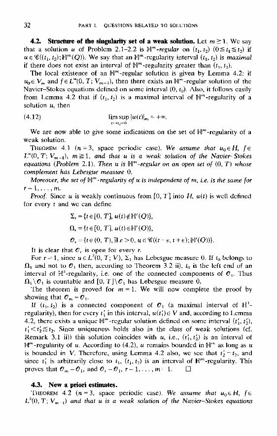
THEOREM 4.1 (n = 3, space periodic case). We assume that u0eH, /eL°°(0, T; Vm_l), m=Sl , and that u is a weak solution of the Navier-Stokesequations (Problem 2.1). Then u is Mm-regular on an open set of (0, T) whosecomplement has Lebesgue measure 0.
Moreover, the set of Hm-regularity of u is independent of m, i.e. is the same forr = 1, . . . , m.
Proof. Since u is weakly continuous from [0, T] into H, u(t] is well definedfor every t and we can define
32 PART I. QUESTIONS RELATED TO SOLUTIONS
4.2. Structure of the singularity set of a weak solution. Let m ̂ 1. We saythat a solution u of Problem 2.1-2.2 is Hm-regular on (f1} r2) (O^f^fz) ifu e <#((*!, f2);Hm(Q)). We say that an Hm-regularity interval (r l5 r2) is maximalif there does not exist an interval of B-Om-regularity greater than ( f l 5 1 2 ) .
The local existence of an Hm-regular solution is given by Lemma 4.2: ifUQ<= Vm and /eL°°(0, T; Vm_ t), then there exists an (HP-regular solution of theNavier-Stokes equations defined on some interval (0, r0). Also, it follows easilyfrom Lemma 4.2 that if ( r l 5 t 2 ) is a maximal interval of Hm-regularity of asolution M, then
It is clear that Or is open for every r.For r= 1, since weL2(0, T; V), Si has Lebesgue measure 0. If t0 belongs to
O,i and not to Ol then, according to Theorem 3.2 ii), f0 is the left end of aninterval of H1-regularity, i.e. one of the connected components of GV Thusn^O1! is countable and [0, TJX^j has Lebesgue measure 0.
The theorem is proved for m = 1. We will now complete the proof byshowing that Om =6^.
If (t\, t2) is a connected component of Ol (a maximal interval of H1-regularity), then for every t{ in this interval, u(t'i)e V and, according to Lemma4.2, there exists a unique IH!m-regular solution defined on some interval (f(, t2),t'1<t2^=t2. Since uniqueness holds also in the class of weak solutions (cf.Remark 3.1 ii)) this solution coincides with u, i.e., ( t { , t 2 ) is an interval ofHm-regularity of u. According to (4.2), u remains bounded in Hm as long as uis bounded in V. Therefore, using Lemma 4.2 also, we see that t2 = t2, andsince t[ is arbitrarily close to f1? (^, t2) is an interval of Hm-regularity. Thisproves that Om =Ol} and
4.3. New a priori estimates.THEOREM 4.2 (n = 3, space periodic case). We assume that u0eH, fe
L2(0, T; Vm_ t) and that u is a weak solution of the Navier-Stokes equations

Then we deduce
NEW A PRIORI ESTIMATES AND APPLICATIONS 33
(Problem 2.1). Then u satisfies
r = l , . . . , m + l, where the constants cr depend on the data v, Q, u0, /, and thea/s are given by
Proof, i) Let (ah ft), i e N , be the connected components of 0^, which arealso maximal intervals of Hm-regularity of u.
On each interval (ah ft), the inequalities (4.1) are satisfied, r = 1,. . . , m, andwe write them in the slightly stronger form
By integration in t from «j to ft, we get
From (4.12), the first term in the left-hand side of this inequality vanishes,since (af, ft) is a maximal interval of IHm-regularity. Thus
By summation of these relations for i e N , we find, since u e L2(0, T; V),
ii) The proof of (4.13) is now made by induction. The result is true forr ~ 1. We assume that it is true for 1, . . . , r, and prove it for r +1 (r^i m).
We have
(by Holder's inequality),

Therefore (4.13) follows for r + 1, due to (4.16) and the inductionassumption.
Remark 4.1. As indicated at the beginning of this section, all the resultshave been established in the periodic case. We do not know whether they arevalid in the bounded case (although it is likely that they are) except for thefollowing special results: (4.1) and (4.2) for r= 1, which coincide with (3.24); inTheorem 4.1 the fact that the complement of Oi in [0, T] has Lebesguemeasure 0 and is closed; and (4.13) for r = 2(«r=|) (same proofs)1.
The following interesting consequence of Theorem 4.2, which relies only on(4.13) with r-2, is valid in both the periodic and the bounded cases.
THEOREM 4.3. We assume that n = 3 and we consider the periodic or boundedcase. We assume that uQeH and /eL°°(0, T; H). Then any weak solution u ofProblem 2.1 belongs to L\Q, T;l°°(0)), O = fl or Q.
Proof. Because of (2.26)
1 Cf. also § 6, and in particular Remark 6.2, for a complete extension of Theorem 4.1 to thebounded case.
where
34 PART I. QUESTIONS RELATED TO SOLUTIONS
and by Holder's inequality
and the right-hand side is finite, thanks to (4.13) (r = 2, cf. Remark 4.1).

j Regularity and Fractional Dimension
If the weak solutions of the Navier-Stokes equations develop singularities, asLeray has conjectured, then a natural problem is to study the nature of thesingularities. B. Mandelbrot conjectured in [l]-[2] that the singularities arelocated on sets of Hausdorff dimension <4 (in space and time), and V. Schefferhas given an estimate of the dimension of the singularities which he succes-sively improved in [l]-[4]. A more recent (and improved) estimate is due to L.Caffarelli-R. Kohn-L. Nirenberg [1]. In this section we present some resultsconcerning the Hausdorff dimension of the singular set of weak solutions,following (for one of them) the presentation in C. Foias-R. Temam [5].
5.1. Hausdorff measure. Time singularities. We recall some basic defini-tions concerning the Hausdorff dimension (cf. H. Federer [1]). Let X be ametric space and let D >0. The D-dimensional Hausdorff measure of a subsetY of X is
where
the infimum being taken over all the coverings of Y by balls Bj such thatdiam By ( = diameter of B,)^e.
It is clear that ^D-e(Y)^De.(Y) for e^e' and fj,D(Y)e[0,+<»]. Since/*D,e(Y)^eD-%Doe(Y) for D>D0, then if ^Da(Y)<™ for some D0e(0,«>)then fxD(Y) = 0 for all D>D0. In this case the number
is called the Hausdorff dimension of Y. If the Hausdorff dimension of a set Y isfinite, then Y is homeomorphic to a subset of a finite dimensional Euclideanspace. Finally, let us also mention the useful fact that JJLD(-) is countablyadditive on the Borel subsets of X (see Federer [1]).
The first result on the Hausdorff dimension of singularities concerns the setof t in [0, T] on which u(t) is singular, u(t)£ V. Actually this is a restatementby V. Scheffer [1] of a result of J. Leray [3] (cf. also S. Kaniel-M. Shinbrot [1]).
THEOREM 5.1. Let n = 3, C = fl or Q, and let u be a weak solution to theNavier-Stokes equations (Problem 2.1). Then there exists a closed sewhose ^-dimensional Hausdorff measure vanishes, and such that u is (at least)continuous from [0, T]\<£ info V.
Proof, i) The proof of this theorem is partly contained in that of Theorem4.1 (cf. also Remark 4.1). We set # = [0, TJXC1!, and we only have to provthat the ^-Hausdorff measure of <£ is 0.
35

36 PART I. QUESTIONS RELATED TO SOLUTIONS
Let (ah ft), i / , be the connected components of Gl. A preliminary result,due to J. Leray [3], is
Then we integrate on (ah ft) to obtain
and we add all these relations for i e I to get
ii) The proof now follows that given in V. Scheffer [1, §3]. For every e >0,we can find a finite part Ie of / such that
The set [0, T]\Uieie («i» ft) is the union of a finite number of mutually disjointclosed intervals, say B,, / = 1,. . . , N. It is clear that U/li Bj ^ $, and since theintervals (ah ft) are mutually disjoint, each interval (at, ft), i£le, is included inone, and only one, interval Bj. We denote by 7, the set of fs such thatBJ =>(«<, ft). It is clear that /E, 7 l 5 . . . , /N , is a partition of I and that J3, =(IU (<*, ft)) U (ft n *) for all / = 1,. . . , N. Hence
diam
and
Letting e -» 0, we find
5.2. Space and time singularities. The second result concerns the Hausdorffdimension in space and time of the set of (possible) singularities of a weak
where K6 depends only on /, v and C (= fl or Q). Thus
Indeed, let (ah ft) be one of these intervals and let te(di, ft). According toTheorem 3.2 and (3.29),
REGULARITY AND FRACTIONAL DIMENSION 37
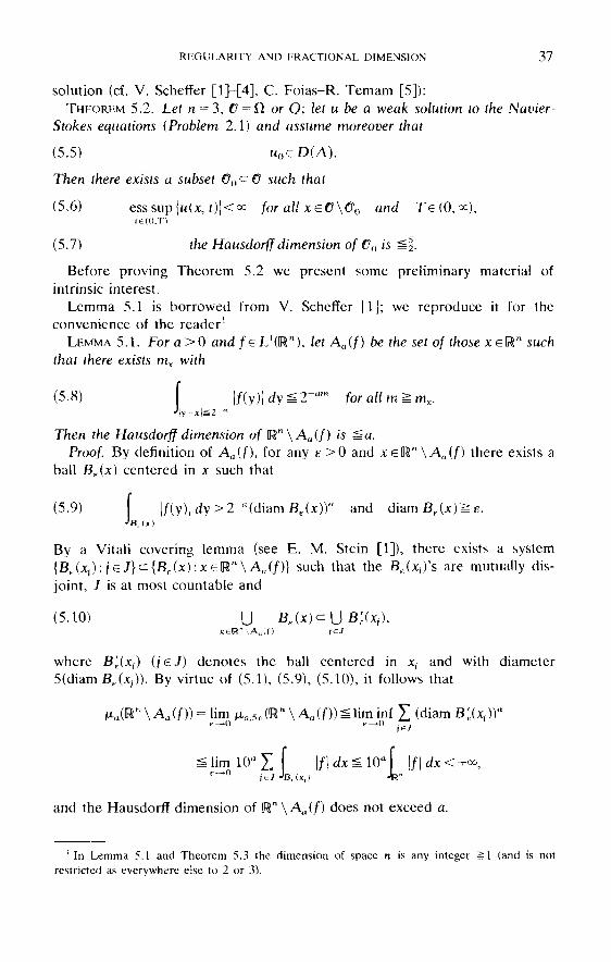
solution (cf. V. Scheffer [l]-[4], C. Foias-R. Temam [5]):THEOREM 5.2. Let n - 3, G = £l or Q; let u be a weak solution to the Navier-
Stokes equations (Problem 2.1) and assume moreover that
Then there exists a subset 00<^0 such that
(5.7) the Hausdorff dimension of
Before proving Theorem 5.2 we present some preliminary material ofintrinsic interest.
Lemma 5.1 is borrowed from V. Scheffer [1]; we reproduce it for theconvenience of the reader1
LEMMA 5.1. For a>0 and feL'([R"), let Aa(f) be the set of those xeUn suchthat there exists mx with
Then the Hausdorff dimension of IR"\Aa(/) is ^a.Proof. By definition of Aa(/), for any e >0 and x e!R" \ Aa(_f) there exists a
ball BF(x) centered in x such that
1 In Lemma 5.1 and Theorem 5.3 the dimension of space n is any integer ^1 (and is notrestricted as everywhere else to 2 or 3).
By a Vitali covering lemma (see E. M. Stein [1]), there exists a system{Be(x,):/eJ}c={BF(x):xe[Fr\Aa(/)} such that the Be(x,-)'s are mutually dis-joint, J is at most countable and
where B'E(XJ) (j&J) denotes the ball centered in xf and with diameter5(diamBE(x,-)). By virtue of (5.1), (5.9), (5.10), it follows that
arid the Hausdorff dimension of [Rn\ Aa(/) does not exceed a.
38 PART I. QUESTIONS RELATED TO SOLUTIONS
THEOREM 5.3. Let G be an open subset in Un and let Te (0, <»), Kp <°° and/eLp(Gx(0, T)) be given. Let moreover
be such that
in the distribution sense in G x (0, T)
and
Then there exists a subset G0 <= G such that
and the Hausdorff dimension of G0 is Simax{n + 2 —2p, 0}.Proof. We infer from (5.11)-(5.12) and the regularity theory for the heat
equation (cf. O. A. Ladyzhenskaya-V. A. Solonnikov-N. N. Ural'ceva [11])that:
(where W2'P(G) is the usual Sobolev space of functions defined on G, whichtogether with all their derivatives up to order 2 belong to LP(G)). If ̂ e Co(G)and vl = (f>v, then u t will satisfy (5.11)-(5.13), and also
where /t is a suitable function which also belongs to Lp(Gx(0, T)).Therefore, taking into account that the Hausdorff measures are Borel meas-
ures, we can consider only the special case
where K is a certain compact set <=(R" while to is of Lebesgue measure =0. It isclear that in this case v(x, t) coincides almost everywhere in J?"x(0, T) withthe function
2 It is well known (cf. for instance J. L. Lions [1] or R. Temam [RT, Chap. Ill, Lemma 1.2]) that ifv satisfies (5.11) and (5.12) then v is equal for almost every f e (0 , T) to a function in«([0, T]; L2(G)), and therefore u(0) makes sense.

REGULARITY AND FRACTIONAL DIMENSION 39
where
and
Therefore we can assume that, for any t e (0, T)\o>, v(x, t) = w(x, t) everywhereon IRn. It follows that for such f's and for all x0e[Rn, we have
(by (4.16) and the change of variables
where, for all
From the classical theorem on the maximal functions (see E. M. Stein [1]), wehave
Since for t e [0, T]\o>, v(x, t)- w0(x, t) is continuous in x, from (5.17) we finallyinfer that
But, setting

40 PART I. QUESTIONS RELATED TO SOLUTIONS
we have for all xeR", fe(0, T), and because of standard estimates on E:
where c'n,c'n,... are suitable constants (with respect to (jc, t}) and
Therefore Aa(g) (see Lemma 5.1) makes sense, and if
obviously
Consequently (since w0 is continuous on [Rnx(0, T)), by virtue of (5.19) wehave

REGULARITY AND FRACTIONAL DIMENSION 41
Therefore the set
is included in R"\Aa(g). From Lemma 5.1 we infer that the Hausdorffdimension of G0 is ^a. The conclusion (5.14) is now obtained by lettinga —» max {0, n + 2 - 2p}.
Remark 5.1. The proof of Theorem 5.2 shows that the result remains validif G = Q and we replace (5.11) by
We now turn to the proof of Theorem 5.2.Proof of Theorem 5.2. Obviously it is sufficient to prove the result for a fixed
Te (0, o°). Also it is clear that each component v(x, t) = w,(x, f) (/ = 1, 2, 3) ofu(t) satisfies (5.11)-(5.12). Since
we find by interpolation that weL r(0, T; L6r/(3r~4)(n)) for every r i=2 (see J. L.Lions-J. Peetre [1]), whereupon, for r = -y, we obtain
It follows that
since
We then get
where (see (5.21))
By referring to the regularity theory for the Stokes system (5.22) (cf. K. K.Golovkin-O. A. Ladyzhenskaya [1], K. K. Golovkin-V. A. Solonnikov [1], V.A. Solonnikov [2]), we see that
3 This boundary condition must be replaced by the periodicity condition when G = Q; seeRemark 5.1.

42 PART I. QUESTIONS RELATED TO SOLUTIONS
for any Ka <|. Thus for v(x, t) = u,(x, t) we obtain
so that by virtue of Theorem 5.3, we obtain that the seton
has the Hausdorff dimension ^5-2a. The conclusion follows by letting

6 Successive Regularity and CompatibilityConditions at t = 0 (Bounded Case)
In this section we assume that n = 2 or 3 and consider the flow in a boundeddomain jQcilR". We are interested in the study of higher regularity propertiesof strong solutions, assuming that the data u0, /, O possess further regularityproperties. While this question is essentially solved in § 4 for the space periodiccase (through Lemmas 4.2 and 4.1), the situation in the bounded case is moreinvolved. In particular, we derive in this section the so-called compatibilityconditions for the Navier-Stokes equations, i.e., the necessary and sufficientconditions on the data (on dfl at t = 0) for the solution u to be smooth up totime t = 0.
6.1. Further properties of the operators A and B. We recall that if (1satisfies (1.7) with r = m + 2 , and if m is an integer >n/2 (m^2 for n — 3, 2),then Hm(fl) is a multiplicative algebra:
For every integer m we define the space
which is a Hilbert space for the norm induced by Hm(n) = Hm(fl)n. It is clearthat Em+i<=Em, for all m and that E0 = H:
The orthogonal projection from L2(H) onto H being denoted by P as before,we introduce the operator s&
which is linear continuous from JEm, mi?2, into E0 = H. Actually the operatorP is linear continuous from Hm((l) into H m (O) Pi H = Em (cf. [RT, Chap. I,Remark 1.6]), and therefore
s£ is linear continuous from Em+2 into Em.
Now if ueE m + 2 n V, m^O, and s£u=feEm, then A u + / = (7-P)Au be-longs to H1, which amounts to saying (cf. §2.5) that there exists peH1^)such that Au+/ = Vp. Hence
43

44 PART I. QUESTIONS RELATED TO SOLUTIONS
and u is the solution to the Stokes problem associated with /. The theorem onthe regularity of the solutions of Stokes problem mentioned in § 2.5 impliesthen that
s& is an isomorphism from E onto
It is clear from (6.6) that2
Operator B. Lemma 2.1 shows us that b(u, v, w) is a trilinear continuousform on Hm '(n)xHm2+1(n)xH if ml + m2>n/2 (or ml + m2^n/2 if m^Oforall 0- This amounts to saying that the operator B defined in (2.41) is bilinearcontinuous from Hm '(ft)x[Hlm2+1(n) into H, under the same conditions onm l 5 m2. Clearly (u • V)u belongs in this case to L2(O) and
We have
LEMMA
Proof. If m = 1, u, v eH2(fl), then obviously (u • V}v eL2(H) and
belongs to L2(H), since the first derivatives of u and v are in L6(H) (at least) andu and v are continuous on H. The operator P mapping fl-flr(^) into Hr(n)nH,B(u, v) = P((u - V ) u ) is in H1(n)nH=E1 .
If m ̂ 2, then ut and DtVj are in H2(O), and their product is too, due to(6.1). Hence (u • V)ueHm(H) and P((u • V)u) as well3.
6.2. Regularity results. If u() and / are given, satisfying
then Theorem 3.2 asserts the existence of a (strong) solution u of Problem 2.2defined on some interval [0, T"], T" = T if n — 2, T'^ T if n = 3. Changing ournotation for convenience, we write T instead of T', and
1 If $ is the inverse of ^|Em42nv ^^M = u' f°r a" u e^m+2n ̂ but in general ^stfu^ u for anarbitrary u e Em+2, m ̂ 0.
2 Because of (6.7) and (6.8), Vm is a closed subspace of Em, for all m e N, the norm induced by£m being equivalent to that of Vm. In the space periodic case, the analogue of Em —H™(Q)r\H isequal to Vm.
3 The proof shows also that B(Em x£m + 1)c Em for m^2.

SUCCESSIVE REGULARITY AND COMPATIBILITY CONDITIONS AT t = 0 45
Our goal is to establish further regularity properties on M, assuming moreregularity on w0, /.
We introduce the space
where m is an integer and / = [m/2] is the integer part of m/2, i.e. m =21 orm = 2 i + l.
We begin by assuming that for some m ̂ 2
and we make the following observation:LEMMA 6.2. If u is a strong solution to the Navier-Stokes equations and u{)
and f satisfy (6.15) for some m^2, then the derivatives at(d]u/dt')(Q), / = ! , . . . , / , can be determined "explicitly''' in terms of u0 and /(O),and
Proof. By successive differentiation of (2.43), we find
where we set <£ ( / ) = d'<J>/dfJ', 8(r) = Bu(r), so that
Now by (6.5), (6.10), (6.15), j3(0) = Bu(0)e£m_1, and u'(0) =Similarly,
The proof continues by induction on / using (6.5), (6.10), (6.15), and showsthat
f oIt is known that for an initial and boundary value problem, the solutions may
not be smooth near f = 0, even if the data are c$co. For Navier-Stokesequations, the following theorem gives the necessary and sufficient conditionson the data for regularity up to t = 0, the compatibility conditions (cf. (6.21)).

46 PART I. QUESTIONS RELATED TO SOLUTIONS
THEOREM 6.1. We assume that n — 2 or 3, H satisfies (1.7) with r =m + 2, m ^2, u0 and f satisfy (6.15) and
4The fact that u(1)eL2(0, T; D(A))nL°°(0, T; V) is obtained by deriving one more a prioriestimate for the Galerkin approximation um of u (cf. (3.42)-(3.45)): that u^ belongs to a boundedset of L2(0, T; D(A))nL°°(0, T; V). As (3.47), (3.52), this estimate is obtained by differentiating(3.45) with respect to t and taking the scalar product in H of the differentiated equation with u^,and Au^,.
The fact that ue <£([(), T]; V) follows by interpolation, like (2.50), after we show that u" =f-i/Au'-B(u', u)-B(u, u')eL2(0, T; H). It is clear that /' and vAu' are in L2(0, T; H). For thequadratic terms, it follows from (2.47), (2.48) that B maps (L2(0, T; D(A))nL°°(0, T; V))2 intoL4(0, T;H).
and that u is a (strong) solution of Problem 2.2.Then a necessary and sufficient condition for u to belong to Wm is that
Proof, i) We first show that the condition (6.20) (which is void for m = 2) isnecessary if m ̂ 3.
We know that u is in <g([0, T]; V). If u belongs to Wm, then u e^([0, T];Em), u'e<g([0, T];Em_2), and necessarily u' takes its values inEm_2 H V, so that u' e <g([0, T]; Em_2 n V) and u'(0) 6 V. The proof is the samefor the other derivatives.
We now prove that under conditions (6.15), (6.20) and (6.21) u is in Wm.ii) For / = !, the equation
together with u(1)(0)e V given by (6.19), allows us to show that4
We continue by induction; once we establish that
we consider (6.17), (6.18) with 7 = / and u(n(0) given by (6.19) and belonging toV (if m = 2J + 1) or to H (if m =21). In a similar manner, we show that
iii) The next step in the proof consists in showing that

SUCCESSIVE REGULARITY AND COMPATIBILITY CONDITIONS AT t = 0 47
For that purpose we write (6.17), (6.18) in the form
f(i) and u()+1) are in <g([0, T]; H) (at least). Because of Lemma 2.1 and (2.36),B is bilinear continuous from V x V into V_1/2. Hence by (6.24), for i =0 , . . . , / , and / = 0 , . . . , / - 1,
Since A is an isomorphism from V3/2 onto V_1/2, (6.27) implies then thatu(j)e^([0, T]; V3/2),/ = 0,. . . ,1-1. Using again Lemma 2.1, B is a bilinearcontinuous operator form V3/2 x V3/2 into H. Thus, for the same values of i and/ as in (6.28),
and (6.26) follows,iv) Finally we show that u e Wm, i.e.,
For j = I, this is included in (6.25). For j = 1 — 1, using (6.10) and (6.26) we findthat
and then (6.5), (6.27) and (6.25) show that u(("1}e <g([0, T]; Em_2l+2). Theproof continues by induction for j = 1 — 2,... ,0.
Theorem 6.1 is proved.
6.3. Other results. We particularize Theorem 6.1 to the case m = 3.THEOREM 6.2. We assume that n = 2 or 3, fl satisfies (1.7) with r = 5,u0e
H3(n)nV,/e<£([0, rfcHX^HH) and d//dreL2(0, T;H). Then the solutionu of Problem 2.2 defined by Theorem 3.2 on some interval [0, T*], 0< T^T,belongs to <£([0, T*];H3(n)n V), if and only if
The only condition left in (6.21) is (6.30). Since u'(G)&El =H1(H)nH,u'(0) • v = 0 on F, and (6.30) is a restrictive assumption for the tangential valueon F of
Another way to formulate (6.30) is this: , where (cf. [RT, Chap.

48 PART I. QUESTIONS RELATED TO SOLUTIONS
I, Thm. 1.5]) q0 is a solution of the Neumann problem:
^0 must be such that the tangential components on F of ̂ o and Vq0 coincide:
(6.32), (6.33) constitute an overdetermined boundary value problem (Cauchyproblem on F for the Laplacian) which does possess a solution.
If the compatibility conditions (6.21) are not satisfied, the other hypothesesof Theorem 6.1 being verified, we get a similar result of regularity onOx(0, T]:
THEOREM 6.3. We make the same hypotheses as in Theorem 6.1, but theconditions in (6.21) are not satisfied5. Then
Proof. Thanks to (3.39), there exists 0< t0< T%, tQ arbitrarily close to 0, suchthat u(f0)eD(A). Equation (6.19) for t0 and j = l shows that w'(f0)eH. Weconclude as in Theorem 6.1 or 3.2 that u'eL2(f0 , T*; V)n^([f0,1*]; H).
We choose r l s t0<t1<T^, t1 arbitrarily close to tQ, such that w'^^e V, andconclude that u 'eL 2 ( f l 9 T*; D(A)}n(€([tl, T*]; V). We then choose f 2 > f i <t2<T%, t2 arbitrarily close to tl, such that u'(t2)eD(A), etc.
Finally we get that u e <g([f,, T*]; Em), u'e <£((>,, T*]; Em_2),. . ., for f, arbi-trarily close to 0, and the result is proved.
Remark 6.1. If F is ^°°, u()e c€eo(£l)n n H, f e ^°°(nx[0, T])", then u e
«°°(n x [0, T])". The ^~ regularity in O x (0, T] was proved in O. A.Ladyzhenskaya [1]. Of course, by combining Theorems 6.1 and 6.2 with theimbedding theorems of Sobolev spaces into spaces of continuously differenti-able functions, one can get partial results of regularity in spaces of ^fc
functions.Remark 6.2. Let u be a weak solution of the Navier-Stokes equations
(Problem 2.1) in the three-dimensional case. Let Ol be the set of H1-regularityof u defined in Theorem 4.1 and Remark 4.1, and let <£ = [0, TJXOV Accordingto Theorem 6.3, if u0eH, f e Wm^2 and hypothesis (6.20) is verified, Oi is alsoan interval of Hr-regularity, r^m,i.e., ue^C^; Hm(ft)n V). This is theanalogue of Theorem 4.1 for the case of a bounded domain.
Remark 6.3. Let u be a weak solution of Navier-Stokes equations (Problem2.1) in the three-dimensional case. We assume that M0eIHl,f eHm-2(H)nH, m^3, is independent of t. Then for every teO,u'(t) makes sense and
5 It suffices also to assume that un e V instead of un e Em D V.

SUCCESSIVE REGULARITY AND COMPATIBILITY CONDITIONS AT t = 0 49
belong to V. If we introduce the analogue i/>(0 of (6.31)
and write that the overdetermined boundary value problem similar to (6.32),(6.33) possesses a solution, we conclude that u(t) belongs, for t in C^ to acomplicated "manifold" of V: i// depends on u(t] (and /); q(t) =jV(div i/f(0, <MO • v), where N is the "Green's function" of the Neumannproblem (6.32): the condition (6.33) is the "equation" of the manifold.
A similar remark holds for every t >0 for a strong solution; similar remarksfollow from the other conditions (6.21) if m ̂ 5.
Remark 6.4. If we introduce pressure, then we clearly get regularity resultsfor pressure:
In the situation of Theorem 6.1,
and in the situation of Theorem 6.3,

This page intentionally left blank

Analyticity in Time
In this section we prove that the strong solutions are analytic in time asD(A)-valued functions. We assume for simplicity that f e H is independent oft: we could as well assume that / is an H-valued analytic function in aneighborhood in C of the positive real axis. The interest of the proof givenbelow is that it is quite simple and relies on the same type of method as thatused for existence. The method applies also to more general nonlinear evolu-tion equations with an analytic nonlinearity.
7.1. The analyticity result. The main result is the following one:THEOREM 7.1. Let there be given u0 and f, u0e V, /e H independent of t.If n=2, the (strong) solution u of Problem 2.2 given by Theorem 3.2 is
analytic in time, in a neighborhood of the positive real axis, as a D(A}-valuedfunction.
If n = 3, the (strong) solution u of Problem 2,2 given by Theorem 3.2 isanalytic in time, in a neighborhood in C of the interval (0, T#), as a D(A)-valued function.
Proof, i) Let C denote the complex plane and Hc the complexified space ofH, whose elements are denoted u + iv, u, v e H, i = V/-^T. Similarly Vc, V'c arethe complexified V, V, and Xc is the complexified space of a real space X. Bylinearity, A (resp. Pm, resp. B) extends to a selfadjoint operator in Hc (resp. tothe orthogonal projection in Hc, Vc, Vc, onto the space Cw,+ • • • +Cwm,resp. a bilinear operator from Vcx Vc into Vc).
Consider now the complexified form of the Galerkin approximation ofNavier-Stokes equations, i.e., (compare with (3.41)-(3.45)) the complexdifferential system in PmHc:
where £eC, and um maps C (or an open subset of C) into PmHc =Cw, + • • • - f Cwm. The complex differential system (7.1), (7.2) possesses aunique solution um defined in C in some neighborhood of the origin.
It is clear that the restriction of um(£) to some interval (0, Tm) of the real axiscoincides with the Galerkin approximation u m ( t ) defined in the real field by(3.41H3.45).
ii) As in the real case, we now prove some a priori estimates on um. We takethe scalar product in Hc of (7.1) with Aum(£)
51
7

52 PART I. QUESTIONS RELATED TO SOLUTIONS
We multiply this relation by eie, with £ = seie, and for fixed 0, |0| < ir/2, we get:
Therefore
The absolute value of the term involving / is less than or equal to
For the term involving B, we use the inequality (2.32), which clearly extends tothe complex case1,
This allows us to write
(by Young's inequality, see (3.10)),where c' depends on the data v, u0, ft.
If we take into account this majorization and (7.4), then (7.3) becomes
The inequality (3.25) is still valid in the complex case
and thus
1 This relation, which is not so good as the first relation (2.31), is valid for both dimensions, n = 1and 3.

ANALYTICITY IN TIME 53
This differential inequality is of the same type as (3.27), setting y(s) =\\u,,,(se'"}\\\ c'4 = ( l / ( c o s 3 0 ) ) ( ( 2 / i > ) \ f \ 2 + c'). We conclude, as in Lemma3.2, that there exists K'(, which depends only on / , v and il (or (2), suchthat
This shows that the solution um of (7.1)-(7.2), which was defined andanalytic in a neighborhood of £ = 0, actually extends to an analytic solution ofthis equation in an open set of C containing (see Fig. 7.1):
The estimate (7.8)-(7.10) shows that
iii) The analyticity of um and Cauchy's formula allow us to deduce from(7.12) a priori estimates on the derivatives of um (with respect to £) on compactsubsets of A(u ( )) . Indeed, for £ e A ( w ( ) ) and k e N , k ^ l .
for
where d = d(£, dA(u,,)) is the distance of £ to the boundary dA(u0) of A(u0).
FIG. 7.1. The region A(u ; )) in C.
54
Therefore
PART I. QUESTIONS RELATED TO SOLUTIONS
Using again Cauchy's formula (7.13) and (7.16), we obtain also for every£eK and keN:
where K' (containing K] is the set
iv) We now pass to the limit, m—»°°. Since the set {ve Vc, \\v\\^p} iscompact in Hc for any 0 < p < o°, we can apply to the sequence um the vector
and by (7.12), for any compact set K<=A(MO)
Considering (7.1), we find that
Thus
and it follows from (7.14) that for every compact subset K of A(u0)
where c'4<™, depends on K and the data,

ANALYTICITY IN TIME 55
version of the classical Vitali's theorem. Thus we can extract a subsequence um,which converges in Hc, uniformly on every compact subset of A(u0) to anHc-valued function u*(£) which is analytic in A(u0) and satisfies obviously:
Since the restriction of u^ to the real axis coincides with the Galerkinapproximation in R+ of the Navier-Stokes equation, it is clear that therestriction of u*(£) to some interval (0, T') of the real axis coincides with theunique (strong) solution u of the Navier-Stokes equations given by Theorem3.2. Hence u* is nothing else than the analytic continuation to A(u0) (at least)of u, and we will denote the limit w(£) instead of w*(£). Secondly the wholesequence um(-) converges to u(-) in the above sense (i.e. uniformly on compactsubsets of A(u0), for the norm of Hc).
Since the injection of D(A) in V is compact, it also follows from (7.16) andVitali's theorem that the sequence um converges to u in V uniformly on everycompact subset of A(u0), and that
with the same constant c^K) as in (7.17). Finally the majorizations (7.14),(7.18) imply that dkujd£,k converges to dku/d£k in V uniformly on everycompact subset K of A(u0), and
K' defined in (7.19).To conclude, we observe that the reasoning made at t = 0 can be made at any
other point t0e (0, o°) such that u(r0)e V. We obtain that u is a D(A)-valuedanalytic function at least in the region of C:
where the union is for those f0's for which (£0e (0, °°) and u(t0)e V). Finally weobserve that, actually, A(u0) = A(||u0||) depends only on the norm in V of u0 anddecreases as ||u0|| increases. Therefore if u is bounded in V on some interval[a,^],supte[a^]||u(r)||^R, then
and this guarantees that the domain of analyticity of u contains the regionmentioned in the statement of Theorem 7.1 (See Fig. 7.2.) The proof ofTheorem 7.1 is complete.

56 PART I. QUESTIONS RELATED TO SOLUTIONS
Fir, 7.2. Uloe(a,3,{'o + A(R)}.
7.2. Remarks.Remark 7.1. Of course the result of analyticity given by Theorem 7.1
applies as well to a weak solution of the Navier-Stokes equations (Problem 2.1,n = 3) near a point t0 belonging to the set of (HI1-regularity (cf. § 4). If f e H isindependent of t, and (a, /3) is a maximal interval of H1-regularity of a weaksolution u, then u is a D(A)-valued analytic function in
Remark 7.2. Theorem 7.1 and Remark 7.1 extend easily to the case where /is an He-valued analytic function of time in a neighborhood of the positive realaxis: it suffices to replace everywhere in the proof A(w()) (or f() + A(u(f0))) by itsintersection with the domain of analyticity of /.
We conclude this section with the following:PROPOSITION 7.1. Under the same hypotheses as in Theorem 7.1, for 0<t^
u0||), Ti(||woll) given by (7.10), the following relations hold:3T,4-* 1
Proof. It suffices to apply (7.22), (7.23) with K = {t}. The distance d(t, dA(u0))appears in the right-hand side of these inequalities, and an elementary calcula-tion shows that for 0 ̂ t ̂ { T\( I I M O I I ) , this distance is
Remark 7.3. When the compatibility conditions (6.21) are not satisfied, u isnot smooth near t = 0 and the H-norm of the derivatives u (k)t tends toinfinity as t —» 0. The relations (7.21), (7.22) give some indications on the wayin which they tend to infinity. A similar result has been obtained by totallydifferent methods by G. looss [1] and by D. Brezis [1].
where
X Lagrangian Representation of the Flow
We assume that the fluid fills a bounded region O of 1R3. The Lagrangianrepresentation of the flow of the fluid, mentioned in § 1, is determined by afunction <£:{a, r}eHx(0, T)—»4>(a, t)e£l, where O(a, t) represents the posi-tion at time t of the particle of fluid which was at point a at time t - 0 (flowstudied for time r, O^r^T) . This also amounts to saying that {t >-»<I>(a, t}} isthe parametric representation of the trajectory of this particle.
The Lagrangian representation of the flow is not used too often because theNavier-Stokes equations in Lagrangian coordinates are highly nonlinear. Itplays an important role, however, in two cases at least: it is used in thenumerical computation of a flow with a free boundary, and, in the mathemati-cal theory of the Navier-Stokes equations, it is the starting point of thegeometrical approach developed by V. I. Arnold [1], D. Ebin-J. Marsden [1],among others.
If we are given u, a strong solution of the Navier-Stokes equations, then it iseasy to determine the trajectories of the particles of fluid for the correspondingflow: for every aefl , the function t •-» 3>(a, t), also denoted £ or £a, is asolution of the ordinary differential equation
with initial (or Cauchy) data
Our goal in this section is to show that, using one of the new a prioriestimates mentioned in § 4, it is possible to determine the trajectories of thefluid (in some weak sense), even if u is a weak solution of the Navier-Stokesequations.
8.1. The main result. We assume for convenience that
and that we are given u, a weak solution of the Navier-Stokes equations(Problem 2.1) associated with u() and /, and that Cl satisfies (1.7) with r = 2.
We have first to give meaning to (8.1), (8.2) since u is not regular.LEMMA 8.1. If ^ is a continuous function from [0, T] into O and u is a weak
solution of Problem 2.1, then u(£(f) , t} is defined for almost every t e[0, T], thefunction f >->u(|(0, t} belongs to LJ(0, T;R3) and (8.1) and (8.2) make sense.
Proof. It follows from Theorem 4.1, Remark 4.1 and Theorem 5.1, that u iscontinuous from [0, T]\£ into D(A), where has Lebesgue measure 0. Dueto (1.7), H2(H) is included in <g(A) (cf. §§2.3 and 2.5, dimension n = 3), andD(A)c=^(fi)3. Hence u(£(f), t) is well defined for every fe[0, T]\£ and is
57

58 PART I. QUESTIONS RELATED TO SOLUTIONS
continuous from [0, T]\ £ into R3. The function t •-> w(£(f), t) is measurable. Ifwe show that this function is integrable, then (8.1) will make sense in thedistribution sense and (8.2) obviously makes sense. But,
and according to Theorem 4.3, t ̂ |w(0|ii_-(n) isThe main result can be stated:THEOREM 8.1. Let £1 be an open bounded set of !R3 which satisfies (1.7) with
r = 2, and let u be a weak solution of the Navier-Stokes equations correspondingto the data u0, f, which satisfy (8.3).
Then, for every a eft, the equations (8.1), (8.2) possess (at least] onecontinuous solution from [0, T] into H. Moreover, we can choose this solution insuch a way that the mapping 4>:{a, f}|-»£a(0, belongs to L°°((lx(0, T))3 1 andd<f>/dteLl({lx(Q,T))3.
8.2. Proof of Theorem 8.1. i) Let wj} / e N, denote the eigenfunctions of theoperator A (cf. (2.17)) and, as in (3.44) we denote by Pm the orthogonalprojector in H on the space spanned by w l 5 . . . , vvm. The function u beingcontinuous from [0, T] into V with u'eL4/3(0, T; V), um is, in particular,continuous from [0, T] into D(A), with iCeL4/3(0, T; D(A)).
Due to Agmon's inequality (2.21) (cf. §2.5), there exists a constant c{depending only on f l , and such that
Pm being a projector in V and D(A),
for every fe[0, T]\£, where
0eLa(0, T) by Theorem 4.2 and Remark 4.1.Now as m -^ oo
Indeed the convergence in L2(0, T; V) is a straightforward consequence of theproperties of Pw and the Lebesgue dominated convergence theorem. Theconvergence in LJ(0, T;L°°(ft)) is proved in a similar manner, using thefollowing consequence of (8.5):
1 and even

2 Since the smooth functions are not dense in L°°, and L2/3(0, T;D(A)) is not a normed space,there is not much flexibility in the construction of a sequence of smooth functions um approximat-ing u in the norm of L^O, T;L°°(ft)).
and by Holder's inequality2
LAGRANGIAN REPRESENTATION OF THE FLOW 59
ii) For every m, we define in a trivial manner an approximation £m of £,where |m is solution of (6.1), (6.2) with u replaced by um. The usual theoremon the Cauchy problem for ordinary differential equations (O.D.E.'s) assertsthat J;m is defined on some interval of time [0, T(m, a)], 0< T(m, a)^= T. Butum i f i—>IR 3 vanishes on dft, and if we extend M™ by 0 outside n, we see that atrajectory £m(t) starting at time t = 0 from a en (condition (8.2)) cannot leaven at_a time <T. Hence T(m,A) = T, and £ma(t) = £ m ( f )ef t for all fe[0, T],(a en).
The theorem on the continuous dependence on a parameter of the solutionof an O.D.E., shows that the function <I>m : ft x [0, T] -> O defined by
is in ^(nxfO, T])3. Since divu m =0, the Jacobian of 3>m,det (D4>m(-, t)IDd) is equal to one for every f and therefore 4>TO(-, r): n >-»• n islocally invertible for every r. Furthermore, if aedfl, |m(f) — a is a trivialsolution of (8.1), (8.2) (with u replaced by um), and hence <I>m(a, i) — a for alla e 80 and for all t. The classical theorems on the global invertibility of <#1
mappings (cf. F. Browder [1]) imply that, for every f, 4>m(-, f) is a CS1
diflfeomorphism from n onto itself. Finally, as div um = 0, $m(-, t) preserves theareas.
iii) We now pass to the limit m —» o°, /or a fixed a G n. Due to (8.6),
and since 0 e L^O, T), the functions ^m = ^ma are equicontinuous. Thus, thereexist a subsequence m' (depending on a) and a continuous function £ = £a from[0, T] into n, such that £„•-*•£, as m'-*o°, uniformly on [0, T]. We willconclude that ^ is a solution of (8.1), (8.2), provided we establish that
But, for

60 PART I. QUESTIONS RELATED TO SOLUTIONS
Because of (8.8), (8.9), it remains, to prove (8.11), to show that
For every t££, u(-,t)eD(A) is a continuous function on H; henceu(£m'(0, 0—*• u(£(t), 0, and iw(|m'(0, 0| = |w(0|i_~(n), and Lebesgue's theoremgives us the result (8.12).
iv) We infer from iii) that, for every fixed a e H, there exists a solution £ = £a
(nof necessarily unique) of (8.1), (8.2). We denote by A(a) the set of continuousfunctions from [0, T] into O which satisfy (8.1), (8.2). According to (8.1), (8.5),a function £ in A(a) belongs to the Sobolev space WM(0, T) = Wia(0, T)3, and|£'(0| = 0(0 almost everywhere (for all t<£ &). We consider now the set-valuedmapping
where Y is the subset of WM(0, T) of functions 77 taking their values in H andsuch that |V(0| = 0(0 almost everywhere; Y is closed in W1'1^, T): it is acomplete metric space. For every a eH, A(a) is not empty because of part iii)of the proof. As for (8.12), one can show easily that A(a) is closed in Y analso that the graph of A is closed.
By the von Neumann measurable selection theorem (recalled in the Appen-dix to this section), A admits a measurable section L, i.e., a measurablemapping L : H •-> Y, with L(a) e A(a) for all a e H. Thus £a = L(a) is a solutionof (6.1), (6.2), and |a(f)en for all re[0, T]. We set 0>(a, 0 = 4(0, and clearly,<i> possesses the desired properties.
Remark 8.1. It would be interesting to prove further properties of <I>: forinstance that 4> preserves the areas, that <£(a, •) is unique at least for almostevery a e H, etc.
8.3. Appendix. For the convenience of the reader, we recall here themeasurable selection theorem (cf. C. Castaing [1]):
THEOREM 8.A. Let X and Y be two separable Banach spaces and A amultiple-valued mapping from X to the set of nonempty closed subsets of Y, thegraph of A being closed.
Then A admits a universally Radon measurable section, i.e., there exists amapping L from X into Y, such that
and L is measurable for any Radon measure defined on the Borel sets of X.

PART II
Questions Related to Stationary Solutions andFunctional Invariant Sets (Attractors)
Orientation. The question studied in Part II pertains to the study of thebehavior of the solutions of the Navier-Stokes equations when t —> Q°, and tothe understanding of turbulence. Of course, before raising such questions, wehave to be sure that a well-defined solution exists for arbitrarily large time;since this question is not solved if n = 3, we will often restrict ourselves to thecase n = 2 or, for n - 3, we will make the (maybe restrictive) assumption that astrong solution exists for all time for the problem considered.
In § 9 we start by describing the classical Couette-Taylor experiment ofhydrodynamics, in which there has recently been a resurgence of interest. Wepresent here our motivations for the problems studied in Part II. In § 10 westudy the time independent solutions of the Navier-Stokes equations. In § 11,which is somewhat technical, we present a squeezing property of the trajec-tories of the flow (in the function space) which seems important. In § 12 weshow that, if the dimension of space is n = 2, then every trajectory converges(in the function space) to a bounded functional invariant set (which may or maynot be an attracting set), and that the HausdorfT dimension of any boundedfunctional invariant set is finite. This supports the physical idea that, in aturbulent flow, all but a finite number of modes are damped.
Throughout §§10 to 12 we are considering the flow in a bounded domain (11or Q) with indifferently either 0 or periodic boundary conditions. We will notrecall this point in the statements of the theorems.
61

This page intentionally left blank

U The Couette-Taylor Experiment
We recall what the Couette flow between rotating cylinders is: the fluid fills adomain H of R3 which is limited by two vertical axisymmetric cylinders with thesame axis (radii r l5 r2, 0<r1<r2) and by two horizontal planes separated by adistance h. The outer cylinder is at rest and the inner one is rotating with anangular velocity o^. This corresponds to the flow in a fixed bounded Lipschitzdomain n of !R3 with vanishing forces per unit volume1 and nonzero boundaryconditions on F = dfl: <£ / 0 in (1.9) (but <£ • v = 0). This case was not studied inPart I to avoid purely technical difficulties, but its mathematical treatment isvery similar to that considered in Part I (cf., e.g., C. Foias-R. Temam [3], [4],[5]; J. C. Saut-R. Temam [2]). When o>1(0 is constant, o>1(0 = w1, a Reynoldsnumber can be defined for this flow (cf. (1.6)), Re = d31r1d/v, d - r2 — rl, whichcorresponds for instance to the choice of L% = d as a characteristic length forthe flow, and to U* = ailrl = the velocity on the inner cylinder as a characteris-tic velocity.
The Taylor experiment on the Couette flow is as follows. We start with thefluid at rest and we increase the angular velocity of the inner cylinder from 0 tosome value o^:
i) If MI (more precisely Re, which has no dimension) is sufficiently small,then after a very short transient period we observe a steady axisymmetric flow.The trajectories of the particles of fluid are essentially circles with the sameaxis as the cylinders.
ii) If oi^Re) is larger than some threshold A', but not too large, then, afterthe transient period, another steady state appears, different from that in i). Acellular mode now appears: the trajectory of the particles of fluid is now thesuperposition of the motion around the axis and a roll-like motion in theazimuthal plane. The steady flow (see Fig. 9.1) remains axisymmetric, and inadjacent cells the fluid particles move in counterrotating spiral paths.
With changing (i.e., increasing) aj1, a cellular structure may lose its stabilityand another cellular steady motion may appear, with more cells.
iii) When w^Re) is larger than a higher threshold value, the flow observedafter the transient period becomes unsteady with its cellular structure per-turbed by circumferential travelling waves. At this point the flow is periodic intime.
As Re increases, the temporal variations of the flow become more complex,quasiperiodic perhaps, with two or more incommensurate frequencies. Finallythe flow becomes totally turbulent with no apparent structure at all.
This is a somewhat simplified description of the phenomena, the flowobserved depending in a sensitive way on the ratio d/l and/or on how the
1 The gravity forces are of the form grad (—pgx3), where Ox3 is a vertical axis pointing upward,and we can incorporate them in the pressure term.
63

64 PART II. QUESTIONS RELATED TO STATIONARY SOLUTIONS
constant angular velocity a)l is attained; different situations may also appear ifthe flow does not start from rest. We refer the reader to T. B. Benjamin [1], T.B. Benjamin-T. Mullin [1], [2], P. R. Fenstermacher-H. L. Swinney-J. P.Gollub [1], H. L. Swinney [1], J. P. Gollub [1]. Let us also mention theremarkable fact reported in T. B. Benjamin [1] that different stable steadymotions have been observed for the same geometry and the same boundaryvelocity (same values of v, rl5 r2, h, Wj).
Although the above description of the experiment is over-simplified, it isquite typical, and similar phenomena are observed for other experiments, suchas Benard flow and flow past a sphere. Let us interpret, for the flows studied inPart I, what the corresponding mathematical problems are. We start from rest(u0 = 0), and we can imagine that f(t) is "increased" from 0 to some value / e Hthrough some complicated path, or through a linear one:A(OeK, increasing from 0 to A^ The parameter2
can play the role of the Reynolds number, L being a characteristic length ofthe domain (H or Q), n the dimension of space and |/| the H-norm of feH.Then the conjectures on bifurcation and onset of turbulence are as follows (cf.D. Ruelle [1], D. Ruelle-F. Takens [1]):
a) If R is sufficiently small, the solution u(t) of Problem 2.2 tends, for t —»<*>5
to u a time independent solution of the Navier-Stokes equations.b) For larger values of R, u may lose its stability and u(i) converges for
2 R has no dimension if p = 1; if p^ 1, the number without dimension isM, = V.

THE COUETTE-TAYLOR EXPERIMENT 65
t—*cc to another stationary solution u'; this can be repeated for higher valuesof R, u ( t ) - » u " , . . . .
c) After a higher threshold, u ( f ) converges, for f — » Q ° , to a time periodicsolution of the Navier-Stokes equations un(f), or to a quasiperiodic solution.
d) For higher values of R, u(t) as r —»<*> tends to lie on a "strange attractor,"such as the product of a Cantor set with an interval. This would explain thechaotic behavior of turbulence.
The small contributions presented below to this list of outstanding problems are:• The proof of a), which is elementary and has been known for a long time;• Some properties of the set of stationary solutions of the Navier-Stokes
equations in connection with b) (§ 10);• Existence and a property of the limit set if n = 2 in the case d) (§ 12).

This page intentionally left blank

10 Stationary Solutions of theNavier-Stokes Equations
Assuming that the forces are independent of time, we are looking for timeindependent solutions of the Navier-Stokes equations, i.e., a function u = u(x)(and a function p = p(x)) which satisfies (1.4), (1.5), and either (1.9) with (/> = 0,or (1.10):
or
In the functional setting of § 2, the problem is
Given / in H (or V), to find u <= V which satisfies
or
10.1. Behavior for r —»°°. The trivial case. We start by recalling briefly theresults of existence and uniqueness of solutions for (10.5)-(10.7).
THEOREM 10.1. We consider the flow in a bounded domain with periodic orzero boundary conditions (<9 = O or Q), and n = 2 or 3. Then:
i) For every f given in V and v>0, there exists at least one solution of(10.5)-(10.7).
ii) /// belongs to H, all the solutions belong to D(A).iii) Finally, if
where cl is a constant depending only on Gl, then the solution of (10.5)-(10.7) isunique.
Proof. We give only the principle of the proof and refer the reader to theliterature for further details.
For existence we implement a Galerkin method (cf. (3.41)-(3.45)) and look,
lcl is the constant in (2.30) when m1 = m3= 1, m2 = 0. Since |/| = >/Aj|/||v. if feH, a sufficientcondition for (10.8) is v2>cl-J\~l\f\, which can be compared to (9.1).
67

68 PART II. QUESTIONS RELATED TO STATIONARY SOLUTIONS
for every m e N , for an approximate solution um,
such that
for every v in Wm = the space spanned by w 1 ? . . . , wm. Equation (10.10) is alsoequivalent to
The existence of a solution um of (10.10)-(10.11) follows from the Brouwerfixed point theorem (cf. [RT, Chap. II, § 1] for the details). Taking v = um in(10.10) and taking into account (2.34), we get
and therefore
We extract from um a sequence um<, which converges weakly in V to somelimit u, and since the injection of V in H is compact, this convergence holdsalso in the norm of H:
um- —» u weakly in V, strongly in H.
Passing to the limit in (10.10) with the sequence m'. we find that u is asolution of (10.6).
To prove ii), we note that if u e V, then Bu e V-i/2 (instead of V) because of(2.36) (applied with ml = 1, m2 = 0, m3 = ̂ ). Hence u = v~lA~l(f-Bu) is inV3/2. Applying again Lemma 2.1 (with ml =|, m2 = 2> m3 = 0), we concludenow that BueH, and thus u is in D(A).
We can provide useful a priori estimates for the norm of u in V and inD(A). Setting v = u in (10.6) we obtain (compare to (10.12)-(10.13))
For the norm in D(A) we infer from (10.7) that
(by the first inequality (2.32))
(by the Schwarz inequality)
(with (10.6)).

STATIONARY SOLUTIONS OF THE NAVIER-STOKES EQUATIONS 69
Finally
For the uniqueness result iii), let us assume that u1 and u2 are two solutionsof (10.6):
Setting v = u}-u2, we obtain by subtracting the second relation from the firstone:
and U j - u2 = 0 if (10.8) holds.Concerning the behavior for t —> °c of the solutions of the time-dependent
Navier-Stokes equations, the easy case (which corresponds to point a) in § 9) isthe following:
THEOREM 10.2. We consider the flow in a bounded domain with periodic orzero boundary conditions (0 = fl or Q) and n = 2 or 3. We are giuen f e H, v>0and we assume that
where c2, c2 depend only on O.Then the solution of (10.7) (denoted ux] is unique. If u(-) is any weak
solution2 of Problem 2.1 with u()e H arbitrary and f(t} = f for all t, then
Proof. Let w ( f ) = u(t) — u^. We have, by differences,
2 If n = 2, u(0 is unique and is a strong solution (at least for t >0). If n = 3, u ( - ) is not necessarilyunique, and we must assume that u ( - ) satisfies the energy inequality (see Remark 3.2).

70 PART II. QUESTIONS RELATED TO STATIONARY SOLUTIONS
and, taking the scalar product with w(t),
Hence, with (2.34),
Using (2.30) with mv = 5, m2 = 1, m3 = 0, we can majorize the right-hand side ofthis equality by
which, because of (2.20), is less than or equal to
with (3.10) this is bounded by
then (10.22) shows that |w(r)| decays exponentially towards 0 when *—><»:
w(0) = u0-u00. Using the estimation (10.17) for w^, we obtain a sufficientcondition for (10.23), which is exactly (10.18).
If we replace u(t] by another stationary solution u* of (10.7) in thecomputations leading to (10.22), we obtain instead of (10.22)
Thus (10-23) and (10.18) ensure that u* = u^; i.e., they are sufficient conditionsfor uniqueness of a stationary solution, like (10.8).
The proof is complete.
3 The proof that <w'(t) , w(t)) = \(dldt) |w(t)|2 is not totally easy when n = 2, and relies on [RT,Chap. Ill, Lemma 1.2]. If n = 3 we do not even have an equality in (10.20), but an inequality ^,which is sufficient for our purposes: a technically similar situation arises in [RT, Chap. Ill, § 3.6].
where c^ = 3(cl/2)4/3. Therefore,
If

STATIONARY SOLUTIONS OF THE NAVIER-STOKES EQUATIONS 71
Remark 10.1. Under the assumptions of Theorem 10.2, consider the linearoperator si from D(A) into H defined by
whose adjoint si* from D(A) into H is given by
Then with the same notation as in the proof of Theorem 10.2, we have
and (10.20) is the same as
The operator ((si + si*}l1) l is self adjoint and compact from H into itself, andthe conclusions of Theorem 10.2 will still hold if we replace (10.18) by theconditions that the eigenvalues of (si+si*}l2 are >0.
10.2. An abstract theorem on stationary solutions. In this section we derivean abstract theorem on the structure of the set of solutions of a generalequation
this theorem will then be applied to (10.7).Nonlinear Fredholm operators. If X and Y are two real Banach spaces, a
linear continuous operator L from X into Y is called a Fredholm operator ifi) dim ker L<°°,
ii) range L is closed,iii) coker L= Y/rangeL has finite dimension.In such a case the index of L is the integer
For instance, if L = Ll + L2 where L^ is compact from X into Y and L2 is anisomorphism (resp. is surjective and dim ker L2 = q), then L is Fredholm ofindex 0 (resp. of index q). For the properties of Fredholm operators, see forinstance R. Palais [1], S. Smale [1].
Now let to be a connected open set of X, and N a nonlinear operator from cointo Y; N is a nonlinear Fredholm map if N is of class (€} and its differentialN'(u) is a Fredholm operator from X into Y, at every point u eco. In this caseit follows from the properties of Fredholm operators that the index of N'(u) isindependent of w ; we define the index of N as the number i ( N ' ( u ) ) .
or

72 PART II. QUESTIONS RELATED TO STATIONARY SOLUTIONS
Let N be a <# l mapping from an open set co of X into Y, X, Y being againtwo real Banach spaces. We recall that u e X is called a regular point of N ifN'(M) is onto, and a singular point of N otherwise. The image given by N ofthe set of singular points of N constitutes the set of singular values of N. Itscomplement in Y constitutes the set of regular values of N. Thus a regularvalue of N is a point /e Y which does not belong to the image N(o>), or suchthat N'(u) is onto at every point u in the preimage N~l(f).
Finally we recall that a mapping N of the preceding type is proper if thepreimage N~l(K] of any compact set K of Y is compact in X.
We will make use of the following infinite dimensional version of Sard'stheorem due to S. Smale [1] (see also K. Geba [1]).
THEOREM. Let X and Y be two real Banach spaces and o> a connected open setof X. If N: a) -> Y is a proper ^ k Fredholm map with k > max (index N, 0), thenthe set of regular values of N is a dense open set of Y.
We deduce easily from this theorem:THEOREM 10.3. Let X and Y be two real Banach spaces and o) a connected
open set of X, and let N: to —> Y be a proper <#fc Fredholm map, k =s 1, of index0.
Then there exists a dense open set o}l in Y and, for every fea)^ N~l(f) is afinite set.
If index N = q>0 and k^q, then there exists a dense open set a)l in Y and,for every /e a)l, N~l(f) is empty or is a manifold in a) of class (&k and dimensionq.
Proof. We just take u>l = the set of regular values of N which is dense andopen by Smale's theorem. For every fea)1, the set N~l(f] is compact since N isproper. If index (N) = 0, then for every f e a>l and u 6 N~l(f], N'(u) is onto (bydefinition of oj^ and is one-to-one since
dim ker N'(u) = dim coker N'(u) = 0.
Thus N'(u) is an isomorphism, and by the implicit function theorem, u is anisolated solution of N(v) =/. We conclude that N~l(f) is compact and made ofisolated points: this set is discrete.
If index (N) = q^k, for every /ea>1, and every u e N ~ l ( f ] , N'(u) is onto andthe dimension of its kernel is q: it follows that N-1(/) is a manifold ofdimension q, of class (€k like N.
Applications of this theorem to the stationary Navier-Stokes equation (andto other equations) will be given below.
10.3. Application to the Navier-Stokes equations. We are going to showthat Theorem 10.3 applies to the stationary Navier-Stokes equation (10.7) inthe following manner:
It follows from (2.36) that B(-, •) is continuous from D(A)xD(A) and evenV3/2x V3/2 into H and N makes sense as a mapping from D(A) into H.

STATIONARY SOLUTIONS OF THE NAVIER-STOKES EQUATIONS 73
LEMMA 10.1. N:D(A)-^-H is proper.Proof. Let K denote a compact set of H. Since K is bounded in H, it follows
from the a priori estimation (10.17) that N~\K) is bounded in D(A) and thuscompact in V3/2. As observed before, B(-, •) is continuous from V3/2x V3/2 intoH, and thus B(N~\K)) is compact in H.
We conclude that the set N~1(K) is included in
which is relatively compact in D(A), and the result follows.We have the following generic properties of the set of stationary solutions to
the Navier-Stokes equations.THEOREM 10.4. We consider the stationary Navier-Stokes equations in a
bounded domain (ft or Q) with periodic or zero boundary conditions, and n = 2or 3.
Then, for every v > 0, there exists a dense open set €V^H such that for everyftOv, the set of solution of (10.5)-(10.7) is finite and odd in number.
On every connected component of Ov, the number of solutions is constant, andeach solution is a ^x function of f.
Proof, i) We apply Theorem 10.3 with the choice of X, Y, N indicated in(10.26) (and w = X). It is clear that N is a ̂ mapping from D(A) into H andthat
It follows from (3.20) that for every ueD(A), the linear mappings
are continuous from V into H and they are therefore compact from D(A) intoH. Since A is an isomorphism from D(A) onto H, it follows from theproperties of Fredholm operators (recalled in § 10.2) that N ' ( u ] is a Fredholmoperator of index 0.
We have shown in Lemma 10.1 that N is proper: all the assumptions ofTheorem 10.3 are satisfied. Setting Ov = the set of regular values of N = N», weconclude that Ov is open and dense in H and, for every f £ @ v , N H/), which isthe set of solutions of (10.7), is finite.
ii) Let (<D'i)je / be the connected components of Ot, (which are open), and let/0, /) be two points of (?, for some i. Let u ( )e N ~'(/0). There exists a continuouscurve
and the implicit function theorem shows the existence and uniqueness of acontinuous curve s^>u(s) with
Since f(s) is a regular value of N, for all s e[0, 1], u(s) is defined for everys, O^sS i l , and therefore u(l}eN '(/i). Such a curve {s>—»w(s)} can be con-

Therefore the Leray-Schauder degree d(Tv, Ag, BR] is well defined, with BR
the ball of D(A) of radius JR. Also, when Ag is a regular value of Tv, i.e., A/ is aregular value of N, the set T~l(\g) is discrete = {u^..., uk}, andd(Tv, Ag, BR) = Xf=i i(Uj) where 1(11,-) = index Uj.
It follows from Theorem 10.1 that there exists A^efO, 1], and for O ^ A ^A*, N~l(\f) contains only one point ux. By arguments similar to that used inthe proof of Theorem 10.1, one can show that N"'(wx) is an isomorphism, andhence for these values of A, d(Tv, Ag, BR) = ±1. By the homotopy invarianceproperty of degree, d(Tv, g, BR) = ±1 and consequently k must be an oddnumber.
The proof of Theorem 10.4 is complete.Remark 10.2.i) The set G is actually unbounded in H; cf. C. Foias-R. Temam [13].ii) Similar generic results have been proved for the flow in a bounded
domain with a nonhomogeneous boundary condition (i.e., c/>7^0 in (1.9)):generic finiteness with respect to / for </> fixed, with respect to </> for / fixed andwith respect to the pair /, </>; see C. Foias-R. Temam [3], [4], J. C. Saut-R.Temam [2], and for the case of time periodic solutions, J. C. Saut-R. Temam[2], R. Temam [7].
iii) When H is unbounded, we lack a compactness theorem for the Sobolevspaces Hm(H) (and lack the Fredholm property). We do not know whetherresults similar to that in Theorem 10.4 are valid in that case; cf. D. Serre [1]where a line of stationary solutions of Navier-Stokes equations is constructedfor an unbounded domain H.
We now present another application of Theorem 10.3, with an operator ofindex 1, leading to a generic result in bifurcation. We denote bythe set of solutions of (1.5)-(1.7) and
74 PART II. QUESTIONS RELATED TO STATIONARY SOLUTIONS
structed, starting from any ukeN~l(f0). Two different curves cannot reach thesame point u^eN"1^) and cannot intersect at all, since this would not beconsistent with the implicit function theorem around U* or around the intersec-tion point. Hence there are at least as many points in N"1^) as in N~l(f0). Bysymmetry the number of points is the same.
It is clear that each solution uk = uk (f) is a ^ °° function of / on every O.iii) It remains to show that the number of solutions is odd. This is an easy
application of the Leray-Schauder degree theory.For fixed v>Q and feCL, we rewrite (1.7) in the form
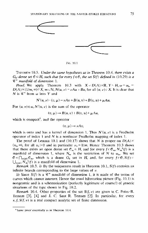
STATIONARY SOLUTIONS OF THE NAVIER-STOKES EQUATIONS 75
FIG. 10.1
THEOREM 10.5. Under the same hypotheses as in Theorem 10.4, there exists aGs-dense set 0<^H, such that for every feO, the set S(f) defined in (10.29) is a*% °° manifold of dimension 1.
Proof. We apply Theorem 10.3 with X = D ( A ) x R , Y = H , <o = <om =D(A)x(l/m,t»)cX, meN,N(u , v) = vAu + Bu, for all (u, v)eX. It is clear thatN is ̂ from w into Y and
For
which is compact4, and the operator
which is onto and has a kernel of dimension 1. Thus JV'(w, v) is a Fredholmoperator of index 1 and N is a nonlinear Fredholm mapping of index 1.
The proof of Lemma 10.1 and (10.17) shows that N is proper on D(A)x(i>0,°°), for all v0>0 and in particular v0=\/m. Hence Theorem 10.3 showsthat there exists an open dense set <9m<=H, and for every f e O m , N m
l ( f ) is amanifold of dimension 1, where Nm is the restriction of N to wm. We set®- Hmisi ^m> which is a dense G8 set in H, and, for every f e O , S ( f ) =Umsi Nm
l(f] is a manifold of dimension 1.Remark 10.3. i) By the uniqueness result in Theorem 10.1, S(f) contains an
infinite branch corresponding to the large values of v.ii) Since S(f) is a ̂ manifold of dimension 1, it is made of the union of
curves which cannot intersect. Hence the usual bifurcation picture (Fig. 10.1) isnongeneric and is a schematization (perfectly legitimate of course!) of genericsituations of the type shown in Fig. 10.2.
Remark 10.4. Other properties of the set S(f, v} are given in C. Foias-R.Temam [3], [4] and J. C. Saut-R. Temam [2]. In particular, for everyv, f, S(f, v} is a real compact analytic set of finite dimension.
4 Same proof essentially as in Theorem 10.4.
is the sum of the operator

76 PART II. QUESTIONS RELATED TO STATIONARY SOLUTIONS
10.4. Counterexamples. A natural question concerning Theorem 10.4 iswhether Cv is the whole space H or just a subset. Since Theorem 10.4 is astraightforward consequence of Theorem 10.3, this question has to be raised atthe level of Theorem 10.3. Unfortunately, the following examples show that wcannot answer this question at the level of generality of the abstract Theorem10.3, since for one of the two examples presented Ov = H, while for the secondone Gv + H.
Example 1. The first example is the one-dimensional Burgers equationwhich has been sometimes considered in the past as a model for the Navier-Stokes equations: consider a given v>0 and a function /:[0, 1]—>1R whichsatisfies
For the functional setting we take H = L"(0, 1), V = Ho(0, 1), D(A) =H1
0(0, 1)DH2(0, 1), Au=-d2u/dx2, for all ueD(A),
Then, given f in H (or V), the problem is to find ueD(A) (or V) whichsatisfies
We can apply Theorem 10.3 with X = D(A), Y = H, N(u) = vAu +Bu. Themapping N is obviously c£°° and
N'(u), as the sum of an isomorphism and a compact operator, is a Fredholmoperator of index 0. Now we claim that every u e D(A) is a regular point, sothat w t = H.
In order to prove that u is a regular point, we have to show that the kernelof N'(u) is 0 (which is equivalent to proving that N'(u) is onto, as indexN'(u) = Q). Let v belong to N'(w); v satisfies
By integration — w' + uv = constant = a, and by a second integration taking intoaccount the boundary conditions we find that v = 0.
Since the solution is unique if / = 0 (u =0), we conclude that
(10.33) (10.30)-(10.31) possesses a unique solution V v, V/.
Example 2. The second example is due to Gh. Minea [1] and corresponds toa space H of finite dimension; actually H = !R3.

STATIONARY SOLUTIONS OF THE NAVIER-STOKES EQUATIONS 77
Theorem 10.3 is applied with X =-- Y = [R3, N ( u ) = vAu + Bu for all w =(u l 5 u2, u3)eR3. The linear operator A is just the identity, and the nonlinear(quadratic) operator B is defined by Bw = (^(u^ + uf), —duiU2, —8uiU3) andpossesses the orthogonality property Bu • u =0. The equation N(u) = f reads
It is elementary to solve this equation explicitly. There are one or threesolutions if |/2| + \fi\ / 0. In the "nongeneric case", /2 = /3 = 0, we get either onesolution, or one solution and a whole circle of solutions: <o, ^ Y in this case.

This page intentionally left blank

J^ J^ The Squeezing Property
In this section we establish a squeezing property of the semigroup ofoperators associated with the time-dependent Navier-Stokes equations. Thisproperty, which will be useful for the next section, is also interesting by itselfand has found other applications (see in particular Foias-Temam [7]): thesqueezing property shows that, up to some error which can be made arbitrarilysmall, the flow is essentially characterized by a finite number of parameters.
11.1. An a priori estimate on strong solutions. The following a prioriestimate is valid for all time; it is a particular case of the more general resultsstated in § 12.3 (Lemma 12.2); we refer the reader to that section for moredetails.
LEMMA 11.1. Assume that u0eH, and f satisfies
f is continuous and bounded from [0, <») into H,
f is continuous and bounded from [0, oo) into V,
and let u be the strong solution to the Navier-Stokes equations given by Theorem3.2, defined on [0, oo) i f n = 2, on [0, T^UQ)] if n = 3.
Then u is bounded in V on [0, oo) if n=2, on [0, T\(u0)] if n — 3, and for everya >0, Au is bounded on [a, oo) if n = 2, on [a, T\(u0)] if n = 3,
where c' depends on ||u0||, /, v, fl (or Q), and c" depends on the same data andfurthermore a.
Remark 11.1. i) If n = 3, (11.2) follows from (3.28)-(3.29), but (11.2) mustbe proved for large time if n = 2.
ii) If u is defined on some interval (TO, T]) and supTo<,STi||u(t)|| = ci<oo then,by inspection of the proof of (11.3), we can see that, for every <*>0,supT +«<tsT |Au(0| = c", where c" depends on c[ and the data u0, /, v, H (orQ).
11.2. The squeezing property. We assume that n = 2 or 3. Let u0 and t>0 begiven in V, ||u0||^K, ||u0|| = -R, and let / be given satisfying
/ is continuous and bounded from [0, oo) into H,
/' is continuous and bounded from [0, oo) into V.
10<a^T1(u0) if n = 3, and in this case the supremum is for O^tgT^Uo) in (11.2) and fora^ t^Tj(u 0 ) in (11.3).
79

80 PART II. QUESTIONS RELATED TO STATIONARY SOLUTIONS
We denote by u and v the strong solutions of Navier-Stokes equationscorresponding respectively to (w0, /) and to (u0, /), which are given by Theorem3.2, and are defined on (0, <») if n = 2 and on [0, T^CR)] if n = 3, where
(see (3.29)).We recall that vvm, Am denote the eigenfunctions and eigenvalues of A and
that Fm is the projector in H (or V, V, D(A)) on the space Wm spanned bywlt. .., wm.
THEOREM 11.1. Under the above hypotheses, for every a >0, there exist twoconstants c5, c6, which depend on a, R, /, v, H (or Q) and such that, for everyt^a, for every m sufficiently large, i.e. satisfying
we have either
or
Proof. We assume in this proof thati) We set
We have, by taking the difference of the equations (2.43) for u and v,
Taking the scalar product, in H, of (11.10) with Pmw(t], we obtain
We apply Lemma 2.1 (i.e. (2.29)) respectively with m l 5 m2, m3 = 2, 0, 0; |, 1, |;0, 1, 1, and we use (11.3) for u and v, with a replaced by a/2:

ii) We now want to prove the alternative (11.7)-(11.8). Let us consider a
2The first relation of (11.19) follows easily from the first relation of (11.17) at a point (n wherep(t ( ))>0. If p(t()) = 0 then either p is not differentiable at t0 (which can only occur on a set of pointst() of measure 0) or dp(f ( ))/dt§0. The differentiability almost everywhere of p follows trivially fromthe differentiability almost everywhere in V of u and v, and thus w = u — v.
THE SQUEEZING PROPERTY
With these lower bounds, (11.11) becomes
81
Since A L ^ A m + 1 and
we have
In a similar manner, taking the scalar product in H of (11.10) withwe obtain
But
and thus
We set A = Am + 1, p = max (c{\\"1/4, c2, c^ c^AT1 '4)- Thus (11.14HH.16) takethe form:
and if
then for almost every t2

82 PART II. QUESTIONS RELATED TO STATIONARY SOLUTIONS
specific point t0, r0 = « if n = 2, a^ to^T^R) if n = 3. If q(f0) = p(fo) then(11.7) is satisfied at t0 and we have nothing to prove. Therefore we assume that
and on the other hand we assume that m is sufficiently large so that
This implies that
in a neighborhood of f0-At this point two possibilities can occur: either (11.22) is valid on the whole
interval [r0-a/2, t0], or (11.22) is valid for t e( f l 9 f0), with t^to-a/2 and
The second possibility is discussed in point iii) of the proof; in the first case,since (11.18) and (11.19) are satisfied on [t0 — a/2, to], we have
and (11.8) follows at t0 with appropriate constants c5, c6.iii) The last step consists in proving (11.7) at
assuming that (11.22) is satisfied on an interval (f1} r0), and (11.23) is satisfiedat
We denote by (11.19)' the differential system obtained by replacing theinequalities in (11.19) by equality signs. It is natural to formally associate with(11.19)' the differential system
and consequently
Due to (11.2),
We prove ve by elementary calculations that remains constant whenare solutions of (11.19) and

THE SQUEEZING PROPERTY 83
By elementary calculations we also check that
when p(-), q(-) are solutions of (11.19), in particular on [fl510\. Thus
By
and on the other hand, with (11.20),
Since
and p(to)<q(t0), we obtain an estimate of the type (11.8) for(p200) + q2(r0))1/2=iV2q(r0).
The proof is complete.Remark 11.2. i) As in Remark 11.1 ii), the squeezing property is valid for
any pair of strong solutions u, v of the Navier-Stokes equations, defined onsome interval (TO, ra), and satisfying
so that
ii) Of course we can replace the coefficient V2 in the right-hand side of(11.6) by any constant (3 > 1. It is clear that in such case c5 and c6 depend alsoon |3.
Remark 11.3. It is reasonable to consider as physically "undistinguishable"two strong solutions u, u, which satisfy (11.8) for some m sufficiently large.Mathematically, we can consider an equivalence relation among the strongsolutions which are defined on (TO, TJ) (and bounded in V on this interval): twosolutions u, u are said to be equivalent if there exist two constants c5, c6 suchthat (11.6)-(11.8) hold on (TO, TJ). It is easy to check that this relation is indeedan equivalence one. The squeezing property implies that Pmu characterizes theequivalence class of u, i.e., characterizes u up to an error exp (-cA^+j).
Remark 11.4. Let us mention an alternate form of the squeezing propertywhich is useful for later purposes.

84 PART II. QUESTIONS RELATED TO STATIONARY SOLUTIONS
Let M and v be two strong solutions of the Navier-Stokes equations, definedand bounded in V on some finite interval r0 Si t ̂ rl < <». For every a > 0, thereexist two constants c*, c* which depend on TO, rl5 a, R, f, v, ft3, such that, on[TQ + CX, rj, we have either (11.7) or
for every m satisfying
The proof is exactly the same, except that in (11.25) and (11.27) we replacethe majorizations
by the estimate (S=C"|W(TO)|) which follows from the next lemma.LEMMA 11.2. // u and v are two strong solutions defined and bounded in V on
a finite interval TQ^^T!, n = 2 or 3, then there exists a constant c" whichdepends on TO, rl5 /, v, ft (or Q), and R, with
such that
Proof. It follows easily from the energy inequality (3.24), valid for strongsolutions, and from the assumptions on u and u, that Au and Av belong toJL2(r0, T! ; H) with their norm in this space bounded by a constant depending onTO, TI, f, v, fl (orQ) and R.
We take the scalar product in H of (11.10) with w(t), and using (2.29),(2.33), (2.34) and (11.30) and Remark 11.1 ii), we get, as for (11.13):
and since |Au|4/3eL^O, T), (11.31) follows from Gronwall's lemma.
3 Here
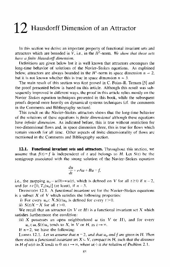
12 Hausdorff Dimension of an Attractor
In this section we derive an important property of functional invariant sets andattractors which are bounded in V, i.e., in the //'-norm. We show that these setshave a finite Hausdorff dimension.
Definitions are given below but it is well known that attractors encompass thelong-time behavior of solutions of the Navier-Stokes equations. As explainedbelow, attractors are always bounded in the //'-norm in space dimension n = 2,but it is not known whether this is true in space dimension n = 3.
The main result of this section was first proved in C. Foias-R. Temam [5] andthe proof presented below is based on this article. Although this result was sub-sequently improved in different ways, the proof in this article relies mostly on theNavier-Stokes equation techniques presented in this book, while the subsequentproofs depend more heavily on dynamical systems techniques (cf. the commentsin the Comments and Bibliography section).
This result on the Navier-Stokes attractors shows that the long-time behaviorof the solutions of these equations \sfinite dimensional although these equationshave infinite dimension. As indicated before, this is true without restriction fortwo-dimensional flows and, in space dimension three, this is true for flows whichremain smooth for all time. Other aspects of finite dimensionality of flows arementioned in the Comments and Bibliography section.
12.1. Functional invariant sets and attractors. Throughout this section, weassume that f(t) = f is independent of t and belongs to H. Let S(t) be thesemigroup associated with the strong solution of the Navier-Stokes equation
i.e., the mapping w 0 = u(0)>-»w(f) , which is defined on V for all t i^O if n = 2,and for re[0, T^UQ)] (at least), if n = 3.
DEFINITION 12.1. A functional invariant set for the Navier-Stokes equationsis a subset X of V which satisfies the following properties:
i) For every u f )e X, S(t}uQ is defined for every f > 0 .ii) S(t)X = X for all f>0 .We recall that an attractor (in V or H) is a functional invariant set X which
satisfies furthermore the condition:iii) X possesses an open neighborhood w (in V or H), and for every
u()e o>, S(t)u0 tends to X, in V or H, as t -»°°.If n=2, we have the following:LEMMA 12.1. Let us assume that n = 2, and that u0 and f are given in H. Then
there exists a functional invariant set X <= V, compact in H, such that the distancein H of u(t) to X tends to 0 as t —> o°, where u(-) is the solution of Problem 2.1.
85

» PART II. QUESTIONS RELATED TO STATIONARY SOLUTIONS
Proof. We set
where the closures are taken in H. An element </> e H is in X if and only if
is bounded in V (cf. Lemma 11.1), so is its closure in V and so is X. ByTheorem 3.2, since n = 2, S(t)<f> is defined for all t >0, for every $ e X, and thefirst condition i) in Definition 12.1 is satisfied. For condition ii) we observe thatS(OX<=X follows easily from the fact that S(t)u(s) = u(s + t), for all s, f ^O .In order to show that S(t)X = X, we note that S(t) is infective because of thetime analyticity property (see § 7) and therefore since the set (12.4) is relativelycompact in H(t0>0], the sequence u ( S j ) , j e N , converges in H whenever thesequence S(t)u(Sj) converges. Indeed, if S(t)u(Sj) converges in H to some limit<f>, as /—»oc (and s,-»o°), then by (12.2), </>eX. The sequence w(s,), beingbounded in V, is relatively compact in H and possesses cluster points in H; if iffand i// are two cluster points, S(t)if/ = S(t)^' -- </> so that i// = i/>, the clusterpoint is unique and the whole sequence M(S;) converges to it in H as j —*• °°.
Finally we show that the distance in H of u(t) to X tends to 0 as t -» oo. Weargue by contradiction. If this were not true, we could find e0>0, and asequence s, —»<», such that
Since «(«,) is bounded in V we can, by extracting a sequence, assume that u(sy)converges in H to some limit if/. By (12.2), «/>eX, in contradiction with
The lemma is proved.
12.2. Hausdorff dimension of functional invariant sets.THEOREM 12.1. Let n = 2 or 3 and let f e H. We assume that X is a functional
invariant set bounded in V. Then the Hausdorff dimension of X is finite and thisdimension is bounded by a number c, which depends on £1 (or Q), i/, |/| and1
Proof, i) We are going to make use of the squeezing property, in theconditions indicated in Remark 11.4: we fix a>0 and choose T0 = 0, T1 = 2a,
1 The bound given in the proof is, in fact, an increasing function of v \ |/| and R.
It is easy to see that X is also equal to
Since for t0>Q, the set
86

of course Yk may be reduced to <£3.ii) We now define a reiterated covering of X.Let BE1!,. . . , B^ be a covering of PmS(Bk HX) by balls of PmH of radius
^rk = 5diam Bk. For those /'s such that PmYk HB^-^ 0, we choose arbitrarilyan ukj & Yk, such that Pmwkj e PmYk nB£], and we denote by Bkj the ball of Hcentered at uk. and of radius
2 Since, by the definition of a functional invariant set, S(t)<f> is defined for every (=SO, for every<£eX we are free to choose TO, TL in Remark 11.4, O^TO^T]<+°°.
3 If Y k^S(B knX) then sup^^ nx)xn dist («fc Yk)=ST] diam Bk.
HAUSDORFF DIMENSION OF AN ATTRACTOR 87
and te[a, 2a]2. We then choose m sufficiently large so that (11.29) is verifiedand (see (11.28))
and the value (or one value) of T) which is appropriate below is
We set S(t) = S, then Theorem 11.1 and Remark 11.4 show us that for a<£,(// e X, we have either
Given r > 0, since X is relatively compact in H, it can be covered by a finitenumber of balls of H of radius <r, say Bl,. . . , BM. By definition, SX = X;hence
and (12.7) implies that for all k = 1,. . . , M, and for all u, v e S(Bk DX) wehave either
Let <$> be an arbitrary point of S(Bk DX) and let Yk be the largest subset ofS(Bk OX), containing <£ and such that
Setting Bk] =0 if B£nPmYk =0, we have
Indeed, if u e S(Bk OX), then there exists u'e Yk (u' = u if u e Yk) such that,by (12.9) and the definition of Yk,

88 PART II. QUESTIONS RELATED TO STATIONARY SOLUTIONS
Then
Since PmS(Bk HX) is included in a ball of PmH of radius c" diam Bk, we have
Since the Bki, k = 1 , . . . , M, j — 1 , . . . , Mk, for all k, constitute a covering ofX by balls of radius ^er, we infer from the definition of ju,TS(X) in (5.2) that
Before proceeding to the next step, let us observe that we can derive anupper bound for Mk.
By Lemma 11.2,
hence
where /m(<r) is, in IRm, the minimum number of balls of radius ^cr which isnecessary to cover a ball of radius 1, /m(or)^2~~m/2cr~m.
iii) We have
This last inequality, valid for any covering of X by balls of radius ^r,implies in its turn
where A = /m(l/4c")e\ By reiteration,
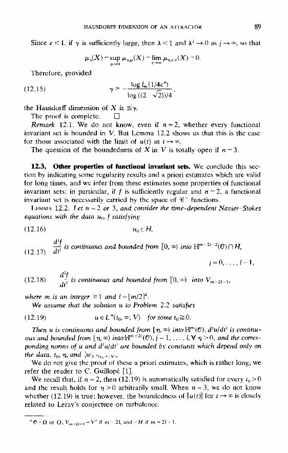
HAUSDORFF DIMENSION OF AN ATTRACTOR 89
Since e < 1, if 7 is sufficiently large, then A < 1 and A ; —» 0 as / —» °o, so that
Therefore, provided
the Hausdorff dimension of X is ^y.The proof is complete.Remark 12.1. We do not know, even if n = 2, whether every functional
invariant set is bounded in V. But Lemma 12.2 shows us that this is the casefor those associated with the limit of u(t) as t—><x>.
The question of the boundedness of X in V is totally open if n = 3.
12.3. Other properties of functional invariant sets. We conclude this sec-tion by indicating some regularity results and a priori estimates which are validfor long times, and we infer from these estimates some properties of functionalinvariant sets; in particular, if / is sufficiently regular and n = 2, a functionalinvariant set is necessarily carried by the space of ^°° functions.
LEMMA 12.2. Let n = 2 or 3, and consider the time-dependent Navier-Stokesequations with the data u0, / satisfying
Then u is continuous and bounded from [T], °°) intoHm(O), d!u/dt' is continu-ous and bounded from [TJ, <») into Hm~2'(€), j = 1, . . . , I, V TJ >0, and the cones-ponding norms of u and d'u/dt' are bounded by constants which depend only onthe data, t0, TJ, and |u|L~(,0)00; v>-
We do not give the proof of these a priori estimates, which is rather long; werefer the reader to C. Guillope [1].
We recall that, if n = 2, then (12.19) is automatically satisfied for every £0>0and the result holds for 17 >0 arbitrarily small. When n = 3, we do not knowwhether (12.19) is true; however, the boundedness of ||u(t)|| for t —> ™ is closelyrelated to Leray's conjecture on turbulence.
where m is an integerWe assume that the solution u to Problem 2.2 satisfies
is continuous and bounded from
is continuous and bounded from

90 PART II. QUESTIONS RELATED TO STATIONARY SOLUTIONS
Let us recall that Leray's hypothesis, and his motivation in introducing theconcept of weak solution was that singularities may develop spontaneouslyover a finite interval. We know that \u(t)\ remains bounded even for weaksolutions but the enstrophy !|n(f)|| may perhaps become infinite. We formulateLeray's assumption in a more precise way:
There exist 12^IR3, T> 0, i»0, u0e K,/e L^O, T; H) such that(12.20) MOll becomes infinite at some time t e (0, T), u being the weak
solution of the Navier-Stokes equations.
Let us assume now that /e L°°(0, o°; H) and is not "too chaotic" at infinity, i.e.,
There exists a > 0 such that for any sequence t, —> +°°, the(12.21) sequence of functions fj(t) = f(t + tj}, 0<f <a possesses at least
one cluster point in L2(0, a; H).
This property is trivially satisfied if / is independent of time, or more generallyif
with
for all s >0, a >0, where c(f) is independent of s. In such a case we have thefollowing result proved elsewhere (cf. C. Foias-R. Temam [13]):
THEOREM 12.2. Given fteIR3, T, v and /eL°°(0,^;H) satisfying (12.21),then either (12.19) or (12.20) holds; i.e., there exists u0e V for which \\u(t)\\becomes infinite on the interval [0, a], a >0 given in (12.21).
Finally we infer from Lemma 12.2 the following regularity result for a func-tional invariant set (or attractor):
THEOREM 12.3. Let us assume that f is independent of t, and f e c€°°(C)n DH5.Then any functional invariant set X, bounded in V, for the corresponding Navier-Stokes equations, is contained in £#°°(<j?)n.
Proof. We consider the semigroup operator S(t) defined at the beginning of§ 12.1. Since S(t)X = X, for all f>0 , and S(t) is one-to-one by the analyticityproperty, every <£ eX is of the form $ = S(t)u0, with u0eX, and therefore byLemma 12.2, <£ is in Hm(0), for all m.
Remark 12.2. i) This result is comparable to regularity results for thesolutions of stationary Navier-Stokes equations, but it applies also to periodic,and quasi periodic solutions, among others.
ii) The conclusion of Theorem 12.2 is valid if we assume only that X isbounded in V1/2+e for some e>0. See C. Guillope [1] for the details.
If we consider the flow in fl(0 = fl), we also need (1.7) with r = °o.5

PART III
Questions Related tothe Numerical Approximation
Orientation. In Part III, containing §§ 13 and 14, we develop some resultsrelated to the numerical approximation of the Navier-Stokes equations. This isfar from being an exhaustive treatment of a subject which is developingrapidly, due to the needs of modern sophisticated technologies and the appear-ance of more and more powerful computers.
Part III does not discuss any practical developments concerning implemen-tation of computational fluid dynamics algorithms1 (though these are impor-tant). It is limited to the presentation of two questions related to the numericalanalysis of the Navier-Stokes equations. The first is the question of stabilityand convergence of a particular nonlinear scheme; this is developed in § 13.The particular scheme was chosen almost arbitrarily among several schemespresently used in large scale computations and for which convergence has beenproved. The second question, considered in § 14, is that of the approximationof the Navier-Stokes equations for large time: in the context of the questionsstudied in § 12 (see also § 9), the problem of numerical computation ofturbulent flows is connected with the computation of u(t) for t large (while theforce, or more generally the excitation, is independent of time). Section 14contains some useful remarks pertaining to this question.
See the comments following § 14.
91
1

This page intentionally left blank

1 ̂ Finite Time Approximation
In this section we study the convergence of a space and time discretizationscheme for the evolution Navier-Stokes equations. This scheme combines adiscretization in time by an alternating direction (or decomposition) methodwith a discretization in space by finite elements. It belongs to a series ofefficient schemes which have been introduced and studied from a theoreticalpoint of view in the past (cf. A. J. Chorin [2], [3], [4], R. Temam [1], [2], [5],[6]), and which have recently regained interest and have been implemented inlarge scale computations for industrial applications (cf. e.g., H. O. Bristeau-R.Glowinski-B. Mantel-J. Periaux-P. Perrier-O. Pironneau [1], R. Glowinski-B.Mantel-J. Periaux [1]).
The proof of convergence is the same as that appearing in [RT, Chap. Ill,§§5, 6, 7] and in R. Temam [1], [2], [4], [5] for closely related schemes.However, for the proof of the strong convergence result which is necessary forthe passage to the limit, we use a compactness argument different and slightlysimpler than that considered in those references. This compactness result isgiven in § 13.3.
13.1. An example of space-time discretization. We consider the flow in abounded domain with periodic or zero boundary condition (i.e., 0 =Cl or Q),and n =2 or 3. We are given u() and / as in Theorem 3.2 and we want toapproximate the strong solution u to Problem 2.2 defined in Theorem 3.2, on[0, T] if n = 2, on [0, T*] if n = 3.
We are given a family of finite dimensional subspaces Vh, he^f, of V, suchthat
For instance we can take ffl = N, Vh=the space spanned by the eigenvectorswi, . . . , wh, and the discretization would correspond to a Galerkin methodbased on the spectral functions. Also Vh may be a more general subspacecorresponding to a more general Galerkin method, but the most interestingcase we have in mind is that in which Vh is a space of finite element functionswith the set ffl properly defined: we refer to [RT, Chap. I, § 4] for the precisedefinition of a possible finite element space (Approximation APX4).
Actually, in order to be able to treat more finite element schemes we willconsider the following more general situation:
is a family of finite dimensional subspaces ofH^O) or HJ(O), such thathe9e Wk is dense in W.
For every h, Vh is a subspace of Wh, such that the family Vh,h 6 $?, constitutes an external approximation1 of V.
1 For the precise definition of an external approximation cf. [RT, Chap. I, § 3.1]. The reader whoso wishes may concentrate on the first, simpler case: Vhc=V with (13.1).
93

Here3 b(u, v,w) is the modification of the nonlinear term which was intro-duced in R. Temam [1], [2] and which guarantees the existence of a solution to(13.8), and the stability of the approximation for (13.8) or similar schemes:
The existence and uniqueness of a solution w™+1/2 for (13.6) follow from theRiesz representation theorem (or Lax-Milgram theorem). The existence of asolution U ™ + I G Wh of (13.8) (a nonlinear finite dimensional problem) followsfrom the Brouwer fixed point theorem, using [RT, Chap. II, (2.34) and Lemma1.4]. Problem (13.6) is just a variant of the linear stationary Stokes problem,and (13.8) is a relatively standard nonlinear Dirichlet problem. We refer toGlowinski, Mantel and Periaux [1] and to F. Thomasset [1], for the practical
2 With the notation of Theorem 3.2, T = T if n = 2, T" = T* = min (T, T^UQ)) if n = 3.3b(u,v, w) may be ^0, while b(u, v, w) = 0, for u, uelHp(ft) (or H^Q)), by lack of the free
divergence property.
94 PART III. QUESTIONS RELATED TO THE NUMERICAL APPROXIMATION
The cases covered by (13.2), (13.3) contain the finite element approxima-tions of V called APX2, APX3, APX3' in [RT, Chap. I, §4] and otherspublished in the literature (cf. M. Bercovier-M. Engelman [1], V. Girault-P.A. Raviart [1], among others).
For every h, let u0h be the projection of u0 in W, on Vh, i.e.,
Let N be an integer2, k - T'/N. For every h and k we recursively define afamily w™+1/2 of elements of Vh, m = 0 , . . . , N-1, i = 1, 2. We start with
Assuming that u° (or more generally u™, m^O) is known, we define u™+l/2
and then u!T+1 as follows:
where
and
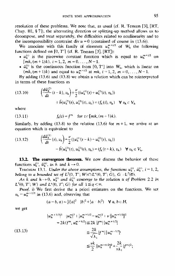
FINITE TIME APPROXIMATION 95
resolution of these problems. We note that, as usual (cf. R. Temam [3], [RT,Chap. Ill, § 7]), the alternating direction or splitting-up method allows us todecompose, and treat separately, the difficulties related to nonlinearity and tothe incompressibility constraint div u = 0 (contained of course in (13.6)).
We associate with this family of elements u™+i/2 of Wh the followingfunctions denned on [0, T] (cf. R. Temam [3], [RT]):
• ukl ) is the piecewise constant function which is equal to u™+l/2 on
[mk, (m + l)k), i = 1, 2, m = 0 , . . ., N-1.• u(
kr) is the continuous function from [0, T'] into Wh, which is linear on
(mk, (m + l)k) and equal to u™+i /2 at mk, i = 1, 2, m = 0 , . . . , N-1.By adding (13.6) and (13.8) we obtain a relation which can be reinterpreted
in terms of these functions as
where
Similarly, by adding (13.8) to the relation (13.6) for m + 1, we arrive at anequation which is equivalent to
13.2. The convergence theorem. We now discuss the behavior of thesefunctions u(
kl), uk
l), as h and k —> 0.THEOREM 13.1. Under the above assumptions, the functions
belong to a bounded set of As k and h —>• 0, uk
l ) and uk° converge to the solution u of Problem 2.2 mand
Proof, i) We first derive the a priori estimates on the functions. We setUK = Uh+V2 in (13.6) and, observing that
we get

96 PART III. QUESTIONS RELATED TO THE NUMERICAL APPROXIMATION
The relations (13.18)-(13.21) amount to saying that the functions Uk\ wk°,i = 1, 2, belong to a bounded set of L°°(0, T'; G), and that w(
fc1}, wk
2), belong to abounded set of L2(0, T'; W). In order to show that u(
k° also belongs to abounded set of L2(0, T'; W), we observe by direct calculation (cf. [RT, Chap.
Adding the relations (13.14) for m =0, . . . , p and (13.16) for m = 0 , . . . , p —1,we find, after dropping unnecessary terms,
By adding the relations (13.14) and (13.16) for m = 0 , . . . , p, we obtain, aftersimplification,
where
Due to (13.4), ||u0J^||u0||, and therefore the sequence uoh is bounded in H.We then conclude that
whence
Similarly, taking vh = u™ + 1 in (13.8) and taking into account (2.34), we obtain
By adding all the relations (13.14), (13.15) for m = 0 , . . . , JV-1, we find
(by the Schwarz inequality).

FINITE TIME APPROXIMATION 97
III, Lemma 4.8]) that
ii) We want to pass to the limit as k —» 0, h —»• 0. Due to the previous a prioriestimates, there exist a subsequence (denoted k, h) and w(1), u<2) inL2(0, T'; W)nL°°(0, T'; G) such that
The relations (13.17) and (13.22) imply that the same is true for u^\ i = 1, 2.Now we infer from (13.17) that
and therefore
so that u(2) = u(1). Also we infer from the properties of the Vh's (whichconstitute an external approximation4 of V) that wm belongs in fact toL2(0, T'; V)nL°°(0, T';H):
The last (and main) step in the proof is to show that u% is a solution toProblem 2.2. We need for that purpose a result of strong convergence whichwill be proved with the help of the compactness theorem in § 13.3.
13.3. A compactness theorem.THEOREM 13.2. Let X and Y be two (not necessarily reflexive) Banach spaces
with
Let <& be a set of functions in Ll(U; Y)HLP(IR;X), p> l , with
For the details see [RT].
uniformly for g e ^;
the support of the functions e e $ is included in a fixed compact of
Then the set ^ is relatively compact in LP(!R; X).
4
the inject ion being compact
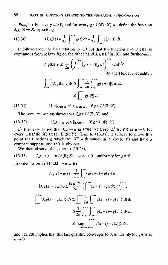
and (13.28) implies that this last quantity converges to 0, uniformly for g e $ asa^O.
98 PART III. QUESTIONS RELATED TO THE NUMERICAL APPROXIMATION
Proof, i) For every a >0, and for every geLp(R; X] we define the functionJag: U i-» X, by setting
It follows from the first relation in (13.30) that the function s •->• (Jag)(s) iscontinuous from [R into X; on the other hand /ageLp(IR; X), and furthermore
The same reasoning shows that JageLl(U; Y) and
ii) It is easy to see that Jag -> g in LP([R; X) (resp. L1^; Y)) as a -» 0 forevery geLp(!R;X) (resp. I/flR; Y)). Due to (13.31), it suffices to prove thispoint for functions g which are ^°° with values in X (resp. Y) and have acompact support, and this is obvious.
We then observe that, due to (13.28),
In order to prove (13.33), we write
by the Holder inequali ty

FINITE TIME APPROXIMATION 99
iii) We now show that
/•• i -3-7 4 \ F°r every a>0 fixed, the set ^a = {/ag, ge <&} is uniformlyequicontinuous in ^(R;X).
Indeed, for every s,teU
Hence we have (13.34).We then apply Ascoli's theorem (cf. Bourbaki [1]) to show that the set ^a is
relatively compact in ^(1R;X). All the functions Jag have their supportincluded in a fixed compact, say [—L — 1, L +1] (assuming that |a| ̂ 1). Due to(13.34), the only assumption of Ascoli's theorem which remains to be checkedis that
(13.35) For every s eR, the set |/ag(s), ge $} is relatively compact in X.
But according to (13.26), it suffices to show that this set is bounded in Y, andwe have with (13.27)
The set <3a is therefore relatively compact in ^(R; X), and due to (13.29) thisset is, for every fixed a, relatively compact in LP(R; X).
iv) Finally we prove that the set ^ itself is relatively compact in LP(IR;X).For instance, we have to prove (cf. Bourbaki [1]) that for every e >0 thereexist a finite number of points g l 5 . . ., gN, in LP(IR; X), such that ^ is includedin the union of the balls centered at & and of radius e.
According to (13.33), for every e>0 there exists a such that
Since ^a is compact, it can be covered by a finite number of balls ofLP(R; X), centered at Jag l5. . . , JagN, and of radius e/3; finally it is clear with

100 PART III. QUESTIONS RELATED TO THE NUMERICAL APPROXIMATION
(13.36) that the balls of LP(U; X) centered at g l 9 . . . , gN, and of radius e cover«.
The proof of Theorem 13.2 is complete.We have a similar result for functions g defined on a bounded interval, say
[o, nTHEOREM 13.3. We assume that X and Y are two Banach spaces which
satisfy (13.26). Let % be a set bounded in L\0, T; Y) and Lp(0, T; X), T>0, p > 1, such that
Then ^ is relatively compact in Lq(0, T; X) for any q, l^=q<p.Proof. This is proved by applying Theorem 13.2 in the following manner.
We consider the set ^ of functions g: g(s) = g(s) if s E [0, T] and = 0 otherwise.The set <$ is bounded in L'flR; Y)DLq([R; X) and satisfies (13.28) for preplaced by q, as
and this goes to 0 uniformly with respect to g e ̂ as a —>• 0.Remark 13.1. Of course, under the assumptions of Theorem 13.2 we can
obtain that ^ is relatively compact in Lp(0, T; X) itself if we assume, instead of(13.37), that
13.4. Proof of Theorem 13.1 (conclusion), i) By application of Theorem13.3, we show that the functions u(
k°, M(k° converge to u strongly in L2(0, T'; G)
or even Lq(0, T';G), l^q«*.By integration of (13.12),

FINITE TIME APPROXIMATION 101
We majorize the absolute value of the right-hand side of this equality asfollows:
Since u(kn is a Vh-valued function5, we can take uh = u(k\t + a)- u(k\t), and
we find after integration with respect to t:
5 This is not the case for u(k
2) (a \Vh-valued function).
Finally we obtain the majorization
where c{ depends only on the data, u(), /, v, fl (or Q), T'. Similarly,
For the term involving b, we use Lemma 2.1 with
by holders os inequality and since
Let v be an arbitrary element of V. We choose for vh an approximation of v,and passing to the limit in (13.45) we get
This, together with (13.24) and (13.41), shows that
(13.44) w(k° and u(
k° converge to u strongly in Lq(0, T; G) V q, 1 ̂ q <oo.
ii) Using (13.44) and the weak convergences obtained in § 13.2 (in particular(13.23)), the passage to the limit in (13.12) is standard. We will just give themain lines of the proof. Let $ be any ^l scalar function on [0, T'] whichvanishes near T'; we multiply (13.11) by tKO» integrate in t and integrate byparts the first term to get
and with (13.17)
As for (13.22), it is easy to check by direct calculation that
We apply Theorem 13.3, as follows. ^ is the family of functions uk1} which is
bounded in L2(0, T; W)nL°°(0, T; G), (Y = W, X = G), p = 2, so that (13.37)follows from (13.40). We conclude that uk
1} is relatively compact inLq(0, T; G), l^q<2, and since u(
k1} converges weakly in Lq(0, T'; G) to u*
(see (13.23)-(13.25)), this means that u^ converges to u*, strongly inLq(0, T'; G), l^q<2. The sequence uk
1} being bounded in L°°(0, T'; G), weconclude from the Lebesgue dominated convergence theorem that we actuallyhave
102 PART III. QUESTIONS RELATED TO THE NUMERICAL APPROXIMATION

FINITE TIME APPROXIMATION 103
(The passage to the limit in the nonlinear term necessitates the strong con-vergence (13.41); cf. [RT].) We deduce from (13.46) that u* is a solution toProblems 2.1-2.2, and since this solution is unique in the present situation, weconclude that u% = u. By uniqueness, the entire sequences u(^\ u^ converge tou as k and h tent to 0. The last step of the proof is to obtain strongconvergence in L2(0, T"; W).

This page intentionally left blank

14 Long Time Approximation of theNavier-Stokes Equations
The study of the long time behavior of the solutions to the Navier-Stokesequations is directly related to an understanding of turbulent flow, as can beseen from Part II. In this section we present two results which tend to indicate,as do those in §§11 and 12, that the flow has, for time large, a finitedimensional structure. The first result is related to the flow itself (§ 14.1); thesecond to its Galerkin approximation (§ 14.2).
14.1. Long time finite dimensional approximation. Let / and g be twocontinuous bounded functions from [0, °°) into H, let w0 and u() be given in V,and let u and v denote the corresponding solutions to Problem 2.2:
where c" depends on a, c' and the data (Lemma 12.2).The space E. Let us now consider a finite dimensional subspace E of V. We
denote by P(E) the orthogonal projector in H onto E, and Q(E) = /-P(E).Since P(E) is not a projector in V, it may happen that ((</>,(/>)) ̂ 0, if$eE, i />eV and P(E)i/> = 0. However (see Lemma 14.1 below), there existsp(E) ,Q^p(E)<l , such that
We assume that u and v are defined and bounded for all time in V:
We recall that this property is automatically satisfied if n = 2 (cf. Lemma 12.2).We recall also that for every a > 0
We also associate with E the two numbers A(E) , ju,(E),

PART III. QUESTIONS RELATED TO THE NUMERICAL APPROXIMATION106
so that
When it is not necessary to mention the dependance on E, we will writesimply P, Q, p, A, /a instead of P(E), and so forth.
We will now prove (14.5).LEMMA 14.1. Under the above assumptions, there exists p = p(E} such that
(14.5) holds.Proof. If this were not true, we could find two sequences <£>,-, j^-,/^1, <£,-e
E, 0;. G V, Pty = 0 such that
We can extract a subsequence, still denoted /, such that </>) converges to somelimit <}>, \\(j>\\ =l,<j>eE (E has finite dimension), and ,̂' converges weakly in Vto i/r, i/f e V, W^ 1, P»A = 0. At the limit, (14.8) gives
so that ||i//|| = 1, $ = k<t> ̂ 0, in contradiction withAn inequality. We consider the two solutions u, v of (14.1)-(14.2), and we
set
(P = P(E),Q = Q(E) = /-P(E)).We apply the operator Q to the difference between (14.1) and (14.2). We
obtain
We then take the scalar product in H with q,
Using Lemma 2.1 (or (2.36)) and (14.5)-(14.7), we find that the right-handside of this inequality is less than or equal to

LONG TIME APPROXIMATION OF THE NAVIER-STOKES EQUATIONS 107
If f=^a, a>0 arbitrary, then this expression is in turn less than or equal to
where e>0 is arbitrary.If
then we set
and we have established:LEMMA 14.2. If (14.3)-(14.5)-(14.7) and (14.9) hold then, for t ^a>0 ,
with v', e as in (14.10).We now proveTHEOREM 14.1. We assume that the space dimension is n = 2 or 3 and that u
and v are solutions of (14.1)-(14.2) uniformly bounded in V. Let E be a finitedimensional subspace of V such that (14.9) is satisfied.
Then, if
we have also
Remark 14.1. Theorem 14.1 shows that if the condition (14.9) is satisfiedthe behavior for t — » < » of u(t] is completely determined by that of P(E)u(t](although we do not know how to recover u(f), knowing P(E}u(t)). Lemma14.3 below shows that (14.9) is satisfied if E is "sufficiently large".

108 PART III. QUESTIONS RELATED TO THE NUMERICAL APPROXIMATION
Proof of Theorem 14.1. We infer from (14.6) and (14.11) that
where
We let 5 -> 0 and then M^ °o and we obtain (14.14).As mentioned before, the following lemma shows that condition (14.9) is
always satisfied if E is sufficiently large.LEMMA 14.3. // Ej} j ^ 1, is an increasing sequence of subspaces of V such that
\JjEj is dense in V, then A(£/)—> +°° as /—»<».Proof. In fact, we will prove that
(14.17) For every integer m there exists jm and, for /i?/m, we haveA(EJm)i=Am,
where Am is the mth eigenvalue of A.
whence for
Given 5>0, there exists M (which we can assume ^a) such that for t ̂ M
Therefore, for t^t0 + M, (14.11) implies
where

and the results follow by letting
14.2. Galerkin approximation. We are going to establish a result similar tothat in Theorem 14.1, for the Galerkin approximation of Navier-Stokesequations when the space dimension n = 2. For simplicity we restrict ourself tothe Galerkin approximation using the eigenfunctions vvm of A (as in § 3.3), andwe will show that if m is sufficiently large, the behavior as t —> °° of theGalerkin approximation um is completely determined by the behavior as t —> °°of a certain number m* of its modes, i.e. the behavior of Pm^um, m^<m.
We start with some complementary remarks on Galerkin approximations.For fixed m, the Galerkin approximation um of the solution u of (14.1) is
defined (see § 3.3) by
where Pm is the projector in H, V, V, D(A), . . . , onto the space spanned bythe first m eigenf unctions of A, w l 5 . . . , vvm.
We have established in § 3.3 some a priori estimates which are valid on afinite interval of time [0, T]; we can obtain a priori estimates valid for all timeas follows.
LONG TIME APPROXIMATION OF THE NAVIER-STOKES EQUATIONS 109
By assumption, for every k,
Hence, for given m and S > 0, there exists /m such that
Thus, for every /i^;m, there exist w l 5 . . . , wm in £,-, with ||w, — w,-||^=5. There-fore if $ E V, (/-?(£;))(/> = 0, we have
This implies

110 PART III. QUESTIONS RELATED TO THE NUMERICAL APPROXIMATION
We infer from (3.46) that
where N(f) = suptg£0 |/(f)|. Thus for every r ^ s ^ O
and |um(0| is bounded for all time:
The following a priori estimate is also verified by um.LEMMA 14.4. 11^(011 is bounded independently of m and t.Proof. For T = a > 0, this is proved on [0, a] in (3.59). In order to obtain the
result for t^a, we consider the analogue of (3.11) for i^ (obtained by takingthe scalar product of (14.18) with Aum; see § 3):
Therefore with (14.21)
and for 0 ̂ s ̂ t, we can show by integration that
If t ̂ a > 0, we integrate in s from t — a to t and we find
Using (14.20), we see that the right-hand side of this inequality is boundedby a constant depending on a and the data, but independent of t and m. Thelemma follows.

LONG TIME APPROXIMATION OF THE NAVIER-STOKES EQUATIONS 111
We can now state the result announced.Let u^ and vm be the Galerkin approximations to the solution u and v of
(14.1)-(14.2),
Because of (2.31) and Lemma 14.4, this quantity is bounded by
Consequently,,
(Qm = I-Pm). Then by subtracting (14.21) from (14.23) and applying Q,̂ tothe equality which we obtain, we arrive at
Proof. We have to obtain an analogue of (14.11); we then proceed as forTheorem 14.1.
We set for m^^m (m* to be determined):
we have
i.e.,
THEOREM 14.2. We assume that n = 2 and that m ̂ m*, m* sufficiently largeso that the condition (14.29) below is verified.
Then, if
The right-hand side is equal to

112 PART III. QUESTIONS RELATED TO THE NUMERICAL APPROXIMATION
If
we set
and we bound the last quantity by
Finally we find
This inequality is totally similar to (14.11), and starting from (14.31) theproof of Theorem 14.2 is the same as that of Theorem 14.1.
Remark 14.2. We did not establish above any connection between thebehavior for t —>°° of u(t) and of its Galerkin approximation um(i). Thisremains an open problem. See however P. Constantin-C. Foias-R. Temam [1].

APPENDIX
Inertial Manifolds and
Navier-Stokes Equations
Inertial manifold is a new concept introduced in 1985 after the publication ofthe first edition of these notes. Although related concepts and results existedearlier, inertial manifolds were introduced under this name in 1985 and system-atically studied for nonlinear dissipative evolution equations since that time. Itwould be beyond the scope of this appendix to make a thorough presentation ofinertial manifolds; we refer the interested reader to more specialized books andarticles (see references below). In this appendix we recall only the concept, themain definitions, and the main results and concentrate on some results specificallyrelated to the Navier-Stokes equations as they appear in the articles of C. Foias-G. Sell-R. Temam [1], [2], M. Kwak [1], and R. Temam-S. Wang [1]. We restrictourselves to space dimension two. Some of the results are not in their final form;a number of problems are still open but we believe they are of sufficient interestto be presented in their current form.
A.I. Inertial manifolds and inertial systems. It was shown in § 12 that attrac-tors for Navier-Stokes equations, which are bounded in the //'-norm, have finitedimension. As indicated in the introduction of § 12, this shows that the long-timebehavior of the solutions to these equations is finite dimensional. The concept ofinertial manifold is an attempt to go further in the reduction of the dynamics ofinfinite-dimensional equations such as the Navier-Stokes equations to that of afinite-dimensional differential equation.
Consider a semigroup of continuous operators {S(t)}t^o in a Hilbert space //(scalar product (•, •), norm | • |). This could be, for instance, the semigroup defined in§ 12 for the Navier-Stokes equations in space dimension two when /(?) = / E His independent of t\ S(t) is then the nonlinear mapping «(0) — u(t) in //, whoseexistence is guaranteed by Theorem 3.1 (in particular (3.34)).
DEFINITION Al. Given a semigroup of operators {S(t)},^o in a Hilbert space//, an inertial manifold for this semigroup (or for the corresponding evolutionequation) is a Lipschitz finite-dimensional manifold M in H such that
for every «o G //, S(t)uQ converges to M
at an exponential rate, i.e.,(A 2)
dist
where c\,C2 depend boundedly on \UQ\ .
113
9A.1)

which fully reproduces the dynamics of the initial equation (or semigroup). Thissystem is called an menial system. More generally an inertial system (or an inertialform) for a semigroup {S(t)}t^o is a finite-dimensional system (or semigroup){Z(r)}rgo which fully reproduces the dynamics of the initial system.1
Having defined inertial manifolds (and inertial systems), we now make somecomments and comparisons with attractors.
Remark A.I. When an attractor j^ exists as well as the inertial manifold Mthen obviously d C M and, if Theorem 12.1 applies, then stf like M has finitedimension. However, there are differences between attractors and inertial mani-folds:
i) Attractors may be complicated sets, even fractals, while inertial manifoldsare required to be smooth, at least Lipschitz manifolds, usually ̂ manifolds.
ii) The convergence of orbits to the attractors may be slow, like for instance anegative power of t or even slower. However the convergence of the orbits to aninertial manifold is required to be exponential. Hence, after a short transient pe-riod, the orbits essentially lie on the inertial manifold M and most of the dynamicstakes place on M.
Remark A.2. See Remark A.4 for some comments on the connection betweeninertial manifolds and turbulence.
A.2. Survey of the main results. In this section we survey some typical resultson inertial manifolds for general equations and give bibliographical references.
We consider in the Hilbert space H an evolution equation
This could be the Navier-Stokes equation written in the form (2.43), with A re-placed by z/A and R(u) = f — Bu. We assume here that A is an unbounded self-adjoint closed positive operator in H with domain D(A) C H, and that R is a %l
mapping from the domain D(Ay] in H of A7, for some y (0 ^ y < 1), into H.The function u = u(t) is a mapping from IR+ (or some interval of 1R) into D(A}.
We assume that the initial value problem (A.3), (A.4) is well posed; i.e., weassume that for every UQ e H there exists a function u continuous from R+ into
1 We realize that this definition is not very precise but prefer to avoid technicalities; see the referencesgiven below for the precise statements.
114 APPENDIX
When an inertial manifold exists, the restriction of S(t) to M defines a finite-dimensional semigroup of operators {L(t)}t^o,

APPENDIX 115
H which satisfies (A.3), (A.4) in some sense. According to Theorem 3.1, thisis true for the Navier-Stokes equations in space dimension two (space periodiccase or flow in a bounded domain). In that case we denote obviously by S(t) theoperator
Assuming also that A"1 is compact, we see that there exists an orthonormalbasis of H, {w/}/eN which consists of eigenvectors of A, i.e., exactly as in (2.17),
Then any u e H (or u e D(A^) for some /3 ^ 0) can be expanded in the form
where the series (A.6) converges in H (or in D(Af3)).For any N IN, let PN denote the orthogonal projector in H onto the space
spanned by w\,..., WN, and let QN = I -P^ be the orthogonal projector in H ontothe space spanned by the vv/, j ^ N + 1. Then for u e //, we write
It is easy to see that equation (A.3) is equivalent to the system
As in (A.8), (A.9) we will omit the indices N and write F, Q, v, z instead of PN, QN,y^, ZN, when N is fixed and no confusion can arise.
There are by now many ways to construct an inertial manifold for equation(A.3)(A.4) (or the semigroup {SU)}rso); m general they produce the inertial man-ifold M as the graph of a function $ from P^H into <2/v//, for some N:
The following result proved in C. Foias-G. Sell-R. Temam [1], [2], is a generaland typical result of existence of inertial manifolds. To avoid technicalities westate it in a fuzzy way without all the assumptions; the interested reader is referredto the references above for the precise statements.

116 APPENDIX
THEOREM A.I. The assumptions are those given above in this Appendix. Wealso assume
i) some technical hypotheses on A and R,ii) X/v+i ^ K i , f o r some N 6 IN,
for some K\,K2 > 0, and some a, 0 ^ a < 1, which depend on A and R.Then there exists a %l mapping $ from P^H into Q^H such that the graph M
of 4> is an inertial manifold for equation (A.3), (A.4) (or the semigroup {S(t)}t^o)-The technical hypotheses mentioned in i) are satisfied by many equations includ-
ing the Navier-Stokes equations in space dimension two. Hypothesis ii) is easilysatisfied for TV sufficiently large, but the most restrictive assumption is hypothesisiii), also called the spectral gap condition. For instance, for the two-dimensionalNavier-Stokes equations, a = 1/2 and since,
(see R. Courant-H. Hilbert [1], G. Metivier [1]) we do not know if iii) is satis-fied. This hypothesis is satisfied and Theorem A. 1 applies for reaction-diffusionequations for which a = 0 (dimension one or two), for certain dissipative evolu-tion equations of mathematical physics (such as the Kuramoto-Sivashinsky, theCahn-Hilliard, or the complex Ginzburg-Landau equations). It applies more gen-erally to "very dissipative" equations, including the Navier-Stokes equations withenhanced viscosity described below.
Before describing these equations of Navier-Stokes type and proceeding withrecent results and open problems, we make a few comments.
Remark A.3 (asymptotic completeness). Another interesting property of inertialmanifolds is the asymptotic completeness property proved in C. Foias-G. Sell- E.Titi [1], and P. Constantin-C. Foias—B. Nicolaenko-R. Temam [1]; namely,
In the physical language of turbulence, (A. 12) means that the high frequencycomponent of the flow, z, is slaved by its low frequency component, y. Othercomments on the relevance of inertial manifolds to turbulence appear in R. Temam[11], [12]. See also the concept of approximate inertial manifolds in C. Foias-O.Manley-R. Temam [2]-[5],
Remark A.4 (inertial manifolds and turbulence). Consider an orbit u = u(t)lying in M; then in view of (A.6), (A.7), and (A. 10), we have, at all times,

APPENDIX 117
Remark A.5. Detailed study of inertial manifolds for dissipative evolution equa-tions appears in the references quoted above; see also J. Mallet-Paret-G. Sell [1]for reaction-diffusion equations in higher dimension, A. Debussche-R. Temam [2]for a general result of existence of inertial manifolds, including the case wherethe operator A is not self-adjoint and an estimate of their dimensions. Manymore results and references appear in the books by P. Constantin-C. Foias-B.Nicolaenko-R. Temam [1], R. Temam [13], and the books edited by C. Foias-B. Nicolaenko-R. Temam [1] and C. Foias-G. Sell-R. Temam [3]. See also thebooks quoted above and the references therein about approximation of inertialmanifolds and attractors. The relations of inertial manifolds with the concept ofslow manifolds in meteorology is addressed in A. Debussche-R. Temam [1], [2]and discussed from a nontechnical point of view in R. Temam [12].
Remark A.6. Relations like (A. 12) open the way for the use of approximateinertial manifolds for the development of multilevel methods for the numericalapproximation of the Navier-Stokes equations; see the references quoted aboveand R. Temam [14].
We conclude § A.2 with the Navier-Stokes-related example.
Example A. 1: Navier-Stokes equation with enhanced viscosity. We consider theNavier-Stokes equations in space dimension n with a higher-order viscosity term(see J. L. Lions [1]):
The functions u = u(x, t) and p = p(x, t) are defined on IR" X 1R+, taking valuesin IR" and IR, respectively, u = (u\,...,un); r 6 IN, and //,v are strictly posi-tive numbers. For // = 0, equations (A. 13), (A. 14) reduce to the incompressibleNavier-Stokes equations.
We consider the space periodic case; hence u and p are periodic in each directionx\,.. .,xn, with period L > 0, i.e., (1.11) holds. We also assume as in Remark 1.1and in the preceding chapters that
where g = (0,L)'!.We consider the same space H as in § 2.1 and set
with domain D(A) = V n H^(£>) where V and H^r(Q) are defined as in § 2.1.Writing
118 APPENDIX
where n is the orthogonal projector in IL2(<2) onto H, equation (A.3) is the sameas (A. 13), (A.14).
We consider the same trilinear form b as in (2.27) and we infer from Lemma2.1 that b is trilinear continuous on Hm'(0 X Hm2+1(e) X 1L2(0 provided m\ =m.2 + 1 > n/4. In particular for m\ — mi + 1 = r, b is trilinear continuous onD(Al/2) X D(Al/2) X H, A as in (A. 15), provided
e.g., r ^ 1 in space dimension 2 ^ n ^ 5. Using the methods of § 2, it is veryeasy to see that (1.11), (A.13), (A.14) define a well-posed initial value problemand that all hypotheses of Theorem A. 1 are satisfied except iii) (see the technicaldetails in C. Foias-G. Sell-R. Temam [1], [2]).
Now we turn our attention to hypothesis iii) in Theorem A.I. By R. Courant-D.Hilbert [1]-G. Metivier [1],
where c is an appropriate constant. Assume momentarily that X# = cN2r/n\ thenfor a = 1/2,
and the spectral gap condition is satisfied for N large provided
It can be shown that this condition, established by assuming that \N = cN2r/n,remains partly valid if we only assume that \# ~ cN2r/n as N -* oo; namely weobtain that the spectral gap condition is satisfied for a sequence Af, of Ns,Nj — ooas / — oo.
In conclusion, under assumption (A. 17), equation (A.13), (A.14) with spaceperiodicity boundary condition (1.11) possesses an inertial manifold. A better(smaller) value of r can be obtained by choosing a more carefully (a smaller).
A.3. Inertial system for the Navier-Stokes equations. In this section wepresent a tentative approach for proving the existence of an inertial form for thespace periodic Navier-Stokes equations in space dimension two, as in M. Kwak[1]. Similar results for the flow around a sphere, as in R. Temam-S. Wang [1],are given in § A.4.2
2 Despite the statements made in these references and in the first printing of the second edition ofthis book, the existence of an inertial form for the Navier-Stokes equations in space dimension two isnot yet fully proved. The difficulty is explained below. Nevertheless we thought the method proposedby M. Kwak sufficiently interesting and promising to warrant presentation in its present form. Thereduction of the Navier-Stokes equations to a system of reaction-diffusion equations is also interestingon its own.

APPENDIX 119
As observed before, Theorem A. 1 does not apply to the two-dimensional Navier-Stokes equations with space periodic boundary conditions. The program of M.Kwak consists of imbedding the Navier-Stokes equations, through what we willcall the Kwak transform, into a reaction-diffusion system for which TheoremA.I might apply and then deducing the existence of an inertial system for theNavier-Stokes equations themselves.
The following presentation, based on R. Temam-S. Wang [1], is much simplerthan the original proof; other results contained in R. Temam-S. Wang [1] arepresented in § A.4. Of course we will not be able to give all the details but wewill emphasize the main points. All the details can be found in R. Temam-S.Wang [1], hereafter referred to as [TW].
It is convenient, in view of § A.4, to introduce the function
Taking the curl of (1.5), we obtain the curl equation
Space periodicity is also required for ^ (£(•, t) <E Hlp(Q) at each time t)3 and from
^ we recover u by the equations
where <// is the stream function. It is clear that (A. 18), (A. 19) are equivalent to thespace periodic Navier-Stokes equations in dimension two.
The appropriate Kwak transform in this case consists of considering the func-tions
For the function spaces and norms the notations are those of § 2.
By straightforward calculation, one can check that /(Q is solution of the system(</?' = d(p/dt):
Here A"1 is the inverse of the Laplace operator from L2(Q) intothe contracted product
3

120 APPENDIX
The embedded system. The embedded system (reaction-diffusion type system)consists of looking for functions £, v, w which are space periodic with period Q,and which satisfy the following equations:
Here v = v/L2, and u, v, w are still defined by (A. 19) and (A. 19') while v and w arenow functions independent of £; r > 0 sufficiently large will be choosen hereafter.Except for the underlined terms, equations (A.21) are the same as (A.20) if wereplace v and w by v and w. We call (A.21) the embedded system.
For simplicity we write U - (£, v, w). The linear operator in (A.21) is thenonself-adjoint operator U — At/,
We consider it an unbounded operator from W2 into Wo, where for s ^ 0, W5 =HS
P(Q) X HSP(Q)2 X HS
P(Q). Then, the notation being obvious, we write (A.21) like(A.3) in the form
One can derive a priori estimates for the solutions of (A.21) and prove theoremsof existence and uniqueness of solutions, similar to Theorem 3.1. As in § 3 wewill establish a priori estimates on the solutions U of (A.21) assuming that they aresufficiently regular, skipping the details of the proof of existence and uniqueness;this is done in two steps:
i) The first step, a key one, is to show that (A.21) converges in some sense to(A.20) as t — oo; this is shown by proving that v(t) - v(t) and w(t) - w(t) convergeto 0 as t —• oo. Note that if £, v, w are solutions of (A.21) then
Hence
Subtracting this equation from the second equation (A.21) we find
and if \JL\ = 4?r2/L2 is the first eigenvalue of the operator
121
The proof is more involved for w — w. As for the derivation of the third equation(A.20), we first observe (using div w = v • u) that w satisfies
Subtracting this equation from the third equation (A.21) we obtain
Upon taking the scalar product in L2(Q) of each side of (A.21) with w - w, wefind
Using appropriate estimates (see [TW]) we infer from (A.28) that
where c\ is a suitable constant independent of r. We now choose r = c\. Dividingthen (A.29) by z/2 and adding this relation to (A.24) we obtain
APPENDIX

This implies that the embedded system "converges" to the original one (i.e., (A. 18)or (A.20)) when t —• oo.
ii) In a second step we derive further a priori estimates.Estimates for £, v = grad £, and w = £w are derived as follows. We take the
scalar product in L2(Q) of the first equation (A.21) with £; we find
Therefore
We multiply (A.32) by //i/4 (m = 47r2/L2) and add this relation to (A.30):
122 APPENDIX
In particular
and this shows that

APPENDIX 123
From (A.33) we infer some estimates similar to (3.4M3.7). In particular
which yields
where K\ depends on (/o, |/|, ^ and L.Further estimates are derived as in (3.9M3.17) by considering higher norms.Recall that, for any s ^ 0, W, = HS
P(Q) X HSP(Q)2 X HS
P(Q) and that D(A) =W2. Then, based on these estimates one proves (see [TW] and compare toTheorem 3.2) the following theorem.
THEOREM A.2. For f given in HP(Q)2 = Hlp(Q)2 and U0 given in D(A), there
exists a unique solution U = U(t) of (A.21) such that (7(0) = UQ, and
Furthermorei) // U0 = /(Co), then U(t) = 7(C(f)) V t i= 0.ii) // I/o + ACo), then
Application of Theorem A.I. We would now like to apply Theorem A.I or, moreprecisely, a version of Theorem A.I adapted to the nonself-adjoint case (see A.Debussche-R. Temam [2], [3], hereafter referred to as [DT2,3]). Remember thatA is not self-adjoint; however its eigenvalues are the numbers (47r2v/L2)(k2 + k2),&i,&2 e IN and its eigenfunctions are proper combinations of sines and cosines.
One of the main points in applying Theorem A. 1 is to check the spectral gapcondition, i.e., hypothesis iii) of Theorem A.I. Here the \# are the numbers(4-K2i'/L2)(k2 + k2), k\,k2 G IN numbered in increasing order and according totheir multiplicity.
Considered in D(A), equation (A.21) is of reaction-diffusion type, i.e., its non-linear terms are continuous functions of U in D(A); for this reason a = 0 inhypothesis iii). Thus the spectral gap condition reduces to a well-known problemin number theory; namely that there are arbitrarily large gaps among the integerswhich are sum of two squares (of integers). Such gaps indeed exist.
Because we need the nonself-adjoint version of Theorem A.I appearing, forinstance, in [DT2,3], a new difficulty arises which is not yet resolved. Indeed someof the requirements in [DT2,3] involve bounding, independently of N, the norms of

124 APPENDIX
the operators eA'P and e~^Q where t ^ 0 and P = PN and Q = QN are the spectralprojectors as above. Although A is not self-adjoint, its generalized eigenvectors(root vectors) are orthogonal and the projectors P and Q are orthogonal. However,the Jordan blocks of A produce some contributions to eAr, e~At, which we are notable to control. The verification of this hypothesis (hypothesis (HI) in [DT3]) hasbeen overlooked in the references using the Kwak transform.
If an inertial manifold and an inertial system for the embedded equation existthen, due to statement i) in Theorem A.2, the inertial form of the embeddedsystem is also an inertial form of the two dimensional Navier-Stokes equation.Write U = Y + Z and write
the equation of the inertial manifold for the embedded system as in (A.7) and(A. 10). Let P be the corresponding operator P = PN; then from (A.8MA.10) and(A.22) we infer the inertial system
That is, we would have proved the following result:
(A.35') There exists a finite-dimensional differential system,namely (A.35), which produces the same dynamicsas the two-dimensional space periodic Navier-Stokes equations.
Remark A.7. i) We assumed that the flow has the same period L in each directionxi,X2- If the periods Lj,L2 are different, then the existence of an inertial mani-fold hinges on the fact that there are arbitrarily large gaps in the set of numbers((L%/L])k\ + £2), k\,&2 e IN. This remains true if Li/L\ is rational and TheoremA.3 is valid in this case as well (see C. Foias-G. Sell-R. Temam [1], [2]).
ii) For the flow in a bounded domain (see § 2.5), the embedded system is notof reaction-diffusion type and the previous method no longer applies.
iii) If j/o is the global attractor for the Navier-Stokes equations and s$ theattractor for the embedded system then s$ = J(^o) and, as far as we know,(A.21) is the simplest imbedded system for which this property is valid.
iv) We could have considered the Navier-Stokes equations in vector form in-stead of the curl equation, using a suitable embedded system. However, for somegeometric reason this is not straightforward for flows around a sphere consideredin § A.4 and, for the sake of simplicity, it was better to start from the curl equationin both cases.
A.4. Flow around a sphere. In this section we consider the flow of an incom-pressible fluid around a two-dimensional sphere; we follow [TW].
4 That is, the same equilibrium points, same time-periodic or time quasi-periodic orbits, same at-tractors, and so on.

APPENDIX 125
There are two reasons for considering such flows:• The first reason is the obvious interest of such flows in meteorology and
climate type problem.• The second reason is related to the spectral gap condition arising in Theorem
A.2. The Laplace operator is now replaced by the Laplace-Beltrami operator onthe sphere which we still denote by A. The eigenvalues and eigenfunctions of Aare known; the eigenfunctions are spherical harmonics and the eigenvalues are thenumbers n(n + 1), n E IN, repeated according to their multiplicity. Then the X./v arenumbers of the form vn(n +1), and there are indeed large gaps in the spectrum.
The corresponding Navier-Stokes equations for the flow around the unit sphereS2 are written
Here A is the Laplace-Beltrami operator on the unit sphere S2 (for vector func-tions), V«v is the covariant derivative of v in the direction u, grad and div are thegradient and divergence operators on S2. The analytic expressions using sphericalcoordinates can be found in [TW] and in many places in the literature (see, e.g.,T. Aubin [1]). We have
Here the curl of a scalar function i// or a vector function u are defined by
where n is the unit outward normal on S2.Now set
and observe that u is completely determined by £ using div u = 0, which implies
Taking the curl of each side of (A.36) we obtain
126 APPENDIX
This equation is the same as (A. 18) except that A is now the Laplace-Beltramioperator and div, curl have to be properly defined. In fact, except for some minorand obvious modifications, all that was said in § A.3 from (A. 18) to (A.35') applieshere. The embedded system is the same as (A.21) (see [TW]). The only modifi-cation necessary occurs when we apply Theorem A.2 and check the spectral gapcondition: here we do not need to invoke the result in number theory. Instead weobserve that there are indeed arbitrarily large gaps in the spectrum which consistsof the numbers vn(n + 1). If \# and \N+I are two different consecutive eigenvalues\N ~ vn(n +1), \N+i = v(n + \)(n + 2), then
Hence all hypotheses of Theorem A. 1 are easily verified, in particular the spectralgap condition. In fact, (A.43) would give the value of N (expressed in terms ofthe data) for which the spectral gap condition is satisfied and hence an estimate ofthe dimension of the inertial manifolds of the embedded system and of the inertialform of the Navier-Stokes equations for the flow around a sphere. However, herewe need again the nonself-adjoint version of Theorem A.I of [DT3] and in thatrespect we meet the same difficulty as in § A.3. Instead of verifying hypothesis(HI) of [DT3] we might perhaps consider different constructions of the inertialmanifold of the embedded system, using another function space. Also the reduc-tion to the reaction-diffusion system (A.21) is not canonical; one might obtain adifferent reaction-diffusion system for which the operator A is self-adjoint. Theseproblems are open.
Remark A.8. It would be very easy to incorporate the Coriolis force k X u inthe model above.

Comments and Bibliography
Most of the results in §§ 2 and 3 are classical and, as mentioned, can befound in the books of O. A. Ladyzhenskaya [1], J. L. Lions [1] and R. Temam[6], and in J. Serrin [1]. The only difference is that we have emphasized a littlemore the space periodic case which is not treated in detail in the literature;also, at the end of § 3 (§ 3.4) we give a simple but interesting result of genericsolvability in the large, due to A. V. Fursikov [1].
The new a priori estimates in § 4 are borrowed from C. Foias-C. Guillope-R. Temam [1]. The results on the Hausdorff dimension of the singular set of aweak solution to the Navier-Stokes equations in § 5 are two typical results, ifnot the most recent. They rely on the ideas of B. Mandelbrot [1], and on thework of V. Scheffer [1], [4] and C. Foias-R. Temam [5]. The result in §5.1(time singularities) is just a restatement by V. Scheffer [1] of an old result of J.Leray [3], and also generalizes a result of S. Kaniel and M. Shinbrot [1]. Theresult in § 5.2, leading to a Hausdorff dimension of singularity ̂ | in space andtime (n = 3), is an extension due to C. Foias-R. Temam [5] of a result by V.Scheffer [3], [4]. The best result presently available along those lines is that ofL. Caffarelli-R. Kohn-L. Nirenberg [1] (the one-dimensional Hausdorff meas-ure of the singular set vanishes).
The set of compatibility conditions given in § 6 was derived in R. Temam [8].The first compatibility condition is mentioned in J. G. Heywood [2]; for thecompatibility conditions, cf. also O. A. Ladyzhenskaya-V. A. Solonnikov [3].In § 7 we give a simple proof of time analyticity of the solutions to theNavier-Stokes equations (with values in D(A)), which is a "complexification"of the standard Galerkin approximation procedure; this presentation is slightlysimpler than the original one given in C. Foias-R. Temam [2], [5]. For otherresults on time analyticity, cf. also C. Foias-C. Guillope-R. Temam [1], and fora proof based on semigroup operators which apparently applies to N.S.E., cf.F. J. Massey III [1].
Finally, in the last section of Part I (§ 8), we use an a priori estimate of § 4, todetermine the Lagrangian representation of the flow associated with a weaksolution of the N.S.E.; for further developments on this new result, cf. C.Foias-C. Guillope-R. Temam [2].
The properties of the set of stationary solutions to the N.S.E. based on theSard-Smale theorem, and derived in § 10, are among the results proved in C.Foias-R. Temam [3], [4]. Results of genericity with respect to the boundaryconditions are not presented here; they use somewhat more sophisticated toolsin analysis and topology, and can be found in J. C. Saut-R. Temam [1], [2]. Forother recent results on the set of stationary solutions, cf. also C. Foias-J. C.Saut [3] and Gh. Minea [1].
The results in §§11 and 12 are taken from C. Foias-R. Temam [5]. Thesqueezing property of the trajectories is used in § 12, and has played a role in
127

128 COMMENTS AND BIBLIOGRAPHY
the proof of other results on the structure of a turbulent flow: cf. in particularC. Foias-R. Temam [7], [8]. The results mentioned in § 12.3 are proved in C.Guillope [1]; a similar result is also announced in J. G. Heywood-R. Ran-nacher [1].
For the numerical approximation of the N.S.E. on a finite time interval (andfor stationary solutions), see the references mentioned in § 13; see also R.Temam [6], and M. Fortin-R. Peyret-R. Temam [1], R. Peyret [1], R. Temam[1], [2], [4], [5], F. Thomasset [1], and the references therein. The compactnesstheorem used in the proof of convergence is new. The results in § 14 are part ofa work in progress; cf. C. Foias-R. Temam [9], C. Foias-O. Manley-R.Temam-Y. Treve [1] and the references there.

Comments and Bibliography:
Update for the Second Edition
A new result published since the first edition of these notes is the Gevrey classregularity of the space periodic solutions of the Navier-Stokes equations whichappeared in C. Foias-R. Temam [13]. This implies a result of space analyticityof the solutions, providing an exponential decay rate of the Fourier coefficientswhen the force / itself is in the same class. The proof, which is short and ratherelementary, is based on appropriate forms of energy estimates.
The results of Chapter 3 on the existence and uniqueness of solutions in spacedimension three have been partly improved by G. Raugel-G. Sell [1], who considerthree-dimensional flows in a thin domain (domain thin in the third direction).Namely, if the thickness e and the data satisfy some set of inequalities, then thesolution exists for large times and remains smooth.
The "new a priori estimates" in Chapter 4 have been extended in several di-rections by G. F. D. Duff [l]-[4] who addresses the case of a bounded domainand of nonzero (nonpotential) volume forces. See also in D. Chae [1], [2] resultsextending those of § 4 to Gevrey classes, combining the methods of C. Foias-C.Guillope-R. Temam [1] and C. Foias-R. Temam [13]. The energy inequalities inLemma 4.1 (derived here as a preliminary result for the "new a priori estimates"in § 4.3) have been improved by W. D. Henshaw-H. O. Kreiss-L. G. Reyna [1].They make explicit the dependence of the bounds on v and on associated nondi-mensional numbers and their proof leads to better bounds than those obtained ifone makes explicit the bounds from Lemma 4.1.
New results partly related to those of Chapter 8 (Lagrangian Representation ofthe Flow) were proved by R. Coifman-P. L. Lions-Y. Meyer-S. Semmes [1].
The problems considered in Part II have been the object of extensive researchduring the past decade; a number of new results have appeared concerning thebehavior for t — oc of the solutions, the concept of attractor, and the idea of fi-nite dimensionality of flows. For the attractors, the result of finite dimensionalityof Navier-Stokes attractors presented in Chapter 12 (and based on C. Foias-R.Temam [5]) have been improved using the concept of Lyapunov exponents andideas from dynamical systems theory. New bounds have been derived on thedimension of attractors which are physically relevant and are related to and con-sistent with the conventional theory of turbulence of Kraichnan (in dimension two)and Kolmogorov (in dimension three); see P. Constantin-C. Foias-O. Manley-R.Temam [1], P. Constantin-C. Foias [1], P. Constantin-C. Foias-R. Temam [2], [3].A thorough description of the results and many more results on attractors fordissipative evolution equations can be found in the following books and in thereferences therein: A. V. Babin-M. I. Vishik [1], C. Foias-O. Manley-R. Temam
129

1 30 COMMENTS AND BIBLIOGRAPHY
[5], J. Hale [1], O. A. Ladyzhenskaya [2], E. Lieb [1], D. Ruelle [4], [5], M. I.Vishik [2]; see also the books edited by C. Foias-B. Nicolaenko-R. Temam [1]and C. Foias-G. Sell-R. Temam [3].
Another result pertaining to finite dimensionality of flows is the concept ofinertial manifolds addressed in the Appendix. The corresponding comments andbibliographical references are given in the Appendix itself. Finally results onfinite dimensionality of flows also appear as part of the concepts of determiningmodes and determining points. Determining modes were introduced and studiedin C. Foias-O. Manley-R. Temam-Y. Treve [1]; determining points (or nodes)were introduced and studied in C. Foias-R. Temam [11], [12]. New developmentsappear in D. A. Jones-E. S. Titi [l]-[3]; reference [3] contains the latest results.
In relation to Part III and in particular Chapter 14, we would like to mentionthe development of new multiresolution algorithms based on the use of approx-imate inertial manifolds. This includes the nonlinear Galerkin method and theincremental unknown method. See C. Foias-O. Manley-R. Temam [2], [3], M.Marion-R. Temam [1], [2], C. Foias-M. Jolly-I. F. Kevrekidis-G. R. Sell-E. S.Titi [1], T. Dubois-F. Jauberteau-R. Temam [1], [2], R. Temam [15], [16], J. G.Heywood-R. Rannacher [2], D. A. Jones-L. G. Margolin-E. S. Titi [1], and B.Garcia-Archilla-J. de Frutos [1], among others; see also R. Temam [16].
References
R. A. ADAMS,[1] Sobolev Spaces, Academic Press, New York, 1975.
S. AGMON,[1] Lectures on Elliptic Boundary Value Problems, Elsevier, New York, 1965.
S. AGMON, A. DOUGLIS AND L. NIRENBERG,[1] Estimates near the boundary for solutions of elliptic partial differential equations satisfying
general boundary conditions, I, II, Comm. Pure Appl. Math., 12 (1959), pp. 623-727; 17(1964), pp. 35-92.
V. I. ARNOLD,[1] Mathematical Methods in Mechanics, Springer-Verlag, New York, 1978.
T. AUBIN,[1] Nonlinear Analysis on Manifolds, Monge-Ampere Equations, Springer-Verlag, New York, Hei-
delberg, Berlin, 1982.A. V. BABIN AND M. I. VISHIK,
[1] Attractors of Evolution Equations, North-Holland, Amsterdam, 1992.C. BARDOS AND C. BESSIS,
[1] Bifurcation Phenomena in Mathematical Physics and Related Topics, Nato Advanced StudyInstitutes Series, D. Reidel, Dordrecht, Boston, London, 1979.
T. B. BENJAMIN,[1] Bifurcation phenomena in steady flows of a viscous fluid, I. Theory, II. Experiments, Proc.
Roy. Soc. London Ser. A, 359 (1978), pp. 1-26; 27-43.T. B. BENJAMIN AND T. MULLIN,
[1] Transition to oscillatory motion in the Taylor experiment, Nature, 288 (1980), pp. 567-569.[2] Anomalous modes in the Taylor experiment, Proc. Roy. Soc. London Ser. A, 377 (1981),
pp. 221-249.A. BENSOUSSAN AND R. TEMAM,
[1] Equations stochastiques du type Navier-Stokes, J. Funct. Anal., 13 (1973), pp. 195-222.M. BERCOVIER AND M. ENGELMAN,
[1] A finite element for the numerical solution of viscous incompressible flows, J. Comp. Phys., 30(1979), pp. 181-201.
C. BESSIS,See C. Bardos and C. Bessis.
N. BOURBAKI,[1] Elements de mathematiques, livre III: topologie generale, Hermann, Paris, 1964.
D. BREZIS,[1] Interpolation de semi-groupes non lineaires, These, Universite de Paris,
M. O. BRISTEAU, R. GLOWINSKI, B. MANTEL, J. PERIAUX, P. PERRIER AND O. PIRONNEAU,[1] A finite element approximation of Navier-Stokes equations for incompressible viscous fluids.
Iterative methods of solutions, in Approximation Methods for Navier-Stokes Problems, R.Rautman, ed., Lecture Notes irt Mathematics 771, Springer-Verlag, New York, 1980, pp.78-128.
F. BROWDER,[1] Nonlinear operators and nonlinear equations of evolution in Banach spaces, Proc. Symposia
in Pure Mathematics, vol. XVIII, part 2, American Mathematical Society, Providence, RI,1976.
L. CAFEARELLI, R. KOHN AND L. NIRENBERG,[1] Partial regularity' of suitable weak solutions of the Navier-Stokes equations, Comm. Pure Appl.
Math., 35(1982), pp. 771-831.C. CASTAING,
[1] Sur les multi-applications mesurables, Rev. Franc. Inf. Rech. Oper., 1 (1967), pp. 91-126.
131

132 REFERENCES
L. CATTABRIGA,[1] Su un problema al contomo relative al sistemo di equazioni di Stokes, Rend. Sem. Mat. Univ.
Padova, 31 (1961), pp. 308-340.D. CHAE,
[1] Remarks on the regularity of weak solutions of the Navier-Stokes equations, Comm. PartialDifferential Equations, 17 (1992), pp. 1267-1285.
[2] Some a priori estimates for weak solutions of the 3D Navier-Stokes equations, J. Math. Anal.Appl., 167 (1992), pp. 236-244.
A. J. CHORIN,[1] Lectures on Turbulence Theory, Publish or Perish, Inc., Boston, 1975.[2] Numerical method for solving incompressible viscous flow problems, J. Comp. Phys., 2 (1967),
pp. 12-26.[3] Numerical solution of the Navier-Stokes equations, Math. Comp., 23 (1968), pp. 341-354.[4] Numerical solution of incompressible flow problems. Stud. Numer. Anal., 2 (1968), pp.
64-71.R. COIFMAN, P. L. LIONS, Y. MEYER AND S. SEMMES,
[1] Compensated compactness and Hardy spaces, J. Math. Pures Appl., 72 (1993), pp. 247-286.P. CONSTANTIN AND C. FOIAS
[1] Global Lyapunov exponents, Kaplan-Yorke formulas and the dimension of the attractors fortwo-dimensional Navier-Stokes equations, Comm. Pure Appl. Math., 38 (1985), pp. 1-27.
P. CONSTANTIN, C. FOIAS, O. MANLEY AND R. TEMAM,[1] Determining modes and fractal dimension of turbulent flows, J. Fluid Mech., 150 (1985), pp.
427-440.P. CONSTANTIN, C. FOIAS, B. NICOLAENKO AND R. TEMAM,
[1] Integral Manifolds and Inertial Manifolds for Dissipative Partial Differential Equations, AppliedMathematical Sciences Series, Vol. 70. Springer-Verlag, New York, 1988.
P. CONSTANTIN, C. FOIAS AND R. TEMAM,[1] On the large time Galerkin approximation of the Navier-Stokes equations, SI AM J. Numer.
Anal., 21 (1984), pp. 615-634.[2] Attractors representing turbulent flows, Mem. Amer. Math. Soc., 53 (1985), pp. 1-67.[3] On the dimension of the attractors in two-dimensional turbulence, Physica D, 30 (1988), pp.
284-296.
R. COURANT AND D. HlLBERT,[1] Methods of Mathematical Physics, Intersciences Publishers, New York 1953.
J. DE FRUTOS,See B. Garcia-Archilla and J. De Frutos.
A. DEBUSSCHE, T. DUBOIS AND F. JAUBERTEAU,[1] The nonlinear Galerkin method: A multiscale method applied to the simulation of homogeneous
turbulent flows, Theoret. Comput. Fluid Dynamics, (1995), to appear.A. DEBUSSCHE AND R. TEMAM,
[1] Inertial manifolds and slow manifolds, Appl. Math. Lett., 4 (1991), pp. 73-76.[2] Inertial manifolds and the slow manifolds in meteorology, Differential Integral Equations, 4
(1991), pp. 897-931.[3] Inertial manifolds and their dimension, in Dynamical Systems, Theory and Applications, S.I.
Andersson, A.E. Andersson, and O. Ottoson, eds., World Scientific Publishing Co., Singapore,1993.
[4] Convergent families of approximate inertial manifolds, J. Math. Pures Appl., 73 (1994), pp.485-522.
A. DOUGLIS,See S. Agmon, A. Doughs and L. Nirenberg.
T. DUBOIS,See A. Debussche, T. Dubois and F. Jauberteau
T. DUBOIS, F. JAUBERTEAU AND R. TEMAM,[1] Solution of the incompressible Navier-Stokes equations by the nonlinear Galerkin method, J.
Sci. Comput., 8 (1993), pp. 213-240.[2] Article in preparation for Computational Mechanics Advances.

REFERENCES 133
G. F. D. DUFF,[1] Navier—Stokes derivative estimates in three space dimensions with boundary values and hodv
forces, C. R. Math. Rep. Acad. Sci. Canada, 11 (1989), pp. 195-200.[2] On derivative estimates for the Navier-Stokes equations in IR3, C. R. Math. Rep. Acad. Sci.
Canada, 12 (1990), pp. 81-86.[3] Derivative estimates for the Navier-Stokes equations in a three dimensional region, Acta Math.,
164(1990), pp. 145-210.[4] Navier-Stokes derivative estimates in three dimensions with boundary values and body forces,
Canad. J. Math., 43 (1991), pp. 1161-1212.D. EBIN AND J. MARSDEN,
[1] Groups of diffeomorphisms and the motion of an incompressible fluid, Ann. Math., 92 (1970),pp. 102-163.
M. ENGELMAN.See M. Bercovier and M. Engelman.
H. FEDERER,[1] Geometric Measure Theory, Springer-Verlag, New York, 1969.
M. J. FEIGENBAUM,[1] Some formalism and predictions of the period doubling onset of chaos, in Nonlinear Problems:
Present and Future, A. R. Bishop, D. K. Campbell and B. Nicolaenko, eds., North-Holland, Amsterdam, 1982, pp. 379-394.
P. R. FENSTERMACHER, H. L. SWINNEY AND J. P. GOLLUB,[1] Dynamical instabilities and the transition to chaotic vortex flow, J. Fluid Mech., 94 (1979),
pp. 103-128.C. FOIAS,
f 1] Statistical study of the Navier-Stokes equations, I & II, Rend. Sem., Mat. Univ. Padova, 48(1972) , pp. 219-348; 49 (1973), pp. 9-123.
See also P. Constantin and C. Foias; P. Constantin, C. Foias, O. Manley and R. Temam; P. Con-stantin, C. Foias, B. Nicolaenko and R. Temam; P. Constantin, C. Foias and R. Temam.
C. FOIAS AND C. GUILLOPH,
] 1 ] On the behavior of the solutions of the Navier-Stokes equations lying on invariant manifolds,J. Differential Equations, 61 (1986), pp. 128-148.
C. FOIAS, C. GUILLOPE AND R. TEMAM,[1] New a priori estimates for Navier-Stokes equations in dimension 3, Comm. Partial Differen-
tial Equations, 6 (1981), pp. 329-359.[2| Lagrangian representation of a flow, J. Differential Equations, 57 (1985), pp. 440-449.
C. FOIAS, M. JOI.LY, I. F. KKVKHKIDIS , G. R. SELL AND E. TITI,[ 1 1 On the computation of inertial manifolds, Phys. Lett. A, 131 (1988), pp. 433-436.
C. FOIAS, O. MANLFY AND R. TKMAM,[ 1 ] Attractors for the Benard problem: Existence and physical bounds on their dimension, J. Non-
linear Anal.-T.M.A., 11 (1987), pp. 939-967.|2| Stir I'interaction des petils et grands tourbillons dans les ecoulements turbulents, C. R. Acad.
Sci. Paris Ser. I Math., 305 (1987), pp. 497-500.[31 On the interaction of small and large eddies in two-dimensional turbulent flows, Math. Model.
Numer. Anal.. 22 (1988). pp. 93-114.|4| Approximate inertial manifolds and effective viscosity in turbulent flows, Phys. Fluids A, 3
(1991), pp. 898-911.[5| Navier-Stokes Equations and Turbulence, Cambridge University Press, London, in preparation.
C. FOIAS, O. MANLEY, R. TEMAM AND Y. TREVE,[1] Asymptotic analysis for the Navier-Stokes equations, Physica D, 9D (1983), pp. 157-188.
G. FOIAS AND G. PRODI,[1] Sur le comportement global des solutions non stationnaires des equations de Navier-Stokes en
dimension 2, Rend. Sem. Mat. Padova, 39 (1967), pp. 1-34.C. FOIAS AND J. C. SAUT,
11 ] Limite du rapport de I 'enstrophie sur I 'energie pour line solution faible des equations de Navier-Stokes, C. R. Acad. Sci. Paris Ser, I, 293 (1981), pp. 241-244.
134 REFERENCES
[2] Asymptotic properties of solutions of the Navier-Stokes equations, expose au Seminaire deMathematiques Appliquees du College de France, Pitman, London, 1982.
[3] Remarques sur les equations de Navier-Stokes stationeries, Ann. Scuola Norm. Sup. Pisa,Serie IV, 10 (1983), pp. 169-177.
C. FOIAS, G. SELL AND R. TEMAM,[1] Varietes inertielles des equations dijferentielles dissipatives, C. R. Acad. Sci. Paris Ser. I Math.,
301 (1985), pp. 139-142.[2] Inertial manifolds for nonlinear evolutionary equations, J. Differential Equations, 73 (1988),
pp. 309-353.[3] Turbulence in fluid flows: A dynamical system approach, IMA Volumes in Mathematics and Its
Applications, Vol. 55, Springer-Verlag, New York, 1993.C. FOIAS, G. SELL AND E. Tin,
[1] Exponential tracking and approximation of menial manifolds for dissipative equations, J. Dy-namics Differential Equations, 1 (1989), pp. 199-244.
C. FOIAS AND R. TEMAM,[I] Sur certaines proprietes generiques des equations de Navier-Stokes, C. R. Acad. Sci. Paris,
280 (1975), p. 563-565.[2] On the stationary statistical solutions of the Navier-Stokes equations and turbulence, Publica-
tions Mathematiques d'Orsay, no. 120-75-28, 1975.[3] Structure of the set of stationary solutions of the Navier-Stokes equations, Comm. Pure Appl.
Math., 30 (1977), pp. 149-164.[4] Remarques sur les equations de Navier-Stokes stationnaires et les phenomenes successifs de
bifurcation, Ann. Scuola Norm. Sup. Pisa, Ser. IV, 5 (1978), pp. 29-63.[5] Some analytic and geometric properties of the solutions of the Navier-Stokes equations. J.
Math. Pures Appl., 58 (1979), pp. 339-368.[6] Homogeneous statistical solutions of Navier-Stokes equations, Indiana Univ. Math. J., 29
(1980), pp. 913-957.[7] A specifically nonlinear property of the semi-group operator of the Navier-Stokes equations,
Comm. Pure Appl. Math., 35 (1982), pp. 197-207.[8] Finite parameter approximative structure of actual flows, in Nonlinear Problems: Present and
Future, A. R. Bishop, D. K. Campbell and B. Nicolaenko, eds., North-Holland, Amster-dam, 1982.
[9] Asymptotic numerical analysis for the Navier-Stokes equations, in Nonlinear Dynamics andTurbulence, G. I. Barenblatt, G. looss, D. D. Joseph, eds., Pitman, London, 1983, pp. 139-155.
[10] Self-similar universal homogeneous statistical solutions of the Navier-Stokes equations, Comm.Math. Phys., 90 (1983), pp. 187-206.
[ I I ] Sur la determination d'un ecoulement fluide par des observations discretes, C. R. Acad. Sci.Paris Ser. I Math., 295 (1982) pp. 239-241; Sur la determination d'un ecoulement fluide pardes observations discretes: Principe de la prediction d'un ecoulement, C. R. Acad. Sci. ParisSer. I Math., 295 (1982), pp. 523-525.
[12] Determination of the solutions of the Navier-Stokes equations by a set of nodal values, Math.Comp., 43 (1984), pp. 117-133.
[13] Gevrey class regularity for the solutions of the Navier-Stokes equations, J. Funct. Anal., 87(1989), pp. 359-369.
M. FORTIN, R. PEYRET AND R. TEMAM,[1] Resolution numerique des equations de Navier-Stokes pour un fluide incompressible, J.
Mecanique, 10 (1971), pp. 357-390.
A. V. FURSIKOV,[1] On some problems of control, Dokl. Akad. Nauk SSSR, (1980), pp. 1066-1070. (In Russian.)
See also M. I. Vishik and A. V. Fursikov.B. GARCIA-ARCHILLA AND J. DE FRUTOS,
[1] Time integration of the nonlinear Galerkin method, Applied Mathematics and ComputationReports, Report 1993/7, Universidad de Valladolid, Spain, July 1993.

REFERENCES 135
K. GEBA,[1] The Leray-Schauder degree and framed bordism, in La theorie des points fixes et ses
applications a Fanalyse, Seminaire de Math. Superieures 1973, Presses de 1'Universite deMontreal, Montreal 1975.
V. GlRAULT AND P. A. RAVIART,
[1] Finite Element Approximation of Navier-Stokes Equations, Lecture Notes in Mathematics749, Springer-Verlag, New York, 1979.
R. GLOWINSKI,See M. O. Bristeau, R. Glowinski, B. Mantel, J. Periaux, P. Perrier and O. Pironneau.
R. GLOWINSKI, B. MANTEL AND J. PERIAUX,[1] Numerical solution of the time dependent Navier-Stokes equations for incompressible viscous
fluids by finite element and alternating direction methods, in Proc. Conference on Numer-ical Methods in Aeronautical Fluid Dynamics, Reading, England, March 30-April 1,1981.
J. P. GOLLUB,[1] Recent experiments on connective turbulence, in Nonlinear Problems: Present and Future, A.
R. Bishop, D. K. Campbell and B. Nicolaenko, eds., North-Holland, Amsterdam, 1982,pp. 403-408.
See also P. R. Fenstermacher, H. L. Swinney and J. P. Gollub; H. L. Swinney and J. P. Gollub.K. K. GOLOVKIN AND O. A. LADYZHENSKAYA,
[1] Solutions of non-stationary boundary value problems for the Navier-Stokes equations, TrudyMat. Inst. Steklov, 59 (1960), pp. 100-114. (In Russian.)
K. K. GOLOVKIN AND V. A. SOLONNIKOV,[1] On the first boundary value problem for non-stationary Navier-Stokes equations, Dokl.
Akad. Nauk. SSSR, 140 (1961), pp. 287-290. (In Russian.)C. GUILLOPE,
[1] Comportement a I'infini des solutions des equations de Navier-Stokes et propriete des ensemblesfonctionnels invariantes (ou attracteurs), C. R. Acad. Sci. Paris Sen I. 294 (1982), pp. 221-224,and Ann. Inst. Fourier (Grenoble), 32 (1982), pp. 151-180.
[2] Remarques a propos du comportement, pour t tendant vers +00, des solutions des equations deNavier-Stokes associees a une force nulle, Bull. Soc. Math. Fr., 111 (1983), pp. 151-180.
See also C. Foias and C. Guillope; C. Foias, C. Guillope and R. Temam.J. HALB,
|1] Asymptotic Behavior of Dissipative Systems, Mathematical Surveys and Monographs, Vol. 25,American Mathematical Society, Providence, 1988.
W. D. HENSHAW, H. O. KREISS AND L. G. RKYNA,[1] Smallest scale estimates for the Navier-Stokes equations for incompressible fluids, Arch. Ra-
tional Mech. Anal., 112 (1990), pp. 21-44.J. G. HEYWOOD,
[1] On the uniqueness questions in the theory of viscous flow, Acta Math., 136 (1976), pp.61-102.
[2] Classical solutions of the Navier-Stokes equations, in Proc. IUTAM Symposium Paderbon,1979, R. Rautmann, ed., Lecture Notes in Mathematics 771, Springer-Verlag, New York,1980.
J. G. HEYWOOD AND R. RANNACHER,[1] Finite approximation of the nonstationary Navier-Stokes problem. Part I: Regularity of
solutions and second-order error estimates for spatial discretization, SIAM J. Numer. Anal.,19 (1982) pp. 275-311.
[2] On the question of turbulence modeling by approximate inertial manifolds and the nonlinearGalerkin method, SIAM J. Numer. Anal., 30 (1993), pp. 1603-1621.
D. HiLBERT,See R. Courant and D. Hilbert,
M. HIRSCH,[1] Differential Topology, Springer-Verlag, New York, 1976.

136 REFERENCES
E. HOPF,[1] Uber die Aufgangswertaufgabe fur die hydrodynamischen Grundliechungen, Math. Nachr., 4
(1951), pp. 213-231.G. looss,
[1] Bifurcation of Maps and Applications, North-Holland, Amsterdam, 1979.F. JAUBERTEAU,
See A. Debussche, T. Dubois and F. Jauberteau; T. Dubois, F. Jauberteau and R. Temam.M. JOLLY,
See C. FOIAS, M. JOLLY, I. F. KEVREKIDIS, G. R. SELL AND E. TITI.D. A. JONES, L. G. MARGOLIN AND E. S. Tin,
[1] On the effectiveness of the approximate inertial manifold: A computational study, Theor. Com-put. Fluid Dynamics, 7 (1995), to appear.
D. A. JONES AND E. S. TITI,[\]On the number of determining modes for the 2D-Navier-Stokes equations, J. Math. Anal. Appl.,
168(1992), pp. 72-88.[2] Determining finite volume elements for the 2D-Navier-Stokes equations, Physica D, 60 (1992),
pp. 165-174.[3] Upper bounds on the number of determining modes, nodes and volume elements for the Navier-
Stokes equations, Indiana Univ. Math. J., 42 (1993).A. V. KAJIKOV,
[1] Resolution of boundary value problems for nonhomogeneous viscous fluids, Dokl. Akad.Nauk SSSR, 216 (1974), pp. 1008-1010. (In Russian.)
S. KANIEL,[1] A kinetic model for a mono-atomic gas, Univ. of Jerusalem, 1981, preprint.
S. KANIEL AND M. SHINBROT,[1] Smoothness of weak solutions of the Navier-Stokes equations, Arch. Rational Mech. Anal.,
24 (1967), pp. 302-324.R. KOHN,
See L. Caffarelli, R. Kohn and L. Nirenberg.I. F. KEVREKIDIS,
See C. Foias, M. Jolly, I. F. Kevrekidis, G. R. Sell and E. Titi.H. O. KREISS,
See W. D. Henshaw, H. O. Kreiss and L. G. Reyna.K. KURATOWSKY AND C. RYLL-NARDZEWSKI,
[1] General theorem on selector, Bull. Acad. Polon. Sci. Ser. Sci. Tech. Mec. Theor. 13 (1965),pp. 273-311.
M. KWAK,[1] Finite dimensional inertial form for the 2D-Navier-Stokes equations, Indiana Univ. Math. J.,
41 (1993), pp. 927-981.O. A. LADYZHENSKAYA,
[1] The Mathematical Theory of Viscous Incompressible Flow, 2nd ed., Gordon and Breach,New York, 1969.
[2] Attactors for Semigroups and Evolution Equations, Accademia Nazionale dei Lincei Series,Cambridge University Press, Cambridge, 1991.
See also K. K. Golovkin and O. A. Ladyzhenskaya.
O. A. LADYZHENSKAYA AND V. A. SOLONNIKOV,[1] On some problems of vector analysis and generalized formulations of Navier-Stokes equa-
tions, Sem. Leningrad, 59 (1976), pp. 81-116. (In Russian.)[2] On the solution of boundary and initial value problems for the Navier-Stokes equations in
domains with non-compact boundaries, Leningrad Universitet Vestnik, 13 (1977), pp.39-47. (In Russian.)
[3] Linear and quasi-linear parabolic equations, Moscow, 1967; English trans., AmericanMathematical Society, Providence, RI.

REFERENCES 137
O. A. LADYZHENSKAYA, V. A. SOLONNIKOV AND N. N. URAL'CEVA,[1] Linear and Quasi Linear Elliptic Equations of Parabolic Type, Vol. 23, Trans. Math.
Monographs 23, American Mathematical Society, Providence, RI, 1968.
O. LANFORD,[1] The Lorenz attraction, in Turbulence and the Navier-Stokes Equations, R. Temam, ed.,
Lecture Notes in Mathematics 565, Springer-Verlag, New York, 1976.[2] A computer-assisted proof of the Feigenbaum conjecture, Bull. Amer. Math. Soc., 6
(1982), pp. 427-434.J. LERAY,
[1] Etude de diverses equations integrales non lineaires et de quelques problemes que poseVhydrodynamique, J. Math. Pures Appl., 12 (1933), pp. 1-82.
[2] Essai sur les mouvements plans d'un liquide visqueux que limitent des parois, J. Math. PuresAppl., 13 (1934), pp. 331-418.
[3] Essai sur le mouvement d'un liquide visqueux emplissant Vespace, Acta Math., 63 (1934),pp. 193-248.
E. LiliB,[1] On characteristic exponents in turbulence, Comm. Math. Phys., 92 (1984), pp. 473^83.
J. L. LIONS,[1] Quelques methodes de resolution des problemes aux limites non lineaires, Dunod, Paris, 1969.[2] On some problems connected with Navier-Stokes equations, in Non Linear Evolution
Equations, M. Grandall, ed., Academic Press, New York, 1978.J. L. LIONS AND E. MAGENES,
[1] Nonhomogeneous Boundary Value Problems and Applications, Springer-Verlag, New York,1972.
J. L. LIONS AND J. PEETRE,[1] Sur une classe d'interpolation, Publ. Inst. Hautes Etudes Sci., 19 (1964), pp. 5-68.
J. L. LIONS AND G. PRODI,[1] Un theoreme d'existence et d'unicite dans les equations de Navier-Stokes en dimension 2, C.
R. Acad. Sci. Paris, 248 (1959), pp. 3519-3521.P. L. LIONS,
See R. Coif man, P.L. Lions, Y. Meyer and S. Semmes.
E. MAGENES,See J. L. Lions and E. Magenes.
J. MALLET-PARET,[1] Negatively invariant sets of compact maps and an extension of a theorem of Carrwright, J.
Differential Equations, 22 (1976), p. 331-348.J. MALLET-PARET AND G. R. SELL,
[ 1 ] Inertial manifolds for reaction diffusion equations in higher space dimensions, J. Amer. Math.Soc., 1 (1988), pp. 805-866.
B. MANDELBROT,[1] Intermittent turbulence and fractal kurtosis and the spectral exponent 5/3+ B, in Turbulence
and Navier-Stokes Equations, R. Temam ed., Lecture Notes in Mathematics 565,Springer-Verlag, New York, 1976, pp. 121-145.
[2] Fractals: Form, Chance and Dimension, Freeman, San Francisco, 1977.O. MANLKY,
See P. Constantin, C. Foias, O. Manley and R. Temam; P. Constantin, C. Foias, O. Manley and Y.Treve; C. Foias, O. Manley and R. Temam; C. Foias, O. Manley, R. Temam and Y. Treve.
B. MANTEL,See M. O. Bristeau, R. Glowinski, B. Mantel, J. Periaux, P. Perrier and O. Pironneau; R.
Glowinski, B. Mantel and J. Periaux.L. G. MARGOLIN,
See D. A. Jones, L. G. Margolin and E. S. Titi.

138 REFERENCES
M. MARION AND R. TEMAM,[1] Nonlinear Galerkin methods, SIAM J. Numer. Anal., 26 (1989), pp. 1137-1157.\2] Nonlinear Galerkin methods: The finite elements case, Numer. Math., 57 (1990), pp. 205-226.
J. MARSDEN,See D. Ebin and J. Marsden.
G. M£TIVIER,[1] Valeurs propres d'operateurs de finis sur la restriction de systemes variationnels a des sous-
espaces, J. Math. Pures Appl., 57 (1978), pp. 133-156.Y. MEYER,
See R. Coifman, P. L. Lions, Y. Meyer and S. Semmes.G. H. MINEA,
Remarques sur Vunicite de la solution stationnaire d'une equation de type Navier-Stokes, RevueRoumaine Math. Pures Appl., 21 (1976), pp. 1071-1075.
T. MULLIN,See T. B. Benjamin and T. Mullin.
B. NlCOLAENKO,
See P. Constantin, C. Foias, B. Nicolaenko and R. Temam.L. NlRENBERG,
See S. Agmon, A. Douglis and L. Nirenberg; L. Caffarelli, R. Kohn and L. Nirenberg.R. PALAIS,
Seminar on the Atiyah-Singer Index Theorem, Ann. Math. Studies 57, Princeton Univ. Press,Princeton, NJ, 1965, Lecture 7.
J. PEETRE,See J. L. Lions and J. Peetre.
J. PERIAUX,See M. O. Bristeau, R. Glowinski, B. Mantel, J. Periaux, P. Perrier and O. Pironneau; R.
Glowinski, B. Mantel and J. Periaux.P. PERRIER,
See M. O. Bristeau, R. Glowinski. B. Mantel, J. Periaux, P. Perrier and O. Pironneau.R. PEYRET,
See M. Fortin, R. Peyret and R. Temam.R. PEYRET AND T. D. TAYLOR,
[1] Computational Methods for Fluid Flow, Springer-Verlag, New York, 1982.O. PIRONNEAU,
See M. O. Bristeau, R. Glowinski, B. Mantel, J. Periaux, P. Perrier and O. Pironneau.G. PRODI,
See C. Foias and G. Prodi, J. L. Lions and G. Prodi.P. RABINOWITZ, ed.,
[1] Advanced Seminar on Applications of Bifurcation Theory, Academic Press, New York,1977.
R. RANNACHER,See J. G. Heywood and R. Rannacher.
G. RAUGEL AND G. SELL,[1] Navier-Stokes equations on thin 3D domains. J. Amer. Math. Soc., 6 (1993), pp. 503-568.
P. A. RAVIART,See V. Girault and P. A. Raviart.
L.G. REYNA,See W. D. Henshaw, H. O. Kreiss and L. G. Reyna.
D. RUELLE,[1] Turbulence and Axiom A attractors, in Proc. Intern. School of Math. Phys., Univ. di
Camerino, 1974, pp. 162-181.[2] Lecture at the International Conference on Theoretical Physics, Rome, June 1977.

REFERENCES 139
[3] Differentiable dynamical systems and the problem of turbulence, Bull. Amer. Math. Soc., 5(1981), pp. 29^2.
[4] Large volume limit of distribution of characteristic exponents in turbulence, Comm. Math.Phys., 87 (1982), pp. 287-302.
[5] Characteristic exponents for a viscous fluid subject to time-dependent forces, Comm. Math.Phys., 92 (1984), pp. 285-300.
D. RUELLE AND F. TAKENS,
[1] On the nature of turbulence, Comm. Math. Phys., 20 (1971), pp. 167-192; Note, 23 (1971),pp. 343-344.
C RYLL-NARDZEWSKI,See K. Kuratowsky and C. Ryll-Nardzewski.
J. C. SAUT,See C. Foias and J. C. Saut.
J. C. SAUT AND R. TEMAM,[1] Generic properties of nonlinear boundary value problems, Comm. Partial Differential Equa-
tions, 4 (1979), pp. 293-319.[2] Generic properties of Navier-Stokes equations: Genericity with respect to the boundary values,
Indiana Univ. Math. J., 29 (1980), pp. 427-446.V. SCHEFFER,
[1] Turbulence and Hausdorff dimension, in Turbulence and Navier-Stokes Equations, R.Temam, ed., Lecture Notes in Mathematics 565, New York, 1976, pp. 94-112.
[2] Partial regularity of solutions to the Navier-Stokes equations, Pacific J. Math., 66 (1976), pp.535-552.
[3] Hausdorff measure and the Navier-Stokes equations, Comm. Math. Phys. 55 (1977), pp.97-112.
[4] The Navier-Stokes equations in space dimension four, Comm. Math. Phys., 61 (1978), pp.41-68.
G. SELL,See G. Raugel and G. Sell.
S. SEMMES,See R. Coifman, P. L. Lions, Y. Meyer and S. Semmes.
D. SERRE,
[1] Droites de solutions pour I'equation de Navier-Stokes stationnaire bidimensionnelle, ApplicableAnal., 13 (1982), pp. 297-306.
[2] Equation de Navier-Stokes stationnaire avec donnees peu regulieres. Application aux problemesde Taylor et de la cavite, Ann. Scuola Norm. Sup. Pisa, 10 (1983), pp. 543-559.
[3] Thesis, Universite de Paris Sud. June 1982.[4] Chute libre d'un solide dans unjiuide visqueux incompressible, Japan J. Appl. Math., 4 (1987),
pp. 99-110.J. SERRIN,
[1] The initial value problem for the Navier-Stokes equations, in Nonlinear Problems, R. E.Langer, ed., Univ. of Wisconsin Press, Madison, 1963, pp. 69-98.
[2] On the interior regularity of weak solutions of Navier-Stokes equations, Arch. RationalMech. Anal., 9 (1962), pp. 187-195.
M. SHINBROT,See S. Kaniel and M. Shinbrot.
J. SIMON,[1] Ecoulement d'un fluide non homogene avec une densite initiale s'annulant, C. R. Acad. Sci.
Paris, 287 (1978), pp. 1009-1012.S. SMALE,
[1] An infinite dimensional version of Sard's theorem, Amer. J. Math., 87 (1965), pp. 861-866.[2] Differentiable dynamical systems, Bull. Amer. Math. Soc., 73 (1967), pp. 747-817.

140 REFERENCES
V. A. SOLONNIKOV,
[1] Estimates of the Green tensor for some boundary problems, Dokl. Akad. Nauk. SSSR, 130(1960), pp. 988-991. (In Russian.)
[2] Estimates of the solutions of a non-stationary linearized system of Navier-Stokes equations,AMS Translation Ser. 2, 75, American Mathematical Society, Providence, RI, 1968, pp.2-116.
See also O. A. Ladyzhenskaya and V. A. Solonnikov; O. A. Ladyzhenskaya, V. A. Solonnikovand N. N. Ural'ceva.
E. M. STEIN,[1] Singular Integrals and Differentiability Properties of Functions, Princeton Univ. Press,
Princeton, NJ, 1970.H. L. SWINNEY,
[1] Doubly-periodic circular Couette flow in experiments compared with theory, in NonlinearProblems: Present and Future, A. R. Bishop, D. K. Campbell and B. Nicolaenko, eds.,North-Holland, Amsterdam, 1982.
See also P. R. Fenstermacher, H. L. Swinney and J. P. Gollub.H. L. SWINNEY AND J. P. GOLLUB, eds.,
[1] Hydrodynamic Instabilities and the Translation to Turbulence, Springer-Verlag, New York,1981.
F. TAKENS,See D. Ruelle and F. Takens.
G. I. TAYLOR,[1] Stability of a viscous liquid contained between two rotating cylinders, Philos. Trans. Roy. Soc.
London Ser. A, 223 (1923), pp. 289-343.R. TEMAM,
[I] Sur rapproximation des solutions des equations de Navier-Stokes, C. R. Acad. Sci. Paris Ser.A, 262 (1966), pp. 219-221.
[2] Une methode d'approximation de la solution des equations de Navier-Stokes, Bull. Soc.Math. France, 98 (1968),*pp. 115-152.
[3] Sur la stabilite et la convergence de la methode des pas fractionnaires, Ann. Mat. Pura Appl.,74 (1968), pp. 191-380.
[4] Sur r approximation de la solution des equations de Navier-Stokes par la methode des pasfractionnaires (I), Arch. Rational Mech. Anal., 33 (1969), pp. 135-153.
[5] Sur r approximation de la solution des equations de Navier-Stokes par la methode des pasfractionnaires (II), Arch. Rational Mech. Anal., 33 (1969), pp. 377-385.
[6] Navier-Stokes Equations, Theory and Numerical Analysis, 2nd ed. North-Holland, Amster-dam, 1979. (Cited in text as [RT].)
[7] Une propriete generique de Vensemble des solutions stationnaires ou periodiques des equationsde Navier-Stokes, in Proc. of the France-Japan Symposium, Tokyo, 1976, H. Fujita, ed.,J.S.P.S., 1978.
[8] Behaviour at time t = 0 of the solutions of semi-linear evolution equations, J. DifferentialEquations, 43 (1982), pp. 73-92.
[9] (ed.) Turbulence and the Navier-Stokes Equations, Lecture Notes in Mathematics 565,Springer-Verlag, New York, 1976.
[10] On the Euler equations of incompressible perfect fluids, J. Funct. Anal., 20 (1975), pp. 32^43.[II] Do menial manifolds apply to turbulence? Physica D, 37 (1989), pp. 146-152.[12] Inertial manifolds, Math. Intelligencer, 12 (1990), pp. 68-74.[13] Infinite Dimensional Dynamical Systems in Mechanics and Physics, Applied Mathematical
Sciences Series, Vol. 68, Springer-Verlag, New York, 1988.[14] Navier-Stokes equations: Theory and approximation, in Handbook of Numerical Analysis, P.
G. Ciarlet and J. L. Lions, eds., Elsevier, New York, in preparation.[15] New emerging methods in numerical analysis: Applications to fluid mechanics, in Incompress-
ible Computational Fluid Dynamics—Trend and Advances, M. Gunzburger and N. Nicolaides,eds., Cambridge University Press, Cambridge, 1993.

REFERENCES 14 1
[16] Incremental unknowns infinite differences, in Proc. of the ICASE/NASA LaRC workshop onAlgorithmic Trends in CFD for the 90s, September 1991, Hampton VA, M. Y. Hussaini, A.Kumar, and M. D. Salas, eds., Springer-Verlag, New York, 1992.
[17] (editor), Inertial manifolds and their application to the simulation of turbulence, special issue,Theoret. Comput. Fluid Dynamics, 7 (1995), to appear.
See also A. Bensoussan and R. Temam; P. Constantin, C. Foias, O. Manley and R. Temam; P.Constantin, C. Foias and R. Temam; A. Debussche, T. Dubois and R. Temam; A. Debusscheand R. Temam; T. Dubois, F. Jauberteau and R. Temam; C. Foias, C. Guillope and R. Temam;C. Foias, O. Manley and R. Temam; C. Foias, O. Manley, R. Temam and Y. Treve; C. Foias, G.Sell and R. Temam; M. Fortin, R. Peyret and R. Temam; M. Marion and R. Temam; J. C. Sautand R. Temam.
R. TEMAM AND S. WANG,[1] Inertial forms of Navier-Stokes equations on the sphere, J. Funct. Anal., 117 (1993), pp. 215-
242.F. THOMASSET,
[1] Implementation of Finite Element Methods for Navier-Stokes Equations, Springer-Verlag,New York, 1981.
E. S. Tin,[1] On a criteronfor locating stable stationary solutions to the Navier-Stokes equations, Nonlinear
Anal. 11 (1987), pp. 1085-1102.[2] Un critere pour I'approximation des solutions periodiques des equations de Navier-Stokes,
C. R. Acad. Sci. Paris Sen I Math., 312 (1991), pp. 41-43.See also C. Foias, M. Jolly, I. F. Kevrekidis, G. R. Sell and E. Titi; D. A. Jones, L. G. Margolin
and E. S. Titi; D. A. Jones and E. S. Titi.Y. TREVE,
See C. Foias, O. Manley, R. Temam and Y. Treve.N. N. URAL'CEVA,
See O. A. Ladyzhenskaya, V. A. Solonnikov and N. N. Ural'ceva.M. VIOT,
[1] Solutions faibles d'equations aux derivees partielles stochastiques non linearies, These, Univ.de Paris, 1982.
M. I. VISHIK,[1] The Cauchy problem for the Hopf equation of quasilinear parabolic equations, Soviet Math.
Doklady, 16 (1975), pp. 1126-1130.[2] As\rnptotic Behaviour of Solutions of Evolutionary Equations, Academia Nazionale dei Lincei
Series, Cambridge University Press, Cambridge, 1992.See also A.V. Babin and M.I. Vishik.
M. I. VISHIK AND A. V. FURSIKOV,[1] Les equations de Hopf, les solutions statistiques, les moments correspondent aux sysfemes
d'equations paraboliques quasi-lineaires, J. Math. Pures Appl., 56 (1977), pp. 85-122.[2] Solutions statistiques homogenes des systemes differentiels paraboliques et du systeme de
Navier-Stokes, Ann, Scuola Norm. Pisa, Ser. 44 (1977), pp. 531-576.[3] Translationally homogeneous statistical solutions and individual solutions with finite energy
of a system of Navier-Stokes equations, Siberian Math. J., 19 (1978), pp. 710-729.I. I. VOROVICH AND V. I. YUDOVICH,
[1] Stationary flows of incompressible viscous fluids, Mat. Sb., 53 (1961), pp. 393-428. (InRussian.)
S. WANG,See R. Temam and S. Wang.
V. I. YUDOVICH,See I. I. Vorovich and V. I. Yudovich.

(continued from inside front cover)
JERROLD E. MARSDEN, Lectures on Geometric Methods in Mathematical PhysicsBRADLEY EFRON, The Jackknife, the Bootstrap, and Other Resampling PlansM. WOODROOFE, Nonlinear Renewal Theory in Sequential AnalysisD. H, SATTINGER, Branching in the Presence of SymmetryR. T^MAM, Navier-Stokes Equations and Nonlinear Functional AnalysisMIKLOS CSORGO, Quantile Processes with Statistical ApplicationsJ. D. BUCKMASTER AND G. S. S. LuDFORD, Lectures on Mathematical CombustionR. E, TARJAN, Data Structures and Network AlgorithmsPAUL WALTMAN, Competition Models in Population BiologyS. R. S. VARADHAN, Large Deviations and ApplicationsKIYOSI Ird, Foundations of Stochastic Differential Equations in Infinite Dimensional SpacesALAN C. NEWELL, Solitons in Mathematics and PhysicsPRANAB KUMAR SEN, Theory and Applications of Sequential NonparametricsLASZL6 LOVASZ, An Algorithmic Theory of Numbers, Graphs and ConvexityE. W. CHENEY, Mitltivariate Approximation Theory: Selected TopicsJOEL SPENCER, Ten Lectures on the Probabilistic MethodPAUL C. FIFE, Dynamics of Internal Layers and Diffusive InterfacesCHARLES K. CHOI, Multivariate SplinesHERBERT S. WILF, Combinatorial Algorithms: An UpdateHENRY C. TUCKWELL, Stochastic Processes in the NeurosciencesFRANK H. CLARKE, Methods of Dynamic and Nonsmooth OptimizationROBERT B. GARDNER, The Method of Equivalence and Its ApplicationsGRACE WAHBA, Spline Models for Observational DataRICHARD S. VARGA, Scientific Computation on Mathematical Problems and ConjecturesINGRID DAUBECHBBS, Ten Lectures on WaveletsSTEPHEN F. MCCORMICK, Multilevel Projection Methods for Partial Differential EquationsHARALD NIEDERREITER, Random Number Generation and Quasi-Monte Carlo MethodsJOEL SPENCER, Ten Lectures on the Probabilistic Method, Second EditionCHARLES A. MICCHELLI, Mathematical Aspects of Geometric ModelingROGER TEMAM, Navier-Stokes Equations and Nonlinear Functional Analysis, Second EditionGLENN SHAFER, Probabilistic Expert SystemsPETER J, HUBER, Robust Statistical Procedures, Second EditionJ. MICHAEL STEELE, Probability Theory and Combinatorial Optimization


![CBMS Innovation [Use of Handheld for Data Gathering] · 1 CBMS Innovation [Use of Handheld for Data Gathering] Province of Tarlac General Activities in Implementing CBMS Step 1 Advocacy](https://static.fdocuments.in/doc/165x107/5e2122c2dafdb9086b0ef648/cbms-innovation-use-of-handheld-for-data-gathering-1-cbms-innovation-use-of-handheld.jpg)