![10 [en] pdf](https://static.fdocuments.in/doc/165x107/58eec22b1a28ab5e278b4615/10-en-pdf.jpg)
frbrich_wp15-10.pdf
42
7/17/2019 frbrich_wp15-10.pdf http://slidepdf.com/reader/full/frbrichwp15-10pdf 1/42 Working Paper Series This paper can be downloaded without charge from: http://www.richmondfed.org/publications/ Approximating time varying structural models with time invariant structures WP 15-10 Fabio Canova BI Norwegian Business School and CEPR Filippo Ferroni Banque de France and University of Surrey Christian Matthes Federal Reserve Bank of Richmond
Transcript of frbrich_wp15-10.pdf

7/17/2019 frbrich_wp15-10.pdf
http://slidepdf.com/reader/full/frbrichwp15-10pdf 1/42
Working Paper Series
This paper can be downloaded without charge from:
http://www.richmondfed.org/publications/
Approximating time varying structuralmodels with time invariant structures
WP 15-10 Fabio CanovaBI Norwegian Business School andCEPR
Filippo FerroniBanque de France and University ofSurrey
Christian MatthesFederal Reserve Bank of Richmond

7/17/2019 frbrich_wp15-10.pdf
http://slidepdf.com/reader/full/frbrichwp15-10pdf 2/42
Approximating time varying structural models withtime invariant structures
Fabio Canova, BI Norwegian Business School and CEPRFilippo Ferroni Banque de France and University of Surrey
Christian
Matthes
Federal
Reserve
Bank
of
Richmond
September 8, 2015Working Paper No. 15-10
Abstract
The paper studies how parameter variation a¤ects the decision rules of a DSGEmodel and structural inference. We provide diagnostics to detect parameter variationsand to ascertain whether they are exogenous or endogenous. Identi…cation and inferen-tial distortions when a constant parameter model is incorrectly assumed are examined.Likelihood and VAR-based estimates of the structural dynamics when parameter vari-
ations are neglected are compared. Time variations in the …nancial frictions of Gertler and Karadi’s (2010) model are studied.
Keywords: Structural model, time varying coe¢ cients, endogenous variations, misspeci…cation.
JEL
Classi…cation:
C10,
E27,
E32.
We thank Michele Lenza, Marco del Negro, Tao Zha, Ferre de Graeve, James Hamilton, FrankSchorfheide, and the participants to seminars at Goethe University, University of Milan, Bank of Eng-land, Carlos III Madrid, Humboldt University Berlin, Federal Reserve Board, and the conferences ESSIM2015; Identi…cation in Macroeconomics, National Bank of Poland; Econometric Methods for business cycle
analysis, forecasting and policy simulations, Norges Bank; the NBER Summer Institute group on Dynamicequilibrium models for comments and suggestions. The views presented in this paper do not re‡ect those of the Banque de France, the Federal Reserve Bank of Richmond, or the Federal Reserve system.
1

7/17/2019 frbrich_wp15-10.pdf
http://slidepdf.com/reader/full/frbrichwp15-10pdf 3/42
1 INTRODUCTION 2
1 Introduction
In macroeconomics it is standard to study models that are structural in the
sense of Hurwicz (1962); that is, models where the parameters characterizingthe preference and the constraints of the agents and the technologies to producegoods and services are invariant to changes in the parameters describing governmentpolicies. Such a requirement is crucial to distinguish structural from reduced formmodels, and to conduct correctly designed policy counterfactuals in dynamicstochastic general equilibrium (DSGE) models.
Recently, Dueker et al. (2007), Fernandez Villaverde and Rubio Ramirez (2007),Canova (2009), Rios Rull and Santaeularia Llopis (2010), Liu et al. (2011), Galvao, etal. (2014), Vavra (2014), Seoane (2014), and Meier and Sprengler (2015) have shownthat DSGE parameters are not time invariant and that variations display smallbut persistent patterns. Parameter variations can not be taken as direct evidence
that DSGE models are not structural. For example, Cogley and Yagihashi (2010),and Chang et al. (2013) showed that parameter variations may result from themisspeci…cation of a time invariant model, while Schmitt Grohe and Uribe (2003)indicated that parameter variations may be needed in certain small open economymodels to ensure the existence of a stationary equilibrium.
The approach the DSGE literature has taken to model parameter variationsfollows the VAR literature (see Cogley and Sargent, 2005, and Primiceri, 2005):they are assumed to be exogenously drifting as independent random walks. Manyeconomic questions, however, hint at the possibility that parameter variationsmay instead be endogenous. For example, is it reasonable to assume that a centralbank reacts to in‡ation in the same way in an expansion or in a contraction? Davig
and Leeper (2006) analyze state-dependent monetary policy rules and describe howthis feature a¤ects structural dynamics. Does the propagation of shocks depend onthe state of private and government debt? Do …scal multipliers depend on inequality,see e.g. Brinca et al. (2014)? Are households as risk averse or as impatient whenthey are wealthy as when they are poor? Questions of this type are potentiallynumerous. Clearly, policy analyses conducted assuming time invariant parametersor an inappropriate form of time variations may be misleading; comparisons of the welfare costs of business cycles biased; and growth prescriptions invalid.
This paper has three main goals. First, we want to characterize the decisionrules of a DSGE when parameter variations are either exogenous or endogenous,and in the latter case, when agents internalize or not the e¤ects that theirdecisions may have on parameter variations. Second, we wish to provide diagnostics
to detect misspeci…cations due to neglected parameter variations. Third, we wantto study the consequences in terms of identi…cation, estimation, and inferenceof using time invariant models when the DGP features parameter variationsand compare likelihood-based and SVAR-based estimates of the structural dynamicswhen parameter variations are neglected.
The existing literature is generally silent on these issues. Seoane (2014) uses
7/17/2019 frbrich_wp15-10.pdf
http://slidepdf.com/reader/full/frbrichwp15-10pdf 4/42
1 INTRODUCTION 3
parameter variations as a respeci…cation tool. Kulish and Pagan (2014) characterizethe decision rules of a DSGE model when predictable structural breaks occur.Magnusson and Mavroedis (2014) and Huang (2014) examine how variations in the
certain parameters may a¤ect the identi…cation of other structural parameters andthe asymptotic theory of maximum likelihood estimators. Fernandez Villaverde etal. (2013) investigate to what extent variations in shock volatility matter for realvariables. Ireland (2007) assumes that trend in‡ation in a standard New Keynesianmodel is driven by structural shocks; Ascari and Sbordone (2014) highlight thatit may be a function of policy decisions.
The next section characterizes the decision rules in a general setup whereboth exogenous and endogenous variations in the parameters regulating preferences,technologies, and constraints are possible. We consider both …rst order and higherorder perturbed approximations. We present a simple RBC example to provideintuition for the results we obtain. We show that if parameter variations are
exogenous, structural dynamics are the same as in a model with no parametervariations. Thus, if one correctly identi…es structural disturbances, she would makeno mistakes in characterizing structural impulse responses, even if she employes aconstant coe¢cient model. Clearly, variance and historical decompositions exerciseswill be distorted, since some sources of disturbances will be omitted. If parametervariations are instead endogenous, structural dynamics may be di¤erent from thoseof a constant coe¢cient model. Di¤erences exist because the income and substitutione¤ects present in the constant coe¢cient model are altered. These conclusions do notnecessarily hold when higher order approximations are used.
Section 3 provides diagnostics to detect misspeci…cation induced by neglecting pa-rameter variations and to distinguish exogenous vs. endogenous parameter variations.
In the context of a Monte Carlo exercise, we show that they are able to detect thetrue DGP with high probability
In section 4 we are interested in measuring the identi…cation repercussions that ne-glected time variations may have for time invariant parameters. Since the likelihoodis constructed using forecast errors, which are generally misspeci…ed when parametervariations are neglected, one expects the likelihood shape to be both ‡attenedand distorted. In the context of the RBC example, we show that indeed bothpathologies occur; we also show that weakly identi…ed (time invariant) parametersdo not become better identi…ed when time variations in other parameters exist.
Section 5 considers structural estimation of a time invariant model when thedata is generated by models with time varying parameters. We expect distortionsbecause the dynamics assumed by the constant coe¢cient model are generallyincorrect and because shock misaggregation is present. Indeed, important biases inparameter estimates are present, occur primarily in parameters controlling income andsubstitution e¤ects, and do not die away as sample size increase. Estimated impulseresponses di¤er from the true ones both in quantitative and qualitative sense.
Section 6 studies whether a less structural time invariant SVARs model cancapture the dynamics induced by structural shocks. We show that the performance

7/17/2019 frbrich_wp15-10.pdf
http://slidepdf.com/reader/full/frbrichwp15-10pdf 5/42
2 THE SETUP 4
is comparable if not superior to the one of structural models. The performanceof SVARs worsens when shocks to the parameters account for a considerableportion of the variability of the endogenous variables but the deterioration is not
as large as with likelihood -based approaches.Section 7 estimates the parameters of Gertler and Karadi’s (2010) model of un-
conventional monetary policy, applies the diagnostics to detect parameter variations,and estimates versions of the model where the bank’s moral hazard parameter is al-lowed to vary over time. We …nd that a …xed coe¢cient model is misspeci…ed, thatmaking parameter variations endogenous function of net worth is preferable, and thatthe dynamic e¤ects of capital quality shocks on the spread and on bank net worthcan be more persistent than previously thought. Section 8 concludes.
2 The setup
The optimality conditions of a DSGE model can be represented as:
E t [f (X t+1; X t; X t1; Z t+1; Z t; t+1; t)] = 0 (1)
where X t is an nx 1 vector of endogenous variables, Z t is an nz 1 vector of strictlyexogenous variables, t = [1t; 2t]; vector of possibly time varying structural pa-rameters, where 2t is a n1nx1 1 vector, nx nx1 ; appearing in the case agentsinternalize the e¤ects that their decisions have on the parameters and 1t is an n1 1vector, while f is a continuous function, assumed to be di¤erentiable up to order q,mapping onto a R
nx space. Since the distinction between variables and parameters isblurred when we allow for parameter variations, we use the convention that parameters
are those variables that typically assumed to be constant by economists.The law of motion of the exogenous variables is:
Z t+1 = (Z t; zt+1) (2)
where is a continuous function, assumed to be di¤erentiable up to order q, mappingonto a R
nz space; zt+1 is a ne 1 vector of i.i.d. structural disturbances with mean
zero and identity covariance matrix; nz ne; 0 is an auxiliary scalar; is aknown ne ne matrix. The law of motion of the structural parameters is:
t+1 = (; X t; U t+1) (3)
where is a continuous function, assumed to be di¤erentiable up to order q, mapping
onto the Rn space; U t is a nu1 vector of exogenous disturbances, n = n1(1+nx1) nu; is a vector of constants: The law of motion of U t+1 is:
U t+1 = (U t; uut+1) (4)
where is continuous and di¤erentiable up to order q, mapping onto the Rnu space;ut is a nu 1 vector of i.i.d. disturbances, with mean zero and identity covariance
matrix, uncorrelated with the zt+1; and u is a known nu nu matrix.

7/17/2019 frbrich_wp15-10.pdf
http://slidepdf.com/reader/full/frbrichwp15-10pdf 6/42
2 THE SETUP 5
The decision rule is assumed to be of the form:
X t = h(X t1; W t; t+1; ) (5)
where h is a continuous function, assumed to be di¤erentiable up to order q, andmapping onto a R
nx space, t+1 = [z0t+1; u0
t+1]0; = diag[z ; u]; W t = [Z 0t; U 0t]0:Few features of the setup need some discussion. First, t will be serially
correlated if U t or X t or both are serially correlated. Second, the vector of structural disturbances z
t+1 may be smaller than the vector of exogenous variablesand the dimension of u
t+1 may be smaller than the dimension of the structuralparameters. Thus, there may be common patterns of variations in Z t+1 andU t+1: Third, we allow for time variations in the parameters regulating preferences,technologies, and constraints, but we do not consider variations in the auxiliaryparameters regulating the law of motion of Z t and U t; as we are not interestedin stochastic volatility, GARCH, or rare events phenomena (as in e.g. Andreasan,
2012), nor in time variations driven by evolving persistence of the exogenousprocesses. Fourth, (5) makes no distinction between states and controls. Thus, ithas the format of a …nal form (endogenous variables as a function of the exogenousvariables and the parameters) rather than of a state space form (control variablesas a function of the states and of the parameters).
2.1 First order approximate decision rule
We start by studying the implications of structural parameters variation for the optimaldecision rule when a …rst order approximate solution is considered. Taking a linearexpansion of (1) around the steady states leads to
0 = E t [F xt+1 + Gxt + Hxt1 + Lzt+1 + M zt + Nt+1 + Ot] (6)
where F = @f=@X t+1, G = @f=@X t, H = @f=@X t1, L = @f=@Z t+1 , M = @f=@Z t,N = @f=@ t+1 O = @f=@ t; all evaluated at the steady states values of (X t; Z t; t)and lower case letters indicate deviations from the steady states. Linear expanding(5) leads to:
xt = P xt1 + Qzt + Rut (7)
where P = @h=@X t1, Q = @h=@Z t, R = @h=@U t; all evaluated at steady state values.
Proposition 2.1. The matrices P, Q, R satisfy:
P solves F P 2 + (G + Nx)P + (H + Ox) = 0.
Given P , Q solves V Q = vec(Lz +M ) and V = 0
zF +I nz(F P +G+N x).
Given P , R solves W R = vec(Nu!u + Ou) where W = ! 0uF + I n (F P +G + Nx)
where u = @ =@U t+1; x = @ =@X t; z = @ =@Z t; !u = @ =@U t, vec denotes the
columnwise vectorization, and where we assume that all the eigenvalues of z and of
!u are strictly less than one in absolute value.

7/17/2019 frbrich_wp15-10.pdf
http://slidepdf.com/reader/full/frbrichwp15-10pdf 7/42
2 THE SETUP 6
Proof. The proof is straightforward. Substituting (7) into (6), we obtain
0 =[F P 2 + (G + Nx)P + (H + Ox)]xt1 + [(F P + G + Nx)Q + F Qz + Lz + M ]zt
+ [(F P + G + Nx)R + F R!u + Nu!u + Ou]ut
Since the solution must hold for every realization of xt1, zt, ut, we need to equatetheir coe¢cient to zero and the result obtains.
Corollary 2.2. If x = 0, the dynamics in response to the structural shocks zt are
identical to those obtained when parameters are time invariant. Variations in the j-th
parameter have instantaneous impact on the endogenous variables xt, if and only if the
jth column of N u!u + Ou 6= 0.
Corollary 2.3. If u = 0 and the matrices N x and Ox are zero, parameter varia-
tions have no e¤ects on the endogenous variables xt.
Proposition 2.1 indicates that the …rst order approximate decision rule will,as in a constant coe¢cient setup, be a VARMA(1,1) but with an additionalset of disturbances. Corollaries 2.2 and 2.3 give conditions under which parametervariations alter the dynamics induced by structural disturbances. If parametervariations are purely exogenous, x = 0, the P and Q matrices are identical tothose of a constant coe¢cient model. Thus, parameter variation adds variabilityto the endogenous variables without altering the dynamics produced by structuraldisturbances. In other words, suppose an economy is perturbed by technologyshocks. Then, the dynamics induced by these shocks do not depend on whetherthe discount factor is constant or time varying, provided technological innovations
are exogenous and unrelated to the innovations in the discount factor.This result implies that if one is able to identify the structural disturbances zt from
a time invariant version of the model, she would make no mistakes in characterizingstructural dynamics. Clearly, variance or historical decomposition exercises will bedistorted, since certain sources of variations (the u
t disturbances) are omitted. Oneinteresting question is whether standard procedures allow a researcher employing atime invariant model to recover z
t from the data when the DGP features time varyingstructural parameters. If not, one would like to know which structural disturbanceabsorbs the missing shocks. Sections 5 and 6 study these issues in a practical example.
On the other hand, if parameter variations are purely endogenous, u = 0, thedynamics in response to structural shocks may be altered. To know if distortionsare present; one needs to check whether the columns of the matrices N x and Oxare
equal to zero. If they are not, a researcher employing a time invariant model is likelyto incorrectly characterize both the structural dynamics and the relative importanceof di¤erent sources of disturbances for the variability of the endogenous variables.
The equilibrium dynamics, as encoded in the P matrix, can thus help us to dis-tinguish between models with endogenous time variation featuring di¤erent laws of motion for the parameters (i.e. the x matrix). Distinguishing between models with
7/17/2019 frbrich_wp15-10.pdf
http://slidepdf.com/reader/full/frbrichwp15-10pdf 8/42
2 THE SETUP 7
exogenous time variation that di¤er in how the parameters respond to exogenous dis-turbances (i.e. the u matrix) is possible if the cross equation restrictions present in Rare di¤erent across models.
2.2 Higher order approximate decision rule
Are the conclusions maintained when higher order approximations are considered? Inthe second order approximation, the …rst order terms are the same as in the linearapproximation. To examine whether quadratic terms will be a¤ected by the presenceof time variations insert (5) in the optimality conditions so that (1) is
0 = E t[F (X t; W t; t+1; )] (8)
The second order approximation of (8) is
E t[(F xxt1 + F wwt + F ) + 0:5(F xx(xt1 xt1) + F ww(wt wt) + F 2) +
F xw(xt1 wt) + F xxt1 + F wwt] = 0(9)
Note that F ; F xxt1; F wwt are all zero, see Schmitt Grohe and Uribe (2004).The second order expansion of (5) is
xt = hxxt1 + hwwt + 0:5(hxx(xt1 xt1) + hww(wt wt) + h2)
+ hxw(xt1 wt) + hxxt1 + hwwt (10)
It is hard to make general statements about the properties of second order solutionsof models with time varying coe¢cients. As long as F xx, F ww , F wx are not a¤ected by
parameter variations, as is the case when variations are exogenous, second order ap-proximations in time varying coe¢cient and in …xed coe¢cient models will be the same.However, when these expressions are a¤ected, the approximations will be di¤erent. Asan example of this latter case, consider the model
E tyt+1 = tx0:95t (11)
xt = 0:8 xt1 + 0:2 x + ut (12)
t = (2 0:5 (exp(1(xt1 x) + exp(2(xt1 x)) + vt (13)
where both vt and ut are i.i.d. and x Ext = 1. It is easy to verify that when 1 = 2;the …rst order solution (including only the terms concerning structural dynamics) is
yt = 0:76xt1 + 0:95ut (14)
and it is the same as in the constant coe¢cient model ( 1 = 2 = 0; vt = 0; 8t), sinceNx and Ox are both zero. However, the second order solution (including only termsconcerning structural dynamics) is
yt = 0:76xt1 + 0:95ut 0:01565x2t1 0:2375u2
t + 0:038xt1ut (15)

7/17/2019 frbrich_wp15-10.pdf
http://slidepdf.com/reader/full/frbrichwp15-10pdf 9/42
2 THE SETUP 8
while the second order solution of the constant coe¢cient model is
yt = 0:76xt1 + 0:95ut 0:01520x2t1 0:2375u2
t 0:038xt1ut (16)
The hxx matrix di¤ers in the two cases because, in general, vt may a¤ect yt+1 andthus alter higher order derivatives.
For higher order approximate solutions, the dynamics induced by structuralshocks in constant coe¢cient and time varying coe¢cient models will generallydi¤er, even with exogenous time variations. For example, in a third order ap-proximation, the optimality conditions will feature terms in F x and F w ; whichrequire a correction of the linear terms to account for uncertainty. Since inthe constant coe¢cient model some shocks are omitted, one should expect thecorrection terms to di¤er in constant and time varying coe¢cient models.
2.3 Discussion
The results we derived require parameter variations to be continuous and smooth.This is in line with the evidence produced by Stock and Watson (1996) and withthe standard practice employed in time varying coe¢cient VAR. Our framework is‡exible and can accommodate once-and-for-all breaks (at a known date), as long asthe transition between states is smooth. For example, a smooth threshold exogenouslyswitching speci…cation can be approximated with t+1 = (1 ) + t + a exp(t T 0)=(b + exp(t T 0)), t = 1; : : : ; T 0 1; T 0; T 0 + 1; : : : T , where a and b are vectors,while t+1 = (1 ) + t + a exp((X t X ))=(b + exp((X t X )); where X is thesteady state value of X t; can approximate smooth threshold endogenously switchingspeci…cations. What the framework does not allow for are Markov switching variations,occurring at unknown dates, as in Liu, et al. (2011), or abrupt changes, as in Davigand Leeper (2006), since the smoothness conditions on the f function may be violated.Note, however, that our model becomes a close approximation to a Markov switchingsetup when the number of states is large.
It is important to emphasize that the (linear) solution we derive is a standard VARwith …xed coe¢cients and additional shocks. Thus, DSGE models with time varyingcoe¢cients do not generate new issues for aggregation or non-fundamentalness rela-tive to a …xed coe¢cient DSGE model. More importantly, it is incorrect to considertime varying coe¢cient VAR as the reduced form counterpart of continuously varyingcoe¢cient DSGE models. One can show that there exists a state space representa-tion of the solution where the (exogenously) time varying coe¢cients play the role of additional states of the model. What Proposition 2.1 shows is that the state space
representation can be solved out to produce a standard VAR representation for theendogenous variables. Moreover, the proposition indicates that the matrices Pand Q will be time varying only if x is itself time varying. Thus, to match thetime varying coe¢cient VAR evidence, it is necessary to consider variations in DSGEauxiliary parameters rather than variations in DSGE structural parameters.
Kulish and Pagan (2014) have developed solution and estimation procedures formodels with abrupt breaks and learning between the states. Their solution for

7/17/2019 frbrich_wp15-10.pdf
http://slidepdf.com/reader/full/frbrichwp15-10pdf 10/42
2 THE SETUP 9
the pre-break and post-break period is a constant coe¢cient VAR, while for thelearning period is a time varying coe¢cient VAR. Thus, a few words distinguishingthe two approaches are needed. First, they are interested in characterizing the
solution during the learning period, when the structure is unchanged, while we areinterested in the decision rule when parameters are continuously varying. Second,their modelling of time variations is abrupt and the solution is designed to deal withthat situation. Third, in our setup expectations are varying with the structure; inKulish and Pagan they vary only in anticipation of a (foreseeable) break.
An alternative way of modelling time variations in (3) would be to makeparameters functions of the exogenous rather than the endogenous variables,t+1 = (; Z t; U t+1) as, for example, in Ireland (2007). While the equations thecoe¢cients of the decision rule solve are di¤erent, the conclusions we have derivedare unchanged by this modi…cation. For, example, in the …rst order approximation, Pnow solves F P 2+GP +H = 0; given P, Q solves V Q = vec(Lz +M +Nzz +Oz)
and V = I nz (F P + G + F z); and given P, R solves W R = vec(Nu!u + Ou),where W = I nz (F P + G + F !u).
While there are obvious economic di¤erences between exogenous vs. endogenouscoe¢cient variations, an alternative (statistical) way to think about the two speci…-cations is that in the former each parameter evolves independently and covariations,if they exist, can be modelled by selecting the matrix u to be of reduced rank.With endogenous variations, instead a set of observable factors (the X ’s) drives com-mon parameter variations. Thus, u is diagonal and full rank, unless some parametervariations are purely endogenous.
As (7) makes clear, it is hard to distinguish models with time varying coe¢cientsfrom time invariant models with an additional set of shocks. In fact, models with n1
structural shocks and n2 time varying parameters, models with n = n1 + n2 struc-tural shocks and models with n1 structural shocks and n2 measurement errors areobservationally equivalent:
xt = P xt1 + Qzt + Rut (17)
= P xt1 + Qzt (18)
= P xt1 + Qzt + vt (19)
where Q = [Q; R]; zt = [z0t; u0t]0, vt = Rut. Thus, when designing time variationdiagnostics, one must rule out a-priori all these potentially observational equivalentstructures. In applications, procedures like the one described in section 3 or the one of
Seoane (2014) can be used to select the interpretation of the additional shocks.Finally, it is useful to compare the (linear) solution we derive with the
solution obtained when coe¢cients are constant but the volatility of the shocksis stochastic. Neglecting second order terms, the solution in this latter case isxt = P xt1 + Qzt + A2
t : Thus, in empirical applications, it is crucial to allow forstochastic volatility to avoid to misrepresent volatility changes for parametervariations - a point made earlier by Sims (2001).

7/17/2019 frbrich_wp15-10.pdf
http://slidepdf.com/reader/full/frbrichwp15-10pdf 11/42
2 THE SETUP 10
2.4 An example
To convey some intuition into the mechanics of corollaries 2.2-2.3, we use a simple,
closed economy, RBC model. The representative agent maximizes
max E 0
1Xt=1
t(C 1
t
1 A
N 1+ t
1 + ) (20)
subject to the sequence of constraints
Y t(1 gt) = C t + K t (1 t)K t1
Y t = tK t1N 1t
where Y t is output, C t consumption, K t the stock of capital, N t is hours worked, andgt = Gt
Y tis the share of government expenditure in output. The system is perturbed
by two exogenous structural disturbances: one to the technology Z t; and one to thegovernment spending share, gt, both assumed to follow time invariant AR(1) processes
ln t = (1 ) ln + ln t1 + e t
ln gt = (1 g) ln g + g ln gt1 + egt (21)
where variables without time subscript denote steady state quantities. There are 12parameters in the model: 6 structural ones ( is the capital share, the risk aversioncoe¢cient, the inverse of the Frisch elasticity of labor supply, A the constant infront of labor in utility, t the time discount factor, and t the depreciation rate),and 6 auxiliary ones (the steady state values of the government expenditure share and
of TFP, (; g); their autoregressive parameters, ( ; g); and their standard deviations( ; g)). We assume that all parameters but t and t are time invariant. Duekeret al. (2007), Liu et al (2011), and Meier and Sprenger (2015) provide evidence thatthese parameters are indeed evolving over time. The …rst order approximation to thelaw of motion of ( t , t) is described below.
The optimality conditions of the problem are:
AC t N t = (1 )(1 gt)Y t=N t (22)
tC t = E t
t+1C
t+1((1 gt+1)Y t+1
K t+1+ 1 t+1
+ E t@ t+1
@K tu(C
t+1; N
t+1)
@ t+1
@K tK
t) (23)
(1 gt)Y t = C t + K t (1 t)K t1 (24)
Y t = tK t1N 1t (25)
Time variations in t and t a¤ect optimal choices in two ways. There is a directe¤ect in the Euler equation and in the resource constraint when t and t are timevarying; and if agents take into account that their decisions may a¤ect parameter
7/17/2019 frbrich_wp15-10.pdf
http://slidepdf.com/reader/full/frbrichwp15-10pdf 12/42
2 THE SETUP 11
variations, there will be a second (endogenous) e¤ect due variations in the derivativesof t+1 and t+1 with respect to the endogenous states - see equation (23).
Note that varying parameters can not be considered wedges in the sense of
Chari et al. (2007), because there are cross-equation restrictions that need to besatis…ed. Furthermore, while the rank of the covariance matrix of the wedges isfull, this is not necessarily the case in our setup.
We specialize this setup to consider various possibilities.
2.4.1 Model A: Constant coe¢cients.
As a benchmark, we let t = t and t = . The optimality conditions are
E t [f (X t+1; X t; X t1; Z t+1; Z t; )] =
E t0BB@
AC t N +1t (1 )(1 gt)Y t
C t E tC
t+1 ((1 gt+1)Y t+1=K t + 1 )
(1 gt)Y t C t + K t (1 )K t1Y t tK t1N 1
t
1CCA = 0 (26)
X t = (K t; Y t; C t; N t)0, Z t = ( t; gt)0: In the steady state, we have:
K
Y =
(1 g)
1 + 1= ;
C
Y = 1
K
Y
g
Y ;
N
Y =
1
1
K
Y
1
; Y =
" A
(1 )(1 g)
C
Y
N
Y
1+ #
(27)
2.4.2 Model B: Exogenous parameter variations
Set dt = t+1= t. We let t+1 (dt+1 (1 ); t+1 (1 ) )0 = U t+1 andpostulate
ud;t+1 = dud;t + ed;t+1 (28)
u;t+1 = u;t + e;t+1 (29)
Since t+1 is exogenous, @ t+1=@K t = @ t+1=@K t = 0 and the f function becomes
E t [f (X t+1; X t; X t1; Z t+1; Z t; t+1; t)] =
E t0BB@
AC t N +1t (1 )(1 gt)Y t
1 dtC
t+1=C
t ((1 gt+1)Y t+1=K t + 1 t+1)(1 gt)Y t C t K t + (1 t)K t1
Y t tK t1N 1t
1CCA = 0 (30)
where X t = (K t; Y t; C t; N t)0, Z t = ( t; gt)0 and t = 1t:With the selected parameterization the steady state values of ( K
Y ; C Y ;
N Y ; Y ) coin-
cide with those of the constant coe¢cient model. In addition, since x = 0, variations
7/17/2019 frbrich_wp15-10.pdf
http://slidepdf.com/reader/full/frbrichwp15-10pdf 13/42
2 THE SETUP 12
in (dt+1; t+1) leave the decision rule matrices P and Q as in model A. Thus, as far asstructural dynamics are concerned, models A and B are observationally equivalent.
To examine whether variations in t have an instantaneous impact on X t, we need
to check the columns of N u!u + Ou.
N uu + Ou =
0BB@
0 01= =
0 K 0 0
1CCA 6= 0 (31)
Note that if dt were a fast moving variable, the impact e¤ect on X t would dependon the persistence of shocks to the growth rate of the discount factor. For example,if d = 0, shocks to the growth rate of the time discount factor have no e¤ects on X t.Thus, if only the discount factor is time varying and variations in its growth rate arei.i.d., models A and B have identical decision rules.
2.4.3 Model C: Endogenous parameter variations, no internalization
Assume that the time variations in the growth rate of the discount factor and in thedepreciation rate are driven by the aggregate capital stock. We specify
t+1 = [u (u l)ea(K tK )] + [u (u l)eb(K tK )] + U ;t+1 (32)
where a; b; u; l are vectors of parameters and U;t+1 is a zero mean, i.i.d. vectorof shocks. This speci…cation is ‡exible and depending on the choice of 0s;we canaccommodate linear or quadratic relationships, which are symmetric or asymmetric.
To ensure that models C and A have the same steady states, we set l = (=2, =2).We assume that agents treat the capital stock appearing in (32) as an aggregatevariable. This assumption is similar to the ’small k -big k’ situation encountered instandard rational expectations models or to the distinction between internal and exter-nal habit formation. Thus, agents’ …rst order conditions do not take into account thefact that their optimal capital choice changes dt and t so @ t+1=@K t = @ t+1=@K t = 0and the equilibrium conditions are then as in (30).Since the f function is the same asin model B, the matrices N and O are unchanged.
To examine whether parameter variations a¤ect the matrices regulating structuraldynamics note that
Nx =0BB@
0 0
0 1= 0 00 0
1CCA (du =2)(11 21) 0 0 0( u =2)(12 22) 0 0 0
(33)
Ox =
0BB@
0 01= 0
0 k0 0
1CCA
(du =2)(11 21) 0 0 0( u =2)(12 22) 0 0 0
(34)

7/17/2019 frbrich_wp15-10.pdf
http://slidepdf.com/reader/full/frbrichwp15-10pdf 14/42
2 THE SETUP 13
Endogenous variations in dt; t leave P and Q una¤ected, unless 1 6= 2 and/or 3 6=4, i.e. unless there are asymmetries in the law of motion of (dt; t). To verify whetherparameter variations impact on Xt, check the columns of Nu!u + Ou. We have:
Nu!u + Ou =
0BB@
0 01= (du =2)(1 + 2) 0
0 K ( u =2)(3 + 4)0 0
1CCA 6= 0 (35)
if 1 6= 2, or 3 6= 4 and regardless of persistence of the shocks to the parameters.
2.4.4 Model D: Endogenous parameter variations, internalization.
We still assume that time variations in the discount factor and in the depreciation rateare driven by the aggregate capital stock and by an exogenous shock, as in equation(32). Contrary to case C, we assume that agents internalize the e¤ects their capitaldecisions have on parameter variations. The relevant derivatives are
d0t+1 @dt+1=@K t = ( u =2)[1e1(K tK ) + 2e2(K tK )] (36)
0t+1 @ t+1=@K t = ( u =2)[3e3(K tK ) + 4e4(K tK )] (37)
In order for the steady states of model D to equal to those of model A, we restrict1 = 2 = 1, 3 = 4 = 3. The optimality conditions are:
0 = E t [f (X t+1; X t; X t1; Z t+1; Z t; t+1; t)] =
E t
0
BB@AC t N +1
t (1 )(1 gt)Y t1 d0t u(C t+1; N t+1)=C
t dt C t+1=C
t ((1 gt+1)Y t+1=K t+1 + 1 t+1 + 0t+1K t)(1 gt)Y t C t K t + (1 t)K t1
Y t tK t1N 1
t
1
CCA(38
where as before X t = (K t; Y t; C t; N t)0, Z t = ( t; gt)0 but now t = (dt; t; d0t; 0t)0 and0BB@
dt+1
t+1d0t+1 0t+1
1CCA = (; K t; U t+1) =
0BB@
2du (du =2)[e1(K tK ) + e1(K tK )] + U ;t+1
2 u ( u =2)[e3(K tK ) + e3(K tK )] + U ;t+1(du =2)[e1(K tK ) + e1(K tK )]
( u =2)[e3(K tK ) + e3(K tK )]
1CCA
(39)The relevant matrices of derivatives evaluated at the steady states are !u = 022,
N = @f @ t+1
=0BB@
0 0 0 0
0 1= u(C; N )=C
K 0 0 0 00 0 0 0
1CCA ; O = @f @ t
=0BB@
0 0 0 0
1= 0 0 00 K 0 00 0 0 0
1CCA
x =
0BB@
0 0 0 00 0 0 0
2( u =2)21 0 0 0
2( u =2)23 0 0 0
1CCA ; u =
0BB@
0 00 0
2( u =2)21 0
0 2( u =2)23
1CCA :

7/17/2019 frbrich_wp15-10.pdf
http://slidepdf.com/reader/full/frbrichwp15-10pdf 15/42
2 THE SETUP 14
Clearly, N x 6= 0, and Nu!u + Ou = 0. Thus, a shock to the law of motion of the parameters alters the dynamics produced by structural shocks, even when therelationship between parameters and states is symmetric:
In sum, parameter variations matter for the structural dynamics either if therelationship between parameters and the states is asymmetric or if agents internalizethe consequences their decisions have on parameter variations, or both.
2.4.5 Impulse responses
Why are structural dynamics in models C and D di¤erent from those in model A?To understand what drives economic di¤erences, we compute impulse responses.For the parameters common to all models, we choose = 0:30, = 0:99, = 0:025, = 2, = 2, A = 4:50, =1; = 0:90, = 0:00712, g = 0:18; g = 0:50 andg = 0:01. For the other parameters, we choose:
Model B : = 0:985; = 0:95 and = 0:002 = 0:07.
Model C : 1 = 0:01; 2 = 0:03; 1 = 0:2; 2 = 0:1, d = = 0:5, u =0:999; u = 0:025.
Model D : 1 = 0:0001; 2 = 0:016; 1 = 0:2; 2 = 0:1, d = 0.0001; = 0:1, u = 0:999; u = 0:025.
Figure 1 reports the responses of hours, capital, consumption, and output to the twostructural shocks in the four models. The …rst column has the responses to technologyshocks; the second has the responses to government expenditure shocks 1.
Note …rst, that the sign of the responses is unchanged by the presence of parameter variations. The responses of models C and D di¤er from those of modelA in the shape and the persistence of consumption and capital responses. Di¤erencesoccur because income and substitution e¤ects are di¤erent. For instance, in responseto technology shocks, agents work and save less and consume more in models C and Dthan in the constant coe¢cients model, while in response to government expenditureshocks, consumption falls more and capital falls less relative to the constant coe¢cientscase. Thus, parameter variations play the same role as uncertainty variations andmake agents desire to smooth less transitory structural shocks.
1 Since the responses of hours and output to government expenditure shocks are di¤erent from what theconventional wisdom indicates, a few words of explanation are needed. In a standard RBC in response togovernment expenditure shocks, hours and output typically increase because of a wealth e¤ect. However,
here the shock a¤ects the share of government expenditure in GDP. Thus, the positive wealth e¤ect onlabor supply is absent because government expenditure increase in exactly the same proportion as output,thus disincentivizing agents to try to increase private output.

7/17/2019 frbrich_wp15-10.pdf
http://slidepdf.com/reader/full/frbrichwp15-10pdf 16/42
3 CHARACTERIZING TIME VARYING MISSPECIFICATION 15
5 10 15 20 25 30 35 40
0.02
0.04
0.06
0.08
0.1
O u t p u t
5 10 15 20 25 30 35 40
0.005
0.01
0.015
0.02
0.025
C o n s u m p t i o n
5 10 15 20 25 30 35 40
0.2
0.4
C a p i t a l
5 10 15 20 25 30 35 40-5
0
5
x 10-3
H o u r s
Techology shocks
5 10 15 20 25 30 35 40-4
-2
0
x 10-3 5 10 15 20 25 30 35 40
-15
-10
-5
x 10-4 5 10 15 20 25 30 35 40
-0.025
-0.02
-0.015
-0.01
-0.005
5 10 15 20 25 30 35 40
-2
-1
0
x 10-3 G expenditure shocks
B C D A
Figure 1: Impulse responses, …rst order approximation
3 Characterizing time varying misspeci…cation
Because the decision rules of constant coe¢cient models are generally misspeci…ed
when the data generating process (DGP) features parameter variations, it isimportant to diagnose potential time varying problems. This section describes twodiagnostics useful for the purpose: one based on ”wedges” and one based on forecasterrors.
Consider the optimality conditions of a constant coe¢cient model
E t
F (X t1; W t; zt+1; )
= 0 (40)
obtained substituting for X t the decision rule:
X t = h(X t1; W t; zt+1; ) (41)
When X t1 has been generated by the constant coe¢cient model, F is a martingaledi¤erence. When instead X t1 has been generated by a time varying coe¢cientmodel
X t = h(X t1; W t; t+1; ) (42)
E[F (X t1; W t; zt+1; )] 6= 0; since z
t+1 6= t+1 and h6= h: Furthermore,F (X t1; W t; z
t+1; ) will be predictable using past values X t1: To see why,

7/17/2019 frbrich_wp15-10.pdf
http://slidepdf.com/reader/full/frbrichwp15-10pdf 17/42
3 CHARACTERIZING TIME VARYING MISSPECIFICATION 16
consider the …rst order approximate optimality conditions. In this system of equations, the wedge is
(F (P
P )2 + G(P
P ))x
t1 +(F (Q Q)z + G(Q Q) + F (P P )(G G))zt +
(F (P P )R + GR + F R!u)ut (43)
When P = P; Q = Q; as in the exogenously varying model, the wedge reduces to
(GR + F R!u)ut (44)
which di¤ers from zero if R 6= 0 and will be predictable using xt j ; j 1; if !u 6= 0:When, as in the endogenously varying model, P 6= P; Q 6= Q; the wedge will di¤erfrom zero, even when R = 0, and will be predictable using past xt1; even when !u = 0.
Hence, to detect time varying misspeci…cation, one can compute wedges and
regress them on the lags of the observables. If they are signi…cant, themartingale di¤erence condition is violated, and there is evidence of time varyingparameters. Note that the diagnostic uses the assumption that the model iscorrectly speci…ed up to parameter variations. If the model is incorrect, lags of the observables may be signi…cant, even without time varying coe¢cients. Inohue,Kuo, and Rossi (2015) apply this idea to detect generic model misspeci…cation.
The logic of the forecast error diagnostic is similar. The linearized decision rulein a constant coe¢cients model is xt = P xt1+Qzt, while in a time varying coe¢cientmodel it is xt = P xt1 + Qzt + Rut. Let vt be the forecast error in predicting xtusing the decision rules of the constant coe¢cient model and the data generated fromthe time varying coe¢cient model: The forecast error can be decomposed as
vt = x jt P xt1 = Qzt + Rut + (P P )xt1 (45)
Thus, forecast errors are functions of the lags of the observables xt1 when P 6= P:However, even if P = P , forecasts error linearly depend on the lags of the observablesif ut is serially correlated. Hence, an alternative way to check for parameter varia-tions involves regressing the forecast errors vt on lagged values of the observables andchecking the signi…cance of the regression coe¢cients.
We apply the two diagnostics to 1,000 samples constructed using the RBCmodel previously considered. Table 1 reports the rejection rate of an F-statistic forthe null hypothesis of no time variations at the 0.05 percent con…dence level.The Euler wedge diagnostic has very good size properties (does not reject the
hypothesis of no time variations) when the model has …xed coe¢cients; whenit has …xed coe¢cients but it is locally misspeci…ed - capacity utilization isneglected; and when the exogenous time variations are i.i.d.. It is somewhatconservative in detecting time variations when exogenous parameter variations arepersistent and has excellent power properties when variations are endogenous.The forecast error diagnostic has good size properties when the DGP has notime variation and no misspeci…cation is present but tends to overreject the null

7/17/2019 frbrich_wp15-10.pdf
http://slidepdf.com/reader/full/frbrichwp15-10pdf 18/42
3 CHARACTERIZING TIME VARYING MISSPECIFICATION 17
DGP Euler wedge Forecast errors outputF-test ct1; rt1 = 0 F-test ct1; nt1; yt1 = 0
T=1000 T=150 T=1000 T=150Fixed coe¢cients 0.00 0.00 0.00 0.00
Fixed coe¤ and capacity utilization 0.001 0.003 1.00 0.98Exogenous TVC no serial correlation 0.07 0.001 0.91 0.24
Exogenous TVC 0.53 0.40 1.00 0.90Endogenous TVC 1.00 0.93 1.00 0.99
Table 1: Percentage of rejections at the 0.05 con…dence level of the null of no time variationsin 1000 experiments. The dependent variable is either the Euler wedge or the forecast errorin the output equation. The regressors are lagged consumption and interest rates for theEuler wedge; lagged output, consumption and hours for the forecast error.
if misspeci…cation is present or exogenous time variations are i.i.d.. On the otherhand, it has good power properties when time variations are present. Becauseof the di¤erences they display, it seems wise to use both diagnostics in empiricalapplications.
3.1 Exogenous vs. endogenous parameter variations
If the diagnostics of the previous subsection indicate the presence of parametervariations, one may interested in knowing whether they are of exogenous orendogenous type. One way to distinguish the two options is to use the DGSE-VARmethodology of Del Negro and Schorfheide (2004). In a DSGE-VAR, one uses theDSGE model as a prior for the VAR of the observable data and employs themarginal likelihood to measure the value of the additional information the DSGEprovides. If the additional observations come from the DGP, the quality of the estimates improves (standard errors are reduced), and the marginal likelihoodincreases. On the other hand, if the additional observations come from a DGPdi¤erent from the one generating the data, biases may be introduced, noise added,and the precision of the estimates and the …t of the model reduced.
Formally, let L(jy) be the likelihood of the VAR model for data y and let g j(j j; M j)be the prior induced by the DSGE model M j using parameters j on the VAR pa-rameters :The marginal likelihood is h j(yj j; M j) = R L(jy)g j(j j ; M j)d; which,
for given y; is a function of M j. Since L(jy) is …xed, h j(yj j ; M j) re‡ects the plausi-bility of g j(j j ; M j) in the data. Thus, if g1 and g2 are two DSGE-based priors andh1(yj 1; M 1) > h2(yj 2; M 2), there is better support for in the data for g1.
Thus, for a given data set, a researcher comparing the marginal likelihoodproduced by adding data from the exogenous and the endogenous speci…cationsshould detect whether the observable sample is more likely to be generatedby one of the two models. We prefer to use the DSGE-VAR device rather

7/17/2019 frbrich_wp15-10.pdf
http://slidepdf.com/reader/full/frbrichwp15-10pdf 19/42
3 CHARACTERIZING TIME VARYING MISSPECIFICATION 18
than comparing the marginal likelihood of di¤erent models directly because smallsamples may led to distortions in marginal likelihood comparisons, distortions that willbe reduced in our DSGE-VAR setup.
T 1=150 T 1=750DGP Model B Model C Model D Model B Model C Model D
Simulated from B 1.00 0.00 0.00 0.99 0.00 0.00Simulated from C 0.01 0.99 0.00 0.00 0.98 0.00Simulated from D 0.00 0.00 1.00 0.00 0.00 0.99
Table 2: Probability that Bayes factor exceeds 3.0 in a sample of 1,000 experiments. Marginallikelihoods are obtained using T=150 data points produced by the models listed in the …rstrow and T 1 simulated data from the model listed in the …rst column. When rows do not sum
to one, the Bayes factor is inconclusive (below 3.0).
Table 2 reports results using this technology in the RBC example. The samplesize is T = 150 and Bayes factors computed when T 1 = 150; 750 simulated data fromthe DSGE listed in the …rst row are added to the actual data and 1,000 experimentsare run. The statistic is powerful since marginal likelihood di¤erences are quite large,even when T 1 = 150.
3.2 Some practical suggestions
Given that, in practice, we do not know if a model is misspeci…ed or not, we
suggest users the following checklist as a way to approach the diagnostic problem:i) Take a conventional model that has been used and tested in the literature and
estimate its structural parameters, potentially allowing for time variations in thevariance of the shocks.
ii) Run the time variation diagnostics and, if time variations are found to bepresent, check whether endogenous vs. exogenous variations are more appropriate.
When the model is of large scale, running regressions on all potential endogenousvariables leads to overparameterization and muticollinearity. Thus, it is importantto select the relevant variables to make the test powerful. We recommend users toemploy the states of the model, as they determine the endogenous variables. Similarly,when performing the exogenous vs. endogenous check, having the proper state
variables for the endogenous speci…cation is important to make the comparisonfair. One way do this is to estimate a model with exogenous time variation, takethe smoothed residuals and run auxiliary regressions of the smoothed residualson potential determinants of time variations. To avoid overparameterization, wealso suggest users to a-priori shrink the coe¢cients of the auxiliary diagnosticregressions toward zero. Rejection of the null of no time variations in this caseprovides stronger con…dence that parameter variations are indeed present.

7/17/2019 frbrich_wp15-10.pdf
http://slidepdf.com/reader/full/frbrichwp15-10pdf 20/42
4 PARAMETER IDENTIFICATION 19
When the diagnostics detect time variations, one needs to specify which parametermay be time varying for the next stage of the analysis. In theory, one couldspecify time variations in all the structural parameters of interest, but this may
lead again to an overparametrized model, which is di¢cult to estimate. We suggesttwo approaches here: either introduce time variations in parameters which have beendocumented in the literature to be unstable or in parameters a researcher suspectsvariations to be present. Alternatively, one could look at the smoothed residuals of the time invariant model, equation by equation, and restrict time variations to theparameters appearing of the equations whose residuals show the largest evidenceof serial correlation.
4 Parameter identi…cation
Since forecast errors are used to construct the likelihood function via the Kalman…lter, one should expect the misspeci…cation present in the forecast errorsto spread to the likelihood function. In this section we examine whether timeinvariant parameters can be identi…ed from a potentially misspeci…ed likelihoodfunction. Canova and Sala (2009) have shown that standard DSGE modelsfeature several population identi…cation problems, intrinsic to the models and tothe solution method employed. The issue we are concerned with here is whetherparameters that could be identi…ed if the correct likelihood is employed becamepoorly identi…ed when the wrong likelihood is used. In other words, we ask whetheridenti…cation problems in time invariant parameters may emerge as a byproductof neglecting variations in other parameters. Magnusson and Mavroedis (2014) haveshown that when GMM is used, time variations in certain parameters help theidenti…cation of time invariant parameters. Huang (2014) quali…es the result byshowing that time variations in weakly identi…ed parameters have no e¤ect on theasymptotic distribution of strongly identi…ed parameters.
Figures 2 and 3 plot the likelihood function of the RBC model in the riskaversion coe¢cient and the share parameter ; and in the labor share andthe autoregressive parameter of the technology ; when the forecast errors of thecorrect model (top row) and of the constant coe¢cient model (bottom row) are usedto construct the likelihood function. The …rst column considers data generatedby the model B, the second and the third data generated by models C and D.
While the likelihood curvature in the correct model is not large, it is easy toverify that the maximum occurs at = 2; = 2; = 0:30; = 0:9 for all three
speci…cations. When the decision rules of the constant coe¢cients model are usedto construct the likelihood function and the true DGP is model B, the likelihoodis ‡attened and the risk aversion coe¢cient become very weakly identi…ed. Whenthe true model features endogenous time variations, distortions are larger. Thelikelihood function becomes locally convex in ; and become weakly identi…ed,and the maximum in the is shifted away from the true value.

7/17/2019 frbrich_wp15-10.pdf
http://slidepdf.com/reader/full/frbrichwp15-10pdf 21/42
4 PARAMETER IDENTIFICATION 20
1.5
2
2.5
1.5
2
2.5
3150
3200
3250
η
True RBC C - Estimated with RBC C
γ
1.5
2
2.5
1.5
2
2.51400
1600
1800
2000
η
True RBC C - Estimated with RBC A
γ
1.5
2
1.5
2
2.5
3190
3200
3210
3220
η
True RBC D - Estimated with
γ
1.5
2
1.5
2
2.52400
2600
2800
η
True RBC D - Estimated with
γ
1.5
2
2.5
1.5
2
2.5
2840
2860
2880
2900
η
True RBC B - Estimated with RBC B
γ
l o g l i k
e l i
1.5
2
2.5
1.5
2
2.50
500
1000
η
True RBC B - Estimated with RBC A
γ
l o g
l i k e l i
Figure 2: Likelihood surfaces
0.8
0.9
1
0.25
0.3
0.352800
3000
3200
3400
ρζ
True RBC C - Estimated with RBC C
α
0.8
0.9
1
0.25
0.3
0.35
1000
1500
2000
2500
ρζ
True RBC C - Estimated with RBC A
α
0.8
0.9
0.25
0.3
0.352500
3000
3500
ρζ
True RBC D - Estimated with
α
0.8
0.9
0.25
0.3
0.35
2000
2500
3000
ρζ
True RBC D - Estimated with
α
0.8
0.9
1
0.25
0.3
0.352800
2850
2900
ρζ
True RBC B - Estimated with RBC B
α
l o g l i k
e l
i
0.8
0.9
1
0.25
0.3
0.35
-2000
0
2000
ρζ
True RBC B - Estimated with RBC A
α
l o g l i k
e l i
Figure 3: Likelihood surfaces

7/17/2019 frbrich_wp15-10.pdf
http://slidepdf.com/reader/full/frbrichwp15-10pdf 22/42
4 PARAMETER IDENTIFICATION 21
These observations are con…rmed by the Koop et al. (2013) statistic, see table 4.Koop et al. show that asymptotically the precision matrix grows at the rate T foridenti…ed parameters and at rate less than T for underidenti…ed parameters. Thus,
the precision of the estimates, scaled by the sample size, converges to a constant foridenti…ed parameters and to zero for underidenti…ed parameters. Furthermore, themagnitude of the constant measures identi…cation strength: a large value indicates astrongly identi…ed parameter; a small value a weakly identi…ed one.
Parameter T=150 T=300 T=500 T=750 T=1000 T=1500 T=2500
DGP Model B, Estimated model A
15.9 17.8 17.2 18.8 18.4 19.3 17.9 28.5 45.7 108.4 81.4 93.6 104.2 90.17z 1.8e+4 2.6e+4 4.2e+4 4.2e+4 4.5e+4 4.9e+4 4.37e+4g 209.2 655.5 2741 2190 2860 3417 2802
927.3 973.8 1.7e+4 1.7e+4 2.4e+4 2.3e+4 2.5e+4 140.2 156.2 264.2 215.5 239.1 252.1 229.3A 28.42 30.67 7.99 10.99 9.15 7.83 9.83
DGP Model C, Estimated model A
822 1033 743 785 759 746 752 2261 3147 2682 2809 2720 2579 2566z 3073 2673 2952 2909 2799 2806 2877g 1.74 2.23 2.44 2.96 3.17 2.82 2.90 4.6e+5 4.4e+5 4.3e+5 4.0e+5 3.8e+5 4.4e+5 4.3e+5 1.8e+4 1.1e+4 1.4e+4 1.2e+4 1.1e+4 1.6e+4 1.5e+4A 351 493 441 505 500 449 444
DGP Model D, Estimated model A 550 575 592 610 545 542 494 3577 2442 2660 2870 2564 2711 2430z 1613 1243 1120 1162 1068 1189 1074g 1.22 1.28 1.44 1.53 1.60 1.62 1.67 5.2e+5 6.7e+5 6.5e+5 6.0e+5 5.7e+5 5.8e+5 5.7e+5 1.1e+4 2.5e+4 2.4e+4 1.9e+4 2.1e+4 2.0e+4 2.1e+4A 488 276 340 382 349 395 334
Table 3: Koop, Pesaran, and Smith diagnostic. Reported are the diagonal elements of theprecision matrix scaled by the sample size
When the DGP is model B and a …xed coe¢cients model is considered, all para-meters are identi…ed, even though A and are only weakly identi…ed. When the DGPare models C and D, all parameters but g seem identi…able. Interestingly, in modelsC and D, g is weakly identi…ed, even when the correct likelihood is used. Thus, timevariations in t and t do not help in the identi…cation of g, in line with Huang (2014).

7/17/2019 frbrich_wp15-10.pdf
http://slidepdf.com/reader/full/frbrichwp15-10pdf 23/42
5 STRUCTURAL ESTIMATION WITH A MISSPECIFIED MODEL 22
5 Structural estimation with a misspeci…ed model
To study the properties of likelihood -based estimates of a misspeci…ed constant
coe¢cients model, we conduct a Monte Carlo exercise. We generate 150 or 1,000data points from versions B, C, D of the RBC model previously considered, estimatethe structural parameters using the likelihood function constructed with the decisionrules of the time invariant model A, and repeat the exercise 150 times using di¤erentshock realizations. We also estimate the structural parameters using the likelihoodconstructed with the correct decision rules (i.e. model B rules if the data is generatedwith model B, etc.) for benchmarking estimation distortions.
We consider two setups: one where parameter variations are small (2-5 percent of the variance of output is explained by shocks to the parameters; henceforth, DGP1) andone where parameter variations are substantial (around 20 percent of the variance of output is explained by shocks to the parameters; henceforth, DGP2). Table 4 has the
results for DGP1: it reports the …xed parameters used to generate the data (column1), the mean posterior estimate (across replications) obtained when the likelihood usesthe correct decision rules (column 2), and the mean posterior estimate, the 5th andthe 95th percentile of the distribution of estimates obtained when the likelihoodfunction uses the decision rules of the time invariant model, when T=150 (columns3-5) and when T=1000 (columns 6-8). Table A1 in the appendix has the results forDGP2. Figures A1 and A2 in the appendix plot the distributions of estimates forthe two DGPs. The vertical line represents the true parameter value; solid blacklines represent distributions obtained with the correct model; solid blue (red) linesrepresent the distributions obtained with the incorrect constant coe¢cient modelwhen T=150 (T=1000). When the model is correctly speci…ed, the distribution of
estimates should collapse around the true value. Thus, if the mean is away fromthe true parameter value and/or the spread of the distribution is large, likelihood-based methods have di¢culties in recovering the constant parameters of the datagenerating process. Figure 4 presents the impulse responses for DGP1: the …rst twocolumns have the responses to technology shocks and government expenditure shocksin model B, the next two the responses in model C, and the last two theresponses in model D. In each box we report the response obtained using meanvalue of the correct distribution of estimates, and the 16th and 84th percentiles of the distribution of responses obtained using the estimated distribution of parametersproduced by the time invariant model. Figure A3 in the appendix has thesame information for DGP2. Table 5 presents the long run variance decompositionfor DGP1 (table A2 has the information for DGP2) when T=150 and the mean
posterior estimate is used in the computations. In the …rst two columns we have thecontribution of technology and government spending shocks in the correct model; thelast two columns have the contribution when the constant coe¢cient model is used.
For the two time varying parameters, we set dt = t+1= t; and assume that inmodel B, t+1 (dt+1(1 ); t+1 (1 ) )0 = U t+1, where = 0:99; =0:025 the components of U t+1 = (ud;t+1; u;t+1)0 are independent AR(1) process with

7/17/2019 frbrich_wp15-10.pdf
http://slidepdf.com/reader/full/frbrichwp15-10pdf 24/42
5 STRUCTURAL ESTIMATION WITH A MISSPECIFIED MODEL 23
persistence d = 0:9; = 0:8; and standard deviations d = 0:002; = 0:07: Formodels C and D, the law of motion of the time varying parameters is t+1 = [u(u l)ea(K tK )] + [u (u l)eb(K tK )] + U t+1; where 0
u = (0:9999; 0:03);
0a = (0:03; 0:2); 0b = (0:031; 0:1); U t+1 is i.i.d. with u=diag(0.03,0.008).
True value Estimated Correct Estimated Time invariant Estimated Time invariantMean Mean 5 percentile 95 percentile Mean 5 percentile 95 percentile
T=150 T=150 T=1000
DGP Model B
= 2:0 2.00 2.03 1.47 2.88 2.32 1.55 3.37 = 2:0 2.02 1.23 -0.14 2.07 0.96 -0.38 2.04z = 0:98 0.97 0.99 0.97 1.00 0.99 0.96 1.00g = 0:5 0.47 0.74 0.60 0.96 0.87 0.77 0.98 = 0:025 0.03 0.01 0.01 0.02 0.01 0.01 0.05
= 0:3 0.30 0.19 0.11 0.28 0.23 0.15 0.40A = 4:5 4.55 2.79 1.33 4.12 2.68 1.23 4.06
DGP Model C
= 2:0 2.00 2.42 1.63 3.85 2.85 1.73 6.14 = 2:0 2.00 0.64 -0.26 1.77 0.60 -0.50 1.79z = 0:98 0.98 0.99 0.97 1.00 0.97 0.85 1.00g = 0:5 0.48 0.43 -0.10 0.96 0.65 0.27 0.98 = 0:025 0.03 0.01 0.01 0.02 0.02 0.01 0.09 = 0:3 0.30 0.22 0.13 0.34 0.29 0.18 0.47A = 4:5 4.49 2.14 1.18 3.47 2.37 1.18 3.66
DGP Model D
= 2:0 2.00 2.58 1.69 3.34 2.40 1.74 3.26 = 2:0 2.01 0.29 -0.28 1.54 1.09 -0.30 1.99z = 0:97 0.96 0.99 0.94 1.00 0.96 0.91 1.00g = 0:5 0.48 0.51 -0.26 0.96 0.66 0.39 0.98 = 0:025 0.02 0.01 0.01 0.03 0.01 0.01 0.02 = 0:3 0.30 0.22 0.14 0.35 0.22 0.15 0.30A = 4:5 4.52 2.32 1.42 3.68 3.45 1.37 4.51
Table 4: Distributions of estimates, DGP1.
A few features of the results are worth discussing. First, when the correct modelis employed, estimation is successful even when T=150, regardless of the DGP andof whether time variations are exogenous or endogenous. Thus, numerical distortionsseem minor. Second, with DGP1, a number of distortions occur when a time invariantmodel is used in estimation. For example, when exogenous variations are present, thepersistence of government spending shock is poorly estimated (mean persistence isabout 50 percent larger than the true one), while estimates of ; and A are severely

7/17/2019 frbrich_wp15-10.pdf
http://slidepdf.com/reader/full/frbrichwp15-10pdf 25/42
5 STRUCTURAL ESTIMATION WITH A MISSPECIFIED MODEL 24
biased downward. The distortions are smaller when the time variations are endogenous(models C and D). Nevertheless, signi…cant downward biases exist in the inverse of theFrisch elasticity , in and . Third, the performance of the time invariant model is
roughly independent of whether the data features external or internal endogenoustime variations and does not improve when the sample size increases.
When parameter variations explain a signi…cant portion of output variability, allfeatures become more striking. For example, when parameter variations are exogenous,estimating a time invariant model leads to an overestimation of the persistence of thestructural shocks. In fact, the only way a time invariant model can accommodate theadditional dynamics and variability present in the endogenous variables is by increasingthe persistence of both shocks. In models C and D the distortions become considerablylarger and, for example, the mean posterior estimate of inverse of the Frisch elasticityis now negative. In addition, the distribution of estimates is typically skewed andmultimodal. Thus, neglected parameter variations are more detrimental when they
account for a signi…cant portion of the variability of the endogenous variables.
10 20 30 40
-2.5
-2
-1.5
-1
-0.5
0
x 1 0-3
H o u r s
Technology
10 20 30 40-4
-3
-2
-1
0
x 10-3 Technology
10 20 30 40
-3
-2
-1
0
1
x 10-3 Technology
10 20 30 40
0.01
0.02
0.03
0.04
0.05
0.06
C a p i t a l
10 20 30 40
0.01
0.02
0.03
0.04
0.05
0.06
10 20 30 40
0.02
0.04
0.06
10 20 30 40
4
6
8
10 x 1 0-3
O u t p u t
10 20 30 40
4
6
8
x 10-3
10 20 30 402
4
6
8
10
x 10-3
10 20 30 40
2.5
3
3.5
4
4.5
x 1 0-3
C o n s u m p t i o n
Model B-A10 20 30 40
2.5
3
3.5
4
4.5
5
x 10-3
Model C-A10 20 30 40
2
2.5
3
x 10-3
Model D-A
10 20 30 40
-3
-2
-1
0
x 10-3 G.expenditure
10 20 30 40
-6
-4
-2
0
x 10-3 G.expenditure
10 20 30 40
-8
-6
-4
-2
0
x 10-3 G.expenditure
10 20 30 40
-15
-10
-5
x 10-3
10 20 30 40
-0.03
-0.02
-0.01
10 20 30 40
-0.03
-0.02
-0.01
10 20 30 40
-4
-3
-2
-1
0
x 10-3
10 20 30 40
-10
-8
-6
-4
-2
0
x 10-3
10 20 30 40
-10
-5
0
x 10-3
10 20 30 40
-3
-2
-1
x 10-4
A84 A16 B50
10 20 30 40
-6
-4
-2
x 10-4
A84 A16 C50
10 20 30 40
-8
-6
-4
-2
x 10-4
A84 A16 D50
Figure 4: Impulse responses, DGP1
Impulse responses are in line with these conclusions. When parameter variationsexplain a small fraction of the variability of output, responses to technology shocks areo¤ in terms of impact magnitude, in particular for output; and the response producedwith estimates of the true model tend to be on the upper limit of the estimated 68percent band produced with estimates of the incorrect model. Interestingly, outputresponses are those more poorly characterized and, consistent with previous …ndings,the misspeci…cation is larger when the true model features exogenous time variations.

7/17/2019 frbrich_wp15-10.pdf
http://slidepdf.com/reader/full/frbrichwp15-10pdf 26/42
5 STRUCTURAL ESTIMATION WITH A MISSPECIFIED MODEL 25
The responses to government expenditure shocks obtained with a time invariant modelare di¤erent from those obtained estimating the correct model in terms of magnitude,shape and persistence. Since the signal that government expenditure shocks produce
is weak, it is not surprising that it is obscured by the presence of parameter variations.The dynamic distortions obtained when parameter variations matter for the vari-
ance of output are generally larger. For example, the persistence of the responses totechnology shocks is poorly estimated. While true responses tend to zero, the bandsobtained estimating a time invariant model do not include zero even after 10 years.
Variable Technology Government Technology Government
DGP: Model B Estimated: Time invariant
Y 94.100 0.300 0.997 0.004C 89.500 0.200 0.999 0.001N 60.200 0.500 0.986 0.014
K 70.200 0.400 0.995 0.006DGP: Model C Estimated: Time invariant
Y 97.200 0.300 0.988 0.016C 88.100 0.300 0.999 0.001N 44.600 0.600 0.990 0.012K 84.400 0.200 0.990 0.014
DGP: Model D Estimated: Time invariant
Y 98.000 0.100 0.993 0.015C 92.200 0.200 0.998 0.003N 35.900 0.500 0.973 0.034K 96.600 0.300 0.992 0.012
Table 5: Long run variance decomposition, DGP1.
What is the contribution of structural shocks to the variability of the endogenousvariables when the forecast errors of the time invariant model are used to constructthe likelihood function? One should expect the structural shocks of the time invariantmodel to be a contaminated version of the structural shocks of the time varying DGPfor two reasons. First, the wrong P matrix is used to compute forecast errors. Second,we are aggregating m (primitive and parameter) shocks into n < m (structural) shocks,thus generating VARMA decision rules where the n structural shocks are functions of the leads and lags of the original disturbances (see e.g. Canova and Paustian, 2011).
Thus, even if the P matrix were correctly speci…ed, distortions should occur, unless theshocks to the parameters are unimportant and feature low persistence.
When parameter variations explain a small portion of output, technology shocks inthe time invariant model absorb the missing variability, regardless of the nature of parameter variations and the e¤ect seems strong for hours worked. When parametervariations explain a larger portion of the variance of output, technology shocks stillabsorb a large amount of the missing variability but, in some cases, spending shocks

7/17/2019 frbrich_wp15-10.pdf
http://slidepdf.com/reader/full/frbrichwp15-10pdf 27/42
6 STRUCTURAL DYNAMICS AND SVAR METHODS 26
also capture the missing variability see, e.g., the case of endogenous variations 2
In sum, for the DGP we consider and the parameterization employed,estimating a constant parameter model when the DGP features time varying
parameters leads to distortions, regardless of the sample size, of whether variationsare exogenous or endogenous, and of whether parameter variations matter for outputvariability or not. The parameters mostly a¤ected are those regulating the estimatedpersistence of the shocks and those controlling income and substitution e¤ects.
6 Structural dynamics and SVAR methods
The previous section showed that if time variations are neglected, structural esti-mates are biased and structural responses distorted. Because of these problems, onemay wonder whether less structural and computationally less demanding methods
can be used if structural dynamics are all that matters to the investigator. Canovaand Paustian (2011) showed that when the model misses features of the DGP,SVAR methods employing robust sign restrictions can be e¤ective in capturingqualitative features of structural dynamics. Here we ask if SVARs are good alsowhen parameter variations are neglected.
The exercise is as follows. Using the illustrative RBC model, we simulate datafrom the decision rules of models B, C, and D when parameter variations generatesmall output volatility (DGP1). We then estimate a VAR, compute residuals, androtate them using an orthonormal matrix. We then keep the resulting impulseresponses if (simultaneously) technology shocks generate a positive response of hours, capital, output, and consumption on impact and government expenditureshocks generate a negative response of hours, output, consumption and capital.These restrictions hold in the four model speci…cations we consider and are robustto variations of the (constant) structural parameters within a reasonable range.We repeat the exercise 150 times and collect the distribution of structuralresponses when the correct and the time invariant SVAR speci…cations are used.Figure 5 plots the median response in the correct model (red line) and the 16th and84th percentiles of the distribution of responses obtained with the time invariantmodel.
Overall, SVAR methods are competitive with structural methods when parametervariations are neglected. When the DGP is model B, the sign and the shape of the responses are correctly captured. Although the responses to technology shocksobtained with the correct model are on the upper bound of the band obtained
with the time invariant model and the responses to government spending shocks
2 We have also performed a Monte Carlo exercise allowing the labor share to be time varying. Variationsin the labor share have been documented in, e.g., Rios Rull and Santaeularia Llopis (2010), and there isevidence that they are strongly countercyclical. This is relevant for our exercise because all four optimatilityconditions are a¤ected by time variations, altering the strength of the income and substitution e¤ectdistortions. Indeed, we do …nd that distortions become quite large and it many cases it becomes di¢cult toestimate the time invariant model regardless of the DGP (results available on request).

7/17/2019 frbrich_wp15-10.pdf
http://slidepdf.com/reader/full/frbrichwp15-10pdf 28/42
7 TIME VARYING FINANCIAL FRICTIONS? 27
obtained with the correct model tend to be on the lower bound of the bandsobtained, no major distortions occur. The performance with the other two DGPsis similar. With model C, it is the magnitude of the response of consumption
that is mainly misrepresented, while with model D it is primarily the persistenceof certain responses that is underestimated.
5 1 0 1 5 2 0
-15
-10
-5
0
x 10-4
H o u r s
T e c h n o l o g y s h o c k s
5 1 0 1 5 2 0
0 . 0 1
0 . 0 2
0 . 0 3
0 . 0 4
C a p i t a l
5 1 0 1 5 2 0
2
3
4
5
6
7
x 10-3
O u t p u t
5 1 0 1 5 2 0
1
1. 5
2
2. 5
3
3. 5
x 10-3
C o n s u m p t i o n
M o d e l s B - A
5 1 0 1 5 2 0
-10
-5
0
5
x 10-4G e x p e n d i tu r e s h o c k s
5 1 0 1 5 2 0
- 0 . 0 4
- 0 . 0 3
- 0 . 0 2
- 0 . 0 1
5 1 0 1 5 2 0
-8
-6
-4
-2
x 10-3
5 1 0 1 5 2 0
-3
-2.5
-2
-1.5
-1
-0.5
x 10-3
u p pe r 8 4 lo we r 1 6 m ea n t ru e
5 1 0 1 5 2 0
-15
-10
-5
0
x 10-4T e c h n o l o g y s h o c k s
5 1 0 1 5 2 0
0 . 0 1
0 . 0 2
0 . 0 3
0 . 0 4
0 . 0 5
5 1 0 1 5 2 0
2
4
6
x 10-3
5 1 0 1 5 2 0
2
4
6
8
x 10-3
M o d e l s C - A
5 1 0 1 5 2 0
-10
-5
0
5
x 10-4G e x p e n d i tu r e s h o c k s
5 1 0 1 5 2 0
- 0 . 0 5
- 0 . 0 4
- 0 . 0 3
- 0 . 0 2
- 0 . 0 1
5 1 0 1 5 2 0
-8
-6
-4
-2x 10
-3
5 1 0 1 5 2 0
-6
-4
-2
x 10-3
u pp er 8 4 l owe r 1 6 m ea n t ru e
5 1 0 1 5 2 0
-15
-10
-5
0
x 10-4T e c h n o l o g y s h o c k s
5 1 0 1 5 2 0
0 . 0 1
0 . 0 2
0 . 0 3
0 . 0 4
0 . 0 5
5 1 0 1 5 2 0
2
4
6
x 10-3
5 1 0 1 5 2 0
1
2
3
4
x 10-3
M o d e l s D - A
5 1 0 1 5 2 0
-10
-5
0
5
x 10-4G e x p e n d i tu r e s h o c k s
5 1 0 1 5 2 0- 0 . 0 6
-0. 05
- 0 . 0 4
- 0 . 0 3
- 0 . 0 2
- 0 . 0 1
5 1 0 1 5 2 0
-8
-6
-4
-2
x 10-3
5 1 0 1 5 2 0
-3
-2.5
-2
-1.5
-1
-0.5
x 10-3
u pp e r 8 4 lo we r 1 6 m ea n tru e
Figure 5: Impulse responses, DGP1, SVAR models.
Recall that there are two sources of misspeci…cation in time invariant models:the P matrix is generally incorrect; aggregation problems are present. Our analysisindicates that, with the DGP we use, i) distortion in the P matrix are small; ii)the Q matrix is not very strongly a¤ected by time variations; iii) shock misaggregationis minor. Because parameter shocks are i.i.d., timing distortions are also small.
7 Time varying …nancial frictions?
We apply the technology we developed to the unconventional monetary policy modelof Gertler and Karadi’s (GK) (2010). Our contribution is three fold. We provide
likelihood estimates of the parameters speci…c to the model (the fraction of capitalthat can be diverted by banks , the proportional transfer to entering bankers !, andthe survival probability of bankers ), which the authors have informally calibratedto match a steady state spread, a steady state leverage, and a notional length of bank activity; we use the diagnostics we developed to gauge the extent of parametervariations; we estimate a model with time variations in and compare its …t with the
7/17/2019 frbrich_wp15-10.pdf
http://slidepdf.com/reader/full/frbrichwp15-10pdf 29/42
7 TIME VARYING FINANCIAL FRICTIONS? 28
…t of the time invariant model augmented with an extra shock; and examine responsesto capital quality shocks in the …xed coe¢cient and the time varying coe¢cient models.
The equations of the GK model are summarized in appendix C. We use U.S. data
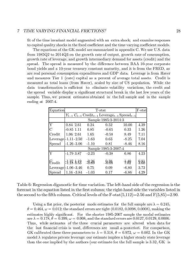
from 1985Q2 to 2014Q3 on the growth rate of output, growth rate of consumption,growth rate of leverage, and growth intermediary demand for assets (credit) and thespread. The spread is measured by the di¤erence between BAA 10-year corporatebond yields and a 10-year treasury constant maturity, and it is from the FRED, asare real personal consumption expenditures and GDP data. Leverage is from Haverand measures Tier 1 (core) capital as a percent of average total assets. Credit ismeasured as total loans (from Haver), scaled by size of US population. While thedata transformation is su¢cient to eliminate volatility variations, the credit andthe spread variable display a signi…cant structural break in the last few years of thesample. Thus, we present estimates obtained in the full sample and in the sampleending at 2007:4.
Equation T-stat F-stat
Y t1 C t1 Creditt1 Leveraget1 Spreadt1
Sample 1985:3-2014:3
Y 0.84 2.61 0.24 0.52 10.00 4.39C -0.85 1.11 0.85 -0.65 0.33 1.26Credit 1.06 2.61 1.65 -0.58 8.49 7.11Leverage -1.11 - 2.50 -1.63 0.63 -8.25 7.04Spread -1.26 -3.06 -1.10 0.81 -8.46 8.16
Sample 1985:3-2007:4
Y -1.79 3.87 -2.23 -0.38 6.86 4.23
C -1.37 1.19 -0.26 0.38 1.40 0.81Credit -1.18 3.53 -0.69 -0.08 7.02 3.60Leverage -1.06 -3.46 0.75 0.09 -6.80 3.72Spread 1.16 -3.84 -1.03 0.17 -6.86 4.29
Table 6: Regression diganostic for time variation. The left-hand side of the regression is theforecast in the equation listed in the …rst column; the right-hand side the variables listed inthe second to the …fth column. Critical levels of the F-stat(5,112)=2.56 and F(5,85)=2.90.
Using a ‡at prior, the posterior mode estimates for the full sample are = 0:245, = 0:464, ! = 0:012; the standard errors are tight (0.0182, 0.0098, 0.0008), making the
estimates highly signi…cant. For the shorter 1985-2007 sample the modal estimatesare = 0:178, = 0:399, ! = 0:008; and the standard errors are 0.0127, 0.0129, 0.0006.Thus, while estimates of the three crucial parameters are altered when data forthe last …nancial crisis is used, di¤erences are small a-posteriori. For comparison,GK calibrated these three parameters to = 0:318, = 0:972, ! = 0:002. In the GKmodel regulates private leverage: our estimate implies a higher steady state leveragethan the one implied by the authors (our estimate for the full sample is 3.32, GK is

7/17/2019 frbrich_wp15-10.pdf
http://slidepdf.com/reader/full/frbrichwp15-10pdf 30/42
7 TIME VARYING FINANCIAL FRICTIONS? 29
1.38), which is closer to the leverage found in the U.S. in corporate and non-corporatebusiness sectors over the sample. Our estimates also suggest that bankers’ survivalprobability is lower than the one assumed by GK (about 10 years).
With the parameter estimates obtained in the full sample, we perform our diagnos-tics. Table 6 indicates that the forecast errors of all equations except consumption arepredictable and, typically, lagged consumption and lagged spread matter. The meanvalue of the Euler wedge is 0.02 with a standard error of 0.03; but both lagged con-sumption and lagged investment to output ratios signi…cantly explain its movements(coe¢cients are respectively -0.10 and 0.72, with standard errors of 0.01 and 0.13).When we run our diagnostics on the shorter sample, we reach the same conclusions:all forecast errors but the one of the consumption equation are predictable, andlagged consumption and lagged spread matter; lagged consumption and laggedinvestment to output ratios predict the wedge (coe¢cients are respectively -0.13 and0.96, with standard errors of 0.02 and 0.23). Thus, the time variations we detect are
not due to the crisis and to the potential break it generates.
Parameter Time Invariant Time Invariant Exogenous TVC Endogenous TVC
6 shocks Function of net worth
h 0.43 (0.006) 0.11 (0.02) 0.19 (0.03) 0.09 (0.02) 0.24 (0.01) 0.97 (0.01) 0.37 (0.03) 0.55 (0.03)! 0.01 (0.008) 0.02 (0.001) 0.02 (0.002) 0.11 (0.008) 0.46 (0.009) 0.80 (0.01) 0 .54 (0.01) 0.52 (0.02)
0.99 (0.004) 0.02 (0.002) 0.03 (0.003)u 0.98 (0.008)
1 0.02 (0.007)2 0.15 (0.009)
Log ML -167.97 1098.32 1546.18 1628.69
Table 7: Parameter estimates, Gertler and Karadi model, standard errors in parenthesis.
Armed with this preliminary evidence, we estimate the model allowing to be timevarying. Since regulates leverage and drives movements in the credit and spreadequations, whose smoothed residuals seem to be the most a¤ected by serial correlation,we opt to make this parameter time varying. We specify
t
= (1
) +
t
1 + e
t; Exogenous variations (46)
t = (2 u (u
2) (exp(1 (X t1 X s)) + exp(2 (X t1 X s))) + et;
Endogenous variations (47)
where X is net bank wealth. We chose bank net wealth as the relevant state in theendogenous speci…cation because of its importance for the spread and the creditvariable. Table 7 reports estimates of selected parameters.

7/17/2019 frbrich_wp15-10.pdf
http://slidepdf.com/reader/full/frbrichwp15-10pdf 31/42
7 TIME VARYING FINANCIAL FRICTIONS? 30
In the model with exogenously varying parameters, variations in t very persistent.Furthermore, estimates of (;!;) are now larger making steady state leverage drop toabout 2.9 and the lifetime of bankers to increase. With the endogenous speci…cation,
estimates of and ! further increase, making steady state leverage fall to 1.9, butbankers’ survival probability is roughly unchanged. The data seem to require a verystrong asymmetric speci…cation for time variations (1 < 2), implying a strong neg-ative relationship between the fraction of funds that bankers can divert and their networth. Finally, note that, in term of marginal likelihood, the endogenous speci…cationis superior to both the exogenous one and the …xed coe¢cient speci…cation augmentedby a shock to bankers’ net worth accumulation equation.
To investigate how inference di¤ers in the three estimated models, we plot in …gure7 the responses of output, in‡ation, investment, net worth, leverage, and the spread toa one percent capital quality shock. The constant coe¢cient speci…cation closely repli-cates the dynamics presented by GK (see their …gure 3). There is a persistent decline
in output and a temporary but strong decline in in‡ation. Investment temporarilyfalls but it then increases because capital is below its steady state. Bankers’ net worthfalls and there is a sharp increase in the spread.
5 10 15 20 25 30 35 40
-10
-8
-6
-4
x 10-3
O u t p u t
5 10 15 20 25 30 35 40
-4
-3
-2
-1
0
1
x 10-3
I n f l a t i o n
5 10 15 20 25 30 35 40
-2
0
2
4
6
x 10-3
I n v e s t m e n t s
5 10 15 20 25 30 35 40
-0.2
-0.15
-0.1
-0.05
N e t w o r t h
5 10 15 20 25 30 35 40
0.05
0.1
0.15
0.2
L e v e r a g e
5 10 15 20 25 30 35 40
0
1
2
3
x 10-3
S p r e a d
Co n st an t E xo g en o us E nd o ge n ou s
Figure 6: Dynamics in response to a capital quality shock
When we allow to be exogenously varying, responses are qualitatively similar.Quantitatively, output falls more on impact but less in the short run; net worth fallsless and the spread increases less in the short run. Thus, making exogenously timevarying, reduces the model’s ability to capture recessionary e¤ects on impact.

7/17/2019 frbrich_wp15-10.pdf
http://slidepdf.com/reader/full/frbrichwp15-10pdf 32/42
8 CONCLUSIONS 31
When variations are endogenous, the model possesses an additional mechanism of propagation of shocks since lower net worth implies higher share of funds diverted bybanks and generally stronger accelerator dynamics. Since the dynamic responses of
net worth are highly persistent, the spread persistently increases making investmentincrease less and output fall more and more persistently relative to the other twocases. Thus, neglecting endogenous variations could impair our ability to correctlymeasure the e¤ects of capital quality shocks.
While the economic interpretation of the relationship between and net worthis beyond the scope of the paper, attempts to endogenize crucial parameters in theGertler and Karadi model exist (see e.g. Bi, Leeper and Leith, 2014; Ferrante, 2014).Their work could provide the microfundations for the evidence we uncover.
8 Conclusions
This paper is interested in i) characterizing the decision rules of a DSGE whenparameter variations are exogenous or endogenous, and in the latter case, whenagents internalize or not the e¤ects their decisions may have on parameter variations;ii) providing diagnostics to detect misspeci…cation driven by parameter variations;and iii) studying the consequences of using time invariant models when theparameters are time varying in terms of identi…cation, estimation, and inference
We show that if parameter variations are purely exogenous, the contemporaneousimpact and the dynamics induced by structural shocks are the same as in a modelwith no parameter variations. However, if parameter variations are endogenous, thestructural dynamics may be di¤erent and the extent of the di¤erence depends on thedetail of the model. We provide diagnostics to detect the misspeci…cation due toneglected parameter variations and describe a marginal likelihood diagnostics torecognize whether exogenous or endogenous time variations should be used.
We highlight that certain parameter identi…cation problems noted in the literaturemay be the result of misspeci…cation due to neglected time variations. Our MonteCarlo study indicates that parameter and impulse response distortions may be largeeven for modest time variations in the parameters. It also shows that, when para-meter variations are neglected, SVAR methods are competitive with more structurallikelihood-based methods, as far as the responses to structural disturbances are con-cerned.
In the context of the Gertler and Karadi (2010) model, we show that the parameterregulating the amount of moral hazard is likely to be time varying. When we allow
variations to be linked to the amount of net worth bankers have, the …t of the modeldramatically improves, primarily because there is an additional propagation channelthat makes spread and thus output responses stronger and more persistent.
Overall, our analysis provide researchers with a new set of tools to help them toassess the quality of their models and respecify certain problematic features.

7/17/2019 frbrich_wp15-10.pdf
http://slidepdf.com/reader/full/frbrichwp15-10pdf 33/42
9 REFERENCES 32
9 References
Andreasen, M. (2012). On the e¤ects of rare disasters and uncertainty shocks for risk
premia in non-linear DSGE models. Review of Economic Dynamics, 15, 293-316.Ascari, G. and A. Sbordone (2014). The macroeconomics of Trend In‡ation. Jour-
nal of Economic Literature, 52, 679-739.Bi, X. Leeper, E, C. Leith (2014). Financial Intermediation and Government debt
default, University of Indiana, manuscript.Brinca, P., Holter, H., P. Krusell, and L. Malafry (2014). Fiscal multipliers in the
21st century. Forthcoming,Journal of Monetary Economics.Canova, F. (2009). What Explains the Great Moderation in the U.S.?: A Structural
Analysis. Journal of the European Economic Association, 7, 697-721.Canova, F. and L. Sala (2009). Back to square one: Identi…cation issues in DSGE
models. Journal of Monetary Economics, 56, 431-449.
Canova, F. and M. Paustian (2011). Business cycle measurement with some theory.Journal of Monetary Economics, 48, 345-361.
Chang, Y., Kim, S. and F. Schorfheide (2013). Labor market heterogeneity and thepolicy-(in)variance of DSGE model parameters’. Journal of the European EconomicAssociation, 11,193-220.
Chari, V.V., Kehoe, P. and Mc Grattan, E. (2007). Business Cycle Accounting.Econometrica, 75, 781-836.
Cogley, T. and T. Yagihashi, (2010). Are DSGE approximating models invariantto policy shifts? The B.E. Journal of Macroeconomics (Contributions), Article 27.
Davig, T. and E. Leeper (2006). Endogenous monetary policy regime changes.NBER International Seminar in Macroeconomics, 345-391. National Bureau of Eco-
nomic Research.Del Negro, M. and F. Schorfheide (2004). Prior from general equilibrium modelsfor VARs. International Economic Review, 45, 643-673.
Dueker, M. Fisher, A. and Dittman, R. (2006). Stochastic Capital Depreciation andthe Co-movements of Hours and Productivity. Berkeley Journals: Topics in Macroeco-nomics, vol 6,3, article 6.
Fernandez Villaverde, J. and J. Rubio Ramirez (2004). Comparing dynamic equi-librium economies to the data. Journal of Econometrics, 123, 153-187.
Fernandez Villaverde, J. and J. Rubio Ramirez (2007). How structural are struc-tural parameters. NBER Macroeconomics Annual, 22, 83-132.
Ferrante, F. (2014) Endogenous loan quality, Federal Reserve Board, manuscript.Galvao, A. , Giraitis, L., Kapetanios, G., and K. Petrova (2014) Local Bayesian
estimation and forecasting with a TVP model, manuscriptGertler, M. and Karadi, P. (2010) A Model of unconventional monetary policy.
Journal of Monetary Economics, 58, 17-34.Huang, N. (2014). Weak Inference for DSGE models with time varying parameters.
Boston College, manuscript.

7/17/2019 frbrich_wp15-10.pdf
http://slidepdf.com/reader/full/frbrichwp15-10pdf 34/42
9 REFERENCES 33
Hurwicz, L. (1962). On the structural form of interdependent systems, in E. Nagel,P. Suppes, A. Tarski (eds.) Logic, Methodology and Philosophy of science: proceedingsof a 1960 international congress. Stanford University Press.
Koop, G., Pesaran, H., and R. Smith (2013). On the identi…cation of BayesianDSGE models. Journal of Business and Economic Statistics, 31, 300-314
Kulish, M. and A. Pagan (2014) Estimation and Solution of models with ex-pectation and structural changes, Dynare working paper 34.
Inohue, A., Kuo, C.H. and B. Rossi, (2015) Identifying sources of model misspec-i…cation, UPF manuscript.
Ireland, P. (2004). Technology shocks in a New Keynesian model. Review of Economics and Statistics, 83, 926-933.
Ireland, P. (2007). Changes in the Federal Reserve In‡ation target: Causes andConsequences. Journal of Money Credit and Banking, 39, 1851-1882.
Liu, Z., Waggoner, D. and T. Zha (2011). Sources of Macroeconomic ‡uctuations:
A regime switching DSGE approach. Quantitative Economics, 2, 251-301.Magnusson, L. and S. Mavroeidis (2014). Identi…cation using stability restrictions.
Econometrica 82, 1799-1851.Meier S. and C.Sprengler (2015). Temporal Stability of Time preferences. Review
of Economics and Statistics, 97(2), 273-286.Mutschler, W. (2014) Identi…cation of DSGE Models - the e¤ect of higher order
Approximation and Pruning, University of Munster, manuscript.Rios Rull J. V. and R. SantaEularia-Llopis, (2010). Redistributive shocks and
productivity shocks. Journal of Monetary Economics,37, 931-948.Schmitt Grohe, S. and M. Uribe (2003). Closing small open economy models.
Journal of International Economics, 62, 161-185.
Schmitt Grohe, S. and M. Uribe (2004). Solving Dynamic General EquilibriumModels using second order approximation to the policy function. Journal of EconomicDynamics and Control, 28, 755-775.
Seoane, H. (2014) Parameter Drifts, Misspeci…cation and the Real Exchange Ratein Emerging Countries, manuscript, Universidad Carlos III Madrid.
Sims, C. (2001) Comment on T. Cogley and T. Sargent, Evolving US postwardynamics, NBER macroeconomic Annual 16.
Stock, J. and Watson, M. (1996). Evidence of Structural Instability in Macroeco-nomic Relationships. Journal of Business and Economic Statistics,14, 11-30.
Vavra, J. (2014). Time varying Phillips curve, NBER working paper 19790.

7/17/2019 frbrich_wp15-10.pdf
http://slidepdf.com/reader/full/frbrichwp15-10pdf 35/42
9 REFERENCES 34
Appendix A: Additional Monte Carlo …gures and tables
5 10
0.2
0.4
0.6
0.8
η
M o d e l B
5 100
0.5
1
M o d e l C
5 100
0.5
1
M o d e l D
-1 0 1 2 3
0.2
0.4
0.6
0.8
γ
-2 0 2
0.2
0.4
0.6
0.8
0 1 2
0.2
0.4
0.6
0.8
0.8 0.9 1
0.2
0.4
0.6
0.8
ρz
0.8 0.9 1
0.2
0.4
0.6
0.8
0.8 0.9 1
0.2
0.4
0.6
0.8
0.5 1
0.2
0.4
0.6
0.8
ρg
- 0. 5 0 0 . 5 1 1 . 5
0.2
0.4
0.6
0.8
-1 0 1
0.2
0.4
0.6
0.8
0. 02 0. 040
0.5
1
δ
0. 02 0. 040
0.5
1
0. 02 0. 040
0.5
1
0. 2 0. 4 0. 6
0.2
0.4
0.6
0.8
α
0. 2 0. 4 0. 6
0.2
0.4
0.6
0.8
0. 2 0. 4 0. 6
0.2
0.4
0.6
0.8
0 5 10
0.2
0. 4
0. 6
0. 8
A
0 5 10
0.2
0. 4
0. 6
0. 8
5 100
0. 5
1
T r ue T = 1 00 I nc or re ct T = 1 00 I nc or re ct T = 1 00 0
Figure A1: Density of estimates; DGP1 (parameter variations explain 2-5 percent of output variance).

7/17/2019 frbrich_wp15-10.pdf
http://slidepdf.com/reader/full/frbrichwp15-10pdf 36/42
9 REFERENCES 35
True Estimated Correct Estimated Time invariant Estimated Time invariantMean Mean 5 percentile 95 percentile Mean 5 percentile 95 percentile
T=150 T=150 T=1000DGP Model B
= 2:0 2.00 2.29 1.53 3.87 2.45 1.61 3.09 = 2:0 2.01 1.11 -0.33 2.06 0.25 -0.27 1.95z = 0:9 0.94 0.99 0.96 1.00 0.99 0.97 1.00g = 0:5 0.47 0.76 0.62 0.96 0.91 0.79 0.98 = 0:025 0.03 0.01 0.01 0.03 0.01 0.01 0.01 = 0:3 0.30 0.19 0.11 0.41 0.21 0.10 0.34A = 4:5 4.53 2.73 1.33 4.14 1.80 1.14 4.16
DGP Model C
= 2:0 2.00 3.40 1.56 7.51 5.19 1.77 22.90
= 2:0 2.00 -0.08 -0.32 0.73 -0.19 -0.35 0.35z = 0:9 0.88 0.99 0.93 1.00 0.99 0.90 1.00g = 0:5 0.48 0.56 0.08 0.97 0.91 0.59 0.98 = 0:025 0.02 0.02 0.01 0.07 0.02 0.01 0.07 = 0:3 0.30 0.26 0.15 0.34 0.26 0.19 0.35A = 4:5 4.50 1.71 1.25 2.77 2.27 1.24 8.17
DGP Model D
= 2:0 2.00 3.05 1.68 4.59 2.40 1.98 4.81 = 2:0 2.00 -0.06 -0.28 0.54 1.63 -0.27 1.98z = 0:9 0.88 0.98 0.90 1.00 0.92 0.91 1.00g = 0:5 0.47 0.42 -0.46 0.96 0.50 0.32 0.97
= 0:025 0.02 0.01 0.01 0.03 0.01 0.01 0.01 = 0:3 0.30 0.23 0.15 0.32 0.21 0.13 0.27A = 4:5 4.49 1.91 1.45 3.57 4.10 1.65 4.51
Table A1: Distributions of estimates, DGP2 (parameter variations explain 20 per-cent of output variance).

7/17/2019 frbrich_wp15-10.pdf
http://slidepdf.com/reader/full/frbrichwp15-10pdf 37/42
9 REFERENCES 36
5 1 0 1 5
0 .2
0 .4
0 .6
0 .8
η
M o d e l B
5 1 0 1 5 2 0 2 5
0 .2
0 .4
0 .6
0 .8
M o d e l C
5 1 0 1 5 2 0
0
0 .5
1
M o d e l D
- 1 0 1 2 3
0 .2
0 .4
0 .6
0 .8
γ
0 1 2
0 .2
0 .4
0 .6
0 .8
0 1 2
0
0 .5
1
0 . 6 0 .8 1
0 .2
0 .4
0 .6
0 .8
ρz
0 . 6 0 .8 1
0
0 .5
1
0 . 6 0 .8 1
0
0 .5
1
- 0 . 5 0 0 . 5 1
0 .2
0 .4
0 .6
0 .8
ρg
- 0 . 5 0 0 . 5 1
0 .2
0 .4
0 .6
0 .8
- 1 0 1
0
0 .5
1
0 . 0 2 0 . 0 4
0
0 .5
1
δ
0 . 0 2 0 . 0 4
0
0 .5
1
0 . 0 2 0 . 0 4
0
0 .5
1
0 0 . 2 0 . 4 0 . 6
0 .2
0 .4
0 .6
0 .8
α
0 . 2 0 . 4 0 . 6
0 .2
0 .4
0 .6
0 .8
0 . 2 0 . 4 0 . 6
0 .2
0 .4
0 .6
0 .8
0 2 4 6 8
0
0 .5
1
A
2 4 6 8
0
0 .5
1
2 4 6 8
0
0 .5
1
T r u e T = 1 0 0 In c o r r e c t T = 1 0 0In c o r r e c t T = 1 0 0 0
Figure A2: Density of estimates, DGP2 (parameter variations explain 20 percent of output variance)

7/17/2019 frbrich_wp15-10.pdf
http://slidepdf.com/reader/full/frbrichwp15-10pdf 38/42
9 REFERENCES 37
1 0 2 0 3 0 4 0
-2
-1
0
x 1 0
- 3
H o u r s
M o d e l B - A
1 0 2 0 3 0 4 0
-4
-2
0
x 1 0
- 3M o d e l C -A
1 0 2 0 3 0 4 0
-4
-2
0
2
x 1 0
- 3M o d e l D -A
1 0 2 0 3 0 4 0
0 . 0 1
0 .0 2
0 .0 3
0 .0 4
0 .0 5
C a p i t a l
1 0 2 0 3 0 4 0
0 . 0 2
0 .0 4
0 .0 6
1 0 2 0 3 0 4 0
0 . 0 1
0 .0 2
0 .0 3
0 .0 4
0 .0 5
1 0 2 0 3 0 4 0
4
6
8
1 0
x 1 0
- 3
O u t p u t
1 0 2 0 3 0 4 0
2
4
6
8
1 0
1 2
x 1 0
- 3
1 0 2 0 3 0 4 0
2
4
6
8
1 0
x 1 0
- 3
1 0 2 0 3 0 4 0
2
3
4
x 1 0
- 3
C o n s u m p t i o n
1 0 2 0 3 0 4 0
1
2
3
4
x 1 0
- 3
1 0 2 0 3 0 4 0
1
2
3
x 1 0
- 3
1 0 2 0 3 0 4 0
-3
-2
-1
0
x 1 0
- 3M o d e l B -A
1 0 2 0 3 0 4 0
-8
-6
-4
-2
0
x 1 0
- 3M o d e l C -A
1 0 2 0 3 0 4 0
- 1 0
-5
0
x 1 0
- 3M o d e l D -A
1 0 2 0 3 0 4 0
-0 . 0 2
-0 .0 1 5
-0 . 0 1
-0 .0 0 5
1 0 2 0 3 0 4 0
-0 . 0 4
-0 . 0 3
-0 . 0 2
-0 . 0 1
1 0 2 0 3 0 4 0
-0 . 0 4
-0 .0 3
-0 .0 2
-0 .0 1
1 0 2 0 3 0 4 0
-4
-2
0
x 1 0
- 3
1 0 2 0 3 0 4 0
- 1 5
-1 0
-5
0
x 1 0
- 3
1 0 2 0 3 0 4 0
- 1 5
-1 0
-5
0
x 1 0
- 3
1 0 2 0 3 0 4 0
-6
-4
-2
x 1 0
- 4
A 8 4 A 1 6 B 5 0
1 0 2 0 3 0 4 0
-6
-4
-2
x 1 0
- 4
A 8 4 A 1 6 C 5 0
1 0 2 0 3 0 4 0
-6
-4
-2
x 1 0
- 4
A 8 4 A 1 6 D 5 0
Figure A3: Impulse responses, DGP2 (parameter variations explain 20 percent of output variance)
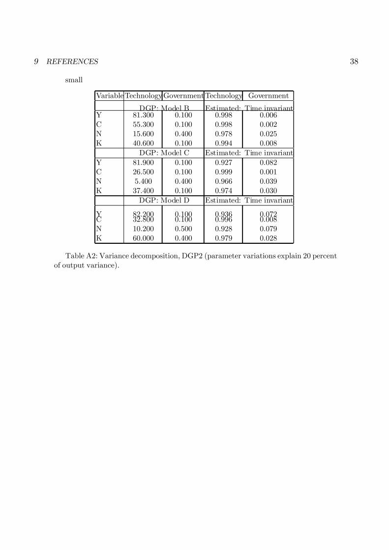
7/17/2019 frbrich_wp15-10.pdf
http://slidepdf.com/reader/full/frbrichwp15-10pdf 39/42
9 REFERENCES 38
small
Variable Technology Government Technology Government
DGP: Model B Estimated: Time invariantY 81.300 0.100 0.998 0.006C 55.300 0.100 0.998 0.002N 15.600 0.400 0.978 0.025K 40.600 0.100 0.994 0.008
DGP: Model C Estimated: Time invariant
Y 81.900 0.100 0.927 0.082C 26.500 0.100 0.999 0.001N 5.400 0.400 0.966 0.039K 37.400 0.100 0.974 0.030
DGP: Model D Estimated: Time invariant
Y 82.200 0.100 0.936 0.072C 32.800 0.100 0.996 0.008N 10.200 0.500 0.928 0.079K 60.000 0.400 0.979 0.028
Table A2: Variance decomposition, DGP2 (parameter variations explain 20 percentof output variance).

7/17/2019 frbrich_wp15-10.pdf
http://slidepdf.com/reader/full/frbrichwp15-10pdf 40/42
9 REFERENCES 39
Appendix B : The RBC model with variable capital utilization of section 3
The representative household maximizes the following stream of future utility
max E 0
1X j=0
t c1
t
1 A
n1+ t
1 + (48)
ct + it = wtnt + rkt ks
t a(ut)kst T t (49)
it = kt (1 )kt1 (50)
kst = utkt1 (51)
where ct is consumption, it investment, kt the stock of capital, and nt is hours worked.Household chooses the utilization rate of capital, ut, and the amount of e¤ective capitalthat she can rent to the …rm, i.e. ks
t . Household receives earnings from supplying labor
and capital services to the …rm, i.e. wt and rk
t respectively, subject to a cost of changingcapital utilization, a(ut)kst . Finally, T t are lump sum taxes levied by the government.
The production function isyt = zt(ks
t )n1t
A fraction of output is consumed by the government and …nanced with lump-sum taxes.The government budget constrain is always balanced, i.e.
gtyt = T t
The optimality conditions of the planner problem are
(1 gt)yt = ct + kt (1 a(ut)ut) kt1
An t c
t = (1 )(1 gt)yt=nt
1 = E t(ct=ct+1)(1 a(ut+1)ut+1 + (1 gt+1)yt+1=kt)
(1 gt)yt=kt1 = ut(a0(ut)ut + a(ut))
yt = zt(utkt1)n1t
a(ut) = 1= + 1
e(ut1) 1
The functional form for the adjustment cost of the capital utilization is in the lastequation and it satis…es a(1) = 0, a0(1) = 1= + 1, a00(1) = (1= + 1). If assume that, in the steady state u = 1, the steady states for ( k
y ; cy ; ny ; n) are the same
as in the RBC model without variable capital utilization.

7/17/2019 frbrich_wp15-10.pdf
http://slidepdf.com/reader/full/frbrichwp15-10pdf 41/42
9 REFERENCES 40
Appendix C : The equations of Gertler and Karadi model
exp(%t) = (exp(C t) h exp(C t1))
h(exp(C t+1) h exp(C t))
(52)1 = exp(Rt) exp(t+1) (53)
exp(t) = exp(%t)
exp(%t1) (54)
exp(Lt)' = exp(%t)exp(P m;t)(1 )exp(Y t)
exp(Lt) (55)
exp( t) = (1 ) exp(t+1)(exp(Rk;t+1) exp(Rt)) + exp(t+1) exp(xt+1) exp( t+1)(56)
exp(t) = (1 ) + exp(t+1) exp(zt+1) exp(t+1) (57)
exp(t) = 1
(1 t)
exp(t)
exp( t) (58)
exp(zt) = (exp(Rk;t) exp(Rt1))(1 t1) exp(t1) + exp(Rt1) (59)
exp(xt) = exp(t)(1 t)
(exp(t1)(1 t1)) exp(zt) (60)
exp(K t) = exp(t) exp(N t)
exp(Qt) (61)
exp(N t) = exp(Net) + exp(Nnt) (62)
exp(N et) = exp(zt) exp(N t1) exp(eNe;t) + t (63)
exp(Nnt) = !(1 t1)exp(Qt) exp( t) exp(K t1) (64)
exp(Rk;t) = (exp(P m;t) exp(Y m;t)
exp(K t1) + exp( t) (exp(Qt)
exp( ))
exp(Qt1) (65)
exp(Y m;t) = exp(at) (exp( t) exp(U t) exp(K t1)) exp(Lt)1 (66)
exp(Qt) = 1 + 0:5i( (Int + I s)
(Int1 + I s 1)2 + i(
(Int + I s)
(Int1 + I s 1)
(Int + I s)
(Int1 + I ss)
exp(t+1)i((Int+1 + I s)
(Int + I s 1)(
(Int+1 + I s)
(Int + I s) )2 (67)
exp( ) = c + b=(1 + ) exp(U t)1+ (68)
exp(Y m)
exp(U t) =
b exp(U t) exp( t) exp(K t1)
exp(P m;t) (69)
Int = exp(I t) exp( ) exp( t) exp(K t1) (70)
exp(K t) = exp( t) exp(K t1) + Int (71)
exp(Gt) = Gs exp(gt) (72)
exp(Y t) = exp(C t) + exp(Gt) + exp(I t) + 0:5i( (Int + I s)
(Int1 + I s 1)2(Int + I s) + exp(K t)(73)
exp(Y m;t) = exp(Y t) exp(Dt) (74)

7/17/2019 frbrich_wp15-10.pdf
http://slidepdf.com/reader/full/frbrichwp15-10pdf 42/42
9 REFERENCES 41
exp(Dt) = exp(Dt1) exp(inflt1) P exp(inflt)
+ (1 )((1 exp(inflt1) P (1 ) exp(inflt) 1)=(1 ))=(1 ) (75)
exp(X t) = 1= exp(P m;t) (76)
exp(F t) = exp(Y t) exp(P m;t) + exp(t+1) exp(inflt+1)(exp(inflt)) P exp(F t+1)(77)
exp(Z t) = exp(Y t) + exp(t+1) exp(inflt+1)1 exp(inflt) P (1) exp(Z t+1) (78)
exp(inflt ) =
1
exp(F t)
exp(Z t) exp(inflt) (79)
(exp(inflt))1 = exp(inflt1) P (1) + (1 )(exp(inflt ))1 (80)
exp(it) = exp(Rt) exp(inflt+1) (81)
exp(it) = exp(it1)i( 1 exp(inflt) (exp(X t)=(=( 1)))y)1i exp(ei;t) (82)
t = (Rk;t+1 Rt Rsk + Rs) + e;t (83)at = a at1 a ea;t (84)
t = t1 e;t (85)
gt = g gt1 eg;t (86)
e;t = e;t1 + e;t (87)
t = t1 + e;t (88)
Note: t = 0; 8t in the basic estimated model. It appears only in the augmented modelof table 7.